neighborhood systems: a qualitative theory for fuzzy - citeseer

Advances in Machine Intelligence and Soft Computing, Volume IV. Ed. Paul Wang, 1997, 132-155.

NEIGHBORHOOD SYSTEMS: A Qualitative Theory for Fuzzy and Rough Sets

T. Y. L in Department of Mathematics and Computer Science San Jose State University San Jose, California 95192-0103 [email protected] and Berkeley Initiative in Soft Computing Department of Electrical Engineering and Computer Science University of California Berkeley, California 94720

Abstract The theory of neighborhood systems is abstracted from the geometric notion of "near" or "negligible distances." It is a "new" theory of the classical concept of neighborhood systems within the context of advanced computing. By definition neighborhood systems include both rough sets and topological spaces as special cases. The deeper and more interesting part is in its interactions with fuzzy sets: Intuitively, qualitative fuzzy sets should be characterized by "elastic" membership functions that can tolerate “a small amount of continuous stretching with limited number of broken points.” Based on neighborhood systems we develop a theory for such qualitative fuzzy sets. As illustrations fuzzy inferences and Lyapunov stability are discussed. Keywords: membership function, neighborhood system, qualitative fuzzy set, rough set, topology.

1. Introduction Uncertainty processing is a fact of life. It is an important part of daily routines. Various theories have been proposed. Two notable theories related to our interests are Lotfi A. Zadeh’s fuzzy set theory [26] and Zdzislaw Pawlak’s rough set theory [20]. In this paper, we discuss these notions from a geometric point of view, namely, the theory of neighborhood systems. Roughly, a neighborhood


system assigns each object a (possibly empty, finite, or infinite) family of non-empty subsets. Such subsets, called neighborhoods, represent the semantics of “near.” Using neighborhoods, one can define open sets, closed sets, and hence the interior and closure of any subset [8], [21]. If we take equivalence classes as neighborhoods, the lower and upper approximations are precisely the interior and closure respectively. From this point of view rough set theory is a special form of neighborhood system theory; it was called category [3]. In fact generalized rough sets based on modal logic are all special forms of neighborhood systems [25]. Formally neighborhoods play the most fundamental role in mathematical analysis. Informally, it is a common and intuitive notion: It is in databases [5], [18], in rough sets [20], in logic [2], in texts of genetic algorithms [6], and many others. In the context of advanced computing a systematic study of neighborhood systems was initiated by this author and his students. It was motivated from database retrieval and data mining [9], [10], [11] [12], [3], [24], [13].

In this paper we also will use neighborhood systems to formulate fuzzy sets. A few words on our philosophical view may be in order: Zadeh’s full agenda is a grand revolution in mathematics and science. It not only fuzzifies mathematics and science, it may fuzzify their foundations, methodologies, and philosophies. We, however, adopt a conservative strategy; we only fuzzify mathematics, but keep its foundation unfuzzified. In other words, though fuzzy theory is designed to express fuzzy and imprecise concepts, the theory itself is crispy and precise -- see figure below. At this point in time our strategy probably is “correct” and effective. With unfuzzified foundations, we can apply both fuzzy and traditional mathematics to real world problems simultaneously, and find consistent solutions.

Fuzzy Mathematics > Fuzzy WorldFuzzy

Traditional Logic and

Mathematics

Crispy


This paper aims towards applications in fuzzy controllers, so we examine the theory from topological point of view; we emphasize “continuous stretching.” For full qualitative fuzzy set theory, we also need to examine it from measure (stochastic) theoretical point of view; in this paper we only touch on it slightly. For the full study we will need to develop a measure theory or theories for neighborhood systems. Interestingly, we find that neighborhood systems are the most natural data structures for belief functions; the study will be report in the near future. Our ultimate goal is an axiomatic fuzzy set theory.

Organization and Acknowledgment

The paper is divided into three parts, neighborhood systems, qualitative fuzzy sets, and applications. The numbering of sections is independent of the partitions. Definitions, theorems, propositions, and corollary are enumerated as one group within each section. This author would like to express his deepest thank to Professor Zadeh for his warm invitation to join the Berkeley Initiative in Soft Computing Group (BISC). His thanks also go to Dr. Martin Wildberger at EPRI, Electric Power Research Institute, for his generous sponsorship.

Part I . A Theory of Neighborhood Systems

2. Neighborhood Systems In this section, we will give a short exposition on the theory of neighborhood systems in the context of advanced computing.

2.1 The Semantics of “ Near” The notion of near is rather imprecise. Let us examine the following two examples. Example 1 Is Santa Monica “near” Los Angels? Answers could vary. For local residents, answers are often “yes.” For visitors who have no cars, answers may be “no.” Example 2 Is 1.73 “near” 3? Again answers vary. Intrinsically “near” is a subjective judgment. One might wonder whether there is a scientific theory for such subjective judgments? Mathematicians have offered a nice solution. They simply include the contexts into the formalism: Given the radius of an acceptable error ε =1/100, is 1.73


“near” 3? Similarly, if a neighborhood system has been assigned to each city in Los Angeles area, then we have a definite answer for Example 1. So a proper formulation for such a question is:

Given a neighborhood system (the context), is p near q?

Example 3. A Context Free Answer Is the sequence { 1, 1/2, 1/3, .., 1/n,... } “near” zero?

The answer is a context free “yes.” In other words, it is a “yes” for all contexts: For any given context, ε > 0, there is a number N = [1/ε] + 1, such that, for all n > N, 1/n is “near” zero, where [1/ε] denotes the biggest integer < 1/ε. For readers who familiar with the standard (ε, δ)-definition of limit can spot the origin of neighborhood systems. Such a contexts free answer is precisely the classical notion of limits, lim n→∞ 1/n = 0. In our language, we may say that limit is the context free answers of “near.” Perhaps we should also point out here that there is no context free answers for the question whether two points (any finite number of points) are near or not.

Roughly speaking mathematical analysis is started from examining infinitesimal which is, in our view, one form of uncertainty. Such a notion can be traced back to Archimedes and Eudoxus. Cauchy's (ε, δ)-definition provided a "definite form" answer to such infinitesimal uncertainty; A. Robinson provided a direct answer (non-standard analysis). On can viewed neighborhood systems is an adoption of (ε, δ)-method to the finite universe.

2.2. Fundamentals of Neighborhood Systems Let U be the universe of discourse and p be an object in U. Definition 2.1. 1. A neighborhood, denoted by N(p), or simply N, of p is a non-empty subset

of U, which may or may not contain the object p. A neighborhood system of an object p, denoted by NS(p), is a maximal family of neighborhoods of p. If p has no (non-empty) neighborhood, then NS(p) is an empty family; in this case, we simply say that p has no neighborhood.

2. A neighborhood system of U, denoted by NS(U) is the collection of NS(p) for all p in U. For simplicity a set U together with NS(U) is called a neighborhood system space (NS-space) or simply neighborhood system.

3. A subset X of U is open if for every object p in X, there is a neighborhood N(p) ⊆ X. A subset X is closed if its complement is open.

4. NS(p) and NS(U) are open if every neighborhood is open. NS(U) is topological, if NS(U) are open and U is the usual topological space [8]. In such a case both NS(U) and the collection of open sets are called topology.


5. An object p is a limit point of a set E, if every neighborhood of p contains a point of E other than p. The set of all limit points of E is call derived set. E together with its derived set is a closed set.

6. NS(U) is discrete, if NS(U)= P(U), the power set. 7. NS(U) is indiscrete, if NS(U)= { U} . 8. NS(U) is serial, if ∀p, N(p) is non-empty (called Frechet (V) space in [21]). 9. NS(U) is reflexive, if ∀p, p ε N(p). 10. NS(U) is symmetric, if ∀p ∀q, q ε N(p) � p ε N(q). 11. NS(U) is transitive, if ∀p ∀q ∀p ∀r, q ε N(p) and r ε N(q) � r ε N(p). 12. NS(U) is Euclidean, if q ε N(p), and r ε N(p), � r ε N(q). Example 2.2. 1. Let U ={ x, y} for example 1 to 5. NS(x) ={ x} , { x, y} ; NS(y) = ϕ ; ϕ is the empty set. Open sets: ϕ, { x} , { x, y} ; { y} is not open. It is not a topological space. 2. NS(x) = { x} , { x, y} ; NS(y)={ x, y} . Open sets: ϕ, { x} , { x, y} ; { y} is not open. It is a topological space. 3. NS(x) ={ x} , { x, y} ; NS(y)= { y} , { x, y} ; Open sets: ϕ, { x} , { y} { x, y} . It is a discrete NS-space. 4. NS(x) ={ x, y} ; NS(y)={ x, y} ; Open sets: ϕ, { x, y} ; { x} and { y} are not open. It is an indiscrete NS-space. 5. NS(x) ={ x} ; NS(y)={ y} ; Open sets: ϕ, { x} , { y} , { x, y} . It is a topological space. 6. Let U be the Euclidean plan, we assign each point p a family of neighborhoods

by open solid disks: ∀ p and ∀ ε,

N(p, ε)={ x : d (x, p) < ε} ,

where d is the usual Euclidean distance. The family of such N(p, ε)'s, ∀ p and ∀ ε, are the neighborhood systems of the usual topology of Euclidean plan. A topological space is a neighborhood system space, but not the converse; see next example.

7. Next, we assign each point p in the Euclidean plan U a unique neighborhood, namely, a open solid disk of radius 2:

N(p, 2) ={ x : d (x, p) < 2} .


Such an assignment gives U a neighborhood system, but not a topological space.

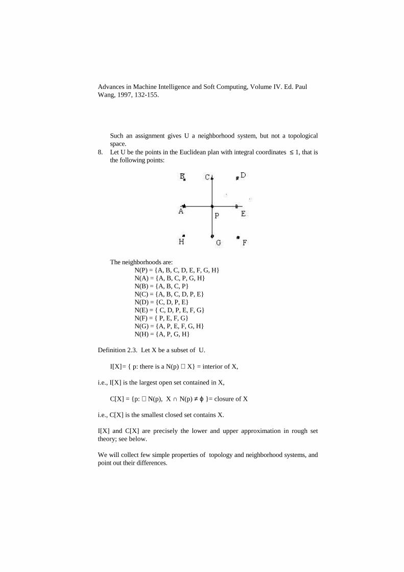
8. Let U be the points in the Euclidean plan with integral coordinates ≤ 1, that is the following points:

The neighborhoods are: N(P) = { A, B, C, D, E, F, G, H} N(A) = { A, B, C, P, G, H} N(B) = { A, B, C, P} N(C) = { A, B, C, D, P, E} N(D) = { C, D, P, E} N(E) = { C, D, P, E, F, G} N(F) = { P, E, F, G} N(G) = { A, P, E, F, G, H}

N(H) = { A, P, G, H} Definition 2.3. Let X be a subset of U.

I[X] = { p: there is a N(p) ⊆ X} = interior of X, i.e., I[X] is the largest open set contained in X,

C[X] = { p: ∀ N(p), X ∩ N(p) ≠ ϕ } = closure of X

i.e., C[X] is the smallest closed set contains X. I[X] and C[X] are precisely the lower and upper approximation in rough set theory; see below. We will collect few simple properties of topology and neighborhood systems, and point out their differences.


Proposition 2.4. 1. A topological space is a neighborhood system space (NS-space), but not the

converse. 2. Intersections and finite unions of closed sets are closed in NS-spaces. 3. In topological spaces, unions and finite intersections of open sets are open.

In NS-spaces, unions is open, but intersections may not be open. 4. In a topological space NS(U) determines and is determined by the collection

of all open sets. This property may or may not be true for neighborhood systems.

5. A neighborhood system is a subbase (see below) of a topology. An open set in NS-space is also open in this topology, the converse may not be true.

A family B of subsets is a base for a topology, if every open set is a union of members of B. A family S of subsets is a subbase, if the finite intersections of members of S is a base. Note that the union and intersection of empty family is the whole space and empty set respectively. We can take a neighborhood system as a subbase of some topology. Note that two distinct neighborhood systems may give the same topology.

2.3. Continuos Mappings and Pullbacks Let U and V be two universes. Let F: U → V be a mapping that assigns, ∀ x ∈ U, a unique object y ∈ V. Definition 2.5. Let NS(U) and NS(V) be two neighborhood systems. F is said to be continuous if ∀ N(y) ∃ N(x) such that F(N(x)) ⊆ N(y). F is called a homeomorphism, if both F and its inverse F-1 are continuous [8]. Let O be any subset of V. We shall write F-1 (O)= { u: F(u) ∈ O} i.e., F-1 (O) is the set of all those objects of U, which are mapped into O by F. The set F-1 (O) is called the complete inverse image (under F) of the set O, we may simply call it the pullback of O (under F).

Let us recall some results from general topology [8]. Let T(V) be the topology of V, namely, the family of all open sets in V. We will write T(U) = { F-1 (O) : O ∈ (V) varies through all open sets in V}


i.e., T(U) is the set of all inverse image of all the open sets in V. It is well known

that T(U) is the smallest topology such that F is continuous [8]. We will call

T(U) the pullback of T(V) under F, or simply pullback of F. Proposition 2.6. Let U be the universe and { Vm } be a family of topological spaces. Let M ={ Fm: U → Vm } be a family of functions. There is a unique minimal topology T(U) such that every Fm is continuous. Such a topology will be called the minimal M-topology. Note that M-topology is not just the union of all the pullback of Fm, it is the smallest topology generated by all the pullbacks.

We have similar results in neighborhood system. Let F(q) = p. We will take F-1 (N(p)) as a neighborhood of q. Let N(p) varies through NS(p), then we have a neighborhood system at q. Let q varies through all objects in U, we have the neighborhood system, NS(U) = { N(q)=F-1(N) : F(q) = p, N(p) ∈ NS(V), q ∈ U} . We will call the procedure of forming NS(q) and NS(U) through the mapping F, pullback of NS(V) under F, or simply pullback of F. We have an analogous results for neighborhood systems. Proposition 2.7. Let U be the universe and { Vm } be a family of neighborhood systems. Let M ={ Fm} be a family of functions. There is a unique minimal neighborhood system NS(U) such that every Fm is continuous.

3. Generalized Rough Sets as Neighborhood Systems Rough set theory can be viewed as an approximation theory using equivalence relations as neighborhoods. It is immediate that on can generalize the theory to any binary relations. In this section, we discuss neighborhood systems that are derived from binary relations.

3.1. Binary Relations and Basic Neighborhoods A minimal neighborhood of p, denoted by MN(p), is a minimal member of NS(p) in the sense that MN(p) contains no member of N(p) as proper subsets. Note that in general such MN(p) may or may not exist. The maximal family of all MN(p) at p will be denoted by MNS(p). The family of MNS(p) for all p will be denoted by MNS(U). Let n(p) be the number of (distinct) MNS(p)’s at p. If n(p) = n is a constant integer for all p, MNS(U) is an n-minimal neighborhood system, and denoted by n-MNS(U).


Let R be a binary relation defined on U, then B(p) = { x : pRx} is a neighborhood of p, called a basic (binary) neighborhood. Let BS(U), called a basic neighborhood system, be the collection of all B(p); note that B(p) can be empty for some p. Note that BS(U) defines and is defined by a binary relation. If R is serial (that is, B(p) is non-empty for all p), then BS(U) is an 1-minimal neighborhood system; this is the most interested case. From the implementation point of view, we can rephrase a basic (binary) neighborhood system as follows: Definition 3.1. A basic neighborhood system BS(U) is a data structure that assigns each datum a set (could be empty) of data. Proposition 3.2. 1. A minimal member of NS(p) may or may not exit. Even for a non-empty

neighborhood system NS(p), MNS(p) could be empty. The neighborhood system of a real number has no minimal neighborhood; NS(p) is an infinite set at for every real number p.

2. A binary relation on U defines and is defined by a basic neighborhood system BS(U).

In Definition 2.1, various neighborhood systems are defined by their local

properties. We summarize their relationships in the following table:

binary relation implications basic (binary) neighborhood serial ↔ serial reflexive ↔ reflexive symmetric ↔ symmetric transitive ↔ transitive Euclidean ↔ Euclidean reflexive, symmetric ↔ Browersche, B reflexive, transitive ↔ S4, (see note) equivalence ↔ clopen topology, S5,

An S4 -neighborhood system is a topological space, however, the converse is not necessary true. Similarly the n-graded binary relations [25] correspond to n-minimal neighborhood systems; we skip the details.


3.2. Rough Sets and Neighborhoods Let R be an equivalence relation on U. It partitions U into equivalence classes. The partition, by abuse of notation, is denoted by R again. The pair (U, R) is called approximation space which is the universe of discourse in rough set theory. The equivalence class containing x will be denoted by [x]. Rough setters view R as an indiscernibility relation, that is, the elements within the equivalence class are indistinguishable by the available information. So the approximation space is a multi-set in which an element x repeats itself as many time as the number of elements in [x]. Taking the this point of view, a subset X can not be adequately described. It can only be approximated. As usual, let ϕ be the empty set. Definition 3.1. Let X be a subset of the approximation space (U, R).

R(X) = { x : [x] ⊆ X} = the lower approximation, R(X) = { x : [x] ∩ X ≠ ϕ } = the upper approximation.

Definition 3.2. The pair (R(X), R(X)) is called a rough set. We should caution the readers that this is a technical definition of rough sets defined by Pawlak [20]. However, rough setters often use “rough set” as any subset X in the approximation space, where R(X) and R(X) are defined. We

also would like to note that the pair (R(X), R(X)) as pair of sets (no knowledge of R) does not characterize rough set. In general, for a subset X there is possibly a subset Y such that

R(X) ⊆ Y ⊆ R(X), but R(X)≠ R(Y) or/and R(X) ≠ R(Y).

As we have remarked earlier that the partition can be regarded a neighborhood system on U. That is, the equivalence class [x] is a neighborhood of y, ∀ y ∈ [x]. We will call such a NS(U) clopen neighborhood system, S5-neighborhood system or Palwak topology [15]. Proposition 3.3 Let (U, R) be an approximation space. NS(U) is a clopen topology.

Part I I A Qualitative Theory of Fuzzy Sets


4. Real Wor ld Fuzzy Sets The goal of this section is to investigate what a real world fuzzy should be. 4.1. Some Cr itical Questions We will start with few fundamental questions: Question 1 Could there be more than one membership functions for a given

fuzzy set? Question 2 (a) Do fuzzy set operations exit, if there are more than one

membership functions for a fuzzy set? (b) Do fuzzy set operations exit in the traditional sense(derived

from logical connective)? Question 3 Could a membership function represent more than one fuzzy sets ? Discussion of Question 1: The status of answers is somewhat inconsistent in the literature. In his book [7, pp. 4], Kandel gave several membership functions for a real world fuzzy set which consists of real numbers that are much greater than 1. Similarly Zimmermann gave a definition for fuzzy numbers by two conditions. So a fuzzy number may have several membership functions [27, pp. 57].

On the other hand, Zimmermann also quoted that “a fuzzy set is represented solely by stating its membership functions” [19], [27, p12]. Moreover, s- and t-norms are defined with implicit assumption that a membership function is unique for each fuzzy set; see the arguments in question 2. Proposal 1. It seems that there are different types of fuzzy sets, so a taxonomy is needed. For qualitative fuzzy sets membership functions are not necessarily unique. Discussion of Question 2: Let us consider the operation, intersection, and assume that it is defined by an arbitrary but a fixed t-norm t(-, -). Let (U, FK) = (U, GK) be a fuzzy set defined by two distinct membership functions FK and GK. Let FH and GH be another pair that define the same fuzzy set (U, FH) = (U, GH). The intersection, ∩, can be defined in two ways: (1) (U, FK) ∩ (U, FH)= (U, FZ), (2) (U, GK) ∩ (U, GH)= (U, GZ),


where FZ = t(FK, FH) and GZ = t(GK, GH). If the intersection does exist, we must show that the “ two” intersections are indeed the same, i.e., (U,FZ) = (U,GZ). If such an equality is proved, the intersection is said to be well-defined. However no contemporary authors have shown such a well-defined-ness. So from the literature, we may conclude that

(1) Either a fuzzy set is defined by a unique membership function, (2) Or fuzzy set operations have not been established. Even in quantitative theory (one membership function for one fuzzy set) [14], we may also want to adopt (2) for different reasons. It might be helpful to point out that rough sets have no set theoretical operations either. So we have Proposal 2 (a) Fuzzy set operations (for qualitative theory) may not exist, (b) Fuzzy set operations (even for quantitative theory) may not be

derived from logical connectives. Discussion of Question 3: Let MF be the space of all membership functions. Qualitative fuzzy sets are defined by subsets of MF. The natural question is: Do these subsets overlap? Or equivalently do they form a crispy partition on MF? There is no explicit answer to this question in the literature. For building a beautiful mathematical theory, it would be nice to have such a partition. However a total space of membership functions is often “continuous.” It is hard to believe there is a natural and crispy partition on such a “continuous” space. We have developed both theories in next section, however, the theory is natural for positive answer, not quite natural for negative answer. Proposal 3 Both positive and negative answers are acceptable, but positive is more natural. Fur ther Discussions: We would like to caution readers that positive answer has “serious” implications: Let FX be a membership function that represents both fuzzy sets A and B. Let C be another fuzzy set with a membership function FZ. Suppose s(FX, FY) is the union defined by some “clever” s-norm. Naturally one may ask which of these two fuzzy sets, A∪B or A∪ C, does s(FX, FY) represent? At current stage, there is no clear answer. At first impression such a phenomenon may sound


"ridiculous," however, after some analysis one may conclude that it is no more surprising than classical "contradiction" (two fuzzy rules are “contradictory” ). For example, a crispy set is the union of singleton, so a fuzzy set is a "weighted union" of singletons. Proposal 4 Fuzzy operations (or connectives) are weighted and multi-valued. This proposal will be in our future study. 4.2 Character istic of Real Wor ld Fuzzy Sets Let the membership space M be the unit interval [0, 1]. Let FX be a membership function, FX: U → M = [0, 1] The subset where membership function FX taking value α will be given a geometric term, α-level-curve or level-curve when α is not explicitly given:

[α ] = { x : FX(x) = α } = α-level-curve

i.e., α-cut minus strong α-cut. There are two special α-level-curves: 1-level-curve and 0-level-curve. They will be called real set (core), denoted by RFX, and complement set, denoted by CFX respectively. We will not use the term core, because it is a special and very important notion in rough set theory. Definition 4.1. The collection of all level-curves is a partition on U, called grade partition. The main goal of this section is to formalize the characteristics of the following intuitive statement:

An “ elastic” membership function can tolerate a small amount of continuous stretching with limited number of broken points.

We need a family of membership functions to express the stretching of a membership function. That is, a real world fuzzy set is defined by a family of membership functions. Following Kandel, membership functions of the same fuzzy set will be called admissible functions or admissible family of membership functions. We still need to specify two contexts. What is small ? What is limited number? To specify these contexts mathematically, we will assume two positive numbers ε and ε' are given. We also need a (additive or non-additive) measure µ that can estimate the "number" of points.


Now we will describe the characteristics of an admissible family of “elastic” membership functions: First let us adopt the notion of "almost everywhere" from mathematical analysis. We say that two functions f(p) and g(p) are equal almost everywhere iff µ (E) < ε', where E={ p : f(p) ≠ g(p) } . In other words f(p) and g(p) are equal for almost all p, and the measure of the set of points where these two functions are not equal is less than ε'. All the constraints, such as "less than" and "equal to," stated below will all be understood as "less than almost everywhere" and "equal to almost everywhere" respectively.

Characteristic (1) The grades of different memberships of the same point should be “near:” FX(x) and FY(x) should belong to the same basic neighborhood of a pre-chosen basic ε-neighborhood system of the unit interval. In other words, the distance between α-level-curve (α = FX(x)) and α’ -level-curve (α’=FY(x)) are less than the chosen ε.

When we stretch the elastic membership function slightly, we do keep some relationship unchanged. Characteristic (2) The grade partition should be the same: FX(x) = FX(y) ⇔ FY(x) = FY(y) for all admissible function FY. In other words, if x and y are in the same α-level-curve for FX, they should be in the same α’ -level-curve for FY. Characteristic (3) The order of the grades of memberships should be the same: FX(x) < FX(y) ⇔ FY(x) < FY(y) for all admissible function FY. In other words, if α-level-curve is lower than β-level-curve (α=FX(x), β=FX(y)), then α’ -curve is lower than β’ -level-curve ((α’=FY(x), β’=FY(y)). Finally, we also want the members who absolutely belong to (or do not belong to) the fuzzy set should stay in (or out of ) the set absolutely Characteristic (4) The set with absolute membership, called real set, should be the same: FX(x) =1 ⇔ FY(x) = 1 for all FY. Characteristic (5) The set with absolute no membership, called complement set, should be maintained: FX(x) =0 ⇔ FY(x) = 0 for all FY. These five “ imprecise” characteristics may characterize what qualitative fuzzy sets should be. Each qualitative fuzzy set is represented by a basic (binary) neighborhood of the space of membership functions. Precise and exact grades of memberships play no role in such qualitative fuzzy sets.


Future Direction. In this paper, we focus on topological point of view, we only touch on measure theoretical point of view briefly. In order to have a complete account on measure theoretic point of view we need to develop a “ finite type measure” theory; one can view neighborhood systems as a “ finite type topological” theory.

5. Topological Aspects of Qualitative Fuzzy Sets Based on the characteristics of the “elastic” membership functions, we will try to define qualitative fuzzy sets formally. For simplicity, we will focus on topological aspects in this section. However, if one interprets constraints properly (e.g., equal is understood as equal almost everywhere) all the results are valid for general qualitative fuzzy sets. 5.1. Fundamentals Let ε be a small number selected. A sub-interval in [0, 1] is said to be an ε-neighborhood, if the length of the sub-interval is 2ε (ε is the radius, 2ε is the diameter). A mapping h: [0, 1] → [0, 1] is called an ε-homeomorphism, if (1) h is a homeomorphism on the closed unit interval (Definition 2.5), and (2) ∀ p in [0, 1], | p - h(p) | <2ε. Let A be a fixed point set that contains at least { 0, 1} . h is called ε-homeomorphism relative to A, if (a) h is an ε-homeomorphism and (b) h keeps the set A pointwise fixed, that is, p = h(p) for all p∈A. In terms of neighborhood systems, h is a ε-homeomorphism relative to A if (1) h is a homeomorphism, (2) { p, h(p)} is contained in a basic ε-neighborhood, and (3) h keeps A pointwise fixed. Intuitively, an ε-homeomorphism is a “ light pulling” of the string from one end to the other end, and keeping A pointwise fixed, where the string is the unit interval made of elastic material. Definition 5.1. Membership functions FX and FY are ε-deformable iff (1) both induce the same minimal topology on U, (2) there exists an ε-homeomorphism h relative to A= { 0, 1} such that FX(x)= h(FY(x)) for all x ∈ U, or FX= h • FY. The binary relation so defined will be called the ε-deformation.


Note that ε-homeomorphism h keeps 0 and 1 fixed, so it is an order preserving map. The binary relation, ε-deformation, is reflexive and symmetric, but may not be transitive. It defines a set of admissible families of membership functions; each family is called an ε-deformable family of membership functions. Geometrically the family is a basic neighborhood in the space of membership functions−see Section 3.1. Definition 5.2. Such an ε-deformable family (a basic neighborhood) of membership functions defines a ε-qualitative fuzzy set. For ε = 1 and A = { 0, 1} , the ε-deformable relation becomes an equivalence relation; it will be called 1-equivalence relation. Theorem 5.3. In a finite universe U = { u1, u2, .., un} , FX and FY are ε-deformable iff (1) both have the same grade partition, (2) | FX(x) - FY(x) | < 2ε for all x in U, (3) The two linear orders of grade partitions are isomorphic. Proof: Note that FX(U) = { FX(u1), FX(u2), .., FX(un)} is a finite discrete set in the closed unit interval [0, 1]. The grade partition (Definition 4.1.) is the pullback of these finite discrete points under FX. So the condition (1) in Theorem 5.3 and (1) in Definition 5.1 are equivalent. It is obvious that (2) of Definition 5.1 implies (2) and (3) of Theorem 5.3 (A homeomorphism keeping { 0.1} fixed is an order preserving map). To see the converse, by (3) of Theorem 5.3, we can have an order preserving map h between FY(U) and FX(U). Then we extend h linearly to the unit interval. By (2) of Theorem 5.3, |x - h(x) | < 2ε, such an extended map h moves points within ε distances. So h is an ε-homeomorphism relative to { 0, 1} . We have established (2) of Definition 5.1. Q E D. Corollary 5.4. The binary relation ε-deformation induces a reflexive and symmetric basic neighborhood system on the space of all membership functions. By taking ε =1, the condition (2) of Theorem 5.3 disappears and sub-intervals reduce to the total interval; we have the following: Corollary 5.5. In a finite universe U = { u1, u2, .., un} , FX and FY are 1- equivalent iff (1) both have the same grade partition, (2) The two linear orders of grade partitions are isomorphic.


Corollary 5.6. In a finite universe U = { u1, u2, .., un} , 1- qualitative fuzzy set is characterized by (1) the grade partition, (2) The linear orders of grade partitions. 5.2. Non-finite universe For non-finite universe, it is much more complicated. We will treat the details in different paper. We will sketch only some results here. As usual the notion of neighborhoods of objects can be generalized to neighborhoods of subsets [8]. Let U has the minimal topology. An α-cut (strong α-cut) is a closed (open) neighborhood of the real set (core). A neighborhood system { Ns} is said to be open-closed-nested chain between two disjoint closed sets A and B, if (1) { Ni} is linearly ordered by inclusion, (2) A= ∩Ns and X \ B= ∪ Ns ,

(3) I(Ns) ⊇ C(N t), if s > t and Ns ≠ N t (Note that if Ns= N t then (3) does not hold).

The maximal chain of open-closed-nested neighborhood system between the real set RFX (core) and complement CFX will be called the maximal chain of FX. Now we have the non-finite set version of Theorem 5.3 -Corollary 5.6. Theorem 5.3∝ Qualitative fuzzy set FX can be characterized by the following two qualitative properties (1) the minimal topologies that are pullbacks of FX and FY are the same, (2) | FX(x) - FY(x) | < 2ε for all x in U, (3) two maximal chains of FX and FY are isomorphic. Corollary 5.4∝. The binary relation ε-deformation induces a reflexive and symmetric basic neighborhood system on the space of all membership functions. Corollary 5.5∝ FX and FY are 1- equivalent iff (1) the minimal topologies that are pullbacks of FX and FY are the same, (2) two maximal chains of FX and FY are isomorphic. Corollary 5.6∝. 1- qualitative fuzzy set is characterized by (1) a topology that is a pullback of the topology of real numbers, (2) a maximal chain.


6. P-Fuzzy Sets Though we believe ε-deformable families (see comments on Question 3) should not form a partition in a membership space, we will offer a “partition theory” for references. Properties of the binary relation, ε-deformation, are induced from the properties of basic ε-neighborhood. In order to have a “partition theory,” we need to have a reflexive, symmetric and transitive basic ε-neighborhood system. So we choose left-closed-right-open intervals as basic ε-neighborhoods (It will work equally well, if we have made "opposite" choice). In other words, we partition the closed unit interval into the following sub-intervals [0, P1), [P1, P2), [P2, P3} ,...[Pn, 1], where the length of all sub-intervals is ε, except the last one [Pn, 1] which may or may not be shorter. Now we can modify Definition 5.1 into the following: Definition 6.1. Membership functions FX and FY are P-equivalent iff (1) both induce the same minimal topology on U, (1a) A={ 0, P1, P2, P3,..., Pn ,1} (2) there exists a ε-homeomorphism h relative to A such that FX(x)= h(FY(x)) for all x ∈ U, or FX= h • FY It is easy to see that P-equivalence is indeed an equivalence relation. We would like to point out that that the fixed point set A is a parameter of P-equivalency. Choosing such a sequence { 0, P1, P2, P3,..., Pn ,1} is not a natural condition. This selection reflects the un-natural-ness of the crispy partition on MF, the membership function space; it is not a desirable theory. Definition 6.2. A P-fuzzy set is a mathematical object that consists of an P-equivalence class of membership functions. The theorem 5.3 can be reformulated as follows: Theorem 6.3. In a finite universe U = { u1, u2, .., un} , FX and FY are P-equivalent iff (1) both have the same grade partition

(2) ∀x, { FX(x), FY(x)} is contained in one of the sub-intervals intervals [0, P1), [P1, P2), [P2, P3} ,...[Pn, 1].

(3) CFX=CFY and RFX=RFY, and two linear orders of grade partitions are isomorphic.

(1) of Theorem 6.3 follows immediately from (1) of Definition 6.1. Since A is a fixed point set, so sub-intervals are mapped into themselves by h. So (2) of


Theorem 6.3 follows. Note that h is a homeomorphism, it is a monotonic map; (3) of Theorem 6.3 is proved. Conversely, let h be a map that maps FY(x) to FX(x), and A onto itself (as identity map on A). We can extend h linearly to the whole unit interval. It is easy to see that such an h is an ε-homeomorphism relative to A. So we have shown that Theorem 6.3 implies Definition 6.1. QED.

Part I I I Applications

7. Qualitative Fuzzy Inference on Finite Universe - Armstrong Inference What is a fuzzy set? If we abstract away from intuition, then a fuzzy set is a mathematical object that is defined by and only by a set (can be a singleton) of membership functions. We could say fuzzy sets are merely new names for real-valued functions. So all the information about a fuzzy set should be carried by and only by membership function(s). We will take this view in this section. Under this view, fuzzy inference is the “usual inference” restricted to information that is carried by real-valued functions. Using this view we are not inventing a new inference, we merely restrict the old notion into a special circumstance. So our view, we believe, is the ‘correct’ view of fuzzy inference or implications.

7.1 Qualitative Fuzzy Sets as Information Carr iers. We will view membership functions as some information carriers; it carries some fuzzy information on a finite universe U. We will organize a collection of membership functions into a Pawlak Information System (PIS) [20]. So Armstrong inference in relational database theory [22] can be treated as inference on information carried by membership functions. Taking this point of view, we have “ fuzzy inference theory” [17]. We should caution readers that it is different from the “usual” fuzzy inference in the literature.

To illustrate the idea more concretely, we take = { FX1, FX2, FX3} and FY

be two collections of membership functions defined on U = { ob-1, ob-2, ob-3, ..., ob-8, ob-9} . and FY can be represented by the table below. Each column represents the values of a membership function.

U FX1 FX2 FX3 ... FY

ob-1 .09 .06 .13 .09


ob-2 .09 .06 .13 .09

ob-3 .09 .11 .06 ... .09

ob-4 .18 .09 .14 .18

ob-5 .18 .09 .14 .18

ob-6 .18 .15 .09 .04

ob-7 .18 .15 .09 .04

ob-8 .18 .15 .09 .04

ob-9 .18 .15 .09 .04

Each fuzzy set gives a grade partition on U. It is clear that FY-grade-partition is coarser than each FXi-grade-partition. Let the intersection be

-partition = ∩FXi-grade-partition.

In rough set language, we say knowledge FY is depended on knowledge . In database language [22], we say “ fuzzy attribute” FY is (extensional) functionally depended on “ fuzzy attributes” . Since this is a paper concerning rough and fuzzy sets, not databases, we will follow Pawlak [20, pp. 45], and define: Definition 7.1. Let and be two collections of membership functions, we will write � iff -partition is coarser than -partition. Intuitively, � means that the information carried by can be inferred from the information carried by , and will be so read. Proposition 7.2. � FY iff FY-partition is coarse than -partition iff FY is continuous on U with -topology. Theorem 7.3. In a finite universe,

(1) FY is a continuous function on U(with the minimal topology) iff (2) ={ FX1, FX2, ..., FXn} � FY

(Information carried by can be inferred from information carried by FY) iff (3) FY is a polynomial over { FX1, FX2,..., FXn}


First “ iff” follows immediately from the definition of continuous function (Definition 2.5) and the minimal topology. Since the universe U is finite, functional dependency can be expressed by polynomial, i.e., FY is a polynomial over FX1, FX2, ..., FXn. Converse is obvious. The proves the second “ iff”

Now, we will transform these “quantitative” results into qualitative one. A qualitative fuzzy set is continuous if its membership functions are all continuous. A qualitative fuzzy set Y is a polynomial over a family of qualitative fuzzy sets Xi if its membership functions FY are polynomial over membership functions

FXi. Recall that FY and FXi is one of the membership functions for the

qualitative fuzzy set Y and Xi respectively.

Theorem 7.4. In a finite universe,

(1) Y is a continuous function on U(with the minimal topology) iff (2) ={ X1, X2, ..., Xn} � Y

(Qualitative fuzzy information carried by can be inferred from qualitativefuzzy information carried by Y) iff (3) Y is a polynomial over { X1, X2,..., Xn}

Proof: By Theorem 5.3, the statement (2) of Theorem 7.4 is the same as (2) of Theorem 7.3. So every FY is continuous on U; This proves the first “ if” . To show the first “only if” , the statement (1) of Theorem 7.4 implies that all FY is continuous over the minimal topology. The base of the minimal topology is the partition. So the FY-partition is coarse than partition; this is true for every FY. This established the (2) of Theorem 7.3. These arguments complete the first “ iff.” Next, let us consider the second “ iff.” Let us assume the condition (2) of Theorem 7.4 is valid. Then every FY is continuous. By Theorem 7.3, every FY is polynomial over FXi. Since the topology is

independent of the choices of FXi, so FY is polynomial over every choices of

FXi; so statement (3) of Theorem 7.4 is proved. Conversely, a polynomial is

continuous if all of its "variables" are continuous. So we have (3) implies (2). QED. From Theorem 7.3, we can easily get the following:


Theorem 7.4 The inferential closure of a family of qualitative fuzzy sets is the polynomial functions over

8. Fuzzy Logic Controllers-Lyapunov Stability In classical fuzzy logic control we have

(Step 1) a set of linguistic rules. By fuzzification, we get

(Step 2) a set of fuzzy rules. In this step, domain experts replace each linguistic constant by a membership function. So the set of linguistic rules is transformed into a set of fuzzy rules. To be more accurate we should say a set of membership function rules, since each linguistic constant is replaced by one membership function. Classical fuzzy designers then use various inference method to transform a set of membership function rules into

(Step 3) a candidate control function.

If designers are lucky, by experiments they may find the candidate is indeed

(Step 4) the desired control function.

Otherwise, they should continue these 4 steps. In our approach, we keep the linguistic rules the same, and will replace membership functions by qualitative fuzzy sets, so we will get

(Step 2') a set of qualitative fuzzy set rules.

Each fuzzy set is represented by an admissible family of membership functions. Fuzzy designers apply various inference method to transform such a set of qualitative fuzzy rules into a family of candidate control functions.

(Step 3') The family forms a “virtual” tubular neighborhood.[1];

By experiments (we will use evolutionary computing), some of these candidates may turn out to be the desirable real control functions.

(Step 4') These real control functions may form a “ tubular neighborhood.”


If we can show further that the tubular neighborhood satisfy the bounded condition, by the definition of Lyapunov’s stability [23], the solutions satisfy the stability condition [16].

9. Conclusions In science, mathematics and engineering, approximation is indispensable. Their fundamental notion is based on the theory of topological spaces (topological neighborhood systems). In computing world such a notion is too restrictive, we propose a generalized or weaker notion, namely, neighborhood systems. It is, intuitively, a "finite type" topology. Classical topology can be viewed as modern formulation of (ε, δ)-definition of limit which provided a "definite form" answer to the infinitesimal uncertainty. Neighborhood systems may be an effective notion in expressing some negligible uncertainty. Fuzziness is, we believe, one form of such an uncertainty. In this paper it seems that we have successfully expressed real world fuzzy sets in terms of neighborhood systems. Interestingly other uncertainty, such as rough sets, belief functions and others also find their tie with neighborhood systems. So the theory of neighborhood systems will well be a fundamental notion of approximation in advanced computing. We will continue to report our findings.

References 1. Aptronix: FIDE, User’s manual, Aptronix, 1992 2. Back, T., Evolutionary Algorithm in Theory and Practice, Oxford

University Press, 1996 3. Bairamian, S., Goal Search in Relational Databases, Thesis, California

State University at Northridge, 1989. 4. Chellas, B., Modal Logic, an Introduction, Cambridge University Press,

1980. 5. Chu, W.W., Neighborhood and associative query answering, Journal of

Intelligent Information Systems, Vol 1, pp 355--382, 1992. 6. Engesser, K., “Some connections between topological and Modal Logic,”

Mathematical Logic Quarterly, 41, 49-64, 1995. 7. Kandel, A., Fuzzy Mathematical Techniques with Applications, Addision-

Wesley, Reading Massachusetts, 1986 8. J. Kelly, General Topology, Van Nostrand, 1955. 9. Lin T.Y. and Bairamian, S., “Neighborhood systems and Goal Queries,”

Pre-prints, California State University, Northridge, 1987


10. Lin, T.Y., “Neighborhood Systems and Relational Databases.” Proceedings of CSC ‘88, February, 1988.

11. Lin, T.Y., “Neighborhood Systems and Approximation in Database and Knowledge Base Systems,” Proceedings of the Fourth International Symposium on Methodologies of Intelligent Systems , Poster Session, October 12-15, 1989.

12. Lin, T.Y. , “Rough Sets, Neighborhood Systems and Approximation,” Fifth International Symposium on Methodologies of Intelligent Systems, Selected Papers, Oct. 1990 ( Q. Liu, K. J. Huang and W. Chen).

13. Lin, T.Y., “Topological Data Models and Approximate Retrieval and Reasoning,” Proceedings of Annual ACM Conference, February, 1989.

14. Lin, T. Y., ”Context Free Fuzzy Sets” , The Fourth Annual International Conference on Fuzzy Theory and Technology, Proceedings of Second Annual Joint Conference on Information Science, Wrightsville Beach, North Carolina, Sept. 28-Oct. 1, 1995, pp. 518-521.

15. Lin, T.Y., A Topological and Fuzzy Rough Sets, Intelligent Decision Support, Kluwer Academic Publishers, Boston, 1992, Chapter 5, Part II. edited by Slowinski.

16. Lin, T. Y., Tseng, C, and Teo, D., “Fuzzy Control and Rough Sets, ” Proceedings of 1996 International Conference on Circuits and System Sciences, Shanghai, China, June 20-25, 1996.

17. Lin, T. Y., Inferences in Finite Fuzzy Universe: A View form Rough Set Theory, First Online Workshop on Soft Computing, Aug 18-30, 1996.

18 Motro, A., “Supporting goal queries in relational databases”, Expert Database Systems, Proceedings of the First International Conference, L. Kerschberg, Institute of Information Management, Technology and Policy, University of S. Carolina, 1986.

19. Negoita, C. and Ralescu, D. , “Applications of Fuzzy Sets to System Analysis.” Basel. Stuttgart, 1975.

20. Pawlak, Z., Rough sets. Theoretical Aspects of Reasoning about Data, Kluwer Academic Publishers, 1991

21. Sierpenski W. and Krieger, C., General Topology, University of Torranto press, 1956

22 Ullman, J., Pinciples of Database and Knowledge-Base Systems, Vol I, Computer Science Press, 1989.

23. Vidyasagar, M., Nonlinear Systems Analysis, 2nd ed., Prentice Hall., 1993 24. Viveros, M., Extraction of Knowledge from a Database, Thesis, California

State University, 1989 25. Yao, Y., and Lin, T.Y., “Generalization of Rough Sets using Modal

Logics” , Intelligent Automation and Soft Computing, an International Journal, to appear, 1996

26. Zadeh, L. A., “Fuzzy Sets, “ Information and Control, 8,1965, pp. 338-353.


27. Zimmermann, H., Fuzzy Set Theory --and its Applications, Second Ed., Kluwer Academic Publisher, 1991.

Tsau Young (T. Y.) L in received his Ph.D from Yale University, and now is a Professor at San Jose State University and Visiting Scholar at BISC, University of California-Berkeley. He is the president of International Rough Set Society. He has been the chair and a member of the program committee of various conferences and workshops. He is also serving as an associate editor and member of editorial board of several international journals. He is interesting in approximate retrieval, approximate reasoning, data mining, data security, fuzzy sets, intelligent control, Petri nets, and rough sets (alphabetical order).

neighborhood systems: a qualitative theory for fuzzy - citeseer

Documents