neil turok, malcolm perry and paul j. steinhardt- m theory model of a big crunch/big bang transition

8/3/2019 Neil Turok, Malcolm Perry and Paul J. Steinhardt- M Theory Model of a Big Crunch/Big Bang Transition

http://slidepdf.com/reader/full/neil-turok-malcolm-perry-and-paul-j-steinhardt-m-theory-model-of-a-big-crunchbig 1/39

M Theory Model of a Big Crunch/Big Bang Transition

Neil Turok1, Malcolm Perry1, and Paul J. Steinhardt2

1DAMTP, Centre for Mathematical Sciences,

Wilberforce Road, Cambridge CB3 0WA, UK and

2Joseph Henry Laboratories, Princeton University, Princeton, NJ 08544, USA,

Institute for Advanced Studies, Olden Lane, Princeton, NJ 08540, USA.

Abstract

We consider a picture in which the transition from a big crunch to a big bang corresponds to the

collision of two empty orbifold planes approaching each other at a constant non-relativistic speed

in a locally flat background space-time, a situation relevant to recently proposed cosmological

models. We show that p-brane states which wind around the extra dimension propagate smoothly

and unambiguously across the orbifold plane collision. In particular we calculate the quantum

mechanical production of winding M2-branes extending from one orbifold to the other. We find

that the resulting density is finite and that the resulting gravitational back-reaction is small. These

winding states, which include the string theory graviton, can be propagated smoothly across the

transition using a perturbative expansion in the membrane tension, an expansion which from

the point of view of string theory is an expansion in inverse powers of α. The conventional

description of a crunch based on Einstein general relativity, involving Kasner or mixmaster behavior

is misleading, we argue, because general relativity is only the leading order approximation to string

theory in an expansion in positive powers of α. In contrast, in the M theory setup we argue that

interactions should be well-behaved because of the smooth evolution of the fields combined with the

fact that the string coupling tends to zero at the crunch. The production of massive Kaluza-Klein

states should also be exponentially suppressed for small collision speeds. We contrast this good

behavior with that found in previous studies of strings in Lorentzian orbifolds.

PACS number(s): 11.25.-w,04.50.+h, 98.80.Cq,98.80.-k

1



Contents

I. Introduction 2

II. The Background Big Crunch/Big Bang Space-time 7

III. General Hamiltonian for p-Branes in Curved Space 10

IV. Winding p-Branes in MC × Rd−1 12

V. Winding states versus bulk states 13

VI. Toy Model: Winding Strings in MC × Rd−1 15

VII. Dynamics of Winding M2-branes 17

VIII. Einstein Gravity versus an Expansion in 1/α 20

IX. Worldsheet Instanton Calculation of Loop Production 22

X. Strings on Lorentzian Orbifolds are not regular 27

XI. Conclusions and Comments 29

Appendix 1: Canonical Treatment of p-Branes in Curved Space 31

Appendix 2: Poisson bracket algebra of the constraints 34

Appendix 3: Equivalence of gauge-fixed Hamiltonian and Lagrangian

equations 35

Appendix 4: Ordering ambiguities and their resolution for relativisticparticles 36

References 38

I. INTRODUCTION

One of the greatest challenges faced by string and M theory is that of describing time-

dependent singularities, such as occur in cosmology and in black holes. These singularities

signal the catastrophic failure of general relativity at short distances, precisely the pathology

that string theory is supposed to cure. Indeed string theory does succeed in removing the

divergences present in perturbative quantum gravity about flat spacetime. String theory

is also known to tolerate singularities in certain static backgrounds such as orbifolds and

2



conifolds. However, studies within string theory thus far have been unable to shed much light

on the far more interesting question of the physical resolution of time-dependent singularities.

In this paper we discuss M theory in one of the simplest possible time-dependent back-

grounds [1, 2], a direct product of d

−1-dimensional flat Euclidean space Rd−1 with two

dimensional compactified Milne space-time, MC , with line element

−dt2 + t2dθ2. (1)

The compactified coordinate θ runs from 0 to θ0. As t runs from −∞ to +∞, the compact

dimension shrinks away and reappears once more, with rapidity θ0. Analyticity in t suggests

that this continuation is unique [3].

Away from t = 0, MC is locally flat, as can be seen by changing to coordinates

T = t cosh θ, Y = t sinh θ in which (1) is just −dT 2 + dY 2. Hence MC × Rd−1 is natu-

rally a solution of any geometrical theory whose field equations are built from the curvature

tensor. However, MC × Rd−1 is nonetheless mathematically singular at t = 0 because the

metric degenerates when the compact dimension disappears. General relativity cannot make

sense of this situation since there ceases to be enough Cauchy data to determine the future

evolution of fields. In fact, the situation is worse than this: within general relativity, generic

perturbations diverge as log|t| as one approaches the singularity [4], signaling the break-

down of perturbation theory and the approach to Kasner or mixmaster behavior, accordingto which the space-time curvature diverges as t−2. Of course, this breakdown of general

relativity presents a challenge: can M theory make sense of the singularity at t = 0?

We are interested in what happens in the immediate vicinity of t = 0, when the compact

dimension approaches, and becomes smaller than, the fundamental membrane tension scale.

The key difference between M theory (or string theory) and local field theories such as general

relativity is the existence of extended objects including those stretching across compactified

dimensions. Such states become very light as the compact dimensions shrink below the

fundamental scale. They are known to play a central role in resolving singularities for

example in orbifolds and in topology-changing transitions [5]. Therefore, it is very natural

to ask what role such states play in big crunch/big bang space-times.

In this paper we shall show that p-branes winding uniformly around the compact dimen-

sion obey equations, obtained by canonical methods, which are completely regular at t = 0.

These methods are naturally invariant under choices of worldvolume coordinates. Therefore

3



we claim that it is possible to unambiguously describe evolution of such states from t < 0 to

t > 0, through a cosmological singularity from the point of view of the low energy effective

theory. Indeed the space-time we consider corresponds locally to one where two empty,

flat, parallel orbifold planes collide, precisely the situation envisaged in recently proposed

cosmological models.

Hence, the calculations we report are directly relevant to the ekpyrotic [6] and cyclic

universe [7] scenarios, in which passage through a singularity of this type is taken to represent

the standard hot big bang. In particular, the equation of state during the dark energy and

contracting phases causes the orbifold planes to be empty, flat, and parallel as they approach

to within a string length [8, 9]. This setup makes it natural to split the study of the collision

of orbifold planes into a separate analysis of the winding modes, which become light near

t = 0, and other modes that become heavy there. This strategy feeds directly into the

considerations in this paper.

The physical reason why winding states are well-behaved is easy to understand. The

obvious problem with a space-time such as compactified Milne is the blue shifting effect felt

by particles which can run around the compact dimension as it shrinks away. As we shall

discuss in detail, winding states wrapping around the compact dimension do not feel any

blue shifting effect because there is no physical motion along their length. Instead, as their

length disappears, from the point of view of the noncompact dimensions, their effective massor tension tends to zero but their energy and momentum remain finite. When such states

are quantized the corresponding fields are well-behaved and the field equations are analytic

at t = 0. In contrast, for bulk, non-winding states, the motion in the θ direction is physical

and it becomes singular as t tends to zero. In the quantum field theory of such states, this

behavior results in logarithmic divergences of the fields near t = 0, even for the lowest modes

of the field which are uniform in θ i.e., the lowest Kaluza-Klein modes (see Section X and

Appendix 4).

We are specially interested in the case of M theory, considered as the theory of branes.

As the compact dimension becomes small, the winding M2-branes we focus on are the

lowest energy states of the theory, and describe a string theory in a certain time-dependent

background. The most remarkable feature of this setup is that the string theory includes a

graviton and, hence, describes perturbative gravity near t = 0. In this paper, we show these

strings, when considered as winding M2-branes, follow smooth evolution (see Section VII)

4



across the singularity, even though the string frame metric degenerates there. Furthermore

we show that this good behavior is only seen in a perturbation expansion in the membrane

tension, corresponding from the string theory point of view to an expansion in inverse powers

of α. We argue that the two-dimensional nonlinear sigma model describing this situation

is renormalizable in such an expansion. The good behavior of the relevant string theory

contrasts sharply with the bad behavior of general relativity. There is no contradiction,

however, because general relativity is only the first approximation to string theory in an

expansion in positive powers of α. Such an expansion is valid when t is much larger than

the fundamental membrane scale, but it fails near the singularity where, as mentioned,

the theory is regular in the opposite (α)−1 expansion. The logarithmic divergences of

perturbations found using the Einstein equations are, thereby, seen to be due to the failure

of the α expansion, and not of M or string theory per se.

When the M theory dimension is small, the modes of the theory are neatly partitioned

into light θ-independent modes and heavy θ-dependent modes. The former set consists of

winding membranes, which describe a string theory including perturbative gravity. This is

the sector within which cosmological perturbations lie, and which will be our prime focus in

this paper.

The θ-dependent modes are likely to be harder to describe. The naive argument that

these modes are problematic because they are blue shifted and, hence, infinitely amplified ast → 0 is suspect because it relies on conventional Einstein gravity, Here we argue that, close

to the brane collision, Einstein gravity is a poor approximation and, instead, perturbative

gravity is described by the non-singular winding sector. The latter does not exhibit blue

shifting behavior near t = 0, so the naive argument does not apply.

Witten has argued [22] that the massive Kaluza-Klein modes of the eleven-dimensional

theory map onto non-perturbative black hole states in the effective string theory. Even

though these black hole states are likely to be hard to describe in detail, we will explain in

Section II why their overall effect is likely to be small. First, in the cosmological scenarios

of interest, the universe enters the regime where perturbative gravity is described by the

winding modes (i.e., the branes are close) with a negligible density of Kaluza-Klein massive

modes. This suppression is a result of the special equation of state in the contracting phase

that precedes this regime [8]. Second, the density of black holes quantum produced due

to the time-dependent background in the vicinity of the collision is likely to be negligible

5



because they are so massive and so large.

For these reasons, we focus at present on the propagation of the perturbative gravity sec-

tor near t = 0 corresponding to the winding M2-brane states. In Section II, we introduce the

compactified Milne background metric that describes the collision between orbifold planes

in the big crunch/big bang transition. We also discuss the motivation for the initial condi-

tions that will be assumed in this paper. The canonical Hamiltonian description of p-branes

in curved space is given in Section III and applied to winding modes in the compactified

Milne background in Section IV. Section V discusses the key difference in the Hamiltonian

description between winding and bulk states that accounts for their different behavior near

the big crunch/big bang transition.

Section VI is the consideration of a toy model in which winding strings are produced as

the branes collide. The winding modes are described semi-classically, and their quantum

production at the bounce is computed. Section VII presents the analogous semi-classical

description of winding M2-branes. Although we cannot solve the theory exactly, we show

the eleven-dimensional theory is well behaved near t = 0 and explain how the apparent

singularity in the dimensionally-reduced string theory is resolved in the membrane picture.

Then, Section VIII makes clear the difference between our calculation, an expansion in

inverse powers of α, versus Einstein gravity, the leading term in an expansion in positive

powers of α. This argument is key to explaining why we think the transition is calculableeven though it appears to be poorly behaved when described by Einstein gravity. Section

IX, then, uses Euclidean instanton methods to study the quantum production of winding

M2-branes (in analogy to the case of winding strings in Section VI) induced by passage

through the singularity, obtaining finite and physically sensible results. In particular, the

resultant density tends to zero as the speed of contraction of the compact dimension is

reduced. We estimate the gravitational back-reaction and show it is small provided θ0, the

rapidity of contraction of the compact dimension, is small.

In Section X, we comment on why our M theory setup is better behaved than the

Lorentzian orbifold case [13] considered in some previous investigations of the big crunch/big

bang transition. The fundamental problem with the latter case, we argue, is that perturba-

tive gravity lies within the bulk sector and not the winding sector as far as the compactified

Milne singularity is concerned. Therefore, it is susceptible to the blueshifting problem men-

tioned above, rendering the string equations singular.

6



II. THE BACKGROUND BIG CRUNCH/BIG BANG SPACE-TIME

The d + 1-dimensional space-time we consider is a direct product of d − 1-dimensional

Euclidean space, Rd−1, and a two-dimensional time-dependent space-time known as com-

pactified Milne space-time, or MC . The line element for MC × Rd−1 is thus

ds2 = −dt2 + t2dθ2 + dx 2, 0 ≤ θ ≤ θ0, −∞ < t < ∞, (2)

where x are Euclidean coordinates on Rd−1, θ parameterizes the compact dimension and t

is the time. The compact dimension may either be a circle, in which case we identify θ with

θ + θ0, or a Z 2 orbifold in which case we identify θ with θ + 2θ0 and further identify θ with

2θ0 − θ. The fixed points θ = 0 and θ = θ0 are then interpreted as tensionless Z 2-branes

approaching at rapidity θ0, colliding at t = 0 to re-emerge with the same relative rapidity.The orbifold reduction is the case of prime interest in the ekpyrotic/cyclic models, orig-

inally motivated by the construction of heterotic M theory from eleven dimensional super-

gravity [10, 11]. In these models, the boundary branes possess nonzero tension. However,

the tension is a subdominant effect near t = 0 and the brane collision is locally well-modeled

by MC × Rd−1 (See Ref. [12]).

The line element (2) is of particular interest because it is locally flat and, hence, an exact

solution not only of d+1-dimensional Einstein gravity but of any higher dimensional gravity

theory whose field equations are constructed from curvature invariants with no cosmological

constant. And even if a small cosmological constant were present, it would not have a large

effect locally so that solutions with a similar local structure in the vicinity of the singularity

would be expected to exist.

Consider the description of (2) within d + 1-dimensional general relativity. When the

compact dimension is small, θ-dependent states become massive and it makes sense to

describe the system using a low energy effective field theory. This may be obtained by the

well known procedure of dimensional reduction. The d +1-dimensional line element (2) may

be rewritten in terms of a d-dimensional Einstein frame metric, g(d)µν , and a scalar field φ:

ds2 = e2φ√

(d−2)/(d−1)dθ2 + e−2φ/√

(d−2)(d−1)g(d)µν dxµdxν . (3)

The numerical coefficients are chosen so that if one substitutes this metric into the d + 1-

dimensional Einstein action and assumes that φ and g(d)µν are both θ-independent, one obtains

7



d-dimensional Einstein gravity with a canonically normalized massless, minimally coupled

scalar field φ. (Here we choose units in which the coefficient of the Ricci scalar in the d-

dimensional Einstein action is 12 . We have also ignored Kaluza-Klein vectors, which play no

role in this argument and are in any case projected out in the orbifold reduction.)

From the viewpoint of the low energy effective theory, the d + 1-dimensional space-time

MC × Rd−1 is reinterpreted as a d-dimensional cosmological solution where t plays the role

of the conformal time. Comparing (2) and (3), the d-dimensional Einstein-frame metric

g(d)µν = a2 ηµν with a ∝ |t|1/(d−2) and the scalar field φ =

(d − 1)/(d − 2)ln|t|. From this

point of view t = 0 is a space-like curvature singularity of the standard big bang type where

the scalar field diverges, and passing through t = 0 would seem to be impossible. However,

by lifting to the higher dimensional viewpoint one sees that the situation is not really so

bad. The line element (2) is in fact static at all times in the noncompact directions x. So for

example, matter localized on the branes would see no blue shifting effect as the singularity

approaches[7]. As we discuss in detail in Section IV, winding states do not see a blue shifting

effect either.

In this paper, we consider an M theory picture with two empty, flat, parallel colliding

orbifold planes and we are interested in the dynamics of the collision region from the point

where the planes are roughly a string length apart. The assumed initial conditions are im-

portant for two reasons. First, they correspond to the simple compactified Milne backgrounddiscussed above. Second, as mentioned in the introduction, this initial condition means that

the excitations neatly divide into light winding modes that are becoming massless and heavy

Kaluza-Klein modes that are becoming massive and decoupling from the low-energy effective

theory.

What we want to show now is that initial conditions with negligible heavy Kaluza-Klein

modes present are naturally produced in cosmological scenarios such a the cyclic model [7,

8]. This justifies our focus on the winding modes throughout the remainder of the paper.

However, the argument is inessential to the rest of the paper and readers willing to accept

the initial conditions without justification may wish to proceed straight away to the next

Section.

The cyclic model assumes a non-perturbative potential hat produces an attractive force

between the orbifold planes. When the branes are far apart, perhaps 10 4 Planck lengths, the

potential energy is positive and small, acting as the dark energy that causes the currently

8



observed accelerated expansion. In the dark energy dominated phase, the branes stretch by

a factor of two in linear dimensions every 14 billion years or so, causing the branes to become

flat, parallel and empty. In the low-energy effective theory, the total energy is dominated

by the scalar field φ whose value determines the distance between branes. As the planes

draw together, the potential energy V (φ) of this field decreases and becomes increasingly

negative until the expansion stops and a contracting phase begins.

A key point is that this contracting phase is described by an attractor solution, which

has an equation of state parameter w ≡ P/ρ 1. The energy density of the scalar field φ

scales as

ρφ ∝ a−(d−1)(1+w) (4)

in this phase. This is a very rapid increase, causing the density in φ to come to dominate

over curvature, anisotropy, matter, or radiation[9]. We now show that φ comes to dominate

over the massive Kaluza-Klein modes. The latter scale as

ρKK ∝ a−(d−1)L−(d−1)/(d−2) (5)

where L is the size of the extra dimension. The first factor is the familiar inverse volume

scaling which all particles suffer. The second factor indicates the effective mass of the

Kaluza-Klein modes. The d + 1-dimensional mass is L−1, but this must be converted to

a d−dimensional mass using the ratios of square roots of the 00 components of the d + 1-

dimensional metric and the d-dimensional metric. This correction produces the second factor

in (5).

From (3), we have L ∝ eφ√

(d−2)/(d−1). Now the key point is that this scales much more

slowly with a than the potential V (φ) which scales as ρφ in (4). Neglecting the scaling with

L, the density of massive Kaluza-Klein modes scales as as ρ1/(1+w)φ . The final suppression

of the density of massive modes relative to the density in φ is therefore ∼ (V i/V f )w/(1+w)

where V i and V f are the magnitudes of the scalar potential when the w 1 phase beginsand ends. For large w, which we need in order to obtain scale-invariant perturbations, this

is an exponentially large factor [7, 8].

The massive Kaluza-Klein modes are, hence, exponentially diluted when the w 1 phase

ends and the Milne phase begins. During the Milne phase, the scalar field is massless and

has an equation of state w = 1, so ρφ scales as a−2(d−1) as the distance between the orbifold

planes shrinks to zero. In this regime, the Kaluza-Klein massive mode density scales in

9



precisely the same way. Therefore, their density remains an exponentially small fraction of

the total density right up to collision: meaning from the string theory point of view that

the black hole states remain exponentially rare.

So we need only worry about black holes produced in the vicinity of the brane collision

itself. From the point of view of the higher dimensional theory, the oscillation frequency

of the masssive Kaluza-Klein modes ω ∼ |θ0t|−1 changes adiabatically, ω/ω2 ∼ θ0 1 for

small θ0, all the way to t = 0. Therefore, one expects little particle production before or after

t = 0. From the dimensionally reduced point of view, the mass of the string theory black

holes is larger than the Hubble constant ∼ t−1, by the same factor θ−10 . From either analysis,

production of such states should be suppressed by a factor e−1/θ0, making it negligible for

small θ0.

In sum, for the cosmological models of interest, the Kaluza-Klein modes are exponentially

rare when the Milne phase begins, and, since their mass increases as the collision approaches,

they should not be generated by the orbifold plane motion. (They effectively decouple from

the low energy effective theory.) Hence, all the properties we want at the outset of our

calculation here are naturally achieved by the contracting phase with w 1, as occurs in

some current cosmological models[8].

III. GENERAL HAMILTONIAN FOR p-BRANES IN CURVED SPACE

The classical and quantum dynamics of p-branes may be treated using canonical methods,

indeed p-branes provide an application par excellence of Dirac’s general method. As Dirac

himself emphasized [19], one of the advantages of the canonical approach is that it allows a

completely general choice of gauge. In contrast, gauge fixed methods tie one to a choice of

gauge before it is apparent whether that gauge is or isn’t a good choice. In the situation of

interest here, where the background space-time is singular, the question of gauge choice is

especially delicate. Hence, the canonical approach is preferable.In this Section we provide an overview of the main results. The technical details are

relegated to Appendix 1. Our starting point is the Polyakov action for a p-brane described

by embedding coordinates xµ in a a background space-time with metric gµν :

S p = −1

2µ p

d p+1σ

√−γ

γ αβ ∂ αxµ∂ β xν gµν − ( p − 1)

, (6)

where µ p is a mass per unit p-volume. The p-brane worldvolume has coordinates σα, where

10



σ0 = τ is the time and σi, i = 1..p are the spatial coordinates.

Variation of the action with respect to γ αβ yields the constraint that for p = 1, γ αβ

equals the induced metric ∂ αxµ∂ β xν gµν whereas for p = 1 γ αβ is conformal to the induced

metric. Substituting these results back into the action one obtains the Nambu action for

the embedding coordinates xµ(σα) i.e., −µ p times the induced p-brane world volume. We

shall go back and forth between the Polyakov and Nambu forms in this paper. The former

is preferable for quantization but the latter is still useful for discussing classical solutions.

The simplest case of (6) is p = 0, a 0-brane or massive particle. Writing γ 00 = −e2 with

e the ‘einbein’, one obtains

S 0 =1

2m

dτ

e−1xµxν gµν − e

, (7)

where we have set µ0 = m and the dot above a variable indicates a derivative with respect

to τ . Variation with respect to e yields the constraint e2 = −xµxν gµν . The canonical

momentum is pµ = mgµν xν e−1 and the constraint implies the familiar mass shell condition

gµν pµ pν = −m2.

The canonical treatment for general p is explained in Appendix 1. The main result is

that a p-brane obeys p + 1 constraints, reading

C

≡πµπν g

µν + µ2 pDet(xµ,ix

ν ,jgµν )

≈0, C i

≡xµ,iπµ

≈0, (8)

where ‘≈ 0’ means ‘weakly zero’ in sense of the Dirac canonical procedure (see Appendix

I). Here the brane embedding coordinates are xµ and their conjugate momentum densities

are πµ. The spatial worldvolume coordinates are σi, i = 1, . . . , p, and the corresponding

partial derivatives are denoted xµ,i. The quantity xµ,ixν ,jgµν is the induced spatial metric on

the p-brane. In Appendix 2 we calculate the Poisson bracket algebra of the constraints (8),

showing that the algebra closes and hence the constraints are all first class. The constraints

(8) are invariant under worldvolume coordinate transformations.

The Hamiltonian giving the most general evolution in worldvolume time τ is then given

by

H =

d pσ

1

2AC + AiC i

, (9)

with C and C i given in (8). The functions A and Ai are completely arbitrary, reflecting

the arbitrariness in the choice of worldvolume time and space coordinates. All coordinate

choices related by nonsingular coordinate transformations give equivalent physical results.

11



For p = 0, anything with a spatial index i can be ignored, except the determinant in

(8) which is replaced by unity. The first constraint is then the usual mass shell condition,

and the Hamiltonian is an arbitrary function of τ times the constraint. The case of p = 1,

i.e., a string, in Minkowski space-time, gµν = ηµν is also simple and familiar. In this

case, the constraints and the Hamiltonian (9) are quadratic. The resulting equations of

motion are linear and hence exactly solvable. The constraints (8) amount to the usual

Virasoro conditions. In general, the p + 1 constraints (8) together with the p +1 free choices

of gauge functions A and Ai reduce the number of physical coordinates and momenta to

2(d + 1) − 2( p + 1) = 2(d − p), the correct number of transverse degrees of freedom for a

p-brane in d spatial dimensions.

IV. WINDING p-BRANES IN MC ×Rd−1

In this paper, we shall study the dynamics of branes which wind around the compact

dimension in MC ×Rd−1, the line element for which is given in (2). This space-time possesses

an isometry θ → θ+constant, so one can consistently truncate the theory to consider p-

branes which wind uniformly around the θ direction. Such configurations may be described

by identifying one of the p-brane spatial coordinates (the p’th spatial coordinate, σ p say)

with θ and to simultaneously insist that that ∂ pxµ = ∂ pπµ = 0.

Through Hamilton’s equations, the constraint θ = σ p implies that πθ = 0. This suggests

that we can set θ = σ p and πθ = 0 and, hence, dimensionally reduce the p-brane to a ( p−1)-

brane. Detailed confirmation that this is indeed consistent proceeds as follows. We compute

the Poisson brackets between all the constraints C , C i, θ − σ p and πθ. Following the Dirac

procedure, we then attempt to build a maximal set of first class constraints. The constraints

C and C i commute with each other, for all σi, but not with θ − σ p and πθ. The solution

is to remove all the πθ and θ,p terms from C and C θ by adding terms involving πθ and

θ,p − 1 = (θ − σ p),p. The new C and C i are now first class since they have weakly vanishing

Poisson brackets with all the constraints, and the remaining second class constraints are

θ − σ p and πθ. For these, construction of the Dirac bracket is trivial and it amounts simply

to canceling the θ and πθ derivatives from the Poisson bracket. The conclusion is that we

can indeed consistently set θ = σ p and πθ = 0. We shall see in the following section that

eliminating θ and πθ in this way results directly in the good behavior of the winding modes

12



as t → 0, in contrast with the bad behavior of bulk modes.

The surviving first class constraints for winding p-branes are those obtained by substi-

tuting θ = σ p and πθ = 0 into the p-brane constraints (8), namely

C ≡ πµπν ηµν

+ µ2 pθ

20t

2

Det(xµ

,ixν ,jηµν ) ≈ 0; C i ≡ x

µ

,iπµ ≈ 0, (10)

where i and j now run from 1 to p − 1 and µ and ν from 0 to d. The t2 term comes from

the θθ component of the MC × Rd−1 background metric (2). We have also re-defined the

momentum density πµ for the p − 1-brane to be θ0 times the momentum density for the p-

brane so that the new Poisson brackets are correctly normalized to give a p − 1-dimensional

delta function. The Hamiltonian is again given by the form (9) with the integral taken over

the remaining p − 1 spatial coordinates.

For p = 1, the reduced string is a d-dimensional particle. πµ is now the momentum pµ

and the determinant appearing in (10) should be interpreted as unity. The second constraint

is trivial since there are no remaining spatial directions. The general Hamiltonian reads:

H 0 = A(τ ) pµ pν η

µν + µ21θ20t2

, (11)

where µ, ν run from 0 to d − 1 and A(τ ) is an arbitrary function of τ . We shall study the

quantum field theory for this Hamiltonian in Section VI.

Comparing (10) with (8), we see that a p-brane which winds around the compact dimen-

sion in MC ×Rd−1 behaves like a p−1-brane in Minkowski spacetime with a time-dependent

effective tension µ pθ0|t|, i.e., the p-brane tension times the size of the compact dimension,

θ0|t|.

V. WINDING STATES VERSUS BULK STATES

We have discussed in detail how in the canonical treatment the coordinate θ and conjugate

momentum density πθ may be eliminated for p-branes winding uniformly around the compactdimension. This is physically reasonable, since motion of a winding p-brane along its own

length (i.e. along θ) is meaningless. This is a crucial difference from bulk states. Whereas

the metric on the space of coordinates for bulk states includes the t2dθ2 term, the metric on

the space of coordinates for winding states does not. As we discuss in detail in Appendix

4, when we quantize the system the square root of the determinant of the metric on the

space of coordinates appears in the quantum field Hamiltonian. For bulk modes the metric

13



on the space of coordinates inherits the singular behavior of the background metric (2),

degenerating at t = 0 so that causing the field equations to become singular at t = 0 even for

θ-independent field modes (see Section X). Conversely, for winding modes the Hamiltonian

operator is regular at t = 0.

The metric on the space of coordinates is defined by the kinetic energy term in the action:

if the action reads S = 12

dτ gIJ x

I xJ + . . ., where xI are the coordinates, then gIJ is the

metric on the space of coordinates. The sum over I includes integration over σ in our case.

This superspace metric is needed for quantizing the theory, for example in the coordinate

representation one needs an inner product on Hilbert space and this involves integration over

coordinates. The determinant of gIJ is needed in order to define this integral (see Appendix

4).

The simplest way to identify the physical degrees of freedom is to choose a gauge, for

example A=constant, Ai = 0. For bulk particles, we can then read off the metric on

coordinate space from the action (7) - in this case it is simply the background metric itself.

We have already derived the Hamiltonian for winding states, and showed how through the

use of Dirac brackets the θ coordinate may be discarded. If we choose the gauge A = 1, Ai =

0 in the Hamiltonian (9) with constraints given in (10), we can construct the corresponding

gauge-fixed action:

S gf =

dτ d p−1σ 12

xµxµηµν − µ2

p−1θ20t2Det(xµ,ixν ,jηµν )

(12)

where µ, ν run over 0 to d − 1 and i, j run from 1 to p − 1. One may check that the

classical equations following from the action (12) are the correct Lagrangian equations for

the p-brane in a certain worldvolume coordinate system and that these equations preserve

the constraints (10) (see Appendix 3).

The metric on the space of coordinates may be inferred from the kinetic term in (12),

and it is just the Minkowski metric. In contrast, as discussed, the metric on the space of

coordinates for bulk states involves the full background metric (2) which degenerates at

t = 0. The difference means that whereas the quantum fields describing winding states

are regular in the neighborhood of t = 0, those describing bulk states exhibit logarithmic

divergences. In the penultimate section of this paper we argue that these divergences are

plausibly the origin of the bad perturbative behavior displayed by strings and particles

propagating on Lorentzian orbifolds, behavior we do not expect to be exhibited in M2-brane

14



winding states in M theory.

VI. TOY MODEL: WINDING STRINGS IN MC ×Rd−1

Before approaching the problem of quantizing winding membranes, we start with a toymodel consisting of winding string states propagating in MC × Rd−1. This problem has also

been considered by others [16, 17] and in more detail than we shall do here. They point

out and exploit interesting analogies with open strings in an electric field. Our focus will be

somewhat different and will serve mainly as a warmup for case of winding M2-branes which

we are more interested in.

Strings winding uniformly around the compact θ dimension in (2) appear as particles

from the d−

dimensional point of view. To study the classical behavior of these particles, it

is convenient to start from the Nambu action for the string,

S = −µ

d2σ

−Det(∂ αxµ∂ β xν gµν ), (13)

where µ is the string tension (to avoid clutter we set µ1 = µ for the remainder of this

section). The string worldsheet coordinates are σα = (τ, σ).

For the winding states we consider, we can set θ = σ, so 0 ≤ σ ≤ θ0. We insist that the

other space-time coordinates of the string xµ = (t, x) do not depend on σ. It is convenient

also to choose the gauge t = τ , in which the action (13) reduces to

S = −µθ0

dt|t|

1 − x 2, (14)

in which t is now the time, not a coordinate. This is the usual square root action for a

relativistic particle, but with a time-dependent mass µθ0|t|. The canonical momentum is

p = µθ0|t|x/

1 − x 2 and the classical Hamiltonian generating evolution in the time t is

H =

p 2 + (µθ0t)2. This is regular at t = 0, indicating that the classical equations should

be regular there.Due to translation invariance, the canonical momentum p is a constant of the motion.

Using this, one obtains the general solution

x = x0 + p

µθ0sinh−1 (µθ0t/| p|) , −∞ < t < ∞, (15)

according to which the particle moves smoothly through the singularity. At early and late

times the large mass slows the motion to a crawl. However, at t = 0 the particle’s mass

15



disappears and it instantaneously reaches the speed of light. The key point for us is that

these winding states have completely unambiguous evolution across t = 0, even though the

background metric (2) is singular there.

Now we turn to quantizing the theory, as a warmup for the membranes we shall consider

in the next section. The relevant classical Hamiltonian was given in (11): it describes a

point particle with a mass µθ0|t|. In a general background space-time, ordering ambiguities

appear, which are reviewed in Appendix 4. However, in the case at hand, there are no

such ambiguities. The metric on the space of coordinates is the Minkowski metric ηµν . The

standard expression for the momentum operator pν = −ih(∂/∂xν ), and the Hamiltonian H

given in (11) are clearly hermitian under integration over coordinate space,

ddx. Finally,

the background curvature R vanishes for our background so there is no curvature term

ambiguity either.

Quantization now proceeds by setting pµ = −i∂ µ (we use units in which h is unity) in

the Hamiltonian constraint (11) which is now an operator acting on the quantum field φ.

Fourier transforming with respect to x, we obtain

φ = −

p 2 + (µθ0t)2

φ, (16)

i.e., the Klein Gordon equation for a particle with a mass µθ0|t|.

Equation (16) is the parabolic cylinder equation. Its detailed properties are dis-cussed in Ref. [20], whose notation we follow. We write the time-dependent frequency

as ω ≡

p 2 + (µθ0t)2. At large times µθ0|t| | p |, ω is slowly varying: ω/ω2 1 so

all modes follow WKB evolution. The general solution behaves as a linear combination of

ω− 1

2 exp(±i

ωdt) ≈ t−1

2 exp±i12 (µθ0t2 + ( p 2lnt)/(µθ0)))

.

For large momentum, p 2 µθ0, the WKB approximation remains valid for all time

since ω/ω2 is never large. In the WKB approximation there is no mode mixing and no

particle production. Therefore for large momentum one expects little particle production.

Departures from WKB are nonperturbative in ω/ω2, as explicit calculation verifies, the

result scaling as ∼ exp(−|ω2/ω|max) ∼ exp(− p 2/µθ0), at large p2.

The parabolic cylinder functions which behave as positive and negative frequency modes

at large times are denoted E (a, x) and E ∗(a, x), where x =√

2µθ0t and a = − p 2/(2µθ0). For

positive x they behave respectively as x−1

2 exp(+i(14

x2 − alnx) and x−1

2 exp(−i(14

x2 − alnx).

Both E (a, x) and E ∗(a, x) are analytic at x = 0. They are uniquely continued to negative

16



values through the relation

E (a, −x) = −ieπaE (a, x) + i√

1 + e2πaE ∗(a, x). (17)

For t < 0, E (a,

−

√2µθ0t) is the positive frequency incoming mode. As we extend t to

positive values, (17) yields the outgoing solution consisting of a linear combination of the

positive frequency solution E ∗ and the negative frequency solution E . The Bogoliubov

coefficient [21] β for modes of momentum p is read off from (17):

β = −ieπa = −ie−1

2π p 2/(µθ0). (18)

The result is exponentially suppressed at large p, hence, the total number of particles per

unit volume created by passage through the singularity is

dd−1 p

(2π)d−1|β |2 =

µθ02π

d−1

2

, (19)

which is finite and tends to zero as the rapidity of the brane collision is diminished.

It is interesting to ask what happens if we attempt to attach the t < 0 half of MC ×Rd−1,

(2) with rapidity parameter θin0 , to the upper half of MC × Rd−1 with a different rapidity

parameter θout0 . After all, the field equations for general relativity break down at t = 0 and,

hence, there is insufficient Cauchy data to uniquely determine the solution to the future.

Hence, it might seem that we have the freedom to attach a future compactified Milne with

any parameter θout0 , since this would still be locally flat away from t = 0 and, hence, a

legitimate string theory background. However it is quickly seen that this is not allowed.

By matching the field φ and its first time derivative ∂ tφ across t = 0, we can determine

the particle production in this case. We find that due to the jump in θ0, the Bogoliubov

coefficient β behaves like ((θin0 )1

2 − (θout0 )1

2 )/

θin0 θout0 , at large momentum, independent of

p. This implies divergent particle production, and indicates that to lowest order one only

obtains sensible results in the analytically- continued background, which has θout0 = θin0 . We

conclude that to retain a physically sensible theory we must have θout0 = θin0 , at least at

lowest order in the interactions.

VII. DYNAMICS OF WINDING M2-BRANES

We now turn to the more complicated but far more interesting case of winding membranes

in MC ×Rd−1. We have in mind eleven-dimensional M theory, where the eleventh, M theory

17



dimension shrinks away to a point. When this dimension is small but static, well known

arguments [22] indicate that M theory should tend to a string theory: type IIA for circle

compactification, heterotic string theory for orbifold compactification. It is precisely the

winding membrane states we are considering which map onto the string theory states as

the M theory dimension becomes small. What makes this case specially interesting is that

the string theory states include the graviton and the dilaton. Hence, by describing string

propagation across t = 0 we are describing the propagation of perturbative gravity across a

singularity, which as explained in Section II is an FRW cosmological singularity from the d

dimensional point of view.

A winding 2-brane is a string from the d-dimensional point of view. As explained in

section III, the Hamiltonian for such strings may be expressed in a general gauge as

H =

dσ

A

2

πµπν η

µν + µ22θ20t2ηµν x

µxν

+ A1xµπµ

, (20)

where A and A1 are arbitrary functions of the worldsheet coordinates σ and τ , and prime

represents the derivative with respect to σ. Here µ, ν run over 0, 1, . . ,d − 1, and primes

denote derivatives with respect to σ. The Hamiltonian is supplemented by the following

first class constraints

πµπν ηµν + µ2

2θ20t2ηµν xµxν

≈0; xµπµ

≈0, (21)

which ensure the Hamiltonian is weakly zero. The latter constraint is the familiar require-

ment that the momentum density is normal to the string.

The key point for us is that the Hamiltonian and the constraints are regular in the

neighborhood of t = 0, implying that for a generic class of worldsheet coordinates the

solutions of the equations of motion are regular there.

As we did with particles, it is instructive to examine the classical theory from the point of

view of the Nambu action. We may directly infer the classical action for winding membranes

on MC × Rd−1 by setting θ = σ2 and ∂ 2t = ∂ 2x = 0. The Nambu action for the 2-brane

then becomes

S = −µ2θ0

d2σ|t|

−Det(∂ αxµ∂ β xν ηµν ), (22)

where σα = (τ, σ) and µ runs over 0,..d − 1. This is precisely the action for a string (13)

in a time-dependent background gµν = θ0|t|ηµν , the appropriate string-frame background

corresponding to MC × Rd−1 in M theory [1].

18



As a prelude to quantization, let us discuss the classical evolution of winding membranes

across t = 0. We can pick worldsheet coordinates so that x0 ≡ t = τ , and x · x = 0. In this

gauge the Nambu action is:

S = −µ2θ0

dtdσ|t||x | 1 − x2

, (23)

and the classical equations are

∂ t

x

= ∂ σ

t2

∂ σx

, ∂ t = t

(x )2

, (24)

where

= |t|

x 2/(1 − ˙x 2) (25)

the energy density along the string is µ2. It may be checked that the solutions of these

equations are regular at t = 0, with the energy and momentum density being finite there.

The local speed of the string hits unity at t = 0, but there is no ambiguity in the resulting

solutions. The data at t = 0 consists of the string coordinates x(σ) and the momentum

density π(σ) = µ2x, which must be normal to x (σ) but is otherwise arbitrary. This is the

same amount of initial data as that pertaining at any other time.

Equations (25) describe strings in a d dimensional flat FRW cosmological background

with ds2 = a(t)2ηµν and scale factor a(t) ∝ t1

2 . The usual cosmological intuition is helpful in

understanding the string evolution. The comparison one must make is between the curvaturescale on the string and the comoving Hubble radius |t|. When |t| is larger than the comoving

curvature scale on the string, the string oscillates as in flat space-time, with fixed proper

amplitude and frequency. However, when |t| falls below the string curvature scale, the

string is ‘frozen’ in comoving coordinates. This point of view is useful in understanding the

qualitative behavior we shall discuss in the next section.

There is one final point we wish to emphasize. In Section II we discussed the general

Hamiltonian for a p-brane in curved space. As we have just seen, a winding M2-brane on

MC × Rd−1 has the same action as a string in the background gµν = |t|ηµν . We could have

considered this case directly using the methods of Section II. The constraints (8) for this

case read:

(θ0|t|)−1ηµν πµπν + µ22θ0|t|ηµν xµxν ≈ 0; xµπµ ≈ 0, (26)

and the Hamiltonian would involve an arbitrary linear combination of the two. These

constraints may be compared with those coming directly from our analysis of winding 2-

19



branes, given by (10) with p = 2. Only the first constraint differs, and only by multiplication

by θ0|t|. For all nonzero θ0|t|, the difference is insignificant: the constraints are equivalent.

Multiplication of the Hamiltonian by any function of the canonical variables merely amounts

to a re-definition of worldsheet time. This is just as it should be: dimensionally reduced

membranes are strings. However, the membrane viewpoint is superior in one respect, namely

that the background metric (2) is non-singular in the physical coordinates (which do not

include θ). That is why the membrane Hamiltonian constraint is nonsingular for these states.

The membrane viewpoint tells us we should multiply the string Hamiltonian by θ0|t| in order

to obtain a string theory which is regular at t = 0. Without knowing about membranes,

the naive reaction might have been to discard the string theory on the basis that the string

frame metric is singular there.

VIII. EINSTEIN GRAVITY VERSUS AN EXPANSION IN 1/α

We are interested in the behavior of M theory, considered as a theory of M2-branes, in

the vicinity of t = 0. The first question is, for what range of |t| is the string description

valid? The effective string tension µ1 is given in terms of the M2-brane tension µ2 by

µ1 = µ2θ0|t|. (27)

The mass scale of stringy excitations is the string scale µ12

1 . For the stringy description to be

valid, this scale must be smaller than the mass of Kaluza-Klein excitations, (θ0|t|)−1. This

condition reads

|t| < µ− 1

3

2 θ−10 . (28)

The second question is: for what range of |t| may the string theory be approximated by d-

dimensional Einstein-dilaton gravity? Recall that the string frame metric is gµν = a2ηµν =

|t

|ηµν , so the curvature scale is a/a

∼1/

|t

|. The approximation holds when the curvature

scale is smaller than the string scale µ12

1 , which implies

|t| > µ− 1

3

2 θ− 1

3

0 . (29)

We conclude that for small θ0 there are three relevant regimes. In units where the membrane

tension µ2 is unity, they are as follows. For |t| > θ−10 the description of M theory in terms of

eleven dimensional Einstein gravity should hold. As |t| falls below θ−10 , the size of the extra

20



dimension falls below the membrane scale and we go over to the ten dimensional string

theory description. In the cosmological scenarios of interest, the incoming state is very

smooth [8, 9], hence this state should be well-described by ten dimensional Einstein-dilaton

gravity, which of course agrees with the eleven dimensional Einstein theory reduced in the

Kaluza-Klein fashion. However, when |t| falls below θ− 1

3

0 , the Einstein-dilaton description

fails and we must employ the fundamental description of strings in order to obtain regular

behavior at t = 0.

Let us consider, then, the relevant string action. As we explained in Section IV, for

winding M2-branes a good gauge choice is A = 1, A1 = 0. The corresponding gauge-fixed

worldsheet action was given in (12): for p = 2 this reads

S gf =

dτdσ

1

2 ηµν

x

µ

x

ν

− µ

2

2θ

2

0t

2

x

µ

x

ν

)

. (30)

where the fields xµ = (t, x) depend on σ and τ . This action describes a two dimensional

field theory with a quartic interaction.

We confine ourselves to some preliminary remarks about the perturbative behavior of

(30) before proceeding to non-perturbative calculations in the next section. In units where

h is unity, the action must be dimensionless. From the d-dimensional point of view, the

coordinates xµ have dimensions of inverse mass and µ has dimensions of mass cubed, so σ/τ

must have dimensions of mass squared. However, the dimensional analysis relevant to thequantization of (30) considered as a two dimensional field theory is quite different: the fields

xµ are dimensionless. From the quartic term we see that µ2θ0 is a dimensionless coupling.

suggesting that perturbation theory in µ2θ0 should be renormalizable. The string tension at

a time t1 is µ1 = µ2θ0|t1|; the usual α expansion is then an expansion in the Regge slope

parameter α = 1/(2πµ1), i.e. in negative powers of µ2θ0. Conversely, the perturbation

expansion we are discussing is an expansion in inverse powers of α.

These considerations point the way to the resolution of an apparent conflict between

two facts. Winding M2-brane evolution is as we have seen smooth through t = 0. We

expect M2-branes to be described by strings near t = 0. The low energy approximation to

string theory is Einstein-dilaton gravity. Yet, as noted above, in Einstein-dilaton gravity,

generic perturbations diverge logarithmically with |t| as t tends to zero. The resolution of

the paradox is that general relativity is the leading term in an expansion in α for the string

theory. As we have shown, however, the good behavior of string theory is only apparent in

21



the opposite expansion, in inverse powers of α.

In order to evolve the incoming state defined at large |t| where general relativity is a

good description, through small |t| where string theory is still valid but general relativity

fails, we must match the standard α expansion onto the new 1/α expansion we have been

discussing. We defer a detailed discussion of this fascinating issue to a future publication.

The action (30) describes a string with a time-dependent tension, which goes to zero at t =

0. There is an extensive literature on the zero-tension limit of string theory (see for example

[23]), in Minkowski space-time. At zero tension the action is (30) but without the second

term. This is the action for an infinite number of massless particles with no interactions.

Quantum mechanically, there is no central charge and no critical dimension. However, as

the tension is introduced, the usual central charge and critical dimension appear[24].

IX. WORLDSHEET INSTANTON CALCULATION OF LOOP PRODUCTION

The string theory we are discussing, with action (30), is nonlinear and therefore difficult to

solve. We can still make substantial progress on questions of physical interest by employing

nonperturbative instanton methods. One of the most interesting questions is whether one

can calculate the quantum production of M2-branes as the universe passes through the big

crunch/big bang transition. As we shall now show, this is indeed possible through Euclidean

instanton techniques.

First, let us reproduce the result obtained in our toy model of winding string production,

equation (18). Equation (16) may be re-interpreted as a time-independent Schrodinger

equation, with t being the coordinate, describing an over-the-barrier wave in a upside-

down harmonic potential. The Bogoliubov coefficient is then just the ratio of the reflection

coefficient R to the transmission coefficient T . For large momentum | p |, R is exponentially

small and T is close to unity since the WKB approximation holds. To compute R we employ

the following approach, described in the book by Heading [27]. (For related approximation

schemes, applied to string production, see Refs. [28, 29].)

The method is to analytically continue the WKB approximate solutions in the complex

t-plane. Defining the WKB frequency, ω =

p2 + (µθ0t)2, one observes there are zeros at

t = ±ip/(µθ0), where the WKB approximation must fail and where the WKB approximate

solutions possess branch cuts. Heading shows that one can compute the reflection coefficient

22



t

/µθο

Re t

Im t

-ip

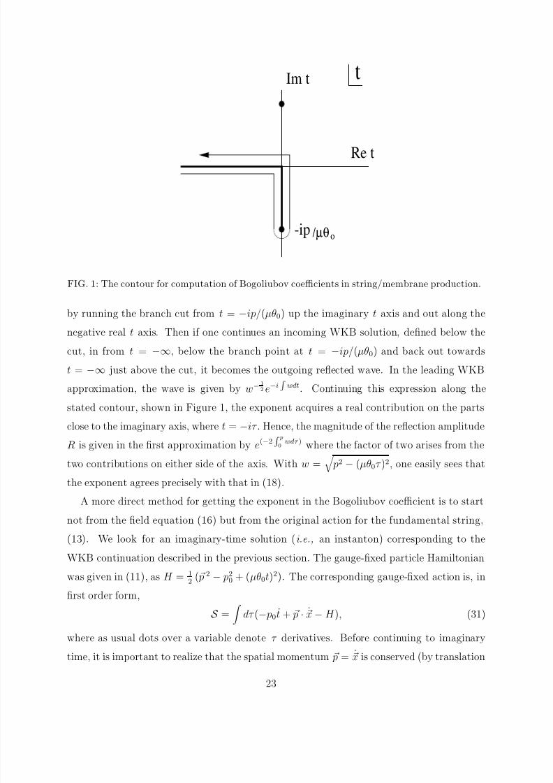
FIG. 1: The contour for computation of Bogoliubov coefficients in string/membrane production.

by running the branch cut from t = −ip/(µθ0) up the imaginary t axis and out along the

negative real t axis. Then if one continues an incoming WKB solution, defined below the

cut, in from t = −∞, below the branch point at t = −ip/(µθ0) and back out towards

t = −∞ just above the cut, it becomes the outgoing reflected wave. In the leading WKB

approximation, the wave is given by w− 1

2 e−i wdt. Continuing this expression along the

stated contour, shown in Figure 1, the exponent acquires a real contribution on the partsclose to the imaginary axis, where t = −iτ . Hence, the magnitude of the reflection amplitude

R is given in the first approximation by e(−2 p0wdτ ) where the factor of two arises from the

two contributions on either side of the axis. With w =

p2 − (µθ0τ )2, one easily sees that

the exponent agrees precisely with that in (18).

A more direct method for getting the exponent in the Bogoliubov coefficient is to start

not from the field equation (16) but from the original action for the fundamental string,

(13). We look for an imaginary-time solution (i.e., an instanton) corresponding to the

WKB continuation described in the previous section. The gauge-fixed particle Hamiltonian

was given in (11), as H = 12 ( p 2 − p20 + (µθ0t)2). The corresponding gauge-fixed action is, in

first order form,

S =

dτ (− p0t + p · x − H ), (31)

where as usual dots over a variable denote τ derivatives. Before continuing to imaginary

time, it is important to realize that the spatial momentum p = x is conserved (by translation

23



invariance). Hence, all states, and in particular the asymptotic states we want, are labeled

by p. We are are interested in the transition amplitude for fixed initial and final p, not x,

and we must use the appropriate action which is not (31), but rather

S =

dτ (− p0t −˙ p · x − H ), (32)

related by an integration by parts. The p · x term contributes only a phase in the Euclidean

path integral (because p remains real) and the x integration produces a delta function

for overall momentum conservation. Notice that if we instead had used the naive action dτ 1

2x 2, we would have obtained a p 2 term in the Euclidean action of the opposite sign.

Similar considerations have been noted elsewhere [30].

Now we continue the action (32) to imaginary time, setting t = −itE and τ = −iτ E .

Eliminating p0, the Euclidean action S E ≡ −iS ) is found to be

S E =

dτ E

1

2

t2E − (µθ0tE )

2 + p 2

+ i p · x

. (33)

where dots now denote derivatives with respect to τ E . The amplitude we want involves tE

running from 0 to | p | and back again: (33) is just the action for a simple harmonic oscillator

and the required instanton is tE = p cos(µθ0τ E ), −π/2 < µθ0τ E < π/2. The corresponding

Euclidean action is

S E = π

2

p 2

µθ0, (34)

giving precisely the exponent in (18).

Now we wish to apply this method to calculating the production of winding membrane

states, described by the action (30). As in the case of analogous calculations of vacuum

bubble nucleation within field theory [31], it is plausible that objects with the greatest

symmetry are produced since non-symmetrical deformations will generally yield a larger

Euclidean action. Therefore one might guess that the dominant production mechanism is

the production of circular loops. Let us start by considering this case. The constraint

πµxµ = 0 implies that the plane of such loops must be perpendicular to their center of

mass momentum pµ. As in the particle production process previously considered, loops

must be produced in pairs carrying equal and opposite momentum. The Hamiltonian for

such circular loops is straightforwardly found to be H = 12 ( p 2 + p2R − p20 + (2πRµθ0t)2),

Following the same steps that led to (33), we infer that the appropriate Euclidean action is

S E =

dτ E

1

2

t2E + R2 − (2πµ2θ0RtE )

2 + p 2

+ i p · x

. (35)

24



This action describes two degrees of freedom tE and R interacting via a positive potential

t2E R2. Up to the trivial symmetries tE → −tE , R → −R, there is only one classical solution

which satisfying the boundary conditions we want, namely starting and ending at tE = 0,

and running up to the zero of the WKB frequency function at 2πµθ0RtE =

| p

|. This solution

has T E = R and the Euclidean action is found to be

S E =(2| p |) 3

2

(2πµ2θ0)1

2

10

dx√

1 − x4. (36)

where the last integral is Γ[ 14

]2/(6√

2π), a constant of order unity which we shall denote I .

The Euclidean action grows like | p | 32 at large momentum: this means that the total

production of loops is finite. Neglecting a possible numerical pre-factor in the Bogoliubov

coefficient, we can estimate the number density of loops produced per unit volume,

n ∼

dd−1 p

(2π)d−1e−2S E = (µ2θ0)(d−1)/3 2

13−7d3 Γ(2(d − 1)/3)

3πd−16 I 2(d−1)/3Γ ((d − 1)/2)

(37)

where I is given above.

From the instanton solution, the characteristic size of the loops and the time when they

are produced are both of the same order, R ∼ |t| ∼ (| p |/µ2θ0)1

2 ∼ (µ2θ0)−1/3. The effective

string tension when they are produced is ∼ µ2θ0|t| ∼ (µ2θ0)2

3 .

We have restricted attention so far to the production of circular loops. It is also important

to ask whether long, irregular strings are also copiously produced. Even though such strings

would be disfavoured energetically, there is an exponentially large density of available states

which could in principle compensate. An estimate may be made along the lines of Ref. [29],

by simply replacing p 2 with p 2 + µ1N , where µ1 is the effective string tension and N is the

level number of the string excitations. This picture only makes sense for times greater than

the string time, so we use the tension at the string time, µ1 ∼ (µ2θ0)2/3. The density of

string states scales as e√N hence one should replace (37) with a sum over N :

∼ N

e√N

dd−1 p e−( p 2+µ1N )

3

4 /µ3

4

1

. (38)

The N 3

4 beats the√

N so the sum is dominated by modest N , indicating that the production

of long strings is suppressed. According to this result, the universe emerges at the string

time with of order one string-scale loop per string-scale volume, i.e. at a density comparable

to but below the Hagedorn density.

25



Another key question is whether gravitational back-reaction effects are likely to be sig-

nificant at the transition. As the universe fills with string loops, what is their effect on the

background geometry? We estimate this as follows. Consider a string loop of radius R in M

theory frame. Its mass M is 2πR times the effective string tension µ2L, where L is the size

of the extra dimension. The effective Einstein-frame gravitational coupling (the inverse of

the coefficient of R/2 in the Lagrangian density) is given by κ2d = κ2

d+1/L. The gravitational

potential produced by such a loop in d spacetime dimensions is[25]

Φ = −κ2d

M

((d − 2)Ad−2Rd−3 (39)

where AD is the area of the unit D-sphere, AD = 2πD+12 /Γ ((D + 1)/2). Specializing to the

case of interest, namely 2-branes in eleven-dimensional M theory, the tension µ2 is related

to the eleven dimensional gravitational coupling by a quantization condition relating to the

four-form flux, reading[26]

µ32 = 2π2/(nκ2

11) (40)

with n an integer. Equations (39) and (40) then imply that the typical gravitational potential

around a string loop is

Φ = − 105

64πµ22R6n

∼ −(µ22R6n)−1 ∼ −θ20/n (41)

up to numerical factors.

We conclude that the gravitational potential on the scale of the loops is of order θ20 and

therefore is consistently small for small collision rapidity. Since the mean separation of

the loops when they are produced is of order their size R, this potential Φ is the typical

gravitational potential throughout space. Multiplying the tt component of the background

metric (2) by 1 +2Φ and redefining t, we conclude that the outgoing metric has an expansion

rapidity of order ∼ θ0(1 + Cθ20) with C a constant of order unity. We conclude that for small

θ0 the gravitational back-reaction due to string loop production is small. Note that loop

production is a quantum mechanical effect taking place smoothly over a time scale of order

(µ2θ0)−1

3 . Therefore if the rapidity of the outgoing branes alters as we have estimated, it

happens smoothly and not like the jump in θ0 discussed at the end of section VI. Therefore

the picture of loop production is consistent with the comments made there.

26



X. STRINGS ON LORENTZIAN ORBIFOLDS ARE NOT REGULAR

We have shown that strings constructed as winding M2-branes on MC × R9 are analytic

in the neighborhood of t = 0. This was the setup originally envisaged in the ekpyrotic model,

where collapse of the M theory dimension was considered. Subsequently, a number of authors

investigated the simpler case of string theory on MC ×R8, considered as a Lorentzian orbifold

solution of ten dimensional string theory. This is a simpler, but different setting, hence we

expressed misgivings[12, 18] about drawing conclusions from these reduced models. We shall

now explain why the behavior in the Lorentzian orbifold models is significantly worse than

in M theory and, hence, why no negative conclusion should be drawn on the basis of the

failed perturbative calculations.

Consider string theory on the background (2). Let us choose the gauge x0

= t = τ , andgµν x

µxµ = 0. In this gauge we express the string solution as θ(t, σ) and x(t, σ). If a classical

solution in this gauge possesses a singularity at t = 0 in the complex t-plane, for all σ, then

there can be no choice of worldsheet coordinates τ and σ which can render the solution

analytic in the neighborhood of t = 0. For if such a choice existed, one could re-express τ in

terms of t and, hence, x(t, σ) would be analytic. We shall show that generically, for strings

on Lorentzian orbifolds, the solutions possess logarithmic singularities i.e., branch points,

rendering them ambiguous as one circumvents the singularity in the complex t-plane.

The demonstration is straightforward, and our argument is similar to that in earlier

papers[2]. We are only interested in the classical equations of motion and we may compute

the relevant Hamiltonian from the Nambu action,

H ≡

dσH =

dσ

π2θ

µt2+

π2

µ+ µ ((tθ)2 + x 2). (42)

The Hamiltonian equations allow generic solutions in which πθ(σ) tends to any function of σ

as t tends to zero. From its definition, the Hamiltonian density H then diverges as t−1

. Theequation of motion for θ is θ = πθ/(t2H), implying that θ → ±t−1 independent of σ. This

implies a leading term θ ∼ ±logt, independent of σ. Recalling that MC may be rewritten

in flat coordinates by setting T = t cosh θ and Y = t sinh θ, one readily understands this

behavior. A geodesic in the (T, Y ) coordinates is just Y = V T , with V a constant. At small

t this requires eθ or e−θ to diverge as t−1, which is just the result we found.

We conclude that generic solutions to the Hamiltonian equations possess branch points at

27



t = 0 meaning that the solutions to the classical equations are ambiguous as one continues

around t = 0 in the complex t-plane. This is a much worse situation that encountered for

winding branes in M theory.

The second problem occurs when we quantize and construct the associated field theory.

Then the bad behavior at t = 0 corresponds to a diverging energy density which renders

perturbation theory invalid. Since the previous problem can be seen even in pointlike states,

let us focus attention on those. As we discuss in detail in Appendix 4, one needs to use

the metric on the space of coordinates in order to construct the quantum Hamiltonian. In

this case, the metric on the space of coordinates is the background metric, (2). The field

equation for point particles is then given from (66): Fourier transforming with respect to x

and θ, it reads

φ + 1t φ = − k 2φ − k2

θt2 φ, (43)

where kθ is quantized in the usual way. This is the equation studied in earlier work[3] on

quantum field theory on MC × Rd−1. The generic solutions of (43) behave for small t as

log t for kθ = 0, or tikθ for kθ = 0. In both cases, the kinetic energy density φ2 diverges as

t−2. Similar behavior is found for linearized vector and tensor fields on MC × Rd−1. These

divergences lead to the breakdown of perturbation theory in classical perturbative gravity,

an effect which is plausibly the root cause of the bad behavior of the associated string theory

scattering amplitudes [13]. As we have stressed, in the sector of M theory considered as a

theory of membranes, describing perturbative gravity, this effect does not occur. The field

equations are regular in the neighbourhood of t = 0 and there is no associated divergence

in the energy density.

With hindsight, one can now see that directly constructing string theory on Lorentzian

orbifolds sheds little light on the M theory case of interest in the ekpyrotic and cyclic models.

Whilst the orbifolding construction provides a global map between incoming and outgoing

free fields, it does not avoid the blueshifting effect which such fields generically suffer as theyapproach t = 0, which seems to lead to singular behavior in the interactions (although Ref.

[14] argues that a resummation may cure this problem).

An alternate approach involving analytic continuation around t = 0 has been simul-

taneously developed, but so far only implemented successfully in linearized cosmological

perturbation theory[3, 12]. This method may in fact turn out to work even in the M theory

context. The point is that by circumnavigating t = 0 in the complex t-plane, maintaining

28



a sufficient distance from the singularity, one may still retain the validity of linear pertur-

bation theory and the use of the Einstein equations all the way along the complex time

contour. The principles behind this would be similar to those familiar in the context of

WKB matching via analytic continuation.

In any case, the main point we wish to make is that now that we have what seems like a

consistent microscopic theory for perturbative gravity, valid all the way through t = 0, we

have a reliable foundation for such investigations.

XI. CONCLUSIONS AND COMMENTS

We have herein proposed an M theoretic model for the passage through a cosmological

singularity in terms of a collision of orbifold planes in a compactified MilneM

C

×R9

background. The model begins with two empty, flat, parallel branes a string length apart

approaching one another at constant rapidity θ0. With this initial condition, we have argued

that the excitations naturally bifurcate into light winding M2-brane modes, and a set of

massive modes including the Kaluza-Klein massive states. It is plausible that the massive

modes decouple as their mass diverges. The light modes incorporate perturbative gravity

and, hence, describe the space-time throughout the transition. Our finding that they are

produced with finite density following dynamical equations that propagate smoothly through

the transition supports the idea that this M-theory picture is well-behaved and predictive.

Our model also suggests a string theory explanation of what goes wrong with Einstein

gravity near the singularity: Einstein gravity is the leading approximation in an expansion

in α, but the winding mode picture is a perturbative expansion in 1/α.

Our considerations have been almost entirely classical or semi-classical, although we

believe the canonical approach we have adopted is a good starting point for a full quantum

theory. Much remains to be done to fully establish the consistency of the picture we are

advocating. In particular, we need to understand the sigma model in (46), and make sure

that it is consistent quantum mechanically in the critical dimension. Second, we need to

learn how to match the standard α expansion to the 1/α expansion which we have argued

should be smooth around t = 0. Third, we need to incorporate string interactions. Although

the vanishing of the string theory coupling around t = 0 suggests that scattering plays a

minor role, the task of fully constructing string perturbation theory in this background

29



remains.

Assuming these nontrivial tasks can be completed, can we say something about the

significance of this example? The most obvious application is to the cyclic and ekpyrotic

universe models which motivated these investigations, and which produce precisely the initial

conditions required. As has been argued elsewhere [1, 8], the vicinity of the collision is

well-modeled by compactified Milne times flat space. Within this model, the calculations

reported here yield estimates of the reheat temperature immediately after the brane collision

i.e. at the beginning of the hot big bang. Furthermore, if our arguments of Section VIII are

correct, they should in principle provide complete matching rules for evolving cosmological

perturbations through singularities of the type occurring in cyclic/ekpyrotic models. As we

discussed briefly in Section X, it is plausible that this matching rule will recover the results

obtained earlier for long-wavelength modes by the analytic continuation method [3, 12],

although that remains to be demonstrated in detail.

Many other questions are raised by our work. Can we extend the treatment to other

time-dependent singularities? The background considered here, MC × R9 is certainly very

special being locally flat. Although the string frame metric is singular, it is conformally flat.

One would like to study more generic string backgrounds corresponding to black holes, or

Kasner/mixmaster spacetimes in general relativity. As we have argued, there is no reason to

take the latter solutions seriously within M theory since they are only solutions of the lowenergy effective theory, which fails in the relevant regime. Nevertheless, they presumably

have counterparts in M theory, and it remains a challenge to find them. We would like

to believe that by constructing one consistent example, namely M theory on MC × R9 we

would be opening the door to an attack on the generic case.

Such a program is admittedly ambitious. However, should it succeed, we believe it would

(and should) completely change our view of cosmology. If the best theories of gravity allow

for a smooth passage through time-dependent singularities, this must profoundly alter our

interpretation of the big bang, and of the major conceptual problems of the standard hot

big bang cosmology.

Acknowledgments We would like to thank L. Boyle, S. Gratton, S. Gubser, G.

Horowitz, S. Kachru, I. Klebanov, F. Quevedo, A. Tolley and P. Townsend for helpful

remarks. This work was supported in part by PPARC, UK (NT and MP) and the US

Department of Energy grants DE-FG02-91ER40671 (PJS). PJS is the Keck Distinguished

30



Visiting Professor at the Institute for Advanced Study with support from the Wm. Keck

Foundation and the Monell Foundation and NT is the Darley Professorial Fellow at Cam-

bridge.

Appendix 1: Canonical Treatment of p-Branes in Curved Space

In this Appendix we review the canonical treatment of p-Brane dynamics in curved space.

A similar approach is taken in the recent work of Capovilla et al. [32]. Earlier treatments

include Refs. [33] and [34].

We start from the action in Polyakov form. No square roots appear and the ensuing gen-

eral Hamiltonian involves only polynomial interactions. The action for a p-brane embedded

in a background space-time with coordinates xµ and metric gµν is:

S = −1

2µ p

d p+1σ

√−γ

γ αβ ∂ αxµ∂ β xν gµν − ( p − 1)

, (44)

where µ p is a mass per unit p-volume. The p-brane worldvolume has coordinates σα, α =

0, 1, . . . , p in which the metric is γ αβ .

One way to proceed is to vary (44) with respect to γ αβ , hence, obtaining the constraint

expressing the worldvolume metric γ αβ in terms of the the induced metric ∂ αxµ∂ β xν gµν .

Substituting back into (44) one obtains the Nambu action for the embedding coordinates

xµ(σ) i.e., −µ p times the induced p-brane world volume.

One can do better, however, by not eliminating the worldvolume metric so soon. Instead it

is better to retain the γ αβ as independent variables and derive the corresponding Hamiltonian

and constraints corresponding to evolution in worldvolume time τ . It is convenient to express

γ αβ in the form frequently used in canonical general relativity: the worldsheet line element

is written

γ αβ dσ

α

dσ

β

= (−α

2

+ β kβ

k

)dτ

2

+ 2β idτdσ

i

+ γ ijdσ

i

dσ

j

, (45)

where σi, i = 1, . . . , p are the spatial worldvolume coordinates, β k is the shift vector and α is

the lapse function. The good property of this representation is that the metric determinant

simplifies: γ = −α2γ .

In the following discussion we shall for the most part assume p > 1 and then comment

31



on the amendments needed for p = 0, 1. Using (45) the action (44) becomes

S = −1

2µ p

dτ d pσαγ

1

2

− 1

α2xµxν gµν + 2

β i

α2xµxν ,igµν + (γ ij − β iβ j

α2)xµ,ix

ν ,jgµν − ( p − 1)

.

(46)

The canonical momenta conjugate to xµ are found to be

πµ = µ pγ

1

2

α(xν − β ixν ,i)gµν . (47)

No time derivatives of α, β i and γ ij appear in the Lagrangian, hence, the corresponding

conjugate momenta vanish. In Dirac’s language [19], these are the primary constraints.

πα ≈ 0, πi ≈ 0, πij ≈ 0. (48)

Since Poisson brackets between momenta vanish, these constraints are first class. The totalHamiltonian H then consists of the usual expression H ≡

d pσ [πAxA − L],

H =

d pσ

α

2µ pγ 1

2

πµπν gµν + β ixµ,iπµ +

µ pαγ 1

2

2

γ ijxµ,ix

ν ,jgµν − ( p − 1)

, (49)

plus an arbitrary linear combination of the primary first class constraints (48).

Additional secondary constraints are obtained from the Hamiltonian equations for πα, πi

and πij . Insisting these vanish as they must for consistency with (48), one finds

C ≡ πµπν gµν + µ2

pγ

γ ijxµ,ixν ,jgµν − ( p − 1)

≈ 0,

C i ≡ xµ,iπµ ≈ 0,

C ij ≡ γ ij − xµ,ixν ,jgµν ≈ 0. (50)

Following Dirac’s procedure, we can now try to eliminate variables using second class con-

straints (constraints whose Poisson brackets with the other constraints does not vanish).

In particular, it makes sense to eliminate γ ij since the corresponding momenta πij vanish

weakly. It is easy to see that C ij are second class since their Poisson brackets with πij arenonzero. Hence, we eliminate γ ij using the C ij constraint, obtaining


pDet(xµ,ixν ,jgµν ) ≈ 0, C i ≡ xµ,iπµ ≈ 0, (51)

as our new constraints, on the remaining variables xµ and πµ. The matrix xµ,ixν ,jgµν is the

induced spatial metric on the brane. When written this way, the C and C i constraints

have zero Poisson brackets with the remaining primary constraints πα and πi. A lengthy

32



but straightforward calculation establishes that all Poisson brackets between C and C i are

weakly vanishing (see Appendix 2) and, hence, that we have a complete set of first class

constraints consisting of πα, πi, C i and C .

The canonical Hamiltonian (49) is now seen to be a linear combination of C and C i, with

coefficients depending on α and β i respectively. The general Hamiltonian consists of a sum of

this term plus an arbitrary linear combination of the first class constraints,

dσ(vαπα+viπi)

where vα and vi are arbitrary functions of the worldvolume coordinates. From Hamilton’s

equations, one infers that α = vα, and β i = vi. Therefore, α and β are completely arbitrary

functions of time. As Dirac emphasizes, one can then forget about α, πα, β i and πi and just

write the total Hamiltonian for the surviving coordinates as xµ and πµ as

H =

d

p

σA

2

πµπν g

µν

+ µ

2

pDet(x

µ

,ix

ν

,jgµν )

+ A

i

x

µ

,iπµ

, (52)

i.e. a linear combination of the constraints (51) with arbitrary coefficients A and Ai. Dif-

ferent choices of A and Ai then correspond to different choices of worldvolume coordinates.

We count the surviving physical degrees of freedom as follows. We start with the 2( d + 1)

coordinates xµ and momenta πµ, each functions of the p + 1 worldvolume coordinates. Then

we impose the p + 1 constraints C = C i = 0. Finally, in order to specify time evolution we

must pick p + 1 arbitrary functions A and Ai. The remaining physical degrees of freedom

are 2(d + 1) − 2( p + 1) = 2(d − p) in number, the right number of transverse coordinatesand momenta for the p-brane.

We have tacitly assumed p > 1 in the above analysis. The following minor amendments

are needed for p = 0 and 1. For p = 0, the worldvolume metric involves α only and one

can ignore anything with an i index except the determinant, which is replaced by unity. In

particular there is no integration over σ in the Hamiltonian, and the canonical momentum

density πµ is replaced by the momentum pµ. The only constraint is

C ≡ pµ pν gµν + µ20 ≈ 0, (53)

which is just the usual mass shell condition. The general Hamiltonian consists of an arbitrary

function of τ times C .

For p = 1 the action (44) is invariant under conformal transformations of the worldvolume

metric, and hence only two independent combinations of the three worldvolume metric

variables appear in the decomposition (45). The corresponding two momenta vanish and

33



these are the primary constraints. Through Hamilton’s equations one finds the following

secondary constraints:


1xµxν gµν ≈ 0,

C 1 ≡ πµxµ ≈ 0, (54)

where primes denote derivatives with respect to σ1 ≡ σ. The general Hamiltonian again

takes the form (52), with p = 1.

Appendix 2: Poisson bracket algebra of the constraints

In the canonical theory [19], one considers arbitrary functions of the canonical variables,

and of the time τ . In our case, the canonical variables are fields xµ(σ) and πµ(σ) depending

upon σ, which is regarded as a continuous index labeling an infinite number of canonical

variables. In particular, the constraints in (51) are infinite in number. In this Appendix we

shall show that the Poisson bracket algebra of the constraints closes, and, hence, that, in

Dirac’s terminology, they are first class.

The Poisson bracket between any two quantities M and N , which may be arbitrary

functions of the canonical variables (local or nonlocal in σ) and of the time τ , is given by

M, N ≡ d p

σ ∂M

∂xµ(σ)

∂N

∂πµ(σ) −∂N

∂xµ(σ)

∂M

∂πµ(σ)

, (55)

where (∂xµ(σ)/∂xν (σ)) = (∂πν (σ)/∂πµ(σ)) = δµν δ p(σ − σ), with other partial derivatives

being zero.

One way to calculate the Poisson brackets between a set of constraints C and C i, is to

start from a putative Hamiltonian

H =

d pσ(A

2C + AiC i), (56)

where A and Ai are arbitrary functions of σ, and then compute Hamilton’s equations for the

τ derivatives of xµ and πµ. We then use these to determine the corresponding τ derivatives

of C and C i. Setting these equal to C, H and C i, H with H given by (56), we are able

to infer the Poisson brackets between the constraints. For the Hamiltonian (56) with C and

C i given in (51), Hamilton’s equations read

xµ = Agµν πν + Aixµ,i

34



πµ = (Aiπµ),i − 1

2Agλν ,µπλπν + µ2

p(Aγ γ ijxν ,j),igµν + µ2 pAgµν Γ

ν λγ γ ijxλ,ix

,j , (57)

where dots denote τ derivatives and γ ij = xµ,ixν ,jgµν is the induced spatial metric on the

brane and γ its determinant. We have made use of the formula dγ = γ γ ijdγ ij .

Using (57), it is a matter of straightforward algebra to compute C and C i and hence infer

all of the Poisson brackets. We find

C (σ), C (σ) =

(8µ2

pγ γ ijC j)(σ)∂

∂σi+ 4µ2

p(γ γ ijC j),i(σ)

δ p(σ − σ)

C (σ), C i(σ) =

2C (σ)

∂

∂σ i+ C ,i(σ)

δ p(σ − σ)

C i(σ), C j(σ) =

C i(σ)

∂

∂σ j+ C j(σ)

∂

∂σi+

∂C i∂σ j

(σ)

δ p(σ − σ). (58)

The right hand side consists of linear combinations of the constraints and, hence, it vanishes

weakly. We conclude that the constraint algebra closes and, hence that the constraints are

first class. Notice that the case of strings, p = 1, is specially simple since γ γ 11 = 1 and the

Poisson bracket algebra is linear, with field-independent structure constants.

The calculation also provides a consistency check on our Hamiltonian (9), which is pre-

cisely of the form (56), since it implies the constraints are preserved under time evolution

in τ .

Appendix 3: Equivalence of gauge-fixed Hamiltonian and Lagrangian equations

In this Appendix we establish that the Lagrangian equations following from the gauge-

fixed action (30) for winding M 2-branes are equivalent to the Lagrangian equations for

a string in the time-dependent background gµν = |t|ηµν , in a certain string worldsheet

coordinate system. This is in accord with our general arguments.

The equations of motion following from the gauge-fixed action (30) are:

x = t2x + 2tt x

t = tx 2 + tt2

+ tt2. (59)

and the constraints take the form

tt = x · x ; t2 = x 2 + t2(x 2 − t2). (60)

35



We want to compare these equations with the Lagrangian equations of motion following

from the Polyakov action (6), with p = 1. These are

∂ τ ((−γ )1

2 γ ττ ∂ τ xµ) + ∂ σ((−γ )

1

2 γ σσ∂ σxµ)

+(−γ )

1

2

Γµ

νλ(γ ττ

∂ τ xν

∂ τ xλ

+ γ σσ

∂ σxν

∂ σxλ

) = 0, (61)

where Γµνλ is the Christoffel symbol for the background metric.

We also have the constraints that the worldsheet metric γ αβ is conformal to the induced

metric on the string. We have the freedom to choose worldsheet coordinates on the string,

but since the equations are conformally invariant, only the conformal class matters. The

choice γ αβ = Ω2diag(−t2, 1) is found to yield the two constraints (60).

For our background, gµν = |t|ηµν , we have nonzero Christoffel symbols Γ000 = 1/(2t),

Γi j0 = Γ

i0 j = δij/(2t), Γ

0ij = δij/(2t), where i runs over the background spatial indices 1 to

d − 1. The string equations of motion (61) are then found to be equivalent to (59), for all

nonzero t.

From the string point of view, this choice of gauge would seem arbitrary, and indeed it

would appear to be degenerate at t = 0. Yet, as we have seen, this gauge choice is just

A = 1 and Ai = 0, which is entirely natural from the canonical point of view. It has the

desirable property that the equations of motion and the constraints are regular at t = 0, and

from the general properties of the canonical formalism we are guaranteed the existence of

an infinite class of coordinate systems, related by nonsingular coordinate transformations,

in which the equations of motion will remain regular.

Appendix 4: Ordering ambiguities and their resolution for relativistic particles

In the main text we have discussed the canonical Hamiltonian treatment of relativistic

particles and p-branes. When one comes to quantize these theories in a general back-

ground, certain ordering ambiguities appear which must be resolved. Here we provide abrief overview, following the more comprehensive discussion in Ref. [15].

The field equation for a relativistic particle is simply the expression of the quantum

Hamiltonian constraint H = 0, in a coordinate space representation. The first task is to

determine the representation of the momentum operator pµ in this representation, and then

that of the Hamiltonian operator H . As we shall now discuss, this requires knowledge of

the metric on the space of coordinates. We shall only deal with the point particle case.

36



The classical Hamiltonian constraint for a massive particle in a background metric gµν

reads

gµν pµ pν + m2 ≈ 0. (62)

First we attempt to determine the coordinate space representation of pµ, consistent with thequantum bracket:

[xµ, pν ] = ihδµν . (63)

One choice is pµ = −ih∂ µ but this is not unique: the representation pµ = −ih(∂ µ + f µ), with

f µ any function of the coordinates xµ and τ , is equally good as far as (63) is concerned.

We now show how f µ may be determined from the additional requirement that pµ be

hermitian i.e., that the momentum be real. In the coordinate space representation, this

requirement reads

χ| pµ|φ ≡

ddx(−g(x))1

2 (χ∗ pµφ) = φ| pµ|χ∗ ≡

ddx(−g(x))1

2 (φ∗ pµχ)∗ (64)

where the integration runs over the space of coordinates and gµν is the metric on that space.

It is straightforward to check that the naive operator −ih∂ µ is in fact not hermitian for

general gµν , but that

pµ = −ih∂ µ +1

4(∂ µ ln(−g)) = −ih(−g)−

1

4 ∂ µ(−g)1

4 (65)

is. This discussion uniquely determines the real part of f µ: an imaginary part may be

absorbed in an unobservable phase of the wavefunction[15].

Similarly, when we consider the Hamiltonian constraint (62), the questions arise of where

to place the gµν relative to the pµ’s, and whether to include any factors of the metric deter-

minant g. The resolution is familiar: if we write the Hamiltonian in covariant derivatives on

the space of coordinates, it will be hermitian since we can integrate by parts ignoring the√

−g factor in the measure. This suggests setting the first term in (62) equal to the scalar

Laplacian:

gµν pµ pν → −h2(−g)−1

2 ∂ µ(−g)1

2 gµν ∂ µ = (−g)−1

4 pµ(−g)1

2 gµν pν (−g)−1

4 . (66)

It is straightforward to check that this is the only choice of ordering and powers of ( −g)

which is hermitian and has the correct classical limit. Nevertheless, this ordering is not

immediately apparent! More generally, one can also include terms involving commutators of

37



pµ which are zero in the classical limit, but which produce the Ricci scalar R in the quantum

Hamiltonian[15]. In the space-time we consider R is zero. Hence, such terms do not arise.

[1] J. Khoury, B.A. Ovrut, N. Seiberg, P.J. Steinhardt and N. Turok, Phys. Rev. D65, 086007

(2002).

[2] G.T. Horowitz and A.R. Steif, Phys. Rev. D42 (1990) 1950; Phys. Lett. B258 (1991) 91.

[3] A.J. Tolley and N. Turok, Phys. Rev. D66 (2002) 106005.

[4] J. Khoury, B. A. Ovrut, P. J. Steinhardt, and N. Turok, Phys. Rev. D66, 046005 (2002).

[5] P. S. Aspinwall, B. R. Greene and D. R. Morrison, hep-th/9309097, Nucl. Phys. B 416, 414

(1994); E. Witten, hep-th/9301042, Nucl. Phys. B 403, 159 (1993).

[6] J. Khoury, B.A. Ovrut, P.J. Steinhardt, and N. Turok, Phys. Rev. D64, 123522 (2001).

[7] P.J. Steinhardt and N. Turok, Science 296, 1436 (2002); Phys. Rev. D65, 126003 (2002).

[8] P.J. Steinhardt and N. Turok, astro-ph/0404480.

[9] J.K. Erickson, D.H. Wesley, P.J. Steinhardt, and N. Turok, Phys. Rev. D69, 063514 (2004).[10] P. Horava and E. Witten, Nucl. Phys. B460 (1996) 506; B475 (1996) 94.

[11] A. Lukas, B.A. Ovrut and D. Waldram, Nucl. Phys. B495 (1997) 365.

[12] A.J. Tolley, N. Turok and P. J. Steinhardt, Phys. Rev. D69, 106005 (2004).

[13] H. Liu, G. Moore and N. Seiberg, JHEP 0206 (2002) 045; JHEP 0210 (2002) 031; O. Aharony,

M. Fabinger, G. Horowitz and E. Silverstein, hep-th/0204158; M. Fabinger and J. Mc-

Greevy, hep-th/0206196; M. Fabinger and S. Hellerman, hep-th/0212223; G.T. Horowitz and

J. Polchinski, Phys. Rev. D66 (2002) 103512; L. Cornalba and M.S. Costa, Phys. Rev. D66

(2002) 066001; L. Cornalba, M.S. Costa and C. Kounnas, Nucl. Phys. B637 (2002) 378;

L. Cornalba and M.S. Costa, hep-th/0302137.

[14] L. Cornalba and M.S. Costa, hep-th/0310099.

[15] B. S. DeWitt, Rev. Mod. Phys. 29, 377 (1957); in Relativity, Groups and Topology , LesHouches lectures (1963), Gordon and Breach, New York, 1964.

[16] C. Bachas, Phys. Lett. B374 37 (1996), hep-th/9511043.

[17] M. Berkooz and B. Pioline, JCAP 0311 (2003) 007, hep-th/0307280; M. Berkooz, B. Pioline

and M. Rozali, hep-th/0405126.

[18] N. Turok, in The Future of Theoretical Physics and Cosmology : Celebrating Stephen Hawk-

ing’s 60th Birthday , eds. G.W. Gibbons, E.P.S. Shellard and S.J. Rankin, Cambridge Univer-

sity Press, 2003.

[19] P.A.M. Dirac, Lectures on Quantum Mechanics, Belfer Graduate School of Science Mono-

graphs Series, New York, 1964.

[20] M. Abramowitz and I.A. Stegun, Handbook of Mathematical Functions, Dover, New York,1970, page 686.

[21] See e.g. N. D. Birrell and P. C. W. Davies, Quantum Fields in Curved Space-time, CUP, 1982.

[22] E. Witten, Nucl. Phys. B471 (1996) 135; Nucl. Phys. B443 (1995) 85.

[23] H.J. de Vega, I. Giannakis, A. Nicolaidis, Mod. Phys. Lett. A10 2479 (1995); I. Antoniadis

and G. Savvidy, hep-th/0402077 and references therein.

[24] A. Nicolaidis, J.E. Paschalis, P.I. Porfyriadis, Phys. Rev. D58 047901 (1998); hep-th/9702185

[25] G.W. Gibbons and K. Maeda, Nucl. Phys. B298 741 (1988).

[26] M.J. Duff, TASI Lectures, hep-th/9912164.

38



[27] J. Heading, Phase Integral Methods, Methuen Physical Monographs, London, 1962, page 85.

[28] A. E. Lawrence and E. Martinec, Class. Quant. Grav. 13 (1996) 63; hep-th/9509149.

[29] S. S. Gubser, hep-th/0305099.

[30] K. Lee, Phys. Rev. Lett., 61 (1988) 263; S. Coleman and K. Lee, Nuc. Phys. B329 (1990)

387.

[31] S. Coleman, Phys. Rev. D15, 2929 (1977); C. G. Callan Jr. and S. Coleman, Phys. Rev. D16,1762 (1977).

[32] R. Capovilla, J. Guven and E. Rojas, hep-th/0404178; Nucl. Phys. Proc. Suppl. 88 337 (2000).

[33] J.A. Azcarraga, J.M. Izquierdo and P.K. Townsend, Phys. Lett. B267 366 (1991); Phys. Rev.

D45 3321 (1992).

[34] J. Gutowski, G. Papadopoulos and P.K. Townsend, Phys.Rev. D60 106006 (1999), hep-

th/9905156.

neil turok, malcolm perry and paul j. steinhardt- m theory model of a big crunch/big bang transition

Documents