nested kriging predictions for datasets with large number of … · 2020-04-05 · nested kriging...
TRANSCRIPT
HAL Id: hal-01345959https://hal.archives-ouvertes.fr/hal-01345959v3
Submitted on 20 Jul 2017
HAL is a multi-disciplinary open accessarchive for the deposit and dissemination of sci-entific research documents, whether they are pub-lished or not. The documents may come fromteaching and research institutions in France orabroad, or from public or private research centers.
L’archive ouverte pluridisciplinaire HAL, estdestinée au dépôt et à la diffusion de documentsscientifiques de niveau recherche, publiés ou non,émanant des établissements d’enseignement et derecherche français ou étrangers, des laboratoirespublics ou privés.
Nested Kriging predictions for datasets with largenumber of observations
Didier Rullière, Nicolas Durrande, François Bachoc, Clément Chevalier
To cite this version:Didier Rullière, Nicolas Durrande, François Bachoc, Clément Chevalier. Nested Kriging predictionsfor datasets with large number of observations. Statistics and Computing, Springer Verlag (Germany),2018, 28 (4), pp.849-867. �10.1007/s11222-017-9766-2�. �hal-01345959v3�

Nested Kriging predictions for datasets with large number ofobservations
Didier Rullière∗, Nicolas Durrande†, François Bachoc‡ and Clément Chevalier§.
Thursday 20th July, 2017
AbstractThis work falls within the context of predicting the value of a real function at some input loca-
tions given a limited number of observations of this function. The Kriging interpolation technique(or Gaussian process regression) is often considered to tackle such a problem but the method suffersfrom its computational burden when the number of observation points is large. We introduce inthis article nested Kriging predictors which are constructed by aggregating sub-models based onsubsets of observation points. This approach is proven to have better theoretical properties thanother aggregation methods that can be found in the literature. Contrarily to some other methodsit can be shown that the proposed aggregation method is consistent. Finally, the practical interestof the proposed method is illustrated on simulated datasets and on an industrial test case with 104
observations in a 6-dimensional space.
Keywords: Gaussian process regression · big data · aggregation methods · best linear unbiasedpredictor · spatial processes.
1 IntroductionGaussian process regression models have proven to be of great interest in many fields when it comes
to predict the output of a function f : D → R, D ⊂ Rd, based on the knowledge of n input-outputtuples (xi, f(xi)) for 1 ≤ i ≤ n [Stein, 2012, Santner et al., 2013, Williams and Rasmussen, 2006].One asset of this method is to provide not only a mean predictor but also a quantification of themodel uncertainty. The Gaussian process regression framework uses a (centered) real-valued Gaussianprocess Y over D as a prior distribution for f and approximates it by the conditional distribution of Ygiven the observations Y (xi) = f(xi) for 1 ≤ i ≤ n. In this framework, we denote by k : D ×D → R
the covariance function (or kernel) of Y : k(x, x′) = Cov [Y (x), Y (x′)], and by X ∈ Dn the vector ofobservation points with entries xi for 1 ≤ i ≤ n.
In the following, we use classical vectorial notations: for any functions f : D → R, g : D ×D → R
and for any vectors A = (a1, . . . , an) ∈ Dn and B = (b1, . . . , bm) ∈ Dm, we denote by f(A) then × 1 real valued vector with components f(ai) and by g(A,B) the n × m real valued matrix withcomponents g(ai, bj), i = 1, . . . , n, j = 1, . . . ,m. With such notations, the conditional distribution ofY given the n× 1 vector of observations Y (X) is Gaussian with mean, covariance and variance:
Mfull(x) = E [Y (x)|Y (X)] = k(x,X)k(X,X)−1Y (X) ,cfull(x, x′) = Cov
[Y (x), Y (x′)|Y (X)
]= k(x, x′)− k(x,X)k(X,X)−1k(X,x′) ,
vfull(x) = cfull(x, x) .(1)
∗Université de Lyon, Université Claude Bernard Lyon 1, ISFA, Laboratoire SAF, EA2429, 50 avenue Tony Garnier,69366 Lyon, France, [email protected].†Corresponding author, Mines Saint-Étienne, H. Fayol Institute, 158 cours Fauriel, Saint-Étienne, France and CNRS
LIMOS, UMR 5168, [email protected].‡Institut de Mathématiques de Toulouse, Université Paul Sabatier, 118 route de Narbonne, 31062 Toulouse, France,
[email protected].§Institute of Statistics, University of Neuchâtel, avenue de Bellevaux 51, 2000 Neuchâtel, Switzerland,
1

Since we do not specify yet the values taken by Y at X, the “mean predictor” Mfull(x) is randomso it is denoted by an upper-case letter M . The approximation of f(x) given the observations f(X)is thus given by mfull(x) = E [Y (x)|Y (X) = f(X)] = k(x,X)k(X,X)−1f(X). This method is quitegeneral since an appropriate choice of the kernel allows to recover the models obtained from variousframeworks such as linear regression and splines models [Wahba, 1990].
One limitation of such models is the computational time required for building models based ona large number of observations. Indeed, these models require computing and inverting the n × ncovariance matrix k(X,X) between the observed values Y (X), which leads to a O(n2) complexity inspace and O(n3) in time. In practice, this computational burden makes Gaussian process regressiondifficult to use when the number of observation points is in the range [103, 104] or greater.
Many methods have been proposed in the literature to overcome this limit. Let us first mentionthat, when the observations are recorded on a regular grid, choosing a separable covariance functionk enables to drastically simplify the inversion of the covariance matrix k(X,X), since the latter canbe written as a Kronecker product. In the same context of gridded data, alternative approaches suchas Gaussian Markov Random Fields are also available [Rue and Held, 2005].
For irregularly spaced data, a common approach in machine learning relies on inducing points.It consists in introducing a set W of pseudo input points and in approximating the full conditionaldistribution Y (x)|Y (X) by Y (x)|Y (W ). The challenge here is to find the best locations for the inducinginputs and to decide which values should be assigned to the outputs at W . Various methods aresuggested in the literature to answer these questions [Guhaniyogi et al., 2011, Hensman et al., 2013,Katzfuss, 2013, Zhang et al., 2015]. One drawback of this kind of approximation is that the predictionsdo not interpolate the observation points any more. Note that this method has recently been combinedwith the Kronecker product method in [Nickson et al., 2015].
Other methods rely on low rank approximations or compactly supported covariance functions. Bothmethods show limitations when the scale dependence is respectively short and large. For more detailsand references, see [Stein, 2014, Maurya, 2016, Bachoc et al., 2017]. Another drawback – which tothe best of our knowledge is little discussed in the literature – is the difficulty to use these methodswhen the dimension of the input space is large (say larger than 10, which is frequent in computerexperiments or machine learning).
Let us also mention that the computation of k(X,X)−1y, for an arbitrary vector y ∈ Rn can be per-formed using iterative algorithms, like the preconditionned conjugate gradient algorithm[Golub and Van Loan, 2012]. Unfortunately, the algorithms need to be run many times when a pos-terior variance – involving the computation of k(X,X)−1k(X,xi) – needs to be computed for a largeset of prediction points.
The method proposed in this paper belongs to the so-called “mixture of experts” family. Thelatter relies on the aggregation of sub-models based on subsets of the data which make them easy tocompute. This kind of methods offers a great flexibility since it can be applied with any covariancefunction and in large dimension while retaining the interpolation property. Some existing “mixture ofexperts” methods are product of experts [Hinton, 2002], and the (robust) Bayesian committee machine[Tresp, 2000, Deisenroth and Ng, 2015]. All these methods are based on a similar approach: for a givenpoint x, each sub-model provides its own prediction (a mean and a variance) and these predictions arethen merged into one single mean and prediction variance. The differences between these methods liein how to aggregate the predictions made by each sub-model. It shall be noted that aggregating expertopinions is the topic of consensus statistical methods (sometimes referred to as opinion synthesis oraveraging methods), where probability distributions representing expert opinions are joined together.Early references are [Winkler, 1968, Winkler, 1981]. A detailed review and an annotated bibliographyis given in [Genest and Zidek, 1986] (see also [Satopää et al., 2016, Ranjan and Gneiting, 2010] for
2
recent related developments). From a probabilistic perspective, usual mixture of experts methodsassume that there is some (conditional) independence between the sub-models. Although this kindof hypothesis leads to efficient computations, it is often violated in practice and may lead to poorpredictions as illustrated in [Samo and Roberts, 2016]. Furthermore, these methods only providepointwise confidence intervals instead of a full Gaussian process posterior distribution.
Since our method is part of the mixture of experts framework, it benefits from the properties of themixture of experts techniques: it does not require the data to be on a grid, the predictions can inter-polate the observations and it can be applied to data with small or large scale dependencies regardlessof the input space dimension. Compared to other mixtures of experts, we relax the usually madeindependence assumption so that the prediction takes into account all n2 pairwise cross-covariancesbetween observations. We show that this addresses two main pitfalls of usual mixture of experts. First,the predictions are more accurate. Second, the theoretical consistency is ensured whereas it is not thecase for the product of experts and the Bayesian committee machine methods. The detailed proofs ofthe later are out of the scope of this paper and we refer the interested reader to [Bachoc et al., 2017]for further details. The proposed method remains computationally affordable: predictions are per-formed in a few seconds for n = 104 and a few minutes for n = 105 using a standard laptop and theproposed online implementation. Finally, the prediction method comes with a naturally associatedinference procedure, which is based on cross validation errors.
The proposed method is presented in Section 2. In Section 3, we introduce an iterative scheme fornesting the predictors derived previously. A procedure for estimating the parameters of models is thengiven in Section 4. Finally, Section 5 compares the method with state-of-the-art aggregation methodson both a simulated dataset and an industrial case study.
2 Pointwise aggregation of expertsLet us now address in more details the framework of this article. The method is based on the
aggregation of sub-models defined on smaller subsets of points. Let X1, . . . , Xp be subvectors of thevector of observations input points X, it is thus possible to define p associated sub-models (or experts)M1, . . . , Mp. For example, the sub-model Mi can be a Gaussian process regression model based ona subset of the data
Mi(x) = E [Y (x)|Y (Xi)] = k(x,Xi)k(Xi, Xi)−1Y (Xi) , (2)
however, we make no Gaussian assumption in this section. For a given prediction point x ∈ D, thep sub-models predictions are gathered into a p × 1 vector M(x) = (M1(x) . . . ,Mp(x))t. The randomcolumn vector (M1(x), . . . ,Mp(x), Y (x))t is supposed to be centered with finite first two moments andwe consider that both the p× 1 covariance vector kM (x) = Cov [M(x), Y (x)] and the p× p covariancematrix KM (x) = Cov [M(x),M(x)] are given. Sub-models aggregation (or mixture of experts) aimsat merging all the pointwise sub-models M1(x), . . . ,Mp(x) into one unique pointwise predictor MA(x)of Y (x). We propose the following aggregation:
Definition 1 (Sub-models aggregation). For a given point x ∈ D, let Mi(x), i ∈ A = {1, . . . , p} besub-models with covariance matrix KM (x). Then, when KM (x) is invertible, we define the sub-modelaggregation as:
MA(x) = kM (x)tKM (x)−1M(x). (3)
In practice, the invertibility condition on KM (x) can be avoided by using matrices pseudo-inverses.Given the vector of observations M(x) = m(x), the associated prediction is
mA(x) = kM (x)tKM (x)−1m(x). (4)
Notice that we are here aggregating random variables rather than their distributions. For dependentnon-elliptical random variables, expressing the probability density function of MA(x) as a function
3

of each expert density Mi(x) is not straightforward. This difference in the approaches implies thatthe proposed method differs from usual consensus aggregations. For example, aggregating randomvariables allows to specify the correlations between the aggregated prediction and the experts whereasaggregating expert distributions into a univariate prediction distribution does not characterize uniquelythese correlations.
Proposition 1 (BLUP). MA(x) is the best linear unbiased predictor of Y (x) that writes∑i∈A αi(x)Mi(x).
The mean squared error vA(x) = E[(Y (x)−MA(x))2] writes
vA(x) = k(x, x)− kM (x)tKM (x)−1kM (x) . (5)
The coefficients {αi(x), i ∈ A} are given by the vector α = kM (x)tKM (x)−1.
Proof. The standard proof applies: The square error writes E[(Y (x)− αtM(x))2] = k(x, x)−2αtkM (x)+
αtKM (x)α. The value of α∗ minimising it can be found by differentiation: −2kM (x) + 2α∗KM (x) = 0which leads to α∗ = KM (x)−1kM (x). Then, vA(x) = k(x, x) − 2α∗tkM (x) + α∗tKM (x)α∗ and theresult holds.
Proposition 2 (Basic properties). Let x be a given prediction point in D.
(i) Linear case: if M(x) is linear in Y (X), i.e. if there exists a p×n deterministic matrix Λ(x) suchthat M(x) = Λ(x)Y (X) and if Λ(x)k(X,X)Λ(x)t is invertible, then MA(x) is linear in Y (X)with {
MA(x) = λA(x)tY (X) ,vA(x) = k(x, x)− λA(x)tk(X,x) .
(6)
where λA(x)t = k(x,X)Λ(x)t(Λ(x)k(X,X)Λ(x)t
)−1Λ(x).
(ii) Interpolation case: if M interpolates Y at X, i.e. if for any component xk of the vector X thereis at least one index ik ∈ A such that Mik(xk) = Y (xk), and if KM (xk) is invertible for anycomponent xk of X, then MA is also interpolating, i.e.{
MA(X) = Y (X) ,vA(X) = 0n ,
(7)
where 0n is a n× 1 vector with entries 0. This property can be extended when some KM (xk) arenot invertible by using pseudo-inverse in place of matrix inverse in Definition 1.
(iii) Gaussian case: if the joint distribution (M(x), Y (x)) is multivariate normal, then the conditionaldistribution of Y (x) given M(x) is normal with moments{
E [Y (x)|Mi(x), i ∈ A] = MA(x) ,V [Y (x)|Mi(x), i ∈ A] = vA(x) .
(8)
Proof. Linearity directly derives from kM (x) = Λ(x)k(X,x) and KM (x) = Λ(x)K(X,X)Λ(x)t.Interpolation: Let k ∈ {1, . . . , n}, and i ∈ A be an index such that Mi(xk) = Y (xk). As KM (xk) =Cov [M(xk),M(xk)], the ith line of KM (xk) is equal to Cov [Mi(xk),M(xk)] = Cov [Y (xk),M(xk)] =kM (xk)t. Setting ei the p dimensional vector having entries 0 except on its ith component, itis thus clear that eitKM (xk) = kM (xk)t. As KM (xk) is assumed to be invertible, then ei
t =kM (xk)tKM (xk)−1, so that MA(xk) = kM (xk)tKM (xk)−1M(xk) = ei
tM(xk) = Mi(xk) = Y (xk).This result can be plugged into the definition of vA to obtain the second part of Eq. (7): vA(xk) =E[(Y (xk)−MA(xk))2] = 0.
Finally the Gaussian case can be proved directly by applying the usual multivariate normal condition-ing formula.
4

Let us assume here that conditions in items (i) and (ii) of Proposition 2 are satisfied, that is thatM(x) is linear in Y (X), and that MA(X) = Y (X). Then, the proposed aggregation method alsobenefits from several other interesting properties:
• First, the aggregation can be seen as an exact conditional process for a slightly different priordistribution on Y . One can indeed define a process YA as YA = MA + ε′A where ε′A is anindependent replicate of Y −MA and withMA as in (3). One can then show that YA(X) = Y (X)and {
MA(x) = E [YA(x)|YA(X)] ,vA(x) = V [YA(x)|YA(X)] .
Denoting kA the covariance function of YA, one can also show that kA(x, x) = k(x, x) for allx ∈ D and kA(X,X) = k(X,X).
• Second, the error between the aggregated model and the full model of Equation (1) can bebounded. For any norm ‖.‖, one can show that there exists some constants λ, µ ∈ R+ such that{
|MA(x)−Mfull(x)| ≤ λ‖k(X,x)‖‖Y (X)‖ ,|vA(x)− vfull(x)| ≤ µ‖k(X,x)‖2 .
One can also show that the differences between the full and aggregated models write as normdifferences, where ‖u‖2K = utk(X,X)−1u:E
[(MA(x)−Mfull(x))2
]= ‖k(X,x)− kA(X,x)‖2K ,
vA(x)− vfull(x) = ‖k(X,x)‖2K − ‖kA(X,x)‖2K .
• Third, contrarily to several other aggregation methods, when sub-models are informative enough,the difference between the aggregated model and the full model vanishes: when M(x) =Λ(x)Y (X) where Λ(x) is a n×n matrix with full rank, then YA
law= Y and YA|YA(X) law= Y |Y (X).Furthermore, in this full-information case,{
MA(x) = Mfull(x) ,vA(x) = vfull(x) .
• Finally, in the Gaussian case and under some supplementary conditions, it can be proven that,contrarily to several other aggregation methods, the proposed method is consistent when thenumber of observation points tends toward infinity. Let (xni)1≤i≤n,n∈N be a triangular array ofobservation points such that for all x ∈ D, limn→∞mini=1,...,n ||xni − x|| = 0. For n ∈ N, letX = (xn1, ..., xnn)t, letM1(x), ...,Mpn(x) be any collection of pn simple Kriging predictors basedon respective design points X1, . . . , Xpn where ∪pni=1Xi = X (with a slight abuse of notation),then
supx∈D
E((Y (x)−MA(x))2
)→n→∞ 0.
One can also exhibit non-consistency results for other aggregation methods of the literature thatdo not use covariances between sub-models.
The full development of these properties is out of the scope of this paper and we dedicate a separatearticle to detail them [Bachoc et al., 2017].
We now illustrate our aggregation method with two simple examples.
Example 1 (Gaussian process regression aggregation). In this example, we set D = R and we approxi-mate the function f(x) = sin(2πx)+x based on a set of five observation points in D: {0.1, 0.3, 0.5, 0.7, 0.9}.These observations are gathered in two column vectors X1 = (0.1, 0.3, 0.5) and X2 = (0.7, 0.9). We use
5

2
1
0
1
2
0.2 0.0 0.2 0.4 0.6 0.8 1.0 1.2
2
1
0
1
2
(a) sub-models to aggregate
0.2 0.0 0.2 0.4 0.6 0.8 1.0 1.2
2
1
0
1
2
(b) aggregated model (solid lines) and full model (dashed lines)
Figure 1: Example of aggregation of two Gaussian process regression models. For each model, werepresent the predicted mean and 95% confidence intervals.
as prior a centered Gaussian process Y with squared exponential covariance k(x, x′) = exp(−12.5(x− x′)2)
in order to build two Kriging sub-models, for i ∈ {1, 2}:{Mi(x) = E [Y (x)|Y (Xi)] = k(x,Xi)k(Xi, Xi)−1Y (Xi) ,mi(x) = E [Y (x)|Y (Xi) = f(Xi)] = k(x,Xi)k(Xi, Xi)−1f(Xi) .
(9)
The expressions required to compute MA as defined in Eq. (3) are for i, j ∈ {1, 2}:(kM (x)
)i
= Cov [Mi(x), Y (x)] = k(x,Xi)k(Xi, Xi)−1k(Xi, x) ,(KM (x)
)i,j
= Cov [Mi(x),Mj(x)] = k(x,Xi)k(Xi, Xi)−1k(Xi, Xj)k(Xj , Xj)−1k(Xj , x) .(10)
Recall mfull(x) = E [Y (x)|Y (X) = f(X)] and vfull(x) = V [Y (x)|Y (X) = f(X)], as it can be seen inFigure 1, the resulting model mA appears to be a very good approximation of mfull and there is onlya slight difference between prediction variances vA and vfull on this example.
Example 2 (Linear regression aggregation). In this distribution-free example, we set D = R andwe consider the process Y (x) = ε1 + ε2x where ε1 and ε2 are independent centered random variableswith unit variance. Y is thus centered with covariance k(x, x′) = 1 + xx′. Furthermore, we considerthat Y is corrupted by some observation noise Yobs(x) = Y (x) + ε3(x) where ε3(x) is an independentwhite noise process with covariance k3(x, x′) = 1{x=x′}. Note that we only make assumptions onthe first two moments of ε1, ε2 or ε3(x) but not on their laws. We introduce five observation pointsgathered in two column vectors: X1 = (0.1, 0.3, 0.5)t and X2 = (0.7, 0.9)t and their associated outputsy1 = (2.05, 0.93, 0.31)t and y2 = (−0.47, 0.12)t. The linear regression sub-models, obtained by squareerror minimization, are Mi(x) = k(x,Xi)(k(Xi, Xi) + Id)−1Yobs(Xi), i ∈ {1, 2}, where Id stands forthe identity matrix. Resulting covariances Cov [Mi(x), Y (x)], Cov [Mi(x),Mj(x)] and aggregated modelMA(x), vA(x) of Eq. (8) are then easily obtained. The resulting model is illustrated in Figure 2.
3 Iterative schemeIn the previous sections, we have seen how to aggregate sub-modelsM1, . . . ,Mp into one unique aggre-gated valueMA. Now, starting from the same sub-models, one can imagine creating several aggregatedvalues, MA1 , . . . ,MAs , each of them based on a subset of {M1, . . . ,Mp}. One can show that theseaggregated values can themselves be aggregated. This makes possible the construction of an iterativealgorithm that merges sub-models at successive steps, according to a tree structure. Such tree-basedschemes are sometimes used to reduce the complexity of models, see e.g. [Tzeng et al., 2005], or toallow parallel computing [Wei et al., 2015].
6

10
5
0
5
10
1.0 0.5 0.0 0.5 1.0 1.5 2.010
5
0
5
10
(a) sub-models to aggregate
1.0 0.5 0.0 0.5 1.0 1.5 2.010
5
0
5
10
(b) aggregated model (solid lines) and full model (dashed lines)
Figure 2: Example of aggregation of two linear regression sub-models. Exhibited confidence bandscorrespond to a difference to mean value of two standard deviations.
1Aν1 = {1, 2}
1Aν1 = {1, 2, 3}
1 2 3
2Aν2 = {4, 5}
4 5ν = 0, nν = 5
ν = 1, nν = 2
ν = 2, nν = 1
Figure 3: One aggregation tree with height ν̄ = 2, n0 = 5 initial leave nodes (observation points) andn1 = 2 sub-models.
The aim of this section is to give a generic algorithm for aggregating sub-models according to a treestructure and to show that the choice of the tree structure helps partially reducing the complexity ofthe algorithm. It also aims at giving perspectives for further large reduction of the global complexity.
Let us introduce some notations. The total height (i.e number of layers) of the tree is denoted ν̄ andthe number of node of a layer ν ∈ {1, . . . , ν̄} is nν . We associate to each node (say node i in layer ν) asub-model Mν
i corresponding to the aggregation of its child node sub-models. In other words, Mνi is
the aggregation of {Mν−1k , k ∈ Aνi } where Aνi is the set of children of node i in layer ν. These notations
are summarized in Figure 3 which details the tree associated with Example 1. In practice, there willbe one root node (nν̄ = 1) and each node will have at least one parent: ∪i=1,...,nνAνi = {1, . . . , nν−1}.Typically, the sets Aνi , i = 1, . . . , nν , are a partition of {1, . . . , nν−1} but this assumption is notrequired and a child node may have several parents (which can generate a lattice rather than a tree).
3.1 Two-Layer aggregation
We discuss in this section the tree structure associated with the case ν̄ = 2 as per the previous exam-ples. With such settings, the first step consists in calculating the initial sub-modelsM1
1 , . . . ,M1p of the
layer ν = 1 and the second one is to aggregate all sub-models of layer ν = 1 into one unique predictorM2
1 (see for example Figure 3). This aggregation is obtained by direct application of Definition 1.In practice the sub-models can be any covariates, like gradients, non-Gaussian underlying factors
or even black-box responses, as soon as cross-covariances and covariances with Y (x) are known. When
7

sub-models are calculated from direct observations Y (x1), . . . , Y (xn), the number of leave nodes atlayer ν = 0 is n0 = n. In further numerical illustrations of Section 5, the sub-models M1
i are simpleKriging predictors of Y (x), with for i = 1, . . . , p,
M1i (x) = k(x,Xi)k(Xi, Xi)−1Y (Xi) ,
Cov[M1i (x), Y (x)
]= k(x,Xi)k(Xi, Xi)−1k(Xi, x) ,
Cov[M1i (x),M1
j (x)]
= k(x,Xi)k(Xi, Xi)−1k(Xi, Xj)k(Xj , Xj)−1k(Xj , x) .(11)
With these particular simple Kriging initial sub-models, the layer ν = 1 corresponds to the aggregationof covariates M0
i (x) = Y (xi) at the previous layer ν = 0, i = 1, . . . , n.
3.2 Multiple Layer aggregation
In order to extend the two-layer settings, one needs to compute covariances among aggregated sub-models. The following proposition gives covariances between aggregated models of a given layer.
Proposition 3 (aggregated models covariances). Let us consider a layer ν ≥ 1 and given aggregatedmodels Mν
1 (x), . . . ,Mνnν (x). Assume that the following covariances (kν(x))i = Cov [Mν
i (x), Y (x)] and(Kν(x))ij = Cov
[Mνi (x),Mν
j (x)]are given, i, j ∈ {1, . . . , nν}. Let nν+1 ≥ 1 be a number of new
aggregated values. Consider subsets Aν+1i of {1, . . . , nν}, i = 1, . . . , nν+1, and assume that Mν+1
i (x)is the aggregation of Mν
k (x), k ∈ Aν+1i . Then
(Mν+1(x))i = αν+1i (x)t
(Mν(x)[Aν+1
i ]
),
Cov[Mν+1i (x), Y (x)
]= αν+1
i (x)t(kν(x)[Aν+1
i ]
),
Cov[Mν+1i (x),Mν+1
j (x)]
= αν+1i (x)t
(Kν(x)[Aν+1
i ,Aν+1j ]
)αν+1j (x) ,
(12)
where the vectors of optimal weights are αν+1i (x) =
(Kν
[Aν+1i ,Aν+1
i ]
)−1 (kν(x)[Aν+1
i ]
)and where kν(x)[Aν+1
i ]
corresponds to the sub-vector of kν(x) of indices in Aν+1i and similarly for Mν(x)[Aν+1
i ] and the sub-matrix Kν(x)[Aν+1
i ,Aν+1i ], which is assumed to be invertible.
Furthermore, Cov[Mν+1i (x), Y (x)
]= Cov
[Mν+1i (x),Mν+1
i (x)].
Proof. This follows immediately from Definition 1: as the aggregated values are linear expressions, thecalculation of their covariances is straightforward. The last equality is simply obtained by insertingthe value of αν+1
i (x) into the expression of Cov[Mν+1i (x),Mν+1
i (x)].
The following algorithm, which is a generic algorithm for aggregating sub-models according toa tree structure, is based on an iterative use of the previous proposition. It is given for one pre-diction point x ∈ D and it assumes that the sub-models are already calculated, starting directlyfrom layer 1. This allows a large variety of sub-models, and avoids the storage of the possibly largecovariance matrix K0(x). Its outputs are the final scalar aggregated model, Mν̄(x), and the scalarcovariance Kν̄(x) from which one deduces the prediction error E
[(Y (x)−Mν̄(x))2] = k(x, x)−Kν̄(x).
In order to give dimensions in the algorithm and to ease the calculation of complexities, we definecνi as the number of children of the sub-model Mν
i , cνi = cardAνi . We also denote cmax = maxν,i
cνi themaximal number of children.
8

Algorithm 1: Nested Kriging algorithm
inputs : M1, vector of length n1 (sub-models evaluated at x)k1, vector of length n1 (covariance between Y (x) and sub-models at x)K1, matrix of size n1 × n1 (covariance between sub-models at x)A, a list describing the tree structure
outputs: Mν̄ , Kν̄
Create vectors M , k of size cmax and matrix K of size cmax × cmaxfor ν = 2, . . . , ν̄ do
Create vectors Mν of size nν and matrix Kν of size nν × nνfor i = 1, . . . , nν do
Create vector αi of size cνiM ← subvector of Mν−1 on AνiK ← submatrix of Kν−1 on Aνiif ν = 2 then k ← k1 else k ← Diag(K)αi ← K−1k
Mν [i]← (αi)tMKν [i, i]← (αi)tkfor j = 1, . . . , i− 1 do
K ← submatrix of Kν−1 on Aνi ×AνjKν [i, j]← (αi)tKαjKν [j, i]← Kν [i, j]
Mν−1, Kν−1 and all αi can be deleted
Notice that Algorithm 1 uses the result (Kν+1(x))ii = (kν+1(x))i from Prop. 3: when we consider ag-gregated models (ν ≥ 2), we do not need to store and compute the vector kν(x) any more. When ν = 1,depending on the initial covariates, Cov
[M1i (x), Y (x)
]is not necessarily equal to Cov
[M1i (x),M1
i (x)]
(this is however the case when M1i (x) are simple Kriging predictors).
For the sake of clarity, some improvements have been omitted in the algorithm above. For instance,covariances can be stored in triangular matrices, one can store two couples (Mν ,Kν) instead of ν̄couples by using objects M(ν mod 2) and K(ν mod 2). Furthermore, it is quite natural to adapt thisalgorithm to parallel computing, but this is out of the scope of this article.
3.3 Complexity
We study here the complexity of Algorithm 1 in space (storage footprint) and in time (execution time).For the sake of clarity we consider in this paragraph a simplified tree where nν is decreasing in ν andeach child has only one parent. This corresponds to the most common structure of trees, withoutoverlapping. Furthermore, at any given level ν, we consider that each node has the same number ofchildren: cνi = cν for all i = 1, . . . , nν . Such a tree will be called regular. In this setting, one easily seesthat nν = nν−1
cν= n
c1...cν, ν ∈ {1, . . . , ν̄}. Complexities obviously depend on the choice of sub-models,
we give here complexities for Kriging sub-models as in Eq. (11), but this can be adapted to otherkinds of sub-models.
For one prediction point x ∈ D, we denote by S the storage footprint of Algorithm 1, and by C itscomplexity in time, including sub-models calculation. One can show that in a particular two-layerssetting with
√n sub-models (ν̄ = 2 and c1 = c2 =
√n), a reachable global complexity for q prediction
points is (see assumptions below and expression details in the proof of Proposition 4)
S = O(n) and qC = O(n2q) . (13)
9

This is to be compared with O(n3)+O(n2q) for the same prediction with the full model. The aggrega-tion of sub-models can be useful when the number of prediction points is smaller than the number ofobservations. Notice that the storage needed for q prediction points is the same as for one predictionpoint, but in some cases (as for leave-one-out errors calculation), it is worth using a O(nq) storage toavoid recalculations of some quantities.
We now detail chosen assumptions on the calculation of S and C, and study the impact of the treestructure on these quantities. For one prediction point x ∈ D, including sub-models calculation, thecomplexity in time can be decomposed into C = Ccov + Cα + Cβ, where
- Ccov is the complexity for computing all cross covariances among initial design points, whichdoes not depend on the tree structure (neither on the number of prediction points).
- Cα is the complexity for building all aggregation predictors, i.e. the sum over ν, i of all operationsin the i-loop in Algorithm 1 (excluding operations in the j-loop).
- Cβ is the complexity for building the covariance matrices among these predictors, i.e. the sumover ν, i, j of all operations in the j-loop in Algorithm 1.
We assume here that there exists two constants α > 0 and β > 0 such that the complexity ofoperations inside the i-loop (excluding those of the j-loop) is αc3
ν , and the complexity of operationsinside the j-loop is βc2
ν . Despite perfectible, this assumption follows from the fact that one usuallyconsiders that the complexity of cν × cν matrix inversion is O(c3
ν) and the complexity of matrix-vectormultiplication is O(c2
ν). We also assume that the tree height ν̄ is finite, and that all numbers of childrencν tend to +∞ as n tends to +∞. This excludes for example binary trees, but makes assumptions oncomplexities more reliable. Under these assumptions, the following proposition details how the treestructure affects the complexities.
Proposition 4 (Complexities). The following storage footprint S and complexities Cα, Cβ hold forthe respective tree structures, when the number of observations n tends to ∞.
(i) The two-layer equilibrated√n-tree, where p = c1 = c2 =
√n, ν̄ = 2, is the optimal storage
footprint tree, andS = O(n) , Cα ∼ αn2 , Cβ ∼
β
2n2 . (14)
(ii) The ν̄-layer equilibrated ν̄√n-tree, where c1 = · · · = cν̄ = ν̄
√n, ν̄ ≥ 2, is such that
S = O(n2−2/ν̄) , Cα ∼ αn1+ 2ν̄ , Cβ ∼
β
2n2 . (15)
(iii) The optimal complexity tree is defined as the regular tree structure that minimizes Cα, as it isnot possible to reduce Cβ to orders lower than O(n2). This tree is such that
S = O
(n
2− 1δν̄−1
), Cα ∼ γαn
1+ 1δν̄−1 , Cβ ∼
β
2n2 , (16)
with δ = 32 and γ = 27
4 δ− ν̄δν̄−1
(1− δ−ν̄
). This tree is obtained for cν = δ
(δ−ν̄n
) δ(ν−1)2(δν̄−1) , ν =
1, . . . , ν̄. In a particular two-layers setting one gets c1 =(
32
)1/5n2/5 and c2 =
(32
)−1/5n3/5,
which leads to Cα = γαn9/5 and Cβ = β2n
2 − β2
(32
) 15 n
75 , where γ = (2
3)−2/5 + (23)3/5 ' 1.96.
Proof. The details of the proof are given in Appendix A.
We have seen that for q prediction points and n observations, a reachable complexity of thealgorithm is O(n2q), which is less than O(n3) + O(n2q) for the same prediction with the full model,when q < n.
10

More precisely, we have shown that the choice of the tree structure helps partially reducing thecomplexity of the algorithm. Indeed, a large tree height ν̄ largely reduces the complexity Cα of matrixinversions in the algorithm. However, Cβ cannot be reduced and one can expect a maximal complexityreduction factor of β
2α+β when using an optimal tree, compared to the equilibrated two-layers√n-tree.
One shall however keep in mind that a lower complexity can lead to larger prediction errors or largerstorage footprint.
As a perspective, approximating cross-covariances between aggregated models would allow to re-duce Cβ to the same order as Cα, which approaches O(n) when ν̄ is large. This thus gives perspectivesfor further large reduction of the global complexity, which are let to future work.
At last, several parts of the algorithm can be computed in parallel execution threads. This is aninteresting feature since sub-models computation at any layer can also be distributed.
4 Parameter estimationConsider a set of covariance functions {σ2kθ, σ
2 ≥ 0, θ ∈ Θ} where kθ is a correlation functionfrom D × D into [−1, 1] depending on some parameters θ such as length-scales. In this section, weaddress the problem of selecting the value of σ2 and θ from the input observation points in X andthe observation vector f(X). The mean predictor mA depends only on θ so it will be written mA,θ.The prediction variance is a function of both θ and σ2. Since it is linear in the latter, the predictionvariance is written σ2vA,θ.
For 1 ≤ i ≤ n, let the leave-one-out mean mA,θ,−i(xi) be computed as mA,θ(xi), but with X, f(X)replaced by X−i, f(X−i), where X−i is obtained by removing the ith line of X. Note that the inputdivision X1, ..., Xp is left unchanged, apart from removing xi when it appears in X1, ..., Xp. Similarly,the tree structure {Aνi } is left unchanged. We define σ2vA,θ,−i(xi) similarly to σ2vA,θ(xi).
We estimate σ2 and θ with a two-step leave-one-out procedure similar to that of [Bachoc, 2013].We first select θ as minimizing the leave-one-out mean square error:
θ̂ ∈ argminθ∈Θ
1n
n∑i=1
(f(xi)−mA,θ,−i(xi))2 . (17)
Second, we set σ2 so that the leave-one-out errors have variance one:
σ̂2 = 1n
n∑i=1
(f(xi)−mA,θ̂,−i(xi)
)2
vA,θ̂,−i(xi).(18)
We implemented an algorithm that computes, for a given covariance parameter θ, the quantitiesmA,θ,−i(xi) and vA,θ,−i(xi) for q different points xi. If the proper storage and precomputations aremade, the computational cost is of O(qn2), which is similar to the cost for predicting at q new locationsusing the model aggregation procedure presented in this paper. However using precomputations, thealgorithm also has a storage cost of O(nq) which excludes using q = n in the case where n is large andprevents computing the right-hand side of Equation (17) exactly. Finally, one may notice that when qpoints are chosen uniformly, without replacement, in the set of all n points, averaging q leave-one-outmean square error yields an unbiased estimate of the leave-one-out mean square error, and can be seenas an approximation of the latter. We thus propose to solve the optimization problem (17) with astochastic gradient descent algorithm described in Chapter 5 of [Bhatnagar et al., 2013]. At each stepof the gradient descent, the projection of the gradient of (17) on a random direction is approximatedby a finite difference. The algorithm is as follows.
11

Algorithm 2: Stochastic gradient descent
inputs : θ0, initial value of θ(ai)i∈N, sequence of increment terms for the gradient descent(δi)i∈N, sequence of step sizes for the finite differencesq, number of leave-one-out predictionsniter, maximal number of iterations
outputs: θ̂
for i = 1, ..., niter doSample a subset Ii of {1, ..., n}, uniformly over all the subsets of {1, ..., n} with cardinalityq.Sample a m-dimensional vector hi from a m-dimensional random vector with independentcomponents, each of them taking the values 1 and −1 with probabilities 1/2.Let
∆i = 12δi
1q
∑j∈Ii
(f(xj)−mA,−j,θi−1+δihi(xj)
)2 − 1q
∑j∈Ii
(f(xj)−mA,−j,θi−1−δihi(xj)
)2 .Let θi = θi−1 − ai∆ihi.
Let θ̂ = θniter .
An implementation in R and C++ of both algorithms 1 and 2 is publicly available on the web-site http://www.clementchevalier.com/index.php/r-packages. In practice, the computation costof q leave-one-out predictions is the sum of a fixed cost – involving in particular the computation ofthe n2 covariances kθ(xi, xj) – and a marginal cost which is proportional to q. When n = 10, 000,these two summands take comparable values for q = 100, which is the setting we use in practice.Following the recommendations in [Bhatnagar et al., 2013], we set δi = c/(i + 1)γ , with γ = 0.101.We set ai = a/(A+ i+ 1)α, with α = 0.602 (as suggested in [Bhatnagar et al., 2013]), or α = 0.2, or acombination of these two values. Typically we run a first gradient descent with α = 0.2, which termi-nation point serves as starting point for a second gradient descent with α = 0.602. Good values of a,c and A depend of the application case. In practice, satisfactory results are obtained for n = 10, 000,d = 10 and p = 100, with niter = 500, in which case the computation time would be around a fewhours on a personal computer with a mono-threaded implementation.
5 Numerical applications
5.1 Comparison with other aggregation methods
We now compare the predictions obtained with various methods when aggregating 15 Kriging sub-models based on two observations each. The test functions are samples of a centered Gaussian processover [0, 1]. The compared models are the nested Kriging model introduced in this article, the fullmodel and other methods developed in the literature:Product of expert (PoE) [Hinton, 2002] is based on the assumption that for a given x, the predic-tions of each sub-model correspond to independent random variables. As a consequence, the aggregatedpredicted density for Y (x) is equal to the product of the sub-models densities : fpoe(y) ∝
∏pi=1 fi(y)
where fi is the predicted density of Y (x) according to the ith sub-model. The PoE correspondsto the normal model developed in [Winkler, 1981], in the case of independent experts, when theconsidered covariance matrix is diagonal (see e.g. section 3.2 in the previously cited article and[van Stein et al., 2015]). Some extensions of this method to consensus Monte-Carlo sampling canbe found in [Scott et al., 2016].Generalized product of expert (GPoE). As discussed in [Deisenroth and Ng, 2015], a major draw-back of Kriging based PoE is that the prediction variance of the aggregated model decreases whenthe number of sub-models increases even in regions with no observation points. [Cao and Fleet, 2014]
12

introduced a variant called generalized product of expert where a weighting term is added to overcomethis issue. The prediction is then given by
fgpoe(y) ∝p∏i=1
(fi(y))βi . (19)
For this benchmark, the parameters βi will be set to 1/p as recommended in [Deisenroth and Ng, 2015].Notice that GPoE corresponds exactly to what consensus literature refers to logarithmic opinion pool,see e.g. Eq.(3.11) in [Genest and Zidek, 1986].Bayesian Committee Machine (BCM) has been introduced in [Tresp, 2000] to aggregate Krigingsub-models. It is based on the assumption of conditional independence of the sub-models given theprocess values at prediction points. The predicted aggregated density is given by
fbcm(y) ∝∏pi=1 fi(y)fY (y)p−1 . (20)
Robust Bayesian committee machine (RBCM) has been introduced in [Deisenroth and Ng, 2015]to correct some supposed flaws from BCM aggregations in the case where there are only few observa-tions in each sub-model. The predicted aggregated density is given by
frbcm(y) ∝∏pi=1(fi(y))βi
(fY (y))−1+∑
iβi, (21)
where βi = 12 [log(V [Y (x)])− log(vi(x))] with vi(x) the predicted variance of the ith sub-model at x.
One advantage of these aggregation methods is their very low complexity. However, GPoE, BCMand RBCM can be proven to be inconsistent [Bachoc et al., 2017]. For the sake of comparison, weadd two other methods to the benchmark:Smallest prediction variance (SPV). For a given prediction point x, the aggregation returns theprediction of the sub-model with the lowest prediction variance:
fspv(y) = fk(y) with k = argmini∈{1,...,p}
vi(x). (22)
Nearest Neighbors (NN). This is not strictly speaking an aggregation method: For a given pre-diction point x, it consists in a kriging predictor based only on the k observations points that are theclosest to x.
These last two methods do not suffer from the inconsistency discussed for the above methods, butthey provide discontinuous predictions. This can be an issue for example if the (aggregated) model isused to perform some optimization tasks.
The test functions are given by samples over [0, 1] of a centered Gaussian process Y with a Matérnkernel of smoothness 5/2. The variance and length-scale parameters of the latter are fixed to σ2 = 1and θ = 0.05. The vector of observation points X consists of 30 random points uniformly distributedon [0, 1] and we consider in this example the aggregation of 15 sub-models based on two points each.Assuming that the observations points are ordered (x1 ≤ ... ≤ xn), each sub-model is trained withtwo consecutive observations points : A1 = {1, 2}, . . . , A15 = {29, 30}. The variance and length-scaleparameters of the sub-models are equal to the values used to generate the process samples.
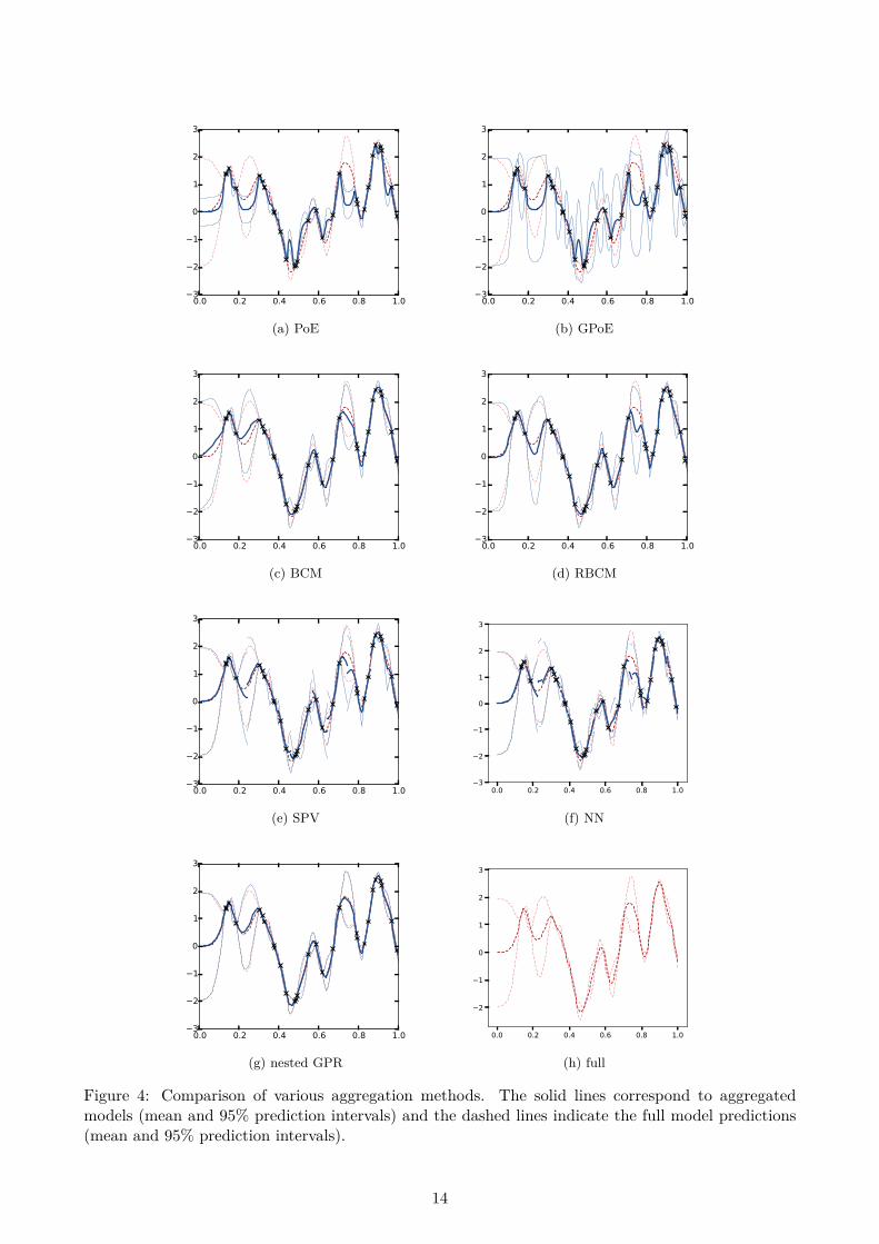
First of all, we will focus on the aggregated models obtained with the different methods for agiven sample path and design of experiments X before looking at the distribution of various criteriawhen replicating the experiment. Figure 4 shows the aggregated models for the aggregation methodsdescribed above. On this example, PoE and GPoE appear respectively to be over- and under-confidentin their predictions and show a mean prediction that tends too quickly to zero as the prediction pointmoves away from the observation points. On the other hand, the predictions from other methods seemmore reliable and the best approximation is obtained with the proposed nested estimation approach.
13
0.0 0.2 0.4 0.6 0.8 1.03
2
1
0
1
2
3
(a) PoE
0.0 0.2 0.4 0.6 0.8 1.03
2
1
0
1
2
3
(b) GPoE
0.0 0.2 0.4 0.6 0.8 1.03
2
1
0
1
2
3
(c) BCM
0.0 0.2 0.4 0.6 0.8 1.03
2
1
0
1
2
3
(d) RBCM
0.0 0.2 0.4 0.6 0.8 1.03
2
1
0
1
2
3
(e) SPV
0.0 0.2 0.4 0.6 0.8 1.03
2
1
0
1
2
3
(f) NN
0.0 0.2 0.4 0.6 0.8 1.03
2
1
0
1
2
3
(g) nested GPR
0.0 0.2 0.4 0.6 0.8 1.0
2
1
0
1
2
3
(h) full
Figure 4: Comparison of various aggregation methods. The solid lines correspond to aggregatedmodels (mean and 95% prediction intervals) and the dashed lines indicate the full model predictions(mean and 95% prediction intervals).
14

This can be confirmed by replicating 50 times the experiment by sampling independently the ob-servation points and the test function. We consider three criteria to quantify the distance betweenthe aggregated model and the full model: the mean square error (MSE) to assess the accuracy ofthe aggregated mean, the mean variance error MVE for the accuracy of the predicted variance andthe mean negative log probability (MNLP) [Williams and Rasmussen, 2006] to quantify the overalldistribution fit. Let m, v (resp. mfull, vfull) denote the mean and variance of the model to be tested(resp. the full model) and let Xt be the vector of test points. These criteria are defined as:
MSE(m,mfull, Xt) = 1nt
nt∑i=1
(m(xt,i)−mfull(xt,i))2 ,
MVE(v, vfull, Xt) = 1nt
nt∑i=1
(v(xt,i)− vfull(xt,i)) ,
MNLP (m, v, f,Xt) = 1nt
nt∑i=1
(12 log(2πv(xt,i)) + (m(xt,i)− f(xt,i))2
2v(xt,i)
).
(23)
Figure 5 shows the boxplots of these criteria for 50 replications of the experiments. It appears thatthe proposed approach gives the best approximation of the full model for the three considered criteria.
full nested NN BCM SPV RBCMGPoE PoE2
1
0
1
2
3
4
5
(a) MNLP
nested NN BCM SPV RBCM GPoE PoE0.00
0.05
0.10
0.15
0.20
0.25
0.30
0.35
0.40
0.45
(b) MSE
nested NN BCM SPV RBCM GPoE PoE0.2
0.1
0.0
0.1
0.2
0.3
0.4
(c) MVE
Figure 5: Quality assessment of the aggregated models for 50 test functions. Each test function isa sample from a Gaussian process and in each case 30 observation points are sampled uniformly on[0, 1]. The test points vector Xt consists of 101 points regularly spaced from xt,1 = 0 to xt,101 = 1.
5.2 Application to a high dimensional input space
We replicate in this section the same experiment as in the previous one but for test functionsdefined over the unit cube in 100 dimensions. We set the number of training points to 10, 000 andwe generate 100 sub-models based on a k-means clustering of the input points. This implies that theaverage number of points per cluster is 100 so we use the 100 closest observation points in the nearestneighbors method. As previously the test functions are random samples of a centered Gaussian processwith squared exponential covariance and we consider two length-scale values to study this parameterinfluence on the methods to compare: a “short” length-scale θ = 2 for which the full model capturesabout 50% of the prior variance and a “large” length-scale θ = 5 for which the full model can explain99% of the prior variance.
The results of the experiment are displayed in Figures 6 and 7. The first striking observation isthat BCM, RBCM and PoE underestimate the variance (since MVEs are negative) and lead to highlyoverconfident models. Regarding the other approaches, NN, SPV and GPoE seem to provide similarglobal accuracy although it can be noted that the Nearest Neighbor method mean predictions areinaccurate for large length-scales. This can be explained by the set of influential neighbors beinglarger than 100 for such values of the length-scales. Finally, it can be seen that the proposed nested
15

method is the one providing the best approximation of the full model. Compared to the other methodsits mean is more accurate and it provides prediction intervals that are smaller than NN, SPV andGPoE while being realistic as shown by the MNLP. This is especially true for large length-scales forwhich the proposed approach is even more competitive.
full nested NN BCM SPV RBCMGPoE PoE
100
101
102
(a) MNLP (log scale)
nested NN BCM SPV RBCM GPoE PoE
10-1
100
101
(b) MSE (log scale)
nested NN BCM SPV RBCM GPoE PoE0.5
0.4
0.3
0.2
0.1
0.0
0.1
0.2
0.3
0.4
(c) MVE
Figure 6: Quality assessment of various aggregation methods. The test functions are given by 50samples from a centered Gaussian process over [0, 1]100 with squared exponential kernel, unit varianceand length-scale θ = 2. The models are built using 10, 000 observations points drawn uniformly inthe input space. These input points are gathered into 100 groups using k-means in order to buildthe sub-models. The test point locations are obtained by sampling uniformly 100 points in the inputspace.
full nested NN BCM SPV RBCMGPoE PoE
0
5
10
15
20
25
30
35
40
(a) MNLP
nested NN BCM SPV RBCM GPoE PoE0.02
0.04
0.06
0.08
0.10
0.12
0.14
0.16
(b) MSE
nested NN BCM SPV RBCM GPoE PoE0.02
0.00
0.02
0.04
0.06
0.08
0.10
0.12
0.14
(c) MVE
Figure 7: Same settings as in Figure 6, but the length-scale of the test functions is 5.
5.3 Application to a large dataset
In this section, we analyze the performance of the proposed method on a test function with one millionobservations.
We use two different test functions. The first one is the Hartman6 test function in dimensiond = 6 (available for example in the DiceKriging R package [Roustant et al., 2012]). The second onein the dimension d = 18 is called here Hartman18 test function: it is simply the sum of three Hart-man6 test functions, each acting on 6 separated parameters: Hartman18(x1:18) = Hartman6(x1:6) +Hartman6(x7:12) + Hartman6(x13:18).
For the Hartman6 test function, the covariance parameters of a squared exponential kernel havebeen estimated once on a subset of points. We give here the obtained length-scales, so that the resultscan be easily reproduced: (0.262, 0.435, 0.423, 0.348, 0.314, 0.299). For the Hartman18 test function,we use two different sets of covariance parameters: the first one is slightly misspecified since it is
16
given by the one estimated for Hartman6 repeated three times, the second one is estimated with usualMLE on a subset of 2000 points. Although the model could be improved with a refined estimation ofthe length-scales, this is sufficient to compare the different methods. The variance parameter has noinfluence on this comparison since we only consider here the performance of the mean predictors.
We consider in this example n = 1, 000, 000 design points and q = 100 predictions points. Severalmethods are considered:
• the Kriging predictor refers to a simple Kriging predictor based on a random sample (withoutreplacement) of 1000 points taken among the initial points. It is mainly computed in order togive an order of the reachable error magnitude for a reasonable learning of the test function, andto see if refined methods really improve the performance of the prediction.
• The Neighbor predictor refers to a simple kriging predictor which gives, for each predictionpoint, the prediction based on its nearest neighbors in the design matrix X. Near100 refers to apredictor based on 100 nearest neighbors, Near1000 refers to a predictor based on 1000 nearestneighbors.
• The Nested method refers to the proposed method in this paper. For one million points, we havechosen a tree structure corresponding to N = 1000 groups of points, each group being obtainedusing kmeans clustering algorithm. Two variants are considered: Nested refers to a clusteringthat is built directly without considering the locations of the prediction points. Nested+ refersto a clustering that is built using these locations (i.e. first q = 100 clusters are built around eachprediction points, without overlapping, and N − q = 900 clusters are built on residual designpoints). In all cases, depending on the location of design points, each cluster size typically varybetween 800 and 1200.
For each run, we draw uniformly a new design matrix X, a new vector of predictions points x, andwe analyze the performance of the predictors. To this aim, the predictions are compared to the truechosen test function, and we collect for each run one mean of errors over all prediction points. Wereproduce the whole experiment on 10 runs. The results are gathered in the boxplots of Figure 8 andFigure 9.
As announced, the Kriging predictor based on a random sample of 1000 points is mainly givento get an order of the errors magnitude with a reasonable learning of the function, but clearly itscomplexity is lower, and it does not reach the precision level of other competitors: other methodsoutperform results based on a random sample of experiments.The nearest neighbor is a clear improvement over the randomly selected training points and thecomputation scheme is relatively simple. However it generates non-continuous mean and variancepredictions, so the practical interest of such a model (e.g. to perform optimization) may be limited.While it performs very well in small dimension, one can see on Figure 9 that it becomes less attractivein higher dimension since it would require to further increase the number of neighbors to provide com-petitive predictions. One can also see that nearest neighbors are also quite sensitive to the estimationof the parameters.The nested procedure has a greater complexity: each run takes around 50 minutes on a modern com-puter with 16 threads (1, 000, 000 observations, 100 prediction points, Hartman18 test function, 1000groups and possible multithreading scalability improvements). The execution time for 100, 000 obser-vations and unchanged other settings is around 30 seconds. Our procedure remains here accurate withconcatenated parameters, contrarily to other methods. It leads to a very good accuracy and sometheoretical advantages previously presented. In relatively small dimension, as in Figure 8, dependingon the length-scales of the underlying process, the closest neighbors may be sufficient to explain thelocal shape of the response. In this case, a judicious choice of the tree structure may improve theaccuracy of the nested method, which is comparable to the one of the 1000 closest neighbors. Inlarger dimension, when local information is not sufficient, the choice of the tree structure has a lowerimpact, and the refinements of the nested method make sense, as they lead to a better accuracy than
17

●
●
Nes
ted+
Nes
ted
Nea
r 100
0
Nea
r 100
Krig
ing 1
000
1e−08
1e−06
1e−04
1e−02Mean square errors (log scale)
(a) Hartman 6
Figure 8: Boxplot of the mean square errors (in log scale), for the Nested procedure and its variant,the nearest neighbors procedure based on 1000 neighbors or 100 neighbors, and for the Kriging methodbased on a random sample of 1000 points. We used one million input points, one hundred predictionpoints and Hartman6 test function.
●
●●
Nes
ted+
Nes
ted
Nea
r 100
0
Nea
r 100
Krig
ing 1
000
0.05
0.10
0.20
0.50
1.00
Mean square errors (log scale)
(a) Hartman 18, concatenated parameters
●
Nes
ted+
Nes
ted
Nea
r 100
0
Nea
r 100
Krig
ing 1
000
0.05
0.10
0.15
0.20
0.25Mean square errors (log scale)
(b) Hartman 18, estimated parameters
Figure 9: Boxplots of mean square errors (in log scale), for the Nested procedure and its variant, thenearest neighbors procedure based on 1000 neighbors or 100 neighbors, and for the Kriging methodbased on a random sample of 1000 points. We used one million input points, one hundred predictionpoints, Hartman18 test function and either concatenated parameters from Hartman6 (left panel) orestimated parameters (right panel).
18

considered local neighbors methods.
Finally, despite greater complexity, the proposed method is still tractable with one million ofobservations. It leads to a better accuracy, especially in high dimension. In small dimension and whenpossible, it can be useful to build the tree structure by using the location of the prediction points,to take the best of both closest neighbors and nested methods. At last, the proposed nested methodmakes an intensive use of cross-covariances between groups and can surely be improved by using abetter estimation of these parameters, or by a transformation of the inputs or the outputs that wouldmake the assumptions more reliable.
5.4 Application to an industrial case study
We consider in this section experimental data on the behavior of a steel test piece subject to cyclesof tension-compression. During these cycles, the evolution of the tensile strain in the test piece ismonitored over time using two methods: by performing the actual physical experiment and by anumerical simulator based on a Chaboche constitutive equation [Lemaitre and Chaboche, 1994]. Thequantity of interest is the misfit between these two experiments. A test piece is described by 6 scalarvariables (E,C1, C2, γ
01 , γ
02 , r), where E is a logarithm transform of the Young’s modulus, C1, C2, γ0
1and γ0
2 are parameters related to the kinematic hardening and r is the radius of the plastic surface atthe stabilized state. The set of admissible inputs is denoted by D ⊂ R6.
Hereafter, we focus on modeling the function f : D → R that returns the logarithm of the L2
norm of the difference between the curve from the actual experiment and the one from the simulator.
In total, we have at our disposal a set of 10, 000 observations [X, f(X)], from which we randomlyextract a learning set [Xl, f(Xl)] of n = 9000 observations and assign the nt = 1000 remainingobservations to a test set [Xt, f(Xt)].
We compare the predictions of f(Xt) obtained from the SPV, PoE, GPoE1, GPoE2, BCM andRBCM aggregation procedures described in Section 5.1 with our nested aggregation procedure. GPoE1corresponds to (19) with βi = 1
2 [log(V [Y (x)]) − log(vi(x))] [Cao and Fleet, 2014] and GPoE2 corre-sponds to (19) with βi = 1/p [Deisenroth and Ng, 2015]. For all these methods, we consider anaggregation tree of height ν̄ = 2 (once sub-models have been evaluated at layer 1, they are all directlyaggregated into one value at layer 2), so that p Gaussian process models are directly aggregated. Thep subsamples form a partition of [Xl, f(Xl)], which is obtained using the k-means clustering algorithm.
Three covariance functions have been considered for the sub-models: (tensorized) exponential,Matérn 3/2 and Matérn 5/2 (see [Williams and Rasmussen, 2006, Roustant et al., 2012] for the defi-nition of these functions). For all studied methods, the Matérn 5/2 covariance seemed to be the mostappropriate to the problem at hand since we obtained overall more accurate results. The results pre-sented hereafter thus focus on this Matérn 5/2 covariance family. Its parameters are estimated withtwo different techniques depending on the aggregation method: for the methods from the literatureand SPV, we follow the recommended procedure which consists in maximizing the sum of the log like-lihoods over the p subsamples of [Xl, f(Xl)] (see [Deisenroth and Ng, 2015]). For the proposed nestedaggregation, we carry out the stochastic-gradient based estimation method described in Section 4,with starting points set to the maximizer of the sum of the log likelihoods.
To assess the quality of a model with predicted mean m and variance v, we compute three qualitycriteria using the test set: MSE and MNLP as per Eq. 23 which are small for a good model, and themean normalized square error (MNSE)
MNSE(m, v, f,Xt) = 1nt
nt∑i=1
(m(xt,i)− f(xt,i))2
v(xt,i),
which should be close to 1.
19

SPV PoE GPoE1 GPoE2 BCM RBCM NestedMSE 0.00416 0.0662 0.0033 0.0662 0.604 0.0625 0.00321MNSE 1.27 20.00 4.55 1.00 219 60.8 0.846MNLP −1.86 7.25 −0.949 −0.765 107 27.2 −1.97
Table 1: Prediction performances of the aggregation of p = 20 sub-models for the steel piece constraintscycles data set. The investigated prediction performance criteria are the mean square error (MSE)which should be minimal, mean normalized square error (MNSE) which should be close to 1 andmean negative log probability (MNLP) which should be small. Bold figures indicate each line’s bestperforming aggregation method.
SPV PoE GPoE1 GPoE2 BCM RBCM NestedMSE 0.00556 0.811 0.0244 0.811 1.84 0.121 0.00418MNSE 1.20 465 34.2 5.16 980 148 0.84700MNLP −1.55 230 14.1 2.13 487 71 −1.7
Table 2: Prediction performances of the aggregation of p = 90 sub-models for the steel piece constraintscycles data set. All other settings are the same as in Table 1.
The prediction results for a given learning and training test set are given in Table 1 for the aggre-gation of p = 20 sub-models and in Table 2 for p = 90. It can be seen that in both cases the proposedmethod outperforms the other aggregation methods for the MSE and MNLP quality criteria. TheMSE has the same order of magnitude for the SPV and our aggregation method, where the predictionerrors are small compared to the empirical variance of the test outputs f(xt,i), i = 1, ..., nt, whichis approximately equal to 0.81. In contrast, the MSE can be significantly larger for all the otheraggregation procedures. For the PoE, GPoE1, BCM and RBCM aggregation techniques, the values ofMNSE are orders of magnitude greater than the target value one, which indicates that the aggregatedmodels are highly overconfident. The GPoE2 aggregation technique is also overconfident when p = 90,where its MNSE is equal to 5.16. The SPV and our aggregation methods provide appropriate predic-tive variances, and our method provides the best combination of predictions and predictive variances,according to the MNLP criterion.
Tables 1 and 2 also show that aggregating p = 20 sub-models gives more accurate models thanaggregating p = 90 sub-models. This suggests that it is a good practice to aggregate few sub-modelsbased on many points instead of aggregating many sub-models based on few points. Although thiswould require further testing to be confirmed, it is not surprising since aggregation methods rely onsome independence assumptions that are not often met in practice.
Tables 3 and 4 show the values of the quality criteria when the subsamples used for the p = 20or p = 90 sub-models are randomly generated into the learning set. They can thus be comparedto Tables 1 and 2 to study the influence of the choice of the support points of the sub-models: thecriteria values are overall better in Tables 1 and 2 so using k-means is beneficial for the aggregationprocedures. In addition, our proposed aggregation technique becomes better in comparison to theother methods, and specifically to SPV, when the subsamples are randomly generated.
All previous results have been obtained for a given random choice of the learning and test sets.We now replicate the procedure 20 times, with the same settings as in Tables 1 (p = 20; subsamplesobtained from the k-means algorithm; Matérn 5/2 covariance function) and 4 (p = 90; subsamplesrandomly selected; Matérn 5/2 covariance function), but with different learning and test sets for eachreplication. The covariance parameters are reestimated for each learning set, by minimizing the sum oflog likelihoods for the SPV, PoE, GPoE1, GPoE2, BCM and RBCM aggregation techniques, and withthe proposed leave-one-out estimation procedure for our nested aggregation method. The boxplots of
20

SPV PoE GPoE1 GPoE2 BCM RBCM NestedMSE 0.0086 0.00763 0.00704 0.00763 0.338 0.274 0.00539MNSE 1.21 9.38 16.6 0.469 178 268 0.864MNLP −1.25 1.75 5.03 −1.21 86.2 130 −1.5
Table 3: Same settings as in Table 1 but when the subsamples are randomly selected.
SPV PoE GPoE1 GPoE2 BCM RBCM NestedMSE 0.0182 0.0293 0.0246 0.0293 0.977 0.686 0.00575MNSE 1.29 42.5 57.2 0.473 852 988 0.867MNLP −0.804 18.3 25.3 −0.517 423 491 −1.37
Table 4: Same settings as in Table 1 but with p = 90 sub-models and where the subsamples arerandomly selected.
the corresponding 20 mean square errors and mean negative log probability are reported in Figures 10and 11. These replications confirm the results obtained previously on single instances of the learningand test set: the proposed nested aggregation and covariance parameter estimation jointly give betterprediction both for the predicted mean and variance than current existing aggregation techniques.
●
nest
ed
SP
V
GP
oE1
GP
oE2
RB
CM
PoE
BC
M
0.005
0.010
0.020
0.050
0.100
0.200
0.500
MSE (log scale)
●●●●
●
●●
●
nest
ed
SP
V
GP
oE1
GP
oE2
RB
CM
PoE
BC
M
0
20
40
60
80
100
120
140
MNLP
●
●
●●
nest
ed
SP
V
GP
oE1
GP
oE2
−2.0
−1.5
−1.0
−0.5
0.0
0.5
MNLP (detail)
Figure 10: Boxplots of 20 values of the mean square error (MSE) prediction criterion and of thelogarithm of the mean negative log probability (MNLP) prediction criterion where the learning andtest sets are randomly generated. The settings are as in Table 1 (p = 20 subsamples obtained fromthe k-means algorithm; Matérn 5/2 covariance function). The covariance parameters are estimated byminimizing the sum of log likelihoods for the SPV, PoE, GPoE1, GPoE2, BCM and RBCM aggregationtechniques, and with our proposed leave-one-out estimation procedure for the nested aggregationprocedure.
Of course, the improvement brought by our proposed aggregation scheme comes with a highercomputational cost: the proposed estimation procedure takes a few hours on a personal computer,against a few tens of minutes for the minimization of the sum of the log likelihoods. Similarly,performing 1000 predictions takes around 30 seconds with our proposed optimal aggregation, againstaround 1 second for the other simpler aggregation procedures. Nevertheless, we believe that theincreased accuracy and robustness of the method we propose is worth the additional computationalburden in many situations.
21

●●
●
●●
●●
●●
●●
●●
nest
ed
SP
V
GP
oE1
GP
oE2
RB
CM
PoE
BC
M
0.005
0.010
0.020
0.050
0.100
0.200
0.500
1.000
MSE (log scale)
●●
nest
ed
SP
V
GP
oE1
GP
oE2
RB
CM
PoE
BC
M
0
100
200
300
400
500
MNLP
nest
ed
SP
V
GP
oE1
GP
oE2
−1.4
−1.2
−1.0
−0.8
−0.6
−0.4
MNLP (detail)
Figure 11: Same settings as in Figure 10 but with p = 90 and where the subsamples are randomlyselected.
6 ConclusionWe have proposed a new method for aggregating sub-models based on subsets of observation points,
with a particular emphasis on Kriging sub-models. Our method can be seen as an optimal linearweighting of sub-models, where the obtained weights are taking into account all pairwise covariancesbetween the sub-models, thus avoiding some usual independence assumptions.
Compared to current existing aggregation techniques, we find several benefits to our our aggregationprocedure. First, it has some good theoretical properties, like consistency or optimality based on aslightly different process which can be simulated. We refer again to [Bachoc et al., 2017] for details.Second, a dedicated covariance parameter estimation procedure is provided, based on a gradientdescent minimization of leave-one-out cross validation errors, where the predictions are performedusing the proposed nested aggregation. Some user-friendly code for computing both prediction andcovariance parameter estimation is publicly available.
At last, numerical results are encouraging. In both simulated data and industrial application, ourmethod is shown to outperform state-of-the-art aggregation techniques. This improvement comeswith an increased computational cost compared to more basic aggregation methods, but the proposednested aggregation remains applicable up to n = 106 observation points, while exact Kriging inferencebecomes intractable around n = 10 000.
We would like to mention two avenues for future research. First, we show that the aggregationmethod we propose can be applied recursively, yielding a nested aggregation technique with smallercomputational cost. It would be interesting to quantify the practical gain one could obtain on realdata sets from this recursive aggregation. Second, we find that the stochastic gradient algorithmwe propose could be further investigated. In particular, theoretical properties could be derived, thepractical implementation could be improved, and the principle could be extended to other criteria forcovariance parameter estimation.
AcknowledgementsPart of this research was conducted within the frame of the Chair in Applied Mathematics OQUAIDO,gathering partners in technological research (BRGM, CEA, IFPEN, IRSN, Safran, Storengy) andacademia (Ecole Centrale de Lyon, Mines Saint-Etienne, University of Grenoble, University of Nice,University of Toulouse and CNRS) around advanced methods for Computer Experiments. The authorswould like to warmly thank Dr. Géraud Blatman and EDF R&D for providing us the industrial testcase. They also thank both editor and reviewers for very precise and constructive comments on thispaper. This paper has been finished during a stay of D. Rullière at Vietnam Institute for Advanced
22

Study in Mathematics, the latter author thanks the VIASM institute and DAMI research chair (DataAnalytics & Models for Insurance) for their support.
References[Bachoc, 2013] Bachoc, F. (2013). Cross validation and maximum likelihood estimations of hyper-
parameters of Gaussian processes with model mispecification. Computational Statistics and DataAnalysis, 66:55–69.
[Bachoc et al., 2017] Bachoc, F., Durrande, N., Rullière, D., and Chevalier, C. (2017). Some propertiesof nested kriging predictors. Technical report hal-01561747.
[Bhatnagar et al., 2013] Bhatnagar, S., Prasad, H., and Prashanth, L. (2013). Stochastic recursivealgorithms for optimization, volume 434. New York: Springer.
[Cao and Fleet, 2014] Cao, Y. and Fleet, D. J. (2014). Generalized Product of Experts for Automaticand Principled Fusion of Gaussian Process Predictions. arXiv preprint arXiv:1410.7827v2, CoRR,abs/1410.7827:1–5. Modern Nonparametrics 3: Automating the Learning Pipeline workshop atNIPS, Montreal.
[Deisenroth and Ng, 2015] Deisenroth, M. P. and Ng, J. W. (2015). Distributed Gaussian processes.Proceedings of the 32nd International Conference on Machine Learning, Lille, France. JMLR:W&CP volume 37.
[Genest and Zidek, 1986] Genest, C. and Zidek, J. V. (1986). Combining probability distributions: Acritique and an annotated bibliography. Statistical Science, 1(1):114–135.
[Golub and Van Loan, 2012] Golub, G. H. and Van Loan, C. F. (2012). Matrix computations, vol-ume 3. JHU Press.
[Guhaniyogi et al., 2011] Guhaniyogi, R., Finley, A. O., Banerjee, S., and Gelfand, A. E. (2011).Adaptive gaussian predictive process models for large spatial datasets. Environmetrics, 22(8):997–1007.
[Hensman et al., 2013] Hensman, J., Fusi, N., and Lawrence, N. D. (2013). Gaussian Processes forBig Data. Uncertainty in Artificial Intelligence conference. paper Id 244.
[Hinton, 2002] Hinton, G. E. (2002). Training products of experts by minimizing contrastive diver-gence. Neural computation, 14(8):1771–1800.
[Katzfuss, 2013] Katzfuss, M. (2013). Bayesian nonstationary spatial modeling for very large datasets.Environmetrics, 24(3):189–200.
[Lemaitre and Chaboche, 1994] Lemaitre, J. and Chaboche, J.-L. (1994). Mechanics of solid materi-als. Cambridge university press.
[Maurya, 2016] Maurya, A. (2016). A well-conditioned and sparse estimation of covariance and inversecovariance matrices using a joint penalty. The Journal of Machine Learning Research, 17(1):4457–4484.
[Nickson et al., 2015] Nickson, T., Gunter, T., Lloyd, C., Osborne, M. A., and Roberts, S.(2015). Blitzkriging: Kronecker-structured stochastic Gaussian processes. arXiv preprintarXiv:1510.07965v2, pages 1–13.
[Ranjan and Gneiting, 2010] Ranjan, R. and Gneiting, T. (2010). Combining probability forecasts.Journal of the Royal Statistical Society: Series B (Statistical Methodology), 72(1):71–91.
23
[Roustant et al., 2012] Roustant, O., Ginsbourger, D., and Deville, Y. (2012). DiceKriging, DiceOp-tim: Two R packages for the analysis of computer experiments by Kriging-based metamodeling andoptimization. Journal of Statistical Software, 51(1).
[Rue and Held, 2005] Rue, H. and Held, L. (2005). Gaussian Markov random fields, Theory andapplications. Chapman & Hall.
[Samo and Roberts, 2016] Samo, Y.-L. K. and Roberts, S. J. (2016). String and membrane gaussianprocesses. Journal of Machine Learning Research, 17(131):1–87.
[Santner et al., 2013] Santner, T. J., Williams, B. J., and Notz, W. I. (2013). The design and analysisof computer experiments. Springer Science & Business Media.
[Satopää et al., 2016] Satopää, V. A., Pemantle, R., and Ungar, L. H. (2016). Modeling probabilityforecasts via information diversity. Journal of the American Statistical Association, 111(516):1623–1633.
[Scott et al., 2016] Scott, S. L., Blocker, A. W., Bonassi, F. V., Chipman, H. A., George, E. I., andMcCulloch, R. E. (2016). Bayes and big data: The consensus monte carlo algorithm. InternationalJournal of Management Science and Engineering Management, 11(2):78–88.
[Stein, 2012] Stein, M. L. (2012). Interpolation of spatial data: some theory for kriging. SpringerScience & Business Media.
[Stein, 2014] Stein, M. L. (2014). Limitations on low rank approximations for covariance matrices ofspatial data. Spatial Statistics, 8:1–19.
[Tresp, 2000] Tresp, V. (2000). A bayesian committee machine. Neural Computation, 12(11):2719–2741.
[Tzeng et al., 2005] Tzeng, S., Huang, H.-C., and Cressie, N. (2005). A fast, optimal spatial-predictionmethod for massive datasets. Journal of the American Statistical Association, 100(472):1343–1357.
[van Stein et al., 2015] van Stein, B., Wang, H., Kowalczyk, W., Bäck, T., and Emmerich, M. (2015).Optimally weighted cluster kriging for big data regression. In International Symposium on IntelligentData Analysis, pages 310–321. Springer.
[Wahba, 1990] Wahba, G. (1990). Spline models for observational data, volume 59. SIAM.
[Wei et al., 2015] Wei, H., Du, Y., Liang, F., Zhou, C., Liu, Z., Yi, J., Xu, K., and Wu, D. (2015).A k-d tree-based algorithm to parallelize kriging interpolation of big spatial data. GIScience &Remote Sensing, 52(1):40–57.
[Williams and Rasmussen, 2006] Williams, C. K. and Rasmussen, C. E. (2006). Gaussian Processesfor Machine Learning. MIT Press.
[Winkler, 1968] Winkler, R. L. (1968). The consensus of subjective probability distributions. Man-agement Science, 15(2):B–61.
[Winkler, 1981] Winkler, R. L. (1981). Combining probability distributions from dependent informa-tion sources. Management Science, 27(4):479–488.
[Zhang et al., 2015] Zhang, B., Sang, H., and Huang, J. Z. (2015). Full-scale approximations of spatio-temporal covariance models for large datasets. Statistica Sinica, pages 99–114.
24

A Proof of Proposition 4Complexities: under chosen assumption on α and β coefficients, for a regular tree and in the caseof simple Kriging sub-models, Cα =
∑ν̄ν=1
∑nνi=1 αc
3ν = α
∑ν̄ν=1 c
3νnν and Cβ =
∑ν̄ν=1
∑nνi=2
∑i−1j=1 βc
2ν =
β2∑ν̄ν=1 nν(nν−1)c2
ν . Notice that the sum starts from ν = 1 in order to include sub-models calculation.Equilibrated trees complexities: In a constant child number setting, when cν = c for all ν, the treestructure ensures that nν = n/cν , thus as c = n1/ν̄ , we get when n → +∞, Cα ∼ αn1+ 2
ν̄ andCβ ∼ β
2n2. The result for equilibrated two-layer tree where ν̄ = 2 directly derives from this one,
and in this case Cα ∼ αn2 and Cβ ∼ β2n
2 (it derives also from the expressions of Cα, Cβ, whenc1 = c2 =
√n, n1 =
√n, n2 = 1). Optimal tree complexities: One easily shows that under the chosen
assumptions Cβ ∼ β2n
2. Thus, it is indeed not possible to reduce the whole complexity to orderslower than O(n2). However, one can choose the tree structure in order to reduce the complexity Cα.For a regular tree, nν = n/(c1 · · · cν) such that ∂
∂cknν = −1{ν≥k}nν/ck. Using a Lagrange multiplier
`, one defines ξ(k) = ck∂∂ck
(Cα − `(c1 · · · cν̄ − n)) = 3αc3knk − α
∑ν̄ν=k c
3νnν − `c1 · · · cν̄ . The tree
structure that minimizes Cα is such that for all k < ν̄, ξ(k) = ξ(k + 1) = 0. Using ck+1nk+1 = nk,
one gets 3c2k+1 = 2c3
k for all k < ν̄, and setting c1 · · · cν̄ = n, cν = δ(δ−ν̄n
) δν−12(δν̄−1) , ν = 1, . . . , ν̄,
with δ = 32 . Setting γ = 27
4 δ− ν̄δν̄−1
(1− δ−ν̄
). After some direct calculations this tree structure
corresponds to complexities, Cα = γαn1+ 1
δν̄−1 and Cβ ∼ β2n
2. In a two-layers setting one gets c1 =(32
)1/5n2/5 and c2 =
(32
)−1/5n3/5, which leads to Cα = γαn9/5 and Cβ = β
2n2 − β
2
(32
) 15 n
75 , where
γ = (23)−2/5 + (2
3)3/5 ' 1.96 (eventually notice that even for values of n of order 105, terms of orderlike n9/5 are not necessarily negligible compared to those of order n2, and that Cβ is slightly affectedby the choice of the tree structure, but the global complexity benefits from the optimization of Cα).Storage footprint: First, covariances can be stored in triangular matrices. So temporary objects M ,k and K in Algorithm 1 require the storage of cmax(cmax + 5)/2 real values. For a given step ν,ν ≥ 2, building all vectors αi requires the storage of
∑nνi=1 c
νi = nν−1 values. At last, for a given
step ν, we simultaneously need objectsMν−1,Kν−1,Mν ,Kν , which require the storage of nν−1(nν−1 +3)/2 + nν(nν + 3)/2 real values. In a regular tree, as nν is decreasing in ν, the storage footprintis S = (cmax(cmax + 5) + n1(n1 + 5) + n2(n2 + 3))/2. Hence the equivalents for S for the differenttree structures, S ∼ n for the two-layer equilibrated tree, S ∼ 1
2n2−2/ν̄ for the ν̄-layer, ν̄ > 2, and
the indicated result for the optimal tree. Simple orders are given in the proposition, which avoidsseparating the case ν̄ = 2 and a cumbersome constant for the optimal tree.
25