nesting and brood-rearing ecology of resident canada …
TRANSCRIPT

NESTING AND BROOD-REARING ECOLOGY OF
RESIDENT CANADA GEESE IN NEW JERSEY
by
Katherine B. Guerena
A thesis submitted to the Faculty of the University of Delaware in partial fulfillment of the requirements for the degree of Master of Science in Wildlife Ecology
Fall 2011
Copyright 2011 Katherine B. Guerena All Rights Reserved

NESTING AND BROOD-REARING ECOLOGY OF
RESIDENT CANADA GEESE IN NEW JERSEY
by
Katherine B. Guerena Approved: __________________________________________________________ Christopher K. Williams, Ph.D. Professor in charge of thesis on behalf of the Advisory Committee Approved: __________________________________________________________ Douglas W. Tallamy, Ph.D. Chair of the Department of Entomology and Wildlife Ecology Approved: __________________________________________________________ Robin W. Morgan, Ph.D. Dean of the College of Agriculture and Natural Resources Approved: __________________________________________________________ Charles G. Riordan, Ph.D. Vice Provost for Graduate and Professional Education

iii
ACKNOWLEDGMENTS I would like to thank New Jersey Division of Fish and Wildlife and the University of
Delaware for funding this project. I would particularly like to thank my graduate committee,
Chris Williams, Jake Bowman, and Paul Castelli for giving me the opportunity to further my
education and research experience at the University of Delaware. A special thanks to Paul
Castelli and Ted Nichols for their guidance and support throughout my time in the field and
behind a desk with New Jersey Fish and Wildlife and the University of Delaware, and for
making this study possible.
I would also like to thank the phenomenally hard-working New Jersey field
technicians and biologists who took wings in the head and bites to the legs to make this
project succeed - Trevor Watts, Marissa Gnoinski, Kurt Bond, Dane Cramer, Joe Garris,
Linda Morschauser, Andrew Dinges, Ken Duren and Kim Tinnes. I would like to show my
appreciation to all of the landowners that granted permission to search for nests, mark
goslings and track broods on their property through the heat of the summer.
I would like to extend a tremendous thank you to my friends and family for their
endless support from near and far. I would also like to send a special thanks to Trevor Watts,
for offering unwavering support during the last few years, as well as a dazzling sense of
humor to get us all through the day. And lastly, I would like to thank my parents, Ed and
Barbara Guerena, for their continuous love and encouragement.

iv
TABLE OF CONTENTS
LIST OF TABLES ......................................................................................................... vi LIST OF FIGURES .................................................................................................... viii ABSTRACT .................................................................................................................... x CHAPTER 1 SPATIALLY-EXPLICIT HABITAT EFFECTS ON NEST SITE
SELECTION AND NEST SUCCESS OF ATLANTIC FLYWAY RESIDENT CANADA GEESE .......................................................................... 1 Introduction ......................................................................................................... 1 Study Area .......................................................................................................... 3 Methods............................................................................................................... 4 Results ................................................................................................................. 7 Discussion ........................................................................................................... 9 Management Implications ................................................................................. 14 Literature Cited ................................................................................................. 15
2 PARAMETERIZING BREEDING SEASON VITAL RATES FOR AN ATLANTIC FLYWAY RESIDENT CANADA GOOSE POPULATION MODEL ............................................................ Error! Bookmark not defined. Introduction ....................................................................................................... 30 Study Area ........................................................................................................ 34 Methods............................................................................................................. 35 Results ............................................................................................................... 45 Discussion ......................................................................................................... 49 Management Implications ................................................................................. 55 Literature Cited ................................................................................................. 56
3 BROOD SURVIVAL OF ATLANTIC FLYWAY RESIDENT POPULATION CANADA GEESE IN NEW JERSEY ................................... 76 Introduction ....................................................................................................... 76 Study Area ........................................................................................................ 78 Methods............................................................................................................. 79 Results ............................................................................................................... 84 Discussion ......................................................................................................... 85 Management Implications ................................................................................. 89 Literature Cited ................................................................................................. 90

v
APPENDIX A. (a) Mean nest initiation date (+/- SE), and (b) Mean hatch date (+/- SE) by physiographic stratum and year for Canada goose nests in New Jersey, USA. .................................................................................................... 103
APPENDIX B. Frequency of Canada goose nest hatches in New Jersey during study years from 1985–1989, 1995–1997, and 2009–2010. ........................... 104
APPENDIX C. Age distribution of breeding adults by age class and sex during 1985–1989 in New Jersey, USA. .................................................................... 105
APPENDIX D. Evaluation of a clutch containment method during hatch in resident Canada geese for mark-recapture study. ........................................... 106 Introduction ..................................................................................................... 106 Study Area ...................................................................................................... 107 Methods........................................................................................................... 107 Results ............................................................................................................. 109 Discussion ....................................................................................................... 110 Literature Cited ............................................................................................... 112

vi
LIST OF TABLES
Table 1.1. Original and reclassified land use/land cover types based on National Oceanic and Atmospheric Administration Coastal Change and Analysis Program (NOAA C-CAP) land cover dataset to model Canada goose nest success and nest occupancy in New Jersey, USA, from 15 March – 15 June 2009–2010. ..................................................... 21
Table 1.2. Original and reclassified land use/land cover types based on New Jersey Land Use/Land Cover (NJ LULC) dataset to model Canada goose nest success and nest occupancy in New Jersey, USA, from 15 Mar – 15 June 2009–2010. ....................................................................... 22
Table 2.1. List of covariates used to build candidate models for nest survival of Canada geese in New Jersey, USA, 1985–2010. Variable subscripts denote measurement scale; site = S, landscape = L. ................................ 67
Table 2.2. Recruitment parameters during nesting seasons of 1985–1989, 1995–1997, and 2009–2010 in New Jersey, USA. I report clutch size at hatch (CSH), nest success (SN), and hatchability (H). Statewide production indices include the number of nests, the number of young produced per nest/breeding pair, and the statewide number of young produced through hatch. Data from 1985–1989 and 1995 did not utilize a plot study area; therefore, statewide estimates were not extrapolated from these years. ................................................................. 68
Table 2.3. Summary of model-selection procedure examining variables affecting the probability of nest survival of AFRP Canada geese in Jersey, USA from 1985–1989. I report Akaike’s Information Criterion (AICc) of the top-ranked model, the relative difference in AIC values compared to the top-ranked model (∆ AIC), the AIC model weight (W), and the number of parameters in the model (K). Variables are described in Table 1. Variable subscripts denote measurement scale; site = S, landscape = L. .......................................................................................... 69
vii
Table 3.1. Summary of model-selection procedure examining variables affecting brood survival of AFRP Canada geese in New Jersey, USA from 2009–2010. I report Akaike’s Information Criterion (AICc), the relative difference in AIC values compared to the top-ranked model (∆ AIC), the AIC model weight (W), and the number of parameters in the model (K). .......................................................................................... 98
Table 3.2. Proportion and survival estimates of total brood loss (STBL), partial brood loss (SPBL), and sample-wide survival estimates (SG) of AFRP Canada goose broods from hatch until recapture during 2009–2010 in New Jersey, USA. .................................................................................... 99

viii
LIST OF FIGURES
Figure 1.1. Locations of all survey plots within five physiographic strata in New Jersey, USA, from 15 March–3 June 2009–2010. .................................. 25
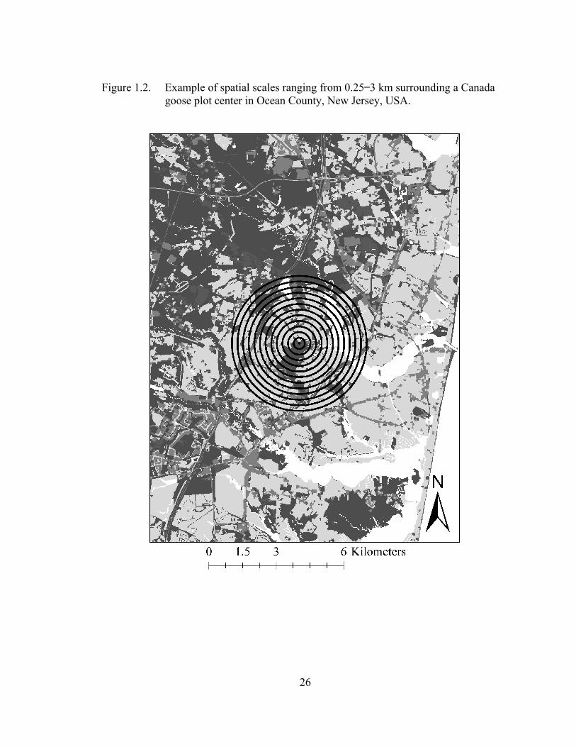
Figure 1.2. Example of spatial scales ranging from 0.25 ̶ 3 km surrounding a Canada goose plot center in Ocean County, New Jersey, USA. ............ 26
Figure 1.3. Mean ± standard error of Spearman’s Rank Correlation Coefficient between explanatory habitat variables measured within buffers of 0.25 to 3 km in 250m increments around each plot center and nest site, and Canada goose (a) nest site selection, and (b) nest success in New Jersey, USA, 2009–2010. Mean proportion of habitat variables measured at each spatial scale are depicted in grey. Black points indicate distances statistically similar to the buffer distance with the strongest correlation. Arrows indicate distance used. ............................ 27
Figure 2.1. Estimate of the breeding population of AFRP Canada geese in New Jersey from 1989–2010 (New Jersey Division of Fish and Wildlife, unpublished data). Error bars denote the coefficients of variation of each estimate. .......................................................................................... 72
Figure 2.2. Proposed population model for Atlantic Flyway Resident Population Canada geese, modified from the AP Canada goose model proposed by Hauser et al. (2007), and the Giant Canada goose model proposed by Collucy et al. (2004) for the Missouri population. Fi is the age-specific fecundity parameter, Ai is age-specific nesting rate, C is clutch size, H is hatchability, SN is nest success rate, and SG is pre-fledge gosling survival rate. The survival parameter, Pi, is based on three age stages; juvenile is from fledge to 1yr, sub-adult is from 1 to 2yr, and adult is annual survival following 2yr. Additionally, select environmental and density-dependent variables are considered in the estimates of nest and pre-fledge gosling survival. .................................. 73
Figure 2.3. Two-hundred fifty randomly placed 1-km2 plot study area, stratified by five physiographic strata in New Jersey, USA. ................................. 74

ix
Figure 2.4. Nest success and standard error of AFRP Canada geese during 1985–1989, 1995–1997, and 2009–2010. ......................................................... 75
Figure 3.1. Twelve locations used to study AFRP Canada goose brood survival during April-July, 2009–2010 in New Jersey, USA. ............................ 100
Figure 3.2. Gosling survival estimate is composed of a proportion of broods that are totally lost during brood-rearing (TBL), and the remaining proportion of broods that are exposed to partial brood loss (PBL). Only broods that have partial losses are present during recapture, making it difficult to distinguish TBL from broods not present (emigrated) during recapture. ............................................................... 101
Figure 3.3. Estimate of daily mortality rates of AFRP Canada goose goslings from hatch until recapture during 2009–2010 in New Jersey, USA. Estimates are based on observations of both broods associated with marked adults and broods identifiable through color marking. ............ 102
Figure A4.1. Eleven locations in New Jersey used to evaluate the effect of a nest containment bag on hatch success of Atlantic Flyway Resident Population Canada geese during 2010 breeding season. ...................... 115
Figure A4.2. (a) Clutch containment bag with hatchling and 3 pipping eggs used during 2010 resident Canada goose nesting season in New Jersey. (b) Nest site with adult protecting clutch and young during hatch period. 116
x
ABSTRACT
The Atlantic Flyway Resident Population (AFRP) of Canada geese (Branta
canadensis) in New Jersey has grown so considerably during the last thirty years that it is
now considered a nuisance in urban areas (United States Fish and Wildlife Service 2003).
New Jersey is also the most densely human populated state in the nation, with intensive
urbanization of agricultural and natural lands. Development of corporate parks and urban
areas with manicured lawns and artificial ponds offer ideal nesting habitat for AFRP
geese, with limited pressure from hunting or natural predators. As a result, spatial
heterogeneity in reproduction and survival must be taken into account in managing the
population. My objectives for this study were to 1) identify the spatial scale/s at which
land use features influence nest site selection and nest success, 2) estimate nesting
parameters across three decades and identify variables that influence productivity, and 3)
estimate pre-fledged gosling survival from hatch until summer molt banding efforts, in
order to assist in developing a spatially-explicit population model for AFRP geese in
New Jersey.
I conducted a two-year (2009–2010) nesting ecology study of AFRP Canada
geese, and compared it to data collected in New Jersey from 1985–1989 and 1995–1997.

xi
Nest searches were conducted on 250 1-km2 plots throughout the state, and 309 nests
were monitored through hatch to determine the fate. I ran a spatial correlation analysis of
land use composition to nest success during 2009–2010 to identify spatial scales at which
geese respond to their environment for nest site selection and nest success. All significant
spatial scales were at or below 2250m for the five classified land use types. Geese
responded to human dominated land uses at a smaller scale than land uses with low
human density. Mean clutch size at hatch in 2009–2010 was 4.66 eggs (SE ± 0.12 eggs)
and 4.76 eggs (SE ± 0.16 eggs), respectively. Mean hatchability in 2009–2010 was 0.86
(SE ± 0.02) and 0.81 (SE ± 0.02), respectively. I estimated nest success at 0.44 (SE ±
0.05) in 2009 and 0.41 (SE ± 0.05) in 2010. Variables important to nest success from
1985–1989 were the age of the nest, year, extreme high temperature, nest density, rural
residential land use at the landscape scale, commercial at the site level, and daily
precipitation. Variables important to nest success for 1995–1997 were the age of the nest,
date of nest initiation, year, physiographic stratum, extreme high temperature, rural
residential land use at the landscape level, and agricultural land use at the site level.
Variables important to nest success for 2009–2010 were the age of the nest and date of
nest initiation. Nest success decreased during the duration of the study, likely due to an
increase in reproductive control efforts.
Additionally, I conducted a two-year (2009–2010) gosling survival study from
hatch until annual banding efforts in late-June at 12 known nesting and brood rearing
sites. To estimate gosling survival, I used 1) mark-recapture of web tagged goslings to
xii
estimate partial brood loss, 2) radio-collared breeding adults to estimate total brood loss,
and 3) observations of broods associated with marked adults and color-marked broods to
quantify mortality during the first two weeks after hatch. The proportion of breeding
adults that experienced total brood loss was 0.316. The remaining proportion of breeding
adults was subject to partial brood loss (0.684), which was estimated at 0.465 (SE ±
0.026) for 56 days. The overall survival estimate for 56 days after hatch was 0.318 (SE ±
0.018). Select environmental and density-dependent variables were used to build
candidate models to identify sources of variation in partial brood loss. The number of
broods at the site was negatively related to brood survival. The percent agriculture within
215 m was positively related to brood survival.
Managers are encouraged to consider scale-dependent relationships in identifying
habitat-wildlife relationships, and if population control of AFRP Canada geese is of
primary interest, then focus on habitat management at the local scale will most likely
have the largest influence. Developing productivity trends should assist in understanding
the dynamics of recruitment as a function of population size, spatial distribution, and
human influence. I recommend that managers consider land use and human development
as important features in identifying the driving forces of productivity in AFRP Canada
geese.
1
Chapter 1
SPATIALLY-EXPLICIT HABITAT EFFECTS ON NEST SITE SELECTION
AND NEST SUCCESS OF ATLANTIC FLYWAY RESIDENT CANADA GEESE
Introduction New Jersey is the most densely human-populated state in the nation, with more
than 460 people/ km2 in 2009 (United States Census Bureau 2011). The resultant demand
for housing, recreation areas, roads, and corporate parks with manicured open lawns and
artificial water sources has reduced the amount of suitable habitat for many wildlife
species, but has created increased urban/suburban nesting and brood rearing habitat for
Atlantic Flyway Resident Population (AFRP) Canada geese (Branta canadensis). A
secondary impact of land use shifts has decreased the amount of land suitable for hunter
harvest, limiting the major mortality factor of fledged AFRP geese (Smith et al. 1999,
Atlantic Flyway Council 2011). Consequently, these conditions have allowed the AFRP
to increase to approximately 106,000 birds in 2000, and a current estimated population of
70,000 in 2011 (New Jersey Division of Fish and Wildlife, unpublished data).
Because human-manipulated landscapes may have influenced recent growth of
the AFRP, direct measurement of its influence on recruitment and annual survival is
critical. Pastor et al. (1997) argued that in order to better understand relationships
between habitat and productivity and inform management control efforts, a need exists to

2
identify the site and landscape scales at which wildlife interact with their environment.
Furthermore, there has been increased recognition that we must consider bird responses
to habitat types at varying or multiple spatial scales (Roland and Taylor 1997, Holland et
al. 2004, Holland et al. 2005). To date, several research efforts have been made to
determine the primary spatially explicit landscape variables that influence the selection of
waterbird nest locations and nest success (e.g. sandhill cranes [Grus Canadensis, Baker et
al. 1995], mallards [Anas platyrhynchos, Zicus et al. 2006], and common loons, [Gavia
immer, Kuhn et al. 2011]).
Although Messmer (2010) found that habitat associations of breeding pair
temperate-nesting Canada geese could be influenced by spatial scales, previous research
has primarily focused on the effects of simple habitat attributes of Canada goose nesting
ecology. For example, nest survival has been found to be positively influenced by
increased commercial, urban, or residential development (Hilley 1976, Ankney 1996,
Owen et al. 1998, Smith et al. 1999, Paine et al. 2003) due to removal of forested/natural
areas, filling of natural water bodies, installation of sod lawns and manmade ponds with
drainage, and reduced predators (Gosser et al. 1997). In contrast, positive correlations
associated with managed ecosystems may be dampened by implementation of
reproductive control programs available to the public by United States Fish and Wildlife
Service, United States Department of Agriculture, and companies specializing in
population control techniques. Lastly, natural lands such as forest, shrub, and wetlands
may have a negative correlation with nest survival due to an increase in terrestrial
predator habitat and tidal flooding in some areas (Wolf 1955, Batt et al. 1992).

3
To maintain efficient management of a growing nuisance population such as with
AFRP geese, it is important to understand spatially explicit habitat effects on their nesting
ecology. Because the direction and magnitude of associations between habitats and
animals may vary across the landscape, this study investigates both site scale and
multiple landscape scale habitat associations on the nest site selection and nest success of
AFRP Canada geese in New Jersey.
Study Area
Nest searches were conducted on 250 randomly located 1-km2 plots, stratified
among five physiographic strata within New Jersey, USA, during 2009–2010 nesting
seasons. The five primary physiographic strata covered within these plots include Ridge
and Valley, Highlands, Northern Piedmont, Coastal Plain, and Salt Marsh habitats (Fig.
1.1). The Ridge and Valley region is composed of forest-covered ridges and river valleys,
providing breeding waterfowl habitat primarily along rivers, freshwater wetlands and
farm ponds and streams associated with agricultural areas. The Highlands region has
recently experienced tremendous human development; however, this stratum offers
breeding waterfowl habitat primarily in areas dominated by freshwater wetlands, rivers,
farm ponds, and reservoirs. Northern Piedmont is a sediment-filled rift basin bound by
the Blue Ridge Mountains and the eastern side of the Appalachians. Low rolling hills and
poorly drained soil hold natural streams and water bodies proving beneficial for
waterfowl. While part of the Coastal Plain offers moist, poorly drained soil, much of this
stratum in New Jersey consists of sandy, infertile soil. Primary breeding waterfowl
habitat includes palustrine wetlands and manmade sandwash ponds. The salt marsh

4
region is tidal wetland primarily consisting of cordgrass (Spartina spp.), and offers both
wintering and breeding habitat for many waterbirds. This stratum is located along the
tributaries of the Atlantic coast and Delaware Bay.
The 250-plot study area has been used by New Jersey Division of Fish and
Wildlife (NJDFW) staff as part of the Atlantic Flyway Breeding Waterfowl Survey
(AFBWS) since the survey was initiated in 1996 (Heusmann and Sauer 1997, Heusmann
and Sauer 2000). The average distance between plots was 4.72 km. For the purpose of
selecting nesting locations, I considered these plots to be independent of each other. All
plots contain habitat adequate for waterfowl, with at least one body of water (e.g. stream,
retention pond, lake, wetland, or reservoir).
Methods
I conducted nest searches on all plots from 15 March–10 May 2009–2010. Of the
250 plots, 181 of these had geese observed during at least one of the three prior AFBWS
years (2006–2008), and were searched 3 times during the laying and incubation period.
The 69 plots where geese had not historically been observed were searched once by
NJDFW biologists during the annual AFBWS from 15 April–10 May. I recorded the
location and monitored weekly of any discovered nests through hatch to determine
whether the nests were successful. Nest success is conventionally defined as the hatch of
at least one egg (Mayfield 1961). I determined the nest fate by either observing: 1)
goslings within the nest bowl, 2) eggshells with intact membranes in the nest bowl,
and/or 3) goslings associated with the adult near the nest. I assumed that the use of
apparent nest success is representative of actual nest success across the population.

5
To explain how nest presence/selection and success could have been influenced
by site and landscape scale habitat variables, I quantified habitat available to geese at
multiple spatial scales. I reclassified 22 land cover categories within the 2005 National
Oceanic and Atmospheric Administration Coastal Change and Analysis Program (NOAA
C-CAP; Dobson et al. 1995) land cover dataset into 5 habitat types including
Urban/Suburban, Rural, Agriculture, Natural, and Water (Table 1.1). This reclassification
was performed to minimize the number of explanatory variables but allow for biological
reasoning behind each correlation analysis. To quantify the relationships between site
scale habitat composition on nest site selection and nest success, I measured the
percentage of the 5 habitat types with a 250 m buffer (Messmer 2010) around the center
of each plot and around each nest location, respectively, using geographic information
system (GIS) software.
To determine the appropriate landscape scale habitat correlations to nest site
selection, I measured the percentage of the habitat types within a series of buffers at
spatial scales ranging from a radius of 0.25 km –16 km at 250 m increments around each
location (using ESRI ArcMap 9.2.x, Fig. 1.2). I minimized the site scale effect on the
landscape scale analyses by removing the 250 m radius site scale buffer from each
landscape scale buffer (Messmer 2010). Some plots held multiple nests, but only the
presence of a randomly determined single nest was used in the analysis to avoid
pseudoreplication. To determine the landscape scale that most influenced nest site
selection and nest success, I performed a correlation analyses between the 5 habitat types
at landscape scales from 0.25–16 km and nest site selection and success (PROC CORR,

6
SAS). I used an initial bootstrapping to obtain Spearman’s Rank correlation coefficients
on 10,000 random samples of 10 points at least 32 km apart for each buffer distance
(Holland et al. 2004). The correlation of the proportion of land cover types to nest
occupancy and nest success resulted in r-values for each habitat category at all tested
spatial scales. I used a Student’s t-test (α = 0.05) to identify ranges of spatial scales that
were statistically similar to the range that exhibited the strongest correlation (Duren
2010). The smallest radius within that range was used as the scale for determining the
landscape scale that was most influential.
In the initial analyses for nest success and nest occupancy, all significant scales
were below 3 km. Because spatial scales were dominated by local scales, I reran the
aforementioned analyses with the 2007 New Jersey Land Use/Land Cover (NJ-LULC; NJ
OIT 2010) dataset because of its increased specificity. In 15 cases, nests with spatial
scales extending into bordering states were then removed from the dataset so that all
further analyses could utilize the NJ-LULC dataset. The NJ-LULC dataset was
reclassified from the original 84 categories into 6 land use/land cover types that both
corresponded with the NOAA C-CAP dataset but also allowed for the separation of
Urban/Suburban habitat into Urban/Suburban Residential and Commercial/Industrial
categories (Table 1.2). I tested spatial scales ranged from 0.25–3 km, including the 0.25
km site scale in order to better explain spatial interactions between site and landscape
scales. I ran a series of correlation analyses on the fate of a bootstrapped sample of 278
nests with the 6 habitat types to determine the most significant spatial scale for each

7
habitat. Spearman’s Rank correlations were graphed with spatial scales ranging from
0.25–3 km radii.
Results
During 15 March–10 May 2009–2010, state biologists and technicians surveyed
250 plots, and determined the fate of 293 AFRP Canada goose nests in all five
physiographic strata. Of these, 163 nests (55.6%) were successful during the 2-year
study. Eighty-two out of 250 plots occupied ≥ 1 nest. For nest site selection, selected
spatial scales for each NJ-LULC type ranged from 500–1000 m (Fig. 1.3a). For nest
success, the spatial scales for each NJ-LULC type ranged from 500–2250 m (Fig. 1.3b).
The proportion of Commercial/Industrial land use ranged from 7.2–8.3% around
plot centers and between 8.7–11.2% around nest sites. At the site level, nest site selection
was positively correlated with Commercial/Industrial land use (r = 0.285; Fig. 1.3ai). At
a landscape scale, Commercial/Industrial land use was most correlated at a 500 m scale (r
= 0.262; Fig. 1.3bi) and decreased as the spatial scale increased beyond this point.
Corresponding to the relationships observed in nest site selection, nest success was most
positively correlated at the site scale (r = 0.115; Fig. 1.3bi) and landscape scale of 500 m
(r = 0.119) and then decreased toward 0 as the spatial scale increased beyond 1000 m.
The proportion of Urban/Suburban Residential land use ranged from 10.0–12.6%
around plot centers and from 9.7–12.6% around nest sites. At the site level (250 m), nest
site selection was positively correlated with Urban/Suburban Residential land (r = 0.286;
Fig. 1.3aii), which, in turn, positively affected nest success (r = 0.062, Fig. 1.3bii). At a
landscape scale, nest site selection was positively correlated with Urban/Suburban

8
Residential land within 500 m (r = 0.215). However, Canada geese nest site selection was
less influenced by increasing amounts of Urban/Suburban Residential habitat at broader
scales. Nest success was most correlated at 750–1000 m scales (r = 0.082–0.084) and
correlations with habitat availability decreased toward 0 as the spatial scale increased
beyond this point.
The proportion of Rural Residential land ranged from 11.1–12.2% around plot
centers and from 11.8–12.8% around nest sites. At the site level, nest site selection was
positively correlated with Rural Residential land (r = 0.106; Fig. 1.3aiii). At a landscape
scale, nest site selection was positively correlated with Rural Residential land at the 750
m scale (r = 0.115), but remained between 0.087–0.129 through a spatial scale of 3 km.
Interestingly, nest success was least correlated with Rural Residential at the site level (r =
0.027); however, correlations improved substantially at the landscape scale of 1000 m
scales (r = 0.116; Fig. 1.3biii).
The proportion of Agricultural land use ranged from 12.7–15.1% around plot
centers and 6.8–9.9% around nest sites. At a site scale, nest site selection was negatively
correlated with Agricultural land use (r = -0.037; Fig. 1.3aiv). However, at increasing
landscape scales, the presence of agriculture improved nest site selection and was most
correlated with a positive nest site selection when available within a 1000 m scale (r =
0.098). The correlation coefficient remained between 0.070 and 0.105 through a spatial
scale of 3 km. Despite the negative correlation between nest site selection and presence
of agriculture at the site scale, nest success was positive (r = 0.130, Fig. 1.3biv) and
remained at a similar correlation out to a landscape scale of 2250 m (r = 0.124).

9
The proportion of Natural habitat ranged from 45.8–47.5% around plot centers
and between 38.5–41.1% around nest sites. Natural habitat was negatively correlated with
nest site selection both at the site scale (r = -0.049; Fig. 1.3av) and landscape scales (r = -
0.079–-0.108). While this negative correlation with nest site selection at the site scale
also translated into a negative correlation with nest success (r = -0.076, Fig. 1.3bv),
Natural habitat became positively correlated with nest success when present at
increasingly larger spatial scales peaking at 2250–2500 m scale (r = 0.059–0.073).
Lastly, the proportion of Water ranged from 7.3–8.3% around plot centers and
from 7.2–16.7% around nest sites. At the site scale, the percent Water was positively
correlated with nest site selection (r = 0.169; Fig. 1.3avi), and while the correlation with
Water improved at the 500–1000 m scale (r = 0.208), it decreased toward 0 as spatial
scales increased beyond this point. Despite the positive correlation with water for nest
site selection, nest success was negatively correlated with the percent water at both the
site scale (r = -0.037, Fig. 1.3bvi) and increasingly at a landscape scale of 1000 m (r = -
0.161). The correlation coefficient remained between -0.126 and -0.178 beyond 1000 m
through 3 km.
Discussion
The investigation of habitat-animal associations relies on our ability to understand
the scale at which wildlife respond to and interact with their environment (Pastor et al.
1997). Spatial scales may vary drastically between species and populations, particularly
with variation in mobility, resource requirements, and population size. A generalist
species such as a temperate-nesting Canada goose, with fewer resource requirements

10
influencing the selection of a nest site, might be expected to respond differently than a
species requiring more specific resources during nesting, such as a sandhill crane (Baker
et al 1995). Variation might also be expected between study areas containing differing
land uses or habitats. For example, a temperate-nesting Canada goose might respond to
its environment at a smaller spatial scale than a sub-arctic nesting Canada goose, due to
the difference in availability of nesting resources and environmental influences such as
timing of snowmelt or seasonal flooding. Our study is among the first to explore how a
human-dominated landscape influences both nest site selection and nest success in
resident Canada geese.
Theoretical hierarchical decisions made by a breeding goose are likely influenced
by an array of variables, including landscape scale attributes, site scale characteristics
such as the presence of water corridors and/or increased visibility to defend against
predators, and biological and ecological considerations such as female philopatry
(Johnson 1980, Batt et al. 1992, Jones 2001) and resource acquisition (Hostetler 1999).
From an evolutionary perspective, it should also be considered that habitat features might
influence nest site selection and nest success similarly (Pulliam 1988), as geese are a
highly adaptive and productive species. Although female philopatry may have a
substantial influence on nest site selection (Batt et al. 1992), behavioral plasticity in nest
site selection has been seen in response to previously failed breeding attempts (Brakhage
1965, Hanson 1965, Anderson 1996, Gosser and Conover 1999). This study demonstrates
that the relationships between nest site selection and nest success in human-dominated

11
landscapes are often variable, and the magnitude and direction of correlations are not
necessarily linked.
We found that site-scale characteristics were important for nest site selection in
Urban Residential and Commercial/Industrial areas. Our results also indicate that land
use influences on nest site selection are at a relatively small scale (≤ 1000 m), in
comparison with the year-round mean home range of resident geese at ~25 km2
(Groepper et al. 2008). Site-scale elements were also important to nest success in
Commercial/Industrial and Agricultural areas. These results are consistent with the
results of prior studies of resident geese (Smith et al. 1999, Cline et al. 2004), in that nest
success is often higher in urban and commercial/industrial areas. We also found that
human-dominated land uses such as Commercial/Industrial and Urban Residential were
related to nest success on a smaller scale (500 m–750 m) than that of land uses that
generally lacked human presence (Agricultural and Natural areas; 2250 m). Rural
Residential land use was related to nest success at a moderate scale (1000 m); areas in
which humans are present at a low density.
Urban and Commercial/Industrial land uses had a stronger relationship with nest
site selection than nest success. Although we expected nest success to be positively
correlated with increased urban land, weakening of the correlation between these land
uses and nest success may be due to anthropogenic impacts in success through
implementation of reproductive control programs in these areas. A key benefit of nesting
in Commercial/Industrial areas is the continual growth and mowing of lawns, making
available key nutrients for developing goslings during brood rearing (Batt et al. 1992).

12
Additionally, a decrease in predator habitat and low resource competition (Cline et al.
2004) has been shown to influence nest site selection. In studying urban influences on
nesting of western burrowing owls (Athene cunicularia hypugaea), Botelho and
Arrowood (1996) suggested that moderate levels of urbanization provide more food and
protection from predators than nearby undeveloped areas. However, at high levels of
urban development, this protection may be offset by other anthropogenic impediments.
Rural Residential land use offers many attributes of an ideal nest site for resident
geese (e.g. food, water, shelter, protection from predators) at multiple spatial scales.
Avoidance of human development by predators and the presence of small ponds could be
interpreted at a smaller scale, while ample brood rearing habitat may also be appealing
within 1–2 km. Conversely, a reproductive control program offered by US Fish and
Wildlife Service allowing private landowners to control nests on their property has
become widely used in these areas. Our results reflect this reduction in nest success,
possibly creating an ecological trap in which nest site attributes are attractive, but geese
are subject to infertility during the nesting period.
The site scale benefits of Agricultural land on nesting geese are not as transparent
as those of the landscape scale, which might include increased food availability during
brood rearing (Batt et al. 1992), presence of wetlands associated with farmland, or
distance to wintering area. Accordingly, our data shows that geese respond to
Agricultural land use at a larger scale in selecting a nest site than urban land uses.
Although Natural land was negatively related to nest success at the site scale, nest
success became positively related to the proportion of Natural lands at increasing
13
landscape scales. These results are consistent with prior literature that natural lands have
lower survival than that of urban land (Smith et al. 1999). Bowman and Harris (1980)
suggest that nesting success reduces in habitats where spatial heterogeneity is decreased
(e.g. transitioning to uniform natural lands), due to decreasing foraging efficiency by
predators.
Like most waterfowl, resident geese prefer nest sites within several meters of a
water body (Hanson 1965), offering protection from terrestrial predators during
incubation and brood-rearing (Batt et al. 1992). Carbaugh et al. (2010) showed that geese
selected nest sites on larger bodies of water more often, which may offer a larger foraging
base and a greater ability to escape from predators. However, our data shows that an
increase in the proportion of water across spatial scales was correlated with a decrease in
nest site selection beyond 750 m. Large scale effects of water such as heavy precipitation
during April and May, as well as spring tides, may cause flooding in areas dominated by
water. Additionally, this may be reflecting differences in other features associated with
water bodies, such as an attraction of predators to water sources, or a decrease in
available brood rearing habitat with an increase in water.
Densely urbanized land use may not be as desirable for nest site selection beyond
a site scale, as seen in this study. Although it has been noted in prior literature that urban
areas are associated with decreased predation and hunting pressure (Gosser et al. 1997,
Atlantic Flyway Council 2011), increased urbanization at a landscape level may lack the
resources necessary for producing young. They may also be more prone to water level
fluctuations, given the high percentage of surfaces with impermeable cover. Although

14
resident Canada geese likely endure less competition for resources than migratory goose
species (Atlantic Flyway Council 2011), the potential for human disturbance may
influence the decision to nest in a human-dominated landscape.
Management Implications
It is important to understand spatially explicit goose-habitat dynamics in order to
direct control efforts in the most economically and ecologically efficient manner and to
better understand the factors that drive population growth in AFRP Canada geese.
Although we used a detailed state-specific land use/land cover dataset in our final
analyses, national land cover datasets can be used in areas where state information is not
available. We used the NOAA C-CAP dataset during initial analyses in order to allow for
an investigation of spatial scales as broad as 16km around a nest. Never-the-less, our
results showed that geese related to land use at much smaller scales, allowing us to utilize
a more detailed dataset and focus management recommendations at a local scale.
Our results show that spatial scales at which nest success is highest correlated
associated are smaller in urban land uses than rural, agricultural, and natural land uses.
We suggest that managers utilize these spatial scales in identifying the effect of landscape
scale habitat variables on nest success. Managers are encouraged to consider scale-
dependent relationships in identifying habitat-wildlife relationships, and if population
control of AFRP Canada geese is of primary interest, then focus on habitat management
at the local scale will most likely have the largest influence.

15
Literature Cited
Anderson, R. G. 1996. Ecology of nesting Canada geese on Old Hickory Reservoir,
Tennessee. Thesis, Tennessee Technological University, Cookeville, Tennessee,
USA.
Ankney, C. D. 1996. An embarrassment of riches: Too many geese. Journal of Wildlife
Management 60:217–223.
Atlantic Flyway Council. 2011. Atlantic flyway resident Canada goose management plan.
Canada Goose Committee, Atlantic Flyway Council Technical Section. Laurel,
Maryland, USA.
Baker, B. W., B. S. Cade, W. L. Mangus, and J. L. McMillen. 1995. Spatial analysis of
sandhill crane nesting habitat. Journal of Wildlife Management 59:752–758.
Batt, B. D. J., A. D. Afton, M. G. Anderson, C. D. Ankney, D. H. Johnson, J. A. Kadlec,
and G. L. Krapu, editors. 1992. Ecology and management of breeding waterfowl.
University of Minnesota Press, Minneapolis, Minnesota, USA.
Botelho, E. S., and P. C. Arrowood. 1996. Nesting success of western burrowing owls in
natural and human-altered environments. Pages 61–68 in Bird, D. A., D. Varland,
and J. Negro, editors. Raptors in human landscapes: adaptations to built and
cultivated environments. Academic Press, San Diego, California, USA.

16
Bowman, G. B., and L. D. Harris. 1980. Effect of spatial heterogeneity on ground-nest
depredation. Journal of Wildlife Management 44:806–813.
Brakhage, G. K. 1965. Biology and behavior of tub-nesting Canada geese. Journal of
Wildlife Management 29:751–771.
Carbaugh, J. S., D. L. Combs, and E. M. Dunton. 2010. Nest-site selection and nesting
ecology of giant Canada geese in central Tennessee. Human-Wildlife Interactions
4:207–212.
Cline, M. L., B. D. Dugger, C. R. Paine, J. D. Thompson, R. A. Montgomery, and K. M.
Dugger. 2004. Factors influencing nest survival of giant Canada geese in
northeastern Illinois. Page 84 in T. J. Moser, R. D. Lien, K. C. VerCauteren, K. F.
Abraham, D. E. Anderson, J. G. Bruggink, J. M. Collucy, D. A. Graber, J. O.
Leafloor, D. R. Luukkonen, R. E. Trost, editors. Demography and reproduction.
Proceedings of the 2003 International Canada Goose Symposium, Madison,
Wisconsin, USA.
Dobson, J. E., E. A. Bright, R. L. Ferguson, D. W. Field, L. L. Wood, K. D. Haddad, H.
Iredale, J. R. Jensen, V. V. Klemas, R. J. Orth, and J. P. Thomas. 1995. NOAA
Coastal Change Analysis Program (CCAP): guidance for regional
implementation, NOAA Technical Report NMFS 123, United States Department
of Commerce, Seattle, Washington, USA.
Duren, K., J. J. Buler, W. Jones, and C. K. Williams. 2011. Multi-scale changes in habitat
relationship with change in observed occupancy of bobwhite quail in the
Delmarva Peninsula, USA. Journal of Wildlife Management 75.
17
Gosser, A. L., M. R. Conover, and T. A. Messmer. 1997. Managing problems caused by
urban Canada geese. Berryman Institute Publication 13, Utah State University,
Logan, Utah, USA.
Gosser, A. L., and M. R. Conover. 1999. Will the availability of insular nesting sites limit
reproduction in urban Canada goose populations? Journal of Wildlife
Management 63:369–373.
Groepper, S. R., P. J. Gabig, M. P. Vrtiska, J. M. Gilsdorf, S. E. Hygnstrom, and L. A.
Powell. 2008. Population and spatial dynamics of resident Canada geese in
southeastern Nebraska. Human-Wildlife Conflicts 2:271–278.
Hanson, H. C. 1965. The giant Canada goose. Southern Illinois University Press,
Carbondale, Illinois, USA.
Heusmann, H. W., and J. R. Sauer. 1997. A survey for mallard pairs in the Atlantic
Flyway. Journal of Wildlife Management 61:1191–1198.
Heusmann, H. W., and J. R. Sauer. 2000. The northeastern states’ waterfowl breeding
population survey. Wildlife Society Bulletin 28:355–364.
Hilley, J. D. 1976. Productivity of a resident giant Canada goose flock in northeastern
South Dakota. Masters Thesis. South Dakota State University, Brookings, South
Dakota, USA.
Holland, J. D., D. G. Bert, and L. Fahrig. 2004. Determining the spatial scale of species'
response to habitat. Bioscience 54:227–233.
Holland, J. D., L. Fahrig, and N. Cappuccino. 2005. Body size affects the spatial scale of
habitat-beetle interactions. Oikos 110:101–108.

18
Hostetler, M. 1999. Scale, birds, and human decisions: a potential for integrative research
in urban ecosystems. Landscape and Urban Planning 45:15–19.
Johnson, D. H. 1980. The comparison of usage and availability measurements for
evaluating resource preference. Ecology 61:65–71.
Jones, J. 2001. Habitat selection studies in avian ecology: A critical review. The Auk
118:557–562.
Mayfield, H. F. 1961. Nesting success calculated from exposure. Wilson Bulletin
73:255–261.
Marzluff, J., and R. Sallabanks. 1998. Avian conservation: Research and management.
Island Press, Washington, D.C, USA.
Messmer, D. J. 2010. Habitat characteristics correlated with the settling patterns of
breeding mallards and Canada geese in the mixed woodland plain of Southern
Ontario. Masters Thesis. The University of Western Ontario, London, Ontario,
Canada.
New Jersey Office of Information Technology. 2010. 2007 New Jersey Land Use/Land
Cover dataset. http://www.state.nj.us/dep/gis/lulc07cshp.html. Last accessed May,
2011.
National Climate Data Center. 2010. Climatography of the United States No. 84: Daily
station normals. National Oceanographic and Atmospheric Administration
Satellite and Information Service.
http://www.ncdc.noaa.gov/oa/climate/normals/usnormalsprods.html. Last
accessed May, 2011.

19
Owen, M., J. Kirby, and D. Salmon. 1998. Canada geese in Great Britain: History,
problems, and prospects. Pages 497–505 in D. H. Rusch, M. D. Samuel., D. D.
Humburg, and B. D. Sullivan, editors. Proceedings International Goose
Symposium, Madison, Wisconsin, USA.
Pastor, J., R. Moen, and Y. Cohen. 1997. Spatial heterogeneities, carrying capacity, and
feedbacks in animal-landscape interactions. Journal of Mammalogy 78:1040–
1052.
Paine, C. R., J. D. Thompson, R. Montgomery, M. Cline, and B. D. Dugger. 2003. Status
and management of Canada geese in northeastern Illinois. Final report W-131-R1
to R3, Illinois Department of Natural Resources, Springfield, USA.
Pulliam, H. R. 1988. Sources, sinks, and population regulation. American Naturalist
132:652–661.
Roland, J., and P. D. Taylor. 1997. Insect parasitoid species respond to forest structure at
different spatial scales. Nature 386:710–713.
Sheaffer, S. E., and R. A. Malecki. 1996. Predicting breeding success of Atlantic
population Canada geese from meteorological variables. Journal of Wildlife
Management 60:882–890.
Smith, A. E., S. R. Craven, and P. D. Curtis. 1999. Managing Canada geese in urban
environments: A technical guide. Jack Berryman Institute Publication 16, and
Cornell University Cooperative Extension, Ithaca, New York, USA.

20
United States Census Bureau. 2011. 2010 Estimated population density in New Jersey.
Washington, D.C.: United States Census Bureau. http://www.census.gov/. Last
accessed May 2011.
Wolf, K. 1955. Some effects of fluctuating and falling water levels on waterfowl
production. The Journal of Wildlife Management 19:13–23.
Zicus, M. C., D. P. Rave, A. Das, M. R. Riggs, and M. L. Buitenwer. 2006. Influence of
land use on mallard nest-structure occupancy. Journal of Wildlife Management
70:1325–1333.

21
Table 1.1. Original and reclassified land use/land cover types based on National Oceanic and Atmospheric Administration Coastal Change and Analysis Program (NOAA C-CAP) land cover dataset to model Canada goose nest success and nest occupancy in New Jersey, USA, from 15 March – 15 June 2009–2010.
Category Original CCAP Land Cover Type (and associated code)
% of New Jersey
Urban/Suburban Developed, High Intensity (2) 12.4 Developed, Medium Intensity (3) Developed, Open Space (5) Rural Developed, Low Intensity (4) 9.0 Agriculture Cultivated (6) 17.5 Pasture/Hay (7) Natural Deciduous Forest (9) 47.1 Evergreen Forest (10) Mixed Forest (11) Wetland, Palustrine Forested (13) Wetland, Palustrine Scrub/Shrub (14) Wetland, Palustrine Emergent (15) Wetland, Palustrine Aquatic Bed (22) Wetland, Estuarine Forested (16) Wetland, Estuarine Scrub/Shrub (17) Wetland, Estuarine Emergent (18) Wetland, Estuarine Aquatic Bed (23) Water Open Water (21) 11.9 Other Other Land 2.1

22
Table 1.2. Original and reclassified land use/land cover types based on New Jersey
Land Use/Land Cover (NJ LULC) dataset to model Canada goose nest success and nest occupancy in New Jersey, USA, from 15 Mar – 15 June 2009–2010.
Category Original NJ-LULC Type (and associated code)
% of New Jersey
Urban/Suburban Residential
Residential, High Density Or Multiple Dwelling (1110) 11.1
Residential, Single Unit, Medium Density (1120)
Mixed Residential (1150) Recreational Land (1800) Rural Residential Residential, Single Unit, Low Density
(1130) 8.8
Residential, Rural, Single Unit (1140) Commercial/Industrial Commercial/Services (1200) 8.0 No Longer Military (1214) Industrial (1300) Industrial And Commercial Complexes
(1500)
Military Installations (1211) Mixed Urban Or Built-Up Land (1600) Other Urban Or Built-Up Land (1700) Cemetery (1710) Upland Rights-Of-Way Developed
(1462)
Upland Rights-Of-Way Undeveloped (1463)
Transportation/Communication/Utilities (1400)
Major Roadway (1410) Mixed Transportation Corridor Overlap
Area (1411)
Bridge Over Water (1419) Railroads (1420) Airport Facilities (1440) Storm Water Basin (1499) Agriculture Cropland And Pastureland (2100) 10.4 Former Agricultural Wetland (Becoming

23
Shrubby, Not Built-Up) (2150) Orchards/Vineyards/Nurseries/Horticultu
ral Areas (2200)
Confined Feeding Operations (2300) Other Agriculture (2400) Natural Deciduous Forest (10–50% Crown
Closure) (4110) 46.9
Deciduous Forest (>50% Crown Closure) (4120)
Coniferous Forest (10–50% Crown Closure) (4210)
Coniferous Forest (>50% Crown Closure) (4220)
Plantation (4230) Mixed Forest (>50% Coniferous With
10–50% Crown Closure) (4311)
Mixed Forest (>50% Coniferous With >50% Crown Closure) (4312)
Mixed Forest (>50% Deciduous With 10–50% Crown Closure) (4321)
Mixed Forest (>50% Deciduous With >50% Crown Closure) (4322)
Old Field (< 25% Brush Covered) (4410) Phragmites Dominate Old Field (4411) Deciduous Brush/Shrubland (4420) Coniferous Brush/Shrubland (4430) Mixed Deciduous/Coniferous
Brush/Shrubland (4440)
Severe Burned Upland Vegetation (4500) Saline Marsh (Low Marsh) (6111) Saline Marsh (High Marsh) (6112) Fresh Water Tidal Marshes (6120) Vegetated Dune Communities (6130) Phragmites Dominate Coastal Wetlands
(6141)
Deciduous Wooded Wetlands (6210) Coniferous Wooded Wetlands (6220) Atlantic White Cedar Wetlands (6221) Deciduous Scrub/Shrub Wetlands (6231) Coniferous Scrub/Shrub Wetlands (6232) Mixed Scrub/Shrub Wetlands
(Deciduous Dom.) (6233)

24
Mixed Scrub/Shrub Wetlands (Coniferous Dom.) (6234)
Herbaceous Wetlands (6240) Phragmites Dominate Interior Wetlands
(6241)
Mixed Wooded Wetlands (Deciduous Dom.) (6251)
Mixed Wooded Wetlands (Coniferous Dom.) (6252)
Unvegetated Flats (6290) Wetland Rights-Of-Way (1461) Cemetery On Wetland (1711) Phragmites Dominate Urban Area (1741) Managed Wetland In Maintained Lawn
Greenspace (1750)
Disturbed Wetlands (Modified) (7430) Severe Burned Wetland Vegetation
(6500)
Agricultural Wetlands (Modified) (2140) Managed Wetland In Built-Up
Maintained Recreational Area (1850)
Water Natural Lakes (5200) 14.8 Artificial Lakes (5300) Tidal Rivers, Inland Bays, And Other
Tidal Waters (5410)
Open Tidal Bays (5411) Dredged Lagoon (5420) Atlantic Ocean (5430) Streams And Canals (5100) Exposed Flats (5190)

25
Figure 1.1. Locations of all survey plots within five physiographic strata in New Jersey, USA, from 15 March–3 June 2009–2010.
26
Figure 1.2. Example of spatial scales ranging from 0.25 ̶ 3 km surrounding a Canada
goose plot center in Ocean County, New Jersey, USA.

27
Figure 1.3. Mean ± standard error of Spearman’s Rank Correlation Coefficient between explanatory habitat variables measured within buffers of 0.25 to 3 km in 250m increments around each plot center and nest site, and Canada goose (a) nest site selection, and (b) nest success in New Jersey, USA, 2009–2010. Mean proportion of habitat variables measured at each spatial scale are depicted in grey. Black points indicate distances statistically similar to the buffer distance with the strongest correlation. Arrows indicate distance used.
(a) Nest site selection (b) Nest success
Spea
rman
’s ra
nk c
orre
latio
n (r
)
i) COMMERCIAL/INDUSTRIAL
Mea
n pr
opor
tion
of e
xpla
nato
ry v
aria
ble
ii) URBAN/SUBURBAN RESIDENTIAL
Distance to plot center (m) Distance to nest site (m)
Spearman’s Rank Correlation Habitat Composition
500 m 500 m 500 m
750 m

28
Figure 1.3, cont.
(a) Nest site selection (b) Nest success
Spea
rman
’s ra
nk c
orre
latio
n (r
)
ii) RURAL RESIDENTIAL
Mea
n pr
opor
tion
of e
xpla
nato
ry v
aria
ble
iii) NATURAL
Distance to plot center (m) Distance to nest site (m)
Spearman’s Rank Correlation Habitat Composition
500 m 750 m 1000 m 1250 m

29
Figure 1.3, cont.
(a) Nest site selection (b) Nest success ii) AGRICULTURAL
Spea
rman
’s ra
nk c
orre
latio
n (r
)
Mea
n pr
opor
tion
of e
xpla
nato
ry v
aria
ble
iii) WATER
Distance to plot center (m) Distance to nest site (m) Spearman’s Rank Correlation Habitat Composition
500 m 1000 m 1000 m 1250 m

30
Chapter 2
NESTING ECOLOGY OF ATLANTIC FLYWAY RESIDENT POPULATION
CANADA GEESE IN NEW JERSEY
Introduction
The establishment of Atlantic Flyway Resident Population (AFRP) Canada geese
(Branta canadensis) has been so successful during the last 75 years that these populations
are now viewed as a nuisance species in urban areas (United States Fish and Wildlife
Service 2003). New Jersey supports the highest density of AFRP Canada geese in the
eastern United States at 4.97 birds/km2 (Bucknall 2004), with a current estimated
population of over 70,000 individuals in 2011 (Fig. 2.1; New Jersey Division of Fish and
Wildlife, unpublished data). New Jersey is also the most densely human-populated state
in the nation, with over 460 people/km2 in 2010 (United States Census Bureau 2011). The
resultant demand for housing, recreation areas, roads, and other development activities
has reduced the amount of suitable habitat for many wildlife species, but created
increased urban/suburban nesting habitat for AFRP Canada geese (Atlantic Flyway
Council 2011). Specifically, the expansion of corporate parks, golf courses, and
recreational areas with manicured open lawns and artificial water sources has created an
ideal habitat for the nesting and brood rearing of AFRP geese. Between 1986–2007,

31
urban land use has increased by 27%, at the expense of 24% of the state’s agricultural
land and 7% of forested land (New Jersey Department of Environmental Protection
2010).
A rising incidence of conflict between AFRP Canada geese and farmers, airport
operations, governmental park systems, private landowners, and local businesses
substantiates the call for population control of the species for the purpose of public health
and safety (Conover and Chasko 1985, Smith et al. 1999). Management of the species
involves a balance of population control through hunter harvest, culling programs, and
reproductive control options. Although all three management techniques are actively
implemented, emphasis is placed on hunter harvest as a primary control effort because it
accounts for the majority of annual mortality (United States Fish and Wildlife Service
2002). While the annual harvest goal to maintain a stable population is ~30% (Atlantic
Flyway Council 2011), current harvest rates of ≤15% are being accomplished (United
States Fish and Wildlife Service 2002). Complicating this disparity, increasing
development of urban areas has also decreased the amount of land suitable for hunter
harvest.
Human intervention of goose productivity through reproductive control has been
increasing during the last two decades (United States Fish and Wildlife Service 2002),
and is implemented by egg treatment and sterilization techniques. Summer mortality for
adult geese is primarily due to culling programs. Reproductive control and summer
culling are not adequately effective as solitary control practices (Allan et al. 1995);
however, an integrated management plan using these techniques has been shown to be a
32
cost-effective way of directly reducing local goose populations (Keefe 1996) when
carried out in high-density nesting and brood-rearing areas such as government-owned
lands and islands in lakes/reservoirs (Atlantic Flyway Council 2011). The efficacy of
control techniques is crucial to its validity, since summer culling has been shown to be
particularly controversial in public opinion (United States Fish and Wildlife Service
2004).
There is not currently a population model designed for management of AFRP
Canada geese to evaluate the effectiveness of these different management techniques.
However, population models have been developed for other populations of Canada geese.
To assist with harvest management of migratory Atlantic Population (AP) geese in the
Atlantic Flyway, an age-based population model incorporating harvest has been proposed
for use by managers (Hauser et al 2007). In this model, a constant reproductive and
survival parameter exists during the first year RtSt(0). Their estimate of RtSt
(0) is a function
of Rt, which is composed of several nesting constants such as timing of the snow melt
and a productivity rate, and St(0), which represents juvenile survival during the first year.
While productivity in migratory geese is primarily driven by meteorological
effects such as snow melt (Sheaffer and Malecki 1996), resident populations in temperate
regions such as New Jersey are not subject to the harsh breeding conditions of the sub-
arctic, and are therefore impacted by other random and/or density-dependent factors.
Natural mortalities of viable eggs and hatched birds during the nesting and brood-rearing
stages likely drive summer mortalities. Nest predation, leaving partial clutches or empty
nest bowls, may lead to the abandonment of a nest, eventual renesting, or cause the adult

33
birds to join the non-breeding population (Nichols et al. 2004). Hatchability and nest
success has also been shown to be negatively related to both nest density (Ewaschuk and
Boag 1972, Hanson 1997), and precipitation causing flooding of waterfowl nest sites
(Hilden 1964, Joyner 1977). Additionally, the breeding age and experience of adult birds
has been shown to affect nest site selection, and ultimately nest success (Raveling 1981,
Hardy and Tacha 1989). Habitat availability and changes in land use may affect the
ability to locate a nest site in the spring, and eventually the success of the nest.
To address some of the reproductive limitations on resident Canada geese,
Coluccy et al. (2004) developed a stage-based matrix population model for Giant Canada
geese in Missouri. A main objective of this model was to understand the relationships
between vital rates and population growth rates. Unlike most sub-arctic nesting goose
populations, precocious breeding has been documented for temperate nesting geese as
young as 1 year old (Hall and McGilvrey 1971, MacInnes and Dunn 1988, Drobney et al.
1999). Coluccy et al. (2004) accounted for heterogeneity in productivity across age
classes by utilizing an age-based nesting rate, clutch size, nest success, hatchability, and
gosling survival. Although this population model is helpful in evaluating control efforts
for Giant Canada geese in Missouri, a habitat-sensitive population model is still
necessary to identify the driving forces of population growth in areas of increased human
development.
To account for these variations in productivity of resident geese, a need exists to
develop a model for AFRP Canada goose populations that is more sensitive to habitat,
environmental and/or density-dependent parameters. Evaluating spatially-explicit

34
productivity parameters of AFRP Canada geese will assist with improved model design
and enhanced measurement of the efficacy of current control practices against population
growth. To accomplish this goal, this study evaluated the nesting ecology of AFRP
Canada geese in New Jersey from both prior research (1985–1989, and 1995–1997) as
well as current investigation (2009–2010) to determine the driving forces of productivity.
Specifically, I (1) documented clutch size, hatchability, and nest success, (2) evaluated
the effects of land use, nest density, and meteorological effects on nest success, and (3)
compared 10 years of nesting data spanning the last 25 years for the purpose of
developing long-term productivity trends in New Jersey.
Study Area
Nesting ecology data was collected within 250 randomly located 1-km2 plots,
stratified by physiographic stratum in New Jersey, which were designated by the Atlantic
Flyway Breeding Waterfowl Survey (AFBWS; Heusmann and Sauer 1997, Heusmann
and Sauer 2000). The five physiographic strata covered within these plots include Ridge
and Valley, Highlands, Northern Piedmont, Coastal Plain, and Salt Marsh habitats (Fig.
2.2). The Ridge and Valley region is composed of forest-covered ridges and river valleys,
providing breeding waterfowl habitat primarily along rivers, freshwater wetlands and
farm ponds and streams associated with agricultural areas. The Highlands region has
recently experienced tremendous human development; however, this stratum offers
breeding waterfowl habitat primarily in areas dominated by freshwater wetlands, rivers,
farm ponds, and reservoirs. Northern Piedmont is a sediment-filled rift basin bound by
the Blue Ridge Mountains and the eastern side of the Appalachians. Low rolling hills and
35
poorly drained soil hold natural streams and water bodies proving beneficial for
waterfowl. While part of the Coastal Plain offers moist, poorly drained soil, much of this
stratum in New Jersey consists of sandy, infertile soil. Primary breeding waterfowl
habitat includes palustrine wetlands and manmade sand wash ponds. The salt marsh
region is tidal wetland primarily consisting of cordgrass (Spartina spp.), and offers both
wintering and breeding habitat for many waterbirds. This stratum is located along the
tributaries of the Atlantic coast and Delaware Bay.
These plots have been used by New Jersey Division of Fish and Wildlife
(NJDFW) staff as part of the Atlantic Flyway Breeding Waterfowl Survey (AFBWS)
since the survey was initiated in 1996 (Heusmann and Sauer 1997, Heusmann and Sauer
2000). The average distance between plots was 4.72 km (SE ± 0.18 km). For the purpose
of selecting nesting locations, these plots were independent of each other. All plots
contained potential waterfowl habitat, with at least one body of water (e.g. stream,
retention pond, lake, or reservoir).
Methods
Population Model
In modifying the Hauser et al. (2007) and Collucy et al. (2004) population
models, the productivity parameter of Fi is expanded to incorporate a series of biological
variables:
Equation 2.1

36
where Fi is productivity parameter, Ai is age-specific nesting rate, C is clutch size at
hatch, H is hatchability, SN is the nest success rate, SG is pre-fledge gosling survival, and
SJ is post-fledge juvenile survival through 1yr. Additionally, select environmental and
density-dependent variables need to be evaluated, including physiographic stratum,
landscape and site scale habitat composition, nest density, and meteorological effects
(Fig. 2.3).
To address these needs, I collected nesting ecology data during the spring of
2009–2010 and compared it to data collected in New Jersey from 1985–1989 and 1995–
1997. Neither age-specific nesting rates nor nest success rates were addressed in this
study; therefore, age-independent fecundity, F, was used as a proxy for age-dependent
fecundity, Fi. Pre-fledged gosling survival, SG, was addressed in a separate study in New
Jersey during 2009–2010 (see Chapter 3).
Field Methods
A nesting ecology study was conducted by NJDFW during 1985–1989, and 1995–
1997. The first 6 years of the study were performed prior to the initiation of the AFBWS
plot system in 1996. During this time, nest searching was conducted statewide and effort
was allocated in rough proportion to the number of AFRP geese found in each area of
New Jersey. Nests were monitored weekly through hatch to determine nest fate and
clutch loss. Band resighting was conducted on all banded adults associated with a nest.
Hand-drawn maps identifying nest locations allowed me to obtain GPS coordinates for
most nests. Site-specific geographic coordinates were assigned to nests without hand-
drawn maps using available nest site data and observer notes for the purpose of

37
addressing trends in nest success as a function of surrounding land use. During 1996–
1997, nests were located and monitored through hatch within the 250 plot study area.
With the assistance of NJDFW, I conducted new nest searches of the 250 plots
during the laying period from 9 March–10 May 2009–2010. The chronology of nest
searches was based on prior nest initiation data from 1996–1997. Nest searches were
conducted during daylight hours between 0800–1700, in order to reduce abandonment
and the interruption of laying (Gloutney et al. 1993). The frequency of nest searches was
based on whether a nest, pair, lone goose, or group of geese was observed on the plot
during the prior 3 years of the AFBWS. Of the 250 plots, nesting geese had not
historically been observed on 69 plots. These plots were searched during the 2009 and
2010 AFBWS between mid-April to early May to assure no nesting activity was present.
Any nests discovered within the 69 plots during the AFBWS were reported immediately
for further nest monitoring.
Once nests were located, I aged embryos utilizing both field candler (modified
from Weller 1956, Cooper and Batt 1972) and egg floating (United States Department of
Agriculture 2009) techniques to estimate the incubation stage and hatch date. Results
from both methods were averaged to gain the most accurate estimate of hatch date (Reiter
and Anderson 2008). I also recorded clutch size, egg loss, predator identification
(Rearden 1951, Sargeant et al. 1998), and adult behavior. The nesting parameters
addressed by this study include mean clutch size, nest survival, mean hatchability (the
number of eggs that hatch within a clutch), mean nest initiation, and mean hatch dates.

38
Clutch size was defined as the number of eggs present in the clutch on the visit
prior to hatch, and only included nests that hatched ≥ 1 egg. For renesting pairs, each
attempt was calculated as a separate clutch. Any change in the number of eggs within
each clutch was recorded during each visit, along with any associated evidence of the
cause of egg loss (Sargeant et al. 1998). I used a Univariate Analysis of Variance
(ANOVA) with Tukey’s post hoc tests (α = 0.05) to test for differences in mean clutch
size among years.
The viability of each egg is important to the overall estimation of productivity.
This number was calculated by dividing the number of unhatched eggs by the total clutch
size of only successful nests. Hatchability of successful nests was equivalent to the
hatchability under natural conditions. Human-induced infertility (addling, oiling, or
puncturing eggs) was likely applied to all eggs within a clutch, causing total nest failure
and was instead included in the estimate of nest survival. I used an ANOVA with
Tukey’s post hoc tests (α = 0.05) to compare differences in hatchability between 1996,
1997, 2009, and 2010. Data from 1985–1989 and 1995 was not used due to a lack of data
collected during the hatch period.
I calculated the age distribution of nesting adults by age class and sex using band
resighting data from 1985–1989. Nest density was calculated by physiographic stratum
during study years that used the AFBWS plot system. The number of nests was divided
by the number of 1-km2 plots within each stratum.
An accurate estimate of nest survival is important in understanding the dynamics
of a population. An apparent nest survival estimate is simply a proportion of the number
39
of successful nests within the total number of nests discovered. However, this method can
overestimate survival because it assumes that survival is constant throughout the entire
nesting process. The Mayfield nest survival model (Mayfield 1961, Mayfield 1975)
avoids the assumption that nests must be monitored from initiation by estimating the
daily probability of nest failure as a function of the observed period. However, the
Mayfield model assumes that survival is constant across the nesting period, and that the
timing of nest failure occurs halfway between nest discovery and the nest visit when
failure was observed. Etterson offered an alternative model based on the Markov
principle that the status of the nest is solely based on the events of the prior day (Etterson
and Bennett 2005, Etterson 2007). Variables can be a combination of categorical or
continuous, and can be inputted using an excel spreadsheet to a MS-DOS user interface
with minimal further programming requirements. I selected the Markov chain model to
determine factors that influenced nest failure, which allows for variation in the exposure
period and does not require a known failure date. Trends in nest success between 1985–
2010 were calculated using linear regression (α = 0.05).
Nests that hatched at least one egg were classified as successful (Mayfield 1961,
Johnson et al. 1992, Bruggink et al. 1994). An unsuccessful nest was recorded as either
infertile, abandoned, flooded, predated, unknown, or a specified combination of the
above. Human-induced reproductive control, such as egg addling or oiling, was observed
throughout the study and was included as “infertile/dead”, due to the difficulty in
distinguishing an addled egg from a naturally infertile or dead egg. I defined the exposure

40
period as the complete day of the first visit through the full day prior to the next visit, in
order to minimize bias due to evaluating duplicate exposure days.
Only nests that were observed in an active state for >1 d were included in this
calculation (i.e. the discovery of a hatched or abandoned nest was ignored). Nest success
was defined as the probability of a nest surviving the laying and incubation periods (SN).
The nesting period was defined by the sum of the laying and the incubation periods. I a
priori estimated the laying period for this study using an average initial clutch size of 5
eggs (Cooper 1978, Rummel 1979, Huskey et al. 1998, Peters et al. 2004, New Jersey
Division of Fish and Wildlife, unpublished data) and the laying rate of 1.5 d/egg laid
(Kossack 1950). The incubation period used for this study was 28 d (Collias and Jahn
1959). I assumed that incubation began the day that the last egg within the clutch was
laid.
Predictive Nest Survival Models
I modeled nest survival to better understand the parameters influencing variation
in productivity. The covariates that were used in candidate models included decade, year,
week of nest initiation (day the first egg was laid in or near the nest bowl), age of the nest
within the nesting period, physiographic stratum, number of nests per site (1985–1989) or
nest density (2009–2010), % extreme daily high temperature, daily precipitation, and 5
landscape-scale and 5 site-scale habitat variables. I did not address observer effect during
this study due to the lack of observer data for some years and because observer effect was
likely confounded with regional observer assignments, and thus would have natural
variation in nest survival associated with each region/observer. Furthermore, I did not

41
include the age of breeding adults in candidate models for nest survival due to the small
sample size of banded birds within the study area.
Two meteorological variables, extreme high temperature and daily precipitation,
were selected to identify key stochastic components that may influence survival. Extreme
high temperatures may be important in that incubating females may take extended
recesses during this time to keep the clutch from overheating. Although extreme low
temperatures or late snowmelt may hinder productivity in sub-arctic nesting geese
(Hauser et al. 2007), this is not likely to affect temperate-nesting populations.
Precipitation may cause flooding of the nest bowl, hinder the ability of the female to
properly incubate the clutch, or inversely cause an increase in productivity due to further
isolation from terrestrial predators. Daily surface data was downloaded from the National
Climate Data Center website. I selected seven weather stations that collected data
spanning the entire study length (1985–2010). I ran a proximity analysis within ArcMap
9.2.x (ESRI 2009) to find the nearest weather station to each nest, with a mean distance
of 26.2 km (SE ± 0.3 km). In order to identify the effect of extreme temperature
conditions during the nesting period, a measurement of the percent away from the daily
normal high temperature was calculated using the equation:
Equation 2.2
where TExtreme was the percent difference of the actual daily high temperature from the
normal daily high temperature, TActual was the actual daily high temperature, and TNormal
was the normal daily high temperature recorded at the weather station. TExtreme was then
averaged across each exposure period.

42
Due to heterogeneity in study area among years, nest density could not be defined
across all years. For study years from 1985–1989, the number of nests per site was used
as a proxy for nest density in nest survival models. For data from 2009–2010, I defined
nest density as the number of nests per 1-km2 plot. Since data from 1995 was prior to the
plot study area, I did not include nest density as a variable in nest survival models for the
1990’s. I also did not include nest density as a variable in nest survival models for the
combined dataset from 1985–2010.
I analyzed surrounding land use and land cover in ArcMap 9.2.x (ESRI 2009)
using 1986, 1995/97, and 2007 New Jersey Land Use/Land Cover (NJ LULC; NJDEP
1998, 2000, 2010) datasets for each study season. The 1986 NJ LULC dataset was used
to estimate habitat composition around nesting locations from 1985–1989. The 1995/97
NJ LULC dataset was used for nesting data from 1995–1997. The 2007 NJ LULC dataset
was used for nesting data from 2009–2010. A buffer area of 250 m2 was used to calculate
nest site-scale characteristics (Messmer 2010). Biologically significant landscape spatial
scales were calculated for each land use type through a series of correlations (Chapter 1,
Figure 1.3). In order to allow for multiple habitat-bird interaction hypotheses, I
reclassified land use types within the New Jersey LULC dataset into five categories:
Urban Residential, Rural Residential, Commercial/Industrial, Agricultural, and Natural
(forest, shrub, and wetlands). Water was not included as a general land use covariate in
nest survival models, but specific components of Water such as palustrine and estuarine
wetlands were inherently represented in Natural land use.

43
I tested candidate models for the three decades separately to identify uniquely
important variables, and also for the entire dataset to determine the overarching important
variables across the study period. I limited the total number of the candidate models for
each analysis to 70 in an iterative step-wise manner according to the following criteria:
• All covariates were used at least once. Some covariates were used more than
others because they frequently appeared in high-ranking models. Covariates
that consistently appeared in low-ranking models were used less often.
Additional covariates were individually added to high-ranking models to
determine their effect on the model.
• Each model included 1–3 landscape scale and 1–3 site scale habitat covariates.
I selected a maximum of six habitat variables to prevent the development of
highly complex models.
• Covariates that were highly correlated (|r| ≥ 0.75) were not used in the same
model.
• Covariates that did not improve the log-likelihood estimate of the model by a
value of > 2 were removed (Burnham and Anderson 2002, Arnold 2010).
• Within the set of candidate models, I also included a global model of all
covariates, a global model of all landscape scale habitat and non-habitat
covariates, a global model of all site scale habitat and non-habitat covariates,
and a null model in which survival was held constant.

44
Model selection was based on the Akaike Information Criterion (AIC; Akaike
1973) values testing for fit and simplicity, and a bias correction term was added for small
sample size (AICc).
Statewide Productivity Indices
NJDFW calculates an annual statewide population index of Canada geese by
extrapolating from survey plots to the total area of the state using standard methodology
established by the Atlantic Flyway Council (Heusmann and Sauer 1997, Heusmann and
Sauer 2000). I calculated an index of the number of nests within the state by extrapolating
the number of nests within the study area to the total area of the state, following this
previously established methodology. I estimated the number of young produced per pair
for each year from 1996–1997 and 2009–2010 using an iteration of Equation 2.1,
whereby I multiplied the mean clutch size, mean hatchability, and mean nest success.
Data from 1985–1989 and 1995 did not utilize a plot study area; therefore, statewide
estimates were not extrapolated from these years. I estimated the total number of young
produced statewide each year by multiplying the number of young produced per pair by
the estimated number of nests within the state. Lastly, I evaluated the accuracy of
estimating annual productivity using observed breeding pairs during the AFBWS by
dividing the number of nests discovered on each plot during nest searches by the total
number of indicated pairs observed within each plot during the AFBWS for each year,
and averaging this value across plots.

45
Results
During the 2009 and 2010 nesting seasons, I located and monitored 309 Canada
goose nests through hatch. Of these, 268 nests had a known fate and were observed in an
active state for >1 d. The mean initiation date across all years was 31 March (SE ± 0.3 d;
Appendix A). The annual mean hatch date across all years ranged from 3 May– 9 May,
with an overall mean of 5 May (Appendix B). I observed 2 peaks in hatching frequency
during 2009 and 2010. In 2009, two peaks occurred on 3 May and 7 May. In 2010, the
two peaks occurred on 1 May and 10 May.
The mean clutch size for all years was 4.74 eggs (SE ± 0.04 eggs). Ninety-two
percent of variance was within years (F(9, 1768) = 15.35, P<0.01). However, mean clutch
size during 1986 was significantly different from all other years (Tukey’s posthoc tests, P
< 0.05). Mean clutch size during 1989 was also significantly different from that of 1987
and 1995. The mean hatchability of successful nests in 1996 was 0.85 (SE ± 0.03). In
1997, mean hatchability was 0.92 (SE ± 0.02). In 2009, mean hatchability was 0.86 (SE ±
0.02). In 2010, the hatchability was 0.81 (SE ± 0.02). The mean hatchability for all years
was 0.84 (SE ± 0.02). Ninety-seven percent of variance was within years (F (3, 312) = 3.83,
P = 0.01). However, hatchability in 1997 was significantly different from that in 2010
(Tukey’s posthoc tests, P < 0.05).
Nest density was 0.53 nests/km2 (SE ± 0.14 nests/km2) in 1996, 0.40 nests/km2
(SE ± 0.10 nests/km2) in 1997, 0.62 nests/km2 (SE ± 0.12 nests/km2) in 2009, and 0.62
nests/km2 (SE ± 0.11 nests/km2) in 2010 (Table 2.2). The age distribution of banded
breeding adults during 1985–1989 was composed of 1.2% 1+ year old birds, 18.0% 2+
46
year old birds, 34.9 % 3+ year old birds, 23.5% 4+ year old birds, 12.5% 5+ year old
birds, 6.4% 6+ year old birds, 1.5% 7+ year old birds, 0.9% 8+ year old birds, 0.9% 9+
year old birds, and 0.3% 10+ year old birds (Appendix C).
An evaluation of egg loss was conducted at each nest site from 2009–2010, for
both partial and full clutch losses. Primary causes of known failure were predation and
dead or infertile eggs. Of the 224 occurrences of egg loss, 38% were by predation, 33%
were by infertility or natural egg death, 15% were from an unknown cause, 10% were
due to abandonment, and 4% were due to flooding. Of the 86 occurrences of egg loss due
to predators, 36% were caused by red fox (Vulpes vulpes), 29% were caused by an
unknown predator, 14% were caused by skunk (Mephitis mephitis), 8% were caused by
raccoon (Procyon lotor), 6% were caused by an unknown mammal, 6% were caused by
an avian predator, and 1% were caused by river otter (Lontra canadensis).
Mean habitat composition within 250 m of the nests during all study years
consisted of 12.6% Urban Residential (SE ± 0.3%), 7.0% Rural Residential (SE ± 0.2%),
16.3% Commercial/Industrial (SE ± 0.3%), 34.6% Natural (SE ± 0.4%), 9.8%
Agriculture (SE ± 0.3%), and 19.7% other land use (SE ± 0.5%). The selected landscape
scales that were most correlated with nest success were 500 m for Commercial/Industrial
(composing 8.7% of the habitat within the distance band), 750 m for Urban Residential
(composing 9.7%), 1000 m for Rural Residential (composing 12.0%), 2250 m for
Agriculture (composing 9.6%), and 2250 m for Natural (composing 38.6%). Mean
extreme high temperature across all exposure periods was +0.019 ºC (SE ± 0.001 ºC).
Mean daily precipitation across all exposure periods was 0.1 cm (SE ± < 0.001 cm).

47
Modeling Nest Survival
During the 10 study years, 1967 nests with a known fate and at least one exposure
period were used to estimate nest survival (Mayfield 1961). There were 4,221 exposure
periods between nest visits, totaling 35,364 exposure days. Of the 4,221 exposure
periods, 3,732 of these exposures ended in an active nest, while 489 exposures ended in
failure. The estimated length of the nesting period based on mean clutch size was 35 days
(SE ± 0.06 days).
The most parsimonious model for data from 1985–1989 included age of the nest
within the nesting period, year, extreme high temperature, number of nests at the site,
daily precipitation, percent Rural Residential at the 1000 m landscape level, and
Commercial/Industrial at the site level, with a weight of 0.92 (Table 2.3a). Estimated nest
success for this period was 0.512 (SE ± 0.057). The age of the nest within the nesting
period, extreme high temperature and precipitation were positively related to nest
success. Nest density was negatively related to nest success. At the landscape level, nest
survival was positively related to Rural Residential land use. At the site level, nest
survival was positively related to Commercial/Industrial land use.
The most parsimonious model for data from 1995–1997 included age of the nest,
week of nest initiation, year, physiographic stratum, extreme high temperature, percent
Agriculture at the site level, and percent Rural Residential at the 1000 m landscape level,
with a weight of 0.85 (Table 2.3b). Estimated nest success for this period was 0.422 (SE
± 0.102). Age of the nest within the nesting period was positively related to nest survival.
Week of nest initiation and extreme high temperature were negatively related to nest
48
survival. At the landscape level, nest survival was negatively related to percent Rural
Residential land use. At the site level, nest survival was negatively related to percent
Agricultural land use.
The most parsimonious model for data from 2009–2010 included age of the nest
and week of nest initiation, with a weight of 0.97 (Table 2.3c). Age of the nest was
positively related to nest survival. Week of nest initiation was negatively related to nest
survival. Estimated nest success for this period through model averaging was 0.403 (SE ±
0.041).
The most parsimonious model for nesting data from all study years (1985–2010)
included age of the nest, week of nest initiation, year, extreme high temperature,
Commercial/Industrial and Urban Residential land uses at the site level and Urban
Residential land use at the 750 m landscape level, with a weight of 0.96 (Table 2.3d).
Estimated nest success for the entire study was 0.491 (SE ± 0.045). Age of the nest,
extreme high temperature, Commercial/Industrial at the site scale and Urban Residential
at the landscape scale were positively related to nest survival. Week of nest initiation and
Urban Residential land use at the site scale were negatively related to nest survival. The
linear regression of year on nest success from 1985–2010 was significant (r2=0.465,
P=0.03; Fig. 2.4).
Statewide Productivity Indices
The New Jersey portion of the AFBWS was conducted within the study area in
conjunction with this project between about 15 April–12 May of 1996–1997, 2009–2010.
In 1996, NJDFW biologists estimated 22,871 Canada goose pairs (CV=0.13) and 69,549
49
total Canada geese in New Jersey (CV=0.13). In 1997, biologists estimated 23,091
Canada goose pairs (CV=0.15) and 85,338 total Canada geese (CV=0.27). In 2009,
biologists estimated 29,916 Canada goose pairs (CV=0.13) and 92,913 total Canada
geese (CV=0.13). In 2010, biologists estimated 27,329 Canada goose pairs (CV = 0.12)
and 76,190 total Canada geese (CV = 0.14). The estimated proportion of indicated goose
pairs with nests was 0.375 (1996), 0.276 (1997), 0.372 (2009), and 0.412 (2010).
The statewide estimated number of young produced per nest during 1996–1997,
and 2009–2010 was 2.14, 3.24, 1.76, and 1.58, respectively (Table 2.2). The index of the
number of young produced statewide in 1996, 1997, 2009, and 2010 based on the
statewide estimated number of nests was 24,061, 30,265, 21,294, and 18,966,
respectively.
Discussion
The New Jersey population of resident Canada geese has experienced a
tremendous increase, from ~ 29,000 geese in 1990 to over 106,000 in 2000. This growth
was likely due to a combination of factors, including a lack of hunting pressure in urban
areas (Smith et al. 1999, Atlantic Flyway Council 2011) during the first half of the
decade, and a hunting moratorium in response to a dramatic decrease in the migratory
Atlantic Population between 1995–1999. Population growth of resident geese slowed
during the early 2000’s, and has since seen a considerable decrease during the last 5 years
from ~104,000 to ~70,000 birds, particularly due to the implementation of special early
and late hunting seasons targeting resident birds, as well as reproductive control
programs. Paired with the heterogeneity in changing land use across the state, these
50
variables have provided a complex narrative of habitat-animal relationships over this
time. Our research tracks the key components of variation in productivity during a period
of fluctuation in the resident goose population, as well as increased urbanization of the
landscape.
The substantial increase in the AFRP goose population (Serie and Cruz 1997)
coincided with intensive urbanization of former forested and agricultural areas. The
increase in human-manipulated habitat has offered abundant resources to this highly
adaptive population. Between 1986–1995, over 130,000 acres of New Jersey were
converted from agriculture, forest, and wetlands to urban areas (NJDEP 2000). Our data
supported past research in highlighting both commercial/industrial and urban land uses as
important factors in nest survival (Cline et al. 2004). During the late 1980’s,
Commercial/Industrial land use at the site scale and Rural Residential at the landscape
scale were positively related to nest success. Reproductive control was not yet a common
practice, and manicured lawns and ponds associated with rural development likely
created ideal nesting habitat for resident geese. However, once control techniques were
more widely accepted during the peak of population growth, it is likely that landowners
intervened, as seen in the leading model for 1995–1997. Farm ponds in rural areas,
although attractive to geese, were possibly controlled during the nesting season to prevent
property damage. Nest success further decreased in 2009–2010, likely due to increased
reproductive control efforts from both public and private sectors (United States Fish and
Wildlife Service, unpublished data). The number of permits issued to New Jersey
applicants by the United States Fish and Wildlife Service to allow goose nest removal

51
increased from 3 to 219 between 1993–2011 (Atlantic Flyway Council 2011), with a
maximum of 972 nests in 2010. Additionally, United States Department of
Agriculture/Wildlife Services has controlled an increasing number of nests in urban areas
annually, from 353 to 890 nests in 2007–2010 (personal communication, W. Anderson,
US Department of Agriculture).
In addition to changing land use, nest density was also an important factor
influencing nest survival during the 1980’s. High-density nesting locations were often
found within corporate parks and golf courses during this time, and our data showed that
the number of nests present at a site was negatively related to nest success. Other studies
have shown that density can play a role in nest survival in large-bodied waterfowl,
primarily through competition for nest sites and resources during nesting (Hanson 1997,
Nummi and Saari 2003), as well as predator influence (Ewaschuk and Boag 1972). Nest
density increased only slightly from 1996–1997 to 2009–2010, likely due to difference in
the direction of population growth between these two periods. Although density-
dependence may have played a role in nest survival during the 1990’s as the population
was increasing, we were unable to account for this variation in our models due to
differences in the study areas between 1995 and 1996–1997.
Nest age and date were two variables that we consistently found important to nest
survival across decades. Nest survival has been shown to be lower during the laying
period in precocial birds (Klett and Johnson 1982, Grand 1995, Garrettson and Rohwer
2001, Grand et al. 2006), due to a shift in behavior among nesting females that occurs
near the transition between laying and incubation periods. Seasonal variation in nest
52
survival has also been found in prior studies (Klett and Johnson 1982, Lepage et al.
1999). Additionally, older, more experienced birds tend to initiate nests earlier in the
season and are more successful breeders (Brakhage 1965, Akesson and Raveling 1984).
Annual production of sub-arctic nesting geese is highly dependent on
meteorological events (Sheaffer and Malecki 1996). However, temperate-nesting geese
do not face these severe weather conditions, and are likely controlled by other non-
meteorological factors. Meteorological variables played an interesting role in our leading
models across decades. During the 1980’s, extreme high temperature and precipitation
were both important variables positively influencing nest survival. However, data from
1995–1997 showed that extreme high temperature had a negative influence on nest
survival. The effect of warmer-than-normal temperature can be beneficial to
thermoregulation of eggs early in the season (Hawkins 1986). However, extremely warm
temperatures can also allow incubating females to leave the nest for longer recesses,
leaving her clutch unprotected against predators (Cooper 1978). Increased daily
precipitation has the potential to cause flooding, but can also produce additional wetland
habitat for nesting (Batt et al. 1992), increase nest attentiveness (Caldwell and Cornwell
1975, Hawkins 1986) and create physical barriers around nests to protect against
predators (Johnson et al. 1989).
Nest phenology in New Jersey was similar to other studies of resident Canada
geese (Rummel 1979, Huskey et al. 1998, Jacobs and Dunn 2004). I observed two peaks
in hatch each year, which may be explained by a combination of renesting attempts by
pairs that lost their nests early in the nesting cycle (Cooper 1978) and late nesting

53
attempts by inexperienced breeders (Jacobs and Dunn 2004). Hatchability did not differ
among years, and was comparable to previous literature on AFRP geese (Jacobs and
Dunn 2004). Clutch size differed significantly between several years; however, much of
the variation was found within years. Mean clutch size is similar to previous literature on
AFRP geese in the mid-Atlantic (Rummel 1979, Huskey et al. 1998).
The spatial distribution of breeding birds observed during the AFBWS in New
Jersey changed during this study, with an increase in the proportion of nests discovered in
the Coastal Plain region from 22.7% to 52.7%, and a decrease in nests discovered in the
Piedmont region from 41.4% to 26.9% from 1996–2010. It is unknown whether this shift
was through movement or fluctuation within separate subpopulations.
The proportion of breeding pairs with nests varied by year, but highlights an
important concept in the natural history of this population. Although some geese may
begin pairing behaviors at 1 year of age, many of these birds are simply “going through
the motions”, before nesting begins at 2 or 3 years of age. Supporting this, Coluccy et al.
(2004) recently estimated nesting rates for 1-yr old Giant Canada geese at 3.9%, 2-yr old
birds at 33.6%, 3-yr old birds at 71.0%, 4-yr old birds at 93.0%, 5-yr old birds at 97.5%,
and 6+ yr old birds with roughly 100% propensity to breed (2001, unpublished data in
Collucy et al. 2004). Further, adult survival is notably higher in urban areas (Balkcom
2010, Huang 2010), resulting in older, more experienced breeders producing full clutches
with more goslings recruited into the population each year (Batt et al. 1992), leading to
spatial heterogeneity in productivity in addition to survival. Consequently, the use of
indicated pair counts uniformly applied across all habitat types may bias annual

54
production estimates. Further research is required to evaluate the relationship between
pairing, age demographics, and propensity to breed in order to quantify this behavior.
Several observations of breeding yearling geese in New Jersey may lead
researchers to include a fecundity loop for 1yr and 2yr old birds in the population model
that accounts for the heterogeneity in age demographics between urban and rural AFRP
geese. It is possible that young breeding birds are inexperienced unsuccessful nesters, or
are the offspring of older, more successful adults that breed earlier in the season, and are
consequently from more productive “stock”. Additionally, reproductive decline in older
birds due to senescence may play a role in urban areas, but has not yet been studied.
Further research in age-based productivity may be necessary to account for these
variations.
Although the occurrence of molt migration in the AFRP is not as extensive as in
the Mississippi Flyway Giant Population (Nichols et al. 2004), artificial reduction in nest
survival through reproductive control has the potential to increase the incidence of molt
migration to shared staging/brood-rearing grounds with migratory populations.
This may cause temporary negative effects on the migratory population due to increased
competition for resources (Hill et al. 2003). However, as resident populations are reduced
over multiple generations, interspecific competition should ultimately decrease on
both sub-arctic breeding and temperate wintering grounds. Targeting urban areas for
reproductive control efforts, in addition to continued support of increased hunting
pressure, should be promoted to reduce the AFRP Canada goose population while
potentially improving sub-arctic nesting migratory populations. Additional research

55
should quantify the immediate and lagged impact of AFRP molt migration on
productivity of migratory populations.
Management Implications
Documenting factors that affect nest survival is an important component of the
monitoring of populations during the implementation phase of population control
program. Data from this study should assist in the development of a more comprehensive
population model for AFRP Canada geese in New Jersey and the Atlantic Flyway.
Developing productivity trends should assist in understanding the dynamics of
recruitment as a function of population size, spatial distribution, and human influence.
This study identifies key variables influencing nest success during the increase
and subsequent decrease of the population over 25 years. Managers are encouraged to
examine these variables while taking into account the current growth status of the
population. In regions where reproductive control programs have not yet been
implemented, urban development should be targeted. Because AFRP productivity
appears to be differentially influenced between urban and rural areas, I recommend that
managers consider land use and human development as important features in identifying
specific management plans to improve efficiency.

56
Literature Cited
Akaike, H. 1973. Information theory as an extension of the maximum likelihood
principle. Pages 267–281 In B. N. Petrov, and F. Csaki, editors. Second
International Symposium on Information Theory. Akademiai Kiado, Japan.
Akesson, T. R., and D. G. Raveling. 1984. Endocrine and behavioral correlates of nesting
in Canada geese. Canadian Journal of Zoology 62:845–850.
Allan, J. R., J. S. Kirby, and C. J. Feare. 1995. The biology and management of Canada
geese Branta canadensis in relation to the management of feral populations.
Wildlife Biology 1:129–143.
Arnold, T. W. 2010. Uninformative parameters and model selection using Akaike's
information criterion. Journal of Wildlife Management 74:1175–1178.
Atlantic Flyway Council. 2011. Atlantic flyway resident Canada goose management plan.
Canada Goose Committee, Atlantic Flyway Council Technical Section. Laurel,
Maryland, USA.
Balkcom, G. D. 2010. Demographic parameters of rural and urban adult resident Canada
geese in Georgia. Journal of Wildlife Management 74:120–123.

57
Batt, B. D. J., A. D. Afton, M. G. Anderson, C. D. Ankney, D. H. Johnson, J. A. Kadlec,
and G. L. Krapu, editors. 1992. Ecology and management of breeding waterfowl.
University of Minnesota Press, Minneapolis, Minnesota, USA.
Brakhage, G. K. 1965. Biology and behavior of tub-nesting Canada geese. Journal of
Wildlife Management 29:751–771.
Bruggink, J. G., T. C. Tacha, J. C. Davies, and K. F. Abraham. 1994. Nesting and brood-
rearing ecology of Mississippi Valley population Canada geese. Wildlife
Monographs 126:3–39.
Bucknall, J. 2004. An integrated Canada goose damage management program in New
Jersey. Pages 143-144 in T. J. Moser, R. D. Lien, K. C. VerCauteren, K. F.
Abraham, D. E. Anderson, J. G. Bruggink, J. M. Collucy, D. A. Graber, J. O.
Leafloor, D. R. Luukkonen, R. E. Trost, editors. Demography and reproduction.
Proceedings of the 2003 International Canada Goose Symposium, Madison,
Wisconsin, USA.
Burnham, K. P., and D. R. Anderson. 2002. Model selection and multi-model inference:
A practical information-theoretic approach. Second edition. Springer-Verlag, New
York, New York, USA.
Caldwell, P. J., and G. W. Cornwell. 1975. Incubation behavior and temperatures of the
Mallard duck. The Auk 92:706–731.
Chapman, J. A., C. J. Henny, and H. M. Wight. 1969. The status, population dynamics
and harvest of the dusky Canada goose. Wildlife Monograph 18:3–48.

58
Cline, M. L., B. D. Dugger, C. R. Paine, J. D. Thompson, R. A. Montgomery, and K. M.
Dugger. 2004. Factors influencing nest survival of giant Canada geese in
northeastern Illinois. Page 84 in T. J. Moser, R. D. Lien, K. C. VerCauteren, K. F.
Abraham, D. E. Anderson, J. G. Bruggink, J. M. Collucy, D. A. Graber, J. O.
Leafloor, D. R. Luukkonen, R. E. Trost, editors. Demography and reproduction.
Proceedings of the 2003 International Canada Goose Symposium, Madison,
Wisconsin, USA.
Coluccy, J. M., D. A. Graber, and R. D. Drobney. 2004. Population modeling for giant
Canada geese and implications for management. Page 169-177 in T. J. Moser, R.
D. Lien, K. C. VerCauteren, K. F. Abraham, D. E. Anderson, J. G. Bruggink, J.
M. Collucy, D. A. Graber, J. O. Leafloor, D. R. Luukkonen, R. E. Trost, editors.
Demography and reproduction. Proceedings of the 2003 International Canada
Goose Symposium, Madison, Wisconsin, USA.
Collias, N. E., and L. R. Jahn. 1959. Social behavior and breeding success in Canada
geese (Branta canadensis) confined under semi-natural conditions. The Auk
76:478–509.
Conover, M. R. and G. G. Chasko. 1985. Nuisance Canada goose problems in the eastern
United States. Wildlife Society Bulletin 13:228–233.
Cooper, J. A. and B. D. J. Batt. 1972. Criteria for aging giant Canada goose embryos.
Journal of Wildlife Management 36:1267–1269.
Cooper, J. A. 1978. The history and breeding biology of the Canada geese in Marshy
Point, Manitoba. Wildlife Monograph 61:1–87.

59
Drobney, R. D., J. M. Checkett, J. M. Coluccy, and D. A. Graber. 1999. Precocious
breeding by yearling giant Canada geese. The Auk 116:1145–1147.
ESRI. 2009. ArcInfo. Version 9.0. Environmental Systems Research Institute, Inc.,
Redlands, California, USA.
Etterson, M. A. and R. S. Bennett. 2005. Including transition probabilities in nest survival
estimation: A Mayfield Markov chain. Ecology 86:1414–1421.
Etterson, M. A., L. R. Nagy, and T. Rodden-Robinson. 2007. Partitioning risk among
different causes of nest failure. The Auk 124:432–443.
Ewaschuk E., and D. A. Boag. 1972. Factors affecting hatching success of densely
nesting Canada geese. Journal of Wildlife Management 36:1097–1106.
Garrettson, P. R., and F. C. Rohwer. 2001. Effects of mammalian predator removal on
production of upland-nesting ducks in North Dakota. Journal of Wildlife
Management 65:398–405.
Gloutney, M. L., R. G. Clark, A. D. Afton, and G. J. Huff. 1993. Timing of nest searches
for upland nesting waterfowl. Journal of Wildlife Management 57:597–601.
Grand, J. B. 1995. Nesting success of ducks on the central Yukon Flats, Alaska. Canadian
Journal of Zoology 73:260–265.
Grand, J. B., T. F. Fondell, D. A. Miller, R. M. Anthony. 2006. Nest survival in dusky
Canada geese (Branta canadensis occidentalis): use of discrete-time models. The
Auk123:198–210.
Hall, L. C., and F. B. McGilvrey. 1971. Nesting by a yearling Canada goose. Journal of
Wildlife Management 35:835–836.
60
Hanson, H. C. 1997. The giant Canada goose. Revised edition. Southern Illinois
University Press, Carbondale, Illinois, USA.
Hanson, H. C. 1997. Characters of age, sex, and sexual maturity in Canada geese. Natural
History Survey Biological Notes 49.
Hardy, J. D., and T. C. Tacha. 1989. Age-related recruitment of Canada geese from the
Mississippi Valley Population. Journal of Wildlife Management 53:97–98.
Hauser, C. E., M. C. Runge, E. G. Cooch, F. A. Johnson, and W. F. Harvey. 2007.
Optimal control of Atlantic population Canada geese. Ecological Modeling 201:
27–36.
Hawkins, L. L. 1986. Nesting behavior of male and female whistling swans and
implications of male incubation. Wildfowl 37:5–27.
Heusmann, H. W. and J. R. Sauer. 1997. A survey for mallard pairs in the Atlantic
Flyway. Journal of Wildlife Management 61:1191–1198.
Heusmann, H. W. and J. R. Sauer. 2000. The northeastern states’ waterfowl breeding
population survey. Wildlife Society Bulletin 282:355–364.
Hilden, O. 1964. Ecology of duck populations in the island group of Valassaaret, Gulf of
Bothnia. Annual Zoological Fennoscandia 1:153–279.
Hill, M. R. J., R. T. Alisauskas, C. D. Ankney, and J. O. Leafloor. 2003. Influence of
body size and condition on harvest and survival of juvenile Canada geese. Journal
of Wildlife Management 67: 530–541.

61
Huang, M. T. 2010. Movement patterns and sub-population structure of resident Canada
geese in Connecticut. Dissertations Collection for University of Connecticut, New
Haven, Connecticut, USA.
Jacobs, K. J., and J. P. Dunn. 2004. Canada goose nest ecology and gosling survival at
Pymatuning Wildlife Management Area, Pennsylvania. Pages 85–91 in T. J.
Moser, K. C. VerCauteren, R. D. Lien, K. F. Abraham, D. E. Anderson, J. G.
Bruggink, J. M. Coluccy, D. A. Graber, J. O. Leafloor, D. R. Luukkonen, and R.
E. Trost, editors. Proceedings of the 2003 International Canada Goose
Symposium, Madison, Wisconsin, USA.
Johnson, D. H., A. B. Sargeant, and R. J. Greenwood. 1989. Importance of individual
species of predators on nesting success of ducks in the Canadian Prairie Pothole
Region. Canadian Journal of Zoology 67:291–297.
Johnson, D. H., J. D. Nichols, and M. D. Schwartz 1992. Population dynamics of
breeding waterfowl. Pages 446–485 in B. D. J. Batt, A. D. Afton, M. G.
Anderson, C. D. Ankney, D. H. Johnson, J. A. Kadlec, and G. L. Krapu, editors.
Ecology and management of breeding waterfowl. University of Minnesota Press,
Minneapolis, Minnesota, USA.
Joyner, D. E. 1977. Nest desertion by ruddy ducks in Utah. Bird Banding 48:19–24.
Keefe, T. 1996. Feasibility study on processing nuisance Canada geese for human
consumption. Minnesota Department of Natural Resources, Forest Lake,
Minnesota, USA.

62
Klett, A. T. and D. H. Johnson. 1982. Variability in nest survival rates and implications
on nesting studies. The Auk 99:77–87.
Krohn, W. B., and E. G. Bizeau. 1980. The Rocky Mountain population of western
Canada goose: Its distribution, habitats and management. Special Scientific
Report Wildlife 229. United States Fish and Wildlife Service, Washington, D.C.,
USA.
Lepage, D., A. Desrochers, and G. Gauthier. 1999. Seasonal decline of growth and
fledging success in snow geese Anser caerulescens: an effect of date or parental
quality? Journal of Avian Biology 30:72–78.
MacInnes, C. D., and E. H. Dunn. 1988. Estimating proportion of an age class nesting in
Canada geese. Journal of Wildlife Management 52:421–423.
Mayfield, H. F. 1961. Nesting success calculated from exposure. Wilson Bulletin
73:255–261.
Mayfield, H. F. 1975. Suggestions for calculating nest success. Wilson Bulletin 87:456–
466.
Messmer, D. J. 2010. Habitat characteristics correlated with the settling patterns of
breeding mallards and Canada geese in the mixed woodland plain of southern
Ontario. Masters Thesis. The University of Western Ontario, London, Canada.
New Jersey Department of Environmental Protection. 1998. 1986 New Jersey Land
Use/Land Cover dataset. Vector Digital Data. Trenton, New Jersey, USA.
http://www.state.nj.us/dep/gis/lulcshp.html. Last accessed May 2011.

63
New Jersey Department of Environmental Protection. 2000. 1995/97 New Jersey Land
Use/Land Cover dataset. Vector Digital Data. Trenton, New Jersey, USA.
http://www.state.nj.us/dep/gis/lulc95shp.html. Last accessed May 2011.
New Jersey Department of Environmental Protection. 2010. 2007 New Jersey Land
Use/Land Cover dataset. Vector Digital Data. Trenton, New Jersey, USA.
http://www.state.nj.us/dep/gis/lulc07cshp.html. Last accessed May 2011.
Nichols, T. C., N. L. Zimpfer, R. V. Raftovich, and P. M. Castelli. 2004. Molt migration
of New Jersey resident Canada geese. Pages 169-177 in T. J. Moser, R. D. Lien,
K. C. VerCauteren, K. F. Abraham, D. E. Anderson, J. G. Bruggink, J. M.
Collucy, D. A. Graber, J. O. Leafloor, D. R. Luukkonen, R. E. Trost, editors.
Demography and reproduction. Proceedings of the 2003 International Canada
Goose Symposium, Madison, Wisconsin, USA.
Nummi, P., and L. Saari. 2003. Density-dependent decline of breeding success in an
introduced, increasing mute swan Cygus olor population. Journal of Avian
Biology 34:105–111.
Peters, M. L., M. J. Sebetich, and J. P. Dunn. 2004. Canada goose reproductive success
and recruitment in southeast Pennsylvania. Pages 223–230 in T. J. Moser, R. D.
Lien, K. C. VerCauteren, K. F. Abraham, D. E. Anderson, J. G. Bruggink, J. M.
Collucy, D. A. Graber, J. O. Leafloor, D. R. Luukkonen, R. E. Trost, editors.
Demography and reproduction. Proceedings of the 2003 International Canada
Goose Symposium, Madison, Wisconsin, USA.
64
Raveling, D. G., and H. G. Lumsden. 1977. Nesting ecology in the Hudson Bay lowlands
of Ontario: Evolution and population regulation. Fish and Wildlife Research
Report 98.
Raveling, D. G. 1981. Survival, experience, and age in relation to breeding success of
Canada geese. Journal of Wildlife Management 45:817–829.
Rearden, J. D. 1951. Identification of waterfowl nest predators. Journal of Wildlife
Management 15: 386–395.
Reiter, M. E., and D. E. Anderson. 2008. Comparison of the egg flotation and egg
candling techniques for estimating incubation day of Canada goose nests. Journal
of Field Ornithology 79:429–437.
Rummel, L. H. 1979. Canada geese of the Patuxent Wildlife Research Center: family
relationships, behavior, and productivity. Thesis, University of Maryland,
Baltimore, Maryland, USA.
Sargeant, A. B., M. A. Sovada, and R. J. Greenwood. 1998. Interpreting evidence of
depredation of duck nests in the prairie pothole region. United States Geological
Survey, Northern Prairie Wildlife Research Center, Jamestown, North Dakota and
Ducks Unlimited, Inc., Memphis, Tennessee, USA.
Serie, J., and B. Cruz. 1997. Atlantic flyway waterfowl harvest and population survey
data. United States Fish and Wildlife Service, Department of the Interior, Laurel,
Maryland, USA.

65
Sheaffer, S. E. and R. A. Malecki. 1996. Predicting breeding success of Atlantic
population Canada geese from meteorological variables. Journal of Wildlife
Management 60:882–890.
Smith, A. E., S. R. Craven, and P. D. Curtis. 1999. Managing Canada geese in urban
environments: A technical guide. Jack Berryman Institute Publication 16, and
Cornell University Cooperative Extension, Ithaca, New York, USA.
Tacha, T. C, J. Parker, and G. F. Martz. 1980. Harvest and mortality of giant Canada
geese in southeastern Michigan. Wildlife Society Bulletin 8:40–45.
United States Census Bureau. 2011. 2010 Estimated population density in New Jersey.
Washington, D.C.: United States Census Bureau. http://www.census.gov/. Last
accessed May 2011.
United States Department of Agriculture. 2009. Management of Canada goose nesting.
Wildlife Services, Animal and Plant Health Inspection Service, United States
Department of Agriculture, Washington, D.C., USA.
United States Fish and Wildlife Service. 2002. Final environmental impact statement:
resident Canada goose management. United States Fish and Wildlife Service,
Washington, D.C., USA.
United States Fish and Wildlife Service. 2003. Urban Conservation Treaty for Migratory
Birds. United States Fish and Wildlife Service, Washington, D.C., USA.
United States Fish and Wildlife Service. 2004. Public participation report for draft
environmental impact statement on resident Canada goose management. United
States Fish and Wildlife Service, Washington, D.C., USA.

66
Weller, M. W. 1956. A simple field candler for waterfowl eggs. Journal of Wildlife
Management 20:111–113.
Zicus, M. C., D. P. Rave, A. Das, M. R. Riggs, and M. L. Buitenwer. 2006. Influence of
land use on Mallard nest-structure occupancy. Journal of Wildlife Management
70:1325–1333.

67
Table 2.1. List of covariates used to build candidate models for nest survival of Canada geese in New Jersey, USA,1985–2010. Variable subscripts denote measurement scale; site = S, landscape = L.
Covariate Type Covariate name Code Mean (+/- SE) Temporal Decade DECADE Year YEAR Week of Nest Initiation INITWEEK 5 April (0.02) Age of Nest AGE Spatial Physiographic Stratum PHYSIO # Nests Per Site DENSITY Nest Density DENS
Meteorological % Extreme daily high temperature HITEMP 0.034 (0.002)
Daily precipitation PRECIP 0.059 (0.002) Habitat Composition Urban ResidentialS URBANS 0.126 (0.003) Rural ResidentialS RURALS 0.070 (0.002) Commercial/IndustrialS COM/INDS 0.163 (0.003) AgriculturalS AGS 0.098 (0.003) NaturalS NATURALS 0.346 (0.004) Urban ResidentialL URBANL 0.142 (0.003) Rural ResidentialL RURALL 0.107 (0.002) Commercial/IndustrialL COM/INDL 0.140 (0.003) AgriculturalL AGL 0.140 (0.002) NaturalL NATURALL 0.397 (0.003)

68
Table 2.2. Recruitment parameters during nesting seasons of 1985–1989, 1995–1997, and 2009–2010 in New Jersey, USA. I report clutch size at hatch (CSH), nest success (SN), and hatchability (H). Statewide production indices include the number of nests, the number of young produced per nest/breeding pair, and the statewide number of young produced through hatch. Data from 1985–1989 and 1995 did not utilize a plot study area; therefore, statewide estimates were not extrapolated from these years.
SAMPLE
STATEWIDE INDICES
Year # nests
Nest Density (# nests/km2) CSH SN H Young
produced per nest # nests Statewide
production mean SE mean SE mean SE mean SE
1985 252 - - 4.86 0.10 0.56 0.04 - - -
- - 1986 280 - - 3.37 0.16 0.80 0.03 - - -
- -
1987 151 - - 5.21 0.12 0.61 0.05 - - -
- - 1988 292 - - 4.94 0.10 0.80 0.03 - - -
- -
1989 245 - - 4.54 0.12 0.67 0.04 - - -
- - 1995 280 - - 5.11 0.10 0.52 0.04 - - -
- -
1996 144 0.53 0.14 4.91 0.16 0.52 0.06 0.84 0.03 2.14
11219 24061 1997 120 0.40 0.10 4.63 0.16 0.76 0.05 0.92 0.02 3.24
9349 30265
2009 155 0.62 0.12 4.66 0.12 0.44 0.05 0.86 0.02 1.76
12076 21294 2010 154 0.62 0.11 4.76 0.16 0.41 0.05 0.81 0.02 1.58
11998 18966

69
Table 2.3. Summary of model-selection procedure examining variables affecting the
probability of nest survival of AFRP Canada geese in Jersey, USA from 1985–1989. I report Akaike’s Information Criterion (AICc) of the top-ranked model, the relative difference in AIC values compared to the top-ranked model (∆ AIC), the AIC model weight (W), and the number of parameters in the model (K). Variables are described in Table 1. Variable subscripts denote measurement scale; site = S, landscape = L.
(a) 1985–1989
Model ∆AIC Weight K Rank AGE, YEAR, HITEMP, DENSITY, RURALL, COM/INDS, PRECIP
0 0.92 11 1
AGE, YEAR, HITEMP, DENSITY, RURALL, COM/INDS
3.03 0.04 10 2
GLOBAL MODELL 4 0.02 19 3 AGE, YEAR, HITEMP, DENSITY, RURALL, NATURALL
4.27 0.01 10 4
AGE, YEAR, HITEMP, DENSITY, RURALL, PRECIP
6.47 0 10 5
AGE, YEAR, HITEMP, DENSITY, RURALL 7.24 0 9 6 AGE, YEAR, HITEMP, DENSITY, RURALL, URBANL
7.71 0 10 7
AGE, YEAR, HITEMP, DENSITY, COM/INDS 8.03 0 9 8 AGE, YEAR, HITEMP, DENSITY, RURALL, COM/INDS, PHYSIO
8.78 0 14 9
AGE, YEAR, HITEMP, DENSITY, RURALL, INITWEEK
8.99 0 10 10
NULL MODEL 109.59 0 1 60 GLOBAL MODELS 2350.15 0 19 61 GLOBAL MODEL 2358.16 0 23 62 AIC value of top model = 1453.43

70
Table 2.3, cont.
(b) 1995–1997
Model ∆AIC Weight K Rank AGE, INITWEEK, YEAR, PHYSIO, RURALL, HITEMP, AGS
0 0.85 11 1
AGE, INITWEEK, YEAR, PHYSIO, RURALL, HITEMP
2.04 0.11 10 2
AGE, INITWEEK, YEAR, PHYSIO, RURALL, AGS
3.56 0.02 10 3
AGE, INITWEEK, YEAR, PHYSIO, RURALL, URBANRESL
5.24 0 10 4
AGE, INITWEEK, YEAR, PHYSIO, RURALL 6.01 0 9 5 AGE, INITWEEK, YEAR, PHYSIO, AGS 6.93 0 9 6 AGE, INITWEEK, YEAR, PHYSIO, HITEMP 7.07 0 9 7 GLOBAL MODEL 7.68 0 21 8 GLOBAL MODELL 7.79 0 16 9 AGE, INITWEEK, YEAR, PHYSIO, URBANL 8.26 0 9 10 GLOBAL MODELS 9.64 0 16 13 NULL MODEL 81.01 0 1 59 AIC value of top model = 688.32
(c) 2009–2010
Model ∆AIC Weight K Rank INITWEEK, AGE 0 0.97 3 1 INITWEEK, HITEMP 4.87 0.01 3 2 INITWEEK 5.23 0.01 2 3 INITWEEK, AGS 5.38 0 3 4 INITWEEK, RURALL 6.23 0 3 5 INITWEEK, RURALS 6.23 0 3 6 INITWEEK, PRECIP 6.86 0 3 7 INITWEEK, AGL 6.88 0 3 8 INITWEEK, YEAR 6.92 0 3 9 INITWEEK, COM/INDL 7.02 0 3 10 GLOBAL MODELL 11.75 0 16 17 GLOBAL MODELS 13.14 0 16 18 GLOBAL MODEL 16.93 0 22 19 NULL MODEL 29.78 0 1 20 AIC value of top model = 546.98
Table 2.3, cont.

71
(d) All Years (1985–1989, 1995–1997, 2009–2010)
Model ∆AIC Weight K Rank AGE, YEAR, INITWEEK, COM/INDS, URBANS, HITEMP, URBANL
0 0.96 16 1
AGE, YEAR, INITWEEK, COM/INDS, URBANS, HITEMP
3.13 0.04 15 2
AGE, YEAR, INITWEEK, COM/INDS, URBANS, URBANSUBL
7.05 0 15 3
GLOBAL MODEL 7.44 0 31 4 AGE, YEAR, INITWEEK, COM/INDS, URBANS, COM/INDL
9.7 0 15 5
AGE, YEAR, INITWEEK, COM/INDS, URBANS 10.7 0 14 6 AGE, YEAR, INITWEEK, COM/INDS, URBANS, PRECIP
11.38 0 15 7
AGE, YEAR, INITWEEK, COM/INDS, URBANS, AGL 12.17 0 15 8 AGE, YEAR, INITWEEK, COM/INDS, URBANS, RURALS
12.33 0 15 9
AGE, YEAR, INITWEEK, COM/INDS, URBANS, AGS 12.41 0 15 10 GLOBAL MODELL 12.46 0 26 11 GLOBAL MODELS 12.66 0 26 15 NULL MODEL 196.15 0 1 57 AIC value of top model = 2754.99

72
Figure 2.1. Estimate of the breeding population of AFRP Canada geese in New Jersey from 1989–2010 (New Jersey Division of Fish and Wildlife, unpublished data). Error bars denote the coefficients of variation of each estimate.

73
Figure 2.2. Proposed population model for Atlantic Flyway Resident Population Canada geese, modified from the AP Canada goose model proposed by Hauser et al. (2007), and the Giant Canada goose model proposed by Collucy et al. (2004) for the Missouri population. Fi is the age-specific fecundity parameter, Ai is age-specific nesting rate, C is clutch size, H is hatchability, SN is nest success rate, and SG is pre-fledge gosling survival rate. The survival parameter, Pi, is based on three age stages; juvenile is from fledge to 1yr, sub-adult is from 1 to 2yr, and adult is annual survival following 2yr. Additionally, select environmental and density-dependent variables are considered in the estimates of nest and pre-fledge gosling survival.
Fi = Ai x C x H x SN(i) x SG x SJ
Variables:HabitatWeather
Nest Density
S3+
F1 F3+F2
S2S1
1 2 3

74
Figure 2.3. Two-hundred fifty randomly placed 1-km2 plot study area, stratified by five
physiographic strata in New Jersey, USA.

75
Figure 2.4. Nest success and standard error of AFRP Canada geese during 1985–1989, 1995–1997, and 2009–2010.
76
Chapter 3
BROOD SURVIVAL OF ATLANTIC FLYWAY RESIDENT POPULATION
CANADA GEESE IN NEW JERSEY
Introduction
Canada goose (Branta canadensis) summer mortality is dominated by losses
during the gosling stage and especially during the first 2 weeks following hatch (Steel et
al. 1957, Brakhage 1965, Zicus 1981, Eberhardt et al. 1989a). For example, estimates of
Atlantic Flyway Resident Population (AFRP) gosling survival have ranged from 24–84%
(Conover 1998, Huskey et al. 1998, Peters et al. 2004, Dunton and Combs 2010),
depending on location and survey technique. Many predators affect AFRP Canada goose
gosling survival during their first weeks, including avian (e.g. American crows [Corvus
brachyrhynchos] and red-tailed hawks [Buteo jamaicensis]), mammalian (e.g. red fox
[Vulpes vulpes], raccoon [Procyon lotor], and striped skunk [Mephitis mephitis]), and
aquatic predators (e.g. snapping turtles [Chelydra serpentine]) (McGilvrey 1969, Ball et
al.1975, Talent et al. 1983, Sargeant and Raveling 1992, Hanson 1997, Conover 1998).
Other factors influencing gosling survival include the availability of brood-rearing
habitat, formation of gang broods (Warhurst et al. 1983, LeBlanc 1987), meteorological
effects (Fondell et al. 2008), age of the adult (Wang 1982, Rockwell et al. 1993, Black
and Owen 1995), density-dependent limitations on gosling fitness (Sedinger et al. 1998)
77
and artificial feeding and protection through human intervention and urban development
(Atlantic Flyway Council 2011, Dunton and Combs 2010).
Unfortunately, obtaining reliable survival estimates of hatchling waterfowl
through fledge has been shown to be very challenging, primarily due to their small size,
precocial behavior, and the habitats in which they live (Stolley et al. 1999). Methods of
measuring gosling survival often include 1) observing changes in the total number of
young present at a location (Geis 1956, Brakhage 1965), 2) observing changes in brood
size (Zicus 1981, Williams et al. 1993a, Flint et al. 1995, Jacobs and Dunn 2004, Peters
et al. 2004, Mainguy et al. 2006), or 3) mark-recapture of individually-marked goslings
(Leafloor et al. 2000, Jacobs and Dunn 2004, Peters et al. 2004, Mainguy et al. 2006).
Observing changes in the total number of young can bias survival estimates, due to
immigration/emigration during the brood-rearing period (Stolley et al. 1999). Observing
changes in marked broods, or broods associated with marked adults can lead to a more
accurate estimate. However, caution must be used in this analysis, as brood-mixing is
often present in goose populations. The mark-recapture technique is the most accurate of
these three methods, but requires a considerable amount of effort to be present during
hatch, track brood movements for two months, and locate all broods during recapture.
Stolley et al. (1999) suggested incorporating mark-recapture techniques using both
individually-marked goslings and radio-marked adults as a more accurate method for
measuring survival during this stage; however, there is potential bias in any study
involving the marking of birds.
Further complicating estimation of survival during the gosling stage is total brood
loss, which is an important component that has proven to be difficult to quantify (Talent

78
et al. 1983, Orthmeyer and Ball 1990, Batt et al. 1992, Williams et al. 1993b, Grand and
Flint 1996, Krapu et al. 2000). In many mark-recapture studies of young geese, only
broods that are present during recapture are used to estimate survival (Bruggink et al.
1994, Leafloor et al. 2000). This is due to the inability to distinguish totally lost broods
from those that are absent during recapture. Broods that experience total loss are
inherently not represented during recapture, and thus must be accounted for using other
methods, such as through the marking of breeding adults. Estimates of total brood loss in
prior gosling survival studies have ranged between 17.2–44.4%, with most occurring
during the first few weeks following hatch (Flint et al. 1995, Stolley et al. 1999). In this
study, we account for brood mixing and adoption in survival estimates, but do not
account for emigration.
Due to biological variability and past methodological biases, it is important to
estimate total gosling survival in the presence of both total and partial brood losses using
multiple methodologies. This is especially important in the AFRP Canada goose
population, which has been increasing and is of concern for damage management.
Therefore, the focus of this study was to estimate 1) total brood loss, 2) partial brood loss
3) brood survival, combining total and partial brood loss estimates, and 4) daily gosling
mortality during the first two weeks following hatch.
Study Area
Nest searches were conducted at 12 locations across 6 counties in New Jersey that
were known nesting and brood rearing sites (Fig. 1). They were also locations where New
Jersey Division of Fish and Wildlife (NJDFW) staff conducted annual molt banding
drives from late June through early July, allowing for a high probability of recapture
79
occasions of marked birds. Locations included 3 state-owned wildlife management areas,
1 fish hatchery in an urban area, 6 municipal parks in suburban residential areas with
associated lakes, 1 county landfill in an urban area, and 1 privately-owned camp in a rural
residential area. All locations were nesting sites with adjacent brood-rearing areas where
Division staff regularly caught broods in the past, leading us to expect little emigration.
Methods
Field Methods
I conducted nest searches with assistance from NJDFW staff at the 12 study
locations throughout the nesting period to locate nests and determine expected hatch
dates from 1 April–10 May 2009 and 2010. I aged embryos utilizing both field candler
(modified from Weller 1956, Cooper and Batt 1972) and egg floating (United States
Department of Agriculture 2009) techniques to estimate the incubation stage and hatch
date. Results from both methods were averaged to gain the most accurate estimate of
hatch date (Reiter and Anderson 2008). During the second year of the study (2010), I
applied 28-gram VHF-mounted neck collars with mortality sensors and a visible unique
4-digit alphanumeric code (Model A3590, Advanced Telemetry Systems, Inc.,
Minnesota) to 50 adult birds incubating monitored nests during the 2 weeks prior to
hatch. This subsample was randomly selected, but depended on the ability to trap the bird
on the nest. Radio-marked adult birds were used to locate broods during the brood-
rearing period (Bruggink et al. 1994).
On the day prior to nest hatch, I used a 12” x 24” plastic expandable mesh bag
(Big Apple Packaging; Appendix D) to contain a random sample of the clutches during
the hatching period to mark entire broods, stratified by location. An evaluation of the

80
effect of these nest bags on hatch success was conducted (Appendix D), and I found no
significant difference between this technique and the control group (t148 = 0.794, P =
0.428; Appendix D). On the day of hatch, I applied monel size #1005–1 fingerling fish
tags (National Band & Tag Company, Kentucky) to the center of the outer web of one
foot of all birds within pipped eggs or healthy hatched goslings (Alliston 1975). A
consecutive three-digit code was imprinted on the topside of the web tag (001–999) for
unique identification during recapture. Eggs were then covered with down and nest
materials from the nest bowl to help prevent avian predation (Rearden 1951). I attempted
to web tag all goslings located at these sites on their hatch date, dependent upon the
number of nests discovered and the availability of field staff on the hatch date.
Randomly selected broods were also color-marked for observable identification to
brood. I applied color markers in several shades to the head and neck on the hatch date.
During the 2009 nesting season, I applied color with Sharpie™ markers in several shades
for identification. During the 2010 nesting season, I used a commercial dye comprised of
50% water/50% alcohol, with trace amounts of dissolved dyes, including Malachite
Green, Rhodamine B (Red), and Methylene Blue (Wadkins 1948, Serie et al. 1983). Dyes
were expected to be observable for approximately 5 weeks (Geis 1956). I randomly
color-marked broods on their hatch date, dependent upon the number of nests discovered,
the number of goslings hatched, and the availability of field staff on the hatch date. After
I placed all goslings and eggs back in the nest bowl, I observed adults until they returned
to the nest. The application of all markers was approved by the Bird Banding Laboratory
(BBL)/USGS Patuxent Wildlife Research Center under banding permit #06460.

81
Observations of color-marked broods and broods associated with marked adults
were completed every other day following hatch for 2 weeks (Bart and Robson 1982),
and then weekly until recapture in late June. Caution was taken to monitor broods from a
distance to avoid observer bias. Information was recorded on brood size, presence of
adults, age class of goslings (Yocum and Harris 1965), observed markers, age (HY/AHY)
of unmarked birds, location, behavior, and formation of gang broods. Brood counts were
not recorded when broods were located in areas of limited visibility, such as heavily
forested or areas with tall grass. Instead, I recorded presence/absence of a mortality signal
for the breeding adult with the location information for that day.
Recapture of web tagged goslings occurred during NJDFW’s annual AFRP
Canada goose molt banding program commencing in late June, in accordance with the
Atlantic Flyway Resident Canada Goose Management Plan (Atlantic Flyway Council
2011). NJDFW staff marked all captured birds with standard federal aluminum leg bands,
and the web tag number of any recaptured goslings. I also recorded measurements of
culmen, tarsus, and ninth primary feather length, and body mass for all marked goslings,
as part of a separate study. Observations of marked adults reported to the BBL were also
used to locate birds and associated broods during the pre-fledged period.
Analytical Methods
I estimated survival in four components: 1) total brood loss from radio-collared
adults, 2) partial brood loss via mark-recapture of web-tagged individuals from hatch
until summer banding efforts, 3) total survival, including total and partial brood loss
estimates, and 4) gosling mortality during the first two weeks following hatch by
observing broods associated with radio-collared adults and color-marked broods. Due to

82
the inability to differentiate broods not present during recapture from broods that
experienced total brood loss, only broods with ≥ 1 gosling present during recapture were
used in estimating partial brood loss (Flint et al. 1995). Observations of broods associated
with radio-collared adults as well as color-marked broods were based on the total sample,
and included both total and partial brood losses.
Total brood loss was defined as the loss of all young associated with a parent
(Bruggink et al. 1994, Leafloor et al. 2000). I estimated total brood loss using
observations from radio-collared adults. Adults (and their associated broods) were
located using VHF telemetry every second day for the first 2 weeks following hatch, and
then once weekly until recapture. A marked adult was assumed to have experienced total
brood loss if it was observed without a brood for ≥ 2 occasions, and the associated
webtagged brood was not recaptured during banding drives. Additionally, we assumed
that marked adults lost their brood if 1) they were not located through observations and
aerial telemetry with a search area ~16.2 km radius around the site after previously being
observed with a brood, and 2) associated marked goslings were not recaptured during
recapture occasions. We accounted for brood adoptions in estimates of total brood loss by
combining observations of total brood loss with the recapture of webtagged goslings. I
conducted a survey during April 2011 in order to verify active radio signals on marked
adults that were not recaptured during molt banding drives in 2010. Detection of a
transmission during this time allowed me to rule out transmitter failure for marked adults
with unknown brood survival, and thus confirm that the adult was not present during the
brood rearing period in 2010. Because we were measuring survival of young associated
83
with marked adults, we assumed that movements outside of our search area during the
brood-rearing period were made by flight without goslings.
To estimate partial brood loss, I used a maximum likelihood estimator (Manly and
Schmutz 2001) to determine the survival of webtagged broods in which ≥1 gosling
survived from hatch through the recapture. Broods that were not present during recapture
were right censored. The mean exposure period for estimating partial brood loss was
calculated using hatch and recapture dates of all broods present during recapture. The
standard error was calculated by generating 50 bootstrapped samples of the data (Manly
and Schmutz 2001). I used six covariates to build 20 a priori candidate models (including
a global and null model) to predict brood survival that were compared using Akaike’s
Information Criterion, with a correction for small sample size (AICc; Burnham and
Anderson 2003). Covariates included hatch date, % development, % forest, and %
agriculture within 215 m of the nest site (Dunton and Combs 2010), number of broods
present at location, and % extreme daily high temperature. To assure normality, the
number of broods present at each location was natural log transformed, percent habitat
compositions was cube root transformed, and extreme high temperature was square root
transformed. Survival estimates of webtagged goslings were pooled among years.
I first calculated the total survival rate and standard error for the sample by taking
the weighted estimate of total brood loss and partial brood loss during the study (Flint et
al. 1995):
Equation 3.1

84
where SG is the sample-wide survival estimate, PTBL is the proportion of broods that
experienced total loss at 0% survival, and SPBL is the survival rate for broods that
experienced partial brood loss (Fig. 3.2).
To confirm total survival rates estimated from Equation 3.1, I also used
observations of changes in brood size of color-marked only broods, as well as broods
associated with neck-collared adults, to quantify fluctuations in the survival rate through
56 days using the iterative Mayfield method (Manly and Schmutz 2001). This method
allowed for brood-mixing and daily estimations of mortality. Observations were made on
the entire sample, and thus included observations of total and partial brood losses.
Observation data was pooled among study years.
Results
I located and monitored 181 and 221 nests through hatch from 1 April–15 June
2009 and 2010. The mean hatch date for both 2009 and 2010 was 30 April (SE ± 0.66 d).
During 2009, I applied webtags to 352 hatchlings from 83 nests. During 2010, I applied
webtags to 555 hatchlings from 130 nests. I recaptured 66 and 163 goslings, from 31 and
75 broods in 2009–2010, respectively. The mean exposure period between hatch and
recapture was 56 d (SE ± 0.73 d).
Out of 50 radio-collared adults in 2010, 38 adults successfully hatched nests. I
attempted to recapture all broods present at each location during recapture, but missed
one due to the inability to bring capture equipment into the brood-rearing site (heavily
wooded swamp). However, I was able to observe this bird with her brood just prior to
recapture. Of the 38 adults with successful nests, 12 adults lost their entire brood prior to

85
recapture. The proportion of radio-collared adults that lost their entire brood (PTBL) was
0.316 for the 38 marked adults.
We recaptured 106 out of 213 webtagged broods during the study. Estimated
survival accounting for partial brood loss was 0.465 (SE ± 0.026) for 56 d, and was most
influenced by the number of broods present at the location and the % agriculture within
215 m of the nest site (AICc weight = 0.586; Table 3.1). Gosling survival was negatively
influenced by the number of broods present, but was positively influenced by the %
agriculture at the nest site.
I used the proportion of broods experiencing partial brood loss of 0.684 (1-PTBL)
to estimate sample-wide survival for both years. The sample-wide estimated survival rate
through 56 d using Equation 3.1 was 0.318 (SE ± 0.018) for 2009–2010 (Table 3.2). To
confirm this estimate, I color marked 85 broods at hatch, and observed marked broods on
99 occasions during 2009–2010. I observed broods associated with 38 marked adults on
149 occasions during 2010. Estimated survival through 56 d using brood observations
was 0.363 (SE ± 0.042). The daily mortality rate fluctuated from 0.032 to 0.364 during
the first 14 days, followed by a rate that did not exceed 0.027 for the remaining duration
of the exposure period (Fig. 3.3).
Discussion
The mortality of pre-fledged goslings is a crucial component in studying
population dynamics of AFRP Canada geese. Due to the complexity in achieving an
accurate survival estimate of these young birds, few estimates are available. Managers are
often left using estimates from other populations that are under a different suite of
circumstances (i.e. density, predator community, habitat type, flooding, or control

86
activities). This is one of the first studies of AFRP Canada goose brood survival to
incorporate marking techniques of individual young along with brood observations of
telemetered adults in an attempt to gain accurate estimates of both total and partial brood
losses from hatch through banding.
Total brood loss is an important component to brood survival, and disregarding it
can critically overestimate survival (Stolley et al. 1999). My total brood loss estimate of
0.316 is similar to prior studies (Rockwell et al. 1987, Eberhardt et al 1989b). In
accounting for total brood loss, my overall estimate of gosling survival was lowered by
0.147 (SE ± 0.032). Stolley et al. (1999) stated that without accounting for total brood
loss, they would have overestimated survival for a population of geese at Fish Springs
National Wildlife Refuge in Utah by 44%. Although many studies attempt to measure
total brood loss through marked adults (Lawrence 1986, Bruggink et al. 1994, Peters et
al. 2004), it is often estimated by looking at the number of marked adults that are
recaptured without broods. However, because molt migration can be common in failed
breeders in some regions (Nichols et al. 2003, Sheaffer et al. 2007) a failed breeder is less
likely to be recaptured in the same brood rearing area two months after peak hatch
(Eberhardt et al. 1989b). In observing adults with radiotransmitter-mounted neck collars,
I was able to identify adults that experienced total brood loss prior to leaving the nesting
area. All observations of total brood loss were recorded within the first 3 weeks following
hatch, similar to prior literature (Flint et al. 1995, Stolley et al. 1999).
My survival estimate of partial brood loss (0.465) was within range, but on the
lower end, of prior studies. However, resident Canada goose gosling survival rates
through banding (B) or fledging (F) vary tremendously by region (e.g. 0.59 in Ohio [F;
87
Warhurst et al. 1983], 0.49–0.66 in Ontario [B; Bruggink et al. 1994], 0.76 in
Connecticut [F; Conover 1998], 0.76 in South Carolina [B; Huskey et al. 1998], 0.60 in
Missouri [F; Collucy 2001], and 0.244–0.76 in Pennsylvania [B; Peters et al. 2004,
Jacobs and Dunn 2004]. Variation in estimates can be due to a mixture of local predator
pressure, human influence on surrounding habitat, meteorological events, and
measurement techniques (Stolley et al. 1999).
While the survival estimate of brood observations was similar to that of my
weighted survival estimate, brood observations allowed me to look closely at daily
mortality rates for the first two weeks following hatch. Mortality fluctuated tremendously
during this time, and accounted for many of the total brood losses. Mortality decreased to
almost 0% beyond this point, supporting the theory that the majority of mortality occurs
early in the brood rearing period (Steel et al. 1957, Brakhage 1965, Zicus 1981, Eberhardt
et al. 1989a).
The frequency of brood observations varied across sites, due to variation in the
visibility of birds in their habitat. In urban-developed areas, broods were more often
reared on large water bodies near manicured lawn areas, and were easier to observe. In
native habitats, broods were usually reared in thick vegetation (low shrubs and forested
areas) near streams and agricultural fields. Supporting these observations, my results of
the mark-recapture analysis showed that agricultural land at the site level was an
important variable in gosling survival. Agriculture fields, often adjacent to fragmented
forest buffers, offer both food and protection from predators and extreme weather for
young broods. Increased agricultural dependence by goose populations during fall-winter
in recent decades (Jefferies and Drent 2006, de Jong 2010) may also be influencing nest

88
site selection. However, I was unable to find prior studies that have addressed agricultural
influence on gosling survival of resident populations.
The effect of hatch date was not important in my leading model for partial brood
loss. However, past studies on subarctic-nesting geese have demonstrated that
vulnerability to predation can be elevated for early-hatching broods, while predator
swamping can reduce the incidence of brood loss as more families hatch in colonial
nesting areas (Cooke et al. 1984).
The locations used to estimate gosling survival were known nesting areas that
were used as banding sites. Therefore, these areas tended to have higher densities of nests
(range = 1–46 nests, mean = 10.1 nests (SE ± 2.7 nests)). I acknowledge that this may
have biased my results due to density-dependent predator pressure (Owen and Black
1989, Larsson and Foslund 1994, Sedinger and Herzog [University of Alaska,
unpublished data]) or density-dependent effects on clutch size (Cooch et al. 1989), which
may, in turn, affect the occurrence of total brood loss. Density-dependent predator
pressure or intraspecific competition may have also influenced emigration of broods.
Although most broods were recaptured near their original nesting locations, one brood
was recaptured 2.4 km away from their nest site during 2009, connected by residential
land and a major roadway. Another brood was recaptured 5 km away from their nest site
at a corporate park during 2010, connected by agricultural fields and small streams.
Dunton and Combs (2010) documented a small subset of transient AFRP broods whose
home range was ~110ha, and classified them as “wanderers”. Such events may be
influenced by high predation rates associated with high-density nesting areas (Owen and
Black 1989, Larsson and Foslund 1994). Therefore, I recognize that my higher density

89
study areas may have negatively influenced individual behavior, movement, and total
brood loss and recommend further research to estimate total brood loss with the addition
of low density nesting areas.
Management Implications
Data from this study fills a critical gap in the development of a spatially-explicit
population model for AFRP Canada geese in New Jersey. Acquiring current reproductive
vital rates will assist in understanding the dynamics of recruitment as a function of
population size. I recommend that managers cautiously utilize this survival estimate in
evaluating annual recruitment, keeping in mind that estimates of total brood loss may
vary by region. The survival estimate of partial brood loss may be more applicable in
areas which experience little or no total brood loss. I encourage managers to include total
brood loss in gosling survival studies, in an effort to prevent overestimation of gosling
survival. Furthermore, use of multiple marking techniques, identifying both individual
goslings and broods through marked adults, allows for verification of survival estimates.
90
Literature Cited
Alliston, G. W. 1975. Web-tagging ducklings in pipped eggs. Journal of Wildlife
Management 39:625–628.
Atlantic Flyway Council. 2011. Atlantic flyway resident Canada goose management plan.
Canada Goose Committee, Atlantic Flyway Council Technical Section. Laurel,
Maryland, USA.
Ball, I. J., D. S. Gilmer, L. M. Cowardin, and J. H. Riechmann. 1975. Survival of wood
duck and mallard broods in north-central Minnesota. Journal of Wildlife
Management 39:776–780.
Bart, J., and D. S. Robson. 1982. Estimating survivorship when the subjects are visited
periodically. Ecology 63:1078–1090.
Batt, B. D. J., A. D. Afton, M. G. Anderson, C. D. Ankney, D. H. Johnson, J. A. Kadlec,
and G. L. Krapu. 1992. Ecology and management of breeding waterfowl.
University of Minnesota Press, Minneapolis, Minnesota, USA.
Black, J. M., and M. Owen. 1995. Reproductive performance and assortative pairing in
relation to age in barnacle geese. Journal of Animal Ecology 64:234–244.
Brakhage, G. K. 1965. Biology and behavior of tub-nesting Canada geese. Journal of
Wildlife Management 29:751–771.

91
Bruggink, J. G., T. C. Tacha, J. C. Davies, and K. F. Abraham. 1994. Nesting and brood-
rearing ecology of Mississippi Valley population Canada geese. Wildlife
Monographs 126.
Burnham, K. P., and D. R. Anderson. 2003. Model selection and inference: a practical
information-theoretic approach. Second edition. Springer-Verlag, New York,
New York, USA.
Coluccy, J. M., D. A. Graber, and R. D. Drobney. 2004. Population modeling for giant
Canada geese and implications for management. Pages 181–186 in T. J. Moser, R.
D. Lien, K. C. VerCauteren, K. F. Abraham, D. E. Anderson, J. G. Bruggink, J.
M. Collucy, D. A. Graber, J. O. Leafloor, D. R. Luukkonen, R. E. Trost, editors.
Demography and reproduction. Proceedings of the 2003 International Canada
Goose Symposium, Madison, Wisconsin, USA.
Conover, M. R. 1998. Reproductive biology of an urban population of Canada geese.
Biology and management of Canada geese. Page 67-70 in T. J. Moser, R. D. Lien,
K. C. VerCauteren, K. F. Abraham, D. E. Anderson, J. G. Bruggink, J. M.
Collucy, D. A. Graber, J. O. Leafloor, D. R. Luukkonen, R. E. Trost, editors.
Demography and reproduction. Proceedings of the 2003 International Canada
Goose Symposium, Madison, Wisconsin, USA.
Cooch, E. G., D. B. Lank, R. F. Rockwell, and F. Cooke. 1989. Long-term decline in
fecundity in a snow goose population: evidence for density dependence? Journal
of Animal Ecology 58:711–726.
92
Cooke, F., C. S. Findlay, and R. F. Rockwell. 1984. Recruitment and the timing of
reproduction in lesser snow geese (Chen caerulescens caerulescens). The Auk
101:451– 58.
Cooper, J. A., and B. D. J. Batt. 1972. Criteria for aging giant Canada goose embryos.
Journal of Wildlife Management 36:1267–1269.
DeJong, A. 2010. Tempo-spatial patterns of foraging by birds in mosaic agricultural
landscapes. Thesis, Swedish University of Agricultural Sciences, Umea, Sweden.
Dunton, E. M., and D. L. Combs. 2010. Movements, habitat selection, associations, and
survival of giant Canada goose broods in central Tennessee. Human-Wildlife
Interactions 4:192–201.
Eberhardt, L. E., R. G. Anthony, and W. H. Rickard. 1989a. Survival of juvenile Canada
geese during the rearing period. Journal of Wildlife Management 53:372–377.
Eberhardt, L. E., R. G. Anthony, and W. H. Rickard. 1989b. Movement and habitat use
by Great Basin Canada goose broods. Journal of Wildlife Management 53:740–
748.
Flint, P. L., J. S. Sedinger, and K. H. Pollock. 1995. Survival of juvenile black brant
during brood rearing. Journal of Wildlife Management 59:455–463.
Fondell, T. F., D. A. Miller, J. B. Grand, and R. M. Anthony. 2008. Survival of dusky
Canada goose goslings in relation to weather and annual nest success. Journal of
Wildlife Management 72:1614–1621.
Geis, M. B. 1956. Productivity of Canada geese in the Flathead Valley, Montana. Journal
of Wildlife Management 20:409–419.

93
Grand, J. B., and P. L. Flint. 1996. Survival of northern pintail ducklings on the Yukon-
Kuskokwim Delta, Alaska. The Condor 98:48–53.
Hanson, H. C. 1997. Characters of age, sex, and sexual maturity in Canada geese. Natural
History Survey Biological Notes 49.
Huskey, S. J., T. T. Fendley, and T.L. Ivey. 1998. Canada goose gosling survival on farm
ponds in the central Piedmont of South Carolina. Pages 95–99 in D. H. Rusch, M.
D. Samuel, D. D. Humburg, and B. D. Sullivan, editors. Biology and management
of Canada geese. Proceedings of the International Canada Goose Symposium,
Madison, Wisconsin, USA.
Jacobs, K. J., and J. P. Dunn. 2004. Canada goose nest ecology and gosling survival at
Pymatuning Wildlife Management Area, Pennsylvania. Pages 85–91 in T. J.
Moser, K. C. VerCauteren, R. D. Lien, K. F. Abraham, D. E. Anderson, J. G.
Bruggink, J. M. Coluccy, D. A. Graber, J. O. Leafloor, D. R. Luukkonen, and R.
E. Trost, editors. Proceedings of the 2003 International Canada Goose
Symposium, Madison, Wisconsin, USA.
Jefferies, R.L., and R. H. Drent. 2006. Arctic geese, migratory connectivity, and
agricultural change: calling the sorcerer’s apprentice to order. Ardea 94:537–554.
Krapu, G., P. Pietz, D. Brandt, and R. Cox, Jr. 2000. Mallard brood survival in prairie
pothole landscapes. Waterfowl 13:18.
Larsson, K., and P. Forslund. 1994. Population dynamics of the barnacle goose Branta
leucopsis in the Baltic area: Density-dependent effects on reproduction. Journal of
Animal Ecology 63:954–962.

94
Lawrence, J. S. 1986. Population ecology of giant Canada geese in west central Illinois.
Ph.D. Thesis, Southern Illinois University, Carbondale, Illinois, USA.
Leafloor, J. O., M. R. J. Hill, D. H. Rusch, K. F. Abraham, and R. K. Ross. 2000. Nesting
ecology and gosling survival of Canada Geese on Akimiski Island, Nunavut,
Canada. Occasional Paper, Canadian Wildlife Service 103:109–116.
LeBlanc, Y. 1987. Egg mass, position in the laying sequence, and brood size in relation
to Canada goose reproductive success. Wilson Bulletin 99:663–672.
Mainguy, J., G. Gauthier, J. F. Giroux, and J. Bêty. 2006. Gosling growth and survival in
relation to brood movements in greater snow geese (Chen caerulescens atlantica).
The Auk 123:1077–1089.
Manly, B. F. J., and J. A. Schmutz. 2001. Estimation of brood and nest survival:
Comparative methods in the presence of heterogeneity. Journal of Wildlife
Management 65:258–270.
McGilvrey, F. B. 1969. Survival in wood duck broods. Journal of Wildlife Management
33:73–76.
Nichols, T. C., N. L. Zimpfer, R. V. Raftovich, and P. M. Castelli. 2004. Molt migration
of New Jersey resident Canada geese. Pages 169–177 in T. J. Moser, R. D. Lien,
K. C. VerCauteren, K. F. Abraham, D. E. Anderson, J. G. Bruggink, J. M.
Collucy, D. A. Graber, J. O. Leafloor, D. R. Luukkonen, R. E. Trost, editors.
Demography and reproduction. Proceedings of the 2003 International Canada
Goose Symposium, Madison, Wisconsin, USA.
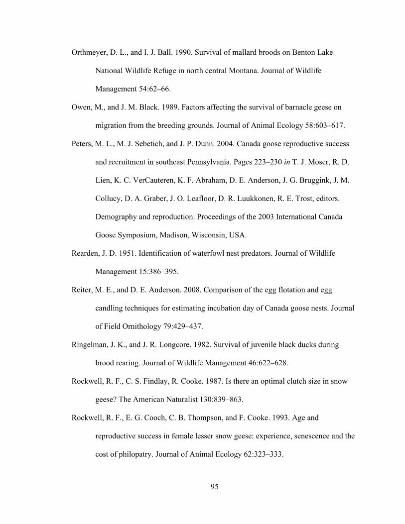
95
Orthmeyer, D. L., and I. J. Ball. 1990. Survival of mallard broods on Benton Lake
National Wildlife Refuge in north central Montana. Journal of Wildlife
Management 54:62–66.
Owen, M., and J. M. Black. 1989. Factors affecting the survival of barnacle geese on
migration from the breeding grounds. Journal of Animal Ecology 58:603–617.
Peters, M. L., M. J. Sebetich, and J. P. Dunn. 2004. Canada goose reproductive success
and recruitment in southeast Pennsylvania. Pages 223–230 in T. J. Moser, R. D.
Lien, K. C. VerCauteren, K. F. Abraham, D. E. Anderson, J. G. Bruggink, J. M.
Collucy, D. A. Graber, J. O. Leafloor, D. R. Luukkonen, R. E. Trost, editors.
Demography and reproduction. Proceedings of the 2003 International Canada
Goose Symposium, Madison, Wisconsin, USA.
Rearden, J. D. 1951. Identification of waterfowl nest predators. Journal of Wildlife
Management 15:386–395.
Reiter, M. E., and D. E. Anderson. 2008. Comparison of the egg flotation and egg
candling techniques for estimating incubation day of Canada goose nests. Journal
of Field Ornithology 79:429–437.
Ringelman, J. K., and J. R. Longcore. 1982. Survival of juvenile black ducks during
brood rearing. Journal of Wildlife Management 46:622–628.
Rockwell, R. F., C. S. Findlay, R. Cooke. 1987. Is there an optimal clutch size in snow
geese? The American Naturalist 130:839–863.
Rockwell, R. F., E. G. Cooch, C. B. Thompson, and F. Cooke. 1993. Age and
reproductive success in female lesser snow geese: experience, senescence and the
cost of philopatry. Journal of Animal Ecology 62:323–333.

96
Sargeant, A. B., and D. G. Raveling. 1992. Mortality during the breeding season. Pages
396–422 in B. D. Batt, A. D. Afton, M. G. Anderson, C. D. Ankney, D. H.
Johnson, J. A. Kadlec, and G. L. Krapu, editors. Ecology and management of
breeding waterfowl. University of Minnesota Press, Minneapolis, Minnesota,
USA.
Sedinger, J. S., M. S. Lindberg, B. T. Person, M. W. Eichholz, M. P. Herzog, and P. L.
Flint. 1998. Density-dependent effects on growth, body size, and clutch size in
black brant. The Auk 115:613–620.
Serie, J. R., D. L. Trauger, and D. E. Sharp. 1983. Migration and winter distributions of
canvasbacks staging on the upper Mississippi River. Journal of Wildlife
Management 47:741–753.
Sheaffer, S. E., R. A. Malecki, B. L. Swift, J. P. Dunn, and K. Scribner. 2007.
Management implications of molt migration by the Atlantic flyway resident
population of Canada geese, Branta canadensis. The Canadian Field-Naturalist
121:313–320.
Steel, P. E., P. D. Dalke, and E. G. Bizeau. 1957. Canada goose production at Gray’s
Lake, Idaho, 1949–1951. Journal of Wildlife Management 21:38–41.
Stolley, D. S., J. A. Bissonette, and J. A. Kadlec. 1999. Evaluation of methods to estimate
gosling survival. Journal of Field Ornithology 70:374–379.
Talent, L. G., R. L. Jarvis, and G. L. Krapu. 1983. Survival of mallard broods in south-
central North Dakota. Condor 85:74–78.

97
United States Department of Agriculture. 2009. Management of Canada goose nesting.
Wildlife Services, Animal and Plant Health Inspection Service, United States
Department of Agriculture, Washington, D.C., USA.
Wadkins, L. A. 1948. Dyeing birds for identification. Journal of Wildlife Management
12:388–391.
Warhurst, R. A., T. A. Bookout, and K. E. Bednairk. 1983. Effect of gang brooding on
survival of Canada goose goslings. Journal of Wildlife Management 47:1119–
1124.
Wang, Y. T. 1982. Factors affecting hatching success and gosling survival in giant
Canada geese. Ph.D. dissertation. Ohio State University, Columbus, Ohio, USA.
Weller, M. W. 1956. A simple field candler for waterfowl eggs. Journal of Wildlife
Management 20:111–113.
Williams, T. D., F. Cooke, E. G. Cooch, and R. F. Rockwell. 1993a. Body condition and
gosling survival in mass-banded lesser snow geese. The Journal of Wildlife
Management 57:555–562.
Williams, T. D., F. Cooke, E. G. Cooch, and R. L. Jefferies. 1993b. Environmental
degradation, food limitation and reproductive output: juvenile survival in lesser
snow geese. Journal of Animal Ecology 62:766–777.
Yocom, C. F., and S. W. Harris. 1965. Plumage descriptions and age data for Canada
goose goslings. Journal of Wildlife Management 29:874–877.
Zicus, M. C. 1981. Canada goose brood behavior and survival estimates at Crex
Meadows, Wisconsin. Wilson Bulletin 93:207–217.

98
Table 3.1. Summary of model-selection procedure examining variables affecting brood survival of AFRP Canada geese in New Jersey, USA from 2009–2010. I report Akaike’s Information Criterion (AICc), the relative difference in AIC values compared to the top-ranked model (∆ AIC), the AIC model weight (W), and the number of parameters in the model (K).
Candidate Models AICc ∆AICc Weight K Density + %Ag 274.361 0.000 0.586 3 HatchDate + Density 277.395 3.034 0.129 3 Density + %Forest 278.305 3.944 0.082 3 Density + HiTemp 278.695 4.334 0.067 3 Density + %Developed 279.135 4.774 0.054 3 HatchDate + HiTemp + Density 279.449 4.970 0.049 4 HiTemp + Density + %Developed 280.501 6.022 0.029 4 HatchDate + Density + %Ag 284.997 10.518 0.003 4 Global Model 286.648 11.556 0.002 7 HatchDate + Density + %Developed 287.763 13.284 0.001 4 HiTemp + %Developed 309.059 34.698 0.000 3 Null Model 309.826 35.582 0.000 1 HiTemp + %Forest 310.553 36.192 0.000 3 HiTemp + %Ag 311.557 37.196 0.000 3 %Ag + %Forest 311.845 37.484 0.000 3 HatchDate + HiTemp 312.093 37.732 0.000 3 HatchDate + %Developed 312.115 37.754 0.000 3 HatchDate + %Forest 312.789 38.428 0.000 3 %Developed + %Ag + % Forest 313.263 38.784 0.000 4 HatchDate + %Ag 313.865 39.504 0.000 3
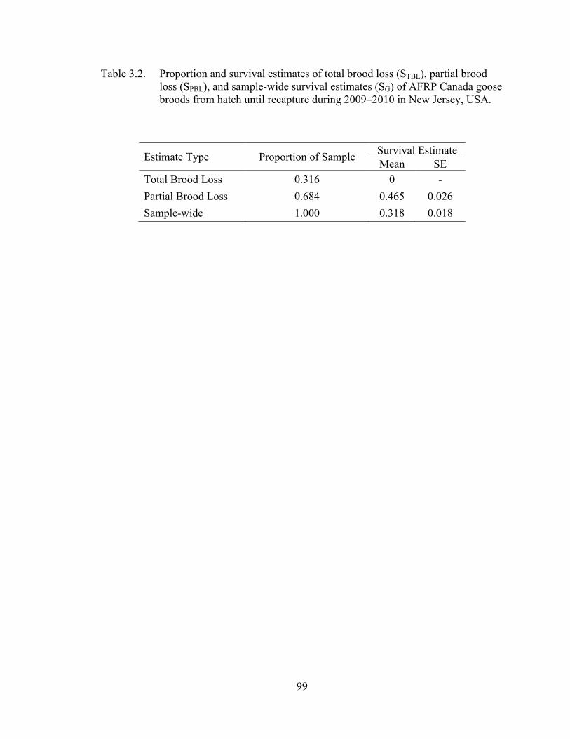
99
Table 3.2. Proportion and survival estimates of total brood loss (STBL), partial brood loss (SPBL), and sample-wide survival estimates (SG) of AFRP Canada goose broods from hatch until recapture during 2009–2010 in New Jersey, USA.
Estimate Type Proportion of Sample Survival Estimate Mean SE
Total Brood Loss 0.316 0 - Partial Brood Loss 0.684 0.465 0.026 Sample-wide 1.000 0.318 0.018

100
Figure 3.1. Twelve locations used to study AFRP Canada goose brood survival during April-July, 2009–2010 in New Jersey, USA.

101
Figure 3.2. Gosling survival estimate is composed of a proportion of broods that are totally lost during brood-rearing (TBL), and the remaining proportion of broods that are exposed to partial brood loss (PBL). Only broods that have partial losses are present during recapture, making it difficult to distinguish TBL from broods not present (emigrated) during recapture.
HATCH RECAPTURE
Complete BroodHatched
Total Brood Loss
Partial Brood Loss
Gosling Survival = (PTBL x 0% Survival) + ((1-PTBL) x SPBL)
(1-PTBL) x SPBL
PTBL x (0% Survival)
ORPartial Brood
Loss (Emigrated)

Figure 3.3. Estimate of daily mortality rates of AFRP Canada goose goslings from hatch until recapture during 2009–2010 in New Jersey, USA. Estimates are based on observations of both broods associated with marked adults and broods identifiable through color marking.
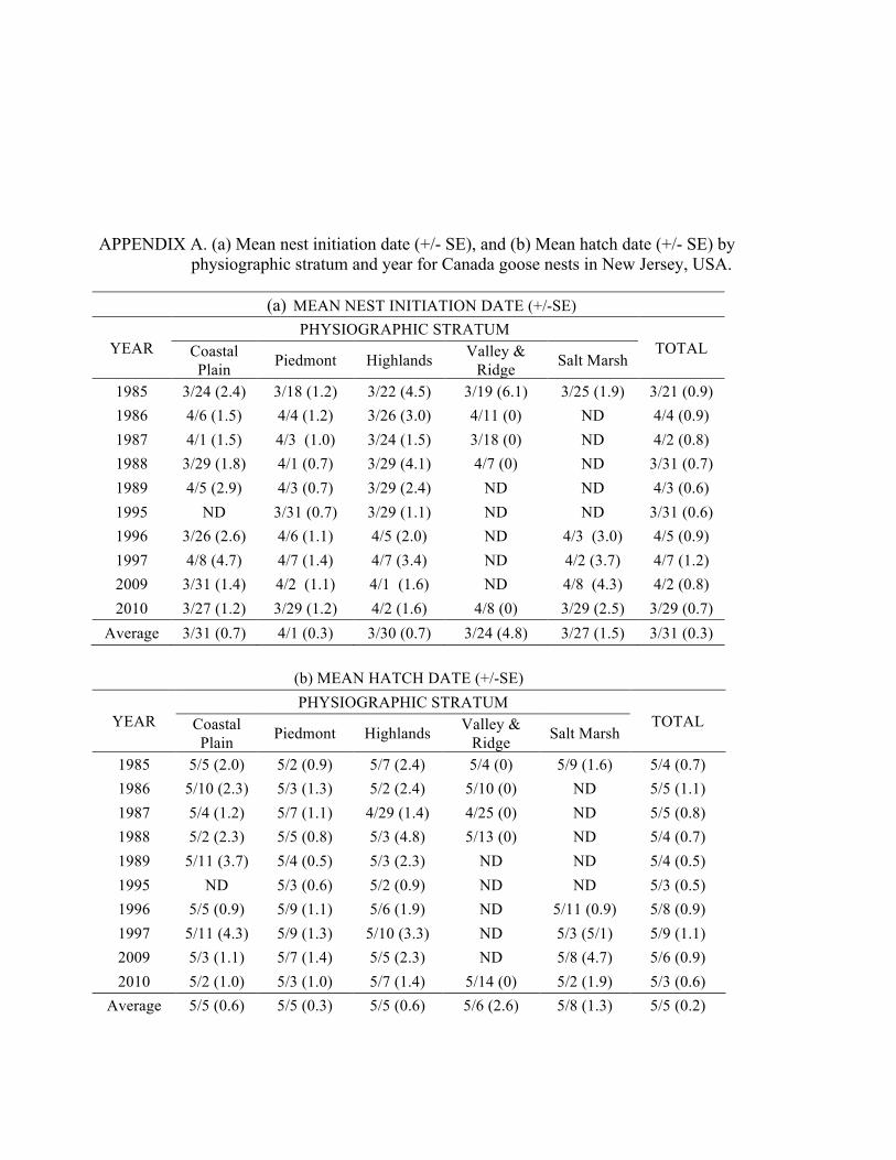
APPENDIX A. (a) Mean nest initiation date (+/- SE), and (b) Mean hatch date (+/- SE) by physiographic stratum and year for Canada goose nests in New Jersey, USA.
(a) MEAN NEST INITIATION DATE (+/-SE)
YEAR PHYSIOGRAPHIC STRATUM
TOTAL Coastal Plain Piedmont Highlands Valley &
Ridge Salt Marsh
1985 3/24 (2.4) 3/18 (1.2) 3/22 (4.5) 3/19 (6.1) 3/25 (1.9) 3/21 (0.9) 1986 4/6 (1.5) 4/4 (1.2) 3/26 (3.0) 4/11 (0) ND 4/4 (0.9) 1987 4/1 (1.5) 4/3 (1.0) 3/24 (1.5) 3/18 (0) ND 4/2 (0.8) 1988 3/29 (1.8) 4/1 (0.7) 3/29 (4.1) 4/7 (0) ND 3/31 (0.7) 1989 4/5 (2.9) 4/3 (0.7) 3/29 (2.4) ND ND 4/3 (0.6) 1995 ND 3/31 (0.7) 3/29 (1.1) ND ND 3/31 (0.6) 1996 3/26 (2.6) 4/6 (1.1) 4/5 (2.0) ND 4/3 (3.0) 4/5 (0.9) 1997 4/8 (4.7) 4/7 (1.4) 4/7 (3.4) ND 4/2 (3.7) 4/7 (1.2) 2009 3/31 (1.4) 4/2 (1.1) 4/1 (1.6) ND 4/8 (4.3) 4/2 (0.8) 2010 3/27 (1.2) 3/29 (1.2) 4/2 (1.6) 4/8 (0) 3/29 (2.5) 3/29 (0.7)
Average 3/31 (0.7) 4/1 (0.3) 3/30 (0.7) 3/24 (4.8) 3/27 (1.5) 3/31 (0.3)
(b) MEAN HATCH DATE (+/-SE)
YEAR PHYSIOGRAPHIC STRATUM
TOTAL Coastal Plain Piedmont Highlands Valley &
Ridge Salt Marsh
1985 5/5 (2.0) 5/2 (0.9) 5/7 (2.4) 5/4 (0) 5/9 (1.6) 5/4 (0.7) 1986 5/10 (2.3) 5/3 (1.3) 5/2 (2.4) 5/10 (0) ND 5/5 (1.1) 1987 5/4 (1.2) 5/7 (1.1) 4/29 (1.4) 4/25 (0) ND 5/5 (0.8) 1988 5/2 (2.3) 5/5 (0.8) 5/3 (4.8) 5/13 (0) ND 5/4 (0.7) 1989 5/11 (3.7) 5/4 (0.5) 5/3 (2.3) ND ND 5/4 (0.5) 1995 ND 5/3 (0.6) 5/2 (0.9) ND ND 5/3 (0.5) 1996 5/5 (0.9) 5/9 (1.1) 5/6 (1.9) ND 5/11 (0.9) 5/8 (0.9) 1997 5/11 (4.3) 5/9 (1.3) 5/10 (3.3) ND 5/3 (5/1) 5/9 (1.1) 2009 5/3 (1.1) 5/7 (1.4) 5/5 (2.3) ND 5/8 (4.7) 5/6 (0.9) 2010 5/2 (1.0) 5/3 (1.0) 5/7 (1.4) 5/14 (0) 5/2 (1.9) 5/3 (0.6)
Average 5/5 (0.6) 5/5 (0.3) 5/5 (0.6) 5/6 (2.6) 5/8 (1.3) 5/5 (0.2)

104
APPENDIX B. Frequency of Canada goose nest hatches in New Jersey during study years from 1985–1989, 1995–1997, and 2009–2010.
0
10
20
30
40
50
60
70
80
90
4/16 4/23 4/30 5/7 5/14 5/21 5/28 6/4
Freq
uenc
y
Hatch date
105
APPENDIX C. Age distribution of breeding adults by age class and sex during 1985–1989 in New Jersey, USA.

Appendix D. Evaluation of a clutch containment method during hatch in resident Canada geese for mark-recapture study.
(Submitted for publication with the Wildlife Society Bulletin)
Introduction
Measuring survival of goslings through fledge has been shown to be very challenging,
primarily due to their small size and the habitats in which they live (Stolley et al. 1999). Most
gosling mortality occurs in the first two weeks following hatching (Steel et al. 1957, Brakhage
1965, Zicus 1981, Eberhardt et al. 1989), making this stage a critical component in estimating
gosling survival. However, results can vary drastically across populations, habitats, techniques,
and/or level of effort (Stolley et al. 1999).
Several approaches are used to estimate gosling survival; including comparing total
hatchling counts to total gosling counts at a later date as well as the comparison of mean number
of hatchlings per nest to mean brood size at a later date. Unfortunately, both inherently
overestimate survival due to the inability to account for total brood loss, brood mixing, or
emigration (Zicus 1981). Mark-resight-recapture can improve estimates, particularly when using a
combination of individually marked hatchlings and marked adults (Stolley et al. 1999). Although
meta-analyses may be beneficial, they rely upon the accuracy of individual studies, which can
vary greatly.
Of additional concern, in a hatchling mark-recapture study, disturbance caused by nest
visits during the brooding period can cause older hatchlings to depart the nest site with the adults
prematurely, leaving the newly hatched birds unprotected, not fully brooded, and possibly

107
abandoned. Brooding of hatchlings in the nest bowl typically lasts about 24 hours (Brakhage
1965), allowing for drying of feathers, thermoregulation, and absorption of the remaining
nutrients from yolk lipids (Batt et al. 1992). The initial brooding period is followed by a
permanent departure from the nest site for brood rearing. Additionally, repeated nest visits are
often required during the last 3–5 days in order to verify the exact hatch date. This added
disruption can increase the likelihood that adults will flee the nest site with only a partial brood
during subsequent visits.
To address problems of partial clutch abandonment and reduce disturbance due to multiple
next visits, we evaluate a method that uses a mesh clutch containment bag during the hatch
period. Containment of the clutch allows for marking of complete broods, with the intent of
minimizing disruption of natural brooding activities and reducing abandonment of newly hatched
birds by fleeing parents.
Study Area
We conducted nest searches at 11 locations across 6 counties in New Jersey that were
known nesting and brood rearing sites (Fig. A4.1). Locations included state-owned wildlife
management areas and fish hatcheries, municipal parks with associated lakes, a closed municipal
landfill, and a privately-owned youth camp. Study sites ranged in size from 6–135 ha. The mean
high temperature for April and May 2010 was 20ºC (69ºF) and 24ºC (76ºF).
Methods
We conducted nest searches by foot and boat during the peak laying period from 1–30
April 2010. Embryos were aged utilizing both field candler (modified from Weller 1956, Cooper
and Batt 1972) and egg floating (United States Department of Agriculture 2009) techniques to
estimate the incubation stage and hatch date. We averaged the results from both methods to gain

108
the most accurate estimate of hatch date (Reiter and Anderson 2008). We randomly assigned all
nests to either a clutch bag treatment or no-clutch bag control group prior to hatch. We stratified
the sample by location in order to reduce bias associated with other variables affecting hatch
success.
On the evening prior to hatch, we contained the clutch of all nests within the treatment
group with a 35.5 cm x 71.0 cm (12” x 24”) green plastic expandable mesh clutch containment
bag (Big Apple Packaging onion sack; $0.14/bag; Fig. A4.2). The mesh size was 4.8 mm x 4.8
mm, offering limited potential for legs or wings to become entangled. We contained a maximum
of 5 eggs within each bag and we used 2 bags if clutch sizes were >5 eggs. We left as much open
space as possible within the bags to facilitate movement of hatching goslings and space for egg
remains and closed bags with an overhand knot to ensure containment of the clutch. After
treatment, we covered each bag with down and materials from the nest bowl to help prevent avian
predation (Rearden 1951). We also visited nests within the control group just prior to hatch, in
order to verify the exact hatch date. We used vocalizations of young, or “peeping”, as an
indication that the nest would hatch in about 2 days (Kossack 1950, Cooper 1978). We used the
presence of egg pipping, evident by a star-shaped crack on the surface of the shell, as an
indication that the nest would hatch within one day.
We revisited all treatment clutches < 18 hrs following containment for hatch. We recorded
the number of hatched goslings within each clutch on their hatch date. We removed goslings as
well as pipped and unpipped eggs from the nest bag. We applied monel size #1005–1 web tags
(Alliston 1975) to the center of the outside web of the right foot of hatchlings and birds within
star-pipped eggs, as part of a separate study of gosling survival. NJDFW staff recaptured marked
goslings during annual molt banding efforts in late June 2010. This study was conducted under a

109
banding permit from the Bird Banding Laboratory/USGS Patuxent Wildlife Research Center
(permit #06460).
We determined the number of eggs that hatched from nests within the control group by
either counting the number of 1) goslings within the nest bowl, 2) eggshells with intact
membranes in the nest bowl, and/or 3) goslings associated with the adult near the nest.
We calculated mean hatch success and standard error for the treatment and control groups
using all nests that were active on the day prior to hatch. Hatch success was defined by the
number of goslings that hatched divided by the number of eggs present on the day prior to hatch.
We assumed that variation in natural hatchability was similar across both the treatment and
control groups. We used a two-tailed Student’s t-test (α = 0.05) to test for differences between the
mean hatch success of the treatment and control groups. We also calculated the proportion of
hatchlings that were successfully marked within each brood for the treatment and control groups,
and tested for differences between the proportions of the two groups using a one-tailed Student’s
t-test (α = 0.025).
Results
We located and monitored 222 Canada goose nests in 2010. We assigned 110 nests to the
treatment group and 111 nests to the control group. Seventy one nests failed during the incubation
period prior to hatch. On the day prior to hatch, 72 nests remained in the treatment group, and 79
nests remained in the control group. The average clutch size was 5.17 eggs (SE ± 0.12 eggs).
The mean hatch success of the treatment group was 0.803 (SE ± 0.02), while the mean
hatch success of the control group was 0.834 (SE ± 0.032). There was no significant difference
between the mean hatch success of nests contained with clutch containment bags and the control
group (t148 = 0.794, P = 0.428). Six hundred thirty-one goslings hatched from 151 nests; and of

110
those, we web tagged 555 goslings for use in a separate gosling survival study. Seven goslings
were found dead in nest bags from the treatment group, and six goslings were found dead in nest
bowls from the control group. We were unable to distinguish natural deaths from those caused by
the clutch containment bag in the field.
The average proportion of hatchlings marked within broods in the treatment group was
0.897 (SE ± 0.042). The average proportion of hatchlings marked within broods in the control
group was 0.824 (SE ± 0.040). There was no significant difference between the proportion of
marked hatchlings within the treatment and control groups (t148 = 1.228, P = 0.111).
Discussion
We did not find a significant difference between the hatch success of the treatment and
control groups. The mean hatch success of nests within the treatment and control groups were
similar to those of other AFRP Canada goose nesting studies (Rummel 1979, Huskey et al. 1998b,
Conover 1998, Peters 2003). We did not mark a significantly larger proportion of hatchlings
whose clutches were contained. However, due to the increased effort involved in visiting nests
early in the day at each location, the overall mean proportion of hatchlings marked within each
brood was very high (0.855 ± 0.029 (SE)). In comparison with nesting locations in the sub-arctic,
our study area included locations that were easily accessible for multiple nest visits with relatively
little travel required. For gosling survival studies of sub-arctic nesting geese, this technique may
offer researchers additional time during the hatch period to be present for marking entire broods.
We observed that incubating females in both the treatment and control groups spent time
tending the contained clutch (i.e. rotating eggs, arranging down and nest materials) immediately
after returning to the nest. We observed no behavioral difference in adults between control and
treatment groups. However, in one instance, a contained clutch of unhatched eggs was found

111
floating in the water adjacent to a nest on the edge of a pond. Given that the clutch was contained
within the bag as a unit, the clutch apparently fell into the water when the female was tending the
nest. Had this clutch not been contained within a bag, perhaps only a single egg would have fallen
into the water.
This methodology successfully ensures that sampling efforts will measure full clutches
with little to no harm to hatchlings. Although containing the clutch during hatch has the potential
to allow for an increased sample size, we did not observe a difference in sample size using this
technique. Nonetheless, we urge prudent caution to minimize potential biases with administering
this technique. First, we applied bags during the later part of the day prior to hatch, and we
removed them following morning to ensure that hatched goslings were not enclosed during the
heat of the day. This issue may not be critical for contained clutches in sub-arctic conditions.
Second, attention must be directed toward ensuring that all nest bags are removed on the hatch
date, and that no unhatched eggs are left contained. This will avoid the rare occurrence of a late-
hatching bird being contained within a nest bag on a warm day after their brood has left the nest
site. Third, although newly hatched goslings are not able to walk, ample space must be given for
movement of hatchlings immediately following hatch. Fourth, when studies are conducted on
public lands, there is the potential that members of the public will observe this technique in
practice and not understand its purpose or that it is not causing undue harm. As a result, signage
may be necessary in nesting areas that are open to the public.

112
Literature Cited
Alliston, W. G. 1975. Web-tagging ducklings in pipped eggs. Journal of Wildlife Management
39:625–628.
Batt, B. D. J., A. D. Afton, M. G. Anderson, C. D. Ankney, D. H. Johnson, J. A. Kadlec, and G.
L. Krapu. 1992. Ecology and Management of Breeding Waterfowl. University of
Minnesota Press, Minnesota.
Brakhage, G. K. 1965. Biology and behavior of tub-nesting Canada geese. Journal of Wildlife
Management 29:751–771.
Conover, M. R. 1998. Reproductive biology of an urban population of Canada geese. Pages 67–
70 in D. H. Rusch, M. D. Samuel, D. D. Humburg, and B. D. Sullivan, editors. Biology
and management of Canada geese. Proceedings of the International Canada Goose
Symposium, Madison, Wisconsin, USA.
Cooper, J. A., and B. D. J. Batt. 1972. Criteria for aging Giant Canada Goose embryos. Journal of
Wildlife Management 36:1267–1269.
Cooper, J. A. 1978. The history and breeding biology of the Canada Geese of Marshy Point,
Manitoba. Wildlife Monograph 61:1–87.
Dunton, E. M., and D. L. Combs. 2010. Movements, habitat selection, associations, and survival
of giant Canada goose broods in central Tennessee. Human-Wildlife Interactions 4:192–
201.

113
Eberhardt, L. E., R. G. Anthony, and W. H. Rickard. 1989. Survival of juvenile Canada geese
during the rearing period. Journal of Wildlife Management 53:372–377.
Huskey, S. J., T. T. Fendley, and T.L. Ivey. 1998a. Canada goose gosling survival on farm ponds
in the central Piedmont of South Carolina. Pages 95–99 in D. H. Rusch, M. D. Samuel, D.
D. Humburg, and B. D. Sullivan, editors. Biology and management of Canada geese.
Proceedings of the International Canada Goose Symposium, Madison, Wisconsin, USA.
Huskey, S. J., T. T. Fendley, and T. L. Ivey and D. E. Baker. 1998b. Canada goose nesting
biology in the central Piedmont of South Carolina. Pages 47–51 in D. H. Rusch, M. D.
Samuel, D. D. Humburg, and B. D. Sullivan, editors. Biology and management of Canada
geese. Proceedings of the International Canada Goose Symposium, Madison, Wisconsin,
USA.
Kossack, C. W. 1950. Breeding habits of Canada geese under refuge conditions. American
Midland Naturalist 43:627–649.
Peters, M. L., M. J. Sebetich, and J. P. Dunn. 2003. Canada goose reproductive success and
recruitment in southeast Pennsylvania. Pages 223–230 in T. J. Moser, R. D. Lien, K. C.
VerCauteren, K. F. Abraham, D. E. Anderson, J. G. Bruggink, J. M. Collucy, D. A.
Graber, J. O. Leafloor, D. R. Luukkonen, R. E. Trost, editors. Demography and
Reproduction. Proceedings of the 2003 International Canada Goose Symposium, Madison,
Wisconsin, USA.
Rearden, J. D. 1951. Identification of waterfowl nest predators. Journal of Wildlife Management
15:386–395.

114
Reiter, M. E., and D. E. Anderson. 2008. Comparison of the egg flotation and egg candling
techniques for estimating incubation day of Canada goose nests. Journal of Field
Ornithology 79:429–437.
Rummel, L. H. 1979. Canada geese of the Patuxent Wildlife Research Center: family
relationships, behavior, and productivity. Thesis, University of Maryland, Baltimore,
USA.
Steel, P. E., P. D. Dalke, and E. G. Bizeau. 1957. Canada goose production at Gray’s Lake, Idaho,
1949–1951. Journal of Wildlife Management 21:38–41.
Stolley, D. S., J. A. Bissonette, and J. A. Kadlec. 1999. Evaluation of methods to estimate gosling
survival. Journal of Field Ornithology 70:374–379.
United States Department of Agriculture. 2009. Management of Canada goose nesting. Wildlife
Services, Animal and Plant Health Inspection Service, United States Department of
Agriculture, Washington, D.C., USA.
Weller, M. W. 1956. A simple field candler for waterfowl eggs. Journal of Wildlife Management
20:111–113.
Zicus, M. C. 1981. Canada goose brood behavior and survival estimates at Crex Meadows,
Wisconsin. Wilson Bulletin 93:207–217.

115
Figure A4.1. Eleven locations in New Jersey used to evaluate the effect of a nest containment bag on hatch success of Atlantic Flyway Resident Population Canada geese during 2010 breeding season.
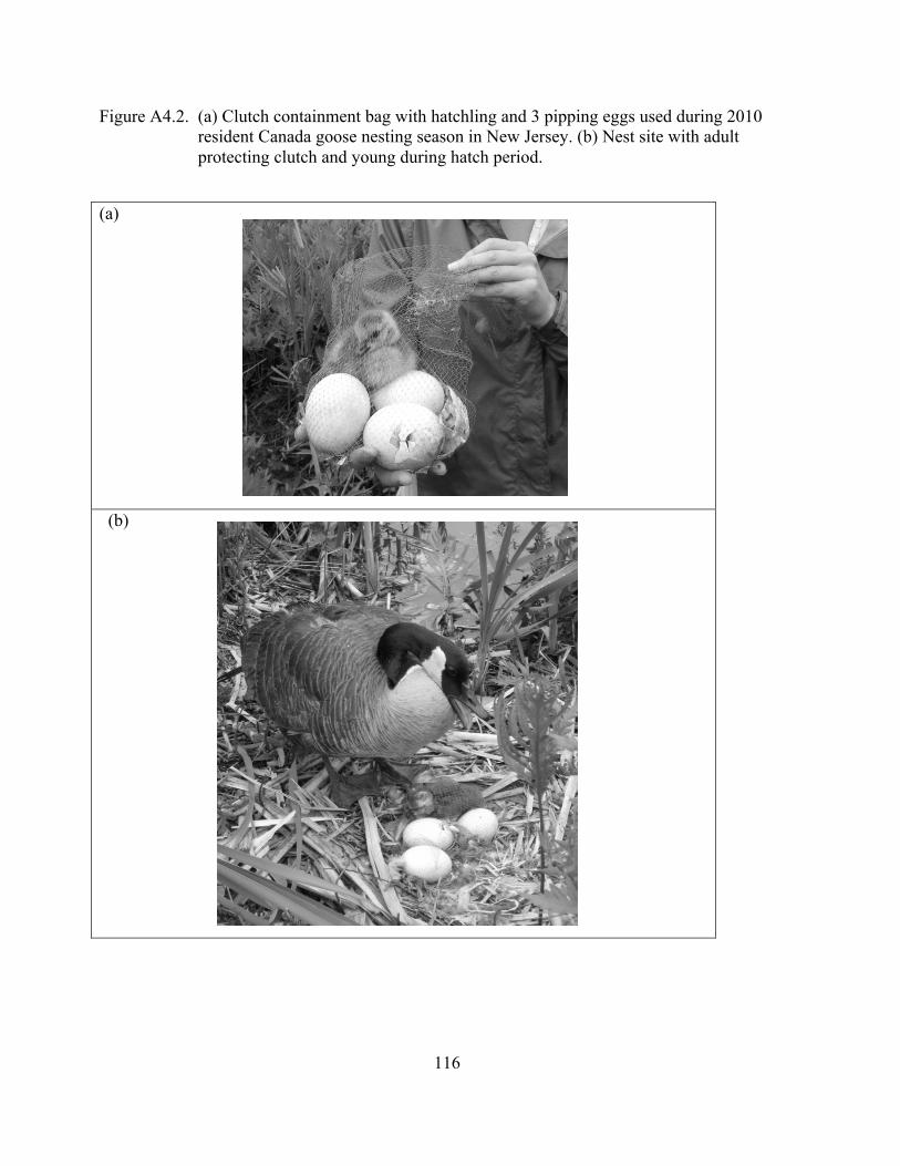
116
Figure A4.2. (a) Clutch containment bag with hatchling and 3 pipping eggs used during 2010 resident Canada goose nesting season in New Jersey. (b) Nest site with adult protecting clutch and young during hatch period.
(a)
(b)