net ecosystem exchange
TRANSCRIPT

WORKSHOP PROCEEDINGS
CRC FOR GREENHOUSE ACCOUNTING
APRIL 2001
Net Ecosystem Exchange

i
© Commonwealth of Australia 2001
ISBN 0957959702
This work is copyright. The Copyright Act 1968 permits fair dealing for study, research, news
reporting, criticism or review. Selected passages, tables or diagrams may be reproduced for
such purposes provided acknowledgment of the source is included. Major extracts from the
document may not be reproduced without the written permission of The Chief Executive, CRC
for Greenhouse Accounting, GPO Box 475, Canberra ACT 2601, Australia.
This is a collection of papers provided by contributors to the Net Ecosystem Exchange
Workshop held by the CRC during April 2001.
Views expressed in the volume are those of the authors and not necessarily those of the
Commonwealth Government nor the Cooperative Research Centre. Neither the authors nor
the Commonwealth nor the CRC accept responsibility for any advice or information that
relates to this material.
Edited by: Dr Miko U.F. Kirschbaum and Rowena Mueller (CRC for Greenhouse Accounting)
Published by:
The Communications Office
CRC for Greenhouse Accounting
GPO Box 475
CANBERRA ACT 2601
email: [email protected]
www: www.greenhouse.crc.org.au
Preferred way to cite this publication:
Kirschbaum, M.U.F. and Mueller, R. (2001) Net Ecosystem Exchange. Cooperative Research
Centre for Greenhouse Accounting.
The CRC for Greenhouse Accounting is a national independent scientific research centre
established in 1999 as an unincorporated joint venture under the AusIndustry CRC Program.
Acknowledgments:
Thanks are due to all workshop participants for their contributions.
Artwork: ANU Graphics
Photograph: Mr Jeff Wilson, ANU
Printer: Canprint Communications

More than a third of Australia's current greenhouse gas emissions are caused by human activities
such as forestry, agriculture and changes in land use. In order to reduce our net emissions from
the land, it is necessary to adopt new management practices to lower them; increase carbon sinks
through afforestation and reforestation; and minimise future emissions through limits on further
deforestation. It is also necessary to understand and account for carbon exchange rates.
Accounting for carbon exchange between the biosphere and the atmosphere is a formidable
scientific task thanks to the sheer size and complexity of the biosphere. Human and natural factors
also interact in intricate ways within the biosphere to determine the ultimate size and direction of
the carbon fluxes (exchanges) involved. Biospheric models are widely used by scientists to help
summarise and organise current understanding of the component processes and for simulating
both current exchange rates and likely future exchange under climate change and modified land
management regimes.
This is the CRC’s second publication. The collection of work represents the scientific contributions
of numerous Australian experts assembled for the Net Ecosystem Exchange Workshop held by the
CRC in Canberra from 18-20 April, 2001. It presents reviews and analyses of the major
eco-physiological factors that affect carbon exchange and features these factors using a range of
biospheric models.
It is hoped that the publication of this set of papers will ensure circulation of the best scientific
understanding at present with respect to the modelling of net ecosystem carbon exchange
for Australia.
Prof Ian Noble FTSE
Chief Executive
Cooperative Research Centre for Greenhouse Accounting
April 2001
Foreword
ii
NEE Workshop Agenda 1
Definitions Of Some Ecological Terms Commonly Used In Carbon Accounting 2
Brief Description Of Several Models For Simulating Net Ecosystem
Exchange In Australia 8
Modelling Radiation Absorption by Plant Canopies 30
Radiation Conversion 33
Plant Respiration 38
The Role of Allocation in Modelling NEE 43
Stand Age Effects on Productivity in Forests: Representation in Models and
Influence on Net Ecosystem Exchange 50
Phenology and Reproduction 58
How Does Ecosystem Water Balance Influence Net Primary Productivity?
- A Discussion 62
Other Soil Constraints on Net Primary Production 71
Nutrient Uptake and Use in Plant Growth 75
The Control Of Ecosystem Carbon Dynamics By The Linkages Between
Above and Belowground Processes 82
Carbon Dynamics and Nutrient Mineralisation 89
Temperature and Moisture Effects on Decomposition 95
Soil Texture Effects on Decomposition and Soil Carbon Storage 103
Acidic Soil pH, Aluminium and Iron Affect Organic Carbon Turnover in Soil 111
Charcoal and Other Resistant Materials 116
Effect of Mechanical Disturbance (Cultivation) on Soil Carbon Dynamics 120
Plant Litter and Decomposition: General Concepts and Model Approaches 124
Rapporteur Reports 130
NEE Workshop Participants 135
Contents
iv

DAY 1 - WEDNESDAY 18 APRIL 2001
Radiation interception - Ying Ping Wang
“The Australian Journal of Plant Physiology” - Jennifer
McCutchan
Radiation conversion - Belinda Medlyn
Respiration - Roger Gifford
Discussion - Wang, Medlyn and Gifford
Allocation - Craig Barton
Mortality and stand age effects on productivity - Michael
Battaglia
Other factors (phenology, reproduction etc.) - Chris Beadle,
as presented by Michael Battaglia
Discussion - Barton and Battaglia
- Wrap up Session
DAY 2 - THURSDAY 19 APRIL 2001
Introduction
The impact of ecosystem water balance on NPP - Derek
Eamus
Other soil constraints (impedence, acidity, salinity, water
logging) - Robert Edis
Nutrient uptake and use in plant growth - John Evans and
Everard Edwards
Discussion - Eamus, Edis, Evans and Edwards
CO2 concentration - Graham Farquhar
Temperature effects on growth - Marilyn Ball and David
Barker
Discussion - Farquhar, Ball and Barker
Linking above and belowground processes - Miko
Kirschbaum
Interactions between carbon dynamics and nutrient miner-
alisation - Peter Grace
Discussion - Kirschbaum and Grace
Wrap up Session
DAY 3 - FRIDAY 20 APRIL 2001
Introduction
Temperature and moisture effects on decomposition rate -
Keryn Paul
Soil texture effects on decomposition and soil C storage -
Evelyn Krull and Jeff Baldock
pH, aluminium and other factors that can inhibit decompo-
sition rates - Ram Dalal
Charcoal and other resistant organic matter - Jan
Skjemstad
Discussion - Paul, Baldock, Krull, Dalal and Skjemstad
Soil disturbance (cultivation) effects on decomposition and
soil C storage - Phil Polglase
Litter quality and quantity - Marc Corbeels
Discussion - Polglase and Corbeels
Linking the processes together - Steve Roxburgh and
Rapporteurs
General discussion
- Final Wrap up Session
N E E W O R K S H O P T H R E E D A Y A G E N D A
NEE Workshop Agenda
1
2
M.U.F Kirschbaum, D. Eamus, R.M. Gifford, S.H. Roxburgh and P.J. Sands
Introduction
The papers in these Workshop Proceedings all deal with Net
Ecosystem Carbon Exchange. In the interest of clarity, this and
other related terms are briefly described in the following.
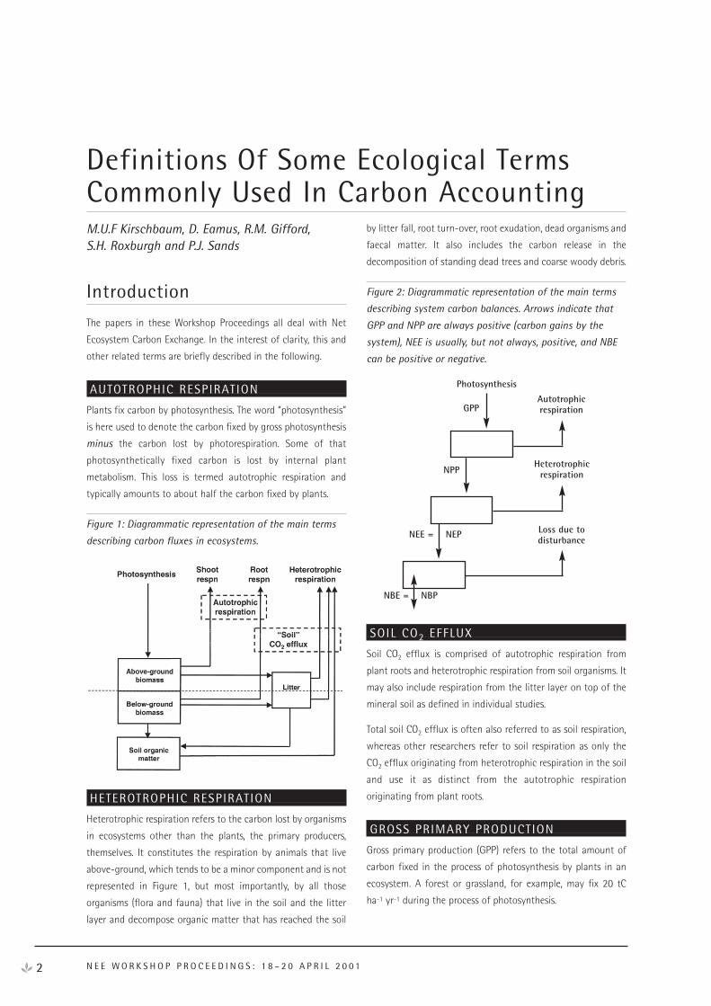
AUTOTROPHIC RESPIRATION
Plants fix carbon by photosynthesis. The word “photosynthesis”
is here used to denote the carbon fixed by gross photosynthesis
minus the carbon lost by photorespiration. Some of that
photosynthetically fixed carbon is lost by internal plant
metabolism. This loss is termed autotrophic respiration and
typically amounts to about half the carbon fixed by plants.
Figure 1: Diagrammatic representation of the main terms
describing carbon fluxes in ecosystems.
HETEROTROPHIC RESPIRATION
Heterotrophic respiration refers to the carbon lost by organisms
in ecosystems other than the plants, the primary producers,
themselves. It constitutes the respiration by animals that live
above-ground, which tends to be a minor component and is not
represented in Figure 1, but most importantly, by all those
organisms (flora and fauna) that live in the soil and the litter
layer and decompose organic matter that has reached the soil
by litter fall, root turn-over, root exudation, dead organisms and
faecal matter. It also includes the carbon release in the
decomposition of standing dead trees and coarse woody debris.
Figure 2: Diagrammatic representation of the main terms
describing system carbon balances. Arrows indicate that
GPP and NPP are always positive (carbon gains by the
system), NEE is usually, but not always, positive, and NBE
can be positive or negative.
SOIL CO2 EFFLUX
Soil CO2 efflux is comprised of autotrophic respiration from
plant roots and heterotrophic respiration from soil organisms. It
may also include respiration from the litter layer on top of the
mineral soil as defined in individual studies.
Total soil CO2 efflux is often also referred to as soil respiration,
whereas other researchers refer to soil respiration as only the
CO2 efflux originating from heterotrophic respiration in the soil
and use it as distinct from the autotrophic respiration
originating from plant roots.
GROSS PRIMARY PRODUCTION
Gross primary production (GPP) refers to the total amount of
carbon fixed in the process of photosynthesis by plants in an
ecosystem. A forest or grassland, for example, may fix 20 tC
ha-1 yr-1 during the process of photosynthesis.
Definitions Of Some Ecological Terms Commonly Used In Carbon Accounting
N E E W O R K S H O P P R O C E E D I N G S : 1 8 – 2 0 A P R I L 2 0 0 1
Photosynthesis
GPP
NPP
NEE = NEP
NBE = NBP
Autotrophicrespiration
Heterotrophicrespiration
Loss due todisturbance
Total global GPP is estimated to be about 120 GtC yr-1 (Gifford
1982; Bolin et al. 2000), and total Australian GPP can be
estimated to be 2-6 GtC yr-1 if one assumes that GPP is 2 times
NPP and uses the estimates of NPP compiled below.
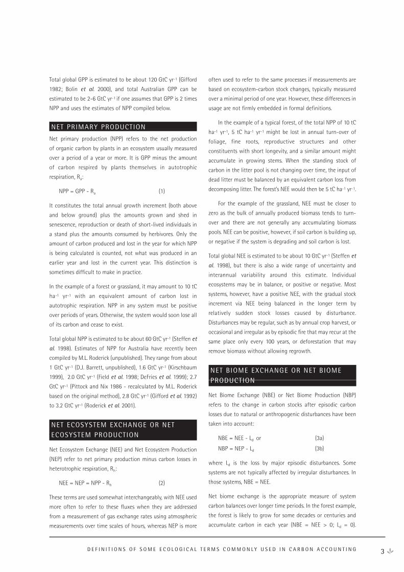
NET PRIMARY PRODUCTION
Net primary production (NPP) refers to the net production
of organic carbon by plants in an ecosystem usually measured
over a period of a year or more. It is GPP minus the amount
of carbon respired by plants themselves in autotrophic
respiration, Ra:
NPP = GPP - Ra (1)
It constitutes the total annual growth increment (both above
and below ground) plus the amounts grown and shed in
senescence, reproduction or death of short-lived individuals in
a stand plus the amounts consumed by herbivores. Only the
amount of carbon produced and lost in the year for which NPP
is being calculated is counted, not what was produced in an
earlier year and lost in the current year. This distinction is
sometimes difficult to make in practice.
In the example of a forest or grassland, it may amount to 10 tC
ha-1 yr-1 with an equivalent amount of carbon lost in
autotrophic respiration. NPP in any system must be positive
over periods of years. Otherwise, the system would soon lose all
of its carbon and cease to exist.
Total global NPP is estimated to be about 60 GtC yr-1 (Steffen et
al. 1998). Estimates of NPP for Australia have recently been
compiled by M.L. Roderick (unpublished). They range from about
1 GtC yr-1 (D.J. Barrett, unpublished), 1.6 GtC yr-1 (Kirschbaum
1999), 2.0 GtC yr-1 (Field et al. 1998; DeFries et al. 1999); 2.7
GtC yr-1 (Pittock and Nix 1986 - recalculated by M.L. Roderick
based on the original method), 2.8 GtC yr-1 (Gifford et al. 1992)
to 3.2 GtC yr-1 (Roderick et al. 2001).
NET ECOSYSTEM EXCHANGE OR NETECOSYSTEM PRODUCTION
Net Ecosystem Exchange (NEE) and Net Ecosystem Production
(NEP) refer to net primary production minus carbon losses in
heterotrophic respiration, Rh:
NEE = NEP = NPP - Rh (2)
These terms are used somewhat interchangeably, with NEE used
more often to refer to these fluxes when they are addressed
from a measurement of gas exchange rates using atmospheric
measurements over time scales of hours, whereas NEP is more
often used to refer to the same processes if measurements are
based on ecosystem-carbon stock changes, typically measured
over a minimal period of one year. However, these differences in
usage are not firmly embedded in formal definitions.
In the example of a typical forest, of the total NPP of 10 tC
ha-1 yr-1, 5 tC ha-1 yr-1 might be lost in annual turn-over of
foliage, fine roots, reproductive structures and other
constituents with short longevity, and a similar amount might
accumulate in growing stems. When the standing stock of
carbon in the litter pool is not changing over time, the input of
dead litter must be balanced by an equivalent carbon loss from
decomposing litter. The forest’s NEE would then be 5 tC ha-1 yr-1.
For the example of the grassland, NEE must be closer to
zero as the bulk of annually produced biomass tends to turn-
over and there are not generally any accumulating biomass
pools. NEE can be positive, however, if soil carbon is building up,
or negative if the system is degrading and soil carbon is lost.
Total global NEE is estimated to be about 10 GtC yr-1 (Steffen et
al. 1998), but there is also a wide range of uncertainty and
interannual variability around this estimate. Individual
ecosystems may be in balance, or positive or negative. Most
systems, however, have a positive NEE, with the gradual stock
increment via NEE being balanced in the longer term by
relatively sudden stock losses caused by disturbance.
Disturbances may be regular, such as by annual crop harvest, or
occasional and irregular as by episodic fire that may recur at the
same place only every 100 years, or deforestation that may
remove biomass without allowing regrowth.
NET BIOME EXCHANGE OR NET BIOMEPRODUCTION
Net Biome Exchange (NBE) or Net Biome Production (NBP)
refers to the change in carbon stocks after episodic carbon
losses due to natural or anthropogenic disturbances have been
taken into account:
NBE = NEE - Ld or (3a)
NBP = NEP - Ld (3b)
where Ld is the loss by major episodic disturbances. Some
systems are not typically affected by irregular disturbances. In
those systems, NBE = NEE.
Net biome exchange is the appropriate measure of system
carbon balances over longer time periods. In the forest example,
the forest is likely to grow for some decades or centuries and
accumulate carbon in each year (NBE = NEE > 0; Ld = 0).
D E F I N I T I O N S O F S O M E E C O L O G I C A L T E R M S C O M M O N L Y U S E D I N C A R B O N A C C O U N T I N G 3
Eventually, the carbon may be lost in a massive disturbance,
such as a fire or harvesting. In the year, when that occurs, the
loss due to disturbance will be much greater than the annual
increment in carbon so that NBE << 0 in that year. Summed
over a longer time period, NBE will be close to zero, with the
many small positive annual increments balanced by the large
loss in the year of disturbance (i.e. NBE = ΣNEE - Ld). In the
grassland system, NEE ≅ NBE is more likely, although systems
subject to fires recurring every few years could have a pattern
similar to that of forest systems, but with smaller and more
frequent peaks and troughs.
Globally, NBE (including the effects of deforestation) is
estimated to have been 0.2 GtC yr-1 from 1980-1989 and 1.4
GtC yr-1 from 1989-1998 (IPCC 2001). This suggests that the
overall global accrual of ecosystem carbon is not wholly
annulled by the carbon loss due to major disturbances,
including deforestation. Historically (before major human
influence), the quantity must have been close to 0 and can only
deviate significantly from 0 while systems are out of
equilibrium.
Although NBE applies to long timescales, it need not necessarily
have to apply to large spatial scales despite the implication by
inclusion of the term ‘biome’. NBE can be monitored at the plot
level over long periods, which might include disturbance events.
In other words, NBE can be applied as much to the plot level as
at larger spatial scales.
There is no explicit definition that distinguishes episodic loss by
major disturbance (Ld ) from loss by heterotrophic respiration
(Rh). Broadly speaking, organic-matter oxidising processes that
occur all year every year in an ecosystem contribute to Rh, while
processes that oxidise organic matter in only some years would
be classed as carbon losses due to disturbances.
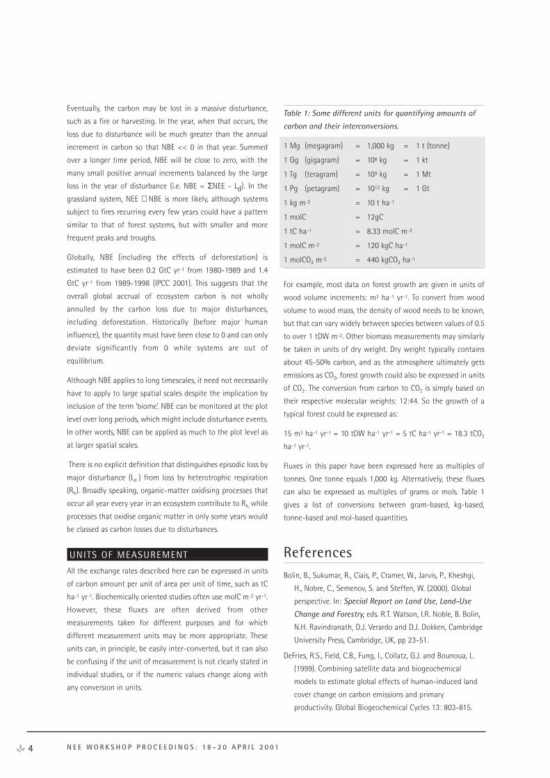
UNITS OF MEASUREMENT
All the exchange rates described here can be expressed in units
of carbon amount per unit of area per unit of time, such as tC
ha-1 yr-1. Biochemically oriented studies often use molC m-2 yr-1.
However, these fluxes are often derived from other
measurements taken for different purposes and for which
different measurement units may be more appropriate. These
units can, in principle, be easily inter-converted, but it can also
be confusing if the unit of measurement is not clearly stated in
individual studies, or if the numeric values change along with
any conversion in units.
Table 1: Some different units for quantifying amounts of
carbon and their interconversions.
1 Mg (megagram) = 1,000 kg = 1 t (tonne)
1 Gg (gigagram) = 106 kg = 1 kt
1 Tg (teragram) = 109 kg = 1 Mt
1 Pg (petagram) = 1012 kg = 1 Gt
1 kg m-2 = 10 t ha-1
1 molC = 12gC
1 tC ha-1 = 8.33 molC m-2
1 molC m-2 = 120 kgC ha-1
1 molCO2 m-2 = 440 kgCO2 ha-1
For example, most data on forest growth are given in units of
wood volume increments: m3 ha-1 yr-1. To convert from wood
volume to wood mass, the density of wood needs to be known,
but that can vary widely between species between values of 0.5
to over 1 tDW m-3. Other biomass measurements may similarly
be taken in units of dry weight. Dry weight typically contains
about 45-50% carbon, and as the atmosphere ultimately gets
emissions as CO2, forest growth could also be expressed in units
of CO2. The conversion from carbon to CO2 is simply based on
their respective molecular weights: 12:44. So the growth of a
typical forest could be expressed as:
15 m3 ha-1 yr-1 = 10 tDW ha-1 yr-1 = 5 tC ha-1 yr-1 = 18.3 tCO2
ha-1 yr-1.
Fluxes in this paper have been expressed here as multiples of
tonnes. One tonne equals 1,000 kg. Alternatively, these fluxes
can also be expressed as multiples of grams or mols. Table 1
gives a list of conversions between gram-based, kg-based,
tonne-based and mol-based quantities.
ReferencesBolin, B., Sukumar, R., Ciais, P., Cramer, W., Jarvis, P., Kheshgi,
H., Nobre, C., Semenov, S. and Steffen, W. (2000). Global
perspective. In: Special Report on Land Use, Land-Use
Change and Forestry, eds. R.T. Watson, I.R. Noble, B. Bolin,
N.H. Ravindranath, D.J. Verardo and D.J. Dokken, Cambridge
University Press, Cambridge, UK, pp 23-51.
DeFries, R.S., Field, C.B., Fung, I., Collatz, G.J. and Bounoua, L.
(1999). Combining satellite data and biogeochemical
models to estimate global effects of human-induced land
cover change on carbon emissions and primary
productivity. Global Biogeochemical Cycles 13: 803-815.
N E E W O R K S H O P P R O C E E D I N G S : 1 8 – 2 0 A P R I L 2 0 0 14
Field, C.B., Behrenfeld, M.J., Randerson, J.T. and Falkowski, P.
(1998). Primary production of the biosphere: integrating
terrestrial and oceanic components. Science 281: 237-239.
Gifford, R.M. (1982). Global photosynthesis in relation to our
food and energy needs. pp 459-495 in “Photosynthesis:
Development, Carbon Metabolism and Plant
Productivity” Vol 2. Ed. Govindjee. New York, Academic
Press.
Gifford, R.M., Cheney, N.P., Noble, J.C., Russell, J.S., Wellington,
A.B., and Zammit, C. (1992). Australian land use, primary
production of vegetation and carbon pools in relation to
atmospheric carbon dioxide concentration. In Gifford, R.M.
and Barson, M.M. (Eds.) Australia’s Renewable Resources:
Sustainability and Global Change. Bureau of Rural
Resources Proceedings No. 14, AGPS, Canberra, pp. 151-
187.
IPCC (2001). Technical Summary of the Working Group I
Report. Intergovernmental Panel on Climate Change
(http://www.ipcc.ch/pub/wg1TARtechsum.pdf), 83 pp.
Kirschbaum, M.U.F. (1999). The effect of climate change on
forest growth in Australia. In: Impacts of global change on
Australian temperate forests. (Howden, S.M. and Gorman,
J.T., eds.), Working Paper Series, 99/08, pp. 62-68.
Pittock, A.B. and Nix, H.A. (1986). The effect of changing
climate on Australian biomass production: a preliminary
study. Climatic Change 8: 243-255.
Roderick, M.L., Farquhar, G.D., Berry, S.L. and Noble, I.R. (2001).
On the direct effect of clouds and atmospheric particles on
the productivity and structure of vegetation. Oecologia (In
press).
Steffen, W., Noble, I., Canadell, J., Apps, M., Schulze, E.-D.,
Jarvis, P.G., Baldocchi, D., Ciais, P., Cramer, W., Ehleringer, J.,
Farquhar, G., Field, C.B., Ghazi, A., Gifford, R., Heimann, M.,
Houghton, R., Kabat, P., Körner, C., Lambin, E., Linder, S.,
Mooney, H.A., Murdiyarso, D., Post. W.M., Prentice, C.,
Raupach, M.R., Schimel, D.S., Shvidenko, A. and Valentini, R.
(1998). The terrestrial carbon cycle: implications for the
Kyoto Protocol. Science 280: 1393-1394.
D E F I N I T I O N S O F S O M E E C O L O G I C A L T E R M S C O M M O N L Y U S E D I N C A R B O N A C C O U N T I N G 5

Papers and Presentations
M.U.F. Kirschbaum, J.O. Carter, P.R. Grace, B.A. Keating, R.J. Keenan, J.J. Landsberg, G.M. McKeon, A.D. Moore, K.I. Paul, D.A. Pepper,M.E. Probert, G.P. Richards, P.J. Sands and J.O. Skjemstad
Introduction
This brief background paper has been compiled for the
workshop on modelling net ecosystem exchange that was held
in Canberra from 18-20 April 2001. It gives brief descriptions of
the models that are currently available in Australia and that are
of interest in modelling net ecosystem exchange for the
Australian continent: APSIM, CENTURY, CenW, FullCAM, G’DAY,
Gendec, GrazPlan, GRASP, Linkages, Promod, Roth-C, Socrates
and 3-PG.
These models deal with the range of different ecosystems that
together constitute the Australian biosphere. Some ecosystems
or components of ecosystems are modelled by more than one
model, but the different models approach their modelling tasks
in different ways by providing more or less detail, and by
including or omitting certain processes or plant or soil pools.
The workshop provided details of the treatment of various
processes in each of these models which are described in other
papers in this volume. This paper gives a brief description for
each of these models to make it easier to better understand the
overall modelling approach in the respective models and gain a
better appreciation of the treatment of specific processes as
they are dealt with in greater detail in the other papers of this
volume.
APSIM
APSIM (Agricultural Production System SIMulator) is a
software system that allows models of crops, pastures, trees, soil
water, nutrients, and erosion to be flexibly configured to
simulate diverse production systems (McCown et al 1996; see
also web site (www.apsim-help.tag.csiro.au)).
The modelling framework has been developed over the last 10
years by the APSRU group (Agricultural Production Systems
Research Unit), a collaborative effort between CSIRO Tropical
Agriculture (now Sustainable Ecosystems) and Qld State
agencies (DPI, DNR). APSRU is currently being renegotiated and
it is likely that its core membership will be expanded to include
CSIRO Land and Water and the Uni of Qld.
A key feature of APSIM, which distinguishes it from many
vegetation specific models, is the central position of the soil
rather than the vegetation. Changes in the status of the soil
state variables are simulated continuously in response to
weather and management. Crops, pastures or trees come and
go, finding the soil in a particular state and leaving it in an
altered state.
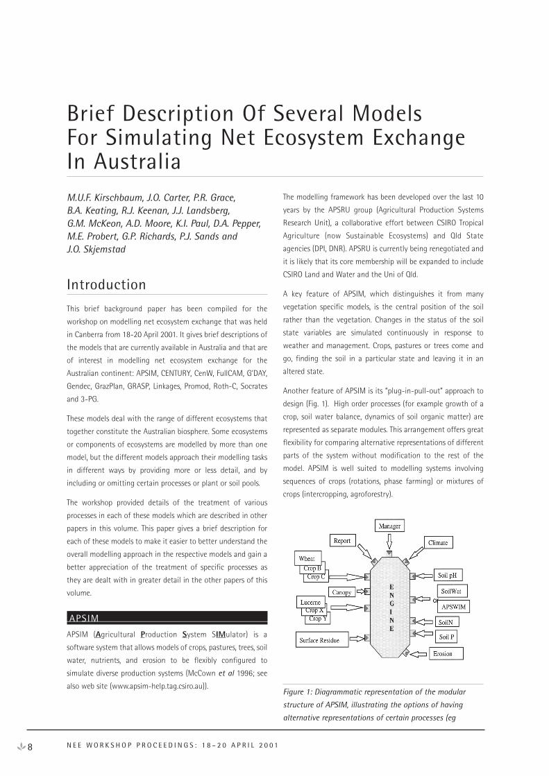
Another feature of APSIM is its “plug-in-pull-out” approach to
design (Fig. 1). High order processes (for example growth of a
crop, soil water balance, dynamics of soil organic matter) are
represented as separate modules. This arrangement offers great
flexibility for comparing alternative representations of different
parts of the system without modification to the rest of the
model. APSIM is well suited to modelling systems involving
sequences of crops (rotations, phase farming) or mixtures of
crops (intercropping, agroforestry).
Figure 1: Diagrammatic representation of the modular
structure of APSIM, illustrating the options of having
alternative representations of certain processes (eg
8 N E E W O R K S H O P P R O C E E D I N G S : 1 8 – 2 0 A P R I L 2 0 0 1
Brief Description Of Several Models For Simulating Net Ecosystem ExchangeIn Australia
SoilWat or APSWIM for the water balance) and multiple
crops.
APSIM models are typically 1-dimensional, with the soil
described as a multi-layered system. The recently released
APSIM v 2.0 provides support for multi-point simulations for
the first time. Most modules operate on a daily time-step. The
minimum climatic data required to run APSIM are daily
maximum and minimum temperature, radiation and rainfall.
The vegetation modules in APSIM use a simple framework to
describe the daily capture and utilization of environmental
resources such as solar radiation, soil water and nutrients. In
response to environmental stimuli, plants develop through
distinct phenological phases, a leaf canopy is produced, incident
radiation is intercepted, absorbed energy is converted into
assimilates which are partitioned between plant components,
including yield.
The functions used in APSIM vegetation modules are outlined in
greater detail on the APSIM web page, and in the document
“Principles of simulating crop growth and development in
APSIM” (Mike Robertson and others in APSRU, unpublished).
APSIM vegetation modules generally include water and
nitrogen as limiting factors; a phosphorus limitation is under
development but at present is only operational for maize.
At the time of writing, modules exist for barley, canola,
chickpea, cowpea, fababean, mungbean, navybean, hemp,
wheat, lucerne, maize, millet, peanut, pigeonpea, sorghum,
sunflower, sugarcane and cotton. A FOREST module provides a
generalised vegetation treatment that has been used for
Eucalyptus, Pinus and other natural plant communities.
The soil water dynamics are described by one of two modules,
either SoilWat (a “cascading bucket” approach) or APSWIM
(based on simultaneous solution of the Richards’ equation for
water flow and the advection-dispersion equation for solute
transport). A comprehensive study comparing the two
approaches found both to be capable of giving good
descriptions of soil water content and solute movement
(Verburg, 1996).
The turnover of organic matter is represented by the SoilN and
Residue modules (Probert et al 1998). APSIM distinguishes
between surface residues and residues in the soil. Within SoilN,
organic materials are conceptualized as fresh organic matter
(FOM), and two soil organic matter pools (BIOM and HUM) that
differ in their rates of decomposition. The soil organic matter
pools are considered to have non-varying C:N ratios.
Decomposition rates are determined by soil water and
temperature, and in the case of FOM its C:N ratio.
APSIM has pioneered very flexible specification of management
regimes in farming systems modelling. The MANAGER module is
controlled by a user defined script language which enables a
diverse range of management operations to be specified in ways
that are conditional on the state of the simulated system. Both
the timing and nature of operations such as sowing, tillage,
residue management, fertilisation, irrigation, crop management,
harvesting etc are all controlled from this script specified by
users. All these operations can be made responsive to the state
of the weather, vegetation or soil system.
APSIM is distributed under a licence system. Currently
approximately 200 licences exist and the model is in active use
in farming systems research in all Australian States except
Tasmania, and in project activities with International
Agricultural Research Centre’s and the National Agricultural
Research System in a number of countries in Africa, in India,
China and Indonesia. APSIM testing is on-going in this diverse
range of situations. Details of specific module testing can be
found within the science documentation on the APSIM web
page (www.apsim-help.tag.csiro.au).
By far the most extensive testing has focused on the simulation
of net primary productivity and economic yield and of
simulation of the dynamics of soil water and soil
carbon/nitrogen under different agricultural systems. The
model’s strengths are in cropping systems, with emerging
capabilities in pasture and forest systems. At this point in time
there is no livestock production capability in APSIM, although
linkages are being explored with the GRAZPLAN / FARMWI$E
effort from CSIRO Plant Industry.
CENTURY
The CENTURY version 5 agroecosystem model is the latest
version of a soil organic model initially developed by Parton et
al. (1987). This model simulates carbon, nitrogen, phosphorus,
and sulphur dynamics on a monthly time step for an annual
cycle over time scales of centuries and millennia and embodies
the best understanding to date of the biogeochemistry of C, N,
P, and S. Plant production can be simulated by using
grassland/crop, forest or savanna system sub-models, with the
flexibility of specifying potential primary production parameters
representing site-specific plant communities. Land use change
can be represented by changing the plant community type
during model runs, i.e. beginning with forest, clearing to pasture
then running a cropping system.
9B R I E F D E S C R I P T I O N O F S E V E R A L M O D E L S F O R S I M U L A T I N G N E T E C O S Y S T E M E X C H A N G E I N A U S T R A L I A
CENTURY was especially developed to deal with a wide range of
cropping system rotations and tillage practices for system
analysis of the effects of management, CO2 fertilisation and
climate change on productivity and sustainability of
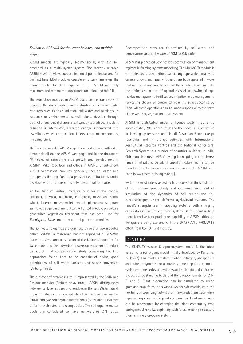
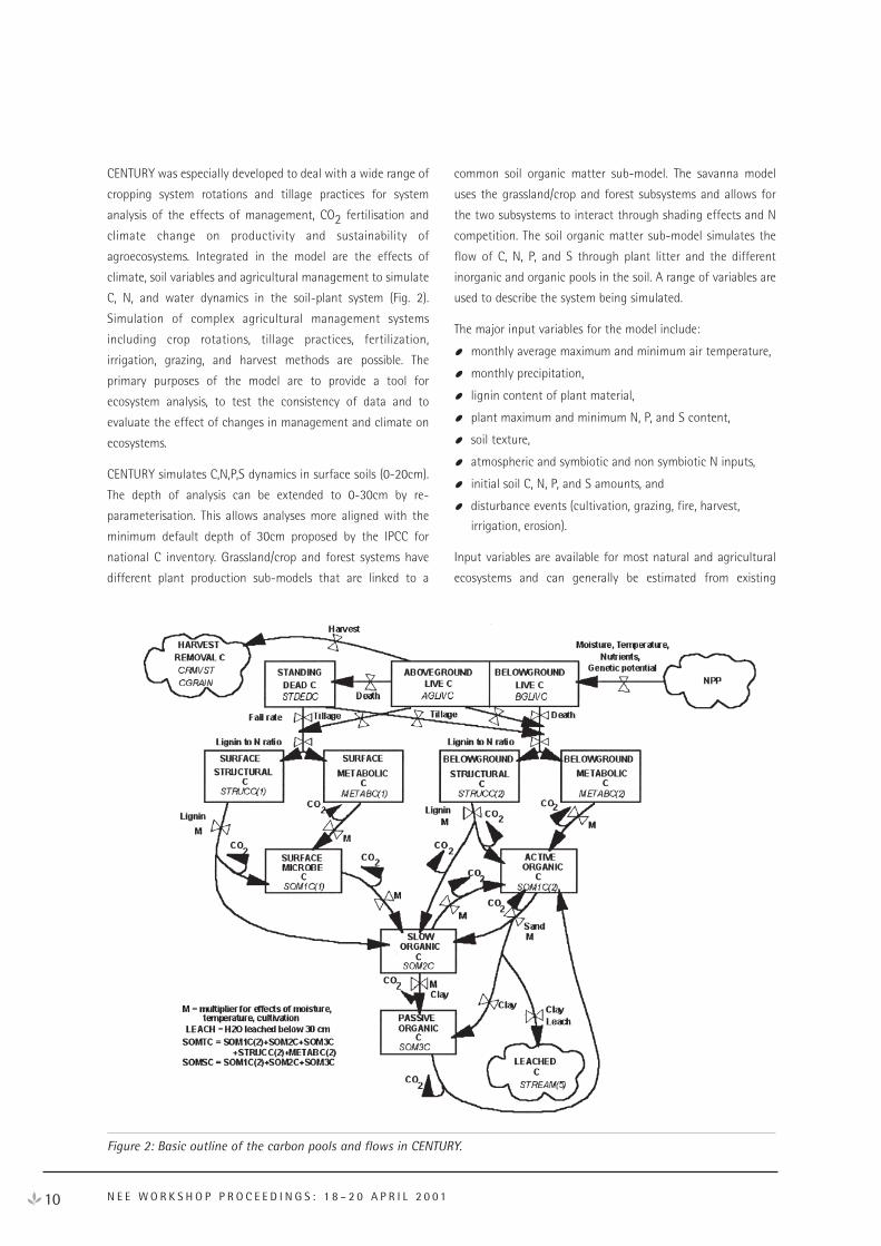
agroecosystems. Integrated in the model are the effects of
climate, soil variables and agricultural management to simulate
C, N, and water dynamics in the soil-plant system (Fig. 2).
Simulation of complex agricultural management systems
including crop rotations, tillage practices, fertilization,
irrigation, grazing, and harvest methods are possible. The
primary purposes of the model are to provide a tool for
ecosystem analysis, to test the consistency of data and to
evaluate the effect of changes in management and climate on
ecosystems.
CENTURY simulates C,N,P,S dynamics in surface soils (0-20cm).
The depth of analysis can be extended to 0-30cm by re-
parameterisation. This allows analyses more aligned with the
minimum default depth of 30cm proposed by the IPCC for
national C inventory. Grassland/crop and forest systems have
different plant production sub-models that are linked to a
common soil organic matter sub-model. The savanna model
uses the grassland/crop and forest subsystems and allows for
the two subsystems to interact through shading effects and N
competition. The soil organic matter sub-model simulates the
flow of C, N, P, and S through plant litter and the different
inorganic and organic pools in the soil. A range of variables are
used to describe the system being simulated.
The major input variables for the model include:
monthly average maximum and minimum air temperature,
monthly precipitation,
lignin content of plant material,
plant maximum and minimum N, P, and S content,
soil texture,
atmospheric and symbiotic and non symbiotic N inputs,
initial soil C, N, P, and S amounts, and
disturbance events (cultivation, grazing, fire, harvest,
irrigation, erosion).
Input variables are available for most natural and agricultural
ecosystems and can generally be estimated from existing
10 N E E W O R K S H O P P R O C E E D I N G S : 1 8 – 2 0 A P R I L 2 0 0 1
Figure 2: Basic outline of the carbon pools and flows in CENTURY.
literature or parameterised from field data. Most of the
parameters controlling the flow of C in the system are in special
file containing ”fixed” parameters however these can be altered
to simulate soils to a greater depth or control the C pool
structure. The user can configure the model considering only C
and N dynamics or a multiple array of elements namely, C, N, P
and or C, N, P, and S. Initial soil carbon and nitrogen can be
entered in parameter files or “spun up” using a long model run
(> 1000 years) and or estimated within the model from simple
regressions based on climate and soil texture. Climate inputs
can be actual data, mean data or average climate with
stochastic rainfall, this combination allows exploration of
climate verses management impacts.
Simulation of carbon isotope concentrations for C14 and C13within the soil matrix is possible within the model. This enables
the user to better calibrate the model when isotope data from
field studies are available. The model is most often used to
simulate the C cycle at the plot or stand scale it has also been
used at continental (VEMAP et al., 1995) and global scales
(Parton et al., 1995) to simulate the carbon cycle under climate
change. While the model has been developed to simulate real
ecosystems at local to global scales, it can also simulate
microcosm experiments where soils are incubated in the
laboratory at known water content and temperature.
The strengths of the CENTURY model are: (1) its ability to model
a diverse array of ecosystems. (2) Capability of simulating a
wide range of disturbance events, especially those relevant to
land use, land use change and forestry. (3) Its extensive use and
testing around the world on a diverse array of systems.
On the other hand the model is largely empirical and the user is
presented with what sometimes appears to be a bewildering
array of parameters. In reality one can usually modify a small
selection of these to give realistic simulations. Many of the
parameters arise from the need to model a wide range of
systems and disturbance events.
The plant production model sub components are probably less
accurate than any number of specialist forest, crop and pasture
growth models, although CENTURY seems to perform quite well
in many situations. A number of other models e.g. CenW, G’DAY
etc have taken elements the basic soil C/N dynamics from
CENTURY and integrated them into their model structure.
The most recently released version of (CENTURY 5) (produce by
a team of scientists at the Natural Resources Ecology Lab
(NREL) Colorado State University) includes a layered soil
physical structure, and new erosion and deposition sub-models.
The model code has been rewritten in C++, reorganised, and
modified to use platform-independent configuration and
output files. Added to this version is a windows based
graphical-user interface providing ease of configuration and
running CENTURY simulations. Documentation and the
model can be downloaded from the NREL web
site, http://www.nrel.colostate.edu/projects/models.html. New
versions of CENTURY that use daily rather than monthly water
balance are under development. These developments allow the
modelling of non-CO2 greenhouse gasses and add to the
already impressive capability of this model.
Evolution of the model will continue as the understanding of
biogeochemical processes improves. The identification of
problem areas where processes are not adequately quantified
and demand for new applications in greenhouse inventory and
climate change will drive further developments.
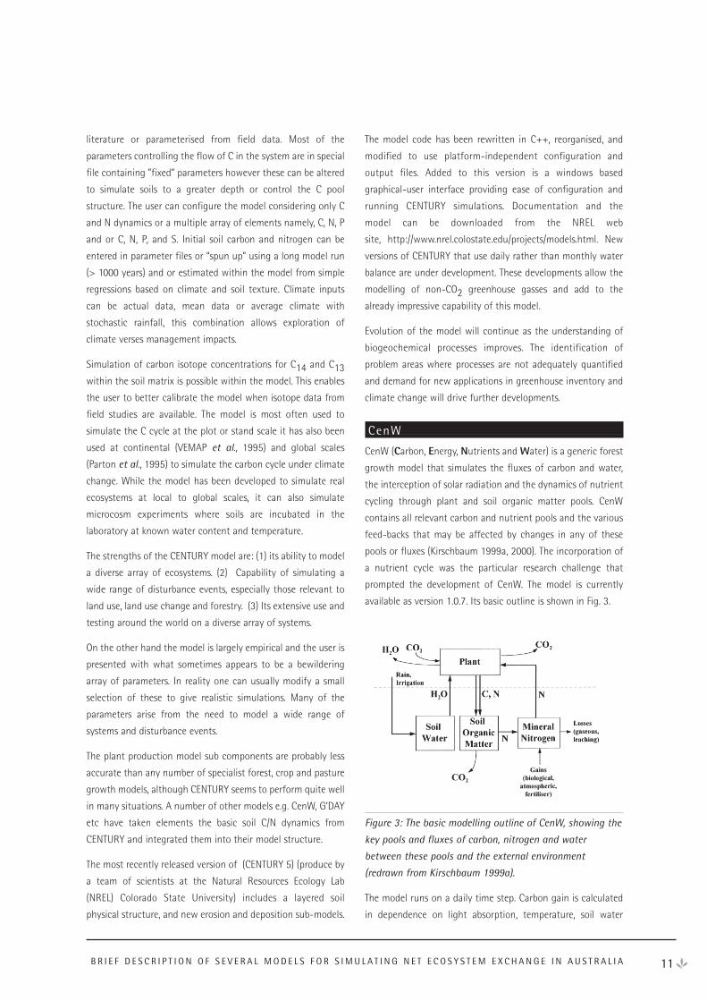
CenW
CenW (Carbon, Energy, Nutrients and Water) is a generic forest
growth model that simulates the fluxes of carbon and water,
the interception of solar radiation and the dynamics of nutrient
cycling through plant and soil organic matter pools. CenW
contains all relevant carbon and nutrient pools and the various
feed-backs that may be affected by changes in any of these
pools or fluxes (Kirschbaum 1999a, 2000). The incorporation of
a nutrient cycle was the particular research challenge that
prompted the development of CenW. The model is currently
available as version 1.0.7. Its basic outline is shown in Fig. 3.
Figure 3: The basic modelling outline of CenW, showing the
key pools and fluxes of carbon, nitrogen and water
between these pools and the external environment
(redrawn from Kirschbaum 1999a).
The model runs on a daily time step. Carbon gain is calculated
in dependence on light absorption, temperature, soil water
11B R I E F D E S C R I P T I O N O F S E V E R A L M O D E L S F O R S I M U L A T I N G N E T E C O S Y S T E M E X C H A N G E I N A U S T R A L I A
status, foliar nitrogen concentration and any foliage damage
due to frost or scorching temperatures during preceding days.
Some photosynthetically fixed carbon is assumed to be lost in
respiration, with daily respiration rate calculated as a constant
fraction of photosynthetic carbon gain or as a function of
temperature and nutritional status.
Allocation to different plant organs is determined by plant
nutrient status, tree height and species-specific allocation
factors. Water use is calculated using the Penman-Monteith
equation, with canopy resistance given by the inverse of
stomatal conductance, which, in turn, is linked to calculated
photosynthetic carbon gain. Water is lost by transpiration, soil
evaporation and, under wet conditions, deep drainage.
Nitrogen can come from a constant rate of atmospheric
deposition, fertiliser addition or mineralisation during the
decomposition of soil organic matter. The model can be run
with or without symbiotic nitrogen fixation. Decomposition rate
is determined by temperature, soil water status and soil organic
matter quality in a modified formulation based on the CENTURY
model.
The nutrient cycle is closed through litter production by the
shedding of plant parts, such as roots, bark, branches and, most
importantly, foliage. Litter is assumed to be produced as a
constant fraction of live biomass pools. In addition, foliage is
shed during drought or when canopies become too dense. Litter
is then added to the organic matter pools from where carbon is
eventually lost and nitrogen becomes available as inorganic
mineral nitrogen.
A fraction of mineral nitrogen is lost by volatilisation in the
mineralisation of organic nitrogen. There can also be nitrogen
losses by leaching or off-site removal of wood.
The model requires as minimum input daily minimum and
maximum temperature and rainfall. Solar radiation is desirable,
but can alternatively be calculated from empirical relationships
of temperature and rainfall. There is also the requirement for a
large number of soils and plant-physiological parameters.
Where site- and species-specific information on these
parameters is not available, parameters can be estimated from
related species, and site-specific information can be based on
typical soils values.
The model has been tested against data from the nutrient and
irrigation experiments at the BFG site near Canberra
(Kirschbaum 1999a) and has been used for simulations of net
primary production and the effect of climate change for the
whole Australian continent (Kirschbaum 1999b). Its primary
application has been the investigation of the complex feed-
back effects that determine ultimate system responses in
climate change simulations (Kirschbaum 1999c).
Ful lCAM
The National Carbon Accounting System (NCAS) has been
established by the Australian Government to provide a
complete carbon accounting and projections capacity for land
based (agricultural and forestry) activities.
An overall system framework (Richards, 2001) was developed to
guide the development of data gathering and analytic projects
and programs which could then be integrated using spatial
modelling approaches. Various models were selected, calibrated
and verified through these projects and programs. A range of
related projects were undertaken to identify, collate and
synthesise the additional data needed to operate the models
continent-wide at a fine spatial and temporal resolution over a
30 year period.
To achieve this multiple pool, activity driven carbon modelling
capacity the NCAS undertook the development of the FullCAM
carbon model. FullCAM is an integrated compendium model
and accounting tool that provides the linkage between the
various sub-models. FullCAM has components that deal with
the biological and management processes which affect carbon
pools and the transfers between pools in forest, agricultural,
transitional (afforestation, reforestation) and mixed (e.g.,
agroforestry) systems. The exchanges of carbon, loss and
uptake, between the terrestrial biological system and the
atmosphere are also accounted for.
The integrated suite of models that comprise FullCAM are: the
physiological growth model for forests, 3PG (Landsberg and
Waring, 1997; Landsberg et. al., 2000; Coops et. al. 1998,
2000a); the carbon accounting model for forests developed by
NCAS, CAMFor (Richards and Evans, 2000a): the carbon
accounting model for cropping and grazing systems, CAMAg
(Richards and Evans, 2000b), the microbial decomposition
model, GENDEC (Moorhead and Reynolds, 1991; Moorhead et.
al., 1999), and the Rothamsted Soil Carbon Model,–Roth C
(Jenkinson, et. al., 1987, Jenkinson et. al., 1991). FullCAM can
run any of these models in a single coordinated simulation,
including any model by itself.
These models have been independently developed for the
various purposes of predicting and accounting for:
soil carbon change in agriculture and forest activities (in
the case of Roth C);
12 N E E W O R K S H O P P R O C E E D I N G S : 1 8 – 2 0 A P R I L 2 0 0 1
determination of rates of decomposition of litter (in the
case of GENDEC); and
prediction of growth in trees (in the case of 3PG).
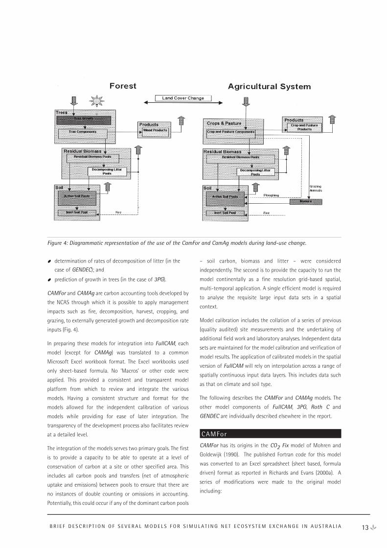
CAMFor and CAMAg are carbon accounting tools developed by
the NCAS through which it is possible to apply management
impacts such as fire, decomposition, harvest, cropping, and
grazing, to externally generated growth and decomposition rate
inputs (Fig. 4).
In preparing these models for integration into FullCAM, each
model (except for CAMAg) was translated to a common
Microsoft Excel workbook format. The Excel workbooks used
only sheet-based formula. No ‘Macros’ or other code were
applied. This provided a consistent and transparent model
platform from which to review and integrate the various
models. Having a consistent structure and format for the
models allowed for the independent calibration of various
models while providing for ease of later integration. The
transparency of the development process also facilitates review
at a detailed level.
The integration of the models serves two primary goals. The first
is to provide a capacity to be able to operate at a level of
conservation of carbon at a site or other specified area. This
includes all carbon pools and transfers (net of atmospheric
uptake and emissions) between pools to ensure that there are
no instances of double counting or omissions in accounting.
Potentially, this could occur if any of the dominant carbon pools
– soil carbon, biomass and litter – were considered
independently. The second is to provide the capacity to run the
model continentally as a fine resolution grid-based spatial,
multi-temporal application. A single efficient model is required
to analyse the requisite large input data sets in a spatial
context.
Model calibration includes the collation of a series of previous
(quality audited) site measurements and the undertaking of
additional field work and laboratory analyses. Independent data
sets are maintained for the model calibration and verification of
model results. The application of calibrated models in the spatial
version of FullCAM will rely on interpolation across a range of
spatially continuous input data layers. This includes data such
as that on climate and soil type.
The following describes the CAMFor and CAMAg models. The
other model components of FullCAM, 3PG, Roth C and
GENDEC are individually described elsewhere in the report.
CAMFor
CAMFor has its origins in the CO2 Fix model of Mohren and
Goldewijk (1990). The published Fortran code for this model
was converted to an Excel spreadsheet (sheet based, formula
driven) format as reported in Richards and Evans (2000a). A
series of modifications were made to the original model
including:
13B R I E F D E S C R I P T I O N O F S E V E R A L M O D E L S F O R S I M U L A T I N G N E T E C O S Y S T E M E X C H A N G E I N A U S T R A L I A
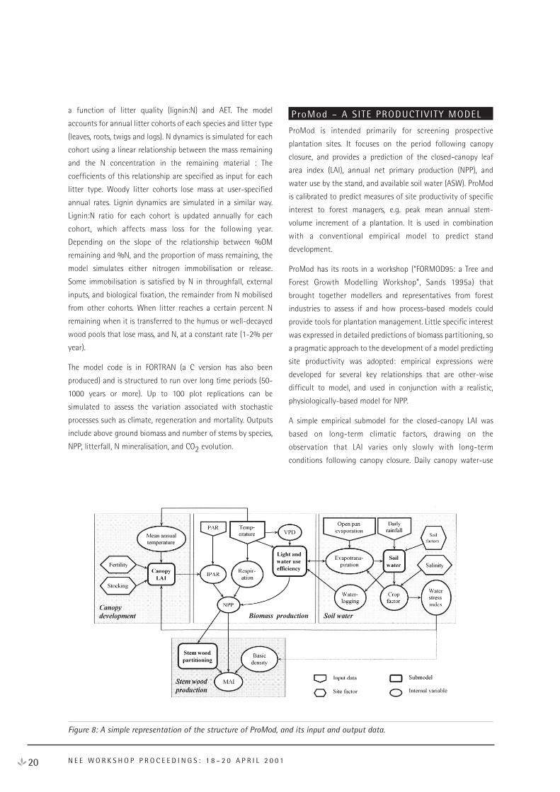
Figure 4: Diagrammatic representation of the use of the CamFor and CamAg models during land-use change.
introduction of an inert soil carbon pool recognising the
nature of carbon in Australian mineral soils, the high
charcoal content and the potential long term protection of
fine organic matter through encapsulation and absorption
by clays;
addition of a fire simulation capacity that could deal with
stand replacing and/or regenerating fires, being either
forest floor fires largely removing litter or crown fires
affecting the whole tree;
modification of wood product pool structures and
lifecycles to reflect those cited in Jaakko Pöyry (1999);
improved resolution of component distinctions of the
standing tree material, splitting coarse and fine roots,
branch and leaf material;
potential to override the soil carbon model component by
directly entering either field data or externally modelled
inputs, and
an added capacity to account from a primary data input of
above-ground mass increment as an alternative to stem
volume increment.
Within FullCAM, the CAMFor sub-component can take its
growth information from any one of three sources:
net primary productivity (NPP) derived from 3PG with
feedback from management actions (thinnings, etc.)
specified in CAMFor;
information entered from external models; and
measures of either above-ground mass increment or stem
volume increment.
Material entering the debris pool (that is the above-ground
coarse and fine litter) and the decay (the root material below
ground shed by live biomass) is accounted in either a
decomposable or resistant fraction, with the potential to apply
separate decomposition rates to each.
The information flowing from 3PG to CAMFor is the total NPP,
as reflected in whole tree productivity/growth. Rules for the
allocation to various tree components and for the turnover
rates that will affect the standing mass increment at any one
time (change in mass as opposed to a total productivity change)
are specified within a CAMFor table.
Neither CAMFor nor 3PG (in this form) deal with a number of
stems, but work on proportional change to mass per unit area.
Thinning activities, such as harvest or fire, which are specified in
CAMFor are treated as a proportional decrease of biomass and
are reflected as an equivalent proportional decrease in canopy
cover within 3PG. For deforestation, the same applies, but with
a large residual of decomposing woody material being the
primary change remaining within CAMFor.
CAMAg
Within FullCAM, CAMAg serves the same roles for cropping and
grazing systems as CAMFor does for forests. The CAMAg model
reflects the impacts of management on carbon accumulation
and allocates masses to various product pools within plants and
to decomposable and resistant organic residues. Yields may be
entered in the model in a variety of ways including above-
ground, total or product mass, along with above- and
belowground turnover rates. The principal human activities that
drive transfers of material in CAMAg are ploughing, herbicide
application, harvest, fire and grazing (with manure return).
With both CAMFor and CAMAg embedded within FullCAM, it is
possible to represent the transitional afforestation,
reforestation and deforestation (change at one site) or mix of
agricultural and forest systems (discrete activities at separate
sites). Under afforestation and reforestation there is a gradual
change from the characteristics of the original pasture or
cropping system, with the mass of organic matter derived from
those systems decomposing and decreasing with declining
input. For deforestation, the same applies, but with a large
residual of decomposing woody material being the primary
change remaining within CAMFor.
Within FullCAM, CAMFor and CAMAg can be proportionally
represented (as under afforestation, reforestation and
deforestation) according to the relative proportions of canopy
cover for each of the woody (CAMFor) and non-woody
(CAMAg) categories. This also provides capacity for modelling
ongoing mixed systems such as agroforestry.
MODEL INTEGRATION
The initial integration of the FullCAM was performed on a
Microsoft Excel developmental version of the forest component
of FullCAM and linked with the Excel versions of the models
3PG, CAMFor, GENDEC and Roth C. The resultant
developmental model, named GRC3, was used to test and refine
the linkages between the models. It formed a 10-megabyte
Excel workbook, which could be used for developmental
purposes, but was not a realistic option for general or routine
application.
The C code based application of FullCAM is a far more efficient
and transportable (e.g., Mac, PC or Unix environments) format,
with run speeds capable of continental scale application at fine
spatial (using ArcBinary file format) and temporal resolution.
14 N E E W O R K S H O P P R O C E E D I N G S : 1 8 – 2 0 A P R I L 2 0 0 1
The linkages between models are sequential, from growth
estimation (3PG for forests only) to management (CAMFor and
CAMAg), decomposition (GENDEC) and soils (Roth C). The key
linkages are as follows:
3PG to CAMFor: is achieved by inputting the total biomass
increment from the 3PG output to the CAMFor biomass table.
Allocation of this material to various tree components (above-
and belowground) will be as per the CAMFor mass distribution
table.
CAMFor to GENDEC: is a transfer of the above-ground debris
pools, splitting the decomposable and resistant material
described in CAMFor between the soluble, cellulose and lignin
plant input pools of GENDEC. When operated in conjunction,
the CAMFor breakdown rates for this material act as a ‘flow’
mechanism to introduce material to the GENDEC model. The
above-ground debris pools of CAMFor thus become holding
pools of material which can flow to GENDEC. Belowground
material is treated independently of GENDEC and is either
transferred directly to the RPM and DPM pools of Roth C from
CAMFor, or, if Roth C is not being implemented, given an
empirical decay within the CAMFor ‘Active’ soils pools.
CAMFor to Roth C (direct): if CAMFor and Roth C are in use
(without GENDEC) the function of the ‘breakdown’ rates in
CAMFor is used to decompose above-ground litter (unless
ploughed in) which is then (minus losses to the atmosphere)
placed in the Roth C ‘HUM’ (humified organic matter)
belowground pool. Root material is transferred to the Roth C
DPM and RPM pools.
CAMAg to GENDEC: the interaction between CAMAg and
GENDEC mirrors that of CAMFor and GENDEC. Again GENDEC
only operates on the pool of above-ground litter.
CAMAg to Roth C (direct): the transfers of material when
CAMAg and Roth C are run together (without GENDEC) are the
same as for CAMFor to Roth C. Belowground material (and
above-ground material ‘ploughed in’) is dealt with in the DPM
and RPM pools of Roth C.
While the model is capable of being run at daily, weekly,
monthly and annual time steps, the NCAS will generally operate
the model at monthly time steps. The choice of time step for
any operation will largely depend on the temporal variability of
the system being modelled and the temporal resolution of the
available data.
The principal testing of FullCAM was carried out on GRC3, the
developmental Excel version, providing maximum transparency
and therefore an ability to track iterations of the spreadsheet
formula. Another advantage was an ability to attach the @Risk
add-on (Palisade 1997). Among other things, @Risk provides a
capacity to implement sensitivity analyses within the Excel
model given specified correlations between the various input
variables. Each specified output is assessed for its sensitivity to
each input variable. Correlations between input variables can be
specified and Monte Carlo analyses run to enable uncertainty
analyses given specified variability. @Risk can also interact with
the FullCAM code version and will be implemented within
developer’s versions of the model.
A range of activities are underway within the NCAS that provide
required calibrations for the various components of the
FullCAM model. Much of this activity was initiated upon
selection of the various component models for independent
programs. Each of these programs provides for ongoing model
testing.
G’DAY
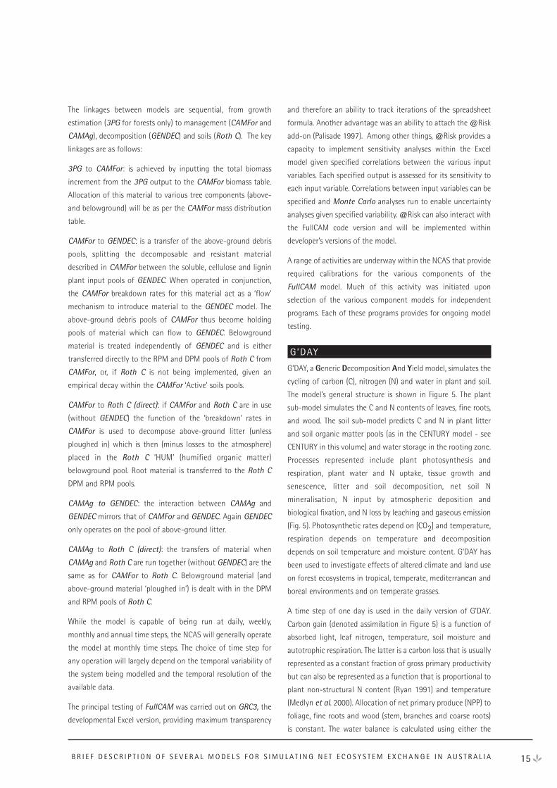
G’DAY, a Generic Decomposition And Yield model, simulates the
cycling of carbon (C), nitrogen (N) and water in plant and soil.
The model’s general structure is shown in Figure 5. The plant
sub-model simulates the C and N contents of leaves, fine roots,
and wood. The soil sub-model predicts C and N in plant litter
and soil organic matter pools (as in the CENTURY model - see
CENTURY in this volume) and water storage in the rooting zone.
Processes represented include plant photosynthesis and
respiration, plant water and N uptake, tissue growth and
senescence, litter and soil decomposition, net soil N
mineralisation, N input by atmospheric deposition and
biological fixation, and N loss by leaching and gaseous emission
(Fig. 5). Photosynthetic rates depend on [CO2] and temperature,
respiration depends on temperature and decomposition
depends on soil temperature and moisture content. G’DAY has
been used to investigate effects of altered climate and land use
on forest ecosystems in tropical, temperate, mediterranean and
boreal environments and on temperate grasses.
A time step of one day is used in the daily version of G’DAY.
Carbon gain (denoted assimilation in Figure 5) is a function of
absorbed light, leaf nitrogen, temperature, soil moisture and
autotrophic respiration. The latter is a carbon loss that is usually
represented as a constant fraction of gross primary productivity
but can also be represented as a function that is proportional to
plant non-structural N content (Ryan 1991) and temperature
(Medlyn et al. 2000). Allocation of net primary produce (NPP) to
foliage, fine roots and wood (stem, branches and coarse roots)
is constant. The water balance is calculated using either the
15B R I E F D E S C R I P T I O N O F S E V E R A L M O D E L S F O R S I M U L A T I N G N E T E C O S Y S T E M E X C H A N G E I N A U S T R A L I A
Penman-Monteith equation or the RESCAP model as specified
in Dewar (1997). Allowance is made for water intercepted by
the canopy, runoff and drainage, and evaporation from a top
soil layer to obtain effective rainfall (infiltration) before
transpiration is calculated. Nitrogen inputs include atmospheric
decomposition, biological fixation and fertilisation. Nitrogen
losses represent N emissions and leaching as well as the removal
of wood and other plant debris. Decomposition and
mineralisation are represented by CENTURY and are based on
functions of soil moisture, soil temperature, and litter quality
(nitrogen and lignin contents). Daily inputs to G’DAY include
total solar radiation (or PAR), maximum and minimum
temperature, and precipitation. G’DAY also requires a range of
site specific parameters, either sourced from empirical studies
or estimations.
Figure 5: Pools and fluxes of C and N in G’DAY.
G’DAY is fully described in Comins and McMurtrie (1993) and
modifications to the plant sub-model is fully described in
Medlyn et al. (2000) and RESCAP in Dewar (1997). For the
CENTURY decomposition sub-model see Parton et al. (1987) for
a detailed description, and modifications are described in Parton
et al. (1993).
GENDEC
GENDEC predicts litter mass loss during decomposition. It does
this by combining elements of microbial physiology and
population dynamics with empirical observations of C and N
pool dynamics, litter mass loss and changing C:N ratios
(Moorhead and Reynolds 1991).
Although GENDEC was originally developed to predict litter
decomposition in the northern Chihuahuan Desert of southern
New Mexico (Moorhead and Reynolds 1991), it has been more
recently applied to decomposition of Artic tussock tundra
(Moorhead and Reynolds 1993) and deciduous tree litter
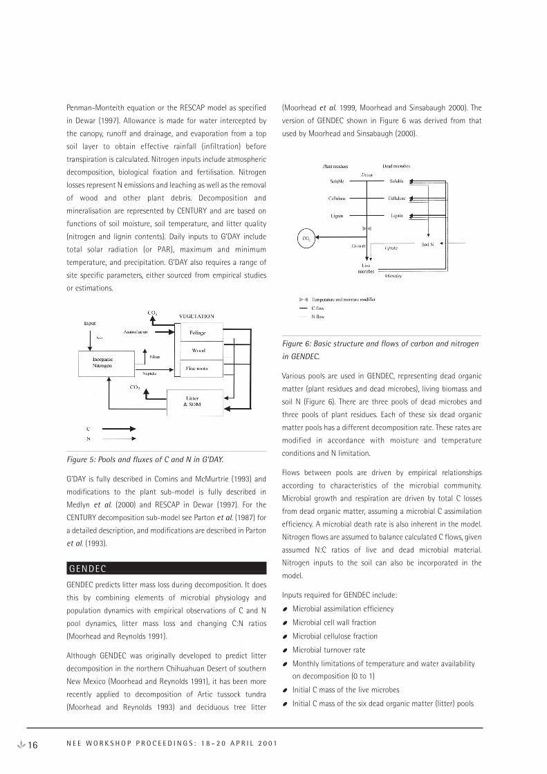
(Moorhead et al. 1999, Moorhead and Sinsabaugh 2000). The
version of GENDEC shown in Figure 6 was derived from that
used by Moorhead and Sinsabaugh (2000).
Figure 6: Basic structure and flows of carbon and nitrogen
in GENDEC.
Various pools are used in GENDEC, representing dead organic
matter (plant residues and dead microbes), living biomass and
soil N (Figure 6). There are three pools of dead microbes and
three pools of plant residues. Each of these six dead organic
matter pools has a different decomposition rate. These rates are
modified in accordance with moisture and temperature
conditions and N limitation.
Flows between pools are driven by empirical relationships
according to characteristics of the microbial community.
Microbial growth and respiration are driven by total C losses
from dead organic matter, assuming a microbial C assimilation
efficiency. A microbial death rate is also inherent in the model.
Nitrogen flows are assumed to balance calculated C flows, given
assumed N:C ratios of live and dead microbial material.
Nitrogen inputs to the soil can also be incorporated in the
model.
Inputs required for GENDEC include:
Microbial assimilation efficiency
Microbial cell wall fraction
Microbial cellulose fraction
Microbial turnover rate
Monthly limitations of temperature and water availability
on decomposition (0 to 1)
Initial C mass of the live microbes
Initial C mass of the six dead organic matter (litter) pools
16 N E E W O R K S H O P P R O C E E D I N G S : 1 8 – 2 0 A P R I L 2 0 0 1
Initial mass of available N and monthly input of N into the
soil
When compared to CENTURY, GENDEC was found to be less
sensitive to site conditions (i.e. temperature and moisture) but
more sensitive to litter quality and soil nitrogen availability
(Moorhead et al. 1999).
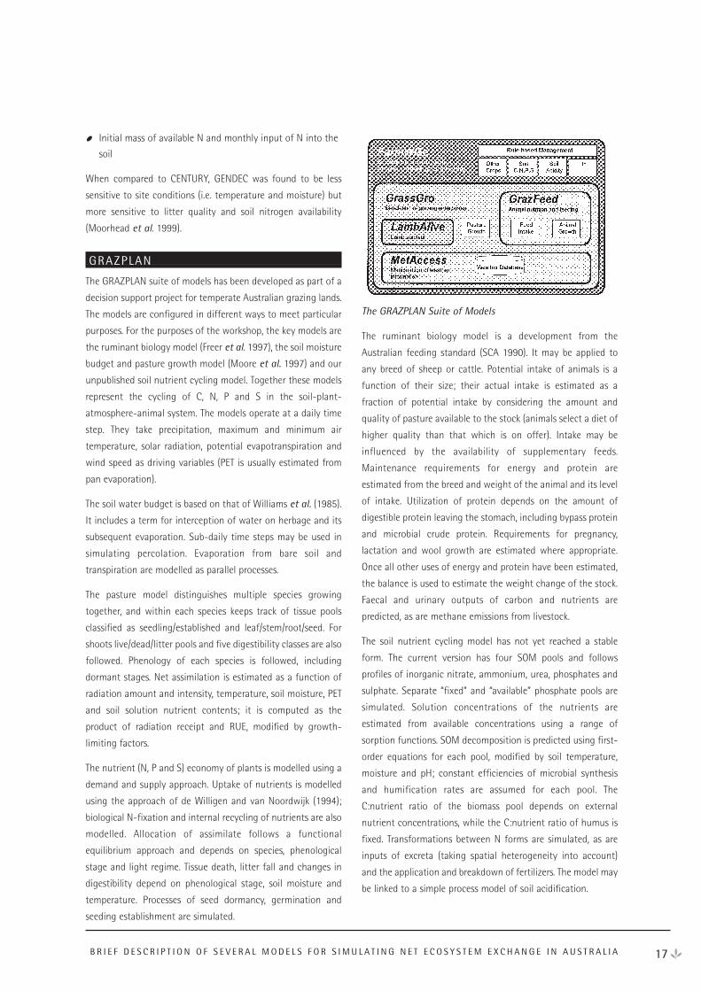
GRAZPLAN
The GRAZPLAN suite of models has been developed as part of a
decision support project for temperate Australian grazing lands.
The models are configured in different ways to meet particular
purposes. For the purposes of the workshop, the key models are
the ruminant biology model (Freer et al. 1997), the soil moisture
budget and pasture growth model (Moore et al. 1997) and our
unpublished soil nutrient cycling model. Together these models
represent the cycling of C, N, P and S in the soil-plant-
atmosphere-animal system. The models operate at a daily time
step. They take precipitation, maximum and minimum air
temperature, solar radiation, potential evapotranspiration and
wind speed as driving variables (PET is usually estimated from
pan evaporation).
The soil water budget is based on that of Williams et al. (1985).
It includes a term for interception of water on herbage and its
subsequent evaporation. Sub-daily time steps may be used in
simulating percolation. Evaporation from bare soil and
transpiration are modelled as parallel processes.
The pasture model distinguishes multiple species growing
together, and within each species keeps track of tissue pools
classified as seedling/established and leaf/stem/root/seed. For
shoots live/dead/litter pools and five digestibility classes are also
followed. Phenology of each species is followed, including
dormant stages. Net assimilation is estimated as a function of
radiation amount and intensity, temperature, soil moisture, PET
and soil solution nutrient contents; it is computed as the
product of radiation receipt and RUE, modified by growth-
limiting factors.
The nutrient (N, P and S) economy of plants is modelled using a
demand and supply approach. Uptake of nutrients is modelled
using the approach of de Willigen and van Noordwijk (1994);
biological N-fixation and internal recycling of nutrients are also
modelled. Allocation of assimilate follows a functional
equilibrium approach and depends on species, phenological
stage and light regime. Tissue death, litter fall and changes in
digestibility depend on phenological stage, soil moisture and
temperature. Processes of seed dormancy, germination and
seeding establishment are simulated.
The GRAZPLAN Suite of Models
The ruminant biology model is a development from the
Australian feeding standard (SCA 1990). It may be applied to
any breed of sheep or cattle. Potential intake of animals is a
function of their size; their actual intake is estimated as a
fraction of potential intake by considering the amount and
quality of pasture available to the stock (animals select a diet of
higher quality than that which is on offer). Intake may be
influenced by the availability of supplementary feeds.
Maintenance requirements for energy and protein are
estimated from the breed and weight of the animal and its level
of intake. Utilization of protein depends on the amount of
digestible protein leaving the stomach, including bypass protein
and microbial crude protein. Requirements for pregnancy,
lactation and wool growth are estimated where appropriate.
Once all other uses of energy and protein have been estimated,
the balance is used to estimate the weight change of the stock.
Faecal and urinary outputs of carbon and nutrients are
predicted, as are methane emissions from livestock.
The soil nutrient cycling model has not yet reached a stable
form. The current version has four SOM pools and follows
profiles of inorganic nitrate, ammonium, urea, phosphates and
sulphate. Separate “fixed” and “available” phosphate pools are
simulated. Solution concentrations of the nutrients are
estimated from available concentrations using a range of
sorption functions. SOM decomposition is predicted using first-
order equations for each pool, modified by soil temperature,
moisture and pH; constant efficiencies of microbial synthesis
and humification rates are assumed for each pool. The
C:nutrient ratio of the biomass pool depends on external
nutrient concentrations, while the C:nutrient ratio of humus is
fixed. Transformations between N forms are simulated, as are
inputs of excreta (taking spatial heterogeneity into account)
and the application and breakdown of fertilizers. The model may
be linked to a simple process model of soil acidification.
17B R I E F D E S C R I P T I O N O F S E V E R A L M O D E L S F O R S I M U L A T I N G N E T E C O S Y S T E M E X C H A N G E I N A U S T R A L I A
These models form the basis of the GRAZPLAN suite of decision
support tools. In particular, the ruminant biology model
underpins the successful GrazFeed decision support tool, which
provides hundreds of users across southern Australia with
tactical advice about livestock nutrition; and the pasture, soil
water and ruminant models are distributed to users in the
GrassGro decision support tool for analyzing grazing systems.
GRASP
GRASP is a ‘pasture growth’ model which combines a soil water
model and a model of above-ground dry-matter flow. It has
been built to meet specific objectives relating to grazing
management of Australian rangelands:
objective assessment of drought and degradation risk in
near-real time (Carter et al. 2000);
simulation of grazing management options including
seasonal forecasting (Ash et al. 2000, McKeon et al. 2000,
Stafford Smith et al. 2000);
assessment of safe carrying capacity (Johnston et al. 1996,
Hall et al. 1998);
evaluation of impact of climate change and CO2 increase
(Hall et al. 1998, Howden et al. 1999);
reconstruction of historical degradation episodes (Carter et
al. 2000).
GRASP has been developed incrementally since 1978 in parallel
with application studies and field trials. Thus the model has
been under constant critique/review in terms of development,
parameterisation, validation and usefulness to client needs.
Currently GRASP is being developed to address issues of deep
drainage, tree growth and death, and grazing land degradation.
Each relationship in the model is described in Littleboy and
McKeon (1997), and a critique of model limitations is given in
Day et al. (1997).
Soil water balanceThe soil water balance in GRASP simulates, on a daily time step,
the processes of soil evaporation, pasture transpiration (Rickert
and McKeon 1982), tree transpiration (Scanlan and McKeon
1993), run-off, and through drainage. Four soil layers are
simulated on a daily time step (0-10cm, 10-50cm, 50-100cm,
>100cm). Soil evaporation occurs from top 50cm, grass
transpiration from top 100cm and tree transpiration from all
four layers. Initially an empirical runoff model has been used
(Scanlan et al. 1996) with run-off calculated as a function of
surface cover, rainfall intensity and soil water deficit. A more
standard hydrological approach (curve numbers linked to cover)
has also been implemented (Yee Yet et al. 1999). Potential
evaporative demand is input as Class A Pan or calculated from
vapour pressure deficit (VPD) and solar radiation.
Dry matter flowThe above-ground pasture processes of growth, senescence of
green tissue, detachment of standing dead, litter
decomposition, animal trampling and consumption are
modelled at a daily time step. Five pasture dry matter pools are
represented: green leaf; green stem; standing dead leaf;
standing dead stem; and surface pasture litter. Plant growth is
calculated as a function of solar radiation interception, air
temperature, VPD, soil moisture or grass transpiration, and
available nitrogen. Growth parameters can be changed for
different levels of CO2. Senescence is a function of frost, soil
water deficit and age. Detachment is a function of season and
rainfall. Litter decomposition is a function of temperature and
surface moisture. Trampling and consumption are functions of
stocking rate (beasts/ha) and pasture availability. Pasture
burning is also simulated by resetting dry matter pools. Daily
climate data are used as inputs and surfaces of daily climate
data (Jeffrey et al. 2000) have been developed to support
application at a national level.
Nitrogen uptake is calculated as a function of transpiration
accumulated from the start of the growing season in each year.
Potential annual nitrogen uptake is a key parameter as nitrogen
limits pasture growth in wetter years (Mott et al. 1985).
Parameters have been derived from data collected in field
studies (>100 sites) specifically designed to measure as many of
the functional parameters (e.g. peak nitrogen yield) as possible
(McKeon et al. 1990, Day et al. 1997). The project has been
generously supported since 1986 by the goodwill of many
pasture scientists in northern Australia. Calibration is usually
restricted to a limited number of parameters (e.g. above-ground
transpiration efficiency, nitrogen uptake per mm of
transpiration, potential regrowth rate after defoliation or
burning). Spatial versions of the model have allowed
parameterisation using (1) extensive ground truthing
measurements of above-ground standing dry matter (>200,000
observations in Queensland, Hassett et al. 2000); and (2) time
series of remotely sensed green cover (NDVI, Carter et al. 2000).
Animal production (annual steer live weight, wool cut) is
calculated at an annual time step from simulated variables such
as percent utilisation, number of green or growing days (Hall et
al. 1998, McKeon et al. 2000).
18 N E E W O R K S H O P P R O C E E D I N G S : 1 8 – 2 0 A P R I L 2 0 0 1
Grazing effects The various effects of grazing on pastures have been simulated
with sub-models of:
perennial grass basal cover which drives potential regrowth
rate;
pasture composition which changes species parameters
(e.g. nitrogen use efficiency, detachment rates);
effects of grazing on plant functioning (water and nitrogen
uptake); and
soil loss affecting available water range and nutrient
availability.
Tree/shrub effectsThe representation of tree/shrub effects has concentrated on
the dominating competitive effect of trees/shrubs for water and
nitrogen (e.g. Scanlan and McKeon 1993, Cafe et al. 1999).
Sub-models of the effects of tree/shrub cover on pasture micro-
climate, pasture species composition, and water, nitrogen and
litter flow are now being developed. J.O. Carter (unpublished) is
developing a tree growth model in GRASP for rangelands.
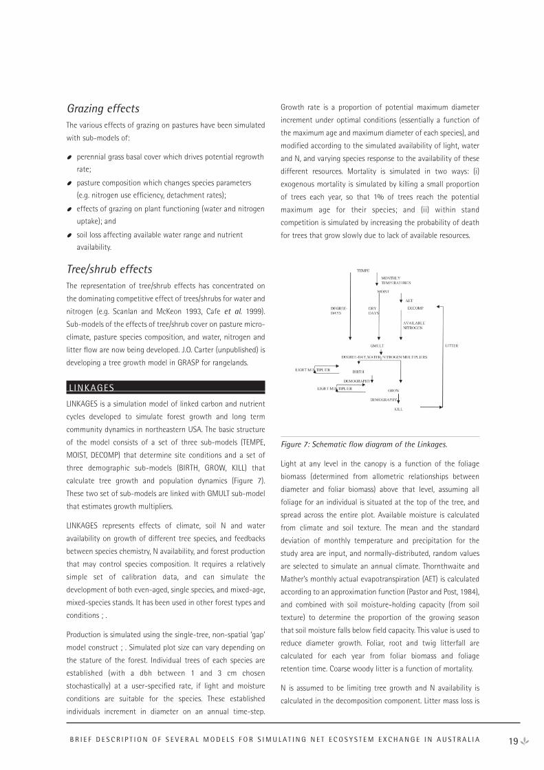
LINKAGES
LINKAGES is a simulation model of linked carbon and nutrient
cycles developed to simulate forest growth and long term
community dynamics in northeastern USA. The basic structure
of the model consists of a set of three sub-models (TEMPE,
MOIST, DECOMP) that determine site conditions and a set of
three demographic sub-models (BIRTH, GROW, KILL) that
calculate tree growth and population dynamics (Figure 7).
These two set of sub-models are linked with GMULT sub-model
that estimates growth multipliers.
LINKAGES represents effects of climate, soil N and water
availability on growth of different tree species, and feedbacks
between species chemistry, N availability, and forest production
that may control species composition. It requires a relatively
simple set of calibration data, and can simulate the
development of both even-aged, single species, and mixed-age,
mixed-species stands. It has been used in other forest types and
conditions ; .
Production is simulated using the single-tree, non-spatial ‘gap’
model construct ; . Simulated plot size can vary depending on
the stature of the forest. Individual trees of each species are
established (with a dbh between 1 and 3 cm chosen
stochastically) at a user-specified rate, if light and moisture
conditions are suitable for the species. These established
individuals increment in diameter on an annual time-step.
Growth rate is a proportion of potential maximum diameter
increment under optimal conditions (essentially a function of
the maximum age and maximum diameter of each species), and
modified according to the simulated availability of light, water
and N, and varying species response to the availability of these
different resources. Mortality is simulated in two ways: (i)
exogenous mortality is simulated by killing a small proportion
of trees each year, so that 1% of trees reach the potential
maximum age for their species; and (ii) within stand
competition is simulated by increasing the probability of death
for trees that grow slowly due to lack of available resources.
Figure 7: Schematic flow diagram of the Linkages.
Light at any level in the canopy is a function of the foliage
biomass (determined from allometric relationships between
diameter and foliar biomass) above that level, assuming all
foliage for an individual is situated at the top of the tree, and
spread across the entire plot. Available moisture is calculated
from climate and soil texture. The mean and the standard
deviation of monthly temperature and precipitation for the
study area are input, and normally-distributed, random values
are selected to simulate an annual climate. Thornthwaite and
Mather’s monthly actual evapotranspiration (AET) is calculated
according to an approximation function (Pastor and Post, 1984),
and combined with soil moisture-holding capacity (from soil
texture) to determine the proportion of the growing season
that soil moisture falls below field capacity. This value is used to
reduce diameter growth. Foliar, root and twig litterfall are
calculated for each year from foliar biomass and foliage
retention time. Coarse woody litter is a function of mortality.
N is assumed to be limiting tree growth and N availability is
calculated in the decomposition component. Litter mass loss is
19B R I E F D E S C R I P T I O N O F S E V E R A L M O D E L S F O R S I M U L A T I N G N E T E C O S Y S T E M E X C H A N G E I N A U S T R A L I A
a function of litter quality (lignin:N) and AET. The model
accounts for annual litter cohorts of each species and litter type
(leaves, roots, twigs and logs). N dynamics is simulated for each
cohort using a linear relationship between the mass remaining
and the N concentration in the remaining material : The
coefficients of this relationship are specified as input for each
litter type. Woody litter cohorts lose mass at user-specified
annual rates. Lignin dynamics are simulated in a similar way.
Lignin:N ratio for each cohort is updated annually for each
cohort, which affects mass loss for the following year.
Depending on the slope of the relationship between %OM
remaining and %N, and the proportion of mass remaining, the
model simulates either nitrogen immobilisation or release.
Some immobilisation is satisfied by N in throughfall, external
inputs, and biological fixation, the remainder from N mobilised
from other cohorts. When litter reaches a certain percent N
remaining when it is transferred to the humus or well-decayed
wood pools that lose mass, and N, at a constant rate (1-2% per
year).
The model code is in FORTRAN (a C version has also been
produced) and is structured to run over long time periods (50-
1000 years or more). Up to 100 plot replications can be
simulated to assess the variation associated with stochastic
processes such as climate, regeneration and mortality. Outputs
include above ground biomass and number of stems by species,
NPP, litterfall, N mineralisation, and CO2 evolution.
ProMod – A SITE PRODUCTIVITY MODEL
ProMod is intended primarily for screening prospective
plantation sites. It focuses on the period following canopy
closure, and provides a prediction of the closed-canopy leaf
area index (LAI), annual net primary production (NPP), and
water use by the stand, and available soil water (ASW). ProMod
is calibrated to predict measures of site productivity of specific
interest to forest managers, e.g. peak mean annual stem-
volume increment of a plantation. It is used in combination
with a conventional empirical model to predict stand
development.
ProMod has its roots in a workshop (“FORMOD95: a Tree and
Forest Growth Modelling Workshop”, Sands 1995a) that
brought together modellers and representatives from forest
industries to assess if and how process-based models could
provide tools for plantation management. Little specific interest
was expressed in detailed predictions of biomass partitioning, so
a pragmatic approach to the development of a model predicting
site productivity was adopted: empirical expressions were
developed for several key relationships that are other-wise
difficult to model, and used in conjunction with a realistic,
physiologically-based model for NPP.
A simple empirical submodel for the closed-canopy LAI was
based on long-term climatic factors, drawing on the
observation that LAI varies only slowly with long-term
conditions following canopy closure. Daily canopy water-use
20 N E E W O R K S H O P P R O C E E D I N G S : 1 8 – 2 0 A P R I L 2 0 0 1
Figure 8: A simple representation of the structure of ProMod, and its input and output data.
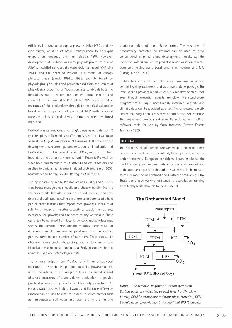
efficiency is a function of vapour pressure deficit (VPD), and the
crop factor, or ratio of actual transpiration to open-pan
evaporation, depends only on relative ASW. However,
development of ProMod was also physiologically realistic as
ASW is modelled using a daily water-balance model (McAlpine
1970), and the heart of ProMod is a model of canopy
photosynthesis (Sands 1995b, 1996) soundly based on
physiological principles and parameterised from the results of
physiological experiments. Production is calculated daily, taking
limitations due to water stress or VPD into account, and
summed to give annual NPP. Predicted NPP is converted to
measures of site productivity through an empirical calibration
based on a comparison of predicted NPP with observed
measures of site productivity frequently used by forest
managers.
ProMod was parameterised for E. globulus using data from 9
research plots in Tasmania and Western Australia, and validated
against 19 E. globulus plots in N Tasmania. Full details of the
development, structure, parameterisation and validation of
ProMod are in Battaglia and Sands (1997), and its structure,
input data and outputs are summarised in Figure 8. ProMod has
since been parameterised for E. nitens and Pinus radiata and
applied to various management-related problems (Sands 2000,
Mummery and Battaglia 2001, Battaglia et al. 2001).
The input data required by ProMod are of a quality and quantity
that forest managers can readily and cheaply obtain. The site
factors are site latitude; measures of soil texture, stoniness,
depth and drainage, including the presence or absence of a hard
pan or other features that impede root growth; a measure of
salinity; an index of the site’s capacity to supply the nutrients
necessary for growth; and the depth to any watertable. These
can often be obtained from local knowledge and soil-data map
sheets. The climatic factors are the monthly mean values of
daily maximum & minimum temperatures, radiation, rainfall,
pan evaporation and number of rain days. These can all be
obtained from a bioclimatic package such as Esoclim, or from
historical meteorological bureau data. ProMod can also be run
using actual daily meteorological data.
The primary output from ProMod is NPP, an unequivocal
measure of the productive potential of a site. However, as this
is of little interest to a manager, NPP was calibrated against
observed measures of stem volume production to provide
practical measures of productivity. Other outputs include LAI,
canopy water use, available soil water, and light use efficiency.
ProMod can be used to infer the extent to which factors such
as temperature, soil-water and site fertility are limiting
production (Battaglia and Sands 1997). The measures of
productivity predicted by ProMod can be used to drive
conventional empirical stand development models, e.g. the
hybrid of ProMod and NitGro predicts the age variation of mean
dominant height, stand basal area, stem volume and MAI
(Battaglia et al. 1999).
ProMod has been implemented as Visual Basic macros running
behind Excel spreadsheets, and as a stand-alone package. The
Excel version provides a convenient, flexible development tool,
even though execution speeds are slow. The stand-alone
program has a simple, user-friendly interface, and site and
climatic data can be provided as a text file, or entered directly
and edited using a data-entry form as part of the user interface.
This implementation was subsequently included on a CD of
software tools for use by farm foresters (Private Forests
Tasmania 1999).
ROTH-C
The Rothamsted soil carbon turnover model (Jenkinson 1990)
was initially developed for grassland, forest, pasture and crops
under temperate European conditions. Figure 9 shows the
model where plant material enters the soil environment and
undergoes decomposition through the soil microbial biomass to
form a number of well defined pools with the emission of CO2.
These pools have varying resistance to degradation, ranging
from highly labile through to inert material.
Figure 9: Schematic Diagram of Rothamsted Model.
Carbon pools are indicated as IOM (inert), HUM (slow
humic), RPM (intermediate resistant plant material), DPM
(readily decomposable plant material) and BIO (biomass).
21B R I E F D E S C R I P T I O N O F S E V E R A L M O D E L S F O R S I M U L A T I N G N E T E C O S Y S T E M E X C H A N G E I N A U S T R A L I A
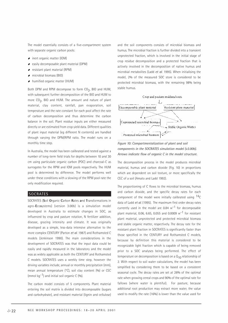
The model essentially consists of a five-compartment system
with separate organic carbon pools:
inert organic matter (IOM)
easily decomposable plant material (DPM)
resistant plant material (RPM)
microbial biomass (BIO)
humified organic matter (HUM)
Both DPM and RPM decompose to form CO2, BIO and HUM,
with subsequent further decomposition of the BIO and HUM to
more CO2, BIO and HUM. The amount and nature of plant
material, clay content, rainfall, pan evaporation, soil
temperature and the rate constant for each pool affect the rate
of carbon decomposition and thus determine the carbon
balance in the soil. Plant residue inputs are either measured
directly or are estimated from crop yield data. Different qualities
of plant input material (eg different N contents) are handled
through varying the DPM/RPM ratio. The model runs on a
monthly time step.
In Australia, the model has been calibrated and tested against a
number of long-term field trials for depths between 10 and 30
cm using particulate organic carbon (POC) and charcoal-C as
surrogates for the RPM and IOM pools respectively. The HUM
pool is determined by difference. The model performs well
under these conditions with a slowing of the RPM pool rate the
only modification required.
SOCRATES
SOCRATES (Soil Organic Carbon Rates and Transformations in
agro-Ecosystems) (version 3.00b) is a simulation model
developed in Australia to estimate changes in SOC, as
influenced by crop and pasture rotation, N fertilizer addition,
disease, grazing intensity and climate. It was originally
developed as a simple, less-data intensive alternative to the
more complex CENTURY (Parton et al. 1987) and Rothamsted C
models (Jenkinson 1990). The main considerations in the
development of SOCRATES was that the input data could be
easily and rapidly measured in the laboratory and the model
was as widely applicable as both the CENTURY and Rothamsted
C models. SOCRATES uses a weekly time step, however the
driving variables include, annual or monthly precipitation (mm),
mean annual temperature (°C), soil clay content (%) or CEC
(mmol kg-1) and initial soil organic C (%).
The carbon model consists of 5 components. Plant material
entering the soil matrix is divided into decomposable (sugars
and carbohydrate), and resistant material (lignin and cellulose)
and the soil components consists of microbial biomass and
humus. The microbial fraction is further divided into a transient
unprotected fraction, which is involved in the initial stage of
crop residue decomposition and a protected fraction that is
actively involved in the decomposition of native humus and
microbial metabolites (Ladd et al. 1995). When initialising the
model, 2% of the measured SOC store is considered to be
protected microbial biomass, with the remaining 98% being
stable humus.
Figure 10: Compartmentalization of plant and soil
components in the SOCRATES simulation model (v3.00b).
Arrows indicate flow of organic C in the model structure.
The decomposition process in the model produces microbial
material, humus and carbon dioxide (Fig. 10) in proportions
which are dependent on soil texture, or more specifically the
CEC of a soil (Amato and Ladd 1992).
The proportioning of C flows to the microbial biomass, humus
and carbon dioxide, and the specific decay rates for each
component of the model were initially calibrated using 14C
data of Ladd et al. (1995). The maximum first order decay rates
currently used in the model are 0.84 w-1 for decomposable
plant material, 0.06, 6.65, 0.055 and 0.0009 w-1 for resistant
plant material, unprotected and protected microbial biomass
and stable organic matter, respectively. The decay rate for the
resistant plant fraction in SOCRATES is significantly faster than
those specified in the CENTURY and Rothamsted C models,
because by definition this material is considered to be
recognizable light fraction which is capable of being removed
prior to a SOC analyses being performed. The effect of
temperature on decomposition is based on a Q10 relationship of
2. With respect to soil water calculations, the model has been
simplified by considering them to be based on a consistent
seasonal cycle. The decay rates are set at 26% of the optimal
rate when growing cereal crops and 90% of the optimal rate for
fallows (where water is plentiful). For pasture, because
additional root production may extract more water, the value
used to modify the rate (16%) is lower than the value used for
22 N E E W O R K S H O P P R O C E E D I N G S : 1 8 – 2 0 A P R I L 2 0 0 1
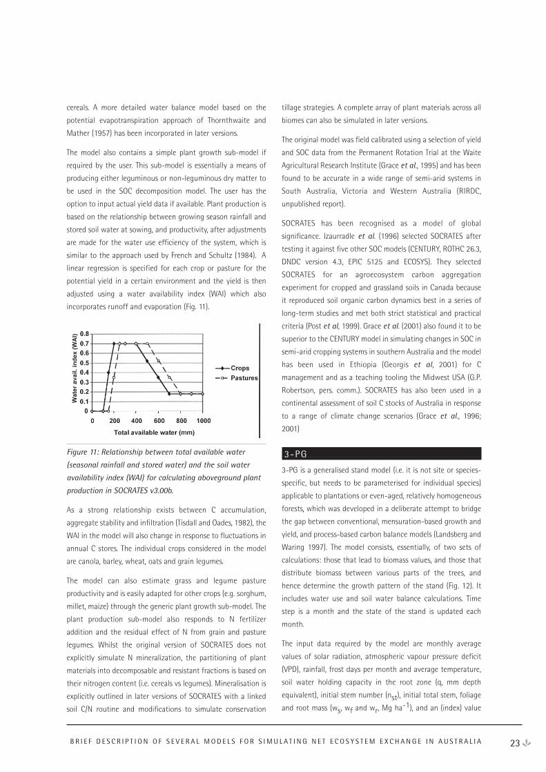
cereals. A more detailed water balance model based on the
potential evapotranspiration approach of Thornthwaite and
Mather (1957) has been incorporated in later versions.
The model also contains a simple plant growth sub-model if
required by the user. This sub-model is essentially a means of
producing either leguminous or non-leguminous dry matter to
be used in the SOC decomposition model. The user has the
option to input actual yield data if available. Plant production is
based on the relationship between growing season rainfall and
stored soil water at sowing, and productivity, after adjustments
are made for the water use efficiency of the system, which is
similar to the approach used by French and Schultz (1984). A
linear regression is specified for each crop or pasture for the
potential yield in a certain environment and the yield is then
adjusted using a water availability index (WAI) which also
incorporates runoff and evaporation (Fig. 11).
Figure 11: Relationship between total available water
(seasonal rainfall and stored water) and the soil water
availability index (WAI) for calculating aboveground plant
production in SOCRATES v3.00b.
As a strong relationship exists between C accumulation,
aggregate stability and infiltration (Tisdall and Oades, 1982), the
WAI in the model will also change in response to fluctuations in
annual C stores. The individual crops considered in the model
are canola, barley, wheat, oats and grain legumes.
The model can also estimate grass and legume pasture
productivity and is easily adapted for other crops (e.g. sorghum,
millet, maize) through the generic plant growth sub-model. The
plant production sub-model also responds to N fertilizer
addition and the residual effect of N from grain and pasture
legumes. Whilst the original version of SOCRATES does not
explicitly simulate N mineralization, the partitioning of plant
materials into decomposable and resistant fractions is based on
their nitrogen content (i.e. cereals vs legumes). Mineralisation is
explicitly outlined in later versions of SOCRATES with a linked
soil C/N routine and modifications to simulate conservation
tillage strategies. A complete array of plant materials across all
biomes can also be simulated in later versions.
The original model was field calibrated using a selection of yield
and SOC data from the Permanent Rotation Trial at the Waite
Agricultural Research Institute (Grace et al., 1995) and has been
found to be accurate in a wide range of semi-arid systems in
South Australia, Victoria and Western Australia (RIRDC,
unpublished report).
SOCRATES has been recognised as a model of global
significance. Izaurradle et al. (1996) selected SOCRATES after
testing it against five other SOC models (CENTURY, ROTHC 26.3,
DNDC version 4.3, EPIC 5125 and ECOSYS). They selected
SOCRATES for an agroecosystem carbon aggregation
experiment for cropped and grassland soils in Canada because
it reproduced soil organic carbon dynamics best in a series of
long-term studies and met both strict statistical and practical
criteria (Post et al, 1999). Grace et al. (2001) also found it to be
superior to the CENTURY model in simulating changes in SOC in
semi-arid cropping systems in southern Australia and the model
has been used in Ethiopia (Georgis et al, 2001) for C
management and as a teaching tooling the Midwest USA (G.P.
Robertson, pers. comm.). SOCRATES has also been used in a
continental assessment of soil C stocks of Australia in response
to a range of climate change scenarios (Grace et al., 1996;
2001)
3-PG
3-PG is a generalised stand model (i.e. it is not site or species-
specific, but needs to be parameterised for individual species)
applicable to plantations or even-aged, relatively homogeneous
forests, which was developed in a deliberate attempt to bridge
the gap between conventional, mensuration-based growth and
yield, and process-based carbon balance models (Landsberg and
Waring 1997). The model consists, essentially, of two sets of
calculations: those that lead to biomass values, and those that
distribute biomass between various parts of the trees, and
hence determine the growth pattern of the stand (Fig. 12). It
includes water use and soil water balance calculations. Time
step is a month and the state of the stand is updated each
month.
The input data required by the model are monthly average
values of solar radiation, atmospheric vapour pressure deficit
(VPD), rainfall, frost days per month and average temperature,
soil water holding capacity in the root zone (q, mm depth
equivalent), initial stem number (nst), initial total stem, foliage
and root mass (ws, wf and wr, Mg ha-1), and an (index) value
23B R I E F D E S C R I P T I O N O F S E V E R A L M O D E L S F O R S I M U L A T I N G N E T E C O S Y S T E M E X C H A N G E I N A U S T R A L I A
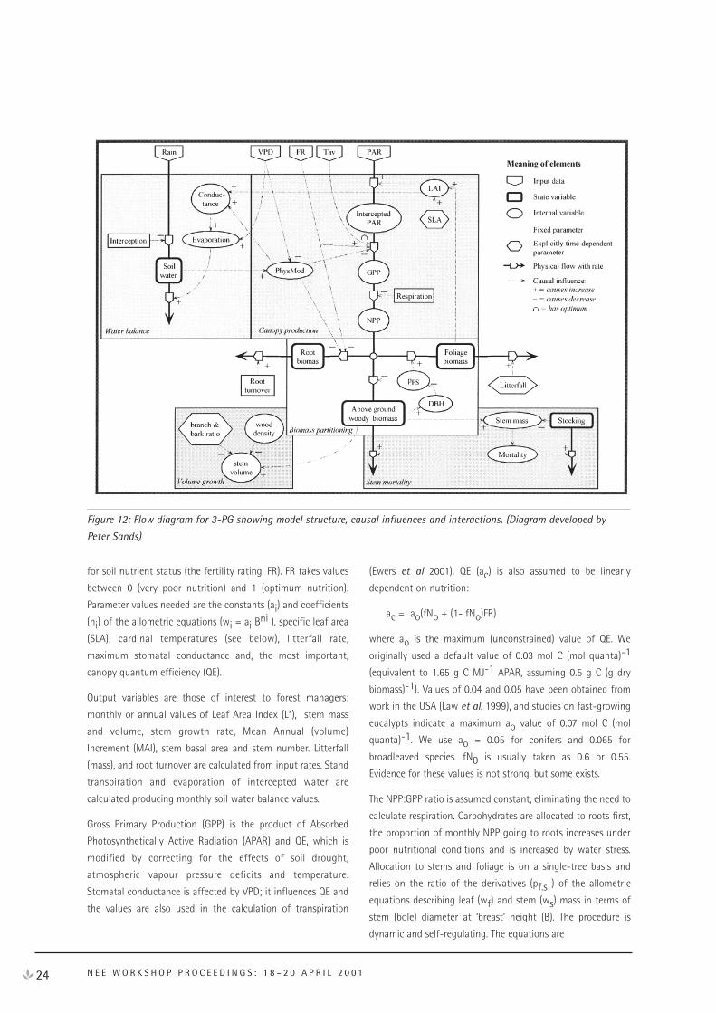
for soil nutrient status (the fertility rating, FR). FR takes values
between 0 (very poor nutrition) and 1 (optimum nutrition).
Parameter values needed are the constants (ai) and coefficients
(ni) of the allometric equations (wi = ai Bni ), specific leaf area
(SLA), cardinal temperatures (see below), litterfall rate,
maximum stomatal conductance and, the most important,
canopy quantum efficiency (QE).
Output variables are those of interest to forest managers:
monthly or annual values of Leaf Area Index (L*), stem mass
and volume, stem growth rate, Mean Annual (volume)
Increment (MAI), stem basal area and stem number. Litterfall
(mass), and root turnover are calculated from input rates. Stand
transpiration and evaporation of intercepted water are
calculated producing monthly soil water balance values.
Gross Primary Production (GPP) is the product of Absorbed
Photosynthetically Active Radiation (APAR) and QE, which is
modified by correcting for the effects of soil drought,
atmospheric vapour pressure deficits and temperature.
Stomatal conductance is affected by VPD; it influences QE and
the values are also used in the calculation of transpiration
(Ewers et al 2001). QE (ac) is also assumed to be linearly
dependent on nutrition:
ac = ao(fNo + (1- fNo)FR)
where ao is the maximum (unconstrained) value of QE. We
originally used a default value of 0.03 mol C (mol quanta)-1
(equivalent to 1.65 g C MJ-1 APAR, assuming 0.5 g C (g dry
biomass)-1). Values of 0.04 and 0.05 have been obtained from
work in the USA (Law et al. 1999), and studies on fast-growing
eucalypts indicate a maximum ao value of 0.07 mol C (mol
quanta)-1. We use ao = 0.05 for conifers and 0.065 for
broadleaved species. fN0 is usually taken as 0.6 or 0.55.
Evidence for these values is not strong, but some exists.
The NPP:GPP ratio is assumed constant, eliminating the need to
calculate respiration. Carbohydrates are allocated to roots first,
the proportion of monthly NPP going to roots increases under
poor nutritional conditions and is increased by water stress.
Allocation to stems and foliage is on a single-tree basis and
relies on the ratio of the derivatives (pf.s ) of the allometric
equations describing leaf (wf) and stem (ws) mass in terms of
stem (bole) diameter at ‘breast’ height (B). The procedure is
dynamic and self-regulating. The equations are
24 N E E W O R K S H O P P R O C E E D I N G S : 1 8 – 2 0 A P R I L 2 0 0 1
Figure 12: Flow diagram for 3-PG showing model structure, causal influences and interactions. (Diagram developed by
Peter Sands)
pf.s = (dwf / dB)/(dws/dB) = af nf B(nf-1) / as ns B(n
s-1) ∫
ap Bnp (1)
pf.s affects the carbon allocation coefficients for foliage (hf),
roots (hr) and stems (hs) - which must sum to unity – through
the relations
hs = ( 1- hf)/( pf.s + 1) and hf = 1- hr - hs. (2)
L* is calculated from SLA, foliage mass/stem and stem number.
Mass losses through litterfall and root turnover can be used as
inputs to stand carbon balance calculations.
Stem size is calculated by inversion of the allometric equation;
stand volume comes from stem mass, wood density and
stocking (stem number per hectare).
Stem mortality is governed by the –3/2 power ‘law’; the point
where mortality starts is set by a stem mass value. This works
well when natural mortality is the main mechanism, although
the start of stem mortality tends to be too abrupt. 3-PG
includes a thinning routine.
3-PG is being evaluated in many countries, including Australia
(Coops et al. 1998; Tickle et al. 2000; Sands and Landsberg
2001), New Zealand (Coops et al. 1998a; White 2000;
Whitehead et al. 2001), the USA (Coops et al. 2000b; Landsberg
et al. 2000; Coops and Waring 2001a, b), South Africa (Dye
2001), Brazil, Chile, the UK (Waring 2000), Denmark, Sweden. It
has been adopted as an operational tool by a major forestry
company (Aracruz Celulose SA) in Brazil, where it will be
implemented in a GIS, in association with calibration plots and
fertilisation experiments. In that application stem number and
volume outputs will be analysed using conventional forestry
product models. It has also been combined with satellite
measurements to give remotely sensed input information into
important physiological driving variables in the model (Coops et
al 1998b; Coops 1999).
EXCEL/Visual Basic software for the 3-PG model has been
developed by Dr Peter Sands (CSIRO DFFP, Hobart) and another
version of the code (produced by Dr Nicholas Coops and Andrew
Loughhead, CSIRO DFFP) is available in C++. This allows spatial
ARC/INFO coverages to be input and spatial estimates of
parameters to be produced. Both of these versions of the code
are available at www.landsberg.com.au and mirrored at CSIRO
FFP WWW site (www.ffp.csiro.au). Peter Sands’ software is
accompanied by a Technical Report on the model (Sands 2001).
ReferencesAber, J.D. and Melillo, J.M. (1980). Litter decomposition:
measuring relative contribution of organic matter and
nitrogen to forest soils. Canadian Journal of Botany 58:
416-421.
Amato, M. and Ladd, J.N. (1992). Decomposition of 14C-
labelled glucose and legume materials in soils: Properties
influencing the accumulation of organic residue C and
microbial biomass C. Soil Biology Biochemistry 24: 455-
464.
Ash, A.J., O’Reagain, P.J., McKeon, G.M. and Stafford Smith, M.
(2000). Managing climate variability in grazing enterprises:
A case study of Dalrymple Shire, north-eastern Australia.
‘Applications of Seasonal Climate Forecasting in
Agricultural and Natural Ecosystems - the Australian
Experience’. (Eds G. Hammer, N. Nicholls and C. Mitchell.)
Kluwer Academic Press: Netherlands. p 253-270.
Battaglia, M., Mummery, D. and Smith, A. (2001). Economic
analysis of site survey and productivity modelling for the
selection of plantation areas. Forest Ecology and
Management (In press).
Battaglia, M. and Sands, P.J. (1997). Modelling site productivity
of Eucalyptus globulus in response to climatic and site
factors. Australian Journal of Plant Physiology 24: 831-
850.
Battaglia, M., Sands, P.J. and Candy, S.G. (1999). Hybrid growth
model to predict height and volume growth in young
Eucalyptus globulus plantations. Forest Ecology and
Management 120: 193-201.
Botkin, D.B. (1993). Forest Dynamics. Oxford Univ. Press,
Oxford.
Cafe, L.M., McKeon, G.M., Dyer, R.M. and Heywood, J.M. (1999).
Trees compete with pastures in the semi-arid tropics of the
Northern Territory. VIth International Rangeland Congress
Proceedings Vol. 1. pp. 291-292.
Carter, J.O., Hall, W.B., Brook, K.D., McKeon, G.M., Day, K.A. and
Paull, C.J. (2000). Aussie GRASS: Australian grassland and
rangeland assessment by spatial simulation. In
‘Applications of Seasonal Climate Forecasting in
Agricultural and Natural Ecosystems - the Australian
Experience’. (Eds G. Hammer, N. Nicholls and C. Mitchell.)
Kluwer Academic Press: Netherlands pp. 329-350.
Comins, H.N. and McMurtrie, R.E. (1993). Long-term response
of nutrient-limited forests to CO2-enrichment; equilibrium
25B R I E F D E S C R I P T I O N O F S E V E R A L M O D E L S F O R S I M U L A T I N G N E T E C O S Y S T E M E X C H A N G E I N A U S T R A L I A

behaviour of plant-soil models. Ecological Applications 3:
666-681.
Coops, N.C. (1999). Linking multi-resolution satellite-derived
estimates of canopy photosynthetic capacity and
meteorological data to assess forest productivity in a Pinus
radiata (D. Don) stand. Photogram. Eng. Remote Sen. 65:
1149-1156.
Coops, N.C. and Waring, R.H. (2001a). Estimating maximum
potential site productivity and site water stress of the
Eastern Siskiyou Mountains of southwestern Oregon using
a satellite driven process model, 3-PGs. Can. J. For. Res.
31: 143-154.
Coops, N.C. and Waring, R.H. (2001b). Assessing forest growth
across southwestern Oregon under a range of current and
future global change scenarios using a process model, 3-
PG. Global Change Biology 7: 15-29.
Coops, N.C., Waring, R.H. Brown, S. and Running, S.W. (2000a).
Predictions of net primary production and seasonal
patterns in water use with forest growth models using
daily and monthly time-steps in south-eastern Oregon.
Ecological Modelling (in press).
Coops, N.C., Waring, R.H., Landsberg, J.J. (1998a). Assessing
forest productivity in Australia and New Zealand using a
physiologically-based model driven with averaged monthly
weather data and satellite-derived estimates of canopy
productivity. For. Ecol. and Manage. 104: 113-127.
Coops, N.C., Waring, R.H. and Landsberg, J.J. (1998b). The
development of a physiological model (3-PG S) to predict
forest productivity using satellite data. In: G. Nabuurs, T.
Nuutinen, H. Bartelink, & M. Koorhonen, eds. Forest
scenario modelling for ecosystem management at
landscape level. EFI Proceedings, pp. 173 –191.
Coops, N.C., Waring, R.H. and Landsberg, J.J. (2000b).
Estimation of potential forest productivity across the
Oregon transect using satellite data and monthly weather
records. Int.J. Remote Sens. (in press).
Day, K.A., McKeon, G.M. and Carter, J.O. (1997). Evaluating the
risks of pasture and land degradation in native pasture in
Queensland. Final report for Rural Industries and Research
Development Corporation project DAQ124A.
Dewar, R.C. (1997). A simple model of light and water use
evaluated for Pinus radiata. Tree Physiology 17: 259-265.
de Willigen P. and van Noordwijk, M. (1994). Diffusion and
mass flow to a root with constant nutrient demand or
behaving as a zero-sink. Soil Science 157: 171-175.
Dye, P.J. (2001). Modelling growth and water use in four Pinus
patula stands with the 3-PG process-based model. South
African For. Jnl. (In press).
Ewers, B.E., Oren, R., Johnsen, K.H. and Landsberg, J.J. (2001).
Estimating maximum mean canopy stomatal conductance
for use in models. Can. J. For. Res. 31: 198-207.
Freer, M., Moore, A.D. and Donnelly, J.R. (1997). GRAZPLAN:
decision support systems for Australian grazing enterprises.
II. The animal biology model for feed intake, production
and reproduction and the GrazFeed DSS. Agric. Systems
54: 77-126.
French, R.J. and Schultz, J.E. (1984). Water use efficiency in
wheat production in a Mediterranean type of environment.
I. The relationship between yield, water use and climate.
Australian Journal of Agricultural Research 35: 743-764.
Georgis, K., Grace, P.R., Reeves, T.G. and Alston, A.M. (2001).
Management options to sustain soil organic matter and
productivity in cropping systems of semi-arid Ethiopia.
Agriculture, Ecosystems and Environment.
Grace, P.R., Bryceson, K, Hennessy, K. and Truscott, M. (1996).
Climate change and soil carbon resources. In Land use in a
changing climate, Maurice Wyndham Series, University of
New England Press, Armidale, pp. 19-32.
Grace, P.R., Bryceson, K., Hennessy, K., Truscott, M. and Post,
W.M. (2001). The potential impact of climate change on
Australia’s soil organic carbon resources. Agriculture,
Ecosystems and Environment (submitted).
Grace, P.R., Georgis, K., Reeves, T.G., Alston, A. (2001).
Simulating changes in soil organic carbon in cropping
systems of the semi-arid Mallee region of Australia.
Agricultural Systems (submitted).
Grace, P.R., Oades, J.M., Keith, H. and Hancock, T.W. (1995).
Trends in wheat yields and soil organic carbon in the
Permanent Rotation Trial at the Waite Agricultural
Research Institute, South Australia. Australian Journal of
Experimental Agriculture 35: 857-864.
Hall, W.B., McKeon, G.M., Carter, J.O., Day, K.A., Howden, S.M.,
Scanlan, J.C., Johnston, P.W. and Burrows, W.H. (1998).
Climate change and Queensland’s grazing lands: II. An
assessment of the impact on animal production from
native pastures. Rangeland Journal 20, 174-202.
Hassett, R.C., Wood, H.L., Carter, J.O. and Danaher, T.J. (2000).
A field method for statewide ground-truthing of a spatial
pasture growth model. Australian Journal of
Experimental Agriculture, 2000, 40: 1069-1079.
26 N E E W O R K S H O P P R O C E E D I N G S : 1 8 – 2 0 A P R I L 2 0 0 1
Howden, S.M., McKeon, G.M., Walker, L., Carter, J.O., Conroy,
J.P., Day, K.A., Hall, W.B., Ash, A.J. and Ghannoum, O. (1999).
Global change impacts on native pastures in south-east
Queensland, Australia. Environmental Modelling and
Software 14, 307-16.
Izaurralde, R.C., McGill, W.B., Jans-Hammermeister, D.C.,
Haugen-Korzyra, K.L. and Hiley, J.C. (1996). Development of
a technique to calculate carbon fluxes in agricultural soils
at the ecodistrict level using simulation models and various
aggregation methods. Interim Report, Submitted to the
Scientific Authority of the Agriculture and Agri-Food
Canada Greenhouse Gas Initiative, University of Alberta,
Edmonton, AB,
Jaakko Pöyry (1999). Usage And Life Cycle Of Wood Products.
National Carbon Accounting System Technical Report No.
8. November 1999.
Jeffrey, S.J., Carter, J.O., Moodie, K.B. and Beswik, A.R. (2001).
Using spatial interpolation to construct a comprehensive
archive of Australian climate data. Environmental
Modelling and Software (in press).
Jenkinson, D.S. (1990). The turnover of organic C and N in soil.
Philosopical Transacations. Royal Society London B329:
361-368.
Jenkinson, D.S., Adams, D.E., Wild, A. (1991). Model estimates
of CO2 emissions from soils in response to global warming.
Nature 352: 304-306.
Jenkinson, D.S., Hart, P.B.S., Rayner, J.H. and Parry, L.C. (1987).
Modelling the turnover of organic matter in long-term
experiments at Rothamsted. Iintercol Bulletin 15: 1–8.
Johnston, P.W., McKeon, G.M. and Day, K.A. (1996). Objective
“safe” grazing capacities for south-west Queensland
Australia: development of a model for individual
properties. Rangeland Journal. 18: 244-258.
Keenan, R.J., Kimmins, J.P. and Pastor, J. (1995). Modelling
ecosystem-level carbon and nutrient dynamics in western
red cedar and western hemlock forests. In J. M. Kelly and
W. W. McFee, ed. Carbon Forms and Functions in Forest
Soils. Soil Science Society of America, Madison, pp. 547-
568.
Kellomäki, S. and Kolstrom, M. (1992). Simulation of tree
species composition and organic matter accumulation in
Finnish boreal forests under changing climatic conditions.
Vegetatio 102: 47-68.
Kirschbaum, M.U.F. (1999a). CenW, a forest growth model with
linked carbon, energy, nutrient and water cycles. Ecological
Modelling 181: 17-59.
Kirschbaum, M.U.F. (1999b). The effect of climate change on
forest growth in Australia. In: Impacts of global change
on Australian temperate forests. (Howden, S.M. and
Gorman, J.T., eds.), Working Paper Series, 99/08, pp. 62-68.
Kirschbaum, M.U.F. (1999c). Modelling forest growth and
carbon storage with increasing CO2 and temperature.
Tellus 51B: 871-888.
Kirschbaum, M.U.F. (2000). CenW: a generic forest growth
model that links carbon, nutrient and water cycles. New
Zealand Journal of Forestry 45: 15-19.
Ladd, J.L, Amato, M., Grace, P.R. and Van Veen, J.A. (1995)
Simulation of 14C turnover through the microbial biomass
in soils incubated with 14C-labelled plant residues. Soil
Biology Biochemistry 27: 777-783.
Landsberg, J.J., Johnson, K.H., Albaugh, T.J., Allen, H.L. and
McKeand, S.E. (2000). Applying 3-PG, a simple process-
based model designed to produce practical results, to data
from loblolly pine experiments. Forest Science. (In press)
Landsberg, J.J., Waring, R.H. (1997). A generalized model of
forest productivity using simplified concepts of radiation-
use efficiency, carbon balance, and partitioning. Forest
Ecology and Management 95: 209-228.
Law, B.E., Waring, R.H., Anthoni, P.M., Aber, J.D. 1999.
Measurements of gross and net ecosystem productivity and
water exchange of a Pinus ponderosa ecosystem, and an
evaluation of two generalized models. Global Change
Biology 5: 1-15
Littleboy, M. and McKeon, G.M. (1997). Subroutine GRASP:
Grass Production Model. Documentation of the Marcoola
Version of Subroutine GRASP. Appendix 2 of “Evaluating
the risks of pasture and land degradation in native pasture
in Queensland”. Final Project Report for the Rural
Industries Research and Development Corporation
DAQ124A, pp. 76.
McAlpine, J.R. (1970). Estimating pasture growth periods and
droughts from simple water balance models. In ‘XI
International Grasslands Congress’, Surfers Paradise,
Queensland (Ed. M. J. T. Norman) pp. 484-487.
McCown, R.L, Hammer, G.L., Hargreaves, J.N.G., Holzworth, D.L
and Freebairn, D.M. (1996). APSIM: a novel software system
for model development, model testing, and simulation in
agricultural systems research. Agricultural Systems 50:
255-271.
McKeon, G.M., Ash, A.J., Hall, W.B. and Stafford Smith M.
(2000). Simulation of grazing strategies for beef
production in north-east Queensland. ‘Applications of
27B R I E F D E S C R I P T I O N O F S E V E R A L M O D E L S F O R S I M U L A T I N G N E T E C O S Y S T E M E X C H A N G E I N A U S T R A L I A
Seasonal Climate Forecasting in Agricultural and Natural
Ecosystems - the Australian Experience’. (Eds G. Hammer, N.
Nicholls and C. Mitchell.) Kluwer Academic Press:
Netherlands. p.227-252.
McKeon, G.M., Day, K.A., Howden, S.M., Mott, J.J., Orr, D.M.,
Scattini, W.J. and Weston, E.J. (1990). Northern Australian
savannas: management for pastoral production. Journal of
Biogeography 17, 355-72.
Medlyn, B.E., McMurtrie, R.E., Dewar, R.C. and Jeffreys, M.P.
(2000). Soil processes dominate the long-term response of
forest net primary productivity to increased temperature
and atmospheric CO2 concentration. Canadian Journal of
Forest Research 30: 873-888.
Mohren, G.M.J and Goldewijk, K.C.G.M. (1990). CO2Fix: a
dynamic model of the CO2 fixation in forest stands.
Rapport 624, De Dorschkamp, Research Institute of Forestry
and Urban Ecology, Wageningen, 96pp.
Moore, A.D., Donnelly, J.R. and Freer, M. (1997). GRAZPLAN:
decision support systems for Australian grazing enterprises.
III. Pasture growth and soil moisture submodels, and the
GrassGro DSS. Agric. Systems 55: 535-582.
Moorhead, D.L., Currie, W.S., Rastetter, E.B., Parton, W.J. and
Harmon, M.E. (1999). Climate and litter quality controls on
decomposition: An analysis of modeling approaches.
Global Biogeochemical Cycles 13: 575-589.
Moorhead, D.L. and Reynolds, J.F. (1991). A general model of
litter decomposition in the northern Chihuahuan Desert.
Ecological Modelling 56: 197-219.
Moorhead, D.L. and Reynolds, J.F. (1993). Effects of climate
change on decomposition in Artic Tussock Tundra: A
modeling synthesis. Artic and Alpine Research 25: 401-
412.
Moorhead, D.L. and Sinsabaugh, R.L. (2000). Simulated
patterns of litter decay predict patterns of extracellular
enzyme activities. Applied Soil Ecology 14: 71-79.
Mott, J.J., Williams, J., Andrew, M.H. and Gillison, A.N. (1985).
Australian savanna ecosystems. In ‘Ecology and
Management of the Worlds Savannas’. (Eds. J.C. Tohill and
J.J. Mott.) pp. 56-82. (Australian Academy of Science:
Canberra.)
Mummery, D., and Battaglia, M. (2001). Environmental
sensitivity analysis as a method of screening for
prospective plantation sites: a case study with E. globulus
in Tasmania. Forest Ecology and Management 140: 51-
63.
Palisade (1997). @RISK vers. 4 – Advanced Risk Analysis for
Spreadsheets. Palisade corporation, New York.
Parton, J.W., Schimel, D.S., Cole, C.V. and Ojima, D. S. (1987).
Analyses of factors controlling soil organic matter levels in
the Great Plains grassland. Soil Science Society America
Journal 51: 1173-1179.
Parton W.J., Scurlock, J.M.O., Ojima D.S., Gilmanov, T.G., Scholes
R.J., Schimel D.S., Kirchner T., Menaut J.-C., Seastedt T.,
Garcia Moya E., Kamnalrut Apinan and Kinyamario J.I.
(1993) Observations and modeling of biomass and soil
organic matter dynamics for the grassland biome
worldwide. Global Biogeochemical Cycles 7: 785-809.
Parton, W.J., Scurlock, J.M.O., Ojima, D.S., Schimel, D.S., Hall,
D.O., Coughenour, M.B., Garcia Moya, E., Gilmanov, T.G.,
Kamnalrut, A., Kinyamario, J.I., Kirchner, T., Kittel, T.G.F.,
Menaut, J.-C., Sala, O.E., Scholes, R.J., and van Veen, J.A..
(1995). Impact of climate change on grassland production
and soil carbon worldwide. Global Change Biology 1:13-22.
717
Pastor, J. and Post, W.M. (1986). Influence of climate, soil
moisture, and succession on forest carbon and nitrogen
cycles. Biogeochemistry 2: 3-27.
Post, W.M., Izaurralde, R.C., Mann, L.K. and Bliss, N. (1999).
Monitoring and verifying soil organic carbon sequestration
In Carbon Sequestration in Soils (Rosenberg, N.J.,
Izaurralde, R.C. and Malone, E.L., eds), Proceeding of the St.
Michaels Workshop: 41-66.
Private Forests Tasmania (1999). “The Farm Forestry Toolbox, an
aid to growing trees in Tasmania”, Private Forests Tasmania,
Kings Meadows, Tasmania, Australia.
Probert, M.E., Dimes, J.P., Keating, B.A., Dalal, R.C. and Strong,
W.M. (1998). APSIM’s water and nitrogen modules and
simulation of the dynamics of water and nitrogen in fallow
systems. Agricultural Systems 56: 1-28.
Richards, G.P. and Evans, D.W. (2000a). CAMFor User Manual v
3.35 National Carbon Accounting System Technical Report
No. 26 (47 pp.), Australian Greenhouse Office.
Richards, G.P. and Evans, D.W. (2000b). CAMAg National
Carbon Accounting System, Australian Greenhouse Office,
Canberra.
Richards, G.P. (2001). The FullCAM Carbon Accounting Model:
Development, Calibration and Implementation for the
National Carbon Accounting System. National Carbon
Accounting System Technical Report No. 28. Australian
Greenhouse Office, Canberra.
28 N E E W O R K S H O P P R O C E E D I N G S : 1 8 – 2 0 A P R I L 2 0 0 1
Rickert, K.G. and McKeon, G.M. (1982). Soil water balance
model: WATSUP. Proceedings of the Australian Society of
Animal Production 14, 198-200.
Ryan M.G. (1991) Effects of climate on plant respiration.
Ecological Applications 1: 157-167.
Sands P.J. (1995a). Proceedings & Report - ForMod95: a Tree &
Forest Growth Modelling Workshop, CSIRO Division of
Forestry and CRC for Temperate Hardwood Forestry, Hobart,
Australia.
Sands, P.J. (1995b). Modelling canopy production. II. From
single-leaf photosynthetic parameters to daily canopy
photosynthesis. Australian Journal of Plant Physiology
22: 603-614.
Sands, P.J. (1996). Modelling canopy production. III. Canopy
light-utilisation efficiency and its sensitivity to
physiological and environmental variables. Australian
Journal of Plant Physiology 23: 103-114.
Sands, P.J. (2001). 3PGPJS – a User-Friendly Interface to 3-PG,
the Landsberg and Waring Model of Forest Productivity.
Tech. Rep. 29(2). CRC for Sustainable Production Forestry
and CSIRO Forestry and Forest Products, Hobart, Tasmania.
Sands, P.J., Battaglia, M. and Mummery, D. (2000). Application
of process-based models to forest management: Experience
with ProMod, a simple plantation productivity model. Tree
Physiology 20: 383-392.
Sands, P.J. and Landsberg, J.J. (2001) Parameterisation of 3-PG
for plantation grown Eucalyptus globulus. For. Ecol. and
Manage. (Submitted)
SCA (1990). Feeding Standards for Australian Livestock.
Ruminants. Standing Committee on Agriculture and
CSIRO, Melbourne, 266 pp.
Scanlan, J.C. and McKeon, G.M. (1993). Competitive effects of
trees on pasture are a function of rainfall distribution and
soil depth. Proceedings of the XVII International Grassland
Congress, Palmerston North, New Zealand, pp. 2231-2.
Scanlan, J.C., Pressland, A.J. and Myles, D.J. (1996). Runoff and
soil movement on mid-slopes in north-east Queensland
grazed woodlands. Rangeland Journal 18, 33-46.
Shugart, H.H. (1984). A Theory of Forest Dynamics. Springer-
Verlag, New York.
Stafford Smith, M., Buxton, R., McKeon, G. and Ash, A. (2000).
Seasonal climate forecasting and the management of
rangelands: Do production benefits translate into
enterprise profits. ‘Applications of Seasonal Climate
Forecasting in Agricultural and Natural Ecosystems - the
Australian Experience’. (Eds G. Hammer, N. Nicholls and C.
Mitchell.) Kluwer Academic Press: Netherlands. p. 271-289.
Thornthwaite, C.W and Mather, J.R. (1957). Instructions and
tables for calculating potential evapotranspiration and the
water balance. Publications in Climatology 10: 183-311.
Tickle, P., Coops, N.C. and Hafner, S. (2000). Assessing forest
productivity across a native eucalypt forest using a process
model, 3-PG SPATIAL. For. Ecol. Manage. (In press).
Tisdall, J.M. and Oades, J.M. (1982). Organic matter and water-
stable aggregates in soils. Journal of Soil Science 33: 141-
163.
VEMAP, Melillo, J.M., Borchers, J., Chaney, J., Fisher, H., Fox, S.,
Haxeltine, A., Janetos, A., Kicklighter, D.W., Kittel, T.G.F.,
McGuire, A.D., McKeown, R., Neilson, R., Nemani, R., Ojima,
D.S., Painter, T., Pan, Y., Parton, W.J., Pierce, L., Pitelka, L.,
Prentice, C., Rizzo, B., Rosenbloom, N.A., Running, S.,
Schimel, D.S., Sitch, S., Smith, T., and Woodward, I. (1995).
Vegetation/ecosystem modeling and analysis project:
comparing biogeography and biogeochemistry models in a
continental-scale study of terrestrial ecosystem responses
to climate change and CO2 doubling. Global
Biogeochemical Cycles 9 :407-437.
Verburg, K. (Ed), (1996). Methodolody in soil water and solute
balance modelling: an evaluation of the APSIM-SoilWat
and SWIMv2 models. Divisional Report No 131, CSIRO
Division of Soils, Canberra, Australia.
Waring, R.H. 2000. A process model analysis of environmental
limitations on growth of Sitka spruce plantations in Great
Britain. Forestry 73: 65-79
White, J.D., Coops, N.C. and Scott, N.A. (2000). Predicting
broad-scale forest and scrub biomass for New Zealand:
Investigating the application of a physiologically based
model. Ecological Modeling 131: 175-190.
Whitehead, D. et al. (2001). Analysis of the growth of rimu
(Dacrydium cupressinum) in south Westland, New
Zealand, using process-based simulation models. Int. Jnl.
Biometeorol. (Submitted).
Williams, J.R., Nicks, A.D. and Arnold, J.G. (1985). Simulator for
water resources in rural basins. J. Hydraulic Engineering,
American Soc. Civil Engineers 111: 970-986.
Yee Yet, J.S., Silburn, D.M. and McKeon, G.M. (1999). Cover
run-off equations which improve the simulation of run-off
in pasture growth models. VIth International Rangeland
Congress Proceedings Vol. 2. pp. 849-850
29B R I E F D E S C R I P T I O N O F S E V E R A L M O D E L S F O R S I M U L A T I N G N E T E C O S Y S T E M E X C H A N G E I N A U S T R A L I A
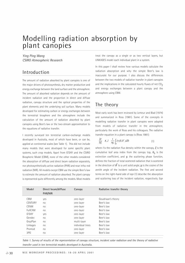
30 N E E W O R K S H O P P R O C E E D I N G S : 1 8 – 2 0 A P R I L 2 0 0 1
Ying Ping WangCSIRO Atmospheric Research
Introduction
The amount of radiation absorbed by plant canopies is one of
the major drivers of photosynthesis, dry matter production and
energy exchange between the land surface and the atmosphere.
The amount of absorbed radiation depends on the amount of
incident radiation and the proportion in direct and diffuse
radiation, canopy structure and the optical properties of the
plant elements and the underlying soil surface. Many models
developed for estimating carbon or energy exchanges between
the terrestrial biosphere and the atmosphere include the
calculation of the amount of radiation absorbed by plant
canopies using Beer’s law or the two-stream approximation to
the equations of radiative transfer.
I recently surveyed ten terrestrial carbon-exchange models
developed in Australia, most of which have been, or can be,
applied at continental scales (see Table 1). This did not include
many models that were developed for some specific plant
systems, such crop models. Apart from G’DAY and the CSIRO
Biospheric Model (CBM), none of the other models considered
the absorption of diffuse and direct beam radiation separately,
nor photosynthetically active radiation (PAR) and near infra-red
radiation (NIR). All models except CBM use the simple Beer’s law
to estimate the amount of radiation absorbed. The plant canopy
is represented quite differently among the models. Most models
treat the canopy as a single or as two vertical layers, but
LINKAGES model each individual plant in a system.
In this paper I shall review how various models calculate the
radiation absorption and why the simple Beer’s law is
inaccurate for our purpose. I also discuss the differences
between the two models of radiative transfer in plant canopies
and the implications in the calculated hourly fluxes of net CO2and energy exchanges between a plant canopy and the
atmosphere using CBM.
The theory
Most early work has been reviewed by Lemeur and Blad (1974)
and summarized in Ross (1981). Some of the concepts in
modelling radiative transfer in plant canopies were adapted
from models of radiative transfer in the atmosphere,
particularly the work of Ross and his colleagues. The radiative
transfer equation in a plant canopy is (Ross 1981):
(1)
where I is the radiation flux density within the canopy, ξ is the
cumulative leaf area index from the canopy top, Kb is the
extinction coefficient, and γ, the scattering phase function,
defines the fraction of total scattered radiation that is scattered
in the direction of θ* to a unit solid angle; µ is the cosine of the
zenith angle of the incident radiation. The first and second
terms on the right-hand side of eqn (1) describe the absorption
and scattering loss of the incident radiation, respectively. Eqn
Modelling radiation absorption byplant canopies
Model Direct beam/diffuse Canopy Radiative transfer theoryPAR/NIR
CBM yes one-layer Goudriaan’s theoryCENTURY no one-layer Beer’s lawCENW no one-layer Beer’s lawFullCAM no one-layer Beer’s lawG’DAY yes one-layer Beer’s lawGendec no one-layer Beer’s lawGrazPlan no multi-layer Beer’s lawLinkages no individual trees Beer’s lawPromod no one-layer Beer’s law3PG no one-layer Beer’s law
Table 1. Survey of results of the representation of canopy structure, incident solar radiation and the theory of radiative
transfer used in ten terrestrial models developed in Australia.
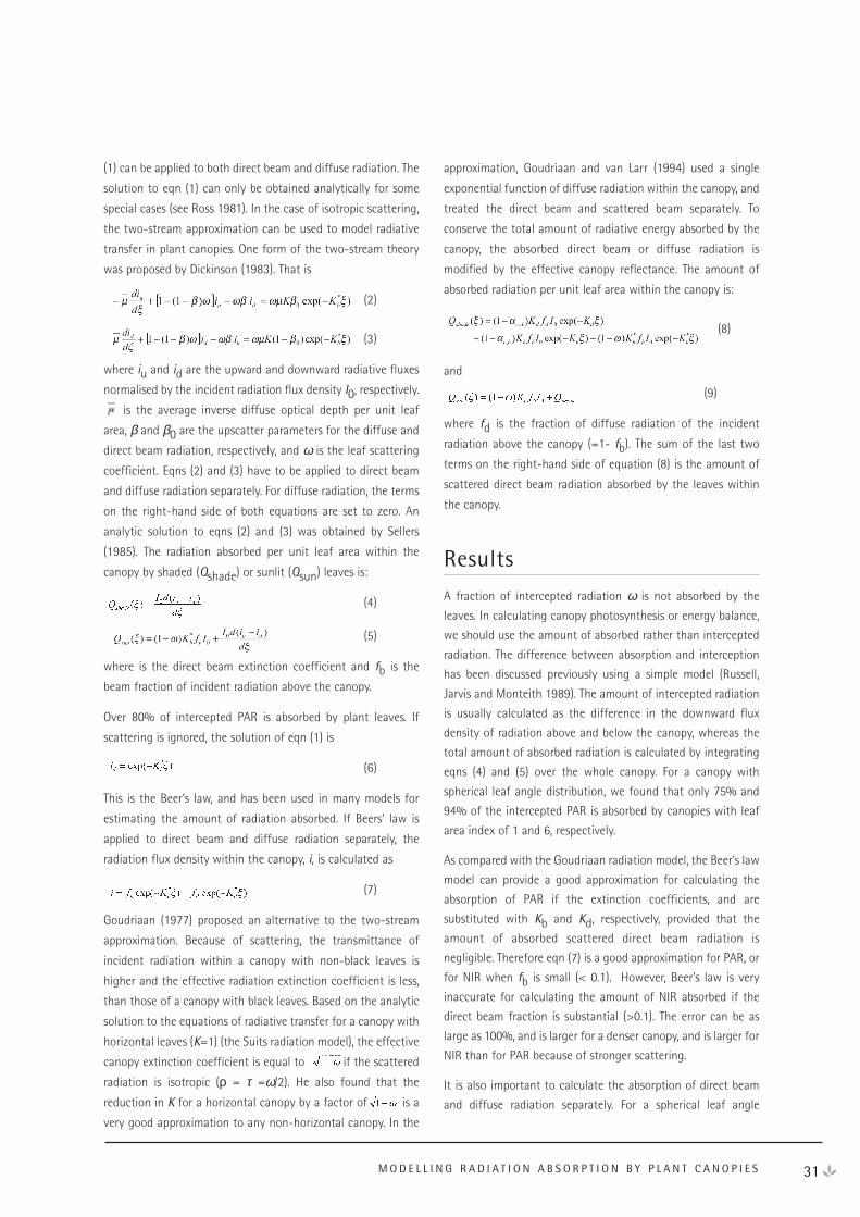
31
(1) can be applied to both direct beam and diffuse radiation. The
solution to eqn (1) can only be obtained analytically for some
special cases (see Ross 1981). In the case of isotropic scattering,
the two-stream approximation can be used to model radiative
transfer in plant canopies. One form of the two-stream theory
was proposed by Dickinson (1983). That is
(2)
(3)
where iu and id are the upward and downward radiative fluxes
normalised by the incident radiation flux density I0, respectively.
is the average inverse diffuse optical depth per unit leaf
area, β and β0 are the upscatter parameters for the diffuse and
direct beam radiation, respectively, and ω is the leaf scattering
coefficient. Eqns (2) and (3) have to be applied to direct beam
and diffuse radiation separately. For diffuse radiation, the terms
on the right-hand side of both equations are set to zero. An
analytic solution to eqns (2) and (3) was obtained by Sellers
(1985). The radiation absorbed per unit leaf area within the
canopy by shaded (Qshade) or sunlit (Qsun) leaves is:
(4)
(5)
where is the direct beam extinction coefficient and fb is the
beam fraction of incident radiation above the canopy.
Over 80% of intercepted PAR is absorbed by plant leaves. If
scattering is ignored, the solution of eqn (1) is
(6)
This is the Beer’s law, and has been used in many models for
estimating the amount of radiation absorbed. If Beers’ law is
applied to direct beam and diffuse radiation separately, the
radiation flux density within the canopy, i, is calculated as
(7)
Goudriaan (1977) proposed an alternative to the two-stream
approximation. Because of scattering, the transmittance of
incident radiation within a canopy with non-black leaves is
higher and the effective radiation extinction coefficient is less,
than those of a canopy with black leaves. Based on the analytic
solution to the equations of radiative transfer for a canopy with
horizontal leaves (K=1) (the Suits radiation model), the effective
canopy extinction coefficient is equal to if the scattered
radiation is isotropic (ρ = τ =ω/2). He also found that the
reduction in K for a horizontal canopy by a factor of is a
very good approximation to any non-horizontal canopy. In the
approximation, Goudriaan and van Larr (1994) used a single
exponential function of diffuse radiation within the canopy, and
treated the direct beam and scattered beam separately. To
conserve the total amount of radiative energy absorbed by the
canopy, the absorbed direct beam or diffuse radiation is
modified by the effective canopy reflectance. The amount of
absorbed radiation per unit leaf area within the canopy is:
(8)
and
(9)
where fd is the fraction of diffuse radiation of the incident
radiation above the canopy (=1- fb). The sum of the last two
terms on the right-hand side of equation (8) is the amount of
scattered direct beam radiation absorbed by the leaves within
the canopy.
Results
A fraction of intercepted radiation ω is not absorbed by the
leaves. In calculating canopy photosynthesis or energy balance,
we should use the amount of absorbed rather than intercepted
radiation. The difference between absorption and interception
has been discussed previously using a simple model (Russell,
Jarvis and Monteith 1989). The amount of intercepted radiation
is usually calculated as the difference in the downward flux
density of radiation above and below the canopy, whereas the
total amount of absorbed radiation is calculated by integrating
eqns (4) and (5) over the whole canopy. For a canopy with
spherical leaf angle distribution, we found that only 75% and
94% of the intercepted PAR is absorbed by canopies with leaf
area index of 1 and 6, respectively.
As compared with the Goudriaan radiation model, the Beer’s law
model can provide a good approximation for calculating the
absorption of PAR if the extinction coefficients, and are
substituted with Kb and Kd, respectively, provided that the
amount of absorbed scattered direct beam radiation is
negligible. Therefore eqn (7) is a good approximation for PAR, or
for NIR when fb is small (< 0.1). However, Beer’s law is very
inaccurate for calculating the amount of NIR absorbed if the
direct beam fraction is substantial (>0.1). The error can be as
large as 100%, and is larger for a denser canopy, and is larger for
NIR than for PAR because of stronger scattering.
It is also important to calculate the absorption of direct beam
and diffuse radiation separately. For a spherical leaf angle
M O D E L L I N G R A D I A T I O N A B S O R P T I O N B Y P L A N T C A N O P I E S
32 N E E W O R K S H O P P R O C E E D I N G S : 1 8 – 2 0 A P R I L 2 0 0 1
distribution, Kd is about 0.72 for PAR, whereas Kb varies from
0.45 to infinity. Models that do not consider the absorption of
direct beam and diffuse radiation separately will give biased
estimates of the amount of radiation absorbed.
In Goudriaan’s model, upward and downward scattering is not
considered separately, and only the absorption of the scattered
direct beam radiation is explicitly considered. The absorption of
scattered diffuse radiation is included by substituting the leaf
scattering coefficient with the canopy albedo for diffuse
radiation. Therefore, the total amount of absorbed diffuse
radiation calculated by Goudriaan’s model and the two–stream
theory is equal if the canopy albedos given by the two models
are also equal. However the vertical profile of absorbed diffuse
radiation predicted by the two models is different. As compared
with the two-stream theory, the Goudriaan model
overestimates the amount of absorbed PAR near the top of the
canopy, and the amount of absorbed NIR near the bottom of
the canopy, because the vertical profile of radiation flux density
as calculated by the Goudriaan model is more uniform than
that calculated by the two-stream theory.
It has been shown that canopy photosynthesis and energy
exchange can be accurately calculated using two big leaves,
sunlit and shaded (de Pury and Farquahr 1997; Wang and
Leuning 1998). Wang and Leuning (1998) used the Goudriaan
radiation model to estimate the amount of PAR and NIR
absorbed by the two big leaves. Using the CBM, I compared the
calculated fluxes of net CO2, latent and sensible heat fluxes for
wheat crops at Wagga Wagga as did Leuning et al. (1998) using
the absorbed radiation estimated by the Goudriaan radiation
model with that by the two-stream theory. I found that the
differences in the estimated fluxes were not significantly
different (< 5%).
The Goudriaan model is simpler than the two-stream theory,
and can be more easily implemented in most models of
terrestrial biosphere that require the amount of absorbed
radiation to be calculated. Because of some empirical elements,
the Goudriaan model should be tested against more field data.
As compared with the two-stream theory, the accuracy of
Goudriaan model depends on the accuracy of the estimated
canopy albedos for direct beam and diffuse radiation. A study is
in progress on comparing the canopy albedo predicted by
Goudriaan model with the field measurements.
Conclusions
We can draw the following conclusions from this study:
processes of photosynthesis and energy exchange in plant
canopies are directly related to the absorbed, rather than
the intercepted amount of radiation. The amount of
absorbed radiation can be significantly less than the
amount of intercepted radiation;
the two-stream theory or Goudriaan radiation treatment
should be used in estimating the amount of radiation
absorbed by plant canopies, particularly in the NIR region
when a significant fraction of the incident radiation is
direct beam.
ReferencesDe Pury, DGG and Farquhar, GD (1997). Simple scaling of
photosynthesis from leaves to canoipies without errors of
big-leaf models. Plant, Cell and Environment, 20:537-557.
Goudriaan, J. (1977). Crop micrometeorology: a simulation
study. PUDOC, Wageningen.
Goudriaan, J. and van Laar, HH (1994). Modelling potential
crop growth processes. Kluwer Academic Publishers,
Dordrecht.
Lemeur, R and Blad, BL (1974). A critical review of light models
for estimating the shortwave radiation regime of plant
canopies. Agricultural Meteorology, 14:255-286.
Leuning, R., Dunin, FX and Wang, YP (1998). ). A two-leaf
model for canopy conductance, photosynthesis and
partitioning of available energy. II. Comparison with
measurements. Agricultural and Forest Meteorology,
91:113-125.
Ross, J (1981). The radiation regime and architecture of
plant stands. Dr W Junk Publishers. The Hague.
Russell, G, Jarvis, PG and Monteith, JL (1989). Absorption of
radiation by canopies and stand growth. In Plant canopies:
their growth, form and function. Eds G. Russell, B.
Marshall and PG Jarvis. Society for Experimental Biology,
Seminar Series 31. Cambridge University Press.
Sellers, PJ (1985). Canopy reflectance, photosynthesis and
transpiration. International Journal of Remote Sensing,
6:1335-1372.
Wang, YP and Leuning, R (1998). A two-leaf model for canopy
conductance, photosynthesis and partitioning of available
energy. I. Model description. Agricultural and Forest
Meteorology, 91:89-111.
Belinda Medlyn, University of New South Wales
With contributions from:Damian Barrett, John Carter, Rod Keenan, Miko Kirschbaum, Joe Landsberg, Andrew Moore,Mike Raupach, Peter Sands, Richard Simpson,Ying Ping Wang
Introduction
At the core of most models of plant production there is a
calculation of photosynthate production. In general, the major
driving factor in this calculation is the radiation intercepted by
the plant. This review summarises the alternative methods used
to calculate conversion of intercepted radiation into
photosynthate.
It should be noted that in Australian conditions the most
limiting resource to photosynthesis is often not light but water
availability. In some models, water availability is treated as one
of a number of factors modifying the rate of radiation
conversion, but in other models the water limitation is
implemented in a ‘minimum limiting factor’ approach, implying
that radiation interception becomes irrelevant for production if
water availability is low. These alternative approaches will be
discussed briefly.
The conversion of radiation into photosynthate at leaf scale is
perhaps the most studied of all plant physiological processes
and hence is relatively well-understood. One outstanding major
scientific issue with modelling this process is the question of
how to scale up to large, heterogeneous areas. This paper will
also discuss issues of scaling and large-scale parameterisation
and validation of models.
Overview of modellingapproaches in Australianmodels
Table 1 gives details of the models considered in this review.
Four different types of “radiation conversion” model can be
distinguished. These are, in order of increasing complexity,
maximum productivity, radiation-use efficiency, big-leaf and
sun-shade models. More information on these approaches is
given below. The water limitation to productivity may be
incorporated by either (1) taking the minimum of radiation-
and water-limited production or (2) multiplying radiation-
limited production by a modifying factor dependent on
available water. In the first approach, water-limited productivity
is generally calculated using a water-use efficiency model,
described briefly below. In the second approach, several
33R A D I A T I O N C O N V E R S I O N
Radiation Conversion
Model
Century
Linkages
3PG
APSIM
GRASP
VAST
GrazPlan
CENW
Promod
G’DAY
Wang & Leuning
GPP / NPP
GPP
NPP
GPP
NPP
NPP
GPP
NPP
GPP
GPP
GPP
GPP
Radiation
Max. prod.
Max. prod.
RUE
RUE
RUE
RUE
Modified RUE
Big-leaf
Big-leaf
Sun-shade
Sun-shade
Water
Modifier
Modifier
Modifier
WUE
WUE
Modifier
Modifier
Modifier
WUE
WUE
Modifier
Ecosystems
All (Grass)
Forests
Forests
Crops
Pasture
All
Pasture
Forests
Forests
All (Forests)
All
Timestep
Month
Month
Month
Day
Day
Month
Day
Day
Day
Day
Hour
Table 1: Models included in this overview. Note: the FullCAM model, also included in the survey, uses 3PG logic for above-
ground production. Key references: 3PG: Landsberg & Waring (1997); APSIM: Meinke et al. (1997); CENTURY: Parton et al.
(1993); CENW: Kirschbaum (1999); G’DAY: Medlyn et al. (2000); GRASP: Littleboy & McKeon (1997); GrazPlan: Moore et al.
(1997); Linkages: Pastor & Post (1986); PROMOD: Sands (1995); VAST: DJ Barrett, pers. comm.; Wang & Leuning (1998).
alternative forms are used for the modifying factor. These
functions are not further discussed here; nor are the effects of
other environmental factors, such as nutrient availability, air
temperature, and plant age, which will be addressed by other
contributors.
Note that some of the models explicitly calculate both gross
primary productivity (GPP) and respiration, whereas others only
calculate net primary production (NPP). The more mechanistic
big-leaf and sun-shade approaches are used only to calculate
GPP, but the maximum productivity model and the radiation
use efficiency approach are used to calculate both GPP and NPP
in different models. Importantly, the logic is identical whether
GPP or NPP is being calculated; only parameter values differ.
Maximum productivity modelThe simplest method of calculating photosynthate production is
adopted in both the CENTURY and LINKAGES models. With this
approach, maximum productivity for a given species is specified
as a parameter to the model. Productivity is then assumed to be
reduced below this maximum by environmental factors such as
radiation, temperature and water and nutrient availability. In
CENTURY, the influence of radiation interception is
incorporated (for forests only) by a modifying factor that
depends exponentially on leaf area index (NREL 2000). In
LINKAGES, the same effect is represented by a non-linear
function of the percentage of full sunlight absorbed (Pastor &
Post 1986).
This approach can be criticised for being too simple. In the case
of LINKAGES, it is used because the model attempts to simulate
mixed-species forests, for which it is extremely difficult to
model radiation interception simply. The CENTURY model uses
the maximum productivity approach because its major focus is
on belowground processes. A known limitation to the CENTURY
implementation of this approach is that effects of incident
radiation are not taken into account. The model performs
adequately in current conditions because of the strong
correlation between radiation and temperature, but this
correlation may not hold in future conditions (e.g. increased
cloudiness) (Parton et al. 1993).
Resource use efficiency modelsThe radiation use efficiency approach is formulated simply as
G = ε Iabs (1)
where G is production (GPP or NPP), Iabs is absorbed radiation,
and ε is a constant, known as the radiation use efficiency (RUE)
(Monteith 1977). It has been suggested that the relation
between G and Iabs is not strictly proportional, as in eqn (1), but
that the RUE is higher at low radiation levels. Some models take
this into account by adding a modifying factor to increase ε at
low Iabs (e.g. GrazPlan, Moore et al. 1997).
The water use efficiency approach is similar:
G = q T (2)
where T is plant transpiration and q is the water-use efficiency
(WUE), which is generally assumed to depend inversely on
atmospheric vapour pressure deficit (e.g. RESCAP, Monteith et
al. 1989; applied to Pinus radiata by Dewar 1997).
The resource-use efficiency approach has been extremely widely
adopted. It is appealingly simple. The radiation-use efficiency, in
particular, is readily applied to remotely-sensed data of
radiation interception. Critics of this model question how
linearity could arise from an essentially non-linear process
(photosynthetic response to light) (e.g. Medlyn 1998); it has
been suggested that linearity could arise through an
optimisation process (Goetz & Prince 1999). The model has also
been criticised on the grounds of auto-correlation in the
estimation of the resource-use efficiency parameter
(Demetriades-Shah et al. 1992). Regardless of these criticisms,
many modellers have found that this approach performs
adequately when model output is tested against observations
of growth (e.g. Landsberg & Waring 1997, Clark et al. 2000).
Big-leaf modelA major difficulty in scaling photosynthesis rates from leaves to
canopies is the non-linearity of the light response of leaf
photosynthesis. This difficulty is overcome in the big-leaf model
by assuming that the maximum rate of leaf photosynthesis
(Amax) is proportional to the fraction of intercepted radiation
throughout the canopy. This assumption essentially allows
equations for leaf photosynthesis to be applied to the canopy as
a whole. The two models using this approach in this survey
(CENW and PROMOD) use the version of the big-leaf model
proposed by Sands (1995), in which instantaneous canopy
photosynthesis is integrated over the day. The advantage of the
big-leaf model is that it is mechanistic but swift at the same
time.
Sun-shade modelIn order to overcome the problem of scaling the non-linear light
response of photosynthesis, highly detailed models of canopy
photosynthesis generally divide the canopy into a large number
of sections with similar incident radiation and calculate the
photosynthetic rate in each section. However, experiments with
34 N E E W O R K S H O P P R O C E E D I N G S : 1 8 – 2 0 A P R I L 2 0 0 1
such models suggest that canopy photosynthesis can be
accurately modelled with a division into just two sections: sunlit
and shaded (e.g. Reynolds et al. 1992). The sun-shade model
approach is based on this observation: canopy photosynthesis is
calculated as the sum of components from sunlit and shaded
foliage, each of which is determined following the big-leaf
approximation (Wang & Leuning 1998, Medlyn et al. 2000). As
with the big-leaf model, this model has the advantage of being
mechanistic, but is somewhat more complex to implement.
Comparison of different approachesThe maximum productivity and resource-use efficiency models
are simple, empirical approaches, easy to understand and
computationally swift. The big-leaf and sun-shade approaches
are more complex but have a stronger mechanistic basis. More
detailed models of radiation conversion are also available, such
as those assuming heterogeneous canopies, but these are
generally regarded as inappropriate for modelling on large
spatial scales.
There have been several papers showing why sun-shade models
should theoretically perform better than big-leaf models (de
Pury & Farquhar 1997); however, the difference between the
models is quite small relative to the errors involved in parameter
estimation. There are also good theoretical reasons for
expecting that the big-leaf and sun-shade models should
perform better than the simpler resource-use efficiency model
but I am not aware of any work in which a direct comparison
has been performed. Certainly, proponents of both approaches
have been successful in modelling NPP at both point and
regional scale (e.g. Coops et al. 1998, Sands et al. 2000). For
example, the Potsdam NPP Model Intercomparison project
(Cramer et al. 1999) compared estimates of global NPP from
models utilising a range of radiation conversion approaches,
including resource-use efficiency and big-leaf models.
Differences between model estimates could not be attributed to
differences in modelling strategy. Similarly, there is little
evidence to demonstrate which is the better of the two
approaches to water limitation, the minimum-limitation or
modifying-factor approach.
Modelling the Australian continent:issues of scaling, parameterisation, andvalidationBroadly speaking, we have a good scientific understanding of
the processes involved in conversion of radiation to
photosynthate and can fairly confidently model these processes
at leaf and canopy scales. An outstanding issue, however, is how
to extend our modelling to large scales. This issue of course
concerns all processes, not just radiation conversion, but since
we are here considering core model structure it is appropriate
to address scaling in this paper. Scaling up from stand to
regional scales is generally achieved by applying a stand-scale
model with parameters appropriate to the region. Two issues are
particularly of concern with this scaling up: the choice of
appropriate parameters, and the validation of model outputs at
regional scale.
ParameterisationAt the stand scale, parameterisation of the big-leaf or sun-
shade models is relatively straightforward because the main
parameters can be related directly to simple physiological
measurements. It is somewhat more difficult to determine the
maximum productivity or radiation-use efficiency parameters.
Two alternative methods are commonly used to obtain these
parameters: they may be estimated from laborious stand-scale
measurements of productivity; or they may be derived from
more complex physiologically-based models.
At regional scale, point to point variation is a problem for
parameterising all types of models. In general, the methodology
used to scale from stands to regions involves applying the same
model repeatedly to a series of grid squares that make up the
region. Parameter values are selected to represent each grid
square. A common approach is to classify the vegetation type of
each grid square and then choose parameter values typical for
each vegetation type. The required spatial information on
vegetation characteristics may be available from existing maps
or from remotely-sensed data (Cramer et al. 1999). There are
two problems with this approach to parameterisation. Firstly,
our knowledge of typical parameter values for different
vegetation types is imprecise. Published values of radiation use
efficiency, for example, vary significantly (Goetz & Prince 1999).
Secondly, there is inevitable heterogeneity within each grid
square. If modelled processes are strongly non-linear, then the
use of a mean parameter value can lead to biassed model
outputs. Raupach et al. (2001) suggest that this problem can be
addressed using statistical estimation, which requires not only
knowledge of mean parameter values but also their variances
and covariances.
ValidationMost of the models covered in this survey have been calibrated
or validated at stand scale at a number of points. Validation
generally takes the form of comparison of model output with
above-ground production at a given site and thus may be
35R A D I A T I O N C O N V E R S I O N
regarded as a test of the full model rather than the GPP
component per se (e.g. Battaglia & Sands 1997, Gilmanov et al.
1997, Clark et al. 2000). Some attempts to test modelled GPP
separately have been made using eddy flux data (Medlyn et al.
1999, Law et al. 2000).
At large scale, there are limited ways to validate model
predictions. One method is to test model output against a
database of physically extensive ground observations (Barrett
2000, Scurlock et al. 1999); a second is to aggregate estimates
of net ecosystem production, using an atmospheric transport
model, for comparison with the international network of
measurements of atmospheric CO2 concentration. Cramer et al.
(1999) also highlight the potential of model comparison for
checking model output.
Summary
Four basic approaches to modelling of radiation conversion are
used in Australian NPP models. Although there may be
theoretical reasons to prefer one approach over another, in
practice each approach appears able to successfully model
radiation conversion. The main unresolved scientific problem
lies not in our understanding of this process, but in our ability
to extend our modelling to large scales.
ReferencesBarrett DJ (2001) Steady state net primary productivity, carbon
stocks and mean residence time of carbon in the Australian
terrestrial biosphere. Global Biogeochem. Cycles (in press).
Battaglia M, Sands PJ (1997) Modelling site productivity of
Eucalyptus globulus in response to climatic and site
factors. Aust. J. Plant Physiol. 24: 831-850.
Clark SG, Donnelly JR, Moore AD (2000) The GrassGro decision
support tool: its effectiveness in simulating pasture and
animal production and value in determining research
priorities. Aust. J. Exp. Agric. 40: 247-256.
Coops NC, Waring RH, Landsberg JJ (1998) Assessing forest
productivity in Australia and New Zealand using a
physiologically-based model driven with averaged monthly
weather data and satellite-derived estimates of canopy
photosynthetic capacity. For. Ecol. Manag. 104: 113-127.
Cramer W, Kicklighter DW, Bondeau A, Moore B, Churkina C,
Nemry B, Ruimy A, Schloss AL (1999) Comparing global
models of terrestrial net primary productivity (NPP):
overview and key results. Global Change Biol. 5 (Suppl. 1):
1-15.
Demetriades-Shah TH, Fuchs M, Kanemasu ET, Flitcroft I (1992)
A note of caution concerning the relationship between
cumulated intercepted solar radiation and crop growth.
Agric. For. Meteorol. 58:193-207
dePury DGG, Farquhar GD (1997) Simple scaling of
photosynthesis from leaves to canopies without the errors
of big-leaf models. Plant Cell. Environ. 20: 537-557.
Dewar RC (1997) A simple model of light and water use
evaluated for Pinus radiata. Tree Physiol. 17: 259-265.
Gilmanov TG, Parton WJ, Ojima DS (1997) Testing the
CENTURY ecosystem level model on data sets from eight
grassland sites in the former USSR representing wide
climatic/soil gradient. Ecol. Model. 96:191-210.
Goetz SJ, Prince SD (1999) Modelling terrestrial carbon
exchange and storage: evidence and implications of
function convergence in light-use efficiency. Adv. Ecol. Res.
28: 57-92.
Kirschbaum MUF (1999). CenW, a forest growth model with
linked carbon, energy, nutrient and water cycles. Ecol.
Model. 181: 17-59.
Landsberg JJ, Waring RH (1997) A generalised model of forest
productivity using simplified concepts of radiation-use
efficiency, carbon balance and partitioning. For. Ecol.
Manag. 95: 209-228.
Law BE, Waring RH, Anthoni PM, Aber JD (2000)
Measurements of gross and net ecosystem productivity and
water vapour exchange of a Pinus ponderosa ecosystem,
and an evaluation of two generalized models. Global
Change Biol. 6: 155-168.
Littleboy M & McKeon G (1997) Evaluating the risks of pasture
and land degradation in native pastures in Queensland.
Appendix 2: Subroutine GRASP: Grass Production Model.
Final Report DAQ-124A for the Rural Industries Research
and Development Commission.
Medlyn BE (1998) Physiological basis of the light use
efficiency model. Tree Physiol. 18:167-176.
Medlyn BE, Broadmeadow MB, Randle T, Matteucci G, Dufrêne
E (1999). Model comparison. In ECOCRAFT: Predicted
Impacts of Rising Carbon Dioxide and Temperature on
Forests in Europe at Stand Scale. Edited by P.G. Jarvis. Final
Project Report to the European Community, pp 97-135.
Medlyn BE, McMurtrie RE, Dewar RC, Jeffreys M. (2000) Soil
processes dominate long-term response of net primary
36 N E E W O R K S H O P P R O C E E D I N G S : 1 8 – 2 0 A P R I L 2 0 0 1

productivity of forests to increased temperature and
atmospheric CO2 concentration. Can. J. Forest Res. 30: 873-
888.
Meinke H, Hammer GL, van Keulen H, Rabbinge R (1997)
Improving wheat simulation capabilities in Australia from a
cropping systems perspective III. The integrated wheat
model (I_WHEAT). Europ. J. Agron. 8: 101-116.
Monteith, JL (1977) Climate and the efficiency of crop
production in Britain. Trans. R. Soc. Lond., Ser. B. 281:277-
294.
Monteith JL, Huda AKS, Midya D (1989) RESCAP: a resource
capture model for sorghum and pearl millet. In Modelling
the Growth and Development of Sorghum and PealMillet.
Edited by SM Virmani, HLS Tandon and G Alagarswamy.
ICRISAT Research Bulletin 12, Patancheru, India, pp 30-34.
Moore AD, Donnelly JR, Freer M (1997) GRAZPLAN: Decision
support systems for Australian grazing enterprises.3.
Pasture growth and soil moisture submodels, and the
GrassGro DSS. Agric. Sys. 55: 535-582.
NREL (2000) CENTURY Soil Organic Matter Model Version 5
User’s Guide and Reference.
http://www.nrel.colostate.edu/projects/century5/reference/i
ndex.htm
Parton WJ, Scurlock JMO, Ojima DS, et al. (1993) Observations
and modeling of biomass and soil organic matter dynamics
for the grassland biome worldwide. Global Biogoechem.
Cycles 7: 785-809.
Pastor J, Post WM (1986) Influence of climate, soil moisture
and succession on forest carbon and nitrogen cycles.
Biogeochem. 2: 3-27.
Raupach MR, Barrett DJ, Briggs PR, Kirby MJ (2001) Terrestrial
biosphere models and forest-atmosphere interactions. In:
Forests and Water (eds. R. Vertessy and H. Elsenbeer).
IUFRO. In press.
Reynolds JF, Chen J, Harley PC, Hilbert DW, Dougherty RL,
Tenhunen JD (1992) Modeling the effects of elevated CO2
on plants: extrapolating leaf response to a canopy. Agric.
For. Meteorol. 61: 69-94.
Sands PJ (1995) Modelling canopy production II. From single-
leaf photosynthetic parameters to daily canopy
photosynthesis. Aust. J. Plant Physiol. 22: 603-614.
Sands PJ, Battaglia M, Mummery D (2000) Application of
process-based models to forest management: experience
with PROMOD, a simple plantation productivity model. Tree
Physiol. 20: 383-392.
Scurlock JMO, Cramer W, Olson RJ, Parton WJ, Prince SD
(1999) Terrestrial NPP: Toward a consistent data set for
global model evaluation. Ecol. Applic. 9: 913-919.
Wang Y P, Leuning R (1998) A two-leaf model for canopy
conductance, photosynthesis and partitioning of available
energy I. Model description and comparison with a multi-
layered model. Agric. For. Meteorol. 91: 89-111.
37R A D I A T I O N C O N V E R S I O N
Roger GiffordCRC for Greenhouse AccountingCSIRO Plant Industry
Introduction
This paper concerns calculation of plant autotrophic respiration
rate, which may emit about half of the CO2 fixed by
photosynthesis (Ryle 1984). At the same time it generates
chemical energy and reducing power as well as metabolites that
are used as the building blocks for synthesis of organic
molecules. It does this through multi-step biochemical
pathways - glycolysis, the TCA cycle and pentose phosphate
pathway and a mitochondrial electron transport chain. Even
though about half the gross photosynthate produced is
dissipated by respiration our capacity to model it falls well short
of our capacity to model photosynthesis.
Mechanistic carbon cycle models are concerned with
calculating the CO2 emitted by whole plant respiration to
subtract from photosynthetic fixation by the leaves. To do this,
understanding of the “logic” of its regulation should be helpful.
The dynamic regulation of respiration is complex. The over-
arching logic behind the regulation of the rate of respiration at
the cellular level is determined by the relative requirements for
chemical energy and reducing power, and C-skeletons for
biosynthesis of complex molecules. At the level of electron
transport in the production of ATP it is the local supply of ADP
and AMP that may be in control.
Respiration may sometimes, however, be controlled by the
supply of its substrate – translocated sucrose. Thus respiration
can be controlled by the photosynthetic source, the utilization
sink, or by a combination of both. A complexity is that, within
the electron transport chain, there is also the potential for an
alternative oxidase to be engaged that has the effect of
allowing respiratory CO2 release without concurrent generation
of ATP. The function of this apparently CO2-wasting respiration
is unclear and its regulation is not understood (Affourtit et al.
2001)
Considered mechanistically from the bottom up, control of
respiratory CO2 release seems hopelessly complicated to capture
in productivity models. Accordingly, simplifying notions about
the high level logic of respiration have had to be devised.
Several approaches have been adopted.
Respiration-modellingapproaches in productivitymodels
Non-explicit treatment of respiration The simplest way to represent respiration is to embed it
implicitly in parameters of empirical growth functions that
don’t explicitly recognise photosynthesis. Many vegetation
production models calculate net primary productivity (i.e new
tissue growth rate) by functions that are calibrated to relate
primary production directly to the environmental drivers and
modulators of plant growth like radiation, water supply,
temperature, nutrition and stress factors. A popular approach to
such models is to calculate NPP as the amount of solar
radiation intercepted or absorbed by green leaves multiplied by
an efficiency of conversion of solar energy into plant dry
matter. The efficiency term may be taken to be constant or to
be a function of some variables such as temperature. Such
models do not need to represent respiration as they enter the
biological hierarchy at a higher level than that of process
physiology, respiration being built into the empirical
parameterisation of the growth functions.
Specific respirationModels that do attempt to include representation of
physiological and biochemical mechanisms of CO2 exchange
need to calculate respiration separately for subtraction from
photosynthesis to determine growth. Thus:
R = Rs(T) . W (1)
where R is respiration rate per plant, W is the dry weight per
plant and Rs is the specific respiration rate that varies with
temperature, T. However, it was found that specific plant
respiration is far from a constant at any given temperature.
Growth and maintenanceSpecific respiration rate is high in young fast growing tissues
and small in non-growing tissues and can respond quickly to
change in environmental factors. This fact led to recognition
that there could be a background or basal rate of specific
respiration combined with a respiration rate that was linked to
the rate at which the tissue or plant was photosynthesising or
growing. This idea was formulated at the whole plant level by
38 N E E W O R K S H O P P R O C E E D I N G S : 1 8 – 2 0 A P R I L 2 0 0 1
Plant Respiration
McCree (1970) and by Thornley (1970). McCree suggested that
the dynamic component be related to the rate of plant
photosynthesis
R= mW + pP (2)
where R is the respiration rate per plant or per unit ground area,
P is the photosynthesis rate per plant or per unit ground area,
m is a respiratory maintenance coefficient and p is a coefficient
for respiration related to photosynthesis rate.
Thornley (1970) showed that the dynamic part could
equivalently be related to new growth (i.e. to photosynthesis
minus respiration)
R = mW + gG = Rm + Rg (3)
Where G is the growth rate per plant or per unit ground area
calculated as (P-R), and g is the growth coefficient.
At the same time it was also recognised that respiration linked
to the rate of growth was mainly that required to energise
synthesis of the new complex molecules (proteins, membranes,
cell walls etc) that constitute growth (Beevers 1970).
It has also been recognised that a substantial part of the energy
requirement for maintenance may be for protein turnover. Thus
another way to express the concept is as:
R = mnWn + gG (4)
where Wn is the N content of the plant and mn is the
maintenance expressed on a nitrogen basis. While it was
conceived that a major energy demand for plant tissue
maintenance would be protein turnover it has also been
recognised that maintenance of membrane integrity and solute
gradients must contribute (Penning de Vries et al. 1983).
A problem with growth and maintenance formulations is that
they are purely notional constructs. Growth and maintenance
are not biochemically distinct. The concept does not withstand
close scrutiny. They are defined only operationally by the
measurement approach adopted and the assumptions involved
in such measurements. There are several approaches to
measuring growth and maintenance components; each involves
different assumptions and therefore measures different
properties of respiration.
Growth and maintenance coefficients measured even by the
same method are not necessarily constant (Amthor 2000) for
several reasons. One is that their values depend on the
composition of the plant being grown and maintained.
Maintenance of wood that is mostly lignocellulosic cell wall
requires much less energy than maintenance of leaves
containing a high fraction of functional enzyme-proteins and
membranes, for example. And the energy for wood growth is
very different from the energy requirement for growing oily or
proteinaceous tissues. Penning de Vries et al. (1983) addressed
the compositional question in determining the growth
coefficient by substituting organic synthesis respiration for
growth respiration assuming that these processes occur at
maximum efficiency and are uninfluenced in their energy
requirement by temperature and stress. They calculated
theoretical energy requirements to synthesise the variety of
compounds found in plants to estimate the synthesis
respiration for a diversity of species.
A second reason why growth and maintenance coefficients are
not constant is that there are carbon (energy) utilizing plant
process that are not readily classified as either growth or
maintenance. Under the growth and maintenance concept such
respiration-requiring processes are forced into one or other of
the coefficients by whatever means is adopted to determine
them. For example, where environmental conditions trigger
operation of the alternative oxidase, which may act as a C
wasting valve, the CO2 emitted does not logically fall under
either growth or maintenance; its classification under a
technique that breaks down respiration into just those two
components is not obvious. Phloem loading for long distance
transport of photoassimilate is energy demanding but services
the carbohydrate requirements of both growth and
maintenance. Similarly, nutrient uptake by the root system
consumes energy; how it should be classified under the growth
and maintenance concept is unclear. Accordingly, van Veen
(1980) suggested that ion uptake requires separate
consideration. However, there are also other energy requiring
processes occurring in plants such as N-fixation in some
species, and nitrate reduction which can occur in roots or leaves
the proportion varying with species (Thornley and Cannell
2000).
Although for a period it became conventional to relate
maintenance respiration closely with protein turnover, the case
is not, however, strong for modelling maintenance respiration
based on the assumption that it is best related to plant N
content.
An alternative way to treat componentsof respiration – the “process-residual”approachTo deal with the unavoidable fuzzy boundaries between
maintenance and growth, Cannell and Thornley (2000)
39P L A N T R E S P I R A T I O N
proposed a different approach in which each respiration-
demanding process is regarded as an independently acting
process which can be assessed individually. In this approach, the
model would first calculate the respiration of each individual
process that can be quantified. For example, there might be
data that would allow calculation of the energy demand of new
synthesis of N-fixation, of N-uptake, of nitrate reduction, of
other ion uptake, and of phloem loading. Then any other
processes not explicitly calculated would be lumped into the
residual respiration. The approach is called the “process-
residual” approach. It is adopted in Thornley’s Hurley Pasture
Model (HPM) and the Edinburgh Forest Model (EFM) (Thornley
and Cannell 2000). The HPM and EFM were run with the
process-residual approach for a full year or full forest rotation,
respectively. It was found that the energy requirements of
mineral nutrition are minute compared with those of new
materials synthesis, phloem loading and the residual
components that cover protein turnover, C-wasting respiration
and maintenance of ion and other gradients in cells and tissues.
Respiration:photosynthesis ratioIt has been found in practice that for whole plants and
ecosystems the ratio of respiration to gross photosynthesis is
conservative over a wide range of plant sizes and growth rates,
CO2 concentrations and temperatures. This is equivalent to
conservatism in carbon use efficiency, CUE (NPP/GPP) and in
respiration to GPP ratio. In practice measurements have shown
that at the whole plant level R:P ratio is typically within the
range 0.35-0.6. Utilization of this approach in models has
experienced a resurgence over the last few years (Gifford, 1994;
1995, Waring et al 1998).
Survey of specific modeltreatments of respiration
Models that have plant productivity as output must deal with
autotrophic respiration in some way, be it implicitly in some
cases. Examples of models for which respiration is embedded
implicitly in the parameters that relate growth to
environmental variables include: the crop models of the APSIM
farm-system suite of models, the rangeland production/
management model GRASP, the ecosystem level forest model
LINKAGES, the agricultural soil C model SOCRATES, the
continental C-cycle model VAST and the forest productivity
model G’Day when simulating water limiting conditions.
Models which assign values of specific respiration include the
carbon cycle model CENTURY, and G’Day when water is not
growth limiting during the growing season. In each case,
specific respiration is expressed as a function of N-
concentration and temperature. Models that utilise the growth
and maintenance approach are the forest productivity model
CenW (as one option) and the forest growth and yield model
Promod. Use of constant values of either R:GPP ratio or
NPP:GPP ratio as inputs are allowed as options in CenW and
G’Day. They are the sole option in the simple terrestrial C-cycle
models CQUEST and CQUESTN, and in the forest growth model
3PG. The forest carbon cycle model FullCAM uses 3PG as a sub-
model and hence relies on the NPP/GPP ratio to expresses
respiration.
Some unresolved issues inautotrophic respiration
There is a significant problem in whole-plant respiration studies
of not being able routinely to measure autotrophic respiration
of leaves by day when photosynthetic CO2 uptake is occurring.
Commonly it is assumed in whole plant studies and models that
respiration continues by day at the rate it does at night, possibly
responding to short term diurnal variation in leaf temperature.
However, there is evidence both for and against a reduction of
leaf autotrophic respiration in the light (Lambers 1997).
There are many papers reporting that plant respiration is
partially suppressed by elevated atmospheric CO2
concentration. Both short term reversible effects and long term
irreversible effects have been described (Drake et al. 1999).
While there are significant doubts about the validity of that
conclusion under doubled CO2 concentration, the reality or not
of the phenomenon has not yet been resolved (Bunce 2001).
Most C-cycle and productivity modelling approaches adopt a
high sensitivity of specific respiration to temperature with a Q10
> 2 (Ryan 1991). However, in the long term, plant respiration
seems to acclimate to a temperature change over several days
to a week (Gifford 1995). The acclimated Q10 may be much less
than 2. For example, whole plant specific respiration of sorghum
plants (Gifford 1992) grown and measured at a range of
constant temperatures was only 1.3 whereas the short-term
sensitivity (hours) of whole plant specific respiration to
temperature was much greater (Figure 1a). When expressed as
a ratio of 24 hour respiration to 24hr photosynthesis per plant,
the sorghum plants showed a low response to growth
temperature (Figure 1b).
40 N E E W O R K S H O P P R O C E E D I N G S : 1 8 – 2 0 A P R I L 2 0 0 1
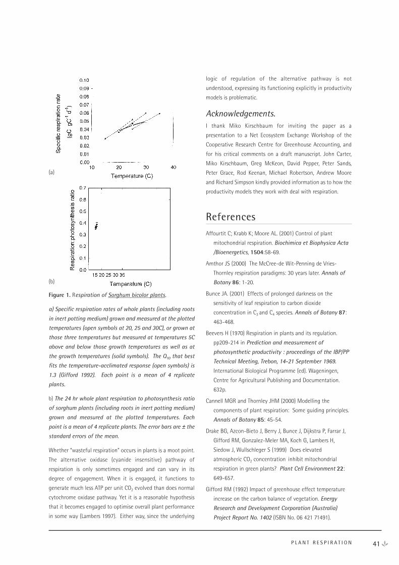
Figure 1. Respiration of Sorghum bicolor plants.
a) Specific respiration rates of whole plants (including roots
in inert potting medium) grown and measured at the plotted
temperatures (open symbols at 20, 25 and 30C), or grown at
those three temperatures but measured at temperatures 5C
above and below those growth temperatures as well as at
the growth temperatures (solid symbols). The Q10 that best
fits the temperature-acclimated response (open symbols) is
1.3 (Gifford 1992). Each point is a mean of 4 replicate
plants.
b) The 24 hr whole plant respiration to photosynthesis ratio
of sorghum plants (including roots in inert potting medium)
grown and measured at the plotted temperatures. Each
point is a mean of 4 replicate plants. The error bars are ± the
standard errors of the mean.
Whether “wasteful respiration” occurs in plants is a moot point.
The alternative oxidase (cyanide insensitive) pathway of
respiration is only sometimes engaged and can vary in its
degree of engagement. When it is engaged, it functions to
generate much less ATP per unit CO2 evolved than does normal
cytochrome oxidase pathway. Yet it is a reasonable hypothesis
that it becomes engaged to optimise overall plant performance
in some way (Lambers 1997). Either way, since the underlying
logic of regulation of the alternative pathway is not
understood, expressing its functioning explicitly in productivity
models is problematic.
Acknowledgements. I thank Miko Kirschbaum for inviting the paper as a
presentation to a Net Ecosystem Exchange Workshop of the
Cooperative Research Centre for Greenhouse Accounting, and
for his critical comments on a draft manuscript. John Carter,
Miko Kirschbaum, Greg McKeon, David Pepper, Peter Sands,
Peter Grace, Rod Keenan, Michael Robertson, Andrew Moore
and Richard Simpson kindly provided information as to how the
productivity models they work with deal with respiration.
ReferencesAffourtit C; Krabb K; Moore AL. (2001) Control of plant
mitochondrial respiration. Biochimica et Biophysica Acta
/Bioenergetics, 1504:58-69.
Amthor JS (2000) The McCree-de Wit-Penning de Vries-
Thornley respiration paradigms: 30 years later. Annals of
Botany 86: 1-20.
Bunce JA. (2001) Effects of prolonged darkness on the
sensitivity of leaf respiration to carbon dioxide
concentration in C3 and C4 species. Annals of Botany 87:
463-468.
Beevers H (1970) Respiration in plants and its regulation.
pp209-214 in Prediction and measurement of
photosynthetic productivity : proceedings of the IBP/PP
Technical Meeting, Trebon, 14-21 September 1969.
International Biological Programme (ed). Wageningen,
Centre for Agricultural Publishing and Documentation.
632p.
Cannell MGR and Thornley JHM (2000) Modelling the
components of plant respiration: Some guiding principles.
Annals of Botany 85: 45-54.
Drake BG, Azcon-Bieto J, Berry J, Bunce J, Dijkstra P, Farrar J,
Gifford RM, Gonzalez-Meler MA, Koch G, Lambers H,
Siedow J, Wullschleger S (1999) Does elevated
atmospheric CO2 concentration inhibit mitochondrial
respiration in green plants? Plant Cell Environment 22:
649-657.
Gifford RM (1992) Impact of greenhouse effect temperature
increase on the carbon balance of vegetation. Energy
Research and Development Corporation (Australia)
Project Report No. 1402 (ISBN No. 06 421 71491).
41P L A N T R E S P I R A T I O N
(a)
(b)

Gifford RM (1994) The global carbon cycle: a viewpoint on the
missing sink. Australian Journal Plant Physiology 21:
1-15.
Gifford RM (1995) Whole plant respiration and photosynthesis
of wheat under increased CO2 concentration and
temperature: long-term vs. short-term distinctions for
modelling. Global Change Biology 1: 385-396.
Lambers H (1997) Oxidation of mitochondrial NADH and
synthesis of ATP. pp200-219 in Plant Metabolism. DT
Dennis, DH Turpin, DD Lefebvre and DB Layzell eds. 2nd
Edition. Addison Wesley Longman, Harlow, UK. 529p.
McCree KJ (1970) An equation for the rate of respiration of
white clover plants grown under controlled conditions.
pp221-229 in Prediction and measurement of
photosynthetic productivity: proceedings of the IBP/PP
Technical Meeting, Trebon, 14-21 September 1969.
International Biological Programme (ed). Wageningen,
Centre for Agricultural Publishing and Documentation.
632p.
Penning de Vries FWT, van Laar HH and Chardon MCM (1983)
Bioenergetics of growth of seeds, fruits, and storage
organs. pp 37-59 in Potential productivity of field crops
under different environments. International Rice Research
Institute, Los Banos, Phillipines.
Ryan MG (1991) Effects of climate change on plant
respiration. Ecological Applications 1: 157–167.
Ryle GJA (1984) Respiration and plant growth. In Palmer JM
(ed) Physiology and Biochemistry of Plant Respiration,
Cambridge University Press, Cambridge, UK.
Thornley JHM (1970) Respiration, growth and maintenance in
plants. Nature 227: 304-305.
Thornley JHM and Cannell MGR (2000) Modelling the
components of plant respiration: Representation and
realism. Annals of Botany 85: 55-67.
van Veen BW (1980) Energy costs of ion transport. pp187-195
in Genetic engineering of osmoregulastion. Impact on
plant production for food, chemicals and energy. (DW
Rains, RC Valentine, A Hollaender, eds). New York, Plenum
Press.
Waring RH, Landsberg JJ and Williams M (1998). Net primary
production of forests: a constant fraction of gross primary
production? Tree Physiology 18: 129–134.
42 N E E W O R K S H O P P R O C E E D I N G S : 1 8 – 2 0 A P R I L 2 0 0 1
Craig Barton CRC for Greenhouse AccountingState Forests of NSW
With contributions from Roddy Dewar, RodKeenan, Keryn Paul, Miko Kirschbaum, JoeLandsberg, Dave Pepper and Peter Sands.
Allocation and its relevance toNet Ecosystem Exchange
Carbon is converted from CO2 to carbohydrate in leaves. This
assimilate is then translocated throughout the plant where it is
either used as fuel for metabolic activity, stored for later use or
built into new structure, resulting in growth and reproduction.
The term allocation is ambiguously used to refer to i) the
proportions of carbon translocated to various plant parts, ii) the
relative growth rates of different plant parts and iii) the
translocation process itself. The reason for this is that in some
models the allocation of carbon (or nitrogen) between plant
parts is largely empirical, based on plant component mass at
harvests (Comins and McMurtrie 1993), while in others it is a
consequence of the transport process (Thornley 1991).
The importance of allocation for modelling net ecosystem
carbon exchange (NEE) is that allocation combined with
mortality and decomposition determines the amount of carbon
sequestered in long term storage pools, such as woody biomass
and soil carbon. Carbon allocated to lignified tissue such as
wood will have a longer residence time in the ecosystem than
that allocated to leaves or fine roots. The relevance of allocation
to NEE depends on the time scale of interest. In annual plants,
that germinate, grow, reproduce and die within one year,
decomposition processes will be more important to NEE than
allocation patterns on time scales of greater than one year.
However, in long-lived species that produce long-lived
structures such as the stems of trees allocation patterns
become increasingly important to NEE at this time scale. Since
the primary interest of this paper is in the impact of allocation
on the long-term (decades) carbon storage by vegetation its
focus will be on allocation in woody perennials.
Despite advances in many areas of plant physiology, the
underlying mechanisms that control the allocation of carbon
within plants are still not understood, and this lack of
knowledge is becoming the limiting factor in the advancement
of mechanistic models of plant growth and function. Allocation
within functional-structural tree models is critical since in the
short term, partitioning of assimilates among the different sink
organs and/or functions determines the relative growth rates of
the various plant components. Assimilate allocation is also
involved in a number of feedback processes which influence
plant development in the long term. For example, developing
leaves are reliant on carbon allocation from functional leaves
however, these leaves will later become carbon sources, thus
affecting future carbon inputs. The complex dynamic and
feedback aspects to allocation have implications for the long
term stability and predictive ability of mechanistic models.
The current state of knowledge
There have been a number of reviews of allocation over the last
few years (see Cannell and Dewar 1994; Lacointe 2000) along
with many papers promoting new or revamped hypotheses. The
review by Cannell and Dewar (1994) is difficult to improve upon
and so I shall borrow from them and include some new work
that has been published in the interim.
In order to understand the underlying controls of allocation it is
helpful to outline the possible drivers of allocation. For a plant
to survive resources must be allocated between various plant
parts and processes:
Allocation for structure: Need leaves to absorb radiation.
Need stems to position leaves in space and to raise the
canopy above competition.
Need roots to absorb nutrients and water, and to anchor
plants.
Need stems to transport water, nutrients and assimilates.
Allocation for metabolic activity:Protein turnover.
Ion gradient maintenance.
Nutrient uptake.
Allocation to storage:Used to allow plant to cope with fluctuating environment.
Allocation to reproduction:Storage in propagules for reproduction.
43T H E R O L E O F A L L O C A T I O N I N M O D E L L I N G N E E
The Role of Allocation in Modelling NEE
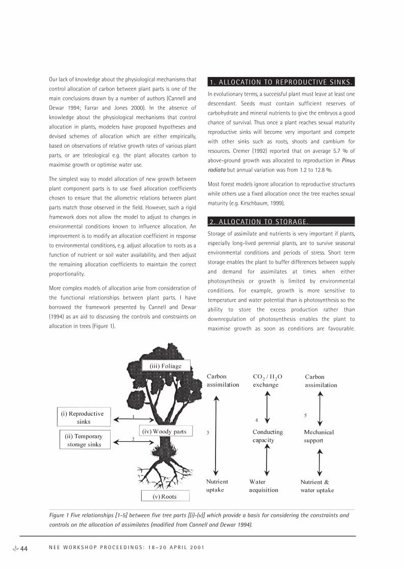
44 N E E W O R K S H O P P R O C E E D I N G S : 1 8 – 2 0 A P R I L 2 0 0 1
Our lack of knowledge about the physiological mechanisms that
control allocation of carbon between plant parts is one of the
main conclusions drawn by a number of authors (Cannell and
Dewar 1994; Farrar and Jones 2000). In the absence of
knowledge about the physiological mechanisms that control
allocation in plants, modelers have proposed hypotheses and
devised schemes of allocation which are either empirically,
based on observations of relative growth rates of various plant
parts, or are teleological e.g. the plant allocates carbon to
maximise growth or optimise water use.
The simplest way to model allocation of new growth between
plant component parts is to use fixed allocation coefficients
chosen to ensure that the allometric relations between plant
parts match those observed in the field. However, such a rigid
framework does not allow the model to adjust to changes in
environmental conditions known to influence allocation. An
improvement is to modify an allocation coefficient in response
to environmental conditions, e.g. adjust allocation to roots as a
function of nutrient or soil water availability, and then adjust
the remaining allocation coefficients to maintain the correct
proportionality.
More complex models of allocation arise from consideration of
the functional relationships between plant parts. I have
borrowed the framework presented by Cannell and Dewar
(1994) as an aid to discussing the controls and constraints on
allocation in trees (Figure 1).
1. ALLOCATION TO REPRODUCTIVE SINKS.
In evolutionary terms, a successful plant must leave at least one
descendant. Seeds must contain sufficient reserves of
carbohydrate and mineral nutrients to give the embryos a good
chance of survival. Thus once a plant reaches sexual maturity
reproductive sinks will become very important and compete
with other sinks such as roots, shoots and cambium for
resources. Cremer (1992) reported that on average 5.7 % of
above-ground growth was allocated to reproduction in Pinus
radiata but annual variation was from 1.2 to 12.8 %.
Most forest models ignore allocation to reproductive structures
while others use a fixed allocation once the tree reaches sexual
maturity (e.g. Kirschbaum, 1999).
2. ALLOCATION TO STORAGE.
Storage of assimilate and nutrients is very important if plants,
especially long-lived perennial plants, are to survive seasonal
environmental conditions and periods of stress. Short term
storage enables the plant to buffer differences between supply
and demand for assimilates at times when either
photosynthesis or growth is limited by environmental
conditions. For example, growth is more sensitive to
temperature and water potential than is photosynthesis so the
ability to store the excess production rather than
downregulation of photosynthesis enables the plant to
maximise growth as soon as conditions are favourable.
Figure 1 Five relationships [1-5] between five tree parts [(i)-(v)] which provide a basis for considering the constraints and
controls on the allocation of assimilates (modified from Cannell and Dewar 1994).
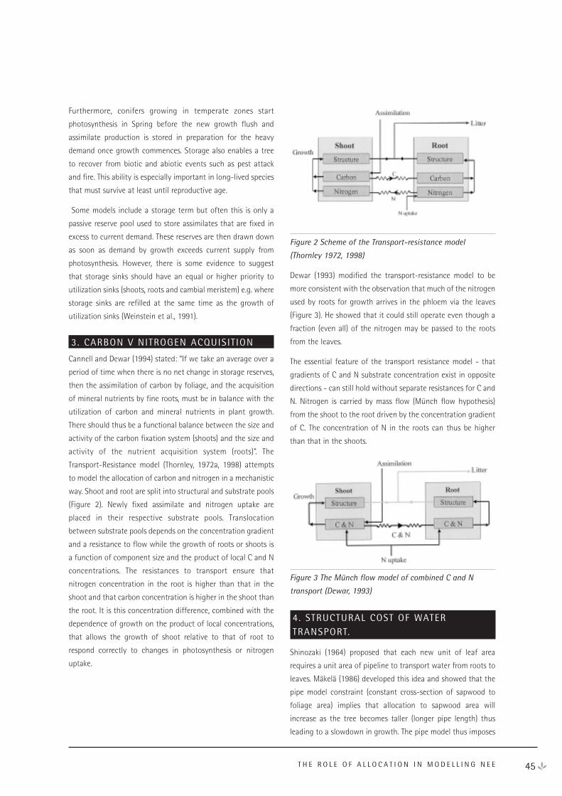
Furthermore, conifers growing in temperate zones start
photosynthesis in Spring before the new growth flush and
assimilate production is stored in preparation for the heavy
demand once growth commences. Storage also enables a tree
to recover from biotic and abiotic events such as pest attack
and fire. This ability is especially important in long-lived species
that must survive at least until reproductive age.
Some models include a storage term but often this is only a
passive reserve pool used to store assimilates that are fixed in
excess to current demand. These reserves are then drawn down
as soon as demand by growth exceeds current supply from
photosynthesis. However, there is some evidence to suggest
that storage sinks should have an equal or higher priority to
utilization sinks (shoots, roots and cambial meristem) e.g. where
storage sinks are refilled at the same time as the growth of
utilization sinks (Weinstein et al., 1991).
3. CARBON V NITROGEN ACQUISIT ION
Cannell and Dewar (1994) stated: “If we take an average over a
period of time when there is no net change in storage reserves,
then the assimilation of carbon by foliage, and the acquisition
of mineral nutrients by fine roots, must be in balance with the
utilization of carbon and mineral nutrients in plant growth.
There should thus be a functional balance between the size and
activity of the carbon fixation system (shoots) and the size and
activity of the nutrient acquisition system (roots)”. The
Transport-Resistance model (Thornley, 1972a, 1998) attempts
to model the allocation of carbon and nitrogen in a mechanistic
way. Shoot and root are split into structural and substrate pools
(Figure 2). Newly fixed assimilate and nitrogen uptake are
placed in their respective substrate pools. Translocation
between substrate pools depends on the concentration gradient
and a resistance to flow while the growth of roots or shoots is
a function of component size and the product of local C and N
concentrations. The resistances to transport ensure that
nitrogen concentration in the root is higher than that in the
shoot and that carbon concentration is higher in the shoot than
the root. It is this concentration difference, combined with the
dependence of growth on the product of local concentrations,
that allows the growth of shoot relative to that of root to
respond correctly to changes in photosynthesis or nitrogen
uptake.
Figure 2 Scheme of the Transport-resistance model
(Thornley 1972, 1998)
Dewar (1993) modified the transport-resistance model to be
more consistent with the observation that much of the nitrogen
used by roots for growth arrives in the phloem via the leaves
(Figure 3). He showed that it could still operate even though a
fraction (even all) of the nitrogen may be passed to the roots
from the leaves.
The essential feature of the transport resistance model - that
gradients of C and N substrate concentration exist in opposite
directions - can still hold without separate resistances for C and
N. Nitrogen is carried by mass flow (Münch flow hypothesis)
from the shoot to the root driven by the concentration gradient
of C. The concentration of N in the roots can thus be higher
than that in the shoots.
Figure 3 The Münch flow model of combined C and N
transport (Dewar, 1993)
4. STRUCTURAL COST OF WATER TRANSPORT.
Shinozaki (1964) proposed that each new unit of leaf area
requires a unit area of pipeline to transport water from roots to
leaves. Mäkelä (1986) developed this idea and showed that the
pipe model constraint (constant cross-section of sapwood to
foliage area) implies that allocation to sapwood area will
increase as the tree becomes taller (longer pipe length) thus
leading to a slowdown in growth. The pipe model thus imposes
45T H E R O L E O F A L L O C A T I O N I N M O D E L L I N G N E E
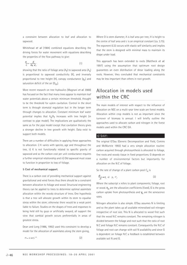
a constraint between allocation to leaf and allocation to
sapwood.
Whitehead et al (1984) combined equations describing the
driving forces for water movement with equations describing
the properties of the flow pathway to give:
(1)
showing that the ratio of foliage area (Af) to sapwood area (As)
is proportional to sapwood conductivity (K), and inversely
proportional to tree height (H), canopy conductance (gc) and
saturation deficit of the air (Dm).
More recent research on tree hydraulics (Magnani et al. 2000)
has focused on the fact that many trees appear to maintain leaf
water potentials above a certain minimum threshold, thought
to be the threshold for xylem cavitation. Control in the short
term is through stomatal regulation but in the longer term
through changes to allocation. Constant minimum leaf water
potential implies that As/Af increases with tree height (in
contrast to pipe model). The implications are qualitatively the
same as for the pipe model except that cavitation theory gives
a stronger decline in tree growth with height. Data exist to
support both models.
There are a number of difficulties in applying these approaches
to allocation. i) K varies with species, age and throughout the
tree, ii) K is not functionally related to specific gravity of
sapwood and so the carbon cost per unit conductance requires
a further empirical relationship and iii) Old sapwood must cease
to function in proportion to loss of foliage.
5 Cost of mechanical support.
There is a carbon cost of providing mechanical support against
gravitational and wind forces thus there should be a constraint
between allocation to foliage and wood. Structural engineering
theory can be applied to trees to determine optimal assimilate
allocation within the woody structure of trees. One hypothesis
is that a tree will allocate growth within its stem to equalise
stress within the stem; otherwise there would be a weak point
liable to failure. Studies on the shapes of trees and responses to
being held still by guys or artificially swayed, all support the
view that cambial growth occurs preferentially in areas of
greatest stress.
Dean and Long (1986, 1992) used this constraint to develop a
model for the allocation of assimilates along the stem giving,
(2)
Where D is stem diameter, A is leaf area per tree, H is height to
the centre of leaf area and c is an empirical constant (ca. 3.75).
The exponent 0.33 occurs with elastic self similarity and implies
that the stem is designed with minimal mass to maintain its
shape under load.
This approach has been extended to roots (Mattheck et al.
1997) using the assumption that optimum root design
guarantees an even distribution of shear loading along the
roots. However, they concluded that mechanical constraints
may be less important than others in root growth.
Allocation in models usedwithin the CRC
The main models of interest with respect to the influence of
allocation on NEE on a multi-year time scale are forest models.
Allocation within crop models is not as important since the
turnover of biomass is annual. I will briefly outline the
approaches used to allocate carbon and nitrogen in the forest
models used within the CRC GA.
G’DAY:
The original G’Day (Generic Decomposition and Yield, Comins
and McMurtrie 1993) had a very simple allocation routine:
carbon acquired through photosynthesis is allocated to foliage,
fine roots and woody tissue in fixed proportions. G depends on
a number of environmental factors but importantly for
allocation on the N:C of foliage.
So the rate of change of a plant carbon pool Cx is
(3)
Where the subscript x refers to plant components; foliage, root
or wood. ηx are the allocation coefficients (fixed), G is the gross
carbon uptake from photosynthesis and γx are the senescence
rates.
Nitrogen allocation is also simple. G’Day assumes N is limiting
and so the plant takes up all available mineralised soil nitrogen
irrespective of root size. This N is allocated to wood first such
that the wood N:C remains constant. The remaining nitrogen is
divided between the foliage and root such that the ratio of root
N:C and foliage N:C remains constant. Consequently the N:C of
foliage and root can change with soil N availability and since G
is dependent on foliage N:C a feedback is established between
available soil N and G.
46 N E E W O R K S H O P P R O C E E D I N G S : 1 8 – 2 0 A P R I L 2 0 0 1
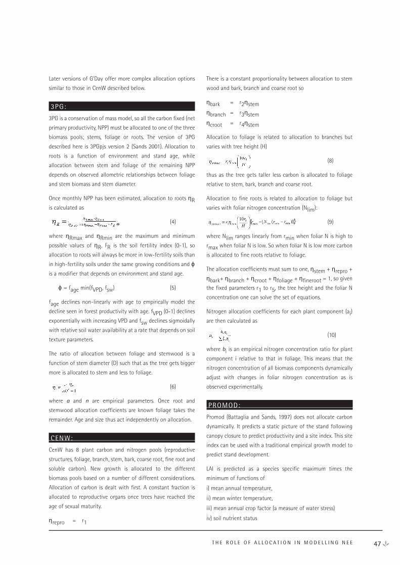
Later versions of G’Day offer more complex allocation options
similar to those in CenW described below.
3PG:
3PG is a conservation of mass model, so all the carbon fixed (net
primary productivity, NPP) must be allocated to one of the three
biomass pools; stems, foliage or roots. The version of 3PG
described here is 3PGpjs version 2 (Sands 2001). Allocation to
roots is a function of environment and stand age, while
allocation between stem and foliage of the remaining NPP
depends on observed allometric relationships between foliage
and stem biomass and stem diameter.
Once monthly NPP has been estimated, allocation to roots ηRis calculated as
(4)
where ηRmax and ηRmin are the maximum and minimum
possible values of ηR, FR is the soil fertility index (0-1), so
allocation to roots will always be more in low-fertility soils than
in high-fertility soils under the same growing conditions and ϕis a modifier that depends on environment and stand age.
ϕ = fage min(fVPD, fsw) (5)
fage declines non-linearly with age to empirically model the
decline seen in forest productivity with age. fVPD (0-1) declines
exponentially with increasing VPD and fsw declines sigmoidally
with relative soil water availability at a rate that depends on soil
texture parameters.
The ratio of allocation between foliage and stemwood is a
function of stem diameter (D) such that as the tree gets bigger
more is allocated to stem and less to foliage.
(6)
where a and n are empirical parameters. Once root and
stemwood allocation coefficients are known foliage takes the
remainder. Age and size thus act independently on allocation.
CENW:
CenW has 8 plant carbon and nitrogen pools (reproductive
structures, foliage, branch, stem, bark, coarse root, fine root and
soluble carbon). New growth is allocated to the different
biomass pools based on a number of different considerations.
Allocation of carbon is dealt with first. A constant fraction is
allocated to reproductive organs once trees have reached the
age of sexual maturity.
ηrepro = r1
There is a constant proportionality between allocation to stem
wood and bark, branch and coarse root so
ηbark = r2ηstemηbranch = r3ηstemηcroot = r4ηstem
Allocation to foliage is related to allocation to branches but
varies with tree height (H)
(8)
thus as the tree gets taller less carbon is allocated to foliage
relative to stem, bark, branch and coarse root.
Allocation to fine roots is related to allocation to foliage but
varies with foliar nitrogen concentration (Nlim):
(9)
where Nlim ranges linearly from rmin when foliar N is high to
rmax when foliar N is low. So when foliar N is low more carbon
is allocated to fine roots relative to foliage.
The allocation coefficients must sum to one, ηstem + ηrepro +
ηbark+ ηbranch + ηcroot + ηfoliage + ηfineroot = 1, so given
the fixed parameters r1 to r5, the tree height and the foliar N
concentration one can solve the set of equations.
Nitrogen allocation coefficients for each plant component (ai)
are then calculated as
(10)
where bi is an empirical nitrogen concentration ratio for plant
component i relative to that in foliage. This means that the
nitrogen concentration of all biomass components dynamically
adjust with changes in foliar nitrogen concentration as is
observed experimentally.
PROMOD:
Promod (Battaglia and Sands, 1997) does not allocate carbon
dynamically. It predicts a static picture of the stand following
canopy closure to predict productivity and a site index. This site
index can be used with a traditional empirical growth model to
predict stand development.
LAI is predicted as a species specific maximum times the
minimum of functions of
i) mean annual temperature,
ii) mean winter temperature,
iii) mean annual crop factor (a measure of water stress)
iv) soil nutrient status
47T H E R O L E O F A L L O C A T I O N I N M O D E L L I N G N E E
Annual net production (Ga) is then calculated as the of sum
daily net biomass production based on this fixed leaf area and
environmental factors. Leaf area and fine root biomass are
assumed to be constant so that allocation to them depends on
the senescence rates. Allocation to the stem (ηstem) is based on
an empirical relationship between ηstem and Ga. Allocation to
coarse root and branches are proportional to allocation to stem.
LINKAGES:
Linkages is a ecosystem level forest model. It can simulate
growth and development of mixed age, mixed species stands
and the main aim is to explore interactions between species
composition and forest floor nutrient mineralisation and
availability as determined by climate and species litter quality.
Individual trees of different species increment in diameter
according to species specific growth functions that are
modified in response to available light water and nutrients. It
deals with allocation through simple allometric functions based
on diameter.
FULLCAM:
The integrated suite of models that comprise FullCAM are the
physiological growth model for forests, 3PG (Landsberg and
Waring 1997); CAMFor (Richards and Evans 2000); the
Australian Greenhouse Office carbon accounting model for
forests based on CO2Fix model of Mohren and Goldewik (1980),
GENDEC (Moorhead and Reynolds 1991; Moorhead et al. 1999)
and the Rothamsted Soil Carbon Model, RothC (Jenkinson et al.
1991). Each of these models have been independently
developed and are suited to run on a monthly time-step.
The linkage between 3PG and CAMFor is achieved by inputting
total biomass increment from 3PG output to the CAMFor
biomass table. Allocation of this material to various tree
components (above and below ground) will be as per the
CAMFor mass distribution table. This table can be filled
manually or by using formula embedded within 3PG.
In terms of allocation of NPP to the various tree components,
FullCAM does not use the allocation calculations in 3-PG.
Instead, the user has to enter the allocation coefficients for
each year of the rotation. For each year, allocation coefficients
need to be known for stem, branches, bark, leaves and twigs,
coarse roots and fine roots. Needing to know these allocation
coefficients is one of the main limitations of FullCAM and is an
area that requires further work.
Summary
Allocation plays an important role in NEE as it determines the
rate at which carbon is stored in long-term storage pools such
as wood and lignified litter.
Cannell and Dewar (1994) summarized it as: “Allocation is the
outcome of many processes rather than a process in its own
right. For short-lived annual species, it may be adequate and
possible to ascribe empirical values to carbon allocation at each
stage of plant development. However, this is not satisfactory or
possible for perennial species, because important changes will
occur in carbon allocation each year and during the lifetime of
the stand. The problem is daunting because carbon allocation
ultimately involves all the internal, environmental and genetic
processes that regulate plant growth”.
Without better understanding of the true physiological
mechanisms that control allocation within plants we are forced
to use allocation routines based on empirical relationships or
constrained by known functional relationships between plant
parts. This is not necessarily a major drawback as we often use
simplified models to represent complex processes with
acceptable results e.g. light use efficiency model.
Models currently used within the CRC use fairly simple
allocation routines based either on fixed allocation coefficients
or fixed proportionality between certain coefficients while
others are modified by environmental factors.
How well these models can predict the effects of climate
change is yet to be tested.
ReferencesBattaglia, M. and Sands, P.J. 1997 Modelling site productivity
of Eucalyptus globulus in response to climatic and site
factors. Australian Journal of Plant Physiology 24, 831-
850.
Cannell, M. G. R. & Dewar, R. C. 1994 Carbon Allocation in
Trees - a Review of Concepts For Modeling. In Advances in
Ecological Research, Vol 25, vol. 25, pp. 59-104.
Comins, H. N. & McMurtrie, R. E. 1993 Long-Term Response of
Nutrient-Limited Forests to CO2 Enrichment - Equilibrium
Behavior of Plant-Soil Models. Ecological Applications 3,
666-681.
Cremer, K.W. 1992. Relations between reproductive growth
and vegetative growth of Pinus radiata. Forest Ecology
and Management 52, 179-199.
48 N E E W O R K S H O P P R O C E E D I N G S : 1 8 – 2 0 A P R I L 2 0 0 1

Dean, T.J. and Long, J.N. 1986 Validity of constant-stress and
elastic-instability principles of stem formation in Pinus
contorta and Trifolium pratense. Annals of Botany 58,
833-840.
Dean, T.J. and Long, J.N. 1992 Influence of leaf area and
canopy structure on size-density relations in even-aged
lodgepole pine stands. Forest Ecology and Management
49, 109-117.
Dewar, R. C. 1993 A root-shoot partitioning model-based on
carbon-nitrogen water interactions and Munch phloem
flow. Functional Ecology 7, 356-368.
Farrar, J. F. & Jones, D. L. 2000 The control of carbon
acquisition by roots. New Phytologist 147, 43-53.
Jenkinson, D. S., Adams, D. E. and Wild, A. 1991 Model
estimates of CO2 emissions from soil in response to global
warming. Nature 351, 304-306.
Kirschbaum, M.U.F. 1999. CenW, a forest growth model with
linked carbon, energy, nutrient and water cycles. Ecological
Modelling 118, 17-59.
Lacointe, A. 2000 Carbon allocation among tree organs: A
review of basic processes and representation in functional-
structural tree models. Annals of Forest Science 57, 521-
533.
Landsberg, J. J. and Waring, R. H. 1997 A generalised model of
forest productivity using simplified concepts of radiation-
use efficiency, carbon balance and partitioning. Forest
Ecology and Management 95, 209-228.
Magnani, F., Mencuccini, M. & Grace, J. 2000 Age-related
decline in stand productivity: the role of structural
acclimation under hydraulic constraints. Plant Cell and
Environment 23, 251-263.
Mäkelä, A.A. 1986. Implications of the pipe model theory on
dry matter partitioning and height growth in trees. Journal
of Theoretical Biology 123 103-120.
Mattheck, C., Teschner, M. and Schafer, J. 1997 Mechanical
control of root growth: A computer simulation. Journal of
Theoretical Biology 184, 261-269.
Moorhead, D. L. and Reynolds, J. F. 1991 A general-model of
litter decomposition in the Northern Chihuahuan desert.
Ecological Modelling 56, 197-219.
Moorhead, D.L., Currie, W.S., Rastetter, E.B., Parton, W.J.,
Harmon, M.E. 1999 Climate and litter quality controls on
decomposition an analysis of modelling approaches. Global
Biogeochemical Cycles, 113, 575-589.
Richards G.P., Evans, D.W. 2000 CAMFor User Manual v 3.35
National Carbon Accounting System Technical Report No.
26 (pp 47), Australian Greenhouse Office.
Sands, P. 2001 3PGps a user friendly interface to 3PG, the
Landsberg and Waring model of forest productivity. CSIRO
Technical report No. 29, Edition 2.
Shinozaki, K., Yoda, K., Hozumi, K., and Kira, T. 1964 A
quantitative analysis of plant form-the pipe model theory
Janpanese Journal of Ecology 14, 97-105.
Thornley, J. H. M. 1972a A balanced quantitative model for
root:shoot ratios in vegetative plants. Annals Of Botany
36, 431-441.
Thornley, J. H. M. 1972b A model to describe the partitioning
of photosynthate during vegetative plant growth. Annals
Of Botany 36, 419-430.
Thornley, J. H. M. 1991 A transport-resistance model of forest
growth and partitioning. Annals Of Botany 68, 211-226.
Thornley, J. H. M. 1998 Modelling shoot:root relations: the only
way forward? Annals Of Botany 81, 165-171.
Thornley, J.H.M. and Johnson, I.R. (1990) Plant and Crop
Modelling. Oxford Science Publications, Oxford.
Weinstein, D. A., Beloin, R. M. & Yanai, R. D. 1991 Modeling
changes in Red Spruce carbon balance and allocation in
response to interacting ozone and nutrient stresses. Tree
Physiology 9, 127-146.
Whitehead, D., Jarvis, P.G. and Waring, R.H. 1984 Stomatal
conductance, transpiration and resistance to water uptake
in a Pinus sylvestris spacing experiment. Canadian
Journal of Forest Research 14, 692-700
49T H E R O L E O F A L L O C A T I O N I N M O D E L L I N G N E E
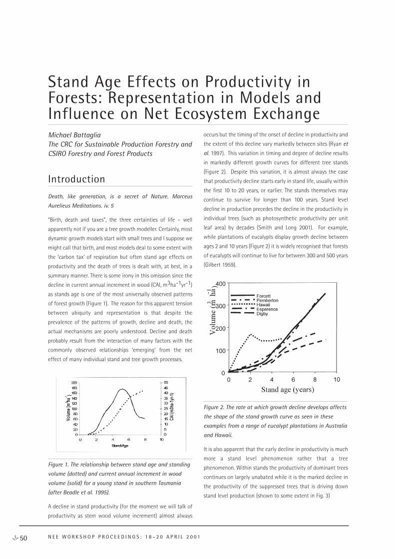
Michael BattagliaThe CRC for Sustainable Production Forestry and CSIRO Forestry and Forest Products
Introduction
Death, like generation, is a secret of Nature. Marceus
Aurelieus Meditations. iv. 5
“Birth, death and taxes”, the three certainties of life – well
apparently not if you are a tree growth modeller. Certainly, most
dynamic growth models start with small trees and I suppose we
might call that birth, and most models deal to some extent with
the ‘carbon tax’ of respiration but often stand age effects on
productivity and the death of trees is dealt with, at best, in a
summary manner. There is some irony in this omission since the
decline in current annual increment in wood (CAI, m3ha-1yr-1)
as stands age is one of the most universally observed patterns
of forest growth (Figure 1). The reason for this apparent tension
between ubiquity and representation is that despite the
prevalence of the patterns of growth, decline and death, the
actual mechanisms are poorly understood. Decline and death
probably result from the interaction of many factors with the
commonly observed relationships ‘emerging’ from the net
effect of many individual stand and tree growth processes.
Figure 1. The relationship between stand age and standing
volume (dotted) and current annual increment in wood
volume (solid) for a young stand in southern Tasmania
(after Beadle et al. 1995).
A decline in stand productivity (for the moment we will talk of
productivity as stem wood volume increment) almost always
occurs but the timing of the onset of decline in productivity and
the extent of this decline vary markedly between sites (Ryan et
al. 1997). This variation in timing and degree of decline results
in markedly different growth curves for different tree stands
(Figure 2). Despite this variation, it is almost always the case
that productivity decline starts early in stand life, usually within
the first 10 to 20 years, or earlier. The stands themselves may
continue to survive for longer than 100 years. Stand level
decline in production precedes the decline in the productivity in
individual trees (such as photosynthetic productivity per unit
leaf area) by decades (Smith and Long 2001). For example,
while plantations of eucalypts display growth decline between
ages 2 and 10 years (Figure 2) it is widely recognised that forests
of eucalypts will continue to live for between 300 and 500 years
(Gilbert 1959).
Figure 2. The rate at which growth decline develops affects
the shape of the stand growth curve as seen in these
examples from a range of eucalypt plantations in Australia
and Hawaii.
It is also apparent that the early decline in productivity is much
more a stand level phenomenon rather that a tree
phenomenon. Within stands the productivity of dominant trees
continues on largely unabated while it is the marked decline in
the productivity of the suppressed trees that is driving down
stand level production (shown to some extent in Fig. 3)
50 N E E W O R K S H O P P R O C E E D I N G S : 1 8 – 2 0 A P R I L 2 0 0 1
Stand Age Effects on Productivity inForests: Representation in Models andInfluence on Net Ecosystem Exchange
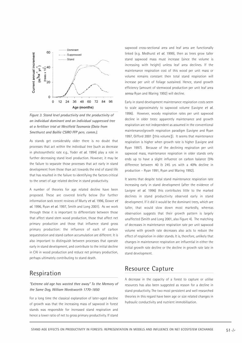
Figure 3. Stand level productivity and the productivity of
an individual dominant and an individual suppressed tree
at a fertiliser trial at Westfield Tasmania (Data from
Smethurst and Baillie CSIRO FFP pers. comm.).
As stands get considerably older there is no doubt that
processes that act within the individual tree (such as decrease
in photosynthetic rate e.g., Yoder et al. 1994) play a role in
further decreasing stand level production. However, it may be
the failure to separate those processes that act early in stand
development from those than act towards the end of stand life
that has resulted in the failure to identifying the factors critical
to the onset of age related decline in stand productivity.
A number of theories for age related decline have been
proposed. These are covered briefly below (for further
information seek recent reviews of Murty et al. 1996, Gower et
al. 1996, Ryan et al. 1997, Smith and Long 2001). As we work
through these it is important to differentiate between those
that affect stand stem wood production, those that affect net
primary production and those that influence stand gross
primary production: the influence of each of carbon
sequestration and stand carbon accumulation are different. It is
also important to distinguish between processes that operate
early in stand development, and contribute to the initial decline
in CAI in wood production and reduce net primary production,
perhaps ultimately contributing to stand death.
Respiration
“Extreme old age has wasted thee away” To the Memory of
the Same Dog, William Wordsworth 1770-1850
For a long time the classical explanation of later-aged decline
of growth was that the increasing mass of sapwood in forest
stands was responsible for increased stand respiration and
hence a lower ratio of net to gross primary productivity. If stand
sapwood cross-sectional area and leaf area are functionally
linked (e.g. Medhurst et al. 1999), then as trees grow taller
stand sapwood mass must increase (since the volume is
increasing with height) unless leaf area declines. If the
maintenance respiration cost of this wood per unit mass or
volume remains constant then total stand respiration will
increase per unit of foliage sustained. Hence, stand growth
efficiency (amount of stemwood production per unit leaf area
sensu Ryan and Waring 1992) will decline.
Early in stand development maintenance respiration costs seem
to scale approximately to sapwood volume (Lavigne et al.
1996). However, woody respiration rates per unit sapwood
decline in older trees: apparently maintenance and growth
respiration are not independent as assumed in the conventional
maintenance/growth respiration paradigm (Lavigne and Ryan
1997, Gifford 2001 {this volume}). It seems that maintenance
respiration is higher when growth rate is higher (Lavigne and
Ryan 1997). Because of the declining respiration per unit
sapwood mass, maintenance respiration in older stands only
ends up to have a slight influence on carbon balance (5%
difference between 40 & 245 yrs with a 40% decline in
production – Ryan 1991, Ryan and Waring 1992).
It seems that despite total stand maintenance respiration rate
increasing early in stand development (after the evidence of
Lavigne et al. 1996) this contributes little to the marked
declines in stand productivity observed early in stand
development. If it did it would be the dominant trees, which are
taller, that would slow down most markedly, whereas
observation suggests that their growth pattern is largely
unaffected (Smith and Long 2001, also Figure 4). The matching
of decreases in maintenance respiration rate per unit sapwood
volume with growth rate decreases also acts to reduce the
effect of respiration in older stands. It is, therefore, unlikely that
changes in maintenance respiration are influential in either the
initial growth rate decline or the decline in growth rate late in
stand development.
Resource Capture
A decrease in the capacity of a forest to capture or utilise
resources has also been suggested as reason for a decline in
stand productivity. The two most persistent and well researched
theories in this regard have been age or size related changes in
hydraulic conductivity and nutrient immobilisation.
51STAND AGE EFFECTS ON PRODUCTIVITY IN FORESTS: REPRESENTATION IN MODELS AND INFLUENCE ON NET ECOSYSTEM EXCHANGE
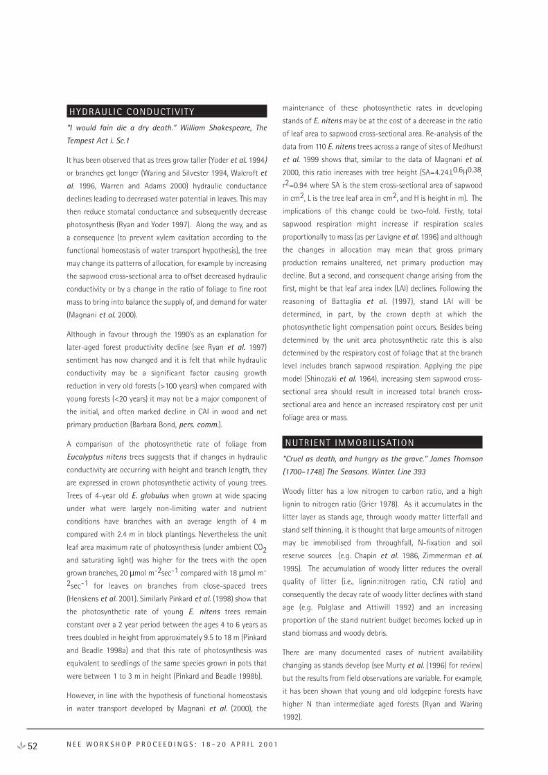
HYDRAULIC CONDUCTIVITY
“I would fain die a dry death.” William Shakespeare, The
Tempest Act i. Sc.1
It has been observed that as trees grow taller (Yoder et al. 1994)
or branches get longer (Waring and Silvester 1994, Walcroft et
al. 1996, Warren and Adams 2000) hydraulic conductance
declines leading to decreased water potential in leaves. This may
then reduce stomatal conductance and subsequently decrease
photosynthesis (Ryan and Yoder 1997). Along the way, and as
a consequence (to prevent xylem cavitation according to the
functional homeostasis of water transport hypothesis), the tree
may change its patterns of allocation, for example by increasing
the sapwood cross-sectional area to offset decreased hydraulic
conductivity or by a change in the ratio of foliage to fine root
mass to bring into balance the supply of, and demand for water
(Magnani et al. 2000).
Although in favour through the 1990’s as an explanation for
later-aged forest productivity decline (see Ryan et al. 1997)
sentiment has now changed and it is felt that while hydraulic
conductivity may be a significant factor causing growth
reduction in very old forests (>100 years) when compared with
young forests (<20 years) it may not be a major component of
the initial, and often marked decline in CAI in wood and net
primary production (Barbara Bond, pers. comm.).
A comparison of the photosynthetic rate of foliage from
Eucalyptus nitens trees suggests that if changes in hydraulic
conductivity are occurring with height and branch length, they
are expressed in crown photosynthetic activity of young trees.
Trees of 4-year old E. globulus when grown at wide spacing
under what were largely non-limiting water and nutrient
conditions have branches with an average length of 4 m
compared with 2.4 m in block plantings. Nevertheless the unit
leaf area maximum rate of photosynthesis (under ambient CO2and saturating light) was higher for the trees with the open
grown branches, 20 µmol m-2sec-1 compared with 18 µmol m-
2sec-1 for leaves on branches from close-spaced trees
(Henskens et al. 2001). Similarly Pinkard et al. (1998) show that
the photosynthetic rate of young E. nitens trees remain
constant over a 2 year period between the ages 4 to 6 years as
trees doubled in height from approximately 9.5 to 18 m (Pinkard
and Beadle 1998a) and that this rate of photosynthesis was
equivalent to seedlings of the same species grown in pots that
were between 1 to 3 m in height (Pinkard and Beadle 1998b).
However, in line with the hypothesis of functional homeostasis
in water transport developed by Magnani et al. (2000), the
maintenance of these photosynthetic rates in developing
stands of E. nitens may be at the cost of a decrease in the ratio
of leaf area to sapwood cross-sectional area. Re-analysis of the
data from 110 E. nitens trees across a range of sites of Medhurst
et al. 1999 shows that, similar to the data of Magnani et al.
2000, this ratio increases with tree height (SA=4.24.L0.6H0.38,
r2=0.94 where SA is the stem cross-sectional area of sapwood
in cm2, L is the tree leaf area in cm2, and H is height in m). The
implications of this change could be two-fold. Firstly, total
sapwood respiration might increase if respiration scales
proportionally to mass (as per Lavigne et al. 1996) and although
the changes in allocation may mean that gross primary
production remains unaltered, net primary production may
decline. But a second, and consequent change arising from the
first, might be that leaf area index (LAI) declines. Following the
reasoning of Battaglia et al. (1997), stand LAI will be
determined, in part, by the crown depth at which the
photosynthetic light compensation point occurs. Besides being
determined by the unit area photosynthetic rate this is also
determined by the respiratory cost of foliage that at the branch
level includes branch sapwood respiration. Applying the pipe
model (Shinozaki et al. 1964), increasing stem sapwood cross-
sectional area should result in increased total branch cross-
sectional area and hence an increased respiratory cost per unit
foliage area or mass.
NUTRIENT IMMOBILISATION
“Cruel as death, and hungry as the grave.” James Thomson
(1700–1748) The Seasons. Winter. Line 393
Woody litter has a low nitrogen to carbon ratio, and a high
lignin to nitrogen ratio (Grier 1978). As it accumulates in the
litter layer as stands age, through woody matter litterfall and
stand self thinning, it is thought that large amounts of nitrogen
may be immobilised from throughfall, N-fixation and soil
reserve sources (e.g. Chapin et al. 1986, Zimmerman et al.
1995). The accumulation of woody litter reduces the overall
quality of litter (i.e., lignin:nitrogen ratio, C:N ratio) and
consequently the decay rate of woody litter declines with stand
age (e.g. Polglase and Attiwill 1992) and an increasing
proportion of the stand nutrient budget becomes locked up in
stand biomass and woody debris.
There are many documented cases of nutrient availability
changing as stands develop (see Murty et al. (1996) for review)
but the results from field observations are variable. For example,
it has been shown that young and old lodgepine forests have
higher N than intermediate aged forests (Ryan and Waring
1992).
52 N E E W O R K S H O P P R O C E E D I N G S : 1 8 – 2 0 A P R I L 2 0 0 1
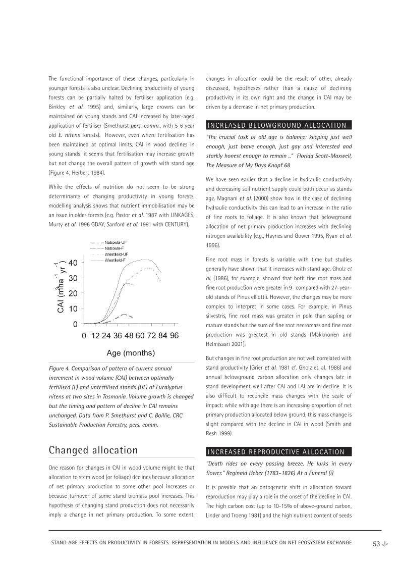
The functional importance of these changes, particularly in
younger forests is also unclear. Declining productivity of young
forests can be partially halted by fertiliser application (e.g.
Binkley et al. 1995) and, similarly, large crowns can be
maintained on young stands and CAI increased by later-aged
application of fertiliser (Smethurst pers. comm., with 5-6 year
old E. nitens forests). However, even where fertilisation has
been maintained at optimal limits, CAI in wood declines in
young stands; it seems that fertilisation may increase growth
but not change the overall pattern of growth with stand age
(Figure 4; Herbert 1984).
While the effects of nutrition do not seem to be strong
determinants of changing productivity in young forests,
modelling analysis shows that nutrient immobilisation may be
an issue in older forests (e.g. Pastor et al. 1987 with LINKAGES,
Murty et al. 1996 GDAY, Sanford et al. 1991 with CENTURY).
Figure 4. Comparison of pattern of current annual
increment in wood volume (CAI) between optimally
fertilised (F) and unfertilised stands (UF) of Eucalyptus
nitens at two sites in Tasmania. Volume growth is changed
but the timing and pattern of decline in CAI remains
unchanged. Data from P. Smethurst and C. Baillie, CRC
Sustainable Production Forestry, pers. comm.
Changed allocation
One reason for changes in CAI in wood volume might be that
allocation to stem wood (or foliage) declines because allocation
of net primary production to some other pool increases or
because turnover of some stand biomass pool increases. This
hypothesis of changing stand production does not necessarily
imply a change in net primary production. To some extent,
changes in allocation could be the result of other, already
discussed, hypotheses rather than a cause of declining
productivity in its own right and the change in CAI may be
driven by a decrease in net primary production.
INCREASED BELOWGROUND ALLOCATION
“The crucial task of old age is balance: keeping just well
enough, just brave enough, just gay and interested and
starkly honest enough to remain ..” Florida Scott-Maxwell,
The Measure of My Days Knopf 68
We have seen earlier that a decline in hydraulic conductivity
and decreasing soil nutrient supply could both occur as stands
age. Magnani et al. (2000) show how in the case of declining
hydraulic conductivity this can lead to an increase in the ratio
of fine roots to foliage. It is also known that belowground
allocation of net primary production increases with declining
nitrogen availability (e.g., Haynes and Gower 1995, Ryan et al.
1996).
Fine root mass in forests is variable with time but studies
generally have shown that it increases with stand age. Gholz et
al. (1986), for example, showed that both fine root mass and
fine root production were greater in 9- compared with 27-year-
old stands of Pinus elliottii. However, the changes may be more
complex to interpret in some cases. For example, in Pinus
silvestris, fine root mass was greater in pole than sapling or
mature stands but the sum of fine root necromass and fine root
production was greatest in old stands (Makknonen and
Helmisaari 2001).
But changes in fine root production are not well correlated with
stand productivity (Grier et al. 1981 cf. Gholz et. al. 1986) and
annual belowground carbon allocation only changes late in
stand development well after CAI and LAI are in decline. It is
also difficult to reconcile mass changes with the scale of
impact: while with age there is an increasing proportion of net
primary production allocated below ground, this mass change is
slight compared with the decline in CAI in wood (Smith and
Resh 1999).
INCREASED REPRODUCTIVE ALLOCATION
“Death rides on every passing breeze, He lurks in every
flower.” Reginald Heber (1783–1826) At a Funeral (i)
It is possible that an ontogenetic shift in allocation toward
reproduction may play a role in the onset of the decline in CAI.
The high carbon cost (up to 10-15% of above-ground carbon,
Linder and Troeng 1981) and the high nutrient content of seeds
53STAND AGE EFFECTS ON PRODUCTIVITY IN FORESTS: REPRESENTATION IN MODELS AND INFLUENCE ON NET ECOSYSTEM EXCHANGE
suggests that it may play a role in decline of growth (evidenced
by decreased wood increment in mast years Eis et al. 1965) and
perhaps in the decline in leaf area if nutrients are in low supply.
However, while allocation to reproduction increases with age,
reproductive output generally is sporadic while growth decline
is not suggesting that its role in the process may be slight (Ryan
et al 1997 after Eis et al. 1965).
OTHER ALLOCATION CHANGES
“My way of life is fallen into the sear, the yellow leaf”
William Shakespeare (1564–1616). The Tragedy of Macbeth.
Could it be that trees have some phenological driven aging
process, as is commonly evidenced in many annual or shorter-
lived plants? There is evidence of phenological aging in tree
meristematic tissues (e.g. grafting of old on to young tissue
leads to mature trait expression, Wiltshire et al. 1992) but
evidence on growth rate relationship is poor and some ‘clones’
of woody plants have been shown essentially to be eternal (e.g.
Potts and Reid 1995)
Individual tree hypothesis,stand structure and stand-levelresource use efficiency
“Death’s truer name is “Onward,”” Tennyson, Life of
Tennyson. Vol. i. 1
If the early aged decline in stand productivity cannot be
explained totally using leaf and tree level ecophysiological
processes, can it be explained using stand-level processes and
observing changes in stand structure with age?
Some recent work suggests that as stands age (in the first years
and coincident with the onset of a decline in CAI in wood) the
efficiency of growing wood per unit of resource used declines
as a result of the stand differentiating into dominant and
suppressed trees (Binkley et al. 2001). Total stand resource use
remains unchanged; that is suppressed trees continue to use
the same quantity of resources, they just do less with these
resources. As was observed in Figure 3 for the Tasmanian
plantation situation, Binkley et al. (2001) observed in their
study plantation that growth efficiency remains high for
dominant trees (0.54 kg [stemwood]/m2[leaf area]) but declines
for non-dominant trees (0.3. kg [stemwood]/m2[leaf area]). The
larger trees in a stand measured by Binkley et al. (2001)
produced 25% more wood per unit of light, water and nitrogen
than the remaining trees. These data find support from earlier
work by O’Hara (1988) who found that stem volume growth per
unit of sapwood area was higher for trees with more sapwood
area. Given that the relationship between sapwood area and
leaf area is usually linear or has an exponent greater than unity
(Medhurst et al. 1999) this suggests increased leaf area
productivity for dominant trees in the study of O’Hara (1988).
These results are perhaps counter-intuitive and until the
processes that underlie the changes in growth efficiency of
suppressed trees are identified then the question must be
considered unresolved. Theoretical studies of Scott et al. (1993)
and estimates of Kaufmann and Ryan (1986) suggest that one
would expect higher average crown leaf area productivity from
trees with relatively low leaf area (since then most leaves are
operating at close to optimal illumination) or among
suppressed trees. The continued maintenance of resource use by
suppressed trees while CAI is declining is itself problematic.
Does this reflect a change in the efficiency of gross primary
production or a change in the allocation pattern (into increased
turnover, other organs or increased respiration)? While some of
these changes sound like a recasting of the earlier hypotheses,
the mixed response between elements of the stand at a young
age may have masked their detection.
Along similar lines it has been hypothesised that as stands
mature, changes in crown structure mean that the unit area
carrying capacity of foliage increases because branches are
longer (Smith and Long 2001). As stands get older stem density
(stems ha-1) declines as a result of stand self-thinning.
Consequently, average branch length (and presumably coarse
root length) increases. It is likely under these conditions that
total stand branch sapwood mass will increase (or LAI and/or
light interception will fall). The result of this will be similar to
that in the discussion of changes in stem sapwood cross-
sectional area above.
Representation in models andimplications for net ecosystemexchange modelling
“These are the arcs, the trophies I erect, That fortify thy
name against old age; And these thy sacred virtues must
protect” Samuel Daniel (1562–1619), Beauty, Time, and Love
Sonnet
While the actual processes (or combination thereof) that
determine the decline of productivity in forest stands remain
unclear the studies carried out to date indicate a number of key
54 N E E W O R K S H O P P R O C E E D I N G S : 1 8 – 2 0 A P R I L 2 0 0 1
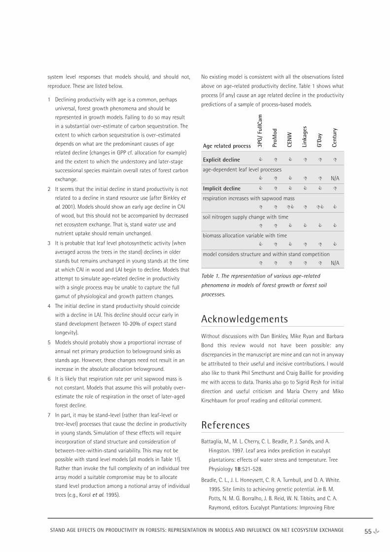
55STAND AGE EFFECTS ON PRODUCTIVITY IN FORESTS: REPRESENTATION IN MODELS AND INFLUENCE ON NET ECOSYSTEM EXCHANGE
3PG
/ Fu
llCam
ProM
od
CEN
W
Link
ages
G’D
ay
Cent
ury
system level responses that models should, and should not,
reproduce. These are listed below.
1 Declining productivity with age is a common, perhaps
universal, forest growth phenomena and should be
represented in growth models. Failing to do so may result
in a substantial over-estimate of carbon sequestration. The
extent to which carbon sequestration is over-estimated
depends on what are the predominant causes of age
related decline (changes in GPP cf. allocation for example)
and the extent to which the understorey and later-stage
successional species maintain overall rates of forest carbon
exchange.
2 It seems that the initial decline in stand productivity is not
related to a decline in stand resource use (after Binkley et
al. 2001). Models should show an early age decline in CAI
of wood, but this should not be accompanied by decreased
net ecosystem exchange. That is, stand water use and
nutrient uptake should remain unchanged.
3 It is probable that leaf level photosynthetic activity (when
averaged across the trees in the stand) declines in older
stands but remains unchanged in young stands at the time
at which CAI in wood and LAI begin to decline. Models that
attempt to simulate age-related decline in productivity
with a single process may be unable to capture the full
gamut of physiological and growth pattern changes.
4 The initial decline in stand productivity should coincide
with a decline in LAI. This decline should occur early in
stand development (between 10-20% of expect stand
longevity).
5 Models should probably show a proportional increase of
annual net primary production to belowground sinks as
stands age. However, these changes need not result in an
increase in the absolute allocation belowground.
6 It is likely that respiration rate per unit sapwood mass is
not constant. Models that assume this will probably over-
estimate the role of respiration in the onset of later-aged
forest decline.
7 In part, it may be stand-level (rather than leaf-level or
tree-level) processes that cause the decline in productivity
in young stands. Simulation of these effects will require
incorporation of stand structure and consideration of
between-tree-within-stand variability. This may not be
possible with stand level models (all models in Table 1!).
Rather than invoke the full complexity of an individual tree
array model a suitable compromise may be to allocate
stand level production among a notional array of individual
trees (e.g., Korol et al. 1995).
No existing model is consistent with all the observations listed
above on age-related productivity decline. Table 1 shows what
process (if any) cause an age related decline in the productivity
predictions of a sample of process-based models.
Age related process
Explicit decline � � � � � �
age-dependent leaf level processes
� � � � � N/A
Implicit decline � � � � � �
respiration increases with sapwood mass
� � �� � �� �
soil nitrogen supply change with time
� � � � � �
biomass allocation variable with time
� � � � � �
model considers structure and within stand competition
� � � � � N/A
Table 1. The representation of various age-related
phenomena in models of forest growth or forest soil
processes.
Acknowledgements
Without discussions with Dan Binkley, Mike Ryan and Barbara
Bond this review would not have been possible: any
discrepancies in the manuscript are mine and can not in anyway
be attributed to their useful and incisive contributions. I would
also like to thank Phil Smethurst and Craig Baillie for providing
me with access to data. Thanks also go to Sigrid Resh for initial
direction and useful criticism and Maria Cherry and Miko
Kirschbaum for proof reading and editorial comment.
ReferencesBattaglia, M., M. L. Cherry, C. L. Beadle, P. J. Sands, and A.
Hingston. 1997. Leaf area index prediction in eucalypt
plantations: effects of water stress and temperature. Tree
Physiology 18:521-528.
Beadle, C. L., J. L. Honeysett, C. R. A. Turnbull, and D. A. White.
1995. Site limits to achieving genetic potential. in B. M.
Potts, N. M. G. Borralho, J. B. Reid, W. N. Tibbits, and C. A.
Raymond, editors. Eucalypt Plantations: Improving Fibre

Yield and Quality Proc. CRCTHF - IUFRO Conf. CRC for
Temperate Hardwood Forestry: Hobart, Hobart, 19-24 Feb
1995.
Binkley, D., M. G. Ryan, J. L. Stape, and H. Barnard. 2001. Age-
related decline in forest ecosystem growth: an individual-
tree, stand-structure hypothesis. Ecosystems submitted.
Chapin, F. S. I., P. M. Vitousek, and K. Van Cleve. 1986. The
nature of nutrient limitation in plant communities.
American Naturalist 127:48-58.
Eis, S., J. Garman, and L. F. Ebell. 1965. Relation between cone
production and diameter increment of Douglas fir
(Psuedotsuga menziessii (Mirb.) Franco), grand fir (Abies
grandis (Dougl.) Lindl.) and Western white pine (Pinus
monticola (Dougl.)). Canadian Journal of Botany 43:1553-
1559.
Gholz, H. L., L. Hendry, and W. P. Cropper. 1986. Organic matter
production and distribution in fine roots in plantations of
slash pine. Canadian Journal of Forest Research 16:529-
538.
Gilbert, J. M. 1959. Forest succession in the Florentine Valley,
Tasmania. Proc. Roy. Soc. Tas. 93:129-151.
Gower, S. T., R. E. McMurtrie, and D. Murty. 1996. Above-
ground net primary production decline with stand age:
potential causes. Trends in Ecology and Evolution 11:378-
382.
Grier, G. C. 1978. A Tsuga heterophylia-Picea sitchensis
ecosystem of coastal Oregon: decomposition and nutrient
balances of fallen logs. Canadian Journal of Forest Research
8:198-206.
Grier, G. C., K. A. Vogt, M. R. Keyes, and R. L. Edmonds. 1981.
Biomass distribution and above-and belowground
production in young and mature Abies amabilis zone
ecosystems of the Washington Cascades. Canadian Journal
of Forest Research 11:155-167.
Haynes, B. E., and S. T. Gower. 1995. Belowground carbon
allocation in unfertilized and fertilized red pine plantations
in northern Wisconsin. Tree Physiology 15:317-325.
Henskens, F., M. Battaglia, M. Cherry, and C. L. Beadle. 2001.
Physiological basis of spacing effects on tree growth and
form in Eucalyptus globulus. Trees Structure and Function
(in press).
Herbert, M. A. 1984. Variation in the growth of and response
to fertilizing black wattle with nitrogen, phosphorus,
potassium and lime over three rotations. Pages 907-920 in
D. G. Grey, A. P. G. Schonau, C. J. Schutz, and A. van Laar,
editors. Symposium on Site and Productivity of Fast
Growing Plantations. South African Forest Research
Institute, Pretoria.
Kaufmann, M. R., and M. G. Ryan. 1986. Environmental,
physiographic, and stand effects on individual tree growth
in subalpine forests. Tree Physiology 2:47-59.
Korol, R.L., Running, S.W. and Milner, K.S. 1995. Incorporating
intertree competition into an ecosystem model. Canadian
Journal of Forest Research 25: 413-424.
Lavigne, M. B., and M. G. Ryan. 1997. Growth and maintenance
respiration rates of aspen, black spruce and jack pine stems
at northern and southern BOREAS sites. Tree Physiology
17:543-551.
Lavigne, M. B., S. E. Franklin, and J. Hunt, E.R. 1996. Estimating
stem maintenance respiration rates of dissimilar balsam fir
stands. Tree Physiology 16:687-695.
Linder, S., and E. Troeng. 1981. The seasonal course of
respiration and photosynthesis in strobili of Scots pine.
Forest Science 2:267-276.
Magnani, F., Mencuccini, and J. C. Grace. 2000. Age-related
decline in stand productivity: the role of structural
acclimation under hydraulic constraints. Plant, Cell and
Environment 23:251-263.
Makkonen, K., and H. Helmisarri. 2001. Fine root biomass and
production in Scots pine stands in relation to stand age.
Tree Physiology 21:193-198.
Medhurst, J. L., M. Battaglia, M. L. Cherry, M. A. Hunt, D. A.
White, and C. L. Beadle. 1999. Allometric relationships for
Eucalyptus nitens (Deame {is that ‘Deane’} and Maiden)
Maiden plantations. Trees, Structure and Function 14:91-
101.
Murty, D., R. E. McMurtrie, and M. G. Ryan. 1996. Declining
forest productivity in aging forest stands: a modeling
analysis of alternative hypotheses. Tree Physiology 16:187-
200.
O.Hara, K. L. 1988. Stand structure and growing space
efficiency following thinning in an even-age Douglas-fir
stand. Canadian Journal of Forest Research 18:859-866.
Pastor, J., R. H. Gardner, V. H. Dale, and W. M. Post. 1987.
Successional changes in nitrogen availability as a potential
factor contributing to spruce decline in boreal North
America. Canadian Journal of Forest Research 17:1394-
1400.
Pinkard, E. A., and C. L. Beadle. 1998a. Patterns of above-
ground carbon allocation of Eucalyptus nitens (Deane and
56 N E E W O R K S H O P P R O C E E D I N G S : 1 8 – 2 0 A P R I L 2 0 0 1
Maiden) Maiden following green pruning. Canadian Journal
of Forest Research 28:1419-1428.
Pinkard, E. A., and C. L. Beadle. 1998b. Regulation of
photosynthesis in Eucalyptus nitens (Deane and Maiden)
Maiden following green pruning. Trees 12:366-376.
Pinkard, E. A., C. L. Beadle, N. J. Davidson, and M. Battaglia.
1998. Photosynthetic responses of Eucalyptus nitens
(Deane and Maiden) Maiden to green pruning. Trees:
Structure and Function 12:119-129.
Polglase, P. J., and P. M. Attiwill. 1992. Nitrogen and
phosphorus cycling in relation to stand age of Eucalyptus
regnans F. Muell.: I. return from plant to soil. Plant Soil
142:156-166.
Potts, B. M., and J. B. Reid. 1985. Analysis of a hybrid swarm
between Eucalyptus risdonii Hook. f. and E. amygdalina
Labill. Aust. J. Bot. 33:543-562.
Ryan, M. 1991. A simple method for estimating gross carbon
budgets for vegetation in forest ecosystems. Tree
Physiology 9:255-266.
Ryan, M. G., and B. J. Yoder. 1997. Hydraulic limits to tree
height and tree growth. Bioscience 47:235-242.
Ryan, M. G., and R. H. Waring. 1992. Maintenance respiration
and stand development in a subalpine lodgepole pine
forest. Ecology 73:2100-2108.
Ryan, M. G., D. Binkley, and J. H. Fownes. 1997. Age-related
decline in forest productivity: pattern and process.
Advances in Ecological Research 27:214-262.
Ryan, M. G., R. M. Hubbard, S. Pongracic, R. J. Raison, and R. E.
McMurtrie. 1996. Foliage, fine-root, woody tissue and
stand respiration in Pinus radiata in relation to nitrogen
status. Tree Physiology 16:333-343.
Scott, R. D., J. N. Long, and F. W. Smith. 1993. Canopy
stratification and leaf area efficiency: a conceptualization.
Forest Ecology and Management 60:143-156.
Shinozaki, K., K. Yoda, K. Hozumi, and T. Kira. 1964. A
quantitative analysis of plant form - the pipe model theory.
I. Basic analyses. Jap. J. Ecol. 14:97-105.
Smith, F. W., and J. N. Long. 2001. Age-related decline in forest
growth: an emergent property. Forest Ecology and
Management 144:175-181.
Smith, F. W., and S. C. Resh. 1999. Age-related changes in
production and belowground carbon allocation in Pinus
contorta forests. Forest Science 45:333-341.
Walcroft, A. S., W. B. Silvester, J. C. Grace, S. D. Carson, and R.
H. Waring. 1996. Effects of branch length on carbon
isotope discrimination in Pinus. Tree Physiology 16:281-
286.
Waring, R. H., and W. B. Silvester. 1994. Variation in foliar 13C
values, within the crowns of Pinus trees. Tree Physiology
14:1203-1213.
Warren, C. R., and M. A. Adams. 2000. Water availability and
branch length determine δ13C in foliage of Pinus pinaster.
Tree Physiology 20:637-643.
Wiltshire, R. J. E., B. M. Potts, and J. B. Reid. 1992. A
paedomorphocline in Eucalyptus: II. Variation in Seedling
Morphology in the E. risdonii/tenuiramis complex. Aust. J.
Bot. 40:789-805.
Yoder, B. J., M. G. Ryan, R. H. Waring, A. W. Schoettle, and M.
R. Kaufmann. 1994. Evidence of reduced photosynthetic
rates in old trees. Forest Science 40:513-527.
Zimmerman, J. K., W. M. Pulliam, D. J. Lodge, V. Quinones-
Orfila, N. Fetcher, S. Guzman-Grajales, J. A. Parrotta, C. E.
Asbury, L. R. Walker, and R. B. Waide. 1995. Nitrogen
immobilization by decomposing woody debris and the
recovery of tropical wet forest from hurricane damage.
Oikos 72:314-322.
57STAND AGE EFFECTS ON PRODUCTIVITY IN FORESTS: REPRESENTATION IN MODELS AND INFLUENCE ON NET ECOSYSTEM EXCHANGE
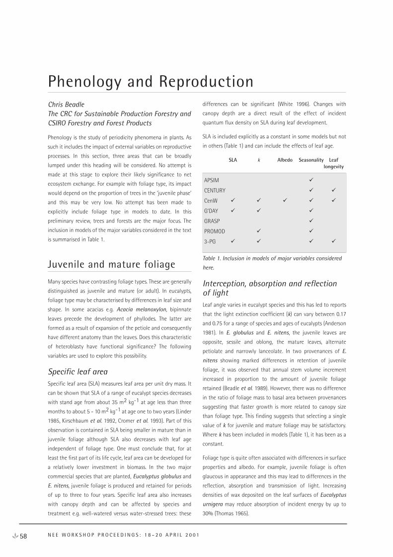
58 N E E W O R K S H O P P R O C E E D I N G S : 1 8 – 2 0 A P R I L 2 0 0 1
Chris BeadleThe CRC for Sustainable Production Forestry and CSIRO Forestry and Forest Products
Phenology is the study of periodicity phenomena in plants. As
such it includes the impact of external variables on reproductive
processes. In this section, three areas that can be broadly
lumped under this heading will be considered. No attempt is
made at this stage to explore their likely significance to net
ecosystem exchange. For example with foliage type, its impact
would depend on the proportion of trees in the ‘juvenile phase’
and this may be very low. No attempt has been made to
explicitly include foliage type in models to date. In this
preliminary review, trees and forests are the major focus. The
inclusion in models of the major variables considered in the text
is summarised in Table 1.
Juvenile and mature foliage
Many species have contrasting foliage types. These are generally
distinguished as juvenile and mature (or adult). In eucalypts,
foliage type may be characterised by differences in leaf size and
shape. In some acacias e.g. Acacia melanoxylon, bipinnate
leaves precede the development of phyllodes. The latter are
formed as a result of expansion of the petiole and consequently
have different anatomy than the leaves. Does this characteristic
of heteroblasty have functional significance? The following
variables are used to explore this possibility.
Specific leaf areaSpecific leaf area (SLA) measures leaf area per unit dry mass. It
can be shown that SLA of a range of eucalypt species decreases
with stand age from about 35 m2 kg-1 at age less than three
months to about 5 - 10 m2 kg-1 at age one to two years (Linder
1985, Kirschbaum et al. 1992, Cromer et al. 1993). Part of this
observation is contained in SLA being smaller in mature than in
juvenile foliage although SLA also decreases with leaf age
independent of foliage type. One must conclude that, for at
least the first part of its life cycle, leaf area can be developed for
a relatively lower investment in biomass. In the two major
commercial species that are planted, Eucalyptus globulus and
E. nitens, juvenile foliage is produced and retained for periods
of up to three to four years. Specific leaf area also increases
with canopy depth and can be affected by species and
treatment e.g. well-watered versus water-stressed trees: these
differences can be significant (White 1996). Changes with
canopy depth are a direct result of the effect of incident
quantum flux density on SLA during leaf development.
SLA is included explicitly as a constant in some models but not
in others (Table 1) and can include the effects of leaf age.
SLA k Albedo Seasonality Leaflongevity
APSIM �
CENTURY � �
CenW � � � � �
G’DAY � � �
GRASP �
PROMOD � �
3-PG � � � �
Table 1. Inclusion in models of major variables considered
here.
Interception, absorption and reflectionof light Leaf angle varies in eucalypt species and this has led to reports
that the light extinction coefficient (k) can vary between 0.17
and 0.75 for a range of species and ages of eucalypts (Anderson
1981). In E. globulus and E. nitens, the juvenile leaves are
opposite, sessile and oblong, the mature leaves, alternate
petiolate and narrowly lanceolate. In two provenances of E.
nitens showing marked differences in retention of juvenile
foliage, it was observed that annual stem volume increment
increased in proportion to the amount of juvenile foliage
retained (Beadle et al. 1989). However, there was no difference
in the ratio of foliage mass to basal area between provenances
suggesting that faster growth is more related to canopy size
than foliage type. This finding suggests that selecting a single
value of k for juvenile and mature foliage may be satisfactory.
Where k has been included in models (Table 1), it has been as a
constant.
Foliage type is quite often associated with differences in surface
properties and albedo. For example, juvenile foliage is often
glaucous in appearance and this may lead to differences in the
reflection, absorption and transmission of light. Increasing
densities of wax deposited on the leaf surfaces of Eucalyptus
urnigera may reduce absorption of incident energy by up to
30% (Thomas 1965).
Phenology and Reproduction
Interception lossRainfall interception, canopy storage of water and
interception loss are, amongst other variables, a function of
leaf shape, size, surface characteristics and orientation
(Jackson 1975). Foliage type may therefore impinge on
rainfall interception.
Resistance to stressThe impact of foliage type on resistance to stress is unclear. One
study suggests that glaucous water-repellent leaves, which are
characteristic of some juvenile foliage, are associated with
increased freezing tolerance (Thomas and Barber 1974).
Gas exchangeBrodribb (1992) demonstrated that, while photosynthetic rates
per unit leaf area were similar between leaves and phyllodes of
A. melanoxylon, leaves had greater rates of photosynthesis per
unit dry mass. Thus, leaves are more efficient than phyllodes at
producing photosynthate per unit of carbon invested in foliage
production. Similar conclusions are likely to pertain to gas
exchange of juvenile and mature foliage of eucalypts that have
distinctive differences in SLA.
Pest and disease riskThe glaucous coating of juvenile leaves may provide a physical
barrier to browsing by adult Paropsis charybdis beetles
(Edwards 1982) and, through its hydrophobicity, resistance to
the deposition and germination of spores of Phaeoeptoria
eucalypti (Heather 1967). These early studies raised an
awareness of the importance of foliage type in pest and disease
attack. However it is not always the juvenile foliage that is the
less susceptible. The female moths of Mnesampela privata,
currently the most prevalent pest problem of eucalypt
plantations in southern Australia, have a greater preference for
juvenile foliage for egg laying (Steinbauer and Floyd 2001). In
the same plantations Mycosphaerella, one of the most
significant of fungal pathogens causing defoliation, is also
prevalent on juvenile foliage (C. Mohammed, pers. comm.).
Pests and diseases are not modelled although some models (e.g.
3-PG), can cope with defoliation. GRASP describes animal
intake and live weight gain.
Persistence of juvenile foliage In many species, juvenile foliage is retained for short periods
only. However the Maidenaria section of the Symphyomyrtus
subgenus that includes E. globulus and E. nitens are
characterised by species that retain their juvenile foliage for
long periods (Noble 1989). Phase change may also be under
genetic control (Jordan et al. 1999) and this raises the
possibility that genotype may be of significance when dealing
with foliage type in models.
Leaf production/litterfall
Australian forests, including all significant planted forests, are
evergreen. However each is subject to periods of leaf expansion
and leaf shedding. Canopy size is therefore a dynamic property
of forests. Leaf area index (L*) is the key measure of canopy size
and the key variable in light interception models describing tree
and stand growth. The magnitude of any seasonal change in L*
will have implications for net ecosystem exchange and, for
example, any conclusions that are reached using remote
sensing techniques and NVDI.
Seasonality There are few time series studies that describe how L* changes
seasonally. In temperate climates in Australia, periods of leaf
development and expansion will, in the absence of water stress,
be largely a function of temperature. Seasonal patterns of
litterfall in temperate eucalypt forest are closely related to
maximum temperature (Turnbull et al. 1983). In tropical and
subtropical climates, rainfall patterns will probably be the major
determinant. Net increases in L* will occur during periods of leaf
expansion, net decreases during periods of litterfall. Seasonal
variation will be higher if periods of maximum leaf production
are out of phase with periods of maximum foliage loss. For
example, increases of foliage mass equivalent to net changes in
L* of between 1.1 and 3.0 between an end of winter minimum
and end of summer maximum were recorded in a range of
treatments in Pinus radiata (Raison et al. 1992).
Several models (CENTURY, CenW, G’DAY, GRASP, 3-PG) include
seasonality in the sense that pools and fluxes change with time
in response to changes in inputs that are driven by changing
environment e.g. temperature and light. The level of detail
included however varies from model to model and some
variables e.g. L* in PROMOD are averages for the annual cycle.
None of the models include seasonality in a strict phenological
sense.
Number of cohorts and leaf longevityLeaf longevity is the period that a leaf remains functional
between initiation and fall and to some extent is an inherent
property of a species. Thus slower growing species, like conifers,
tend to have longer leaf longevities than faster growing species,
59P H E N O L O G Y A N D R E P R O D U C T I O N
like eucalypts (Beadle 1997) but the activity of leaves is lower in
the former than the latter. Factors like light environment will
affect longevity. Thus leaves on isolated trees and in developing
stands will tend to have greater leaf longevity because they
remain above the light compensation point for longer periods
than leaves in closed forests.
Cohorts refer to the numbers of age classes of leaves that
contribute to the canopy. Not unexpectedly, the number of
cohorts tends to be greater the slower growing the species. The
activity of each cohort tends to decrease with age. More
cohorts mean greater variation in photosynthetic activity both
vertically and horizontally through the canopy.
Leaf longevity is modelled in some instances (CENTURY, CenW,
3-PG) but cohorts are not included.
Growth habitSome species have a continuous growth habit. This is driven by
a naked bud system that allows growth as long as critical values
of the factors that allow growth, available water and nutrients,
high and low temperature limits, have not been exceeded.
Eucalypts are the prime example of this habit and there may be
several periods of growth in any annual cycle. In contrast, P.
radiata produces a dormant bud and there is usually a period
when no growth occurs, though in Australia, there may be more
than one phase of growth in any annual cycle. Growth habit is
an inherent property of a species. In exotic environments, this
may determine where a species will grow.
Growth habit is modelled in the sense that growth will occur
when the conditions are suitable for carbon gain. Phenological
switches are not included in forest models though are in APSIM
and CENTURY so that grain/seed yield can be predicted.
Pests and diseases The impacts of pests and diseases on leaf area development are
complex. Leaf spot diseases like Mycosphaerella effectively
reduce the amount of leaf area for light interception (Lundquist
and Parnell 1987) and eventual leaf death increases litterfall.
Diseases, like Phytophthora cinnamomi, that affect the
conducting tissues and cause water stress (Dawson and Weste
1984), may reduce light-use efficiency and photosynthesis.
Defoliating insects reduce leaf area though this may be offset
by an increase in the photosynthetic capacity of the remaining
foliage as well as an increase in the rate of development and
increased photosynthetic capacity of new foliage, similar to
that observed following green pruning (Caldwell et al. 1981,
Senock et al. 1991, Pinkard et al. 1998).
The effects of pests and diseases are not modelled in any of the
forest models though grasses and crops can be grazed (e.g. in
GRASP).
Reproduction
Partitioning of carbon to reproductivestructuresEstimates of standing biomass and its partitioning rarely
include reproductive structures. In a study in Eucalyptus
teretecornis plantations, the partitioning of dry mass to
reproductive parts varied between 0.56 and 0.79% of total
biomass in five- to eight-year-old plantations (Bargali et al.
1991). These numbers are arguably low. In a study of a range of
species in the Brookhaven National Forest in New York,
partitioning of above-ground dry mass to fruits, peduncles and
flowers varied between 0.28 and 8.7% (Whittaker and
Woodwell 1968). Thus values can be significant. It is likely that
a proportion of reproductive effort will be affected by
environmental controls and environmental stress. Partitioning
to reproductive structures is modelled in CenW.
Impact on carbon storedSome reproductive structures, like pollen and seed production,
have a rapid turnover. Thus reproduction may be a drain on
carbon resources that is not measured. Its magnitude may be
significant, with maybe up to 5-10% of total carbon gain going
to reproduction and therefore not being stored. It is even more
important for nutrients because of their higher concentration
in reproductive compared to other tissues (M. Kirschbaum,
CSIRO Forestry and Forest Products, 2001, pers. comm.).
The following also need to be considered.
seasonality of reproductive effort
triggers for flowering (photoperiod, vernalisation)
degree days
succession (global change context)
Reproductive effort is particularly relevant to crop models
(Merv Probert, CSIRO Tropical Agriculture, 2001, pers. comm.)
where partitioning into the reproductive structures is the
measure of harvestable yield. The growth of agricultural crops is
also driven by heat units and modified by photoperiod,
vernalisation and environmental stress. Some of these issues are
considered by APSIM and CENTURY.
60 N E E W O R K S H O P P R O C E E D I N G S : 1 8 – 2 0 A P R I L 2 0 0 1
ReferencesAnderson, M.C. (1981). The geometry of leaf distribution in
some south-eastern Australian forests. Agric. Meteorol. 25,
195-205.
Bargali, S.S., Singh, S.P. and Singh, R.P. (1991). Structure and
function of an age series of eucalypt plantations in Central
Himalaya. I. Dry matter dynamics. Ann. Bot. 69, 405-411.
Beadle, C.L., McLeod, D.E., Turnbull, C.R.A., Ratkowsky, D.A. and
McLeod, R. (1989). Juvenile/total foliage ratios in
Eucalyptus nitens and the growth of stands and individual
trees. Trees 3, 117-124.
Beadle, C.L. (1997). Dynamics of leaf and canopy development.
In: Management of soil, water and nutrients in tropical
plantation forests (E.K.S. Nambiar and A.G. Brown, eds).
Australian Centre for International Agricultural Research.
pp 169-212.
Brodribb, T. (1992). A physiological comparison of leaves and
phyllodesin Acacia melanoxylon. Hons thesis, University of
Tasmania. 50 pp.
Caldwell, M.M., Richards, J.H., Johnson, D.A., Nowak, R.S. and
Dzuree, R.S. (1981). Coping with herbivory: photosynthetic
capacity and resource allocation in two semiarid
Agropyron bunch grasses. Oecologia 50, 14-24.
Cromer, R.N., Cameron, D.M., Rance, S. J, Ryan, P.J. and Brown,
M. (1993). Response to nutrients in Eucalyptus grandis. I.
Biomass accumulation. For. Ecol. Manage. 62, 211-230.
Dawson, P. and Weste, G. (1984). Impact of root infection by
Phytophthora cinnamomi on the water relations of two
Eucalyptus species that differ in susceptibility.
Phytopathology 74, 486-490.
Edwards, P.B. (1982). Do waxes on juvenile Eucalyptus leaves
provide protection from grazing insects? Aust. J. Ecol. 7,
347-352.
Heather, W.A. (1967). Leaf characteristics of Eucalyptus
bicostata Maiden et al. seedlings affecting the deposition
and germination of spores of Phaeoseptoria eucalypti
(Hansf.) Walker. Aust. J. Biol. Sci. 20, 1155-1160.
Jackson, I.J. (1975). Relationships between rainfall parameters
and interception by tropical forest. J. Hydrol. 24,215-238.
Jordan, G., Potts, B.M., and Wiltshire, R. (1999). Strong,
independent quantitative genetic control of vegetative
phase change and first flowering in Eucalyptus globulus
ssp. globulus. Heredity 83, 179-187.
Kirschbaum, M.U.F. , Bellingham, D.W. and Cromer, R.N. (1992).
Growth analysis of the effects of phosphorus nutrition in
Eucalyptus grandis seedlings. Aust. J. Plant Physiol. 19,
55-66.
Linder, S. (1985). Potential and actual production in Australian
forest stands. In: Research for forest management (J.J.
Landberg & W. Parsons, eds). CSIRO, Melbourne. pp 11-35.
Lundquist, J.E. and Parnell, R.C. (1987). Effects of
Mycosphaerella leaf spot on growth of Eucalyptus nitens.
S. Afr. For. J. 140, 51-59.
Noble, I.R. (1989). Ecological traits of the Eucalyptus L’Herit
subgenera Monocalyptus and Symphyomyrtus. Aust. J. Bot.
37, 207-224.
Pinkard, E.A., Beadle, C.L., Davidson, N.J. and Battaglia, M.
(1998). Photosynthetic responses of Eucalyptus nitens
(Deane and Maiden)Maiden to green pruning. Trees 12,
119-129.
Raison, R.J., Khanna, P.K., Benson, M.L., Myers, B.J., McMurtrie,
R.E. and Lang, A.R.G. (1992). Dynamics of Pinus radiata
foliage in relation to water and nitrogen stress: II Needle
loss and temporal changes in foliage mass. For. Ecol.
Manage. 52, 159-178.
Senock, R.S., Sisson, W.B. and Donart, G.B. (1991).
Compensatory photosynthesis of Sporobolus flexuosus
(Thurb.)Rydb. Following simulated herbivory in the
Chihuahuan desert. Bot. Gaz. 152, 275-281.
Steinbauer, M.J. and Floyd, R.B. (2001). Risk assessment for
Autumn Gum Moth. CRC Sustainable Production Forestry
Technical Report 55, 19-22.
Thomas, D.A. (1965). Physiological aspects in natural selection
in the cline of Eucalyptus urnigera. PhD Thesis, University
of Tasmania. 377 pp.
Thomas, D.A. and Barber, H.N. (1974). Studies on leaf
characteristics of a cline of Eucalyptus urnigera from
Mount Wellington, Tasmania. I. Water repellency and the
freezing of leaves. Aust. J. Bot. 22, 501-512.
Turnbull, C.R.A. and Madden, J.L. (1983). Realtionship of
litterfall to basal area and climatic variables in cool
temperate forests of southern Tasmania. Aust. J. Ecol. 8,
425-431.
White, D.A. (1996). Physiological responses to drought of
Eucalyptus globulus and Eucalyptus nitens plantations.
PhD Thesis, University of Tasmania. 166 pp.
Whittaker, R.H. and Woodwell, G.M. (1968). Dimension and
production relations of trees and shrubs in the Brookhaven
Forest, New York. J. Ecol. 56, 1-25.
61P H E N O L O G Y A N D R E P R O D U C T I O N
Derek EamusUniversity of Technology, Sydney
Abstract
Net primary productivity is determined by the rate of
photosynthesis and the rate of autotrophic respiration.
Photosynthetic carbon gain of a canopy is determined by leaf-
scale photosynthesis, by interception of light by a canopy, the
amount of canopy and the efficiency of utilisation of light
energy.
It is axiomatic that the water balance of an ecosystem
influences the NPP of an ecosystem, but what are the
mechanisms by which water balance influences NPP? The aims
of this paper are to look at some of these mechanisms, to
highlight some of those processes that do not feature
sufficiently prominently in some models of NPP and to assess
the extent to which Australian ecosystems are water limited.
Water balance of an ecosystem is determined by input, loss and
storage. Inputs include direct inputs to the ecosystem as
rainfall, mist, fog and snow melt. Few models account for the
last three. Indirect inputs include surface flow (flooding), river
flow and groundwater flow of water that arrived in other
ecosystems. Few models account for these processes. Outputs
include evapotranspiration, surface and lateral soil flows out of
the ecosystem and deep percolation to depths 2 m below the
maximum rooting depth of the vegetation. There is patchy
accommodation of all 3 processes in most models of NPP in
Australia. A significant relationship between rainfall and above-
ground biomass or NPP is observed for most of the Australian
continent.
Introduction
The purpose of this reviewThe first aim of this brief review is to address the question:
What mechanisms link ecosystem water balance to NPP?
A second aim is to highlight which of these processes are
infrequently incorporated into models through a comparison of
several models of productivity used in Australia. Finally, a brief
discussion of the relationship between rainfall and biomass or
NPP is given for Australia.
Net primary productivityNet primary productivity is an important quantitative
characteristic of an ecosystem (Churkina et al. 1999), and much
effort has been expended to determine NPP of different
ecosystems around the world (Kicklighter et al. 1999). Seasonal
changes in NPP, resulting from seasonal changes in net
ecosystem exchange, and the temporal displacement between
carbon gain through photosynthesis and carbon loss through
respiration, are principal causes of seasonal changes in
atmospheric CO2 (Keeling et al. 1996). NPP can be used in
estimating crop yield and forest production. Because
measurements of NPP of all ecosystems, at all times, are
impractical, terrestrial models are used to estimate NPP.
Ecosystem water balance – a prioriconsiderationsEcosystem water balance is here defined as the water status
(water potential) of vegetation, the water content of the depth
of soil that interacts with vegetation (and therefore inclusive of
groundwater and an associated capillary fringe) and the water
content of the atmosphere interacting with vegetation.
The water balance of an ecosystem is determined by the
difference in rates of input and loss of water. Storage of water
within the system acts as a buffer, which can moderate the
response of vegetation to changes in input and loss. Three
storage sites exist – soil, plant and atmosphere. Plant storage
capacity is small and quickly depleted in vegetation. Recharge
of plant water occurs daily and probably seasonally. However,
water stored in plants may influence daily patterns of
vegetation water use and should not be ignored. Rates of water
use, of course, correlate well with NPP; reduced rates of water
use resulting from reduced water availability, occur with
concomitant reductions in rates of photosynthesis.
Stored soil water content can be very large (or small),
depending on soil type, rooting depth, rainfall and the
availability of groundwater. The contribution of soil stores can
be very substantial, for example in north Australian savannas
62 N E E W O R K S H O P P R O C E E D I N G S : 1 8 – 2 0 A P R I L 2 0 0 1
How Does Ecosystem Water BalanceInfluence Net Primary Productivity? - A Discussion
(Cook et al. 1998). Changes in soil water content are a major
cause of changes in NPP. There is an increasing realisation that
changes in groundwater availability and groundwater quality
(especially salt content) are having an influence on NPP.
The water vapour pressure of the lower atmosphere is subject to
large daily and seasonal fluctuations, and can cause significant
changes in rates of photosynthesis and hence NPP through
stomatal responses.
Input of water to an individual ecosystem can be in the form of
rain, mist, fog and snow, directly into an ecosystem. In addition,
water input can be the result of lateral flow of soil water and
groundwater, floodwater, or river water, all of which may arrive
from an adjacent ecosystem. Few models accommodate these
latter sources, despite their importance in some systems. The
importance of river water and groundwater has been
established for Eucalyptus camaldulensis and other species in
numerous sites (Thorburn and Walker 1993; George et al. 1999).
The loss of water from an ecosystem is the result of several
processes. These include:
transpiration from vegetation;
evaporation from soil, surface water and wet canopies;
surface flow out of the ecosystem;
lateral flow through the soil to streams/rivers/lakes; and
percolation to depths 1-2 m below the rooting zone of
vegetation (where it is unavailable to vegetation and
therefore considered ‘out’ of the ecosystem) and
subsequent groundwater recharge.
Transpiration is the most frequently modelled process, despite
the importance of other loss processes.
Short-term change compared to long-term differences, in ecosystem waterbalanceNPP can be compared at one site, through time, and therefore
the issue is – how do changes in water balance within an
ecosystem influence NPP of that system? Alternatively, NPP of
ecosystems that differ in annual water balance can be
compared, and therefore the issue is – how do differences in
water balance of different ecosystem contribute to observed
differences in NPP? Most of what is written below can be
applied to both questions.
Linkages between ecosystemwater balance, ecosystemprocesses and NPP
ABOVE-GROUND PROCESSES
Stomatal conductanceStomatal aperture is the end-point resolution of a large number
of input variables. Of particular interest are the impacts of soil
water content, atmospheric water content and plant water
status on stomatal conductance (gs). Declining soil water
content results in a decline in aperture and hence gs. This
decline is rarely linear. Similarly, increases in leaf-to-air vapour
pressure difference cause non-linear declines in gs. These
responses are common knowledge, and we have an increasing
understanding of the cellular mechanisms underlying these
responses, based upon chemical (abscisic acid and xylem sap
pH) and hydraulic signals. However, infrequently acknowledged
are, first, the interaction of soil water and atmospheric water
content as a determinant of gs; second, the difference in
stomatal responses to these factors among different species
and different plant functional types (for example, different
phenological guilds or C3 versus C4 plants); and third, the
influence of leaf age and leaf developmental history on
stomatal responses.
Leaf water potential is a useful measure of plant water status
but it is a poor instantaneous predictor of gs during a day as
there is an inverse relationship between gs and leaf water
potential during a day such that as leaf water potential declines
in the morning, gs increases. However, maximum gs over a
period of many days does decline as leaf water potential
declines during the development of soil water deficit (Davies et
al. 1994).
Leaf turgor potential correlates well with gs but is not
incorporated in any models as field data are not available.
However, pre-dawn leaf water potential does correlate with gsand such data are more readily available (Prior et al. 1997).
Pre-dawn water potential is an intuitively useful parameter
since it integrates soil water availability over the root zone.
Plants regulate the difference in water potential (Ψw) between
root and leaf (Eamus and Prior 2001). As soil Ψw declines, leaf
Ψw declines to maintain a gradient of Ψw for water uptake
from soil to leaf. However, if plants regulate the difference to
remain within set-limits, gs must vary to regulate water loss,
thereby regulating leaf Ψw. Consequently a threshold leaf Ψw
63H O W D O E S E C O S Y S T E M W A T E R B A L A N C E I N F L U E N C E N E T P R I M A R Y P R O D U C T I V I T Y ? - A D I S C U S S I O N
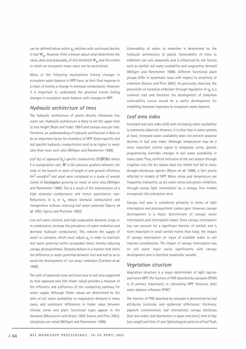
can be defined below which gs declines with continued decline
in leaf Ψw. However, little is known about what determines the
value, daily and seasonally, of this threshold Ψw and the extent
to which an ecosystem mean value can be ascertained.
Many of the following mechanisms linking changes in
ecosystem water balance to NPP have, as their final response in
a chain of events, a change in stomatal conductance. However,
it is important to understand the proximal events linking
changes in ecosystem water balance with changes in NPP.
Hydraulic architecture of treesThe hydraulic architecture of plants directly influences tree
water use. Hydraulic architecture is likely to set the upper limit
to tree height (Ryan and Yoder 1997) and canopy area per tree.
Therefore, an understanding of hydraulic architecture is likely to
be an important factor for modellers of NPP. Xylem specific and
leaf specific hydraulic conductivities tend to be higher in mesic
sites than more xeric sites (Willigen and Pammenter 1998).
Leaf (kl) or sapwood (ks) specific conductivity (E/(δP/δx) where
E is transpiration rate; δP is the pressure gradient between the
ends of the branch or stem of length x) and growth efficiency
(m3 wood/m2 leaf area) were correlated in a study of several
clones of Eucalyptus growing on mesic or xeric sites (Willigen
and Pammenter 1998). This is a result of the maintenance of a
high stomatal conductance and hence assimilation rate.
Reductions in kl or ks reduce stomatal conductance and
transpiration without reducing leaf water potential (Sperry et
al. 1993; Sperry and Pockman 1993).
Low soil water content, and high evaporative demand, singly or
in combination, increase the prevalence of xylem embolism and
decrease hydraulic conductance. This reduces the supply of
water to canopies, which must adjust gs in order to maintain
leaf water potential within acceptable limits, thereby reducing
canopy photosynthesis. Stomata behave in a manner that limits
the difference in water potential between root and leaf so as to
avoid the development of ‘run-away’ embolism (Cochard et al.
1996).
The ratio of sapwood cross-sectional area to leaf area supported
by that sapwood area (the Huber value) provides a measure of
the efficiency and sufficiency of the conducting pathway for
water supply. Although Huber values are determined by the
ratio of soil water availability to evaporative demand in many
cases, and systematic differences in Huber value between
climate zones and plant functional types appear in the
literature (Mencuccini and Grace, 1995; Eamus and Prior 2001),
exceptions are noted (Willigen and Pammenter 1998).
Vulnerability of xylem to embolism is determined by the
hydraulic architecture of plants. Vulnerability of trees to
embolism can vary seasonally and is influenced by site factors
such as rainfall, soil water availability and evaporative demand
(Willigen and Pammenter 1998). Different functional plant
groups differ in systematic ways with respect to sensitivity to
embolism (Eamus and Prior 2001). As previously observed, the
prevention of excessive embolism through regulation of gs is a
common trait and therefore the development of embolism
vulnerability curves would be a useful development for
modelling stomatal responses to ecosystem water balance.
Leaf area indexIncreased leaf area index (LAI) with increasing water availability
is commonly observed. However, it is clear that in some systems
at least, increased water availability does not prevent seasonal
declines in leaf area index. Although temperature may be a
more important control signal in temperate zones, genetic
programming overrides changes in soil water availability in
many cases. Thus, artificial extension of the wet season through
irrigation into the dry season does not inhibit leaf fall in many
drought-deciduous species (Myers et al. 1998), a fact poorly
reflected in models of NPP. Water stress and temperature are
frequently interactive, as are water stress and photo-inhibition,
through excess light interception by a canopy. Few models
incorporate this interactive term.
Canopy leaf area is considered primarily in terms of light
interception and photosynthetic carbon gain. However, canopy
development is a major determinant of canopy water
interception and interception losses. Since canopy interception
loss can account for a significant fraction of rainfall, and is
more important in small rainfall events than large, the impact
of canopy interception on input of available water to soil
requires consideration. The impact of canopy interception loss
on soil water input varies significantly with canopy
development and is therefore seasonally variable.
Vegetation structureVegetation structure is a major determinant of light capture
and hence NPP. The fraction of PAR absorbed by canopies (fPAR)
is of primary importance in calculating NPP. However, does
water balance influence fPAR?
The fraction of PAR absorbed by canopies is determined by leaf
attributes (cuticular and epidermal reflectance; thickness;
pigment concentration; leaf orientation); canopy attributes
(leaf area index; leaf distribution in space and time;) time of day
(sun angle) and time of year (phenological patterns of leaf flush
64 N E E W O R K S H O P P R O C E E D I N G S : 1 8 – 2 0 A P R I L 2 0 0 1
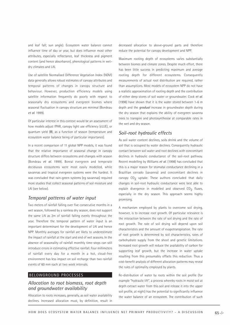
and leaf fall; sun angle). Ecosystem water balance cannot
influence time of day or year, but does influence most other
attributes, especially reflectance, leaf thickness and pigment
content (and hence absorbance), phenological patterns in wet-
dry climates and LAI.
Use of satellite Normalised Difference Vegetation Index (NDVI)
data generally allows robust estimates of canopy attributes and
temporal patterns of changes in canopy structure and
behaviour. However, production efficiency models using
satellite information frequently do poorly with respect to
seasonally dry ecosystems and evergreen biomes where
seasonal fluctuation in canopy structure are minimal (Bondeau
et al. 1999).
Of particular interest in this context would be an assessment of
how models adjust fPAR, canopy light use efficiency (cLUE), or
quantum yield (θ), as a function of season (temperature and
ecosystem water balance being of particular importance).
In a recent comparison of 11 global NPP models, it was found
that the relative importance of seasonal change in canopy
structure differs between ecosystems and changes with season
(Bondeau et al. 1999). Boreal evergreen and temperate
deciduous ecosystems were most easily modelled, while
savannas and tropical evergreen systems were the hardest. It
was concluded that rain-green systems (eg savannas) required
more studies that collect seasonal patterns of soil moisture and
LAI (see below).
Temporal patterns of water inputTwo meters of rainfall falling over five consecutive months in a
wet season, followed by a rainless dry season, does not support
the same LAI as 2m of rainfall falling evenly throughout the
year. Therefore the temporal pattern of water input is an
important determinant for the development of LAI and hence
NPP. Monthly averages for rainfall are likely to underestimate
the impact of rainfall at the start and end of wet seasons. In the
absence of seasonality of rainfall monthly time-steps can still
introduce errors in estimating effective rainfall. Four millimeters
of rainfall every day for a month in a hot, cloud-free
environment has less impact on soil recharge than two rainfall
events of 60 mm each at two week intervals.
BELOWGROUND PROCESSES
Allocation to root biomass, root depthand groundwater availabilityAllocation to roots increases, generally, as soil water availability
declines. Increased allocation must, by definition, result in
decreased allocation to above-ground parts and therefore
reduce the potential for canopy development and NPP.
Maximum rooting depth of ecosystems varies substantially
between biomes and climate zones. Despite much effort, there
has been little success in predicting maximum and average
rooting depth for different ecosystems. Consequently
measurements of actual root distribution are required, rather
than assumptions. Most models of ecosystem NPP do not have
a realistic approximation of rooting depth and the contribution
of either deep stores of soil water or groundwater. Cook et al.
(1998) have shown that it is the water stored between 1-6 m
depth and the gradual increase in groundwater depth during
the dry season that explains the ability of evergreen savanna
trees to transpire and photosynthesise at comparable rates in
the wet and dry season.
Soil-root hydraulic effectsAs soil water content declines, soils shrink and the volume of
soil that is occupied by water declines. Consequently hydraulic
contact between soil water and root declines with concomitant
declines in hydraulic conductance of the soil-root pathway.
Recent modelling by Williams et al. (1998) has concluded that
this is a major reason for stomatal conductance declining in a
Brazillian cerrado (savanna) and concomitant declines in
canopy CO2 uptake. These authors concluded that daily
changes in soil-root hydraulic conductance were best able to
explain divergence in modelled and observed CO2 fluxes,
especially in the dry season. This approach seems highly
promising.
A mechanism employed by plants to overcome soil drying,
however, is to increase root growth. Of particular relevance is
the interaction between the rate of soil drying and the rate of
root growth. The rate of soil drying will depend upon soil
characteristics and the amount of evapotranspiration. The rate
of root growth is determined by soil characteristics, rates of
carbohydrate supply from the shoot and genetic limitations.
Increased root growth will reduce the availability of carbon for
supporting leaf growth, but the increase in water uptake
resulting from this presumably offsets this reduction. Thus a
cost-benefit analysis of different allocation patterns may reveal
the rules of optimality employed by plants.
Re-distribution of water by roots within the soil profile (for
example “hydraulic lift”, a process whereby roots in moist soil at
depth extract water from this soil and release it into the upper
soil profile, at night) has the potential to significantly influence
the water balance of an ecosystem. The contribution of such
65H O W D O E S E C O S Y S T E M W A T E R B A L A N C E I N F L U E N C E N E T P R I M A R Y P R O D U C T I V I T Y ? - A D I S C U S S I O N
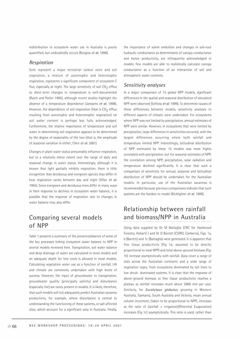
redistribution to ecosystem water use in Australia is poorly
quantified, but undoubtedly occurs (Burgess et al. 1998).
RespirationSoils represent a major terrestrial carbon store and soil
respiration, a mixture of autotrophic and heterotophic
respiration, represents a significant component of ecosystem C
flux, especially at night. The large sensitivity of soil CO2 efflux
to short-term changes in temperature is well-documented
(Raich and Potter 1995), although recent studies highlight the
absence of a temperature dependence (Janssens et al. 1998).
However, the dependence of soil respiration (that is CO2 efflux
resulting from autotrophic and heterotrophic respiration) on
soil water content is perhaps less fully acknowledged.
Furthermore, the relative importance of temperature and soil
water in determining soil respiration appears to be determined
by the degree of seasonality of the two (that is, the amplitude
of seasonal variation in either; Chen et al. 2001).
Changes in plant water status presumably influence respiration,
but to a relatively minor extent over the range of daily and
seasonal change in water status. Interestingly, although it is
known that light partially inhibits respiration, there is little
recognition that deciduous and evergreen species may differ in
how respiration varies between day and night (Villar et al.
1995). Since evergreen and deciduous trees differ in many ways
in their response to declines in ecosystem water balance, it is
possible that the response of respiration rate to changes in
water balance may also differ.
Comparing several models of NPP
Table 1 presents a summary of the presence/absence of some of
the key processes linking ecosystem water balance to NPP in
several models reviewed here. Transpiration, soil water balance
and deep drainage of water are calculated in most models and
an adequate depth for tree roots is allowed in most models.
Calculating vegetation water use as a function of rainfall, LAI
and climate are commonly undertaken with high levels of
success. However, the input of groundwater to transpiration,
groundwater quality (principally salinity) and disturbance
(especially fire) are rarely present in models. It is likely, therefore,
that such models will not adequately predict Australian savanna
productivity, for example, where disturbance is central to
understanding the functioning of these systems, or salt affected
sites, which account for a significant area in Australia. Finally,
the importance of xylem embolism and changes in soil-root
hydraulic conductance as determinants of canopy conductance
and hence productivity, are infrequently acknowledged in
models. Few models are able to realistically calculate canopy
conductance as a function of an interaction of soil and
atmospheric water contents.
Sensitivity analysesIn a major comparison of 15 global NPP models, significant
differences in the spatial and seasonal distribution of simulated
NPP were observed (Schloss et al. 1999). To determine causes of
these differences between models, sensitivity analyses to
different aspects of climate were undertaken. For ecosystems
where NPP was not limited by precipitation, annual estimates of
NPP were similar. However, in ecosystems that were limited by
precipitation, large differences in sensitivities occurred, with the
largest differences occurring where both rainfall and
temperature limited NPP. Interestingly, latitudinal distribution
of NPP estimated by these 15 models was most highly
correlated with precipitation, but for seasonal estimates of NPP,
the correlation among NPP, precipitation, solar radiation and
temperature declined significantly. It is clear that such a
comparison of sensitivity for annual, seasonal and latitudinal
distribution of NPP should be undertaken for the Australian
models. In particular, use of the Australian savannas is
recommended because previous comparisons indicate that such
systems are the hardest to model (Kicklighter et al. 1999).
Relationship between rainfalland biomass/NPP in Australia
Using data supplied by Dr M Battaglia (CRC for Hardwood
Forestry, Hobart) ) and Dr D Barrett (CSIRO, Canberra), Figs. 1a,
b (Barrett) and 1c (Battaglia) were generated. It is apparent that
fine tissue productivity (Fig 1a; assumed to be directly
proportional to total NPP) and total above-ground biomass (Fig.
1b) increase asymptotically with rainfall. Data cover a range of
sites across the Australian continent and a wide range of
vegetation types, from ecosystems dominated by tall trees to
low shrub- dominated systems. It is clear that the response of
above-ground biomass or fine tissue productivity reaches a
plateau as rainfall increases much above 2000 mm per year.
Similarly, for Eucalytpus globulus, growing in Western
Australia, Tasmania, South Australia and Victoria, mean annual
volume increment, (taken to be proportional to NPP), increases
as the ratio of (rainfall + irrigation)/(Potential Evaporation)
increases (Fig 1c) asymptotically. This ratio is used, rather than
66 N E E W O R K S H O P P R O C E E D I N G S : 1 8 – 2 0 A P R I L 2 0 0 1
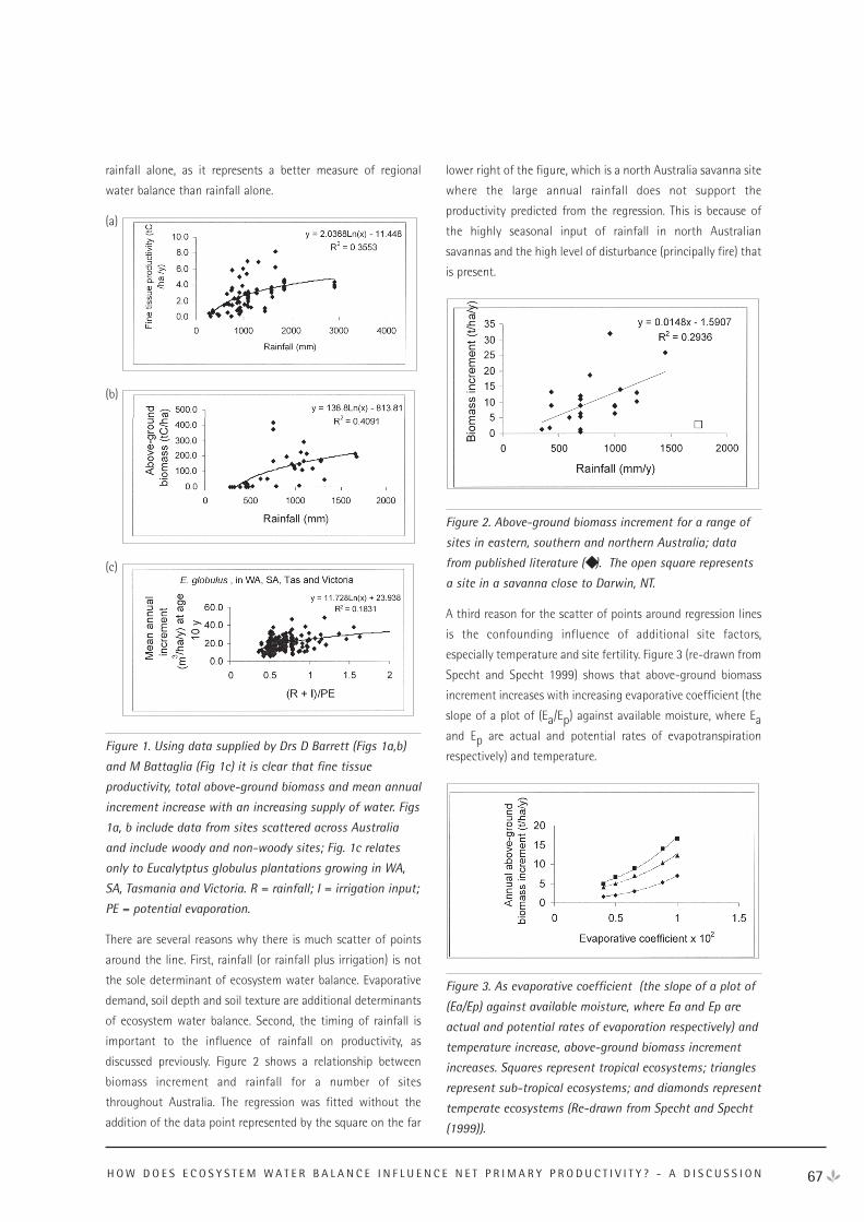
rainfall alone, as it represents a better measure of regional
water balance than rainfall alone.
(a)
(b)
(c)
Figure 1. Using data supplied by Drs D Barrett (Figs 1a,b)
and M Battaglia (Fig 1c) it is clear that fine tissue
productivity, total above-ground biomass and mean annual
increment increase with an increasing supply of water. Figs
1a, b include data from sites scattered across Australia
and include woody and non-woody sites; Fig. 1c relates
only to Eucalytptus globulus plantations growing in WA,
SA, Tasmania and Victoria. R = rainfall; I = irrigation input;
PE = potential evaporation.
There are several reasons why there is much scatter of points
around the line. First, rainfall (or rainfall plus irrigation) is not
the sole determinant of ecosystem water balance. Evaporative
demand, soil depth and soil texture are additional determinants
of ecosystem water balance. Second, the timing of rainfall is
important to the influence of rainfall on productivity, as
discussed previously. Figure 2 shows a relationship between
biomass increment and rainfall for a number of sites
throughout Australia. The regression was fitted without the
addition of the data point represented by the square on the far
lower right of the figure, which is a north Australia savanna site
where the large annual rainfall does not support the
productivity predicted from the regression. This is because of
the highly seasonal input of rainfall in north Australian
savannas and the high level of disturbance (principally fire) that
is present.
Figure 2. Above-ground biomass increment for a range of
sites in eastern, southern and northern Australia; data
from published literature (◆ ). The open square represents
a site in a savanna close to Darwin, NT.
A third reason for the scatter of points around regression lines
is the confounding influence of additional site factors,
especially temperature and site fertility. Figure 3 (re-drawn from
Specht and Specht 1999) shows that above-ground biomass
increment increases with increasing evaporative coefficient (the
slope of a plot of (Ea/Ep) against available moisture, where Eaand Ep are actual and potential rates of evapotranspiration
respectively) and temperature.
Figure 3. As evaporative coefficient (the slope of a plot of
(Ea/Ep) against available moisture, where Ea and Ep are
actual and potential rates of evaporation respectively) and
temperature increase, above-ground biomass increment
increases. Squares represent tropical ecosystems; triangles
represent sub-tropical ecosystems; and diamonds represent
temperate ecosystems (Re-drawn from Specht and Specht
(1999)).
67H O W D O E S E C O S Y S T E M W A T E R B A L A N C E I N F L U E N C E N E T P R I M A R Y P R O D U C T I V I T Y ? - A D I S C U S S I O N
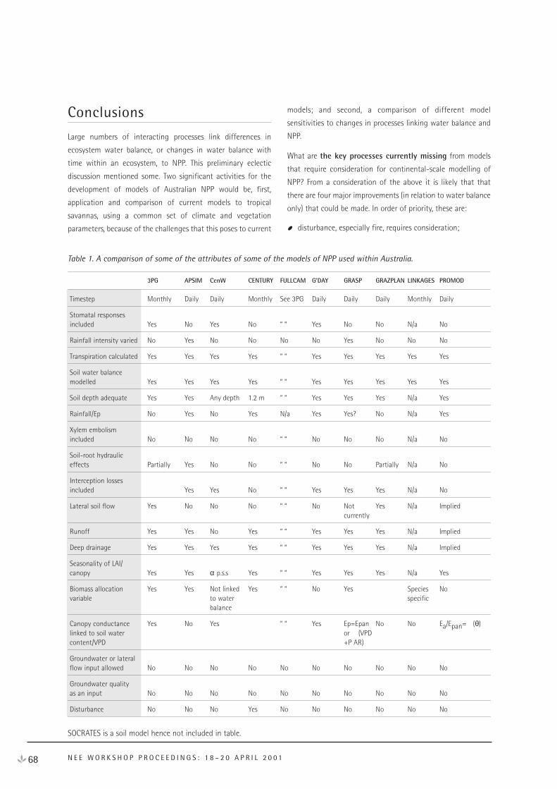
Conclusions
Large numbers of interacting processes link differences in
ecosystem water balance, or changes in water balance with
time within an ecosystem, to NPP. This preliminary eclectic
discussion mentioned some. Two significant activities for the
development of models of Australian NPP would be, first,
application and comparison of current models to tropical
savannas, using a common set of climate and vegetation
parameters, because of the challenges that this poses to current
models; and second, a comparison of different model
sensitivities to changes in processes linking water balance and
NPP.
What are the key processes currently missing from models
that require consideration for continental-scale modelling of
NPP? From a consideration of the above it is likely that that
there are four major improvements (in relation to water balance
only) that could be made. In order of priority, these are:
disturbance, especially fire, requires consideration;
68 N E E W O R K S H O P P R O C E E D I N G S : 1 8 – 2 0 A P R I L 2 0 0 1
Table 1. A comparison of some of the attributes of some of the models of NPP used within Australia.
3PG APSIM CenW CENTURY FULLCAM G’DAY GRASP GRAZPLAN LINKAGES PROMOD
Timestep Monthly Daily Daily Monthly See 3PG Daily Daily Daily Monthly Daily
Stomatal responses included Yes No Yes No “ “ Yes No No N/a No
Rainfall intensity varied No Yes No No No No Yes No No No
Transpiration calculated Yes Yes Yes Yes “ “ Yes Yes Yes Yes Yes
Soil water balance modelled Yes Yes Yes Yes “ “ Yes Yes Yes Yes Yes
Soil depth adequate Yes Yes Any depth 1.2 m “ “ Yes Yes Yes N/a Yes
Rainfall/Ep No Yes No Yes N/a Yes Yes? No N/a Yes
Xylem embolism included No No No No “ “ No No No N/a No
Soil-root hydraulic effects Partially Yes No No “ “ No No Partially N/a No
Interception losses included Yes Yes No “ “ Yes Yes Yes N/a No
Lateral soil flow Yes No No No “ “ No Not Yes N/a Impliedcurrently
Runoff Yes Yes No Yes “ “ Yes Yes Yes N/a Implied
Deep drainage Yes Yes Yes Yes “ “ Yes Yes Yes N/a Implied
Seasonality of LAI/canopy Yes Yes α p.s.s Yes “ “ Yes Yes Yes N/a Yes
Biomass allocation Yes Yes Not linked Yes “ “ No Yes Species Novariable to water specific
balance
Canopy conductance Yes No Yes “ “ Yes Ep=Epan No No Ea/Epan= � (θ)linked to soil water or � (VPDcontent/VPD +P AR)
Groundwater or lateral flow input allowed No No No No No No No No No No
Groundwater quality as an input No No No No No No No No No No
Disturbance No No No Yes No No No No No No
SOCRATES is a soil model hence not included in table.
empirical data are required for Australian ecosystems on
the relationships among biomass allocation, site aridity (for
example monthly rainfall/potential evaporation) and site
fertility so that these can be incorporated into models;
ecosystem-scale canopy conductance response
characteristics relative to monthly aridity index;
finally, allowance for a contribution to transpired water
other than rainfall (groundwater and associated capillary
fringe; and lateral flow).
ReferencesBondeau, A., Kicklighter, D.W. and Kaduk, J. 1999. Comparing
global models of terrestrial net primary productivity:
importance of vegetation structure on seasonal NPP
estimates. Global Change Biology 5 (suppl) 35-45.
Burgess, S.S.O., Adams, M.A., Turner, N.C., and Ong, C.K. 1998.
The redistribution of soil water by tree root systems.
Oecologia 115, 306-311.
Chen, X., Eamus, D., and Hutley, L.B., 2001. Seasonal patterns of
soil carbon dioxide efflux from a wet-dry tropical savanna
of northern Australia. Submitted, Australian Journal of
Botany.
Churkina, G., Running, S.W. and Schloss, A.L.1999. Comparing
global models of terrestrial net primary productivity: the
importance of water availability. Global Change Biology 5
(suppl) 46-55.
Cochard, H., Breda, N. and Granier, A. 1996. Whole tree
hydraulic conductance and water loss regulation in
Quercus during drought—evidence for stomatal control of
embolism. Annales des Sciences Forestieres 53, 197-206.
Cook, P.G., Hatton, T.H., Pidsley, D., Herczeg, A.L., O’Grady, A.
and Eamus, D. 1998. Water balance of a tropical woodland
ecosystem, northern Australia: a combination of micro-
meteorological, soil physical and groundwater chemical
approaches. Journal of Hydrology 210, 161-177.
Davies, W.J., Mansfield, T.A. and Hetherington, A.M. 1994. How
do chemical signals work in plants that grow in drying soil?
Plant Physiology 104, 309-314.
Eamus, D. and Prior, L. 2001. Ecophysiology of trees of
seasonally dry tropics, with particular reference to
phenological comparisons. Advances in Ecological Research
32, 113-197.
George, R.J., Nulsen, R.A., Ferdowsian, R., and Raper, G.P. 1999.
Interactions between trees and groundwaters in recharge
and discharge areas – A survey of Western Australian sites.
Agricultural Water Management 39, 91-113.
Keeling, C.D., Chin, J.F.S. and Whorf, T.P. 1996. Increased
activity of northern vegetation inferred from atmospheric
CO2 measurements. Nature 382, 146-149.
Kicklighter, D.W., Bondeau, A., Schloss, A.L., Kaduk, J. and
McGuire, A.D. 1999. Comparing global models of terrestrial
NPP: global patterns and differentiation by major biomes.
Global Change Biology 5 (Suppl), 16-24.
Mencuccini, M. and Grace, J. 1995. Climate influences the leaf-
area/sapwood area ratio in Scots pine. Tree Physiology 15,
1-10.
Myers, B.A., Williams, R.J., Fordyce, I., Duff, G.A. and Eamus, D.
1998. Does irrigation affect leaf phenology in deciduous
and evergreen trees of the savanna of northern Australia?
Australian Journal of Ecology 23, 329-339.
Prior, L.D., Eamus, D. and Duff, G.A. 1997. Seasonal and diurnal
patterns of carbon assimilation, stomatal conductance and
leaf water potential in E. tetrodonta saplings in a wet-dry
savanna in northern Australia. Australian Journal of Botany
45, 241-258.
Raich, J.W. and Potter, C.S. 1995. Global patterns of CO2emission from soils. Global Biogeochemical Cycles 9, 23-36.
Ryan, M.G. and Yoder, B.J. 1997. Hydraulic limits to tree height
and tree growth. BioScience 47, 235-242.
Schloss, A.L., Kicklighter, D.W., Kaduk, J. and Wittenberg,
U.1999. Comparing global models of terrestrial NPP:
comparison of NPP to climate and NDVI. Global Change
Biology 5 (Suppl.) 25 –34.
Specht, R.L., and Specht A. 1999. Australian plant
communities: Dynamics of structure, growth and
biodiversity. Oxford University Press.
Sperry, J.S., Alder, N.N. and Eastlack, S.E., 1993. The effect of
reduced hydraulic conductance on stomatal conductance
and xylem cavitation. Journal of Experimental Botany 44,
1075-1082.
Sperry, J.S. and Pockman, W.T. 1993. Limitation of transpiration
by hydraulic conductance and xylem cavitation in Betula
occidentalis. Plant, Cell and Environment 11, 35-40.
Thorburn, P.J. and Walker, G.R. 1993. The source of water
transpired by E. camaldulensis: Soil, groundwater or
streams. In ‘Stable isotopes and plant carbon/water
relations’. J R Ehleringer, A E Hall and G D Farquhar (Eds).
San Diego Academic Press. Pp 511-527.
69H O W D O E S E C O S Y S T E M W A T E R B A L A N C E I N F L U E N C E N E T P R I M A R Y P R O D U C T I V I T Y ? - A D I S C U S S I O N

70 N E E W O R K S H O P P R O C E E D I N G S : 1 8 – 2 0 A P R I L 2 0 0 1
Villar, R., Held, A. and Merino, J. 1995. Dark leaf respiration in
light and darkness of an evergreen and deciduous plant
species. Plant Physiology 107, 421-427.
Williams, M., Malhi, Y., Nobre, A.D., Rastetter, E.B., Grace, J. and
Pereira, M.G. 1998. Seasonal variation in net carbon
exchange and evapotranspiration in a Brazilian rain forest:
a modelling analysis. Plant, Cell and Environment 21, 953-
968.
Willigen, C.V. and Pammenter, N.W. 1998. Relationship
between growth and xylem hydraulic characteristics of
clones of Eucalyptus at contrasting sites. Tree Physiology
18, 595-600.
71
Robert EdisThe University of Melbourne
Introduction
The modelling of net ecosystem exchange of C requires the
incorporation of all factors that influence the sequestering of C
as biomass (primary production) or the release of C as CO2
through respiration by plants or soil micro-organisms. Which
factors are included, and how they are included will depend
upon their importance to the objectives of the exercise. Implicit
treatment of some important factors may be adequate, whilst
explicit incorporation in modelling may be required for others.
In this paper, consideration is given to select soil constraints
that may warrant explicit inclusion in modelling continental
(Australia) net ecosystem exchange. Various aspects of net
primary production are dealt with elsewhere in these
proceeding, in particular water and nutrients. In this paper the
soil constraints considered are salinity, waterlogging,
impedance (excessive soil strength), and soil acidity. These
constraints need to be considered in terms of their impacts
upon biomass production and turnover of organic matter;
distribution of significant effects across the continent; if and
how to model, and; what measurements are possibly required.
The Issues
SalinityHigh concentrations of salt in soil decrease plant performance
through increased osmotic potential which decreases the free
energy of soil water, and through phytotoxic effects of the
component ions. The sensitivity of plants to salts (in Australia,
principally NaCl) varies markedly between species, varieties and
individuals. In general there is a level of salinity, as indicated by
the electrical conductivity (saturated extract) (ECse), below
which there is little or no effect and above which there is a near
linear decrease in productivity with increasing ECse (Peverill et
al. 1999). In Australia, salinisation of the rootzone is generally
the result of rising watertables of saline groundwaters. As a
result, salinisation is often coincident with waterlogging of part
of the rootzone. Tree species vary greatly in their tolerance to
salinity and waterlogging (Lambert and Turner, 2000). At very
high levels of salinity the productivity of the land is
insignificant, and biomass accumulation of even the most
tolerant species in negligible.
About 2 Mha of Australia is estimated to be affected by human-
induced salinity to some extent, but estimates vary between 0.8
(Schofield, 1992) and 3.8 Mha (Poulter and Chaffer, 1991).
Much of it occurring in SW Western Australia and within the
wheat belt of South Australia, Victoria, New South Wales and
Queensland. Approximately 5.7 Mha are within regions mapped
to be at risk or affected by dryland salinity. It has been
estimated that in 50 years’ time the area of regions with a high
risk may increase to 17 Mha (three times as much as now)
(National Land and Water Audit 2000). Only about 0.5 Mha are
thought to be extremely effected (Lambert and Turner, 2000),
and given the greater ease at which extreme impact can be
identified, this estimate of area is likely to be reliable.
Given that salinisation in Australia is mostly driven by sometimes
complex hydrology at catchment or landscape scales, modelling
the build-up of salts in the rootzone in response to plant water
use is unlikely to be useful at the continental scale. Also, given
the variability of susceptibility of plants to salinity, low-level
salinity effects are likely to be countered by selection of more
tolerant varieties, making modelling of subtle impacts on NEE
impractical. Where high salt concentrations exist in soil that
inhibit root growth, the effect maybe accommodated by
restricting effective rooting depth or through the use of root
hospitality factors (Probert and Keating, 2000). This approach
requires site property factors, which are yet to be devised but
could be incorporated into plant production models. This
effectively treats salinisation as a static site factor modifying
process rates, rather than as a dynamic process. Possibly such
factors could be developed for areas where salinity is a major
issue, such as SW Western Australia, but this is probably not
warranted Australia wide, except for the purposes of scenario
testing. Whilst models such as APSIM (Probert and Keating,
2000) have the capacity to model salt build-up in response to
plant water use, this level of complexity is probably not
warranted given that salinisation is largely driven by regional
hydrologic processes. Possibly the most parsimonious way to
deal with salinity effects on NEE would be through estimated
areas of extreme salinisation taken out of production for
O T H E R S O I L C O N S T R A I N T S O N N E T P R I M A R Y P R O D U C T I O N
Other Soil Constraints on Net Primary Production
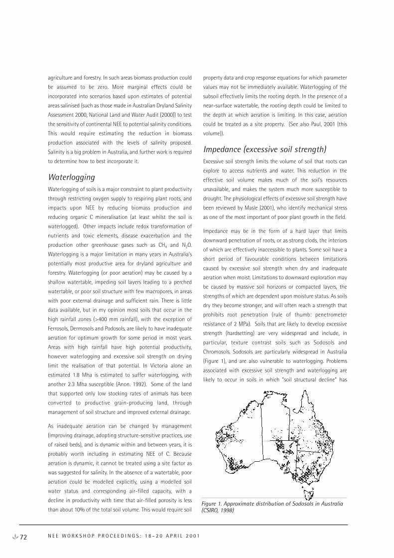
agriculture and forestry. In such areas biomass production could
be assumed to be zero. More marginal effects could be
incorporated into scenarios based upon estimates of potential
areas salinised (such as those made in Australian Dryland Salinity
Assessment 2000, National Land and Water Audit (2000)) to test
the sensitivity of continental NEE to potential salinity conditions.
This would require estimating the reduction in biomass
production associated with the levels of salinity proposed.
Salinity is a big problem in Australia, and further work is required
to determine how to best incorporate it.
WaterloggingWaterlogging of soils is a major constraint to plant productivity
through restricting oxygen supply to respiring plant roots, and
impacts upon NEE by reducing biomass production and
reducing organic C mineralisation (at least whilst the soil is
waterlogged). Other impacts include redox transformation of
nutrients and toxic elements, disease exacerbation and the
production other greenhouse gases such as CH4 and N2O.
Waterlogging is a major limitation in many years in Australia’s
potentially most productive area for dryland agriculture and
forestry. Waterlogging (or poor aeration) may be caused by a
shallow watertable, impeding soil layers leading to a perched
watertable, or poor soil structure with few macropores, in areas
with poor external drainage and sufficient rain. There is little
data available, but in my opinion most soils that occur in the
high rainfall zones (>400 mm rainfall), with the exception of
Ferrosols, Dermosols and Podosols, are likely to have inadequate
aeration for optimum growth for some period in most years.
Areas with high rainfall have high potential productivity,
however waterlogging and excessive soil strength on drying
limit the realisation of that potential. In Victoria alone an
estimated 1.8 Mha is estimated to suffer waterlogging, with
another 2.3 Mha susceptible (Anon. 1992). Some of the land
that supported only low stocking rates of animals has been
converted to productive grain-producing land, through
management of soil structure and improved external drainage.
As inadequate aeration can be changed by management
(improving drainage, adopting structure-sensitive practices, use
of raised beds), and is dynamic within and between years, it is
probably worth including in estimating NEE of C. Because
aeration is dynamic, it cannot be treated using a site factor as
was suggested for salinity. In the absence of a watertable, poor
aeration could be modelled explicitly, using a modelled soil
water status and corresponding air-filled capacity, with a
decline in productivity with time that air-filled porosity is less
than about 10% of the total soil volume. This would require soil
property data and crop response equations for which parameter
values may not be immediately available. Waterlogging of the
subsoil effectively limits the rooting depth. In the presence of a
near-surface watertable, the rooting depth could be limited to
the depth at which aeration is limiting. In this case, aeration
could be treated as a site property. (See also Paul, 2001 (this
volume)).
Impedance (excessive soil strength)Excessive soil strength limits the volume of soil that roots can
explore to access nutrients and water. This reduction in the
effective soil volume makes much of the soil’s resources
unavailable, and makes the system much more susceptible to
drought. The physiological effects of excessive soil strength have
been reviewed by Masle (2001), who identify mechanical stress
as one of the most important of poor plant growth in the field.
Impedance may be in the form of a hard layer that limits
downward penetration of roots, or as strong clods, the interiors
of which are effectively inaccessible to plants. Some soil have a
short period of favourable conditions between limitations
caused by excessive soil strength when dry and inadequate
aeration when moist. Limitations to downward exploration may
be caused by massive soil horizons or compacted layers, the
strengths of which are dependent upon moisture status. As soils
dry they become stronger, and will often reach a strength that
prohibits root penetration (rule of thumb: penetrometer
resistance of 2 MPa). Soils that are likely to develop excessive
strength (hardsetting) are very widespread and include, in
particular, texture contrast soils such as Sodosols and
Chromosols. Sodosols are particularly widespread in Australia
(Figure 1), and are also vulnerable to waterlogging. Problems
associated with excessive soil strength and waterlogging are
likely to occur in soils in which “soil structural decline” has
72 N E E W O R K S H O P P R O C E E D I N G S : 1 8 – 2 0 A P R I L 2 0 0 1
Figure 1. Approximate distribution of Sodosols in Australia(CSIRO, 1998)
occurred. In Victoria, 30% of total land is estimated to be
severely degraded in terms of soil structure, and 37%
moderately degraded, adding up to about 9.8 Mha in this state
alone (Office of the Commissioner for the Environment, 1991).
The impact of impedance on organic C turnover is uncertain,
with clodiness likely to afford some level of protection of
internal organic matter.
Modelling the development of excessive strength with drying is
problematic. As soil moisture-dependent strength is a dynamic
property, it cannot be treated as a site factor, but needs to be
modelled with time. One approach is to consider a reduction in
the effective soil volume being explored, and varying this
according to moisture status (and therefore strength). Another
approach could be to use the non-limiting water range. As poor
aeration and excessive soil strength often occur at the same site
at different times of the year, it has been proposed that they be
considered together using the concept of least or non- limiting
water range (Letey 1985, Zou et al., 2000). This is the range of
water contents above which aeration is limiting and below
which soil strength is limiting. The period of time spent outside
the non-limiting range could be used to adjust productivity
down, and would need to be species specific.
Downward exploration of roots may also be due to indurated
(hardened) material such as laterite, hardpans or rock, the
strength of which may be effectively independent of moisture
status. The impact of layers with permanent excessive strength
could be dealt with in modelling by limiting the rooting depth,
although the extent of these layers in the landscape is not
comprehensively known.
Whilst impedance has a major impact on productivity, the
extent of these impacts, and how they are effected by
management, warrants further urgent investigation. Then the
best way forward to model NEE may become clearer.
Soil AcidityThere are estimated to be 33.4 MHa of acid soils (pH < 4.8
calcium chloride extract) Australia wide, with 13.5 MHa in NSW
alone (AACM International Pty Ltd, 1995). They occur mainly to
the west and north of the Great Dividing Range, in arable and
grassland areas with rainfall > 500 mm pa. These areas are also
prone to dryland salinization. The estimated production losses
are > $100 M annually.
The effect of low pH on plant growth is mostly through the
increased mobility of toxic elements, particularly aluminium
and manganese, and through reduction in the availability of
some nutrients such as calcium. Low soil pH is in itself not
usually driving lowered productivity. Therefore, the impact of a
given low pH will vary from soil to soil. In addition, plants vary
in their sensitivity to exchangeable aluminium. Models such as
APSIM can be used to estimate proton balances in soil, and
thereby model how soil pH is likely to change with time under
a production system (Probert and Keating, 2000; Verburg et al.,
2001). However, the ability to simulate soil pH does not of itself
provide a means of simulating long-term effects of soil
acidification in the whole system (Probert and Keating, 2000).
The biggest modelling knowledge gap appears to be the
estimation of impact of pH, rather than the dynamics of pH
change. These impacts could probably be treated as a site
property factor. There is therefore, a need to be able to better
describe the impact of acidification on different plants on
different soils (in particular, with different exchangeable
aluminium contents). Then, since soil acidity is sensitive to
management (for example, addition of lime), scenarios testing
the impact of different management and policy choices on NEE
could be made.
Triage and Conclusions
1 Given the large area impacted by impedance and poor
aeration, and that the productivity of these areas could be
substantially increased if these limitations were alleviated, it
seems reasonable to give them the highest priority for
attention. This is further supported by the dynamic nature of
aeration and strength within and between years. To be
useful in a greenhouse accounting context, models would
need to be sensitive to the impact of management decisions
on NEE, not only of CO2 but also gases such as methane and
nitrous oxide.
2 Soil acidification impacts upon net primary productivity, but
the confounding influences of variable plant sensitivity,
variable effects on soil chemistry (such as on aluminium
release), and management make modelling difficult. It may
be more useful to include the impact of acidity in local
calibration of models, and include acidity as a site factor.
Scenarios of future NEE could be run, for example with and
without liming, if system responses to acidification were
better understood.
3 As with acidity, salinity may be best dealt with in the local
calibrations of models including salinity as a site factor, with
the exceptions of extreme manifestations. Extreme
manifestations could be treated as zero or minimal
productivity, and the impact of the expansion of severely
73O T H E R S O I L C O N S T R A I N T S O N N E T P R I M A R Y P R O D U C T I O N
affected lands thus estimated. The rate of organic matter
decomposition under these conditions requires further
investigation.
In conclusion, poor aeration and excessive soil strength have
been identified as the most pressing issues that require
attention. Further work is required not just for modelling, but
also for understanding the impacts and extent of these
constraints and the role of management in alleviating or
worsening them. There is much activity underway at present in
assessing our land systems (for example, the National Land and
Water Resources Audit), and the comments made in this
preliminary paper will need refinement and change as a result
of further, more detailed analyses.
ReferencesAACM International Pty Ltd (1995). “Social and Economic
Feasibility of Ameliorating Soil Acidification – A
National Review”. The Land and Water Resources
Research and Development Corporation, Canberra.
Anon (1992). Victoria’s Decade of Landcare Plan. Landcare
Australia, Melbourne.
CSIRO (1998). The Australian Soil Classification (web version).
http://www.cbr.clw.csiro.au/aclep/asc/soilhome.htm
Lambert, M. and Turner, J. (2000). “Commercial Forest
Plantations on Saline Lands” CSIRO Publishing,
Melbourne.
Letey, J. (1985). Relationship between soil physical properties
and crop production. Advances in Soil Science. 1:277-294.
Masle, J. (2001). High soil strength: Mechanical forces at play
on root morphogenesis and in root:shoot signalling. In:
“Roots the Hidden Half “ (3rd Edition) In press.
National Land and Water Audit (2000). Australian Dryland
Salinity Assessment 2000, National Land and Water
Resources Audit c/o Land & Water Australia On behalf of
the Commonwealth of Australia (see also
http://anra.skm.com.au/ANRA/land/docs/national/Salinity_C
ontents.html)
Office of the Commissioner for the Environment (1991). 1991
State of the Environment Report: Agriculture and Victoria’s
Environment.
Peverill, K.I., Sparrow, L.A. and Reuter, D.J. (Eds) (1999). “Soil
Analysis: an Interpretation Manual”, CSIRO Publishing,
Melbourne.
Poulter, D.G. and Chaffer, L.C. (1991). Dryland salinity: some
economic issues. Agriculture and Resources Quality. 3:
361-370
Probert, M.E. and Keating, B.A. (2000). What soil constraints
should be included in crop and forest models? Agriculture,
Ecosystems and Environment. 82: 273-281.
Scofield, N.J. (1992). Tree planting for dryland salinity control
in Australia. Agroforestry Systems. 20:1-23
Verburg, K. Braschkat, J., Hochman, Z., Moore, A.D., Helyar, K.R.,
Probert M.E., Hargreaves, J.N.G. and Simpson, R.J. (2001).
Modelling acidification processes in agricultural systems.
In: Z. Rengel (Ed) “Handbook of Soil Acidity” (Chapter 7).
In press.
Zou, C., Sands, R., Buchan, G. and Hudson, I. (2000). Least
limiting water range: a potential indicator of physical
quality of forest soils. Australian Journal of Soil Science.
38: 947-958.
74 N E E W O R K S H O P P R O C E E D I N G S : 1 8 – 2 0 A P R I L 2 0 0 1
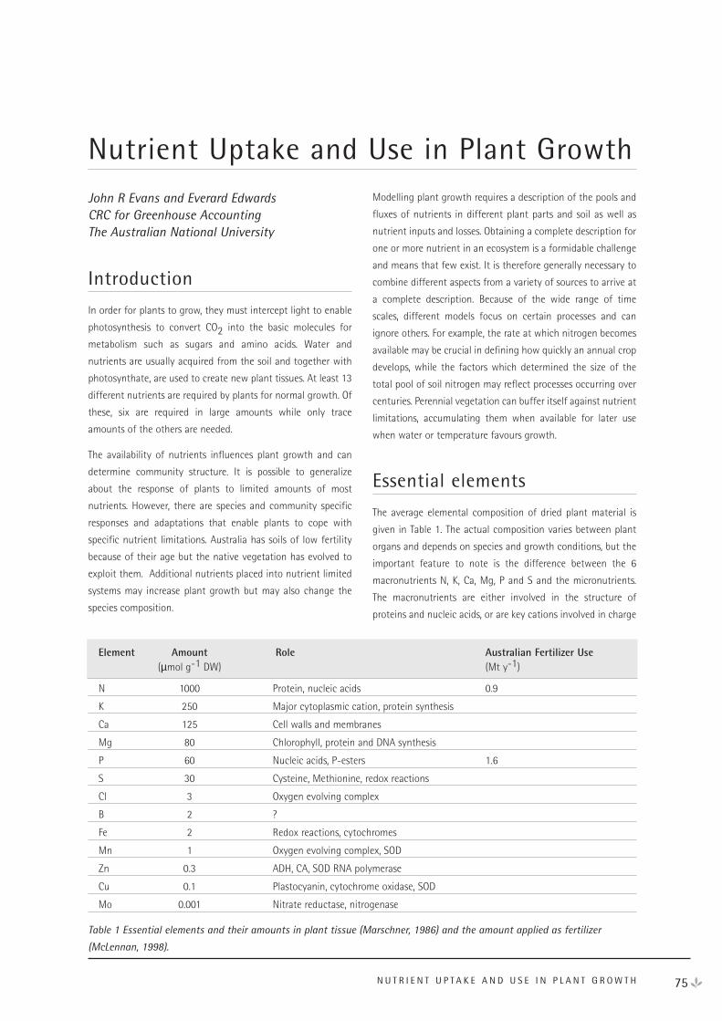
75
John R Evans and Everard EdwardsCRC for Greenhouse AccountingThe Australian National University
Introduction
In order for plants to grow, they must intercept light to enable
photosynthesis to convert CO2 into the basic molecules for
metabolism such as sugars and amino acids. Water and
nutrients are usually acquired from the soil and together with
photosynthate, are used to create new plant tissues. At least 13
different nutrients are required by plants for normal growth. Of
these, six are required in large amounts while only trace
amounts of the others are needed.
The availability of nutrients influences plant growth and can
determine community structure. It is possible to generalize
about the response of plants to limited amounts of most
nutrients. However, there are species and community specific
responses and adaptations that enable plants to cope with
specific nutrient limitations. Australia has soils of low fertility
because of their age but the native vegetation has evolved to
exploit them. Additional nutrients placed into nutrient limited
systems may increase plant growth but may also change the
species composition.
Modelling plant growth requires a description of the pools and
fluxes of nutrients in different plant parts and soil as well as
nutrient inputs and losses. Obtaining a complete description for
one or more nutrient in an ecosystem is a formidable challenge
and means that few exist. It is therefore generally necessary to
combine different aspects from a variety of sources to arrive at
a complete description. Because of the wide range of time
scales, different models focus on certain processes and can
ignore others. For example, the rate at which nitrogen becomes
available may be crucial in defining how quickly an annual crop
develops, while the factors which determined the size of the
total pool of soil nitrogen may reflect processes occurring over
centuries. Perennial vegetation can buffer itself against nutrient
limitations, accumulating them when available for later use
when water or temperature favours growth.
Essential elements
The average elemental composition of dried plant material is
given in Table 1. The actual composition varies between plant
organs and depends on species and growth conditions, but the
important feature to note is the difference between the 6
macronutrients N, K, Ca, Mg, P and S and the micronutrients.
The macronutrients are either involved in the structure of
proteins and nucleic acids, or are key cations involved in charge
N U T R I E N T U P T A K E A N D U S E I N P L A N T G R O W T H
Nutrient Uptake and Use in Plant Growth
Element Amount Role Australian Fertilizer Use(µmol g-1 DW) (Mt y-1)
N 1000 Protein, nucleic acids 0.9
K 250 Major cytoplasmic cation, protein synthesis
Ca 125 Cell walls and membranes
Mg 80 Chlorophyll, protein and DNA synthesis
P 60 Nucleic acids, P-esters 1.6
S 30 Cysteine, Methionine, redox reactions
Cl 3 Oxygen evolving complex
B 2 ?
Fe 2 Redox reactions, cytochromes
Mn 1 Oxygen evolving complex, SOD
Zn 0.3 ADH, CA, SOD RNA polymerase
Cu 0.1 Plastocyanin, cytochrome oxidase, SOD
Mo 0.001 Nitrate reductase, nitrogenase
Table 1 Essential elements and their amounts in plant tissue (Marschner, 1986) and the amount applied as fertilizer
(McLennan, 1998).
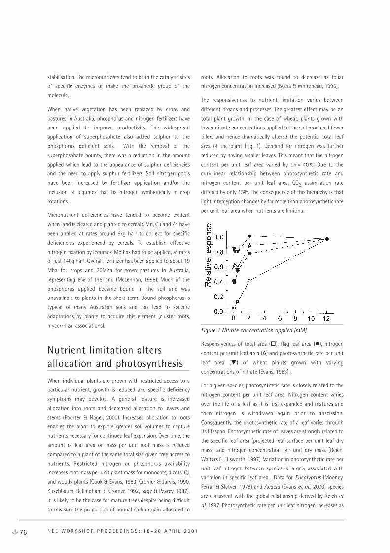
stabilisation. The micronutrients tend to be in the catalytic sites
of specific enzymes or make the prosthetic group of the
molecule.
When native vegetation has been replaced by crops and
pastures in Australia, phosphorus and nitrogen fertilizers have
been applied to improve productivity. The widespread
application of superphosphate also added sulphur to the
phosphorus deficient soils. With the removal of the
superphosphate bounty, there was a reduction in the amount
applied which lead to the appearance of sulphur deficiencies
and the need to apply sulphur fertilizers. Soil nitrogen pools
have been increased by fertilizer application and/or the
inclusion of legumes that fix nitrogen symbiotically in crop
rotations.
Micronutrient deficiencies have tended to become evident
when land is cleared and planted to cereals. Mn, Cu and Zn have
been applied at rates around 6kg ha-1 to correct for specific
deficiencies experienced by cereals. To establish effective
nitrogen fixation by legumes, Mo has had to be applied, at rates
of just 140g ha-1. Overall, fertilizer has been applied to about 19
Mha for crops and 30Mha for sown pastures in Australia,
representing 6% of the land (McLennan, 1998). Much of the
phosphorus applied became bound in the soil and was
unavailable to plants in the short term. Bound phosphorus is
typical of many Australian soils and has lead to specific
adaptations by plants to acquire this element (cluster roots,
mycorrhizal associations).
Nutrient limitation altersallocation and photosynthesis
When individual plants are grown with restricted access to a
particular nutrient, growth is reduced and specific deficiency
symptoms may develop. A general feature is increased
allocation into roots and decreased allocation to leaves and
stems (Poorter & Nagel, 2000). Increased allocation to roots
enables the plant to explore greater soil volumes to capture
nutrients necessary for continued leaf expansion. Over time, the
amount of leaf area or mass per unit root mass is reduced
compared to a plant of the same total size given free access to
nutrients. Restricted nitrogen or phosphorus availability
increases root mass per unit plant mass for monocots, dicots, C4and woody plants (Cook & Evans, 1983, Cromer & Jarvis, 1990,
Kirschbaum, Bellingham & Cromer, 1992, Sage & Pearcy, 1987).
It is likely to be the case for mature trees despite being difficult
to measure the proportion of annual carbon gain allocated to
roots. Allocation to roots was found to decrease as foliar
nitrogen concentration increased (Beets & Whitehead, 1996).
The responsiveness to nutrient limitation varies between
different organs and processes. The greatest effect may be on
total plant growth. In the case of wheat, plants grown with
lower nitrate concentrations applied to the soil produced fewer
tillers and hence dramatically altered the potential total leaf
area of the plant (Fig. 1). Demand for nitrogen was further
reduced by having smaller leaves. This meant that the nitrogen
content per unit leaf area varied by only 40%. Due to the
curvilinear relationship between photosynthetic rate and
nitrogen content per unit leaf area, CO2 assimilation rate
differed by only 15%. The consequence of this hierarchy is that
light interception changes by far more than photosynthetic rate
per unit leaf area when nutrients are limiting.
Figure 1 Nitrate concentration applied (mM)
Responsiveness of total area (�), flag leaf area (�), nitrogen
content per unit leaf area (∆) and photosynthetic rate per unit
leaf area (�) of wheat plants grown with varying
concentrations of nitrate (Evans, 1983).
For a given species, photosynthetic rate is closely related to the
nitrogen content per unit leaf area. Nitrogen content varies
over the life of a leaf as it is first expanded and matures and
then nitrogen is withdrawn again prior to abscission.
Consequently, the photosynthetic rate of a leaf varies through
its lifespan. Photosynthetic rate of leaves are strongly related to
the specific leaf area (projected leaf surface per unit leaf dry
mass) and nitrogen concentration per unit dry mass (Reich,
Walters & Ellsworth, 1997). Variation in photosynthetic rate per
unit leaf nitrogen between species is largely associated with
variation in specific leaf area. Data for Eucalyptus (Mooney,
Ferrar & Slatyer, 1978) and Acacia (Evans et al., 2000) species
are consistent with the global relationship derived by Reich et
al. 1997. Photosynthetic rate per unit leaf nitrogen increases as
76 N E E W O R K S H O P P R O C E E D I N G S : 1 8 – 2 0 A P R I L 2 0 0 1
specific leaf area increases. However, leaf lifespan tends to
decrease as specific leaf area increases, so photosynthesis per
unit nitrogen over the lifespan of a leaf would reveal a different
relationship.
Strategies for acquiringnutrients
In each environment, nutrient concentrations vary between soil
horizons, will depend on the soil chemistry and may vary in time
depending on temperature and moisture. Different plant species
may exploit different niches within the same environment,
gaining access to nutrients that are not available to other
species. The soil horizon that is explored by roots varies greatly
between species. Perennial vegetation can have long-lived roots
that penetrate deeply into the soil, whereas ephemeral and
annual species tend to colonise surface soil more extensively.
Much of the nutrient capital is present in the surface litter and
soil layers and so roots proliferate there. The volume of soil that
can be explored by a given root mass varies greatly between
species and is related to branching patterns and specific root
length. Fine roots have a limited lifespan and may not be
present in a given patch of soil when a nutrient becomes
available. For some species, roots proliferate when they sense
the presence of a nutrient.
Some roots have a specialised structure and physiology to
enable them to capture a particular nutrient. For example, most
Australian soils have low phosphorus levels and much of the
phosphorus is bound to Fe or Al. Proteaceous species, as well as
some other genera (e.g. white lupin) form cluster roots
(Dinkelaker, Hengeler & Marschner, 1995, Watt & Evans, 1999).
These dense arrays of short rootlets look like bottlebrushes and
can form extensive mats in the litter layer near the soil surface
or can be distributed through the soil. They exude organic acids
and phosphatases that solubilize phosphorus bound in the soil
or in organic matter, enabling uptake by the plant. Cluster roots
have very high rates of exudation compared to other roots, but
even species without these specialised root structures can
chemically modify the soil to assist in extracting phosphorus by
exuding citrate e.g. Danthonia (Barrett & Gifford, 1999) or
phosphatases e.g. wheat (Barrett, Richardson & Gifford, 1998).
Having a dimorphic root structure may enable plants to extract
nutrients from soil that would otherwise be too dry for roots to
function normally. In the deep sands in WA, deep sinker roots
can extract water from depth and rehydrate surface soil layers,
thereby enabling the finer surface roots to continue to function
into early summer (Pate & Dawson, 1999).
Other roots have developed symbiotic associations with
nitrogen fixing bacteria or mycorrhizae to enable them to
capture a scarce nutrient. Legumes can fix nitrogen from the air
in their nodules in exchange for carbon compounds supplied by
the host. Over time, this can lead to a significant buildup of
organic nitrogen that cycles through the litter and can become
available to non-leguminous co-occurring species. Plants that
fix nitrogen symbiotically seem to have greater requirements
for phosphorus, which is why phosphatic fertilizers are
generally applied to improved pastures containing legumes. The
trace element molybdenum has also had to be applied in much
of Australia to overcome deficiencies as this element is required
by the nitrogenase enzyme. Roots of many species form
associations with mycorrhizae that improve phosphorus and/or
nitrogen nutrition of the host plant. The very fine fungal
threads can explore much larger soil volumes for a given
amount of biomass than plant roots which enables access to
poorly mobile elements like phosphorus. They are also able to
chemically extract nutrients bound either to soil particles or in
organic matter, which may not be present in the soil solution.
Quantification of the amount of nutrient acquired through
symbiotic associations is difficult. It has been estimated that
symbiotic nitrogen fixation contributes 1900 kt y-1 to Australian
soils, compared to fertilizer applications of 380 kt y-1, while
atmospheric nitrogen deposition of 1150kt y-1 is roughly
balanced by that released back to the atmosphere by fire 1200
kt y-1 (McLaughlin, Fillery & Till, 1992). Since that estimate,
nitrogenous fertilizer use has increased to 900 kt y-1 (McLennan,
1998), but it is applied to only a small proportion of Australia’s
land surface.
Net Primary Productivity andfoliar nitrogen contentBecause photosynthesis is driven by light and is associated with
transpiration, it is not surprising that there are good
correlations between plant growth and either intercepted
radiation or cumulative transpiration. In many instances, it may
be easier to predict growth calculated from intercepted
radiation or transpiration than to measure growth directly.
Generally these approaches have conversion coefficients that
are reduced by stresses and require calibration. Altering nutrient
availability in a given environment can change the productivity
of the vegetation. Improved nutrition may enable greater leaf
area production that results in greater interception of light and
77N U T R I E N T U P T A K E A N D U S E I N P L A N T G R O W T H
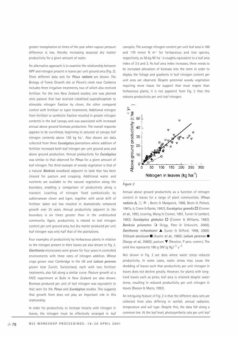
greater transpiration at times of the year when vapour pressure
difference is low, thereby increasing seasonal dry matter
productivity for a given amount of water.
An alternative approach is to examine the relationship between
NPP and nitrogen present in leaves per unit ground area (Fig. 2).
Three different data sets for Pinus radiata are shown. The
Biology of Forest Growth site at Pierce’s creek near Canberra
includes three irrigation treatments, two of which also received
fertilizer. For the two New Zealand studies, one was planted
onto pasture that had received cobaltised superphosphate to
stimulate nitrogen fixation by clover, the other compared
control with fertilizer or lupin treatments. Additional nitrogen
from fertilizer or symbiotic fixation resulted in greater nitrogen
contents in the leaf canopy and was associated with increased
annual above ground biomass production. The overall response
appears to be curvilinear, beginning to saturate at canopy leaf
nitrogen contents above 150 kg ha-1. Also shown are data
collected from three Eucalyptus plantations where addition of
fertilizer increased both leaf nitrogen per unit ground area and
above ground production. Annual productivity for Eucalyptus
was similar to that observed for Pinus for a given amount of
leaf nitrogen. The third example of woody vegetation is that of
a natural Banksia woodland adjacent to land that has been
cleared for pasture and cropping. Additional water and
nutrients are available to the natural vegetation along the
boundary, enabling a comparison of productivity along a
transect. Leaching of nitrogen fixed symbiotically by
subterranean clover and lupin, together with aerial drift of
fertiliser laden soil has resulted in dramatically enhanced
growth over 25 years. Annual productivity adjacent to the
boundary is six times greater than in the undisturbed
community. Again, productivity is related to leaf nitrogen
content per unit ground area, but dry matter produced per unit
leaf nitrogen was only half that of the plantations.
Four examples of productivity by herbaceous plants in relation
to the nitrogen present in their leaves are also shown in Fig. 2.
Danthonia microcosms were grown for four years in controlled
environments with three rates of nitrogen addition. Wheat
crops grown near Cambridge in the UK and Lolium perenne
grown near Zurich, Switzerland, each with two fertilizer
treatments, also fall along a similar curve. Pasture growth at a
FACE experiment at Bulls in New Zealand are also shown.
Biomass produced per unit of leaf nitrogen was equivalent to
that seen for the Pinus and Eucalyptus studies. This suggests
that growth form does not play an important role in this
relationship.
In order for productivity to increase linearly with nitrogen in
leaves, the nitrogen must be effectively arranged in leaf
canopies. The average nitrogen content per unit leaf area is 100
and 170 mmol N m-2 for herbaceous and tree species,
respectively, so 50 kg NF ha-1 is roughly equivalent to a leaf area
index of 3.5 and 2. As leaf area index increases, there needs to
be increased allocation of biomass into the stem in order to
display the foliage and gradients in leaf nitrogen content per
unit area are observed. Despite perennial woody vegetation
requiring more tissue for support that must respire than
herbaceous plants, it is not apparent from Fig. 2 that this
reduces productivity per unit leaf nitrogen.
Figure 2
Annual above ground productivity as a function of nitrogen
content in leaves for a range of plant communities. (Pinus
radiata ∆, ∇ , ; Beets & Madgwick, 1988, Beets & Pollock,
1987a, b, Crane & Banks, 1992); Eucalyptus grandis� (Cromer
et al., 1993, Leuning, Wang & Cromer, 1991, Turner & Lambert,
1983); Eucalyptus globulus � (Cromer & Williams, 1982);
Banksia prionotes � Grigg, Pate & Unkovich, 2000);
Danthonia richardsonii � (Lutze & Gifford, 1998, 2000);
Triticum aestivum � (Austin et al., 1980); Lolium perenne �
(Daepp et al., 2000)); pasture � (Newton, P pers. comm.). The
solid line represents 180 g DM (g NF)-1 y-1
Not shown in Fig. 2 are data where water stress reduced
productivity. In some cases, water stress may cause the
shedding of leaves such that productivity per unit nitrogen in
leaves does not decline greatly. However, for plants with long-
lived leaves such as pines, leaf area is retained despite water
stress, resulting in reduced productivity per unit nitrogen in
leaves (Raison & Myers, 1992).
An intriguing feature of Fig. 2 is that the different data sets are
collected from sites differing in rainfall, annual radiation,
temperature and soil type. Despite this, the data fall along a
common line. At the leaf level, photosynthetic rate per unit leaf
78 N E E W O R K S H O P P R O C E E D I N G S : 1 8 – 2 0 A P R I L 2 0 0 1
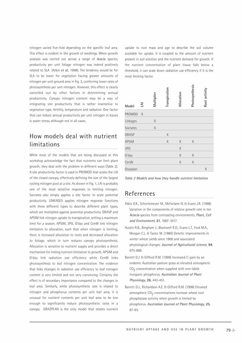
79
nitrogen varied five-fold depending on the specific leaf area.
This effect is evident in the growth of seedlings. When growth
analysis was carried out across a range of Acacia species,
productivity per unit foliage nitrogen was indeed positively
related to SLA (Atkin et al., 1998). The tendency would be for
SLA to be lower for vegetation having greater amounts of
nitrogen per unit ground area in Fig. 2, conferring lower rates of
photosynthesis per unit nitrogen. However, this effect is clearly
cancelled out by other factors in determining annual
productivity. Canopy nitrogen content may be a way of
integrating site productivity that is rather insensitive to
vegetation type, fertility, temperature and radiation. One factor
that can reduce annual productivity per unit nitrogen in leaves
is water stress, although not in all cases.
How models deal with nutrientlimitations
While most of the models that are being discussed at this
workshop acknowledge the fact that nutrients can limit plant
growth, they deal with the problem in different ways (Table 2).
A site productivity factor is used in PROMOD that scales the LAI
of the closed canopy, effectively defining the size of the largest
cycling nitrogen pool at a site. As shown in Fig. 1, LAI is probably
one of the most sensitive responses to limiting nitrogen.
Socrates also simply applies a site factor to scale potential
productivity. LINKAGES applies nitrogen response functions
with three different types to describe different plant types,
which are multiplied against potential productivity. GRASP and
APSIM link nitrogen uptake to transpiration, setting a maximum
limit for a season. APSIM, 3PG, G’day and CenW link nitrogen
limitation to allocation, such that when nitrogen is limiting,
there is increased allocation to roots and decreased allocation
to foliage, which in turn reduces canopy photosynthesis.
Allocation is sensitive to nutrient supply and provides a direct
mechanism for linking nutrient limitation to growth. APSIM and
G’day link radiation use efficiency while CenW links
photosynthesis to leaf nitrogen concentration. The evidence
that links changes in radiation use efficiency to leaf nitrogen
content is very limited and not very convincing. Certainly the
effect is of secondary importance compared to the changes in
leaf area. Similarly, while photosynthetic rate is related to
nitrogen and phosphorus contents per unit leaf area, it is
unusual for nutrient contents per unit leaf area to be low
enough to significantly reduce photosynthetic rates in a
canopy. GRAZPLAN is the only model that relates nutrient
uptake to root mass and age to describe the soil volume
available for uptake. It is coupled to the amount of nutrient
present in soil solution and the nutrient demand for growth. If
the nutrient concentration of plant tissue falls below a
threshold, it can scale down radiation use efficiency if it is the
most limiting factor.
Model
PROMOD X
Linkages X
Socrates X
GRASP X
APSIM X X X
3PG X
G’day X X
CenW X X
Grazplan X
Table 2 Models and how they handle nutrient limitation
ReferencesAtkin O.K., Schortemeyer M., McFarlane N. & Evans J.R. (1998)
Variation in the components of relative growth rate in ten
Acacia species from contrasting environments. Plant, Cell
and Environment, 21, 1007-1017.
Austin R.B., Bingham J., Blackwell R.D., Evans L.T., Ford M.A.,
Morgan C.L. & Taylor M. (1980) Genetic improvements in
winter wheat yields since 1900 and associated
physiological changes. Journal of Agricultural science, 94,
675-689.
Barrett D.J. & Gifford R.M. (1999) Increased C-gain by an
endemic Australian pasture grass at elevated atmospheric
CO2 concentration when supplied with non-labile
inorganic phosphorus. Australian Journal of Plant
Physiology, 26, 443-451.
Barrett D.J., Richardson A.E. & Gifford R.M. (1998) Elevated
atmospheric CO2 concentrations increase wheat root
phosphatase activity when growth is limited by
phosphorus. Australian Journal of Plant Physiology, 25,
87-93.
N U T R I E N T U P T A K E A N D U S E I N P L A N T G R O W T H
LAI
Mul
tipl
ier
Tran
spira
tion
Allo
cati
on
Phot
osyn
thes
is
Root
act
ivit
y
Beets P.N. & Madgwick H.A.I. (1988) Above-ground dry matter
and nutrient content of Pinus radiata as affected by lupin,
fertiliser, thinning, and stand age. New Zealand Journal of
Forestry Science, 18, 43-64.
Beets P.N. & Pollock D.S. (1987a) Accumulation and
partitioning of dry matter in Pinus radiata as related to
stand age and thinning. New Zealand Journal of Forestry
Science, 17, 246-271.
Beets P.N. & Pollock D.S. (1987b) Uptake and accumulation of
nitrogen in Pinus radiata stands as related to age and
thinning. New Zealand Journal of Forestry Science, 17,
353-371.
Beets P.N. & Whitehead D. (1996) Carbon partitioning in Pinus
radiata stands in relation to foliage nitrogen status. Tree
Physiology, 16, 131-138.
Cook M.G. & Evans L.T. (1983) Nutrient responses of seedlings
of wild and cultivated Oryza species. Field Crops Research,
6, 205-218.
Crane W.J.B. & Banks J.C.G. (1992) Accumulation and
retranslocation of foliar nitrogen in fertilized and irrigated
Pinus-radiata. Forest Ecology and Management, 52,
201-223.
Cromer R.N., Cameron D.M., Rance S.J., Ryan P.A. & Brown M.
(1993) Response to nutrients in Eucalyptus-grandis.1.
biomass accumulation. Forest Ecology and Management,
62, 211-230.
Cromer R.N. & Jarvis P.G. (1990) Growth and biomass
partitioning in Eucalyptus-grandis seedlings in response
to nitrogen supply. Australian Journal of Plant
Physiology, 17, 503-515.
Cromer R.N. & Williams E.R. (1982) Biomass and nutrient
accumulation in a planted E. globulus (Labill.) fertilizer
trial. Australian Journal of Botany, 30, 265-278.
Daepp M., Suter D., Almeida J.P.F., Isopp H., Hartwig U.A.,
Frehner M., Blum H., Nosberger J. & Luscher A. (2000) Yield
response of Lolium perenne swards to free air CO2enrichment increased over six years in a high N input
system on fertile soil. Global Change Biology, 6, 805-816.
Dinkelaker B., Hengeler C. & Marschner H. (1995) Distribution
and function of proteoid roots and other root clusters.
Botanica Acta, 108, 183-200.
Evans J.R. (1983) Nitrogen and photosynthesis in the flag leaf
of wheat (Triticum aestivum L.). Plant Physiology, 72,
297-302.
Evans J.R., Schortemeyer M., McFarlane N. & Atkin O.K. (2000)
Photosynthetic characteristics of 10 Acacia species grown
under ambient and elevated atmospheric CO2. Australian
Journal of Plant Physiology, 27, 13-25.
Grigg A.M., Pate J.S. & Unkovich M.J. (2000) Responses of
native woody taxa in Banksia woodland to incursion of
groundwater and nutrients from bordering agricultural
land. Australian Journal of Botany, 48, 777-792.
Kirschbaum M.U.F., Bellingham D.W. & Cromer R.N. (1992)
Growth analysis of the effect of phosphorus-nutrition on
seedings of Eucalyptus-grandis. Australian Journal of
Plant Physiology, 19, 55-66.
Leuning R., Wang Y.P. & Cromer R.N. (1991) Model simulations
of spatial distributions and daily totals of photosynthesis in
Eucalyptus grandis canopies. Oecologia, 88, 494-503.
Lutze J.L. & Gifford R.M. (1998) Carbon accumulation,
distribution and water use of Danthonia richardsonii
swards in response to CO2 and nitrogen supply over four
years of growth. Global Change Biology, 4, 851-861.
Lutze J.L. & Gifford R.M. (2000) Nitrogen accumulation and
distribution in Danthonia richardsonii swards in response
to CO2 and nitrogen supply over four years of growth.
Global Change Biology, 6, 1-12.
Marschner H. (1986) Mineral nutrition of higher plants.
Academic, London.
McLaughlin M.J., Fillery I.R. & Till A.R. (1992) Operation of the
phosphorus, sulphur and nitrogen cycles. In: Australia’s
renewable Resources: Sustainability and Global Change
(eds R.M. Gifford & M.M. Barson), pp. 67-116.
McLennan W. (1998) Year Book Australia. Australian Bureau
of Statistics.
Mooney H.A., Ferrar P.J. & Slatyer R.O. (1978) Photosynthetic
capacity and carbon allocation patterns in diverse growth
forms of Eucalyptus. Oecologia, 36, 103-111.
Pate J. & Dawson T. (1999) Novel techniques for assessing the
performance of woody plants in uptake and utilization of
carbon, water and nutrients: Implications for designing
agricultural mimic systems. In: Agriculture as a Mimic of
Natural Ecosystems (eds E. Lefroy, R. Hobbs, M. O’Connor,
JS, & Pate). Kluwer, Dordrech.
Poorter H. & Nagel O. (2000) The role of biomass allocation in
the growth response of plants to different levels of light,
CO2, nutrients and water: a quantitative review. Australian
Journal of Plant Physiology, 27, 595-607.
80 N E E W O R K S H O P P R O C E E D I N G S : 1 8 – 2 0 A P R I L 2 0 0 1

Raison R.J. & Myers B.J. (1992) The biology of forest growth
experiment - linking water and nitrogen availability to the
growth of pinus-radiata. Forest Ecology and
Management, 52, 279-308.
Reich P.B., Walters M.B. & Ellsworth D.S. (1997) From tropics to
tundra - global convergence in plant functioning.
Proceedings of the National Academy of Sciences of the
United States of America, 94, 13730-13734.
Sage R.F. & Pearcy R.W. (1987) The nitrogen use efficiency of
C3 and C4 plants 1. Leaf nitrogen, growth, and biomass
partitioning in Chenopodium album (L.) and Amaranthus
retroflexus (L.). Plant Physiology, 84, 954-958.
Turner J. & Lambert M.J. (1983) Nutrient cycling within a 27-
year-old Eucalyptus grandis plantation in New South
Wales. Forest Ecology and Management, 6, 155-168.
Watt M. & Evans J.R. (1999) Proteoid roots. Physiology and
development. Plant Physiology, 121, 317-323.
81N U T R I E N T U P T A K E A N D U S E I N P L A N T G R O W T H
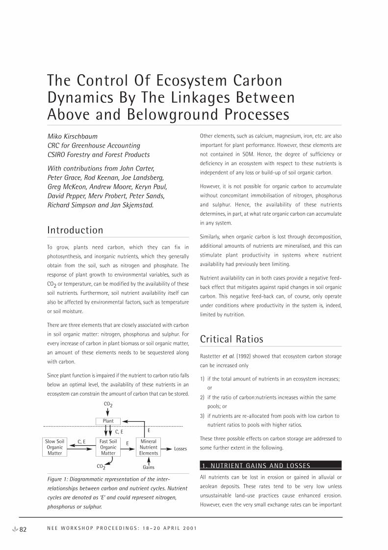
82 N E E W O R K S H O P P R O C E E D I N G S : 1 8 – 2 0 A P R I L 2 0 0 1
Miko KirschbaumCRC for Greenhouse AccountingCSIRO Forestry and Forest Products
With contributions from John Carter, Peter Grace, Rod Keenan, Joe Landsberg, Greg McKeon, Andrew Moore, Keryn Paul, David Pepper, Merv Probert, Peter Sands, Richard Simpson and Jan Skjemstad.
Introduction
To grow, plants need carbon, which they can fix in
photosynthesis, and inorganic nutrients, which they generally
obtain from the soil, such as nitrogen and phosphate. The
response of plant growth to environmental variables, such as
CO2 or temperature, can be modified by the availability of these
soil nutrients. Furthermore, soil nutrient availability itself can
also be affected by environmental factors, such as temperature
or soil moisture.
There are three elements that are closely associated with carbon
in soil organic matter: nitrogen, phosphorus and sulphur. For
every increase of carbon in plant biomass or soil organic matter,
an amount of these elements needs to be sequestered along
with carbon.
Since plant function is impaired if the nutrient to carbon ratio falls
below an optimal level, the availability of these nutrients in an
ecosystem can constrain the amount of carbon that can be stored.
Figure 1: Diagrammatic representation of the inter-
relationships between carbon and nutrient cycles. Nutrient
cycles are denoted as ‘E’ and could represent nitrogen,
phosphorus or sulphur.
Other elements, such as calcium, magnesium, iron, etc. are also
important for plant performance. However, these elements are
not contained in SOM. Hence, the degree of sufficiency or
deficiency in an ecosystem with respect to these nutrients is
independent of any loss or build-up of soil organic carbon.
However, it is not possible for organic carbon to accumulate
without concomitant immobilisation of nitrogen, phosphorus
and sulphur. Hence, the availability of these nutrients
determines, in part, at what rate organic carbon can accumulate
in any system.
Similarly, when organic carbon is lost through decomposition,
additional amounts of nutrients are mineralised, and this can
stimulate plant productivity in systems where nutrient
availability had previously been limiting.
Nutrient availability can in both cases provide a negative feed-
back effect that mitigates against rapid changes in soil organic
carbon. This negative feed-back can, of course, only operate
under conditions where productivity in the system is, indeed,
limited by nutrition.
Critical Ratios
Rastetter et al. (1992) showed that ecosystem carbon storage
can be increased only
1) if the total amount of nutrients in an ecosystem increases;
or
2) if the ratio of carbon:nutrients increases within the same
pools; or
3) if nutrients are re-allocated from pools with low carbon to
nutrient ratios to pools with higher ratios.
These three possible effects on carbon storage are addressed to
some further extent in the following.
1. NUTRIENT GAINS AND LOSSES
All nutrients can be lost in erosion or gained in alluvial or
aeolean deposits. These rates tend to be very low unless
unsustainable land-use practices cause enhanced erosion.
However, even the very small exchange rates can be important
The Control Of Ecosystem CarbonDynamics By The Linkages BetweenAbove and Belowground Processes
Plant
CO2
GainsCO2
E
E
C, E
C, E
LossesFast SoilOrganicMatter
MineralNutrientElements
Slow SoilOrganicMatter
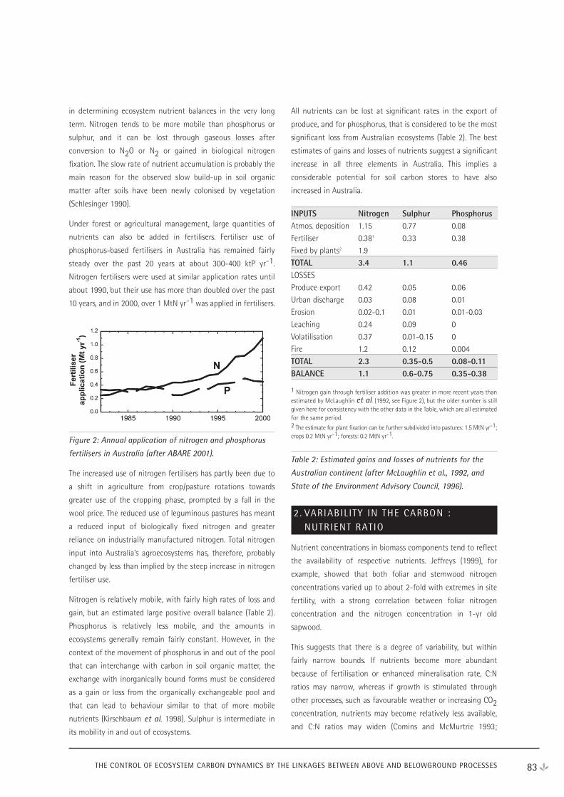
83
in determining ecosystem nutrient balances in the very long
term. Nitrogen tends to be more mobile than phosphorus or
sulphur, and it can be lost through gaseous losses after
conversion to N2O or N2 or gained in biological nitrogen
fixation. The slow rate of nutrient accumulation is probably the
main reason for the observed slow build-up in soil organic
matter after soils have been newly colonised by vegetation
(Schlesinger 1990).
Under forest or agricultural management, large quantities of
nutrients can also be added in fertilisers. Fertiliser use of
phosphorus-based fertilisers in Australia has remained fairly
steady over the past 20 years at about 300-400 ktP yr-1.
Nitrogen fertilisers were used at similar application rates until
about 1990, but their use has more than doubled over the past
10 years, and in 2000, over 1 MtN yr-1 was applied in fertilisers.
Figure 2: Annual application of nitrogen and phosphorus
fertilisers in Australia (after ABARE 2001).
The increased use of nitrogen fertilisers has partly been due to
a shift in agriculture from crop/pasture rotations towards
greater use of the cropping phase, prompted by a fall in the
wool price. The reduced use of leguminous pastures has meant
a reduced input of biologically fixed nitrogen and greater
reliance on industrially manufactured nitrogen. Total nitrogen
input into Australia’s agroecosystems has, therefore, probably
changed by less than implied by the steep increase in nitrogen
fertiliser use.
Nitrogen is relatively mobile, with fairly high rates of loss and
gain, but an estimated large positive overall balance (Table 2).
Phosphorus is relatively less mobile, and the amounts in
ecosystems generally remain fairly constant. However, in the
context of the movement of phosphorus in and out of the pool
that can interchange with carbon in soil organic matter, the
exchange with inorganically bound forms must be considered
as a gain or loss from the organically exchangeable pool and
that can lead to behaviour similar to that of more mobile
nutrients (Kirschbaum et al. 1998). Sulphur is intermediate in
its mobility in and out of ecosystems.
All nutrients can be lost at significant rates in the export of
produce, and for phosphorus, that is considered to be the most
significant loss from Australian ecosystems (Table 2). The best
estimates of gains and losses of nutrients suggest a significant
increase in all three elements in Australia. This implies a
considerable potential for soil carbon stores to have also
increased in Australia.
INPUTS Nitrogen Sulphur Phosphorus Atmos. deposition 1.15 0.77 0.08
Fertiliser 0.381 0.33 0.38
Fixed by plants2 1.9
TOTAL 3.4 1.1 0.46LOSSES
Produce export 0.42 0.05 0.06
Urban discharge 0.03 0.08 0.01
Erosion 0.02-0.1 0.01 0.01-0.03
Leaching 0.24 0.09 0
Volatilisation 0.37 0.01-0.15 0
Fire 1.2 0.12 0.004
TOTAL 2.3 0.35-0.5 0.08-0.11BALANCE 1.1 0.6-0.75 0.35-0.38
1 Nitrogen gain through fertiliser addition was greater in more recent years thanestimated by McLaughlin et al. (1992, see Figure 2), but the older number is stillgiven here for consistency with the other data in the Table, which are all estimatedfor the same period.2 The estimate for plant fixation can be further subdivided into pastures: 1.5 MtN yr-1;crops 0.2 MtN yr-1; forests: 0.2 MtN yr-1.
Table 2: Estimated gains and losses of nutrients for the
Australian continent (after McLaughlin et al., 1992, and
State of the Environment Advisory Council, 1996).
2. VARIABIL ITY IN THE CARBON : NUTRIENT RATIO
Nutrient concentrations in biomass components tend to reflect
the availability of respective nutrients. Jeffreys (1999), for
example, showed that both foliar and stemwood nitrogen
concentrations varied up to about 2-fold with extremes in site
fertility, with a strong correlation between foliar nitrogen
concentration and the nitrogen concentration in 1-yr old
sapwood.
This suggests that there is a degree of variability, but within
fairly narrow bounds. If nutrients become more abundant
because of fertilisation or enhanced mineralisation rate, C:N
ratios may narrow, whereas if growth is stimulated through
other processes, such as favourable weather or increasing CO2concentration, nutrients may become relatively less available,
and C:N ratios may widen (Comins and McMurtrie 1993;
THE CONTROL OF ECOSYSTEM CARBON DYNAMICS BY THE LINKAGES BETWEEN ABOVE AND BELOWGROUND PROCESSES
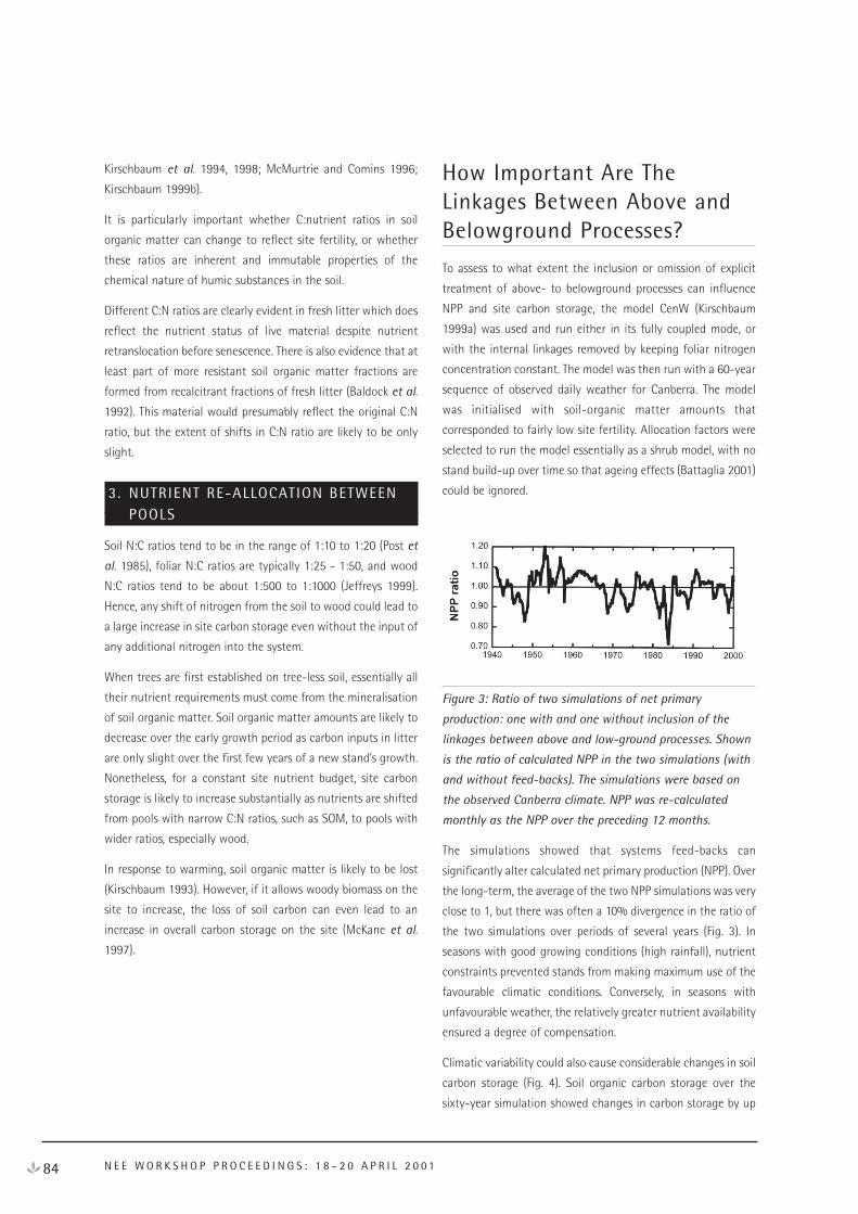
84 N E E W O R K S H O P P R O C E E D I N G S : 1 8 – 2 0 A P R I L 2 0 0 1
Kirschbaum et al. 1994, 1998; McMurtrie and Comins 1996;
Kirschbaum 1999b).
It is particularly important whether C:nutrient ratios in soil
organic matter can change to reflect site fertility, or whether
these ratios are inherent and immutable properties of the
chemical nature of humic substances in the soil.
Different C:N ratios are clearly evident in fresh litter which does
reflect the nutrient status of live material despite nutrient
retranslocation before senescence. There is also evidence that at
least part of more resistant soil organic matter fractions are
formed from recalcitrant fractions of fresh litter (Baldock et al.
1992). This material would presumably reflect the original C:N
ratio, but the extent of shifts in C:N ratio are likely to be only
slight.
3. NUTRIENT RE-ALLOCATION BETWEEN POOLS
Soil N:C ratios tend to be in the range of 1:10 to 1:20 (Post et
al. 1985), foliar N:C ratios are typically 1:25 - 1:50, and wood
N:C ratios tend to be about 1:500 to 1:1000 (Jeffreys 1999).
Hence, any shift of nitrogen from the soil to wood could lead to
a large increase in site carbon storage even without the input of
any additional nitrogen into the system.
When trees are first established on tree-less soil, essentially all
their nutrient requirements must come from the mineralisation
of soil organic matter. Soil organic matter amounts are likely to
decrease over the early growth period as carbon inputs in litter
are only slight over the first few years of a new stand’s growth.
Nonetheless, for a constant site nutrient budget, site carbon
storage is likely to increase substantially as nutrients are shifted
from pools with narrow C:N ratios, such as SOM, to pools with
wider ratios, especially wood.
In response to warming, soil organic matter is likely to be lost
(Kirschbaum 1993). However, if it allows woody biomass on the
site to increase, the loss of soil carbon can even lead to an
increase in overall carbon storage on the site (McKane et al.
1997).
How Important Are TheLinkages Between Above andBelowground Processes?
To assess to what extent the inclusion or omission of explicit
treatment of above- to belowground processes can influence
NPP and site carbon storage, the model CenW (Kirschbaum
1999a) was used and run either in its fully coupled mode, or
with the internal linkages removed by keeping foliar nitrogen
concentration constant. The model was then run with a 60-year
sequence of observed daily weather for Canberra. The model
was initialised with soil-organic matter amounts that
corresponded to fairly low site fertility. Allocation factors were
selected to run the model essentially as a shrub model, with no
stand build-up over time so that ageing effects (Battaglia 2001)
could be ignored.
Figure 3: Ratio of two simulations of net primary
production: one with and one without inclusion of the
linkages between above and low-ground processes. Shown
is the ratio of calculated NPP in the two simulations (with
and without feed-backs). The simulations were based on
the observed Canberra climate. NPP was re-calculated
monthly as the NPP over the preceding 12 months.
The simulations showed that systems feed-backs can
significantly alter calculated net primary production (NPP). Over
the long-term, the average of the two NPP simulations was very
close to 1, but there was often a 10% divergence in the ratio of
the two simulations over periods of several years (Fig. 3). In
seasons with good growing conditions (high rainfall), nutrient
constraints prevented stands from making maximum use of the
favourable climatic conditions. Conversely, in seasons with
unfavourable weather, the relatively greater nutrient availability
ensured a degree of compensation.
Climatic variability could also cause considerable changes in soil
carbon storage (Fig. 4). Soil organic carbon storage over the
sixty-year simulation showed changes in carbon storage by up
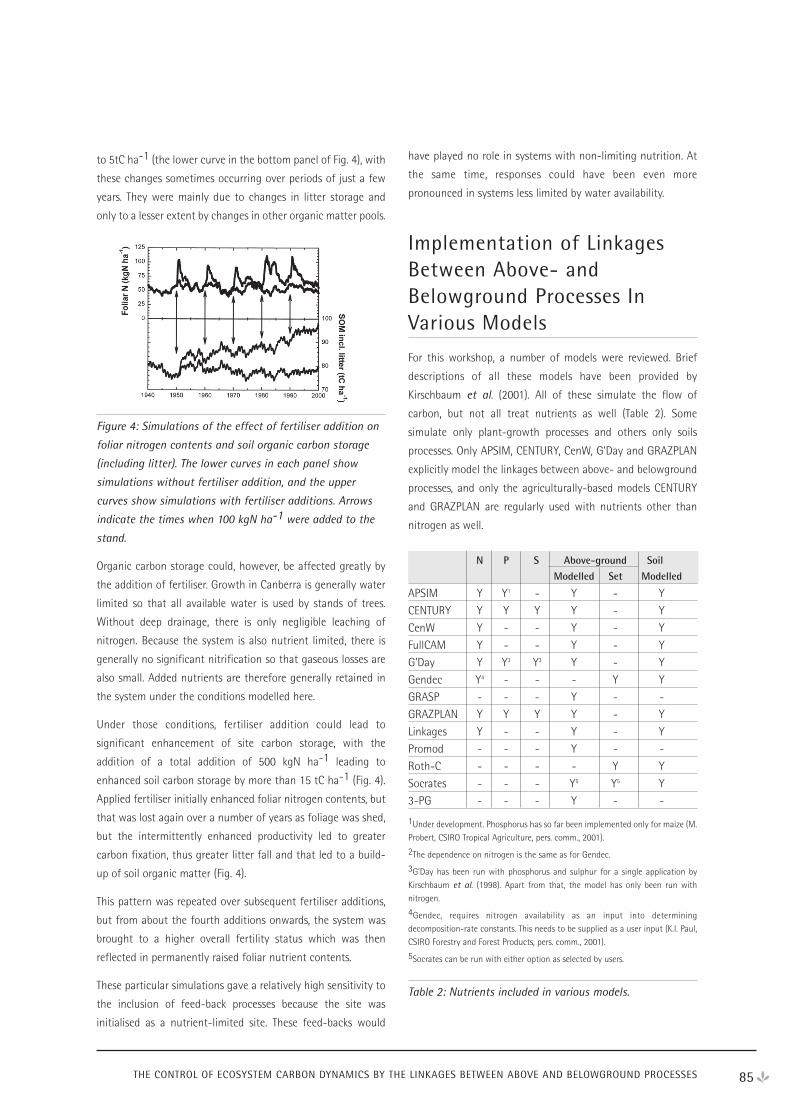
85
to 5tC ha-1 (the lower curve in the bottom panel of Fig. 4), with
these changes sometimes occurring over periods of just a few
years. They were mainly due to changes in litter storage and
only to a lesser extent by changes in other organic matter pools.
Figure 4: Simulations of the effect of fertiliser addition on
foliar nitrogen contents and soil organic carbon storage
(including litter). The lower curves in each panel show
simulations without fertiliser addition, and the upper
curves show simulations with fertiliser additions. Arrows
indicate the times when 100 kgN ha-1 were added to the
stand.
Organic carbon storage could, however, be affected greatly by
the addition of fertiliser. Growth in Canberra is generally water
limited so that all available water is used by stands of trees.
Without deep drainage, there is only negligible leaching of
nitrogen. Because the system is also nutrient limited, there is
generally no significant nitrification so that gaseous losses are
also small. Added nutrients are therefore generally retained in
the system under the conditions modelled here.
Under those conditions, fertiliser addition could lead to
significant enhancement of site carbon storage, with the
addition of a total addition of 500 kgN ha-1 leading to
enhanced soil carbon storage by more than 15 tC ha-1 (Fig. 4).
Applied fertiliser initially enhanced foliar nitrogen contents, but
that was lost again over a number of years as foliage was shed,
but the intermittently enhanced productivity led to greater
carbon fixation, thus greater litter fall and that led to a build-
up of soil organic matter (Fig. 4).
This pattern was repeated over subsequent fertiliser additions,
but from about the fourth additions onwards, the system was
brought to a higher overall fertility status which was then
reflected in permanently raised foliar nutrient contents.
These particular simulations gave a relatively high sensitivity to
the inclusion of feed-back processes because the site was
initialised as a nutrient-limited site. These feed-backs would
have played no role in systems with non-limiting nutrition. At
the same time, responses could have been even more
pronounced in systems less limited by water availability.
Implementation of LinkagesBetween Above- andBelowground Processes InVarious Models
For this workshop, a number of models were reviewed. Brief
descriptions of all these models have been provided by
Kirschbaum et al. (2001). All of these simulate the flow of
carbon, but not all treat nutrients as well (Table 2). Some
simulate only plant-growth processes and others only soils
processes. Only APSIM, CENTURY, CenW, G’Day and GRAZPLAN
explicitly model the linkages between above- and belowground
processes, and only the agriculturally-based models CENTURY
and GRAZPLAN are regularly used with nutrients other than
nitrogen as well.
N P S Above-ground Soil
Modelled Set Modelled
APSIM Y Y1 - Y - Y
CENTURY Y Y Y Y - Y
CenW Y - - Y - Y
FullCAM Y - - Y - Y
G’Day Y Y3 Y3 Y - Y
Gendec Y4 - - - Y Y
GRASP - - - Y - -
GRAZPLAN Y Y Y Y - Y
Linkages Y - - Y - Y
Promod - - - Y - -
Roth-C - - - - Y Y
Socrates - - - Y5 Y5 Y
3-PG - - - Y - -
1Under development. Phosphorus has so far been implemented only for maize (M.Probert, CSIRO Tropical Agriculture, pers. comm., 2001).
2The dependence on nitrogen is the same as for Gendec.
3G’Day has been run with phosphorus and sulphur for a single application byKirschbaum et al. (1998). Apart from that, the model has only been run withnitrogen.
4Gendec, requires nitrogen availability as an input into determiningdecomposition-rate constants. This needs to be supplied as a user input (K.I. Paul,CSIRO Forestry and Forest Products, pers. comm., 2001).
5Socrates can be run with either option as selected by users.
Table 2: Nutrients included in various models.
THE CONTROL OF ECOSYSTEM CARBON DYNAMICS BY THE LINKAGES BETWEEN ABOVE AND BELOWGROUND PROCESSES
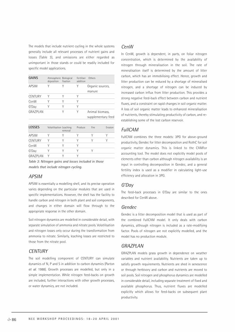
86 N E E W O R K S H O P P R O C E E D I N G S : 1 8 – 2 0 A P R I L 2 0 0 1
The models that include nutrient cycling in the whole systems
generally include all relevant processes of nutrient gains and
losses (Table 3), and omissions are either regarded as
unimportant in those stands or could be readily included for
specific model applications.
GAINS Atmospheric Biological Fertiliser Othersdeposition fixation addition
APSIM Y Y Y Organic sources,
manure
CENTURY Y Y Y
CenW Y Y Y
G’Day Y Y Y
GRAZPLAN Y Y Animal biomass,
supplementary feed
LOSSES Volatilisation Leaching Produce Fire Erosionremoval
APSIM Y Y Y Y Y
CENTURY Y Y Y Y Y
CenW Y Y Y
G’Day Y Y Y Y
GRAZPLAN Y Y Y
Table 3: Nitrogen gains and losses included in those
models that include nitrogen cycling.
APSIMAPSIM is essentially a modelling shell, and its precise operation
varies depending on the particular modules that are used in
specific implementations. However, the shell has the facility to
handle carbon and nitrogen in both plant and soil components,
and changes in either domain will flow through to the
appropriate response in the other domain.
Soil nitrogen dynamics are modelled in considerable detail, with
separate simulation of ammonia and nitrate pools. Volatilisation
and nitrogen losses only occur during the transformation from
ammonia to nitrate. Similarly, leaching losses are restricted to
those from the nitrate pool.
CENTURYThe soil modelling component of CENTURY can simulate
dynamics of N, P and S in addition to carbon dynamics (Parton
et al. 1988). Growth processes are modelled, but only in a
simple implementation. While nitrogen feed-backs on growth
are included, further interactions with other growth processes,
or water dynamics, are not included.
CenWIn CenW, growth is dependent, in parts, on foliar nitrogen
concentration, which is determined by the availability of
nitrogen through mineralisation in the soil. The rate of
mineralisation itself is determined by the amount of litter
carbon, which has an immobilising effect. Hence, growth and
litter production can be reduced by a shortage of mineralised
nitrogen, and a shortage of nitrogen can be induced by
increased carbon influx from litter production. This provides a
strong negative feed-back effect between carbon and nutrient
fluxes, and a constraint on rapid changes in soil organic matter.
A loss of soil organic matter leads to enhanced mineralisation
of nutrients, thereby stimulating productivity of carbon, and re-
establishing some of the lost carbon reservoir.
FullCAMFullCAM combines the three models: 3PG for above-ground
productivity, Gendec for litter decomposition and RothC for soil
organic matter dynamics. This is linked to the CAMFor
accounting tool. The model does not explicitly model pools of
elements other than carbon although nitrogen availability is an
input in controlling decomposition in Gendec, and a general
fertility index is used as a modifier in calculating light-use
efficiency and allocation in 3PG.
G’DayThe feed-back processes in G’Day are similar to the ones
described for CenW above.
GendecGendec is a litter decomposition model that is used as part of
the combined FullCAM model. It only deals with carbon
dynamics, although nitrogen is included as a rate-modifying
factor. Pools of nitrogen are not explicitly modelled, and the
model has no production module.
GRAZPLANGRAZPLAN models grass growth in dependence on weather
variables and nutrient availability. Nutrients are taken up to
satisfy growth requirements. Nutrients are shed in senescence
or through herbivory and carbon and nutrients are moved to
soil pools. Soil nitrogen and phosphorus dynamics are modelled
in considerable detail, including separate treatment of fixed and
available phosphorus. Thus, nutrient fluxes are modelled
explicitly which allows for feed-backs on subsequent plant
productivity.
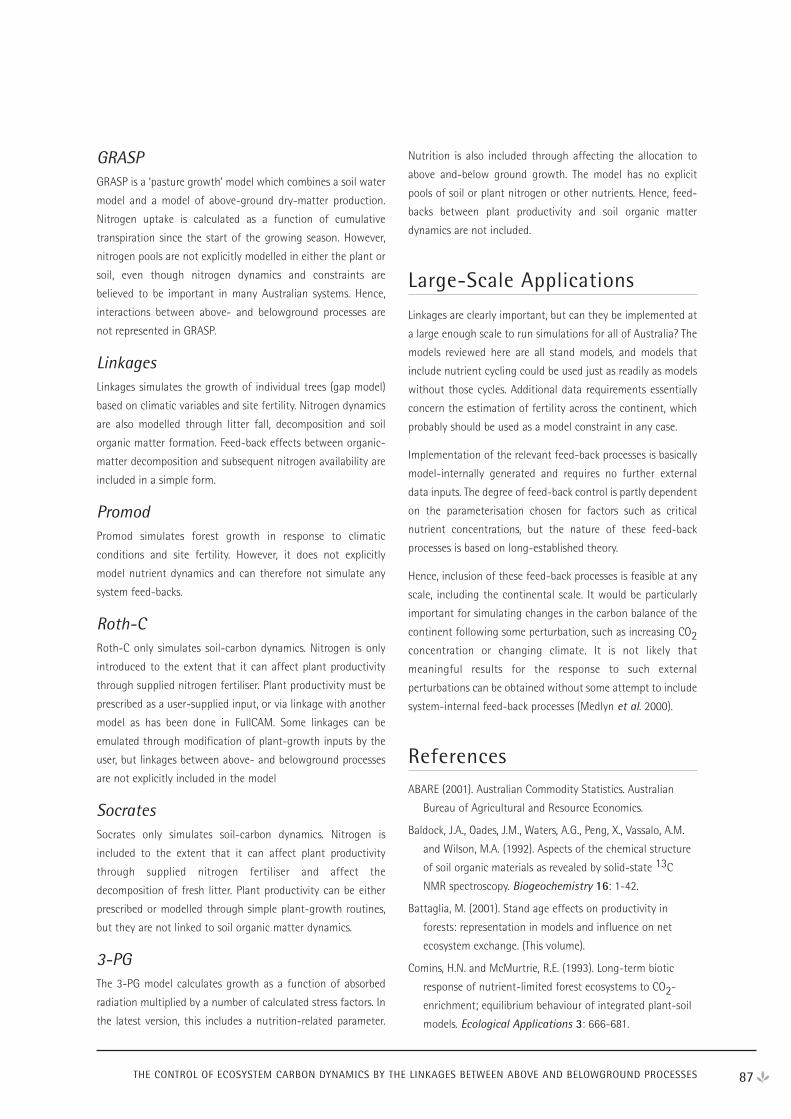
GRASPGRASP is a ‘pasture growth’ model which combines a soil water
model and a model of above-ground dry-matter production.
Nitrogen uptake is calculated as a function of cumulative
transpiration since the start of the growing season. However,
nitrogen pools are not explicitly modelled in either the plant or
soil, even though nitrogen dynamics and constraints are
believed to be important in many Australian systems. Hence,
interactions between above- and belowground processes are
not represented in GRASP.
LinkagesLinkages simulates the growth of individual trees (gap model)
based on climatic variables and site fertility. Nitrogen dynamics
are also modelled through litter fall, decomposition and soil
organic matter formation. Feed-back effects between organic-
matter decomposition and subsequent nitrogen availability are
included in a simple form.
PromodPromod simulates forest growth in response to climatic
conditions and site fertility. However, it does not explicitly
model nutrient dynamics and can therefore not simulate any
system feed-backs.
Roth-CRoth-C only simulates soil-carbon dynamics. Nitrogen is only
introduced to the extent that it can affect plant productivity
through supplied nitrogen fertiliser. Plant productivity must be
prescribed as a user-supplied input, or via linkage with another
model as has been done in FullCAM. Some linkages can be
emulated through modification of plant-growth inputs by the
user, but linkages between above- and belowground processes
are not explicitly included in the model
SocratesSocrates only simulates soil-carbon dynamics. Nitrogen is
included to the extent that it can affect plant productivity
through supplied nitrogen fertiliser and affect the
decomposition of fresh litter. Plant productivity can be either
prescribed or modelled through simple plant-growth routines,
but they are not linked to soil organic matter dynamics.
3-PGThe 3-PG model calculates growth as a function of absorbed
radiation multiplied by a number of calculated stress factors. In
the latest version, this includes a nutrition-related parameter.
Nutrition is also included through affecting the allocation to
above and-below ground growth. The model has no explicit
pools of soil or plant nitrogen or other nutrients. Hence, feed-
backs between plant productivity and soil organic matter
dynamics are not included.
Large-Scale Applications
Linkages are clearly important, but can they be implemented at
a large enough scale to run simulations for all of Australia? The
models reviewed here are all stand models, and models that
include nutrient cycling could be used just as readily as models
without those cycles. Additional data requirements essentially
concern the estimation of fertility across the continent, which
probably should be used as a model constraint in any case.
Implementation of the relevant feed-back processes is basically
model-internally generated and requires no further external
data inputs. The degree of feed-back control is partly dependent
on the parameterisation chosen for factors such as critical
nutrient concentrations, but the nature of these feed-back
processes is based on long-established theory.
Hence, inclusion of these feed-back processes is feasible at any
scale, including the continental scale. It would be particularly
important for simulating changes in the carbon balance of the
continent following some perturbation, such as increasing CO2concentration or changing climate. It is not likely that
meaningful results for the response to such external
perturbations can be obtained without some attempt to include
system-internal feed-back processes (Medlyn et al. 2000).
ReferencesABARE (2001). Australian Commodity Statistics. Australian
Bureau of Agricultural and Resource Economics.
Baldock, J.A., Oades, J.M., Waters, A.G., Peng, X., Vassalo, A.M.
and Wilson, M.A. (1992). Aspects of the chemical structure
of soil organic materials as revealed by solid-state 13C
NMR spectroscopy. Biogeochemistry 16: 1-42.
Battaglia, M. (2001). Stand age effects on productivity in
forests: representation in models and influence on net
ecosystem exchange. (This volume).
Comins, H.N. and McMurtrie, R.E. (1993). Long-term biotic
response of nutrient-limited forest ecosystems to CO2-
enrichment; equilibrium behaviour of integrated plant-soil
models. Ecological Applications 3: 666-681.
87THE CONTROL OF ECOSYSTEM CARBON DYNAMICS BY THE LINKAGES BETWEEN ABOVE AND BELOWGROUND PROCESSES
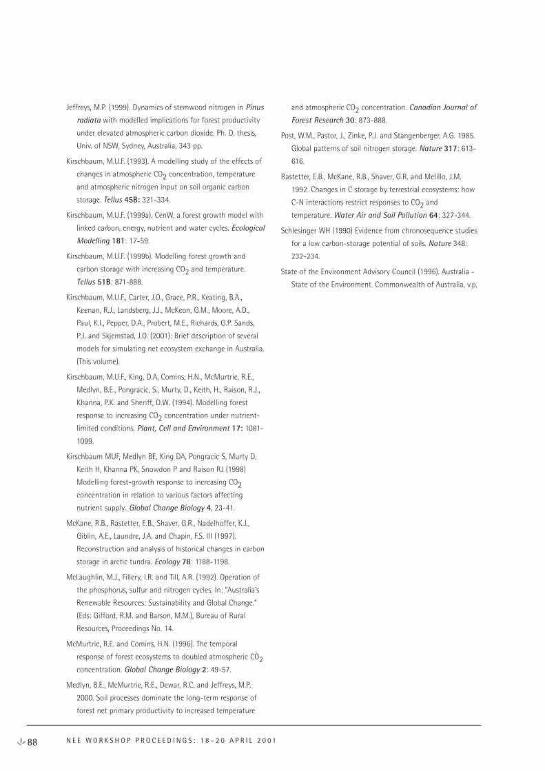
Jeffreys, M.P. (1999). Dynamics of stemwood nitrogen in Pinus
radiata with modelled implications for forest productivity
under elevated atmospheric carbon dioxide. Ph. D. thesis,
Univ. of NSW, Sydney, Australia, 343 pp.
Kirschbaum, M.U.F. (1993). A modelling study of the effects of
changes in atmospheric CO2 concentration, temperature
and atmospheric nitrogen input on soil organic carbon
storage. Tellus 45B: 321-334.
Kirschbaum, M.U.F. (1999a). CenW, a forest growth model with
linked carbon, energy, nutrient and water cycles. Ecological
Modelling 181: 17-59.
Kirschbaum, M.U.F. (1999b). Modelling forest growth and
carbon storage with increasing CO2 and temperature.
Tellus 51B: 871-888.
Kirschbaum, M.U.F., Carter, J.O., Grace, P.R., Keating, B.A.,
Keenan, R.J., Landsberg, J.J., McKeon, G.M., Moore, A.D.,
Paul, K.I., Pepper, D.A., Probert, M.E., Richards, G.P. Sands,
P.J. and Skjemstad, J.O. (2001): Brief description of several
models for simulating net ecosystem exchange in Australia.
(This volume).
Kirschbaum, M.U.F., King, D.A, Comins, H.N., McMurtrie, R.E.,
Medlyn, B.E., Pongracic, S., Murty, D., Keith, H., Raison, R.J.,
Khanna, P.K. and Sheriff, D.W. (1994). Modelling forest
response to increasing CO2 concentration under nutrient-
limited conditions. Plant, Cell and Environment 17: 1081-
1099.
Kirschbaum MUF, Medlyn BE, King DA, Pongracic S, Murty D,
Keith H, Khanna PK, Snowdon P and Raison RJ (1998)
Modelling forest-growth response to increasing CO2concentration in relation to various factors affecting
nutrient supply. Global Change Biology 4, 23-41.
McKane, R.B., Rastetter, E.B., Shaver, G.R., Nadelhoffer, K.J.,
Giblin, A.E., Laundre, J.A. and Chapin, F.S. III (1997).
Reconstruction and analysis of historical changes in carbon
storage in arctic tundra. Ecology 78: 1188-1198.
McLaughlin, M.J., Fillery, I.R. and Till, A.R. (1992). Operation of
the phosphorus, sulfur and nitrogen cycles. In: “Australia’s
Renewable Resources: Sustainability and Global Change.”
(Eds: Gifford, R.M. and Barson, M.M.), Bureau of Rural
Resources, Proceedings No. 14.
McMurtrie, R.E. and Comins, H.N. (1996). The temporal
response of forest ecosystems to doubled atmospheric CO2concentration. Global Change Biology 2: 49-57.
Medlyn, B.E., McMurtrie, R.E., Dewar, R.C. and Jeffreys, M.P.
2000. Soil processes dominate the long-term response of
forest net primary productivity to increased temperature
and atmospheric CO2 concentration. Canadian Journal of
Forest Research 30: 873-888.
Post, W.M., Pastor, J., Zinke, P.J. and Stangenberger, A.G. 1985.
Global patterns of soil nitrogen storage. Nature 317: 613-
616.
Rastetter, E.B., McKane, R.B., Shaver, G.R. and Melillo, J.M.
1992. Changes in C storage by terrestrial ecosystems: how
C-N interactions restrict responses to CO2 and
temperature. Water Air and Soil Pollution 64: 327-344.
Schlesinger WH (1990) Evidence from chronosequence studies
for a low carbon-storage potential of soils. Nature 348:
232-234.
State of the Environment Advisory Council (1996). Australia -
State of the Environment. Commonwealth of Australia, v.p.
88 N E E W O R K S H O P P R O C E E D I N G S : 1 8 – 2 0 A P R I L 2 0 0 1
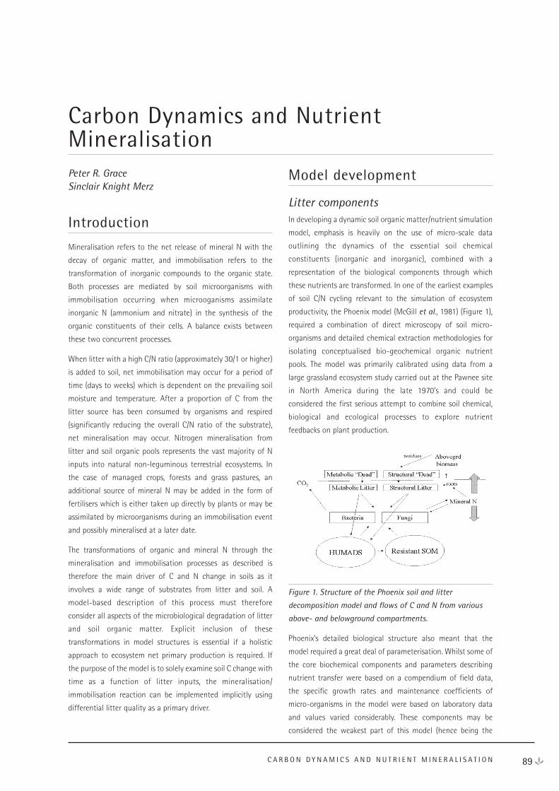
89C A R B O N D Y N A M I C S A N D N U T R I E N T M I N E R A L I S A T I O N
Peter R. GraceSinclair Knight Merz
Introduction
Mineralisation refers to the net release of mineral N with the
decay of organic matter, and immobilisation refers to the
transformation of inorganic compounds to the organic state.
Both processes are mediated by soil microorganisms with
immobilisation occurring when microoganisms assimilate
inorganic N (ammonium and nitrate) in the synthesis of the
organic constituents of their cells. A balance exists between
these two concurrent processes.
When litter with a high C/N ratio (approximately 30/1 or higher)
is added to soil, net immobilisation may occur for a period of
time (days to weeks) which is dependent on the prevailing soil
moisture and temperature. After a proportion of C from the
litter source has been consumed by organisms and respired
(significantly reducing the overall C/N ratio of the substrate),
net mineralisation may occur. Nitrogen mineralisation from
litter and soil organic pools represents the vast majority of N
inputs into natural non-leguminous terrestrial ecosystems. In
the case of managed crops, forests and grass pastures, an
additional source of mineral N may be added in the form of
fertilisers which is either taken up directly by plants or may be
assimilated by microorganisms during an immobilisation event
and possibly mineralised at a later date.
The transformations of organic and mineral N through the
mineralisation and immobilisation processes as described is
therefore the main driver of C and N change in soils as it
involves a wide range of substrates from litter and soil. A
model-based description of this process must therefore
consider all aspects of the microbiological degradation of litter
and soil organic matter. Explicit inclusion of these
transformations in model structures is essential if a holistic
approach to ecosystem net primary production is required. If
the purpose of the model is to solely examine soil C change with
time as a function of litter inputs, the mineralisation/
immobilisation reaction can be implemented implicitly using
differential litter quality as a primary driver.
Model development
Litter componentsIn developing a dynamic soil organic matter/nutrient simulation
model, emphasis is heavily on the use of micro-scale data
outlining the dynamics of the essential soil chemical
constituents (inorganic and inorganic), combined with a
representation of the biological components through which
these nutrients are transformed. In one of the earliest examples
of soil C/N cycling relevant to the simulation of ecosystem
productivity, the Phoenix model (McGill et al., 1981) (Figure 1),
required a combination of direct microscopy of soil micro-
organisms and detailed chemical extraction methodologies for
isolating conceptualised bio-geochemical organic nutrient
pools. The model was primarily calibrated using data from a
large grassland ecosystem study carried out at the Pawnee site
in North America during the late 1970’s and could be
considered the first serious attempt to combine soil chemical,
biological and ecological processes to explore nutrient
feedbacks on plant production.
Figure 1. Structure of the Phoenix soil and litter
decomposition model and flows of C and N from various
above- and belowground compartments.
Phoenix’s detailed biological structure also meant that the
model required a great deal of parameterisation. Whilst some of
the core biochemical components and parameters describing
nutrient transfer were based on a compendium of field data,
the specific growth rates and maintenance coefficients of
micro-organisms in the model were based on laboratory data
and values varied considerably. These components may be
considered the weakest part of this model (hence being the
Carbon Dynamics and NutrientMineralisation
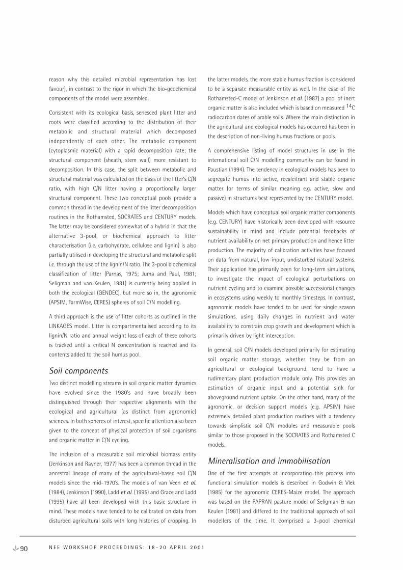
reason why this detailed microbial representation has lost
favour), in contrast to the rigor in which the bio-geochemical
components of the model were assembled.
Consistent with its ecological basis, senesced plant litter and
roots were classified according to the distribution of their
metabolic and structural material which decomposed
independently of each other. The metabolic component
(cytoplasmic material) with a rapid decomposition rate; the
structural component (sheath, stem wall) more resistant to
decomposition. In this case, the split between metabolic and
structural material was calculated on the basis of the litter’s C/N
ratio, with high C/N litter having a proportionally larger
structural component. These two conceptual pools provide a
common thread in the development of the litter decomposition
routines in the Rothamsted, SOCRATES and CENTURY models.
The latter may be considered somewhat of a hybrid in that the
alternative 3-pool, or biochemical approach to litter
characterisation (i.e. carbohydrate, cellulose and lignin) is also
partially utilised in developing the structural and metabolic split
i.e. through the use of the lignin/N ratio. The 3-pool biochemical
classification of litter (Parnas, 1975; Juma and Paul, 1981;
Seligman and van Keulen, 1981) is currently being applied in
both the ecological (GENDEC), but more so in, the agronomic
(APSIM, FarmWise, CERES) spheres of soil C/N modelling.
A third approach is the use of litter cohorts as outlined in the
LINKAGES model. Litter is compartmentalised according to its
lignin/N ratio and annual weight loss of each of these cohorts
is tracked until a critical N concentration is reached and its
contents added to the soil humus pool.
Soil componentsTwo distinct modelling streams in soil organic matter dynamics
have evolved since the 1980’s and have broadly been
distinguished through their respective alignments with the
ecological and agricultural (as distinct from agronomic)
sciences. In both spheres of interest, specific attention also been
given to the concept of physical protection of soil organisms
and organic matter in C/N cycling.
The inclusion of a measurable soil microbial biomass entity
(Jenkinson and Rayner, 1977) has been a common thread in the
ancestral lineage of many of the agricultural-based soil C/N
models since the mid-1970’s. The models of van Veen et al.
(1984), Jenkinson (1990), Ladd et al. (1995) and Grace and Ladd
(1995) have all been developed with this basic structure in
mind. These models have tended to be calibrated on data from
disturbed agricultural soils with long histories of cropping. In
the latter models, the more stable humus fraction is considered
to be a separate measurable entity as well. In the case of the
Rothamsted-C model of Jenkinson et al. (1987) a pool of inert
organic matter is also included which is based on measured 14C
radiocarbon dates of arable soils. Where the main distinction in
the agricultural and ecological models has occurred has been in
the description of non-living humus fractions or pools.
A comprehensive listing of model structures in use in the
international soil C/N modelling community can be found in
Paustian (1994). The tendency in ecological models has been to
segregate humus into active, recalcitrant and stable organic
matter (or terms of similar meaning e.g. active, slow and
passive) in structures best represented by the CENTURY model.
Models which have conceptual soil organic matter components
(e.g. CENTURY) have historically been developed with resource
sustainability in mind and include potential feedbacks of
nutrient availability on net primary production and hence litter
production. The majority of calibration activities have focused
on data from natural, low-input, undisturbed natural systems.
Their application has primarily been for long-term simulations,
to investigate the impact of ecological perturbations on
nutrient cycling and to examine possible successional changes
in ecosystems using weekly to monthly timesteps. In contrast,
agronomic models have tended to be used for single season
simulations, using daily changes in nutrient and water
availability to constrain crop growth and development which is
primarily driven by light interception.
In general, soil C/N models developed primarily for estimating
soil organic matter storage, whether they be from an
agricultural or ecological background, tend to have a
rudimentary plant production module only. This provides an
estimation of organic input and a potential sink for
aboveground nutrient uptake. On the other hand, many of the
agronomic, or decision support models (e.g. APSIM) have
extremely detailed plant production routines with a tendency
towards simplistic soil C/N modules and measurable pools
similar to those proposed in the SOCRATES and Rothamsted C
models.
Mineralisation and immobilisation One of the first attempts at incorporating this process into
functional simulation models is described in Godwin & Vlek
(1985) for the agronomic CERES-Maize model. The approach
was based on the PAPRAN pasture model of Seligman & van
Keulen (1981) and differed to the traditional approach of soil
modellers of the time. It comprised a 3-pool chemical
90 N E E W O R K S H O P P R O C E E D I N G S : 1 8 – 2 0 A P R I L 2 0 0 1
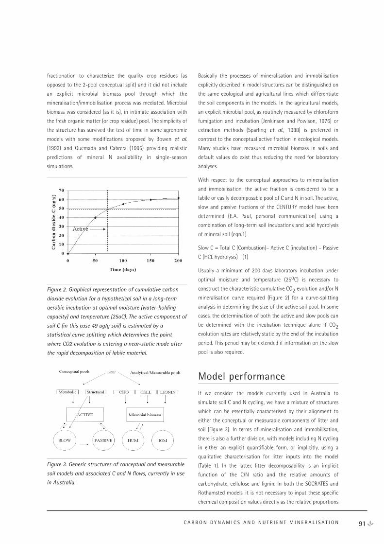
fractionation to characterize the quality crop residues (as
opposed to the 2-pool conceptual split) and it did not include
an explicit microbial biomass pool through which the
mineralisation/immobilisation process was mediated. Microbial
biomass was considered (as it is), in intimate association with
the fresh organic matter (or crop residue) pool. The simplicity of
the structure has survived the test of time in some agronomic
models with some modifications proposed by Bowen et al.
(1993) and Quemada and Cabrera (1995) providing realistic
predictions of mineral N availability in single-season
simulations.
Figure 2. Graphical representation of cumulative carbon
dioxide evolution for a hypothetical soil in a long-term
aerobic incubation at optimal moisture (water-holding
capacity) and temperature (25oC). The active component of
soil C (in this case 49 ug/g soil) is estimated by a
statistical curve splitting which determines the point
where CO2 evolution is entering a near-static mode after
the rapid decomposition of labile material.
Figure 3. Generic structures of conceptual and measurable
soil models and associated C and N flows, currently in use
in Australia.
Basically the processes of mineralisation and immobilisation
explicitly described in model structures can be distinguished on
the same ecological and agricultural lines which differentiate
the soil components in the models. In the agricultural models,
an explicit microbial pool, as routinely measured by chloroform
fumigation and incubation (Jenkinson and Powlson, 1976) or
extraction methods (Sparling et al., 1988) is preferred in
contrast to the conceptual active fraction in ecological models.
Many studies have measured microbial biomass in soils and
default values do exist thus reducing the need for laboratory
analyses.
With respect to the conceptual approaches to mineralisation
and immobilisation, the active fraction is considered to be a
labile or easily decomposable pool of C and N in soil. The active,
slow and passive fractions of the CENTURY model have been
determined (E.A. Paul, personal communication) using a
combination of long-term soil incubations and acid hydrolysis
of mineral soil (eqn.1)
Slow C = Total C (Combustion)– Active C (incubation) – Passive
C (HCL hydrolysis) (1)
Usually a minimum of 200 days laboratory incubation under
optimal moisture and temperature (25oC) is necessary to
construct the characteristic cumulative CO2 evolution and/or N
mineralisation curve required (Figure 2) for a curve-splitting
analysis in determining the size of the active soil pool. In some
cases, the determination of both the active and slow pools can
be determined with the incubation technique alone if CO2evolution rates are relatively static by the end of the incubation
period. This period may be extended if information on the slow
pool is also required.
Model performance
If we consider the models currently used in Australia to
simulate soil C and N cycling, we have a mixture of structures
which can be essentially characterised by their alignment to
either the conceptual or measurable components of litter and
soil (Figure 3). In terms of mineralisation and immobilisation,
there is also a further division, with models including N cycling
in either an explicit quantifiable form, or implicitly, using a
qualitative characterisation for litter inputs into the model
(Table 1). In the latter, litter decomposability is an implicit
function of the C/N ratio and the relative amounts of
carbohydrate, cellulose and lignin. In both the SOCRATES and
Rothamsted models, it is not necessary to input these specific
chemical composition values directly as the relative proportions
91C A R B O N D Y N A M I C S A N D N U T R I E N T M I N E R A L I S A T I O N
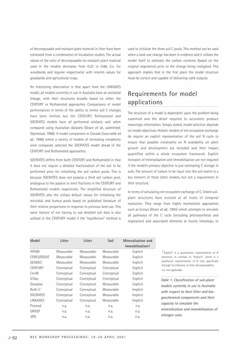
92 N E E W O R K S H O P P R O C E E D I N G S : 1 8 – 2 0 A P R I L 2 0 0 1
of decomposable and resistant plant material in litter have been
estimated from a combination of incubation studies. The actual
values of the ratio of decomposable-to-resistant plant material
used in the models decreases from 0.25 to 0.66, (i.e. for
woodlands and legume respectively) with interim values for
grasslands and agricultural crops.
An interesting observation is that apart from the LINKAGES
model, all models currently in use in Australia have an ancestral
linkage, with their structures broadly based on either the
CENTURY or Rothamsted approaches. Comparisons of model
performances in terms of the ability to mimic soil C changes
have been limited, but the CENTURY, Rothamsted and
SOCRATES models have all performed similarly well when
compared using Australian datasets (Grace et al., submitted;
Skjemstad, 1996). A model comparison in Canada (Izaurralde et
al., 1996) where a variety of models of increasing complexity
were compared, selected the SOCRATES model ahead of the
CENTURY and Rothamsted approaches.
SOCRATES differs from both CENTURY and Rothamsted in that
it does not require a detailed fractionation of the soil to be
performed prior for initialising the soil carbon pools. This is
because SOCRATES does not possess a third soil carbon pool,
analogous to the passive or inert fractions in the CENTURY and
Rothamsted models respectively. The simplified structure of
SOCRATES also the utilises default values for initialising the
microbial and humus pools based on published literature of
their relative proportions in response to previous land use. This
same feature of not having to use detailed soil data is also
utilised in the CENTURY model if the “equilibrium” method is
used to initialise the three soil C pools. This method can be used
when a land-use change has been in evidence and it utilises the
model itself to estimate the carbon contents (based on the
original vegetation) prior to the change being instigated. This
approach implies that in the first place the model structure
must be correct and capable of delivering valid outputs.
Requirements for modelapplications
The structure of a model is dependent upon the problem being
examined and the detail required to accurately produce
meaningly information. Simply stated, model selection depends
on model objectives. Holistic models of net ecosystem exchange
do require an explicit representation of the soil N cycle to
ensure that possible constraints on N availability on plant
growth and development are included and their impact
quantified within a whole ecosystem framework. Explicit
inclusion of mineralisation and immobilisation are not required
if the model’s primary objective is just estimating C storage in
soils. The amount of carbon to be input into the soil matrix is a
key element of these latter models, but not a requirement in
their structure.
In terms of simulating net ecosystem exchange of C, linked soil-
plant structures have evolved at all levels of temporal
resolution. They range from highly mechanistic approaches
such as Ecosys (Grant et al., 1993) which attempts to simulate
all pathways of the C cycle (including photosynthesis and
respiration) and associated elements at hourly timesteps, to
Model
APSIM
CERES/DSSAT
GENDEC
CENTURY
CenW
G’Day
Grazplan
Roth-C
SOCRATES
LINKAGES
Promod
GRASP
3PG
Litter
Measurable
Measurable
Measurable
Conceptual
Conceptual
Conceptual
Conceptual
Conceptual
Conceptual
Conceptual
n.a.
n.a.
n.a.
Litter
Measurable
Measurable
Measurable
Conceptual
Conceptual
Conceptual
Conceptual
Conceptual
Conceptual
Conceptual
n.a.
n.a.
n.a.
Soil
Measurable
Measurable
Measurable
Conceptual
Conceptual
Conceptual
Measurable
Measurable
Measurable
Measurable
n.a.
n.a.
n.a.
Mineralisation andImmobilisation1
Explicit
Explicit
Explicit
Explicit
Explicit
Explicit
Explicit
Implicit
Implicit
Implicit
n.a
n.a.
n.a.
1”Explicit” is a quantitative representation of Ndynamics, in contrast to “Implicit”, which is aqualitative representation of N only, specificallythrough its influence on litter decomposability.
n.a. not applicable
Table 1. Classification of soil-plant
models currently in use in Australia
with respect to their litter and bio-
geochemical components and their
capacity to simulate the
mineralisation and immobilisation of
nitrogen soils.
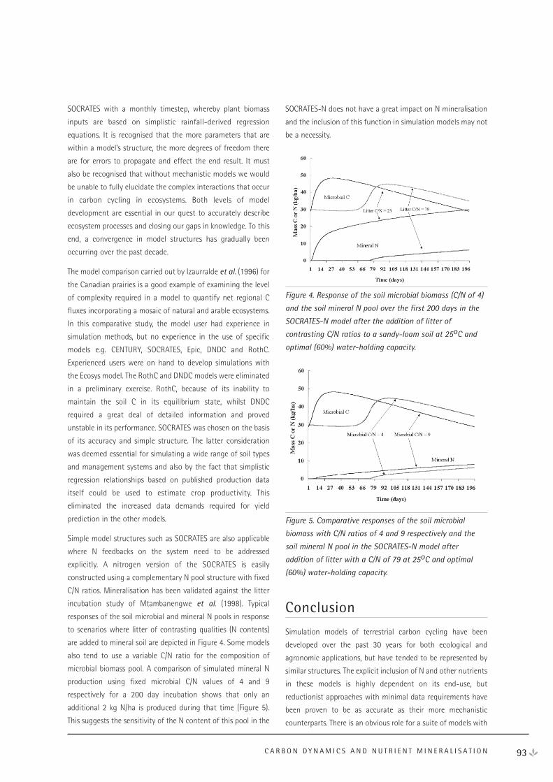
SOCRATES with a monthly timestep, whereby plant biomass
inputs are based on simplistic rainfall-derived regression
equations. It is recognised that the more parameters that are
within a model’s structure, the more degrees of freedom there
are for errors to propagate and effect the end result. It must
also be recognised that without mechanistic models we would
be unable to fully elucidate the complex interactions that occur
in carbon cycling in ecosystems. Both levels of model
development are essential in our quest to accurately describe
ecosystem processes and closing our gaps in knowledge. To this
end, a convergence in model structures has gradually been
occurring over the past decade.
The model comparison carried out by Izaurralde et al. (1996) for
the Canadian prairies is a good example of examining the level
of complexity required in a model to quantify net regional C
fluxes incorporating a mosaic of natural and arable ecosystems.
In this comparative study, the model user had experience in
simulation methods, but no experience in the use of specific
models e.g. CENTURY, SOCRATES, Epic, DNDC and RothC.
Experienced users were on hand to develop simulations with
the Ecosys model. The RothC and DNDC models were eliminated
in a preliminary exercise. RothC, because of its inability to
maintain the soil C in its equilibrium state, whilst DNDC
required a great deal of detailed information and proved
unstable in its performance. SOCRATES was chosen on the basis
of its accuracy and simple structure. The latter consideration
was deemed essential for simulating a wide range of soil types
and management systems and also by the fact that simplistic
regression relationships based on published production data
itself could be used to estimate crop productivity. This
eliminated the increased data demands required for yield
prediction in the other models.
Simple model structures such as SOCRATES are also applicable
where N feedbacks on the system need to be addressed
explicitly. A nitrogen version of the SOCRATES is easily
constructed using a complementary N pool structure with fixed
C/N ratios. Mineralisation has been validated against the litter
incubation study of Mtambanengwe et al. (1998). Typical
responses of the soil microbial and mineral N pools in response
to scenarios where litter of contrasting qualities (N contents)
are added to mineral soil are depicted in Figure 4. Some models
also tend to use a variable C/N ratio for the composition of
microbial biomass pool. A comparison of simulated mineral N
production using fixed microbial C/N values of 4 and 9
respectively for a 200 day incubation shows that only an
additional 2 kg N/ha is produced during that time (Figure 5).
This suggests the sensitivity of the N content of this pool in the
SOCRATES-N does not have a great impact on N mineralisation
and the inclusion of this function in simulation models may not
be a necessity.
Figure 4. Response of the soil microbial biomass (C/N of 4)
and the soil mineral N pool over the first 200 days in the
SOCRATES-N model after the addition of litter of
contrasting C/N ratios to a sandy-loam soil at 25oC and
optimal (60%) water-holding capacity.
Figure 5. Comparative responses of the soil microbial
biomass with C/N ratios of 4 and 9 respectively and the
soil mineral N pool in the SOCRATES-N model after
addition of litter with a C/N of 79 at 25oC and optimal
(60%) water-holding capacity.
Conclusion
Simulation models of terrestrial carbon cycling have been
developed over the past 30 years for both ecological and
agronomic applications, but have tended to be represented by
similar structures. The explicit inclusion of N and other nutrients
in these models is highly dependent on its end-use, but
reductionist approaches with minimal data requirements have
been proven to be as accurate as their more mechanistic
counterparts. There is an obvious role for a suite of models with
93C A R B O N D Y N A M I C S A N D N U T R I E N T M I N E R A L I S A T I O N
94 N E E W O R K S H O P P R O C E E D I N G S : 1 8 – 2 0 A P R I L 2 0 0 1
increasingly complexity in examining the net ecosystem
exchange of carbon. This capacity to look at ecosystems with
varying detail will ensure that problem solving in terrestrial
biology and ecology remains a converging and not a diverging
science. Convergence with creativity will increase the essential
element of collaboration and scientific sharing that is required
for progress to be made in understanding, mitigating and
adapting to the impacts of global climate change.
ReferencesBowen, W.T., Jones, J.W., Carsky, R.J. and Quintana, J.O. (1993)
Evaluation of the nitrogen model of CERES-Maize
following legume green manure corporation. Agron. J. 85,
153-159.
Godwin, D.C. and Vlek, P.G. (1985) Simulation of nitrogen
dynamics in wheat cropping systems. In Day, W. and Atkin,
R.K. (Eds.), Wheat Growth and Modelling. Plenum
Publishing Corp, New York, 311-332.
Grace, P.R., Georgis, K., Reeves, T.G. and Alston, A.M.
(submitted) Simulating changes in soil organic carbon in
cropping systems of the semi-arid Mallee region of
Australia. Ag. Systems.
Grace, P.R. and Ladd, J.N. (1995) SOCRATES (Soil Organic
Carbon Reserves and Transformations in agro-Eco-Systems).
CRC for Soil and Land Management, Adelaide, 17pp.
Grant, R.F., Juma, N.G. and McGill, W.B. (1993) Simulation of
carbon and nitrogen transformations in soil: Mineralisation.
Soil Biol. Biochem. 25, 1317-1329.
Izaurralde, R.C., McGill, W.B., Jans-Hammermeister, D.C.,
Haugen-Korzyra, K.L. and Hiley, J.C. (1996) Development of
a technique to calculate carbon fluxes in agricultural soils
at the eco-district level using simulation models and
various aggregation methods. Interim Report, Submitted to
the Scientific Authority of the Agriculture and Agri-Food
Canada Greenhouse Gas Initiative, University of Alberta,
Edmonton, 69pp.
Jenkinson, D.S. (1990) The turnover of organic C and N in soil.
Phil. Trans. Roy. Soc. Lon. B 329, 361-368.
Jenkinson, D.S., Hart, P.B.S., Rayner, J.H. and Parry, L.C. (1987)
Modelling the turnover of organic matter in long-term
experiments at Rothamsted. INTECOL Bulletin 15, 1-8.
Jenkinson, D.S. and Rayner, J.H. (1977) The turnover of soil
organic matter in some of the Rothamsted classical
experiments. Soil Sci. 123, 298-305.
Jenkinson, D.S. and Powlson, D.S. (1976) The effect of biocidal
treatments on metabolism in soil. V. A method of
measuring soil biomass. Soil Biol. Biochem. 8, 209-
Juma, N.G., and Paul, E.A. 1981. Use of tracers and computer
simulation techniques to assess mineralization and
immobilization of soil nitrogen. In: Frissel, M.J. and van
Veen, J.A. (Eds.), Simulation of Nitrogen Behavior of Soil-
Plant Systems. Pudoc, Wageningen, 145-154.
Ladd, J.N., Amato, M., Grace, P.R. and van Veen, J.A., 1995.
Simulation of 14C turnover through the microbial biomass
in soils incubated with 14C-labelled plant residues. Soil
Biol. Biochem. 27, 777-783.
McGill, W.B., Hunt, H.W., Woodmansee, R.G. and Reuss, J.O. (1981)
Phoenix, a model of the dynamics of carbon and nitrogen in
grassland soils. In: Clark, F.E., Rosswall, T. (Eds.), Terrestrial
Nitrogen Cycles. Ecol. Bull. (Stockholm). 33, 49-115.
Mtambanengwe, F., Chivaura-Mususa, C. and Kirchmannn, H.
(1998) Assessment of plant-litter quality related to short-
term carbon and nitrogen mineralisation in soil. In:
Bergstrom, L. and Kirchmann, H. (Eds.), Carbon and
Nitrogen Dynamics in Natural and Agricultural Tropical
Ecosystems, CAB International, Wallingford, 85-102.
Parnas, H. (1975) Model for decomposition of organic material
by microorganisms. Soil Biol. Biochem. 7, 161-169.
Paustian, K. (1994) In: Pankhurst, C.E., Doube, B.M., Gupta,
V.V.S.R. and Grace, P.R. (Eds.), Soil Biota: Management in
Sustainable Farming Systems, CSIRO, Melbourne.
Quemada, M. and Cabrera, M.L. (1995) CERES-N model
predictions of nitrogen mineralised from cover crop
residues. Soil Sci. Soc. Amer. J. 59, 1059-1065.
Seligman, N.C. and van Keulen, H. (1981) PAPRAN: A
simulation model of annual pasture production limited by
rainfall and nitrogen. In: Frissel, M.J and van Veen, J.A.
(Eds.), Simulation of Nitrogen Behaviour of Soil-Plant
Systems, PUDOC, Wageningen, Netherlands, 191-221.
Skjemstad, J. (1996) Determining the potential for carbon
sequestration in Australian soils. Final Report RIRDC project
CSO-5A, 66pp.
Sparling G.P. and West, A.W. (1988) A direct extraction method
to estimate soil microbial C: calibration in situ using
microbial respiration and 14C labelled cells. Soil Biol.
Biochem. 20, 337–343.
vanVeen, J.A., Ladd, J.N. and Frissel, M.J. (1984) Modelling C
and N turnover through the microbial biomass in soil. Plant
Soil 76, 257-274
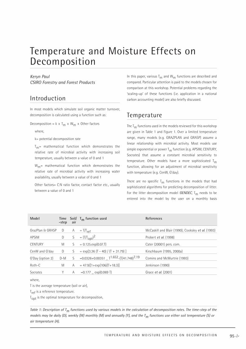
95T E M P E R A T U R E A N D M O I S T U R E E F F E C T S O N D E C O M P O S I T I O N
Keryn PaulCSIRO Forestry and Forest Products
Introduction
In most models which simulate soil organic matter turnover,
decomposition is calculated using a function such as:
Decomposition = k x Tm x Wm x Other factors
where,
k= potential decomposition rate
Tm= mathematical function which demonstrates the
relative rate of microbial activity with increasing soil
temperature, usually between a value of 0 and 1
Wm= mathematical function which demonstrates the
relative rate of microbial activity with increasing water
availability, usually between a value of 0 and 1
Other factors= C:N ratio factor, contact factor etc., usually
between a value of 0 and 1
In this paper, various Tm and Wm functions are described and
compared. Particular attention is paid to the models chosen for
comparison at this workshop. Potential problems regarding the
‘scaling-up’ of these functions (i.e. application in a national
carbon accounting model) are also briefly discussed.
Temperature
The Tm functions used in the models reviewed for this workshop
are given in Table 1 and Figure 1. Over a limited temperature
range, many models (e.g. GRAZPLAN and GRASP) assume a
linear relationship with microbial activity. Most models use
simple exponential or power Tm function (e.g. APSIM, CENTURY,
Socrates) that assume a constant microbial sensitivity to
temperature. Other models have a more sophisticated Tmfunction, allowing for an adjustment of microbial sensitivity
with temperature (e.g. CenW, G’day).
There are no specific Tm functions in the models that had
sophisticated algorithms for predicting decomposition of litter.
For the litter decomposition model GENDEC, Tm needs to be
entered into the model by the user on a monthly basis
Temperature and Moisture Effects onDecomposition
Model Time Soil/ Tm function used References-step air
GrazPlan & GRASP D A = T/Tref McCaskill and Blair (1990); Cooksley et al. (1993)
APSIM D S = (T/Topt)2 Probert et al. (1998)
CENTURY M S = 0.125.exp(0.07.T) Cater (20001) pers. com.
CenW and G’day D S = exp[3.36 (T - 40) / (T + 31.79) ] Kirschbaum (1995, 2000a)
G’Day (option 2) D-M S =0.0326+0.00351 _ T1.652-(T/41.748)7.19 Comins and McMurtrie (1993)
Roth-C M A = 47.9/[1+exp(106/(T+18.3)] Jenkinson (1990)
Socrates Y A =0.177 _ exp(0.069 T) Grace et al. (2001)
Table 1: Description of Tm functions used by various models in the calculation of decomposition rates. The time-step of the
models may be daily (D), weekly (W) monthly (M) and annually (Y), and the Tm functions use either soil temperature (S) or
air temperature (A).
where,
T is the average temperature (soil or air),
Tref is a reference temperature.
Topt is the optimal temperature for decomposition,
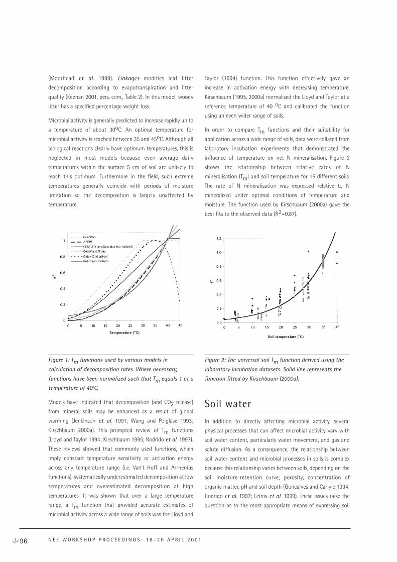
(Moorhead et al. 1999). Linkages modifies leaf litter
decomposition according to evapotranspiration and litter
quality (Keenan 2001, pers. com., Table 2). In this model, woody
litter has a specified percentage weight loss.
Microbial activity is generally predicted to increase rapidly up to
a temperature of about 30oC. An optimal temperature for
microbial activity is reached between 35 and 45oC. Although all
biological reactions clearly have optimum temperatures, this is
neglected in most models because even average daily
temperatures within the surface 5 cm of soil are unlikely to
reach this optimum. Furthermore in the field, such extreme
temperatures generally coincide with periods of moisture
limitation so the decomposition is largely unaffected by
temperature.
Figure 1: Tm functions used by various models in
calculation of decomposition rates. Where necessary,
functions have been normalized such that Tm equals 1 at a
temperature of 40oC.
Models have indicated that decomposition (and CO2 release)
from mineral soils may be enhanced as a result of global
warming (Jenkinson et al. 1991; Wang and Polglase 1993;
Kirschbaum 2000a). This prompted review of Tm functions
(Lloyd and Taylor 1994; Kirschbaum 1995; Rodrido et al. 1997).
These reviews showed that commonly used functions, which
imply constant temperature sensitivity or activation energy
across any temperature range (i.e. Van’t Hoff and Arrhenius
functions), systematically underestimated decomposition at low
temperatures and overestimated decomposition at high
temperatures. It was shown that over a large temperature
range, a Tm function that provided accurate estimates of
microbial activity across a wide range of soils was the Lloyd and
Taylor (1994) function. This function effectively gave an
increase in activation energy with decreasing temperature.
Kirschbaum (1995, 2000a) normalised the Lloyd and Taylor at a
reference temperature of 40 oC and calibrated the function
using an even wider range of soils.
In order to compare Tm functions and their suitability for
application across a wide range of soils, data were collated from
laboratory incubation experiments that demonstrated the
influence of temperature on net N mineralisation. Figure 2
shows the relationship between relative rates of N
mineralisation (Tm) and soil temperature for 15 different soils.
The rate of N mineralisation was expressed relative to N
mineralised under optimal conditions of temperature and
moisture. The function used by Kirschbaum (2000a) gave the
best fits to the observed data (R2=0.87).
Figure 2: The universal soil Tm function derived using the
laboratory incubation datasets. Solid line represents the
function fitted by Kirschbaum (2000a).
Soil water
In addition to directly affecting microbial activity, several
physical processes that can affect microbial activity vary with
soil water content, particularly water movement, and gas and
solute diffusion. As a consequence, the relationship between
soil water content and microbial processes in soils is complex
because this relationship varies between soils, depending on the
soil moisture-retention curve, porosity, concentration of
organic matter, pH and soil depth (Goncalves and Carlyle 1994;
Rodrigo et al. 1997; Leiros et al. 1999). These issues raise the
question as to the most appropriate means of expressing soil
96 N E E W O R K S H O P P R O C E E D I N G S : 1 8 – 2 0 A P R I L 2 0 0 1
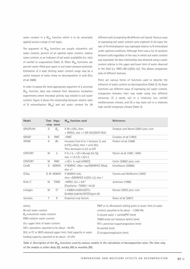
97T E M P E R A T U R E A N D M O I S T U R E E F F E C T S O N D E C O M P O S I T I O N
water content in a Wm function which is to be universally
applied across a range of soil types.
The argument of Wm functions are usually volumetric soil
water content, percent of an optimal water content, relative
water content, or an indicator of soil water availability (i.e. ratio
of rainfall to evaporation) (Table 2). Other Wm functions use
percent water-filled pore space or soil water pressure potential.
Estimation of a least limiting water content range may be a
useful measure of water stress on decomposition in soils (Zou
et al. 2000).
In order to assess the most appropriate argument of a universal
Wm function, data was collated from laboratory incubation
experiments where microbial activity was related to soil water
content. Figure 3 shows the relationship between relative rates
of N mineralisation (Wm) and soil water content for 28
different soils (comprising 40 different soil layers). Various ways
of expressing soil water content were explored. In all cases, the
rate of N mineralisation was expressed relative to N mineralised
under optimal conditions. Although there was a lot of variation
between soils regardless of the way in which soil water content
was expressed, the best relationship was obtained using a water
content relative to the upper and lower limit of water observed
in the field (i.e. RWC=(W-LL)/(UL-LL)). This allows comparison
soils of different textures.
There are various forms of functions used to describe the
influence of water content on decomposition (Table 2). As these
functions use different ways of expressing soil water content,
comparison between then was made using two different
scenarios: (i) a sandy soil in a relatively low rainfall
mediterranean climate, and (ii) a clay loam soil in a relatively
high rainfall temperate climate (Table 3).
Model Time Argu- Wm function used References-step ment
GRAZPLAN D Øv If W<=DUL, then Simpson and Moore (2001) pers. com.= W/DUL, else =1-(W-DUL)/(SAT-DUL)
GRASP D RWC =RWC Cooksley et al. (1993)
APSIM D Øv Increases from 0 to 1 between LL and Probert et al. (1998)0.5*(LL+DUL), then 1 until DUL. Then decreases to 0.5 at SAT
CENTURY M S If S<1.5, =1/[1+30.exp(-8.5 S)], Parton et al. (1987, 1994) else =1-0.7.(S-1.5)/1.5
CENTURY M RWC =1/[1+ 4. exp(-6.RWC)] Carter (20001) pers. com.
CenW D W/WHC If W/WHC <Max =sqrt[(W/WHC) /Max], Kirschbaum (2000b)else =1
G’Day D, W W/WHC If W/WHC<0.6, Comins and McMurtrie (1993)then =((W/WHC)-LL)/(UL-LL), else 1
Roth-C M TSMD =MIN(1, 0.2 + 0.8 * Jenkinson (1990) (ClayFactor -TSMD) / 16.53)
Linkages M ET = 0.9804+0.09352(ET)+ Keenan (2001) pers. com.[0.4956-0.001927(ET)]*(lignin:N)
Socrates Y R Empirical crop factors Grace et al. (2001)
Table 2: Description of the Wm functions used by various models in the calculation of decomposition rates. The time-step
of the models is either daily (D), weekly (W) or monthly (M).
where,
W=soil water contentØv=volumetric water content
RWC=relative water content
UL= upper limit of water content
SAT= saturation, assumed to be about –10 kPa
DUL or FC or WHC=drained upper limit, field capacity or water
holding capacity, assumed to be about –25 kPa
PWP or LL=Permanent wilting point or lower limit of water
content, assumed to be about –1,500 kPa
S=stored water + rainfall/PET (mm)
TSMD=total soil moisture deficit (mm)
PET= potential evapotranspiration (mm)
R=rainfall (mm)
ET=evapotranspiration (mm)
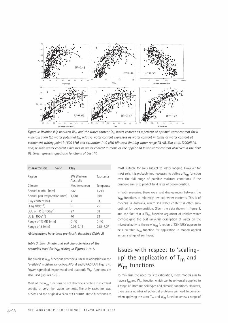
98 N E E W O R K S H O P P R O C E E D I N G S : 1 8 – 2 0 A P R I L 2 0 0 1
Characteristic Sand Clay
Region SW Western Tasmania Australia
Climate Mediterranean Temperate
Annual rainfall (mm) 632 1,214
Annual pan evaporation (mm) 1,448 699
Clay content (%) 7 33
LL (g 100g-1) 5 25
DUL or FC (g 100g-1) 27 38
UL (g 100g-1) 40 52
Range of TSMD (mm) 0-40 0-40
Range of S (mm) 0.06-2.16 0.61-7.07
Abbreviations have been previously described (Table 2)
Table 3: Site, climate and soil characteristics of the
scenarios used for Wm testing in Figures 3 to 7.
The simplest Wm functions describe a linear relationships in the
“available” moisture range (e.g. APSIM and GRAZPLAN, Figure 4).
Power, sigmoidal, exponential and quadratic Wm functions are
also used (Figures 5-8).
Most of the Wm functions do not describe a decline in microbial
activity at very high water contents. The only exception was
APSIM and the original version of CENTURY. These functions are
most suitable for soils subject to water logging. However for
most soils it is probably not necessary to define a Wm function
over the full range of possible moisture conditions if the
principle aim is to predict field rates of decomposition.
In both scenarios, there were vast discrepancies between the
Wm functions at relatively low soil water contents. This is of
concern in Australia, where soil water content is often sub-
optimal for decomposition. Given the data shown in Figure 3,
and the fact that a Wm function argument of relative water
content gave the best universal description of water on the
microbial activity, the new Wm function of CENTURY appears to
be a suitable Wm function for application in models applied
across a range of soil types.
Issues with respect to ‘scaling-up’ the application of Tm andWm functions
To minimise the need for site calibration, most models aim to
have a Tm and Wm function which can be universally applied to
a range of litter and soil types and climatic conditions. However,
there are a number of potential problems we need to consider
when applying the same Tm and Wm function across a range of
Figure 3: Relationship between Wm and the water content (a); water content as a percent of optimal water content for N
mineralisation (b); water potential (c); relative water content expresses as water content in terms of water content at
permanent wilting point (-1500 kPa) and saturation (-10 kPa) (d); least limiting water range (LLWR, Zou et al. (2000)) (e),
and; relative water content expresses as water content in terms of the upper and lower water content observed in the field
(f). Lines represent quadratic functions of best fit.
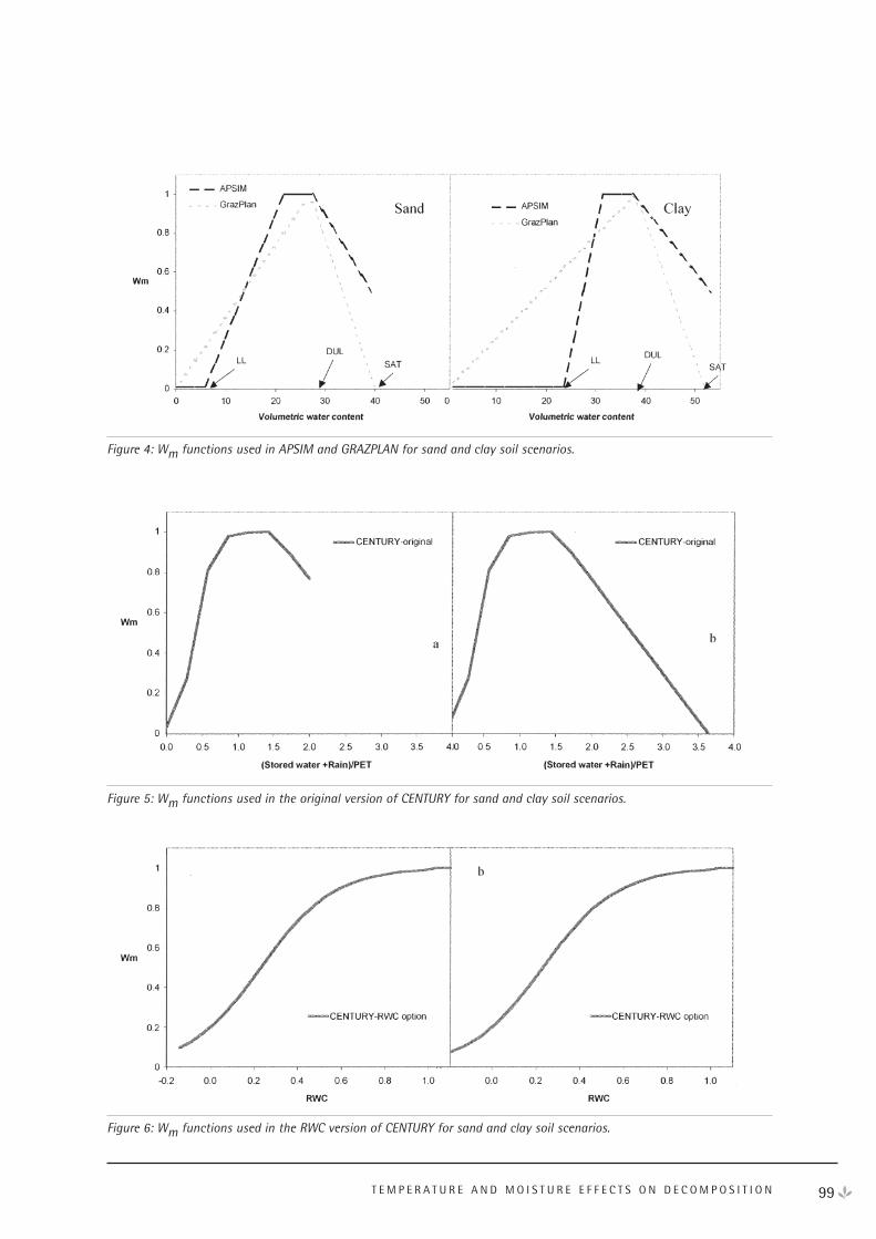
99T E M P E R A T U R E A N D M O I S T U R E E F F E C T S O N D E C O M P O S I T I O N
Figure 4: Wm functions used in APSIM and GRAZPLAN for sand and clay soil scenarios.
Figure 5: Wm functions used in the original version of CENTURY for sand and clay soil scenarios.
Figure 6: Wm functions used in the RWC version of CENTURY for sand and clay soil scenarios.
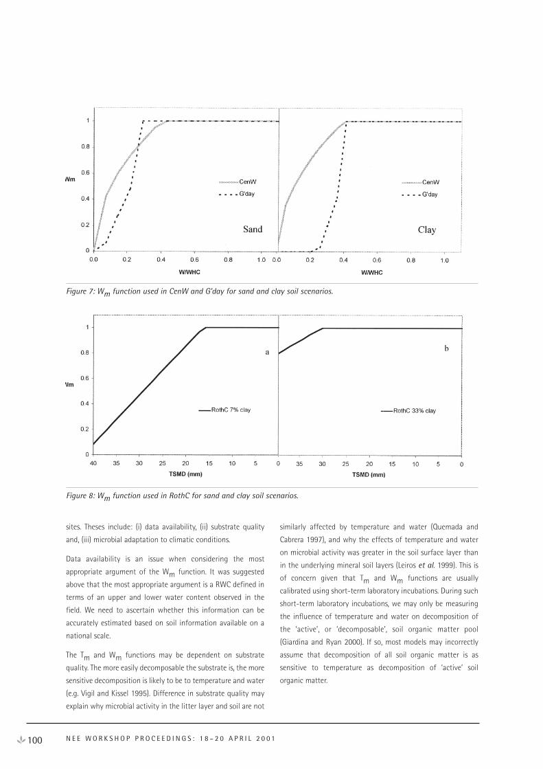
100 N E E W O R K S H O P P R O C E E D I N G S : 1 8 – 2 0 A P R I L 2 0 0 1
sites. Theses include: (i) data availability, (ii) substrate quality
and, (iii) microbial adaptation to climatic conditions.
Data availability is an issue when considering the most
appropriate argument of the Wm function. It was suggested
above that the most appropriate argument is a RWC defined in
terms of an upper and lower water content observed in the
field. We need to ascertain whether this information can be
accurately estimated based on soil information available on a
national scale.
The Tm and Wm functions may be dependent on substrate
quality. The more easily decomposable the substrate is, the more
sensitive decomposition is likely to be to temperature and water
(e.g. Vigil and Kissel 1995). Difference in substrate quality may
explain why microbial activity in the litter layer and soil are not
similarly affected by temperature and water (Quemada and
Cabrera 1997), and why the effects of temperature and water
on microbial activity was greater in the soil surface layer than
in the underlying mineral soil layers (Leiros et al. 1999). This is
of concern given that Tm and Wm functions are usually
calibrated using short-term laboratory incubations. During such
short-term laboratory incubations, we may only be measuring
the influence of temperature and water on decomposition of
the ‘active’, or ‘decomposable’, soil organic matter pool
(Giardina and Ryan 2000). If so, most models may incorrectly
assume that decomposition of all soil organic matter is as
sensitive to temperature as decomposition of ‘active’ soil
organic matter.
Figure 7: Wm function used in CenW and G’day for sand and clay soil scenarios.
Figure 8: Wm function used in RothC for sand and clay soil scenarios.
It is unlikely that microbes in a very warm-wet environment will
be as equally sensitive to changes in temperature and moisture
as microbes in a cold-dry environment. It is often suggested
that sensitivity of microbial communities generally decreases
with increasing mean annual temperature and rainfall (e.g.
Kirschbaum 1995). This may be why turnover was similar across
82 sites of different annual temperature (Giardina and Ryan
2000). Indeed, both the population and metabolism of the
microbial population changes with water content (e.g. Sulkava
et al. 1996), and microbes may adapt to the variations in the
frequency of wetting and drying cycles (Paul et al. 1999).
Conclusion
Further work is required to test whether or not significant
improvements can be made to prediction of decomposition by
having: (i) different Tm and/or Wm functions for soil organic
matter pools of differing substrate quality, or (ii) an allowance
for adaptation to climate. Perhaps the most important issue
relating to ‘scaling-up’ the application of the Tm and Wmfunctions is to ensure that these functions have been calibrated
using data obtained from a wide range of soil types or
appropriate depth. If Tm and Wm functions are also to be
applied to litter decomposition algorithms, additional
calibration will be required since microbial sensitivity to
temperature and water are unlikely to be the same in litter as in
soil.
Acknowledgments
John Carter, Marc Corbeels, Peter Grace, Rod Keenan, Miko
Kirschbaum, Andrew Moore, Dave Pepper, Merv Probert, Richard
Simpson are thanked for their help in preparing this paper.
Partap Khanna, Tony O’Connell, Phil Polglase, Philip Smethurst
and are also thanked for the use of their unpublished data.
ReferencesComins, H.N., and McMurtrie, R.E. (1993). Long-term response
of nutrient-limited forests to CO2 enrichment: Equilibrium
behavior of plant-soil models. Ecological Applications, 3:
666-681.
Cooksley, D.G., Prinsen, J.H., Paton, C.J., Lisle, A.T. (1993). Rate
of decomposition and release of nutrients for litter in a
Heteropogon contortus-Bothriochloa bladhii dominant
native pasture. Proceedings of the XVII International
Grasslands Congress. pp. 1557-1559.
Giardina,C.P., Ryan,M.G. (2000). Evidence that decomposition
rates of organic carbon in mineral soil do not vary with
temperature. Nature, 404: 858-861.
Goncalves, J.L.M., Carlyle, J.C. (1994). Modelling the influence
of moisture and temperature on net nitrogen
mineralization in a forested sandy soil. Soil Biology
Biochemistry, 26: 1557-1564.
Grace, P.R., Georgis, K., Reeves, T.G., Altston, A. (2001).
Simulating changes in soil organic carbon in cropping
systems of the semi-arid Mallee region of Australia.
Agricultural Systems. In Press.
Jenkinson, D.S. (1990). The turnover of organic carbon and
nitrogen in soil. Philosophical Transactions of the Royal
Society of London. Series B, Biological Sciences; 329:p361-
368
Jenkinson, D.S., Adams, D.E., Wild, A. (1991). Model estimates
of COsub(2) emissions from soil in response to global
warming. Nature, 351: 304-306.
Kirschbaum, M.U.F., 1995. The temperature dependence of soil
organic matter decomposition and the effect of global
warming on soil organic carbon storage. Soil Biology and
Biochemistry 27, 753-760.
Kirschbaum, M.U.F., 2000a. Will changes in soil organic matter
act as a positive or negative feedback on global warming?
Biogeochemistry 48, 21-51.
Kirschbaum, M.U.F., 2000b. CenW: a generic forest growth
model that links carbon, nutrient and water cycles. New
Zealand Journal of Forestry 45, 15-19.
Leiros, M.C.,Trasar-Cepeda, C., Seoane, S., Gil-Sotres, F. (1999).
Dependence of mineralization of soil organic matter on
temperature and moisture. Soil Biology Biochemistry, 31:
Soil Biology Biochemistry: 327-335.
Lloyd, J., Taylor, J.A. (1994). On the temperature dependence of
soil respiration. Functional Ecology, 8: 315-323.
McCaskil, MR, and Blair, GJ. (1990). A model of S, P and N
uptake by perennial pasture. Model construction. Fertilizer
Research, 22: 161-172.
Moorhead, D.L., Reynolds, J.F. (1991). A general model of litter
decomposition in the northern Chihauhuan Desert.
Ecological Modelling, 56: 197-219.
Moorhead, D.L., Currie, W.S., Rastetter, E.B., Parton, W.J.,
Harmon, M.E. (1999). Climate and litter quality controls on
101T E M P E R A T U R E A N D M O I S T U R E E F F E C T S O N D E C O M P O S I T I O N

decomposition: An analysis of modelling approaches.
Global Biogeochemical cycles, 13: 575-589.
Rodrigo, A., Recous, S., Neel, C., Mary, B. (1997). Modelling
temperature and moisture effects on C-N transformations
in soils: comparison of nine models. Ecological Modelling,
102: 325-339.
Probert, M.E., Dimers, J.P., Keating, B.A., Dalal, R.C., Strong,
W.M. (1998). APSIM’s water and nitrogen modules and
simulation of the dynamics of water and nitrogen in fallow
systems. Agricultural Systems, 56, 1-28.
Paul K I, Black A S and Conyers MK 1999 Influence of moist-
dry cycles on pH changes in surface soils. Australian
Journal of Soil Research, 37: 1057-1072.
Parton WJ; Schimel DS; Cole CV, and Ojima DS. (1987).
Analysis of factors controlling soil organic matter levels in
Great Plains Grasslands. Soil Science Society of America
Journal, 51: 1173-1179.
Parton, W.J, Schimel, D.S., Ojima, D.S., Bryant, R.B., and Arnold,
R.W., (1994). A general model for soil organic matter
dynamics: sensitivity to litter chemistry, texture and
management. Quantitative modeling of soil forming
processes: proceedings of a symposium sponsored by
Divisions S-5 and S-9 of the Soil Science Society of
America in Minneapolis, Minnesota, USA, 2 Nov. 1992.
Madison, USA: Soil Science Society of America Inc.; pp.
p147-167.
Quemada, M., Cabrera, M.L. (1997). Temperature and moisture
effects on C and N mineralization from surface applied
clover residue. Plant and Soil, 189: 127-137
Sierra, J. (1997). Temperature and soil moisture dependence of
N mineralization in intact soil cores. Soil Biology
Biochemistry, 27: 1557-1563.
Sulkava, P., Huhta, V., Laakso, J. (1996). Impact of soil faunal
structure on decomposition and N-mineralisation in
relation to temperature and moisture in forest soil.
Pedobiologia, 40: 505-513.
Vigil, M.F., Kissel, D.E. (1995). Rate of nitrogen mineralized from
incorporated crop residues as influenced by temperature.
Soil Science Society of America Journal, 59: 1636-1644.
Wang, Y.P., Polglase, P.J. (1993). Carbon balance in the tundra,
boreal forest and humid tropical forest during climate
change: scaling up from leaf physiology and soil carbon
dynamics. Plant, Cell and Environment, 18: 1226-1244.
Zou, C., Sands, R. Buchan, G. Hudson, I. (2000) Least limiting
water range: a potential indicator of physical quality of
forest soil. Australian Journal of Soil Research, 38: 947-958.
102 N E E W O R K S H O P P R O C E E D I N G S : 1 8 – 2 0 A P R I L 2 0 0 1
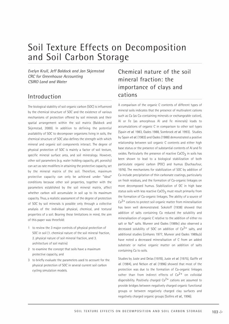
103S O I L T E X T U R E E F F E C T S O N D E C O M P O S I T I O N A N D S O I L C A R B O N S T O R A G E
Evelyn Krull, Jeff Baldock and Jan SkjemstadCRC for Greenhouse AccountingCSIRO Land and Water
Introduction
The biological stability of soil organic carbon (SOC) is influenced
by the chemical structure of SOC and the existence of various
mechanisms of protection offered by soil minerals and their
spatial arrangement within the soil matrix (Baldock and
Skjemstad, 2000). In addition to defining the potential
availability of SOC to decomposer organisms living in soils, the
chemical structure of SOC also defines the strength with which
mineral and organic soil components interact. The degree of
physical protection of SOC is mainly a factor of soil texture,
specific mineral surface area, and soil mineralogy. However,
other soil parameters (e.g. water holding capacity, pH, porosity)
can act as rate modifiers in attaining the protective capacity, set
by the mineral matrix of the soil. Therefore, maximum
protective capacity can only be achieved under “ideal”
conditions because other soil properties, together with the
parameters established by the soil mineral matrix, affect
whether carbon will accumulate in soil up to its maximum
capacity. Thus, a realistic assessment of the degree of protection
of SOC by soil minerals is possible only through a collective
analysis of the individual physical, chemical, and textural
properties of a soil. Bearing these limitations in mind, the aim
of this paper was threefold:
1 to review the 3 major controls of physical protection of
SOC in soil (1. chemical nature of the soil mineral fraction,
2. physical nature of soil mineral fraction, and 3.
architecture of soil matrix)
2 to examine the concept that soils have a maximum
protective capacity, and
3 to briefly evaluate the parameters used to account for the
physical protection of SOC in several current soil carbon
cycling simulation models.
Chemical nature of the soilmineral fraction: theimportance of clays andcations
A comparison of the organic C contents of different types of
mineral soils indicates that the presence of multivalent cations
such as Ca (as Ca-containing minerals or exchangeable cation),
Al or Fe (as amorphous Al and Fe minerals) leads to
accumulations of organic C in comparison to other soil types
(Spain et al. 1983, Oades 1988, Sombroek et al. 1993). Studies
by Spain et al. (1983) and Oades (1988) demonstrated a positive
relationship between soil organic C contents and either high
base status or the presence of substantial contents of Al and Fe
oxides. Particularly the presence of reactive CaCO3 in soils has
been shown to lead to a biological stabilization of both
particulate organic carbon (POC) and humus (Duchaufour,
1976). The mechanisms for stabilization of SOC by addition of
Ca include precipitation of thin carbonate coatings, particularly
on fresh residues, and the formation of Ca-organic linkages on
more decomposed humus. Stabilization of OC in high base
status soils with less reactive CaCO3 must result primarily from
the formation of Ca-organic linkages. The ability of a source of
Ca2+ cations to protect soil organic matter from mineralisation
has been well demonstrated. Sokoloff (1938) showed that
addition of salts containing Ca reduced the solubility and
mineralisation of organic C relative to the addition of either no
salt or Na+ salts. Muneer and Oades (1989c) also observed a
decreased solubility of SOC on addition of Ca2+ salts, and
additional studies (Linhares 1977, Muneer and Oades 1989a,b)
have noted a decreased mineralisation of C from an added
substrate or native organic matter on addition of salts
containing Ca to soils.
Studies by Juste and Delas (1970), Juste et al. (1975), Gaiffe et
al. (1984), and Nelson et al. (1996) showed that most of the
protection was due to the formation of Ca-organic linkages
rather than from indirect effects of Ca2+ on colloidal
dispersibility. Positively charged Ca2+ cations are assumed to
provide bridges between negatively charged organic functional
groups or between negatively charged clay surfaces and
negatively charged organic groups (Sollins et al., 1996).
Soil Texture Effects on Decompositionand Soil Carbon Storage
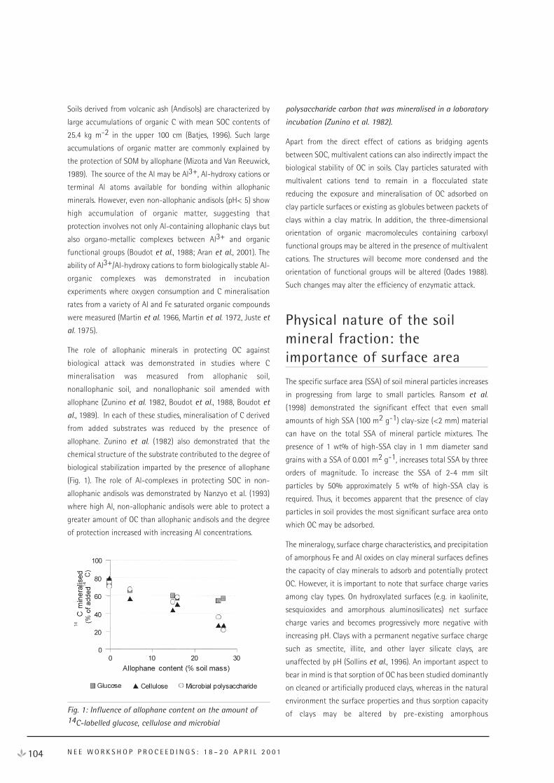
Soils derived from volcanic ash (Andisols) are characterized by
large accumulations of organic C with mean SOC contents of
25.4 kg m-2 in the upper 100 cm (Batjes, 1996). Such large
accumulations of organic matter are commonly explained by
the protection of SOM by allophane (Mizota and Van Reeuwick,
1989). The source of the Al may be Al3+, Al-hydroxy cations or
terminal Al atoms available for bonding within allophanic
minerals. However, even non-allophanic andisols (pH< 5) show
high accumulation of organic matter, suggesting that
protection involves not only Al-containing allophanic clays but
also organo-metallic complexes between Al3+ and organic
functional groups (Boudot et al., 1988; Aran et al., 2001). The
ability of Al3+/Al-hydroxy cations to form biologically stable Al-
organic complexes was demonstrated in incubation
experiments where oxygen consumption and C mineralisation
rates from a variety of Al and Fe saturated organic compounds
were measured (Martin et al. 1966, Martin et al. 1972, Juste et
al. 1975).
The role of allophanic minerals in protecting OC against
biological attack was demonstrated in studies where C
mineralisation was measured from allophanic soil,
nonallophanic soil, and nonallophanic soil amended with
allophane (Zunino et al. 1982, Boudot et al., 1988, Boudot et
al., 1989). In each of these studies, mineralisation of C derived
from added substrates was reduced by the presence of
allophane. Zunino et al. (1982) also demonstrated that the
chemical structure of the substrate contributed to the degree of
biological stabilization imparted by the presence of allophane
(Fig. 1). The role of Al-complexes in protecting SOC in non-
allophanic andisols was demonstrated by Nanzyo et al. (1993)
where high Al, non-allophanic andisols were able to protect a
greater amount of OC than allophanic andisols and the degree
of protection increased with increasing Al concentrations.
Fig. 1: Influence of allophane content on the amount of14C-labelled glucose, cellulose and microbial
polysaccharide carbon that was mineralised in a laboratory
incubation (Zunino et al. 1982).
Apart from the direct effect of cations as bridging agents
between SOC, multivalent cations can also indirectly impact the
biological stability of OC in soils. Clay particles saturated with
multivalent cations tend to remain in a flocculated state
reducing the exposure and mineralisation of OC adsorbed on
clay particle surfaces or existing as globules between packets of
clays within a clay matrix. In addition, the three-dimensional
orientation of organic macromolecules containing carboxyl
functional groups may be altered in the presence of multivalent
cations. The structures will become more condensed and the
orientation of functional groups will be altered (Oades 1988).
Such changes may alter the efficiency of enzymatic attack.
Physical nature of the soilmineral fraction: theimportance of surface area
The specific surface area (SSA) of soil mineral particles increases
in progressing from large to small particles. Ransom et al.
(1998) demonstrated the significant effect that even small
amounts of high SSA (100 m2 g-1) clay-size (<2 mm) material
can have on the total SSA of mineral particle mixtures. The
presence of 1 wt% of high-SSA clay in 1 mm diameter sand
grains with a SSA of 0.001 m2 g-1, increases total SSA by three
orders of magnitude. To increase the SSA of 2-4 mm silt
particles by 50% approximately 5 wt% of high-SSA clay is
required. Thus, it becomes apparent that the presence of clay
particles in soil provides the most significant surface area onto
which OC may be adsorbed.
The mineralogy, surface charge characteristics, and precipitation
of amorphous Fe and Al oxides on clay mineral surfaces defines
the capacity of clay minerals to adsorb and potentially protect
OC. However, it is important to note that surface charge varies
among clay types. On hydroxylated surfaces (e.g. in kaolinite,
sesquioxides and amorphous aluminosilicates) net surface
charge varies and becomes progressively more negative with
increasing pH. Clays with a permanent negative surface charge
such as smectite, illite, and other layer silicate clays, are
unaffected by pH (Sollins et al., 1996). An important aspect to
bear in mind is that sorption of OC has been studied dominantly
on cleaned or artificially produced clays, whereas in the natural
environment the surface properties and thus sorption capacity
of clays may be altered by pre-existing amorphous
104 N E E W O R K S H O P P R O C E E D I N G S : 1 8 – 2 0 A P R I L 2 0 0 1
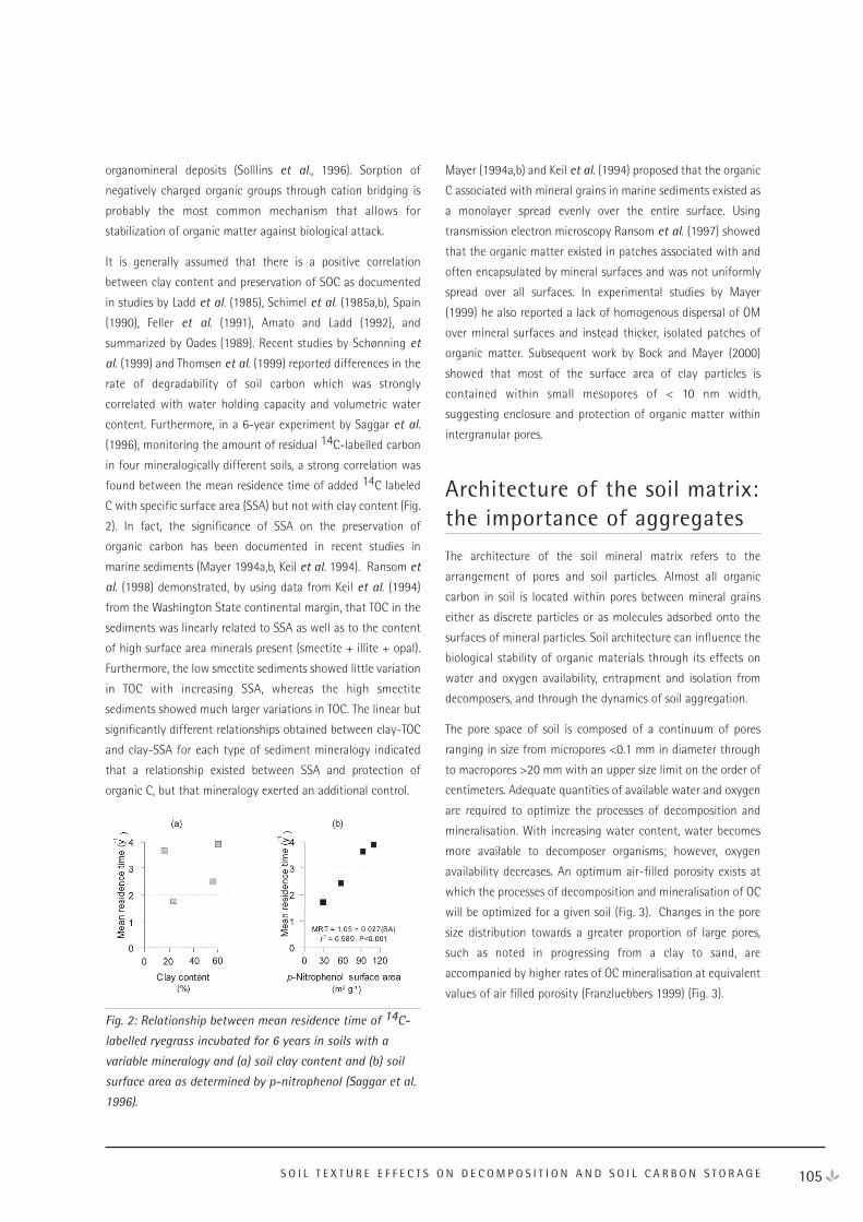
organomineral deposits (Solllins et al., 1996). Sorption of
negatively charged organic groups through cation bridging is
probably the most common mechanism that allows for
stabilization of organic matter against biological attack.
It is generally assumed that there is a positive correlation
between clay content and preservation of SOC as documented
in studies by Ladd et al. (1985), Schimel et al. (1985a,b), Spain
(1990), Feller et al. (1991), Amato and Ladd (1992), and
summarized by Oades (1989). Recent studies by Schønning et
al. (1999) and Thomsen et al. (1999) reported differences in the
rate of degradability of soil carbon which was strongly
correlated with water holding capacity and volumetric water
content. Furthermore, in a 6-year experiment by Saggar et al.
(1996), monitoring the amount of residual 14C-labelled carbon
in four mineralogically different soils, a strong correlation was
found between the mean residence time of added 14C labeled
C with specific surface area (SSA) but not with clay content (Fig.
2). In fact, the significance of SSA on the preservation of
organic carbon has been documented in recent studies in
marine sediments (Mayer 1994a,b, Keil et al. 1994). Ransom et
al. (1998) demonstrated, by using data from Keil et al. (1994)
from the Washington State continental margin, that TOC in the
sediments was linearly related to SSA as well as to the content
of high surface area minerals present (smectite + illite + opal).
Furthermore, the low smectite sediments showed little variation
in TOC with increasing SSA, whereas the high smectite
sediments showed much larger variations in TOC. The linear but
significantly different relationships obtained between clay-TOC
and clay-SSA for each type of sediment mineralogy indicated
that a relationship existed between SSA and protection of
organic C, but that mineralogy exerted an additional control.
Fig. 2: Relationship between mean residence time of 14C-
labelled ryegrass incubated for 6 years in soils with a
variable mineralogy and (a) soil clay content and (b) soil
surface area as determined by p-nitrophenol (Saggar et al.
1996).
Mayer (1994a,b) and Keil et al. (1994) proposed that the organic
C associated with mineral grains in marine sediments existed as
a monolayer spread evenly over the entire surface. Using
transmission electron microscopy Ransom et al. (1997) showed
that the organic matter existed in patches associated with and
often encapsulated by mineral surfaces and was not uniformly
spread over all surfaces. In experimental studies by Mayer
(1999) he also reported a lack of homogenous dispersal of OM
over mineral surfaces and instead thicker, isolated patches of
organic matter. Subsequent work by Bock and Mayer (2000)
showed that most of the surface area of clay particles is
contained within small mesopores of < 10 nm width,
suggesting enclosure and protection of organic matter within
intergranular pores.
Architecture of the soil matrix:the importance of aggregates
The architecture of the soil mineral matrix refers to the
arrangement of pores and soil particles. Almost all organic
carbon in soil is located within pores between mineral grains
either as discrete particles or as molecules adsorbed onto the
surfaces of mineral particles. Soil architecture can influence the
biological stability of organic materials through its effects on
water and oxygen availability, entrapment and isolation from
decomposers, and through the dynamics of soil aggregation.
The pore space of soil is composed of a continuum of pores
ranging in size from micropores <0.1 mm in diameter through
to macropores >20 mm with an upper size limit on the order of
centimeters. Adequate quantities of available water and oxygen
are required to optimize the processes of decomposition and
mineralisation. With increasing water content, water becomes
more available to decomposer organisms; however, oxygen
availability decreases. An optimum air-filled porosity exists at
which the processes of decomposition and mineralisation of OC
will be optimized for a given soil (Fig. 3). Changes in the pore
size distribution towards a greater proportion of large pores,
such as noted in progressing from a clay to sand, are
accompanied by higher rates of OC mineralisation at equivalent
values of air filled porosity (Franzluebbers 1999) (Fig. 3).
105S O I L T E X T U R E E F F E C T S O N D E C O M P O S I T I O N A N D S O I L C A R B O N S T O R A G E
Fig. 3: Changes in mineralisation of C with changes in air-
filled porosity and for uncompressed and compressed soils
with (a) 10 % clay and (b) 28 % clay (modified from
Franzleubbers 1999).
Most importantly, the pore size distribution of a soil also
influences the ability of decomposer organisms to reach
potential organic substrates. Kilbertus (1980) suggested that
bacteria can only enter pores >3 mm. Within pore sizes less
than this lower limit, decomposition of OC can only occur via
diffusion of extracellular enzymes away from organisms
towards a substrate and then diffusion of the products of
enzyme reactions back to the organisms. With increasing clay
content, the proportion of the total porosity found in small
pores increases, and the potential stabilisation of OC against
biological attack due to the exclusion of decomposer organisms
increases. Van der Linden et al. (1989) showed that protozoa
and nematodes are excluded from pores <5 mm and <30 mm,
respectively. Thus OC residing in pores smaller than these
diameters in the form of molecules, small particles, or bacterial
or fungal tissues will not be susceptible to decomposition or
predation by soil fauna.
Scanning electron micrographs of clay-organic matrices in soil
indicate that OC is not uniformly distributed in soil matrices
and that much of the OC is not in direct contact with or
intimately associated with mineral surfaces. OC can exist as
discrete particles, masses of amorphous materials typified by
the mucilage exuded by microorganisms, or individual
molecules adsorbed to mineral particles (Ladd et al. 1993,
Ransom et al. 1997). Thus, encapsulation of OC by flocculation
of clay particles, adsorption of mineral particles around organic
particles, or formation of stable aggregates will influence the
biological stability of OC as it places a physical barrier between
potential substrates and decomposer organisms or their
extracellular enzymes. Encapsulation can occur at size scales
ranging from nanometres (e.g. encapsulation of OC into pores
between packets of clay particles) to centimeters (e.g.
encapsulation of a piece of plant residue by mineral particles).
Soil mineral particles are typically bound together into larger
secondary particles referred to as aggregates. Chemical,
microbial, plant, and physical processes affect the degree of soil
aggregation. Microbes and soil animals promote aggregation by
excreting binding agents and forming fecal pellets (Lynch and
Bragg, 1985) and root exudates may flocculate colloids to bind
or stabilize aggregates (Glinski and Lipiec, 1990). The intimate
association between mineralogy, aggregation, and protection of
organic matter is suggested by the observation that Fe-oxide
rich soils and allophanic soils constitute the most firmly micro-
aggregated soils (Churchman and Tate, 1986, 1987) and that
aggregation increased and C mineralisation decreased with the
addition of Ca2+ (Muneer and Oades, 1989a,b).
Soil aggregation is a transient property and aggregates are
continually being formed and destroyed. The protection of OC
against biological attack by encapsulation within an aggregate
will be greatest where aggregate stability is high and aggregate
turnover is low. Amelung and Zech (1996) demonstrated the
influence of aggregation on the biological stability of OC. OC
buried within aggregates was associated with organic materials
having a higher C/N ratio, higher content of less biologically
altered lignin, and a higher content of neutral sugars than OC
associated with the 0 –0.5 mm external layer of aggregate
surfaces.
Maximum capacity of soils toprotect organic matter
The three mechanisms involved in the protection of OC against
biological attack in soil are determined by the mineralogy and
size distribution of soil mineral particles. For each mechanism,
only a finite amount of OC can be protected (e.g. Hassink, 1996;
Hassink et al., 1997). As a result, each soil will have a finite
capacity to protect OC against biological attack. The proportion
of OC added to a soil that can be protected will depend on the
extent of saturation of the protective capacity. In soils where
the protective capacity is not saturated, further additions of
OCwill increase soil OC contents. Where the protective capacity
is saturated, OC added to the soil will remain in a biologically
available form, be mineralized provided the appropriate suite of
decomposer organisms and environmental conditions are
present, and contribute little to soil OC content.
It is important to recognise that protection rarely equates to a
permanent and complete removal of OC from the decomposing
pool, but rather equates to a reduction in the rate of
decomposition relative to the same form of OC existing in an
106 N E E W O R K S H O P P R O C E E D I N G S : 1 8 – 2 0 A P R I L 2 0 0 1
unprotected state. One exception to this generalization may be
the potential trapping of OC within the interlayer spaces of
layer silicate clay minerals (Theng et al. 1986). As protected OC
is slowly mineralized, its position in the protected pool is filled
with new OC provided a source of the correct type of OM exists.
Physical protection in soilcarbon models
The soil carbon simulation models that will be examined in this
paper include APSIM, Soil Carbon Manager/SOCRATES,
CENTURY, CenWY, and ROTH-C. All of the models include
algorithms that attempt to account for the influence of soil
texture on OC mineralisation, and thus SOC protection, in a
direct (as individual parameters such as clay content) or indirect
way (included within other parameters, such as rate of
produced CO2).
APSIM (www.apsim-help.tag.csiro.au) does not consider directly
the physical parameters of the soil and consists of only two
SOM pools: BIOM (organic carbon associated with the labile soil
microbial biomass and microbial products) and HUM (remaining
SOC). It is assumed that some of the HUM pool, which is
specified at initialization as the amount of inert carbon, is not
subject to mineralisation. This inert carbon is similar to the
“passive pool” in other models, such as CENTURY, and is
considered the most recalcitrant fraction that remains after
long periods of decomposition (Probert et al., 1998). In order to
adjust for soil texture effects on rate of decomposition, the
proportion of HUM that includes inert C would need to be
manipulated. This is a somewhat unsatisfactory solution
because:
1 the user has to gather substantial information about the
protective capacities of a soil to decide on an appropriate
adjustment of inert carbon (alternatively, the user might be
tempted into “making the curve fit” by “blindly” adjusting
the inert carbon to achieve the desired outcome),
2 physical protection of OC is not equivalent to an inert
carbon pool as it is a transient phenomenon that can
include relatively labile OC and in turn is also subject to
destabilization and release of SOC (Baldock and Skjemstad,
2000),
3 physical protection is highly depended on attributes such
as water holding capacity, clay content, and mineralogy,
which have to be taken into account.
By comparison, SOCRATES does not use an inert pool whereas
its successor (Soil Carbon Manager) includes an inert or
charcoal pool. Soil Carbon Manager directly attempts to model
SOM protection by including clay content, CEC or soil texture
parameters, which alter the decay rate of the labile carbon pools
and determine how much carbon is released as CO2 and how
much goes into the humus (stable) and microbial biomass pools
(regression relationship between organic recycling and CO2evolution based on the CEC vs CO2/biomass data of Amato and
Ladd (1992) and Ladd et al. (1995). A greater amount of clay (or
higher CEC) is considered to physically “protect” SOM and is
calculated by estimating a value “pcorg” from CEC of the soil.
When % clay or texture (clay, silty clay, sandy loam, etc.) is
entered, CEC is calculated from the empirical formula
CEC = 11.46 * clay % - 51.3
If CEC is > 100, pcorg = (0.04 * CEC + 34.4)/100
If CEC is < 100, pcorg = (0.14 * CEC + 15.0)/100
These calculations allow for a more direct estimate of the
physical protection of OC if the amount of clay is considered to
be a reliable estimate. As outlined in this paper, clay content by
itself might not fully describe protection of SOC but these
parameters together with climatic data probably allow for a
reasonable approximation.
The latest version of the CENTURY model (Century 5) also
accounts for protection of SOC by including site parameters for
texture for each soil layer (e.g. SAND (1…10), SILT (1…10)) which
influences the turnover rate of the active SOC and the
efficiency of stabilizing active SOC into slow SOC. Century 5
also accounts for changes in texture due to erosion and
deposition events as well as for homogenization with
cultivation, which is related to the degree of disturbance and
therefore to rate of decomposition.
CenW accounts for decomposition rates by using a modified
formulation based on the original CENTURY model, which
includes an input variable for soil texture (Kirschbaum, 1999,
2000).
Roth-C 26.3 does not adjust for soil texture by using a rate
modifying factor but by altering the partitioning between CO2evolved and the sum of BIO and HUM formed during
decomposition. The ratio CO2/(BIO + HUM) = x is calculated
from the clay content of the soil:
X = 1.67 (1.85 + 1.60 exp(-0.0786 %clay))
This function results in an asymptotic decline of CO2 with
increasing clay content, approaching equilibrium at 30% clay
content. It is worthwhile noting that this equation differs from
the one given in Jenkinson (1990), which preferably uses CEC
107S O I L T E X T U R E E F F E C T S O N D E C O M P O S I T I O N A N D S O I L C A R B O N S T O R A G E
instead of clay content to account for differences in kaolinitic
vs smectitic clay.
To conclude, the incorporation of physical protection of SOC in
most soil models is only dealt with in a simplified way as clay
content or CEC. Furthermore, there is no feedback mechanism
included from other parameters such as water content or pH,
which would enhance or reduce the protective mechanism, nor
is the finite protective capacity of soil addressed. Unfortunately,
models that tried to include physical protection in a more
detailed way (such as the Verberne model: Verberne et al., 1990;
Whitmore et al., 1997) do not achieve comparably good results
as for example CENTURY or Roth-C (Smith et al., 1997). Future
models might benefit in their estimate of physical protection by
including feedback mechanisms that acknowledge the intimate
relationships that define the physical protective capacity of soil,
namely water holding capacity, specific surface area, and clay
content.
ReferencesAmato, M.A. Ladd, J.N., 1992. Decomposition of 14C-labelled
glucose and legume material in soils: properties influencing
the accumulation of organic residue C and microbial
biomass C. Soil Biology and Biochemistry 24, 455-464.
Amelung, W., Zech, W., 1996. Organic species in ped surface
and core fractions along a climosequence in the prairie,
North America. Geoderma 74, 193-206.
Aran, D., Gury, M., and Jeanroy, E., 2001, Organo-metallic
complexes in an Andosol: a comparative study with a
Cambisol and Podzol. Geoderma 99, 65-79.
Baldock, J.A,. Skjemstad, J.O., 2000. Role of the soil matrix and
minerals in protecting natural organic materials against.
Organic Geochemistry 31, 697-710.
Batjes, N.H., 1996, Total carbon and nitrogen in the soils of the
world. European Journal of Soil Science 47, 151-163.
Bock, M.J., Mayer, L.M., 2000. Mesodensity organo-clay
associations in a near-shore sediment. Marine Geology 163,
65–75.
Boudot, J.P. Bel Hadi Brahim, A., Chone, T., 1988. Dependence
of carbon and nitrogen mineralisation rates upon
amorphous metallic constituents and allophanes in
highland soils. Geoderma 42, 245-260.
Boudot, J.P., Bel Hadi Brahim, A., Steiman, R., Seigle-Murandi,
F., 1989. Biodegradation of synthetic organo-metallic
complexes of iron and aluminium with selected metal to
carbon ratios. Soil Biology and Biochemistry 21, 961-966.
Churchman, G.J., Tate, K.R., 1986. Aggregation of clay in six
New Zealand soil types as measured by disaggregation
procedures. Geoderma 37, 207-220.
Churchman, G.J., Tate, K.R., 1987. Stability of aggregates of
different size grades in allophonic soils from volcanic ash in
New Zealand. Journal of Soil Science 38, 19-27.
Duchaufour, P., 1976. Dynamics of organic matter in soils of
temperate regions: its action on pedogenesis. Geoderma
15, 31-40.
Feller, C., Fritsch, E., Poss, R., Valentin, C., 1991. Effets de la
texture sur le stockage et al. dynamique des matieres
organique dans quelque sols ferrungineux et ferrallitiques
(Afrique de l’Ouest, en particulier). Cahiers ORSTOM, Serie
Pedologie 26, 25-36.
Franzleubbers, A.J., 1999. Microbial activity in response to
water-filled pore space of variably eroded southern
Piedmont soils. Applied Soil Ecology 11, 91-101.
Gaiffe, M., Duquet, G., Tavant, H., Tavant, Y., Bruckert, S., 1984.
Stabilité biologique et comportement phyique d’un
complet argilo-humic placé dans différentes condition de
saturation en calcium ou en potassium. Plant and Soil 77,
271-284.
Glinski, J., Lipiec, J., 1990. Soil physical conditions and plant
roots. CRC Press, Boca Raton, FL.
Hassink, J., 1996. Preservation of plant residues in soil differing
in unsaturated protective capacity. Soil Science Society of
America Journal 60, 487-491
Hassink, J., Whitmore, A.P., Kubát, J., 1997. Size and density
fractionation of soil organic matter and the physical
capacity of soils to protect organic matter. European
Journal of Agronomy 7, 189-199.
Jenkinson, D.S., 1990, The turnover of organic carbon and
nitrogen in soil. Philosophical Transactions of the Royal
Society of London B 329, 361-368.
Juste, C. Delas, J., 1970. Comparison par une méthod
respirométique, des solubilités bioliquies d’un humate de
calcium et du’un humate de sodium. Comptes Rendus
Hebdomadaires des Seances de l’Academie des Sciences, D
270, 1127-1129.
Juste, C., Delas, J., Langon, M., 1975. Comparison de la
stabilités biologique de différents humates metalliques.
Comptes Rendus Hebdomadaires des Seances de
l’Academie des Sciences, D 281, 1685-1688.
108 N E E W O R K S H O P P R O C E E D I N G S : 1 8 – 2 0 A P R I L 2 0 0 1
Keil, R.G., Tsamakis, E., Fuh, C.B., Giddings, C., Hedges, J.I.,
1994. Mineralogical and textural controls on the organic
composition of coastal marine sediments: Hydrodynamic
separation using SPLITT-fractionation. Geochemica et
Cosmochimica Acta 58, 879-893.
Kilbertus, G., 1980. Microhabitats in soil aggregates. Their
relationship with bacterial biomass and size of procaryotes
present. Revue d’Ecologie et de Biologie du Sol 17, 543-
557.
Kirschbaum, M.U.F., 1999, CenW, a forest growth model with
linked carbon, energy, nutrient and water cycles. Ecological
Modelling 181: 17-59.
Kirschbaum, M.U.F., 2000, CenW: a generic forest growth
model that links carbon, nutrient and water cycles. New
Zealand Journal of Forestry 45: 15-19
Ladd, J.N., Amato, M. Oades, J.M., 1985. Decomposition of
plant materials in Australian soils. III Residual organic and
microbial biomass C and N from isotope-labelled legume
materials and soil organic matter decomposing under field
conditions. Australian Journal of Soil Research 23, 603-611.
Ladd, J. N., Foster, R.C., Skjemstad, J.O., 1993. Soil structure:
carbon and nitrogen metabolism. Geoderma 56, 401-434.
Ladd, J.N., Amato, M., Grace, P.R., Van Veen, J.A., 1995.
Simulation of 14C turnover through the microbial biomass
in soils incubated with 14C-labelled plant residues.Soil
Biology and Biochemistry 27, 777-783.
Linhares, M., 1977. Contribution de l’ion calcium à la
stabilisation biologique de la matière organique des sols.
Thése Doc. Spéc., Université de Bordeaux III.
Lynch, J.M., Bragg, E., 1985. Microorganisms and soil aggregate
stability. Australian Journal of Soil Research 27, 411-423
Martin, J.P., Ervin, J.O., Shepard, S.J., 1966. Decomposition of
the iron, aluminium, zinc, and copper salts or complexes of
some microbial and plant polysaccharides in soils. Soil
Science Society of America Proceedings 30, 196-200.
Martin, J.P., Ervin, J.O., Richards, S.J., 1972. Decomposition and
binding action of some mannose containing microbial
polysaccharides and their Fe, Al, Cu, and Zn complexes. Soil
Science 113, 322-327.
Mayer, L.M., 1994a. Surface area control of organic carbon
accumulation in continental shelf sediments. Geochimca et
Cosmochimica Acta 58, 1271-1284.
Mayer, L.M., 1994b. Relationships between mineral surfaces
and organic carbon concentrations in soils and sediments.
Chemical Geology 114, 347-363.
Mayer, L.M., 1999, Extent of coverage of mineral surfaces by
organic matter in marine sediments. Geochim. Cosmochim.
Acta 63, 207-215.
Mizota, C., Van Reeuwijk, L.P., 1989. Clay mineralogy and
chemistry of soils formed under volcanic material in diverse
climatic regions. Soil Monograph 2, ISRIC, Wageningen.
Muneer, M., Oades, J.M., 1989a. The role of Ca-organic
interactions in soil aggregate stability. 1. Laboratory studies
with 14C-glucose, CaCO3, CaSO4·2H2O. Australian Journal
of Soil Research 27, 389-399.
Muneer, M., Oades, J.M., 1989b. The role of Ca-organic
interactions in soil aggregate stability. 2. Field studies with14C-labelled straw, CaCO3, CaSO4·2H2O. Australian Journal
of Soil Research 27, 401-409.
Muneer, M., Oades, J.M., 1989c. The role of Ca-organic
interactions in soil aggregate stability. 3. Mechanisms and
models. Australian Journal of Soil Research 27, 411-423.
Nanzyo, M., Dahlgren, R., and Shoji, S., 1993, Chemical
characteristics of volcanic ash soils. In: Nanzyo, M.,
Dahlgren, R., and Shoji, S., eds., Volcanic Ash Soils. Genesis,
Properties and Utilisation. Dev. Soil Sci. 21 Elsevier,
Amsterdam, Netherlands, 145-187.
Nelson, P.N., Ladd, J.N., Oades, J.M., 1996. Decomposition of14C-labelled plant material in a salt affected soil. Soil
Biology and Biochemistry 28, 433–441.
Oades, J.M., 1988. The retention of organic matter in soils.
Biogeochemistry 5, 35-70.
Oades, J.M., 1989. An introduction to organic matter in
mineral soils. In Dixon, J.B., Weed, S.B. (Ed.) Minerals in Soil
Environments, 2nd Edition. Soil Science Society of America,
Madison, WI, USA. pp. 89-159
Probert, M.E., Dimes, J.P., Keating, B.A., Dalal, R.C., and Strong,
W.M, 1998, APSIM’s water and nitrogen modules and
simulation of the dynamics of water and nitrogen in fallow
systems. Agricultural Systems 56, 1-28.
Ransom, B., Bennett, R.H., Baerwald, R., 1997. In situ organic
matter in recent marine sediments: A TEM investigation of
organic matter preservation on continental margins and
the monolayer hypothesis. Marine Geology 138, 1-9.
Ransom, B., Kim, D., Kastner, M., Wainwright, S., 1998. Organic
matter preservation on continental slopes: Importance of
mineralogy and surface area. Geochimca et Cosmochimica
Acta 62, 1329-1345.
Saggar, S., Parshotam, A., Sparling, G.P., Feltham, C.W., Hart,
P.B.S., 1996. 14C-labelled ryegrass turnover and residence
109S O I L T E X T U R E E F F E C T S O N D E C O M P O S I T I O N A N D S O I L C A R B O N S T O R A G E
110 N E E W O R K S H O P P R O C E E D I N G S : 1 8 – 2 0 A P R I L 2 0 0 1
times in soils varying in clay content and mineralogy. Soil
Biology and Biochemistry 28, 1677-1686.
Schimel, D.S., Coleman, D.C., Horton, K.A., 1985a. Soil organic
matter dynamics in paired rangeland and cropland
toposequences in North Dakota. Geoderma 36, 201-214.
Schimel, D.S., Stillwell, M.A., Woodmansee, R.G., 1985b.
Biogeochemistry of C, N, and P in a soil catena of the short
grass steppe. Ecology 66, 276-282.
Schjønning, P., Thomsen, I.K., Møberg, J.P., de Jonge, H.,
Kristensen, K., Christensen, B.T., 1999. 1.Turnover of organic
matter in differently textured soils: I. Physical
characteristics of structurally disturbed and intact soils.
Geoderma 89, 177-198.
Smith, P., Smith, J.U., Powlson, D.S., McGill, W.B., Arah, J.R.M.,
Chertov, O.G., Coleman, K., Franko, U., Frolking, S.,
Jenkinson, D.S., Jensen, L.S., Kelly, R.H., Klein-Gunnewick, H.,
Komarov, A.S., Li, C., Molina, J.A.E., Mueller, T., Parton, W.J.,
Thornley, J.H.M., Whitmore, A.P., 1997. A comparison of the
performance of nine soil organic matter models using
datasets from seven long-term experiments. Geoderma 81,
153-225.
Sokoloff, V.P., 1938. Effect of neutral salts of sodium and
calcium on carbon and nitrogen in soils. Journal of
Agricultural Research 57, 201-216.
Sollins, P., Homann, P., and Caldwell, B.A., 1996, Stabilization
and destabilization of soil organic matter: mechanisms and
controls. Geoderma 74, 65-105
Sombroek, W.G., Nachtergaele, F.O., Hebel, A., 1993. Amounts,
dynamics and sequestering of carbon in tropical and
subtropical soils. Ambio 22, 417-426.
Spain, A. , 1990. Influence of environmental conditions and
some soil chemical properties on the carbon and nitrogen
contents of some Australian rainforest soils. Australian
Journal of Soil Research 28, 825-839.
Spain, A.V., Isbell, R.F., Probert, M.E., 1983. Soil organic matter.
In Soils, an Australian Viewpoint. CSIRO, Melbourne,
Australia/Academic Press, London, UK. pp. 551-563
Theng, B.K.G., Churchman, G.J., Newman, R.H., 1986. The
occurrence of interlayer clay-organic complexes in two
New Zealand soils. Soil Science 142, 262-266.
Thomsen, I.K., Schjønning, P., Jensen, B., Kristensen, K.,
Christensen, B.T., 1999. Turnover of organic matter in
differently textured soils. II. Microbial activity as influenced
by soil water regimes. Geoderma 89, 199-218.
van der Linden, A.M.A., Jeurisson, L.J.J., Van Veen, J.A.,
Schippers, G., 1989. Turnover of soil microbial biomass as
influence by soil compaction. In Attansen, J., Henriksen, K.
(Ed.) Nitrogen in Organic Wastes Applied to Soil. Academic
Press, London, UK. pp. 25-36.
Verberne, E.L.J., Hassink, J., de Willingen, P., Groot, J.J.R., van
Veen, J.A., 1990. Modelling organic matter dynamics in
different soils. Netherlands Journal of Agricultural Science
38, 221-238.
Whitmore, A.P., Klein-Gunnewiek, H., Crocker, G.J., Klír, J.,
Körschens, M., Poulton, P.R., 1997. Simulating trends in soil
organic carbon in long-term experiments using the
Verberne/MOTOR model. Geoderma 81, 137-151.
Zunino, H., Borie, F., Aguilera, S., Martin, J.P., Haider, K., 1982.
Decomposition of 14C-labeled glucose, plant and microbial
products and phenols in volcanic ash-derived soils of Chile.
Soil Biology and Biochemistry 14, 37-43.
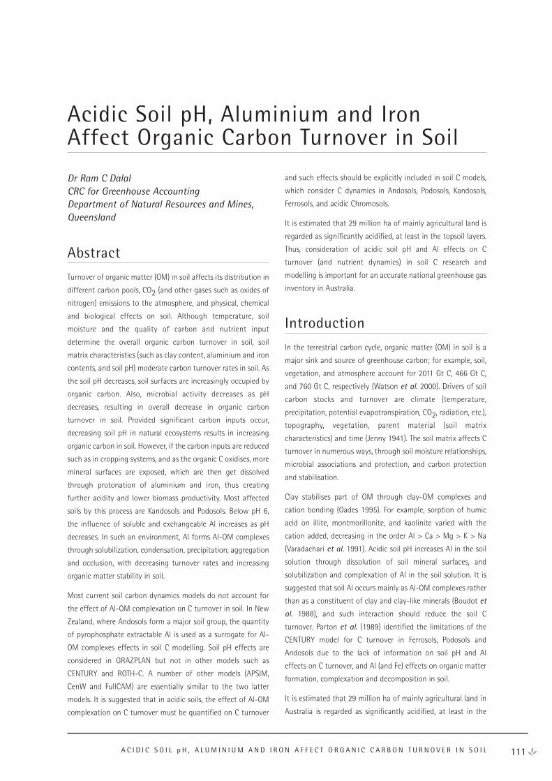
111A C I D I C S O I L p H , A L U M I N I U M A N D I R O N A F F E C T O R G A N I C C A R B O N T U R N O V E R I N S O I L
Dr Ram C DalalCRC for Greenhouse AccountingDepartment of Natural Resources and Mines,Queensland
Abstract
Turnover of organic matter (OM) in soil affects its distribution in
different carbon pools, CO2 (and other gases such as oxides of
nitrogen) emissions to the atmosphere, and physical, chemical
and biological effects on soil. Although temperature, soil
moisture and the quality of carbon and nutrient input
determine the overall organic carbon turnover in soil, soil
matrix characteristics (such as clay content, aluminium and iron
contents, and soil pH) moderate carbon turnover rates in soil. As
the soil pH decreases, soil surfaces are increasingly occupied by
organic carbon. Also, microbial activity decreases as pH
decreases, resulting in overall decrease in organic carbon
turnover in soil. Provided significant carbon inputs occur,
decreasing soil pH in natural ecosystems results in increasing
organic carbon in soil. However, if the carbon inputs are reduced
such as in cropping systems, and as the organic C oxidises, more
mineral surfaces are exposed, which are then get dissolved
through protonation of aluminium and iron, thus creating
further acidity and lower biomass productivity. Most affected
soils by this process are Kandosols and Podosols. Below pH 6,
the influence of soluble and exchangeable Al increases as pH
decreases. In such an environment, Al forms Al-OM complexes
through solubilization, condensation, precipitation, aggregation
and occlusion, with decreasing turnover rates and increasing
organic matter stability in soil.
Most current soil carbon dynamics models do not account for
the effect of Al-OM complexation on C turnover in soil. In New
Zealand, where Andosols form a major soil group, the quantity
of pyrophosphate extractable Al is used as a surrogate for Al-
OM complexes effects in soil C modelling. Soil pH effects are
considered in GRAZPLAN but not in other models such as
CENTURY and ROTH-C. A number of other models (APSIM,
CenW and FullCAM) are essentially similar to the two latter
models. It is suggested that in acidic soils, the effect of Al-OM
complexation on C turnover must be quantified on C turnover
and such effects should be explicitly included in soil C models,
which consider C dynamics in Andosols, Podosols, Kandosols,
Ferrosols, and acidic Chromosols.
It is estimated that 29 million ha of mainly agricultural land is
regarded as significantly acidified, at least in the topsoil layers.
Thus, consideration of acidic soil pH and Al effects on C
turnover (and nutrient dynamics) in soil C research and
modelling is important for an accurate national greenhouse gas
inventory in Australia.
Introduction
In the terrestrial carbon cycle, organic matter (OM) in soil is a
major sink and source of greenhouse carbon; for example, soil,
vegetation, and atmosphere account for 2011 Gt C, 466 Gt C,
and 760 Gt C, respectively (Watson et al. 2000). Drivers of soil
carbon stocks and turnover are climate (temperature,
precipitation, potential evapotranspiration, CO2, radiation, etc.),
topography, vegetation, parent material (soil matrix
characteristics) and time (Jenny 1941). The soil matrix affects C
turnover in numerous ways, through soil moisture relationships,
microbial associations and protection, and carbon protection
and stabilisation.
Clay stabilises part of OM through clay-OM complexes and
cation bonding (Oades 1995). For example, sorption of humic
acid on illite, montmorillonite, and kaolinite varied with the
cation added, decreasing in the order Al > Ca > Mg > K > Na
(Varadachari et al. 1991). Acidic soil pH increases Al in the soil
solution through dissolution of soil mineral surfaces, and
solubilization and complexation of Al in the soil solution. It is
suggested that soil Al occurs mainly as Al-OM complexes rather
than as a constituent of clay and clay-like minerals (Boudot et
al. 1988), and such interaction should reduce the soil C
turnover. Parton et al. (1989) identified the limitations of the
CENTURY model for C turnover in Ferrosols, Podosols and
Andosols due to the lack of information on soil pH and Al
effects on C turnover, and Al (and Fe) effects on organic matter
formation, complexation and decomposition in soil.
It is estimated that 29 million ha of mainly agricultural land in
Australia is regarded as significantly acidified, at least in the
Acidic Soil pH, Aluminium and IronAffect Organic Carbon Turnover in Soil
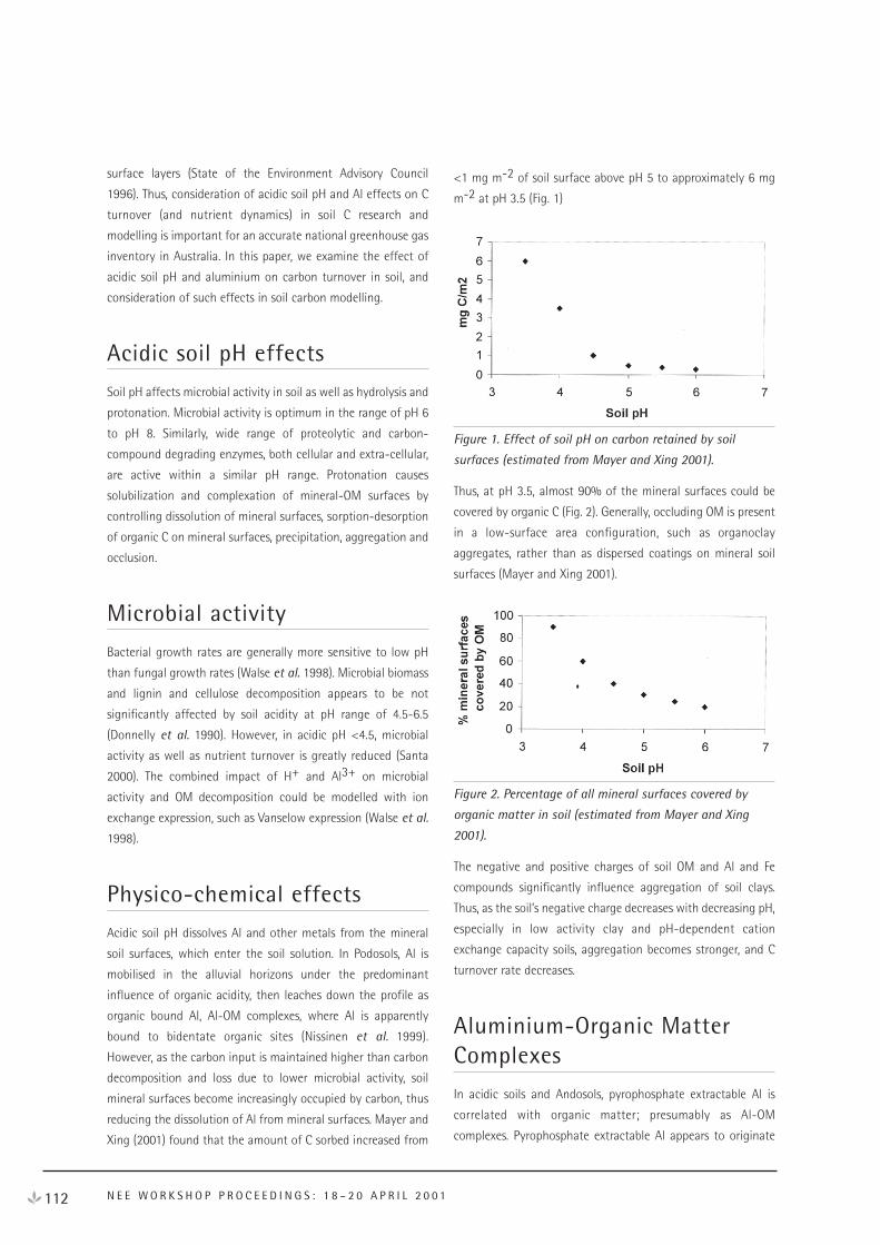
surface layers (State of the Environment Advisory Council
1996). Thus, consideration of acidic soil pH and Al effects on C
turnover (and nutrient dynamics) in soil C research and
modelling is important for an accurate national greenhouse gas
inventory in Australia. In this paper, we examine the effect of
acidic soil pH and aluminium on carbon turnover in soil, and
consideration of such effects in soil carbon modelling.
Acidic soil pH effects
Soil pH affects microbial activity in soil as well as hydrolysis and
protonation. Microbial activity is optimum in the range of pH 6
to pH 8. Similarly, wide range of proteolytic and carbon-
compound degrading enzymes, both cellular and extra-cellular,
are active within a similar pH range. Protonation causes
solubilization and complexation of mineral-OM surfaces by
controlling dissolution of mineral surfaces, sorption-desorption
of organic C on mineral surfaces, precipitation, aggregation and
occlusion.
Microbial activity
Bacterial growth rates are generally more sensitive to low pH
than fungal growth rates (Walse et al. 1998). Microbial biomass
and lignin and cellulose decomposition appears to be not
significantly affected by soil acidity at pH range of 4.5-6.5
(Donnelly et al. 1990). However, in acidic pH <4.5, microbial
activity as well as nutrient turnover is greatly reduced (Santa
2000). The combined impact of H+ and Al3+ on microbial
activity and OM decomposition could be modelled with ion
exchange expression, such as Vanselow expression (Walse et al.
1998).
Physico-chemical effects
Acidic soil pH dissolves Al and other metals from the mineral
soil surfaces, which enter the soil solution. In Podosols, Al is
mobilised in the alluvial horizons under the predominant
influence of organic acidity, then leaches down the profile as
organic bound Al, Al-OM complexes, where Al is apparently
bound to bidentate organic sites (Nissinen et al. 1999).
However, as the carbon input is maintained higher than carbon
decomposition and loss due to lower microbial activity, soil
mineral surfaces become increasingly occupied by carbon, thus
reducing the dissolution of Al from mineral surfaces. Mayer and
Xing (2001) found that the amount of C sorbed increased from
<1 mg m-2 of soil surface above pH 5 to approximately 6 mg
m-2 at pH 3.5 (Fig. 1)
Figure 1. Effect of soil pH on carbon retained by soil
surfaces (estimated from Mayer and Xing 2001).
Thus, at pH 3.5, almost 90% of the mineral surfaces could be
covered by organic C (Fig. 2). Generally, occluding OM is present
in a low-surface area configuration, such as organoclay
aggregates, rather than as dispersed coatings on mineral soil
surfaces (Mayer and Xing 2001).
Figure 2. Percentage of all mineral surfaces covered by
organic matter in soil (estimated from Mayer and Xing
2001).
The negative and positive charges of soil OM and Al and Fe
compounds significantly influence aggregation of soil clays.
Thus, as the soil’s negative charge decreases with decreasing pH,
especially in low activity clay and pH-dependent cation
exchange capacity soils, aggregation becomes stronger, and C
turnover rate decreases.
Aluminium-Organic MatterComplexes
In acidic soils and Andosols, pyrophosphate extractable Al is
correlated with organic matter; presumably as Al-OM
complexes. Pyrophosphate extractable Al appears to originate
112 N E E W O R K S H O P P R O C E E D I N G S : 1 8 – 2 0 A P R I L 2 0 0 1
from the dissolution and dispersion of Al and Al hydroxides (and
Fe hydroxides) associated with organic matter (Skjemstad 1992;
Kaiser and Zech 1996; Sollins et al. 1996). Percival et al. (2000)
found that pyrophosphate extractable Al strongly related to soil
C across all soils in New Zealand grasslands.
The Al-OM complexes are formed through the processes of
solubilization of Al and C, condensation, precipitation, and
aggregation of Al-OM complexes and their occlusion within the
soil matrix. The stability of Al-OM complexes increases as Al-OM
complexes become aggregated and occluded within the soil
matrix. Conversely, C turnover rate decreases as the extent of
aggregation and occlusion of Al-OM complexes increases in soil.
Boudot (1992) showed that C mineralisation decreased as the
Al: C ratio increased in Al-C complexes. Similarly, Tate (1992)
found that soils with very high pyrophosphate extractable Al
had very low soil C turnover, and it has been suggested that Al-
OM complexes, as determined by pyrophosphate extraction
should have a 25-year C turnover time (Veldkemp 1994).
At lower pH, Al is released from oxides, hydrous-oxides and
mineral surfaces due to dissolution and then Al complexes with
organic matter; O-alkyl sites are preferred over the alkyl sites.
Stevenson (1982) listed the major Al-OM sites, in order of
affinity, as follows: -C-OH > -NH2 > -N=N- > -COOH > -C-O-
C- >> -C=O. For aromatic C, Al-OM complexes are in the order
of affinity: -COOH-OH > -OH-OH- > -COOH-COOH > -COOH
(Tam and McColl 1990). Aluminium increases precipitation of
not only Al-OM complexes but also increases their sorption and
precipitation on other soil mineral surfaces. Moreover, Al (and
Fe) forms polyvalent cationic bonding with OM and mineral
surfaces and thereby increases aggregation (Oades 1995), for
example in Andosols, Ferrosols, Kandosols and Chromosols.
Aggregation is stabilised further through fungal activity,
producing biopolyphenols and polysaccharides. Furthermore,
Al-OM complexes become occluded within aggregates, high in
clay such as in Podosols, whereas in low clay soils, mineral
particles are occluded within Al-OM complexes.
However, refined analytical techniques are required which can
differentiate in soil the range of Al-OM complexes (Kaiser and
Zech 1996) before the C turnover rates could be studied.
Currently, decomposition rates are inferred from analytical
procedures since it is difficult to isolate intact Al-OM complexes
(Salm et al. 2000)
The Al-OM complexes are disaggregated by mechanical
disturbance, tree clearing and cultivation, loss in organic matter,
accessibility to interaggregated OM and decreased input of
aggregate stabilisers. For example, Al: C ratio declines rapidly as
the OM is lost from a pasture soil when it is converted to
cropping. Unfortunately, turnover rates of carbon in such
aggregates are not known since dynamics of these aggregates
is poorly understood.
In summary, we know about Al-OM complexes from synthetic
complexes such as Al-fulvic acid complexes, and Al-citrate
complexes. There is an indirect evidence of Al-OM complexes in
soil from regression analysis, pyrolysis and extraction
procedures but little direct evidence of Al-OM turnover rates in
soil. We know that Al-OM complexes are very important in
Ferrosols, Andosols, Chromosols and Podosols, but they play an
important role in C turnover in all soils. Hence, it is the least
understood area in OM fluxes, both in terms of C inputs and C
fluxes.
Soil carbon modelling needs to include pH and Al effects both
on Net Primary Production and C turnover. Some progress to
include pH effects has been made in GRAZPLAN (Moore et al.
1997; Andrew Moore, CSIRO Plant Industry, pers. comm.),
Gendec (Moorhead and Sinsagaugh 2000) and APSIM (Probert
et al. 1998) on nitrogen transformation but not explicitly on Al
effects on C turnover. New Zealand soil C models consider
pyrophosphate extractable Al in their C simulations to account
for passive pool in ROTH-C, based on 14C data of soil carbon
(Kevin Tate, Manaaki Whenua Landcare Research, N.Z., pers.
comm.) although explicit dynamic C turnover in Al-OM
complexes is unknown.
For example, in the current version of the GRAZPLAN, soil pH
affects C decomposition and nitrification processes.
Decomposition rates are multiplied by a modifier in the range of
0 or 1 as follows:
Z (pH) = 0 pH <= 3.2
Z (pH) = (pH-3.2)/(4.5-3.2) 3.2 < pH <= 4.5
Z (pH) = 1 pH > 4.5
Nitrification rates are multiplied by a similar modifier as
follows:
Z (pH) = 0 pH <= 3.5
Z (pH) = (pH-3.5)/(6.0-3.5) 3.5 < pH <= 6.0
Z (pH) = 1 6.0 < pH <= 8.5
Z (pH) = 1 - (pH-8.5)/(9.0-8.5) 8.5 < pH <= 9.0
Z (pH) = 0 pH > 9.0
pH values are taken in 1:5 CaCl2. These functions are crude
representations of the combined effects of pH and Al (Andrew
113A C I D I C S O I L p H , A L U M I N I U M A N D I R O N A F F E C T O R G A N I C C A R B O N T U R N O V E R I N S O I L
Moore and Richard Simpson, CSIRO Plant Industry, pers.
comm.).
Since, Australia has an estimated 29 million ha of acidic soils, it
is important to include the effects of pH and Al in C turnover in
soil C modelling and research to improve the national
greenhouse gas inventory as well as organic matter
management in these soils.
Acknowledgements
I am thankful to Andrew Moore and Kevin Tate for sharing their
ideas and information on inclusion of pH and Al in soil C
modelling.
ReferencesState of the Environment Advisory Council (1996) Land
resources. Pp.6: 31-32. Australia State of the
Environment 1996. CSIRO Publishing, Collingwood,
Victoria.
Boudot JP (1992) Relative efficiency of complexed aluminium,
non-crystalline Al hydroxides, allophane, and imogolite in
retarding the biodegradation of citric acid. Geoderma 52,
29-39.
Boudot JP, Bel Hadj BA, Chone T (1988) Dependence of carbon
and nitrogen mineralisation rates upon amorphous metallic
constituents and allophanes in highland soils. Geoderma
42, 245-260.
Donnelly PK, Entry JA, Crawford DL, Cromack K Jr (1990).
Cellulose and lignin degradation in forest soils: response to
moisture, temperature, and acidity. Microbial Ecology 20,
289-295.
Jenny H (1941) ‘Factors of soil formation’. (McGraw-Hill, New
York.)
Kaiser K, Zech W (1996) Defects in estimation of aluminium in
humus complexes of podsolic soils by pyrophosphate
extraction. Soil Science 161, 452-458.
Mayer LM, Xing B (2001) Organic matter-surface area
relationships in acid soils. Soil Science Society of America
Journal 65, 250-258.
Moore AD, Donnelly JR, Freer M (1997) GRAZPLAN: decision
support systems for Australian Grazing enterprises. III.
Pasture growth and soil moisture sub models, and the
GrassGro DSS. Agricultural Systems 55,535-582.
Moorhead DL, Sinsabaugh RL (2000) Simulated patterns of
litter decay predict patterns of extracellular enzyme
activities. Applied Soil Ecology 14, 71-79.
Nissinen A, Ilvesniemi H, Tanskanen N (1999) Equilibria of
weak acids and organic Al complexes explain activity of H+
and Al3+ in a salt extract of exchangeable cations.
European Journal of Soil Science 50, 675-686.
Oades JM (1995) Recent advances in organomineral
interactions: implications for carbon cycling and soil
structure. In ‘Environmental impact of soil component
interactions’. Vol. 1 (Eds PM Huang, J Berthelin, JM Bollag,
WB McGill, AL Page) pp. 119-134. (Lewis Publishers: Boca
Raton, FL.)
Parton WJ, Sanford RL, Sanchez PA, Stewart JWB, Bonde T,
Crosley D, van Veen H, Yost R (1989) Modelling soil organic
matter dynamics in tropical soils. In ‘Dynamics of soil
organic matter in tropical soils’. (Eds. DC Coleman, JM
Oades, G Uehara) pp. 153-171. (University of Hawaii:
Honolulu USA.)
Percival HJ, Parfitt RL, Scott NA (2000) Factors controlling soil
carbon levels in New Zealand grasslands: Is clay content
important? Soil Science Society of America Journal 64,
1623-1630.
Probert ME, Dimes JP, Keating BA, Dalal, RC, Strong WM (1998)
APSIM’s water and nitrogen modules and simulation of the
dynamics of water and nitrogen in fallow systems.
Agricultural Systems 56, 1-28.
Salm C van der, Westerveld JW, Verstraten JM (2000) Release
rates of Al from inorganic and organic compounds in a
sandy podsol, during laboratory experiments. Geoderma
96, 173-198.
Santa RI (2000) Biomass estimation and nutrient pools in four
Quercus pyrenaica in Sierra de Gata Mountains,
Salamanca, Spain. Forest Ecology and Management 132,
127-141.
Skjemstad JO (1992) Genesis of podzols on coastal dunes in
southern Queensland: III. The role of aluminium-organic
complexes in profile development. Australian Journal of
Soil Research 30, 645-665.
Sollins P, Homann P, Caldwell BA (1996) Stabilization and
destabilization of soil organic matter: Mechanisms and
controls. Geoderma 74, 65-105.
Stevenson FJ (1982) ‘Humus chemistry genesis, composition,
reactions’. p. 339 (John Wiley & Sons: New York.)
Tate KR (1992) Assessment, based on a climosequence of soil
in tussock grasslands, of soil carbon storage and release in
114 N E E W O R K S H O P P R O C E E D I N G S : 1 8 – 2 0 A P R I L 2 0 0 1

response to global warming. Journal of Soil Science 43,
697-707.
Tam SC, McColl JG (1990) Aluminium- and calcium-binding
affinities of some organic ligands in acidic conditions.
Journal of Environmental Quality 19, 514-520.
Varadachari C, Mondal AH, Ghosh K (1991) Some aspects of
clay humus complexation: Effects of exchangeable cations
and lattice charge. Soil Science 151, 220-227.
Veldkemp E (1994) Organic carbon turnover in three tropical
soils under pasture after deforestation. Soil Science
Society of America Journal 58, 175-180.
Walse C, Berg B, Sverdrup H (1998). Review and synthesis of
experimental data on organic matter decomposition with
respect to the effect of temperature, moisture, and acidity.
Environmental Reviews 6, 25-40.
Watson RT, Noble IR, Bolin B, Ravindranath NH, Verardo DJ,
Dokken DJ (2000) ‘Land Use, Land-use Change, and
Forestry: A Special Report of the IPCC’. (Cambridge
University Press: Cambridge, U.K.)
115A C I D I C S O I L p H , A L U M I N I U M A N D I R O N A F F E C T O R G A N I C C A R B O N T U R N O V E R I N S O I L
116 N E E W O R K S H O P P R O C E E D I N G S : 1 8 – 2 0 A P R I L 2 0 0 1
Jan SkjemstadCRC for Greenhouse AccountingCSIRO Land & Water
Introduction
Most models dealing with the turnover of soil organic carbon
include a soil carbon pool that is either inert or has a turnover
time measured in centuries or millennia. The strongest evidence
of the presence of such a pool or pools comes from radiocarbon
dating of soils that shows that in some cases, even in surface
horizons, the mean residence time (MRT) for organic carbon can
exceed 1000 years (Anderson and Paul, 1984). Since modern
carbon in the form of plant residues is constantly being added
to active surface soils, these soils must contain some organic
carbon which is much older than the MRT of the soil as a whole.
Several mechanisms for imparting resistance (recalcitrance)
have been evoked. These mechanisms range from strong
interaction with the mineral matrix (Hassink, 1997), chemical
recalcitrance imparted through strong humification processes
(Anderson and Paul, 1984) and the presence of significant
quantities of finely-divided charcoal (Skjemstad et al., 1998).
Despite the inclusion of inert or resistant pools in many models,
few define the nature of this material (McGill, 1996). Some
attempts have been made to measure these “old” resistant pools
with varying degrees of success. All of these methods assume
that chemical recalcitrance is the most significant factor for
long-term protection. Clay content is included in many models
and is considered to reduce decomposition rates, but only in
respect to more active pools.
In this presentation, the role of the resistant/inert/recalcitrant
pools in five specific models (APSIM, Century, CenW, RothC and
SOCRATES) is discussed along with issues of measurement both
by chemical and isotopic means.
Models and Approaches
The five models considered and means by which a highly
resistant pool is considered is given below.
APSIM considers an inert carbon (INERT-C) pool which is
uncoupled from soil carbon decomposition processes.
Profile distribution of OC has been used as an indicator of
the size of the INERT-C pool.
Century and CenW consider a passive or resistant pool,
coupled to both the slow and active pools. Carbon flow
from the slow and active pools to the passive pool is
moderated by clay content, temperature and soil water
while the decomposition of the passive pool is influenced
only by temperature and soil water. The turnover time of
the passive pool is in the order of 1000 years.
The RothC and SOCRATES models also consider an inert
organic matter (IOM) pool uncoupled from soil carbon
decomposition processes. In the RothC model, the inert
pool is considered to be radiocarbon “dead” with a turnover
time of at least 50,000 years.
Measurement of ResistantPools
In almost all cases, the size of the resistant pool is determined
by fitting the model to available site data or by regression. In
some cases, estimates of the other pools are made and the
resistant pool determined by subtraction. Radiocarbon dating
has been used in conjunction with the RothC model to estimate
the IOM pool. Here, an age is given to each of the pools and
from the radiocarbon age of the total soil carbon, the
contribution of each pool can be proportioned. In some cases,
direct measurement or estimation of this pool has been
attempted.
Estimates of the INERT-C pool of the APSIM model have been
made using the total carbon in the deeper horizons of profiles.
This assumes that the INERT-C of each horizon of the profile is
relatively constant and that almost all the carbon in the lower
profile is inert (Merv Probert pers. comm.). This approximation
probably provides data of the correct magnitude and could be
useful where no other information is available. It could
however, clearly have difficulties in soils with complex profiles
such as podzols and alluvial soils.
The passive pool of the Century model has been equated to the
non-hydrolysable soil carbon fraction (Paul et al., 1997). Acid
hydrolysis (reflux with 6M HCl) effectively removes
carbohydrate and protein materials, leaving largely intact the
more biologically recalcitrant alkyl and aryl materials. Paul et al.
(1997) demonstrated that, on average, the non-hydrolysable
Charcoal and Other Resistant Materials
carbon comprised between 23 and 70% of the soil carbon and
was about 1500 years older than the bulk soil carbon.
Soil charcoal measurements have been used as estimates of the
IOM pool in both the RothC and SOCRATES models (Skjemstad
and Janik, 1996). Charcoal, measured by 13C NMR spectroscopy
following photo-oxidation, seems to fit well with the IOM pools
of these models and although charcoal would not be expected
to be completely inert, its turnover would be expected to be at
least as slow as the Century passive pool. The difference is that
a charcoal pool would need to be uncoupled from the other soil
carbon pools but would be directly influenced by the rate and
mass of biomass burning.
Controversies
Inert?A major issue with a number of the models discussed above is
whether any organic based material can in fact be inert or even
turn over in time spans of tens of millennia in a biologically
active surface soil. The radiocarbon age of surface soil samples
rarely exceeds 2,000 years and is often no more than a few
hundred years (Leavitt et al. 1996). This suggests that very old,
inert pools can not be significant in most surface soils and
should not show a high degree of variability among different
soil types. Evidence suggests that this is not so however, and
that equilibrium values for soil carbon under exploitive
cropping conditions can be highly variable (Dalal and Mayer,
1984).
Chemical or Physical?The only major mechanisms that can provide a high degree of
protection to soil organic matter are chemical recalcitrance, a
strong interaction with the mineral matrix in such a way that
the protected material is effectively removed from the
biosphere or a combination of both. The former mechanism
suggests the formation of organic moieties that are chemically
different to the more labile pools or at least contain functional
groups that impart recalcitrance. Both aromatic (Skjemstad et
al., 1996) and long-chained alkyl (Baldock et al., 1992)
structures have been suggested as candidates for imparting
biological recalcitrance to soil organic matter.
During exploitive cultivation, plant residue inputs are low and
soil carbon levels can be reduced to as little as 30% of the
carbon in the initial undisturbed surface horizon (Dalal and
Mayer, 1986). Under these conditions, any highly recalcitrant
organic moiety should be concentrated as the more active soil
carbon pools decrease. Using solid-state 13C NMR spectroscopy,
Skjemstad et al. (2001) showed that the only functional group
that showed a relative increase with prolonged cropping was
the aryl-C and this could be attributed to the presence of
charcoal. The alkyl carbons remained constant or declined.
It therefore seems unlikely that physical processes are involved
in the long-term protection of soil organic matter. Adsorption
processes such as clay-OM and metal-OM interactions can be
demonstrated to slow decomposition processes (Martin and
Haider, 1986), but it is unlikely that these processes can slow
decomposition enough to give the high MRTs measured in
biologically active surface soils.
Radiocarbon datingSince charcoal is highly resistant to biological decomposition
and other oxidative processes, the presence of aryl carbon in the
form of finely-divided (<53 mm) charcoal is a significant factor
in determining the turnover of soil carbon. Few attempts have
been made to measure the age of finely divided soil charcoals.
Skjemstad et al. (1996) showed for one Australian soil that the
photo-oxidation resistant carbon fraction, which was >70%
charcoal, was in fact ~1,300 years older than the bulk soil.
Similarly, charcoal separated by photo-oxidation from a set of
German soils was shown to be as much as 4000 years older than
the bulk soil (unpublished data). In one case, the differences
were not large but here the MRT of the bulk soil was ~5,000
years.
Leavitt et al., (1996) showed for 30 surface soil samples that
reflux with 6M HCl also increased the radiocarbon age of the
organic matter by about 1000 y. Both acid hydrolysis and
photo-oxidation therefore appear to selectively remove
younger carbon and preserve older carbon. Either method
therefore probably effectively separates a fraction which could
be used as a passive or “inert” fraction in soil carbon modelling,
at least in surface soils.
Invariably, soil organic carbon age increases with depth,
indicating that turnover rates also increase with depth. In most
soils, there is very little change in the chemistry of soil organic
matter with increasing depth. Polysaccharides often decrease
with depth reflecting a decrease in plant residues but this
decrease is not sufficient to account for the large increases in
radiocarbon age. With increasing depth, microbial biomass and
activity decline leaving larger volumes of soil with very low, if
any, biological activity. Organic materials that survive the initial
processes of decomposition would be effectively removed from
contact with the biosphere and coupled with physical
117C H A R C O A L A N D O T H E R R E S I S T A N T M A T E R I A L S
protection mechanisms that prevent their movement in the soil,
could remain isolated from the biosphere for many years
perhaps even millennia. Both of the methods discussed above
assume recalcitrance inferred through chemical structure of the
substrate and therefore would be inadequate for establishing a
soil carbon pool structure in subsoils. Here, it might be more
appropriate to decrease turnover rates of the slower pools to
compensate for reduced biological activity.
For models like Century where the passive pool is coupled to the
turnover of the other pools, a high radiocarbon age for the
passive pool would be expected. Material is cycled through the
slow and passive pools repeatedly so that the most recalcitrant
“old” material accumulates. If charcoal is considered however,
fire history and transport processes may be more important. For
ecosystems with long fire histories, charcoal should form the
basis of an “old” pool but if fire history was only recent, then
this recalcitrant pool could have a relative young radiocarbon
age.
MethodologiesA comparison of the amount and nature of the material
remaining after acid hydrolysis or photo-oxidation treatments
for a <53 mm fraction from a duplex soil showed that the acid
hydrolysis method recovered about 40% of the original carbon
whereas the photo-oxidation method recovered only 25%
(unpublished data). Similarly, the chemical nature of the two
fractions were different. The hydrolyzed fraction consisted of a
mixture of aryl (including charcoal) and long-chained alkyl
materials while the photo-oxidized fraction was dominated by
aryl carbon (charcoal). The two methods therefore clearly
recover different organic moieties and are not interchangeable.
Even with the measurement of charcoal or black carbon (BC),
methods and recoveries vary considerably. Schmidt et al. (2001)
compared five different methods of BC estimation and found
that the photo-oxidation method could recover >500 times
more BC than some of the thermal methods. Since BC is a
continuum of combustion products from lightly charred
biomass to refractory soot, it is likely that the different methods
determine different windows in the continuum. Many of the
thermal methods, which are thought to determine soot, showed
little variation in BC between soil types and so would have little
value for soil carbon modelling purposes. It is clear however,
that better comparisons of analytical techniques are required
together with better definitions of what is being determined.
Conclusions
Soil carbon turnover models require a pool with a turnover time
probably exceeding 1,000 years to account for the relative old
radiocarbon ages measured in some surface soils. Although a
number of “old” recalcitrant fractions of organic carbon can be
separated from soil and can show radiocarbon ages much older
than the bulk soil, none of these can be defined as truly inert.
Chemical recalcitrance appears to be the only mechanism by
which soil organic carbon can be protected for long periods of
time in active surface soils. 13C NMR studies show that the only
chemical structures that appear to survive decomposition
processes are aryl in nature and are mostly due to finely-divided
charcoal. For longer-term modelling, some estimates of the rate
of charcoal production will need to be considered. Some long-
chained alkyl materials may also be resistant to decomposition.
Of the techniques used to measure resistant soil organic matter,
only two, photo-oxidation and acid hydrolysis, appear to show
promise. These methods both recover relatively old pools but
appear to determine different fractions of carbon and are not
interchangeable. A combination of these techniques may be
more informative, but better estimates of the turnover times of
these fractions are needed.
ReferencesAnderson, D.W. and Paul, E.A. (1984). Organo-mineral
complexes and their study by radiocarbon dating. Soil
Science Society of America Journal 48: 298-301.
Baldock, J.A., Oades, J.M., Waters, A.G., Peng, X., Vassallo, A.M.
and Wilson, M.A. (1992). Aspects of the chemical structure
of soil organic materials as revealed by solid-state 13C
NMR spectroscopy. Australian Journal of Soil Research
28: 213-225.
Dalal, R.C. and Mayer, R.J. (1986). Long-term trends in fertility
of soils under continuous cultivation and cereal cropping in
southern Queensland. II Total organic carbon and its rate of
loss from the soil profile. Australian Journal of Soil
Research 24: 281-292.
Hassink, J. (1997). The capacity of soils to preserve organic C
and N by their association with clay and silt particles. Plant
and Soil 191: 77-81.
Leavitt, S.W., Follett, R.F. and Paul, E.A. (1996). Estimation of
slow- and fast-cycling soil organic carbon pools from 6N
HCl Hydrolysis. Radiocarbon 38: 231-239.
118 N E E W O R K S H O P P R O C E E D I N G S : 1 8 – 2 0 A P R I L 2 0 0 1
Martin, J.P. and Haider, K. (1986). Influence of mineral colloids
on turnover rates of soil organic matter. In “Interactions of
Soil Minerals with Natural Organics and Microbes.” Eds.
P.M. Huang and M. Schnitzer. pp.283-304. SSSA Special
Publication Number 17. (SSSA, Inc. Madison, Wisconsin,
USA).
McGill, W.B. (1996). Review and classification of ten soil
organic matter models. In “Evaluation of Soil Organic
Matter Models.” Eds. D.S. Powlson, P. Smith and J.U. Smith.
pp. 111-132. NATO ANSI Series no 1, vol 38. (Springer
Verlag).
Paul, E.A., Follett, R.F., Leavitt, S.W., Halvorson, A., Peterson, G.A.
and Lyon, D.J. (1997). Radiocarbon dating for
determination of soil organic matter pool sizes and
dynamics. Soil Science Society of America Journal 61:
1058-1067.
Schmidt, M.W.I., Skjemstad, J.O., Czimczik, C.I., Glaser, B.,
Prentice, K.M., Gelinas, Y. and Kuhlbusch, T.A.J. (2001).
Comparative analysis of black carbon in soils. Global
Biogeochemical Cycles. 15: 163-168.
Skjemstad, J.O., Clarke, P., Taylor, J.A., Oades, J.M. and McClure,
S.G. (1996). The chemistry and nature of protected carbon
in soil. Australian Journal of Soil Research 34: 251-271.
Skjemstad, J.O., Dalal, R.C., Janik, L.J. and McGowan, J.A. (2001).
Changes in chemical nature of soil organic carbon in
Vertisols under wheat in southeastern Australia. Australian
Journal of Soil Research 39: 343-359.
Skjemstad, J.O. and Janik, L.J. (1996). Climate change:
determining the potential for carbon sequestration in
Australian soils. Final Report for RIRDC Project CSO-5A.
Skjemstad, J.O., Janik, L.J. and Taylor, J.A. (1998). Non-living soil
organic matter: what do we know about it? Australian
Journal of Experimental Agriculture 38: 667-680.
119C H A R C O A L A N D O T H E R R E S I S T A N T M A T E R I A L S
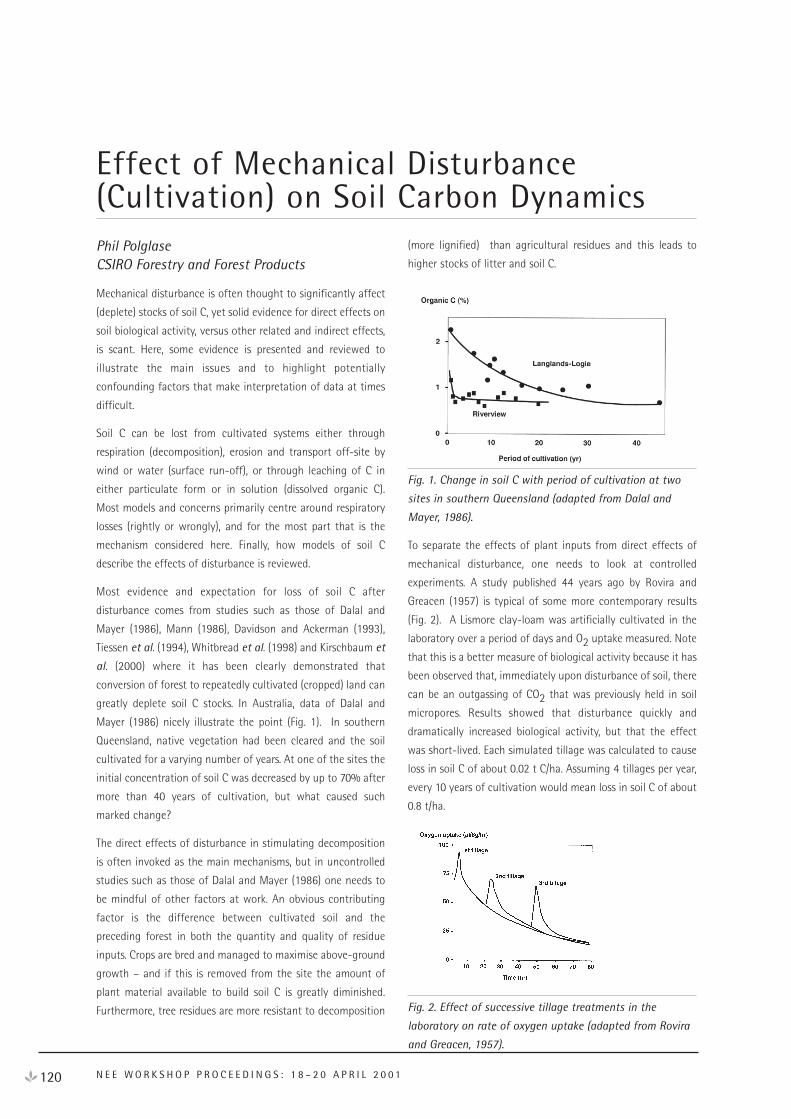
120 N E E W O R K S H O P P R O C E E D I N G S : 1 8 – 2 0 A P R I L 2 0 0 1
Phil PolglaseCSIRO Forestry and Forest Products
Mechanical disturbance is often thought to significantly affect
(deplete) stocks of soil C, yet solid evidence for direct effects on
soil biological activity, versus other related and indirect effects,
is scant. Here, some evidence is presented and reviewed to
illustrate the main issues and to highlight potentially
confounding factors that make interpretation of data at times
difficult.
Soil C can be lost from cultivated systems either through
respiration (decomposition), erosion and transport off-site by
wind or water (surface run-off), or through leaching of C in
either particulate form or in solution (dissolved organic C).
Most models and concerns primarily centre around respiratory
losses (rightly or wrongly), and for the most part that is the
mechanism considered here. Finally, how models of soil C
describe the effects of disturbance is reviewed.
Most evidence and expectation for loss of soil C after
disturbance comes from studies such as those of Dalal and
Mayer (1986), Mann (1986), Davidson and Ackerman (1993),
Tiessen et al. (1994), Whitbread et al. (1998) and Kirschbaum et
al. (2000) where it has been clearly demonstrated that
conversion of forest to repeatedly cultivated (cropped) land can
greatly deplete soil C stocks. In Australia, data of Dalal and
Mayer (1986) nicely illustrate the point (Fig. 1). In southern
Queensland, native vegetation had been cleared and the soil
cultivated for a varying number of years. At one of the sites the
initial concentration of soil C was decreased by up to 70% after
more than 40 years of cultivation, but what caused such
marked change?
The direct effects of disturbance in stimulating decomposition
is often invoked as the main mechanisms, but in uncontrolled
studies such as those of Dalal and Mayer (1986) one needs to
be mindful of other factors at work. An obvious contributing
factor is the difference between cultivated soil and the
preceding forest in both the quantity and quality of residue
inputs. Crops are bred and managed to maximise above-ground
growth – and if this is removed from the site the amount of
plant material available to build soil C is greatly diminished.
Furthermore, tree residues are more resistant to decomposition
(more lignified) than agricultural residues and this leads to
higher stocks of litter and soil C.
Fig. 1. Change in soil C with period of cultivation at two
sites in southern Queensland (adapted from Dalal and
Mayer, 1986).
To separate the effects of plant inputs from direct effects of
mechanical disturbance, one needs to look at controlled
experiments. A study published 44 years ago by Rovira and
Greacen (1957) is typical of some more contemporary results
(Fig. 2). A Lismore clay-loam was artificially cultivated in the
laboratory over a period of days and O2 uptake measured. Note
that this is a better measure of biological activity because it has
been observed that, immediately upon disturbance of soil, there
can be an outgassing of CO2 that was previously held in soil
micropores. Results showed that disturbance quickly and
dramatically increased biological activity, but that the effect
was short-lived. Each simulated tillage was calculated to cause
loss in soil C of about 0.02 t C/ha. Assuming 4 tillages per year,
every 10 years of cultivation would mean loss in soil C of about
0.8 t/ha.
Fig. 2. Effect of successive tillage treatments in the
laboratory on rate of oxygen uptake (adapted from Rovira
and Greacen, 1957).
Effect of Mechanical Disturbance(Cultivation) on Soil Carbon Dynamics
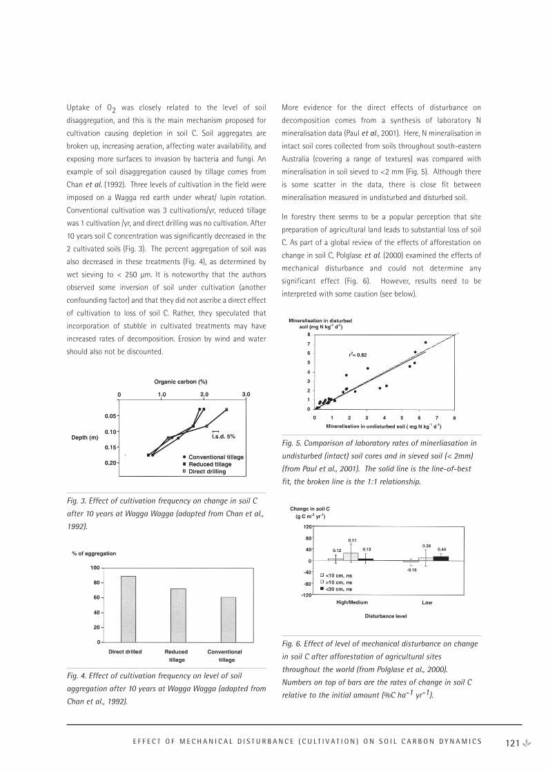
Uptake of O2 was closely related to the level of soil
disaggregation, and this is the main mechanism proposed for
cultivation causing depletion in soil C. Soil aggregates are
broken up, increasing aeration, affecting water availability, and
exposing more surfaces to invasion by bacteria and fungi. An
example of soil disaggregation caused by tillage comes from
Chan et al. (1992). Three levels of cultivation in the field were
imposed on a Wagga red earth under wheat/ lupin rotation.
Conventional cultivation was 3 cultivations/yr, reduced tillage
was 1 cultivation /yr, and direct drilling was no cultivation. After
10 years soil C concentration was significantly decreased in the
2 cultivated soils (Fig. 3). The percent aggregation of soil was
also decreased in these treatments (Fig. 4), as determined by
wet sieving to < 250 µm. It is noteworthy that the authors
observed some inversion of soil under cultivation (another
confounding factor) and that they did not ascribe a direct effect
of cultivation to loss of soil C. Rather, they speculated that
incorporation of stubble in cultivated treatments may have
increased rates of decomposition. Erosion by wind and water
should also not be discounted.
Fig. 3. Effect of cultivation frequency on change in soil C
after 10 years at Wagga Wagga (adapted from Chan et al.,
1992).
Fig. 4. Effect of cultivation frequency on level of soil
aggregation after 10 years at Wagga Wagga (adapted from
Chan et al., 1992).
More evidence for the direct effects of disturbance on
decomposition comes from a synthesis of laboratory N
mineralisation data (Paul et al., 2001). Here, N mineralisation in
intact soil cores collected from soils throughout south-eastern
Australia (covering a range of textures) was compared with
mineralisation in soil sieved to <2 mm (Fig. 5). Although there
is some scatter in the data, there is close fit between
mineralisation measured in undisturbed and disturbed soil.
In forestry there seems to be a popular perception that site
preparation of agricultural land leads to substantial loss of soil
C. As part of a global review of the effects of afforestation on
change in soil C, Polglase et al. (2000) examined the effects of
mechanical disturbance and could not determine any
significant effect (Fig. 6). However, results need to be
interpreted with some caution (see below).
Fig. 5. Comparison of laboratory rates of minerliasation in
undisturbed (intact) soil cores and in sieved soil (< 2mm)
(from Paul et al., 2001). The solid line is the line-of-best
fit, the broken line is the 1:1 relationship.
Fig. 6. Effect of level of mechanical disturbance on change
in soil C after afforestation of agricultural sites
throughout the world (from Polglase et al., 2000).
Numbers on top of bars are the rates of change in soil C
relative to the initial amount (%C ha-1 yr-1).
121E F F E C T O F M E C H A N I C A L D I S T U R B A N C E ( C U L T I V A T I O N ) O N S O I L C A R B O N D Y N A M I C S
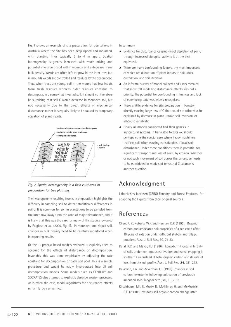
Fig. 7 shows an example of site preparation for plantations in
Australia where the site has been deep ripped and mounded,
with planting lines typically 3 to 4 m apart. Spatial
heterogeneity is greatly increased with much mixing and
potential inversion of soil within mounds, and a decrease in soil
bulk density. Weeds are often left to grow in the inter-row, but
in mounds weeds are controlled and residues left to decompose.
Thus, when trees are young, soil in the mound has few inputs
from fresh residues whereas older residues continue to
decompose, in a somewhat inverted soil. It should not therefore
be surprising that soil C would decrease in mounded soil, but
not necessarily due to the direct effects of mechanical
disturbance, rather it is equally likely to be caused by temporary
cessation of plant inputs.
Fig. 7. Spatial heterogeneity in a field cultivated in
preparation for tree planting.
The heterogeneity resulting from site preparation highlights the
difficulty in sampling soil to detect statistically differences in
soil C. It is common for soil in plantations to be sampled from
the inter-row, away from the zone of major disturbance, and it
is likely that this was the case for many of the studies reviewed
by Polglase et al., (2000, Fig. 6). In mounded and ripped soil,
changes in bulk density need to be carefully monitored when
interpreting results.
Of the 11 process-based models reviewed, 6 explicitly tried to
account for the effects of disturbance on decomposition.
Invariably this was done empirically by adjusting the rate
constant for decomposition of each soil pool. This is a simple
procedure and would be easily incorporated into all soil
decomposition models. Some models such as CENTURY and
SOCRATES also attempt to explicitly describe erosion processes.
As is often the case, model algorithms for disturbance effects
remain largely unverified.
In summary,
Evidence for disturbance causing direct depletion of soil C
through increased biological activity is at the best
equivocal.
There are many confounding factors, the most important
of which are disruption of plant inputs to soil under
cultivation, and soil inversion.
An informal survey of model builders and users revealed
that most felt modelling disturbance effects was not a
priority. The potential for confounding influences and lack
of convincing data was widely recognised.
There is little evidence for site preparation in forestry
directly causing large loss of C that could not otherwise be
explained by decrease in plant uptake, soil inversion, or
inherent variability.
Finally, all models considered had their genesis in
agricultural systems. In harvested forests we should
perhaps note the special case where heavy machinery
trafficks soil, often causing considerable, if localised,
disturbance. Under these conditions there is potential for
significant transport and loss of soil C by erosion. Whether
or not such movement of soil across the landscape needs
to be considered in models of terrestrial C balance is
another question.
Acknowledgment
I thank Kris Jacobsen (CSIRO Forestry and Forest Products) for
adapting the Figures from their original sources.
ReferencesChan, K. Y., Roberts, W.P. and Heenan, D.P. (1992). Organic
carbon and associated soil properties of a red earth after
10 years of rotation under different stubble and tillage
practices. Aust. J. Soil Res., 30, 71-83.
Dalal, R.C. and Mayer, R.J. (1986). Long-term trends in fertility
of soils under continuous cultivation and cereal cropping in
southern Queensland. II Total organic carbon and its rate of
loss from the soil profile. Aust. J. Soil Res., 24, 281-292.
Davidson, E.A. and Ackerman, I.L. (1993). Changes in soil
carbon inventories following cultivation of previously
amended soils. Biogeochem., 20, 161-193.
Kirschbaum, M.U.F., Murty, D., McGilvray, H. and McMurtrie,
R.E. (2000): How does soil organic carbon change after
122 N E E W O R K S H O P P R O C E E D I N G S : 1 8 – 2 0 A P R I L 2 0 0 1

conversion from forest to agricultural land uses? Climate
Change Newsletter, Bureau of Resource Sciences 12: 5-7.
Mann, L.K. (1986). Changes in soil carbon storage after
cultivation. Soil Sci., 142, 279-288.
Paul, K.I., Polglase, P.J., O’Connell, A.M. , and Carlyle, J.C. (2001).
Soil Nitrogen Availability Predictor (SNAP): A method to
estimate nitrogen mineralisation in forest soils. Divisional
Report. CSIRO Forestry and Forest Products, Canberra.
Polglase, P.J., Paul, K, I, Khanna, P.K., Nyakuengama, J.G.,
O’Connell, A.M., Grove, T.S., and Battaglia, M. (2000).
Change in soil carbon following afforestation or
reforestation: Review of experimental evidence and
development of a conceptual framework. National Carbon
Accounting System Technical Report No. 20. Australian
Greenhouse Office:Canberra. 102 p.
Rovira, A. D. and Greacen, E.L. (1957). The effect of aggregate
disruption on the activity of microorgansims in the soil.
Aust. J. Agric. Res., 8, 659-679.
Tiessen, Cuevas, E., and Chacon, P. (1994). The role of soil
organic matter in sustaining soil fertility. Nature, 371, 783-
785.
Whitbread, A.M., Lefroy, R.D.B., and Blair, G.J. (1998). A survey
of the impacts of cropping on soil physical and chemical
properties in north-western New South Wales. Aust. J. Soil.
Res., 36, 669-681.
123E F F E C T O F M E C H A N I C A L D I S T U R B A N C E ( C U L T I V A T I O N ) O N S O I L C A R B O N D Y N A M I C S
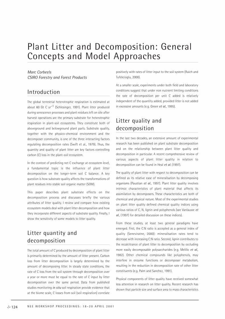
124 N E E W O R K S H O P P R O C E E D I N G S : 1 8 – 2 0 A P R I L 2 0 0 1
Marc CorbeelsCSIRO Forestry and Forest Products
Introduction
The global terrestrial heterotrophic respiration is estimated at
about 60 Gt C yr-1 (Schlesinger, 1991). Plant litter produced
during senescence processes and plant residues left on site after
harvest operations are the primary substrate for heterotrophic
respiration in plant-soil ecosystems. They constitute both of
aboveground and belowground plant parts. Substrate quality,
together with the physico-chemical environment and the
decomposer community, is one of the three interacting factors
regulating decomposition rates (Swift et al., 1979). Thus, the
quantity and quality of plant litter are key factors controlling
carbon (C) loss in the plant-soil ecosystem.
In the context of predicting net C exchange at ecosystem level,
a fundamental topic is the influence of plant litter
decomposition on the longer-term soil C balance. A key
question is how substrate quality affects the transformations of
plant residues into stable soil organic matter (SOM).
This paper describes plant substrate effects on the
decomposition process and discusses briefly the various
attributes of litter quality. I review and compare how existing
ecosystem models deal with plant litter decomposition and how
they incorporate different aspects of substrate quality. Finally, I
show the sensitivity of some models to litter quality.
Litter quantity anddecomposition
The total amount of C produced by decomposition of plant litter
is primarily determined by the amount of litter present. Carbon
loss from litter decomposition is largely determined by the
amount of decomposing litter. In steady state conditions, the
rate of C loss from the soil system through decomposition over
a year or more must be equal to the rate of C input by litter
decomposition over the same period. Data from published
studies monitoring in situ soil respiration provide evidence that
at the biome scale, C losses from soil (soil respiration) correlate
positively with rates of litter input to the soil system (Raich and
Tufekcioglu, 2000).
At a smaller scale, experiments under both field and laboratory
conditions suggest that under non nutrient limiting conditions
the rate of decomposition per unit C added is relatively
independent of the quantity added, provided litter is not added
in excessive amounts (e.g. Green et al., 1995).
Litter quality anddecomposition
In the last two decades, an extensive amount of experimental
research has been published on plant substrate decomposition
and on the relationship between plant litter quality and
decomposition in particular. A recent comprehensive review of
various aspects of plant litter quality in relation to
decomposition can be found in Heal et al. (1997).
The quality of plant litter with respect to decomposition can be
defined as its relative ease of mineralisation by decomposing
organisms (Paustian et al., 1997). Plant litter quality involves
intrinsic characteristics of plant material that affects its
assimilation by decomposers. These characteristics are both of
chemical and physical nature. Most of the experimental studies
on plant litter quality defined chemical quality indices using
various ratios of C, N, lignin and polyphenols (see Vanlauwe et
al., (1997) for detailed discussion on these indices).
From these studies, at least two general paradigms have
emerged. First, the C:N ratio is accepted as a general index of
quality (Seneviratne, 2000): mineralisation rates tend to
decrease with increasing C:N ratio. Second, lignin contributes to
the recalcitrance of plant litter to decomposition by occluding
more easily decomposable polysaccharides (e.g. Melillo et al.,
1982). Other chemical compounds like polyphenols, may
interfere in enzyme functions or decomposer metabolism,
resulting in the reduction in decomposition rate of other litter
constituents (e.g. Palm and Sanchez, 1991).
Physical components of litter quality have received somewhat
less attention in research on litter quality. Recent research has
shown that particle size and surface area to mass characteristics
Plant Litter and Decomposition: GeneralConcepts and Model Approaches
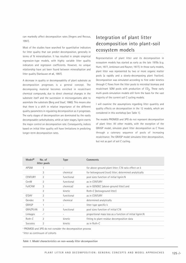
125P L A N T L I T T E R A N D D E C O M P O S I T I O N : G E N E R A L C O N C E P T S A N D M O D E L A P P R O A C H E S
can markedly affect decomposition rates (Angers and Recous,
1997).
Most of the studies have searched for quantitative indicators
for litter quality that can predict decomposition, generally in
terms of N mineralisation. It has resulted in simple empirical
regression-type models, with highly variable litter quality
indicators and regression coefficients. However, no unique
relationship have yet been found between mineralisation and
litter quality (Vanlauwe et al., 1997).
A decrease in quality or decomposability of plant substrate as
decomposition progresses is a general concept. The
decomposing material becomes enriched in recalcitrant
chemical compounds, due to direct chemical changes in the
substrate itself and the succession in microorganisms able to
assimilate the substrate (Berg and Staaf, 1980). This means also
that there is a shift in relative importance of the different
quality parameters in regulating decomposition as it progresses.
The early stages of decomposition are dominated by the easily
decomposable carbohydrates, while at later stages, lignin exerts
the major control on decomposition rate. Consequently, indices
based on initial litter quality will have limitations in predicting
longer-term decomposition rates.
Integration of plant litterdecomposition into plant-soilecosystem models
Representation of plant litter and its decomposition in
ecosystem models has started as early as the late 1970s (e.g.
Hunt, 1977, Jenkinson and Rayner, 1977). In those early models,
plant litter was represented by two or more organic matter
pools (a rapidly and a slowly-decomposing plant fraction).
Decomposition was simulated according to first order kinetics
through C flows from the litter pools to microbial biomass and
recalcitrant SOM pools with production of CO2. These early
multi-pools simulation models still form the basis for the vast
majority of the current soil C cycling models.
I will examine the assumptions regarding litter quantity and
quality effects on decomposition in the 12 models, which are
considered in this workshop (see Table 1).
The models PROMOD and 3PG do not represent decomposition
of plant litter. All other models, with the exception of the
GRASP model, simulate plant litter decomposition as C flows
through a catenary sequence of pools of increasing
recalcitrance. The GRASP model simulates litter decomposition,
but not as part of soil C cycling.
Modela No. of Type Commentslitter pools
APSIM 1 - for above-ground plant litter; C:N ratio effect on k
3 chemical for belowground (root) litter; determined analytically
CENTURY 2 functional pool sizes function of initial lignin:N
CenW 2 functional as in CENTURY
FullCAM 3 chemical/ as in GENDEC (above-ground litter) and
2 kinetic Roth-C (belowground litter)
G’DAY 2 functional as in CENTURY
Gendec 3 chemical determined analytically
GRASP 1 - litter type specific k
GRAZPLAN 2 functional pool sizes function of initial C:N
Linkages -b - proportional mass loss as a function of initial lignin:N
Roth-C 2 kinetic fitting to plant residue decomposition data
Socrates 2 kinetic as in Roth-C
a PROMOD and 3PG do not consider the decomposition processb litter as continuum of cohorts
Table 1. Model characteristics on non-woody litter decomposition
Plant substrate for decomposition is represented as a single C
pool in the APSIM (in the case of above-ground litter) and
GRASP models. In those models, the only option to incorporate
litter quality is by varying the specific decomposition rate k as a
function of litter type. For example, simulations with APSIM
suggest that the k value for E. grandis litter (0.025 day-1) is
considerable lower than a default value (0.1 day-1) proposed by
Probert et al. (1998) for simulations of mineralisation dynamics
in grain and/or legume cropping systems. This is despite the
incorporation of a decay rate modifier, which is a function of
the initial residue C:N ratio. Also, simulation of the
decomposition of sugar cane residues indicated that the C:N
factor on decomposition did not describe the litter quality
effects satisfactorily (Thorburn et al., 2001). These results
suggest the need for a more complex description of plant litter
decomposition to overcome the requirement of residue-specific
k values.
The Linkages model considers plant substrate for decomposition
as a continuum of cohorts, which represent annual inputs of
species-specific litter at various stages of decomposition. For
non-woody litter, the lignin:N ratio is used as a quality attribute
and it is assumed that percent mass loss for a given site is
linearly related to this ratio. The Linkages model is an empirical
regression-type model and, hence, limited to the conditions for
which it has been developed. Once a litter cohort reaches an
advanced critical stage of decomposition, it is transferred to a
combined pool of soil humus.
The other simulation models represent plant substrates by two
or more discrete C pools, but differ in their criteria of
compartmentalisation (Table 1). These criteria can be chemically,
kinetically or functionally defined.
One of the first multi-pool decomposition models was
developed by Minderman (1968) and included several
analytically determined chemical fractions of plant substrates.
Chemically defined pools recognize the discrete chemical
components of litter, but the question arises whether the
individual chemical fractions decompose independently. The
Gendec and APSIM (for root litter) models distinguish three
discrete chemical components of plant litter: labile
carbohydrates (water-soluble), holocellulose and acid-insoluble
(lignin-like) compounds. These pools can be analytically
determined through a proximate analysis, e.g. the Van Soest
Acid Detergent Fiber method. Simulations with models
adopting this approach indicated that for short-term C
decomposition of plant residues under laboratory conditions,
litter quality can be well represented by the Van Soest fractions,
provided that interactions are considered between different
compounds (Corbeels et al., 1999; Henriksen and Breland,
1999).
Kinetically defined pools are conceptual substrate fractions that
are determined by fitting the decomposition model to
experimental data on substrate decomposition. Double
exponential decay models are an example of models with
kinetically defined pools (e.g. O’Connell, 1997). The combination
of a relative small labile pool with a larger, more resistant pool
is a good description of the two phase decomposition of most
plant residues: a rapid initial loss, followed by a slower mass loss
rate. This type of models generally fit short-term decomposition
of plant residues well. Kinetically defined pools do not directly
correspond to experimentally verifiable fractions. Therefore, it
may lead to uncertainties on how to transpose these
conceptual pools to different types of plant litter. The Roth-C
and Socrates model distinguish two kinetically defined pools of
plant litter: decomposable (DPM) and resistant plant material
(RPM). In these models the DPM/RPM is the sole attribute for
litter quality. Values for the DPM/RPM ratio refer to biomes and
were estimated by fitting the Roth-C model to measured data
of plant material decomposition (Jenkinson et al., 1991).
Recently, Skjemstad et al. (2001) showed that the particulate
organic C (>53um) fraction in soil could represent the RPM
fraction in Roth-C, provided that the decomposition rate
constant of the RPM pool was reduced 3-fold.
The functionally or morphologically defined compartmen-
talisation of plant litter defines a metabolic (a labile or rapidly
decomposing fraction) pool versus a structural (a resistant or
slowly decomposing fraction) pool of plant litter. The metabolic
component constitutes the cell cytoplasmic compounds of the
plant cells, whereas the structural pool represents cell wall
compounds with bound proteins and lignified structures. This
concept of litter compartmentalisation recognizes that both cell
structures decompose somewhat independently and that the
physical structure of plant material at the micro-scale is an
important attribute to quality. The size of these functional pools
is determined by a regression type function of litter quality
attributes. Examples of this type of litter characterisation are
found in the CENTURY and GRAZPLAN models. CENTURY divides
plant residues into a metabolic and structural pool as a function
of the initial lignin:N ratio of the litter, such that the fraction of
litter going into the structural pool increases with increasing
lignin:N ratio. GRAZPLAN adopts the concept of Hunt (1977)
and uses the initial residue C:N ratio as litter quality attribute to
divide litter into a metabolic and structural pool. The
regression-type functions allow extrapolation of the functional
126 N E E W O R K S H O P P R O C E E D I N G S : 1 8 – 2 0 A P R I L 2 0 0 1
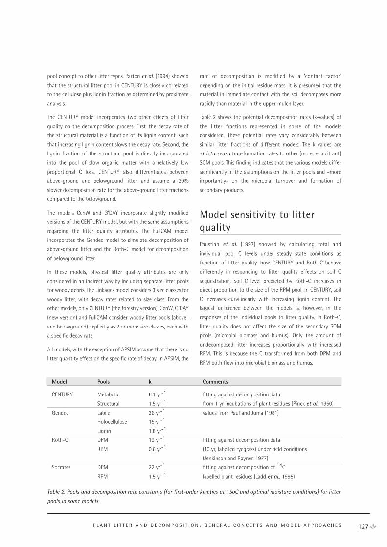
127P L A N T L I T T E R A N D D E C O M P O S I T I O N : G E N E R A L C O N C E P T S A N D M O D E L A P P R O A C H E S
pool concept to other litter types. Parton et al. (1994) showed
that the structural litter pool in CENTURY is closely correlated
to the cellulose plus lignin fraction as determined by proximate
analysis.
The CENTURY model incorporates two other effects of litter
quality on the decomposition process. First, the decay rate of
the structural material is a function of its lignin content, such
that increasing lignin content slows the decay rate. Second, the
lignin fraction of the structural pool is directly incorporated
into the pool of slow organic matter with a relatively low
proportional C loss. CENTURY also differentiates between
above-ground and belowground litter, and assume a 20%
slower decomposition rate for the above-ground litter fractions
compared to the belowground.
The models CenW and G’DAY incorporate slightly modified
versions of the CENTURY model, but with the same assumptions
regarding the litter quality attributes. The FullCAM model
incorporates the Gendec model to simulate decomposition of
above-ground litter and the Roth-C model for decomposition
of belowground litter.
In these models, physical litter quality attributes are only
considered in an indirect way by including separate litter pools
for woody debris. The Linkages model considers 3 size classes for
woody litter, with decay rates related to size class. From the
other models, only CENTURY (the forestry version), CenW, G’DAY
(new version) and FullCAM consider woody litter pools (above-
and belowground) explicitly as 2 or more size classes, each with
a specific decay rate.
All models, with the exception of APSIM assume that there is no
litter quantity effect on the specific rate of decay. In APSIM, the
rate of decomposition is modified by a ‘contact factor’
depending on the initial residue mass. It is presumed that the
material in immediate contact with the soil decomposes more
rapidly than material in the upper mulch layer.
Table 2 shows the potential decomposition rates (k-values) of
the litter fractions represented in some of the models
considered. These potential rates vary considerably between
similar litter fractions of different models. The k-values are
strictu sensu transformation rates to other (more recalcitrant)
SOM pools. This finding indicates that the various models differ
significantly in the assumptions on the litter pools and –more
importantly- on the microbial turnover and formation of
secondary products.
Model sensitivity to litterquality
Paustian et al. (1997) showed by calculating total and
individual pool C levels under steady state conditions as
function of litter quality, how CENTURY and Roth-C behave
differently in responding to litter quality effects on soil C
sequestration. Soil C level predicted by Roth-C increases in
direct proportion to the size of the RPM pool. In CENTURY, soil
C increases curvilinearly with increasing lignin content. The
largest difference between the models is, however, in the
responses of the individual pools to litter quality. In Roth-C,
litter quality does not affect the size of the secondary SOM
pools (microbial biomass and humus). Only the amount of
undecomposed litter increases proportionally with increased
RPM. This is because the C transformed from both DPM and
RPM both flow into microbial biomass and humus.
Model Pools k Comments
CENTURY Metabolic 6.1 yr-1 fitting against decomposition data
Structural 1.5 yr-1 from 1 yr incubations of plant residues (Pinck et al., 1950)
Gendec Labile 36 yr-1 values from Paul and Juma (1981)
Holocellulose 15 yr-1
Lignin 1.8 yr-1
Roth-C DPM 19 yr-1 fitting against decomposition data
RPM 0.6 yr-1 (10 yr, labelled ryegrass) under field conditions
(Jenkinson and Rayner, 1977)
Socrates DPM 22 yr-1 fitting against decomposition of 14C
RPM 1.5 yr-1 labelled plant residues (Ladd et al., 1995)
Table 2. Pools and decomposition rate constants (for first-order kinetics at 15oC and optimal moisture conditions) for litter
pools in some models
In CENTURY, all secondary pools respond to lignin content. Both
the slow and passive pool show a linear response to lignin
content, mainly as a consequence of the fact that the lignin
fraction of the structural pool is directly incorporated in the
slow pool. These different assumptions in the models raise the
question of litter quality effects on the chemical nature of SOM.
Experimental results are not clear on the importance of plant
lignin as precursors of soil humic substances. The role of
phenolic compounds from plant sources in reacting with other
organic compounds to form stable complexes is generally
accepted, but does not account for the wide variety of
structures found in humic substances (Cadish and Giller, 2001).
Conclusions and someomissions
Substrate quality is a key factor regulating the decomposition
of litter and transformation of litter C into soil humus. Largely
based on results from short-term decomposition studies, most
models include biochemical composition or chemical attributes
(initial C:N or lignin:N ratio) as litter quality parameter. The
Roth-C and SOCRATES models define two conceptual litter
pools by fitting the model to long-term decomposition data.
Uncertainty exists on how litter quality affects transformations
of litter C into stable soil organic matter. The effect of litter
quality on transformation processes is not well considered in
the simulation models. Only CENTURY considers the direct
effect of recalcitrant compounds such as lignin on C
sequestration by allocating the lignin fraction of litter directly
to the slowly-decomposing SOM pool. Whether this concept
adequately represents the reality is not known and remains to
be thoroughly tested. New analytical techniques, such as
nuclear magnetic resonance (NMR) spectroscopy may
contribute to a better mechanistic understanding of litter
quality effects on SOM chemistry.
ReferencesAngers D and Recous S 1997 Decomposition of wheat straw
and rye in soil as affected by particle size. Plant Soil 189:
197-203.
Berg B and Staaf H (1980) Decomposition rate and chemical
changes of Scots pine needle litter. II. Influence of chemical
composition. In: Persson T (Ed.), Structure and Function of
Northern Coniferous Forests- An ecosystem study.
Ecological Bulletins (Stockholm) 32: 373-390.
Cadisch G and Giller KE (2001) Soil organic matter
management: the roles of residue quality in C
sequestration and N supply. In: Rees RM, Ball BC, Campbell
CD and Watson CA (Eds.), Sustainable management of soil
organic matter. pp 97- 111. CAB International.
Corbeels M, Hofman G, Van Cleemput O (1999) Simulation net
N immobilisation and mineralisation in substrate-amended
soils by the NCSOIL computer model. Biology and fertility
of Soils 28: 422-430.
Green CJ, Blackmer AM and Horton R (1995) Nitrogen effects
on conservation of carbon during corn residue
decomposition in soil. Soil Science Society of America
Journal 59: 453-459.
Heal OW, Anderson JM, Swift MJ (1997) Plant litter quality and
decomposition: An historical overview. In Cadisch G and
Giller KE (Eds.), Driven By Nature. Plant Litter Quality and
Decomposition. pp 3-30. CAB International, Wallingford.
Henriksen TM and Breland TA (1999) Evaluation of criteria for
describing crop residue degradability in a model of carbon
and nitrogen turnover in soil. Soil Biology and Biochemistry
31: 1135-1149.
Hunt HW (1977) A simulation model for decomposition in
grasslands. Ecology 58: 469-484.
Jenkinson DS, Adams DE and Wild A (1991) Model estimates of
CO2 emissions from soil in response to global warming.
Nature 351: 304-306.
Jenkinson DS and Rayner JH (1977) The turnover of soil
organic matter in some of the Rothamsted classical
experiments. Soil Science 123:298-305.
Ladd JN, Amato M, Grace PR and Van Veen JA (1995)
Simulation of 14C turnover through the microbial biomass
in soils incubated with 14C labelled plant residues. Soil
Biology and Biochemistry27: 777-783.
Melillo JM, Aber JD and Muratore JF (1982) Nitrogen and
lignin control of hardwood leaf litter decomposition
dynamics. Ecology 63: 621-626.
Minderman G (1968) Addition, decomposition and
accumulation of organic matter in forests. Journal of
Ecology 56: 355-362.
O’Connell AM (1997) Decomposition of slash residues in
thinned regrowth eucalypt forest in Western Australia.
Journal of Applied Ecology 34: 111- 122.
128 N E E W O R K S H O P P R O C E E D I N G S : 1 8 – 2 0 A P R I L 2 0 0 1

Palm CA and Sanchez PA (1991) Nitrogen release from the
leaves of some tropical legumes as affected by their lignin
and polyphenolic contents. Soil Biology Biochemistry 23:
83-88.
Parton WJ, Ojima D.S. Cole CV and Schimel DS (1994) A
general model for soil organic matter dynamics: sensitivity
to litter chemistry, texture and management. In: Bryant RB
and Arnold RW (Eds.), Quantitative modeling of soil
forming processes. pp147-167. SSSA Special Publication no
39. SSSA, Madison, Wisconsin, USA.
Paul EA and Juma NG (1981) Mineralization and
immobilization of soil nitrogen by microorganisms. In: Clark
FE and Rosswall T (Eds.), Terrestrial nitrogen cycles.
Ecological Bulletins (Stockholm) 33: 179-199.
Paustian K, Ågren GI and Bosatta E (1997) Modelling litter
quality effects on decomposition and soil organic matter
dynamics. In: Cadisch G and Giller KE (Eds.), Driven by
nature: plant litter quality and decomposition. pp 313-335.
CAB International.
Pinck LA, Allison FE and Sherman MS (1950) Maintenance of
soil organic matter:II Losses of carbon and nitrogen from
young and mature plant material during decomposition in
soil. Soil Science 69: 391-401.
Probert MP, Dimes JP, Keating BA, Dalal RC and Strong WM
(1998) APSIM’s water and nitrogen modules and simulation
of the dynamics of water and nitrogen in fallow systems.
Agricultural Systems: 56, 1-26.
Raich JW and Tufekcioglu A (2000) Vegetation and soil
respiration: correlations and controls. Biogeochemistry 48:
71-90.
Schlesinger WH (1991) Biogeochemistry: an analysis of global
change. Academic Press, New York.
Seneviratne G (2000) Litter quality and nitrogen release in
tropical agriculture: a synthesis. Biology and Fertility of
Soils 31: 60-64.
Skjemstad JO, Dalal RC, Janik LJ and McGowan JA (2001)
Changes in chemical nature of soil organic carbon in
Vertisols under wheat in south-eastern Queensland.
Australian Journal of Soil Research 39: 343-359.
Swift MJ, Heal OW and Anderson JM (1979) Decomposition in
terrestrial ecosystems. Blackwell Oxford, UK, 372pp.
Thorburn PJ, Probert ME, Robertson FA (2001) Modelling
decomposition of sugar cane surface residues with APSIM-
Residue. Field Crops Research 70: 223-232.
Vanlauwe B, Diels J, Sanginga N. And Merckx R. (1997) Residue
quality and decomposition: an unsteady relationship? In:
In: Cadisch G and Giller KE (Eds.), Driven by nature: plant
litter quality and decomposition. p 157-166. CAB
International.
129P L A N T L I T T E R A N D D E C O M P O S I T I O N : G E N E R A L C O N C E P T S A N D M O D E L A P P R O A C H E S
130 N E E W O R K S H O P P R O C E E D I N G S : 1 8 – 2 0 A P R I L 2 0 0 1
S. Roxburgh, C. Barton, M. Battaglia, M. Corbeels, D. Eamus, J. Evans, R. Gifford, B. Henry, R. Keenan, E. Krull, B. Medlyn, D. Pepper, J. Skjemsted, K. Tate.
Overview
Over the course of the workshop the rapporteurs provided
summaries of the discussions that took place at the end of each
session, as well as highlighting some of the major results to
emerge from the presentations.
The summary reports below focus predominantly on the issues
raised during discussion, but also include those results that
were particularly relevant to the overall aims of the workshop:
(1) to describe the specific processes that together control
net ecosystem exchange;
(2) to highlight current controversies or remaining
unresolved issues;
(3) detail how various processes are dealt with in the various
models of interest in modelling carbon exchange for
Australia;
(4) discuss what processes should be included in continental-
scale models of the Australian biosphere.
Day 1—Wednesday 18 April 2001
Morning Session (Radiation interception, Radiation
conversion, Respiration)
Chair: Craig Pearson
Rapporteurs: David Pepper, Jan Skjemsted
Presenters: Yingping Wang, Belinda Medlyn, Roger
Gifford
The first two presentations in this session summarised current
methodologies used in modelling radiation interception and
radiation conversion. With respect to radiation interception it
was noted that many models use Beer’s law to calculate
radiation extinguishment through plant canopies, and that the
calculations are based on the assumption that all radiation is
considered to be ‘direct beam’. However, the importance of
splitting radiation into direct beam and diffuse fractions was
highlighted, and that diffuse light within plant canopies should
be accounted for in order to appropriately quantify the within-
canopy light environment. This has important implications for
modelling vegetation growth at all scales.
With respect to estimating respiration, it was noted that there
are several ways in which respiration can be defined, and a
suggestion was put forward that the CRC ought to produce a
consensus definition of the components of plant respiration,
and after further discussion it was decided that one outcome of
the workshop would be the development of a set of definitions
of the components of ecosystem gas exchange. Such a set of
definitions has been produced and is being published as part of
these proceedings. There was some discussion regarding the
respiration:gross primary production ratio approach to
estimating plant respiration. This is based on the observation of
a reasonably conservative respiration: primary production ratio
of around 0.4-0.6, measured across a wide variety of plant
growth forms. Although it was noted that there are, in the
literature, examples which fall outside this range, the overall
feeling was that, in particular for continental-scale carbon
budget modelling, the conservative nature of the ratio could be
effectively utilised.
A general point was made that we can quantify the small-scale
analyses quite well, but the real challenge lies in scaling the
processes up through time and space.
Afternoon Session (Allocation, Mortality and stand age effects
on productivity, Other factors (phenology, reproduction, ..))
Chair: Graham Farquhar
Rapporteurs: Derek Eamus, Beverly Henry
Presenters: Craig Barton, Michael Battaglia, Chris Beadle
(read by M. Battaglia)
There was general agreement that knowledge of these
processes is much-less well-known than those in the first
session. For example the mechanisms underlying allocation to
plant parts remain largely unknown, and therefore we are
forced to use empirical relationships. Most current models use
either a fixed allocation coefficient or fixed proportionality
between certain coefficients with others modified by
environmental factors. A similar situation exists for changes in
productivity with stand-age – where the patterns of age-
related decline in productivity are well documented, but the
underlying reasons remain elusive, and rarely appear in current
models of NPP. There was a brief discussion on how such effects
Rapporteur Reports
could be parameterised across large spatial scales, resulting in a
general agreement that better understanding the underlying
processes is required.
Much of the discussion focussed on belowground allocation, its
potential importance and how it could be measured. Root
windows, serial coring and mini-rhizotrons were suggested as
some of the available methodologies. To provide some
approximate figures, Kevin Tate reported that in NZ, a study in
a pine plantation showed about 25% of NPP to be allocated
belowground, with a comparable figure of 80% in a tussock
grassland. It was noted that the difficulty in measuring
allocation lies in the fact that it involves fluxes of material, and
to quantify it through examination of standing stocks requires
knowledge of the rates of input and the rates of output. This is
especially problematic for belowground allocation, given the
difficulties involved in quantifying belowground processes in
general.
At the end of the discussion Miko Kirschbaum suggested a
combined projects to run some common scenarios across the
different models under consideration. This was not taken up at
the time, but if interest is wide enough this could be the focus
for follow-up work.
Day 2 - Thursday 19 April 2001
Morning Session (The impact of ecosystem water balance on
NPP, Other soil constraints (impedance, acidity, salinity, water
logging), Nutrient uptake and use in plant growth)
Chair: Roger Gifford
Rapporteurs: Michael Battaglia, Rod Keenan
Presenters: Derek Eamus Rob Edis, John Evans
With respect to modelling ecosystem water budgets (and their
impact on NPP) it was admitted that while some terms in the
water balance equations are well studied, there are many which
are poorly understood, yet they are critical for understanding
water budget/NPP relations at larger spatial scales. These
include groundwater dynamics, lateral flows, canopy
interception, and the importance of patterns of rainfall events
and their intensity (and not just the averages). Another critical
gap in our current knowledge is being able to reconcile the fact
that to understand regional water dynamics it is necessary to
address water in the soil profile down to and beyond the
rooting depth, yet our current methodologies focus on the
much smaller soil volume within the first metre or so of the
surface.
In the discussion of Other Soil Constraints, it was highlighted
that the major constraints of salinity, soil acidity, waterlogging
and soil strength are all dependent on correct quantification of
the regional water budgets, further highlighting the importance
of understanding both small and large-scale water dynamics in
Australian ecosystems.
With respect to nutrient uptake and plant growth, the
importance of the major limiting nutrients (N, P, S) in Australian
ecosystems were considered, and it was noted that all of the
models under consideration in the workshop account for
nutrient effects on growth to some extent – but that some
models handle the relationships better than others. A
generalised relationship between N content of leaves and
annual NPP was presented. However in discussion it was
suggested that variation in this relationship in the range of
foliar N contents and NPP where many Australian ecosystems
reside may make meaningful extrapolation difficult.
Discussions both during and following the session raised the
possibility that savanna ecosystems could be used as an
example for cross-model comparisons. This is because tree/grass
systems offer many challenges for estimating NEE, such as
marked seasonality, the importance of groundwater in
determining vegetation patterns, and the importance of
disturbance (fire), among others. Particular issues raised
included a discussion of the importance of fire in these
ecosystems, and what the most important features would be to
include in large-scale modelling studies. Two issues emerged.
The first was the importance of the tree/grass balance, and in
particular understanding tree mortality and canopy death in
response to the disturbance. The second was a need to
understand the role that fire plays in the cycling of nutrients,
particularly with respect to the highly seasonal rainfall patterns
which also impact on nutrient loads via. e.g. the flush of
nutrients out of the system following the first rains of the
season.
The major issues to emerge from the session included the
importance of understanding large-scale water budgets -
including a better understanding of rooting depth (which
usually goes well beyond the ability to take measurements of
soil properties, at least over wide areas) and defining effective
rooting volumes. Although not addressed by ecosystem models
at present, the effects of waterlogging & soil strength, acidity
and salinity are all potentially important factors in determining
the NEE of Australian ecosystems, and some effort needs to be
put into the assessment of their importance, and to develop the
methods for explicit descriptions in ecosystem models.
131R A P P O R T E U R R E P O R T S
Afternoon Session 1 (CO2 concentration, Temperature
effects on growth)
Chair: Kevin Tate
Rapporteurs: Roger Gifford
Presenters: Graham Farquhar, Marilyn Ball
A common theme running through the content of the
presentations and discussions in this session was the challenge
of taking what is well studied and hence well known at the
individual-plant level (and other small spatial scales) and using
this information to scale up through space, to eventually attain
the correct representation of the processes at regional and
continental scales. For example, photosynthesis at the
leaf/individual level is well understood and well modelled,
hence we are in a good position to start scaling up (as indeed
has been done in a number of international models). In this case
the limitation is not in the model representation of the
underlying process, but in determining how that process is
affected by all of the other factors that come into play as one
moves to the larger scales. In discussion, the point was made
that, when interpreting patterns of ecosystem carbon sources
and sinks, it is only possible to disentangle historical/stand-age
related effects from CO2 fertilisation effects and recent
management if the lasting effects of historical disturbances can
be factored out of the analysis. At regional and continental
scales this therefore requires some knowledge of the
disturbance histories of the vegetation over several decades.
In Marilyn Ball’s presentation on ‘Temperature effects’, and in
the discussion that followed, two important points directly
related to this scaling issue were made. The first was the
concept of ‘sensitivity to initial conditions’, whereby events
which result in seemingly small differences at one time
accumulate to eventually result in large effects later on, and
that the timing of those events, in this case seasonally extreme
frost and heat events, is critical. The second point echoed the
earlier discussion on ecosystem water balances, and highlighted
that the ‘average’ climate, rainfall, etc. is often an inappropriate
descriptor of the system, as it is the variability, and in particular
the occurrence of extreme events, which are critical to
determining the system behaviour, especially changes in species
composition. This has important implications for modelling NEE
at continental scales, as it is often tempting to use e.g.
‘averaged’ climate values as parameter estimates when little is
known about the underlying processes, yet by using such
averages introduces the danger of excluding critical drivers of
the system.
Of the models under consideration in the workshop only CenW
specifically includes the effects of extreme temperature events
on NEE processes. None of the models allow for the
accumulation of the effects of events occurring earlier in time.
Afternoon Session 2 (Linking above and belowground
processes, Interactions between carbon dynamics and nutrient
mineralisation)
Chair: Rod Keenan
Rapporteurs: Marc Corbeels, Craig Barton
Presenters: Miko Kirschbaum, Peter Grace
The importance of including nutrient cycles, and in particular
nitrogen, when considering ecosystem carbon gain and loss was
further highlighted in the presentations in this session. In
particular, the importance of incorporating the feedbacks
between plant growth and the flux of nutrients from above- to
below ground via litterfall was identified as a feature of NEE
modelling that demands attention. For example, using the
CenW model, Miko Kirschbaum showed how omitting a
negative feedback between growth and N availability can
significantly alter predictions of NPP. If growth is enhanced, it
can lead to increased litter production, and the increased
amount of soil organic carbon can then act to immobilise
nitrogen in the soil and thereby reduce nitrogen availability for
plants. If this feed-back effect is not simulated, it would
increase the expected variability in NPP in response to various
perturbations.
The importance of considering the role of soil microbes in
nutrient cycling, and in particular their role in fixing and
immobilising N was highlighted by Peter Grace, who also spent
some time considering more general issues of modelling
ecological systems, with particular reference to the distinction
between model components and parameters which on the one
hand are conceptual and ‘modelable’ vs. those which are more
pragmatic, in the sense that they might not encapsulate all of
the detail possible, but are defined in such a way that they can
be readily ‘measured’ and quantified empirically. This provided
the impetus for the discussion which followed.
It was generally agreed that when considering soil organic
matter, it is not strictly accurate to define separate ‘pools’ of
carbon and nutrients, with each pool having a characteristic
turnover time. In reality, soil organic matter constitutes a
continuum of turnover times without discrete boundaries, yet
in the models in current use the pools are regarded as discrete
entities. There was some discussion about the ‘minimum
requirements’ for an effective continental model of carbon
132 N E E W O R K S H O P P R O C E E D I N G S : 1 8 – 2 0 A P R I L 2 0 0 1
stocks and fluxes. Whilst the general consensus was such a
question is difficult to answer, over and above the obvious
statement that a model must be as simple as possible but no
more, there was general agreement that nutrients (possibly
more than just N) should be included as a constraint. It was
suggested that obtaining adequate data on N, P and other
nutrient cycles at the continental scale could be a limiting
factor to progress, although it was pointed out that the
tendencies for conservation of mass-ratios among the major
elements provides useable constraints. A number of
contributors to the discussion highlighted the importance of
keeping the modelling as simple as possible, due to both
practicalities of running a spatially-explicit simulation exercise
over a continent the size of Australia, and also for the data
requirements for both model parameterisation and validation.
Day 3 - Friday 20 April 2001
Morning Session (Temperature and moisture effects on
decomposition rate, Soil texture effects on decomposition and
soil C storage, pH, aluminium and other factors that can inhibit
decomposition rates, Charcoal and other resistant organic
matter)
Chair: Martin Schutz
Rapporteurs: John Evans, Kevin Tate
Presenters: Keryn Paul, Evelyn Krull, Ram Dalal,
Jan Skjemstad
Soil carbon dynamics, and in particular the decomposition of
organic matter and soil building processes, are of central
importance in understanding the carbon cycle, yet it is in these
areas that much of our current knowledge is lacking. Sensitivity
of decomposition rates to temperature and water is included in
all models considered, however the way in which these effects
are incorporated is through simple ‘modifier’ functions -
empirical functions which generate a scalar multiplier whose
value is dependent upon the current temperature or water
status. Given the complexity of the processes involved, and the
spatial variability in both temperature and water at all spatial
scales, it would seem that this is the only feasible approach to
take. However, in discussion it was highlighted that care must
be taken to make sure that the underlying empirical
relationships are both robust, and are able to be validly applied
outside of the experimental conditions within which they were
derived.
In the consideration of soil texture effects on decomposition
and soil C storage, it is clear that both chemical and physical
‘protection’ of organic matter in the soil matrix plays an
important role in setting absolute decomposition rates, and
hence in determining both the stocks and fluxes of
belowground carbon. Such effects are not currently considered
in NEE models, despite the potential for manipulating the soil’s
protective capacity as a means of managing terrestrial carbon
dynamics. There was some discussion over the current status of
Australian soils, the potential to increase their protective
capacity, and how this might vary between soils which had
undergone prior disturbance, such as agricultural soils, and soils
under more natural conditions. Other factors that were
considered, and which influence decomposition include pH and
aluminium. Australian ecosystems in which these influences
might be important, and the capacity for building them into our
modelling frameworks, need to be assessed
In the consideration of chemically resistant soil carbon, the
distinction was drawn between the different pool definitions
that have been used, the various turnover times commonly
associated with those pools, and the current methods used in
their estimation.
In determining the carbon stocks at large spatial scales two
issues were raised. The first considered the data availability for
estimating broadscale estimates of bulk-density. At present the
best data available are based on general relationships with soil
type, particle size distributions etc. The second issue was the
potential for large-scale (landscape � regional) lateral spread
of carbon via windblown and waterborn material. This may be
particularly important in Australia as fires are widespread,
resulting in potentially significant lateral transport. There is also
evidence that stores of carbon in river sediments, particularly in
flooded areas, can be very high. A suggestion was made that the
importance of such lateral carbon movement in the Australian
context be examined. It was also noted that much of our
available data on belowground carbon dynamics comes from
grassland/agricultural systems, and that data under forest
conditions is under-represented. This is particularly important,
given the contribution of Australia’s forested ecosystems
towards the total continental carbon inventory.
Afternoon Session (Soil disturbance (cultivation) effects on
decomposition and soil C storage, Litter quality and quantity).
Chair: John Raison
Rapporteurs: Evelyn Krull, Belinda Medlyn
Presenters: Phil Polglase, Marc Corbeels
Mechanical disturbance has many impacts on both the
structure and function of soils, and has the potential to
133R A P P O R T E U R R E P O R T S

influence the rates of carbon sequestration and loss. One
difficultly in studying these effects is that decline in TOC
following disturbance is often confounded with changes in the
management regime, such as the subsequent planting of crops
with different productivities, which leads to changes in the
rates of carbon-input to the soil. Although wind and water
erosion are potentially important forces, the discussion mostly
focussed on agriculture, plantation forestry and other managed
systems. The key question is whether cultivation and other
management practices result in a loss of carbon from soils, such
as whether site preparation before establishing new plantations
can lead to a decrease in soil organic carbon. With respect to
the practice of direct drilling vs. minimum tillage, under
Australian conditions the situation is confounded by other
factors, such as lower-input crops that are routinely used under
no-till situations. Some results were presented that showed that
over long periods of time, disturbed and undisturbed sites did
not differ significantly in their rates of carbon loss.
Globally there is a strong relationship between total litterfall in
forested ecosystems and total soil respiration. Litter quality, in
terms of its chemical properties, the physical sizes of particles,
the presence of microbial inhibitory substances and the activity
of the decomposers also contribute to determine the effective
rates of litter decomposition. With respect to modelling the
process, most models assume linear first-order decay processes.
During discussion, the question was raised on what the simplest
approach to take would be in terms of a continental modelling
capacity. It was suggested that the vegetation could be
stratified into a number of biomes (10 was the figure proposed),
and that litter qualities and behaviours could be assigned to
each. It was the feeling of the presenters that the appropriate
information at this scale for the Australian environment is
available.
It was noted that larger scale processes, such as climatic change
and disturbance, have the potential to cause large changes in
the microbial micro-environment, and hence have the potential
to override the finer-scaled processes considered here.
134 N E E W O R K S H O P P R O C E E D I N G S : 1 8 – 2 0 A P R I L 2 0 0 1
135N E E W O R K S H O P P A R T I C I P A N T S
Jeffery Baldock CSIRO Land and Water [email protected]
Marilyn BallResearch School of Biological Sciences, The Australian National University [email protected]
David Barker Research School of Biological Sciences, The Australian National University [email protected]
Michele BarsonCRCGA & Bureau of Rural Sciences. [email protected]
Craig BartonForest Research & Development Division,State Forests of NSW [email protected]
John CarterQld Department of Natural Resourcesand Mines [email protected]
Annette CowieForest Research & Development Division, State Forests of NSW [email protected]
Ram DalalQld Department of Natural Resourcesand Mines [email protected]
Ian DaviesResearch School of Biological Sciences, The Australian National University [email protected]
Everard EdwardsThe Research School of BiologicalSciences, The Australian National University [email protected]
John EvansResearch School of Biological Sciences, The Australian National University [email protected]
Graham FarquharResearch School of Biological Sciences, The Australian National University [email protected]
Roger Gifford CSIRO Plant Industry [email protected]
Lan Bin GuoCSIRO Plant [email protected]
Rod KeenanBureau of Rural Sciences [email protected]
Miko KirschbaumCSIRO Forestry and Forest Products [email protected]
Evelyn KrullCSIRO Land and Water [email protected]
Brendan MackeyDepartment of Geography, The Australian National University [email protected]
Greg McKeon Qld Department of Natural Resourcesand Mines [email protected]
Angela Newey CSIRO Plant Industry [email protected]
Ian Noble (CEO, CRCGA)Research School of Biological Sciences, The Australian National University [email protected]
Craig PearsonBureau of Rural Sciences [email protected]
Wayne PippenResearch School of Biological Sciences, The Australian National University [email protected]
John RaisonCSIRO Forestry and Forest Products [email protected]
Kema RanatungaBureau of Rural Sciences [email protected]
Lucy RandallBureau of Rural Sciences [email protected]
Michael RoderickResearch School of Biological Sciences, The Australian National University [email protected]
Stephen RoxburghResearch School of Biological Sciences, The Australian National University [email protected]
Martin SchutzCRC for Greenhouse [email protected]
Jan SkjemstadCSIRO Land and Water [email protected]
Julie StylesResearch School of Biological Sciences, The Australian National University [email protected]
NEE Workshop: CRC Participants
Brian AtwellMacquarie [email protected]
Troy BaisdenLandcare Research, New [email protected]
Michael BattagliaCSIRO Forestry and Forest Products andCooperative Research Centre forSustainable Production Forestry [email protected]
Chris Beadle Cooperative Research Centre forSustainable Production Forestry andCSIRO Forestry and Forest Products [email protected]
Nicholas CoopsCSIRO Forestry and Forest Products [email protected]
Marc CorbeelsCSIRO Forestry and Forest Products [email protected]
Derek EamusDepartment of Environmental Science, University of Technology [email protected]
Robert EdisInstitute of Land and Food Resources, University of [email protected]
Peter GraceSinclair Knight Merz [email protected]
Beverley HenryQld Department of Natural Resourcesand Mines [email protected]
Brian Keating CSIRO Sustainable Ecosystems [email protected]
Heather KeithCSIRO Forestry and Forest Products [email protected]
Joe LandsbergLandsberg [email protected]
Ray LeuningCSIRO Land and [email protected]
Beth LoveysVisiting Fellow, Research School ofBiological Sciences, The Australian National University [email protected]
Don McGuireForestry South [email protected]
Belinda MedlynSchool of Biological Sciences, University of New South [email protected]
Andrew MooreCSIRO Plant Industry [email protected]
Keryn PaulCSIRO Forestry and Forest Products [email protected]
David PepperSchool of Biological Science, University of New South [email protected]
Philip PolglaseCSIRO Forestry and Forest Products [email protected]
Merv ProbertCSIRO Sustainable Ecosystems [email protected]
Gary Richards Australian Greenhouse Office [email protected]
Peter SandsCSIRO Forestry and Forest Products andCooperative Research Centre forSustainable Production Forestry [email protected]
Kevin TateLandcare Research, New [email protected]
Craig TrotterLandcare Research, [email protected]
Ying Ping WangCSIRO Atmospheric Research [email protected]
Anthony WhitbreadCSIRO Sustainable [email protected]
136 N E E W O R K S H O P P R O C E E D I N G S : 1 8 – 2 0 A P R I L 2 0 0 1
NON-CRC Participants