network analyzer basics - rf114

David Ballo

Hewlett-Packard CompanyMicrowave Instruments Division1400 Fountaingrove ParkwaySanta Rosa, California 95403U.S.A.

1997 Back to Basics Seminar

(c) Hewlett-Packard Company

Network Analyzer Basics

Abstract

This presentation covers the principles of measuring

high-frequency electrical networks with network analyzers.

You will learn what kind of measurements are made with

network analyzers, and how they allow you to characterize

both linear and nonlinear behavior of your devices. The

session starts with RF fundamentals such as transmission

lines and the Smith Chart, leading to the concepts of

reflection, transmission and S-parameters. The next

section covers all the major components in a network

analyzer, including the advantages and limitations of

different hardware approaches. Error modeling, accuracy

enhancement, and various calibration techniques will then

be presented. Finally, some typical swept-frequency and

swept-power measurements commonly performed on filters

and amplifiers will be covered. An advanced-topics section

is included as a pointer to more information.

Author

David Ballo is currently a Marketing Engineer for

Hewlett-Packard's Microwave Instruments Division in

Santa Rosa, California. David has worked for HP for over

16 years, where he has acquired extensive RF and

microwave measurement experience. After getting a BSEE

from the University of Washington in Seattle in 1980, he

spent the first ten years in R&D doing analog and RF circuit

design on a variety of Modular Measurement System (MMS)

instruments. He followed that with a year in

manufacturing. For the past five years, he has worked in

the marketing department developing application notes,

magazine articles, and seminar papers on topics including

TWT amplifier test, group delay and AM to PM conversion

of frequency- translating devices, adjacent-channel power

measurements, design and calibration of RF fixtures for

surface-mount devices, and efficient test of multiport

devices.

Slide #1

Wecome to Network Analyzer Basics.

H Network Analyzer BasicsDJB 12/96 na_basic.pre


Author:

David Ballo

1 - 1

HNetwork Analyzer Basics

Slide #2

This module is not about computer networks! When the name "network analyzer" was coined many years ago,

there were no such things as computer networks. Back then, networks always referred to electrical networks.

Today, when we refer to the things that network analyzers measure, we speak mostly about devices and

components.


Network analysis is not...

Router

Bridge

Repeater

Hub

Your IEEE 802.3 X.25 ISDN switched-packet data stream is running at 147 MBPS with a BER of 1.523 X 10 . . . -9

1 - 2


Slide #3

Here are some examples of the types of devices that you can test with network analyzers. They include both

passive and active devices (and some that have attributes of both). Many of these devices need to be

characterized for both linear and nonlinear behavior. It is not possible to completely characterize all of these

devices with just one piece of test equipment.

The next slide shows a model covering the wide range of measurements necessary for complete linear and

nonlinear characterization of devices. This model requires a variety of stimulus and response tools. It takes a

large range of test equipment to accomplish all of the measurements shown on this chart. Some instruments are

optimized for one test only (like bit-error rate), while others, like network analyzers, are much more

general-purpose in nature. Network analyzers can measure both linear and nonlinear behavior of devices,

although the measurement techniques are different (frequency versus power sweeps for example). This module

focuses on swept-frequency and swept-power measurements made with network analyzers.


What types of devices are tested?

Integration

Hig

hLo

w

Antennas

SwitchesMultiplexersMixersSamplersMultipliers

Diodes

DuplexersDiplexersFiltersCouplersBridgesSplitters, dividersCombinersIsolatorsCirculatorsAttenuatorsAdaptersOpens, shorts, loadsDelay linesCablesTransmission linesWaveguideResonatorsDielectricsR, L, C's

RFICsMMICsT/R modulesTransceivers

ReceiversTunersConverters

VCAsAmplifiers

VCOsVTFsOscillatorsModulatorsVCAtten's

Transistors

Device type ActivePassive

1 - 3


Slide #4

Here is a key to many of the abbreviations used above:

Response Measurement

84000 HP 84000 high-volume RFIC tester ACP Adjacent channel power

Ded. Testers Dedicated (usually one-box) testers AM-PM AM to PM conversion

VSA Vector signal analyzer BER Bit-error rate

SA Spectrum analyzer Compr'n Gain compression

VNA Vector network analyzer Constell. Constellation diagram

TG/SA Tracking generator/spectrum analyzer EVM Error-vector magnitude

SNA Scalar network analyzer Eye Eye diagram

NF Mtr. Noise-figure meter GD Group delay

Imped. An. Impedance analyzer (LCR meter) Harm. Dist. Harmonic distortion

Power Mtr. Power meter NF Noise figure

Det./Scope Diode detector/oscilloscope Regrowth Spectral regrowth

Rtn Ls Return loss

VSWR Voltage standing wave ratio


Device Test Measurement Model

NF

Stimulus type ComplexSimple

Resp

on

se t

oo

lC

ompl

exS

impl

e

DC CW Swept Swept Noise 2-tone Multi- Complex Pulsed- Protocol freq power tone modulation RF

Det/Scope

Param. An.

NF Mtr.

Imped. An.

Power Mtr.

SNA

VNA

SA

VSA

84000

TG/SA

Ded. Testers

I-V

Absol. Power

Gain/Flatness

LCR/Z

Harm. Dist.LO stabilityImage Rej.

Gain/Flat.Phase/GDIsolationRtn Ls/VSWRImpedanceS-parameters

Compr'nAM-PM

RFIC test

Full call sequence

Pulsed S-parm.Pulse profiling

BEREVMACP

RegrowthConstell.

Eye

Intermodulation DistortionNF

Measurement plane

1 - 4


Slide #5


Agenda

Why do we test components?

What measurements do we make?Smith chart review

Transmission line basics

Reflection and transmission parameters

S-parameter definition

Network analyzer hardwareSignal separation devices

Broadband versus narrowband detectionDynamic range

T/R versus S-parameter test sets

Three versus four samplers

Error models and calibrationTypes of measurement error

One- and two-port models

Error-correction choices

TRL versus TRL*

Basic uncertainty calculations

Typical measurements

Advanced topics

1 - 5


Slide #6

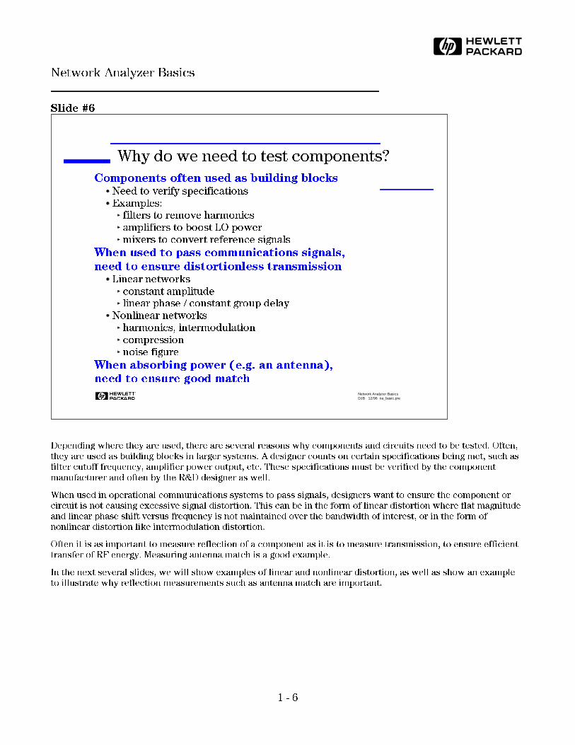
Depending where they are used, there are several reasons why components and circuits need to be tested. Often,

they are used as building blocks in larger systems. A designer counts on certain specifications being met, such as

filter cutoff frequency, amplifier power output, etc. These specifications must be verified by the component

manufacturer and often by the R&D designer as well.

When used in operational communications systems to pass signals, designers want to ensure the component or

circuit is not causing excessive signal distortion. This can be in the form of linear distortion where flat magnitude

and linear phase shift versus frequency is not maintained over the bandwidth of interest, or in the form of

nonlinear distortion like intermodulation distortion.

Often it is as important to measure reflection of a component as it is to measure transmission, to ensure efficient

transfer of RF energy. Measuring antenna match is a good example.

In the next several slides, we will show examples of linear and nonlinear distortion, as well as show an example

to illustrate why reflection measurements such as antenna match are important.


Why do we need to test components?

Components often used as building blocks

Need to verify specifications

Examples:

filters to remove harmonics

amplifiers to boost LO power

mixers to convert reference signals

When used to pass communications signals,

need to ensure distortionless transmission

Linear networks

constant amplitude

linear phase / constant group delay

Nonlinear networks

harmonics, intermodulation

compression

noise figure

When absorbing power (e.g. an antenna),

need to ensure good match

1 - 6


Slide #7

We have already mentioned that many devices exhibit both linear and nonlinear behavior. Before we explore the

different types of signal distortion that can occur, lets review the differences between linear and nonlinear

behavior. Devices that behave linearly only impose magnitude and phase changes on input signals. Any sinusoid

appearing at the input will also appear at the output at the same frequency. No new signals are created.

Non-linear devices can shift input signals in frequency (a mixer for example) and/or create new signals in the form

of harmonics or intermodulation products. Many components that behave linearly under most signal conditions

can exhibit nonlinear behavior if driven with a large enough input signal. This is true for both passive devices like

filters and active devices like amplifiers.


Linear Versus Nonlinear Behavior

Linear behavior:

input and output frequencies

are the same (no additional

frequencies created)

output frequency only

undergoes magnitude and

phase change

Time

A

to

Frequencyf1

Time

Sin 360 * f * t°

Frequency

A phase shift =

to * 360 * f°

1f

DUT

A * Sin 360 * f ( t - t )° °

Input Output

Time

Frequency

Nonlinear behavior:

output frequency may undergo

frequency shift (e.g. with mixers)

additional frequencies created

(harmonics, intermodulation)

f1

1 - 7


Slide #8

Now lets examine how linear networks can cause signal distortion. There are two criteria that must be satisfied

for linear distortionless transmission. First, the amplitude (magnitude) response of the device or system must be

flat over the bandwidth of interest. This means all frequencies within the bandwidth will be attenuated identically.

Second, the phase response must be linear over the bandwidth of interest.

How can magnitude and phase distortion occur? The following two examples will illustrate how both magnitude

and phase responses can introduce linear distortion onto signals.


Criteria for Distortionless Transmission

Linear Networks

Constant amplitude over

bandwidth of interest

Mag

nitu

de

Pha

se

Frequency Frequency

Linear phase over

bandwidth of interest

1 - 8


Slide #9

Here is an example of a square wave (consisting of three sinusoids) applied to a bandpass filter. The filter

imposes a non-uniform amplitude change to each frequency component. Even though no phase changes are

introduced, the frequency components no longer sum to a square wave at the output. The square wave is now

severely distorted, having become more sinusoidal in nature.


Magnitude Variation with Frequency

F(t) = sin wt + 1 /3 sin 3wt + 1 /5 sin 5wt

Frequency Frequency Frequency

Mag

nitu

de

Time

Linear Network

Time

1 - 9


Slide #10

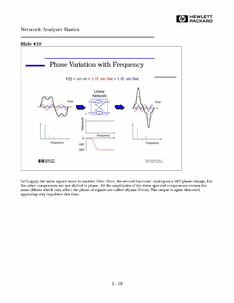
Let's apply the same square wave to another filter. Here, the second harmonic undergoes a 180o phase change, but

the other components are not shifted in phase. All the amplitudes of the three spectral components remain the

same (filters which only affect the phase of signals are called allpass filters). The output is again distorted,

appearing very impulsive this time.


Phase Variation with Frequency

Frequency

Mag

nitu

de

Linear Network

Frequency

Frequency

Time

0

-180

-360

°

°

°

Time

F(t) = sin wt + 1 /3 sin 3wt + 1 /5 sin 5wt

1 - 10


Slide #11

We have just seen how linear networks can cause distortion. Devices which behave nonlinearly also introduce

distortion. The example above shows an amplifier that is overdriven, causing the signal at the output to "clip" due

to saturation in the amplifier. Because the output signal is no longer a pure sinusoid, harmonics are present at

integer multiples of the input frequency.

Passive devices can also exhibit nonlinear behavior at high power levels. A common example is an L-C filter that

uses inductors made with magnetic cores. Magnetic materials often display hysteresis effects, which are highly

nonlinear.


Criteria for Distortionless Transmission

Nonlinear Networks

Frequency Frequency

TimeTime

Saturation, crossover, intermodulation, and other

nonlinear effects can cause signal distortion

1 - 11


Slide #12

We have just seen some examples of important transmission measurements for characterizing distortion.

Reflection measurements are also important in many applications to characterize input or output impedance

(match). For devices that are meant to efficiently transmit or absorb RF power (a transmission line or an

antenna), match is very important. Match is an indication of how much signal is reflected back to the source.

In this example, the radio station on the left is not operating anywhere near peak efficiency. A wire is not a very

good transmission line (it radiates some of the signal as well as reflect a large portion back to the amplifier).

Similarly, the broken antenna represents a very poor RF match, causing high reflection.

On the right, the radio station has installed a good transmission line and a good antenna. The effective radiated

power has increased tenfold (10 dB), resulting in √10 or 3.16 times greater distance for a given signal power. Thismeans ten times more listeners, more advertising revenue, and more profit! The amplifier, transmission line and the

antenna all need to be measured to ensure that this example of efficient power transmission actually occurs.


Example Where Match is Important

Wire and bad antenna (poor

match at 97 MHz) results in

150 W radiated power

Proper transmission line and

antenna results in 1500 W radiated

power - signal is received about

three times further!

Good match between antenna and RF amplifier is extremely

important to radio stations to get maximum radiated power

KPWR FM 97KPWR FM 97

1 - 12


Slide #13

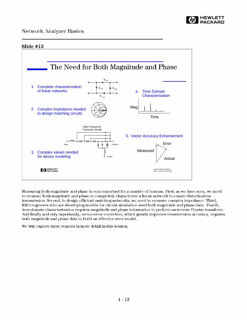
Measuring both magnitude and phase is very important for a number of reasons. First, as we have seen, we need

to measure both magnitude and phase to completely characterize a linear network to ensure distortionless

transmission. Second, to design efficient matching networks, we need to measure complex impedance. Third,

R&D engineers who are developing models for circuit simulation need both magnitude and phase data. Fourth,

time-domain characterization requires magnitude and phase information to perform an inverse Fourier transform.

And finally and very importantly, vector-error correction, which greatly improves measurement accuracy, requires

both magnitude and phase data to build an effective error model.

We will explore these reasons in more detail in this session.


The Need for Both Magnitude and Phase

Complex impedance needed to design matching circuits

Complex values needed for device modeling

4. Time Domain Characterization

Mag

Time

Complete characterization of linear networks

1.

2.

3.

S

S

S 11

21

22

12

S

Vector Accuracy Enhancement

Error

Measured

Actual

5.

High Frequency Transistor Model

CollectorBase

Emitter

1 - 13


Slide #14

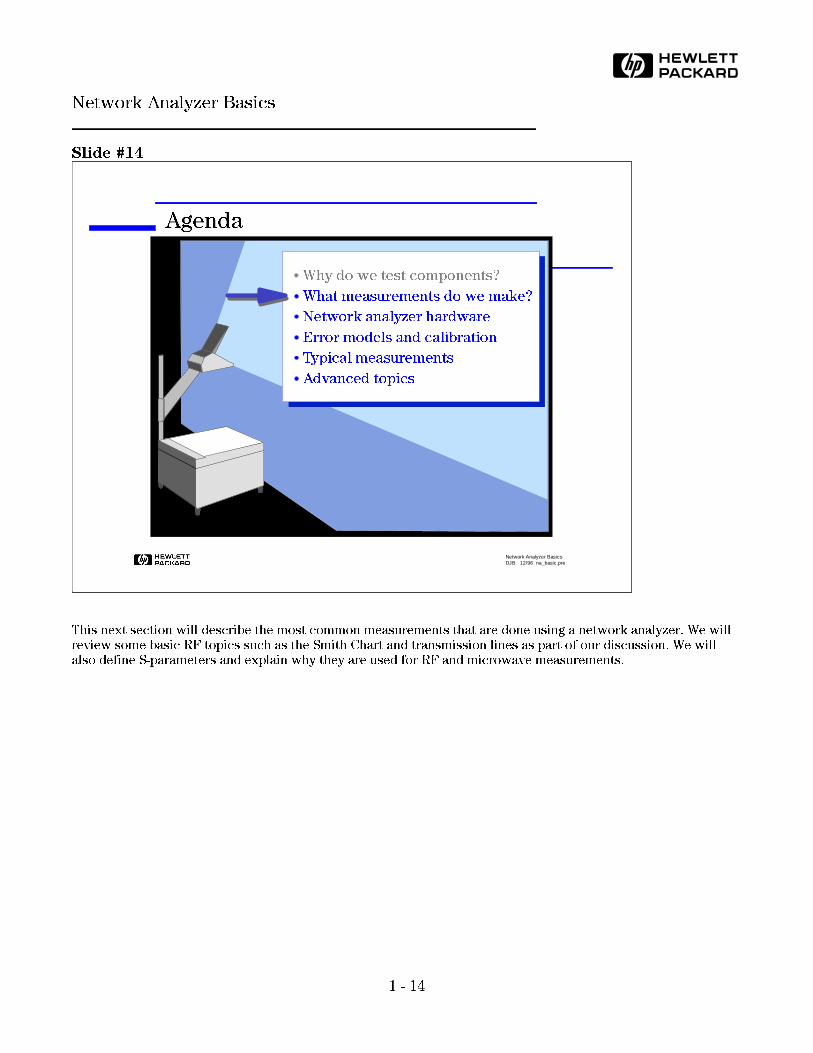
This next section will describe the most common measurements that are done using a network analyzer. We will

review some basic RF topics such as the Smith Chart and transmission lines as part of our discussion. We will

also define S-parameters and explain why they are used for RF and microwave measurements.


Agenda


What measurements do we make?

Network analyzer hardware

Error models and calibration


Advanced topics

1 - 14


Slide #15

The most fundamental concept of high-frequency network analysis involves incident, reflected and transmitted

waves traveling along transmission lines. It is helpful to think of traveling waves along a transmission line in

terms of a lightwave analogy. We can imagine incident light striking some optical component like a clear lens.

Some of the light is reflected off the surface of the lens, but most of the light continues on through the lens. If the

lens had mirrored surfaces, then most of the light would be reflected and little or none would be transmitted.

This concept is valid for RF signals as well.

Network analysis is concerned with accurately measuring the three signals shown above (incident, reflected,

transmitted), except our electromagnetic energy is in the RF range instead of the optical range, and our

components are electrical devices or networks instead of lenses and mirrors.


High-Frequency Device Characterization

Incident

Reflected

Transmitted

Lightwave Analogy

1 - 15


Slide #16

The amount of reflection that occurs when characterizing a device depends on the impedance the incident signal

sees. Let's review how complex reflection and impedance values are displayed. Since any impedance can be

represented as a real and imaginary part (R+jX or G+jB), we can easily see how these quantities can be plotted on

a rectilinear grid known as the complex impedance plane. Unfortunately, the open circuit (quite a common

impedance value) appears at infinity on the x-axis.

The polar plot is very useful since the entire impedance plane is covered. But instead of actually plotting

impedance, we display the reflection coefficient in vector form. The magnitude of the vector is the distance from

the center of the display, and phase is displayed as the angle of vector referenced to a flat line from the center to

the rightmost edge. The drawback of polar plots is that impedance values cannot be read directly from the

display.

Since there is a one-to-one correspondence between complex impedance and reflection coefficient, we can map

the positive real half of the complex impedance plane onto the polar display. The result is the Smith chart. All

values of reactance and all positive values of resistance from 0 to ∞ fall within the outer circle of the Smith chart.

Loci of constant resistance now appear as circles, and loci of constant reactance appear as arcs. Impedances on

the Smith chart are always normalized to the characteristic impedance of the test system (Zo, which is usually 50

or 75 ohms). A perfect termination (Zo) appears in the center of the chart.


Smith Chart Review.

-90o

0o180

o+-.2

.4

.6

.8

1.0

90o

∞∞00

0 +R

+jX

-jX

∞∞

Smith Chart maps

rectilinear impedance

plane onto polar plane

Rectilinear impedance

plane

Polar plane

Z = ZoL

= 0Γ

Constant X

Constant R

Z = L

= 0 O

1Γ

Smith Chart

(open)

ΓLZ = 0

= ±180 O1

(short)

1 - 16


Slide #17

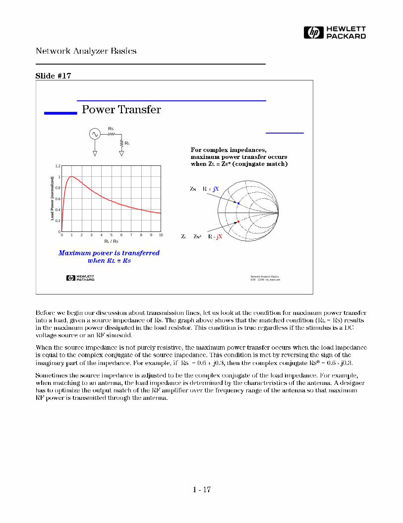
Before we begin our discussion about transmission lines, let us look at the condition for maximum power transfer

into a load, given a source impedance of Rs. The graph above shows that the matched condition (RL = RS) results

in the maximum power dissipated in the load resistor. This condition is true regardless if the stimulus is a DC

voltage source or an RF sinusoid.

When the source impedance is not purely resistive, the maximum power transfer occurs when the load impedance

is equal to the complex conjugate of the source impedance. This condition is met by reversing the sign of the

imaginary part of the impedance. For example, if RS = 0.6 + j0.3, then the complex conjugate RS* = 0.6 - j0.3.

Sometimes the source impedance is adjusted to be the complex conjugate of the load impedance. For example,

when matching to an antenna, the load impedance is determined by the characteristics of the antenna. A designer

has to optimize the output match of the RF amplifier over the frequency range of the antenna so that maximum

RF power is transmitted through the antenna.


Power Transfer

0 1 2 3 4 5 6 7 8 9 100

0.2

0.4

0.6

0.8

1

1.2

Load

Pow

er (

norm

aliz

ed)

RL / RS

RS

RL

Maximum power is transferred

when RL = RS

For complex impedances,

maximum power transfer occurs

when ZL = ZS* (conjugate match)

Zs = R + jX

ZL

= Zs* = R - jX

1 - 17


Slide #18

The need for efficient transfer of RF power is one of the main reasons behind the use of transmission lines. At low

frequencies where the wavelength of the signals are much larger than the length of the circuit conductors, a

simple wire is very useful for carrying power. Current travels down the wire easily, and voltage and current are

the same no matter where we measure along the wire.

At high frequencies however, the wavelength of signals of interest are comparable to or much smaller than the

length of conductors. In this case, power transmission can best be thought of in terms of traveling waves. When

the transmission line is terminated in its characteristic impedance Z0 (which is generally a pure resistance such as

50 or 75 Ω), maximum power is transferred to the load. When the termination is not Z0, the portion of the signal

which is not absorbed by the load is reflected back toward the source. This creates a condition where the voltage

along the transmission line varies with position.

We will examine the incident and reflected waves on a transmission line with different load conditions in the next

three slides.


Transmission Line Review

Low frequencies

Wavelength >> wire length

Current (I) travels down wires easily for efficient power transmission

Voltage and current not dependent on position

High frequencies

Wavelength ≈ or << wire (transmission line) length

Need transmission-line structures for efficient power transmission

Matching to characteristic impedance (Z0)

is very important for low reflection

Voltage dependent on position along line

I

1 - 18


Slide #19

Since a transmission line terminated in its characteristic impedance results in maximum transfer of power to the

load, there is no reflected signal. This result is the same as if the transmission line was infinitely long. If we were

to look at the envelope of the RF signal versus distance along the transmission line, it would be constant (no

standing-wave pattern). This is because there is energy flowing in one direction only.


Transmission Line Terminated with Zo

For reflection, a transmission line terminated in Zo

behaves like an infinitely long transmission line

Zs = Zo

Zo

Vrefl = 0! (all the incident

power is absorbed in the load)

Vinc

Zo = characteristic impedance

of transmission line

1 - 19


Slide #20

Next, let's terminate our line in a short circuit. Since purely reactive elements cannot dissipate any power, and

there is nowhere else for the energy to go, a reflected wave is launched back down the line toward the source. For

Ohm's law to be satisfied (no voltage across the short), this reflected wave must be equal in voltage magnitude to

the incident wave, and be 180o out of phase with it. This satisfies the condition that the total voltage must equal

zero at the plane of the short circuit. Our reflected and incident voltage (and current) waves will be identical in

magnitude but traveling in the opposite direction.

Now let us leave our line open. This time, Ohm's law tells us that the open can support no current. Therefore, our

reflected current wave must be 180oout of phase with respect to the incident wave (the voltage wave will be in

phase with the incident wave). This guarantees that current at the open will be zero. Again, our reflected and

incident current (and voltage) waves will be identical in magnitude, but traveling in the opposite direction. For

both the short and open cases, a standing-wave pattern will be set up on the transmission line. The valleys will be

at zero and the peaks at twice the incident voltage level. The peaks and valleys of the short and open will be

shifted in position along the line with respect to each other, in order to satisfy Ohm's law as described above.


Transmission Line Terminated with Short, Open

Zs = Zo

Vrefl

Vinc

For reflection, a transmission line terminated in

a short or open reflects all power back to source

In phase (0 ) for open

Out of phase (180 ) for shorto

o

1 - 20


Slide #21

Finally, let's terminate our line with a 25 Ω resistor (an impedance between the full reflection of an open or short

circuit and the perfect termination of a 50 Ω load). Some (but not all) of our incident energy will be absorbed in

the load, and some will be reflected back towards the source. We will find that our reflected voltage wave will

have an amplitude 1/3 that of the incident wave, and that the two waves will be 180o out of phase at the load. The

phase relationship between the incident and reflected waves will change as a function of distance along the

transmission line from the load. The valleys of the standing-wave pattern will no longer go zero, and the peak will

be less than that of the short/open case.


Transmission Line Terminated with 25 Ω

Zs = Zo

ZL = 25 Ω

Vrefl

Vinc

Standing wave pattern does not

go to zero as with short or open

1 - 21


Slide #22

Now that we fully understand the relationship of electromagnetic waves, we must also recognize the terms used

to describe them. We will show how to measure the incident, reflected and the transmitted waves. Common

network analyzer terminology has the incident wave measured with the R (for reference) channel. The reflected

wave is measured with the A channel and the transmitted wave is measured with the B channel. With amplitude

and phase information of these three waves, we can quantify the reflection and transmission characteristics of our

device under test (DUT). Some of the common measured terms are scalar in nature (the phase part is ignored or

not measured), while others are vector (both magnitude and phase are measured). For example, return loss is a

scalar measurement of reflection, while impedance is a vector reflection measurement.

Ratioed reflection is often shown as A/R and ratioed transmission is often shown as B/R, relating to the

measurement channels used in the network analyzer.


High-Frequency Device Characterization

Transmitted

Incident

TRANSMISSION

Gain / Loss

S-ParametersS21,S12

GroupDelay

TransmissionCoefficient

Insertion Phase

Reflected

Incident

REFLECTION

SWR

S-ParametersS11,S22 Reflection

Coefficient

Impedance, Admittance

R+jX, G+jB

ReturnLoss

Γ, ρ Τ,τ

Incident

Reflected

Transmitted

RB

A

A

R=

B

R=

1 - 22


Slide #23

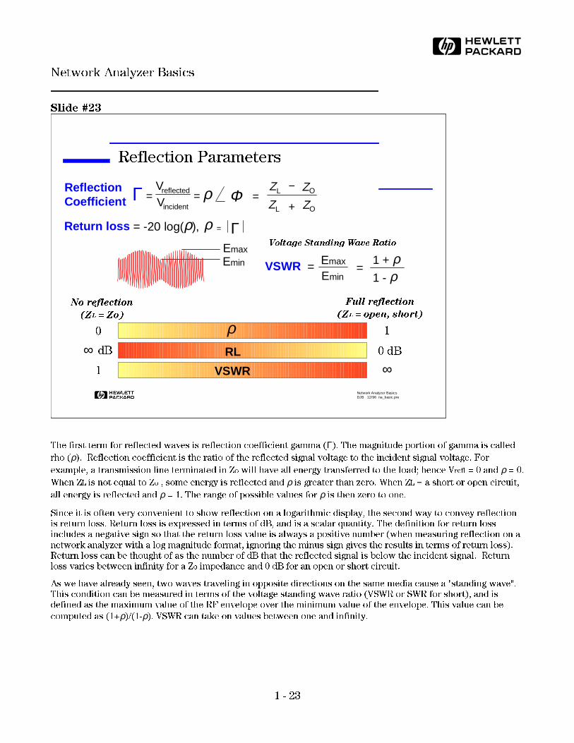
The first term for reflected waves is reflection coefficient gamma (Γ). The magnitude portion of gamma is called

rho (ρ). Reflection coefficient is the ratio of the reflected signal voltage to the incident signal voltage. For

example, a transmission line terminated in Zo will have all energy transferred to the load; hence Vrefl = 0 and ρ = 0.

When ZL is not equal to Zo , some energy is reflected and ρ is greater than zero. When ZL = a short or open circuit,

all energy is reflected and ρ = 1. The range of possible values for ρ is then zero to one.

Since it is often very convenient to show reflection on a logarithmic display, the second way to convey reflection

is return loss. Return loss is expressed in terms of dB, and is a scalar quantity. The definition for return loss

includes a negative sign so that the return loss value is always a positive number (when measuring reflection on a

network analyzer with a log magnitude format, ignoring the minus sign gives the results in terms of return loss).

Return loss can be thought of as the number of dB that the reflected signal is below the incident signal. Return

loss varies between infinity for a Zo impedance and 0 dB for an open or short circuit.

As we have already seen, two waves traveling in opposite directions on the same media cause a "standing wave".

This condition can be measured in terms of the voltage standing wave ratio (VSWR or SWR for short), and is

defined as the maximum value of the RF envelope over the minimum value of the envelope. This value can be

computed as (1+ρ)/(1-ρ). VSWR can take on values between one and infinity.


Reflection Parameters

=ZL − ZO

ZL + OZ

ReflectionCoefficient =

Vreflected

Vincident= ρ ΦΓ

=ρ Γ

∞ dB

No reflection

(ZL = Zo)

ρρRL

VSWR

0 1

Full reflection

(ZL = open, short)

0 dB

1 ∞

Return loss = -20 log(ρ),

VSWR = Emax

Emin=

1 + ρ1 - ρ

Voltage Standing Wave RatioEmax

Emin

1 - 23


Slide #24

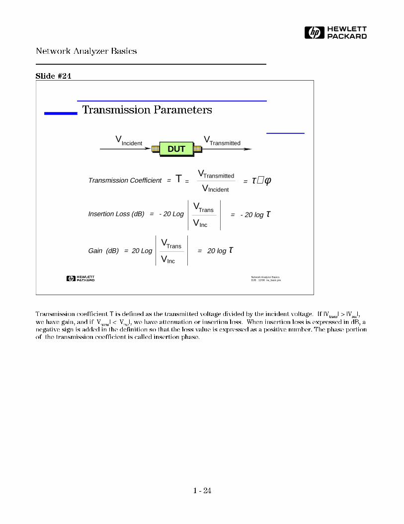
Transmission coefficient Τ is defined as the transmitted voltage divided by the incident voltage. If |Vtrans

| > |Vinc

|,

we have gain, and if |Vtrans

| < |Vinc

|, we have attenuation or insertion loss. When insertion loss is expressed in dB, a

negative sign is added in the definition so that the loss value is expressed as a positive number. The phase portion

of the transmission coefficient is called insertion phase.


Transmission Parameters

VTransmittedVIncident

Transmission Coefficient = Τ =VTransmitted

VIncident = τ∠φ

DUT

Gain (dB) = 20 Log VTrans

VInc

= 20 log τ

Insertion Loss (dB) = - 20 Log VTrans

VInc

= - 20 log τ

1 - 24


Slide #25

Looking at insertion phase directly is usually not very useful. This is because the phase has a negative slope with

respect to frequency due to the electrical length of the device (the longer the device, the greater the slope). Since

it is only the deviation from linear phase which causes distortion, it is desirable to remove the linear portion of

the phase response. This can be accomplished by using the electrical delay feature of the network analyzer to

cancel the electrical length of the DUT. This results in a high-resolution display of phase distortion (deviation

from linear phase).


Deviation from Linear Phase

Use electrical delay to remove linear portion of phase response

Linear electrical length added

+ yields

Frequency

(Electrical delay function)

Frequency

RF filter response Deviation from linear phase

Pha

se 1

/D

ivo

Pha

se 4

5 /D

ivo

Frequency

Low resolution High resolution

1 - 25


Slide #26

Another useful measure of phase distortion is group delay. Group delay is a measure of the transit time of a signal

through the device under test, versus frequency. Group delay is calculated by differentiating the insertion-phase

response of the DUT versus frequency. Another way to say this is that group delay is a measure of the slope of the

transmission phase response. The linear portion of the phase response is converted to a constant value

(representing the average signal-transit time) and deviations from linear phase are transformed into deviations

from constant group delay. The variations in group delay cause signal distortion, just as deviations from linear

phase cause distortion. Group delay is just another way to look at linear phase distortion.


What is group delay?

Deviation from constant group delay indicates distortion

Average delay indicates transit time

Frequency

Group DelayGroupDelay

Average Delay

Phaset o

t g

Group Delay (t )g

=−1

360 o

= −d φd ω

d φd f

in radians

in radians/sec

in degrees

in Hzf

φωφ

2=( )fω π

φ∆φ

Frequency

*

∆ωω

1 - 26


Slide #27

Why are both deviation from linear phase and group delay commonly measured? Depending on the device, both

may be important. Specifying a maximum peak-to-peak value of phase ripple is not sufficient to completely

characterize a device since the slope of the phase ripple is dependent on the number of ripples which occur per

unit of frequency. Group delay takes this into account since it is the differentiated phase response. Group delay is

often a more accurate indication of phase distortion. The plot above shows that the same value of peak-to-peak

phase ripple can result in substantially different group delay responses. The response on the right with the larger

group-delay variation would cause more signal distortion.


Why measure group delay?

Same p-p phase ripple can result in different group delay

Pha

se

Pha

se

Gro

up

Del

ay

Gro

up

Del

ay

−−d φφd ωω

−−d φφd ωω

f

f

f

f

1 - 27


Slide #28

In order to completely characterize an unknown linear two-port device, we must make measurements under

various conditions and compute a set of parameters. These parameters can be used to completely describe the

electrical behavior of our device (or "network"), even under source and load conditions other than when we made

our measurements. For low-frequency characterization of devices, the three most commonly measured

parameters are the H, Y and Z-parameters. All of these parameters require measuring the total voltage or current

as a function of frequency at the input or output nodes (ports) of the device. Furthermore, we have to apply either

open or short circuits as part of the measurement. Extending measurements of these parameters to high

frequencies is not very practical.


Low-Frequency Network Characterization

H-parameters

V1 = h11I1 + h12V2

V2 = h21I1 + h22V2

Y-parameters

I1 = y11V1 + y12V2

I2 = y21V1 + y22V2

Z-parameters

V1 = z11I1 + z12I2

V2 = z21I1 + z22I2

h11 = V1

I1 V2=0

h12 = V1

V2 I1=0

(requires short circuit)

(requires open circuit)

All of these parameters require measuring

voltage and current (as a function of frequency)

1 - 28


Slide #29

At high frequencies, it is very hard to measure total voltage and current at the device ports. One cannot simply

connect a voltmeter or current probe and get accurate measurements due to the impedance of the probes

themselves and the difficulty of placing the probes at the desired positions. In addition, active devices may

oscillate or self-destruct with the connection of shorts and opens.

Clearly, some other way of characterizing high-frequency networks is needed that doesn't have these drawbacks.

That is why scattering or S-parameters were developed. S-parameters have many advantages over the previously

mentioned H, Y or Z-parameters. They relate to familiar measurements such as gain, loss, and reflection

coefficient. They are relatively easy to measure, and don't require the connection of undesirable loads to the

device under test. The measured S-parameters of multiple devices can be cascaded to predict overall system

performance. They are analytically convenient for CAD programs and flow-graph analysis. And, H, Y, or

Z-parameters can be derived from S-parameters if desired.

An N-port DUT has N2 S-parameters. So, a two-port device has four S-parameters. The numbering convention for

S-parameters is that the first number following the "S" is the port where energy emerges, and the second number

is the port where energy enters. So, S21 is a measure of power coming out port 2 as a result of applying an RF

stimulus to port 1. When the numbers are the same (e.g., S11), it indicates a reflection measurement.


Limitations of H, Y, Z Parameters

(Why use S-parameters?)

H,Y, Z parameters

Hard to measure total voltage and current

at device ports at high frequencies

Active devices may oscillate or self-destruct with shorts / opens

S-parameters

Relate to familiar measurements

(gain, loss, reflection coefficient ...)

Relatively easy to measure

Can cascade S-parameters of multiple

devices to predict system performance

Analytically convenient

CAD programs

Flow-graph analysis

Can compute H, Y,or Z parameters from S-parameters if desired

Incident TransmittedS21

S11Reflected S22

Reflected

Transmitted Incidentb1

a1b2

a2S12

DUT

b1 = S11a1 +S12 a2b2 = S21 a1 + S22 a2

Port 1 Port 2

1 - 29


Slide #30

S11 and S21 are determined by measuring the magnitude and phase of the incident, reflected and transmitted

signals when the output is terminated in a perfect Zo (a load that equals the characteristic impedance of the test

system). This condition guarantees that a2 is zero. S11 is equivalent to the input complex reflection coefficient or

impedance of the DUT, and S21 is the forward complex transmission coefficient.

Likewise, by placing the source at port 2 and terminating port 1 in a perfect load (making a1 zero), S22 and S12

measurements can be made. S22 is equivalent to the output complex reflection coefficient or output impedance of

the DUT, and S12 is the reverse complex transmission coefficient.

The accuracy of S-parameter measurements depends greatly on how good a termination we apply to the port not

being stimulated. Anything other than a perfect load will result in a1 or a

2 not being zero (which violates the

definition for S-parameters). When the DUT is connected to the test ports of a network analyzer and we don't

account for imperfect test port match, we have not done a very good job satisfying the condition of a perfect

termination. For this reason, two-port error correction, which corrects for source and load match, is very

important for accurate S-parameter measurements (two-port correction is covered in the calibration section).


Measuring S-Parameters

S 11 = ReflectedIncident

=b1

a 1 a2 = 0

S 21 =Transmitted

Incident=

b2

a 1 a2 = 0

S 22 = ReflectedIncident

=b2

a 2 a1 = 0

S 12 =Transmitted

Incident=

b1

a 2 a1 = 0

Incident TransmittedS 21

S 11Reflected

b 1

a 1

b 2

Z0

Loada2 = 0

DUTForward

1IncidentTransmitted S 12

S22

Reflected

b2

a2

b

a1 = 0DUTZ0

LoadReverse

1 - 30


Slide #31

So far we have only covered measurements of linear behavior, but we know that nonlinear behavior can also

cause severe signal distortion. The most common nonlinear measurements are harmonic and intermodulation

distortion (usually measured with spectrum analyzers and signal sources), gain compression and AM-to-PM

conversion (usually measured with network analyzers and power sweeps), and noise figure. Noise figure can be

measured with a variety of instruments.

We will cover swept-power measurements using a network analyzer in the typical-measurements section of this

presentation.


Measuring Nonlinear Behavior

Most common measurements:

Using a spectrum analyzer + source(s)

harmonics, particularly second and third

intermodulation products resulting from two or more carriers

Using a network analyzer and power sweeps

gain compression

AM to PM conversion

Noise figure

RL 0 dBm ATTEN 10 dB 10 dB / DIV

CENTER 20.00000 MHz SPAN 10.00 kHzRB 30 Hz VB 30 Hz ST 20 sec LPF

8563A SPECTRUM AN AL YZER 9 k Hz - 26. 5 GHz

LPFDUT

1 - 31


Slide #32

Now that we have seen some of the measurements that are commonly done with network and spectrum

analyzers, it might be helpful to review the main differences between these instruments. Network analyzers are

used to measure components, devices, circuits, and sub-assemblies. They contain both a source and multiple

receivers, and generally display ratioed amplitude and phase information (frequency or power sweeps). A

network analyzer is always looking at a known signal (in terms of frequency), since it is a stimulus-response

system. With network analyzers, it is harder to get an (accurate) trace on the display, but very easy to interpret

the results. With vector-error correction, network analyzers provide much higher measurement accuracy than

spectrum analyzers.

Spectrum analyzers are most often used to measure signal characteristics such as carrier level, sidebands,

harmonics, phase noise, etc., on unknown signals. They are most commonly configured as a single-channel

receiver, without a source. Because of the flexibility needed to analyze signals, spectrum analyzers generally have

a much wider range of IF bandwidths available than most network analyzers. Spectrum analyzers are often used

with external sources for nonlinear stimulus/response testing. When combined with a tracking generator,

spectrum analyzers can be used for scalar component testing (magnitude versus frequency, but no phase

measurements). With spectrum analyzers, it is easy to get a trace on the display, but interpreting the results can

be much more difficult than with a network analyzer.


What is the difference between

network and spectrum analyzers?

.

Am

plitu

de R

atio

Frequency

Pow

er

Frequency

Network analyzers:

measure components, devices, circuits, sub-assembliescontain source and receiverdisplay ratioed amplitude and phase (frequency or power sweeps)

Spectrum analyzers:

measure signal amplitude characteristics (carrier level, sidebands, harmonics...)are receivers only (single channel)can be used for scalar component test (no

phase) with tracking gen. or ext. source(s)

Hard: getting (accurate) trace

Easy: interpreting results

Easy: getting trace

Hard: interpreting results

8563A SPECTRUM ANAL YZ ER 9 k Hz - 26. 5 G Hz

Measures

known

signal

Measures

unknown

signals

1 - 32


Slide #33

In this next section, we will look at how network analyzers actually work. The major pieces of a network analyzer

block diagram will be discussed in some detail.


Agenda






Advanced topics

1 - 33


Slide #34

Here is a generalized block diagram of a network analyzer, showing the major signal processing sections. In order

to measure the incident, reflected and transmitted signal, four sections are required:

1. Source for stimulus

2. Signal-separation devices

3. Receiver that provides detection

4. Processor/display for calculating and reviewing the results

We will examine each of these in more detail.


Generalized Network Analyzer

Block Diagram

RECEIVER / DETECTOR

PROCESSOR / DISPLAY

REFLECTED(A)

TRANSMITTED(B)

INCIDENT (R)

SIGNAL

SEPARATION

SOURCE

Incident

Reflected

Transmitted

DUT

1 - 34


Slide #35

The signal source supplies the stimulus for our stimulus-response test system. We can either sweep the frequency

of the source or sweep its power level. Traditionally, network analyzers used a separate source. These sources

were either based on open-loop voltage-controlled oscillators (VCOs) which were cheaper, or more expensive

synthesized sweepers which provided higher performance, especially for measuring narrowband devices.

Excessive phase noise on open-loop VCOs degrades measurement accuracy considerably when measuring

narrowband components over small frequency spans. Most network analyzers that HP sells today have integrated,

synthesized sources.


Source

Supplies stimulus for system

Swept frequency or power

Traditionally NAs used separate source

Open-loop VCOs

Synthesized sweepers

Most HP analyzers sold today have integrated, synthesized sources

Integrated, synthesized sources

1 - 35


Slide #36

The next major area we will cover is the signal separation block. The hardware used for this function is generally

called the "test set". The test set can be a separate box or integrated within the network analyzer.

There are two functions that our signal-separation hardware must provide. The first is to measure a portion of the

incident signal to provide a reference for ratioing. This can be done with splitters or directional couplers. Splitters

are usually resistive. They are non-directional devices (more on directionality later) and can be very broadband.

The trade-off is that they usually have 6 dB or more of loss in each arm.

Directional couplers can be built with very low loss (through the main arm) and good isolation and directivity.

However, it is hard to make them operate at low frequencies. This can be a problem in RF network analyzers,

where low frequency coverage is important.


Signal Separation

Splitter

usually resistive

non-directional

broadband

Measuring incident signals for ratioing

6 dB50 Ω

50 Ω6 dB

Coupler

directional

low loss

good isolation, directivity

hard to get low freq performance

Main signal

Coupled signal

1 - 36


Slide #37

The second function of the signal-splitting hardware is to separate the incident (forward) and reflected (reverse)

traveling waves at the input of our DUT. Again, couplers are ideal in that they are directional, have low loss, and

high reverse isolation. However, due to the difficulty of making truly broadband couplers, bridges are often used.

Bridges are very useful for measuring reflection because they can be made to work over a very wide range of

frequencies. The main trade-off is that they exhibit more loss to the transmitted signal, resulting in less power

delivered to the DUT for a given source power.


Signal Separation

Coupler

directional

low loss

good isolation, directivity

hard to get low freq performance

Detector

Test Port

Separating incident and reflected signals

Bridge

used to measure

reflected signals only

broadband

higher loss

1 - 37


Slide #38

The directional coupler measures (couples) a portion of the signal traveling in one direction only. The signal

flowing through the main arm is shown as a solid line, and the coupled signal is shown as a dotted line.

The signal appearing at the coupled port is reduced by an amount known as the coupling factor. This is measured

by placing the coupler in the forward direction and measuring the power at the coupled port, relative to the

incident power:

Coupling Factor (dB) = -10 log (Pfwd-cpl/Pin)

In this example of a 20 dB directional coupler, the level of a signal at the coupled port is 20 dB below that of the

input port. The loss through the main arm is only .046 dB. There are also frequency response terms associated

with the main-arm response and the coupling factor, expressed in terms of ± dB.


Forward Coupling Factor

Z

Source

0

0 dBm1 mW

−.046 dBm.99 mW

-20 dBm.01 mW

Coupling, forward

Example of 20 dB Coupler

Coupling Factor (dB) = -10 logPcoupling forward

P incident

1 - 38


Slide #39

Ideally, a signal traveling in the coupler's reverse direction will not appear at all at the coupled port, since its

energy is either absorbed in the coupler's internal load or the external termination at the end of the main arm. In

reality, however, some energy does leak through the coupled arm, as a result of finite isolation.

To measure isolation, we turn the coupler around and send power in the reverse direction. Isolation is defined as

the leakage power at the coupled port relative to the incident power:

Isolation (dB) = -10 log (Prev-cpl /Pin)


Directional Coupler Isolation (Reverse Coupling Factor)

Z

Source

0

0 dBm 1 mW

−.046 dBm.99 mW

-50 dBm.00001 mW

Coupling, reverse

Example of 20 dB Coupler "turned around"

Isolation Factor (dB) = -10 logPcoupled reverse

Pincident

this is an error signal

during measurements

1 - 39


Slide #40

One of the most important measured parameter for couplers is their directivity. Directivity is a measure of a

coupler's ability to separate signals flowing in opposite directions within the coupler. It can be thought of as the

dynamic range available for reflection measurements. By definition, directivity is the difference (in dB) between

the reverse coupling factor (isolation) and the forward coupling factor.

When measuring the forward and reverse coupling factors, notice that the coupler is terminated in a Zo load and

that we apply the same input power level. Therefore, directivity is defined as:

Directivity (dB) = 10 log (Pfwd-cpl /Prev-cpl)

Equivalent expressions for directivity are:

Directivity = [Coupling Factor/Isolation] (linear)

= Isolation (dB) - Coupling Factor (dB)

In the example above, our coupler exhibits a directivity of 30 dB. This means that during a reflection

measurement, the directivity error signal is at best 30 dB below the desired signal (when measuring a device with

full reflection or ρ = 1). The better the match of the device under test, the more measurement error the directivity

error term will cause.


Directional Coupler Directivity

Directivity (dB) = 10 log Pcoupled forward

Pcoupled reverse

Directivity = Coupling FactorIsolation

Directivity (dB) = Isolation (dB) - Coupling Factor (dB)

Example of 20 dB Coupler with 50 dB isolation:

Directivity = 50 dB - 20 dB = 30 dB

1 - 40


Slide #41

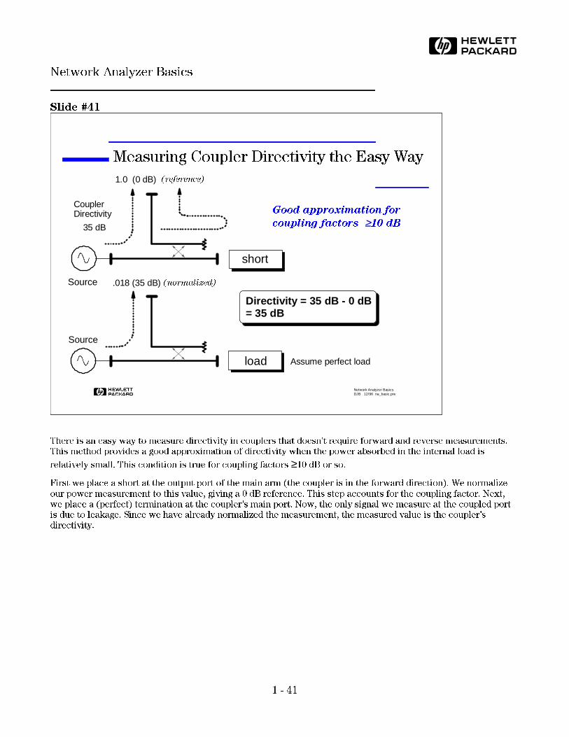
There is an easy way to measure directivity in couplers that doesn't require forward and reverse measurements.

This method provides a good approximation of directivity when the power absorbed in the internal load is

relatively small. This condition is true for coupling factors ≥10 dB or so.

First we place a short at the output port of the main arm (the coupler is in the forward direction). We normalize

our power measurement to this value, giving a 0 dB reference. This step accounts for the coupling factor. Next,

we place a (perfect) termination at the coupler's main port. Now, the only signal we measure at the coupled port

is due to leakage. Since we have already normalized the measurement, the measured value is the coupler's

directivity.


Measuring Coupler Directivity the Easy Way

short

1.0 (0 dB) (reference)

Coupler Directivity

35 dB

load

Directivity = 35 dB - 0 dB = 35 dB

Assume perfect load

.018 (35 dB) (normalized)Source

Source

Good approximation for

coupling factors ≥≥10 dB

1 - 41


Slide #42

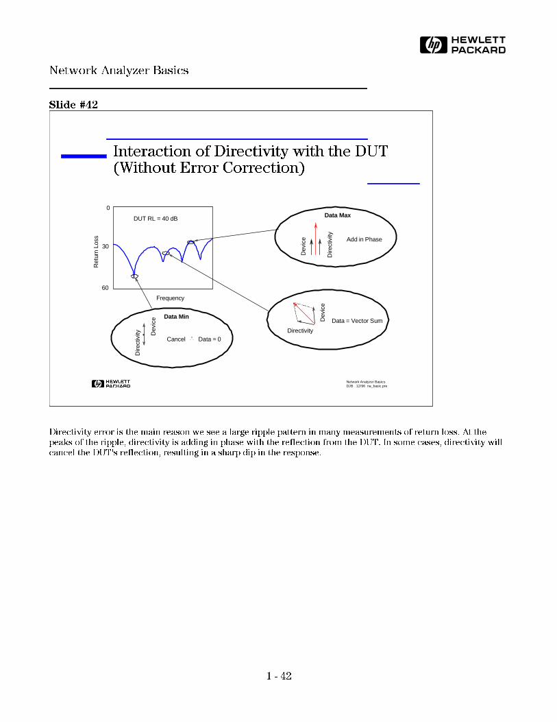
Directivity error is the main reason we see a large ripple pattern in many measurements of return loss. At the

peaks of the ripple, directivity is adding in phase with the reflection from the DUT. In some cases, directivity will

cancel the DUT's reflection, resulting in a sharp dip in the response.


Interaction of Directivity with the DUT (Without Error Correction)

Data Max

Add in Phase

Dev

ice

Dire

ctiv

ity

Ret

urn

Loss

Frequency

0

30

60

DUT RL = 40 dB

Cancel Data ≈ 0

Dev

ice

Directivity

Data = Vector Sum

Dire

ctiv

ity Dev

ice Data Min

1 - 42


Slide #43

Another device used for measuring reflected signals is the directional bridge. Its operation is similar to the simple

Wheatstone bridge. If all four arms are equal in resistance (50 Ω connected to the test port) a voltage null is

measured (the bridge is balanced). If the test-port load is not 50 Ω, then the voltage across the bridge is

proportional to the mismatch presented by the DUT's input. The bridge is imbalanced in this case. If we measure

both magnitude and phase across the bridge, we can measure the complex impedance at the test port.

A bridge's equivalent directivity is the ratio (or difference in dB) between maximum balance (measuring a perfect

Zo load) and minimum balance (measuring a short or open). The effect of bridge directivity on measurement

uncertainty is exactly the same as we discussed for couplers.


Directional Bridge

Detector

Test Port

50 Ω50 Ω

50 Ω

50 ohm load at test port balances the

bridge - detector reads zero

Extent of bridge imbalance

indicates impedance

Measuring magnitude and phase of

imbalance gives complex impedance

"Directivity" is difference between

maximum and minimum balance

1 - 43


Slide #44

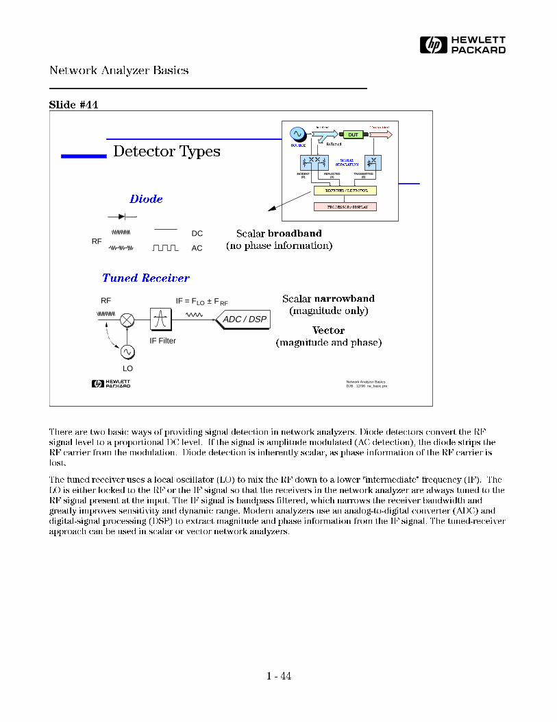
There are two basic ways of providing signal detection in network analyzers. Diode detectors convert the RF

signal level to a proportional DC level. If the signal is amplitude modulated (AC detection), the diode strips the

RF carrier from the modulation. Diode detection is inherently scalar, as phase information of the RF carrier is

lost.

The tuned receiver uses a local oscillator (LO) to mix the RF down to a lower "intermediate" frequency (IF). The

LO is either locked to the RF or the IF signal so that the receivers in the network analyzer are always tuned to the

RF signal present at the input. The IF signal is bandpass filtered, which narrows the receiver bandwidth and

greatly improves sensitivity and dynamic range. Modern analyzers use an analog-to-digital converter (ADC) and

digital-signal processing (DSP) to extract magnitude and phase information from the IF signal. The tuned-receiver

approach can be used in scalar or vector network analyzers.


Detector Types

Tuned Receiver

Scalar broadband

(no phase information)

Scalar narrowband

(magnitude only)

Vector

(magnitude and phase)

Diode

DC

ACRF

IF Filter

IF = F LO F RF±RF

LO

ADC / DSP

RECEIVER / DETECTOR

PROCESSOR / DISPLAY

REFLECTED(A)

TRANSMITTED(B)

INCIDENT (R)

SIGNAL

SEPARATION

SOURCE

Incident

Reflected

Transmitted

DUT

1 - 44


Slide #45

The main advantages of diode detectors are broadband frequency coverage ( < 10 MHz on the low end to > 26.5

GHz at the high end) and they are inexpensive compared to a tuned receiver. Diode detectors provide medium

sensitivity and dynamic range: they can measure signals to -50 dBm or so and have a dynamic range around 60

dB. Their broadband nature limits their sensitivity and makes them sensitive to source harmonics and other

spurious signals. Dynamic range is improved in measurements by increasing input power.

AC detection eliminates the DC drift of the diode as an error source, resulting in more accurate measurements.

This scheme also reduces noise and other unwanted signals. The major benefit of DC detection is that there is no

modulation of the RF signal, which can have adverse effects on the measurement of some devices. Examples

include amplifiers with AGC or large DC gain, and narrowband filters.

One application where broadband diode detectors are very useful is measuring frequency-translating devices,

particularly those with internal LOs. See slide 94 for a description of reference material.


Broadband Diode Detection

Easy to make broadband

Inexpensive compared to tuned receiver

Good for measuring frequency-translating devices

Improve dynamic range by increasing power

Medium sensitivity / dynamic range

10 MHz 26.5 GHz

1 - 45


Slide #46

Tuned receivers provide the best sensitivity and dynamic range, and also provide harmonic and spurious-signal

rejection. The narrow IF filter produces a considerably lower noise floor, resulting in a significant sensitivity

improvement. For example, a microwave vector network analyzer (using a tuned receiver) might have a 3 kHz IF

bandwidth, where a scalar analyzer's diode detector noise bandwidth might be 26.5 GHz. Measurement dynamic

range is improved with tuned receivers by increasing input power, by decreasing IF bandwidth, or by averaging.

The latter two techniques provide a trade off between noise floor and measurement speed. Averaging reduces the

noise floor of the network analyzer (as opposed to just reducing the noise excursions as happens when averaging

spectrum analyzer data) because we are averaging complex data. Without phase information, averaging does not

improve analyzer sensitivity.

The same block diagram features that produce increased dynamic range also eliminate harmonic and spurious

responses. As was mentioned earlier, the RF signal is downconverted and filtered before it is measured. The

harmonics associated with the source are also downconverted, but they appear at frequencies outside the IF

bandwidth and are therefore removed by filtering.


Narrowband Detection - Tuned Receiver

Best sensitivity / dynamic range

Provides harmonic / spurious signal rejection

Improve dynamic range by increasing power,

decreasing IF bandwidth, or averaging

Trade off noise floor and measurement speed

ADC / DSP

10 MHz 26.5 GHz

1 - 46


Slide #47

Tuned receivers can be implemented with mixer- or sampler-based front ends. It is often cheaper and easier to

make wideband front ends using samplers instead of mixers, especially for microwave frequency coverage.

Samplers are used with many of HP's network analyzers, such as the HP 8753D RF family and the HP 8720D

microwave family of analyzers.

The sampler uses diodes to sample very short time slices of the incoming RF signal. Conceptually, the sampler

can be thought of as a mixer with an internal pulse generator. The pulse generator creates a broadband

frequency spectrum (often referred to as a "comb") composed of harmonics of the LO. The RF signal mixes with

one of the spectral lines (or "comb tooth") to produce the desired IF. Compared to a mixer-based network

analyzer, the LO in a sampler-based front end covers a much smaller frequency range, and a broadband mixer is

no longer needed. The tradeoff is that the phase-lock algorithms for locking to the various comb teeth is more

complex and time consuming.

Sampler-based front ends also have somewhat less dynamic range than those based on mixers and fundamental

LOs. This is due to the fact that additional noise is converted into the IF from all of the comb teeth. Network

analyzers with narrowband detection based on samplers still have far greater dynamic range than analyzers that

use diode detection.


Front Ends: Mixers Versus Samplers

It is cheaper and easier to

make broadband front ends

using samplers instead of mixers

Mixer-based front end

ADC / DSP

Sampler-based front end

S

Harmonic generator

f

frequency "comb"

ADC / DSP

1 - 47


Slide #48

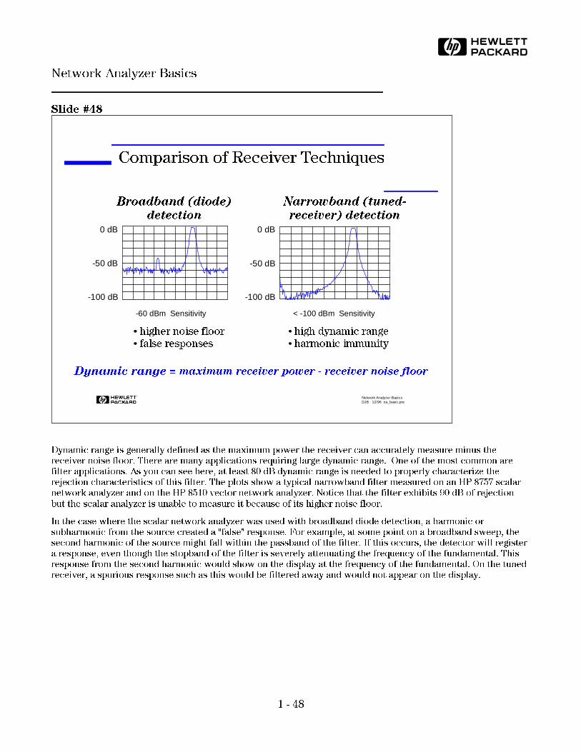
Dynamic range is generally defined as the maximum power the receiver can accurately measure minus the

receiver noise floor. There are many applications requiring large dynamic range. One of the most common are

filter applications. As you can see here, at least 80 dB dynamic range is needed to properly characterize the

rejection characteristics of this filter. The plots show a typical narrowband filter measured on an HP 8757 scalar

network analyzer and on the HP 8510 vector network analyzer. Notice that the filter exhibits 90 dB of rejection

but the scalar analyzer is unable to measure it because of its higher noise floor.

In the case where the scalar network analyzer was used with broadband diode detection, a harmonic or

subharmonic from the source created a "false" response. For example, at some point on a broadband sweep, the

second harmonic of the source might fall within the passband of the filter. If this occurs, the detector will register

a response, even though the stopband of the filter is severely attenuating the frequency of the fundamental. This

response from the second harmonic would show on the display at the frequency of the fundamental. On the tuned

receiver, a spurious response such as this would be filtered away and would not appear on the display.


Comparison of Receiver Techniques

< -100 dBm Sensitivity

0 dB

-50 dB

-100 dB

0 dB

-50 dB

-100 dB

-60 dBm Sensitivity

Broadband (diode)

detection

Narrowband (tuned-

receiver) detection

higher noise floor

false responses

high dynamic range

harmonic immunity

Dynamic range = maximum receiver power - receiver noise floor

1 - 48


Slide #49

This plot shows the effect that interfering signals (sinusoids or noise) have on measurement accuracy. To get low

measurement uncertainty, more dynamic range is needed than the device exhibits. For example, to get less than

0.1 dB magnitude error and less than 1 degree phase error, our noise floor needs to be more than 35 dB below our

measured power levels! To achieve that level of accuracy while measuring 80 dB of rejection would require 115

dB of dynamic range. This could be accomplished by averaging test data with a tuned-receiver based network

analyzer. HP network analyzers often have a clear competitive advantage by providing greater dynamic range than

competitor's network analyzers.


Dynamic Range and Accuracy

Dynamic range is very important

for measurement accuracy!

Error Due to Interfering Signal

0 -5 -10 -15 -20 -25 -30 -35 -40 -45 -50 -55 -60 -65 -700.001

0.01

0.1

1

10

100

Interfering signal (dB)

Error (dB, deg)

+ magn (dB)

- magn (dB)

phase (± deg)phase error

magn error

1 - 49


Slide #50

Here is a picture of a traditional scalar system consisting of a processor/display unit and a stand-alone source (HP

8757D and HP 8370B). This type of system requires external splitters, couplers, detectors, and bridges. While not

as common as they used to be, scalar systems such as this are good for low-cost microwave scalar applications


Traditional Scalar Analyzer

RF R A B

Traditional scalar system consists

of processor/display and source

Example: HP 8757D

requires external detectors, couplers, bridges, splitters

good for low-cost microwave scalar applications

Detector

DUT

BridgeTermination

Reflection Transmission

Detector

Detector

RF R A B

DUT

1 - 50


Slide #51

A modern scalar network analyzer has all of the components needed for reflection and transmission

measurements built-in to the instrument, such as a synthesized source, a test set, and a large display. Some scalar

network analyzers even have attributes of vector analyzers such as narrowband detection and vector error

correction (one-port and enhanced-response calibration). These instruments exhibit very high dynamic range and

good measurement accuracy.


Modern Scalar Analyzer

Synthesized source

Narrowband and

broadband detectors

Transmission/reflection

test set

Everything necessary for transmission

and reflection measurements is internal!

Large display

One-port (reflection) and response

(transmission) calibrations

1 - 51


H

Slide #52

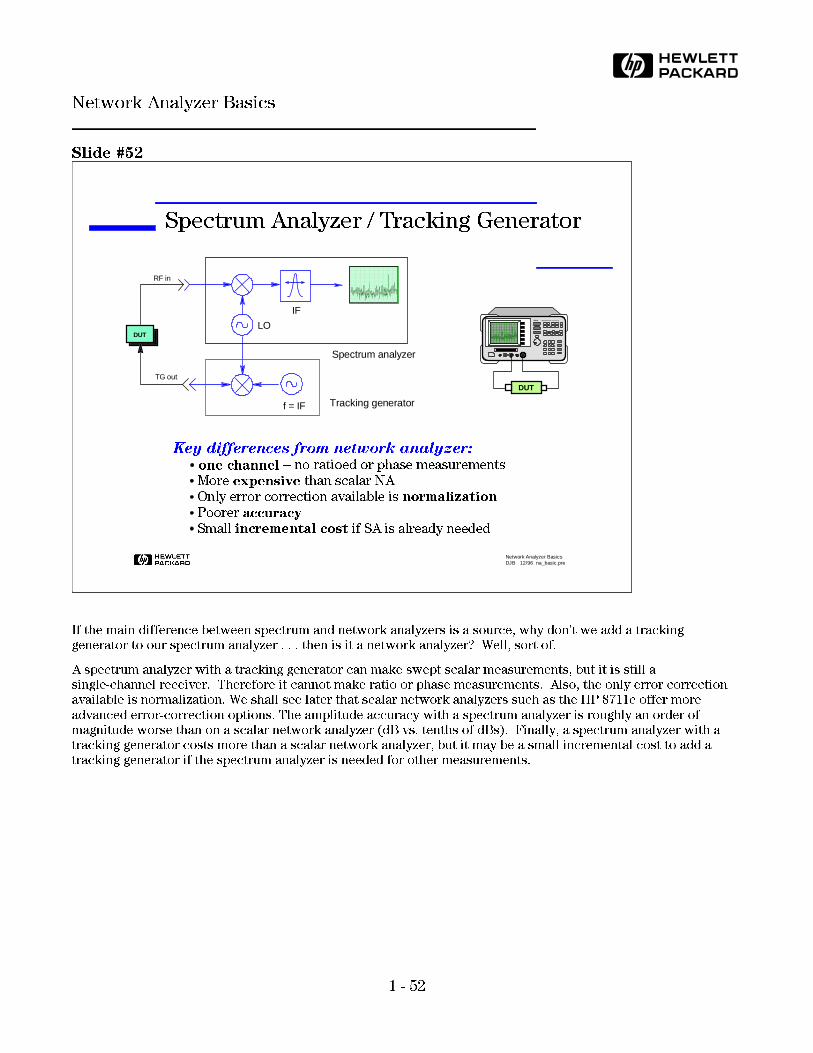
If the main difference between spectrum and network analyzers is a source, why don't we add a tracking

generator to our spectrum analyzer . . . then is it a network analyzer? Well, sort of.

A spectrum analyzer with a tracking generator can make swept scalar measurements, but it is still a

single-channel receiver. Therefore it cannot make ratio or phase measurements. Also, the only error correction

available is normalization. We shall see later that scalar network analyzers such as the HP 8711c offer more

advanced error-correction options. The amplitude accuracy with a spectrum analyzer is roughly an order of

magnitude worse than on a scalar network analyzer (dB vs. tenths of dBs). Finally, a spectrum analyzer with a

tracking generator costs more than a scalar network analyzer, but it may be a small incremental cost to add a

tracking generator if the spectrum analyzer is needed for other measurements.


Spectrum Analyzer / Tracking Generator

Tracking generator

RF in

TG out

f = IF

Spectrum analyzer

IF

LODUT

Key differences from network analyzer:one channel -- no ratioed or phase measurements

More expensive than scalar NA

Only error correction available is normalization

Poorer accuracy

Small incremental cost if SA is already needed

8563A SPECTRUM ANALYZER 9 kHz - 26.5 G Hz

DUT

1 - 52


H

Slide #53

Here is a block diagram of a modern vector network analyzer. It features an integrated source, a sampler-based

front end, and a tuned receiver providing magnitude and phase data with vector-error correction. The test set (the

portion of the instrument that contains the signal-separation devices and the switches for directing the RF power)

can either be transmission/reflection (T/R) based or an S-parameter test set.

Modern scalar analyzers like the 8711C and 8713C look very similar to this block diagram, but they don't display

phase information on the screen. Internally, however, they are essentially vector analyzers. This capability lets

them make much more accurate measurements than traditional scalar analyzers.


Modern Vector Analyzer

Note: modern scalar analyzers like HP 8711/13C look

just like vector analyzers, but they don't display phase

Features:

integrated source

sampler-based front end

tuned receiver

magnitude and phase

vector-error correction

T/R or S-parameter test sets

A

B

R

S

S

S

4 kHz

4 kHz

4 kHz

TestSet

RF

300 kHzto

3 GHz

Reference

Synthesizer15 MHz to 60 MHz

MUX

996 kHz

Phase Lock

Source Receiver

ADC CPU Display

Digital Control

DUT

φ detector

TestSet

1 - 53


H

Slide #54

There are two basic types of test sets that are used with network analyzers. For transmission/reflection (T/R) test

sets, the RF power always comes out of test port one and test port two is always connected to a receiver in the

analyzer. To measure reverse transmission or output reflection of the DUT, we must disconnect it, turn it around,

and re-connect it to the analyzer. T/R-based network analyzers offer only response and one-port calibrations, so

measurement accuracy is not as good as that which can be achieved with S-parameter test sets. However,

T/R-based analyzers are more economical.

S-parameter test sets allow both forward and reverse measurements on the DUT, which are needed to

characterize all four S-parameters. RF power can come out of either test port one or two, and either test port can

be connected to a receiver. S-parameter test sets also allow full two-port (12-term) error correction, which is the

most accurate form available. S-parameter network analyzers provide more performance than T/R-based

analyzers, but cost more due to extra RF components in the test set.

There are two different types of transfer switches that can be used in an S-parameter test set: solid-state and

mechanical. Solid-state switches have the advantage of infinite lifetimes (assuming they are not damaged by too

much power from the DUT). However, they are more lossy so they reduce the maximum output power of the

network analyzer. Mechanical switches have very low loss and therefore allow higher output powers. Their main

disadvantage is that eventually they wear out (after 5 million cycles or so). When using a network analyzer with

mechanical switches, measurements are generally done in single-sweep mode, so the transfer switch is not

continously switching.


T/R Versus S-Parameter Test Sets

RF always comes out port 1

port 2 is always receiver

response, one-port cal available

RF comes out port 1 or port 2

forward and reverse measurements

two-port calibration possible

Transmission/Reflection Test Set

Port 1 Port 2

Source

B

R

A

DUTFwd

Port 1 Port 2

Transfer switch

Source

B

R

A

S-Parameter Test Set

DUTFwd Rev

1 - 54


H

Slide #55

There are two basic S-parameter test set architectures: one employing three samplers (or mixers) and one

employing four samplers (or mixers). The three-sampler architecture is simpler and less expensive, but the

calibration choices are not as good. This type of network analyzer can do TRL* and LRM* calibrations (more on

this later), but not true TRL or LRM.

Four-sampler analyzers are more expensive but provide better accuracy for noncoaxial measurements. We will

cover this in more detail in the discussion about TRL in the next section.


Three Versus Four-Channel Analyzers

Port 1

Transfer switch

Port 2

Source

B

R1

A

R2

Port 1 Port 2

Transfer switch

Source

B

R

A

3 samplerscheaper

TRL*, LRM* cal only

includes:

HP 8753D

HP 8720D (std.)

4 samplersmore expensive

true TRL, LRM cal

includes

HP 8720D (opt. 400)

HP 8510C

1 - 55


H

Slide #56

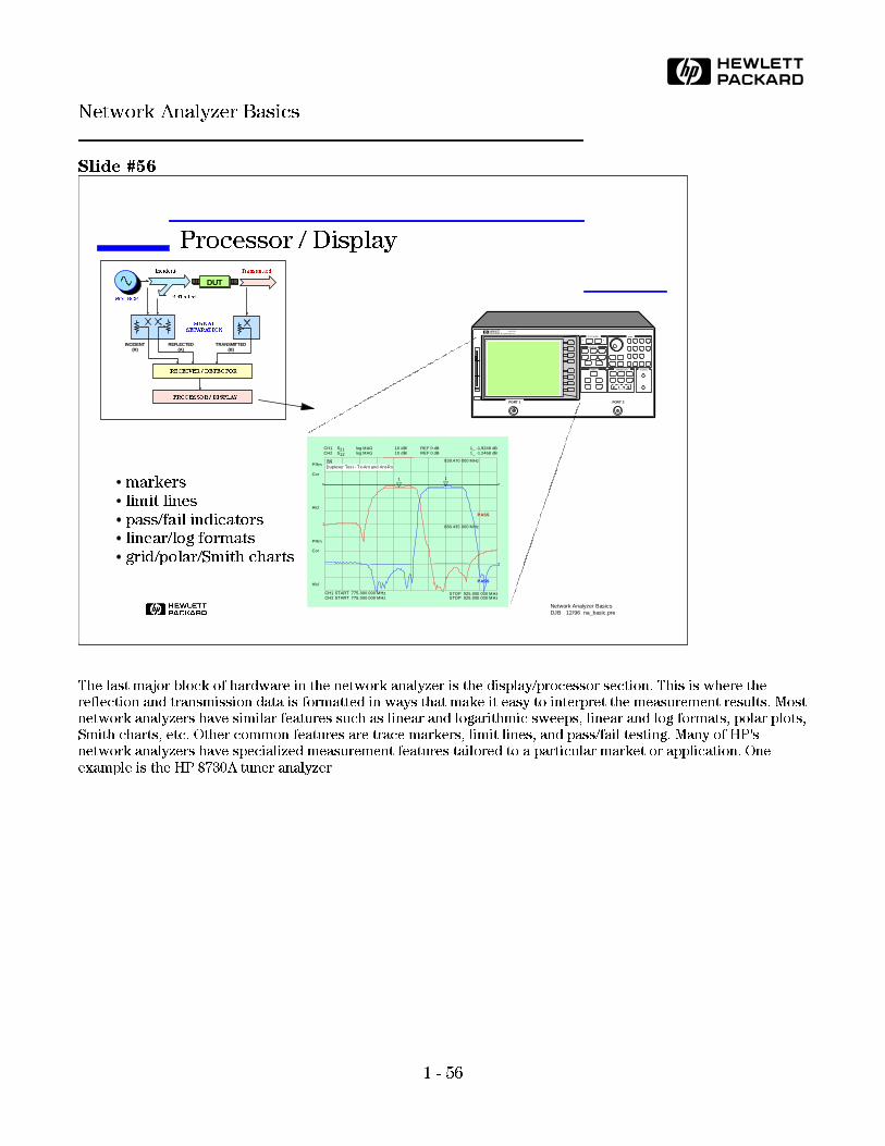
The last major block of hardware in the network analyzer is the display/processor section. This is where the

reflection and transmission data is formatted in ways that make it easy to interpret the measurement results. Most

network analyzers have similar features such as linear and logarithmic sweeps, linear and log formats, polar plots,

Smith charts, etc. Other common features are trace markers, limit lines, and pass/fail testing. Many of HP's

network analyzers have specialized measurement features tailored to a particular market or application. One

example is the HP 8730A tuner analyzer


Processor / Display

RECEIVER / DETECTOR

PROCESSOR / DISPLAY

REFLECTED(A)

TRANSMITTED(B)

INCIDENT (R)

SIGNAL

SEPARATION

SOURCE

Incident

Reflected

Transmitted

DUT

HACTIVE CHANNEL

RESPONSE

STIMULUS

ENTRY

INSTRUMENT STATE R CHANNEL

R L T S

HP-IB STATUS

NET WORK ANALYZER

50 MHz-20GHz

PORT 2PORT 1

CH1 S21 log MAG 10 dB/ REF 0 dB

CH1 START 775.000 000 MHz STOP 925.000 000 MHz

Cor

Hld

PRm

CH2 S12 log MAG REF 0 dB10 dB/


Duplexer Test - Tx-Ant and Ant-Rx

Cor

Hld

PRm

1

1

1_ -1.9248 dB

839.470 000 MHz

PASS

2

1

1_ -1.2468 dB

880.435 000 MHz

PASS

markers

limit lines

pass/fail indicators

linear/log formats

grid/polar/Smith charts

1 - 56


H

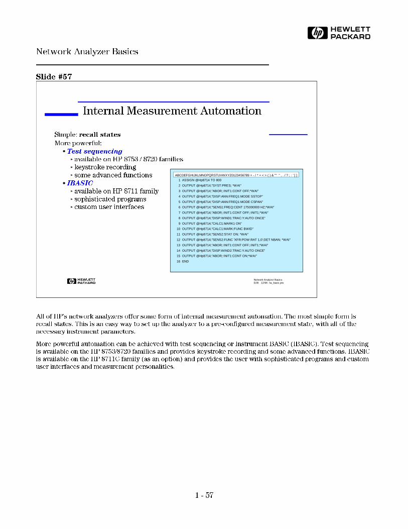
Slide #57

All of HP's network analyzers offer some form of internal measurement automation. The most simple form is

recall states. This is an easy way to set up the analyzer to a pre-configured measurement state, with all of the

necessary instrument parameters.

More powerful automation can be achieved with test sequencing or Instrument BASIC (IBASIC). Test sequencing

is available on the HP 8753/8720 families and provides keystroke recording and some advanced functions. IBASIC

is available on the HP 8711C family (as an option) and provides the user with sophisticated programs and custom

user interfaces and measurement personalities.


Internal Measurement Automation

Simple: recall states

More powerful:

Test sequencing

available on HP 8753 / 8720 families

keystroke recording

some advanced functions

IBASIC

available on HP 8711 family

sophisticated programs

custom user interfaces

ABCDEFGHIJKLMNOPQRSTUVWXYZ0123456789 + - / * = < > ( ) & "" " , . / ? ; : ' [ ]

1 ASSIGN @Hp8714 TO 800

2 OUTPUT @Hp8714;"SYST:PRES; *WAI"

3 OUTPUT @Hp8714;"ABOR;:INIT1:CONT OFF;*WAI"

4 OUTPUT @Hp8714;"DISP:ANN:FREQ1:MODE SSTOP"

5 OUTPUT @Hp8714;"DISP:ANN:FREQ1:MODE CSPAN"

6 OUTPUT @Hp8714;"SENS1:FREQ:CENT 175000000 HZ;*WAI"

7 OUTPUT @Hp8714;"ABOR;:INIT1:CONT OFF;:INIT1;*WAI"

8 OUTPUT @Hp8714;"DISP:WIND1:TRAC:Y:AUTO ONCE"

9 OUTPUT @Hp8714;"CALC1:MARK1 ON"

10 OUTPUT @Hp8714;"CALC1:MARK:FUNC BWID"

11 OUTPUT @Hp8714;"SENS2:STAT ON; *WAI"

12 OUTPUT @Hp8714;"SENS2:FUNC 'XFR:POW:RAT 1,0';DET NBAN; *WAI"

13 OUTPUT @Hp8714;"ABOR;:INIT1:CONT OFF;:INIT1;*WAI"

14 OUTPUT @Hp8714;"DISP:WIND2:TRAC:Y:AUTO ONCE"

15 OUTPUT @Hp8714;"ABOR;:INIT1:CONT ON;*WAI"

16 END

1 - 57


H

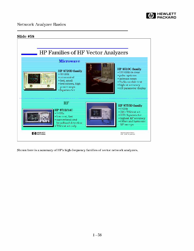
Slide #58

Shown here is a summary of HP's high-frequency families of vector network analyzers.


HP Families of HF Vector Analyzers

Microwave

RF

HP 8510C family110 GHz in coax

pulse systems

antenna meas.

Tx/Rx module testhighest accuracy

4 S-parameter display

HP 8720D family40 GHz

economical

fast, smalltest mixers, high-

power ampsS-parameter

HP 8712/14C3 GHzlow cost, fast

narrowband and

broadband detectionT/R test set only

HP 8753D family6 GHz

52C: T/R test set53D: S-parameter

highest RF accuracy

Offset and harmonic RF sweeps

1 - 58


H

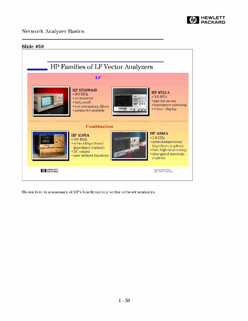
Slide #59

Shown here is a summary of HP's low-frequency vector network analyzers.


HP Families of LF Vector Analyzers

HP E5100A/B

300 MHz

economicalfast, small

test resonators, filters

parameter analysis

HP 8751A

500 MHz

fast list sweepimpedance matching

4 trace display

HP 4195A

500 MHz

network/spectrum/

impedance (option)DC outputuser-defined functions

HP 4396A

1.8 GHznetwork/spectrum/

impedance (option)fast, highest accuracy

time-gated spectrum

(option)

LF

Combination

1 - 59


H

Slide #60

In this next section, we will talk about the need for error correction and how it is accomplished. Why do we even

need error-correction and calibration? It is impossible to make perfect hardware which obviously would not need

any form of error correction. Even making the hardware good enough to not require any error correction for most

devices would be extremely expensive. The best balance is to make the hardware as good as practically possible,

balancing performance and cost. Error correction is then very useful to improve measurement accuracy.


Agenda






Advanced topics

Why do we even need error-correction

and calibration?It is impossible to make perfect hardware

It would be extremely expensive to make hardware

good enough to not require any error correction

1 - 60


H

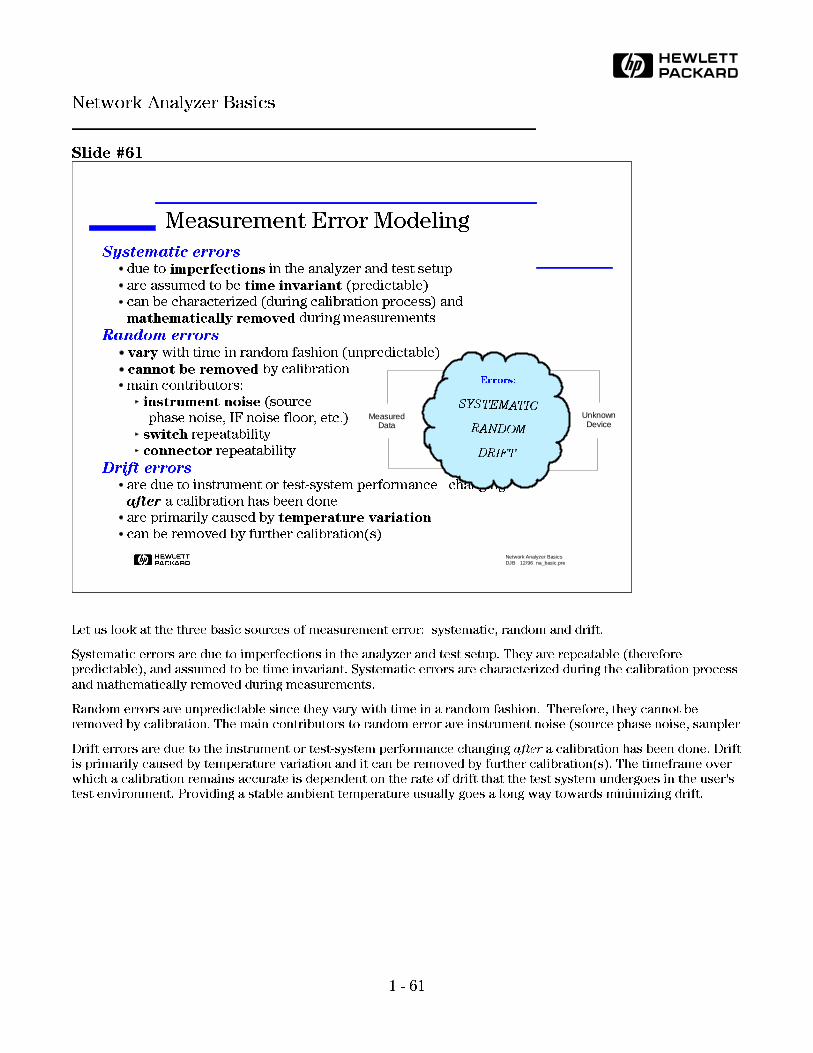
Slide #61

Let us look at the three basic sources of measurement error: systematic, random and drift.

Systematic errors are due to imperfections in the analyzer and test setup. They are repeatable (therefore

predictable), and assumed to be time invariant. Systematic errors are characterized during the calibration process

and mathematically removed during measurements.

Random errors are unpredictable since they vary with time in a random fashion. Therefore, they cannot be

removed by calibration. The main contributors to random error are instrument noise (source phase noise, sampler

Drift errors are due to the instrument or test-system performance changing after a calibration has been done. Drift

is primarily caused by temperature variation and it can be removed by further calibration(s). The timeframe over

which a calibration remains accurate is dependent on the rate of drift that the test system undergoes in the user's

test environment. Providing a stable ambient temperature usually goes a long way towards minimizing drift.


Measurement Error Modeling

Systematic errorsdue to imperfections in the analyzer and test setup

are assumed to be time invariant (predictable)

can be characterized (during calibration process) and

mathematically removed during measurements

Random errors

vary with time in random fashion (unpredictable)

cannot be removed by calibration

main contributors:

instrument noise (source

phase noise, IF noise floor, etc.)

switch repeatability

connector repeatability

Drift errorsare due to instrument or test-system performance changing

after a calibration has been done

are primarily caused by temperature variation

can be removed by further calibration(s)

Unknown Device

Measured Data

SSYSYSTTEEMMATATIICC

RRAANNDDOMOM

DDRRIFTIFT

Errors:

1 - 61


H

Slide #62

Shown here are the major systematic errors associated with network measurements. The errors relating to signal

leakage are directivity and crosstalk. Errors related to signal reflections are source and load match. The final

class of errors are related to frequency response of the receivers, and are called reflection and transmission

tracking. The full two-port error model includes all six of these terms for the forward direction and the same six

(with different data) in the reverse direction, for a total of twelve error terms. This is why we often refer to

two-port calibration as twelve-term error correction.


Systematic Measurement Errors

AA BB

Source

Mismatch

Load

Mismatch

CrosstalkDirectivity

DUT

Frequency response

reflection tracking (A/R)

transmission tracking (B/R)

RR

Six forward and six reverse error terms

yields 12 error terms for two-port devices

1 - 62


H

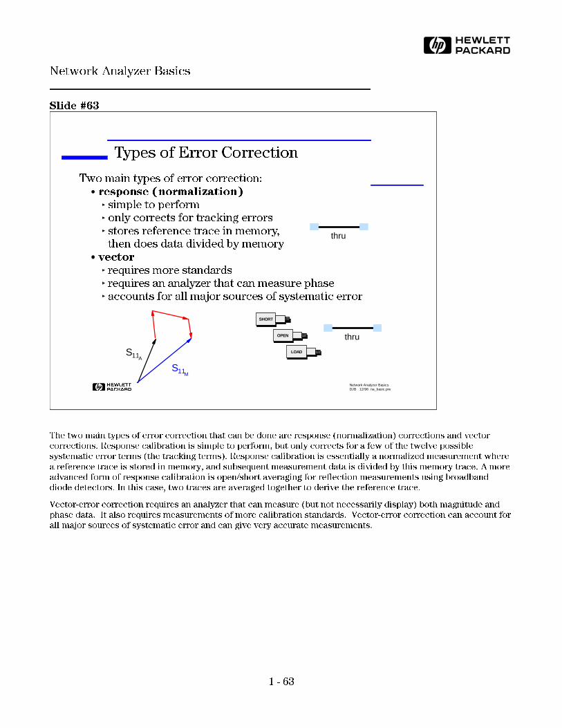
Slide #63

The two main types of error correction that can be done are response (normalization) corrections and vector

corrections. Response calibration is simple to perform, but only corrects for a few of the twelve possible

systematic error terms (the tracking terms). Response calibration is essentially a normalized measurement where

a reference trace is stored in memory, and subsequent measurement data is divided by this memory trace. A more

advanced form of response calibration is open/short averaging for reflection measurements using broadband

diode detectors. In this case, two traces are averaged together to derive the reference trace.

Vector-error correction requires an analyzer that can measure (but not necessarily display) both magnitude and

phase data. It also requires measurements of more calibration standards. Vector-error correction can account for

all major sources of systematic error and can give very accurate measurements.


Types of Error Correction

Two main types of error correction:

response (normalization)

simple to perform

only corrects for tracking errors

stores reference trace in memory, then does data divided by memory

vector

requires more standards

requires an analyzer that can measure phase

accounts for all major sources of systematic error

S11M

S11A

SHORT

OPEN

LOAD

thru

thru

1 - 63


H

Slide #64

Vector-error correction is the process of characterizing systematic error terms by measuring known calibration

standards, and then removing the effects of these errors from subsequent measurements.

One-port calibration is used for reflection measurements and can measure and remove three systematic error

terms (directivity, source match, and reflection tracking). Full two-port calibration can be used for both reflection

and transmission measurements, and all twelve systematic error terms are measured and removed. Two-port

calibration usually requires twelve measurements on four known standards (short-open-load-thru or SOLT). Some

standards are measured multiple times (e.g., the thru standard is usually measured four times). The standards

themselves are defined in a cal-kit definition file, which is stored in the network analyzer. HP network analyzers

contain all of the cal-kit definitions for our standard calibration kits. In order to make accurate measurements, the

cal-kit definition MUST MATCH THE ACTUAL CALIBRATION KIT USED!


What is Vector-Error Correction?

Process of characterizing systematic error terms

measure known standards

remove effects from subsequent measurements.

1-port calibration (reflection measurements)

only 3 systematic error terms measured

directivity, source match, and reflection tracking

Full 2-port calibration (reflection and transmission measurements)

12 systematic error terms measured

usually requires 12 measurements on four known standards (SOLT)

Some standards can be measured multiple times

(e.g., THRU is usually measured four times)

Standards defined in cal kit definition file

network analyzer contains standard cal kit definitions

CAL KIT DEFINITION MUST MATCH ACTUAL CAL KIT USED!

1 - 64


H

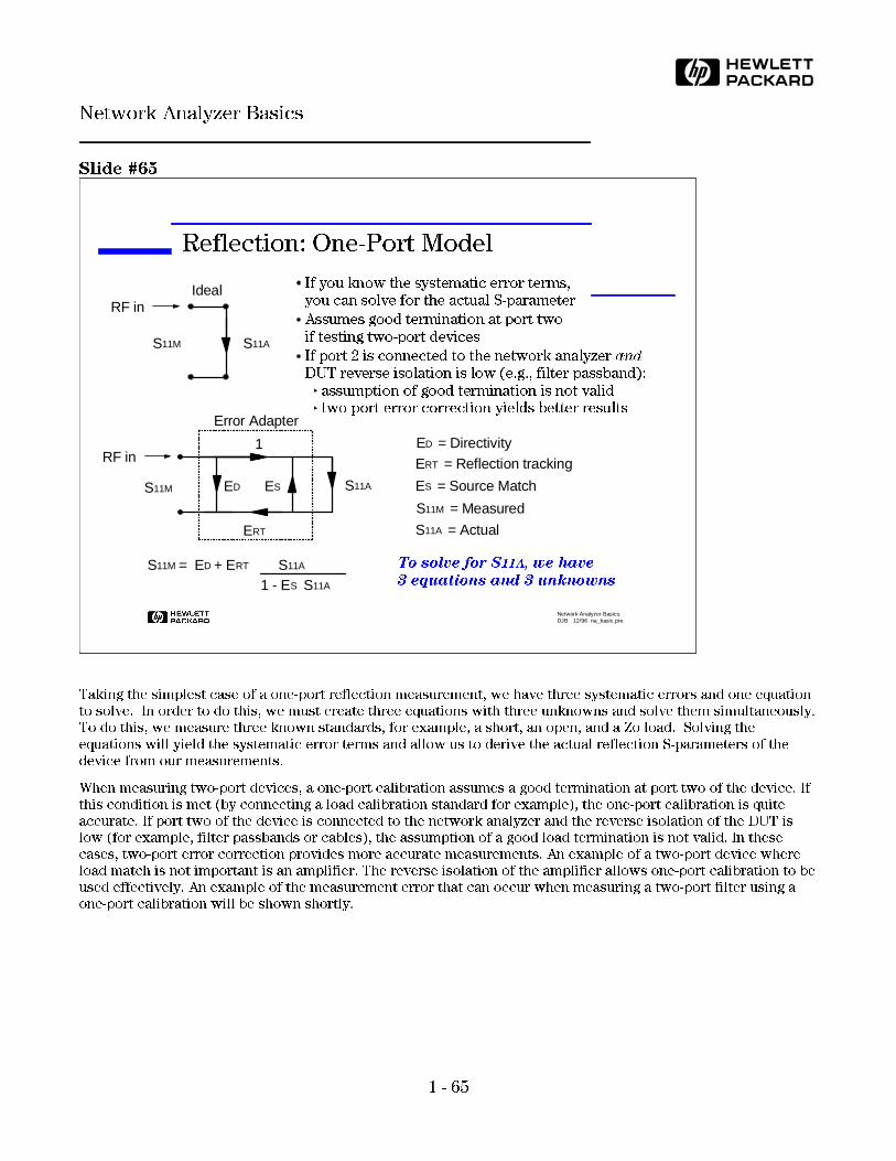
Slide #65

Taking the simplest case of a one-port reflection measurement, we have three systematic errors and one equation

to solve. In order to do this, we must create three equations with three unknowns and solve them simultaneously.

To do this, we measure three known standards, for example, a short, an open, and a Zo load. Solving the

equations will yield the systematic error terms and allow us to derive the actual reflection S-parameters of the

device from our measurements.

When measuring two-port devices, a one-port calibration assumes a good termination at port two of the device. If

this condition is met (by connecting a load calibration standard for example), the one-port calibration is quite

accurate. If port two of the device is connected to the network analyzer and the reverse isolation of the DUT is

low (for example, filter passbands or cables), the assumption of a good load termination is not valid. In these

cases, two-port error correction provides more accurate measurements. An example of a two-port device where

load match is not important is an amplifier. The reverse isolation of the amplifier allows one-port calibration to be

used effectively. An example of the measurement error that can occur when measuring a two-port filter using a

one-port calibration will be shown shortly.


Reflection: One-Port Model

S11M = ED + ERT S11A

1 - ES S11A

ED = DirectivityERT = Reflection tracking

ES = Source Match

S11M = Measured

S11A = Actual

To solve for S11A, we have

3 equations and 3 unknowns

S11M S11AES

ERT

ED

1RF in

Error Adapter

S11M S11A

RF inIdeal If you know the systematic error terms,

you can solve for the actual S-parameter

Assumes good termination at port two

if testing two-port devices

If port 2 is connected to the network analyzer and

DUT reverse isolation is low (e.g., filter passband):

assumption of good termination is not valid

two-port error correction yields better results

1 - 65


H

Slide #66

Shown here is a plot of reflection with and without one-port calibration. Without error correction, we see the

classic ripple pattern caused by the systematic errors interfering with the measured signal. The error-corrected

trace is much smoother and better represents the device's actual reflection performance.


Before and After One-Port Calibration

Data BeforeError Correction

Data AfterError Correction

0

20

40

60

6000 12000

2.0

Ret

urn

Loss

(dB

)

VS

WR

1.1

1.01

1.001

1 - 66


H

Slide #67

Whenever possible, reflection calibrations should be done with a cal kit that matches the connector type of the

DUT. If adapters need to be used to mate the calibrated test system to the DUT, the effect of these adapters on

measurement accuracy can be very large. This error is often ignored, which may or may not be acceptable. As the

flow-graph shows, the adapter causes an error signal which can add or subtract with the desired signal from the

DUT. Worst-case effective directivity (in dB) is now:

-20 log (ρcoupler + ρadapter)

If the adapter has a SWR of say 1.5 (the less-expensive variety), the effective directivity of the coupler drops to

around 14 dB worst case, even if the coupler itself had infinite directivity! In other words, with a perfect Zo load

(ρL = 0) on the output of the adapter; the reflected signal appearing at the coupled port would only be 14 dB less

than the reflection from a short or open circuit. Stacking adapters compounds the problem, as is illustrated above.

Consequently, it is very important to use quality adapters (or preferably, no adapters at all) in your measurement

system, so system directivity is not excessively degraded. While error-correction can mitigate the effect of

adapters on the test port, our system is more susceptible to drift with degraded raw (uncorrected) directivity.


Adapter Considerations

TerminationAdapter DUT

= total ρ

adapter DUT+ρ ρ

Worst-caseSystem Directivity

28 dB

17 dB

14 dB

APC-7 to SMA (m)SWR:1.06

APC-7 to N (f) + N (m) to SMA (m)SWR:1.05 SWR:1.25

APC-7 to N (m) + N (f) to SMA (f) + SMA (m) to (m)SWR:1.05 SWR:1.25 SWR:1.15

Adapting from APC-7 to SMA (m)

Coupler directivity = 40 dB

leakage signal

desired signal

reflection

from adapter

APC-7 calibration done here

DUT has SMA (f)

connectors

1 - 67


H

Slide #68

Two-port error correction is the most accurate form of error correction since it accounts for all of the major

sources of systematic error. The error model for a two-port device is shown above. Shown below are the

equations to derive the actual device S-parameters from the measured S-parameters, once the systematic error

terms have been characterized. Notice that each actual S-parameter is a function of all four measured

S-parameters. The network analyzer must make a forward and reverse sweep to update any one S-parameter.

Luckily, you don't need to know these equations to use network analyzers!!!


Two-Port Error Correction

Notice that each actual S-parameter is a function of all four measured S-parameters

Analyzer must make forward and reverse sweep to update any one S-parameter

Luckily, you don't need to know these equations to use network analyzers!!!

Port 1 Port 2E

S11

S21

S12

S22

ESED

ERT

ETT

EL

= Directivity

= Source Match

= Reflection Tracking

= Load Match

= Transmission Tracking

= Isolation

ES

ED

ERT

ETT

EL

EX

a1

b1

A

A

A

A

X

a2

b2 Forward model

1 - 68


H

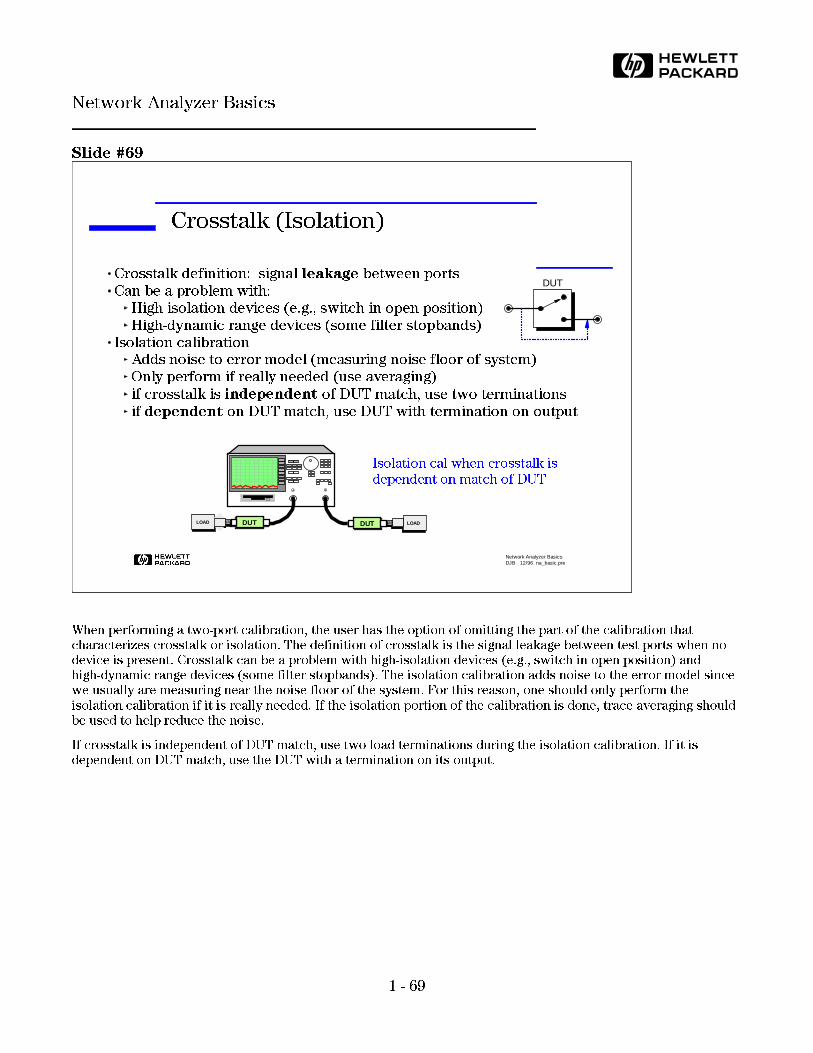
Slide #69

When performing a two-port calibration, the user has the option of omitting the part of the calibration that

characterizes crosstalk or isolation. The definition of crosstalk is the signal leakage between test ports when no

device is present. Crosstalk can be a problem with high-isolation devices (e.g., switch in open position) and

high-dynamic range devices (some filter stopbands). The isolation calibration adds noise to the error model since

we usually are measuring near the noise floor of the system. For this reason, one should only perform the

isolation calibration if it is really needed. If the isolation portion of the calibration is done, trace averaging should

be used to help reduce the noise.

If crosstalk is independent of DUT match, use two load terminations during the isolation calibration. If it is

dependent on DUT match, use the DUT with a termination on its output.


Crosstalk (Isolation)

Crosstalk definition: signal leakage between ports

Can be a problem with:

High-isolation devices (e.g., switch in open position)

High-dynamic range devices (some filter stopbands)

Isolation calibration

Adds noise to error model (measuring noise floor of system)

Only perform if really needed (use averaging)

if crosstalk is independent of DUT match, use two terminations

if dependent on DUT match, use DUT with termination on output

DUT

DUT LOADDUTLOAD

Isolation cal when crosstalk is

dependent on match of DUT

1 - 69


H

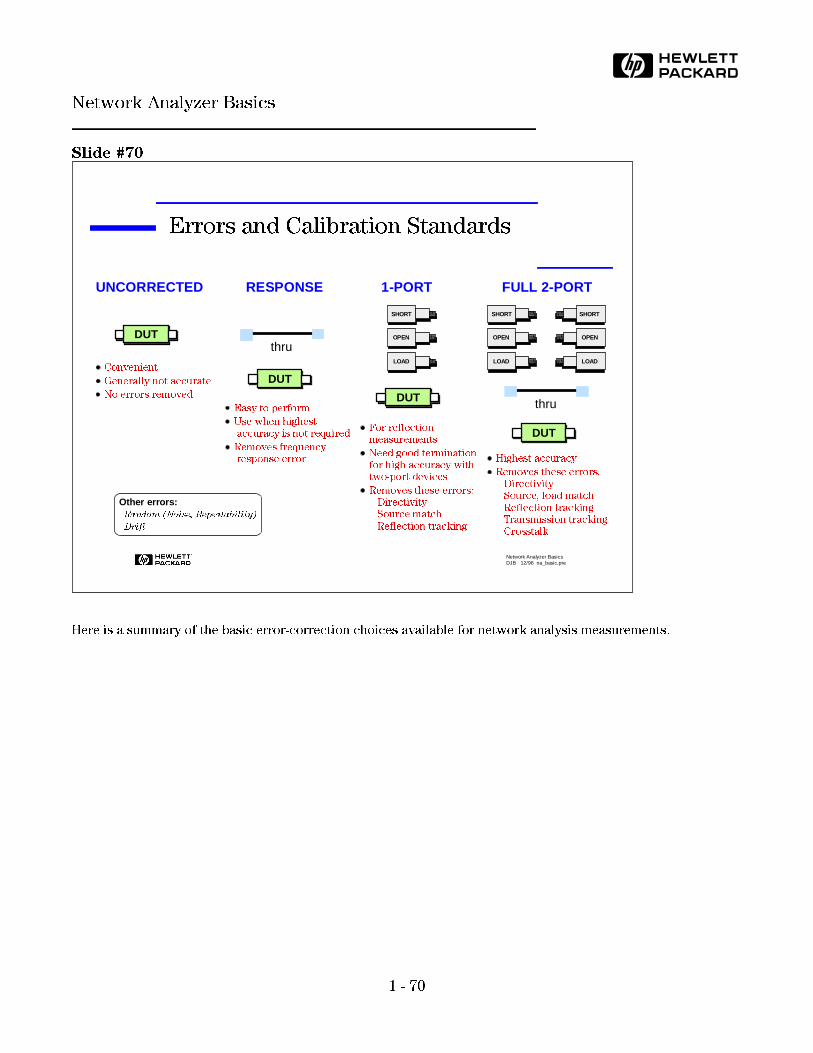
Slide #70

Here is a summary of the basic error-correction choices available for network analysis measurements.


Errors and Calibration Standards

Convenient

Generally not accurate

No errors removed

Easy to perform

Use when highest

accuracy is not required

Removes frequency

response error

For reflection

measurements

Need good termination

for high accuracy with

two-port devices

Removes these errors:

Directivity

Source match

Reflection tracking

Highest accuracy

Removes these errors:

Directivity

Source, load match

Reflection tracking

Transmission tracking

Crosstalk

UNCORRECTED RESPONSE 1-PORT FULL 2-PORT

Other errors: Random (Noise, Repeatability)

Drift

DUT

DUT

DUT

DUT

SHORT

OPEN

LOAD

SHORT

OPEN

LOAD

SHORT

OPEN

LOAD

thru

thru

1 - 70


H

Slide #71

Although the previous slide showed mechanical calibration standards, HP offers a solid-state calibration solution

which makes two-port calibration fast, easy, and less prone to operator errors. This system consists of a control

unit and various calibration modules. The calibration modules are solid-state devices with programmable,

repeatable impedance states. These states are characterized at the HP factory using a TRL-calibrated network

analyzer, making the ECal modules transfer standards (rather than direct standards). ECal provides accuracy

better than SOLT, but somewhat less than TRL.

The various impedance states in the modules are achieved by PIN-diode switches which shunt the transmission

line to ground. The number of diodes and their location vary depending upon the module's frequency range. A

multitude of reflection coefficients can be generated by applying various combinations of the shunts. With no

shunts, the network acts as a low loss transmission line. High isolation between the ports is obtained by driving

several of the PIN shunts simultaneously. Four different states are used to compute the error terms at each

frequency point. Four states are used because this gives the best trade-off between high accuracy and the time

required for the calibration. With four reflection states, we have four equations but only three unknowns. To

achieve the best accuracy from this over-determined set of equations, a least-squares-fit algorithm is used. Adding

more impedance states at each frequency point would further improve accuracy but at the expense of more

calibration time.


ECal: Electronic Calibration (HP 85060 series)

Impedance States

achieved by shunting transmission line with

PIN-diode switches in various combinations

13 reflective states, from low to high reflection

two thru states plus one isolation state

programmable and highly repeatable

characterized by TRL-calibrated network analyzer

Calibration

four known impedance states presented at each

frequency (providing redundant information)

uses least-squares fit to calculate error terms

yields accuracy between SOLT and TRL

Example distribution of impedance states for reflection calibration at one frequency

1

12

7

5

H

HP 85062A Electronic Calibration Module 0. 045 - 2 GHz

1 - 71


H

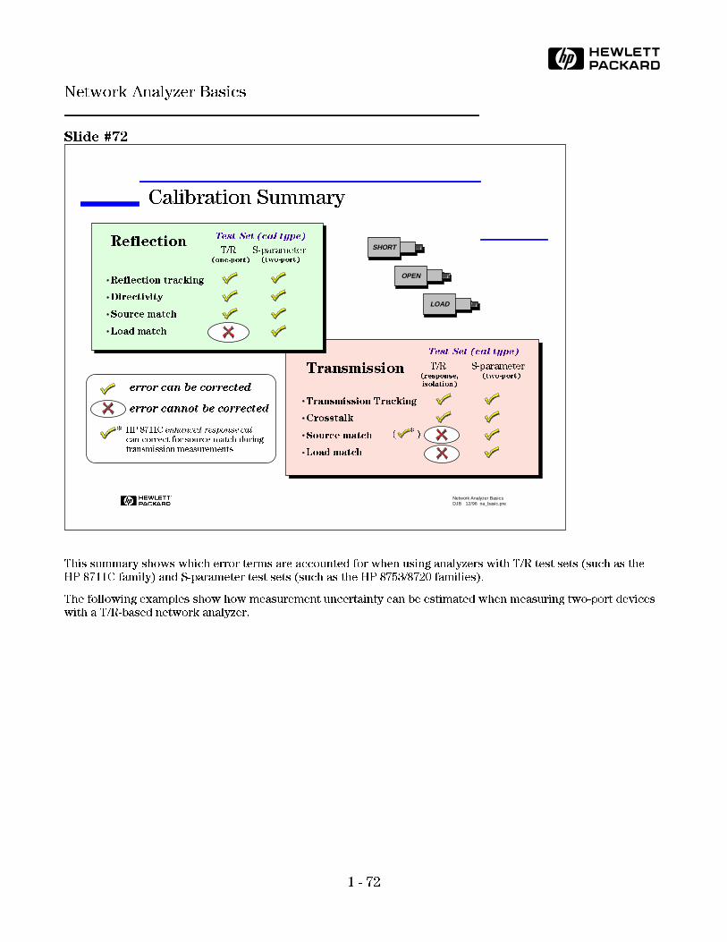
Slide #72

This summary shows which error terms are accounted for when using analyzers with T/R test sets (such as the

HP 8711C family) and S-parameter test sets (such as the HP 8753/8720 families).

The following examples show how measurement uncertainty can be estimated when measuring two-port devices

with a T/R-based network analyzer.


Calibration Summary

Transmission Tracking

Crosstalk

Source match

Load match

S-parameter (two-port)

T/R (response,

isolation)

Reflection tracking

Directivity

Source match

Load match

S-parameter (two-port)

T/R (one-port)

Reflection

Transmission

Test Set (cal type)

Test Set (cal type)

*( )

error cannot be corrected

* HP 8711C enhanced response cal can correct for source match during transmission measurements

error can be corrected

SHORT

OPEN

LOAD

1 - 72


H

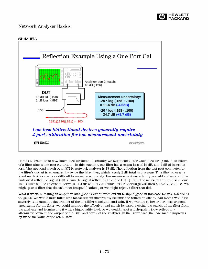
Slide #73

Here is an example of how much measurement uncertainty we might encounter when measuring the input match

of a filter after a one-port calibration. In this example, our filter has a return loss of 16 dB, and 1 dB of insertion

loss. The raw load match of an 8711C network analyzer is 18 dB. The reflection from the test port connected to

the filter's output is attenuated by twice the filter loss, which is only 2 dB total in this case. This illustrates why

low-loss devices are more difficult to measure accurately. For measurement uncertainty, we add and subtract the

undesired reflection signal (.100) from the signal reflecting from the DUT (.158). The measured return loss of our

16 dB filter will be anywhere between 11.4 dB and 24.7 dB, which is a rather large variation (-4.6 dB, +8.7 dB). We

might pass a filter that doesn't meet its specifications, or we might reject a filter that did.

What if we were testing an amplifier with good isolation from output to input (good in this case means isolation is

>> gain)? We would have much less measurement uncertainty because the reflection due to load match would be

severely attenuated by the product of the amplifier's isolation and gain. If we wanted to lower our measurement

uncertainty for the filter, we could improve the effective load match by disconnecting the output of the filter from

the analyzer and terminating it with a high-quality load, or we could insert a high-quality (low reflection)

attenuator between the output of the DUT and port 2 of the analyzer. In the latter case, the load match improves

by twice the value of the attenuator.


Reflection Example Using a One-Port Cal

DUT16 dB RL (.158)1 dB loss (.891)

Analyzer port 2 match:18 dB (.126)

.158

(.891)(.126)(.891) = .100

Measurement uncertainty: -20 * log (.158 + .100) = 11.4 dB (-4.6dB)

-20 * log (.158 - .100) = 24.7 dB (+8.7 dB)

Low-loss bidirectional devices generally require

2-port calibration for low measurement uncertainty

1 - 73


H

Slide #74

Let's do an example transmission measurement using only response calibration. The first step is to make a thru

connection between the two test ports. We will use the test port specifications with a response cal for the HP

8711C family. The ripple caused by this amount of mismatch is easily calculated as shown above (± 0.22 dB). This

amount of error is now present in our reference data, and it has to be added to the uncertainty when the DUT is

measured to compute the worst-case overall measurement uncertainty.


Transmission Example Using Response Cal

RL = 14 dB (.200)

RL = 18 dB (.126)

Thru calibration (normalization) builds error into

measurement due to source and load match interaction

Calibration Uncertainty = (1 ± ρ ρ ρ ρ )

S L

= (1 ± (.200)(.126) = ± 0.22 dB

1 - 74


H

Slide #75

Now lets look at the measurement uncertainty when the DUT is inserted. We will use the same loss and mismatch

specifications for the DUT and analyzer as before. We have three main error signals due to reflections between

the ports of the analyzer and the DUT. There are higher-order reflections present as well, but they don't add any

significant error since they are small compared to the three main terms. One of the signals passes through the

DUT twice, so it is attenuated by twice the loss of the DUT. The worst case is when all of the reflected error

signals add together in-phase (.020 + .020 + .032 = .072). In that case, we get a measurement uncertainty of +0.60

dB, -0.65 dB. The total measurement uncertainty, which must include the 0.22 dB of error incorporated into our

calibration measurement, is about ± 0.85 dB.


Transmission Example (continued)

Source match = 14 dB (.200)

1

(.126)(.158) = .020

(.158)(.200) = .032

(.126)(.891)(.200)(.891) = .020

Measurement uncertainty = 1 ± (.020+.020+.032) = 1 ± .072 = + 0.60 dB - 0.65 dB

DUT1 dB loss (.891)16 dB RL (.158)

Total measurement uncertainty: +0.60 + 0.22 = +0 .82 dB -0.65 - 0.22 = - 0.87 dB

Load match = 18 dB (.126)

1 - 75


H

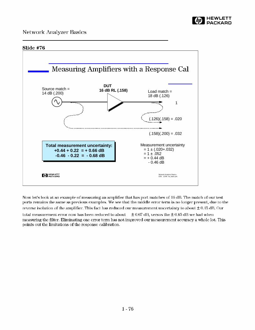
Slide #76

Now let's look at an example of measuring an amplifier that has port matches of 16 dB. The match of our test

ports remains the same as previous examples. We see that the middle error term is no longer present, due to the

reverse isolation of the amplifier. This fact has reduced our measurement uncertainty to about ± 0.45 dB. Our

total measurement error now has been reduced to about ± 0.67 dB, versus the ± 0.85 dB we had when

measuring the filter. Eliminating one error term has not improved our measurement accuracy a whole lot. This

points out the limitations of the response calibration.


Measuring Amplifiers with a Response Cal

Total measurement uncertainty: +0.44 + 0.22 = + 0.66 dB -0.46 - 0.22 = - 0.68 dB

Measurement uncertainty = 1 ± (.020+.032) = 1 ± .052 = + 0.44 dB - 0.46 dB

1

(.126)(.158) = .020

DUT16 dB RL (.158)

(.158)(.200) = .032

Source match = 14 dB (.200) Load match =

18 dB (.126)

1 - 76


H

Slide #77

A new feature of the 8711C family of RF economy network analyzers is the enhanced response calibration. This

calibration requires the measurement of short, open, load, and thru standards for transmission measurements.

Essentially, it combines a one-port cal and a response cal to allow correction of source match during transmission

measurements. Recall that a standard response calibration (such as found in the HP 8711B, 8752C, or 8753D)

cannot correct for the source and load match error terms.

The enhanced response calibration improves the effective source match during transmission measurements to

around 35 dB, instead of the 14 dB we used in the previous examples. This greatly reduces the calibration error (±0.02 dB instead of ± 0.22 dB), as well as the two measurement error terms that involve interaction with the

effective source match. Our total measurement error is now ± 0.24 dB, instead of the previously calculated ± 0.85

dB. While this result is not as good as what can be achieved with full 2-port error correction (see next slide), it is

a large improvement over the standard response cal and may be adequate for many applications.


Transmission Measurements using the Enhanced Response Calibration

Measurement uncertainty = 1 ± (.020+.0018+.0028) = 1 ± .0246 = + 0.211 dB - 0.216

Total measurement uncertainty: 0.22 + .02 = ± 0.24 dB

Calibration Uncertainty = (1 ± ρ ρ ρ ρ )

S L

= (1 ± (.0178)(.126) = ± .02 dB

Effective source match = 35 dB!

Source match = 35 dB (.0178)

1

(.126)(.158) = .020

(.126)(.891)(.0178)(.891) = .0018

DUT1 dB loss (.891)16 dB RL (.158) Load match =

18 dB (.126)

(.158)(.0178) = .0028

1 - 77


H

Slide #78

Here is an example of calculating measurement error after a two-port calibration has been done. HP provides

numbers on network analyzer data sheets for effective directivity, source and load match, tracking, and isolation,

sometimes for several different calibration kits. The errors when measuring our example filter have been greatly

reduced (0.5 dB reflection error, 0.06 dB transmission error). Phase errors would be similarly small. Note that this

is a worst-case analysis since it is unlikely that all the errors would add in-phase. A less conservative approach to

calculating measurement uncertainty would be to use a root-sum-squares (RSS) method.


Calculating Measurement Uncertainty After a Two-Port Calibration

Corrected error terms:

(8753D 1.3-3 GHz Type-N)

Directivity = 47 dB

Source match = 36 dB

Load match = 47 dB

Refl. tracking = .019 dB

Trans. tracking = .026 dB

Isolation = 100 dB

DUT1 dB loss (.891)16 dB RL (.158)

Reflection uncertainty

S11 = S11 ± (E + S11 E + S21 S12 E + S11 E )aa aam2

a D S L RT

= .158 ± (.0045+.158 *.0158 + .891 *.0045 + .158*.0022) 2 2

= .158 ± .0088 = 16 dB +0.53 dB, -0.44 dB

Transmission uncertainty

= .891 ± .0059 = 1 dB ± 0.06 dB

S21 = S21 ± (E + S11 E + S22 E + S21 S12 E E + S21 E )aa aam a I S L TTa S L

= .891 ± (10 + .158*.0158 + .158*.0045 + .891 *.0158*.0045 + .891*.003)-6 2

1 - 78


H

Slide #79

Let's look at some actual measurements done on a bandpass filter with different levels of error correction. The

uncorrected trace shows considerable loss and ripple. In fact, the passband response varies about ± 1 dB around

filter's center frequency. Is the filter really this bad? No. What we are actually measuring is the sum of the filter's

response and that of our test system.

Performing a normalization prior to the measurement of the filter will remove the frequency response of the

system (tracking error) from the measurement. The loss that was removed was most likely caused by the test

cables. After normalization, the frequency response of the filter still contains ripple caused by an interaction

between the system's source and load match. This ripple even goes above the 0 dB reference line, indicating gain!

However, we know that a passive device cannot amplify signals. This apparent anomaly is due to mismatch

measurement error.

The measurement shown after a two-port calibration is the most accurate of the three measurements shown.

Using vector-error correction, the filter's passband response shows variation of about ± 0.1 dB around its center

frequency. This increased level of measurement flatness will ensure minimum amplitude distortion, increase

confidence in the filter's design, and ultimately increase manufacturing yields due to lower test-failure rates.


Response versus Two-Port Calibration

CH1 S21&M log MAG 1 dB/ REF 0 dB

Cor

CH2 MEM log MAG REF 0 dB1 dB/

Cor

Uncorrected

After 2-port calibration

START 2 000.000 MHz STOP 6 000.000 MHzx2 1 2

After response calibration

Measuring filter insertion loss

1 - 79


H

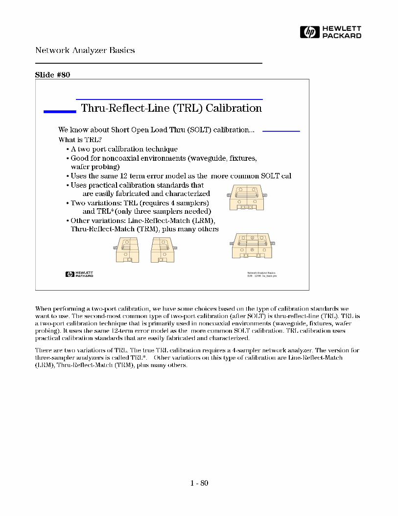
Slide #80

When performing a two-port calibration, we have some choices based on the type of calibration standards we

want to use. The second-most common type of two-port calibration (after SOLT) is thru-reflect-line (TRL). TRL is

a two-port calibration technique that is primarily used in noncoaxial environments (waveguide, fixtures, wafer

probing). It uses the same 12-term error model as the more common SOLT calibration. TRL calibration uses

practical calibration standards that are easily fabricated and characterized.

There are two variations of TRL. The true TRL calibration requires a 4-sampler network analyzer. The version for

three-sampler analyzers is called TRL*. Other variations on this type of calibration are Line-Reflect-Match

(LRM), Thru-Reflect-Match (TRM), plus many others.


Thru-Reflect-Line (TRL) Calibration

We know about Short-Open-Load-Thru (SOLT) calibration...

What is TRL?

A two-port calibration technique

Good for noncoaxial environments (waveguide, fixtures,

wafer probing)

Uses the same 12-term error model as the more common SOLT cal

Uses practical calibration standards that

are easily fabricated and characterized

Two variations: TRL (requires 4 samplers)

and TRL*(only three samplers needed)

Other variations: Line-Reflect-Match (LRM),

Thru-Reflect-Match (TRM), plus many others

1 - 80


H

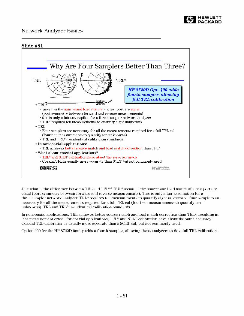
Slide #81

Just what is the difference between TRL and TRL*? TRL* assumes the source and load match of a test port are

equal (port symmetry between forward and reverse measurements). This is only a fair assumption for a

three-sampler network analyzer. TRL* requires ten measurements to quantify eight unknowns. Four samplers are

necessary for all the measurements required for a full TRL cal (fourteen measurements to quantify ten

unknowns). TRL and TRL* use identical calibration standards.

In noncoaxial applications, TRL achieves better source match and load match correction than TRL*, resulting in

less measurement error. For coaxial applications, TRL* and SOLT calibration have about the same accuracy.

Coaxial TRL calibration is usually more accurate than a SOLT cal, but not commonly used.

Option 400 for the HP 8720D family adds a fourth sampler, allowing these analyzers to do a full TRL calibration.


Why Are Four Samplers Better Than Three?

TRL TRL*

HP 8720D Opt. 400 adds

fourth sampler, allowing

full TRL calibration

TRL*

assumes the source and load match of a test port are equal (port symmetry between forward and reverse measurements)this is only a fair assumption for a three-sampler network analyzerTRL* requires ten measurements to quantify eight unknowns

TRL

Four samplers are necessary for all the measurements required for a full TRL cal (fourteen measurements to quantify ten unknowns)TRL and TRL* use identical calibration standards

In noncoaxial applications:

TRL achieves better source match and load match correction than TRL*

What about coaxial applications?

TRL* and SOLT calibration have about the same accuracyCoaxial TRL is usually more accurate than SOLT but not commonly used

1 - 81


H

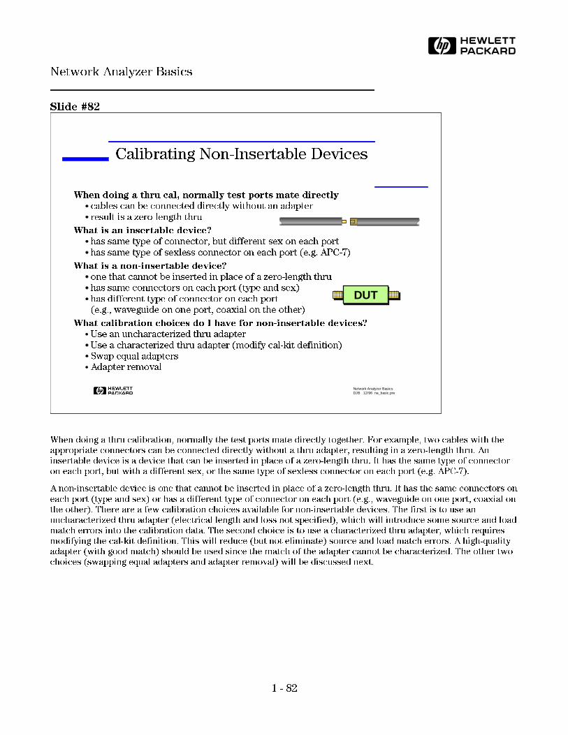
Slide #82

When doing a thru calibration, normally the test ports mate directly together. For example, two cables with the

appropriate connectors can be connected directly without a thru adapter, resulting in a zero-length thru. An

insertable device is a device that can be inserted in place of a zero-length thru. It has the same type of connector

on each port, but with a different sex, or the same type of sexless connector on each port (e.g. APC-7).

A non-insertable device is one that cannot be inserted in place of a zero-length thru. It has the same connectors on

each port (type and sex) or has a different type of connector on each port (e.g., waveguide on one port, coaxial on

the other). There are a few calibration choices available for non-insertable devices. The first is to use an

uncharacterized thru adapter (electrical length and loss not specified), which will introduce some source and load

match errors into the calibration data. The second choice is to use a characterized thru adapter, which requires

modifying the cal-kit definition. This will reduce (but not eliminate) source and load match errors. A high-quality

adapter (with good match) should be used since the match of the adapter cannot be characterized. The other two

choices (swapping equal adapters and adapter removal) will be discussed next.


Calibrating Non-Insertable Devices

When doing a thru cal, normally test ports mate directly

cables can be connected directly without an adapter

result is a zero-length thru

What is an insertable device?

has same type of connector, but different sex on each port

has same type of sexless connector on each port (e.g. APC-7)

What is a non-insertable device?

one that cannot be inserted in place of a zero-length thru

has same connectors on each port (type and sex)

has different type of connector on each port

(e.g., waveguide on one port, coaxial on the other)

What calibration choices do I have for non-insertable devices?

Use an uncharacterized thru adapter

Use a characterized thru adapter (modify cal-kit definition)

Swap equal adapters

Adapter removal

DUT

1 - 82


H

Slide #83

The swap equal adapter method requires the use of two precision matched adapters which are "equal", but have

connectors of different sexes (e.g., 7 mm/Type N (m) and 7 mm/Type N (f)) To be equal, the adapters need to

have the same match, Zo, insertion loss, and electrical delay. Many of HP's calibration kits include matched

adapters.

The first step in the procedure is to perform a transmission calibration using the first adapter. Then, adapter A is

removed, and adapter B is placed on port two. Adapter B becomes the effective test port. The reflection

calibration is then performed on both test ports. Then the DUT is measured with adapter B in place.

The errors remaining after calibration with this method are equal to the differences between the two adapters that

are used. The technique provides good accuracy, but not as good as the more complicated adapter-removal

technique.


Swap Equal Adapters Method

DUTPort 1 Port 2

1. Transmission cal using adapter A.

2. Reflection cal using adapter B.

3. Measure DUT using adapter B.

Port 1 Port 2Adapter A

Adapter B

Port 1 Port 2

Adapter B

Port 1 Port 2DUT

Accuracy depends on how well

the adapters are matched - loss,

electrical length, match and

impedance should all be equal

1 - 83


H

Slide #84

Adapter removal calibration provides the most complete and accurate calibration procedure for non-insertable

devices. It is a feature available in the HP 8510 family of network analyzers. This method uses a cal adapter that

has the same connectors as the non-insertable DUT. The electrical length of the adapter must be specified within

1/4 wavelength at each frequency. HP's type-N, 3.5 mm, and 2.4 mm cal kits for the HP 8510 contain adapters that

have been specified for this purpose.

Two full 2-port calibrations are needed for adapter removal calibration. The first calibration is performed with

the precision cal adapter on port two, and the data is saved into a cal set. Next, the second calibration is

performed with the precision cal adapter on port one, and the data is saved into a second cal set. Pressing the

adapter-removal cal softkey causes the HP 8510 to use the two sets of cal data to generate a new set of error

coefficients that remove the effects of the cal adapter. This adapter can then be removed so that the DUT can be

measured in its place.


Adapter Removal Calibration

In firmware of HP 8510 family

Can be accomplished with E-Cal (HP 85060) and HP 8753/8720 families

Uses adapter with same connectors as DUT

Adapter's electrical length must be specified within 1/4 wavelength

adapters supplied with HP type-N, 3.5mm, and 2.4mm cal kits are already defined

for other adapters, measure electrical length and modify cal-kit definition

Calibration is very accurate and traceable

See Product Note 8510-13 for more details

1. Perform 2-port cal with adapter on port 2. Save in cal set 1.

2. Perform 2-port cal with adapter on port 1. Save in cal set 2.

4. Measure DUT without cal adapter.

3. Use ADAPTER REMOVAL to generate new cal set.

[CAL] [MORE] [MODIFY CAL SET][ADAPTER REMOVAL]

DUTPort 1 Port 2

Cal Set 1

Port 1 Port 2Adapter B

Cal Adapter

Cal Adapter

Cal Set 2

Port 1 Port 2Adapter B

Port 2Adapter B

DUTPort 1

1 - 84


H

Slide #85

This section will cover some typical measurements. We will look at swept-frequency testing of a filter and

swept-power testing of an amplifier.


Agenda






Advanced topics

1 - 85


H

Slide #86

Shown above are the frequency responses of a filter. On the left and bottom we see the transmission response in

log magnitude format, and on the right we see the reflection response (return loss).

The most commonly measured filter characteristics are insertion loss and bandwidth, shown on the lower plot

with an expanded vertical scale. Another common parameter we might measure is out-of-band rejection. This is a

measure of how well a filter passes signals within its bandwidth while simultaneously rejecting all other signals

outside of that same bandwidth. The ability of a test system to measure out-of-band rejection is directly

dependent on its system dynamic-range specification.

The return loss plot is very typical, showing high reflection (near 0 dB) in the stopbands, and reasonable match in

the passband. Most passive filters work in this manner. A special class of filters exist that are absorbtive in both

the passband and stopband. These filters exhibit a good match over a broad frequency range.


Frequency Sweep - Filter Test


CENTER 200.000 MHz SPAN 50.000 MHz

log MAG 10 dB/ REF 0 dBCH1 S21

START .300 000 MHz STOP 400.000 000 MHz

Cor

69.1 dB

Stopband

rejection

Return loss

SCH1 21 log MAG 1 dB/ REF 0 dB

Cor

Cor

START 2 000.000 MHz STOP 6 000.000 MHzx2 1 2

Insertion loss

m1: 4.000 000 GHz -0.16 dBm2-ref: 2.145 234 GHz 0.00 dB

1

2ref

1 - 86


H

Slide #87

Many network analyzers have the ability to do power sweeps as well as frequency sweeps. Power sweeps help

characterize the nonlinear performance of an amplifier. Shown above is a plot of an amplifier's output power

versus input power at a single frequency. Amplifier gain at any particular power level is the slope of this curve.

Notice that the amplifier has a linear region of operation where gain is constant and is independent of power level.

The gain in this region is commonly referred to as "small-signal gain". At some point as the input power is

increased, the amplifier gain appears to decrease, and the amplifier is said to be in compression. Under this

nonlinear condition, the amplifier output is no longer sinusoidal -- some of the output power is present in

harmonics, rather than occurring only at the fundamental frequency. As input power is increased even more, the

amplifier becomes saturated, and output power remains constant. At this point the amplifier gain is essentially

zero, since further increases in input power result in no change in output power. Saturated output power can be

read directly from the above plot.

In order to measure the saturated output power of an amplifier, the network analyzer must be able to provide a

power sweep with sufficient output power to drive the amplifier from its linear region into saturation. A preamp

at the input of the amplifier under test may be necessary to achieve this.


Power Sweep - Compression

Saturated output power

Out

put P

ow

er (

dBm

)

Input Power (dBm)

Compression region

Linear region (slope = small-signal gain)

1 - 87


H

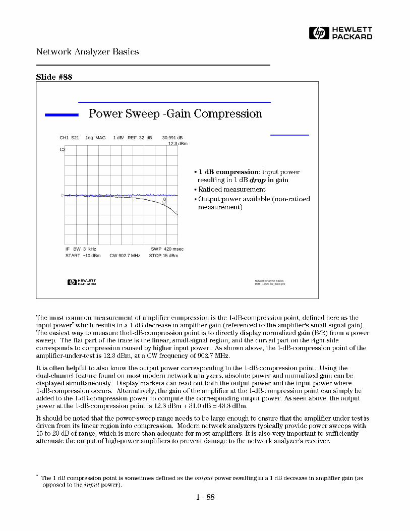
Slide #88

The most common measurement of amplifier compression is the 1-dB-compression point, defined here as the

input power* which results in a 1-dB decrease in amplifier gain (referenced to the amplifier's small-signal gain).

The easiest way to measure the1-dB-compression point is to directly display normalized gain (B/R) from a power

sweep. The flat part of the trace is the linear, small-signal region, and the curved part on the right side

corresponds to compression caused by higher input power. As shown above, the 1-dB-compression point of the

amplifier-under-test is 12.3 dBm, at a CW frequency of 902.7 MHz.

It is often helpful to also know the output power corresponding to the 1-dB-compression point. Using the

dual-channel feature found on most modern network analyzers, absolute power and normalized gain can be

displayed simultaneously. Display markers can read out both the output power and the input power where

1-dB-compression occurs. Alternatively, the gain of the amplifier at the 1-dB-compression point can simply be

added to the 1-dB-compression power to compute the corresponding output power. As seen above, the output

power at the 1-dB-compression point is 12.3 dBm + 31.0 dB = 43.3 dBm.

It should be noted that the power-sweep range needs to be large enough to ensure that the amplifier under test is

driven from its linear region into compression. Modern network analyzers typically provide power sweeps with

15 to 20 dB of range, which is more than adequate for most amplifiers. It is also very important to sufficiently

attenuate the output of high-power amplifiers to prevent damage to the network analyzer's receiver.

*

The 1-dB-compression point is sometimes defined as the output power resulting in a 1-dB decrease in amplifier gain (as

opposed to the input power).


Power Sweep -Gain Compression

0

CH1 S21 1og MAG 1 dB/ REF 32 dB 30.991 dB 12.3 dBmC2

IF BW 3 kHz SWP 420 msec

START −10 dBm CW 902.7 MHz STOP 15 dBm

0

1 dB compression: input power

resulting in 1 dB drop in gain

Ratioed measurement

Output power available (non-ratioed

measurement)

1 - 88


H

Slide #89

Another common measurement which helps characterize the nonlinear behavior of amplifiers is AM-PM

conversion, which is a measure of the amount of undesired phase deviation (the PM) which is induced by

amplitude variations inherent in the system (the AM). In a communications system, this unwanted PM is caused

by unintentional amplitude variations such as power supply ripple, thermal drift, or multipath fading, or by

intentional amplitude change that is a result of the type of modulation used, such as the case with QAM or burst

modulation.

AM-PM conversion is a particularly critical parameter in systems where phase (angular) modulation is employed,

because undesired phase distortion causes analog signal degradation, or increased bit-error rates (BER) in digital

systems. Examples of common modulation types that use phase modulation are FM, QPSK, or 16QAM. While it is

easy to measure the BER of a digital communication system, this measurement alone does not provide any insight

into the underlying phenomena which cause bit errors. AM-PM conversion is one of the fundamental contributors

to BER, and therefore it is important to quantify this parameter in communication systems.

AM-to-PM conversion is usually defined as the change in output phase for a 1-dB increment in the input power to

the amplifier, expressed in degrees-per-dB (o/dB). An ideal amplifier would have no interaction between its phase

response and the level of the input signal. AM-PM conversion can be measured by performing a power sweep

with a vector network analyzer, using the same transmission setup that we used for gain compression. The

displayed data is formatted as the phase of S21 (transmission) versus power. AM-PM conversion can be computed

by choosing a small amplitude increment (typically 1 dB) centered at a particular RF power level, and noting the

resultant change in phase. The easiest way to read out the amplitude and phase deltas is to use trace markers.

Dividing the phase change by the amplitude change yields AM-PM conversion. The plot above shows AM-PM

conversion of 0.86 o/dB, centered at an input power of -4.5 dBm and an output power of 16.0 dBm.


Power Sweep - AM to PM Conversion

1:Transmission Log Mag 1.0 dB/ Ref 21.50 dB

Use transmission setup

with a power sweepDisplay phase of S21

AM - PM = 0.86 deg/dB

Start -10.00 dBm Stop 0.00 dBmCW 900.000 MHzStart -10.00 dBm Stop 0.00 dBmCW 900.000 MHz

2:Transmission /M Phase 5.0 deg/ Ref -115.7 deg

1

2

1

1

2

Ch1:Mkr1 -4.50 dBm 20.48 dB

Ch2:Mkr2 1.00 dB 0.86 deg

1 - 89


H

Slide #90

This last section is meant to provide pointers to reference material to cover these topics in more detail.


Agenda






Advanced topics

Time domain

Frequency-translating devices

High-power amplifiers

Multiport devices

In-fixture measurements

Crystal Resonators

Balanced-Cables

1 - 90


H

Slide #91

Time-domain reflectometry is a very useful tool that allows us to measure impedance versus distance. One good

application for TDR is fixture design and the design of corresponding in-fixture calibration standards. There are

two basic ways to perform TDR measurements. One way is accomplished by generating a high-speed step

function (usually a few hundred millivolts in amplitude) and measuring it with a high-speed oscilloscope. This

technique provides measurements with a high update rate, which allows real-time adjustments. It is very easy to

determine which transition is which, as the designer can place a probe on a transition and look for the spike on

the TDR trace. However, in general, oscilloscopes cannot display data in the frequency domain as can a network

analyzer.

The second technique uses a vector network analyzer making normal frequency-domain swept measurements.

The inverse-Fourier transform is used to transform the frequency-domain reflection data to the time domain,

yielding TDR measurements. While the update rate is much slower, the advantage is that one instrument can be

used to provide both time and frequency-domain measurements. When using a network analyzer, the spatial

resolution is inversely proportional to the frequency span of the measurement -- i.e., the higher the stop frequency

(for a given start frequency), the smaller the distance that can be resolved. For this reason, it is often necessary to

make microwave measurements on devices such as fixtures in order to get sufficient resolution to analyze the

various transitions. The maximum distance that can be examined is also inversely proportionate to frequency

span. It is important to use two-port error correction in conjunction with time-domain measurements.


Time-Domain Reflectometry (TDR)

Analyze impedance versus timeDifferentiate inductive and capacitive transitions

High-speed oscilloscope:

yields fast update rate

200 mV step typical

Network analyzer:

broadband frequency sweep (often requires microwave VNA)inverse FFT to compute time-domain

resolution inversely proportional to frequency span

Zo

inductive transition

capacitive transition

non-Zo termination

1 - 91


H

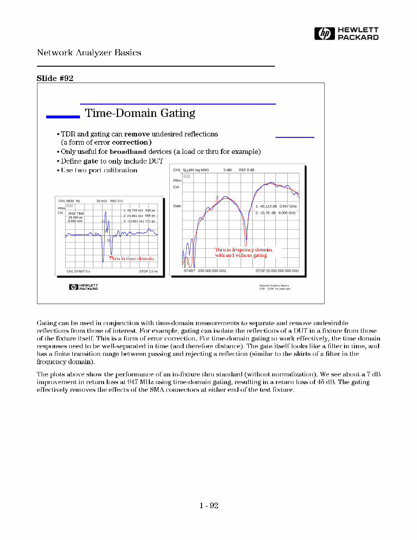
Slide #92

Gating can be used in conjunction with time-domain measurements to separate and remove undesirable

reflections from those of interest. For example, gating can isolate the reflections of a DUT in a fixture from those

of the fixture itself. This is a form of error correction. For time-domain gating to work effectively, the time domain

responses need to be well-separated in time (and therefore distance). The gate itself looks like a filter in time, and

has a finite transition range between passing and rejecting a reflection (similar to the skirts of a filter in the

frequency domain).

The plots above show the performance of an in-fixture thru standard (without normalization). We see about a 7 dB

improvement in return loss at 947 MHz using time-domain gating, resulting in a return loss of 45 dB. The gating

effectively removes the effects of the SMA connectors at either end of the test fixture.


Time-Domain Gating

TDR and gating can remove undesired reflections

(a form of error correction)

Only useful for broadband devices (a load or thru for example)

Define gate to only include DUT

Use two-port calibration CH1 S11&M log MAG 5 dB/ REF 0 dB

START .050 000 000 GHz STOP 20.050 000 000 GHz

Gate

Cor

PRm

1

2

2: -15.78 dB 6.000 GHz

1: -45.113 dB 0.947 GHz

CH1 MEM Re 20 mU/ REF 0 U

CH1 START 0 s STOP 1.5 ns

CorPRm

RISE TIME 29.994 ps 8.992 mm

1

2

3

1: 48.729 mU 638 ps

2: 24.961 mU 668 ps

3: -10.891 mU 721 ps

Thru in time domain

Thru in frequency domain,

with and without gating

1 - 92


H

Slide #93

Time-domain transmission (TDT) is a similar tool which uses the transmission response instead of the reflection

response. It is useful in analyzing signal timing in devices such as SAW filters. Gating is also useful for TDT. In the

above example, a designer could look at the frequency response of the main surface wave without the leakage and

triple-travel error signals.


Time-Domain Transmission


START -1 us STOP 6 us

Cor RF Leakage

SurfaceWave

TripleTravel

RF Output

RF Input

Triple Travel

Main Wave

Leakage


Cor

Gate on

Gate off

1 - 93


H

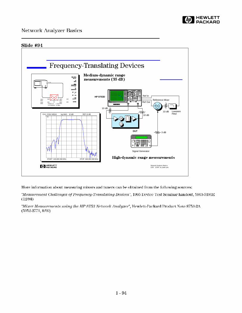
Slide #94

More information about measuring mixers and tuners can be obtained from the following sources:

"Measurement Challenges of Frequency-Translating Devices", 1995 Device Test Seminar handout, 5963-5191E

(12/94)

"Mixer Measurements using the HP 8753 Network Analyzer", Hewlett-Packard Product Note 8753-2A

(5952-2771, 8/90)


Frequency-Translating Devices

CH1 CONV MEAS log MAG 10 dB/ REF 10 dB

START 640.000 000 MHz STOP 660.000 000 MHz

1 2

R IN

start: 900 MHzstop: 650 MHz FIXED LO: 1 GHz

LO POWER: 13 dBm

start: 100 MHzstop: 350 MHz

H

ACTIVE CHANNEL

RESPONSE

STIM ULUS

EN TRY

INSTRUMENT STATE R CHAN NEL

R L T S

HP-I B STATUS

8753DNETWORK ANALYZER

30 KHz -3GHz

PRO BE POWER FU SED

PORT 2PORT 1

Ref In

10 dB

Reference Mixer

3 dB

10 dB

10 dB

Signal Generator

Lowpass Filter

HP 8753D

Ref Out

IF

LO

RF

LO

DUT

High-dynamic range measurements

Medium-dynamic range

measurements (35 dB)

1 - 94


H

Slide #95

More information about measuring high-power amplifiers can be obtained from the following sources:

"Measurement Solutions for Test Base-Station Amplifiers", 1996 Device Test Seminar handout, 5964-9803E

(4/96)

"Modern Solutions for Testing RF Communications Amplifiers", 1995 Device Test Seminar handout, 5963-5191E

(12/94)

"Amplifier Measurements using the HP 8753 Network Analyzer", Hewlett-Packard Product Note 8753-1

(5956-4361, 5/88)

"Testing Amplifiers and Active Devices with the HP 8720 Network Analyzer", Hewlett-Packard Product Note

8720-1 (5091-1942E, 8/91)

"HP 85108 Series Network Analyzer Systems for Isothermal, High-Power, and Pulsed Applications", Product

Overview, (5091-8965E, '94)

"HP 85118 Series High Power Amplifier Test System", Product Overview (5963-9930E, 5/95)


High-Power Amplifiers

Source

B

R

A

+43 dBm max input (20 watts!)

Preamp

AUT

HP 8720D Option 085

HP 85118A High-Power Amplifier Test System

DUT

H

ACTIVE CHANNEL

RESPONSE

STIMULUS

ENTRY

INSTRUMENT STATE R CHANNEL

R L T S

HP-I B STATUS

8753DNETWORK ANALYZER

30 KHz-3GHzPROBE POWER

FUSED

PORT 2PORT 1

Ref In

AUT

Preamp

HP 8753D

1 - 95


H

Slide #96

More information about measuring multiport devices can be obtained from the following source:

"Improve Test Throughput for Duplexers and Other Multiport Devices", 1996 Device Test Seminar handout,

5964-9803E (4/96)


Multiport Device Test

Multiport test sets:

improve throughput by reducing the number

of connections to DUTs with more than 2 ports

allow simultaneous viewing of two paths

(good for tuning duplexers)

include mechanical or solid-state switches,

50 or 75 ohms

degrade raw performance so calibration is a

must (use two-port cals whenever possible)

Directional CouplerTest Set

Port 1

Port 2 Port 3

Port 2

Port 1

Note: unused ports

are terminated

log MAG 10 dB/ REF 0 dB 1_ -1.9248 dBCH1 S21


Cor

Hld

PRm

CH2 S12 log MAG REF 0 dB10 dB/


Cor

Hld

PRm

1

1

839.470 000 MHz

PASS

2

1

1_ -1.2468 dB

880.435 000 MHz

PASS

Duplexer Test - Tx-Ant and Ant-Rx

1 - 96


H

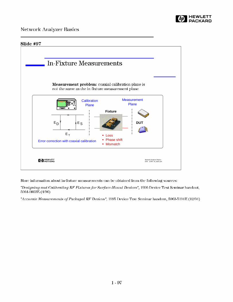
Slide #97

More information about in-fixture measurements can be obtained from the following sources:

"Designing and Calibrating RF Fixtures for Surface-Mount Devices", 1996 Device Test Seminar handout,

5964-9803E (4/96)

"Accurate Measurements of Packaged RF Devices", 1995 Device Test Seminar handout, 5963-5191E (12/94)


In-Fixture Measurements

Measurement problem: coaxial calibration plane is

not the same as the in-fixture measurement plane

Error correction with coaxial calibration

E E

E

D S

T Loss Phase shift Mismatch

CalibrationPlane

MeasurementPlane

DUT

Fixture

1 - 97


H

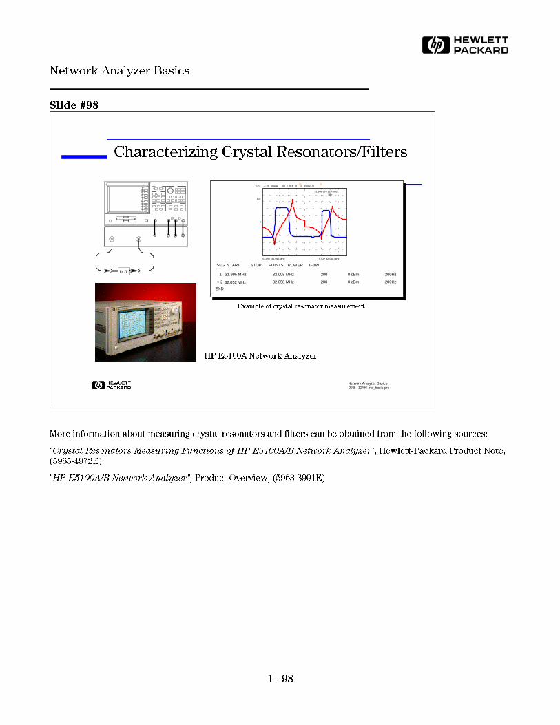
Slide #98

More information about measuring crystal resonators and filters can be obtained from the following sources:

"Crystal Resonators Measuring Functions of HP E5100A/B Network Analyzer", Hewlett-Packard Product Note,

(5965-4972E)

"HP E5100A/B Network Analyzer", Product Overview, (5963-3991E)


Characterizing Crystal Resonators/Filters

DUT

HP E5100A Network Analyzer

1 31.995 MHz

> 2

END

32.008 MHz

32.058 MHz

200

200

0 dBm

0 dBm

200Hz

200Hz

SEG START STOP POINTS POWER IFBW

32.052 MHz

Ch1

Cor

Z: R phase 40 / REF 0 1: 15.621 U

START 31.995 MHz STOP 32.058 MHz

31.998 984 925 MHzMin

1

Example of crystal resonator measurement

1 - 98


H

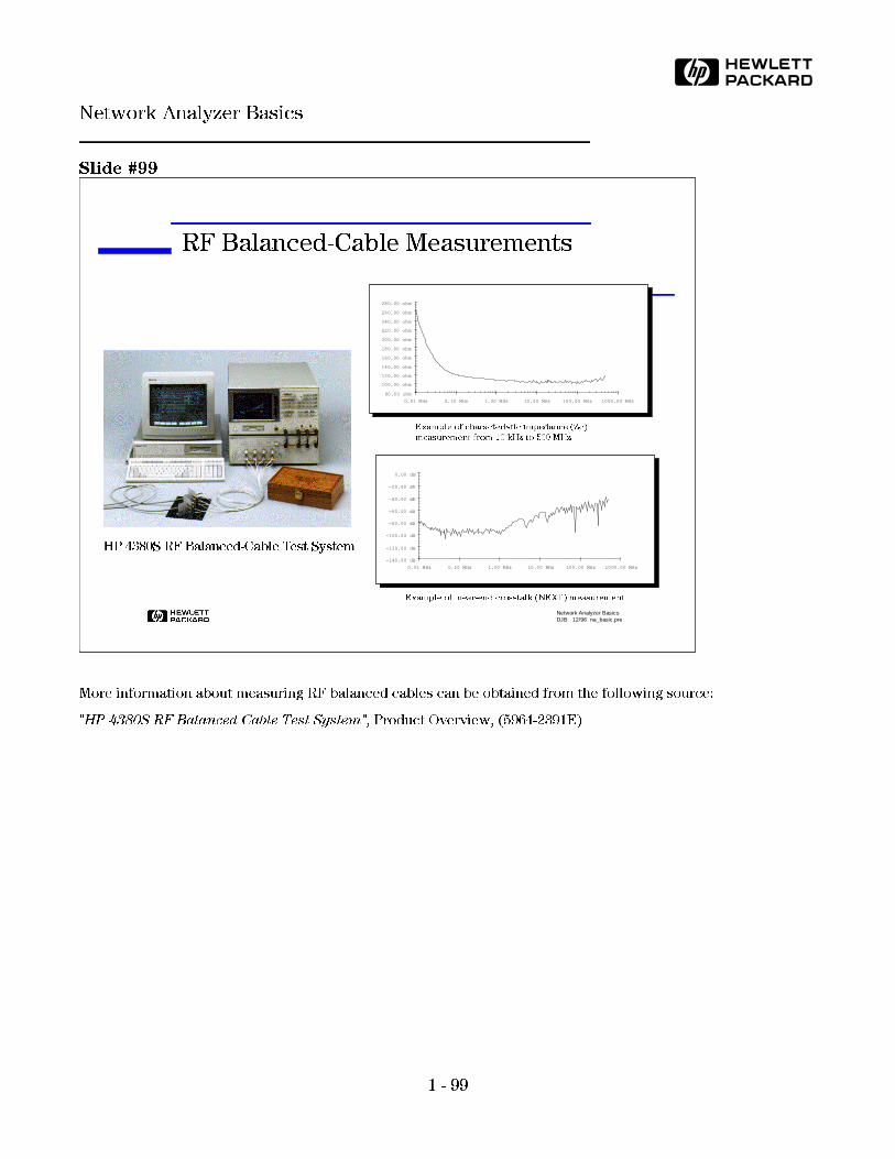
Slide #99

More information about measuring RF balanced cables can be obtained from the following source:

"HP 4380S RF Balanced Cable Test System", Product Overview, (5964-2391E)


RF Balanced-Cable Measurements

Example of characteristic impedance (Zc)

measurement from 10 kHz to 500 MHz

HP 4380S RF Balanced-Cable Test System

80.00 ohm

100.00 ohm

120.00 ohm

140.00 ohm

160.00 ohm

180.00 ohm

200.00 ohm

220.00 ohm

240.00 ohm

260.00 ohm

280.00 ohm

0.01 MHz 0.10 MHz 1.00 MHz 10.00 MHz 100.00 MHz 1000.00 MHz

Example of near-end crosstalk (NEXT) measurement

-140.00 dB

-120.00 dB

-100.00 dB

-80.00 dB

-60.00 dB

-40.00 dB

-20.00 dB

0.00 dB

0.01 MHz 0.10 MHz 1.00 MHz 10.00 MHz 100.00 MHz 1000.00 MHz

1 - 99


H

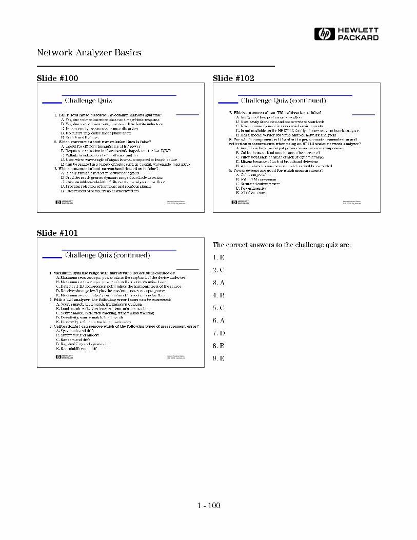
Slide #100

Slide #101

Slide #102

The correct answers to the challenge quiz are:

1. E

2. C

3. A

4. B

5. C

6. A

7. D

8. B

9. E


Challenge Quiz

1. Can filters cause distortion in communications systems?

A. Yes, due to impairment of phase and magnitude response

B. Yes, due to nonlinear components such as ferrite inductors

C. No, only active devices can cause distortion

D. No, filters only cause linear phase shifts

E. Both A and B above

2. Which statement about transmission lines is false?

A. Useful for efficient transmission of RF power

B. Requires termination in characteristic impedance for low VSWR

C. Voltage is independent of position along line

D. Used when wavelength of signal is small compared to length of line

E. Can be realized in a variety of forms such as coaxial, waveguide, microstrip

3. Which statement about narrowband detection is false?

A. Is only available in vector network analyzers

B. Provides much greater dynamic range than diode detection

C. Uses variable-bandwidth IF filters to set analyzer noise floor

D. Provides rejection of harmonic and spurious signals

E. Uses mixers or samplers as downconverters


Challenge Quiz (continued)

4. Maximum dynamic range with narrowband detection is defined as:

A. Maximum receiver input power minus the stopband of the device under test

B. Maximum receiver input power minus the receiver's noise floor

C. Detector 1-dB-compression point minus the harmonic level of the source

D. Receiver damage level plus the maximum source output power

E. Maximum source output power minus the receiver's noise floor

5. With a T/R analyzer, the following error terms can be corrected:

A. Source match, load match, transmission tracking

B. Load match, reflection tracking, transmission tracking

C. Source match, reflection tracking, transmission tracking

D. Directivity, source match, load match

E. Directivity, reflection tracking, load match

6. Calibration(s) can remove which of the following types of measurement error?

A. Systematic and drift

B. Systematic and random

C. Random and drift

D. Repeatability and systematic

E. Repeatability and drift


Challenge Quiz (continued)

7. Which statement about TRL calibration is false?

A. Is a type of two-port error correction

B. Uses easily fabricated and characterized standards

C. Most commonly used in noncoaxial environments

D. Is not available on the HP 8720D family of microwave network analyzers

E. Has a special version for three-sampler network analyzers

8. For which component is it hardest to get accurate transmission and

reflection measurements when using an 8711B scalar network analyzer?

A. Amplifiers because output power causes receiver compression

B. Cables because load match cannot be corrected

C. Filter stopbands because of lack of dynamic range

D. Mixers because of lack of broadband detectors

E. Attenuators because source match cannot be corrected

9. Power sweeps are good for which measurements?

A. Gain compression

B. AM to PM conversion

C. Saturated output power

D. Power linearity

E. All of the above

1 - 100


H

Date Subject to ChangeCopyright 1997Hewlett-Packard CompanyPrinted in U.S.A. 4/975965-7917E

H

network analyzer basics - rf114

Documents