network-based robust fault detection with incomplete measurements
TRANSCRIPT

INTERNATIONAL JOURNAL OF ADAPTIVE CONTROL AND SIGNAL PROCESSINGInt. J. Adapt. Control Signal Process. 2009; 23:737–756Published online 7 November 2008 in Wiley InterScience (www.interscience.wiley.com). DOI: 10.1002/acs.1084
Network-based robust fault detection withincomplete measurements
Xiao He1, Zidong Wang2 and D. H. Zhou1,∗,†
1Tsinghua National Laboratory for Information Science and Technology, and Department of Automation,Tsinghua University, Beijing 100084, People’s Republic of China
2Department of Information Systems and Computing, Brunel University, Uxbridge,Middlesex UB8 3PH, U.K.
SUMMARY
In this paper, we deal with the robust fault detection problem for a class of discrete-time networkedsystems with unknown inputs. Three types of incomplete measurements frequently occurred in a networkenvironment are simultaneously considered, which include (1) measurements with communication delays,(2) measurements with packet dropouts, and (3) measurements with signal quantization. A unified measure-ment model utilizing a set of Kronecker delta functions is proposed to describe the delay and missingphenomenon, and the quantization is assumed to be of the logarithmic type. Attention is focused onthe analysis and design of a robust full-order fault detection filter such that, for all admissible unknowninputs and incomplete measurements, the error between residual and fault is kept as small as possible.By augmenting the states of the original system and the fault detection filter, the addressed robustfault detection problem is converted into an auxiliary robust H∞ filtering problem. Parameter-dependentand delay-probability-dependent approaches are developed in the design process in order to have a lessconservative result. Sufficient conditions for the existence of the desired robust fault detection filters areestablished in terms of certain linear matrix inequalities (LMIs), and explicit parameters of the desiredfilter are then characterized if these LMIs are feasible. A numerical example is provided to illustrate theapplicability of the proposed technique. Copyright q 2008 John Wiley & Sons, Ltd.
Received 25 May 2008; Accepted 16 September 2008
KEY WORDS: robust fault detection; H∞ filtering; networked systems; random communication delays;packet dropout; signal quantization; linear matrix inequality (LMI)
∗Correspondence to: D. H. Zhou, Tsinghua National Laboratory for Information Science and Technology, andDepartment of Automation, Tsinghua University, Beijing 100084, People’s Republic of China.
†E-mail: [email protected], [email protected]
Contract/grant sponsor: NSFC; contract/grant numbers: 60721003, 60736026
Copyright q 2008 John Wiley & Sons, Ltd.

738 X. HE, Z. WANG AND D. H. ZHOU
1. INTRODUCTION
In recent years, the fault detection and isolation (FDI) as well as the fault-tolerant control (FTC)techniques have received persistent research interest in response to the increasing complexity andsafety demand of real time systems [1–3]. In general, FTC can be categorized into (1) passiveFTC using feedback control laws that are robust with respect to possible system faults and (2)active FTC (using an FDI unit and accommodation technique). As a prerequisite for further faultaccommodation, FDI plays an important role in active FTC process [4, 5]. The key step of FDIis the generation of a residual that can then be compared with a prescribed threshold in orderto determine whether a fault occurs [6]. In the existing literature, a widely adopted model-basedfault detection technique is to convert the FDI problem into an auxiliary optimization problem, inwhich the H∞ norm of transfer function matrix from unknown input to residual is made small,while the H∞ norm (or the smallest nonzero singular value) of transfer function from fault toresidual is made large [7]. In [8], the robust fault detection problem has been transformed into anH∞ model match problem. In [9], another approach to robust fault detection problem has beenbrought forward to make the error between residual and weighted fault as small as possible, whichcan be implemented by using an auxiliary robust H∞ filtering approach [10].
On another research front, with the rapid development of network technologies, more andmore control systems are executed over communication networks. This kind of systems are callednetworked control systems (NCSs), which have many advantages such as low cost, reduced weightand power requirements, simple installation and maintenance, and high reliability [11]. However,since the network cable is of limited capacity, new interesting and challenging issues inevitablyemerge, for example, the transmission delay, packet dropout, signal quantization, scheduling confu-sion, etc. Recently, there have been initial results on NCSs [11–13], among which considerableattention has been focused on network-based FDI problems [14]. In [15], the fault detectionproblem for systems with missing measurements has been studied. In [16], the fault detectionproblem has been investigated by taking both the communication delay and the measurementmissing into account in a unified way. For more detailed results, we refer the readers to [17, 18]and the references therein. Although networked FDI problem has begun to draw some researchattention, there have been very limited papers that take multiple network-induced phenomenoninto account, and the purpose of this paper is therefore to shorten such a gap.
In the present paper, we tackle three kinds of typically encountered incomplete measurements thatare induced by the finite-bit communication channel in a simultaneous way. These three incompletemeasurements comprise (1) measurements with communication delays, (2) measurements withdata missing, and (3) measurements with signal quantization. The quantization is assumed to be ofthe logarithmic type and a novel measurement model including a set of Kronecker delta functionsis proposed to describe the delay and missing phenomenon in a unified way [19]. Based on this, anew network-based robust fault detection problem is brought forward and then converted into anauxiliary robust H∞ filtering problem for an uncertain parameter system. Sufficient conditions forthe existence of the desired robust fault detection filter are established in terms of certain linearmatrix inequalities (LMIs). A numerical example is finally provided to illustrate the effectivenessand applicability of the proposed design method.
The main contributions of this paper can be summarized as follows: (i) three types of typicalincomplete measurements are simultaneously considered due to the limited bandwidth of networkcable; (ii) a kind of discrete-time state delayed networked systems with polytopic parameteruncertainty is studied; and (iii) both the delay-probability-dependent and the parameter-dependent
Copyright q 2008 John Wiley & Sons, Ltd. Int. J. Adapt. Control Signal Process. 2009; 23:737–756DOI: 10.1002/acs

NETWORK-BASED ROBUST FAULT DETECTION 739
techniques are employed to achieve a less conservative design result. The rest of this paper isorganized as follows. In the next section, the network-based robust fault detection problem isformulated and is then transformed into an auxiliary H∞ filter design problem. In Section 3, thenetwork-based robust fault detection filter analysis result is proposed, and the corresponding filterdesign problem is dealt with in Section 4. A numerical example is given in Section 5 and someconcluding remarks are provided in Section 6.
Notations: Rn and Rn×m denote, respectively, the n dimensional Euclidean space and the set ofall n×m real matrices. P>0 means that P is real symmetric and positive definite. The subscript‘T’ denotes the matrix transpose. Prob{e} represents the occurrence probability of the event e, andE{x} stands for the expectation of the stochastic variable x . l2[0,∞) is the space of all square-summable vector functions over [0,∞), and ‖x‖ is the standard l2 norm of x , i.e. ‖x‖=(xTx)1/2.In symmetric block matrices, we use ‘∗’ to represent a term that is induced by symmetry. diag{. . .}stands for a block-diagonal matrix and the notation diagq{�} is employed to stand for diag{� · · ·�︸ ︷︷ ︸
q
}.
Matrices, if their dimensions are not explicitly stated, are assumed to be compatible for algebraicoperations.
2. PROBLEM FORMULATION AND PRELIMINARIES
Consider the following class of linear discrete-time networked system with multiple state delays:
xk+1= A�0xk+
q∑i=1
A�i xk−i +B�
wwk+B�f fk
xk =�k, k=−q,−q+1, . . . ,0 (1)
where xk ∈ Rn is the state vector; wk ∈ Rp is the unknown input belonging to l2[0,∞); fk ∈ Rl
is the fault to be detected; i=1, . . . ,q are known constant time delays. �k is a given real initialsequence on [−q,0].
The insertion of network cable between measurement node and fault detection filter causesrandom delay and data missing phenomena, which can be described by the following measurementmodel:
yk =�(�k,0)C�0 xk+
q∑i=1
�(�k, i)C�i xk−i +D�
wwk (2)
where yk ∈ Rm is the input signal to the fault detection filter without taking the quantization effectinto consideration. �(�k, i)(0�i�q) are Kronecker delta functions with E{�(�k, i)}=Prob{�k =i}= pi , where pi (0�i�q) are known positive scalars and
∑qi=0 pi�1. �k is a stochastic vari-
able used to determine, at time k, how large the occurred delay is and the possibility of datamissing.
Remark 1The measurement model in (2) is a substantial extension of the missing model in [20], which caneasily describe the delay and missing phenomena in a unified way. At a certain time instant, oneof the following cases (random events) occurs: the case of measurement missing, the case of no
Copyright q 2008 John Wiley & Sons, Ltd. Int. J. Adapt. Control Signal Process. 2009; 23:737–756DOI: 10.1002/acs

740 X. HE, Z. WANG AND D. H. ZHOU
time delay, the case of one-step delay, the case of two-step delay, . . . , the case of q-step delay.Similar to [20, 21], the sequence of �k is assumed to be mutually independent, see [19] for detaileddiscussion about this measurement model.
In a network environment, it is quite common that the data are quantized before being transmittedto another node. The map of the quantization process is
yk =g(yk)=[g1(y(1)k ),g2(y
(2)k ), . . . ,gm(y(m)
k )]T
In the present paper, the quantizer is assumed to be of the logarithmic type. For each g j (·)(1� j�m),the set of quantization levels is described by
U j ={±u( j)i , u( j)
i =�ij u( j)0 , i=0,±1,±2, . . .}∪{0}, 0<� j<1, u( j)
0 >0
Each of the quantization level corresponds to a segment such that the quantizer maps the wholesegment to this quantization level.
As was stated in [22], the logarithmic quantizer is given by
g j (y( j)k )=
⎧⎪⎪⎪⎪⎪⎪⎨⎪⎪⎪⎪⎪⎪⎩
u( j)i ,
1
1+� ju( j)i <y( j)
k � 1
1−� ju( j)i
0, y( j)k =0
−g j (−y( j)k ), y( j)
k <0
with � j =(1−� j )/(1+� j ). From the above definition, we can easily have g j (y( j)k )=(1+�( j)
k )y( j)k
where |�( j)k |�� j . The quantizing effect can be then transformed into sector bound uncertainties.
Defining �k =diag{�(1)k , . . . ,�(m)
k }, we can express the measurements with quantization effect as
yk = (I +�k)yk
= �(�k,0)(I +�k)C�0 xk+
q∑i=1
�(�k, i)(I +�k)C�i xk−i +(I +�k)D
�wwk (3)
All the system matrices in (1) and (3) are supposed to be constant and have appropriatedimensions. Note that it may be difficult or impossible to obtain an exact mathematical model inpractice. In other words, modeling errors are unavoidable. Therefore, in this paper, we considerthe case where the system parameters are subject to uncertainties of polytopic type, i.e.
�� :=(A�0, A
�1, . . . , A
�q , B
�w, B�
f ,C�0 ,C
�1 , . . . ,C
�q ,D
�w)∈R (4)
where R is a given convex polyhedral domain described by v vertices:
R :={��
∣∣∣�� =v∑
r=1�r�
r ;v∑
r=1�r =1, �r�0
}(5)
and �r :=(Ar0, A
r1, . . . , A
rq , B
rw, Br
f ,Cr0,C
r1, . . . ,C
rq ,D
rw) denotes the r th vertex of the polytope.
Copyright q 2008 John Wiley & Sons, Ltd. Int. J. Adapt. Control Signal Process. 2009; 23:737–756DOI: 10.1002/acs

NETWORK-BASED ROBUST FAULT DETECTION 741
Consider a full-order fault detection filter of the form
xk+1 = Gxk+K yk
rk = Lxk(6)
where xk ∈ Rn is the filter state vector and rk ∈ Rl is the so-called residual that is compatible withthe fault vector.
Our aim is to design a filter of the type (6) that makes the error between residual and fault signal
as small as possible. Defining �=diag{�1, . . . ,�m} and Fk =�k�−1
, we can obtain an unknownreal-valued time-varying matrix satisfying Fk FT
k �I . Furthermore, by denoting
�k =[xk
xk
], vk =
[wk
fk
]and rk =rk− fk (7)
we have the overall fault detection dynamics governed by
�k+1 = A�0�k+[�(�k,0)− p0]A�
0�k+q∑
i=1A
�i Z�k−i +
q∑i=1
[�(�k, i)− pi ]A�i Z�k−i +B
�vk
rk = C��k+D
�vk
(8)
where
A�0=
[A�0 0
p0K (I +�k)C�0 G
]= A�
0+ p0 H�Fk E
�0
A�0=
[0 0
K (I +�k)C�0 0
]= A�
0+ H�Fk E�0
A�i =
[A�i
pi K (I +�k)C�i
]= A�
i + pi H�Fk E
�i
A�i =
[0
K (I +�k)C�i
]= A�
i + H�Fk E�i
B� =
[B�
w B�f
K (I +�k)D�w 0
]= B�+ H�Fk J
�
A�0=
[A�0 0
p0KC�0 G
], A�
0=[
0 0
KC�0 0
], A�
i =[
A�i
pi KC�i
]
Copyright q 2008 John Wiley & Sons, Ltd. Int. J. Adapt. Control Signal Process. 2009; 23:737–756DOI: 10.1002/acs

742 X. HE, Z. WANG AND D. H. ZHOU
A�i =
[0
KC�i
], B� =
[B�
w B�f
K D�w 0
], H� =
[0
K
]
E�0 =[�C�
0 0], E�i = �C�
i , J � =[�D�w 0]
C� :=[0 L], D
� :=[0 − I ], Z :=[I 0]
After the above manipulations, the network-based robust fault detection filter design (NRFDF)problem can now be formulated as an auxiliary robust H∞ filtering problem: design a robustH∞ filter of the form (6) for system (1)–(3) such that, for all admissible uncertain param-eters and possible incomplete measurements, the following two requirements are satisfied:(i) the overall fault detection dynamics (8) is robustly exponentially mean-square stable [20]when wk =0 and fk =0; (ii) under zero initial condition, the infimum of � is made small in thefeasibility of
supvk �=0
E{‖rk‖2}‖vk‖2 <�2, �>0 (9)
Define a residual evaluation function Jk and a threshold Jth of the following form:
Jk ={
k∑s=0
rTs rs
}1/2
, Jth= supw∈l2, f =0
E{Jk} (10)
Based on (10), the occurrence of faults can be detected by comparing Jk with Jth according tothe following rules:
Jk>Jth⇒with faults⇒alarm
Jk�Jth⇒no faults
3. ANALYSIS OF ROBUST FAULT DETECTION FILTER
In this section, we propose NRFDF analysis results for system (1) in the presence of incom-plete measurements (3). The following lemma will be useful in deriving our main results in thesequel.
Lemma 1Consider system (1)–(3) with fixed and known parameters. For a given fault detection filter (6) and ascalar �>0, the fault detection dynamic (8) is exponentially mean-square stable when vk =0 and alsosatisfies (9) under zero initial conditions if there exist matrices 0<P�T= P� ∈R2n×2n , 0<Q�T
i =Q�
i ∈Rn×n , 0<X�Ti = X�
i ∈R2n×2n , Y �i ∈R2n×n , 0<Z�T
i = Z�i ∈Rn×n , 0<R�T
i = R�i ∈R(p+l)×(p+l),
Copyright q 2008 John Wiley & Sons, Ltd. Int. J. Adapt. Control Signal Process. 2009; 23:737–756DOI: 10.1002/acs

NETWORK-BASED ROBUST FAULT DETECTION 743
S�i ∈R(p+l)×n , 0<T �T
i =T �i ∈Rn×n (i=1, . . . ,q) such that the following LMIs:
⎡⎢⎢⎢⎢⎢⎢⎢⎢⎢⎢⎢⎢⎢⎢⎢⎢⎢⎢⎢⎢⎢⎢⎢⎢⎢⎢⎢⎢⎢⎢⎢⎢⎢⎣
−I 0 0 0 C�
0 D�
0
∗ −P�d 0 0 0 d P
�d A
�d 0 0
∗ ∗ −P� 0 0P�A
�0 0 0 0
∗ ∗ ∗ −P� P�A�0 P�A
�c P�B
�0
∗ ∗ ∗ ∗ −P�+�� −Y �c
q∑i=1
ZTS�Ti (A
�0− I )TZT��
∗ ∗ ∗ ∗ ∗ −Q�d −S�T
c A�Td ZT��
∗ ∗ ∗ ∗ ∗ ∗q∑
i=1i R�
i −�2 I B�TZT��
∗ ∗ ∗ ∗ ∗ ∗ ∗ −��
⎤⎥⎥⎥⎥⎥⎥⎥⎥⎥⎥⎥⎥⎥⎥⎥⎥⎥⎥⎥⎥⎥⎥⎥⎥⎥⎥⎥⎥⎥⎥⎥⎥⎥⎦
<0 (11)
⎡⎣X�
i Y �i
∗ Z�i
⎤⎦�0,
⎡⎣R�
i S�i
∗ T �i
⎤⎦�0, i=1, . . . ,q (12)
hold, where �� =∑qi=1 (i X�
i +ZTY �Ti +Y �
i Z+ZTQ�i Z), �� =∑q
i=1 i(Z�i +T �
i ), A�c =[A�
1, . . . ,
A�q ], i =√
pi (0�i�q), d =diag{1 I2n, . . . ,q I2n}, P�d =diagq{P�}, Q�
d =diag{Q�1, . . . ,Q
�q},
A�d =diag{A�
1, . . . ,A�q}, Y �
c =[Y �1 , . . . ,Y �
q ], S�c =[S�
1 , . . . , S�q ], and A
�0, A
�0, A
�i , A
�i , B
�, C
�,
D�, Z are defined as in (8).
ProofThe proof is similar to that of Theorem 1 in [16], which is omitted here. �
Next, we give an equivalent form of Lemma 1.
Lemma 2Consider the networked system (1)–(3) with fixed and known parameters. For a given fault detectionfilter (6) and a prescribed scalar �>0, the overall fault detection dynamic (8) is exponentially mean-square stable when vk =0 and also satisfies (9) under zero initial conditions if there exist matrices0<P�T= P� ∈R2n×2n , M ∈R2n×2n , 0<Q�T
i =Q�i ∈Rn×n , N ∈Rn×n , 0<X�T
i = X�i ∈R2n×2n , Y �
i ∈R2n×n , 0<Z�T
i = Z�i ∈Rn×n , 0<R�T
i = R�i ∈R(p+l)×(p+l), S�
i ∈R(p+l)×n , 0<T �Ti =T �
i ∈Rn×n and
Copyright q 2008 John Wiley & Sons, Ltd. Int. J. Adapt. Control Signal Process. 2009; 23:737–756DOI: 10.1002/acs

744 X. HE, Z. WANG AND D. H. ZHOU
scalars ε�i >0, ε�
a>0, ε�b>0, 1�i�q , such that (12) and the following LMI hold:⎡
⎢⎢⎢⎢⎢⎢⎢⎢⎢⎢⎢⎢⎢⎣
−I 0 �13 0 0 0
∗ �22 �23 0 �25 0
∗ ∗ �33 �34 0 �36
∗ ∗ ∗ �44 0 0
∗ ∗ ∗ ∗ �55 0
∗ ∗ ∗ ∗ ∗ �66
⎤⎥⎥⎥⎥⎥⎥⎥⎥⎥⎥⎥⎥⎥⎦
<0 (13)
where
�13=[C�0 D
�], �22=diag{P�d −MT
d −Md , P�−MT−M, P�−MT−M}
�23=
⎡⎢⎢⎢⎣
0 dMTd A
�d 0
0MT A�
0 0 0
MT A�0 MT A�
c MT B�
⎤⎥⎥⎥⎦ , �25=diag{dMT
d H�d ,0M
T H�,MT H�}
�33=
⎡⎢⎢⎢⎢⎢⎢⎣
−P�+�� −Y �c
q∑i=1
ZTS�Ti
∗ −Q�d −S�T
c
∗ ∗q∑
i=1i R�
i −�2 I
⎤⎥⎥⎥⎥⎥⎥⎦ , �34=
⎡⎢⎢⎢⎣
( A�0− I )TZTN
A�Td ZTN
B�TZTN
⎤⎥⎥⎥⎦
�36=
⎡⎢⎢⎢⎣
0 ε�a E
�T0 ε�
b p0 E�T0
��d E
�Td 0 ε�
b pd E�Tc
0 0 ε�b J
�T
⎤⎥⎥⎥⎦ , �44=��−NT−N
�55=�66=diag{−��d ,−ε�
a I,−ε�b I }
and A�c =[ A�
1, . . . , A�q ], A�
d =diag{ A�1, . . . , A
�q}, H�
d =diagq{H�}, E�d =diag{E�
1 , . . . , E�q}, Ec=
[E�1 , . . . , E
�q ], pd =diag{p1 I, . . . , pq I }, ��
d =diag{ε�1 I, . . . ,ε
�q I }. ��, ��, d , P
�d , Q
�d , Y
�c , S
�c are
defined as in Lemma 1.
ProofIn order to prove Lemma 2, we need to show that (13) leads to (11). From (13), we have therelationship that MT+M−P�>0. Since P� is positive definite, M can be confirmed to be nonsin-gular. From (M−P�)T(P�)−1(M−P�)�0, we obtain MT(P�)−1M�M+MT−P�. Similarly,
Copyright q 2008 John Wiley & Sons, Ltd. Int. J. Adapt. Control Signal Process. 2009; 23:737–756DOI: 10.1002/acs

NETWORK-BASED ROBUST FAULT DETECTION 745
MTd (P�
d )−1Md�Md +MTd −P�
d and NT(��)−1N�N+NT−�� also hold. Together with (13),we get ⎡
⎢⎢⎢⎢⎢⎢⎢⎢⎢⎢⎢⎣
−I 0 �13 0 0 0
∗ �22 �23 0 �25 0
∗ ∗ �33 �34 0 �36
∗ ∗ ∗ �44 0 0
∗ ∗ ∗ ∗ �55 0
∗ ∗ ∗ ∗ ∗ �66
⎤⎥⎥⎥⎥⎥⎥⎥⎥⎥⎥⎥⎦
<0 (14)
where �22=diag{−MTd (P�
d )−1Md , −MT(P�)−1M, −MT(P�)−1M}, �44=−NT(��)−1N .
Define �=diag{M−1d P�
d , M−1P�, M−1P�} and �=N−1��. Pre- and post-multiply (14) by
diag{I, �, I, �, I, I } and its transpose. Consider the parameters defined in (9), from Lemma 2 of[20], we can obtain (11) after appropriate row and column exchanges. By using Lemma 1, wecan further confirm that the fault detection dynamic (8) is exponentially mean-square stable andsatisfies (9), which concludes the proof. �
The introduction of additional free matrices M and N , which can eliminate the product terms ofP�, Z� and T � with the system matrices, provides us with an effective way to get a less conservativethan the ‘quadratic result’ [16] when parameter uncertainties are taken into consideration in theNRFDF analysis procedure. Next, we give the NRFDF analysis result for the polytopic-typeuncertain systems using the parameter-dependent approach.
Theorem 1Consider the networked system (1)–(3) with uncertain parameters satisfying (4). For a givenfault detection filter (6) and a prescribed scalar �>0, the fault detection dynamic (8) is robustlyexponentially mean-square stable and satisfies (9) if there exist 0<PrT= Pr ∈R2n×2n , 0<QrT
i =Qr
i ∈Rn×n , 0<XrTi = Xr
i ∈R2n×2n , Yri ∈R2n×n , 0<ZrT
i = Zri ∈Rn×n , 0<RrT
i = Rri ∈R(p+l)×(p+l),
Sri ∈R(p+l)×n , 0<T rTi =T r
i ∈Rn×n , εri >0, εra>0, εrb>0 (1�i�q, 1�r�v) and M ∈R2n×2n ,N ∈Rn×n such that, for all i=1, . . . ,q and r =1, . . . ,v, the following LMIs hold:⎡
⎢⎢⎢⎢⎢⎢⎢⎢⎢⎢⎣
−I 0 �13 0 0 0
∗ �22 �23 0 �25 0
∗ ∗ �33 �34 0 �36
∗ ∗ ∗ �44 0 0
∗ ∗ ∗ ∗ �55 0
∗ ∗ ∗ ∗ ∗ �66
⎤⎥⎥⎥⎥⎥⎥⎥⎥⎥⎥⎦
<0 (15)
[Xri Y r
i
∗ Zri
]�0,
[Rri Sri
∗ T ri
]�0 (16)
Copyright q 2008 John Wiley & Sons, Ltd. Int. J. Adapt. Control Signal Process. 2009; 23:737–756DOI: 10.1002/acs

746 X. HE, Z. WANG AND D. H. ZHOU
where
�22=diag{Prd −MT
d −Md , Pr −MT−M, Pr −MT−M}
�23=
⎡⎢⎢⎢⎢⎣
0 dMTd A
rd 0
0MT Ar
0 0 0
MT Ar0 MT Ar
c MT Br
⎤⎥⎥⎥⎥⎦
�33=
⎡⎢⎢⎢⎢⎢⎢⎢⎢⎣
−Pr +�r −Yrc
q∑i=1
ZTSrTi
∗ −Qrd −SrTc
∗ ∗q∑
i=1i Rr
i −�2 I
⎤⎥⎥⎥⎥⎥⎥⎥⎥⎦
, �34=
⎡⎢⎢⎢⎢⎣
( Ar0− I )TZTN
ArTc ZTN
BrTZTN
⎤⎥⎥⎥⎥⎦
�36=
⎡⎢⎢⎢⎢⎣
0 εra ErT0 εrb p0 E
rT0
�rd E
rTd 0 εrb pd E
rTc
0 0 εrb JrT
⎤⎥⎥⎥⎥⎦ , �44=�r −NT−N
and Prd =diagq{Pr },Qr
d =diagq{Qr1, . . . ,Q
rq}, Yr
c =[Yr1 , . . . ,Yr
q ], Src =[Sr1, . . . , Srq ], �r =∑qi=1
(i Xri +ZTYrT
i +Yri Z+ZTQr
i Z),�r =∑qi=1 i(Z
ri +T r
i ), Arc =[ Ar
1, . . . , Arq ], Ar
d=diag{ Ar1, . . ., A
rq},
Erd =diag{Er
i , . . . , Erq}, Er
c =[Er1, . . . , E
rq ], and pd , d are defined as in Lemma 2.
ProofFor any system with uncertain parameters satisfying (4), one can always find coefficients�r (r =1, . . . ,v) such that �=∑v
r=1 �r�r ,∑v
r=1 �r =1, �r�0. We define the following matrices:
P� =v∑
r=1�r P
r , Q�i =
v∑r=1
�r Qri , X�
i =v∑
r=1�r X
ri , Y �
i =v∑
r=1�rY
ri
Z�i =
v∑r=1
�r Zri , R�
i =v∑
r=1�r R
ri , S�
i =v∑
r=1�r S
ri , T �
i =v∑
r=1�r T
ri
Multiplying the corresponding r =1, . . . ,v inequalities in (15) and (16) by �r and then summingup, we obtain (13) and (18). It then follows from Lemma 2 that the fault detection dynamic (8) isrobustly exponentially mean-square stable and satisfies (9). This ends the proof. �
Remark 2In Theorem 1, for each vertex of the uncertain system (8), an individual Lyapunov function isused. This way, we are able to acquire a less conservative result than the one using a commonLyapunov function for all uncertain system parameters.
Copyright q 2008 John Wiley & Sons, Ltd. Int. J. Adapt. Control Signal Process. 2009; 23:737–756DOI: 10.1002/acs

NETWORK-BASED ROBUST FAULT DETECTION 747
4. DESIGN OF ROBUST FAULT DETECTION FILTER
Theorem 1 provides a sufficient condition for the filtering error system (8) to be robustly expo-nentially mean-square stable while achieving the H∞-norm constraint (9). Our goal hereafter isto derive the expression of the filter parameters of (6). In this section, we focus on the NRFDFdesign problems for uncertain system (1) with incomplete measurement of the form (3).
Theorem 2Consider the networked system (1) with incomplete measurement (3) and let �>0 be a givenscalar. An admissible full-order robust fault detection filter of the form (6) exists if thereexist matrices V ∈Rn×n , F ∈Rn×n , U ∈Rn×n , N ∈Rn×n , G∈Rn×n , K ∈Rn×m , L ∈Rl×n , and0<PrT
1 = Pr1 ∈Rn×n , Pr
2 ∈Rn×n , 0<PrT3 = Pr
3 ∈Rn×n , 0<QrTi =Qr
i ∈Rn×n , 0<XrT1i = Xr
1i ∈Rn×n ,Xr2i ∈Rn×n , 0<XrT
3i = Xr3i ∈Rn×n , Y r
1i ∈Rn×n , Y r2i ∈Rn×n , 0<ZrT
i = Zri ∈Rn×n , 0<RrT
i = Rri ∈
R(p+l)×(p+l), Sri ∈R(p+l)×n , 0<T rTi =T r
i ∈Rn×n (i=1, . . . ,q,r =1, . . . ,v) such that the followingLMIs:
⎡⎢⎢⎢⎢⎢⎢⎢⎢⎢⎢⎢⎢⎢⎢⎢⎣
−I 0 13 0 0 0
∗ 22 23 0 25 0
∗ ∗ 33 34 0 36
∗ ∗ ∗ 44 0 0
∗ ∗ ∗ ∗ 55 0
∗ ∗ ∗ ∗ ∗ 66
⎤⎥⎥⎥⎥⎥⎥⎥⎥⎥⎥⎥⎥⎥⎥⎥⎦
<0 (17)
⎡⎣ Pr
1 Pr2
∗ Pr3
⎤⎦>0,
⎡⎢⎢⎢⎣
[Xr1i X r
2i
∗ Xr3i
] [Y r1i
Y r2i
]
∗ Zri
⎤⎥⎥⎥⎦�0,
⎡⎣Rr
i Sri
∗ T ri
⎤⎦�0 (18)
hold, where
13=[[0 L] 0 [0 − I ]], 22=diag {1d , 1, 1} , 23=⎡⎢⎣
0 2 0
3 0 0
4 5 6
⎤⎥⎦
25=diag
{[d Kd
0
],
[0 K
0
],
[K
0
]}
Copyright q 2008 John Wiley & Sons, Ltd. Int. J. Adapt. Control Signal Process. 2009; 23:737–756DOI: 10.1002/acs
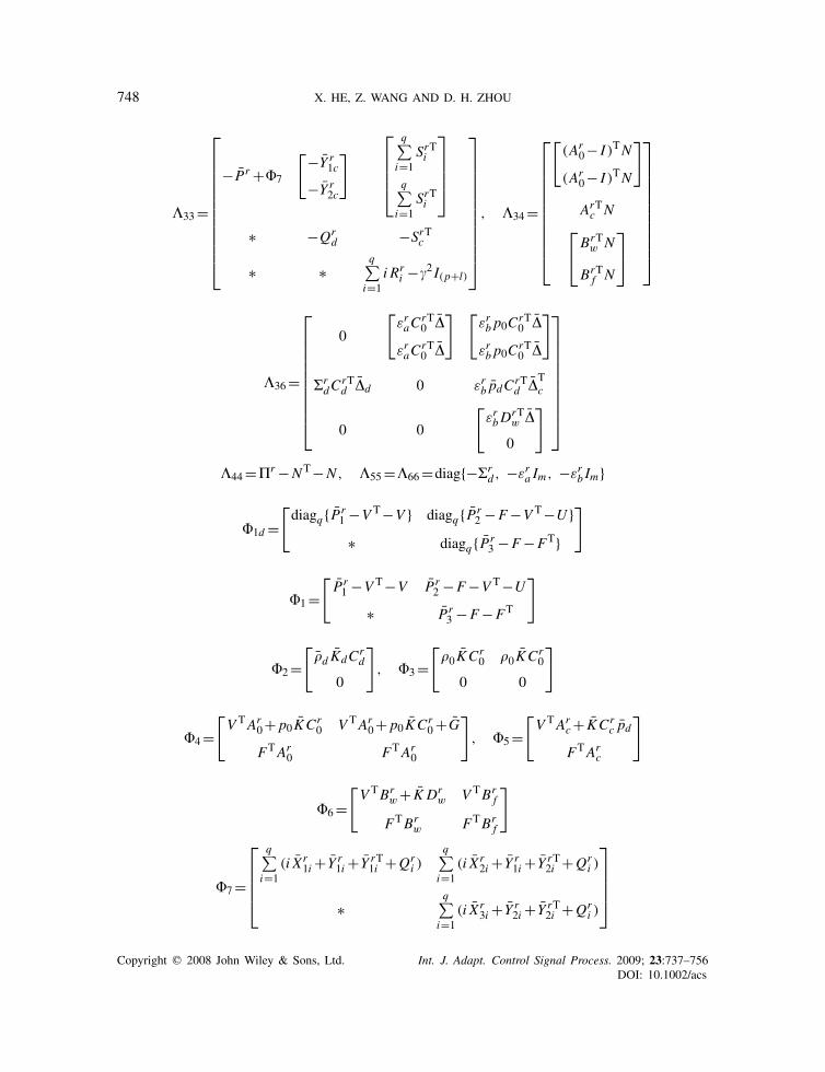
748 X. HE, Z. WANG AND D. H. ZHOU
33=
⎡⎢⎢⎢⎢⎢⎢⎢⎢⎢⎢⎢⎣
−Pr +7
[−Y r1c
−Y r2c
] ⎡⎢⎢⎢⎣
q∑i=1
SrTi
q∑i=1
SrTi
⎤⎥⎥⎥⎦
∗ −Qrd −SrTc
∗ ∗q∑
i=1i Rr
i −�2 I(p+l)
⎤⎥⎥⎥⎥⎥⎥⎥⎥⎥⎥⎥⎦
, 34=
⎡⎢⎢⎢⎢⎢⎢⎢⎢⎢⎢⎣
[(Ar
0− I )TN
(Ar0− I )TN
]
ArTc N⎡
⎣BrTw N
BrTf N
⎤⎦
⎤⎥⎥⎥⎥⎥⎥⎥⎥⎥⎥⎦
36=
⎡⎢⎢⎢⎢⎢⎢⎢⎢⎢⎣
0
[εraC
rT0 �
εraCrT0 �
] [εrb p0C
rT0 �
εrb p0CrT0 �
]
�rdC
rTd �d 0 εrb pdC
rTd �
Tc
0 0
[εrbD
rTw �
0
]
⎤⎥⎥⎥⎥⎥⎥⎥⎥⎥⎦
44=�r −NT−N , 55=66=diag{−�rd , −εra Im, −εrb Im}
1d =[diagq{Pr
1 −V T−V } diagq{Pr2 −F−V T−U }
∗ diagq{Pr3 −F−FT}
]
1=[Pr1 −V T−V Pr
2 −F−V T−U
∗ Pr3 −F−FT
]
2=[
d KdCrd
0
], 3=
[0 KCr
0 0 KCr0
0 0
]
4=[V TAr
0+ p0 KCr0 V TAr
0+ p0 KCr0+G
FTAr0 FTAr
0
], 5=
[V TAr
c+ KCrc pd
FTArc
]
6=[V TBr
w + K Drw V TBr
f
FTBrw FTBr
f
]
7=
⎡⎢⎢⎢⎣
q∑i=1
(i Xr1i + Y r
1i + Y rT1i +Qr
i )q∑
i=1(i Xr
2i + Y r1i + Y rT
2i +Qri )
∗q∑
i=1(i Xr
3i + Y r2i + Y rT
2i +Qri )
⎤⎥⎥⎥⎦
Copyright q 2008 John Wiley & Sons, Ltd. Int. J. Adapt. Control Signal Process. 2009; 23:737–756DOI: 10.1002/acs

NETWORK-BASED ROBUST FAULT DETECTION 749
and pd =diag{p1 In, . . . , pq In}, i =√pi (0�i�q), d =diag{1 In, . . . ,q In}, Kd =diagq{K },
Y r1c=[Y r
11, . . . , Yr1q ], Y r
2c=[Y r21, . . . , Y
r2q ], Cr
d =diag{Cr1, . . . ,C
rq}, Ar
c =[Ar1, . . . , A
rq ], Cr
c =[Cr1, . . . ,
Crq ], �r =∑q
j=1 i(Zri +T r
i ), �rd =diag{εr1 I, . . . ,εrq I }. Moreover, if (17)–(18) are true, the desired
filter parameters can be given by
G=U−1G, K =U−1 K , L= L (19)
ProofNote that a sufficient condition is given in Theorem 1 for the NRFDF analysis problem with agiven filter. It follows from (15) that MT+M−Pr>0 holds for any 1�r�v. Since Pr is positivedefinite, it can be confirmed that M is nonsingular [10]. Partition M , M−1 and Pr as follows:
M=[M11 M12
M21 M22
], M−1=
[W11 W12
W21 W22
], Pr =
[Pr1 Pr
2
∗ Pr3
](20)
where the partitioning of the above three matrices is compatible with that of A0 defined in (8).Introducing the following matrices:
T1=[M11 I
M21 0
], T2=
[I W11
0 W21
](21)
imply that M−1T1=T2 and MT2=T1. Define T2d :=diagq{T2} and let
Pr =[Pr1 Pr
2
∗ Pr3
]=TT
2 PrT2, Xr
i =[Xr1i X r
2i
∗ Xr3i
]=TT
2 Xri T2, Yi =
[Y r1i
Y r2i
]=TT
2Y ji
Then, performing congruence transformation to (15) by diag{I,diag{T2d ,T2,T2},diag{T2, I, I },I, I, I }, we can obtain ⎡
⎢⎢⎢⎢⎢⎢⎢⎢⎢⎢⎢⎢⎣
−I 0 13 0 0 0
∗ 22 23 0 25 0
∗ ∗ 33 34 0 36
∗ ∗ ∗ 44 0 0
∗ ∗ ∗ ∗ 55 0
∗ ∗ ∗ ∗ ∗ 66
⎤⎥⎥⎥⎥⎥⎥⎥⎥⎥⎥⎥⎥⎦
<0 (22)
where
13=[[0 LW21] 0 [0 − I ]], 22=diag(q+2){1}, 23=
⎡⎢⎢⎣
0 2 0
3 0 0
4 5 6
⎤⎥⎥⎦
Copyright q 2008 John Wiley & Sons, Ltd. Int. J. Adapt. Control Signal Process. 2009; 23:737–756DOI: 10.1002/acs

750 X. HE, Z. WANG AND D. H. ZHOU
25=diag
{ddiagq
{[MT
21K
0
]}, 0
[MT
21K
0
],
[MT
21K
0
]}
33=
⎡⎢⎢⎢⎢⎢⎢⎢⎢⎢⎢⎢⎣
−Pr +7
[−Y r1c
−Y r2c
] ⎡⎢⎢⎢⎣
q∑i=1
SrTi
q∑i=1
WT11S
rTi
⎤⎥⎥⎥⎦
∗ −Qrd −SrTc
∗ ∗q∑
i=1i Rr
i −�2 I
⎤⎥⎥⎥⎥⎥⎥⎥⎥⎥⎥⎥⎦
, 34=
⎡⎢⎢⎢⎢⎢⎢⎢⎢⎣
[(Ar
0− I )TN
WT11(A
r0− I )TN
]
ArTc N[
BrTw N
BrTf N
]
⎤⎥⎥⎥⎥⎥⎥⎥⎥⎦
36=
⎡⎢⎢⎢⎢⎢⎢⎢⎢⎣
0 εra
[CrT0 �
WT11C
rT0 �
]εrb p0
[CrT0 �
WT11C
rT0 �
]
�rdC
rTd �d 0 εrb pdC
rTd �
Tc
0 0 εrb
[DrT
w �
0
]
⎤⎥⎥⎥⎥⎥⎥⎥⎥⎦
44=�r −NT−N , 55= 66=diag{−�rd , −εra I, −εrb I }
1=[Pr1 −MT
11−M11 Pr2 − I −MT
11W11−MT21W21
∗ Pr3 −W11−WT
11
]
2=diag
{[1M
T21KCr
1
0
], . . . ,
[qM
T21KCr
q
0
]}, 3 :=0
[MT
21KCr0 MT
21KCr0W11
0 0
]
4=[MT
11Ar0+ p0M
T21KCr
0 MT11A
r0W11+ p0M
T21KCr
0W11+MT21GW21
Ar0 Ar
0W11
]
5=[MT
11Ard +MT
21KCrd pd
Ard
], 6=
[MT
11Brw +MT
21K Drw MT
11Brf
Brw Br
f
]
7=
⎡⎢⎢⎢⎣
q∑i=1
(i Xr1i + Y r
1i + Y rT1i +Qr
i )q∑
i=1(i Xr
2i + Y r1iW11+ Y rT
2i +Qri W11)
∗q∑
i=1(i Xr
3i + Y r2iW11+WT
11YrT2i +WT
11Qri W11)
⎤⎥⎥⎥⎦
Y r1c=[Y r
11, . . . , Yr1q ], Y r
2c=[Y r21, . . . , Y
r2q ]
Copyright q 2008 John Wiley & Sons, Ltd. Int. J. Adapt. Control Signal Process. 2009; 23:737–756DOI: 10.1002/acs

NETWORK-BASED ROBUST FAULT DETECTION 751
Define a new matrix I∈R2qn×2qn with its entries being I�, (2−1)� =I(+q)�,2� =1 for all1��q and 1���n, and other entries being all zero. Once again, performing congruence trans-formation to (22) by diag{I,diag{I, I, I }, I, I, I, I }, it can be inferred that (22) is equivalent to
⎡⎢⎢⎢⎢⎢⎢⎢⎢⎢⎢⎢⎢⎣
−I 0 13 0 0 0
∗ 22 23 0 25 0
∗ ∗ 33 34 0 36
∗ ∗ ∗ 44 0 0
∗ ∗ ∗ ∗ 55 0
∗ ∗ ∗ ∗ ∗ 66
⎤⎥⎥⎥⎥⎥⎥⎥⎥⎥⎥⎥⎥⎦
<0 (23)
where
22=diag
{[diagq{Pr
1 −MT11−M11} diagq{Pr
2 − I −MT11W11−MT
21W21}∗ diagq{Pr
3 −W11−WT11}
], 1, 1
}
23=
⎡⎢⎢⎣
0 2 0
3 0 0
4 5 6
⎤⎥⎥⎦ , 25=diag
{[dM
T21d Kd
0
],
[0M
T21K
0
],
[MT
21K
0
]}
2=[
dMT21d KdC
rd
0
], M21d =diagq{M21}, Kd =diagq{K }, d =diag{1 In, . . . ,q In}
Furthermore, let
Pr =[Pr1 Pr
2
∗ Pr3
]=
[I 0
0 W−111
]T[Pr1 Pr
2
∗ Pr3
][I 0
0 W−111
]
For all 1�i�q ,
Xri =
[Xr1i X r
2i
∗ Xr3i
]=
[I 0
0 W−111
]T
Xri
[I 0
0 W−111
], Y r
i =[Y r1i
Y r2i
]=
[I 0
0 W−111
]T
Y ri
DefineS1=diag{diagq{I },diagq{W−111 }, I,W−1
11 , I,W−111 } andS2=diag{I,W−1
11 , I, I }. Performingcongruence transformations to (23) by diag{I,S1,S2, I, I, I } and defining the following matrix
Copyright q 2008 John Wiley & Sons, Ltd. Int. J. Adapt. Control Signal Process. 2009; 23:737–756DOI: 10.1002/acs

752 X. HE, Z. WANG AND D. H. ZHOU
variables:
V =M11, F=W−1, U =MT21W21W
−111 , G=MT
21GW21W−111 , K =MT
21K , L= LW21W−111 (24)
we can easily obtain (17).With similar manipulations, we can also get (18). Since every step in our derivation is an equiv-
alent transformation, it can be confirmed from Theorem 1 that (17)–(18) are sufficient conditionsguaranteeing that the system (8) is robustly exponentially mean-square stable, as well as the H∞norm constraint (9) is achieved.
Furthermore, we know from (17) that V , F , U are all nonsingular matrices, so we can alwaysfind square and nonsingular matrices M21 and S21 satisfying UF−1=MT
21S21 [20]. Therefore, itresults from (24) that:
G0=M−T21 GF−1S−1
21 , K0=M−T21 K , L0= L F−1S−1
21 (25)
By substituting the parameters in (25) into the transfer function of the filter and considering therelationship U =MT
21S21F , we obtain
T (z)= L F−1S−121 (z I −M−T
21 GF−1S−121 )−1M−T
21 K = L(z I −U−1G)−1U−1 K (26)
which means that the desired filter parameters can also be given by (19). This ends the proof.�
In Theorem 2, there are no products of unknown matrices with G, K , and L , so the full-orderrobust fault detection filter can be obtained by solving convex optimization problems in formof LMIs with the help of efficient interior-point algorithms [23]. Note that (17) are LMIs overboth the matrix variables and the prescribed scalar �2. This implies that �2 can be included as anoptimization variable for LMI (17), which allow us to obtain the minimum level bound for theoverall fault detection dynamic (8). A sub-optimal fault detection filter can be readily found bysolving the following problem.
Problem 1The sub-optimal NRFDF design can be brought forward as:
minV,F,U,N ,G,K ,L,Pr1>0,Pr2>0,Pr3>0,Qr
i >0,Xr1i>0,
Xr2i ,Xr3i>0,Y r1i ,Y
r2i ,Z
ri >0,Rri >0,Sri ,Tri >0 ∀r=1,...,v
�2, s.t. (17) and (18) (27)
Remark 3The size of delays and the probability of the stochastic variable �k are included in the NRFDFdesign process. Therefore, Theorem 2 provides us with a delay-probability-dependent approach,which can reduce the design conservation of the robust fault detection filters [10, 16].Remark 4In most cases, it is not necessary to estimate fk in practice. By introducing a weighting matrix tolet rk approach the weighted fault fk[9, 19], we can design a NRFDF for a fault with a certainfrequency interval, and this offers us a possibility to consider the fault isolation problem.
Copyright q 2008 John Wiley & Sons, Ltd. Int. J. Adapt. Control Signal Process. 2009; 23:737–756DOI: 10.1002/acs

NETWORK-BASED ROBUST FAULT DETECTION 753
5. A NUMERICAL EXAMPLE
In this section, a numerical example is employed to illustrate the proposed method. For simplicity,let q=2 and �−2=�−1=�0=0. The parameters of the discrete-time networked system (1) areas follows:
A0=[0 0.1
� 0.3
], A1=
[0 0.1
0.3 0.1
], A2=
[0.1 0.4
0 0.2
], Bw =
[0.1 0
0 0.3
]
B f =[−0.1
0.2
], C0=[2 ], C1=C2=[2 5], Dw =[0.2 −0.1]
There are two uncertain parameters in the system with their uncertain ranges 0.15���0.25,4� �6. In this case, the vertex number (v) of the polytope is 4.
Consider the parameters of the logarithmic quantizer as u10=u20=1 and �1=�2=0.9. Fork=0,1, . . . ,300, the unknown input wk is taken as exp(−k/50)×nk , where nk is uniformlydistributed over [−0.5,0.5]. The fault signal fk =1 when k=100,101, . . . ,200 and fk =0 other-wise. �k is assumed to obey the distribution law given in Table I, which means that the measurementscan be ideally transmitted over network with probability 0.6, one-step delay happens with prob-ability 0.2, two-step delay occurs with probability 0.1, and the measurements are missing withprobability 0.1.
For simplicity, we impose Rri = Sri =T r
i =0 (1�i�q, 1�r�v) in our design process. With theabove parameters and from Theorem 2, we can solve the NRFDF design problem using MatlabLMI toolbox [24]. The robust H∞ attenuation level is minimized to achieve a bound �opt=1.0036,and the parameters of the sub-optimal fault detection filter are given by
G=[0.0065 0.3569
0.1504 0.4464
], K =
[0.0322
0.0549
], L=[0.0038 0.0015]
Next, we give the time-domain simulation result. The uncertain parameters, which are unknownin the design process of the fault detection filter, are randomly set to be �=0.26, =4.89.Figures 1–3 show the result.
In Figure 1, the measurement mode is described. The values 0, 1, 2, and 3 correspond to thecases that measurements transmitted over the network ideally, with one-step delay, with two-stepdelay, and with missing packets, respectively.
Figure 2 shows the measurements without (dotted line) and with (solid line) quantization, andthe latter is actually used by the robust fault detection filter.
Table I. The distribution law of �k .
�k 0 1 2 Others
Probability 0.6 0.2 0.1 0.1
Copyright q 2008 John Wiley & Sons, Ltd. Int. J. Adapt. Control Signal Process. 2009; 23:737–756DOI: 10.1002/acs

754 X. HE, Z. WANG AND D. H. ZHOU
0 50 100 150 200 250 300–0.5
0
0.5
1
1.5
2
2.5
3
3.5
Time step k
Mea
sure
men
t mod
e ov
er n
etw
ork
Figure 1. Measurement mode over network.
0 50 100 150 200 250 300
0
–5
5
10
15
20
25
Time step k
Mea
sure
men
ts w
ithou
t and
with
qua
ntiz
atio
n
Without quantizationWith quantization
Figure 2. Measurement with and without quantization.
The evolution of the residual evaluation function is given in Figure 3. We select a threshold asJth=4.4008×10⁻⁵ after 400 Monte Carlo simulations with no faults. From Figure 3, it can beshown that 4.106×10−5= J (111)<Jth<J (112)=4.475×10⁻⁶, which means that the fault can bedetected in 12 time steps after its occurrence.
Copyright q 2008 John Wiley & Sons, Ltd. Int. J. Adapt. Control Signal Process. 2009; 23:737–756DOI: 10.1002/acs

NETWORK-BASED ROBUST FAULT DETECTION 755
80 100 120 140 160 180 2000
1
2
3
4
5
6
7x 10⁻⁴
Time step k
Eva
luat
ion
func
tion
of r
esid
ual
Figure 3. Residual evaluation function.
6. CONCLUSION
In this paper, a robust fault detection problem for a class of discrete-time networked systems withmultiple state delays and unknown input has been dealt with. Measurements with random delay,stochastic dropout, as well as signal logarithmic quantization have been simultaneously considered.After properly state augmenting, the original robust fault detection problem can be formulated intoan auxiliary H∞ filtering problem. We have proposed a sufficient condition in terms of a set ofLMIs, which can be easily solved as a convex optimization problem. Delay-probability-dependentand parameter-dependent approaches have been used to get a less conservative design result.A numerical example has been provided to illustrate the applicability of the proposed technique.
REFERENCES
1. Patton R, Frank P, Clark R. Issue of Fault Diagnosis for Dynamic Systems. Springer: Berlin, 2000.2. Frank PM, Ding SX, Koppen-Seliger B. Current developments in the theory of FDI. Proceedings of
SAFEPROCESS, Budapest, Hungary, 2000; 16–27.3. Kinnaert M. Fault diagnosis based on analytical models for linear and nonlinear systems—a tutorial. Proceedings
of SAFEPROCESS, Washington, DC, 2003; 37–50.4. Mahmoud M, Jiang J, Zhang Y. Stabilization of active fault tolerant control systems with imperfect fault detection
and diagnosis. Stochastic Analysis and Applications 2003; 21(3):673–701.5. Wang Y, Zhou D, Gao F. Robust fault-tolerant control of a class of non-minimum phase nonlinear processes.
Journal of Process Control 2007; 17(6):523–537.6. Zhou D, Frank P. Fault diagnostics and fault tolerant control. IEEE Transactions on Aerospace and Electronic
Systems 1998; 34(2):420–427.7. Ding SX, Jeinsch T, Frank PM, Ding EL. A unified approach to the optimization of fault detection systems.
International Journal of Adaptive Control and Signal Processing 2000; 14(7):725–745.8. Zhong M, Ding SX, Lam J, Wang H. An LMI approach to design robust fault detection filter for uncertain LTI
systems. Automatica 2003; 39(3):543–550.
Copyright q 2008 John Wiley & Sons, Ltd. Int. J. Adapt. Control Signal Process. 2009; 23:737–756DOI: 10.1002/acs
756 X. HE, Z. WANG AND D. H. ZHOU
9. Zhong M, Ye H, Shi P, Wang G. Fault detection for Markovian jump systems. IEE Proceedings and ControlTheory Applications 2005; 152(4):397–402.
10. Gao H, Wang C. A delay-dependent approach to robust H∞ filtering for uncertain discrete-time state-delayedsystems. IEEE Transactions on Signal Processing 2004; 52(6):1631–1640.
11. Zhang W, Branicky MS, Phillips SM. Stability of networked control systems. IEEE Control Systems Magazine2001; 21(1):84–99.
12. Sha L, Abdelzaher T, Arzen KE et al. Real time scheduling theory: a historical perspective. Real-Time Systems2004; 28(2–3):101–155.
13. Andersson M, Henriksson D, Cervin A, Arzen K. Simulation of wireless networked control systems. Proceedingsof the 44th IEEE Conference on Decision and Control, and the European Control Conference, Seville, Spain,2005; 476–481.
14. Roberts C, Dassanayake HPB, Lehrasab N, Goodman CJ. Distributed quantitative and qualitative fault diagnosis:railway junction case study. Control Engineering Practice 2002; 10(4):419–429.
15. Zhang P, Ding SX, Frank PM, Sader M. Fault detection of networked control systems with missing measurements.Proceedings of Asian Control Conference, Melbourne, Australia, 2004; 1258–1263.
16. He X, Wang Z, Zhou D. Robust H∞ filtering for networked systems with multiple state-delays. InternationalJournal of Control 2007; 80(8):1217–1232.
17. Fang H, Ye H, Zhong M. Fault diagnosis of networked control systems. Proceedings of SAFEPROCESS, Beijing,2006; 1–12.
18. Patton R, Kambhampati C, Casavola A, Zhang P, Ding S, Sauter D. A generic strategy for fault-tolerance incontrol systems distributed over a network. European Journal of Control 2007; 13(2–3):280–296.
19. He X, Wang Z, Ji Y, Zhou D. Network-based fault detection for discrete-time state-delay systems: a newmeasurement model. International Journal of Adaptive Control and Signal Processing 2007; DOI: 10.1002/acs.1000.
20. Wang Z, Yang F, Ho DWC, Liu X. Robust H∞ filtering for stochastic time-delay systems with missingmeasurements. IEEE Transactions on Signal Processing 2006; 54(7):2579–2587.
21. Wang Z, Ho DWC, Liu X. Variance-constrained filtering for uncertain stochastic systems with missingmeasurements. IEEE Transactions on Automatic Control 2003; 48(7):1254–1258.
22. Fu M, Xie L. The sector bound approach to quantized feedback control. IEEE Transactions on Automatic Control2005; 50(11):1698–1711.
23. Boyd S, Ghaoui LE, Feron E, Balakrishnan V. Linear Matrix Inequalities in System and Control Theory. SIAM:Philadelphia, 1994.
24. Gahinet P, Nemirovski A, Laub AJ, Chilali M. The LMI Control Toolbox. For Use with Matlab. The MathWorksInc.: Natick, MA, 1995.
Copyright q 2008 John Wiley & Sons, Ltd. Int. J. Adapt. Control Signal Process. 2009; 23:737–756DOI: 10.1002/acs