network coding - an introduction - calit2

Network Coding - an Introduction

Ralf Koetter and Muriel MedardUniversity of Illinois, Urbana-Champaign

Massachusetts Institute of Technology

Goals of Class

• To provide a general introduction to the new field of network coding

• To provide sufficient tools to enable the participants to apply and develop network coding methods in diverse applications

• To place network coding in the context of traditional network operation

Outline

• Basics of networks, routing and network coding:– Introduction to routing in traditional networks

• routing along shortest paths• routing for recovery

– Introduction to concepts of network coding• Algebraic foundations:

– Formal setup of linear network coding– Algebraic formulation– Algebraic min cut max flow condition– The basic multicast theorem– Other scenarios solvable with algebraic framework– Delays in networks

Outline (contd)

• More multicast - constructing codes– Coding gain is unbounded– Construction based on algebraic system– Construction based on flows– Undirected networks

Outline (contd)

• Decentralized code construction and network coding for multicast with a cost criterion– Randomized construction and its error behavior– Performance of distributed randomized construction -

case studies– Robustness of randomized methods– Traditional methods based on flows - a review– Trees for multicasting - a review– Network coding with a cost criterion - flow-based

methods for multicasting through linear programming– Distributed operation - one approach– A special case - wireless networks– Sample ISPs

Outline(contd)

• Non-multicast:– The algebraic difficulty– Vector solutions vs. instantaneous– Issue of linearity– Is the non-multicast case interesting?

Outline(contd)

• Network coding for multicast - relation to compression and generalization of Slepian-Wolf– Review of Slepian-Wolf– Distributed network compression– Error exponents– Source-channel separation issues – Code construction for finite field multiple access networks

• Network coding for security and robustness– Network coding for detecting attacks– Network management requirements for robustness– Centralized versus distributed network management

• New directions

Main topics

• Routing in networks operates in a manner akin to a transportation problem in which we seek to transport goods (data) in a cost-efficient fashion (multicast is a notable exception)

• Data is compressed and recovered at the edges• Cost is defined according to a given cost of routes or by

adjusting to the flows• Current approaches do not generally make use of the fact that

data (bits) are being transmitted

Shortest Paths

• Interior gateway protocol• Option 1 (routing information protocol (RIP)):

– vector distance protocol: each gateway propagates a list of the networks it can reach and the distance to each network

– gateways use the list to compute new routes, then propagate their list of reachable networks

• Option 2 (open shortest path first (OSPF)):– link-state protocol: each gateway propagates status of its

individual connections to networks– protocol delivers each link state message to all other

participating gateways– if new link state information arrives, then gateway recomputes

next-hop along shortest path to each destination

OSPF

• OSPF has each gateway maintain a topology graph• Each node is either a gateway or a network• If a physical connection exists between two objects in an

internet, the OSPF graph contains a pair of directed edges between the nodes representing the objects

• Note: gateways engage in active propagation of routing information while hosts acquire routing information passively and never propagate it

OSPF

• Weights can be asymmetric: w(i,j) need not be equal to w(j,i)• All weights are positive• Weights are assigned by the network manager

G1

G2

G3

Network N N

G2G1

G3

w(1,N)

w(1,N) w(N,2)

w(2,N)w(N,3)

w(3,N)

Shortest Path Algorithms

• Shortest path between two nodes: length = weight• Directed graphs (digraphs) (recall that MSTs were on undirected

graphs), edges are called arcs and have a direction (i,j) ≠ (j,i)• Shortest path problem: a directed path from A to B is a sequence of

distinct nodes A, n1, n2, …, nk, B, where (A, n1), (n1, n2), …, (nk, B) are directed arcs - find the shortest such path

• Variants of the problem: find shortest path from an origin to all nodes or from all nodes to an origin

• Assumption: all cycles have non-negative length• Three main algorithms:

– Dijsktra– Bellman-Ford– Floyd-Warshall

Bellman-Ford

• Allows negative lengths, but not negative cycles• B-F works at looking at negative lengths from every node to

node 1• If arc (i,j) does not exist, we set d(i,j) to • We look at walks: consider the shortest walk from node i to 1

after at most h arcs• Algorithm:

– Dh+1(i) = minover all j[d(i,j) + Dh(i)]for all i other than 1– we terminate when Dh+1(i) = Dh(i)

• The Dh+1(i) are the lengths of the shortest path from i to 1 with no more than h arcs in it

Bellman-Ford

• Let us show this by induction– D1(i) = d(i,1)for every i other than 1, since one hop corresponds

to having a single arc– now suppose this holds for some h, let us show it for h+1: we

assume that for all k ≤ h, Dk(i) is the length of the shortest walk from i to 1 with k arcs or fewer

– minover all j[d(i,j) + Dh(i)] allows up to h+1 arcs, but Dh(i) would have fewer than h arcs, so min[Dh(i), minover all j[d(i,j) + Dh(i)]] = Dh+1(i)

• Time complexity: A, where A is the number of arcs, for at most N-1 nodes (note: A can be up to (N-1)2 )

• In practice, B-F still often performs better than Dijkstra (O(N2))

Distributed Asynchronous B-F

• The algorithms we investigated work well when we have a single centralized entity doing all the computation - what happens when we have a network that is operating in a distributed and asynchronous fashion?

• Let us call N(i) the set of nodes that are neighbors of node i• At every time t, every node i other than 1 has available :

– Dij(t): estimate of shortest distance of each neighbor node

j in N(i) which was last communicated to node i– Di(t): estimate of the shortest distance of node i which was

last computed at node i using B-F


• D1(t) = 0 at all times• Each node i has available link lengths d(i,j) for all j in N(i)• Distance estimates change only at time t0, t1, .., tm, where tm

becomes infinitely large at m becomes infinitely large• At these times:

– Di(t) = minj in N(i)[d(i,j) + Dij(t)], but leaves estimate Di

j(t) for all j in N(i) unchanged

– node i receives from one or more neighbors their Dj, which becomes Di

j (all other Dij are unchanged)

– node i is idle

OR

OR


• Assumptions:– if there is a link (i,j), there is also a link (j,i)– no negative length cycles– nodes never stop updating estimates and receiving

updated estimates– old distance information is eventually purged– distances are fixed

• Under those conditions:for any initial Dij(t0), Di(t), for some

tm, eventually all values Di(t) = Di for all t greater than tm

Failure recovery

• Often asynchronous distributed Bellman-Ford works even when there are changes, including failures

• However, the algorithm may take a long time to recover from a failure that is located on a shortest path, particularly if the alternate path is much longer than the original path (bad news phenomenon)

destination

1

1

100

Rerouting

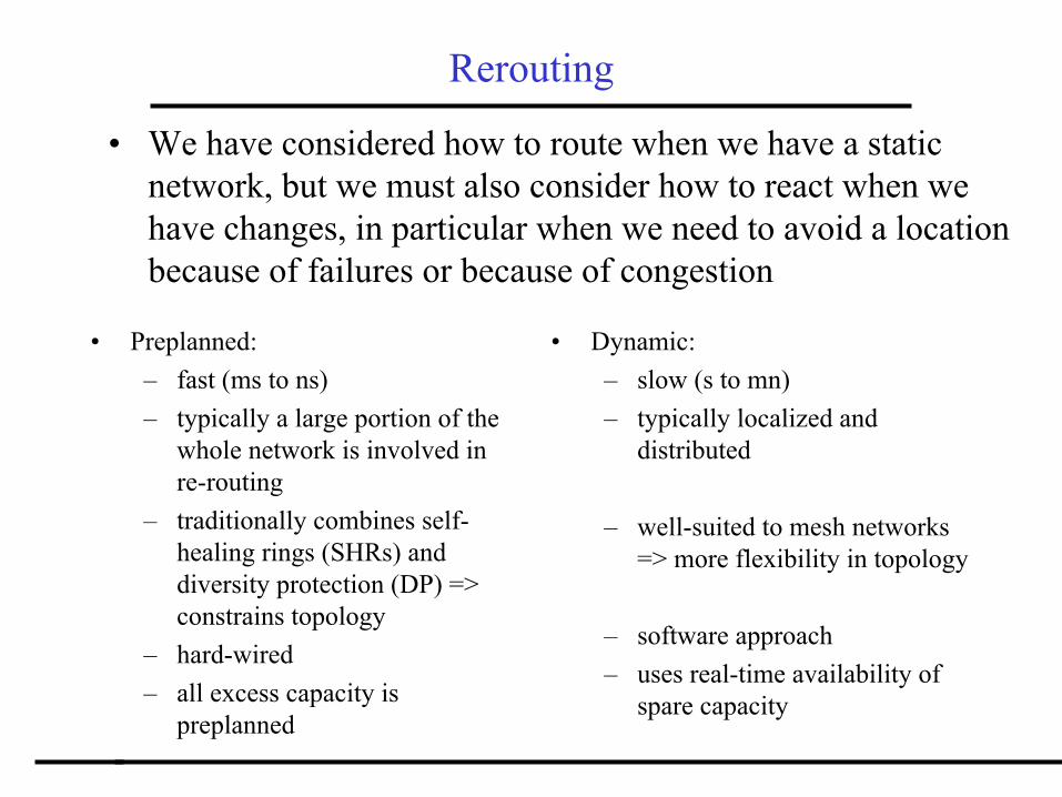
• We have considered how to route when we have a static network, but we must also consider how to react when we have changes, in particular when we need to avoid a location because of failures or because of congestion

• Preplanned:– fast (ms to ns)– typically a large portion of the

whole network is involved in re-routing

– traditionally combines self-healing rings (SHRs) and diversity protection (DP) => constrains topology

– hard-wired– all excess capacity is

preplanned

• Dynamic:– slow (s to mn)– typically localized and

distributed

– well-suited to mesh networks => more flexibility in topology

– software approach– uses real-time availability of

spare capacity

Example of rerouting in the IP world

• Internet control message protocol (ICMP)• Gateway generates ICMP error message, for instance for

congestion• ICMP redirect: “ipdirect” specifies a pointer to a buffer in which

there is a packet, an interface number, pointer to a new route• How do we get new route?

– First: check the interface is other than the one over which the packet arrives

– Second: run “rtget” (route get) to compute route to machine that sent datagram, returns a pointer to a structure describing the route

• If the failure or congestion is temporary, we may use flow control instead of a new route

Rerouting for ATM

• ATM is part datagram, part circuit oriented, so recovery methods span many different types

• Dynamic methods release connections and then seek ways of re-establishing them: not necessarily per VP or VC approach– private network to network interface (PNNI) crankback– distributed restoration algorithms (DRAs)

• Circuit-oriented methods often have preplanned component and work on a per VC, VP basis– dedicated shared VPs, VCs or soft VPs, VCs

PNNI self-healing

• PNNI is how ATM switches talk to each other• Around failure or congestion area, initiate crankback• End equipment (CPE: customer premise equipment) initiates

a new connection• In phase 2 PNNI, automatic call rerouting, freeing up CPEs

from having to instigate new calls, the ATM setup message includes a request for a fault-tolerant connection

NE NE NECPE CPE

Network element

Before failure

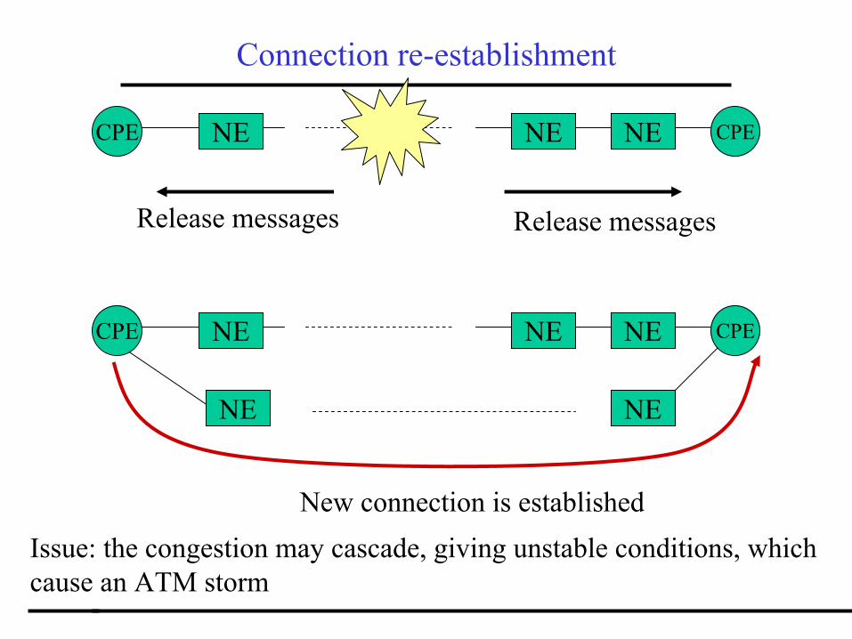
Connection re-establishment

NE NE NECPE CPE

Release messages Release messages

NE NE NECPE CPE

NE NE

New connection is establishedIssue: the congestion may cascade, giving unstable conditions, whichcause an ATM storm

DRAs

NE NE

sender chooser

Help messages

New routes

NE NE

sender chooser

Help messages

New routes

sender

NE NE

sender

New routes

sender

chooserHelp messagesNE The DRAs have at least one end node

transmit help messagesto some nodes around them, usuallywithin a certain hop radius, and new routes, possible splitting flows, are selected and used

Circuit-oriented methods

• Circuit-oriented methods seek to replace a route with another one, whether end-to-end or over some portion that is affected by a failure

• Several issues arise:– How do we perform recovery in a bandwidth-efficient

manner– How does recovery interface with network management– What sort of granularity do we need– What happens when a node rather than a link fails

Rings: Path and Link/Node Rerouting

UPSR: automatic path switchingon Unidirectional Path Switched Ring

BLSR: link/node rerouting onBidirectional Line Switched Ring

Path-based methods

• Live back-up

– backup bandwidth is dedicated– only receiver is involved– fast but bandwidth inefficient

• Failure triggered back-up

– backup bandwidth is shared– sender and receiver are involved– slow but bandwidth efficient

Before After

Before After

Rerouting as a code

s

t u

b1

b1

b1

b1

w

s . dt,w + s . d u,w = b1

s

t u

b1

w

dt,w + du,w = b1

a. Live path protection b. Link recovery

b1 b1

Rerouting as a code

• Live path protection: we have an extra supervisory signal s =1 when the primary path is live, s =0 otherwise

• Failure-triggered path protection: the backup signal is multiplied by s

• Link recovery: – di,h = dk, i+ dh, i for the primary link (i, h) emanating from i, where (k,

i) is the primary link into i and (h, i) is the secondary link into i– for secondary link emanating from i, the code is di,k =di,h . si, h + di, h

di,h

idk, i

k hdi,k dh, i

Codes and routes

• In effect, every routing and rerouting scheme can be mapped to some type of code, which may involve the presence of a network management component

• Thus, removing the restrictions of routing can only improve performance - can we actively make use of this generality?

Network coding

• The canonical example

s

t u

y z

x

b1

b1

b1

b1

b2

b2

b2

b2

s

t u

y z

w

b1

b1

b1

b1 + b2

b2

b2

b2

xb1 + b2b1 + b2

Coding across the network - have I seen this before?

• Several source-based systems exist or have been proposed• Routing diversity to average out the loss of packets over

the network• Access several mirror sites rather than single one• The data is then coded across packets in order to withstand

the loss of packets without incurring the loss of all packets• Rather than select the “best” route, routes are diverse

enough that congestion in one location will not bring down a whole stream

• This may be done with traditional Reed-Solomon erasure codes or with Tornado codes

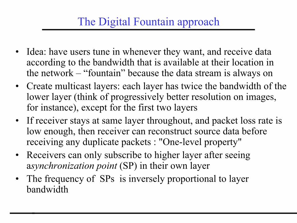
The Digital Fountain approach

• Idea: have users tune in whenever they want, and receive data according to the bandwidth that is available at their location in the network – “fountain” because the data stream is always on

• Create multicast layers: each layer has twice the bandwidth of the lower layer (think of progressively better resolution on images,for instance), except for the first two layers

• If receiver stays at same layer throughout, and packet loss rate is low enough, then receiver can reconstruct source data before receiving any duplicate packets : "One-level property"

• Receivers can only subscribe to higher layer after seeingasynchronization point (SP) in their own layer

• The frequency of SPs is inversely proportional to layer bandwidth

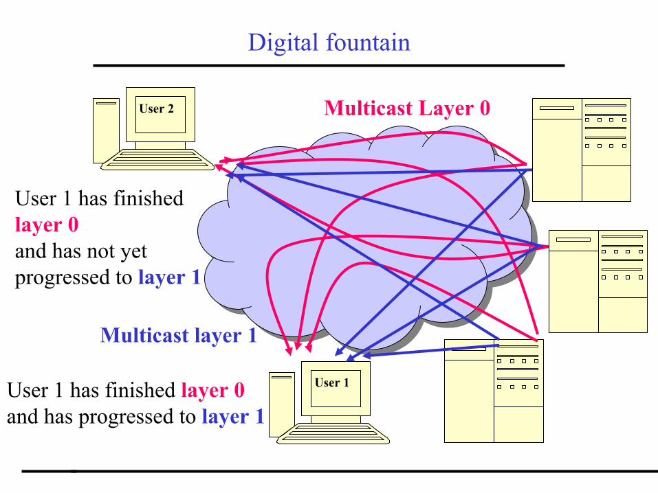
Digital fountain

User 2

User 1

Multicast Layer 0

User 1 has finished layer 0and has progressed to layer 1

Multicast layer 1

User 1 has finished layer 0and has not yet progressed to layer 1

Network coding vs. Coding for networks

• The source-based approaches consider the networks as in effect channels with ergodic erasures or errors, and code over them, attempting to reduce excessive redundancy

• The data is expanded, not combined to adapt to topology and capacity

• Underlying coding for networks, traditional routing problems remain, which yield the virtual channel over which coding takes place

• Network coding subsumes all functions of routing - algebraic data manipulation and forwarding are fused

II — Algebraic Foundations of Network Coding

⇒

S

S

SR

R

R

1

2

3

1

2

3

A network

⇒ A(I − F )−1BT = I

Why an “algebraic” characterization?

• Graph-theoretic proofs are cumbersome

• Generalizations are possible

• Equations are easier managed than graphs

• Powerful tools available

2

Problem Description

S

S

SR

R

R

1

2

3

1

2

3

A network

Vertices: V

Edges: E ⊆ V × V , e = (v, u) ∈ E

Edge capacity: C(e)

Network: G = (V, E)

Source nodes: {v1, v2, . . . , vN} ⊆ V

Sink nodes: {u1, u2, . . . , uK} ⊆ V

3

µ input random processes at v:� (v) = {X(v,1), X(v,2), . . . , X(v, µ(v)}

ν Output random processes at u:

� (u) = {Z(u,1), Z(u,2), . . . , Z(u, ν(u))}

Random processes on edges: Y (e)

A connection:c = (v, u, � (v, u)), � (v, u) ⊆ � (v)

A connection is established if � (u) ⊃ � (v, u)

Set of connections: �

The pair (G, � ) defines a network coding problem .

4

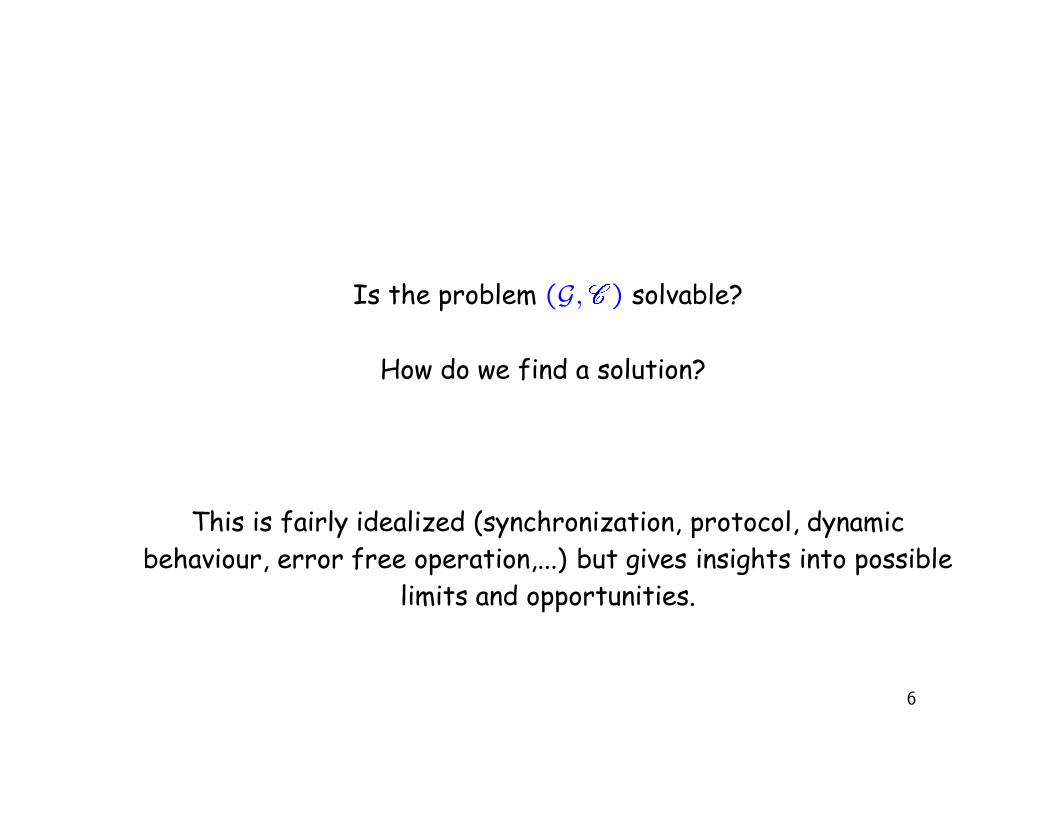
Is the problem (G, � ) solvable?

How do we find a solution?

This is fairly idealized (synchronization, protocol, dynamic

behaviour, error free,...) but gives insights into possible limits and

opportunities.

5

Is the problem (G, � ) solvable?

How do we find a solution?

This is fairly idealized (synchronization, protocol, dynamic

behaviour, error free operation,...) but gives insights into possible

limits and opportunities.

6

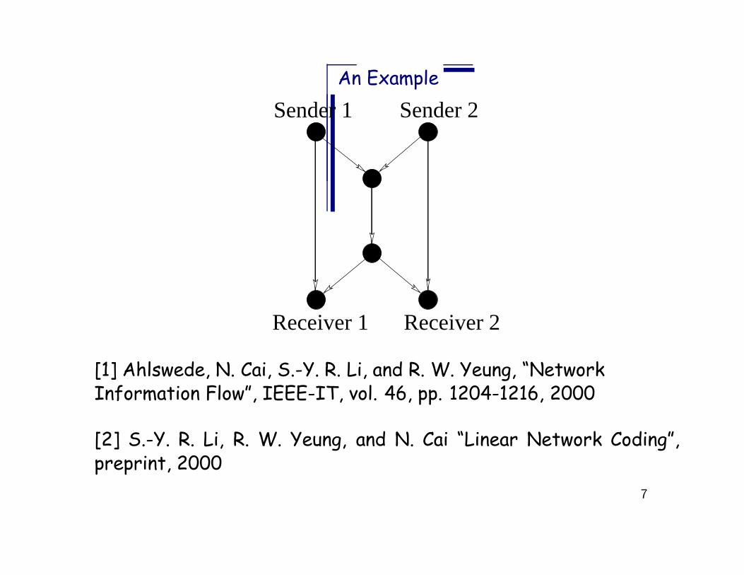
An Example

Receiver 1 Receiver 2

Sender 1 Sender 2

[1] Ahlswede, N. Cai, S.-Y. R. Li, and R. W. Yeung, “NetworkInformation Flow”, IEEE-IT, vol. 46, pp. 1204-1216, 2000

[2] S.-Y. R. Li, R. W. Yeung, and N. Cai “Linear Network Coding”,preprint, 2000

7

More Simplifications — Linear Network Codes

C(e) = 1 (links have the same capacity)H(X(v, i)) = 1 (sources have the same rate)The X(v, i) are mutually independent.Vector symbols of length m elements in F2m.

(F2m is the finite field with m elements we can add, subtract, divideand multiply elements in F2m without going crazy!)

This is necessary to define linear operations.

8

More Simplifications — Linear Network Codes

All operations at network nodes are linear!

e eX(v,i)

Y(e )Y(e )21

e3 Y(e )3

21

Y (e3) =∑

i

αiX(v, i) +∑

j=1,2

βjY (ej)

At a receiver (terminal) node:

e eY(e )Y(e )

n1

e3 3

n1

Z(e )

Z(v, j) =n∑

j=1

εjY (ej).

9

A simple example

e

e

e

e

e

XZ

X Z

1

2

1

2

3

4

5

1

2

Y (e1) = α1,e1X1 + α2,e1X2

Y (e2) = α1,e2X1 + α2,e2X2

Y (e3) = βe1,e3Y (e1)

Y (e4) = βe1,e4Y (e1)

Y (e5) = βe2,e5Y (e2) + βe3,e5Y (e3)

Z1 = εe4,1Y (e4) + εe5,1Y (e5)

Z2 = εe4,2Y (e4) + εe5,2Y (e5)

10

e

e

e

e

e

XZ

X Z

1

2

1

2

3

4

5

1

2

In matrix form (after solving the linear system)(

Z1

Z2

)

=

(εe4,1 εe5,1

εe4,2 εe5,2

)

︸︷︷︸B

(βe1,e4

0βe1,e3βe3,e5 βe2,e5

)

︸︷︷︸G

(α1,e1

α1,e2

α2,e1α2,e2

)

︸︷︷︸A

(X1

X2

)

We define three matrices A, G, B

The main question becomes: Is G invertible?

11

The transfer matrix

Let a matrix F be defined as an |E|×|E| matrix where fi,j is definedas βei,ej, i.e. the coefficient with which Y (ei) is mixed into Yej .

e

e

e

e

e

XZ

X Z

1

2

1

2

3

4

5

1

2 F =

0 0 βe1,e3βe1,e4

00 0 0 0 βe2,e5

0 0 0 0 βe3,e5

0 0 0 0 00 0 0 0 0

Summing the “path gains”:

P = I + F + F 2 + . . . = (I − F )−1 =

0 0 βe1,e3βe1,e4

βe1,e3βe3,e5

0 0 0 0 βe2,e5

0 0 0 0 βe3,e5

0 0 0 0 00 0 0 0 0

Observe that G = (I − F )−1 is polynomial

12

A linear system

X(v,1)

X(w,1)

X(w,2)

X(v’,1)

Z(u,1)

Z(u,2)

Z(u,3)

Z(u’,1)

A linear network

Input vector: xT = (X(v,1), X(v,2), . . . , X(v′, µ(v′)))

Output vector: zT = (Z(u,1), Z(u,2), . . . , Z(u′, ν(u′)))

Transfer matrix: M , z = Mx = B · G · A x

ξ = (ξ1, ξ2, . . . , ) = (. . . , αe,l, . . . , βe′,e, . . . , εe′,j, . . .)

13

z = Mx = B · (I − F T)−1︸︷︷︸

GT

·A x

ξ = (ξ1, ξ2, . . . , ) = (. . . , αe,l, . . . , βe′,e, . . . , εe′,j, . . .)

For acyclic networks the elements of G (and hence M)

are polynomial functions in variables ξ = (ξ1, ξ2, . . . , )

⇒ an algebraic characterization of flows....

14

An algebraic Min-Cut Max-Flow condition

Let network be given with a source v and a sink v′ . The followingthree statements are equivalent:

1. A point-to-point connection c = (v, v′, � (v, v′)) is possible.

2. The Min-Cut Max-Flow bound is satisfied for a rate R(c) =

| � (v, v′)|.

3. The determinant of the R(c)×R(c) transfer matrix M is nonzeroover the ring of polynomials F2[ξ]

3. ⇒ We have to study the solution sets of polynomial equations.

15

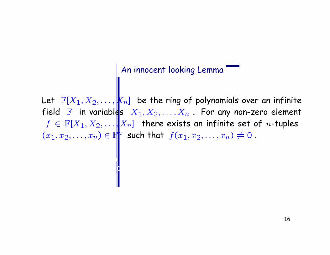
An innocent looking Lemma

Let F[X1, X2, . . . , Xn] be the ring of polynomials over an infinite

field F in variables X1, X2, . . . , Xn . For any non-zero element

f ∈ F[X1, X2, . . . , Xn] there exists an infinite set of n-tuples

(x1, x2, . . . , xn) ∈ Fn such that f(x1, x2, . . . , xn) 6= 0 .

(x6 − x4 − x2 + x) does not have have a non-solution in F2, F3, F4

but in F5 we have 26 − 24 − 22 + 2 = 46 ≡ 1(mod 5).

16

An innocent looking Lemma

Let F[X1, X2, . . . , Xn] be the ring of polynomials over an infinite

field F in variables X1, X2, . . . , Xn . For any non-zero element

f ∈ F[X1, X2, . . . , Xn] there exists an infinite set of n-tuples

(x1, x2, . . . , xn) ∈ Fn such that f(x1, x2, . . . , xn) 6= 0 .

(x6 − x4 − x2 + x) does not have have a non-solution in F2, F3, F4

but in F5 we have 26 − 24 − 22 + 2 = 46 ≡ 1(mod 5).

17

Another Example:

v

v

v

v

4

1

3

2

v

v

v

v

4

1

3

2

X(v,1)

X(v,2)

X(v,3)

Z(v’,1)

Z(v’,2)

Z(v’,3)

a) b)e

e

e

ee

e

e1

4

3

26

5

7

� = (v1, v4, {X(v1,1), X(v,2), X(v1,3)})

A =

αe1,1 αe2,1 αe3,1

αe1,2 αe2,2 αe3,2

αe1,3 αe2,3 αe3,3

, B =

εe5,1 εe5,2 εe5,3

εe6,1 εe6,2 εe6,3

εe7,1 εe7,2 εe7,3

.

M = A

βe1,e5 βe1,e4βe4,e6 βe1,e4βe4,e7

βe2,e5βe2,e4

βe4,e6βe2,e4

βe4,e7

0 βe3,e6βe3,e6

BT .

det(M) = det(A)det(B)

(βe1,e5βe2,e4 − βe2,e5βe1,e5)(βe4,e6βe3,e7 − βe4,e7βe3,e6)

Choose the coefficients so that det(M) 6= 0!

18

Multicast:� = {(v, u1, � (v)), (v, u2, � (v)), . . . , (v, uK, � (v))}

Z ZZ

Z

ZZZZZ

11 12

13

21

23

22

31

32

33

1

X

X

X

2

3

Multicast network

� ��

� � � � � � � ��

� � � � � � � ��

� ��

� ��

� ��

� ��

A

(I−F)

=

B−1

M

M is a | � (v)| × K| � (v)| matrix.

19

Multicast:

� � � � � � � � � � � � � � � � � ��

� � � � � � � � � � � � � � � � � ��

M1 M M2 3Multicast network

Z ZZ

Z

ZZZZZ

11 12

13

21

23

22

31

32

33

1

X

X

X

2

3

System Transfer matrix

� = {(v, u1, � (v)), (v, u2, � (v)), . . . , (v, uK, � (v))}

M is a | � (v)| × K| � (v)| matrix.

mi(ξ) = det(Mi(ξ))

Choose the coefficients in F̄ so that all mi(ξ) are unequal to zero.

Find a solution of∏

i mi(ξ) 6= 0

20

The main Multicast Theorem:

Theorem Let (G, � ) be a multicast network coding problem. There

exists a linear network coding solution for (G, � ) over a finite field

F2m for some large enough m if and only if there exists a flow of

sufficient capacity between the source and each sink individually.

(We will see later how large m will have to be — it's not too bad)

21

Other (derived) problems: Multisource — Multicast� = {(v, u1, � (v)), (v, u2, � (v)), . . . , (v, uK, � (v))}

Z ZZ

Z

ZZZZZ

11 12

13

21

23

22

31

32

33

1

X

X

X

2

3

Multicast network

� � ��

� � ��

� � � � � � � ��

� � � � � � � ��

� � ��

� � ��

� � ��

� � ��

� � ��

� � ��

� � � ��

� � � ��

(I−F) B−1

X’

X’

11

12

Z’Z’

Z’Z’

Z’Z’

32

31

2122

1112

A =

M

22

Other (derived) problems: Multisource — Multicast

Theorem Let a linear, acyclic, delay-free network G be given with a

set of desired connections � = {(vi, uj, � (vi)) : i = 0,1, . . . N, j =

1,2, . . . K} . The network problem (G, � ) is solvable if and only

if the Min-Cut Max-Flow bound is satisfied for any cut between all

source nodes {vi : i = 0,1, . . . N} and any sink node uj .

23

Other (derived) problems: One source — Disjoint Muticasts� = {(v, uj, � (v, uj)) : j = 1,2, . . . K}, � (v, uj) ∩ � (v, ui) = ∅

� � � � � � � ��

� � � � � � � ��

� ��

��

��

� ��

� ��

� �

��

� � ��

� � ��

� � � � ��

� � � � ��

(I−F) B−1

Z

X

X

Multicast network

X 1

X

X

2

3

4

5

A

=

M

=?

24

One source — Disjoint Muticasts + Multicasts� = {(v, uj, � (v, uj)) : j = 1,2, . . . K} ∪ {(v, u`, � (v)) : j = K + 1, K +

2, . . . K + N}, � (v, uj) ∩ � (v, ui) = ∅

� ��

� ��

� � ��

� � � � � ��

� � �

� � � ��

� � ��

� � ��

� � ��

� � ��

� � � ��

Z

X

X

X 1

X

X

2

3

4

5

(I−F) B−1

A =

25

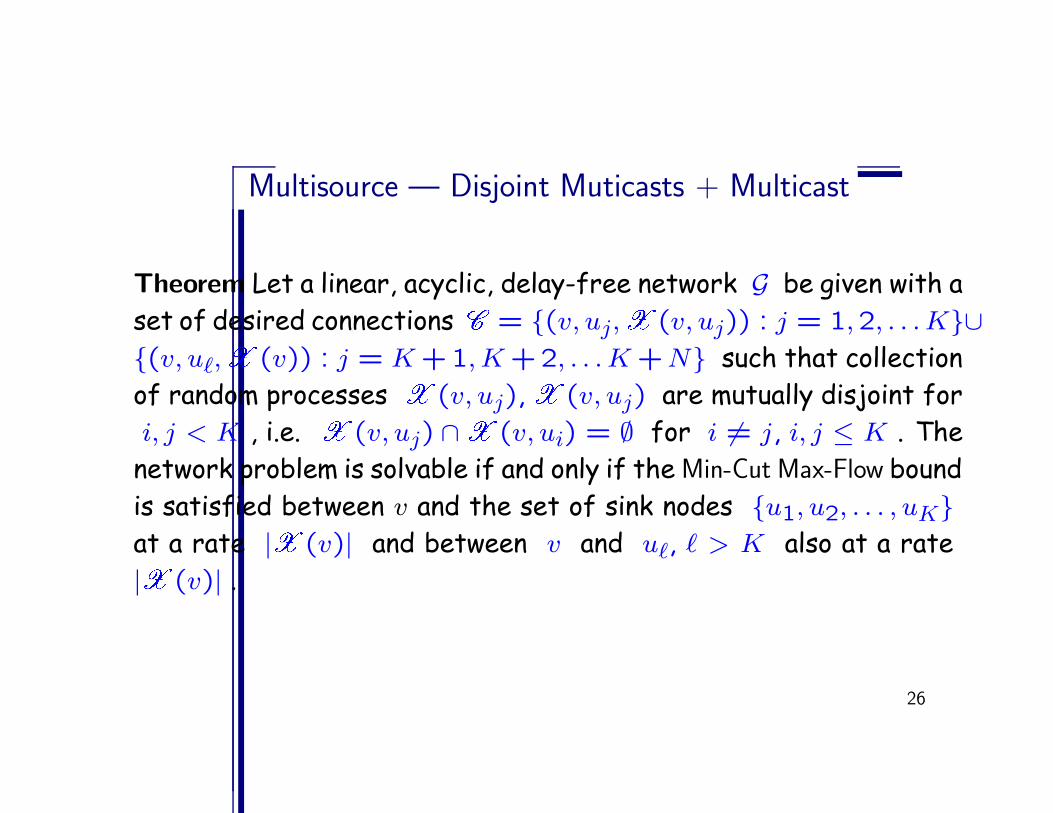
Multisource — Disjoint Muticasts + Multicast

Theorem Let a linear, acyclic, delay-free network G be given with a

set of desired connections � = {(v, uj, � (v, uj)) : j = 1,2, . . . K}∪

{(v, u`, � (v)) : j = K +1, K +2, . . . K +N} such that collection

of random processes � (v, uj), � (v, uj) are mutually disjoint for

i, j < K , i.e. � (v, uj) ∩ � (v, ui) = ∅ for i 6= j, i, j ≤ K . The

network problem is solvable if and only if the Min-Cut Max-Flow bound

is satisfied between v and the set of sink nodes {u1, u2, . . . , uK}

at a rate | � (v)| and between v and u`, ` > K also at a rate

| � (v)| .

26

Other (derived) problems: Two level Multicasts� = {(v, u1, � (v, u1))} ∪ {(v, u2, � (v)}

� � � � � � ��

� � � � � � ��

� � � ��

� � � ��

� ��

� � � ��

� � � ��

(I−F) B−1

A

X

X

X 1

X

X

2

3

4

5

27

Other (derived) problems: Two Level Multicast

Theorem(“Two-level multicast”) Let an acyclic network G be given

with a set of desired connections

� = {(v, u1, � (v, u1)), (v, u2, � (v))

The network problem is solvable if and only if the Min-Cut Max-Flow

bound is satisfied between v and u1 at a rate | � (v, u1)| and be-

tween v and u2 at a rate | � (v)|.

28

So far so good!

What about networks with cycles?

What about networks with delays?

What about robustness?

Do we really need network coding for multicast?

29

So far so good!

What about networks with cycles?

What about networks with delays?

What about robustness?

Do we really need network coding for multicast? YES

30

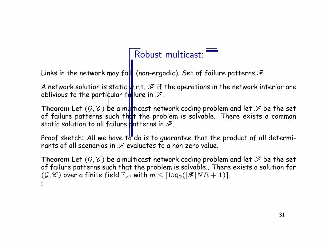
Robust multicast:

Links in the network may fail. (non-ergodic). Set of failure patterns: �

A network solution is static w.r.t. � if the operations in the network interior areoblivious to the particular failure in � .

Theorem Let (G, � ) be a multicast network coding problem and let � be the setof failure patterns such that the problem is solvable. There exists a commonstatic solution to all failure patterns in � .

Proof sketch: All we have to do is to guarantee that the product of all determi-nants of all scenarios in � evaluates to a non zero value.

Theorem Let (G, � ) be a multicast network coding problem and let � be the setof failure patterns such that the problem is solvable.. There exists a solution for(G, � ) over a finite field F2m with m ≤ dlog2(| � |NR + 1)e....

31

Linear Networks with Delays

We transmit random processes in a delay variable D on links, i.e.

X(v, j)(D) =∞∑

`=0

X`(v, j)D`,

Z(v, j)(D) =∞∑

`=0

Z`(v, j)D`,

Y (e)(D) =∞∑

`=0

Y`(e)D`.

Conceptually, we consider an entire sequence in D as one symbol and

work over the field of formal power series.

32

(D)

(D)(D)

(D)e e

X(v,i)Y(e )

21

e3 Y(e )

2

3

Y(e )1

Y (e3)(D) =∑

i

αiDX(v, i)(D) +∑

j=1,2

βjDY (ej)(D)

(other functions with memory are possible but not necessary)

33

At a receiver (terminal) node we have to allow for “rational” func-tions:

(D)

(D)(D)e e

Y(e )n1

e3 3

n

Z(e )

Y(e )1

Y (e)(D) =∑∞

`=0 Y`(e)D`, Z(v, j)(D) =

∑∞`=0 Z`(v, j)D`

Z`(v, j) =n∑

j=1

µ∑

k=0

εj,kY`−k(ej) +µ

∑

k=1

λkZ`−k(v, j)

or Z(v, j)(D) =∑n

j=1εj,k(D)

λ(D)Y (ej)(D)

34

The transfer matrix with delays

e

e

e

e

e

XZ

X Z

1

2

1

2

3

4

5

1

2 F =

0 0 Dβe1,e3 Dβe1,e4 00 0 0 0 Dβe2,e5

0 0 0 0 Dβe3,e5

0 0 0 0 00 0 0 0 0


P = I+DF+D2F 2+. . . = (I−DF )−1 =

0 0 Dβe1,e3Dβe1,e4

D2βe1,e3βe3,e5

0 0 0 0 Dβe2,e5

0 0 0 0 Dβe3,e5

0 0 0 0 00 0 0 0 0

Observe that G = (I − DF )−1 is polynomial over F2(D).

35

An algebraic Min-Cut Max-Flow condition with delays

Let network be given with a source v and a sink v′ . The following

three statements are equivalent:



| � (v, v′)|.

3. The determinant of the R(c)×R(c) transfer matrix M is nonzero

over the ring of polynomials F2(D)[ξ] with coefficients from

the field of rational functions.

36

It is only that....

We have to study the solution sets of polynomial equations over

F2(D).

At receiver nodes we have to allow for memory and the possibility

of implementing rational functions!

This is neccessary since now we have to invert a transfer matrix

which has as elements polynomials over F2(D).

37

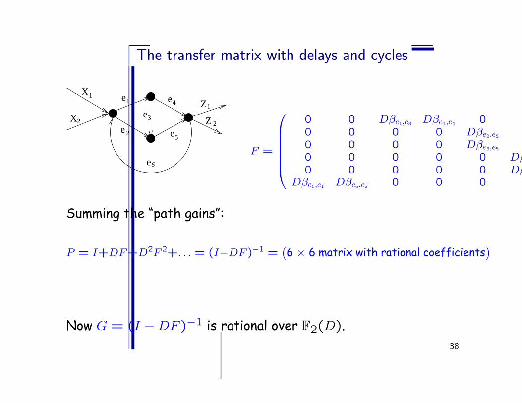
The transfer matrix with delays and cycles

e

e

e

e

e

XZ

X Z

1

2

1

2

3

4

5

1

2

e6

F =

0 0 Dβe1,e3Dβe1,e4

0 00 0 0 0 Dβe2,e5 00 0 0 0 Dβe3,e5

00 0 0 0 0 Dβe4,e6

0 0 0 0 0 Dβe5,e6

Dβe6,e1Dβe6,e2

0 0 0 0


P = I+DF+D2F 2+. . . = (I−DF )−1 =(6 × 6 matrix with rational coefficients

)

Now G = (I − DF )−1 is rational over F2(D).

38

Delays and cycle - or really nothing has happened....

Let network be given with a source v and a sink v′ . The following

three statements are equivalent:



| � (v, v′)|.

3. The determinant of the R(c)×R(c) transfer matrix M is nonzero

over the ring of polynomials F2(D)[ξ] with coefficients from

the field of rational functions.

39

Multicast:� = {(v, u1, � (v)), (v, u2, � (v)), . . . , (v, uK, � (v))}

Z ZZ

Z

ZZZZZ

11 12

13

21

23

22

31

32

33

1

X

X

X

2

3

Multicast network

� ��

� � � � � � � ��

� � � � � � � ��

� ��

� ��

� ��

� � ��

A

(I−F)

=

B−1

M

M is a | � (v)| × K| � (v)| matrix.

40

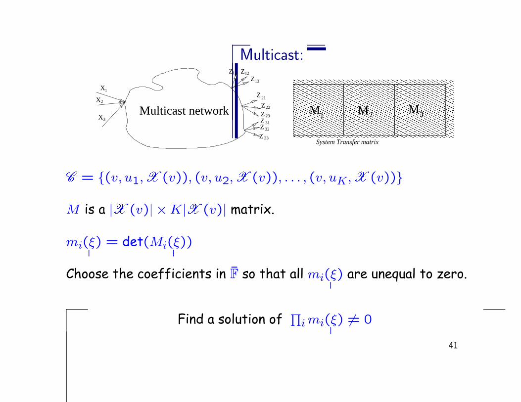
Multicast:

� � � � � � � � � � � � � � � � � ��

� � � � � � � � � � � � � � � � � ��

M1 M M2 3Multicast network

Z ZZ

Z

ZZZZZ

11 12

13

21

23

22

31

32

33

1

X

X

X

2

3

System Transfer matrix

� = {(v, u1, � (v)), (v, u2, � (v)), . . . , (v, uK, � (v))}

M is a | � (v)| × K| � (v)| matrix.

mi(ξ) = det(Mi(ξ))

Choose the coefficients in F̄ so that all mi(ξ) are unequal to zero.

Find a solution of∏

i mi(ξ) 6= 0

41

The main Multicast Theorem:

Theorem Let (G, � ) be a multicast network coding problem on a

graph which may have a cyclic structure. There exists a linear net-

work coding solution for (G, � ) over a finite field F2m for some

large enough m if and only if there exists a flow of sufficient ca-

pacity between the source and each sink individually.

42

Theorems, Theorems.....

43

Summary

• Connecting network information flow problems to algebraic equa-tions yields powerful tools for analysis of networks.

• Multicast especially well suited for the approach since we have

to find “non solutions” to equations, which can easily be accom-

plished in large fields.

• Many network scenarios can be derived from the multicast setup.

• The general non multicast setup will be treated later (much less

is known).

44

• Field size?

• How do we find solutions?

• Is network coding really helpful or just a singular occurrence?

network coding - an introduction - calit2

Documents