network flow models for power grids - iti algorithmik i · master thesis network flow models for...
TRANSCRIPT

Master Thesis
Network Flow Modelsfor Power Grids
Franziska WegnerJanuary 15, 2014
Reviewer: Prof. Dr. Dorothea Wagner and Prof. Dr. Peter SandersAdvisors: Dr. Martin Nollenburg
Dr. Ignaz RutterDr. Tamara Mchedlidze
Institute of Theoretical Informatics, AlgorithmicsFacility of Informatics
Karlsruhe Institute of Technology
KIT – University of the State of Baden-Wuerttemberg and National Laboratory of the Helmholtz Association www.kit.edu

Name: Franziska WegnerStudent ID: 1612804Pursued Degree: Master of Science
Date of Submission: January 15, 2014Editing Time: 6 Months
Acknowledgments:
I would like to thank my family and friends for their support; my colleagues for the inspiringdiscussions, and all reviewers for the helpful suggestions and improvements regarding thisthesis.
In addition, I would like to thank TransnetBW for the provided data and, in particular,Guntram Zeitler for the presentation at the TransnetBW substation in Wendlingen andfor the discussions and support via mail and in person.
Finally, I would like to thank Prof. Dr. Dorothea Wagner and Prof. Dr. Peter Sanders forthe opportunity to work on an exciting interdisciplinary topic.
Contact Information:
Author :Franziska WegnerEmail: [email protected]
University :Karlsruhe Institute of TechnologyKaiserstraße 1276131 Karlsruhe, GermanyPhone: +49 721 608-0Fax: +49 721 608-44290Email: [email protected]://www.kit.edu/

Statement of Authorship:
I hereby declare that this thesis is composed by myself and nobody else, unless otherwiseacknowledged in the text or bibliography. Verbatim and contentual borrowed text passagesare specifically marked in the document. Furthermore, I follow the constitution of theKarlsruhe Institute of Technology for protection of good academic experience.
Karlsruhe, den 15. January 2014
i

Abstract
In recent years, power grids and their operation have been becoming increasingly complexdue to expanding renewable energy sources, independent power producers and planningof smart energy consumers. Current methods for calculating optimal power flows, whichdetermine the cheapest energy production for each generator and, based on this, determinethe electrical flow, rely on non-linear, numerical methods. Here, an electrical flow complieswith physical laws and is only seldomly influenced by the network operator. At this point,graph theory, in particular flow algorithms, offer the possibility to efficiently calculateoptimal power flows on networks, given the assumption that the flow can be controlledat each node of the network. It is due to the aforementioned compliance with physicallaws—and the resulting fact that electrical flows are not controlled—that flow algorithmsin electricity networks have been left unattended.
In this thesis, we consider graph-theoretical flow methods in electricity networks and showthat these yield electrical flows of considerable quality. We present two approaches: Thefirst approach considers the generator productions of flow models and uses them as inputfor the power flow method. We use a range of heuristics to obtain physically bettergenerator productions. A second approach tries to implement flows in electricity networksby equipping each node with an electric control system. Arbitrary flow algorithms can thenbe applied to electricity networks and it turns out that the minimization of production costsand line losses results in a balanced model, which additionally features reduced generatorproduction costs. Moreover, by weighting both criteria, that is, production costs andline losses, the resulting search space is clearly bounded. From an economic point of view,however, introducing control devices at each node of the network is currently not affordablefor network providers. For this reason, we combine the flow model for cost minimizationand flow balancing with the optimal power flow, such that nodes having control devices andnodes having no such devices can be combined arbitrarily. This model exhibits interestingproperties; one of them being the optimal amount of control systems that are necessary toreach the optimal flow. It turns out that only few control nodes are required to gain fullcontrol of the electrical flow. For each of the flow models we present experiments usingreal data to demonstrate the models’ properties.
Zusammenfassung
Elektrische Netzwerke und deren Betrieb werden zunehmend komplexer durch die Erweite-rung von erneuerbaren Energiequellen, unabhangigen Energieerzeugern und der Planungvon intelligenten Energieabnehmern. Aktuelle Verfahren zur optimalen Lastflussberech-nung, die die gunstigste Energieproduktion fur jeden Generator bestimmen und darausden elektrischen Fluss berechnen, beruhen auf nicht-linearen Methoden aus der Numerik.Dabei folgt ein elektrischer Fluss physikalischen Gesetzmaßigkeiten und wird nur seltenvon Netzbetreibern aktiv beeinflusst. Die Graphentheorie, im speziellen Flussalgorithmen,bieten die Moglichkeit effizient optimale Flusse auf Netzwerken zu erzeugen. Es wird jedochvorausgesetzt, dass an jedem Knoten der Fluss kontrolliert werden kann. Flussalgorithmenwurden daher lange in elektrischen Netzwerken vernachlassigt, da der elektrische Fluss derPhysik folgte und nicht gesteuert wird.
Diese Arbeit beschaftigt sich mit graphentheoretischen Flussen in elektrischen Netzwer-ken und zeigt, dass Flussmethoden auf elektrischen Netzwerken angewendet werden kon-nen, um physikalisch gute Flusse zu erzeugen. Aus diesem Grunde werden zwei Ansatzevorgestellt: Im ersten Ansatz werden die von den Flussmodellen erzeugten Generatorpro-duktionen in die Lastflussmethode eingesetzt. Dabei werden eine Reihe von Heuristiken
iii

angewandt, um eine physikalisch bessere Generatorproduktion zu erhalten. Ein zweiterAnsatz versucht Flusse in elektrischen Netzwerken umzusetzen, indem jeder Knoten mitSteuerelektronik ausgestattet wird. Dadurch konnen beliebige Flussalgorithmen auf elek-trischen Netzwerken angewandt werden und es stellt sich heraus, dass das Minimieren derProduktionskosten und der Leitungsverluste zu einem balancierten Modell fuhrt, welcheszudem kostengunstige Generatorproduktionen erlaubt. Durch die Gewichtung der Krite-rien Produktionskosten und Leistungsverluste entsteht zudem eine Paretokurve, die denErgebnisraum klar abgrenzt. Nun ware aus Netzbetreibersicht ein Steuergerat an jedemKnoten eine unwirtschaftliche bzw. unmoglich zu finanzierende Losung. Daher wird diesesFlussmodell zur Kostenminimierung und Flussbalancierung mit dem optimalen Leistungs-fluss so kombiniert, dass man Steuerknoten und elektrische Knoten ohne Steuerelementbeliebig kombinieren kann. Dieses Modell bietet interessante Eigenschaften, die dann auchzur optimalen Anzahl an steuerbaren Knoten im elektrischen Netzwerk fuhren und zeigen,dass mit wenigen Steuerelementen der Leistungsfluss so beeinflusst werden kann, dass erimmernoch zu einer optimalen Losung fuhrt. Zu allen Flussmodellen werden Experimenteanhand realer Daten durchgefuhrt, um die Eigenschaften der Modelle zu verdeutlichen.
iv

Contents
1. Introduction 1
2. Related Work 3
3. Preliminaries 73.1. Graph Theory Notation . . . . . . . . . . . . . . . . . . . . . . . . . . . . . 73.2. Linear Programming and Integer Linear Programming . . . . . . . . . . . . 8
4. Power Flow in Electricity Networks 114.1. Transmission Line Parameters . . . . . . . . . . . . . . . . . . . . . . . . . . 114.2. Properties of Transmission Lines . . . . . . . . . . . . . . . . . . . . . . . . 204.3. Power Flow . . . . . . . . . . . . . . . . . . . . . . . . . . . . . . . . . . . . 204.4. Direct Current Approximation . . . . . . . . . . . . . . . . . . . . . . . . . 23
5. Flow-Based Approaches 255.1. Transformation to an s-t-Graph . . . . . . . . . . . . . . . . . . . . . . . . . 255.2. Standard Flow Model . . . . . . . . . . . . . . . . . . . . . . . . . . . . . . 285.3. Balanced Flow Model . . . . . . . . . . . . . . . . . . . . . . . . . . . . . . 315.4. Bottleneck Flow Model . . . . . . . . . . . . . . . . . . . . . . . . . . . . . . 335.5. Minimum Cost Flow Model . . . . . . . . . . . . . . . . . . . . . . . . . . . 375.6. Combination of Cost Minimization and Balancing . . . . . . . . . . . . . . . 39
6. Hybrid Model 436.1. Mathematical Model . . . . . . . . . . . . . . . . . . . . . . . . . . . . . . . 436.2. Mathematical Properties . . . . . . . . . . . . . . . . . . . . . . . . . . . . . 446.3. Structural Findings . . . . . . . . . . . . . . . . . . . . . . . . . . . . . . . . 496.4. Case Study . . . . . . . . . . . . . . . . . . . . . . . . . . . . . . . . . . . . 49
7. Conclusion 51
8. Appendix 53A. 30-Bus Electricity Network . . . . . . . . . . . . . . . . . . . . . . . . . . . 54B. 57-Bus Electricity Network . . . . . . . . . . . . . . . . . . . . . . . . . . . 55C. 118-Bus Electricity Network . . . . . . . . . . . . . . . . . . . . . . . . . . . 56
Bibliography 64
v

List of Figures
3.1. A cycle with vertices vi, vi+1 and vi+2. . . . . . . . . . . . . . . . . . . . . . 83.2. A tree with orange marked leafs. . . . . . . . . . . . . . . . . . . . . . . . . 83.3. Linear programming time complexity and method overview. . . . . . . . . . 9
4.1. Transmission network of Switzerland. . . . . . . . . . . . . . . . . . . . . . . 114.2. A 14-bus electricity network. . . . . . . . . . . . . . . . . . . . . . . . . . . 124.3. Basic structure of a multi-voltage level electricity network. . . . . . . . . . . 134.4. Impedance Z in a circuit. . . . . . . . . . . . . . . . . . . . . . . . . . . . . 184.5. Admittance Y in a circuit. . . . . . . . . . . . . . . . . . . . . . . . . . . . . 184.6. Explanation of the Kirchhoff’s current law in a circuit. . . . . . . . . . . . . 214.7. Explanation of the Kirchhoff’s voltage law in a circuit. . . . . . . . . . . . . 21
5.1. Transformation of an electricity network NE to a s-t-network Nst. . . . . . 275.2. Standard flow and optimal power flow on an 14-bus electricity network. . . 285.3. Plots for the standard flow model on an 14-bus electricity network. . . . . . 305.4. Balanced flow and optimal power flow on an 14-bus electricity network. . . 325.5. Plots for the balanced model on an 14-bus electricity network. . . . . . . . . 335.6. Bottleneck flow and optimal power flow on an 14-bus electricity network. . 355.7. Plots for the bottleneck model on an 14-bus electricity network. . . . . . . . 365.8. Visualization of linear approximations. . . . . . . . . . . . . . . . . . . . . . 375.9. Total power generation cost of all previous models. . . . . . . . . . . . . . . 395.10. The weighted curve appears as Pareto curve, where λ · γ + (1− λ) · `. . . . 41
6.1. Cut vertices splitting the network N into blocks. . . . . . . . . . . . . . . . 466.4. Cycles which have at most one common vertex split the network into blocks. 476.2. A cycle with a maximum cyclic flow of x ≡ 3. . . . . . . . . . . . . . . . . . 476.3. A cactus. . . . . . . . . . . . . . . . . . . . . . . . . . . . . . . . . . . . . . 476.5. Plots for the hybrid model on an 14 bus electricity network. . . . . . . . . . 50
7.1. Planned high voltage direct current transmission lines in Germany for re-newable energy integration. . . . . . . . . . . . . . . . . . . . . . . . . . . . 52
A.1. A 30-bus electricity network. . . . . . . . . . . . . . . . . . . . . . . . . . . 54A.2. Plots for the 30-bus electricity network. . . . . . . . . . . . . . . . . . . . . 54B.3. A 57-bus electricity network. . . . . . . . . . . . . . . . . . . . . . . . . . . 55B.4. Plots for the 57-bus electricity network. . . . . . . . . . . . . . . . . . . . . 55C.5. A 118-bus electricity network. . . . . . . . . . . . . . . . . . . . . . . . . . . 56C.6. Plots for the 118-bus electricity network. . . . . . . . . . . . . . . . . . . . . 56
vi

List of Algorithms
5.1. Solving the multi-objective linear program bottleneck flow . . . . . . . . . . 36
5.2. Piecewise Linear Approximation . . . . . . . . . . . . . . . . . . . . . . . . . 38
List of Tables
4.1. Load flow bus specification from [81]. . . . . . . . . . . . . . . . . . . . . . . 16
5.1. Merging parallel transmission lines of an electricity network. . . . . . . . . . 26
vii


List of Abbreviations
p.u. Per-Unit System, is a relativ and absolute representation of electrical param-eter.
τ Transformer Tap Ratio
Θ Phase Angle
B Shunt Susceptance
C Condenser
G Shunt Conductance
Pg Real Power Generation
Qd Reactive Power Demand
Qg Reactive Power Generation
R Resistance
rs Series Resistance
Rpu Resistance in per unit
X Reactance
xs Series reactance
Xpu Reactance in per unit
Y Admittance
Z Impedance
AC Alternating Current
DC Direct Current
DLF Distribution Loss Factor
FACTS Flexible Alternating Current Transmission System
IEEE Institute of Electrical and Electronics Engineers; a world-wide organizationfor standardization in information technology.
ix

List of Tables
IEP Improved Evolutionary Program
ILP Integer Linear Program
IPP Independent Power Producer
KCL Kirchoff’s Current Law
KVL Kirchoff’s Voltage Law
LMP Locational Margine Pricing
LP Linear Program
MILP Mixed Integer Linear Programs
MVar Mega Volt-Ampere Reactive, SI derived unit of power; a unit is used in ACelectricity networks to distinguish reactive power from real power (1V AR =1W = 1V · 1A).
MW Megawatt, SI derived unit of power (1W = 1V · 1A)
OPF Optimal Power Flow
OPFSA Optimal Power Flow Simulated Annealing
PF Power Flow
PSO Particle Swarm Optimization
PV Photo Voltaic
RHS Right-Hand Side
SA Simulated Annealing
SCOPF Security Constrained Optimal Power Flow
SI International System of Units
SI Swarm Intelligence
TCUL Tap Change under Load Transformer
TLF Transmission Loss Factor
UPFC Unified Power Flow Controller
V Voltage
x

1. Introduction
Power grids, also known as electricity networks, are networks, which satisfy our dailyenergy demand and consist of generators (producing energy), transmission lines for energytransportation and energy consumers. The energy flows in an electricity network obeylaws of physics, and this flow can be hardly controlled. For electrical analysis, like demandsatisfaction, costs optimization and fault tolerances, an energy flow calculation is necessary.This results in a non-linear optimization problem that is currently solved by numericalmethods known as power flow (PF) to calculate the electrical flow of a given generatorproduction, and optimal power flow (OPF) to calculate the optimal energy production foreach generator and the resulting power flow.
Since the complexity and network size w.r.t. power grids has been growing, the efficiencyof these flow calculation methods has become increasingly important. Multiple methodsbased on power flows have been developed recently [45]. However, the direction relatingpower flow to other types of flows in networks has not been investigated. These flowproblems (for example transportation, fluid flows) have the property that the amountof flow on an edge depends only on the capacity of the edge. For this type of problem,traditional flow algorithms well-investigated in theoretical computer science can be applied.To apply flow algorithms on electricity networks, each node has to be able to distribute theflow according to a given flow. Control devices, which are able to influence the electricalflow, are, for example, flexible alternating current transmission systems (FACTS) [44]. Inthis thesis, we investigate electricity networks under the assumption that either all or apart of nodes are supplied with such a control device. To apply traditional flow algorithmson electricity networks, we initially assume FACTS devices at each node.
We start with investigating power networks where FACTS are placed on each node andas another approach to compare the models with the current OPF method we use thecalculated generator productions of the models in the PF method to calculate an electricalflow of the models generator productions. We first apply a simple standard flow modeland then remedy its disadvantages. The standard flow model produces an electrical flow,where some transmission lines are close to the thermal limits and a lot of transmissionlines are not in use. In order to spread the electrical flow in the network we try to balancethe flow on all transmission lines. The first idea to achieve an equally balanced flow is togive all transmission lines the same priority. This is done by minimizing the flow whenonly half of the transmission line capacity is used. As each transmission line is balanced
1

Chapter 1. Introduction
with the same priority, there are some lines which have more load than others. Thesetransmission lines are called bottleneck lines and contribute potential vulnerabilities inthe electricity network. Thus, a second balancing heuristic prioritizes bottleneck edges tobalance the flow on these edges and minimizes the maximum edge flow in the electricitynetwork by iteratively reducing the flow on all edges. The standard flow model and bothof its balancing variations have high energy production costs, since these models do nottake cost functions of each generator into account. Unfortunately, these cost functionsare not available in our experimental data. We use the method from Zimmermann etal. [84] to produce generator cost functions from existing data sets. We target to minimizegeneration costs using the produced cost functions. Additionally, we would like to keepthe produced flow balanced. To achieve this we take into account the line losses providedby our data. We claim that the use of line losses results in a decrease of the flow on thebottleneck edges. However, optimizing generation costs and line losses at the same timeare two opposing problems. We combine these two optimization functions into one usinga weighting optimization method and investigate its solution space.
In the second part of the thesis we make our assumption more realistic and investigateelectricity networks, in which only part of the nodes are supplied with FACTS devices.We propose a new model, which merges the electrical power flow model with the graphtheoretical flow model with generator and loss minimization. We theoretically investigatethe properties of these models and show, e.g., for the 14-bus system [6], that FACTS mayprovide better solutions in electricity networks. Our case studies with this combined modelshow for the 14-bus system that only a small number of FACTS is sufficient to provide anoptimal solution and to control the whole flow in this electricity network.
Thesis Outline
In Chapter 2, we give an overview of related work on electricity networks and flow al-gorithms. It presents existing approaches in computer science with regard to electricitynetworks.
Chapter 3 provides the general notations and definitions of graph theoretical concepts andlinear optimization. We introduce different graph types, representations and components,and describe the differences between linear programming and integer linear programming.
Fundamental concepts of electricity networks are presented in Chapter 4. We first describethe standard data format and its components in more detail to understand the structureof such a network. Afterwards, we mention power flow methods, which are part of theoptimal power flow calculation, and the approximation of a direct current (DC) electricitynetwork by an alternating current (AC) electricity network.
Chapter 5 provides the results of our investigations of flow algorithms on electricity net-works, where FACTS devices are placed on all nodes, or using the calculated generatorproduction of the model in the power flow (PF) method to get the resulting electricalflow. We start with a transformation of an electricity network into a graph-theoreticalflow network. To this transformed electricity network we apply several flow models likethe standard flow model, two balancing heuristics and a balanced cost minimization model.Each model is established by some case studies.
In Chapter 6, we make the model introduced in Chapter 5 more realistic by assuming thatnot all nodes can be supplied with FACTS. We prove several theoretical properties of thismodel. Finally, we describe the results of its case studies.
We summarize this thesis with regards to the results and case studies, and give a briefoutlook regarding possible future work in Chapter 7.
2

2. Related Work
In the first half of the 20th century, power flow calculations and optimal power flow analysiswere done by rules of thumb or by tools including slide rules and analog network analyz-ers. The first publication with regards to digital load flows was provided by Dunstan in1954 [31], in which he described the loop and track method. Since this method includes acomplex matrix inversion for which a special data preparation is necessary and since it isstrongly limited in network size, an iterative nodal power flow analysis was introduced in1956 by Ward and Hale [80]. They show that nodal analyses have advantages in contrastto the mesh analysis presented by Dunstan and Henderson [31, 42]. In the same yearShipley and Hochdorf [70] provided different types of load flow solutions as well. In 1957,Brown and Tinney [22] published an iterative nodal method to solve load flow problemsautomatically. The difference to prior digital solutions is that the digital power analysisfrom Brown and Tinney has an improved performance, comparable to analog analyzers,and provides the same problem size, while the complexity compared to prior solutionsdecreases. The first fully optimal power flow formulation was introduced by Capentier in1962 [24]. Capentier shows that the optimal power flow is a difficult problem for solversbecause of its non-linearity. Non-linear solvers cannot guarantee a globally optimal solu-tion, are not robust and are not fast. Therefore, Peschon et al. discuss in their paper from1968 [63] an efficient computation of the optimal power flow based on the Newton-Raphsonmethod. This method was successfully applied to electricity networks with hundreds ofbuses. Then, in 1985, a sparsity method for the optimal power flow problem was publishedby Tinney [75]. In the paper, he emphasizes advantages like data reduction and increas-ing speed. A survey summarizing past results of optimal power flow in power grids haspublished in 1991 by Huneault and Galiana [45].
Computer Science Research in Power Grids
There are many research areas in computer science which try to tackle the optimal powerflow problem, including fuzzy logic, neural networks, genetic algorithms, artificial intelli-gence methods, evolutionary computing, ant colony research and particle swarm research.In the following, we present some research in this area.
One of the first works in fuzzy logic regarding optimal power flows was presented byMiranda et al. in 1992 [51] using prior results with respect to fuzzy power flow fromMiranda and Matos in 1989 [50], and Miranda et al. in 1990 [52]. In this paper, they give
3

Chapter 2. Related Work
a fuzzy model for the optimal power flow problem, where generations and load are modeledas fuzzy numbers. They provide measurements for the robustness and exposure to futurescenarios and identify critical network elements. Based on this work, Abdul-Rahmanand Shahidepour [14] formulated in 1993 an application for the reactance power planningincluding static security constraints, while the voltage constraints in each area are modeledas fuzzy sets. A fuzzy multi-objective approach for the optimal power flow problem waspublished in 1997 by Ramesh and Li [64]. They minimize two conflicting fuzzy goals,which have as objective the secure and economic operation. In 2004, Padhy [61] presenteda hybrid model for congestion analysis in an electricity network including both real andreactive power in a deregulated fuzzy environment. As a result, this model provides acongestion-free network by increasing financial benefits. In the same year, El-Saadawi etal. [33] provided a new fuzzy optimization approach to thermal unit commitment (TUC),which involves only thermal units and minimizes the cost of generation, while meetingcertain constraints. The demand, reserve requirements and production costs are fuzzy setsused to find an optimal solution by incorporating fuzzy operations and ”if-then” rules. Ahybrid model for economic dispatching—meaning short-term determination of an optimalgenerator production—in electrical networks, combining fuzzy adaptive particle swarmoptimization and evolutionary algorithms, was published by Niknam in 2010 [54]. In thispaper, the hybrid model is accurate and converges quickly; the objective function can bedifferentiable, non-differentiable, convex or non-convex; and variables can be continuousor discrete. In 2012, Shabani et al. [69] presented a fuzzy-based method for optimalplacements of unified power flow controllers (UPFC) to enhance the optimal power flowby using non-linear programming.
Another field in computer science is evolutionary computing. The first research work inthis areas was presented by Roa-Sepulveda and Pavez-Lazo in 2003 [66]. They presentan evolutionary algorithm—simulated annealing (SA)—on electricity networks for an op-timal power flow and verify that simulated annealing renders a useful approach to solvethe optimal power flow problem. Principally, simulated annealing for optimal power flow(OPFSA) achieves the globally optimal solution, but requires a proper selection of anneal-ing parameters and a long computation time. In 2004, Somasundaram et al. [71] publishedan evolutionary algorithm for the security constrained optimal power flow (SCOPF) andshow that the approach is simple, reliable, efficient and suitable for online applications.Jayabarathi et al. [47] show different evolutionary programming techniques with regardsto all kinds of economic dispatch problems in 2005. These evolutionary techniques canfind the optimal or nearly optimal solution of all types of economic dispatch problems, in-cluding all types of cost functions and a variety of constraints. As for the previous paper,the execution time is long, and therefore not useful in practice. In 2005, from the view-point of a generation company, Attaviriyanupap et al. [18] published a paper to optimizethe profit of generation companies on deregulated power markets by using evolutionarycomputing. Ongsakul and Jirapong [58] use evolutionary programming to find an opti-mal allocation of flexible alternating current transmission systems (FACTS) devices, suchthat the optimal placement of FACTS improves (maximizes) the total transfer capability(TTC). In 2007, three papers were published regarding optimal power flow, evolutionarycomputing, and optimal FACTS parameters. The first one, due to Domınguez-Navarro etal. [30], determines optimal FACTS parameters in electricity networks by using evolution-ary strategies. It shortly summarizes the possibilities of FACTS in electricity networksand obtains the best point of operation of FACTS devices. The second publication bySood [72] uses evolutionary programming for optimal power flow (OPF) and validates theresults with respect to deregulated power system analyses. The third paper by Ongsakuland Tantimaporn [59] provides an improved evolutionary program (IEP) for optimal powerflow, which can be parallized, and therefore reduces the computing time while preservingthe quality of the solution. One of the more recent works was published early 2014 by
4

Reddy and Abhyankar [65] and presents a fast evolutionary algorithm for optimal powerflows.
Genetic algorithms (see Goldberg [39]) generally use principles of nature, for examplenatural selection and survival of the fittest. Genetic algorithms are also used to tackleoptimal power flow problems in electricity networks. One of the first publications is dueto Walters and Sheble [79], including a reference to the master thesis of Walter [78] in1991. They present a genetic-based algorithm for the economic dispatch problem. Thisapproach requires several runs to adapt the model, but also shows that genetic algorithmsare powerful optimization tools with the advantage of being able to handle any type ofunit characteristic data. To provide a solution in large-scale power systems, Chen andChang [25] present a generic algorithm for economic dispatching for large electricity net-works in 1995. In contrast to other genetic approaches, it directly uses a coding, searchesfor many optimal points in parallel, provides blindness to redundant information and usesprobabilistic rules, resulting in a robust and global optimization algorithm. In 2000, Chunand Li [26] showed a hybrid genetic algorithm to solve optimal power flows on electricitynetworks with FACTS. A genetic algorithm for the optimal allocation and types of FACTSdevices in deregulated electricity markets was presented by Cai et al. [23] in 2004. Theyminimize the system costs function and simultaneously decide the location, types and rat-ing of FACTS devices, which leads to an effective and practical method. Another approachpublished by Devaraj and Yegnanarayana in 2005 [29] uses generic algorithms for optimalpower flows to enhance the security in electricity networks. In this approach, the optimalreal power generator production and the phase angles of the phase-shifting transformersare determined. They show that the algorithm is useful in practice, as computation timeand space usage is low. In 2006, Todorovski and Rajicic [76] provided an initializationmethod to overcome the problem of inefficient starting values for voltage angles in geneticalgorithms for optimal power flow (OPF). This approach improves the performance ofgenetic algorithms for optimal power flow.
Swarm intelligence (SI) is a collective behavior observed in nature, where each agent isself-organized. An example for such a behavior are ants. In 2001, Abido [15] published aparticle swarm optimization (PSO) for optimal power flows. This new approach providesan efficient and robust method. A more general work from 2008 by del Vallo et al. [28]describes the possibilities of particle swarm optimization in power systems by explainingconcepts and variants, since this approach effectively solves large-scale non-linear opti-mization problems. A survey of particle swarm optimization in electricity networks wasgiven by AlRashidi and El-Hawary in 2009 [16]. With regards to ant colonies, a short-termgeneration scheduling of thermal power systems was provided by Yu and Song in 2000 [82].The idea is that co-operating agents like ants work together to find an optimal solutionto this problem. This work confirms the applicability of ant colonies to short-term gener-ation scheduling problems of thermal power systems. In 2009, Gasbaoui and Allaoua [36]presented another ant colony optimization approach regarding optimal power flow settingsof control variables. They examine the efficiency and robustness of this approach withrespect to fuel cost minimization, improved voltage profiles and voltage stability.
This is just a rough overview of some research areas in computer science regarding optimalpower flow and FACTS in electricity networks. Unfortunately, these has not yet been anyresearch on graph-theoretical flow algorithms.
Research in Graph-theoretical Flow Networks
The first flow network problem was formulated by Harris in 1954 in the context of railnetworks. A possibility to solve the Harris’ problem is to use the simplex method providedby Danzig in 1951 [27]. Ford and Fulkerson published the first known flow algorithm and
5

Chapter 2. Related Work
the minimum cut theorem in 1955 [35]. In 1972, Edmonds and Karp [32] improved thetime complexity of flow algorithms to O(nm2) by providing a shortest augmenting pathalgorithm. An efficient flow algorithm, named push–relabel maximum flow algorithm, waspublished by Goldberg and Tarjan [37] in 1986 having a runtime of O(nm log(n2/m)). Therelationship of flow algorithms to the transportation problem is provided by a historicaloutline by Schrijver in 2000 [67]. In 1990, Goldberg et al. [38] published a detailed surveycovering the years 1950 to 1989.
6

3. Preliminaries
This is a fundamental introduction to the tools that are used in this thesis. The appliedterminology for this document is presented below. In addition, a theoretical backgroundconcerning computational complexity can be found in Arora and Barak [17], Papadim-itriou [62] and Blaser and Manthey [19], and concerning graph theory in Bollobas [21].
3.1. Graph Theory Notation
Directed and Undirected Graph. A directed graph is defined by G = (V,A), wherethe finite sets V and A ⊆ V ×V denote the vertices and arcs, respectively. The cardinalitiesof the set of vertices is given by n = |V | and of the set of arcs by m = |A|. An arc A isdefined by two vertices (u, v), where u, v ∈ V . A vertex u is incident to an arc (u, v) if thisarc represents an incoming or outgoing arc of vertex u. Two vertices u and v are adjacentif they have a common arc (u, v) ∈ A or (v, u) ∈ A and the neighborhood is described asv ∈ Γ(u), where v is in the neighborhood of u.
For undirected graphs we define G = (V,E), where the finite set E represents the edgeswithout a specified direction. That is, each edge (u, v) ∈ E also includes its reciprocal(v, u) ∈ E. The remaining definitions are similar to those of directed graphs, replacing Aby E.
We distinguish between arcs A and edges E to make the difference between directed andundirected graphs obvious.
Capacitive Graph. A capactive directed graph is denoted by G = (V,A, c), wherec : A → Rm≥0. The function c defines for each arc a = (u, v) ∈ A a capacity c(a). For acapacitive undirected graph G = (V,E, c) the capacity function maps from A to R, i.e.,c : A→ R, because each edge allows the flow in both directions. We set c(u, v) = −c(v, u).
Directed Presentation of an Undirected Graph. It is possible to convert anundirected graph into a directed graph without loss of generality. For this each edge(u, v) ∈ E is represented by two arcs (u, v), (v, u) ∈ A and a capacity function c : A→ Rm≥0,where c(u, v) = c(v, u). Or in other words, the directed representation is formed by theoriginal graph and by its backward graph G, and therefore Gnew = G ∪G.
7

Chapter 3. Preliminaries
Degree. The degree of a vertex u in a directed graph is split into an incoming degreein(u) of the incoming arcs quantity |(u, v) ∈ A| and an outgoing degree out(u) of theoutgoing arcs quantity |(u, v) ∈ A|. In an undirected graph, deg(u) denotes the numberof edges incident to vertex u.
vi
vi+2
vi+1
Figure 3.1.: A cycle with verticesvi, vi+1 and vi+2.
Cycle. A cycle C in a graph G = (V,E) is a set ofvertices C = vi, vi+1, . . . , vk, which together build aclosed path in G, where C ⊆ V . In Figure 3.1, a closedpath is (vi, vi+1, vi+2, vi). Thus, a cycle is a path, wherethe starting vertex is also the ending vertex.
Figure 3.2.: A tree with orangemarked leafs.
Tree. A tree T = (V,E) is a connected undirectedgraph without cycles. Thus, there exists exactly one pathbetween each vertex pair in T . The vertex set V is sep-arated into internal vertices with degree greater than 1and leafs with degree 1. The number of edges in E is|E| = m = n − 1. An example is shown in Figure 3.2,where the orange marked vertices are leafs and the blackvertices are inner vertices. The number of edges for this
example is 7 and the number of vertices is 8, where m = 8− 1 = 7.
3.2. Linear Programming and Integer Linear Programming
Many problems can be formulated as a linear optimization problem, better known aslinear program (LP) [20, pp.1-26]. Some well-known examples are the minimum-weightor shortest-path problem, the maximum-flow and minimum-cut problem and the trans-portation problem whose formulations and descriptions can be found in [53, pp. 55-82].Nemhauser and Wolsey [53, pp. 30-41] present some efficient solvers. In this thesis GurobiOptimization [5] in combination with MATLAB [7] is used to solve LPs, integer linearprograms (ILPs) and their combination.
Linear Programs. Linear programming optimizes an objective function zLP subject tocertain constraints. Depending on the problem, optimization means that the objectivefunction is minimized or maximized. But it is sufficient to use minimization. In case ofmaximization the objective function is negated. This also works the other way around.
The problem has to satisfy the following properties to form a linear optimization problem:
• linear objective function zLP : Rn → R,
• constraints with linear equations or inequalities.
The objective function consists of a vector c = (c1, . . . , cn)T representing the constantcoefficients (e.g. costs) and a vector of variables x = (x1, . . . , xn)T ∈ Rn≥0 representing theunknown values which have to be determined. The objective function is defined as
zLP = c> · x. (3.1)
The constraints consist of a matrix A ∈ Rm×n, where m is the number of constraints, theabove vector x and a restriction vector b = (b1, . . . , bm). The vector b forms the right-handside (RHS) of the equations. For example:
aj · x ≤ bj , j = 1, . . . ,m
aj · x = bj , j = 1, . . . ,m
aj · x ≥ bj , j = 1, . . . ,m.
8

3.2. Linear Programming and Integer Linear Programming
Linear Algebra(linear equation)
Linear Programming(LP)
(solving linear equationsin non-negative
variables and linearin-equalities)
• Gaussian Elimination Method
Integer LinearProgramming (ILP)(solving linear equationsin non-negative integervariables and linear
in-equalities in integers)
• Simplex Method (polynomial time in average)
• Ellipsoid Method (1979 Khachiyan)
• Interior Point Method (1984 Karmarkar)
Deterministic Polynomial Time
NP-Complete
• Branch and Cut
• Heuristic Methods (Tabu Search)
Figure 3.3.: The difference in time complexity of linear programs and integer linearprograms is highlighted by the dashed line. Each problem can be solvedby the methods listed on the right hand side. The arrows in the figureindicate the increasing difficulty of the methods.
With the non-negativity condition xi ≥ 0 the constraints get easier. If x is a free variable,which means it can either be positive, negative or zero, it is possible to convert this freevariable into a non-negative variable by setting
xi = x+i − x−i ,
where x+i ≥ 0 and x−i ≥ 0.
It is possible to transform inequality constraints into equality constraints by simply usingslack or surplus variables explained in Examples 1 and 2. Conversely, it is also possible toreplace one equality by two in-equality constraints.
Bol [20] shows that linear programs are solvable in deterministic polynomial time. Somemethods to solve linear programs are given in Figure 3.3.
Example 1. A slack variable is used to transform an inequality into an equality byperforming the following step
aj · x ≤ b⇔ aj · x+ slack = b, slack ≥ 0.
Example 2. A surplus variable is used to transform an in-equality to an equality
aj · x ≥ b⇔ aj · x− surplus = b surplus ≥ 0
Integer Linear Programs and Mixed Integer Linear Programs. Integer linearprograms are used to solve problems, where the variables are integers x ∈ Zn. Morespecifically, it is given by
zILP = maxc>x : Ax ≤ b, x ∈ Zn≥0,
9

Chapter 3. Preliminaries
where b = (b1, . . . , bm), c ∈ Rn and A ∈ Rm×n are given. For ILPs all variables are integer.In a mixed integer linear program (MILP) some variables are restricted to Zni and theother variables are in Rnj . It is denoted by
zMILP = maxc>x+ d>y : A1x+A2y ≤ b, x ∈ Rnx≥0, y ∈ Zny≥0,
where b = (b1, . . . , bm), c ∈ Rnx , d ∈ Rny , A1 ∈ Rm×nx and A2 ∈ Rm×ny are given. Asshown in Figure 3.3, these problems are NP-complete and a study of their computationalcomplexity is available in Trauth and Woolsey [77].
10

4. Power Flow in Electricity Networks
Electricity networks, like the one shown in Figure 4.1, satisfy our daily energy demand. Dueto the change in the ecological behavior of countries, these networks have been becomingincreasingly complex. Thus, the countries have started to employ renewable energy sources,independent power producers (IPP)
FRANCE
AUSTRIA
GERMANY
ITALY
Substation220 kVSubstation
380 kV
Substation
LIECHTENSTEIN
Figure 4.1.: Transmission network of Switzerland from [3].
and smart energy consumers.To analyze the network withregards to demand satisfac-tion, optimal energy pro-duction, fault tolerance andmuch more, it is necessary tocompute a flow of energy insuch an electricity network.Energy flows in an electric-ity network obey elementallaws of physics. To calculatethe amount of energy flow-ing through each edge, tradi-tionally the Power Flow (PF)method is used. In contrastto that, the Optimal PowerFlow (OPF) method is usedto calculate the electrical flow by minimizing the production costs. Both OPF and PFmethods are non-linear optimization problems; they are important tools for network op-erators and solutions for them have been improving over decades.
An electricity network includes multiple components like lines, transformers, generatorsand much more. In this chapter, we introduce the properties of these components (Sec-tion 4.1 and 4.2) and then describe in detail the PF method for both direct and alternatingcurrent. We also define a vocabulary which is used throughout this thesis and in the useddata from the Washington University [6].
4.1. Transmission Line Parameters
A common way to describe the parameters of an electricity network is provided by thewidely-accepted IEEE format described in [40]. A file of this format contains the following
11

Chapter 4. Power Flow in Electricity Networks
fields: bus data, branch data, loss zones, interchange data and tie lines. In the following,we describe the most common transmission line parameters regarding the example datafrom the Washington University [6]. Prior to this, however, we describe the structure of anelectricity network and the notion of a per-unit-system, which is required for the exampledata set.
General Structure of an Electricity Network. The electricity network shown inFigure 4.2 is called a 14-bus system, since this electricity network has 14 buses, numberedone to fourteen. It is one of the sample networks from the Washington University [6]. Thelines connecting the buses represent the transmission lines and are named branches. Therecan be multiple branches between two buses (see for example the lines connecting buses 1and 2). An arrow at a bus means that there is a power demand, denoted by Sd, at this bus.Sd consists of real power demand, denoted by Pd, and reactive power demand, denotedby Qd. Buses with demand are also called load buses. Buses which are connected with agenerator G (denoted by G) or a condenser C (denoted by C) represent the generator buseswhich are the power supplies in an electricity network. In AC a generator marked with Ghas both a real power output Pg and a reactive power output Qg, where C has only reactivepower output and G has both real and reactive outputs. The symbols with two separatedserrated lines represent transformers, which normally change the voltage level.
Per-Unit-System. The power transmitted over a line is denoted by P and is defined asthe product of voltage V and current I
P = V × I. (4.1)
So, if there is a fixed power that we would like transmit, then we can vary V and I to getthis result. As the current I is transmitted over the line, there exist power losses whichare determined as
Ploss = R× I2 = R×(P
V
)2
, (4.2)
where R is the resistance, I the current and Ploss denotes the line losses. Notice that theresistance R for each line is fixed. Thus, Equation 4.2 shows that, for small current values
Figure 4.2.: A 14-bus electricity network with five generator buses, eleven load busesand transmission lines.
12

4.1. Transmission Line Parameters
I, the power losses become vanishingly low. In addition, using high voltages and therebydecreasing the current to reach the transferring power, which is shown in Equation 4.1,results in small line losses, but increases the costs for the transmission system. This resultsin a trade-off between I and V .
In practice, the high-voltage lines are commonly used in transmission networks for largedistance transmissions and low-voltage lines are used in distribution network for short-distance transmissions. Thus, in an electricity network there typically exist multiple nom-inal voltage levels, where nominal voltage denotes the voltage during normal operation.An example of such a network is shown in Figure 4.3, where different voltage levels fordifferent network levels—transmission and distribution—are shown.
To make the calculation in an electricity network with multiple voltage levels easier, theper-unit-system is used as a normalization. Within a voltage level each bus voltage ismeasured with regards to the nominal voltage. The nominal voltage is defined as 1.0 perunit voltage. The following equation represents the conversion into per unit (p.u.):
per unit = current valuebase value (4.3)
Each power grid from the University of Washington [6] described below has a so-calledMega Volt-Ampere base (MVA base) for the whole bus system. This MVA base is thepower base Sbase. In transmission systems, as well as in the IEEE examples, it is set
G
26 & 69kV 13 & 4kV 120 & 240kV
138 & 230kV
SubtransmissionConsumer
PrimaryConsumer
SecondaryConsumer
TransmissionConsumer
Substation -Transformer
LegendBlack: Transmission NetworkCyan: Distribution NetworkG – Generator−I – Load138, 230, 345, 400,
500 and 765 kV
Figure 4.3.: Basic structure of a multi-voltage level electricity network. The networkcontains a generator G, transmission lines colored in black, step-downtransformers and distribution lines colored in cyan. The transformerstransform the high voltage to a lower level. Furthermore, there are fourdifferent consumers shown with four different voltage levels: a transmis-sion consumer with a high voltage connection and a subtransmission, pri-mary and secondary consumers with medium to low voltage connections.We use the voltage levels and notations described by the U.S.-CanadaPower System Outage Task Force [55].
13

Chapter 4. Power Flow in Electricity Networks
to 100 MVA. Furthermore, the voltage base Vbase and the current base Ibase are used tocalculate each other.
Sbase3φ =√
3 · Vbasel2l × Ibase = 3 · Ibase × Vbasel2g
The term√
3 . . . is used in the base calculation of a three-phase system only [41]. The sameholds for the Vbasel2l , where l2l stands for line to line and l2g for line to ground [34]. Thisis the specification of the nominal voltages in a three-phase system. In contrast to power,the current Ibase is only applied to one of the three phases. These systems are common inAC generation, transmission and distribution networks [74] and are often denoted by 3φ.In contrast to this, single-phase systems are denoted by 1φ and are common systems forend-user AC power sockets [74].
As shown above, the known electrical formulas can be used for calculating, for example,the impedance Z in per-unit-system:
Zbase =V 2basel2l
Sbase3φ=Vbasel2lIbase
, Zpu =Z
Zbase,
where Z is in Ω (Ohm). To convert from one base to another, the current per-unit-valueis multiplied by the division of Zoldbase by Znewbase:
Znewpu = Zoldpu ·ZoldbaseZnewbase
= Zoldpu ·(V oldbase
)2 · Snewbase(V newbase
)2 · Soldbase. Transformer. A transformer is a system of coils which turns the voltage at one end(source) into a higher, lower or same voltage at the other end (sink). It is also known asenergy coupling system and assembled by coils, a core and a casing [43, 73, pp. 131, pp.103]. The coils consist of copper or aluminum windings. These windings are insulatedfrom each other to prevent, for example, shorts. A transformer is made of at least twocoils, one at the ”from end” (called primary) and one at the ”to end” (called secondary),where the primary coil often denotes the coil at the higher voltage level [43, p. 131]. Thecore is made of magnetic metal like iron. There exist two losses which are influenced by thecore: the hysteresis losses, which are directly proportional to the volume of the core (orcore lamination), and eddy current losses, which are directly proportional to the thicknessof the core (or core lamination). Large power transformers use many thin laminations ofhigh-grade electrical sheet steel as core [57], which are stacked and insulated to minimizethe above losses.
Occasionally, the voltage at the primary end differs from the expected voltage. As thetransformer only changes the voltage by a ratio between the primary and secondary coil,the voltage on the secondary coil differs from the expected voltage if the primary voltagediffers from the expected voltage. This may result in problems, since the transmission linesand devices in the subnetwork of the secondary coil are made for the nominal voltage. Inaddition, if the voltage is lower than the nominal voltage, the losses increase. Therefore,on large power transformers, taps are used on the primary coil. These taps work as anoffset for any higher or lower voltage input at the primary coil to get the expected nominalvoltage at the secondary coil.
The simplified mode of operation is based on a magnetic field within the core, which iscreated by the primary coil. This generated magnetic flow within the core is denoted bythe magnetic flux φ. This magnetic flux induces a voltage Vs into the secondary winding.If the number at the secondary coil is less than the one at the primary coil, then thevoltage and current decrease, and vice versa.
Bus Data Specification. The bus data describes the available properties of a bus. Thesequence of data in the IEEE format [40] is as follows:
14
4.1. Transmission Line Parameters
1. Bus number
Each bus has its unique number, which is used for easier handling of the nodes.
2. Name
Interrelates the bus number with the real name.
3. Load flow area number
The area number shows in which region or facility the bus is located.
4. Loss zone number
In addition to the area number, a loss zone number is defined. Zones are normallyseparated by transformers, and each zone has a different voltage base and there-fore different power loss properties (described in Equation 4.2). Zones are used tocalculate the transmission loss factor (TLF) and distribution loss factor (DLF) [1].Therefore, these zones are normally used for locational marginal pricing (LMP) cal-culation [60].
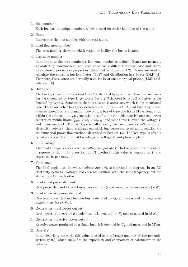
5. Bus type
The bus type can be either a load bus l ∈ L denoted by type 0, synchronous condenserbus c ∈ C denoted by type 1, generator bus g ∈ G denoted by type 2 or reference busdenoted by type 3. Sometimes there is also an isolated bus, which is not mentionedhere. There are other bus types details shown in Table 4.1. A load bus of type zerois unregulated and is a demand node only, a bus of type one holds MVar generationwithin the voltage limits, a generation bus of type two holds reactive and real powergeneration within limits Qmin < Qg < Qmax, and type three is given the voltage Vand phase angle Θ. The last type is called swing bus, slack bus, or v-theta. In anelectricity network, there is always one slack bus necessary to obtain a solution viathe numerical power flow methods described in Section 4.3. The last type is often atype-two bus with additional knowledge of voltage V and phase angle Θ.
6. Final voltage
The final voltage is also known as voltage magnitude V . In the power flow modeling,it represents the initial guess for the PF method. This value is denoted by V andexpressed in per unit.
7. Final angle
The final angle, also known as voltage angle Θ, is expressed in degrees. In an ACelectricity network, voltages and currents oscillate with the same frequency, but areshifted by Θ to each other.
8. Load - real power demand
Real power demand for one bus is denoted by Pd and measured in megawatts (MW).
9. Load - reactive power demand
Reactive power demand for one bus is denoted by Qd and measured in mega volt-ampere reactive (MVar).
10. Generation - real power output
Real power produced by a single bus. It is denoted by Pg and measured in MW.
11. Generation - reactive power output
Reactive power produced by a single bus. It is denoted by Qg and measured in MVar.
12. Base KV
In an electricity network, this value is used as a reference quantity of the per-unit-system (p.u.), which simplifies the expression and comparison of parameters in thenetwork.
15

Chapter 4. Power Flow in Electricity Networks
Table 4.1.: Load flow bus specification from [81].
Bus Type P Q |V| Θ Comments
Load
X X
Usual load representation.
Voltage Controlled
X X
Assume |V | is held constant no matter what Qis.
Generator orSynchronousCondenser
X
X X
X
Generator or synchronous condenser (P = 0) hasVAR limits,
• Qmin minimum Var limit,
• Qmax maximum Var limit,
• |V | is held as long as Qg is within limits.
Fixed Z to Ground Only Z is given.Reference
X X
”Swing bus” must adjust net power to hold volt-age constant (essential for solution).
13. Set point
A generator bus g ∈ G is a voltage controlled bus and its voltage is set by theoperators. The reactance power produced Qg is controlled by changing its referenceset point [68, p. 174]. It is specified in per-unit-system.
14. Maximum voltage, MW or MVar limit
This value is denoted by Vmax and represents the upper bound for the voltage mag-nitude of a bus in our case, but it may also describe the maximum real or reactivepower. This depends on the user of the IEEE data format.
15. Minimum voltage, MW or MVar limit
This value is denoted by Vmin and represents the lower bound for the voltage mag-nitude of a bus in our case. As above, it may also describe the minimum real orreactive power.
16. Resistors, Capacitors or Reactors - Shunt conductance G
Is produced by existing electrical fields around resistors, capacitors or reactors andrepresents an impedance absorption. Therefore, it is represented with a negativesign and its unit is MW. The specification of this parameter in the IEEE sheet is inper-unit-system:
Gpu =GMW
SBase
17. Resistors, Capacitors or Reactors - Shunt susceptance B
Represents an impedance injection measured in MVar. As it is an injection; its sign
16

4.1. Transmission Line Parameters
is positive. Similar to shunt conductance G, the specification of this parameter inthe IEEE sheet is in per-unit-system.
Bpu =BMV ar
SBase
Conductance G and susceptance B comprise the real and the imaginary part ofadmittance Y = G+ j ·B. Both are shown in Figure 4.5.
18. Remote controlled bus number
Represents the number of the remote controlled bus.
Branch Data Specification. The branch data reconstruct the power grid includingrestrictions and transmission line parameters. As above, we use the IEEE format [40] todescribe the most important line values and properties. A single branch is denoted by(f, t), where f is the from bus and t is the end bus of it.
1. From Bus
2. To Bus
3. Load flow area
This parameter is already explained in the above bus data specification at Point 3.
4. Loss zone
Loss zones are described in the above bus data specification at Point 4.
5. Circuit
Since the electricity network is a multigraph, the number of parallel transmissionlines are mentioned with the circuit value. If there is just a single line the value isone.
6. Type
There are multiple possible line types that can be present:
• 0 Transmission lineRepresents a standard branch.
• 1 Fixed tapFor this transformer type, the voltage angle and voltage ratio, which isequivalent to the tap ratio τ , are fixed.
• 2 Variable tap for voltage control (TCUL, LTC)Here, the voltage angle Θ is fixed and the voltage ratio is variable. Loadtapchangers (LTC), which keep the voltage at a low level, or tap changeunder load transformers (TCUL) for voltage control in subtransmission anddistribution networks are possible devices.
• 3 Variable tap (turns ratio) for MVar controlIn this case, the transformer controls the reactive power by a variable voltageratio. The voltage angle Θ is fixed.
• 4 Variable phase angle for MW controlFor type four, the voltage ratio is fixed and the phase angle Θ is variable.The real power is controlled by phase shifters, which is described in Point 14.
The standard transmission line is represented by a type zero. In contrast to this, theother types represent transformer lines. The transformer tap and voltage ratio are
17

Chapter 4. Power Flow in Electricity Networks
Z = R+ j ·X
Figure 4.4.: The impedance Z con-sists of a real termR (resistance) and animaginary term X (re-actance).
j ·B G
Y = G+ j ·B
Figure 4.5.: The admittance Y con-sisting of the conduc-tance G and suscep-tance B, which repre-sent the real and imagi-nary part, respectively.
described in more detail at Point 13 and describe the common usage of a transformer,as already described above. The line type which changes the voltage angle by a shiftangle Θshift is described at Point 14 and describes a transformer which, for example,splits the real power P over multiple lines.
7. Resistance
The branch resistance Rpu is expressed in per-unit. Sometimes it is denoted by r orrs, which denotes the series resistance. It represents the real term of the impedanceZ shown in Figure 4.4:
Rpu = RZbase
(4.4)
8. Reactance
The branch reactance Xpu is expressed in per-unit and can also be denoted by a smallletter x, or, in case of branches, it is often denoted by xs, called series reactance.The resistance and reactance define the impedance
Rpu + j ·Xpu (4.5)
in per-unit. As shown in Equation 4.5 and in Figure 4.4, it represents the imaginaryterm.
9. Total Line Charging Susceptance
This value represents the total line charging susception B in per unit. The descriptioncan be found in the above bus data specification at Point 17.
10. Line MVA rating Number 1, 2 and 3
These values represent the line rating with the lowest value to the left (first value).In our case, the left value represents the normal MVA rating (long term rating),the second value represents the short term value, and the last one represents theemergency value (highest value). The lowest non-zero value is put to the left. Theseparameters specify the maximum power which can be transmitted over one line. InGermany, there is only one value for a branch, but, for example in France, there existthree values, where the long term capacity is used for the normal operation and theother two capacities represent short term and emergency values, where the branch isshut down after a specified time to prevent branch outages [83]. If the value is zero,then the line is unlimited.
11. Control Bus Number
The control bus number denotes the bus whose voltage is controlled. If it is controlledby a variable tap transformer for voltage control (branch type 2), then the side atPoint 12 has to be specified. Otherwise, if the branch is not of type two, the side isalways zero.
18

4.1. Transmission Line Parameters
12. Side
The location of the controlled bus is specified by
• 0: Controlled bus is one of the terminals,
• 1: Controlled bus is on the tap side, and
• 2: Controlled bus is on the impedance side (Z bus, see Table 4.1).
13. Transformer tap ratio
The ratio of turns in the primary coil and those in the secondary coil of a transformeris known as tap ratio and denoted is by τ . For example, if the primary coil consistsof nine turns and the secondary coil of three turns, then the turn ratio is 3 : 1. Thus,the voltage at the primary coil is three times greater than at the secondary coil. Theturn ratio is equivalent to the voltage ratio and current ratio
VpVs
=IpIs
=NpNs, (4.6)
where Vp (resp., Vs) is the primary (resp., secondary) voltage, Ip (resp., Is) is theprimary (resp., secondary) current and Np (resp., Ns) the number of turns of theprimary (resp., secondary) coil. The tap is the connection point at the primarywindings of the transformer. This tap selects a certain number of windings withinthe transformer to create the expected voltage at the secondary coil. If the line doesnot represent a transformer connection, but a standard branch, then the tap ratio isequal to zero.
14. Transformer phase shifter angle
Transformer phase shifter angles (denoted by Θshift) are angles which are set in aphase-shifting transformer (also known as phase angle regulating transformer , phaseangle regulator or quadrature booster). A phase-shifting transformer, in contrast toa standard transformer, controls the real power flow in an AC three-phase electricitynetwork. Particularly, it splits the real power over multiple lines through a phaseangle. The purpose of such a power transformer is to handle parallel lines withdifferent voltage level, capacities, or to combine cables and overhead transmissionlines. It helps to avoid overloaded cables and therefore stabilizes the network. Inaddition, these transformers work in both directions.
15. Minimum tap or phase shift
This entry either describes the minimum tap ratio from Point 13 or the minimumphase shift angle described in Point 14. This depends on the IEEE data format usecase.
16. Maximum tap or phase shift
Similar to Point 15, but using the maximum.
17. Step size
18. Minimum voltage, MVar or MW limit
Either the minimum voltage Vmin, reactive power Qmin (MVar) or real power Pmin(MW) limit is described here. This always depends on the use case of the dataformat.
19. Maximum voltage, MVar or MW limit
Similar to Point 18, but using the maximum instead.
19

Chapter 4. Power Flow in Electricity Networks
Generation Costs. As the normal IEEE data does not provide any generation costs, thegenerator cost functions are built from the existing data set. For this, we use the methoddescribed by Zimmerman [84]. If there is a real power generation Pg, the cost function isdefined by
γ = 10Pgk2 + 20k, (4.7)
where k is the amount of generation. Otherwise, if there is only a reactive power generationQg, the generator costs function is given by
γ = 0.01k2 + 40k. (4.8)
These functions are necessary to calculate the optimal power flow (OPF), the power flow,that satisfy the demand, minimizes the generation cost [81, 41, 85, 84, 86, 87].
4.2. Properties of Transmission Lines
In the first part, we described the components of an electrical network. In this section,the fundamental properties of an electricity network will be described to prepare for theremaining sections. These properties describe in general, how these components worktogether. For more details about transmission line properties, we refer to [41, 81]. Westart with the two Kirchhoff’s laws.
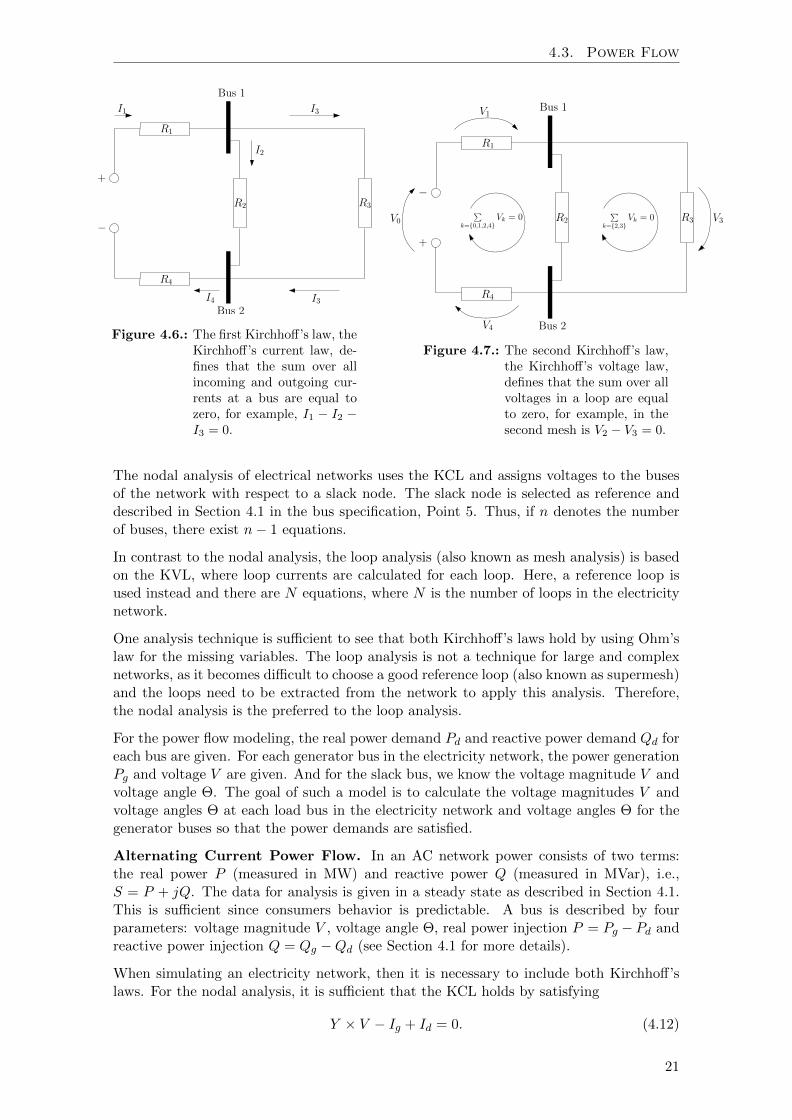
The first Kirchhoff’s law, known as Kirchhoff’s current law (KCL), implies that the incom-ing current into a bus is the same as the outgoing and it holds for all buses in the electricitynetwork (see Figure 4.6). It is also called charge conservation law and is formally writtenas:
n∑k=1
Ik = 0, (4.9)
where I is the current and index k is the bus, for k = 1, . . . , n.
The second Kirchhoff’s law is the Kirchhoff’s voltage law (KVL) and describes the behaviorof voltages in a loop (also known as mesh) with
∑k∈C
Vk = 0, (4.10)
where C is the set of buses that comprise a loop and Vk describes the k-th voltage drop(also known as potential drop). Thus, the sum over all potential differences is equal tozero, which is shown in Figure 4.7. This is the energy conservation law.
In relation to the two Kirchhoff’s laws stands the Ohm’s law, which is defined by
R = VI , (4.11)
where V is the voltage, I is the current and R denotes the resistance. For AC electricitynetworks, the resistance R is replaced by the impedance Z, which was already mentionedin Section 4.1. It describes the proportionality between current I and voltage V .
4.3. Power Flow
In an electricity network, the flow of the power is mostly determined by both Kirschhoff’slaws and Ohm’s law. To analyse such networks with regards to, e.g. fault analysis,stability studies and economic calculation, it is necessary to simulate the electrical flowin an electricity network. This is done by power flow analysis methods. There exist twoclassical power flow analysis methods: the nodal analysis and the loop analysis, whichrefer to the usage of first and second Kirchhoff’s law, respectively.
20
4.3. Power Flow
Bus 1
Bus 2
R1
R2
R4
R3
I1 I3
I2
I3I4
+
−
Figure 4.6.: The first Kirchhoff’s law, theKirchhoff’s current law, de-fines that the sum over allincoming and outgoing cur-rents at a bus are equal tozero, for example, I1 − I2 −I3 = 0.
Bus 1
Bus 2
R1
R2
R4
R3
−
+
V1
V4
V3∑
k=0,1,2,4Vk = 0
∑k=2,3
Vk = 0V0
Figure 4.7.: The second Kirchhoff’s law,the Kirchhoff’s voltage law,defines that the sum over allvoltages in a loop are equalto zero, for example, in thesecond mesh is V2 − V3 = 0.
The nodal analysis of electrical networks uses the KCL and assigns voltages to the busesof the network with respect to a slack node. The slack node is selected as reference anddescribed in Section 4.1 in the bus specification, Point 5. Thus, if n denotes the numberof buses, there exist n− 1 equations.
In contrast to the nodal analysis, the loop analysis (also known as mesh analysis) is basedon the KVL, where loop currents are calculated for each loop. Here, a reference loop isused instead and there are N equations, where N is the number of loops in the electricitynetwork.
One analysis technique is sufficient to see that both Kirchhoff’s laws hold by using Ohm’slaw for the missing variables. The loop analysis is not a technique for large and complexnetworks, as it becomes difficult to choose a good reference loop (also known as supermesh)and the loops need to be extracted from the network to apply this analysis. Therefore,the nodal analysis is the preferred to the loop analysis.
For the power flow modeling, the real power demand Pd and reactive power demand Qd foreach bus are given. For each generator bus in the electricity network, the power generationPg and voltage V are given. And for the slack bus, we know the voltage magnitude V andvoltage angle Θ. The goal of such a model is to calculate the voltage magnitudes V andvoltage angles Θ at each load bus in the electricity network and voltage angles Θ for thegenerator buses so that the power demands are satisfied.
Alternating Current Power Flow. In an AC network power consists of two terms:the real power P (measured in MW) and reactive power Q (measured in MVar), i.e.,S = P + jQ. The data for analysis is given in a steady state as described in Section 4.1.This is sufficient since consumers behavior is predictable. A bus is described by fourparameters: voltage magnitude V , voltage angle Θ, real power injection P = Pg − Pd andreactive power injection Q = Qg −Qd (see Section 4.1 for more details).
When simulating an electricity network, then it is necessary to include both Kirchhoff’slaws. For the nodal analysis, it is sufficient that the KCL holds by satisfying
Y × V − Ig + Id = 0. (4.12)
21

Chapter 4. Power Flow in Electricity Networks
As the electricity networks are based on power S, including real and reactive terms, itis reformulated to the power base. Power is defined by S = V × I and therefore we canreformulate the Equation 4.12 by
V (Y × V − Ig + Id) = 0⇔ V (Y × V )− Sg + Sd = 0
(4.13)
In total, the electricity network has n buses and Equation 4.13 is represented by n − 1equations. These equations include a complex term Y × V . For simplification, theseequations are reformulated to real term equations, which results in 2 · (n − 1) real termequations, consisting of n− 1 real power equations and n− 1 reactive power equations:
Pk = Vk∑
m=Γ(k)
(Vm (gkmcos (Θk −Θm) + bkmsin (Θk −Θm)))
︸ ︷︷ ︸
− Pgk
︸︷︷︸
+ Pdk
︸︷︷︸transmission lines transformer, reactors, capacitors, ··· production demand
Qk =
︷ ︸︸ ︷Vk
∑
m=Γ(k)
(Vm (gkmsin (Θk −Θm) + bkmcos (Θk −Θm)))−︷︸︸︷Qgk +
︷︸︸︷Qdk
(4.14)Equations 4.14 are for all buses m incident to bus k, where index k denotes the observedbus, for k = 1, . . . , n. The components gkm and bkm are part of the admittance, which isdescribed in Section 4.1 at Point 17. Equations 4.14 are non-linear equations, since theyinclude sin(x) and cos(x). In Section 3.2, we described methods to solve linear equations,but not non-linear ones. In this case, an iterative numerical method is necessary. One ofthe most popular methods is the Newton-Raphson method. The approach starts with anestimation of the unknown variable x0 with voltage V0 and voltage angle Θ0 (also knownas initial guess) and then f(x) is written as Taylor series:
f(x) = f(x0) +
(∂f∂x
∣∣∣x=x0
)(x− x0) + 1
2
(∂2f∂x2
∣∣∣x=x0
)(x− x0) + · · · (4.15)
For the Newton-Raphson method the Taylor series can be cut after the second term, sincethe remaining part is negligible. This results in a linearized equation system. For thepower flow equation it holds that the sum is equal to zero. Therefore, f(x) = 0 and
xi ≈ x0 −(∂f∂x
∣∣∣x=x0
)−1
f(x0). (4.16)
The Newton-Raphson method is an iterative method, where in each iteration the error ∆xdecreases and the convergence depends on the initial guess x0, but converges fast. As wetalk about AC power equation, the non-linearity leads to possibly multiple results, wherethe initial guess also determines to which solution the method converges.
Revert to the nodal analysis the Equation 4.15 forms a matrix, where f represents the realand reactive power in Equation 4.14, and x the voltage magnitude V and voltage anglesΘ. The Jacobian matrix is
J(Θ, V ) =
∂P1∂Θ1
∂P1∂V1
∂P1∂Θ2
∂P1∂V2
. . . ∂P1∂Θn−1
∂P1∂Vn−1
∂Q1
∂Θ1
∂Q1
∂V1∂Q1
∂Θ2
∂Q1
∂V2. . . ∂Q1
∂Θn−1
∂Q1
∂Vn−1∂P2∂Θ1
∂P2∂V1
∂P2∂Θn−1
∂P2∂Vn−1
∂Q2
∂Θ1
∂Q2
∂V1∂Q2
∂Θn−1
∂Q2
∂Vn−1
.... . .
...∂Pn−1
∂Θ1
∂Pn−1
∂V1
∂Pn−1
∂Θn−1
∂Pn−1
∂Vn−1∂Qn−1
∂Θ1
∂Qn−1
∂V1. . . ∂Qn−1
∂Θn−1
∂Qn−1
∂Vn−1
(4.17)
22

4.4. Direct Current Approximation
The linearized equation system is solved for the next iterations by using the next estimationfor voltage magnitude V and voltage angle Θ. This iteration ends if the error ∆x lies inthe tolerance ε. Typical initial guesses are V0 = 1 for voltage magnitude and Θ = 0 forvoltage angles or there may exists past results. This provides just a short overview of thepower flow problem. Further information are available at [81, 41].
4.4. Direct Current Approximation
Often it is sufficient to assume that the considered network is a DC network. This sim-plification provides a linear model and considers only the real part pf = R(sf ) of theAC power network. As the DC electricity network is linear, the methods mentioned inSection 3.2 can be applied to calculate the voltage magnitudes V and voltage angles Θ.Examples for using a DC approximation instead of an exact AC model are shown in [60].
To approximate an AC network with a DC one four simplification are applied from [81,85, 84, 86, 87].
1. As the real part of the power S is used, while the reactive power Q is neglected.
2. The branches in a DC electricity network are assumed to be lossless lines. FromSection 4.1 follows, that the series resistance rs and charging capacitance bc arenegligible. Thus, the series admittance ys for rs ≈ 0 and bc ≈ 0 can be written as
ys = 1zs
= 1rs+jxs
≈ 1jxs. (4.18)
As the branches are assumed to be lossless, the power injection at both ends of thebranch is the same, but negative, since the power flows into the other direction, thatis,
pf = −pt. (4.19)
3. The bus voltage magnitudes are close to one per unit, such that
vi ≈ ejΘi . (4.20)
4. Voltage angle difference ∆Θ is very small over all branches, i.e., it can be assumedthat:
sin(Θf −Θt −Θshift) = Θf −Θt −Θshift (4.21)
By using these assumptions, Zimmerman et al.[85] show that the relationship between realpower flow and voltage angles for a branch i is given by
(pi) = Bi(Θi) + (Pshifti), (4.22)
where (pi) is a vector with entries for each bus, Bi is the adjacency matrix multiplied withbi = 1/(xsiτi), and (Pshifti) is a vector with entries for each bus, where Pshifti = bi ·Θshift.The B matrix can be seen analogously to the admittance matrix of the AC electricitynetwork. Thus, the DC power balancing equation of the nodal analysis is given by
gp(Θ, Pg) = B ·Θ + Pshift + Pd +Gsh − Pg = 0. (4.23)
Function gp in Equation 4.23 is also called mismatch.
23


5. Flow-Based Approaches
This chapter addresses the topic graph theoretical flows in electricity networks. The goalis it to show that it is possible to apply graph theoretical flows on electricity networksthereby obtain good physical flows. Applying flows on electricity networks implies slightchanges to the network. Each vertex has to include electric control systems, for exam-ple flexible alternating current transmission systems (FACTS). After having explained thetransformation of an electricity network, these transformed networks are used by our mod-els. We start with a standard flow model and improve this model with regards to existingproblems, such that we get two balancing heuristics, where the first balances the flow uni-formly and the second one prioritize bottleneck edges. The standard flow and its variantshave too high generator production costs. Therefore, we optimize the flow with regards togenerator productions, but balancing has to be achieved, too. That is, the model includesthe minimization of the line losses, to become balanced. Within the case studies, we applythese flows directly on the network and get a solution for a network with FACTS at eachnode. But to use these models in a realistic context, which means that there are only afew FACTS in the electricity network, the generator production of these models is insertedin a power flow (PF) calculation. This approach uses the standard method to calculateelectrical flows and shows the behavior of an electrical flow by using different generatorproductions of different models.
The fundamentals for flow algorithms and linear programming were introduced in Chap-ter 3. In addition, all models are implemented in MATLAB R2013a by using Gurobi5.5.0.
5.1. Transformation to an s-t-Graph
To apply flow models on electricity networks or other networks it is necessary to transformthese networks to s-t-networks with one source and one sink to generate flows. Therefore,we interpret the electricity networks with regard to graph theoretical terms and define thesources and sinks of these network structures to connect these sources (resp., sinks) toone supersource s (resp., supersink t). This transformation also simplifies the work in thegraph theoretical area and provides clear mathematical descriptions.
Given an electrical network NE = (B,G,L, T , C,D, cE , γE , `E , BE , PshiftE , . . . ) as shown inFigure 4.2 with a set of buses B and a multiset of transmission lines D, each connecting
25

Chapter 5. Flow-Based Approaches
Table 5.1.: Merging parallel transmission lines results in an adaption of the electricalparameters. An edge ej ∈ Ej , where Ej is a set of duplicates with Ej ⊆ E′
and E′ is a multiset. The quantity of duplicates is denoted with kj := |Ej |.All edges ej incident to u and v with kj > 1, are merged to one single edgeej : (u, v) ∈ E, where E is a single set, for each j = 1, . . . , kj . By replacing with the parameter identifier, the total parameter is calculated for thesetransmission lines, e.g., for resistance: is replaced by R.
=k∑i=1i = 1/
k∑i=1
1i = 1 = 2 = · · · = k
Real Power P 7
Reactive Power Q 7
Capacity c 7
Current I 7
Admittance Y 7
Resistance R 7
Inductivity L 7
Impedance Z 7
Voltage U 7
two buses. A bus can be a transformer t ∈ T , or can be connected with a generatorg ∈ G, a consumer l ∈ L, a transformer t ∈ T , a condenser k ∈ C and other electricalcomponents, where B = G ∪ L ∪ T ∪ C. These components were described in more detailin Chapter 4. Furthermore, network NE provides functions like cE , γE , `E , BE , PshiftE
and others, where
• cE : D → R is the capacity on the transmission lines;
• γE : G → R≥0 is the generation cost (or production cost) of a generator g ∈ G;
• `E : D → R≥0 describes the losses of all transmission lines in D dependent onresistance R of each line;
• BE : D → R≥0 is dependent on reactance X and tap ratio τ and is defined in interval(0, 1];
• PshiftE : D → R≥0 describes the transformer shift angles, where phase angles reg-ulating how the transformer distributes the power over multiple lines between twobuses by changing the transformer shift angles;
• electrical networks provide much more data and include much more devices as sug-gested in Chapter 4, which are not of interest for this thesis.
To transform NE = (B,G,L, T , C,D, cE , γE , `E , Bb, Pshift, . . . ) to a capacitive s-t-networkNst = (G = (V,E), c, γ, `, Bb, Pshift) we define that each bus b ∈ B is represented by a vertexu ∈ V , where |V | = n (shown in Figure 5.1a). Transmission lines between two buses uand v corresponds to edges (u, v) ∈ E′, where E′ is a multiset. The multigraph G′ is thentransformed to a simple graph G (in Nst), which is shown in Figure 5.1b. By mergingparallel lines, the following parameters must be adapted: real power P , reactive power Q,resistance R, reactance X, capacity c, voltage U , current I, inductivity L, impedance Z,admittance Y and all related parameters, which is shown in Table 5.1.
Buses connected to generators in G, which are responsible for real and reactive power, andcondensers in C, which are responsible for reactive power, are connected to an additionalvertex s (see Figure 5.1c), which is called source. Buses connected to consumers in L (alsoknown as buses with load) are connected to an additional vertex t ∈ V , called sink alsoshown in Figure 5.1d. Transformers in T and other components need no special modeling,
26

5.1. Transformation to an s-t-Graph
1
2
5
6
12
1314
11 109
7
8
4
3
(a) The highlighted areas on the left side are buses b ∈ B in NE . These busesare represented by vertices v ∈ V in Nst shown on the right side.
(1, 5) ∈ E
1
2
5
6
12
1314
11 109
7
8
4
3
(b) A Network NE can have multiple transmission lines per bus pair (high-lighted red). These transmission lines are represented by edges (u, v) ∈kE′ and the resulting multigraph G′ is modified to a simple graph G inNst, such, that there is only one edge per vertex pair.
s
Generator
1
2
5
6
12
1314
11 109
7
8
4
3
(c) Buses b ∈ B which are connected with a real and/or a reactive powergenerator (highlighted green) are connected with a vertex s, known assource.
t
s
Generator
Load
1
2
5
6
12
1314
11 109
7
8
4
3
(d) Loads in NE are represented by an arrow (highlighted yellow) and busesb ∈ B connected with a load are expressed with an edge to a vertex t,known as sink.
Figure 5.1.: Transformation of an electricity network NE (left side) to a s-t-networkNst (right side) using a 14 bus system [6] as example.
27

Chapter 5. Flow-Based Approaches
(a) Flow fstd of the standard flowmodel in the electrical networkN .
(b) Flow fopf of theoptimal power flowmodel in the elec-trical network N .
Figure 5.2.: The electricity network N is the 14-bus network from the WashingtonUniversity [6]. The helper vertices s (source) and t (sink) are highlightedin yellow.
as they are parameters in the data set, which are used in functions. Function c, γ, `, Band Pshift are defined for Nst the following way:
• c : E → R≥0 is the edge capacity;
• γ : E → R≥0 is the generation cost where γ(u, v) = 0 if s /∈ u, v;• ` : E → R≥0 describes the losses, which are defined to be zero for all edges adjacent
to s and t;
• B : E → R≥0 is the inverse reactance defined in interval (0, 1] and
• Pshift : E → R≥0 describes the transformer shift angles and is mostly zero.
The source vertex s has the total amount of power production of all generators in G andcondensers in C. The edge capacity for edges (s, u) ∈ E for all u ∈ V corresponds to themaximum production for the generator g ∈ G and condensers k ∈ C at u. The sink vertext owns the total amount of load of all consumers l ∈ L. Edge capacities for (v, t) ∈ E forall v ∈ V are equivalent to the load at vertex v.
5.2. Standard Flow Model
Electrical flows, which we call power flows, are physically predetermined. Since the elec-trical flow uses laws of physics, there is just a little control in current electricity networksprovided by a few flexible alternating current transmission system (FACTS). Modeling astandard flow on an electricity network expects at each vertex, that there exists a fullcontrol over the power flow. Therefore, we assume FACTS at all vertices, which providesus the necessary control, and the transformation of the electricity network described in
28

5.2. Standard Flow Model
the previous section is used to apply flows. Our intention is to see problems or a behaviorwhile applying this standard flow model to electricity networks, which gives us an idea ofpossible improvements. Within the case study, we use the flow directly produced by thestandard flow on an electricity network to understand the flow behavior and in additionto that, we use the generator productions of the standard flow model in the PF methodto achieve realistic flows on electricity networks. This section describes the mathematicalmodel of a standard flow and the corresponding experiments.
We realize a minimum cost flow, where we apply the same cost to each edge. The flow hasto satisfy the flow conservation for each vertex, which means that the outgoing flow at avertex is the same as the incoming flow. This can be related to the Kirchhoff’s currentlaw (KCL) described in Section 4.2. Furthermore, the flow on each edge is limited withregards to the capacity function in an electricity network, which is related to the thermallimit of a transmission line. The objective function represents the flow costs, which weminimize.
Mathematical model description. An electricity network N = (G = (V,A), c, s, t) is acapacitive graph G with vertex set V and arc set A. In addition, this network includes asource s and a sink t, and a function c : A→ R, which describes the arc capacities. Sincewe use a direct representation of an undirected graph (see Section 3.1), c(u, v) = c(v, u)for all (u, v) ∈ A.
Let N be an electricity network and let f : A → R be a function. Function f is called afeasible flow on N , if it satisfies the flow conservation
∑v∈V
f(u, v) = 0 ∀ u ∈ V \ s, t∑
u:(s,u)∈Af(s, u) =
∑v:(v,t)∈A
f(v, t) =∑
v:(v,t)∈Ac(v, t) ∀ u, v ∈ V \ s, t (5.1)
and in addition, the capacity constraints
f(u, v) ≤ c(u, v) ∀ (u, v) ∈ A. (5.2)
The network cost for network N and function f is the following:
z(N, f) =∑
(u,v)∈Af(u, v) (5.3)
The flow f(u, v) is understood as a variant and the Equations 5.1 and 5.2 denote the linearconstraints. By minimizing the objective function in Equation 5.3 subject to these linearconstraints, a linear program is formed, which we denote as standard flow LP. It minimizesthe costs of a flow.
Case Study. In the case studies we use two approaches to compare the models. The firston is to assume FACTS at each vertex in the electricity network. This approach allows usto apply the model on the electricity network and the flow can be directly compared withthe one of the OPF. Since the resulting flow is—in most cases—totally different to the oneof the OPF, as it does not model any physical laws, and it is not easy to declare if the flowis good or not, we provide a second approach to compare the models. In this approach,we insert the generator production of the model (here the standard model) and insert it inthe PF method. This shows us the electrical flow of the calculated generator productionand the model results can be used in a realistic electricity network without FACTS (orjust a few FACTS).
Applying a standard flow model on an electrical network N generates a flow fstd on N ,which is shown for the bus network 14 from the Washington University [6] in Figure 5.2a.
29

Chapter 5. Flow-Based Approaches
−100
−50
0
50
100
150
200
250
0 10 20 30 40 50 60Edge
LoadDeviation(M
W)
Standard Flow Alg. vs. OPF
(a) Edge flow deviation between the op-timal power flow model (OPF) anda standard flow model in N is plot-ted with fopf(ei)− fopf(ei) for all i =1, . . . , n. The edges are sorted by theoriginal graph input.
0
50
100
150
200
250
0 10 20 30 40 50 600
50
100
150
200
250
0 10 20 30 40 50 60Edges sorted by OPF
Load(M
W)
Optimal Power Flow
0.34 % Generator Input
Standard Flow Algorithm
(b) The standard flow generator produc-tion and a dummy production are in-cluded in the power flow(PF) calcu-lation. For comparison the optimalpower flow(OPF) is plotted and alledges are sorted decreasing with re-gards to the OPF.
Figure 5.3.: Plots for the 14 bus electrical network N from the Washington Univer-sity [6] using the standard flow model.
The networkN in Figure 5.2a represents a directed representation of an undirected network(see Section 3.1). For the optimal power flow fopf in Figure 5.2b the network N is anundirected graph.
To compare the flow fstd in N of the standard flow model and the OPF fopf in N , we takea closer look at the edge flow deviation in Figure 5.3a. Figure 5.3a shows, that the biggestdeviations are located in the first ten edges, where the edges are in the original data setorder. More specific, the main difference is in the power generation on edges (s, u) ∈ E forall u ∈ V \s, t, e.g., the edge e1 = (s,Bus1) has a deviation of 217.82 MW. Of course, asthere exist five generators, the missing power production is distributed to the other fourgenerators. The reason for this behavior is that we do not take into account any generatorparameters, apart from the capacities.
Another conspicuity is that some edges are included in the flow fstd of the standard flowmodel, but not in the OPF flow fopf and vice versa. Furthermore, a possible problem canbe high loaded edges close to the capacity, also known as bottleneck edges.
Summarizing, this simple model gives us information about possible problems:
• Arcs may overloaded in a network with worse generator distribution,
• No balancing of generation and flow, and
• Production costs are disregarded.
The last point becomes clear, if we compare the production costs of the OPF with 7642USD, and the standard flow model with 10386 USD. Thus, the production costs has to beincluded in the model to get an economical suggestive result.
In addition, if we use the generator production of the standard flow model in the powerflow model (see Figure 5.3b), the electrical flow calculated by the power flow model resultsin a totally different flow. In Figure 5.3b, the peaks at edge e11, which correspondsto edge (s,Bus2), and edge e33 corresponding to edge (s,Bus3) show that the main flow
30

5.3. Balanced Flow Model
differences are at the generators, but it also shows that in a network with a good generatordistribution the maximum flow on an edge is low, because the production is located closeto the consumption.
5.3. Balanced Flow Model
The experimental evaluation of the standard flow model from Section 5.2 shows that thereare some problems. One of them is an unbalanced flow, where the edge flows are close tothe capacity, which may produce bottlenecks and leads to faster attrition. Capacities oftransmission lines are thermal limits, and therefore a convergence to this limit stress theselines. For that, the flow has to be balanced to relieve these edges and to provide a morerobust flow. The idea is to balance all edges uniformly by minimizing the difference to halfof their capacity. We show how to model a flow on an edge pair (u, v) and (v, u), whileusing just one edge of them. In addition, we combine the balancing ideas with the previousmodel, which includes the conservation of flow on each vertex, the capacity constraints oneach edge and the cost minimization. This section introduces the mathematical modelfor a uniform balancing and provides examples to see further problems and improvementcapabilities. As for the previous model, two evaluation variants are used to interpret thismodel with regards to electricity networks. The first variant applies the flow directly to thenetwork and the second one uses the calculated generator productions in the PF method.
Mathematical model description. The electrical network N = (G = (V,A), c, s, t) isthe same network as defined in the previous section. In addition, f is a flow in N if itsatisfies the flow conservation and capacity constraints from Equations 5.1 and 5.2.
Let N be an electrical network, let y(u, v) ∈ 0, 1 with y(u, v) = y(v, u) for all (u, v) ∈ A.A feasible function f in N is given by
f(u, v)− y(u, v) · c(u, v) ≤ 0,f(v, u) + y(v, u) · c(v, u) ≤ c(v, u).
(5.4)
Equation 5.4 conveys, that the flow is restricted to one of the edges per vertex pair (u, v)and (v, u).
Let N be an electricity network. We would like the flow on each edge (u, v) ∈ E to be asclose to 50% of the maximum load as possible, that is
f(u, v) + f(v, u)≈ c(u,v)2 . (5.5)
By subtracting c(u, v)/2 from this approximation we ideally obtain a term close to zero,that is
f(u, v) + f(v, u)− c(u,v)2 ≈ 0. (5.6)
We introduce a term ∆(u, v), such that
−∆(u, v) ≤ f(u, v) + f(v, u)− c(u,v)2 ≤ ∆(u, v), (5.7)
in order to measure the deviation of actual load (f(u, v) + f(v, u)) and desired load(c(u, v)/2). This ∆(u, v) is ideally zero and therefore, the goal is to minimize ∆(u, v).
This model has the goal to provide a balanced feasible flow on an electrical network byminimizing the distance to half of the capacity. The flow cost is the following
z(N, f) =∑
(u,v)∈Af(u, v) +
∑(u,v)∈A
∆(u, v) (5.8)
31

Chapter 5. Flow-Based Approaches
(a) Flow fbal of the balanced flowmodel in the electrical networkN .
(b) Flow fopf of the optimal powerflow in the electrical networkN .
Figure 5.4.: The electrical network N is the 14-bus network from the WashingtonUniversity [6]. The helper vertices s (source) and t (sink) are highlightedin yellow.
From Equations 5.2, 5.4, 5.7 and by minimize Equation 5.8, we get a MILP, which we callbalanced MILP shown in Equation 5.9.
minimize z(N, f) =∑
(u,v)∈Af(u, v) +
∑(u,v)∈A
∆(u, v)
s.t.∑v∈V
f(u, v) = 0∑
u:(s,u)∈Af(s, u) =
∑v:(v,t)∈A
c(v, t)
∑u:(s,u)∈A
f(s, u) − ∑v:(v,t)∈A
f(v, t) = 0
f(u, v) ≤ c(u, v)f(u, v) − y · c(u, v) ≤ 0f(u, v) + y · c(u, v) ≤ c(u, v)
f(u, v) + f(v, u) − ∆(u, v) ≤ c(u,v)2
f(u, v) + f(v, u) + ∆(u, v) ≥ c(u,v)2
y ∈ 0, 1, ∆(u, v) ∈ Rf(u, v) ∈ R≥0 ∀(u, v) ∈ A.
(5.9)
Case studies. The goal of the balanced flow model is a power equipartitioning over alledges by minimizing the difference to half of the capacity of each edge (see Equation 5.7).
32

5.4. Bottleneck Flow Model
−100
−50
0
50
100
150
200
250
0 10 20 30 40 50 60Edge
LoadDeviation(M
W)
−100
−50
0
50
100
150
200
250
0 10 20 30 40 50 60
Standard Flow Alg. vs. OPFBalanced Flow Alg. vs. OPF
(a) Edge flow deviation between an op-timal power flow (OPF) and a bal-anced flow model including all previ-ous models.
0
50
100
150
200
250
0 10 20 30 40 50 600
50
100
150
200
250
0 10 20 30 40 50 600
50
100
150
200
250
0 10 20 30 40 50 60Edges sorted by OPF
Load(M
W)
Optimal Power Flow
0.34 % Generator Input
Standard Flow AlgorithmBalanced Flow Algorithm
(b) Generator productions of some mod-els are used to calculate a flow usingthe power flow model on the networkN .
Figure 5.5.: Plots for the 14-bus electrical network N from the Washington Univer-sity [6] concerning the balanced flow model and all previous models.
Furthermore, the flow can only use one direction per vertex pair, which Equation 5.4describes. Figure 5.4 shows the flow fbal of the balanced flow model (see Figure 5.4a) andfopf of the optimal power flow side by side. Cyclic flows can build possible solutions of thebalanced flow model, which can be gathered from Figure 5.4a. There, buses 6− 11− 10−9− 14− 13 form a cycle with a redundant flow of 423.00 MW, which is not realistic.
In Figure 5.5a, the edge deviation is presented. As for the standard flow model thebiggest deviation can be found within the first ten edges. The reason is that the generatorproduction for bus 1 is zero MW and therefore the deviation at e1 = (s,Bus1) is 220.97MW since the OPF model has a production of 220.97 MW at bus 1. Thus, the missinggenerator production at bus 1 is distributed over the other generators. From Figure 5.5a wecan gather that there are much more edges which differ from the OPF model by using thebalanced flow model. The reason is that the balanced flow model attempts to distributethe flow over all edges. In Figure 5.5b we can see the resulting flow of the power flowmodel by using the generator production of the balanced flow model. It exhibits nearlythe same behavior as the standard flow model as the generator production slightly differs.
Overall, the balanced flow model probably provides a more balanced flow inN , but considerin particular all edges. A problem is that there still exist distortions, which can becomeproblematic regarding load peaks in a real network.
As for the standard flow model the production costs are not modeled. Therefore, thebalanced flow model has a production cost of 10394 USD, which in comparison with thestandard flow model with 10386 USD is worse. But this always depends on the network Nand the distribution of the generators. In comparison, the OPF model has costs of 7642USD.
5.4. Bottleneck Flow Model
Another approach to balance the flow on an electricity network is provided in this section.Again, balancing is done, since the standard flow model produces flows, which are closeto the maximum capacity and this leads to faster attrition. In the previous section, the
33

Chapter 5. Flow-Based Approaches
balanced flow provides edges, which are still high charged. In practice and in this the-sis, these edges are denoted by bottleneck edges. Bottleneck edges lead to problems innetworks, for example line outage, system instabilities and others. In meshed networkslike in Germany, there exist fewer bottleneck edges then in non-meshed networks. Dueto renewable energies the number of bottleneck edges increases, e.g., ENTSOE indicatesthat 80% of 100 identified bottlenecks are related to renewable energy resources (RES) [2].Furthermore, the distance between consumer location and generation location changes,e.g., in France electrical heating is often used, and during winter the generation in Franceis not sufficient [4]. In this time they also use energy generated in Germany, Poland andCzech Republic. Thus, Germany, especially Baden-Wuerttemberg, serves as energy trans-fer network [83]. The network of Baden-Wuerttemberg is not designed for such a big loadand the number of bottlenecks increases in transfer situations. Even though Germany usesthe k − 1 rule [83] bottlenecks constitute a system vulnerability. Thus, this section pri-oritize bottleneck edges higher than other edges to archive a lower bottleneck flow withinthe electricity network. At the beginning, we describe the model and subsequently theexperiments are explained to understand possible problems.
The bottleneck flow intends to balance the flow by taking bottleneck edges more into ac-count. The objective function minimizes the maximum edge flow and reduces the flowequally over all edges in the electricity network. This is done iteratively. In each iterationwe fix the flow on bottleneck edges with a flow equal to the minimum possible bottleneckflow and reduce the upper bound of all non-fixed edges to that flow. This prevents varia-tions in the maximum flow, since the reduced flow at one bottleneck edge is not shifted toanother one as the maximum edge flow correlates with the reduced flow on this bottleneckedge. The flow conservation holds for each vertex and in addition, the edges are limited toa capacity function c. This approach reduces the maximum bottleneck flow and therefore,relieves the edges.
Mathematical model description. We use the same electricity network N = (G =(V,A), c, s, t) as already mentioned in all previous sections. As before, a feasible flowf is defined by the flow conservation from Equation 5.1 and capacity constraints fromEquation 5.2.
Let N be an electricity network with a feasible flow f . A bottleneck edge e is definedby f(e) ≥ f(e′) for all e = (u, v) ∈ A. Thus, a balanced flow minimizes the flow on thebottleneck edges to a ∆ while reducing the flow equally on all edges. The ∆ denotes thesmallest possible bottleneck flow (maximum edge flow) in the electricity network and alsorepresents the maximum flow for all observed edges. The flow cost for this network isdefined by
z(N, f, (u, v)) = ∆ (5.10)
Now, we iteratively minimize Equation 5.10. In each iteration we get a ∆, which is theminimum of the maximum flow for the current iteration. Furthermore, in each iterationwe fix the flow of an arc (u, v), where f(u, v) = ∆, and update the upper bound for allarcs to ∆. This is done for all edges, while prioritizing bottleneck edges, or until ∆ isequal to zero. By minimizing the objective function in Equation 5.10, and applying the
34

5.4. Bottleneck Flow Model
(a) Flow fbn of the bottleneck flowmodel in the electrical networkN .
(b) Flow fstd of the optimal powerflow in the electrical networkN .
Figure 5.6.: The electrical network N is the 14 bus network from the WashingtonUniversity [6]. The helper vertices s (source) and t (sink) are highlightedin yellow.
constraints from Equations 5.1 and 5.2, we get a LP for one iteration, which we denote asbottleneck LP. One iteration is shown in Equation 5.11.
minimize z(N, f) =∆
s.t. ∆ −f(u, v) ≥ 0∑v∈V
f(u, v) = 0∑
u:(s,u)∈Af(s, u) =
∑v:(v,t)∈A
c(v, t)
∑u:(s,u)∈A
f(s, u)− ∑v:(v,t)∈A
f(v, t) = 0
f(u, v) ≤ c(u, v)f(u, v) ≥ 0 ∀(u, v) ∈ A.
(5.11)
Algorithm 5.1 shows such a method to solve the bottleneck flow. We iteratively minimizeEquation 5.10.
Case Study. The bottleneck flow fbn is shown in Figure 5.6a and builds another approachto balance a flow on an electrical network N . Instead of minimizing the difference to halfof the capacity, this model try to minimize the flow on bottleneck edges. Minimizing themaximum flow on an edge is a iterative LP, which is shown in Algorithm 5.1.
35
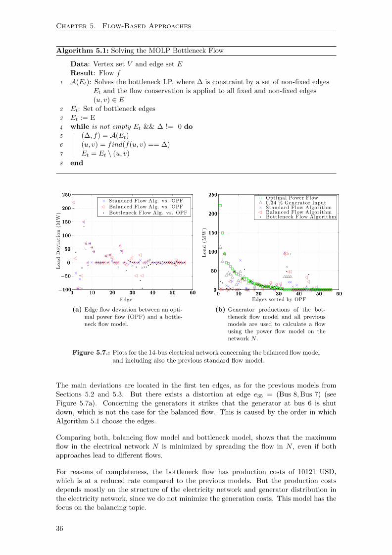
Chapter 5. Flow-Based Approaches
Algorithm 5.1: Solving the MOLP Bottleneck Flow
Data: Vertex set V and edge set EResult: Flow f
1 A(Et): Solves the bottleneck LP, where ∆ is constraint by a set of non-fixed edgesEt and the flow conservation is applied to all fixed and non-fixed edges(u, v) ∈ E
2 Et: Set of bottleneck edges3 Et := E4 while is not empty Et && ∆ != 0 do5 (∆, f) = A(Et)6 (u, v) = find(f(u, v) == ∆)7 Et = Et \ (u, v)
8 end
−100
−50
0
50
100
150
200
250
0 10 20 30 40 50 60
Edge
LoadDeviation(M
W)
−100
−50
0
50
100
150
200
250
0 10 20 30 40 50 60−100
−50
0
50
100
150
200
250
0 10 20 30 40 50 60
Standard Flow Alg. vs. OPFBalanced Flow Alg. vs. OPFBottleneck Flow Alg. vs. OPF
(a) Edge flow deviation between an opti-mal power flow (OPF) and a bottle-neck flow model.
0
50
100
150
200
250
0 10 20 30 40 50 600
50
100
150
200
250
0 10 20 30 40 50 600
50
100
150
200
250
0 10 20 30 40 50 600
50
100
150
200
250
0 10 20 30 40 50 60Edges sorted by OPF
Load(M
W)
Optimal Power Flow0.34 % Generator InputStandard Flow AlgorithmBalanced Flow AlgorithmBottleneck Flow Algorithm
(b) Generator productions of the bot-tleneck flow model and all previousmodels are used to calculate a flowusing the power flow model on thenetwork N .
Figure 5.7.: Plots for the 14-bus electrical network concerning the balanced flow modeland including also the previous standard flow model.
The main deviations are located in the first ten edges, as for the previous models fromSections 5.2 and 5.3. But there exists a distortion at edge e35 = (Bus 8,Bus 7) (seeFigure 5.7a). Concerning the generators it strikes that the generator at bus 6 is shutdown, which is not the case for the balanced flow. This is caused by the order in whichAlgorithm 5.1 choose the edges.
Comparing both, balancing flow model and bottleneck model, shows that the maximumflow in the electrical network N is minimized by spreading the flow in N , even if bothapproaches lead to different flows.
For reasons of completeness, the bottleneck flow has production costs of 10121 USD,which is at a reduced rate compared to the previous models. But the production costsdepends mostly on the structure of the electricity network and generator distribution inthe electricity network, since we do not minimize the generation costs. This model has thefocus on the balancing topic.
36

5.5. Minimum Cost Flow Model
5.5. Minimum Cost Flow Model
In all previous models we just took care about the flow in an electricity network. We focuson balancing a flow to prevent edges close to the thermal limit. Another important factorare power production costs, which affect the consumer price. This section focuses on aglobal optimal solution of the total production costs to improve the network efficiency.
Generation costs are strongly dependent on the generation kind, e.g., renewable energylike wind farms and photovoltaic plants (PV), nuclear power plants or fossil power plants.Furthermore, within these different kinds are efficiency differences dependent on the ageand other factors [41]. The IEEE data provided by the Washington University [6] doesnot cover information about generation costs. But by using the method described inSection 4.1, these data are synthetically produced. Thus, we can assume that there is apolynomial cost function for each generator.
In this section, we approximate these polynomial functions to stay linear and show thegenerator cost functions of the 14 bus system. In addition, the mathematical model isdescribed and some case studies to show missing properties of such a flow.
The idea of this model is to reduce the generator production costs to get an optimalsolution. Each generator provides a convex cost function, which we piecewise linear ap-proximate. In addition, the standard flow conservation and the capacity limits are used asalready mentioned in the previous sections. The objective function minimizes the generatorcosts and always selects the right linear function for each interval.
Mathematical model description An electrical network N = (G = (V,E), c, γ, s, t) inthis model includes an additional function γ : E → R≥0 to the previous models, whichdescribes the generator costs, where γ(u, v) = 0 for u, v 6= s. Furthermore, this modelworks on an undirected graph with edge set E.
Let N be an electrical network and let f : V × V → R be an antisymmetric function, i.e.,f(u, v) = −f(v, u) for all (u, v) ∈ E. Thus, f is a feasible flow if the flow conservation ofEquation 5.1 and capacity constraints from Equation 5.2 are fulfilled.
hi(f(u, v)) ≥ mi · f(u, v) + ni
hi
f(u, v)
γ(f(u, v))
(a) Linear approximation of afunction γ(f(u, v)) is a set H oflinear functions, where hi ∈ H.The topmost section is used byapplying hi ≥ mi · f(u, v) +ni.
Genera
tionCosts(U
SD)
Real Power (MW) or Reactive Power (MVar)
0
2000
4000
6000
8000
10000
12000
14000
16000
18000
20000
50 100 150 200 250
Polynoms
Piecew ise Linear Approximations
(b) Piecewise linear function of the 14-busnetwork are represented by the red linesand the polynomial is displayed by thegray dashed line.
Figure 5.8.: Visualization of linear approximations.
37
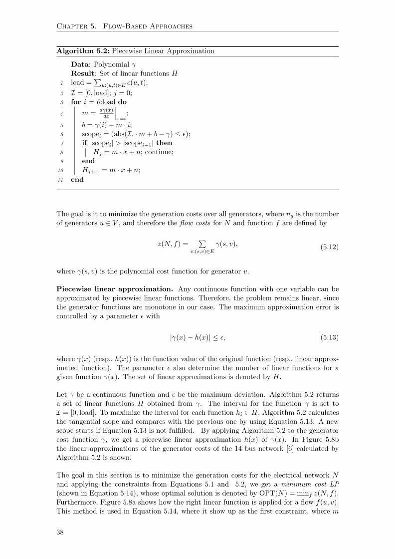
Chapter 5. Flow-Based Approaches
Algorithm 5.2: Piecewise Linear Approximation
Data: Polynomial γResult: Set of linear functions H
1 load =∑
u:(u,t)∈E c(u, t);
2 I = [0, load]; j = 0;3 for i = 0:load do
4 m = dγ(x)dx
∣∣∣x=i
;
5 b = γ(i)−m · i;6 scopei = (abs(I. ·m+ b− γ) ≤ ε);7 if |scopei| > |scopei−1| then8 Hj = m · x+ n; continue;9 end
10 Hj++ = m · x+ n;
11 end
The goal is it to minimize the generation costs over all generators, where ng is the numberof generators u ∈ V , and therefore the flow costs for N and function f are defined by
z(N, f) =∑
v:(s,v)∈Eγ(s, v), (5.12)
where γ(s, v) is the polynomial cost function for generator v.
Piecewise linear approximation. Any continuous function with one variable can beapproximated by piecewise linear functions. Therefore, the problem remains linear, sincethe generator functions are monotone in our case. The maximum approximation error iscontrolled by a parameter ε with
|γ(x)− h(x)| ≤ ε, (5.13)
where γ(x) (resp., h(x)) is the function value of the original function (resp., linear approx-imated function). The parameter ε also determine the number of linear functions for agiven function γ(x). The set of linear approximations is denoted by H.
Let γ be a continuous function and ε be the maximum deviation. Algorithm 5.2 returnsa set of linear functions H obtained from γ. The interval for the function γ is set toI = [0, load]. To maximize the interval for each function hi ∈ H, Algorithm 5.2 calculatesthe tangential slope and compares with the previous one by using Equation 5.13. A newscope starts if Equation 5.13 is not fulfilled. By applying Algorithm 5.2 to the generatorcost function γ, we get a piecewise linear approximation h(x) of γ(x). In Figure 5.8bthe linear approximations of the generator costs of the 14 bus network [6] calculated byAlgorithm 5.2 is shown.
The goal in this section is to minimize the generation costs for the electrical network Nand applying the constraints from Equations 5.1 and 5.2, we get a minimum cost LP(shown in Equation 5.14), whose optimal solution is denoted by OPT(N) = minf z(N, f).Furthermore, Figure 5.8a shows how the right linear function is applied for a flow f(u, v).This method is used in Equation 5.14, where it show up as the first constraint, where m
38

5.6. Combination of Cost Minimization and Balancing
7642.59
10386.01 10394.3410124.89
7644.55
0
2000
4000
6000
8000
10000
12000
OPF Standard
Mode l
Balanced
Mode l
Bott le -
neck
Mode l
Minimum
Cost Mode l
Total Cost for Bus14 System
Figure 5.9.: Total power generation cost of all previous models.
is the vector denoting the slope and n the vector denoting the points of intersection withthe y-axes for all linear approximations in h(s, v).
minimize z(N, f) =∑
v:(s,v)∈Eh(s, v)
s.t. h(s, v) − m ·f(u, v) ≥ n∑v∈V
f(u, v) = 0∑
u:(s,u)∈Ef(s, u) =
∑v:(v,t)∈E
c(v, t)
∑u:(s,u)∈E
f(s, u)− ∑v:(v,t)∈E
f(v, t) = 0
f(u, v) ≤ c(u, v)hi ∈ R≥0, f(u, v) ∈ R ∀(u, v) ∈ E.
(5.14)
Case Studies. The goal of this model was to minimize the generator costs of a networkN to achieve an economical result. In all previous models, the generation costs were muchhigher than for the OPF model. This model provides a solution close to the OPF model,which is shown in Figure 5.9. The reason for the slightly variation is that the linearapproximation is not as good as the original generator cost function. But, the problem isstill linear.
This model just uses the standard flow model constraints from Section 5.2 to calculate afeasible flow. But it is also possible to combine this model with the balanced or bottleneckflow model from Section 5.3 and 5.4, respectively. Therefore, we see this model as acomponent, which has to be included in the modeling.
5.6. Combination of Cost Minimization and Balancing
In Sections 5.3 and 5.4, two balancing heuristics were presented. Recall that the reason forthis balancing are flows close to the thermal limits of a transmission line. Balancing theflow on transmission lines results in a small flow on highly loaded lines and balancing thegenerator outputs results in a more spreaded flow in the electrical network. Both together
39

Chapter 5. Flow-Based Approaches
unload bottleneck edges as they spread the generated flow into different subnetworks andlead to a more local flow. Therefore, we use the loss functions of each transmission lineto balance the flow and provide a more local spread. In addition, the goal is to minimizethe generator production costs. However, balancing the flow can negatively influence theproduction costs. For a network operator the following is important [56, 11]:
1. Demand and supply meet each other,
2. Satisfy transmission line constraints,
3. Balancing the network and
4. Minimize the generation costs.
Combining such a balancing approach with the minimum cost flow shown in Section 5.5results in a new model, which is described in this section. We will show a method tocombine two problems with a different nature. And, as in the previous sections, we definethe mathematical model first and then, we provide a case study for this model.
The idea of this model is to minimize the generator production costs, while balancing theflow in the network. The objective function is weighted with regards to these two goals.To balance the flow in the network we minimize the losses in the network, which reducesthe distance between generation and load, since it minimizes the flow costs for each edge.In combination with the minimization of the generation costs, we get a more spread andbalanced flow. The flow on bottleneck edge is reduced, since these edges are often placedbetween two meshed networks. In addition, this model uses the flow conservation andcapacity constraints of the previous models and the line loss function is a piecewise linearapproximation, which we get by applying the Algorithm 5.2 on this function.
Mathematical model description. In addition to the previous model, an electricalnetwork N = (G = (V,E), c, γ, `, B, Pshift, s, t) includes—in this model—the loss function`, reverse reactance B and transformer shift angles Pshift. Furthermore, f : V × V → R isan antisymmetric function and f is call a feasible flow on G if the flow conservation fromEquation 5.1 and capacity constraints from Equation 5.2 hold.
The goal of this section is to minimize generation costs and losses to receive a minimalbalanced cost flow. The network costs for network N are defined by
zλ(N, f) =∑
(u,v)∈Eλ · γ(f(u, v)) + (1− λ)`(f(u, v)), (5.15)
where λ ∈ [0, 1] denotes the weighting factor.
Combining the objective function of Equation 5.15 with the constraints in Equations 5.1and 5.2 results in a new model, which we denote as minimum balanced cost model.
Case Study. The model has two competing subproblems. Therefore, the weighted summethod [46] is used in this case. This method is called MOLP shown in Section 3.2. Like inSection 5.5 the piecewise linear approximation is used for both functions, generator costs γand line losses `, to stay linear. To combine the two functions, the problems are weightedagainst each other by using a weight factor λ. For the experiments it is interesting toget to know how these problems behave by changing the weight λ. The resulting curvecorresponds to a Pareto curve as Figure 5.2a suggests. The curve bounds the sample spacebelow.
In Figure 5.10 production costs in USD and losses in MW are shown. If loss costsshould be measured in USD/MWh the current energy price can be used, which are inaverage 0.12 USD/kWh (corresponding to 120 USD/MWh) for domestic consumers or0.06 USD/kWh (approximately 60 USD/MWh) for industrial consumers in the united
40

5.6. Combination of Cost Minimization and Balancing
Losses·Sbase (MW)
Costs(U
SD)
7500
8000
8500
9000
9500
0 500 1000 1500 2000
λ = 0.5
λ = 0.1
λ = 0.9 7644-
162.09
Combined ModelOPF: P loss= 1790.46 MWand C = 7642.59 USD
(a) Weighted curve of the combined flowmodel from λ = 0.1 to 0.9.
Losses ·Sbase (MW)
Costs(U
SD)
7500
8000
8500
9000
9500
10000
10500
800 1000 1200 1400 1600 1800
λ = 0.5
λ = 0
λ = 17643-
860.23—
Combined Model incl. PFOPF incl. PF: P loss= 1790.46 MWand C = 7642.59 USD
(b) Weighted curve of the combined flowmodel production included in thepower flow model for λ = 0..1.
Figure 5.10.: The weighted curve appears as Pareto curve, where λ · γ + (1− λ) · `.
states [8]. The prices for the European network are available for domestic consumers atEurostat [9] and for industrial consumers at Eurostat [10]. Another possibility is to usethe generation costs for the amount of losses, or stronger use the additional generationcosts for the losses. But all variation show, that losses are not negligible.
We do not provide the used methods in Sections 5.2, 5.3 and 5.4 to compare the modelswith OPF, or include the generator productions into the PF and then comparing it withthe OPF, since our focus in this model is to optimize generation costs and line losses.Thus, we compare this model with regards to this two goals.
41


6. Hybrid Model
The models introduced in Chapter 5 assume that there is a FACTS at each node. Thisassumption is uneconomical and not practical, because FACTS are currently too expen-sive [83]. For example, in Germany there is currently only one FACTS (close to Kiel [83])installed in the transmission network. To create a more realistic model, we define a hybridmodel that combines the model described in Section 5.6 with the electrical model describedin Section 4.3. The hybrid model allows placement of FACTS on a subset of several nodesof the network. A natural question to ask is how many FACTS nodes are necessary in aparticular network in order to gain full control over the electricity flow. In particular, in14-bus system, a small number of FACTS are sufficient to influence the power flow suchthat it remains optimal.
We start with the mathematical description of the hybrid model. After having shownmathematical properties, we prove different characteristics of this model to understand itspossibilities and limits. Within this section, the optimal placement of FACTS is one ofthe results. At the end of this chapter, we present experiments which also confirm theproperties of this model.
6.1. Mathematical Model
The model fusion of the electrical model in Section 4.4 and the flow model from Section 5.6,which includes cost minimization and balancing, is described in this section. In reality,power grids contain a few (expensive) advanced FACTS nodes in combination with existingstandard electrical nodes. Thus, we need a flow model that can optimize the power flow insuch a hybrid power grid. This mathematical model forms the basis for the next section,where we prove structural properties of this model. We describe the flow conservationin graph theoretical and electrical senses and the scope of both below. In addition, theobjective of this model is explained and resembles that of Section 5.6.
As in Section 4.1, an electricity network N = (G, c, γ, `, B, Pshift, s, t) is a graph G withtwo specified vertices s (source) and t (sink), provided together with functions c, γ, `, B,and Pshift on the edges of G, where
• c : E → R≥0 is the edge capacity;
• γ : E → R≥0 is the generation cost where γ(u, v) = 0 if s /∈ u, v;• ` : E → R≥0 describes the losses, which are defined to be zero for all edges adjacent
to s and t;
43

Chapter 6. Hybrid Model
• B : E → R≥0 is the inverse reactance and
• Pshift : E → R≥0 describes the transformer shift angles.
Graph G is called the underlying graph of network N .
Let V = v1, . . . , vn be the vertex set of G. A FACTS vector x = (x1, . . . , xn) ∈ 0, 1nis defined as follows:
xi =
1, if vertex vi has a FACTS,
0, otherwise.(6.1)
We use Fx = vi ∈ V : xi = 1 and Ex = (u, v) ∈ E : u ∈ Fx ∨ v ∈ Fx to denotethe subset of FACTS vertices and edges incident to a FACTS vertex as indicated by x,respectively. For two FACTS vectors x and y we write x ≤ y if and only if xi ≤ yi, for alli ∈ 1, . . . , n. We use the notation G(x) (resp., N(x)) for the graph G (resp., electricalnetwork N), where FACTS are placed as indicated by x.
Let N be an electrical network and let f : V × V → R be an antisymmetric function, i.e.,f(u, v) = −f(v, u) for all u, v ∈ E and f(u, v) = f(v, u) = 0 for all u, v /∈ E. Recallthat f is called flow on G if the following holds:
∑v:u,v∈E
f(u, v) = 0 ∀ u ∈ V \ s, t∑
u:(s,u)∈Ef(s, u) =
∑v:(v,t)∈E
f(v, t) =∑
v:(v,t)∈Ec(v, t)
f(u, v) ≤ c(u, v) ∀ u, v ∈ E
(6.2)
We say that f is electrically feasible for the electrical network N(x), where x is a FACTvector, if there exist phase angles Θ(u) for all u ∈ V \Fx, such that for each (u, v) ∈ E\Ex:
f(u, v) = B(u, v) · (Θ(u)−Θ(v)) + Pshift(u, v). (6.3)
In this section our goal is to minimize both generation costs and edge losses, so we definethe network cost for network N(x) and function f to be the following multi-objectivefunction parameterized by a weighting factor λ ∈ [0, 1]:
zλ(N(x), f) =∑
(u,v)∈Eλ · γ(u, v) + (1− λ) · `(u, v) (6.4)
Given a network N(x) for a FACTS vector x, Equation 6.2 and Equation 6.3 togetherwith the objective function given by Equation 6.4, which we seek to minimize, comprisea MOLP (which we will refer to as Hybrid-MOLP) with f and Θ being variable vectors.A feasible solution of such a MOLP is shortly denoted by s = (f,Θ) and the value of anoptimal solution for a fixed parameter λ by OPT(N(x), λ) = minf zλ(N(x), f).
6.2. Mathematical Properties
From Zeitler [83] we know that FACTS are expensive. Thus, it is interesting to know if thesolution improves by increasing the number of FACTS and where the best placement ofFACTS is. By exploiting the structure of an electrical network it may be possible determinethe minimum number of FACTS that are needed for an optimal solution. Therefore, weprove several properties of electrical networks in the following.
First of all, we want to know if a feasible solution in an electrical network with a FACTSvector xi also provides a solution in the same electrical network with a FACTS vector xi+1,where xi+1 ≥ xi. This is crucial, since it would otherwise it become problematic to showthat the quality of the solution improves by increasing number of FACTS.
44

6.2. Mathematical Properties
Lemma 1. Let N be an electrical network and let x ≤ y be two FACTS vectors. Iff : V × V → R is an electrically feasible function for N(x), then it is also an electricallyfeasible function for N(y).
Proof. Let Θx(u) be the transformer shift angles for N(x). Since we know x ≤ y, itfollows that Fx ⊆ Fy, Ex ⊆ Ey. We define Θy(u) := Θx(u) for u ∈ V \ Fy. Therefore,E \Ey ⊆ E \Ex and f |E\Ey (u, v) = f(u, v) for all (u, v) ∈ E \Ey, which, together with thedefinition of electrical feasibility (see Equation 6.3), shows that f is an electrically feasiblefunction for N(y).
This shows that a solution remains feasible by increasing the number of FACTS in anelectrical network and therefore the solution for a of FACTS vector x is at least as goodas the solution for a FACTS vector y ≤ x in an electrical network. The result helps us toprove the monotonic behavior of zλ(N(x), f).
Consider a Hybrid-MOLP for the electrical network N(x) (resp., N(y)) called MOLPA(resp., MOLPB) and let A (resp., B) be the set of feasible solutions for MOLPA (resp.,MOLPB). Let s = (f,Θ) ∈ A. As a solution for MOLPA, f and Θ fulfill Equations 6.2and 6.3. From the latter it follows that f is electrically feasible for N(x) with phase anglesΘ. Therefore, by Lemma 1, f is electrically feasible for N(y). Since f is a flow in N(x),(Equation 6.2 fulfilled) it is also a flow in N(y), and therefore s is a feasible solution forMOLPB, i.e., s ∈ B. This proves that A ⊆ B, and therefore, the following corollary holds.
Corollary 2. Let N be an electrical network and let x and y be two FACTS vectors withx ≤ y. Then it holds that OPT(N(y), λ) ≤ OPT(N(x), λ) for all λ ∈ [0, 1].
From Corollary 2 it follows that adding more FACTS to any FACTS vector provides animproved or equal solution. Now we know that it could make sense to include FACTS inan electrical network, because the solution may improve.
It is interesting to see when the solution improves with the number of FACTS. From Sec-tion 5.1 we know that a FACTS vertex influences incoming and outgoing edges. Therefore,a vertex cover is sufficient to get the same optimal solution as for the electrical networkwith FACTS on all vertices. A vertex cover is a set where each edge of N is incident to atleast one vertex in the vertex cover set. In the following, we explain some notation that isused for the next steps.
Let N = (G = (V,E), c, γ, `, B, Pshift, s, t) be an electrical network and V ′ ⊆ V . ThenN [V ′] = N ′ = (G′ = (V ′, E′), c′, γ′, `′, B′, P ′shift, s, t) is the subnetwork of N induced by V ′,denoted by N ′ v N , with V ′ ⊆ V , E′ ⊆ E and the functions implicitly restricted to G′.
Let x be a FACTS vector. A FACTSless electrical network N ′ = (G′ = (V ′, E′), c′, γ′, `′, B′,P ′shift, s, t) of N(x) is a subnetwork N ′ v N induced by vertices V ′, where V ′ ⊆ V \Fx andE′ ⊆ E \ Ex.
Let C = v1, . . . , vl be a set of cut vertices, which split the network into a set of blocksH =H1, . . . ,Hk, where Vi ⊂ V denotes the set of vertices in Hi and Ei ⊂ E is analogouslydefined. The restriction of an antisymmetric function to block Hi is denoted by fi := f |Hi .
Lemma 3. Let N be a FACTSless network and let v ∈ V be a vertex in the underlyinggraph. Then N has an electrically feasible function if and only if it has an electricallyfeasible function with Θ(v) = c for an arbitrary constant c.
Proof. Let f be an electrically feasible function in N with Θ(u) for all u ∈ V , such thatEquation 6.3 holds. Let c be an arbitrary constant and Θ′(v) = c the new value of Θ(v).
45
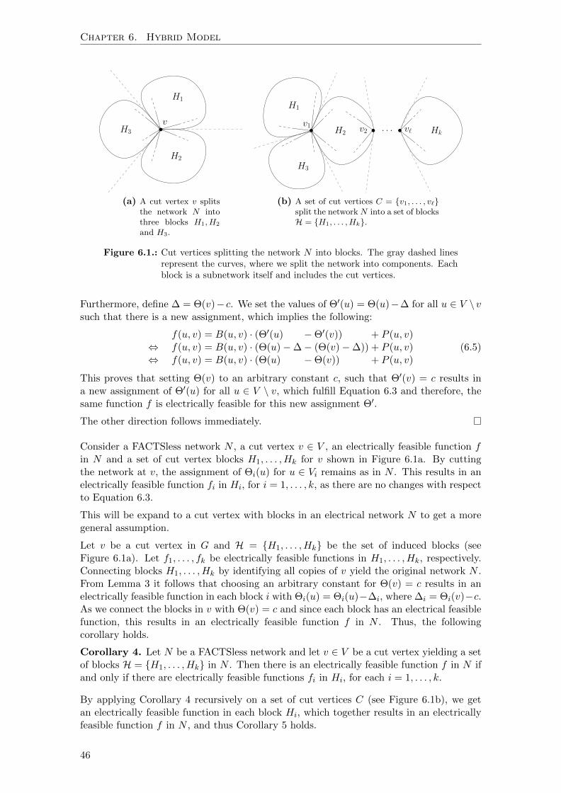
Chapter 6. Hybrid Model
v
H1
H2
H3
(a) A cut vertex v splitsthe network N intothree blocks H1, H2
and H3.
v1
H1
H2
H3
v2 v`. . . Hk
(b) A set of cut vertices C = v1, . . . , v`split the network N into a set of blocksH = H1, . . . , Hk.
Figure 6.1.: Cut vertices splitting the network N into blocks. The gray dashed linesrepresent the curves, where we split the network into components. Eachblock is a subnetwork itself and includes the cut vertices.
Furthermore, define ∆ = Θ(v)− c. We set the values of Θ′(u) = Θ(u)−∆ for all u ∈ V \vsuch that there is a new assignment, which implies the following:
f(u, v) = B(u, v) · (Θ′(u) −Θ′(v)) + P (u, v)⇔ f(u, v) = B(u, v) · (Θ(u)−∆− (Θ(v)−∆)) + P (u, v)⇔ f(u, v) = B(u, v) · (Θ(u) −Θ(v)) + P (u, v)
(6.5)
This proves that setting Θ(v) to an arbitrary constant c, such that Θ′(v) = c results ina new assignment of Θ′(u) for all u ∈ V \ v, which fulfill Equation 6.3 and therefore, thesame function f is electrically feasible for this new assignment Θ′.
The other direction follows immediately.
Consider a FACTSless network N , a cut vertex v ∈ V , an electrically feasible function fin N and a set of cut vertex blocks H1, . . . ,Hk for v shown in Figure 6.1a. By cuttingthe network at v, the assignment of Θi(u) for u ∈ Vi remains as in N . This results in anelectrically feasible function fi in Hi, for i = 1, . . . , k, as there are no changes with respectto Equation 6.3.
This will be expand to a cut vertex with blocks in an electrical network N to get a moregeneral assumption.
Let v be a cut vertex in G and H = H1, . . . ,Hk be the set of induced blocks (seeFigure 6.1a). Let f1, . . . , fk be electrically feasible functions in H1, . . . ,Hk, respectively.Connecting blocks H1, . . . ,Hk by identifying all copies of v yield the original network N .From Lemma 3 it follows that choosing an arbitrary constant for Θ(v) = c results in anelectrically feasible function in each block i with Θi(u) = Θi(u)−∆i, where ∆i = Θi(v)−c.As we connect the blocks in v with Θ(v) = c and since each block has an electrical feasiblefunction, this results in an electrically feasible function f in N . Thus, the followingcorollary holds.
Corollary 4. Let N be a FACTSless network and let v ∈ V be a cut vertex yielding a setof blocks H = H1, . . . ,Hk in N . Then there is an electrically feasible function f in N ifand only if there are electrically feasible functions fi in Hi, for each i = 1, . . . , k.
By applying Corollary 4 recursively on a set of cut vertices C (see Figure 6.1b), we getan electrically feasible function in each block Hi, which together results in an electricallyfeasible function f in N , and thus Corollary 5 holds.
46
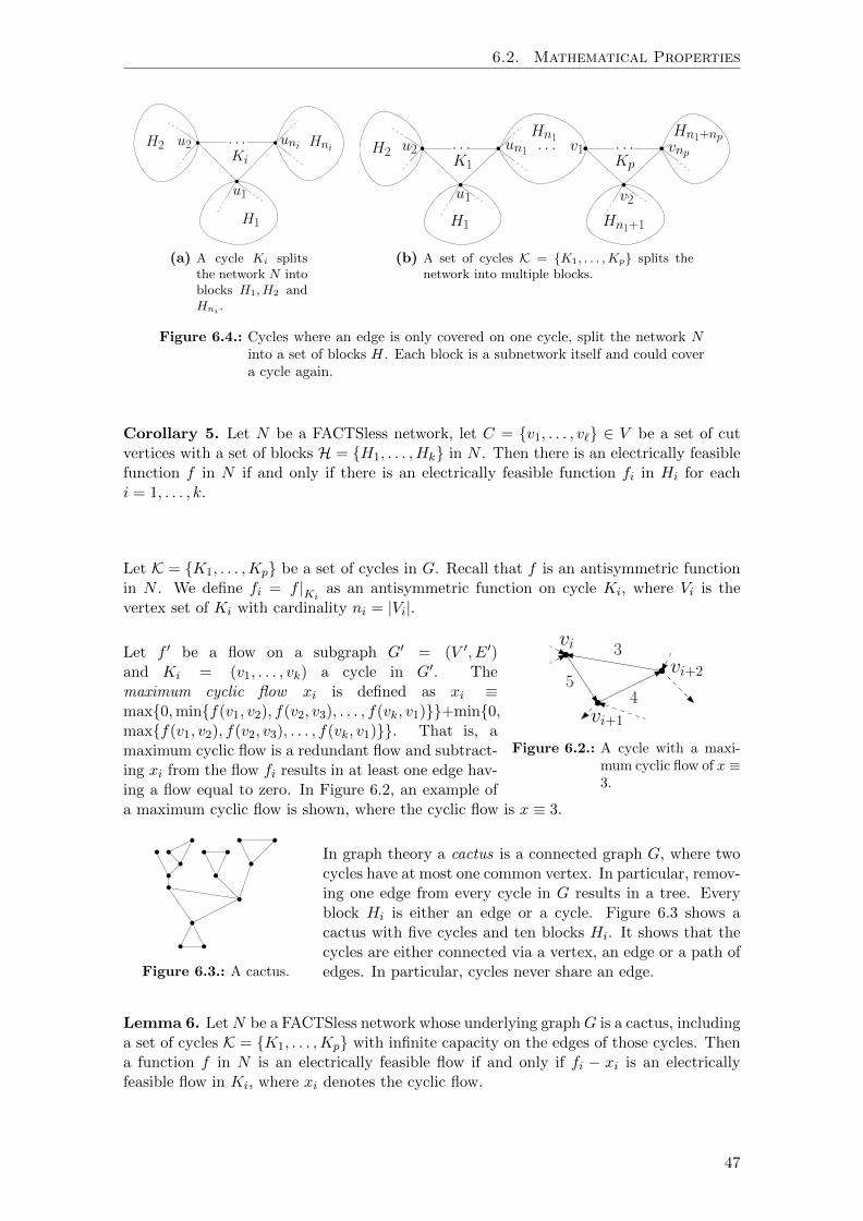
6.2. Mathematical Properties
H2 u2 uni Hni
H1
u1
. . .Ki
(a) A cycle Ki splitsthe network N intoblocks H1, H2 andHni .
H2 u2 un1Hn1
H1
u1
. . .K1
vnp
Hn1+np
Hn1+1
v2
. . .Kp
v1. . .
(b) A set of cycles K = K1, . . . ,Kp splits thenetwork into multiple blocks.
Figure 6.4.: Cycles where an edge is only covered on one cycle, split the network Ninto a set of blocks H. Each block is a subnetwork itself and could covera cycle again.
Corollary 5. Let N be a FACTSless network, let C = v1, . . . , v` ∈ V be a set of cutvertices with a set of blocks H = H1, . . . ,Hk in N . Then there is an electrically feasiblefunction f in N if and only if there is an electrically feasible function fi in Hi for eachi = 1, . . . , k.
Let K = K1, . . . ,Kp be a set of cycles in G. Recall that f is an antisymmetric functionin N . We define fi = f |Ki as an antisymmetric function on cycle Ki, where Vi is thevertex set of Ki with cardinality ni = |Vi|.
vi
vi+1
vi+2
3
45
Figure 6.2.: A cycle with a maxi-mum cyclic flow of x ≡3.
Let f ′ be a flow on a subgraph G′ = (V ′, E′)and Ki = (v1, . . . , vk) a cycle in G′. Themaximum cyclic flow xi is defined as xi ≡max0,minf(v1, v2), f(v2, v3), . . . , f(vk, v1)+min0,maxf(v1, v2), f(v2, v3), . . . , f(vk, v1). That is, amaximum cyclic flow is a redundant flow and subtract-ing xi from the flow fi results in at least one edge hav-ing a flow equal to zero. In Figure 6.2, an example ofa maximum cyclic flow is shown, where the cyclic flow is x ≡ 3.
Figure 6.3.: A cactus.
In graph theory a cactus is a connected graph G, where twocycles have at most one common vertex. In particular, remov-ing one edge from every cycle in G results in a tree. Everyblock Hi is either an edge or a cycle. Figure 6.3 shows acactus with five cycles and ten blocks Hi. It shows that thecycles are either connected via a vertex, an edge or a path ofedges. In particular, cycles never share an edge.
Lemma 6. LetN be a FACTSless network whose underlying graphG is a cactus, includinga set of cycles K = K1, . . . ,Kp with infinite capacity on the edges of those cycles. Thena function f in N is an electrically feasible flow if and only if fi − xi is an electricallyfeasible flow in Ki, where xi denotes the cyclic flow.
47

Chapter 6. Hybrid Model
Proof. Let f be a feasible flow in N and let K = K1, . . . ,Kp be the set of all cyclesin N . We consider a cycle Ki with vertices Vi = u1, . . . , uni (see Figure 6.4a). FromEquation 6.3 and the cyclic flow for cycle Ki we obtain:
B(u1, u2) −B(u1, u2) 0 . . . −10 B(u2, u3) −B(u2, u3) . . . −1...
. . ....
−B(uni , u1) . . . B(uni , u1) −1
·
Θ(u1)Θ(u2)
...Θ(uni)xi
= (fi)− (Pshifti),
(6.6)where xi is the cyclic flow on Ki, (fi) and (Pshifti) are row vectors with (fi) = (fi(u1, u2),fi(u2, u3), . . . , fi(uni , u1)) and (Pshifti) = (Pshifti(u1, u2), Pshifti(u2, u3), . . . , Pshifti(uni , u1))for all j = 1, . . . , ni. By applying the Gaussian elimination method, the matrix in Equa-tion 6.6 is in row echelon form and the last line is reduced to
−(ni−1∑j=1
B(uni ,Bu1 )
B(uj ,uj+1) + 1
)xi = fi(uni , u1) +
ni−1∑j=1
((fi(uj , uj+1)− Pshifti(uj , uj+1)) · B(uni ,Bu1 )
B(uj ,uj+1)
)
(6.7)
This shows that Equation 6.6 is a linear independent equation system and therefore thereexist solutions for Θ(ui) for all ui ∈ Vi for the value xi from Equation 6.7. In addition, wecan freely choose one Θ(ui) value in Ki, since we have n− 1 constraints on n variables.
As we look at a single cycle Ki in N there are vertices where the incoming flow or outgoingflow is bigger. To achieve the conservation of flow we set vertices with more outgoing (resp.,incoming) then incoming (resp., outgoing) flow to be a source (resp., sink).
This shows that there exists an electrically feasible function in Ki. If f is a flow, then thecapacity constrain for a given capacity ci has to hold, that is
xi + fi ≤ ci. (6.8)
As the capacity on cycles is set to infinity Equation 6.8 holds by assumption.
Consider that each cycle Ki is a block denoted by Hi and each block is connected via a cutvertex ui to the other blocks (see Figure 6.4). Then we can directly apply Corollary 5, suchthat there exists an electrically feasible assignment of phase angles in Hi for an arbitraryΘ(ui), for each i = 1, . . . , ni. Thus, fi does not change the flow of the other blocks, andtherefore there exists an electrically feasible flow in N .
Lemma 6 has some limitations. First of all, consider a cycle Ki with three vertices u, vand w in Vi. Furthermore, we set Pshift = 0 and B(u,v) = 1 for each u, v ∈ Vi. Then, fromEquation 6.6 we obtain:
Θ(u)−Θ(v)− x = f1,Θ(v)−Θ(w)− x = f2,Θ(w)−Θ(u)− x = f3.
(6.9)
It follows that x = −1/3(f1 +f2 +f3). By setting the flow fi equally to the capacities, thenadding the cyclic flow x to the flow fi, we get a capacity exceedance. This is the reason forsetting the capacities in Lemma 6 to infinity. In addition, adding a cyclic flow increasesthe line losses, which have a direct influence to the total flow costs zλ, and therefore thesolution is not optimal anymore.
48

6.3. Structural Findings
6.3. Structural Findings
In the previous section, we examined the properties of a hybrid model. Since FACTS areexpensive, these properties are used to determine the optimal placement of FACTS in anelectricity network to reach an optimal flow. We show that a flow is controllable in treeand cactus structures, which are used to determine the placement of FACTS.
We first decided to put FACTS everywhere to control the whole flow in the electricity net-work in order to reach an optimal solution (see Chapter 5). This, however, is uneconomicalfor the network operator, and therefore we developed the hybrid model. In Section 6.2, weshow that a placement of FACTS with regards to a vertex cover set is sufficient to controlthe whole flow in the electricity network and to reach an optimal flow in N . Further-more, using the definition of flow from Section 6.2, from Corollary 5 the following theoremfollows:
Theorem 1. Let N = (G = (V,E), c, γ, `, B, Pshift, s, t) be a FACTSless network, whoseunderlying graph is a tree. For any flow f on N there exists phase angles Θ : V → R, suchthat f is an electrically feasible flow.
Definition 1. Two flow functions f and f ′ are called equivalent if they differ by a set ofcyclic flows.
From Lemma 6 we get the next theorem.
Theorem 2. Let N = (G = (V,E), c, γ, `, B, Pshift, s, t) be a FACTSless network, whoseunderlying graph is a cactus, where c = ∞ on all cycle edges. For any flow f , existsΘ : V → R, such that there exists an electrically feasible flow f ′ on N which is equivalentto f .
Definition 2 (Feedback Vertex Set). A feedback vertex set V ′ inN = (G = (V,E), c, γ, `, B,Pshift, s, t) is a set of vertices V ′ ⊆ V such that N [V \ V ′] is a forest in N .
By applying Theorem 1 the following theorem holds:
Theorem 3. Let N = (G = (V,E), c, γ, `, B, Pshift, s, t) be an arbitrary electrical networkand let V ′ ⊂ V be a feedback vertex set of G. Assume that FACTS are placed at all thenodes of V ′. Then any flow on N is an electrically feasible flow.
One can seek to find the minimum feedback vertex set, however this is NP-hard [48].
6.4. Case Study
The hybrid model combines the electrical model with the balanced cost flow model fromSection 5.6. As in the previous model our goal is to minimize transmission line lossesand generation costs. For each FACTS vectors, we get a Pareto curve similar to those inSection 5.6, where FACTS are placed on all vertices. Figure 6.5 displays the behavior fora specific weighting factor λ (here λ = 0.5) and all possible FACTS vectors for the 14-busnetwork, which are in total 214−1 different FACTS vectors allocations with different totalflow costs zλ.
In Figure 6.5a, the magenta lines denote the lines with the same total flow costs zλ. Theoptimal value for zλ is given by xn, where FACTS vector xn describes an electrical networkwith FACTS on every vertex. The worst value for zλ provides FACTS vector x1 withoutFACTS. Vertices s (source) and t (sink) are always FACTS, as they control the totalgeneration and load (see Section 5.1). This approves the monotonical properties of the
49

Chapter 6. Hybrid Model
Losses ·S b a se(MW)
Costs(U
SD)
7940
7945
7950
7955
7960
7965
665 670 675 680
x1
xnγmin
`min
7938.52-
662.88
—
4308.48
4307.49
4314.28
4305.37
Hybrid Mode l
OPF: ` = 1350.66 MW, γ = 7642.59 USD
x1: ` = 673.19 MW, γ = 7955.36 USD
xn: ` = 670.38 MW, γ = 7940.36 USD
γmin: ` = 678.45 MW, γ = 7938.52 USD
`min: ` = 662.88 MW, γ = 7952.10 USD
(a) Losses in MW and costs in USD of allpossible FACTS vectors for λ = 0.5.
Number of FACTS
z0.5
4305
4306
4307
4308
4309
4310
4311
4312
4313
4314
4315
0 2 4 6 8 10 12 14
(b) Distribution of function values zλ fordifferent quantities of FACTS of allpossible FACTS vectors for λ = 0.5.
Figure 6.5.: The number of FACTS determine the quality of the solution. Therefore,the 14 bus network is used to visualize the monotonicity of the solutionspace and the number of FACTS, which results in a good solution.
hybrid model with regards to x1 and xn from Corollary 2. In Lemma 1 and Corollary 2 weproved that an increasing number of FACTS results in a better or equally good solution forzλ as with less FACTS. Furthermore, the FACTS vector with the lowest loss value (resp.,cost value) is marked with `min (resp., γmin). Thus, for a specific weight factor λ, thevalues are bounded below by three functions f`min
, fγmin and fmin zλ , which describe thesame minimum losses, minimum costs and minimum function values of the hybrid model,respectively.
In Figure 6.5b the FACTS vectors with the same FACTS quantity are listed at the samevertical line. From Figure 6.5b it can be extracted that four FACTS—if placed at theright nodes—for the 14 bus network are sufficient to get an approximately equally goodresult as for the electrical network with FACTS on all vertices. Thus, the structure of thenetwork and the right positioning of FACTS is not irrelevant to achieve an optimal flowin the network, which we already mentioned in Lemmas and Corollaries 3 to 6.
In the example data sets from the Washington University [6], some edges have a resistanceequal to zero. Thus, the costs for line losses are for each flow on these lines equal tozero. This causes cyclic flows up to the maximum capacity. To prevent cyclic flows in anelectrical network, edges with a resistance equal to zero are set to ε. The plots in Figure 6.5using these changed resistance data, and thus have slightly higher values than using theoriginal data. The optimal power flow result has higher losses and for scaling reasons it isjust mentioned in the legend for reference.
50

7. Conclusion
In this thesis, we studied how classical methods for the calculation of flow in networkscan be adapted to the calculation of power flows in electricity networks. While methodsfor the calculation of power flow in electricity networks have been improved over decades,classical flow algorithms have not been utilized due to multiple differences in the natureof usual flow and power flow.
In the beginning of this thesis, we tried to understand basic functional operations of elec-tricity network. Afterwards, we considered graph-theoretical methods in electricity net-works and presented two approaches: The first approach used the generator productionsof flow models as input for the power flow (PF) method in order to obtain an electricalflow. We made use of different heuristics to get a better generator production. The secondapproach considered FACTS at each node of the electricity network. This gave us the pos-sibility to apply classical flow methods to compute the power flow in electricity networks.The flow produced this way was unbalanced, thus some branches were much heavier usedthan the others. We considered two heuristics to produce a more balanced flow. Thefirst one balanced all edges to half of the capacity, while the second one prioritized bottle-neck edges. These heuristics resulted in worse generator production costs in comparisonto the OPF method. Thus, as a next step, we minimized the generator cost functions,which resulted in optimal generation costs, however the flow was still unbalanced. Wetherefore combined the two objectives, generation costs and balancing, which was doneby minimizing the weighted sum of generator costs and line losses. This model yieldedgood results regarding the combination of generator costs and balancing. Motivated bythe fact that placing FACTS at every node is too expensive, we introduced a hybrid flowmodel for networks containing nodes with and without FACTS. This model integratedthe PF method into the model which minimizes both generation cost and losses. Finally,we proved several theoretical properties of networks containing nodes with and withoutFACTS. In particular, we described the set of nodes where FACTS have to placed suchthat the electrical flow can be found using only a classical flow computation method.
The initial target of this work was to improve the efficiency of power flow calculation.The models we have developed are based on calculations of flow in networks; a task forwhich efficient algorithms exist. Thus, we expected that the developed models performbetter than the classical methods for power flow calculation, which include the solving ofnon-linear optimization problems. Testing the efficiency of our models is one of the futureresearch directions.
51

Chapter 7. Conclusion
Amprion GmbH
TransnetBW GmbH
50hertz GmbH
Tennet GmbHPhillipsburg
Osterath
Emden
Figure 7.1.: The planned HVDC transmission line expansion in Germany from [12, 13]to improve the integration of the offshore wind farms and other renewableenergy plants. The black consecutive line represents the plant ULTRA-NET.
In the future, it would be interesting to optimize more than just production costs andlosses in electricity networks. Thus, possible research directions include failure analysisand optimization of the structure of electricity networks. Furthermore, we know fromTransnetBW [12, 13, 83], that the energy produced by offshore wind farms in NorthernGermany should be distributed over the country, since the energy consumed is not ashigh as the energy produced in this region. There are projects which construct new highvoltage direct current (HVDC) transmission lines from the north to the south of Germany(for example, the ULTRANET in Figure 7.1). In this context, optimizing the energydistribution in an AC electricity network containing HVDC transmission lines, as well asoptimizing the construction of those transmission lines open up further possible areas ofresearch.
52

8. Appendix
53

Chapter 8. Appendix
A. 30-Bus Electricity Network
Figure A.1.: A 30-bus electricity network from the University of Washington [6].
−100
−50
0
50
100
150
200
250
0 20 40 60 80 100 120
Edge
LoadDeviation(M
W)
−100
−50
0
50
100
150
200
250
0 20 40 60 80 100 120−100
−50
0
50
100
150
200
250
0 20 40 60 80 100 120
Standard Flow Alg. vs. OPFBalanced Flow Alg. vs. OPFBottleneck Flow Alg. vs. OPF
(a) Edge flow deviation between an opti-mal power flow (OPF) and the graphtheoretical flow models.
0
50
100
150
200
250
0 20 40 60 80 100 1200
50
100
150
200
250
0 20 40 60 80 100 1200
50
100
150
200
250
0
50
100
150
200
250
Edges sorted by OPF
Load(M
W)
Optimal Power Flow0.31 % Generator InputStandard Flow AlgorithmBalanced Flow AlgorithmBottleneck Flow Algorithm
(b) Generator productions of the graphtheoretical flow models are used tocalculate an electrical flow using thepower flow (PF) method. The edgesare decreasingly sorted by the OPFflow on the edges.
Genera
tionCosts(U
SD)
Real Power (MW) or React ive Power (MVar)
0
5000
10000
15000
20000
25000
50 100 150 200 250
Polynoms
Piecewise Linear Approximations
(c) Piecewise linear generator cost func-tions of the 30-bus network are pre-sented by the red lines and thepolynomial is displayed by the graydashed line.
8343.40
11083.26
10088.3210367.09
8345.76
0
2000
4000
6000
8000
10000
12000
OPF Standard
Mode l
Balanced
Mode l
Bott le -
neck
Mode l
Minimum
Cost Mode l
Total Cost for Bus30 System
(d) Total power generation cost of allsimple weighted flow models of thisthesis.
Figure A.2.: Plots for the 30-bus electricity network.
54

B. 57-Bus Electricity Network
B. 57-Bus Electricity Network
Figure B.3.: A 57-bus electricity network from the University of Washington [6].
−100
−50
0
50
100
150
200
0 50 100 150 200 250
Edge
LoadDeviation(M
W)
−100
−50
0
50
100
150
200
0 50 100 150 200 250−100
−50
0
50
100
150
200
0 50 100 150 200 250
Standard Flow Alg. vs. OPFBalanced Flow Alg. vs. OPFBottleneck Flow Alg. vs. OPF
(a) Edge flow deviation between an opti-mal power flow (OPF) and the graphtheoretical flow models.
0
100
200
300
400
500
0 50 100 150 200 2500
100
200
300
400
500
0 50 100 150 200 2500
100
200
300
400
500
0 50 100 150 200 2500
100
200
300
400
500
0 50 100 150 200 250
Edges sorted by OPF
Load(M
W)
Optimal Power Flow0.63 % Generator InputStandard Flow AlgorithmBalanced Flow AlgorithmBottleneck Flow Algorithm
(b) Generator productions of the graphtheoretical flow models are used tocalculate an electrical flow using thepower flow (PF) method. The edgesare decreasingly sorted by the OPFflow on the edges.
Genera
tionCosts×103(U
SD)
Real Power (MW) or React ive Power (MVar)
0
50
100
150
200
250
300
350
400
200 400 600 800 1000 1200
Polynoms
Piecewise Linear Approximations
(c) Piecewise linear generator cost func-tions of the 57-bus network are pre-sented by the red lines and thepolynomial is displayed by the graydashed line.
41006.7443251.65
58853.87
48433.84
41013.53
0
100
200
300
400
500
600
OPF StandardMode l
BalancedMode l
Bott le -neckMode l
MinimumCost Mode l
Genera
torCosts×
102(U
SD)
Total Cost for Bus57 System
(d) Total power generation cost of allsimple weighted flow models of thisthesis.
Figure B.4.: Plots for the 57-bus electricity network.
55

Chapter 8. Appendix
C. 118-Bus Electricity Network
Figure C.5.: A 118-bus electricity network from the University of Washington [6].
−200
−100
0
100
200
300
400
500
600
0 100 200 300 400 500 600
Edge
LoadDeviation(M
W)
−200
−100
0
100
200
300
400
500
600
0 100 200 300 400 500 600−200
−100
0
100
200
300
400
500
600
0 100 200 300 400 500 600
Standard Flow Alg. vs. OPFBalanced Flow Alg. vs. OPFBottleneck Flow Alg. vs. OPF
(a) Edge flow deviation between an opti-mal power flow (OPF) and the graphtheoretical flow models.
0
100
200
300
400
500
600
0 100 200 300 400 500 6000
100
200
300
400
500
600
0 100 200 300 400 500 6000
100
200
300
400
500
600
0 100 200 300 400 500 6000
100
200
300
400
500
600
0 100 200 300 400 500 600
Edges sorted by OPF
Load(M
W)
Optimal Power Flow0.43 % Generator InputStandard Flow AlgorithmBalanced Flow AlgorithmBottleneck Flow Algorithm
(b) Generator productions of the graphtheoretical flow models are used tocalculate an electrical flow using thepower flow (PF) method. The edgesare decreasingly sorted by the OPFflow on the edges.
Genera
tionCosts×105(U
SD)
Real Power (MW) or React ive Power (MVar)
0
50
100
150
200
250
300
350
400
450
0 1000 2000 3000 4000
Polynoms
Piecewise Linear Approximations
(c) Piecewise linear generator cost func-tions of the 118-bus network arepresented by the red lines and thepolynomial is displayed by the graydashed line.
125947.88
165392.34
412193.37
189203.53
125966.56
0
50
100
150
200
250
300
350
400
450
OPF StandardMode l
BalancedMode l
Bott le -neckMode l
MinimumCost Mode l
Genera
torCosts×
103(U
SD)
Total Cost for Bus118 System
(d) Total power generation cost of allsimple weighted flow models of thisthesis.
Figure C.6.: Plots for the 118-bus electricity network.
56

Bibliography
[1] Distribution Loss Factor Calculation Methodology. @ONLINE, August 2004. URLhttp://www.aer.gov.au/sites/default/files/Aurora%20-%20distribution%
20loss%20factor%20calculation%20methodology.PDF. Accessed: 2014-01-14.(Cited on page 15.)
[2] Ten-Year Network Development Plan 2012. @ONLINE, May 2012. URLhttp://www.entsoe.eu/major-projects/ten-year-network-development-plan/
tyndp-2012/. Accessed: 2013-12-17. (Cited on page 34.)
[3] Swiss National Electricity Network. @ONLINE, February 2012. URLhttp://www.geni.org/globalenergy/library/national_energy_grid/
switzerland/swissnationalelectricitygrid.shtml. Accessed: 2014-01-04.(Cited on page 11.)
[4] Winterkalte – Deutscher Strom rettet Frankreich. @ONLINE, February 2012. URLhttp://www.manager-magazin.de/unternehmen/energie/a-814075.html. Ac-cessed: 2013-12-17. (Cited on page 34.)
[5] GUROBI OPTIMIZER – State of the Art Mathematical Programming Solver.@ONLINE, 2013. URL http://www.gurobi.com/products/gurobi-optimizer/
gurobi-overview. Accessed: 2013-08-06. (Cited on page 8.)
[6] Resources – Power Systems Test Case Archive. @ONLINE, 2013. URL http://www.
ee.washington.edu/research/pstca/. Accessed: 2013-08-13. (Cited on pages 2,11, 12, 13, 27, 28, 29, 30, 32, 33, 35, 37, 38, 50, 54, 55, and 56.)
[7] MATLAB – The Language of Technical Computing. @ONLINE, 2013. URL http:
//www.mathworks.com/products/matlab/. Accessed: 2013-08-06. (Cited on page 8.)
[8] Electricity Monthly Update. @ONLINE, December 2013. URL http://www.eia.
gov/electricity/monthly/update/end_use.cfm#tabs_prices-3. Accessed: 2014-01-14. (Cited on page 41.)
[9] Electricity Prices for Domestic Consumers. @ONLINE, December 2013. URLhttp://appsso.eurostat.ec.europa.eu/nui/submitViewTableAction.do. Ac-cessed: 2013-12-27. (Cited on page 41.)
[10] Electricity Prices for Industrial Consumers. @ONLINE, December 2013. URL http:
//appsso.eurostat.ec.europa.eu/nui/show.do?dataset=nrg_pc_205&lang=en.Accessed: 2013-12-27. (Cited on page 41.)
[11] How we Balance the Country’s Electricity Transmission System. @ONLINE, August2013. URL http://www.nationalgrid.com/uk/Electricity/AboutElectricity/
Balancing+the+network/. Accessed: 2013-08-14. (Cited on page 40.)
[12] Ultranet. @ONLINE, n/s. URL http://www.amprion.net/netzausbau/
ultranet-hintergrund. Accessed: 2014-01-04. (Cited on page 52.)
57

Bibliography
[13] Steckbrief zum Projekt – Ultranet. @ONLINE, n/s. URL http://www.transnetbw.
de/de/uebertragungsnetz/dialog-netzbau/osterath-philippsburg. Accessed:2014-01-04. (Cited on page 52.)
[14] K. H. Abdul-Rahman and S. M. Shahidehpour. Application of Fuzzy Sets to Opti-mal Reactive Power Planning with Security Constraints. In Power Industry Com-puter Application Conference, 1993. Conference Proceedings, pages 124–130, 1993.doi: 10.1109/PICA.1993.291026. URL http://dx.doi.org/10.1109/PICA.1993.
291026. (Cited on page 4.)
[15] M. A. Abido. Optimal Power Flow using Particle Swarm Optimization. InternationalJournal of Electrical Power & Energy Systems, 24(7):563–571, 2002. ISSN 0142-0615. doi: 10.1016/S0142-0615(01)00067-9. URL http://dx.doi.org/10.1016/
S0142-0615(01)00067-9. (Cited on page 5.)
[16] M. R. AlRashidi and M. E. El-Hawary. A Survey of Particle Swarm OptimizationApplications in Electric Power Systems. Evolutionary Computation, IEEE Transac-tions on, 13(4):913–918, 2009. ISSN 1089-778X. doi: 10.1109/TEVC.2006.880326.URL http://dx.doi.org/10.1109/TEVC.2006.880326. (Cited on page 5.)
[17] S. Arora and B. Barak. Computational Complexity: A Modern Approach. Cam-bridge University Press, New York, NY, USA, 1st edition, 2009. ISBN 0521424267,9780521424264. (Cited on page 7.)
[18] P. Attaviriyanupap, H. Kita, E. Tanaka, and J. Hasegawa. New Bidding Strat-egy Formulation for Day-Ahead Energy and Reserve Markets based on Evolution-ary Programming. International Journal of Electrical Power & Energy Systems,27(3):157–167, 2005. ISSN 0142-0615. doi: 10.1016/j.ijepes.2004.09.005. URLhttp://dx.doi.org/10.1016/j.ijepes.2004.09.005. (Cited on page 4.)
[19] M. Blaser and B. Manthey. Smoothed Complexity Theory. CoRR, abs/1202.1, 2012.doi: 10.1007/978-3-642-32589-2\ 20. URL http://link.springer.com/chapter/
10.1007%2F978-3-642-32589-2_20. (Cited on page 7.)
[20] G. Bol. Lineare Optimierung: Theorie und Anwendungen. Athenaum Paperbacks.Athenaum-Verlag, 1980. ISBN 9783761050279. (Cited on pages 8 and 9.)
[21] B. Bollobas. Graph theory: An Introductory Course. Springer Verlag”
New York,1979. Includes index. (Cited on page 7.)
[22] R. J. Brown and W. F. Tinney. Digital Solutions for Large Power Networks. Powerapparatus and systems, part iii. transactions of the american institute of electrical en-gineers, 76(3):347–351, 1957. ISSN 0097-2460. doi: 10.1109/AIEEPAS.1957.4499563.URL http://dx.doi.org/10.1109/AIEEPAS.1957.4499563. (Cited on page 3.)
[23] L. J. Cai, I. Erlich, and G. Stamtsis. Optimal Choice and Allocation of FACTS De-vices in Deregulated Electricity Market using Genetic Algorithms. In Power SystemsConference and Exposition, 2004. IEEE PES, volume 1, pages 201–207, 2004. doi: 10.1109/PSCE.2004.1397562. URL http://dx.doi.org/10.1109/PSCE.2004.1397562.(Cited on page 5.)
[24] J. Carpentier. Contribution to the Economic Dispatch Problem. Bull. Sac. FranceElect., 8(-):431–437, 1962. (Cited on page 3.)
[25] P.-H. Chen and H.-C. Chang. Large-Scale Economic Dispatch by Genetic Algorithm.Power Systems, IEEE Transactions on, 10(4):1919–1926, 1995. ISSN 0885-8950.doi: 10.1109/59.476058. URL http://dx.doi.org/10.1109/59.476058. (Cited onpage 5.)
58

Bibliography
[26] T. S. Chung and Y. Z. Li. A Hybrid GA Approach for OPF with Considerationof FACTS Devices. Power Engineering Review, IEEE, 20(8):54–57, 2000. ISSN0272-1724. doi: 10.1109/39.857456. URL http://dx.doi.org/10.1109/39.857456.(Cited on page 5.)
[27] G. B. Dantzig. Maximization of a Linear Function of Variables Subject to LinearInequalities, in Activity Analysis of Production and Allocation, chapter XXI. Wi-ley, New York, 1951. URL http://cowles.econ.yale.edu/P/cm/m13/m13-21.pdf.(Cited on page 5.)
[28] Y. Del Valle, G. K. Venayagamoorthy, S. Mohagheghi, J.-C. Hernandez, and R. G.Harley. Particle Swarm Optimization: Basic Concepts, Variants and Applicationsin Power Systems. Evolutionary Computation, IEEE Transactions on, 12(2):171–195,2008. ISSN 1089-778X. doi: 10.1109/TEVC.2007.896686. URL http://dx.doi.org/
10.1109/TEVC.2007.896686. (Cited on page 5.)
[29] D. Devaraj and B. Yegnanarayana. Genetic-Algorithm-based Optimal Power Fow forSecurity Enhancement. Generation, Transmission and Distribution, IEE Proceedings-, 152(6):899–905, 2005. ISSN 1350-2360. doi: 10.1049/ip-gtd:20045234. URL http:
//dx.doi.org/10.1049/ip-gtd:20045234. (Cited on page 5.)
[30] J. A. Domınguez-Navarro, J. L. Bernal-Agustın, A. Dıaz, D. Requena, and E. P.Vargas. Optimal Parameters of FACTS Devices in Electric Power Systems ApplyingEvolutionary Strategies. International Journal of Electrical Power & Energy Systems,29(1):83–90, 2007. ISSN 0142-0615. doi: 10.1016/j.ijepes.2006.05.003. URL http:
//dx.doi.org/10.1016/j.ijepes.2006.05.003. (Cited on page 4.)
[31] L. A. Dunstan. Digital Load Flow Studies. Power apparatus and systems, part iii.transactions of the american institute of electrical engineers, 73(1):–, 1954. ISSN 0097-2460. doi: 10.1109/AIEEPAS.1954.4498891. URL http://dx.doi.org/10.1109/
AIEEPAS.1954.4498891. (Cited on page 3.)
[32] J. Edmonds and R. M. Karp. Theoretical Improvements in Algorithmic Efficiencyfor Network Flow Problems. J. ACM, 19(2):248–264, Apr. 1972. ISSN 0004-5411.doi: 10.1145/321694.321699. URL http://doi.acm.org/10.1145/321694.321699.(Cited on page 6.)
[33] M. M. El-Saadawi, M. A. Tantawi, and E. Tawfik. A Fuzzy Optimization-basedApproach to Large Scale Thermal Unit Commitment. Electric Power Systems Re-search, 72(3):245–252, 2004. ISSN 0378-7796. doi: 10.1016/j.epsr.2004.04.009. URLhttp://dx.doi.org/10.1016/j.epsr.2004.04.009. (Cited on page 4.)
[34] O. Elgerd. Electric Energy Systems Theory: An Introduction. Tata McGraw-Hill,1983. ISBN 9780070992863. (Cited on page 14.)
[35] L. R. Ford and D. R. Fulkerson. Maximal Flow through a Network. Canadian Journalof Mathematics, 8:399–404, 1955. URL http://www.rand.org/pubs/papers/P605/.(Cited on page 6.)
[36] B. Gasbaoui and B. Allaoua. Ant Colony Optimization Applied on CombinatorialProblem for Optimal Power Flow Solution. Leonardo Journal of Sciences, 14:1–17,2009. ISSN 1583-0233. URL http://ljs.academicdirect.org/A14/001_017.pdf.(Cited on page 5.)
[37] A. V. Goldberg and R. E. Tarjan. A New Approach to the Maximum Flow Problem.In Proceedings of the Eighteenth Annual ACM Symposium on Theory of Computing,STOC ’86, pages 136–146, New York, NY, USA, 1986. ACM. ISBN 0-89791-193-8. doi:10.1145/12130.12144. URL http://doi.acm.org/10.1145/12130.12144. (Cited onpage 6.)
59

Bibliography
[38] A. V. Goldberg, E. Tardos, and R. E. Tarjan. Flows, Paths and VLSI, chapter NetworkFlow Algorithms, pages 101–164. In Korte et al. [49], 1990. ISBN 9783540526858.URL http://www.springer.com/new+%26+forthcoming+titles+(default)/book/
978-3-642-75766-2. (Cited on page 6.)
[39] D. E. Goldberg. Genetic Algorithms in Search, Optimization and Machine Learning.Addison-Wesley Longman Publishing Co., Inc., Boston, MA, USA, 1st edition, 1989.ISBN 0201157675. (Cited on page 5.)
[40] W. Group. Common Format For Exchange of Solved Load Flow Data. IEEE Trans-actions on Power Apparatus and Systems, PAS-92(6):1916–1925, Nov. 1973. ISSN0018-9510. doi: 10.1109/TPAS.1973.293571. URL http://dx.doi.org/10.1109/
TPAS.1973.293571. (Cited on pages 11, 14, and 17.)
[41] H. Happoldt and D. Oeding. Elektrische Kraftwerke und Netze. Springer-VerlagGmbH, 1978. ISBN 9783540083057. URL http://link.springer.com/book/10.
1007%2F978-3-662-06962-2. (Cited on pages 14, 20, 23, and 37.)
[42] J. M. Henderson. Automatic Digital Computer Solution of Load Flow Studies. Powerapparatus and systems, part iii. transactions of the american institute of electricalengineers, 73(2):–, 1954. ISSN 0097-2460. doi: 10.1109/AIEEPAS.1954.4499023.URL http://dx.doi.org/10.1109/AIEEPAS.1954.4499023. (Cited on page 3.)
[43] J. Hindmarsh. Electrical machines and their applications. Pergamon internationallibrary of science, technology, engineering, and social studies. Pergamon Press, 1984.ISBN 9780080305721. (Cited on page 14.)
[44] N. Hingorani. Flexible AC transmission. IEEE Spectrum, 30(4):40–45, April 1993.ISSN 0018-9235. doi: 10.1109/6.206621. URL http://dx.doi.org/10.1109/6.
206621. (Cited on page 1.)
[45] M. Huneault and F. D. Galiana. A Survey of the Optimal Power Flow Literature.Power Systems, IEEE Transactions on, 6(2):762–770, 1991. ISSN 0885-8950. doi:10.1109/59.76723. URL http://dx.doi.org/10.1109/59.76723. (Cited on pages 1and 3.)
[46] A. A. Ibrahim, A. Mohamed, and H. Shareef. Application of Quantum-inspired Bi-nary Gravitational Search Algorithm for Optimal Power Quality Monitor Placement.In Proceedings of the 11th WSEAS International Conference on Artificial Intelli-gence, Knowledge Engineering and Data Bases, AIKED’12, pages 27–32, StevensPoint, Wisconsin, USA, 2012. World Scientific and Engineering Academy and Society(WSEAS). ISBN 978-1-61804-068-8. URL http://dl.acm.org/citation.cfm?id=
2183067.2183073. (Cited on page 40.)
[47] T. Jayabarathi, K. Jayaprakash, D. N. Jeyakumar, and T. Raghunathan. EvolutionaryProgramming Techniques for Different Kinds of Economic Dispatch Problems. ElectricPower Systems Research, 73(2):169–176, 2005. ISSN 0378-7796. doi: 10.1016/j.epsr.2004.08.001. URL http://dx.doi.org/10.1016/j.epsr.2004.08.001. (Cited onpage 4.)
[48] R. Karp. Reducibility among combinatorial problems. In R. Miller andJ. Thatcher, editors, Complexity of Computer Computations, pages 85–103.Plenum Press, 1972. URL http://link.springer.com/chapter/10.1007%
2F978-1-4684-2001-2_9. (Cited on page 49.)
[49] B. Korte, L. Lovasz, J. Pomel, and A. Schrijver, editors. Flows, Paths and VLSI.Algorithms and combinatorics. Springer-Verlag, Berlin, 1990. ISBN 9783540526858.URL http://www.springer.com/new+%26+forthcoming+titles+(default)/book/
978-3-642-75766-2. (Cited on page 60.)
60

Bibliography
[50] V. Miranda and M. A. Matos. Distribution System Planning with Fuzzy Modelsand Techniques. In Electricity Distribution, 1989. CIRED 1989. 10th InternationalConference on, volume 6, pages 472–476, 1989. URL http://ieeexplore.ieee.org/
xpl/articleDetails.jsp?arnumber=206126&navigation=1. (Cited on page 3.)
[51] V. Miranda and J. T. Saraiva. Fuzzy Modelling of Power System Optimal LoadFlow. Power Systems, IEEE Transactions on, 7(2):843–849, 1992. ISSN 0885-8950.doi: 10.1109/59.141794. URL http://dx.doi.org/10.1109/59.141794. (Cited onpage 3.)
[52] V. Miranda, M. A. Matos, and J. T. Saraiva. Fuzzy Load Flow – New AlgorithmsIncoorporating Uncertain Generation and Load Representation, 10th PSCC, Graz,August 1990. In Proceedings of the 10th PSCC. Butterworths, London, 1990. (Citedon page 3.)
[53] G. L. Nemhauser and L. A. Wolsey. Integer and Combinatorial Optimization. Wiley-Interscience series in discrete mathematics and optimization. Wiley, New York [u.a.],1988. ISBN 0-471-82819-X. (Cited on page 8.)
[54] T. Niknam. A New Fuzzy Adaptive Hybrid Particle Swarm Optimization Algorithmfor Non-Linear, Non-Smooth and Non-Convex Economic Dispatch Problem. AppliedEnergy, 87(1):327–339, 2010. ISSN 0306-2619. doi: 10.1016/j.apenergy.2009.05.016.URL http://dx.doi.org/10.1016/j.apenergy.2009.05.016. (Cited on page 4.)
[55] N/s. Final Report on the August 14, 2003 Blackout in the United States and Canada:Causes and Recommendations. Technical report, U.S.-Canada Power System OutageTask Force, 2004. URL http://www.ferc.gov/industries/electric/indus-act/
reliability/blackout/ch1-3.pdf. (Cited on page 13.)
[56] T. P. O. of Science and Technology. Future Electricity Networks. pages1–4, 2011. URL http://www.parliament.uk/documents/post/postpn_
372-future-electricity-networks.pdf. (Cited on page 40.)
[57] J. Olivares-Galvan, P. Georgilakis, E. Campero-Littlewood, and R. Escarela-Perez.Core Lamination Selection for Distribution Transformers based on Sensitivity Anal-ysis. Electrical Engineering, 95(1):33–42, 2013. ISSN 0948-7921. doi: 10.1007/s00202-012-0237-7. URL http://dx.doi.org/10.1007/s00202-012-0237-7. (Citedon page 14.)
[58] W. Ongsakul and P. Jirapong. Optimal Allocation of FACTS Devices to EnhanceTotal Transfer Capability using Evolutionary Programming. In Circuits and Systems,2005. ISCAS 2005. IEEE International Symposium on, volume 5, pages 4175–4178,2005. doi: 10.1109/ISCAS.2005.1465551. URL http://dx.doi.org/10.1109/ISCAS.
2005.1465551. (Cited on page 4.)
[59] W. Ongsakul and T. Tantimaporn. Optimal Power Flow by Improved EvolutionaryProgramming. Electric Power Components and Systems, 34(1):79–95, 2006. doi: 10.1080/15325000691001458. URL http://dx.doi.org/10.1080/15325000691001458.(Cited on page 4.)
[60] T. J. Overbye, X. Cheng, and Y. Sun. A Comparison of the AC and DC Power FlowModels for LMP Calculations. In 37th Annual Hawaii International Conference onSystem Sciences, 2004. Proceedings of the, page 9 pp. IEEE, 2004. ISBN 0-7695-2056-1. doi: 10.1109/HICSS.2004.1265164. URL http://dx.doi.org/10.1109/HICSS.
2004.1265164. (Cited on pages 15 and 23.)
[61] N. P. Padhy. Congestion Management under Deregulated Fuzzy Environment. InElectric Utility Deregulation, Restructuring and Power Technologies, 2004. (DRPT
61

Bibliography
2004). Proceedings of the 2004 IEEE International Conference on, volume 1, pages133–139, 2004. doi: 10.1109/DRPT.2004.1338481. URL http://dx.doi.org/10.
1109/DRPT.2004.1338481. (Cited on page 4.)
[62] C. M. Papadimitriou. Computational Complexity. Addison-Wesley, Reading, Mas-sachusetts, 1994. ISBN 0201530821. (Cited on page 7.)
[63] J. Peschon, D. S. Piercy, W. F. Tinney, O. J. Tveit, and M. Cuenod. OptimumControl of Reactive Power Flow. Power Apparatus and Systems, IEEE Transactionson, PAS-87(1):40–48, 1968. ISSN 0018-9510. doi: 10.1109/TPAS.1968.292254. URLhttp://dx.doi.org/10.1109/TPAS.1968.292254. (Cited on page 3.)
[64] V. C. Ramesh and X. Li. A Fuzzy Multiobjective Approach to Contingency Con-strained OPF. Power Systems, IEEE Transactions on, 12(3):1348–1354, 1997. ISSN0885-8950. doi: 10.1109/59.630480. URL http://dx.doi.org/10.1109/59.630480.(Cited on page 4.)
[65] S. S. Reddy, P. R. Bijwe, and A. R. Abhyankar. Faster Evolutionary Algorithm basedOptimal Power Flow using Incremental Variables. International Journal of ElectricalPower & Energy Systems, 54(0):198–210, 2014. ISSN 0142-0615. doi: 10.1016/j.ijepes.2013.07.019. URL http://dx.doi.org/10.1016/j.ijepes.2013.07.019. (Cited onpage 5.)
[66] C. A. Roa-Sepulveda and B. J. Pavez-Lazo. A Solution to the Optimal Power Flowusing Simulated Annealing. International Journal of Electrical Power & Energy Sys-tems, 25(1):47–57, 2003. ISSN 0142-0615. doi: 10.1016/S0142-0615(02)00020-0. URLhttp://dx.doi.org/10.1016/S0142-0615(02)00020-0. (Cited on page 4.)
[67] A. Schrijver. On the History of the Transportation and Maximum Flow Prob-lems. Mathematical Programming, 91(3):437–445, 2002. ISSN 0025-5610. doi:10.1007/s101070100259. URL http://dx.doi.org/10.1007/s101070100259. (Citedon page 6.)
[68] H. Seifi and M. Sepasian. Electric Power System Planning: Issues, Algorithms andSolutions. Power Systems. Springer, 2011. ISBN 9783642179891. URL http://
www.springer.com/engineering/energy+technology/book/978-3-642-17988-4.(Cited on page 16.)
[69] M. Shabani and M. R. A. Pahlavani. Fuzzy-based Multi-Objective Optimal Placementof Unified Power Flow Controller. Applied Sciences Research, 8(1):290–300, 2012.ISSN 1819-544X. URL http://www.aensiweb.com/jasr/jasr/2012/290-300.pdf.(Cited on page 4.)
[70] R. B. Shipley and M. Hochdorf. Exact Economic Dispatch – Digital Computer So-lution. Power apparatus and systems, part iii. transactions of the american insti-tute of electrical engineers, 75(3):–, 1956. ISSN 0097-2460. doi: 10.1109/AIEEPAS.1956.4499417. URL http://dx.doi.org/10.1109/AIEEPAS.1956.4499417. (Citedon page 3.)
[71] P. Somasundaram, K. Kuppusamy, and R. P. K. Devi. Evolutionary Programmingbased Security Constrained Optimal Power Flow. Electric Power Systems Research,72(2):137–145, 2004. ISSN 0378-7796. doi: 10.1016/j.epsr.2004.02.006. URL http:
//dx.doi.org/10.1016/j.epsr.2004.02.006. (Cited on page 4.)
[72] Y. R. Sood. Evolutionary Programming based Optimal Power Flow and its Validationfor Deregulated Power System Analysis. International Journal of Electrical Power &Energy Systems, 29(1):65–75, 2007. ISSN 0142-0615. doi: 10.1016/j.ijepes.2006.03.024. URL http://dx.doi.org/10.1016/j.ijepes.2006.03.024. (Cited on page 4.)
62

Bibliography
[73] E. Spring. Elektrische Maschinen. Springer-Lehrbuch. Springer, 2009. ISBN9783642008856. URL http://books.google.de/books?id=ZH5f23QgHdMC. (Citedon page 14.)
[74] W. D. Stevenson. Elements of Power System Analysis (McGraw-Hill electrical andelectronic engineering series). McGraw-Hill, 3 edition, 1975. ISBN 0070612854. (Citedon page 14.)
[75] W. F. Tinney, V. Brandwajn, and S. M. Chan. Sparse Vector Methods. PowerApparatus and Systems, IEEE Transactions on, PAS-104(2):295–301, 1985. ISSN0018-9510. doi: 10.1109/TPAS.1985.319043. URL http://dx.doi.org/10.1109/
TPAS.1985.319043. (Cited on page 3.)
[76] M. Todorovski and D. Rajicic. An Initialization Procedure in Solving Optimal PowerFlow by Genetic Algorithm. Power Systems, IEEE Transactions on, 21(2):480–487,2006. ISSN 0885-8950. doi: 10.1109/TPWRS.2006.873120. URL http://dx.doi.
org/10.1109/TPWRS.2006.873120. (Cited on page 5.)
[77] C. A. Trauth and R. E. Woolsey. Integer Linear Programming: A Study in Compu-tational Efficiency. Management Science, 15(9):481–493, May 1969. ISSN 0025-1909.doi: 10.1287/mnsc.15.9.481. URL http://dx.doi.org/10.1287/mnsc.15.9.481.(Cited on page 10.)
[78] D. C. Walters. An Application of Genetic Algorithms to the Economic Dispatch ofPower Generation. Master’s thesis, Auburn University, May 1991. (Cited on page 5.)
[79] D. C. Walters and G. B. Sheble. Genetic Algorithm Solution of Economic Dispatchwith Valve Point Loading. Power Systems, IEEE Transactions on, 8(3):1325–1332,1993. ISSN 0885-8950. doi: 10.1109/59.260861. URL http://dx.doi.org/10.1109/
59.260861. (Cited on page 5.)
[80] J. B. Ward and H. W. Hale. Digital Computer Solution of Power-Flow Problems.Power apparatus and systems, part iii. transactions of the american institute of elec-trical engineers, 75(3):–, 1956. ISSN 0097-2460. doi: 10.1109/AIEEPAS.1956.4499318.URL http://dx.doi.org/10.1109/AIEEPAS.1956.4499318. (Cited on page 3.)
[81] A. J. Wood and B. F. Wollenberg. Power Generation, Op-eration, and Control. John Wiley & Sons, New York, 1996.ISBN 9783761050279. URL http://www.scribd.com/doc/21295897/
E-BOOK-Power-Generation-Operation-y-Control-Allen-Wood. Includes in-dex. (Cited on pages vii, 16, 20, and 23.)
[82] I. K. Yu and Y. H. Song. A Novel Short-Term Generation Scheduling Techniqueof Thermal Units using Ant Colony Search Algorithms. International Journal ofElectrical Power & Energy Systems, 23(6):471–479, 2001. ISSN 0142-0615. doi: 10.1016/S0142-0615(00)00065-X. URL http://dx.doi.org/10.1016/S0142-0615(00)
00065-X. (Cited on page 5.)
[83] G. Zeitler. Vorstellung von TransnetBW am KIT. @PRESENTATION, 20.09.2013.(Cited on pages 18, 34, 43, 44, and 52.)
[84] R. D. Zimmerman and C. E. Murillo-Sanchez. User’s Manual, 2011. URL http:
//www.pserc.cornell.edu/matpower/. (Cited on pages 2, 20, and 23.)
[85] R. D. Zimmerman, C. E. Murillo-sanchez, and U. A. D. Manizales. MATPOWER ’s Extensible Optimal Power Flow Architecture. Technical report, 2009. URL http:
//www.pserc.cornell.edu/matpower/. (Cited on pages 20 and 23.)
63

Bibliography
[86] R. D. Zimmerman, C. E. Murillo-Sanchez, and R. J. Thomas. MATPOWER’s Ex-tensible Optimal Power Fow Architecture. In 2009 IEEE Power & Energy Soci-ety General Meeting, pages 1–7. IEEE, July 2009. ISBN 978-1-4244-4241-6. doi:10.1109/PES.2009.5275967. URL http://dx.doi.org/10.1109/PES.2009.5275967.(Cited on pages 20 and 23.)
[87] R. D. Zimmerman, C. E. Murillo-Sanchez, and R. J. Thomas. MATPOWER: Steady-State Operations, Planning, and Analysis Tools for Power Systems Research andEducation. IEEE Transactions on Power Systems, 26(1):12–19, Feb. 2011. ISSN0885-8950. doi: 10.1109/TPWRS.2010.2051168. URL http://dx.doi.org/10.1109/
TPWRS.2010.2051168. (Cited on pages 20 and 23.)
64