network-induced supervised learning: network-induced classification (ni-c) and network-induced...

Network-Induced Supervised Learning: Network-InducedClassification (NI-C) and Network-Induced Regression (NI-R)

Marco S. ReisCIEPQPF – Dept. of Chemical Engineering, University of Coimbra, Polo 11-Rua Silvio Lima, Coimbra 3030-790,

Portugal

DOI 10.1002/aic.13946Published online December 26, 2012 in Wiley Online Library (wileyonlinelibrary.com).

Current supervised approaches, such as classification and regression methodologies, are strongly focused on optimizingestimation accuracy metrics, leaving the interpretation of the results produced as a secondary concern. However, in theanalysis of complex systems, one of the main interests is precisely the induction of relevant associations, to understand orclarify the way the system operates. Two related frameworks for addressing supervised learning problems (classificationand regression) are presented, that incorporate interpretational-oriented analysis features right from the onset of theanalysis. These features constrain the predictive space, in order to introduce interpretable elements in the final model.Interestingly, such constraints do not usually compromise the methods’ performance, when compared to their unconstrainedversions. The frameworks, called network-induced classification (NI-C), and network-induced regression (NI-R), share acommon methodological backbone, and are described in detail, as well as applied to real-world case studies. VVC 2012

American Institute of Chemical Engineers AIChE J, 59: 1570–1587, 2013

Keywords: partial correlation, clustering, classification, regression, knowledge extraction, generalized topologicaloverlap measure, linear discriminant analysis, partial least squares, ordinary least squares

Introduction

With the increasing ability to collect data from complexsystems regarding phenomena going on at different scales ofspace and time, new opportunities emerge for studying theirbehavior by adopting a data-driven perspective. In this con-text, inductive learning from ‘‘well’’ collected data, eitherresulting from carefully planned experimental designs orfrom observational studies, present itself as a valid alterna-tive to the bottom-up, first-principles-based modeling para-digm, enabling the accumulation of information and theextraction of knowledge from the processes under analysis.Several classes of data-driven methodologies are quite popu-lar nowadays for exploring the potential of information con-tained in data, such as:• Exploratory data analysis methods (EDA), comprising a

large toolbox of graphical, tabular and numerical methods,including unsupervised methodologies, such as principalcomponent analysis (PCA1-3) and clustering algorithms,which analyze the natural correlated and clustered structuredof data, both in the variable and observation modes;• Regression (or prediction) methods, where the goal is to

develop a prediction function for the systems quantitativeresponses of interest, such as linear regression (e.g., ordinaryleast squares, OLS4,5; principal components regression,PCR;1,3 partial least squares, PLS1,3,6–10; ridge regression,RR11,12), nonlinear regression13 and nonparametric regres-

sion (e.g., nearest-neighbor regression, NNR, and Kernelmethods;11 classification and regression trees, CART14);• Classification methods, similarly to regression methods,

try to estimate a given property of the system (an outputvariable), but which is now in the form of a finite set ofmutually exclusive qualitative levels (called ‘‘labels’’ or‘‘classes’’), spanning all the possible states in an exhaustiveway. Classification methods can be grouped according todifferent criteria, such as parametric vs. nonparametric,according to the restrictive assumptions made about the dis-tributions underlying data generation; probabilistic vs. deter-ministic or algorithmic, if the methods make use or not, ofsome notions of probability calculus in their derivation andin the analysis and interpretation of results; linear vs. nonlin-ear methods, if the way variables are combined in order tobuild the classification components (discriminants) or theboundaries separating class regions (two results that areclosely linked) are linear or nonlinear; or even according toabsence vs. presence of a capability for providing a no-classification output, as some methods are focused on findingthe maximal separating subspaces, i.e., on discriminatingclasses looking for class dissimilarities (e.g., the linear andquadratic discriminant analysis classifiers, LDA, QDA,15,16

and partial least squares for discriminant analysis,PLS-DA17), while others on modeling individually each class(e.g., soft independent modeling by class analogy, SIMCA,18

UNEQ,19 and the general Bayes classifier), focusing on thesimilarity between objects relative to a given class, and onlythese have in principle the functionality for providing a no-classification output, in case a sample fails to belong to anyof the modeled classes; on the other hand, the former

Correspondence concerning this article should be addressed to M. S. Reis [email protected].

VVC 2012 American Institute of Chemical Engineers

1570 AIChE JournalMay 2013 Vol. 59, No. 5

methods (i.e., those focused on finding maximal separatingsubspaces), essentially divide the features space in a set ofmutually exclusive regions, corresponding to the availableclasses, usually not contemplating no-classification regions.

As both regression/prediction and classification methods,require the preliminary knowledge of some sort of outputvariables during the training stage, in order to estimate themodels’ parameters, they are known as supervised methodol-ogies (in contrast to methods such as PCA or clustering, thatdo not require such information about the values of any sys-tems’ response or labeling variable, in order to supervise orguide the training stage).

Data-driven methodologies,20-25 such as those presentedpreviously, are essentially primarily focused on aspects con-nected with explaining the variability of data, such as totalvariation in PCA, quality of fitness in OLS, prediction abilityin PLS and classification rate in LDA or LQA. Only at a sec-ond stage, the issue of model interpretation begins to beaddressed, looking to the estimated values of the parametersand some other related quantities. This subordination of inter-pretation regarding predictability, until now taken forgranted, presents a number of drawbacks and hinders certainrelevant activities where the analysis of the structure of thesystem, more than the estimates of its outputs, is the relevantissue. For instance, in process improvement activities, orwhile analyzing a new complex reaction, one is primarilyinterested in the way and how variables/reactants interact, inorder to design a better system or to conduct the next roundof experimental identification trials. Another example occursin the analysis of natural systems, such as metabolic or generegulation networks. Here, the focus is also strongly centeredon extracting the correct connectivity and causal structure ofthe system, rather than in predicting accurately the amountsof metabolites/proteins produced. In this article, we presenttwo supervised frameworks, one for classification and anotherfor regression, called network-induced classification (NI-C),and network-induced regression (NI-R), respectively, that areable to bring interpretational features to the forefront of theanalysis goals. A brief reference to the main representativesof such classes of supervised methodologies will be providedin the next paragraphs, in order to better contextualize andclarify the contributions made with the proposed approaches.

Classification methods

A classifier is the final component in the whole sequenceof stages that constitute a pattern recognition application,which begin with the acquisition of data from a given sam-ple or entity under analysis and end up with the estimationof its class or label (Figure 1). This entire sequence is devel-oped, optimized and tuned for each application, without dis-regarding or overlooking any stage, especially those closerto data acquisition, as they can determine, in an irreversible

way, the quality of what can be done afterward, in the clas-sification stage. Therefore, issues such as experimentaldesign and data collection,26 random sampling and variableselection16,27 must be properly addressed before a given clas-sifier is selected, a decision that is closely connected to thescatter patterns exhibited by data for the different classes,and in particular on how they are separated and distributed.

More specifically, a classifier is essentially a map fromthe N-dimensional measurement space RN , onto the set ofclass labels X ¼ x1;x2;…;xg

� �, providing, for each new

observation vector z2RN, an estimate for the correspondingclass x zð Þ : RN ! X.

The proper development of the classifier entails severalsteps. Among these, one can refer (1) the selection ofadequate datasets for selecting, training and testing the clas-sifiers (representative of the range of conditions found inpractice, with a balanced representation of all classes), (2)definition and selection of features derived from measure-ments (features selection)27 or how they should be com-bined, in a suitable way (e.g., using PCA, PLS or LDA), inorder to better discriminate observations from differentclasses (feature extraction), (3) development of the classifier(still using the training dataset), which could be either aunique methodology or an ensemble of methodologies, com-bined, for instance, through a (possibly weighted) majorityvoting procedure, or in a sequential way, and (4) assessmentof the classifier predictive performance, using a test dataset,if such is available (if not, approaches such as cross-valida-tion can still provide a good estimate of its generalizationpower). Some common examples of classifiers used in prac-tice include: the linear and quadratic discriminant analysisclassifiers (LDA, LQA),15,16 logistic regression (LR),11 par-tial least squares for discriminant analysis (PLSADA),17 arti-ficial neural networks (ANN),16 support vector machines(SVM),28 k-nearest neighbor classification (k-NN),11 Parzenclassification,11 and soft independent modeling of class anal-ogy (SIMCA),18 among others.

Regression methods

Several empirical modeling frameworks have been pro-posed, but the ones based on a linear regression formulationstand out, given their widespread use. This happens to be so,because of the large and widespread body of knowledgeregarding the analysis of this class of models, as well as themany computational platforms currently available to imple-ment it. The general model structure for a linear regressionmodel can be simply written as

Y ¼ b0 þ b1x1 þ b2x2 þ � � � þ bmxm þ e (1)

where, Y represents the output variable, and xj

� �j¼1:m

the

input variables. The coefficients are known as partial

Figure 1. The essential stages in a pattern recognition problem.

(1) Experiment, from which a sample with a class label is obtained x2X where X is the finite set containing all possible classes

(such labels are assumingly known in the training phase, but unknown in the test or implementation phase), (2) then, such a sam-

ple is subject to measurement or observation, using a dedicated sensor or device, (3) from which a vector of features z, is pro-

duced, and (4) will support the attribution of a class label to the sample, after being processed by a previously selected and trained

classifier. [Color figure can be viewed in the online issue, which is available at wileyonlinelibrary.com.]

AIChE Journal May 2013 Vol. 59, No. 5 Published on behalf of the AIChE DOI 10.1002/aic 1571

regression coefficients bj

� �j¼1:m

, and b0 is the intercept. The

term e is the model error term or residue, which is a randomvariable that introduces a stochastic component into thelinear regression model, for describing the unstructuredvariability of the processes, i.e., that part of the Y variabilitynot captured by the input variables. Usually, this term isconsidered to possess the following properties: zero mean,constant variance and follows a serially independent normalprobability distribution, in which case the model parameters

bj

� �j¼0:m

, are estimated optimally through the least-squares

method. However, sometimes the constant variance assump-tion needs to be relaxed in order to meet the data features,and the parameter estimation procedure must be modifiedaccordingly. For instance, when the variance of the outputerror term varies, but it is known, weighted least squaresshould be applied instead of ordinary least squares. Somemodels also include errors in the inputs, besides the outputerror. Examples of these approaches include multiple leastsquares29,30 (MLS, input and output error variances areassumed to be known), orthogonal distance regression (ODR,error variances of inputs and outputs are equal), and constantvariance ratio (CVR, error variances of inputs and outputs aredifferent, but their ratio is constant). The last two methods(ODR and CVR) do not assume error variances to be known,falling within the scope of the so called, error-in-variablesmethods (EIV).13,31

On the other hand, methodologies have been proposedthat consider the existence of an inner latent variable modelstructure generating the linear relationship presented in Eq.1. In others words, such a linear relationship does not repre-sent the generating mechanism underlying observed data, butit is just the external manifestation of an inner model struc-ture of the type

X ¼ TPþ E

Y ¼ TQþ F(2)

where X and Y are the n � m and n � r matrices of inputs andoutputs, respectively T is the matrix of latent variables (eachrow corresponds to a different vector of observations of the platent variables, one variable in each column), P and Q arematrices of coefficients (called loadings), and E and F are then � m and n � r matrices of residuals, respectively. Theparameters of this model can be estimated using differentlatent variable frameworks, such as principal componentsregression (PCR)1,3 or partial least squares (also known asprojection to latent structures, PLS),1,3,6–10 that basicallyfollow different procedures for estimating the internalparameters, in terms of which, the coefficients of the modelcan be established. The parameter estimation procedure basedon latent variables models can also incorporate explicitinformation about the error structures, if such is available, asreported elsewhere.32–35

Other classes of criteria used for estimating linear regres-sion models include the case of restricted estimators (e.g.,ridge regression and LASSO) and the class of robust estima-tors (e.g., the M-, GM- and Siegles repeated median estima-tors, among others).36 Nonlinear regression techniques canalso be used, when parameters are not linearly related to theoutput, even though the search of the solution in such casesis subject to the usual problems found in nonlinear optimiza-tion problems (namely, the existence of local optima).13

Network induced supervised learning frameworks

Looking back at all the classifiers and regression method-ologies referred earlier, which represent different categories

of approaches available for addressing the classification andregression problems, respectively, one can verify that theyeither operate by combining all variables together, properly

weighting all the input variables according to the criteria ofthe underlying algorithm, or consider each isolated variablein turn, when developing the final models, in a stage-wise

fashion. Despite the quality of results one can alreadyachieve with the current methodologies, there is a clear mis-match between such internal mechanisms and those found in

the real world. In fact, in the aforementioned algorithms,only the two extreme situations, occur, namely: either allelements that are considered in the analysis (as some may

have been disregarded during the feature selection stage), aresimultaneously involved (with different intensities, but stillactive; e.g., PLS, PCR, PLS-DA, LDA, SIMCA), or they act

in an independent way (e.g., CART, k-NN). There is noroom to accommodate intermediate situations. However, inmost real world systems, the mechanisms are such that there

are groups of features, with different dimensions and compo-sitions, which are actively involved in the variety of sys-tems’ functions, even though sometimes cooperate and act

together in certain phenomena. Therefore, the true nature ofsystems is based on subsets of variables cooperatively interact-ing together, and not on isolated variables acting independently

or on the entire set composed by all variables, acting simulta-neously and in a coherent way.

Such a mismatch between the internal structure of currentsupervised learning methods (namely, classifiers and regres-sion methods) and that of real world systems, hinders, fromour perspective, a more in-depth extraction of useful infor-mation from data when addressing problems in real applica-tion scenarios. This is especially relevant in certain keybranches of modern science, such as, for instance, in the bio-systems and health fields, where increasingly large amountsof data are being gathered from different entities (organs, tis-sues, cells, etc.) with distinct characteristics (phenotypes, dis-eases), and the goal is not only to develop a predictiveapproach to use in future samples, but, on an equal level ofimportance, to identify which elements under analysis (varia-bles) are involved in such manifestations (for developingmarkers or infer the molecular origins of the disease).

It is now widely accepted that most complex systems, suchas those with which we interact and study on a daily basis, ei-ther from natural sources (living systems, such as bacteria,cells, organisms) or artificial origins (industrial plants, com-puter networks), share some common structural features. Inparticular, they show organization patterns of modularity, hi-erarchy and specialization, among others.37–40 What this evi-dence tell us, is that, more often than not, the active elementsin the expression of a given phenotype, or in the developmentof a given characteristic, which originate a given class labelor response level, are in fact organized in clusters of differentsizes, composed by elements that are highly interactive (coop-erative) when they are operating. Furthermore, in some cases(for some class labels or response levels) they may be silent(not operating at all), which, in an extreme case means thatthey may be inactive for all conditions under study (i.e., theyare not involved in the conditions studied, even though werecontemplated during data collection), whereas for other cases,they may act, along with other clusters, in a synergistic way,

1572 DOI 10.1002/aic Published on behalf of the AIChE May 2013 Vol. 59, No. 5 AIChE Journal

to build the observed manifestations. In this work, classifica-tion and regression frameworks are proposed to address thefollowing analysis questions, being also flexible enough to beproperly tuned for different application situations: (1) howmany clusters are active and what is their composition; (2) inwhich class manifestations are the clusters/variables moreinvolved in (classification) or to which response are theymore strongly associated with (regression), and (3) and howare they involved (e.g., what is the sign/trend of their interac-tion).

Each one of the two proposed frameworks is composed bytwo stages. The first stage is common to both frameworks,and involves the identification of the underlying networkmodules, while the second stage is specific of the type ofsupervised problem considered, and regards the developmentof the appropriate selection of modules (or clusters of varia-bles) to use, and the construction of the predictive model forclassification or regression. Thus, we can think of theseapproaches as two realizations of an integrated frameworkfor supervised learning, according to the type of problem toaddress: classification or regression. Figure 2, schematicallysummarizes this perspective.

This article is organized as follows. In the next section, abrief overview of the methods used in this work is given, inorder to set the necessary theoretical background and clarifythe notation used. In the following section, the proposedframeworks, NI-C and NI-R, are described in detail, namelytheir common backbone (first stage), and distinctive features(second stage). Then, the results of the proposed frameworksare presented, regarding their application to four real worlddatasets, and compared with those from benchmark methods,that represent the NI-C and NI-R counterparts, if no interpre-tational-oriented constrains were considered (the benchmarksare the same methods used in our frameworks, but withoutthe preliminary stages of clustering formation and selection).With such comparison, one can assess what is the associatedloss/gain in performance, strictly arising from the proposedprocedures, other methodological components remainingconstant, such as the classifier or regression method adopted.

The proposed frameworks are then discussed, and finallytheir essential features, as well as the results obtained, sum-marized, in the conclusions section.

Methods

In this section, a brief introduction is provided to themethods underlying the proposed supervised learning frame-works. We start with a revision of the concept of partial cor-relation, whose computation is instrumental in the first stageof the implementation of the network-induced frameworks.In particular, partial correlations are employed for obtaininga similarity measure between features or variables, fromwhich clusters can be formed. The complete measure of sim-ilarity adopted here, will take into account the number ofneighbors a given pair of nodes share in common (‘‘fea-tures’’ or ‘‘variables’’ will be here also referred as ‘‘nodes’’,which can be connected or not, according to the magnitudeof the partial correlation coefficients computed for each pair;the partial correlation magnitude constitutes a measure of thestrength of the association for each pair of variables, aftercontrolling for the effects of other variables). Such a similar-ity measure, called generalized topological overlap measure(GTOM), and the associated clustering algorithm (network-induced clustering), will be presented in detail in the nextsection. Finally, a brief reference to the well-known method-ologies of linear discriminant analysis, ordinary least squares(OLS) and partial least squares (PLS), will also be made, notonly because they integrate the proposed methodologies, butare also used as benchmarks, for comparing the performan-ces of the methods proposed, as they provide the results forthe unconstrained counterparts of the NI-supervised learningmethodologies.

Partial correlation

Partial correlation is a statistical concept developed forevaluating the degree of association between two entities, af-ter the effects associated with others are removed from theanalysis (or ‘‘controlled for’’), i.e., after the part of the mu-tual association that can be explained by prespecified third-parties, is discounted or removed from the analysis. There-fore, while the conventional correlation analysis measuresthe marginal linear association between a pair of variables,with the partial correlation, one is able to infer the magni-tude of the association that is unique to such a pair of varia-bles, when a set of other variables are controlled for, i.e.,kept constant, meaning that they are not interfering, in anyway, in the establishment of the observed associationbetween the pair of variables under analysis. Let us take forinstance the graph represented in Figure 3, where a simu-lated stochastic process (a ‘‘fork’’, in this case) is beingdriven by node Z, which is naturally associated with nodesA and B, with marginal correlations rAZ ¼ 0.8 and rBZ ¼0.6. This causal relationship leads to the existence of aninduced marginal correlation between nodes A and B, ofmagnitude rAB ¼ 0.48, even though they do not actuallyinteract in any direct, causal way. Therefore, it is clear fromthe analysis of this example, that all variables are signifi-cantly associated regarding the marginal correlation or Pear-son correlation measure.

However, if one computes all the partial correlations forthis case, after controlling for the variable not included inthe pair under analysis, i.e., rXY�W , where X and Y are thepair of variables whose association we are interested in

Figure 2. The integrated supervised learning frame-work, with its two stages: the first stage iscommon to the classification (NI-C) andregression (NI-R) frameworks, while the sec-ond stage is specific of the particular type ofproblem to address.

[Color figure can be viewed in the online issue, which is

available at wileyonlinelibrary.com.]


assessing, and W is the variable under control, the followingresults are found, where we can clearly discern the direct,causal associations from the others rAZ�B ¼ 0:7295,rBZ�A ¼ 0:4104 and rAB�Z ¼ 0. The fact that rAB�Z ¼ 0., meansthat A and B are not correlated when the effect of Z is pre-viously removed from both variables, which correctly leadus to the conclusion that the marginal correlation of 0.48between nodes A and B originates from this variable. Tosum up, the use of the partial correlation instead of thewidely used Pearson correlation, allows for increasing the re-solution with which we discern direct and indirect associa-tions between variables, being also bounded to take valuesbetween �1 and 1.

rAZ�B, rBZ�A and rAB�Z, are examples of the computation offirst-order partial correlations (because only one variable isbeing controlled for). If we consider the marginal correlationas a zeroth-order correlation, then the following formulassummarize the equations for computing the partial correla-tions of orders up to 2:41

zeroth-order correlation : rAB ¼ cov A;Bð Þffiffiffiffiffiffiffiffiffiffiffiffiffiffiffiffiffiffiffiffiffiffiffiffiffiffivar Að Þvar Bð Þ

p (3)

first orderpartial correlation : rAB�Z ¼ rAB � rAZrBZffiffiffiffiffiffiffiffiffiffiffiffiffiffiffiffiffiffiffiffiffiffiffiffiffiffiffiffiffiffiffiffiffiffiffiffi1� r2

AZ

� �1� r2

BZð Þq

(4)

second-order partial correlation :

rAB�ZW ¼ rAB�Z �rAW�ZrBW�Zffiffiffiffiffiffiffiffiffiffiffiffiffiffiffiffiffiffiffiffiffiffiffiffiffiffiffiffiffiffiffiffiffiffiffiffiffiffiffiffiffiffiffi�1�r2

AW�Z��

1�r2BW�Z

�q(5)

Another way to compute the partial correlation betweentwo variables A and B, when controlling for a finite set ofother variables, say S, consists of implementing the follow-ing sequence of steps:

1. Compute a regression model, where variable A is theresponse variable and variables in the set S are the regres-sors (or input variables), and save the regression residuals,thus obtained, eA;

2. Do the same for variable B, i.e., estimate anotherregression model, where variable B is now the response vari-able and variables in the set S, the corresponding regressors,and again save the regression residuals eB;

3. The partial correlation coefficient between A and B,controlling for S, is just the Pearson correlation coefficientbetween the residuals computed in steps 1 and 2, i.e., eA andeB, respectively, rAB�S ¼ reA ;eB

.With this procedure, as long as the regression models can

be estimated from data, the corresponding higher-order par-tial correlation coefficients can be determined. It can there-fore be easily employed for computing any higher-order par-tial correlation coefficients. In particular, it can be used tocompute the partial correlation between pairs of variables,controlling for all the remaining ones, which will be referredhere as full-order partial correlation coefficients (foPC).

Linear discriminant analysis (LDA)

Linear discriminant analysis is a multivariate analysistechnique, proposed by R. A. Fisher in the late 1930s, forfinding the directions in the variables’ space, that most dis-criminate the samples according to the classes they belongto (hence, the name from which it is also known as Fisherdiscriminant analysis, FDA). Taken together, these directionswill define a subspace, where the projected samples are max-imally separated among all the subspaces with the samedimensionality. They are computed by finding the linearcombinations that maximize the ratio of the between groupsvariability to the within groups variability, under the con-straint that each one of the extracted linear discriminantsLDi, satisfy LDT

i SpooledLDi ¼ 1, for i � LDmax, whereSpooled is the pooled estimator of the common covariancematrix. The discriminant directions are optimal under theassumptions that the conditional probability density functionsfor the classes follow multivariate normal distributions withequal covariances. LDmax is the maximum number of lin-ear discriminants that are possible to extract, a number thatis upper-bounded, according to the number of variables m,and the number of classes to separate g, more precisely,LDmax ¼ min{m, g �1}. The linear discriminants alsohave the property that, LDT

i SpooledLDj ¼ 0, for i 6¼ j.15

The linear discriminants provide an adequate summary ofthe discriminating power contained in the set of variablesunder analysis, and, therefore, can potentially simplify the taskfor classifiers, as the observations from different classesappear maximally separated in such subspaces. One exampleof a classifier that is widely used in practice, being derivedfrom similar assumptions to those considered in FDA, is thelinear classifier. The linear classifier is a Bayes classifier,which has optimal properties regarding the overall classifica-tion risk, a quantity where misclassification costs are alsotaken into account, through an appropriate cost function (opti-mality, taken under the assumption that the hypothesis maderegarding the class-conditional probability density functionsand prior distributions, are valid). The linear classifier is aBayes classifier with a uniform cost function (i.e., one thatgives ‘‘0’’ cost if the estimate is correct, and cost ‘‘1’’, if it isnot), and where the distributions for the classes are assumed tofollow a multivariate normal probability density function withthe same covariance matrix. Its implementation consists on (1)first estimating the posterior probabilities for all classes xk2X,given the measurement vector z, i.e., P xkjzð Þ :

P xkjzð Þ ¼ P zjxkð ÞP xkð ÞP zð Þ (6)

where P zjxkð Þ is the class-conditional probability densityfunction for class xk (multivariate normal probability density

Figure 3. A graph (known as a ‘‘fork’’) containing anode Z, that is inducing, simultaneously, vari-ation in nodes A and B, therefore, creating, inan indirect way, a marginal associationbetween these two nodes.




functions with equal covariance matrices), P (xk) is the priorprobability for class xk; and then (2) attributing to a givensample, the class label corresponding to the maximal posteriorprobability, after it is computed for each and every class:

x zð Þ ¼ arg maxx2X

P xkjzð Þf g (7)

After introducing the aforementioned distributions into Eq.6, and applying logarithms (a monotone increasing transfor-mation that does not change the optimal solution), this pro-cedure simply consists of computing g linear functions of z,and picking the class for the function holding the highestscore. The fact that these classification functions are linear,and, therefore, the boundaries separating the regions in thevariables’ domain corresponding to each class are also lin-ear, justify the name by which this classifier is known, the‘‘linear classifier’’.

Ordinary least squares (OLS)

The formulation of OLS was already presented in the intro-ductory section, whose model structure is given by Eq. 1. If them inputs are all gathered in a n � m þ 1ð Þ matrix X, having inthe first column only ones, namely

X ¼1 x11 � � �... ..

.� � �

1 xn1 � � �

x1m

..

.

xnm

264

375 (8)

and y represents the n � 1 vector with the responses, while the

model coefficients vector b, is given by b ¼ b0 b1 � � � bm½ �T ,

then the OLS estimate for the model coefficients, b, isobtained from the following expression

b ¼ XTX� ��1

XTy (9)

More details about OLS can be easily found in the classi-cal linear regression literature.4,5

Partial least squares (PLS)

When the input variables are strongly correlated, the OLSmethod present problems, namely in computing the term(XT

X)�1 of Eq. 9 (matrix XTX becomes ill-conditioned), and

the variances of the estimated coefficients, given by the di-agonal elements of the variance-covariance matrix var (b) ¼r2 (XT

X)�1, also increase sharply in this situation, leading tounreliable solutions for the parameter estimation problem.This is the multicollinearity problem of OLS, for which sev-eral approaches can be used to address it, namely (1) vari-able selection methodologies (e.g., forward addition, back-ward removal, forward stepwise and best subsets); (2)shrinkage or restricted estimation methodologies (e.g., ridgeregression and LASSO); and (3) dimension selection meth-odologies (e.g., principal components regression, PCR, andpartial least squares or projection to latent structures, PLS).

In this context, PLS offers an adequate solution to thisproblem, by interpreting the presence of collinearity as anexternal manifestation of an inner latent variable structure,of the type shown in (2). In this way, instead of degradingthe solution, collinearity will in fact stabilize the PLS esti-mates. PLS essentially operates by finding those linear com-binations of the input variables that show the largest covari-ance with the output (in case there is only one output, which

is not necessarily the case, as PLS can also be applied tomultiple outputs situations), while respecting some orthogon-ality conditions regarding the linear combinations found inthe previous stages.3,6,10,42 As the goal of PLS is to maxi-mize the covariance between the linear combinations of theinputs and the output, it depends on the scale in which thevariables are expressed. Therefore, variables need to beproperly preprocessed. In this work, all variables were previ-ously centered at the mean and scaled to unit variance (apreprocessing method usually known as autoscaling). Eachlinear combination (also called a ‘‘variate’’), say ti ¼ Xwi,corresponds to a latent variable in the PLS model (where wi

is the ith vector of weights for the linear combinations, andti the associated score vector with the values for the ithlatent variable). The number of latent variables (or variates)in use, defines the complexity of the PLS model. This num-ber is usually found by some cross-validation method (e.g.,Leave-One-Out, K-fold, or Monte-Carlo, among others). Atmost, there would be as many latent variables (or PLSdimensions) as the number of inputs, in which case the PLSand OLS solutions are exactly equal. In the end, the PLSmodel can be recast into a formula such as (1), and imple-mented straightforwardly in this way.

Network-Induced Supervised LearningFrameworks

In this section, we present and describe the proceduresunderlying the building blocks of the integrated frameworkfor supervised learning (Figure 2). In particular, the commonalgorithmic backbone shared by network-induced classifica-tion (NI-C) and network-induced regression (NI-R) isaddressed, i.e., the network-induced clustering algorithm(Stage I), as well as the distinct features of these two meth-odologies (Stage II). Each block is described separately,given their marked differences and modular nature.

Network-induced clustering (stage I)

In this subsection, the network-induced clustering, basedon the generalized topological overlap measure, is presented.The starting point, is the computation of the pairwise partialcorrelations, as described previously, which enable us tobuild a picture of which variables are more directly associ-ated. A map of such associations is obtained by thresholdingthe coefficients using a criterion for statistical significance,developed in the scope of the hypothesis testing statisticalframework. The final result takes the form of an adjacencymatrix Adj, i.e., a matrix composed only with ones andzeroes, where a ‘‘one’’ in the position of Adj, means thatvariable or node ‘‘i’’ is linked to (or associated with) vari-able or node ‘‘j’’.

More specifically, the partial correlations for every pair ofvariables are first computed, while controlling for the othervariables. From the options available, we opt primarily tocontrol for the effects of all the remaining variables (full-order partial correlation foPC), besides the pair whose directassociation is to be inferred from the partial correlation coef-ficients (the procedure based on regression residuals wasadopted), but we have also considered the first- and second-order partial correlations, computed using formulas (4) and(5), in the analysis of the case studies (1oPC and 2oPC,respectively), in order to get more insight regarding the con-sequences of using a given order for the partial correlations,something that is not currently firmly established. The (m �m) matrix of partial correlations coefficients PC, that contains


in the position (i, j) the partial correlation between variable iand j, is then subject to a binarization operation, that sets to 0all the coefficients whose magnitude falls under the baselineof statistical significance, for a predefined significance levela, while the value of 1 is set for all the other, significant coef-ficients. Such a binarization procedure43 consists on firsttransforming the partial correlation coefficients of order ord,rij,ord, into Zij,ord through the following expression,

Zij;ord ¼ 0:5 � ln1 þ rij;ord

1 � rij;ord

� �(10)

and then into Z-scores, that are approximately normallydistributed, using the formula

Z ¼ Zij;ordffiffiffiffiffiffiffiffiffiffiffiffiffiffiffiffiffiffiffiffiffiffiffiffiffiffiffiffiffiffiffiffi1= n � 3 � ordð Þ

p (11)

With such a Z-statistic, the statistical test for significancecan be carried out, after which all those coefficients whoseZ-score is such that Zj j\Za=2 are set to zero (Za=2 is theupper a=2 � 100% percentage point for the normal distribu-tion), while the others, i.e., those that are statistically signifi-cant (at a significance level of a), are set to 1. The resultingmatrix containing only zeros and ones is an adjacency matrixthat reflects the direct associations among pairs of variables.

The adjacency matrix, obtained in this way (Adj), is themathematical codification of an undirected, unweighted graph,and is the basic input to the computation of the topologicalsimilarity, according to a criterion that, instead of just lookingto what happens between each pair of variables (as is usuallydone), also incorporates an assessment of the number of com-mon nodes, or variables, that are shared by their neighbor-hoods. With such an analysis, one tries to increase the robust-ness of the subsequent clustering procedure against false-posi-tives (related to the identification of spurious significantpartial-correlations in the adjacency matrix). In fact, there issome empirical evidence that two highly interacting variablesusually extend such interaction among several routes linkingthem. In this context, Ravasz et al.37 proposed the use of a top-ological overlap (similarity) measure (TOM), defined by

TOM i; jð Þ ¼ l i; jð Þ þ Adj i; jð Þmin ki; kj

� �þ 1 � Adj i; jð Þ

(12)

where l i; jð Þ ¼P

u 6¼i;j Adj i; uð Þ � Adj u; jð Þ, i.e., is the number

of neighbors shared by nodes i and j and ki ¼P

u6¼i Adj i; uð Þ,the number of links in node i. In this sense, two variables aresaid to a have a high-topological overlap, if they are alsoconnected to approximately the same set of variables in thegraph defined by their adjacency matrix. In biosystems,variables/nodes showing a high-topological overlap tend tobe involved in the same function, and, therefore, constituteintrinsic system modules. By extending this rational to othersystems, we expect to gather those variables belonging to thesame functional groups, which act together in the developmentof the characteristics one aims to correctly classify or predict.This measure was later on extended to higher-order neighbor-hoods,44 in order to increase the sensitivity of the similaritymeasure, giving rise to the generalized topological overlapmeasure (GTOM). The order of the neighborhood is definedby the parameter l, which determines the l-step neighbors foreach input node, being GTOM a measure of the agreement

between two such sets (for l ¼ 1, the definition reduces toTOM, while the situation for l ¼ 0, corresponds to using justthe direct links in the adjacency matrix). In this article, wehave used the GTOM measure of pairwise interconnectedness,with l ¼ 2.

Once the GTOM similarity matrix is obtained; it is usedto run a hierarchical clustering algorithm, with linkage crite-ria set to the unweighted average distance. Using the factthat it has 1 as an upper bound; the topological overlap mea-sure gives rise to the following overlap-based distance mea-sure, based on which one can implement a conventionalclustering algorithm

dl i; jð Þ ¼ 1 � GTOMl i; jð Þ (13)

where the index l defines the order to be used in the GTOM

computations. We call this entire procedure for establishing

groups of variables/features/nodes, based on a preliminary

representation of their association network, network-induced

clustering (NI-Clustering).By analyzing the dendrogram resulting from the hierarchi-

cal clustering algorithm (see e.g., Figure 4), as well as theTOM plot (a matrix-like plot, where the topological overlapmeasure is substituted by colors reflecting the similaritydegree between variables, after they are reordered accordingto the results of the clustering algorithm, appearing noworganized by their mutual similarity), a number of clusters ornatural variable groups, reflecting the variables direct associa-tions, and, therefore, their potentially similar functional role,can be proposed (NCLUST). We have also computed the ‘‘sil-houette’’ values S(i), for each variable, that provides a measureof how close a variable from each cluster is from the variablesgrouped in other clusters. This measure ranges from þ1 (forvariables that are distant from neighbor clusters, indicating awell-defined clustering structure), to �1 (for variables that arenot clearly in one cluster, or were assigned to the wrong clus-ter). The following formula is used for computing the ‘‘silhou-ette’’ scores for each variable i

S ið Þ ¼ min AVER BETWEEN i; kð Þð Þ � AVER WITHIN ið Þð Þmax AVER WITHIN ið Þ;min AVER BETWEEN i; kð Þð Þð Þ

(14)

Figure 4. Example of a dendrogram for the NI-Cluster-ing algorithm, based on the GTOM similarity’sdistance matrix computed from an adjacencymatrix derived using partial correlation infor-mation (full order; data from the ‘‘Roughness’’dataset).

The number of groups suggested after analysis of the

dendrogam is NCLUST ¼ 3. [Color figure can be viewed

in the online issue, which is available at wileyonlineli-

brary.com.]


where AVER WITHIN ið Þ stands for the average distance fromeach variable i, to the others in the same cluster, andAVER BETWEEN i; kð Þ is the average distance between theith variable and all others from cluster k. By representinggraphically the silhouette values for each clustering solution,or computing their overall mean, it is possible to make certainqualitative inferences about the group structure for differentnumbers of clustering conditions, including different values ofNCLUST, being another supporting tool for defining thisparameter. Even though there are some methods proposed inthe literature that, more or less, allow for an automaticselection of the number of clusters to use (see Ref. 45 for a listof possible methodologies), we believe that it is both wise andopportune to let the user control this parameter, because thisstage is an important source of relevant information about thestructure of the underlying system (which variables areassociated, how many natural groups they form, etc.), andalso because the automatic methods do not function well allthe times. Furthermore, the clustering method may also requiresome fine tuning in some particular applications, somethingthat can only be detected by direct analysis of the clusteringresults.

Network-induced classification, NI-C (Stage II)

After completing the segmentation of variables into func-tional groups, using the NIAClustering procedure, the train-ing stage computations proceed to Stage II (Figure 5). If theproblem under analysis is a classification problem, than thenetwork-induced classification branch is selected. In thiscase, the following step involves the computation of a num-ber of linear discriminants for each cluster of variables.

These linear discriminants provide a summary of the dis-criminatory power associated with each group of variables,being optimal for the case where observations arise frommultivariate normal distributions with equal covariance mat-rices and cluster-dependent mean vectors, but also function-ing well in other situations where the observations for differ-ent classes are linearly separable. The number of linear dis-criminants or variates (a variate is a linear combination ofvariables, e.g., a linear discriminant) that are computed for agiven cluster of variables k, is given by the expressionmin m kð Þ; g � 1;NVCf g, where m(k) is the number of varia-bles in group k, g is the number of class categories presentin data, and NVC is a user defined parameter that establishesan upper bound for the maximum number of variates to com-pute for each cluster. Usually NVC is kept to a small valuesuch as 2 or 3, as the discriminatory dimensions associatedwith a specific functional group are not expected to be large.However, if a cluster contains a large number of variables,perhaps because they could not be properly clustered intoseveral groups, then this number can be set to higher values,since the several complex phenomena structuring the forma-tion of different class categories (labels), involving all thesevariables, may require more variates, in order to be properlydescribed. In this work, we set these number to NVC ¼ 2,and only try higher values if some classification limitationsare detected, that could be reasonably attributed to a lownumber for NVC. How large this number can be set, is notcritical, the only consequence being that the computationtime increases in the next step of the method.

In the next step of NI-C, all the discriminants arising fromthe different variables groups are gathered into a singlegroup, and all their combinations with one, two, three andfour discriminants, are tested, regardless of the clusters ofvariables they are relative, in order to assess which combina-tion and size, presents more potential from the standpoint ofclassification performance. Combinations of higher order canalso be tested. However, from some accumulated experiencegathered so far, usually four or fewer combinations are suffi-cient for achieving good classification performances, repre-senting a good comprise between the goal of exploring allpossible combinations that might improve classification per-formance, and the time spent in the search (as this is a com-binatorial problem, and the number of combinations toexplore usually increases very significantly after this point).

With such a procedure, we select the variates or discriminantsthat are really relevant for classification, and, therefore, identifywhich variable groups are playing major roles in the develop-ment of the class labels that one wishes to discriminate. Theanalysis can then proceed to a finer level, by looking to the dis-criminant loadings for the selected linear discriminants, whosemagnitude and signal allow for a better screening about whichvariables are more significantly involved in the phenomenaunder analysis and their interplay in this process. This is an im-portant source of information regarding the variables understudy, that can be easily explored within the scope of the pro-posed method.

Another important aspect of this procedure is that groupsof variables that are not significantly involved in the genera-tion of the class categories are automatically discarded, astheir linear discriminants will not be selected in the combi-natorial analysis driven by a classification performance crite-rion. In other words, the method has a variable selectioncapacity built-in by design that eliminates variables not cor-related with the classification labels.

Figure 5. Block diagram for the training phase of theintegrated supervised learning framework,comprising NI-C and NI-R in Stage II.




The procedure used for analyzing each combinatorial trialcombination of linear discriminants consists of a ‘‘quasi-Monte Carlo cross-validation’’ methodology, where, afterrandomly splitting observations into ‘‘train’’ and ‘‘test’’ sets,according to a user specified split fraction (here the ‘‘test’’set always contained 20% of the total number of samplesavailable), a classifier involving a particular combination ofdiscriminant scores of a given size is trained and tested. Theprocedure tests exhaustively all linear discriminants combi-nations of a given size, and save the combination thatachieved the best classification performance on the test sets,before moving to the analysis of another combination size.The performance of each particular combination is computedfrom the classification results obtained in several successiveMonte Carlo cross-validation runs (in our case, 20). Perform-ance was measured using classification accuracy measures.In particular, either the global accuracy (the overall mean ofthe percentage of correct class predictions obtained in eachMonte Carlo cross-validation trial) and the class-mean accu-racy (average of the mean accuracies for each class, givenby the percentages of correct class attributions in eachMonte Carlo trial, for each class label), were used.

In the end of this procedure, when all combination sizeswere considered, the results are summarized by collectingthe best performance achieved with combinations of sizeone, two, three, etc., and plotted in a graph, which providesan adequate support to the selection of the maximum numberof variates to use in the final model NVmod. Figure 6 pro-vides an example of such a plot, for the same dataset usedin Figure 4. In this plot, the classification scores (meanglobal error rates, obtained with Monte Carlo cross valida-tion) are represented for different numbers of linear discrimi-nants considered. Also indicated in this figure, are the bestcombinations found, when considering one variate (the 1stlinear discriminant from cluster 2), two variates (the 1st andthe 2nd linear discriminants from cluster 2), three variates(the 1st linear discriminants from clusters 1, 2 and 3) and

four variates (the 1st and the 2nd linear discriminants fromcluster 1 and 2). Analyzing Figure 6, it can be seen that nopredictive advantage can be expected from considering com-binations with more than 3 linear discriminants, therefore,NVMod was set to 3.

In the case depicted in this figure, cluster 2 seems to beplaying a major role in the discrimination of class categories.The term ‘‘quasi’’ for this methodology, arises from the factthat the linear discriminants used in it, are those computedfrom the original, complete dataset. This allows for fastercomputations, comparing to the situation where the NI-Clustering algorithm is run for every Monte Carlo realiza-tion, along with the associated linear discriminants, but it isslightly optimistic in the number of discriminants suggestedfor achieving the best performance. For this reason, we sug-gest to test the method with at least one additional linear dis-criminant than the number suggested by the plot, if the esti-mated performance between them is not very different.

Finally, in the fourth and last stage of the procedure, aclassifier is developed using the best combination of lineardiscriminants for the selected combination size. In this work,we have used the linear classifier, but any other classificationapproach can be adopted, if expected to be more adequate.Before deploying the classifier, its performance should bemore thoroughly evaluated. This can be accomplished usingdifferent approaches such as using an independent test set oradopting re-sampling approaches such as cross-validation,bootstrap, etc., some of which will be referred in the nextsection, where the results achieved with NI-C are compara-tively assessed with a reference methodology (benchmark).The reference methodology used only differs from NI-C inthe fact that no preliminary variable clustering is made.With such a comparison, it is possible to analyze whetherthe NI-Clustering and variates selection procedures, that ena-ble the extraction of useful information from the nature ofthe actions and interactions among the variables in the phe-nomena under analysis, are limiting, in any significant way,the performance of the classifier.

Once the methodology is properly ‘‘trained’’, i.e., its ad-justable parameters set (NCLUST, NVC, NVMod) and therequired quantities estimated (e.g., the internal parameters ofthe linear discriminant analysis and the classifier), it is readyfor use with new, independent data. In this phase, called, the‘‘test phase’’, the procedure simply consists of picking upthe variables clusters involved in the selected linear discrimi-nants, combining them using the linear discriminant loadingsfrom which the associated discriminant scores are easilycomputed, which will be straightforwardly processed by the(trained) classifier, in order to provide estimates for the classlabels.

Network-induced regression, NI-R (Stage II)

In case the problem under analysis falls in the category ofa regression problem, then the network-induced regressionbranch in Figure 5 should be selected and followed, for con-tinuing the Stage II computations of the training phase. Inthis situation, the methodology proceeds by computing thelinear combinations (variates) for the groups of variablesidentified with the NI-Clustering algorithm (during Stage I),which present predictive potential for explaining theobserved variability of the output variable y. They corre-spond to the first PLS X-scores ti ¼ Xwi, after using the var-iables for each cluster of inputs, along with the output vari-able y (wi represents the ith PLS weighing vector). The

Figure 6. Plot of the performance for the best combi-nation of a given size (one, two, etc.) vs. the sizeof the combinations.

In this case, it is apparent that the best global perform-

ance is achieved with combinations of size 2 or 3.

Legend: CL–Cluster identifier; DL-linear discriminant

identifier, regarding the cluster it is relative to. (Data

from the ‘‘Roughness’’ dataset.) [Color figure can be

viewed in the online issue, which is available at wileyon-

linelibrary.com.]


number of variates computed for each cluster is given bymin m kð Þ;NVCf g, where m (k) is the number of variables ingroup k. Then, all such X-scores or variates are gathered to-gether, and a procedure is run in order to select those withthe highest potential predictive power. In this work, we haveused two ‘‘variates selection’’ procedures, depending on thenumber of combinations of variates to consider in the finalmodel (NVMod). If NVMod\5, the procedure consists ofexhaustively considering all possible combinations of vari-ates with size 1, 2, …, NVMod variates, and then pickingthe one leading to the lowest root mean square error ofcross-validation (RMSECV), following a procedure similarto the selection of linear discriminants in NI-C. One cannotice that, after a certain number of variates the predictiveperformance levels-off or degrades. Analyzing such behav-ior, it is possible to set the final value for the parameterNVMod. However, for NVMod�5, such procedure tends tobe too time-consuming to be used in practice, in a routinefashion, and a good alternative is to adopt, under these cir-cumstances, a ‘‘forward stepwise’’ variable selection proto-col. This protocol consists of successively selecting variates,as long as they bring a statistically significant contribution tothe amount of y-variability that is explained by the model(evaluated with a partial F-test). On the other hand, variatesthat have already been selected to incorporate the model inearlier stages, may also be discarded later on, if their contri-bution becomes redundant or not significant, after the intro-duction of other variates.5,46 This procedure is fast and usu-ally lead to good models (although not necessarily optimal),despite its criteria is not so much centered on the predictionability as in the case of the cross-validation methodology,but rather more on the quality of fitness of the estimatedmodel to the collected data.

Once the ‘‘best’’ set of variates to adopt is selected, it willbe used to build the model, providing the new set of predic-tive regressors. The final model may consist of an OLS orPLS model involving such set of variates, depending on thechoice of the user, after analyzing the nature of the variatesand, in particular, the eventual presence of multicollinearityin such set. Clusters whose variates were not selected forincorporating the model, correspond to variables effectivelydiscarded from the analysis. This variable selection function-ality is naturally built into the NI-R procedure, leading tomodels that tend to be rather parsimonious, and easily inter-pretable.

After the training stage, the model estimated as describedpreviously, can be analyzed and interpreted, or used for pre-diction of a new dataset (test conditions). Regarding inter-pretation, some points may be worthwhile analyzing, suchas, for instance (1) the composition of clusters formed in thefeatures extraction module and, in particular, the onesregarding clusters whose variates have a dominant role inthe final model, and (2) the weights of the variables in eachvariate (especially in the dominant ones) whcih contain in-formation about their individual importance and mutual rela-tionships, when explaining the variability of the response.For a more global analysis of the role of each variable, onecan also estimate the global effect of each one of them, inthe final model, by computing the following ‘‘Variable Im-portance in Projection’’ type of metric VIPNI-R, defined as

VIPNI�R kð Þ ¼Xj2Xk

b2j � w2

k;j

n o(15)

where Xk stands for set of variates containing variable k, andwk,j is the corresponding kth entry of the PLS weighting vectorused to compute the jth variate. bj stands for the regressioncoefficient affecting the jth variate, in the final modelinvolving the selected variates. For proper interpretation, thismetric requires variables to be previously ‘‘autoscaled’’ (ashappened in this case), so that the coefficients only reflect theirroles in the model, and not the units in which variables areexpressed or the variability they present.

For applying the estimated model to future situations (testconditions), the input variables of the new dataset must firstbe preprocessed with the same parameters used for the train-ing set, after which the same clusters are gathered, their vari-ates computed with the same PLS weighting vectors and,finally, the selected variates are picked up and composedwith the regression vector estimated during the trainingstage, leading to the prediction of the outputs.

Case Studies

The methodologies described in the previous section weretested with several datasets arising from different applicationscenarios, in order to illustrate their main features and high-light their potential, namely in extracting useful informationfrom data, without compromising classification or predictionperformance. In fact, we have found out that sometimes suchperformance is even improved, meaning that the two goals are,in fact, compatible, rather than antagonistic. In order to putinto test this statement, we analyze the effect of constrainingthe application of benchmark methods with our network-induced approaches (NI-C and NI-R), that eliminate some vari-ables and model the selected ones in a certain restricted way(as variates). This is accomplished by comparing the NIapproaches with their unconstrained counterparts, correspond-ing to the use of the same benchmark methods, but with com-plete freedom to use all the available variables, without anyadditional external constraint. To make results comparable, itis indeed important that the same method (the benchmark) isadopted in both situations, in order to clarify the impact ofintroducing the NI constrains. For instance, in the study of NI-C, the linear classifier (described in section Methods) wasadopted for this purpose, therefore, playing the role of bench-mark method. As for NI-R, we have used the OLS and PLSmethods as benchmarks.

All computations were conducted in the Matlab environ-ment, mostly using code developed in-house, but some func-tions were also employed from other sources, namely: theMatlab’s Statistics toolbox (for hierarchical clustering andlinear classification); the computation of the GTOM similar-ity metric was based on the code developed by Joaquin Goniand Inigo Martincorena (University of Navarra); the method-ology suggested in Ref. 47 and used in Ref. 43 (code avail-able at http://cheed.nus.edu.sg/� chels/DOWNLOADS.htm)for developing an adjacency matrix considering only reducedorder partial-correlations (e.g., first-order or second-orderpartial correlations), was also used.

Datasets

Several datasets were employed to analyze and test theproposed classification and regression procedures. Amongthe several cases studies analyzed, we will report here theresults concerning the datasets referred bellow.

Wine Dataset. Is a X(178 � 13) dataset, i.e., it is com-posed of 13 descriptors and 178 samples. Variables consist


of analytically measured wine constituents, and the classlabels regard three different cultivators from the same regionof Italy. The dataset (available at http://archive.ics.uci.edu/ml/datasets/Wine), does not usually raise significant prob-lems in the development of a proper classifier, and, there-fore, constitutes one situation where the benchmark classifieris expected to outreach the proposed NI-C methodology. Thechallenge here is rather to see if the performance degradationimposed with the purpose of enhancing interpretation, is sig-nificant or not.

Roughness Dataset. This is a X(36 � 11) dataset, wherevariables regard geometrical-oriented features that summa-rize different aspects of an accurate profile taken from asheet of paper, at the roughness scale (which is a fine scale),using high-resolution mechanical stylus profilometry.48,49 Forthese dataset, one has, in addition, two variables available: aqualitative variable and a quantitative one. The qualitativevariable regards an evaluation made by a panel of expertsabout the quality of article sheets in what concerns to theirsensorial perception of surface roughness. Three class labelsare used in the assessment, and the panel is basically tryingto reproduce, in a controlled way, the evaluation made byreal final users. The purpose of the classification study is tosee if such an evaluation can be predicted on the basis ofobjective geometrical features of the roughness profile. Onthe other hand, the quantitative variable is relative to themeasurements made by the so called ‘‘Bendtsen tester’’, adevice used in process monitoring routines, for inferring arti-cle roughness. Its values will be also predicted, using theprofiles’ geometrical features as model inputs.

Pulp and Paper Dataset. These dataset contains an exten-sive collection of process measurements from several sectionsof a paper production facility (X-variables), as well as meas-urements of the tensile stiffness orientation angle (TSO) in sev-eral positions (nine) of the transversal direction (usually called‘‘cross-direction’’) of the paper being produced in the papermachine (Y-variables). TSO shows good correlation with fiberorientation, which is a structural parameter of central impor-tance in most paper applications (even though it also dependson other factors besides fiber orientation, such as the paper dry-ing conditions). Each profile of TSO measurements, corre-sponds to a given data acquisition time, for which the processconditions are also known. The purpose of this study is to de-velop a regression model that predicts the basic patterns of theTSO profiles in terms of process variables, in order to provideprocess engineers with a tool that allows for a better control ofthe fiber orientation profile and to stabilize their variability,two problems with significant relevancy in practice. More in-formation about this industrial process and the data collected isprovided in the results section.

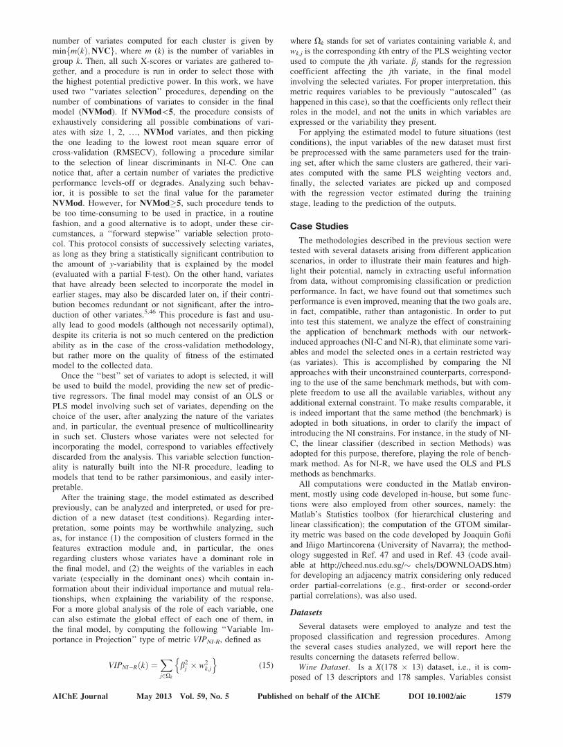
Results for network-induced classification (NI-C)

The comparative assessment of NI-C and its benchmarkmethod (the linear classifier), is based on the analysis of thefigure of merit, global accuracy (overall percentage of cor-rect class assignments), which was computed in three differ-ent ways, as described below.

Resubstitution Accuracy. In this case, the classificationaccuracy is computed with the same dataset used to ‘‘train’’the methodology. It is a measure of the method’s self-consis-tency, i.e., its ability for classifying the same observationsthat were used to develop it. Resubstitution accuracy doesnot provide much information about the classification per-formance with new, never before seen data, and may even

lead to rather poor models in this sense, if one blindly seeksto optimize it by overfitting the training dataset. However, amethod cannot be accepted has good, if it fails this self-con-sistency test, meaning that it is a necessary condition, butnot sufficient, for methods selection.

Monte-Carlo Cross-Validation Accuracy. In Monte-Carlocross-validation (MC-CV), a random train/test data split isperformed a number of times, say, k ¼ 1,…,N_CV_TRIALS,where the training set is used to estimate the model parame-ters and the test set to evaluate its performance (i.e., to com-pute the accuracy for trial k). In each trial k, the adjustableparameters are fixed to values previously estimated(NCLUST, NVC, NVMod), but the algorithm estimate theexact clusters composition, linear discriminants and classifierparameters, in each trial. In the end, a classification measureis obtained by averaging the accuracy scores obtained for alltrials, which characterizes the predictive accuracy of themethodology for the specific set of adjustable parametersadopted (its standard deviation is also computed, in order toprovide a measure of the uncertainty, to complement the in-formation conveyed by the mean). As a portion of the obser-vations is left out in each trial for testing the methodology,MC-CV provides an indication about the performance of themethod with new data, being a good alternative for situa-tions where data is scarce, and no test dataset is available.The method has some limitations however, when the numberof classes is high and with rather few samples per class. Thereason for this limitation lies in the following: during theMonte Carlo trials, in these circumstances, one of the classesmay not be properly represented in the training datasets,leading to poor classification models, and, therefore, to badclassification performances for such trials (a nonstratifiedsampling cross-validation approach was adopted in thiswork, as it tends to provide more conservative estimates ofthe methods accuracy). This may lead to quite unreliableestimates of the methods’ performance. In these situations,the following methodology is advisable.

Leave-One-Out Cross-Validation Accuracy. This method-ology is similar to the previous one, but now the splitting isnot random, but deterministic. In each trial, exactly one sam-ple is left out for testing the method, while the remainingones are used to estimate it, following the same procedureadopted in the Monte Carlo cross-validation approach.Therefore, in the end, we have exactly as many estimates asthe number of samples in the dataset, from which it is possi-ble to compute the overall accuracy (this figure has no vari-ability, when taken for a given dataset). Leave-one-outcross-validation (LOO-CV) usually provides a more optimis-tic estimate for the classification performance, when com-pared to MC-CV, but is more reliable for situations whenfewer observations are available per class. As our case stud-ies comprehend situations where the datasets used vary sig-nificantly in size, we will use both types of validation meth-odologies (MC-CV and LOO-CV), in order to characterizethe methods’ performances.

For the benefit of space, not all the outputs produced andanalyzed in each case study will be presented in this article,although some will be shown to better illustrate the methods’procedures and analysis features. The summary of the classi-fication results obtained for each dataset is presented in Ta-ble 1, where it also appears specified the order of the partialcorrelations used in the computations, as well as the methodparameters selected, according to the methodologiesdescribed in the preceding section.


Results for the Wine Dataset. As mentioned before, thewine dataset does not pose, in general, significant problemsto classifiers for achieving classification scores of good qual-ity, and, therefore, our goal in using it, is to analyze thepotential performance degradation of our methodology rela-tive to the benchmark in this simpler situation, which isexpected to arise due the constraints imposed by consideringonly a maximum of three linear discriminants (NVMod ¼3). Looking to the results presented in Table 1, and in partic-ular to what concerns the resubstitution accuracy, it is possi-ble to see that the benchmark method gets the full score of100% of correct classifications, whereas our method fallsbehind by 1,7% or 0.6% (depending on the partial correla-tion order considered). The fact that the benchmark methodalways overtakes the proposed methodology in this consis-tency test hardly can be directly extrapolated as meaning abetter predictive classification performance, as it may wellbe due to some overfitting of the training data, in which caseit may, in part, compromise its prediction accuracy. There-fore, one should always interpret the resubstitution testresults with some reserve, using them in order to checkmainly whether the methods under analysis did not fail onsuch basic testing condition, but without giving much rele-vance to small performance differences.

Regarding the tests that provide more information about themethods predictive ability, we can see that the MC-CV accu-racy is slightly lower for the proposed methodology (howeverperfectly within the error bands for the mean values of thebenchmark method), being virtually the same for the case ofsecond-order partial correlations. The results for the more op-timistic (less conservative) LOO-CV accuracy, again providesa very slight edge of the benchmark method.

To sum-up, one can see from the analysis of the resultsobtained in this case study, that the performance degradationwas really small, even though that NI-C potentially led to alower number of variables when using full-order partial cor-relations. In fact, in this situation, when selecting the numberof variates to retain in our methodology, there is one particu-lar cluster whose discriminants are more prevalently selectedfor the classification model (Cluster 2, Figure 7). This meansthat the other cluster is not playing such a significant role inthe classification task, which may indicate that its wine com-pounds are not very relevant for discriminating the threewine producers from the same region. This information notonly carries a significant interpretational value, but also ena-bles the selection of candidate compounds as ‘‘producermarkers’’, which can act as their specific production finger-

prints. (Note that during the MC- and LOO- cross-validationtrials for computing the predictive accuracies, one does notcontrol the selections made by the method regarding theclusters formed and linear discriminants selected, but onlythe methods parameters NCLUST, NVC, NVMod, whichare kept constant, and were preliminarily selected using Fig-ure 7, and, therefore, cannot guarantee that the aforemen-tioned comments will be valid in every cross-validation trial,as they are for the full dataset.)

Results for the Roughness Dataset Some preliminaryplots obtained in the analysis of these dataset were alreadypresented earlier (Figures 4 and 6). As can be seen from Ta-ble 1, our method tends to present now slightly better meanprediction accuracies than the benchmark, under cross-vali-dation conditions, meaning that the constraints raised by thetopological-driven organization of variables and the limitednumber of variates allowed to build the model, are not com-promising the performance of the classifier. It can also beseen that the performance obtained with the second-orderpartial correlation was, in this case, slightly lower. The

Figure 7. Plot of the performance for the best combi-nation of a given size (one, two, etc.) vs. thesize of the combinations.

In this case, the size chosen was NVMod ¼ 3, as after

this point the improvement in performance is minor.

Legend: CL–Cluster identifier; DL-linear discriminant

identifier, regarding the cluster it is relative to. (Data

from the ‘‘Wine’’ dataset.) [Color figure can be viewed

in the online issue, which is available at wileyonlineli-

brary. com.]

Table 1. Results for the NI-C Framework and the Benchmark Method (Linear Classifier): Global Accuracy (%) Computedusing Resubstitution (consistency test), Monte-Carlo Cross-Validation (MC-CV, the Standard Deviation appears inside

Parenthesis) and Leave-One-Out Cross-Validation (LOO-CV)

Case studyPartial correlation

order

Method’s adjustableparameters

Global accuracy measures (%)1st line:Proposed method (NI-C) 2nd line: Benchmark

NCLUST NVC NVMod Re-subs. MC-CV LOO-CV

Wine foPC 2 2 3 98.3 98.2 (1.9) 97.2100 98.3 (1.5) 98.9

2oPC 2 2 3 99.4 97.1 (2.3) 97.8100 98.3 (1.5) 98.9

Roughness foPC 3 2 3 97.2 89.3 (13.8) 94.4100 82.9 (11.0) 88.9

2oPC 4 2 3 97.2 85.0 (10.8) 77.8100 82.0 (11.0) 88.9

Note: The method adjustable parameters used, and the order of the partial correlation adopted for computing the adjacency matrix, are also shown.


variables that are more relevant for classification are thosepertaining to cluster 2 (in the case where full-order partialcorrelations are employed), as discriminants from this clusterare always selected, independently of the combination sizeconsidered (see Figure 6). This cluster is formed by the pro-filometry descriptors 50 [Ra, Rq, Rt, RS, RSm, Rdq, RKu],which were already found to be good candidates for describ-ing the roughness behavior of the paper surface.48

Results for network-induced regression (NI-R)

In this section, we analyze two real world case studies,which illustrate the main features, flexibility and applicationpotential of NI-R. Several graphical outputs and informationare presented for each situation, in order to exemplify itsimplementation in practice, and the predictive performanceof the estimated models are computed, for establishing aproper comparison with that achieved with the benchmarkmethods (OLS and PLS).

The predictive performance is evaluated through MonteCarlo cross-validation and leave-one-out cross-validation. InMonte Carlo cross-validation, a random set with approxi-mately 20% of the samples in the training dataset is left asideand, with the remaining samples, a model is estimated andused to predict the values for the output variables in the sam-ples left aside. The following quantities are then computed, ineach cross-validation trial (k), the first one relative to a mea-sure of the prediction error incurred in that trial, while the sec-ond represents an extension of the well-known coefficient ofdetermination R2, to the cross-validation context

RMSECVðkÞ ¼

ffiffiffiffiffiffiffiffiffiffiffiffiffiffiffiffiffiffiffiffiffiffiffiffiffiffiffiffiffiffiPnout

i¼1 yi � yið Þ2

nout

s(16)

R2CV kð Þ ¼ 1 �

Pnout

i¼1 yi � yið Þ2Pnout

i¼1 yi � �youtð Þ2(17)

where nout represents the number of observations left out in thekth cross-validation run (k ¼ 1,…,20) and yout the respectivemean of the output variable. This procedure is repeated 20times, in order to mitigate distortions from the randomallocation of observations in the two groups. In the end, theoverall mean and standard deviation for these two quantities,RMSECV and R2

CV , are computed and reported.As for LOO-CV, the procedure is similar, but only one

observation is left aside in turn. This procedure stops whenall observations were left aside once and only once, afterwhich the following quantities are computed for evaluatingthe predictive ability of the method:

RMSELOO�CVðkÞ ¼

ffiffiffiffiffiffiffiffiffiffiffiffiffiffiffiffiffiffiffiffiffiffiffiffiffiffiffiffiffiffiffiffiffiffiffiffiPni¼1 y ið Þ � y ið Þ

� �2

n

s(18)

R2LOO�CV kð Þ ¼ 1 �

Pni¼1 y ið Þ � y ið Þ

� �2Pni¼1 y ið Þ � �y

� �2(19)

where, y(i) and y(i) stand for the value of the output variableand its estimate, respectively, regarding the trial where the ithobservation is left out. Notice that, with LOO-CV, these twoquantities are fixed, for a given training dataset (no mean andstandard deviation are then reported, as happens in the MonteCarlo cross-validation approach).

For comparison purposes, the predictive performancesobtained with PLS and OLS (when appropriate) will also bepresented, as these methods represent the best approxima-tions of the unconstrained counterparts of NI-R, i.e., theyrepresent the solutions that would be obtained if no interpre-tational-oriented constraints were enforced in NI-R. Theseresults will enable the evaluation of the impact of introduc-ing the interpretational-oriented restrictions in the modelingstage, on the method’s prediction ability, relatively to theunconstrained situation, where all variables are employedand their parameters estimated freely.

Also reported is the fitting ability of the methods, givenby the root mean square error of calibration (RMSEC),obtained with the same dataset used for estimating the model(i.e., under resubstitution conditions), and the respectivecoefficient of determination R2:

RMSEC ¼

ffiffiffiffiffiffiffiffiffiffiffiffiffiffiffiffiffiffiffiffiffiffiffiffiffiPn

i¼1

yi � yið Þ2

n

vuuut(20)

R2 ¼ 1 �

Pn

i¼1

yi � yið Þ2

Pn

i¼1

yi � �yð Þ2¼

Pn

i¼1

yi � �yið Þ2

Pn

i¼1

yi � �yð Þ2(21)

These quantities provide a simple measure of how wellthe estimated model fit the data that were used to develop it,therefore offering a straightforward analysis of its quality offitness, but they are of very limited value for assessing themethod’s predictive performance.

Results for the Roughness Dataset This case study is the

continuation of the one presented in the previous subsection.

The same 11 input variables regarding geometrical-oriented

features at the roughness scale (the finer scale of analysis),

and computed from accurate profiles taken over a sheet of

paper, using high-resolution mechanical stylus profilometry,

correspond also to the set of X-variables adopted here. How-

ever, for each of the 36 observations available, besides the

classification labels used to implement the classification

methods, another type of measurement was collected, for

each sample, using an equipment called, the ‘‘Bendtsen tes-

ter’’. The measurement principle of this instrument, consists

of quantifying the amount of air that escapes, during a given

period of time, between a standardized ring put over the pa-

per sheet and the sheet itself, at constant pressure.50 This

equipment is able to provide an inferential measure of sur-

face roughness, in a short period of time, but its interpreta-

tion is not clear, as many aspects of the paper structure can

interfere. Therefore, it would be interesting to explain the

variability of Bendtsen measurements in terms of fundamen-

tal geometrical features of the paper surface; in order to

understand from which structural characteristics it mainly

depends on. This can be achieved by defining the Bendtsen

tester values as the output variable of the analysis y, and de-

velop a regression model to explain its variability. The final

Bendtsen value used for each sample is the mean of five

replicated measurements.In order to apply the NI-R framework to these dataset, 4

clusters of variables were considered now (NCLUST ¼ 4)for the case where the order of the partial correlation is 2,as a result of the analysis of the variables dendrogram for


the NI-clustering algorithm and the associated TOM plot,presented in Figure 8a). The silhouette plot (Figure 8b)confirms the adequacy of the clusters formed, as all valuesfor the input variables are positive, indicating that theytend to be more distant from others belonging to theneighbor clusters, when comparing to those on the samecluster.

After defining the number of variable clusters, the num-ber of variates to include in the final model must be set,looking to the evolution of the cross-validated errors forincreasing values of this parameter, leading to NVMod ¼4. The NI-R results obtained for such a model are pre-sented in the first line of Table 2. As can be appreciated,the fitting ability of the NI-R model is very good (re-sub-stitution). It also leads to the best prediction accuracyscores when evaluated with the LOO-CV method, relativelyto the benchmark methods, even though its variability is

higher under MC-CV, due to its more complex structureand the limited amount of data available (only 36 observa-tions), which naturally leads to some variation in the mod-els developed, when 20% of the data is removed from thetraining set in each trial of the MC-CV procedure. There-fore, introducing interpretational constrains in the model, asproposed in the NI-R methodology, does not seem to haveany tangible and significant effect in prediction accuracy inthis case study, and can help the interpretation of results.For instance, the VIPNI-R scores seem to indicate an impor-tant contribution of the parameter RSm, the mean width ofprofile elements, and Rdq, the RMS slope of profile, in theexplanation of the variability of measurements provided bythe Bendtsen tester (Figure 9). As this instrument operatesaccording to the principle of air leakage, it indeed makessense that the profile elements’ width (an element is asequence of a ‘‘mountain’’/‘‘valley’’ in the profile) has animportant impact in the amount of air flow, the sameapplying to other profile element’s features, such as theirslope.

This case study illustrates the ability of the NI-R methodto introduce interpretational elements in the analysis, withoutcompromising prediction ability.

Results for the Pulp and Paper Dataset As referredbefore, the outputs considered in this case study are themeasurements of the TSO angle at 9 positions in the cross-direction of a paper machine. The TSO profiles analyzed arepresented in Figure 10a). They correspond to process condi-tions, for which one also has available the corresponding X-variables (process variables). In order to implement NI-R,these profiles were first decomposed using principal compo-nent analysis (PCA), and the first two scores, T1 and T2,which explain approximately 82.5% of the whole variabilityof the profiles, were used as the output variables for analysisy1 and y2. The loads for these first two principal components(PC) are presented in Figure 10b), where we can see that thefirst PC (PC1) represents a contrast between the TSO anglesin the two sides of the paper machine, while the second PC(PC2) gives more weight to the central measurements, beingable to explain the presence and variability of bias in theTSO angle, in such an important section of the papermachine. Therefore, the two PCs represent different aspectsof the fiber orientation profile, and the goal here is to findout which of the 37 process variables studied, are mostinvolved in the variability of each PC, in order to developactuation policies for better controlling the cross-directionaluniformity of this parameter.

NI-R models were developed for PC1 and PC2 as outputvariables. During this process, where the various methods’parameters were tuned, it was verified that the order of thepartial correlation used in NI-clustering algorithm leading tothe best predictions, differ according to the output variablebeing addressed. For PC1, the best results were achievedwith the full-order version, whereas for PC2, the second-order coefficients lead to the best prediction scores (Table2). Given the number of clusters identified for each situation([5), the ‘‘forward stepwise’’ variable selection algorithmwas employed in order to select the variates that will inte-grate each one of the two models. The VIPNI-R plots for thefinal models, i.e., for each PC of the TSO profile, are pre-sented in Figure 11, where it can be seen that there are morevariables affecting the tilting of the TSO profile (PC1), thanits bias at the central region of the paper machine (PC2).This result means that there is an opportunity to manipulate

Figure 8. Auxiliary plots for selecting the number ofclusters (NCLUST) in the ‘‘roughness’’ casestudy.

(a) Dendrogram and TOM plot, and (b) Silhouette plot.

(They correspond to case where second-order partial

correlations are used for computing the generalized top-

ological similarity measure, GTOM). [Color figure can

be viewed in the online issue, which is available at

wileyonlinelibrary.com.]


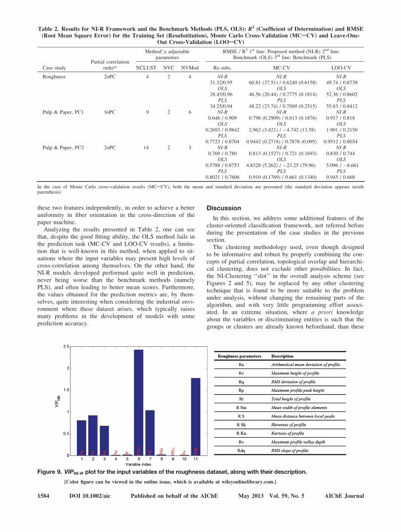
these two features independently, in order to achieve a betteruniformity in fiber orientation in the cross-direction of thepaper machine.

Analyzing the results presented in Table 2, one can seethat, despite the good fitting ability, the OLS method fails inthe prediction task (MC-CV and LOO-CV results), a limita-tion that is well-known in this method, when applied to sit-uations where the input variables may present high levels ofcross-correlation among themselves. On the other hand, theNI-R models developed performed quite well in prediction,never being worse than the benchmark methods (namelyPLS), and often leading to better mean scores. Furthermore,the values obtained for the prediction metrics are, by them-selves, quite interesting when considering the industrial envi-ronment where these dataset arises, which typically raisesmany problems in the development of models with someprediction accuracy.

Discussion

In this section, we address some additional features of thecluster-oriented classification framework, not referred beforeduring the presentation of the case studies in the previoussection.

The clustering methodology used, even though designedto be informative and robust by properly combining the con-cepts of partial correlation, topological overlap and hierarchi-cal clustering, does not exclude other possibilities. In fact,the NI-Clustering ‘‘slot’’ in the overall analysis scheme (seeFigures 2 and 5), may be replaced by any other clusteringtechnique that is found to be more suitable to the problemunder analysis, without changing the remaining parts of thealgorithm, and with very little programming effort associ-ated. In an extreme situation, where a priori knowledgeabout the variables or discriminating entities is such that thegroups or clusters are already known beforehand, than these

Table 2. Results for NI-R Framework and the Benchmark Methods (PLS, OLS): R2 (Coefficient of Determination) and RMSE(Root Mean Square Error) for the Training Set (Resubstitution), Monte Carlo Cross-Validation (MCACV) and Leave-One-

Out Cross-Validation (LOOACV)

Case studyPartial correlation

order*

Method’;s adjustableparameters

RMSE / R2 1st line: Proposed method (NI-R) 2nd line:Benchmark (OLS) 3rd line: Benchmark (PLS)

NCLUST NVC NVMod Re-subs. MC-CV LOO-CV

Roughness 2oPC 4 2 4 NI-R NI-R NI-R31.32/0.95 60.81 (37.51) / 0.6240 (0.6158) 49.74 / 0.8739

OLS OLS OLS28.45/0.96 46.56 (20.44) / 0.7775 (0.1814) 52.36 / 0.8602

PLS PLS PLS34.25/0.94 48.22 (23.74) / 0.7569 (0.2515) 55.83 / 0.8412

Pulp & Paper, PC1 foPC 9 2 6 NI-R NI-R NI-R0.646 / 0.909 0.798 (0.2909) / 0.813 (0.1876) 0.917 / 0.818

OLS OLS OLS0.2693 / 0.9842 2.962 (3.421) / �4.742 (13.58) 1.901 / 0.2150

PLS PLS PLS0.7723 / 0.8704 0.9442 (0.2718) / 0.7878 (0.095) 0.9512 / 0.8034

Pulp & Paper, PC2 2oPC 14 2 3 NI-R NI-R NI-R0.769 / 0.780 0.813 (0.1527) / 0.721 (0.1693) 0.830 / 0.744

OLS OLS OLS0.5788 / 0.8753 4.8328 (5.262) / �23.25 (79.96) 5.096 / �8.661

PLS PLS PLS0.8021 / 0.7606 0.910 (0.1769) / 0.661 (0.1340) 0.945 / 0.668

In the case of Monte Carlo cross-validation results (MCACV), both the mean and standard deviation are presented (the standard deviation appears insideparenthesis)

Figure 9. VIPNI-R plot for the input variables of the roughness dataset, along with their description.

[Color figure can be viewed in the online issue, which is available at wileyonlinelibrary.com.]


can immediately be used as the final result from the cluster-ing operation. Therefore, NI-Clustering can be implementedeither in ‘‘data-driven’’ mode, strictly based on collecteddata, or in ‘‘knowledge-driven’’ mode, where backgroundknowledge is used to introduce interpretational constrains inthe form of variable clusters. The important issue, is thatclusters or groups of variables reflect some deeper associa-tion among the variables, that could be recognized and maybe associated with particular roles, operations, functions,etc., so that, after implementing NI-C or NI-R, one can beable to extract and combine knowledge from the two rele-vant data modes, namely the variables structure (from clus-tering), and the observations structure (from the classificationor regression tasks).

Naturally, sometimes, clustering approaches do not lead toclear and identifiable clusters and some variables might beassigned to the wrong groups. The way the proposed classifi-cation framework deals with this problem, is through theselection of linear discriminants also belonging to other clus-ters where relevant variables for classification are dispersed,if such improves the estimated classification performance ofthe method. Of course this leads to a less parsimonious solu-tion, but brings the capability of mitigating the effects of anot so well succeeded clustering operation.

The same flexibility applies to the classifier and linearregression methods adopted. Any methodology can be usedinstead of the linear classifier and linear regressionapproaches used in this work. For example, in situationswhere the distribution of the observations from the severalclasses, in the mulivariate space, present peculiar shapes,such might really be necessary, but to start with the simple,and so often effective, linear framework, is recommended.

We would also like to point out that the second stage of

the proposed NI approaches, where the respective modeling

tasks are conducted (Figure 2), consists also of a two-steps

process: in the first step, the best models within each cluster

are obtained, giving rise to a number of variates; in the sec-

ond step, variates from all clusters are combined, in order to

derive the final classification or regression model. In other

words, the first modeling step regards developing models

within each cluster, while in the second step the problem of

finding the best synergistic association between the variates

is considered.Finally, as in the implementation of any predictive frame-

work, one should always exercise some care regardingextrapolation, by checking if the measurements under analy-sis fall within the region used to develop them. This can beaccomplished, for instance, by computing the estimatedMahalanobis distances to the center of the training dataset,and verifying if they are of the same magnitude as thoseused in the training stage, as well as looking at the residualsaround the selected variates, and check if they are of thesame magnitude as those computed in the training stage.

Conclusions

We have presented in this article, an integrated supervisedlearning framework with the ability to explore the natural

Figure 10. A set of real TSO profiles from the pulp andpaper dataset (a) and the loads for the firsttwo principal components obtained from aPCA decomposition, applied to such a set(b).

[Color figure can be viewed in the online issue, which

is available at wileyonlinelibrary.com.]

Figure 11. VIPNI-R plot for the process variables affecting the TSO profiles in the pulp and paper dataset (a) NI-Rmodel for PC1, and (b) NI-R model for PC2.

[Color figure can be viewed in the online issue, which is available at wileyonlinelibrary.com.]


structure of variables, for predicting class labels, through themethodology called network-induced classification (NI-C),and for estimating the level of a continuous response, usingnetwork-induced regression (NI-R). The variables structureis described by their direct mutual affinity, inferred frompartial correlation coefficients. The connective arrangement,resulting from retaining only the most relevant (strongest)links is coded in the form of an adjacency matrix, fromwhich the topological overlap between any pair of variablesis computed, as a measure of the variables affinity. This isfinally employed for running a clustering algorithm, in orderto identify groups of variables with strong mutual topologi-cal similarities (network-induced clustering). Then, at a sec-ond stage, these clusters are subjected to a selection opera-tion, according to their discrimination or predictive power,depending on the type of application (classification or regres-sion). Clusters found relevant will provide variates to beused in the final model, whereas others are tacitly removedfrom the analysis.

This framework elucidates which are the natural clustersof variables present, associated with some sort of systemsfunction, operation, etc., that are furthermore driving the pre-diction of outputs (class labels or a continuous response).Therefore, NI-C and NI-R enable the interception of the twosources of knowledge arising from data: variables structureand observations structure. The results presented illustratethat such knowledge can indeed be extracted, without com-promising the classification and prediction accuracies.

The proposed methodology finds interesting applicationsin the analysis of datasets from a variety of sources, such asthose arising from biosystems, where one is concerned inexplaining both the variable structure and natural groups ofspecimens, and industrial systems, where data is increasinglycomplex, and models that are both parsimonious and inform-ative are required to support the analysis. Future work willaddress applications in other scenarios, as well as try to bet-ter clarify the role of the partial correlation order in thescope of the proposed methodology.

Acknowledgments

The author acknowledges financial support through project PTDC/EQU-ESI/108374/2008, cofinanced by the Portuguese FCT and Euro-pean Union’s FEDER, through ‘‘Eixo I do Programa Operacional Fac-tores de Competitividade (POFC)’’ of QREN (with ref. FCOMP-01-0124-FEDER-010397).

Literature Cited

1. Jackson JE. A User’s Guide to Principal Components. New York:Wiley; 1991.

2. Johnson RA, Wichern DW. Applied Multivariate Statistical Analysis.3rd ed. Englewood Cliffs, NJ: Prentice Hall; 1992.

3. Martens H, Naes T. Multivariate Calibration. Chichester: Wiley; 1989.4. Chaterjee S, Price B. Regression Analysis by Example. 2nd ed. New

York:Wiley; 1998.5. Draper NR, Smith H. Applied Regression Analysis. 3rd ed. NY:

Wiley; 1998.6. Geladi P, Kowalski BR. Partial least-squares regression: a tutorial.

Anal Chimi Acta. 1986;185:1–17.7. Haaland DM, Thomas EV. Partial least-squares methods for spectral

analysis. 1. relation to other quantitative calibration methods and theextraction of qualitative information. Anal Chem. 1988;60:1193–1202.

8. Helland IS. On the structure of partial least-squares regression. Com-mun Statist Simula. 1988;607–17(2):581.

9. Hoskuldsson A. Prediction Methods in Science and Technology.Ventura, CA: Thor Publishing; 1996.

10. Wold S, Sjostrom M, Eriksson L. PLSAregression: A basic tool ofchemometrics. Chemo Intell Lab Syst. 2001;58:109–130.

11. Hastie T, Tibshirani R, Friedman J. The Elements of StatisticalLearning. New York, NY: Springer; 2001.

12. Hoerl AE, Kennard RW. Ridge regression: biased estimation fornonorthogonal problems. Technometrics. 1970;12(1):55–67.

13. Seber GAF, Wild CJ. Nonlinear Regression. New York: Wiley; 1989.14. Breiman L, Friedman JH, Olshen RA, Stone CJ. Classification and

Regression Trees. Belmont, CA: Wadsworth International Group; 1984.15. Johnson RA, Wichern DW. Applied Multivariate Statistical Analysis.

5th ed. Upper Sadle River, NJ: Prentice Hall; 2002.16. Van der Heijden F, Duin RPW, De Ridder D, Tax DMJ. Classification,

Parameter Estimation and State Estimation. Chichester: Wiley; 2004.17. Barker M, Rayens W. Partial least squares for descrimination. J

Chemometrics. 2003;17:166–173.18. Wold S, Sjostrom M. SIMCA: a method for analyzing chemical

data in terms of similarity and analogy. Chemon Theory Appl.1977;243–282

19. Derde MP, Massart DL. UNEQ: A disjoint modelling technique forpattern recognition based on normal distribution. Anal Chimi Acta.1986;184:33–51.

20. Kadlec P, Gabrys B, S. S. Data-driven Soft Sensors in the processindustry. Comp Chem. Eng. 2009;33(4):795–814.

21. Kresta JV, MacGregor JF, Marlin TE. Multivariate statistical monitoringof process operating performance. Can J Chem Eng. 1991;69:35–47.

22. Lin B, Recke B, Knudsen JKH, Jørgensen SB. A systematic approachfor soft sensor development. Comp Chem Eng. 2007;31(5):419–425.

23. MacGregor JF, Kourti T. Multivariate Statistical Treatment of His-torical Data for Productivity and Quality Improvements. Paper pre-sented at: Foundation of Computer Aided Process Operations -FOCAPO 98; 1998.

24. Reis MS. A Multiscale Empirical Modeling Framework for SystemIdentification J Process Contr. 2009;19(9):1546–1557.

25. Saraiva PM, Stephanopoulos G. Continuous Process Improvementthrough Inductive and Analogical Learning. AIChE Journal.1992;38(2):161–183.

26. Box GEP, Hunter JS, Hunter WG. Statistics for Experimenters: Design,Innovation, and Discovery. 2nd ed. Hoboken, NJ: Wiley; 2005.

27. Guyon I, Elisseeff A. An Introduction to Variable and FeatureSelection. J Machine Learn Res. 2003;3:1157–1182.

28. Vapnik V. The Nature of Statistical Learning Theory. 2nd ed. NewYork: Springer-Verlag; 2000.

29. Lisy JM, Cholvadova A, Kutej J. Multiple Straight-line LeastSquares Analysis with Uncertainties in all Variables. Comput Chem.1990;14:189–192.

30. Martınez A, Riu J, Rius FX. Evaluating Bias in Method ComparisonStudies Using Linear Regression with Errors in Both Axes. J Che-mom. 2002;16:41–53.

31. Mandel J. Fitting Straight Lines when both Variables are subject toError. J Quality Technol. 1984;19(1):1–14.

32. Reis MS, Saraiva PM. A comparative study of linear regressionmethods in noisy environments. J Chemom. 2004;18(12):526–536.

33. Reis MS, Saraiva PM. Integration of data uncertainty in linear regres-sion and process optimization. AIChE J. 2005;51(11):3007–3019.

34. Wentzell PD, Andrews DT, Hamilton DC, Faber K, Kowalski BR.Maximum likelihood principal component analysis. J Chemom.1997;11:339–366.

35. Wentzell PD, Andrews DT, Kowalski BR. Maximum likelihoodmultivariate calibration. Anal Chem. 1997;69:2299–2311.

36. Møller SF, Von Frere J, Bro R. Robust methods for multivariatedata analysis. J Chemom. 2005;19:549–563.

37. Ravasz E, Somera AL, Mongru DA, Oltvai ZN, Barabasi A-L. Hier-archical organization of modularity in metabolic networks. Science.2002;297:1551–1555.

38. Clauset A, Moore C, Newman MEJ. Hierarchical structure and theprediction of missing links in networks. Nature. 2008;453:98–101.

39. Guimera R, Amaral LAN. Functional cartography of complex meta-bolic netwoks. Nature. 2005;433(24):895–900.

40. Newman JAS. Modularity and community structure in networks.Proc Nat Acad Sci. 2006;103(23):8577–8582.

41. Sokal RR, Rohlf FJ. Biometry - The Principles and Practice of Sta-tistics in Biological Research. 3rd ed. New York: W.H. Freeman &Co.; 1994.

42. Hoskuldsson A. PLS regression methods. J Chemom. 1988;2:211–228.43. Rao KR, Lakshminarayanan S. Partial correlation based variable

selection approach for multivariate data classification methods. Che-mom Intell Lab Syst. 2007(86):68–81.

44. Yip AM, Horvath S. Gene network interconnectedness and the gener-alized topological overlap measure. BMC Bioinform. 2007;8(22):1–14.


45. Dillon WR, Goldstein M. Multivariate Analysis - Methods andapplications. New York: Wiley; 1984.

46. Montegomery DC, Peck EA, Vining GG. Introduction to LinearRegression Analysis. 4th ed. Hoboken, NJ: Wiley; 2006.

47. de la Fuente A, Bing N, Hoeschele I, Mendes P. Discovery of mean-ingful associations in genomic data using partial correlation coeffi-cients. Bioinformatics. 2004;20(18):3565–3574.

48. Reis MS, Saraiva PM. Analysis and classification of the paper sur-face. Indust Eng Chem Res. 2010;49(5):2493–2502.

49. Angelico D, Reis MS, Costa R, Saraiva PM, Ataıde J. Profilometry:A Technique to Characterize Paper Surface. Paper presented at:Tecnicelpa - XIX Encontro Nacional, 2005;Tomar, Portugal.

50. Costa R, Angelico D, Reis MS, Ataıde J, Saraiva PM. Paper superfi-cial waviness: conception and implementation of an industrial statis-tical measurement system. Anal Chimi Acta. 2005;544:135–142.

Manuscript received Aug. 3, 2011, revision received Apr. 4, 2012, and finalrevision received Oct. 10, 2012.


network-induced supervised learning: network-induced classification (ni-c) and network-induced...

Documents