network planning in electricity supply industry yu yue

THE HONG KONG POLYTECHNIC UNIVERSITY DEPARTMENT OF ELECTRICAL ENGINEERING

1

Project ID: PT_FYP_62

Network Planning in Electricity Supply Industry by

YU YUE

13018698D

Final Report

Bachelor of Engineering (Honours) in

Electrical Engineering

Of

The Hong Kong Polytechnic University Supervisor: Dr. C.W.YU Date: 07-11-2016


i

Abstract

In power system, network planning is an important element of good grid construction to ensure

normal operation of power system. Good grid construction relies on scientific network planning,

so strengthening the power network planning can effectively improve the level of grid

construction.

In this project, linear programming is introduced to help in the long range design of the

transmission network of an electric power system. The aim of using linear programming is to

conceive a workable network for a rapidly growing region at a future time when loads have more

than doubled, new generating stations are not yet connected into the system and new voltage

levels may be needed. A minimization linear programming problem is formulated using the

combination of a DC power flow model and a transportation network mode. The DC power flow

solves for the existing transmission circuits obeying both of Kirchhoff’s laws.

The transportation network solves for the “overload” flow by requiring only that the flow

conservation law at each node be satisfied. This transportation model is solved only when

electrical flow limits are reached. The nodal connectivity matrix of the transportation network

constitutes the key point for the joint solution of the two models. The problem is formulated as

the minimization of the discounted capital investments associated with the system expansion

over the planning horizon, subject to the line flow constraints and the system power balance

constraint (sum of generation equal sum of load) not considering losses. This method produces

an indication of those corridors where capacity shortage exists, where new circuits are needed,

and determines how much transmission capacity is needed.

A user-friendly program using linear programming is developed to deal with this complex

problem.


ii

Acknowledgment

I wish to express my gratitude to Dr. Chi-wai YU, Adjunct Associate Professor, Department of

Electrical Engineering, for giving me a lot of useful advice and encouraging me to successfully

complete my project. Dr.YU has provided his professional suggestions to me so that the project

can work more efficient and has been solved those difficulties.

Dr. Yu-fai FUNG, Senior Teaching Fellow, Department of Electrical Engineering is thanks for

his excellent guidance and support received to complete this project.


iii

Table of Contents

Abstract ........................................................................................................................................... i

Acknowledgements ....................................................................................................................... ii

1. Introduction ............................................................................................................................. 1

2. Objectives................................................................................................................................. 4

3. Background ............................................................................................................................. 5

3.1 Network Planning ........................................................................................................... 5

3.2 Linear Programming ...................................................................................................... 7

3.3 Software .......................................................................................................................... 8

4. Methodology .......................................................................................................................... 11

4.1 Block Diagram of Program Design ............................................................................. 11

4.2 Creating a MATLAB GUI with GUIDE..................................................................... 12

4.3 The Direct Current Load Flow Equations ................................................................... 15

4.4 System Model ............................................................................................................... 19

4.5 Formulation as a Linear Programming Problem ........................................................ 20

4.6 Optimization Toolbox of MATLAB ........................................................................... 21

4.7 Data arrangement.......................................................................................................... 22

4.8 Program Progress.......................................................................................................... 24


iv

5. Results .................................................................................................................................... 31

6. Discussions ............................................................................................................................. 40

7. Conclusions ............................................................................................................................ 41

7.1 The Linear Programming Method ............................................................................... 41

7.2 Graphical User Interfaces program in MATLAB ...................................................... 43

Referrences .................................................................................................................................. 45


1

1. Introduction

The electric power system engineer is faced with the challenging tasks of planning and operating

successfully one of the most complex systems of today’s civilization. This demands a knowledge,

first of all, of the priorities and objectives involved. The basic requirement is to meet the demand

for electric energy (load) in the area served by the system. A prime objective is to perform the

service at the lowest possible cost.

The physical power system structure is compelled to change due to the load growth. New

generation need to be added to the system in order to satisfy the new load requirements. Ideally,

it would suffice to develop new generation at those places where the load exists. Practically this

is not the case and for the majority of power systems, the new generation has to be placed away

from the load centers. In the process, decisions have to be made in order to select the best kind of

generating plants and sitting and the best routes for the transmission and distribution systems.

This decision process places a problem of very large magnitude in the hands of the power system

engineer. It is necessary to develop strategies to assure that the decisions made are the best or at

least nearly the best. The goal is to decide on a system design that minimizes systems costs while

meeting a forecasted future load profile and some reliability criterion. This is what is basically

known as “electric power system planning”.

Ideally, the long range planning of a whole power system should be carried out on an integrated

basis. However, to make the practical problems of the system design tractable, it is convenient to

break the procedure down into parts associated with the main subsystems: generation,

transmission and distribution. This type of hierarchical decomposition is logical from several

points of view [1].

The first point to consider is that various completion times are associated with the discrete items


2

that include a remote system expansion plan. The next consideration is the problems and design

philosophies associated with the different parts of the total power system are inherently

dissimilar. For example, distribution system planners require detailed knowledge of localized

geographic areas and must be familiar with thousands of small components, such as distribution

transformers, switches and re-closers. The analysis of these devices does not usually require

complex models. At the other extreme, generation planning is carried out a more aggregate

system-wide level and is concerned with several relatively large generation units, generally

having modes of interaction that are more complex to analyze. Consequently, the models and

criteria currently used to design the various subsystems are also different [2]. In this project, we

are concerned with planning the transmission subsystem, the lead time of which is between two

and five years.

As evidenced by the literature, the use of linear programming (LP) as a mathematical

optimization tool with linearized formulations of the power system expansion planning problem

has been extensive [2]. The linear approach has been advocated on the grounds that in contrast

with the non-linear alternative, the LP solution is highly reliable and accuracy is adequate for

most planning purposes.

As mentioned before, the prime objective of this project is to find a mathematical model for the

transmission planning problem which can automatically identify the minimum (less costly)

reinforcements (transmission lines) to the network and the corridors where such reinforcements

are necessary.

In this project, MATLAB is chosen as the implementation language and tool. The linear

programming is introduced to solve the network planning problems. The development of

algorithms to efficiently solve particular large-scale systems has become a major concern in


3

applied mathematical programming. Linear programming demonstrated the ability to solve the

optimization problems, like transmission network expansion planning problem.


4

2. Objectives

Most existing methods for transmission network planning are designed to find an optimal

network development through the years to satisfy the intermediate electrical requirements of the

system. Few attempts have been made to try to find a long range network design that could serve

as guideline for the short term network reinforcements. As mentioned before, the main difficulty

lies in the several nodes being considered during the planning process could be unconnected to

the existing network. Standard electrical analysis techniques cannot be used during this

preliminary planning stage of the network. It is at this point where the contributions described in

this project are most valuable.

The objectives of this project are:

I. To develop theoretical aspects of the transmission network planning problem by considering

the operational constraints for transmission horizon planning.

II. To solve the transmission network planning problem by taking into account conditions in the

power system operation such as the possibility of a generation plant to operate at the limit

and pool operation conditions satisfied.

III. To optimize the network planning in order to satisfy the economy, reliability and safety of

the electricity supply system.

IV. To develop a user-friendly program to simulate the transmission network planning problem.


5

3. Background

3.1 Network Planning

Network planning is an important part of power system planning. Its task is to find out an

optimal network configuration according to a generation planning scheme and load growth for

the planning period so as to deliver electricity safely and economically [3].

Transmission planning is closely related to generation planning. Because generation requires

greater lead time, it is planned before transmission. When transmission planning is undertaken,

the sites, sizes and characteristics of future generation additions are presumably already

established. The information related to load growth and available transmission corridors is also

normally at the disposal of the transmission planner.

When load increases or new load centers develop and when new generators are added, they are

in effect initially connected to the existing network, through zero capacity transmission links.

The lack of transmission capacity automatically creates an overload situation resolved only by

adding lines of appropriate capacity to interconnect the new elements to the system or to

reinforce the existing system. The problem reduces to determining where, when and in what

amount to expand the transmission system so that no overloaded lines are produced under certain

given condition for some future forecasted load level. Of course the expansion plan sought is

always the minimum cost plan.

One of the major difficulties of the transmission planning problem comes from the tremendous

number of possible alternative derived from the combination of all possible transmission lines

that can be built in the system to relieve the overload.

The planning methods and the computer aids used in planning are closely interrelated. As

computer aid advance so do the methods; as more sophisticated planning methods evolve, they


6

create demand for more advanced computer aid.

At the present time there seems to be unanimous opinion regarding the approach to the power

system planning problem: build up a long term coherent perspective (a horizon system) which

will serve as a guideline for short and medium term technical-economic studies and thus

determine intermediate reinforcements in a long term perspective. In order words, design a long

range horizon system which biases the design of the year by year (through time) evolving

network. The question is how to find such a reliable horizon system in a network where future

planned generation and new load points are still unconnected to the present network. This is a

real challenge to most existing methods for which the planning of a next development stage of

the network relies on a previous planned stage.

Over the years, numerous methods have been proposed to solve the long range planning problem

with automatic computer technique. Perhaps, the biggest incentive for the development of some

of those methods was the rapid growth of computer facilities. The problem has been approached

in many different ways. Optimization technique being among the more popular used tools.

One of the early proposals to formulate the criteria of the power system design in such a way that

the problem could be solved by an automatic optimization process was put forward by Knight [4]

in 1960. He used a pure integer programming method (IP) to decide upon the transmission

network reinforcements and to minimize an economic objective function of the electrical

network, subject to a set of linear inequalities representing security requirements. However, this

approach was severely limited by the dimensionality of the problem and the performance of the

earlier IP codes.

Alternative attempts to devise automatic computer methods to solve networks of realistic size

have often resorted to heuristic approaches [5].


7

A variety of static optimization procedures have been proposed. The majority of these

procedures assume as known, the present network, and the costs of building transmission lines,

the future loads and generation levels and the availability of transmission corridors.

Garver [6] considered the static problem of designing a network so as to meet a specific load.

Here the problem is formulated as a power flow problem. Linear programming is used to find the

most direct route from generation to loads: all rights of way can carry power, but those without

initial transmission lines are penalized to encourage flow through the existing network.

The linear programming minimization in effect, minimizes an approximation to cost of new

facilities, as the guide numbers that penalize an overload can be related to cost of constructing a

line in the corridors. The discrete additions of transmission circuits are determined using a

round-up procedure. A line is added to the right of way having the largest overload and a new

linear flow is computed. The process terminates when all overloads have been eliminated. The

estimated flow in the final network is fairly close to those computed by a standard load flow.

3.2 Linear Programming

Linear Programming is concerned with the optimizing (minimizing or maximizing) a linear

function while satisfying a set of linear equality or inequality constraints or restrictions.

The objective function takes the linear form

Z = ∑ c x (3. 1)

Where Z is the value to be optimized. The x are the decision variables to be determined and the

c are the (known) cost coefficients [7, 8].

The restrictions assume the form

∑a =,≥,≤ b x ≥ 0 (3. 2)


8

Or

a x + a x +⋯+ a x =,≥,≤ b (3. 3)

a x + a x +⋯+ a x =,≥,≤ b (3. 4)

…………

a x + a x +⋯+ a x =,≥,≤ b (3. 5)

x ≥ 0, x ≥ 0,… , x ≥ 0

Where

i = 1,2,… , mandj = 1,2,… , n

3.3 Software

MATLAB will be used to develop and analyze linear algorithms. MATLAB language is an

interactive mathematical manuscript language syntax which is similar to C/C++. The easiest way

to execute MATLAB code in MATLAB program command window prompt (>>) enter the code,

MATLAB will immediately return the operating result (if any). In this project, MATLAB can be

seen as an interactive mathematical terminal, in simple terms, a powerful computer. MATLAB

code can also be stored in a .m suffix named text file and then call it in the command window or

other functions directly.


9

Figure 3 - 1 MATLAB R2009 Print screen

MATLAB provides a set of data analysis, the development of algorithms and create the

numerical methods of models. MATLAB languages include common mathematical functions to

support engineering and scientific computing. Core processors is to optimize the use of

mathematical function library, we can quickly perform vector and matrix operations.

The graphical user interface development environment (GUIDE) supports MATLAB program to

quickly create a graphical user interface [9].

GUIDE provides tools to design user interfaces for custom apps. Using the GUIDE Layout

Editor, the UI GUIDE can be graphically designed then automatically generated the MATLAB

code for constructing the UI which the behavior of the program can be modified to program.


10

Figure 3 - 2 The GUIDE interface


11

4. Methodology

4.1 Block Diagram of Program Design

Figure 4 - 1 the flowchart for the Network Planning Tool

The flow chart shows how the program is worked. The transmission network system data

will be inputted by user. The system data will be transferred to corresponding matrix and

linearized the deterministic constraints around the power flow problem. The problem will

be solved as a linear programming problem. The answers will be checked whether they


12

are below system tolerances. If they are failed, user is required to input system data again.

If the answer is acceptable, the final answer will be updated by the program.

4.2 Creating a MATLAB GUI with GUIDE

4.2.1 Open a New UI in the GUIDE Layout Editor

a. Start GUIDE by typing guide at the MATLAB prompt [10].

Figure 4 - 2 MATLAB prompt

b. In the GUIDE Quick Start dialog box, select the Blank GUI (Default) template, and then

click OK.


13

Figure 4 - 3 starting window to design

c. Display the names of the components in the component palette:

Figure 4 - 4 Window to design each component in a GUI system

4.2.2 Components using in this project

The program layout uses with UI components such as push button, edit text, static text, list box,

table and panel. UI component functions create interactive components for my program. The

appearance and behavior of a particular component can be modified by changing certain property


14

values. Layout functions modify certain aspects of my design, such as the alignment or the visual

stacking order of components.

Figure 4 - 5 Components in GUI

4.2.3 Code the Behavior of the Application

When the layout is saved in the previous section, Save the Layout, GUIDE created two

files: a FIG-file (“simple_gui.fig”), and a program file (“simple_gui.m”). However, the

software is not responsive because “simple_gui.m” does not contain any statements that

perform actions. Code is required to be added to the file to make the application

functional.

Each of the push buttons creates a different type of plot using the data specified by the

current selection in the pop-up menu. The push button callbacks get data from the

handles structure and then plot it.

Display the Surf push button callback in the MATLAB Editor. In the Layout Editor,

right-click the Surf push button, and then select View Callbacks > Callback.


15

Figure 4 - 6 Push button call back

In the Editor, the cursor moves to the Surf push button callback in the code file, which

contains this code:

Figure 4 - 7 Codes in code file

4.3 The Direct Current Load Flow Equations

In a power system, power flows from the generating stations to the load centers. In this process,

many things require investigation, such as the profile of the bus voltages, flow of MW and

MVAR in transmission lines, effect of rearranging circuits and installations of regulating devices,

etc., for different loading conditions. Modern power systems have became too so large and

complex that these investigations have to be done with some sort of simulation of the system.

This simulation and subsequent assessment of power flow study is the determination of complex

voltages of the system buses. Active and reactive flows can be determined in terms of these

complex voltages.


16

The equations resulting from the mathematical model for load flow studies in power system are

non-linear. This fact may signal great difficulties to the power system analyst in obtaining

analytical solutions. However, there are well established algorithms to obtain numerical solutions

using digital computers [11].

Non-linear load flow techniques are time consuming and costly, especially if multiple runs are

needed. Also it is not always essential to have a highly accurate solution. The direct current (DC)

load flow model is a linearized version of the non-linear alternating current (AC) load flow. The

solution provided by a DC load flow is appropriate for most studies in power systems and

particularly for power system planning studies.

The DC load flow is derived by assuming some practical simplifications of the actual load flow

equations. Before considering these simplifications, it is instructive to derive the general power

flow equations of a power system.

For a network having n nodes excluding ground, a set of following equations (one for each node)

can be written.

I = ∑ Y V i = 1,2,… , n (4. 1)

Where

I = complex current entering at ith bus.

V = complex voltage to ground of the bus m.

Y = complex admittance between buses i and m.

When i = m it is the driving point admittance, otherwise it is the transfer admittance.

In a power system, the complex power is a more important quantity than current. Then complex

power input into a bus can be expressed as:

P + jQ = V I ∗ (4. 2)


17

The superscript * in the above equation indicates conjugation. Substituting equation (4.1) into

equation (4.2):

P + jQ = V ∑ Y ∗ V ∗ i = 1,2, … , n (4. 3)

Equation (4.3) can be expressed in the following form:

P + jQ = V ∑ Y V [cos (δ − δ − δ ) + jsin(δ − δ − δ )] (4. 4)

Separating equation (4.4) into its real and imaginary parts:

P =V G +∑ VV Y cos (δ, − δ − δ ) (4. 5)

Q =−V B +∑ VV Y sin (δ, − δ − δ ) (4. 6)

Where Gii and Bii indicate the self-conductance and susceptance respectively of the bus i. Gii

is the sum of the line charging conductances and series conductances of the line connected to the

bus i. Writing Gio for the charging conductances and Gim for the series conductance, equation 4.5

can be written as

P = V G +V ∑ G + V ∑ V Y, [cos (δ, − δ ) cos(θ ) + sin(δ −

δmsin (θim)] (4. 7)

By insulation design of power systems, the contribution to Pi due to the first right hand side term

of equation 4.7 is negligible small and can be safely neglected.

Considering now equation 4.6, the coefficient Bii can be split in two components

B = B −∑ B,

Where Bio is the susceptance to ground of the ith bus.

Equation 4.6 can be written as

Q =−V B +V ∑ B + V ∑ V Y, [sin (δ, − δ ) cos(θ ) −

cos(δ −δ )sin(θ )] (4. 8)

In practical power systems, the following assumptions are almost always valid.


18

a. Bus voltage magnitude is very nearly equal to 1.0 per unit.

b. X/R ratios for transmission lines and transformers are typically greater than 2 and for HV

and EHV networks, this ratio is 7:1 up to 10:1. This means that

xim > rim ; Gim = 0 and Bim = -1/xim

c. The phase angle difference δim =δi -δm is very small such that if the first term of the Taylor

series is taken for the sin and cos, they will be as follows

cos(δim) = 1.0 and sin(δim) =δim

d. All shunt elements are disregarded.

Applying the above approximation to equation 4.7 and 4.8 gives

P =∑ B δ, (4. 9)

Q = 0 (4. 10)

Where δim is expressed in radians.

Equation 4.9 can be written as follows

P =∑ B δ, −∑ B δ, =B δ −∑ B δ, (4. 11)

Obviously, Bim = -1 / Xim and Bii = ∑ 1 / Xim

Equation 4.11 can be written in matrix form as:

[P] =[B][δ] (4. 12)

Where

[P] is the n x 1 vector of bus power injections.

[δ] is the n x 1 vector of power angles (in radians).

[B] is the n x n system susceptance matrix.

Finally, the vector [P] can also be represented as [PG] – [PL].

Thus, equation 4.12 can be expressed as:


19

−[B][δ] + [P ] = [P ] (4. 13)

[PG] is the n x 1 vector of node generated power.

[PL] is the n x 1 vector of active power load.

4.4 System Model

The model starts with equation 4.13 which defines the DC load flow formulation of the power

flow problem.

If the unlimited capacity relief network (UCRN) power flow is designed by the vector [PD]

representing the power flow through the forward directed arcs and by the [PD’] representing the

power flow through the backward directed arcs, the power conveyance at all nodes touched by

UCRN, is given by

[K] [P ]forforwarddirectedarcs (4. 14)

And

[K] [P ′]forbackwarddirectedarcs (4. 15)

[K]t is the transpose of the connectivity matrix of the forward arcs of UCRN.

The joint solution of the UCRN and existing network results in the least costly power flow for

the entire model which also satisfies the load requirements. An UCRN overload path in the

solution, indicated where to plan new facilities to avoid transmission overloads.

For a joint solution, equation 4.13 which accounts for the power flow in the existing network has

to be incorporated with equation 4.14 and 4.15 to consider the load flow through UCRN. The

relationship becomes:

[P ] − [B][δ] + [K] [P ] −[K] [P ′] = [P ] (4. 16)


20

Although in the present formulation it is desirable to make maximum use of the existing

transmission network, the power flow Pα on any existing line must lie within the specified

transmission capacity limit for that line. In general

|Pα| ≤ Pα (4. 17)

Where

Pαmax = maximum capacity of line α under specific conditions such as normal, long term

emergency or short term emergency.

The restriction implied by equation 4.17 can be expressed in matrix form as

−[P] ≥ [T][δ] ≤ [P] (4. 18)

[T] = [Q][H] (4. 19)

Where [Q] is an m x m diagonal matrix whose elements are the line susceptance of the existing

network and [H] is the line-node incidence matrix for the existing transmission network. Matrix

[T] can be defined as the transmission susceptance incidence matrix [2].

4.5 Formulation as a Linear Programming Problem

The objective of a linear programming problem is to find the minimum or maximum value of a

linear cost function, generally identified as an objective function subject to a set of linear

constraints. In this project, the capital investment in new facilities constitutes the objective

function to be minimized.

Z = [C ] [P ] + [C ] [P ′] (4. 20)

Where

[CD]t is the transposed vector of the surrogate cost of overload flows through the unlimited

capacity relief network (UCRN).


21

The value given to [CD]t resembles the present value of the cost of building a transmission line

along the given corridor, for a known time in the future: the horizon year [2].

Let’s now formulate the entire planning problem as a linear programming problem in matrix

form.

MinZ = [C ] [P ] +[C ] [P ′] (4. 21)

Subject to:

−[B][δ] + [P ] + [K] [P ] −[K] [P ′] = [P ] (4. 22)

And to the transmission capacity constraint of equation 4.18, which can be written as

[T][δ] ≤ [P] (4. 23)

[T][δ] ≤ −[P] (4. 24)

With [δ], [PD] and [PD’] ≥ 0, [PG] ≤ [PG]Sch.

[PG]Sch. = Scheduled generation vector.

4.6 Optimization Toolbox of MATLAB

In this part, we demonstrate the basic steps in using the Optimization Toolbox of MATLAB to

solve linear programming problems. Linear programs can be solved with MATLAB by using the

function linprog. To use linprog, a linear program is specified in the following form

maximize f x (4. 25)

subject to Ax ≤ b (4. 26)

A x = b (4. 27)

l ≤ x ≤ u (4. 28)

with

Decision matrix: x = [x , x , …, x ]T


22

Cost coefficient array: fT = [f , f , …, f ]

Constant array: b = [b , b , …, b ]T

For example, the statement is

returns a vector x that represent the optimal solution and the optimal objective function value

fval of the linear program specified by the data [12].

4.7 Data arrangement

The generation of the data arrangement is as follows:

1) List all nodes of the network in the paths section, including the new nodes to be considered

during the planning process.

2) Describe the existing non alterable network (NAN network) of the system in terms of the bus

admittance matrix.

3) Include in paths section all those lines or corridors that do not change and describe them by

the bus columns and admittances.

4) Describe the generation by columns and nodes.

5) Describe the alterable network as follow:

a. Terminal Angles

a.1 For new corridors, identify the terminal angles of their forward and reverse flow

direction by defining the rows L ANCX-Y and L ANCY-X (where X and Y are the

terminal of the corridor), and by defining directional multipliers.


23

a.2 For existing alterable corridors identify their terminal angles by defining one row

E ANGZ-K (where Z and K are the terminal nodes of the corridor), and by specifying

their multipliers in the corresponding columns.

b. Control Rows

For all alterable corridors define the following control rows. Assume terminals X and Y.

L FLWX-Y is to determine the actual power flow through the corridor

L ALTX-Y is to control the integer solution alternative

L nLIX-Y and L nLIY-X are to control the uniqueness of the solution in the forward

and backward direction of the corridor respectively. n refers to the number of lines

present in the solution alternative. n goes from 1 to Nt for new corridors and from 0 to

Nr for existing alterable corridors.

c. Power Flow

Describe the power flow through the altered corridors, by columns and rows.

d. Identification of Alterable Corridors

Describe the alterable corridors in terms of line admittance, terminal nodes, terminal angles

and control rows.

e. Define Integer Variable

Describe the integer variables of the problem, by defining their markers.

f. Identify Integer Solution Alternatives

Describe the integer solution alternative at every alterable corridor, by integer variables

specified by columns with cost, terminal angles, and control rows elements.


24

6) Describe the right hand side constants for the load at the nodes, the rating existing non

alterable corridors, the alternative selection per corridor and the angle relationships for the

new corridors.

7) Describe the ranges of the existing non alterable corridors, with the reverse direction of flow.

8) Identify in the paths section, the equalities constraints.

9) Describe the bounds on the bus angles, the generators and the altered corridors.

10) Solve the problem using MATLAB.

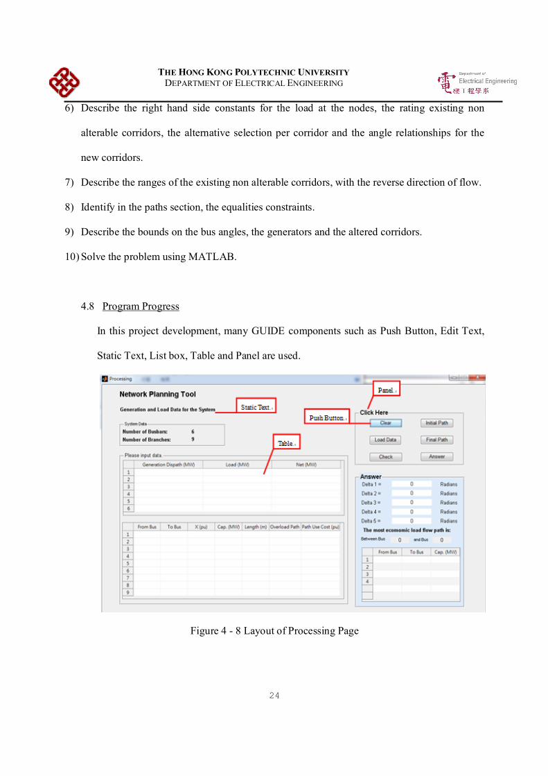
4.8 Program Progress

In this project development, many GUIDE components such as Push Button, Edit Text,

Static Text, List box, Table and Panel are used.

Figure 4 - 8 Layout of Processing Page


25

Function “isempty(A)” returns logical 1 (true) if A is an empty array and logical 0 (false)

otherwise. An empty array has at least one dimension of size zero, for example, 0-by-0 or

0-by-5. Function “isnumeric(A)” returns true if A is a numeric array and false otherwise.

Function “warndlg(warningstring)” displays a dialog box entitled, Warning Dialog,

containing the message specified by warning string. The warning string argument can be

a character vector or cell array of character vectors.

Figure 4 - 9 Codes for checking whether the input data is valid

Function ‘findobj’ is used to find objects knowing their 'tag' property. It returns handle of

the first found object which property “propertyName” is equal to “propertyValue”. If

such an object does not exist, the function returns an empty matrix.


26

Figure 4 - 10 codes for getting data

This code is one of the push buttons call back function in this program. Associate this

function with the push button Call-back property to make it execute when the end user

clicks on the push button. If the user input the invalid data, an error message will be

displayed to warn them. This makes sure that user input will not break my code.

Figure 4 - 11 Codes for opening the next page


27

The following codes are used to get the data from the table which user had inputted. The cell

data will be stored in variable “System_Data”.

Figure 4 - 12 Codes for getting data from user’s input

Function “t = uitable (parent,Name,Value)” specifies table property values using one or more

Name, Value argument pairs. These following codes are used to create customized table [13].

Figure 4 - 13 Codes for creating table programmatically


28

The path matrix can be formulated from the column 1 and 2 of System Table 2 as follow:

Figure 4 - 14 Codes for setting paths data

The nodal admittance matrix can be formed from column three of user input table by using for

loop.

Figure 4 - 15 Codes for setting nodal admittance matrix


29

After converting data from GUI to matrix, the linear programming problems can be formulated.

Figure 4 - 16 Codes for formulating linear programming problem

To solve the linear programming problem by using function ‘linprog’.

Figure 4 - 17 Codes for using function “linprog()”

The user input data in two tables can be cleared by clicking “Clear” button.

Figure 4 - 18 Codes for clearing user input data


30

Codes of showing path diagram:

Figure 4 - 19 Codes for showing path diagram

Function for checking the constraints.

Figure 4 - 20 Codes for a checking function


31

5. Results

The followings are layouts for data input.

Figure 5 - 1 Layout of Main Page

First, user is requested for inputting the system information (Number of Busbars and

Number of Branches), as they are main factor to formulate the transmission network

planning problem. Different numbers of busbars and branches have different transmission

path; thus, this step is necessary. For example, the number of burbars is six and the

number of branched is nine


32

Figure 5 - 2 User input data in Main Page

If the user input data is empty or non positive integer, a warning dialog will be displayed to warn

the user to input valid data. The program will go on when user inputted valid data.

Figure 5 - 3 Warning Message


33

After the user inputted the system data in Main Page, the program will go to Processing Page for

users to further processing. The layout will be displayed according to the previous input of user.

In this example, it programmatically generated one 6 x 3 table and one 9 x 7 table and load the

default data of IEEE 6-bus test system. The data can be revised by user.

Figure 5 - 4 Layout of Processing Page

For this six bus example, the system data can be transferred into the following tableau

representation.


34

Figure 5 - 5 Tableau Representation of Equation 4.16 for the Six Bus Example

After the user inputted the data, the program will analyze the data and solve them as a linear

programming problem and by clicking button “Answer” in the Processing Page, the answer will

be displayed in Figure 5 - 5.

Figure 5 - 6 Showing Answer

Relation RHS-9.17 2.5 0 1.67 5 1 0 0 0 0 0 0 0 0 0 0 δ1 = 0.82.5 -10 5 2.5 0 0 0 0 1 0 0 0 -1 0 0 0 δ2 = 2.40 5 -10 0 5 0 1 0 0 0 0 -1 0 0 0 1 δ3 = 0.4

1.67 2.5 0 -4.17 0 0 0 0 0 1 0 0 0 -1 0 0 δ4 = 1.65 0 5 0 -10 0 0 0 0 0 1 1 0 0 -1 -1 δ5 = 2.40 0 0 0 0 0 0 1 -1 -1 -1 0 1 1 1 0 PG1 = 0

PG3PG6pf7pf8pf9pf6pb7pb8pb9pb6

–B m KT –KT


35

After clicking the button “Clear” in the Processing Page, the program will clear all the data that

user inputted before and let the user to input data again.

Figure 5 - 7 after clicking the button “Clear”

The default data can be reloaded to the tables after clicking the button “Load Data” in the

Processing Page.

Figure 5 - 8 after clicking the “Load Data” button


36

The existing path of the network can be drawn by clicking button “Initial Path” in the Processing

Page.

Figure 5 - 9 after clicking button “Initial Path”

The optimized path can be shown after clicking button “Final Path” in the Processing Page.

Figure 5 - 10 after clicking button “Final Path”


37

After clicking the button “Check” in the Processing Page, a “Check Constraints” message box

will run.

Figure 5 - 11 “Check Constraints” message box

Constraints one is referring to equation 4.18, it takes the form shown in Figure 5 – 12.

Figure 5 - 12 form of equation 4.18

If the user chose “Constraints 1”, the program will check the solution is fulfil the Limitation 1 or

not, if yes, the “Limitation 1” message box will show.

-1 2.5 -2.5 0 0 0 δ1 1-0.8 1.67 0 0 -1.67 0 δ2 0.8-1 5 0 0 0 -5 δ3 1-1 0 5 -5 0 0 δ4 1-1 0 2.5 0 -2.5 0 δ5 1-1 0 0 5 0 5 1

≤≤


38

Figure 5 - 13 Limitation 1

Constraints two is referring to equation 4.19, for the six bus example, the matrices [Q], [H] and

[T] are as shown in Figure 5 – 14, Figure 5 – 15 and Figure 5 – 16 respectively.

Figure 5 - 14 matrix [Q]

Figure 5 - 15 matrix [H]

B12B14

B15B23

B24B35

Q

1 -1 0 0 01 0 0 -1 01 0 0 0 -10 1 -1 0 00 1 0 -1 00 0 1 0 -1

H


39

Figure 5 - 16 matrix [T]

Giving values to the susceptance coefficients of matrix [T] according to the data inputted by user,

the matrix [T] for the six bus example is obtained. This matrix is shown in Figure 5 - 17.

Figure 5 - 17 Answer of matrix [T]

If the user chose “Constraints 2”, the program will check the solution is fulfil the Limitation 2 or

not, if yes, the “Limitation 2” message box will show.

Figure 5 - 18 Limitation 2

B12 –B12 0 0 0B14 0 0 –B14 0B15 0 0 0 –B150 B23 –B23 0 00 B24 0 –B24 00 0 B35 0 –B35

T

2.5 -2.5 0 0 01.67 0 0 -1.67 05 0 0 0 -50 5 -5 0 00 2.5 0 -2.5 00 0 5 0 -5

T


40

6. Discussion

To learn how to program a computer in a modern language with serious graphical

capabilities, is to take hole of a tool of remarkable flexibility a first course in programming

and is oriented toward integration with science, mathematics and engineering. In order to

easily build useful graphical tools for exploring computational models, it takes a lot of time

to learn the MATLAB programming language to provide a graphical, mathematical and

user-friendly program.

The calculation of network planning design is quite complex and tedious. It takes time to

consider how the program can achieve and improve the work. I have search and find many

material such as books, websites and e-books to solve them.

Apart from that, the user is required to input data before the calculating the problem. It is

necessary to obtain and save the data and use it in the next pages. To solve this problem, I

try to find different books and websites to learn how to store and send the data in MATLAB

programming language.

The project had been spent a lot of time in learning the MATLAB programming language

and power system load flow calculation.

The project would be able to plot the network path after well planning to simulate the

network planning problem. It is because the program will solve the problems on different

busbars system with various paths. It must be built up database to store and deal with the

input variables. However, constraints that the network planning must satisfy are very

complex. It is difficult to obtain a complete network planning mathematical model and it is

even more difficult to solve it.


41

7. Conclusions

7.1 The Linear Programming Method

This project is to establish a program for solving the power system planning problem by

using linear programming technique. It is aimed at the development of preliminary

transmission network designs. In this project, uses the linear programming technique to

determine a power flow pattern that minimizes a cost function. The method has the

flexibility to study situations where no network presently exist and is very effective in

identifying those transmission corridors where capacity shortage exist, where to add new

transmission facilities and how much new capacity is needed. The feature of the method

is the solving of a linear DC power flow in conjunction with a transportation model. The

transportation network is composed of all those corridors, either with existing circuits and

capacity to be expanded or new affordable corridors along which new transmission

circuits can be constructed. The linear DC transmission model is solved for the existing

facilities obeying both of Kirchhoff’s laws: flow conservation at each bus and voltage

conservation around each loop. The transportation model is solved for the overload by

obeying only the bus flow conservation law while minimizing a cost objective function.

The transportation model comes into play when new buses, unconnected to the network,

are present and / or when existing lines would be overloaded. The transportation network

delivers to the load centers in the most economic way, that amount of active power that

otherwise would overload the existing circuits.

The amount of overload resulting from the linear programming solution indicates how

much capacity (what voltage level and conductor size) to add. The application of the

model to the long range planning of a six bus example serves to illustrate the method.


42

This method is very well suited for computer planner interactive studies and gives the

planner the opportunity to observe directly the effect on the network of very

reinforcement and decide.

The linear programming method is used in identifying the set of less costly corridors

required in the system in order to be able to find a feasible long range design for that

network.

Besides being the cheapest, the solution produced by this method identifies the required

minimum number of corridors necessary to be included in the network study in order to

that a feasible expansion plan could be found. After identifying the minimum required

expandable corridors, the planner is free to add any other corridor that he considers

convenient for other that economic reasons.

At the very initial planning stage, it could be difficult for the planner to decide which

expandable corridors to include in the study. Reasons like high transmission building

costs, environmental restrictions, high cost of land, etc. may prohibit the inclusion of

certain right-of-ways into the analysis. Perhaps some of those uneconomic corridors may

be necessary in the study in order to obtain a feasible solution. To be safe, it is

recommended that at the very initial stage (identification of the most economic set of

expandable corridors) of the planning process, all right-of-ways be included. Costly and

difficult to afford corridors with the characteristics mentioned above, may be included in

the analysis giving to them high surrogate cost.

The result of applying the method to an electrical network will tell which of those

corridors are essential in the analysis and which can be left out. Thus, in using this

method, it is recommended to include in the transportation network model, as many


43

overload paths as the condition allow.

It should be pointed out that, for the network planning problem as a whole, there is no

clear demarcation between the scheme formation and evaluation and between the

methods used in the scheme formation and evaluation. The best combination of methods

and algorithms will point the way towards improved network planning.

7.2 Graphical User Interfaces program in MATLAB

A Graphical User Interfaces (GUI) program in MATLAB is used to solve the problem.

Simulation of the power system models becomes much easier when modifying a variable

in a GUI rather than running the program from a command prompt. Matlab is currently

not only used as a mathematical manipulation tool, but also for the design and simulation

of various dynamic systems.

The use of this software adds the benefit of obtaining additional information given with

the solution. This permits the planner to consider some expansion possibilities other than

the proposed by the solution itself without losing feasibility and without resorting to a

new run of the program. This additional information will aid in production cost /

transmission investment trade-offs, new generation sitting, re-conducting and building of

old transmission lines and also networks that include more that on voltage level.


44

Reference

[1] M. Munasinghe 1945-, W. G. Scott and M. Gellerson, The Economics of Power System

Reliability and Planning : Theory and Case Study. Baltimore: Published for the World Bank by

Johns Hopkins University Press, 1979.

[2] R. V. Villasana, "Transmission network planning using linear and linear mixed integer

programming," 1993.

[3] T. Gönen, Electrical Power Transmission System Engineering: Analysis and Design. Boca

Raton, FL: Boca Raton, FL : CRC Press/Taylor & Francis Group, 2014, 2014.

[4] U. G. W. Knight, "The logical design of electrical networks using linear programming

methods," Proc. IEE A Power Eng. UK, vol. 107, pp. 306, 1960.

[5] R. L. Grimsdale and P. H. Sinclare, "The design of housing-estate distribution systems using

a digital computer," Proc. IEE A Power Eng. UK, vol. 107, pp. 295, 1960.

[6] L. Garver, "Transmission Network Estimation Using Linear Programming," Power

Apparatus and Systems, IEEE Transactions on, vol. PAS-89, pp. 1688-1697, 1970.

[7] M. S. Bazaraa and J., Linear Programming and Network Flows. New York: Wiley, 1990.

[8] R. H. Kwon, Introduction to Linear Optimization and Extensions with MATLAB®. Boca

Raton, Fla: CRC Press/Taylor & Francis Group, 2014.

[9] (). MATLAB GUI - MATLAB. Available: https://www.mathworks.com/discovery/matlab-

gui.html?s_tid=gn_loc_drop.

[10] W. Bober 1930- and A. Stevens 1964-, Numerical and Analytical Methods with MATLAB

for Electrical Engineers. Boca Raton: CRC Press, 2013.

[11] O. I. Elgerd 1925-, Electric Energy Systems Theory : An Introduction. New York: McGraw-

Hill, 1982.


45

[12] C. S. Lent 1956-, Learning to Program with MATLAB : Building GUI Tools. Hoboken, N.J:

John Wiley and Sons, Inc, 2013.

[13] (). Create table UI component - MATLAB uitable. Available:

http://www.mathworks.com/help/matlab/ref/uitable.html?s_tid=gn_loc_drop

network planning in electricity supply industry yu yue

Documents