networks and operating systems chapter 8: network · pdf filenetworks and operating systems...
TRANSCRIPT
Networks and Operating Systems Chapter 8: Network Layer
Donald Kossmann & Torsten Höfler Frühjahrssemester 2013
© Systems Group | Department of Computer Science | ETH Zürich

2
Overview • Network layer services • IP, the Internet Protocol
– Model – Message format – Fragmentation and reassembly
• IP Addressing • Additional Protocols • Routing
– Basics – Interior Gateway Protocols (IGP)
• distance vector protocols: RIP • Link state protocols: OSPF
– Interdomain Routing (BGP) • Path vector protocol
• IPv6 • (Routers)
3
Network Layer Services
4
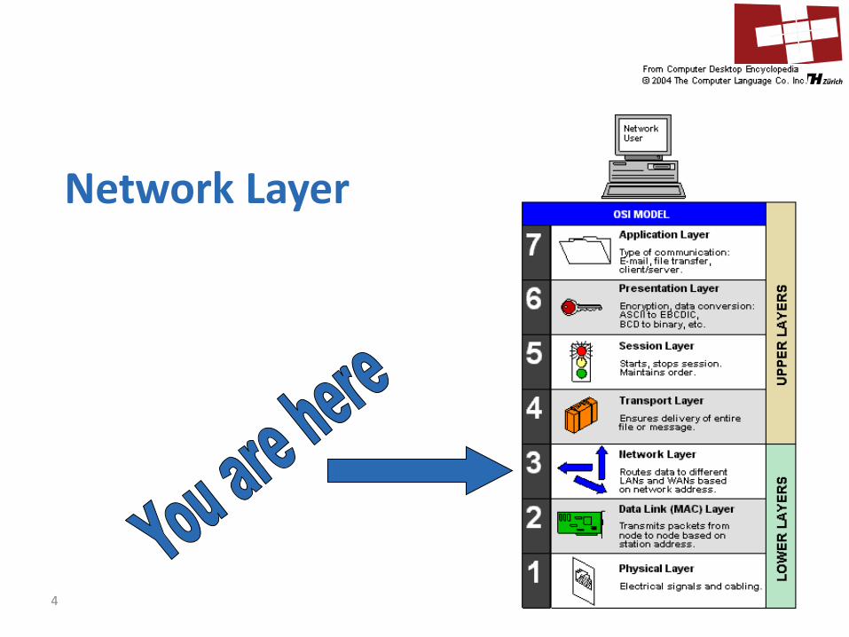
Network Layer
5
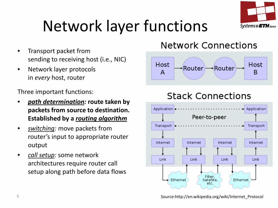
• Transport packet from sending to receiving host (i.e., NIC)
• Network layer protocols in every host, router
Three important functions: • path determination: route taken by
packets from source to destination. Established by a routing algorithm
• switching: move packets from router’s input to appropriate router output
• call setup: some network architectures require router call setup along path before data flows
Network layer functions
Source:http://en.wikipedia.org/wiki/Internet_Protocol
6
Network service model
The service model defines the “channel” transporting packets from sender to receiver:
• guaranteed bandwidth? • preservation of inter-packet timing (no jitter)? • loss-free delivery? • in-order delivery? • congestion feedback to sender? The network layer can work under two service models: • Virtual circuit • Datagrams
7
Virtual Circuits
• Source-to-destination path tries to behave like a physical circuit • The network layer maintains the illusion of a circuit:
– call setup for each call before data can flow (teardown after) – each packet carries VC identifier (instead of destination ID) – every router on source-destination path maintains “state” for
each passing connection – link, router resources (bandwidth, buffers) may be allocated to
VC
8
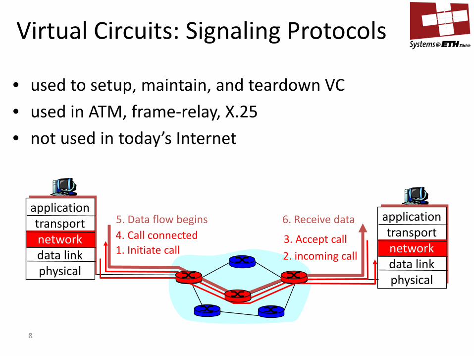
Virtual Circuits: Signaling Protocols
• used to setup, maintain, and teardown VC • used in ATM, frame-relay, X.25 • not used in today’s Internet
application transport network data link physical
application transport network data link physical
1. Initiate call 2. incoming call 3. Accept call 4. Call connected
5. Data flow begins 6. Receive data
9
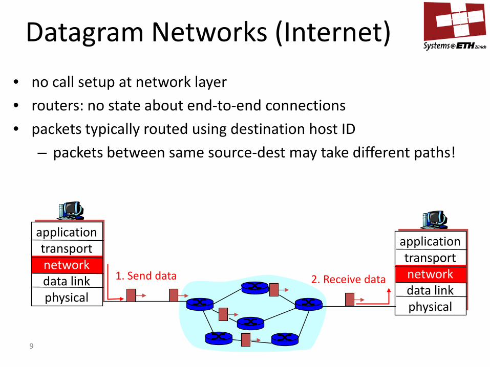
Datagram Networks (Internet) • no call setup at network layer • routers: no state about end-to-end connections • packets typically routed using destination host ID
– packets between same source-dest may take different paths!
application transport network data link physical
application transport network data link physical
1. Send data 2. Receive data
10
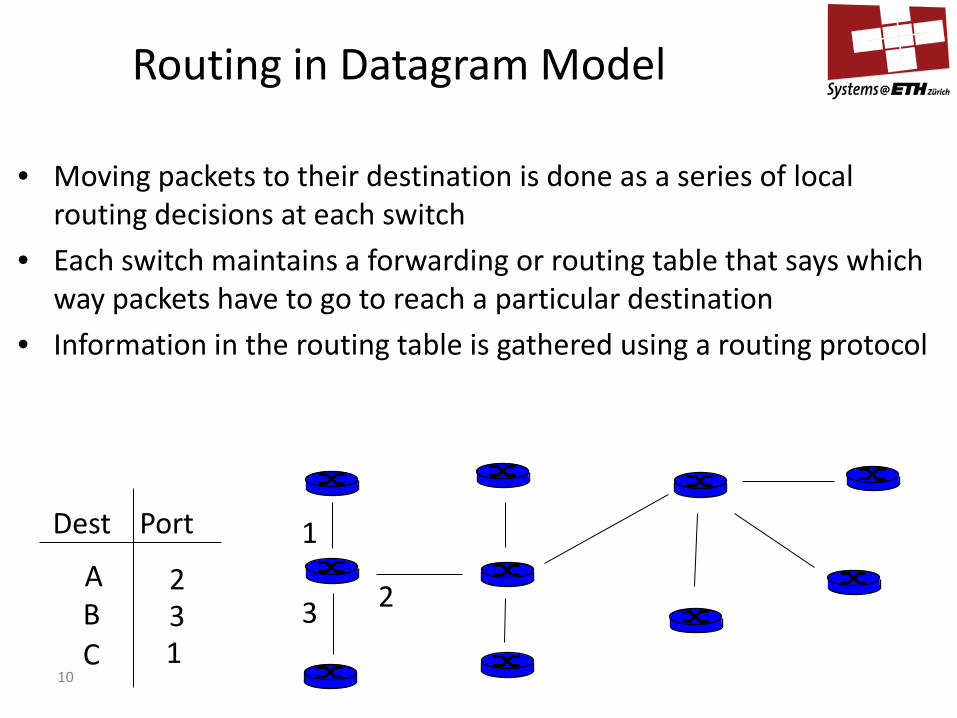
Routing in Datagram Model
• Moving packets to their destination is done as a series of local routing decisions at each switch
• Each switch maintains a forwarding or routing table that says which way packets have to go to reach a particular destination
• Information in the routing table is gathered using a routing protocol
Dest Port
A
C B
1 3 2
1
2 3
11
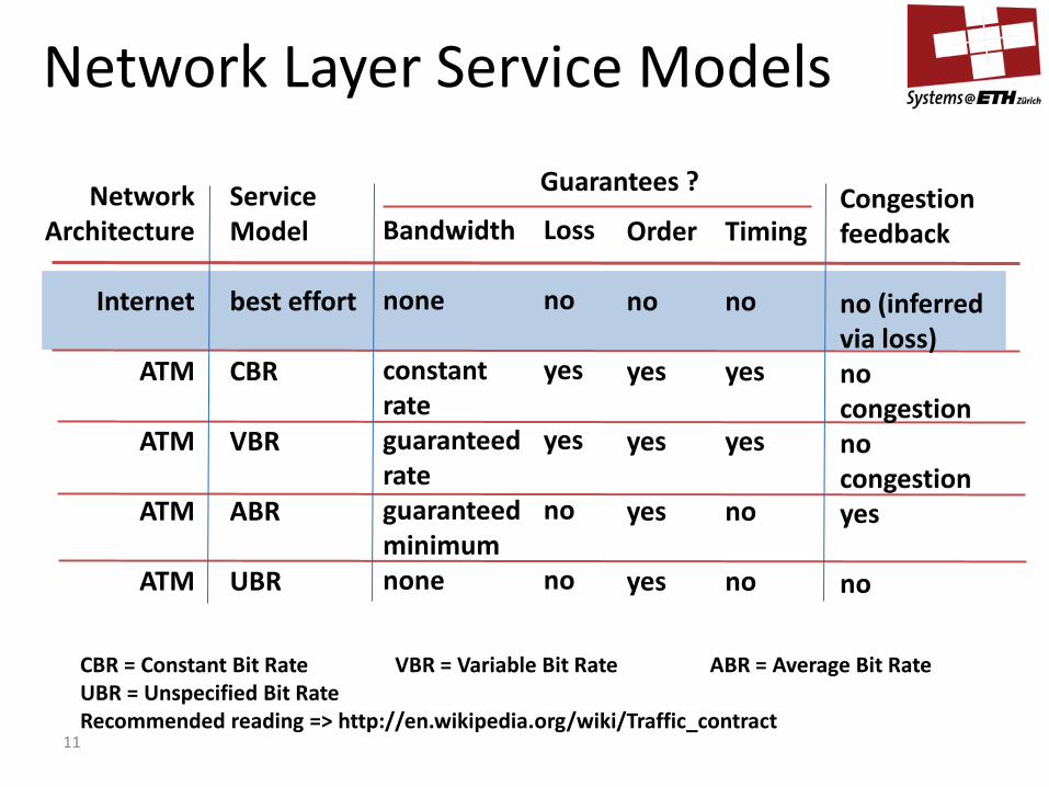
Network Layer Service Models
Network Architecture
Internet
ATM
ATM
ATM
ATM
Service Model best effort CBR VBR ABR UBR
Bandwidth none constant rate guaranteed rate guaranteed minimum none
Loss no yes yes no no
Order no yes yes yes yes
Timing no yes yes no no
Congestion feedback no (inferred via loss) no congestion no congestion yes no
Guarantees ?
CBR = Constant Bit Rate VBR = Variable Bit Rate ABR = Average Bit Rate UBR = Unspecified Bit Rate Recommended reading => http://en.wikipedia.org/wiki/Traffic_contract
12
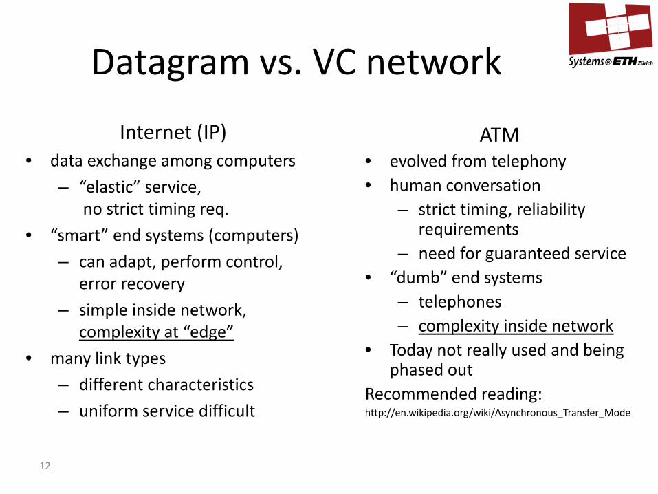
Datagram vs. VC network
Internet (IP) • data exchange among computers
– “elastic” service, no strict timing req.
• “smart” end systems (computers) – can adapt, perform control,
error recovery – simple inside network,
complexity at “edge” • many link types
– different characteristics – uniform service difficult
ATM • evolved from telephony • human conversation
– strict timing, reliability requirements
– need for guaranteed service • “dumb” end systems
– telephones – complexity inside network
• Today not really used and being phased out
Recommended reading: http://en.wikipedia.org/wiki/Asynchronous_Transfer_Mode

13
Internet Protocol (IP)
14
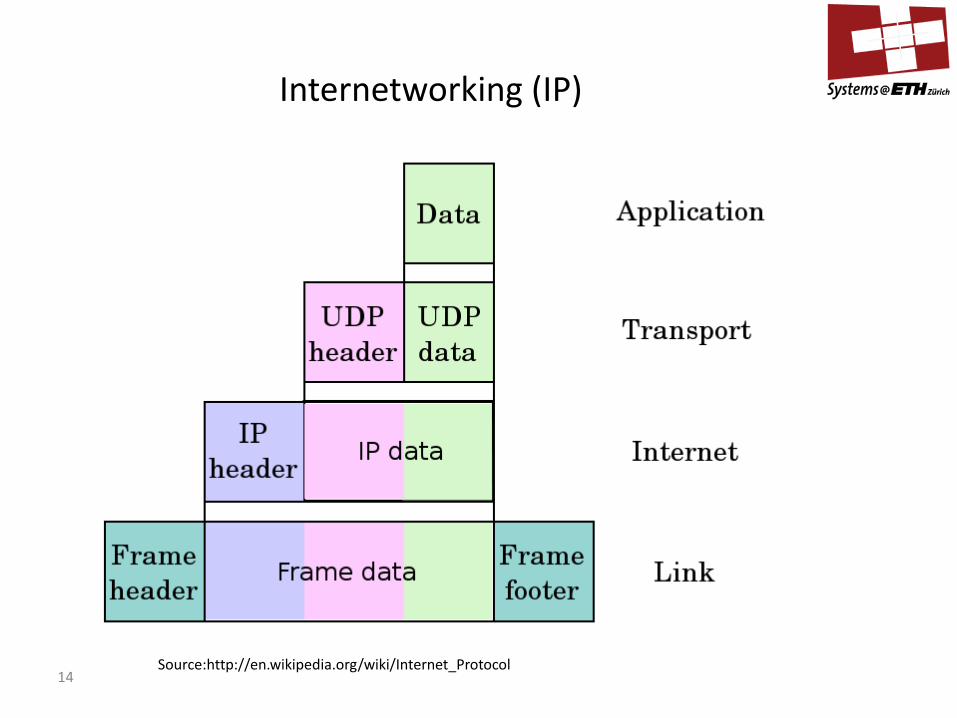
Internetworking (IP)
Source:http://en.wikipedia.org/wiki/Internet_Protocol
15
Internetworking (IP)
• The Internet Protocol – Datagram based
• best effort, unreliable • simple routers • packet fragmentation and reassembly
– Addressing schema • IP Addresses
– Routing protocols (e.g., BGP)
16
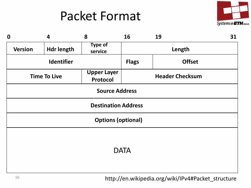
Packet Format
DATA
Version Hdr length Type of service Length
Identifier Flags Offset
Time To Live Upper Layer
Protocol Header Checksum
Destination Address
Source Address
Options (optional)
0 4 8 16 19 31
http://en.wikipedia.org/wiki/IPv4#Packet_structure
17
Fragmentation and Reassembly
• IP needs to work over many different physical networks – networks have different maximum packet sizes – IP needs to fragment and reassemble packets to make them
fit in the frames of the next layer • Every network has a Maximum Transmission Unit: the largest IP
datagram it can carry in the payload of a frame • Fragment when needed, reassemble only at destination • The fields “identifier”, “flag”, and “offset” are used to mark the
fragments and reassemble them as needed. • (N.B. This fragmentation happens in addition to fragmentation at
the transport layer.)
18
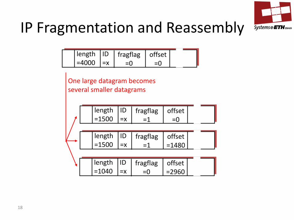
IP Fragmentation and Reassembly ID =x
offset =0
fragflag =0
length =4000
ID =x
offset =0
fragflag =1
length =1500
ID =x
offset =1480
fragflag =1
length =1500
ID =x
offset =2960
fragflag =0
length =1040
One large datagram becomes several smaller datagrams
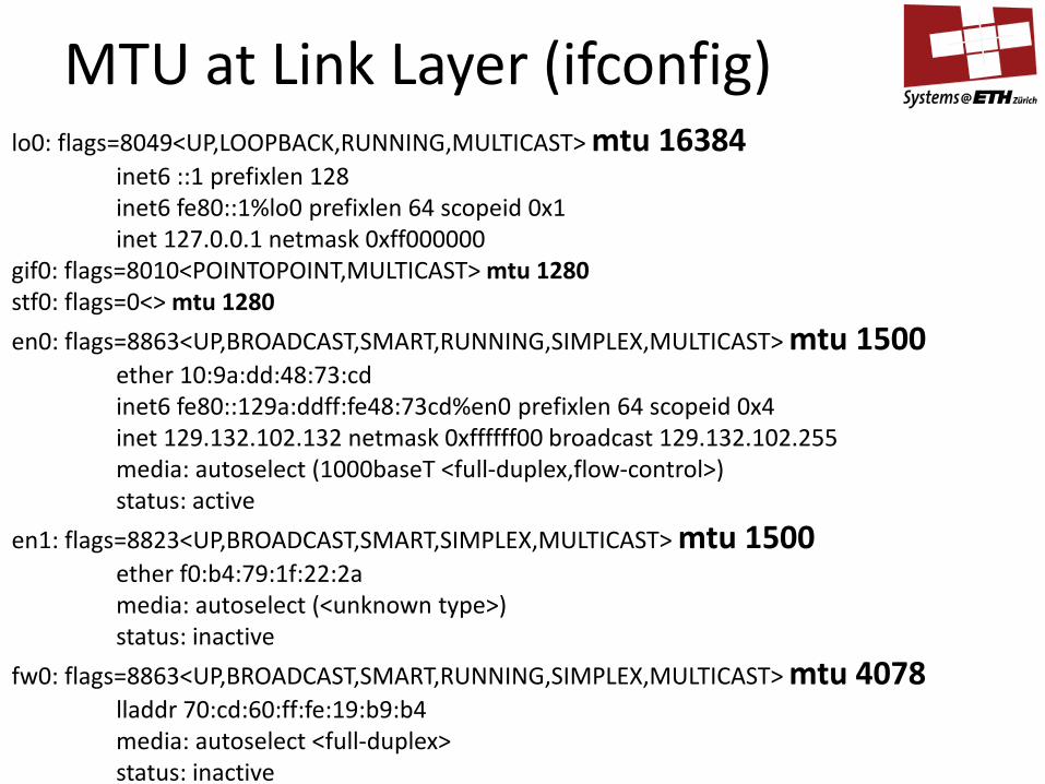
MTU at Link Layer (ifconfig) lo0: flags=8049<UP,LOOPBACK,RUNNING,MULTICAST> mtu 16384 inet6 ::1 prefixlen 128 inet6 fe80::1%lo0 prefixlen 64 scopeid 0x1 inet 127.0.0.1 netmask 0xff000000 gif0: flags=8010<POINTOPOINT,MULTICAST> mtu 1280 stf0: flags=0<> mtu 1280 en0: flags=8863<UP,BROADCAST,SMART,RUNNING,SIMPLEX,MULTICAST> mtu 1500 ether 10:9a:dd:48:73:cd inet6 fe80::129a:ddff:fe48:73cd%en0 prefixlen 64 scopeid 0x4 inet 129.132.102.132 netmask 0xffffff00 broadcast 129.132.102.255 media: autoselect (1000baseT <full-duplex,flow-control>) status: active en1: flags=8823<UP,BROADCAST,SMART,SIMPLEX,MULTICAST> mtu 1500 ether f0:b4:79:1f:22:2a media: autoselect (<unknown type>) status: inactive fw0: flags=8863<UP,BROADCAST,SMART,RUNNING,SIMPLEX,MULTICAST> mtu 4078 lladdr 70:cd:60:ff:fe:19:b9:b4 media: autoselect <full-duplex> status: inactive

20
IP Addresses
21
IP Addressing
• The Internet Protocol is meant as a protocol to communicate across networks: Internetworking – There is not a single network; hierarchy of networks – Routing happens within networks & across networks – Addresses are designed to reflect the hierarchical
organization of the networks comprising the Internet
22
IP Addresses
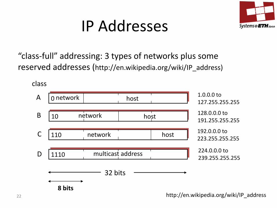
0 network host
10 network host
110 network host
1110 multicast address
A
B
C
D
class 1.0.0.0 to 127.255.255.255
128.0.0.0 to 191.255.255.255
192.0.0.0 to 223.255.255.255
224.0.0.0 to 239.255.255.255
32 bits
“class-full” addressing: 3 types of networks plus some reserved addresses (http://en.wikipedia.org/wiki/IP_address)
8 bits http://en.wikipedia.org/wiki/IP_address

23
Initial Internet Design
Class A Class A Class A
Up to 126 class A (wide area) networks
Class B Class B Class B Class B Class B Class B
class B (campus area) networks (64x256)
class C (local area) networks (32x256x256)
Class C Class C Class C Class C Class C Class C Class C
24
IP Addressing 223.1.1.1
223.1.1.2
223.1.1.3
223.1.1.4 223.1.2.9
223.1.2.2
223.1.2.1
223.1.3.2 223.1.3.1
223.1.3.27
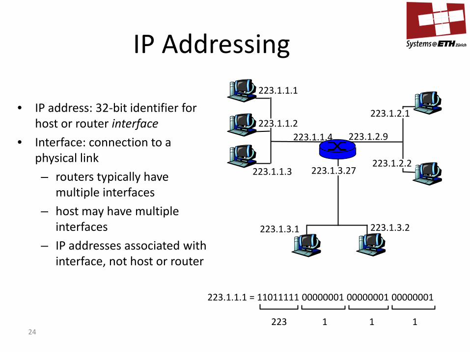
223.1.1.1 = 11011111 00000001 00000001 00000001
223 1 1 1
• IP address: 32-bit identifier for
host or router interface • Interface: connection to a
physical link – routers typically have
multiple interfaces – host may have multiple
interfaces – IP addresses associated with
interface, not host or router
25
IP Addressing 223.1.1.1
223.1.1.2
223.1.1.3
223.1.1.4 223.1.2.9
223.1.2.2
223.1.2.1
223.1.3.2 223.1.3.1
223.1.3.27
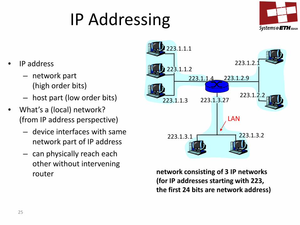
network consisting of 3 IP networks (for IP addresses starting with 223, the first 24 bits are network address)
LAN
• IP address
– network part (high order bits)
– host part (low order bits) • What’s a (local) network?
(from IP address perspective) – device interfaces with same
network part of IP address – can physically reach each
other without intervening router

26
IP Addressing: CIDR
• class-full addressing: – inefficient use of address space, address space exhaustion – e.g., class B net allocated enough addresses for 65K hosts, even if only 2K
hosts in that network • CIDR: Classless InterDomain Routing
– improvement over basic IP addressing for more efficient use of addresses – network portion of address of arbitrary length – address format: a.b.c.d/x, where x is number of bits defining the network
portion of address
11001000 00010111 0001000 0 00000000
network part
host part
200.23.16.0/23 http://en.wikipedia.org/wiki/Classless_Inter-Domain_Routing
27
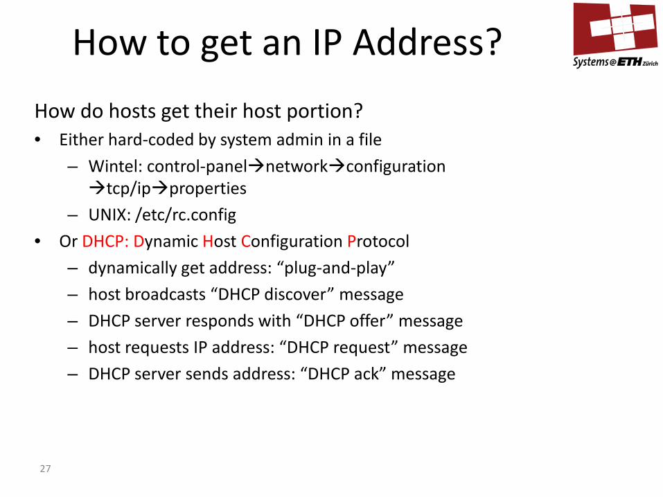
How to get an IP Address? How do hosts get their host portion? • Either hard-coded by system admin in a file
– Wintel: control-panelnetworkconfiguration tcp/ipproperties
– UNIX: /etc/rc.config • Or DHCP: Dynamic Host Configuration Protocol
– dynamically get address: “plug-and-play” – host broadcasts “DHCP discover” message – DHCP server responds with “DHCP offer” message – host requests IP address: “DHCP request” message – DHCP server sends address: “DHCP ack” message
28
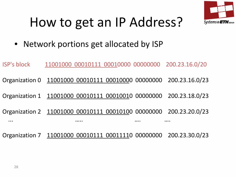
How to get an IP Address?
• Network portions get allocated by ISP
ISP's block 11001000 00010111 00010000 00000000 200.23.16.0/20 Organization 0 11001000 00010111 00010000 00000000 200.23.16.0/23 Organization 1 11001000 00010111 00010010 00000000 200.23.18.0/23 Organization 2 11001000 00010111 00010100 00000000 200.23.20.0/23 ... ….. …. …. Organization 7 11001000 00010111 00011110 00000000 200.23.30.0/23
29
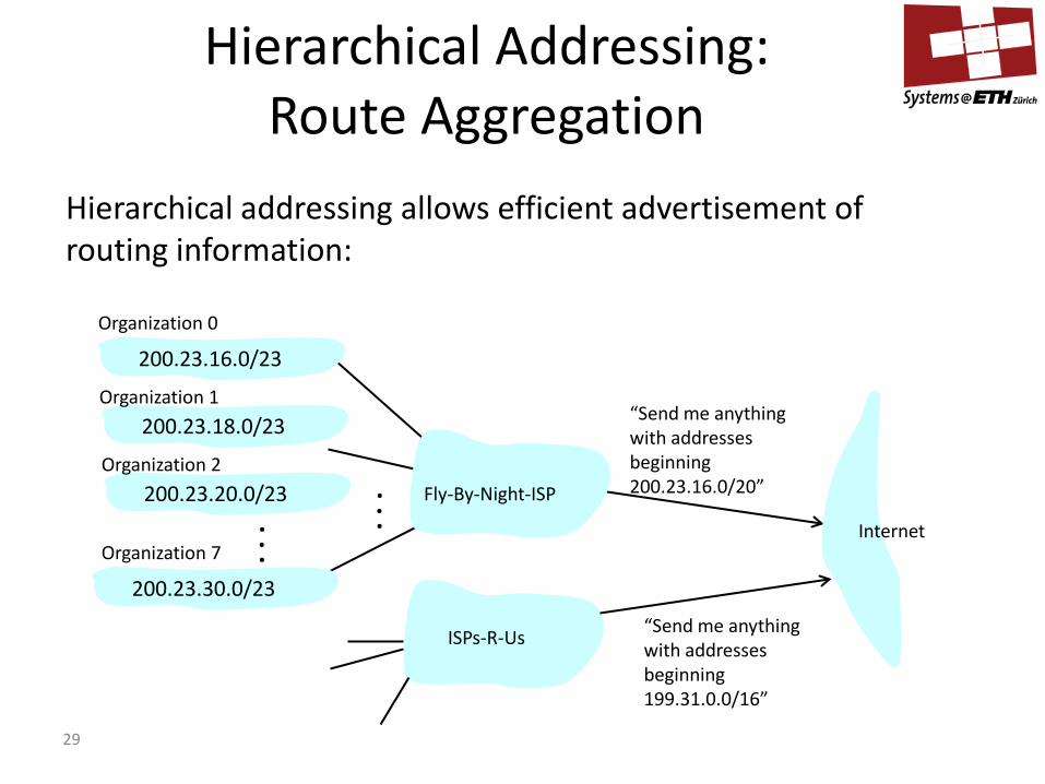
“Send me anything with addresses beginning 200.23.16.0/20”
200.23.16.0/23
200.23.18.0/23
200.23.30.0/23
Fly-By-Night-ISP
Organization 0
Organization 7 Internet
Organization 1
ISPs-R-Us “Send me anything with addresses beginning 199.31.0.0/16”
200.23.20.0/23 Organization 2
. . .
. . .
Hierarchical addressing allows efficient advertisement of routing information:
Hierarchical Addressing: Route Aggregation

30
What if Organization 1 wants to change the provider? ISPs-R-Us now has a more specific route to Organization 1.
“Send me anything with addresses beginning 200.23.16.0/20”
200.23.16.0/23
200.23.18.0/23
200.23.30.0/23
Fly-By-Night-ISP
Organization 0
Organization 7 Internet
Organization 1
ISPs-R-Us “Send me anything with addresses beginning 199.31.0.0/16 or 200.23.18.0/23”
200.23.20.0/23 Organization 2
. . .
. . .
Hierarchical Addressing: Specific Routes
31
IP Addressing • How does an ISP get a block of addresses?
– from another (bigger) ISP or – with ICANN: Internet Corporation for Assigned
Names and Numbers • allocates addresses • manages DNS • assigns domain names, resolves disputes
• Will there be enough IP addresses, ever? – No, there are some hacks around the corner (later)

32
Known as “forwarding” IP datagram:
223.1.1.1
223.1.1.2
223.1.1.3
223.1.1.4 223.1.2.9
223.1.2.2
223.1.2.1
223.1.3.2 223.1.3.1
223.1.3.27
A
B E
misc fields
source IP addr
dest IP addr data
datagram remains unchanged, as it travels from source to destination
addr fields of interest here
Dest.Netw. next router #hops 223.1.1 1 223.1.2 223.1.1.4 2 223.1.3 223.1.1.4 2
routing table in A
Getting a Datagram from Source to Destination
33
223.1.1.1
223.1.1.2
223.1.1.3
223.1.1.4 223.1.2.9
223.1.2.2
223.1.2.1
223.1.3.2 223.1.3.1
223.1.3.27
A
B E
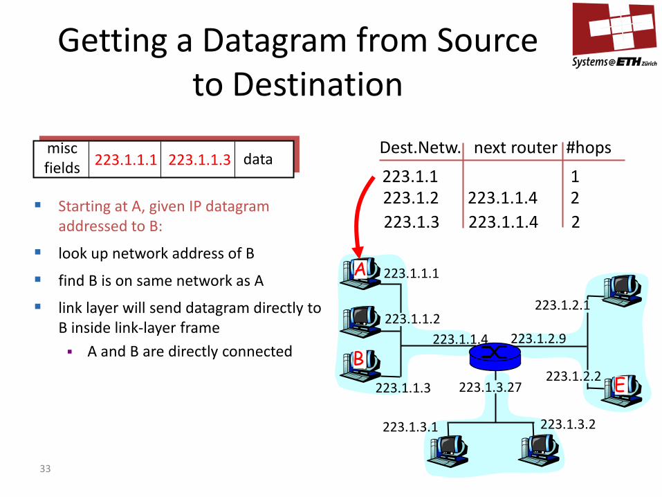
Starting at A, given IP datagram addressed to B:
look up network address of B
find B is on same network as A
link layer will send datagram directly to B inside link-layer frame A and B are directly connected
Dest.Netw. next router #hops 223.1.1 1 223.1.2 223.1.1.4 2 223.1.3 223.1.1.4 2
misc fields 223.1.1.1 223.1.1.3 data
Getting a Datagram from Source to Destination
34
223.1.1.1
223.1.1.2
223.1.1.3
223.1.1.4 223.1.2.9
223.1.2.2
223.1.2.1
223.1.3.2 223.1.3.1
223.1.3.27
A
B E
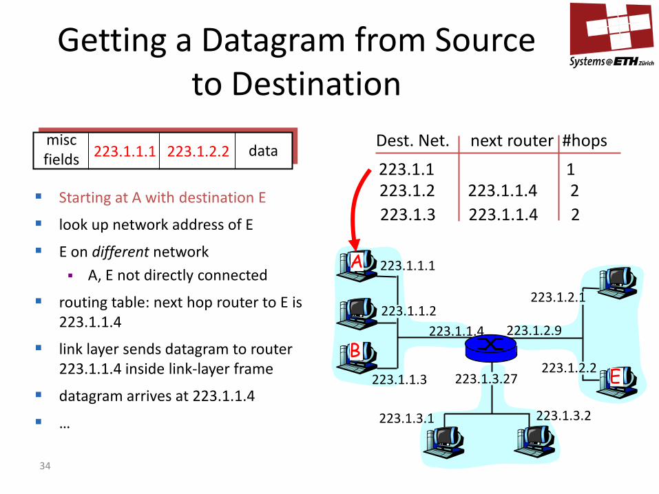
Dest. Net. next router #hops 223.1.1 1 223.1.2 223.1.1.4 2 223.1.3 223.1.1.4 2
Starting at A with destination E
look up network address of E
E on different network A, E not directly connected
routing table: next hop router to E is 223.1.1.4
link layer sends datagram to router 223.1.1.4 inside link-layer frame
datagram arrives at 223.1.1.4
…
misc fields 223.1.1.1 223.1.2.2 data
Getting a Datagram from Source to Destination
35
223.1.1.1
223.1.1.2
223.1.1.3
223.1.1.4 223.1.2.9
223.1.2.2
223.1.2.1
223.1.3.2 223.1.3.1
223.1.3.27
A
B E
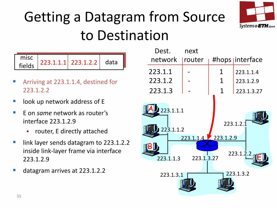
Arriving at 223.1.1.4, destined for 223.1.2.2
look up network address of E
E on same network as router’s interface 223.1.2.9 router, E directly attached
link layer sends datagram to 223.1.2.2 inside link-layer frame via interface 223.1.2.9
datagram arrives at 223.1.2.2
misc fields 223.1.1.1 223.1.2.2 data network router #hops interface
223.1.1 - 1 223.1.1.4 223.1.2 - 1 223.1.2.9
223.1.3 - 1 223.1.3.27
Dest. next
Getting a Datagram from Source to Destination

36
Additional protocols dealing with Network Layer information

37
ICMP: Internet Control Message Protocol
• used by hosts, routers, gateways to exchange network-level information – error reporting: unreachable
host, network, port, protocol – echo request/reply (used by ping)
• network-layer “above” IP: – ICMP msgs carried in IP
datagrams • ICMP message: type, code plus first 8
bytes of IP datagram causing error
Some typical types/codes Type Code description 0 0 echo reply (ping) 3 0 dest. network unreachable 3 1 dest host unreachable 3 2 dest protocol unreachable 3 3 dest port unreachable 3 6 dest network unknown 3 7 dest host unknown 4 0 source quench (congestion control - not used) 8 0 echo request (ping) 9 0 route advertisement 10 0 router discovery 11 0 TTL expired 12 0 bad IP header
38
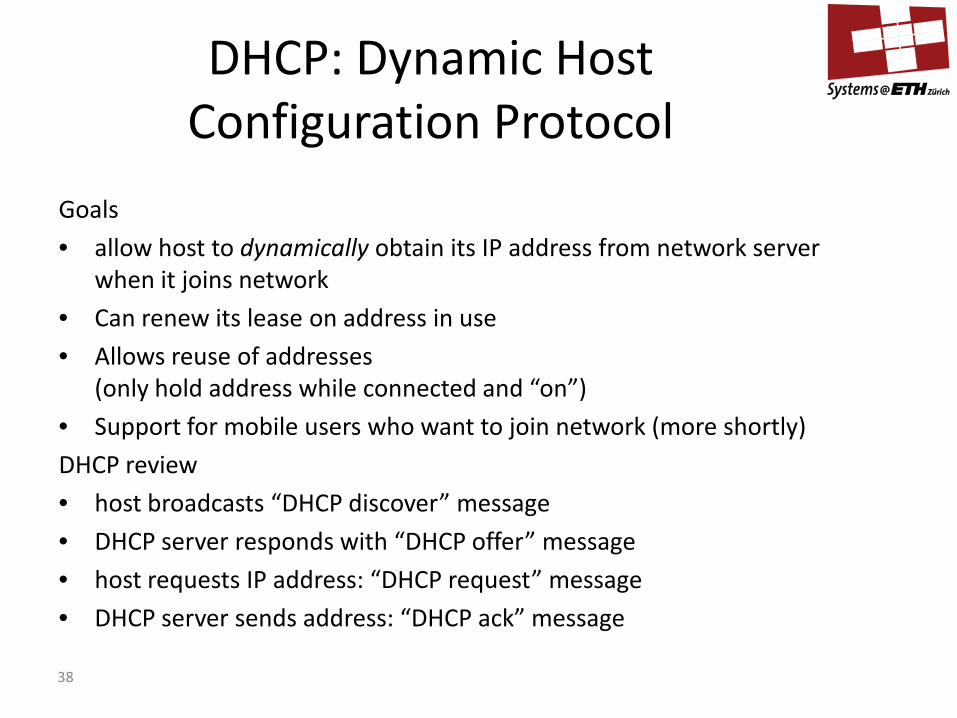
Goals • allow host to dynamically obtain its IP address from network server
when it joins network • Can renew its lease on address in use • Allows reuse of addresses
(only hold address while connected and “on”) • Support for mobile users who want to join network (more shortly) DHCP review • host broadcasts “DHCP discover” message • DHCP server responds with “DHCP offer” message • host requests IP address: “DHCP request” message • DHCP server sends address: “DHCP ack” message
DHCP: Dynamic Host Configuration Protocol

39
223.1.1.1
223.1.1.2
223.1.1.3
223.1.1.4 223.1.2.9
223.1.2.2
223.1.2.1
223.1.3.2 223.1.3.1
223.1.3.27
A
B E
DHCP server
arriving DHCP client needs address in this network
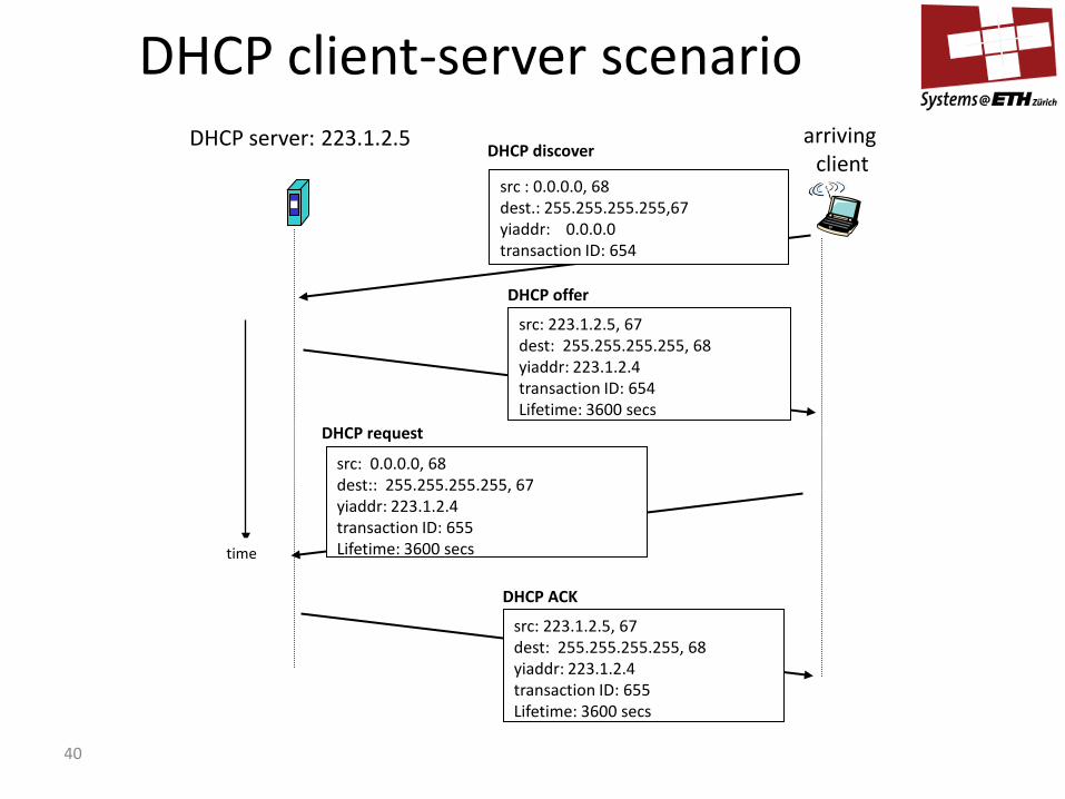
DHCP client-server scenario
40
DHCP server: 223.1.2.5 arriving client
time
DHCP discover
src : 0.0.0.0, 68 dest.: 255.255.255.255,67 yiaddr: 0.0.0.0 transaction ID: 654
DHCP offer
src: 223.1.2.5, 67 dest: 255.255.255.255, 68 yiaddr: 223.1.2.4 transaction ID: 654 Lifetime: 3600 secs
DHCP request
src: 0.0.0.0, 68 dest:: 255.255.255.255, 67 yiaddr: 223.1.2.4 transaction ID: 655 Lifetime: 3600 secs
DHCP ACK
src: 223.1.2.5, 67 dest: 255.255.255.255, 68 yiaddr: 223.1.2.4 transaction ID: 655 Lifetime: 3600 secs
DHCP client-server scenario
41
10.0.0.1
10.0.0.2
10.0.0.3
10.0.0.4
138.76.29.7
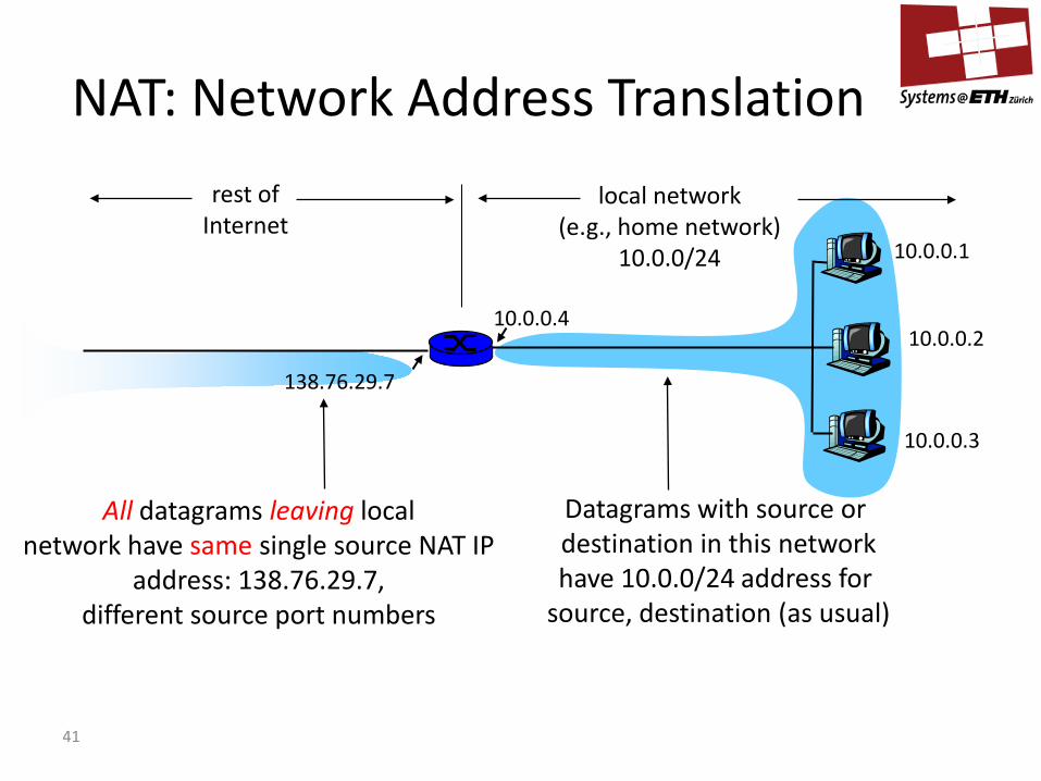
local network (e.g., home network)
10.0.0/24
rest of Internet
Datagrams with source or destination in this network have 10.0.0/24 address for
source, destination (as usual)
All datagrams leaving local network have same single source NAT IP
address: 138.76.29.7, different source port numbers
NAT: Network Address Translation
42
• Motivation – local network uses just one IP address for outside world – no need to be allocated range of addresses from ISP – just one IP address is used for all devices – can change addresses of devices in local network without
notifying outside world – can change ISP without changing addresses of devices in local
network – devices inside local net not explicitly addressable, visible by
outside world (a security plus). – BUT: machines cannot be servers!
NAT: Network Address Translation
43
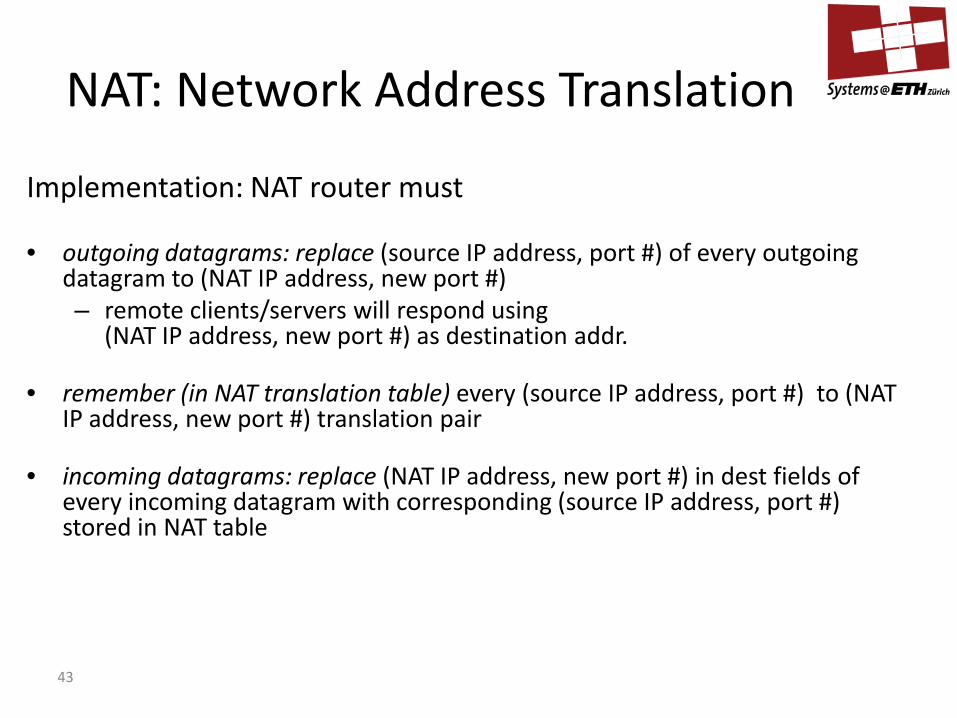
Implementation: NAT router must
• outgoing datagrams: replace (source IP address, port #) of every outgoing datagram to (NAT IP address, new port #) – remote clients/servers will respond using
(NAT IP address, new port #) as destination addr.
• remember (in NAT translation table) every (source IP address, port #) to (NAT IP address, new port #) translation pair
• incoming datagrams: replace (NAT IP address, new port #) in dest fields of every incoming datagram with corresponding (source IP address, port #) stored in NAT table
NAT: Network Address Translation

44
10.0.0.1
10.0.0.2
10.0.0.3
S: 10.0.0.1, 3345 D: 128.119.40.186, 80
1
10.0.0.4
138.76.29.7
1: host 10.0.0.1 sends datagram to 128.119.40, 80
NAT translation table WAN side addr LAN side addr 138.76.29.7, 5001 10.0.0.1, 3345
…… ……
S: 128.119.40.186, 80 D: 10.0.0.1, 3345
4
S: 138.76.29.7, 5001 D: 128.119.40.186, 80 2
2: NAT router changes datagram source addr from 10.0.0.1, 3345 to 138.76.29.7, 5001, updates table
S: 128.119.40.186, 80 D: 138.76.29.7, 5001
3 3: Reply arrives dest. address: 138.76.29.7, 5001
4: NAT router changes datagram dest addr from 138.76.29.7, 5001 to 10.0.0.1, 3345
NAT: Network Address Translation

45
• 16-bit port-number field – 60,000 simultaneous connections with a single
LAN-side address! • NAT is controversial
– routers should only process up to Layer 3 – violates end-to-end argument
• NAT possibility must be taken into account by app designers, e.g., P2P applications
– address shortage should instead be solved by IPv6 • delays in deployment of IPv6
NAT: Network Address Translation
Network of Networks
• Metaphor: Traffic Networks – planes, trains, busses, cars – places where networks intersect (airport, station, …)
• Problems – how to allocate addresses across networks – how to route to places across networks; often route
involves crossing networks – giving guarantees for routes, dealing with failures,
changes • There are many ways to get to Rome!
Skype, Chats
• Problem: Since your home PC does not know its publically usable IP address in a NAT scheme, how does it establish a connection to others?
• Idea: Need to connect to a host first. – with this connection, host learns publically usable IP – can forward that IP address to chat/Skype partner
48
Routing
49
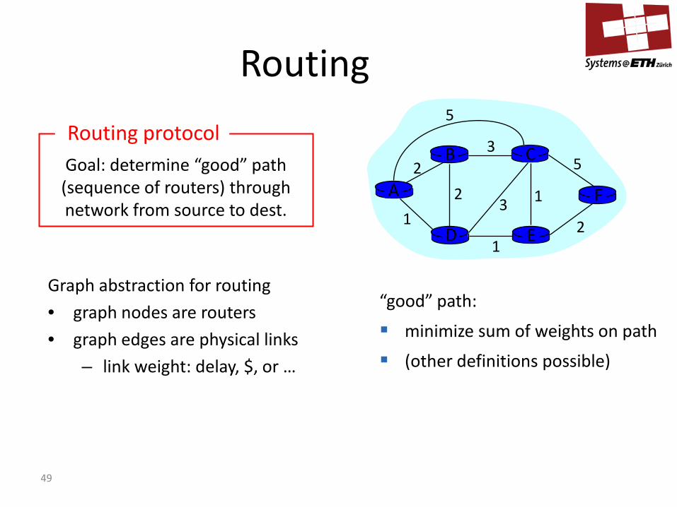
Routing
Graph abstraction for routing • graph nodes are routers • graph edges are physical links
– link weight: delay, $, or …
Goal: determine “good” path (sequence of routers) through network from source to dest.
Routing protocol
A
E D
C B
F 2
2 1
3
1
1
2
5 3
5
“good” path:
minimize sum of weights on path
(other definitions possible)
50
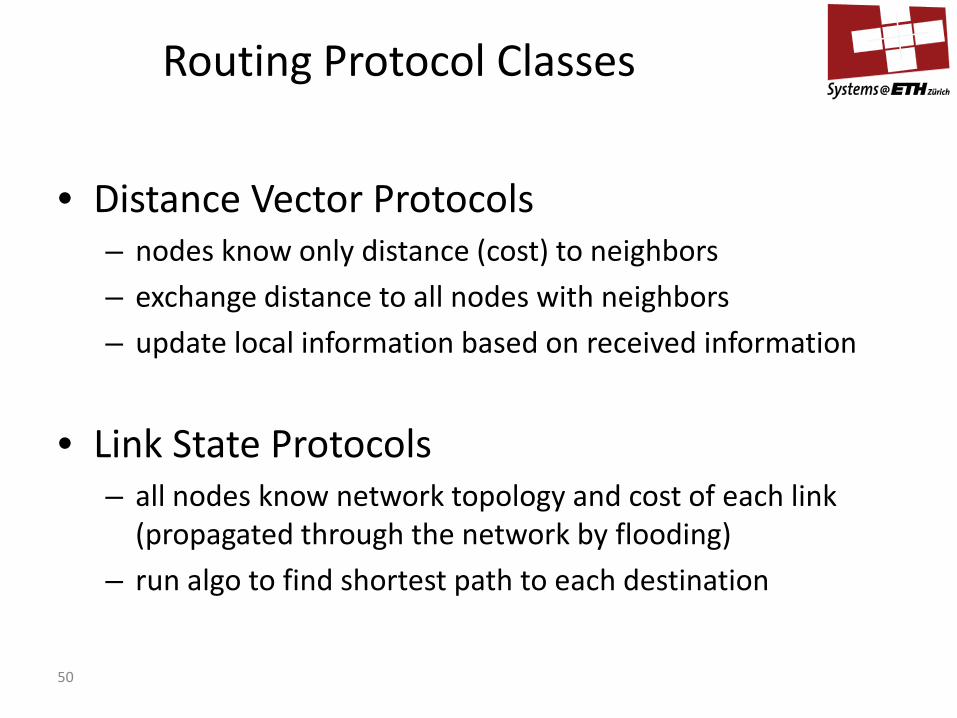
Routing Protocol Classes
• Distance Vector Protocols – nodes know only distance (cost) to neighbors – exchange distance to all nodes with neighbors – update local information based on received information
• Link State Protocols – all nodes know network topology and cost of each link
(propagated through the network by flooding) – run algo to find shortest path to each destination

51
Properties of Routing Protocols
• Information needed – messages involved to gather information – storage necessary to keep the information – (less is better)
• Convergence – how fast until it stabilizes? – how fast it reacts to changes? – (faster is better)
• Security – can malicious routers game the network?
52
Distance Vector Protocols RIP (Routing Information Protocol)
53
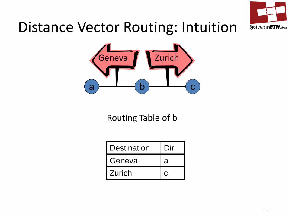
Distance Vector Routing: Intuition
b a c
Geneva Zurich
Routing Table of b
Destination Dir Geneva a Zurich c
54
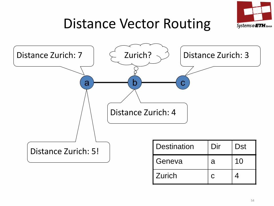
Distance Vector Routing
b a c
Distance Zurich: 3 Distance Zurich: 7 Zurich?
Distance Zurich: 4
Distance Zurich: 5! Destination Dir Dst
Geneva a 10
Zurich c 4
55
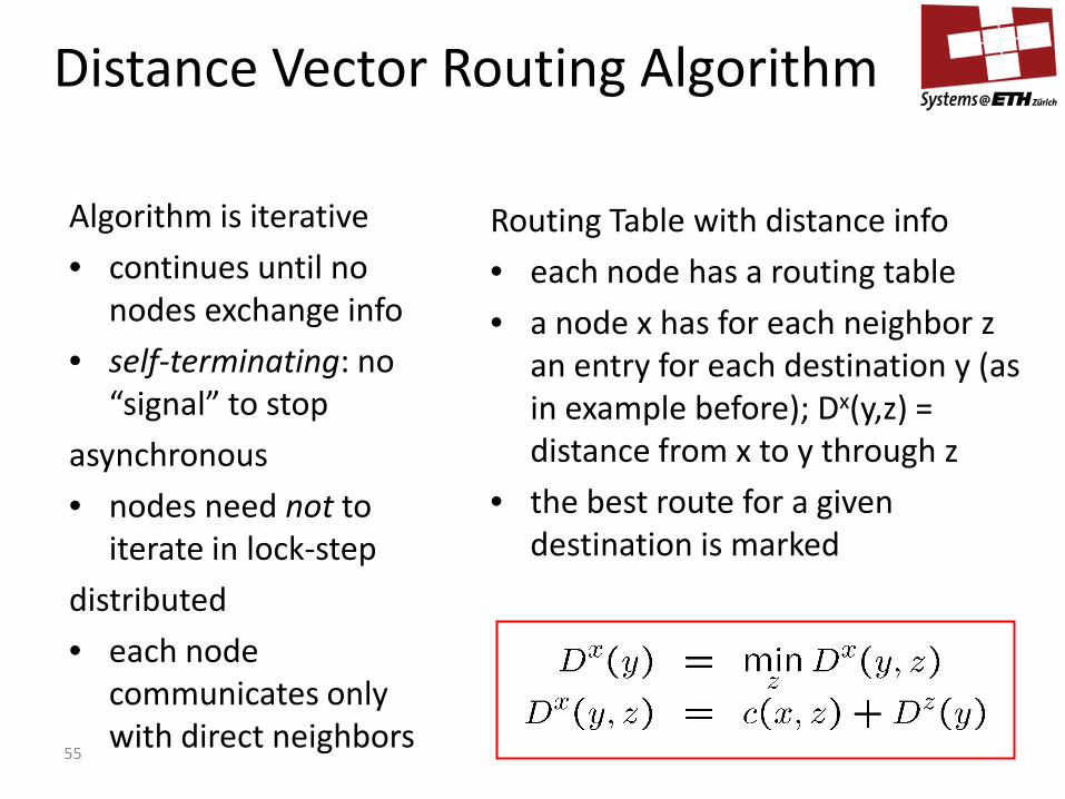
Distance Vector Routing Algorithm
Algorithm is iterative • continues until no
nodes exchange info • self-terminating: no
“signal” to stop asynchronous • nodes need not to
iterate in lock-step distributed • each node
communicates only with direct neighbors
Routing Table with distance info • each node has a routing table • a node x has for each neighbor z
an entry for each destination y (as in example before); Dx(y,z) = distance from x to y through z
• the best route for a given destination is marked
56
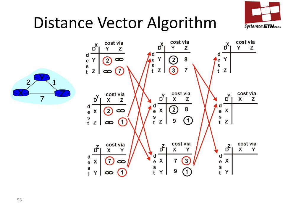
Distance Vector Algorithm
X Z 1 2
7
Y
57
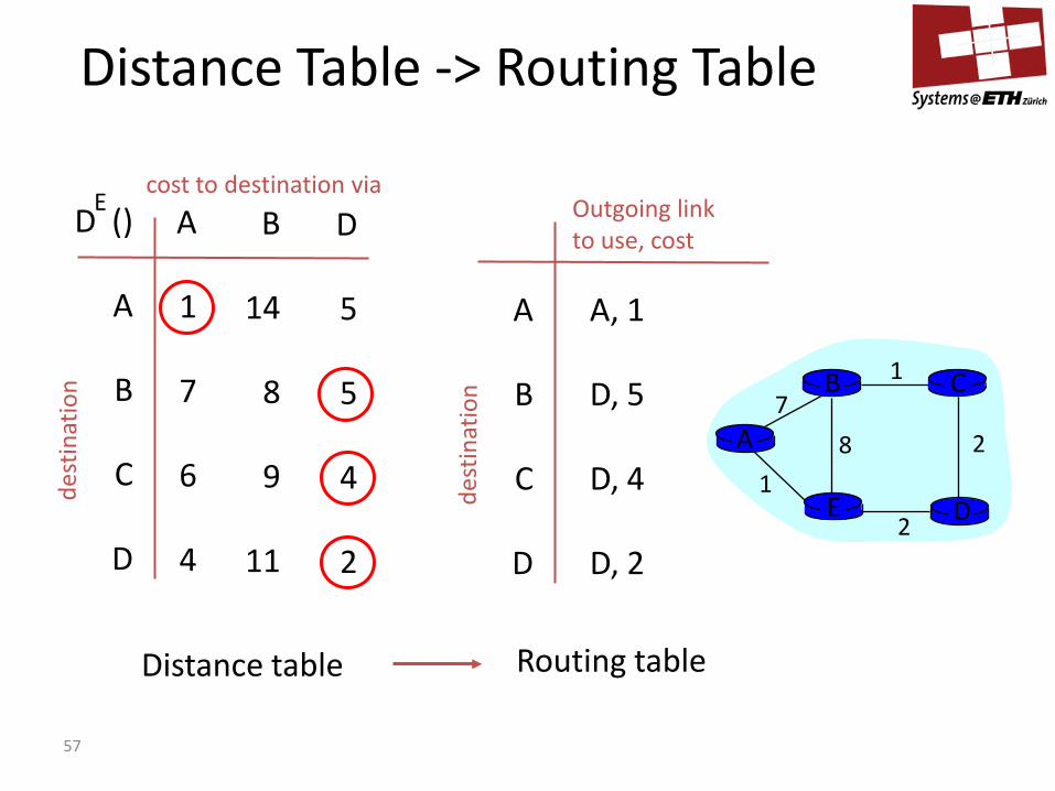
Distance Table -> Routing Table
D ()
A
B
C
D
A
1
7
6
4
B
14
8
9
11
D
5
5
4
2
E cost to destination via
A
B
C
D
A, 1
D, 5
D, 4
D, 2
Outgoing link to use, cost
Distance table Routing table
A
E D
C B 7
8 1
2
1
2
58
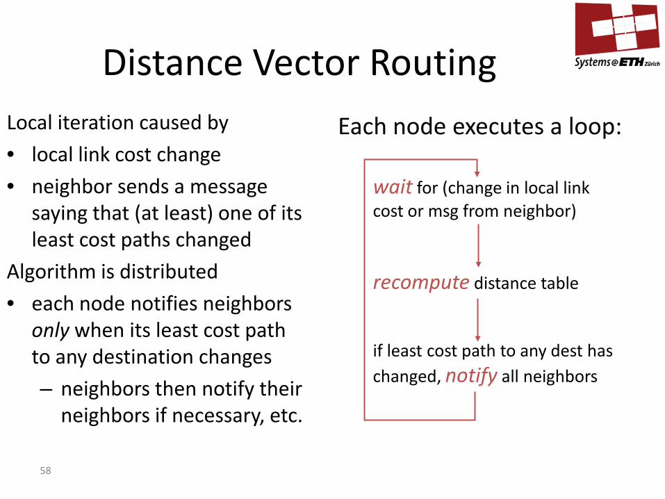
Distance Vector Routing Local iteration caused by • local link cost change • neighbor sends a message
saying that (at least) one of its least cost paths changed
Algorithm is distributed • each node notifies neighbors
only when its least cost path to any destination changes – neighbors then notify their
neighbors if necessary, etc.
wait for (change in local link cost or msg from neighbor)
recompute distance table
if least cost path to any dest has changed, notify all neighbors
Each node executes a loop:
59
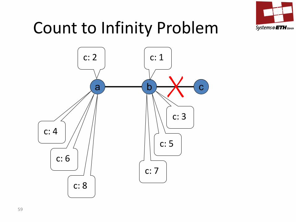
Count to Infinity Problem
b a c
c: 2 c: 1
c: 3 c: 4
c: 5 c: 6
c: 7 c: 8
60
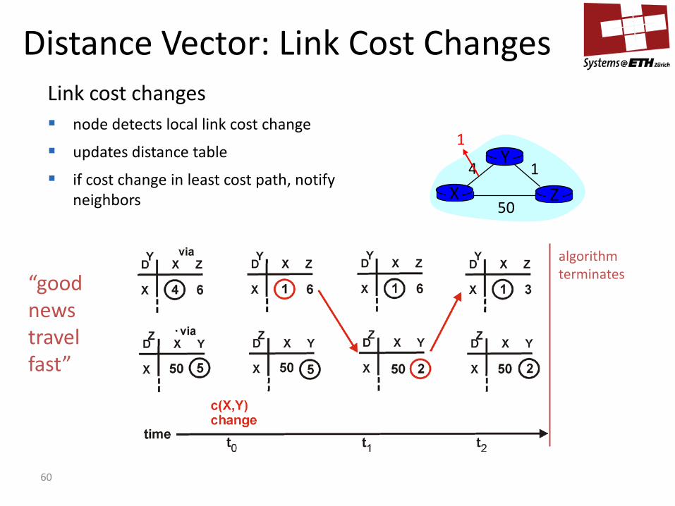
Distance Vector: Link Cost Changes Link cost changes node detects local link cost change
updates distance table
if cost change in least cost path, notify neighbors X Z
1 4
50
Y 1
algorithm terminates “good
news travel fast”

61
Distance Vector: link cost changes • What if the cost of a link grows? • Compare to the “count to infinity” • (We discuss give fix later) X Z
1 4
50
Y 60
algorithm continues
on!
62
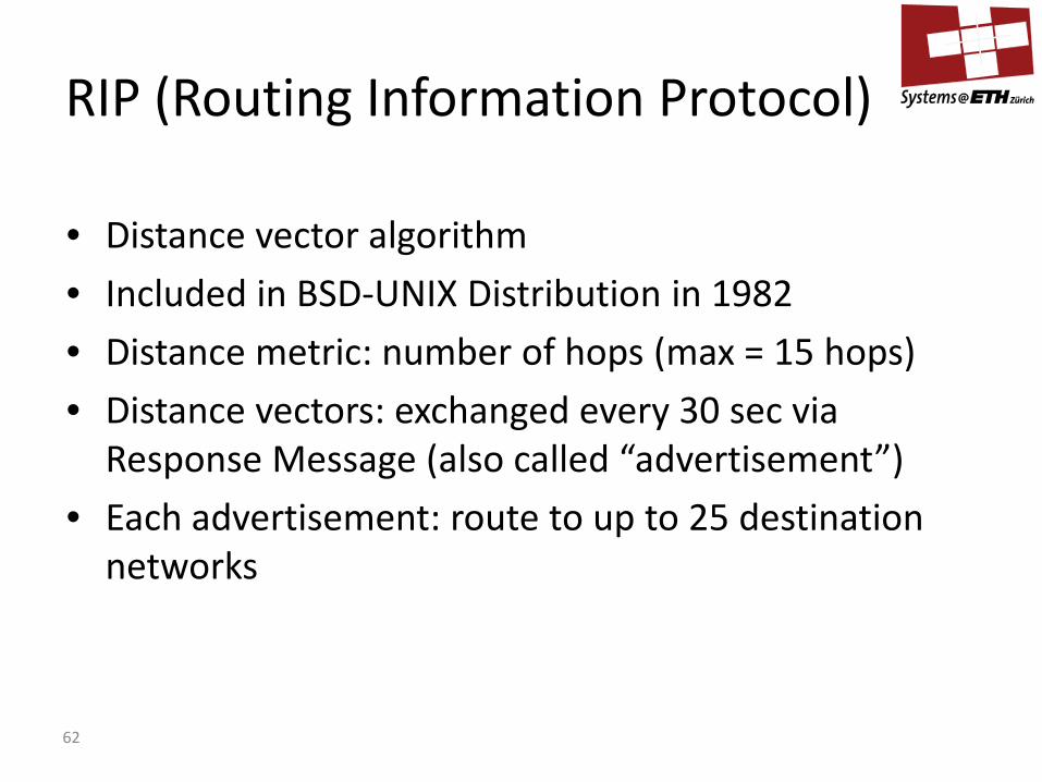
RIP (Routing Information Protocol)
• Distance vector algorithm • Included in BSD-UNIX Distribution in 1982 • Distance metric: number of hops (max = 15 hops) • Distance vectors: exchanged every 30 sec via
Response Message (also called “advertisement”) • Each advertisement: route to up to 25 destination
networks
63
If no advertisement heard after 180 sec then neighbor/link declared dead – routes via neighbor invalidated – new advertisements sent to neighbors – neighbors in turn send out new advertisements (if tables changed) – link failure info quickly propagates to entire network – poison reverse (next slide) used to prevent ping-pong loops
(infinite distance = 16 hops)
RIP: Link Failure and Recovery

64
Distance Vector: Poisoned Reverse
If Z routes through Y to get to X : Z tells Y its (Z’s) distance to X is
infinite (so Y won’t route to X via Z) Avoids the loop between 2 nodes
X Z 1 4
50
Y 60
algorithm terminates
65
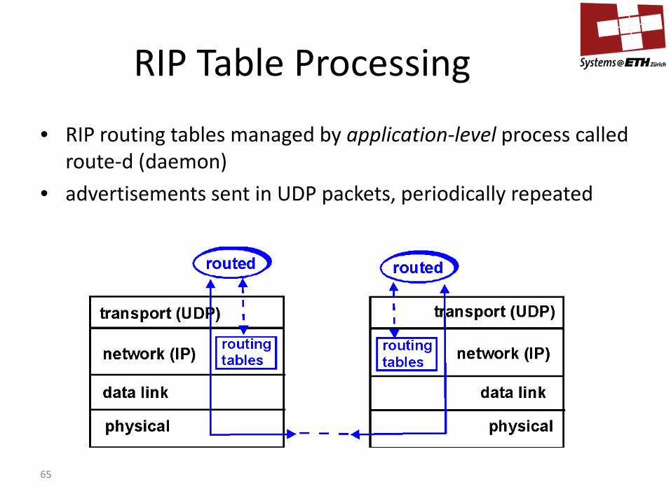
• RIP routing tables managed by application-level process called route-d (daemon)
• advertisements sent in UDP packets, periodically repeated
RIP Table Processing
66
• CISCO proprietary; successor of RIP (mid 80s) • Distance Vector, like RIP • several cost metrics (delay, bandwidth, reliability,
load, etc.) • uses TCP to exchange routing updates • Loop-free routing via Distributed Updating Algorithm
(DUAL) based on diffused computation
[E]IGRP: [Enhanced] Interior Gateway Routing Protocol

67
Link state routing protocols OSPF (Open Shortest Path First)
68
Link State Routing (Intuition) • Every node knows the topology and cost of every link
– Achieved through flooding • Nodes send the information on their links and
neighbors to all neighbors • Nodes forward information about other nodes
to their neighbors • ACKs used to prevent message loss • Sequence numbers used to compare versions
• With the information on topology and cost – Calculate the shortest path to every possible dest.
• e.g., use Dijkstra’s algorithm
69
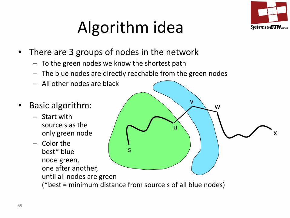
Algorithm idea
s
u
v w
x
• There are 3 groups of nodes in the network – To the green nodes we know the shortest path – The blue nodes are directly reachable from the green nodes – All other nodes are black
• Basic algorithm: – Start with
source s as the only green node
– Color the best* blue node green, one after another, until all nodes are green (*best = minimum distance from source s of all blue nodes)

70
Link state routing algorithm: Dijkstra
Dijkstra’s algorithm • net topology, link costs known to all
nodes – accomplished via “link state
broadcast” – all nodes have same info ideally – (of course, not true in reality
because of propagation delays) • computes single-source shortest
path tree – gives routing table for source
Notation • c(i,j): link cost from node i to j.
Can be infinite if not direct neighbors, costs define adjacency matrix.
• v.distance: current value of cost of path from source s to destination v.
• v.visited: boolean variable that determines if optimal path to v was found.
• v.pred: the predecessor node of v in the routing tree.
• B: the set of blue nodes.
71
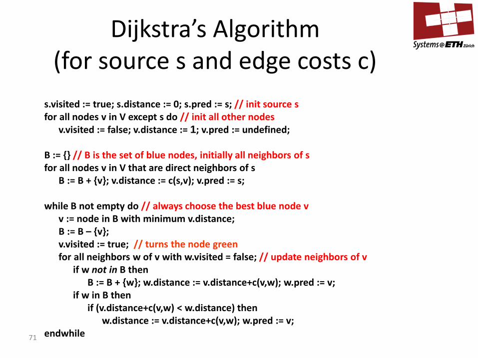
Dijkstra’s Algorithm (for source s and edge costs c)
s.visited := true; s.distance := 0; s.pred := s; // init source s for all nodes v in V except s do // init all other nodes v.visited := false; v.distance := 1; v.pred := undefined; B := {} // B is the set of blue nodes, initially all neighbors of s for all nodes v in V that are direct neighbors of s B := B + {v}; v.distance := c(s,v); v.pred := s; while B not empty do // always choose the best blue node v v := node in B with minimum v.distance; B := B – {v}; v.visited := true; // turns the node green for all neighbors w of v with w.visited = false; // update neighbors of v if w not in B then B := B + {w}; w.distance := v.distance+c(v,w); w.pred := v; if w in B then if (v.distance+c(v,w) < w.distance) then w.distance := v.distance+c(v,w); w.pred := v; endwhile

72
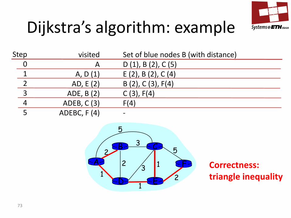
Dijkstra’s algorithm: example Step
0 1 2 3 4 5
visited A
A, D (1) AD, E (2)
ADE, B (2) ADEB, C (3)
ADEBC, F (4)
A
E D
C B
F 2
2 1
3
1
1
2
5 3
5
Set of blue nodes B (with distance) D (1), B (2), C (5) E (2), B (2), C (4) B (2), C (3), F(4) C (3), F(4) F(4) -
73
Dijkstra’s algorithm: example Step
0 1 2 3 4 5
visited A
A, D (1) AD, E (2)
ADE, B (2) ADEB, C (3)
ADEBC, F (4)
A
E D
C B
F 2
2 1
3
1
1
2
5 3
5
Set of blue nodes B (with distance) D (1), B (2), C (5) E (2), B (2), C (4) B (2), C (3), F(4) C (3), F(4) F(4) -
Correctness: triangle inequality
74
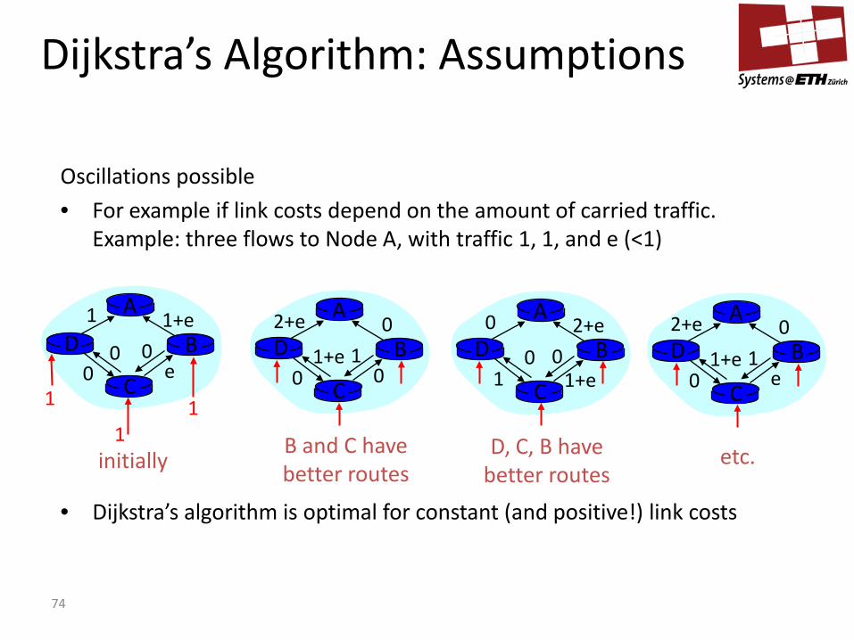
Dijkstra’s Algorithm: Assumptions
Oscillations possible • For example if link costs depend on the amount of carried traffic.
Example: three flows to Node A, with traffic 1, 1, and e (<1)
• Dijkstra’s algorithm is optimal for constant (and positive!) link costs
A
D
C
B 1 1+e
e 0
1
1 1
0 0
A
D
C
B 2+e 0
0 0 1+e 1
A
D
C
B 0 2+e
1+e 1 0 0
A
D
C
B 2+e 0
e 0 1+e 1
initially B and C have better routes
D, C, B have better routes
etc.
75
OSPF (Open Shortest Path First)
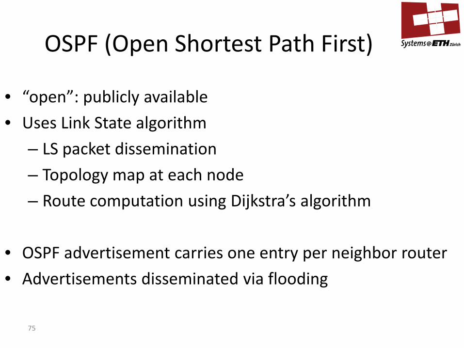
• “open”: publicly available • Uses Link State algorithm
– LS packet dissemination – Topology map at each node – Route computation using Dijkstra’s algorithm
• OSPF advertisement carries one entry per neighbor router • Advertisements disseminated via flooding
76
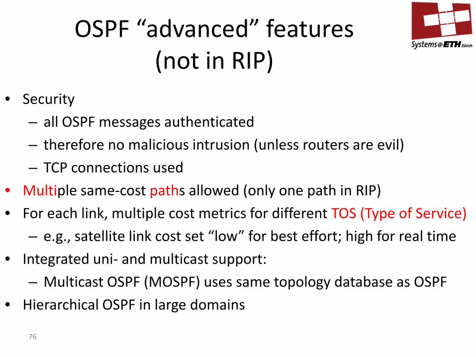
OSPF “advanced” features (not in RIP)
• Security
– all OSPF messages authenticated – therefore no malicious intrusion (unless routers are evil) – TCP connections used
• Multiple same-cost paths allowed (only one path in RIP) • For each link, multiple cost metrics for different TOS (Type of Service)
– e.g., satellite link cost set “low” for best effort; high for real time • Integrated uni- and multicast support:
– Multicast OSPF (MOSPF) uses same topology database as OSPF • Hierarchical OSPF in large domains
77
Hierarchical OSPF

78
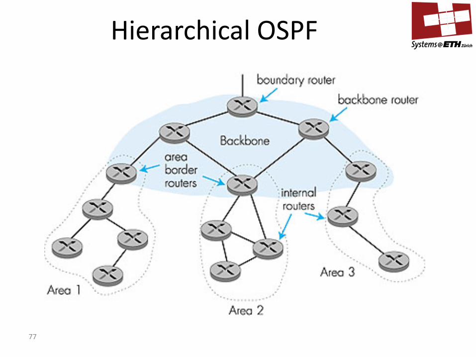
Hierarchical OSPF
• Two-level hierarchy: local area or backbone – Link-state advertisements only in area – each node has detailed area topology but only knows
direction (shortest path) to networks in other areas. • Area border routers
– “summarize” distances to networks in own area – advertise to other area border routers.
• Backbone routers – run OSPF routing limited to backbone.
• Boundary routers – connect to other autonomous systems.
79
Comparing routing algorithms
80
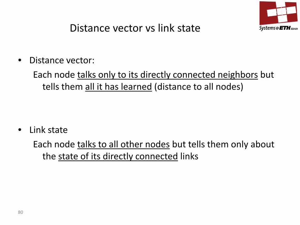
Distance vector vs link state
• Distance vector: Each node talks only to its directly connected neighbors but
tells them all it has learned (distance to all nodes)
• Link state Each node talks to all other nodes but tells them only about
the state of its directly connected links
81
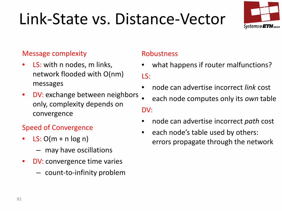
Message complexity • LS: with n nodes, m links,
network flooded with O(nm) messages
• DV: exchange between neighbors only, complexity depends on convergence
Speed of Convergence • LS: O(m + n log n)
– may have oscillations • DV: convergence time varies
– count-to-infinity problem
Robustness • what happens if router malfunctions? LS: • node can advertise incorrect link cost • each node computes only its own table DV: • node can advertise incorrect path cost • each node’s table used by others:
errors propagate through the network
Link-State vs. Distance-Vector
Link-State vs. Distance-Vector
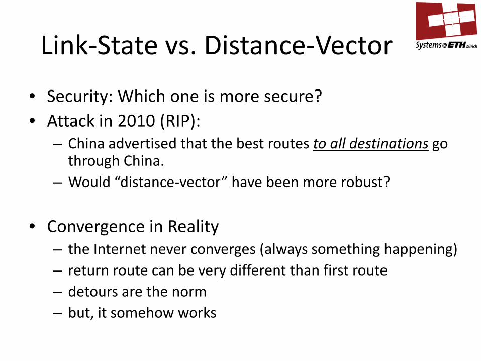
• Security: Which one is more secure? • Attack in 2010 (RIP):
– China advertised that the best routes to all destinations go through China.
– Would “distance-vector” have been more robust?
• Convergence in Reality – the Internet never converges (always something happening) – return route can be very different than first route – detours are the norm – but, it somehow works

83
Overview • Network layer services • IP, the Internet Protocol
– Model – Message format – Fragmentation and reassembly
• IP Addressing • Additional Protocols • Routing
– Basics – Interior Gateway Protocols (IGP)
• distance vector protocols: RIP • Link state protocols: OSPF
– Interdomain Routing (BGP) • Path vector protocol
• IPv6 • (Routers)

84
Interdomain routing - Border Gateway Protocol (BGP)
85
Hierarchical Routing
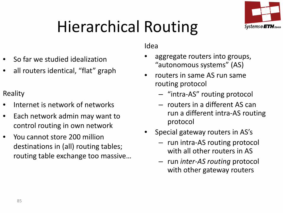
• So far we studied idealization • all routers identical, “flat” graph Reality • Internet is network of networks • Each network admin may want to
control routing in own network • You cannot store 200 million
destinations in (all) routing tables; routing table exchange too massive…
Idea • aggregate routers into groups,
“autonomous systems” (AS) • routers in same AS run same
routing protocol – “intra-AS” routing protocol – routers in a different AS can
run a different intra-AS routing protocol
• Special gateway routers in AS’s – run intra-AS routing protocol
with all other routers in AS – run inter-AS routing protocol
with other gateway routers

86
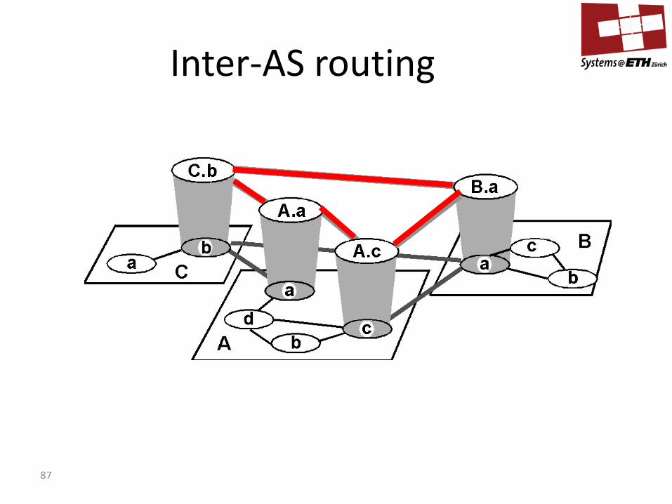
inter-AS, intra-AS routing in
gateway A.c
network layer
link layer
physical layer
a
b
b
a a C
A
B d
A.a A.c
C.b B.a
c b
c
Intra-AS and Inter-AS routing Gateways: • perform inter-AS
routing amongst themselves
• perform intra-AS routers with other routers in their AS
87
Inter-AS routing
88
routing table
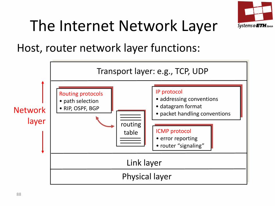
The Internet Network Layer Host, router network layer functions:
Routing protocols • path selection • RIP, OSPF, BGP
IP protocol • addressing conventions • datagram format • packet handling conventions
ICMP protocol • error reporting • router “signaling”
Transport layer: e.g., TCP, UDP
Link layer Physical layer
Network layer
90
BGP (Border Gateway Protocol)
• BGP is the Internet de-facto standard • Path Vector protocol
1) Receive BGP update (announce or withdrawal) from a neighbor. 2) Update routing table. 3) Does update affect active route? (Loop detection, policy, etc.) If yes,
send update to all neighbors that are allowed by policy.
MinRouteAdver: At most 1 announce per neighbor per 30+jitter seconds.
Store the active routes of the neighbors.

91
BGP details • BGP messages exchanged using TCP. • BGP messages
– OPEN: opens TCP connection to peer and authenticates sender – UPDATE: advertises new path (or withdraws old) – KEEPALIVE keeps connection alive in absence of UPDATES;
also ACKs OPEN request – NOTIFICATION: reports errors in previous msg;
also used to close connection
• Policy – Even if two BGP routers are connected they may not announce all
their routes or use all the routes of the other – Example: if AS A does not want to route traffic of AS B, then A should
simply not announce anything to B.
92
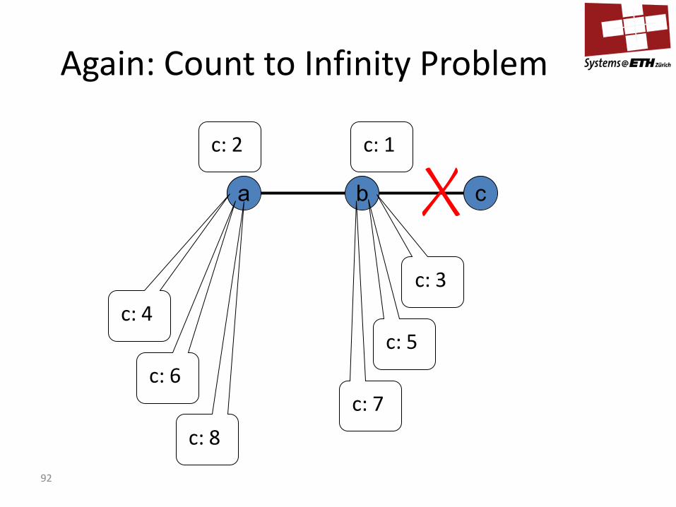
Again: Count to Infinity Problem
b a c
c: 2 c: 1
c: 3 c: 4
c: 5 c: 6
c: 7 c: 8
93
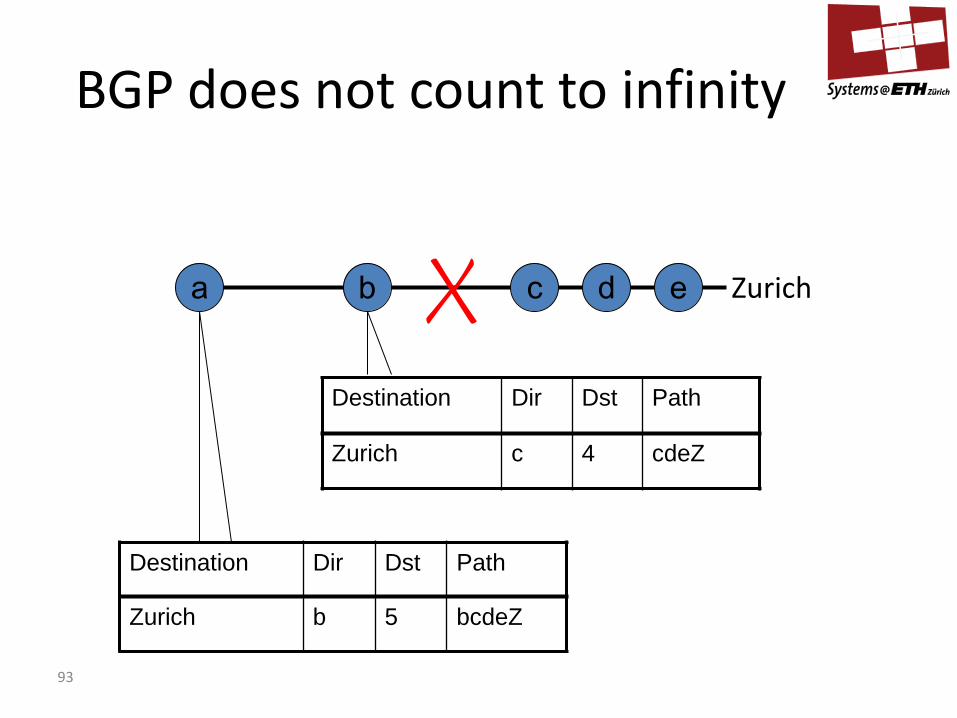
BGP does not count to infinity
Destination Dir Dst Path
Zurich c 4 cdeZ
b a c d e
Destination Dir Dst Path
Zurich b 5 bcdeZ
Zurich
94
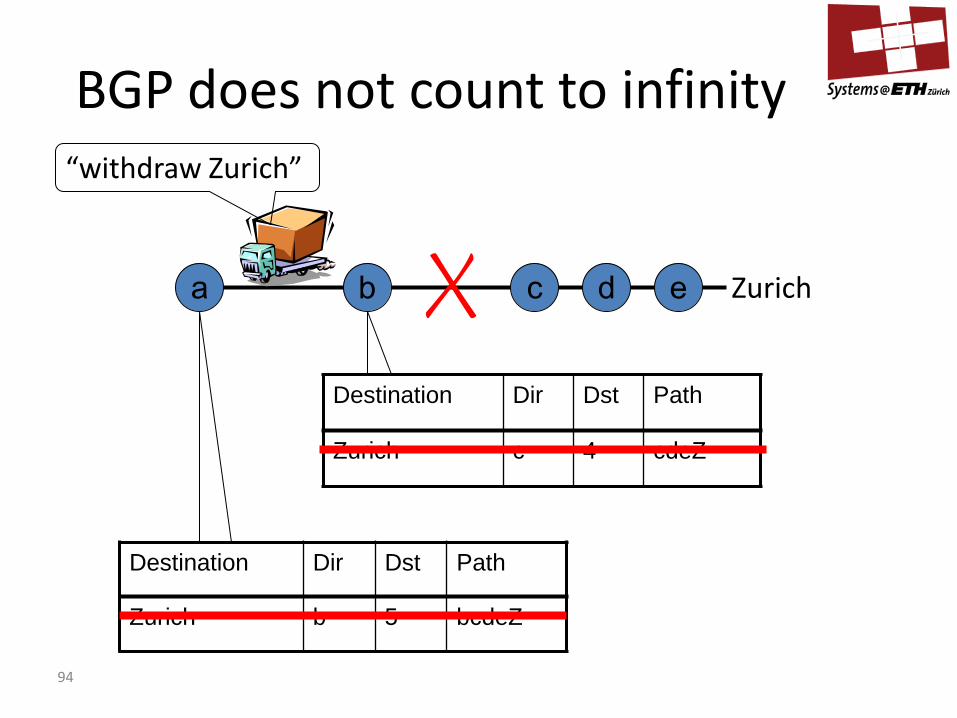
Destination Dir Dst Path
Zurich c 4 cdeZ
b a c d e
Destination Dir Dst Path
Zurich b 5 bcdeZ
Zurich
“withdraw Zurich”
BGP does not count to infinity
95
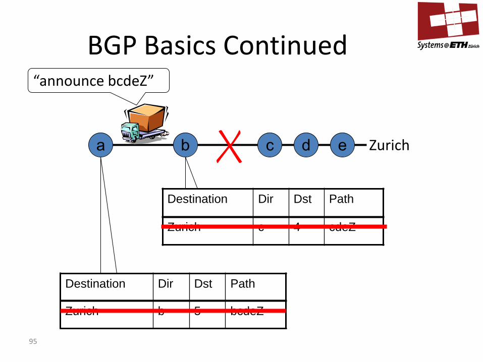
BGP Basics Continued
Destination Dir Dst Path
Zurich c 4 cdeZ
b a c d e
Destination Dir Dst Path
Zurich b 5 bcdeZ
Zurich
“announce bcdeZ”
96
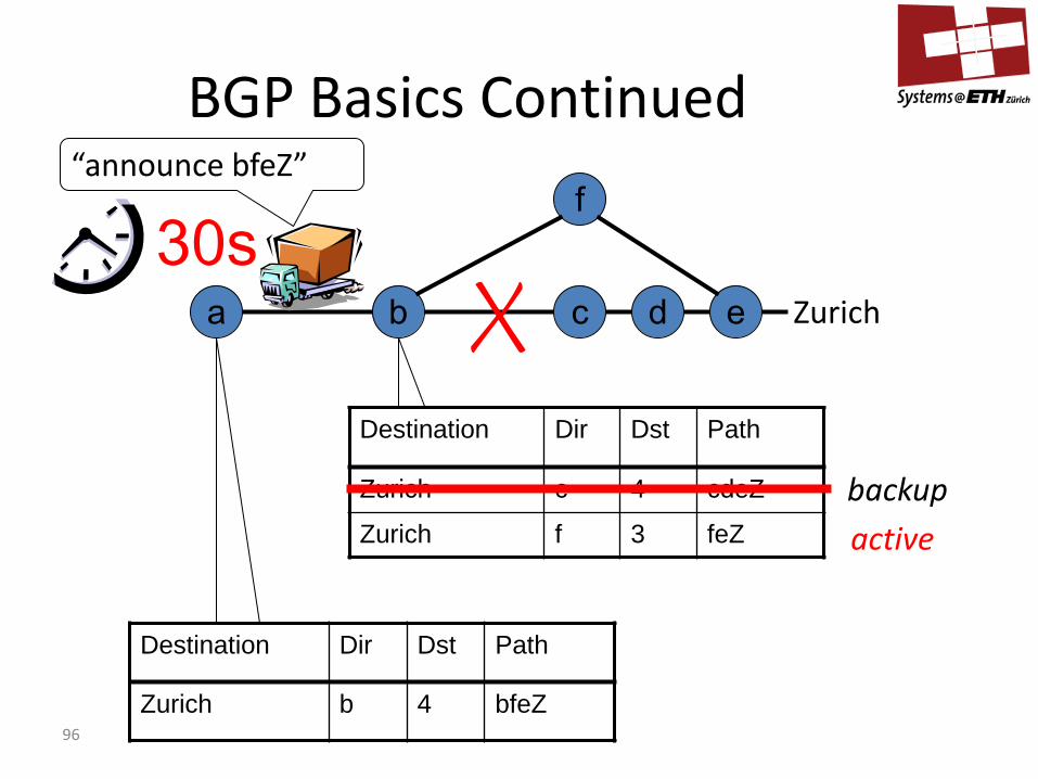
BGP Basics Continued
Destination Dir Dst Path
Zurich c 4 cdeZ
Zurich f 3 feZ
b a c d e
Destination Dir Dst Path
Zurich b 4 bfeZ
Zurich
“announce bfeZ” f
active backup
30s
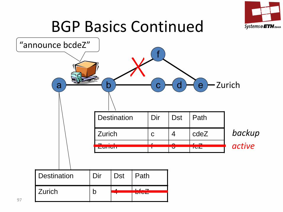
97
BGP Basics Continued
Destination Dir Dst Path
Zurich c 4 cdeZ
Zurich f 3 feZ
b a c d e
Destination Dir Dst Path
Zurich b 4 bfeZ
Zurich
“announce bcdeZ” f
active backup
98
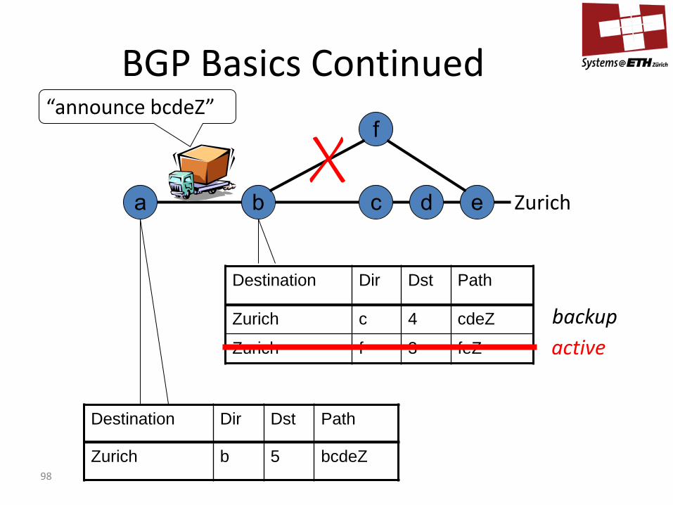
BGP Basics Continued
Destination Dir Dst Path
Zurich c 4 cdeZ
Zurich f 3 feZ
b a c d e
Destination Dir Dst Path
Zurich b 5 bcdeZ
Zurich
“announce bcdeZ” f
active backup
99
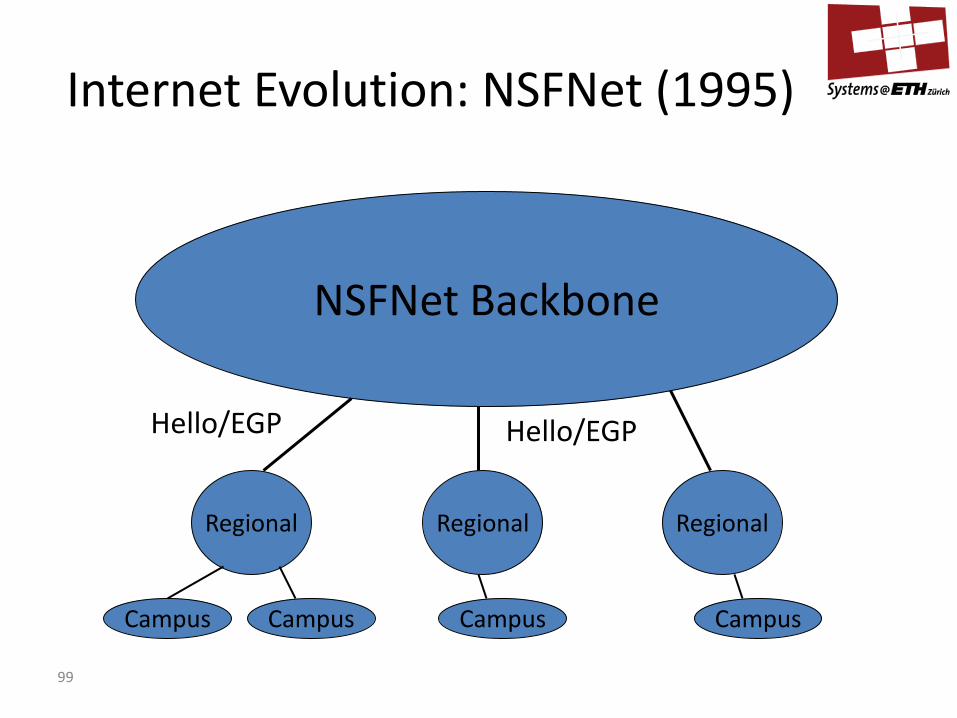
NSFNet Backbone
Regional Regional Regional
Campus Campus Campus Campus
Hello/EGP Hello/EGP
Internet Evolution: NSFNet (1995)
100
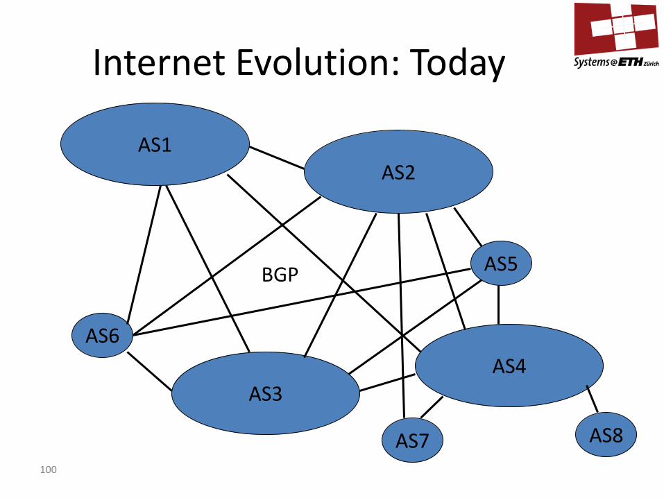
AS1 AS2
AS3 AS4
AS8
AS5
AS7
AS6
BGP
Internet Evolution: Today

101
Experimental Setup
• Analyzed secondary paths of 20x20 AS pairs: – Inject and monitor BGP faults. – Survey providers on policies.

102
0
20
40
60
80
100
0 20 40 60 80 100 120 140 160
Seconds Until Convergence
Cum
ulat
ive
Per
cent
age
New Link → New Route New Link → Better RouteFailure, Backup exists Failure, No Backup
180
BGP Convergence Times
103
BGP Convergence Results
• If a link comes up, the convergence time is in the
order of time to forward a message on the shortest path.
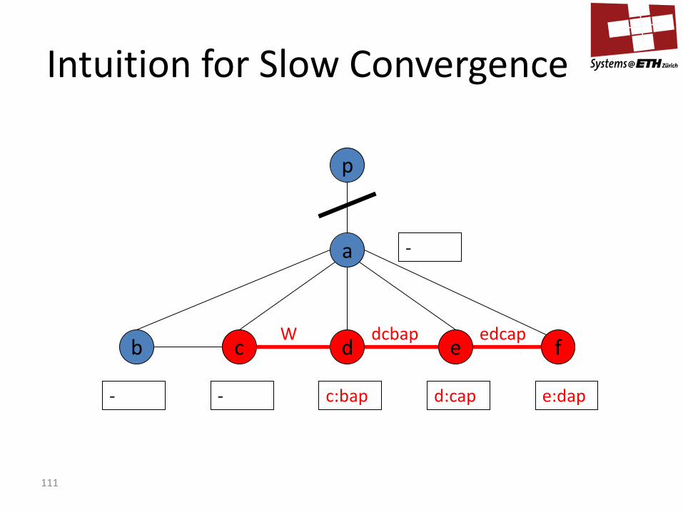
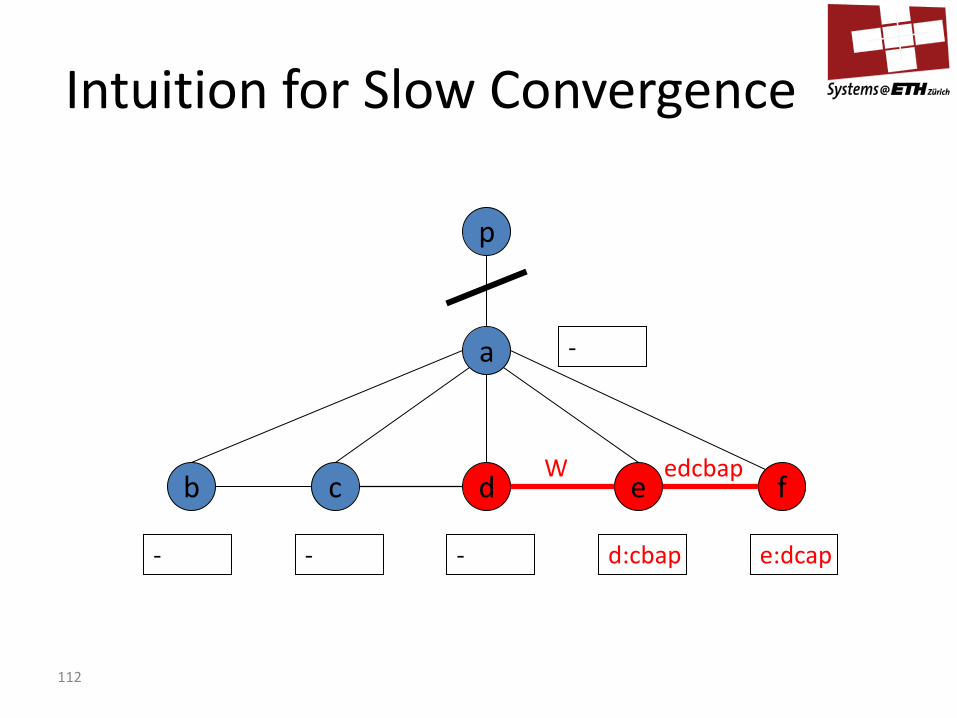
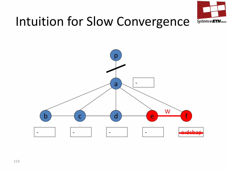
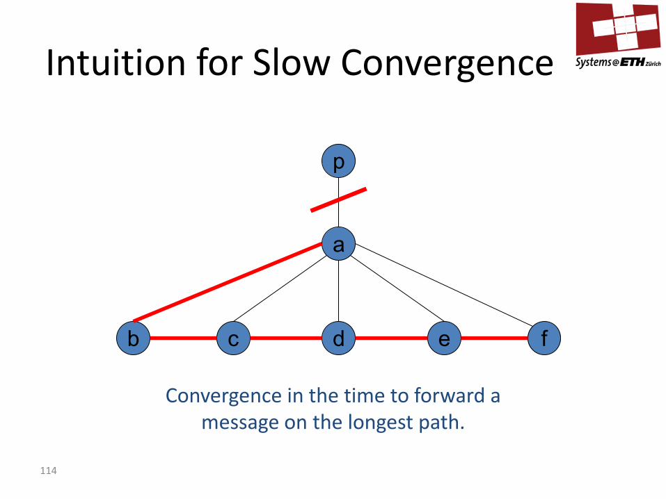
• If a link goes down, the convergence time is in the order of time to forward a message on the longest path.

104
a
b c d e f
p
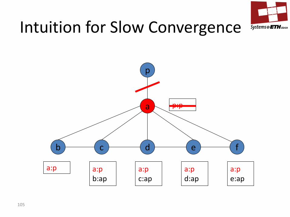
a:p e:ap
a:p d:ap
a:p c:ap
a:p b:ap
a:p
p:p
Intuition for Slow Convergence
105
a
b c d e f
p
a:p e:ap
a:p d:ap
a:p c:ap
a:p b:ap
a:p
p:p
Intuition for Slow Convergence

106
a
b c d e f
p
a:p e:ap
a:p d:ap
a:p c:ap
a:p b:ap
a:p
p:p
W W W W W
Intuition for Slow Convergence

107
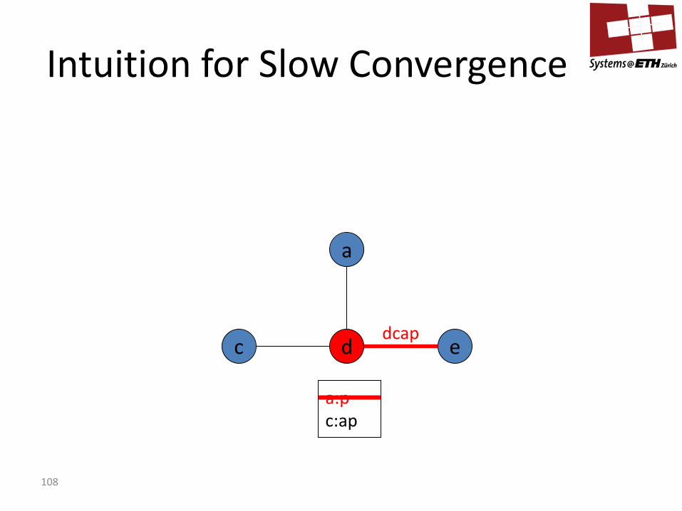
d e
a:p c:ap
W
a
c
Intuition for Slow Convergence
108
d e
a:p c:ap
dcap
a
c
Intuition for Slow Convergence

edap
dcap
109
a
b c d e f
p
a:p e:ap
a:p d:ap
a:p c:ap
a:p b:ap
a:p
p:p
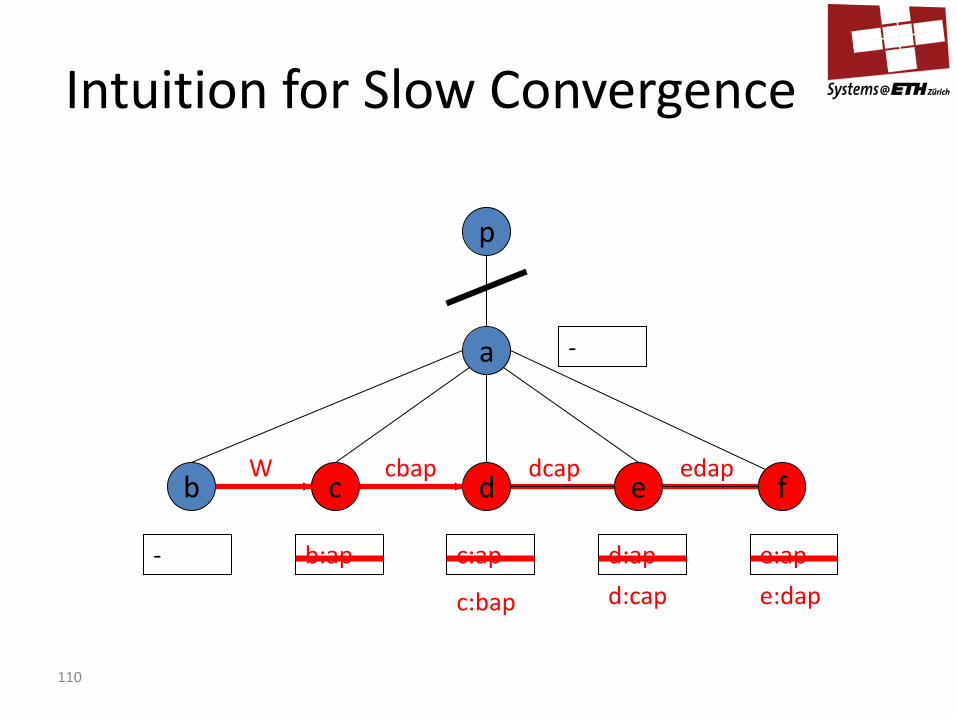
W cbap
Intuition for Slow Convergence
edap
dcap
110
a
b c d e f
p
e:ap d:ap c:ap b:ap -
-
cbap
W
c:bap d:cap e:dap
Intuition for Slow Convergence
111
a
b c d e f
p
e:dap d:cap c:bap - -
-
W dcbap edcap
Intuition for Slow Convergence
112
a
b c d e f
p
e:dcap d:cbap - - -
-
W edcbap
Intuition for Slow Convergence
113
a
b c d e f
p
e:dcbap - - - -
-
W
Intuition for Slow Convergence
114
a
b c d e f
p
Convergence in the time to forward a message on the longest path.
Intuition for Slow Convergence
115
a
p
c
f h
g
d
e
i
b
j
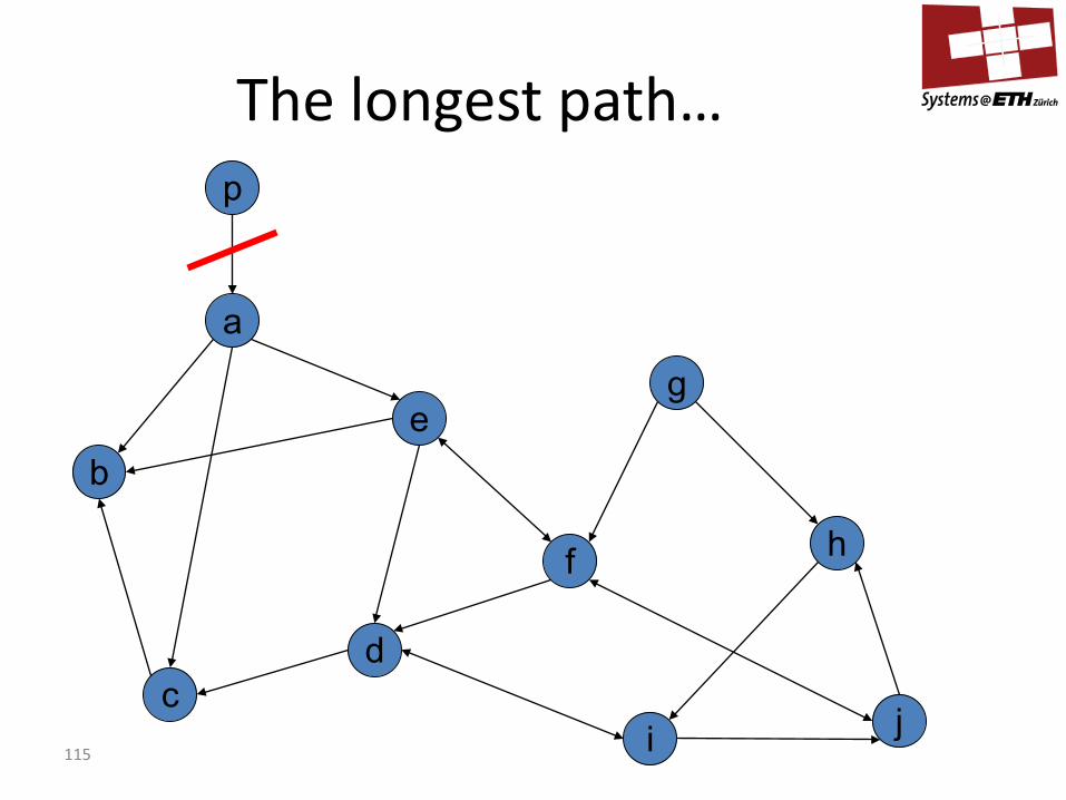
The longest path…
116
a
p
c
f h
g
d
e
i
b
j
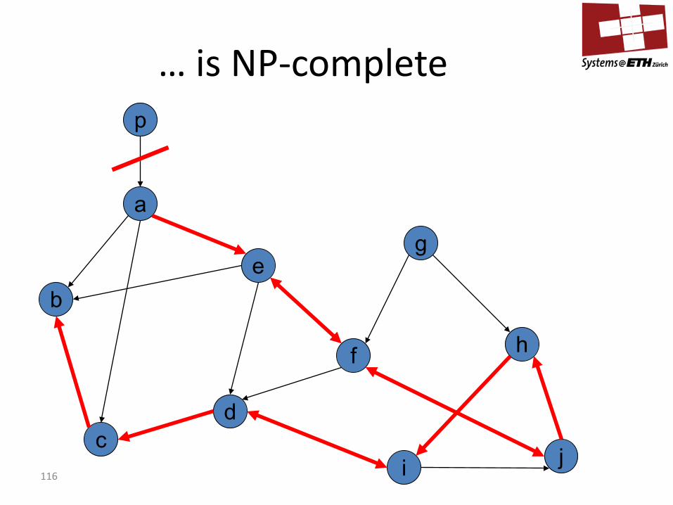
… is NP-complete

117
a
b c d e f
p
edap
W
edcap
edcbap
W
Remember the Example
118
What might help?
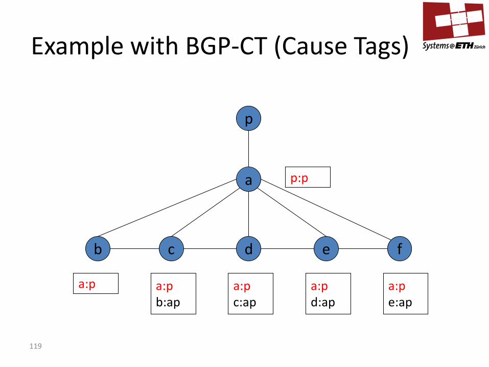
• Idea: Attach a “cause tag” to the withdrawal message identifying the failed link/node (for a given prefix).
• It can be shown that a cause tag reduces the convergence time to the shortest path
• Problems – Since BGP is widely deployed, it cannot be changed easily – ISP’s (AS’s) don’t like the world to know that it is their link that is not
stable, and cause tags do exactly that. – Race conditions make the cause tags protocol intricate
119
a
b c d e f
p
a:p e:ap
a:p d:ap
a:p c:ap
a:p b:ap
a:p
p:p
Example with BGP-CT (Cause Tags)
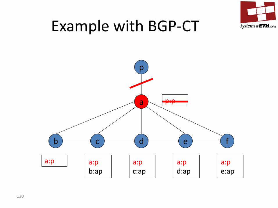
120
a
b c d e f
p
a:p e:ap
a:p d:ap
a:p c:ap
a:p b:ap
a:p
p:p
Example with BGP-CT

121
a
b c d e f
p
a:p e:ap
a:p d:ap
a:p c:ap
a:p b:ap
a:p
p:p
W(ap) W(ap) W(ap) W(ap) W(ap)
Example with BGP-CT
122
p
b c
x
e f
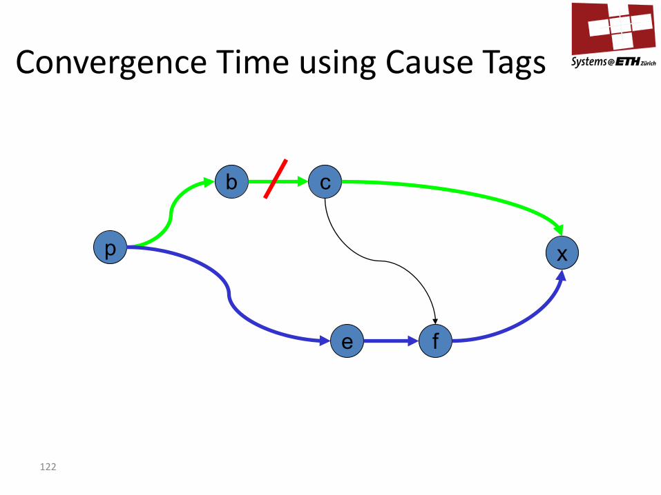
Convergence Time using Cause Tags

123
p
b c
x
e f
Convergence Time using Cause Tags
124
p
b c
x
e f
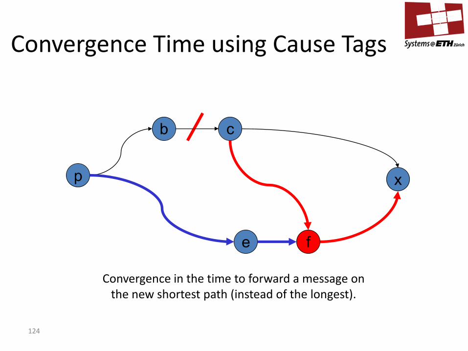
Convergence in the time to forward a message on the new shortest path (instead of the longest).
Convergence Time using Cause Tags
125
• Policy
– Inter-AS: admin wants control over how its traffic routed, and who routes through its net.
– Intra-AS: single admin, so no policy decisions needed • Scale
– hierarchical routing saves table size, reduced update traffic • Performance
– Intra-AS: can focus on performance – Inter-AS: policy / security may dominate over performance
Why are Intra- and Inter-AS routing different?

126
IPv6

127
• Initial motivation
– 32-bit address space almost completely allocated. • Additional motivation
– header format helps speed processing/forwarding – header changes to facilitate QoS (quality of service) – new “anycast” address: route to “best” of several
replicated servers • IPv6 datagram format:
– fixed-length 40 byte header – no fragmentation allowed
IPv6
128
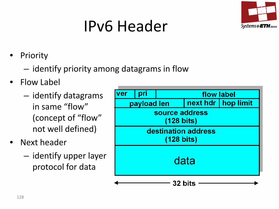
IPv6 Header
• Priority – identify priority among datagrams in flow
• Flow Label – identify datagrams
in same “flow” (concept of “flow” not well defined)
• Next header – identify upper layer
protocol for data

129
Other Changes from IPv4
• Checksum – removed entirely to reduce processing time at each hop
• Options – allowed, but outside of header – indicated by “Next Header” field
• ICMPv6: new version of ICMP – additional message types, e.g. “Packet Too Big” – multicast group management functions

130
Transition From IPv4 To IPv6
• Not all routers can be upgraded simultaneously – no “flag days” – How will the network operate with mixed IPv4
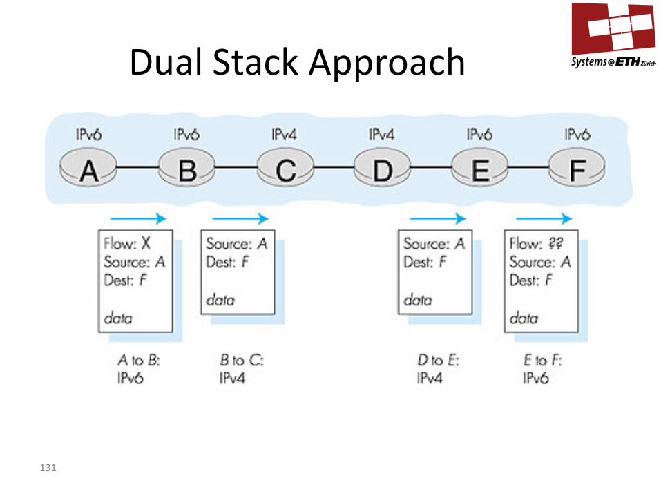
and IPv6 routers? • Two proposed approaches
– Dual Stack • some routers with dual stack (v6, v4) can
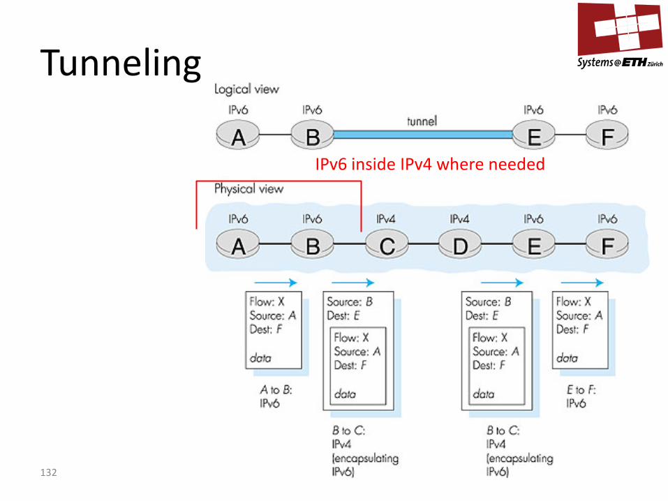
“translate” between formats – Tunneling
• IPv6 carried as payload in IPv4 datagram among IPv4 routers
131
Dual Stack Approach
132
IPv6 inside IPv4 where needed
Tunneling
133
Routers (Bonus Material, not covered in class)
134
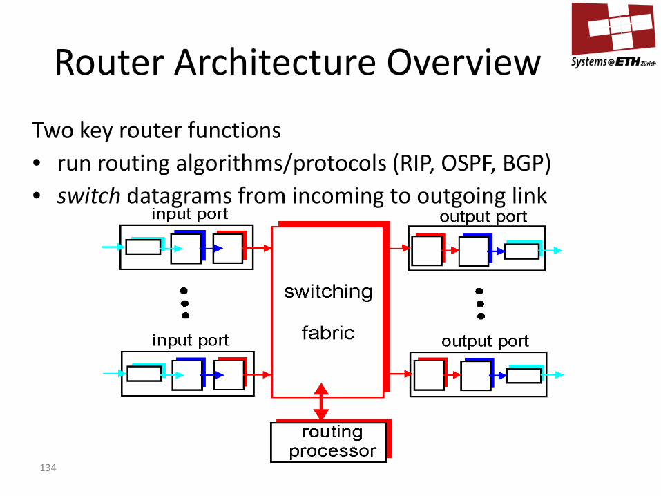
Two key router functions • run routing algorithms/protocols (RIP, OSPF, BGP) • switch datagrams from incoming to outgoing link
Router Architecture Overview
135
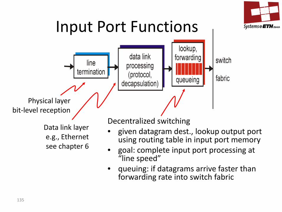
Decentralized switching • given datagram dest., lookup output port
using routing table in input port memory • goal: complete input port processing at
“line speed” • queuing: if datagrams arrive faster than
forwarding rate into switch fabric
Physical layer bit-level reception
Data link layer e.g., Ethernet see chapter 6
Input Port Functions
136
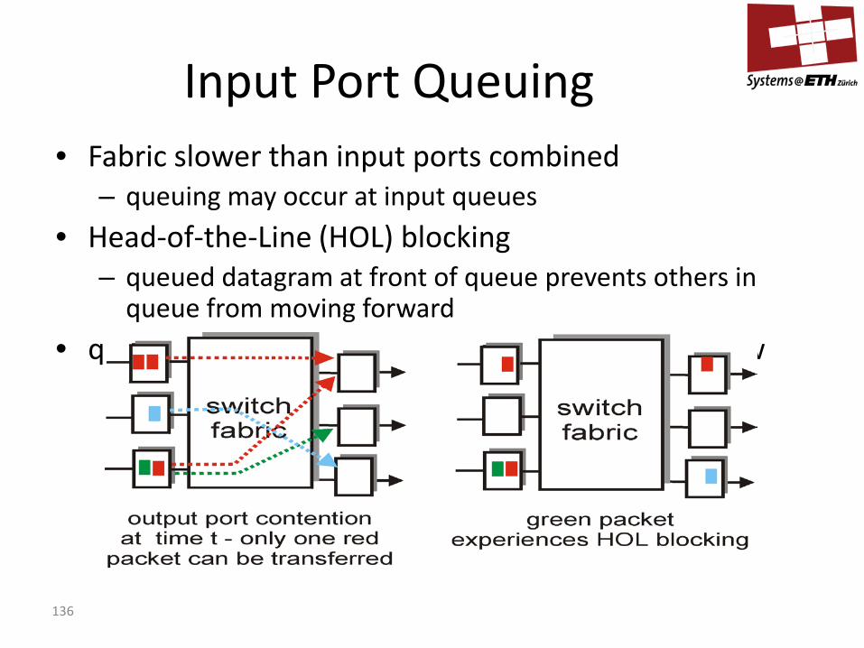
• Fabric slower than input ports combined
– queuing may occur at input queues • Head-of-the-Line (HOL) blocking
– queued datagram at front of queue prevents others in queue from moving forward
• queuing delay and loss due to input buffer overflow
Input Port Queuing
137
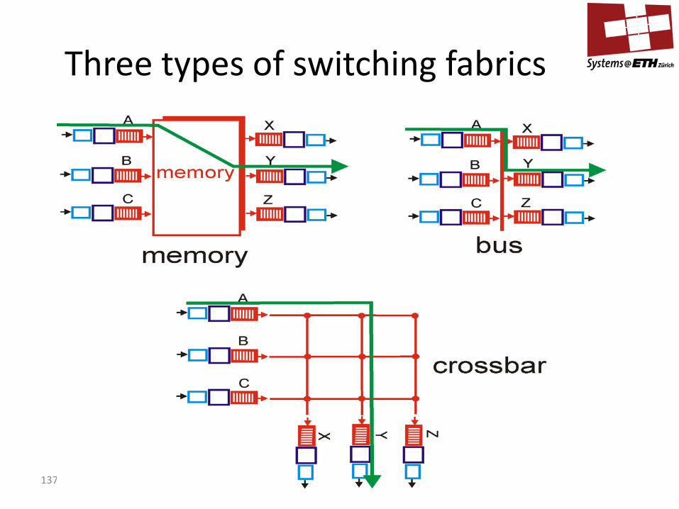
Three types of switching fabrics
138
Input Port
Output Port
Memory
System Bus
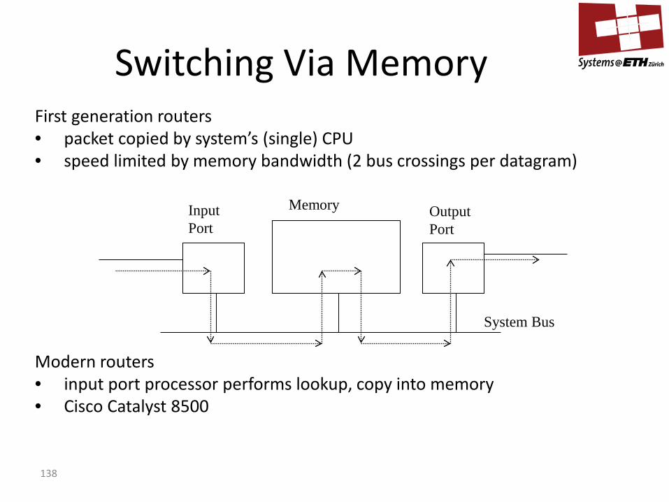
Switching Via Memory
First generation routers • packet copied by system’s (single) CPU • speed limited by memory bandwidth (2 bus crossings per datagram)
Modern routers • input port processor performs lookup, copy into memory • Cisco Catalyst 8500
139
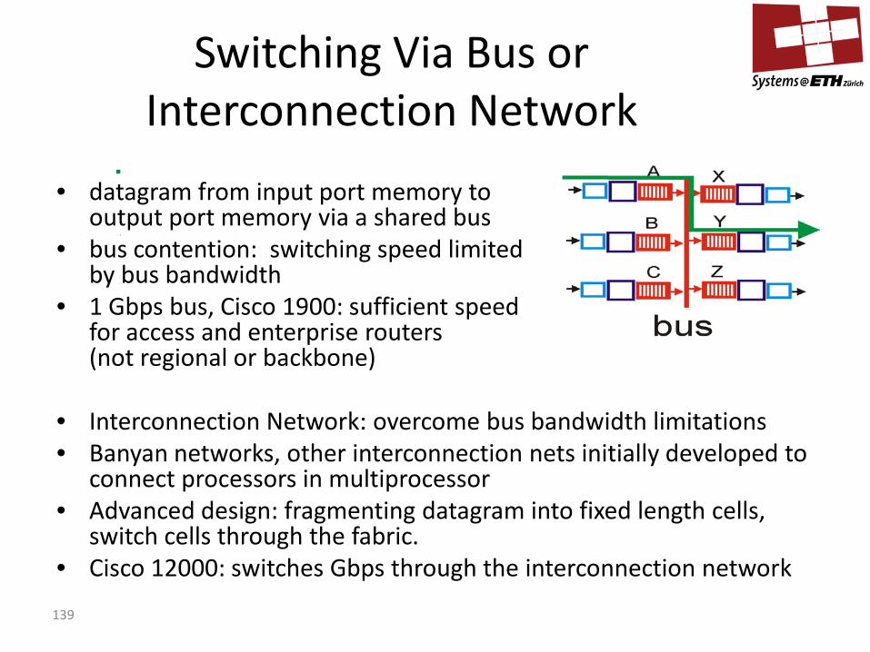
• datagram from input port memory to
output port memory via a shared bus • bus contention: switching speed limited
by bus bandwidth • 1 Gbps bus, Cisco 1900: sufficient speed
for access and enterprise routers (not regional or backbone)
• Interconnection Network: overcome bus bandwidth limitations • Banyan networks, other interconnection nets initially developed to
connect processors in multiprocessor • Advanced design: fragmenting datagram into fixed length cells,
switch cells through the fabric. • Cisco 12000: switches Gbps through the interconnection network
Switching Via Bus or Interconnection Network
140
5 Level 4 2 1 0
0000
0001
0010
0011
0100
0101
0110
0111
1000
1001
1010
1011
1100
1101
1110
1111
Bit string
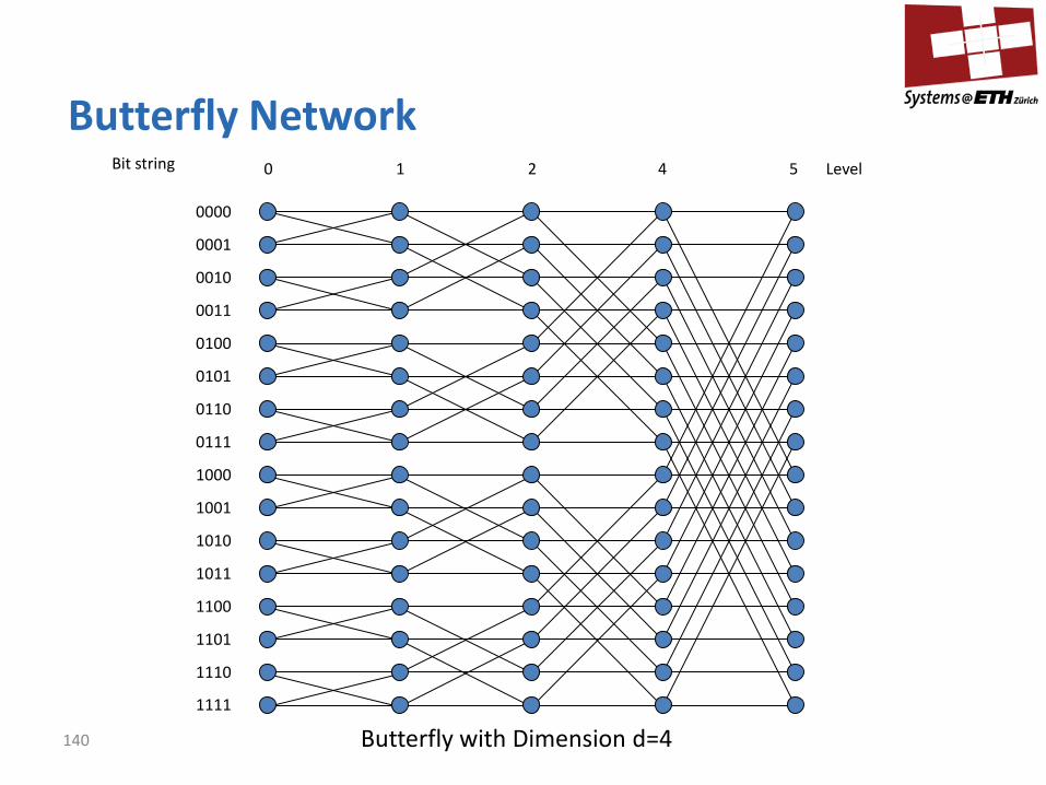
Butterfly with Dimension d=4
Butterfly Network
141
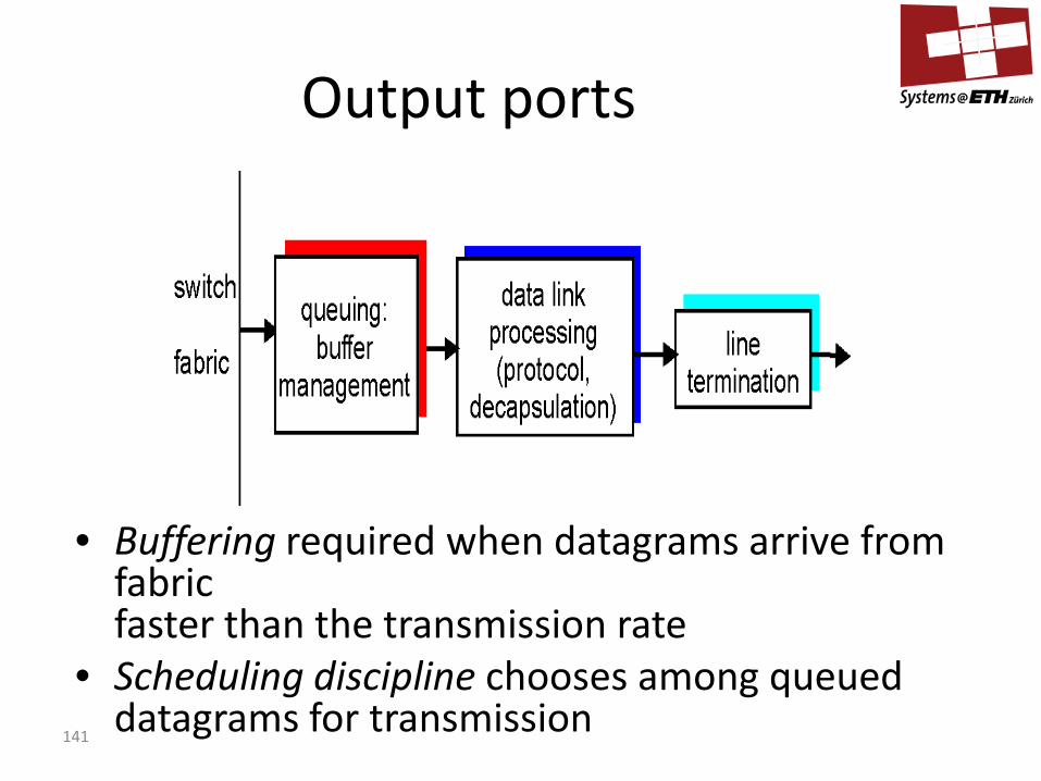
• Buffering required when datagrams arrive from fabric faster than the transmission rate
• Scheduling discipline chooses among queued datagrams for transmission
Output ports