networkx reference · networkx reference release 2.1 aric hagberg, dan schult, pieter swart jan 22,...
TRANSCRIPT

NetworkX ReferenceRelease 2.1
Aric Hagberg, Dan Schult, Pieter Swart
Jan 22, 2018


CONTENTS
1 Introduction 11.1 NetworkX Basics . . . . . . . . . . . . . . . . . . . . . . . . . . . . . . . . . . . . . . . . . . . . . 11.2 Graphs . . . . . . . . . . . . . . . . . . . . . . . . . . . . . . . . . . . . . . . . . . . . . . . . . . 21.3 Graph Creation . . . . . . . . . . . . . . . . . . . . . . . . . . . . . . . . . . . . . . . . . . . . . . 21.4 Graph Reporting . . . . . . . . . . . . . . . . . . . . . . . . . . . . . . . . . . . . . . . . . . . . . 31.5 Algorithms . . . . . . . . . . . . . . . . . . . . . . . . . . . . . . . . . . . . . . . . . . . . . . . . 41.6 Drawing . . . . . . . . . . . . . . . . . . . . . . . . . . . . . . . . . . . . . . . . . . . . . . . . . 41.7 Data Structure . . . . . . . . . . . . . . . . . . . . . . . . . . . . . . . . . . . . . . . . . . . . . . 5
2 Graph types 72.1 Which graph class should I use? . . . . . . . . . . . . . . . . . . . . . . . . . . . . . . . . . . . . . 72.2 Basic graph types . . . . . . . . . . . . . . . . . . . . . . . . . . . . . . . . . . . . . . . . . . . . . 7
3 Algorithms 1213.1 Approximations and Heuristics . . . . . . . . . . . . . . . . . . . . . . . . . . . . . . . . . . . . . 1213.2 Assortativity . . . . . . . . . . . . . . . . . . . . . . . . . . . . . . . . . . . . . . . . . . . . . . . 1323.3 Bipartite . . . . . . . . . . . . . . . . . . . . . . . . . . . . . . . . . . . . . . . . . . . . . . . . . 1413.4 Boundary . . . . . . . . . . . . . . . . . . . . . . . . . . . . . . . . . . . . . . . . . . . . . . . . . 1693.5 Bridges . . . . . . . . . . . . . . . . . . . . . . . . . . . . . . . . . . . . . . . . . . . . . . . . . . 1713.6 Centrality . . . . . . . . . . . . . . . . . . . . . . . . . . . . . . . . . . . . . . . . . . . . . . . . . 1733.7 Chains . . . . . . . . . . . . . . . . . . . . . . . . . . . . . . . . . . . . . . . . . . . . . . . . . . 1973.8 Chordal . . . . . . . . . . . . . . . . . . . . . . . . . . . . . . . . . . . . . . . . . . . . . . . . . . 1983.9 Clique . . . . . . . . . . . . . . . . . . . . . . . . . . . . . . . . . . . . . . . . . . . . . . . . . . 2013.10 Clustering . . . . . . . . . . . . . . . . . . . . . . . . . . . . . . . . . . . . . . . . . . . . . . . . 2053.11 Coloring . . . . . . . . . . . . . . . . . . . . . . . . . . . . . . . . . . . . . . . . . . . . . . . . . 2103.12 Communicability . . . . . . . . . . . . . . . . . . . . . . . . . . . . . . . . . . . . . . . . . . . . . 2133.13 Communities . . . . . . . . . . . . . . . . . . . . . . . . . . . . . . . . . . . . . . . . . . . . . . . 2153.14 Components . . . . . . . . . . . . . . . . . . . . . . . . . . . . . . . . . . . . . . . . . . . . . . . 2243.15 Connectivity . . . . . . . . . . . . . . . . . . . . . . . . . . . . . . . . . . . . . . . . . . . . . . . 2393.16 Cores . . . . . . . . . . . . . . . . . . . . . . . . . . . . . . . . . . . . . . . . . . . . . . . . . . . 2693.17 Covering . . . . . . . . . . . . . . . . . . . . . . . . . . . . . . . . . . . . . . . . . . . . . . . . . 2723.18 Cycles . . . . . . . . . . . . . . . . . . . . . . . . . . . . . . . . . . . . . . . . . . . . . . . . . . 2733.19 Cuts . . . . . . . . . . . . . . . . . . . . . . . . . . . . . . . . . . . . . . . . . . . . . . . . . . . . 2773.20 Directed Acyclic Graphs . . . . . . . . . . . . . . . . . . . . . . . . . . . . . . . . . . . . . . . . . 2813.21 Dispersion . . . . . . . . . . . . . . . . . . . . . . . . . . . . . . . . . . . . . . . . . . . . . . . . 2883.22 Distance Measures . . . . . . . . . . . . . . . . . . . . . . . . . . . . . . . . . . . . . . . . . . . . 2883.23 Distance-Regular Graphs . . . . . . . . . . . . . . . . . . . . . . . . . . . . . . . . . . . . . . . . . 2903.24 Dominance . . . . . . . . . . . . . . . . . . . . . . . . . . . . . . . . . . . . . . . . . . . . . . . . 2933.25 Dominating Sets . . . . . . . . . . . . . . . . . . . . . . . . . . . . . . . . . . . . . . . . . . . . . 2943.26 Efficiency . . . . . . . . . . . . . . . . . . . . . . . . . . . . . . . . . . . . . . . . . . . . . . . . . 295
i

3.27 Eulerian . . . . . . . . . . . . . . . . . . . . . . . . . . . . . . . . . . . . . . . . . . . . . . . . . . 2973.28 Flows . . . . . . . . . . . . . . . . . . . . . . . . . . . . . . . . . . . . . . . . . . . . . . . . . . . 2993.29 Graphical degree sequence . . . . . . . . . . . . . . . . . . . . . . . . . . . . . . . . . . . . . . . . 3263.30 Hierarchy . . . . . . . . . . . . . . . . . . . . . . . . . . . . . . . . . . . . . . . . . . . . . . . . . 3293.31 Hybrid . . . . . . . . . . . . . . . . . . . . . . . . . . . . . . . . . . . . . . . . . . . . . . . . . . 3303.32 Isolates . . . . . . . . . . . . . . . . . . . . . . . . . . . . . . . . . . . . . . . . . . . . . . . . . . 3313.33 Isomorphism . . . . . . . . . . . . . . . . . . . . . . . . . . . . . . . . . . . . . . . . . . . . . . . 3323.34 Link Analysis . . . . . . . . . . . . . . . . . . . . . . . . . . . . . . . . . . . . . . . . . . . . . . . 3463.35 Link Prediction . . . . . . . . . . . . . . . . . . . . . . . . . . . . . . . . . . . . . . . . . . . . . . 3533.36 Matching . . . . . . . . . . . . . . . . . . . . . . . . . . . . . . . . . . . . . . . . . . . . . . . . . 3593.37 Minors . . . . . . . . . . . . . . . . . . . . . . . . . . . . . . . . . . . . . . . . . . . . . . . . . . 3613.38 Maximal independent set . . . . . . . . . . . . . . . . . . . . . . . . . . . . . . . . . . . . . . . . . 3663.39 Operators . . . . . . . . . . . . . . . . . . . . . . . . . . . . . . . . . . . . . . . . . . . . . . . . . 3673.40 Reciprocity . . . . . . . . . . . . . . . . . . . . . . . . . . . . . . . . . . . . . . . . . . . . . . . . 3763.41 Rich Club . . . . . . . . . . . . . . . . . . . . . . . . . . . . . . . . . . . . . . . . . . . . . . . . . 3773.42 Shortest Paths . . . . . . . . . . . . . . . . . . . . . . . . . . . . . . . . . . . . . . . . . . . . . . 3783.43 Simple Paths . . . . . . . . . . . . . . . . . . . . . . . . . . . . . . . . . . . . . . . . . . . . . . . 4073.44 Structural holes . . . . . . . . . . . . . . . . . . . . . . . . . . . . . . . . . . . . . . . . . . . . . . 4113.45 Swap . . . . . . . . . . . . . . . . . . . . . . . . . . . . . . . . . . . . . . . . . . . . . . . . . . . 4143.46 Tournament . . . . . . . . . . . . . . . . . . . . . . . . . . . . . . . . . . . . . . . . . . . . . . . . 4153.47 Traversal . . . . . . . . . . . . . . . . . . . . . . . . . . . . . . . . . . . . . . . . . . . . . . . . . 4183.48 Tree . . . . . . . . . . . . . . . . . . . . . . . . . . . . . . . . . . . . . . . . . . . . . . . . . . . . 4283.49 Triads . . . . . . . . . . . . . . . . . . . . . . . . . . . . . . . . . . . . . . . . . . . . . . . . . . . 4433.50 Vitality . . . . . . . . . . . . . . . . . . . . . . . . . . . . . . . . . . . . . . . . . . . . . . . . . . 4433.51 Voronoi cells . . . . . . . . . . . . . . . . . . . . . . . . . . . . . . . . . . . . . . . . . . . . . . . 4443.52 Wiener index . . . . . . . . . . . . . . . . . . . . . . . . . . . . . . . . . . . . . . . . . . . . . . . 445
4 Functions 4474.1 Graph . . . . . . . . . . . . . . . . . . . . . . . . . . . . . . . . . . . . . . . . . . . . . . . . . . . 4474.2 Nodes . . . . . . . . . . . . . . . . . . . . . . . . . . . . . . . . . . . . . . . . . . . . . . . . . . . 4504.3 Edges . . . . . . . . . . . . . . . . . . . . . . . . . . . . . . . . . . . . . . . . . . . . . . . . . . . 4514.4 Self loops . . . . . . . . . . . . . . . . . . . . . . . . . . . . . . . . . . . . . . . . . . . . . . . . . 4524.5 Attributes . . . . . . . . . . . . . . . . . . . . . . . . . . . . . . . . . . . . . . . . . . . . . . . . . 4544.6 Freezing graph structure . . . . . . . . . . . . . . . . . . . . . . . . . . . . . . . . . . . . . . . . . 457
5 Graph generators 4595.1 Atlas . . . . . . . . . . . . . . . . . . . . . . . . . . . . . . . . . . . . . . . . . . . . . . . . . . . 4595.2 Classic . . . . . . . . . . . . . . . . . . . . . . . . . . . . . . . . . . . . . . . . . . . . . . . . . . 4605.3 Expanders . . . . . . . . . . . . . . . . . . . . . . . . . . . . . . . . . . . . . . . . . . . . . . . . 4675.4 Lattice . . . . . . . . . . . . . . . . . . . . . . . . . . . . . . . . . . . . . . . . . . . . . . . . . . 4685.5 Small . . . . . . . . . . . . . . . . . . . . . . . . . . . . . . . . . . . . . . . . . . . . . . . . . . . 4715.6 Random Graphs . . . . . . . . . . . . . . . . . . . . . . . . . . . . . . . . . . . . . . . . . . . . . 4755.7 Duplication Divergence . . . . . . . . . . . . . . . . . . . . . . . . . . . . . . . . . . . . . . . . . 4845.8 Degree Sequence . . . . . . . . . . . . . . . . . . . . . . . . . . . . . . . . . . . . . . . . . . . . . 4855.9 Random Clustered . . . . . . . . . . . . . . . . . . . . . . . . . . . . . . . . . . . . . . . . . . . . 4915.10 Directed . . . . . . . . . . . . . . . . . . . . . . . . . . . . . . . . . . . . . . . . . . . . . . . . . 4925.11 Geometric . . . . . . . . . . . . . . . . . . . . . . . . . . . . . . . . . . . . . . . . . . . . . . . . 4965.12 Line Graph . . . . . . . . . . . . . . . . . . . . . . . . . . . . . . . . . . . . . . . . . . . . . . . . 5035.13 Ego Graph . . . . . . . . . . . . . . . . . . . . . . . . . . . . . . . . . . . . . . . . . . . . . . . . 5055.14 Stochastic . . . . . . . . . . . . . . . . . . . . . . . . . . . . . . . . . . . . . . . . . . . . . . . . . 5065.15 Intersection . . . . . . . . . . . . . . . . . . . . . . . . . . . . . . . . . . . . . . . . . . . . . . . . 5065.16 Social Networks . . . . . . . . . . . . . . . . . . . . . . . . . . . . . . . . . . . . . . . . . . . . . 5085.17 Community . . . . . . . . . . . . . . . . . . . . . . . . . . . . . . . . . . . . . . . . . . . . . . . . 5095.18 Trees . . . . . . . . . . . . . . . . . . . . . . . . . . . . . . . . . . . . . . . . . . . . . . . . . . . 514
ii

5.19 Non Isomorphic Trees . . . . . . . . . . . . . . . . . . . . . . . . . . . . . . . . . . . . . . . . . . 5165.20 Triads . . . . . . . . . . . . . . . . . . . . . . . . . . . . . . . . . . . . . . . . . . . . . . . . . . . 5175.21 Joint Degree Sequence . . . . . . . . . . . . . . . . . . . . . . . . . . . . . . . . . . . . . . . . . . 5175.22 Mycielski . . . . . . . . . . . . . . . . . . . . . . . . . . . . . . . . . . . . . . . . . . . . . . . . . 519
6 Linear algebra 5216.1 Graph Matrix . . . . . . . . . . . . . . . . . . . . . . . . . . . . . . . . . . . . . . . . . . . . . . . 5216.2 Laplacian Matrix . . . . . . . . . . . . . . . . . . . . . . . . . . . . . . . . . . . . . . . . . . . . . 5226.3 Spectrum . . . . . . . . . . . . . . . . . . . . . . . . . . . . . . . . . . . . . . . . . . . . . . . . . 5256.4 Algebraic Connectivity . . . . . . . . . . . . . . . . . . . . . . . . . . . . . . . . . . . . . . . . . . 5266.5 Attribute Matrices . . . . . . . . . . . . . . . . . . . . . . . . . . . . . . . . . . . . . . . . . . . . 529
7 Converting to and from other data formats 5337.1 To NetworkX Graph . . . . . . . . . . . . . . . . . . . . . . . . . . . . . . . . . . . . . . . . . . . 5337.2 Dictionaries . . . . . . . . . . . . . . . . . . . . . . . . . . . . . . . . . . . . . . . . . . . . . . . . 5347.3 Lists . . . . . . . . . . . . . . . . . . . . . . . . . . . . . . . . . . . . . . . . . . . . . . . . . . . 5357.4 Numpy . . . . . . . . . . . . . . . . . . . . . . . . . . . . . . . . . . . . . . . . . . . . . . . . . . 5367.5 Scipy . . . . . . . . . . . . . . . . . . . . . . . . . . . . . . . . . . . . . . . . . . . . . . . . . . . 5407.6 Pandas . . . . . . . . . . . . . . . . . . . . . . . . . . . . . . . . . . . . . . . . . . . . . . . . . . 543
8 Relabeling nodes 5478.1 Relabeling . . . . . . . . . . . . . . . . . . . . . . . . . . . . . . . . . . . . . . . . . . . . . . . . 547
9 Reading and writing graphs 5519.1 Adjacency List . . . . . . . . . . . . . . . . . . . . . . . . . . . . . . . . . . . . . . . . . . . . . . 5519.2 Multiline Adjacency List . . . . . . . . . . . . . . . . . . . . . . . . . . . . . . . . . . . . . . . . . 5549.3 Edge List . . . . . . . . . . . . . . . . . . . . . . . . . . . . . . . . . . . . . . . . . . . . . . . . . 5589.4 GEXF . . . . . . . . . . . . . . . . . . . . . . . . . . . . . . . . . . . . . . . . . . . . . . . . . . . 5649.5 GML . . . . . . . . . . . . . . . . . . . . . . . . . . . . . . . . . . . . . . . . . . . . . . . . . . . 5669.6 Pickle . . . . . . . . . . . . . . . . . . . . . . . . . . . . . . . . . . . . . . . . . . . . . . . . . . . 5719.7 GraphML . . . . . . . . . . . . . . . . . . . . . . . . . . . . . . . . . . . . . . . . . . . . . . . . . 5739.8 JSON . . . . . . . . . . . . . . . . . . . . . . . . . . . . . . . . . . . . . . . . . . . . . . . . . . . 5759.9 LEDA . . . . . . . . . . . . . . . . . . . . . . . . . . . . . . . . . . . . . . . . . . . . . . . . . . . 5809.10 YAML . . . . . . . . . . . . . . . . . . . . . . . . . . . . . . . . . . . . . . . . . . . . . . . . . . 5819.11 SparseGraph6 . . . . . . . . . . . . . . . . . . . . . . . . . . . . . . . . . . . . . . . . . . . . . . 5839.12 Pajek . . . . . . . . . . . . . . . . . . . . . . . . . . . . . . . . . . . . . . . . . . . . . . . . . . . 5899.13 GIS Shapefile . . . . . . . . . . . . . . . . . . . . . . . . . . . . . . . . . . . . . . . . . . . . . . . 591
10 Drawing 59310.1 Matplotlib . . . . . . . . . . . . . . . . . . . . . . . . . . . . . . . . . . . . . . . . . . . . . . . . 59310.2 Graphviz AGraph (dot) . . . . . . . . . . . . . . . . . . . . . . . . . . . . . . . . . . . . . . . . . . 60210.3 Graphviz with pydot . . . . . . . . . . . . . . . . . . . . . . . . . . . . . . . . . . . . . . . . . . . 60410.4 Graph Layout . . . . . . . . . . . . . . . . . . . . . . . . . . . . . . . . . . . . . . . . . . . . . . . 607
11 Exceptions 61311.1 Exceptions . . . . . . . . . . . . . . . . . . . . . . . . . . . . . . . . . . . . . . . . . . . . . . . . 613
12 Utilities 61512.1 Helper Functions . . . . . . . . . . . . . . . . . . . . . . . . . . . . . . . . . . . . . . . . . . . . . 61512.2 Data Structures and Algorithms . . . . . . . . . . . . . . . . . . . . . . . . . . . . . . . . . . . . . 61712.3 Random Sequence Generators . . . . . . . . . . . . . . . . . . . . . . . . . . . . . . . . . . . . . . 61712.4 Decorators . . . . . . . . . . . . . . . . . . . . . . . . . . . . . . . . . . . . . . . . . . . . . . . . 61912.5 Cuthill-Mckee Ordering . . . . . . . . . . . . . . . . . . . . . . . . . . . . . . . . . . . . . . . . . 62212.6 Context Managers . . . . . . . . . . . . . . . . . . . . . . . . . . . . . . . . . . . . . . . . . . . . 624
iii

13 Glossary 625
A Tutorial 627A.1 Creating a graph . . . . . . . . . . . . . . . . . . . . . . . . . . . . . . . . . . . . . . . . . . . . . 627A.2 Nodes . . . . . . . . . . . . . . . . . . . . . . . . . . . . . . . . . . . . . . . . . . . . . . . . . . . 627A.3 Edges . . . . . . . . . . . . . . . . . . . . . . . . . . . . . . . . . . . . . . . . . . . . . . . . . . . 628A.4 What to use as nodes and edges . . . . . . . . . . . . . . . . . . . . . . . . . . . . . . . . . . . . . 629A.5 Accessing edges and neighbors . . . . . . . . . . . . . . . . . . . . . . . . . . . . . . . . . . . . . 629A.6 Adding attributes to graphs, nodes, and edges . . . . . . . . . . . . . . . . . . . . . . . . . . . . . . 630A.7 Directed graphs . . . . . . . . . . . . . . . . . . . . . . . . . . . . . . . . . . . . . . . . . . . . . . 631A.8 Multigraphs . . . . . . . . . . . . . . . . . . . . . . . . . . . . . . . . . . . . . . . . . . . . . . . . 632A.9 Graph generators and graph operations . . . . . . . . . . . . . . . . . . . . . . . . . . . . . . . . . 632A.10 Analyzing graphs . . . . . . . . . . . . . . . . . . . . . . . . . . . . . . . . . . . . . . . . . . . . . 633A.11 Drawing graphs . . . . . . . . . . . . . . . . . . . . . . . . . . . . . . . . . . . . . . . . . . . . . 633
Bibliography 637
Python Module Index 639
Index 643
iv
CHAPTER
ONE
INTRODUCTION
The structure of NetworkX can be seen by the organization of its source code. The package provides classes for graphobjects, generators to create standard graphs, IO routines for reading in existing datasets, algorithms to analyze theresulting networks and some basic drawing tools.
Most of the NetworkX API is provided by functions which take a graph object as an argument. Methods of the graphobject are limited to basic manipulation and reporting. This provides modularity of code and documentation. It alsomakes it easier for newcomers to learn about the package in stages. The source code for each module is meant to beeasy to read and reading this Python code is actually a good way to learn more about network algorithms, but we haveput a lot of effort into making the documentation sufficient and friendly. If you have suggestions or questions pleasecontact us by joining the NetworkX Google group.
Classes are named using CamelCase (capital letters at the start of each word). functions, methods and variablenames are lower_case_underscore (lowercase with an underscore representing a space between words).
1.1 NetworkX Basics
After starting Python, import the networkx module with (the recommended way)
>>> import networkx as nx
To save repetition, in the documentation we assume that NetworkX has been imported this way.
If importing networkx fails, it means that Python cannot find the installed module. Check your installation and yourPYTHONPATH.
The following basic graph types are provided as Python classes:
Graph This class implements an undirected graph. It ignores multiple edges between two nodes. It does allowself-loop edges between a node and itself.
DiGraph Directed graphs, that is, graphs with directed edges. Provides operations common to directed graphs, (asubclass of Graph).
MultiGraph A flexible graph class that allows multiple undirected edges between pairs of nodes. The additionalflexibility leads to some degradation in performance, though usually not significant.
MultiDiGraph A directed version of a MultiGraph.
Empty graph-like objects are created with
>>> G = nx.Graph()>>> G = nx.DiGraph()>>> G = nx.MultiGraph()>>> G = nx.MultiDiGraph()
1

NetworkX Reference, Release 2.1
All graph classes allow any hashable object as a node. Hashable objects include strings, tuples, integers, and more.Arbitrary edge attributes such as weights and labels can be associated with an edge.
The graph internal data structures are based on an adjacency list representation and implemented using Python dictio-nary datastructures. The graph adjacency structure is implemented as a Python dictionary of dictionaries; the outerdictionary is keyed by nodes to values that are themselves dictionaries keyed by neighboring node to the edge at-tributes associated with that edge. This “dict-of-dicts” structure allows fast addition, deletion, and lookup of nodesand neighbors in large graphs. The underlying datastructure is accessed directly by methods (the programming in-terface “API”) in the class definitions. All functions, on the other hand, manipulate graph-like objects solely viathose API methods and not by acting directly on the datastructure. This design allows for possible replacement of the‘dicts-of-dicts’-based datastructure with an alternative datastructure that implements the same methods.
1.2 Graphs
The first choice to be made when using NetworkX is what type of graph object to use. A graph (network) is a collectionof nodes together with a collection of edges that are pairs of nodes. Attributes are often associated with nodes and/oredges. NetworkX graph objects come in different flavors depending on two main properties of the network:
• Directed: Are the edges directed? Does the order of the edge pairs (𝑢, 𝑣) matter? A directed graph is specifiedby the “Di” prefix in the class name, e.g. DiGraph(). We make this distinction because many classical graphproperties are defined differently for directed graphs.
• Multi-edges: Are multiple edges allowed between each pair of nodes? As you might imagine, multiple edgesrequires a different data structure, though clever users could design edge data attributes to support this function-ality. We provide a standard data structure and interface for this type of graph using the prefix “Multi”, e.g.,MultiGraph().
The basic graph classes are named: Graph, DiGraph, MultiGraph, and MultiDiGraph
1.2.1 Nodes and Edges
The next choice you have to make when specifying a graph is what kinds of nodes and edges to use.
If the topology of the network is all you care about then using integers or strings as the nodes makes sense and youneed not worry about edge data. If you have a data structure already in place to describe nodes you can simply usethat structure as your nodes provided it is hashable. If it is not hashable you can use a unique identifier to representthe node and assign the data as a node attribute.
Edges often have data associated with them. Arbitrary data can be associated with edges as an edge attribute. If thedata is numeric and the intent is to represent a weighted graph then use the ‘weight’ keyword for the attribute. Someof the graph algorithms, such as Dijkstra’s shortest path algorithm, use this attribute name by default to get the weightfor each edge.
Attributes can be assigned to an edge by using keyword/value pairs when adding edges. You can use any keyword toname your attribute and can then query the edge data using that attribute keyword.
Once you’ve decided how to encode the nodes and edges, and whether you have an undirected/directed graph with orwithout multiedges you are ready to build your network.
1.3 Graph Creation
NetworkX graph objects can be created in one of three ways:
• Graph generators—standard algorithms to create network topologies.
2 Chapter 1. Introduction

NetworkX Reference, Release 2.1
• Importing data from pre-existing (usually file) sources.
• Adding edges and nodes explicitly.
Explicit addition and removal of nodes/edges is the easiest to describe. Each graph object supplies methods to manip-ulate the graph. For example,
>>> import networkx as nx>>> G = nx.Graph()>>> G.add_edge(1, 2) # default edge data=1>>> G.add_edge(2, 3, weight=0.9) # specify edge data
Edge attributes can be anything:
>>> import math>>> G.add_edge('y', 'x', function=math.cos)>>> G.add_node(math.cos) # any hashable can be a node
You can add many edges at one time:
>>> elist = [(1, 2), (2, 3), (1, 4), (4, 2)]>>> G.add_edges_from(elist)>>> elist = [('a', 'b', 5.0), ('b', 'c', 3.0), ('a', 'c', 1.0), ('c', 'd', 7.3)]>>> G.add_weighted_edges_from(elist)
See the Tutorial for more examples.
Some basic graph operations such as union and intersection are described in the operators module documentation.
Graph generators such as binomial_graph() and erdos_renyi_graph() are provided in the graph genera-tors subpackage.
For importing network data from formats such as GML, GraphML, edge list text files see the reading and writinggraphs subpackage.
1.4 Graph Reporting
Class views provide basic reporting of nodes, neighbors, edges and degree. These views provide iteration over theproperties as well as membership queries and data attribute lookup. The views refer to the graph data structure sochanges to the graph are reflected in the views. This is analogous to dictionary views in Python 3. If you want tochange the graph while iterating you will need to use e.g. for e in list(G.edges):. The views provideset-like operations, e.g. union and intersection, as well as dict-like lookup and iteration of the data attributes us-ing G.edges[u, v]['color'] and for e, datadict in G.edges.items():. Methods G.edges.items() and G.edges.values() are familiar from python dicts. In addition G.edges.data() providesspecific attribute iteration e.g. for e, e_color in G.edges.data('color'):.
The basic graph relationship of an edge can be obtained in two ways. One can look for neighbors of a node or one canlook for edges. We jokingly refer to people who focus on nodes/neighbors as node-centric and people who focus onedges as edge-centric. The designers of NetworkX tend to be node-centric and view edges as a relationship betweennodes. You can see this by our choice of lookup notation like G[u] providing neighbors (adjacency) while edgelookup is G.edges[u, v]. Most data structures for sparse graphs are essentially adjacency lists and so fit thisperspective. In the end, of course, it doesn’t really matter which way you examine the graph. G.edges removesduplicate representations of undirected edges while neighbor reporting across all nodes will naturally report bothdirections.
Any properties that are more complicated than edges, neighbors and degree are provided by functions. For exam-ple nx.triangles(G, n) gives the number of triangles which include node n as a vertex. These functions are
1.4. Graph Reporting 3

NetworkX Reference, Release 2.1
grouped in the code and documentation under the term algorithms.
1.5 Algorithms
A number of graph algorithms are provided with NetworkX. These include shortest path, and breadth first search (seetraversal), clustering and isomorphism algorithms and others. There are many that we have not developed yet too. Ifyou implement a graph algorithm that might be useful for others please let us know through the NetworkX Googlegroup or the Github Developer Zone.
As an example here is code to use Dijkstra’s algorithm to find the shortest weighted path:
>>> G = nx.Graph()>>> e = [('a', 'b', 0.3), ('b', 'c', 0.9), ('a', 'c', 0.5), ('c', 'd', 1.2)]>>> G.add_weighted_edges_from(e)>>> print(nx.dijkstra_path(G, 'a', 'd'))['a', 'c', 'd']
1.6 Drawing
While NetworkX is not designed as a network drawing tool, we provide a simple interface to drawing packagesand some simple layout algorithms. We interface to the excellent Graphviz layout tools like dot and neato with the(suggested) pygraphviz package or the pydot interface. Drawing can be done using external programs or the MatplotlibPython package. Interactive GUI interfaces are possible, though not provided. The drawing tools are provided in themodule drawing.
The basic drawing functions essentially place the nodes on a scatterplot using the positions you provide via a dictionaryor the positions are computed with a layout function. The edges are lines between those dots.
>>> import matplotlib.pyplot as plt>>> G = nx.cubical_graph()>>> plt.subplot(121)<matplotlib.axes._subplots.AxesSubplot object at ...>>>> nx.draw(G) # default spring_layout>>> plt.subplot(122)<matplotlib.axes._subplots.AxesSubplot object at ...>>>> nx.draw(G, pos=nx.circular_layout(G), nodecolor='r', edge_color='b')
4 Chapter 1. Introduction

NetworkX Reference, Release 2.1
See the examples for more ideas.
1.7 Data Structure
NetworkX uses a “dictionary of dictionaries of dictionaries” as the basic network data structure. This allows fastlookup with reasonable storage for large sparse networks. The keys are nodes so G[u] returns an adjacency dictionarykeyed by neighbor to the edge attribute dictionary. A view of the adjacency data structure is provided by the dict-likeobject G.adj as e.g. for node, nbrsdict in G.adj.items():. The expression G[u][v] returns theedge attribute dictionary itself. A dictionary of lists would have also been possible, but not allow fast edge detectionnor convenient storage of edge data.
Advantages of dict-of-dicts-of-dicts data structure:
• Find edges and remove edges with two dictionary look-ups.
• Prefer to “lists” because of fast lookup with sparse storage.
• Prefer to “sets” since data can be attached to edge.
• G[u][v] returns the edge attribute dictionary.
• n in G tests if node n is in graph G.
• for n in G: iterates through the graph.
• for nbr in G[n]: iterates through neighbors.
1.7. Data Structure 5

NetworkX Reference, Release 2.1
As an example, here is a representation of an undirected graph with the edges (𝐴,𝐵) and (𝐵,𝐶).
>>> G = nx.Graph()>>> G.add_edge('A', 'B')>>> G.add_edge('B', 'C')>>> print(G.adj){'A': {'B': {}}, 'C': {'B': {}}, 'B': {'A': {}, 'C': {}}}
The data structure gets morphed slightly for each base graph class. For DiGraph two dict-of-dicts-of-dicts structuresare provided, one for successors (G.succ) and one for predecessors (G.pred). For MultiGraph/MultiDiGraphwe use a dict-of-dicts-of-dicts-of-dicts1 where the third dictionary is keyed by an edge key identifier to the fourthdictionary which contains the edge attributes for that edge between the two nodes.
Graphs provide two interfaces to the edge data attributes: adjacency and edges. So G[u][v]['width'] is the sameas G.edges[u, v]['width'].
>>> G = nx.Graph()>>> G.add_edge(1, 2, color='red', weight=0.84, size=300)>>> print(G[1][2]['size'])300>>> print(G.edges[1, 2]['color'])red
• ;
• ;
• .
1 “It’s dictionaries all the way down.”
6 Chapter 1. Introduction

CHAPTER
TWO
GRAPH TYPES
NetworkX provides data structures and methods for storing graphs.
All NetworkX graph classes allow (hashable) Python objects as nodes and any Python object can be assigned as anedge attribute.
The choice of graph class depends on the structure of the graph you want to represent.
2.1 Which graph class should I use?
Graph Type NetworkX ClassUndirected Simple GraphDirected Simple DiGraphWith Self-loops Graph, DiGraphWith Parallel edges MultiGraph, MultiDiGraph
2.2 Basic graph types
2.2.1 Graph—Undirected graphs with self loops
Overview
class Graph(incoming_graph_data=None, **attr)Base class for undirected graphs.
A Graph stores nodes and edges with optional data, or attributes.
Graphs hold undirected edges. Self loops are allowed but multiple (parallel) edges are not.
Nodes can be arbitrary (hashable) Python objects with optional key/value attributes. By convention None is notused as a node.
Edges are represented as links between nodes with optional key/value attributes.
Parameters
• incoming_graph_data (input graph (optional, default: None)) – Data to initialize graph. IfNone (default) an empty graph is created. The data can be any format that is supported bythe to_networkx_graph() function, currently including edge list, dict of dicts, dict of lists,NetworkX graph, NumPy matrix or 2d ndarray, SciPy sparse matrix, or PyGraphviz graph.
7

NetworkX Reference, Release 2.1
• attr (keyword arguments, optional (default= no attributes)) – Attributes to add to graph askey=value pairs.
See also:
DiGraph, MultiGraph, MultiDiGraph, OrderedGraph
Examples
Create an empty graph structure (a “null graph”) with no nodes and no edges.
>>> G = nx.Graph()
G can be grown in several ways.
Nodes:
Add one node at a time:
>>> G.add_node(1)
Add the nodes from any container (a list, dict, set or even the lines from a file or the nodes from another graph).
>>> G.add_nodes_from([2, 3])>>> G.add_nodes_from(range(100, 110))>>> H = nx.path_graph(10)>>> G.add_nodes_from(H)
In addition to strings and integers any hashable Python object (except None) can represent a node, e.g. acustomized node object, or even another Graph.
>>> G.add_node(H)
Edges:
G can also be grown by adding edges.
Add one edge,
>>> G.add_edge(1, 2)
a list of edges,
>>> G.add_edges_from([(1, 2), (1, 3)])
or a collection of edges,
>>> G.add_edges_from(H.edges)
If some edges connect nodes not yet in the graph, the nodes are added automatically. There are no errors whenadding nodes or edges that already exist.
Attributes:
Each graph, node, and edge can hold key/value attribute pairs in an associated attribute dictionary (the keysmust be hashable). By default these are empty, but can be added or changed using add_edge, add_node or directmanipulation of the attribute dictionaries named graph, node and edge respectively.
8 Chapter 2. Graph types

NetworkX Reference, Release 2.1
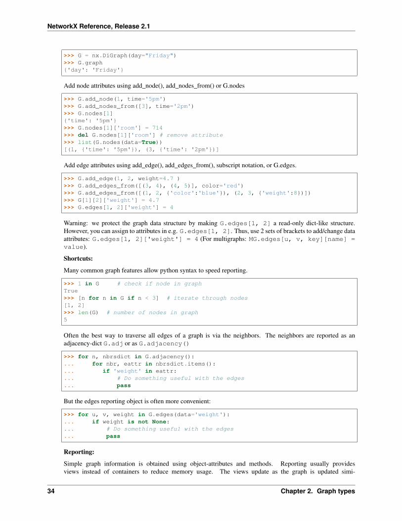
>>> G = nx.Graph(day="Friday")>>> G.graph{'day': 'Friday'}
Add node attributes using add_node(), add_nodes_from() or G.nodes
>>> G.add_node(1, time='5pm')>>> G.add_nodes_from([3], time='2pm')>>> G.nodes[1]{'time': '5pm'}>>> G.nodes[1]['room'] = 714 # node must exist already to use G.nodes>>> del G.nodes[1]['room'] # remove attribute>>> list(G.nodes(data=True))[(1, {'time': '5pm'}), (3, {'time': '2pm'})]
Add edge attributes using add_edge(), add_edges_from(), subscript notation, or G.edges.
>>> G.add_edge(1, 2, weight=4.7 )>>> G.add_edges_from([(3, 4), (4, 5)], color='red')>>> G.add_edges_from([(1, 2, {'color': 'blue'}), (2, 3, {'weight': 8})])>>> G[1][2]['weight'] = 4.7>>> G.edges[1, 2]['weight'] = 4
Warning: we protect the graph data structure by making G.edges a read-only dict-like structure. However, youcan assign to attributes in e.g. G.edges[1, 2]. Thus, use 2 sets of brackets to add/change data attributes:G.edges[1, 2]['weight'] = 4 (For multigraphs: MG.edges[u, v, key][name] = value).
Shortcuts:
Many common graph features allow python syntax to speed reporting.
>>> 1 in G # check if node in graphTrue>>> [n for n in G if n < 3] # iterate through nodes[1, 2]>>> len(G) # number of nodes in graph5
Often the best way to traverse all edges of a graph is via the neighbors. The neighbors are reported as anadjacency-dict G.adj or as G.adjacency()
>>> for n, nbrsdict in G.adjacency():... for nbr, eattr in nbrsdict.items():... if 'weight' in eattr:... # Do something useful with the edges... pass
But the edges() method is often more convenient:
>>> for u, v, weight in G.edges.data('weight'):... if weight is not None:... # Do something useful with the edges... pass
Reporting:
Simple graph information is obtained using object-attributes and methods. Reporting typically providesviews instead of containers to reduce memory usage. The views update as the graph is updated simi-larly to dict-views. The objects nodes, `edges and adj provide access to data attributes via lookup
2.2. Basic graph types 9

NetworkX Reference, Release 2.1
(e.g. nodes[n], `edges[u, v], adj[u][v]) and iteration (e.g. nodes.items(), nodes.data('color'), nodes.data('color', default='blue') and similarly for edges) Views existfor nodes, edges, neighbors()/adj and degree.
For details on these and other miscellaneous methods, see below.
Subclasses (Advanced):
The Graph class uses a dict-of-dict-of-dict data structure. The outer dict (node_dict) holds adjacency informationkeyed by node. The next dict (adjlist_dict) represents the adjacency information and holds edge data keyed byneighbor. The inner dict (edge_attr_dict) represents the edge data and holds edge attribute values keyed byattribute names.
Each of these three dicts can be replaced in a subclass by a user defined dict-like object. In general, the dict-likefeatures should be maintained but extra features can be added. To replace one of the dicts create a new graphclass by changing the class(!) variable holding the factory for that dict-like structure. The variable names arenode_dict_factory, adjlist_inner_dict_factory, adjlist_outer_dict_factory, and edge_attr_dict_factory.
node_dict_factory [function, (default: dict)] Factory function to be used to create the dict containing nodeattributes, keyed by node id. It should require no arguments and return a dict-like object
adjlist_outer_dict_factory [function, (default: dict)] Factory function to be used to create the outer-most dictin the data structure that holds adjacency info keyed by node. It should require no arguments and return adict-like object.
adjlist_inner_dict_factory [function, (default: dict)] Factory function to be used to create the adjacency listdict which holds edge data keyed by neighbor. It should require no arguments and return a dict-like object
edge_attr_dict_factory [function, (default: dict)] Factory function to be used to create the edge attribute dictwhich holds attrbute values keyed by attribute name. It should require no arguments and return a dict-likeobject.
Examples
Create a low memory graph class that effectively disallows edge attributes by using a single attribute dict for alledges. This reduces the memory used, but you lose edge attributes.
>>> class ThinGraph(nx.Graph):... all_edge_dict = {'weight': 1}... def single_edge_dict(self):... return self.all_edge_dict... edge_attr_dict_factory = single_edge_dict>>> G = ThinGraph()>>> G.add_edge(2, 1)>>> G[2][1]{'weight': 1}>>> G.add_edge(2, 2)>>> G[2][1] is G[2][2]True
Please see ordered for more examples of creating graph subclasses by overwriting the base class dict witha dictionary-like object.
10 Chapter 2. Graph types

NetworkX Reference, Release 2.1
Methods
Adding and removing nodes and edges
Graph.__init__([incoming_graph_data]) Initialize a graph with edges, name, or graph attributes.Graph.add_node(node_for_adding, **attr) Add a single node node_for_adding and update node
attributes.Graph.add_nodes_from(nodes_for_adding, **attr) Add multiple nodes.Graph.remove_node(n) Remove node n.Graph.remove_nodes_from(nodes) Remove multiple nodes.Graph.add_edge(u_of_edge, v_of_edge, **attr) Add an edge between u and v.Graph.add_edges_from(ebunch_to_add, **attr) Add all the edges in ebunch_to_add.Graph.add_weighted_edges_from(ebunch_to_add) Add weighted edges in ebunch_to_add with specified
weight attrGraph.remove_edge(u, v) Remove the edge between u and v.Graph.remove_edges_from(ebunch) Remove all edges specified in ebunch.Graph.clear() Remove all nodes and edges from the graph.
networkx.Graph.__init__
Graph.__init__(incoming_graph_data=None, **attr)Initialize a graph with edges, name, or graph attributes.
Parameters
• incoming_graph_data (input graph (optional, default: None)) – Data to initialize graph. IfNone (default) an empty graph is created. The data can be an edge list, or any NetworkXgraph object. If the corresponding optional Python packages are installed the data can alsobe a NumPy matrix or 2d ndarray, a SciPy sparse matrix, or a PyGraphviz graph.
• attr (keyword arguments, optional (default= no attributes)) – Attributes to add to graph askey=value pairs.
See also:
convert()
Examples
>>> G = nx.Graph() # or DiGraph, MultiGraph, MultiDiGraph, etc>>> G = nx.Graph(name='my graph')>>> e = [(1, 2), (2, 3), (3, 4)] # list of edges>>> G = nx.Graph(e)
Arbitrary graph attribute pairs (key=value) may be assigned
>>> G = nx.Graph(e, day="Friday")>>> G.graph{'day': 'Friday'}
2.2. Basic graph types 11

NetworkX Reference, Release 2.1
networkx.Graph.add_node
Graph.add_node(node_for_adding, **attr)Add a single node node_for_adding and update node attributes.
Parameters
• node_for_adding (node) – A node can be any hashable Python object except None.
• attr (keyword arguments, optional) – Set or change node attributes using key=value.
See also:
add_nodes_from()
Examples
>>> G = nx.Graph() # or DiGraph, MultiGraph, MultiDiGraph, etc>>> G.add_node(1)>>> G.add_node('Hello')>>> K3 = nx.Graph([(0, 1), (1, 2), (2, 0)])>>> G.add_node(K3)>>> G.number_of_nodes()3
Use keywords set/change node attributes:
>>> G.add_node(1, size=10)>>> G.add_node(3, weight=0.4, UTM=('13S', 382871, 3972649))
Notes
A hashable object is one that can be used as a key in a Python dictionary. This includes strings, numbers, tuplesof strings and numbers, etc.
On many platforms hashable items also include mutables such as NetworkX Graphs, though one should becareful that the hash doesn’t change on mutables.
networkx.Graph.add_nodes_from
Graph.add_nodes_from(nodes_for_adding, **attr)Add multiple nodes.
Parameters
• nodes_for_adding (iterable container) – A container of nodes (list, dict, set, etc.). OR Acontainer of (node, attribute dict) tuples. Node attributes are updated using the attribute dict.
• attr (keyword arguments, optional (default= no attributes)) – Update attributes for all nodesin nodes. Node attributes specified in nodes as a tuple take precedence over attributes spec-ified via keyword arguments.
See also:
add_node()
12 Chapter 2. Graph types

NetworkX Reference, Release 2.1
Examples
>>> G = nx.Graph() # or DiGraph, MultiGraph, MultiDiGraph, etc>>> G.add_nodes_from('Hello')>>> K3 = nx.Graph([(0, 1), (1, 2), (2, 0)])>>> G.add_nodes_from(K3)>>> sorted(G.nodes(), key=str)[0, 1, 2, 'H', 'e', 'l', 'o']
Use keywords to update specific node attributes for every node.
>>> G.add_nodes_from([1, 2], size=10)>>> G.add_nodes_from([3, 4], weight=0.4)
Use (node, attrdict) tuples to update attributes for specific nodes.
>>> G.add_nodes_from([(1, dict(size=11)), (2, {'color':'blue'})])>>> G.nodes[1]['size']11>>> H = nx.Graph()>>> H.add_nodes_from(G.nodes(data=True))>>> H.nodes[1]['size']11
networkx.Graph.remove_node
Graph.remove_node(n)Remove node n.
Removes the node n and all adjacent edges. Attempting to remove a non-existent node will raise an exception.
Parameters n (node) – A node in the graph
Raises NetworkXError – If n is not in the graph.
See also:
remove_nodes_from()
Examples
>>> G = nx.path_graph(3) # or DiGraph, MultiGraph, MultiDiGraph, etc>>> list(G.edges)[(0, 1), (1, 2)]>>> G.remove_node(1)>>> list(G.edges)[]
networkx.Graph.remove_nodes_from
Graph.remove_nodes_from(nodes)Remove multiple nodes.
2.2. Basic graph types 13

NetworkX Reference, Release 2.1
Parameters nodes (iterable container) – A container of nodes (list, dict, set, etc.). If a node in thecontainer is not in the graph it is silently ignored.
See also:
remove_node()
Examples
>>> G = nx.path_graph(3) # or DiGraph, MultiGraph, MultiDiGraph, etc>>> e = list(G.nodes)>>> e[0, 1, 2]>>> G.remove_nodes_from(e)>>> list(G.nodes)[]
networkx.Graph.add_edge
Graph.add_edge(u_of_edge, v_of_edge, **attr)Add an edge between u and v.
The nodes u and v will be automatically added if they are not already in the graph.
Edge attributes can be specified with keywords or by directly accessing the edge’s attribute dictionary. Seeexamples below.
Parameters
• u, v (nodes) – Nodes can be, for example, strings or numbers. Nodes must be hashable (andnot None) Python objects.
• attr (keyword arguments, optional) – Edge data (or labels or objects) can be assigned usingkeyword arguments.
See also:
add_edges_from() add a collection of edges
Notes
Adding an edge that already exists updates the edge data.
Many NetworkX algorithms designed for weighted graphs use an edge attribute (by default weight) to hold anumerical value.
Examples
The following all add the edge e=(1, 2) to graph G:
>>> G = nx.Graph() # or DiGraph, MultiGraph, MultiDiGraph, etc>>> e = (1, 2)>>> G.add_edge(1, 2) # explicit two-node form>>> G.add_edge(*e) # single edge as tuple of two nodes>>> G.add_edges_from([(1, 2)]) # add edges from iterable container
14 Chapter 2. Graph types

NetworkX Reference, Release 2.1
Associate data to edges using keywords:
>>> G.add_edge(1, 2, weight=3)>>> G.add_edge(1, 3, weight=7, capacity=15, length=342.7)
For non-string attribute keys, use subscript notation.
>>> G.add_edge(1, 2)>>> G[1][2].update({0: 5})>>> G.edges[1, 2].update({0: 5})
networkx.Graph.add_edges_from
Graph.add_edges_from(ebunch_to_add, **attr)Add all the edges in ebunch_to_add.
Parameters
• ebunch_to_add (container of edges) – Each edge given in the container will be added tothe graph. The edges must be given as as 2-tuples (u, v) or 3-tuples (u, v, d) where d is adictionary containing edge data.
• attr (keyword arguments, optional) – Edge data (or labels or objects) can be assigned usingkeyword arguments.
See also:
add_edge() add a single edge
add_weighted_edges_from() convenient way to add weighted edges
Notes
Adding the same edge twice has no effect but any edge data will be updated when each duplicate edge is added.
Edge attributes specified in an ebunch take precedence over attributes specified via keyword arguments.
Examples
>>> G = nx.Graph() # or DiGraph, MultiGraph, MultiDiGraph, etc>>> G.add_edges_from([(0, 1), (1, 2)]) # using a list of edge tuples>>> e = zip(range(0, 3), range(1, 4))>>> G.add_edges_from(e) # Add the path graph 0-1-2-3
Associate data to edges
>>> G.add_edges_from([(1, 2), (2, 3)], weight=3)>>> G.add_edges_from([(3, 4), (1, 4)], label='WN2898')
networkx.Graph.add_weighted_edges_from
Graph.add_weighted_edges_from(ebunch_to_add, weight=’weight’, **attr)Add weighted edges in ebunch_to_add with specified weight attr
2.2. Basic graph types 15

NetworkX Reference, Release 2.1
Parameters
• ebunch_to_add (container of edges) – Each edge given in the list or container will be addedto the graph. The edges must be given as 3-tuples (u, v, w) where w is a number.
• weight (string, optional (default= ‘weight’)) – The attribute name for the edge weights tobe added.
• attr (keyword arguments, optional (default= no attributes)) – Edge attributes to add/updatefor all edges.
See also:
add_edge() add a single edge
add_edges_from() add multiple edges
Notes
Adding the same edge twice for Graph/DiGraph simply updates the edge data. For MultiGraph/MultiDiGraph,duplicate edges are stored.
Examples
>>> G = nx.Graph() # or DiGraph, MultiGraph, MultiDiGraph, etc>>> G.add_weighted_edges_from([(0, 1, 3.0), (1, 2, 7.5)])
networkx.Graph.remove_edge
Graph.remove_edge(u, v)Remove the edge between u and v.
Parameters u, v (nodes) – Remove the edge between nodes u and v.
Raises NetworkXError – If there is not an edge between u and v.
See also:
remove_edges_from() remove a collection of edges
Examples
>>> G = nx.path_graph(4) # or DiGraph, etc>>> G.remove_edge(0, 1)>>> e = (1, 2)>>> G.remove_edge(*e) # unpacks e from an edge tuple>>> e = (2, 3, {'weight':7}) # an edge with attribute data>>> G.remove_edge(*e[:2]) # select first part of edge tuple
16 Chapter 2. Graph types

NetworkX Reference, Release 2.1
networkx.Graph.remove_edges_from
Graph.remove_edges_from(ebunch)Remove all edges specified in ebunch.
Parameters ebunch (list or container of edge tuples) – Each edge given in the list or container willbe removed from the graph. The edges can be:
• 2-tuples (u, v) edge between u and v.
• 3-tuples (u, v, k) where k is ignored.
See also:
remove_edge() remove a single edge
Notes
Will fail silently if an edge in ebunch is not in the graph.
Examples
>>> G = nx.path_graph(4) # or DiGraph, MultiGraph, MultiDiGraph, etc>>> ebunch=[(1, 2), (2, 3)]>>> G.remove_edges_from(ebunch)
networkx.Graph.clear
Graph.clear()Remove all nodes and edges from the graph.
This also removes the name, and all graph, node, and edge attributes.
Examples
>>> G = nx.path_graph(4) # or DiGraph, MultiGraph, MultiDiGraph, etc>>> G.clear()>>> list(G.nodes)[]>>> list(G.edges)[]
Reporting nodes edges and neighbors
Graph.nodes A NodeView of the Graph as G.nodes or G.nodes().Graph.__iter__() Iterate over the nodes.Graph.has_node(n) Return True if the graph contains the node n.Graph.__contains__(n) Return True if n is a node, False otherwise.
Continued on next page
2.2. Basic graph types 17

NetworkX Reference, Release 2.1
Table 2.2 – continued from previous pageGraph.edges An EdgeView of the Graph as G.edges or G.edges().Graph.has_edge(u, v) Return True if the edge (u, v) is in the graph.Graph.get_edge_data(u, v[, default]) Return the attribute dictionary associated with edge (u, v).Graph.neighbors(n) Return an iterator over all neighbors of node n.Graph.adj Graph adjacency object holding the neighbors of each
node.Graph.__getitem__(n) Return a dict of neighbors of node n.Graph.adjacency() Return an iterator over (node, adjacency dict) tuples for all
nodes.Graph.nbunch_iter([nbunch]) Return an iterator over nodes contained in nbunch that are
also in the graph.
networkx.Graph.nodes
Graph.nodesA NodeView of the Graph as G.nodes or G.nodes().
Can be used as G.nodes for data lookup and for set-like operations. Can also be used as G.nodes(data='color', default=None) to return a NodeDataView which reports specific node databut no set operations. It presents a dict-like interface as well with G.nodes.items() iterating over (node,nodedata) 2-tuples and G.nodes[3]['foo'] providing the value of the foo attribute for node 3. Inaddition, a view G.nodes.data('foo') provides a dict-like interface to the foo attribute of each node.G.nodes.data('foo', default=1) provides a default for nodes that do not have attribute foo.
Parameters
• data (string or bool, optional (default=False)) – The node attribute returned in 2-tuple (n,ddict[data]). If True, return entire node attribute dict as (n, ddict). If False, return just thenodes n.
• default (value, optional (default=None)) – Value used for nodes that dont have the requestedattribute. Only relevant if data is not True or False.
Returns
Allows set-like operations over the nodes as well as node attribute dict lookup and calling toget a NodeDataView. A NodeDataView iterates over (n, data) and has no set operations. ANodeView iterates over n and includes set operations.
When called, if data is False, an iterator over nodes. Otherwise an iterator of 2-tuples (node,attribute value) where the attribute is specified in data. If data is True then the attribute becomesthe entire data dictionary.
Return type NodeView
Notes
If your node data is not needed, it is simpler and equivalent to use the expression for n in G, or list(G).
Examples
There are two simple ways of getting a list of all nodes in the graph:
18 Chapter 2. Graph types

NetworkX Reference, Release 2.1
>>> G = nx.path_graph(3)>>> list(G.nodes)[0, 1, 2]>>> list(G)[0, 1, 2]
To get the node data along with the nodes:
>>> G.add_node(1, time='5pm')>>> G.nodes[0]['foo'] = 'bar'>>> list(G.nodes(data=True))[(0, {'foo': 'bar'}), (1, {'time': '5pm'}), (2, {})]>>> list(G.nodes.data())[(0, {'foo': 'bar'}), (1, {'time': '5pm'}), (2, {})]
>>> list(G.nodes(data='foo'))[(0, 'bar'), (1, None), (2, None)]>>> list(G.nodes.data('foo'))[(0, 'bar'), (1, None), (2, None)]
>>> list(G.nodes(data='time'))[(0, None), (1, '5pm'), (2, None)]>>> list(G.nodes.data('time'))[(0, None), (1, '5pm'), (2, None)]
>>> list(G.nodes(data='time', default='Not Available'))[(0, 'Not Available'), (1, '5pm'), (2, 'Not Available')]>>> list(G.nodes.data('time', default='Not Available'))[(0, 'Not Available'), (1, '5pm'), (2, 'Not Available')]
If some of your nodes have an attribute and the rest are assumed to have a default attribute value you can createa dictionary from node/attribute pairs using the default keyword argument to guarantee the value is neverNone:
>>> G = nx.Graph()>>> G.add_node(0)>>> G.add_node(1, weight=2)>>> G.add_node(2, weight=3)>>> dict(G.nodes(data='weight', default=1)){0: 1, 1: 2, 2: 3}
networkx.Graph.__iter__
Graph.__iter__()Iterate over the nodes. Use: ‘for n in G’.
Returns niter – An iterator over all nodes in the graph.
Return type iterator
Examples
2.2. Basic graph types 19
NetworkX Reference, Release 2.1
>>> G = nx.path_graph(4) # or DiGraph, MultiGraph, MultiDiGraph, etc>>> [n for n in G][0, 1, 2, 3]>>> list(G)[0, 1, 2, 3]
networkx.Graph.has_node
Graph.has_node(n)Return True if the graph contains the node n.
Identical to n in G
Parameters n (node)
Examples
>>> G = nx.path_graph(3) # or DiGraph, MultiGraph, MultiDiGraph, etc>>> G.has_node(0)True
It is more readable and simpler to use
>>> 0 in GTrue
networkx.Graph.__contains__
Graph.__contains__(n)Return True if n is a node, False otherwise. Use: ‘n in G’.
Examples
>>> G = nx.path_graph(4) # or DiGraph, MultiGraph, MultiDiGraph, etc>>> 1 in GTrue
networkx.Graph.edges
Graph.edgesAn EdgeView of the Graph as G.edges or G.edges().
edges(self, nbunch=None, data=False, default=None)
The EdgeView provides set-like operations on the edge-tuples as well as edge attribute lookup. When called,it also provides an EdgeDataView object which allows control of access to edge attributes (but does not pro-vide set-like operations). Hence, G.edges[u, v]['color'] provides the value of the color attribute foredge (u, v) while for (u, v, c) in G.edges.data('color', default='red'): iteratesthrough all the edges yielding the color attribute with default 'red' if no color attribute exists.
20 Chapter 2. Graph types

NetworkX Reference, Release 2.1
Parameters
• nbunch (single node, container, or all nodes (default= all nodes)) – The view will onlyreport edges incident to these nodes.
• data (string or bool, optional (default=False)) – The edge attribute returned in 3-tuple (u, v,ddict[data]). If True, return edge attribute dict in 3-tuple (u, v, ddict). If False, return 2-tuple(u, v).
• default (value, optional (default=None)) – Value used for edges that dont have the requestedattribute. Only relevant if data is not True or False.
Returns edges – A view of edge attributes, usually it iterates over (u, v) or (u, v, d) tuples of edges,but can also be used for attribute lookup as edges[u, v]['foo'].
Return type EdgeView
Notes
Nodes in nbunch that are not in the graph will be (quietly) ignored. For directed graphs this returns the out-edges.
Examples
>>> G = nx.path_graph(3) # or MultiGraph, etc>>> G.add_edge(2, 3, weight=5)>>> [e for e in G.edges][(0, 1), (1, 2), (2, 3)]>>> G.edges.data() # default data is {} (empty dict)EdgeDataView([(0, 1, {}), (1, 2, {}), (2, 3, {'weight': 5})])>>> G.edges.data('weight', default=1)EdgeDataView([(0, 1, 1), (1, 2, 1), (2, 3, 5)])>>> G.edges([0, 3]) # only edges incident to these nodesEdgeDataView([(0, 1), (3, 2)])>>> G.edges(0) # only edges incident to a single node (use G.adj[0]?)EdgeDataView([(0, 1)])
networkx.Graph.has_edge
Graph.has_edge(u, v)Return True if the edge (u, v) is in the graph.
This is the same as v in G[u] without KeyError exceptions.
Parameters u, v (nodes) – Nodes can be, for example, strings or numbers. Nodes must be hashable(and not None) Python objects.
Returns edge_ind – True if edge is in the graph, False otherwise.
Return type bool
Examples
2.2. Basic graph types 21

NetworkX Reference, Release 2.1
>>> G = nx.path_graph(4) # or DiGraph, MultiGraph, MultiDiGraph, etc>>> G.has_edge(0, 1) # using two nodesTrue>>> e = (0, 1)>>> G.has_edge(*e) # e is a 2-tuple (u, v)True>>> e = (0, 1, {'weight':7})>>> G.has_edge(*e[:2]) # e is a 3-tuple (u, v, data_dictionary)True
The following syntax are equivalent:
>>> G.has_edge(0, 1)True>>> 1 in G[0] # though this gives KeyError if 0 not in GTrue
networkx.Graph.get_edge_data
Graph.get_edge_data(u, v, default=None)Return the attribute dictionary associated with edge (u, v).
This is identical to G[u][v] except the default is returned instead of an exception is the edge doesn’t exist.
Parameters
• u, v (nodes)
• default (any Python object (default=None)) – Value to return if the edge (u, v) is not found.
Returns edge_dict – The edge attribute dictionary.
Return type dictionary
Examples
>>> G = nx.path_graph(4) # or DiGraph, MultiGraph, MultiDiGraph, etc>>> G[0][1]{}
Warning: Assigning to G[u][v] is not permitted. But it is safe to assign attributes G[u][v]['foo']
>>> G[0][1]['weight'] = 7>>> G[0][1]['weight']7>>> G[1][0]['weight']7
>>> G = nx.path_graph(4) # or DiGraph, MultiGraph, MultiDiGraph, etc>>> G.get_edge_data(0, 1) # default edge data is {}{}>>> e = (0, 1)>>> G.get_edge_data(*e) # tuple form{}>>> G.get_edge_data('a', 'b', default=0) # edge not in graph, return 00
22 Chapter 2. Graph types

NetworkX Reference, Release 2.1
networkx.Graph.neighbors
Graph.neighbors(n)Return an iterator over all neighbors of node n.
This is identical to iter(G[n])
Parameters n (node) – A node in the graph
Returns neighbors – An iterator over all neighbors of node n
Return type iterator
Raises NetworkXError – If the node n is not in the graph.
Examples
>>> G = nx.path_graph(4) # or DiGraph, MultiGraph, MultiDiGraph, etc>>> [n for n in G.neighbors(0)][1]
Notes
It is usually more convenient (and faster) to access the adjacency dictionary as G[n]:
>>> G = nx.Graph() # or DiGraph, MultiGraph, MultiDiGraph, etc>>> G.add_edge('a', 'b', weight=7)>>> G['a']AtlasView({'b': {'weight': 7}})>>> G = nx.path_graph(4)>>> [n for n in G[0]][1]
networkx.Graph.adj
Graph.adjGraph adjacency object holding the neighbors of each node.
This object is a read-only dict-like structure with node keys and neighbor-dict values. The neighbor-dict is keyedby neighbor to the edge-data-dict. So G.adj[3][2]['color'] = 'blue' sets the color of the edge (3,2) to "blue".
Iterating over G.adj behaves like a dict. Useful idioms include for nbr, datadict in G.adj[n].items():.
The neighbor information is also provided by subscripting the graph. So for nbr, foovalue inG[node].data('foo', default=1): works.
For directed graphs, G.adj holds outgoing (successor) info.
networkx.Graph.__getitem__
Graph.__getitem__(n)Return a dict of neighbors of node n. Use: ‘G[n]’.
2.2. Basic graph types 23

NetworkX Reference, Release 2.1
Parameters n (node) – A node in the graph.
Returns adj_dict – The adjacency dictionary for nodes connected to n.
Return type dictionary
Notes
G[n] is the same as G.adj[n] and similar to G.neighbors(n) (which is an iterator over G.adj[n])
Examples
>>> G = nx.path_graph(4) # or DiGraph, MultiGraph, MultiDiGraph, etc>>> G[0]AtlasView({1: {}})
networkx.Graph.adjacency
Graph.adjacency()Return an iterator over (node, adjacency dict) tuples for all nodes.
For directed graphs, only outgoing neighbors/adjacencies are included.
Returns adj_iter – An iterator over (node, adjacency dictionary) for all nodes in the graph.
Return type iterator
Examples
>>> G = nx.path_graph(4) # or DiGraph, MultiGraph, MultiDiGraph, etc>>> [(n, nbrdict) for n, nbrdict in G.adjacency()][(0, {1: {}}), (1, {0: {}, 2: {}}), (2, {1: {}, 3: {}}), (3, {2: {}})]
networkx.Graph.nbunch_iter
Graph.nbunch_iter(nbunch=None)Return an iterator over nodes contained in nbunch that are also in the graph.
The nodes in nbunch are checked for membership in the graph and if not are silently ignored.
Parameters nbunch (single node, container, or all nodes (default= all nodes)) – The view will onlyreport edges incident to these nodes.
Returns niter – An iterator over nodes in nbunch that are also in the graph. If nbunch is None,iterate over all nodes in the graph.
Return type iterator
Raises NetworkXError – If nbunch is not a node or or sequence of nodes. If a node in nbunch isnot hashable.
See also:
Graph.__iter__()
24 Chapter 2. Graph types

NetworkX Reference, Release 2.1
Notes
When nbunch is an iterator, the returned iterator yields values directly from nbunch, becoming exhausted whennbunch is exhausted.
To test whether nbunch is a single node, one can use “if nbunch in self:”, even after processing with this routine.
If nbunch is not a node or a (possibly empty) sequence/iterator or None, a NetworkXError is raised. Also, ifany object in nbunch is not hashable, a NetworkXError is raised.
Counting nodes edges and neighbors
Graph.order() Return the number of nodes in the graph.Graph.number_of_nodes() Return the number of nodes in the graph.Graph.__len__() Return the number of nodes.Graph.degree A DegreeView for the Graph as G.degree or G.degree().Graph.size([weight]) Return the number of edges or total of all edge weights.Graph.number_of_edges([u, v]) Return the number of edges between two nodes.
networkx.Graph.order
Graph.order()Return the number of nodes in the graph.
Returns nnodes – The number of nodes in the graph.
Return type int
See also:
number_of_nodes(), __len__()
networkx.Graph.number_of_nodes
Graph.number_of_nodes()Return the number of nodes in the graph.
Returns nnodes – The number of nodes in the graph.
Return type int
See also:
order(), __len__()
Examples
>>> G = nx.path_graph(3) # or DiGraph, MultiGraph, MultiDiGraph, etc>>> len(G)3
2.2. Basic graph types 25
NetworkX Reference, Release 2.1
networkx.Graph.__len__
Graph.__len__()Return the number of nodes. Use: ‘len(G)’.
Returns nnodes – The number of nodes in the graph.
Return type int
Examples
>>> G = nx.path_graph(4) # or DiGraph, MultiGraph, MultiDiGraph, etc>>> len(G)4
networkx.Graph.degree
Graph.degreeA DegreeView for the Graph as G.degree or G.degree().
The node degree is the number of edges adjacent to the node. The weighted node degree is the sum of the edgeweights for edges incident to that node.
This object provides an iterator for (node, degree) as well as lookup for the degree for a single node.
Parameters
• nbunch (single node, container, or all nodes (default= all nodes)) – The view will onlyreport edges incident to these nodes.
• weight (string or None, optional (default=None)) – The name of an edge attribute that holdsthe numerical value used as a weight. If None, then each edge has weight 1. The degree isthe sum of the edge weights adjacent to the node.
Returns
• If a single node is requested
• deg (int) – Degree of the node
• OR if multiple nodes are requested
• nd_view (A DegreeView object capable of iterating (node, degree) pairs)
Examples
>>> G = nx.path_graph(4) # or DiGraph, MultiGraph, MultiDiGraph, etc>>> G.degree[0] # node 0 has degree 11>>> list(G.degree([0, 1, 2]))[(0, 1), (1, 2), (2, 2)]
26 Chapter 2. Graph types

NetworkX Reference, Release 2.1
networkx.Graph.size
Graph.size(weight=None)Return the number of edges or total of all edge weights.
Parameters weight (string or None, optional (default=None)) – The edge attribute that holds thenumerical value used as a weight. If None, then each edge has weight 1.
Returns
size – The number of edges or (if weight keyword is provided) the total weight sum.
If weight is None, returns an int. Otherwise a float (or more general numeric if the weights aremore general).
Return type numeric
See also:
number_of_edges()
Examples
>>> G = nx.path_graph(4) # or DiGraph, MultiGraph, MultiDiGraph, etc>>> G.size()3
>>> G = nx.Graph() # or DiGraph, MultiGraph, MultiDiGraph, etc>>> G.add_edge('a', 'b', weight=2)>>> G.add_edge('b', 'c', weight=4)>>> G.size()2>>> G.size(weight='weight')6.0
networkx.Graph.number_of_edges
Graph.number_of_edges(u=None, v=None)Return the number of edges between two nodes.
Parameters u, v (nodes, optional (default=all edges)) – If u and v are specified, return the numberof edges between u and v. Otherwise return the total number of all edges.
Returns nedges – The number of edges in the graph. If nodes u and v are specified return thenumber of edges between those nodes. If the graph is directed, this only returns the number ofedges from u to v.
Return type int
See also:
size()
Examples
For undirected graphs, this method counts the total number of edges in the graph:
2.2. Basic graph types 27
NetworkX Reference, Release 2.1
>>> G = nx.path_graph(4)>>> G.number_of_edges()3
If you specify two nodes, this counts the total number of edges joining the two nodes:
>>> G.number_of_edges(0, 1)1
For directed graphs, this method can count the total number of directed edges from u to v:
>>> G = nx.DiGraph()>>> G.add_edge(0, 1)>>> G.add_edge(1, 0)>>> G.number_of_edges(0, 1)1
Making copies and subgraphs
Graph.copy([as_view]) Return a copy of the graph.Graph.to_undirected([as_view]) Return an undirected copy of the graph.Graph.to_directed([as_view]) Return a directed representation of the graph.Graph.subgraph(nodes) Return a SubGraph view of the subgraph induced on
nodes.Graph.edge_subgraph(edges) Returns the subgraph induced by the specified edges.Graph.fresh_copy() Return a fresh copy graph with the same data structure.
networkx.Graph.copy
Graph.copy(as_view=False)Return a copy of the graph.
The copy method by default returns a shallow copy of the graph and attributes. That is, if an attribute isa container, that container is shared by the original an the copy. Use Python’s copy.deepcopy for newcontainers.
If as_view is True then a view is returned instead of a copy.
Notes
All copies reproduce the graph structure, but data attributes may be handled in different ways. There are fourtypes of copies of a graph that people might want.
Deepcopy – The default behavior is a “deepcopy” where the graph structure as well as all data attributes and anyobjects they might contain are copied. The entire graph object is new so that changes in the copy do not affectthe original object. (see Python’s copy.deepcopy)
Data Reference (Shallow) – For a shallow copy the graph structure is copied but the edge, node and graph at-tribute dicts are references to those in the original graph. This saves time and memory but could cause confusionif you change an attribute in one graph and it changes the attribute in the other. NetworkX does not provide thislevel of shallow copy.
28 Chapter 2. Graph types

NetworkX Reference, Release 2.1
Independent Shallow – This copy creates new independent attribute dicts and then does a shallow copy of theattributes. That is, any attributes that are containers are shared between the new graph and the original. This isexactly what dict.copy() provides. You can obtain this style copy using:
>>> G = nx.path_graph(5)>>> H = G.copy()>>> H = G.copy(as_view=False)>>> H = nx.Graph(G)>>> H = G.fresh_copy().__class__(G)
Fresh Data – For fresh data, the graph structure is copied while new empty data attribute dicts are created. Theresulting graph is independent of the original and it has no edge, node or graph attributes. Fresh copies are notenabled. Instead use:
>>> H = G.fresh_copy()>>> H.add_nodes_from(G)>>> H.add_edges_from(G.edges)
View – Inspired by dict-views, graph-views act like read-only versions of the original graph, providing a copyof the original structure without requiring any memory for copying the information.
See the Python copy module for more information on shallow and deep copies, https://docs.python.org/2/library/copy.html.
Parameters as_view (bool, optional (default=False)) – If True, the returned graph-view provides aread-only view of the original graph without actually copying any data.
Returns G – A copy of the graph.
Return type Graph
See also:
to_directed() return a directed copy of the graph.
Examples
>>> G = nx.path_graph(4) # or DiGraph, MultiGraph, MultiDiGraph, etc>>> H = G.copy()
networkx.Graph.to_undirected
Graph.to_undirected(as_view=False)Return an undirected copy of the graph.
Parameters as_view (bool (optional, default=False)) – If True return a view of the original undi-rected graph.
Returns G – A deepcopy of the graph.
Return type Graph/MultiGraph
See also:
Graph(), copy(), add_edge(), add_edges_from()
2.2. Basic graph types 29

NetworkX Reference, Release 2.1
Notes
This returns a “deepcopy” of the edge, node, and graph attributes which attempts to completely copy all of thedata and references.
This is in contrast to the similar G = nx.DiGraph(D) which returns a shallow copy of the data.
See the Python copy module for more information on shallow and deep copies, https://docs.python.org/2/library/copy.html.
Warning: If you have subclassed DiGraph to use dict-like objects in the data structure, those changes do nottransfer to the Graph created by this method.
Examples
>>> G = nx.path_graph(2) # or MultiGraph, etc>>> H = G.to_directed()>>> list(H.edges)[(0, 1), (1, 0)]>>> G2 = H.to_undirected()>>> list(G2.edges)[(0, 1)]
networkx.Graph.to_directed
Graph.to_directed(as_view=False)Return a directed representation of the graph.
Returns G – A directed graph with the same name, same nodes, and with each edge (u, v, data)replaced by two directed edges (u, v, data) and (v, u, data).
Return type DiGraph
Notes
This returns a “deepcopy” of the edge, node, and graph attributes which attempts to completely copy all of thedata and references.
This is in contrast to the similar D=DiGraph(G) which returns a shallow copy of the data.
See the Python copy module for more information on shallow and deep copies, https://docs.python.org/2/library/copy.html.
Warning: If you have subclassed Graph to use dict-like objects in the data structure, those changes do nottransfer to the DiGraph created by this method.
Examples
>>> G = nx.Graph() # or MultiGraph, etc>>> G.add_edge(0, 1)>>> H = G.to_directed()>>> list(H.edges)[(0, 1), (1, 0)]
30 Chapter 2. Graph types

NetworkX Reference, Release 2.1
If already directed, return a (deep) copy
>>> G = nx.DiGraph() # or MultiDiGraph, etc>>> G.add_edge(0, 1)>>> H = G.to_directed()>>> list(H.edges)[(0, 1)]
networkx.Graph.subgraph
Graph.subgraph(nodes)Return a SubGraph view of the subgraph induced on nodes.
The induced subgraph of the graph contains the nodes in nodes and the edges between those nodes.
Parameters nodes (list, iterable) – A container of nodes which will be iterated through once.
Returns G – A subgraph view of the graph. The graph structure cannot be changed but node/edgeattributes can and are shared with the original graph.
Return type SubGraph View
Notes
The graph, edge and node attributes are shared with the original graph. Changes to the graph structure is ruledout by the view, but changes to attributes are reflected in the original graph.
To create a subgraph with its own copy of the edge/node attributes use: G.subgraph(nodes).copy()
For an inplace reduction of a graph to a subgraph you can remove nodes: G.remove_nodes_from([n for n in Gif n not in set(nodes)])
Examples
>>> G = nx.path_graph(4) # or DiGraph, MultiGraph, MultiDiGraph, etc>>> H = G.subgraph([0, 1, 2])>>> list(H.edges)[(0, 1), (1, 2)]
networkx.Graph.edge_subgraph
Graph.edge_subgraph(edges)Returns the subgraph induced by the specified edges.
The induced subgraph contains each edge in edges and each node incident to any one of those edges.
Parameters edges (iterable) – An iterable of edges in this graph.
Returns G – An edge-induced subgraph of this graph with the same edge attributes.
Return type Graph
2.2. Basic graph types 31

NetworkX Reference, Release 2.1
Notes
The graph, edge, and node attributes in the returned subgraph view are references to the corresponding attributesin the original graph. The view is read-only.
To create a full graph version of the subgraph with its own copy of the edge or node attributes, use:
>>> G.edge_subgraph(edges).copy()
Examples
>>> G = nx.path_graph(5)>>> H = G.edge_subgraph([(0, 1), (3, 4)])>>> list(H.nodes)[0, 1, 3, 4]>>> list(H.edges)[(0, 1), (3, 4)]
networkx.Graph.fresh_copy
Graph.fresh_copy()Return a fresh copy graph with the same data structure.
A fresh copy has no nodes, edges or graph attributes. It is the same data structure as the current graph. Thismethod is typically used to create an empty version of the graph.
Notes
If you subclass the base class you should overwrite this method to return your class of graph.
2.2.2 DiGraph—Directed graphs with self loops
Overview
class DiGraph(incoming_graph_data=None, **attr)Base class for directed graphs.
A DiGraph stores nodes and edges with optional data, or attributes.
DiGraphs hold directed edges. Self loops are allowed but multiple (parallel) edges are not.
Nodes can be arbitrary (hashable) Python objects with optional key/value attributes. By convention None is notused as a node.
Edges are represented as links between nodes with optional key/value attributes.
Parameters
• incoming_graph_data (input graph (optional, default: None)) – Data to initialize graph. IfNone (default) an empty graph is created. The data can be any format that is supported bythe to_networkx_graph() function, currently including edge list, dict of dicts, dict of lists,NetworkX graph, NumPy matrix or 2d ndarray, SciPy sparse matrix, or PyGraphviz graph.
32 Chapter 2. Graph types

NetworkX Reference, Release 2.1
• attr (keyword arguments, optional (default= no attributes)) – Attributes to add to graph askey=value pairs.
See also:
Graph, MultiGraph, MultiDiGraph, OrderedDiGraph
Examples
Create an empty graph structure (a “null graph”) with no nodes and no edges.
>>> G = nx.DiGraph()
G can be grown in several ways.
Nodes:
Add one node at a time:
>>> G.add_node(1)
Add the nodes from any container (a list, dict, set or even the lines from a file or the nodes from another graph).
>>> G.add_nodes_from([2, 3])>>> G.add_nodes_from(range(100, 110))>>> H = nx.path_graph(10)>>> G.add_nodes_from(H)
In addition to strings and integers any hashable Python object (except None) can represent a node, e.g. acustomized node object, or even another Graph.
>>> G.add_node(H)
Edges:
G can also be grown by adding edges.
Add one edge,
>>> G.add_edge(1, 2)
a list of edges,
>>> G.add_edges_from([(1, 2), (1, 3)])
or a collection of edges,
>>> G.add_edges_from(H.edges)
If some edges connect nodes not yet in the graph, the nodes are added automatically. There are no errors whenadding nodes or edges that already exist.
Attributes:
Each graph, node, and edge can hold key/value attribute pairs in an associated attribute dictionary (the keysmust be hashable). By default these are empty, but can be added or changed using add_edge, add_node or directmanipulation of the attribute dictionaries named graph, node and edge respectively.
2.2. Basic graph types 33
NetworkX Reference, Release 2.1
>>> G = nx.DiGraph(day="Friday")>>> G.graph{'day': 'Friday'}
Add node attributes using add_node(), add_nodes_from() or G.nodes
>>> G.add_node(1, time='5pm')>>> G.add_nodes_from([3], time='2pm')>>> G.nodes[1]{'time': '5pm'}>>> G.nodes[1]['room'] = 714>>> del G.nodes[1]['room'] # remove attribute>>> list(G.nodes(data=True))[(1, {'time': '5pm'}), (3, {'time': '2pm'})]
Add edge attributes using add_edge(), add_edges_from(), subscript notation, or G.edges.
>>> G.add_edge(1, 2, weight=4.7 )>>> G.add_edges_from([(3, 4), (4, 5)], color='red')>>> G.add_edges_from([(1, 2, {'color':'blue'}), (2, 3, {'weight':8})])>>> G[1][2]['weight'] = 4.7>>> G.edges[1, 2]['weight'] = 4
Warning: we protect the graph data structure by making G.edges[1, 2] a read-only dict-like structure.However, you can assign to attributes in e.g. G.edges[1, 2]. Thus, use 2 sets of brackets to add/change dataattributes: G.edges[1, 2]['weight'] = 4 (For multigraphs: MG.edges[u, v, key][name] =value).
Shortcuts:
Many common graph features allow python syntax to speed reporting.
>>> 1 in G # check if node in graphTrue>>> [n for n in G if n < 3] # iterate through nodes[1, 2]>>> len(G) # number of nodes in graph5
Often the best way to traverse all edges of a graph is via the neighbors. The neighbors are reported as anadjacency-dict G.adj or as G.adjacency()
>>> for n, nbrsdict in G.adjacency():... for nbr, eattr in nbrsdict.items():... if 'weight' in eattr:... # Do something useful with the edges... pass
But the edges reporting object is often more convenient:
>>> for u, v, weight in G.edges(data='weight'):... if weight is not None:... # Do something useful with the edges... pass
Reporting:
Simple graph information is obtained using object-attributes and methods. Reporting usually providesviews instead of containers to reduce memory usage. The views update as the graph is updated simi-
34 Chapter 2. Graph types

NetworkX Reference, Release 2.1
larly to dict-views. The objects nodes, `edges and adj provide access to data attributes via lookup(e.g. nodes[n], `edges[u, v], adj[u][v]) and iteration (e.g. nodes.items(), nodes.data('color'), nodes.data('color', default='blue') and similarly for edges) Views existfor nodes, edges, neighbors()/adj and degree.
For details on these and other miscellaneous methods, see below.
Subclasses (Advanced):
The Graph class uses a dict-of-dict-of-dict data structure. The outer dict (node_dict) holds adjacency informationkeyed by node. The next dict (adjlist_dict) represents the adjacency information and holds edge data keyed byneighbor. The inner dict (edge_attr_dict) represents the edge data and holds edge attribute values keyed byattribute names.
Each of these three dicts can be replaced in a subclass by a user defined dict-like object. In general, the dict-likefeatures should be maintained but extra features can be added. To replace one of the dicts create a new graphclass by changing the class(!) variable holding the factory for that dict-like structure. The variable names arenode_dict_factory, adjlist_inner_dict_factory, adjlist_outer_dict_factory, and edge_attr_dict_factory.
node_dict_factory [function, (default: dict)] Factory function to be used to create the dict containing nodeattributes, keyed by node id. It should require no arguments and return a dict-like object
adjlist_outer_dict_factory [function, (default: dict)] Factory function to be used to create the outer-most dictin the data structure that holds adjacency info keyed by node. It should require no arguments and return adict-like object.
adjlist_inner_dict_factory [function, optional (default: dict)] Factory function to be used to create the adja-cency list dict which holds edge data keyed by neighbor. It should require no arguments and return adict-like object
edge_attr_dict_factory [function, optional (default: dict)] Factory function to be used to create the edge at-tribute dict which holds attrbute values keyed by attribute name. It should require no arguments and returna dict-like object.
Examples
Create a low memory graph class that effectively disallows edge attributes by using a single attribute dict for alledges. This reduces the memory used, but you lose edge attributes.
>>> class ThinGraph(nx.Graph):... all_edge_dict = {'weight': 1}... def single_edge_dict(self):... return self.all_edge_dict... edge_attr_dict_factory = single_edge_dict>>> G = ThinGraph()>>> G.add_edge(2, 1)>>> G[2][1]{'weight': 1}>>> G.add_edge(2, 2)>>> G[2][1] is G[2][2]True
Please see ordered for more examples of creating graph subclasses by overwriting the base class dict witha dictionary-like object.
2.2. Basic graph types 35

NetworkX Reference, Release 2.1
Methods
Adding and removing nodes and edges
DiGraph.__init__([incoming_graph_data]) Initialize a graph with edges, name, or graph attributes.DiGraph.add_node(node_for_adding, **attr) Add a single node node_for_adding and update node
attributes.DiGraph.add_nodes_from(nodes_for_adding,**attr)
Add multiple nodes.
DiGraph.remove_node(n) Remove node n.DiGraph.remove_nodes_from(nodes) Remove multiple nodes.DiGraph.add_edge(u_of_edge, v_of_edge, **attr) Add an edge between u and v.DiGraph.add_edges_from(ebunch_to_add, **attr) Add all the edges in ebunch_to_add.DiGraph.add_weighted_edges_from(ebunch_to_add)Add weighted edges in ebunch_to_add with specified
weight attrDiGraph.remove_edge(u, v) Remove the edge between u and v.DiGraph.remove_edges_from(ebunch) Remove all edges specified in ebunch.DiGraph.clear() Remove all nodes and edges from the graph.
networkx.DiGraph.__init__
DiGraph.__init__(incoming_graph_data=None, **attr)Initialize a graph with edges, name, or graph attributes.
Parameters
• incoming_graph_data (input graph (optional, default: None)) – Data to initialize graph. IfNone (default) an empty graph is created. The data can be an edge list, or any NetworkXgraph object. If the corresponding optional Python packages are installed the data can alsobe a NumPy matrix or 2d ndarray, a SciPy sparse matrix, or a PyGraphviz graph.
• attr (keyword arguments, optional (default= no attributes)) – Attributes to add to graph askey=value pairs.
See also:
convert()
Examples
>>> G = nx.Graph() # or DiGraph, MultiGraph, MultiDiGraph, etc>>> G = nx.Graph(name='my graph')>>> e = [(1, 2), (2, 3), (3, 4)] # list of edges>>> G = nx.Graph(e)
Arbitrary graph attribute pairs (key=value) may be assigned
>>> G = nx.Graph(e, day="Friday")>>> G.graph{'day': 'Friday'}
36 Chapter 2. Graph types

NetworkX Reference, Release 2.1
networkx.DiGraph.add_node
DiGraph.add_node(node_for_adding, **attr)Add a single node node_for_adding and update node attributes.
Parameters
• node_for_adding (node) – A node can be any hashable Python object except None.
• attr (keyword arguments, optional) – Set or change node attributes using key=value.
See also:
add_nodes_from()
Examples
>>> G = nx.Graph() # or DiGraph, MultiGraph, MultiDiGraph, etc>>> G.add_node(1)>>> G.add_node('Hello')>>> K3 = nx.Graph([(0, 1), (1, 2), (2, 0)])>>> G.add_node(K3)>>> G.number_of_nodes()3
Use keywords set/change node attributes:
>>> G.add_node(1, size=10)>>> G.add_node(3, weight=0.4, UTM=('13S', 382871, 3972649))
Notes
A hashable object is one that can be used as a key in a Python dictionary. This includes strings, numbers, tuplesof strings and numbers, etc.
On many platforms hashable items also include mutables such as NetworkX Graphs, though one should becareful that the hash doesn’t change on mutables.
networkx.DiGraph.add_nodes_from
DiGraph.add_nodes_from(nodes_for_adding, **attr)Add multiple nodes.
Parameters
• nodes_for_adding (iterable container) – A container of nodes (list, dict, set, etc.). OR Acontainer of (node, attribute dict) tuples. Node attributes are updated using the attribute dict.
• attr (keyword arguments, optional (default= no attributes)) – Update attributes for all nodesin nodes. Node attributes specified in nodes as a tuple take precedence over attributes spec-ified via keyword arguments.
See also:
add_node()
2.2. Basic graph types 37

NetworkX Reference, Release 2.1
Examples
>>> G = nx.Graph() # or DiGraph, MultiGraph, MultiDiGraph, etc>>> G.add_nodes_from('Hello')>>> K3 = nx.Graph([(0, 1), (1, 2), (2, 0)])>>> G.add_nodes_from(K3)>>> sorted(G.nodes(), key=str)[0, 1, 2, 'H', 'e', 'l', 'o']
Use keywords to update specific node attributes for every node.
>>> G.add_nodes_from([1, 2], size=10)>>> G.add_nodes_from([3, 4], weight=0.4)
Use (node, attrdict) tuples to update attributes for specific nodes.
>>> G.add_nodes_from([(1, dict(size=11)), (2, {'color':'blue'})])>>> G.nodes[1]['size']11>>> H = nx.Graph()>>> H.add_nodes_from(G.nodes(data=True))>>> H.nodes[1]['size']11
networkx.DiGraph.remove_node
DiGraph.remove_node(n)Remove node n.
Removes the node n and all adjacent edges. Attempting to remove a non-existent node will raise an exception.
Parameters n (node) – A node in the graph
Raises NetworkXError – If n is not in the graph.
See also:
remove_nodes_from()
Examples
>>> G = nx.path_graph(3) # or DiGraph, MultiGraph, MultiDiGraph, etc>>> list(G.edges)[(0, 1), (1, 2)]>>> G.remove_node(1)>>> list(G.edges)[]
networkx.DiGraph.remove_nodes_from
DiGraph.remove_nodes_from(nodes)Remove multiple nodes.
38 Chapter 2. Graph types

NetworkX Reference, Release 2.1
Parameters nodes (iterable container) – A container of nodes (list, dict, set, etc.). If a node in thecontainer is not in the graph it is silently ignored.
See also:
remove_node()
Examples
>>> G = nx.path_graph(3) # or DiGraph, MultiGraph, MultiDiGraph, etc>>> e = list(G.nodes)>>> e[0, 1, 2]>>> G.remove_nodes_from(e)>>> list(G.nodes)[]
networkx.DiGraph.add_edge
DiGraph.add_edge(u_of_edge, v_of_edge, **attr)Add an edge between u and v.
The nodes u and v will be automatically added if they are not already in the graph.
Edge attributes can be specified with keywords or by directly accessing the edge’s attribute dictionary. Seeexamples below.
Parameters
• u, v (nodes) – Nodes can be, for example, strings or numbers. Nodes must be hashable (andnot None) Python objects.
• attr (keyword arguments, optional) – Edge data (or labels or objects) can be assigned usingkeyword arguments.
See also:
add_edges_from() add a collection of edges
Notes
Adding an edge that already exists updates the edge data.
Many NetworkX algorithms designed for weighted graphs use an edge attribute (by default weight) to hold anumerical value.
Examples
The following all add the edge e=(1, 2) to graph G:
>>> G = nx.Graph() # or DiGraph, MultiGraph, MultiDiGraph, etc>>> e = (1, 2)>>> G.add_edge(1, 2) # explicit two-node form>>> G.add_edge(*e) # single edge as tuple of two nodes>>> G.add_edges_from( [(1, 2)] ) # add edges from iterable container
2.2. Basic graph types 39

NetworkX Reference, Release 2.1
Associate data to edges using keywords:
>>> G.add_edge(1, 2, weight=3)>>> G.add_edge(1, 3, weight=7, capacity=15, length=342.7)
For non-string attribute keys, use subscript notation.
>>> G.add_edge(1, 2)>>> G[1][2].update({0: 5})>>> G.edges[1, 2].update({0: 5})
networkx.DiGraph.add_edges_from
DiGraph.add_edges_from(ebunch_to_add, **attr)Add all the edges in ebunch_to_add.
Parameters
• ebunch_to_add (container of edges) – Each edge given in the container will be added to thegraph. The edges must be given as 2-tuples (u, v) or 3-tuples (u, v, d) where d is a dictionarycontaining edge data.
• attr (keyword arguments, optional) – Edge data (or labels or objects) can be assigned usingkeyword arguments.
See also:
add_edge() add a single edge
add_weighted_edges_from() convenient way to add weighted edges
Notes
Adding the same edge twice has no effect but any edge data will be updated when each duplicate edge is added.
Edge attributes specified in an ebunch take precedence over attributes specified via keyword arguments.
Examples
>>> G = nx.Graph() # or DiGraph, MultiGraph, MultiDiGraph, etc>>> G.add_edges_from([(0, 1), (1, 2)]) # using a list of edge tuples>>> e = zip(range(0, 3), range(1, 4))>>> G.add_edges_from(e) # Add the path graph 0-1-2-3
Associate data to edges
>>> G.add_edges_from([(1, 2), (2, 3)], weight=3)>>> G.add_edges_from([(3, 4), (1, 4)], label='WN2898')
networkx.DiGraph.add_weighted_edges_from
DiGraph.add_weighted_edges_from(ebunch_to_add, weight=’weight’, **attr)Add weighted edges in ebunch_to_add with specified weight attr
40 Chapter 2. Graph types

NetworkX Reference, Release 2.1
Parameters
• ebunch_to_add (container of edges) – Each edge given in the list or container will be addedto the graph. The edges must be given as 3-tuples (u, v, w) where w is a number.
• weight (string, optional (default= ‘weight’)) – The attribute name for the edge weights tobe added.
• attr (keyword arguments, optional (default= no attributes)) – Edge attributes to add/updatefor all edges.
See also:
add_edge() add a single edge
add_edges_from() add multiple edges
Notes
Adding the same edge twice for Graph/DiGraph simply updates the edge data. For MultiGraph/MultiDiGraph,duplicate edges are stored.
Examples
>>> G = nx.Graph() # or DiGraph, MultiGraph, MultiDiGraph, etc>>> G.add_weighted_edges_from([(0, 1, 3.0), (1, 2, 7.5)])
networkx.DiGraph.remove_edge
DiGraph.remove_edge(u, v)Remove the edge between u and v.
Parameters u, v (nodes) – Remove the edge between nodes u and v.
Raises NetworkXError – If there is not an edge between u and v.
See also:
remove_edges_from() remove a collection of edges
Examples
>>> G = nx.Graph() # or DiGraph, etc>>> nx.add_path(G, [0, 1, 2, 3])>>> G.remove_edge(0, 1)>>> e = (1, 2)>>> G.remove_edge(*e) # unpacks e from an edge tuple>>> e = (2, 3, {'weight':7}) # an edge with attribute data>>> G.remove_edge(*e[:2]) # select first part of edge tuple
2.2. Basic graph types 41
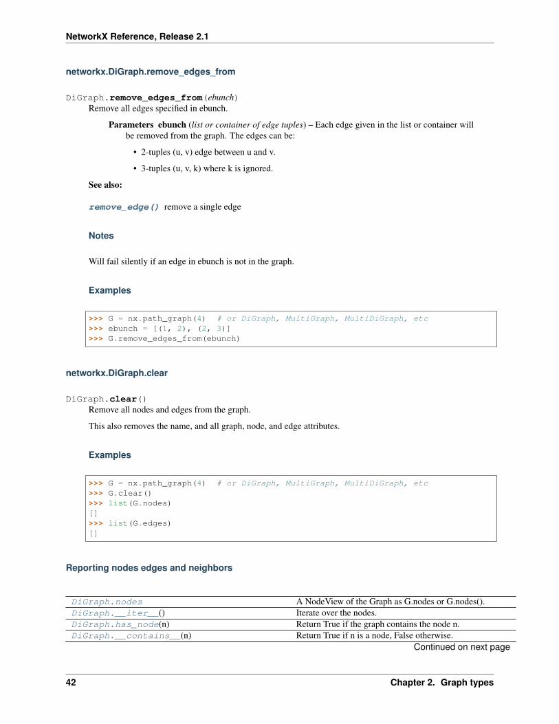
NetworkX Reference, Release 2.1
networkx.DiGraph.remove_edges_from
DiGraph.remove_edges_from(ebunch)Remove all edges specified in ebunch.
Parameters ebunch (list or container of edge tuples) – Each edge given in the list or container willbe removed from the graph. The edges can be:
• 2-tuples (u, v) edge between u and v.
• 3-tuples (u, v, k) where k is ignored.
See also:
remove_edge() remove a single edge
Notes
Will fail silently if an edge in ebunch is not in the graph.
Examples
>>> G = nx.path_graph(4) # or DiGraph, MultiGraph, MultiDiGraph, etc>>> ebunch = [(1, 2), (2, 3)]>>> G.remove_edges_from(ebunch)
networkx.DiGraph.clear
DiGraph.clear()Remove all nodes and edges from the graph.
This also removes the name, and all graph, node, and edge attributes.
Examples
>>> G = nx.path_graph(4) # or DiGraph, MultiGraph, MultiDiGraph, etc>>> G.clear()>>> list(G.nodes)[]>>> list(G.edges)[]
Reporting nodes edges and neighbors
DiGraph.nodes A NodeView of the Graph as G.nodes or G.nodes().DiGraph.__iter__() Iterate over the nodes.DiGraph.has_node(n) Return True if the graph contains the node n.DiGraph.__contains__(n) Return True if n is a node, False otherwise.
Continued on next page
42 Chapter 2. Graph types

NetworkX Reference, Release 2.1
Table 2.6 – continued from previous pageDiGraph.edges An OutEdgeView of the DiGraph as G.edges or G.edges().DiGraph.out_edges An OutEdgeView of the DiGraph as G.edges or G.edges().DiGraph.in_edges An InEdgeView of the Graph as G.in_edges or
G.in_edges().DiGraph.has_edge(u, v) Return True if the edge (u, v) is in the graph.DiGraph.get_edge_data(u, v[, default]) Return the attribute dictionary associated with edge (u, v).DiGraph.neighbors(n) Return an iterator over successor nodes of n.DiGraph.adj Graph adjacency object holding the neighbors of each
node.DiGraph.__getitem__(n) Return a dict of neighbors of node n.DiGraph.successors(n) Return an iterator over successor nodes of n.DiGraph.succ Graph adjacency object holding the successors of each
node.DiGraph.predecessors(n) Return an iterator over predecessor nodes of n.DiGraph.pred Graph adjacency object holding the predecessors of each
node.DiGraph.adjacency() Return an iterator over (node, adjacency dict) tuples for all
nodes.DiGraph.nbunch_iter([nbunch]) Return an iterator over nodes contained in nbunch that are
also in the graph.
networkx.DiGraph.nodes
DiGraph.nodesA NodeView of the Graph as G.nodes or G.nodes().
Can be used as G.nodes for data lookup and for set-like operations. Can also be used as G.nodes(data='color', default=None) to return a NodeDataView which reports specific node databut no set operations. It presents a dict-like interface as well with G.nodes.items() iterating over (node,nodedata) 2-tuples and G.nodes[3]['foo'] providing the value of the foo attribute for node 3. Inaddition, a view G.nodes.data('foo') provides a dict-like interface to the foo attribute of each node.G.nodes.data('foo', default=1) provides a default for nodes that do not have attribute foo.
Parameters
• data (string or bool, optional (default=False)) – The node attribute returned in 2-tuple (n,ddict[data]). If True, return entire node attribute dict as (n, ddict). If False, return just thenodes n.
• default (value, optional (default=None)) – Value used for nodes that dont have the requestedattribute. Only relevant if data is not True or False.
Returns
Allows set-like operations over the nodes as well as node attribute dict lookup and calling toget a NodeDataView. A NodeDataView iterates over (n, data) and has no set operations. ANodeView iterates over n and includes set operations.
When called, if data is False, an iterator over nodes. Otherwise an iterator of 2-tuples (node,attribute value) where the attribute is specified in data. If data is True then the attribute becomesthe entire data dictionary.
Return type NodeView
2.2. Basic graph types 43

NetworkX Reference, Release 2.1
Notes
If your node data is not needed, it is simpler and equivalent to use the expression for n in G, or list(G).
Examples
There are two simple ways of getting a list of all nodes in the graph:
>>> G = nx.path_graph(3)>>> list(G.nodes)[0, 1, 2]>>> list(G)[0, 1, 2]
To get the node data along with the nodes:
>>> G.add_node(1, time='5pm')>>> G.nodes[0]['foo'] = 'bar'>>> list(G.nodes(data=True))[(0, {'foo': 'bar'}), (1, {'time': '5pm'}), (2, {})]>>> list(G.nodes.data())[(0, {'foo': 'bar'}), (1, {'time': '5pm'}), (2, {})]
>>> list(G.nodes(data='foo'))[(0, 'bar'), (1, None), (2, None)]>>> list(G.nodes.data('foo'))[(0, 'bar'), (1, None), (2, None)]
>>> list(G.nodes(data='time'))[(0, None), (1, '5pm'), (2, None)]>>> list(G.nodes.data('time'))[(0, None), (1, '5pm'), (2, None)]
>>> list(G.nodes(data='time', default='Not Available'))[(0, 'Not Available'), (1, '5pm'), (2, 'Not Available')]>>> list(G.nodes.data('time', default='Not Available'))[(0, 'Not Available'), (1, '5pm'), (2, 'Not Available')]
If some of your nodes have an attribute and the rest are assumed to have a default attribute value you can createa dictionary from node/attribute pairs using the default keyword argument to guarantee the value is neverNone:
>>> G = nx.Graph()>>> G.add_node(0)>>> G.add_node(1, weight=2)>>> G.add_node(2, weight=3)>>> dict(G.nodes(data='weight', default=1)){0: 1, 1: 2, 2: 3}
networkx.DiGraph.__iter__
DiGraph.__iter__()Iterate over the nodes. Use: ‘for n in G’.
44 Chapter 2. Graph types

NetworkX Reference, Release 2.1
Returns niter – An iterator over all nodes in the graph.
Return type iterator
Examples
>>> G = nx.path_graph(4) # or DiGraph, MultiGraph, MultiDiGraph, etc>>> [n for n in G][0, 1, 2, 3]>>> list(G)[0, 1, 2, 3]
networkx.DiGraph.has_node
DiGraph.has_node(n)Return True if the graph contains the node n.
Identical to n in G
Parameters n (node)
Examples
>>> G = nx.path_graph(3) # or DiGraph, MultiGraph, MultiDiGraph, etc>>> G.has_node(0)True
It is more readable and simpler to use
>>> 0 in GTrue
networkx.DiGraph.__contains__
DiGraph.__contains__(n)Return True if n is a node, False otherwise. Use: ‘n in G’.
Examples
>>> G = nx.path_graph(4) # or DiGraph, MultiGraph, MultiDiGraph, etc>>> 1 in GTrue
networkx.DiGraph.edges
DiGraph.edgesAn OutEdgeView of the DiGraph as G.edges or G.edges().
edges(self, nbunch=None, data=False, default=None)
2.2. Basic graph types 45
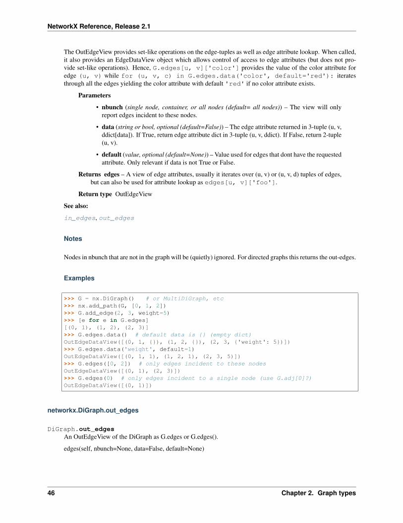
NetworkX Reference, Release 2.1
The OutEdgeView provides set-like operations on the edge-tuples as well as edge attribute lookup. When called,it also provides an EdgeDataView object which allows control of access to edge attributes (but does not pro-vide set-like operations). Hence, G.edges[u, v]['color'] provides the value of the color attribute foredge (u, v) while for (u, v, c) in G.edges.data('color', default='red'): iteratesthrough all the edges yielding the color attribute with default 'red' if no color attribute exists.
Parameters
• nbunch (single node, container, or all nodes (default= all nodes)) – The view will onlyreport edges incident to these nodes.
• data (string or bool, optional (default=False)) – The edge attribute returned in 3-tuple (u, v,ddict[data]). If True, return edge attribute dict in 3-tuple (u, v, ddict). If False, return 2-tuple(u, v).
• default (value, optional (default=None)) – Value used for edges that dont have the requestedattribute. Only relevant if data is not True or False.
Returns edges – A view of edge attributes, usually it iterates over (u, v) or (u, v, d) tuples of edges,but can also be used for attribute lookup as edges[u, v]['foo'].
Return type OutEdgeView
See also:
in_edges, out_edges
Notes
Nodes in nbunch that are not in the graph will be (quietly) ignored. For directed graphs this returns the out-edges.
Examples
>>> G = nx.DiGraph() # or MultiDiGraph, etc>>> nx.add_path(G, [0, 1, 2])>>> G.add_edge(2, 3, weight=5)>>> [e for e in G.edges][(0, 1), (1, 2), (2, 3)]>>> G.edges.data() # default data is {} (empty dict)OutEdgeDataView([(0, 1, {}), (1, 2, {}), (2, 3, {'weight': 5})])>>> G.edges.data('weight', default=1)OutEdgeDataView([(0, 1, 1), (1, 2, 1), (2, 3, 5)])>>> G.edges([0, 2]) # only edges incident to these nodesOutEdgeDataView([(0, 1), (2, 3)])>>> G.edges(0) # only edges incident to a single node (use G.adj[0]?)OutEdgeDataView([(0, 1)])
networkx.DiGraph.out_edges
DiGraph.out_edgesAn OutEdgeView of the DiGraph as G.edges or G.edges().
edges(self, nbunch=None, data=False, default=None)
46 Chapter 2. Graph types

NetworkX Reference, Release 2.1
The OutEdgeView provides set-like operations on the edge-tuples as well as edge attribute lookup. When called,it also provides an EdgeDataView object which allows control of access to edge attributes (but does not pro-vide set-like operations). Hence, G.edges[u, v]['color'] provides the value of the color attribute foredge (u, v) while for (u, v, c) in G.edges.data('color', default='red'): iteratesthrough all the edges yielding the color attribute with default 'red' if no color attribute exists.
Parameters
• nbunch (single node, container, or all nodes (default= all nodes)) – The view will onlyreport edges incident to these nodes.
• data (string or bool, optional (default=False)) – The edge attribute returned in 3-tuple (u, v,ddict[data]). If True, return edge attribute dict in 3-tuple (u, v, ddict). If False, return 2-tuple(u, v).
• default (value, optional (default=None)) – Value used for edges that dont have the requestedattribute. Only relevant if data is not True or False.
Returns edges – A view of edge attributes, usually it iterates over (u, v) or (u, v, d) tuples of edges,but can also be used for attribute lookup as edges[u, v]['foo'].
Return type OutEdgeView
See also:
in_edges, out_edges
Notes
Nodes in nbunch that are not in the graph will be (quietly) ignored. For directed graphs this returns the out-edges.
Examples
>>> G = nx.DiGraph() # or MultiDiGraph, etc>>> nx.add_path(G, [0, 1, 2])>>> G.add_edge(2, 3, weight=5)>>> [e for e in G.edges][(0, 1), (1, 2), (2, 3)]>>> G.edges.data() # default data is {} (empty dict)OutEdgeDataView([(0, 1, {}), (1, 2, {}), (2, 3, {'weight': 5})])>>> G.edges.data('weight', default=1)OutEdgeDataView([(0, 1, 1), (1, 2, 1), (2, 3, 5)])>>> G.edges([0, 2]) # only edges incident to these nodesOutEdgeDataView([(0, 1), (2, 3)])>>> G.edges(0) # only edges incident to a single node (use G.adj[0]?)OutEdgeDataView([(0, 1)])
networkx.DiGraph.in_edges
DiGraph.in_edgesAn InEdgeView of the Graph as G.in_edges or G.in_edges().
in_edges(self, nbunch=None, data=False, default=None):
Parameters
2.2. Basic graph types 47

NetworkX Reference, Release 2.1
• nbunch (single node, container, or all nodes (default= all nodes)) – The view will onlyreport edges incident to these nodes.
• data (string or bool, optional (default=False)) – The edge attribute returned in 3-tuple (u, v,ddict[data]). If True, return edge attribute dict in 3-tuple (u, v, ddict). If False, return 2-tuple(u, v).
• default (value, optional (default=None)) – Value used for edges that dont have the requestedattribute. Only relevant if data is not True or False.
Returns in_edges – A view of edge attributes, usually it iterates over (u, v) or (u, v, d) tuples ofedges, but can also be used for attribute lookup as edges[u, v]['foo'].
Return type InEdgeView
See also:
edges
networkx.DiGraph.has_edge
DiGraph.has_edge(u, v)Return True if the edge (u, v) is in the graph.
This is the same as v in G[u] without KeyError exceptions.
Parameters u, v (nodes) – Nodes can be, for example, strings or numbers. Nodes must be hashable(and not None) Python objects.
Returns edge_ind – True if edge is in the graph, False otherwise.
Return type bool
Examples
>>> G = nx.path_graph(4) # or DiGraph, MultiGraph, MultiDiGraph, etc>>> G.has_edge(0, 1) # using two nodesTrue>>> e = (0, 1)>>> G.has_edge(*e) # e is a 2-tuple (u, v)True>>> e = (0, 1, {'weight':7})>>> G.has_edge(*e[:2]) # e is a 3-tuple (u, v, data_dictionary)True
The following syntax are equivalent:
>>> G.has_edge(0, 1)True>>> 1 in G[0] # though this gives KeyError if 0 not in GTrue
networkx.DiGraph.get_edge_data
DiGraph.get_edge_data(u, v, default=None)Return the attribute dictionary associated with edge (u, v).
48 Chapter 2. Graph types
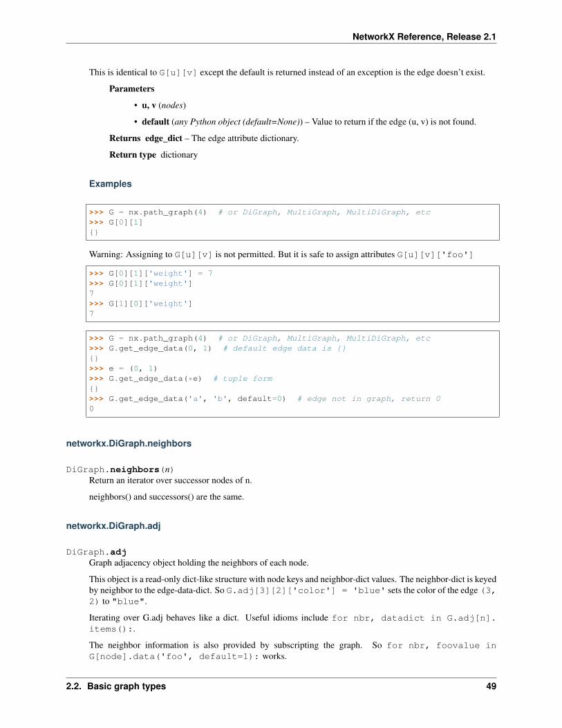
NetworkX Reference, Release 2.1
This is identical to G[u][v] except the default is returned instead of an exception is the edge doesn’t exist.
Parameters
• u, v (nodes)
• default (any Python object (default=None)) – Value to return if the edge (u, v) is not found.
Returns edge_dict – The edge attribute dictionary.
Return type dictionary
Examples
>>> G = nx.path_graph(4) # or DiGraph, MultiGraph, MultiDiGraph, etc>>> G[0][1]{}
Warning: Assigning to G[u][v] is not permitted. But it is safe to assign attributes G[u][v]['foo']
>>> G[0][1]['weight'] = 7>>> G[0][1]['weight']7>>> G[1][0]['weight']7
>>> G = nx.path_graph(4) # or DiGraph, MultiGraph, MultiDiGraph, etc>>> G.get_edge_data(0, 1) # default edge data is {}{}>>> e = (0, 1)>>> G.get_edge_data(*e) # tuple form{}>>> G.get_edge_data('a', 'b', default=0) # edge not in graph, return 00
networkx.DiGraph.neighbors
DiGraph.neighbors(n)Return an iterator over successor nodes of n.
neighbors() and successors() are the same.
networkx.DiGraph.adj
DiGraph.adjGraph adjacency object holding the neighbors of each node.
This object is a read-only dict-like structure with node keys and neighbor-dict values. The neighbor-dict is keyedby neighbor to the edge-data-dict. So G.adj[3][2]['color'] = 'blue' sets the color of the edge (3,2) to "blue".
Iterating over G.adj behaves like a dict. Useful idioms include for nbr, datadict in G.adj[n].items():.
The neighbor information is also provided by subscripting the graph. So for nbr, foovalue inG[node].data('foo', default=1): works.
2.2. Basic graph types 49

NetworkX Reference, Release 2.1
For directed graphs, G.adj holds outgoing (successor) info.
networkx.DiGraph.__getitem__
DiGraph.__getitem__(n)Return a dict of neighbors of node n. Use: ‘G[n]’.
Parameters n (node) – A node in the graph.
Returns adj_dict – The adjacency dictionary for nodes connected to n.
Return type dictionary
Notes
G[n] is the same as G.adj[n] and similar to G.neighbors(n) (which is an iterator over G.adj[n])
Examples
>>> G = nx.path_graph(4) # or DiGraph, MultiGraph, MultiDiGraph, etc>>> G[0]AtlasView({1: {}})
networkx.DiGraph.successors
DiGraph.successors(n)Return an iterator over successor nodes of n.
neighbors() and successors() are the same.
networkx.DiGraph.succ
DiGraph.succGraph adjacency object holding the successors of each node.
This object is a read-only dict-like structure with node keys and neighbor-dict values. The neighbor-dict iskeyed by neighbor to the edge-data-dict. So G.succ[3][2]['color'] = 'blue' sets the color of theedge (3, 2) to "blue".
Iterating over G.succ behaves like a dict. Useful idioms include for nbr, datadict in G.succ[n].items():. A data-view not provided by dicts also exists: for nbr, foovalue in G.succ[node].data('foo'): and a default can be set via a default argument to the data method.
The neighbor information is also provided by subscripting the graph. So for nbr, foovalue inG[node].data('foo', default=1): works.
For directed graphs, G.adj is identical to G.succ.
networkx.DiGraph.predecessors
DiGraph.predecessors(n)Return an iterator over predecessor nodes of n.
50 Chapter 2. Graph types

NetworkX Reference, Release 2.1
networkx.DiGraph.pred
DiGraph.predGraph adjacency object holding the predecessors of each node.
This object is a read-only dict-like structure with node keys and neighbor-dict values. The neighbor-dict iskeyed by neighbor to the edge-data-dict. So G.pred[2][3]['color'] = 'blue' sets the color of theedge (3, 2) to "blue".
Iterating over G.pred behaves like a dict. Useful idioms include for nbr, datadict in G.pred[n].items():. A data-view not provided by dicts also exists: for nbr, foovalue in G.pred[node].data('foo'): A default can be set via a default argument to the data method.
networkx.DiGraph.adjacency
DiGraph.adjacency()Return an iterator over (node, adjacency dict) tuples for all nodes.
For directed graphs, only outgoing neighbors/adjacencies are included.
Returns adj_iter – An iterator over (node, adjacency dictionary) for all nodes in the graph.
Return type iterator
Examples
>>> G = nx.path_graph(4) # or DiGraph, MultiGraph, MultiDiGraph, etc>>> [(n, nbrdict) for n, nbrdict in G.adjacency()][(0, {1: {}}), (1, {0: {}, 2: {}}), (2, {1: {}, 3: {}}), (3, {2: {}})]
networkx.DiGraph.nbunch_iter
DiGraph.nbunch_iter(nbunch=None)Return an iterator over nodes contained in nbunch that are also in the graph.
The nodes in nbunch are checked for membership in the graph and if not are silently ignored.
Parameters nbunch (single node, container, or all nodes (default= all nodes)) – The view will onlyreport edges incident to these nodes.
Returns niter – An iterator over nodes in nbunch that are also in the graph. If nbunch is None,iterate over all nodes in the graph.
Return type iterator
Raises NetworkXError – If nbunch is not a node or or sequence of nodes. If a node in nbunch isnot hashable.
See also:
Graph.__iter__()
2.2. Basic graph types 51

NetworkX Reference, Release 2.1
Notes
When nbunch is an iterator, the returned iterator yields values directly from nbunch, becoming exhausted whennbunch is exhausted.
To test whether nbunch is a single node, one can use “if nbunch in self:”, even after processing with this routine.
If nbunch is not a node or a (possibly empty) sequence/iterator or None, a NetworkXError is raised. Also, ifany object in nbunch is not hashable, a NetworkXError is raised.
Counting nodes edges and neighbors
DiGraph.order() Return the number of nodes in the graph.DiGraph.number_of_nodes() Return the number of nodes in the graph.DiGraph.__len__() Return the number of nodes.DiGraph.degree A DegreeView for the Graph as G.degree or G.degree().DiGraph.in_degree An InDegreeView for (node, in_degree) or in_degree for
single node.DiGraph.out_degree An OutDegreeView for (node, out_degree)DiGraph.size([weight]) Return the number of edges or total of all edge weights.DiGraph.number_of_edges([u, v]) Return the number of edges between two nodes.
networkx.DiGraph.order
DiGraph.order()Return the number of nodes in the graph.
Returns nnodes – The number of nodes in the graph.
Return type int
See also:
number_of_nodes(), __len__()
networkx.DiGraph.number_of_nodes
DiGraph.number_of_nodes()Return the number of nodes in the graph.
Returns nnodes – The number of nodes in the graph.
Return type int
See also:
order(), __len__()
Examples
>>> G = nx.path_graph(3) # or DiGraph, MultiGraph, MultiDiGraph, etc>>> len(G)3
52 Chapter 2. Graph types

NetworkX Reference, Release 2.1
networkx.DiGraph.__len__
DiGraph.__len__()Return the number of nodes. Use: ‘len(G)’.
Returns nnodes – The number of nodes in the graph.
Return type int
Examples
>>> G = nx.path_graph(4) # or DiGraph, MultiGraph, MultiDiGraph, etc>>> len(G)4
networkx.DiGraph.degree
DiGraph.degreeA DegreeView for the Graph as G.degree or G.degree().
The node degree is the number of edges adjacent to the node. The weighted node degree is the sum of the edgeweights for edges incident to that node.
This object provides an iterator for (node, degree) as well as lookup for the degree for a single node.
Parameters
• nbunch (single node, container, or all nodes (default= all nodes)) – The view will onlyreport edges incident to these nodes.
• weight (string or None, optional (default=None)) – The name of an edge attribute that holdsthe numerical value used as a weight. If None, then each edge has weight 1. The degree isthe sum of the edge weights adjacent to the node.
Returns
• If a single node is requested
• deg (int) – Degree of the node
• OR if multiple nodes are requested
• nd_iter (iterator) – The iterator returns two-tuples of (node, degree).
See also:
in_degree, out_degree
Examples
>>> G = nx.DiGraph() # or MultiDiGraph>>> nx.add_path(G, [0, 1, 2, 3])>>> G.degree(0) # node 0 with degree 11>>> list(G.degree([0, 1, 2]))[(0, 1), (1, 2), (2, 2)]
2.2. Basic graph types 53

NetworkX Reference, Release 2.1
networkx.DiGraph.in_degree
DiGraph.in_degreeAn InDegreeView for (node, in_degree) or in_degree for single node.
The node in_degree is the number of edges pointing to the node. The weighted node degree is the sum of theedge weights for edges incident to that node.
This object provides an iteration over (node, in_degree) as well as lookup for the degree for a single node.
Parameters
• nbunch (single node, container, or all nodes (default= all nodes)) – The view will onlyreport edges incident to these nodes.
• weight (string or None, optional (default=None)) – The name of an edge attribute that holdsthe numerical value used as a weight. If None, then each edge has weight 1. The degree isthe sum of the edge weights adjacent to the node.
Returns
• If a single node is requested
• deg (int) – In-degree of the node
• OR if multiple nodes are requested
• nd_iter (iterator) – The iterator returns two-tuples of (node, in-degree).
See also:
degree, out_degree
Examples
>>> G = nx.DiGraph()>>> nx.add_path(G, [0, 1, 2, 3])>>> G.in_degree(0) # node 0 with degree 00>>> list(G.in_degree([0, 1, 2]))[(0, 0), (1, 1), (2, 1)]
networkx.DiGraph.out_degree
DiGraph.out_degreeAn OutDegreeView for (node, out_degree)
The node out_degree is the number of edges pointing out of the node. The weighted node degree is the sum ofthe edge weights for edges incident to that node.
This object provides an iterator over (node, out_degree) as well as lookup for the degree for a single node.
Parameters
• nbunch (single node, container, or all nodes (default= all nodes)) – The view will onlyreport edges incident to these nodes.
• weight (string or None, optional (default=None)) – The name of an edge attribute that holdsthe numerical value used as a weight. If None, then each edge has weight 1. The degree isthe sum of the edge weights adjacent to the node.
54 Chapter 2. Graph types

NetworkX Reference, Release 2.1
Returns
• If a single node is requested
• deg (int) – Out-degree of the node
• OR if multiple nodes are requested
• nd_iter (iterator) – The iterator returns two-tuples of (node, out-degree).
See also:
degree, in_degree
Examples
>>> G = nx.DiGraph()>>> nx.add_path(G, [0, 1, 2, 3])>>> G.out_degree(0) # node 0 with degree 11>>> list(G.out_degree([0, 1, 2]))[(0, 1), (1, 1), (2, 1)]
networkx.DiGraph.size
DiGraph.size(weight=None)Return the number of edges or total of all edge weights.
Parameters weight (string or None, optional (default=None)) – The edge attribute that holds thenumerical value used as a weight. If None, then each edge has weight 1.
Returns
size – The number of edges or (if weight keyword is provided) the total weight sum.
If weight is None, returns an int. Otherwise a float (or more general numeric if the weights aremore general).
Return type numeric
See also:
number_of_edges()
Examples
>>> G = nx.path_graph(4) # or DiGraph, MultiGraph, MultiDiGraph, etc>>> G.size()3
>>> G = nx.Graph() # or DiGraph, MultiGraph, MultiDiGraph, etc>>> G.add_edge('a', 'b', weight=2)>>> G.add_edge('b', 'c', weight=4)>>> G.size()2>>> G.size(weight='weight')6.0
2.2. Basic graph types 55

NetworkX Reference, Release 2.1
networkx.DiGraph.number_of_edges
DiGraph.number_of_edges(u=None, v=None)Return the number of edges between two nodes.
Parameters u, v (nodes, optional (default=all edges)) – If u and v are specified, return the numberof edges between u and v. Otherwise return the total number of all edges.
Returns nedges – The number of edges in the graph. If nodes u and v are specified return thenumber of edges between those nodes. If the graph is directed, this only returns the number ofedges from u to v.
Return type int
See also:
size()
Examples
For undirected graphs, this method counts the total number of edges in the graph:
>>> G = nx.path_graph(4)>>> G.number_of_edges()3
If you specify two nodes, this counts the total number of edges joining the two nodes:
>>> G.number_of_edges(0, 1)1
For directed graphs, this method can count the total number of directed edges from u to v:
>>> G = nx.DiGraph()>>> G.add_edge(0, 1)>>> G.add_edge(1, 0)>>> G.number_of_edges(0, 1)1
Making copies and subgraphs
DiGraph.copy([as_view]) Return a copy of the graph.DiGraph.to_undirected([reciprocal, as_view]) Return an undirected representation of the digraph.DiGraph.to_directed([as_view]) Return a directed representation of the graph.DiGraph.subgraph(nodes) Return a SubGraph view of the subgraph induced on
nodes.DiGraph.edge_subgraph(edges) Returns the subgraph induced by the specified edges.DiGraph.reverse([copy]) Return the reverse of the graph.DiGraph.fresh_copy() Return a fresh copy graph with the same data structure.
56 Chapter 2. Graph types

NetworkX Reference, Release 2.1
networkx.DiGraph.copy
DiGraph.copy(as_view=False)Return a copy of the graph.
The copy method by default returns a shallow copy of the graph and attributes. That is, if an attribute isa container, that container is shared by the original an the copy. Use Python’s copy.deepcopy for newcontainers.
If as_view is True then a view is returned instead of a copy.
Notes
All copies reproduce the graph structure, but data attributes may be handled in different ways. There are fourtypes of copies of a graph that people might want.
Deepcopy – The default behavior is a “deepcopy” where the graph structure as well as all data attributes and anyobjects they might contain are copied. The entire graph object is new so that changes in the copy do not affectthe original object. (see Python’s copy.deepcopy)
Data Reference (Shallow) – For a shallow copy the graph structure is copied but the edge, node and graph at-tribute dicts are references to those in the original graph. This saves time and memory but could cause confusionif you change an attribute in one graph and it changes the attribute in the other. NetworkX does not provide thislevel of shallow copy.
Independent Shallow – This copy creates new independent attribute dicts and then does a shallow copy of theattributes. That is, any attributes that are containers are shared between the new graph and the original. This isexactly what dict.copy() provides. You can obtain this style copy using:
>>> G = nx.path_graph(5)>>> H = G.copy()>>> H = G.copy(as_view=False)>>> H = nx.Graph(G)>>> H = G.fresh_copy().__class__(G)
Fresh Data – For fresh data, the graph structure is copied while new empty data attribute dicts are created. Theresulting graph is independent of the original and it has no edge, node or graph attributes. Fresh copies are notenabled. Instead use:
>>> H = G.fresh_copy()>>> H.add_nodes_from(G)>>> H.add_edges_from(G.edges)
View – Inspired by dict-views, graph-views act like read-only versions of the original graph, providing a copyof the original structure without requiring any memory for copying the information.
See the Python copy module for more information on shallow and deep copies, https://docs.python.org/2/library/copy.html.
Parameters as_view (bool, optional (default=False)) – If True, the returned graph-view provides aread-only view of the original graph without actually copying any data.
Returns G – A copy of the graph.
Return type Graph
See also:
to_directed() return a directed copy of the graph.
2.2. Basic graph types 57

NetworkX Reference, Release 2.1
Examples
>>> G = nx.path_graph(4) # or DiGraph, MultiGraph, MultiDiGraph, etc>>> H = G.copy()
networkx.DiGraph.to_undirected
DiGraph.to_undirected(reciprocal=False, as_view=False)Return an undirected representation of the digraph.
Parameters
• reciprocal (bool (optional)) – If True only keep edges that appear in both directions in theoriginal digraph.
• as_view (bool (optional, default=False)) – If True return an undirected view of the originaldirected graph.
Returns G – An undirected graph with the same name and nodes and with edge (u, v, data) if either(u, v, data) or (v, u, data) is in the digraph. If both edges exist in digraph and their edge data isdifferent, only one edge is created with an arbitrary choice of which edge data to use. You mustcheck and correct for this manually if desired.
Return type Graph
See also:
Graph(), copy(), add_edge(), add_edges_from()
Notes
If edges in both directions (u, v) and (v, u) exist in the graph, attributes for the new undirected edge will be acombination of the attributes of the directed edges. The edge data is updated in the (arbitrary) order that theedges are encountered. For more customized control of the edge attributes use add_edge().
This returns a “deepcopy” of the edge, node, and graph attributes which attempts to completely copy all of thedata and references.
This is in contrast to the similar G=DiGraph(D) which returns a shallow copy of the data.
See the Python copy module for more information on shallow and deep copies, https://docs.python.org/2/library/copy.html.
Warning: If you have subclassed DiGraph to use dict-like objects in the data structure, those changes do nottransfer to the Graph created by this method.
Examples
>>> G = nx.path_graph(2) # or MultiGraph, etc>>> H = G.to_directed()>>> list(H.edges)[(0, 1), (1, 0)]>>> G2 = H.to_undirected()>>> list(G2.edges)[(0, 1)]
58 Chapter 2. Graph types

NetworkX Reference, Release 2.1
networkx.DiGraph.to_directed
DiGraph.to_directed(as_view=False)Return a directed representation of the graph.
Returns G – A directed graph with the same name, same nodes, and with each edge (u, v, data)replaced by two directed edges (u, v, data) and (v, u, data).
Return type DiGraph
Notes
This returns a “deepcopy” of the edge, node, and graph attributes which attempts to completely copy all of thedata and references.
This is in contrast to the similar D=DiGraph(G) which returns a shallow copy of the data.
See the Python copy module for more information on shallow and deep copies, https://docs.python.org/2/library/copy.html.
Warning: If you have subclassed Graph to use dict-like objects in the data structure, those changes do nottransfer to the DiGraph created by this method.
Examples
>>> G = nx.Graph() # or MultiGraph, etc>>> G.add_edge(0, 1)>>> H = G.to_directed()>>> list(H.edges)[(0, 1), (1, 0)]
If already directed, return a (deep) copy
>>> G = nx.DiGraph() # or MultiDiGraph, etc>>> G.add_edge(0, 1)>>> H = G.to_directed()>>> list(H.edges)[(0, 1)]
networkx.DiGraph.subgraph
DiGraph.subgraph(nodes)Return a SubGraph view of the subgraph induced on nodes.
The induced subgraph of the graph contains the nodes in nodes and the edges between those nodes.
Parameters nodes (list, iterable) – A container of nodes which will be iterated through once.
Returns G – A subgraph view of the graph. The graph structure cannot be changed but node/edgeattributes can and are shared with the original graph.
Return type SubGraph View
2.2. Basic graph types 59
NetworkX Reference, Release 2.1
Notes
The graph, edge and node attributes are shared with the original graph. Changes to the graph structure is ruledout by the view, but changes to attributes are reflected in the original graph.
To create a subgraph with its own copy of the edge/node attributes use: G.subgraph(nodes).copy()
For an inplace reduction of a graph to a subgraph you can remove nodes: G.remove_nodes_from([n for n in Gif n not in set(nodes)])
Examples
>>> G = nx.path_graph(4) # or DiGraph, MultiGraph, MultiDiGraph, etc>>> H = G.subgraph([0, 1, 2])>>> list(H.edges)[(0, 1), (1, 2)]
networkx.DiGraph.edge_subgraph
DiGraph.edge_subgraph(edges)Returns the subgraph induced by the specified edges.
The induced subgraph contains each edge in edges and each node incident to any one of those edges.
Parameters edges (iterable) – An iterable of edges in this graph.
Returns G – An edge-induced subgraph of this graph with the same edge attributes.
Return type Graph
Notes
The graph, edge, and node attributes in the returned subgraph view are references to the corresponding attributesin the original graph. The view is read-only.
To create a full graph version of the subgraph with its own copy of the edge or node attributes, use:
>>> G.edge_subgraph(edges).copy()
Examples
>>> G = nx.path_graph(5)>>> H = G.edge_subgraph([(0, 1), (3, 4)])>>> list(H.nodes)[0, 1, 3, 4]>>> list(H.edges)[(0, 1), (3, 4)]
60 Chapter 2. Graph types

NetworkX Reference, Release 2.1
networkx.DiGraph.reverse
DiGraph.reverse(copy=True)Return the reverse of the graph.
The reverse is a graph with the same nodes and edges but with the directions of the edges reversed.
Parameters copy (bool optional (default=True)) – If True, return a new DiGraph holding the re-versed edges. If False, the reverse graph is created using a view of the original graph.
networkx.DiGraph.fresh_copy
DiGraph.fresh_copy()Return a fresh copy graph with the same data structure.
A fresh copy has no nodes, edges or graph attributes. It is the same data structure as the current graph. Thismethod is typically used to create an empty version of the graph.
Notes
If you subclass the base class you should overwrite this method to return your class of graph.
2.2.3 MultiGraph—Undirected graphs with self loops and parallel edges
Overview
class MultiGraph(incoming_graph_data=None, **attr)An undirected graph class that can store multiedges.
Multiedges are multiple edges between two nodes. Each edge can hold optional data or attributes.
A MultiGraph holds undirected edges. Self loops are allowed.
Nodes can be arbitrary (hashable) Python objects with optional key/value attributes. By convention None is notused as a node.
Edges are represented as links between nodes with optional key/value attributes.
Parameters
• incoming_graph_data (input graph (optional, default: None)) – Data to initialize graph. IfNone (default) an empty graph is created. The data can be any format that is supported bythe to_networkx_graph() function, currently including edge list, dict of dicts, dict of lists,NetworkX graph, NumPy matrix or 2d ndarray, SciPy sparse matrix, or PyGraphviz graph.
• attr (keyword arguments, optional (default= no attributes)) – Attributes to add to graph askey=value pairs.
See also:
Graph, DiGraph, MultiDiGraph, OrderedMultiGraph
2.2. Basic graph types 61

NetworkX Reference, Release 2.1
Examples
Create an empty graph structure (a “null graph”) with no nodes and no edges.
>>> G = nx.MultiGraph()
G can be grown in several ways.
Nodes:
Add one node at a time:
>>> G.add_node(1)
Add the nodes from any container (a list, dict, set or even the lines from a file or the nodes from another graph).
>>> G.add_nodes_from([2, 3])>>> G.add_nodes_from(range(100, 110))>>> H = nx.path_graph(10)>>> G.add_nodes_from(H)
In addition to strings and integers any hashable Python object (except None) can represent a node, e.g. acustomized node object, or even another Graph.
>>> G.add_node(H)
Edges:
G can also be grown by adding edges.
Add one edge,
>>> key = G.add_edge(1, 2)
a list of edges,
>>> keys = G.add_edges_from([(1, 2), (1, 3)])
or a collection of edges,
>>> keys = G.add_edges_from(H.edges)
If some edges connect nodes not yet in the graph, the nodes are added automatically. If an edge already exists,an additional edge is created and stored using a key to identify the edge. By default the key is the lowest unusedinteger.
>>> keys = G.add_edges_from([(4,5,{'route':28}), (4,5,{'route':37})])>>> G[4]AdjacencyView({3: {0: {}}, 5: {0: {}, 1: {'route': 28}, 2: {'route': 37}}})
Attributes:
Each graph, node, and edge can hold key/value attribute pairs in an associated attribute dictionary (the keysmust be hashable). By default these are empty, but can be added or changed using add_edge, add_node or directmanipulation of the attribute dictionaries named graph, node and edge respectively.
>>> G = nx.MultiGraph(day="Friday")>>> G.graph{'day': 'Friday'}
62 Chapter 2. Graph types

NetworkX Reference, Release 2.1
Add node attributes using add_node(), add_nodes_from() or G.nodes
>>> G.add_node(1, time='5pm')>>> G.add_nodes_from([3], time='2pm')>>> G.nodes[1]{'time': '5pm'}>>> G.nodes[1]['room'] = 714>>> del G.nodes[1]['room'] # remove attribute>>> list(G.nodes(data=True))[(1, {'time': '5pm'}), (3, {'time': '2pm'})]
Add edge attributes using add_edge(), add_edges_from(), subscript notation, or G.edges.
>>> key = G.add_edge(1, 2, weight=4.7 )>>> keys = G.add_edges_from([(3, 4), (4, 5)], color='red')>>> keys = G.add_edges_from([(1,2,{'color':'blue'}), (2,3,{'weight':8})])>>> G[1][2][0]['weight'] = 4.7>>> G.edges[1, 2, 0]['weight'] = 4
Warning: we protect the graph data structure by making G.edges[1, 2] a read-only dict-like structure.However, you can assign to attributes in e.g. G.edges[1, 2]. Thus, use 2 sets of brackets to add/change dataattributes: G.edges[1, 2]['weight'] = 4 (For multigraphs: MG.edges[u, v, key][name] =value).
Shortcuts:
Many common graph features allow python syntax to speed reporting.
>>> 1 in G # check if node in graphTrue>>> [n for n in G if n<3] # iterate through nodes[1, 2]>>> len(G) # number of nodes in graph5>>> G[1] # adjacency dict-like view keyed by neighbor to edge attributesAdjacencyView({2: {0: {'weight': 4}, 1: {'color': 'blue'}}})
Often the best way to traverse all edges of a graph is via the neighbors. The neighbors are reported as anadjacency-dict G.adj or as G.adjacency().
>>> for n, nbrsdict in G.adjacency():... for nbr, keydict in nbrsdict.items():... for key, eattr in keydict.items():... if 'weight' in eattr:... # Do something useful with the edges... pass
But the edges() method is often more convenient:
>>> for u, v, keys, weight in G.edges(data='weight', keys=True):... if weight is not None:... # Do something useful with the edges... pass
Reporting:
Simple graph information is obtained using methods and object-attributes. Reporting usually providesviews instead of containers to reduce memory usage. The views update as the graph is updated simi-larly to dict-views. The objects nodes, `edges and adj provide access to data attributes via lookup
2.2. Basic graph types 63

NetworkX Reference, Release 2.1
(e.g. nodes[n], `edges[u, v], adj[u][v]) and iteration (e.g. nodes.items(), nodes.data('color'), nodes.data('color', default='blue') and similarly for edges) Views existfor nodes, edges, neighbors()/adj and degree.
For details on these and other miscellaneous methods, see below.
Subclasses (Advanced):
The MultiGraph class uses a dict-of-dict-of-dict-of-dict data structure. The outer dict (node_dict) holds adja-cency information keyed by node. The next dict (adjlist_dict) represents the adjacency information and holdsedge_key dicts keyed by neighbor. The edge_key dict holds each edge_attr dict keyed by edge key. The innerdict (edge_attr_dict) represents the edge data and holds edge attribute values keyed by attribute names.
Each of these four dicts in the dict-of-dict-of-dict-of-dict structure can be replaced by a user defined dict-likeobject. In general, the dict-like features should be maintained but extra features can be added. To replace oneof the dicts create a new graph class by changing the class(!) variable holding the factory for that dict-likestructure. The variable names are node_dict_factory, adjlist_inner_dict_factory, adjlist_outer_dict_factory, andedge_attr_dict_factory.
node_dict_factory [function, (default: dict)] Factory function to be used to create the dict containing nodeattributes, keyed by node id. It should require no arguments and return a dict-like object
adjlist_outer_dict_factory [function, (default: dict)] Factory function to be used to create the outer-most dictin the data structure that holds adjacency info keyed by node. It should require no arguments and return adict-like object.
adjlist_inner_dict_factory [function, (default: dict)] Factory function to be used to create the adjacency listdict which holds multiedge key dicts keyed by neighbor. It should require no arguments and return adict-like object.
edge_key_dict_factory [function, (default: dict)] Factory function to be used to create the edge key dict whichholds edge data keyed by edge key. It should require no arguments and return a dict-like object.
edge_attr_dict_factory [function, (default: dict)] Factory function to be used to create the edge attribute dictwhich holds attrbute values keyed by attribute name. It should require no arguments and return a dict-likeobject.
Examples
Please see ordered for examples of creating graph subclasses by overwriting the base class dict with adictionary-like object.
Methods
Adding and removing nodes and edges
MultiGraph.__init__([incoming_graph_data]) Initialize a graph with edges, name, or graph attributes.MultiGraph.add_node(node_for_adding, **attr) Add a single node node_for_adding and update node
attributes.MultiGraph.add_nodes_from(nodes_for_adding,. . . )
Add multiple nodes.
MultiGraph.remove_node(n) Remove node n.MultiGraph.remove_nodes_from(nodes) Remove multiple nodes.MultiGraph.add_edge(u_for_edge, v_for_edge) Add an edge between u and v.
Continued on next page
64 Chapter 2. Graph types

NetworkX Reference, Release 2.1
Table 2.9 – continued from previous pageMultiGraph.add_edges_from(ebunch_to_add,**attr)
Add all the edges in ebunch_to_add.
MultiGraph.add_weighted_edges_from(ebunch_to_add)Add weighted edges in ebunch_to_add with specifiedweight attr
MultiGraph.new_edge_key(u, v) Return an unused key for edges between nodes u and v.MultiGraph.remove_edge(u, v[, key]) Remove an edge between u and v.MultiGraph.remove_edges_from(ebunch) Remove all edges specified in ebunch.MultiGraph.clear() Remove all nodes and edges from the graph.
networkx.MultiGraph.__init__
MultiGraph.__init__(incoming_graph_data=None, **attr)Initialize a graph with edges, name, or graph attributes.
Parameters
• incoming_graph_data (input graph) – Data to initialize graph. If incom-ing_graph_data=None (default) an empty graph is created. The data can be an edge list,or any NetworkX graph object. If the corresponding optional Python packages are installedthe data can also be a NumPy matrix or 2d ndarray, a SciPy sparse matrix, or a PyGraphvizgraph.
• attr (keyword arguments, optional (default= no attributes)) – Attributes to add to graph askey=value pairs.
See also:
convert()
Examples
>>> G = nx.Graph() # or DiGraph, MultiGraph, MultiDiGraph, etc>>> G = nx.Graph(name='my graph')>>> e = [(1, 2), (2, 3), (3, 4)] # list of edges>>> G = nx.Graph(e)
Arbitrary graph attribute pairs (key=value) may be assigned
>>> G = nx.Graph(e, day="Friday")>>> G.graph{'day': 'Friday'}
networkx.MultiGraph.add_node
MultiGraph.add_node(node_for_adding, **attr)Add a single node node_for_adding and update node attributes.
Parameters
• node_for_adding (node) – A node can be any hashable Python object except None.
• attr (keyword arguments, optional) – Set or change node attributes using key=value.
See also:
add_nodes_from()
2.2. Basic graph types 65

NetworkX Reference, Release 2.1
Examples
>>> G = nx.Graph() # or DiGraph, MultiGraph, MultiDiGraph, etc>>> G.add_node(1)>>> G.add_node('Hello')>>> K3 = nx.Graph([(0, 1), (1, 2), (2, 0)])>>> G.add_node(K3)>>> G.number_of_nodes()3
Use keywords set/change node attributes:
>>> G.add_node(1, size=10)>>> G.add_node(3, weight=0.4, UTM=('13S', 382871, 3972649))
Notes
A hashable object is one that can be used as a key in a Python dictionary. This includes strings, numbers, tuplesof strings and numbers, etc.
On many platforms hashable items also include mutables such as NetworkX Graphs, though one should becareful that the hash doesn’t change on mutables.
networkx.MultiGraph.add_nodes_from
MultiGraph.add_nodes_from(nodes_for_adding, **attr)Add multiple nodes.
Parameters
• nodes_for_adding (iterable container) – A container of nodes (list, dict, set, etc.). OR Acontainer of (node, attribute dict) tuples. Node attributes are updated using the attribute dict.
• attr (keyword arguments, optional (default= no attributes)) – Update attributes for all nodesin nodes. Node attributes specified in nodes as a tuple take precedence over attributes spec-ified via keyword arguments.
See also:
add_node()
Examples
>>> G = nx.Graph() # or DiGraph, MultiGraph, MultiDiGraph, etc>>> G.add_nodes_from('Hello')>>> K3 = nx.Graph([(0, 1), (1, 2), (2, 0)])>>> G.add_nodes_from(K3)>>> sorted(G.nodes(), key=str)[0, 1, 2, 'H', 'e', 'l', 'o']
Use keywords to update specific node attributes for every node.
>>> G.add_nodes_from([1, 2], size=10)>>> G.add_nodes_from([3, 4], weight=0.4)
66 Chapter 2. Graph types

NetworkX Reference, Release 2.1
Use (node, attrdict) tuples to update attributes for specific nodes.
>>> G.add_nodes_from([(1, dict(size=11)), (2, {'color':'blue'})])>>> G.nodes[1]['size']11>>> H = nx.Graph()>>> H.add_nodes_from(G.nodes(data=True))>>> H.nodes[1]['size']11
networkx.MultiGraph.remove_node
MultiGraph.remove_node(n)Remove node n.
Removes the node n and all adjacent edges. Attempting to remove a non-existent node will raise an exception.
Parameters n (node) – A node in the graph
Raises NetworkXError – If n is not in the graph.
See also:
remove_nodes_from()
Examples
>>> G = nx.path_graph(3) # or DiGraph, MultiGraph, MultiDiGraph, etc>>> list(G.edges)[(0, 1), (1, 2)]>>> G.remove_node(1)>>> list(G.edges)[]
networkx.MultiGraph.remove_nodes_from
MultiGraph.remove_nodes_from(nodes)Remove multiple nodes.
Parameters nodes (iterable container) – A container of nodes (list, dict, set, etc.). If a node in thecontainer is not in the graph it is silently ignored.
See also:
remove_node()
Examples
>>> G = nx.path_graph(3) # or DiGraph, MultiGraph, MultiDiGraph, etc>>> e = list(G.nodes)>>> e[0, 1, 2]>>> G.remove_nodes_from(e)
2.2. Basic graph types 67

NetworkX Reference, Release 2.1
>>> list(G.nodes)[]
networkx.MultiGraph.add_edge
MultiGraph.add_edge(u_for_edge, v_for_edge, key=None, **attr)Add an edge between u and v.
The nodes u and v will be automatically added if they are not already in the graph.
Edge attributes can be specified with keywords or by directly accessing the edge’s attribute dictionary. Seeexamples below.
Parameters
• u_for_edge, v_for_edge (nodes) – Nodes can be, for example, strings or numbers. Nodesmust be hashable (and not None) Python objects.
• key (hashable identifier, optional (default=lowest unused integer)) – Used to distinguishmultiedges between a pair of nodes.
• attr (keyword arguments, optional) – Edge data (or labels or objects) can be assigned usingkeyword arguments.
Returns
Return type The edge key assigned to the edge.
See also:
add_edges_from() add a collection of edges
Notes
To replace/update edge data, use the optional key argument to identify a unique edge. Otherwise a new edgewill be created.
NetworkX algorithms designed for weighted graphs cannot use multigraphs directly because it is not clearhow to handle multiedge weights. Convert to Graph using edge attribute ‘weight’ to enable weighted graphalgorithms.
Default keys are generated using the method new_edge_key(). This method can be overridden by subclass-ing the base class and providing a custom new_edge_key() method.
Examples
The following all add the edge e=(1, 2) to graph G:
>>> G = nx.MultiGraph()>>> e = (1, 2)>>> ekey = G.add_edge(1, 2) # explicit two-node form>>> G.add_edge(*e) # single edge as tuple of two nodes1>>> G.add_edges_from( [(1, 2)] ) # add edges from iterable container[2]
68 Chapter 2. Graph types

NetworkX Reference, Release 2.1
Associate data to edges using keywords:
>>> ekey = G.add_edge(1, 2, weight=3)>>> ekey = G.add_edge(1, 2, key=0, weight=4) # update data for key=0>>> ekey = G.add_edge(1, 3, weight=7, capacity=15, length=342.7)
For non-string attribute keys, use subscript notation.
>>> ekey = G.add_edge(1, 2)>>> G[1][2][0].update({0: 5})>>> G.edges[1, 2, 0].update({0: 5})
networkx.MultiGraph.add_edges_from
MultiGraph.add_edges_from(ebunch_to_add, **attr)Add all the edges in ebunch_to_add.
Parameters
• ebunch_to_add (container of edges) – Each edge given in the container will be added tothe graph. The edges can be:
– 2-tuples (u, v) or
– 3-tuples (u, v, d) for an edge data dict d, or
– 3-tuples (u, v, k) for not iterable key k, or
– 4-tuples (u, v, k, d) for an edge with data and key k
• attr (keyword arguments, optional) – Edge data (or labels or objects) can be assigned usingkeyword arguments.
Returns
Return type A list of edge keys assigned to the edges in ebunch.
See also:
add_edge() add a single edge
add_weighted_edges_from() convenient way to add weighted edges
Notes
Adding the same edge twice has no effect but any edge data will be updated when each duplicate edge is added.
Edge attributes specified in an ebunch take precedence over attributes specified via keyword arguments.
Default keys are generated using the method new_edge_key(). This method can be overridden by subclass-ing the base class and providing a custom new_edge_key() method.
Examples
>>> G = nx.Graph() # or DiGraph, MultiGraph, MultiDiGraph, etc>>> G.add_edges_from([(0, 1), (1, 2)]) # using a list of edge tuples>>> e = zip(range(0, 3), range(1, 4))>>> G.add_edges_from(e) # Add the path graph 0-1-2-3
2.2. Basic graph types 69
NetworkX Reference, Release 2.1
Associate data to edges
>>> G.add_edges_from([(1, 2), (2, 3)], weight=3)>>> G.add_edges_from([(3, 4), (1, 4)], label='WN2898')
networkx.MultiGraph.add_weighted_edges_from
MultiGraph.add_weighted_edges_from(ebunch_to_add, weight=’weight’, **attr)Add weighted edges in ebunch_to_add with specified weight attr
Parameters
• ebunch_to_add (container of edges) – Each edge given in the list or container will be addedto the graph. The edges must be given as 3-tuples (u, v, w) where w is a number.
• weight (string, optional (default= ‘weight’)) – The attribute name for the edge weights tobe added.
• attr (keyword arguments, optional (default= no attributes)) – Edge attributes to add/updatefor all edges.
See also:
add_edge() add a single edge
add_edges_from() add multiple edges
Notes
Adding the same edge twice for Graph/DiGraph simply updates the edge data. For MultiGraph/MultiDiGraph,duplicate edges are stored.
Examples
>>> G = nx.Graph() # or DiGraph, MultiGraph, MultiDiGraph, etc>>> G.add_weighted_edges_from([(0, 1, 3.0), (1, 2, 7.5)])
networkx.MultiGraph.new_edge_key
MultiGraph.new_edge_key(u, v)Return an unused key for edges between nodes u and v.
The nodes u and v do not need to be already in the graph.
Notes
In the standard MultiGraph class the new key is the number of existing edges between u and v (increasedif necessary to ensure unused). The first edge will have key 0, then 1, etc. If an edge is removed furthernew_edge_keys may not be in this order.
Parameters u, v (nodes)
Returns key
70 Chapter 2. Graph types

NetworkX Reference, Release 2.1
Return type int
networkx.MultiGraph.remove_edge
MultiGraph.remove_edge(u, v, key=None)Remove an edge between u and v.
Parameters
• u, v (nodes) – Remove an edge between nodes u and v.
• key (hashable identifier, optional (default=None)) – Used to distinguish multiple edges be-tween a pair of nodes. If None remove a single (arbitrary) edge between u and v.
Raises NetworkXError – If there is not an edge between u and v, or if there is no edge with thespecified key.
See also:
remove_edges_from() remove a collection of edges
Examples
>>> G = nx.MultiGraph()>>> nx.add_path(G, [0, 1, 2, 3])>>> G.remove_edge(0, 1)>>> e = (1, 2)>>> G.remove_edge(*e) # unpacks e from an edge tuple
For multiple edges
>>> G = nx.MultiGraph() # or MultiDiGraph, etc>>> G.add_edges_from([(1, 2), (1, 2), (1, 2)]) # key_list returned[0, 1, 2]>>> G.remove_edge(1, 2) # remove a single (arbitrary) edge
For edges with keys
>>> G = nx.MultiGraph() # or MultiDiGraph, etc>>> G.add_edge(1, 2, key='first')'first'>>> G.add_edge(1, 2, key='second')'second'>>> G.remove_edge(1, 2, key='second')
networkx.MultiGraph.remove_edges_from
MultiGraph.remove_edges_from(ebunch)Remove all edges specified in ebunch.
Parameters ebunch (list or container of edge tuples) – Each edge given in the list or container willbe removed from the graph. The edges can be:
• 2-tuples (u, v) All edges between u and v are removed.
• 3-tuples (u, v, key) The edge identified by key is removed.
2.2. Basic graph types 71

NetworkX Reference, Release 2.1
• 4-tuples (u, v, key, data) where data is ignored.
See also:
remove_edge() remove a single edge
Notes
Will fail silently if an edge in ebunch is not in the graph.
Examples
>>> G = nx.path_graph(4) # or DiGraph, MultiGraph, MultiDiGraph, etc>>> ebunch=[(1, 2), (2, 3)]>>> G.remove_edges_from(ebunch)
Removing multiple copies of edges
>>> G = nx.MultiGraph()>>> keys = G.add_edges_from([(1, 2), (1, 2), (1, 2)])>>> G.remove_edges_from([(1, 2), (1, 2)])>>> list(G.edges())[(1, 2)]>>> G.remove_edges_from([(1, 2), (1, 2)]) # silently ignore extra copy>>> list(G.edges) # now empty graph[]
networkx.MultiGraph.clear
MultiGraph.clear()Remove all nodes and edges from the graph.
This also removes the name, and all graph, node, and edge attributes.
Examples
>>> G = nx.path_graph(4) # or DiGraph, MultiGraph, MultiDiGraph, etc>>> G.clear()>>> list(G.nodes)[]>>> list(G.edges)[]
Reporting nodes edges and neighbors
MultiGraph.nodes A NodeView of the Graph as G.nodes or G.nodes().MultiGraph.__iter__() Iterate over the nodes.MultiGraph.has_node(n) Return True if the graph contains the node n.
Continued on next page
72 Chapter 2. Graph types

NetworkX Reference, Release 2.1
Table 2.10 – continued from previous pageMultiGraph.__contains__(n) Return True if n is a node, False otherwise.MultiGraph.edges Return an iterator over the edges.MultiGraph.has_edge(u, v[, key]) Return True if the graph has an edge between nodes u and
v.MultiGraph.get_edge_data(u, v[, key, default]) Return the attribute dictionary associated with edge (u, v).MultiGraph.neighbors(n) Return an iterator over all neighbors of node n.MultiGraph.adj Graph adjacency object holding the neighbors of each
node.MultiGraph.__getitem__(n) Return a dict of neighbors of node n.MultiGraph.adjacency() Return an iterator over (node, adjacency dict) tuples for all
nodes.MultiGraph.nbunch_iter([nbunch]) Return an iterator over nodes contained in nbunch that are
also in the graph.
networkx.MultiGraph.nodes
MultiGraph.nodesA NodeView of the Graph as G.nodes or G.nodes().
Can be used as G.nodes for data lookup and for set-like operations. Can also be used as G.nodes(data='color', default=None) to return a NodeDataView which reports specific node databut no set operations. It presents a dict-like interface as well with G.nodes.items() iterating over (node,nodedata) 2-tuples and G.nodes[3]['foo'] providing the value of the foo attribute for node 3. Inaddition, a view G.nodes.data('foo') provides a dict-like interface to the foo attribute of each node.G.nodes.data('foo', default=1) provides a default for nodes that do not have attribute foo.
Parameters
• data (string or bool, optional (default=False)) – The node attribute returned in 2-tuple (n,ddict[data]). If True, return entire node attribute dict as (n, ddict). If False, return just thenodes n.
• default (value, optional (default=None)) – Value used for nodes that dont have the requestedattribute. Only relevant if data is not True or False.
Returns
Allows set-like operations over the nodes as well as node attribute dict lookup and calling toget a NodeDataView. A NodeDataView iterates over (n, data) and has no set operations. ANodeView iterates over n and includes set operations.
When called, if data is False, an iterator over nodes. Otherwise an iterator of 2-tuples (node,attribute value) where the attribute is specified in data. If data is True then the attribute becomesthe entire data dictionary.
Return type NodeView
Notes
If your node data is not needed, it is simpler and equivalent to use the expression for n in G, or list(G).
Examples
There are two simple ways of getting a list of all nodes in the graph:
2.2. Basic graph types 73

NetworkX Reference, Release 2.1
>>> G = nx.path_graph(3)>>> list(G.nodes)[0, 1, 2]>>> list(G)[0, 1, 2]
To get the node data along with the nodes:
>>> G.add_node(1, time='5pm')>>> G.nodes[0]['foo'] = 'bar'>>> list(G.nodes(data=True))[(0, {'foo': 'bar'}), (1, {'time': '5pm'}), (2, {})]>>> list(G.nodes.data())[(0, {'foo': 'bar'}), (1, {'time': '5pm'}), (2, {})]
>>> list(G.nodes(data='foo'))[(0, 'bar'), (1, None), (2, None)]>>> list(G.nodes.data('foo'))[(0, 'bar'), (1, None), (2, None)]
>>> list(G.nodes(data='time'))[(0, None), (1, '5pm'), (2, None)]>>> list(G.nodes.data('time'))[(0, None), (1, '5pm'), (2, None)]
>>> list(G.nodes(data='time', default='Not Available'))[(0, 'Not Available'), (1, '5pm'), (2, 'Not Available')]>>> list(G.nodes.data('time', default='Not Available'))[(0, 'Not Available'), (1, '5pm'), (2, 'Not Available')]
If some of your nodes have an attribute and the rest are assumed to have a default attribute value you can createa dictionary from node/attribute pairs using the default keyword argument to guarantee the value is neverNone:
>>> G = nx.Graph()>>> G.add_node(0)>>> G.add_node(1, weight=2)>>> G.add_node(2, weight=3)>>> dict(G.nodes(data='weight', default=1)){0: 1, 1: 2, 2: 3}
networkx.MultiGraph.__iter__
MultiGraph.__iter__()Iterate over the nodes. Use: ‘for n in G’.
Returns niter – An iterator over all nodes in the graph.
Return type iterator
Examples
74 Chapter 2. Graph types

NetworkX Reference, Release 2.1
>>> G = nx.path_graph(4) # or DiGraph, MultiGraph, MultiDiGraph, etc>>> [n for n in G][0, 1, 2, 3]>>> list(G)[0, 1, 2, 3]
networkx.MultiGraph.has_node
MultiGraph.has_node(n)Return True if the graph contains the node n.
Identical to n in G
Parameters n (node)
Examples
>>> G = nx.path_graph(3) # or DiGraph, MultiGraph, MultiDiGraph, etc>>> G.has_node(0)True
It is more readable and simpler to use
>>> 0 in GTrue
networkx.MultiGraph.__contains__
MultiGraph.__contains__(n)Return True if n is a node, False otherwise. Use: ‘n in G’.
Examples
>>> G = nx.path_graph(4) # or DiGraph, MultiGraph, MultiDiGraph, etc>>> 1 in GTrue
networkx.MultiGraph.edges
MultiGraph.edgesReturn an iterator over the edges.
edges(self, nbunch=None, data=False, keys=False, default=None)
The EdgeView provides set-like operations on the edge-tuples as well as edge attribute lookup. When called,it also provides an EdgeDataView object which allows control of access to edge attributes (but does not pro-vide set-like operations). Hence, G.edges[u, v]['color'] provides the value of the color attribute foredge (u, v) while for (u, v, c) in G.edges(data='color', default='red'): iteratesthrough all the edges yielding the color attribute.
2.2. Basic graph types 75

NetworkX Reference, Release 2.1
Edges are returned as tuples with optional data and keys in the order (node, neighbor, key, data).
Parameters
• nbunch (single node, container, or all nodes (default= all nodes)) – The view will onlyreport edges incident to these nodes.
• data (string or bool, optional (default=False)) – The edge attribute returned in 3-tuple (u, v,ddict[data]). If True, return edge attribute dict in 3-tuple (u, v, ddict). If False, return 2-tuple(u, v).
• keys (bool, optional (default=False)) – If True, return edge keys with each edge.
• default (value, optional (default=None)) – Value used for edges that dont have the requestedattribute. Only relevant if data is not True or False.
Returns edges – A view of edge attributes, usually it iterates over (u, v) (u, v, k) or (u, v, k, d) tuplesof edges, but can also be used for attribute lookup as edges[u, v, k]['foo'].
Return type MultiEdgeView
Notes
Nodes in nbunch that are not in the graph will be (quietly) ignored. For directed graphs this returns the out-edges.
Examples
>>> G = nx.MultiGraph() # or MultiDiGraph>>> nx.add_path(G, [0, 1, 2])>>> key = G.add_edge(2, 3, weight=5)>>> [e for e in G.edges()][(0, 1), (1, 2), (2, 3)]>>> G.edges.data() # default data is {} (empty dict)MultiEdgeDataView([(0, 1, {}), (1, 2, {}), (2, 3, {'weight': 5})])>>> G.edges.data('weight', default=1)MultiEdgeDataView([(0, 1, 1), (1, 2, 1), (2, 3, 5)])>>> G.edges(keys=True) # default keys are integersMultiEdgeView([(0, 1, 0), (1, 2, 0), (2, 3, 0)])>>> G.edges.data(keys=True)MultiEdgeDataView([(0, 1, 0, {}), (1, 2, 0, {}), (2, 3, 0, {'weight': 5})])>>> G.edges.data('weight', default=1, keys=True)MultiEdgeDataView([(0, 1, 0, 1), (1, 2, 0, 1), (2, 3, 0, 5)])>>> G.edges([0, 3])MultiEdgeDataView([(0, 1), (3, 2)])>>> G.edges(0)MultiEdgeDataView([(0, 1)])
networkx.MultiGraph.has_edge
MultiGraph.has_edge(u, v, key=None)Return True if the graph has an edge between nodes u and v.
This is the same as v in G[u] or key in G[u][v] without KeyError exceptions.
Parameters
• u, v (nodes) – Nodes can be, for example, strings or numbers.
76 Chapter 2. Graph types

NetworkX Reference, Release 2.1
• key (hashable identifier, optional (default=None)) – If specified return True only if the edgewith key is found.
Returns edge_ind – True if edge is in the graph, False otherwise.
Return type bool
Examples
Can be called either using two nodes u, v, an edge tuple (u, v), or an edge tuple (u, v, key).
>>> G = nx.MultiGraph() # or MultiDiGraph>>> nx.add_path(G, [0, 1, 2, 3])>>> G.has_edge(0, 1) # using two nodesTrue>>> e = (0, 1)>>> G.has_edge(*e) # e is a 2-tuple (u, v)True>>> G.add_edge(0, 1, key='a')'a'>>> G.has_edge(0, 1, key='a') # specify keyTrue>>> e=(0, 1, 'a')>>> G.has_edge(*e) # e is a 3-tuple (u, v, 'a')True
The following syntax are equivalent:
>>> G.has_edge(0, 1)True>>> 1 in G[0] # though this gives :exc:`KeyError` if 0 not in GTrue
networkx.MultiGraph.get_edge_data
MultiGraph.get_edge_data(u, v, key=None, default=None)Return the attribute dictionary associated with edge (u, v).
This is identical to G[u][v][key] except the default is returned instead of an exception is the edge doesn’texist.
Parameters
• u, v (nodes)
• default (any Python object (default=None)) – Value to return if the edge (u, v) is not found.
• key (hashable identifier, optional (default=None)) – Return data only for the edge withspecified key.
Returns edge_dict – The edge attribute dictionary.
Return type dictionary
2.2. Basic graph types 77

NetworkX Reference, Release 2.1
Examples
>>> G = nx.MultiGraph() # or MultiDiGraph>>> key = G.add_edge(0, 1, key='a', weight=7)>>> G[0][1]['a'] # key='a'{'weight': 7}>>> G.edges[0, 1, 'a'] # key='a'{'weight': 7}
Warning: we protect the graph data structure by making G.edges and G[1][2] read-only dict-like structures.However, you can assign values to attributes in e.g. G.edges[1, 2, 'a'] or G[1][2]['a'] using anadditional bracket as shown next. You need to specify all edge info to assign to the edge data associated with anedge.
>>> G[0][1]['a']['weight'] = 10>>> G.edges[0, 1, 'a']['weight'] = 10>>> G[0][1]['a']['weight']10>>> G.edges[1, 0, 'a']['weight']10
>>> G = nx.MultiGraph() # or MultiDiGraph>>> nx.add_path(G, [0, 1, 2, 3])>>> G.get_edge_data(0, 1){0: {}}>>> e = (0, 1)>>> G.get_edge_data(*e) # tuple form{0: {}}>>> G.get_edge_data('a', 'b', default=0) # edge not in graph, return 00
networkx.MultiGraph.neighbors
MultiGraph.neighbors(n)Return an iterator over all neighbors of node n.
This is identical to iter(G[n])
Parameters n (node) – A node in the graph
Returns neighbors – An iterator over all neighbors of node n
Return type iterator
Raises NetworkXError – If the node n is not in the graph.
Examples
>>> G = nx.path_graph(4) # or DiGraph, MultiGraph, MultiDiGraph, etc>>> [n for n in G.neighbors(0)][1]
78 Chapter 2. Graph types

NetworkX Reference, Release 2.1
Notes
It is usually more convenient (and faster) to access the adjacency dictionary as G[n]:
>>> G = nx.Graph() # or DiGraph, MultiGraph, MultiDiGraph, etc>>> G.add_edge('a', 'b', weight=7)>>> G['a']AtlasView({'b': {'weight': 7}})>>> G = nx.path_graph(4)>>> [n for n in G[0]][1]
networkx.MultiGraph.adj
MultiGraph.adjGraph adjacency object holding the neighbors of each node.
This object is a read-only dict-like structure with node keys and neighbor-dict values. The neighbor-dict is keyedby neighbor to the edgekey-data-dict. So G.adj[3][2][0]['color'] = 'blue' sets the color of theedge (3, 2, 0) to "blue".
Iterating over G.adj behaves like a dict. Useful idioms include for nbr, nbrdict in G.adj[n].items():.
The neighbor information is also provided by subscripting the graph. So for nbr, foovalue inG[node].data('foo', default=1): works.
For directed graphs, G.adj holds outgoing (successor) info.
networkx.MultiGraph.__getitem__
MultiGraph.__getitem__(n)Return a dict of neighbors of node n. Use: ‘G[n]’.
Parameters n (node) – A node in the graph.
Returns adj_dict – The adjacency dictionary for nodes connected to n.
Return type dictionary
Notes
G[n] is the same as G.adj[n] and similar to G.neighbors(n) (which is an iterator over G.adj[n])
Examples
>>> G = nx.path_graph(4) # or DiGraph, MultiGraph, MultiDiGraph, etc>>> G[0]AtlasView({1: {}})
2.2. Basic graph types 79

NetworkX Reference, Release 2.1
networkx.MultiGraph.adjacency
MultiGraph.adjacency()Return an iterator over (node, adjacency dict) tuples for all nodes.
For directed graphs, only outgoing neighbors/adjacencies are included.
Returns adj_iter – An iterator over (node, adjacency dictionary) for all nodes in the graph.
Return type iterator
Examples
>>> G = nx.path_graph(4) # or DiGraph, MultiGraph, MultiDiGraph, etc>>> [(n, nbrdict) for n, nbrdict in G.adjacency()][(0, {1: {}}), (1, {0: {}, 2: {}}), (2, {1: {}, 3: {}}), (3, {2: {}})]
networkx.MultiGraph.nbunch_iter
MultiGraph.nbunch_iter(nbunch=None)Return an iterator over nodes contained in nbunch that are also in the graph.
The nodes in nbunch are checked for membership in the graph and if not are silently ignored.
Parameters nbunch (single node, container, or all nodes (default= all nodes)) – The view will onlyreport edges incident to these nodes.
Returns niter – An iterator over nodes in nbunch that are also in the graph. If nbunch is None,iterate over all nodes in the graph.
Return type iterator
Raises NetworkXError – If nbunch is not a node or or sequence of nodes. If a node in nbunch isnot hashable.
See also:
Graph.__iter__()
Notes
When nbunch is an iterator, the returned iterator yields values directly from nbunch, becoming exhausted whennbunch is exhausted.
To test whether nbunch is a single node, one can use “if nbunch in self:”, even after processing with this routine.
If nbunch is not a node or a (possibly empty) sequence/iterator or None, a NetworkXError is raised. Also, ifany object in nbunch is not hashable, a NetworkXError is raised.
Counting nodes edges and neighbors
MultiGraph.order() Return the number of nodes in the graph.MultiGraph.number_of_nodes() Return the number of nodes in the graph.
Continued on next page
80 Chapter 2. Graph types

NetworkX Reference, Release 2.1
Table 2.11 – continued from previous pageMultiGraph.__len__() Return the number of nodes.MultiGraph.degree A DegreeView for the Graph as G.degree or G.degree().MultiGraph.size([weight]) Return the number of edges or total of all edge weights.MultiGraph.number_of_edges([u, v]) Return the number of edges between two nodes.
networkx.MultiGraph.order
MultiGraph.order()Return the number of nodes in the graph.
Returns nnodes – The number of nodes in the graph.
Return type int
See also:
number_of_nodes(), __len__()
networkx.MultiGraph.number_of_nodes
MultiGraph.number_of_nodes()Return the number of nodes in the graph.
Returns nnodes – The number of nodes in the graph.
Return type int
See also:
order(), __len__()
Examples
>>> G = nx.path_graph(3) # or DiGraph, MultiGraph, MultiDiGraph, etc>>> len(G)3
networkx.MultiGraph.__len__
MultiGraph.__len__()Return the number of nodes. Use: ‘len(G)’.
Returns nnodes – The number of nodes in the graph.
Return type int
Examples
>>> G = nx.path_graph(4) # or DiGraph, MultiGraph, MultiDiGraph, etc>>> len(G)4
2.2. Basic graph types 81

NetworkX Reference, Release 2.1
networkx.MultiGraph.degree
MultiGraph.degreeA DegreeView for the Graph as G.degree or G.degree().
The node degree is the number of edges adjacent to the node. The weighted node degree is the sum of the edgeweights for edges incident to that node.
This object provides an iterator for (node, degree) as well as lookup for the degree for a single node.
Parameters
• nbunch (single node, container, or all nodes (default= all nodes)) – The view will onlyreport edges incident to these nodes.
• weight (string or None, optional (default=None)) – The name of an edge attribute that holdsthe numerical value used as a weight. If None, then each edge has weight 1. The degree isthe sum of the edge weights adjacent to the node.
Returns
• If a single node is requested
• deg (int) – Degree of the node, if a single node is passed as argument.
• OR if multiple nodes are requested
• nd_iter (iterator) – The iterator returns two-tuples of (node, degree).
Examples
>>> G = nx.Graph() # or DiGraph, MultiGraph, MultiDiGraph, etc>>> nx.add_path(G, [0, 1, 2, 3])>>> G.degree(0) # node 0 with degree 11>>> list(G.degree([0, 1]))[(0, 1), (1, 2)]
networkx.MultiGraph.size
MultiGraph.size(weight=None)Return the number of edges or total of all edge weights.
Parameters weight (string or None, optional (default=None)) – The edge attribute that holds thenumerical value used as a weight. If None, then each edge has weight 1.
Returns
size – The number of edges or (if weight keyword is provided) the total weight sum.
If weight is None, returns an int. Otherwise a float (or more general numeric if the weights aremore general).
Return type numeric
See also:
number_of_edges()
82 Chapter 2. Graph types

NetworkX Reference, Release 2.1
Examples
>>> G = nx.path_graph(4) # or DiGraph, MultiGraph, MultiDiGraph, etc>>> G.size()3
>>> G = nx.Graph() # or DiGraph, MultiGraph, MultiDiGraph, etc>>> G.add_edge('a', 'b', weight=2)>>> G.add_edge('b', 'c', weight=4)>>> G.size()2>>> G.size(weight='weight')6.0
networkx.MultiGraph.number_of_edges
MultiGraph.number_of_edges(u=None, v=None)Return the number of edges between two nodes.
Parameters u, v (nodes, optional (Gefault=all edges)) – If u and v are specified, return the numberof edges between u and v. Otherwise return the total number of all edges.
Returns nedges – The number of edges in the graph. If nodes u and v are specified return thenumber of edges between those nodes. If the graph is directed, this only returns the number ofedges from u to v.
Return type int
See also:
size()
Examples
For undirected multigraphs, this method counts the total number of edges in the graph:
>>> G = nx.MultiGraph()>>> G.add_edges_from([(0, 1), (0, 1), (1, 2)])[0, 1, 0]>>> G.number_of_edges()3
If you specify two nodes, this counts the total number of edges joining the two nodes:
>>> G.number_of_edges(0, 1)2
For directed multigraphs, this method can count the total number of directed edges from u to v:
>>> G = nx.MultiDiGraph()>>> G.add_edges_from([(0, 1), (0, 1), (1, 0)])[0, 1, 0]>>> G.number_of_edges(0, 1)2>>> G.number_of_edges(1, 0)1
2.2. Basic graph types 83

NetworkX Reference, Release 2.1
Making copies and subgraphs
MultiGraph.copy([as_view]) Return a copy of the graph.MultiGraph.to_undirected([as_view]) Return an undirected copy of the graph.MultiGraph.to_directed([as_view]) Return a directed representation of the graph.MultiGraph.subgraph(nodes) Return a SubGraph view of the subgraph induced on nodes
in nodes.MultiGraph.edge_subgraph(edges) Returns the subgraph induced by the specified edges.MultiGraph.fresh_copy() Return a fresh copy graph with the same data structure.
networkx.MultiGraph.copy
MultiGraph.copy(as_view=False)Return a copy of the graph.
The copy method by default returns a shallow copy of the graph and attributes. That is, if an attribute isa container, that container is shared by the original an the copy. Use Python’s copy.deepcopy for newcontainers.
If as_view is True then a view is returned instead of a copy.
Notes
All copies reproduce the graph structure, but data attributes may be handled in different ways. There are fourtypes of copies of a graph that people might want.
Deepcopy – The default behavior is a “deepcopy” where the graph structure as well as all data attributes and anyobjects they might contain are copied. The entire graph object is new so that changes in the copy do not affectthe original object. (see Python’s copy.deepcopy)
Data Reference (Shallow) – For a shallow copy the graph structure is copied but the edge, node and graph at-tribute dicts are references to those in the original graph. This saves time and memory but could cause confusionif you change an attribute in one graph and it changes the attribute in the other. NetworkX does not provide thislevel of shallow copy.
Independent Shallow – This copy creates new independent attribute dicts and then does a shallow copy of theattributes. That is, any attributes that are containers are shared between the new graph and the original. This isexactly what dict.copy() provides. You can obtain this style copy using:
>>> G = nx.path_graph(5)>>> H = G.copy()>>> H = G.copy(as_view=False)>>> H = nx.Graph(G)>>> H = G.fresh_copy().__class__(G)
Fresh Data – For fresh data, the graph structure is copied while new empty data attribute dicts are created. Theresulting graph is independent of the original and it has no edge, node or graph attributes. Fresh copies are notenabled. Instead use:
>>> H = G.fresh_copy()>>> H.add_nodes_from(G)>>> H.add_edges_from(G.edges)
84 Chapter 2. Graph types

NetworkX Reference, Release 2.1
View – Inspired by dict-views, graph-views act like read-only versions of the original graph, providing a copyof the original structure without requiring any memory for copying the information.
See the Python copy module for more information on shallow and deep copies, https://docs.python.org/2/library/copy.html.
Parameters as_view (bool, optional (default=False)) – If True, the returned graph-view provides aread-only view of the original graph without actually copying any data.
Returns G – A copy of the graph.
Return type Graph
See also:
to_directed() return a directed copy of the graph.
Examples
>>> G = nx.path_graph(4) # or DiGraph, MultiGraph, MultiDiGraph, etc>>> H = G.copy()
networkx.MultiGraph.to_undirected
MultiGraph.to_undirected(as_view=False)Return an undirected copy of the graph.
Returns G – A deepcopy of the graph.
Return type Graph/MultiGraph
See also:
copy(), add_edge(), add_edges_from()
Notes
This returns a “deepcopy” of the edge, node, and graph attributes which attempts to completely copy all of thedata and references.
This is in contrast to the similar G = nx.MultiGraph(D) which returns a shallow copy of the data.
See the Python copy module for more information on shallow and deep copies, https://docs.python.org/2/library/copy.html.
Warning: If you have subclassed MultiiGraph to use dict-like objects in the data structure, those changes do nottransfer to the MultiGraph created by this method.
Examples
>>> G = nx.path_graph(2) # or MultiGraph, etc>>> H = G.to_directed()>>> list(H.edges)[(0, 1), (1, 0)]>>> G2 = H.to_undirected()
2.2. Basic graph types 85

NetworkX Reference, Release 2.1
>>> list(G2.edges)[(0, 1)]
networkx.MultiGraph.to_directed
MultiGraph.to_directed(as_view=False)Return a directed representation of the graph.
Returns G – A directed graph with the same name, same nodes, and with each edge (u, v, data)replaced by two directed edges (u, v, data) and (v, u, data).
Return type MultiDiGraph
Notes
This returns a “deepcopy” of the edge, node, and graph attributes which attempts to completely copy all of thedata and references.
This is in contrast to the similar D=DiGraph(G) which returns a shallow copy of the data.
See the Python copy module for more information on shallow and deep copies, https://docs.python.org/2/library/copy.html.
Warning: If you have subclassed MultiGraph to use dict-like objects in the data structure, those changes do nottransfer to the MultiDiGraph created by this method.
Examples
>>> G = nx.Graph() # or MultiGraph, etc>>> G.add_edge(0, 1)>>> H = G.to_directed()>>> list(H.edges)[(0, 1), (1, 0)]
If already directed, return a (deep) copy
>>> G = nx.DiGraph() # or MultiDiGraph, etc>>> G.add_edge(0, 1)>>> H = G.to_directed()>>> list(H.edges)[(0, 1)]
networkx.MultiGraph.subgraph
MultiGraph.subgraph(nodes)Return a SubGraph view of the subgraph induced on nodes in nodes.
The induced subgraph of the graph contains the nodes in nodes and the edges between those nodes.
Parameters nodes (list, iterable) – A container of nodes which will be iterated through once.
Returns G – A subgraph view of the graph. The graph structure cannot be changed but node/edgeattributes can and are shared with the original graph.
86 Chapter 2. Graph types

NetworkX Reference, Release 2.1
Return type SubGraph View
Notes
The graph, edge and node attributes are shared with the original graph. Changes to the graph structure is ruledout by the view, but changes to attributes are reflected in the original graph.
To create a subgraph with its own copy of the edge/node attributes use: G.subgraph(nodes).copy()
For an inplace reduction of a graph to a subgraph you can remove nodes: G.remove_nodes_from([n for n in Gif n not in set(nodes)])
Examples
>>> G = nx.Graph() # or DiGraph, MultiGraph, MultiDiGraph, etc>>> nx.add_path(G, [0, 1, 2, 3])>>> H = G.subgraph([0, 1, 2])>>> list(H.edges)[(0, 1), (1, 2)]
networkx.MultiGraph.edge_subgraph
MultiGraph.edge_subgraph(edges)Returns the subgraph induced by the specified edges.
The induced subgraph contains each edge in edges and each node incident to any one of those edges.
Parameters edges (iterable) – An iterable of edges in this graph.
Returns G – An edge-induced subgraph of this graph with the same edge attributes.
Return type Graph
Notes
The graph, edge, and node attributes in the returned subgraph view are references to the corresponding attributesin the original graph. The view is read-only.
To create a full graph version of the subgraph with its own copy of the edge or node attributes, use:
>>> G.edge_subgraph(edges).copy()
Examples
>>> G = nx.path_graph(5)>>> H = G.edge_subgraph([(0, 1), (3, 4)])>>> list(H.nodes)[0, 1, 3, 4]>>> list(H.edges)[(0, 1), (3, 4)]
2.2. Basic graph types 87

NetworkX Reference, Release 2.1
networkx.MultiGraph.fresh_copy
MultiGraph.fresh_copy()Return a fresh copy graph with the same data structure.
A fresh copy has no nodes, edges or graph attributes. It is the same data structure as the current graph. Thismethod is typically used to create an empty version of the graph.
Notes
If you subclass the base class you should overwrite this method to return your class of graph.
2.2.4 MultiDiGraph—Directed graphs with self loops and parallel edges
Overview
class MultiDiGraph(incoming_graph_data=None, **attr)A directed graph class that can store multiedges.
Multiedges are multiple edges between two nodes. Each edge can hold optional data or attributes.
A MultiDiGraph holds directed edges. Self loops are allowed.
Nodes can be arbitrary (hashable) Python objects with optional key/value attributes. By convention None is notused as a node.
Edges are represented as links between nodes with optional key/value attributes.
Parameters
• incoming_graph_data (input graph (optional, default: None)) – Data to initialize graph. IfNone (default) an empty graph is created. The data can be any format that is supported bythe to_networkx_graph() function, currently including edge list, dict of dicts, dict of lists,NetworkX graph, NumPy matrix or 2d ndarray, SciPy sparse matrix, or PyGraphviz graph.
• attr (keyword arguments, optional (default= no attributes)) – Attributes to add to graph askey=value pairs.
See also:
Graph, DiGraph, MultiGraph, OrderedMultiDiGraph
Examples
Create an empty graph structure (a “null graph”) with no nodes and no edges.
>>> G = nx.MultiDiGraph()
G can be grown in several ways.
Nodes:
Add one node at a time:
>>> G.add_node(1)
Add the nodes from any container (a list, dict, set or even the lines from a file or the nodes from another graph).
88 Chapter 2. Graph types
NetworkX Reference, Release 2.1
>>> G.add_nodes_from([2, 3])>>> G.add_nodes_from(range(100, 110))>>> H = nx.path_graph(10)>>> G.add_nodes_from(H)
In addition to strings and integers any hashable Python object (except None) can represent a node, e.g. acustomized node object, or even another Graph.
>>> G.add_node(H)
Edges:
G can also be grown by adding edges.
Add one edge,
>>> key = G.add_edge(1, 2)
a list of edges,
>>> keys = G.add_edges_from([(1, 2), (1, 3)])
or a collection of edges,
>>> keys = G.add_edges_from(H.edges)
If some edges connect nodes not yet in the graph, the nodes are added automatically. If an edge already exists,an additional edge is created and stored using a key to identify the edge. By default the key is the lowest unusedinteger.
>>> keys = G.add_edges_from([(4,5,dict(route=282)), (4,5,dict(route=37))])>>> G[4]AdjacencyView({5: {0: {}, 1: {'route': 282}, 2: {'route': 37}}})
Attributes:
Each graph, node, and edge can hold key/value attribute pairs in an associated attribute dictionary (the keysmust be hashable). By default these are empty, but can be added or changed using add_edge, add_node or directmanipulation of the attribute dictionaries named graph, node and edge respectively.
>>> G = nx.MultiDiGraph(day="Friday")>>> G.graph{'day': 'Friday'}
Add node attributes using add_node(), add_nodes_from() or G.nodes
>>> G.add_node(1, time='5pm')>>> G.add_nodes_from([3], time='2pm')>>> G.nodes[1]{'time': '5pm'}>>> G.nodes[1]['room'] = 714>>> del G.nodes[1]['room'] # remove attribute>>> list(G.nodes(data=True))[(1, {'time': '5pm'}), (3, {'time': '2pm'})]
Add edge attributes using add_edge(), add_edges_from(), subscript notation, or G.edges.
2.2. Basic graph types 89

NetworkX Reference, Release 2.1
>>> key = G.add_edge(1, 2, weight=4.7 )>>> keys = G.add_edges_from([(3, 4), (4, 5)], color='red')>>> keys = G.add_edges_from([(1,2,{'color':'blue'}), (2,3,{'weight':8})])>>> G[1][2][0]['weight'] = 4.7>>> G.edges[1, 2, 0]['weight'] = 4
Warning: we protect the graph data structure by making G.edges[1, 2] a read-only dict-like structure.However, you can assign to attributes in e.g. G.edges[1, 2]. Thus, use 2 sets of brackets to add/change dataattributes: G.edges[1, 2]['weight'] = 4 (For multigraphs: MG.edges[u, v, key][name] =value).
Shortcuts:
Many common graph features allow python syntax to speed reporting.
>>> 1 in G # check if node in graphTrue>>> [n for n in G if n<3] # iterate through nodes[1, 2]>>> len(G) # number of nodes in graph5>>> G[1] # adjacency dict-like view keyed by neighbor to edge attributesAdjacencyView({2: {0: {'weight': 4}, 1: {'color': 'blue'}}})
Often the best way to traverse all edges of a graph is via the neighbors. The neighbors are available as anadjacency-view G.adj object or via the method G.adjacency().
>>> for n, nbrsdict in G.adjacency():... for nbr, keydict in nbrsdict.items():... for key, eattr in keydict.items():... if 'weight' in eattr:... # Do something useful with the edges... pass
But the edges() method is often more convenient:
>>> for u, v, keys, weight in G.edges(data='weight', keys=True):... if weight is not None:... # Do something useful with the edges... pass
Reporting:
Simple graph information is obtained using methods and object-attributes. Reporting usually providesviews instead of containers to reduce memory usage. The views update as the graph is updated simi-larly to dict-views. The objects nodes, `edges and adj provide access to data attributes via lookup(e.g. nodes[n], `edges[u, v], adj[u][v]) and iteration (e.g. nodes.items(), nodes.data('color'), nodes.data('color', default='blue') and similarly for edges) Views existfor nodes, edges, neighbors()/adj and degree.
For details on these and other miscellaneous methods, see below.
Subclasses (Advanced):
The MultiDiGraph class uses a dict-of-dict-of-dict-of-dict structure. The outer dict (node_dict) holds adjacencyinformation keyed by node. The next dict (adjlist_dict) represents the adjacency information and holds edge_keydicts keyed by neighbor. The edge_key dict holds each edge_attr dict keyed by edge key. The inner dict(edge_attr_dict) represents the edge data and holds edge attribute values keyed by attribute names.
90 Chapter 2. Graph types

NetworkX Reference, Release 2.1
Each of these four dicts in the dict-of-dict-of-dict-of-dict structure can be replaced by a user defined dict-likeobject. In general, the dict-like features should be maintained but extra features can be added. To replace oneof the dicts create a new graph class by changing the class(!) variable holding the factory for that dict-likestructure. The variable names are node_dict_factory, adjlist_inner_dict_factory, adjlist_outer_dict_factory, andedge_attr_dict_factory.
node_dict_factory [function, (default: dict)] Factory function to be used to create the dict containing nodeattributes, keyed by node id. It should require no arguments and return a dict-like object
adjlist_outer_dict_factory [function, (default: dict)] Factory function to be used to create the outer-most dictin the data structure that holds adjacency info keyed by node. It should require no arguments and return adict-like object.
adjlist_inner_dict_factory [function, (default: dict)] Factory function to be used to create the adjacency listdict which holds multiedge key dicts keyed by neighbor. It should require no arguments and return adict-like object.
edge_key_dict_factory [function, (default: dict)] Factory function to be used to create the edge key dict whichholds edge data keyed by edge key. It should require no arguments and return a dict-like object.
edge_attr_dict_factory [function, (default: dict)] Factory function to be used to create the edge attribute dictwhich holds attrbute values keyed by attribute name. It should require no arguments and return a dict-likeobject.
Examples
Please see ordered for examples of creating graph subclasses by overwriting the base class dict with adictionary-like object.
Methods
Adding and Removing Nodes and Edges
MultiDiGraph.__init__([incoming_graph_data]) Initialize a graph with edges, name, or graph attributes.MultiDiGraph.add_node(node_for_adding, **attr) Add a single node node_for_adding and update node
attributes.MultiDiGraph.add_nodes_from(. . . ) Add multiple nodes.MultiDiGraph.remove_node(n) Remove node n.MultiDiGraph.remove_nodes_from(nodes) Remove multiple nodes.MultiDiGraph.add_edge(u_for_edge, v_for_edge) Add an edge between u and v.MultiDiGraph.add_edges_from(ebunch_to_add,. . . )
Add all the edges in ebunch_to_add.
MultiDiGraph.add_weighted_edges_from(. . . [,. . . ])
Add weighted edges in ebunch_to_add with specifiedweight attr
MultiDiGraph.new_edge_key(u, v) Return an unused key for edges between nodes u and v.MultiDiGraph.remove_edge(u, v[, key]) Remove an edge between u and v.MultiDiGraph.remove_edges_from(ebunch) Remove all edges specified in ebunch.MultiDiGraph.clear() Remove all nodes and edges from the graph.
networkx.MultiDiGraph.__init__
MultiDiGraph.__init__(incoming_graph_data=None, **attr)Initialize a graph with edges, name, or graph attributes.
2.2. Basic graph types 91

NetworkX Reference, Release 2.1
Parameters
• incoming_graph_data (input graph) – Data to initialize graph. If incom-ing_graph_data=None (default) an empty graph is created. The data can be an edge list,or any NetworkX graph object. If the corresponding optional Python packages are installedthe data can also be a NumPy matrix or 2d ndarray, a SciPy sparse matrix, or a PyGraphvizgraph.
• attr (keyword arguments, optional (default= no attributes)) – Attributes to add to graph askey=value pairs.
See also:
convert()
Examples
>>> G = nx.Graph() # or DiGraph, MultiGraph, MultiDiGraph, etc>>> G = nx.Graph(name='my graph')>>> e = [(1, 2), (2, 3), (3, 4)] # list of edges>>> G = nx.Graph(e)
Arbitrary graph attribute pairs (key=value) may be assigned
>>> G = nx.Graph(e, day="Friday")>>> G.graph{'day': 'Friday'}
networkx.MultiDiGraph.add_node
MultiDiGraph.add_node(node_for_adding, **attr)Add a single node node_for_adding and update node attributes.
Parameters
• node_for_adding (node) – A node can be any hashable Python object except None.
• attr (keyword arguments, optional) – Set or change node attributes using key=value.
See also:
add_nodes_from()
Examples
>>> G = nx.Graph() # or DiGraph, MultiGraph, MultiDiGraph, etc>>> G.add_node(1)>>> G.add_node('Hello')>>> K3 = nx.Graph([(0, 1), (1, 2), (2, 0)])>>> G.add_node(K3)>>> G.number_of_nodes()3
Use keywords set/change node attributes:
92 Chapter 2. Graph types
NetworkX Reference, Release 2.1
>>> G.add_node(1, size=10)>>> G.add_node(3, weight=0.4, UTM=('13S', 382871, 3972649))
Notes
A hashable object is one that can be used as a key in a Python dictionary. This includes strings, numbers, tuplesof strings and numbers, etc.
On many platforms hashable items also include mutables such as NetworkX Graphs, though one should becareful that the hash doesn’t change on mutables.
networkx.MultiDiGraph.add_nodes_from
MultiDiGraph.add_nodes_from(nodes_for_adding, **attr)Add multiple nodes.
Parameters
• nodes_for_adding (iterable container) – A container of nodes (list, dict, set, etc.). OR Acontainer of (node, attribute dict) tuples. Node attributes are updated using the attribute dict.
• attr (keyword arguments, optional (default= no attributes)) – Update attributes for all nodesin nodes. Node attributes specified in nodes as a tuple take precedence over attributes spec-ified via keyword arguments.
See also:
add_node()
Examples
>>> G = nx.Graph() # or DiGraph, MultiGraph, MultiDiGraph, etc>>> G.add_nodes_from('Hello')>>> K3 = nx.Graph([(0, 1), (1, 2), (2, 0)])>>> G.add_nodes_from(K3)>>> sorted(G.nodes(), key=str)[0, 1, 2, 'H', 'e', 'l', 'o']
Use keywords to update specific node attributes for every node.
>>> G.add_nodes_from([1, 2], size=10)>>> G.add_nodes_from([3, 4], weight=0.4)
Use (node, attrdict) tuples to update attributes for specific nodes.
>>> G.add_nodes_from([(1, dict(size=11)), (2, {'color':'blue'})])>>> G.nodes[1]['size']11>>> H = nx.Graph()>>> H.add_nodes_from(G.nodes(data=True))>>> H.nodes[1]['size']11
2.2. Basic graph types 93
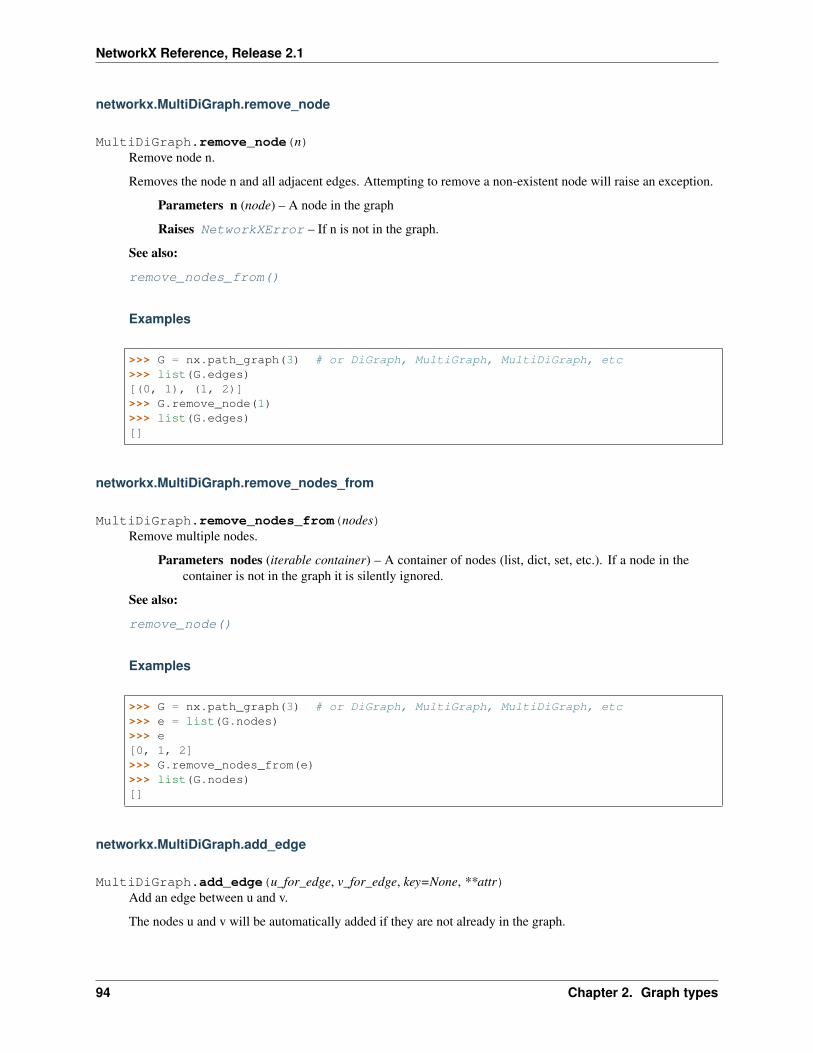
NetworkX Reference, Release 2.1
networkx.MultiDiGraph.remove_node
MultiDiGraph.remove_node(n)Remove node n.
Removes the node n and all adjacent edges. Attempting to remove a non-existent node will raise an exception.
Parameters n (node) – A node in the graph
Raises NetworkXError – If n is not in the graph.
See also:
remove_nodes_from()
Examples
>>> G = nx.path_graph(3) # or DiGraph, MultiGraph, MultiDiGraph, etc>>> list(G.edges)[(0, 1), (1, 2)]>>> G.remove_node(1)>>> list(G.edges)[]
networkx.MultiDiGraph.remove_nodes_from
MultiDiGraph.remove_nodes_from(nodes)Remove multiple nodes.
Parameters nodes (iterable container) – A container of nodes (list, dict, set, etc.). If a node in thecontainer is not in the graph it is silently ignored.
See also:
remove_node()
Examples
>>> G = nx.path_graph(3) # or DiGraph, MultiGraph, MultiDiGraph, etc>>> e = list(G.nodes)>>> e[0, 1, 2]>>> G.remove_nodes_from(e)>>> list(G.nodes)[]
networkx.MultiDiGraph.add_edge
MultiDiGraph.add_edge(u_for_edge, v_for_edge, key=None, **attr)Add an edge between u and v.
The nodes u and v will be automatically added if they are not already in the graph.
94 Chapter 2. Graph types

NetworkX Reference, Release 2.1
Edge attributes can be specified with keywords or by directly accessing the edge’s attribute dictionary. Seeexamples below.
Parameters
• u_for_edge, v_for_edge (nodes) – Nodes can be, for example, strings or numbers. Nodesmust be hashable (and not None) Python objects.
• key (hashable identifier, optional (default=lowest unused integer)) – Used to distinguishmultiedges between a pair of nodes.
• attr_dict (dictionary, optional (default= no attributes)) – Dictionary of edge attributes.Key/value pairs will update existing data associated with the edge.
• attr (keyword arguments, optional) – Edge data (or labels or objects) can be assigned usingkeyword arguments.
Returns
Return type The edge key assigned to the edge.
See also:
add_edges_from() add a collection of edges
Notes
To replace/update edge data, use the optional key argument to identify a unique edge. Otherwise a new edgewill be created.
NetworkX algorithms designed for weighted graphs cannot use multigraphs directly because it is not clearhow to handle multiedge weights. Convert to Graph using edge attribute ‘weight’ to enable weighted graphalgorithms.
Default keys are generated using the method new_edge_key(). This method can be overridden by subclass-ing the base class and providing a custom new_edge_key() method.
Examples
The following all add the edge e=(1, 2) to graph G:
>>> G = nx.MultiDiGraph()>>> e = (1, 2)>>> key = G.add_edge(1, 2) # explicit two-node form>>> G.add_edge(*e) # single edge as tuple of two nodes1>>> G.add_edges_from( [(1, 2)] ) # add edges from iterable container[2]
Associate data to edges using keywords:
>>> key = G.add_edge(1, 2, weight=3)>>> key = G.add_edge(1, 2, key=0, weight=4) # update data for key=0>>> key = G.add_edge(1, 3, weight=7, capacity=15, length=342.7)
For non-string attribute keys, use subscript notation.
2.2. Basic graph types 95

NetworkX Reference, Release 2.1
>>> ekey = G.add_edge(1, 2)>>> G[1][2][0].update({0: 5})>>> G.edges[1, 2, 0].update({0: 5})
networkx.MultiDiGraph.add_edges_from
MultiDiGraph.add_edges_from(ebunch_to_add, **attr)Add all the edges in ebunch_to_add.
Parameters
• ebunch_to_add (container of edges) – Each edge given in the container will be added tothe graph. The edges can be:
– 2-tuples (u, v) or
– 3-tuples (u, v, d) for an edge data dict d, or
– 3-tuples (u, v, k) for not iterable key k, or
– 4-tuples (u, v, k, d) for an edge with data and key k
• attr (keyword arguments, optional) – Edge data (or labels or objects) can be assigned usingkeyword arguments.
Returns
Return type A list of edge keys assigned to the edges in ebunch.
See also:
add_edge() add a single edge
add_weighted_edges_from() convenient way to add weighted edges
Notes
Adding the same edge twice has no effect but any edge data will be updated when each duplicate edge is added.
Edge attributes specified in an ebunch take precedence over attributes specified via keyword arguments.
Default keys are generated using the method new_edge_key(). This method can be overridden by subclass-ing the base class and providing a custom new_edge_key() method.
Examples
>>> G = nx.Graph() # or DiGraph, MultiGraph, MultiDiGraph, etc>>> G.add_edges_from([(0, 1), (1, 2)]) # using a list of edge tuples>>> e = zip(range(0, 3), range(1, 4))>>> G.add_edges_from(e) # Add the path graph 0-1-2-3
Associate data to edges
>>> G.add_edges_from([(1, 2), (2, 3)], weight=3)>>> G.add_edges_from([(3, 4), (1, 4)], label='WN2898')
96 Chapter 2. Graph types

NetworkX Reference, Release 2.1
networkx.MultiDiGraph.add_weighted_edges_from
MultiDiGraph.add_weighted_edges_from(ebunch_to_add, weight=’weight’, **attr)Add weighted edges in ebunch_to_add with specified weight attr
Parameters
• ebunch_to_add (container of edges) – Each edge given in the list or container will be addedto the graph. The edges must be given as 3-tuples (u, v, w) where w is a number.
• weight (string, optional (default= ‘weight’)) – The attribute name for the edge weights tobe added.
• attr (keyword arguments, optional (default= no attributes)) – Edge attributes to add/updatefor all edges.
See also:
add_edge() add a single edge
add_edges_from() add multiple edges
Notes
Adding the same edge twice for Graph/DiGraph simply updates the edge data. For MultiGraph/MultiDiGraph,duplicate edges are stored.
Examples
>>> G = nx.Graph() # or DiGraph, MultiGraph, MultiDiGraph, etc>>> G.add_weighted_edges_from([(0, 1, 3.0), (1, 2, 7.5)])
networkx.MultiDiGraph.new_edge_key
MultiDiGraph.new_edge_key(u, v)Return an unused key for edges between nodes u and v.
The nodes u and v do not need to be already in the graph.
Notes
In the standard MultiGraph class the new key is the number of existing edges between u and v (increasedif necessary to ensure unused). The first edge will have key 0, then 1, etc. If an edge is removed furthernew_edge_keys may not be in this order.
Parameters u, v (nodes)
Returns key
Return type int
2.2. Basic graph types 97
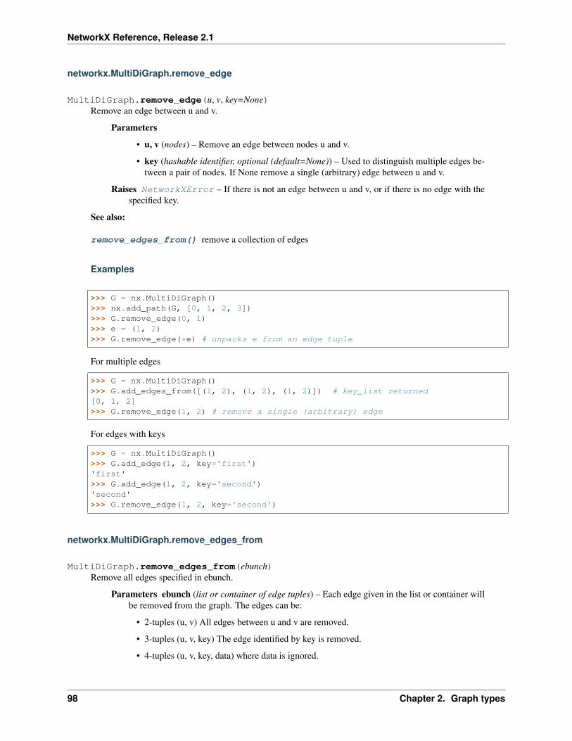
NetworkX Reference, Release 2.1
networkx.MultiDiGraph.remove_edge
MultiDiGraph.remove_edge(u, v, key=None)Remove an edge between u and v.
Parameters
• u, v (nodes) – Remove an edge between nodes u and v.
• key (hashable identifier, optional (default=None)) – Used to distinguish multiple edges be-tween a pair of nodes. If None remove a single (arbitrary) edge between u and v.
Raises NetworkXError – If there is not an edge between u and v, or if there is no edge with thespecified key.
See also:
remove_edges_from() remove a collection of edges
Examples
>>> G = nx.MultiDiGraph()>>> nx.add_path(G, [0, 1, 2, 3])>>> G.remove_edge(0, 1)>>> e = (1, 2)>>> G.remove_edge(*e) # unpacks e from an edge tuple
For multiple edges
>>> G = nx.MultiDiGraph()>>> G.add_edges_from([(1, 2), (1, 2), (1, 2)]) # key_list returned[0, 1, 2]>>> G.remove_edge(1, 2) # remove a single (arbitrary) edge
For edges with keys
>>> G = nx.MultiDiGraph()>>> G.add_edge(1, 2, key='first')'first'>>> G.add_edge(1, 2, key='second')'second'>>> G.remove_edge(1, 2, key='second')
networkx.MultiDiGraph.remove_edges_from
MultiDiGraph.remove_edges_from(ebunch)Remove all edges specified in ebunch.
Parameters ebunch (list or container of edge tuples) – Each edge given in the list or container willbe removed from the graph. The edges can be:
• 2-tuples (u, v) All edges between u and v are removed.
• 3-tuples (u, v, key) The edge identified by key is removed.
• 4-tuples (u, v, key, data) where data is ignored.
98 Chapter 2. Graph types

NetworkX Reference, Release 2.1
See also:
remove_edge() remove a single edge
Notes
Will fail silently if an edge in ebunch is not in the graph.
Examples
>>> G = nx.path_graph(4) # or DiGraph, MultiGraph, MultiDiGraph, etc>>> ebunch=[(1, 2), (2, 3)]>>> G.remove_edges_from(ebunch)
Removing multiple copies of edges
>>> G = nx.MultiGraph()>>> keys = G.add_edges_from([(1, 2), (1, 2), (1, 2)])>>> G.remove_edges_from([(1, 2), (1, 2)])>>> list(G.edges())[(1, 2)]>>> G.remove_edges_from([(1, 2), (1, 2)]) # silently ignore extra copy>>> list(G.edges) # now empty graph[]
networkx.MultiDiGraph.clear
MultiDiGraph.clear()Remove all nodes and edges from the graph.
This also removes the name, and all graph, node, and edge attributes.
Examples
>>> G = nx.path_graph(4) # or DiGraph, MultiGraph, MultiDiGraph, etc>>> G.clear()>>> list(G.nodes)[]>>> list(G.edges)[]
Reporting nodes edges and neighbors
MultiDiGraph.nodes A NodeView of the Graph as G.nodes or G.nodes().MultiDiGraph.__iter__() Iterate over the nodes.MultiDiGraph.has_node(n) Return True if the graph contains the node n.MultiDiGraph.__contains__(n) Return True if n is a node, False otherwise.
Continued on next page
2.2. Basic graph types 99

NetworkX Reference, Release 2.1
Table 2.14 – continued from previous pageMultiDiGraph.edges An OutMultiEdgeView of the Graph as G.edges or
G.edges().MultiDiGraph.out_edges An OutMultiEdgeView of the Graph as G.edges or
G.edges().MultiDiGraph.in_edges An InMultiEdgeView of the Graph as G.in_edges or
G.in_edges().MultiDiGraph.has_edge(u, v[, key]) Return True if the graph has an edge between nodes u and
v.MultiDiGraph.get_edge_data(u, v[, key, default]) Return the attribute dictionary associated with edge (u, v).MultiDiGraph.neighbors(n) Return an iterator over successor nodes of n.MultiDiGraph.adj Graph adjacency object holding the neighbors of each
node.MultiDiGraph.__getitem__(n) Return a dict of neighbors of node n.MultiDiGraph.successors(n) Return an iterator over successor nodes of n.MultiDiGraph.succ Graph adjacency object holding the successors of each
node.MultiDiGraph.predecessors(n) Return an iterator over predecessor nodes of n.MultiDiGraph.succ Graph adjacency object holding the successors of each
node.MultiDiGraph.adjacency() Return an iterator over (node, adjacency dict) tuples for all
nodes.MultiDiGraph.nbunch_iter([nbunch]) Return an iterator over nodes contained in nbunch that are
also in the graph.
networkx.MultiDiGraph.nodes
MultiDiGraph.nodesA NodeView of the Graph as G.nodes or G.nodes().
Can be used as G.nodes for data lookup and for set-like operations. Can also be used as G.nodes(data='color', default=None) to return a NodeDataView which reports specific node databut no set operations. It presents a dict-like interface as well with G.nodes.items() iterating over (node,nodedata) 2-tuples and G.nodes[3]['foo'] providing the value of the foo attribute for node 3. Inaddition, a view G.nodes.data('foo') provides a dict-like interface to the foo attribute of each node.G.nodes.data('foo', default=1) provides a default for nodes that do not have attribute foo.
Parameters
• data (string or bool, optional (default=False)) – The node attribute returned in 2-tuple (n,ddict[data]). If True, return entire node attribute dict as (n, ddict). If False, return just thenodes n.
• default (value, optional (default=None)) – Value used for nodes that dont have the requestedattribute. Only relevant if data is not True or False.
Returns
Allows set-like operations over the nodes as well as node attribute dict lookup and calling toget a NodeDataView. A NodeDataView iterates over (n, data) and has no set operations. ANodeView iterates over n and includes set operations.
When called, if data is False, an iterator over nodes. Otherwise an iterator of 2-tuples (node,attribute value) where the attribute is specified in data. If data is True then the attribute becomesthe entire data dictionary.
Return type NodeView
100 Chapter 2. Graph types

NetworkX Reference, Release 2.1
Notes
If your node data is not needed, it is simpler and equivalent to use the expression for n in G, or list(G).
Examples
There are two simple ways of getting a list of all nodes in the graph:
>>> G = nx.path_graph(3)>>> list(G.nodes)[0, 1, 2]>>> list(G)[0, 1, 2]
To get the node data along with the nodes:
>>> G.add_node(1, time='5pm')>>> G.nodes[0]['foo'] = 'bar'>>> list(G.nodes(data=True))[(0, {'foo': 'bar'}), (1, {'time': '5pm'}), (2, {})]>>> list(G.nodes.data())[(0, {'foo': 'bar'}), (1, {'time': '5pm'}), (2, {})]
>>> list(G.nodes(data='foo'))[(0, 'bar'), (1, None), (2, None)]>>> list(G.nodes.data('foo'))[(0, 'bar'), (1, None), (2, None)]
>>> list(G.nodes(data='time'))[(0, None), (1, '5pm'), (2, None)]>>> list(G.nodes.data('time'))[(0, None), (1, '5pm'), (2, None)]
>>> list(G.nodes(data='time', default='Not Available'))[(0, 'Not Available'), (1, '5pm'), (2, 'Not Available')]>>> list(G.nodes.data('time', default='Not Available'))[(0, 'Not Available'), (1, '5pm'), (2, 'Not Available')]
If some of your nodes have an attribute and the rest are assumed to have a default attribute value you can createa dictionary from node/attribute pairs using the default keyword argument to guarantee the value is neverNone:
>>> G = nx.Graph()>>> G.add_node(0)>>> G.add_node(1, weight=2)>>> G.add_node(2, weight=3)>>> dict(G.nodes(data='weight', default=1)){0: 1, 1: 2, 2: 3}
networkx.MultiDiGraph.__iter__
MultiDiGraph.__iter__()Iterate over the nodes. Use: ‘for n in G’.
2.2. Basic graph types 101

NetworkX Reference, Release 2.1
Returns niter – An iterator over all nodes in the graph.
Return type iterator
Examples
>>> G = nx.path_graph(4) # or DiGraph, MultiGraph, MultiDiGraph, etc>>> [n for n in G][0, 1, 2, 3]>>> list(G)[0, 1, 2, 3]
networkx.MultiDiGraph.has_node
MultiDiGraph.has_node(n)Return True if the graph contains the node n.
Identical to n in G
Parameters n (node)
Examples
>>> G = nx.path_graph(3) # or DiGraph, MultiGraph, MultiDiGraph, etc>>> G.has_node(0)True
It is more readable and simpler to use
>>> 0 in GTrue
networkx.MultiDiGraph.__contains__
MultiDiGraph.__contains__(n)Return True if n is a node, False otherwise. Use: ‘n in G’.
Examples
>>> G = nx.path_graph(4) # or DiGraph, MultiGraph, MultiDiGraph, etc>>> 1 in GTrue
networkx.MultiDiGraph.edges
MultiDiGraph.edgesAn OutMultiEdgeView of the Graph as G.edges or G.edges().
edges(self, nbunch=None, data=False, keys=False, default=None)
102 Chapter 2. Graph types

NetworkX Reference, Release 2.1
The OutMultiEdgeView provides set-like operations on the edge-tuples as well as edge attribute lookup. Whencalled, it also provides an EdgeDataView object which allows control of access to edge attributes (but does notprovide set-like operations). Hence, G.edges[u, v]['color'] provides the value of the color attributefor edge (u, v) while for (u, v, c) in G.edges(data='color', default='red'): iter-ates through all the edges yielding the color attribute with default 'red' if no color attribute exists.
Edges are returned as tuples with optional data and keys in the order (node, neighbor, key, data).
Parameters
• nbunch (single node, container, or all nodes (default= all nodes)) – The view will onlyreport edges incident to these nodes.
• data (string or bool, optional (default=False)) – The edge attribute returned in 3-tuple (u, v,ddict[data]). If True, return edge attribute dict in 3-tuple (u, v, ddict). If False, return 2-tuple(u, v).
• keys (bool, optional (default=False)) – If True, return edge keys with each edge.
• default (value, optional (default=None)) – Value used for edges that dont have the requestedattribute. Only relevant if data is not True or False.
Returns edges – A view of edge attributes, usually it iterates over (u, v) (u, v, k) or (u, v, k, d) tuplesof edges, but can also be used for attribute lookup as edges[u, v, k]['foo'].
Return type EdgeView
Notes
Nodes in nbunch that are not in the graph will be (quietly) ignored. For directed graphs this returns the out-edges.
Examples
>>> G = nx.MultiDiGraph()>>> nx.add_path(G, [0, 1, 2])>>> key = G.add_edge(2, 3, weight=5)>>> [e for e in G.edges()][(0, 1), (1, 2), (2, 3)]>>> list(G.edges(data=True)) # default data is {} (empty dict)[(0, 1, {}), (1, 2, {}), (2, 3, {'weight': 5})]>>> list(G.edges(data='weight', default=1))[(0, 1, 1), (1, 2, 1), (2, 3, 5)]>>> list(G.edges(keys=True)) # default keys are integers[(0, 1, 0), (1, 2, 0), (2, 3, 0)]>>> list(G.edges(data=True, keys=True))[(0, 1, 0, {}), (1, 2, 0, {}), (2, 3, 0, {'weight': 5})]>>> list(G.edges(data='weight', default=1, keys=True))[(0, 1, 0, 1), (1, 2, 0, 1), (2, 3, 0, 5)]>>> list(G.edges([0, 2]))[(0, 1), (2, 3)]>>> list(G.edges(0))[(0, 1)]
See also:
in_edges, out_edges
2.2. Basic graph types 103

NetworkX Reference, Release 2.1
networkx.MultiDiGraph.out_edges
MultiDiGraph.out_edgesAn OutMultiEdgeView of the Graph as G.edges or G.edges().
edges(self, nbunch=None, data=False, keys=False, default=None)
The OutMultiEdgeView provides set-like operations on the edge-tuples as well as edge attribute lookup. Whencalled, it also provides an EdgeDataView object which allows control of access to edge attributes (but does notprovide set-like operations). Hence, G.edges[u, v]['color'] provides the value of the color attributefor edge (u, v) while for (u, v, c) in G.edges(data='color', default='red'): iter-ates through all the edges yielding the color attribute with default 'red' if no color attribute exists.
Edges are returned as tuples with optional data and keys in the order (node, neighbor, key, data).
Parameters
• nbunch (single node, container, or all nodes (default= all nodes)) – The view will onlyreport edges incident to these nodes.
• data (string or bool, optional (default=False)) – The edge attribute returned in 3-tuple (u, v,ddict[data]). If True, return edge attribute dict in 3-tuple (u, v, ddict). If False, return 2-tuple(u, v).
• keys (bool, optional (default=False)) – If True, return edge keys with each edge.
• default (value, optional (default=None)) – Value used for edges that dont have the requestedattribute. Only relevant if data is not True or False.
Returns edges – A view of edge attributes, usually it iterates over (u, v) (u, v, k) or (u, v, k, d) tuplesof edges, but can also be used for attribute lookup as edges[u, v, k]['foo'].
Return type EdgeView
Notes
Nodes in nbunch that are not in the graph will be (quietly) ignored. For directed graphs this returns the out-edges.
Examples
>>> G = nx.MultiDiGraph()>>> nx.add_path(G, [0, 1, 2])>>> key = G.add_edge(2, 3, weight=5)>>> [e for e in G.edges()][(0, 1), (1, 2), (2, 3)]>>> list(G.edges(data=True)) # default data is {} (empty dict)[(0, 1, {}), (1, 2, {}), (2, 3, {'weight': 5})]>>> list(G.edges(data='weight', default=1))[(0, 1, 1), (1, 2, 1), (2, 3, 5)]>>> list(G.edges(keys=True)) # default keys are integers[(0, 1, 0), (1, 2, 0), (2, 3, 0)]>>> list(G.edges(data=True, keys=True))[(0, 1, 0, {}), (1, 2, 0, {}), (2, 3, 0, {'weight': 5})]>>> list(G.edges(data='weight', default=1, keys=True))[(0, 1, 0, 1), (1, 2, 0, 1), (2, 3, 0, 5)]>>> list(G.edges([0, 2]))[(0, 1), (2, 3)]
104 Chapter 2. Graph types

NetworkX Reference, Release 2.1
>>> list(G.edges(0))[(0, 1)]
See also:
in_edges, out_edges
networkx.MultiDiGraph.in_edges
MultiDiGraph.in_edgesAn InMultiEdgeView of the Graph as G.in_edges or G.in_edges().
in_edges(self, nbunch=None, data=False, keys=False, default=None)
Parameters
• nbunch (single node, container, or all nodes (default= all nodes)) – The view will onlyreport edges incident to these nodes.
• data (string or bool, optional (default=False)) – The edge attribute returned in 3-tuple (u, v,ddict[data]). If True, return edge attribute dict in 3-tuple (u, v, ddict). If False, return 2-tuple(u, v).
• keys (bool, optional (default=False)) – If True, return edge keys with each edge.
• default (value, optional (default=None)) – Value used for edges that dont have the requestedattribute. Only relevant if data is not True or False.
Returns in_edges – A view of edge attributes, usually it iterates over (u, v) or (u, v, k) or (u, v, k, d)tuples of edges, but can also be used for attribute lookup as edges[u, v, k]['foo'].
Return type InMultiEdgeView
See also:
edges
networkx.MultiDiGraph.has_edge
MultiDiGraph.has_edge(u, v, key=None)Return True if the graph has an edge between nodes u and v.
This is the same as v in G[u] or key in G[u][v] without KeyError exceptions.
Parameters
• u, v (nodes) – Nodes can be, for example, strings or numbers.
• key (hashable identifier, optional (default=None)) – If specified return True only if the edgewith key is found.
Returns edge_ind – True if edge is in the graph, False otherwise.
Return type bool
Examples
Can be called either using two nodes u, v, an edge tuple (u, v), or an edge tuple (u, v, key).
2.2. Basic graph types 105

NetworkX Reference, Release 2.1
>>> G = nx.MultiGraph() # or MultiDiGraph>>> nx.add_path(G, [0, 1, 2, 3])>>> G.has_edge(0, 1) # using two nodesTrue>>> e = (0, 1)>>> G.has_edge(*e) # e is a 2-tuple (u, v)True>>> G.add_edge(0, 1, key='a')'a'>>> G.has_edge(0, 1, key='a') # specify keyTrue>>> e=(0, 1, 'a')>>> G.has_edge(*e) # e is a 3-tuple (u, v, 'a')True
The following syntax are equivalent:
>>> G.has_edge(0, 1)True>>> 1 in G[0] # though this gives :exc:`KeyError` if 0 not in GTrue
networkx.MultiDiGraph.get_edge_data
MultiDiGraph.get_edge_data(u, v, key=None, default=None)Return the attribute dictionary associated with edge (u, v).
This is identical to G[u][v][key] except the default is returned instead of an exception is the edge doesn’texist.
Parameters
• u, v (nodes)
• default (any Python object (default=None)) – Value to return if the edge (u, v) is not found.
• key (hashable identifier, optional (default=None)) – Return data only for the edge withspecified key.
Returns edge_dict – The edge attribute dictionary.
Return type dictionary
Examples
>>> G = nx.MultiGraph() # or MultiDiGraph>>> key = G.add_edge(0, 1, key='a', weight=7)>>> G[0][1]['a'] # key='a'{'weight': 7}>>> G.edges[0, 1, 'a'] # key='a'{'weight': 7}
Warning: we protect the graph data structure by making G.edges and G[1][2] read-only dict-like structures.However, you can assign values to attributes in e.g. G.edges[1, 2, 'a'] or G[1][2]['a'] using anadditional bracket as shown next. You need to specify all edge info to assign to the edge data associated with anedge.
106 Chapter 2. Graph types

NetworkX Reference, Release 2.1
>>> G[0][1]['a']['weight'] = 10>>> G.edges[0, 1, 'a']['weight'] = 10>>> G[0][1]['a']['weight']10>>> G.edges[1, 0, 'a']['weight']10
>>> G = nx.MultiGraph() # or MultiDiGraph>>> nx.add_path(G, [0, 1, 2, 3])>>> G.get_edge_data(0, 1){0: {}}>>> e = (0, 1)>>> G.get_edge_data(*e) # tuple form{0: {}}>>> G.get_edge_data('a', 'b', default=0) # edge not in graph, return 00
networkx.MultiDiGraph.neighbors
MultiDiGraph.neighbors(n)Return an iterator over successor nodes of n.
neighbors() and successors() are the same.
networkx.MultiDiGraph.adj
MultiDiGraph.adjGraph adjacency object holding the neighbors of each node.
This object is a read-only dict-like structure with node keys and neighbor-dict values. The neighbor-dict is keyedby neighbor to the edgekey-dict. So G.adj[3][2][0]['color'] = 'blue' sets the color of the edge(3, 2, 0) to "blue".
Iterating over G.adj behaves like a dict. Useful idioms include for nbr, datadict in G.adj[n].items():.
The neighbor information is also provided by subscripting the graph. So for nbr, foovalue inG[node].data('foo', default=1): works.
For directed graphs, G.adj holds outgoing (successor) info.
networkx.MultiDiGraph.__getitem__
MultiDiGraph.__getitem__(n)Return a dict of neighbors of node n. Use: ‘G[n]’.
Parameters n (node) – A node in the graph.
Returns adj_dict – The adjacency dictionary for nodes connected to n.
Return type dictionary
2.2. Basic graph types 107

NetworkX Reference, Release 2.1
Notes
G[n] is the same as G.adj[n] and similar to G.neighbors(n) (which is an iterator over G.adj[n])
Examples
>>> G = nx.path_graph(4) # or DiGraph, MultiGraph, MultiDiGraph, etc>>> G[0]AtlasView({1: {}})
networkx.MultiDiGraph.successors
MultiDiGraph.successors(n)Return an iterator over successor nodes of n.
neighbors() and successors() are the same.
networkx.MultiDiGraph.succ
MultiDiGraph.succGraph adjacency object holding the successors of each node.
This object is a read-only dict-like structure with node keys and neighbor-dict values. The neighbor-dict is keyedby neighbor to the edgekey-dict. So G.adj[3][2][0]['color'] = 'blue' sets the color of the edge(3, 2, 0) to "blue".
Iterating over G.adj behaves like a dict. Useful idioms include for nbr, datadict in G.adj[n].items():.
The neighbor information is also provided by subscripting the graph. So for nbr, foovalue inG[node].data('foo', default=1): works.
For directed graphs, G.succ is identical to G.adj.
networkx.MultiDiGraph.predecessors
MultiDiGraph.predecessors(n)Return an iterator over predecessor nodes of n.
networkx.MultiDiGraph.adjacency
MultiDiGraph.adjacency()Return an iterator over (node, adjacency dict) tuples for all nodes.
For directed graphs, only outgoing neighbors/adjacencies are included.
Returns adj_iter – An iterator over (node, adjacency dictionary) for all nodes in the graph.
Return type iterator
108 Chapter 2. Graph types
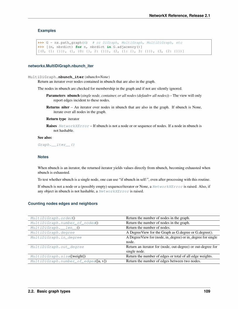
NetworkX Reference, Release 2.1
Examples
>>> G = nx.path_graph(4) # or DiGraph, MultiGraph, MultiDiGraph, etc>>> [(n, nbrdict) for n, nbrdict in G.adjacency()][(0, {1: {}}), (1, {0: {}, 2: {}}), (2, {1: {}, 3: {}}), (3, {2: {}})]
networkx.MultiDiGraph.nbunch_iter
MultiDiGraph.nbunch_iter(nbunch=None)Return an iterator over nodes contained in nbunch that are also in the graph.
The nodes in nbunch are checked for membership in the graph and if not are silently ignored.
Parameters nbunch (single node, container, or all nodes (default= all nodes)) – The view will onlyreport edges incident to these nodes.
Returns niter – An iterator over nodes in nbunch that are also in the graph. If nbunch is None,iterate over all nodes in the graph.
Return type iterator
Raises NetworkXError – If nbunch is not a node or or sequence of nodes. If a node in nbunch isnot hashable.
See also:
Graph.__iter__()
Notes
When nbunch is an iterator, the returned iterator yields values directly from nbunch, becoming exhausted whennbunch is exhausted.
To test whether nbunch is a single node, one can use “if nbunch in self:”, even after processing with this routine.
If nbunch is not a node or a (possibly empty) sequence/iterator or None, a NetworkXError is raised. Also, ifany object in nbunch is not hashable, a NetworkXError is raised.
Counting nodes edges and neighbors
MultiDiGraph.order() Return the number of nodes in the graph.MultiDiGraph.number_of_nodes() Return the number of nodes in the graph.MultiDiGraph.__len__() Return the number of nodes.MultiDiGraph.degree A DegreeView for the Graph as G.degree or G.degree().MultiDiGraph.in_degree A DegreeView for (node, in_degree) or in_degree for single
node.MultiDiGraph.out_degree Return an iterator for (node, out-degree) or out-degree for
single node.MultiDiGraph.size([weight]) Return the number of edges or total of all edge weights.MultiDiGraph.number_of_edges([u, v]) Return the number of edges between two nodes.
2.2. Basic graph types 109

NetworkX Reference, Release 2.1
networkx.MultiDiGraph.order
MultiDiGraph.order()Return the number of nodes in the graph.
Returns nnodes – The number of nodes in the graph.
Return type int
See also:
number_of_nodes(), __len__()
networkx.MultiDiGraph.number_of_nodes
MultiDiGraph.number_of_nodes()Return the number of nodes in the graph.
Returns nnodes – The number of nodes in the graph.
Return type int
See also:
order(), __len__()
Examples
>>> G = nx.path_graph(3) # or DiGraph, MultiGraph, MultiDiGraph, etc>>> len(G)3
networkx.MultiDiGraph.__len__
MultiDiGraph.__len__()Return the number of nodes. Use: ‘len(G)’.
Returns nnodes – The number of nodes in the graph.
Return type int
Examples
>>> G = nx.path_graph(4) # or DiGraph, MultiGraph, MultiDiGraph, etc>>> len(G)4
networkx.MultiDiGraph.degree
MultiDiGraph.degreeA DegreeView for the Graph as G.degree or G.degree().
110 Chapter 2. Graph types
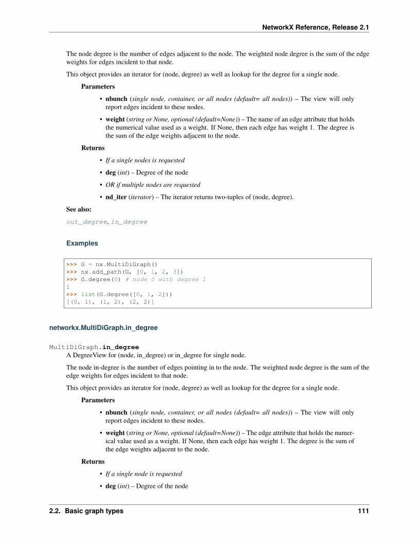
NetworkX Reference, Release 2.1
The node degree is the number of edges adjacent to the node. The weighted node degree is the sum of the edgeweights for edges incident to that node.
This object provides an iterator for (node, degree) as well as lookup for the degree for a single node.
Parameters
• nbunch (single node, container, or all nodes (default= all nodes)) – The view will onlyreport edges incident to these nodes.
• weight (string or None, optional (default=None)) – The name of an edge attribute that holdsthe numerical value used as a weight. If None, then each edge has weight 1. The degree isthe sum of the edge weights adjacent to the node.
Returns
• If a single nodes is requested
• deg (int) – Degree of the node
• OR if multiple nodes are requested
• nd_iter (iterator) – The iterator returns two-tuples of (node, degree).
See also:
out_degree, in_degree
Examples
>>> G = nx.MultiDiGraph()>>> nx.add_path(G, [0, 1, 2, 3])>>> G.degree(0) # node 0 with degree 11>>> list(G.degree([0, 1, 2]))[(0, 1), (1, 2), (2, 2)]
networkx.MultiDiGraph.in_degree
MultiDiGraph.in_degreeA DegreeView for (node, in_degree) or in_degree for single node.
The node in-degree is the number of edges pointing in to the node. The weighted node degree is the sum of theedge weights for edges incident to that node.
This object provides an iterator for (node, degree) as well as lookup for the degree for a single node.
Parameters
• nbunch (single node, container, or all nodes (default= all nodes)) – The view will onlyreport edges incident to these nodes.
• weight (string or None, optional (default=None)) – The edge attribute that holds the numer-ical value used as a weight. If None, then each edge has weight 1. The degree is the sum ofthe edge weights adjacent to the node.
Returns
• If a single node is requested
• deg (int) – Degree of the node
2.2. Basic graph types 111
NetworkX Reference, Release 2.1
• OR if multiple nodes are requested
• nd_iter (iterator) – The iterator returns two-tuples of (node, in-degree).
See also:
degree, out_degree
Examples
>>> G = nx.MultiDiGraph()>>> nx.add_path(G, [0, 1, 2, 3])>>> G.in_degree(0) # node 0 with degree 00>>> list(G.in_degree([0, 1, 2]))[(0, 0), (1, 1), (2, 1)]
networkx.MultiDiGraph.out_degree
MultiDiGraph.out_degreeReturn an iterator for (node, out-degree) or out-degree for single node.
out_degree(self, nbunch=None, weight=None)
The node out-degree is the number of edges pointing out of the node. This function returns the out-degree for asingle node or an iterator for a bunch of nodes or if nothing is passed as argument.
Parameters
• nbunch (single node, container, or all nodes (default= all nodes)) – The view will onlyreport edges incident to these nodes.
• weight (string or None, optional (default=None)) – The edge attribute that holds the numer-ical value used as a weight. If None, then each edge has weight 1. The degree is the sum ofthe edge weights.
Returns
• If a single node is requested
• deg (int) – Degree of the node
• OR if multiple nodes are requested
• nd_iter (iterator) – The iterator returns two-tuples of (node, out-degree).
See also:
degree, in_degree
Examples
>>> G = nx.MultiDiGraph()>>> nx.add_path(G, [0, 1, 2, 3])>>> G.out_degree(0) # node 0 with degree 11>>> list(G.out_degree([0, 1, 2]))[(0, 1), (1, 1), (2, 1)]
112 Chapter 2. Graph types

NetworkX Reference, Release 2.1
networkx.MultiDiGraph.size
MultiDiGraph.size(weight=None)Return the number of edges or total of all edge weights.
Parameters weight (string or None, optional (default=None)) – The edge attribute that holds thenumerical value used as a weight. If None, then each edge has weight 1.
Returns
size – The number of edges or (if weight keyword is provided) the total weight sum.
If weight is None, returns an int. Otherwise a float (or more general numeric if the weights aremore general).
Return type numeric
See also:
number_of_edges()
Examples
>>> G = nx.path_graph(4) # or DiGraph, MultiGraph, MultiDiGraph, etc>>> G.size()3
>>> G = nx.Graph() # or DiGraph, MultiGraph, MultiDiGraph, etc>>> G.add_edge('a', 'b', weight=2)>>> G.add_edge('b', 'c', weight=4)>>> G.size()2>>> G.size(weight='weight')6.0
networkx.MultiDiGraph.number_of_edges
MultiDiGraph.number_of_edges(u=None, v=None)Return the number of edges between two nodes.
Parameters u, v (nodes, optional (Gefault=all edges)) – If u and v are specified, return the numberof edges between u and v. Otherwise return the total number of all edges.
Returns nedges – The number of edges in the graph. If nodes u and v are specified return thenumber of edges between those nodes. If the graph is directed, this only returns the number ofedges from u to v.
Return type int
See also:
size()
Examples
For undirected multigraphs, this method counts the total number of edges in the graph:
2.2. Basic graph types 113

NetworkX Reference, Release 2.1
>>> G = nx.MultiGraph()>>> G.add_edges_from([(0, 1), (0, 1), (1, 2)])[0, 1, 0]>>> G.number_of_edges()3
If you specify two nodes, this counts the total number of edges joining the two nodes:
>>> G.number_of_edges(0, 1)2
For directed multigraphs, this method can count the total number of directed edges from u to v:
>>> G = nx.MultiDiGraph()>>> G.add_edges_from([(0, 1), (0, 1), (1, 0)])[0, 1, 0]>>> G.number_of_edges(0, 1)2>>> G.number_of_edges(1, 0)1
Making copies and subgraphs
MultiDiGraph.copy([as_view]) Return a copy of the graph.MultiDiGraph.to_undirected([reciprocal,as_view])
Return an undirected representation of the digraph.
MultiDiGraph.to_directed([as_view]) Return a directed representation of the graph.MultiDiGraph.subgraph(nodes) Return a SubGraph view of the subgraph induced on nodes
in nodes.MultiDiGraph.edge_subgraph(edges) Returns the subgraph induced by the specified edges.MultiDiGraph.reverse([copy]) Return the reverse of the graph.MultiDiGraph.fresh_copy() Return a fresh copy graph with the same data structure.
networkx.MultiDiGraph.copy
MultiDiGraph.copy(as_view=False)Return a copy of the graph.
The copy method by default returns a shallow copy of the graph and attributes. That is, if an attribute isa container, that container is shared by the original an the copy. Use Python’s copy.deepcopy for newcontainers.
If as_view is True then a view is returned instead of a copy.
Notes
All copies reproduce the graph structure, but data attributes may be handled in different ways. There are fourtypes of copies of a graph that people might want.
Deepcopy – The default behavior is a “deepcopy” where the graph structure as well as all data attributes and anyobjects they might contain are copied. The entire graph object is new so that changes in the copy do not affectthe original object. (see Python’s copy.deepcopy)
114 Chapter 2. Graph types

NetworkX Reference, Release 2.1
Data Reference (Shallow) – For a shallow copy the graph structure is copied but the edge, node and graph at-tribute dicts are references to those in the original graph. This saves time and memory but could cause confusionif you change an attribute in one graph and it changes the attribute in the other. NetworkX does not provide thislevel of shallow copy.
Independent Shallow – This copy creates new independent attribute dicts and then does a shallow copy of theattributes. That is, any attributes that are containers are shared between the new graph and the original. This isexactly what dict.copy() provides. You can obtain this style copy using:
>>> G = nx.path_graph(5)>>> H = G.copy()>>> H = G.copy(as_view=False)>>> H = nx.Graph(G)>>> H = G.fresh_copy().__class__(G)
Fresh Data – For fresh data, the graph structure is copied while new empty data attribute dicts are created. Theresulting graph is independent of the original and it has no edge, node or graph attributes. Fresh copies are notenabled. Instead use:
>>> H = G.fresh_copy()>>> H.add_nodes_from(G)>>> H.add_edges_from(G.edges)
View – Inspired by dict-views, graph-views act like read-only versions of the original graph, providing a copyof the original structure without requiring any memory for copying the information.
See the Python copy module for more information on shallow and deep copies, https://docs.python.org/2/library/copy.html.
Parameters as_view (bool, optional (default=False)) – If True, the returned graph-view provides aread-only view of the original graph without actually copying any data.
Returns G – A copy of the graph.
Return type Graph
See also:
to_directed() return a directed copy of the graph.
Examples
>>> G = nx.path_graph(4) # or DiGraph, MultiGraph, MultiDiGraph, etc>>> H = G.copy()
networkx.MultiDiGraph.to_undirected
MultiDiGraph.to_undirected(reciprocal=False, as_view=False)Return an undirected representation of the digraph.
Parameters
• reciprocal (bool (optional)) – If True only keep edges that appear in both directions in theoriginal digraph.
• as_view (bool (optional, default=False)) – If True return an undirected view of the originaldirected graph.
2.2. Basic graph types 115

NetworkX Reference, Release 2.1
Returns G – An undirected graph with the same name and nodes and with edge (u, v, data) if either(u, v, data) or (v, u, data) is in the digraph. If both edges exist in digraph and their edge data isdifferent, only one edge is created with an arbitrary choice of which edge data to use. You mustcheck and correct for this manually if desired.
Return type MultiGraph
See also:
MultiGraph(), copy(), add_edge(), add_edges_from()
Notes
This returns a “deepcopy” of the edge, node, and graph attributes which attempts to completely copy all of thedata and references.
This is in contrast to the similar D=MultiiGraph(G) which returns a shallow copy of the data.
See the Python copy module for more information on shallow and deep copies, https://docs.python.org/2/library/copy.html.
Warning: If you have subclassed MultiDiGraph to use dict-like objects in the data structure, those changes donot transfer to the MultiGraph created by this method.
Examples
>>> G = nx.path_graph(2) # or MultiGraph, etc>>> H = G.to_directed()>>> list(H.edges)[(0, 1), (1, 0)]>>> G2 = H.to_undirected()>>> list(G2.edges)[(0, 1)]
networkx.MultiDiGraph.to_directed
MultiDiGraph.to_directed(as_view=False)Return a directed representation of the graph.
Returns G – A directed graph with the same name, same nodes, and with each edge (u, v, data)replaced by two directed edges (u, v, data) and (v, u, data).
Return type MultiDiGraph
Notes
This returns a “deepcopy” of the edge, node, and graph attributes which attempts to completely copy all of thedata and references.
This is in contrast to the similar D=DiGraph(G) which returns a shallow copy of the data.
See the Python copy module for more information on shallow and deep copies, https://docs.python.org/2/library/copy.html.
Warning: If you have subclassed MultiGraph to use dict-like objects in the data structure, those changes do nottransfer to the MultiDiGraph created by this method.
116 Chapter 2. Graph types

NetworkX Reference, Release 2.1
Examples
>>> G = nx.Graph() # or MultiGraph, etc>>> G.add_edge(0, 1)>>> H = G.to_directed()>>> list(H.edges)[(0, 1), (1, 0)]
If already directed, return a (deep) copy
>>> G = nx.DiGraph() # or MultiDiGraph, etc>>> G.add_edge(0, 1)>>> H = G.to_directed()>>> list(H.edges)[(0, 1)]
networkx.MultiDiGraph.subgraph
MultiDiGraph.subgraph(nodes)Return a SubGraph view of the subgraph induced on nodes in nodes.
The induced subgraph of the graph contains the nodes in nodes and the edges between those nodes.
Parameters nodes (list, iterable) – A container of nodes which will be iterated through once.
Returns G – A subgraph view of the graph. The graph structure cannot be changed but node/edgeattributes can and are shared with the original graph.
Return type SubGraph View
Notes
The graph, edge and node attributes are shared with the original graph. Changes to the graph structure is ruledout by the view, but changes to attributes are reflected in the original graph.
To create a subgraph with its own copy of the edge/node attributes use: G.subgraph(nodes).copy()
For an inplace reduction of a graph to a subgraph you can remove nodes: G.remove_nodes_from([n for n in Gif n not in set(nodes)])
Examples
>>> G = nx.path_graph(4) # or DiGraph, MultiGraph, MultiDiGraph, etc>>> H = G.subgraph([0, 1, 2])>>> list(H.edges)[(0, 1), (1, 2)]
networkx.MultiDiGraph.edge_subgraph
MultiDiGraph.edge_subgraph(edges)Returns the subgraph induced by the specified edges.
The induced subgraph contains each edge in edges and each node incident to any one of those edges.
2.2. Basic graph types 117

NetworkX Reference, Release 2.1
Parameters edges (iterable) – An iterable of edges in this graph.
Returns G – An edge-induced subgraph of this graph with the same edge attributes.
Return type Graph
Notes
The graph, edge, and node attributes in the returned subgraph view are references to the corresponding attributesin the original graph. The view is read-only.
To create a full graph version of the subgraph with its own copy of the edge or node attributes, use:
>>> G.edge_subgraph(edges).copy()
Examples
>>> G = nx.path_graph(5)>>> H = G.edge_subgraph([(0, 1), (3, 4)])>>> list(H.nodes)[0, 1, 3, 4]>>> list(H.edges)[(0, 1), (3, 4)]
networkx.MultiDiGraph.reverse
MultiDiGraph.reverse(copy=True)Return the reverse of the graph.
The reverse is a graph with the same nodes and edges but with the directions of the edges reversed.
Parameters copy (bool optional (default=True)) – If True, return a new DiGraph holding the re-versed edges. If False, the reverse graph is created using a view of the original graph.
networkx.MultiDiGraph.fresh_copy
MultiDiGraph.fresh_copy()Return a fresh copy graph with the same data structure.
A fresh copy has no nodes, edges or graph attributes. It is the same data structure as the current graph. Thismethod is typically used to create an empty version of the graph.
Notes
If you subclass the base class you should overwrite this method to return your class of graph.
2.2.5 Ordered Graphs—Consistently ordered graphs
Consistently ordered variants of the default base classes.
118 Chapter 2. Graph types

NetworkX Reference, Release 2.1
The Ordered (Di/Multi/MultiDi) Graphs give a consistent order for reporting of nodes and edges. The order of nodereporting agrees with node adding, but for edges, the order is not necessarily the order that the edges were added.
In general, you should use the default (i.e., unordered) graph classes. However, there are times (e.g., when testing)when you may need the order preserved.
class OrderedGraph(incoming_graph_data=None, **attr)Consistently ordered variant of Graph.
class OrderedDiGraph(incoming_graph_data=None, **attr)Consistently ordered variant of DiGraph.
class OrderedMultiGraph(incoming_graph_data=None, **attr)Consistently ordered variant of MultiGraph.
class OrderedMultiDiGraph(incoming_graph_data=None, **attr)Consistently ordered variant of MultiDiGraph.
Note: NetworkX uses dicts to store the nodes and neighbors in a graph. So the reporting of nodes and edges forthe base graph classes will not necessarily be consistent across versions and platforms. If you need the order of nodesand edges to be consistent (e.g., when writing automated tests), please see OrderedGraph, OrderedDiGraph,OrderedMultiGraph, or OrderedMultiDiGraph, which behave like the base graph classes but give a consis-tent order for reporting of nodes and edges.
2.2. Basic graph types 119

NetworkX Reference, Release 2.1
120 Chapter 2. Graph types

CHAPTER
THREE
ALGORITHMS
3.1 Approximations and Heuristics
Approximations of graph properties and Heuristic functions for optimization problems.
Warning: The approximation submodule is not imported in the top-level networkx.
These functions can be imported with from networkx.algorithms importapproximation.
3.1.1 Connectivity
Fast approximation for node connectivity
all_pairs_node_connectivity(G[, nbunch, cut-off])
Compute node connectivity between all pairs of nodes.
local_node_connectivity(G, source, target[, . . . ]) Compute node connectivity between source and target.node_connectivity(G[, s, t]) Returns an approximation for node connectivity for a graph
or digraph G.
networkx.algorithms.approximation.connectivity.all_pairs_node_connectivity
all_pairs_node_connectivity(G, nbunch=None, cutoff=None)Compute node connectivity between all pairs of nodes.
Pairwise or local node connectivity between two distinct and nonadjacent nodes is the minimum number ofnodes that must be removed (minimum separating cutset) to disconnect them. By Menger’s theorem, this isequal to the number of node independent paths (paths that share no nodes other than source and target). Whichis what we compute in this function.
This algorithm is a fast approximation that gives an strict lower bound on the actual number of node independentpaths between two nodes1. It works for both directed and undirected graphs.
Parameters
• G (NetworkX graph)
1 White, Douglas R., and Mark Newman. 2001 A Fast Algorithm for Node-Independent Paths. Santa Fe Institute Working Paper #01-07-035http://eclectic.ss.uci.edu/~drwhite/working.pdf
121

NetworkX Reference, Release 2.1
• nbunch (container) – Container of nodes. If provided node connectivity will be computedonly over pairs of nodes in nbunch.
• cutoff (integer) – Maximum node connectivity to consider. If None, the minimum degreeof source or target is used as a cutoff in each pair of nodes. Default value None.
Returns K – Dictionary, keyed by source and target, of pairwise node connectivity
Return type dictionary
See also:
local_node_connectivity(), all_pairs_node_connectivity()
References
networkx.algorithms.approximation.connectivity.local_node_connectivity
local_node_connectivity(G, source, target, cutoff=None)Compute node connectivity between source and target.
Pairwise or local node connectivity between two distinct and nonadjacent nodes is the minimum number ofnodes that must be removed (minimum separating cutset) to disconnect them. By Menger’s theorem, this isequal to the number of node independent paths (paths that share no nodes other than source and target). Whichis what we compute in this function.
This algorithm is a fast approximation that gives an strict lower bound on the actual number of node independentpaths between two nodes1. It works for both directed and undirected graphs.
Parameters
• G (NetworkX graph)
• source (node) – Starting node for node connectivity
• target (node) – Ending node for node connectivity
• cutoff (integer) – Maximum node connectivity to consider. If None, the minimum degreeof source or target is used as a cutoff. Default value None.
Returns k – pairwise node connectivity
Return type integer
Examples
>>> # Platonic octahedral graph has node connectivity 4>>> # for each non adjacent node pair>>> from networkx.algorithms import approximation as approx>>> G = nx.octahedral_graph()>>> approx.local_node_connectivity(G, 0, 5)4
1 White, Douglas R., and Mark Newman. 2001 A Fast Algorithm for Node-Independent Paths. Santa Fe Institute Working Paper #01-07-035http://eclectic.ss.uci.edu/~drwhite/working.pdf
122 Chapter 3. Algorithms

NetworkX Reference, Release 2.1
Notes
This algorithm1 finds node independents paths between two nodes by computing their shortest path using BFS,marking the nodes of the path found as ‘used’ and then searching other shortest paths excluding the nodesmarked as used until no more paths exist. It is not exact because a shortest path could use nodes that, if the pathwere longer, may belong to two different node independent paths. Thus it only guarantees an strict lower boundon node connectivity.
Note that the authors propose a further refinement, losing accuracy and gaining speed, which is not implementedyet.
See also:
all_pairs_node_connectivity(), node_connectivity()
References
networkx.algorithms.approximation.connectivity.node_connectivity
node_connectivity(G, s=None, t=None)Returns an approximation for node connectivity for a graph or digraph G.
Node connectivity is equal to the minimum number of nodes that must be removed to disconnect G or render ittrivial. By Menger’s theorem, this is equal to the number of node independent paths (paths that share no nodesother than source and target).
If source and target nodes are provided, this function returns the local node connectivity: the minimum numberof nodes that must be removed to break all paths from source to target in G.
This algorithm is based on a fast approximation that gives an strict lower bound on the actual number of nodeindependent paths between two nodes1. It works for both directed and undirected graphs.
Parameters
• G (NetworkX graph) – Undirected graph
• s (node) – Source node. Optional. Default value: None.
• t (node) – Target node. Optional. Default value: None.
Returns K – Node connectivity of G, or local node connectivity if source and target are provided.
Return type integer
Examples
>>> # Platonic octahedral graph is 4-node-connected>>> from networkx.algorithms import approximation as approx>>> G = nx.octahedral_graph()>>> approx.node_connectivity(G)4
1 White, Douglas R., and Mark Newman. 2001 A Fast Algorithm for Node-Independent Paths. Santa Fe Institute Working Paper #01-07-035http://eclectic.ss.uci.edu/~drwhite/working.pdf
3.1. Approximations and Heuristics 123

NetworkX Reference, Release 2.1
Notes
This algorithm1 finds node independents paths between two nodes by computing their shortest path using BFS,marking the nodes of the path found as ‘used’ and then searching other shortest paths excluding the nodesmarked as used until no more paths exist. It is not exact because a shortest path could use nodes that, if the pathwere longer, may belong to two different node independent paths. Thus it only guarantees an strict lower boundon node connectivity.
See also:
all_pairs_node_connectivity(), local_node_connectivity()
References
3.1.2 K-components
Fast approximation for k-component structure
k_components(G[, min_density]) Returns the approximate k-component structure of a graphG.
networkx.algorithms.approximation.kcomponents.k_components
k_components(G, min_density=0.95)Returns the approximate k-component structure of a graph G.
A k-component is a maximal subgraph of a graph G that has, at least, node connectivity k: we need to remove atleast k nodes to break it into more components. k-components have an inherent hierarchical structure becausethey are nested in terms of connectivity: a connected graph can contain several 2-components, each of whichcan contain one or more 3-components, and so forth.
This implementation is based on the fast heuristics to approximate the k-component sturcture of a graph1.Which, in turn, it is based on a fast approximation algorithm for finding good lower bounds of the number ofnode independent paths between two nodes2.
Parameters
• G (NetworkX graph) – Undirected graph
• min_density (Float) – Density relaxation treshold. Default value 0.95
Returns k_components – Dictionary with connectivity level k as key and a list of sets of nodes thatform a k-component of level k as values.
Return type dict
Examples
>>> # Petersen graph has 10 nodes and it is triconnected, thus all>>> # nodes are in a single component on all three connectivity levels>>> from networkx.algorithms import approximation as apxa
1 Torrents, J. and F. Ferraro (2015) Structural Cohesion: Visualization and Heuristics for Fast Computation. https://arxiv.org/pdf/1503.04476v12 White, Douglas R., and Mark Newman (2001) A Fast Algorithm for Node-Independent Paths. Santa Fe Institute Working Paper #01-07-035
http://eclectic.ss.uci.edu/~drwhite/working.pdf
124 Chapter 3. Algorithms
NetworkX Reference, Release 2.1
>>> G = nx.petersen_graph()>>> k_components = apxa.k_components(G)
Notes
The logic of the approximation algorithm for computing the k-component structure1 is based on repeatedlyapplying simple and fast algorithms for k-cores and biconnected components in order to narrow down thenumber of pairs of nodes over which we have to compute White and Newman’s approximation algorithm forfinding node independent paths2. More formally, this algorithm is based on Whitney’s theorem, which statesan inclusion relation among node connectivity, edge connectivity, and minimum degree for any graph G. Thistheorem implies that every k-component is nested inside a k-edge-component, which in turn, is contained in ak-core. Thus, this algorithm computes node independent paths among pairs of nodes in each biconnected partof each k-core, and repeats this procedure for each k from 3 to the maximal core number of a node in the inputgraph.
Because, in practice, many nodes of the core of level k inside a bicomponent actually are part of a componentof level k, the auxiliary graph needed for the algorithm is likely to be very dense. Thus, we use a complementgraph data structure (see AntiGraph) to save memory. AntiGraph only stores information of the edges thatare not present in the actual auxiliary graph. When applying algorithms to this complement graph data structure,it behaves as if it were the dense version.
See also:
k_components()
References
3.1.3 Clique
Functions for computing large cliques.
max_clique(G) Find the Maximum Cliqueclique_removal(G) Repeatedly remove cliques from the graph.large_clique_size(G) Find the size of a large clique in a graph.
networkx.algorithms.approximation.clique.max_clique
max_clique(G)Find the Maximum Clique
Finds the 𝑂(|𝑉 |/(𝑙𝑜𝑔|𝑉 |)2) apx of maximum clique/independent set in the worst case.
Parameters G (NetworkX graph) – Undirected graph
Returns clique – The apx-maximum clique of the graph
Return type set
Notes
A clique in an undirected graph G = (V, E) is a subset of the vertex set C subseteq V such that for every twovertices in C there exists an edge connecting the two. This is equivalent to saying that the subgraph induced by
3.1. Approximations and Heuristics 125

NetworkX Reference, Release 2.1
C is complete (in some cases, the term clique may also refer to the subgraph).
A maximum clique is a clique of the largest possible size in a given graph. The clique number omega(G) ofa graph G is the number of vertices in a maximum clique in G. The intersection number of G is the smallestnumber of cliques that together cover all edges of G.
https://en.wikipedia.org/wiki/Maximum_clique
References
networkx.algorithms.approximation.clique.clique_removal
clique_removal(G)Repeatedly remove cliques from the graph.
Results in a 𝑂(|𝑉 |/(log |𝑉 |)2) approximation of maximum clique and independent set. Returns the largestindependent set found, along with found maximal cliques.
Parameters G (NetworkX graph) – Undirected graph
Returns max_ind_cliques – 2-tuple of Maximal Independent Set and list of maximal cliques (sets).
Return type (set, list) tuple
References
networkx.algorithms.approximation.clique.large_clique_size
large_clique_size(G)Find the size of a large clique in a graph.
A clique is a subset of nodes in which each pair of nodes is adjacent. This function is a heuristic for finding thesize of a large clique in the graph.
Parameters G (NetworkX graph)
Returns The size of a large clique in the graph.
Return type int
Notes
This implementation is from1. Its worst case time complexity is 𝑂(𝑛𝑑2), where n is the number of nodes in thegraph and d is the maximum degree.
This function is a heuristic, which means it may work well in practice, but there is no rigorous mathematicalguarantee on the ratio between the returned number and the actual largest clique size in the graph.
References
See also:1 Pattabiraman, Bharath, et al. “Fast Algorithms for the Maximum Clique Problem on Massive Graphs with Applications to Overlapping
Community Detection.” Internet Mathematics 11.4-5 (2015): 421–448. <https://dx.doi.org/10.1080/15427951.2014.986778>
126 Chapter 3. Algorithms

NetworkX Reference, Release 2.1
networkx.algorithms.approximation.clique.max_clique() A function that returns an ap-proximate maximum clique with a guarantee on the approximation ratio.
networkx.algorithms.clique Functions for finding the exact maximum clique in a graph.
3.1.4 Clustering
average_clustering(G[, trials]) Estimates the average clustering coefficient of G.
networkx.algorithms.approximation.clustering_coefficient.average_clustering
average_clustering(G, trials=1000)Estimates the average clustering coefficient of G.
The local clustering of each node in G is the fraction of triangles that actually exist over all possible triangles inits neighborhood. The average clustering coefficient of a graph G is the mean of local clusterings.
This function finds an approximate average clustering coefficient for G by repeating n times (defined intrials) the following experiment: choose a node at random, choose two of its neighbors at random, andcheck if they are connected. The approximate coefficient is the fraction of triangles found over the number oftrials1.
Parameters
• G (NetworkX graph)
• trials (integer) – Number of trials to perform (default 1000).
Returns c – Approximated average clustering coefficient.
Return type float
References
3.1.5 Dominating Set
Functions for finding node and edge dominating sets.
A dominating set for an undirected graph G with vertex set V and edge set E is a subset D of V such that every vertexnot in D is adjacent to at least one member of D. An edge dominating set is a subset F of E such that every edge notin F is incident to an endpoint of at least one edge in F.
min_weighted_dominating_set(G[, weight]) Returns a dominating set that approximates the minimumweight node dominating set.
min_edge_dominating_set(G) Return minimum cardinality edge dominating set.
networkx.algorithms.approximation.dominating_set.min_weighted_dominating_set
min_weighted_dominating_set(G, weight=None)Returns a dominating set that approximates the minimum weight node dominating set.
Parameters1 Schank, Thomas, and Dorothea Wagner. Approximating clustering coefficient and transitivity. Universität Karlsruhe, Fakultät für Informatik,
2004. http://www.emis.ams.org/journals/JGAA/accepted/2005/SchankWagner2005.9.2.pdf
3.1. Approximations and Heuristics 127

NetworkX Reference, Release 2.1
• G (NetworkX graph) – Undirected graph.
• weight (string) – The node attribute storing the weight of an edge. If provided, the nodeattribute with this key must be a number for each node. If not provided, each node is assumedto have weight one.
Returns min_weight_dominating_set – A set of nodes, the sum of whose weights is no more than(log w(V)) w(V^*), where w(V) denotes the sum of the weights of each node in the graphand w(V^*) denotes the sum of the weights of each node in the minimum weight dominatingset.
Return type set
Notes
This algorithm computes an approximate minimum weighted dominating set for the graph G. The returnedsolution has weight (log w(V)) w(V^*), where w(V) denotes the sum of the weights of each node in thegraph and w(V^*) denotes the sum of the weights of each node in the minimum weight dominating set for thegraph.
This implementation of the algorithm runs in 𝑂(𝑚) time, where 𝑚 is the number of edges in the graph.
References
networkx.algorithms.approximation.dominating_set.min_edge_dominating_set
min_edge_dominating_set(G)Return minimum cardinality edge dominating set.
Parameters G (NetworkX graph) – Undirected graph
Returns min_edge_dominating_set – Returns a set of dominating edges whose size is no morethan 2 * OPT.
Return type set
Notes
The algorithm computes an approximate solution to the edge dominating set problem. The result is no morethan 2 * OPT in terms of size of the set. Runtime of the algorithm is 𝑂(|𝐸|).
3.1.6 Independent Set
Independent Set
Independent set or stable set is a set of vertices in a graph, no two of which are adjacent. That is, it is a set I of verticessuch that for every two vertices in I, there is no edge connecting the two. Equivalently, each edge in the graph has atmost one endpoint in I. The size of an independent set is the number of vertices it contains.
A maximum independent set is a largest independent set for a given graph G and its size is denoted 𝛼(G). The problemof finding such a set is called the maximum independent set problem and is an NP-hard optimization problem. Assuch, it is unlikely that there exists an efficient algorithm for finding a maximum independent set of a graph.
Wikipedia: Independent set
Independent set algorithm is based on the following paper:
128 Chapter 3. Algorithms

NetworkX Reference, Release 2.1
𝑂(|𝑉 |/(𝑙𝑜𝑔|𝑉 |)2) apx of maximum clique/independent set.
Boppana, R., & Halldórsson, M. M. (1992). Approximating maximum independent sets by excluding subgraphs. BITNumerical Mathematics, 32(2), 180–196. Springer. doi:10.1007/BF01994876
maximum_independent_set(G) Return an approximate maximum independent set.
networkx.algorithms.approximation.independent_set.maximum_independent_set
maximum_independent_set(G)Return an approximate maximum independent set.
Parameters G (NetworkX graph) – Undirected graph
Returns iset – The apx-maximum independent set
Return type Set
Notes
Finds the 𝑂(|𝑉 |/(𝑙𝑜𝑔|𝑉 |)2) apx of independent set in the worst case.
References
3.1.7 Matching
Graph Matching
Given a graph G = (V,E), a matching M in G is a set of pairwise non-adjacent edges; that is, no two edges share acommon vertex.
Wikipedia: Matching
min_maximal_matching(G) Returns the minimum maximal matching of G.
networkx.algorithms.approximation.matching.min_maximal_matching
min_maximal_matching(G)Returns the minimum maximal matching of G. That is, out of all maximal matchings of the graph G, the smallestis returned.
Parameters G (NetworkX graph) – Undirected graph
Returns min_maximal_matching – Returns a set of edges such that no two edges share a commonendpoint and every edge not in the set shares some common endpoint in the set. Cardinality willbe 2*OPT in the worst case.
Return type set
3.1. Approximations and Heuristics 129

NetworkX Reference, Release 2.1
Notes
The algorithm computes an approximate solution fo the minimum maximal cardinality matching problem. Thesolution is no more than 2 * OPT in size. Runtime is 𝑂(|𝐸|).
References
3.1.8 Ramsey
Ramsey numbers.
ramsey_R2(G) Approximately computes the Ramsey number R(2;s,t)for graph.
networkx.algorithms.approximation.ramsey.ramsey_R2
ramsey_R2(G)Approximately computes the Ramsey number R(2;s,t) for graph.
Parameters G (NetworkX graph) – Undirected graph
Returns max_pair – Maximum clique, Maximum independent set.
Return type (set, set) tuple
3.1.9 Steiner Tree
metric_closure(G[, weight]) Return the metric closure of a graph.steiner_tree(G, terminal_nodes[, weight]) Return an approximation to the minimum Steiner tree of a
graph.
networkx.algorithms.approximation.steinertree.metric_closure
metric_closure(G, weight=’weight’)Return the metric closure of a graph.
The metric closure of a graph G is the complete graph in which each edge is weighted by the shortest pathdistance between the nodes in G .
Parameters G (NetworkX graph)
Returns Metric closure of the graph G.
Return type NetworkX graph
networkx.algorithms.approximation.steinertree.steiner_tree
steiner_tree(G, terminal_nodes, weight=’weight’)Return an approximation to the minimum Steiner tree of a graph.
Parameters
• G (NetworkX graph)
130 Chapter 3. Algorithms

NetworkX Reference, Release 2.1
• terminal_nodes (list) – A list of terminal nodes for which minimum steiner tree is to befound.
Returns Approximation to the minimum steiner tree of G induced by terminal_nodes .
Return type NetworkX graph
Notes
Steiner tree can be approximated by computing the minimum spanning tree of the subgraph of the metric closureof the graph induced by the terminal nodes, where the metric closure of G is the complete graph in which eachedge is weighted by the shortest path distance between the nodes in G . This algorithm produces a tree whoseweight is within a (2 - (2 / t)) factor of the weight of the optimal Steiner tree where t is number of terminalnodes.
3.1.10 Vertex Cover
Functions for computing an approximate minimum weight vertex cover.
A vertex cover is a subset of nodes such that each edge in the graph is incident to at least one node in the subset.
min_weighted_vertex_cover(G[, weight]) Returns an approximate minimum weighted vertex cover.
networkx.algorithms.approximation.vertex_cover.min_weighted_vertex_cover
min_weighted_vertex_cover(G, weight=None)Returns an approximate minimum weighted vertex cover.
The set of nodes returned by this function is guaranteed to be a vertex cover, and the total weight of the set isguaranteed to be at most twice the total weight of the minimum weight vertex cover. In other words,
𝑤(𝑆) ≤ 2 * 𝑤(𝑆*),
where 𝑆 is the vertex cover returned by this function, 𝑆* is the vertex cover of minimum weight out of all vertexcovers of the graph, and 𝑤 is the function that computes the sum of the weights of each node in that given set.
Parameters
• G (NetworkX graph)
• weight (string, optional (default = None)) – If None, every node has weight 1. If a string,use this node attribute as the node weight. A node without this attribute is assumed to haveweight 1.
Returns min_weighted_cover – Returns a set of nodes whose weight sum is no more than twicethe weight sum of the minimum weight vertex cover.
Return type set
Notes
For a directed graph, a vertex cover has the same definition: a set of nodes such that each edge in the graph isincident to at least one node in the set. Whether the node is the head or tail of the directed edge is ignored.
3.1. Approximations and Heuristics 131

NetworkX Reference, Release 2.1
This is the local-ratio algorithm for computing an approximate vertex cover. The algorithm greedily reducesthe costs over edges, iteratively building a cover. The worst-case runtime of this implementation is 𝑂(𝑚 log 𝑛),where 𝑛 is the number of nodes and 𝑚 the number of edges in the graph.
References
3.2 Assortativity
3.2.1 Assortativity
degree_assortativity_coefficient(G[, x, y,. . . ])
Compute degree assortativity of graph.
attribute_assortativity_coefficient(G,attribute)
Compute assortativity for node attributes.
numeric_assortativity_coefficient(G,attribute)
Compute assortativity for numerical node attributes.
degree_pearson_correlation_coefficient(G[,. . . ])
Compute degree assortativity of graph.
networkx.algorithms.assortativity.degree_assortativity_coefficient
degree_assortativity_coefficient(G, x=’out’, y=’in’, weight=None, nodes=None)Compute degree assortativity of graph.
Assortativity measures the similarity of connections in the graph with respect to the node degree.
Parameters
• G (NetworkX graph)
• x (string (‘in’,’out’)) – The degree type for source node (directed graphs only).
• y (string (‘in’,’out’)) – The degree type for target node (directed graphs only).
• weight (string or None, optional (default=None)) – The edge attribute that holds the numer-ical value used as a weight. If None, then each edge has weight 1. The degree is the sum ofthe edge weights adjacent to the node.
• nodes (list or iterable (optional)) – Compute degree assortativity only for nodes in container.The default is all nodes.
Returns r – Assortativity of graph by degree.
Return type float
Examples
>>> G=nx.path_graph(4)>>> r=nx.degree_assortativity_coefficient(G)>>> print("%3.1f"%r)-0.5
132 Chapter 3. Algorithms
NetworkX Reference, Release 2.1
See also:
attribute_assortativity_coefficient(), numeric_assortativity_coefficient(),neighbor_connectivity(), degree_mixing_dict(), degree_mixing_matrix()
Notes
This computes Eq. (21) in Ref.1 , where e is the joint probability distribution (mixing matrix) of the degrees. IfG is directed than the matrix e is the joint probability of the user-specified degree type for the source and target.
References
networkx.algorithms.assortativity.attribute_assortativity_coefficient
attribute_assortativity_coefficient(G, attribute, nodes=None)Compute assortativity for node attributes.
Assortativity measures the similarity of connections in the graph with respect to the given attribute.
Parameters
• G (NetworkX graph)
• attribute (string) – Node attribute key
• nodes (list or iterable (optional)) – Compute attribute assortativity for nodes in container.The default is all nodes.
Returns r – Assortativity of graph for given attribute
Return type float
Examples
>>> G=nx.Graph()>>> G.add_nodes_from([0,1],color='red')>>> G.add_nodes_from([2,3],color='blue')>>> G.add_edges_from([(0,1),(2,3)])>>> print(nx.attribute_assortativity_coefficient(G,'color'))1.0
Notes
This computes Eq. (2) in Ref.1 , trace(M)-sum(M))/(1-sum(M), where M is the joint probability distribution(mixing matrix) of the specified attribute.
1 M. E. J. Newman, Mixing patterns in networks, Physical Review E, 67 026126, 20031 M. E. J. Newman, Mixing patterns in networks, Physical Review E, 67 026126, 2003
3.2. Assortativity 133

NetworkX Reference, Release 2.1
References
networkx.algorithms.assortativity.numeric_assortativity_coefficient
numeric_assortativity_coefficient(G, attribute, nodes=None)Compute assortativity for numerical node attributes.
Assortativity measures the similarity of connections in the graph with respect to the given numeric attribute.The numeric attribute must be an integer.
Parameters
• G (NetworkX graph)
• attribute (string) – Node attribute key. The corresponding attribute value must be an integer.
• nodes (list or iterable (optional)) – Compute numeric assortativity only for attributes ofnodes in container. The default is all nodes.
Returns r – Assortativity of graph for given attribute
Return type float
Examples
>>> G=nx.Graph()>>> G.add_nodes_from([0,1],size=2)>>> G.add_nodes_from([2,3],size=3)>>> G.add_edges_from([(0,1),(2,3)])>>> print(nx.numeric_assortativity_coefficient(G,'size'))1.0
Notes
This computes Eq. (21) in Ref.1 , for the mixing matrix of of the specified attribute.
References
networkx.algorithms.assortativity.degree_pearson_correlation_coefficient
degree_pearson_correlation_coefficient(G, x=’out’, y=’in’, weight=None, nodes=None)Compute degree assortativity of graph.
Assortativity measures the similarity of connections in the graph with respect to the node degree.
This is the same as degree_assortativity_coefficient but uses the potentially faster scipy.stats.pearsonr function.
Parameters
• G (NetworkX graph)
• x (string (‘in’,’out’)) – The degree type for source node (directed graphs only).
• y (string (‘in’,’out’)) – The degree type for target node (directed graphs only).
1 M. E. J. Newman, Mixing patterns in networks Physical Review E, 67 026126, 2003
134 Chapter 3. Algorithms

NetworkX Reference, Release 2.1
• weight (string or None, optional (default=None)) – The edge attribute that holds the numer-ical value used as a weight. If None, then each edge has weight 1. The degree is the sum ofthe edge weights adjacent to the node.
• nodes (list or iterable (optional)) – Compute pearson correlation of degrees only for speci-fied nodes. The default is all nodes.
Returns r – Assortativity of graph by degree.
Return type float
Examples
>>> G=nx.path_graph(4)>>> r=nx.degree_pearson_correlation_coefficient(G)>>> print("%3.1f"%r)-0.5
Notes
This calls scipy.stats.pearsonr.
References
3.2.2 Average neighbor degree
average_neighbor_degree(G[, source, target, . . . ]) Returns the average degree of the neighborhood of eachnode.
networkx.algorithms.assortativity.average_neighbor_degree
average_neighbor_degree(G, source=’out’, target=’out’, nodes=None, weight=None)Returns the average degree of the neighborhood of each node.
The average neighborhood degree of a node i is
𝑘𝑛𝑛,𝑖 =1
|𝑁(𝑖)|∑
𝑗∈𝑁(𝑖)
𝑘𝑗
where N(i) are the neighbors of node i and k_j is the degree of node j which belongs to N(i). For weightedgraphs, an analogous measure can be defined1,
𝑘𝑤𝑛𝑛,𝑖 =1
𝑠𝑖
∑𝑗∈𝑁(𝑖)
𝑤𝑖𝑗𝑘𝑗
where s_i is the weighted degree of node i, w_{ij} is the weight of the edge that links i and j and N(i)are the neighbors of node i.
Parameters
• G (NetworkX graph)1 A. Barrat, M. Barthélemy, R. Pastor-Satorras, and A. Vespignani, “The architecture of complex weighted networks”. PNAS 101 (11):
3747–3752 (2004).
3.2. Assortativity 135

NetworkX Reference, Release 2.1
• source (string (“in”|”out”)) – Directed graphs only. Use “in”- or “out”-degree for sourcenode.
• target (string (“in”|”out”)) – Directed graphs only. Use “in”- or “out”-degree for targetnode.
• nodes (list or iterable, optional) – Compute neighbor degree for specified nodes. The defaultis all nodes in the graph.
• weight (string or None, optional (default=None)) – The edge attribute that holds the numer-ical value used as a weight. If None, then each edge has weight 1.
Returns d – A dictionary keyed by node with average neighbors degree value.
Return type dict
Examples
>>> G=nx.path_graph(4)>>> G.edges[0, 1]['weight'] = 5>>> G.edges[2, 3]['weight'] = 3
>>> nx.average_neighbor_degree(G){0: 2.0, 1: 1.5, 2: 1.5, 3: 2.0}>>> nx.average_neighbor_degree(G, weight='weight'){0: 2.0, 1: 1.1666666666666667, 2: 1.25, 3: 2.0}
>>> G=nx.DiGraph()>>> nx.add_path(G, [0, 1, 2, 3])>>> nx.average_neighbor_degree(G, source='in', target='in'){0: 1.0, 1: 1.0, 2: 1.0, 3: 0.0}
>>> nx.average_neighbor_degree(G, source='out', target='out'){0: 1.0, 1: 1.0, 2: 0.0, 3: 0.0}
Notes
For directed graphs you can also specify in-degree or out-degree by passing keyword arguments.
See also:
average_degree_connectivity()
References
3.2.3 Average degree connectivity
average_degree_connectivity(G[, source, . . . ]) Compute the average degree connectivity of graph.k_nearest_neighbors(G[, source, target, . . . ]) Compute the average degree connectivity of graph.
136 Chapter 3. Algorithms

NetworkX Reference, Release 2.1
networkx.algorithms.assortativity.average_degree_connectivity
average_degree_connectivity(G, source=’in+out’, target=’in+out’, nodes=None, weight=None)Compute the average degree connectivity of graph.
The average degree connectivity is the average nearest neighbor degree of nodes with degree k. For weightedgraphs, an analogous measure can be computed using the weighted average neighbors degree defined in1, for anode i, as
𝑘𝑤𝑛𝑛,𝑖 =1
𝑠𝑖
∑𝑗∈𝑁(𝑖)
𝑤𝑖𝑗𝑘𝑗
where s_i is the weighted degree of node i, w_{ij} is the weight of the edge that links i and j, and N(i)are the neighbors of node i.
Parameters
• G (NetworkX graph)
• source (“in”|”out”|”in+out” (default:”in+out”)) – Directed graphs only. Use “in”- or“out”-degree for source node.
• target (“in”|”out”|”in+out” (default:”in+out”) – Directed graphs only. Use “in”- or“out”-degree for target node.
• nodes (list or iterable (optional)) – Compute neighbor connectivity for these nodes. Thedefault is all nodes.
• weight (string or None, optional (default=None)) – The edge attribute that holds the numer-ical value used as a weight. If None, then each edge has weight 1.
Returns d – A dictionary keyed by degree k with the value of average connectivity.
Return type dict
Raises ValueError – If either source or target are not one of ‘in’, ‘out’, or ‘in+out’.
Examples
>>> G=nx.path_graph(4)>>> G.edges[1, 2]['weight'] = 3>>> nx.k_nearest_neighbors(G){1: 2.0, 2: 1.5}>>> nx.k_nearest_neighbors(G, weight='weight'){1: 2.0, 2: 1.75}
See also:
neighbors_average_degree()
Notes
This algorithm is sometimes called “k nearest neighbors” and is also available as k_nearest_neighbors.
1 A. Barrat, M. Barthélemy, R. Pastor-Satorras, and A. Vespignani, “The architecture of complex weighted networks”. PNAS 101 (11):3747–3752 (2004).
3.2. Assortativity 137
NetworkX Reference, Release 2.1
References
networkx.algorithms.assortativity.k_nearest_neighbors
k_nearest_neighbors(G, source=’in+out’, target=’in+out’, nodes=None, weight=None)Compute the average degree connectivity of graph.
The average degree connectivity is the average nearest neighbor degree of nodes with degree k. For weightedgraphs, an analogous measure can be computed using the weighted average neighbors degree defined in1, for anode i, as
𝑘𝑤𝑛𝑛,𝑖 =1
𝑠𝑖
∑𝑗∈𝑁(𝑖)
𝑤𝑖𝑗𝑘𝑗
where s_i is the weighted degree of node i, w_{ij} is the weight of the edge that links i and j, and N(i)are the neighbors of node i.
Parameters
• G (NetworkX graph)
• source (“in”|”out”|”in+out” (default:”in+out”)) – Directed graphs only. Use “in”- or“out”-degree for source node.
• target (“in”|”out”|”in+out” (default:”in+out”) – Directed graphs only. Use “in”- or“out”-degree for target node.
• nodes (list or iterable (optional)) – Compute neighbor connectivity for these nodes. Thedefault is all nodes.
• weight (string or None, optional (default=None)) – The edge attribute that holds the numer-ical value used as a weight. If None, then each edge has weight 1.
Returns d – A dictionary keyed by degree k with the value of average connectivity.
Return type dict
Raises ValueError – If either source or target are not one of ‘in’, ‘out’, or ‘in+out’.
Examples
>>> G=nx.path_graph(4)>>> G.edges[1, 2]['weight'] = 3>>> nx.k_nearest_neighbors(G){1: 2.0, 2: 1.5}>>> nx.k_nearest_neighbors(G, weight='weight'){1: 2.0, 2: 1.75}
See also:
neighbors_average_degree()
Notes
This algorithm is sometimes called “k nearest neighbors” and is also available as k_nearest_neighbors.
1 A. Barrat, M. Barthélemy, R. Pastor-Satorras, and A. Vespignani, “The architecture of complex weighted networks”. PNAS 101 (11):3747–3752 (2004).
138 Chapter 3. Algorithms
NetworkX Reference, Release 2.1
References
3.2.4 Mixing
attribute_mixing_matrix(G, attribute[, . . . ]) Return mixing matrix for attribute.degree_mixing_matrix(G[, x, y, weight, . . . ]) Return mixing matrix for attribute.degree_mixing_dict(G[, x, y, weight, nodes, . . . ]) Return dictionary representation of mixing matrix for de-
gree.attribute_mixing_dict(G, attribute[, nodes, . . . ]) Return dictionary representation of mixing matrix for at-
tribute.
networkx.algorithms.assortativity.attribute_mixing_matrix
attribute_mixing_matrix(G, attribute, nodes=None, mapping=None, normalized=True)Return mixing matrix for attribute.
Parameters
• G (graph) – NetworkX graph object.
• attribute (string) – Node attribute key.
• nodes (list or iterable (optional)) – Use only nodes in container to build the matrix. Thedefault is all nodes.
• mapping (dictionary, optional) – Mapping from node attribute to integer index in matrix. Ifnot specified, an arbitrary ordering will be used.
• normalized (bool (default=False)) – Return counts if False or probabilities if True.
Returns m – Counts or joint probability of occurrence of attribute pairs.
Return type numpy array
networkx.algorithms.assortativity.degree_mixing_matrix
degree_mixing_matrix(G, x=’out’, y=’in’, weight=None, nodes=None, normalized=True)Return mixing matrix for attribute.
Parameters
• G (graph) – NetworkX graph object.
• x (string (‘in’,’out’)) – The degree type for source node (directed graphs only).
• y (string (‘in’,’out’)) – The degree type for target node (directed graphs only).
• nodes (list or iterable (optional)) – Build the matrix using only nodes in container. Thedefault is all nodes.
• weight (string or None, optional (default=None)) – The edge attribute that holds the numer-ical value used as a weight. If None, then each edge has weight 1. The degree is the sum ofthe edge weights adjacent to the node.
• normalized (bool (default=False)) – Return counts if False or probabilities if True.
Returns m – Counts, or joint probability, of occurrence of node degree.
Return type numpy array
3.2. Assortativity 139

NetworkX Reference, Release 2.1
networkx.algorithms.assortativity.degree_mixing_dict
degree_mixing_dict(G, x=’out’, y=’in’, weight=None, nodes=None, normalized=False)Return dictionary representation of mixing matrix for degree.
Parameters
• G (graph) – NetworkX graph object.
• x (string (‘in’,’out’)) – The degree type for source node (directed graphs only).
• y (string (‘in’,’out’)) – The degree type for target node (directed graphs only).
• weight (string or None, optional (default=None)) – The edge attribute that holds the numer-ical value used as a weight. If None, then each edge has weight 1. The degree is the sum ofthe edge weights adjacent to the node.
• normalized (bool (default=False)) – Return counts if False or probabilities if True.
Returns d – Counts or joint probability of occurrence of degree pairs.
Return type dictionary
networkx.algorithms.assortativity.attribute_mixing_dict
attribute_mixing_dict(G, attribute, nodes=None, normalized=False)Return dictionary representation of mixing matrix for attribute.
Parameters
• G (graph) – NetworkX graph object.
• attribute (string) – Node attribute key.
• nodes (list or iterable (optional)) – Unse nodes in container to build the dict. The default isall nodes.
• normalized (bool (default=False)) – Return counts if False or probabilities if True.
Examples
>>> G=nx.Graph()>>> G.add_nodes_from([0,1],color='red')>>> G.add_nodes_from([2,3],color='blue')>>> G.add_edge(1,3)>>> d=nx.attribute_mixing_dict(G,'color')>>> print(d['red']['blue'])1>>> print(d['blue']['red']) # d symmetric for undirected graphs1
Returns d – Counts or joint probability of occurrence of attribute pairs.
Return type dictionary
140 Chapter 3. Algorithms

NetworkX Reference, Release 2.1
3.3 Bipartite
This module provides functions and operations for bipartite graphs. Bipartite graphs B = (U, V, E) have twonode sets U,V and edges in E that only connect nodes from opposite sets. It is common in the literature to use anspatial analogy referring to the two node sets as top and bottom nodes.
The bipartite algorithms are not imported into the networkx namespace at the top level so the easiest way to use themis with:
>>> import networkx as nx>>> from networkx.algorithms import bipartite
NetworkX does not have a custom bipartite graph class but the Graph() or DiGraph() classes can be used to representbipartite graphs. However, you have to keep track of which set each node belongs to, and make sure that there is noedge between nodes of the same set. The convention used in NetworkX is to use a node attribute named bipartitewith values 0 or 1 to identify the sets each node belongs to. This convention is not enforced in the source code ofbipartite functions, it’s only a recommendation.
For example:
>>> B = nx.Graph()>>> # Add nodes with the node attribute "bipartite">>> B.add_nodes_from([1, 2, 3, 4], bipartite=0)>>> B.add_nodes_from(['a', 'b', 'c'], bipartite=1)>>> # Add edges only between nodes of opposite node sets>>> B.add_edges_from([(1, 'a'), (1, 'b'), (2, 'b'), (2, 'c'), (3, 'c'), (4, 'a')])
Many algorithms of the bipartite module of NetworkX require, as an argument, a container with all the nodes thatbelong to one set, in addition to the bipartite graph B. The functions in the bipartite package do not check that the nodeset is actually correct nor that the input graph is actually bipartite. If B is connected, you can find the two node setsusing a two-coloring algorithm:
>>> nx.is_connected(B)True>>> bottom_nodes, top_nodes = bipartite.sets(B)
However, if the input graph is not connected, there are more than one possible colorations. This is the reason why werequire the user to pass a container with all nodes of one bipartite node set as an argument to most bipartite functions.In the face of ambiguity, we refuse the temptation to guess and raise an AmbiguousSolution Exception if theinput graph for bipartite.sets is disconnected.
Using the bipartite node attribute, you can easily get the two node sets:
>>> top_nodes = {n for n, d in B.nodes(data=True) if d['bipartite']==0}>>> bottom_nodes = set(B) - top_nodes
So you can easily use the bipartite algorithms that require, as an argument, a container with all nodes that belong toone node set:
>>> print(round(bipartite.density(B, bottom_nodes), 2))0.5>>> G = bipartite.projected_graph(B, top_nodes)
All bipartite graph generators in NetworkX build bipartite graphs with the bipartite node attribute. Thus, you canuse the same approach:
3.3. Bipartite 141

NetworkX Reference, Release 2.1
>>> RB = bipartite.random_graph(5, 7, 0.2)>>> RB_top = {n for n, d in RB.nodes(data=True) if d['bipartite']==0}>>> RB_bottom = set(RB) - RB_top>>> list(RB_top)[0, 1, 2, 3, 4]>>> list(RB_bottom)[5, 6, 7, 8, 9, 10, 11]
For other bipartite graph generators see Generators.
3.3.1 Basic functions
Bipartite Graph Algorithms
is_bipartite(G) Returns True if graph G is bipartite, False if not.is_bipartite_node_set(G, nodes) Returns True if nodes and G/nodes are a bipartition of G.sets(G[, top_nodes]) Returns bipartite node sets of graph G.color(G) Returns a two-coloring of the graph.density(B, nodes) Return density of bipartite graph B.degrees(B, nodes[, weight]) Return the degrees of the two node sets in the bipartite
graph B.
networkx.algorithms.bipartite.basic.is_bipartite
is_bipartite(G)Returns True if graph G is bipartite, False if not.
Parameters G (NetworkX graph)
Examples
>>> from networkx.algorithms import bipartite>>> G = nx.path_graph(4)>>> print(bipartite.is_bipartite(G))True
See also:
color(), is_bipartite_node_set()
networkx.algorithms.bipartite.basic.is_bipartite_node_set
is_bipartite_node_set(G, nodes)Returns True if nodes and G/nodes are a bipartition of G.
Parameters
• G (NetworkX graph)
• nodes (list or container) – Check if nodes are a one of a bipartite set.
142 Chapter 3. Algorithms

NetworkX Reference, Release 2.1
Examples
>>> from networkx.algorithms import bipartite>>> G = nx.path_graph(4)>>> X = set([1,3])>>> bipartite.is_bipartite_node_set(G,X)True
Notes
For connected graphs the bipartite sets are unique. This function handles disconnected graphs.
networkx.algorithms.bipartite.basic.sets
sets(G, top_nodes=None)Returns bipartite node sets of graph G.
Raises an exception if the graph is not bipartite or if the input graph is disconnected and thus more than one validsolution exists. See bipartite documentation for further details on how bipartite graphs are handled inNetworkX.
Parameters
• G (NetworkX graph)
• top_nodes (container) – Container with all nodes in one bipartite node set. If not suppliedit will be computed. But if more than one solution exists an exception will be raised.
Returns (X,Y) – One set of nodes for each part of the bipartite graph.
Return type two-tuple of sets
Raises
• AmbiguousSolution : Exception – Raised if the input bipartite graph is disconnected and nocontainer with all nodes in one bipartite set is provided. When determining the nodes ineach bipartite set more than one valid solution is possible if the input graph is disconnected.
• NetworkXError: Exception – Raised if the input graph is not bipartite.
Examples
>>> from networkx.algorithms import bipartite>>> G = nx.path_graph(4)>>> X, Y = bipartite.sets(G)>>> list(X)[0, 2]>>> list(Y)[1, 3]
See also:
color()
3.3. Bipartite 143

NetworkX Reference, Release 2.1
networkx.algorithms.bipartite.basic.color
color(G)Returns a two-coloring of the graph.
Raises an exception if the graph is not bipartite.
Parameters G (NetworkX graph)
Returns color – A dictionary keyed by node with a 1 or 0 as data for each node color.
Return type dictionary
Raises exc:NetworkXError if the graph is not two-colorable.
Examples
>>> from networkx.algorithms import bipartite>>> G = nx.path_graph(4)>>> c = bipartite.color(G)>>> print(c){0: 1, 1: 0, 2: 1, 3: 0}
You can use this to set a node attribute indicating the biparite set:
>>> nx.set_node_attributes(G, c, 'bipartite')>>> print(G.nodes[0]['bipartite'])1>>> print(G.nodes[1]['bipartite'])0
networkx.algorithms.bipartite.basic.density
density(B, nodes)Return density of bipartite graph B.
Parameters
• G (NetworkX graph)
• nodes (list or container) – Nodes in one node set of the bipartite graph.
Returns d – The bipartite density
Return type float
Examples
>>> from networkx.algorithms import bipartite>>> G = nx.complete_bipartite_graph(3,2)>>> X=set([0,1,2])>>> bipartite.density(G,X)1.0>>> Y=set([3,4])>>> bipartite.density(G,Y)1.0
144 Chapter 3. Algorithms

NetworkX Reference, Release 2.1
Notes
The container of nodes passed as argument must contain all nodes in one of the two bipartite node sets to avoidambiguity in the case of disconnected graphs. See bipartite documentation for further details on howbipartite graphs are handled in NetworkX.
See also:
color()
networkx.algorithms.bipartite.basic.degrees
degrees(B, nodes, weight=None)Return the degrees of the two node sets in the bipartite graph B.
Parameters
• G (NetworkX graph)
• nodes (list or container) – Nodes in one node set of the bipartite graph.
• weight (string or None, optional (default=None)) – The edge attribute that holds the numer-ical value used as a weight. If None, then each edge has weight 1. The degree is the sum ofthe edge weights adjacent to the node.
Returns (degX,degY) – The degrees of the two bipartite sets as dictionaries keyed by node.
Return type tuple of dictionaries
Examples
>>> from networkx.algorithms import bipartite>>> G = nx.complete_bipartite_graph(3,2)>>> Y=set([3,4])>>> degX,degY=bipartite.degrees(G,Y)>>> dict(degX){0: 2, 1: 2, 2: 2}
Notes
The container of nodes passed as argument must contain all nodes in one of the two bipartite node sets to avoidambiguity in the case of disconnected graphs. See bipartite documentation for further details on howbipartite graphs are handled in NetworkX.
See also:
color(), density()
3.3.2 Matching
Provides functions for computing a maximum cardinality matching in a bipartite graph.
If you don’t care about the particular implementation of the maximum matching algorithm, simply use themaximum_matching(). If you do care, you can import one of the named maximum matching algorithms directly.
3.3. Bipartite 145

NetworkX Reference, Release 2.1
For example, to find a maximum matching in the complete bipartite graph with two vertices on the left and threevertices on the right:
>>> import networkx as nx>>> G = nx.complete_bipartite_graph(2, 3)>>> left, right = nx.bipartite.sets(G)>>> list(left)[0, 1]>>> list(right)[2, 3, 4]>>> nx.bipartite.maximum_matching(G){0: 2, 1: 3, 2: 0, 3: 1}
The dictionary returned by maximum_matching() includes a mapping for vertices in both the left and right vertexsets.
eppstein_matching(G[, top_nodes]) Returns the maximum cardinality matching of the bipartitegraph G.
hopcroft_karp_matching(G[, top_nodes]) Returns the maximum cardinality matching of the bipartitegraph G.
to_vertex_cover(G, matching[, top_nodes]) Returns the minimum vertex cover corresponding to thegiven maximum matching of the bipartite graph G.
networkx.algorithms.bipartite.matching.eppstein_matching
eppstein_matching(G, top_nodes=None)Returns the maximum cardinality matching of the bipartite graph G.
Parameters
• G (NetworkX graph) – Undirected bipartite graph
• top_nodes (container) – Container with all nodes in one bipartite node set. If not suppliedit will be computed. But if more than one solution exists an exception will be raised.
Returns matches – The matching is returned as a dictionary, matching, such that matching[v]== w if node v is matched to node w. Unmatched nodes do not occur as a key in mate.
Return type dictionary
Raises AmbiguousSolution : Exception – Raised if the input bipartite graph is disconnected and nocontainer with all nodes in one bipartite set is provided. When determining the nodes in eachbipartite set more than one valid solution is possible if the input graph is disconnected.
Notes
This function is implemented with David Eppstein’s version of the algorithm Hopcroft–Karp algorithm (seehopcroft_karp_matching()), which originally appeared in the Python Algorithms and Data Structureslibrary (PADS).
See bipartite documentation for further details on how bipartite graphs are handled in NetworkX.
See also:
hopcroft_karp_matching()
146 Chapter 3. Algorithms

NetworkX Reference, Release 2.1
networkx.algorithms.bipartite.matching.hopcroft_karp_matching
hopcroft_karp_matching(G, top_nodes=None)Returns the maximum cardinality matching of the bipartite graph G.
Parameters
• G (NetworkX graph) – Undirected bipartite graph
• top_nodes (container) – Container with all nodes in one bipartite node set. If not suppliedit will be computed. But if more than one solution exists an exception will be raised.
Returns matches – The matching is returned as a dictionary, matches, such that matches[v]== w if node v is matched to node w. Unmatched nodes do not occur as a key in mate.
Return type dictionary
Raises AmbiguousSolution : Exception – Raised if the input bipartite graph is disconnected and nocontainer with all nodes in one bipartite set is provided. When determining the nodes in eachbipartite set more than one valid solution is possible if the input graph is disconnected.
Notes
This function is implemented with the Hopcroft–Karp matching algorithm for bipartite graphs.
See bipartite documentation for further details on how bipartite graphs are handled in NetworkX.
See also:
eppstein_matching()
References
networkx.algorithms.bipartite.matching.to_vertex_cover
to_vertex_cover(G, matching, top_nodes=None)Returns the minimum vertex cover corresponding to the given maximum matching of the bipartite graph G.
Parameters
• G (NetworkX graph) – Undirected bipartite graph
• matching (dictionary) – A dictionary whose keys are vertices in G and whose values are thedistinct neighbors comprising the maximum matching for G, as returned by, for example,maximum_matching(). The dictionary must represent the maximum matching.
• top_nodes (container) – Container with all nodes in one bipartite node set. If not suppliedit will be computed. But if more than one solution exists an exception will be raised.
Returns vertex_cover – The minimum vertex cover in G.
Return type set
Raises AmbiguousSolution : Exception – Raised if the input bipartite graph is disconnected and nocontainer with all nodes in one bipartite set is provided. When determining the nodes in eachbipartite set more than one valid solution is possible if the input graph is disconnected.
3.3. Bipartite 147

NetworkX Reference, Release 2.1
Notes
This function is implemented using the procedure guaranteed by Konig’s theorem, which proves an equivalencebetween a maximum matching and a minimum vertex cover in bipartite graphs.
Since a minimum vertex cover is the complement of a maximum independent set for any graph, one can computethe maximum independent set of a bipartite graph this way:
>>> import networkx as nx>>> G = nx.complete_bipartite_graph(2, 3)>>> matching = nx.bipartite.maximum_matching(G)>>> vertex_cover = nx.bipartite.to_vertex_cover(G, matching)>>> independent_set = set(G) - vertex_cover>>> print(list(independent_set))[2, 3, 4]
See bipartite documentation for further details on how bipartite graphs are handled in NetworkX.
3.3.3 Matrix
Biadjacency matrices
biadjacency_matrix(G, row_order[, . . . ]) Return the biadjacency matrix of the bipartite graph G.from_biadjacency_matrix(A[, create_using, . . . ]) Creates a new bipartite graph from a biadjacency matrix
given as a SciPy sparse matrix.
networkx.algorithms.bipartite.matrix.biadjacency_matrix
biadjacency_matrix(G, row_order, column_order=None, dtype=None, weight=’weight’, format=’csr’)Return the biadjacency matrix of the bipartite graph G.
Let G = (U, V, E) be a bipartite graph with node sets U = u_{1},...,u_{r} and V = v_{1},...,v_{s}. The biadjacency matrix1 is the r x s matrix B in which b_{i,j} = 1 if, and only if, (u_i,v_j) in E. If the parameter weight is not None and matches the name of an edge attribute, its value isused instead of 1.
Parameters
• G (graph) – A NetworkX graph
• row_order (list of nodes) – The rows of the matrix are ordered according to the list of nodes.
• column_order (list, optional) – The columns of the matrix are ordered according to the listof nodes. If column_order is None, then the ordering of columns is arbitrary.
• dtype (NumPy data-type, optional) – A valid NumPy dtype used to initialize the array. IfNone, then the NumPy default is used.
• weight (string or None, optional (default=’weight’)) – The edge data key used to provideeach value in the matrix. If None, then each edge has weight 1.
• format (str in {‘bsr’, ‘csr’, ‘csc’, ‘coo’, ‘lil’, ‘dia’, ‘dok’}) – The type of the matrix to bereturned (default ‘csr’). For some algorithms different implementations of sparse matricescan perform better. See2 for details.
1 https://en.wikipedia.org/wiki/Adjacency_matrix#Adjacency_matrix_of_a_bipartite_graph2 Scipy Dev. References, “Sparse Matrices”, https://docs.scipy.org/doc/scipy/reference/sparse.html
148 Chapter 3. Algorithms

NetworkX Reference, Release 2.1
Returns M – Biadjacency matrix representation of the bipartite graph G.
Return type SciPy sparse matrix
Notes
No attempt is made to check that the input graph is bipartite.
For directed bipartite graphs only successors are considered as neighbors. To obtain an adjacency matrix withones (or weight values) for both predecessors and successors you have to generate two biadjacency matriceswhere the rows of one of them are the columns of the other, and then add one to the transpose of the other.
See also:
adjacency_matrix(), from_biadjacency_matrix()
References
networkx.algorithms.bipartite.matrix.from_biadjacency_matrix
from_biadjacency_matrix(A, create_using=None, edge_attribute=’weight’)Creates a new bipartite graph from a biadjacency matrix given as a SciPy sparse matrix.
Parameters
• A (scipy sparse matrix) – A biadjacency matrix representation of a graph
• create_using (NetworkX graph) – Use specified graph for result. The default is Graph()
• edge_attribute (string) – Name of edge attribute to store matrix numeric value. The datawill have the same type as the matrix entry (int, float, (real,imag)).
Notes
The nodes are labeled with the attribute bipartite set to an integer 0 or 1 representing membership in part 0or part 1 of the bipartite graph.
If create_using is an instance of networkx.MultiGraph or networkx.MultiDiGraph and theentries of A are of type int, then this function returns a multigraph (of the same type as create_using)with parallel edges. In this case, edge_attribute will be ignored.
See also:
biadjacency_matrix(), from_numpy_matrix()
References
[1] https://en.wikipedia.org/wiki/Adjacency_matrix#Adjacency_matrix_of_a_bipartite_graph
3.3.4 Projections
One-mode (unipartite) projections of bipartite graphs.
3.3. Bipartite 149

NetworkX Reference, Release 2.1
projected_graph(B, nodes[, multigraph]) Returns the projection of B onto one of its node sets.weighted_projected_graph(B, nodes[, ratio]) Returns a weighted projection of B onto one of its node
sets.collaboration_weighted_projected_graph(B,nodes)
Newman’s weighted projection of B onto one of its nodesets.
overlap_weighted_projected_graph(B,nodes[, . . . ])
Overlap weighted projection of B onto one of its node sets.
generic_weighted_projected_graph(B,nodes[, . . . ])
Weighted projection of B with a user-specified weight func-tion.
networkx.algorithms.bipartite.projection.projected_graph
projected_graph(B, nodes, multigraph=False)Returns the projection of B onto one of its node sets.
Returns the graph G that is the projection of the bipartite graph B onto the specified nodes. They retain theirattributes and are connected in G if they have a common neighbor in B.
Parameters
• B (NetworkX graph) – The input graph should be bipartite.
• nodes (list or iterable) – Nodes to project onto (the “bottom” nodes).
• multigraph (bool (default=False)) – If True return a multigraph where the multiple edgesrepresent multiple shared neighbors. They edge key in the multigraph is assigned to thelabel of the neighbor.
Returns Graph – A graph that is the projection onto the given nodes.
Return type NetworkX graph or multigraph
Examples
>>> from networkx.algorithms import bipartite>>> B = nx.path_graph(4)>>> G = bipartite.projected_graph(B, [1, 3])>>> list(G)[1, 3]>>> list(G.edges())[(1, 3)]
If nodes a, and b are connected through both nodes 1 and 2 then building a multigraph results in two edges inthe projection onto [a, b]:
>>> B = nx.Graph()>>> B.add_edges_from([('a', 1), ('b', 1), ('a', 2), ('b', 2)])>>> G = bipartite.projected_graph(B, ['a', 'b'], multigraph=True)>>> print([sorted((u, v)) for u, v in G.edges()])[['a', 'b'], ['a', 'b']]
150 Chapter 3. Algorithms

NetworkX Reference, Release 2.1
Notes
No attempt is made to verify that the input graph B is bipartite. Returns a simple graph that is the projection ofthe bipartite graph B onto the set of nodes given in list nodes. If multigraph=True then a multigraph is returnedwith an edge for every shared neighbor.
Directed graphs are allowed as input. The output will also then be a directed graph with edges if there is adirected path between the nodes.
The graph and node properties are (shallow) copied to the projected graph.
See bipartite documentation for further details on how bipartite graphs are handled in NetworkX.
See also:
is_bipartite(), is_bipartite_node_set(), sets(), weighted_projected_graph(),collaboration_weighted_projected_graph(), overlap_weighted_projected_graph(),generic_weighted_projected_graph()
networkx.algorithms.bipartite.projection.weighted_projected_graph
weighted_projected_graph(B, nodes, ratio=False)Returns a weighted projection of B onto one of its node sets.
The weighted projected graph is the projection of the bipartite network B onto the specified nodes with weightsrepresenting the number of shared neighbors or the ratio between actual shared neighbors and possible sharedneighbors if ratio is True1. The nodes retain their attributes and are connected in the resulting graph ifthey have an edge to a common node in the original graph.
Parameters
• B (NetworkX graph) – The input graph should be bipartite.
• nodes (list or iterable) – Nodes to project onto (the “bottom” nodes).
• ratio (Bool (default=False)) – If True, edge weight is the ratio between actual shared neigh-bors and possible shared neighbors. If False, edges weight is the number of shared neigh-bors.
Returns Graph – A graph that is the projection onto the given nodes.
Return type NetworkX graph
Examples
>>> from networkx.algorithms import bipartite>>> B = nx.path_graph(4)>>> G = bipartite.weighted_projected_graph(B, [1, 3])>>> list(G)[1, 3]>>> list(G.edges(data=True))[(1, 3, {'weight': 1})]>>> G = bipartite.weighted_projected_graph(B, [1, 3], ratio=True)>>> list(G.edges(data=True))[(1, 3, {'weight': 0.5})]
1 Borgatti, S.P. and Halgin, D. In press. “Analyzing Affiliation Networks”. In Carrington, P. and Scott, J. (eds) The Sage Handbook of SocialNetwork Analysis. Sage Publications.
3.3. Bipartite 151

NetworkX Reference, Release 2.1
Notes
No attempt is made to verify that the input graph B is bipartite. The graph and node properties are (shallow)copied to the projected graph.
See bipartite documentation for further details on how bipartite graphs are handled in NetworkX.
See also:
is_bipartite(), is_bipartite_node_set(), sets(), collaboration_weighted_projected_graph(),overlap_weighted_projected_graph(), generic_weighted_projected_graph(),projected_graph()
References
networkx.algorithms.bipartite.projection.collaboration_weighted_projected_graph
collaboration_weighted_projected_graph(B, nodes)Newman’s weighted projection of B onto one of its node sets.
The collaboration weighted projection is the projection of the bipartite network B onto the specified nodes withweights assigned using Newman’s collaboration model1:
𝑤𝑢,𝑣 =∑𝑘
𝛿𝑘𝑢𝛿𝑘𝑣
𝑑𝑘 − 1
where u and v are nodes from the bottom bipartite node set, and k is a node of the top node set. The value d_kis the degree of node k in the bipartite network and delta_{u}^{k} is 1 if node u is linked to node k in theoriginal bipartite graph or 0 otherwise.
The nodes retain their attributes and are connected in the resulting graph if have an edge to a common node inthe original bipartite graph.
Parameters
• B (NetworkX graph) – The input graph should be bipartite.
• nodes (list or iterable) – Nodes to project onto (the “bottom” nodes).
Returns Graph – A graph that is the projection onto the given nodes.
Return type NetworkX graph
Examples
>>> from networkx.algorithms import bipartite>>> B = nx.path_graph(5)>>> B.add_edge(1, 5)>>> G = bipartite.collaboration_weighted_projected_graph(B, [0, 2, 4, 5])>>> list(G)[0, 2, 4, 5]>>> for edge in G.edges(data=True): print(edge)...(0, 2, {'weight': 0.5})(0, 5, {'weight': 0.5})
1 Scientific collaboration networks: II. Shortest paths, weighted networks, and centrality, M. E. J. Newman, Phys. Rev. E 64, 016132 (2001).
152 Chapter 3. Algorithms

NetworkX Reference, Release 2.1
(2, 4, {'weight': 1.0})(2, 5, {'weight': 0.5})
Notes
No attempt is made to verify that the input graph B is bipartite. The graph and node properties are (shallow)copied to the projected graph.
See bipartite documentation for further details on how bipartite graphs are handled in NetworkX.
See also:
is_bipartite(), is_bipartite_node_set(), sets(), weighted_projected_graph(),overlap_weighted_projected_graph(), generic_weighted_projected_graph(),projected_graph()
References
networkx.algorithms.bipartite.projection.overlap_weighted_projected_graph
overlap_weighted_projected_graph(B, nodes, jaccard=True)Overlap weighted projection of B onto one of its node sets.
The overlap weighted projection is the projection of the bipartite network B onto the specified nodes withweights representing the Jaccard index between the neighborhoods of the two nodes in the original bipartitenetwork1:
𝑤𝑣,𝑢 =|𝑁(𝑢) ∩𝑁(𝑣)||𝑁(𝑢) ∪𝑁(𝑣)|
or if the parameter ‘jaccard’ is False, the fraction of common neighbors by minimum of both nodes degree inthe original bipartite graph1:
𝑤𝑣,𝑢 =|𝑁(𝑢) ∩𝑁(𝑣)|
𝑚𝑖𝑛(|𝑁(𝑢)|, |𝑁(𝑣)|)
The nodes retain their attributes and are connected in the resulting graph if have an edge to a common node inthe original bipartite graph.
Parameters
• B (NetworkX graph) – The input graph should be bipartite.
• nodes (list or iterable) – Nodes to project onto (the “bottom” nodes).
• jaccard (Bool (default=True))
Returns Graph – A graph that is the projection onto the given nodes.
Return type NetworkX graph
Examples
1 Borgatti, S.P. and Halgin, D. In press. Analyzing Affiliation Networks. In Carrington, P. and Scott, J. (eds) The Sage Handbook of SocialNetwork Analysis. Sage Publications.
3.3. Bipartite 153

NetworkX Reference, Release 2.1
>>> from networkx.algorithms import bipartite>>> B = nx.path_graph(5)>>> nodes = [0, 2, 4]>>> G = bipartite.overlap_weighted_projected_graph(B, nodes)>>> list(G)[0, 2, 4]>>> list(G.edges(data=True))[(0, 2, {'weight': 0.5}), (2, 4, {'weight': 0.5})]>>> G = bipartite.overlap_weighted_projected_graph(B, nodes, jaccard=False)>>> list(G.edges(data=True))[(0, 2, {'weight': 1.0}), (2, 4, {'weight': 1.0})]
Notes
No attempt is made to verify that the input graph B is bipartite. The graph and node properties are (shallow)copied to the projected graph.
See bipartite documentation for further details on how bipartite graphs are handled in NetworkX.
See also:
is_bipartite(), is_bipartite_node_set(), sets(), weighted_projected_graph(),collaboration_weighted_projected_graph(), generic_weighted_projected_graph(),projected_graph()
References
networkx.algorithms.bipartite.projection.generic_weighted_projected_graph
generic_weighted_projected_graph(B, nodes, weight_function=None)Weighted projection of B with a user-specified weight function.
The bipartite network B is projected on to the specified nodes with weights computed by a user-specified func-tion. This function must accept as a parameter the neighborhood sets of two nodes and return an integer or afloat.
The nodes retain their attributes and are connected in the resulting graph if they have an edge to a common nodein the original graph.
Parameters
• B (NetworkX graph) – The input graph should be bipartite.
• nodes (list or iterable) – Nodes to project onto (the “bottom” nodes).
• weight_function (function) – This function must accept as parameters the same input graphthat this function, and two nodes; and return an integer or a float. The default functioncomputes the number of shared neighbors.
Returns Graph – A graph that is the projection onto the given nodes.
Return type NetworkX graph
154 Chapter 3. Algorithms

NetworkX Reference, Release 2.1
Examples
>>> from networkx.algorithms import bipartite>>> # Define some custom weight functions>>> def jaccard(G, u, v):... unbrs = set(G[u])... vnbrs = set(G[v])... return float(len(unbrs & vnbrs)) / len(unbrs | vnbrs)...>>> def my_weight(G, u, v, weight='weight'):... w = 0... for nbr in set(G[u]) & set(G[v]):... w += G[u][nbr].get(weight, 1) + G[v][nbr].get(weight, 1)... return w...>>> # A complete bipartite graph with 4 nodes and 4 edges>>> B = nx.complete_bipartite_graph(2, 2)>>> # Add some arbitrary weight to the edges>>> for i,(u,v) in enumerate(B.edges()):... B.edges[u, v]['weight'] = i + 1...>>> for edge in B.edges(data=True):... print(edge)...(0, 2, {'weight': 1})(0, 3, {'weight': 2})(1, 2, {'weight': 3})(1, 3, {'weight': 4})>>> # By default, the weight is the number of shared neighbors>>> G = bipartite.generic_weighted_projected_graph(B, [0, 1])>>> print(list(G.edges(data=True)))[(0, 1, {'weight': 2})]>>> # To specify a custom weight function use the weight_function parameter>>> G = bipartite.generic_weighted_projected_graph(B, [0, 1], weight_→˓function=jaccard)>>> print(list(G.edges(data=True)))[(0, 1, {'weight': 1.0})]>>> G = bipartite.generic_weighted_projected_graph(B, [0, 1], weight_function=my_→˓weight)>>> print(list(G.edges(data=True)))[(0, 1, {'weight': 10})]
Notes
No attempt is made to verify that the input graph B is bipartite. The graph and node properties are (shallow)copied to the projected graph.
See bipartite documentation for further details on how bipartite graphs are handled in NetworkX.
See also:
is_bipartite(), is_bipartite_node_set(), sets(), weighted_projected_graph(),collaboration_weighted_projected_graph(), overlap_weighted_projected_graph(),projected_graph()
3.3. Bipartite 155

NetworkX Reference, Release 2.1
3.3.5 Spectral
Spectral bipartivity measure.
spectral_bipartivity(G[, nodes, weight]) Returns the spectral bipartivity.
networkx.algorithms.bipartite.spectral.spectral_bipartivity
spectral_bipartivity(G, nodes=None, weight=’weight’)Returns the spectral bipartivity.
Parameters
• G (NetworkX graph)
• nodes (list or container optional(default is all nodes)) – Nodes to return value of spectralbipartivity contribution.
• weight (string or None optional (default = ‘weight’)) – Edge data key to use for edgeweights. If None, weights set to 1.
Returns sb – A single number if the keyword nodes is not specified, or a dictionary keyed by nodewith the spectral bipartivity contribution of that node as the value.
Return type float or dict
Examples
>>> from networkx.algorithms import bipartite>>> G = nx.path_graph(4)>>> bipartite.spectral_bipartivity(G)1.0
Notes
This implementation uses Numpy (dense) matrices which are not efficient for storing large sparse graphs.
See also:
color()
References
3.3.6 Clustering
clustering(G[, nodes, mode]) Compute a bipartite clustering coefficient for nodes.average_clustering(G[, nodes, mode]) Compute the average bipartite clustering coefficient.latapy_clustering(G[, nodes, mode]) Compute a bipartite clustering coefficient for nodes.robins_alexander_clustering(G) Compute the bipartite clustering of G.
156 Chapter 3. Algorithms

NetworkX Reference, Release 2.1
networkx.algorithms.bipartite.cluster.clustering
clustering(G, nodes=None, mode=’dot’)Compute a bipartite clustering coefficient for nodes.
The bipartie clustering coefficient is a measure of local density of connections defined as1:
𝑐𝑢 =
∑𝑣∈𝑁(𝑁(𝑣)) 𝑐𝑢𝑣
|𝑁(𝑁(𝑢))|
where N(N(u)) are the second order neighbors of u in G excluding u, and c_{uv} is the pairwise clusteringcoefficient between nodes u and v.
The mode selects the function for c_{uv} which can be:
dot:
𝑐𝑢𝑣 =|𝑁(𝑢) ∩𝑁(𝑣)||𝑁(𝑢) ∪𝑁(𝑣)|
min:
𝑐𝑢𝑣 =|𝑁(𝑢) ∩𝑁(𝑣)|
𝑚𝑖𝑛(|𝑁(𝑢)|, |𝑁(𝑣)|)
max:
𝑐𝑢𝑣 =|𝑁(𝑢) ∩𝑁(𝑣)|
𝑚𝑎𝑥(|𝑁(𝑢)|, |𝑁(𝑣)|)
Parameters
• G (graph) – A bipartite graph
• nodes (list or iterable (optional)) – Compute bipartite clustering for these nodes. The defaultis all nodes in G.
• mode (string) – The pariwise bipartite clustering method to be used in the computation. Itmust be “dot”, “max”, or “min”.
Returns clustering – A dictionary keyed by node with the clustering coefficient value.
Return type dictionary
Examples
>>> from networkx.algorithms import bipartite>>> G = nx.path_graph(4) # path graphs are bipartite>>> c = bipartite.clustering(G)>>> c[0]0.5>>> c = bipartite.clustering(G,mode='min')>>> c[0]1.0
See also:
robins_alexander_clustering(), square_clustering(), average_clustering()1 Latapy, Matthieu, Clémence Magnien, and Nathalie Del Vecchio (2008). Basic notions for the analysis of large two-mode networks. Social
Networks 30(1), 31–48.
3.3. Bipartite 157

NetworkX Reference, Release 2.1
References
networkx.algorithms.bipartite.cluster.average_clustering
average_clustering(G, nodes=None, mode=’dot’)Compute the average bipartite clustering coefficient.
A clustering coefficient for the whole graph is the average,
𝐶 =1
𝑛
∑𝑣∈𝐺
𝑐𝑣,
where n is the number of nodes in G.
Similar measures for the two bipartite sets can be defined1
𝐶𝑋 =1
|𝑋|∑𝑣∈𝑋
𝑐𝑣,
where X is a bipartite set of G.
Parameters
• G (graph) – a bipartite graph
• nodes (list or iterable, optional) – A container of nodes to use in computing the average.The nodes should be either the entire graph (the default) or one of the bipartite sets.
• mode (string) – The pariwise bipartite clustering method. It must be “dot”, “max”, or “min”
Returns clustering – The average bipartite clustering for the given set of nodes or the entire graphif no nodes are specified.
Return type float
Examples
>>> from networkx.algorithms import bipartite>>> G=nx.star_graph(3) # star graphs are bipartite>>> bipartite.average_clustering(G)0.75>>> X,Y=bipartite.sets(G)>>> bipartite.average_clustering(G,X)0.0>>> bipartite.average_clustering(G,Y)1.0
See also:
clustering()
Notes
The container of nodes passed to this function must contain all of the nodes in one of the bipartite sets(“top” or “bottom”) in order to compute the correct average bipartite clustering coefficients. See bipartitedocumentation for further details on how bipartite graphs are handled in NetworkX.
1 Latapy, Matthieu, Clémence Magnien, and Nathalie Del Vecchio (2008). Basic notions for the analysis of large two-mode networks. SocialNetworks 30(1), 31–48.
158 Chapter 3. Algorithms

NetworkX Reference, Release 2.1
References
networkx.algorithms.bipartite.cluster.latapy_clustering
latapy_clustering(G, nodes=None, mode=’dot’)Compute a bipartite clustering coefficient for nodes.
The bipartie clustering coefficient is a measure of local density of connections defined as1:
𝑐𝑢 =
∑𝑣∈𝑁(𝑁(𝑣)) 𝑐𝑢𝑣
|𝑁(𝑁(𝑢))|
where N(N(u)) are the second order neighbors of u in G excluding u, and c_{uv} is the pairwise clusteringcoefficient between nodes u and v.
The mode selects the function for c_{uv} which can be:
dot:
𝑐𝑢𝑣 =|𝑁(𝑢) ∩𝑁(𝑣)||𝑁(𝑢) ∪𝑁(𝑣)|
min:
𝑐𝑢𝑣 =|𝑁(𝑢) ∩𝑁(𝑣)|
𝑚𝑖𝑛(|𝑁(𝑢)|, |𝑁(𝑣)|)max:
𝑐𝑢𝑣 =|𝑁(𝑢) ∩𝑁(𝑣)|
𝑚𝑎𝑥(|𝑁(𝑢)|, |𝑁(𝑣)|)
Parameters
• G (graph) – A bipartite graph
• nodes (list or iterable (optional)) – Compute bipartite clustering for these nodes. The defaultis all nodes in G.
• mode (string) – The pariwise bipartite clustering method to be used in the computation. Itmust be “dot”, “max”, or “min”.
Returns clustering – A dictionary keyed by node with the clustering coefficient value.
Return type dictionary
Examples
>>> from networkx.algorithms import bipartite>>> G = nx.path_graph(4) # path graphs are bipartite>>> c = bipartite.clustering(G)>>> c[0]0.5>>> c = bipartite.clustering(G,mode='min')>>> c[0]1.0
See also:
robins_alexander_clustering(), square_clustering(), average_clustering()1 Latapy, Matthieu, Clémence Magnien, and Nathalie Del Vecchio (2008). Basic notions for the analysis of large two-mode networks. Social
Networks 30(1), 31–48.
3.3. Bipartite 159
NetworkX Reference, Release 2.1
References
networkx.algorithms.bipartite.cluster.robins_alexander_clustering
robins_alexander_clustering(G)Compute the bipartite clustering of G.
Robins and Alexander1 defined bipartite clustering coefficient as four times the number of four cycles C_4divided by the number of three paths L_3 in a bipartite graph:
𝐶𝐶4 =4 * 𝐶4
𝐿3
Parameters G (graph) – a bipartite graph
Returns clustering – The Robins and Alexander bipartite clustering for the input graph.
Return type float
Examples
>>> from networkx.algorithms import bipartite>>> G = nx.davis_southern_women_graph()>>> print(round(bipartite.robins_alexander_clustering(G), 3))0.468
See also:
latapy_clustering(), square_clustering()
References
3.3.7 Redundancy
Node redundancy for bipartite graphs.
node_redundancy(G[, nodes]) Computes the node redundancy coefficients for the nodesin the bipartite graph G.
networkx.algorithms.bipartite.redundancy.node_redundancy
node_redundancy(G, nodes=None)Computes the node redundancy coefficients for the nodes in the bipartite graph G.
The redundancy coefficient of a node v is the fraction of pairs of neighbors of v that are both linked to othernodes. In a one-mode projection these nodes would be linked together even if v were not there.
More formally, for any vertex v, the redundancy coefficient of ‘v‘ is defined by
𝑟𝑐(𝑣) =|{{𝑢,𝑤} ⊆ 𝑁(𝑣), ∃𝑣′ = 𝑣, (𝑣′, 𝑢) ∈ 𝐸 and (𝑣′, 𝑤) ∈ 𝐸}|
|𝑁(𝑣)|(|𝑁(𝑣)|−1)2
,
1 Robins, G. and M. Alexander (2004). Small worlds among interlocking directors: Network structure and distance in bipartite graphs. Compu-tational & Mathematical Organization Theory 10(1), 69–94.
160 Chapter 3. Algorithms

NetworkX Reference, Release 2.1
where N(v) is the set of neighbors of v in G.
Parameters
• G (graph) – A bipartite graph
• nodes (list or iterable (optional)) – Compute redundancy for these nodes. The default is allnodes in G.
Returns redundancy – A dictionary keyed by node with the node redundancy value.
Return type dictionary
Examples
Compute the redundancy coefficient of each node in a graph:
>>> import networkx as nx>>> from networkx.algorithms import bipartite>>> G = nx.cycle_graph(4)>>> rc = bipartite.node_redundancy(G)>>> rc[0]1.0
Compute the average redundancy for the graph:
>>> import networkx as nx>>> from networkx.algorithms import bipartite>>> G = nx.cycle_graph(4)>>> rc = bipartite.node_redundancy(G)>>> sum(rc.values()) / len(G)1.0
Compute the average redundancy for a set of nodes:
>>> import networkx as nx>>> from networkx.algorithms import bipartite>>> G = nx.cycle_graph(4)>>> rc = bipartite.node_redundancy(G)>>> nodes = [0, 2]>>> sum(rc[n] for n in nodes) / len(nodes)1.0
Raises NetworkXError – If any of the nodes in the graph (or in nodes, if specified) has (out-)degree less than two (which would result in division by zero, according to the definition of theredundancy coefficient).
References
3.3.8 Centrality
closeness_centrality(G, nodes[, normalized]) Compute the closeness centrality for nodes in a bipartitenetwork.
Continued on next page
3.3. Bipartite 161

NetworkX Reference, Release 2.1
Table 3.23 – continued from previous pagedegree_centrality(G, nodes) Compute the degree centrality for nodes in a bipartite net-
work.betweenness_centrality(G, nodes) Compute betweenness centrality for nodes in a bipartite
network.
networkx.algorithms.bipartite.centrality.closeness_centrality
closeness_centrality(G, nodes, normalized=True)Compute the closeness centrality for nodes in a bipartite network.
The closeness of a node is the distance to all other nodes in the graph or in the case that the graph is not connectedto all other nodes in the connected component containing that node.
Parameters
• G (graph) – A bipartite network
• nodes (list or container) – Container with all nodes in one bipartite node set.
• normalized (bool, optional) – If True (default) normalize by connected component size.
Returns closeness – Dictionary keyed by node with bipartite closeness centrality as the value.
Return type dictionary
See also:
betweenness_centrality(), degree_centrality(), sets(), is_bipartite()
Notes
The nodes input parameter must conatin all nodes in one bipartite node set, but the dictionary returned containsall nodes from both node sets. See bipartite documentation for further details on how bipartite graphsare handled in NetworkX.
Closeness centrality is normalized by the minimum distance possible. In the bipartite case the minimum distancefor a node in one bipartite node set is 1 from all nodes in the other node set and 2 from all other nodes in its ownset1. Thus the closeness centrality for node v in the two bipartite sets U with n nodes and V with m nodes is
𝑐𝑣 =𝑚 + 2(𝑛− 1)
𝑑, for𝑣 ∈ 𝑈,
𝑐𝑣 =𝑛 + 2(𝑚− 1)
𝑑, for𝑣 ∈ 𝑉,
where d is the sum of the distances from v to all other nodes.
Higher values of closeness indicate higher centrality.
As in the unipartite case, setting normalized=True causes the values to normalized further to n-1 / size(G)-1where n is the number of nodes in the connected part of graph containing the node. If the graph is not completelyconnected, this algorithm computes the closeness centrality for each connected part separately.
1 Borgatti, S.P. and Halgin, D. In press. “Analyzing Affiliation Networks”. In Carrington, P. and Scott, J. (eds) The Sage Handbook of SocialNetwork Analysis. Sage Publications. http://www.steveborgatti.com/research/publications/bhaffiliations.pdf
162 Chapter 3. Algorithms

NetworkX Reference, Release 2.1
References
networkx.algorithms.bipartite.centrality.degree_centrality
degree_centrality(G, nodes)Compute the degree centrality for nodes in a bipartite network.
The degree centrality for a node v is the fraction of nodes connected to it.
Parameters
• G (graph) – A bipartite network
• nodes (list or container) – Container with all nodes in one bipartite node set.
Returns centrality – Dictionary keyed by node with bipartite degree centrality as the value.
Return type dictionary
See also:
betweenness_centrality(), closeness_centrality(), sets(), is_bipartite()
Notes
The nodes input parameter must conatin all nodes in one bipartite node set, but the dictionary returned con-tains all nodes from both bipartite node sets. See bipartite documentation for further details on howbipartite graphs are handled in NetworkX.
For unipartite networks, the degree centrality values are normalized by dividing by the maximum possible degree(which is n-1 where n is the number of nodes in G).
In the bipartite case, the maximum possible degree of a node in a bipartite node set is the number of nodes in theopposite node set1. The degree centrality for a node v in the bipartite sets U with n nodes and V with m nodes is
𝑑𝑣 =𝑑𝑒𝑔(𝑣)
𝑚, for𝑣 ∈ 𝑈,
𝑑𝑣 =𝑑𝑒𝑔(𝑣)
𝑛, for𝑣 ∈ 𝑉,
where deg(v) is the degree of node v.
References
networkx.algorithms.bipartite.centrality.betweenness_centrality
betweenness_centrality(G, nodes)Compute betweenness centrality for nodes in a bipartite network.
Betweenness centrality of a node v is the sum of the fraction of all-pairs shortest paths that pass through v.
Values of betweenness are normalized by the maximum possible value which for bipartite graphs is limited bythe relative size of the two node sets1.
1 Borgatti, S.P. and Halgin, D. In press. “Analyzing Affiliation Networks”. In Carrington, P. and Scott, J. (eds) The Sage Handbook of SocialNetwork Analysis. Sage Publications. http://www.steveborgatti.com/research/publications/bhaffiliations.pdf
1 Borgatti, S.P. and Halgin, D. In press. “Analyzing Affiliation Networks”. In Carrington, P. and Scott, J. (eds) The Sage Handbook of SocialNetwork Analysis. Sage Publications. http://www.steveborgatti.com/research/publications/bhaffiliations.pdf
3.3. Bipartite 163

NetworkX Reference, Release 2.1
Let n be the number of nodes in the node set U and m be the number of nodes in the node set V, then nodes in Uare normalized by dividing by
1
2[𝑚2(𝑠 + 1)2 + 𝑚(𝑠 + 1)(2𝑡− 𝑠− 1) − 𝑡(2𝑠− 𝑡 + 3)],
where
𝑠 = (𝑛− 1) ÷𝑚, 𝑡 = (𝑛− 1) mod 𝑚,
and nodes in V are normalized by dividing by
1
2[𝑛2(𝑝 + 1)2 + 𝑛(𝑝 + 1)(2𝑟 − 𝑝− 1) − 𝑟(2𝑝− 𝑟 + 3)],
where,
𝑝 = (𝑚− 1) ÷ 𝑛, 𝑟 = (𝑚− 1) mod 𝑛.
Parameters
• G (graph) – A bipartite graph
• nodes (list or container) – Container with all nodes in one bipartite node set.
Returns betweenness – Dictionary keyed by node with bipartite betweenness centrality as the value.
Return type dictionary
See also:
degree_centrality(), closeness_centrality(), sets(), is_bipartite()
Notes
The nodes input parameter must contain all nodes in one bipartite node set, but the dictionary returned containsall nodes from both node sets. See bipartite documentation for further details on how bipartite graphsare handled in NetworkX.
References
3.3.9 Generators
Generators and functions for bipartite graphs.
complete_bipartite_graph(n1, n2[, cre-ate_using])
Return the complete bipartite graph K_{n_1,n_2}.
configuration_model(aseq, bseq[, . . . ]) Return a random bipartite graph from two given degree se-quences.
havel_hakimi_graph(aseq, bseq[, create_using]) Return a bipartite graph from two given degree sequencesusing a Havel-Hakimi style construction.
reverse_havel_hakimi_graph(aseq, bseq[, . . . ]) Return a bipartite graph from two given degree sequencesusing a Havel-Hakimi style construction.
alternating_havel_hakimi_graph(aseq, bseq[,. . . ])
Return a bipartite graph from two given degree sequencesusing an alternating Havel-Hakimi style construction.
Continued on next page
164 Chapter 3. Algorithms

NetworkX Reference, Release 2.1
Table 3.24 – continued from previous pagepreferential_attachment_graph(aseq, p[, . . . ]) Create a bipartite graph with a preferential attachment
model from a given single degree sequence.random_graph(n, m, p[, seed, directed]) Return a bipartite random graph.gnmk_random_graph(n, m, k[, seed, directed]) Return a random bipartite graph G_{n,m,k}.
networkx.algorithms.bipartite.generators.complete_bipartite_graph
complete_bipartite_graph(n1, n2, create_using=None)Return the complete bipartite graph K_{n_1,n_2}.
Composed of two partitions with n_1 nodes in the first and n_2 nodes in the second. Each node in the first isconnected to each node in the second.
Parameters
• n1 (integer) – Number of nodes for node set A.
• n2 (integer) – Number of nodes for node set B.
• create_using (NetworkX graph instance, optional) – Return graph of this type.
Notes
Node labels are the integers 0 to n_1 + n_2 - 1.
The nodes are assigned the attribute ‘bipartite’ with the value 0 or 1 to indicate which bipartite set the nodebelongs to.
networkx.algorithms.bipartite.generators.configuration_model
configuration_model(aseq, bseq, create_using=None, seed=None)Return a random bipartite graph from two given degree sequences.
Parameters
• aseq (list) – Degree sequence for node set A.
• bseq (list) – Degree sequence for node set B.
• create_using (NetworkX graph instance, optional) – Return graph of this type.
• seed (integer, optional) – Seed for random number generator.
• Nodes from the set A are connected to nodes in the set B by
• choosing randomly from the possible free stubs, one in A and
• one in B.
Notes
The sum of the two sequences must be equal: sum(aseq)=sum(bseq) If no graph type is specified use MultiGraphwith parallel edges. If you want a graph with no parallel edges use create_using=Graph() but then the resultingdegree sequences might not be exact.
The nodes are assigned the attribute ‘bipartite’ with the value 0 or 1 to indicate which bipartite set the nodebelongs to.
3.3. Bipartite 165

NetworkX Reference, Release 2.1
This function is not imported in the main namespace. To use it you have to explicitly import the bipartitepackage.
networkx.algorithms.bipartite.generators.havel_hakimi_graph
havel_hakimi_graph(aseq, bseq, create_using=None)Return a bipartite graph from two given degree sequences using a Havel-Hakimi style construction.
Nodes from the set A are connected to nodes in the set B by connecting the highest degree nodes in set A to thehighest degree nodes in set B until all stubs are connected.
Parameters
• aseq (list) – Degree sequence for node set A.
• bseq (list) – Degree sequence for node set B.
• create_using (NetworkX graph instance, optional) – Return graph of this type.
Notes
This function is not imported in the main namespace. To use it you have to explicitly import the bipartitepackage.
The sum of the two sequences must be equal: sum(aseq)=sum(bseq) If no graph type is specified use MultiGraphwith parallel edges. If you want a graph with no parallel edges use create_using=Graph() but then the resultingdegree sequences might not be exact.
The nodes are assigned the attribute ‘bipartite’ with the value 0 or 1 to indicate which bipartite set the nodebelongs to.
networkx.algorithms.bipartite.generators.reverse_havel_hakimi_graph
reverse_havel_hakimi_graph(aseq, bseq, create_using=None)Return a bipartite graph from two given degree sequences using a Havel-Hakimi style construction.
Nodes from set A are connected to nodes in the set B by connecting the highest degree nodes in set A to thelowest degree nodes in set B until all stubs are connected.
Parameters
• aseq (list) – Degree sequence for node set A.
• bseq (list) – Degree sequence for node set B.
• create_using (NetworkX graph instance, optional) – Return graph of this type.
Notes
This function is not imported in the main namespace. To use it you have to explicitly import the bipartitepackage.
The sum of the two sequences must be equal: sum(aseq)=sum(bseq) If no graph type is specified use MultiGraphwith parallel edges. If you want a graph with no parallel edges use create_using=Graph() but then the resultingdegree sequences might not be exact.
The nodes are assigned the attribute ‘bipartite’ with the value 0 or 1 to indicate which bipartite set the nodebelongs to.
166 Chapter 3. Algorithms

NetworkX Reference, Release 2.1
networkx.algorithms.bipartite.generators.alternating_havel_hakimi_graph
alternating_havel_hakimi_graph(aseq, bseq, create_using=None)Return a bipartite graph from two given degree sequences using an alternating Havel-Hakimi style construction.
Nodes from the set A are connected to nodes in the set B by connecting the highest degree nodes in set A toalternatively the highest and the lowest degree nodes in set B until all stubs are connected.
Parameters
• aseq (list) – Degree sequence for node set A.
• bseq (list) – Degree sequence for node set B.
• create_using (NetworkX graph instance, optional) – Return graph of this type.
Notes
This function is not imported in the main namespace. To use it you have to explicitly import the bipartitepackage.
The sum of the two sequences must be equal: sum(aseq)=sum(bseq) If no graph type is specified use MultiGraphwith parallel edges. If you want a graph with no parallel edges use create_using=Graph() but then the resultingdegree sequences might not be exact.
The nodes are assigned the attribute ‘bipartite’ with the value 0 or 1 to indicate which bipartite set the nodebelongs to.
networkx.algorithms.bipartite.generators.preferential_attachment_graph
preferential_attachment_graph(aseq, p, create_using=None, seed=None)Create a bipartite graph with a preferential attachment model from a given single degree sequence.
Parameters
• aseq (list) – Degree sequence for node set A.
• p (float) – Probability that a new bottom node is added.
• create_using (NetworkX graph instance, optional) – Return graph of this type.
• seed (integer, optional) – Seed for random number generator.
References
Notes
This function is not imported in the main namespace. To use it you have to explicitly import the bipartitepackage.
networkx.algorithms.bipartite.generators.random_graph
random_graph(n, m, p, seed=None, directed=False)Return a bipartite random graph.
This is a bipartite version of the binomial (Erdos-Rényi) graph.
3.3. Bipartite 167

NetworkX Reference, Release 2.1
Parameters
• n (int) – The number of nodes in the first bipartite set.
• m (int) – The number of nodes in the second bipartite set.
• p (float) – Probability for edge creation.
• seed (int, optional) – Seed for random number generator (default=None).
• directed (bool, optional (default=False)) – If True return a directed graph
Notes
This function is not imported in the main namespace. To use it you have to explicitly import the bipartitepackage.
The bipartite random graph algorithm chooses each of the n*m (undirected) or 2*nm (directed) possible edgeswith probability p.
This algorithm is 𝑂(𝑛 + 𝑚) where 𝑚 is the expected number of edges.
The nodes are assigned the attribute ‘bipartite’ with the value 0 or 1 to indicate which bipartite set the nodebelongs to.
See also:
gnp_random_graph(), configuration_model()
References
networkx.algorithms.bipartite.generators.gnmk_random_graph
gnmk_random_graph(n, m, k, seed=None, directed=False)Return a random bipartite graph G_{n,m,k}.
Produces a bipartite graph chosen randomly out of the set of all graphs with n top nodes, m bottom nodes, andk edges.
Parameters
• n (int) – The number of nodes in the first bipartite set.
• m (int) – The number of nodes in the second bipartite set.
• k (int) – The number of edges
• seed (int, optional) – Seed for random number generator (default=None).
• directed (bool, optional (default=False)) – If True return a directed graph
Examples
from networkx.algorithms import bipartite G = bipartite.gnmk_random_graph(10,20,50)
See also:
gnm_random_graph()
168 Chapter 3. Algorithms

NetworkX Reference, Release 2.1
Notes
This function is not imported in the main namespace. To use it you have to explicitly import the bipartitepackage.
If k > m * n then a complete bipartite graph is returned.
This graph is a bipartite version of the G_{nm} random graph model.
3.3.10 Covering
Functions related to graph covers.
min_edge_cover(G[, matching_algorithm]) Returns a set of edges which constitutes the minimum edgecover of the graph.
networkx.algorithms.bipartite.covering.min_edge_cover
min_edge_cover(G, matching_algorithm=None)Returns a set of edges which constitutes the minimum edge cover of the graph.
The smallest edge cover can be found in polynomial time by finding a maximum matching and extending itgreedily so that all nodes are covered.
Parameters
• G (NetworkX graph) – An undirected bipartite graph.
• matching_algorithm (function) – A function that returns a maximum cardinality matchingin a given bipartite graph. The function must take one input, the graph G, and return a dic-tionary mapping each node to its mate. If not specified, hopcroft_karp_matching()will be used. Other possibilities include eppstein_matching(),
Returns A set of the edges in a minimum edge cover of the graph, given as pairs of nodes. It containsboth the edges (u, v) and (v, u) for given nodes u and v among the edges of minimumedge cover.
Return type set
Notes
An edge cover of a graph is a set of edges such that every node of the graph is incident to at least one edge ofthe set. A minimum edge cover is an edge covering of smallest cardinality.
Due to its implementation, the worst-case running time of this algorithm is bounded by the worst-case runningtime of the function matching_algorithm.
3.4 Boundary
Routines to find the boundary of a set of nodes.
An edge boundary is a set of edges, each of which has exactly one endpoint in a given set of nodes (or, in the case ofdirected graphs, the set of edges whose source node is in the set).
3.4. Boundary 169

NetworkX Reference, Release 2.1
A node boundary of a set S of nodes is the set of (out-)neighbors of nodes in S that are outside S.
edge_boundary(G, nbunch1[, nbunch2, data, . . . ]) Returns the edge boundary of nbunch1.node_boundary(G, nbunch1[, nbunch2]) Returns the node boundary of nbunch1.
3.4.1 networkx.algorithms.boundary.edge_boundary
edge_boundary(G, nbunch1, nbunch2=None, data=False, keys=False, default=None)Returns the edge boundary of nbunch1.
The edge boundary of a set S with respect to a set T is the set of edges (u, v) such that u is in S and v is in T. IfT is not specified, it is assumed to be the set of all nodes not in S.
Parameters
• G (NetworkX graph)
• nbunch1 (iterable) – Iterable of nodes in the graph representing the set of nodes whose edgeboundary will be returned. (This is the set S from the definition above.)
• nbunch2 (iterable) – Iterable of nodes representing the target (or “exterior”) set of nodes.(This is the set T from the definition above.) If not specified, this is assumed to be the set ofall nodes in G not in nbunch1.
• keys (bool) – This parameter has the same meaning as in MultiGraph.edges().
• data (bool or object) – This parameter has the same meaning as in MultiGraph.edges().
• default (object) – This parameter has the same meaning as in MultiGraph.edges().
Returns An iterator over the edges in the boundary of nbunch1 with respect to nbunch2. Ifkeys, data, or default are specified and G is a multigraph, then edges are returned withkeys and/or data, as in MultiGraph.edges().
Return type iterator
Notes
Any element of nbunch that is not in the graph G will be ignored.
nbunch1 and nbunch2 are usually meant to be disjoint, but in the interest of speed and generality, that is notrequired here.
3.4.2 networkx.algorithms.boundary.node_boundary
node_boundary(G, nbunch1, nbunch2=None)Returns the node boundary of nbunch1.
The node boundary of a set S with respect to a set T is the set of nodes v in T such that for some u in S, there isan edge joining u to v. If T is not specified, it is assumed to be the set of all nodes not in S.
Parameters
• G (NetworkX graph)
• nbunch1 (iterable) – Iterable of nodes in the graph representing the set of nodes whose nodeboundary will be returned. (This is the set S from the definition above.)
170 Chapter 3. Algorithms

NetworkX Reference, Release 2.1
• nbunch2 (iterable) – Iterable of nodes representing the target (or “exterior”) set of nodes.(This is the set T from the definition above.) If not specified, this is assumed to be the set ofall nodes in G not in nbunch1.
Returns The node boundary of nbunch1 with respect to nbunch2.
Return type set
Notes
Any element of nbunch that is not in the graph G will be ignored.
nbunch1 and nbunch2 are usually meant to be disjoint, but in the interest of speed and generality, that is notrequired here.
3.5 Bridges
Bridge-finding algorithms.
bridges(G[, root]) Generate all bridges in a graph.has_bridges(G[, root]) Decide whether a graph has any bridges.
3.5.1 networkx.algorithms.bridges.bridges
bridges(G, root=None)Generate all bridges in a graph.
A bridge in a graph is an edge whose removal causes the number of connected components of the graph toincrease. Equivalently, a bridge is an edge that does not belong to any cycle.
Parameters
• G (undirected graph)
• root (node (optional)) – A node in the graph G. If specified, only the bridges in the connectedcomponent containing this node will be returned.
Yields e (edge) – An edge in the graph whose removal disconnects the graph (or causes the numberof connected components to increase).
Raises NodeNotFound – If root is not in the graph G.
Examples
The barbell graph with parameter zero has a single bridge:
>>> G = nx.barbell_graph(10, 0)>>> list(nx.bridges(G))[(9, 10)]
3.5. Bridges 171

NetworkX Reference, Release 2.1
Notes
This is an implementation of the algorithm described in _[1]. An edge is a bridge iff it is not contained in anychain. Chains are found using the networkx.chain_decomposition() function.
Ignoring polylogarithmic factors, the worst-case time complexity is the same as the networkx.chain_decomposition() function, 𝑂(𝑚 + 𝑛), where 𝑛 is the number of nodes in the graph and 𝑚 isthe number of edges.
References
3.5.2 networkx.algorithms.bridges.has_bridges
has_bridges(G, root=None)Decide whether a graph has any bridges.
A bridge in a graph is an edge whose removal causes the number of connected components of the graph toincrease.
Parameters
• G (undirected graph)
• root (node (optional)) – A node in the graph G. If specified, only the bridges in the connectedcomponent containing this node will be considered.
Returns Whether the graph (or the connected component containing root) has any bridges.
Return type bool
Raises NodeNotFound – If root is not in the graph G.
Examples
The barbell graph with parameter zero has a single bridge:
>>> G = nx.barbell_graph(10, 0)>>> nx.has_bridges(G)True
On the other hand, the cycle graph has no bridges:
>>> G = nx.cycle_graph(5)>>> nx.has_bridges(G)False
Notes
This implementation uses the networkx.bridges() function, so it shares its worst-case time complexity,𝑂(𝑚 + 𝑛), ignoring polylogarithmic factors, where 𝑛 is the number of nodes in the graph and 𝑚 is the numberof edges.
172 Chapter 3. Algorithms
NetworkX Reference, Release 2.1
3.6 Centrality
3.6.1 Degree
degree_centrality(G) Compute the degree centrality for nodes.in_degree_centrality(G) Compute the in-degree centrality for nodes.out_degree_centrality(G) Compute the out-degree centrality for nodes.
networkx.algorithms.centrality.degree_centrality
degree_centrality(G)Compute the degree centrality for nodes.
The degree centrality for a node v is the fraction of nodes it is connected to.
Parameters G (graph) – A networkx graph
Returns nodes – Dictionary of nodes with degree centrality as the value.
Return type dictionary
See also:
betweenness_centrality(), load_centrality(), eigenvector_centrality()
Notes
The degree centrality values are normalized by dividing by the maximum possible degree in a simple graph n-1where n is the number of nodes in G.
For multigraphs or graphs with self loops the maximum degree might be higher than n-1 and values of degreecentrality greater than 1 are possible.
networkx.algorithms.centrality.in_degree_centrality
in_degree_centrality(G)Compute the in-degree centrality for nodes.
The in-degree centrality for a node v is the fraction of nodes its incoming edges are connected to.
Parameters G (graph) – A NetworkX graph
Returns nodes – Dictionary of nodes with in-degree centrality as values.
Return type dictionary
Raises NetworkXNotImplemented: – If G is undirected.
See also:
degree_centrality(), out_degree_centrality()
Notes
The degree centrality values are normalized by dividing by the maximum possible degree in a simple graph n-1where n is the number of nodes in G.
3.6. Centrality 173
NetworkX Reference, Release 2.1
For multigraphs or graphs with self loops the maximum degree might be higher than n-1 and values of degreecentrality greater than 1 are possible.
networkx.algorithms.centrality.out_degree_centrality
out_degree_centrality(G)Compute the out-degree centrality for nodes.
The out-degree centrality for a node v is the fraction of nodes its outgoing edges are connected to.
Parameters G (graph) – A NetworkX graph
Returns nodes – Dictionary of nodes with out-degree centrality as values.
Return type dictionary
Raises NetworkXNotImplemented: – If G is undirected.
See also:
degree_centrality(), in_degree_centrality()
Notes
The degree centrality values are normalized by dividing by the maximum possible degree in a simple graph n-1where n is the number of nodes in G.
For multigraphs or graphs with self loops the maximum degree might be higher than n-1 and values of degreecentrality greater than 1 are possible.
3.6.2 Eigenvector
eigenvector_centrality(G[, max_iter, tol, . . . ]) Compute the eigenvector centrality for the graph G.eigenvector_centrality_numpy(G[, weight,. . . ])
Compute the eigenvector centrality for the graph G.
katz_centrality(G[, alpha, beta, max_iter, . . . ]) Compute the Katz centrality for the nodes of the graph G.katz_centrality_numpy(G[, alpha, beta, . . . ]) Compute the Katz centrality for the graph G.
networkx.algorithms.centrality.eigenvector_centrality
eigenvector_centrality(G, max_iter=100, tol=1e-06, nstart=None, weight=None)Compute the eigenvector centrality for the graph G.
Eigenvector centrality computes the centrality for a node based on the centrality of its neighbors. The eigenvec-tor centrality for node 𝑖 is
𝐴𝑥 = 𝜆𝑥
where 𝐴 is the adjacency matrix of the graph G with eigenvalue 𝜆. By virtue of the Perron–Frobenius theorem,there is a unique and positive solution if 𝜆 is the largest eigenvalue associated with the eigenvector of theadjacency matrix 𝐴 (2).
Parameters
• G (graph) – A networkx graph2 Mark E. J. Newman. Networks: An Introduction. Oxford University Press, USA, 2010, pp. 169.
174 Chapter 3. Algorithms

NetworkX Reference, Release 2.1
• max_iter (integer, optional (default=100)) – Maximum number of iterations in powermethod.
• tol (float, optional (default=1.0e-6)) – Error tolerance used to check convergence in powermethod iteration.
• nstart (dictionary, optional (default=None)) – Starting value of eigenvector iteration foreach node.
• weight (None or string, optional (default=None)) – If None, all edge weights are consideredequal. Otherwise holds the name of the edge attribute used as weight.
Returns nodes – Dictionary of nodes with eigenvector centrality as the value.
Return type dictionary
Examples
>>> G = nx.path_graph(4)>>> centrality = nx.eigenvector_centrality(G)>>> sorted((v, '{:0.2f}'.format(c)) for v, c in centrality.items())[(0, '0.37'), (1, '0.60'), (2, '0.60'), (3, '0.37')]
Raises
• NetworkXPointlessConcept – If the graph G is the null graph.
• NetworkXError – If each value in nstart is zero.
• PowerIterationFailedConvergence – If the algorithm fails to converge to thespecified tolerance within the specified number of iterations of the power iteration method.
See also:
eigenvector_centrality_numpy(), pagerank(), hits()
Notes
The measure was introduced by1 and is discussed in2.
The power iteration method is used to compute the eigenvector and convergence is not guaranteed. Our methodstops after max_iter iterations or when the change in the computed vector between two iterations is smallerthan an error tolerance of G.number_of_nodes() * tol. This implementation uses (𝐴 + 𝐼) rather thanthe adjacency matrix 𝐴 because it shifts the spectrum to enable discerning the correct eigenvector even fornetworks with multiple dominant eigenvalues.
For directed graphs this is “left” eigenvector centrality which corresponds to the in-edges in the graph. Forout-edges eigenvector centrality first reverse the graph with G.reverse().
1 Phillip Bonacich. “Power and Centrality: A Family of Measures.” American Journal of Sociology 92(5):1170–1182, 1986 <http://www.leonidzhukov.net/hse/2014/socialnetworks/papers/Bonacich-Centrality.pdf>
3.6. Centrality 175

NetworkX Reference, Release 2.1
References
networkx.algorithms.centrality.eigenvector_centrality_numpy
eigenvector_centrality_numpy(G, weight=None, max_iter=50, tol=0)Compute the eigenvector centrality for the graph G.
Eigenvector centrality computes the centrality for a node based on the centrality of its neighbors. The eigenvec-tor centrality for node 𝑖 is
𝐴𝑥 = 𝜆𝑥
where 𝐴 is the adjacency matrix of the graph G with eigenvalue 𝜆. By virtue of the Perron–Frobenius theorem,there is a unique and positive solution if 𝜆 is the largest eigenvalue associated with the eigenvector of theadjacency matrix 𝐴 (2).
Parameters
• G (graph) – A networkx graph
• weight (None or string, optional (default=None)) – The name of the edge attribute used asweight. If None, all edge weights are considered equal.
• max_iter (integer, optional (default=100)) – Maximum number of iterations in powermethod.
• tol (float, optional (default=1.0e-6)) – Relative accuracy for eigenvalues (stopping crite-rion). The default value of 0 implies machine precision.
Returns nodes – Dictionary of nodes with eigenvector centrality as the value.
Return type dictionary
Examples
>>> G = nx.path_graph(4)>>> centrality = nx.eigenvector_centrality_numpy(G)>>> print(['{} {:0.2f}'.format(node, centrality[node]) for node in centrality])['0 0.37', '1 0.60', '2 0.60', '3 0.37']
See also:
eigenvector_centrality(), pagerank(), hits()
Notes
The measure was introduced by1.
This algorithm uses the SciPy sparse eigenvalue solver (ARPACK) to find the largest eigenvalue/eigenvectorpair.
For directed graphs this is “left” eigenvector centrality which corresponds to the in-edges in the graph. Forout-edges eigenvector centrality first reverse the graph with G.reverse().
Raises NetworkXPointlessConcept – If the graph G is the null graph.
2 Mark E. J. Newman: Networks: An Introduction. Oxford University Press, USA, 2010, pp. 169.1 Phillip Bonacich: Power and Centrality: A Family of Measures. American Journal of Sociology 92(5):1170–1182, 1986 http://www.
leonidzhukov.net/hse/2014/socialnetworks/papers/Bonacich-Centrality.pdf
176 Chapter 3. Algorithms

NetworkX Reference, Release 2.1
References
networkx.algorithms.centrality.katz_centrality
katz_centrality(G, alpha=0.1, beta=1.0, max_iter=1000, tol=1e-06, nstart=None, normalized=True,weight=None)
Compute the Katz centrality for the nodes of the graph G.
Katz centrality computes the centrality for a node based on the centrality of its neighbors. It is a generalizationof the eigenvector centrality. The Katz centrality for node 𝑖 is
𝑥𝑖 = 𝛼∑𝑗
𝐴𝑖𝑗𝑥𝑗 + 𝛽,
where 𝐴 is the adjacency matrix of graph G with eigenvalues 𝜆.
The parameter 𝛽 controls the initial centrality and
𝛼 <1
𝜆max.
Katz centrality computes the relative influence of a node within a network by measuring the number of theimmediate neighbors (first degree nodes) and also all other nodes in the network that connect to the node underconsideration through these immediate neighbors.
Extra weight can be provided to immediate neighbors through the parameter 𝛽. Connections made with distantneighbors are, however, penalized by an attenuation factor 𝛼 which should be strictly less than the inverse largesteigenvalue of the adjacency matrix in order for the Katz centrality to be computed correctly. More informationis provided in1.
Parameters
• G (graph) – A NetworkX graph.
• alpha (float) – Attenuation factor
• beta (scalar or dictionary, optional (default=1.0)) – Weight attributed to the immediateneighborhood. If not a scalar, the dictionary must have an value for every node.
• max_iter (integer, optional (default=1000)) – Maximum number of iterations in powermethod.
• tol (float, optional (default=1.0e-6)) – Error tolerance used to check convergence in powermethod iteration.
• nstart (dictionary, optional) – Starting value of Katz iteration for each node.
• normalized (bool, optional (default=True)) – If True normalize the resulting values.
• weight (None or string, optional (default=None)) – If None, all edge weights are consideredequal. Otherwise holds the name of the edge attribute used as weight.
Returns nodes – Dictionary of nodes with Katz centrality as the value.
Return type dictionary
Raises
• NetworkXError – If the parameter beta is not a scalar but lacks a value for at least onenode
• PowerIterationFailedConvergence – If the algorithm fails to converge to thespecified tolerance within the specified number of iterations of the power iteration method.
1 Mark E. J. Newman: Networks: An Introduction. Oxford University Press, USA, 2010, p. 720.
3.6. Centrality 177

NetworkX Reference, Release 2.1
Examples
>>> import math>>> G = nx.path_graph(4)>>> phi = (1 + math.sqrt(5)) / 2.0 # largest eigenvalue of adj matrix>>> centrality = nx.katz_centrality(G, 1/phi - 0.01)>>> for n, c in sorted(centrality.items()):... print("%d %0.2f" % (n, c))0 0.371 0.602 0.603 0.37
See also:
katz_centrality_numpy(), eigenvector_centrality(), eigenvector_centrality_numpy(),pagerank(), hits()
Notes
Katz centrality was introduced by2.
This algorithm it uses the power method to find the eigenvector corresponding to the largest eigenvalue of theadjacency matrix of G. The parameter alpha should be strictly less than the inverse of largest eigenvalue of theadjacency matrix for the algorithm to converge. You can use max(nx.adjacency_spectrum(G)) to get𝜆max the largest eigenvalue of the adjacency matrix. The iteration will stop after max_iter iterations or anerror tolerance of number_of_nodes(G) * tol has been reached.
When 𝛼 = 1/𝜆max and 𝛽 = 0, Katz centrality is the same as eigenvector centrality.
For directed graphs this finds “left” eigenvectors which corresponds to the in-edges in the graph. For out-edgesKatz centrality first reverse the graph with G.reverse().
References
networkx.algorithms.centrality.katz_centrality_numpy
katz_centrality_numpy(G, alpha=0.1, beta=1.0, normalized=True, weight=None)Compute the Katz centrality for the graph G.
Katz centrality computes the centrality for a node based on the centrality of its neighbors. It is a generalizationof the eigenvector centrality. The Katz centrality for node 𝑖 is
𝑥𝑖 = 𝛼∑𝑗
𝐴𝑖𝑗𝑥𝑗 + 𝛽,
where 𝐴 is the adjacency matrix of graph G with eigenvalues 𝜆.
The parameter 𝛽 controls the initial centrality and
𝛼 <1
𝜆max.
2 Leo Katz: A New Status Index Derived from Sociometric Index. Psychometrika 18(1):39–43, 1953 http://phya.snu.ac.kr/~dkim/PRL87278701.pdf
178 Chapter 3. Algorithms

NetworkX Reference, Release 2.1
Katz centrality computes the relative influence of a node within a network by measuring the number of theimmediate neighbors (first degree nodes) and also all other nodes in the network that connect to the node underconsideration through these immediate neighbors.
Extra weight can be provided to immediate neighbors through the parameter 𝛽. Connections made with distantneighbors are, however, penalized by an attenuation factor 𝛼 which should be strictly less than the inverse largesteigenvalue of the adjacency matrix in order for the Katz centrality to be computed correctly. More informationis provided in1.
Parameters
• G (graph) – A NetworkX graph
• alpha (float) – Attenuation factor
• beta (scalar or dictionary, optional (default=1.0)) – Weight attributed to the immediateneighborhood. If not a scalar the dictionary must have an value for every node.
• normalized (bool) – If True normalize the resulting values.
• weight (None or string, optional) – If None, all edge weights are considered equal. Other-wise holds the name of the edge attribute used as weight.
Returns nodes – Dictionary of nodes with Katz centrality as the value.
Return type dictionary
Raises NetworkXError – If the parameter beta is not a scalar but lacks a value for at least onenode
Examples
>>> import math>>> G = nx.path_graph(4)>>> phi = (1 + math.sqrt(5)) / 2.0 # largest eigenvalue of adj matrix>>> centrality = nx.katz_centrality_numpy(G, 1/phi)>>> for n, c in sorted(centrality.items()):... print("%d %0.2f" % (n, c))0 0.371 0.602 0.603 0.37
See also:
katz_centrality(), eigenvector_centrality_numpy(), eigenvector_centrality(),pagerank(), hits()
Notes
Katz centrality was introduced by2.
This algorithm uses a direct linear solver to solve the above equation. The parameter alpha should be strictlyless than the inverse of largest eigenvalue of the adjacency matrix for there to be a solution. You can usemax(nx.adjacency_spectrum(G)) to get 𝜆max the largest eigenvalue of the adjacency matrix.
1 Mark E. J. Newman: Networks: An Introduction. Oxford University Press, USA, 2010, p. 720.2 Leo Katz: A New Status Index Derived from Sociometric Index. Psychometrika 18(1):39–43, 1953 http://phya.snu.ac.kr/~dkim/
PRL87278701.pdf
3.6. Centrality 179

NetworkX Reference, Release 2.1
When 𝛼 = 1/𝜆max and 𝛽 = 0, Katz centrality is the same as eigenvector centrality.
For directed graphs this finds “left” eigenvectors which corresponds to the in-edges in the graph. For out-edgesKatz centrality first reverse the graph with G.reverse().
References
3.6.3 Closeness
closeness_centrality(G[, u, distance, . . . ]) Compute closeness centrality for nodes.
networkx.algorithms.centrality.closeness_centrality
closeness_centrality(G, u=None, distance=None, wf_improved=True, reverse=False)Compute closeness centrality for nodes.
Closeness centrality1 of a node u is the reciprocal of the average shortest path distance to u over all n-1reachable nodes.
𝐶(𝑢) =𝑛− 1∑𝑛−1
𝑣=1 𝑑(𝑣, 𝑢),
where d(v, u) is the shortest-path distance between v and u, and n is the number of nodes that can reach u.
Notice that higher values of closeness indicate higher centrality.
Wasserman and Faust propose an improved formula for graphs with more than one connected component. Theresult is “a ratio of the fraction of actors in the group who are reachable, to the average distance” from thereachable actors2. You might think this scale factor is inverted but it is not. As is, nodes from small componentsreceive a smaller closeness value. Letting N denote the number of nodes in the graph,
𝐶𝑊𝐹 (𝑢) =𝑛− 1
𝑁 − 1
𝑛− 1∑𝑛−1𝑣=1 𝑑(𝑣, 𝑢)
,
Parameters
• G (graph) – A NetworkX graph
• u (node, optional) – Return only the value for node u
• distance (edge attribute key, optional (default=None)) – Use the specified edge attribute asthe edge distance in shortest path calculations
• wf_improved (bool, optional (default=True)) – If True, scale by the fraction of nodes reach-able. This gives the Wasserman and Faust improved formula. For single component graphsit is the same as the original formula.
• reverse (bool, optional (default=False)) – If True and G is a digraph, reverse the edges ofG, using successors instead of predecessors.
Returns nodes – Dictionary of nodes with closeness centrality as the value.
Return type dictionary
See also:
betweenness_centrality(), load_centrality(), eigenvector_centrality(),degree_centrality()
1 Linton C. Freeman: Centrality in networks: I. Conceptual clarification. Social Networks 1:215-239, 1979. http://leonidzhukov.ru/hse/2013/socialnetworks/papers/freeman79-centrality.pdf
2 pg. 201 of Wasserman, S. and Faust, K., Social Network Analysis: Methods and Applications, 1994, Cambridge University Press.
180 Chapter 3. Algorithms
NetworkX Reference, Release 2.1
Notes
The closeness centrality is normalized to (n-1)/(|G|-1) where n is the number of nodes in the connectedpart of graph containing the node. If the graph is not completely connected, this algorithm computes the close-ness centrality for each connected part separately scaled by that parts size.
If the ‘distance’ keyword is set to an edge attribute key then the shortest-path length will be computed usingDijkstra’s algorithm with that edge attribute as the edge weight.
References
3.6.4 Current Flow Closeness
current_flow_closeness_centrality(G[,. . . ])
Compute current-flow closeness centrality for nodes.
networkx.algorithms.centrality.current_flow_closeness_centrality
current_flow_closeness_centrality(G, weight=None, dtype=<type ’float’>, solver=’lu’)Compute current-flow closeness centrality for nodes.
Current-flow closeness centrality is variant of closeness centrality based on effective resistance between nodesin a network. This metric is also known as information centrality.
Parameters
• G (graph) – A NetworkX graph.
• weight (None or string, optional (default=None)) – If None, all edge weights are consideredequal. Otherwise holds the name of the edge attribute used as weight.
• dtype (data type (default=float)) – Default data type for internal matrices. Set to np.float32for lower memory consumption.
• solver (string (default=’lu’)) – Type of linear solver to use for computing the flow matrix.Options are “full” (uses most memory), “lu” (recommended), and “cg” (uses least memory).
Returns nodes – Dictionary of nodes with current flow closeness centrality as the value.
Return type dictionary
See also:
closeness_centrality()
Notes
The algorithm is from Brandes1.
See also2 for the original definition of information centrality.
1 Ulrik Brandes and Daniel Fleischer, Centrality Measures Based on Current Flow. Proc. 22nd Symp. Theoretical Aspects of Computer Science(STACS ‘05). LNCS 3404, pp. 533-544. Springer-Verlag, 2005. http://algo.uni-konstanz.de/publications/bf-cmbcf-05.pdf
2 Karen Stephenson and Marvin Zelen: Rethinking centrality: Methods and examples. Social Networks 11(1):1-37, 1989. http://dx.doi.org/10.1016/0378-8733(89)90016-6
3.6. Centrality 181

NetworkX Reference, Release 2.1
References
3.6.5 (Shortest Path) Betweenness
betweenness_centrality(G[, k, normalized, . . . ]) Compute the shortest-path betweenness centrality fornodes.
edge_betweenness_centrality(G[, k, . . . ]) Compute betweenness centrality for edges.betweenness_centrality_subset(G, sources,. . . )
Compute betweenness centrality for a subset of nodes.
edge_betweenness_centrality_subset(G,. . . [, . . . ])
Compute betweenness centrality for edges for a subset ofnodes.
networkx.algorithms.centrality.betweenness_centrality
betweenness_centrality(G, k=None, normalized=True, weight=None, endpoints=False, seed=None)Compute the shortest-path betweenness centrality for nodes.
Betweenness centrality of a node 𝑣 is the sum of the fraction of all-pairs shortest paths that pass through 𝑣
𝑐𝐵(𝑣) =∑𝑠,𝑡∈𝑉
𝜎(𝑠, 𝑡|𝑣)
𝜎(𝑠, 𝑡)
where 𝑉 is the set of nodes, 𝜎(𝑠, 𝑡) is the number of shortest (𝑠, 𝑡)-paths, and 𝜎(𝑠, 𝑡|𝑣) is the number of thosepaths passing through some node 𝑣 other than 𝑠, 𝑡. If 𝑠 = 𝑡, 𝜎(𝑠, 𝑡) = 1, and if 𝑣 ∈ 𝑠, 𝑡, 𝜎(𝑠, 𝑡|𝑣) = 02.
Parameters
• G (graph) – A NetworkX graph.
• k (int, optional (default=None)) – If k is not None use k node samples to estimate between-ness. The value of k <= n where n is the number of nodes in the graph. Higher values givebetter approximation.
• normalized (bool, optional) – If True the betweenness values are normalized by 2/((n-1)(n-2)) for graphs, and 1/((n-1)(n-2)) for directed graphs where n is thenumber of nodes in G.
• weight (None or string, optional (default=None)) – If None, all edge weights are consideredequal. Otherwise holds the name of the edge attribute used as weight.
• endpoints (bool, optional) – If True include the endpoints in the shortest path counts.
Returns nodes – Dictionary of nodes with betweenness centrality as the value.
Return type dictionary
See also:
edge_betweenness_centrality(), load_centrality()2 Ulrik Brandes: On Variants of Shortest-Path Betweenness Centrality and their Generic Computation. Social Networks 30(2):136-145, 2008.
http://www.inf.uni-konstanz.de/algo/publications/b-vspbc-08.pdf
182 Chapter 3. Algorithms

NetworkX Reference, Release 2.1
Notes
The algorithm is from Ulrik Brandes1. See4 for the original first published version and2 for details on algorithmsfor variations and related metrics.
For approximate betweenness calculations set k=#samples to use k nodes (“pivots”) to estimate the betweennessvalues. For an estimate of the number of pivots needed see3.
For weighted graphs the edge weights must be greater than zero. Zero edge weights can produce an infinitenumber of equal length paths between pairs of nodes.
References
networkx.algorithms.centrality.edge_betweenness_centrality
edge_betweenness_centrality(G, k=None, normalized=True, weight=None, seed=None)Compute betweenness centrality for edges.
Betweenness centrality of an edge 𝑒 is the sum of the fraction of all-pairs shortest paths that pass through 𝑒
𝑐𝐵(𝑒) =∑𝑠,𝑡∈𝑉
𝜎(𝑠, 𝑡|𝑒)𝜎(𝑠, 𝑡)
where 𝑉 is the set of nodes, 𝜎(𝑠, 𝑡) is the number of shortest (𝑠, 𝑡)-paths, and 𝜎(𝑠, 𝑡|𝑒) is the number of thosepaths passing through edge 𝑒2.
Parameters
• G (graph) – A NetworkX graph.
• k (int, optional (default=None)) – If k is not None use k node samples to estimate between-ness. The value of k <= n where n is the number of nodes in the graph. Higher values givebetter approximation.
• normalized (bool, optional) – If True the betweenness values are normalized by 2/(𝑛(𝑛−1)) for graphs, and 1/(𝑛(𝑛− 1)) for directed graphs where 𝑛 is the number of nodes in G.
• weight (None or string, optional (default=None)) – If None, all edge weights are consideredequal. Otherwise holds the name of the edge attribute used as weight.
Returns edges – Dictionary of edges with betweenness centrality as the value.
Return type dictionary
See also:
betweenness_centrality(), edge_load()
Notes
The algorithm is from Ulrik Brandes1.1 Ulrik Brandes: A Faster Algorithm for Betweenness Centrality. Journal of Mathematical Sociology 25(2):163-177, 2001. http://www.inf.
uni-konstanz.de/algo/publications/b-fabc-01.pdf4 Linton C. Freeman: A set of measures of centrality based on betweenness. Sociometry 40: 35–41, 1977 http://moreno.ss.uci.edu/23.pdf3 Ulrik Brandes and Christian Pich: Centrality Estimation in Large Networks. International Journal of Bifurcation and Chaos 17(7):2303-2318,
2007. http://www.inf.uni-konstanz.de/algo/publications/bp-celn-06.pdf2 Ulrik Brandes: On Variants of Shortest-Path Betweenness Centrality and their Generic Computation. Social Networks 30(2):136-145, 2008.
http://www.inf.uni-konstanz.de/algo/publications/b-vspbc-08.pdf1 A Faster Algorithm for Betweenness Centrality. Ulrik Brandes, Journal of Mathematical Sociology 25(2):163-177, 2001. http://www.inf.
uni-konstanz.de/algo/publications/b-fabc-01.pdf
3.6. Centrality 183

NetworkX Reference, Release 2.1
For weighted graphs the edge weights must be greater than zero. Zero edge weights can produce an infinitenumber of equal length paths between pairs of nodes.
References
networkx.algorithms.centrality.betweenness_centrality_subset
betweenness_centrality_subset(G, sources, targets, normalized=False, weight=None)Compute betweenness centrality for a subset of nodes.
𝑐𝐵(𝑣) =∑
𝑠∈𝑆,𝑡∈𝑇
𝜎(𝑠, 𝑡|𝑣)
𝜎(𝑠, 𝑡)
where 𝑆 is the set of sources, 𝑇 is the set of targets, 𝜎(𝑠, 𝑡) is the number of shortest (𝑠, 𝑡)-paths, and 𝜎(𝑠, 𝑡|𝑣)is the number of those paths passing through some node 𝑣 other than 𝑠, 𝑡. If 𝑠 = 𝑡, 𝜎(𝑠, 𝑡) = 1, and if 𝑣 ∈ 𝑠, 𝑡,𝜎(𝑠, 𝑡|𝑣) = 02.
Parameters
• G (graph) – A NetworkX graph.
• sources (list of nodes) – Nodes to use as sources for shortest paths in betweenness
• targets (list of nodes) – Nodes to use as targets for shortest paths in betweenness
• normalized (bool, optional) – If True the betweenness values are normalized by 2/((𝑛 −1)(𝑛− 2)) for graphs, and 1/((𝑛− 1)(𝑛− 2)) for directed graphs where 𝑛 is the number ofnodes in G.
• weight (None or string, optional (default=None)) – If None, all edge weights are consideredequal. Otherwise holds the name of the edge attribute used as weight.
Returns nodes – Dictionary of nodes with betweenness centrality as the value.
Return type dictionary
See also:
edge_betweenness_centrality(), load_centrality()
Notes
The basic algorithm is from1.
For weighted graphs the edge weights must be greater than zero. Zero edge weights can produce an infinitenumber of equal length paths between pairs of nodes.
The normalization might seem a little strange but it is the same as in between-ness_centrality() and is designed to make betweenness_centrality(G) be the same as between-ness_centrality_subset(G,sources=G.nodes(),targets=G.nodes()).
2 Ulrik Brandes: On Variants of Shortest-Path Betweenness Centrality and their Generic Computation. Social Networks 30(2):136-145, 2008.http://www.inf.uni-konstanz.de/algo/publications/b-vspbc-08.pdf
1 Ulrik Brandes, A Faster Algorithm for Betweenness Centrality. Journal of Mathematical Sociology 25(2):163-177, 2001. http://www.inf.uni-konstanz.de/algo/publications/b-fabc-01.pdf
184 Chapter 3. Algorithms

NetworkX Reference, Release 2.1
References
networkx.algorithms.centrality.edge_betweenness_centrality_subset
edge_betweenness_centrality_subset(G, sources, targets, normalized=False, weight=None)Compute betweenness centrality for edges for a subset of nodes.
𝑐𝐵(𝑣) =∑
𝑠∈𝑆,𝑡∈𝑇
𝜎(𝑠, 𝑡|𝑒)𝜎(𝑠, 𝑡)
where 𝑆 is the set of sources, 𝑇 is the set of targets, 𝜎(𝑠, 𝑡) is the number of shortest (𝑠, 𝑡)-paths, and 𝜎(𝑠, 𝑡|𝑒)is the number of those paths passing through edge 𝑒2.
Parameters
• G (graph) – A networkx graph.
• sources (list of nodes) – Nodes to use as sources for shortest paths in betweenness
• targets (list of nodes) – Nodes to use as targets for shortest paths in betweenness
• normalized (bool, optional) – If True the betweenness values are normalized by 2/(n(n-1)) for graphs, and 1/(n(n-1)) for directed graphs where n is the number ofnodes in G.
• weight (None or string, optional (default=None)) – If None, all edge weights are consideredequal. Otherwise holds the name of the edge attribute used as weight.
Returns edges – Dictionary of edges with Betweenness centrality as the value.
Return type dictionary
See also:
betweenness_centrality(), edge_load()
Notes
The basic algorithm is from1.
For weighted graphs the edge weights must be greater than zero. Zero edge weights can produce an infinitenumber of equal length paths between pairs of nodes.
The normalization might seem a little strange but it is the same as inedge_betweenness_centrality() and is designed to make edge_betweenness_centrality(G) be the same asedge_betweenness_centrality_subset(G,sources=G.nodes(),targets=G.nodes()).
References
3.6.6 Current Flow Betweenness
2 Ulrik Brandes: On Variants of Shortest-Path Betweenness Centrality and their Generic Computation. Social Networks 30(2):136-145, 2008.http://www.inf.uni-konstanz.de/algo/publications/b-vspbc-08.pdf
1 Ulrik Brandes, A Faster Algorithm for Betweenness Centrality. Journal of Mathematical Sociology 25(2):163-177, 2001. http://www.inf.uni-konstanz.de/algo/publications/b-fabc-01.pdf
3.6. Centrality 185

NetworkX Reference, Release 2.1
current_flow_betweenness_centrality(G[,. . . ])
Compute current-flow betweenness centrality for nodes.
edge_current_flow_betweenness_centrality(G)Compute current-flow betweenness centrality for edges.approximate_current_flow_betweenness_centrality(G)Compute the approximate current-flow betweenness cen-
trality for nodes.current_flow_betweenness_centrality_subset(G,. . . )
Compute current-flow betweenness centrality for subsets ofnodes.
edge_current_flow_betweenness_centrality_subset(G,. . . )
Compute current-flow betweenness centrality for edges us-ing subsets of nodes.
networkx.algorithms.centrality.current_flow_betweenness_centrality
current_flow_betweenness_centrality(G, normalized=True, weight=None, dtype=<type’float’>, solver=’full’)
Compute current-flow betweenness centrality for nodes.
Current-flow betweenness centrality uses an electrical current model for information spreading in contrast tobetweenness centrality which uses shortest paths.
Current-flow betweenness centrality is also known as random-walk betweenness centrality2.
Parameters
• G (graph) – A NetworkX graph
• normalized (bool, optional (default=True)) – If True the betweenness values are normalizedby 2/[(n-1)(n-2)] where n is the number of nodes in G.
• weight (string or None, optional (default=None)) – Key for edge data used as the edgeweight. If None, then use 1 as each edge weight.
• dtype (data type (float)) – Default data type for internal matrices. Set to np.float32 for lowermemory consumption.
• solver (string (default=’lu’)) – Type of linear solver to use for computing the flow matrix.Options are “full” (uses most memory), “lu” (recommended), and “cg” (uses least memory).
Returns nodes – Dictionary of nodes with betweenness centrality as the value.
Return type dictionary
See also:
approximate_current_flow_betweenness_centrality(), betweenness_centrality(),edge_betweenness_centrality(), edge_current_flow_betweenness_centrality()
Notes
Current-flow betweenness can be computed in 𝑂(𝐼(𝑛 − 1) + 𝑚𝑛 log 𝑛) time1, where 𝐼(𝑛 − 1) is the timeneeded to compute the inverse Laplacian. For a full matrix this is 𝑂(𝑛3) but using sparse methods you canachieve 𝑂(𝑛𝑚
√𝑘) where 𝑘 is the Laplacian matrix condition number.
The space required is 𝑂(𝑛𝑤) where 𝑤 is the width of the sparse Laplacian matrix. Worse case is 𝑤 = 𝑛 for𝑂(𝑛2).
2 A measure of betweenness centrality based on random walks, M. E. J. Newman, Social Networks 27, 39-54 (2005).1 Centrality Measures Based on Current Flow. Ulrik Brandes and Daniel Fleischer, Proc. 22nd Symp. Theoretical Aspects of Computer Science
(STACS ‘05). LNCS 3404, pp. 533-544. Springer-Verlag, 2005. http://algo.uni-konstanz.de/publications/bf-cmbcf-05.pdf
186 Chapter 3. Algorithms
NetworkX Reference, Release 2.1
If the edges have a ‘weight’ attribute they will be used as weights in this algorithm. Unspecified weights are setto 1.
References
networkx.algorithms.centrality.edge_current_flow_betweenness_centrality
edge_current_flow_betweenness_centrality(G, normalized=True, weight=None, dtype=<type’float’>, solver=’full’)
Compute current-flow betweenness centrality for edges.
Current-flow betweenness centrality uses an electrical current model for information spreading in contrast tobetweenness centrality which uses shortest paths.
Current-flow betweenness centrality is also known as random-walk betweenness centrality2.
Parameters
• G (graph) – A NetworkX graph
• normalized (bool, optional (default=True)) – If True the betweenness values are normalizedby 2/[(n-1)(n-2)] where n is the number of nodes in G.
• weight (string or None, optional (default=None)) – Key for edge data used as the edgeweight. If None, then use 1 as each edge weight.
• dtype (data type (default=float)) – Default data type for internal matrices. Set to np.float32for lower memory consumption.
• solver (string (default=’lu’)) – Type of linear solver to use for computing the flow matrix.Options are “full” (uses most memory), “lu” (recommended), and “cg” (uses least memory).
Returns nodes – Dictionary of edge tuples with betweenness centrality as the value.
Return type dictionary
Raises NetworkXError – The algorithm does not support DiGraphs. If the input graph is aninstance of DiGraph class, NetworkXError is raised.
See also:
betweenness_centrality(), edge_betweenness_centrality(),current_flow_betweenness_centrality()
Notes
Current-flow betweenness can be computed in 𝑂(𝐼(𝑛 − 1) + 𝑚𝑛 log 𝑛) time1, where 𝐼(𝑛 − 1) is the timeneeded to compute the inverse Laplacian. For a full matrix this is 𝑂(𝑛3) but using sparse methods you canachieve 𝑂(𝑛𝑚
√𝑘) where 𝑘 is the Laplacian matrix condition number.
The space required is 𝑂(𝑛𝑤) where 𝑤 is the width of the sparse Laplacian matrix. Worse case is 𝑤 = 𝑛 for𝑂(𝑛2).
If the edges have a ‘weight’ attribute they will be used as weights in this algorithm. Unspecified weights are setto 1.
2 A measure of betweenness centrality based on random walks, M. E. J. Newman, Social Networks 27, 39-54 (2005).1 Centrality Measures Based on Current Flow. Ulrik Brandes and Daniel Fleischer, Proc. 22nd Symp. Theoretical Aspects of Computer Science
(STACS ‘05). LNCS 3404, pp. 533-544. Springer-Verlag, 2005. http://algo.uni-konstanz.de/publications/bf-cmbcf-05.pdf
3.6. Centrality 187

NetworkX Reference, Release 2.1
References
networkx.algorithms.centrality.approximate_current_flow_betweenness_centrality
approximate_current_flow_betweenness_centrality(G, normalized=True, weight=None,dtype=<type ’float’>, solver=’full’,epsilon=0.5, kmax=10000)
Compute the approximate current-flow betweenness centrality for nodes.
Approximates the current-flow betweenness centrality within absolute error of epsilon with high probability1.
Parameters
• G (graph) – A NetworkX graph
• normalized (bool, optional (default=True)) – If True the betweenness values are normalizedby 2/[(n-1)(n-2)] where n is the number of nodes in G.
• weight (string or None, optional (default=None)) – Key for edge data used as the edgeweight. If None, then use 1 as each edge weight.
• dtype (data type (float)) – Default data type for internal matrices. Set to np.float32 for lowermemory consumption.
• solver (string (default=’lu’)) – Type of linear solver to use for computing the flow matrix.Options are “full” (uses most memory), “lu” (recommended), and “cg” (uses least memory).
• epsilon (float) – Absolute error tolerance.
• kmax (int) – Maximum number of sample node pairs to use for approximation.
Returns nodes – Dictionary of nodes with betweenness centrality as the value.
Return type dictionary
See also:
current_flow_betweenness_centrality()
Notes
The running time is 𝑂((1/𝜖2)𝑚√𝑘 log 𝑛) and the space required is 𝑂(𝑚) for 𝑛 nodes and 𝑚 edges.
If the edges have a ‘weight’ attribute they will be used as weights in this algorithm. Unspecified weights are setto 1.
References
networkx.algorithms.centrality.current_flow_betweenness_centrality_subset
current_flow_betweenness_centrality_subset(G, sources, targets, normalized=True,weight=None, dtype=<type ’float’>,solver=’lu’)
Compute current-flow betweenness centrality for subsets of nodes.
Current-flow betweenness centrality uses an electrical current model for information spreading in contrast tobetweenness centrality which uses shortest paths.
1 Ulrik Brandes and Daniel Fleischer: Centrality Measures Based on Current Flow. Proc. 22nd Symp. Theoretical Aspects of Computer Science(STACS ‘05). LNCS 3404, pp. 533-544. Springer-Verlag, 2005. http://algo.uni-konstanz.de/publications/bf-cmbcf-05.pdf
188 Chapter 3. Algorithms

NetworkX Reference, Release 2.1
Current-flow betweenness centrality is also known as random-walk betweenness centrality2.
Parameters
• G (graph) – A NetworkX graph
• sources (list of nodes) – Nodes to use as sources for current
• targets (list of nodes) – Nodes to use as sinks for current
• normalized (bool, optional (default=True)) – If True the betweenness values are normalizedby b=b/(n-1)(n-2) where n is the number of nodes in G.
• weight (string or None, optional (default=None)) – Key for edge data used as the edgeweight. If None, then use 1 as each edge weight.
• dtype (data type (float)) – Default data type for internal matrices. Set to np.float32 for lowermemory consumption.
• solver (string (default=’lu’)) – Type of linear solver to use for computing the flow matrix.Options are “full” (uses most memory), “lu” (recommended), and “cg” (uses least memory).
Returns nodes – Dictionary of nodes with betweenness centrality as the value.
Return type dictionary
See also:
approximate_current_flow_betweenness_centrality(), betweenness_centrality(),edge_betweenness_centrality(), edge_current_flow_betweenness_centrality()
Notes
Current-flow betweenness can be computed in 𝑂(𝐼(𝑛 − 1) + 𝑚𝑛 log 𝑛) time1, where 𝐼(𝑛 − 1) is the timeneeded to compute the inverse Laplacian. For a full matrix this is 𝑂(𝑛3) but using sparse methods you canachieve 𝑂(𝑛𝑚
√𝑘) where 𝑘 is the Laplacian matrix condition number.
The space required is 𝑂(𝑛𝑤) where 𝑤 is the width of the sparse Laplacian matrix. Worse case is 𝑤 = 𝑛 for𝑂(𝑛2).
If the edges have a ‘weight’ attribute they will be used as weights in this algorithm. Unspecified weights are setto 1.
References
networkx.algorithms.centrality.edge_current_flow_betweenness_centrality_subset
edge_current_flow_betweenness_centrality_subset(G, sources, targets, normalized=True,weight=None, dtype=<type ’float’>,solver=’lu’)
Compute current-flow betweenness centrality for edges using subsets of nodes.
Current-flow betweenness centrality uses an electrical current model for information spreading in contrast tobetweenness centrality which uses shortest paths.
Current-flow betweenness centrality is also known as random-walk betweenness centrality2.
2 A measure of betweenness centrality based on random walks, M. E. J. Newman, Social Networks 27, 39-54 (2005).1 Centrality Measures Based on Current Flow. Ulrik Brandes and Daniel Fleischer, Proc. 22nd Symp. Theoretical Aspects of Computer Science
(STACS ‘05). LNCS 3404, pp. 533-544. Springer-Verlag, 2005. http://algo.uni-konstanz.de/publications/bf-cmbcf-05.pdf2 A measure of betweenness centrality based on random walks, M. E. J. Newman, Social Networks 27, 39-54 (2005).
3.6. Centrality 189

NetworkX Reference, Release 2.1
Parameters
• G (graph) – A NetworkX graph
• sources (list of nodes) – Nodes to use as sources for current
• targets (list of nodes) – Nodes to use as sinks for current
• normalized (bool, optional (default=True)) – If True the betweenness values are normalizedby b=b/(n-1)(n-2) where n is the number of nodes in G.
• weight (string or None, optional (default=None)) – Key for edge data used as the edgeweight. If None, then use 1 as each edge weight.
• dtype (data type (float)) – Default data type for internal matrices. Set to np.float32 for lowermemory consumption.
• solver (string (default=’lu’)) – Type of linear solver to use for computing the flow matrix.Options are “full” (uses most memory), “lu” (recommended), and “cg” (uses least memory).
Returns nodes – Dictionary of edge tuples with betweenness centrality as the value.
Return type dict
See also:
betweenness_centrality(), edge_betweenness_centrality(),current_flow_betweenness_centrality()
Notes
Current-flow betweenness can be computed in 𝑂(𝐼(𝑛 − 1) + 𝑚𝑛 log 𝑛) time1, where 𝐼(𝑛 − 1) is the timeneeded to compute the inverse Laplacian. For a full matrix this is 𝑂(𝑛3) but using sparse methods you canachieve 𝑂(𝑛𝑚
√𝑘) where 𝑘 is the Laplacian matrix condition number.
The space required is 𝑂(𝑛𝑤) where 𝑤 is the width of the sparse Laplacian matrix. Worse case is 𝑤 = 𝑛 for𝑂(𝑛2).
If the edges have a ‘weight’ attribute they will be used as weights in this algorithm. Unspecified weights are setto 1.
References
3.6.7 Communicability Betweenness
communicability_betweenness_centrality(G[,. . . ])
Return subgraph communicability for all pairs of nodes inG.
networkx.algorithms.centrality.communicability_betweenness_centrality
communicability_betweenness_centrality(G, normalized=True)Return subgraph communicability for all pairs of nodes in G.
Communicability betweenness measure makes use of the number of walks connecting every pair of nodes as thebasis of a betweenness centrality measure.
1 Centrality Measures Based on Current Flow. Ulrik Brandes and Daniel Fleischer, Proc. 22nd Symp. Theoretical Aspects of Computer Science(STACS ‘05). LNCS 3404, pp. 533-544. Springer-Verlag, 2005. http://algo.uni-konstanz.de/publications/bf-cmbcf-05.pdf
190 Chapter 3. Algorithms

NetworkX Reference, Release 2.1
Parameters G (graph)
Returns nodes – Dictionary of nodes with communicability betweenness as the value.
Return type dictionary
Raises NetworkXError – If the graph is not undirected and simple.
Notes
Let G=(V,E) be a simple undirected graph with n nodes and m edges, and A denote the adjacency matrix of G.
Let G(r)=(V,E(r)) be the graph resulting from removing all edges connected to node r but not the nodeitself.
The adjacency matrix for G(r) is A+E(r), where E(r) has nonzeros only in row and column r.
The subraph betweenness of a node r is1
𝜔𝑟 =1
𝐶
∑𝑝
∑𝑞
𝐺𝑝𝑟𝑞
𝐺𝑝𝑞, 𝑝 = 𝑞, 𝑞 = 𝑟,
where G_{prq}=(e^{A}_{pq} - (e^{A+E(r)})_{pq} is the number of walks involving node r,G_{pq}=(e^{A})_{pq} is the number of closed walks starting at node p and ending at node q, andC=(n-1)^{2}-(n-1) is a normalization factor equal to the number of terms in the sum.
The resulting omega_{r} takes values between zero and one. The lower bound cannot be attained for aconnected graph, and the upper bound is attained in the star graph.
References
Examples
>>> G = nx.Graph([(0,1),(1,2),(1,5),(5,4),(2,4),(2,3),(4,3),(3,6)])>>> cbc = nx.communicability_betweenness_centrality(G)
3.6.8 Load
load_centrality(G[, v, cutoff, normalized, . . . ]) Compute load centrality for nodes.edge_load_centrality(G[, cutoff]) Compute edge load.
networkx.algorithms.centrality.load_centrality
load_centrality(G, v=None, cutoff=None, normalized=True, weight=None)Compute load centrality for nodes.
The load centrality of a node is the fraction of all shortest paths that pass through that node.
Parameters
• G (graph) – A networkx graph.
1 Ernesto Estrada, Desmond J. Higham, Naomichi Hatano, “Communicability Betweenness in Complex Networks” Physica A 388 (2009) 764-774. https://arxiv.org/abs/0905.4102
3.6. Centrality 191
NetworkX Reference, Release 2.1
• normalized (bool, optional (default=True)) – If True the betweenness values are normalizedby b=b/(n-1)(n-2) where n is the number of nodes in G.
• weight (None or string, optional (default=None)) – If None, edge weights are ignored.Otherwise holds the name of the edge attribute used as weight.
• cutoff (bool, optional (default=None)) – If specified, only consider paths of length <= cut-off.
Returns nodes – Dictionary of nodes with centrality as the value.
Return type dictionary
See also:
betweenness_centrality()
Notes
Load centrality is slightly different than betweenness. It was originally introduced by2. For this load algorithmsee1.
References
networkx.algorithms.centrality.edge_load_centrality
edge_load_centrality(G, cutoff=False)Compute edge load.
WARNING: This concept of edge load has not been analysed or discussed outside of NetworkX that we knowof. It is based loosely on load_centrality in the sense that it counts the number of shortest paths which crosseach edge. This function is for demonstration and testing purposes.
Parameters
• G (graph) – A networkx graph
• cutoff (bool, optional (default=False)) – If specified, only consider paths of length <= cut-off.
Returns
• A dict keyed by edge 2-tuple to the number of shortest paths
• which use that edge. Where more than one path is shortest
• the count is divided equally among paths.
3.6.9 Subgraph
subgraph_centrality(G) Return subgraph centrality for each node in G.subgraph_centrality_exp(G) Return the subgraph centrality for each node of G.estrada_index(G) Return the Estrada index of a the graph G.
2 Kwang-Il Goh, Byungnam Kahng and Doochul Kim Universal behavior of Load Distribution in Scale-Free Networks. Physical Review Letters87(27):1–4, 2001. http://phya.snu.ac.kr/~dkim/PRL87278701.pdf
1 Mark E. J. Newman: Scientific collaboration networks. II. Shortest paths, weighted networks, and centrality. Physical Review E 64, 016132,2001. http://journals.aps.org/pre/abstract/10.1103/PhysRevE.64.016132
192 Chapter 3. Algorithms

NetworkX Reference, Release 2.1
networkx.algorithms.centrality.subgraph_centrality
subgraph_centrality(G)Return subgraph centrality for each node in G.
Subgraph centrality of a node n is the sum of weighted closed walks of all lengths starting and ending at noden. The weights decrease with path length. Each closed walk is associated with a connected subgraph (1).
Parameters G (graph)
Returns nodes – Dictionary of nodes with subgraph centrality as the value.
Return type dictionary
Raises NetworkXError – If the graph is not undirected and simple.
See also:
subgraph_centrality_exp() Alternative algorithm of the subgraph centrality for each node of G.
Notes
This version of the algorithm computes eigenvalues and eigenvectors of the adjacency matrix.
Subgraph centrality of a node u in G can be found using a spectral decomposition of the adjacency matrix1,
𝑆𝐶(𝑢) =
𝑁∑𝑗=1
(𝑣𝑢𝑗 )2𝑒𝜆𝑗 ,
where v_j is an eigenvector of the adjacency matrix A of G corresponding corresponding to the eigenvaluelambda_j.
Examples
(Example from1) >>> G = nx.Graph([(1,2),(1,5),(1,8),(2,3),(2,8),(3,4),(3,6),(4,5),(4,7),(5,6),(6,7),(7,8)]) >>> sc= nx.subgraph_centrality(G) >>> print([‘%s %0.2f’%(node,sc[node]) for node in sorted(sc)]) [‘1 3.90’, ‘2 3.90’,‘3 3.64’, ‘4 3.71’, ‘5 3.64’, ‘6 3.71’, ‘7 3.64’, ‘8 3.90’]
References
networkx.algorithms.centrality.subgraph_centrality_exp
subgraph_centrality_exp(G)Return the subgraph centrality for each node of G.
Subgraph centrality of a node n is the sum of weighted closed walks of all lengths starting and ending at noden. The weights decrease with path length. Each closed walk is associated with a connected subgraph (1).
Parameters G (graph)
Returns nodes – Dictionary of nodes with subgraph centrality as the value.
1 Ernesto Estrada, Juan A. Rodriguez-Velazquez, “Subgraph centrality in complex networks”, Physical Review E 71, 056103 (2005). https://arxiv.org/abs/cond-mat/0504730
1 Ernesto Estrada, Juan A. Rodriguez-Velazquez, “Subgraph centrality in complex networks”, Physical Review E 71, 056103 (2005). https://arxiv.org/abs/cond-mat/0504730
3.6. Centrality 193
NetworkX Reference, Release 2.1
Return type dictionary
Raises NetworkXError – If the graph is not undirected and simple.
See also:
subgraph_centrality() Alternative algorithm of the subgraph centrality for each node of G.
Notes
This version of the algorithm exponentiates the adjacency matrix.
The subgraph centrality of a node u in G can be found using the matrix exponential of the adjacency matrix ofG1,
𝑆𝐶(𝑢) = (𝑒𝐴)𝑢𝑢.
References
Examples
(Example from1) >>> G = nx.Graph([(1,2),(1,5),(1,8),(2,3),(2,8),(3,4),(3,6),(4,5),(4,7),(5,6),(6,7),(7,8)]) >>> sc= nx.subgraph_centrality_exp(G) >>> print([‘%s %0.2f’%(node,sc[node]) for node in sorted(sc)]) [‘1 3.90’, ‘23.90’, ‘3 3.64’, ‘4 3.71’, ‘5 3.64’, ‘6 3.71’, ‘7 3.64’, ‘8 3.90’]
networkx.algorithms.centrality.estrada_index
estrada_index(G)Return the Estrada index of a the graph G.
The Estrada Index is a topological index of folding or 3D “compactness” (1).
Parameters G (graph)
Returns estrada index
Return type float
Raises NetworkXError – If the graph is not undirected and simple.
Notes
Let G=(V,E) be a simple undirected graph with n nodes and letlambda_{1}leqlambda_{2}leqcdotslambda_{n} be a non-increasing ordering of the eigen-values of its adjacency matrix A. The Estrada index is (1,2)
𝐸𝐸(𝐺) =
𝑛∑𝑗=1
𝑒𝜆𝑗 .
1 E. Estrada, “Characterization of 3D molecular structure”, Chem. Phys. Lett. 319, 713 (2000). http://dx.doi.org/10.1016/S0009-2614(00)00158-5
2 José Antonio de la Peñaa, Ivan Gutman, Juan Rada, “Estimating the Estrada index”, Linear Algebra and its Applications. 427, 1 (2007).http://dx.doi.org/10.1016/j.laa.2007.06.020
194 Chapter 3. Algorithms

NetworkX Reference, Release 2.1
References
Examples
>>> G=nx.Graph([(0,1),(1,2),(1,5),(5,4),(2,4),(2,3),(4,3),(3,6)])>>> ei=nx.estrada_index(G)
3.6.10 Harmonic Centrality
harmonic_centrality(G[, nbunch, distance]) Compute harmonic centrality for nodes.
networkx.algorithms.centrality.harmonic_centrality
harmonic_centrality(G, nbunch=None, distance=None)Compute harmonic centrality for nodes.
Harmonic centrality1 of a node u is the sum of the reciprocal of the shortest path distances from all other nodesto u
𝐶(𝑢) =∑𝑣 =𝑢
1
𝑑(𝑣, 𝑢)
where d(v, u) is the shortest-path distance between v and u.
Notice that higher values indicate higher centrality.
Parameters
• G (graph) – A NetworkX graph
• nbunch (container) – Container of nodes. If provided harmonic centrality will be computedonly over the nodes in nbunch.
• distance (edge attribute key, optional (default=None)) – Use the specified edge attribute asthe edge distance in shortest path calculations. If None, then each edge will have distanceequal to 1.
Returns nodes – Dictionary of nodes with harmonic centrality as the value.
Return type dictionary
See also:
betweenness_centrality(), load_centrality(), eigenvector_centrality(),degree_centrality(), closeness_centrality()
Notes
If the ‘distance’ keyword is set to an edge attribute key then the shortest-path length will be computed usingDijkstra’s algorithm with that edge attribute as the edge weight.
1 Boldi, Paolo, and Sebastiano Vigna. “Axioms for centrality.” Internet Mathematics 10.3-4 (2014): 222-262.
3.6. Centrality 195

NetworkX Reference, Release 2.1
References
3.6.11 Reaching
local_reaching_centrality(G, v[, paths, . . . ]) Returns the local reaching centrality of a node in a directedgraph.
global_reaching_centrality(G[, weight, . . . ]) Returns the global reaching centrality of a directed graph.
networkx.algorithms.centrality.local_reaching_centrality
local_reaching_centrality(G, v, paths=None, weight=None, normalized=True)Returns the local reaching centrality of a node in a directed graph.
The local reaching centrality of a node in a directed graph is the proportion of other nodes reachable from thatnode1.
Parameters
• G (DiGraph) – A NetworkX DiGraph.
• v (node) – A node in the directed graph G.
• paths (dictionary (default=None)) – If this is not None it must be a dictionary rep-resentation of single-source shortest paths, as computed by, for example, networkx.shortest_path() with source node v. Use this keyword argument if you intend toinvoke this function many times but don’t want the paths to be recomputed each time.
• weight (None or string, optional (default=None)) – Attribute to use for edge weights. IfNone, each edge weight is assumed to be one. A higher weight implies a stronger connec-tion between nodes and a shorter path length.
• normalized (bool, optional (default=True)) – Whether to normalize the edge weights bythe total sum of edge weights.
Returns h – The local reaching centrality of the node v in the graph G.
Return type float
Examples
>>> import networkx as nx>>> G = nx.DiGraph()>>> G.add_edges_from([(1, 2), (1, 3)])>>> nx.local_reaching_centrality(G, 3)0.0>>> G.add_edge(3, 2)>>> nx.local_reaching_centrality(G, 3)0.5
See also:
global_reaching_centrality()
1 Mones, Enys, Lilla Vicsek, and Tamás Vicsek. “Hierarchy Measure for Complex Networks.” PLoS ONE 7.3 (2012): e33799. https://dx.doi.org/10.1371/journal.pone.0033799
196 Chapter 3. Algorithms

NetworkX Reference, Release 2.1
References
networkx.algorithms.centrality.global_reaching_centrality
global_reaching_centrality(G, weight=None, normalized=True)Returns the global reaching centrality of a directed graph.
The global reaching centrality of a weighted directed graph is the average over all nodes of the differencebetween the local reaching centrality of the node and the greatest local reaching centrality of any node in thegraph1. For more information on the local reaching centrality, see local_reaching_centrality().Informally, the local reaching centrality is the proportion of the graph that is reachable from the neighbors ofthe node.
Parameters
• G (DiGraph) – A networkx DiGraph.
• weight (None or string, optional (default=None)) – Attribute to use for edge weights. IfNone, each edge weight is assumed to be one. A higher weight implies a stronger connec-tion between nodes and a shorter path length.
• normalized (bool, optional (default=True)) – Whether to normalize the edge weights bythe total sum of edge weights.
Returns h – The global reaching centrality of the graph.
Return type float
Examples
>>> import networkx as nx>>> G = nx.DiGraph()>>> G.add_edge(1, 2)>>> G.add_edge(1, 3)>>> nx.global_reaching_centrality(G)1.0>>> G.add_edge(3, 2)>>> nx.global_reaching_centrality(G)0.75
See also:
local_reaching_centrality()
References
3.7 Chains
Functions for finding chains in a graph.
chain_decomposition(G[, root]) Return the chain decomposition of a graph.
1 Mones, Enys, Lilla Vicsek, and Tamás Vicsek. “Hierarchy Measure for Complex Networks.” PLoS ONE 7.3 (2012): e33799. https://dx.doi.org/10.1371/journal.pone.0033799
3.7. Chains 197
NetworkX Reference, Release 2.1
3.7.1 networkx.algorithms.chains.chain_decomposition
chain_decomposition(G, root=None)Return the chain decomposition of a graph.
The chain decomposition of a graph with respect a depth-first search tree is a set of cycles or paths derived fromthe set of fundamental cycles of the tree in the following manner. Consider each fundamental cycle with respectto the given tree, represented as a list of edges beginning with the nontree edge oriented away from the root ofthe tree. For each fundamental cycle, if it overlaps with any previous fundamental cycle, just take the initialnon-overlapping segment, which is a path instead of a cycle. Each cycle or path is called a chain. For moreinformation, see1.
Parameters
• G (undirected graph)
• root (node (optional)) – A node in the graph G. If specified, only the chain decompositionfor the connected component containing this node will be returned. This node indicates theroot of the depth-first search tree.
Yields chain (list) – A list of edges representing a chain. There is no guarantee on the orientationof the edges in each chain (for example, if a chain includes the edge joining nodes 1 and 2, thechain may include either (1, 2) or (2, 1)).
Raises NodeNotFound – If root is not in the graph G.
Notes
The worst-case running time of this implementation is linear in the number of nodes and number of edges1.
References
3.8 Chordal
Algorithms for chordal graphs.
A graph is chordal if every cycle of length at least 4 has a chord (an edge joining two nodes not adjacent in the cycle).https://en.wikipedia.org/wiki/Chordal_graph
is_chordal(G) Checks whether G is a chordal graph.chordal_graph_cliques(G) Returns the set of maximal cliques of a chordal graph.chordal_graph_treewidth(G) Returns the treewidth of the chordal graph G.find_induced_nodes(G, s, t[, treewidth_bound]) Returns the set of induced nodes in the path from s to t.
3.8.1 networkx.algorithms.chordal.is_chordal
is_chordal(G)Checks whether G is a chordal graph.
A graph is chordal if every cycle of length at least 4 has a chord (an edge joining two nodes not adjacent in thecycle).
1 Jens M. Schmidt (2013). “A simple test on 2-vertex- and 2-edge-connectivity.” Information Processing Letters, 113, 241–244. Elsevier.<http://dx.doi.org/10.1016/j.ipl.2013.01.016>
198 Chapter 3. Algorithms

NetworkX Reference, Release 2.1
Parameters G (graph) – A NetworkX graph.
Returns chordal – True if G is a chordal graph and False otherwise.
Return type bool
Raises NetworkXError – The algorithm does not support DiGraph, MultiGraph and MultiDi-Graph. If the input graph is an instance of one of these classes, a NetworkXError is raised.
Examples
>>> import networkx as nx>>> e=[(1,2),(1,3),(2,3),(2,4),(3,4),(3,5),(3,6),(4,5),(4,6),(5,6)]>>> G=nx.Graph(e)>>> nx.is_chordal(G)True
Notes
The routine tries to go through every node following maximum cardinality search. It returns False when it findsthat the separator for any node is not a clique. Based on the algorithms in1.
References
3.8.2 networkx.algorithms.chordal.chordal_graph_cliques
chordal_graph_cliques(G)Returns the set of maximal cliques of a chordal graph.
The algorithm breaks the graph in connected components and performs a maximum cardinality search in eachcomponent to get the cliques.
Parameters G (graph) – A NetworkX graph
Returns cliques
Return type A set containing the maximal cliques in G.
Raises NetworkXError – The algorithm does not support DiGraph, MultiGraph and MultiDi-Graph. If the input graph is an instance of one of these classes, a NetworkXError is raised.The algorithm can only be applied to chordal graphs. If the input graph is found to be non-chordal, a NetworkXError is raised.
Examples
>>> import networkx as nx>>> e= [(1,2),(1,3),(2,3),(2,4),(3,4),(3,5),(3,6),(4,5),(4,6),(5,6),(7,8)]>>> G = nx.Graph(e)>>> G.add_node(9)>>> setlist = nx.chordal_graph_cliques(G)
1 R. E. Tarjan and M. Yannakakis, Simple linear-time algorithms to test chordality of graphs, test acyclicity of hypergraphs, and selectivelyreduce acyclic hypergraphs, SIAM J. Comput., 13 (1984), pp. 566–579.
3.8. Chordal 199

NetworkX Reference, Release 2.1
3.8.3 networkx.algorithms.chordal.chordal_graph_treewidth
chordal_graph_treewidth(G)Returns the treewidth of the chordal graph G.
Parameters G (graph) – A NetworkX graph
Returns treewidth – The size of the largest clique in the graph minus one.
Return type int
Raises NetworkXError – The algorithm does not support DiGraph, MultiGraph and MultiDi-Graph. If the input graph is an instance of one of these classes, a NetworkXError is raised.The algorithm can only be applied to chordal graphs. If the input graph is found to be non-chordal, a NetworkXError is raised.
Examples
>>> import networkx as nx>>> e = [(1,2),(1,3),(2,3),(2,4),(3,4),(3,5),(3,6),(4,5),(4,6),(5,6),(7,8)]>>> G = nx.Graph(e)>>> G.add_node(9)>>> nx.chordal_graph_treewidth(G)3
References
3.8.4 networkx.algorithms.chordal.find_induced_nodes
find_induced_nodes(G, s, t, treewidth_bound=9223372036854775807)Returns the set of induced nodes in the path from s to t.
Parameters
• G (graph) – A chordal NetworkX graph
• s (node) – Source node to look for induced nodes
• t (node) – Destination node to look for induced nodes
• treewith_bound (float) – Maximum treewidth acceptable for the graph H. The search forinduced nodes will end as soon as the treewidth_bound is exceeded.
Returns I – The set of induced nodes in the path from s to t in G
Return type Set of nodes
Raises NetworkXError – The algorithm does not support DiGraph, MultiGraph and MultiDi-Graph. If the input graph is an instance of one of these classes, a NetworkXError is raised.The algorithm can only be applied to chordal graphs. If the input graph is found to be non-chordal, a NetworkXError is raised.
Examples
200 Chapter 3. Algorithms

NetworkX Reference, Release 2.1
>>> import networkx as nx>>> G=nx.Graph()>>> G = nx.generators.classic.path_graph(10)>>> I = nx.find_induced_nodes(G,1,9,2)>>> list(I)[1, 2, 3, 4, 5, 6, 7, 8, 9]
Notes
G must be a chordal graph and (s,t) an edge that is not in G.
If a treewidth_bound is provided, the search for induced nodes will end as soon as the treewidth_bound isexceeded.
The algorithm is inspired by Algorithm 4 in1. A formal definition of induced node can also be found on thatreference.
References
3.9 Clique
Functions for finding and manipulating cliques.
Finding the largest clique in a graph is NP-complete problem, so most of these algorithms have an exponential runningtime; for more information, see the Wikipedia article on the clique problem1.
enumerate_all_cliques(G) Returns all cliques in an undirected graph.find_cliques(G) Returns all maximal cliques in an undirected graph.make_max_clique_graph(G[, create_using]) Returns the maximal clique graph of the given graph.make_clique_bipartite(G[, fpos, . . . ]) Returns the bipartite clique graph corresponding to G.graph_clique_number(G[, cliques]) Returns the clique number of the graph.graph_number_of_cliques(G[, cliques]) Returns the number of maximal cliques in the graph.node_clique_number(G[, nodes, cliques]) Returns the size of the largest maximal clique containing
each given node.number_of_cliques(G[, nodes, cliques]) Returns the number of maximal cliques for each node.cliques_containing_node(G[, nodes, cliques]) Returns a list of cliques containing the given node.
3.9.1 networkx.algorithms.clique.enumerate_all_cliques
enumerate_all_cliques(G)Returns all cliques in an undirected graph.
This function returns an iterator over cliques, each of which is a list of nodes. The iteration is ordered bycardinality of the cliques: first all cliques of size one, then all cliques of size two, etc.
Parameters G (NetworkX graph) – An undirected graph.
Returns An iterator over cliques, each of which is a list of nodes in G. The cliques are orderedaccording to size.
1 Learning Bounded Treewidth Bayesian Networks. Gal Elidan, Stephen Gould; JMLR, 9(Dec):2699–2731, 2008. http://jmlr.csail.mit.edu/papers/volume9/elidan08a/elidan08a.pdf
1 clique problem:: https://en.wikipedia.org/wiki/Clique_problem
3.9. Clique 201

NetworkX Reference, Release 2.1
Return type iterator
Notes
To obtain a list of all cliques, use list(enumerate_all_cliques(G)). However, be aware that in theworst-case, the length of this list can be exponential in the number of nodes in the graph (for example, whenthe graph is the complete graph). This function avoids storing all cliques in memory by only keeping currentcandidate node lists in memory during its search.
The implementation is adapted from the algorithm by Zhang, et al. (2005)1 to output all cliques discovered.
This algorithm ignores self-loops and parallel edges, since cliques are not conventionally defined with suchedges.
References
3.9.2 networkx.algorithms.clique.find_cliques
find_cliques(G)Returns all maximal cliques in an undirected graph.
For each node v, a maximal clique for v is a largest complete subgraph containing v. The largest maximal cliqueis sometimes called the maximum clique.
This function returns an iterator over cliques, each of which is a list of nodes. It is an iterative implementation,so should not suffer from recursion depth issues.
Parameters G (NetworkX graph) – An undirected graph.
Returns An iterator over maximal cliques, each of which is a list of nodes in G. The order of cliquesis arbitrary.
Return type iterator
See also:
find_cliques_recursive() A recursive version of the same algorithm.
Notes
To obtain a list of all maximal cliques, use list(find_cliques(G)). However, be aware that in the worst-case, the length of this list can be exponential in the number of nodes in the graph (for example, when the graphis the complete graph). This function avoids storing all cliques in memory by only keeping current candidatenode lists in memory during its search.
This implementation is based on the algorithm published by Bron and Kerbosch (1973)1, as adapted by Tomita,Tanaka and Takahashi (2006)2 and discussed in Cazals and Karande (2008)3. It essentially unrolls the re-
1 Yun Zhang, Abu-Khzam, F.N., Baldwin, N.E., Chesler, E.J., Langston, M.A., Samatova, N.F., “Genome-Scale Computational Approaches toMemory-Intensive Applications in Systems Biology”. Supercomputing, 2005. Proceedings of the ACM/IEEE SC 2005 Conference, pp. 12, 12–18Nov. 2005. <http://dx.doi.org/10.1109/SC.2005.29>.
1 Bron, C. and Kerbosch, J. “Algorithm 457: finding all cliques of an undirected graph”. Communications of the ACM 16, 9 (Sep. 1973),575–577. <http://portal.acm.org/citation.cfm?doid=362342.362367>
2 Etsuji Tomita, Akira Tanaka, Haruhisa Takahashi, “The worst-case time complexity for generating all maximal cliques and computationalexperiments”, Theoretical Computer Science, Volume 363, Issue 1, Computing and Combinatorics, 10th Annual International Conference onComputing and Combinatorics (COCOON 2004), 25 October 2006, Pages 28–42 <http://dx.doi.org/10.1016/j.tcs.2006.06.015>
3 F. Cazals, C. Karande, “A note on the problem of reporting maximal cliques”, Theoretical Computer Science, Volume 407, Issues 1–3, 6November 2008, Pages 564–568, <http://dx.doi.org/10.1016/j.tcs.2008.05.010>
202 Chapter 3. Algorithms

NetworkX Reference, Release 2.1
cursion used in the references to avoid issues of recursion stack depth (for a recursive implementation, seefind_cliques_recursive()).
This algorithm ignores self-loops and parallel edges, since cliques are not conventionally defined with suchedges.
References
3.9.3 networkx.algorithms.clique.make_max_clique_graph
make_max_clique_graph(G, create_using=None)Returns the maximal clique graph of the given graph.
The nodes of the maximal clique graph of G are the cliques of G and an edge joins two cliques if the cliques arenot disjoint.
Parameters
• G (NetworkX graph)
• create_using (NetworkX graph) – If provided, this graph will be cleared and the nodes andedges of the maximal clique graph will be added to this graph.
Returns A graph whose nodes are the cliques of G and whose edges join two cliques if they are notdisjoint.
Return type NetworkX graph
Notes
This function behaves like the following code:
import networkx as nxG = nx.make_clique_bipartite(G)cliques = [v for v in G.nodes() if G.nodes[v]['bipartite'] == 0]G = nx.bipartite.project(G, cliques)G = nx.relabel_nodes(G, {-v: v - 1 for v in G})
It should be faster, though, since it skips all the intermediate steps.
3.9.4 networkx.algorithms.clique.make_clique_bipartite
make_clique_bipartite(G, fpos=None, create_using=None, name=None)Returns the bipartite clique graph corresponding to G.
In the returned bipartite graph, the “bottom” nodes are the nodes of G and the “top” nodes represent the maximalcliques of G. There is an edge from node v to clique C in the returned graph if and only if v is an element of C.
Parameters
• G (NetworkX graph) – An undirected graph.
• fpos (bool) – If True or not None, the returned graph will have an additional attribute, pos,a dictionary mapping node to position in the Euclidean plane.
• create_using (NetworkX graph) – If provided, this graph will be cleared and the nodes andedges of the bipartite graph will be added to this graph.
3.9. Clique 203

NetworkX Reference, Release 2.1
Returns
A bipartite graph whose “bottom” set is the nodes of the graph G, whose “top” set is the cliquesof G, and whose edges join nodes of G to the cliques that contain them.
The nodes of the graph G have the node attribute ‘bipartite’ set to 1 and the nodes representingcliques have the node attribute ‘bipartite’ set to 0, as is the convention for bipartite graphs inNetworkX.
Return type NetworkX graph
3.9.5 networkx.algorithms.clique.graph_clique_number
graph_clique_number(G, cliques=None)Returns the clique number of the graph.
The clique number of a graph is the size of the largest clique in the graph.
Parameters
• G (NetworkX graph) – An undirected graph.
• cliques (list) – A list of cliques, each of which is itself a list of nodes. If not specified, thelist of all cliques will be computed, as by find_cliques().
Returns The size of the largest clique in G.
Return type int
Notes
You should provide cliques if you have already computed the list of maximal cliques, in order to avoid anexponential time search for maximal cliques.
3.9.6 networkx.algorithms.clique.graph_number_of_cliques
graph_number_of_cliques(G, cliques=None)Returns the number of maximal cliques in the graph.
Parameters
• G (NetworkX graph) – An undirected graph.
• cliques (list) – A list of cliques, each of which is itself a list of nodes. If not specified, thelist of all cliques will be computed, as by find_cliques().
Returns The number of maximal cliques in G.
Return type int
Notes
You should provide cliques if you have already computed the list of maximal cliques, in order to avoid anexponential time search for maximal cliques.
204 Chapter 3. Algorithms

NetworkX Reference, Release 2.1
3.9.7 networkx.algorithms.clique.node_clique_number
node_clique_number(G, nodes=None, cliques=None)Returns the size of the largest maximal clique containing each given node.
Returns a single or list depending on input nodes. Optional list of cliques can be input if already computed.
3.9.8 networkx.algorithms.clique.number_of_cliques
number_of_cliques(G, nodes=None, cliques=None)Returns the number of maximal cliques for each node.
Returns a single or list depending on input nodes. Optional list of cliques can be input if already computed.
3.9.9 networkx.algorithms.clique.cliques_containing_node
cliques_containing_node(G, nodes=None, cliques=None)Returns a list of cliques containing the given node.
Returns a single list or list of lists depending on input nodes. Optional list of cliques can be input if alreadycomputed.
3.10 Clustering
Algorithms to characterize the number of triangles in a graph.
triangles(G[, nodes]) Compute the number of triangles.transitivity(G) Compute graph transitivity, the fraction of all possible tri-
angles present in G.clustering(G[, nodes, weight]) Compute the clustering coefficient for nodes.average_clustering(G[, nodes, weight, . . . ]) Compute the average clustering coefficient for the graph G.square_clustering(G[, nodes]) Compute the squares clustering coefficient for nodes.generalized_degree(G[, nodes]) Compute the generalized degree for nodes.
3.10.1 networkx.algorithms.cluster.triangles
triangles(G, nodes=None)Compute the number of triangles.
Finds the number of triangles that include a node as one vertex.
Parameters
• G (graph) – A networkx graph
• nodes (container of nodes, optional (default= all nodes in G)) – Compute triangles for nodesin this container.
Returns out – Number of triangles keyed by node label.
Return type dictionary
3.10. Clustering 205

NetworkX Reference, Release 2.1
Examples
>>> G=nx.complete_graph(5)>>> print(nx.triangles(G,0))6>>> print(nx.triangles(G)){0: 6, 1: 6, 2: 6, 3: 6, 4: 6}>>> print(list(nx.triangles(G,(0,1)).values()))[6, 6]
Notes
When computing triangles for the entire graph each triangle is counted three times, once at each node. Selfloops are ignored.
3.10.2 networkx.algorithms.cluster.transitivity
transitivity(G)Compute graph transitivity, the fraction of all possible triangles present in G.
Possible triangles are identified by the number of “triads” (two edges with a shared vertex).
The transitivity is
𝑇 = 3#𝑡𝑟𝑖𝑎𝑛𝑔𝑙𝑒𝑠
#𝑡𝑟𝑖𝑎𝑑𝑠.
Parameters G (graph)
Returns out – Transitivity
Return type float
Examples
>>> G = nx.complete_graph(5)>>> print(nx.transitivity(G))1.0
3.10.3 networkx.algorithms.cluster.clustering
clustering(G, nodes=None, weight=None)Compute the clustering coefficient for nodes.
For unweighted graphs, the clustering of a node u is the fraction of possible triangles through that node thatexist,
𝑐𝑢 =2𝑇 (𝑢)
𝑑𝑒𝑔(𝑢)(𝑑𝑒𝑔(𝑢) − 1),
where T(u) is the number of triangles through node u and deg(u) is the degree of u.
206 Chapter 3. Algorithms

NetworkX Reference, Release 2.1
For weighted graphs, the clustering is defined as the geometric average of the subgraph edge weights1,
𝑐𝑢 =1
𝑑𝑒𝑔(𝑢)(𝑑𝑒𝑔(𝑢) − 1))
∑𝑢𝑣
(��𝑢𝑣��𝑢𝑤��𝑣𝑤)1/3.
The edge weights hat{w}_{uv} are normalized by the maximum weight in the network hat{w}_{uv} =w_{uv}/max(w).
The value of c_u is assigned to 0 if deg(u) < 2.
Parameters
• G (graph)
• nodes (container of nodes, optional (default=all nodes in G)) – Compute clustering fornodes in this container.
• weight (string or None, optional (default=None)) – The edge attribute that holds the numer-ical value used as a weight. If None, then each edge has weight 1.
Returns out – Clustering coefficient at specified nodes
Return type float, or dictionary
Examples
>>> G=nx.complete_graph(5)>>> print(nx.clustering(G,0))1.0>>> print(nx.clustering(G)){0: 1.0, 1: 1.0, 2: 1.0, 3: 1.0, 4: 1.0}
Notes
Self loops are ignored.
References
3.10.4 networkx.algorithms.cluster.average_clustering
average_clustering(G, nodes=None, weight=None, count_zeros=True)Compute the average clustering coefficient for the graph G.
The clustering coefficient for the graph is the average,
𝐶 =1
𝑛
∑𝑣∈𝐺
𝑐𝑣,
where n is the number of nodes in G.
Parameters
• G (graph)
1 Generalizations of the clustering coefficient to weighted complex networks by J. Saramäki, M. Kivelä, J.-P. Onnela, K. Kaski, and J. Kertész,Physical Review E, 75 027105 (2007). http://jponnela.com/web_documents/a9.pdf
3.10. Clustering 207

NetworkX Reference, Release 2.1
• nodes (container of nodes, optional (default=all nodes in G)) – Compute average clusteringfor nodes in this container.
• weight (string or None, optional (default=None)) – The edge attribute that holds the numer-ical value used as a weight. If None, then each edge has weight 1.
• count_zeros (bool) – If False include only the nodes with nonzero clustering in the average.
Returns avg – Average clustering
Return type float
Examples
>>> G=nx.complete_graph(5)>>> print(nx.average_clustering(G))1.0
Notes
This is a space saving routine; it might be faster to use the clustering function to get a list and then take theaverage.
Self loops are ignored.
References
3.10.5 networkx.algorithms.cluster.square_clustering
square_clustering(G, nodes=None)Compute the squares clustering coefficient for nodes.
For each node return the fraction of possible squares that exist at the node1
𝐶4(𝑣) =
∑𝑘𝑣
𝑢=1
∑𝑘𝑣
𝑤=𝑢+1 𝑞𝑣(𝑢,𝑤)∑𝑘𝑣
𝑢=1
∑𝑘𝑣
𝑤=𝑢+1[𝑎𝑣(𝑢,𝑤) + 𝑞𝑣(𝑢,𝑤)],
where q_v(u,w) are the number of common neighbors of u and w other than v (ie squares), and a_v(u,w) = (k_u - (1+q_v(u,w)+theta_{uv}))(k_w - (1+q_v(u,w)+theta_{uw})), wheretheta_{uw} = 1 if u and w are connected and 0 otherwise.
Parameters
• G (graph)
• nodes (container of nodes, optional (default=all nodes in G)) – Compute clustering fornodes in this container.
Returns c4 – A dictionary keyed by node with the square clustering coefficient value.
Return type dictionary
1 Pedro G. Lind, Marta C. González, and Hans J. Herrmann. 2005 Cycles and clustering in bipartite networks. Physical Review E (72) 056127.
208 Chapter 3. Algorithms

NetworkX Reference, Release 2.1
Examples
>>> G=nx.complete_graph(5)>>> print(nx.square_clustering(G,0))1.0>>> print(nx.square_clustering(G)){0: 1.0, 1: 1.0, 2: 1.0, 3: 1.0, 4: 1.0}
Notes
While C_3(v) (triangle clustering) gives the probability that two neighbors of node v are connected with eachother, C_4(v) is the probability that two neighbors of node v share a common neighbor different from v. Thisalgorithm can be applied to both bipartite and unipartite networks.
References
3.10.6 networkx.algorithms.cluster.generalized_degree
generalized_degree(G, nodes=None)Compute the generalized degree for nodes.
For each node, the generalized degree shows how many edges of given triangle multiplicity the node is connectedto. The triangle multiplicity of an edge is the number of triangles an edge participates in. The generalizeddegree of node i can be written as a vector mathbf{k}_i=(k_i^{(0)}, dotsc, k_i^{(N-2)})where k_i^{(j)} is the number of edges attached to node i that participate in j triangles.
Parameters
• G (graph)
• nodes (container of nodes, optional (default=all nodes in G)) – Compute the generalizeddegree for nodes in this container.
Returns out – Generalized degree of specified nodes. The Counter is keyed by edge triangle multi-plicity.
Return type Counter, or dictionary of Counters
Examples
>>> G=nx.complete_graph(5)>>> print(nx.generalized_degree(G,0))Counter({3: 4})>>> print(nx.generalized_degree(G)){0: Counter({3: 4}), 1: Counter({3: 4}), 2: Counter({3: 4}), 3: Counter({3: 4}),→˓4: Counter({3: 4})}
To recover the number of triangles attached to a node:
>>> k1 = nx.generalized_degree(G,0)>>> sum([k*v for k,v in k1.items()])/2 == nx.triangles(G,0)True
3.10. Clustering 209
NetworkX Reference, Release 2.1
Notes
In a network of N nodes, the highest triangle multiplicty an edge can have is N-2.
The return value does not include a zero entry if no edges of a particular triangle multiplicity are present.
The number of triangles node i is attached to can be recovered from the generalized degreemathbf{k}_i=(k_i^{(0)}, dotsc, k_i^{(N-2)}) by (k_i^{(1)}+2k_i^{(2)}+dotsc+(N-2)k_i^{(N-2)})/2.
References
3.11 Coloring
greedy_color(G[, strategy, interchange]) Color a graph using various strategies of greedy graph col-oring.
3.11.1 networkx.algorithms.coloring.greedy_color
greedy_color(G, strategy=’largest_first’, interchange=False)Color a graph using various strategies of greedy graph coloring.
Attempts to color a graph using as few colors as possible, where no neighbours of a node can have same coloras the node itself. The given strategy determines the order in which nodes are colored.
The strategies are described in1, and smallest-last is based on2.
Parameters
• G (NetworkX graph)
• strategy (string or function(G, colors)) – A function (or a string representing a function) thatprovides the coloring strategy, by returning nodes in the ordering they should be colored. Gis the graph, and colors is a dictionary of the currently assigned colors, keyed by nodes.The function must return an iterable over all the nodes in G.
If the strategy function is an iterator generator (that is, a function with yield statements),keep in mind that the colors dictionary will be updated after each yield, since thisfunction chooses colors greedily.
If strategy is a string, it must be one of the following, each of which represents one ofthe built-in strategy functions.
– 'largest_first'
– 'random_sequential'
– 'smallest_last'
– 'independent_set'
– 'connected_sequential_bfs'
– 'connected_sequential_dfs'
1 Adrian Kosowski, and Krzysztof Manuszewski, Classical Coloring of Graphs, Graph Colorings, 2-19, 2004. ISBN 0-8218-3458-4.2 David W. Matula, and Leland L. Beck, “Smallest-last ordering and clustering and graph coloring algorithms.” J. ACM 30, 3 (July 1983),
417–427. <http://dx.doi.org/10.1145/2402.322385>
210 Chapter 3. Algorithms

NetworkX Reference, Release 2.1
– 'connected_sequential' (alias for the previous strategy)
– 'strategy_saturation_largest_first'
– 'DSATUR' (alias for the previous strategy)
• interchange (bool) – Will use the color interchange algorithm described by3 if set to True.
Note that strategy_saturation_largest_first andstrategy_independent_set do not work with interchange. Furthermore, ifyou use interchange with your own strategy function, you cannot rely on the values in thecolors argument.
Returns
• A dictionary with keys representing nodes and values representing
• corresponding coloring.
Examples
>>> G = nx.cycle_graph(4)>>> d = nx.coloring.greedy_color(G, strategy='largest_first')>>> d in [{0: 0, 1: 1, 2: 0, 3: 1}, {0: 1, 1: 0, 2: 1, 3: 0}]True
Raises NetworkXPointlessConcept – If strategy isstrategy_saturation_largest_first or strategy_independent_setand interchange is True.
References
Some node ordering strategies are provided for use with greedy_color().
strategy_connected_sequential(G, colors[,. . . ])
Returns an iterable over nodes in G in the order given by abreadth-first or depth-first traversal.
strategy_connected_sequential_dfs(G, col-ors)
Returns an iterable over nodes in G in the order given by adepth-first traversal.
strategy_connected_sequential_bfs(G, col-ors)
Returns an iterable over nodes in G in the order given by abreadth-first traversal.
strategy_independent_set(G, colors) Uses a greedy independent set removal strategy to deter-mine the colors.
strategy_largest_first(G, colors) Returns a list of the nodes of G in decreasing order by de-gree.
strategy_random_sequential(G, colors) Returns a random permutation of the nodes of G as a list.strategy_saturation_largest_first(G, col-ors)
Iterates over all the nodes of G in “saturation order” (alsoknown as “DSATUR”).
strategy_smallest_last(G, colors) Returns a deque of the nodes of G, “smallest” last.
3 Maciej M. Sysło, Marsingh Deo, Janusz S. Kowalik, Discrete Optimization Algorithms with Pascal Programs, 415-424, 1983. ISBN 0-486-45353-7.
3.11. Coloring 211

NetworkX Reference, Release 2.1
3.11.2 networkx.algorithms.coloring.strategy_connected_sequential
strategy_connected_sequential(G, colors, traversal=’bfs’)Returns an iterable over nodes in G in the order given by a breadth-first or depth-first traversal.
traversal must be one of the strings 'dfs' or 'bfs', representing depth-first traversal or breadth-firsttraversal, respectively.
The generated sequence has the property that for each node except the first, at least one neighbor appearedearlier in the sequence.
G is a NetworkX graph. colors is ignored.
3.11.3 networkx.algorithms.coloring.strategy_connected_sequential_dfs
strategy_connected_sequential_dfs(G, colors)Returns an iterable over nodes in G in the order given by a depth-first traversal.
The generated sequence has the property that for each node except the first, at least one neighbor appearedearlier in the sequence.
G is a NetworkX graph. colors is ignored.
3.11.4 networkx.algorithms.coloring.strategy_connected_sequential_bfs
strategy_connected_sequential_bfs(G, colors)Returns an iterable over nodes in G in the order given by a breadth-first traversal.
The generated sequence has the property that for each node except the first, at least one neighbor appearedearlier in the sequence.
G is a NetworkX graph. colors is ignored.
3.11.5 networkx.algorithms.coloring.strategy_independent_set
strategy_independent_set(G, colors)Uses a greedy independent set removal strategy to determine the colors.
This function updates colors in-place and return None, unlike the other strategy functions in this module.
This algorithm repeatedly finds and removes a maximal independent set, assigning each node in the set anunused color.
G is a NetworkX graph.
This strategy is related to strategy_smallest_last(): in that strategy, an independent set of size one ischosen at each step instead of a maximal independent set.
3.11.6 networkx.algorithms.coloring.strategy_largest_first
strategy_largest_first(G, colors)Returns a list of the nodes of G in decreasing order by degree.
G is a NetworkX graph. colors is ignored.
212 Chapter 3. Algorithms

NetworkX Reference, Release 2.1
3.11.7 networkx.algorithms.coloring.strategy_random_sequential
strategy_random_sequential(G, colors)Returns a random permutation of the nodes of G as a list.
G is a NetworkX graph. colors is ignored.
3.11.8 networkx.algorithms.coloring.strategy_saturation_largest_first
strategy_saturation_largest_first(G, colors)Iterates over all the nodes of G in “saturation order” (also known as “DSATUR”).
G is a NetworkX graph. colors is a dictionary mapping nodes of G to colors, for those nodes that have alreadybeen colored.
3.11.9 networkx.algorithms.coloring.strategy_smallest_last
strategy_smallest_last(G, colors)Returns a deque of the nodes of G, “smallest” last.
Specifically, the degrees of each node are tracked in a bucket queue. From this, the node of minimum degree isrepeatedly popped from the graph, updating its neighbors’ degrees.
G is a NetworkX graph. colors is ignored.
This implementation of the strategy runs in 𝑂(𝑛 + 𝑚) time (ignoring polylogarithmic factors), where 𝑛 is thenumber of nodes and 𝑚 is the number of edges.
This strategy is related to strategy_independent_set(): if we interpret each node removed as anindependent set of size one, then this strategy chooses an independent set of size one instead of a maximalindependent set.
3.12 Communicability
Communicability.
communicability(G) Return communicability between all pairs of nodes in G.communicability_exp(G) Return communicability between all pairs of nodes in G.
3.12.1 networkx.algorithms.communicability_alg.communicability
communicability(G)Return communicability between all pairs of nodes in G.
The communicability between pairs of nodes in G is the sum of closed walks of different lengths starting at nodeu and ending at node v.
Parameters G (graph)
Returns comm – Dictionary of dictionaries keyed by nodes with communicability as the value.
Return type dictionary of dictionaries
Raises NetworkXError – If the graph is not undirected and simple.
3.12. Communicability 213

NetworkX Reference, Release 2.1
See also:
communicability_exp() Communicability between all pairs of nodes in G using spectral decomposition.
communicability_betweenness_centrality() Communicability betweeness centrality for eachnode in G.
Notes
This algorithm uses a spectral decomposition of the adjacency matrix. Let G=(V,E) be a simple undirectedgraph. Using the connection between the powers of the adjacency matrix and the number of walks in the graph,the communicability between nodes u and v based on the graph spectrum is1
𝐶(𝑢, 𝑣) =
𝑛∑𝑗=1
𝜑𝑗(𝑢)𝜑𝑗(𝑣)𝑒𝜆𝑗 ,
where phi_{j}(u) is the urm{th} element of the jrm{th} orthonormal eigenvector of the adjacencymatrix associated with the eigenvalue lambda_{j}.
References
Examples
>>> G = nx.Graph([(0,1),(1,2),(1,5),(5,4),(2,4),(2,3),(4,3),(3,6)])>>> c = nx.communicability(G)
3.12.2 networkx.algorithms.communicability_alg.communicability_exp
communicability_exp(G)Return communicability between all pairs of nodes in G.
Communicability between pair of node (u,v) of node in G is the sum of closed walks of different lengths startingat node u and ending at node v.
Parameters G (graph)
Returns comm – Dictionary of dictionaries keyed by nodes with communicability as the value.
Return type dictionary of dictionaries
Raises NetworkXError – If the graph is not undirected and simple.
See also:
communicability() Communicability between pairs of nodes in G.
communicability_betweenness_centrality() Communicability betweeness centrality for eachnode in G.
1 Ernesto Estrada, Naomichi Hatano, “Communicability in complex networks”, Phys. Rev. E 77, 036111 (2008). https://arxiv.org/abs/0707.0756
214 Chapter 3. Algorithms

NetworkX Reference, Release 2.1
Notes
This algorithm uses matrix exponentiation of the adjacency matrix.
Let G=(V,E) be a simple undirected graph. Using the connection between the powers of the adjacency matrixand the number of walks in the graph, the communicability between nodes u and v is1,
𝐶(𝑢, 𝑣) = (𝑒𝐴)𝑢𝑣,
where A is the adjacency matrix of G.
References
Examples
>>> G = nx.Graph([(0,1),(1,2),(1,5),(5,4),(2,4),(2,3),(4,3),(3,6)])>>> c = nx.communicability_exp(G)
3.13 Communities
Functions for computing and measuring community structure.
The functions in this class are not imported into the top-level networkx namespace. You can access these functionsby importing the networkx.algorithms.community module, then accessing the functions as attributes ofcommunity. For example:
>>> import networkx as nx>>> from networkx.algorithms import community>>> G = nx.barbell_graph(5, 1)>>> communities_generator = community.girvan_newman(G)>>> top_level_communities = next(communities_generator)>>> next_level_communities = next(communities_generator)>>> sorted(map(sorted, next_level_communities))[[0, 1, 2, 3, 4], [5], [6, 7, 8, 9, 10]]
3.13.1 Bipartitions
Functions for computing the Kernighan–Lin bipartition algorithm.
kernighan_lin_bisection(G[, partition, . . . ]) Partition a graph into two blocks using the Kernighan–Linalgorithm.
networkx.algorithms.community.kernighan_lin.kernighan_lin_bisection
kernighan_lin_bisection(G, partition=None, max_iter=10, weight=’weight’)Partition a graph into two blocks using the Kernighan–Lin algorithm.
This algorithm paritions a network into two sets by iteratively swapping pairs of nodes to reduce the edge cut
1 Ernesto Estrada, Naomichi Hatano, “Communicability in complex networks”, Phys. Rev. E 77, 036111 (2008). https://arxiv.org/abs/0707.0756
3.13. Communities 215

NetworkX Reference, Release 2.1
between the two sets.
Parameters
• G (graph)
• partition (tuple) – Pair of iterables containing an intial partition. If not specified, a randombalanced partition is used.
• max_iter (int) – Maximum number of times to attempt swaps to find an improvemementbefore giving up.
• weight (key) – Edge data key to use as weight. If None, the weights are all set to one.
Returns partition – A pair of sets of nodes representing the bipartition.
Return type tuple
Raises NetworkXError – If partition is not a valid partition of the nodes of the graph.
References
3.13.2 Generators
Functions for generating graphs with community structure.
LFR_benchmark_graph(n, tau1, tau2, mu[, . . . ]) Returns the LFR benchmark graph for testing community-finding algorithms.
networkx.algorithms.community.community_generators.LFR_benchmark_graph
LFR_benchmark_graph(n, tau1, tau2, mu, average_degree=None, min_degree=None, max_degree=None,min_community=None, max_community=None, tol=1e-07, max_iters=500,seed=None)
Returns the LFR benchmark graph for testing community-finding algorithms.
This algorithm proceeds as follows:
1. Find a degree sequence with a power law distribution, and minimum value min_degree, which hasapproximate average degree average_degree. This is accomplished by either
(a) specifying min_degree and not average_degree,
(b) specifying average_degree and not min_degree, in which case a suitable minimum degreewill be found.
max_degree can also be specified, otherwise it will be set to n. Each node u will have mumathrm{deg}(u) edges joining it to nodes in communities other than its own and (1 - mu)mathrm{deg}(u) edges joining it to nodes in its own community.
2. Generate community sizes according to a power law distribution with exponent tau2. Ifmin_community and max_community are not specified they will be selected to be min_degreeand max_degree, respectively. Community sizes are generated until the sum of their sizes equals n.
3. Each node will be randomly assigned a community with the condition that the community is large enoughfor the node’s intra-community degree, (1 - mu) mathrm{deg}(u) as described in step 2. If acommunity grows too large, a random node will be selected for reassignment to a new community, untilall nodes have been assigned a community.
216 Chapter 3. Algorithms

NetworkX Reference, Release 2.1
4. Each node u then adds (1 - mu) mathrm{deg}(u) intra-community edges and mumathrm{deg}(u) inter-community edges.
Parameters
• n (int) – Number of nodes in the created graph.
• tau1 (float) – Power law exponent for the degree distribution of the created graph. Thisvalue must be strictly greater than one.
• tau2 (float) – Power law exponent for the community size distribution in the created graph.This value must be strictly greater than one.
• mu (float) – Fraction of intra-community edges incident to each node. This value must bein the interval [0, 1].
• average_degree (float) – Desired average degree of nodes in the created graph. This valuemust be in the interval [0, n]. Exactly one of this and min_degree must be specified,otherwise a NetworkXError is raised.
• min_degree (int) – Minimum degree of nodes in the created graph. This value must be inthe interval [0, n]. Exactly one of this and average_degree must be specified, otherwisea NetworkXError is raised.
• max_degree (int) – Maximum degree of nodes in the created graph. If not specified, this isset to n, the total number of nodes in the graph.
• min_community (int) – Minimum size of communities in the graph. If not specified, this isset to min_degree.
• max_community (int) – Maximum size of communities in the graph. If not specified, thisis set to n, the total number of nodes in the graph.
• tol (float) – Tolerance when comparing floats, specifically when comparing average degreevalues.
• max_iters (int) – Maximum number of iterations to try to create the community sizes, de-gree distribution, and community affiliations.
• seed (int) – A seed for the random number generator.
Returns
G – The LFR benchmark graph generated according to the specified parameters.
Each node in the graph has a node attribute 'community' that stores the community (that is,the set of nodes) that includes it.
Return type NetworkX graph
Raises
• NetworkXError – If any of the parameters do not meet their upper and lower bounds:
– tau1 and tau2 must be less than or equal to one.
– mu must be in [0, 1].
– max_degree must be in {1, . . . , n}.
– min_community and max_community must be in {0, . . . , n}.
If not exactly one of average_degree and min_degree is specified.
If min_degree is not specified and a suitable min_degree cannot be found.
3.13. Communities 217
NetworkX Reference, Release 2.1
• ExceededMaxIterations – If a valid degree sequence cannot be created withinmax_iters number of iterations.
If a valid set of community sizes cannot be created within max_iters number of iterations.
If a valid community assignment cannot be created within 10 * n * max_iters num-ber of iterations.
Examples
Basic usage:
>>> from networkx.algorithms.community import LFR_benchmark_graph>>> n = 250>>> tau1 = 3>>> tau2 = 1.5>>> mu = 0.1>>> G = LFR_benchmark_graph(n, tau1, tau2, mu, average_degree=5,... min_community=20, seed=10)
Continuing the example above, you can get the communities from the node attributes of the graph:
>>> communities = {frozenset(G.nodes[v]['community']) for v in G}
Notes
This algorithm differs slightly from the original way it was presented in [1].
1. Rather than connecting the graph via a configuration model then rewiring to match the intra-communityand inter-community degrees, we do this wiring explicitly at the end, which should be equivalent.
2. The code posted on the author’s website [2] calculates the random power law distributed variables and theiraverage using continuous approximations, whereas we use the discrete distributions here as both degreeand community size are discrete.
Though the authors describe the algorithm as quite robust, testing during development indicates that a somewhatnarrower parameter set is likely to successfully produce a graph. Some suggestions have been provided in theevent of exceptions.
References
3.13.3 K-Clique
k_clique_communities(G, k[, cliques]) Find k-clique communities in graph using the percolationmethod.
networkx.algorithms.community.kclique.k_clique_communities
k_clique_communities(G, k, cliques=None)Find k-clique communities in graph using the percolation method.
A k-clique community is the union of all cliques of size k that can be reached through adjacent (sharing k-1nodes) k-cliques.
218 Chapter 3. Algorithms

NetworkX Reference, Release 2.1
Parameters
• G (NetworkX graph)
• k (int) – Size of smallest clique
• cliques (list or generator) – Precomputed cliques (use networkx.find_cliques(G))
Returns
Return type Yields sets of nodes, one for each k-clique community.
Examples
>>> from networkx.algorithms.community import k_clique_communities>>> G = nx.complete_graph(5)>>> K5 = nx.convert_node_labels_to_integers(G,first_label=2)>>> G.add_edges_from(K5.edges())>>> c = list(k_clique_communities(G, 4))>>> list(c[0])[0, 1, 2, 3, 4, 5, 6]>>> list(k_clique_communities(G, 6))[]
References
3.13.4 Label propagation
Label propagation community detection algorithms.
asyn_lpa_communities(G[, weight]) Returns communities in G as detected by asynchronous la-bel propagation.
label_propagation_communities(G) Generates community sets determined by label propagation
networkx.algorithms.community.label_propagation.asyn_lpa_communities
asyn_lpa_communities(G, weight=None)Returns communities in G as detected by asynchronous label propagation.
The asynchronous label propagation algorithm is described in1. The algorithm is probabilistic and the foundcommunities may vary on different executions.
The algorithm proceeds as follows. After initializing each node with a unique label, the algorithm repeatedly setsthe label of a node to be the label that appears most frequently among that nodes neighbors. The algorithm haltswhen each node has the label that appears most frequently among its neighbors. The algorithm is asynchronousbecause each node is updated without waiting for updates on the remaining nodes.
This generalized version of the algorithm in1 accepts edge weights.
Parameters
• G (Graph)
1 Raghavan, Usha Nandini, Réka Albert, and Soundar Kumara. “Near linear time algorithm to detect community structures in large-scalenetworks.” Physical Review E 76.3 (2007): 036106.
3.13. Communities 219

NetworkX Reference, Release 2.1
• weight (string) – The edge attribute representing the weight of an edge. If None, eachedge is assumed to have weight one. In this algorithm, the weight of an edge is used indetermining the frequency with which a label appears among the neighbors of a node: ahigher weight means the label appears more often.
Returns communities – Iterable of communities given as sets of nodes.
Return type iterable
Notes
Edge weight attributes must be numerical.
References
networkx.algorithms.community.label_propagation.label_propagation_communities
label_propagation_communities(G)Generates community sets determined by label propagation
Finds communities in G using a semi-synchronous label propagation method[1]_. This method combines theadvantages of both the synchronous and asynchronous models. Not implemented for directed graphs.
Parameters G (graph) – An undirected NetworkX graph.
Yields communities (generator) – Yields sets of the nodes in each community.
Raises NetworkXNotImplemented – If the graph is directed
References
3.13.5 Fluid Communities
Asynchronous Fluid Communities algorithm for community detection.
asyn_fluidc(G, k[, max_iter]) Returns communities in G as detected by Fluid Communi-ties algorithm.
networkx.algorithms.community.asyn_fluidc.asyn_fluidc
asyn_fluidc(G, k, max_iter=100)Returns communities in G as detected by Fluid Communities algorithm.
The asynchronous fluid communities algorithm is described in1. The algorithm is based on the simple idea offluids interacting in an environment, expanding and pushing each other. It’s initialization is random, so foundcommunities may vary on different executions.
The algorithm proceeds as follows. First each of the initial k communities is initialized in a random vertex in thegraph. Then the algorithm iterates over all vertices in a random order, updating the community of each vertexbased on its own community and the communities of its neighbours. This process is performed several timesuntil convergence. At all times, each community has a total density of 1, which is equally distributed among
1 Parés F., Garcia-Gasulla D. et al. “Fluid Communities: A Competitive and Highly Scalable Community Detection Algorithm”. [https://arxiv.org/pdf/1703.09307.pdf].
220 Chapter 3. Algorithms

NetworkX Reference, Release 2.1
the vertices it contains. If a vertex changes of community, vertex densities of affected communities are adjustedimmediately. When a complete iteration over all vertices is done, such that no vertex changes the community itbelongs to, the algorithm has converged and returns.
This is the original version of the algorithm described in1. Unfortunately, it does not support weighted graphsyet.
Parameters
• G (Graph)
• k (integer) – The number of communities to be found.
• max_iter (integer) – The number of maximum iterations allowed. By default 15.
Returns communities – Iterable of communities given as sets of nodes.
Return type iterable
Notes
k variable is not an optional argument.
References
3.13.6 Measuring partitions
Functions for measuring the quality of a partition (into communities).
coverage(*args, **kw) Returns the coverage of a partition.performance(*args, **kw) Returns the performance of a partition.
networkx.algorithms.community.quality.coverage
coverage(*args, **kw)Returns the coverage of a partition.
The coverage of a partition is the ratio of the number of intra-community edges to the total number of edges inthe graph.
Parameters
• G (NetworkX graph)
• partition (sequence) – Partition of the nodes of G, represented as a sequence of sets ofnodes. Each block of the partition represents a community.
Returns The coverage of the partition, as defined above.
Return type float
Raises NetworkXError – If partition is not a valid partition of the nodes of G.
Notes
If G is a multigraph, the multiplicity of edges is counted.
3.13. Communities 221

NetworkX Reference, Release 2.1
References
networkx.algorithms.community.quality.performance
performance(*args, **kw)Returns the performance of a partition.
The performance of a partition is the ratio of the number of intra-community edges plus inter-community non-edges with the total number of potential edges.
Parameters
• G (NetworkX graph) – A simple graph (directed or undirected).
• partition (sequence) – Partition of the nodes of G, represented as a sequence of sets ofnodes. Each block of the partition represents a community.
Returns The performance of the partition, as defined above.
Return type float
Raises NetworkXError – If partition is not a valid partition of the nodes of G.
References
3.13.7 Partitions via centrality measures
Functions for computing communities based on centrality notions.
girvan_newman(G[, most_valuable_edge]) Finds communities in a graph using the Girvan–Newmanmethod.
networkx.algorithms.community.centrality.girvan_newman
girvan_newman(G, most_valuable_edge=None)Finds communities in a graph using the Girvan–Newman method.
Parameters
• G (NetworkX graph)
• most_valuable_edge (function) – Function that takes a graph as input and outputs an edge.The edge returned by this function will be recomputed and removed at each iteration of thealgorithm.
If not specified, the edge with the highest networkx.edge_betweenness_centrality() will be used.
Returns Iterator over tuples of sets of nodes in G. Each set of node is a community, each tuple is asequence of communities at a particular level of the algorithm.
Return type iterator
Examples
To get the first pair of communities:
222 Chapter 3. Algorithms

NetworkX Reference, Release 2.1
>>> G = nx.path_graph(10)>>> comp = girvan_newman(G)>>> tuple(sorted(c) for c in next(comp))([0, 1, 2, 3, 4], [5, 6, 7, 8, 9])
To get only the first k tuples of communities, use itertools.islice():
>>> import itertools>>> G = nx.path_graph(8)>>> k = 2>>> comp = girvan_newman(G)>>> for communities in itertools.islice(comp, k):... print(tuple(sorted(c) for c in communities))...([0, 1, 2, 3], [4, 5, 6, 7])([0, 1], [2, 3], [4, 5, 6, 7])
To stop getting tuples of communities once the number of communities is greater than k, use itertools.takewhile():
>>> import itertools>>> G = nx.path_graph(8)>>> k = 4>>> comp = girvan_newman(G)>>> limited = itertools.takewhile(lambda c: len(c) <= k, comp)>>> for communities in limited:... print(tuple(sorted(c) for c in communities))...([0, 1, 2, 3], [4, 5, 6, 7])([0, 1], [2, 3], [4, 5, 6, 7])([0, 1], [2, 3], [4, 5], [6, 7])
To just choose an edge to remove based on the weight:
>>> from operator import itemgetter>>> G = nx.path_graph(10)>>> edges = G.edges()>>> nx.set_edge_attributes(G, {(u, v): v for u, v in edges}, 'weight')>>> def heaviest(G):... u, v, w = max(G.edges(data='weight'), key=itemgetter(2))... return (u, v)...>>> comp = girvan_newman(G, most_valuable_edge=heaviest)>>> tuple(sorted(c) for c in next(comp))([0, 1, 2, 3, 4, 5, 6, 7, 8], [9])
To utilize edge weights when choosing an edge with, for example, the highest betweenness centrality:
>>> from networkx import edge_betweenness_centrality as betweenness>>> def most_central_edge(G):... centrality = betweenness(G, weight='weight')... return max(centrality, key=centrality.get)...>>> G = nx.path_graph(10)>>> comp = girvan_newman(G, most_valuable_edge=most_central_edge)>>> tuple(sorted(c) for c in next(comp))([0, 1, 2, 3, 4], [5, 6, 7, 8, 9])
3.13. Communities 223

NetworkX Reference, Release 2.1
To specify a different ranking algorithm for edges, use the most_valuable_edge keyword argument:
>>> from networkx import edge_betweenness_centrality>>> from random import random>>> def most_central_edge(G):... centrality = edge_betweenness_centrality(G)... max_cent = max(centrality.values())... # Scale the centrality values so they are between 0 and 1,... # and add some random noise.... centrality = {e: c / max_cent for e, c in centrality.items()}... # Add some random noise.... centrality = {e: c + random() for e, c in centrality.items()}... return max(centrality, key=centrality.get)...>>> G = nx.path_graph(10)>>> comp = girvan_newman(G, most_valuable_edge=most_central_edge)
Notes
The Girvan–Newman algorithm detects communities by progressively removing edges from the original graph.The algorithm removes the “most valuable” edge, traditionally the edge with the highest betweenness centrality,at each step. As the graph breaks down into pieces, the tightly knit community structure is exposed and theresult can be depicted as a dendrogram.
3.13.8 Validating partitions
Helper functions for community-finding algorithms.
is_partition(G, communities) Return True if and only if communities is a partition ofthe nodes of G.
networkx.algorithms.community.community_utils.is_partition
is_partition(G, communities)Return True if and only if communities is a partition of the nodes of G.
A partition of a universe set is a family of pairwise disjoint sets whose union is the entire universe set.
G is a NetworkX graph.
communities is an iterable of sets of nodes of G. This iterable will be consumed multiple times during theexecution of this function.
3.14 Components
3.14.1 Connectivity
is_connected(G) Return True if the graph is connected, False otherwise.number_connected_components(G) Return the number of connected components.
Continued on next page
224 Chapter 3. Algorithms

NetworkX Reference, Release 2.1
Table 3.54 – continued from previous pageconnected_components(G) Generate connected components.connected_component_subgraphs(G[, copy]) DEPRECATED: Use (G.subgraph(c) for c in
connected_components(G))node_connected_component(G, n) Return the set of nodes in the component of graph contain-
ing node n.
networkx.algorithms.components.is_connected
is_connected(G)Return True if the graph is connected, False otherwise.
Parameters G (NetworkX Graph) – An undirected graph.
Returns connected – True if the graph is connected, false otherwise.
Return type bool
Raises NetworkXNotImplemented: – If G is directed.
Examples
>>> G = nx.path_graph(4)>>> print(nx.is_connected(G))True
See also:
is_strongly_connected(), is_weakly_connected(), is_semiconnected(),is_biconnected(), connected_components()
Notes
For undirected graphs only.
networkx.algorithms.components.number_connected_components
number_connected_components(G)Return the number of connected components.
Parameters G (NetworkX graph) – An undirected graph.
Returns n – Number of connected components
Return type integer
See also:
connected_components(), number_weakly_connected_components(),number_strongly_connected_components()
Notes
For undirected graphs only.
3.14. Components 225

NetworkX Reference, Release 2.1
networkx.algorithms.components.connected_components
connected_components(G)Generate connected components.
Parameters G (NetworkX graph) – An undirected graph
Returns comp – A generator of sets of nodes, one for each component of G.
Return type generator of sets
Raises NetworkXNotImplemented: – If G is directed.
Examples
Generate a sorted list of connected components, largest first.
>>> G = nx.path_graph(4)>>> nx.add_path(G, [10, 11, 12])>>> [len(c) for c in sorted(nx.connected_components(G), key=len, reverse=True)][4, 3]
If you only want the largest connected component, it’s more efficient to use max instead of sort.
>>> largest_cc = max(nx.connected_components(G), key=len)
See also:
strongly_connected_components(), weakly_connected_components()
Notes
For undirected graphs only.
networkx.algorithms.components.connected_component_subgraphs
connected_component_subgraphs(G, copy=True)DEPRECATED: Use (G.subgraph(c) for c in connected_components(G))
Or (G.subgraph(c).copy() for c in connected_components(G))
networkx.algorithms.components.node_connected_component
node_connected_component(G, n)Return the set of nodes in the component of graph containing node n.
Parameters
• G (NetworkX Graph) – An undirected graph.
• n (node label) – A node in G
Returns comp – A set of nodes in the component of G containing node n.
Return type set
Raises NetworkXNotImplemented: – If G is directed.
226 Chapter 3. Algorithms

NetworkX Reference, Release 2.1
See also:
connected_components()
Notes
For undirected graphs only.
3.14.2 Strong connectivity
is_strongly_connected(G) Test directed graph for strong connectivity.number_strongly_connected_components(G) Return number of strongly connected components in graph.strongly_connected_components(G) Generate nodes in strongly connected components of
graph.strongly_connected_component_subgraphs(G[,copy])
DEPRECATED: Use (G.subgraph(c) for c instrongly_connected_components(G))
strongly_connected_components_recursive(G)Generate nodes in strongly connected components ofgraph.
kosaraju_strongly_connected_components(G[,. . . ])
Generate nodes in strongly connected components ofgraph.
condensation(G[, scc]) Returns the condensation of G.
networkx.algorithms.components.is_strongly_connected
is_strongly_connected(G)Test directed graph for strong connectivity.
A directed graph is strongly connected if and only if every vertex in the graph is reachable from every othervertex.
Parameters G (NetworkX Graph) – A directed graph.
Returns connected – True if the graph is strongly connected, False otherwise.
Return type bool
Raises NetworkXNotImplemented: – If G is undirected.
See also:
is_weakly_connected(), is_semiconnected(), is_connected(), is_biconnected(),strongly_connected_components()
Notes
For directed graphs only.
networkx.algorithms.components.number_strongly_connected_components
number_strongly_connected_components(G)Return number of strongly connected components in graph.
Parameters G (NetworkX graph) – A directed graph.
3.14. Components 227

NetworkX Reference, Release 2.1
Returns n – Number of strongly connected components
Return type integer
Raises NetworkXNotImplemented: – If G is undirected.
See also:
strongly_connected_components(), number_connected_components(),number_weakly_connected_components()
Notes
For directed graphs only.
networkx.algorithms.components.strongly_connected_components
strongly_connected_components(G)Generate nodes in strongly connected components of graph.
Parameters G (NetworkX Graph) – A directed graph.
Returns comp – A generator of sets of nodes, one for each strongly connected component of G.
Return type generator of sets
Raises NetworkXNotImplemented : – If G is undirected.
Examples
Generate a sorted list of strongly connected components, largest first.
>>> G = nx.cycle_graph(4, create_using=nx.DiGraph())>>> nx.add_cycle(G, [10, 11, 12])>>> [len(c) for c in sorted(nx.strongly_connected_components(G),... key=len, reverse=True)][4, 3]
If you only want the largest component, it’s more efficient to use max instead of sort.
>>> largest = max(nx.strongly_connected_components(G), key=len)
See also:
connected_components(), weakly_connected_components(),kosaraju_strongly_connected_components()
Notes
Uses Tarjan’s algorithm[1]_ with Nuutila’s modifications[2]_. Nonrecursive version of algorithm.
228 Chapter 3. Algorithms

NetworkX Reference, Release 2.1
References
networkx.algorithms.components.strongly_connected_component_subgraphs
strongly_connected_component_subgraphs(G, copy=True)DEPRECATED: Use (G.subgraph(c) for c in strongly_connected_components(G))
Or (G.subgraph(c).copy() for c in strongly_connected_components(G))
networkx.algorithms.components.strongly_connected_components_recursive
strongly_connected_components_recursive(G)Generate nodes in strongly connected components of graph.
Recursive version of algorithm.
Parameters G (NetworkX Graph) – A directed graph.
Returns comp – A generator of sets of nodes, one for each strongly connected component of G.
Return type generator of sets
Raises NetworkXNotImplemented : – If G is undirected.
Examples
Generate a sorted list of strongly connected components, largest first.
>>> G = nx.cycle_graph(4, create_using=nx.DiGraph())>>> nx.add_cycle(G, [10, 11, 12])>>> [len(c) for c in sorted(nx.strongly_connected_components_recursive(G),... key=len, reverse=True)][4, 3]
If you only want the largest component, it’s more efficient to use max instead of sort.
>>> largest = max(nx.strongly_connected_components_recursive(G), key=len)
See also:
connected_components()
Notes
Uses Tarjan’s algorithm[1]_ with Nuutila’s modifications[2]_.
References
networkx.algorithms.components.kosaraju_strongly_connected_components
kosaraju_strongly_connected_components(G, source=None)Generate nodes in strongly connected components of graph.
Parameters G (NetworkX Graph) – A directed graph.
3.14. Components 229

NetworkX Reference, Release 2.1
Returns comp – A genrator of sets of nodes, one for each strongly connected component of G.
Return type generator of sets
Raises NetworkXNotImplemented: – If G is undirected.
Examples
Generate a sorted list of strongly connected components, largest first.
>>> G = nx.cycle_graph(4, create_using=nx.DiGraph())>>> nx.add_cycle(G, [10, 11, 12])>>> [len(c) for c in sorted(nx.kosaraju_strongly_connected_components(G),... key=len, reverse=True)][4, 3]
If you only want the largest component, it’s more efficient to use max instead of sort.
>>> largest = max(nx.kosaraju_strongly_connected_components(G), key=len)
See also:
strongly_connected_components()
Notes
Uses Kosaraju’s algorithm.
networkx.algorithms.components.condensation
condensation(G, scc=None)Returns the condensation of G.
The condensation of G is the graph with each of the strongly connected components contracted into a singlenode.
Parameters
• G (NetworkX DiGraph) – A directed graph.
• scc (list or generator (optional, default=None)) – Strongly connected components. If pro-vided, the elements in sccmust partition the nodes in G. If not provided, it will be calculatedas scc=nx.strongly_connected_components(G).
Returns C – The condensation graph C of G. The node labels are integers corresponding to the indexof the component in the list of strongly connected components of G. C has a graph attributenamed ‘mapping’ with a dictionary mapping the original nodes to the nodes in C to which theybelong. Each node in C also has a node attribute ‘members’ with the set of original nodes in Gthat form the SCC that the node in C represents.
Return type NetworkX DiGraph
Raises NetworkXNotImplemented: – If G is undirected.
230 Chapter 3. Algorithms

NetworkX Reference, Release 2.1
Notes
After contracting all strongly connected components to a single node, the resulting graph is a directed acyclicgraph.
3.14.3 Weak connectivity
is_weakly_connected(G) Test directed graph for weak connectivity.number_weakly_connected_components(G) Return the number of weakly connected components in G.weakly_connected_components(G) Generate weakly connected components of G.weakly_connected_component_subgraphs(G[,copy])
DEPRECATED: Use (G.subgraph(c) for c inweakly_connected_components(G))
networkx.algorithms.components.is_weakly_connected
is_weakly_connected(G)Test directed graph for weak connectivity.
A directed graph is weakly connected if and only if the graph is connected when the direction of the edgebetween nodes is ignored.
Note that if a graph is strongly connected (i.e. the graph is connected even when we account for directionality),it is by definition weakly connected as well.
Parameters G (NetworkX Graph) – A directed graph.
Returns connected – True if the graph is weakly connected, False otherwise.
Return type bool
Raises NetworkXNotImplemented: – If G is undirected.
See also:
is_strongly_connected(), is_semiconnected(), is_connected(), is_biconnected(),weakly_connected_components()
Notes
For directed graphs only.
networkx.algorithms.components.number_weakly_connected_components
number_weakly_connected_components(G)Return the number of weakly connected components in G.
Parameters G (NetworkX graph) – A directed graph.
Returns n – Number of weakly connected components
Return type integer
Raises NetworkXNotImplemented: – If G is undirected.
3.14. Components 231

NetworkX Reference, Release 2.1
See also:
weakly_connected_components(), number_connected_components(),number_strongly_connected_components()
Notes
For directed graphs only.
networkx.algorithms.components.weakly_connected_components
weakly_connected_components(G)Generate weakly connected components of G.
Parameters G (NetworkX graph) – A directed graph
Returns comp – A generator of sets of nodes, one for each weakly connected component of G.
Return type generator of sets
Raises NetworkXNotImplemented: – If G is undirected.
Examples
Generate a sorted list of weakly connected components, largest first.
>>> G = nx.path_graph(4, create_using=nx.DiGraph())>>> nx.add_path(G, [10, 11, 12])>>> [len(c) for c in sorted(nx.weakly_connected_components(G),... key=len, reverse=True)][4, 3]
If you only want the largest component, it’s more efficient to use max instead of sort:
>>> largest_cc = max(nx.weakly_connected_components(G), key=len)
See also:
connected_components(), strongly_connected_components()
Notes
For directed graphs only.
networkx.algorithms.components.weakly_connected_component_subgraphs
weakly_connected_component_subgraphs(G, copy=True)DEPRECATED: Use (G.subgraph(c) for c in weakly_connected_components(G))
Or (G.subgraph(c).copy() for c in weakly_connected_components(G))
3.14.4 Attracting components
232 Chapter 3. Algorithms

NetworkX Reference, Release 2.1
is_attracting_component(G) Returns True if G consists of a single attracting component.number_attracting_components(G) Returns the number of attracting components in G.attracting_components(G) Generates the attracting components in G.attracting_component_subgraphs(G[, copy]) DEPRECATED: Use (G.subgraph(c) for c in
attracting_components(G))
networkx.algorithms.components.is_attracting_component
is_attracting_component(G)Returns True if G consists of a single attracting component.
Parameters G (DiGraph, MultiDiGraph) – The graph to be analyzed.
Returns attracting – True if G has a single attracting component. Otherwise, False.
Return type bool
Raises NetworkXNotImplemented : – If the input graph is undirected.
See also:
attracting_components(), number_attracting_components()
networkx.algorithms.components.number_attracting_components
number_attracting_components(G)Returns the number of attracting components in G.
Parameters G (DiGraph, MultiDiGraph) – The graph to be analyzed.
Returns n – The number of attracting components in G.
Return type int
Raises NetworkXNotImplemented : – If the input graph is undirected.
See also:
attracting_components(), is_attracting_component()
networkx.algorithms.components.attracting_components
attracting_components(G)Generates the attracting components in G.
An attracting component in a directed graph G is a strongly connected component with the property that arandom walker on the graph will never leave the component, once it enters the component.
The nodes in attracting components can also be thought of as recurrent nodes. If a random walker enters theattractor containing the node, then the node will be visited infinitely often.
Parameters G (DiGraph, MultiDiGraph) – The graph to be analyzed.
Returns attractors – A generator of sets of nodes, one for each attracting component of G.
Return type generator of sets
Raises NetworkXNotImplemented : – If the input graph is undirected.
3.14. Components 233

NetworkX Reference, Release 2.1
See also:
number_attracting_components(), is_attracting_component()
networkx.algorithms.components.attracting_component_subgraphs
attracting_component_subgraphs(G, copy=True)DEPRECATED: Use (G.subgraph(c) for c in attracting_components(G))
Or (G.subgraph(c).copy() for c in attracting_components(G))
3.14.5 Biconnected components
is_biconnected(G) Return True if the graph is biconnected, False otherwise.biconnected_components(G) Return a generator of sets of nodes, one set for each bicon-
nectedbiconnected_component_edges(G) Return a generator of lists of edges, one list for each bicon-
nected component of the input graph.biconnected_component_subgraphs(G[, copy]) DEPRECATED: Use (G.subgraph(c) for c in
biconnected_components(G))articulation_points(G) Yield the articulation points, or cut vertices, of a graph.
networkx.algorithms.components.is_biconnected
is_biconnected(G)Return True if the graph is biconnected, False otherwise.
A graph is biconnected if, and only if, it cannot be disconnected by removing only one node (and all edgesincident on that node). If removing a node increases the number of disconnected components in the graph, thatnode is called an articulation point, or cut vertex. A biconnected graph has no articulation points.
Parameters G (NetworkX Graph) – An undirected graph.
Returns biconnected – True if the graph is biconnected, False otherwise.
Return type bool
Raises NetworkXNotImplemented : – If the input graph is not undirected.
Examples
>>> G = nx.path_graph(4)>>> print(nx.is_biconnected(G))False>>> G.add_edge(0, 3)>>> print(nx.is_biconnected(G))True
See also:
biconnected_components(), articulation_points(), biconnected_component_edges(),is_strongly_connected(), is_weakly_connected(), is_connected(),is_semiconnected()
234 Chapter 3. Algorithms

NetworkX Reference, Release 2.1
Notes
The algorithm to find articulation points and biconnected components is implemented using a non-recursivedepth-first-search (DFS) that keeps track of the highest level that back edges reach in the DFS tree. A node nis an articulation point if, and only if, there exists a subtree rooted at n such that there is no back edge fromany successor of n that links to a predecessor of n in the DFS tree. By keeping track of all the edges traversedby the DFS we can obtain the biconnected components because all edges of a bicomponent will be traversedconsecutively between articulation points.
References
networkx.algorithms.components.biconnected_components
biconnected_components(G)Return a generator of sets of nodes, one set for each biconnected component of the graph
Biconnected components are maximal subgraphs such that the removal of a node (and all edges incident on thatnode) will not disconnect the subgraph. Note that nodes may be part of more than one biconnected component.Those nodes are articulation points, or cut vertices. The removal of articulation points will increase the numberof connected components of the graph.
Notice that by convention a dyad is considered a biconnected component.
Parameters G (NetworkX Graph) – An undirected graph.
Returns nodes – Generator of sets of nodes, one set for each biconnected component.
Return type generator
Raises NetworkXNotImplemented : – If the input graph is not undirected.
See also:
k_components() this function is a special case where k=2
bridge_components() similar to this function, but is defined using 2-edge-connectivity instead of 2-node-connectivity.
Examples
>>> G = nx.lollipop_graph(5, 1)>>> print(nx.is_biconnected(G))False>>> bicomponents = list(nx.biconnected_components(G))>>> len(bicomponents)2>>> G.add_edge(0, 5)>>> print(nx.is_biconnected(G))True>>> bicomponents = list(nx.biconnected_components(G))>>> len(bicomponents)1
You can generate a sorted list of biconnected components, largest first, using sort.
3.14. Components 235
NetworkX Reference, Release 2.1
>>> G.remove_edge(0, 5)>>> [len(c) for c in sorted(nx.biconnected_components(G), key=len, reverse=True)][5, 2]
If you only want the largest connected component, it’s more efficient to use max instead of sort.
>>> Gc = max(nx.biconnected_components(G), key=len)
See also:
is_biconnected(), articulation_points(), biconnected_component_edges()
Notes
The algorithm to find articulation points and biconnected components is implemented using a non-recursivedepth-first-search (DFS) that keeps track of the highest level that back edges reach in the DFS tree. A node nis an articulation point if, and only if, there exists a subtree rooted at n such that there is no back edge fromany successor of n that links to a predecessor of n in the DFS tree. By keeping track of all the edges traversedby the DFS we can obtain the biconnected components because all edges of a bicomponent will be traversedconsecutively between articulation points.
References
networkx.algorithms.components.biconnected_component_edges
biconnected_component_edges(G)Return a generator of lists of edges, one list for each biconnected component of the input graph.
Biconnected components are maximal subgraphs such that the removal of a node (and all edges incident on thatnode) will not disconnect the subgraph. Note that nodes may be part of more than one biconnected compo-nent. Those nodes are articulation points, or cut vertices. However, each edge belongs to one, and only one,biconnected component.
Notice that by convention a dyad is considered a biconnected component.
Parameters G (NetworkX Graph) – An undirected graph.
Returns edges – Generator of lists of edges, one list for each bicomponent.
Return type generator of lists
Raises NetworkXNotImplemented : – If the input graph is not undirected.
Examples
>>> G = nx.barbell_graph(4, 2)>>> print(nx.is_biconnected(G))False>>> bicomponents_edges = list(nx.biconnected_component_edges(G))>>> len(bicomponents_edges)5>>> G.add_edge(2, 8)>>> print(nx.is_biconnected(G))True>>> bicomponents_edges = list(nx.biconnected_component_edges(G))
236 Chapter 3. Algorithms

NetworkX Reference, Release 2.1
>>> len(bicomponents_edges)1
See also:
is_biconnected(), biconnected_components(), articulation_points()
Notes
The algorithm to find articulation points and biconnected components is implemented using a non-recursivedepth-first-search (DFS) that keeps track of the highest level that back edges reach in the DFS tree. A node nis an articulation point if, and only if, there exists a subtree rooted at n such that there is no back edge fromany successor of n that links to a predecessor of n in the DFS tree. By keeping track of all the edges traversedby the DFS we can obtain the biconnected components because all edges of a bicomponent will be traversedconsecutively between articulation points.
References
networkx.algorithms.components.biconnected_component_subgraphs
biconnected_component_subgraphs(G, copy=True)DEPRECATED: Use (G.subgraph(c) for c in biconnected_components(G))
Or (G.subgraph(c).copy() for c in biconnected_components(G))
networkx.algorithms.components.articulation_points
articulation_points(G)Yield the articulation points, or cut vertices, of a graph.
An articulation point or cut vertex is any node whose removal (along with all its incident edges) increases thenumber of connected components of a graph. An undirected connected graph without articulation points isbiconnected. Articulation points belong to more than one biconnected component of a graph.
Notice that by convention a dyad is considered a biconnected component.
Parameters G (NetworkX Graph) – An undirected graph.
Yields node – An articulation point in the graph.
Raises NetworkXNotImplemented : – If the input graph is not undirected.
Examples
>>> G = nx.barbell_graph(4, 2)>>> print(nx.is_biconnected(G))False>>> len(list(nx.articulation_points(G)))4>>> G.add_edge(2, 8)>>> print(nx.is_biconnected(G))True>>> len(list(nx.articulation_points(G)))0
3.14. Components 237

NetworkX Reference, Release 2.1
See also:
is_biconnected(), biconnected_components(), biconnected_component_edges()
Notes
The algorithm to find articulation points and biconnected components is implemented using a non-recursivedepth-first-search (DFS) that keeps track of the highest level that back edges reach in the DFS tree. A node nis an articulation point if, and only if, there exists a subtree rooted at n such that there is no back edge fromany successor of n that links to a predecessor of n in the DFS tree. By keeping track of all the edges traversedby the DFS we can obtain the biconnected components because all edges of a bicomponent will be traversedconsecutively between articulation points.
References
3.14.6 Semiconnectedness
is_semiconnected(G) Return True if the graph is semiconnected, False otherwise.
networkx.algorithms.components.is_semiconnected
is_semiconnected(G)Return True if the graph is semiconnected, False otherwise.
A graph is semiconnected if, and only if, for any pair of nodes, either one is reachable from the other, or theyare mutually reachable.
Parameters G (NetworkX graph) – A directed graph.
Returns semiconnected – True if the graph is semiconnected, False otherwise.
Return type bool
Raises
• NetworkXNotImplemented : – If the input graph is undirected.
• NetworkXPointlessConcept : – If the graph is empty.
Examples
>>> G=nx.path_graph(4,create_using=nx.DiGraph())>>> print(nx.is_semiconnected(G))True>>> G=nx.DiGraph([(1, 2), (3, 2)])>>> print(nx.is_semiconnected(G))False
See also:
is_strongly_connected(), is_weakly_connected(), is_connected(),is_biconnected()
238 Chapter 3. Algorithms

NetworkX Reference, Release 2.1
3.15 Connectivity
Connectivity and cut algorithms
3.15.1 Edge-augmentation
Algorithms for finding k-edge-augmentations
A k-edge-augmentation is a set of edges, that once added to a graph, ensures that the graph is k-edge-connected; i.e.the graph cannot be disconnected unless k or more edges are removed. Typically, the goal is to find the augmentationwith minimum weight. In general, it is not gaurenteed that a k-edge-augmentation exists.
See also:
edge_kcomponents algorithms for finding k-edge-connected components
connectivity algorithms for determening edge connectivity.
k_edge_augmentation(G, k[, avail, weight, . . . ]) Finds set of edges to k-edge-connect G.is_k_edge_connected(G, k) Tests to see if a graph is k-edge-connected.is_locally_k_edge_connected(G, s, t, k) Tests to see if an edge in a graph is locally k-edge-
connected.
networkx.algorithms.connectivity.edge_augmentation.k_edge_augmentation
k_edge_augmentation(G, k, avail=None, weight=None, partial=False)Finds set of edges to k-edge-connect G.
Adding edges from the augmentation to G make it impossible to disconnect G unless k or more edges areremoved. This function uses the most efficient function available (depending on the value of k and if the problemis weighted or unweighted) to search for a minimum weight subset of available edges that k-edge-connects G. Ingeneral, finding a k-edge-augmentation is NP-hard, so solutions are not garuenteed to be minimal. Furthermore,a k-edge-augmentation may not exist.
Parameters
• G (NetworkX graph) – An undirected graph.
• k (integer) – Desired edge connectivity
• avail (dict or a set of 2 or 3 tuples) – The available edges that can be used in the augmenta-tion.
If unspecified, then all edges in the complement of G are available. Otherwise, each item isan available edge (with an optinal weight).
In the unweighted case, each item is an edge (u, v).
In the weighted case, each item is a 3-tuple (u, v, d) or a dict with items (u, v):d. The third item, d, can be a dictionary or a real number. If d is a dictionary d[weight]correspondings to the weight.
• weight (string) – key to use to find weights if avail is a set of 3-tuples where the thirditem in each tuple is a dictionary.
• partial (boolean) – If partial is True and no feasible k-edge-augmentation exists, then all apartial k-edge-augmentation is generated. Adding the edges in a partial augmentation to G,
3.15. Connectivity 239

NetworkX Reference, Release 2.1
minimizes the number of k-edge-connected components and maximizes the edge connectiv-ity between those components. For details, see partial_k_edge_augmentation().
Yields edge (tuple) – Edges that, once added to G, would cause G to become k-edge-connected.If partial is False, an error is raised if this is not possible. Otherwise, generated edges form apartial augmentation, which k-edge-connects any part of G where it is possible, and maximallyconnects the remaining parts.
Raises
• NetworkXUnfeasible: – If partial is False and no k-edge-augmentation exists.
• NetworkXNotImplemented: – If the input graph is directed or a multigraph.
• ValueError: – If k is less than 1
Notes
When k=1 this returns an optimal solution.
When k=2 and avail is None, this returns an optimal solution. Otherwise when k=2, this returns a 2-approximation of the optimal solution.
For k>3, this problem is NP-hard and this uses a randomized algorithm that produces a feasible solution,but provides no gaurentees on the solution weight.
Example
>>> # Unweighted cases>>> G = nx.path_graph((1, 2, 3, 4))>>> G.add_node(5)>>> sorted(nx.k_edge_augmentation(G, k=1))[(1, 5)]>>> sorted(nx.k_edge_augmentation(G, k=2))[(1, 5), (5, 4)]>>> sorted(nx.k_edge_augmentation(G, k=3))[(1, 4), (1, 5), (2, 5), (3, 5), (4, 5)]>>> complement = list(nx.k_edge_augmentation(G, k=5, partial=True))>>> G.add_edges_from(complement)>>> nx.edge_connectivity(G)4
Example
>>> # Weighted cases>>> G = nx.path_graph((1, 2, 3, 4))>>> G.add_node(5)>>> # avail can be a tuple with a dict>>> avail = [(1, 5, {'weight': 11}), (2, 5, {'weight': 10})]>>> sorted(nx.k_edge_augmentation(G, k=1, avail=avail, weight='weight'))[(2, 5)]>>> # or avail can be a 3-tuple with a real number>>> avail = [(1, 5, 11), (2, 5, 10), (4, 3, 1), (4, 5, 51)]>>> sorted(nx.k_edge_augmentation(G, k=2, avail=avail))[(1, 5), (2, 5), (4, 5)]
240 Chapter 3. Algorithms
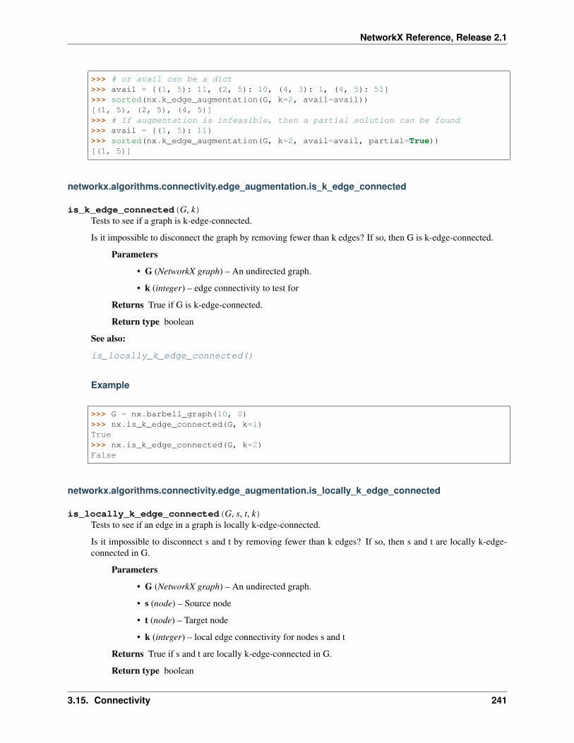
NetworkX Reference, Release 2.1
>>> # or avail can be a dict>>> avail = {(1, 5): 11, (2, 5): 10, (4, 3): 1, (4, 5): 51}>>> sorted(nx.k_edge_augmentation(G, k=2, avail=avail))[(1, 5), (2, 5), (4, 5)]>>> # If augmentation is infeasible, then a partial solution can be found>>> avail = {(1, 5): 11}>>> sorted(nx.k_edge_augmentation(G, k=2, avail=avail, partial=True))[(1, 5)]
networkx.algorithms.connectivity.edge_augmentation.is_k_edge_connected
is_k_edge_connected(G, k)Tests to see if a graph is k-edge-connected.
Is it impossible to disconnect the graph by removing fewer than k edges? If so, then G is k-edge-connected.
Parameters
• G (NetworkX graph) – An undirected graph.
• k (integer) – edge connectivity to test for
Returns True if G is k-edge-connected.
Return type boolean
See also:
is_locally_k_edge_connected()
Example
>>> G = nx.barbell_graph(10, 0)>>> nx.is_k_edge_connected(G, k=1)True>>> nx.is_k_edge_connected(G, k=2)False
networkx.algorithms.connectivity.edge_augmentation.is_locally_k_edge_connected
is_locally_k_edge_connected(G, s, t, k)Tests to see if an edge in a graph is locally k-edge-connected.
Is it impossible to disconnect s and t by removing fewer than k edges? If so, then s and t are locally k-edge-connected in G.
Parameters
• G (NetworkX graph) – An undirected graph.
• s (node) – Source node
• t (node) – Target node
• k (integer) – local edge connectivity for nodes s and t
Returns True if s and t are locally k-edge-connected in G.
Return type boolean
3.15. Connectivity 241

NetworkX Reference, Release 2.1
See also:
is_k_edge_connected()
Example
>>> from networkx.algorithms.connectivity import is_locally_k_edge_connected>>> G = nx.barbell_graph(10, 0)>>> is_locally_k_edge_connected(G, 5, 15, k=1)True>>> is_locally_k_edge_connected(G, 5, 15, k=2)False>>> is_locally_k_edge_connected(G, 1, 5, k=2)True
3.15.2 K-edge-components
Algorithms for finding k-edge-connected components and subgraphs.
A k-edge-connected component (k-edge-cc) is a maximal set of nodes in G, such that all pairs of node have an edge-connectivity of at least k.
A k-edge-connected subgraph (k-edge-subgraph) is a maximal set of nodes in G, such that the subgraph of G definedby the nodes has an edge-connectivity at least k.
k_edge_components(G, k) Generates nodes in each maximal k-edge-connected com-ponent in G.
k_edge_subgraphs(G, k) Generates nodes in each maximal k-edge-connected sub-graph in G.
bridge_components(G) Finds all bridge-connected components G.EdgeComponentAuxGraph A simple algorithm to find all k-edge-connected compo-
nents in a graph.
networkx.algorithms.connectivity.edge_kcomponents.k_edge_components
k_edge_components(G, k)Generates nodes in each maximal k-edge-connected component in G.
Parameters
• G (NetworkX graph)
• k (Integer) – Desired edge connectivity
Returns k_edge_components – will have k-edge-connectivity in the graph G.
Return type a generator of k-edge-ccs. Each set of returned nodes
See also:
local_edge_connectivity()
k_edge_subgraphs() similar to this function, but the subgraph defined by the nodes must also have k-edge-connectivity.
k_components() similar to this function, but uses node-connectivity instead of edge-connectivity
242 Chapter 3. Algorithms
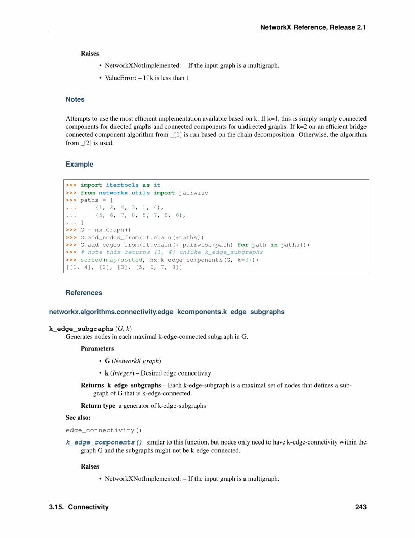
NetworkX Reference, Release 2.1
Raises
• NetworkXNotImplemented: – If the input graph is a multigraph.
• ValueError: – If k is less than 1
Notes
Attempts to use the most efficient implementation available based on k. If k=1, this is simply simply connectedcomponents for directed graphs and connected components for undirected graphs. If k=2 on an efficient bridgeconnected component algorithm from _[1] is run based on the chain decomposition. Otherwise, the algorithmfrom _[2] is used.
Example
>>> import itertools as it>>> from networkx.utils import pairwise>>> paths = [... (1, 2, 4, 3, 1, 4),... (5, 6, 7, 8, 5, 7, 8, 6),... ]>>> G = nx.Graph()>>> G.add_nodes_from(it.chain(*paths))>>> G.add_edges_from(it.chain(*[pairwise(path) for path in paths]))>>> # note this returns {1, 4} unlike k_edge_subgraphs>>> sorted(map(sorted, nx.k_edge_components(G, k=3)))[[1, 4], [2], [3], [5, 6, 7, 8]]
References
networkx.algorithms.connectivity.edge_kcomponents.k_edge_subgraphs
k_edge_subgraphs(G, k)Generates nodes in each maximal k-edge-connected subgraph in G.
Parameters
• G (NetworkX graph)
• k (Integer) – Desired edge connectivity
Returns k_edge_subgraphs – Each k-edge-subgraph is a maximal set of nodes that defines a sub-graph of G that is k-edge-connected.
Return type a generator of k-edge-subgraphs
See also:
edge_connectivity()
k_edge_components() similar to this function, but nodes only need to have k-edge-connctivity within thegraph G and the subgraphs might not be k-edge-connected.
Raises
• NetworkXNotImplemented: – If the input graph is a multigraph.
3.15. Connectivity 243

NetworkX Reference, Release 2.1
• ValueError: – If k is less than 1
Notes
Attempts to use the most efficient implementation available based on k. If k=1, or k=2 and the graph is undi-rected, then this simply calls k_edge_components. Otherwise the algorithm from _[1] is used.
Example
>>> import itertools as it>>> from networkx.utils import pairwise>>> paths = [... (1, 2, 4, 3, 1, 4),... (5, 6, 7, 8, 5, 7, 8, 6),... ]>>> G = nx.Graph()>>> G.add_nodes_from(it.chain(*paths))>>> G.add_edges_from(it.chain(*[pairwise(path) for path in paths]))>>> # note this does not return {1, 4} unlike k_edge_components>>> sorted(map(sorted, nx.k_edge_subgraphs(G, k=3)))[[1], [2], [3], [4], [5, 6, 7, 8]]
References
networkx.algorithms.connectivity.edge_kcomponents.bridge_components
bridge_components(G)Finds all bridge-connected components G.
Parameters G (NetworkX undirected graph)
Returns bridge_components
Return type a generator of 2-edge-connected components
See also:
k_edge_subgraphs() this function is a special case for an undirected graph where k=2.
biconnected_components() similar to this function, but is defined using 2-node-connectivity instead of2-edge-connectivity.
Raises NetworkXNotImplemented: – If the input graph is directed or a multigraph.
Notes
Bridge-connected components are also known as 2-edge-connected components.
244 Chapter 3. Algorithms

NetworkX Reference, Release 2.1
Example
>>> # The barbell graph with parameter zero has a single bridge>>> G = nx.barbell_graph(5, 0)>>> from networkx.algorithms.connectivity.edge_kcomponents import bridge_→˓components>>> sorted(map(sorted, bridge_components(G)))[[0, 1, 2, 3, 4], [5, 6, 7, 8, 9]]
networkx.algorithms.connectivity.edge_kcomponents.EdgeComponentAuxGraph
class EdgeComponentAuxGraphA simple algorithm to find all k-edge-connected components in a graph.
Constructing the AuxillaryGraph (which may take some time) allows for the k-edge-ccs to be found in lineartime for arbitrary k.
Notes
This implementation is based on1. The idea is to construct an auxillary graph from which the k-edge-ccs can beextracted in linear time. The auxillary graph is constructed in 𝑂(|𝑉 | · 𝐹 ) operations, where F is the complexityof max flow. Querying the components takes an additional 𝑂(|𝑉 |) operations. This algorithm can be slow forlarge graphs, but it handles an arbitrary k and works for both directed and undirected inputs.
The undirected case for k=1 is exactly connected components. The undirected case for k=2 is exactly bridgeconnected components. The directed case for k=1 is exactly strongly connected components.
References
Example
>>> import itertools as it>>> from networkx.utils import pairwise>>> from networkx.algorithms.connectivity import EdgeComponentAuxGraph>>> # Build an interesting graph with multiple levels of k-edge-ccs>>> paths = [... (1, 2, 3, 4, 1, 3, 4, 2), # a 3-edge-cc (a 4 clique)... (5, 6, 7, 5), # a 2-edge-cc (a 3 clique)... (1, 5), # combine first two ccs into a 1-edge-cc... (0,), # add an additional disconnected 1-edge-cc... ]>>> G = nx.Graph()>>> G.add_nodes_from(it.chain(*paths))>>> G.add_edges_from(it.chain(*[pairwise(path) for path in paths]))>>> # Constructing the AuxGraph takes about O(n ** 4)>>> aux_graph = EdgeComponentAuxGraph.construct(G)>>> # Once constructed, querying takes O(n)>>> sorted(map(sorted, aux_graph.k_edge_components(k=1)))[[0], [1, 2, 3, 4, 5, 6, 7]]>>> sorted(map(sorted, aux_graph.k_edge_components(k=2)))
1 Wang, Tianhao, et al. (2015) A simple algorithm for finding all k-edge-connected components. http://journals.plos.org/plosone/article?id=10.1371/journal.pone.0136264
3.15. Connectivity 245

NetworkX Reference, Release 2.1
[[0], [1, 2, 3, 4], [5, 6, 7]]>>> sorted(map(sorted, aux_graph.k_edge_components(k=3)))[[0], [1, 2, 3, 4], [5], [6], [7]]>>> sorted(map(sorted, aux_graph.k_edge_components(k=4)))[[0], [1], [2], [3], [4], [5], [6], [7]]
Example
>>> # The auxillary graph is primarilly used for k-edge-ccs but it>>> # can also speed up the queries of k-edge-subgraphs by refining the>>> # search space.>>> import itertools as it>>> from networkx.utils import pairwise>>> from networkx.algorithms.connectivity import EdgeComponentAuxGraph>>> paths = [... (1, 2, 4, 3, 1, 4),... ]>>> G = nx.Graph()>>> G.add_nodes_from(it.chain(*paths))>>> G.add_edges_from(it.chain(*[pairwise(path) for path in paths]))>>> aux_graph = EdgeComponentAuxGraph.construct(G)>>> sorted(map(sorted, aux_graph.k_edge_subgraphs(k=3)))[[1], [2], [3], [4]]>>> sorted(map(sorted, aux_graph.k_edge_components(k=3)))[[1, 4], [2], [3]]
__init__()x.__init__(. . . ) initializes x; see help(type(x)) for signature
Methods
construct(EdgeComponentAuxGraph, G) Builds an auxillary graph encoding edge-connectivitybetween nodes.
k_edge_components(k) Queries the auxillary graph for k-edge-connected com-ponents.
k_edge_subgraphs(k) Queries the auxillary graph for k-edge-connected sub-graphs.
3.15.3 K-node-components
Moody and White algorithm for k-components
k_components(G[, flow_func]) Returns the k-component structure of a graph G.
networkx.algorithms.connectivity.kcomponents.k_components
k_components(G, flow_func=None)Returns the k-component structure of a graph G.
A k-component is a maximal subgraph of a graph G that has, at least, node connectivity k: we need to remove at
246 Chapter 3. Algorithms

NetworkX Reference, Release 2.1
least k nodes to break it into more components. k-components have an inherent hierarchical structure becausethey are nested in terms of connectivity: a connected graph can contain several 2-components, each of whichcan contain one or more 3-components, and so forth.
Parameters
• G (NetworkX graph)
• flow_func (function) – Function to perform the underlying flow computations. Default valueedmonds_karp(). This function performs better in sparse graphs with right tailed degreedistributions. shortest_augmenting_path() will perform better in denser graphs.
Returns k_components – Dictionary with all connectivity levels k in the input Graph as keys and alist of sets of nodes that form a k-component of level k as values.
Return type dict
Raises NetworkXNotImplemented: – If the input graph is directed.
Examples
>>> # Petersen graph has 10 nodes and it is triconnected, thus all>>> # nodes are in a single component on all three connectivity levels>>> G = nx.petersen_graph()>>> k_components = nx.k_components(G)
Notes
Moody and White1 (appendix A) provide an algorithm for identifying k-components in a graph, which isbased on Kanevsky’s algorithm2 for finding all minimum-size node cut-sets of a graph (implemented inall_node_cuts() function):
1. Compute node connectivity, k, of the input graph G.
2. Identify all k-cutsets at the current level of connectivity using Kanevsky’s algorithm.
3. Generate new graph components based on the removal of these cutsets. Nodes in a cutset belong to bothsides of the induced cut.
4. If the graph is neither complete nor trivial, return to 1; else end.
This implementation also uses some heuristics (see3 for details) to speed up the computation.
See also:
node_connectivity(), all_node_cuts()
biconnected_components() special case of this function when k=2
k_edge_components() similar to this function, but uses edge-connectivity instead of node-connectivity
1 Moody, J. and D. White (2003). Social cohesion and embeddedness: A hierarchical conception of social groups. American SociologicalReview 68(1), 103–28. http://www2.asanet.org/journals/ASRFeb03MoodyWhite.pdf
2 Kanevsky, A. (1993). Finding all minimum-size separating vertex sets in a graph. Networks 23(6), 533–541. http://onlinelibrary.wiley.com/doi/10.1002/net.3230230604/abstract
3 Torrents, J. and F. Ferraro (2015). Structural Cohesion: Visualization and Heuristics for Fast Computation. https://arxiv.org/pdf/1503.04476v1
3.15. Connectivity 247

NetworkX Reference, Release 2.1
References
3.15.4 K-node-cutsets
Kanevsky all minimum node k cutsets algorithm.
all_node_cuts(G[, k, flow_func]) Returns all minimum k cutsets of an undirected graph G.
networkx.algorithms.connectivity.kcutsets.all_node_cuts
all_node_cuts(G, k=None, flow_func=None)Returns all minimum k cutsets of an undirected graph G.
This implementation is based on Kanevsky’s algorithm1 for finding all minimum-size node cut-sets of an undi-rected graph G; ie the set (or sets) of nodes of cardinality equal to the node connectivity of G. Thus if removed,would break G into two or more connected components.
Parameters
• G (NetworkX graph) – Undirected graph
• k (Integer) – Node connectivity of the input graph. If k is None, then it is computed. Defaultvalue: None.
• flow_func (function) – Function to perform the underlying flow computations. Default valueedmonds_karp. This function performs better in sparse graphs with right tailed degree dis-tributions. shortest_augmenting_path will perform better in denser graphs.
Returns cuts – Each node cutset has cardinality equal to the node connectivity of the input graph.
Return type a generator of node cutsets
Examples
>>> # A two-dimensional grid graph has 4 cutsets of cardinality 2>>> G = nx.grid_2d_graph(5, 5)>>> cutsets = list(nx.all_node_cuts(G))>>> len(cutsets)4>>> all(2 == len(cutset) for cutset in cutsets)True>>> nx.node_connectivity(G)2
Notes
This implementation is based on the sequential algorithm for finding all minimum-size separating vertex sets ina graph1. The main idea is to compute minimum cuts using local maximum flow computations among a set ofnodes of highest degree and all other non-adjacent nodes in the Graph. Once we find a minimum cut, we add anedge between the high degree node and the target node of the local maximum flow computation to make surethat we will not find that minimum cut again.
1 Kanevsky, A. (1993). Finding all minimum-size separating vertex sets in a graph. Networks 23(6), 533–541. http://onlinelibrary.wiley.com/doi/10.1002/net.3230230604/abstract
248 Chapter 3. Algorithms

NetworkX Reference, Release 2.1
See also:
node_connectivity(), edmonds_karp(), shortest_augmenting_path()
References
3.15.5 Flow-based disjoint paths
Flow based node and edge disjoint paths.
edge_disjoint_paths(G, s, t[, flow_func, . . . ]) Returns the edges disjoint paths between source and target.node_disjoint_paths(G, s, t[, flow_func, . . . ]) Computes node disjoint paths between source and target.
networkx.algorithms.connectivity.disjoint_paths.edge_disjoint_paths
edge_disjoint_paths(G, s, t, flow_func=None, cutoff=None, auxiliary=None, residual=None)Returns the edges disjoint paths between source and target.
Edge disjoint paths are paths that do not share any edge. The number of edge disjoint paths between source andtarget is equal to their edge connectivity.
Parameters
• G (NetworkX graph)
• s (node) – Source node for the flow.
• t (node) – Sink node for the flow.
• flow_func (function) – A function for computing the maximum flow among a pair ofnodes. The function has to accept at least three parameters: a Digraph, a source node,and a target node. And return a residual network that follows NetworkX conventions (seemaximum_flow() for details). If flow_func is None, the default maximum flow function(edmonds_karp()) is used. The choice of the default function may change from versionto version and should not be relied on. Default value: None.
• cutoff (int) – Maximum number of paths to yield. Some of the maximum flow algorithms,such as edmonds_karp() (the default) and shortest_augmenting_path() sup-port the cutoff parameter, and will terminate when the flow value reaches or exceeds thecutoff. Other algorithms will ignore this parameter. Default value: None.
• auxiliary (NetworkX DiGraph) – Auxiliary digraph to compute flow based edge connectiv-ity. It has to have a graph attribute called mapping with a dictionary mapping node namesin G and in the auxiliary digraph. If provided it will be reused instead of recreated. Defaultvalue: None.
• residual (NetworkX DiGraph) – Residual network to compute maximum flow. If providedit will be reused instead of recreated. Default value: None.
Returns paths – A generator of edge independent paths.
Return type generator
Raises
• NetworkXNoPath : exception – If there is no path between source and target.
• NetworkXError : exception – If source or target are not in the graph G.
3.15. Connectivity 249

NetworkX Reference, Release 2.1
See also:
node_disjoint_paths(), edge_connectivity(), maximum_flow(), edmonds_karp(),preflow_push(), shortest_augmenting_path()
Examples
We use in this example the platonic icosahedral graph, which has node edge connectivity 5, thus there are 5 edgedisjoint paths between any pair of nodes.
>>> G = nx.icosahedral_graph()>>> len(list(nx.edge_disjoint_paths(G, 0, 6)))5
If you need to compute edge disjoint paths on several pairs of nodes in the same graph, it is recommended thatyou reuse the data structures that NetworkX uses in the computation: the auxiliary digraph for edge connectivity,and the residual network for the underlying maximum flow computation.
Example of how to compute edge disjoint paths among all pairs of nodes of the platonic icosahedral graphreusing the data structures.
>>> import itertools>>> # You also have to explicitly import the function for>>> # building the auxiliary digraph from the connectivity package>>> from networkx.algorithms.connectivity import (... build_auxiliary_edge_connectivity)>>> H = build_auxiliary_edge_connectivity(G)>>> # And the function for building the residual network from the>>> # flow package>>> from networkx.algorithms.flow import build_residual_network>>> # Note that the auxiliary digraph has an edge attribute named capacity>>> R = build_residual_network(H, 'capacity')>>> result = {n: {} for n in G}>>> # Reuse the auxiliary digraph and the residual network by passing them>>> # as arguments>>> for u, v in itertools.combinations(G, 2):... k = len(list(nx.edge_disjoint_paths(G, u, v, auxiliary=H, residual=R)))... result[u][v] = k>>> all(result[u][v] == 5 for u, v in itertools.combinations(G, 2))True
You can also use alternative flow algorithms for computing edge disjoint paths. For instance, in densenetworks the algorithm shortest_augmenting_path() will usually perform better than the defaultedmonds_karp() which is faster for sparse networks with highly skewed degree distributions. Alternativeflow functions have to be explicitly imported from the flow package.
>>> from networkx.algorithms.flow import shortest_augmenting_path>>> len(list(nx.edge_disjoint_paths(G, 0, 6, flow_func=shortest_augmenting_path)))5
Notes
This is a flow based implementation of edge disjoint paths. We compute the maximum flow between source andtarget on an auxiliary directed network. The saturated edges in the residual network after running the maximum
250 Chapter 3. Algorithms
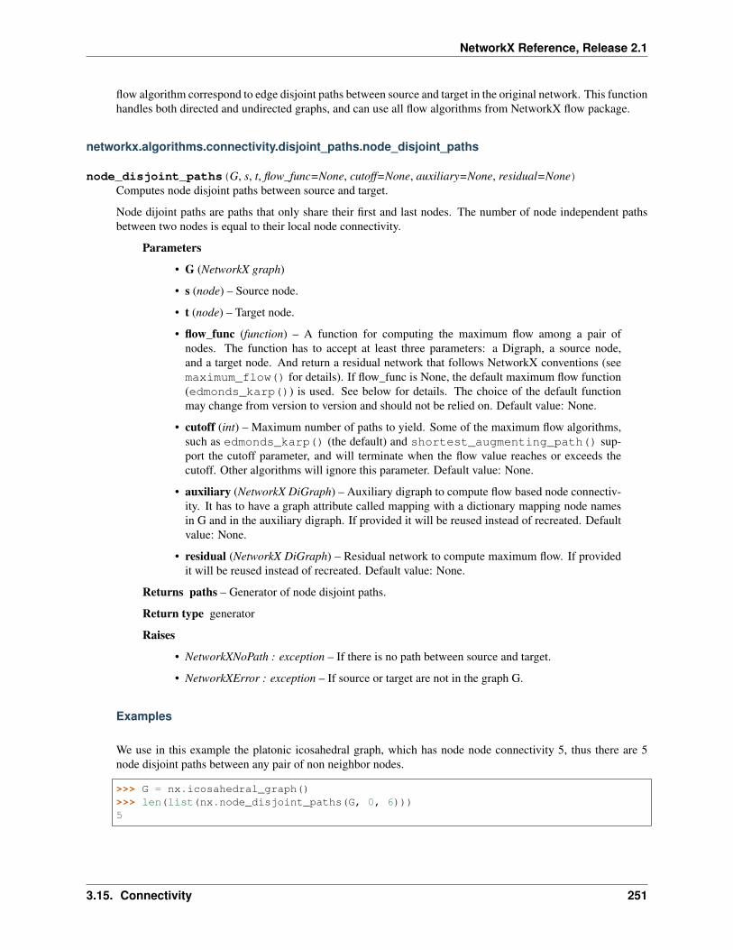
NetworkX Reference, Release 2.1
flow algorithm correspond to edge disjoint paths between source and target in the original network. This functionhandles both directed and undirected graphs, and can use all flow algorithms from NetworkX flow package.
networkx.algorithms.connectivity.disjoint_paths.node_disjoint_paths
node_disjoint_paths(G, s, t, flow_func=None, cutoff=None, auxiliary=None, residual=None)Computes node disjoint paths between source and target.
Node dijoint paths are paths that only share their first and last nodes. The number of node independent pathsbetween two nodes is equal to their local node connectivity.
Parameters
• G (NetworkX graph)
• s (node) – Source node.
• t (node) – Target node.
• flow_func (function) – A function for computing the maximum flow among a pair ofnodes. The function has to accept at least three parameters: a Digraph, a source node,and a target node. And return a residual network that follows NetworkX conventions (seemaximum_flow() for details). If flow_func is None, the default maximum flow function(edmonds_karp()) is used. See below for details. The choice of the default functionmay change from version to version and should not be relied on. Default value: None.
• cutoff (int) – Maximum number of paths to yield. Some of the maximum flow algorithms,such as edmonds_karp() (the default) and shortest_augmenting_path() sup-port the cutoff parameter, and will terminate when the flow value reaches or exceeds thecutoff. Other algorithms will ignore this parameter. Default value: None.
• auxiliary (NetworkX DiGraph) – Auxiliary digraph to compute flow based node connectiv-ity. It has to have a graph attribute called mapping with a dictionary mapping node namesin G and in the auxiliary digraph. If provided it will be reused instead of recreated. Defaultvalue: None.
• residual (NetworkX DiGraph) – Residual network to compute maximum flow. If providedit will be reused instead of recreated. Default value: None.
Returns paths – Generator of node disjoint paths.
Return type generator
Raises
• NetworkXNoPath : exception – If there is no path between source and target.
• NetworkXError : exception – If source or target are not in the graph G.
Examples
We use in this example the platonic icosahedral graph, which has node node connectivity 5, thus there are 5node disjoint paths between any pair of non neighbor nodes.
>>> G = nx.icosahedral_graph()>>> len(list(nx.node_disjoint_paths(G, 0, 6)))5
3.15. Connectivity 251
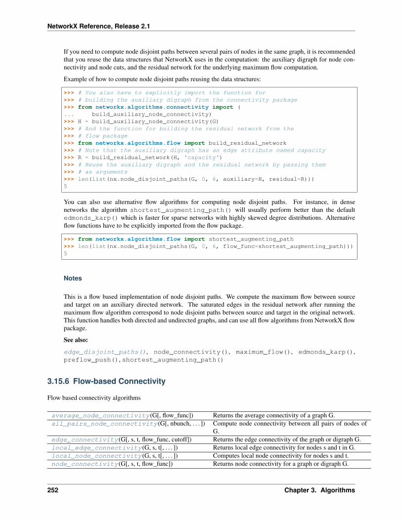
NetworkX Reference, Release 2.1
If you need to compute node disjoint paths between several pairs of nodes in the same graph, it is recommendedthat you reuse the data structures that NetworkX uses in the computation: the auxiliary digraph for node con-nectivity and node cuts, and the residual network for the underlying maximum flow computation.
Example of how to compute node disjoint paths reusing the data structures:
>>> # You also have to explicitly import the function for>>> # building the auxiliary digraph from the connectivity package>>> from networkx.algorithms.connectivity import (... build_auxiliary_node_connectivity)>>> H = build_auxiliary_node_connectivity(G)>>> # And the function for building the residual network from the>>> # flow package>>> from networkx.algorithms.flow import build_residual_network>>> # Note that the auxiliary digraph has an edge attribute named capacity>>> R = build_residual_network(H, 'capacity')>>> # Reuse the auxiliary digraph and the residual network by passing them>>> # as arguments>>> len(list(nx.node_disjoint_paths(G, 0, 6, auxiliary=H, residual=R)))5
You can also use alternative flow algorithms for computing node disjoint paths. For instance, in densenetworks the algorithm shortest_augmenting_path() will usually perform better than the defaultedmonds_karp() which is faster for sparse networks with highly skewed degree distributions. Alternativeflow functions have to be explicitly imported from the flow package.
>>> from networkx.algorithms.flow import shortest_augmenting_path>>> len(list(nx.node_disjoint_paths(G, 0, 6, flow_func=shortest_augmenting_path)))5
Notes
This is a flow based implementation of node disjoint paths. We compute the maximum flow between sourceand target on an auxiliary directed network. The saturated edges in the residual network after running themaximum flow algorithm correspond to node disjoint paths between source and target in the original network.This function handles both directed and undirected graphs, and can use all flow algorithms from NetworkX flowpackage.
See also:
edge_disjoint_paths(), node_connectivity(), maximum_flow(), edmonds_karp(),preflow_push(), shortest_augmenting_path()
3.15.6 Flow-based Connectivity
Flow based connectivity algorithms
average_node_connectivity(G[, flow_func]) Returns the average connectivity of a graph G.all_pairs_node_connectivity(G[, nbunch, . . . ]) Compute node connectivity between all pairs of nodes of
G.edge_connectivity(G[, s, t, flow_func, cutoff]) Returns the edge connectivity of the graph or digraph G.local_edge_connectivity(G, s, t[, . . . ]) Returns local edge connectivity for nodes s and t in G.local_node_connectivity(G, s, t[, . . . ]) Computes local node connectivity for nodes s and t.node_connectivity(G[, s, t, flow_func]) Returns node connectivity for a graph or digraph G.
252 Chapter 3. Algorithms

NetworkX Reference, Release 2.1
networkx.algorithms.connectivity.connectivity.average_node_connectivity
average_node_connectivity(G, flow_func=None)Returns the average connectivity of a graph G.
The average connectivity bar{kappa} of a graph G is the average of local node connectivity over all pairs ofnodes of G1 .
��(𝐺) =
∑𝑢,𝑣 𝜅𝐺(𝑢, 𝑣)(
𝑛2
)Parameters
• G (NetworkX graph) – Undirected graph
• flow_func (function) – A function for computing the maximum flow among a pair ofnodes. The function has to accept at least three parameters: a Digraph, a source node,and a target node. And return a residual network that follows NetworkX conventions (seemaximum_flow() for details). If flow_func is None, the default maximum flow function(edmonds_karp()) is used. See local_node_connectivity() for details. Thechoice of the default function may change from version to version and should not be reliedon. Default value: None.
Returns K – Average node connectivity
Return type float
See also:
local_node_connectivity(), node_connectivity(), edge_connectivity(),maximum_flow(), edmonds_karp(), preflow_push(), shortest_augmenting_path()
References
networkx.algorithms.connectivity.connectivity.all_pairs_node_connectivity
all_pairs_node_connectivity(G, nbunch=None, flow_func=None)Compute node connectivity between all pairs of nodes of G.
Parameters
• G (NetworkX graph) – Undirected graph
• nbunch (container) – Container of nodes. If provided node connectivity will be computedonly over pairs of nodes in nbunch.
• flow_func (function) – A function for computing the maximum flow among a pair ofnodes. The function has to accept at least three parameters: a Digraph, a source node,and a target node. And return a residual network that follows NetworkX conventions (seemaximum_flow() for details). If flow_func is None, the default maximum flow function(edmonds_karp()) is used. See below for details. The choice of the default functionmay change from version to version and should not be relied on. Default value: None.
Returns all_pairs – A dictionary with node connectivity between all pairs of nodes in G, or innbunch if provided.
Return type dict
1 Beineke, L., O. Oellermann, and R. Pippert (2002). The average connectivity of a graph. Discrete mathematics 252(1-3), 31-45. http://www.sciencedirect.com/science/article/pii/S0012365X01001807
3.15. Connectivity 253

NetworkX Reference, Release 2.1
See also:
local_node_connectivity(), edge_connectivity(), local_edge_connectivity(),maximum_flow(), edmonds_karp(), preflow_push(), shortest_augmenting_path()
networkx.algorithms.connectivity.connectivity.edge_connectivity
edge_connectivity(G, s=None, t=None, flow_func=None, cutoff=None)Returns the edge connectivity of the graph or digraph G.
The edge connectivity is equal to the minimum number of edges that must be removed to disconnect G or renderit trivial. If source and target nodes are provided, this function returns the local edge connectivity: the minimumnumber of edges that must be removed to break all paths from source to target in G.
Parameters
• G (NetworkX graph) – Undirected or directed graph
• s (node) – Source node. Optional. Default value: None.
• t (node) – Target node. Optional. Default value: None.
• flow_func (function) – A function for computing the maximum flow among a pair ofnodes. The function has to accept at least three parameters: a Digraph, a source node,and a target node. And return a residual network that follows NetworkX conventions (seemaximum_flow() for details). If flow_func is None, the default maximum flow function(edmonds_karp()) is used. See below for details. The choice of the default functionmay change from version to version and should not be relied on. Default value: None.
• cutoff (integer, float) – If specified, the maximum flow algorithm will terminate when theflow value reaches or exceeds the cutoff. This is only for the algorithms that support thecutoff parameter: edmonds_karp() and shortest_augmenting_path(). Otheralgorithms will ignore this parameter. Default value: None.
Returns K – Edge connectivity for G, or local edge connectivity if source and target were provided
Return type integer
Examples
>>> # Platonic icosahedral graph is 5-edge-connected>>> G = nx.icosahedral_graph()>>> nx.edge_connectivity(G)5
You can use alternative flow algorithms for the underlying maximum flow computation. In dense net-works the algorithm shortest_augmenting_path() will usually perform better than the defaultedmonds_karp(), which is faster for sparse networks with highly skewed degree distributions. Alternativeflow functions have to be explicitly imported from the flow package.
>>> from networkx.algorithms.flow import shortest_augmenting_path>>> nx.edge_connectivity(G, flow_func=shortest_augmenting_path)5
If you specify a pair of nodes (source and target) as parameters, this function returns the value of local edgeconnectivity.
254 Chapter 3. Algorithms

NetworkX Reference, Release 2.1
>>> nx.edge_connectivity(G, 3, 7)5
If you need to perform several local computations among different pairs of nodes on the same graph,it is recommended that you reuse the data structures used in the maximum flow computations. Seelocal_edge_connectivity() for details.
Notes
This is a flow based implementation of global edge connectivity. For undirected graphs the algorithm works byfinding a ‘small’ dominating set of nodes of G (see algorithm 7 in1 ) and computing local maximum flow (seelocal_edge_connectivity()) between an arbitrary node in the dominating set and the rest of nodes init. This is an implementation of algorithm 6 in1 . For directed graphs, the algorithm does n calls to the maximumflow function. This is an implementation of algorithm 8 in1 .
See also:
local_edge_connectivity(), local_node_connectivity(), node_connectivity(),maximum_flow(), edmonds_karp(), preflow_push(), shortest_augmenting_path(),k_edge_components(), k_edge_subgraphs()
References
networkx.algorithms.connectivity.connectivity.local_edge_connectivity
local_edge_connectivity(G, s, t, flow_func=None, auxiliary=None, residual=None, cutoff=None)Returns local edge connectivity for nodes s and t in G.
Local edge connectivity for two nodes s and t is the minimum number of edges that must be removed to discon-nect them.
This is a flow based implementation of edge connectivity. We compute the maximum flow on an auxiliarydigraph build from the original network (see below for details). This is equal to the local edge connectivitybecause the value of a maximum s-t-flow is equal to the capacity of a minimum s-t-cut (Ford and Fulkersontheorem)1 .
Parameters
• G (NetworkX graph) – Undirected or directed graph
• s (node) – Source node
• t (node) – Target node
• flow_func (function) – A function for computing the maximum flow among a pair ofnodes. The function has to accept at least three parameters: a Digraph, a source node,and a target node. And return a residual network that follows NetworkX conventions (seemaximum_flow() for details). If flow_func is None, the default maximum flow function(edmonds_karp()) is used. See below for details. The choice of the default functionmay change from version to version and should not be relied on. Default value: None.
• auxiliary (NetworkX DiGraph) – Auxiliary digraph for computing flow based edge connec-tivity. If provided it will be reused instead of recreated. Default value: None.
1 Abdol-Hossein Esfahanian. Connectivity Algorithms. http://www.cse.msu.edu/~cse835/Papers/Graph_connectivity_revised.pdf1 Abdol-Hossein Esfahanian. Connectivity Algorithms. http://www.cse.msu.edu/~cse835/Papers/Graph_connectivity_revised.pdf
3.15. Connectivity 255

NetworkX Reference, Release 2.1
• residual (NetworkX DiGraph) – Residual network to compute maximum flow. If providedit will be reused instead of recreated. Default value: None.
• cutoff (integer, float) – If specified, the maximum flow algorithm will terminate when theflow value reaches or exceeds the cutoff. This is only for the algorithms that support thecutoff parameter: edmonds_karp() and shortest_augmenting_path(). Otheralgorithms will ignore this parameter. Default value: None.
Returns K – local edge connectivity for nodes s and t.
Return type integer
Examples
This function is not imported in the base NetworkX namespace, so you have to explicitly import it from theconnectivity package:
>>> from networkx.algorithms.connectivity import local_edge_connectivity
We use in this example the platonic icosahedral graph, which has edge connectivity 5.
>>> G = nx.icosahedral_graph()>>> local_edge_connectivity(G, 0, 6)5
If you need to compute local connectivity on several pairs of nodes in the same graph, it is recommended thatyou reuse the data structures that NetworkX uses in the computation: the auxiliary digraph for edge connectivity,and the residual network for the underlying maximum flow computation.
Example of how to compute local edge connectivity among all pairs of nodes of the platonic icosahedral graphreusing the data structures.
>>> import itertools>>> # You also have to explicitly import the function for>>> # building the auxiliary digraph from the connectivity package>>> from networkx.algorithms.connectivity import (... build_auxiliary_edge_connectivity)>>> H = build_auxiliary_edge_connectivity(G)>>> # And the function for building the residual network from the>>> # flow package>>> from networkx.algorithms.flow import build_residual_network>>> # Note that the auxiliary digraph has an edge attribute named capacity>>> R = build_residual_network(H, 'capacity')>>> result = dict.fromkeys(G, dict())>>> # Reuse the auxiliary digraph and the residual network by passing them>>> # as parameters>>> for u, v in itertools.combinations(G, 2):... k = local_edge_connectivity(G, u, v, auxiliary=H, residual=R)... result[u][v] = k>>> all(result[u][v] == 5 for u, v in itertools.combinations(G, 2))True
You can also use alternative flow algorithms for computing edge connectivity. For instance, in densenetworks the algorithm shortest_augmenting_path() will usually perform better than the defaultedmonds_karp() which is faster for sparse networks with highly skewed degree distributions. Alternativeflow functions have to be explicitly imported from the flow package.
256 Chapter 3. Algorithms

NetworkX Reference, Release 2.1
>>> from networkx.algorithms.flow import shortest_augmenting_path>>> local_edge_connectivity(G, 0, 6, flow_func=shortest_augmenting_path)5
Notes
This is a flow based implementation of edge connectivity. We compute the maximum flow using, by default, theedmonds_karp() algorithm on an auxiliary digraph build from the original input graph:
If the input graph is undirected, we replace each edge (u,‘v‘) with two reciprocal arcs (u, v) and (v, u) andthen we set the attribute ‘capacity’ for each arc to 1. If the input graph is directed we simply add the ‘capacity’attribute. This is an implementation of algorithm 1 in1.
The maximum flow in the auxiliary network is equal to the local edge connectivity because the value of amaximum s-t-flow is equal to the capacity of a minimum s-t-cut (Ford and Fulkerson theorem).
See also:
edge_connectivity(), local_node_connectivity(), node_connectivity(),maximum_flow(), edmonds_karp(), preflow_push(), shortest_augmenting_path()
References
networkx.algorithms.connectivity.connectivity.local_node_connectivity
local_node_connectivity(G, s, t, flow_func=None, auxiliary=None, residual=None, cutoff=None)Computes local node connectivity for nodes s and t.
Local node connectivity for two non adjacent nodes s and t is the minimum number of nodes that must beremoved (along with their incident edges) to disconnect them.
This is a flow based implementation of node connectivity. We compute the maximum flow on an auxiliarydigraph build from the original input graph (see below for details).
Parameters
• G (NetworkX graph) – Undirected graph
• s (node) – Source node
• t (node) – Target node
• flow_func (function) – A function for computing the maximum flow among a pair ofnodes. The function has to accept at least three parameters: a Digraph, a source node,and a target node. And return a residual network that follows NetworkX conventions (seemaximum_flow() for details). If flow_func is None, the default maximum flow function(edmonds_karp()) is used. See below for details. The choice of the default functionmay change from version to version and should not be relied on. Default value: None.
• auxiliary (NetworkX DiGraph) – Auxiliary digraph to compute flow based node connectiv-ity. It has to have a graph attribute called mapping with a dictionary mapping node namesin G and in the auxiliary digraph. If provided it will be reused instead of recreated. Defaultvalue: None.
• residual (NetworkX DiGraph) – Residual network to compute maximum flow. If providedit will be reused instead of recreated. Default value: None.
3.15. Connectivity 257

NetworkX Reference, Release 2.1
• cutoff (integer, float) – If specified, the maximum flow algorithm will terminate when theflow value reaches or exceeds the cutoff. This is only for the algorithms that support thecutoff parameter: edmonds_karp() and shortest_augmenting_path(). Otheralgorithms will ignore this parameter. Default value: None.
Returns K – local node connectivity for nodes s and t
Return type integer
Examples
This function is not imported in the base NetworkX namespace, so you have to explicitly import it from theconnectivity package:
>>> from networkx.algorithms.connectivity import local_node_connectivity
We use in this example the platonic icosahedral graph, which has node connectivity 5.
>>> G = nx.icosahedral_graph()>>> local_node_connectivity(G, 0, 6)5
If you need to compute local connectivity on several pairs of nodes in the same graph, it is recommended thatyou reuse the data structures that NetworkX uses in the computation: the auxiliary digraph for node connectivity,and the residual network for the underlying maximum flow computation.
Example of how to compute local node connectivity among all pairs of nodes of the platonic icosahedral graphreusing the data structures.
>>> import itertools>>> # You also have to explicitly import the function for>>> # building the auxiliary digraph from the connectivity package>>> from networkx.algorithms.connectivity import (... build_auxiliary_node_connectivity)...>>> H = build_auxiliary_node_connectivity(G)>>> # And the function for building the residual network from the>>> # flow package>>> from networkx.algorithms.flow import build_residual_network>>> # Note that the auxiliary digraph has an edge attribute named capacity>>> R = build_residual_network(H, 'capacity')>>> result = dict.fromkeys(G, dict())>>> # Reuse the auxiliary digraph and the residual network by passing them>>> # as parameters>>> for u, v in itertools.combinations(G, 2):... k = local_node_connectivity(G, u, v, auxiliary=H, residual=R)... result[u][v] = k...>>> all(result[u][v] == 5 for u, v in itertools.combinations(G, 2))True
You can also use alternative flow algorithms for computing node connectivity. For instance, in densenetworks the algorithm shortest_augmenting_path() will usually perform better than the defaultedmonds_karp() which is faster for sparse networks with highly skewed degree distributions. Alternativeflow functions have to be explicitly imported from the flow package.
258 Chapter 3. Algorithms

NetworkX Reference, Release 2.1
>>> from networkx.algorithms.flow import shortest_augmenting_path>>> local_node_connectivity(G, 0, 6, flow_func=shortest_augmenting_path)5
Notes
This is a flow based implementation of node connectivity. We compute the maximum flow using, by default,the edmonds_karp() algorithm (see: maximum_flow()) on an auxiliary digraph build from the originalinput graph:
For an undirected graph G having n nodes and m edges we derive a directed graph H with 2n nodes and 2m+narcs by replacing each original node v with two nodes v_A, v_B linked by an (internal) arc in H. Then for eachedge (u, v) in G we add two arcs (u_B, v_A) and (v_B, u_A) in H. Finally we set the attribute capacity = 1 foreach arc in H1 .
For a directed graph G having n nodes and m arcs we derive a directed graph H with 2n nodes and m+n arcs byreplacing each original node v with two nodes v_A, v_B linked by an (internal) arc (v_A, v_B) in H. Then foreach arc (u, v) in G we add one arc (u_B, v_A) in H. Finally we set the attribute capacity = 1 for each arc in H.
This is equal to the local node connectivity because the value of a maximum s-t-flow is equal to the capacity ofa minimum s-t-cut.
See also:
local_edge_connectivity(), node_connectivity(), minimum_node_cut(),maximum_flow(), edmonds_karp(), preflow_push(), shortest_augmenting_path()
References
networkx.algorithms.connectivity.connectivity.node_connectivity
node_connectivity(G, s=None, t=None, flow_func=None)Returns node connectivity for a graph or digraph G.
Node connectivity is equal to the minimum number of nodes that must be removed to disconnect G or render ittrivial. If source and target nodes are provided, this function returns the local node connectivity: the minimumnumber of nodes that must be removed to break all paths from source to target in G.
Parameters
• G (NetworkX graph) – Undirected graph
• s (node) – Source node. Optional. Default value: None.
• t (node) – Target node. Optional. Default value: None.
• flow_func (function) – A function for computing the maximum flow among a pair ofnodes. The function has to accept at least three parameters: a Digraph, a source node,and a target node. And return a residual network that follows NetworkX conventions (seemaximum_flow() for details). If flow_func is None, the default maximum flow function(edmonds_karp()) is used. See below for details. The choice of the default functionmay change from version to version and should not be relied on. Default value: None.
Returns K – Node connectivity of G, or local node connectivity if source and target are provided.
1 Kammer, Frank and Hanjo Taubig. Graph Connectivity. in Brandes and Erlebach, ‘Network Analysis: Methodological Foundations’,Lecture Notes in Computer Science, Volume 3418, Springer-Verlag, 2005. http://www.informatik.uni-augsburg.de/thi/personen/kammer/Graph_Connectivity.pdf
3.15. Connectivity 259

NetworkX Reference, Release 2.1
Return type integer
Examples
>>> # Platonic icosahedral graph is 5-node-connected>>> G = nx.icosahedral_graph()>>> nx.node_connectivity(G)5
You can use alternative flow algorithms for the underlying maximum flow computation. In dense net-works the algorithm shortest_augmenting_path() will usually perform better than the defaultedmonds_karp(), which is faster for sparse networks with highly skewed degree distributions. Alternativeflow functions have to be explicitly imported from the flow package.
>>> from networkx.algorithms.flow import shortest_augmenting_path>>> nx.node_connectivity(G, flow_func=shortest_augmenting_path)5
If you specify a pair of nodes (source and target) as parameters, this function returns the value of local nodeconnectivity.
>>> nx.node_connectivity(G, 3, 7)5
If you need to perform several local computations among different pairs of nodes on the same graph,it is recommended that you reuse the data structures used in the maximum flow computations. Seelocal_node_connectivity() for details.
Notes
This is a flow based implementation of node connectivity. The algorithm works by solving 𝑂((𝑛−𝛿−1+𝛿(𝛿−1)/2)) maximum flow problems on an auxiliary digraph. Where 𝛿 is the minimum degree of G. For details aboutthe auxiliary digraph and the computation of local node connectivity see local_node_connectivity().This implementation is based on algorithm 11 in1.
See also:
local_node_connectivity(), edge_connectivity(), maximum_flow(),edmonds_karp(), preflow_push(), shortest_augmenting_path()
References
3.15.7 Flow-based Minimum Cuts
Flow based cut algorithms
minimum_edge_cut(G[, s, t, flow_func]) Returns a set of edges of minimum cardinality that discon-nects G.
minimum_node_cut(G[, s, t, flow_func]) Returns a set of nodes of minimum cardinality that discon-nects G.
Continued on next page
1 Abdol-Hossein Esfahanian. Connectivity Algorithms. http://www.cse.msu.edu/~cse835/Papers/Graph_connectivity_revised.pdf
260 Chapter 3. Algorithms

NetworkX Reference, Release 2.1
Table 3.67 – continued from previous pageminimum_st_edge_cut(G, s, t[, flow_func, . . . ]) Returns the edges of the cut-set of a minimum (s, t)-cut.minimum_st_node_cut(G, s, t[, flow_func, . . . ]) Returns a set of nodes of minimum cardinality that discon-
nect source from target in G.
networkx.algorithms.connectivity.cuts.minimum_edge_cut
minimum_edge_cut(G, s=None, t=None, flow_func=None)Returns a set of edges of minimum cardinality that disconnects G.
If source and target nodes are provided, this function returns the set of edges of minimum cardinality that, ifremoved, would break all paths among source and target in G. If not, it returns a set of edges of minimumcardinality that disconnects G.
Parameters
• G (NetworkX graph)
• s (node) – Source node. Optional. Default value: None.
• t (node) – Target node. Optional. Default value: None.
• flow_func (function) – A function for computing the maximum flow among a pair ofnodes. The function has to accept at least three parameters: a Digraph, a source node,and a target node. And return a residual network that follows NetworkX conventions (seemaximum_flow() for details). If flow_func is None, the default maximum flow function(edmonds_karp()) is used. See below for details. The choice of the default functionmay change from version to version and should not be relied on. Default value: None.
Returns cutset – Set of edges that, if removed, would disconnect G. If source and target nodes areprovided, the set contians the edges that if removed, would destroy all paths between source andtarget.
Return type set
Examples
>>> # Platonic icosahedral graph has edge connectivity 5>>> G = nx.icosahedral_graph()>>> len(nx.minimum_edge_cut(G))5
You can use alternative flow algorithms for the underlying maximum flow computation. In dense net-works the algorithm shortest_augmenting_path() will usually perform better than the defaultedmonds_karp(), which is faster for sparse networks with highly skewed degree distributions. Alternativeflow functions have to be explicitly imported from the flow package.
>>> from networkx.algorithms.flow import shortest_augmenting_path>>> len(nx.minimum_edge_cut(G, flow_func=shortest_augmenting_path))5
If you specify a pair of nodes (source and target) as parameters, this function returns the value of local edgeconnectivity.
>>> nx.edge_connectivity(G, 3, 7)5
3.15. Connectivity 261

NetworkX Reference, Release 2.1
If you need to perform several local computations among different pairs of nodes on the same graph,it is recommended that you reuse the data structures used in the maximum flow computations. Seelocal_edge_connectivity() for details.
Notes
This is a flow based implementation of minimum edge cut. For undirected graphs the algorithm works byfinding a ‘small’ dominating set of nodes of G (see algorithm 7 in1) and computing the maximum flow betweenan arbitrary node in the dominating set and the rest of nodes in it. This is an implementation of algorithm 6in1. For directed graphs, the algorithm does n calls to the max flow function. The function raises an error if thedirected graph is not weakly connected and returns an empty set if it is weakly connected. It is an implementationof algorithm 8 in1.
See also:
minimum_st_edge_cut(), minimum_node_cut(), stoer_wagner(),node_connectivity(), edge_connectivity(), maximum_flow(), edmonds_karp(),preflow_push(), shortest_augmenting_path()
References
networkx.algorithms.connectivity.cuts.minimum_node_cut
minimum_node_cut(G, s=None, t=None, flow_func=None)Returns a set of nodes of minimum cardinality that disconnects G.
If source and target nodes are provided, this function returns the set of nodes of minimum cardinality that, ifremoved, would destroy all paths among source and target in G. If not, it returns a set of nodes of minimumcardinality that disconnects G.
Parameters
• G (NetworkX graph)
• s (node) – Source node. Optional. Default value: None.
• t (node) – Target node. Optional. Default value: None.
• flow_func (function) – A function for computing the maximum flow among a pair ofnodes. The function has to accept at least three parameters: a Digraph, a source node,and a target node. And return a residual network that follows NetworkX conventions (seemaximum_flow() for details). If flow_func is None, the default maximum flow function(edmonds_karp()) is used. See below for details. The choice of the default functionmay change from version to version and should not be relied on. Default value: None.
Returns cutset – Set of nodes that, if removed, would disconnect G. If source and target nodes areprovided, the set contians the nodes that if removed, would destroy all paths between source andtarget.
Return type set
1 Abdol-Hossein Esfahanian. Connectivity Algorithms. http://www.cse.msu.edu/~cse835/Papers/Graph_connectivity_revised.pdf
262 Chapter 3. Algorithms

NetworkX Reference, Release 2.1
Examples
>>> # Platonic icosahedral graph has node connectivity 5>>> G = nx.icosahedral_graph()>>> node_cut = nx.minimum_node_cut(G)>>> len(node_cut)5
You can use alternative flow algorithms for the underlying maximum flow computation. In dense net-works the algorithm shortest_augmenting_path() will usually perform better than the defaultedmonds_karp(), which is faster for sparse networks with highly skewed degree distributions. Alternativeflow functions have to be explicitly imported from the flow package.
>>> from networkx.algorithms.flow import shortest_augmenting_path>>> node_cut == nx.minimum_node_cut(G, flow_func=shortest_augmenting_path)True
If you specify a pair of nodes (source and target) as parameters, this function returns a local st node cut.
>>> len(nx.minimum_node_cut(G, 3, 7))5
If you need to perform several local st cuts among different pairs of nodes on the same graph, it is recommendedthat you reuse the data structures used in the maximum flow computations. See minimum_st_node_cut()for details.
Notes
This is a flow based implementation of minimum node cut. The algorithm is based in solving a number ofmaximum flow computations to determine the capacity of the minimum cut on an auxiliary directed network thatcorresponds to the minimum node cut of G. It handles both directed and undirected graphs. This implementationis based on algorithm 11 in1.
See also:
minimum_st_node_cut(), minimum_cut(), minimum_edge_cut(), stoer_wagner(),node_connectivity(), edge_connectivity(), maximum_flow(), edmonds_karp(),preflow_push(), shortest_augmenting_path()
References
networkx.algorithms.connectivity.cuts.minimum_st_edge_cut
minimum_st_edge_cut(G, s, t, flow_func=None, auxiliary=None, residual=None)Returns the edges of the cut-set of a minimum (s, t)-cut.
This function returns the set of edges of minimum cardinality that, if removed, would destroy all paths amongsource and target in G. Edge weights are not considered. See minimum_cut() for computing minimum cutsconsidering edge weights.
Parameters
• G (NetworkX graph)
1 Abdol-Hossein Esfahanian. Connectivity Algorithms. http://www.cse.msu.edu/~cse835/Papers/Graph_connectivity_revised.pdf
3.15. Connectivity 263

NetworkX Reference, Release 2.1
• s (node) – Source node for the flow.
• t (node) – Sink node for the flow.
• auxiliary (NetworkX DiGraph) – Auxiliary digraph to compute flow based node connectiv-ity. It has to have a graph attribute called mapping with a dictionary mapping node namesin G and in the auxiliary digraph. If provided it will be reused instead of recreated. Defaultvalue: None.
• flow_func (function) – A function for computing the maximum flow among a pair ofnodes. The function has to accept at least three parameters: a Digraph, a source node,and a target node. And return a residual network that follows NetworkX conventions (seemaximum_flow() for details). If flow_func is None, the default maximum flow function(edmonds_karp()) is used. See node_connectivity() for details. The choice ofthe default function may change from version to version and should not be relied on. Defaultvalue: None.
• residual (NetworkX DiGraph) – Residual network to compute maximum flow. If providedit will be reused instead of recreated. Default value: None.
Returns cutset – Set of edges that, if removed from the graph, will disconnect it.
Return type set
See also:
minimum_cut(), minimum_node_cut(), minimum_edge_cut(), stoer_wagner(),node_connectivity(), edge_connectivity(), maximum_flow(), edmonds_karp(),preflow_push(), shortest_augmenting_path()
Examples
This function is not imported in the base NetworkX namespace, so you have to explicitly import it from theconnectivity package:
>>> from networkx.algorithms.connectivity import minimum_st_edge_cut
We use in this example the platonic icosahedral graph, which has edge connectivity 5.
>>> G = nx.icosahedral_graph()>>> len(minimum_st_edge_cut(G, 0, 6))5
If you need to compute local edge cuts on several pairs of nodes in the same graph, it is recommended that youreuse the data structures that NetworkX uses in the computation: the auxiliary digraph for edge connectivity,and the residual network for the underlying maximum flow computation.
Example of how to compute local edge cuts among all pairs of nodes of the platonic icosahedral graph reusingthe data structures.
>>> import itertools>>> # You also have to explicitly import the function for>>> # building the auxiliary digraph from the connectivity package>>> from networkx.algorithms.connectivity import (... build_auxiliary_edge_connectivity)>>> H = build_auxiliary_edge_connectivity(G)>>> # And the function for building the residual network from the>>> # flow package>>> from networkx.algorithms.flow import build_residual_network
264 Chapter 3. Algorithms

NetworkX Reference, Release 2.1
>>> # Note that the auxiliary digraph has an edge attribute named capacity>>> R = build_residual_network(H, 'capacity')>>> result = dict.fromkeys(G, dict())>>> # Reuse the auxiliary digraph and the residual network by passing them>>> # as parameters>>> for u, v in itertools.combinations(G, 2):... k = len(minimum_st_edge_cut(G, u, v, auxiliary=H, residual=R))... result[u][v] = k>>> all(result[u][v] == 5 for u, v in itertools.combinations(G, 2))True
You can also use alternative flow algorithms for computing edge cuts. For instance, in dense networks the algo-rithm shortest_augmenting_path() will usually perform better than the default edmonds_karp()which is faster for sparse networks with highly skewed degree distributions. Alternative flow functions have tobe explicitly imported from the flow package.
>>> from networkx.algorithms.flow import shortest_augmenting_path>>> len(minimum_st_edge_cut(G, 0, 6, flow_func=shortest_augmenting_path))5
networkx.algorithms.connectivity.cuts.minimum_st_node_cut
minimum_st_node_cut(G, s, t, flow_func=None, auxiliary=None, residual=None)Returns a set of nodes of minimum cardinality that disconnect source from target in G.
This function returns the set of nodes of minimum cardinality that, if removed, would destroy all paths amongsource and target in G.
Parameters
• G (NetworkX graph)
• s (node) – Source node.
• t (node) – Target node.
• flow_func (function) – A function for computing the maximum flow among a pair ofnodes. The function has to accept at least three parameters: a Digraph, a source node,and a target node. And return a residual network that follows NetworkX conventions (seemaximum_flow() for details). If flow_func is None, the default maximum flow function(edmonds_karp()) is used. See below for details. The choice of the default functionmay change from version to version and should not be relied on. Default value: None.
• auxiliary (NetworkX DiGraph) – Auxiliary digraph to compute flow based node connectiv-ity. It has to have a graph attribute called mapping with a dictionary mapping node namesin G and in the auxiliary digraph. If provided it will be reused instead of recreated. Defaultvalue: None.
• residual (NetworkX DiGraph) – Residual network to compute maximum flow. If providedit will be reused instead of recreated. Default value: None.
Returns cutset – Set of nodes that, if removed, would destroy all paths between source and targetin G.
Return type set
3.15. Connectivity 265

NetworkX Reference, Release 2.1
Examples
This function is not imported in the base NetworkX namespace, so you have to explicitly import it from theconnectivity package:
>>> from networkx.algorithms.connectivity import minimum_st_node_cut
We use in this example the platonic icosahedral graph, which has node connectivity 5.
>>> G = nx.icosahedral_graph()>>> len(minimum_st_node_cut(G, 0, 6))5
If you need to compute local st cuts between several pairs of nodes in the same graph, it is recommended thatyou reuse the data structures that NetworkX uses in the computation: the auxiliary digraph for node connectivityand node cuts, and the residual network for the underlying maximum flow computation.
Example of how to compute local st node cuts reusing the data structures:
>>> # You also have to explicitly import the function for>>> # building the auxiliary digraph from the connectivity package>>> from networkx.algorithms.connectivity import (... build_auxiliary_node_connectivity)>>> H = build_auxiliary_node_connectivity(G)>>> # And the function for building the residual network from the>>> # flow package>>> from networkx.algorithms.flow import build_residual_network>>> # Note that the auxiliary digraph has an edge attribute named capacity>>> R = build_residual_network(H, 'capacity')>>> # Reuse the auxiliary digraph and the residual network by passing them>>> # as parameters>>> len(minimum_st_node_cut(G, 0, 6, auxiliary=H, residual=R))5
You can also use alternative flow algorithms for computing minimum st node cuts. For instance, in densenetworks the algorithm shortest_augmenting_path() will usually perform better than the defaultedmonds_karp() which is faster for sparse networks with highly skewed degree distributions. Alternativeflow functions have to be explicitly imported from the flow package.
>>> from networkx.algorithms.flow import shortest_augmenting_path>>> len(minimum_st_node_cut(G, 0, 6, flow_func=shortest_augmenting_path))5
Notes
This is a flow based implementation of minimum node cut. The algorithm is based in solving a number ofmaximum flow computations to determine the capacity of the minimum cut on an auxiliary directed network thatcorresponds to the minimum node cut of G. It handles both directed and undirected graphs. This implementationis based on algorithm 11 in1.
See also:
minimum_node_cut(), minimum_edge_cut(), stoer_wagner(), node_connectivity(),edge_connectivity(), maximum_flow(), edmonds_karp(), preflow_push(),shortest_augmenting_path()
1 Abdol-Hossein Esfahanian. Connectivity Algorithms. http://www.cse.msu.edu/~cse835/Papers/Graph_connectivity_revised.pdf
266 Chapter 3. Algorithms

NetworkX Reference, Release 2.1
References
3.15.8 Stoer-Wagner minimum cut
Stoer-Wagner minimum cut algorithm.
stoer_wagner(G[, weight, heap]) Returns the weighted minimum edge cut using the Stoer-Wagner algorithm.
networkx.algorithms.connectivity.stoerwagner.stoer_wagner
stoer_wagner(G, weight=’weight’, heap=<class ’networkx.utils.heaps.BinaryHeap’>)Returns the weighted minimum edge cut using the Stoer-Wagner algorithm.
Determine the minimum edge cut of a connected graph using the Stoer-Wagner algorithm. In weighted cases,all weights must be nonnegative.
The running time of the algorithm depends on the type of heaps used:
Type of heap Running timeBinary heap 𝑂(𝑛(𝑚 + 𝑛) log 𝑛)Fibonacci heap 𝑂(𝑛𝑚 + 𝑛2 log 𝑛)
Pairing heap 𝑂(22√log log𝑛𝑛𝑚 + 𝑛2 log 𝑛)
Parameters
• G (NetworkX graph) – Edges of the graph are expected to have an attribute named by theweight parameter below. If this attribute is not present, the edge is considered to have unitweight.
• weight (string) – Name of the weight attribute of the edges. If the attribute is not present,unit weight is assumed. Default value: ‘weight’.
• heap (class) – Type of heap to be used in the algorithm. It should be a subclass of MinHeapor implement a compatible interface.
If a stock heap implementation is to be used, BinaryHeap is recommeded overPairingHeap for Python implementations without optimized attribute accesses (e.g.,CPython) despite a slower asymptotic running time. For Python implementations with opti-mized attribute accesses (e.g., PyPy), PairingHeap provides better performance. Defaultvalue: BinaryHeap.
Returns
• cut_value (integer or float) – The sum of weights of edges in a minimum cut.
• partition (pair of node lists) – A partitioning of the nodes that defines a minimum cut.
Raises
• NetworkXNotImplemented – If the graph is directed or a multigraph.
• NetworkXError – If the graph has less than two nodes, is not connected or has a negative-weighted edge.
3.15. Connectivity 267

NetworkX Reference, Release 2.1
Examples
>>> G = nx.Graph()>>> G.add_edge('x', 'a', weight=3)>>> G.add_edge('x', 'b', weight=1)>>> G.add_edge('a', 'c', weight=3)>>> G.add_edge('b', 'c', weight=5)>>> G.add_edge('b', 'd', weight=4)>>> G.add_edge('d', 'e', weight=2)>>> G.add_edge('c', 'y', weight=2)>>> G.add_edge('e', 'y', weight=3)>>> cut_value, partition = nx.stoer_wagner(G)>>> cut_value4
3.15.9 Utils for flow-based connectivity
Utilities for connectivity package
build_auxiliary_edge_connectivity(G) Auxiliary digraph for computing flow based edge connec-tivity
build_auxiliary_node_connectivity(G) Creates a directed graph D from an undirected graph G tocompute flow based node connectivity.
networkx.algorithms.connectivity.utils.build_auxiliary_edge_connectivity
build_auxiliary_edge_connectivity(G)Auxiliary digraph for computing flow based edge connectivity
If the input graph is undirected, we replace each edge (u,‘v‘) with two reciprocal arcs (u, v) and (v, u) andthen we set the attribute ‘capacity’ for each arc to 1. If the input graph is directed we simply add the ‘capacity’attribute. Part of algorithm 1 in1 .
References
networkx.algorithms.connectivity.utils.build_auxiliary_node_connectivity
build_auxiliary_node_connectivity(G)Creates a directed graph D from an undirected graph G to compute flow based node connectivity.
For an undirected graph G having n nodes and m edges we derive a directed graph D with 2n nodes and 2m+narcs by replacing each original node v with two nodes vA, vB linked by an (internal) arc in D. Then for eachedge (u, v) in G we add two arcs (uB, vA) and (vB, uA) in D. Finally we set the attribute capacity = 1 for eacharc in D1.
For a directed graph having n nodes and m arcs we derive a directed graph D with 2n nodes and m+n arcs byreplacing each original node v with two nodes vA, vB linked by an (internal) arc (vA, vB) in D. Then for each
1 Abdol-Hossein Esfahanian. Connectivity Algorithms. (this is a chapter, look for the reference of the book). http://www.cse.msu.edu/~cse835/Papers/Graph_connectivity_revised.pdf
1 Kammer, Frank and Hanjo Taubig. Graph Connectivity. in Brandes and Erlebach, ‘Network Analysis: Methodological Foundations’,Lecture Notes in Computer Science, Volume 3418, Springer-Verlag, 2005. http://www.informatik.uni-augsburg.de/thi/personen/kammer/Graph_Connectivity.pdf
268 Chapter 3. Algorithms

NetworkX Reference, Release 2.1
arc (u, v) in G we add one arc (uB, vA) in D. Finally we set the attribute capacity = 1 for each arc in D.
A dictionary with a mapping between nodes in the original graph and the auxiliary digraph is stored as a graphattribute: H.graph[‘mapping’].
References
3.16 Cores
Find the k-cores of a graph.
The k-core is found by recursively pruning nodes with degrees less than k.
See the following references for details:
An O(m) Algorithm for Cores Decomposition of Networks Vladimir Batagelj and Matjaz Zaversnik, 2003. https://arxiv.org/abs/cs.DS/0310049
Generalized Cores Vladimir Batagelj and Matjaz Zaversnik, 2002. https://arxiv.org/pdf/cs/0202039
For directed graphs a more general notion is that of D-cores which looks at (k, l) restrictions on (in, out) degree. The(k, k) D-core is the k-core.
D-cores: Measuring Collaboration of Directed Graphs Based on Degeneracy Christos Giatsidis, Dimitrios M. Thilikos,Michalis Vazirgiannis, ICDM 2011. http://www.graphdegeneracy.org/dcores_ICDM_2011.pdf
core_number(G) Return the core number for each vertex.k_core(G[, k, core_number]) Return the k-core of G.k_shell(G[, k, core_number]) Return the k-shell of G.k_crust(G[, k, core_number]) Return the k-crust of G.k_corona(G, k[, core_number]) Return the k-corona of G.
3.16.1 networkx.algorithms.core.core_number
core_number(G)Return the core number for each vertex.
A k-core is a maximal subgraph that contains nodes of degree k or more.
The core number of a node is the largest value k of a k-core containing that node.
Parameters G (NetworkX graph) – A graph or directed graph
Returns core_number – A dictionary keyed by node to the core number.
Return type dictionary
Raises NetworkXError – The k-core is not implemented for graphs with self loops or paralleledges.
Notes
Not implemented for graphs with parallel edges or self loops.
For directed graphs the node degree is defined to be the in-degree + out-degree.
3.16. Cores 269

NetworkX Reference, Release 2.1
References
3.16.2 networkx.algorithms.core.k_core
k_core(G, k=None, core_number=None)Return the k-core of G.
A k-core is a maximal subgraph that contains nodes of degree k or more.
Parameters
• G (NetworkX graph) – A graph or directed graph
• k (int, optional) – The order of the core. If not specified return the main core.
• core_number (dictionary, optional) – Precomputed core numbers for the graph G.
Returns G – The k-core subgraph
Return type NetworkX graph
Raises NetworkXError – The k-core is not defined for graphs with self loops or parallel edges.
Notes
The main core is the core with the largest degree.
Not implemented for graphs with parallel edges or self loops.
For directed graphs the node degree is defined to be the in-degree + out-degree.
Graph, node, and edge attributes are copied to the subgraph.
See also:
core_number()
References
3.16.3 networkx.algorithms.core.k_shell
k_shell(G, k=None, core_number=None)Return the k-shell of G.
The k-shell is the subgraph induced by nodes with core number k. That is, nodes in the k-core that are not in the(k+1)-core.
Parameters
• G (NetworkX graph) – A graph or directed graph.
• k (int, optional) – The order of the shell. If not specified return the outer shell.
• core_number (dictionary, optional) – Precomputed core numbers for the graph G.
Returns G – The k-shell subgraph
Return type NetworkX graph
Raises NetworkXError – The k-shell is not implemented for graphs with self loops or paralleledges.
270 Chapter 3. Algorithms
NetworkX Reference, Release 2.1
Notes
This is similar to k_corona but in that case only neighbors in the k-core are considered.
Not implemented for graphs with parallel edges or self loops.
For directed graphs the node degree is defined to be the in-degree + out-degree.
Graph, node, and edge attributes are copied to the subgraph.
See also:
core_number(), k_corona()
References
3.16.4 networkx.algorithms.core.k_crust
k_crust(G, k=None, core_number=None)Return the k-crust of G.
The k-crust is the graph G with the k-core removed.
Parameters
• G (NetworkX graph) – A graph or directed graph.
• k (int, optional) – The order of the shell. If not specified return the main crust.
• core_number (dictionary, optional) – Precomputed core numbers for the graph G.
Returns G – The k-crust subgraph
Return type NetworkX graph
Raises NetworkXError – The k-crust is not implemented for graphs with self loops or paralleledges.
Notes
This definition of k-crust is different than the definition in1. The k-crust in1 is equivalent to the k+1 crust of thisalgorithm.
Not implemented for graphs with parallel edges or self loops.
For directed graphs the node degree is defined to be the in-degree + out-degree.
Graph, node, and edge attributes are copied to the subgraph.
See also:
core_number()
1 A model of Internet topology using k-shell decomposition Shai Carmi, Shlomo Havlin, Scott Kirkpatrick, Yuval Shavitt, and Eran Shir, PNASJuly 3, 2007 vol. 104 no. 27 11150-11154 http://www.pnas.org/content/104/27/11150.full
3.16. Cores 271
NetworkX Reference, Release 2.1
References
3.16.5 networkx.algorithms.core.k_corona
k_corona(G, k, core_number=None)Return the k-corona of G.
The k-corona is the subgraph of nodes in the k-core which have exactly k neighbours in the k-core.
Parameters
• G (NetworkX graph) – A graph or directed graph
• k (int) – The order of the corona.
• core_number (dictionary, optional) – Precomputed core numbers for the graph G.
Returns G – The k-corona subgraph
Return type NetworkX graph
Raises NetworkXError – The k-cornoa is not defined for graphs with self loops or parallel edges.
Notes
Not implemented for graphs with parallel edges or self loops.
For directed graphs the node degree is defined to be the in-degree + out-degree.
Graph, node, and edge attributes are copied to the subgraph.
See also:
core_number()
References
3.17 Covering
Functions related to graph covers.
min_edge_cover(G[, matching_algorithm]) Returns a set of edges which constitutes the minimum edgecover of the graph.
is_edge_cover(G, cover) Decides whether a set of edges is a valid edge cover of thegraph.
3.17.1 networkx.algorithms.covering.min_edge_cover
min_edge_cover(G, matching_algorithm=None)Returns a set of edges which constitutes the minimum edge cover of the graph.
A smallest edge cover can be found in polynomial time by finding a maximum matching and extending itgreedily so that all nodes are covered.
Parameters
272 Chapter 3. Algorithms

NetworkX Reference, Release 2.1
• G (NetworkX graph) – An undirected bipartite graph.
• matching_algorithm (function) – A function that returns a maximum cardinality matchingin a given bipartite graph. The function must take one input, the graph G, and return a dic-tionary mapping each node to its mate. If not specified, hopcroft_karp_matching()will be used. Other possibilities include eppstein_matching(), or matching algo-rithms in the networkx.algorithms.matching module.
Returns min_cover – It contains all the edges of minimum edge cover in form of tuples. It containsboth the edges (u, v) and (v, u) for given nodes u and v among the edges of minimumedge cover.
Return type set
Notes
An edge cover of a graph is a set of edges such that every node of the graph is incident to at least one edge ofthe set. The minimum edge cover is an edge covering of smallest cardinality.
Due to its implementation, the worst-case running time of this algorithm is bounded by the worst-case runningtime of the function matching_algorithm.
Minimum edge cover for bipartite graph can also be found using the function present in networkx.algorithms.bipartite.covering
3.17.2 networkx.algorithms.covering.is_edge_cover
is_edge_cover(G, cover)Decides whether a set of edges is a valid edge cover of the graph.
Given a set of edges, whether it is an edge covering can be decided if we just check whether all nodes of thegraph has an edge from the set, incident on it.
Parameters
• G (NetworkX graph) – An undirected bipartite graph.
• cover (set) – Set of edges to be checked.
Returns Whether the set of edges is a valid edge cover of the graph.
Return type bool
Notes
An edge cover of a graph is a set of edges such that every node of the graph is incident to at least one edge ofthe set.
3.18 Cycles
3.18.1 Cycle finding algorithms
3.18. Cycles 273

NetworkX Reference, Release 2.1
cycle_basis(G[, root]) Returns a list of cycles which form a basis for cycles of G.simple_cycles(G) Find simple cycles (elementary circuits) of a directed
graph.find_cycle(G[, source, orientation]) Returns the edges of a cycle found via a directed, depth-
first traversal.minimum_cycle_basis(G[, weight]) Returns a minimum weight cycle basis for G
3.18.2 networkx.algorithms.cycles.cycle_basis
cycle_basis(G, root=None)Returns a list of cycles which form a basis for cycles of G.
A basis for cycles of a network is a minimal collection of cycles such that any cycle in the network can be writtenas a sum of cycles in the basis. Here summation of cycles is defined as “exclusive or” of the edges. Cycle basesare useful, e.g. when deriving equations for electric circuits using Kirchhoff’s Laws.
Parameters
• G (NetworkX Graph)
• root (node, optional) – Specify starting node for basis.
Returns
• A list of cycle lists. Each cycle list is a list of nodes
• which forms a cycle (loop) in G.
Examples
>>> G = nx.Graph()>>> nx.add_cycle(G, [0, 1, 2, 3])>>> nx.add_cycle(G, [0, 3, 4, 5])>>> print(nx.cycle_basis(G, 0))[[3, 4, 5, 0], [1, 2, 3, 0]]
Notes
This is adapted from algorithm CACM 4911.
References
See also:
simple_cycles()
3.18.3 networkx.algorithms.cycles.simple_cycles
simple_cycles(G)Find simple cycles (elementary circuits) of a directed graph.
1 Paton, K. An algorithm for finding a fundamental set of cycles of a graph. Comm. ACM 12, 9 (Sept 1969), 514-518.
274 Chapter 3. Algorithms

NetworkX Reference, Release 2.1
A simple cycle, or elementary circuit, is a closed path where no node appears twice. Two elemen-tary circuits are distinct if they are not cyclic permutations of each other.
This is a nonrecursive, iterator/generator version of Johnson’s algorithm1. There may be better algorithms forsome cases23.
Parameters G (NetworkX DiGraph) – A directed graph
Returns cycle_generator – A generator that produces elementary cycles of the graph. Each cycleis represented by a list of nodes along the cycle.
Return type generator
Examples
>>> edges = [(0, 0), (0, 1), (0, 2), (1, 2), (2, 0), (2, 1), (2, 2)]>>> G = nx.DiGraph(edges)>>> len(list(nx.simple_cycles(G)))5
To filter the cycles so that they don’t include certain nodes or edges, copy your graph and eliminate those nodesor edges before calling
>>> copyG = G.copy()>>> copyG.remove_nodes_from([1])>>> copyG.remove_edges_from([(0, 1)])>>> len(list(nx.simple_cycles(copyG)))3
Notes
The implementation follows pp. 79-80 in1.
The time complexity is 𝑂((𝑛 + 𝑒)(𝑐 + 1)) for 𝑛 nodes, 𝑒 edges and 𝑐 elementary circuits.
References
See also:
cycle_basis()
3.18.4 networkx.algorithms.cycles.find_cycle
find_cycle(G, source=None, orientation=’original’)Returns the edges of a cycle found via a directed, depth-first traversal.
Parameters
• G (graph) – A directed/undirected graph/multigraph.
1 Finding all the elementary circuits of a directed graph. D. B. Johnson, SIAM Journal on Computing 4, no. 1, 77-84, 1975. http://dx.doi.org/10.1137/0204007
2 Enumerating the cycles of a digraph: a new preprocessing strategy. G. Loizou and P. Thanish, Information Sciences, v. 27, 163-182, 1982.3 A search strategy for the elementary cycles of a directed graph. J.L. Szwarcfiter and P.E. Lauer, BIT NUMERICAL MATHEMATICS, v. 16,
no. 2, 192-204, 1976.
3.18. Cycles 275

NetworkX Reference, Release 2.1
• source (node, list of nodes) – The node from which the traversal begins. If None, then asource is chosen arbitrarily and repeatedly until all edges from each node in the graph aresearched.
• orientation (‘original’ | ‘reverse’ | ‘ignore’) – For directed graphs and directed multigraphs,edge traversals need not respect the original orientation of the edges. When set to ‘reverse’,then every edge will be traversed in the reverse direction. When set to ‘ignore’, then eachdirected edge is treated as a single undirected edge that can be traversed in either direction.For undirected graphs and undirected multigraphs, this parameter is meaningless and is notconsulted by the algorithm.
Returns edges – A list of directed edges indicating the path taken for the loop. If no cycle is found,then an exception is raised. For graphs, an edge is of the form (u, v) where u and v are thetail and head of the edge as determined by the traversal. For multigraphs, an edge is of the form(u, v, key), where key is the key of the edge. When the graph is directed, then u and vare always in the order of the actual directed edge. If orientation is ‘ignore’, then an edge takesthe form (u, v, key, direction) where direction indicates if the edge was followed inthe forward (tail to head) or reverse (head to tail) direction. When the direction is forward, thevalue of direction is ‘forward’. When the direction is reverse, the value of direction is‘reverse’.
Return type directed edges
Raises NetworkXNoCycle – If no cycle was found.
Examples
In this example, we construct a DAG and find, in the first call, that there are no directed cycles, and so anexception is raised. In the second call, we ignore edge orientations and find that there is an undirected cycle.Note that the second call finds a directed cycle while effectively traversing an undirected graph, and so, wefound an “undirected cycle”. This means that this DAG structure does not form a directed tree (which is alsoknown as a polytree).
>>> import networkx as nx>>> G = nx.DiGraph([(0, 1), (0, 2), (1, 2)])>>> try:... nx.find_cycle(G, orientation='original')... except:... pass...>>> list(nx.find_cycle(G, orientation='ignore'))[(0, 1, 'forward'), (1, 2, 'forward'), (0, 2, 'reverse')]
3.18.5 networkx.algorithms.cycles.minimum_cycle_basis
minimum_cycle_basis(G, weight=None)Returns a minimum weight cycle basis for G
Minimum weight means a cycle basis for which the total weight (length for unweighted graphs) of all the cyclesis minimum.
Parameters
• G (NetworkX Graph)
• weight (string) – name of the edge attribute to use for edge weights
276 Chapter 3. Algorithms

NetworkX Reference, Release 2.1
Returns
• A list of cycle lists. Each cycle list is a list of nodes
• which forms a cycle (loop) in G. Note that the nodes are not
• necessarily returned in a order by which they appear in the cycle
Examples
>>> G=nx.Graph()>>> G.add_cycle([0,1,2,3])>>> G.add_cycle([0,3,4,5])>>> print(nx.minimum_cycle_basis(G))[[0, 1, 2, 3], [0, 3, 4, 5]]
References
[1] Kavitha, Telikepalli, et al. “An O(m^2n) Algorithm for Minimum Cycle Basis of Graphs.” http://link.springer.com/article/10.1007/s00453-007-9064-z [2] de Pina, J. 1995. Applications of shortest path methods.Ph.D. thesis, University of Amsterdam, Netherlands
See also:
simple_cycles(), cycle_basis()
3.19 Cuts
Functions for finding and evaluating cuts in a graph.
boundary_expansion(G, S) Returns the boundary expansion of the set S.conductance(G, S[, T, weight]) Returns the conductance of two sets of nodes.cut_size(G, S[, T, weight]) Returns the size of the cut between two sets of nodes.edge_expansion(G, S[, T, weight]) Returns the edge expansion between two node sets.mixing_expansion(G, S[, T, weight]) Returns the mixing expansion between two node sets.node_expansion(G, S) Returns the node expansion of the set S.normalized_cut_size(G, S[, T, weight]) Returns the normalized size of the cut between two sets of
nodes.volume(G, S[, weight]) Returns the volume of a set of nodes.
3.19.1 networkx.algorithms.cuts.boundary_expansion
boundary_expansion(G, S)Returns the boundary expansion of the set S.
The boundary expansion is the quotient of the size of the edge boundary and the cardinality of S. [1]
Parameters
• G (NetworkX graph)
• S (sequence) – A sequence of nodes in G.
3.19. Cuts 277

NetworkX Reference, Release 2.1
Returns The boundary expansion of the set S.
Return type number
See also:
edge_expansion(), mixing_expansion(), node_expansion()
References
3.19.2 networkx.algorithms.cuts.conductance
conductance(G, S, T=None, weight=None)Returns the conductance of two sets of nodes.
The conductance is the quotient of the cut size and the smaller of the volumes of the two sets. [1]
Parameters
• G (NetworkX graph)
• S (sequence) – A sequence of nodes in G.
• T (sequence) – A sequence of nodes in G.
• weight (object) – Edge attribute key to use as weight. If not specified, edges have weightone.
Returns The conductance between the two sets S and T.
Return type number
See also:
cut_size(), edge_expansion(), normalized_cut_size(), volume()
References
3.19.3 networkx.algorithms.cuts.cut_size
cut_size(G, S, T=None, weight=None)Returns the size of the cut between two sets of nodes.
A cut is a partition of the nodes of a graph into two sets. The cut size is the sum of the weights of the edges“between” the two sets of nodes.
Parameters
• G (NetworkX graph)
• S (sequence) – A sequence of nodes in G.
• T (sequence) – A sequence of nodes in G. If not specified, this is taken to be the set comple-ment of S.
• weight (object) – Edge attribute key to use as weight. If not specified, edges have weightone.
Returns Total weight of all edges from nodes in set S to nodes in set T (and, in the case of directedgraphs, all edges from nodes in T to nodes in S).
Return type number
278 Chapter 3. Algorithms

NetworkX Reference, Release 2.1
Examples
In the graph with two cliques joined by a single edges, the natural bipartition of the graph into two blocks, onefor each clique, yields a cut of weight one:
>>> G = nx.barbell_graph(3, 0)>>> S = {0, 1, 2}>>> T = {3, 4, 5}>>> nx.cut_size(G, S, T)1
Each parallel edge in a multigraph is counted when determining the cut size:
>>> G = nx.MultiGraph(['ab', 'ab'])>>> S = {'a'}>>> T = {'b'}>>> nx.cut_size(G, S, T)2
Notes
In a multigraph, the cut size is the total weight of edges including multiplicity.
3.19.4 networkx.algorithms.cuts.edge_expansion
edge_expansion(G, S, T=None, weight=None)Returns the edge expansion between two node sets.
The edge expansion is the quotient of the cut size and the smaller of the cardinalities of the two sets. [1]
Parameters
• G (NetworkX graph)
• S (sequence) – A sequence of nodes in G.
• T (sequence) – A sequence of nodes in G.
• weight (object) – Edge attribute key to use as weight. If not specified, edges have weightone.
Returns The edge expansion between the two sets S and T.
Return type number
See also:
boundary_expansion(), mixing_expansion(), node_expansion()
References
3.19.5 networkx.algorithms.cuts.mixing_expansion
mixing_expansion(G, S, T=None, weight=None)Returns the mixing expansion between two node sets.
The mixing expansion is the quotient of the cut size and twice the number of edges in the graph. [1]
3.19. Cuts 279

NetworkX Reference, Release 2.1
Parameters
• G (NetworkX graph)
• S (sequence) – A sequence of nodes in G.
• T (sequence) – A sequence of nodes in G.
• weight (object) – Edge attribute key to use as weight. If not specified, edges have weightone.
Returns The mixing expansion between the two sets S and T.
Return type number
See also:
boundary_expansion(), edge_expansion(), node_expansion()
References
3.19.6 networkx.algorithms.cuts.node_expansion
node_expansion(G, S)Returns the node expansion of the set S.
The node expansion is the quotient of the size of the node boundary of S and the cardinality of S. [1]
Parameters
• G (NetworkX graph)
• S (sequence) – A sequence of nodes in G.
Returns The node expansion of the set S.
Return type number
See also:
boundary_expansion(), edge_expansion(), mixing_expansion()
References
3.19.7 networkx.algorithms.cuts.normalized_cut_size
normalized_cut_size(G, S, T=None, weight=None)Returns the normalized size of the cut between two sets of nodes.
The normalized cut size is the cut size times the sum of the reciprocal sizes of the volumes of the two sets. [1]
Parameters
• G (NetworkX graph)
• S (sequence) – A sequence of nodes in G.
• T (sequence) – A sequence of nodes in G.
• weight (object) – Edge attribute key to use as weight. If not specified, edges have weightone.
Returns The normalized cut size between the two sets S and T.
280 Chapter 3. Algorithms

NetworkX Reference, Release 2.1
Return type number
Notes
In a multigraph, the cut size is the total weight of edges including multiplicity.
See also:
conductance(), cut_size(), edge_expansion(), volume()
References
3.19.8 networkx.algorithms.cuts.volume
volume(G, S, weight=None)Returns the volume of a set of nodes.
The volume of a set S is the sum of the (out-)degrees of nodes in S (taking into account parallel edges inmultigraphs). [1]
Parameters
• G (NetworkX graph)
• S (sequence) – A sequence of nodes in G.
• weight (object) – Edge attribute key to use as weight. If not specified, edges have weightone.
Returns The volume of the set of nodes represented by S in the graph G.
Return type number
See also:
conductance(), cut_size(), edge_expansion(), edge_boundary(),normalized_cut_size()
References
3.20 Directed Acyclic Graphs
Algorithms for directed acyclic graphs (DAGs).
Note that most of these functions are only guaranteed to work for DAGs. In general, these functions do not check foracyclic-ness, so it is up to the user to check for that.
ancestors(G, source) Return all nodes having a path to source in G.descendants(G, source) Return all nodes reachable from source in G.topological_sort(G) Return a generator of nodes in topologically sorted order.lexicographical_topological_sort(G[, key]) Return a generator of nodes in lexicographically topologi-
cally sorted order.is_directed_acyclic_graph(G) Return True if the graph G is a directed acyclic graph
(DAG) or False if not.Continued on next page
3.20. Directed Acyclic Graphs 281

NetworkX Reference, Release 2.1
Table 3.74 – continued from previous pageis_aperiodic(G) Return True if G is aperiodic.transitive_closure(G) Returns transitive closure of a directed graphtransitive_reduction(G) Returns transitive reduction of a directed graphantichains(G) Generates antichains from a directed acyclic graph (DAG).dag_longest_path(G[, weight, default_weight]) Returns the longest path in a directed acyclic graph (DAG).dag_longest_path_length(G[, weight, . . . ]) Returns the longest path length in a DAGdag_to_branching(G) Returns a branching representing all (overlapping) paths
from root nodes to leaf nodes in the given directed acyclicgraph.
3.20.1 networkx.algorithms.dag.ancestors
ancestors(G, source)Return all nodes having a path to source in G.
Parameters
• G (NetworkX DiGraph) – A directed acyclic graph (DAG)
• source (node in G)
Returns The ancestors of source in G
Return type set()
3.20.2 networkx.algorithms.dag.descendants
descendants(G, source)Return all nodes reachable from source in G.
Parameters
• G (NetworkX DiGraph) – A directed acyclic graph (DAG)
• source (node in G)
Returns The descendants of source in G
Return type set()
3.20.3 networkx.algorithms.dag.topological_sort
topological_sort(G)Return a generator of nodes in topologically sorted order.
A topological sort is a nonunique permutation of the nodes such that an edge from u to v implies that u appearsbefore v in the topological sort order.
Parameters G (NetworkX digraph) – A directed acyclic graph (DAG)
Returns An iterable of node names in topological sorted order.
Return type iterable
Raises
• NetworkXError – Topological sort is defined for directed graphs only. If the graph G isundirected, a NetworkXError is raised.
282 Chapter 3. Algorithms
NetworkX Reference, Release 2.1
• NetworkXUnfeasible – If G is not a directed acyclic graph (DAG) no topological sortexists and a NetworkXUnfeasible exception is raised. This can also be raised if G ischanged while the returned iterator is being processed.
• RuntimeError – If G is changed while the returned iterator is being processed.
Examples
To get the reverse order of the topological sort:
>>> DG = nx.DiGraph([(1, 2), (2, 3)])>>> list(reversed(list(nx.topological_sort(DG))))[3, 2, 1]
Notes
This algorithm is based on a description and proof in “Introduction to Algorithms: A Creative Approach”1 .
See also:
is_directed_acyclic_graph(), lexicographical_topological_sort()
References
3.20.4 networkx.algorithms.dag.lexicographical_topological_sort
lexicographical_topological_sort(G, key=None)Return a generator of nodes in lexicographically topologically sorted order.
A topological sort is a nonunique permutation of the nodes such that an edge from u to v implies that u appearsbefore v in the topological sort order.
Parameters
• G (NetworkX digraph) – A directed acyclic graph (DAG)
• key (function, optional) – This function maps nodes to keys with which to resolve ambigui-ties in the sort order. Defaults to the identity function.
Returns An iterable of node names in lexicographical topological sort order.
Return type iterable
Raises
• NetworkXError – Topological sort is defined for directed graphs only. If the graph G isundirected, a NetworkXError is raised.
• NetworkXUnfeasible – If G is not a directed acyclic graph (DAG) no topological sortexists and a NetworkXUnfeasible exception is raised. This can also be raised if G ischanged while the returned iterator is being processed.
• RuntimeError – If G is changed while the returned iterator is being processed.
1 Manber, U. (1989). Introduction to Algorithms - A Creative Approach. Addison-Wesley.
3.20. Directed Acyclic Graphs 283

NetworkX Reference, Release 2.1
Notes
This algorithm is based on a description and proof in “Introduction to Algorithms: A Creative Approach”1 .
See also:
topological_sort()
References
3.20.5 networkx.algorithms.dag.is_directed_acyclic_graph
is_directed_acyclic_graph(G)Return True if the graph G is a directed acyclic graph (DAG) or False if not.
Parameters G (NetworkX graph)
Returns True if G is a DAG, False otherwise
Return type bool
3.20.6 networkx.algorithms.dag.is_aperiodic
is_aperiodic(G)Return True if G is aperiodic.
A directed graph is aperiodic if there is no integer k > 1 that divides the length of every cycle in the graph.
Parameters G (NetworkX DiGraph) – A directed graph
Returns True if the graph is aperiodic False otherwise
Return type bool
Raises NetworkXError – If G is not directed
Notes
This uses the method outlined in1, which runs in 𝑂(𝑚) time given 𝑚 edges in G. Note that a graph is notaperiodic if it is acyclic as every integer trivial divides length 0 cycles.
References
3.20.7 networkx.algorithms.dag.transitive_closure
transitive_closure(G)Returns transitive closure of a directed graph
The transitive closure of G = (V,E) is a graph G+ = (V,E+) such that for all v,w in V there is an edge (v,w) in E+if and only if there is a non-null path from v to w in G.
Parameters G (NetworkX DiGraph) – A directed graph
1 Manber, U. (1989). Introduction to Algorithms - A Creative Approach. Addison-Wesley.1 Jarvis, J. P.; Shier, D. R. (1996), “Graph-theoretic analysis of finite Markov chains,” in Shier, D. R.; Wallenius, K. T., Applied Mathematical
Modeling: A Multidisciplinary Approach, CRC Press.
284 Chapter 3. Algorithms

NetworkX Reference, Release 2.1
Returns The transitive closure of G
Return type NetworkX DiGraph
Raises NetworkXNotImplemented – If G is not directed
References
3.20.8 networkx.algorithms.dag.transitive_reduction
transitive_reduction(G)Returns transitive reduction of a directed graph
The transitive reduction of G = (V,E) is a graph G- = (V,E-) such that for all v,w in V there is an edge (v,w) inE- if and only if (v,w) is in E and there is no path from v to w in G with length greater than 1.
Parameters G (NetworkX DiGraph) – A directed acyclic graph (DAG)
Returns The transitive reduction of G
Return type NetworkX DiGraph
Raises NetworkXError – If G is not a directed acyclic graph (DAG) transitive reduction is notuniquely defined and a NetworkXError exception is raised.
References
https://en.wikipedia.org/wiki/Transitive_reduction
3.20.9 networkx.algorithms.dag.antichains
antichains(G)Generates antichains from a directed acyclic graph (DAG).
An antichain is a subset of a partially ordered set such that any two elements in the subset are incomparable.
Parameters G (NetworkX DiGraph) – A directed acyclic graph (DAG)
Returns
Return type generator object
Raises
• NetworkXNotImplemented – If G is not directed
• NetworkXUnfeasible – If G contains a cycle
Notes
This function was originally developed by Peter Jipsen and Franco Saliola for the SAGE project. It’s includedin NetworkX with permission from the authors. Original SAGE code at:
https://github.com/sagemath/sage/blob/master/src/sage/combinat/posets/hasse_diagram.py
3.20. Directed Acyclic Graphs 285
NetworkX Reference, Release 2.1
References
3.20.10 networkx.algorithms.dag.dag_longest_path
dag_longest_path(G, weight=’weight’, default_weight=1)Returns the longest path in a directed acyclic graph (DAG).
If G has edges with weight attribute the edge data are used as weight values.
Parameters
• G (NetworkX DiGraph) – A directed acyclic graph (DAG)
• weight (str, optional) – Edge data key to use for weight
• default_weight (int, optional) – The weight of edges that do not have a weight attribute
Returns Longest path
Return type list
Raises NetworkXNotImplemented – If G is not directed
See also:
dag_longest_path_length()
3.20.11 networkx.algorithms.dag.dag_longest_path_length
dag_longest_path_length(G, weight=’weight’, default_weight=1)Returns the longest path length in a DAG
Parameters
• G (NetworkX DiGraph) – A directed acyclic graph (DAG)
• weight (string, optional) – Edge data key to use for weight
• default_weight (int, optional) – The weight of edges that do not have a weight attribute
Returns Longest path length
Return type int
Raises NetworkXNotImplemented – If G is not directed
See also:
dag_longest_path()
3.20.12 networkx.algorithms.dag.dag_to_branching
dag_to_branching(G)Returns a branching representing all (overlapping) paths from root nodes to leaf nodes in the given directedacyclic graph.
As described in networkx.algorithms.tree.recognition, a branching is a directed forest in whicheach node has at most one parent. In other words, a branching is a disjoint union of arborescences. For thisfunction, each node of in-degree zero in G becomes a root of one of the arborescences, and there will be one leafnode for each distinct path from that root to a leaf node in G.
286 Chapter 3. Algorithms
NetworkX Reference, Release 2.1
Each node v in G with k parents becomes k distinct nodes in the returned branching, one for each parent, andthe sub-DAG rooted at v is duplicated for each copy. The algorithm then recurses on the children of each copyof v.
Parameters G (NetworkX graph) – A directed acyclic graph.
Returns
The branching in which there is a bijection between root-to-leaf paths in G (in which multiplepaths may share the same leaf) and root-to-leaf paths in the branching (in which there is a uniquepath from a root to a leaf).
Each node has an attribute ‘source’ whose value is the original node to which this node corre-sponds. No other graph, node, or edge attributes are copied into this new graph.
Return type DiGraph
Raises
• NetworkXNotImplemented – If G is not directed, or if G is a multigraph.
• HasACycle – If G is not acyclic.
Examples
To examine which nodes in the returned branching were produced by which original node in the directed acyclicgraph, we can collect the mapping from source node to new nodes into a dictionary. For example, consider thedirected diamond graph:
>>> from collections import defaultdict>>> from operator import itemgetter>>>>>> G = nx.DiGraph(nx.utils.pairwise('abd'))>>> G.add_edges_from(nx.utils.pairwise('acd'))>>> B = nx.dag_to_branching(G)>>>>>> sources = defaultdict(set)>>> for v, source in B.nodes(data='source'):... sources[source].add(v)>>> len(sources['a'])1>>> len(sources['d'])2
To copy node attributes from the original graph to the new graph, you can use a dictionary like the one con-structed in the above example:
>>> for source, nodes in sources.items():... for v in nodes:... B.node[v].update(G.node[source])
Notes
This function is not idempotent in the sense that the node labels in the returned branching may be uniquelygenerated each time the function is invoked. In fact, the node labels may not be integers; in order to relabelthe nodes to be more readable, you can use the networkx.convert_node_labels_to_integers()function.
3.20. Directed Acyclic Graphs 287

NetworkX Reference, Release 2.1
The current implementation of this function uses networkx.prefix_tree(), so it is subject to the limita-tions of that function.
3.21 Dispersion
3.21.1 Dispersion
dispersion(G[, u, v, normalized, alpha, b, c]) Calculate dispersion between u and v in G.
networkx.algorithms.centrality.dispersion
dispersion(G, u=None, v=None, normalized=True, alpha=1.0, b=0.0, c=0.0)Calculate dispersion between u and v in G.
A link between two actors (u and v) has a high dispersion when their mutual ties (s and t) are not well connectedwith each other.
Parameters
• G (graph) – A NetworkX graph.
• u (node, optional) – The source for the dispersion score (e.g. ego node of the network).
• v (node, optional) – The target of the dispersion score if specified.
• normalized (bool) – If True (default) normalize by the embededness of the nodes (u and v).
Returns nodes – If u (v) is specified, returns a dictionary of nodes with dispersion score for all“target” (“source”) nodes. If neither u nor v is specified, returns a dictionary of dictionaries forall nodes ‘u’ in the graph with a dispersion score for each node ‘v’.
Return type dictionary
Notes
This implementation follows Lars Backstrom and Jon Kleinberg1. Typical usage would be to run dispersion onthe ego network 𝐺𝑢 if 𝑢 were specified. Running dispersion() with neither 𝑢 nor 𝑣 specified can take sometime to complete.
References
3.22 Distance Measures
Graph diameter, radius, eccentricity and other properties.
center(G[, e, usebounds]) Return the center of the graph G.diameter(G[, e, usebounds]) Return the diameter of the graph G.eccentricity(G[, v, sp]) Return the eccentricity of nodes in G.
Continued on next page
1 Romantic Partnerships and the Dispersion of Social Ties: A Network Analysis of Relationship Status on Facebook. Lars Backstrom, JonKleinberg. https://arxiv.org/pdf/1310.6753v1.pdf
288 Chapter 3. Algorithms
NetworkX Reference, Release 2.1
Table 3.76 – continued from previous pageperiphery(G[, e, usebounds]) Return the periphery of the graph G.radius(G[, e, usebounds]) Return the radius of the graph G.
3.22.1 networkx.algorithms.distance_measures.center
center(G, e=None, usebounds=False)Return the center of the graph G.
The center is the set of nodes with eccentricity equal to radius.
Parameters
• G (NetworkX graph) – A graph
• e (eccentricity dictionary, optional) – A precomputed dictionary of eccentricities.
Returns c – List of nodes in center
Return type list
3.22.2 networkx.algorithms.distance_measures.diameter
diameter(G, e=None, usebounds=False)Return the diameter of the graph G.
The diameter is the maximum eccentricity.
Parameters
• G (NetworkX graph) – A graph
• e (eccentricity dictionary, optional) – A precomputed dictionary of eccentricities.
Returns d – Diameter of graph
Return type integer
See also:
eccentricity()
3.22.3 networkx.algorithms.distance_measures.eccentricity
eccentricity(G, v=None, sp=None)Return the eccentricity of nodes in G.
The eccentricity of a node v is the maximum distance from v to all other nodes in G.
Parameters
• G (NetworkX graph) – A graph
• v (node, optional) – Return value of specified node
• sp (dict of dicts, optional) – All pairs shortest path lengths as a dictionary of dictionaries
Returns ecc – A dictionary of eccentricity values keyed by node.
Return type dictionary
3.22. Distance Measures 289
NetworkX Reference, Release 2.1
3.22.4 networkx.algorithms.distance_measures.periphery
periphery(G, e=None, usebounds=False)Return the periphery of the graph G.
The periphery is the set of nodes with eccentricity equal to the diameter.
Parameters
• G (NetworkX graph) – A graph
• e (eccentricity dictionary, optional) – A precomputed dictionary of eccentricities.
Returns p – List of nodes in periphery
Return type list
3.22.5 networkx.algorithms.distance_measures.radius
radius(G, e=None, usebounds=False)Return the radius of the graph G.
The radius is the minimum eccentricity.
Parameters
• G (NetworkX graph) – A graph
• e (eccentricity dictionary, optional) – A precomputed dictionary of eccentricities.
Returns r – Radius of graph
Return type integer
3.23 Distance-Regular Graphs
3.23.1 Distance-regular graphs
is_distance_regular(G) Returns True if the graph is distance regular, False other-wise.
is_strongly_regular(G) Returns True if and only if the given graph is strongly reg-ular.
intersection_array(G) Returns the intersection array of a distance-regular graph.global_parameters(b, c) Return global parameters for a given intersection array.
3.23.2 networkx.algorithms.distance_regular.is_distance_regular
is_distance_regular(G)Returns True if the graph is distance regular, False otherwise.
A connected graph G is distance-regular if for any nodes x,y and any integers i,j=0,1,. . . ,d (where d is the graphdiameter), the number of vertices at distance i from x and distance j from y depends only on i,j and the graphdistance between x and y, independently of the choice of x and y.
Parameters G (Networkx graph (undirected))
Returns True if the graph is Distance Regular, False otherwise
290 Chapter 3. Algorithms

NetworkX Reference, Release 2.1
Return type bool
Examples
>>> G=nx.hypercube_graph(6)>>> nx.is_distance_regular(G)True
See also:
intersection_array(), global_parameters()
Notes
For undirected and simple graphs only
References
3.23.3 networkx.algorithms.distance_regular.is_strongly_regular
is_strongly_regular(G)Returns True if and only if the given graph is strongly regular.
An undirected graph is strongly regular if
• it is regular,
• each pair of adjacent vertices has the same number of neighbors in common,
• each pair of nonadjacent vertices has the same number of neighbors in common.
Each strongly regular graph is a distance-regular graph. Conversely, if a distance-regular graph has di-ameter two, then it is a strongly regular graph. For more information on distance-regular graphs, seeis_distance_regular().
Parameters G (NetworkX graph) – An undirected graph.
Returns Whether G is strongly regular.
Return type bool
Examples
The cycle graph on five vertices is strongly regular. It is two-regular, each pair of adjacent vertices has no sharedneighbors, and each pair of nonadjacent vertices has one shared neighbor:
>>> import networkx as nx>>> G = nx.cycle_graph(5)>>> nx.is_strongly_regular(G)True
3.23. Distance-Regular Graphs 291
NetworkX Reference, Release 2.1
3.23.4 networkx.algorithms.distance_regular.intersection_array
intersection_array(G)Returns the intersection array of a distance-regular graph.
Given a distance-regular graph G with integers b_i, c_i,i = 0,. . . .,d such that for any 2 vertices x,y in G at adistance i=d(x,y), there are exactly c_i neighbors of y at a distance of i-1 from x and b_i neighbors of y at adistance of i+1 from x.
A distance regular graph’s intersection array is given by, [b_0,b_1,. . . ..b_{d-1};c_1,c_2,. . . ..c_d]
Parameters G (Networkx graph (undirected))
Returns b,c
Return type tuple of lists
Examples
>>> G=nx.icosahedral_graph()>>> nx.intersection_array(G)([5, 2, 1], [1, 2, 5])
References
See also:
global_parameters()
3.23.5 networkx.algorithms.distance_regular.global_parameters
global_parameters(b, c)Return global parameters for a given intersection array.
Given a distance-regular graph G with integers b_i, c_i,i = 0,. . . .,d such that for any 2 vertices x,y in G at adistance i=d(x,y), there are exactly c_i neighbors of y at a distance of i-1 from x and b_i neighbors of y at adistance of i+1 from x.
Thus, a distance regular graph has the global parameters, [[c_0,a_0,b_0],[c_1,a_1,b_1],. . . . . . ,[c_d,a_d,b_d]] forthe intersection array [b_0,b_1,. . . ..b_{d-1};c_1,c_2,. . . ..c_d] where a_i+b_i+c_i=k , k= degree of every vertex.
Parameters
• b (list)
• c (list)
Returns An iterable over three tuples.
Return type iterable
Examples
292 Chapter 3. Algorithms

NetworkX Reference, Release 2.1
>>> G = nx.dodecahedral_graph()>>> b, c = nx.intersection_array(G)>>> list(nx.global_parameters(b, c))[(0, 0, 3), (1, 0, 2), (1, 1, 1), (1, 1, 1), (2, 0, 1), (3, 0, 0)]
References
See also:
intersection_array()
3.24 Dominance
Dominance algorithms.
immediate_dominators(G, start) Returns the immediate dominators of all nodes of a directedgraph.
dominance_frontiers(G, start) Returns the dominance frontiers of all nodes of a directedgraph.
3.24.1 networkx.algorithms.dominance.immediate_dominators
immediate_dominators(G, start)Returns the immediate dominators of all nodes of a directed graph.
Parameters
• G (a DiGraph or MultiDiGraph) – The graph where dominance is to be computed.
• start (node) – The start node of dominance computation.
Returns idom – A dict containing the immediate dominators of each node reachable from start.
Return type dict keyed by nodes
Raises
• NetworkXNotImplemented – If G is undirected.
• NetworkXError – If start is not in G.
Notes
Except for start, the immediate dominators are the parents of their corresponding nodes in the dominator tree.
Examples
>>> G = nx.DiGraph([(1, 2), (1, 3), (2, 5), (3, 4), (4, 5)])>>> sorted(nx.immediate_dominators(G, 1).items())[(1, 1), (2, 1), (3, 1), (4, 3), (5, 1)]
3.24. Dominance 293

NetworkX Reference, Release 2.1
References
3.24.2 networkx.algorithms.dominance.dominance_frontiers
dominance_frontiers(G, start)Returns the dominance frontiers of all nodes of a directed graph.
Parameters
• G (a DiGraph or MultiDiGraph) – The graph where dominance is to be computed.
• start (node) – The start node of dominance computation.
Returns df – A dict containing the dominance frontiers of each node reachable from start as lists.
Return type dict keyed by nodes
Raises
• NetworkXNotImplemented – If G is undirected.
• NetworkXError – If start is not in G.
Examples
>>> G = nx.DiGraph([(1, 2), (1, 3), (2, 5), (3, 4), (4, 5)])>>> sorted((u, sorted(df)) for u, df in nx.dominance_frontiers(G, 1).items())[(1, []), (2, [5]), (3, [5]), (4, [5]), (5, [])]
References
3.25 Dominating Sets
Functions for computing dominating sets in a graph.
dominating_set(G[, start_with]) Finds a dominating set for the graph G.is_dominating_set(G, nbunch) Checks if nbunch is a dominating set for G.
3.25.1 networkx.algorithms.dominating.dominating_set
dominating_set(G, start_with=None)Finds a dominating set for the graph G.
A dominating set for a graph with node set V is a subset D of V such that every node not in D is adjacent to atleast one member of D1.
Parameters
• G (NetworkX graph)
• start_with (node (default=None)) – Node to use as a starting point for the algorithm.
Returns D – A dominating set for G.
1 https://en.wikipedia.org/wiki/Dominating_set
294 Chapter 3. Algorithms

NetworkX Reference, Release 2.1
Return type set
Notes
This function is an implementation of algorithm 7 in2 which finds some dominating set, not necessarily thesmallest one.
See also:
is_dominating_set()
References
3.25.2 networkx.algorithms.dominating.is_dominating_set
is_dominating_set(G, nbunch)Checks if nbunch is a dominating set for G.
A dominating set for a graph with node set V is a subset D of V such that every node not in D is adjacent to atleast one member of D1.
Parameters
• G (NetworkX graph)
• nbunch (iterable) – An iterable of nodes in the graph G.
See also:
dominating_set()
References
3.26 Efficiency
Provides functions for computing the efficiency of nodes and graphs.
efficiency(G, u, v) Returns the efficiency of a pair of nodes in a graph.local_efficiency(G) Returns the average local efficiency of the graph.global_efficiency(G) Returns the average global efficiency of the graph.
3.26.1 networkx.algorithms.efficiency.efficiency
efficiency(G, u, v)Returns the efficiency of a pair of nodes in a graph.
The efficiency of a pair of nodes is the multiplicative inverse of the shortest path distance between the nodes1.Returns 0 if no path between nodes.
2 Abdol-Hossein Esfahanian. Connectivity Algorithms. http://www.cse.msu.edu/~cse835/Papers/Graph_connectivity_revised.pdf1 https://en.wikipedia.org/wiki/Dominating_set1 Latora, Vito, and Massimo Marchiori. “Efficient behavior of small-world networks.” Physical Review Letters 87.19 (2001): 198701. <http:
//dx.doi.org/10.1103/PhysRevLett.87.198701>
3.26. Efficiency 295

NetworkX Reference, Release 2.1
Parameters
• G (networkx.Graph) – An undirected graph for which to compute the average localefficiency.
• u, v (node) – Nodes in the graph G.
Returns Multiplicative inverse of the shortest path distance between the nodes.
Return type float
Notes
Edge weights are ignored when computing the shortest path distances.
See also:
local_efficiency(), global_efficiency()
References
3.26.2 networkx.algorithms.efficiency.local_efficiency
local_efficiency(G)Returns the average local efficiency of the graph.
The efficiency of a pair of nodes in a graph is the multiplicative inverse of the shortest path distance between thenodes. The local efficiency of a node in the graph is the average global efficiency of the subgraph induced bythe neighbors of the node. The average local efficiency is the average of the local efficiencies of each node1.
Parameters G (networkx.Graph) – An undirected graph for which to compute the average localefficiency.
Returns The average local efficiency of the graph.
Return type float
Notes
Edge weights are ignored when computing the shortest path distances.
See also:
global_efficiency()
References
3.26.3 networkx.algorithms.efficiency.global_efficiency
global_efficiency(G)Returns the average global efficiency of the graph.
1 Latora, Vito, and Massimo Marchiori. “Efficient behavior of small-world networks.” Physical Review Letters 87.19 (2001): 198701. <http://dx.doi.org/10.1103/PhysRevLett.87.198701>
296 Chapter 3. Algorithms

NetworkX Reference, Release 2.1
The efficiency of a pair of nodes in a graph is the multiplicative inverse of the shortest path distance between thenodes. The average global efficiency of a graph is the average efficiency of all pairs of nodes1.
Parameters G (networkx.Graph) – An undirected graph for which to compute the averageglobal efficiency.
Returns The average global efficiency of the graph.
Return type float
Notes
Edge weights are ignored when computing the shortest path distances.
See also:
local_efficiency()
References
3.27 Eulerian
Eulerian circuits and graphs.
is_eulerian(G) Returns True if and only if G is Eulerian.eulerian_circuit(G[, source, keys]) Returns an iterator over the edges of an Eulerian circuit in
G.
3.27.1 networkx.algorithms.euler.is_eulerian
is_eulerian(G)Returns True if and only if G is Eulerian.
A graph is Eulerian if it has an Eulerian circuit. An Eulerian circuit is a closed walk that includes each edge ofa graph exactly once.
Parameters G (NetworkX graph) – A graph, either directed or undirected.
Examples
>>> nx.is_eulerian(nx.DiGraph({0: [3], 1: [2], 2: [3], 3: [0, 1]}))True>>> nx.is_eulerian(nx.complete_graph(5))True>>> nx.is_eulerian(nx.petersen_graph())False
1 Latora, Vito, and Massimo Marchiori. “Efficient behavior of small-world networks.” Physical Review Letters 87.19 (2001): 198701. <http://dx.doi.org/10.1103/PhysRevLett.87.198701>
3.27. Eulerian 297

NetworkX Reference, Release 2.1
Notes
If the graph is not connected (or not strongly connected, for directed graphs), this function returns False.
3.27.2 networkx.algorithms.euler.eulerian_circuit
eulerian_circuit(G, source=None, keys=False)Returns an iterator over the edges of an Eulerian circuit in G.
An Eulerian circuit is a closed walk that includes each edge of a graph exactly once.
Parameters
• G (NetworkX graph) – A graph, either directed or undirected.
• source (node, optional) – Starting node for circuit.
• keys (bool) – If False, edges generated by this function will be of the form (u, v). Oth-erwise, edges will be of the form (u, v, k). This option is ignored unless G is a multi-graph.
Returns edges – An iterator over edges in the Eulerian circuit.
Return type iterator
Raises NetworkXError – If the graph is not Eulerian.
See also:
is_eulerian()
Notes
This is a linear time implementation of an algorithm adapted from1.
For general information about Euler tours, see2.
References
Examples
To get an Eulerian circuit in an undirected graph:
>>> G = nx.complete_graph(3)>>> list(nx.eulerian_circuit(G))[(0, 2), (2, 1), (1, 0)]>>> list(nx.eulerian_circuit(G, source=1))[(1, 2), (2, 0), (0, 1)]
To get the sequence of vertices in an Eulerian circuit:
>>> [u for u, v in nx.eulerian_circuit(G)][0, 2, 1]
1 J. Edmonds, E. L. Johnson. Matching, Euler tours and the Chinese postman. Mathematical programming, Volume 5, Issue 1 (1973), 111-114.2 https://en.wikipedia.org/wiki/Eulerian_path
298 Chapter 3. Algorithms

NetworkX Reference, Release 2.1
3.28 Flows
3.28.1 Maximum Flow
maximum_flow(flowG, _s, _t[, capacity, . . . ]) Find a maximum single-commodity flow.maximum_flow_value(flowG, _s, _t[, . . . ]) Find the value of maximum single-commodity flow.minimum_cut(flowG, _s, _t[, capacity, flow_func]) Compute the value and the node partition of a minimum (s,
t)-cut.minimum_cut_value(flowG, _s, _t[, capacity, . . . ]) Compute the value of a minimum (s, t)-cut.
networkx.algorithms.flow.maximum_flow
maximum_flow(flowG, _s, _t, capacity=’capacity’, flow_func=None, **kwargs)Find a maximum single-commodity flow.
Parameters
• flowG (NetworkX graph) – Edges of the graph are expected to have an attribute called ‘ca-pacity’. If this attribute is not present, the edge is considered to have infinite capacity.
• _s (node) – Source node for the flow.
• _t (node) – Sink node for the flow.
• capacity (string) – Edges of the graph G are expected to have an attribute capacity thatindicates how much flow the edge can support. If this attribute is not present, the edge isconsidered to have infinite capacity. Default value: ‘capacity’.
• flow_func (function) – A function for computing the maximum flow among a pair of nodesin a capacitated graph. The function has to accept at least three parameters: a Graph orDigraph, a source node, and a target node. And return a residual network that follows Net-workX conventions (see Notes). If flow_func is None, the default maximum flow function(preflow_push()) is used. See below for alternative algorithms. The choice of thedefault function may change from version to version and should not be relied on. Defaultvalue: None.
• kwargs (Any other keyword parameter is passed to the function that) – computes the maxi-mum flow.
Returns
• flow_value (integer, float) – Value of the maximum flow, i.e., net outflow from the source.
• flow_dict (dict) – A dictionary containing the value of the flow that went through each edge.
Raises
• NetworkXError – The algorithm does not support MultiGraph and MultiDiGraph. If theinput graph is an instance of one of these two classes, a NetworkXError is raised.
• NetworkXUnbounded – If the graph has a path of infinite capacity, the value of a feasibleflow on the graph is unbounded above and the function raises a NetworkXUnbounded.
See also:
maximum_flow_value(), minimum_cut(), minimum_cut_value(), edmonds_karp(),preflow_push(), shortest_augmenting_path()
3.28. Flows 299

NetworkX Reference, Release 2.1
Notes
The function used in the flow_func paramter has to return a residual network that follows NetworkX conventions:
The residual network R from an input graph G has the same nodes as G. R is a DiGraph that contains a pair ofedges (u, v) and (v, u) iff (u, v) is not a self-loop, and at least one of (u, v) and (v, u) exists inG.
For each edge (u, v) in R, R[u][v]['capacity'] is equal to the capacity of (u, v) in G if it exists inG or zero otherwise. If the capacity is infinite, R[u][v]['capacity'] will have a high arbitrary finite valuethat does not affect the solution of the problem. This value is stored in R.graph['inf']. For each edge (u,v) in R, R[u][v]['flow'] represents the flow function of (u, v) and satisfies R[u][v]['flow']== -R[v][u]['flow'].
The flow value, defined as the total flow into t, the sink, is stored in R.graph['flow_value']. Reacha-bility to t using only edges (u, v) such that R[u][v]['flow'] < R[u][v]['capacity'] inducesa minimum s-t cut.
Specific algorithms may store extra data in R.
The function should supports an optional boolean parameter value_only. When True, it can optionally terminatethe algorithm as soon as the maximum flow value and the minimum cut can be determined.
Examples
>>> import networkx as nx>>> G = nx.DiGraph()>>> G.add_edge('x','a', capacity=3.0)>>> G.add_edge('x','b', capacity=1.0)>>> G.add_edge('a','c', capacity=3.0)>>> G.add_edge('b','c', capacity=5.0)>>> G.add_edge('b','d', capacity=4.0)>>> G.add_edge('d','e', capacity=2.0)>>> G.add_edge('c','y', capacity=2.0)>>> G.add_edge('e','y', capacity=3.0)
maximum_flow returns both the value of the maximum flow and a dictionary with all flows.
>>> flow_value, flow_dict = nx.maximum_flow(G, 'x', 'y')>>> flow_value3.0>>> print(flow_dict['x']['b'])1.0
You can also use alternative algorithms for computing the maximum flow by using the flow_func parameter.
>>> from networkx.algorithms.flow import shortest_augmenting_path>>> flow_value == nx.maximum_flow(G, 'x', 'y',... flow_func=shortest_augmenting_path)[0]True
networkx.algorithms.flow.maximum_flow_value
maximum_flow_value(flowG, _s, _t, capacity=’capacity’, flow_func=None, **kwargs)Find the value of maximum single-commodity flow.
300 Chapter 3. Algorithms

NetworkX Reference, Release 2.1
Parameters
• flowG (NetworkX graph) – Edges of the graph are expected to have an attribute called ‘ca-pacity’. If this attribute is not present, the edge is considered to have infinite capacity.
• _s (node) – Source node for the flow.
• _t (node) – Sink node for the flow.
• capacity (string) – Edges of the graph G are expected to have an attribute capacity thatindicates how much flow the edge can support. If this attribute is not present, the edge isconsidered to have infinite capacity. Default value: ‘capacity’.
• flow_func (function) – A function for computing the maximum flow among a pair of nodesin a capacitated graph. The function has to accept at least three parameters: a Graph orDigraph, a source node, and a target node. And return a residual network that follows Net-workX conventions (see Notes). If flow_func is None, the default maximum flow function(preflow_push()) is used. See below for alternative algorithms. The choice of thedefault function may change from version to version and should not be relied on. Defaultvalue: None.
• kwargs (Any other keyword parameter is passed to the function that) – computes the maxi-mum flow.
Returns flow_value – Value of the maximum flow, i.e., net outflow from the source.
Return type integer, float
Raises
• NetworkXError – The algorithm does not support MultiGraph and MultiDiGraph. If theinput graph is an instance of one of these two classes, a NetworkXError is raised.
• NetworkXUnbounded – If the graph has a path of infinite capacity, the value of a feasibleflow on the graph is unbounded above and the function raises a NetworkXUnbounded.
See also:
maximum_flow(), minimum_cut(), minimum_cut_value(), edmonds_karp(),preflow_push(), shortest_augmenting_path()
Notes
The function used in the flow_func paramter has to return a residual network that follows NetworkX conventions:
The residual network R from an input graph G has the same nodes as G. R is a DiGraph that contains a pair ofedges (u, v) and (v, u) iff (u, v) is not a self-loop, and at least one of (u, v) and (v, u) exists inG.
For each edge (u, v) in R, R[u][v]['capacity'] is equal to the capacity of (u, v) in G if it exists inG or zero otherwise. If the capacity is infinite, R[u][v]['capacity'] will have a high arbitrary finite valuethat does not affect the solution of the problem. This value is stored in R.graph['inf']. For each edge (u,v) in R, R[u][v]['flow'] represents the flow function of (u, v) and satisfies R[u][v]['flow']== -R[v][u]['flow'].
The flow value, defined as the total flow into t, the sink, is stored in R.graph['flow_value']. Reacha-bility to t using only edges (u, v) such that R[u][v]['flow'] < R[u][v]['capacity'] inducesa minimum s-t cut.
Specific algorithms may store extra data in R.
3.28. Flows 301

NetworkX Reference, Release 2.1
The function should supports an optional boolean parameter value_only. When True, it can optionally terminatethe algorithm as soon as the maximum flow value and the minimum cut can be determined.
Examples
>>> import networkx as nx>>> G = nx.DiGraph()>>> G.add_edge('x','a', capacity=3.0)>>> G.add_edge('x','b', capacity=1.0)>>> G.add_edge('a','c', capacity=3.0)>>> G.add_edge('b','c', capacity=5.0)>>> G.add_edge('b','d', capacity=4.0)>>> G.add_edge('d','e', capacity=2.0)>>> G.add_edge('c','y', capacity=2.0)>>> G.add_edge('e','y', capacity=3.0)
maximum_flow_value computes only the value of the maximum flow:
>>> flow_value = nx.maximum_flow_value(G, 'x', 'y')>>> flow_value3.0
You can also use alternative algorithms for computing the maximum flow by using the flow_func parameter.
>>> from networkx.algorithms.flow import shortest_augmenting_path>>> flow_value == nx.maximum_flow_value(G, 'x', 'y',... flow_func=shortest_augmenting_path)True
networkx.algorithms.flow.minimum_cut
minimum_cut(flowG, _s, _t, capacity=’capacity’, flow_func=None, **kwargs)Compute the value and the node partition of a minimum (s, t)-cut.
Use the max-flow min-cut theorem, i.e., the capacity of a minimum capacity cut is equal to the flow value of amaximum flow.
Parameters
• flowG (NetworkX graph) – Edges of the graph are expected to have an attribute called ‘ca-pacity’. If this attribute is not present, the edge is considered to have infinite capacity.
• _s (node) – Source node for the flow.
• _t (node) – Sink node for the flow.
• capacity (string) – Edges of the graph G are expected to have an attribute capacity thatindicates how much flow the edge can support. If this attribute is not present, the edge isconsidered to have infinite capacity. Default value: ‘capacity’.
• flow_func (function) – A function for computing the maximum flow among a pair of nodesin a capacitated graph. The function has to accept at least three parameters: a Graph orDigraph, a source node, and a target node. And return a residual network that follows Net-workX conventions (see Notes). If flow_func is None, the default maximum flow function(preflow_push()) is used. See below for alternative algorithms. The choice of thedefault function may change from version to version and should not be relied on. Defaultvalue: None.
302 Chapter 3. Algorithms

NetworkX Reference, Release 2.1
• kwargs (Any other keyword parameter is passed to the function that) – computes the maxi-mum flow.
Returns
• cut_value (integer, float) – Value of the minimum cut.
• partition (pair of node sets) – A partitioning of the nodes that defines a minimum cut.
Raises NetworkXUnbounded – If the graph has a path of infinite capacity, all cuts have infinitecapacity and the function raises a NetworkXError.
See also:
maximum_flow(), maximum_flow_value(), minimum_cut_value(), edmonds_karp(),preflow_push(), shortest_augmenting_path()
Notes
The function used in the flow_func paramter has to return a residual network that follows NetworkX conventions:
The residual network R from an input graph G has the same nodes as G. R is a DiGraph that contains a pair ofedges (u, v) and (v, u) iff (u, v) is not a self-loop, and at least one of (u, v) and (v, u) exists inG.
For each edge (u, v) in R, R[u][v]['capacity'] is equal to the capacity of (u, v) in G if it exists inG or zero otherwise. If the capacity is infinite, R[u][v]['capacity'] will have a high arbitrary finite valuethat does not affect the solution of the problem. This value is stored in R.graph['inf']. For each edge (u,v) in R, R[u][v]['flow'] represents the flow function of (u, v) and satisfies R[u][v]['flow']== -R[v][u]['flow'].
The flow value, defined as the total flow into t, the sink, is stored in R.graph['flow_value']. Reacha-bility to t using only edges (u, v) such that R[u][v]['flow'] < R[u][v]['capacity'] inducesa minimum s-t cut.
Specific algorithms may store extra data in R.
The function should supports an optional boolean parameter value_only. When True, it can optionally terminatethe algorithm as soon as the maximum flow value and the minimum cut can be determined.
Examples
>>> import networkx as nx>>> G = nx.DiGraph()>>> G.add_edge('x','a', capacity = 3.0)>>> G.add_edge('x','b', capacity = 1.0)>>> G.add_edge('a','c', capacity = 3.0)>>> G.add_edge('b','c', capacity = 5.0)>>> G.add_edge('b','d', capacity = 4.0)>>> G.add_edge('d','e', capacity = 2.0)>>> G.add_edge('c','y', capacity = 2.0)>>> G.add_edge('e','y', capacity = 3.0)
minimum_cut computes both the value of the minimum cut and the node partition:
>>> cut_value, partition = nx.minimum_cut(G, 'x', 'y')>>> reachable, non_reachable = partition
3.28. Flows 303

NetworkX Reference, Release 2.1
‘partition’ here is a tuple with the two sets of nodes that define the minimum cut. You can compute the cut setof edges that induce the minimum cut as follows:
>>> cutset = set()>>> for u, nbrs in ((n, G[n]) for n in reachable):... cutset.update((u, v) for v in nbrs if v in non_reachable)>>> print(sorted(cutset))[('c', 'y'), ('x', 'b')]>>> cut_value == sum(G.edges[u, v]['capacity'] for (u, v) in cutset)True
You can also use alternative algorithms for computing the minimum cut by using the flow_func parameter.
>>> from networkx.algorithms.flow import shortest_augmenting_path>>> cut_value == nx.minimum_cut(G, 'x', 'y',... flow_func=shortest_augmenting_path)[0]True
networkx.algorithms.flow.minimum_cut_value
minimum_cut_value(flowG, _s, _t, capacity=’capacity’, flow_func=None, **kwargs)Compute the value of a minimum (s, t)-cut.
Use the max-flow min-cut theorem, i.e., the capacity of a minimum capacity cut is equal to the flow value of amaximum flow.
Parameters
• flowG (NetworkX graph) – Edges of the graph are expected to have an attribute called ‘ca-pacity’. If this attribute is not present, the edge is considered to have infinite capacity.
• _s (node) – Source node for the flow.
• _t (node) – Sink node for the flow.
• capacity (string) – Edges of the graph G are expected to have an attribute capacity thatindicates how much flow the edge can support. If this attribute is not present, the edge isconsidered to have infinite capacity. Default value: ‘capacity’.
• flow_func (function) – A function for computing the maximum flow among a pair of nodesin a capacitated graph. The function has to accept at least three parameters: a Graph orDigraph, a source node, and a target node. And return a residual network that follows Net-workX conventions (see Notes). If flow_func is None, the default maximum flow function(preflow_push()) is used. See below for alternative algorithms. The choice of thedefault function may change from version to version and should not be relied on. Defaultvalue: None.
• kwargs (Any other keyword parameter is passed to the function that) – computes the maxi-mum flow.
Returns cut_value – Value of the minimum cut.
Return type integer, float
Raises NetworkXUnbounded – If the graph has a path of infinite capacity, all cuts have infinitecapacity and the function raises a NetworkXError.
See also:
maximum_flow(), maximum_flow_value(), minimum_cut(), edmonds_karp(),preflow_push(), shortest_augmenting_path()
304 Chapter 3. Algorithms

NetworkX Reference, Release 2.1
Notes
The function used in the flow_func paramter has to return a residual network that follows NetworkX conventions:
The residual network R from an input graph G has the same nodes as G. R is a DiGraph that contains a pair ofedges (u, v) and (v, u) iff (u, v) is not a self-loop, and at least one of (u, v) and (v, u) exists inG.
For each edge (u, v) in R, R[u][v]['capacity'] is equal to the capacity of (u, v) in G if it exists inG or zero otherwise. If the capacity is infinite, R[u][v]['capacity'] will have a high arbitrary finite valuethat does not affect the solution of the problem. This value is stored in R.graph['inf']. For each edge (u,v) in R, R[u][v]['flow'] represents the flow function of (u, v) and satisfies R[u][v]['flow']== -R[v][u]['flow'].
The flow value, defined as the total flow into t, the sink, is stored in R.graph['flow_value']. Reacha-bility to t using only edges (u, v) such that R[u][v]['flow'] < R[u][v]['capacity'] inducesa minimum s-t cut.
Specific algorithms may store extra data in R.
The function should supports an optional boolean parameter value_only. When True, it can optionally terminatethe algorithm as soon as the maximum flow value and the minimum cut can be determined.
Examples
>>> import networkx as nx>>> G = nx.DiGraph()>>> G.add_edge('x','a', capacity = 3.0)>>> G.add_edge('x','b', capacity = 1.0)>>> G.add_edge('a','c', capacity = 3.0)>>> G.add_edge('b','c', capacity = 5.0)>>> G.add_edge('b','d', capacity = 4.0)>>> G.add_edge('d','e', capacity = 2.0)>>> G.add_edge('c','y', capacity = 2.0)>>> G.add_edge('e','y', capacity = 3.0)
minimum_cut_value computes only the value of the minimum cut:
>>> cut_value = nx.minimum_cut_value(G, 'x', 'y')>>> cut_value3.0
You can also use alternative algorithms for computing the minimum cut by using the flow_func parameter.
>>> from networkx.algorithms.flow import shortest_augmenting_path>>> cut_value == nx.minimum_cut_value(G, 'x', 'y',... flow_func=shortest_augmenting_path)True
3.28.2 Edmonds-Karp
edmonds_karp(G, s, t[, capacity, residual, . . . ]) Find a maximum single-commodity flow using theEdmonds-Karp algorithm.
3.28. Flows 305

NetworkX Reference, Release 2.1
networkx.algorithms.flow.edmonds_karp
edmonds_karp(G, s, t, capacity=’capacity’, residual=None, value_only=False, cutoff=None)Find a maximum single-commodity flow using the Edmonds-Karp algorithm.
This function returns the residual network resulting after computing the maximum flow. See below for detailsabout the conventions NetworkX uses for defining residual networks.
This algorithm has a running time of 𝑂(𝑛𝑚2) for 𝑛 nodes and 𝑚 edges.
Parameters
• G (NetworkX graph) – Edges of the graph are expected to have an attribute called ‘capacity’.If this attribute is not present, the edge is considered to have infinite capacity.
• s (node) – Source node for the flow.
• t (node) – Sink node for the flow.
• capacity (string) – Edges of the graph G are expected to have an attribute capacity thatindicates how much flow the edge can support. If this attribute is not present, the edge isconsidered to have infinite capacity. Default value: ‘capacity’.
• residual (NetworkX graph) – Residual network on which the algorithm is to be executed. IfNone, a new residual network is created. Default value: None.
• value_only (bool) – If True compute only the value of the maximum flow. This parameterwill be ignored by this algorithm because it is not applicable.
• cutoff (integer, float) – If specified, the algorithm will terminate when the flow value reachesor exceeds the cutoff. In this case, it may be unable to immediately determine a minimumcut. Default value: None.
Returns R – Residual network after computing the maximum flow.
Return type NetworkX DiGraph
Raises
• NetworkXError – The algorithm does not support MultiGraph and MultiDiGraph. If theinput graph is an instance of one of these two classes, a NetworkXError is raised.
• NetworkXUnbounded – If the graph has a path of infinite capacity, the value of a feasibleflow on the graph is unbounded above and the function raises a NetworkXUnbounded.
See also:
maximum_flow(), minimum_cut(), preflow_push(), shortest_augmenting_path()
Notes
The residual network R from an input graph G has the same nodes as G. R is a DiGraph that contains a pair ofedges (u, v) and (v, u) iff (u, v) is not a self-loop, and at least one of (u, v) and (v, u) exists inG.
For each edge (u, v) in R, R[u][v]['capacity'] is equal to the capacity of (u, v) in G if it exists inG or zero otherwise. If the capacity is infinite, R[u][v]['capacity'] will have a high arbitrary finite valuethat does not affect the solution of the problem. This value is stored in R.graph['inf']. For each edge (u,v) in R, R[u][v]['flow'] represents the flow function of (u, v) and satisfies R[u][v]['flow']== -R[v][u]['flow'].
306 Chapter 3. Algorithms

NetworkX Reference, Release 2.1
The flow value, defined as the total flow into t, the sink, is stored in R.graph['flow_value']. Ifcutoff is not specified, reachability to t using only edges (u, v) such that R[u][v]['flow'] <R[u][v]['capacity'] induces a minimum s-t cut.
Examples
>>> import networkx as nx>>> from networkx.algorithms.flow import edmonds_karp
The functions that implement flow algorithms and output a residual network, such as this one, are not importedto the base NetworkX namespace, so you have to explicitly import them from the flow package.
>>> G = nx.DiGraph()>>> G.add_edge('x','a', capacity=3.0)>>> G.add_edge('x','b', capacity=1.0)>>> G.add_edge('a','c', capacity=3.0)>>> G.add_edge('b','c', capacity=5.0)>>> G.add_edge('b','d', capacity=4.0)>>> G.add_edge('d','e', capacity=2.0)>>> G.add_edge('c','y', capacity=2.0)>>> G.add_edge('e','y', capacity=3.0)>>> R = edmonds_karp(G, 'x', 'y')>>> flow_value = nx.maximum_flow_value(G, 'x', 'y')>>> flow_value3.0>>> flow_value == R.graph['flow_value']True
3.28.3 Shortest Augmenting Path
shortest_augmenting_path(G, s, t[, . . . ]) Find a maximum single-commodity flow using the shortestaugmenting path algorithm.
networkx.algorithms.flow.shortest_augmenting_path
shortest_augmenting_path(G, s, t, capacity=’capacity’, residual=None, value_only=False,two_phase=False, cutoff=None)
Find a maximum single-commodity flow using the shortest augmenting path algorithm.
This function returns the residual network resulting after computing the maximum flow. See below for detailsabout the conventions NetworkX uses for defining residual networks.
This algorithm has a running time of 𝑂(𝑛2𝑚) for 𝑛 nodes and 𝑚 edges.
Parameters
• G (NetworkX graph) – Edges of the graph are expected to have an attribute called ‘capacity’.If this attribute is not present, the edge is considered to have infinite capacity.
• s (node) – Source node for the flow.
• t (node) – Sink node for the flow.
• capacity (string) – Edges of the graph G are expected to have an attribute capacity thatindicates how much flow the edge can support. If this attribute is not present, the edge is
3.28. Flows 307

NetworkX Reference, Release 2.1
considered to have infinite capacity. Default value: ‘capacity’.
• residual (NetworkX graph) – Residual network on which the algorithm is to be executed. IfNone, a new residual network is created. Default value: None.
• value_only (bool) – If True compute only the value of the maximum flow. This parameterwill be ignored by this algorithm because it is not applicable.
• two_phase (bool) – If True, a two-phase variant is used. The two-phase variant improvesthe running time on unit-capacity networks from 𝑂(𝑛𝑚) to 𝑂(min(𝑛2/3,𝑚1/2)𝑚). Defaultvalue: False.
• cutoff (integer, float) – If specified, the algorithm will terminate when the flow value reachesor exceeds the cutoff. In this case, it may be unable to immediately determine a minimumcut. Default value: None.
Returns R – Residual network after computing the maximum flow.
Return type NetworkX DiGraph
Raises
• NetworkXError – The algorithm does not support MultiGraph and MultiDiGraph. If theinput graph is an instance of one of these two classes, a NetworkXError is raised.
• NetworkXUnbounded – If the graph has a path of infinite capacity, the value of a feasibleflow on the graph is unbounded above and the function raises a NetworkXUnbounded.
See also:
maximum_flow(), minimum_cut(), edmonds_karp(), preflow_push()
Notes
The residual network R from an input graph G has the same nodes as G. R is a DiGraph that contains a pair ofedges (u, v) and (v, u) iff (u, v) is not a self-loop, and at least one of (u, v) and (v, u) exists inG.
For each edge (u, v) in R, R[u][v]['capacity'] is equal to the capacity of (u, v) in G if it exists inG or zero otherwise. If the capacity is infinite, R[u][v]['capacity'] will have a high arbitrary finite valuethat does not affect the solution of the problem. This value is stored in R.graph['inf']. For each edge (u,v) in R, R[u][v]['flow'] represents the flow function of (u, v) and satisfies R[u][v]['flow']== -R[v][u]['flow'].
The flow value, defined as the total flow into t, the sink, is stored in R.graph['flow_value']. Ifcutoff is not specified, reachability to t using only edges (u, v) such that R[u][v]['flow'] <R[u][v]['capacity'] induces a minimum s-t cut.
Examples
>>> import networkx as nx>>> from networkx.algorithms.flow import shortest_augmenting_path
The functions that implement flow algorithms and output a residual network, such as this one, are not importedto the base NetworkX namespace, so you have to explicitly import them from the flow package.
308 Chapter 3. Algorithms

NetworkX Reference, Release 2.1
>>> G = nx.DiGraph()>>> G.add_edge('x','a', capacity=3.0)>>> G.add_edge('x','b', capacity=1.0)>>> G.add_edge('a','c', capacity=3.0)>>> G.add_edge('b','c', capacity=5.0)>>> G.add_edge('b','d', capacity=4.0)>>> G.add_edge('d','e', capacity=2.0)>>> G.add_edge('c','y', capacity=2.0)>>> G.add_edge('e','y', capacity=3.0)>>> R = shortest_augmenting_path(G, 'x', 'y')>>> flow_value = nx.maximum_flow_value(G, 'x', 'y')>>> flow_value3.0>>> flow_value == R.graph['flow_value']True
3.28.4 Preflow-Push
preflow_push(G, s, t[, capacity, residual, . . . ]) Find a maximum single-commodity flow using the highest-label preflow-push algorithm.
networkx.algorithms.flow.preflow_push
preflow_push(G, s, t, capacity=’capacity’, residual=None, global_relabel_freq=1, value_only=False)Find a maximum single-commodity flow using the highest-label preflow-push algorithm.
This function returns the residual network resulting after computing the maximum flow. See below for detailsabout the conventions NetworkX uses for defining residual networks.
This algorithm has a running time of 𝑂(𝑛2√𝑚) for 𝑛 nodes and 𝑚 edges.
Parameters
• G (NetworkX graph) – Edges of the graph are expected to have an attribute called ‘capacity’.If this attribute is not present, the edge is considered to have infinite capacity.
• s (node) – Source node for the flow.
• t (node) – Sink node for the flow.
• capacity (string) – Edges of the graph G are expected to have an attribute capacity thatindicates how much flow the edge can support. If this attribute is not present, the edge isconsidered to have infinite capacity. Default value: ‘capacity’.
• residual (NetworkX graph) – Residual network on which the algorithm is to be executed. IfNone, a new residual network is created. Default value: None.
• global_relabel_freq (integer, float) – Relative frequency of applying the global relabelingheuristic to speed up the algorithm. If it is None, the heuristic is disabled. Default value: 1.
• value_only (bool) – If False, compute a maximum flow; otherwise, compute a maximumpreflow which is enough for computing the maximum flow value. Default value: False.
Returns R – Residual network after computing the maximum flow.
Return type NetworkX DiGraph
Raises
3.28. Flows 309

NetworkX Reference, Release 2.1
• NetworkXError – The algorithm does not support MultiGraph and MultiDiGraph. If theinput graph is an instance of one of these two classes, a NetworkXError is raised.
• NetworkXUnbounded – If the graph has a path of infinite capacity, the value of a feasibleflow on the graph is unbounded above and the function raises a NetworkXUnbounded.
See also:
maximum_flow(), minimum_cut(), edmonds_karp(), shortest_augmenting_path()
Notes
The residual network R from an input graph G has the same nodes as G. R is a DiGraph that contains a pair ofedges (u, v) and (v, u) iff (u, v) is not a self-loop, and at least one of (u, v) and (v, u) exists inG. For each node u in R, R.nodes[u]['excess'] represents the difference between flow into u and flowout of u.
For each edge (u, v) in R, R[u][v]['capacity'] is equal to the capacity of (u, v) in G if it exists inG or zero otherwise. If the capacity is infinite, R[u][v]['capacity'] will have a high arbitrary finite valuethat does not affect the solution of the problem. This value is stored in R.graph['inf']. For each edge (u,v) in R, R[u][v]['flow'] represents the flow function of (u, v) and satisfies R[u][v]['flow']== -R[v][u]['flow'].
The flow value, defined as the total flow into t, the sink, is stored in R.graph['flow_value']. Reacha-bility to t using only edges (u, v) such that R[u][v]['flow'] < R[u][v]['capacity'] inducesa minimum s-t cut.
Examples
>>> import networkx as nx>>> from networkx.algorithms.flow import preflow_push
The functions that implement flow algorithms and output a residual network, such as this one, are not importedto the base NetworkX namespace, so you have to explicitly import them from the flow package.
>>> G = nx.DiGraph()>>> G.add_edge('x','a', capacity=3.0)>>> G.add_edge('x','b', capacity=1.0)>>> G.add_edge('a','c', capacity=3.0)>>> G.add_edge('b','c', capacity=5.0)>>> G.add_edge('b','d', capacity=4.0)>>> G.add_edge('d','e', capacity=2.0)>>> G.add_edge('c','y', capacity=2.0)>>> G.add_edge('e','y', capacity=3.0)>>> R = preflow_push(G, 'x', 'y')>>> flow_value = nx.maximum_flow_value(G, 'x', 'y')>>> flow_value == R.graph['flow_value']True>>> # preflow_push also stores the maximum flow value>>> # in the excess attribute of the sink node t>>> flow_value == R.nodes['y']['excess']True>>> # For some problems, you might only want to compute a>>> # maximum preflow.>>> R = preflow_push(G, 'x', 'y', value_only=True)>>> flow_value == R.graph['flow_value']
310 Chapter 3. Algorithms

NetworkX Reference, Release 2.1
True>>> flow_value == R.nodes['y']['excess']True
3.28.5 Dinitz
dinitz(G, s, t[, capacity, residual, . . . ]) Find a maximum single-commodity flow using Dinitz’ al-gorithm.
networkx.algorithms.flow.dinitz
dinitz(G, s, t, capacity=’capacity’, residual=None, value_only=False, cutoff=None)Find a maximum single-commodity flow using Dinitz’ algorithm.
This function returns the residual network resulting after computing the maximum flow. See below for detailsabout the conventions NetworkX uses for defining residual networks.
This algorithm has a running time of 𝑂(𝑛2𝑚) for 𝑛 nodes and 𝑚 edges1.
Parameters
• G (NetworkX graph) – Edges of the graph are expected to have an attribute called ‘capacity’.If this attribute is not present, the edge is considered to have infinite capacity.
• s (node) – Source node for the flow.
• t (node) – Sink node for the flow.
• capacity (string) – Edges of the graph G are expected to have an attribute capacity thatindicates how much flow the edge can support. If this attribute is not present, the edge isconsidered to have infinite capacity. Default value: ‘capacity’.
• residual (NetworkX graph) – Residual network on which the algorithm is to be executed. IfNone, a new residual network is created. Default value: None.
• value_only (bool) – If True compute only the value of the maximum flow. This parameterwill be ignored by this algorithm because it is not applicable.
• cutoff (integer, float) – If specified, the algorithm will terminate when the flow value reachesor exceeds the cutoff. In this case, it may be unable to immediately determine a minimumcut. Default value: None.
Returns R – Residual network after computing the maximum flow.
Return type NetworkX DiGraph
Raises
• NetworkXError – The algorithm does not support MultiGraph and MultiDiGraph. If theinput graph is an instance of one of these two classes, a NetworkXError is raised.
• NetworkXUnbounded – If the graph has a path of infinite capacity, the value of a feasibleflow on the graph is unbounded above and the function raises a NetworkXUnbounded.
See also:
maximum_flow(), minimum_cut(), preflow_push(), shortest_augmenting_path()1 Dinitz’ Algorithm: The Original Version and Even’s Version. 2006. Yefim Dinitz. In Theoretical Computer Science. Lecture Notes in
Computer Science. Volume 3895. pp 218-240. http://www.cs.bgu.ac.il/~dinitz/Papers/Dinitz_alg.pdf
3.28. Flows 311

NetworkX Reference, Release 2.1
Notes
The residual network R from an input graph G has the same nodes as G. R is a DiGraph that contains a pair ofedges (u, v) and (v, u) iff (u, v) is not a self-loop, and at least one of (u, v) and (v, u) exists inG.
For each edge (u, v) in R, R[u][v]['capacity'] is equal to the capacity of (u, v) in G if it exists inG or zero otherwise. If the capacity is infinite, R[u][v]['capacity'] will have a high arbitrary finite valuethat does not affect the solution of the problem. This value is stored in R.graph['inf']. For each edge (u,v) in R, R[u][v]['flow'] represents the flow function of (u, v) and satisfies R[u][v]['flow']== -R[v][u]['flow'].
The flow value, defined as the total flow into t, the sink, is stored in R.graph['flow_value']. Ifcutoff is not specified, reachability to t using only edges (u, v) such that R[u][v]['flow'] <R[u][v]['capacity'] induces a minimum s-t cut.
Examples
>>> import networkx as nx>>> from networkx.algorithms.flow import dinitz
The functions that implement flow algorithms and output a residual network, such as this one, are not importedto the base NetworkX namespace, so you have to explicitly import them from the flow package.
>>> G = nx.DiGraph()>>> G.add_edge('x','a', capacity=3.0)>>> G.add_edge('x','b', capacity=1.0)>>> G.add_edge('a','c', capacity=3.0)>>> G.add_edge('b','c', capacity=5.0)>>> G.add_edge('b','d', capacity=4.0)>>> G.add_edge('d','e', capacity=2.0)>>> G.add_edge('c','y', capacity=2.0)>>> G.add_edge('e','y', capacity=3.0)>>> R = dinitz(G, 'x', 'y')>>> flow_value = nx.maximum_flow_value(G, 'x', 'y')>>> flow_value3.0>>> flow_value == R.graph['flow_value']True
References
3.28.6 Boykov-Kolmogorov
boykov_kolmogorov(G, s, t[, capacity, . . . ]) Find a maximum single-commodity flow using Boykov-Kolmogorov algorithm.
networkx.algorithms.flow.boykov_kolmogorov
boykov_kolmogorov(G, s, t, capacity=’capacity’, residual=None, value_only=False, cutoff=None)Find a maximum single-commodity flow using Boykov-Kolmogorov algorithm.
312 Chapter 3. Algorithms

NetworkX Reference, Release 2.1
This function returns the residual network resulting after computing the maximum flow. See below for detailsabout the conventions NetworkX uses for defining residual networks.
This algorithm has worse case complexity 𝑂(𝑛2𝑚|𝐶|) for 𝑛 nodes, 𝑚 edges, and |𝐶| the cost of the minimumcut1. This implementation uses the marking heuristic defined in2 which improves its running time in manypractical problems.
Parameters
• G (NetworkX graph) – Edges of the graph are expected to have an attribute called ‘capacity’.If this attribute is not present, the edge is considered to have infinite capacity.
• s (node) – Source node for the flow.
• t (node) – Sink node for the flow.
• capacity (string) – Edges of the graph G are expected to have an attribute capacity thatindicates how much flow the edge can support. If this attribute is not present, the edge isconsidered to have infinite capacity. Default value: ‘capacity’.
• residual (NetworkX graph) – Residual network on which the algorithm is to be executed. IfNone, a new residual network is created. Default value: None.
• value_only (bool) – If True compute only the value of the maximum flow. This parameterwill be ignored by this algorithm because it is not applicable.
• cutoff (integer, float) – If specified, the algorithm will terminate when the flow value reachesor exceeds the cutoff. In this case, it may be unable to immediately determine a minimumcut. Default value: None.
Returns R – Residual network after computing the maximum flow.
Return type NetworkX DiGraph
Raises
• NetworkXError – The algorithm does not support MultiGraph and MultiDiGraph. If theinput graph is an instance of one of these two classes, a NetworkXError is raised.
• NetworkXUnbounded – If the graph has a path of infinite capacity, the value of a feasibleflow on the graph is unbounded above and the function raises a NetworkXUnbounded.
See also:
maximum_flow(), minimum_cut(), preflow_push(), shortest_augmenting_path()
Notes
The residual network R from an input graph G has the same nodes as G. R is a DiGraph that contains a pair ofedges (u, v) and (v, u) iff (u, v) is not a self-loop, and at least one of (u, v) and (v, u) exists inG.
For each edge (u, v) in R, R[u][v]['capacity'] is equal to the capacity of (u, v) in G if it exists inG or zero otherwise. If the capacity is infinite, R[u][v]['capacity'] will have a high arbitrary finite valuethat does not affect the solution of the problem. This value is stored in R.graph['inf']. For each edge (u,v) in R, R[u][v]['flow'] represents the flow function of (u, v) and satisfies R[u][v]['flow']== -R[v][u]['flow'].
1 Boykov, Y., & Kolmogorov, V. (2004). An experimental comparison of min-cut/max-flow algorithms for energy minimization in vision.Pattern Analysis and Machine Intelligence, IEEE Transactions on, 26(9), 1124-1137. http://www.csd.uwo.ca/~yuri/Papers/pami04.pdf
2 Vladimir Kolmogorov. Graph-based Algorithms for Multi-camera Reconstruction Problem. PhD thesis, Cornell University, CS Department,2003. pp. 109-114. https://pub.ist.ac.at/~vnk/papers/thesis.pdf
3.28. Flows 313

NetworkX Reference, Release 2.1
The flow value, defined as the total flow into t, the sink, is stored in R.graph['flow_value']. Ifcutoff is not specified, reachability to t using only edges (u, v) such that R[u][v]['flow'] <R[u][v]['capacity'] induces a minimum s-t cut.
Examples
>>> import networkx as nx>>> from networkx.algorithms.flow import boykov_kolmogorov
The functions that implement flow algorithms and output a residual network, such as this one, are not importedto the base NetworkX namespace, so you have to explicitly import them from the flow package.
>>> G = nx.DiGraph()>>> G.add_edge('x','a', capacity=3.0)>>> G.add_edge('x','b', capacity=1.0)>>> G.add_edge('a','c', capacity=3.0)>>> G.add_edge('b','c', capacity=5.0)>>> G.add_edge('b','d', capacity=4.0)>>> G.add_edge('d','e', capacity=2.0)>>> G.add_edge('c','y', capacity=2.0)>>> G.add_edge('e','y', capacity=3.0)>>> R = boykov_kolmogorov(G, 'x', 'y')>>> flow_value = nx.maximum_flow_value(G, 'x', 'y')>>> flow_value3.0>>> flow_value == R.graph['flow_value']True
A nice feature of the Boykov-Kolmogorov algorithm is that a partition of the nodes that defines a minimum cutcan be easily computed based on the search trees used during the algorithm. These trees are stored in the graphattribute trees of the residual network.
>>> source_tree, target_tree = R.graph['trees']>>> partition = (set(source_tree), set(G) - set(source_tree))
Or equivalently:
>>> partition = (set(G) - set(target_tree), set(target_tree))
References
3.28.7 Gomory-Hu Tree
gomory_hu_tree(G[, capacity, flow_func]) Returns the Gomory-Hu tree of an undirected graph G.
networkx.algorithms.flow.gomory_hu_tree
gomory_hu_tree(G, capacity=’capacity’, flow_func=None)Returns the Gomory-Hu tree of an undirected graph G.
A Gomory-Hu tree of an undirected graph with capacities is a weighted tree that represents the minimum s-tcuts for all s-t pairs in the graph.
314 Chapter 3. Algorithms

NetworkX Reference, Release 2.1
It only requires n-1 minimum cut computations instead of the obvious n(n-1)/2. The tree represents alls-t cuts as the minimum cut value among any pair of nodes is the minimum edge weight in the shortest pathbetween the two nodes in the Gomory-Hu tree.
The Gomory-Hu tree also has the property that removing the edge with the minimum weight in the shortest pathbetween any two nodes leaves two connected components that form a partition of the nodes in G that defines theminimum s-t cut.
See Examples section below for details.
Parameters
• G (NetworkX graph) – Undirected graph
• capacity (string) – Edges of the graph G are expected to have an attribute capacity thatindicates how much flow the edge can support. If this attribute is not present, the edge isconsidered to have infinite capacity. Default value: ‘capacity’.
• flow_func (function) – Function to perform the underlying flow computations. Default valueedmonds_karp(). This function performs better in sparse graphs with right tailed degreedistributions. shortest_augmenting_path() will perform better in denser graphs.
Returns Tree – A NetworkX graph representing the Gomory-Hu tree of the input graph.
Return type NetworkX graph
Raises
• NetworkXNotImplemented : Exception – Raised if the input graph is directed.
• NetworkXError: Exception – Raised if the input graph is an empty Graph.
Examples
>>> G = nx.karate_club_graph()>>> nx.set_edge_attributes(G, 1, 'capacity')>>> T = nx.gomory_hu_tree(G)>>> # The value of the minimum cut between any pair... # of nodes in G is the minimum edge weight in the... # shortest path between the two nodes in the... # Gomory-Hu tree.... def minimum_edge_weight_in_shortest_path(T, u, v):... path = nx.shortest_path(T, u, v, weight='weight')... return min((T[u][v]['weight'], (u,v)) for (u, v) in zip(path, path[1:]))>>> u, v = 0, 33>>> cut_value, edge = minimum_edge_weight_in_shortest_path(T, u, v)>>> cut_value10>>> nx.minimum_cut_value(G, u, v)10>>> # The Comory-Hu tree also has the property that removing the... # edge with the minimum weight in the shortest path between... # any two nodes leaves two connected components that form... # a partition of the nodes in G that defines the minimum s-t... # cut.... cut_value, edge = minimum_edge_weight_in_shortest_path(T, u, v)>>> T.remove_edge(*edge)>>> U, V = list(nx.connected_components(T))>>> # Thus U and V form a partition that defines a minimum cut... # between u and v in G. You can compute the edge cut set,
3.28. Flows 315

NetworkX Reference, Release 2.1
... # that is, the set of edges that if removed from G will
... # disconnect u from v in G, with this information:
... cutset = set()>>> for x, nbrs in ((n, G[n]) for n in U):... cutset.update((x, y) for y in nbrs if y in V)>>> # Because we have set the capacities of all edges to 1... # the cutset contains ten edges... len(cutset)10>>> # You can use any maximum flow algorithm for the underlying... # flow computations using the argument flow_func... from networkx.algorithms import flow>>> T = nx.gomory_hu_tree(G, flow_func=flow.boykov_kolmogorov)>>> cut_value, edge = minimum_edge_weight_in_shortest_path(T, u, v)>>> cut_value10>>> nx.minimum_cut_value(G, u, v, flow_func=flow.boykov_kolmogorov)10
Notes
This implementation is based on Gusfield approach1 to compute Comory-Hu trees, which does not require nodecontractions and has the same computational complexity than the original method.
See also:
minimum_cut(), maximum_flow()
References
3.28.8 Utils
build_residual_network(G, capacity) Build a residual network and initialize a zero flow.
networkx.algorithms.flow.build_residual_network
build_residual_network(G, capacity)Build a residual network and initialize a zero flow.
The residual network R from an input graph G has the same nodes as G. R is a DiGraph that contains a pair ofedges (u, v) and (v, u) iff (u, v) is not a self-loop, and at least one of (u, v) and (v, u) exists inG.
For each edge (u, v) in R, R[u][v]['capacity'] is equal to the capacity of (u, v) in G if it exists inG or zero otherwise. If the capacity is infinite, R[u][v]['capacity'] will have a high arbitrary finite valuethat does not affect the solution of the problem. This value is stored in R.graph['inf']. For each edge (u,v) in R, R[u][v]['flow'] represents the flow function of (u, v) and satisfies R[u][v]['flow']== -R[v][u]['flow'].
The flow value, defined as the total flow into t, the sink, is stored in R.graph['flow_value']. Ifcutoff is not specified, reachability to t using only edges (u, v) such that R[u][v]['flow'] <R[u][v]['capacity'] induces a minimum s-t cut.
1 Gusfield D: Very simple methods for all pairs network flow analysis. SIAM J Comput 19(1):143-155, 1990.
316 Chapter 3. Algorithms
NetworkX Reference, Release 2.1
3.28.9 Network Simplex
network_simplex(G[, demand, capacity, weight]) Find a minimum cost flow satisfying all demands in di-graph G.
min_cost_flow_cost(G[, demand, capacity, weight]) Find the cost of a minimum cost flow satisfying all de-mands in digraph G.
min_cost_flow(G[, demand, capacity, weight]) Return a minimum cost flow satisfying all demands in di-graph G.
cost_of_flow(G, flowDict[, weight]) Compute the cost of the flow given by flowDict on graphG.
max_flow_min_cost(G, s, t[, capacity, weight]) Return a maximum (s, t)-flow of minimum cost.
networkx.algorithms.flow.network_simplex
network_simplex(G, demand=’demand’, capacity=’capacity’, weight=’weight’)Find a minimum cost flow satisfying all demands in digraph G.
This is a primal network simplex algorithm that uses the leaving arc rule to prevent cycling.
G is a digraph with edge costs and capacities and in which nodes have demand, i.e., they want to send or receivesome amount of flow. A negative demand means that the node wants to send flow, a positive demand meansthat the node want to receive flow. A flow on the digraph G satisfies all demand if the net flow into each node isequal to the demand of that node.
Parameters
• G (NetworkX graph) – DiGraph on which a minimum cost flow satisfying all demands is tobe found.
• demand (string) – Nodes of the graph G are expected to have an attribute demand that indi-cates how much flow a node wants to send (negative demand) or receive (positive demand).Note that the sum of the demands should be 0 otherwise the problem in not feasible. If thisattribute is not present, a node is considered to have 0 demand. Default value: ‘demand’.
• capacity (string) – Edges of the graph G are expected to have an attribute capacity thatindicates how much flow the edge can support. If this attribute is not present, the edge isconsidered to have infinite capacity. Default value: ‘capacity’.
• weight (string) – Edges of the graph G are expected to have an attribute weight that indicatesthe cost incurred by sending one unit of flow on that edge. If not present, the weight isconsidered to be 0. Default value: ‘weight’.
Returns
• flowCost (integer, float) – Cost of a minimum cost flow satisfying all demands.
• flowDict (dictionary) – Dictionary of dictionaries keyed by nodes such that flowDict[u][v]is the flow edge (u, v).
Raises
• NetworkXError – This exception is raised if the input graph is not directed, not con-nected or is a multigraph.
• NetworkXUnfeasible – This exception is raised in the following situations:
– The sum of the demands is not zero. Then, there is no flow satisfying all demands.
– There is no flow satisfying all demand.
3.28. Flows 317

NetworkX Reference, Release 2.1
• NetworkXUnbounded – This exception is raised if the digraph G has a cycle of negativecost and infinite capacity. Then, the cost of a flow satisfying all demands is unboundedbelow.
Notes
This algorithm is not guaranteed to work if edge weights or demands are floating point numbers (overflows androundoff errors can cause problems). As a workaround you can use integer numbers by multiplying the relevantedge attributes by a convenient constant factor (eg 100).
See also:
cost_of_flow(), max_flow_min_cost(), min_cost_flow(), min_cost_flow_cost()
Examples
A simple example of a min cost flow problem.
>>> import networkx as nx>>> G = nx.DiGraph()>>> G.add_node('a', demand=-5)>>> G.add_node('d', demand=5)>>> G.add_edge('a', 'b', weight=3, capacity=4)>>> G.add_edge('a', 'c', weight=6, capacity=10)>>> G.add_edge('b', 'd', weight=1, capacity=9)>>> G.add_edge('c', 'd', weight=2, capacity=5)>>> flowCost, flowDict = nx.network_simplex(G)>>> flowCost24>>> flowDict{'a': {'c': 1, 'b': 4}, 'c': {'d': 1}, 'b': {'d': 4}, 'd': {}}
The mincost flow algorithm can also be used to solve shortest path problems. To find the shortest path betweentwo nodes u and v, give all edges an infinite capacity, give node u a demand of -1 and node v a demand a 1. Thenrun the network simplex. The value of a min cost flow will be the distance between u and v and edges carryingpositive flow will indicate the path.
>>> G=nx.DiGraph()>>> G.add_weighted_edges_from([('s', 'u' ,10), ('s' ,'x' ,5),... ('u', 'v' ,1), ('u' ,'x' ,2),... ('v', 'y' ,1), ('x' ,'u' ,3),... ('x', 'v' ,5), ('x' ,'y' ,2),... ('y', 's' ,7), ('y' ,'v' ,6)])>>> G.add_node('s', demand = -1)>>> G.add_node('v', demand = 1)>>> flowCost, flowDict = nx.network_simplex(G)>>> flowCost == nx.shortest_path_length(G, 's', 'v', weight='weight')True>>> sorted([(u, v) for u in flowDict for v in flowDict[u] if flowDict[u][v] > 0])[('s', 'x'), ('u', 'v'), ('x', 'u')]>>> nx.shortest_path(G, 's', 'v', weight = 'weight')['s', 'x', 'u', 'v']
It is possible to change the name of the attributes used for the algorithm.
318 Chapter 3. Algorithms

NetworkX Reference, Release 2.1
>>> G = nx.DiGraph()>>> G.add_node('p', spam=-4)>>> G.add_node('q', spam=2)>>> G.add_node('a', spam=-2)>>> G.add_node('d', spam=-1)>>> G.add_node('t', spam=2)>>> G.add_node('w', spam=3)>>> G.add_edge('p', 'q', cost=7, vacancies=5)>>> G.add_edge('p', 'a', cost=1, vacancies=4)>>> G.add_edge('q', 'd', cost=2, vacancies=3)>>> G.add_edge('t', 'q', cost=1, vacancies=2)>>> G.add_edge('a', 't', cost=2, vacancies=4)>>> G.add_edge('d', 'w', cost=3, vacancies=4)>>> G.add_edge('t', 'w', cost=4, vacancies=1)>>> flowCost, flowDict = nx.network_simplex(G, demand='spam',... capacity='vacancies',... weight='cost')>>> flowCost37>>> flowDict{'a': {'t': 4}, 'd': {'w': 2}, 'q': {'d': 1}, 'p': {'q': 2, 'a': 2}, 't': {'q': 1,→˓ 'w': 1}, 'w': {}}
References
networkx.algorithms.flow.min_cost_flow_cost
min_cost_flow_cost(G, demand=’demand’, capacity=’capacity’, weight=’weight’)Find the cost of a minimum cost flow satisfying all demands in digraph G.
G is a digraph with edge costs and capacities and in which nodes have demand, i.e., they want to send or receivesome amount of flow. A negative demand means that the node wants to send flow, a positive demand meansthat the node want to receive flow. A flow on the digraph G satisfies all demand if the net flow into each node isequal to the demand of that node.
Parameters
• G (NetworkX graph) – DiGraph on which a minimum cost flow satisfying all demands is tobe found.
• demand (string) – Nodes of the graph G are expected to have an attribute demand that indi-cates how much flow a node wants to send (negative demand) or receive (positive demand).Note that the sum of the demands should be 0 otherwise the problem in not feasible. If thisattribute is not present, a node is considered to have 0 demand. Default value: ‘demand’.
• capacity (string) – Edges of the graph G are expected to have an attribute capacity thatindicates how much flow the edge can support. If this attribute is not present, the edge isconsidered to have infinite capacity. Default value: ‘capacity’.
• weight (string) – Edges of the graph G are expected to have an attribute weight that indicatesthe cost incurred by sending one unit of flow on that edge. If not present, the weight isconsidered to be 0. Default value: ‘weight’.
Returns flowCost – Cost of a minimum cost flow satisfying all demands.
Return type integer, float
Raises
3.28. Flows 319

NetworkX Reference, Release 2.1
• NetworkXError – This exception is raised if the input graph is not directed or not con-nected.
• NetworkXUnfeasible – This exception is raised in the following situations:
– The sum of the demands is not zero. Then, there is no flow satisfying all demands.
– There is no flow satisfying all demand.
• NetworkXUnbounded – This exception is raised if the digraph G has a cycle of negativecost and infinite capacity. Then, the cost of a flow satisfying all demands is unboundedbelow.
See also:
cost_of_flow(), max_flow_min_cost(), min_cost_flow(), network_simplex()
Notes
This algorithm is not guaranteed to work if edge weights or demands are floating point numbers (overflows androundoff errors can cause problems). As a workaround you can use integer numbers by multiplying the relevantedge attributes by a convenient constant factor (eg 100).
Examples
A simple example of a min cost flow problem.
>>> import networkx as nx>>> G = nx.DiGraph()>>> G.add_node('a', demand = -5)>>> G.add_node('d', demand = 5)>>> G.add_edge('a', 'b', weight = 3, capacity = 4)>>> G.add_edge('a', 'c', weight = 6, capacity = 10)>>> G.add_edge('b', 'd', weight = 1, capacity = 9)>>> G.add_edge('c', 'd', weight = 2, capacity = 5)>>> flowCost = nx.min_cost_flow_cost(G)>>> flowCost24
networkx.algorithms.flow.min_cost_flow
min_cost_flow(G, demand=’demand’, capacity=’capacity’, weight=’weight’)Return a minimum cost flow satisfying all demands in digraph G.
G is a digraph with edge costs and capacities and in which nodes have demand, i.e., they want to send or receivesome amount of flow. A negative demand means that the node wants to send flow, a positive demand meansthat the node want to receive flow. A flow on the digraph G satisfies all demand if the net flow into each node isequal to the demand of that node.
Parameters
• G (NetworkX graph) – DiGraph on which a minimum cost flow satisfying all demands is tobe found.
• demand (string) – Nodes of the graph G are expected to have an attribute demand that indi-cates how much flow a node wants to send (negative demand) or receive (positive demand).
320 Chapter 3. Algorithms

NetworkX Reference, Release 2.1
Note that the sum of the demands should be 0 otherwise the problem in not feasible. If thisattribute is not present, a node is considered to have 0 demand. Default value: ‘demand’.
• capacity (string) – Edges of the graph G are expected to have an attribute capacity thatindicates how much flow the edge can support. If this attribute is not present, the edge isconsidered to have infinite capacity. Default value: ‘capacity’.
• weight (string) – Edges of the graph G are expected to have an attribute weight that indicatesthe cost incurred by sending one unit of flow on that edge. If not present, the weight isconsidered to be 0. Default value: ‘weight’.
Returns flowDict – Dictionary of dictionaries keyed by nodes such that flowDict[u][v] is the flowedge (u, v).
Return type dictionary
Raises
• NetworkXError – This exception is raised if the input graph is not directed or not con-nected.
• NetworkXUnfeasible – This exception is raised in the following situations:
– The sum of the demands is not zero. Then, there is no flow satisfying all demands.
– There is no flow satisfying all demand.
• NetworkXUnbounded – This exception is raised if the digraph G has a cycle of negativecost and infinite capacity. Then, the cost of a flow satisfying all demands is unboundedbelow.
See also:
cost_of_flow(), max_flow_min_cost(), min_cost_flow_cost(), network_simplex()
Notes
This algorithm is not guaranteed to work if edge weights or demands are floating point numbers (overflows androundoff errors can cause problems). As a workaround you can use integer numbers by multiplying the relevantedge attributes by a convenient constant factor (eg 100).
Examples
A simple example of a min cost flow problem.
>>> import networkx as nx>>> G = nx.DiGraph()>>> G.add_node('a', demand = -5)>>> G.add_node('d', demand = 5)>>> G.add_edge('a', 'b', weight = 3, capacity = 4)>>> G.add_edge('a', 'c', weight = 6, capacity = 10)>>> G.add_edge('b', 'd', weight = 1, capacity = 9)>>> G.add_edge('c', 'd', weight = 2, capacity = 5)>>> flowDict = nx.min_cost_flow(G)
3.28. Flows 321
NetworkX Reference, Release 2.1
networkx.algorithms.flow.cost_of_flow
cost_of_flow(G, flowDict, weight=’weight’)Compute the cost of the flow given by flowDict on graph G.
Note that this function does not check for the validity of the flow flowDict. This function will fail if the graph Gand the flow don’t have the same edge set.
Parameters
• G (NetworkX graph) – DiGraph on which a minimum cost flow satisfying all demands is tobe found.
• weight (string) – Edges of the graph G are expected to have an attribute weight that indicatesthe cost incurred by sending one unit of flow on that edge. If not present, the weight isconsidered to be 0. Default value: ‘weight’.
• flowDict (dictionary) – Dictionary of dictionaries keyed by nodes such that flowDict[u][v]is the flow edge (u, v).
Returns cost – The total cost of the flow. This is given by the sum over all edges of the product ofthe edge’s flow and the edge’s weight.
Return type Integer, float
See also:
max_flow_min_cost(), min_cost_flow(), min_cost_flow_cost(), network_simplex()
Notes
This algorithm is not guaranteed to work if edge weights or demands are floating point numbers (overflows androundoff errors can cause problems). As a workaround you can use integer numbers by multiplying the relevantedge attributes by a convenient constant factor (eg 100).
networkx.algorithms.flow.max_flow_min_cost
max_flow_min_cost(G, s, t, capacity=’capacity’, weight=’weight’)Return a maximum (s, t)-flow of minimum cost.
G is a digraph with edge costs and capacities. There is a source node s and a sink node t. This function finds amaximum flow from s to t whose total cost is minimized.
Parameters
• G (NetworkX graph) – DiGraph on which a minimum cost flow satisfying all demands is tobe found.
• s (node label) – Source of the flow.
• t (node label) – Destination of the flow.
• capacity (string) – Edges of the graph G are expected to have an attribute capacity thatindicates how much flow the edge can support. If this attribute is not present, the edge isconsidered to have infinite capacity. Default value: ‘capacity’.
• weight (string) – Edges of the graph G are expected to have an attribute weight that indicatesthe cost incurred by sending one unit of flow on that edge. If not present, the weight isconsidered to be 0. Default value: ‘weight’.
322 Chapter 3. Algorithms
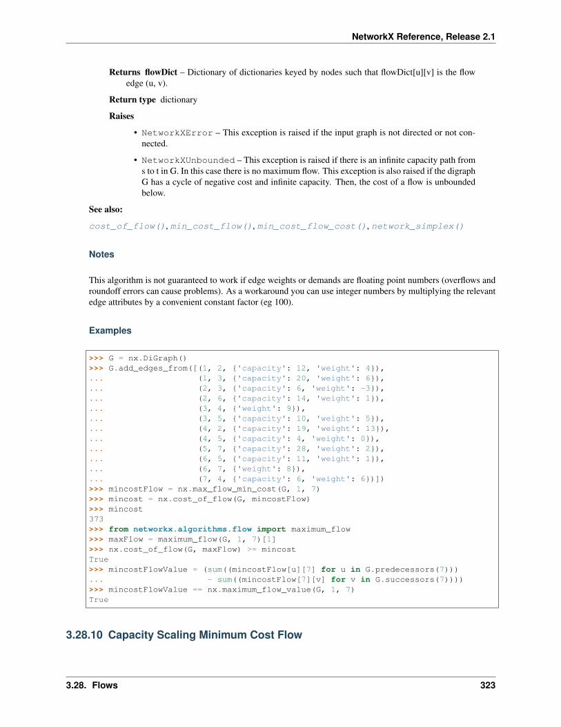
NetworkX Reference, Release 2.1
Returns flowDict – Dictionary of dictionaries keyed by nodes such that flowDict[u][v] is the flowedge (u, v).
Return type dictionary
Raises
• NetworkXError – This exception is raised if the input graph is not directed or not con-nected.
• NetworkXUnbounded – This exception is raised if there is an infinite capacity path froms to t in G. In this case there is no maximum flow. This exception is also raised if the digraphG has a cycle of negative cost and infinite capacity. Then, the cost of a flow is unboundedbelow.
See also:
cost_of_flow(), min_cost_flow(), min_cost_flow_cost(), network_simplex()
Notes
This algorithm is not guaranteed to work if edge weights or demands are floating point numbers (overflows androundoff errors can cause problems). As a workaround you can use integer numbers by multiplying the relevantedge attributes by a convenient constant factor (eg 100).
Examples
>>> G = nx.DiGraph()>>> G.add_edges_from([(1, 2, {'capacity': 12, 'weight': 4}),... (1, 3, {'capacity': 20, 'weight': 6}),... (2, 3, {'capacity': 6, 'weight': -3}),... (2, 6, {'capacity': 14, 'weight': 1}),... (3, 4, {'weight': 9}),... (3, 5, {'capacity': 10, 'weight': 5}),... (4, 2, {'capacity': 19, 'weight': 13}),... (4, 5, {'capacity': 4, 'weight': 0}),... (5, 7, {'capacity': 28, 'weight': 2}),... (6, 5, {'capacity': 11, 'weight': 1}),... (6, 7, {'weight': 8}),... (7, 4, {'capacity': 6, 'weight': 6})])>>> mincostFlow = nx.max_flow_min_cost(G, 1, 7)>>> mincost = nx.cost_of_flow(G, mincostFlow)>>> mincost373>>> from networkx.algorithms.flow import maximum_flow>>> maxFlow = maximum_flow(G, 1, 7)[1]>>> nx.cost_of_flow(G, maxFlow) >= mincostTrue>>> mincostFlowValue = (sum((mincostFlow[u][7] for u in G.predecessors(7)))... - sum((mincostFlow[7][v] for v in G.successors(7))))>>> mincostFlowValue == nx.maximum_flow_value(G, 1, 7)True
3.28.10 Capacity Scaling Minimum Cost Flow
3.28. Flows 323
NetworkX Reference, Release 2.1
capacity_scaling(G[, demand, capacity, . . . ]) Find a minimum cost flow satisfying all demands in di-graph G.
networkx.algorithms.flow.capacity_scaling
capacity_scaling(G, demand=’demand’, capacity=’capacity’, weight=’weight’, heap=<class ’net-workx.utils.heaps.BinaryHeap’>)
Find a minimum cost flow satisfying all demands in digraph G.
This is a capacity scaling successive shortest augmenting path algorithm.
G is a digraph with edge costs and capacities and in which nodes have demand, i.e., they want to send or receivesome amount of flow. A negative demand means that the node wants to send flow, a positive demand meansthat the node want to receive flow. A flow on the digraph G satisfies all demand if the net flow into each node isequal to the demand of that node.
Parameters
• G (NetworkX graph) – DiGraph or MultiDiGraph on which a minimum cost flow satisfyingall demands is to be found.
• demand (string) – Nodes of the graph G are expected to have an attribute demand that indi-cates how much flow a node wants to send (negative demand) or receive (positive demand).Note that the sum of the demands should be 0 otherwise the problem in not feasible. If thisattribute is not present, a node is considered to have 0 demand. Default value: ‘demand’.
• capacity (string) – Edges of the graph G are expected to have an attribute capacity thatindicates how much flow the edge can support. If this attribute is not present, the edge isconsidered to have infinite capacity. Default value: ‘capacity’.
• weight (string) – Edges of the graph G are expected to have an attribute weight that indicatesthe cost incurred by sending one unit of flow on that edge. If not present, the weight isconsidered to be 0. Default value: ‘weight’.
• heap (class) – Type of heap to be used in the algorithm. It should be a subclass of MinHeapor implement a compatible interface.
If a stock heap implementation is to be used, BinaryHeap is recommeded overPairingHeap for Python implementations without optimized attribute accesses (e.g.,CPython) despite a slower asymptotic running time. For Python implementations with opti-mized attribute accesses (e.g., PyPy), PairingHeap provides better performance. Defaultvalue: BinaryHeap.
Returns
• flowCost (integer) – Cost of a minimum cost flow satisfying all demands.
• flowDict (dictionary) – If G is a digraph, a dict-of-dicts keyed by nodes such that flow-Dict[u][v] is the flow on edge (u, v). If G is a MultiDiGraph, a dict-of-dicts-of-dicts keyedby nodes so that flowDict[u][v][key] is the flow on edge (u, v, key).
Raises
• NetworkXError – This exception is raised if the input graph is not directed, not con-nected.
• NetworkXUnfeasible – This exception is raised in the following situations:
– The sum of the demands is not zero. Then, there is no flow satisfying all demands.
– There is no flow satisfying all demand.
324 Chapter 3. Algorithms

NetworkX Reference, Release 2.1
• NetworkXUnbounded – This exception is raised if the digraph G has a cycle of negativecost and infinite capacity. Then, the cost of a flow satisfying all demands is unboundedbelow.
Notes
This algorithm does not work if edge weights are floating-point numbers.
See also:
network_simplex()
Examples
A simple example of a min cost flow problem.
>>> import networkx as nx>>> G = nx.DiGraph()>>> G.add_node('a', demand = -5)>>> G.add_node('d', demand = 5)>>> G.add_edge('a', 'b', weight = 3, capacity = 4)>>> G.add_edge('a', 'c', weight = 6, capacity = 10)>>> G.add_edge('b', 'd', weight = 1, capacity = 9)>>> G.add_edge('c', 'd', weight = 2, capacity = 5)>>> flowCost, flowDict = nx.capacity_scaling(G)>>> flowCost24>>> flowDict{'a': {'c': 1, 'b': 4}, 'c': {'d': 1}, 'b': {'d': 4}, 'd': {}}
It is possible to change the name of the attributes used for the algorithm.
>>> G = nx.DiGraph()>>> G.add_node('p', spam = -4)>>> G.add_node('q', spam = 2)>>> G.add_node('a', spam = -2)>>> G.add_node('d', spam = -1)>>> G.add_node('t', spam = 2)>>> G.add_node('w', spam = 3)>>> G.add_edge('p', 'q', cost = 7, vacancies = 5)>>> G.add_edge('p', 'a', cost = 1, vacancies = 4)>>> G.add_edge('q', 'd', cost = 2, vacancies = 3)>>> G.add_edge('t', 'q', cost = 1, vacancies = 2)>>> G.add_edge('a', 't', cost = 2, vacancies = 4)>>> G.add_edge('d', 'w', cost = 3, vacancies = 4)>>> G.add_edge('t', 'w', cost = 4, vacancies = 1)>>> flowCost, flowDict = nx.capacity_scaling(G, demand = 'spam',... capacity = 'vacancies',... weight = 'cost')>>> flowCost37>>> flowDict{'a': {'t': 4}, 'd': {'w': 2}, 'q': {'d': 1}, 'p': {'q': 2, 'a': 2}, 't': {'q': 1,→˓ 'w': 1}, 'w': {}}
3.28. Flows 325

NetworkX Reference, Release 2.1
3.29 Graphical degree sequence
Test sequences for graphiness.
is_graphical(sequence[, method]) Returns True if sequence is a valid degree sequence.is_digraphical(in_sequence, out_sequence) Returns True if some directed graph can realize the in- and
out-degree sequences.is_multigraphical(sequence) Returns True if some multigraph can realize the sequence.is_pseudographical(sequence) Returns True if some pseudograph can realize the se-
quence.is_valid_degree_sequence_havel_hakimi(. . . ) Returns True if deg_sequence can be realized by a simple
graph.is_valid_degree_sequence_erdos_gallai(. . . ) Returns True if deg_sequence can be realized by a simple
graph.
3.29.1 networkx.algorithms.graphical.is_graphical
is_graphical(sequence, method=’eg’)Returns True if sequence is a valid degree sequence.
A degree sequence is valid if some graph can realize it.
Parameters
• sequence (list or iterable container) – A sequence of integer node degrees
• method (“eg” | “hh”) – The method used to validate the degree sequence. “eg” correspondsto the Erdos-Gallai algorithm, and “hh” to the Havel-Hakimi algorithm.
Returns valid – True if the sequence is a valid degree sequence and False if not.
Return type bool
Examples
>>> G = nx.path_graph(4)>>> sequence = (d for n, d in G.degree())>>> nx.is_graphical(sequence)True
References
Erdos-Gallai [EG1960], [choudum1986]
Havel-Hakimi [havel1955], [hakimi1962], [CL1996]
3.29.2 networkx.algorithms.graphical.is_digraphical
is_digraphical(in_sequence, out_sequence)Returns True if some directed graph can realize the in- and out-degree sequences.
Parameters
326 Chapter 3. Algorithms

NetworkX Reference, Release 2.1
• in_sequence (list or iterable container) – A sequence of integer node in-degrees
• out_sequence (list or iterable container) – A sequence of integer node out-degrees
Returns valid – True if in and out-sequences are digraphic False if not.
Return type bool
Notes
This algorithm is from Kleitman and Wang1. The worst case runtime is 𝑂(𝑠× log 𝑛) where 𝑠 and 𝑛 are the sumand length of the sequences respectively.
References
3.29.3 networkx.algorithms.graphical.is_multigraphical
is_multigraphical(sequence)Returns True if some multigraph can realize the sequence.
Parameters deg_sequence (list) – A list of integers
Returns valid – True if deg_sequence is a multigraphic degree sequence and False if not.
Return type bool
Notes
The worst-case run time is 𝑂(𝑛) where 𝑛 is the length of the sequence.
References
3.29.4 networkx.algorithms.graphical.is_pseudographical
is_pseudographical(sequence)Returns True if some pseudograph can realize the sequence.
Every nonnegative integer sequence with an even sum is pseudographical (see1).
Parameters sequence (list or iterable container) – A sequence of integer node degrees
Returns valid – True if the sequence is a pseudographic degree sequence and False if not.
Return type bool
Notes
The worst-case run time is 𝑂(𝑛) where n is the length of the sequence.
1 D.J. Kleitman and D.L. Wang Algorithms for Constructing Graphs and Digraphs with Given Valences and Factors, Discrete Mathematics,6(1), pp. 79-88 (1973)
1 F. Boesch and F. Harary. “Line removal algorithms for graphs and their degree lists”, IEEE Trans. Circuits and Systems, CAS-23(12), pp.778-782 (1976).
3.29. Graphical degree sequence 327

NetworkX Reference, Release 2.1
References
3.29.5 networkx.algorithms.graphical.is_valid_degree_sequence_havel_hakimi
is_valid_degree_sequence_havel_hakimi(deg_sequence)Returns True if deg_sequence can be realized by a simple graph.
The validation proceeds using the Havel-Hakimi theorem. Worst-case run time is 𝑂(𝑠) where 𝑠 is the sum ofthe sequence.
Parameters deg_sequence (list) – A list of integers where each element specifies the degree of anode in a graph.
Returns valid – True if deg_sequence is graphical and False if not.
Return type bool
Notes
The ZZ condition says that for the sequence d if
|𝑑| >=(max(𝑑) + min(𝑑) + 1)2
4 * min(𝑑)
then d is graphical. This was shown in Theorem 6 in1.
References
[havel1955], [hakimi1962], [CL1996]
3.29.6 networkx.algorithms.graphical.is_valid_degree_sequence_erdos_gallai
is_valid_degree_sequence_erdos_gallai(deg_sequence)Returns True if deg_sequence can be realized by a simple graph.
The validation is done using the Erdos-Gallai theorem [EG1960].
Parameters deg_sequence (list) – A list of integers
Returns valid – True if deg_sequence is graphical and False if not.
Return type bool
Notes
This implementation uses an equivalent form of the Erdos-Gallai criterion. Worst-case run time is 𝑂(𝑛) where𝑛 is the length of the sequence.
Specifically, a sequence d is graphical if and only if the sum of the sequence is even and for all strong indices kin the sequence,
1 I.E. Zverovich and V.E. Zverovich. “Contributions to the theory of graphic sequences”, Discrete Mathematics, 105, pp. 292-303 (1992).
328 Chapter 3. Algorithms
NetworkX Reference, Release 2.1
𝑘∑𝑖=1
𝑑𝑖 ≤ 𝑘(𝑘 − 1) +
𝑛∑𝑗=𝑘+1
min(𝑑𝑖, 𝑘) = 𝑘(𝑛− 1) − (𝑘
𝑘−1∑𝑗=0
𝑛𝑗 −𝑘−1∑𝑗=0
𝑗𝑛𝑗)
A strong index k is any index where d_k >= k and the value n_j is the number of occurrences of j in d. Themaximal strong index is called the Durfee index.
This particular rearrangement comes from the proof of Theorem 3 in2.
The ZZ condition says that for the sequence d if
|𝑑| >=(max(𝑑) + min(𝑑) + 1)2
4 * min(𝑑)
then d is graphical. This was shown in Theorem 6 in2.
References
[EG1960], [choudum1986]
3.30 Hierarchy
Flow Hierarchy.
flow_hierarchy(G[, weight]) Returns the flow hierarchy of a directed network.
3.30.1 networkx.algorithms.hierarchy.flow_hierarchy
flow_hierarchy(G, weight=None)Returns the flow hierarchy of a directed network.
Flow hierarchy is defined as the fraction of edges not participating in cycles in a directed graph1.
Parameters
• G (DiGraph or MultiDiGraph) – A directed graph
• weight (key,optional (default=None)) – Attribute to use for node weights. If None theweight defaults to 1.
Returns h – Flow heirarchy value
Return type float
Notes
The algorithm described in1 computes the flow hierarchy through exponentiation of the adjacency matrix. Thisfunction implements an alternative approach that finds strongly connected components. An edge is in a cycle if
2 I.E. Zverovich and V.E. Zverovich. “Contributions to the theory of graphic sequences”, Discrete Mathematics, 105, pp. 292-303 (1992).1 Luo, J.; Magee, C.L. (2011), Detecting evolving patterns of self-organizing networks by flow hierarchy measurement, Complexity, Volume 16
Issue 6 53-61. DOI: 10.1002/cplx.20368 http://web.mit.edu/~cmagee/www/documents/28-DetectingEvolvingPatterns_FlowHierarchy.pdf
3.30. Hierarchy 329

NetworkX Reference, Release 2.1
and only if it is in a strongly connected component, which can be found in 𝑂(𝑚) time using Tarjan’s algorithm.
References
3.31 Hybrid
Provides functions for finding and testing for locally (k, l)-connected graphs.
kl_connected_subgraph(G, k, l[, low_memory,. . . ])
Returns the maximum locally (k, l)-connected sub-graph of G.
is_kl_connected(G, k, l[, low_memory]) Returns True if and only if G is locally (k, l)-connected.
3.31.1 networkx.algorithms.hybrid.kl_connected_subgraph
kl_connected_subgraph(G, k, l, low_memory=False, same_as_graph=False)Returns the maximum locally (k, l)-connected subgraph of G.
A graph is locally (k, l)-connected if for each edge (u, v) in the graph there are at least l edge-disjointpaths of length at most k joining u to v.
Parameters
• G (NetworkX graph) – The graph in which to find a maximum locally (k, l)-connectedsubgraph.
• k (integer) – The maximum length of paths to consider. A higher number means a looserconnectivity requirement.
• l (integer) – The number of edge-disjoint paths. A higher number means a stricter connec-tivity requirement.
• low_memory (bool) – If this is True, this function uses an algorithm that uses slightly moretime but less memory.
• same_as_graph (bool) – If True then return a tuple of the form (H, is_same), whereH is the maximum locally (k, l)-connected subgraph and is_same is a Boolean repre-senting whether G is locally (k, l)-connected (and hence, whether H is simply a copy ofthe input graph G).
Returns If same_as_graph is True, then this function returns a two-tuple as described above.Otherwise, it returns only the maximum locally (k, l)-connected subgraph.
Return type NetworkX graph or two-tuple
See also:
is_kl_connected()
References
3.31.2 networkx.algorithms.hybrid.is_kl_connected
is_kl_connected(G, k, l, low_memory=False)Returns True if and only if G is locally (k, l)-connected.
330 Chapter 3. Algorithms

NetworkX Reference, Release 2.1
A graph is locally (k, l)-connected if for each edge (u, v) in the graph there are at least l edge-disjointpaths of length at most k joining u to v.
Parameters
• G (NetworkX graph) – The graph to test for local (k, l)-connectedness.
• k (integer) – The maximum length of paths to consider. A higher number means a looserconnectivity requirement.
• l (integer) – The number of edge-disjoint paths. A higher number means a stricter connec-tivity requirement.
• low_memory (bool) – If this is True, this function uses an algorithm that uses slightly moretime but less memory.
Returns Whether the graph is locally (k, l)-connected subgraph.
Return type bool
See also:
kl_connected_subgraph()
References
3.32 Isolates
Functions for identifying isolate (degree zero) nodes.
is_isolate(G, n) Determines whether a node is an isolate.isolates(G) Iterator over isolates in the graph.
3.32.1 networkx.algorithms.isolate.is_isolate
is_isolate(G, n)Determines whether a node is an isolate.
An isolate is a node with no neighbors (that is, with degree zero). For directed graphs, this means no in-neighborsand no out-neighbors.
Parameters
• G (NetworkX graph)
• n (node) – A node in G.
Returns is_isolate – True if and only if n has no neighbors.
Return type bool
Examples
>>> G=nx.Graph()>>> G.add_edge(1,2)>>> G.add_node(3)>>> nx.is_isolate(G,2)
3.32. Isolates 331

NetworkX Reference, Release 2.1
False>>> nx.is_isolate(G,3)True
3.32.2 networkx.algorithms.isolate.isolates
isolates(G)Iterator over isolates in the graph.
An isolate is a node with no neighbors (that is, with degree zero). For directed graphs, this means no in-neighborsand no out-neighbors.
Parameters G (NetworkX graph)
Returns An iterator over the isolates of G.
Return type iterator
Examples
To get a list of all isolates of a graph, use the list constructor:
>>> G = nx.Graph()>>> G.add_edge(1, 2)>>> G.add_node(3)>>> list(nx.isolates(G))[3]
To remove all isolates in the graph, first create a list of the isolates, then use Graph.remove_nodes_from():
>>> G.remove_nodes_from(list(nx.isolates(G)))>>> list(G)[1, 2]
For digraphs, isolates have zero in-degree and zero out_degre:
>>> G = nx.DiGraph([(0, 1), (1, 2)])>>> G.add_node(3)>>> list(nx.isolates(G))[3]
3.33 Isomorphism
is_isomorphic(G1, G2[, node_match, edge_match]) Returns True if the graphs G1 and G2 are isomorphic andFalse otherwise.
could_be_isomorphic(G1, G2) Returns False if graphs are definitely not isomorphic.fast_could_be_isomorphic(G1, G2) Returns False if graphs are definitely not isomorphic.faster_could_be_isomorphic(G1, G2) Returns False if graphs are definitely not isomorphic.
332 Chapter 3. Algorithms

NetworkX Reference, Release 2.1
3.33.1 networkx.algorithms.isomorphism.is_isomorphic
is_isomorphic(G1, G2, node_match=None, edge_match=None)Returns True if the graphs G1 and G2 are isomorphic and False otherwise.
Parameters
• G1, G2 (graphs) – The two graphs G1 and G2 must be the same type.
• node_match (callable) – A function that returns True if node n1 in G1 and n2 in G2 shouldbe considered equal during the isomorphism test. If node_match is not specified then nodeattributes are not considered.
The function will be called like
node_match(G1.nodes[n1], G2.nodes[n2]).
That is, the function will receive the node attribute dictionaries for n1 and n2 as inputs.
• edge_match (callable) – A function that returns True if the edge attribute dictionary forthe pair of nodes (u1, v1) in G1 and (u2, v2) in G2 should be considered equal during theisomorphism test. If edge_match is not specified then edge attributes are not considered.
The function will be called like
edge_match(G1[u1][v1], G2[u2][v2]).
That is, the function will receive the edge attribute dictionaries of the edges under consider-ation.
Notes
Uses the vf2 algorithm1.
Examples
>>> import networkx.algorithms.isomorphism as iso
For digraphs G1 and G2, using ‘weight’ edge attribute (default: 1)
>>> G1 = nx.DiGraph()>>> G2 = nx.DiGraph()>>> nx.add_path(G1, [1,2,3,4], weight=1)>>> nx.add_path(G2, [10,20,30,40], weight=2)>>> em = iso.numerical_edge_match('weight', 1)>>> nx.is_isomorphic(G1, G2) # no weights consideredTrue>>> nx.is_isomorphic(G1, G2, edge_match=em) # match weightsFalse
For multidigraphs G1 and G2, using ‘fill’ node attribute (default: ‘’)
>>> G1 = nx.MultiDiGraph()>>> G2 = nx.MultiDiGraph()>>> G1.add_nodes_from([1,2,3], fill='red')>>> G2.add_nodes_from([10,20,30,40], fill='red')
1 L. P. Cordella, P. Foggia, C. Sansone, M. Vento, “An Improved Algorithm for Matching Large Graphs”, 3rd IAPR-TC15 Workshop on Graph-based Representations in Pattern Recognition, Cuen, pp. 149-159, 2001. http://amalfi.dis.unina.it/graph/db/papers/vf-algorithm.pdf
3.33. Isomorphism 333

NetworkX Reference, Release 2.1
>>> nx.add_path(G1, [1,2,3,4], weight=3, linewidth=2.5)>>> nx.add_path(G2, [10,20,30,40], weight=3)>>> nm = iso.categorical_node_match('fill', 'red')>>> nx.is_isomorphic(G1, G2, node_match=nm)True
For multidigraphs G1 and G2, using ‘weight’ edge attribute (default: 7)
>>> G1.add_edge(1,2, weight=7)1>>> G2.add_edge(10,20)1>>> em = iso.numerical_multiedge_match('weight', 7, rtol=1e-6)>>> nx.is_isomorphic(G1, G2, edge_match=em)True
For multigraphs G1 and G2, using ‘weight’ and ‘linewidth’ edge attributes with default values 7 and 2.5. Alsousing ‘fill’ node attribute with default value ‘red’.
>>> em = iso.numerical_multiedge_match(['weight', 'linewidth'], [7, 2.5])>>> nm = iso.categorical_node_match('fill', 'red')>>> nx.is_isomorphic(G1, G2, edge_match=em, node_match=nm)True
See also:
numerical_node_match(), numerical_edge_match(), numerical_multiedge_match(),categorical_node_match(), categorical_edge_match(), categorical_multiedge_match()
References
3.33.2 networkx.algorithms.isomorphism.could_be_isomorphic
could_be_isomorphic(G1, G2)Returns False if graphs are definitely not isomorphic. True does NOT guarantee isomorphism.
Parameters G1, G2 (graphs) – The two graphs G1 and G2 must be the same type.
Notes
Checks for matching degree, triangle, and number of cliques sequences.
3.33.3 networkx.algorithms.isomorphism.fast_could_be_isomorphic
fast_could_be_isomorphic(G1, G2)Returns False if graphs are definitely not isomorphic.
True does NOT guarantee isomorphism.
Parameters G1, G2 (graphs) – The two graphs G1 and G2 must be the same type.
334 Chapter 3. Algorithms

NetworkX Reference, Release 2.1
Notes
Checks for matching degree and triangle sequences.
3.33.4 networkx.algorithms.isomorphism.faster_could_be_isomorphic
faster_could_be_isomorphic(G1, G2)Returns False if graphs are definitely not isomorphic.
True does NOT guarantee isomorphism.
Parameters G1, G2 (graphs) – The two graphs G1 and G2 must be the same type.
Notes
Checks for matching degree sequences.
3.33.5 Advanced Interface to VF2 Algorithm
VF2 Algorithm
VF2 Algorithm
An implementation of VF2 algorithm for graph ismorphism testing.
The simplest interface to use this module is to call networkx.is_isomorphic().
Introduction
The GraphMatcher and DiGraphMatcher are responsible for matching graphs or directed graphs in a predeterminedmanner. This usually means a check for an isomorphism, though other checks are also possible. For example, asubgraph of one graph can be checked for isomorphism to a second graph.
Matching is done via syntactic feasibility. It is also possible to check for semantic feasibility. Feasibility, then, isdefined as the logical AND of the two functions.
To include a semantic check, the (Di)GraphMatcher class should be subclassed, and the semantic_feasibility() functionshould be redefined. By default, the semantic feasibility function always returns True. The effect of this is thatsemantics are not considered in the matching of G1 and G2.
Examples
Suppose G1 and G2 are isomorphic graphs. Verification is as follows:
>>> from networkx.algorithms import isomorphism>>> G1 = nx.path_graph(4)>>> G2 = nx.path_graph(4)>>> GM = isomorphism.GraphMatcher(G1,G2)>>> GM.is_isomorphic()True
3.33. Isomorphism 335

NetworkX Reference, Release 2.1
GM.mapping stores the isomorphism mapping from G1 to G2.
>>> GM.mapping{0: 0, 1: 1, 2: 2, 3: 3}
Suppose G1 and G2 are isomorphic directed graphs graphs. Verification is as follows:
>>> G1 = nx.path_graph(4, create_using=nx.DiGraph())>>> G2 = nx.path_graph(4, create_using=nx.DiGraph())>>> DiGM = isomorphism.DiGraphMatcher(G1,G2)>>> DiGM.is_isomorphic()True
DiGM.mapping stores the isomorphism mapping from G1 to G2.
>>> DiGM.mapping{0: 0, 1: 1, 2: 2, 3: 3}
Subgraph Isomorphism
Graph theory literature can be ambiguious about the meaning of the above statement, and we seek to clarify it now.
In the VF2 literature, a mapping M is said to be a graph-subgraph isomorphism iff M is an isomorphism between G2and a subgraph of G1. Thus, to say that G1 and G2 are graph-subgraph isomorphic is to say that a subgraph of G1 isisomorphic to G2.
Other literature uses the phrase ‘subgraph isomorphic’ as in ‘G1 does not have a subgraph isomorphic to G2’. Anotheruse is as an in adverb for isomorphic. Thus, to say that G1 and G2 are subgraph isomorphic is to say that a subgraphof G1 is isomorphic to G2.
Finally, the term ‘subgraph’ can have multiple meanings. In this context, ‘subgraph’ always means a ‘node-inducedsubgraph’. Edge-induced subgraph isomorphisms are not directly supported, but one should be able to perform thecheck by making use of nx.line_graph(). For subgraphs which are not induced, the term ‘monomorphism’ is preferredover ‘isomorphism’. Currently, it is not possible to check for monomorphisms.
Let G=(N,E) be a graph with a set of nodes N and set of edges E.
If G’=(N’,E’) is a subgraph, then: N’ is a subset of N E’ is a subset of E
If G’=(N’,E’) is a node-induced subgraph, then: N’ is a subset of N E’ is the subset of edges in E relating nodes inN’
If G’=(N’,E’) is an edge-induced subgraph, then: N’ is the subset of nodes in N related by edges in E’ E’ is a subsetof E
References
[1] Luigi P. Cordella, Pasquale Foggia, Carlo Sansone, Mario Vento, “A (Sub)Graph Isomorphism Algorithm forMatching Large Graphs”, IEEE Transactions on Pattern Analysis and Machine Intelligence, vol. 26, no. 10, pp.1367-1372, Oct., 2004. http://ieeexplore.ieee.org/iel5/34/29305/01323804.pdf
[2] L. P. Cordella, P. Foggia, C. Sansone, M. Vento, “An Improved Algorithm for Matching Large Graphs”, 3rdIAPR-TC15 Workshop on Graph-based Representations in Pattern Recognition, Cuen, pp. 149-159, 2001.http://amalfi.dis.unina.it/graph/db/papers/vf-algorithm.pdf
See also:
syntactic_feasibliity, semantic_feasibility
336 Chapter 3. Algorithms

NetworkX Reference, Release 2.1
Notes
The implementation handles both directed and undirected graphs as well as multigraphs. However, it does require thatnodes in the graph are orderable (in addition to the general NetworkX requirement that nodes are hashable). If thenodes in your graph are not orderable, you can convert them to an orderable type (int, for example) by using thenetworkx.relabel() function. You can store the dictionary of old-to-new node labels to retrieve the originalnode labels after running the isomorphism algorithm:
>>> G = nx.Graph()>>> node1, node2 = object(), object()>>> G.add_nodes_from([node1, node2])>>> mapping = {k: v for v, k in enumerate(G)}>>> G = nx.relabel_nodes(G, mapping)
In general, the subgraph isomorphism problem is NP-complete whereas the graph isomorphism problem is most likelynot NP-complete (although no polynomial-time algorithm is known to exist).
Graph Matcher
GraphMatcher.__init__(G1, G2[, node_match,. . . ])
Initialize graph matcher.
GraphMatcher.initialize() Reinitializes the state of the algorithm.GraphMatcher.is_isomorphic() Returns True if G1 and G2 are isomorphic graphs.GraphMatcher.subgraph_is_isomorphic() Returns True if a subgraph of G1 is isomorphic to G2.GraphMatcher.isomorphisms_iter() Generator over isomorphisms between G1 and G2.GraphMatcher.subgraph_isomorphisms_iter() Generator over isomorphisms between a subgraph of G1
and G2.GraphMatcher.candidate_pairs_iter() Iterator over candidate pairs of nodes in G1 and G2.GraphMatcher.match() Extends the isomorphism mapping.GraphMatcher.semantic_feasibility(G1_node,. . . )
Returns True if mapping G1_node to G2_node is semanti-cally feasible.
GraphMatcher.syntactic_feasibility(G1_node,. . . )
Returns True if adding (G1_node, G2_node) is syntacti-cally feasible.
networkx.algorithms.isomorphism.GraphMatcher.__init__
GraphMatcher.__init__(G1, G2, node_match=None, edge_match=None)Initialize graph matcher.
Parameters
• G1, G2 (graph) – The graphs to be tested.
• node_match (callable) – A function that returns True iff node n1 in G1 and n2 in G2 shouldbe considered equal during the isomorphism test. The function will be called like:
node_match(G1.nodes[n1], G2.nodes[n2])
That is, the function will receive the node attribute dictionaries of the nodes under consider-ation. If None, then no attributes are considered when testing for an isomorphism.
• edge_match (callable) – A function that returns True iff the edge attribute dictionary forthe pair of nodes (u1, v1) in G1 and (u2, v2) in G2 should be considered equal during theisomorphism test. The function will be called like:
3.33. Isomorphism 337

NetworkX Reference, Release 2.1
edge_match(G1[u1][v1], G2[u2][v2])
That is, the function will receive the edge attribute dictionaries of the edges under consider-ation. If None, then no attributes are considered when testing for an isomorphism.
networkx.algorithms.isomorphism.GraphMatcher.initialize
GraphMatcher.initialize()Reinitializes the state of the algorithm.
This method should be redefined if using something other than GMState. If only subclassing GraphMatcher, aredefinition is not necessary.
networkx.algorithms.isomorphism.GraphMatcher.is_isomorphic
GraphMatcher.is_isomorphic()Returns True if G1 and G2 are isomorphic graphs.
networkx.algorithms.isomorphism.GraphMatcher.subgraph_is_isomorphic
GraphMatcher.subgraph_is_isomorphic()Returns True if a subgraph of G1 is isomorphic to G2.
networkx.algorithms.isomorphism.GraphMatcher.isomorphisms_iter
GraphMatcher.isomorphisms_iter()Generator over isomorphisms between G1 and G2.
networkx.algorithms.isomorphism.GraphMatcher.subgraph_isomorphisms_iter
GraphMatcher.subgraph_isomorphisms_iter()Generator over isomorphisms between a subgraph of G1 and G2.
networkx.algorithms.isomorphism.GraphMatcher.candidate_pairs_iter
GraphMatcher.candidate_pairs_iter()Iterator over candidate pairs of nodes in G1 and G2.
networkx.algorithms.isomorphism.GraphMatcher.match
GraphMatcher.match()Extends the isomorphism mapping.
This function is called recursively to determine if a complete isomorphism can be found between G1 and G2. Itcleans up the class variables after each recursive call. If an isomorphism is found, we yield the mapping.
338 Chapter 3. Algorithms

NetworkX Reference, Release 2.1
networkx.algorithms.isomorphism.GraphMatcher.semantic_feasibility
GraphMatcher.semantic_feasibility(G1_node, G2_node)Returns True if mapping G1_node to G2_node is semantically feasible.
networkx.algorithms.isomorphism.GraphMatcher.syntactic_feasibility
GraphMatcher.syntactic_feasibility(G1_node, G2_node)Returns True if adding (G1_node, G2_node) is syntactically feasible.
This function returns True if it is adding the candidate pair to the current partial isomorphism mapping isallowable. The addition is allowable if the inclusion of the candidate pair does not make it impossible for anisomorphism to be found.
DiGraph Matcher
DiGraphMatcher.__init__(G1, G2[, . . . ]) Initialize graph matcher.DiGraphMatcher.initialize() Reinitializes the state of the algorithm.DiGraphMatcher.is_isomorphic() Returns True if G1 and G2 are isomorphic graphs.DiGraphMatcher.subgraph_is_isomorphic() Returns True if a subgraph of G1 is isomorphic to G2.DiGraphMatcher.isomorphisms_iter() Generator over isomorphisms between G1 and G2.DiGraphMatcher.subgraph_isomorphisms_iter()Generator over isomorphisms between a subgraph of G1
and G2.DiGraphMatcher.candidate_pairs_iter() Iterator over candidate pairs of nodes in G1 and G2.DiGraphMatcher.match() Extends the isomorphism mapping.DiGraphMatcher.semantic_feasibility(G1_node,. . . )
Returns True if mapping G1_node to G2_node is semanti-cally feasible.
DiGraphMatcher.syntactic_feasibility(. . . ) Returns True if adding (G1_node, G2_node) is syntacti-cally feasible.
networkx.algorithms.isomorphism.DiGraphMatcher.__init__
DiGraphMatcher.__init__(G1, G2, node_match=None, edge_match=None)Initialize graph matcher.
Parameters
• G1, G2 (graph) – The graphs to be tested.
• node_match (callable) – A function that returns True iff node n1 in G1 and n2 in G2 shouldbe considered equal during the isomorphism test. The function will be called like:
node_match(G1.nodes[n1], G2.nodes[n2])
That is, the function will receive the node attribute dictionaries of the nodes under consider-ation. If None, then no attributes are considered when testing for an isomorphism.
• edge_match (callable) – A function that returns True iff the edge attribute dictionary forthe pair of nodes (u1, v1) in G1 and (u2, v2) in G2 should be considered equal during theisomorphism test. The function will be called like:
edge_match(G1[u1][v1], G2[u2][v2])
3.33. Isomorphism 339

NetworkX Reference, Release 2.1
That is, the function will receive the edge attribute dictionaries of the edges under consider-ation. If None, then no attributes are considered when testing for an isomorphism.
networkx.algorithms.isomorphism.DiGraphMatcher.initialize
DiGraphMatcher.initialize()Reinitializes the state of the algorithm.
This method should be redefined if using something other than DiGMState. If only subclassing GraphMatcher,a redefinition is not necessary.
networkx.algorithms.isomorphism.DiGraphMatcher.is_isomorphic
DiGraphMatcher.is_isomorphic()Returns True if G1 and G2 are isomorphic graphs.
networkx.algorithms.isomorphism.DiGraphMatcher.subgraph_is_isomorphic
DiGraphMatcher.subgraph_is_isomorphic()Returns True if a subgraph of G1 is isomorphic to G2.
networkx.algorithms.isomorphism.DiGraphMatcher.isomorphisms_iter
DiGraphMatcher.isomorphisms_iter()Generator over isomorphisms between G1 and G2.
networkx.algorithms.isomorphism.DiGraphMatcher.subgraph_isomorphisms_iter
DiGraphMatcher.subgraph_isomorphisms_iter()Generator over isomorphisms between a subgraph of G1 and G2.
networkx.algorithms.isomorphism.DiGraphMatcher.candidate_pairs_iter
DiGraphMatcher.candidate_pairs_iter()Iterator over candidate pairs of nodes in G1 and G2.
networkx.algorithms.isomorphism.DiGraphMatcher.match
DiGraphMatcher.match()Extends the isomorphism mapping.
This function is called recursively to determine if a complete isomorphism can be found between G1 and G2. Itcleans up the class variables after each recursive call. If an isomorphism is found, we yield the mapping.
340 Chapter 3. Algorithms

NetworkX Reference, Release 2.1
networkx.algorithms.isomorphism.DiGraphMatcher.semantic_feasibility
DiGraphMatcher.semantic_feasibility(G1_node, G2_node)Returns True if mapping G1_node to G2_node is semantically feasible.
networkx.algorithms.isomorphism.DiGraphMatcher.syntactic_feasibility
DiGraphMatcher.syntactic_feasibility(G1_node, G2_node)Returns True if adding (G1_node, G2_node) is syntactically feasible.
This function returns True if it is adding the candidate pair to the current partial isomorphism mapping isallowable. The addition is allowable if the inclusion of the candidate pair does not make it impossible for anisomorphism to be found.
Match helpers
categorical_node_match(attr, default) Returns a comparison function for a categorical node at-tribute.
categorical_edge_match(attr, default) Returns a comparison function for a categorical edge at-tribute.
categorical_multiedge_match(attr, default) Returns a comparison function for a categorical edge at-tribute.
numerical_node_match(attr, default[, rtol, atol]) Returns a comparison function for a numerical node at-tribute.
numerical_edge_match(attr, default[, rtol, atol]) Returns a comparison function for a numerical edge at-tribute.
numerical_multiedge_match(attr, default[, . . . ]) Returns a comparison function for a numerical edge at-tribute.
generic_node_match(attr, default, op) Returns a comparison function for a generic attribute.generic_edge_match(attr, default, op) Returns a comparison function for a generic attribute.generic_multiedge_match(attr, default, op) Returns a comparison function for a generic attribute.
networkx.algorithms.isomorphism.categorical_node_match
categorical_node_match(attr, default)Returns a comparison function for a categorical node attribute.
The value(s) of the attr(s) must be hashable and comparable via the == operator since they are placed into aset([]) object. If the sets from G1 and G2 are the same, then the constructed function returns True.
Parameters
• attr (string | list) – The categorical node attribute to compare, or a list of categorical nodeattributes to compare.
• default (value | list) – The default value for the categorical node attribute, or a list of defaultvalues for the categorical node attributes.
Returns match – The customized, categorical node_match function.
Return type function
3.33. Isomorphism 341

NetworkX Reference, Release 2.1
Examples
>>> import networkx.algorithms.isomorphism as iso>>> nm = iso.categorical_node_match('size', 1)>>> nm = iso.categorical_node_match(['color', 'size'], ['red', 2])
networkx.algorithms.isomorphism.categorical_edge_match
categorical_edge_match(attr, default)Returns a comparison function for a categorical edge attribute.
The value(s) of the attr(s) must be hashable and comparable via the == operator since they are placed into aset([]) object. If the sets from G1 and G2 are the same, then the constructed function returns True.
Parameters
• attr (string | list) – The categorical edge attribute to compare, or a list of categorical edgeattributes to compare.
• default (value | list) – The default value for the categorical edge attribute, or a list of defaultvalues for the categorical edge attributes.
Returns match – The customized, categorical edge_match function.
Return type function
Examples
>>> import networkx.algorithms.isomorphism as iso>>> nm = iso.categorical_edge_match('size', 1)>>> nm = iso.categorical_edge_match(['color', 'size'], ['red', 2])
networkx.algorithms.isomorphism.categorical_multiedge_match
categorical_multiedge_match(attr, default)Returns a comparison function for a categorical edge attribute.
The value(s) of the attr(s) must be hashable and comparable via the == operator since they are placed into aset([]) object. If the sets from G1 and G2 are the same, then the constructed function returns True.
Parameters
• attr (string | list) – The categorical edge attribute to compare, or a list of categorical edgeattributes to compare.
• default (value | list) – The default value for the categorical edge attribute, or a list of defaultvalues for the categorical edge attributes.
Returns match – The customized, categorical edge_match function.
Return type function
342 Chapter 3. Algorithms

NetworkX Reference, Release 2.1
Examples
>>> import networkx.algorithms.isomorphism as iso>>> nm = iso.categorical_multiedge_match('size', 1)>>> nm = iso.categorical_multiedge_match(['color', 'size'], ['red', 2])
networkx.algorithms.isomorphism.numerical_node_match
numerical_node_match(attr, default, rtol=1e-05, atol=1e-08)Returns a comparison function for a numerical node attribute.
The value(s) of the attr(s) must be numerical and sortable. If the sorted list of values from G1 and G2 are thesame within some tolerance, then the constructed function returns True.
Parameters
• attr (string | list) – The numerical node attribute to compare, or a list of numerical nodeattributes to compare.
• default (value | list) – The default value for the numerical node attribute, or a list of defaultvalues for the numerical node attributes.
• rtol (float) – The relative error tolerance.
• atol (float) – The absolute error tolerance.
Returns match – The customized, numerical node_match function.
Return type function
Examples
>>> import networkx.algorithms.isomorphism as iso>>> nm = iso.numerical_node_match('weight', 1.0)>>> nm = iso.numerical_node_match(['weight', 'linewidth'], [.25, .5])
networkx.algorithms.isomorphism.numerical_edge_match
numerical_edge_match(attr, default, rtol=1e-05, atol=1e-08)Returns a comparison function for a numerical edge attribute.
The value(s) of the attr(s) must be numerical and sortable. If the sorted list of values from G1 and G2 are thesame within some tolerance, then the constructed function returns True.
Parameters
• attr (string | list) – The numerical edge attribute to compare, or a list of numerical edgeattributes to compare.
• default (value | list) – The default value for the numerical edge attribute, or a list of defaultvalues for the numerical edge attributes.
• rtol (float) – The relative error tolerance.
• atol (float) – The absolute error tolerance.
Returns match – The customized, numerical edge_match function.
3.33. Isomorphism 343

NetworkX Reference, Release 2.1
Return type function
Examples
>>> import networkx.algorithms.isomorphism as iso>>> nm = iso.numerical_edge_match('weight', 1.0)>>> nm = iso.numerical_edge_match(['weight', 'linewidth'], [.25, .5])
networkx.algorithms.isomorphism.numerical_multiedge_match
numerical_multiedge_match(attr, default, rtol=1e-05, atol=1e-08)Returns a comparison function for a numerical edge attribute.
The value(s) of the attr(s) must be numerical and sortable. If the sorted list of values from G1 and G2 are thesame within some tolerance, then the constructed function returns True.
Parameters
• attr (string | list) – The numerical edge attribute to compare, or a list of numerical edgeattributes to compare.
• default (value | list) – The default value for the numerical edge attribute, or a list of defaultvalues for the numerical edge attributes.
• rtol (float) – The relative error tolerance.
• atol (float) – The absolute error tolerance.
Returns match – The customized, numerical edge_match function.
Return type function
Examples
>>> import networkx.algorithms.isomorphism as iso>>> nm = iso.numerical_multiedge_match('weight', 1.0)>>> nm = iso.numerical_multiedge_match(['weight', 'linewidth'], [.25, .5])
networkx.algorithms.isomorphism.generic_node_match
generic_node_match(attr, default, op)Returns a comparison function for a generic attribute.
The value(s) of the attr(s) are compared using the specified operators. If all the attributes are equal, then theconstructed function returns True.
Parameters
• attr (string | list) – The node attribute to compare, or a list of node attributes to compare.
• default (value | list) – The default value for the node attribute, or a list of default values forthe node attributes.
• op (callable | list) – The operator to use when comparing attribute values, or a list of opera-tors to use when comparing values for each attribute.
344 Chapter 3. Algorithms

NetworkX Reference, Release 2.1
Returns match – The customized, generic node_match function.
Return type function
Examples
>>> from operator import eq>>> from networkx.algorithms.isomorphism.matchhelpers import close>>> from networkx.algorithms.isomorphism import generic_node_match>>> nm = generic_node_match('weight', 1.0, close)>>> nm = generic_node_match('color', 'red', eq)>>> nm = generic_node_match(['weight', 'color'], [1.0, 'red'], [close, eq])
networkx.algorithms.isomorphism.generic_edge_match
generic_edge_match(attr, default, op)Returns a comparison function for a generic attribute.
The value(s) of the attr(s) are compared using the specified operators. If all the attributes are equal, then theconstructed function returns True.
Parameters
• attr (string | list) – The edge attribute to compare, or a list of edge attributes to compare.
• default (value | list) – The default value for the edge attribute, or a list of default values forthe edge attributes.
• op (callable | list) – The operator to use when comparing attribute values, or a list of opera-tors to use when comparing values for each attribute.
Returns match – The customized, generic edge_match function.
Return type function
Examples
>>> from operator import eq>>> from networkx.algorithms.isomorphism.matchhelpers import close>>> from networkx.algorithms.isomorphism import generic_edge_match>>> nm = generic_edge_match('weight', 1.0, close)>>> nm = generic_edge_match('color', 'red', eq)>>> nm = generic_edge_match(['weight', 'color'], [1.0, 'red'], [close, eq])
networkx.algorithms.isomorphism.generic_multiedge_match
generic_multiedge_match(attr, default, op)Returns a comparison function for a generic attribute.
The value(s) of the attr(s) are compared using the specified operators. If all the attributes are equal, then theconstructed function returns True. Potentially, the constructed edge_match function can be slow since it mustverify that no isomorphism exists between the multiedges before it returns False.
Parameters
3.33. Isomorphism 345

NetworkX Reference, Release 2.1
• attr (string | list) – The edge attribute to compare, or a list of node attributes to compare.
• default (value | list) – The default value for the edge attribute, or a list of default values forthe dgeattributes.
• op (callable | list) – The operator to use when comparing attribute values, or a list of opera-tors to use when comparing values for each attribute.
Returns match – The customized, generic edge_match function.
Return type function
Examples
>>> from operator import eq>>> from networkx.algorithms.isomorphism.matchhelpers import close>>> from networkx.algorithms.isomorphism import generic_node_match>>> nm = generic_node_match('weight', 1.0, close)>>> nm = generic_node_match('color', 'red', eq)>>> nm = generic_node_match(['weight', 'color'],... [1.0, 'red'],... [close, eq])...
3.34 Link Analysis
3.34.1 PageRank
PageRank analysis of graph structure.
pagerank(G[, alpha, personalization, . . . ]) Return the PageRank of the nodes in the graph.pagerank_numpy(G[, alpha, personalization, . . . ]) Return the PageRank of the nodes in the graph.pagerank_scipy(G[, alpha, personalization, . . . ]) Return the PageRank of the nodes in the graph.google_matrix(G[, alpha, personalization, . . . ]) Return the Google matrix of the graph.
networkx.algorithms.link_analysis.pagerank_alg.pagerank
pagerank(G, alpha=0.85, personalization=None, max_iter=100, tol=1e-06, nstart=None, weight=’weight’,dangling=None)
Return the PageRank of the nodes in the graph.
PageRank computes a ranking of the nodes in the graph G based on the structure of the incoming links. It wasoriginally designed as an algorithm to rank web pages.
Parameters
• G (graph) – A NetworkX graph. Undirected graphs will be converted to a directed graphwith two directed edges for each undirected edge.
• alpha (float, optional) – Damping parameter for PageRank, default=0.85.
• personalization (dict, optional) – The “personalization vector” consisting of a dictionarywith a key some subset of graph nodes and personalization value each of those. At least one
346 Chapter 3. Algorithms

NetworkX Reference, Release 2.1
personalization value must be non-zero. If not specfiied, a nodes personalization value willbe zero. By default, a uniform distribution is used.
• max_iter (integer, optional) – Maximum number of iterations in power method eigenvaluesolver.
• tol (float, optional) – Error tolerance used to check convergence in power method solver.
• nstart (dictionary, optional) – Starting value of PageRank iteration for each node.
• weight (key, optional) – Edge data key to use as weight. If None weights are set to 1.
• dangling (dict, optional) – The outedges to be assigned to any “dangling” nodes, i.e., nodeswithout any outedges. The dict key is the node the outedge points to and the dict valueis the weight of that outedge. By default, dangling nodes are given outedges according tothe personalization vector (uniform if not specified). This must be selected to result in anirreducible transition matrix (see notes under google_matrix). It may be common to havethe dangling dict to be the same as the personalization dict.
Returns pagerank – Dictionary of nodes with PageRank as value
Return type dictionary
Examples
>>> G = nx.DiGraph(nx.path_graph(4))>>> pr = nx.pagerank(G, alpha=0.9)
Notes
The eigenvector calculation is done by the power iteration method and has no guarantee of convergence. Theiteration will stop after an error tolerance of len(G) * tol has been reached. If the number of iterationsexceed max_iter, a networkx.exception.PowerIterationFailedConvergence exception israised.
The PageRank algorithm was designed for directed graphs but this algorithm does not check if the input graphis directed and will execute on undirected graphs by converting each edge in the directed graph to two edges.
See also:
pagerank_numpy(), pagerank_scipy(), google_matrix()
Raises PowerIterationFailedConvergence – If the algorithm fails to converge to thespecified tolerance within the specified number of iterations of the power iteration method.
References
networkx.algorithms.link_analysis.pagerank_alg.pagerank_numpy
pagerank_numpy(G, alpha=0.85, personalization=None, weight=’weight’, dangling=None)Return the PageRank of the nodes in the graph.
PageRank computes a ranking of the nodes in the graph G based on the structure of the incoming links. It wasoriginally designed as an algorithm to rank web pages.
Parameters
3.34. Link Analysis 347

NetworkX Reference, Release 2.1
• G (graph) – A NetworkX graph. Undirected graphs will be converted to a directed graphwith two directed edges for each undirected edge.
• alpha (float, optional) – Damping parameter for PageRank, default=0.85.
• personalization (dict, optional) – The “personalization vector” consisting of a dictionarywith a key some subset of graph nodes and personalization value each of those. At least onepersonalization value must be non-zero. If not specfiied, a nodes personalization value willbe zero. By default, a uniform distribution is used.
• weight (key, optional) – Edge data key to use as weight. If None weights are set to 1.
• dangling (dict, optional) – The outedges to be assigned to any “dangling” nodes, i.e., nodeswithout any outedges. The dict key is the node the outedge points to and the dict valueis the weight of that outedge. By default, dangling nodes are given outedges according tothe personalization vector (uniform if not specified) This must be selected to result in anirreducible transition matrix (see notes under google_matrix). It may be common to havethe dangling dict to be the same as the personalization dict.
Returns pagerank – Dictionary of nodes with PageRank as value.
Return type dictionary
Examples
>>> G = nx.DiGraph(nx.path_graph(4))>>> pr = nx.pagerank_numpy(G, alpha=0.9)
Notes
The eigenvector calculation uses NumPy’s interface to the LAPACK eigenvalue solvers. This will be the fastestand most accurate for small graphs.
This implementation works with Multi(Di)Graphs. For multigraphs the weight between two nodes is set to bethe sum of all edge weights between those nodes.
See also:
pagerank(), pagerank_scipy(), google_matrix()
References
networkx.algorithms.link_analysis.pagerank_alg.pagerank_scipy
pagerank_scipy(G, alpha=0.85, personalization=None, max_iter=100, tol=1e-06, weight=’weight’, dan-gling=None)
Return the PageRank of the nodes in the graph.
PageRank computes a ranking of the nodes in the graph G based on the structure of the incoming links. It wasoriginally designed as an algorithm to rank web pages.
Parameters
• G (graph) – A NetworkX graph. Undirected graphs will be converted to a directed graphwith two directed edges for each undirected edge.
• alpha (float, optional) – Damping parameter for PageRank, default=0.85.
348 Chapter 3. Algorithms

NetworkX Reference, Release 2.1
• personalization (dict, optional) – The “personalization vector” consisting of a dictionarywith a key some subset of graph nodes and personalization value each of those. At least onepersonalization value must be non-zero. If not specfiied, a nodes personalization value willbe zero. By default, a uniform distribution is used.
• max_iter (integer, optional) – Maximum number of iterations in power method eigenvaluesolver.
• tol (float, optional) – Error tolerance used to check convergence in power method solver.
• weight (key, optional) – Edge data key to use as weight. If None weights are set to 1.
• dangling (dict, optional) – The outedges to be assigned to any “dangling” nodes, i.e., nodeswithout any outedges. The dict key is the node the outedge points to and the dict valueis the weight of that outedge. By default, dangling nodes are given outedges according tothe personalization vector (uniform if not specified) This must be selected to result in anirreducible transition matrix (see notes under google_matrix). It may be common to havethe dangling dict to be the same as the personalization dict.
Returns pagerank – Dictionary of nodes with PageRank as value
Return type dictionary
Examples
>>> G = nx.DiGraph(nx.path_graph(4))>>> pr = nx.pagerank_scipy(G, alpha=0.9)
Notes
The eigenvector calculation uses power iteration with a SciPy sparse matrix representation.
This implementation works with Multi(Di)Graphs. For multigraphs the weight between two nodes is set to bethe sum of all edge weights between those nodes.
See also:
pagerank(), pagerank_numpy(), google_matrix()
Raises PowerIterationFailedConvergence – If the algorithm fails to converge to thespecified tolerance within the specified number of iterations of the power iteration method.
References
networkx.algorithms.link_analysis.pagerank_alg.google_matrix
google_matrix(G, alpha=0.85, personalization=None, nodelist=None, weight=’weight’, dan-gling=None)
Return the Google matrix of the graph.
Parameters
• G (graph) – A NetworkX graph. Undirected graphs will be converted to a directed graphwith two directed edges for each undirected edge.
• alpha (float) – The damping factor.
3.34. Link Analysis 349

NetworkX Reference, Release 2.1
• personalization (dict, optional) – The “personalization vector” consisting of a dictionarywith a key some subset of graph nodes and personalization value each of those. At least onepersonalization value must be non-zero. If not specfiied, a nodes personalization value willbe zero. By default, a uniform distribution is used.
• nodelist (list, optional) – The rows and columns are ordered according to the nodes innodelist. If nodelist is None, then the ordering is produced by G.nodes().
• weight (key, optional) – Edge data key to use as weight. If None weights are set to 1.
• dangling (dict, optional) – The outedges to be assigned to any “dangling” nodes, i.e., nodeswithout any outedges. The dict key is the node the outedge points to and the dict valueis the weight of that outedge. By default, dangling nodes are given outedges according tothe personalization vector (uniform if not specified) This must be selected to result in anirreducible transition matrix (see notes below). It may be common to have the dangling dictto be the same as the personalization dict.
Returns A – Google matrix of the graph
Return type NumPy matrix
Notes
The matrix returned represents the transition matrix that describes the Markov chain used in PageRank. ForPageRank to converge to a unique solution (i.e., a unique stationary distribution in a Markov chain), the transitionmatrix must be irreducible. In other words, it must be that there exists a path between every pair of nodes in thegraph, or else there is the potential of “rank sinks.”
This implementation works with Multi(Di)Graphs. For multigraphs the weight between two nodes is set to bethe sum of all edge weights between those nodes.
See also:
pagerank(), pagerank_numpy(), pagerank_scipy()
3.34.2 Hits
Hubs and authorities analysis of graph structure.
hits(G[, max_iter, tol, nstart, normalized]) Return HITS hubs and authorities values for nodes.hits_numpy(G[, normalized]) Return HITS hubs and authorities values for nodes.hits_scipy(G[, max_iter, tol, normalized]) Return HITS hubs and authorities values for nodes.hub_matrix(G[, nodelist]) Return the HITS hub matrix.authority_matrix(G[, nodelist]) Return the HITS authority matrix.
networkx.algorithms.link_analysis.hits_alg.hits
hits(G, max_iter=100, tol=1e-08, nstart=None, normalized=True)Return HITS hubs and authorities values for nodes.
The HITS algorithm computes two numbers for a node. Authorities estimates the node value based on theincoming links. Hubs estimates the node value based on outgoing links.
Parameters
• G (graph) – A NetworkX graph
350 Chapter 3. Algorithms

NetworkX Reference, Release 2.1
• max_iter (interger, optional) – Maximum number of iterations in power method.
• tol (float, optional) – Error tolerance used to check convergence in power method iteration.
• nstart (dictionary, optional) – Starting value of each node for power method iteration.
• normalized (bool (default=True)) – Normalize results by the sum of all of the values.
Returns (hubs,authorities) – Two dictionaries keyed by node containing the hub and authorityvalues.
Return type two-tuple of dictionaries
Raises PowerIterationFailedConvergence – If the algorithm fails to converge to thespecified tolerance within the specified number of iterations of the power iteration method.
Examples
>>> G=nx.path_graph(4)>>> h,a=nx.hits(G)
Notes
The eigenvector calculation is done by the power iteration method and has no guarantee of convergence. Theiteration will stop after max_iter iterations or an error tolerance of number_of_nodes(G)*tol has been reached.
The HITS algorithm was designed for directed graphs but this algorithm does not check if the input graph isdirected and will execute on undirected graphs.
References
networkx.algorithms.link_analysis.hits_alg.hits_numpy
hits_numpy(G, normalized=True)Return HITS hubs and authorities values for nodes.
The HITS algorithm computes two numbers for a node. Authorities estimates the node value based on theincoming links. Hubs estimates the node value based on outgoing links.
Parameters
• G (graph) – A NetworkX graph
• normalized (bool (default=True)) – Normalize results by the sum of all of the values.
Returns (hubs,authorities) – Two dictionaries keyed by node containing the hub and authorityvalues.
Return type two-tuple of dictionaries
Examples
>>> G=nx.path_graph(4)>>> h,a=nx.hits(G)
3.34. Link Analysis 351
NetworkX Reference, Release 2.1
Notes
The eigenvector calculation uses NumPy’s interface to LAPACK.
The HITS algorithm was designed for directed graphs but this algorithm does not check if the input graph isdirected and will execute on undirected graphs.
References
networkx.algorithms.link_analysis.hits_alg.hits_scipy
hits_scipy(G, max_iter=100, tol=1e-06, normalized=True)Return HITS hubs and authorities values for nodes.
The HITS algorithm computes two numbers for a node. Authorities estimates the node value based on theincoming links. Hubs estimates the node value based on outgoing links.
Parameters
• G (graph) – A NetworkX graph
• max_iter (interger, optional) – Maximum number of iterations in power method.
• tol (float, optional) – Error tolerance used to check convergence in power method iteration.
• nstart (dictionary, optional) – Starting value of each node for power method iteration.
• normalized (bool (default=True)) – Normalize results by the sum of all of the values.
Returns (hubs,authorities) – Two dictionaries keyed by node containing the hub and authorityvalues.
Return type two-tuple of dictionaries
Examples
>>> G=nx.path_graph(4)>>> h,a=nx.hits(G)
Notes
This implementation uses SciPy sparse matrices.
The eigenvector calculation is done by the power iteration method and has no guarantee of convergence. Theiteration will stop after max_iter iterations or an error tolerance of number_of_nodes(G)*tol has been reached.
The HITS algorithm was designed for directed graphs but this algorithm does not check if the input graph isdirected and will execute on undirected graphs.
Raises PowerIterationFailedConvergence – If the algorithm fails to converge to thespecified tolerance within the specified number of iterations of the power iteration method.
352 Chapter 3. Algorithms

NetworkX Reference, Release 2.1
References
networkx.algorithms.link_analysis.hits_alg.hub_matrix
hub_matrix(G, nodelist=None)Return the HITS hub matrix.
networkx.algorithms.link_analysis.hits_alg.authority_matrix
authority_matrix(G, nodelist=None)Return the HITS authority matrix.
3.35 Link Prediction
Link prediction algorithms.
resource_allocation_index(G[, ebunch]) Compute the resource allocation index of all node pairs inebunch.
jaccard_coefficient(G[, ebunch]) Compute the Jaccard coefficient of all node pairs in ebunch.adamic_adar_index(G[, ebunch]) Compute the Adamic-Adar index of all node pairs in
ebunch.preferential_attachment(G[, ebunch]) Compute the preferential attachment score of all node pairs
in ebunch.cn_soundarajan_hopcroft(G[, ebunch, commu-nity])
Count the number of common neighbors of all node pairsin ebunch using community information.
ra_index_soundarajan_hopcroft(G[, ebunch,. . . ])
Compute the resource allocation index of all node pairs inebunch using community information.
within_inter_cluster(G[, ebunch, delta, . . . ]) Compute the ratio of within- and inter-cluster commonneighbors of all node pairs in ebunch.
3.35.1 networkx.algorithms.link_prediction.resource_allocation_index
resource_allocation_index(G, ebunch=None)Compute the resource allocation index of all node pairs in ebunch.
Resource allocation index of u and v is defined as∑𝑤∈Γ(𝑢)∩Γ(𝑣)
1
|Γ(𝑤)|
where Γ(𝑢) denotes the set of neighbors of 𝑢.
Parameters
• G (graph) – A NetworkX undirected graph.
• ebunch (iterable of node pairs, optional (default = None)) – Resource allocation index willbe computed for each pair of nodes given in the iterable. The pairs must be given as 2-tuples(u, v) where u and v are nodes in the graph. If ebunch is None then all non-existent edges inthe graph will be used. Default value: None.
Returns piter – An iterator of 3-tuples in the form (u, v, p) where (u, v) is a pair of nodes and p istheir resource allocation index.
3.35. Link Prediction 353

NetworkX Reference, Release 2.1
Return type iterator
Examples
>>> import networkx as nx>>> G = nx.complete_graph(5)>>> preds = nx.resource_allocation_index(G, [(0, 1), (2, 3)])>>> for u, v, p in preds:... '(%d, %d) -> %.8f' % (u, v, p)...'(0, 1) -> 0.75000000''(2, 3) -> 0.75000000'
References
3.35.2 networkx.algorithms.link_prediction.jaccard_coefficient
jaccard_coefficient(G, ebunch=None)Compute the Jaccard coefficient of all node pairs in ebunch.
Jaccard coefficient of nodes u and v is defined as
|Γ(𝑢) ∩ Γ(𝑣)||Γ(𝑢) ∪ Γ(𝑣)|
where Γ(𝑢) denotes the set of neighbors of 𝑢.
Parameters
• G (graph) – A NetworkX undirected graph.
• ebunch (iterable of node pairs, optional (default = None)) – Jaccard coefficient will becomputed for each pair of nodes given in the iterable. The pairs must be given as 2-tuples(u, v) where u and v are nodes in the graph. If ebunch is None then all non-existent edges inthe graph will be used. Default value: None.
Returns piter – An iterator of 3-tuples in the form (u, v, p) where (u, v) is a pair of nodes and p istheir Jaccard coefficient.
Return type iterator
Examples
>>> import networkx as nx>>> G = nx.complete_graph(5)>>> preds = nx.jaccard_coefficient(G, [(0, 1), (2, 3)])>>> for u, v, p in preds:... '(%d, %d) -> %.8f' % (u, v, p)...'(0, 1) -> 0.60000000''(2, 3) -> 0.60000000'
354 Chapter 3. Algorithms

NetworkX Reference, Release 2.1
References
3.35.3 networkx.algorithms.link_prediction.adamic_adar_index
adamic_adar_index(G, ebunch=None)Compute the Adamic-Adar index of all node pairs in ebunch.
Adamic-Adar index of u and v is defined as ∑𝑤∈Γ(𝑢)∩Γ(𝑣)
1
log |Γ(𝑤)|
where Γ(𝑢) denotes the set of neighbors of 𝑢.
Parameters
• G (graph) – NetworkX undirected graph.
• ebunch (iterable of node pairs, optional (default = None)) – Adamic-Adar index will becomputed for each pair of nodes given in the iterable. The pairs must be given as 2-tuples(u, v) where u and v are nodes in the graph. If ebunch is None then all non-existent edges inthe graph will be used. Default value: None.
Returns piter – An iterator of 3-tuples in the form (u, v, p) where (u, v) is a pair of nodes and p istheir Adamic-Adar index.
Return type iterator
Examples
>>> import networkx as nx>>> G = nx.complete_graph(5)>>> preds = nx.adamic_adar_index(G, [(0, 1), (2, 3)])>>> for u, v, p in preds:... '(%d, %d) -> %.8f' % (u, v, p)...'(0, 1) -> 2.16404256''(2, 3) -> 2.16404256'
References
3.35.4 networkx.algorithms.link_prediction.preferential_attachment
preferential_attachment(G, ebunch=None)Compute the preferential attachment score of all node pairs in ebunch.
Preferential attachment score of u and v is defined as
|Γ(𝑢)||Γ(𝑣)|
where Γ(𝑢) denotes the set of neighbors of 𝑢.
Parameters
• G (graph) – NetworkX undirected graph.
3.35. Link Prediction 355

NetworkX Reference, Release 2.1
• ebunch (iterable of node pairs, optional (default = None)) – Preferential attachment scorewill be computed for each pair of nodes given in the iterable. The pairs must be given as2-tuples (u, v) where u and v are nodes in the graph. If ebunch is None then all non-existentedges in the graph will be used. Default value: None.
Returns piter – An iterator of 3-tuples in the form (u, v, p) where (u, v) is a pair of nodes and p istheir preferential attachment score.
Return type iterator
Examples
>>> import networkx as nx>>> G = nx.complete_graph(5)>>> preds = nx.preferential_attachment(G, [(0, 1), (2, 3)])>>> for u, v, p in preds:... '(%d, %d) -> %d' % (u, v, p)...'(0, 1) -> 16''(2, 3) -> 16'
References
3.35.5 networkx.algorithms.link_prediction.cn_soundarajan_hopcroft
cn_soundarajan_hopcroft(G, ebunch=None, community=’community’)
Count the number of common neighbors of all node pairs in ebunch using community information.
For two nodes 𝑢 and 𝑣, this function computes the number of common neighbors and bonus one for eachcommon neighbor belonging to the same community as 𝑢 and 𝑣. Mathematically,
|Γ(𝑢) ∩ Γ(𝑣)| +∑
𝑤∈Γ(𝑢)∩Γ(𝑣)
𝑓(𝑤)
where 𝑓(𝑤) equals 1 if 𝑤 belongs to the same community as 𝑢 and 𝑣 or 0 otherwise and Γ(𝑢) denotes the set ofneighbors of 𝑢.
Parameters
• G (graph) – A NetworkX undirected graph.
• ebunch (iterable of node pairs, optional (default = None)) – The score will be computedfor each pair of nodes given in the iterable. The pairs must be given as 2-tuples (u, v) whereu and v are nodes in the graph. If ebunch is None then all non-existent edges in the graphwill be used. Default value: None.
• community (string, optional (default = ‘community’)) – Nodes attribute name containingthe community information. G[u][community] identifies which community u belongs to.Each node belongs to at most one community. Default value: ‘community’.
Returns piter – An iterator of 3-tuples in the form (u, v, p) where (u, v) is a pair of nodes and p istheir score.
Return type iterator
356 Chapter 3. Algorithms

NetworkX Reference, Release 2.1
Examples
>>> import networkx as nx>>> G = nx.path_graph(3)>>> G.nodes[0]['community'] = 0>>> G.nodes[1]['community'] = 0>>> G.nodes[2]['community'] = 0>>> preds = nx.cn_soundarajan_hopcroft(G, [(0, 2)])>>> for u, v, p in preds:... '(%d, %d) -> %d' % (u, v, p)'(0, 2) -> 2'
References
3.35.6 networkx.algorithms.link_prediction.ra_index_soundarajan_hopcroft
ra_index_soundarajan_hopcroft(G, ebunch=None, community=’community’)Compute the resource allocation index of all node pairs in ebunch using community information.
For two nodes 𝑢 and 𝑣, this function computes the resource allocation index considering only common neighborsbelonging to the same community as 𝑢 and 𝑣. Mathematically,∑
𝑤∈Γ(𝑢)∩Γ(𝑣)
𝑓(𝑤)
|Γ(𝑤)|
where 𝑓(𝑤) equals 1 if 𝑤 belongs to the same community as 𝑢 and 𝑣 or 0 otherwise and Γ(𝑢) denotes the set ofneighbors of 𝑢.
Parameters
• G (graph) – A NetworkX undirected graph.
• ebunch (iterable of node pairs, optional (default = None)) – The score will be computedfor each pair of nodes given in the iterable. The pairs must be given as 2-tuples (u, v) whereu and v are nodes in the graph. If ebunch is None then all non-existent edges in the graphwill be used. Default value: None.
• community (string, optional (default = ‘community’)) – Nodes attribute name containingthe community information. G[u][community] identifies which community u belongs to.Each node belongs to at most one community. Default value: ‘community’.
Returns piter – An iterator of 3-tuples in the form (u, v, p) where (u, v) is a pair of nodes and p istheir score.
Return type iterator
Examples
>>> import networkx as nx>>> G = nx.Graph()>>> G.add_edges_from([(0, 1), (0, 2), (1, 3), (2, 3)])>>> G.nodes[0]['community'] = 0>>> G.nodes[1]['community'] = 0>>> G.nodes[2]['community'] = 1>>> G.nodes[3]['community'] = 0
3.35. Link Prediction 357

NetworkX Reference, Release 2.1
>>> preds = nx.ra_index_soundarajan_hopcroft(G, [(0, 3)])>>> for u, v, p in preds:... '(%d, %d) -> %.8f' % (u, v, p)'(0, 3) -> 0.50000000'
References
3.35.7 networkx.algorithms.link_prediction.within_inter_cluster
within_inter_cluster(G, ebunch=None, delta=0.001, community=’community’)Compute the ratio of within- and inter-cluster common neighbors of all node pairs in ebunch.
For two nodes u and v, if a common neighbor w belongs to the same community as them, w is considered aswithin-cluster common neighbor of u and v. Otherwise, it is considered as inter-cluster common neighbor ofu and v. The ratio between the size of the set of within- and inter-cluster common neighbors is defined as theWIC measure.1
Parameters
• G (graph) – A NetworkX undirected graph.
• ebunch (iterable of node pairs, optional (default = None)) – The WIC measure will becomputed for each pair of nodes given in the iterable. The pairs must be given as 2-tuples(u, v) where u and v are nodes in the graph. If ebunch is None then all non-existent edges inthe graph will be used. Default value: None.
• delta (float, optional (default = 0.001)) – Value to prevent division by zero in case thereis no inter-cluster common neighbor between two nodes. See1 for details. Default value:0.001.
• community (string, optional (default = ‘community’)) – Nodes attribute name containingthe community information. G[u][community] identifies which community u belongs to.Each node belongs to at most one community. Default value: ‘community’.
Returns piter – An iterator of 3-tuples in the form (u, v, p) where (u, v) is a pair of nodes and p istheir WIC measure.
Return type iterator
Examples
>>> import networkx as nx>>> G = nx.Graph()>>> G.add_edges_from([(0, 1), (0, 2), (0, 3), (1, 4), (2, 4), (3, 4)])>>> G.nodes[0]['community'] = 0>>> G.nodes[1]['community'] = 1>>> G.nodes[2]['community'] = 0>>> G.nodes[3]['community'] = 0>>> G.nodes[4]['community'] = 0>>> preds = nx.within_inter_cluster(G, [(0, 4)])>>> for u, v, p in preds:... '(%d, %d) -> %.8f' % (u, v, p)...
1 Jorge Carlos Valverde-Rebaza and Alneu de Andrade Lopes. Link prediction in complex networks based on cluster information. In Proceedingsof the 21st Brazilian conference on Advances in Artificial Intelligence (SBIA‘12) http://dx.doi.org/10.1007/978-3-642-34459-6_10
358 Chapter 3. Algorithms

NetworkX Reference, Release 2.1
'(0, 4) -> 1.99800200'>>> preds = nx.within_inter_cluster(G, [(0, 4)], delta=0.5)>>> for u, v, p in preds:... '(%d, %d) -> %.8f' % (u, v, p)...'(0, 4) -> 1.33333333'
References
3.36 Matching
Functions for computing and verifying matchings in a graph.
is_matching(G, matching) Decides whether the given set or dictionary represents avalid matching in G.
is_maximal_matching(G, matching) Decides whether the given set or dictionary represents avalid maximal matching in G.
maximal_matching(G) Find a maximal matching in the graph.max_weight_matching(G[, maxcardinality, weight]) Compute a maximum-weighted matching of G.
3.36.1 networkx.algorithms.matching.is_matching
is_matching(G, matching)Decides whether the given set or dictionary represents a valid matching in G.
A matching in a graph is a set of edges in which no two distinct edges share a common endpoint.
Parameters
• G (NetworkX graph)
• matching (dict or set) – A dictionary or set representing a matching. If a dictionary, itmust have matching[u] == v and matching[v] == u for each edge (u, v) inthe matching. If a set, it must have elements of the form (u, v), where (u, v) is anedge in the matching.
Returns Whether the given set or dictionary represents a valid matching in the graph.
Return type bool
3.36.2 networkx.algorithms.matching.is_maximal_matching
is_maximal_matching(G, matching)Decides whether the given set or dictionary represents a valid maximal matching in G.
A maximal matching in a graph is a matching in which adding any edge would cause the set to no longer be avalid matching.
Parameters
• G (NetworkX graph)
• matching (dict or set) – A dictionary or set representing a matching. If a dictionary, itmust have matching[u] == v and matching[v] == u for each edge (u, v) in
3.36. Matching 359

NetworkX Reference, Release 2.1
the matching. If a set, it must have elements of the form (u, v), where (u, v) is anedge in the matching.
Returns Whether the given set or dictionary represents a valid maximal matching in the graph.
Return type bool
3.36.3 networkx.algorithms.matching.maximal_matching
maximal_matching(G)Find a maximal matching in the graph.
A matching is a subset of edges in which no node occurs more than once. A maximal matching cannot add moreedges and still be a matching.
Parameters G (NetworkX graph) – Undirected graph
Returns matching – A maximal matching of the graph.
Return type set
Notes
The algorithm greedily selects a maximal matching M of the graph G (i.e. no superset of M exists). It runs in𝑂(|𝐸|) time.
3.36.4 networkx.algorithms.matching.max_weight_matching
max_weight_matching(G, maxcardinality=False, weight=’weight’)Compute a maximum-weighted matching of G.
A matching is a subset of edges in which no node occurs more than once. The weight of a matching is the sumof the weights of its edges. A maximal matching cannot add more edges and still be a matching. The cardinalityof a matching is the number of matched edges.
Parameters
• G (NetworkX graph) – Undirected graph
• maxcardinality (bool, optional (default=False)) – If maxcardinality is True, compute themaximum-cardinality matching with maximum weight among all maximum-cardinalitymatchings.
• weight (string, optional (default=’weight’)) – Edge data key corresponding to the edgeweight. If key not found, uses 1 as weight.
Returns matching – A maximal matching of the graph.
Return type set
Notes
If G has edges with weight attributes the edge data are used as weight values else the weights are assumed to be1.
This function takes time O(number_of_nodes ** 3).
360 Chapter 3. Algorithms

NetworkX Reference, Release 2.1
If all edge weights are integers, the algorithm uses only integer computations. If floating point weights are used,the algorithm could return a slightly suboptimal matching due to numeric precision errors.
This method is based on the “blossom” method for finding augmenting paths and the “primal-dual” method forfinding a matching of maximum weight, both methods invented by Jack Edmonds1.
Bipartite graphs can also be matched using the functions present in networkx.algorithms.bipartite.matching.
References
3.37 Minors
Provides functions for computing minors of a graph.
contracted_edge(G, edge[, self_loops]) Returns the graph that results from contracting the specifiededge.
contracted_nodes(G, u, v[, self_loops]) Returns the graph that results from contracting u and v.identified_nodes(G, u, v[, self_loops]) Returns the graph that results from contracting u and v.quotient_graph(G, partition[, . . . ]) Returns the quotient graph of G under the specified equiva-
lence relation on nodes.
3.37.1 networkx.algorithms.minors.contracted_edge
contracted_edge(G, edge, self_loops=True)Returns the graph that results from contracting the specified edge.
Edge contraction identifies the two endpoints of the edge as a single node incident to any edge that was incidentto the original two nodes. A graph that results from edge contraction is called a minor of the original graph.
Parameters
• G (NetworkX graph) – The graph whose edge will be contracted.
• edge (tuple) – Must be a pair of nodes in G.
• self_loops (Boolean) – If this is True, any edges (including edge) joining the endpoints ofedge in G become self-loops on the new node in the returned graph.
Returns A new graph object of the same type as G (leaving G unmodified) with endpoints of edgeidentified in a single node. The right node of edge will be merged into the left one, so only theleft one will appear in the returned graph.
Return type Networkx graph
Raises ValueError – If edge is not an edge in G.
Examples
Attempting to contract two nonadjacent nodes yields an error:
1 “Efficient Algorithms for Finding Maximum Matching in Graphs”, Zvi Galil, ACM Computing Surveys, 1986.
3.37. Minors 361

NetworkX Reference, Release 2.1
>>> import networkx as nx>>> G = nx.cycle_graph(4)>>> nx.contracted_edge(G, (1, 3))Traceback (most recent call last):...
ValueError: Edge (1, 3) does not exist in graph G; cannot contract it
Contracting two adjacent nodes in the cycle graph on n nodes yields the cycle graph on n - 1 nodes:
>>> import networkx as nx>>> C5 = nx.cycle_graph(5)>>> C4 = nx.cycle_graph(4)>>> M = nx.contracted_edge(C5, (0, 1), self_loops=False)>>> nx.is_isomorphic(M, C4)True
See also:
contracted_nodes(), quotient_graph()
3.37.2 networkx.algorithms.minors.contracted_nodes
contracted_nodes(G, u, v, self_loops=True)Returns the graph that results from contracting u and v.
Node contraction identifies the two nodes as a single node incident to any edge that was incident to the originaltwo nodes.
Parameters
• G (NetworkX graph) – The graph whose nodes will be contracted.
• u, v (nodes) – Must be nodes in G.
• self_loops (Boolean) – If this is True, any edges joining u and v in G become self-loops onthe new node in the returned graph.
Returns A new graph object of the same type as G (leaving G unmodified) with u and v identifiedin a single node. The right node v will be merged into the node u, so only u will appear in thereturned graph.
Return type Networkx graph
Notes
For multigraphs, the edge keys for the realigned edges may not be the same as the edge keys for the old edges.This is natural because edge keys are unique only within each pair of nodes.
Examples
Contracting two nonadjacent nodes of the cycle graph on four nodes C_4 yields the path graph (ignoring paralleledges):
>>> G = nx.cycle_graph(4)>>> M = nx.contracted_nodes(G, 1, 3)>>> P3 = nx.path_graph(3)
362 Chapter 3. Algorithms

NetworkX Reference, Release 2.1
>>> nx.is_isomorphic(M, P3)True
>>> G = nx.MultiGraph(P3)>>> M = nx.contracted_nodes(G, 0, 2)>>> M.edgesMultiEdgeView([(0, 1, 0), (0, 1, 1)])
>>> G = nx.Graph([(1,2), (2,2)])>>> H = nx.contracted_nodes(G, 1, 2, self_loops=False)>>> list(H.nodes())[1]>>> list(H.edges())[(1, 1)]
See also:
contracted_edge(), quotient_graph()
Notes
This function is also available as identified_nodes.
3.37.3 networkx.algorithms.minors.identified_nodes
identified_nodes(G, u, v, self_loops=True)Returns the graph that results from contracting u and v.
Node contraction identifies the two nodes as a single node incident to any edge that was incident to the originaltwo nodes.
Parameters
• G (NetworkX graph) – The graph whose nodes will be contracted.
• u, v (nodes) – Must be nodes in G.
• self_loops (Boolean) – If this is True, any edges joining u and v in G become self-loops onthe new node in the returned graph.
Returns A new graph object of the same type as G (leaving G unmodified) with u and v identifiedin a single node. The right node v will be merged into the node u, so only u will appear in thereturned graph.
Return type Networkx graph
Notes
For multigraphs, the edge keys for the realigned edges may not be the same as the edge keys for the old edges.This is natural because edge keys are unique only within each pair of nodes.
Examples
Contracting two nonadjacent nodes of the cycle graph on four nodes C_4 yields the path graph (ignoring paralleledges):
3.37. Minors 363

NetworkX Reference, Release 2.1
>>> G = nx.cycle_graph(4)>>> M = nx.contracted_nodes(G, 1, 3)>>> P3 = nx.path_graph(3)>>> nx.is_isomorphic(M, P3)True
>>> G = nx.MultiGraph(P3)>>> M = nx.contracted_nodes(G, 0, 2)>>> M.edgesMultiEdgeView([(0, 1, 0), (0, 1, 1)])
>>> G = nx.Graph([(1,2), (2,2)])>>> H = nx.contracted_nodes(G, 1, 2, self_loops=False)>>> list(H.nodes())[1]>>> list(H.edges())[(1, 1)]
See also:
contracted_edge(), quotient_graph()
Notes
This function is also available as identified_nodes.
3.37.4 networkx.algorithms.minors.quotient_graph
quotient_graph(G, partition, edge_relation=None, node_data=None, edge_data=None, relabel=False,create_using=None)
Returns the quotient graph of G under the specified equivalence relation on nodes.
Parameters
• G (NetworkX graph) – The graph for which to return the quotient graph with the specifiednode relation.
• partition (function or list of sets) – If a function, this function must represent an equivalencerelation on the nodes of G. It must take two arguments u and v and return True exactly whenu and v are in the same equivalence class. The equivalence classes form the nodes in thereturned graph.
If a list of sets, the list must form a valid partition of the nodes of the graph. That is, eachnode must be in exactly one block of the partition.
• edge_relation (Boolean function with two arguments) – This function must represent anedge relation on the blocks of G in the partition induced by node_relation. It must taketwo arguments, B and C, each one a set of nodes, and return True exactly when there shouldbe an edge joining block B to block C in the returned graph.
If edge_relation is not specified, it is assumed to be the following relation. Block B isrelated to block C if and only if some node in B is adjacent to some node in C, according tothe edge set of G.
• edge_data (function) – This function takes two arguments, B and C, each one a set of nodes,and must return a dictionary representing the edge data attributes to set on the edge joiningB and C, should there be an edge joining B and C in the quotient graph (if no such edge
364 Chapter 3. Algorithms

NetworkX Reference, Release 2.1
occurs in the quotient graph as determined by edge_relation, then the output of thisfunction is ignored).
If the quotient graph would be a multigraph, this function is not applied, since the edge datafrom each edge in the graph G appears in the edges of the quotient graph.
• node_data (function) – This function takes one argument, B, a set of nodes in G, and mustreturn a dictionary representing the node data attributes to set on the node representing B inthe quotient graph. If None, the following node attributes will be set:
– ‘graph’, the subgraph of the graph G that this block represents,
– ‘nnodes’, the number of nodes in this block,
– ‘nedges’, the number of edges within this block,
– ‘density’, the density of the subgraph of G that this block represents.
• relabel (bool) – If True, relabel the nodes of the quotient graph to be nonnegative integers.Otherwise, the nodes are identified with frozenset instances representing the blocksgiven in partition.
• create_using (NetworkX graph) – If specified, this must be an instance of a NetworkX graphclass. The nodes and edges of the quotient graph will be added to this graph and returned.If not specified, the returned graph will have the same type as the input graph.
Returns The quotient graph of G under the equivalence relation specified by partition. If thepartition were given as a list of set instances and relabel is False, each node will be afrozenset corresponding to the same set.
Return type NetworkX graph
Raises NetworkXException – If the given partition is not a valid partition of the nodes of G.
Examples
The quotient graph of the complete bipartite graph under the “same neighbors” equivalence relation is K_2.Under this relation, two nodes are equivalent if they are not adjacent but have the same neighbor set:
>>> import networkx as nx>>> G = nx.complete_bipartite_graph(2, 3)>>> same_neighbors = lambda u, v: (u not in G[v] and v not in G[u]... and G[u] == G[v])>>> Q = nx.quotient_graph(G, same_neighbors)>>> K2 = nx.complete_graph(2)>>> nx.is_isomorphic(Q, K2)True
The quotient graph of a directed graph under the “same strongly connected component” equivalence relationis the condensation of the graph (see condensation()). This example comes from the Wikipedia article‘Strongly connected component‘_:
>>> import networkx as nx>>> G = nx.DiGraph()>>> edges = ['ab', 'be', 'bf', 'bc', 'cg', 'cd', 'dc', 'dh', 'ea',... 'ef', 'fg', 'gf', 'hd', 'hf']>>> G.add_edges_from(tuple(x) for x in edges)>>> components = list(nx.strongly_connected_components(G))>>> sorted(sorted(component) for component in components)[['a', 'b', 'e'], ['c', 'd', 'h'], ['f', 'g']]
3.37. Minors 365

NetworkX Reference, Release 2.1
>>>>>> C = nx.condensation(G, components)>>> component_of = C.graph['mapping']>>> same_component = lambda u, v: component_of[u] == component_of[v]>>> Q = nx.quotient_graph(G, same_component)>>> nx.is_isomorphic(C, Q)True
Node identification can be represented as the quotient of a graph under the equivalence relation that places thetwo nodes in one block and each other node in its own singleton block:
>>> import networkx as nx>>> K24 = nx.complete_bipartite_graph(2, 4)>>> K34 = nx.complete_bipartite_graph(3, 4)>>> C = nx.contracted_nodes(K34, 1, 2)>>> nodes = {1, 2}>>> is_contracted = lambda u, v: u in nodes and v in nodes>>> Q = nx.quotient_graph(K34, is_contracted)>>> nx.is_isomorphic(Q, C)True>>> nx.is_isomorphic(Q, K24)True
The blockmodeling technique described in1 can be implemented as a quotient graph:
>>> G = nx.path_graph(6)>>> partition = [{0, 1}, {2, 3}, {4, 5}]>>> M = nx.quotient_graph(G, partition, relabel=True)>>> list(M.edges())[(0, 1), (1, 2)]
References
3.38 Maximal independent set
Algorithm to find a maximal (not maximum) independent set.
maximal_independent_set(G[, nodes]) Return a random maximal independent set guaranteed tocontain a given set of nodes.
3.38.1 networkx.algorithms.mis.maximal_independent_set
maximal_independent_set(G, nodes=None)Return a random maximal independent set guaranteed to contain a given set of nodes.
An independent set is a set of nodes such that the subgraph of G induced by these nodes contains no edges. Amaximal independent set is an independent set such that it is not possible to add a new node and still get anindependent set.
Parameters
• G (NetworkX graph)
1 Patrick Doreian, Vladimir Batagelj, and Anuska Ferligoj. Generalized Blockmodeling. Cambridge University Press, 2004.
366 Chapter 3. Algorithms

NetworkX Reference, Release 2.1
• nodes (list or iterable) – Nodes that must be part of the independent set. This set of nodesmust be independent.
Returns indep_nodes – List of nodes that are part of a maximal independent set.
Return type list
Raises
• NetworkXUnfeasible – If the nodes in the provided list are not part of the graph or donot form an independent set, an exception is raised.
• NetworkXNotImplemented – If G is directed.
Examples
>>> G = nx.path_graph(5)>>> nx.maximal_independent_set(G)[4, 0, 2]>>> nx.maximal_independent_set(G, [1])[1, 3]
Notes
This algorithm does not solve the maximum independent set problem.
3.39 Operators
Unary operations on graphs
complement(G) Return the graph complement of G.reverse(G[, copy]) Return the reverse directed graph of G.
3.39.1 networkx.algorithms.operators.unary.complement
complement(G)Return the graph complement of G.
Parameters G (graph) – A NetworkX graph
Returns GC
Return type A new graph.
Notes
Note that complement() does not create self-loops and also does not produce parallel edges for MultiGraphs.
Graph, node, and edge data are not propagated to the new graph.
3.39. Operators 367

NetworkX Reference, Release 2.1
3.39.2 networkx.algorithms.operators.unary.reverse
reverse(G, copy=True)Return the reverse directed graph of G.
Parameters
• G (directed graph) – A NetworkX directed graph
• copy (bool) – If True, then a new graph is returned. If False, then the graph is reversed inplace.
Returns H – The reversed G.
Return type directed graph
Operations on graphs including union, intersection, difference.
compose(G, H) Return a new graph of G composed with H.union(G, H[, rename, name]) Return the union of graphs G and H.disjoint_union(G, H) Return the disjoint union of graphs G and H.intersection(G, H) Return a new graph that contains only the edges that exist
in both G and H.difference(G, H) Return a new graph that contains the edges that exist in G
but not in H.symmetric_difference(G, H) Return new graph with edges that exist in either G or H but
not both.
3.39.3 networkx.algorithms.operators.binary.compose
compose(G, H)Return a new graph of G composed with H.
Composition is the simple union of the node sets and edge sets. The node sets of G and H do not need to bedisjoint.
Parameters G, H (graph) – A NetworkX graph
Returns C
Return type A new graph with the same type as G
Notes
It is recommended that G and H be either both directed or both undirected. Attributes from H take precedentover attributes from G.
For MultiGraphs, the edges are identified by incident nodes AND edge-key. This can cause surprises (i.e., edge(1, 2) may or may not be the same in two graphs) if you use MultiGraph without keeping track of edge keys.
3.39.4 networkx.algorithms.operators.binary.union
union(G, H, rename=(None, None), name=None)Return the union of graphs G and H.
Graphs G and H must be disjoint, otherwise an exception is raised.
368 Chapter 3. Algorithms

NetworkX Reference, Release 2.1
Parameters
• G,H (graph) – A NetworkX graph
• rename (bool , default=(None, None)) – Node names of G and H can be changed by spec-ifying the tuple rename=(‘G-‘,’H-‘) (for example). Node “u” in G is then renamed “G-u”and “v” in H is renamed “H-v”.
• name (string) – Specify the name for the union graph
Returns U
Return type A union graph with the same type as G.
Notes
To force a disjoint union with node relabeling, use disjoint_union(G,H) or convert_node_labels_to integers().
Graph, edge, and node attributes are propagated from G and H to the union graph. If a graph attribute is presentin both G and H the value from H is used.
See also:
disjoint_union()
3.39.5 networkx.algorithms.operators.binary.disjoint_union
disjoint_union(G, H)Return the disjoint union of graphs G and H.
This algorithm forces distinct integer node labels.
Parameters G,H (graph) – A NetworkX graph
Returns U
Return type A union graph with the same type as G.
Notes
A new graph is created, of the same class as G. It is recommended that G and H be either both directed or bothundirected.
The nodes of G are relabeled 0 to len(G)-1, and the nodes of H are relabeled len(G) to len(G)+len(H)-1.
Graph, edge, and node attributes are propagated from G and H to the union graph. If a graph attribute is presentin both G and H the value from H is used.
3.39.6 networkx.algorithms.operators.binary.intersection
intersection(G, H)Return a new graph that contains only the edges that exist in both G and H.
The node sets of H and G must be the same.
Parameters G,H (graph) – A NetworkX graph. G and H must have the same node sets.
Returns GH
3.39. Operators 369

NetworkX Reference, Release 2.1
Return type A new graph with the same type as G.
Notes
Attributes from the graph, nodes, and edges are not copied to the new graph. If you want a new graph of theintersection of G and H with the attributes (including edge data) from G use remove_nodes_from() as follows
>>> G=nx.path_graph(3)>>> H=nx.path_graph(5)>>> R=G.copy()>>> R.remove_nodes_from(n for n in G if n not in H)
3.39.7 networkx.algorithms.operators.binary.difference
difference(G, H)Return a new graph that contains the edges that exist in G but not in H.
The node sets of H and G must be the same.
Parameters G,H (graph) – A NetworkX graph. G and H must have the same node sets.
Returns D
Return type A new graph with the same type as G.
Notes
Attributes from the graph, nodes, and edges are not copied to the new graph. If you want a new graph ofthe difference of G and H with with the attributes (including edge data) from G use remove_nodes_from() asfollows:
>>> G = nx.path_graph(3)>>> H = nx.path_graph(5)>>> R = G.copy()>>> R.remove_nodes_from(n for n in G if n in H)
3.39.8 networkx.algorithms.operators.binary.symmetric_difference
symmetric_difference(G, H)Return new graph with edges that exist in either G or H but not both.
The node sets of H and G must be the same.
Parameters G,H (graph) – A NetworkX graph. G and H must have the same node sets.
Returns D
Return type A new graph with the same type as G.
Notes
Attributes from the graph, nodes, and edges are not copied to the new graph.
370 Chapter 3. Algorithms

NetworkX Reference, Release 2.1
Operations on many graphs.
compose_all(graphs) Return the composition of all graphs.union_all(graphs[, rename]) Return the union of all graphs.disjoint_union_all(graphs) Return the disjoint union of all graphs.intersection_all(graphs) Return a new graph that contains only the edges that exist
in all graphs.
3.39.9 networkx.algorithms.operators.all.compose_all
compose_all(graphs)Return the composition of all graphs.
Composition is the simple union of the node sets and edge sets. The node sets of the supplied graphs need notbe disjoint.
Parameters graphs (list) – List of NetworkX graphs
Returns C
Return type A graph with the same type as the first graph in list
Notes
It is recommended that the supplied graphs be either all directed or all undirected.
Graph, edge, and node attributes are propagated to the union graph. If a graph attribute is present in multiplegraphs, then the value from the last graph in the list with that attribute is used.
3.39.10 networkx.algorithms.operators.all.union_all
union_all(graphs, rename=(None, ))Return the union of all graphs.
The graphs must be disjoint, otherwise an exception is raised.
Parameters
• graphs (list of graphs) – List of NetworkX graphs
• rename (bool , default=(None, None)) – Node names of G and H can be changed by spec-ifying the tuple rename=(‘G-‘,’H-‘) (for example). Node “u” in G is then renamed “G-u”and “v” in H is renamed “H-v”.
Returns U
Return type a graph with the same type as the first graph in list
Notes
To force a disjoint union with node relabeling, use disjoint_union_all(G,H) or convert_node_labels_to integers().
Graph, edge, and node attributes are propagated to the union graph. If a graph attribute is present in multiplegraphs, then the value from the last graph in the list with that attribute is used.
See also:
3.39. Operators 371

NetworkX Reference, Release 2.1
union(), disjoint_union_all()
3.39.11 networkx.algorithms.operators.all.disjoint_union_all
disjoint_union_all(graphs)Return the disjoint union of all graphs.
This operation forces distinct integer node labels starting with 0 for the first graph in the list and numberingconsecutively.
Parameters graphs (list) – List of NetworkX graphs
Returns U
Return type A graph with the same type as the first graph in list
Notes
It is recommended that the graphs be either all directed or all undirected.
Graph, edge, and node attributes are propagated to the union graph. If a graph attribute is present in multiplegraphs, then the value from the last graph in the list with that attribute is used.
3.39.12 networkx.algorithms.operators.all.intersection_all
intersection_all(graphs)Return a new graph that contains only the edges that exist in all graphs.
All supplied graphs must have the same node set.
Parameters graphs_list (list) – List of NetworkX graphs
Returns R
Return type A new graph with the same type as the first graph in list
Notes
Attributes from the graph, nodes, and edges are not copied to the new graph.
Graph products.
cartesian_product(G, H) Return the Cartesian product of G and H.lexicographic_product(G, H) Return the lexicographic product of G and H.strong_product(G, H) Return the strong product of G and H.tensor_product(G, H) Return the tensor product of G and H.power(G, k) Returns the specified power of a graph.
3.39.13 networkx.algorithms.operators.product.cartesian_product
cartesian_product(G, H)Return the Cartesian product of G and H.
The Cartesian product 𝑃 of the graphs 𝐺 and 𝐻 has a node set that is the Cartesian product of the node sets,
372 Chapter 3. Algorithms
NetworkX Reference, Release 2.1
𝑉 (𝑃 ) = 𝑉 (𝐺) × 𝑉 (𝐻). 𝑃 has an edge ((𝑢, 𝑣), (𝑥, 𝑦)) if and only if either 𝑢 is equal to 𝑥 and both 𝑣 and 𝑦 areadjacent in 𝐻 or if 𝑣 is equal to 𝑦 and both 𝑢 and 𝑥 are adjacent in 𝐺.
Parameters G, H (graphs) – Networkx graphs.
Returns P – The Cartesian product of G and H. P will be a multi-graph if either G or H is a multi-graph. Will be a directed if G and H are directed, and undirected if G and H are undirected.
Return type NetworkX graph
Raises NetworkXError – If G and H are not both directed or both undirected.
Notes
Node attributes in P are two-tuple of the G and H node attributes. Missing attributes are assigned None.
Examples
>>> G = nx.Graph()>>> H = nx.Graph()>>> G.add_node(0, a1=True)>>> H.add_node('a', a2='Spam')>>> P = nx.cartesian_product(G, H)>>> list(P)[(0, 'a')]
Edge attributes and edge keys (for multigraphs) are also copied to the new product graph
3.39.14 networkx.algorithms.operators.product.lexicographic_product
lexicographic_product(G, H)Return the lexicographic product of G and H.
The lexicographical product 𝑃 of the graphs 𝐺 and 𝐻 has a node set that is the Cartesian product of the nodesets, 𝑉 (𝑃 ) = 𝑉 (𝐺)× 𝑉 (𝐻). 𝑃 has an edge ((𝑢, 𝑣), (𝑥, 𝑦)) if and only if (𝑢, 𝑣) is an edge in 𝐺 or 𝑢 == 𝑣 and(𝑥, 𝑦) is an edge in 𝐻 .
Parameters G, H (graphs) – Networkx graphs.
Returns P – The Cartesian product of G and H. P will be a multi-graph if either G or H is a multi-graph. Will be a directed if G and H are directed, and undirected if G and H are undirected.
Return type NetworkX graph
Raises NetworkXError – If G and H are not both directed or both undirected.
Notes
Node attributes in P are two-tuple of the G and H node attributes. Missing attributes are assigned None.
Examples
3.39. Operators 373

NetworkX Reference, Release 2.1
>>> G = nx.Graph()>>> H = nx.Graph()>>> G.add_node(0, a1=True)>>> H.add_node('a', a2='Spam')>>> P = nx.lexicographic_product(G, H)>>> list(P)[(0, 'a')]
Edge attributes and edge keys (for multigraphs) are also copied to the new product graph
3.39.15 networkx.algorithms.operators.product.strong_product
strong_product(G, H)Return the strong product of G and H.
The strong product 𝑃 of the graphs 𝐺 and 𝐻 has a node set that is the Cartesian product of the node sets,𝑉 (𝑃 ) = 𝑉 (𝐺) × 𝑉 (𝐻). 𝑃 has an edge ((𝑢, 𝑣), (𝑥, 𝑦)) if and only if 𝑢 == 𝑣 and (𝑥, 𝑦) is an edge in 𝐻 , or𝑥 == 𝑦 and (𝑢, 𝑣) is an edge in 𝐺, or (𝑢, 𝑣) is an edge in 𝐺 and (𝑥, 𝑦) is an edge in 𝐻 .
Parameters G, H (graphs) – Networkx graphs.
Returns P – The Cartesian product of G and H. P will be a multi-graph if either G or H is a multi-graph. Will be a directed if G and H are directed, and undirected if G and H are undirected.
Return type NetworkX graph
Raises NetworkXError – If G and H are not both directed or both undirected.
Notes
Node attributes in P are two-tuple of the G and H node attributes. Missing attributes are assigned None.
Examples
>>> G = nx.Graph()>>> H = nx.Graph()>>> G.add_node(0, a1=True)>>> H.add_node('a', a2='Spam')>>> P = nx.strong_product(G, H)>>> list(P)[(0, 'a')]
Edge attributes and edge keys (for multigraphs) are also copied to the new product graph
3.39.16 networkx.algorithms.operators.product.tensor_product
tensor_product(G, H)Return the tensor product of G and H.
The tensor product 𝑃 of the graphs 𝐺 and 𝐻 has a node set that is the tensor product of the node sets, 𝑉 (𝑃 ) =𝑉 (𝐺) × 𝑉 (𝐻). 𝑃 has an edge ((𝑢, 𝑣), (𝑥, 𝑦)) if and only if (𝑢, 𝑥) is an edge in 𝐺 and (𝑣, 𝑦) is an edge in 𝐻 .
Tensor product is sometimes also referred to as the categorical product, direct product, cardinal product orconjunction.
374 Chapter 3. Algorithms

NetworkX Reference, Release 2.1
Parameters G, H (graphs) – Networkx graphs.
Returns P – The tensor product of G and H. P will be a multi-graph if either G or H is a multi-graph,will be a directed if G and H are directed, and undirected if G and H are undirected.
Return type NetworkX graph
Raises NetworkXError – If G and H are not both directed or both undirected.
Notes
Node attributes in P are two-tuple of the G and H node attributes. Missing attributes are assigned None.
Examples
>>> G = nx.Graph()>>> H = nx.Graph()>>> G.add_node(0, a1=True)>>> H.add_node('a', a2='Spam')>>> P = nx.tensor_product(G, H)>>> list(P)[(0, 'a')]
Edge attributes and edge keys (for multigraphs) are also copied to the new product graph
3.39.17 networkx.algorithms.operators.product.power
power(G, k)Returns the specified power of a graph.
The 𝑘‘𝑡ℎ𝑝𝑜𝑤𝑒𝑟𝑜𝑓𝑎𝑠𝑖𝑚𝑝𝑙𝑒𝑔𝑟𝑎𝑝ℎ : 𝑚𝑎𝑡ℎ : ‘𝐺, denoted 𝐺𝑘, is a graph on the same set of nodes in which twodistinct nodes 𝑢 and 𝑣 are adjacent in 𝐺𝑘 if and only if the shortest path distance between 𝑢 and 𝑣 in 𝐺 is atmost 𝑘.
Parameters
• G (graph) – A NetworkX simple graph object.
• k (positive integer) – The power to which to raise the graph G.
Returns G to the power k.
Return type NetworkX simple graph
Raises
• ValueError – If the exponent k is not positive.
• NetworkXNotImplemented – If G is not a simple graph.
Examples
The number of edges will never decrease when taking successive powers:
3.39. Operators 375

NetworkX Reference, Release 2.1
>>> G = nx.path_graph(4)>>> list(nx.power(G, 2).edges)[(0, 1), (0, 2), (1, 2), (1, 3), (2, 3)]>>> list(nx.power(G, 3).edges)[(0, 1), (0, 2), (0, 3), (1, 2), (1, 3), (2, 3)]
The k`th power of a cycle graph on *n* nodes is the complete graph on *n*nodes, if `k is at least n // 2:
>>> G = nx.cycle_graph(5)>>> H = nx.complete_graph(5)>>> nx.is_isomorphic(nx.power(G, 2), H)True>>> G = nx.cycle_graph(8)>>> H = nx.complete_graph(8)>>> nx.is_isomorphic(nx.power(G, 4), H)True
References
Notes
This definition of “power graph” comes from Exercise 3.1.6 of Graph Theory by Bondy and Murty1.
3.40 Reciprocity
Algorithms to calculate reciprocity in a directed graph.
reciprocity(G[, nodes]) Compute the reciprocity in a directed graph.overall_reciprocity(G) Compute the reciprocity for the whole graph.
3.40.1 networkx.algorithms.reciprocity.reciprocity
reciprocity(G, nodes=None)Compute the reciprocity in a directed graph.
The reciprocity of a directed graph is defined as the ratio of the number of edges pointing in both directions tothe total number of edges in the graph. Formally, 𝑟 = |(𝑢, 𝑣) ∈ 𝐺|(𝑣, 𝑢) ∈ 𝐺|/|(𝑢, 𝑣) ∈ 𝐺|.
The reciprocity of a single node u is defined similarly, it is the ratio of the number of edges in both directions tothe total number of edges attached to node u.
Parameters
• G (graph) – A networkx directed graph
• nodes (container of nodes, optional (default=whole graph)) – Compute reciprocity fornodes in this container.
1
10. (a) Bondy, U. S. R. Murty, Graph Theory. Springer, 2008.
376 Chapter 3. Algorithms

NetworkX Reference, Release 2.1
Returns out – Reciprocity keyed by node label.
Return type dictionary
Notes
The reciprocity is not defined for isolated nodes. In such cases this function will return None.
3.40.2 networkx.algorithms.reciprocity.overall_reciprocity
overall_reciprocity(G)Compute the reciprocity for the whole graph.
See the doc of reciprocity for the definition.
Parameters G (graph) – A networkx graph
3.41 Rich Club
Functions for computing rich-club coefficients.
rich_club_coefficient(G[, normalized, Q]) Returns the rich-club coefficient of the graph G.
3.41.1 networkx.algorithms.richclub.rich_club_coefficient
rich_club_coefficient(G, normalized=True, Q=100)Returns the rich-club coefficient of the graph G.
For each degree k, the rich-club coefficient is the ratio of the number of actual to the number of potential edgesfor nodes with degree greater than k:
𝜑(𝑘) =2𝐸𝑘
𝑁𝑘(𝑁𝑘 − 1)
where N_k is the number of nodes with degree larger than k, and E_k is the number of edges among thosenodes.
Parameters
• G (NetworkX graph) – Undirected graph with neither parallel edges nor self-loops.
• normalized (bool (optional)) – Normalize using randomized network as in1
• Q (float (optional, default=100)) – If normalized is True, perform Q * m double-edgeswaps, where m is the number of edges in G, to use as a null-model for normalization.
Returns rc – A dictionary, keyed by degree, with rich-club coefficient values.
Return type dictionary
1 Julian J. McAuley, Luciano da Fontoura Costa, and Tibério S. Caetano, “The rich-club phenomenon across complex network hierarchies”,Applied Physics Letters Vol 91 Issue 8, August 2007. https://arxiv.org/abs/physics/0701290
3.41. Rich Club 377

NetworkX Reference, Release 2.1
Examples
>>> G = nx.Graph([(0, 1), (0, 2), (1, 2), (1, 3), (1, 4), (4, 5)])>>> rc = nx.rich_club_coefficient(G, normalized=False)>>> rc[0]0.4
Notes
The rich club definition and algorithm are found in1. This algorithm ignores any edge weights and is not definedfor directed graphs or graphs with parallel edges or self loops.
Estimates for appropriate values of Q are found in2.
References
3.42 Shortest Paths
Compute the shortest paths and path lengths between nodes in the graph.
These algorithms work with undirected and directed graphs.
shortest_path(G[, source, target, weight]) Compute shortest paths in the graph.all_shortest_paths(G, source, target[, weight]) Compute all shortest paths in the graph.shortest_path_length(G[, source, target, weight]) Compute shortest path lengths in the graph.average_shortest_path_length(G[, weight]) Return the average shortest path length.has_path(G, source, target) Return True if G has a path from source to target.
3.42.1 networkx.algorithms.shortest_paths.generic.shortest_path
shortest_path(G, source=None, target=None, weight=None)Compute shortest paths in the graph.
Parameters
• G (NetworkX graph)
• source (node, optional) – Starting node for path. If not specified, compute shortest paths foreach possible starting node.
• target (node, optional) – Ending node for path. If not specified, compute shortest paths toall possible nodes.
• weight (None or string, optional (default = None)) – If None, every edge hasweight/distance/cost 1. If a string, use this edge attribute as the edge weight. Any edgeattribute not present defaults to 1.
Returns
path – All returned paths include both the source and target in the path.
2 R. Milo, N. Kashtan, S. Itzkovitz, M. E. J. Newman, U. Alon, “Uniform generation of random graphs with arbitrary degree sequences”, 2006.https://arxiv.org/abs/cond-mat/0312028
378 Chapter 3. Algorithms

NetworkX Reference, Release 2.1
If the source and target are both specified, return a single list of nodes in a shortest path from thesource to the target.
If only the source is specified, return a dictionary keyed by targets with a list of nodes in ashortest path from the source to one of the targets.
If only the target is specified, return a dictionary keyed by sources with a list of nodes in ashortest path from one of the sources to the target.
If neither the source nor target are specified return a dictionary of dictionaries withpath[source][target]=[list of nodes in path].
Return type list or dictionary
Examples
>>> G = nx.path_graph(5)>>> print(nx.shortest_path(G, source=0, target=4))[0, 1, 2, 3, 4]>>> p = nx.shortest_path(G, source=0) # target not specified>>> p[4][0, 1, 2, 3, 4]>>> p = nx.shortest_path(G, target=4) # source not specified>>> p[0][0, 1, 2, 3, 4]>>> p = nx.shortest_path(G) # source, target not specified>>> p[0][4][0, 1, 2, 3, 4]
Notes
There may be more than one shortest path between a source and target. This returns only one of them.
See also:
all_pairs_shortest_path(), all_pairs_dijkstra_path(),single_source_shortest_path(), single_source_dijkstra_path()
3.42.2 networkx.algorithms.shortest_paths.generic.all_shortest_paths
all_shortest_paths(G, source, target, weight=None)Compute all shortest paths in the graph.
Parameters
• G (NetworkX graph)
• source (node) – Starting node for path.
• target (node) – Ending node for path.
• weight (None or string, optional (default = None)) – If None, every edge hasweight/distance/cost 1. If a string, use this edge attribute as the edge weight. Any edgeattribute not present defaults to 1.
Returns paths – A generator of all paths between source and target.
Return type generator of lists
3.42. Shortest Paths 379

NetworkX Reference, Release 2.1
Examples
>>> G = nx.Graph()>>> nx.add_path(G, [0, 1, 2])>>> nx.add_path(G, [0, 10, 2])>>> print([p for p in nx.all_shortest_paths(G, source=0, target=2)])[[0, 1, 2], [0, 10, 2]]
Notes
There may be many shortest paths between the source and target.
See also:
shortest_path(), single_source_shortest_path(), all_pairs_shortest_path()
3.42.3 networkx.algorithms.shortest_paths.generic.shortest_path_length
shortest_path_length(G, source=None, target=None, weight=None)Compute shortest path lengths in the graph.
Parameters
• G (NetworkX graph)
• source (node, optional) – Starting node for path. If not specified, compute shortest pathlengths using all nodes as source nodes.
• target (node, optional) – Ending node for path. If not specified, compute shortest pathlengths using all nodes as target nodes.
• weight (None or string, optional (default = None)) – If None, every edge hasweight/distance/cost 1. If a string, use this edge attribute as the edge weight. Any edgeattribute not present defaults to 1.
Returns
length – If the source and target are both specified, return the length of the shortest path fromthe source to the target.
If only the source is specified, return a dict keyed by target to the shortest path length from thesource to that target.
If only the target is specified, return a dict keyed by source to the shortest path length from thatsource to the target.
If neither the source nor target are specified, return an iterator over (source, dictionary) wheredictionary is keyed by target to shortest path length from source to that target.
Return type int or iterator
Raises NetworkXNoPath – If no path exists between source and target.
Examples
380 Chapter 3. Algorithms

NetworkX Reference, Release 2.1
>>> G = nx.path_graph(5)>>> nx.shortest_path_length(G, source=0, target=4)4>>> p = nx.shortest_path_length(G, source=0) # target not specified>>> p[4]4>>> p = nx.shortest_path_length(G, target=4) # source not specified>>> p[0]4>>> p = dict(nx.shortest_path_length(G)) # source,target not specified>>> p[0][4]4
Notes
The length of the path is always 1 less than the number of nodes involved in the path since the length measuresthe number of edges followed.
For digraphs this returns the shortest directed path length. To find path lengths in the reverse direction useG.reverse(copy=False) first to flip the edge orientation.
See also:
all_pairs_shortest_path_length(), all_pairs_dijkstra_path_length(),single_source_shortest_path_length(), single_source_dijkstra_path_length()
3.42.4 networkx.algorithms.shortest_paths.generic.average_shortest_path_length
average_shortest_path_length(G, weight=None)Return the average shortest path length.
The average shortest path length is
𝑎 =∑𝑠,𝑡∈𝑉
𝑑(𝑠, 𝑡)
𝑛(𝑛− 1)
where V is the set of nodes in G, d(s, t) is the shortest path from s to t, and n is the number of nodes in G.
Parameters
• G (NetworkX graph)
• weight (None or string, optional (default = None)) – If None, every edge hasweight/distance/cost 1. If a string, use this edge attribute as the edge weight. Any edgeattribute not present defaults to 1.
Raises
• NetworkXPointlessConcept – If G is the null graph (that is, the graph on zero nodes).
• NetworkXError – If G is not connected (or not weakly connected, in the case of a directedgraph).
3.42. Shortest Paths 381

NetworkX Reference, Release 2.1
Examples
>>> G = nx.path_graph(5)>>> nx.average_shortest_path_length(G)2.0
For disconnected graphs, you can compute the average shortest path length for each component
>>> G = nx.Graph([(1, 2), (3, 4)])>>> for C in nx.connected_component_subgraphs(G):... print(nx.average_shortest_path_length(C))1.01.0
3.42.5 networkx.algorithms.shortest_paths.generic.has_path
has_path(G, source, target)Return True if G has a path from source to target.
Parameters
• G (NetworkX graph)
• source (node) – Starting node for path
• target (node) – Ending node for path
3.42.6 Advanced Interface
Shortest path algorithms for unweighted graphs.
single_source_shortest_path(G, source[, cut-off])
Compute shortest path between source and all other nodesreachable from source.
single_source_shortest_path_length(G,source)
Compute the shortest path lengths from source to all reach-able nodes.
all_pairs_shortest_path(G[, cutoff]) Compute shortest paths between all nodes.all_pairs_shortest_path_length(G[, cutoff]) Computes the shortest path lengths between all nodes in G.predecessor(G, source[, target, cutoff, . . . ]) Returns dict of predecessors for the path from source to all
nodes in G
networkx.algorithms.shortest_paths.unweighted.single_source_shortest_path
single_source_shortest_path(G, source, cutoff=None)Compute shortest path between source and all other nodes reachable from source.
Parameters
• G (NetworkX graph)
• source (node label) – Starting node for path
• cutoff (integer, optional) – Depth to stop the search. Only paths of length <= cutoff arereturned.
Returns lengths – Dictionary, keyed by target, of shortest paths.
382 Chapter 3. Algorithms

NetworkX Reference, Release 2.1
Return type dictionary
Examples
>>> G = nx.path_graph(5)>>> path = nx.single_source_shortest_path(G, 0)>>> path[4][0, 1, 2, 3, 4]
Notes
The shortest path is not necessarily unique. So there can be multiple paths between the source and each targetnode, all of which have the same ‘shortest’ length. For each target node, this function returns only one of thosepaths.
See also:
shortest_path()
networkx.algorithms.shortest_paths.unweighted.single_source_shortest_path_length
single_source_shortest_path_length(G, source, cutoff=None)Compute the shortest path lengths from source to all reachable nodes.
Parameters
• G (NetworkX graph)
• source (node) – Starting node for path
• cutoff (integer, optional) – Depth to stop the search. Only paths of length <= cutoff arereturned.
Returns lengths – Dict keyed by node to shortest path length to source.
Return type dict
Examples
>>> G = nx.path_graph(5)>>> length = nx.single_source_shortest_path_length(G, 0)>>> length[4]4>>> for node in length:... print('{}: {}'.format(node, length[node]))0: 01: 12: 23: 34: 4
See also:
shortest_path_length()
3.42. Shortest Paths 383

NetworkX Reference, Release 2.1
networkx.algorithms.shortest_paths.unweighted.all_pairs_shortest_path
all_pairs_shortest_path(G, cutoff=None)Compute shortest paths between all nodes.
Parameters
• G (NetworkX graph)
• cutoff (integer, optional) – Depth at which to stop the search. Only paths of length at mostcutoff are returned.
Returns lengths – Dictionary, keyed by source and target, of shortest paths.
Return type dictionary
Examples
>>> G = nx.path_graph(5)>>> path = dict(nx.all_pairs_shortest_path(G))>>> print(path[0][4])[0, 1, 2, 3, 4]
See also:
floyd_warshall()
networkx.algorithms.shortest_paths.unweighted.all_pairs_shortest_path_length
all_pairs_shortest_path_length(G, cutoff=None)Computes the shortest path lengths between all nodes in G.
Parameters
• G (NetworkX graph)
• cutoff (integer, optional) – Depth at which to stop the search. Only paths of length at mostcutoff are returned.
Returns lengths – (source, dictionary) iterator with dictionary keyed by target and shortest pathlength as the key value.
Return type iterator
Notes
The iterator returned only has reachable node pairs.
Examples
>>> G = nx.path_graph(5)>>> length = dict(nx.all_pairs_shortest_path_length(G))>>> for node in [0, 1, 2, 3, 4]:... print('1 - {}: {}'.format(node, length[1][node]))1 - 0: 11 - 1: 0
384 Chapter 3. Algorithms

NetworkX Reference, Release 2.1
1 - 2: 11 - 3: 21 - 4: 3>>> length[3][2]1>>> length[2][2]0
networkx.algorithms.shortest_paths.unweighted.predecessor
predecessor(G, source, target=None, cutoff=None, return_seen=None)Returns dict of predecessors for the path from source to all nodes in G
Parameters
• G (NetworkX graph)
• source (node label) – Starting node for path
• target (node label, optional) – Ending node for path. If provided only predecessors betweensource and target are returned
• cutoff (integer, optional) – Depth to stop the search. Only paths of length <= cutoff arereturned.
Returns pred – Dictionary, keyed by node, of predecessors in the shortest path.
Return type dictionary
Examples
>>> G = nx.path_graph(4)>>> list(G)[0, 1, 2, 3]>>> nx.predecessor(G, 0){0: [], 1: [0], 2: [1], 3: [2]}
Shortest path algorithms for weighed graphs.
dijkstra_predecessor_and_distance(G,source)
Compute weighted shortest path length and predecessors.
dijkstra_path(G, source, target[, weight]) Returns the shortest weighted path from source to target inG.
dijkstra_path_length(G, source, target[, weight]) Returns the shortest weighted path length in G from sourceto target.
single_source_dijkstra(G, source[, target, . . . ]) Find shortest weighted paths and lengths from a sourcenode.
single_source_dijkstra_path(G, source[, . . . ]) Find shortest weighted paths in G from a source node.single_source_dijkstra_path_length(G,source)
Find shortest weighted path lengths in G from a sourcenode.
multi_source_dijkstra_path(G, sources[, . . . ]) Find shortest weighted paths in G from a given set of sourcenodes.
multi_source_dijkstra_path_length(G,sources)
Find shortest weighted path lengths in G from a given setof source nodes.
Continued on next page
3.42. Shortest Paths 385

NetworkX Reference, Release 2.1
Table 3.114 – continued from previous pageall_pairs_dijkstra_path(G[, cutoff, weight]) Compute shortest paths between all nodes in a weighted
graph.all_pairs_dijkstra_path_length(G[, cutoff,. . . ])
Compute shortest path lengths between all nodes in aweighted graph.
bidirectional_dijkstra(G, source, target[, . . . ]) Dijkstra’s algorithm for shortest paths using bidirectionalsearch.
bellman_ford_path(G, source, target[, weight]) Returns the shortest path from source to target in aweighted graph G.
bellman_ford_path_length(G, source, target) Returns the shortest path length from source to target in aweighted graph.
single_source_bellman_ford_path(G, source[,. . . ])
Compute shortest path between source and all other reach-able nodes for a weighted graph.
single_source_bellman_ford_path_length(G,source)
Compute the shortest path length between source and allother reachable nodes for a weighted graph.
all_pairs_bellman_ford_path(G[, cutoff,weight])
Compute shortest paths between all nodes in a weightedgraph.
all_pairs_bellman_ford_path_length(G[,. . . ])
Compute shortest path lengths between all nodes in aweighted graph.
single_source_bellman_ford(G, source[, . . . ]) Compute shortest paths and lengths in a weighted graph G.bellman_ford_predecessor_and_distance(G,source)
Compute shortest path lengths and predecessors on shortestpaths in weighted graphs.
negative_edge_cycle(G[, weight]) Return True if there exists a negative edge cycle anywherein G.
johnson(G[, weight]) Uses Johnson’s Algorithm to compute shortest paths.
networkx.algorithms.shortest_paths.weighted.dijkstra_predecessor_and_distance
dijkstra_predecessor_and_distance(G, source, cutoff=None, weight=’weight’)Compute weighted shortest path length and predecessors.
Uses Dijkstra’s Method to obtain the shortest weighted paths and return dictionaries of predecessors for eachnode and distance for each node from the source.
Parameters
• G (NetworkX graph)
• source (node label) – Starting node for path
• cutoff (integer or float, optional) – Depth to stop the search. Only return paths with length<= cutoff.
• weight (string or function) – If this is a string, then edge weights will be accessed viathe edge attribute with this key (that is, the weight of the edge joining u to v will be G.edges[u, v][weight]). If no such edge attribute exists, the weight of the edge isassumed to be one.
If this is a function, the weight of an edge is the value returned by the function. The func-tion must accept exactly three positional arguments: the two endpoints of an edge and thedictionary of edge attributes for that edge. The function must return a number.
Returns pred, distance – Returns two dictionaries representing a list of predecessors of a node andthe distance to each node. Warning: If target is specified, the dicts are incomplete as they onlycontain information for the nodes along a path to target.
Return type dictionaries
386 Chapter 3. Algorithms

NetworkX Reference, Release 2.1
Notes
Edge weight attributes must be numerical. Distances are calculated as sums of weighted edges traversed.
The list of predecessors contains more than one element only when there are more than one shortest paths to thekey node.
Examples
>>> import networkx as nx>>> G = nx.path_graph(5, create_using = nx.DiGraph())>>> pred, dist = nx.dijkstra_predecessor_and_distance(G, 0)>>> sorted(pred.items())[(0, []), (1, [0]), (2, [1]), (3, [2]), (4, [3])]>>> sorted(dist.items())[(0, 0), (1, 1), (2, 2), (3, 3), (4, 4)]
>>> pred, dist = nx.dijkstra_predecessor_and_distance(G, 0, 1)>>> sorted(pred.items())[(0, []), (1, [0])]>>> sorted(dist.items())[(0, 0), (1, 1)]
networkx.algorithms.shortest_paths.weighted.dijkstra_path
dijkstra_path(G, source, target, weight=’weight’)Returns the shortest weighted path from source to target in G.
Uses Dijkstra’s Method to compute the shortest weighted path between two nodes in a graph.
Parameters
• G (NetworkX graph)
• source (node) – Starting node
• target (node) – Ending node
• weight (string or function) – If this is a string, then edge weights will be accessed viathe edge attribute with this key (that is, the weight of the edge joining u to v will be G.edges[u, v][weight]). If no such edge attribute exists, the weight of the edge isassumed to be one.
If this is a function, the weight of an edge is the value returned by the function. The func-tion must accept exactly three positional arguments: the two endpoints of an edge and thedictionary of edge attributes for that edge. The function must return a number.
Returns path – List of nodes in a shortest path.
Return type list
Raises NetworkXNoPath – If no path exists between source and target.
3.42. Shortest Paths 387

NetworkX Reference, Release 2.1
Examples
>>> G=nx.path_graph(5)>>> print(nx.dijkstra_path(G,0,4))[0, 1, 2, 3, 4]
Notes
Edge weight attributes must be numerical. Distances are calculated as sums of weighted edges traversed.
The weight function can be used to hide edges by returning None. So weight = lambda u, v, d: 1if d['color']=="red" else None will find the shortest red path.
The weight function can be used to include node weights.
>>> def func(u, v, d):... node_u_wt = G.nodes[u].get('node_weight', 1)... node_v_wt = G.nodes[v].get('node_weight', 1)... edge_wt = d.get('weight', 1)... return node_u_wt/2 + node_v_wt/2 + edge_wt
In this example we take the average of start and end node weights of an edge and add it to the weight of theedge.
See also:
bidirectional_dijkstra(), bellman_ford_path()
networkx.algorithms.shortest_paths.weighted.dijkstra_path_length
dijkstra_path_length(G, source, target, weight=’weight’)Returns the shortest weighted path length in G from source to target.
Uses Dijkstra’s Method to compute the shortest weighted path length between two nodes in a graph.
Parameters
• G (NetworkX graph)
• source (node label) – starting node for path
• target (node label) – ending node for path
• weight (string or function) – If this is a string, then edge weights will be accessed viathe edge attribute with this key (that is, the weight of the edge joining u to v will be G.edges[u, v][weight]). If no such edge attribute exists, the weight of the edge isassumed to be one.
If this is a function, the weight of an edge is the value returned by the function. The func-tion must accept exactly three positional arguments: the two endpoints of an edge and thedictionary of edge attributes for that edge. The function must return a number.
Returns length – Shortest path length.
Return type number
Raises NetworkXNoPath – If no path exists between source and target.
388 Chapter 3. Algorithms

NetworkX Reference, Release 2.1
Examples
>>> G=nx.path_graph(5)>>> print(nx.dijkstra_path_length(G,0,4))4
Notes
Edge weight attributes must be numerical. Distances are calculated as sums of weighted edges traversed.
The weight function can be used to hide edges by returning None. So weight = lambda u, v, d: 1if d['color']=="red" else None will find the shortest red path.
See also:
bidirectional_dijkstra(), bellman_ford_path_length()
networkx.algorithms.shortest_paths.weighted.single_source_dijkstra
single_source_dijkstra(G, source, target=None, cutoff=None, weight=’weight’)Find shortest weighted paths and lengths from a source node.
Compute the shortest path length between source and all other reachable nodes for a weighted graph.
Uses Dijkstra’s algorithm to compute shortest paths and lengths between a source and all other reachable nodesin a weighted graph.
Parameters
• G (NetworkX graph)
• source (node label) – Starting node for path
• target (node label, optional) – Ending node for path
• cutoff (integer or float, optional) – Depth to stop the search. Only return paths with length<= cutoff.
• weight (string or function) – If this is a string, then edge weights will be accessed viathe edge attribute with this key (that is, the weight of the edge joining u to v will be G.edges[u, v][weight]). If no such edge attribute exists, the weight of the edge isassumed to be one.
If this is a function, the weight of an edge is the value returned by the function. The func-tion must accept exactly three positional arguments: the two endpoints of an edge and thedictionary of edge attributes for that edge. The function must return a number.
Returns distance, path – If target is None, paths and lengths to all nodes are computed. The returnvalue is a tuple of two dictionaries keyed by target nodes. The first dictionary stores distance toeach target node. The second stores the path to each target node. If target is not None, returnsa tuple (distance, path), where distance is the distance from source to target and path is a listrepresenting the path from source to target.
Return type pair of dictionaries, or numeric and list.
3.42. Shortest Paths 389

NetworkX Reference, Release 2.1
Examples
>>> G = nx.path_graph(5)>>> length, path = nx.single_source_dijkstra(G, 0)>>> print(length[4])4>>> for node in [0, 1, 2, 3, 4]:... print('{}: {}'.format(node, length[node]))0: 01: 12: 23: 34: 4>>> path[4][0, 1, 2, 3, 4]>>> length, path = nx.single_source_dijkstra(G, 0, 1)>>> length1>>> path[0, 1]
Notes
Edge weight attributes must be numerical. Distances are calculated as sums of weighted edges traversed.
The weight function can be used to hide edges by returning None. So weight = lambda u, v, d: 1if d['color']=="red" else None will find the shortest red path.
Based on the Python cookbook recipe (119466) at http://aspn.activestate.com/ASPN/Cookbook/Python/Recipe/119466
This algorithm is not guaranteed to work if edge weights are negative or are floating point numbers (overflowsand roundoff errors can cause problems).
See also:
single_source_dijkstra_path(), single_source_dijkstra_path_length(),single_source_bellman_ford()
networkx.algorithms.shortest_paths.weighted.single_source_dijkstra_path
single_source_dijkstra_path(G, source, cutoff=None, weight=’weight’)Find shortest weighted paths in G from a source node.
Compute shortest path between source and all other reachable nodes for a weighted graph.
Parameters
• G (NetworkX graph)
• source (node) – Starting node for path.
• cutoff (integer or float, optional) – Depth to stop the search. Only return paths with length<= cutoff.
• weight (string or function) – If this is a string, then edge weights will be accessed viathe edge attribute with this key (that is, the weight of the edge joining u to v will be G.
390 Chapter 3. Algorithms

NetworkX Reference, Release 2.1
edges[u, v][weight]). If no such edge attribute exists, the weight of the edge isassumed to be one.
If this is a function, the weight of an edge is the value returned by the function. The func-tion must accept exactly three positional arguments: the two endpoints of an edge and thedictionary of edge attributes for that edge. The function must return a number.
Returns paths – Dictionary of shortest path lengths keyed by target.
Return type dictionary
Examples
>>> G=nx.path_graph(5)>>> path=nx.single_source_dijkstra_path(G,0)>>> path[4][0, 1, 2, 3, 4]
Notes
Edge weight attributes must be numerical. Distances are calculated as sums of weighted edges traversed.
The weight function can be used to hide edges by returning None. So weight = lambda u, v, d: 1if d['color']=="red" else None will find the shortest red path.
See also:
single_source_dijkstra(), single_source_bellman_ford()
networkx.algorithms.shortest_paths.weighted.single_source_dijkstra_path_length
single_source_dijkstra_path_length(G, source, cutoff=None, weight=’weight’)Find shortest weighted path lengths in G from a source node.
Compute the shortest path length between source and all other reachable nodes for a weighted graph.
Parameters
• G (NetworkX graph)
• source (node label) – Starting node for path
• cutoff (integer or float, optional) – Depth to stop the search. Only return paths with length<= cutoff.
• weight (string or function) – If this is a string, then edge weights will be accessed viathe edge attribute with this key (that is, the weight of the edge joining u to v will be G.edges[u, v][weight]). If no such edge attribute exists, the weight of the edge isassumed to be one.
If this is a function, the weight of an edge is the value returned by the function. The func-tion must accept exactly three positional arguments: the two endpoints of an edge and thedictionary of edge attributes for that edge. The function must return a number.
Returns length – Dict keyed by node to shortest path length from source.
Return type dict
3.42. Shortest Paths 391

NetworkX Reference, Release 2.1
Examples
>>> G = nx.path_graph(5)>>> length = nx.single_source_dijkstra_path_length(G, 0)>>> length[4]4>>> for node in [0, 1, 2, 3, 4]:... print('{}: {}'.format(node, length[node]))0: 01: 12: 23: 34: 4
Notes
Edge weight attributes must be numerical. Distances are calculated as sums of weighted edges traversed.
The weight function can be used to hide edges by returning None. So weight = lambda u, v, d: 1if d['color']=="red" else None will find the shortest red path.
See also:
single_source_dijkstra(), single_source_bellman_ford_path_length()
networkx.algorithms.shortest_paths.weighted.multi_source_dijkstra_path
multi_source_dijkstra_path(G, sources, cutoff=None, weight=’weight’)Find shortest weighted paths in G from a given set of source nodes.
Compute shortest path between any of the source nodes and all other reachable nodes for a weighted graph.
Parameters
• G (NetworkX graph)
• sources (non-empty set of nodes) – Starting nodes for paths. If this is just a set containing asingle node, then all paths computed by this function will start from that node. If there aretwo or more nodes in the set, the computed paths may begin from any one of the start nodes.
• cutoff (integer or float, optional) – Depth to stop the search. Only return paths with length<= cutoff.
• weight (string or function) – If this is a string, then edge weights will be accessed viathe edge attribute with this key (that is, the weight of the edge joining u to v will be G.edges[u, v][weight]). If no such edge attribute exists, the weight of the edge isassumed to be one.
If this is a function, the weight of an edge is the value returned by the function. The func-tion must accept exactly three positional arguments: the two endpoints of an edge and thedictionary of edge attributes for that edge. The function must return a number.
Returns paths – Dictionary of shortest paths keyed by target.
Return type dictionary
392 Chapter 3. Algorithms
NetworkX Reference, Release 2.1
Examples
>>> G = nx.path_graph(5)>>> path = nx.multi_source_dijkstra_path(G, {0, 4})>>> path[1][0, 1]>>> path[3][4, 3]
Notes
Edge weight attributes must be numerical. Distances are calculated as sums of weighted edges traversed.
The weight function can be used to hide edges by returning None. So weight = lambda u, v, d: 1if d['color']=="red" else None will find the shortest red path.
Raises ValueError – If sources is empty.
See also:
multi_source_dijkstra(), multi_source_bellman_ford()
networkx.algorithms.shortest_paths.weighted.multi_source_dijkstra_path_length
multi_source_dijkstra_path_length(G, sources, cutoff=None, weight=’weight’)Find shortest weighted path lengths in G from a given set of source nodes.
Compute the shortest path length between any of the source nodes and all other reachable nodes for a weightedgraph.
Parameters
• G (NetworkX graph)
• sources (non-empty set of nodes) – Starting nodes for paths. If this is just a set containing asingle node, then all paths computed by this function will start from that node. If there aretwo or more nodes in the set, the computed paths may begin from any one of the start nodes.
• cutoff (integer or float, optional) – Depth to stop the search. Only return paths with length<= cutoff.
• weight (string or function) – If this is a string, then edge weights will be accessed viathe edge attribute with this key (that is, the weight of the edge joining u to v will be G.edges[u, v][weight]). If no such edge attribute exists, the weight of the edge isassumed to be one.
If this is a function, the weight of an edge is the value returned by the function. The func-tion must accept exactly three positional arguments: the two endpoints of an edge and thedictionary of edge attributes for that edge. The function must return a number.
Returns length – Dict keyed by node to shortest path length to nearest source.
Return type dict
3.42. Shortest Paths 393

NetworkX Reference, Release 2.1
Examples
>>> G = nx.path_graph(5)>>> length = nx.multi_source_dijkstra_path_length(G, {0, 4})>>> for node in [0, 1, 2, 3, 4]:... print('{}: {}'.format(node, length[node]))0: 01: 12: 23: 14: 0
Notes
Edge weight attributes must be numerical. Distances are calculated as sums of weighted edges traversed.
The weight function can be used to hide edges by returning None. So weight = lambda u, v, d: 1if d['color']=="red" else None will find the shortest red path.
Raises ValueError – If sources is empty.
See also:
multi_source_dijkstra()
networkx.algorithms.shortest_paths.weighted.all_pairs_dijkstra_path
all_pairs_dijkstra_path(G, cutoff=None, weight=’weight’)Compute shortest paths between all nodes in a weighted graph.
Parameters
• G (NetworkX graph)
• cutoff (integer or float, optional) – Depth to stop the search. Only return paths with length<= cutoff.
• weight (string or function) – If this is a string, then edge weights will be accessed viathe edge attribute with this key (that is, the weight of the edge joining u to v will be G.edges[u, v][weight]). If no such edge attribute exists, the weight of the edge isassumed to be one.
If this is a function, the weight of an edge is the value returned by the function. The func-tion must accept exactly three positional arguments: the two endpoints of an edge and thedictionary of edge attributes for that edge. The function must return a number.
Returns distance – Dictionary, keyed by source and target, of shortest paths.
Return type dictionary
Examples
>>> G = nx.path_graph(5)>>> path = dict(nx.all_pairs_dijkstra_path(G))>>> print(path[0][4])[0, 1, 2, 3, 4]
394 Chapter 3. Algorithms

NetworkX Reference, Release 2.1
Notes
Edge weight attributes must be numerical. Distances are calculated as sums of weighted edges traversed.
See also:
floyd_warshall(), all_pairs_bellman_ford_path()
networkx.algorithms.shortest_paths.weighted.all_pairs_dijkstra_path_length
all_pairs_dijkstra_path_length(G, cutoff=None, weight=’weight’)Compute shortest path lengths between all nodes in a weighted graph.
Parameters
• G (NetworkX graph)
• cutoff (integer or float, optional) – Depth to stop the search. Only return paths with length<= cutoff.
• weight (string or function) – If this is a string, then edge weights will be accessed viathe edge attribute with this key (that is, the weight of the edge joining u to v will be G.edges[u, v][weight]). If no such edge attribute exists, the weight of the edge isassumed to be one.
If this is a function, the weight of an edge is the value returned by the function. The func-tion must accept exactly three positional arguments: the two endpoints of an edge and thedictionary of edge attributes for that edge. The function must return a number.
Returns distance – (source, dictionary) iterator with dictionary keyed by target and shortest pathlength as the key value.
Return type iterator
Examples
>>> G = nx.path_graph(5)>>> length = dict(nx.all_pairs_dijkstra_path_length(G))>>> for node in [0, 1, 2, 3, 4]:... print('1 - {}: {}'.format(node, length[1][node]))1 - 0: 11 - 1: 01 - 2: 11 - 3: 21 - 4: 3>>> length[3][2]1>>> length[2][2]0
Notes
Edge weight attributes must be numerical. Distances are calculated as sums of weighted edges traversed.
The dictionary returned only has keys for reachable node pairs.
3.42. Shortest Paths 395

NetworkX Reference, Release 2.1
networkx.algorithms.shortest_paths.weighted.bidirectional_dijkstra
bidirectional_dijkstra(G, source, target, weight=’weight’)Dijkstra’s algorithm for shortest paths using bidirectional search.
Parameters
• G (NetworkX graph)
• source (node) – Starting node.
• target (node) – Ending node.
• weight (string or function) – If this is a string, then edge weights will be accessed viathe edge attribute with this key (that is, the weight of the edge joining u to v will be G.edges[u, v][weight]). If no such edge attribute exists, the weight of the edge isassumed to be one.
If this is a function, the weight of an edge is the value returned by the function. The func-tion must accept exactly three positional arguments: the two endpoints of an edge and thedictionary of edge attributes for that edge. The function must return a number.
Returns length, path – length is the distance from source to target. path is a list of nodes on a pathfrom source to target.
Return type number and list
Raises NetworkXNoPath – If no path exists between source and target.
Examples
>>> G = nx.path_graph(5)>>> length, path = nx.bidirectional_dijkstra(G, 0, 4)>>> print(length)4>>> print(path)[0, 1, 2, 3, 4]
Notes
Edge weight attributes must be numerical. Distances are calculated as sums of weighted edges traversed.
In practice bidirectional Dijkstra is much more than twice as fast as ordinary Dijkstra.
Ordinary Dijkstra expands nodes in a sphere-like manner from the source. The radius of this sphere will even-tually be the length of the shortest path. Bidirectional Dijkstra will expand nodes from both the source andthe target, making two spheres of half this radius. Volume of the first sphere is pi*r*r while the others are2*pi*r/2*r/2, making up half the volume.
This algorithm is not guaranteed to work if edge weights are negative or are floating point numbers (overflowsand roundoff errors can cause problems).
See also:
shortest_path(), shortest_path_length()
396 Chapter 3. Algorithms

NetworkX Reference, Release 2.1
networkx.algorithms.shortest_paths.weighted.bellman_ford_path
bellman_ford_path(G, source, target, weight=’weight’)Returns the shortest path from source to target in a weighted graph G.
Parameters
• G (NetworkX graph)
• source (node) – Starting node
• target (node) – Ending node
• weight (string, optional (default=’weight’)) – Edge data key corresponding to the edgeweight
Returns path – List of nodes in a shortest path.
Return type list
Raises NetworkXNoPath – If no path exists between source and target.
Examples
>>> G=nx.path_graph(5)>>> print(nx.bellman_ford_path(G, 0, 4))[0, 1, 2, 3, 4]
Notes
Edge weight attributes must be numerical. Distances are calculated as sums of weighted edges traversed.
See also:
dijkstra_path(), bellman_ford_path_length()
networkx.algorithms.shortest_paths.weighted.bellman_ford_path_length
bellman_ford_path_length(G, source, target, weight=’weight’)Returns the shortest path length from source to target in a weighted graph.
Parameters
• G (NetworkX graph)
• source (node label) – starting node for path
• target (node label) – ending node for path
• weight (string, optional (default=’weight’)) – Edge data key corresponding to the edgeweight
Returns length – Shortest path length.
Return type number
Raises NetworkXNoPath – If no path exists between source and target.
3.42. Shortest Paths 397

NetworkX Reference, Release 2.1
Examples
>>> G=nx.path_graph(5)>>> print(nx.bellman_ford_path_length(G,0,4))4
Notes
Edge weight attributes must be numerical. Distances are calculated as sums of weighted edges traversed.
See also:
dijkstra_path_length(), bellman_ford_path()
networkx.algorithms.shortest_paths.weighted.single_source_bellman_ford_path
single_source_bellman_ford_path(G, source, cutoff=None, weight=’weight’)Compute shortest path between source and all other reachable nodes for a weighted graph.
Parameters
• G (NetworkX graph)
• source (node) – Starting node for path.
• weight (string, optional (default=’weight’)) – Edge data key corresponding to the edgeweight
• cutoff (integer or float, optional) – Depth to stop the search. Only paths of length <= cutoffare returned.
Returns paths – Dictionary of shortest path lengths keyed by target.
Return type dictionary
Examples
>>> G=nx.path_graph(5)>>> path=nx.single_source_bellman_ford_path(G,0)>>> path[4][0, 1, 2, 3, 4]
Notes
Edge weight attributes must be numerical. Distances are calculated as sums of weighted edges traversed.
See also:
single_source_dijkstra(), single_source_bellman_ford()
398 Chapter 3. Algorithms

NetworkX Reference, Release 2.1
networkx.algorithms.shortest_paths.weighted.single_source_bellman_ford_path_length
single_source_bellman_ford_path_length(G, source, cutoff=None, weight=’weight’)Compute the shortest path length between source and all other reachable nodes for a weighted graph.
Parameters
• G (NetworkX graph)
• source (node label) – Starting node for path
• weight (string, optional (default=’weight’)) – Edge data key corresponding to the edgeweight.
• cutoff (integer or float, optional) – Depth to stop the search. Only paths of length <= cutoffare returned.
Returns length – (target, shortest path length) iterator
Return type iterator
Examples
>>> G = nx.path_graph(5)>>> length = dict(nx.single_source_bellman_ford_path_length(G, 0))>>> length[4]4>>> for node in [0, 1, 2, 3, 4]:... print('{}: {}'.format(node, length[node]))0: 01: 12: 23: 34: 4
Notes
Edge weight attributes must be numerical. Distances are calculated as sums of weighted edges traversed.
See also:
single_source_dijkstra(), single_source_bellman_ford()
networkx.algorithms.shortest_paths.weighted.all_pairs_bellman_ford_path
all_pairs_bellman_ford_path(G, cutoff=None, weight=’weight’)Compute shortest paths between all nodes in a weighted graph.
Parameters
• G (NetworkX graph)
• weight (string, optional (default=’weight’)) – Edge data key corresponding to the edgeweight
• cutoff (integer or float, optional) – Depth to stop the search. Only paths of length <= cutoffare returned.
3.42. Shortest Paths 399

NetworkX Reference, Release 2.1
Returns distance – Dictionary, keyed by source and target, of shortest paths.
Return type dictionary
Examples
>>> G = nx.path_graph(5)>>> path = dict(nx.all_pairs_bellman_ford_path(G))>>> print(path[0][4])[0, 1, 2, 3, 4]
Notes
Edge weight attributes must be numerical. Distances are calculated as sums of weighted edges traversed.
See also:
floyd_warshall(), all_pairs_dijkstra_path()
networkx.algorithms.shortest_paths.weighted.all_pairs_bellman_ford_path_length
all_pairs_bellman_ford_path_length(G, cutoff=None, weight=’weight’)Compute shortest path lengths between all nodes in a weighted graph.
Parameters
• G (NetworkX graph)
• weight (string, optional (default=’weight’)) – Edge data key corresponding to the edgeweight
• cutoff (integer or float, optional) – Depth to stop the search. Only paths of length <= cutoffare returned.
Returns distance – (source, dictionary) iterator with dictionary keyed by target and shortest pathlength as the key value.
Return type iterator
Examples
>>> G = nx.path_graph(5)>>> length = dict(nx.all_pairs_bellman_ford_path_length(G))>>> for node in [0, 1, 2, 3, 4]:... print('1 - {}: {}'.format(node, length[1][node]))1 - 0: 11 - 1: 01 - 2: 11 - 3: 21 - 4: 3>>> length[3][2]1>>> length[2][2]0
400 Chapter 3. Algorithms

NetworkX Reference, Release 2.1
Notes
Edge weight attributes must be numerical. Distances are calculated as sums of weighted edges traversed.
The dictionary returned only has keys for reachable node pairs.
networkx.algorithms.shortest_paths.weighted.single_source_bellman_ford
single_source_bellman_ford(G, source, target=None, cutoff=None, weight=’weight’)Compute shortest paths and lengths in a weighted graph G.
Uses Bellman-Ford algorithm for shortest paths.
Parameters
• G (NetworkX graph)
• source (node label) – Starting node for path
• target (node label, optional) – Ending node for path
• cutoff (integer or float, optional) – Depth to stop the search. Only paths of length <= cutoffare returned.
Returns distance, path – If target is None, returns a tuple of two dictionaries keyed by node. Thefirst dictionary stores distance from one of the source nodes. The second stores the path fromone of the sources to that node. If target is not None, returns a tuple of (distance, path) wheredistance is the distance from source to target and path is a list representing the path from sourceto target.
Return type pair of dictionaries, or numeric and list
Examples
>>> G = nx.path_graph(5)>>> length, path = nx.single_source_bellman_ford(G, 0)>>> print(length[4])4>>> for node in [0, 1, 2, 3, 4]:... print('{}: {}'.format(node, length[node]))0: 01: 12: 23: 34: 4>>> path[4][0, 1, 2, 3, 4]>>> length, path = nx.single_source_bellman_ford(G, 0, 1)>>> length1>>> path[0, 1]
Notes
Edge weight attributes must be numerical. Distances are calculated as sums of weighted edges traversed.
3.42. Shortest Paths 401

NetworkX Reference, Release 2.1
See also:
single_source_dijkstra(), single_source_bellman_ford_path(),single_source_bellman_ford_path_length()
networkx.algorithms.shortest_paths.weighted.bellman_ford_predecessor_and_distance
bellman_ford_predecessor_and_distance(G, source, target=None, cutoff=None,weight=’weight’)
Compute shortest path lengths and predecessors on shortest paths in weighted graphs.
The algorithm has a running time of 𝑂(𝑚𝑛) where 𝑛 is the number of nodes and 𝑚 is the number of edges. Itis slower than Dijkstra but can handle negative edge weights.
Parameters
• G (NetworkX graph) – The algorithm works for all types of graphs, including directedgraphs and multigraphs.
• source (node label) – Starting node for path
• weight (string or function) – If this is a string, then edge weights will be accessed viathe edge attribute with this key (that is, the weight of the edge joining u to v will be G.edges[u, v][weight]). If no such edge attribute exists, the weight of the edge isassumed to be one.
If this is a function, the weight of an edge is the value returned by the function. The func-tion must accept exactly three positional arguments: the two endpoints of an edge and thedictionary of edge attributes for that edge. The function must return a number.
Returns pred, dist – Returns two dictionaries keyed by node to predecessor in the path and to thedistance from the source respectively. Warning: If target is specified, the dicts are incomplete asthey only contain information for the nodes along a path to target.
Return type dictionaries
Raises NetworkXUnbounded – If the (di)graph contains a negative cost (di)cycle, the algorithmraises an exception to indicate the presence of the negative cost (di)cycle. Note: any negativeweight edge in an undirected graph is a negative cost cycle.
Examples
>>> import networkx as nx>>> G = nx.path_graph(5, create_using = nx.DiGraph())>>> pred, dist = nx.bellman_ford_predecessor_and_distance(G, 0)>>> sorted(pred.items())[(0, [None]), (1, [0]), (2, [1]), (3, [2]), (4, [3])]>>> sorted(dist.items())[(0, 0), (1, 1), (2, 2), (3, 3), (4, 4)]
>>> pred, dist = nx.bellman_ford_predecessor_and_distance(G, 0, 1)>>> sorted(pred.items())[(0, [None]), (1, [0])]>>> sorted(dist.items())[(0, 0), (1, 1)]
402 Chapter 3. Algorithms

NetworkX Reference, Release 2.1
>>> from nose.tools import assert_raises>>> G = nx.cycle_graph(5, create_using = nx.DiGraph())>>> G[1][2]['weight'] = -7>>> assert_raises(nx.NetworkXUnbounded, nx.bellman_ford_→˓predecessor_and_distance, G, 0)
Notes
Edge weight attributes must be numerical. Distances are calculated as sums of weighted edges traversed.
The dictionaries returned only have keys for nodes reachable from the source.
In the case where the (di)graph is not connected, if a component not containing the source contains a negativecost (di)cycle, it will not be detected.
networkx.algorithms.shortest_paths.weighted.negative_edge_cycle
negative_edge_cycle(G, weight=’weight’)Return True if there exists a negative edge cycle anywhere in G.
Parameters
• G (NetworkX graph)
• weight (string or function) – If this is a string, then edge weights will be accessed viathe edge attribute with this key (that is, the weight of the edge joining u to v will be G.edges[u, v][weight]). If no such edge attribute exists, the weight of the edge isassumed to be one.
If this is a function, the weight of an edge is the value returned by the function. The func-tion must accept exactly three positional arguments: the two endpoints of an edge and thedictionary of edge attributes for that edge. The function must return a number.
Returns negative_cycle – True if a negative edge cycle exists, otherwise False.
Return type bool
Examples
>>> import networkx as nx>>> G = nx.cycle_graph(5, create_using = nx.DiGraph())>>> print(nx.negative_edge_cycle(G))False>>> G[1][2]['weight'] = -7>>> print(nx.negative_edge_cycle(G))True
Notes
Edge weight attributes must be numerical. Distances are calculated as sums of weighted edges traversed.
This algorithm uses bellman_ford_predecessor_and_distance() but finds negative cycles on any component byfirst adding a new node connected to every node, and starting bellman_ford_predecessor_and_distance on thatnode. It then removes that extra node.
3.42. Shortest Paths 403

NetworkX Reference, Release 2.1
networkx.algorithms.shortest_paths.weighted.johnson
johnson(G, weight=’weight’)Uses Johnson’s Algorithm to compute shortest paths.
Johnson’s Algorithm finds a shortest path between each pair of nodes in a weighted graph even if negativeweights are present.
Parameters
• G (NetworkX graph)
• weight (string or function) – If this is a string, then edge weights will be accessed viathe edge attribute with this key (that is, the weight of the edge joining u to v will be G.edges[u, v][weight]). If no such edge attribute exists, the weight of the edge isassumed to be one.
If this is a function, the weight of an edge is the value returned by the function. The func-tion must accept exactly three positional arguments: the two endpoints of an edge and thedictionary of edge attributes for that edge. The function must return a number.
Returns distance – Dictionary, keyed by source and target, of shortest paths.
Return type dictionary
Raises NetworkXError – If given graph is not weighted.
Examples
>>> import networkx as nx>>> graph = nx.DiGraph()>>> graph.add_weighted_edges_from([('0', '3', 3), ('0', '1', -5),... ('0', '2', 2), ('1', '2', 4), ('2', '3', 1)])>>> paths = nx.johnson(graph, weight='weight')>>> paths['0']['2']['0', '1', '2']
Notes
Johnson’s algorithm is suitable even for graphs with negative weights. It works by using the Bellman–Fordalgorithm to compute a transformation of the input graph that removes all negative weights, allowing Dijkstra’salgorithm to be used on the transformed graph.
The time complexity of this algorithm is 𝑂(𝑛2 log 𝑛+ 𝑛𝑚), where 𝑛 is the number of nodes and 𝑚 the numberof edges in the graph. For dense graphs, this may be faster than the Floyd–Warshall algorithm.
See also:
floyd_warshall_predecessor_and_distance(), floyd_warshall_numpy(),all_pairs_shortest_path(), all_pairs_shortest_path_length(),all_pairs_dijkstra_path(), bellman_ford_predecessor_and_distance(),all_pairs_bellman_ford_path(), all_pairs_bellman_ford_path_length()
3.42.7 Dense Graphs
Floyd-Warshall algorithm for shortest paths.
404 Chapter 3. Algorithms

NetworkX Reference, Release 2.1
floyd_warshall(G[, weight]) Find all-pairs shortest path lengths using Floyd’s algorithm.floyd_warshall_predecessor_and_distance(G[,. . . ])
Find all-pairs shortest path lengths using Floyd’s algorithm.
floyd_warshall_numpy(G[, nodelist, weight]) Find all-pairs shortest path lengths using Floyd’s algorithm.
networkx.algorithms.shortest_paths.dense.floyd_warshall
floyd_warshall(G, weight=’weight’)Find all-pairs shortest path lengths using Floyd’s algorithm.
Parameters
• G (NetworkX graph)
• weight (string, optional (default= ‘weight’)) – Edge data key corresponding to the edgeweight.
Returns distance – A dictionary, keyed by source and target, of shortest paths distances betweennodes.
Return type dict
Notes
Floyd’s algorithm is appropriate for finding shortest paths in dense graphs or graphs with negative weights whenDijkstra’s algorithm fails. This algorithm can still fail if there are negative cycles. It has running time 𝑂(𝑛3)with running space of 𝑂(𝑛2).
See also:
floyd_warshall_predecessor_and_distance(), floyd_warshall_numpy(),all_pairs_shortest_path(), all_pairs_shortest_path_length()
networkx.algorithms.shortest_paths.dense.floyd_warshall_predecessor_and_distance
floyd_warshall_predecessor_and_distance(G, weight=’weight’)Find all-pairs shortest path lengths using Floyd’s algorithm.
Parameters
• G (NetworkX graph)
• weight (string, optional (default= ‘weight’)) – Edge data key corresponding to the edgeweight.
Returns predecessor,distance – Dictionaries, keyed by source and target, of predecessors and dis-tances in the shortest path.
Return type dictionaries
Notes
Floyd’s algorithm is appropriate for finding shortest paths in dense graphs or graphs with negative weights whenDijkstra’s algorithm fails. This algorithm can still fail if there are negative cycles. It has running time 𝑂(𝑛3)with running space of 𝑂(𝑛2).
3.42. Shortest Paths 405

NetworkX Reference, Release 2.1
See also:
floyd_warshall(), floyd_warshall_numpy(), all_pairs_shortest_path(),all_pairs_shortest_path_length()
networkx.algorithms.shortest_paths.dense.floyd_warshall_numpy
floyd_warshall_numpy(G, nodelist=None, weight=’weight’)Find all-pairs shortest path lengths using Floyd’s algorithm.
Parameters
• G (NetworkX graph)
• nodelist (list, optional) – The rows and columns are ordered by the nodes in nodelist. Ifnodelist is None then the ordering is produced by G.nodes().
• weight (string, optional (default= ‘weight’)) – Edge data key corresponding to the edgeweight.
Returns distance – A matrix of shortest path distances between nodes. If there is no path betweento nodes the corresponding matrix entry will be Inf.
Return type NumPy matrix
Notes
Floyd’s algorithm is appropriate for finding shortest paths in dense graphs or graphs with negative weights whenDijkstra’s algorithm fails. This algorithm can still fail if there are negative cycles. It has running time 𝑂(𝑛3)with running space of 𝑂(𝑛2).
3.42.8 A* Algorithm
Shortest paths and path lengths using the A* (“A star”) algorithm.
astar_path(G, source, target[, heuristic, . . . ]) Return a list of nodes in a shortest path between source andtarget using the A* (“A-star”) algorithm.
astar_path_length(G, source, target[, . . . ]) Return the length of the shortest path between source andtarget using the A* (“A-star”) algorithm.
networkx.algorithms.shortest_paths.astar.astar_path
astar_path(G, source, target, heuristic=None, weight=’weight’)Return a list of nodes in a shortest path between source and target using the A* (“A-star”) algorithm.
There may be more than one shortest path. This returns only one.
Parameters
• G (NetworkX graph)
• source (node) – Starting node for path
• target (node) – Ending node for path
406 Chapter 3. Algorithms

NetworkX Reference, Release 2.1
• heuristic (function) – A function to evaluate the estimate of the distance from the a node tothe target. The function takes two nodes arguments and must return a number.
• weight (string, optional (default=’weight’)) – Edge data key corresponding to the edgeweight.
Raises NetworkXNoPath – If no path exists between source and target.
Examples
>>> G = nx.path_graph(5)>>> print(nx.astar_path(G, 0, 4))[0, 1, 2, 3, 4]>>> G = nx.grid_graph(dim=[3, 3]) # nodes are two-tuples (x,y)>>> nx.set_edge_attributes(G, {e: e[1][0]*2 for e in G.edges()}, 'cost')>>> def dist(a, b):... (x1, y1) = a... (x2, y2) = b... return ((x1 - x2) ** 2 + (y1 - y2) ** 2) ** 0.5>>> print(nx.astar_path(G, (0, 0), (2, 2), heuristic=dist, weight='cost'))[(0, 0), (0, 1), (0, 2), (1, 2), (2, 2)]
See also:
shortest_path(), dijkstra_path()
networkx.algorithms.shortest_paths.astar.astar_path_length
astar_path_length(G, source, target, heuristic=None, weight=’weight’)Return the length of the shortest path between source and target using the A* (“A-star”) algorithm.
Parameters
• G (NetworkX graph)
• source (node) – Starting node for path
• target (node) – Ending node for path
• heuristic (function) – A function to evaluate the estimate of the distance from the a node tothe target. The function takes two nodes arguments and must return a number.
Raises NetworkXNoPath – If no path exists between source and target.
See also:
astar_path()
3.43 Simple Paths
all_simple_paths(G, source, target[, cutoff]) Generate all simple paths in the graph G from source totarget.
is_simple_path(G, nodes) Returns True if and only if the given nodes form a simplepath in G.
Continued on next page
3.43. Simple Paths 407

NetworkX Reference, Release 2.1
Table 3.117 – continued from previous pageshortest_simple_paths(G, source, target[, . . . ]) Generate all simple paths in the graph G from source to
target, starting from shortest ones.
3.43.1 networkx.algorithms.simple_paths.all_simple_paths
all_simple_paths(G, source, target, cutoff=None)Generate all simple paths in the graph G from source to target.
A simple path is a path with no repeated nodes.
Parameters
• G (NetworkX graph)
• source (node) – Starting node for path
• target (node) – Ending node for path
• cutoff (integer, optional) – Depth to stop the search. Only paths of length <= cutoff arereturned.
Returns path_generator – A generator that produces lists of simple paths. If there are no pathsbetween the source and target within the given cutoff the generator produces no output.
Return type generator
Examples
This iterator generates lists of nodes:
>>> G = nx.complete_graph(4)>>> for path in nx.all_simple_paths(G, source=0, target=3):... print(path)...[0, 1, 2, 3][0, 1, 3][0, 2, 1, 3][0, 2, 3][0, 3]
You can generate only those paths that are shorter than a certain length by using the cutoff keyword argument:
>>> paths = nx.all_simple_paths(G, source=0, target=3, cutoff=2)>>> print(list(paths))[[0, 1, 3], [0, 2, 3], [0, 3]]
To get each path as the corresponding list of edges, you can use the networkx.utils.pairwise() helperfunction:
>>> paths = nx.all_simple_paths(G, source=0, target=3)>>> for path in map(nx.utils.pairwise, paths):... print(list(path))[(0, 1), (1, 2), (2, 3)][(0, 1), (1, 3)][(0, 2), (2, 1), (1, 3)][(0, 2), (2, 3)][(0, 3)]
408 Chapter 3. Algorithms

NetworkX Reference, Release 2.1
Iterate over each path from the root nodes to the leaf nodes in a directed acyclic graph using a functionalprogramming approach:
>>> from itertools import chain>>> from itertools import product>>> from itertools import starmap>>> from functools import partial>>>>>> chaini = chain.from_iterable>>>>>> G = nx.DiGraph([(0, 1), (1, 2), (0, 3), (3, 2)])>>> roots = (v for v, d in G.in_degree() if d == 0)>>> leaves = (v for v, d in G.out_degree() if d == 0)>>> all_paths = partial(nx.all_simple_paths, G)>>> list(chaini(starmap(all_paths, product(roots, leaves))))[[0, 1, 2], [0, 3, 2]]
The same list computed using an iterative approach:
>>> G = nx.DiGraph([(0, 1), (1, 2), (0, 3), (3, 2)])>>> roots = (v for v, d in G.in_degree() if d == 0)>>> leaves = (v for v, d in G.out_degree() if d == 0)>>> all_paths = []>>> for root in roots:... for leaf in leaves:... paths = nx.all_simple_paths(G, root, leaf)... all_paths.extend(paths)>>> all_paths[[0, 1, 2], [0, 3, 2]]
Notes
This algorithm uses a modified depth-first search to generate the paths1. A single path can be found in 𝑂(𝑉 +𝐸)time but the number of simple paths in a graph can be very large, e.g. 𝑂(𝑛!) in the complete graph of order 𝑛.
References
See also:
all_shortest_paths(), shortest_path()
3.43.2 networkx.algorithms.simple_paths.is_simple_path
is_simple_path(G, nodes)Returns True if and only if the given nodes form a simple path in G.
A simple path in a graph is a nonempty sequence of nodes in which no node appears more than once in thesequence, and each adjacent pair of nodes in the sequence is adjacent in the graph.
Parameters nodes (list) – A list of one or more nodes in the graph G.
Returns Whether the given list of nodes represents a simple path in G.
Return type bool
1 R. Sedgewick, “Algorithms in C, Part 5: Graph Algorithms”, Addison Wesley Professional, 3rd ed., 2001.
3.43. Simple Paths 409

NetworkX Reference, Release 2.1
Notes
A list of zero nodes is not a path and a list of one node is a path. Here’s an explanation why.
This function operates on node paths. One could also consider edge paths. There is a bijection between nodepaths and edge paths.
The length of a path is the number of edges in the path, so a list of nodes of length n corresponds to a path oflength n - 1. Thus the smallest edge path would be a list of zero edges, the empty path. This corresponds to alist of one node.
To convert between a node path and an edge path, you can use code like the following:
>>> from networkx.utils import pairwise>>> nodes = [0, 1, 2, 3]>>> edges = list(pairwise(nodes))>>> edges[(0, 1), (1, 2), (2, 3)]>>> nodes = [edges[0][0]] + [v for u, v in edges]>>> nodes[0, 1, 2, 3]
Examples
>>> G = nx.cycle_graph(4)>>> nx.is_simple_path(G, [2, 3, 0])True>>> nx.is_simple_path(G, [0, 2])False
3.43.3 networkx.algorithms.simple_paths.shortest_simple_paths
shortest_simple_paths(G, source, target, weight=None)
Generate all simple paths in the graph G from source to target, starting from shortest ones.
A simple path is a path with no repeated nodes.
If a weighted shortest path search is to be used, no negative weights are allawed.
Parameters
• G (NetworkX graph)
• source (node) – Starting node for path
• target (node) – Ending node for path
• weight (string) – Name of the edge attribute to be used as a weight. If None all edges areconsidered to have unit weight. Default value None.
Returns path_generator – A generator that produces lists of simple paths, in order from shortest tolongest.
Return type generator
Raises
• NetworkXNoPath – If no path exists between source and target.
410 Chapter 3. Algorithms
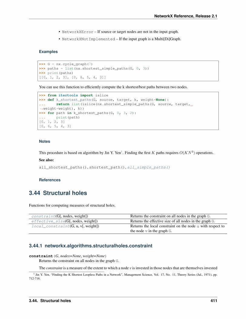
NetworkX Reference, Release 2.1
• NetworkXError – If source or target nodes are not in the input graph.
• NetworkXNotImplemented – If the input graph is a Multi[Di]Graph.
Examples
>>> G = nx.cycle_graph(7)>>> paths = list(nx.shortest_simple_paths(G, 0, 3))>>> print(paths)[[0, 1, 2, 3], [0, 6, 5, 4, 3]]
You can use this function to efficiently compute the k shortest/best paths between two nodes.
>>> from itertools import islice>>> def k_shortest_paths(G, source, target, k, weight=None):... return list(islice(nx.shortest_simple_paths(G, source, target,→˓weight=weight), k))>>> for path in k_shortest_paths(G, 0, 3, 2):... print(path)[0, 1, 2, 3][0, 6, 5, 4, 3]
Notes
This procedure is based on algorithm by Jin Y. Yen1. Finding the first 𝐾 paths requires 𝑂(𝐾𝑁3) operations.
See also:
all_shortest_paths(), shortest_path(), all_simple_paths()
References
3.44 Structural holes
Functions for computing measures of structural holes.
constraint(G[, nodes, weight]) Returns the constraint on all nodes in the graph G.effective_size(G[, nodes, weight]) Returns the effective size of all nodes in the graph G.local_constraint(G, u, v[, weight]) Returns the local constraint on the node u with respect to
the node v in the graph G.
3.44.1 networkx.algorithms.structuralholes.constraint
constraint(G, nodes=None, weight=None)Returns the constraint on all nodes in the graph G.
The constraint is a measure of the extent to which a node v is invested in those nodes that are themselves invested1 Jin Y. Yen, “Finding the K Shortest Loopless Paths in a Network”, Management Science, Vol. 17, No. 11, Theory Series (Jul., 1971), pp.
712-716.
3.44. Structural holes 411

NetworkX Reference, Release 2.1
in the neighbors of v. Formally, the constraint on v, denoted c(v), is defined by
𝑐(𝑣) =∑
𝑤∈𝑁(𝑣)∖{𝑣}
ℓ(𝑣, 𝑤)
where N(v) is the subset of the neighbors of v that are either predecessors or successors of v andell(v, w) is the local constraint on v with respect to w1. For the definition of local constraint, seelocal_constraint().
Parameters
• G (NetworkX graph) – The graph containing v. This can be either directed or undirected.
• nodes (container, optional) – Container of nodes in the graph G to compute the constraint.If None, the constraint of every node is computed.
• weight (None or string, optional) – If None, all edge weights are considered equal. Other-wise holds the name of the edge attribute used as weight.
Returns Dictionary with nodes as keys and the constraint on the node as values.
Return type dict
See also:
local_constraint()
References
3.44.2 networkx.algorithms.structuralholes.effective_size
effective_size(G, nodes=None, weight=None)Returns the effective size of all nodes in the graph G.
The effective size of a node’s ego network is based on the concept of redundancy. A person’s ego networkhas redundancy to the extent that her contacts are connected to each other as well. The nonredundant part of aperson’s relationships it’s the effective size of her ego network1. Formally, the effective size of a node 𝑢, denoted𝑒(𝑢), is defined by
𝑒(𝑢) =∑
𝑣∈𝑁(𝑢)∖{𝑢}
⎛⎝1 −∑
𝑤∈𝑁(𝑣)
𝑝𝑢𝑤𝑚𝑣𝑤
⎞⎠where 𝑁(𝑢) is the set of neighbors of 𝑢 and 𝑝𝑢𝑤 is the normalized mutual weight of the (directed or undirected)edges joining 𝑢 and 𝑣, for each vertex 𝑢 and 𝑣1. And 𝑚𝑣𝑤 is the mutual weight of 𝑣 and 𝑤 divided by 𝑣 highestmutual weight with any of its neighbors. The mutual weight of 𝑢 and 𝑣 is the sum of the weights of edges joiningthem (edge weights are assumed to be one if the graph is unweighted).
For the case of unweighted and undirected graphs, Borgatti proposed a simplified formula to compute effectivesize2
𝑒(𝑢) = 𝑛− 2𝑡
𝑛
where t is the number of ties in the ego network (not including ties to ego) and n is the number of nodes(excluding ego).
1 Burt, Ronald S. “Structural holes and good ideas”. American Journal of Sociology (110): 349–399.1 Burt, Ronald S. Structural Holes: The Social Structure of Competition. Cambridge: Harvard University Press, 1995.2 Borgatti, S. “Structural Holes: Unpacking Burt’s Redundancy Measures” CONNECTIONS 20(1):35-38. http://www.analytictech.com/
connections/v20(1)/holes.htm
412 Chapter 3. Algorithms

NetworkX Reference, Release 2.1
Parameters
• G (NetworkX graph) – The graph containing v. Directed graphs are treated like undirectedgraphs when computing neighbors of v.
• nodes (container, optional) – Container of nodes in the graph G to compute the effectivesize. If None, the effective size of every node is computed.
• weight (None or string, optional) – If None, all edge weights are considered equal. Other-wise holds the name of the edge attribute used as weight.
Returns Dictionary with nodes as keys and the constraint on the node as values.
Return type dict
Notes
Burt also defined the related concept of efficency of a node’s ego network, which is its effective size divided bythe degree of that node1. So you can easily compute efficencty:
>>> G = nx.DiGraph()>>> G.add_edges_from([(0, 1), (0, 2), (1, 0), (2, 1)])>>> esize = nx.effective_size(G)>>> efficency = {n: v / G.degree(n) for n, v in esize.items()}
See also:
constraint()
References
3.44.3 networkx.algorithms.structuralholes.local_constraint
local_constraint(G, u, v, weight=None)Returns the local constraint on the node u with respect to the node v in the graph G.
Formally, the local constraint on u with respect to v, denoted ℓ(𝑣), is defined by
ℓ(𝑢, 𝑣) =
⎛⎝𝑝𝑢𝑣 +∑
𝑤∈𝑁(𝑣)
𝑝𝑢𝑤𝑝𝑤𝑣
⎞⎠2
,
where 𝑁(𝑣) is the set of neighbors of 𝑣 and 𝑝𝑢𝑣 is the normalized mutual weight of the (directed or undirected)edges joining 𝑢 and 𝑣, for each vertex 𝑢 and 𝑣1. The mutual weight of 𝑢 and 𝑣 is the sum of the weights of edgesjoining them (edge weights are assumed to be one if the graph is unweighted).
Parameters
• G (NetworkX graph) – The graph containing u and v. This can be either directed or undi-rected.
• u (node) – A node in the graph G.
• v (node) – A node in the graph G.
• weight (None or string, optional) – If None, all edge weights are considered equal. Other-wise holds the name of the edge attribute used as weight.
1 Burt, Ronald S. “Structural holes and good ideas”. American Journal of Sociology (110): 349–399.
3.44. Structural holes 413

NetworkX Reference, Release 2.1
Returns The constraint of the node v in the graph G.
Return type float
See also:
constraint()
References
3.45 Swap
Swap edges in a graph.
double_edge_swap(G[, nswap, max_tries]) Swap two edges in the graph while keeping the node de-grees fixed.
connected_double_edge_swap(G[, nswap, . . . ]) Attempts the specified number of double-edge swaps in thegraph G.
3.45.1 networkx.algorithms.swap.double_edge_swap
double_edge_swap(G, nswap=1, max_tries=100)Swap two edges in the graph while keeping the node degrees fixed.
A double-edge swap removes two randomly chosen edges u-v and x-y and creates the new edges u-x and v-y:
u--v u vbecomes | |
x--y x y
If either the edge u-x or v-y already exist no swap is performed and another attempt is made to find a suitableedge pair.
Parameters
• G (graph) – An undirected graph
• nswap (integer (optional, default=1)) – Number of double-edge swaps to perform
• max_tries (integer (optional)) – Maximum number of attempts to swap edges
Returns G – The graph after double edge swaps.
Return type graph
Notes
Does not enforce any connectivity constraints.
The graph G is modified in place.
3.45.2 networkx.algorithms.swap.connected_double_edge_swap
connected_double_edge_swap(G, nswap=1, _window_threshold=3)Attempts the specified number of double-edge swaps in the graph G.
414 Chapter 3. Algorithms

NetworkX Reference, Release 2.1
A double-edge swap removes two randomly chosen edges (u, v) and (x, y) and creates the new edges(u, x) and (v, y):
u--v u vbecomes | |
x--y x y
If either (u, x) or (v, y) already exist, then no swap is performed so the actual number of swapped edgesis always at most nswap.
Parameters
• G (graph) – An undirected graph
• nswap (integer (optional, default=1)) – Number of double-edge swaps to perform
• _window_threshold (integer) – The window size below which connectedness of the graphwill be checked after each swap.
The “window” in this function is a dynamically updated integer that represents the number ofswap attempts to make before checking if the graph remains connected. It is an optimizationused to decrease the running time of the algorithm in exchange for increased complexity ofimplementation.
If the window size is below this threshold, then the algorithm checks after each swap if thegraph remains connected by checking if there is a path joining the two nodes whose edgewas just removed. If the window size is above this threshold, then the algorithm performsdo all the swaps in the window and only then check if the graph is still connected.
Returns The number of successful swaps
Return type int
Raises NetworkXError – If the input graph is not connected, or if the graph has fewer than fournodes.
Notes
The initial graph G must be connected, and the resulting graph is connected. The graph G is modified in place.
References
3.46 Tournament
Functions concerning tournament graphs.
A tournament graph is a complete oriented graph. In other words, it is a directed graph in which there is exactly onedirected edge joining each pair of distinct nodes. For each function in this module that accepts a graph as input, youmust provide a tournament graph. The responsibility is on the caller to ensure that the graph is a tournament graph.
To access the functions in this module, you must access them through the networkx.algorithms.tournamentmodule:
>>> import networkx as nx>>> from networkx.algorithms import tournament>>> G = nx.DiGraph([(0, 1), (1, 2), (2, 0)])
3.46. Tournament 415

NetworkX Reference, Release 2.1
>>> tournament.is_tournament(G)True
hamiltonian_path(G) Returns a Hamiltonian path in the given tournament graph.is_reachable(G, s, t) Decides whether there is a path from s to t in the tourna-
ment.is_strongly_connected(G) Decides whether the given tournament is strongly con-
nected.is_tournament(G) Returns True if and only if G is a tournament.random_tournament(n) Returns a random tournament graph on n nodes.score_sequence(G) Returns the score sequence for the given tournament graph.
3.46.1 networkx.algorithms.tournament.hamiltonian_path
hamiltonian_path(G)Returns a Hamiltonian path in the given tournament graph.
Each tournament has a Hamiltonian path. If furthermore, the tournament is strongly connected, then the returnedHamiltonian path is a Hamiltonian cycle (by joining the endpoints of the path).
Parameters G (NetworkX graph) – A directed graph representing a tournament.
Returns Whether the given graph is a tournament graph.
Return type bool
Notes
This is a recursive implementation with an asymptotic running time of 𝑂(𝑛2), ignoring multiplicative polylog-arithmic factors, where 𝑛 is the number of nodes in the graph.
3.46.2 networkx.algorithms.tournament.is_reachable
is_reachable(G, s, t)Decides whether there is a path from s to t in the tournament.
This function is more theoretically efficient than the reachability checks than the shortest path algorithms innetworkx.algorithms.shortest_paths.
The given graph must be a tournament, otherwise this function’s behavior is undefined.
Parameters
• G (NetworkX graph) – A directed graph representing a tournament.
• s (node) – A node in the graph.
• t (node) – A node in the graph.
Returns Whether there is a path from s to t in G.
Return type bool
416 Chapter 3. Algorithms

NetworkX Reference, Release 2.1
Notes
Although this function is more theoretically efficient than the generic shortest path functions, a speedup requiresthe use of parallelism. Though it may in the future, the current implementation does not use parallelism, thusyou may not see much of a speedup.
This algorithm comes from [1].
References
3.46.3 networkx.algorithms.tournament.is_strongly_connected
is_strongly_connected(G)Decides whether the given tournament is strongly connected.
This function is more theoretically efficient than the is_strongly_connected() function.
The given graph must be a tournament, otherwise this function’s behavior is undefined.
Parameters G (NetworkX graph) – A directed graph representing a tournament.
Returns Whether the tournament is strongly connected.
Return type bool
Notes
Although this function is more theoretically efficient than the generic strong connectivity function, a speeduprequires the use of parallelism. Though it may in the future, the current implementation does not use parallelism,thus you may not see much of a speedup.
This algorithm comes from [1].
References
3.46.4 networkx.algorithms.tournament.is_tournament
is_tournament(G)Returns True if and only if G is a tournament.
A tournament is a directed graph, with neither self-loops nor multi-edges, in which there is exactly one directededge joining each pair of distinct nodes.
Parameters G (NetworkX graph) – A directed graph representing a tournament.
Returns Whether the given graph is a tournament graph.
Return type bool
Notes
Some definitions require a self-loop on each node, but that is not the convention used here.
3.46. Tournament 417

NetworkX Reference, Release 2.1
3.46.5 networkx.algorithms.tournament.random_tournament
random_tournament(n)Returns a random tournament graph on n nodes.
Parameters n (int) – The number of nodes in the returned graph.
Returns Whether the given graph is a tournament graph.
Return type bool
Notes
This algorithm adds, for each pair of distinct nodes, an edge with uniformly random orientation. In other words,binom{n}{2} flips of an unbiased coin decide the orientations of the edges in the graph.
3.46.6 networkx.algorithms.tournament.score_sequence
score_sequence(G)Returns the score sequence for the given tournament graph.
The score sequence is the sorted list of the out-degrees of the nodes of the graph.
Parameters G (NetworkX graph) – A directed graph representing a tournament.
Returns A sorted list of the out-degrees of the nodes of G.
Return type list
3.47 Traversal
3.47.1 Depth First Search
Basic algorithms for depth-first searching the nodes of a graph.
dfs_edges(G[, source, depth_limit]) Iterate over edges in a depth-first-search (DFS).dfs_tree(G[, source, depth_limit]) Return oriented tree constructed from a depth-first-search
from source.dfs_predecessors(G[, source, depth_limit]) Return dictionary of predecessors in depth-first-search
from source.dfs_successors(G[, source, depth_limit]) Return dictionary of successors in depth-first-search from
source.dfs_preorder_nodes(G[, source, depth_limit]) Generate nodes in a depth-first-search pre-ordering starting
at source.dfs_postorder_nodes(G[, source, depth_limit]) Generate nodes in a depth-first-search post-ordering start-
ing at source.dfs_labeled_edges(G[, source, depth_limit]) Iterate over edges in a depth-first-search (DFS) labeled by
type.
418 Chapter 3. Algorithms

NetworkX Reference, Release 2.1
networkx.algorithms.traversal.depth_first_search.dfs_edges
dfs_edges(G, source=None, depth_limit=None)Iterate over edges in a depth-first-search (DFS).
Parameters
• G (NetworkX graph)
• source (node, optional) – Specify starting node for depth-first search and return edges in thecomponent reachable from source.
• depth_limit (int, optional (default=len(G))) – Specify the maximum search depth.
Returns edges – A generator of edges in the depth-first-search.
Return type generator
Examples
>>> G = nx.path_graph(5)>>> list(nx.dfs_edges(G, source=0))[(0, 1), (1, 2), (2, 3), (3, 4)]>>> list(nx.dfs_edges(G, source=0, depth_limit=2))[(0, 1), (1, 2)]
Notes
If a source is not specified then a source is chosen arbitrarily and repeatedly until all components in the graphare searched.
The implementation of this function is adapted from David Eppstein’s depth-first search function in PADS, withmodifications to allow depth limits based on the Wikipedia article “Depth-limited search”.
See also:
dfs_preorder_nodes(), dfs_postorder_nodes(), dfs_labeled_edges()
networkx.algorithms.traversal.depth_first_search.dfs_tree
dfs_tree(G, source=None, depth_limit=None)Return oriented tree constructed from a depth-first-search from source.
Parameters
• G (NetworkX graph)
• source (node, optional) – Specify starting node for depth-first search.
• depth_limit (int, optional (default=len(G))) – Specify the maximum search depth.
Returns T – An oriented tree
Return type NetworkX DiGraph
3.47. Traversal 419

NetworkX Reference, Release 2.1
Examples
>>> G = nx.path_graph(5)>>> T = nx.dfs_tree(G, source=0, depth_limit=2)>>> list(T.edges())[(0, 1), (1, 2)]>>> T = nx.dfs_tree(G, source=0)>>> list(T.edges())[(0, 1), (1, 2), (2, 3), (3, 4)]
networkx.algorithms.traversal.depth_first_search.dfs_predecessors
dfs_predecessors(G, source=None, depth_limit=None)Return dictionary of predecessors in depth-first-search from source.
Parameters
• G (NetworkX graph)
• source (node, optional) – Specify starting node for depth-first search and return edges in thecomponent reachable from source.
• depth_limit (int, optional (default=len(G))) – Specify the maximum search depth.
Returns pred – A dictionary with nodes as keys and predecessor nodes as values.
Return type dict
Examples
>>> G = nx.path_graph(4)>>> nx.dfs_predecessors(G, source=0){1: 0, 2: 1, 3: 2}>>> nx.dfs_predecessors(G, source=0, depth_limit=2){1: 0, 2: 1}
Notes
If a source is not specified then a source is chosen arbitrarily and repeatedly until all components in the graphare searched.
The implementation of this function is adapted from David Eppstein’s depth-first search function in PADS, withmodifications to allow depth limits based on the Wikipedia article “Depth-limited search”.
networkx.algorithms.traversal.depth_first_search.dfs_successors
dfs_successors(G, source=None, depth_limit=None)Return dictionary of successors in depth-first-search from source.
Parameters
• G (NetworkX graph)
• source (node, optional) – Specify starting node for depth-first search and return edges in thecomponent reachable from source.
420 Chapter 3. Algorithms

NetworkX Reference, Release 2.1
• depth_limit (int, optional (default=len(G))) – Specify the maximum search depth.
Returns succ – A dictionary with nodes as keys and list of successor nodes as values.
Return type dict
Examples
>>> G = nx.path_graph(5)>>> nx.dfs_successors(G, source=0){0: [1], 1: [2], 2: [3], 3: [4]}>>> nx.dfs_successors(G, source=0, depth_limit=2){0: [1], 1: [2]}
Notes
If a source is not specified then a source is chosen arbitrarily and repeatedly until all components in the graphare searched.
The implementation of this function is adapted from David Eppstein’s depth-first search function in PADS, withmodifications to allow depth limits based on the Wikipedia article “Depth-limited search”.
networkx.algorithms.traversal.depth_first_search.dfs_preorder_nodes
dfs_preorder_nodes(G, source=None, depth_limit=None)Generate nodes in a depth-first-search pre-ordering starting at source.
Parameters
• G (NetworkX graph)
• source (node, optional) – Specify starting node for depth-first search and return edges in thecomponent reachable from source.
• depth_limit (int, optional (default=len(G))) – Specify the maximum search depth.
Returns nodes – A generator of nodes in a depth-first-search pre-ordering.
Return type generator
Examples
>>> G = nx.path_graph(5)>>> list(nx.dfs_preorder_nodes(G, source=0))[0, 1, 2, 3, 4]>>> list(nx.dfs_preorder_nodes(G, source=0, depth_limit=2))[0, 1, 2]
Notes
If a source is not specified then a source is chosen arbitrarily and repeatedly until all components in the graphare searched.
3.47. Traversal 421

NetworkX Reference, Release 2.1
The implementation of this function is adapted from David Eppstein’s depth-first search function in PADS, withmodifications to allow depth limits based on the Wikipedia article “Depth-limited search”.
See also:
dfs_edges(), dfs_postorder_nodes(), dfs_labeled_edges()
networkx.algorithms.traversal.depth_first_search.dfs_postorder_nodes
dfs_postorder_nodes(G, source=None, depth_limit=None)Generate nodes in a depth-first-search post-ordering starting at source.
Parameters
• G (NetworkX graph)
• source (node, optional) – Specify starting node for depth-first search and return edges in thecomponent reachable from source.
• depth_limit (int, optional (default=len(G))) – Specify the maximum search depth.
Returns nodes – A generator of nodes in a depth-first-search post-ordering.
Return type generator
Examples
>>> G = nx.path_graph(5)>>> list(nx.dfs_postorder_nodes(G, source=0))[4, 3, 2, 1, 0]>>> list(nx.dfs_postorder_nodes(G, source=0, depth_limit=2))[1, 0]
Notes
If a source is not specified then a source is chosen arbitrarily and repeatedly until all components in the graphare searched.
The implementation of this function is adapted from David Eppstein’s depth-first search function in PADS, withmodifications to allow depth limits based on the Wikipedia article “Depth-limited search”.
See also:
dfs_edges(), dfs_preorder_nodes(), dfs_labeled_edges()
networkx.algorithms.traversal.depth_first_search.dfs_labeled_edges
dfs_labeled_edges(G, source=None, depth_limit=None)Iterate over edges in a depth-first-search (DFS) labeled by type.
Parameters
• G (NetworkX graph)
• source (node, optional) – Specify starting node for depth-first search and return edges in thecomponent reachable from source.
• depth_limit (int, optional (default=len(G))) – Specify the maximum search depth.
422 Chapter 3. Algorithms

NetworkX Reference, Release 2.1
Returns edges – A generator of triples of the form (u, v, d), where (u, v) is the edge being exploredin the depth-first search and d is one of the strings ‘forward’, ‘nontree’, or ‘reverse’. A ‘forward’edge is one in which u has been visited but v has not. A ‘nontree’ edge is one in which both uand v have been visited but the edge is not in the DFS tree. A ‘reverse’ edge is on in which bothu and v have been visited and the edge is in the DFS tree.
Return type generator
Examples
The labels reveal the complete transcript of the depth-first search algorithm in more detail than, for example,dfs_edges():
>>> from pprint import pprint>>>>>> G = nx.DiGraph([(0, 1), (1, 2), (2, 1)])>>> pprint(list(nx.dfs_labeled_edges(G, source=0)))[(0, 0, 'forward'),(0, 1, 'forward'),(1, 2, 'forward'),(2, 1, 'nontree'),(1, 2, 'reverse'),(0, 1, 'reverse'),(0, 0, 'reverse')]
Notes
If a source is not specified then a source is chosen arbitrarily and repeatedly until all components in the graphare searched.
The implementation of this function is adapted from David Eppstein’s depth-first search function in PADS, withmodifications to allow depth limits based on the Wikipedia article “Depth-limited search”.
See also:
dfs_edges(), dfs_preorder_nodes(), dfs_postorder_nodes()
3.47.2 Breadth First Search
Basic algorithms for breadth-first searching the nodes of a graph.
bfs_edges(G, source[, reverse]) Iterate over edges in a breadth-first-search starting atsource.
bfs_tree(G, source[, reverse]) Return an oriented tree constructed from of a breadth-first-search starting at source.
bfs_predecessors(G, source) Returns an iterator of predecessors in breadth-first-searchfrom source.
bfs_successors(G, source) Returns an iterator of successors in breadth-first-searchfrom source.
3.47. Traversal 423

NetworkX Reference, Release 2.1
networkx.algorithms.traversal.breadth_first_search.bfs_edges
bfs_edges(G, source, reverse=False)Iterate over edges in a breadth-first-search starting at source.
Parameters
• G (NetworkX graph)
• source (node) – Specify starting node for breadth-first search and return edges in the com-ponent reachable from source.
• reverse (bool, optional) – If True traverse a directed graph in the reverse direction
Returns edges – A generator of edges in the breadth-first-search.
Return type generator
Examples
To get the edges in a breadth-first search:
>>> G = nx.path_graph(3)>>> list(nx.bfs_edges(G, 0))[(0, 1), (1, 2)]
To get the nodes in a breadth-first search order:
>>> G = nx.path_graph(3)>>> root = 2>>> edges = nx.bfs_edges(G, root)>>> nodes = [root] + [v for u, v in edges]>>> nodes[2, 1, 0]
Notes
Based on http://www.ics.uci.edu/~eppstein/PADS/BFS.py by D. Eppstein, July 2004.
networkx.algorithms.traversal.breadth_first_search.bfs_tree
bfs_tree(G, source, reverse=False)Return an oriented tree constructed from of a breadth-first-search starting at source.
Parameters
• G (NetworkX graph)
• source (node) – Specify starting node for breadth-first search and return edges in the com-ponent reachable from source.
• reverse (bool, optional) – If True traverse a directed graph in the reverse direction
Returns T – An oriented tree
Return type NetworkX DiGraph
424 Chapter 3. Algorithms

NetworkX Reference, Release 2.1
Examples
>>> G = nx.path_graph(3)>>> print(list(nx.bfs_tree(G,1).edges()))[(1, 0), (1, 2)]
Notes
Based on http://www.ics.uci.edu/~eppstein/PADS/BFS.py by D. Eppstein, July 2004.
networkx.algorithms.traversal.breadth_first_search.bfs_predecessors
bfs_predecessors(G, source)Returns an iterator of predecessors in breadth-first-search from source.
Parameters
• G (NetworkX graph)
• source (node) – Specify starting node for breadth-first search and return edges in the com-ponent reachable from source.
Returns pred – (node, predecessors) iterator where predecessors is the list of predecessors of thenode.
Return type iterator
Examples
>>> G = nx.path_graph(3)>>> print(dict(nx.bfs_predecessors(G, 0))){1: 0, 2: 1}>>> H = nx.Graph()>>> H.add_edges_from([(0, 1), (0, 2), (1, 3), (1, 4), (2, 5), (2, 6)])>>> dict(nx.bfs_predecessors(H, 0)){1: 0, 2: 0, 3: 1, 4: 1, 5: 2, 6: 2}
Notes
Based on http://www.ics.uci.edu/~eppstein/PADS/BFS.py by D. Eppstein, July 2004.
networkx.algorithms.traversal.breadth_first_search.bfs_successors
bfs_successors(G, source)Returns an iterator of successors in breadth-first-search from source.
Parameters
• G (NetworkX graph)
• source (node) – Specify starting node for breadth-first search and return edges in the com-ponent reachable from source.
3.47. Traversal 425

NetworkX Reference, Release 2.1
Returns succ – (node, successors) iterator where successors is the list of successors of the node.
Return type iterator
Examples
>>> G = nx.path_graph(3)>>> print(dict(nx.bfs_successors(G,0))){0: [1], 1: [2]}>>> H = nx.Graph()>>> H.add_edges_from([(0, 1), (0, 2), (1, 3), (1, 4), (2, 5), (2, 6)])>>> dict(nx.bfs_successors(H, 0)){0: [1, 2], 1: [3, 4], 2: [5, 6]}
Notes
Based on http://www.ics.uci.edu/~eppstein/PADS/BFS.py by D. Eppstein, July 2004.
3.47.3 Beam search
Basic algorithms for breadth-first searching the nodes of a graph.
bfs_beam_edges(G, source, value[, width]) Iterates over edges in a beam search.
networkx.algorithms.traversal.beamsearch.bfs_beam_edges
bfs_beam_edges(G, source, value, width=None)Iterates over edges in a beam search.
The beam search is a generalized breadth-first search in which only the “best” w neighbors of the current nodeare enqueued, where w is the beam width and “best” is an application-specific heuristic. In general, a beamsearch with a small beam width might not visit each node in the graph.
Parameters
• G (NetworkX graph)
• source (node) – Starting node for the breadth-first search; this function iterates over onlythose edges in the component reachable from this node.
• value (function) – A function that takes a node of the graph as input and returns a realnumber indicating how “good” it is. A higher value means it is more likely to be visitedsooner during the search. When visiting a new node, only the width neighbors with thehighest value are enqueued (in decreasing order of value).
• width (int (default = None)) – The beam width for the search. This is the number of neigh-bors (ordered by value) to enqueue when visiting each new node.
Yields edge – Edges in the beam search starting from source, given as a pair of nodes.
426 Chapter 3. Algorithms

NetworkX Reference, Release 2.1
Examples
To give nodes with, for example, a higher centrality precedence during the search, set the value function toreturn the centrality value of the node:
>>> G = nx.karate_club_graph()>>> centrality = nx.eigenvector_centrality(G)>>> source = 0>>> width = 5>>> for u, v in nx.bfs_beam_edges(G, source, centrality.get, width):... print((u, v))
3.47.4 Depth First Search on Edges
Depth First Search on Edges
Algorithms for a depth-first traversal of edges in a graph.
edge_dfs(G[, source, orientation]) A directed, depth-first traversal of edges in G, beginning atsource.
networkx.algorithms.traversal.edgedfs.edge_dfs
edge_dfs(G, source=None, orientation=’original’)A directed, depth-first traversal of edges in G, beginning at source.
Parameters
• G (graph) – A directed/undirected graph/multigraph.
• source (node, list of nodes) – The node from which the traversal begins. If None, then asource is chosen arbitrarily and repeatedly until all edges from each node in the graph aresearched.
• orientation (‘original’ | ‘reverse’ | ‘ignore’) – For directed graphs and directed multigraphs,edge traversals need not respect the original orientation of the edges. When set to ‘reverse’,then every edge will be traversed in the reverse direction. When set to ‘ignore’, then eachdirected edge is treated as a single undirected edge that can be traversed in either direction.For undirected graphs and undirected multigraphs, this parameter is meaningless and is notconsulted by the algorithm.
Yields edge (directed edge) – A directed edge indicating the path taken by the depth-first traversal.For graphs, edge is of the form (u, v) where u and v are the tail and head of the edge asdetermined by the traversal. For multigraphs, edge is of the form (u, v, key), where keyis the key of the edge. When the graph is directed, then u and v are always in the order of theactual directed edge. If orientation is ‘reverse’ or ‘ignore’, then edge takes the form (u, v,key, direction) where direction is a string, ‘forward’ or ‘reverse’, that indicates if theedge was traversed in the forward (tail to head) or reverse (head to tail) direction, respectively.
Examples
3.47. Traversal 427

NetworkX Reference, Release 2.1
>>> import networkx as nx>>> nodes = [0, 1, 2, 3]>>> edges = [(0, 1), (1, 0), (1, 0), (2, 1), (3, 1)]
>>> list(nx.edge_dfs(nx.Graph(edges), nodes))[(0, 1), (1, 2), (1, 3)]
>>> list(nx.edge_dfs(nx.DiGraph(edges), nodes))[(0, 1), (1, 0), (2, 1), (3, 1)]
>>> list(nx.edge_dfs(nx.MultiGraph(edges), nodes))[(0, 1, 0), (1, 0, 1), (0, 1, 2), (1, 2, 0), (1, 3, 0)]
>>> list(nx.edge_dfs(nx.MultiDiGraph(edges), nodes))[(0, 1, 0), (1, 0, 0), (1, 0, 1), (2, 1, 0), (3, 1, 0)]
>>> list(nx.edge_dfs(nx.DiGraph(edges), nodes, orientation='ignore'))[(0, 1, 'forward'), (1, 0, 'forward'), (2, 1, 'reverse'), (3, 1, 'reverse')]
>>> list(nx.edge_dfs(nx.MultiDiGraph(edges), nodes, orientation='ignore'))[(0, 1, 0, 'forward'), (1, 0, 0, 'forward'), (1, 0, 1, 'reverse'), (2, 1, 0,→˓'reverse'), (3, 1, 0, 'reverse')]
Notes
The goal of this function is to visit edges. It differs from the more familiar depth-first traversal of nodes, asprovided by networkx.algorithms.traversal.depth_first_search.dfs_edges(), in thatit does not stop once every node has been visited. In a directed graph with edges [(0, 1), (1, 2), (2, 1)], the edge(2, 1) would not be visited if not for the functionality provided by this function.
See also:
dfs_edges()
3.48 Tree
3.48.1 Recognition
Recognition Tests
A forest is an acyclic, undirected graph, and a tree is a connected forest. Depending on the subfield, there are variousconventions for generalizing these definitions to directed graphs.
In one convention, directed variants of forest and tree are defined in an identical manner, except that the direction ofthe edges is ignored. In effect, each directed edge is treated as a single undirected edge. Then, additional restrictionsare imposed to define branchings and arborescences.
In another convention, directed variants of forest and tree correspond to the previous convention’s branchings andarborescences, respectively. Then two new terms, polyforest and polytree, are defined to correspond to the otherconvention’s forest and tree.
Summarizing:
428 Chapter 3. Algorithms

NetworkX Reference, Release 2.1
+-----------------------------+| Convention A | Convention B |+=============================+| forest | polyforest || tree | polytree || branching | forest || arborescence | tree |+-----------------------------+
Each convention has its reasons. The first convention emphasizes definitional similarity in that directed forests andtrees are only concerned with acyclicity and do not have an in-degree constraint, just as their undirected counterparts donot. The second convention emphasizes functional similarity in the sense that the directed analog of a spanning tree isa spanning arborescence. That is, take any spanning tree and choose one node as the root. Then every edge is assigneda direction such there is a directed path from the root to every other node. The result is a spanning arborescence.
NetworkX follows convention “A”. Explicitly, these are:
undirected forest An undirected graph with no undirected cycles.
undirected tree A connected, undirected forest.
directed forest A directed graph with no undirected cycles. Equivalently, the underlying graph structure (whichignores edge orientations) is an undirected forest. In convention B, this is known as a polyforest.
directed tree A weakly connected, directed forest. Equivalently, the underlying graph structure (which ignores edgeorientations) is an undirected tree. In convention B, this is known as a polytree.
branching A directed forest with each node having, at most, one parent. So the maximum in-degree is equal to 1. Inconvention B, this is known as a forest.
arborescence A directed tree with each node having, at most, one parent. So the maximum in-degree is equal to 1.In convention B, this is known as a tree.
For trees and arborescences, the adjective “spanning” may be added to designate that the graph, when considered asa forest/branching, consists of a single tree/arborescence that includes all nodes in the graph. It is true, by definition,that every tree/arborescence is spanning with respect to the nodes that define the tree/arborescence and so, it mightseem redundant to introduce the notion of “spanning”. However, the nodes may represent a subset of nodes from alarger graph, and it is in this context that the term “spanning” becomes a useful notion.
is_tree(G) Returns True if G is a tree.is_forest(G) Returns True if G is a forest.is_arborescence(G) Returns True if G is an arborescence.is_branching(G) Returns True if G is a branching.
networkx.algorithms.tree.recognition.is_tree
is_tree(G)Returns True if G is a tree.
A tree is a connected graph with no undirected cycles.
For directed graphs, G is a tree if the underlying graph is a tree. The underlying graph is obtained by treatingeach directed edge as a single undirected edge in a multigraph.
Parameters G (graph) – The graph to test.
Returns b – A boolean that is True if G is a tree.
Return type bool
3.48. Tree 429
NetworkX Reference, Release 2.1
Notes
In another convention, a directed tree is known as a polytree and then tree corresponds to an arborescence.
See also:
is_arborescence()
networkx.algorithms.tree.recognition.is_forest
is_forest(G)Returns True if G is a forest.
A forest is a graph with no undirected cycles.
For directed graphs, G is a forest if the underlying graph is a forest. The underlying graph is obtained by treatingeach directed edge as a single undirected edge in a multigraph.
Parameters G (graph) – The graph to test.
Returns b – A boolean that is True if G is a forest.
Return type bool
Notes
In another convention, a directed forest is known as a polyforest and then forest corresponds to a branching.
See also:
is_branching()
networkx.algorithms.tree.recognition.is_arborescence
is_arborescence(G)Returns True if G is an arborescence.
An arborescence is a directed tree with maximum in-degree equal to 1.
Parameters G (graph) – The graph to test.
Returns b – A boolean that is True if G is an arborescence.
Return type bool
Notes
In another convention, an arborescence is known as a tree.
See also:
is_tree()
430 Chapter 3. Algorithms

NetworkX Reference, Release 2.1
networkx.algorithms.tree.recognition.is_branching
is_branching(G)Returns True if G is a branching.
A branching is a directed forest with maximum in-degree equal to 1.
Parameters G (directed graph) – The directed graph to test.
Returns b – A boolean that is True if G is a branching.
Return type bool
Notes
In another convention, a branching is also known as a forest.
See also:
is_forest()
3.48.2 Branchings and Spanning Arborescences
Algorithms for finding optimum branchings and spanning arborescences.
This implementation is based on:
J. Edmonds, Optimum branchings, J. Res. Natl. Bur. Standards 71B (1967), 233–240. URL: http://archive.org/details/jresv71Bn4p233
branching_weight(G[, attr, default]) Returns the total weight of a branching.greedy_branching(G[, attr, default, kind]) Returns a branching obtained through a greedy algorithm.maximum_branching(G[, attr, default]) Returns a maximum branching from G.minimum_branching(G[, attr, default]) Returns a minimum branching from G.maximum_spanning_arborescence(G[, attr, de-fault])
Returns a maximum spanning arborescence from G.
minimum_spanning_arborescence(G[, attr, de-fault])
Returns a minimum spanning arborescence from G.
Edmonds(G[, seed]) Edmonds algorithm for finding optimal branchings andspanning arborescences.
networkx.algorithms.tree.branchings.branching_weight
branching_weight(G, attr=’weight’, default=1)Returns the total weight of a branching.
networkx.algorithms.tree.branchings.greedy_branching
greedy_branching(G, attr=’weight’, default=1, kind=’max’)Returns a branching obtained through a greedy algorithm.
This algorithm is wrong, and cannot give a proper optimal branching. However, we include it for pedagogicalreasons, as it can be helpful to see what its outputs are.
3.48. Tree 431
NetworkX Reference, Release 2.1
The output is a branching, and possibly, a spanning arborescence. However, it is not guaranteed to be optimalin either case.
Parameters
• G (DiGraph) – The directed graph to scan.
• attr (str) – The attribute to use as weights. If None, then each edge will be treated equallywith a weight of 1.
• default (float) – When attr is not None, then if an edge does not have that attribute,default specifies what value it should take.
• kind (str) – The type of optimum to search for: ‘min’ or ‘max’ greedy branching.
Returns B – The greedily obtained branching.
Return type directed graph
networkx.algorithms.tree.branchings.maximum_branching
maximum_branching(G, attr=’weight’, default=1)Returns a maximum branching from G.
Parameters
• G ((multi)digraph-like) – The graph to be searched.
• attr (str) – The edge attribute used to in determining optimality.
• default (float) – The value of the edge attribute used if an edge does not have the attributeattr.
Returns B – A maximum branching.
Return type (multi)digraph-like
networkx.algorithms.tree.branchings.minimum_branching
minimum_branching(G, attr=’weight’, default=1)Returns a minimum branching from G.
Parameters
• G ((multi)digraph-like) – The graph to be searched.
• attr (str) – The edge attribute used to in determining optimality.
• default (float) – The value of the edge attribute used if an edge does not have the attributeattr.
Returns B – A minimum branching.
Return type (multi)digraph-like
networkx.algorithms.tree.branchings.maximum_spanning_arborescence
maximum_spanning_arborescence(G, attr=’weight’, default=1)Returns a maximum spanning arborescence from G.
Parameters
432 Chapter 3. Algorithms

NetworkX Reference, Release 2.1
• G ((multi)digraph-like) – The graph to be searched.
• attr (str) – The edge attribute used to in determining optimality.
• default (float) – The value of the edge attribute used if an edge does not have the attributeattr.
Returns B – A maximum spanning arborescence.
Return type (multi)digraph-like
Raises NetworkXException – If the graph does not contain a maximum spanning arborescence.
networkx.algorithms.tree.branchings.minimum_spanning_arborescence
minimum_spanning_arborescence(G, attr=’weight’, default=1)Returns a minimum spanning arborescence from G.
Parameters
• G ((multi)digraph-like) – The graph to be searched.
• attr (str) – The edge attribute used to in determining optimality.
• default (float) – The value of the edge attribute used if an edge does not have the attributeattr.
Returns B – A minimum spanning arborescence.
Return type (multi)digraph-like
Raises NetworkXException – If the graph does not contain a minimum spanning arborescence.
networkx.algorithms.tree.branchings.Edmonds
class Edmonds(G, seed=None)Edmonds algorithm for finding optimal branchings and spanning arborescences.
__init__(G, seed=None)
Methods
__init__(G[, seed])find_optimum([attr, default, kind, style]) Returns a branching from G.
3.48.3 Encoding and decoding
Functions for encoding and decoding trees.
Since a tree is a highly restricted form of graph, it can be represented concisely in several ways. This module includesfunctions for encoding and decoding trees in the form of nested tuples and Prüfer sequences. The former requires arooted tree, whereas the latter can be applied to unrooted trees. Furthermore, there is a bijection from Prüfer sequencesto labeled trees.
from_nested_tuple(sequence[, . . . ]) Returns the rooted tree corresponding to the given nestedtuple.
Continued on next page
3.48. Tree 433

NetworkX Reference, Release 2.1
Table 3.128 – continued from previous pageto_nested_tuple(T, root[, canonical_form]) Returns a nested tuple representation of the given tree.from_prufer_sequence(sequence) Returns the tree corresponding to the given Prüfer se-
quence.to_prufer_sequence(T) Returns the Prüfer sequence of the given tree.
networkx.algorithms.tree.coding.from_nested_tuple
from_nested_tuple(sequence, sensible_relabeling=False)Returns the rooted tree corresponding to the given nested tuple.
The nested tuple representation of a tree is defined recursively. The tree with one node and no edges is rep-resented by the empty tuple, (). A tree with k subtrees is represented by a tuple of length k in which eachelement is the nested tuple representation of a subtree.
Parameters
• sequence (tuple) – A nested tuple representing a rooted tree.
• sensible_relabeling (bool) – Whether to relabel the nodes of the tree so that nodes arelabeled in increasing order according to their breadth-first search order from the root node.
Returns The tree corresponding to the given nested tuple, whose root node is node 0. Ifsensible_labeling is True, nodes will be labeled in breadth-first search order startingfrom the root node.
Return type NetworkX graph
Notes
This function is not the inverse of to_nested_tuple(); the only guarantee is that the rooted trees areisomorphic.
See also:
to_nested_tuple(), from_prufer_sequence()
Examples
Sensible relabeling ensures that the nodes are labeled from the root starting at 0:
>>> balanced = (((), ()), ((), ()))>>> T = nx.from_nested_tuple(balanced, sensible_relabeling=True)>>> edges = [(0, 1), (0, 2), (1, 3), (1, 4), (2, 5), (2, 6)]>>> all((u, v) in T.edges() or (v, u) in T.edges() for (u, v) in edges)True
networkx.algorithms.tree.coding.to_nested_tuple
to_nested_tuple(T, root, canonical_form=False)Returns a nested tuple representation of the given tree.
The nested tuple representation of a tree is defined recursively. The tree with one node and no edges is rep-resented by the empty tuple, (). A tree with k subtrees is represented by a tuple of length k in which eachelement is the nested tuple representation of a subtree.
434 Chapter 3. Algorithms

NetworkX Reference, Release 2.1
Parameters
• T (NetworkX graph) – An undirected graph object representing a tree.
• root (node) – The node in T to interpret as the root of the tree.
• canonical_form (bool) – If True, each tuple is sorted so that the function returns a canon-ical form for rooted trees. This means “lighter” subtrees will appear as nested tuples before“heavier” subtrees. In this way, each isomorphic rooted tree has the same nested tuple rep-resentation.
Returns A nested tuple representation of the tree.
Return type tuple
Notes
This function is not the inverse of from_nested_tuple(); the only guarantee is that the rooted trees areisomorphic.
See also:
from_nested_tuple(), to_prufer_sequence()
Examples
The tree need not be a balanced binary tree:
>>> T = nx.Graph()>>> T.add_edges_from([(0, 1), (0, 2), (0, 3)])>>> T.add_edges_from([(1, 4), (1, 5)])>>> T.add_edges_from([(3, 6), (3, 7)])>>> root = 0>>> nx.to_nested_tuple(T, root)(((), ()), (), ((), ()))
Continuing the above example, if canonical_form is True, the nested tuples will be sorted:
>>> nx.to_nested_tuple(T, root, canonical_form=True)((), ((), ()), ((), ()))
Even the path graph can be interpreted as a tree:
>>> T = nx.path_graph(4)>>> root = 0>>> nx.to_nested_tuple(T, root)((((),),),)
networkx.algorithms.tree.coding.from_prufer_sequence
from_prufer_sequence(sequence)Returns the tree corresponding to the given Prüfer sequence.
A Prüfer sequence is a list of n - 2 numbers between 0 and n - 1, inclusive. The tree corresponding to a givenPrüfer sequence can be recovered by repeatedly joining a node in the sequence with a node with the smallestpotential degree according to the sequence.
3.48. Tree 435

NetworkX Reference, Release 2.1
Parameters sequence (list) – A Prüfer sequence, which is a list of n - 2 integers between zero andn - 1, inclusive.
Returns The tree corresponding to the given Prüfer sequence.
Return type NetworkX graph
Notes
There is a bijection from labeled trees to Prüfer sequences. This function is the inverse of thefrom_prufer_sequence() function.
Sometimes Prüfer sequences use nodes labeled from 1 to n instead of from 0 to n - 1. This function requiresnodes to be labeled in the latter form. You can use networkx.relabel_nodes() to relabel the nodes ofyour tree to the appropriate format.
This implementation is from1 and has a running time of 𝑂(𝑛 log 𝑛).
References
See also:
from_nested_tuple(), to_prufer_sequence()
Examples
There is a bijection between Prüfer sequences and labeled trees, so this function is the inverse of theto_prufer_sequence() function:
>>> edges = [(0, 3), (1, 3), (2, 3), (3, 4), (4, 5)]>>> tree = nx.Graph(edges)>>> sequence = nx.to_prufer_sequence(tree)>>> sequence[3, 3, 3, 4]>>> tree2 = nx.from_prufer_sequence(sequence)>>> list(tree2.edges()) == edgesTrue
networkx.algorithms.tree.coding.to_prufer_sequence
to_prufer_sequence(T)Returns the Prüfer sequence of the given tree.
A Prüfer sequence is a list of n - 2 numbers between 0 and n - 1, inclusive. The tree corresponding to a givenPrüfer sequence can be recovered by repeatedly joining a node in the sequence with a node with the smallestpotential degree according to the sequence.
Parameters T (NetworkX graph) – An undirected graph object representing a tree.
Returns The Prüfer sequence of the given tree.
Return type list
1 Wang, Xiaodong, Lei Wang, and Yingjie Wu. “An optimal algorithm for Prufer codes.” Journal of Software Engineering and Applications2.02 (2009): 111. <http://dx.doi.org/10.4236/jsea.2009.22016>
436 Chapter 3. Algorithms
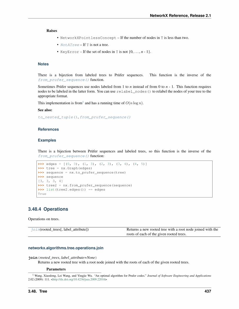
NetworkX Reference, Release 2.1
Raises
• NetworkXPointlessConcept – If the number of nodes in T is less than two.
• NotATree – If T is not a tree.
• KeyError – If the set of nodes in T is not {0, . . . , n - 1}.
Notes
There is a bijection from labeled trees to Prüfer sequences. This function is the inverse of thefrom_prufer_sequence() function.
Sometimes Prüfer sequences use nodes labeled from 1 to n instead of from 0 to n - 1. This function requiresnodes to be labeled in the latter form. You can use relabel_nodes() to relabel the nodes of your tree to theappropriate format.
This implementation is from1 and has a running time of 𝑂(𝑛 log 𝑛).
See also:
to_nested_tuple(), from_prufer_sequence()
References
Examples
There is a bijection between Prüfer sequences and labeled trees, so this function is the inverse of thefrom_prufer_sequence() function:
>>> edges = [(0, 3), (1, 3), (2, 3), (3, 4), (4, 5)]>>> tree = nx.Graph(edges)>>> sequence = nx.to_prufer_sequence(tree)>>> sequence[3, 3, 3, 4]>>> tree2 = nx.from_prufer_sequence(sequence)>>> list(tree2.edges()) == edgesTrue
3.48.4 Operations
Operations on trees.
join(rooted_trees[, label_attribute]) Returns a new rooted tree with a root node joined with theroots of each of the given rooted trees.
networkx.algorithms.tree.operations.join
join(rooted_trees, label_attribute=None)Returns a new rooted tree with a root node joined with the roots of each of the given rooted trees.
Parameters1 Wang, Xiaodong, Lei Wang, and Yingjie Wu. “An optimal algorithm for Prufer codes.” Journal of Software Engineering and Applications
2.02 (2009): 111. <http://dx.doi.org/10.4236/jsea.2009.22016>
3.48. Tree 437

NetworkX Reference, Release 2.1
• rooted_trees (list) – A list of pairs in which each left element is a NetworkX graph objectrepresenting a tree and each right element is the root node of that tree. The nodes of thesetrees will be relabeled to integers.
• label_attribute (str) – If provided, the old node labels will be stored in the new tree underthis node attribute. If not provided, the node attribute '_old' will store the original labelof the node in the rooted trees given in the input.
Returns The rooted tree whose subtrees are the given rooted trees. The new root node is la-beled 0. Each non-root node has an attribute, as described under the keyword argumentlabel_attribute, that indicates the label of the original node in the input tree.
Return type NetworkX graph
Notes
Graph, edge, and node attributes are propagated from the given rooted trees to the created tree. If there areany overlapping graph attributes, those from later trees will overwrite those from earlier trees in the tuple ofpositional arguments.
Examples
Join two full balanced binary trees of height h to get a full balanced binary tree of depth h + 1:
>>> h = 4>>> left = nx.balanced_tree(2, h)>>> right = nx.balanced_tree(2, h)>>> joined_tree = nx.join([(left, 0), (right, 0)])>>> nx.is_isomorphic(joined_tree, nx.balanced_tree(2, h + 1))True
3.48.5 Spanning Trees
Algorithms for calculating min/max spanning trees/forests.
minimum_spanning_tree(G[, weight, . . . ]) Returns a minimum spanning tree or forest on an undi-rected graph G.
maximum_spanning_tree(G[, weight, . . . ]) Returns a maximum spanning tree or forest on an undi-rected graph G.
minimum_spanning_edges(G[, algorithm, . . . ]) Generate edges in a minimum spanning forest of an undi-rected weighted graph.
maximum_spanning_edges(G[, algorithm, . . . ]) Generate edges in a maximum spanning forest of an undi-rected weighted graph.
networkx.algorithms.tree.mst.minimum_spanning_tree
minimum_spanning_tree(G, weight=’weight’, algorithm=’kruskal’, ignore_nan=False)Returns a minimum spanning tree or forest on an undirected graph G.
Parameters
• G (undirected graph) – An undirected graph. If G is connected, then the algorithm finds a
438 Chapter 3. Algorithms
NetworkX Reference, Release 2.1
spanning tree. Otherwise, a spanning forest is found.
• weight (str) – Data key to use for edge weights.
• algorithm (string) – The algorithm to use when finding a minimum spanning tree. Validchoices are ‘kruskal’, ‘prim’, or ‘boruvka’. The default is ‘kruskal’.
• ignore_nan (bool (default: False)) – If a NaN is found as an edge weight normally anexception is raised. If ignore_nan is True then that edge is ignored instead.
Returns G – A minimum spanning tree or forest.
Return type NetworkX Graph
Examples
>>> G = nx.cycle_graph(4)>>> G.add_edge(0, 3, weight=2)>>> T = nx.minimum_spanning_tree(G)>>> sorted(T.edges(data=True))[(0, 1, {}), (1, 2, {}), (2, 3, {})]
Notes
For Boruvka’s algorithm, each edge must have a weight attribute, and each edge weight must be distinct.
For the other algorithms, if the graph edges do not have a weight attribute a default weight of 1 will be used.
There may be more than one tree with the same minimum or maximum weight. See networkx.tree.recognition for more detailed definitions.
Isolated nodes with self-loops are in the tree as edgeless isolated nodes.
networkx.algorithms.tree.mst.maximum_spanning_tree
maximum_spanning_tree(G, weight=’weight’, algorithm=’kruskal’, ignore_nan=False)Returns a maximum spanning tree or forest on an undirected graph G.
Parameters
• G (undirected graph) – An undirected graph. If G is connected, then the algorithm finds aspanning tree. Otherwise, a spanning forest is found.
• weight (str) – Data key to use for edge weights.
• algorithm (string) – The algorithm to use when finding a minimum spanning tree. Validchoices are ‘kruskal’, ‘prim’, or ‘boruvka’. The default is ‘kruskal’.
• ignore_nan (bool (default: False)) – If a NaN is found as an edge weight normally anexception is raised. If ignore_nan is True then that edge is ignored instead.
Returns G – A minimum spanning tree or forest.
Return type NetworkX Graph
3.48. Tree 439

NetworkX Reference, Release 2.1
Examples
>>> G = nx.cycle_graph(4)>>> G.add_edge(0, 3, weight=2)>>> T = nx.maximum_spanning_tree(G)>>> sorted(T.edges(data=True))[(0, 1, {}), (0, 3, {'weight': 2}), (1, 2, {})]
Notes
For Boruvka’s algorithm, each edge must have a weight attribute, and each edge weight must be distinct.
For the other algorithms, if the graph edges do not have a weight attribute a default weight of 1 will be used.
There may be more than one tree with the same minimum or maximum weight. See networkx.tree.recognition for more detailed definitions.
Isolated nodes with self-loops are in the tree as edgeless isolated nodes.
networkx.algorithms.tree.mst.minimum_spanning_edges
minimum_spanning_edges(G, algorithm=’kruskal’, weight=’weight’, keys=True, data=True, ig-nore_nan=False)
Generate edges in a minimum spanning forest of an undirected weighted graph.
A minimum spanning tree is a subgraph of the graph (a tree) with the minimum sum of edge weights. A spanningforest is a union of the spanning trees for each connected component of the graph.
Parameters
• G (undirected Graph) – An undirected graph. If G is connected, then the algorithm finds aspanning tree. Otherwise, a spanning forest is found.
• algorithm (string) – The algorithm to use when finding a minimum spanning tree. Validchoices are ‘kruskal’, ‘prim’, or ‘boruvka’. The default is ‘kruskal’.
• weight (string) – Edge data key to use for weight (default ‘weight’).
• keys (bool) – Whether to yield edge key in multigraphs in addition to the edge. If G is not amultigraph, this is ignored.
• data (bool, optional) – If True yield the edge data along with the edge.
• ignore_nan (bool (default: False)) – If a NaN is found as an edge weight normally anexception is raised. If ignore_nan is True then that edge is ignored instead.
Returns
edges – An iterator over edges in a maximum spanning tree of G. Edges connecting nodes u andv are represented as tuples: (u, v, k, d) or (u, v, k) or (u, v, d) or (u, v)
If G is a multigraph, keys indicates whether the edge key k will be reported in the third positionin the edge tuple. data indicates whether the edge datadict d will appear at the end of the edgetuple.
If G is not a multigraph, the tuples are (u, v, d) if data is True or (u, v) if data isFalse.
Return type iterator
440 Chapter 3. Algorithms

NetworkX Reference, Release 2.1
Examples
>>> from networkx.algorithms import tree
Find minimum spanning edges by Kruskal’s algorithm
>>> G = nx.cycle_graph(4)>>> G.add_edge(0, 3, weight=2)>>> mst = tree.minimum_spanning_edges(G, algorithm='kruskal', data=False)>>> edgelist = list(mst)>>> sorted(edgelist)[(0, 1), (1, 2), (2, 3)]
Find minimum spanning edges by Prim’s algorithm
>>> G = nx.cycle_graph(4)>>> G.add_edge(0, 3, weight=2)>>> mst = tree.minimum_spanning_edges(G, algorithm='prim', data=False)>>> edgelist = list(mst)>>> sorted(edgelist)[(0, 1), (1, 2), (2, 3)]
Notes
For Boruvka’s algorithm, each edge must have a weight attribute, and each edge weight must be distinct.
For the other algorithms, if the graph edges do not have a weight attribute a default weight of 1 will be used.
Modified code from David Eppstein, April 2006 http://www.ics.uci.edu/~eppstein/PADS/
networkx.algorithms.tree.mst.maximum_spanning_edges
maximum_spanning_edges(G, algorithm=’kruskal’, weight=’weight’, keys=True, data=True, ig-nore_nan=False)
Generate edges in a maximum spanning forest of an undirected weighted graph.
A maximum spanning tree is a subgraph of the graph (a tree) with the maximum possible sum of edge weights.A spanning forest is a union of the spanning trees for each connected component of the graph.
Parameters
• G (undirected Graph) – An undirected graph. If G is connected, then the algorithm finds aspanning tree. Otherwise, a spanning forest is found.
• algorithm (string) – The algorithm to use when finding a maximum spanning tree. Validchoices are ‘kruskal’, ‘prim’, or ‘boruvka’. The default is ‘kruskal’.
• weight (string) – Edge data key to use for weight (default ‘weight’).
• keys (bool) – Whether to yield edge key in multigraphs in addition to the edge. If G is not amultigraph, this is ignored.
• data (bool, optional) – If True yield the edge data along with the edge.
• ignore_nan (bool (default: False)) – If a NaN is found as an edge weight normally anexception is raised. If ignore_nan is True then that edge is ignored instead.
3.48. Tree 441

NetworkX Reference, Release 2.1
Returns
edges – An iterator over edges in a maximum spanning tree of G. Edges connecting nodes u andv are represented as tuples: (u, v, k, d) or (u, v, k) or (u, v, d) or (u, v)
If G is a multigraph, keys indicates whether the edge key k will be reported in the third positionin the edge tuple. data indicates whether the edge datadict d will appear at the end of the edgetuple.
If G is not a multigraph, the tuples are (u, v, d) if data is True or (u, v) if data isFalse.
Return type iterator
Examples
>>> from networkx.algorithms import tree
Find maximum spanning edges by Kruskal’s algorithm
>>> G = nx.cycle_graph(4)>>> G.add_edge(0, 3, weight=2)>>> mst = tree.maximum_spanning_edges(G, algorithm='kruskal', data=False)>>> edgelist = list(mst)>>> sorted(edgelist)[(0, 1), (0, 3), (1, 2)]
Find maximum spanning edges by Prim’s algorithm
>>> G = nx.cycle_graph(4)>>> G.add_edge(0, 3, weight=2) # assign weight 2 to edge 0-3>>> mst = tree.maximum_spanning_edges(G, algorithm='prim', data=False)>>> edgelist = list(mst)>>> sorted(edgelist)[(0, 1), (0, 3), (3, 2)]
Notes
For Boruvka’s algorithm, each edge must have a weight attribute, and each edge weight must be distinct.
For the other algorithms, if the graph edges do not have a weight attribute a default weight of 1 will be used.
Modified code from David Eppstein, April 2006 http://www.ics.uci.edu/~eppstein/PADS/
3.48.6 Exceptions
Functions for encoding and decoding trees.
Since a tree is a highly restricted form of graph, it can be represented concisely in several ways. This module includesfunctions for encoding and decoding trees in the form of nested tuples and Prüfer sequences. The former requires arooted tree, whereas the latter can be applied to unrooted trees. Furthermore, there is a bijection from Prüfer sequencesto labeled trees.
442 Chapter 3. Algorithms

NetworkX Reference, Release 2.1
NotATree Raised when a function expects a tree (that is, a connectedundirected graph with no cycles) but gets a non-tree graphas input instead.
networkx.algorithms.tree.coding.NotATree
exception NotATreeRaised when a function expects a tree (that is, a connected undirected graph with no cycles) but gets a non-treegraph as input instead.
3.49 Triads
Functions for analyzing triads of a graph.
triadic_census(G) Determines the triadic census of a directed graph.
3.49.1 networkx.algorithms.triads.triadic_census
triadic_census(G)Determines the triadic census of a directed graph.
The triadic census is a count of how many of the 16 possible types of triads are present in a directed graph.
Parameters G (digraph) – A NetworkX DiGraph
Returns census – Dictionary with triad names as keys and number of occurrences as values.
Return type dict
Notes
This algorithm has complexity 𝑂(𝑚) where 𝑚 is the number of edges in the graph.
See also:
triad_graph()
References
3.50 Vitality
Vitality measures.
closeness_vitality(G[, node, weight, . . . ]) Returns the closeness vitality for nodes in the graph.
3.50. Vitality 443
NetworkX Reference, Release 2.1
3.50.1 networkx.algorithms.vitality.closeness_vitality
closeness_vitality(G, node=None, weight=None, wiener_index=None)Returns the closeness vitality for nodes in the graph.
The closeness vitality of a node, defined in Section 3.6.2 of [1], is the change in the sum of distances betweenall node pairs when excluding that node.
Parameters
• G (NetworkX graph) – A strongly-connected graph.
• weight (string) – The name of the edge attribute used as weight. This is passed directly tothe wiener_index() function.
• node (object) – If specified, only the closeness vitality for this node will be returned. Oth-erwise, a dictionary mappping each node to its closeness vitality will be returned.
Other Parameters wiener_index (number) – If you have already computed the Wiener index of thegraph G, you can provide that value here. Otherwise, it will be computed for you.
Returns
If node is None, this function returnes a dictionary with nodes as keys and closeness vitality asthe value. Otherwise, it returns only the closeness vitality for the specified node.
The closeness vitality of a node may be negative infinity if removing that node would disconnectthe graph.
Return type dictionary or float
Examples
>>> G = nx.cycle_graph(3)>>> nx.closeness_vitality(G){0: 2.0, 1: 2.0, 2: 2.0}
See also:
closeness_centrality()
References
3.51 Voronoi cells
Functions for computing the Voronoi cells of a graph.
voronoi_cells(G, center_nodes[, weight]) Returns the Voronoi cells centered at center_nodeswith respect to the shortest-path distance metric.
3.51.1 networkx.algorithms.voronoi.voronoi_cells
voronoi_cells(G, center_nodes, weight=’weight’)Returns the Voronoi cells centered at center_nodes with respect to the shortest-path distance metric.
444 Chapter 3. Algorithms

NetworkX Reference, Release 2.1
If C is a set of nodes in the graph and c is an element of C, the Voronoi cell centered at a node c is the set of allnodes v that are closer to c than to any other center node in C with respect to the shortest-path distance metric.1
For directed graphs, this will compute the “outward” Voronoi cells, as defined in1, in which distance is measuredfrom the center nodes to the target node. For the “inward” Voronoi cells, use the DiGraph.reverse()method to reverse the orientation of the edges before invoking this function on the directed graph.
Parameters
• G (NetworkX graph)
• center_nodes (set) – A nonempty set of nodes in the graph G that represent the center of theVoronoi cells.
• weight (string or function) – The edge attribute (or an arbitrary function) representingthe weight of an edge. This keyword argument is as described in the documentation formulti_source_dijkstra_path(), for example.
Returns A mapping from center node to set of all nodes in the graph closer to that center node thanto any other center node. The keys of the dictionary are the element of center_nodes, andthe values of the dictionary form a partition of the nodes of G.
Return type dictionary
Examples
To get only the partition of the graph induced by the Voronoi cells, take the collection of all values in the returneddictionary:
>>> G = nx.path_graph(6)>>> center_nodes = {0, 3}>>> cells = nx.voronoi_cells(G, center_nodes)>>> partition = set(map(frozenset, cells.values()))>>> sorted(map(sorted, partition))[[0, 1], [2, 3, 4, 5]]
Raises ValueError – If center_nodes is empty.
References
3.52 Wiener index
Functions related to the Wiener index of a graph.
wiener_index(G[, weight]) Returns the Wiener index of the given graph.
3.52.1 networkx.algorithms.wiener.wiener_index
wiener_index(G, weight=None)Returns the Wiener index of the given graph.
1 Erwig, Martin. (2000), “The graph Voronoi diagram with applications.” Networks, 36: 156–163. <dx.doi.org/10.1002/1097-0037(200010)36:3<156::AID-NET2>3.0.CO;2-L>
3.52. Wiener index 445

NetworkX Reference, Release 2.1
The Wiener index of a graph is the sum of the shortest-path distances between each pair of reachable nodes. Forpairs of nodes in undirected graphs, only one orientation of the pair is counted.
Parameters
• G (NetworkX graph)
• weight (object) – The edge attribute to use as distance when computing shortest-path dis-tances. This is passed directly to the networkx.shortest_path_length() func-tion.
Returns The Wiener index of the graph G.
Return type float
Raises NetworkXError – If the graph G is not connected.
Notes
If a pair of nodes is not reachable, the distance is assumed to be infinity. This means that for graphs that are notstrongly-connected, this function returns inf.
The Wiener index is not usually defined for directed graphs, however this function uses the natural generalizationof the Wiener index to directed graphs.
Examples
The Wiener index of the (unweighted) complete graph on n nodes equals the number of pairs of the n nodes,since each pair of nodes is at distance one:
>>> import networkx as nx>>> n = 10>>> G = nx.complete_graph(n)>>> nx.wiener_index(G) == n * (n - 1) / 2True
Graphs that are not strongly-connected have infinite Wiener index:
>>> G = nx.empty_graph(2)>>> nx.wiener_index(G)inf
446 Chapter 3. Algorithms

CHAPTER
FOUR
FUNCTIONS
Functional interface to graph methods and assorted utilities.
4.1 Graph
degree(G[, nbunch, weight]) Return a degree view of single node or of nbunch of nodes.degree_histogram(G) Return a list of the frequency of each degree value.density(G) Return the density of a graph.info(G[, n]) Print short summary of information for the graph G or the
node n.create_empty_copy(G[, with_data]) Return a copy of the graph G with all of the edges removed.is_directed(G) Return True if graph is directed.add_star(G_to_add_to, nodes_for_star, **attr) Add a star to Graph G_to_add_to.add_path(G_to_add_to, nodes_for_path, **attr) Add a path to the Graph G_to_add_to.add_cycle(G_to_add_to, nodes_for_cycle, **attr) Add a cycle to the Graph G_to_add_to.
4.1.1 networkx.classes.function.degree
degree(G, nbunch=None, weight=None)Return a degree view of single node or of nbunch of nodes. If nbunch is ommitted, then return degrees of allnodes.
4.1.2 networkx.classes.function.degree_histogram
degree_histogram(G)Return a list of the frequency of each degree value.
Parameters G (Networkx graph) – A graph
Returns hist – A list of frequencies of degrees. The degree values are the index in the list.
Return type list
Notes
Note: the bins are width one, hence len(list) can be large (Order(number_of_edges))
447

NetworkX Reference, Release 2.1
4.1.3 networkx.classes.function.density
density(G)Return the density of a graph.
The density for undirected graphs is
𝑑 =2𝑚
𝑛(𝑛− 1),
and for directed graphs is
𝑑 =𝑚
𝑛(𝑛− 1),
where n is the number of nodes and m is the number of edges in G.
Notes
The density is 0 for a graph without edges and 1 for a complete graph. The density of multigraphs can be higherthan 1.
Self loops are counted in the total number of edges so graphs with self loops can have density higher than 1.
4.1.4 networkx.classes.function.info
info(G, n=None)Print short summary of information for the graph G or the node n.
Parameters
• G (Networkx graph) – A graph
• n (node (any hashable)) – A node in the graph G
4.1.5 networkx.classes.function.create_empty_copy
create_empty_copy(G, with_data=True)Return a copy of the graph G with all of the edges removed.
Parameters
• G (graph) – A NetworkX graph
• with_data (bool (default=True)) – Propagate Graph and Nodes data to the new graph.
See also:
empty_graph()
4.1.6 networkx.classes.function.is_directed
is_directed(G)Return True if graph is directed.
448 Chapter 4. Functions

NetworkX Reference, Release 2.1
4.1.7 networkx.classes.function.add_star
add_star(G_to_add_to, nodes_for_star, **attr)Add a star to Graph G_to_add_to.
The first node in nodes_for_star is the middle of the star. It is connected to all other nodes.
Parameters
• nodes_for_star (iterable container) – A container of nodes.
• attr (keyword arguments, optional (default= no attributes)) – Attributes to add to every edgein star.
See also:
add_path(), add_cycle()
Examples
>>> G = nx.Graph()>>> nx.add_star(G, [0, 1, 2, 3])>>> nx.add_star(G, [10, 11, 12], weight=2)
4.1.8 networkx.classes.function.add_path
add_path(G_to_add_to, nodes_for_path, **attr)Add a path to the Graph G_to_add_to.
Parameters
• nodes_for_path (iterable container) – A container of nodes. A path will be constructedfrom the nodes (in order) and added to the graph.
• attr (keyword arguments, optional (default= no attributes)) – Attributes to add to every edgein path.
See also:
add_star(), add_cycle()
Examples
>>> G = nx.Graph()>>> nx.add_path(G, [0, 1, 2, 3])>>> nx.add_path(G, [10, 11, 12], weight=7)
4.1.9 networkx.classes.function.add_cycle
add_cycle(G_to_add_to, nodes_for_cycle, **attr)Add a cycle to the Graph G_to_add_to.
Parameters
• nodes_for_cycle (iterable container) – A container of nodes. A cycle will be constructedfrom the nodes (in order) and added to the graph.
4.1. Graph 449

NetworkX Reference, Release 2.1
• attr (keyword arguments, optional (default= no attributes)) – Attributes to add to every edgein cycle.
See also:
add_path(), add_star()
Examples
>>> G = nx.Graph() # or DiGraph, MultiGraph, MultiDiGraph, etc>>> nx.add_cycle(G, [0, 1, 2, 3])>>> nx.add_cycle(G, [10, 11, 12], weight=7)
4.2 Nodes
nodes(G) Return an iterator over the graph nodes.number_of_nodes(G) Return the number of nodes in the graph.all_neighbors(graph, node) Returns all of the neighbors of a node in the graph.non_neighbors(graph, node) Returns the non-neighbors of the node in the graph.common_neighbors(G, u, v) Return the common neighbors of two nodes in a graph.
4.2.1 networkx.classes.function.nodes
nodes(G)Return an iterator over the graph nodes.
4.2.2 networkx.classes.function.number_of_nodes
number_of_nodes(G)Return the number of nodes in the graph.
4.2.3 networkx.classes.function.all_neighbors
all_neighbors(graph, node)Returns all of the neighbors of a node in the graph.
If the graph is directed returns predecessors as well as successors.
Parameters
• graph (NetworkX graph) – Graph to find neighbors.
• node (node) – The node whose neighbors will be returned.
Returns neighbors – Iterator of neighbors
Return type iterator
450 Chapter 4. Functions

NetworkX Reference, Release 2.1
4.2.4 networkx.classes.function.non_neighbors
non_neighbors(graph, node)Returns the non-neighbors of the node in the graph.
Parameters
• graph (NetworkX graph) – Graph to find neighbors.
• node (node) – The node whose neighbors will be returned.
Returns non_neighbors – Iterator of nodes in the graph that are not neighbors of the node.
Return type iterator
4.2.5 networkx.classes.function.common_neighbors
common_neighbors(G, u, v)Return the common neighbors of two nodes in a graph.
Parameters
• G (graph) – A NetworkX undirected graph.
• u, v (nodes) – Nodes in the graph.
Returns cnbors – Iterator of common neighbors of u and v in the graph.
Return type iterator
Raises NetworkXError – If u or v is not a node in the graph.
Examples
>>> G = nx.complete_graph(5)>>> sorted(nx.common_neighbors(G, 0, 1))[2, 3, 4]
4.3 Edges
edges(G[, nbunch]) Return an edge view of edges incident to nodes in nbunch.number_of_edges(G) Return the number of edges in the graph.non_edges(graph) Returns the non-existent edges in the graph.
4.3.1 networkx.classes.function.edges
edges(G, nbunch=None)Return an edge view of edges incident to nodes in nbunch.
Return all edges if nbunch is unspecified or nbunch=None.
For digraphs, edges=out_edges
4.3. Edges 451
NetworkX Reference, Release 2.1
4.3.2 networkx.classes.function.number_of_edges
number_of_edges(G)Return the number of edges in the graph.
4.3.3 networkx.classes.function.non_edges
non_edges(graph)Returns the non-existent edges in the graph.
Parameters graph (NetworkX graph.) – Graph to find non-existent edges.
Returns non_edges – Iterator of edges that are not in the graph.
Return type iterator
4.4 Self loops
selfloop_edges(G[, data, keys, default]) Returns an iterator over selfloop edges.number_of_selfloops(G) Return the number of selfloop edges.nodes_with_selfloops(G) Returns an iterator over nodes with self loops.
4.4.1 networkx.classes.function.selfloop_edges
selfloop_edges(G, data=False, keys=False, default=None)Returns an iterator over selfloop edges.
A selfloop edge has the same node at both ends.
Parameters
• data (string or bool, optional (default=False)) – Return selfloop edges as two tuples (u,v) (data=False) or three-tuples (u, v, datadict) (data=True) or three-tuples (u, v, datavalue)(data=’attrname’)
• keys (bool, optional (default=False)) – If True, return edge keys with each edge.
• default (value, optional (default=None)) – Value used for edges that dont have the requestedattribute. Only relevant if data is not True or False.
Returns edgeiter – An iterator over all selfloop edges.
Return type iterator over edge tuples
See also:
nodes_with_selfloops(), number_of_selfloops()
Examples
>>> G = nx.MultiGraph() # or Graph, DiGraph, MultiDiGraph, etc>>> ekey = G.add_edge(1, 1)>>> ekey = G.add_edge(1, 2)>>> list(nx.selfloop_edges(G))[(1, 1)]
452 Chapter 4. Functions

NetworkX Reference, Release 2.1
>>> list(nx.selfloop_edges(G, data=True))[(1, 1, {})]>>> list(nx.selfloop_edges(G, keys=True))[(1, 1, 0)]>>> list(nx.selfloop_edges(G, keys=True, data=True))[(1, 1, 0, {})]
4.4.2 networkx.classes.function.number_of_selfloops
number_of_selfloops(G)Return the number of selfloop edges.
A selfloop edge has the same node at both ends.
Returns nloops – The number of selfloops.
Return type int
See also:
nodes_with_selfloops(), selfloop_edges()
Examples
>>> G = nx.Graph() # or DiGraph, MultiGraph, MultiDiGraph, etc>>> G.add_edge(1, 1)>>> G.add_edge(1, 2)>>> nx.number_of_selfloops(G)1
4.4.3 networkx.classes.function.nodes_with_selfloops
nodes_with_selfloops(G)Returns an iterator over nodes with self loops.
A node with a self loop has an edge with both ends adjacent to that node.
Returns nodelist – A iterator over nodes with self loops.
Return type iterator
See also:
selfloop_edges(), number_of_selfloops()
Examples
>>> G = nx.Graph() # or DiGraph, MultiGraph, MultiDiGraph, etc>>> G.add_edge(1, 1)>>> G.add_edge(1, 2)>>> list(nx.nodes_with_selfloops(G))[1]
4.4. Self loops 453

NetworkX Reference, Release 2.1
4.5 Attributes
set_node_attributes(G, values[, name]) Sets node attributes from a given value or dictionary of val-ues.
get_node_attributes(G, name) Get node attributes from graphset_edge_attributes(G, values[, name]) Sets edge attributes from a given value or dictionary of val-
ues.get_edge_attributes(G, name) Get edge attributes from graph
4.5.1 networkx.classes.function.set_node_attributes
set_node_attributes(G, values, name=None)Sets node attributes from a given value or dictionary of values.
Parameters
• G (NetworkX Graph)
• values (scalar value, dict-like) – What the node attribute should be set to. If values is nota dictionary, then it is treated as a single attribute value that is then applied to every node inG. This means that if you provide a mutable object, like a list, updates to that object will bereflected in the node attribute for each edge. The attribute name will be name.
If values is a dict or a dict of dict, the corresponding node’s attributes will be updated tovalues.
• name (string (optional, default=None)) – Name of the node attribute to set if values is ascalar.
Examples
After computing some property of the nodes of a graph, you may want to assign a node attribute to store thevalue of that property for each node:
>>> G = nx.path_graph(3)>>> bb = nx.betweenness_centrality(G)>>> isinstance(bb, dict)True>>> nx.set_node_attributes(G, bb, 'betweenness')>>> G.nodes[1]['betweenness']1.0
If you provide a list as the second argument, updates to the list will be reflected in the node attribute for eachnode:
>>> G = nx.path_graph(3)>>> labels = []>>> nx.set_node_attributes(G, labels, 'labels')>>> labels.append('foo')>>> G.nodes[0]['labels']['foo']>>> G.nodes[1]['labels']['foo']>>> G.nodes[2]['labels']['foo']
454 Chapter 4. Functions

NetworkX Reference, Release 2.1
If you provide a dictionary of dictionaries as the second argument, the entire dictionary will be used to updatenode attributes:
>>> G = nx.path_graph(3)>>> attrs = {0: {'attr1': 20, 'attr2': 'nothing'}, 1: {'attr2': 3}}>>> nx.set_node_attributes(G, attrs)>>> G.nodes[0]['attr1']20>>> G.nodes[0]['attr2']'nothing'>>> G.nodes[1]['attr2']3>>> G.nodes[2]{}
4.5.2 networkx.classes.function.get_node_attributes
get_node_attributes(G, name)Get node attributes from graph
Parameters
• G (NetworkX Graph)
• name (string) – Attribute name
Returns
Return type Dictionary of attributes keyed by node.
Examples
>>> G = nx.Graph()>>> G.add_nodes_from([1, 2, 3], color='red')>>> color = nx.get_node_attributes(G, 'color')>>> color[1]'red'
4.5.3 networkx.classes.function.set_edge_attributes
set_edge_attributes(G, values, name=None)Sets edge attributes from a given value or dictionary of values.
Parameters
• G (NetworkX Graph)
• values (scalar value, dict-like) – What the edge attribute should be set to. If values is nota dictionary, then it is treated as a single attribute value that is then applied to every edge inG. This means that if you provide a mutable object, like a list, updates to that object will bereflected in the edge attribute for each edge. The attribute name will be name.
If values is a dict or a dict of dict, the corresponding edge’ attributes will be updated tovalues. For multigraphs, the tuples must be of the form (u, v, key), where u andv are nodes and key is the key corresponding to the edge. For non-multigraphs, the keysmust be tuples of the form (u, v).
4.5. Attributes 455

NetworkX Reference, Release 2.1
• name (string (optional, default=None)) – Name of the edge attribute to set if values is ascalar.
Examples
After computing some property of the edges of a graph, you may want to assign a edge attribute to store thevalue of that property for each edge:
>>> G = nx.path_graph(3)>>> bb = nx.edge_betweenness_centrality(G, normalized=False)>>> nx.set_edge_attributes(G, bb, 'betweenness')>>> G.edges[1, 2]['betweenness']2.0
If you provide a list as the second argument, updates to the list will be reflected in the edge attribute for eachedge:
>>> labels = []>>> nx.set_edge_attributes(G, labels, 'labels')>>> labels.append('foo')>>> G.edges[0, 1]['labels']['foo']>>> G.edges[1, 2]['labels']['foo']
If you provide a dictionary of dictionaries as the second argument, the entire dictionary will be used to updateedge attributes:
>>> G = nx.path_graph(3)>>> attrs = {(0, 1): {'attr1': 20, 'attr2': 'nothing'},... (1, 2): {'attr2': 3}}>>> nx.set_edge_attributes(G, attrs)>>> G[0][1]['attr1']20>>> G[0][1]['attr2']'nothing'>>> G[1][2]['attr2']3
4.5.4 networkx.classes.function.get_edge_attributes
get_edge_attributes(G, name)Get edge attributes from graph
Parameters
• G (NetworkX Graph)
• name (string) – Attribute name
Returns
• Dictionary of attributes keyed by edge. For (di)graphs, the keys are
• 2-tuples of the form ((u, v). For multi(di)graphs, the keys are 3-tuples of )
• the form ((u, v, key).)
456 Chapter 4. Functions

NetworkX Reference, Release 2.1
Examples
>>> G = nx.Graph()>>> nx.add_path(G, [1, 2, 3], color='red')>>> color = nx.get_edge_attributes(G, 'color')>>> color[(1, 2)]'red'
4.6 Freezing graph structure
freeze(G) Modify graph to prevent further change by adding or re-moving nodes or edges.
is_frozen(G) Return True if graph is frozen.
4.6.1 networkx.classes.function.freeze
freeze(G)Modify graph to prevent further change by adding or removing nodes or edges.
Node and edge data can still be modified.
Parameters G (graph) – A NetworkX graph
Examples
>>> G = nx.path_graph(4)>>> G = nx.freeze(G)>>> try:... G.add_edge(4, 5)... except nx.NetworkXError as e:... print(str(e))Frozen graph can't be modified
Notes
To “unfreeze” a graph you must make a copy by creating a new graph object:
>>> graph = nx.path_graph(4)>>> frozen_graph = nx.freeze(graph)>>> unfrozen_graph = nx.Graph(frozen_graph)>>> nx.is_frozen(unfrozen_graph)False
See also:
is_frozen()
4.6. Freezing graph structure 457

NetworkX Reference, Release 2.1
4.6.2 networkx.classes.function.is_frozen
is_frozen(G)Return True if graph is frozen.
Parameters G (graph) – A NetworkX graph
See also:
freeze()
458 Chapter 4. Functions

CHAPTER
FIVE
GRAPH GENERATORS
5.1 Atlas
Generators for the small graph atlas.
graph_atlas(i) Returns graph number i from the Graph Atlas.graph_atlas_g() Return the list of all graphs with up to seven nodes named
in the Graph Atlas.
5.1.1 networkx.generators.atlas.graph_atlas
graph_atlas(i)Returns graph number i from the Graph Atlas.
For more information, see graph_atlas_g().
Parameters i (int) – The index of the graph from the atlas to get. The graph at index 0 is assumedto be the null graph.
Returns A list of Graph objects, the one at index i corresponding to the graph i in the Graph Atlas.
Return type list
See also:
graph_atlas_g()
Notes
The time required by this function increases linearly with the argument i, since it reads a large file sequentiallyin order to generate the graph1.
References
5.1.2 networkx.generators.atlas.graph_atlas_g
graph_atlas_g()Return the list of all graphs with up to seven nodes named in the Graph Atlas.
1 Ronald C. Read and Robin J. Wilson, An Atlas of Graphs. Oxford University Press, 1998.
459

NetworkX Reference, Release 2.1
The graphs are listed in increasing order by
1. number of nodes,
2. number of edges,
3. degree sequence (for example 111223 < 112222),
4. number of automorphisms,
in that order, with three exceptions as described in the Notes section below. This causes the list to correspondwith the index of the graphs in the Graph Atlas [atlas], with the first graph, G[0], being the null graph.
Returns A list of Graph objects, the one at index i corresponding to the graph i in the Graph Atlas.
Return type list
See also:
graph_atlas()
Notes
This function may be expensive in both time and space, since it reads a large file sequentially in order to populatethe list.
Although the NetworkX atlas functions match the order of graphs given in the “Atlas of Graphs” book, thereare (at least) three errors in the ordering described in the book. The following three pairs of nodes violate thelexicographically nondecreasing sorted degree sequence rule:
• graphs 55 and 56 with degree sequences 001111 and 000112,
• graphs 1007 and 1008 with degree sequences 3333444 and 3333336,
• graphs 1012 and 1213 with degree sequences 1244555 and 1244456.
References
5.2 Classic
Generators for some classic graphs.
The typical graph generator is called as follows:
>>> G = nx.complete_graph(100)
returning the complete graph on n nodes labeled 0, .., 99 as a simple graph. Except for empty_graph, all the generatorsin this module return a Graph class (i.e. a simple, undirected graph).
balanced_tree(r, h[, create_using]) Return the perfectly balanced r-ary tree of height h.barbell_graph(m1, m2[, create_using]) Return the Barbell Graph: two complete graphs connected
by a path.complete_graph(n[, create_using]) Return the complete graph K_n with n nodes.complete_multipartite_graph(*subset_sizes) Returns the complete multipartite graph with the specified
subset sizes.circular_ladder_graph(n[, create_using]) Return the circular ladder graph 𝐶𝐿𝑛 of length n.cycle_graph(n[, create_using]) Return the cycle graph 𝐶𝑛 of cyclically connected nodes.
Continued on next page
460 Chapter 5. Graph generators
NetworkX Reference, Release 2.1
Table 5.2 – continued from previous pagedorogovtsev_goltsev_mendes_graph(n[, . . . ]) Return the hierarchically constructed Dorogovtsev-
Goltsev-Mendes graph.empty_graph([n, create_using]) Return the empty graph with n nodes and zero edges.ladder_graph(n[, create_using]) Return the Ladder graph of length n.lollipop_graph(m, n[, create_using]) Return the Lollipop Graph; K_m connected to P_n.null_graph([create_using]) Return the Null graph with no nodes or edges.path_graph(n[, create_using]) Return the Path graph P_n of linearly connected nodes.star_graph(n[, create_using]) Return the star graphtrivial_graph([create_using]) Return the Trivial graph with one node (with label 0) and
no edges.turan_graph(n, r) Return the Turan Graphwheel_graph(n[, create_using]) Return the wheel graph
5.2.1 networkx.generators.classic.balanced_tree
balanced_tree(r, h, create_using=None)Return the perfectly balanced r-ary tree of height h.
Parameters
• r (int) – Branching factor of the tree; each node will have r children.
• h (int) – Height of the tree.
• create_using (Graph, optional (default None)) – If provided this graph is cleared of nodesand edges and filled with the new graph. Usually used to set the type of the graph.
Returns G – A balanced r-ary tree of height h.
Return type NetworkX graph
Notes
This is the rooted tree where all leaves are at distance h from the root. The root has degree r and all otherinternal nodes have degree r + 1.
Node labels are integers, starting from zero.
A balanced tree is also known as a complete r-ary tree.
5.2.2 networkx.generators.classic.barbell_graph
barbell_graph(m1, m2, create_using=None)Return the Barbell Graph: two complete graphs connected by a path.
For 𝑚1 > 1 and 𝑚2 >= 0.
Two identical complete graphs 𝐾𝑚1 form the left and right bells, and are connected by a path 𝑃𝑚2.
The 2*m1+m2 nodes are numbered 0, ..., m1-1 for the left barbell, m1, ..., m1+m2-1 for thepath, and m1+m2, ..., 2*m1+m2-1 for the right barbell.
The 3 subgraphs are joined via the edges (m1-1, m1) and (m1+m2-1, m1+m2). If m2=0, this is merelytwo complete graphs joined together.
This graph is an extremal example in David Aldous and Jim Fill’s e-text on Random Walks on Graphs.
5.2. Classic 461

NetworkX Reference, Release 2.1
5.2.3 networkx.generators.classic.complete_graph
complete_graph(n, create_using=None)Return the complete graph K_n with n nodes.
Parameters
• n (int or iterable container of nodes) – If n is an integer, nodes are from range(n). If n is acontainer of nodes, those nodes appear in the graph.
• create_using (Graph, optional (default None)) – If provided this graph is cleared of nodesand edges and filled with the new graph. Usually used to set the type of the graph.
Examples
>>> G = nx.complete_graph(9)>>> len(G)9>>> G.size()36>>> G = nx.complete_graph(range(11, 14))>>> list(G.nodes())[11, 12, 13]>>> G = nx.complete_graph(4, nx.DiGraph())>>> G.is_directed()True
5.2.4 networkx.generators.classic.complete_multipartite_graph
complete_multipartite_graph(*subset_sizes)Returns the complete multipartite graph with the specified subset sizes.
Parameters subset_sizes (tuple of integers or tuple of node iterables) – The arguments can eitherall be integer number of nodes or they can all be iterables of nodes. If integers, they representthe number of vertices in each subset of the multipartite graph. If iterables, each is used to createthe nodes for that subset. The length of subset_sizes is the number of subsets.
Returns
G – Returns the complete multipartite graph with the specified subsets.
For each node, the node attribute ‘subset’ is an integer indicating which subset contains the node.
Return type NetworkX Graph
Examples
Creating a complete tripartite graph, with subsets of one, two, and three vertices, respectively.
>>> import networkx as nx>>> G = nx.complete_multipartite_graph(1, 2, 3)>>> [G.nodes[u]['subset'] for u in G][0, 1, 1, 2, 2, 2]>>> list(G.edges(0))[(0, 1), (0, 2), (0, 3), (0, 4), (0, 5)]>>> list(G.edges(2))
462 Chapter 5. Graph generators

NetworkX Reference, Release 2.1
[(2, 0), (2, 3), (2, 4), (2, 5)]>>> list(G.edges(4))[(4, 0), (4, 1), (4, 2)]
>>> G = nx.complete_multipartite_graph('a', 'bc', 'def')>>> [G.nodes[u]['subset'] for u in sorted(G)][0, 1, 1, 2, 2, 2]
Notes
This function generalizes several other graph generator functions.
• If no subset sizes are given, this returns the null graph.
• If a single subset size n is given, this returns the empty graph on n nodes.
• If two subset sizes m and n are given, this returns the complete bipartite graph on m + n nodes.
• If subset sizes 1 and n are given, this returns the star graph on n + 1 nodes.
See also:
complete_bipartite_graph()
5.2.5 networkx.generators.classic.circular_ladder_graph
circular_ladder_graph(n, create_using=None)Return the circular ladder graph 𝐶𝐿𝑛 of length n.
𝐶𝐿𝑛 consists of two concentric n-cycles in which each of the n pairs of concentric nodes are joined by an edge.
Node labels are the integers 0 to n-1
5.2.6 networkx.generators.classic.cycle_graph
cycle_graph(n, create_using=None)Return the cycle graph 𝐶𝑛 of cyclically connected nodes.
𝐶𝑛 is a path with its two end-nodes connected.
Parameters
• n (int or iterable container of nodes) – If n is an integer, nodes are from range(n). If n isa container of nodes, those nodes appear in the graph.
• create_using (Graph, optional (default Graph())) – If provided this graph is cleared ofnodes and edges and filled with the new graph. Usually used to set the type of the graph.
Notes
If create_using is directed, the direction is in increasing order.
5.2. Classic 463

NetworkX Reference, Release 2.1
5.2.7 networkx.generators.classic.dorogovtsev_goltsev_mendes_graph
dorogovtsev_goltsev_mendes_graph(n, create_using=None)Return the hierarchically constructed Dorogovtsev-Goltsev-Mendes graph.
n is the generation. See: arXiv:/cond-mat/0112143 by Dorogovtsev, Goltsev and Mendes.
5.2.8 networkx.generators.classic.empty_graph
empty_graph(n=0, create_using=None)Return the empty graph with n nodes and zero edges.
Parameters
• n (int or iterable container of nodes (default = 0)) – If n is an integer, nodes are fromrange(n). If n is a container of nodes, those nodes appear in the graph.
• create_using (Graph, optional (default Graph())) – If provided this graph is cleared ofnodes and edges and filled with the new graph. Usually used to set the type of the graph.
Examples
>>> G = nx.empty_graph(10)>>> G.number_of_nodes()10>>> G.number_of_edges()0>>> G = nx.empty_graph("ABC")>>> G.number_of_nodes()3>>> sorted(G)['A', 'B', 'C']
Notes
The variable create_using should point to a “graph”-like object that will be cleared (nodes and edges will beremoved) and refitted as an empty “graph” with nodes specified in n. This capability is useful for specifying theclass-nature of the resulting empty “graph” (i.e. Graph, DiGraph, MyWeirdGraphClass, etc.).
The variable create_using has two main uses: Firstly, the variable create_using can be used to create an emptydigraph, multigraph, etc. For example,
>>> n = 10>>> G = nx.empty_graph(n, create_using=nx.DiGraph())
will create an empty digraph on n nodes.
Secondly, one can pass an existing graph (digraph, multigraph, etc.) via create_using. For example, if G is anexisting graph (resp. digraph, multigraph, etc.), then empty_graph(n, create_using=G) will empty G (i.e. deleteall nodes and edges using G.clear()) and then add n nodes and zero edges, and return the modified graph.
See also create_empty_copy(G).
464 Chapter 5. Graph generators

NetworkX Reference, Release 2.1
5.2.9 networkx.generators.classic.ladder_graph
ladder_graph(n, create_using=None)Return the Ladder graph of length n.
This is two paths of n nodes, with each pair connected by a single edge.
Node labels are the integers 0 to 2*n - 1.
5.2.10 networkx.generators.classic.lollipop_graph
lollipop_graph(m, n, create_using=None)Return the Lollipop Graph; K_m connected to P_n.
This is the Barbell Graph without the right barbell.
Parameters
• m, n (int or iterable container of nodes (default = 0)) – If an integer, nodes are fromrange(m) and range(m,m+n). If a container, the entries are the coordinate of the node.
The nodes for m appear in the complete graph 𝐾𝑚 and the nodes for n appear in the path𝑃𝑛
• create_using (Graph, optional (default Graph())) – If provided this graph is cleared ofnodes and edges and filled with the new graph. Usually used to set the type of the graph.
Notes
The 2 subgraphs are joined via an edge (m-1, m). If n=0, this is merely a complete graph.
(This graph is an extremal example in David Aldous and Jim Fill’s etext on Random Walks on Graphs.)
5.2.11 networkx.generators.classic.null_graph
null_graph(create_using=None)Return the Null graph with no nodes or edges.
See empty_graph for the use of create_using.
5.2.12 networkx.generators.classic.path_graph
path_graph(n, create_using=None)Return the Path graph P_n of linearly connected nodes.
Parameters
• n (int or iterable) – If an integer, node labels are 0 to n with center 0. If an iterable of nodes,the center is the first.
• create_using (Graph, optional (default Graph())) – If provided this graph is cleared ofnodes and edges and filled with the new graph. Usually used to set the type of the graph.
5.2. Classic 465
NetworkX Reference, Release 2.1
5.2.13 networkx.generators.classic.star_graph
star_graph(n, create_using=None)Return the star graph
The star graph consists of one center node connected to n outer nodes.
Parameters
• n (int or iterable) – If an integer, node labels are 0 to n with center 0. If an iterable of nodes,the center is the first.
• create_using (Graph, optional (default Graph())) – If provided this graph is cleared ofnodes and edges and filled with the new graph. Usually used to set the type of the graph.
Notes
The graph has n+1 nodes for integer n. So star_graph(3) is the same as star_graph(range(4)).
5.2.14 networkx.generators.classic.trivial_graph
trivial_graph(create_using=None)Return the Trivial graph with one node (with label 0) and no edges.
5.2.15 networkx.generators.classic.turan_graph
turan_graph(n, r)Return the Turan Graph
The Turan Graph is a complete multipartite graph on 𝑛 vertices with 𝑟 disjoint subsets. It is the graph with theedges for any graph with 𝑛 vertices and 𝑟 disjoint subsets.
Given 𝑛 and 𝑟, we generate a complete multipartite graph with 𝑟 − (𝑛 mod 𝑟) partitions of size 𝑛/𝑟, roundeddown, and 𝑛 mod 𝑟 partitions of size 𝑛/𝑟 + 1, rounded down.
Parameters
• n (int) – The number of vertices.
• r (int) – The number of partitions. Must be less than or equal to n.
Notes
Must satisfy 1 <= 𝑟 <= 𝑛. The graph has (𝑟 − 1)(𝑛2)/(2𝑟) edges, rounded down.
5.2.16 networkx.generators.classic.wheel_graph
wheel_graph(n, create_using=None)Return the wheel graph
The wheel graph consists of a hub node connected to a cycle of (n-1) nodes.
Parameters
466 Chapter 5. Graph generators

NetworkX Reference, Release 2.1
• n (int or iterable) – If an integer, node labels are 0 to n with center 0. If an iterable of nodes,the center is the first.
• create_using (Graph, optional (default Graph())) – If provided this graph is cleared ofnodes and edges and filled with the new graph. Usually used to set the type of the graph.
• Node labels are the integers 0 to n - 1.
5.3 Expanders
Provides explicit constructions of expander graphs.
margulis_gabber_galil_graph(n[, cre-ate_using])
Return the Margulis-Gabber-Galil undirected MultiGraphon n^2 nodes.
chordal_cycle_graph(p[, create_using]) Return the chordal cycle graph on p nodes.
5.3.1 networkx.generators.expanders.margulis_gabber_galil_graph
margulis_gabber_galil_graph(n, create_using=None)Return the Margulis-Gabber-Galil undirected MultiGraph on n^2 nodes.
The undirected MultiGraph is regular with degree 8. Nodes are integer pairs. The second-largest eigenvalue ofthe adjacency matrix of the graph is at most 5 sqrt{2}, regardless of n.
Parameters
• n (int) – Determines the number of nodes in the graph: n^2.
• create_using (graph-like) – A graph-like object that receives the constructed edges. If None,then a MultiGraph instance is used.
Returns G – The constructed undirected multigraph.
Return type graph
Raises NetworkXError – If the graph is directed or not a multigraph.
5.3.2 networkx.generators.expanders.chordal_cycle_graph
chordal_cycle_graph(p, create_using=None)Return the chordal cycle graph on p nodes.
The returned graph is a cycle graph on p nodes with chords joining each vertex x to its inverse modulo p. Thisgraph is a (mildly explicit) 3-regular expander1.
p must be a prime number.
Parameters
• p (a prime number) – The number of vertices in the graph. This also indicates where thechordal edges in the cycle will be created.
• create_using (graph-like) – A graph-like object that receives the constructed edges. If None,then a MultiGraph instance is used.
1 Theorem 4.4.2 in A. Lubotzky. “Discrete groups, expanding graphs and invariant measures”, volume 125 of Progress in Mathematics.Birkhäuser Verlag, Basel, 1994.
5.3. Expanders 467

NetworkX Reference, Release 2.1
Returns G – The constructed undirected multigraph.
Return type graph
Raises NetworkXError – If the graph provided in create_using is directed or not a multi-graph.
References
5.4 Lattice
Functions for generating grid graphs and lattices
The grid_2d_graph(), triangular_lattice_graph(), and hexagonal_lattice_graph() func-tions correspond to the three regular tilings of the plane, the square, triangular, and hexagonal tilings, respectively.grid_graph() and hypercube_graph() are similar for arbitrary dimensions. Useful relevent discussion canbe found about Triangular Tiling, and Square, Hex and Triangle Grids
grid_2d_graph(m, n[, periodic, create_using]) Returns the two-dimensional grid graph.grid_graph(dim[, periodic]) Returns the n-dimensional grid graph.hexagonal_lattice_graph(m, n[, periodic, . . . ]) Returns an m by n hexagonal lattice graph.hypercube_graph(n) Returns the n-dimensional hypercube graph.triangular_lattice_graph(m, n[, periodic, . . . ]) Returns the 𝑚 by 𝑛 triangular lattice graph.
5.4.1 networkx.generators.lattice.grid_2d_graph
grid_2d_graph(m, n, periodic=False, create_using=None)Returns the two-dimensional grid graph.
The grid graph has each node connected to its four nearest neighbors.
Parameters
• m, n (int or iterable container of nodes) – If an integer, nodes are from range(n). If acontainer, elements become the coordinate of the nodes.
• periodic (bool (default: False)) – If this is True the nodes on the grid boundaries are joinedto the corresponding nodes on the opposite grid boundaries.
• create_using (NetworkX graph (default: Graph())) – If provided this graph is cleared ofnodes and edges and filled with the new graph. Usually used to set the type of the graph.
Returns The (possibly periodic) grid graph of the specified dimensions.
Return type NetworkX graph
5.4.2 networkx.generators.lattice.grid_graph
grid_graph(dim, periodic=False)Returns the n-dimensional grid graph.
The dimension n is the length of the list dim and the size in each dimension is the value of the correspondinglist element.
Parameters
468 Chapter 5. Graph generators

NetworkX Reference, Release 2.1
• dim (list or tuple of numbers or iterables of nodes) – ‘dim’ is a tuple or list with, for eachdimension, either a number that is the size of that dimension or an iterable of nodes for thatdimension. The dimension of the grid_graph is the length of dim.
• periodic (bool) – If periodic is True the nodes on the grid boundaries are joined tothe corresponding nodes on the opposite grid boundaries.
Returns The (possibly periodic) grid graph of the specified dimensions.
Return type NetworkX graph
Examples
To produce a 2 by 3 by 4 grid graph, a graph on 24 nodes:
>>> from networkx import grid_graph>>> G = grid_graph(dim=[2, 3, 4])>>> len(G)24>>> G = grid_graph(dim=[range(7, 9), range(3, 6)])>>> len(G)6
5.4.3 networkx.generators.lattice.hexagonal_lattice_graph
hexagonal_lattice_graph(m, n, periodic=False, with_positions=True, create_using=None)Returns an m by n hexagonal lattice graph.
The hexagonal lattice graph is a graph whose nodes and edges are the hexagonal tiling of the plane.
The returned graph will have m rows and n columns of hexagons. Odd numbered columns are shifted up relativeto even numbered columns.
Positions of nodes are computed by default or with_positions is True. Node positions creating thestandard embedding in the plane with sidelength 1 and are stored in the node attribute ‘pos’. pos = nx.get_node_attributes(G, 'pos') creates a dict ready for drawing.
Parameters
• m (int) – The number of rows of hexagons in the lattice.
• n (int) – The number of columns of hexagons in the lattice.
• periodic (bool) – Whether to make a periodic grid by joining the boundary vertices. Forthis to work n must be odd and both n > 1 and m > 1. The periodic connections createanother row and column of hexagons so these graphs have fewer nodes as boundary nodesare identified.
• with_positions (bool (default: True)) – Store the coordinates of each node in the graph nodeattribute ‘pos’. The coordinates provide a lattice with vertical columns of hexagons offsetto interleave and cover the plane. Periodic positions shift the nodes vertically in a nonlinearway so the edges don’t overlap so much.
• create_using (NetworkX graph) – If specified, this must be an instance of a NetworkX graphclass. It will be cleared of nodes and edges and filled with the new graph. Usually used toset the type of the graph. If graph is directed, edges will point up or right.
Returns The m by n hexagonal lattice graph.
5.4. Lattice 469

NetworkX Reference, Release 2.1
Return type NetworkX graph
5.4.4 networkx.generators.lattice.hypercube_graph
hypercube_graph(n)Returns the n-dimensional hypercube graph.
The nodes are the integers between 0 and 2 ** n - 1, inclusive.
For more information on the hypercube graph, see the Wikipedia article Hypercube graph.
Parameters n (int) – The dimension of the hypercube. The number of nodes in the graph will be 2** n.
Returns The hypercube graph of dimension n.
Return type NetworkX graph
5.4.5 networkx.generators.lattice.triangular_lattice_graph
triangular_lattice_graph(m, n, periodic=False, with_positions=True, create_using=None)Returns the 𝑚 by 𝑛 triangular lattice graph.
The triangular lattice graph is a two-dimensional grid graph in which each square unit has a diagonal edge (eachgrid unit has a chord).
The returned graph has 𝑚 rows and 𝑛 columns of triangles. Rows and columns include both triangles pointingup and down. Rows form a strip of constant height. Columns form a series of diamond shapes, staggered withthe columns on either side. Another way to state the size is that the nodes form a grid of m+1 rows and (n +1) // 2 columns. The odd row nodes are shifted horizontally relative to the even rows.
Directed graph types have edges pointed up or right.
Positions of nodes are computed by default or with_positions is True. The position of each node(embedded in a euclidean plane) is stored in the graph using equilateral triangles with sidelength 1. The heightbetween rows of nodes is thus
√(3)/2. Nodes lie in the first quadrant with the node (0, 0) at the origin.
Parameters
• m (int) – The number of rows in the lattice.
• n (int) – The number of columns in the lattice.
• periodic (bool (default: False)) – If True, join the boundary vertices of the grid using pe-riodic boundary conditions. The join between boundaries is the final row and column oftriangles. This means there is one row and one column fewer nodes for the periodic lattice.Periodic lattices require m >= 3, n >= 5 and are allowed but misaligned if m or n are odd
• with_positions (bool (default: True)) – Store the coordinates of each node in the graphnode attribute ‘pos’. The coordinates provide a lattice with equilateral triangles. Periodicpositions shift the nodes vertically in a nonlinear way so the edges don’t overlap so much.
• create_using (NetworkX graph) – If specified, this must be an instance of a NetworkX graphclass. It will be cleared of nodes and edges and filled with the new graph. Usually used toset the type of the graph.
Returns The m by n triangular lattice graph.
Return type NetworkX graph
470 Chapter 5. Graph generators

NetworkX Reference, Release 2.1
5.5 Small
Various small and named graphs, together with some compact generators.
make_small_graph(graph_description[, . . . ]) Return the small graph described by graph_description.LCF_graph(n, shift_list, repeats[, create_using]) Return the cubic graph specified in LCF notation.bull_graph([create_using]) Return the Bull graph.chvatal_graph([create_using]) Return the Chvátal graph.cubical_graph([create_using]) Return the 3-regular Platonic Cubical graph.desargues_graph([create_using]) Return the Desargues graph.diamond_graph([create_using]) Return the Diamond graph.dodecahedral_graph([create_using]) Return the Platonic Dodecahedral graph.frucht_graph([create_using]) Return the Frucht Graph.heawood_graph([create_using]) Return the Heawood graph, a (3,6) cage.house_graph([create_using]) Return the House graph (square with triangle on top).house_x_graph([create_using]) Return the House graph with a cross inside the house
square.icosahedral_graph([create_using]) Return the Platonic Icosahedral graph.krackhardt_kite_graph([create_using]) Return the Krackhardt Kite Social Network.moebius_kantor_graph([create_using]) Return the Moebius-Kantor graph.octahedral_graph([create_using]) Return the Platonic Octahedral graph.pappus_graph() Return the Pappus graph.petersen_graph([create_using]) Return the Petersen graph.sedgewick_maze_graph([create_using]) Return a small maze with a cycle.tetrahedral_graph([create_using]) Return the 3-regular Platonic Tetrahedral graph.truncated_cube_graph([create_using]) Return the skeleton of the truncated cube.truncated_tetrahedron_graph([create_using]) Return the skeleton of the truncated Platonic tetrahedron.tutte_graph([create_using]) Return the Tutte graph.
5.5.1 networkx.generators.small.make_small_graph
make_small_graph(graph_description, create_using=None)Return the small graph described by graph_description.
graph_description is a list of the form [ltype,name,n,xlist]
Here ltype is one of “adjacencylist” or “edgelist”, name is the name of the graph and n the number of nodes.This constructs a graph of n nodes with integer labels 0,..,n-1.
If ltype=”adjacencylist” then xlist is an adjacency list with exactly n entries, in with the j’th entry (which can beempty) specifies the nodes connected to vertex j. e.g. the “square” graph C_4 can be obtained by
>>> G=nx.make_small_graph(["adjacencylist","C_4",4,[[2,4],[1,3],[2,4],[1,3]]])
or, since we do not need to add edges twice,
>>> G=nx.make_small_graph(["adjacencylist","C_4",4,[[2,4],[3],[4],[]]])
If ltype=”edgelist” then xlist is an edge list written as [[v1,w2],[v2,w2],. . . ,[vk,wk]], where vj and wj integersin the range 1,..,n e.g. the “square” graph C_4 can be obtained by
>>> G=nx.make_small_graph(["edgelist","C_4",4,[[1,2],[3,4],[2,3],[4,1]]])
5.5. Small 471

NetworkX Reference, Release 2.1
Use the create_using argument to choose the graph class/type.
5.5.2 networkx.generators.small.LCF_graph
LCF_graph(n, shift_list, repeats, create_using=None)Return the cubic graph specified in LCF notation.
LCF notation (LCF=Lederberg-Coxeter-Fruchte) is a compressed notation used in the generation of variouscubic Hamiltonian graphs of high symmetry. See, for example, dodecahedral_graph, desargues_graph, hea-wood_graph and pappus_graph below.
n (number of nodes) The starting graph is the n-cycle with nodes 0,. . . ,n-1. (The null graph is returned if n <0.)
shift_list = [s1,s2,..,sk], a list of integer shifts mod n,
repeats integer specifying the number of times that shifts in shift_list are successively applied to each v_currentin the n-cycle to generate an edge between v_current and v_current+shift mod n.
For v1 cycling through the n-cycle a total of k*repeats with shift cycling through shiftlist repeats times connectv1 with v1+shift mod n
The utility graph 𝐾3,3
>>> G = nx.LCF_graph(6, [3, -3], 3)
The Heawood graph
>>> G = nx.LCF_graph(14, [5, -5], 7)
See http://mathworld.wolfram.com/LCFNotation.html for a description and references.
5.5.3 networkx.generators.small.bull_graph
bull_graph(create_using=None)Return the Bull graph.
5.5.4 networkx.generators.small.chvatal_graph
chvatal_graph(create_using=None)Return the Chvátal graph.
5.5.5 networkx.generators.small.cubical_graph
cubical_graph(create_using=None)Return the 3-regular Platonic Cubical graph.
5.5.6 networkx.generators.small.desargues_graph
desargues_graph(create_using=None)Return the Desargues graph.
472 Chapter 5. Graph generators

NetworkX Reference, Release 2.1
5.5.7 networkx.generators.small.diamond_graph
diamond_graph(create_using=None)Return the Diamond graph.
5.5.8 networkx.generators.small.dodecahedral_graph
dodecahedral_graph(create_using=None)Return the Platonic Dodecahedral graph.
5.5.9 networkx.generators.small.frucht_graph
frucht_graph(create_using=None)Return the Frucht Graph.
The Frucht Graph is the smallest cubical graph whose automorphism group consists only of the identity element.
5.5.10 networkx.generators.small.heawood_graph
heawood_graph(create_using=None)Return the Heawood graph, a (3,6) cage.
5.5.11 networkx.generators.small.house_graph
house_graph(create_using=None)Return the House graph (square with triangle on top).
5.5.12 networkx.generators.small.house_x_graph
house_x_graph(create_using=None)Return the House graph with a cross inside the house square.
5.5.13 networkx.generators.small.icosahedral_graph
icosahedral_graph(create_using=None)Return the Platonic Icosahedral graph.
5.5.14 networkx.generators.small.krackhardt_kite_graph
krackhardt_kite_graph(create_using=None)Return the Krackhardt Kite Social Network.
A 10 actor social network introduced by David Krackhardt to illustrate: degree, betweenness, centrality, close-ness, etc. The traditional labeling is: Andre=1, Beverley=2, Carol=3, Diane=4, Ed=5, Fernando=6, Garth=7,Heather=8, Ike=9, Jane=10.
5.5. Small 473

NetworkX Reference, Release 2.1
5.5.15 networkx.generators.small.moebius_kantor_graph
moebius_kantor_graph(create_using=None)Return the Moebius-Kantor graph.
5.5.16 networkx.generators.small.octahedral_graph
octahedral_graph(create_using=None)Return the Platonic Octahedral graph.
5.5.17 networkx.generators.small.pappus_graph
pappus_graph()Return the Pappus graph.
5.5.18 networkx.generators.small.petersen_graph
petersen_graph(create_using=None)Return the Petersen graph.
5.5.19 networkx.generators.small.sedgewick_maze_graph
sedgewick_maze_graph(create_using=None)Return a small maze with a cycle.
This is the maze used in Sedgewick,3rd Edition, Part 5, Graph Algorithms, Chapter 18, e.g. Figure 18.2 andfollowing. Nodes are numbered 0,..,7
5.5.20 networkx.generators.small.tetrahedral_graph
tetrahedral_graph(create_using=None)Return the 3-regular Platonic Tetrahedral graph.
5.5.21 networkx.generators.small.truncated_cube_graph
truncated_cube_graph(create_using=None)Return the skeleton of the truncated cube.
5.5.22 networkx.generators.small.truncated_tetrahedron_graph
truncated_tetrahedron_graph(create_using=None)Return the skeleton of the truncated Platonic tetrahedron.
5.5.23 networkx.generators.small.tutte_graph
tutte_graph(create_using=None)Return the Tutte graph.
474 Chapter 5. Graph generators

NetworkX Reference, Release 2.1
5.6 Random Graphs
Generators for random graphs.
fast_gnp_random_graph(n, p[, seed, directed]) Returns a 𝐺𝑛,𝑝 random graph, also known as an Erdos-Rényi graph or a binomial graph.
gnp_random_graph(n, p[, seed, directed]) Returns a 𝐺𝑛,𝑝 random graph, also known as an Erdos-Rényi graph or a binomial graph.
dense_gnm_random_graph(n, m[, seed]) Returns a 𝐺𝑛,𝑚 random graph.gnm_random_graph(n, m[, seed, directed]) Returns a 𝐺𝑛,𝑚 random graph.erdos_renyi_graph(n, p[, seed, directed]) Returns a 𝐺𝑛,𝑝 random graph, also known as an Erdos-
Rényi graph or a binomial graph.binomial_graph(n, p[, seed, directed]) Returns a 𝐺𝑛,𝑝 random graph, also known as an Erdos-
Rényi graph or a binomial graph.newman_watts_strogatz_graph(n, k, p[, seed]) Return a Newman–Watts–Strogatz small-world graph.watts_strogatz_graph(n, k, p[, seed]) Return a Watts–Strogatz small-world graph.connected_watts_strogatz_graph(n, k, p[, . . . ]) Returns a connected Watts–Strogatz small-world graph.random_regular_graph(d, n[, seed]) Returns a random 𝑑-regular graph on 𝑛 nodes.barabasi_albert_graph(n, m[, seed]) Returns a random graph according to the Barabási–Albert
preferential attachment model.powerlaw_cluster_graph(n, m, p[, seed]) Holme and Kim algorithm for growing graphs with pow-
erlaw degree distribution and approximate average cluster-ing.
random_kernel_graph(n, kernel_integral[, . . . ]) Return an random graph based on the specified kernel.random_lobster(n, p1, p2[, seed]) Returns a random lobster graph.random_shell_graph(constructor[, seed]) Returns a random shell graph for the constructor given.random_powerlaw_tree(n[, gamma, seed, tries]) Returns a tree with a power law degree distribution.random_powerlaw_tree_sequence(n[, gamma,. . . ])
Returns a degree sequence for a tree with a power law dis-tribution.
5.6.1 networkx.generators.random_graphs.fast_gnp_random_graph
fast_gnp_random_graph(n, p, seed=None, directed=False)Returns a 𝐺𝑛,𝑝 random graph, also known as an Erdos-Rényi graph or a binomial graph.
Parameters
• n (int) – The number of nodes.
• p (float) – Probability for edge creation.
• seed (int, optional) – Seed for random number generator (default=None).
• directed (bool, optional (default=False)) – If True, this function returns a directed graph.
Notes
The 𝐺𝑛,𝑝 graph algorithm chooses each of the [𝑛(𝑛− 1)]/2 (undirected) or 𝑛(𝑛− 1) (directed) possible edgeswith probability 𝑝.
This algorithm1 runs in 𝑂(𝑛 + 𝑚) time, where m is the expected number of edges, which equals 𝑝𝑛(𝑛− 1)/2.This should be faster than gnp_random_graph() when 𝑝 is small and the expected number of edges is small
1 Vladimir Batagelj and Ulrik Brandes, “Efficient generation of large random networks”, Phys. Rev. E, 71, 036113, 2005.
5.6. Random Graphs 475

NetworkX Reference, Release 2.1
(that is, the graph is sparse).
See also:
gnp_random_graph()
References
5.6.2 networkx.generators.random_graphs.gnp_random_graph
gnp_random_graph(n, p, seed=None, directed=False)Returns a 𝐺𝑛,𝑝 random graph, also known as an Erdos-Rényi graph or a binomial graph.
The 𝐺𝑛,𝑝 model chooses each of the possible edges with probability 𝑝.
The functions binomial_graph() and erdos_renyi_graph() are aliases of this function.
Parameters
• n (int) – The number of nodes.
• p (float) – Probability for edge creation.
• seed (int, optional) – Seed for random number generator (default=None).
• directed (bool, optional (default=False)) – If True, this function returns a directed graph.
See also:
fast_gnp_random_graph()
Notes
This algorithm2 runs in 𝑂(𝑛2) time. For sparse graphs (that is, for small values of 𝑝),fast_gnp_random_graph() is a faster algorithm.
References
5.6.3 networkx.generators.random_graphs.dense_gnm_random_graph
dense_gnm_random_graph(n, m, seed=None)Returns a 𝐺𝑛,𝑚 random graph.
In the 𝐺𝑛,𝑚 model, a graph is chosen uniformly at random from the set of all graphs with 𝑛 nodes and 𝑚 edges.
This algorithm should be faster than gnm_random_graph() for dense graphs.
Parameters
• n (int) – The number of nodes.
• m (int) – The number of edges.
• seed (int, optional) – Seed for random number generator (default=None).
2
5. (a) Gilbert, Random Graphs, Ann. Math. Stat., 30, 1141 (1959).
476 Chapter 5. Graph generators

NetworkX Reference, Release 2.1
See also:
gnm_random_graph()
Notes
Algorithm by Keith M. Briggs Mar 31, 2006. Inspired by Knuth’s Algorithm S (Selection sampling technique),in section 3.4.2 of1.
References
5.6.4 networkx.generators.random_graphs.gnm_random_graph
gnm_random_graph(n, m, seed=None, directed=False)Returns a 𝐺𝑛,𝑚 random graph.
In the 𝐺𝑛,𝑚 model, a graph is chosen uniformly at random from the set of all graphs with 𝑛 nodes and 𝑚 edges.
This algorithm should be faster than dense_gnm_random_graph() for sparse graphs.
Parameters
• n (int) – The number of nodes.
• m (int) – The number of edges.
• seed (int, optional) – Seed for random number generator (default=None).
• directed (bool, optional (default=False)) – If True return a directed graph
See also:
dense_gnm_random_graph()
5.6.5 networkx.generators.random_graphs.erdos_renyi_graph
erdos_renyi_graph(n, p, seed=None, directed=False)Returns a 𝐺𝑛,𝑝 random graph, also known as an Erdos-Rényi graph or a binomial graph.
The 𝐺𝑛,𝑝 model chooses each of the possible edges with probability 𝑝.
The functions binomial_graph() and erdos_renyi_graph() are aliases of this function.
Parameters
• n (int) – The number of nodes.
• p (float) – Probability for edge creation.
• seed (int, optional) – Seed for random number generator (default=None).
• directed (bool, optional (default=False)) – If True, this function returns a directed graph.
See also:
fast_gnp_random_graph()
1 Donald E. Knuth, The Art of Computer Programming, Volume 2/Seminumerical algorithms, Third Edition, Addison-Wesley, 1997.
5.6. Random Graphs 477
NetworkX Reference, Release 2.1
Notes
This algorithm2 runs in 𝑂(𝑛2) time. For sparse graphs (that is, for small values of 𝑝),fast_gnp_random_graph() is a faster algorithm.
References
5.6.6 networkx.generators.random_graphs.binomial_graph
binomial_graph(n, p, seed=None, directed=False)Returns a 𝐺𝑛,𝑝 random graph, also known as an Erdos-Rényi graph or a binomial graph.
The 𝐺𝑛,𝑝 model chooses each of the possible edges with probability 𝑝.
The functions binomial_graph() and erdos_renyi_graph() are aliases of this function.
Parameters
• n (int) – The number of nodes.
• p (float) – Probability for edge creation.
• seed (int, optional) – Seed for random number generator (default=None).
• directed (bool, optional (default=False)) – If True, this function returns a directed graph.
See also:
fast_gnp_random_graph()
Notes
This algorithm2 runs in 𝑂(𝑛2) time. For sparse graphs (that is, for small values of 𝑝),fast_gnp_random_graph() is a faster algorithm.
References
5.6.7 networkx.generators.random_graphs.newman_watts_strogatz_graph
newman_watts_strogatz_graph(n, k, p, seed=None)Return a Newman–Watts–Strogatz small-world graph.
Parameters
• n (int) – The number of nodes.
• k (int) – Each node is joined with its k nearest neighbors in a ring topology.
• p (float) – The probability of adding a new edge for each edge.
• seed (int, optional) – The seed for the random number generator (the default is None).
2
5. (a) Gilbert, Random Graphs, Ann. Math. Stat., 30, 1141 (1959).
2
5. (a) Gilbert, Random Graphs, Ann. Math. Stat., 30, 1141 (1959).
478 Chapter 5. Graph generators
NetworkX Reference, Release 2.1
Notes
First create a ring over 𝑛 nodes1. Then each node in the ring is connected with its 𝑘 nearest neighbors (or 𝑘 − 1neighbors if 𝑘 is odd). Then shortcuts are created by adding new edges as follows: for each edge (𝑢, 𝑣) in theunderlying “𝑛-ring with 𝑘 nearest neighbors” with probability 𝑝 add a new edge (𝑢,𝑤) with randomly-chosenexisting node 𝑤. In contrast with watts_strogatz_graph(), no edges are removed.
See also:
watts_strogatz_graph()
References
5.6.8 networkx.generators.random_graphs.watts_strogatz_graph
watts_strogatz_graph(n, k, p, seed=None)Return a Watts–Strogatz small-world graph.
Parameters
• n (int) – The number of nodes
• k (int) – Each node is joined with its k nearest neighbors in a ring topology.
• p (float) – The probability of rewiring each edge
• seed (int, optional) – Seed for random number generator (default=None)
See also:
newman_watts_strogatz_graph(), connected_watts_strogatz_graph()
Notes
First create a ring over 𝑛 nodes1. Then each node in the ring is joined to its 𝑘 nearest neighbors (or 𝑘 − 1neighbors if 𝑘 is odd). Then shortcuts are created by replacing some edges as follows: for each edge (𝑢, 𝑣)in the underlying “𝑛-ring with 𝑘 nearest neighbors” with probability 𝑝 replace it with a new edge (𝑢,𝑤) withuniformly random choice of existing node 𝑤.
In contrast with newman_watts_strogatz_graph(), the random rewiring does not in-crease the number of edges. The rewired graph is not guaranteed to be connected as inconnected_watts_strogatz_graph().
References
5.6.9 networkx.generators.random_graphs.connected_watts_strogatz_graph
connected_watts_strogatz_graph(n, k, p, tries=100, seed=None)Returns a connected Watts–Strogatz small-world graph.
Attempts to generate a connected graph by repeated generation of Watts–Strogatz small-world graphs. Anexception is raised if the maximum number of tries is exceeded.
1 M. E. J. Newman and D. J. Watts, Renormalization group analysis of the small-world network model, Physics Letters A, 263, 341, 1999.http://dx.doi.org/10.1016/S0375-9601(99)00757-4
1 Duncan J. Watts and Steven H. Strogatz, Collective dynamics of small-world networks, Nature, 393, pp. 440–442, 1998.
5.6. Random Graphs 479

NetworkX Reference, Release 2.1
Parameters
• n (int) – The number of nodes
• k (int) – Each node is joined with its k nearest neighbors in a ring topology.
• p (float) – The probability of rewiring each edge
• tries (int) – Number of attempts to generate a connected graph.
• seed (int, optional) – The seed for random number generator.
See also:
newman_watts_strogatz_graph(), watts_strogatz_graph()
5.6.10 networkx.generators.random_graphs.random_regular_graph
random_regular_graph(d, n, seed=None)Returns a random 𝑑-regular graph on 𝑛 nodes.
The resulting graph has no self-loops or parallel edges.
Parameters
• d (int) – The degree of each node.
• n (integer) – The number of nodes. The value of 𝑛× 𝑑 must be even.
• seed (hashable object) – The seed for random number generator.
Notes
The nodes are numbered from 0 to 𝑛− 1.
Kim and Vu’s paper2 shows that this algorithm samples in an asymptotically uniform way from the space ofrandom graphs when 𝑑 = 𝑂(𝑛1/3−𝜖).
Raises NetworkXError – If 𝑛× 𝑑 is odd or 𝑑 is greater than or equal to 𝑛.
References
5.6.11 networkx.generators.random_graphs.barabasi_albert_graph
barabasi_albert_graph(n, m, seed=None)Returns a random graph according to the Barabási–Albert preferential attachment model.
A graph of 𝑛 nodes is grown by attaching new nodes each with 𝑚 edges that are preferentially attached toexisting nodes with high degree.
Parameters
• n (int) – Number of nodes
• m (int) – Number of edges to attach from a new node to existing nodes
• seed (int, optional) – Seed for random number generator (default=None).
Returns G2 Jeong Han Kim and Van H. Vu, Generating random regular graphs, Proceedings of the thirty-fifth ACM symposium on Theory of computing,
San Diego, CA, USA, pp 213–222, 2003. http://portal.acm.org/citation.cfm?id=780542.780576
480 Chapter 5. Graph generators
NetworkX Reference, Release 2.1
Return type Graph
Raises NetworkXError – If m does not satisfy 1 <= m < n.
References
5.6.12 networkx.generators.random_graphs.powerlaw_cluster_graph
powerlaw_cluster_graph(n, m, p, seed=None)Holme and Kim algorithm for growing graphs with powerlaw degree distribution and approximate averageclustering.
Parameters
• n (int) – the number of nodes
• m (int) – the number of random edges to add for each new node
• p (float,) – Probability of adding a triangle after adding a random edge
• seed (int, optional) – Seed for random number generator (default=None).
Notes
The average clustering has a hard time getting above a certain cutoff that depends on m. This cutoff is oftenquite low. The transitivity (fraction of triangles to possible triangles) seems to decrease with network size.
It is essentially the Barabási–Albert (BA) growth model with an extra step that each random edge is followedby a chance of making an edge to one of its neighbors too (and thus a triangle).
This algorithm improves on BA in the sense that it enables a higher average clustering to be attained if desired.
It seems possible to have a disconnected graph with this algorithm since the initial m nodes may not be all linkedto a new node on the first iteration like the BA model.
Raises NetworkXError – If m does not satisfy 1 <= m <= n or p does not satisfy 0 <= p<= 1.
References
5.6.13 networkx.generators.random_graphs.random_kernel_graph
random_kernel_graph(n, kernel_integral, kernel_root=None, seed=None)Return an random graph based on the specified kernel.
The algorithm chooses each of the [𝑛(𝑛− 1)]/2 possible edges with probability specified by a kernel 𝜅(𝑥, 𝑦)1.The kernel 𝜅(𝑥, 𝑦) must be a symmetric (in 𝑥, 𝑦), non-negative, bounded function.
Parameters
• n (int) – The number of nodes
• kernal_integral (function) – Function that returns the definite integral of the kernel 𝜅(𝑥, 𝑦),𝐹 (𝑦, 𝑎, 𝑏) :=
∫ 𝑏
𝑎𝜅(𝑥, 𝑦)𝑑𝑥
1 Bollobás, Béla, Janson, S. and Riordan, O. “The phase transition in inhomogeneous random graphs”, Random Structures Algorithms, 31,3–122, 2007.
5.6. Random Graphs 481

NetworkX Reference, Release 2.1
• kernel_root (function (optional)) – Function that returns the root 𝑏 of the equation𝐹 (𝑦, 𝑎, 𝑏) = 𝑟. If None, the root is found using scipy.optimize.brentq() (thisrequires SciPy).
• seed (int, optional) – Seed for random number generator (default=None)
Notes
The kernel is specified through its definite integral which must be provided as one of the arguments. If theintegral and root of the kernel integral can be found in 𝑂(1) time then this algorithm runs in time 𝑂(𝑛 + 𝑚)where m is the expected number of edges2.
The nodes are set to integers from 0 to 𝑛− 1.
Examples
Generate an Erdos–Rényi random graph 𝐺(𝑛, 𝑐/𝑛), with kernel 𝜅(𝑥, 𝑦) = 𝑐 where 𝑐 is the mean expecteddegree.
>>> def integral(u, w, z):... return c * (z - w)>>> def root(u, w, r):... return r / c + w>>> c = 1>>> graph = nx.random_kernel_graph(1000, integral, root)
See also:
gnp_random_graph(), expected_degree_graph()
References
5.6.14 networkx.generators.random_graphs.random_lobster
random_lobster(n, p1, p2, seed=None)Returns a random lobster graph.
A lobster is a tree that reduces to a caterpillar when pruning all leaf nodes. A caterpillar is a tree that reduces toa path graph when pruning all leaf nodes; setting p2 to zero produces a caterpillar.
Parameters
• n (int) – The expected number of nodes in the backbone
• p1 (float) – Probability of adding an edge to the backbone
• p2 (float) – Probability of adding an edge one level beyond backbone
• seed (int, optional) – Seed for random number generator (default=None).
2 Hagberg A, Lemons N (2015), “Fast Generation of Sparse Random Kernel Graphs”. PLoS ONE 10(9): e0135177, 2015.doi:10.1371/journal.pone.0135177
482 Chapter 5. Graph generators

NetworkX Reference, Release 2.1
5.6.15 networkx.generators.random_graphs.random_shell_graph
random_shell_graph(constructor, seed=None)Returns a random shell graph for the constructor given.
Parameters
• constructor (list of three-tuples) – Represents the parameters for a shell, starting at thecenter shell. Each element of the list must be of the form (n, m, d), where n is thenumber of nodes in the shell, m is the number of edges in the shell, and d is the ratio ofinter-shell (next) edges to intra-shell edges. If d is zero, there will be no intra-shell edges,and if d is one there will be all possible intra-shell edges.
• seed (int, optional) – Seed for random number generator (default=None).
Examples
>>> constructor = [(10, 20, 0.8), (20, 40, 0.8)]>>> G = nx.random_shell_graph(constructor)
5.6.16 networkx.generators.random_graphs.random_powerlaw_tree
random_powerlaw_tree(n, gamma=3, seed=None, tries=100)Returns a tree with a power law degree distribution.
Parameters
• n (int) – The number of nodes.
• gamma (float) – Exponent of the power law.
• seed (int, optional) – Seed for random number generator (default=None).
• tries (int) – Number of attempts to adjust the sequence to make it a tree.
Raises NetworkXError – If no valid sequence is found within the maximum number of attempts.
Notes
A trial power law degree sequence is chosen and then elements are swapped with new elements from a powerlawdistribution until the sequence makes a tree (by checking, for example, that the number of edges is one smallerthan the number of nodes).
5.6.17 networkx.generators.random_graphs.random_powerlaw_tree_sequence
random_powerlaw_tree_sequence(n, gamma=3, seed=None, tries=100)Returns a degree sequence for a tree with a power law distribution.
Parameters
• n (int,) – The number of nodes.
• gamma (float) – Exponent of the power law.
• seed (int, optional) – Seed for random number generator (default=None).
• tries (int) – Number of attempts to adjust the sequence to make it a tree.
5.6. Random Graphs 483

NetworkX Reference, Release 2.1
Raises NetworkXError – If no valid sequence is found within the maximum number of attempts.
Notes
A trial power law degree sequence is chosen and then elements are swapped with new elements from a powerlaw distribution until the sequence makes a tree (by checking, for example, that the number of edges is onesmaller than the number of nodes).
5.7 Duplication Divergence
Functions for generating graphs based on the “duplication” method.
These graph generators start with a small initial graph then duplicate nodes and (partially) duplicate their edges. Thesefunctions are generally inspired by biological networks.
duplication_divergence_graph(n, p[, seed]) Returns an undirected graph using the duplication-divergence model.
partial_duplication_graph(N, n, p, q[, seed]) Return a random graph using the partial duplication model.
5.7.1 networkx.generators.duplication.duplication_divergence_graph
duplication_divergence_graph(n, p, seed=None)Returns an undirected graph using the duplication-divergence model.
A graph of n nodes is created by duplicating the initial nodes and retaining edges incident to the original nodeswith a retention probability p.
Parameters
• n (int) – The desired number of nodes in the graph.
• p (float) – The probability for retaining the edge of the replicated node.
• seed (int, optional) – A seed for the random number generator of random (default=None).
Returns G
Return type Graph
Raises NetworkXError – If p is not a valid probability. If n is less than 2.
Notes
This algorithm appears in [1].
This implementation disallows the possibility of generating disconnected graphs.
References
5.7.2 networkx.generators.duplication.partial_duplication_graph
partial_duplication_graph(N, n, p, q, seed=None)Return a random graph using the partial duplication model.
484 Chapter 5. Graph generators

NetworkX Reference, Release 2.1
Parameters
• N (int) – The total number of nodes in the final graph.
• n (int) – The number of nodes in the initial clique.
• p (float) – The probability of joining each neighbor of a node to the duplicate node. Mustbe a number in the between zero and one, inclusive.
• q (float) – The probability of joining the source node to the duplicate node. Must be anumber in the between zero and one, inclusive.
• seed (int, optional) – Seed for random number generator (default=None).
Notes
A graph of nodes is grown by creating a fully connected graph of size n. The following procedure is thenrepeated until a total of N nodes have been reached.
1. A random node, u, is picked and a new node, v, is created.
2. For each neighbor of u an edge from the neighbor to v is created with probability p.
3. An edge from u to v is created with probability q.
This algorithm appears in [1].
This implementation allows the possibility of generating disconnected graphs.
References
5.8 Degree Sequence
Generate graphs with a given degree sequence or expected degree sequence.
configuration_model(deg_sequence[, . . . ]) Return a random graph with the given degree sequence.directed_configuration_model(. . . [, . . . ]) Return a directed_random graph with the given degree se-
quences.expected_degree_graph(w[, seed, selfloops]) Return a random graph with given expected degrees.havel_hakimi_graph(deg_sequence[, create_using]) Return a simple graph with given degree sequence con-
structed using the Havel-Hakimi algorithm.directed_havel_hakimi_graph(in_deg_sequence,. . . )
Return a directed graph with the given degree sequences.
degree_sequence_tree(deg_sequence[, . . . ]) Make a tree for the given degree sequence.random_degree_sequence_graph(sequence[, . . . ]) Return a simple random graph with the given degree se-
quence.
5.8.1 networkx.generators.degree_seq.configuration_model
configuration_model(deg_sequence, create_using=None, seed=None)Return a random graph with the given degree sequence.
The configuration model generates a random pseudograph (graph with parallel edges and self loops) by ran-domly assigning edges to match the given degree sequence.
5.8. Degree Sequence 485

NetworkX Reference, Release 2.1
Parameters
• deg_sequence (list of nonnegative integers) – Each list entry corresponds to the degree of anode.
• create_using (graph, optional (default MultiGraph)) – Return graph of this type. The in-stance will be cleared.
• seed (hashable object, optional) – Seed for random number generator.
Returns G – A graph with the specified degree sequence. Nodes are labeled starting at 0 with anindex corresponding to the position in deg_sequence.
Return type MultiGraph
Raises NetworkXError – If the degree sequence does not have an even sum.
See also:
is_graphical()
Notes
As described by Newman1.
A non-graphical degree sequence (not realizable by some simple graph) is allowed since this function returnsgraphs with self loops and parallel edges. An exception is raised if the degree sequence does not have an evensum.
This configuration model construction process can lead to duplicate edges and loops. You can remove theself-loops and parallel edges (see below) which will likely result in a graph that doesn’t have the exact degreesequence specified.
The density of self-loops and parallel edges tends to decrease as the number of nodes increases. However,typically the number of self-loops will approach a Poisson distribution with a nonzero mean, and similarly forthe number of parallel edges. Consider a node with k stubs. The probability of being joined to another stub ofthe same node is basically (k - 1) / N, where k is the degree and N is the number of nodes. So the probability ofa self-loop scales like c / N for some constant c. As N grows, this means we expect c self-loops. Similarly forparallel edges.
References
Examples
You can create a degree sequence following a particular distribution by using the one of the distribution functionsin random_sequence (or one of your own). For example, to create an undirected multigraph on one hundrednodes with degree sequence chosen from the power law distribution:
>>> sequence = nx.random_powerlaw_tree_sequence(100, tries=5000)>>> G = nx.configuration_model(sequence)>>> len(G)100>>> actual_degrees = [d for v, d in G.degree()]>>> actual_degrees == sequenceTrue
1 M.E.J. Newman, “The structure and function of complex networks”, SIAM REVIEW 45-2, pp 167-256, 2003.
486 Chapter 5. Graph generators

NetworkX Reference, Release 2.1
The returned graph is a multigraph, which may have parallel edges. To remove any parallel edges from thereturned graph:
>>> G = nx.Graph(G)
Similarly, to remove self-loops:
>>> G.remove_edges_from(nx.selfloop_edges(G))
5.8.2 networkx.generators.degree_seq.directed_configuration_model
directed_configuration_model(in_degree_sequence, out_degree_sequence, create_using=None,seed=None)
Return a directed_random graph with the given degree sequences.
The configuration model generates a random directed pseudograph (graph with parallel edges and self loops) byrandomly assigning edges to match the given degree sequences.
Parameters
• in_degree_sequence (list of nonnegative integers) – Each list entry corresponds to the in-degree of a node.
• out_degree_sequence (list of nonnegative integers) – Each list entry corresponds to theout-degree of a node.
• create_using (graph, optional (default MultiDiGraph)) – Return graph of this type. Theinstance will be cleared.
• seed (hashable object, optional) – Seed for random number generator.
Returns G – A graph with the specified degree sequences. Nodes are labeled starting at 0 with anindex corresponding to the position in deg_sequence.
Return type MultiDiGraph
Raises NetworkXError – If the degree sequences do not have the same sum.
See also:
configuration_model()
Notes
Algorithm as described by Newman1.
A non-graphical degree sequence (not realizable by some simple graph) is allowed since this function returnsgraphs with self loops and parallel edges. An exception is raised if the degree sequences does not have the samesum.
This configuration model construction process can lead to duplicate edges and loops. You can remove theself-loops and parallel edges (see below) which will likely result in a graph that doesn’t have the exact degreesequence specified. This “finite-size effect” decreases as the size of the graph increases.
1 Newman, M. E. J. and Strogatz, S. H. and Watts, D. J. Random graphs with arbitrary degree distributions and their applications Phys. Rev. E,64, 026118 (2001)
5.8. Degree Sequence 487

NetworkX Reference, Release 2.1
References
Examples
One can modify the in- and out-degree sequences from an existing directed graph in order to create a newdirected graph. For example, here we modify the directed path graph:
>>> D = nx.DiGraph([(0, 1), (1, 2), (2, 3)])>>> din = list(d for n, d in D.in_degree())>>> dout = list(d for n, d in D.out_degree())>>> din.append(1)>>> dout[0] = 2>>> # We now expect an edge from node 0 to a new node, node 3.... D = nx.directed_configuration_model(din, dout)
The returned graph is a directed multigraph, which may have parallel edges. To remove any parallel edges fromthe returned graph:
>>> D = nx.DiGraph(D)
Similarly, to remove self-loops:
>>> D.remove_edges_from(nx.selfloop_edges(D))
5.8.3 networkx.generators.degree_seq.expected_degree_graph
expected_degree_graph(w, seed=None, selfloops=True)Return a random graph with given expected degrees.
Given a sequence of expected degrees 𝑊 = (𝑤0, 𝑤1, . . . , 𝑤𝑛−1) of length 𝑛 this algorithm assigns an edgebetween node 𝑢 and node 𝑣 with probability
𝑝𝑢𝑣 =𝑤𝑢𝑤𝑣∑
𝑘 𝑤𝑘.
Parameters
• w (list) – The list of expected degrees.
• selfloops (bool (default=True)) – Set to False to remove the possibility of self-loop edges.
• seed (hashable object, optional) – The seed for the random number generator.
Returns
Return type Graph
Examples
>>> z=[10 for i in range(100)]>>> G=nx.expected_degree_graph(z)
488 Chapter 5. Graph generators

NetworkX Reference, Release 2.1
Notes
The nodes have integer labels corresponding to index of expected degrees input sequence.
The complexity of this algorithm is 𝒪(𝑛 + 𝑚) where 𝑛 is the number of nodes and 𝑚 is the expected numberof edges.
The model in1 includes the possibility of self-loop edges. Set selfloops=False to produce a graph without selfloops.
For finite graphs this model doesn’t produce exactly the given expected degree sequence. Instead the expecteddegrees are as follows.
For the case without self loops (selfloops=False),
𝐸[𝑑𝑒𝑔(𝑢)] =∑𝑣 =𝑢
𝑝𝑢𝑣 = 𝑤𝑢
(1 − 𝑤𝑢∑
𝑘 𝑤𝑘
).
NetworkX uses the standard convention that a self-loop edge counts 2 in the degree of a node, so with self loops(selfloops=True),
𝐸[𝑑𝑒𝑔(𝑢)] =∑𝑣 =𝑢
𝑝𝑢𝑣 + 2𝑝𝑢𝑢 = 𝑤𝑢
(1 +
𝑤𝑢∑𝑘 𝑤𝑘
).
References
5.8.4 networkx.generators.degree_seq.havel_hakimi_graph
havel_hakimi_graph(deg_sequence, create_using=None)Return a simple graph with given degree sequence constructed using the Havel-Hakimi algorithm.
Parameters
• deg_sequence (list of integers) – Each integer corresponds to the degree of a node (need notbe sorted).
• create_using (graph, optional (default Graph)) – Return graph of this type. The instancewill be cleared. Directed graphs are not allowed.
Raises NetworkXException – For a non-graphical degree sequence (i.e. one not realizable bysome simple graph).
Notes
The Havel-Hakimi algorithm constructs a simple graph by successively connecting the node of highest degreeto other nodes of highest degree, resorting remaining nodes by degree, and repeating the process. The resultinggraph has a high degree-associativity. Nodes are labeled 1,.., len(deg_sequence), corresponding to their positionin deg_sequence.
The basic algorithm is from Hakimi1 and was generalized by Kleitman and Wang2.
1 Fan Chung and L. Lu, Connected components in random graphs with given expected degree sequences, Ann. Combinatorics, 6, pp. 125-145,2002.
1 Hakimi S., On Realizability of a Set of Integers as Degrees of the Vertices of a Linear Graph. I, Journal of SIAM, 10(3), pp. 496-506 (1962)2 Kleitman D.J. and Wang D.L. Algorithms for Constructing Graphs and Digraphs with Given Valences and Factors Discrete Mathematics, 6(1),
pp. 79-88 (1973)
5.8. Degree Sequence 489
NetworkX Reference, Release 2.1
References
5.8.5 networkx.generators.degree_seq.directed_havel_hakimi_graph
directed_havel_hakimi_graph(in_deg_sequence, out_deg_sequence, create_using=None)Return a directed graph with the given degree sequences.
Parameters
• in_deg_sequence (list of integers) – Each list entry corresponds to the in-degree of a node.
• out_deg_sequence (list of integers) – Each list entry corresponds to the out-degree of anode.
• create_using (graph, optional (default DiGraph)) – Return graph of this type. The instancewill be cleared.
Returns G – A graph with the specified degree sequences. Nodes are labeled starting at 0 with anindex corresponding to the position in deg_sequence
Return type DiGraph
Raises NetworkXError – If the degree sequences are not digraphical.
See also:
configuration_model()
Notes
Algorithm as described by Kleitman and Wang1.
References
5.8.6 networkx.generators.degree_seq.degree_sequence_tree
degree_sequence_tree(deg_sequence, create_using=None)Make a tree for the given degree sequence.
A tree has #nodes-#edges=1 so the degree sequence must have len(deg_sequence)-sum(deg_sequence)/2=1
5.8.7 networkx.generators.degree_seq.random_degree_sequence_graph
random_degree_sequence_graph(sequence, seed=None, tries=10)Return a simple random graph with the given degree sequence.
If the maximum degree 𝑑𝑚 in the sequence is 𝑂(𝑚1/4) then the algorithm produces almost uniform randomgraphs in 𝑂(𝑚𝑑𝑚) time where 𝑚 is the number of edges.
Parameters
• sequence (list of integers) – Sequence of degrees
• seed (hashable object, optional) – Seed for random number generator
• tries (int, optional) – Maximum number of tries to create a graph1 D.J. Kleitman and D.L. Wang Algorithms for Constructing Graphs and Digraphs with Given Valences and Factors Discrete Mathematics, 6(1),
pp. 79-88 (1973)
490 Chapter 5. Graph generators

NetworkX Reference, Release 2.1
Returns G – A graph with the specified degree sequence. Nodes are labeled starting at 0 with anindex corresponding to the position in the sequence.
Return type Graph
Raises
• NetworkXUnfeasible – If the degree sequence is not graphical.
• NetworkXError – If a graph is not produced in specified number of tries
See also:
is_graphical(), configuration_model()
Notes
The generator algorithm1 is not guaranteed to produce a graph.
References
Examples
>>> sequence = [1, 2, 2, 3]>>> G = nx.random_degree_sequence_graph(sequence)>>> sorted(d for n, d in G.degree())[1, 2, 2, 3]
5.9 Random Clustered
Generate graphs with given degree and triangle sequence.
random_clustered_graph(joint_degree_sequence) Generate a random graph with the given joint independentedge degree and triangle degree sequence.
5.9.1 networkx.generators.random_clustered.random_clustered_graph
random_clustered_graph(joint_degree_sequence, create_using=None, seed=None)Generate a random graph with the given joint independent edge degree and triangle degree sequence.
This uses a configuration model-like approach to generate a random graph (with parallel edges and self-loops)by randomly assigning edges to match the given joint degree sequence.
The joint degree sequence is a list of pairs of integers of the form [(𝑑1,𝑖, 𝑑1,𝑡), . . . , (𝑑𝑛,𝑖, 𝑑𝑛,𝑡)]. According tothis list, vertex 𝑢 is a member of 𝑑𝑢,𝑡 triangles and has 𝑑𝑢,𝑖 other edges. The number 𝑑𝑢,𝑡 is the triangle degreeof 𝑢 and the number 𝑑𝑢,𝑖 is the independent edge degree.
Parameters
• joint_degree_sequence (list of integer pairs) – Each list entry corresponds to the indepen-dent edge degree and triangle degree of a node.
1 Moshen Bayati, Jeong Han Kim, and Amin Saberi, A sequential algorithm for generating random graphs. Algorithmica, Volume 58, Number4, 860-910, DOI: 10.1007/s00453-009-9340-1
5.9. Random Clustered 491

NetworkX Reference, Release 2.1
• create_using (graph, optional (default MultiGraph)) – Return graph of this type. The in-stance will be cleared.
• seed (hashable object, optional) – The seed for the random number generator.
Returns G – A graph with the specified degree sequence. Nodes are labeled starting at 0 with anindex corresponding to the position in deg_sequence.
Return type MultiGraph
Raises NetworkXError – If the independent edge degree sequence sum is not even or the triangledegree sequence sum is not divisible by 3.
Notes
As described by Miller1 (see also Newman2 for an equivalent description).
A non-graphical degree sequence (not realizable by some simple graph) is allowed since this function returnsgraphs with self loops and parallel edges. An exception is raised if the independent degree sequence does nothave an even sum or the triangle degree sequence sum is not divisible by 3.
This configuration model-like construction process can lead to duplicate edges and loops. You can remove theself-loops and parallel edges (see below) which will likely result in a graph that doesn’t have the exact degreesequence specified. This “finite-size effect” decreases as the size of the graph increases.
References
Examples
>>> deg = [(1, 0), (1, 0), (1, 0), (2, 0), (1, 0), (2, 1), (0, 1), (0, 1)]>>> G = nx.random_clustered_graph(deg)
To remove parallel edges:
>>> G = nx.Graph(G)
To remove self loops:
>>> G.remove_edges_from(nx.selfloop_edges(G))
5.10 Directed
Generators for some directed graphs, including growing network (GN) graphs and scale-free graphs.
gn_graph(n[, kernel, create_using, seed]) Return the growing network (GN) digraph with n nodes.gnr_graph(n, p[, create_using, seed]) Return the growing network with redirection (GNR) di-
graph with n nodes and redirection probability p.Continued on next page
1 Joel C. Miller. “Percolation and epidemics in random clustered networks”. In: Physical review. E, Statistical, nonlinear, and soft matterphysics 80 (2 Part 1 August 2009).
2 M. E. J. Newman. “Random Graphs with Clustering”. In: Physical Review Letters 103 (5 July 2009)
492 Chapter 5. Graph generators

NetworkX Reference, Release 2.1
Table 5.10 – continued from previous pagegnc_graph(n[, create_using, seed]) Return the growing network with copying (GNC) digraph
with n nodes.random_k_out_graph(n, k, alpha[, . . . ]) Returns a random k-out graph with preferential attachment.scale_free_graph(n[, alpha, beta, gamma, . . . ]) Returns a scale-free directed graph.
5.10.1 networkx.generators.directed.gn_graph
gn_graph(n, kernel=None, create_using=None, seed=None)Return the growing network (GN) digraph with n nodes.
The GN graph is built by adding nodes one at a time with a link to one previously added node. The target nodefor the link is chosen with probability based on degree. The default attachment kernel is a linear function of thedegree of a node.
The graph is always a (directed) tree.
Parameters
• n (int) – The number of nodes for the generated graph.
• kernel (function) – The attachment kernel.
• create_using (graph, optional (default DiGraph)) – Return graph of this type. The instancewill be cleared.
• seed (hashable object, optional) – The seed for the random number generator.
Examples
To create the undirected GN graph, use the to_directed() method:
>>> D = nx.gn_graph(10) # the GN graph>>> G = D.to_undirected() # the undirected version
To specify an attachment kernel, use the kernel keyword argument:
>>> D = nx.gn_graph(10, kernel=lambda x: x ** 1.5) # A_k = k^1.5
References
5.10.2 networkx.generators.directed.gnr_graph
gnr_graph(n, p, create_using=None, seed=None)Return the growing network with redirection (GNR) digraph with n nodes and redirection probability p.
The GNR graph is built by adding nodes one at a time with a link to one previously added node. The previoustarget node is chosen uniformly at random. With probabiliy p the link is instead “redirected” to the successornode of the target.
The graph is always a (directed) tree.
Parameters
• n (int) – The number of nodes for the generated graph.
• p (float) – The redirection probability.
5.10. Directed 493
NetworkX Reference, Release 2.1
• create_using (graph, optional (default DiGraph)) – Return graph of this type. The instancewill be cleared.
• seed (hashable object, optional) – The seed for the random number generator.
Examples
To create the undirected GNR graph, use the to_directed() method:
>>> D = nx.gnr_graph(10, 0.5) # the GNR graph>>> G = D.to_undirected() # the undirected version
References
5.10.3 networkx.generators.directed.gnc_graph
gnc_graph(n, create_using=None, seed=None)Return the growing network with copying (GNC) digraph with n nodes.
The GNC graph is built by adding nodes one at a time with a link to one previously added node (chosenuniformly at random) and to all of that node’s successors.
Parameters
• n (int) – The number of nodes for the generated graph.
• create_using (graph, optional (default DiGraph)) – Return graph of this type. The instancewill be cleared.
• seed (hashable object, optional) – The seed for the random number generator.
References
5.10.4 networkx.generators.directed.random_k_out_graph
random_k_out_graph(n, k, alpha, self_loops=True, seed=None)Returns a random k-out graph with preferential attachment.
A random k-out graph with preferential attachment is a multidigraph generated by the following algorithm.
1. Begin with an empty digraph, and initially set each node to have weight alpha.
2. Choose a node u with out-degree less than k uniformly at random.
3. Choose a node v from with probability proportional to its weight.
4. Add a directed edge from u to v, and increase the weight of v by one.
5. If each node has out-degree k, halt, otherwise repeat from step 2.
For more information on this model of random graph, see [1].
Parameters
• n (int) – The number of nodes in the returned graph.
• k (int) – The out-degree of each node in the returned graph.
494 Chapter 5. Graph generators

NetworkX Reference, Release 2.1
• alpha (float) – A positive float representing the initial weight of each vertex. A highernumber means that in step 3 above, nodes will be chosen more like a true uniformly randomsample, and a lower number means that nodes are more likely to be chosen as their in-degreeincreases. If this parameter is not positive, a ValueError is raised.
• self_loops (bool) – If True, self-loops are allowed when generating the graph.
• seed (int) – If provided, this is used as the seed for the random number generator.
Returns A k-out-regular multidigraph generated according to the above algorithm.
Return type MultiDiGraph
Raises ValueError – If alpha is not positive.
Notes
The returned multidigraph may not be strongly connected, or even weakly connected.
References
[1]: Peterson, Nicholas R., and Boris Pittel. “Distance between two random k-out digraphs, with and withoutpreferential attachment.” arXiv preprint arXiv:1311.5961 (2013). <https://arxiv.org/abs/1311.5961>
5.10.5 networkx.generators.directed.scale_free_graph
scale_free_graph(n, alpha=0.41, beta=0.54, gamma=0.05, delta_in=0.2, delta_out=0, cre-ate_using=None, seed=None)
Returns a scale-free directed graph.
Parameters
• n (integer) – Number of nodes in graph
• alpha (float) – Probability for adding a new node connected to an existing node chosenrandomly according to the in-degree distribution.
• beta (float) – Probability for adding an edge between two existing nodes. One existing nodeis chosen randomly according the in-degree distribution and the other chosen randomlyaccording to the out-degree distribution.
• gamma (float) – Probability for adding a new node connected to an existing node chosenrandomly according to the out-degree distribution.
• delta_in (float) – Bias for choosing ndoes from in-degree distribution.
• delta_out (float) – Bias for choosing ndoes from out-degree distribution.
• create_using (graph, optional (default MultiDiGraph)) – Use this graph instance to startthe process (default=3-cycle).
• seed (integer, optional) – Seed for random number generator
Examples
Create a scale-free graph on one hundred nodes:
5.10. Directed 495

NetworkX Reference, Release 2.1
>>> G = nx.scale_free_graph(100)
Notes
The sum of alpha, beta, and gamma must be 1.
References
5.11 Geometric
Generators for geometric graphs.
random_geometric_graph(n, radius[, dim, pos, p]) Returns a random geometric graph in the unit cube of di-mensions dim.
soft_random_geometric_graph(n, radius[, . . . ]) Returns a soft random geometric graph in the unit cube ofdimensions dim.
geographical_threshold_graph(n, theta[, . . . ]) Returns a geographical threshold graph.waxman_graph(n[, beta, alpha, L, domain, metric]) Return a Waxman random graph.navigable_small_world_graph(n[, p, q, r, . . . ]) Return a navigable small-world graph.thresholded_random_geometric_graph(n, . . . [,. . . ])
Returns a thresholded random geometric graph in the unitcube of dimensions dim.
5.11.1 networkx.generators.geometric.random_geometric_graph
random_geometric_graph(n, radius, dim=2, pos=None, p=2)Returns a random geometric graph in the unit cube of dimensions dim.
The random geometric graph model places n nodes uniformly at random in the unit cube. Two nodes are joinedby an edge if the distance between the nodes is at most radius.
Edges are determined using a KDTree when SciPy is available. This reduces the time complexity from 𝑂(𝑛2)to 𝑂(𝑛).
Parameters
• n (int or iterable) – Number of nodes or iterable of nodes
• radius (float) – Distance threshold value
• dim (int, optional) – Dimension of graph
• pos (dict, optional) – A dictionary keyed by node with node positions as values.
• p (float, optional) – Which Minkowski distance metric to use. p has to meet the condition1 <= p <= infinity.
If this argument is not specified, the 𝐿2 metric (the Euclidean distance metric), p = 2 is used.This should not be confused with the p of an Erdos-Rényi random graph, which representsprobability.
Returns A random geometric graph, undirected and without self-loops. Each node has a node at-tribute 'pos' that stores the position of that node in Euclidean space as provided by the poskeyword argument or, if pos was not provided, as generated by this function.
496 Chapter 5. Graph generators

NetworkX Reference, Release 2.1
Return type Graph
Examples
Create a random geometric graph on twenty nodes where nodes are joined by an edge if their distance is at most0.1:
>>> G = nx.random_geometric_graph(20, 0.1)
Notes
This uses a k-d tree to build the graph.
The pos keyword argument can be used to specify node positions so you can create an arbitrary distributionand domain for positions.
For example, to use a 2D Gaussian distribution of node positions with mean (0, 0) and standard deviation 2:
>>> import random>>> n = 20>>> pos = {i: (random.gauss(0, 2), random.gauss(0, 2)) for i in range(n)}>>> G = nx.random_geometric_graph(n, 0.2, pos=pos)
References
5.11.2 networkx.generators.geometric.soft_random_geometric_graph
soft_random_geometric_graph(n, radius, dim=2, pos=None, p=2, p_dist=None)Returns a soft random geometric graph in the unit cube of dimensions dim.
The soft random geometric graph [1] model places n nodes uniformly at random in the unit cube. Two nodes ofdistance, dist, computed by the p-Minkowski distance metric are joined by an edge with probability p_dist ifthe computed distance metric value of the nodes is at most radius, otherwise they are not joined.
Edges within radius of each other are determined using a KDTree when SciPy is available. This reduces thetime complexity from 𝑂(𝑛2) to 𝑂(𝑛).
Parameters
• n (int or iterable) – Number of nodes or iterable of nodes
• radius (float) – Distance threshold value
• dim (int, optional) – Dimension of graph
• pos (dict, optional) – A dictionary keyed by node with node positions as values.
• p (float, optional) – Which Minkowski distance metric to use. p has to meet the condition1 <= p <= infinity.
If this argument is not specified, the 𝐿2 metric (the Euclidean distance metric), p = 2 is used.
This should not be confused with the p of an Erdos-Rényi random graph, which representsprobability.
5.11. Geometric 497
NetworkX Reference, Release 2.1
• p_dist (function, optional) – A probability density function computing the probability ofconnecting two nodes that are of distance, dist, computed by the Minkowski distance met-ric. The probability density function, p_dist, must be any function that takes the metricvalue as input and outputs a single probability value between 0-1. The scipy.stats packagehas many probability distribution functions implemented and tools for custom probabilitydistribution defintions [2], and passing the .pdf method of scipy.stats distributions can beused here. If the probability function, p_dist, is not supplied, the default function is anexponential distribution with rate parameter 𝜆 = 1.
Returns A soft random geometric graph, undirected and without self-loops. Each node has a nodeattribute 'pos' that stores the position of that node in Euclidean space as provided by the poskeyword argument or, if pos was not provided, as generated by this function.
Return type Graph
Examples
Default Graph:
G = nx.soft_random_geometric_graph(50, 0.2)
Custom Graph:
Create a soft random geometric graph on 100 uniformly distributed nodes where nodes are joined by an edgewith probability computed from an exponential distribution with rate parameter 𝜆 = 1 if their Euclidean distanceis at most 0.2.
Notes
This uses a k-d tree to build the graph.
The pos keyword argument can be used to specify node positions so you can create an arbitrary distributionand domain for positions.
For example, to use a 2D Gaussian distribution of node positions with mean (0, 0) and standard deviation 2
The scipy.stats package can be used to define the probaility distribution with the .pdf method used as p_dist.
>>> import random>>> import math>>> n = 100>>> pos = {i: (random.gauss(0, 2), random.gauss(0, 2)) for i in range(n)}>>> def p_dist(dist): return math.exp(-dist)>>> G = nx.soft_random_geometric_graph(n, 0.2, pos=pos, p_dist=p_dist)
References
5.11.3 networkx.generators.geometric.geographical_threshold_graph
geographical_threshold_graph(n, theta, dim=2, pos=None, weight=None, metric=None,p_dist=None)
Returns a geographical threshold graph.
498 Chapter 5. Graph generators
NetworkX Reference, Release 2.1
The geographical threshold graph model places 𝑛 nodes uniformly at random in a rectangular domain. Eachnode 𝑢 is assigned a weight 𝑤𝑢. Two nodes 𝑢 and 𝑣 are joined by an edge if
(𝑤𝑢 + 𝑤𝑣)ℎ(𝑟) ≥ 𝜃
where r is the distance between u and v, h(r) is a probability of connection as a function of r, and 𝜃 as thethreshold parameter. h(r) corresponds to the p_dist parameter.
Parameters
• n (int or iterable) – Number of nodes or iterable of nodes
• theta (float) – Threshold value
• dim (int, optional) – Dimension of graph
• pos (dict) – Node positions as a dictionary of tuples keyed by node.
• weight (dict) – Node weights as a dictionary of numbers keyed by node.
• metric (function) – A metric on vectors of numbers (represented as lists or tuples). Thismust be a function that accepts two lists (or tuples) as input and yields a number as output.The function must also satisfy the four requirements of a metric. Specifically, if 𝑑 is thefunction and 𝑥, 𝑦, and 𝑧 are vectors in the graph, then 𝑑 must satisfy
1. 𝑑(𝑥, 𝑦) ≥ 0,
2. 𝑑(𝑥, 𝑦) = 0 if and only if 𝑥 = 𝑦,
3. 𝑑(𝑥, 𝑦) = 𝑑(𝑦, 𝑥),
4. 𝑑(𝑥, 𝑧) ≤ 𝑑(𝑥, 𝑦) + 𝑑(𝑦, 𝑧).
If this argument is not specified, the Euclidean distance metric is used.
• p_dist (function, optional) – A probability density function computing the probability ofconnecting two nodes that are of distance, r, computed by metric. The probability densityfunction, p_dist, must be any function that takes the metric value as input and outputs asingle probability value between 0-1. The scipy.stats package has many probability distri-bution functions implemented and tools for custom probability distribution defintions [2],and passing the .pdf method of scipy.stats distributions can be used here. If the probabilityfunction, p_dist, is not supplied, the default exponential function :math: r^{-2} is used.
Returns
A random geographic threshold graph, undirected and without self-loops.
Each node has a node attribute pos that stores the position of that node in Euclidean spaceas provided by the pos keyword argument or, if pos was not provided, as generated by thisfunction. Similarly, each node has a node attribute weight that stores the weight of that nodeas provided or as generated.
Return type Graph
Examples
Specify an alternate distance metric using the metric keyword argument. For example, to use the taxicabmetric instead of the default Euclidean metric:
>>> dist = lambda x, y: sum(abs(a - b) for a, b in zip(x, y))>>> G = nx.geographical_threshold_graph(10, 0.1, metric=dist)
5.11. Geometric 499

NetworkX Reference, Release 2.1
Notes
If weights are not specified they are assigned to nodes by drawing randomly from the exponential distributionwith rate parameter 𝜆 = 1. To specify weights from a different distribution, use the weight keyword argument:
>>> import random>>> n = 20>>> w = {i: random.expovariate(5.0) for i in range(n)}>>> G = nx.geographical_threshold_graph(20, 50, weight=w)
If node positions are not specified they are randomly assigned from the uniform distribution.
Starting in NetworkX 2.1 the parameter alpha is deprecated and replaced with the customizable p_distfunction parameter, which defaults to r^-2 if p_dist is not supplied. To reproduce networks of earlier Net-workX versions, a custom function needs to be defined and passed as the p_dist parameter. For example,if the parameter alpha = 2 was used in NetworkX 2.0, the custom function def custom_dist(r): r**-2 can bepassed in versions >=2.1 as the parameter p_dist = custom_dist to produce an equivalent network. Note thechange in sign from +2 to -2 in this parameter change.
References
5.11.4 networkx.generators.geometric.waxman_graph
waxman_graph(n, beta=0.4, alpha=0.1, L=None, domain=(0, 0, 1, 1), metric=None)Return a Waxman random graph.
The Waxman random graph model places n nodes uniformly at random in a rectangular domain. Each pair ofnodes at distance d is joined by an edge with probability
𝑝 = 𝛽 exp(−𝑑/𝛼𝐿).
This function implements both Waxman models, using the L keyword argument.
• Waxman-1: if L is not specified, it is set to be the maximum distance between any pair of nodes.
• Waxman-2: if L is specified, the distance between a pair of nodes is chosen uniformly at random from theinterval [0, L].
Parameters
• n (int or iterable) – Number of nodes or iterable of nodes
• beta (float) – Model parameter
• alpha (float) – Model parameter
• L (float, optional) – Maximum distance between nodes. If not specified, the actual distanceis calculated.
• domain (four-tuple of numbers, optional) – Domain size, given as a tuple of the form(x_min, y_min, x_max, y_max).
• metric (function) – A metric on vectors of numbers (represented as lists or tuples). Thismust be a function that accepts two lists (or tuples) as input and yields a number as output.The function must also satisfy the four requirements of a metric. Specifically, if 𝑑 is thefunction and 𝑥, 𝑦, and 𝑧 are vectors in the graph, then 𝑑 must satisfy
1. 𝑑(𝑥, 𝑦) ≥ 0,
500 Chapter 5. Graph generators

NetworkX Reference, Release 2.1
2. 𝑑(𝑥, 𝑦) = 0 if and only if 𝑥 = 𝑦,
3. 𝑑(𝑥, 𝑦) = 𝑑(𝑦, 𝑥),
4. 𝑑(𝑥, 𝑧) ≤ 𝑑(𝑥, 𝑦) + 𝑑(𝑦, 𝑧).
If this argument is not specified, the Euclidean distance metric is used.
Returns A random Waxman graph, undirected and without self-loops. Each node has a node at-tribute 'pos' that stores the position of that node in Euclidean space as generated by thisfunction.
Return type Graph
Examples
Specify an alternate distance metric using the metric keyword argument. For example, to use the “taxicabmetric” instead of the default Euclidean metric:
>>> dist = lambda x, y: sum(abs(a - b) for a, b in zip(x, y))>>> G = nx.waxman_graph(10, 0.5, 0.1, metric=dist)
Notes
Starting in NetworkX 2.0 the parameters alpha and beta align with their usual roles in the probability distribution.In earlier versions their positions in the expresssion were reversed. Their position in the calling sequencereversed as well to minimize backward incompatibility.
References
5.11.5 networkx.generators.geometric.navigable_small_world_graph
navigable_small_world_graph(n, p=1, q=1, r=2, dim=2, seed=None)Return a navigable small-world graph.
A navigable small-world graph is a directed grid with additional long-range connections that are chosen ran-domly.
[. . . ] we begin with a set of nodes [. . . ] that are identified with the set of lattice points in an 𝑛 × 𝑛square, {(𝑖, 𝑗) : 𝑖 ∈ {1, 2, . . . , 𝑛}, 𝑗 ∈ {1, 2, . . . , 𝑛}}, and we define the lattice distance betweentwo nodes (𝑖, 𝑗) and (𝑘, 𝑙) to be the number of “lattice steps” separating them: 𝑑((𝑖, 𝑗), (𝑘, 𝑙)) =|𝑘 − 𝑖| + |𝑙 − 𝑗|.
For a universal constant 𝑝 >= 1, the node 𝑢 has a directed edge to every other node within lattice dis-tance 𝑝—these are its local contacts. For universal constants 𝑞 >= 0 and 𝑟 >= 0 we also constructdirected edges from 𝑢 to 𝑞 other nodes (the long-range contacts) using independent random trials;the 𝑖‘𝑡ℎ𝑑𝑖𝑟𝑒𝑐𝑡𝑒𝑑𝑒𝑑𝑔𝑒𝑓𝑟𝑜𝑚 : 𝑚𝑎𝑡ℎ : ‘𝑢 has endpoint 𝑣 with probability proportional to [𝑑(𝑢, 𝑣)]−𝑟.
—1
Parameters
• n (int) – The length of one side of the lattice; the number of nodes in the graph is therefore𝑛2.
1 J. Kleinberg. The small-world phenomenon: An algorithmic perspective. Proc. 32nd ACM Symposium on Theory of Computing, 2000.
5.11. Geometric 501
NetworkX Reference, Release 2.1
• p (int) – The diameter of short range connections. Each node is joined with every other nodewithin this lattice distance.
• q (int) – The number of long-range connections for each node.
• r (float) – Exponent for decaying probability of connections. The probability of connectingto a node at lattice distance 𝑑 is 1/𝑑𝑟.
• dim (int) – Dimension of grid
• seed (int, optional) – Seed for random number generator (default=None).
References
5.11.6 networkx.generators.geometric.thresholded_random_geometric_graph
thresholded_random_geometric_graph(n, radius, theta, dim=2, pos=None, weight=None, p=2)Returns a thresholded random geometric graph in the unit cube of dimensions dim.
The thresholded random geometric graph [1] model places n nodes uniformly at random in the unit cube. Eachnode u is assigned a weight 𝑤𝑢. Two nodes u and v are joined by an edge if they are within the maximumconenction distance, radius computed by the p-Minkowski distance and the summation of weights 𝑤𝑢 + 𝑤𝑣
is greater than or equal to the threshold parameter theta.
Edges within radius of each other are determined using a KDTree when SciPy is available. This reduces thetime complexity from 𝑂(𝑛2) to 𝑂(𝑛).
Parameters
• n (int or iterable) – Number of nodes or iterable of nodes
• radius (float) – Distance threshold value
• theta (float) – Threshold value
• dim (int, optional) – Dimension of graph
• pos (dict, optional) – A dictionary keyed by node with node positions as values.
• weight (dict, optional) – Node weights as a dictionary of numbers keyed by node.
• p (float, optional) – Which Minkowski distance metric to use. p has to meet the condition1 <= p <= infinity.
If this argument is not specified, the 𝐿2 metric (the Euclidean distance metric), p = 2 is used.
This should not be confused with the p of an Erdos-Rényi random graph, which representsprobability.
Returns
A thresholded random geographic graph, undirected and without self-loops.
Each node has a node attribute 'pos' that stores the position of that node in Euclidean spaceas provided by the pos keyword argument or, if pos was not provided, as generated by thisfunction. Similarly, each node has a nodethre attribute 'weight' that stores the weight of thatnode as provided or as generated.
Return type Graph
502 Chapter 5. Graph generators

NetworkX Reference, Release 2.1
Examples
Default Graph:
G = nx.thresholded_random_geometric_graph(50, 0.2, 0.1)
Custom Graph:
Create a thresholded random geometric graph on 50 uniformly distributed nodes where nodes are joined byan edge if their sum weights drawn from a exponential distribution with rate = 5 are >= theta = 0.1 and theirEuclidean distance is at most 0.2.
Notes
This uses a k-d tree to build the graph.
The pos keyword argument can be used to specify node positions so you can create an arbitrary distributionand domain for positions.
For example, to use a 2D Gaussian distribution of node positions with mean (0, 0) and standard deviation 2
If weights are not specified they are assigned to nodes by drawing randomly from the exponential distributionwith rate parameter 𝜆 = 1. To specify weights from a different distribution, use the weight keyword argument:
::
>>> import random>>> import math>>> n = 50>>> pos = {i: (random.gauss(0, 2), random.gauss(0, 2)) for i in range(n)}>>> w = {i: random.expovariate(5.0) for i in range(n)}>>> G = nx.thresholded_random_geometric_graph(n, 0.2, 0.1, pos=pos, weight=w)
References
5.12 Line Graph
Functions for generating line graphs.
line_graph(G[, create_using]) Returns the line graph of the graph or digraph G.inverse_line_graph(G) Returns the inverse line graph of graph G.
5.12.1 networkx.generators.line.line_graph
line_graph(G, create_using=None)Returns the line graph of the graph or digraph G.
The line graph of a graph G has a node for each edge in G and an edge joining those nodes if the two edges inG share a common node. For directed graphs, nodes are adjacent exactly when the edges they represent form adirected path of length two.
The nodes of the line graph are 2-tuples of nodes in the original graph (or 3-tuples for multigraphs, with the keyof the edge as the third element).
5.12. Line Graph 503

NetworkX Reference, Release 2.1
For information about self-loops and more discussion, see the Notes section below.
Parameters G (graph) – A NetworkX Graph, DiGraph, MultiGraph, or MultiDigraph.
Returns L – The line graph of G.
Return type graph
Examples
>>> import networkx as nx>>> G = nx.star_graph(3)>>> L = nx.line_graph(G)>>> print(sorted(map(sorted, L.edges()))) # makes a 3-clique, K3[[(0, 1), (0, 2)], [(0, 1), (0, 3)], [(0, 2), (0, 3)]]
Notes
Graph, node, and edge data are not propagated to the new graph. For undirected graphs, the nodes in G must besortable, otherwise the constructed line graph may not be correct.
Self-loops in undirected graphs
For an undirected graph G without multiple edges, each edge can be written as a set {u, v}. Its line graphL has the edges of G as its nodes. If x and y are two nodes in L, then {x, y} is an edge in L if and onlyif the intersection of x and y is nonempty. Thus, the set of all edges is determined by the set of all pairwiseintersections of edges in G.
Trivially, every edge in G would have a nonzero intersection with itself, and so every node in L should havea self-loop. This is not so interesting, and the original context of line graphs was with simple graphs, whichhad no self-loops or multiple edges. The line graph was also meant to be a simple graph and thus, self-loops inL are not part of the standard definition of a line graph. In a pairwise intersection matrix, this is analogous toexcluding the diagonal entries from the line graph definition.
Self-loops and multiple edges in G add nodes to L in a natural way, and do not require any fundamental changesto the definition. It might be argued that the self-loops we excluded before should now be included. However,the self-loops are still “trivial” in some sense and thus, are usually excluded.
Self-loops in directed graphs
For a directed graph G without multiple edges, each edge can be written as a tuple (u, v). Its line graph L hasthe edges of G as its nodes. If x and y are two nodes in L, then (x, y) is an edge in L if and only if the tail ofx matches the head of y, for example, if x = (a, b) and y = (b, c) for some vertices a, b, and c in G.
Due to the directed nature of the edges, it is no longer the case that every edge in G should have a self-loop inL. Now, the only time self-loops arise is if a node in G itself has a self-loop. So such self-loops are no longer“trivial” but instead, represent essential features of the topology of G. For this reason, the historical developmentof line digraphs is such that self-loops are included. When the graph G has multiple edges, once again onlysuperficial changes are required to the definition.
References
• Harary, Frank, and Norman, Robert Z., “Some properties of line digraphs”, Rend. Circ. Mat. Palermo, II.Ser. 9 (1960), 161–168.
504 Chapter 5. Graph generators

NetworkX Reference, Release 2.1
• Hemminger, R. L.; Beineke, L. W. (1978), “Line graphs and line digraphs”, in Beineke, L. W.; Wilson, R.J., Selected Topics in Graph Theory, Academic Press Inc., pp. 271–305.
5.12.2 networkx.generators.line.inverse_line_graph
inverse_line_graph(G)Returns the inverse line graph of graph G.
If H is a graph, and G is the line graph of H, such that H = L(G). Then H is the inverse line graph of G.
Not all graphs are line graphs and these do not have an inverse line graph. In these cases this generator returnsa NetworkXError.
Parameters G (graph) – A NetworkX Graph
Returns H – The inverse line graph of G.
Return type graph
Raises
• NetworkXNotImplemented – If G is directed or a multigraph
• NetworkXError – If G is not a line graph
Notes
This is an implementation of the Roussopoulos algorithm.
References
• Roussopolous, N, “A max {m, n} algorithm for determining the graph H from its line graph G”, Informa-tion Processing Letters 2, (1973), 108–112.
5.13 Ego Graph
Ego graph.
ego_graph(G, n[, radius, center, . . . ]) Returns induced subgraph of neighbors centered at node nwithin a given radius.
5.13.1 networkx.generators.ego.ego_graph
ego_graph(G, n, radius=1, center=True, undirected=False, distance=None)Returns induced subgraph of neighbors centered at node n within a given radius.
Parameters
• G (graph) – A NetworkX Graph or DiGraph
• n (node) – A single node
• radius (number, optional) – Include all neighbors of distance<=radius from n.
5.13. Ego Graph 505

NetworkX Reference, Release 2.1
• center (bool, optional) – If False, do not include center node in graph
• undirected (bool, optional) – If True use both in- and out-neighbors of directed graphs.
• distance (key, optional) – Use specified edge data key as distance. For example, settingdistance=’weight’ will use the edge weight to measure the distance from the node n.
Notes
For directed graphs D this produces the “out” neighborhood or successors. If you want the neighborhood ofpredecessors first reverse the graph with D.reverse(). If you want both directions use the keyword argumentundirected=True.
Node, edge, and graph attributes are copied to the returned subgraph.
5.14 Stochastic
Functions for generating stochastic graphs from a given weighted directed graph.
stochastic_graph(G[, copy, weight]) Returns a right-stochastic representation of directed graphG.
5.14.1 networkx.generators.stochastic.stochastic_graph
stochastic_graph(G, copy=True, weight=’weight’)Returns a right-stochastic representation of directed graph G.
A right-stochastic graph is a weighted digraph in which for each node, the sum of the weights of all the out-edgesof that node is 1. If the graph is already weighted (for example, via a ‘weight’ edge attribute), the reweightingtakes that into account.
Parameters
• G (directed graph) – A DiGraph or MultiDiGraph.
• copy (boolean, optional) – If this is True, then this function returns a new graph with thestochastic reweighting. Otherwise, the original graph is modified in-place (and also re-turned, for convenience).
• weight (edge attribute key (optional, default=’weight’)) – Edge attribute key used for read-ing the existing weight and setting the new weight. If no attribute with this key is found foran edge, then the edge weight is assumed to be 1. If an edge has a weight, it must be a apositive number.
5.15 Intersection
Generators for random intersection graphs.
uniform_random_intersection_graph(n, m, p[,. . . ])
Return a uniform random intersection graph.
Continued on next page
506 Chapter 5. Graph generators

NetworkX Reference, Release 2.1
Table 5.15 – continued from previous pagek_random_intersection_graph(n, m, k) Return a intersection graph with randomly chosen attribute
sets for each node that are of equal size (k).general_random_intersection_graph(n, m, p) Return a random intersection graph with independent prob-
abilities for connections between node and attribute sets.
5.15.1 networkx.generators.intersection.uniform_random_intersection_graph
uniform_random_intersection_graph(n, m, p, seed=None)Return a uniform random intersection graph.
Parameters
• n (int) – The number of nodes in the first bipartite set (nodes)
• m (int) – The number of nodes in the second bipartite set (attributes)
• p (float) – Probability of connecting nodes between bipartite sets
• seed (int, optional) – Seed for random number generator (default=None).
See also:
gnp_random_graph()
References
5.15.2 networkx.generators.intersection.k_random_intersection_graph
k_random_intersection_graph(n, m, k)Return a intersection graph with randomly chosen attribute sets for each node that are of equal size (k).
Parameters
• n (int) – The number of nodes in the first bipartite set (nodes)
• m (int) – The number of nodes in the second bipartite set (attributes)
• k (float) – Size of attribute set to assign to each node.
• seed (int, optional) – Seed for random number generator (default=None).
See also:
gnp_random_graph(), uniform_random_intersection_graph()
References
5.15.3 networkx.generators.intersection.general_random_intersection_graph
general_random_intersection_graph(n, m, p)Return a random intersection graph with independent probabilities for connections between node and attributesets.
Parameters
• n (int) – The number of nodes in the first bipartite set (nodes)
• m (int) – The number of nodes in the second bipartite set (attributes)
5.15. Intersection 507
NetworkX Reference, Release 2.1
• p (list of floats of length m) – Probabilities for connecting nodes to each attribute
• seed (int, optional) – Seed for random number generator (default=None).
See also:
gnp_random_graph(), uniform_random_intersection_graph()
References
5.16 Social Networks
Famous social networks.
karate_club_graph() Return Zachary’s Karate Club graph.davis_southern_women_graph() Return Davis Southern women social network.florentine_families_graph() Return Florentine families graph.
5.16.1 networkx.generators.social.karate_club_graph
karate_club_graph()Return Zachary’s Karate Club graph.
Each node in the returned graph has a node attribute ‘club’ that indicates the name of the club to which themember represented by that node belongs, either ‘Mr. Hi’ or ‘Officer’.
Examples
To get the name of the club to which a node belongs:
>>> import networkx as nx>>> G = nx.karate_club_graph()>>> G.nodes[5]['club']'Mr. Hi'>>> G.nodes[9]['club']'Officer'
References
5.16.2 networkx.generators.social.davis_southern_women_graph
davis_southern_women_graph()Return Davis Southern women social network.
This is a bipartite graph.
508 Chapter 5. Graph generators

NetworkX Reference, Release 2.1
References
5.16.3 networkx.generators.social.florentine_families_graph
florentine_families_graph()Return Florentine families graph.
References
5.17 Community
Generators for classes of graphs used in studying social networks.
caveman_graph(l, k) Returns a caveman graph of l cliques of size k.connected_caveman_graph(l, k) Returns a connected caveman graph of l cliques of size k.relaxed_caveman_graph(l, k, p[, seed]) Return a relaxed caveman graph.random_partition_graph(sizes, p_in, p_out[, . . . ]) Return the random partition graph with a partition of sizes.planted_partition_graph(l, k, p_in, p_out[, . . . ]) Return the planted l-partition graph.gaussian_random_partition_graph(n, s, v, . . . ) Generate a Gaussian random partition graph.ring_of_cliques(num_cliques, clique_size) Defines a “ring of cliques” graph.windmill_graph(n, k) Generate a windmill graph.
5.17.1 networkx.generators.community.caveman_graph
caveman_graph(l, k)Returns a caveman graph of l cliques of size k.
Parameters
• l (int) – Number of cliques
• k (int) – Size of cliques
Returns G – caveman graph
Return type NetworkX Graph
Notes
This returns an undirected graph, it can be converted to a directed graph using nx.to_directed(), or amultigraph using nx.MultiGraph(nx.caveman_graph(l, k)). Only the undirected version is de-scribed in1 and it is unclear which of the directed generalizations is most useful.
Examples
>>> G = nx.caveman_graph(3, 3)
1 Watts, D. J. ‘Networks, Dynamics, and the Small-World Phenomenon.’ Amer. J. Soc. 105, 493-527, 1999.
5.17. Community 509

NetworkX Reference, Release 2.1
See also:
connected_caveman_graph()
References
5.17.2 networkx.generators.community.connected_caveman_graph
connected_caveman_graph(l, k)Returns a connected caveman graph of l cliques of size k.
The connected caveman graph is formed by creating n cliques of size k, then a single edge in each clique isrewired to a node in an adjacent clique.
Parameters
• l (int) – number of cliques
• k (int) – size of cliques
Returns G – connected caveman graph
Return type NetworkX Graph
Notes
This returns an undirected graph, it can be converted to a directed graph using nx.to_directed(), or amultigraph using nx.MultiGraph(nx.caveman_graph(l, k)). Only the undirected version is de-scribed in1 and it is unclear which of the directed generalizations is most useful.
Examples
>>> G = nx.connected_caveman_graph(3, 3)
References
5.17.3 networkx.generators.community.relaxed_caveman_graph
relaxed_caveman_graph(l, k, p, seed=None)Return a relaxed caveman graph.
A relaxed caveman graph starts with l cliques of size k. Edges are then randomly rewired with probability p tolink different cliques.
Parameters
• l (int) – Number of groups
• k (int) – Size of cliques
• p (float) – Probabilty of rewiring each edge.
• seed (int,optional) – Seed for random number generator(default=None)
1 Watts, D. J. ‘Networks, Dynamics, and the Small-World Phenomenon.’ Amer. J. Soc. 105, 493-527, 1999.
510 Chapter 5. Graph generators

NetworkX Reference, Release 2.1
Returns G – Relaxed Caveman Graph
Return type NetworkX Graph
Raises NetworkXError: – If p is not in [0,1]
Examples
>>> G = nx.relaxed_caveman_graph(2, 3, 0.1, seed=42)
References
5.17.4 networkx.generators.community.random_partition_graph
random_partition_graph(sizes, p_in, p_out, seed=None, directed=False)Return the random partition graph with a partition of sizes.
A partition graph is a graph of communities with sizes defined by s in sizes. Nodes in the same group areconnected with probability p_in and nodes of different groups are connected with probability p_out.
Parameters
• sizes (list of ints) – Sizes of groups
• p_in (float) – probability of edges with in groups
• p_out (float) – probability of edges between groups
• directed (boolean optional, default=False) – Whether to create a directed graph
• seed (int optional, default None) – A seed for the random number generator
Returns G – random partition graph of size sum(gs)
Return type NetworkX Graph or DiGraph
Raises NetworkXError – If p_in or p_out is not in [0,1]
Examples
>>> G = nx.random_partition_graph([10,10,10],.25,.01)>>> len(G)30>>> partition = G.graph['partition']>>> len(partition)3
Notes
This is a generalization of the planted-l-partition described in1. It allows for the creation of groups of any size.
The partition is store as a graph attribute ‘partition’.
1 Santo Fortunato ‘Community Detection in Graphs’ Physical Reports Volume 486, Issue 3-5 p. 75-174. https://arxiv.org/abs/0906.0612
5.17. Community 511

NetworkX Reference, Release 2.1
References
5.17.5 networkx.generators.community.planted_partition_graph
planted_partition_graph(l, k, p_in, p_out, seed=None, directed=False)Return the planted l-partition graph.
This model partitions a graph with n=l*k vertices in l groups with k vertices each. Vertices of the same groupare linked with a probability p_in, and vertices of different groups are linked with probability p_out.
Parameters
• l (int) – Number of groups
• k (int) – Number of vertices in each group
• p_in (float) – probability of connecting vertices within a group
• p_out (float) – probability of connected vertices between groups
• seed (int,optional) – Seed for random number generator(default=None)
• directed (bool,optional (default=False)) – If True return a directed graph
Returns G – planted l-partition graph
Return type NetworkX Graph or DiGraph
Raises NetworkXError: – If p_in,p_out are not in [0,1] or
Examples
>>> G = nx.planted_partition_graph(4, 3, 0.5, 0.1,seed=42)
See also:
random_partition_model()
References
5.17.6 networkx.generators.community.gaussian_random_partition_graph
gaussian_random_partition_graph(n, s, v, p_in, p_out, directed=False, seed=None)Generate a Gaussian random partition graph.
A Gaussian random partition graph is created by creating k partitions each with a size drawn from a normaldistribution with mean s and variance s/v. Nodes are connected within clusters with probability p_in and betweenclusters with probability p_out[1]
Parameters
• n (int) – Number of nodes in the graph
• s (float) – Mean cluster size
• v (float) – Shape parameter. The variance of cluster size distribution is s/v.
• p_in (float) – Probabilty of intra cluster connection.
• p_out (float) – Probability of inter cluster connection.
512 Chapter 5. Graph generators

NetworkX Reference, Release 2.1
• directed (boolean, optional default=False) – Whether to create a directed graph or not
• seed (int) – Seed value for random number generator
Returns G – gaussian random partition graph
Return type NetworkX Graph or DiGraph
Raises NetworkXError – If s is > n If p_in or p_out is not in [0,1]
Notes
Note the number of partitions is dependent on s,v and n, and that the last partition may be considerably smaller,as it is sized to simply fill out the nodes [1]
See also:
random_partition_graph()
Examples
>>> G = nx.gaussian_random_partition_graph(100,10,10,.25,.1)>>> len(G)100
References
5.17.7 networkx.generators.community.ring_of_cliques
ring_of_cliques(num_cliques, clique_size)Defines a “ring of cliques” graph.
A ring of cliques graph is consisting of cliques, connected through single links. Each clique is a complete graph.
Parameters
• num_cliques (int) – Number of cliques
• clique_size (int) – Size of cliques
Returns G – ring of cliques graph
Return type NetworkX Graph
Raises NetworkXError – If the number of cliques is lower than 2 or if the size of cliques issmaller than 2.
Examples
>>> G = nx.ring_of_cliques(8, 4)
See also:
connected_caveman_graph()
5.17. Community 513

NetworkX Reference, Release 2.1
Notes
The connected_caveman_graph graph removes a link from each clique to connect it with the next clique.Instead, the ring_of_cliques graph simply adds the link without removing any link from the cliques.
5.17.8 networkx.generators.community.windmill_graph
windmill_graph(n, k)Generate a windmill graph. A windmill graph is a graph of n cliques each of size k that are all joined at onenode. It can be thought of as taking a disjoint union of n cliques of size k, selecting one point from each, andcontracting all of the selected points. Alternatively, one could generate n cliques of size k-1 and one node thatis connected to all other nodes in the graph.
Parameters
• n (int) – Number of cliques
• k (int) – Size of cliques
Returns G – windmill graph with n cliques of size k
Return type NetworkX Graph
Raises NetworkXError – If the number of cliques is less than two If the size of the cliques areless than two
Examples
>>> G = nx.windmill_graph(4, 5)
Notes
The node labeled 0 will be the node connected to all other nodes. Note that windmill graphs are usually denotedWd(k,n), so the parameters are in the opposite order as the parameters of this method.
5.18 Trees
Functions for generating trees.
random_tree(n[, seed]) Returns a uniformly random tree on n nodes.prefix_tree(paths) Creates a directed prefix tree from the given list of iterables.
5.18.1 networkx.generators.trees.random_tree
random_tree(n, seed=None)Returns a uniformly random tree on n nodes.
Parameters
• n (int) – A positive integer representing the number of nodes in the tree.
514 Chapter 5. Graph generators

NetworkX Reference, Release 2.1
• seed (int) – A seed for the random number generator.
Returns A tree, given as an undirected graph, whose nodes are numbers in the set {0, . . . , n - 1}.
Return type NetworkX graph
Raises NetworkXPointlessConcept – If n is zero (because the null graph is not a tree).
Notes
The current implementation of this function generates a uniformly random Prüfer sequence then converts thatto a tree via the from_prufer_sequence() function. Since there is a bijection between Prüfer sequencesof length n - 2 and trees on n nodes, the tree is chosen uniformly at random from the set of all trees on n nodes.
5.18.2 networkx.generators.trees.prefix_tree
prefix_tree(paths)Creates a directed prefix tree from the given list of iterables.
Parameters paths (iterable of lists) – An iterable over “paths”, which are themselves lists of nodes.Common prefixes among these paths are converted into common initial segments in the gener-ated tree.
Most commonly, this may be an iterable over lists of integers, or an iterable over Python strings.
Returns
A directed graph representing an arborescence consisting of the prefix tree generated by paths.Nodes are directed “downward”, from parent to child. A special “synthetic” root node is addedto be the parent of the first node in each path. A special “synthetic” leaf node, the “nil” node, isadded to be the child of all nodes representing the last element in a path. (The addition of thisnil node technically makes this not an arborescence but a directed acyclic graph; removing thenil node makes it an arborescence.)
Each node has an attribute ‘source’ whose value is the original element of the path to which thisnode corresponds. The ‘source’ of the root node is None, and the ‘source’ of the nil node isNIL.
The root node is the only node of in-degree zero in the graph, and the nil node is the only nodeof out-degree zero. For convenience, the nil node can be accessed via the NIL attribute; forexample:
>>> from networkx.generators.trees import NIL>>> paths = ['ab', 'abs', 'ad']>>> T = nx.prefix_tree(paths)>>> T.predecessors(NIL)
Return type DiGraph
Notes
The prefix tree is also known as a trie.
5.18. Trees 515
NetworkX Reference, Release 2.1
Examples
Create a prefix tree from a list of strings with some common prefixes:
>>> strings = ['ab', 'abs', 'ad']>>> T, root = nx.prefix_tree(strings)
Continuing the above example, to recover the original paths that generated the prefix tree, traverse up the treefrom the NIL node to the root:
>>> from networkx.generators.trees import NIL>>>>>> strings = ['ab', 'abs', 'ad']>>> T, root = nx.prefix_tree(strings)>>> recovered = []>>> for v in T.predecessors(NIL):... s = ''... while v != root:... # Prepend the character `v` to the accumulator `s`.... s = str(T.node[v]['source']) + s... # Each non-nil, non-root node has exactly one parent.... v = next(T.predecessors(v))... recovered.append(s)>>> sorted(recovered)['ab', 'abs', 'ad']
5.19 Non Isomorphic Trees
Implementation of the Wright, Richmond, Odlyzko and McKay (WROM) algorithm for the enumeration of all non-isomorphic free trees of a given order. Rooted trees are represented by level sequences, i.e., lists in which the i-thelement specifies the distance of vertex i to the root.
nonisomorphic_trees(order[, create]) Returns a list of nonisomporphic treesnumber_of_nonisomorphic_trees(order) Returns the number of nonisomorphic trees
5.19.1 networkx.generators.nonisomorphic_trees.nonisomorphic_trees
nonisomorphic_trees(order, create=’graph’)Returns a list of nonisomporphic trees
Parameters
• order (int) – order of the desired tree(s)
• create (graph or matrix (default=”Graph)) – If graph is selected a list of trees will bereturned, if matrix is selected a list of adjancency matrix will be returned
Returns
• G (List of NetworkX Graphs)
• M (List of Adjacency matrices)
516 Chapter 5. Graph generators

NetworkX Reference, Release 2.1
References
5.19.2 networkx.generators.nonisomorphic_trees.number_of_nonisomorphic_trees
number_of_nonisomorphic_trees(order)Returns the number of nonisomorphic trees
Parameters order (int) – order of the desired tree(s)
Returns length
Return type Number of nonisomorphic graphs for the given order
References
5.20 Triads
Functions that generate the triad graphs, that is, the possible digraphs on three nodes.
triad_graph(triad_name) Returns the triad graph with the given name.
5.20.1 networkx.generators.triads.triad_graph
triad_graph(triad_name)Returns the triad graph with the given name.
Each string in the following tuple is a valid triad name:
('003', '012', '102', '021D', '021U', '021C', '111D', '111U','030T', '030C', '201', '120D', '120U', '120C', '210', '300')
Each triad name corresponds to one of the possible valid digraph on three nodes.
Parameters triad_name (string) – The name of a triad, as described above.
Returns The digraph on three nodes with the given name. The nodes of the graph are the single-character strings ‘a’, ‘b’, and ‘c’.
Return type DiGraph
Raises ValueError – If triad_name is not the name of a triad.
See also:
triadic_census()
5.21 Joint Degree Sequence
Generate graphs with a given joint degree
is_valid_joint_degree(joint_degrees) Checks whether the given joint degree dictionary is realiz-able as a simple graph.
Continued on next page
5.21. Joint Degree Sequence 517

NetworkX Reference, Release 2.1
Table 5.21 – continued from previous pagejoint_degree_graph(joint_degrees[, seed]) Generates a random simple graph with the given joint de-
gree dictionary.
5.21.1 networkx.generators.joint_degree_seq.is_valid_joint_degree
is_valid_joint_degree(joint_degrees)Checks whether the given joint degree dictionary is realizable as a simple graph.
A joint degree dictionary is a dictionary of dictionaries, in which entry joint_degrees[k][l] is an integerrepresenting the number of edges joining nodes of degree k with nodes of degree l. Such a dictionary is realizableas a simple graph if and only if the following conditions are satisfied.
• each entry must be an integer,
• the total number of nodes of degree k, computed by sum(joint_degrees[k].values()) / k,must be an integer,
• the total number of edges joining nodes of degree k with nodes of degree l cannot exceed the totalnumber of possible edges,
• each diagonal entry joint_degrees[k][k] must be even (this is a convention assumed by thejoint_degree_graph() function).
Parameters joint_degrees (dictionary of dictionary of integers) – A joint degree dictionary in whichentry joint_degrees[k][l] is the number of edges joining nodes of degree k with nodesof degree l.
Returns Whether the given joint degree dictionary is realizable as a simple graph.
Return type bool
References
5.21.2 networkx.generators.joint_degree_seq.joint_degree_graph
joint_degree_graph(joint_degrees, seed=None)Generates a random simple graph with the given joint degree dictionary.
Parameters
• joint_degrees (dictionary of dictionary of integers) – A joint degree dictionary in whichentry joint_degrees[k][l] is the number of edges joining nodes of degree k withnodes of degree l.
• seed (hashable object, optional) – Seed for random number generator.
Returns G – A graph with the specified joint degree dictionary.
Return type Graph
Raises NetworkXError – If joint_degrees dictionary is not realizable.
518 Chapter 5. Graph generators

NetworkX Reference, Release 2.1
Notes
In each iteration of the “while loop” the algorithm picks two disconnected nodes v and w, of degree k and lcorrespondingly, for which joint_degrees[k][l] has not reached its target yet. It then adds edge (v, w)and increases the number of edges in graph G by one.
The intelligence of the algorithm lies in the fact that it is always possible to add an edge between such discon-nected nodes v and w, even if one or both nodes do not have free stubs. That is made possible by executing a“neighbor switch”, an edge rewiring move that releases a free stub while keeping the joint degree of G the same.
The algorithm continues for E (number of edges) iterations of the “while loop”, at the which point all entries ofthe given joint_degrees[k][l] have reached their target values and the construction is complete.
References
Examples
>>> import networkx as nx>>> joint_degrees = {1: {4: 1},... 2: {2: 2, 3: 2, 4: 2},... 3: {2: 2, 4: 1},... 4: {1: 1, 2: 2, 3: 1}}>>> G=nx.joint_degree_graph(joint_degrees)>>>
5.22 Mycielski
Functions related to the Mycielski Operation and the Mycielskian family of graphs.
mycielskian(G[, iterations]) Returns the Mycielskian of a simple, undirected graph Gmycielski_graph(n) Generator for the n_th Mycielski Graph.
5.22.1 networkx.generators.mycielski.mycielskian
mycielskian(G, iterations=1)Returns the Mycielskian of a simple, undirected graph G
The Mycielskian of graph preserves a graph’s triangle free property while increasing the chromatic number by1.
The Mycielski Operation on a graph, 𝐺 = (𝑉,𝐸), constructs a new graph with 2|𝑉 | + 1 nodes and 3|𝐸| + |𝑉 |edges.
The construction is as follows:
Let 𝑉 = 0, ..., 𝑛− 1. Construct another vertex set 𝑈 = 𝑛, ..., 2𝑛 and a vertex, w. Construct a new graph, M,with vertices 𝑈
⋃𝑉⋃𝑤. For edges, (𝑢, 𝑣) ∈ 𝐸 add edges (𝑢, 𝑣), (𝑢, 𝑣 + 𝑛), and (𝑢 + 𝑛, 𝑣) to M. Finally, for
all vertices 𝑢 ∈ 𝑈 , add edge (𝑢,𝑤) to M.
The Mycielski Operation can be done multiple times by repeating the above process iteratively.
More information can be found at https://en.wikipedia.org/wiki/Mycielskian
5.22. Mycielski 519

NetworkX Reference, Release 2.1
Parameters
• G (graph) – A simple, undirected NetworkX graph
• iterations (int) – The number of iterations of the Mycielski operation to preform on G.Defaults to 1. Must be a non-negative integer.
Returns M – The Mycielskian of G after the specified number of iterations.
Return type graph
Notes
Graph, node, and edge data are not necessarily propagated to the new graph.
5.22.2 networkx.generators.mycielski.mycielski_graph
mycielski_graph(n)Generator for the n_th Mycielski Graph.
The Mycielski family of graphs is an infinite set of graphs. 𝑀1 is the singleton graph, 𝑀2 is two vertices withan edge, and, for 𝑖 > 2, 𝑀𝑖 is the Mycielskian of 𝑀𝑖−1.
More information can be found at http://mathworld.wolfram.com/MycielskiGraph.html
Parameters n (int) – The desired Mycielski Graph.
Returns M – The n_th Mycielski Graph
Return type graph
Notes
The first graph in the Mycielski sequence is the singleton graph. The Mycielskian of this graph is not the 𝑃2
graph, but rather the 𝑃2 graph with an extra, isolated vertex. The second Mycielski graph is the 𝑃2 graph, so thefirst two are hard coded. The remaining graphs are generated using the Mycielski operation.
520 Chapter 5. Graph generators

CHAPTER
SIX
LINEAR ALGEBRA
6.1 Graph Matrix
Adjacency matrix and incidence matrix of graphs.
adjacency_matrix(G[, nodelist, weight]) Return adjacency matrix of G.incidence_matrix(G[, nodelist, edgelist, . . . ]) Return incidence matrix of G.
6.1.1 networkx.linalg.graphmatrix.adjacency_matrix
adjacency_matrix(G, nodelist=None, weight=’weight’)Return adjacency matrix of G.
Parameters
• G (graph) – A NetworkX graph
• nodelist (list, optional) – The rows and columns are ordered according to the nodes innodelist. If nodelist is None, then the ordering is produced by G.nodes().
• weight (string or None, optional (default=’weight’)) – The edge data key used to provideeach value in the matrix. If None, then each edge has weight 1.
Returns A – Adjacency matrix representation of G.
Return type SciPy sparse matrix
Notes
For directed graphs, entry i,j corresponds to an edge from i to j.
If you want a pure Python adjacency matrix representation try networkx.convert.to_dict_of_dicts which willreturn a dictionary-of-dictionaries format that can be addressed as a sparse matrix.
For MultiGraph/MultiDiGraph with parallel edges the weights are summed. See to_numpy_matrix for otheroptions.
The convention used for self-loop edges in graphs is to assign the diagonal matrix entry value to the edge weightattribute (or the number 1 if the edge has no weight attribute). If the alternate convention of doubling the edgeweight is desired the resulting Scipy sparse matrix can be modified as follows:
>>> import scipy as sp>>> G = nx.Graph([(1,1)])
521

NetworkX Reference, Release 2.1
>>> A = nx.adjacency_matrix(G)>>> print(A.todense())[[1]]>>> A.setdiag(A.diagonal()*2)>>> print(A.todense())[[2]]
See also:
to_numpy_matrix(), to_scipy_sparse_matrix(), to_dict_of_dicts()
6.1.2 networkx.linalg.graphmatrix.incidence_matrix
incidence_matrix(G, nodelist=None, edgelist=None, oriented=False, weight=None)Return incidence matrix of G.
The incidence matrix assigns each row to a node and each column to an edge. For a standard incidence matrix a1 appears wherever a row’s node is incident on the column’s edge. For an oriented incidence matrix each edgeis assigned an orientation (arbitrarily for undirected and aligning to direction for directed). A -1 appears for thetail of an edge and 1 for the head of the edge. The elements are zero otherwise.
Parameters
• G (graph) – A NetworkX graph
• nodelist (list, optional (default= all nodes in G)) – The rows are ordered according to thenodes in nodelist. If nodelist is None, then the ordering is produced by G.nodes().
• edgelist (list, optional (default= all edges in G)) – The columns are ordered according tothe edges in edgelist. If edgelist is None, then the ordering is produced by G.edges().
• oriented (bool, optional (default=False)) – If True, matrix elements are +1 or -1 for thehead or tail node respectively of each edge. If False, +1 occurs at both nodes.
• weight (string or None, optional (default=None)) – The edge data key used to provide eachvalue in the matrix. If None, then each edge has weight 1. Edge weights, if used, should bepositive so that the orientation can provide the sign.
Returns A – The incidence matrix of G.
Return type SciPy sparse matrix
Notes
For MultiGraph/MultiDiGraph, the edges in edgelist should be (u,v,key) 3-tuples.
“Networks are the best discrete model for so many problems in applied mathematics”1.
References
6.2 Laplacian Matrix
Laplacian matrix of graphs.
1 Gil Strang, Network applications: A = incidence matrix, http://academicearth.org/lectures/network-applications-incidence-matrix
522 Chapter 6. Linear algebra

NetworkX Reference, Release 2.1
laplacian_matrix(G[, nodelist, weight]) Return the Laplacian matrix of G.normalized_laplacian_matrix(G[, nodelist,. . . ])
Return the normalized Laplacian matrix of G.
directed_laplacian_matrix(G[, nodelist, . . . ]) Return the directed Laplacian matrix of G.
6.2.1 networkx.linalg.laplacianmatrix.laplacian_matrix
laplacian_matrix(G, nodelist=None, weight=’weight’)Return the Laplacian matrix of G.
The graph Laplacian is the matrix L = D - A, where A is the adjacency matrix and D is the diagonal matrix ofnode degrees.
Parameters
• G (graph) – A NetworkX graph
• nodelist (list, optional) – The rows and columns are ordered according to the nodes innodelist. If nodelist is None, then the ordering is produced by G.nodes().
• weight (string or None, optional (default=’weight’)) – The edge data key used to computeeach value in the matrix. If None, then each edge has weight 1.
Returns L – The Laplacian matrix of G.
Return type SciPy sparse matrix
Notes
For MultiGraph/MultiDiGraph, the edges weights are summed.
See also:
to_numpy_matrix(), normalized_laplacian_matrix()
6.2.2 networkx.linalg.laplacianmatrix.normalized_laplacian_matrix
normalized_laplacian_matrix(G, nodelist=None, weight=’weight’)Return the normalized Laplacian matrix of G.
The normalized graph Laplacian is the matrix
𝑁 = 𝐷−1/2𝐿𝐷−1/2
where L is the graph Laplacian and D is the diagonal matrix of node degrees.
Parameters
• G (graph) – A NetworkX graph
• nodelist (list, optional) – The rows and columns are ordered according to the nodes innodelist. If nodelist is None, then the ordering is produced by G.nodes().
• weight (string or None, optional (default=’weight’)) – The edge data key used to computeeach value in the matrix. If None, then each edge has weight 1.
Returns N – The normalized Laplacian matrix of G.
Return type NumPy matrix
6.2. Laplacian Matrix 523

NetworkX Reference, Release 2.1
Notes
For MultiGraph/MultiDiGraph, the edges weights are summed. See to_numpy_matrix for other options.
If the Graph contains selfloops, D is defined as diag(sum(A,1)), where A is the adjacency matrix2.
See also:
laplacian_matrix()
References
6.2.3 networkx.linalg.laplacianmatrix.directed_laplacian_matrix
directed_laplacian_matrix(G, nodelist=None, weight=’weight’, walk_type=None, alpha=0.95)Return the directed Laplacian matrix of G.
The graph directed Laplacian is the matrix
𝐿 = 𝐼 − (Φ1/2𝑃Φ−1/2 + Φ−1/2𝑃𝑇 Φ1/2)/2
where I is the identity matrix, P is the transition matrix of the graph, and Phi a matrix with the Perron vectorof P in the diagonal and zeros elsewhere.
Depending on the value of walk_type, P can be the transition matrix induced by a random walk, a lazy randomwalk, or a random walk with teleportation (PageRank).
Parameters
• G (DiGraph) – A NetworkX graph
• nodelist (list, optional) – The rows and columns are ordered according to the nodes innodelist. If nodelist is None, then the ordering is produced by G.nodes().
• weight (string or None, optional (default=’weight’)) – The edge data key used to computeeach value in the matrix. If None, then each edge has weight 1.
• walk_type (string or None, optional (default=None)) – If None, P is selected depending onthe properties of the graph. Otherwise is one of ‘random’, ‘lazy’, or ‘pagerank’
• alpha (real) – (1 - alpha) is the teleportation probability used with pagerank
Returns L – Normalized Laplacian of G.
Return type NumPy array
Raises
• NetworkXError – If NumPy cannot be imported
• NetworkXNotImplemnted – If G is not a DiGraph
Notes
Only implemented for DiGraphs
See also:
laplacian_matrix()
2 Steve Butler, Interlacing For Weighted Graphs Using The Normalized Laplacian, Electronic Journal of Linear Algebra, Volume 16, pp. 90-98,March 2007.
524 Chapter 6. Linear algebra

NetworkX Reference, Release 2.1
References
6.3 Spectrum
Eigenvalue spectrum of graphs.
laplacian_spectrum(G[, weight]) Return eigenvalues of the Laplacian of Gadjacency_spectrum(G[, weight]) Return eigenvalues of the adjacency matrix of G.
6.3.1 networkx.linalg.spectrum.laplacian_spectrum
laplacian_spectrum(G, weight=’weight’)Return eigenvalues of the Laplacian of G
Parameters
• G (graph) – A NetworkX graph
• weight (string or None, optional (default=’weight’)) – The edge data key used to computeeach value in the matrix. If None, then each edge has weight 1.
Returns evals – Eigenvalues
Return type NumPy array
Notes
For MultiGraph/MultiDiGraph, the edges weights are summed. See to_numpy_matrix for other options.
See also:
laplacian_matrix()
6.3.2 networkx.linalg.spectrum.adjacency_spectrum
adjacency_spectrum(G, weight=’weight’)Return eigenvalues of the adjacency matrix of G.
Parameters
• G (graph) – A NetworkX graph
• weight (string or None, optional (default=’weight’)) – The edge data key used to computeeach value in the matrix. If None, then each edge has weight 1.
Returns evals – Eigenvalues
Return type NumPy array
Notes
For MultiGraph/MultiDiGraph, the edges weights are summed. See to_numpy_matrix for other options.
See also:
6.3. Spectrum 525

NetworkX Reference, Release 2.1
adjacency_matrix()
6.4 Algebraic Connectivity
Algebraic connectivity and Fiedler vectors of undirected graphs.
algebraic_connectivity(G[, weight, . . . ]) Return the algebraic connectivity of an undirected graph.fiedler_vector(G[, weight, normalized, tol, . . . ]) Return the Fiedler vector of a connected undirected graph.spectral_ordering(G[, weight, normalized, . . . ]) Compute the spectral_ordering of a graph.
6.4.1 networkx.linalg.algebraicconnectivity.algebraic_connectivity
algebraic_connectivity(G, weight=’weight’, normalized=False, tol=1e-08,method=’tracemin_pcg’)
Return the algebraic connectivity of an undirected graph.
The algebraic connectivity of a connected undirected graph is the second smallest eigenvalue of its Laplacianmatrix.
Parameters
• G (NetworkX graph) – An undirected graph.
• weight (object, optional (default: None)) – The data key used to determine the weight ofeach edge. If None, then each edge has unit weight.
• normalized (bool, optional (default: False)) – Whether the normalized Laplacian matrix isused.
• tol (float, optional (default: 1e-8)) – Tolerance of relative residual in eigenvalue computa-tion.
• method (string, optional (default: ‘tracemin_pcg’)) – Method of eigenvalue computation. Itmust be one of the tracemin options shown below (TraceMIN), ‘lanczos’ (Lanczos iteration)or ‘lobpcg’ (LOBPCG).
The TraceMIN algorithm uses a linear system solver. The following values allow specifyingthe solver to be used.
Value Solver‘tracemin_pcg’ Preconditioned conjugate gradient method‘tracemin_chol’ Cholesky factorization‘tracemin_lu’ LU factorization
Returns algebraic_connectivity – Algebraic connectivity.
Return type float
Raises
• NetworkXNotImplemented – If G is directed.
• NetworkXError – If G has less than two nodes.
526 Chapter 6. Linear algebra

NetworkX Reference, Release 2.1
Notes
Edge weights are interpreted by their absolute values. For MultiGraph’s, weights of parallel edges are summed.Zero-weighted edges are ignored.
To use Cholesky factorization in the TraceMIN algorithm, the scikits.sparse package must be installed.
See also:
laplacian_matrix()
6.4.2 networkx.linalg.algebraicconnectivity.fiedler_vector
fiedler_vector(G, weight=’weight’, normalized=False, tol=1e-08, method=’tracemin_pcg’)Return the Fiedler vector of a connected undirected graph.
The Fiedler vector of a connected undirected graph is the eigenvector corresponding to the second smallesteigenvalue of the Laplacian matrix of of the graph.
Parameters
• G (NetworkX graph) – An undirected graph.
• weight (object, optional (default: None)) – The data key used to determine the weight ofeach edge. If None, then each edge has unit weight.
• normalized (bool, optional (default: False)) – Whether the normalized Laplacian matrix isused.
• tol (float, optional (default: 1e-8)) – Tolerance of relative residual in eigenvalue computa-tion.
• method (string, optional (default: ‘tracemin_pcg’)) – Method of eigenvalue computation. Itmust be one of the tracemin options shown below (TraceMIN), ‘lanczos’ (Lanczos iteration)or ‘lobpcg’ (LOBPCG).
The TraceMIN algorithm uses a linear system solver. The following values allow specifyingthe solver to be used.
Value Solver‘tracemin_pcg’ Preconditioned conjugate gradient method‘tracemin_chol’ Cholesky factorization‘tracemin_lu’ LU factorization
Returns fiedler_vector – Fiedler vector.
Return type NumPy array of floats.
Raises
• NetworkXNotImplemented – If G is directed.
• NetworkXError – If G has less than two nodes or is not connected.
Notes
Edge weights are interpreted by their absolute values. For MultiGraph’s, weights of parallel edges are summed.Zero-weighted edges are ignored.
6.4. Algebraic Connectivity 527

NetworkX Reference, Release 2.1
To use Cholesky factorization in the TraceMIN algorithm, the scikits.sparse package must be installed.
See also:
laplacian_matrix()
6.4.3 networkx.linalg.algebraicconnectivity.spectral_ordering
spectral_ordering(G, weight=’weight’, normalized=False, tol=1e-08, method=’tracemin_pcg’)Compute the spectral_ordering of a graph.
The spectral ordering of a graph is an ordering of its nodes where nodes in the same weakly connected compo-nents appear contiguous and ordered by their corresponding elements in the Fiedler vector of the component.
Parameters
• G (NetworkX graph) – A graph.
• weight (object, optional (default: None)) – The data key used to determine the weight ofeach edge. If None, then each edge has unit weight.
• normalized (bool, optional (default: False)) – Whether the normalized Laplacian matrix isused.
• tol (float, optional (default: 1e-8)) – Tolerance of relative residual in eigenvalue computa-tion.
• method (string, optional (default: ‘tracemin_pcg’)) – Method of eigenvalue computation. Itmust be one of the tracemin options shown below (TraceMIN), ‘lanczos’ (Lanczos iteration)or ‘lobpcg’ (LOBPCG).
The TraceMIN algorithm uses a linear system solver. The following values allow specifyingthe solver to be used.
Value Solver‘tracemin_pcg’ Preconditioned conjugate gradient method‘tracemin_chol’ Cholesky factorization‘tracemin_lu’ LU factorization
Returns spectral_ordering – Spectral ordering of nodes.
Return type NumPy array of floats.
Raises NetworkXError – If G is empty.
Notes
Edge weights are interpreted by their absolute values. For MultiGraph’s, weights of parallel edges are summed.Zero-weighted edges are ignored.
To use Cholesky factorization in the TraceMIN algorithm, the scikits.sparse package must be installed.
See also:
laplacian_matrix()
528 Chapter 6. Linear algebra

NetworkX Reference, Release 2.1
6.5 Attribute Matrices
Functions for constructing matrix-like objects from graph attributes.
attr_matrix(G[, edge_attr, node_attr, . . . ]) Returns a NumPy matrix using attributes from G.attr_sparse_matrix(G[, edge_attr, . . . ]) Returns a SciPy sparse matrix using attributes from G.
6.5.1 networkx.linalg.attrmatrix.attr_matrix
attr_matrix(G, edge_attr=None, node_attr=None, normalized=False, rc_order=None, dtype=None, or-der=None)
Returns a NumPy matrix using attributes from G.
If only G is passed in, then the adjacency matrix is constructed.
Let A be a discrete set of values for the node attribute node_attr. Then the elements of A represent the rowsand columns of the constructed matrix. Now, iterate through every edge e=(u,v) in G and consider the valueof the edge attribute edge_attr. If ua and va are the values of the node attribute node_attr for u and v,respectively, then the value of the edge attribute is added to the matrix element at (ua, va).
Parameters
• G (graph) – The NetworkX graph used to construct the NumPy matrix.
• edge_attr (str, optional) – Each element of the matrix represents a running total of thespecified edge attribute for edges whose node attributes correspond to the rows/cols of thematirx. The attribute must be present for all edges in the graph. If no attribute is specified,then we just count the number of edges whose node attributes correspond to the matrixelement.
• node_attr (str, optional) – Each row and column in the matrix represents a particular valueof the node attribute. The attribute must be present for all nodes in the graph. Note, thevalues of this attribute should be reliably hashable. So, float values are not recommended.If no attribute is specified, then the rows and columns will be the nodes of the graph.
• normalized (bool, optional) – If True, then each row is normalized by the summation of itsvalues.
• rc_order (list, optional) – A list of the node attribute values. This list specifies the orderingof rows and columns of the array. If no ordering is provided, then the ordering will berandom (and also, a return value).
Other Parameters
• dtype (NumPy data-type, optional) – A valid NumPy dtype used to initialize the array.Keep in mind certain dtypes can yield unexpected results if the array is to be normalized.The parameter is passed to numpy.zeros(). If unspecified, the NumPy default is used.
• order ({‘C’, ‘F’}, optional) – Whether to store multidimensional data in C- or Fortran-contiguous (row- or column-wise) order in memory. This parameter is passed tonumpy.zeros(). If unspecified, the NumPy default is used.
Returns
• M (NumPy matrix) – The attribute matrix.
• ordering (list) – If rc_order was specified, then only the matrix is returned. However, ifrc_order was None, then the ordering used to construct the matrix is returned as well.
6.5. Attribute Matrices 529

NetworkX Reference, Release 2.1
Examples
Construct an adjacency matrix:
>>> try:... import numpy as np... np.set_printoptions(legacy="1.13")... except TypeError:... pass>>> G = nx.Graph()>>> G.add_edge(0, 1, thickness=1, weight=3)>>> G.add_edge(0, 2, thickness=2)>>> G.add_edge(1, 2, thickness=3)>>> nx.attr_matrix(G, rc_order=[0, 1, 2])matrix([[ 0., 1., 1.],
[ 1., 0., 1.],[ 1., 1., 0.]])
Alternatively, we can obtain the matrix describing edge thickness.
>>> nx.attr_matrix(G, edge_attr='thickness', rc_order=[0, 1, 2])matrix([[ 0., 1., 2.],
[ 1., 0., 3.],[ 2., 3., 0.]])
We can also color the nodes and ask for the probability distribution over all edges (u,v) describing:
Pr(v has color Y | u has color X)
>>> G.nodes[0]['color'] = 'red'>>> G.nodes[1]['color'] = 'red'>>> G.nodes[2]['color'] = 'blue'>>> rc = ['red', 'blue']>>> nx.attr_matrix(G, node_attr='color', normalized=True, rc_order=rc)matrix([[ 0.33333333, 0.66666667],
[ 1. , 0. ]])
For example, the above tells us that for all edges (u,v):
Pr( v is red | u is red) = 1/3 Pr( v is blue | u is red) = 2/3
Pr( v is red | u is blue) = 1 Pr( v is blue | u is blue) = 0
Finally, we can obtain the total weights listed by the node colors.
>>> nx.attr_matrix(G, edge_attr='weight', node_attr='color', rc_order=rc)matrix([[ 3., 2.],
[ 2., 0.]])
Thus, the total weight over all edges (u,v) with u and v having colors:
(red, red) is 3 # the sole contribution is from edge (0,1) (red, blue) is 2 # contributions from edges(0,2) and (1,2) (blue, red) is 2 # same as (red, blue) since graph is undirected (blue, blue) is 0 # thereare no edges with blue endpoints
530 Chapter 6. Linear algebra

NetworkX Reference, Release 2.1
6.5.2 networkx.linalg.attrmatrix.attr_sparse_matrix
attr_sparse_matrix(G, edge_attr=None, node_attr=None, normalized=False, rc_order=None,dtype=None)
Returns a SciPy sparse matrix using attributes from G.
If only G is passed in, then the adjacency matrix is constructed.
Let A be a discrete set of values for the node attribute node_attr. Then the elements of A represent the rowsand columns of the constructed matrix. Now, iterate through every edge e=(u,v) in G and consider the valueof the edge attribute edge_attr. If ua and va are the values of the node attribute node_attr for u and v,respectively, then the value of the edge attribute is added to the matrix element at (ua, va).
Parameters
• G (graph) – The NetworkX graph used to construct the NumPy matrix.
• edge_attr (str, optional) – Each element of the matrix represents a running total of thespecified edge attribute for edges whose node attributes correspond to the rows/cols of thematirx. The attribute must be present for all edges in the graph. If no attribute is specified,then we just count the number of edges whose node attributes correspond to the matrixelement.
• node_attr (str, optional) – Each row and column in the matrix represents a particular valueof the node attribute. The attribute must be present for all nodes in the graph. Note, thevalues of this attribute should be reliably hashable. So, float values are not recommended.If no attribute is specified, then the rows and columns will be the nodes of the graph.
• normalized (bool, optional) – If True, then each row is normalized by the summation of itsvalues.
• rc_order (list, optional) – A list of the node attribute values. This list specifies the orderingof rows and columns of the array. If no ordering is provided, then the ordering will berandom (and also, a return value).
Other Parameters dtype (NumPy data-type, optional) – A valid NumPy dtype used to initialize thearray. Keep in mind certain dtypes can yield unexpected results if the array is to be normalized.The parameter is passed to numpy.zeros(). If unspecified, the NumPy default is used.
Returns
• M (SciPy sparse matrix) – The attribute matrix.
• ordering (list) – If rc_order was specified, then only the matrix is returned. However, ifrc_order was None, then the ordering used to construct the matrix is returned as well.
Examples
Construct an adjacency matrix:
>>> G = nx.Graph()>>> G.add_edge(0,1,thickness=1,weight=3)>>> G.add_edge(0,2,thickness=2)>>> G.add_edge(1,2,thickness=3)>>> M = nx.attr_sparse_matrix(G, rc_order=[0,1,2])>>> M.todense()matrix([[ 0., 1., 1.],
[ 1., 0., 1.],[ 1., 1., 0.]])
6.5. Attribute Matrices 531

NetworkX Reference, Release 2.1
Alternatively, we can obtain the matrix describing edge thickness.
>>> M = nx.attr_sparse_matrix(G, edge_attr='thickness', rc_order=[0,1,2])>>> M.todense()matrix([[ 0., 1., 2.],
[ 1., 0., 3.],[ 2., 3., 0.]])
We can also color the nodes and ask for the probability distribution over all edges (u,v) describing:
Pr(v has color Y | u has color X)
>>> G.nodes[0]['color'] = 'red'>>> G.nodes[1]['color'] = 'red'>>> G.nodes[2]['color'] = 'blue'>>> rc = ['red', 'blue']>>> M = nx.attr_sparse_matrix(G, node_attr='color',→˓ normalized=True, rc_order=rc)>>> M.todense()matrix([[ 0.33333333, 0.66666667],
[ 1. , 0. ]])
For example, the above tells us that for all edges (u,v):
Pr( v is red | u is red) = 1/3 Pr( v is blue | u is red) = 2/3
Pr( v is red | u is blue) = 1 Pr( v is blue | u is blue) = 0
Finally, we can obtain the total weights listed by the node colors.
>>> M = nx.attr_sparse_matrix(G, edge_attr='weight',→˓ node_attr='color', rc_order=rc)>>> M.todense()matrix([[ 3., 2.],
[ 2., 0.]])
Thus, the total weight over all edges (u,v) with u and v having colors:
(red, red) is 3 # the sole contribution is from edge (0,1) (red, blue) is 2 # contributions from edges(0,2) and (1,2) (blue, red) is 2 # same as (red, blue) since graph is undirected (blue, blue) is 0 # thereare no edges with blue endpoints
532 Chapter 6. Linear algebra

CHAPTER
SEVEN
CONVERTING TO AND FROM OTHER DATA FORMATS
7.1 To NetworkX Graph
Functions to convert NetworkX graphs to and from other formats.
The preferred way of converting data to a NetworkX graph is through the graph constuctor. The constructor calls theto_networkx_graph() function which attempts to guess the input type and convert it automatically.
Examples
Create a graph with a single edge from a dictionary of dictionaries
>>> d={0: {1: 1}} # dict-of-dicts single edge (0,1)>>> G=nx.Graph(d)
See also:
nx_agraph, nx_pydot
to_networkx_graph(data[, create_using, . . . ]) Make a NetworkX graph from a known data structure.
7.1.1 networkx.convert.to_networkx_graph
to_networkx_graph(data, create_using=None, multigraph_input=False)Make a NetworkX graph from a known data structure.
The preferred way to call this is automatically from the class constructor
>>> d = {0: {1: {'weight':1}}} # dict-of-dicts single edge (0,1)>>> G = nx.Graph(d)
instead of the equivalent
>>> G = nx.from_dict_of_dicts(d)
Parameters
• data (object to be converted) –
Current known types are: any NetworkX graph dict-of-dicts dict-of-lists list of edgesPandas DataFrame (row per edge) numpy matrix numpy ndarray scipy sparse matrix py-graphviz agraph
533

NetworkX Reference, Release 2.1
• create_using (NetworkX graph) – Use specified graph for result. Otherwise a new graph iscreated.
• multigraph_input (bool (default False)) – If True and data is a dict_of_dicts, try to createa multigraph assuming dict_of_dict_of_lists. If data and create_using are both multigraphsthen create a multigraph from a multigraph.
7.2 Dictionaries
to_dict_of_dicts(G[, nodelist, edge_data]) Return adjacency representation of graph as a dictionary ofdictionaries.
from_dict_of_dicts(d[, create_using, . . . ]) Return a graph from a dictionary of dictionaries.
7.2.1 networkx.convert.to_dict_of_dicts
to_dict_of_dicts(G, nodelist=None, edge_data=None)Return adjacency representation of graph as a dictionary of dictionaries.
Parameters
• G (graph) – A NetworkX graph
• nodelist (list) – Use only nodes specified in nodelist
• edge_data (list, optional) – If provided, the value of the dictionary will be set to edge_datafor all edges. This is useful to make an adjacency matrix type representation with 1 asthe edge data. If edgedata is None, the edgedata in G is used to fill the values. If G is amultigraph, the edgedata is a dict for each pair (u,v).
7.2.2 networkx.convert.from_dict_of_dicts
from_dict_of_dicts(d, create_using=None, multigraph_input=False)Return a graph from a dictionary of dictionaries.
Parameters
• d (dictionary of dictionaries) – A dictionary of dictionaries adjacency representation.
• create_using (NetworkX graph) – Use specified graph for result. Otherwise a new graph iscreated.
• multigraph_input (bool (default False)) – When True, the values of the inner dict are as-sumed to be containers of edge data for multiple edges. Otherwise this routine assumes theedge data are singletons.
Examples
>>> dod = {0: {1: {'weight': 1}}} # single edge (0,1)>>> G = nx.from_dict_of_dicts(dod)
or
>>> G = nx.Graph(dod) # use Graph constructor
534 Chapter 7. Converting to and from other data formats

NetworkX Reference, Release 2.1
7.3 Lists
to_dict_of_lists(G[, nodelist]) Return adjacency representation of graph as a dictionary oflists.
from_dict_of_lists(d[, create_using]) Return a graph from a dictionary of lists.to_edgelist(G[, nodelist]) Return a list of edges in the graph.from_edgelist(edgelist[, create_using]) Return a graph from a list of edges.
7.3.1 networkx.convert.to_dict_of_lists
to_dict_of_lists(G, nodelist=None)Return adjacency representation of graph as a dictionary of lists.
Parameters
• G (graph) – A NetworkX graph
• nodelist (list) – Use only nodes specified in nodelist
Notes
Completely ignores edge data for MultiGraph and MultiDiGraph.
7.3.2 networkx.convert.from_dict_of_lists
from_dict_of_lists(d, create_using=None)Return a graph from a dictionary of lists.
Parameters
• d (dictionary of lists) – A dictionary of lists adjacency representation.
• create_using (NetworkX graph) – Use specified graph for result. Otherwise a new graph iscreated.
Examples
>>> dol = {0: [1]} # single edge (0,1)>>> G = nx.from_dict_of_lists(dol)
or
>>> G = nx.Graph(dol) # use Graph constructor
7.3.3 networkx.convert.to_edgelist
to_edgelist(G, nodelist=None)Return a list of edges in the graph.
Parameters
• G (graph) – A NetworkX graph
7.3. Lists 535

NetworkX Reference, Release 2.1
• nodelist (list) – Use only nodes specified in nodelist
7.3.4 networkx.convert.from_edgelist
from_edgelist(edgelist, create_using=None)Return a graph from a list of edges.
Parameters
• edgelist (list or iterator) – Edge tuples
• create_using (NetworkX graph) – Use specified graph for result. Otherwise a new graph iscreated.
Examples
>>> edgelist = [(0, 1)] # single edge (0,1)>>> G = nx.from_edgelist(edgelist)
or
>>> G = nx.Graph(edgelist) # use Graph constructor
7.4 Numpy
Functions to convert NetworkX graphs to and from numpy/scipy matrices.
The preferred way of converting data to a NetworkX graph is through the graph constuctor. The constructor calls theto_networkx_graph() function which attempts to guess the input type and convert it automatically.
Examples
Create a 10 node random graph from a numpy matrix
>>> import numpy as np>>> a = np.reshape(np.random.random_integers(0, 1, size=100), (10, 10))>>> D = nx.DiGraph(a)
or equivalently
>>> D = nx.to_networkx_graph(a, create_using=nx.DiGraph())
See also:
nx_agraph, nx_pydot
to_numpy_matrix(G[, nodelist, dtype, order, . . . ]) Return the graph adjacency matrix as a NumPy matrix.to_numpy_recarray(G[, nodelist, dtype, order]) Return the graph adjacency matrix as a NumPy recarray.from_numpy_matrix(A[, parallel_edges, . . . ]) Return a graph from numpy matrix.
536 Chapter 7. Converting to and from other data formats

NetworkX Reference, Release 2.1
7.4.1 networkx.convert_matrix.to_numpy_matrix
to_numpy_matrix(G, nodelist=None, dtype=None, order=None, multigraph_weight=<built-in functionsum>, weight=’weight’, nonedge=0.0)
Return the graph adjacency matrix as a NumPy matrix.
Parameters
• G (graph) – The NetworkX graph used to construct the NumPy matrix.
• nodelist (list, optional) – The rows and columns are ordered according to the nodes innodelist. If nodelist is None, then the ordering is produced by G.nodes().
• dtype (NumPy data type, optional) – A valid single NumPy data type used to initialize thearray. This must be a simple type such as int or numpy.float64 and not a compound datatype (see to_numpy_recarray) If None, then the NumPy default is used.
• order ({‘C’, ‘F’}, optional) – Whether to store multidimensional data in C- or Fortran-contiguous (row- or column-wise) order in memory. If None, then the NumPy default isused.
• multigraph_weight ({sum, min, max}, optional) – An operator that determines how weightsin multigraphs are handled. The default is to sum the weights of the multiple edges.
• weight (string or None optional (default = ‘weight’)) – The edge attribute that holds thenumerical value used for the edge weight. If an edge does not have that attribute, then thevalue 1 is used instead.
• nonedge (float (default = 0.0)) – The matrix values corresponding to nonedges are typicallyset to zero. However, this could be undesirable if there are matrix values corresponding toactual edges that also have the value zero. If so, one might prefer nonedges to have someother value, such as nan.
Returns M – Graph adjacency matrix
Return type NumPy matrix
See also:
to_numpy_recarray(), from_numpy_matrix()
Notes
The matrix entries are assigned to the weight edge attribute. When an edge does not have a weight attribute, thevalue of the entry is set to the number 1. For multiple (parallel) edges, the values of the entries are determinedby the multigraph_weight parameter. The default is to sum the weight attributes for each of the paralleledges.
When nodelist does not contain every node in G, the matrix is built from the subgraph of G that is inducedby the nodes in nodelist.
The convention used for self-loop edges in graphs is to assign the diagonal matrix entry value to the weightattribute of the edge (or the number 1 if the edge has no weight attribute). If the alternate convention of doublingthe edge weight is desired the resulting Numpy matrix can be modified as follows:
>>> import numpy as np>>> G = nx.Graph([(1, 1)])>>> A = nx.to_numpy_matrix(G)>>> Amatrix([[ 1.]])>>> A.A[np.diag_indices_from(A)] *= 2
7.4. Numpy 537

NetworkX Reference, Release 2.1
>>> Amatrix([[ 2.]])
Examples
>>> G = nx.MultiDiGraph()>>> G.add_edge(0, 1, weight=2)0>>> G.add_edge(1, 0)0>>> G.add_edge(2, 2, weight=3)0>>> G.add_edge(2, 2)1>>> nx.to_numpy_matrix(G, nodelist=[0, 1, 2])matrix([[ 0., 2., 0.],
[ 1., 0., 0.],[ 0., 0., 4.]])
7.4.2 networkx.convert_matrix.to_numpy_recarray
to_numpy_recarray(G, nodelist=None, dtype=None, order=None)Return the graph adjacency matrix as a NumPy recarray.
Parameters
• G (graph) – The NetworkX graph used to construct the NumPy matrix.
• nodelist (list, optional) – The rows and columns are ordered according to the nodes innodelist. If nodelist is None, then the ordering is produced by G.nodes().
• dtype (NumPy data-type, optional) – A valid NumPy named dtype used to initialize theNumPy recarray. The data type names are assumed to be keys in the graph edge attributedictionary.
• order ({‘C’, ‘F’}, optional) – Whether to store multidimensional data in C- or Fortran-contiguous (row- or column-wise) order in memory. If None, then the NumPy default isused.
Returns M – The graph with specified edge data as a Numpy recarray
Return type NumPy recarray
Notes
When nodelist does not contain every node in G, the matrix is built from the subgraph of G that is inducedby the nodes in nodelist.
Examples
538 Chapter 7. Converting to and from other data formats

NetworkX Reference, Release 2.1
>>> G = nx.Graph()>>> G.add_edge(1, 2, weight=7.0, cost=5)>>> A = nx.to_numpy_recarray(G, dtype=[('weight', float), ('cost', int)])>>> print(A.weight)[[ 0. 7.][ 7. 0.]]
>>> print(A.cost)[[0 5][5 0]]
7.4.3 networkx.convert_matrix.from_numpy_matrix
from_numpy_matrix(A, parallel_edges=False, create_using=None)Return a graph from numpy matrix.
The numpy matrix is interpreted as an adjacency matrix for the graph.
Parameters
• A (numpy matrix) – An adjacency matrix representation of a graph
• parallel_edges (Boolean) – If this is True, create_using is a multigraph, and A is aninteger matrix, then entry (i, j) in the matrix is interpreted as the number of parallel edgesjoining vertices i and j in the graph. If it is False, then the entries in the adjacency matrixare interpreted as the weight of a single edge joining the vertices.
• create_using (NetworkX graph) – Use specified graph for result. The default is Graph()
Notes
If create_using is an instance of networkx.MultiGraph or networkx.MultiDiGraph,parallel_edges is True, and the entries of A are of type int, then this function returns a multigraph(of the same type as create_using) with parallel edges.
If create_using is an undirected multigraph, then only the edges indicated by the upper triangle of thematrix A will be added to the graph.
If the numpy matrix has a single data type for each matrix entry it will be converted to an appropriate Pythondata type.
If the numpy matrix has a user-specified compound data type the names of the data fields will be used as attributekeys in the resulting NetworkX graph.
See also:
to_numpy_matrix(), to_numpy_recarray()
Examples
Simple integer weights on edges:
>>> import numpy as np>>> A = np.matrix([[1, 1], [2, 1]])>>> G = nx.from_numpy_matrix(A)
7.4. Numpy 539

NetworkX Reference, Release 2.1
If create_using is a multigraph and the matrix has only integer entries, the entries will be interpreted asweighted edges joining the vertices (without creating parallel edges):
>>> A = np.matrix([[1, 1], [1, 2]])>>> G = nx.from_numpy_matrix(A, create_using=nx.MultiGraph())>>> G[1][1]AtlasView({0: {'weight': 2}})
If create_using is a multigraph and the matrix has only integer entries but parallel_edges is True,then the entries will be interpreted as the number of parallel edges joining those two vertices:
>>> A = np.matrix([[1, 1], [1, 2]])>>> temp = nx.MultiGraph()>>> G = nx.from_numpy_matrix(A, parallel_edges=True, create_using=temp)>>> G[1][1]AtlasView({0: {'weight': 1}, 1: {'weight': 1}})
User defined compound data type on edges:
>>> dt = [('weight', float), ('cost', int)]>>> A = np.matrix([[(1.0, 2)]], dtype=dt)>>> G = nx.from_numpy_matrix(A)>>> list(G.edges())[(0, 0)]>>> G[0][0]['cost']2>>> G[0][0]['weight']1.0
7.5 Scipy
to_scipy_sparse_matrix(G[, nodelist, dtype, . . . ]) Return the graph adjacency matrix as a SciPy sparse ma-trix.
from_scipy_sparse_matrix(A[, . . . ]) Creates a new graph from an adjacency matrix given as aSciPy sparse matrix.
7.5.1 networkx.convert_matrix.to_scipy_sparse_matrix
to_scipy_sparse_matrix(G, nodelist=None, dtype=None, weight=’weight’, format=’csr’)Return the graph adjacency matrix as a SciPy sparse matrix.
Parameters
• G (graph) – The NetworkX graph used to construct the NumPy matrix.
• nodelist (list, optional) – The rows and columns are ordered according to the nodes innodelist. If nodelist is None, then the ordering is produced by G.nodes().
• dtype (NumPy data-type, optional) – A valid NumPy dtype used to initialize the array. IfNone, then the NumPy default is used.
• weight (string or None optional (default=’weight’)) – The edge attribute that holds thenumerical value used for the edge weight. If None then all edge weights are 1.
• format (str in {‘bsr’, ‘csr’, ‘csc’, ‘coo’, ‘lil’, ‘dia’, ‘dok’}) – The type of the matrix to be
540 Chapter 7. Converting to and from other data formats

NetworkX Reference, Release 2.1
returned (default ‘csr’). For some algorithms different implementations of sparse matricescan perform better. See1 for details.
Returns M – Graph adjacency matrix.
Return type SciPy sparse matrix
Notes
The matrix entries are populated using the edge attribute held in parameter weight. When an edge does not havethat attribute, the value of the entry is 1.
For multiple edges the matrix values are the sums of the edge weights.
When nodelist does not contain every node in G, the matrix is built from the subgraph of G that is inducedby the nodes in nodelist.
Uses coo_matrix format. To convert to other formats specify the format= keyword.
The convention used for self-loop edges in graphs is to assign the diagonal matrix entry value to the weightattribute of the edge (or the number 1 if the edge has no weight attribute). If the alternate convention of doublingthe edge weight is desired the resulting Scipy sparse matrix can be modified as follows:
>>> import scipy as sp>>> G = nx.Graph([(1, 1)])>>> A = nx.to_scipy_sparse_matrix(G)>>> print(A.todense())[[1]]>>> A.setdiag(A.diagonal() * 2)>>> print(A.todense())[[2]]
Examples
>>> G = nx.MultiDiGraph()>>> G.add_edge(0, 1, weight=2)0>>> G.add_edge(1, 0)0>>> G.add_edge(2, 2, weight=3)0>>> G.add_edge(2, 2)1>>> S = nx.to_scipy_sparse_matrix(G, nodelist=[0, 1, 2])>>> print(S.todense())[[0 2 0][1 0 0][0 0 4]]
1 Scipy Dev. References, “Sparse Matrices”, https://docs.scipy.org/doc/scipy/reference/sparse.html
7.5. Scipy 541

NetworkX Reference, Release 2.1
References
7.5.2 networkx.convert_matrix.from_scipy_sparse_matrix
from_scipy_sparse_matrix(A, parallel_edges=False, create_using=None, edge_attribute=’weight’)Creates a new graph from an adjacency matrix given as a SciPy sparse matrix.
Parameters
• A (scipy sparse matrix) – An adjacency matrix representation of a graph
• parallel_edges (Boolean) – If this is True, create_using is a multigraph, and A is aninteger matrix, then entry (i, j) in the matrix is interpreted as the number of parallel edgesjoining vertices i and j in the graph. If it is False, then the entries in the adjacency matrixare interpreted as the weight of a single edge joining the vertices.
• create_using (NetworkX graph) – Use specified graph for result. The default is Graph()
• edge_attribute (string) – Name of edge attribute to store matrix numeric value. The datawill have the same type as the matrix entry (int, float, (real,imag)).
Notes
If create_using is an instance of networkx.MultiGraph or networkx.MultiDiGraph,parallel_edges is True, and the entries of A are of type int, then this function returns a multigraph(of the same type as create_using) with parallel edges. In this case, edge_attribute will be ignored.
If create_using is an undirected multigraph, then only the edges indicated by the upper triangle of thematrix A will be added to the graph.
Examples
>>> import scipy as sp>>> A = sp.sparse.eye(2, 2, 1)>>> G = nx.from_scipy_sparse_matrix(A)
If create_using is a multigraph and the matrix has only integer entries, the entries will be interpreted asweighted edges joining the vertices (without creating parallel edges):
>>> A = sp.sparse.csr_matrix([[1, 1], [1, 2]])>>> G = nx.from_scipy_sparse_matrix(A, create_using=nx.MultiGraph())>>> G[1][1]AtlasView({0: {'weight': 2}})
If create_using is a multigraph and the matrix has only integer entries but parallel_edges is True,then the entries will be interpreted as the number of parallel edges joining those two vertices:
>>> A = sp.sparse.csr_matrix([[1, 1], [1, 2]])>>> G = nx.from_scipy_sparse_matrix(A, parallel_edges=True,... create_using=nx.MultiGraph())>>> G[1][1]AtlasView({0: {'weight': 1}, 1: {'weight': 1}})
542 Chapter 7. Converting to and from other data formats

NetworkX Reference, Release 2.1
7.6 Pandas
to_pandas_adjacency(G[, nodelist, dtype, . . . ]) Return the graph adjacency matrix as a Pandas DataFrame.from_pandas_adjacency(df[, create_using]) Return a graph from Pandas DataFrame.to_pandas_edgelist(G[, source, target, . . . ]) Return the graph edge list as a Pandas DataFrame.from_pandas_edgelist(df[, source, target, . . . ]) Return a graph from Pandas DataFrame containing an edge
list.
7.6.1 networkx.convert_matrix.to_pandas_adjacency
to_pandas_adjacency(G, nodelist=None, dtype=None, order=None, multigraph_weight=<built-infunction sum>, weight=’weight’, nonedge=0.0)
Return the graph adjacency matrix as a Pandas DataFrame.
Parameters
• G (graph) – The NetworkX graph used to construct the Pandas DataFrame.
• nodelist (list, optional) – The rows and columns are ordered according to the nodes innodelist. If nodelist is None, then the ordering is produced by G.nodes().
• multigraph_weight ({sum, min, max}, optional) – An operator that determines how weightsin multigraphs are handled. The default is to sum the weights of the multiple edges.
• weight (string or None, optional) – The edge attribute that holds the numerical value usedfor the edge weight. If an edge does not have that attribute, then the value 1 is used instead.
• nonedge (float, optional) – The matrix values corresponding to nonedges are typically set tozero. However, this could be undesirable if there are matrix values corresponding to actualedges that also have the value zero. If so, one might prefer nonedges to have some othervalue, such as nan.
Returns df – Graph adjacency matrix
Return type Pandas DataFrame
Notes
The DataFrame entries are assigned to the weight edge attribute. When an edge does not have a weight attribute,the value of the entry is set to the number 1. For multiple (parallel) edges, the values of the entries are determinedby the ‘multigraph_weight’ parameter. The default is to sum the weight attributes for each of the parallel edges.
When nodelist does not contain every node in G, the matrix is built from the subgraph of G that is inducedby the nodes in nodelist.
The convention used for self-loop edges in graphs is to assign the diagonal matrix entry value to the weightattribute of the edge (or the number 1 if the edge has no weight attribute). If the alternate convention of doublingthe edge weight is desired the resulting Pandas DataFrame can be modified as follows:
>>> import pandas as pd>>> import numpy as np>>> G = nx.Graph([(1, 1)])>>> df = nx.to_pandas_adjacency(G, dtype=int)>>> df
11 1>>> df.values[np.diag_indices_from(df)] *= 2
7.6. Pandas 543
NetworkX Reference, Release 2.1
>>> df1
1 2
Examples
>>> G = nx.MultiDiGraph()>>> G.add_edge(0, 1, weight=2)0>>> G.add_edge(1, 0)0>>> G.add_edge(2, 2, weight=3)0>>> G.add_edge(2, 2)1>>> nx.to_pandas_adjacency(G, nodelist=[0, 1, 2], dtype=int)
0 1 20 0 2 01 1 0 02 0 0 4
7.6.2 networkx.convert_matrix.from_pandas_adjacency
from_pandas_adjacency(df, create_using=None)Return a graph from Pandas DataFrame.
The Pandas DataFrame is interpreted as an adjacency matrix for the graph.
Parameters
• df (Pandas DataFrame) – An adjacency matrix representation of a graph
• create_using (NetworkX graph) – Use specified graph for result. The default is Graph()
Notes
If the numpy matrix has a single data type for each matrix entry it will be converted to an appropriate Pythondata type.
If the numpy matrix has a user-specified compound data type the names of the data fields will be used as attributekeys in the resulting NetworkX graph.
See also:
to_pandas_adjacency()
Examples
Simple integer weights on edges:
>>> import pandas as pd>>> df = pd.DataFrame([[1, 1], [2, 1]])>>> df
544 Chapter 7. Converting to and from other data formats

NetworkX Reference, Release 2.1
0 10 1 11 2 1>>> G = nx.from_pandas_adjacency(df)>>> G.name = 'Graph from pandas adjacency matrix'>>> print(nx.info(G))Name: Graph from pandas adjacency matrixType: GraphNumber of nodes: 2Number of edges: 3Average degree: 3.0000
7.6.3 networkx.convert_matrix.to_pandas_edgelist
to_pandas_edgelist(G, source=’source’, target=’target’, nodelist=None, dtype=None, order=None)Return the graph edge list as a Pandas DataFrame.
Parameters
• G (graph) – The NetworkX graph used to construct the Pandas DataFrame.
• source (str or int, optional) – A valid column name (string or iteger) for the source nodes(for the directed case).
• target (str or int, optional) – A valid column name (string or iteger) for the target nodes (forthe directed case).
• nodelist (list, optional) – Use only nodes specified in nodelist
Returns df – Graph edge list
Return type Pandas DataFrame
Examples
>>> G = nx.Graph([('A', 'B', {'cost': 1, 'weight': 7}),... ('C', 'E', {'cost': 9, 'weight': 10})])>>> df = nx.to_pandas_edgelist(G, nodelist=['A', 'C'])>>> df
cost source target weight0 1 A B 71 9 C E 10
7.6.4 networkx.convert_matrix.from_pandas_edgelist
from_pandas_edgelist(df, source=’source’, target=’target’, edge_attr=None, create_using=None)Return a graph from Pandas DataFrame containing an edge list.
The Pandas DataFrame should contain at least two columns of node names and zero or more columns of nodeattributes. Each row will be processed as one edge instance.
Note: This function iterates over DataFrame.values, which is not guaranteed to retain the data type acrosscolumns in the row. This is only a problem if your row is entirely numeric and a mix of ints and floats. In thatcase, all values will be returned as floats. See the DataFrame.iterrows documentation for an example.
Parameters
7.6. Pandas 545

NetworkX Reference, Release 2.1
• df (Pandas DataFrame) – An edge list representation of a graph
• source (str or int) – A valid column name (string or iteger) for the source nodes (for thedirected case).
• target (str or int) – A valid column name (string or iteger) for the target nodes (for thedirected case).
• edge_attr (str or int, iterable, True) – A valid column name (str or integer) or list of columnnames that will be used to retrieve items from the row and add them to the graph as edgeattributes. If True, all of the remaining columns will be added.
• create_using (NetworkX graph) – Use specified graph for result. The default is Graph()
See also:
to_pandas_edgelist()
Examples
Simple integer weights on edges:
>>> import pandas as pd>>> import numpy as np>>> r = np.random.RandomState(seed=5)>>> ints = r.random_integers(1, 10, size=(3,2))>>> a = ['A', 'B', 'C']>>> b = ['D', 'A', 'E']>>> df = pd.DataFrame(ints, columns=['weight', 'cost'])>>> df[0] = a>>> df['b'] = b>>> df
weight cost 0 b0 4 7 A D1 7 1 B A2 10 9 C E>>> G = nx.from_pandas_edgelist(df, 0, 'b', ['weight', 'cost'])>>> G['E']['C']['weight']10>>> G['E']['C']['cost']9>>> edges = pd.DataFrame({'source': [0, 1, 2],... 'target': [2, 2, 3],... 'weight': [3, 4, 5],... 'color': ['red', 'blue', 'blue']})>>> G = nx.from_pandas_edgelist(edges, edge_attr=True)>>> G[0][2]['color']'red'
546 Chapter 7. Converting to and from other data formats

CHAPTER
EIGHT
RELABELING NODES
8.1 Relabeling
convert_node_labels_to_integers(G[, . . . ]) Return a copy of the graph G with the nodes relabeled usingconsecutive integers.
relabel_nodes(G, mapping[, copy]) Relabel the nodes of the graph G.
8.1.1 networkx.relabel.convert_node_labels_to_integers
convert_node_labels_to_integers(G, first_label=0, ordering=’default’, label_attribute=None)Return a copy of the graph G with the nodes relabeled using consecutive integers.
Parameters
• G (graph) – A NetworkX graph
• first_label (int, optional (default=0)) – An integer specifying the starting offset in number-ing nodes. The new integer labels are numbered first_label, . . . , n-1+first_label.
• ordering (string) – “default” : inherit node ordering from G.nodes() “sorted” : inherit nodeordering from sorted(G.nodes()) “increasing degree” : nodes are sorted by increasing degree“decreasing degree” : nodes are sorted by decreasing degree
• label_attribute (string, optional (default=None)) – Name of node attribute to store oldlabel. If None no attribute is created.
Notes
Node and edge attribute data are copied to the new (relabeled) graph.
See also:
relabel_nodes()
8.1.2 networkx.relabel.relabel_nodes
relabel_nodes(G, mapping, copy=True)Relabel the nodes of the graph G.
Parameters
• G (graph) – A NetworkX graph
547

NetworkX Reference, Release 2.1
• mapping (dictionary) – A dictionary with the old labels as keys and new labels as values.A partial mapping is allowed.
• copy (bool (optional, default=True)) – If True return a copy, or if False relabel the nodes inplace.
Examples
To create a new graph with nodes relabeled according to a given dictionary:
>>> G = nx.path_graph(3)>>> sorted(G)[0, 1, 2]>>> mapping = {0: 'a', 1: 'b', 2: 'c'}>>> H = nx.relabel_nodes(G, mapping)>>> sorted(H)['a', 'b', 'c']
Nodes can be relabeled with any hashable object, including numbers and strings:
>>> import string>>> G = nx.path_graph(26) # nodes are integers 0 through 25>>> sorted(G)[:3][0, 1, 2]>>> mapping = dict(zip(G, string.ascii_lowercase))>>> G = nx.relabel_nodes(G, mapping) # nodes are characters a through z>>> sorted(G)[:3]['a', 'b', 'c']>>> mapping = dict(zip(G, range(1, 27)))>>> G = nx.relabel_nodes(G, mapping) # nodes are integers 1 through 26>>> sorted(G)[:3][1, 2, 3]
To perform a partial in-place relabeling, provide a dictionary mapping only a subset of the nodes, and set thecopy keyword argument to False:
>>> G = nx.path_graph(3) # nodes 0-1-2>>> mapping = {0: 'a', 1: 'b'} # 0->'a' and 1->'b'>>> G = nx.relabel_nodes(G, mapping, copy=False)>>> sorted(G, key=str)[2, 'a', 'b']
A mapping can also be given as a function:
>>> G = nx.path_graph(3)>>> H = nx.relabel_nodes(G, lambda x: x ** 2)>>> list(H)[0, 1, 4]
Notes
Only the nodes specified in the mapping will be relabeled.
The keyword setting copy=False modifies the graph in place. Relabel_nodes avoids naming collisions by build-ing a directed graph from mapping which specifies the order of relabelings. Naming collisions, such as a->b,b->c, are ordered such that “b” gets renamed to “c” before “a” gets renamed “b”. In cases of circular mappings
548 Chapter 8. Relabeling nodes

NetworkX Reference, Release 2.1
(e.g. a->b, b->a), modifying the graph is not possible in-place and an exception is raised. In that case, usecopy=True.
See also:
convert_node_labels_to_integers()
8.1. Relabeling 549

NetworkX Reference, Release 2.1
550 Chapter 8. Relabeling nodes

CHAPTER
NINE
READING AND WRITING GRAPHS
9.1 Adjacency List
9.1.1 Adjacency List
Read and write NetworkX graphs as adjacency lists.
Adjacency list format is useful for graphs without data associated with nodes or edges and for nodes that can bemeaningfully represented as strings.
Format
The adjacency list format consists of lines with node labels. The first label in a line is the source node. Further labelsin the line are considered target nodes and are added to the graph along with an edge between the source node andtarget node.
The graph with edges a-b, a-c, d-e can be represented as the following adjacency list (anything following the # in aline is a comment):
a b c # source target targetd e
read_adjlist(path[, comments, delimiter, . . . ]) Read graph in adjacency list format from path.write_adjlist(G, path[, comments, . . . ]) Write graph G in single-line adjacency-list format to path.parse_adjlist(lines[, comments, delimiter, . . . ]) Parse lines of a graph adjacency list representation.generate_adjlist(G[, delimiter]) Generate a single line of the graph G in adjacency list for-
mat.
9.1.2 networkx.readwrite.adjlist.read_adjlist
read_adjlist(path, comments=’#’, delimiter=None, create_using=None, nodetype=None, encoding=’utf-8’)
Read graph in adjacency list format from path.
Parameters
• path (string or file) – Filename or file handle to read. Filenames ending in .gz or .bz2 willbe uncompressed.
• create_using (NetworkX graph container) – Use given NetworkX graph for holding nodesor edges.
551

NetworkX Reference, Release 2.1
• nodetype (Python type, optional) – Convert nodes to this type.
• comments (string, optional) – Marker for comment lines
• delimiter (string, optional) – Separator for node labels. The default is whitespace.
Returns G – The graph corresponding to the lines in adjacency list format.
Return type NetworkX graph
Examples
>>> G=nx.path_graph(4)>>> nx.write_adjlist(G, "test.adjlist")>>> G=nx.read_adjlist("test.adjlist")
The path can be a filehandle or a string with the name of the file. If a filehandle is provided, it has to be openedin ‘rb’ mode.
>>> fh=open("test.adjlist", 'rb')>>> G=nx.read_adjlist(fh)
Filenames ending in .gz or .bz2 will be compressed.
>>> nx.write_adjlist(G,"test.adjlist.gz")>>> G=nx.read_adjlist("test.adjlist.gz")
The optional nodetype is a function to convert node strings to nodetype.
For example
>>> G=nx.read_adjlist("test.adjlist", nodetype=int)
will attempt to convert all nodes to integer type.
Since nodes must be hashable, the function nodetype must return hashable types (e.g. int, float, str, frozenset -or tuples of those, etc.)
The optional create_using parameter is a NetworkX graph container. The default is Graph(), an undirectedgraph. To read the data as a directed graph use
>>> G=nx.read_adjlist("test.adjlist", create_using=nx.DiGraph())
Notes
This format does not store graph or node data.
See also:
write_adjlist()
9.1.3 networkx.readwrite.adjlist.write_adjlist
write_adjlist(G, path, comments=’#’, delimiter=’ ’, encoding=’utf-8’)Write graph G in single-line adjacency-list format to path.
Parameters
552 Chapter 9. Reading and writing graphs

NetworkX Reference, Release 2.1
• G (NetworkX graph)
• path (string or file) – Filename or file handle for data output. Filenames ending in .gz or.bz2 will be compressed.
• comments (string, optional) – Marker for comment lines
• delimiter (string, optional) – Separator for node labels
• encoding (string, optional) – Text encoding.
Examples
>>> G=nx.path_graph(4)>>> nx.write_adjlist(G,"test.adjlist")
The path can be a filehandle or a string with the name of the file. If a filehandle is provided, it has to be openedin ‘wb’ mode.
>>> fh=open("test.adjlist",'wb')>>> nx.write_adjlist(G, fh)
Notes
This format does not store graph, node, or edge data.
See also:
read_adjlist(), generate_adjlist()
9.1.4 networkx.readwrite.adjlist.parse_adjlist
parse_adjlist(lines, comments=’#’, delimiter=None, create_using=None, nodetype=None)Parse lines of a graph adjacency list representation.
Parameters
• lines (list or iterator of strings) – Input data in adjlist format
• create_using (NetworkX graph container) – Use given NetworkX graph for holding nodesor edges.
• nodetype (Python type, optional) – Convert nodes to this type.
• comments (string, optional) – Marker for comment lines
• delimiter (string, optional) – Separator for node labels. The default is whitespace.
Returns G – The graph corresponding to the lines in adjacency list format.
Return type NetworkX graph
Examples
9.1. Adjacency List 553

NetworkX Reference, Release 2.1
>>> lines = ['1 2 5',... '2 3 4',... '3 5',... '4',... '5']>>> G = nx.parse_adjlist(lines, nodetype=int)>>> nodes = [1, 2, 3, 4, 5]>>> all(node in G for node in nodes)True>>> edges = [(1, 2), (1, 5), (2, 3), (2, 4), (3, 5)]>>> all((u, v) in G.edges() or (v, u) in G.edges() for (u, v) in edges)True
See also:
read_adjlist()
9.1.5 networkx.readwrite.adjlist.generate_adjlist
generate_adjlist(G, delimiter=’ ’)Generate a single line of the graph G in adjacency list format.
Parameters
• G (NetworkX graph)
• delimiter (string, optional) – Separator for node labels
Returns lines – Lines of data in adjlist format.
Return type string
Examples
>>> G = nx.lollipop_graph(4, 3)>>> for line in nx.generate_adjlist(G):... print(line)0 1 2 31 2 32 33 44 55 66
See also:
write_adjlist(), read_adjlist()
9.2 Multiline Adjacency List
9.2.1 Multi-line Adjacency List
Read and write NetworkX graphs as multi-line adjacency lists.
554 Chapter 9. Reading and writing graphs
NetworkX Reference, Release 2.1
The multi-line adjacency list format is useful for graphs with nodes that can be meaningfully represented as strings.With this format simple edge data can be stored but node or graph data is not.
Format
The first label in a line is the source node label followed by the node degree d. The next d lines are target node labelsand optional edge data. That pattern repeats for all nodes in the graph.
The graph with edges a-b, a-c, d-e can be represented as the following adjacency list (anything following the # in aline is a comment):
# example.multiline-adjlista 2bcd 1e
read_multiline_adjlist(path[, comments, . . . ]) Read graph in multi-line adjacency list format from path.write_multiline_adjlist(G, path[, . . . ]) Write the graph G in multiline adjacency list format to pathparse_multiline_adjlist(lines[, comments, . . . ]) Parse lines of a multiline adjacency list representation of a
graph.generate_multiline_adjlist(G[, delimiter]) Generate a single line of the graph G in multiline adjacency
list format.
9.2.2 networkx.readwrite.multiline_adjlist.read_multiline_adjlist
read_multiline_adjlist(path, comments=’#’, delimiter=None, create_using=None, nodetype=None,edgetype=None, encoding=’utf-8’)
Read graph in multi-line adjacency list format from path.
Parameters
• path (string or file) – Filename or file handle to read. Filenames ending in .gz or .bz2 willbe uncompressed.
• create_using (NetworkX graph container) – Use given NetworkX graph for holding nodesor edges.
• nodetype (Python type, optional) – Convert nodes to this type.
• edgetype (Python type, optional) – Convert edge data to this type.
• comments (string, optional) – Marker for comment lines
• delimiter (string, optional) – Separator for node labels. The default is whitespace.
Returns G
Return type NetworkX graph
Examples
>>> G=nx.path_graph(4)>>> nx.write_multiline_adjlist(G,"test.adjlist")>>> G=nx.read_multiline_adjlist("test.adjlist")
9.2. Multiline Adjacency List 555

NetworkX Reference, Release 2.1
The path can be a file or a string with the name of the file. If a file s provided, it has to be opened in ‘rb’ mode.
>>> fh=open("test.adjlist", 'rb')>>> G=nx.read_multiline_adjlist(fh)
Filenames ending in .gz or .bz2 will be compressed.
>>> nx.write_multiline_adjlist(G,"test.adjlist.gz")>>> G=nx.read_multiline_adjlist("test.adjlist.gz")
The optional nodetype is a function to convert node strings to nodetype.
For example
>>> G=nx.read_multiline_adjlist("test.adjlist", nodetype=int)
will attempt to convert all nodes to integer type.
The optional edgetype is a function to convert edge data strings to edgetype.
>>> G=nx.read_multiline_adjlist("test.adjlist")
The optional create_using parameter is a NetworkX graph container. The default is Graph(), an undirectedgraph. To read the data as a directed graph use
>>> G=nx.read_multiline_adjlist("test.adjlist", create_using=nx.DiGraph())
Notes
This format does not store graph, node, or edge data.
See also:
write_multiline_adjlist()
9.2.3 networkx.readwrite.multiline_adjlist.write_multiline_adjlist
write_multiline_adjlist(G, path, delimiter=’ ’, comments=’#’, encoding=’utf-8’)Write the graph G in multiline adjacency list format to path
Parameters
• G (NetworkX graph)
• comments (string, optional) – Marker for comment lines
• delimiter (string, optional) – Separator for node labels
• encoding (string, optional) – Text encoding.
Examples
>>> G=nx.path_graph(4)>>> nx.write_multiline_adjlist(G,"test.adjlist")
The path can be a file handle or a string with the name of the file. If a file handle is provided, it has to be openedin ‘wb’ mode.
556 Chapter 9. Reading and writing graphs

NetworkX Reference, Release 2.1
>>> fh=open("test.adjlist",'wb')>>> nx.write_multiline_adjlist(G,fh)
Filenames ending in .gz or .bz2 will be compressed.
>>> nx.write_multiline_adjlist(G,"test.adjlist.gz")
See also:
read_multiline_adjlist()
9.2.4 networkx.readwrite.multiline_adjlist.parse_multiline_adjlist
parse_multiline_adjlist(lines, comments=’#’, delimiter=None, create_using=None, node-type=None, edgetype=None)
Parse lines of a multiline adjacency list representation of a graph.
Parameters
• lines (list or iterator of strings) – Input data in multiline adjlist format
• create_using (NetworkX graph container) – Use given NetworkX graph for holding nodesor edges.
• nodetype (Python type, optional) – Convert nodes to this type.
• comments (string, optional) – Marker for comment lines
• delimiter (string, optional) – Separator for node labels. The default is whitespace.
Returns G – The graph corresponding to the lines in multiline adjacency list format.
Return type NetworkX graph
Examples
>>> lines = ['1 2',... "2 {'weight':3, 'name': 'Frodo'}",... "3 {}",... "2 1",... "5 {'weight':6, 'name': 'Saruman'}"]>>> G = nx.parse_multiline_adjlist(iter(lines), nodetype=int)>>> list(G)[1, 2, 3, 5]
9.2.5 networkx.readwrite.multiline_adjlist.generate_multiline_adjlist
generate_multiline_adjlist(G, delimiter=’ ’)Generate a single line of the graph G in multiline adjacency list format.
Parameters
• G (NetworkX graph)
• delimiter (string, optional) – Separator for node labels
Returns lines – Lines of data in multiline adjlist format.
9.2. Multiline Adjacency List 557

NetworkX Reference, Release 2.1
Return type string
Examples
>>> G = nx.lollipop_graph(4, 3)>>> for line in nx.generate_multiline_adjlist(G):... print(line)0 31 {}2 {}3 {}1 22 {}3 {}2 13 {}3 14 {}4 15 {}5 16 {}6 0
See also:
write_multiline_adjlist(), read_multiline_adjlist()
9.3 Edge List
9.3.1 Edge Lists
Read and write NetworkX graphs as edge lists.
The multi-line adjacency list format is useful for graphs with nodes that can be meaningfully represented as strings.With the edgelist format simple edge data can be stored but node or graph data is not. There is no way of representingisolated nodes unless the node has a self-loop edge.
Format
You can read or write three formats of edge lists with these functions.
Node pairs with no data:
1 2
Python dictionary as data:
1 2 {'weight':7, 'color':'green'}
Arbitrary data:
1 2 7 green
558 Chapter 9. Reading and writing graphs

NetworkX Reference, Release 2.1
read_edgelist(path[, comments, delimiter, . . . ]) Read a graph from a list of edges.write_edgelist(G, path[, comments, . . . ]) Write graph as a list of edges.read_weighted_edgelist(path[, comments, . . . ]) Read a graph as list of edges with numeric weights.write_weighted_edgelist(G, path[, comments,. . . ])
Write graph G as a list of edges with numeric weights.
generate_edgelist(G[, delimiter, data]) Generate a single line of the graph G in edge list format.parse_edgelist(lines[, comments, delimiter, . . . ]) Parse lines of an edge list representation of a graph.
9.3.2 networkx.readwrite.edgelist.read_edgelist
read_edgelist(path, comments=’#’, delimiter=None, create_using=None, nodetype=None, data=True,edgetype=None, encoding=’utf-8’)
Read a graph from a list of edges.
Parameters
• path (file or string) – File or filename to read. If a file is provided, it must be opened in ‘rb’mode. Filenames ending in .gz or .bz2 will be uncompressed.
• comments (string, optional) – The character used to indicate the start of a comment.
• delimiter (string, optional) – The string used to separate values. The default is whitespace.
• create_using (Graph container, optional,) – Use specified container to build graph. Thedefault is networkx.Graph, an undirected graph.
• nodetype (int, float, str, Python type, optional) – Convert node data from strings to specifiedtype
• data (bool or list of (label,type) tuples) – Tuples specifying dictionary key names and typesfor edge data
• edgetype (int, float, str, Python type, optional OBSOLETE) – Convert edge data from stringsto specified type and use as ‘weight’
• encoding (string, optional) – Specify which encoding to use when reading file.
Returns G – A networkx Graph or other type specified with create_using
Return type graph
Examples
>>> nx.write_edgelist(nx.path_graph(4), "test.edgelist")>>> G=nx.read_edgelist("test.edgelist")
>>> fh=open("test.edgelist", 'rb')>>> G=nx.read_edgelist(fh)>>> fh.close()
>>> G=nx.read_edgelist("test.edgelist", nodetype=int)>>> G=nx.read_edgelist("test.edgelist",create_using=nx.DiGraph())
Edgelist with data in a list:
9.3. Edge List 559

NetworkX Reference, Release 2.1
>>> textline = '1 2 3'>>> fh = open('test.edgelist','w')>>> d = fh.write(textline)>>> fh.close()>>> G = nx.read_edgelist('test.edgelist', nodetype=int, data=(('weight',float),))>>> list(G)[1, 2]>>> list(G.edges(data=True))[(1, 2, {'weight': 3.0})]
See parse_edgelist() for more examples of formatting.
See also:
parse_edgelist()
Notes
Since nodes must be hashable, the function nodetype must return hashable types (e.g. int, float, str, frozenset -or tuples of those, etc.)
9.3.3 networkx.readwrite.edgelist.write_edgelist
write_edgelist(G, path, comments=’#’, delimiter=’ ’, data=True, encoding=’utf-8’)Write graph as a list of edges.
Parameters
• G (graph) – A NetworkX graph
• path (file or string) – File or filename to write. If a file is provided, it must be opened in‘wb’ mode. Filenames ending in .gz or .bz2 will be compressed.
• comments (string, optional) – The character used to indicate the start of a comment
• delimiter (string, optional) – The string used to separate values. The default is whitespace.
• data (bool or list, optional) – If False write no edge data. If True write a string representationof the edge data dictionary.. If a list (or other iterable) is provided, write the keys specifiedin the list.
• encoding (string, optional) – Specify which encoding to use when writing file.
Examples
>>> G=nx.path_graph(4)>>> nx.write_edgelist(G, "test.edgelist")>>> G=nx.path_graph(4)>>> fh=open("test.edgelist",'wb')>>> nx.write_edgelist(G, fh)>>> nx.write_edgelist(G, "test.edgelist.gz")>>> nx.write_edgelist(G, "test.edgelist.gz", data=False)
>>> G=nx.Graph()>>> G.add_edge(1,2,weight=7,color='red')>>> nx.write_edgelist(G,'test.edgelist',data=False)
560 Chapter 9. Reading and writing graphs

NetworkX Reference, Release 2.1
>>> nx.write_edgelist(G,'test.edgelist',data=['color'])>>> nx.write_edgelist(G,'test.edgelist',data=['color','weight'])
See also:
write_edgelist(), write_weighted_edgelist()
9.3.4 networkx.readwrite.edgelist.read_weighted_edgelist
read_weighted_edgelist(path, comments=’#’, delimiter=None, create_using=None, nodetype=None,encoding=’utf-8’)
Read a graph as list of edges with numeric weights.
Parameters
• path (file or string) – File or filename to read. If a file is provided, it must be opened in ‘rb’mode. Filenames ending in .gz or .bz2 will be uncompressed.
• comments (string, optional) – The character used to indicate the start of a comment.
• delimiter (string, optional) – The string used to separate values. The default is whitespace.
• create_using (Graph container, optional,) – Use specified container to build graph. Thedefault is networkx.Graph, an undirected graph.
• nodetype (int, float, str, Python type, optional) – Convert node data from strings to specifiedtype
• encoding (string, optional) – Specify which encoding to use when reading file.
Returns G – A networkx Graph or other type specified with create_using
Return type graph
Notes
Since nodes must be hashable, the function nodetype must return hashable types (e.g. int, float, str, frozenset -or tuples of those, etc.)
Example edgelist file format.
With numeric edge data:
# read with# >>> G=nx.read_weighted_edgelist(fh)# source target dataa b 1a c 3.14159d e 42
9.3.5 networkx.readwrite.edgelist.write_weighted_edgelist
write_weighted_edgelist(G, path, comments=’#’, delimiter=’ ’, encoding=’utf-8’)Write graph G as a list of edges with numeric weights.
Parameters
• G (graph) – A NetworkX graph
9.3. Edge List 561

NetworkX Reference, Release 2.1
• path (file or string) – File or filename to write. If a file is provided, it must be opened in‘wb’ mode. Filenames ending in .gz or .bz2 will be compressed.
• comments (string, optional) – The character used to indicate the start of a comment
• delimiter (string, optional) – The string used to separate values. The default is whitespace.
• encoding (string, optional) – Specify which encoding to use when writing file.
Examples
>>> G=nx.Graph()>>> G.add_edge(1,2,weight=7)>>> nx.write_weighted_edgelist(G, 'test.weighted.edgelist')
See also:
read_edgelist(), write_edgelist(), write_weighted_edgelist()
9.3.6 networkx.readwrite.edgelist.generate_edgelist
generate_edgelist(G, delimiter=’ ’, data=True)Generate a single line of the graph G in edge list format.
Parameters
• G (NetworkX graph)
• delimiter (string, optional) – Separator for node labels
• data (bool or list of keys) – If False generate no edge data. If True use a dictionary repre-sentation of edge data. If a list of keys use a list of data values corresponding to the keys.
Returns lines – Lines of data in adjlist format.
Return type string
Examples
>>> G = nx.lollipop_graph(4, 3)>>> G[1][2]['weight'] = 3>>> G[3][4]['capacity'] = 12>>> for line in nx.generate_edgelist(G, data=False):... print(line)0 10 20 31 21 32 33 44 55 6
562 Chapter 9. Reading and writing graphs

NetworkX Reference, Release 2.1
>>> for line in nx.generate_edgelist(G):... print(line)0 1 {}0 2 {}0 3 {}1 2 {'weight': 3}1 3 {}2 3 {}3 4 {'capacity': 12}4 5 {}5 6 {}
>>> for line in nx.generate_edgelist(G,data=['weight']):... print(line)0 10 20 31 2 31 32 33 44 55 6
See also:
write_adjlist(), read_adjlist()
9.3.7 networkx.readwrite.edgelist.parse_edgelist
parse_edgelist(lines, comments=’#’, delimiter=None, create_using=None, nodetype=None,data=True)
Parse lines of an edge list representation of a graph.
Parameters
• lines (list or iterator of strings) – Input data in edgelist format
• comments (string, optional) – Marker for comment lines
• delimiter (string, optional) – Separator for node labels
• create_using (NetworkX graph container, optional) – Use given NetworkX graph for hold-ing nodes or edges.
• nodetype (Python type, optional) – Convert nodes to this type.
• data (bool or list of (label,type) tuples) – If False generate no edge data or if True use adictionary representation of edge data or a list tuples specifying dictionary key names andtypes for edge data.
Returns G – The graph corresponding to lines
Return type NetworkX Graph
Examples
Edgelist with no data:
9.3. Edge List 563

NetworkX Reference, Release 2.1
>>> lines = ["1 2",... "2 3",... "3 4"]>>> G = nx.parse_edgelist(lines, nodetype = int)>>> list(G)[1, 2, 3, 4]>>> list(G.edges())[(1, 2), (2, 3), (3, 4)]
Edgelist with data in Python dictionary representation:
>>> lines = ["1 2 {'weight':3}",... "2 3 {'weight':27}",... "3 4 {'weight':3.0}"]>>> G = nx.parse_edgelist(lines, nodetype = int)>>> list(G)[1, 2, 3, 4]>>> list(G.edges(data=True))[(1, 2, {'weight': 3}), (2, 3, {'weight': 27}), (3, 4, {'weight': 3.0})]
Edgelist with data in a list:
>>> lines = ["1 2 3",... "2 3 27",... "3 4 3.0"]>>> G = nx.parse_edgelist(lines, nodetype = int, data=(('weight',float),))>>> list(G)[1, 2, 3, 4]>>> list(G.edges(data=True))[(1, 2, {'weight': 3.0}), (2, 3, {'weight': 27.0}), (3, 4, {'weight': 3.0})]
See also:
read_weighted_edgelist()
9.4 GEXF
Read and write graphs in GEXF format.
GEXF (Graph Exchange XML Format) is a language for describing complex network structures, their associated dataand dynamics.
This implementation does not support mixed graphs (directed and undirected edges together).
9.4.1 Format
GEXF is an XML format. See https://gephi.org/gexf/format/schema.html for the specification and https://gephi.org/gexf/format/basic.html for examples.
read_gexf(path[, node_type, relabel, version]) Read graph in GEXF format from path.write_gexf(G, path[, encoding, prettyprint, . . . ]) Write G in GEXF format to path.relabel_gexf_graph(G) Relabel graph using “label” node keyword for node label.
564 Chapter 9. Reading and writing graphs

NetworkX Reference, Release 2.1
9.4.2 networkx.readwrite.gexf.read_gexf
read_gexf(path, node_type=None, relabel=False, version=’1.2draft’)Read graph in GEXF format from path.
“GEXF (Graph Exchange XML Format) is a language for describing complex networks structures, their associ-ated data and dynamics”1.
Parameters
• path (file or string) – File or file name to write. File names ending in .gz or .bz2 will becompressed.
• node_type (Python type (default: None)) – Convert node ids to this type if not None.
• relabel (bool (default: False)) – If True relabel the nodes to use the GEXF node “label”attribute instead of the node “id” attribute as the NetworkX node label.
• version (string (default: 1.2draft)) – Version of GEFX File Format (see https://gephi.org/gexf/format/schema.html). Supported values: “1.1draft”, “1.2draft”
Returns graph – If no parallel edges are found a Graph or DiGraph is returned. Otherwise a Multi-Graph or MultiDiGraph is returned.
Return type NetworkX graph
Notes
This implementation does not support mixed graphs (directed and undirected edges together).
References
9.4.3 networkx.readwrite.gexf.write_gexf
write_gexf(G, path, encoding=’utf-8’, prettyprint=True, version=’1.2draft’)Write G in GEXF format to path.
“GEXF (Graph Exchange XML Format) is a language for describing complex networks structures, their associ-ated data and dynamics”1.
Node attributes are checked according to the version of the GEXF schemas used for parameters which are notuser defined, e.g. visualization ‘viz’2. See example for usage.
Parameters
• G (graph) – A NetworkX graph
• path (file or string) – File or file name to write. File names ending in .gz or .bz2 will becompressed.
• encoding (string (optional, default: ‘utf-8’)) – Encoding for text data.
• prettyprint (bool (optional, default: True)) – If True use line breaks and indenting in outputXML.
1 GEXF File Format, https://gephi.org/gexf/format/1 GEXF File Format, https://gephi.org/gexf/format/2 GEXF viz schema 1.1, https://gephi.org/gexf/1.1draft/viz
9.4. GEXF 565

NetworkX Reference, Release 2.1
Examples
>>> G = nx.path_graph(4)>>> nx.write_gexf(G, "test.gexf")
# visualization data >>> G.nodes[0][‘viz’] = {‘size’: 54} >>> G.nodes[0][‘viz’][‘position’] = {‘x’ : 0, ‘y’ : 1}>>> G.nodes[0][‘viz’][‘color’] = {‘r’ : 0, ‘g’ : 0, ‘b’ : 256}
Notes
This implementation does not support mixed graphs (directed and undirected edges together).
The node id attribute is set to be the string of the node label. If you want to specify an id use set it as node data,e.g. node[‘a’][‘id’]=1 to set the id of node ‘a’ to 1.
References
9.4.4 networkx.readwrite.gexf.relabel_gexf_graph
relabel_gexf_graph(G)Relabel graph using “label” node keyword for node label.
Parameters G (graph) – A NetworkX graph read from GEXF data
Returns H – A NetworkX graph with relabed nodes
Return type graph
Raises NetworkXError – If node labels are missing or not unique while relabel=True.
Notes
This function relabels the nodes in a NetworkX graph with the “label” attribute. It also handles relabeling thespecific GEXF node attributes “parents”, and “pid”.
9.5 GML
Read graphs in GML format.
“GML, the G>raph Modelling Language, is our proposal for a portable file format for graphs. GML’s key features areportability, simple syntax, extensibility and flexibility. A GML file consists of a hierarchical key-value lists. Graphscan be annotated with arbitrary data structures. The idea for a common file format was born at the GD‘95; this proposalis the outcome of many discussions. GML is the standard file format in the Graphlet graph editor system. It has beenovertaken and adapted by several other systems for drawing graphs.”
GML files are stored using a 7-bit ASCII encoding with any extended ASCII characters (iso8859-1) appearing asHTML character entities. You will need to give some thought into how the exported data should interact with differentlanguages and even different Python versions. Re-importing from gml is also a concern.
Without specifying a stringizer/destringizer, the code is capable of handlingint/float/str/dict/list data as required by the GML specification. For other data types, you need toexplicitly supply a stringizer/destringizer.
566 Chapter 9. Reading and writing graphs

NetworkX Reference, Release 2.1
For better interoperability of data generated by Python 2 and Python 3, we’ve provided literal_stringizerand literal_destringizer.
For additional documentation on the GML file format, please see the GML website.
Several example graphs in GML format may be found on Mark Newman’s Network data page.
read_gml(path[, label, destringizer]) Read graph in GML format from path.write_gml(G, path[, stringizer]) Write a graph G in GML format to the file or file handle
path.parse_gml(lines[, label, destringizer]) Parse GML graph from a string or iterable.generate_gml(G[, stringizer]) Generate a single entry of the graph G in GML format.literal_destringizer(rep) Convert a Python literal to the value it represents.literal_stringizer(value) Convert a value to a Python literal in GML representa-
tion.
9.5.1 networkx.readwrite.gml.read_gml
read_gml(path, label=’label’, destringizer=None)Read graph in GML format from path.
Parameters
• path (filename or filehandle) – The filename or filehandle to read from.
• label (string, optional) – If not None, the parsed nodes will be renamed according to nodeattributes indicated by label. Default value: ‘label’.
• destringizer (callable, optional) – A destringizer that recovers values stored as stringsin GML. If it cannot convert a string to a value, a ValueError is raised. Default value :None.
Returns G – The parsed graph.
Return type NetworkX graph
Raises NetworkXError – If the input cannot be parsed.
See also:
write_gml(), parse_gml(), literal_destringizer()
Notes
GML files are stored using a 7-bit ASCII encoding with any extended ASCII characters (iso8859-1) appearingas HTML character entities. Without specifying a stringizer/destringizer, the code is capable ofhandling int/float/str/dict/list data as required by the GML specification. For other data types, youneed to explicitly supply a stringizer/destringizer.
For additional documentation on the GML file format, please see the GML website.
See the module docstring networkx.readwrite.gml for additional details.
9.5. GML 567

NetworkX Reference, Release 2.1
Examples
>>> G = nx.path_graph(4)>>> nx.write_gml(G, 'test.gml')>>> H = nx.read_gml('test.gml')
9.5.2 networkx.readwrite.gml.write_gml
write_gml(G, path, stringizer=None)Write a graph G in GML format to the file or file handle path.
Parameters
• G (NetworkX graph) – The graph to be converted to GML.
• path (filename or filehandle) – The filename or filehandle to write. Files whose names endwith .gz or .bz2 will be compressed.
• stringizer (callable, optional) – A stringizerwhich converts non-int/non-float/non-dictvalues into strings. If it cannot convert a value into a string, it should raise a ValueErrorto indicate that. Default value: None.
Raises NetworkXError – If stringizer cannot convert a value into a string, or the value toconvert is not a string while stringizer is None.
See also:
read_gml(), generate_gml(), literal_stringizer()
Notes
Graph attributes named ‘directed’, ‘multigraph’, ‘node’ or ‘edge’, node attributes named ‘id’ or ‘label’, edgeattributes named ‘source’ or ‘target’ (or ‘key’ if G is a multigraph) are ignored because these attribute names areused to encode the graph structure.
GML files are stored using a 7-bit ASCII encoding with any extended ASCII characters (iso8859-1) appearingas HTML character entities. Without specifying a stringizer/destringizer, the code is capable ofhandling int/float/str/dict/list data as required by the GML specification. For other data types, youneed to explicitly supply a stringizer/destringizer.
For additional documentation on the GML file format, please see the GML website.
See the module docstring networkx.readwrite.gml for additional details.
Examples
>>> G = nx.path_graph(4)>>> nx.write_gml(G, "test.gml")
Filenames ending in .gz or .bz2 will be compressed.
>>> nx.write_gml(G, "test.gml.gz")
568 Chapter 9. Reading and writing graphs

NetworkX Reference, Release 2.1
9.5.3 networkx.readwrite.gml.parse_gml
parse_gml(lines, label=’label’, destringizer=None)Parse GML graph from a string or iterable.
Parameters
• lines (string or iterable of strings) – Data in GML format.
• label (string, optional) – If not None, the parsed nodes will be renamed according to nodeattributes indicated by label. Default value: ‘label’.
• destringizer (callable, optional) – A destringizer that recovers values stored as stringsin GML. If it cannot convert a string to a value, a ValueError is raised. Default value :None.
Returns G – The parsed graph.
Return type NetworkX graph
Raises NetworkXError – If the input cannot be parsed.
See also:
write_gml(), read_gml(), literal_destringizer()
Notes
This stores nested GML attributes as dictionaries in the NetworkX graph, node, and edge attribute structures.
GML files are stored using a 7-bit ASCII encoding with any extended ASCII characters (iso8859-1) appearingas HTML character entities. Without specifying a stringizer/destringizer, the code is capable ofhandling int/float/str/dict/list data as required by the GML specification. For other data types, youneed to explicitly supply a stringizer/destringizer.
For additional documentation on the GML file format, please see the GML website.
See the module docstring networkx.readwrite.gml for additional details.
9.5.4 networkx.readwrite.gml.generate_gml
generate_gml(G, stringizer=None)Generate a single entry of the graph G in GML format.
Parameters
• G (NetworkX graph) – The graph to be converted to GML.
• stringizer (callable, optional) – A stringizerwhich converts non-int/non-float/non-dictvalues into strings. If it cannot convert a value into a string, it should raise a ValueErrorto indicate that. Default value: None.
Returns lines – Lines of GML data. Newlines are not appended.
Return type generator of strings
Raises NetworkXError – If stringizer cannot convert a value into a string, or the value toconvert is not a string while stringizer is None.
See also:
literal_stringizer()
9.5. GML 569

NetworkX Reference, Release 2.1
Notes
Graph attributes named ‘directed’, ‘multigraph’, ‘node’ or ‘edge’, node attributes named ‘id’ or ‘label’, edgeattributes named ‘source’ or ‘target’ (or ‘key’ if G is a multigraph) are ignored because these attribute names areused to encode the graph structure.
GML files are stored using a 7-bit ASCII encoding with any extended ASCII characters (iso8859-1) appearingas HTML character entities. Without specifying a stringizer/destringizer, the code is capable ofhandling int/float/str/dict/list data as required by the GML specification. For other data types, youneed to explicitly supply a stringizer/destringizer.
For additional documentation on the GML file format, please see the GML website.
See the module docstring networkx.readwrite.gml for additional details.
Examples
>>> G = nx.Graph()>>> G.add_node("1")>>> print("\n".join(nx.generate_gml(G)))graph [node [
id 0label "1"
]]>>> G = nx.OrderedMultiGraph([("a", "b"), ("a", "b")])>>> print("\n".join(nx.generate_gml(G)))graph [multigraph 1node [
id 0label "a"
]node [
id 1label "b"
]edge [
source 0target 1key 0
]edge [
source 0target 1key 1
]]
9.5.5 networkx.readwrite.gml.literal_destringizer
literal_destringizer(rep)Convert a Python literal to the value it represents.
Parameters rep (string) – A Python literal.
570 Chapter 9. Reading and writing graphs
NetworkX Reference, Release 2.1
Returns value – The value of the Python literal.
Return type object
Raises ValueError – If rep is not a Python literal.
9.5.6 networkx.readwrite.gml.literal_stringizer
literal_stringizer(value)Convert a value to a Python literal in GML representation.
Parameters value (object) – The value to be converted to GML representation.
Returns rep – A double-quoted Python literal representing value. Unprintable characters are re-placed by XML character references.
Return type string
Raises ValueError – If value cannot be converted to GML.
Notes
literal_stringizer is largely the same as repr in terms of functionality but attempts prefix unicodeand bytes literals with u and b to provide better interoperability of data generated by Python 2 and Python 3.
The original value can be recovered using the networkx.readwrite.gml.literal_destringizer() function.
9.6 Pickle
9.6.1 Pickled Graphs
Read and write NetworkX graphs as Python pickles.
“The pickle module implements a fundamental, but powerful algorithm for serializing and de-serializing a Pythonobject structure. “Pickling” is the process whereby a Python object hierarchy is converted into a byte stream, and“unpickling” is the inverse operation, whereby a byte stream is converted back into an object hierarchy.”
Note that NetworkX graphs can contain any hashable Python object as node (not just integers and strings). For arbitrarydata types it may be difficult to represent the data as text. In that case using Python pickles to store the graph data canbe used.
Format
See https://docs.python.org/2/library/pickle.html
read_gpickle(path) Read graph object in Python pickle format.write_gpickle(G, path[, protocol]) Write graph in Python pickle format.
9.6. Pickle 571

NetworkX Reference, Release 2.1
9.6.2 networkx.readwrite.gpickle.read_gpickle
read_gpickle(path)Read graph object in Python pickle format.
Pickles are a serialized byte stream of a Python object1. This format will preserve Python objects used as nodesor edges.
Parameters path (file or string) – File or filename to write. Filenames ending in .gz or .bz2 will beuncompressed.
Returns G – A NetworkX graph
Return type graph
Examples
>>> G = nx.path_graph(4)>>> nx.write_gpickle(G, "test.gpickle")>>> G = nx.read_gpickle("test.gpickle")
References
9.6.3 networkx.readwrite.gpickle.write_gpickle
write_gpickle(G, path, protocol=2)Write graph in Python pickle format.
Pickles are a serialized byte stream of a Python object1. This format will preserve Python objects used as nodesor edges.
Parameters
• G (graph) – A NetworkX graph
• path (file or string) – File or filename to write. Filenames ending in .gz or .bz2 will becompressed.
• protocol (integer) – Pickling protocol to use. Default value: pickle.HIGHEST_PROTOCOL.
Examples
>>> G = nx.path_graph(4)>>> nx.write_gpickle(G, "test.gpickle")
1 https://docs.python.org/2/library/pickle.html1 https://docs.python.org/2/library/pickle.html
572 Chapter 9. Reading and writing graphs

NetworkX Reference, Release 2.1
References
9.7 GraphML
9.7.1 GraphML
Read and write graphs in GraphML format.
This implementation does not support mixed graphs (directed and unidirected edges together), hyperedges, nestedgraphs, or ports.
“GraphML is a comprehensive and easy-to-use file format for graphs. It consists of a language core to describe thestructural properties of a graph and a flexible extension mechanism to add application-specific data. Its main featuresinclude support of
• directed, undirected, and mixed graphs,
• hypergraphs,
• hierarchical graphs,
• graphical representations,
• references to external data,
• application-specific attribute data, and
• light-weight parsers.
Unlike many other file formats for graphs, GraphML does not use a custom syntax. Instead, it is based on XML andhence ideally suited as a common denominator for all kinds of services generating, archiving, or processing graphs.”
http://graphml.graphdrawing.org/
Format
GraphML is an XML format. See http://graphml.graphdrawing.org/specification.html for the specification and http://graphml.graphdrawing.org/primer/graphml-primer.html for examples.
read_graphml(path[, node_type, edge_key_type]) Read graph in GraphML format from path.write_graphml(G, path[, encoding, . . . ]) Write G in GraphML XML format to path
9.7.2 networkx.readwrite.graphml.read_graphml
read_graphml(path, node_type=<type ’str’>, edge_key_type=<type ’int’>)Read graph in GraphML format from path.
Parameters
• path (file or string) – File or filename to write. Filenames ending in .gz or .bz2 will becompressed.
• node_type (Python type (default: str)) – Convert node ids to this type
• edge_key_type (Python type (default: int)) – Convert graphml edge ids to this type as keyof multi-edges
9.7. GraphML 573

NetworkX Reference, Release 2.1
Returns graph – If no parallel edges are found a Graph or DiGraph is returned. Otherwise a Multi-Graph or MultiDiGraph is returned.
Return type NetworkX graph
Notes
Default node and edge attributes are not propagated to each node and edge. They can be obtained from G.graph and applied to node and edge attributes if desired using something like this:
>>> default_color = G.graph['node_default']['color']>>> for node, data in G.nodes(data=True):... if 'color' not in data:... data['color']=default_color>>> default_color = G.graph['edge_default']['color']>>> for u, v, data in G.edges(data=True):... if 'color' not in data:... data['color']=default_color
This implementation does not support mixed graphs (directed and unidirected edges together), hypergraphs,nested graphs, or ports.
For multigraphs the GraphML edge “id” will be used as the edge key. If not specified then they “key” attributewill be used. If there is no “key” attribute a default NetworkX multigraph edge key will be provided.
Files with the yEd “yfiles” extension will can be read but the graphics information is discarded.
yEd compressed files (“file.graphmlz” extension) can be read by renaming the file to “file.graphml.gz”.
9.7.3 networkx.readwrite.graphml.write_graphml
write_graphml(G, path, encoding=’utf-8’, prettyprint=True, infer_numeric_types=False)Write G in GraphML XML format to path
This function uses the LXML framework and should be faster than the version using the xml library.
Parameters
• G (graph) – A networkx graph
• path (file or string) – File or filename to write. Filenames ending in .gz or .bz2 will becompressed.
• encoding (string (optional)) – Encoding for text data.
• prettyprint (bool (optional)) – If True use line breaks and indenting in output XML.
• infer_numeric_types (boolean) – Determine if numeric types should be generalized. Forexample, if edges have both int and float ‘weight’ attributes, we infer in GraphML that bothare floats.
Examples
>>> G = nx.path_graph(4)>>> nx.write_graphml_lxml(G, "fourpath.graphml")
574 Chapter 9. Reading and writing graphs

NetworkX Reference, Release 2.1
Notes
This implementation does not support mixed graphs (directed and unidirected edges together) hyperedges,nested graphs, or ports.
9.8 JSON
9.8.1 JSON data
Generate and parse JSON serializable data for NetworkX graphs.
These formats are suitable for use with the d3.js examples https://d3js.org/
The three formats that you can generate with NetworkX are:
• node-link like in the d3.js example https://bl.ocks.org/mbostock/4062045
• tree like in the d3.js example https://bl.ocks.org/mbostock/4063550
• adjacency like in the d3.js example https://bost.ocks.org/mike/miserables/
node_link_data(G[, attrs]) Return data in node-link format that is suitable for JSONserialization and use in Javascript documents.
node_link_graph(data[, directed, . . . ]) Return graph from node-link data format.adjacency_data(G[, attrs]) Return data in adjacency format that is suitable for JSON
serialization and use in Javascript documents.adjacency_graph(data[, directed, . . . ]) Return graph from adjacency data format.tree_data(G, root[, attrs]) Return data in tree format that is suitable for JSON serial-
ization and use in Javascript documents.tree_graph(data[, attrs]) Return graph from tree data format.jit_data(G[, indent]) Return data in JIT JSON format.jit_graph(data[, create_using]) Read a graph from JIT JSON.
9.8.2 networkx.readwrite.json_graph.node_link_data
node_link_data(G, attrs=None)Return data in node-link format that is suitable for JSON serialization and use in Javascript documents.
Parameters
• G (NetworkX graph)
• attrs (dict) – A dictionary that contains five keys ‘source’, ‘target’, ‘name’, ‘key’ and ‘link’.The corresponding values provide the attribute names for storing NetworkX-internal graphdata. The values should be unique. Default value:
dict(source='source', target='target', name='id',key='key', link='links')
If some user-defined graph data use these attribute names as data keys, they may be silentlydropped.
Returns data – A dictionary with node-link formatted data.
Return type dict
9.8. JSON 575

NetworkX Reference, Release 2.1
Raises NetworkXError – If values in attrs are not unique.
Examples
>>> from networkx.readwrite import json_graph>>> G = nx.Graph([('A', 'B')])>>> data1 = json_graph.node_link_data(G)>>> H = nx.gn_graph(2)>>> data2 = json_graph.node_link_data(H, {'link': 'edges', 'source': 'from',→˓'target': 'to'})
To serialize with json
>>> import json>>> s1 = json.dumps(data1)>>> s2 = json.dumps(data2, default={'link': 'edges', 'source': 'from', 'target':→˓'to'})
Notes
Graph, node, and link attributes are stored in this format. Note that attribute keys will be converted to strings inorder to comply with JSON.
Attribute ‘key’ is only used for multigraphs.
See also:
node_link_graph(), adjacency_data(), tree_data()
9.8.3 networkx.readwrite.json_graph.node_link_graph
node_link_graph(data, directed=False, multigraph=True, attrs=None)Return graph from node-link data format.
Parameters
• data (dict) – node-link formatted graph data
• directed (bool) – If True, and direction not specified in data, return a directed graph.
• multigraph (bool) – If True, and multigraph not specified in data, return a multigraph.
• attrs (dict) – A dictionary that contains five keys ‘source’, ‘target’, ‘name’, ‘key’ and ‘link’.The corresponding values provide the attribute names for storing NetworkX-internal graphdata. Default value:
dict(source=’source’, target=’target’, name=’id’, key=’key’, link=’links’)
Returns G – A NetworkX graph object
Return type NetworkX graph
Examples
576 Chapter 9. Reading and writing graphs

NetworkX Reference, Release 2.1
>>> from networkx.readwrite import json_graph>>> G = nx.Graph([('A', 'B')])>>> data = json_graph.node_link_data(G)>>> H = json_graph.node_link_graph(data)
Notes
Attribute ‘key’ is only used for multigraphs.
See also:
node_link_data(), adjacency_data(), tree_data()
9.8.4 networkx.readwrite.json_graph.adjacency_data
adjacency_data(G, attrs={’id’: ’id’, ’key’: ’key’})Return data in adjacency format that is suitable for JSON serialization and use in Javascript documents.
Parameters
• G (NetworkX graph)
• attrs (dict) – A dictionary that contains two keys ‘id’ and ‘key’. The corresponding valuesprovide the attribute names for storing NetworkX-internal graph data. The values should beunique. Default value: dict(id='id', key='key').
If some user-defined graph data use these attribute names as data keys, they may be silentlydropped.
Returns data – A dictionary with adjacency formatted data.
Return type dict
Raises NetworkXError – If values in attrs are not unique.
Examples
>>> from networkx.readwrite import json_graph>>> G = nx.Graph([(1,2)])>>> data = json_graph.adjacency_data(G)
To serialize with json
>>> import json>>> s = json.dumps(data)
Notes
Graph, node, and link attributes will be written when using this format but attribute keys must be strings if youwant to serialize the resulting data with JSON.
The default value of attrs will be changed in a future release of NetworkX.
See also:
9.8. JSON 577

NetworkX Reference, Release 2.1
adjacency_graph(), node_link_data(), tree_data()
9.8.5 networkx.readwrite.json_graph.adjacency_graph
adjacency_graph(data, directed=False, multigraph=True, attrs={’id’: ’id’, ’key’: ’key’})Return graph from adjacency data format.
Parameters data (dict) – Adjacency list formatted graph data
Returns
• G (NetworkX graph) – A NetworkX graph object
• directed (bool) – If True, and direction not specified in data, return a directed graph.
• multigraph (bool) – If True, and multigraph not specified in data, return a multigraph.
• attrs (dict) – A dictionary that contains two keys ‘id’ and ‘key’. The corresponding valuesprovide the attribute names for storing NetworkX-internal graph data. The values should beunique. Default value: dict(id='id', key='key').
Examples
>>> from networkx.readwrite import json_graph>>> G = nx.Graph([(1,2)])>>> data = json_graph.adjacency_data(G)>>> H = json_graph.adjacency_graph(data)
Notes
The default value of attrs will be changed in a future release of NetworkX.
See also:
adjacency_graph(), node_link_data(), tree_data()
9.8.6 networkx.readwrite.json_graph.tree_data
tree_data(G, root, attrs={’children’: ’children’, ’id’: ’id’})Return data in tree format that is suitable for JSON serialization and use in Javascript documents.
Parameters
• G (NetworkX graph) – G must be an oriented tree
• root (node) – The root of the tree
• attrs (dict) – A dictionary that contains two keys ‘id’ and ‘children’. The correspondingvalues provide the attribute names for storing NetworkX-internal graph data. The valuesshould be unique. Default value: dict(id='id', children='children').
If some user-defined graph data use these attribute names as data keys, they may be silentlydropped.
Returns data – A dictionary with node-link formatted data.
Return type dict
578 Chapter 9. Reading and writing graphs

NetworkX Reference, Release 2.1
Raises NetworkXError – If values in attrs are not unique.
Examples
>>> from networkx.readwrite import json_graph>>> G = nx.DiGraph([(1,2)])>>> data = json_graph.tree_data(G,root=1)
To serialize with json
>>> import json>>> s = json.dumps(data)
Notes
Node attributes are stored in this format but keys for attributes must be strings if you want to serialize withJSON.
Graph and edge attributes are not stored.
The default value of attrs will be changed in a future release of NetworkX.
See also:
tree_graph(), node_link_data(), node_link_data()
9.8.7 networkx.readwrite.json_graph.tree_graph
tree_graph(data, attrs={’children’: ’children’, ’id’: ’id’})Return graph from tree data format.
Parameters data (dict) – Tree formatted graph data
Returns
• G (NetworkX DiGraph)
• attrs (dict) – A dictionary that contains two keys ‘id’ and ‘children’. The correspondingvalues provide the attribute names for storing NetworkX-internal graph data. The valuesshould be unique. Default value: dict(id='id', children='children').
Examples
>>> from networkx.readwrite import json_graph>>> G = nx.DiGraph([(1,2)])>>> data = json_graph.tree_data(G,root=1)>>> H = json_graph.tree_graph(data)
Notes
The default value of attrs will be changed in a future release of NetworkX.
See also:
9.8. JSON 579

NetworkX Reference, Release 2.1
tree_graph(), node_link_data(), adjacency_data()
9.8.8 networkx.readwrite.json_graph.jit_data
jit_data(G, indent=None)Return data in JIT JSON format.
Parameters
• G (NetworkX Graph)
• indent (optional, default=None) – If indent is a non-negative integer, then JSON array el-ements and object members will be pretty-printed with that indent level. An indent levelof 0, or negative, will only insert newlines. None (the default) selects the most compactrepresentation.
Returns data
Return type JIT JSON string
9.8.9 networkx.readwrite.json_graph.jit_graph
jit_graph(data, create_using=None)Read a graph from JIT JSON.
Parameters
• data (JSON Graph Object)
• create_using (Networkx Graph, optional (default: Graph())) – Return graph of this type.The provided instance will be cleared.
Returns G
Return type NetworkX Graph built from create_using if provided.
9.9 LEDA
Read graphs in LEDA format.
LEDA is a C++ class library for efficient data types and algorithms.
9.9.1 Format
See http://www.algorithmic-solutions.info/leda_guide/graphs/leda_native_graph_fileformat.html
read_leda(path[, encoding]) Read graph in LEDA format from path.parse_leda(lines) Read graph in LEDA format from string or iterable.
9.9.2 networkx.readwrite.leda.read_leda
read_leda(path, encoding=’UTF-8’)Read graph in LEDA format from path.
580 Chapter 9. Reading and writing graphs

NetworkX Reference, Release 2.1
Parameters path (file or string) – File or filename to read. Filenames ending in .gz or .bz2 will beuncompressed.
Returns G
Return type NetworkX graph
Examples
G=nx.read_leda(‘file.leda’)
References
9.9.3 networkx.readwrite.leda.parse_leda
parse_leda(lines)Read graph in LEDA format from string or iterable.
Parameters lines (string or iterable) – Data in LEDA format.
Returns G
Return type NetworkX graph
Examples
G=nx.parse_leda(string)
References
9.10 YAML
9.10.1 YAML
Read and write NetworkX graphs in YAML format.
“YAML is a data serialization format designed for human readability and interaction with scripting languages.” Seehttp://www.yaml.org for documentation.
Format
http://pyyaml.org/wiki/PyYAML
read_yaml(path) Read graph in YAML format from path.write_yaml(G_to_be_yaml, . . . ) Write graph G in YAML format to path.
9.10. YAML 581

NetworkX Reference, Release 2.1
9.10.2 networkx.readwrite.nx_yaml.read_yaml
read_yaml(path)Read graph in YAML format from path.
YAML is a data serialization format designed for human readability and interaction with scripting languages1.
Parameters path (file or string) – File or filename to read. Filenames ending in .gz or .bz2 will beuncompressed.
Returns G
Return type NetworkX graph
Examples
>>> G=nx.path_graph(4)>>> nx.write_yaml(G,'test.yaml')>>> G=nx.read_yaml('test.yaml')
References
9.10.3 networkx.readwrite.nx_yaml.write_yaml
write_yaml(G_to_be_yaml, path_for_yaml_output, **kwds)Write graph G in YAML format to path.
YAML is a data serialization format designed for human readability and interaction with scripting languages1.
Parameters
• G (graph) – A NetworkX graph
• path (file or string) – File or filename to write. Filenames ending in .gz or .bz2 will becompressed.
Notes
To use encoding on the output file include e.g. encoding='utf-8' in the keyword arguments.
Examples
>>> G=nx.path_graph(4)>>> nx.write_yaml(G,'test.yaml')
1 http://www.yaml.org1 http://www.yaml.org
582 Chapter 9. Reading and writing graphs

NetworkX Reference, Release 2.1
References
9.11 SparseGraph6
Functions for reading and writing graphs in the graph6 or sparse6 file formats.
According to the author of these formats,
graph6 and sparse6 are formats for storing undirected graphs in a compact manner, using only printableASCII characters. Files in these formats have text type and contain one line per graph.
graph6 is suitable for small graphs, or large dense graphs. sparse6 is more space-efficient for large sparsegraphs.
—graph6 and sparse6 homepage
9.11.1 Graph6
Functions for reading and writing graphs in the graph6 format.
The graph6 file format is suitable for small graphs or large dense graphs. For large sparse graphs, use the sparse6format.
For more information, see the graph6 homepage.
from_graph6_bytes(string) Read a simple undirected graph in graph6 format fromstring.
read_graph6(path) Read simple undirected graphs in graph6 format from path.to_graph6_bytes(G[, nodes, header]) Convert a simple undirected graph to bytes in graph6 for-
mat.write_graph6(G, path[, nodes, header]) Write a simple undirected graph to a path in graph6 format.
networkx.readwrite.graph6.from_graph6_bytes
from_graph6_bytes(string)Read a simple undirected graph in graph6 format from string.
Parameters string (string) – Data in graph6 format, without a trailing newline.
Returns G
Return type Graph
Raises
• NetworkXError – If the string is unable to be parsed in graph6 format
• ValueError – If any character c in the input string does not satisfy 63 <= ord(c) <127.
Examples
>>> G = nx.from_graph6_bytes(b'A_')>>> sorted(G.edges())[(0, 1)]
9.11. SparseGraph6 583

NetworkX Reference, Release 2.1
See also:
read_graph6(), write_graph6()
References
networkx.readwrite.graph6.read_graph6
read_graph6(path)Read simple undirected graphs in graph6 format from path.
Parameters path (file or string) – File or filename to write.
Returns G – If the file contains multiple lines then a list of graphs is returned
Return type Graph or list of Graphs
Raises NetworkXError – If the string is unable to be parsed in graph6 format
Examples
You can read a graph6 file by giving the path to the file:
>>> import tempfile>>> with tempfile.NamedTemporaryFile() as f:... _ = f.write(b'>>graph6<<A_\n')... _ = f.seek(0)... G = nx.read_graph6(f.name)>>> list(G.edges())[(0, 1)]
You can also read a graph6 file by giving an open file-like object:
>>> import tempfile>>> with tempfile.NamedTemporaryFile() as f:... _ = f.write(b'>>graph6<<A_\n')... _ = f.seek(0)... G = nx.read_graph6(f)>>> list(G.edges())[(0, 1)]
See also:
from_graph6_bytes(), write_graph6()
References
networkx.readwrite.graph6.to_graph6_bytes
to_graph6_bytes(G, nodes=None, header=True)Convert a simple undirected graph to bytes in graph6 format.
Parameters
• G (Graph (undirected))
584 Chapter 9. Reading and writing graphs

NetworkX Reference, Release 2.1
• nodes (list or iterable) – Nodes are labeled 0. . . n-1 in the order provided. If None theordering given by G.nodes() is used.
• header (bool) – If True add ‘>>graph6<<’ bytes to head of data.
Raises
• NetworkXNotImplemented – If the graph is directed or is a multigraph.
• ValueError – If the graph has at least 2 ** 36 nodes; the graph6 format is only definedfor graphs of order less than 2 ** 36.
Examples
>>> nx.to_graph6_bytes(nx.path_graph(2))b'>>graph6<<A_\n'
See also:
from_graph6_bytes(), read_graph6(), write_graph6_bytes()
Notes
The returned bytes end with a newline character.
The format does not support edge or node labels, parallel edges or self loops. If self loops are present they aresilently ignored.
References
networkx.readwrite.graph6.write_graph6
write_graph6(G, path, nodes=None, header=True)Write a simple undirected graph to a path in graph6 format.
Parameters
• G (Graph (undirected))
• path (str) – The path naming the file to which to write the graph.
• nodes (list or iterable) – Nodes are labeled 0. . . n-1 in the order provided. If None theordering given by G.nodes() is used.
• header (bool) – If True add ‘>>graph6<<’ string to head of data
Raises
• NetworkXNotImplemented – If the graph is directed or is a multigraph.
• ValueError – If the graph has at least 2 ** 36 nodes; the graph6 format is only definedfor graphs of order less than 2 ** 36.
9.11. SparseGraph6 585

NetworkX Reference, Release 2.1
Examples
You can write a graph6 file by giving the path to a file:
>>> import tempfile>>> with tempfile.NamedTemporaryFile() as f:... nx.write_graph6(nx.path_graph(2), f.name)... _ = f.seek(0)... print(f.read())b'>>graph6<<A_\n'
See also:
from_graph6_bytes(), read_graph6()
Notes
The function writes a newline character after writing the encoding of the graph.
The format does not support edge or node labels, parallel edges or self loops. If self loops are present they aresilently ignored.
References
9.11.2 Sparse6
Functions for reading and writing graphs in the sparse6 format.
The sparse6 file format is a space-efficient format for large sparse graphs. For small graphs or large dense graphs, usethe graph6 file format.
For more information, see the sparse6 homepage.
from_sparse6_bytes(string) Read an undirected graph in sparse6 format from string.read_sparse6(path) Read an undirected graph in sparse6 format from path.to_sparse6_bytes(G[, nodes, header]) Convert an undirected graph to bytes in sparse6 format.write_sparse6(G, path[, nodes, header]) Write graph G to given path in sparse6 format.
networkx.readwrite.sparse6.from_sparse6_bytes
from_sparse6_bytes(string)Read an undirected graph in sparse6 format from string.
Parameters string (string) – Data in sparse6 format
Returns G
Return type Graph
Raises NetworkXError – If the string is unable to be parsed in sparse6 format
586 Chapter 9. Reading and writing graphs

NetworkX Reference, Release 2.1
Examples
>>> G = nx.from_sparse6_bytes(b':A_')>>> sorted(G.edges())[(0, 1), (0, 1), (0, 1)]
See also:
read_sparse6(), write_sparse6()
References
networkx.readwrite.sparse6.read_sparse6
read_sparse6(path)Read an undirected graph in sparse6 format from path.
Parameters path (file or string) – File or filename to write.
Returns G – If the file contains multple lines then a list of graphs is returned
Return type Graph/Multigraph or list of Graphs/MultiGraphs
Raises NetworkXError – If the string is unable to be parsed in sparse6 format
Examples
You can read a sparse6 file by giving the path to the file:
>>> import tempfile>>> with tempfile.NamedTemporaryFile() as f:... _ = f.write(b'>>sparse6<<:An\n')... _ = f.seek(0)... G = nx.read_sparse6(f.name)>>> list(G.edges())[(0, 1)]
You can also read a sparse6 file by giving an open file-like object:
>>> import tempfile>>> with tempfile.NamedTemporaryFile() as f:... _ = f.write(b'>>sparse6<<:An\n')... _ = f.seek(0)... G = nx.read_sparse6(f)>>> list(G.edges())[(0, 1)]
See also:
read_sparse6(), from_sparse6_bytes()
9.11. SparseGraph6 587

NetworkX Reference, Release 2.1
References
networkx.readwrite.sparse6.to_sparse6_bytes
to_sparse6_bytes(G, nodes=None, header=True)Convert an undirected graph to bytes in sparse6 format.
Parameters
• G (Graph (undirected))
• nodes (list or iterable) – Nodes are labeled 0. . . n-1 in the order provided. If None theordering given by G.nodes() is used.
• header (bool) – If True add ‘>>sparse6<<’ bytes to head of data.
Raises
• NetworkXNotImplemented – If the graph is directed.
• ValueError – If the graph has at least 2 ** 36 nodes; the sparse6 format is only de-fined for graphs of order less than 2 ** 36.
Examples
>>> nx.to_sparse6_bytes(nx.path_graph(2))b'>>sparse6<<:An\n'
See also:
to_sparse6_bytes(), read_sparse6(), write_sparse6_bytes()
Notes
The returned bytes end with a newline character.
The format does not support edge or node labels.
References
networkx.readwrite.sparse6.write_sparse6
write_sparse6(G, path, nodes=None, header=True)Write graph G to given path in sparse6 format.
Parameters
• G (Graph (undirected))
• path (file or string) – File or filename to write
• nodes (list or iterable) – Nodes are labeled 0. . . n-1 in the order provided. If None theordering given by G.nodes() is used.
• header (bool) – If True add ‘>>sparse6<<’ string to head of data
Raises NetworkXError – If the graph is directed
588 Chapter 9. Reading and writing graphs

NetworkX Reference, Release 2.1
Examples
You can write a sparse6 file by giving the path to the file:
>>> import tempfile>>> with tempfile.NamedTemporaryFile() as f:... nx.write_sparse6(nx.path_graph(2), f.name)... print(f.read())b'>>sparse6<<:An\n'
You can also write a sparse6 file by giving an open file-like object:
>>> with tempfile.NamedTemporaryFile() as f:... nx.write_sparse6(nx.path_graph(2), f)... _ = f.seek(0)... print(f.read())b'>>sparse6<<:An\n'
See also:
read_sparse6(), from_sparse6_bytes()
Notes
The format does not support edge or node labels.
References
9.12 Pajek
9.12.1 Pajek
Read graphs in Pajek format.
This implementation handles directed and undirected graphs including those with self loops and parallel edges.
Format
See http://vlado.fmf.uni-lj.si/pub/networks/pajek/doc/draweps.htm for format information.
read_pajek(path[, encoding]) Read graph in Pajek format from path.write_pajek(G, path[, encoding]) Write graph in Pajek format to path.parse_pajek(lines) Parse Pajek format graph from string or iterable.
9.12.2 networkx.readwrite.pajek.read_pajek
read_pajek(path, encoding=’UTF-8’)Read graph in Pajek format from path.
Parameters path (file or string) – File or filename to write. Filenames ending in .gz or .bz2 will beuncompressed.
9.12. Pajek 589

NetworkX Reference, Release 2.1
Returns G
Return type NetworkX MultiGraph or MultiDiGraph.
Examples
>>> G=nx.path_graph(4)>>> nx.write_pajek(G, "test.net")>>> G=nx.read_pajek("test.net")
To create a Graph instead of a MultiGraph use
>>> G1=nx.Graph(G)
References
See http://vlado.fmf.uni-lj.si/pub/networks/pajek/doc/draweps.htm for format information.
9.12.3 networkx.readwrite.pajek.write_pajek
write_pajek(G, path, encoding=’UTF-8’)Write graph in Pajek format to path.
Parameters
• G (graph) – A Networkx graph
• path (file or string) – File or filename to write. Filenames ending in .gz or .bz2 will becompressed.
Examples
>>> G=nx.path_graph(4)>>> nx.write_pajek(G, "test.net")
References
See http://vlado.fmf.uni-lj.si/pub/networks/pajek/doc/draweps.htm for format information.
9.12.4 networkx.readwrite.pajek.parse_pajek
parse_pajek(lines)Parse Pajek format graph from string or iterable.
Parameters lines (string or iterable) – Data in Pajek format.
Returns G
Return type NetworkX graph
590 Chapter 9. Reading and writing graphs

NetworkX Reference, Release 2.1
See also:
read_pajek()
9.13 GIS Shapefile
9.13.1 Shapefile
Generates a networkx.DiGraph from point and line shapefiles.
“The Esri Shapefile or simply a shapefile is a popular geospatial vector data format for geographic information systemssoftware. It is developed and regulated by Esri as a (mostly) open specification for data interoperability among Esriand other software products.” See https://en.wikipedia.org/wiki/Shapefile for additional information.
read_shp(path[, simplify, geom_attrs, strict]) Generates a networkx.DiGraph from shapefiles.write_shp(G, outdir) Writes a networkx.DiGraph to two shapefiles, edges and
nodes.
9.13.2 networkx.readwrite.nx_shp.read_shp
read_shp(path, simplify=True, geom_attrs=True, strict=True)Generates a networkx.DiGraph from shapefiles. Point geometries are translated into nodes, lines into edges.Coordinate tuples are used as keys. Attributes are preserved, line geometries are simplified into start and endcoordinates. Accepts a single shapefile or directory of many shapefiles.
“The Esri Shapefile or simply a shapefile is a popular geospatial vector data format for geographic informationsystems software1.”
Parameters
• path (file or string) – File, directory, or filename to read.
• simplify (bool) – If True, simplify line geometries to start and end coordinates. If False, andline feature geometry has multiple segments, the non-geometric attributes for that featurewill be repeated for each edge comprising that feature.
• geom_attrs (bool) – If True, include the Wkb, Wkt and Json geometry attributes with eachedge.
NOTE: if these attributes are available, write_shp will use them to write the geometry. Ifnodes store the underlying coordinates for the edge geometry as well (as they do when theyare read via this method) and they change, your geomety will be out of sync.
• strict (bool) – If True, raise NetworkXError when feature geometry is missing or Geom-etryType is not supported. If False, silently ignore missing or unsupported geometry infeatures.
Returns G
Return type NetworkX graph
Raises
• ImportError – If ogr module is not available.
• RuntimeError – If file cannot be open or read.
1 https://en.wikipedia.org/wiki/Shapefile
9.13. GIS Shapefile 591

NetworkX Reference, Release 2.1
• NetworkXError – If strict=True and feature is missing geometry or GeometryType is notsupported.
Examples
>>> G=nx.read_shp('test.shp')
References
9.13.3 networkx.readwrite.nx_shp.write_shp
write_shp(G, outdir)Writes a networkx.DiGraph to two shapefiles, edges and nodes. Nodes and edges are expected to have a WellKnown Binary (Wkb) or Well Known Text (Wkt) key in order to generate geometries. Also acceptable are nodeswith a numeric tuple key (x,y).
“The Esri Shapefile or simply a shapefile is a popular geospatial vector data format for geographic informationsystems software1.”
Parameters outdir (directory path) – Output directory for the two shapefiles.
Returns
Return type None
Examples
nx.write_shp(digraph, ‘/shapefiles’) # doctest +SKIP
References
1 https://en.wikipedia.org/wiki/Shapefile
592 Chapter 9. Reading and writing graphs

CHAPTER
TEN
DRAWING
NetworkX provides basic functionality for visualizing graphs, but its main goal is to enable graph analysis rather thanperform graph visualization. In the future, graph visualization functionality may be removed from NetworkX or onlyavailable as an add-on package.
Proper graph visualization is hard, and we highly recommend that people visualize their graphs with tools dedicated tothat task. Notable examples of dedicated and fully-featured graph visualization tools are Cytoscape, Gephi, Graphvizand, for LaTeX typesetting, PGF/TikZ. To use these and other such tools, you should export your NetworkX graph intoa format that can be read by those tools. For example, Cytoscape can read the GraphML format, and so, networkx.write_graphml(G) might be an appropriate choice.
10.1 Matplotlib
10.1.1 Matplotlib
Draw networks with matplotlib.
See also:
matplotlib http://matplotlib.org/
pygraphviz http://pygraphviz.github.io/
draw(G[, pos, ax]) Draw the graph G with Matplotlib.draw_networkx(G[, pos, arrows, with_labels]) Draw the graph G using Matplotlib.draw_networkx_nodes(G, pos[, nodelist, . . . ]) Draw the nodes of the graph G.draw_networkx_edges(G, pos[, edgelist, . . . ]) Draw the edges of the graph G.draw_networkx_labels(G, pos[, labels, . . . ]) Draw node labels on the graph G.draw_networkx_edge_labels(G, pos[, . . . ]) Draw edge labels.draw_circular(G, **kwargs) Draw the graph G with a circular layout.draw_kamada_kawai(G, **kwargs) Draw the graph G with a Kamada-Kawai force-directed
layout.draw_random(G, **kwargs) Draw the graph G with a random layout.draw_spectral(G, **kwargs) Draw the graph G with a spectral layout.draw_spring(G, **kwargs) Draw the graph G with a spring layout.draw_shell(G, **kwargs) Draw networkx graph with shell layout.
593

NetworkX Reference, Release 2.1
10.1.2 networkx.drawing.nx_pylab.draw
draw(G, pos=None, ax=None, **kwds)Draw the graph G with Matplotlib.
Draw the graph as a simple representation with no node labels or edge labels and using the full Matplotlib figurearea and no axis labels by default. See draw_networkx() for more full-featured drawing that allows title, axislabels etc.
Parameters
• G (graph) – A networkx graph
• pos (dictionary, optional) – A dictionary with nodes as keys and positions as values. Ifnot specified a spring layout positioning will be computed. See networkx.drawing.layout for functions that compute node positions.
• ax (Matplotlib Axes object, optional) – Draw the graph in specified Matplotlib axes.
• kwds (optional keywords) – See networkx.draw_networkx() for a description of optionalkeywords.
Examples
>>> G = nx.dodecahedral_graph()>>> nx.draw(G)>>> nx.draw(G, pos=nx.spring_layout(G)) # use spring layout
See also:
draw_networkx(), draw_networkx_nodes(), draw_networkx_edges(),draw_networkx_labels(), draw_networkx_edge_labels()
Notes
This function has the same name as pylab.draw and pyplot.draw so beware when using
>>> from networkx import *
since you might overwrite the pylab.draw function.
With pyplot use
>>> import matplotlib.pyplot as plt>>> import networkx as nx>>> G = nx.dodecahedral_graph()>>> nx.draw(G) # networkx draw()>>> plt.draw() # pyplot draw()
Also see the NetworkX drawing examples at https://networkx.github.io/documentation/latest/auto_examples/index.html
10.1.3 networkx.drawing.nx_pylab.draw_networkx
draw_networkx(G, pos=None, arrows=True, with_labels=True, **kwds)Draw the graph G using Matplotlib.
594 Chapter 10. Drawing

NetworkX Reference, Release 2.1
Draw the graph with Matplotlib with options for node positions, labeling, titles, and many other drawing fea-tures. See draw() for simple drawing without labels or axes.
Parameters
• G (graph) – A networkx graph
• pos (dictionary, optional) – A dictionary with nodes as keys and positions as values. Ifnot specified a spring layout positioning will be computed. See networkx.drawing.layout for functions that compute node positions.
• arrows (bool, optional (default=True)) – For directed graphs, if True draw arrowheads.Note: Arrows will be the same color as edges.
• arrowstyle (str, optional (default=’-|>’)) – For directed graphs, choose the style of thearrowsheads. See :py:class: matplotlib.patches.ArrowStyle for more options.
• arrowsize (int, optional (default=10)) – For directed graphs, choose the size of thearrow head head’s length and width. See :py:class: matplotlib.patches.FancyArrowPatch for attribute mutation_scale for more info.
• with_labels (bool, optional (default=True)) – Set to True to draw labels on the nodes.
• ax (Matplotlib Axes object, optional) – Draw the graph in the specified Matplotlib axes.
• nodelist (list, optional (default G.nodes())) – Draw only specified nodes
• edgelist (list, optional (default=G.edges())) – Draw only specified edges
• node_size (scalar or array, optional (default=300)) – Size of nodes. If an array is specifiedit must be the same length as nodelist.
• node_color (color string, or array of floats, (default=’r’)) – Node color. Can be a singlecolor format string, or a sequence of colors with the same length as nodelist. If numeric val-ues are specified they will be mapped to colors using the cmap and vmin,vmax parameters.See matplotlib.scatter for more details.
• node_shape (string, optional (default=’o’)) – The shape of the node. Specification is asmatplotlib.scatter marker, one of ‘so^>v<dph8’.
• alpha (float, optional (default=1.0)) – The node and edge transparency
• cmap (Matplotlib colormap, optional (default=None)) – Colormap for mapping intensitiesof nodes
• vmin,vmax (float, optional (default=None)) – Minimum and maximum for node colormapscaling
• linewidths ([None | scalar | sequence]) – Line width of symbol border (default =1.0)
• width (float, optional (default=1.0)) – Line width of edges
• edge_color (color string, or array of floats (default=’r’)) – Edge color. Can be a single colorformat string, or a sequence of colors with the same length as edgelist. If numeric values arespecified they will be mapped to colors using the edge_cmap and edge_vmin,edge_vmaxparameters.
• edge_cmap (Matplotlib colormap, optional (default=None)) – Colormap for mapping in-tensities of edges
• edge_vmin,edge_vmax (floats, optional (default=None)) – Minimum and maximum foredge colormap scaling
• style (string, optional (default=’solid’)) – Edge line style (solid|dashed|dotted,dashdot)
10.1. Matplotlib 595

NetworkX Reference, Release 2.1
• labels (dictionary, optional (default=None)) – Node labels in a dictionary keyed by node oftext labels
• font_size (int, optional (default=12)) – Font size for text labels
• font_color (string, optional (default=’k’ black)) – Font color string
• font_weight (string, optional (default=’normal’)) – Font weight
• font_family (string, optional (default=’sans-serif’)) – Font family
• label (string, optional) – Label for graph legend
Notes
For directed graphs, arrows are drawn at the head end. Arrows can be turned off with keyword arrows=False.
Examples
>>> G = nx.dodecahedral_graph()>>> nx.draw(G)>>> nx.draw(G, pos=nx.spring_layout(G)) # use spring layout
>>> import matplotlib.pyplot as plt>>> limits = plt.axis('off') # turn of axis
Also see the NetworkX drawing examples at https://networkx.github.io/documentation/latest/auto_examples/index.html
See also:
draw(), draw_networkx_nodes(), draw_networkx_edges(), draw_networkx_labels(),draw_networkx_edge_labels()
10.1.4 networkx.drawing.nx_pylab.draw_networkx_nodes
draw_networkx_nodes(G, pos, nodelist=None, node_size=300, node_color=’r’, node_shape=’o’, al-pha=1.0, cmap=None, vmin=None, vmax=None, ax=None, linewidths=None,edgecolors=None, label=None, **kwds)
Draw the nodes of the graph G.
This draws only the nodes of the graph G.
Parameters
• G (graph) – A networkx graph
• pos (dictionary) – A dictionary with nodes as keys and positions as values. Positions shouldbe sequences of length 2.
• ax (Matplotlib Axes object, optional) – Draw the graph in the specified Matplotlib axes.
• nodelist (list, optional) – Draw only specified nodes (default G.nodes())
• node_size (scalar or array) – Size of nodes (default=300). If an array is specified it mustbe the same length as nodelist.
596 Chapter 10. Drawing

NetworkX Reference, Release 2.1
• node_color (color string, or array of floats) – Node color. Can be a single color formatstring (default=’r’), or a sequence of colors with the same length as nodelist. If numeric val-ues are specified they will be mapped to colors using the cmap and vmin,vmax parameters.See matplotlib.scatter for more details.
• node_shape (string) – The shape of the node. Specification is as matplotlib.scatter marker,one of ‘so^>v<dph8’ (default=’o’).
• alpha (float or array of floats) – The node transparency. This can be a single alpha value(default=1.0), in which case it will be applied to all the nodes of color. Otherwise, if it isan array, the elements of alpha will be applied to the colors in order (cycling through alphamultiple times if necessary).
• cmap (Matplotlib colormap) – Colormap for mapping intensities of nodes (default=None)
• vmin,vmax (floats) – Minimum and maximum for node colormap scaling (default=None)
• linewidths ([None | scalar | sequence]) – Line width of symbol border (default =1.0)
• edgecolors ([None | scalar | sequence]) – Colors of node borders (default = node_color)
• label ([None| string]) – Label for legend
Returns PathCollection of the nodes.
Return type matplotlib.collections.PathCollection
Examples
>>> G = nx.dodecahedral_graph()>>> nodes = nx.draw_networkx_nodes(G, pos=nx.spring_layout(G))
Also see the NetworkX drawing examples at https://networkx.github.io/documentation/latest/auto_examples/index.html
See also:
draw(), draw_networkx(), draw_networkx_edges(), draw_networkx_labels(),draw_networkx_edge_labels()
10.1.5 networkx.drawing.nx_pylab.draw_networkx_edges
draw_networkx_edges(G, pos, edgelist=None, width=1.0, edge_color=’k’, style=’solid’, alpha=1.0,arrowstyle=’-|>’, arrowsize=10, edge_cmap=None, edge_vmin=None,edge_vmax=None, ax=None, arrows=True, label=None, node_size=300,nodelist=None, node_shape=’o’, **kwds)
Draw the edges of the graph G.
This draws only the edges of the graph G.
Parameters
• G (graph) – A networkx graph
• pos (dictionary) – A dictionary with nodes as keys and positions as values. Positions shouldbe sequences of length 2.
• edgelist (collection of edge tuples) – Draw only specified edges(default=G.edges())
• width (float, or array of floats) – Line width of edges (default=1.0)
10.1. Matplotlib 597

NetworkX Reference, Release 2.1
• edge_color (color string, or array of floats) – Edge color. Can be a single color format string(default=’r’), or a sequence of colors with the same length as edgelist. If numeric values arespecified they will be mapped to colors using the edge_cmap and edge_vmin,edge_vmaxparameters.
• style (string) – Edge line style (default=’solid’) (solid|dashed|dotted,dashdot)
• alpha (float) – The edge transparency (default=1.0)
• edge_ cmap (Matplotlib colormap) – Colormap for mapping intensities of edges (de-fault=None)
• edge_vmin,edge_vmax (floats) – Minimum and maximum for edge colormap scaling (de-fault=None)
• ax (Matplotlib Axes object, optional) – Draw the graph in the specified Matplotlib axes.
• arrows (bool, optional (default=True)) – For directed graphs, if True draw arrowheads.Note: Arrows will be the same color as edges.
• arrowstyle (str, optional (default=’-|>’)) – For directed graphs, choose the style of thearrow heads. See :py:class: matplotlib.patches.ArrowStyle for more options.
• arrowsize (int, optional (default=10)) – For directed graphs, choose the size of thearrow head head’s length and width. See :py:class: matplotlib.patches.FancyArrowPatch for attribute mutation_scale for more info.
• label ([None| string]) – Label for legend
Returns
• matplotlib.collection.LineCollection – LineCollection of the edges
• list of matplotlib.patches.FancyArrowPatch – FancyArrowPatch instances of the di-rected edges
• Depending whether the drawing includes arrows or not.
Notes
For directed graphs, arrows are drawn at the head end. Arrows can be turned off with keyword arrows=False.Be sure to include ‘node_size’ as a keyword argument; arrows are drawn considering the size of nodes.
Examples
>>> G = nx.dodecahedral_graph()>>> edges = nx.draw_networkx_edges(G, pos=nx.spring_layout(G))
>>> G = nx.DiGraph()>>> G.add_edges_from([(1, 2), (1, 3), (2, 3)])>>> arcs = nx.draw_networkx_edges(G, pos=nx.spring_layout(G))>>> alphas = [0.3, 0.4, 0.5]>>> for i, arc in enumerate(arcs): # change alpha values of arcs... arc.set_alpha(alphas[i])
Also see the NetworkX drawing examples at https://networkx.github.io/documentation/latest/auto_examples/index.html
See also:
598 Chapter 10. Drawing

NetworkX Reference, Release 2.1
draw(), draw_networkx(), draw_networkx_nodes(), draw_networkx_labels(),draw_networkx_edge_labels()
10.1.6 networkx.drawing.nx_pylab.draw_networkx_labels
draw_networkx_labels(G, pos, labels=None, font_size=12, font_color=’k’, font_family=’sans-serif’,font_weight=’normal’, alpha=1.0, bbox=None, ax=None, **kwds)
Draw node labels on the graph G.
Parameters
• G (graph) – A networkx graph
• pos (dictionary) – A dictionary with nodes as keys and positions as values. Positions shouldbe sequences of length 2.
• labels (dictionary, optional (default=None)) – Node labels in a dictionary keyed by node oftext labels
• font_size (int) – Font size for text labels (default=12)
• font_color (string) – Font color string (default=’k’ black)
• font_family (string) – Font family (default=’sans-serif’)
• font_weight (string) – Font weight (default=’normal’)
• alpha (float) – The text transparency (default=1.0)
• ax (Matplotlib Axes object, optional) – Draw the graph in the specified Matplotlib axes.
Returns dict of labels keyed on the nodes
Return type dict
Examples
>>> G = nx.dodecahedral_graph()>>> labels = nx.draw_networkx_labels(G, pos=nx.spring_layout(G))
Also see the NetworkX drawing examples at https://networkx.github.io/documentation/latest/auto_examples/index.html
See also:
draw(), draw_networkx(), draw_networkx_nodes(), draw_networkx_edges(),draw_networkx_edge_labels()
10.1.7 networkx.drawing.nx_pylab.draw_networkx_edge_labels
draw_networkx_edge_labels(G, pos, edge_labels=None, label_pos=0.5, font_size=10,font_color=’k’, font_family=’sans-serif’, font_weight=’normal’,alpha=1.0, bbox=None, ax=None, rotate=True, **kwds)
Draw edge labels.
Parameters
• G (graph) – A networkx graph
10.1. Matplotlib 599

NetworkX Reference, Release 2.1
• pos (dictionary) – A dictionary with nodes as keys and positions as values. Positions shouldbe sequences of length 2.
• ax (Matplotlib Axes object, optional) – Draw the graph in the specified Matplotlib axes.
• alpha (float) – The text transparency (default=1.0)
• edge_labels (dictionary) – Edge labels in a dictionary keyed by edge two-tuple of text labels(default=None). Only labels for the keys in the dictionary are drawn.
• label_pos (float) – Position of edge label along edge (0=head, 0.5=center, 1=tail)
• font_size (int) – Font size for text labels (default=12)
• font_color (string) – Font color string (default=’k’ black)
• font_weight (string) – Font weight (default=’normal’)
• font_family (string) – Font family (default=’sans-serif’)
• bbox (Matplotlib bbox) – Specify text box shape and colors.
• clip_on (bool) – Turn on clipping at axis boundaries (default=True)
Returns dict of labels keyed on the edges
Return type dict
Examples
>>> G = nx.dodecahedral_graph()>>> edge_labels = nx.draw_networkx_edge_labels(G, pos=nx.spring_layout(G))
Also see the NetworkX drawing examples at https://networkx.github.io/documentation/latest/auto_examples/index.html
See also:
draw(), draw_networkx(), draw_networkx_nodes(), draw_networkx_edges(),draw_networkx_labels()
10.1.8 networkx.drawing.nx_pylab.draw_circular
draw_circular(G, **kwargs)Draw the graph G with a circular layout.
Parameters
• G (graph) – A networkx graph
• kwargs (optional keywords) – See networkx.draw_networkx() for a description of optionalkeywords, with the exception of the pos parameter which is not used by this function.
10.1.9 networkx.drawing.nx_pylab.draw_kamada_kawai
draw_kamada_kawai(G, **kwargs)Draw the graph G with a Kamada-Kawai force-directed layout.
Parameters
• G (graph) – A networkx graph
600 Chapter 10. Drawing

NetworkX Reference, Release 2.1
• kwargs (optional keywords) – See networkx.draw_networkx() for a description of optionalkeywords, with the exception of the pos parameter which is not used by this function.
10.1.10 networkx.drawing.nx_pylab.draw_random
draw_random(G, **kwargs)Draw the graph G with a random layout.
Parameters
• G (graph) – A networkx graph
• kwargs (optional keywords) – See networkx.draw_networkx() for a description of optionalkeywords, with the exception of the pos parameter which is not used by this function.
10.1.11 networkx.drawing.nx_pylab.draw_spectral
draw_spectral(G, **kwargs)Draw the graph G with a spectral layout.
Parameters
• G (graph) – A networkx graph
• kwargs (optional keywords) – See networkx.draw_networkx() for a description of optionalkeywords, with the exception of the pos parameter which is not used by this function.
10.1.12 networkx.drawing.nx_pylab.draw_spring
draw_spring(G, **kwargs)Draw the graph G with a spring layout.
Parameters
• G (graph) – A networkx graph
• kwargs (optional keywords) – See networkx.draw_networkx() for a description of optionalkeywords, with the exception of the pos parameter which is not used by this function.
10.1.13 networkx.drawing.nx_pylab.draw_shell
draw_shell(G, **kwargs)Draw networkx graph with shell layout.
Parameters
• G (graph) – A networkx graph
• kwargs (optional keywords) – See networkx.draw_networkx() for a description of optionalkeywords, with the exception of the pos parameter which is not used by this function.
10.1. Matplotlib 601

NetworkX Reference, Release 2.1
10.2 Graphviz AGraph (dot)
10.2.1 Graphviz AGraph
Interface to pygraphviz AGraph class.
Examples
>>> G = nx.complete_graph(5)>>> A = nx.nx_agraph.to_agraph(G)>>> H = nx.nx_agraph.from_agraph(A)
See also:
Pygraphviz http://pygraphviz.github.io/
from_agraph(A[, create_using]) Return a NetworkX Graph or DiGraph from a PyGraphvizgraph.
to_agraph(N) Return a pygraphviz graph from a NetworkX graph N.write_dot(G, path) Write NetworkX graph G to Graphviz dot format on path.read_dot(path) Return a NetworkX graph from a dot file on path.graphviz_layout(G[, prog, root, args]) Create node positions for G using Graphviz.pygraphviz_layout(G[, prog, root, args]) Create node positions for G using Graphviz.
10.2.2 networkx.drawing.nx_agraph.from_agraph
from_agraph(A, create_using=None)Return a NetworkX Graph or DiGraph from a PyGraphviz graph.
Parameters
• A (PyGraphviz AGraph) – A graph created with PyGraphviz
• create_using (NetworkX graph class instance) – The output is created using the given graphclass instance
Examples
>>> K5 = nx.complete_graph(5)>>> A = nx.nx_agraph.to_agraph(K5)>>> G = nx.nx_agraph.from_agraph(A)>>> G = nx.nx_agraph.from_agraph(A)
Notes
The Graph G will have a dictionary G.graph_attr containing the default graphviz attributes for graphs, nodesand edges.
Default node attributes will be in the dictionary G.node_attr which is keyed by node.
602 Chapter 10. Drawing

NetworkX Reference, Release 2.1
Edge attributes will be returned as edge data in G. With edge_attr=False the edge data will be the Graphviz edgeweight attribute or the value 1 if no edge weight attribute is found.
10.2.3 networkx.drawing.nx_agraph.to_agraph
to_agraph(N)Return a pygraphviz graph from a NetworkX graph N.
Parameters N (NetworkX graph) – A graph created with NetworkX
Examples
>>> K5 = nx.complete_graph(5)>>> A = nx.nx_agraph.to_agraph(K5)
Notes
If N has an dict N.graph_attr an attempt will be made first to copy properties attached to the graph (seefrom_agraph) and then updated with the calling arguments if any.
10.2.4 networkx.drawing.nx_agraph.write_dot
write_dot(G, path)Write NetworkX graph G to Graphviz dot format on path.
Parameters
• G (graph) – A networkx graph
• path (filename) – Filename or file handle to write
10.2.5 networkx.drawing.nx_agraph.read_dot
read_dot(path)Return a NetworkX graph from a dot file on path.
Parameters path (file or string) – File name or file handle to read.
10.2.6 networkx.drawing.nx_agraph.graphviz_layout
graphviz_layout(G, prog=’neato’, root=None, args=”)Create node positions for G using Graphviz.
Parameters
• G (NetworkX graph) – A graph created with NetworkX
• prog (string) – Name of Graphviz layout program
• root (string, optional) – Root node for twopi layout
• args (string, optional) – Extra arguments to Graphviz layout program
• Returns (dictionary) – Dictionary of x, y, positions keyed by node.
10.2. Graphviz AGraph (dot) 603
NetworkX Reference, Release 2.1
Examples
>>> G = nx.petersen_graph()>>> pos = nx.nx_agraph.graphviz_layout(G)>>> pos = nx.nx_agraph.graphviz_layout(G, prog='dot')
Notes
This is a wrapper for pygraphviz_layout.
10.2.7 networkx.drawing.nx_agraph.pygraphviz_layout
pygraphviz_layout(G, prog=’neato’, root=None, args=”)Create node positions for G using Graphviz.
Parameters
• G (NetworkX graph) – A graph created with NetworkX
• prog (string) – Name of Graphviz layout program
• root (string, optional) – Root node for twopi layout
• args (string, optional) – Extra arguments to Graphviz layout program
• Returns (dictionary) – Dictionary of x, y, positions keyed by node.
Examples
>>> G = nx.petersen_graph()>>> pos = nx.nx_agraph.graphviz_layout(G)>>> pos = nx.nx_agraph.graphviz_layout(G, prog='dot')
10.3 Graphviz with pydot
10.3.1 Pydot
Import and export NetworkX graphs in Graphviz dot format using pydot.
Either this module or nx_agraph can be used to interface with graphviz.
See also:
pydot https://github.com/erocarrera/pydot
Graphviz http://www.research.att.com/sw/tools/graphviz/
DOT
from_pydot(P) Return a NetworkX graph from a Pydot graph.to_pydot(N) Return a pydot graph from a NetworkX graph N.write_dot(G, path) Write NetworkX graph G to Graphviz dot format on path.
Continued on next page
604 Chapter 10. Drawing

NetworkX Reference, Release 2.1
Table 10.3 – continued from previous pageread_dot(path) Return a NetworkX MultiGraph or MultiDiGraph
from the dot file with the passed path.graphviz_layout(G[, prog, root]) Create node positions using Pydot and Graphviz.pydot_layout(G[, prog, root]) Create node positions using pydot and Graphviz.
10.3.2 networkx.drawing.nx_pydot.from_pydot
from_pydot(P)Return a NetworkX graph from a Pydot graph.
Parameters P (Pydot graph) – A graph created with Pydot
Returns G – A MultiGraph or MultiDiGraph.
Return type NetworkX multigraph
Examples
>>> K5 = nx.complete_graph(5)>>> A = nx.nx_pydot.to_pydot(K5)>>> G = nx.nx_pydot.from_pydot(A) # return MultiGraph
# make a Graph instead of MultiGraph >>> G = nx.Graph(nx.nx_pydot.from_pydot(A))
10.3.3 networkx.drawing.nx_pydot.to_pydot
to_pydot(N)Return a pydot graph from a NetworkX graph N.
Parameters N (NetworkX graph) – A graph created with NetworkX
Examples
>>> K5 = nx.complete_graph(5)>>> P = nx.nx_pydot.to_pydot(K5)
Notes
10.3.4 networkx.drawing.nx_pydot.write_dot
write_dot(G, path)Write NetworkX graph G to Graphviz dot format on path.
Path can be a string or a file handle.
10.3. Graphviz with pydot 605

NetworkX Reference, Release 2.1
10.3.5 networkx.drawing.nx_pydot.read_dot
read_dot(path)Return a NetworkX MultiGraph or MultiDiGraph from the dot file with the passed path.
If this file contains multiple graphs, only the first such graph is returned. All graphs _except_ the first are silentlyignored.
Parameters path (str or file) – Filename or file handle.
Returns G – A MultiGraph or MultiDiGraph.
Return type MultiGraph or MultiDiGraph
Notes
Use G = nx.Graph(read_dot(path)) to return a Graph instead of a MultiGraph.
10.3.6 networkx.drawing.nx_pydot.graphviz_layout
graphviz_layout(G, prog=’neato’, root=None, **kwds)Create node positions using Pydot and Graphviz.
Returns a dictionary of positions keyed by node.
Examples
>>> G = nx.complete_graph(4)>>> pos = nx.nx_pydot.graphviz_layout(G)>>> pos = nx.nx_pydot.graphviz_layout(G, prog='dot')
Notes
This is a wrapper for pydot_layout.
10.3.7 networkx.drawing.nx_pydot.pydot_layout
pydot_layout(G, prog=’neato’, root=None, **kwds)Create node positions using pydot and Graphviz.
Parameters
• G (Graph) – NetworkX graph to be laid out.
• prog (optional[str]) – Basename of the GraphViz command with which to layout this graph.Defaults to neato, the default GraphViz command for undirected graphs.
Returns Dictionary of positions keyed by node.
Return type dict
606 Chapter 10. Drawing

NetworkX Reference, Release 2.1
Examples
>>> G = nx.complete_graph(4)>>> pos = nx.nx_pydot.pydot_layout(G)>>> pos = nx.nx_pydot.pydot_layout(G, prog='dot')
10.4 Graph Layout
10.4.1 Layout
Node positioning algorithms for graph drawing.
For random_layout() the possible resulting shape is a square of side [0, scale] (default: [0, 1]) Changing centershifts the layout by that amount.
For the other layout routines, the extent is [center - scale, center + scale] (default: [-1, 1]).
Warning: Most layout routines have only been tested in 2-dimensions.
circular_layout(G[, scale, center, dim]) Position nodes on a circle.kamada_kawai_layout(G[, dist, pos, weight, . . . ]) Position nodes using Kamada-Kawai path-length cost-
function.random_layout(G[, center, dim, random_state]) Position nodes uniformly at random in the unit square.rescale_layout(pos[, scale]) Return scaled position array to (-scale, scale) in all axes.shell_layout(G[, nlist, scale, center, dim]) Position nodes in concentric circles.spring_layout(G[, k, pos, fixed, . . . ]) Position nodes using Fruchterman-Reingold force-directed
algorithm.spectral_layout(G[, weight, scale, center, dim]) Position nodes using the eigenvectors of the graph Lapla-
cian.
10.4.2 networkx.drawing.layout.circular_layout
circular_layout(G, scale=1, center=None, dim=2)Position nodes on a circle.
Parameters
• G (NetworkX graph or list of nodes) – A position will be assigned to every node in G.
• scale (number (default: 1)) – Scale factor for positions.
• center (array-like or None) – Coordinate pair around which to center the layout.
• dim (int) – Dimension of layout. If dim>2, the remaining dimensions are set to zero in thereturned positions.
Returns pos – A dictionary of positions keyed by node
Return type dict
10.4. Graph Layout 607

NetworkX Reference, Release 2.1
Examples
>>> G = nx.path_graph(4)>>> pos = nx.circular_layout(G)
Notes
This algorithm currently only works in two dimensions and does not try to minimize edge crossings.
10.4.3 networkx.drawing.layout.kamada_kawai_layout
kamada_kawai_layout(G, dist=None, pos=None, weight=’weight’, scale=1, center=None, dim=2)Position nodes using Kamada-Kawai path-length cost-function.
Parameters
• G (NetworkX graph or list of nodes) – A position will be assigned to every node in G.
• dist (float (default=None)) – A two-level dictionary of optimal distances between nodes,indexed by source and destination node. If None, the distance is computed using short-est_path_length().
• pos (dict or None optional (default=None)) – Initial positions for nodes as a dictionary withnode as keys and values as a coordinate list or tuple. If None, then use circular_layout().
• weight (string or None optional (default=’weight’)) – The edge attribute that holds thenumerical value used for the edge weight. If None, then all edge weights are 1.
• scale (number (default: 1)) – Scale factor for positions.
• center (array-like or None) – Coordinate pair around which to center the layout.
• dim (int) – Dimension of layout.
Returns pos – A dictionary of positions keyed by node
Return type dict
Examples
>>> G = nx.path_graph(4)>>> pos = nx.kamada_kawai_layout(G)
10.4.4 networkx.drawing.layout.random_layout
random_layout(G, center=None, dim=2, random_state=None)Position nodes uniformly at random in the unit square.
For every node, a position is generated by choosing each of dim coordinates uniformly at random on the interval[0.0, 1.0).
NumPy (http://scipy.org) is required for this function.
Parameters
• G (NetworkX graph or list of nodes) – A position will be assigned to every node in G.
608 Chapter 10. Drawing

NetworkX Reference, Release 2.1
• center (array-like or None) – Coordinate pair around which to center the layout.
• dim (int) – Dimension of layout.
• random_state (int, RandomState instance or None optional (default=None)) – Set the ran-dom state for deterministic node layouts. If int, random_state is the seed used by therandom number generator, if numpy.random.RandomState instance, random_state isthe random number generator, if None, the random number generator is the RandomStateinstance used by numpy.random.
Returns pos – A dictionary of positions keyed by node
Return type dict
Examples
>>> G = nx.lollipop_graph(4, 3)>>> pos = nx.random_layout(G)
10.4.5 networkx.drawing.layout.rescale_layout
rescale_layout(pos, scale=1)Return scaled position array to (-scale, scale) in all axes.
The function acts on NumPy arrays which hold position information. Each position is one row of the array. Thedimension of the space equals the number of columns. Each coordinate in one column.
To rescale, the mean (center) is subtracted from each axis separately. Then all values are scaled so that thelargest magnitude value from all axes equals scale (thus, the aspect ratio is preserved). The resulting NumPyArray is returned (order of rows unchanged).
Parameters
• pos (numpy array) – positions to be scaled. Each row is a position.
• scale (number (default: 1)) – The size of the resulting extent in all directions.
Returns pos – scaled positions. Each row is a position.
Return type numpy array
10.4.6 networkx.drawing.layout.shell_layout
shell_layout(G, nlist=None, scale=1, center=None, dim=2)Position nodes in concentric circles.
Parameters
• G (NetworkX graph or list of nodes) – A position will be assigned to every node in G.
• nlist (list of lists) – List of node lists for each shell.
• scale (number (default: 1)) – Scale factor for positions.
• center (array-like or None) – Coordinate pair around which to center the layout.
• dim (int) – Dimension of layout, currently only dim=2 is supported.
Returns pos – A dictionary of positions keyed by node
10.4. Graph Layout 609

NetworkX Reference, Release 2.1
Return type dict
Examples
>>> G = nx.path_graph(4)>>> shells = [[0], [1, 2, 3]]>>> pos = nx.shell_layout(G, shells)
Notes
This algorithm currently only works in two dimensions and does not try to minimize edge crossings.
10.4.7 networkx.drawing.layout.spring_layout
spring_layout(G, k=None, pos=None, fixed=None, iterations=50, threshold=0.0001, weight=’weight’,scale=1, center=None, dim=2, random_state=None)
Position nodes using Fruchterman-Reingold force-directed algorithm.
Parameters
• G (NetworkX graph or list of nodes) – A position will be assigned to every node in G.
• k (float (default=None)) – Optimal distance between nodes. If None the distance is set to1/sqrt(n) where n is the number of nodes. Increase this value to move nodes farther apart.
• pos (dict or None optional (default=None)) – Initial positions for nodes as a dictionarywith node as keys and values as a coordinate list or tuple. If None, then use random initialpositions.
• fixed (list or None optional (default=None)) – Nodes to keep fixed at initial position.
• iterations (int optional (default=50)) – Maximum number of iterations taken
• threshold (float optional (default = 1e-4)) – Threshold for relative error in node positionchanges. The iteration stops if the error is below this threshold.
• weight (string or None optional (default=’weight’)) – The edge attribute that holds thenumerical value used for the edge weight. If None, then all edge weights are 1.
• scale (number (default: 1)) – Scale factor for positions. Not used unless fixed is None.
• center (array-like or None) – Coordinate pair around which to center the layout. Not usedunless fixed is None.
• dim (int) – Dimension of layout.
• random_state (int, RandomState instance or None optional (default=None)) – Set the ran-dom state for deterministic node layouts. If int, random_state is the seed used by therandom number generator, if numpy.random.RandomState instance, random_state isthe random number generator, if None, the random number generator is the RandomStateinstance used by numpy.random.
Returns pos – A dictionary of positions keyed by node
Return type dict
610 Chapter 10. Drawing
NetworkX Reference, Release 2.1
Examples
>>> G = nx.path_graph(4)>>> pos = nx.spring_layout(G)
# The same using longer but equivalent function name >>> pos = nx.fruchterman_reingold_layout(G)
10.4.8 networkx.drawing.layout.spectral_layout
spectral_layout(G, weight=’weight’, scale=1, center=None, dim=2)Position nodes using the eigenvectors of the graph Laplacian.
Parameters
• G (NetworkX graph or list of nodes) – A position will be assigned to every node in G.
• weight (string or None optional (default=’weight’)) – The edge attribute that holds thenumerical value used for the edge weight. If None, then all edge weights are 1.
• scale (number (default: 1)) – Scale factor for positions.
• center (array-like or None) – Coordinate pair around which to center the layout.
• dim (int) – Dimension of layout.
Returns pos – A dictionary of positions keyed by node
Return type dict
Examples
>>> G = nx.path_graph(4)>>> pos = nx.spectral_layout(G)
Notes
Directed graphs will be considered as undirected graphs when positioning the nodes.
For larger graphs (>500 nodes) this will use the SciPy sparse eigenvalue solver (ARPACK).
10.4. Graph Layout 611

NetworkX Reference, Release 2.1
612 Chapter 10. Drawing
CHAPTER
ELEVEN
EXCEPTIONS
11.1 Exceptions
Base exceptions and errors for NetworkX.
class NetworkXExceptionBase class for exceptions in NetworkX.
class NetworkXErrorException for a serious error in NetworkX
class NetworkXPointlessConceptRaised when a null graph is provided as input to an algorithm that cannot use it.
The null graph is sometimes considered a pointless concept1, thus the name of the exception.
References
class NetworkXAlgorithmErrorException for unexpected termination of algorithms.
class NetworkXUnfeasibleException raised by algorithms trying to solve a problem instance that has no feasible solution.
class NetworkXNoPathException for algorithms that should return a path when running on graphs where such a path does not exist.
class NetworkXNoCycleException for algorithms that should return a cycle when running on graphs where such a cycle does not exist.
class NodeNotFoundException raised if requested node is not present in the graph
class HasACycleRaised if a graph has a cycle when an algorithm expects that it will have no cycles.
class NetworkXUnboundedException raised by algorithms trying to solve a maximization or a minimization problem instance that is un-bounded.
class NetworkXNotImplementedException raised by algorithms not implemented for a type of graph.
1 Harary, F. and Read, R. “Is the Null Graph a Pointless Concept?” In Graphs and Combinatorics Conference, George Washington University.New York: Springer-Verlag, 1973.
613

NetworkX Reference, Release 2.1
class AmbiguousSolutionRaised if more than one valid solution exists for an intermediary step of an algorithm.
In the face of ambiguity, refuse the temptation to guess. This may occur, for example, when trying to determinethe bipartite node sets in a disconnected bipartite graph when computing bipartite matchings.
class ExceededMaxIterationsRaised if a loop iterates too many times without breaking.
This may occur, for example, in an algorithm that computes progressively better approximations to a value butexceeds an iteration bound specified by the user.
class PowerIterationFailedConvergence(num_iterations, *args, **kw)Raised when the power iteration method fails to converge within a specified iteration limit.
num_iterations is the number of iterations that have been completed when this exception was raised.
614 Chapter 11. Exceptions
CHAPTER
TWELVE
UTILITIES
12.1 Helper Functions
Miscellaneous Helpers for NetworkX.
These are not imported into the base networkx namespace but can be accessed, for example, as
>>> import networkx>>> networkx.utils.is_string_like('spam')True
is_string_like(obj) Check if obj is string.flatten(obj[, result]) Return flattened version of (possibly nested) iterable ob-
ject.iterable(obj) Return True if obj is iterable with a well-defined len().is_list_of_ints(intlist) Return True if list is a list of ints.make_str(x) Return the string representation of t.generate_unique_node() Generate a unique node label.default_opener(filename) Opens filename using system’s default program.pairwise(iterable[, cyclic]) s -> (s0, s1), (s1, s2), (s2, s3), . . .groups(many_to_one) Converts a many-to-one mapping into a one-to-many map-
ping.create_random_state([random_state]) Returns a numpy.random.RandomState instance depending
on input.
12.1.1 networkx.utils.misc.is_string_like
is_string_like(obj)Check if obj is string.
12.1.2 networkx.utils.misc.flatten
flatten(obj, result=None)Return flattened version of (possibly nested) iterable object.
615

NetworkX Reference, Release 2.1
12.1.3 networkx.utils.misc.iterable
iterable(obj)Return True if obj is iterable with a well-defined len().
12.1.4 networkx.utils.misc.is_list_of_ints
is_list_of_ints(intlist)Return True if list is a list of ints.
12.1.5 networkx.utils.misc.make_str
make_str(x)Return the string representation of t.
12.1.6 networkx.utils.misc.generate_unique_node
generate_unique_node()Generate a unique node label.
12.1.7 networkx.utils.misc.default_opener
default_opener(filename)Opens filename using system’s default program.
Parameters filename (str) – The path of the file to be opened.
12.1.8 networkx.utils.misc.pairwise
pairwise(iterable, cyclic=False)s -> (s0, s1), (s1, s2), (s2, s3), . . .
12.1.9 networkx.utils.misc.groups
groups(many_to_one)Converts a many-to-one mapping into a one-to-many mapping.
many_to_one must be a dictionary whose keys and values are all hashable.
The return value is a dictionary mapping values from many_to_one to sets of keys from many_to_one thathave that value.
For example:
>>> from networkx.utils import groups>>> many_to_one = {'a': 1, 'b': 1, 'c': 2, 'd': 3, 'e': 3}>>> groups(many_to_one){1: {'a', 'b'}, 2: {'c'}, 3: {'d', 'e'}}
616 Chapter 12. Utilities

NetworkX Reference, Release 2.1
12.1.10 networkx.utils.misc.create_random_state
create_random_state(random_state=None)Returns a numpy.random.RandomState instance depending on input.
Parameters random_state (int or RandomState instance or None optional (default=None))– If int, random_state is the seed used by the random number generator, ifnumpy.random.RandomState instance, random_state is the random number generator, ifNone, the random number generator is the RandomState instance used by numpy.random.
12.2 Data Structures and Algorithms
Union-find data structure.
UnionFind.union(*objects) Find the sets containing the objects and merge them all.
12.2.1 networkx.utils.union_find.UnionFind.union
UnionFind.union(*objects)Find the sets containing the objects and merge them all.
12.3 Random Sequence Generators
Utilities for generating random numbers, random sequences, and random selections.
powerlaw_sequence(n[, exponent]) Return sample sequence of length n from a power law dis-tribution.
cumulative_distribution(distribution) Return normalized cumulative distribution from discretedistribution.
discrete_sequence(n[, distribution, . . . ]) Return sample sequence of length n from a given discretedistribution or discrete cumulative distribution.
zipf_rv(alpha[, xmin, seed]) Return a random value chosen from the Zipf distribution.random_weighted_sample(mapping, k) Return k items without replacement from a weighted sam-
ple.weighted_choice(mapping) Return a single element from a weighted sample.
12.3.1 networkx.utils.random_sequence.powerlaw_sequence
powerlaw_sequence(n, exponent=2.0)Return sample sequence of length n from a power law distribution.
12.3.2 networkx.utils.random_sequence.cumulative_distribution
cumulative_distribution(distribution)Return normalized cumulative distribution from discrete distribution.
12.3. Random Sequence Generators 617
NetworkX Reference, Release 2.1
12.3.3 networkx.utils.random_sequence.discrete_sequence
discrete_sequence(n, distribution=None, cdistribution=None)Return sample sequence of length n from a given discrete distribution or discrete cumulative distribution.
One of the following must be specified.
distribution = histogram of values, will be normalized
cdistribution = normalized discrete cumulative distribution
12.3.4 networkx.utils.random_sequence.zipf_rv
zipf_rv(alpha, xmin=1, seed=None)Return a random value chosen from the Zipf distribution.
The return value is an integer drawn from the probability distribution
𝑝(𝑥) =𝑥−𝛼
𝜁(𝛼, 𝑥min),
where 𝜁(𝛼, 𝑥min) is the Hurwitz zeta function.
Parameters
• alpha (float) – Exponent value of the distribution
• xmin (int) – Minimum value
• seed (int) – Seed value for random number generator
Returns x – Random value from Zipf distribution
Return type int
Raises ValueError: – If xmin < 1 or If alpha <= 1
Notes
The rejection algorithm generates random values for a the power-law distribution in uniformly bounded expectedtime dependent on parameters. See1 for details on its operation.
Examples
>>> nx.zipf_rv(alpha=2, xmin=3, seed=42)
References
12.3.5 networkx.utils.random_sequence.random_weighted_sample
random_weighted_sample(mapping, k)Return k items without replacement from a weighted sample.
The input is a dictionary of items with weights as values.
1 Luc Devroye, Non-Uniform Random Variate Generation, Springer-Verlag, New York, 1986.
618 Chapter 12. Utilities

NetworkX Reference, Release 2.1
12.3.6 networkx.utils.random_sequence.weighted_choice
weighted_choice(mapping)Return a single element from a weighted sample.
The input is a dictionary of items with weights as values.
12.4 Decorators
open_file(path_arg[, mode]) Decorator to ensure clean opening and closing of files.not_implemented_for(*graph_types) Decorator to mark algorithms as not implementednodes_or_number(which_args) Decorator to allow number of nodes or container of nodes.preserve_random_state(func) Decorator to preserve the numpy.random state during a
function.random_state(random_state_index) Decorator to generate a numpy.random.RandomState in-
stance.
12.4.1 networkx.utils.decorators.open_file
open_file(path_arg, mode=’r’)Decorator to ensure clean opening and closing of files.
Parameters
• path_arg (int) – Location of the path argument in args. Even if the argument is a namedpositional argument (with a default value), you must specify its index as a positional argu-ment.
• mode (str) – String for opening mode.
Returns _open_file – Function which cleanly executes the io.
Return type function
Examples
Decorate functions like this:
@open_file(0,'r')def read_function(pathname):
pass
@open_file(1,'w')def write_function(G,pathname):
pass
@open_file(1,'w')def write_function(G, pathname='graph.dot')
pass
@open_file('path', 'w+')def another_function(arg, **kwargs):
path = kwargs['path']pass
12.4. Decorators 619
NetworkX Reference, Release 2.1
12.4.2 networkx.utils.decorators.not_implemented_for
not_implemented_for(*graph_types)Decorator to mark algorithms as not implemented
Parameters graph_types (container of strings) – Entries must be one of ‘directed’,’undirected’,‘multigraph’, ‘graph’.
Returns _require – The decorated function.
Return type function
Raises
• NetworkXNotImplemented
• If any of the packages cannot be imported
Notes
Multiple types are joined logically with “and”. For “or” use multiple @not_implemented_for() lines.
Examples
Decorate functions like this:
@not_implemnted_for('directed')def sp_function(G):
pass
@not_implemnted_for('directed','multigraph')def sp_np_function(G):
pass
12.4.3 networkx.utils.decorators.nodes_or_number
nodes_or_number(which_args)Decorator to allow number of nodes or container of nodes.
Parameters which_args (int or sequence of ints) – Location of the node arguments in args. Even ifthe argument is a named positional argument (with a default value), you must specify its indexas a positional argument. If more than one node argument is allowed, can be a list of locations.
Returns _nodes_or_numbers – Function which replaces int args with ranges.
Return type function
Examples
Decorate functions like this:
@nodes_or_number(0)def empty_graph(nodes):
pass
620 Chapter 12. Utilities

NetworkX Reference, Release 2.1
@nodes_or_number([0,1])def grid_2d_graph(m1, m2, periodic=False):
pass
@nodes_or_number(1)def full_rary_tree(r, n)
# r is a number. n can be a number of a list of nodespass
12.4.4 networkx.utils.decorators.preserve_random_state
preserve_random_state(func)Decorator to preserve the numpy.random state during a function.
Parameters func (function) – function around which to preserve the random state.
Returns wrapper – Function which wraps the input function by saving the state before calling thefunction and restoring the function afterward.
Return type function
Examples
Decorate functions like this:
@preserve_random_statedef do_random_stuff(x, y):
return x + y * numpy.random.random()
Notes
If numpy.random is not importable, the state is not saved or restored.
12.4.5 networkx.utils.decorators.random_state
random_state(random_state_index)Decorator to generate a numpy.random.RandomState instance.
Argument position random_state_index is processed by create_random_state.
Parameters random_state_index (int) – Location of the random_state argument in args that is tobe used to generate the numpy.random.RandomState instance. Even if the argument is a namedpositional argument (with a default value), you must specify its index as a positional argument.
Returns _random_state – Function whose random_state keyword argument is a RandomState in-stance.
Return type function
12.4. Decorators 621
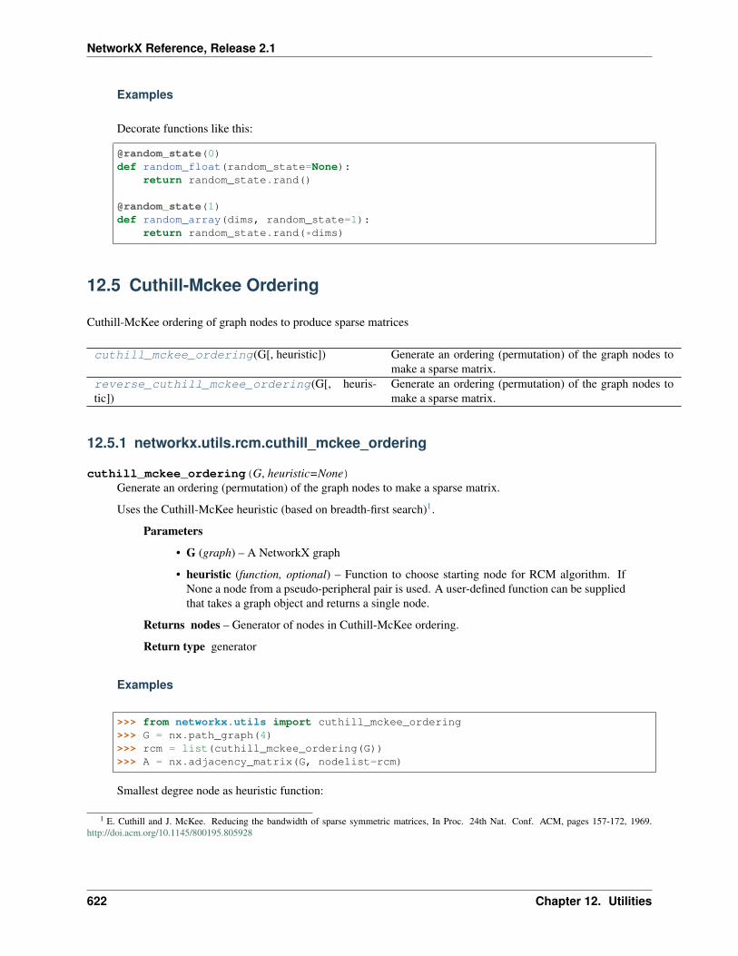
NetworkX Reference, Release 2.1
Examples
Decorate functions like this:
@random_state(0)def random_float(random_state=None):
return random_state.rand()
@random_state(1)def random_array(dims, random_state=1):
return random_state.rand(*dims)
12.5 Cuthill-Mckee Ordering
Cuthill-McKee ordering of graph nodes to produce sparse matrices
cuthill_mckee_ordering(G[, heuristic]) Generate an ordering (permutation) of the graph nodes tomake a sparse matrix.
reverse_cuthill_mckee_ordering(G[, heuris-tic])
Generate an ordering (permutation) of the graph nodes tomake a sparse matrix.
12.5.1 networkx.utils.rcm.cuthill_mckee_ordering
cuthill_mckee_ordering(G, heuristic=None)Generate an ordering (permutation) of the graph nodes to make a sparse matrix.
Uses the Cuthill-McKee heuristic (based on breadth-first search)1.
Parameters
• G (graph) – A NetworkX graph
• heuristic (function, optional) – Function to choose starting node for RCM algorithm. IfNone a node from a pseudo-peripheral pair is used. A user-defined function can be suppliedthat takes a graph object and returns a single node.
Returns nodes – Generator of nodes in Cuthill-McKee ordering.
Return type generator
Examples
>>> from networkx.utils import cuthill_mckee_ordering>>> G = nx.path_graph(4)>>> rcm = list(cuthill_mckee_ordering(G))>>> A = nx.adjacency_matrix(G, nodelist=rcm)
Smallest degree node as heuristic function:
1 E. Cuthill and J. McKee. Reducing the bandwidth of sparse symmetric matrices, In Proc. 24th Nat. Conf. ACM, pages 157-172, 1969.http://doi.acm.org/10.1145/800195.805928
622 Chapter 12. Utilities

NetworkX Reference, Release 2.1
>>> def smallest_degree(G):... return min(G, key=G.degree)>>> rcm = list(cuthill_mckee_ordering(G, heuristic=smallest_degree))
See also:
reverse_cuthill_mckee_ordering()
Notes
The optimal solution the the bandwidth reduction is NP-complete2.
References
12.5.2 networkx.utils.rcm.reverse_cuthill_mckee_ordering
reverse_cuthill_mckee_ordering(G, heuristic=None)Generate an ordering (permutation) of the graph nodes to make a sparse matrix.
Uses the reverse Cuthill-McKee heuristic (based on breadth-first search)1.
Parameters
• G (graph) – A NetworkX graph
• heuristic (function, optional) – Function to choose starting node for RCM algorithm. IfNone a node from a pseudo-peripheral pair is used. A user-defined function can be suppliedthat takes a graph object and returns a single node.
Returns nodes – Generator of nodes in reverse Cuthill-McKee ordering.
Return type generator
Examples
>>> from networkx.utils import reverse_cuthill_mckee_ordering>>> G = nx.path_graph(4)>>> rcm = list(reverse_cuthill_mckee_ordering(G))>>> A = nx.adjacency_matrix(G, nodelist=rcm)
Smallest degree node as heuristic function:
>>> def smallest_degree(G):... return min(G, key=G.degree)>>> rcm = list(reverse_cuthill_mckee_ordering(G, heuristic=smallest_degree))
See also:
cuthill_mckee_ordering()
2 Steven S. Skiena. 1997. The Algorithm Design Manual. Springer-Verlag New York, Inc., New York, NY, USA.1 E. Cuthill and J. McKee. Reducing the bandwidth of sparse symmetric matrices, In Proc. 24th Nat. Conf. ACM, pages 157-72, 1969.
http://doi.acm.org/10.1145/800195.805928
12.5. Cuthill-Mckee Ordering 623

NetworkX Reference, Release 2.1
Notes
The optimal solution the the bandwidth reduction is NP-complete2.
References
12.6 Context Managers
reversed(*args, **kwds) A context manager for temporarily reversing a directedgraph in place.
12.6.1 networkx.utils.contextmanagers.reversed
reversed(*args, **kwds)A context manager for temporarily reversing a directed graph in place.
This is a no-op for undirected graphs.
Parameters G (graph) – A NetworkX graph.
2 Steven S. Skiena. 1997. The Algorithm Design Manual. Springer-Verlag New York, Inc., New York, NY, USA.
624 Chapter 12. Utilities

CHAPTER
THIRTEEN
GLOSSARY
dictionary A Python dictionary maps keys to values. Also known as “hashes”, or “associative arrays” in otherprogramming languages. See https://docs.python.org/2/tutorial/datastructures.html#dictionaries
edge Edges are either two-tuples of nodes (u, v) or three tuples of nodes with an edge attribute dictionary (u,v, dict).
ebunch An iteratable container of edge tuples like a list, iterator, or file.
edge attribute Edges can have arbitrary Python objects assigned as attributes by using keyword/value pairs whenadding an edge assigning to the G.edges[u][v] attribute dictionary for the specified edge u-v.
hashable An object is hashable if it has a hash value which never changes during its lifetime (it needs a __hash__()method), and can be compared to other objects (it needs an __eq__() or __cmp__() method). Hashableobjects which compare equal must have the same hash value.
Hashability makes an object usable as a dictionary key and a set member, because these data structures use thehash value internally.
All of Python’s immutable built-in objects are hashable, while no mutable containers (such as lists or dictionar-ies) are. Objects which are instances of user-defined classes are hashable by default; they all compare unequal,and their hash value is their id().
Definition from https://docs.python.org/2/glossary.html
nbunch An nbunch is a single node, container of nodes or None (representing all nodes). It can be a list, set, graph,etc.. To filter an nbunch so that only nodes actually in G appear, use G.nbunch_iter(nbunch).
node A node can be any hashable Python object except None.
node attribute Nodes can have arbitrary Python objects assigned as attributes by using keyword/value pairs whenadding a node or assigning to the G.nodes[n] attribute dictionary for the specified node n.
625

NetworkX Reference, Release 2.1
626 Chapter 13. Glossary

APPENDIX
A
TUTORIAL
This guide can help you start working with NetworkX.
A.1 Creating a graph
Create an empty graph with no nodes and no edges.
>>> import networkx as nx>>> G = nx.Graph()
By definition, a Graph is a collection of nodes (vertices) along with identified pairs of nodes (called edges, links,etc). In NetworkX, nodes can be any hashable object e.g., a text string, an image, an XML object, another Graph, acustomized node object, etc.
Note: Python’s None object should not be used as a node as it determines whether optional function arguments havebeen assigned in many functions.
A.2 Nodes
The graph G can be grown in several ways. NetworkX includes many graph generator functions and facilities to readand write graphs in many formats. To get started though we’ll look at simple manipulations. You can add one node ata time,
>>> G.add_node(1)
add a list of nodes,
>>> G.add_nodes_from([2, 3])
or add any iterable container of nodes. You can also add nodes along with node attributes if your container yields2-tuples (node, node_attribute_dict). Node attributes are discussed further below.
>>> H = nx.path_graph(10)>>> G.add_nodes_from(H)
Note that G now contains the nodes of H as nodes of G. In contrast, you could use the graph H as a node in G.
>>> G.add_node(H)
627

NetworkX Reference, Release 2.1
The graph G now contains H as a node. This flexibility is very powerful as it allows graphs of graphs, graphs of files,graphs of functions and much more. It is worth thinking about how to structure your application so that the nodes areuseful entities. Of course you can always use a unique identifier in G and have a separate dictionary keyed by identifierto the node information if you prefer.
Note: You should not change the node object if the hash depends on its contents.
A.3 Edges
G can also be grown by adding one edge at a time,
>>> G.add_edge(1, 2)>>> e = (2, 3)>>> G.add_edge(*e) # unpack edge tuple*
by adding a list of edges,
>>> G.add_edges_from([(1, 2), (1, 3)])
or by adding any ebunch of edges. An ebunch is any iterable container of edge-tuples. An edge-tuple can be a2-tuple of nodes or a 3-tuple with 2 nodes followed by an edge attribute dictionary, e.g., (2, 3, {'weight':3.1415}). Edge attributes are discussed further below
>>> G.add_edges_from(H.edges)
There are no complaints when adding existing nodes or edges. For example, after removing all nodes and edges,
>>> G.clear()
we add new nodes/edges and NetworkX quietly ignores any that are already present.
>>> G.add_edges_from([(1, 2), (1, 3)])>>> G.add_node(1)>>> G.add_edge(1, 2)>>> G.add_node("spam") # adds node "spam">>> G.add_nodes_from("spam") # adds 4 nodes: 's', 'p', 'a', 'm'>>> G.add_edge(3, 'm')
At this stage the graph G consists of 8 nodes and 3 edges, as can be seen by:
>>> G.number_of_nodes()8>>> G.number_of_edges()3
We can examine the nodes and edges. Four basic graph properties facilitate reporting: G.nodes, G.edges, G.adjand G.degree. These are set-like views of the nodes, edges, neighbors (adjacencies), and degrees of nodes in agraph. They offer a continually updated read-only view into the graph structure. They are also dict-like in that youcan look up node and edge data attributes via the views and iterate with data attributes using methods .items(),.data('span'). If you want a specific container type instead of a view, you can specify one. Here we use lists,though sets, dicts, tuples and other containers may be better in other contexts.
628 Appendix A. Tutorial

NetworkX Reference, Release 2.1
>>> list(G.nodes)['a', 1, 2, 3, 'spam', 'm', 'p', 's']>>> list(G.edges)[(1, 2), (1, 3), (3, 'm')]>>> list(G.adj[1]) # or list(G.neighbors(1))[2, 3]>>> G.degree[1] # the number of edges incident to 12
One can specify to report the edges and degree from a subset of all nodes using an nbunch. An nbunch is any of: None(meaning all nodes), a node, or an iterable container of nodes that is not itself a node in the graph.
>>> G.edges([2, 'm'])EdgeDataView([(2, 1), ('m', 3)])>>> G.degree([2, 3])DegreeView({2: 1, 3: 2})
One can remove nodes and edges from the graph in a similar fashion to adding. Use meth-ods Graph.remove_node(), Graph.remove_nodes_from(), Graph.remove_edge() and Graph.remove_edges_from(), e.g.
>>> G.remove_node(2)>>> G.remove_nodes_from("spam")>>> list(G.nodes)[1, 3, 'spam']>>> G.remove_edge(1, 3)
When creating a graph structure by instantiating one of the graph classes you can specify data in several formats.
>>> G.add_edge(1, 2)>>> H = nx.DiGraph(G) # create a DiGraph using the connections from G>>> list(H.edges())[(1, 2), (2, 1)]>>> edgelist = [(0, 1), (1, 2), (2, 3)]>>> H = nx.Graph(edgelist)
A.4 What to use as nodes and edges
You might notice that nodes and edges are not specified as NetworkX objects. This leaves you free to use meaningfulitems as nodes and edges. The most common choices are numbers or strings, but a node can be any hashable object(except None), and an edge can be associated with any object x using G.add_edge(n1, n2, object=x).
As an example, n1 and n2 could be protein objects from the RCSB Protein Data Bank, and x could refer to an XMLrecord of publications detailing experimental observations of their interaction.
We have found this power quite useful, but its abuse can lead to unexpected surprises unless one is familiar with Python.If in doubt, consider using convert_node_labels_to_integers() to obtain a more traditional graph withinteger labels.
A.5 Accessing edges and neighbors
In addition to the views Graph.edges(), and Graph.adj(), access to edges and neighbors is possible usingsubscript notation.
A.4. What to use as nodes and edges 629

NetworkX Reference, Release 2.1
>>> G[1] # same as G.adj[1]AtlasView({2: {}})>>> G[1][2]{}>>> G.edges[1, 2]{}
You can get/set the attributes of an edge using subscript notation if the edge already exists.
>>> G.add_edge(1, 3)>>> G[1][3]['color'] = "blue">>> G.edges[1, 2]['color'] = "red"
Fast examination of all (node, adjacency) pairs is achieved using G.adjacency(), or G.adj.items(). Notethat for undirected graphs, adjacency iteration sees each edge twice.
>>> FG = nx.Graph()>>> FG.add_weighted_edges_from([(1, 2, 0.125), (1, 3, 0.75), (2, 4, 1.2), (3, 4, 0.→˓375)])>>> for n, nbrs in FG.adj.items():... for nbr, eattr in nbrs.items():... wt = eattr['weight']... if wt < 0.5: print('(%d, %d, %.3f)' % (n, nbr, wt))(1, 2, 0.125)(2, 1, 0.125)(3, 4, 0.375)(4, 3, 0.375)
Convenient access to all edges is achieved with the edges property.
>>> for (u, v, wt) in FG.edges.data('weight'):... if wt < 0.5: print('(%d, %d, %.3f)' % (u, v, wt))(1, 2, 0.125)(3, 4, 0.375)
A.6 Adding attributes to graphs, nodes, and edges
Attributes such as weights, labels, colors, or whatever Python object you like, can be attached to graphs, nodes, oredges.
Each graph, node, and edge can hold key/value attribute pairs in an associated attribute dictionary (the keys must behashable). By default these are empty, but attributes can be added or changed using add_edge, add_node or directmanipulation of the attribute dictionaries named G.graph, G.nodes, and G.edges for a graph G.
A.6.1 Graph attributes
Assign graph attributes when creating a new graph
>>> G = nx.Graph(day="Friday")>>> G.graph{'day': 'Friday'}
Or you can modify attributes later
630 Appendix A. Tutorial
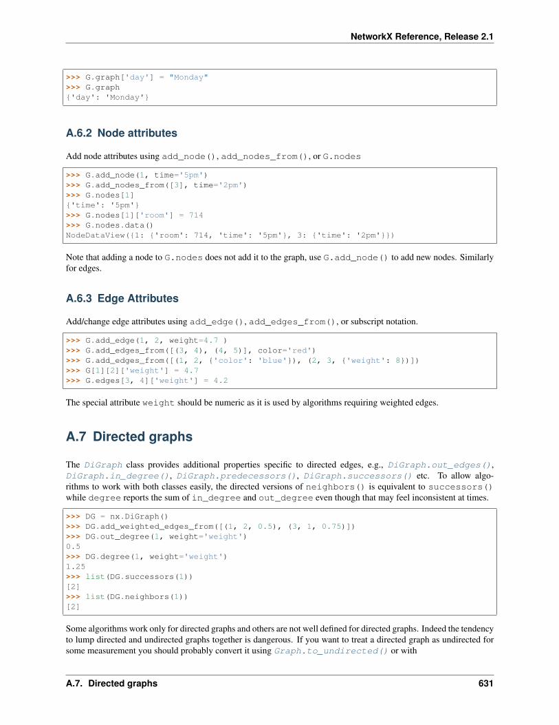
NetworkX Reference, Release 2.1
>>> G.graph['day'] = "Monday">>> G.graph{'day': 'Monday'}
A.6.2 Node attributes
Add node attributes using add_node(), add_nodes_from(), or G.nodes
>>> G.add_node(1, time='5pm')>>> G.add_nodes_from([3], time='2pm')>>> G.nodes[1]{'time': '5pm'}>>> G.nodes[1]['room'] = 714>>> G.nodes.data()NodeDataView({1: {'room': 714, 'time': '5pm'}, 3: {'time': '2pm'}})
Note that adding a node to G.nodes does not add it to the graph, use G.add_node() to add new nodes. Similarlyfor edges.
A.6.3 Edge Attributes
Add/change edge attributes using add_edge(), add_edges_from(), or subscript notation.
>>> G.add_edge(1, 2, weight=4.7 )>>> G.add_edges_from([(3, 4), (4, 5)], color='red')>>> G.add_edges_from([(1, 2, {'color': 'blue'}), (2, 3, {'weight': 8})])>>> G[1][2]['weight'] = 4.7>>> G.edges[3, 4]['weight'] = 4.2
The special attribute weight should be numeric as it is used by algorithms requiring weighted edges.
A.7 Directed graphs
The DiGraph class provides additional properties specific to directed edges, e.g., DiGraph.out_edges(),DiGraph.in_degree(), DiGraph.predecessors(), DiGraph.successors() etc. To allow algo-rithms to work with both classes easily, the directed versions of neighbors() is equivalent to successors()while degree reports the sum of in_degree and out_degree even though that may feel inconsistent at times.
>>> DG = nx.DiGraph()>>> DG.add_weighted_edges_from([(1, 2, 0.5), (3, 1, 0.75)])>>> DG.out_degree(1, weight='weight')0.5>>> DG.degree(1, weight='weight')1.25>>> list(DG.successors(1))[2]>>> list(DG.neighbors(1))[2]
Some algorithms work only for directed graphs and others are not well defined for directed graphs. Indeed the tendencyto lump directed and undirected graphs together is dangerous. If you want to treat a directed graph as undirected forsome measurement you should probably convert it using Graph.to_undirected() or with
A.7. Directed graphs 631

NetworkX Reference, Release 2.1
>>> H = nx.Graph(G) # convert G to undirected graph
A.8 Multigraphs
NetworkX provides classes for graphs which allow multiple edges between any pair of nodes. The MultiGraphand MultiDiGraph classes allow you to add the same edge twice, possibly with different edge data. This can bepowerful for some applications, but many algorithms are not well defined on such graphs. Where results are welldefined, e.g., MultiGraph.degree() we provide the function. Otherwise you should convert to a standard graphin a way that makes the measurement well defined.
>>> MG = nx.MultiGraph()>>> MG.add_weighted_edges_from([(1, 2, 0.5), (1, 2, 0.75), (2, 3, 0.5)])>>> dict(MG.degree(weight='weight')){1: 1.25, 2: 1.75, 3: 0.5}>>> GG = nx.Graph()>>> for n, nbrs in MG.adjacency():... for nbr, edict in nbrs.items():... minvalue = min([d['weight'] for d in edict.values()])... GG.add_edge(n, nbr, weight = minvalue)...>>> nx.shortest_path(GG, 1, 3)[1, 2, 3]
A.9 Graph generators and graph operations
In addition to constructing graphs node-by-node or edge-by-edge, they can also be generated by
1. Applying classic graph operations, such as:
subgraph(G, nbunch) - induced subgraph view of G on nodes in nbunchunion(G1,G2) - graph uniondisjoint_union(G1,G2) - graph union assuming all nodes are differentcartesian_product(G1,G2) - return Cartesian product graphcompose(G1,G2) - combine graphs identifying nodes common to bothcomplement(G) - graph complementcreate_empty_copy(G) - return an empty copy of the same graph classconvert_to_undirected(G) - return an undirected representation of Gconvert_to_directed(G) - return a directed representation of G
2. Using a call to one of the classic small graphs, e.g.,
>>> petersen = nx.petersen_graph()>>> tutte = nx.tutte_graph()>>> maze = nx.sedgewick_maze_graph()>>> tet = nx.tetrahedral_graph()
3. Using a (constructive) generator for a classic graph, e.g.,
>>> K_5 = nx.complete_graph(5)>>> K_3_5 = nx.complete_bipartite_graph(3, 5)>>> barbell = nx.barbell_graph(10, 10)>>> lollipop = nx.lollipop_graph(10, 20)
632 Appendix A. Tutorial

NetworkX Reference, Release 2.1
4. Using a stochastic graph generator, e.g.,
>>> er = nx.erdos_renyi_graph(100, 0.15)>>> ws = nx.watts_strogatz_graph(30, 3, 0.1)>>> ba = nx.barabasi_albert_graph(100, 5)>>> red = nx.random_lobster(100, 0.9, 0.9)
5. Reading a graph stored in a file using common graph formats, such as edge lists, adjacency lists, GML,GraphML, pickle, LEDA and others.
>>> nx.write_gml(red, "path.to.file")>>> mygraph = nx.read_gml("path.to.file")
For details on graph formats see Reading and writing graphs and for graph generator functions see Graph generators
A.10 Analyzing graphs
The structure of G can be analyzed using various graph-theoretic functions such as:
>>> G = nx.Graph()>>> G.add_edges_from([(1, 2), (1, 3)])>>> G.add_node("spam") # adds node "spam">>> list(nx.connected_components(G))[set([1, 2, 3]), set(['spam'])]>>> sorted(d for n, d in G.degree())[0, 1, 1, 2]>>> nx.clustering(G){1: 0, 2: 0, 3: 0, 'spam': 0}
Some functions with large output iterate over (node, value) 2-tuples. These are easily stored in a dict structure ifyou desire.
>>> sp = dict(nx.all_pairs_shortest_path(G))>>> sp[3]{1: [3, 1], 2: [3, 1, 2], 3: [3]}
See Algorithms for details on graph algorithms supported.
A.11 Drawing graphs
NetworkX is not primarily a graph drawing package but basic drawing with Matplotlib as well as an interface to usethe open source Graphviz software package are included. These are part of the networkx.drawing module andwill be imported if possible.
First import Matplotlib’s plot interface (pylab works too)
>>> import matplotlib.pyplot as plt
You may find it useful to interactively test code using ipython -pylab, which combines the power of ipython andmatplotlib and provides a convenient interactive mode.
To test if the import of networkx.drawing was successful draw G using one of
A.10. Analyzing graphs 633

NetworkX Reference, Release 2.1
>>> G = nx.petersen_graph()>>> plt.subplot(121)<matplotlib.axes._subplots.AxesSubplot object at ...>>>> nx.draw(G, with_labels=True, font_weight='bold')>>> plt.subplot(122)<matplotlib.axes._subplots.AxesSubplot object at ...>>>> nx.draw_shell(G, nlist=[range(5, 10), range(5)], with_labels=True, font_weight=→˓'bold')
0
1
23
4
5
6
7
8
9
0
1
2
3
4
5
67
89
when drawing to an interactive display. Note that you may need to issue a Matplotlib
>>> plt.show()
command if you are not using matplotlib in interactive mode (see Matplotlib FAQ ).
>>> options = {... 'node_color': 'black',... 'node_size': 100,... 'width': 3,... }>>> plt.subplot(221)<matplotlib.axes._subplots.AxesSubplot object at ...>>>> nx.draw_random(G, **options)>>> plt.subplot(222)<matplotlib.axes._subplots.AxesSubplot object at ...>>>> nx.draw_circular(G, **options)
634 Appendix A. Tutorial

NetworkX Reference, Release 2.1
>>> plt.subplot(223)<matplotlib.axes._subplots.AxesSubplot object at ...>>>> nx.draw_spectral(G, **options)>>> plt.subplot(224)<matplotlib.axes._subplots.AxesSubplot object at ...>>>> nx.draw_shell(G, nlist=[range(5,10), range(5)], **options)
You can find additional options via draw_networkx() and layouts via layout. You can use multiple shells withdraw_shell().
>>> G = nx.dodecahedral_graph()>>> shells = [[2, 3, 4, 5, 6], [8, 1, 0, 19, 18, 17, 16, 15, 14, 7], [9, 10, 11, 12,→˓13]]>>> nx.draw_shell(G, nlist=shells, **options)
A.11. Drawing graphs 635

NetworkX Reference, Release 2.1
To save drawings to a file, use, for example
>>> nx.draw(G)>>> plt.savefig("path.png")
writes to the file path.png in the local directory. If Graphviz and PyGraphviz or pydot, are available on your system,you can also use nx_agraph.graphviz_layout(G) or nx_pydot.graphviz_layout(G) to get the nodepositions, or write the graph in dot format for further processing.
>>> from networkx.drawing.nx_pydot import write_dot>>> pos = nx.nx_agraph.graphviz_layout(G)>>> nx.draw(G, pos=pos)>>> write_dot(G, 'file.dot')
See Drawing for additional details.
• ;
• ;
• .
636 Appendix A. Tutorial

BIBLIOGRAPHY
[atlas] Ronald C. Read and Robin J. Wilson, An Atlas of Graphs. Oxford University Press, 1998.
637

NetworkX Reference, Release 2.1
638 Bibliography

PYTHON MODULE INDEX
anetworkx.algorithms.approximation, 121networkx.algorithms.approximation.clique,
125networkx.algorithms.approximation.clustering_coefficient,
127networkx.algorithms.approximation.connectivity,
121networkx.algorithms.approximation.dominating_set,
127networkx.algorithms.approximation.independent_set,
128networkx.algorithms.approximation.kcomponents,
124networkx.algorithms.approximation.matching,
129networkx.algorithms.approximation.ramsey,
130networkx.algorithms.approximation.steinertree,
130networkx.algorithms.approximation.vertex_cover,
131networkx.algorithms.assortativity, 132networkx.algorithms.bipartite, 141networkx.algorithms.bipartite.basic, 142networkx.algorithms.bipartite.centrality,
161networkx.algorithms.bipartite.cluster,
156networkx.algorithms.bipartite.covering,
169networkx.algorithms.bipartite.generators,
164networkx.algorithms.bipartite.matching,
145networkx.algorithms.bipartite.matrix,
148networkx.algorithms.bipartite.projection,
149networkx.algorithms.bipartite.redundancy,
160networkx.algorithms.bipartite.spectral,
156networkx.algorithms.boundary, 169networkx.algorithms.bridges, 171networkx.algorithms.centrality, 288networkx.algorithms.chains, 197networkx.algorithms.chordal, 198networkx.algorithms.clique, 201networkx.algorithms.cluster, 205networkx.algorithms.coloring, 210networkx.algorithms.communicability_alg,
213networkx.algorithms.community, 215networkx.algorithms.community.asyn_fluidc,
220networkx.algorithms.community.centrality,
222networkx.algorithms.community.community_generators,
216networkx.algorithms.community.community_utils,
224networkx.algorithms.community.kclique,
218networkx.algorithms.community.kernighan_lin,
215networkx.algorithms.community.label_propagation,
219networkx.algorithms.community.quality,
221networkx.algorithms.components, 224networkx.algorithms.connectivity, 239networkx.algorithms.connectivity.connectivity,
252networkx.algorithms.connectivity.cuts,
260networkx.algorithms.connectivity.disjoint_paths,
249networkx.algorithms.connectivity.edge_augmentation,
239networkx.algorithms.connectivity.edge_kcomponents,
242networkx.algorithms.connectivity.kcomponents,
246
639
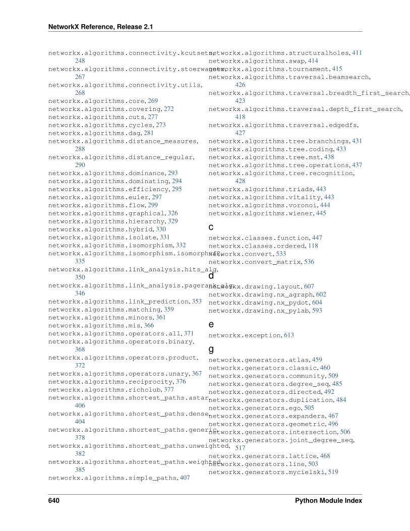
NetworkX Reference, Release 2.1
networkx.algorithms.connectivity.kcutsets,248
networkx.algorithms.connectivity.stoerwagner,267
networkx.algorithms.connectivity.utils,268
networkx.algorithms.core, 269networkx.algorithms.covering, 272networkx.algorithms.cuts, 277networkx.algorithms.cycles, 273networkx.algorithms.dag, 281networkx.algorithms.distance_measures,
288networkx.algorithms.distance_regular,
290networkx.algorithms.dominance, 293networkx.algorithms.dominating, 294networkx.algorithms.efficiency, 295networkx.algorithms.euler, 297networkx.algorithms.flow, 299networkx.algorithms.graphical, 326networkx.algorithms.hierarchy, 329networkx.algorithms.hybrid, 330networkx.algorithms.isolate, 331networkx.algorithms.isomorphism, 332networkx.algorithms.isomorphism.isomorphvf2,
335networkx.algorithms.link_analysis.hits_alg,
350networkx.algorithms.link_analysis.pagerank_alg,
346networkx.algorithms.link_prediction, 353networkx.algorithms.matching, 359networkx.algorithms.minors, 361networkx.algorithms.mis, 366networkx.algorithms.operators.all, 371networkx.algorithms.operators.binary,
368networkx.algorithms.operators.product,
372networkx.algorithms.operators.unary, 367networkx.algorithms.reciprocity, 376networkx.algorithms.richclub, 377networkx.algorithms.shortest_paths.astar,
406networkx.algorithms.shortest_paths.dense,
404networkx.algorithms.shortest_paths.generic,
378networkx.algorithms.shortest_paths.unweighted,
382networkx.algorithms.shortest_paths.weighted,
385networkx.algorithms.simple_paths, 407
networkx.algorithms.structuralholes, 411networkx.algorithms.swap, 414networkx.algorithms.tournament, 415networkx.algorithms.traversal.beamsearch,
426networkx.algorithms.traversal.breadth_first_search,
423networkx.algorithms.traversal.depth_first_search,
418networkx.algorithms.traversal.edgedfs,
427networkx.algorithms.tree.branchings, 431networkx.algorithms.tree.coding, 433networkx.algorithms.tree.mst, 438networkx.algorithms.tree.operations, 437networkx.algorithms.tree.recognition,
428networkx.algorithms.triads, 443networkx.algorithms.vitality, 443networkx.algorithms.voronoi, 444networkx.algorithms.wiener, 445
cnetworkx.classes.function, 447networkx.classes.ordered, 118networkx.convert, 533networkx.convert_matrix, 536
dnetworkx.drawing.layout, 607networkx.drawing.nx_agraph, 602networkx.drawing.nx_pydot, 604networkx.drawing.nx_pylab, 593
enetworkx.exception, 613
gnetworkx.generators.atlas, 459networkx.generators.classic, 460networkx.generators.community, 509networkx.generators.degree_seq, 485networkx.generators.directed, 492networkx.generators.duplication, 484networkx.generators.ego, 505networkx.generators.expanders, 467networkx.generators.geometric, 496networkx.generators.intersection, 506networkx.generators.joint_degree_seq,
517networkx.generators.lattice, 468networkx.generators.line, 503networkx.generators.mycielski, 519
640 Python Module Index

NetworkX Reference, Release 2.1
networkx.generators.nonisomorphic_trees,516
networkx.generators.random_clustered,491
networkx.generators.random_graphs, 475networkx.generators.small, 471networkx.generators.social, 508networkx.generators.stochastic, 506networkx.generators.trees, 514networkx.generators.triads, 517
lnetworkx.linalg.algebraicconnectivity,
526networkx.linalg.attrmatrix, 529networkx.linalg.graphmatrix, 521networkx.linalg.laplacianmatrix, 522networkx.linalg.spectrum, 525
rnetworkx.readwrite.adjlist, 551networkx.readwrite.edgelist, 558networkx.readwrite.gexf, 564networkx.readwrite.gml, 566networkx.readwrite.gpickle, 571networkx.readwrite.graph6, 583networkx.readwrite.graphml, 573networkx.readwrite.json_graph, 575networkx.readwrite.leda, 580networkx.readwrite.multiline_adjlist,
554networkx.readwrite.nx_shp, 591networkx.readwrite.nx_yaml, 581networkx.readwrite.pajek, 589networkx.readwrite.sparse6, 586networkx.relabel, 547
unetworkx.utils, 615networkx.utils.contextmanagers, 624networkx.utils.decorators, 619networkx.utils.misc, 615networkx.utils.random_sequence, 617networkx.utils.rcm, 622networkx.utils.union_find, 617
Python Module Index 641

NetworkX Reference, Release 2.1
642 Python Module Index

INDEX
Symbols__contains__() (DiGraph method), 45__contains__() (Graph method), 20__contains__() (MultiDiGraph method), 102__contains__() (MultiGraph method), 75__getitem__() (DiGraph method), 50__getitem__() (Graph method), 23__getitem__() (MultiDiGraph method), 107__getitem__() (MultiGraph method), 79__init__() (DiGraph method), 36__init__() (DiGraphMatcher method), 339__init__() (EdgeComponentAuxGraph method), 246__init__() (Edmonds method), 433__init__() (Graph method), 11__init__() (GraphMatcher method), 337__init__() (MultiDiGraph method), 91__init__() (MultiGraph method), 65__iter__() (DiGraph method), 44__iter__() (Graph method), 19__iter__() (MultiDiGraph method), 101__iter__() (MultiGraph method), 74__len__() (DiGraph method), 53__len__() (Graph method), 26__len__() (MultiDiGraph method), 110__len__() (MultiGraph method), 81
Aadamic_adar_index() (in module net-
workx.algorithms.link_prediction), 355add_cycle() (in module networkx.classes.function), 449add_edge() (DiGraph method), 39add_edge() (Graph method), 14add_edge() (MultiDiGraph method), 94add_edge() (MultiGraph method), 68add_edges_from() (DiGraph method), 40add_edges_from() (Graph method), 15add_edges_from() (MultiDiGraph method), 96add_edges_from() (MultiGraph method), 69add_node() (DiGraph method), 37add_node() (Graph method), 12add_node() (MultiDiGraph method), 92add_node() (MultiGraph method), 65
add_nodes_from() (DiGraph method), 37add_nodes_from() (Graph method), 12add_nodes_from() (MultiDiGraph method), 93add_nodes_from() (MultiGraph method), 66add_path() (in module networkx.classes.function), 449add_star() (in module networkx.classes.function), 449add_weighted_edges_from() (DiGraph method), 40add_weighted_edges_from() (Graph method), 15add_weighted_edges_from() (MultiDiGraph method), 97add_weighted_edges_from() (MultiGraph method), 70adj (DiGraph attribute), 49adj (Graph attribute), 23adj (MultiDiGraph attribute), 107adj (MultiGraph attribute), 79adjacency() (DiGraph method), 51adjacency() (Graph method), 24adjacency() (MultiDiGraph method), 108adjacency() (MultiGraph method), 80adjacency_data() (in module net-
workx.readwrite.json_graph), 577adjacency_graph() (in module net-
workx.readwrite.json_graph), 578adjacency_matrix() (in module net-
workx.linalg.graphmatrix), 521adjacency_spectrum() (in module net-
workx.linalg.spectrum), 525algebraic_connectivity() (in module net-
workx.linalg.algebraicconnectivity), 526all_neighbors() (in module networkx.classes.function),
450all_node_cuts() (in module net-
workx.algorithms.connectivity.kcutsets),248
all_pairs_bellman_ford_path() (in module net-workx.algorithms.shortest_paths.weighted),399
all_pairs_bellman_ford_path_length() (in module net-workx.algorithms.shortest_paths.weighted),400
all_pairs_dijkstra_path() (in module net-workx.algorithms.shortest_paths.weighted),394
643

NetworkX Reference, Release 2.1
all_pairs_dijkstra_path_length() (in module net-workx.algorithms.shortest_paths.weighted),395
all_pairs_node_connectivity() (in module net-workx.algorithms.approximation.connectivity),121
all_pairs_node_connectivity() (in module net-workx.algorithms.connectivity.connectivity),253
all_pairs_shortest_path() (in module net-workx.algorithms.shortest_paths.unweighted),384
all_pairs_shortest_path_length() (in module net-workx.algorithms.shortest_paths.unweighted),384
all_shortest_paths() (in module net-workx.algorithms.shortest_paths.generic),379
all_simple_paths() (in module net-workx.algorithms.simple_paths), 408
alternating_havel_hakimi_graph() (in module net-workx.algorithms.bipartite.generators), 167
AmbiguousSolution (class in networkx), 613ancestors() (in module networkx.algorithms.dag), 282antichains() (in module networkx.algorithms.dag), 285approximate_current_flow_betweenness_centrality() (in
module networkx.algorithms.centrality), 188articulation_points() (in module net-
workx.algorithms.components), 237astar_path() (in module net-
workx.algorithms.shortest_paths.astar), 406astar_path_length() (in module net-
workx.algorithms.shortest_paths.astar), 407asyn_fluidc() (in module net-
workx.algorithms.community.asyn_fluidc),220
asyn_lpa_communities() (in module net-workx.algorithms.community.label_propagation),219
attr_matrix() (in module networkx.linalg.attrmatrix), 529attr_sparse_matrix() (in module net-
workx.linalg.attrmatrix), 531attracting_component_subgraphs() (in module net-
workx.algorithms.components), 234attracting_components() (in module net-
workx.algorithms.components), 233attribute_assortativity_coefficient() (in module net-
workx.algorithms.assortativity), 133attribute_mixing_dict() (in module net-
workx.algorithms.assortativity), 140attribute_mixing_matrix() (in module net-
workx.algorithms.assortativity), 139authority_matrix() (in module net-
workx.algorithms.link_analysis.hits_alg),
353average_clustering() (in module net-
workx.algorithms.approximation.clustering_coefficient),127
average_clustering() (in module net-workx.algorithms.bipartite.cluster), 158
average_clustering() (in module net-workx.algorithms.cluster), 207
average_degree_connectivity() (in module net-workx.algorithms.assortativity), 137
average_neighbor_degree() (in module net-workx.algorithms.assortativity), 135
average_node_connectivity() (in module net-workx.algorithms.connectivity.connectivity),253
average_shortest_path_length() (in module net-workx.algorithms.shortest_paths.generic),381
Bbalanced_tree() (in module networkx.generators.classic),
461barabasi_albert_graph() (in module net-
workx.generators.random_graphs), 480barbell_graph() (in module networkx.generators.classic),
461bellman_ford_path() (in module net-
workx.algorithms.shortest_paths.weighted),397
bellman_ford_path_length() (in module net-workx.algorithms.shortest_paths.weighted),397
bellman_ford_predecessor_and_distance() (in modulenetworkx.algorithms.shortest_paths.weighted),402
betweenness_centrality() (in module net-workx.algorithms.bipartite.centrality), 163
betweenness_centrality() (in module net-workx.algorithms.centrality), 182
betweenness_centrality_subset() (in module net-workx.algorithms.centrality), 184
bfs_beam_edges() (in module net-workx.algorithms.traversal.beamsearch),426
bfs_edges() (in module net-workx.algorithms.traversal.breadth_first_search),424
bfs_predecessors() (in module net-workx.algorithms.traversal.breadth_first_search),425
bfs_successors() (in module net-workx.algorithms.traversal.breadth_first_search),425
bfs_tree() (in module net-
644 Index

NetworkX Reference, Release 2.1
workx.algorithms.traversal.breadth_first_search),424
biadjacency_matrix() (in module net-workx.algorithms.bipartite.matrix), 148
biconnected_component_edges() (in module net-workx.algorithms.components), 236
biconnected_component_subgraphs() (in module net-workx.algorithms.components), 237
biconnected_components() (in module net-workx.algorithms.components), 235
bidirectional_dijkstra() (in module net-workx.algorithms.shortest_paths.weighted),396
binomial_graph() (in module net-workx.generators.random_graphs), 478
boundary_expansion() (in module net-workx.algorithms.cuts), 277
boykov_kolmogorov() (in module net-workx.algorithms.flow), 312
branching_weight() (in module net-workx.algorithms.tree.branchings), 431
bridge_components() (in module net-workx.algorithms.connectivity.edge_kcomponents),244
bridges() (in module networkx.algorithms.bridges), 171build_auxiliary_edge_connectivity() (in module net-
workx.algorithms.connectivity.utils), 268build_auxiliary_node_connectivity() (in module net-
workx.algorithms.connectivity.utils), 268build_residual_network() (in module net-
workx.algorithms.flow), 316bull_graph() (in module networkx.generators.small), 472
Ccandidate_pairs_iter() (DiGraphMatcher method), 340candidate_pairs_iter() (GraphMatcher method), 338capacity_scaling() (in module networkx.algorithms.flow),
324cartesian_product() (in module net-
workx.algorithms.operators.product), 372categorical_edge_match() (in module net-
workx.algorithms.isomorphism), 342categorical_multiedge_match() (in module net-
workx.algorithms.isomorphism), 342categorical_node_match() (in module net-
workx.algorithms.isomorphism), 341caveman_graph() (in module net-
workx.generators.community), 509center() (in module net-
workx.algorithms.distance_measures), 289chain_decomposition() (in module net-
workx.algorithms.chains), 198chordal_cycle_graph() (in module net-
workx.generators.expanders), 467
chordal_graph_cliques() (in module net-workx.algorithms.chordal), 199
chordal_graph_treewidth() (in module net-workx.algorithms.chordal), 200
chvatal_graph() (in module networkx.generators.small),472
circular_ladder_graph() (in module net-workx.generators.classic), 463
circular_layout() (in module networkx.drawing.layout),607
clear() (DiGraph method), 42clear() (Graph method), 17clear() (MultiDiGraph method), 99clear() (MultiGraph method), 72clique_removal() (in module net-
workx.algorithms.approximation.clique),126
cliques_containing_node() (in module net-workx.algorithms.clique), 205
closeness_centrality() (in module net-workx.algorithms.bipartite.centrality), 162
closeness_centrality() (in module net-workx.algorithms.centrality), 180
closeness_vitality() (in module net-workx.algorithms.vitality), 444
clustering() (in module net-workx.algorithms.bipartite.cluster), 157
clustering() (in module networkx.algorithms.cluster), 206cn_soundarajan_hopcroft() (in module net-
workx.algorithms.link_prediction), 356collaboration_weighted_projected_graph() (in module
networkx.algorithms.bipartite.projection), 152color() (in module networkx.algorithms.bipartite.basic),
144common_neighbors() (in module net-
workx.classes.function), 451communicability() (in module net-
workx.algorithms.communicability_alg),213
communicability_betweenness_centrality() (in modulenetworkx.algorithms.centrality), 190
communicability_exp() (in module net-workx.algorithms.communicability_alg),214
complement() (in module net-workx.algorithms.operators.unary), 367
complete_bipartite_graph() (in module net-workx.algorithms.bipartite.generators), 165
complete_graph() (in module net-workx.generators.classic), 462
complete_multipartite_graph() (in module net-workx.generators.classic), 462
compose() (in module net-workx.algorithms.operators.binary), 368
Index 645

NetworkX Reference, Release 2.1
compose_all() (in module net-workx.algorithms.operators.all), 371
condensation() (in module net-workx.algorithms.components), 230
conductance() (in module networkx.algorithms.cuts), 278configuration_model() (in module net-
workx.algorithms.bipartite.generators), 165configuration_model() (in module net-
workx.generators.degree_seq), 485connected_caveman_graph() (in module net-
workx.generators.community), 510connected_component_subgraphs() (in module net-
workx.algorithms.components), 226connected_components() (in module net-
workx.algorithms.components), 226connected_double_edge_swap() (in module net-
workx.algorithms.swap), 414connected_watts_strogatz_graph() (in module net-
workx.generators.random_graphs), 479constraint() (in module net-
workx.algorithms.structuralholes), 411contracted_edge() (in module net-
workx.algorithms.minors), 361contracted_nodes() (in module net-
workx.algorithms.minors), 362convert_node_labels_to_integers() (in module net-
workx.relabel), 547copy() (DiGraph method), 57copy() (Graph method), 28copy() (MultiDiGraph method), 114copy() (MultiGraph method), 84core_number() (in module networkx.algorithms.core),
269cost_of_flow() (in module networkx.algorithms.flow),
322could_be_isomorphic() (in module net-
workx.algorithms.isomorphism), 334coverage() (in module net-
workx.algorithms.community.quality), 221create_empty_copy() (in module net-
workx.classes.function), 448create_random_state() (in module networkx.utils.misc),
617cubical_graph() (in module networkx.generators.small),
472cumulative_distribution() (in module net-
workx.utils.random_sequence), 617current_flow_betweenness_centrality() (in module net-
workx.algorithms.centrality), 186current_flow_betweenness_centrality_subset() (in mod-
ule networkx.algorithms.centrality), 188current_flow_closeness_centrality() (in module net-
workx.algorithms.centrality), 181cut_size() (in module networkx.algorithms.cuts), 278
cuthill_mckee_ordering() (in module net-workx.utils.rcm), 622
cycle_basis() (in module networkx.algorithms.cycles),274
cycle_graph() (in module networkx.generators.classic),463
Ddag_longest_path() (in module networkx.algorithms.dag),
286dag_longest_path_length() (in module net-
workx.algorithms.dag), 286dag_to_branching() (in module net-
workx.algorithms.dag), 286davis_southern_women_graph() (in module net-
workx.generators.social), 508default_opener() (in module networkx.utils.misc), 616degree (DiGraph attribute), 53degree (Graph attribute), 26degree (MultiDiGraph attribute), 110degree (MultiGraph attribute), 82degree() (in module networkx.classes.function), 447degree_assortativity_coefficient() (in module net-
workx.algorithms.assortativity), 132degree_centrality() (in module net-
workx.algorithms.bipartite.centrality), 163degree_centrality() (in module net-
workx.algorithms.centrality), 173degree_histogram() (in module net-
workx.classes.function), 447degree_mixing_dict() (in module net-
workx.algorithms.assortativity), 140degree_mixing_matrix() (in module net-
workx.algorithms.assortativity), 139degree_pearson_correlation_coefficient() (in module net-
workx.algorithms.assortativity), 134degree_sequence_tree() (in module net-
workx.generators.degree_seq), 490degrees() (in module net-
workx.algorithms.bipartite.basic), 145dense_gnm_random_graph() (in module net-
workx.generators.random_graphs), 476density() (in module net-
workx.algorithms.bipartite.basic), 144density() (in module networkx.classes.function), 448desargues_graph() (in module net-
workx.generators.small), 472descendants() (in module networkx.algorithms.dag), 282dfs_edges() (in module net-
workx.algorithms.traversal.depth_first_search),419
dfs_labeled_edges() (in module net-workx.algorithms.traversal.depth_first_search),422
646 Index

NetworkX Reference, Release 2.1
dfs_postorder_nodes() (in module net-workx.algorithms.traversal.depth_first_search),422
dfs_predecessors() (in module net-workx.algorithms.traversal.depth_first_search),420
dfs_preorder_nodes() (in module net-workx.algorithms.traversal.depth_first_search),421
dfs_successors() (in module net-workx.algorithms.traversal.depth_first_search),420
dfs_tree() (in module net-workx.algorithms.traversal.depth_first_search),419
diameter() (in module net-workx.algorithms.distance_measures), 289
diamond_graph() (in module networkx.generators.small),473
dictionary, 625difference() (in module net-
workx.algorithms.operators.binary), 370DiGraph (class in networkx), 32dijkstra_path() (in module net-
workx.algorithms.shortest_paths.weighted),387
dijkstra_path_length() (in module net-workx.algorithms.shortest_paths.weighted),388
dijkstra_predecessor_and_distance() (in module net-workx.algorithms.shortest_paths.weighted),386
dinitz() (in module networkx.algorithms.flow), 311directed_configuration_model() (in module net-
workx.generators.degree_seq), 487directed_havel_hakimi_graph() (in module net-
workx.generators.degree_seq), 490directed_laplacian_matrix() (in module net-
workx.linalg.laplacianmatrix), 524discrete_sequence() (in module net-
workx.utils.random_sequence), 618disjoint_union() (in module net-
workx.algorithms.operators.binary), 369disjoint_union_all() (in module net-
workx.algorithms.operators.all), 372dispersion() (in module networkx.algorithms.centrality),
288dodecahedral_graph() (in module net-
workx.generators.small), 473dominance_frontiers() (in module net-
workx.algorithms.dominance), 294dominating_set() (in module net-
workx.algorithms.dominating), 294dorogovtsev_goltsev_mendes_graph() (in module net-
workx.generators.classic), 464double_edge_swap() (in module net-
workx.algorithms.swap), 414draw() (in module networkx.drawing.nx_pylab), 594draw_circular() (in module networkx.drawing.nx_pylab),
600draw_kamada_kawai() (in module net-
workx.drawing.nx_pylab), 600draw_networkx() (in module net-
workx.drawing.nx_pylab), 594draw_networkx_edge_labels() (in module net-
workx.drawing.nx_pylab), 599draw_networkx_edges() (in module net-
workx.drawing.nx_pylab), 597draw_networkx_labels() (in module net-
workx.drawing.nx_pylab), 599draw_networkx_nodes() (in module net-
workx.drawing.nx_pylab), 596draw_random() (in module networkx.drawing.nx_pylab),
601draw_shell() (in module networkx.drawing.nx_pylab),
601draw_spectral() (in module networkx.drawing.nx_pylab),
601draw_spring() (in module networkx.drawing.nx_pylab),
601duplication_divergence_graph() (in module net-
workx.generators.duplication), 484
Eebunch, 625eccentricity() (in module net-
workx.algorithms.distance_measures), 289edge, 625edge attribute, 625edge_betweenness_centrality() (in module net-
workx.algorithms.centrality), 183edge_betweenness_centrality_subset() (in module net-
workx.algorithms.centrality), 185edge_boundary() (in module net-
workx.algorithms.boundary), 170edge_connectivity() (in module net-
workx.algorithms.connectivity.connectivity),254
edge_current_flow_betweenness_centrality() (in modulenetworkx.algorithms.centrality), 187
edge_current_flow_betweenness_centrality_subset() (inmodule networkx.algorithms.centrality), 189
edge_dfs() (in module net-workx.algorithms.traversal.edgedfs), 427
edge_disjoint_paths() (in module net-workx.algorithms.connectivity.disjoint_paths),249
Index 647
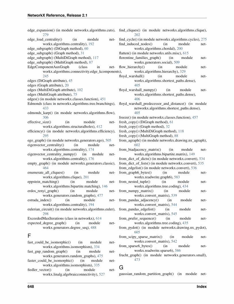
NetworkX Reference, Release 2.1
edge_expansion() (in module networkx.algorithms.cuts),279
edge_load_centrality() (in module net-workx.algorithms.centrality), 192
edge_subgraph() (DiGraph method), 60edge_subgraph() (Graph method), 31edge_subgraph() (MultiDiGraph method), 117edge_subgraph() (MultiGraph method), 87EdgeComponentAuxGraph (class in net-
workx.algorithms.connectivity.edge_kcomponents),245
edges (DiGraph attribute), 45edges (Graph attribute), 20edges (MultiDiGraph attribute), 102edges (MultiGraph attribute), 75edges() (in module networkx.classes.function), 451Edmonds (class in networkx.algorithms.tree.branchings),
433edmonds_karp() (in module networkx.algorithms.flow),
306effective_size() (in module net-
workx.algorithms.structuralholes), 412efficiency() (in module networkx.algorithms.efficiency),
295ego_graph() (in module networkx.generators.ego), 505eigenvector_centrality() (in module net-
workx.algorithms.centrality), 174eigenvector_centrality_numpy() (in module net-
workx.algorithms.centrality), 176empty_graph() (in module networkx.generators.classic),
464enumerate_all_cliques() (in module net-
workx.algorithms.clique), 201eppstein_matching() (in module net-
workx.algorithms.bipartite.matching), 146erdos_renyi_graph() (in module net-
workx.generators.random_graphs), 477estrada_index() (in module net-
workx.algorithms.centrality), 194eulerian_circuit() (in module networkx.algorithms.euler),
298ExceededMaxIterations (class in networkx), 614expected_degree_graph() (in module net-
workx.generators.degree_seq), 488
Ffast_could_be_isomorphic() (in module net-
workx.algorithms.isomorphism), 334fast_gnp_random_graph() (in module net-
workx.generators.random_graphs), 475faster_could_be_isomorphic() (in module net-
workx.algorithms.isomorphism), 335fiedler_vector() (in module net-
workx.linalg.algebraicconnectivity), 527
find_cliques() (in module networkx.algorithms.clique),202
find_cycle() (in module networkx.algorithms.cycles), 275find_induced_nodes() (in module net-
workx.algorithms.chordal), 200flatten() (in module networkx.utils.misc), 615florentine_families_graph() (in module net-
workx.generators.social), 509flow_hierarchy() (in module net-
workx.algorithms.hierarchy), 329floyd_warshall() (in module net-
workx.algorithms.shortest_paths.dense),405
floyd_warshall_numpy() (in module net-workx.algorithms.shortest_paths.dense),406
floyd_warshall_predecessor_and_distance() (in modulenetworkx.algorithms.shortest_paths.dense),405
freeze() (in module networkx.classes.function), 457fresh_copy() (DiGraph method), 61fresh_copy() (Graph method), 32fresh_copy() (MultiDiGraph method), 118fresh_copy() (MultiGraph method), 88from_agraph() (in module networkx.drawing.nx_agraph),
602from_biadjacency_matrix() (in module net-
workx.algorithms.bipartite.matrix), 149from_dict_of_dicts() (in module networkx.convert), 534from_dict_of_lists() (in module networkx.convert), 535from_edgelist() (in module networkx.convert), 536from_graph6_bytes() (in module net-
workx.readwrite.graph6), 583from_nested_tuple() (in module net-
workx.algorithms.tree.coding), 434from_numpy_matrix() (in module net-
workx.convert_matrix), 539from_pandas_adjacency() (in module net-
workx.convert_matrix), 544from_pandas_edgelist() (in module net-
workx.convert_matrix), 545from_prufer_sequence() (in module net-
workx.algorithms.tree.coding), 435from_pydot() (in module networkx.drawing.nx_pydot),
605from_scipy_sparse_matrix() (in module net-
workx.convert_matrix), 542from_sparse6_bytes() (in module net-
workx.readwrite.sparse6), 586frucht_graph() (in module networkx.generators.small),
473
Ggaussian_random_partition_graph() (in module net-
648 Index

NetworkX Reference, Release 2.1
workx.generators.community), 512general_random_intersection_graph() (in module net-
workx.generators.intersection), 507generalized_degree() (in module net-
workx.algorithms.cluster), 209generate_adjlist() (in module networkx.readwrite.adjlist),
554generate_edgelist() (in module net-
workx.readwrite.edgelist), 562generate_gml() (in module networkx.readwrite.gml), 569generate_multiline_adjlist() (in module net-
workx.readwrite.multiline_adjlist), 557generate_unique_node() (in module networkx.utils.misc),
616generic_edge_match() (in module net-
workx.algorithms.isomorphism), 345generic_multiedge_match() (in module net-
workx.algorithms.isomorphism), 345generic_node_match() (in module net-
workx.algorithms.isomorphism), 344generic_weighted_projected_graph() (in module net-
workx.algorithms.bipartite.projection), 154geographical_threshold_graph() (in module net-
workx.generators.geometric), 498get_edge_attributes() (in module net-
workx.classes.function), 456get_edge_data() (DiGraph method), 48get_edge_data() (Graph method), 22get_edge_data() (MultiDiGraph method), 106get_edge_data() (MultiGraph method), 77get_node_attributes() (in module net-
workx.classes.function), 455girvan_newman() (in module net-
workx.algorithms.community.centrality),222
global_efficiency() (in module net-workx.algorithms.efficiency), 296
global_parameters() (in module net-workx.algorithms.distance_regular), 292
global_reaching_centrality() (in module net-workx.algorithms.centrality), 197
gn_graph() (in module networkx.generators.directed),493
gnc_graph() (in module networkx.generators.directed),494
gnm_random_graph() (in module net-workx.generators.random_graphs), 477
gnmk_random_graph() (in module net-workx.algorithms.bipartite.generators), 168
gnp_random_graph() (in module net-workx.generators.random_graphs), 476
gnr_graph() (in module networkx.generators.directed),493
gomory_hu_tree() (in module networkx.algorithms.flow),
314google_matrix() (in module net-
workx.algorithms.link_analysis.pagerank_alg),349
Graph (class in networkx), 7graph_atlas() (in module networkx.generators.atlas), 459graph_atlas_g() (in module networkx.generators.atlas),
459graph_clique_number() (in module net-
workx.algorithms.clique), 204graph_number_of_cliques() (in module net-
workx.algorithms.clique), 204graphviz_layout() (in module net-
workx.drawing.nx_agraph), 603graphviz_layout() (in module net-
workx.drawing.nx_pydot), 606greedy_branching() (in module net-
workx.algorithms.tree.branchings), 431greedy_color() (in module net-
workx.algorithms.coloring), 210grid_2d_graph() (in module networkx.generators.lattice),
468grid_graph() (in module networkx.generators.lattice), 468groups() (in module networkx.utils.misc), 616
Hhamiltonian_path() (in module net-
workx.algorithms.tournament), 416harmonic_centrality() (in module net-
workx.algorithms.centrality), 195has_bridges() (in module networkx.algorithms.bridges),
172has_edge() (DiGraph method), 48has_edge() (Graph method), 21has_edge() (MultiDiGraph method), 105has_edge() (MultiGraph method), 76has_node() (DiGraph method), 45has_node() (Graph method), 20has_node() (MultiDiGraph method), 102has_node() (MultiGraph method), 75has_path() (in module net-
workx.algorithms.shortest_paths.generic),382
HasACycle (class in networkx), 613hashable, 625havel_hakimi_graph() (in module net-
workx.algorithms.bipartite.generators), 166havel_hakimi_graph() (in module net-
workx.generators.degree_seq), 489heawood_graph() (in module networkx.generators.small),
473hexagonal_lattice_graph() (in module net-
workx.generators.lattice), 469
Index 649

NetworkX Reference, Release 2.1
hits() (in module net-workx.algorithms.link_analysis.hits_alg),350
hits_numpy() (in module net-workx.algorithms.link_analysis.hits_alg),351
hits_scipy() (in module net-workx.algorithms.link_analysis.hits_alg),352
hopcroft_karp_matching() (in module net-workx.algorithms.bipartite.matching), 147
house_graph() (in module networkx.generators.small),473
house_x_graph() (in module networkx.generators.small),473
hub_matrix() (in module net-workx.algorithms.link_analysis.hits_alg),353
hypercube_graph() (in module net-workx.generators.lattice), 470
Iicosahedral_graph() (in module net-
workx.generators.small), 473identified_nodes() (in module net-
workx.algorithms.minors), 363immediate_dominators() (in module net-
workx.algorithms.dominance), 293in_degree (DiGraph attribute), 54in_degree (MultiDiGraph attribute), 111in_degree_centrality() (in module net-
workx.algorithms.centrality), 173in_edges (DiGraph attribute), 47in_edges (MultiDiGraph attribute), 105incidence_matrix() (in module net-
workx.linalg.graphmatrix), 522info() (in module networkx.classes.function), 448initialize() (DiGraphMatcher method), 340initialize() (GraphMatcher method), 338intersection() (in module net-
workx.algorithms.operators.binary), 369intersection_all() (in module net-
workx.algorithms.operators.all), 372intersection_array() (in module net-
workx.algorithms.distance_regular), 292inverse_line_graph() (in module net-
workx.generators.line), 505is_aperiodic() (in module networkx.algorithms.dag), 284is_arborescence() (in module net-
workx.algorithms.tree.recognition), 430is_attracting_component() (in module net-
workx.algorithms.components), 233is_biconnected() (in module net-
workx.algorithms.components), 234
is_bipartite() (in module net-workx.algorithms.bipartite.basic), 142
is_bipartite_node_set() (in module net-workx.algorithms.bipartite.basic), 142
is_branching() (in module net-workx.algorithms.tree.recognition), 431
is_chordal() (in module networkx.algorithms.chordal),198
is_connected() (in module net-workx.algorithms.components), 225
is_digraphical() (in module net-workx.algorithms.graphical), 326
is_directed() (in module networkx.classes.function), 448is_directed_acyclic_graph() (in module net-
workx.algorithms.dag), 284is_distance_regular() (in module net-
workx.algorithms.distance_regular), 290is_dominating_set() (in module net-
workx.algorithms.dominating), 295is_edge_cover() (in module net-
workx.algorithms.covering), 273is_eulerian() (in module networkx.algorithms.euler), 297is_forest() (in module net-
workx.algorithms.tree.recognition), 430is_frozen() (in module networkx.classes.function), 458is_graphical() (in module net-
workx.algorithms.graphical), 326is_isolate() (in module networkx.algorithms.isolate), 331is_isomorphic() (DiGraphMatcher method), 340is_isomorphic() (GraphMatcher method), 338is_isomorphic() (in module net-
workx.algorithms.isomorphism), 333is_k_edge_connected() (in module net-
workx.algorithms.connectivity.edge_augmentation),241
is_kl_connected() (in module net-workx.algorithms.hybrid), 330
is_list_of_ints() (in module networkx.utils.misc), 616is_locally_k_edge_connected() (in module net-
workx.algorithms.connectivity.edge_augmentation),241
is_matching() (in module net-workx.algorithms.matching), 359
is_maximal_matching() (in module net-workx.algorithms.matching), 359
is_multigraphical() (in module net-workx.algorithms.graphical), 327
is_partition() (in module net-workx.algorithms.community.community_utils),224
is_pseudographical() (in module net-workx.algorithms.graphical), 327
is_reachable() (in module net-workx.algorithms.tournament), 416
650 Index

NetworkX Reference, Release 2.1
is_semiconnected() (in module net-workx.algorithms.components), 238
is_simple_path() (in module net-workx.algorithms.simple_paths), 409
is_string_like() (in module networkx.utils.misc), 615is_strongly_connected() (in module net-
workx.algorithms.components), 227is_strongly_connected() (in module net-
workx.algorithms.tournament), 417is_strongly_regular() (in module net-
workx.algorithms.distance_regular), 291is_tournament() (in module net-
workx.algorithms.tournament), 417is_tree() (in module net-
workx.algorithms.tree.recognition), 429is_valid_degree_sequence_erdos_gallai() (in module net-
workx.algorithms.graphical), 328is_valid_degree_sequence_havel_hakimi() (in module
networkx.algorithms.graphical), 328is_valid_joint_degree() (in module net-
workx.generators.joint_degree_seq), 518is_weakly_connected() (in module net-
workx.algorithms.components), 231isolates() (in module networkx.algorithms.isolate), 332isomorphisms_iter() (DiGraphMatcher method), 340isomorphisms_iter() (GraphMatcher method), 338iterable() (in module networkx.utils.misc), 616
Jjaccard_coefficient() (in module net-
workx.algorithms.link_prediction), 354jit_data() (in module networkx.readwrite.json_graph),
580jit_graph() (in module networkx.readwrite.json_graph),
580johnson() (in module net-
workx.algorithms.shortest_paths.weighted),404
join() (in module networkx.algorithms.tree.operations),437
joint_degree_graph() (in module net-workx.generators.joint_degree_seq), 518
Kk_clique_communities() (in module net-
workx.algorithms.community.kclique), 218k_components() (in module net-
workx.algorithms.approximation.kcomponents),124
k_components() (in module net-workx.algorithms.connectivity.kcomponents),246
k_core() (in module networkx.algorithms.core), 270k_corona() (in module networkx.algorithms.core), 272
k_crust() (in module networkx.algorithms.core), 271k_edge_augmentation() (in module net-
workx.algorithms.connectivity.edge_augmentation),239
k_edge_components() (in module net-workx.algorithms.connectivity.edge_kcomponents),242
k_edge_subgraphs() (in module net-workx.algorithms.connectivity.edge_kcomponents),243
k_nearest_neighbors() (in module net-workx.algorithms.assortativity), 138
k_random_intersection_graph() (in module net-workx.generators.intersection), 507
k_shell() (in module networkx.algorithms.core), 270kamada_kawai_layout() (in module net-
workx.drawing.layout), 608karate_club_graph() (in module net-
workx.generators.social), 508katz_centrality() (in module net-
workx.algorithms.centrality), 177katz_centrality_numpy() (in module net-
workx.algorithms.centrality), 178kernighan_lin_bisection() (in module net-
workx.algorithms.community.kernighan_lin),215
kl_connected_subgraph() (in module net-workx.algorithms.hybrid), 330
kosaraju_strongly_connected_components() (in modulenetworkx.algorithms.components), 229
krackhardt_kite_graph() (in module net-workx.generators.small), 473
Llabel_propagation_communities() (in module net-
workx.algorithms.community.label_propagation),220
ladder_graph() (in module networkx.generators.classic),465
laplacian_matrix() (in module net-workx.linalg.laplacianmatrix), 523
laplacian_spectrum() (in module net-workx.linalg.spectrum), 525
large_clique_size() (in module net-workx.algorithms.approximation.clique),126
latapy_clustering() (in module net-workx.algorithms.bipartite.cluster), 159
LCF_graph() (in module networkx.generators.small), 472lexicographic_product() (in module net-
workx.algorithms.operators.product), 373lexicographical_topological_sort() (in module net-
workx.algorithms.dag), 283
Index 651

NetworkX Reference, Release 2.1
LFR_benchmark_graph() (in module net-workx.algorithms.community.community_generators),216
line_graph() (in module networkx.generators.line), 503literal_destringizer() (in module net-
workx.readwrite.gml), 570literal_stringizer() (in module networkx.readwrite.gml),
571load_centrality() (in module net-
workx.algorithms.centrality), 191local_constraint() (in module net-
workx.algorithms.structuralholes), 413local_edge_connectivity() (in module net-
workx.algorithms.connectivity.connectivity),255
local_efficiency() (in module net-workx.algorithms.efficiency), 296
local_node_connectivity() (in module net-workx.algorithms.approximation.connectivity),122
local_node_connectivity() (in module net-workx.algorithms.connectivity.connectivity),257
local_reaching_centrality() (in module net-workx.algorithms.centrality), 196
lollipop_graph() (in module networkx.generators.classic),465
Mmake_clique_bipartite() (in module net-
workx.algorithms.clique), 203make_max_clique_graph() (in module net-
workx.algorithms.clique), 203make_small_graph() (in module net-
workx.generators.small), 471make_str() (in module networkx.utils.misc), 616margulis_gabber_galil_graph() (in module net-
workx.generators.expanders), 467match() (DiGraphMatcher method), 340match() (GraphMatcher method), 338max_clique() (in module net-
workx.algorithms.approximation.clique),125
max_flow_min_cost() (in module net-workx.algorithms.flow), 322
max_weight_matching() (in module net-workx.algorithms.matching), 360
maximal_independent_set() (in module net-workx.algorithms.mis), 366
maximal_matching() (in module net-workx.algorithms.matching), 360
maximum_branching() (in module net-workx.algorithms.tree.branchings), 432
maximum_flow() (in module networkx.algorithms.flow),299
maximum_flow_value() (in module net-workx.algorithms.flow), 300
maximum_independent_set() (in module net-workx.algorithms.approximation.independent_set),129
maximum_spanning_arborescence() (in module net-workx.algorithms.tree.branchings), 432
maximum_spanning_edges() (in module net-workx.algorithms.tree.mst), 441
maximum_spanning_tree() (in module net-workx.algorithms.tree.mst), 439
metric_closure() (in module net-workx.algorithms.approximation.steinertree),130
min_cost_flow() (in module networkx.algorithms.flow),320
min_cost_flow_cost() (in module net-workx.algorithms.flow), 319
min_edge_cover() (in module net-workx.algorithms.bipartite.covering), 169
min_edge_cover() (in module net-workx.algorithms.covering), 272
min_edge_dominating_set() (in module net-workx.algorithms.approximation.dominating_set),128
min_maximal_matching() (in module net-workx.algorithms.approximation.matching),129
min_weighted_dominating_set() (in module net-workx.algorithms.approximation.dominating_set),127
min_weighted_vertex_cover() (in module net-workx.algorithms.approximation.vertex_cover),131
minimum_branching() (in module net-workx.algorithms.tree.branchings), 432
minimum_cut() (in module networkx.algorithms.flow),302
minimum_cut_value() (in module net-workx.algorithms.flow), 304
minimum_cycle_basis() (in module net-workx.algorithms.cycles), 276
minimum_edge_cut() (in module net-workx.algorithms.connectivity.cuts), 261
minimum_node_cut() (in module net-workx.algorithms.connectivity.cuts), 262
minimum_spanning_arborescence() (in module net-workx.algorithms.tree.branchings), 433
minimum_spanning_edges() (in module net-workx.algorithms.tree.mst), 440
minimum_spanning_tree() (in module net-workx.algorithms.tree.mst), 438
652 Index

NetworkX Reference, Release 2.1
minimum_st_edge_cut() (in module net-workx.algorithms.connectivity.cuts), 263
minimum_st_node_cut() (in module net-workx.algorithms.connectivity.cuts), 265
mixing_expansion() (in module net-workx.algorithms.cuts), 279
moebius_kantor_graph() (in module net-workx.generators.small), 474
multi_source_dijkstra_path() (in module net-workx.algorithms.shortest_paths.weighted),392
multi_source_dijkstra_path_length() (in module net-workx.algorithms.shortest_paths.weighted),393
MultiDiGraph (class in networkx), 88MultiGraph (class in networkx), 61mycielski_graph() (in module net-
workx.generators.mycielski), 520mycielskian() (in module net-
workx.generators.mycielski), 519
Nnavigable_small_world_graph() (in module net-
workx.generators.geometric), 501nbunch, 625nbunch_iter() (DiGraph method), 51nbunch_iter() (Graph method), 24nbunch_iter() (MultiDiGraph method), 109nbunch_iter() (MultiGraph method), 80negative_edge_cycle() (in module net-
workx.algorithms.shortest_paths.weighted),403
neighbors() (DiGraph method), 49neighbors() (Graph method), 23neighbors() (MultiDiGraph method), 107neighbors() (MultiGraph method), 78network_simplex() (in module net-
workx.algorithms.flow), 317networkx.algorithms.approximation (module), 121networkx.algorithms.approximation.clique (module), 125networkx.algorithms.approximation.clustering_coefficient
(module), 127networkx.algorithms.approximation.connectivity (mod-
ule), 121networkx.algorithms.approximation.dominating_set
(module), 127networkx.algorithms.approximation.independent_set
(module), 128networkx.algorithms.approximation.kcomponents (mod-
ule), 124networkx.algorithms.approximation.matching (module),
129networkx.algorithms.approximation.ramsey (module),
130
networkx.algorithms.approximation.steinertree (module),130
networkx.algorithms.approximation.vertex_cover (mod-ule), 131
networkx.algorithms.assortativity (module), 132networkx.algorithms.bipartite (module), 141networkx.algorithms.bipartite.basic (module), 142networkx.algorithms.bipartite.centrality (module), 161networkx.algorithms.bipartite.cluster (module), 156networkx.algorithms.bipartite.covering (module), 169networkx.algorithms.bipartite.generators (module), 164networkx.algorithms.bipartite.matching (module), 145networkx.algorithms.bipartite.matrix (module), 148networkx.algorithms.bipartite.projection (module), 149networkx.algorithms.bipartite.redundancy (module), 160networkx.algorithms.bipartite.spectral (module), 156networkx.algorithms.boundary (module), 169networkx.algorithms.bridges (module), 171networkx.algorithms.centrality (module), 173, 288networkx.algorithms.chains (module), 197networkx.algorithms.chordal (module), 198networkx.algorithms.clique (module), 201networkx.algorithms.cluster (module), 205networkx.algorithms.coloring (module), 210networkx.algorithms.communicability_alg (module), 213networkx.algorithms.community (module), 215networkx.algorithms.community.asyn_fluidc (module),
220networkx.algorithms.community.centrality (module), 222networkx.algorithms.community.community_generators
(module), 216networkx.algorithms.community.community_utils (mod-
ule), 224networkx.algorithms.community.kclique (module), 218networkx.algorithms.community.kernighan_lin (module),
215networkx.algorithms.community.label_propagation
(module), 219networkx.algorithms.community.quality (module), 221networkx.algorithms.components (module), 224networkx.algorithms.connectivity (module), 239networkx.algorithms.connectivity.connectivity (module),
252networkx.algorithms.connectivity.cuts (module), 260networkx.algorithms.connectivity.disjoint_paths (mod-
ule), 249networkx.algorithms.connectivity.edge_augmentation
(module), 239networkx.algorithms.connectivity.edge_kcomponents
(module), 242networkx.algorithms.connectivity.kcomponents (mod-
ule), 246networkx.algorithms.connectivity.kcutsets (module), 248
Index 653
NetworkX Reference, Release 2.1
networkx.algorithms.connectivity.stoerwagner (module),267
networkx.algorithms.connectivity.utils (module), 268networkx.algorithms.core (module), 269networkx.algorithms.covering (module), 272networkx.algorithms.cuts (module), 277networkx.algorithms.cycles (module), 273networkx.algorithms.dag (module), 281networkx.algorithms.distance_measures (module), 288networkx.algorithms.distance_regular (module), 290networkx.algorithms.dominance (module), 293networkx.algorithms.dominating (module), 294networkx.algorithms.efficiency (module), 295networkx.algorithms.euler (module), 297networkx.algorithms.flow (module), 299networkx.algorithms.graphical (module), 326networkx.algorithms.hierarchy (module), 329networkx.algorithms.hybrid (module), 330networkx.algorithms.isolate (module), 331networkx.algorithms.isomorphism (module), 332networkx.algorithms.isomorphism.isomorphvf2 (mod-
ule), 335networkx.algorithms.link_analysis.hits_alg (module),
350networkx.algorithms.link_analysis.pagerank_alg (mod-
ule), 346networkx.algorithms.link_prediction (module), 353networkx.algorithms.matching (module), 359networkx.algorithms.minors (module), 361networkx.algorithms.mis (module), 366networkx.algorithms.operators.all (module), 371networkx.algorithms.operators.binary (module), 368networkx.algorithms.operators.product (module), 372networkx.algorithms.operators.unary (module), 367networkx.algorithms.reciprocity (module), 376networkx.algorithms.richclub (module), 377networkx.algorithms.shortest_paths.astar (module), 406networkx.algorithms.shortest_paths.dense (module), 404networkx.algorithms.shortest_paths.generic (module),
378networkx.algorithms.shortest_paths.unweighted (mod-
ule), 382networkx.algorithms.shortest_paths.weighted (module),
385networkx.algorithms.simple_paths (module), 407networkx.algorithms.structuralholes (module), 411networkx.algorithms.swap (module), 414networkx.algorithms.tournament (module), 415networkx.algorithms.traversal.beamsearch (module), 426networkx.algorithms.traversal.breadth_first_search (mod-
ule), 423networkx.algorithms.traversal.depth_first_search (mod-
ule), 418networkx.algorithms.traversal.edgedfs (module), 427
networkx.algorithms.tree.branchings (module), 431networkx.algorithms.tree.coding (module), 433networkx.algorithms.tree.mst (module), 438networkx.algorithms.tree.operations (module), 437networkx.algorithms.tree.recognition (module), 428networkx.algorithms.triads (module), 443networkx.algorithms.vitality (module), 443networkx.algorithms.voronoi (module), 444networkx.algorithms.wiener (module), 445networkx.classes.function (module), 447networkx.classes.ordered (module), 118networkx.convert (module), 533networkx.convert_matrix (module), 536networkx.drawing.layout (module), 607networkx.drawing.nx_agraph (module), 602networkx.drawing.nx_pydot (module), 604networkx.drawing.nx_pylab (module), 593networkx.exception (module), 613networkx.generators.atlas (module), 459networkx.generators.classic (module), 460networkx.generators.community (module), 509networkx.generators.degree_seq (module), 485networkx.generators.directed (module), 492networkx.generators.duplication (module), 484networkx.generators.ego (module), 505networkx.generators.expanders (module), 467networkx.generators.geometric (module), 496networkx.generators.intersection (module), 506networkx.generators.joint_degree_seq (module), 517networkx.generators.lattice (module), 468networkx.generators.line (module), 503networkx.generators.mycielski (module), 519networkx.generators.nonisomorphic_trees (module), 516networkx.generators.random_clustered (module), 491networkx.generators.random_graphs (module), 475networkx.generators.small (module), 471networkx.generators.social (module), 508networkx.generators.stochastic (module), 506networkx.generators.trees (module), 514networkx.generators.triads (module), 517networkx.linalg.algebraicconnectivity (module), 526networkx.linalg.attrmatrix (module), 529networkx.linalg.graphmatrix (module), 521networkx.linalg.laplacianmatrix (module), 522networkx.linalg.spectrum (module), 525networkx.readwrite.adjlist (module), 551networkx.readwrite.edgelist (module), 558networkx.readwrite.gexf (module), 564networkx.readwrite.gml (module), 566networkx.readwrite.gpickle (module), 571networkx.readwrite.graph6 (module), 583networkx.readwrite.graphml (module), 573networkx.readwrite.json_graph (module), 575networkx.readwrite.leda (module), 580
654 Index
NetworkX Reference, Release 2.1
networkx.readwrite.multiline_adjlist (module), 554networkx.readwrite.nx_shp (module), 591networkx.readwrite.nx_yaml (module), 581networkx.readwrite.pajek (module), 589networkx.readwrite.sparse6 (module), 586networkx.relabel (module), 547networkx.utils (module), 615networkx.utils.contextmanagers (module), 624networkx.utils.decorators (module), 619networkx.utils.misc (module), 615networkx.utils.random_sequence (module), 617networkx.utils.rcm (module), 622networkx.utils.union_find (module), 617NetworkXAlgorithmError (class in networkx), 613NetworkXError (class in networkx), 613NetworkXException (class in networkx), 613NetworkXNoCycle (class in networkx), 613NetworkXNoPath (class in networkx), 613NetworkXNotImplemented (class in networkx), 613NetworkXPointlessConcept (class in networkx), 613NetworkXUnbounded (class in networkx), 613NetworkXUnfeasible (class in networkx), 613new_edge_key() (MultiDiGraph method), 97new_edge_key() (MultiGraph method), 70newman_watts_strogatz_graph() (in module net-
workx.generators.random_graphs), 478node, 625node attribute, 625node_boundary() (in module net-
workx.algorithms.boundary), 170node_clique_number() (in module net-
workx.algorithms.clique), 205node_connected_component() (in module net-
workx.algorithms.components), 226node_connectivity() (in module net-
workx.algorithms.approximation.connectivity),123
node_connectivity() (in module net-workx.algorithms.connectivity.connectivity),259
node_disjoint_paths() (in module net-workx.algorithms.connectivity.disjoint_paths),251
node_expansion() (in module networkx.algorithms.cuts),280
node_link_data() (in module net-workx.readwrite.json_graph), 575
node_link_graph() (in module net-workx.readwrite.json_graph), 576
node_redundancy() (in module net-workx.algorithms.bipartite.redundancy),160
NodeNotFound (class in networkx), 613nodes (DiGraph attribute), 43
nodes (Graph attribute), 18nodes (MultiDiGraph attribute), 100nodes (MultiGraph attribute), 73nodes() (in module networkx.classes.function), 450nodes_or_number() (in module net-
workx.utils.decorators), 620nodes_with_selfloops() (in module net-
workx.classes.function), 453non_edges() (in module networkx.classes.function), 452non_neighbors() (in module networkx.classes.function),
451nonisomorphic_trees() (in module net-
workx.generators.nonisomorphic_trees),516
normalized_cut_size() (in module net-workx.algorithms.cuts), 280
normalized_laplacian_matrix() (in module net-workx.linalg.laplacianmatrix), 523
not_implemented_for() (in module net-workx.utils.decorators), 620
NotATree, 443null_graph() (in module networkx.generators.classic),
465number_attracting_components() (in module net-
workx.algorithms.components), 233number_connected_components() (in module net-
workx.algorithms.components), 225number_of_cliques() (in module net-
workx.algorithms.clique), 205number_of_edges() (DiGraph method), 56number_of_edges() (Graph method), 27number_of_edges() (in module net-
workx.classes.function), 452number_of_edges() (MultiDiGraph method), 113number_of_edges() (MultiGraph method), 83number_of_nodes() (DiGraph method), 52number_of_nodes() (Graph method), 25number_of_nodes() (in module net-
workx.classes.function), 450number_of_nodes() (MultiDiGraph method), 110number_of_nodes() (MultiGraph method), 81number_of_nonisomorphic_trees() (in module net-
workx.generators.nonisomorphic_trees), 517number_of_selfloops() (in module net-
workx.classes.function), 453number_strongly_connected_components() (in module
networkx.algorithms.components), 227number_weakly_connected_components() (in module
networkx.algorithms.components), 231numeric_assortativity_coefficient() (in module net-
workx.algorithms.assortativity), 134numerical_edge_match() (in module net-
workx.algorithms.isomorphism), 343numerical_multiedge_match() (in module net-
Index 655

NetworkX Reference, Release 2.1
workx.algorithms.isomorphism), 344numerical_node_match() (in module net-
workx.algorithms.isomorphism), 343
Ooctahedral_graph() (in module net-
workx.generators.small), 474open_file() (in module networkx.utils.decorators), 619order() (DiGraph method), 52order() (Graph method), 25order() (MultiDiGraph method), 110order() (MultiGraph method), 81OrderedDiGraph (class in networkx), 119OrderedGraph (class in networkx), 119OrderedMultiDiGraph (class in networkx), 119OrderedMultiGraph (class in networkx), 119out_degree (DiGraph attribute), 54out_degree (MultiDiGraph attribute), 112out_degree_centrality() (in module net-
workx.algorithms.centrality), 174out_edges (DiGraph attribute), 46out_edges (MultiDiGraph attribute), 104overall_reciprocity() (in module net-
workx.algorithms.reciprocity), 377overlap_weighted_projected_graph() (in module net-
workx.algorithms.bipartite.projection), 153
Ppagerank() (in module net-
workx.algorithms.link_analysis.pagerank_alg),346
pagerank_numpy() (in module net-workx.algorithms.link_analysis.pagerank_alg),347
pagerank_scipy() (in module net-workx.algorithms.link_analysis.pagerank_alg),348
pairwise() (in module networkx.utils.misc), 616pappus_graph() (in module networkx.generators.small),
474parse_adjlist() (in module networkx.readwrite.adjlist),
553parse_edgelist() (in module networkx.readwrite.edgelist),
563parse_gml() (in module networkx.readwrite.gml), 569parse_leda() (in module networkx.readwrite.leda), 581parse_multiline_adjlist() (in module net-
workx.readwrite.multiline_adjlist), 557parse_pajek() (in module networkx.readwrite.pajek), 590partial_duplication_graph() (in module net-
workx.generators.duplication), 484path_graph() (in module networkx.generators.classic),
465
performance() (in module net-workx.algorithms.community.quality), 222
periphery() (in module net-workx.algorithms.distance_measures), 290
petersen_graph() (in module networkx.generators.small),474
planted_partition_graph() (in module net-workx.generators.community), 512
power() (in module net-workx.algorithms.operators.product), 375
PowerIterationFailedConvergence (class in networkx),614
powerlaw_cluster_graph() (in module net-workx.generators.random_graphs), 481
powerlaw_sequence() (in module net-workx.utils.random_sequence), 617
pred (DiGraph attribute), 51predecessor() (in module net-
workx.algorithms.shortest_paths.unweighted),385
predecessors() (DiGraph method), 50predecessors() (MultiDiGraph method), 108preferential_attachment() (in module net-
workx.algorithms.link_prediction), 355preferential_attachment_graph() (in module net-
workx.algorithms.bipartite.generators), 167prefix_tree() (in module networkx.generators.trees), 515preflow_push() (in module networkx.algorithms.flow),
309preserve_random_state() (in module net-
workx.utils.decorators), 621projected_graph() (in module net-
workx.algorithms.bipartite.projection), 150pydot_layout() (in module networkx.drawing.nx_pydot),
606pygraphviz_layout() (in module net-
workx.drawing.nx_agraph), 604
Qquotient_graph() (in module net-
workx.algorithms.minors), 364
Rra_index_soundarajan_hopcroft() (in module net-
workx.algorithms.link_prediction), 357radius() (in module net-
workx.algorithms.distance_measures), 290ramsey_R2() (in module net-
workx.algorithms.approximation.ramsey),130
random_clustered_graph() (in module net-workx.generators.random_clustered), 491
random_degree_sequence_graph() (in module net-workx.generators.degree_seq), 490
656 Index

NetworkX Reference, Release 2.1
random_geometric_graph() (in module net-workx.generators.geometric), 496
random_graph() (in module net-workx.algorithms.bipartite.generators), 167
random_k_out_graph() (in module net-workx.generators.directed), 494
random_kernel_graph() (in module net-workx.generators.random_graphs), 481
random_layout() (in module networkx.drawing.layout),608
random_lobster() (in module net-workx.generators.random_graphs), 482
random_partition_graph() (in module net-workx.generators.community), 511
random_powerlaw_tree() (in module net-workx.generators.random_graphs), 483
random_powerlaw_tree_sequence() (in module net-workx.generators.random_graphs), 483
random_regular_graph() (in module net-workx.generators.random_graphs), 480
random_shell_graph() (in module net-workx.generators.random_graphs), 483
random_state() (in module networkx.utils.decorators),621
random_tournament() (in module net-workx.algorithms.tournament), 418
random_tree() (in module networkx.generators.trees),514
random_weighted_sample() (in module net-workx.utils.random_sequence), 618
read_adjlist() (in module networkx.readwrite.adjlist), 551read_dot() (in module networkx.drawing.nx_agraph), 603read_dot() (in module networkx.drawing.nx_pydot), 606read_edgelist() (in module networkx.readwrite.edgelist),
559read_gexf() (in module networkx.readwrite.gexf), 565read_gml() (in module networkx.readwrite.gml), 567read_gpickle() (in module networkx.readwrite.gpickle),
572read_graph6() (in module networkx.readwrite.graph6),
584read_graphml() (in module networkx.readwrite.graphml),
573read_leda() (in module networkx.readwrite.leda), 580read_multiline_adjlist() (in module net-
workx.readwrite.multiline_adjlist), 555read_pajek() (in module networkx.readwrite.pajek), 589read_shp() (in module networkx.readwrite.nx_shp), 591read_sparse6() (in module networkx.readwrite.sparse6),
587read_weighted_edgelist() (in module net-
workx.readwrite.edgelist), 561read_yaml() (in module networkx.readwrite.nx_yaml),
582
reciprocity() (in module net-workx.algorithms.reciprocity), 376
relabel_gexf_graph() (in module net-workx.readwrite.gexf), 566
relabel_nodes() (in module networkx.relabel), 547relaxed_caveman_graph() (in module net-
workx.generators.community), 510remove_edge() (DiGraph method), 41remove_edge() (Graph method), 16remove_edge() (MultiDiGraph method), 98remove_edge() (MultiGraph method), 71remove_edges_from() (DiGraph method), 42remove_edges_from() (Graph method), 17remove_edges_from() (MultiDiGraph method), 98remove_edges_from() (MultiGraph method), 71remove_node() (DiGraph method), 38remove_node() (Graph method), 13remove_node() (MultiDiGraph method), 94remove_node() (MultiGraph method), 67remove_nodes_from() (DiGraph method), 38remove_nodes_from() (Graph method), 13remove_nodes_from() (MultiDiGraph method), 94remove_nodes_from() (MultiGraph method), 67rescale_layout() (in module networkx.drawing.layout),
609resource_allocation_index() (in module net-
workx.algorithms.link_prediction), 353reverse() (DiGraph method), 61reverse() (in module net-
workx.algorithms.operators.unary), 368reverse() (MultiDiGraph method), 118reverse_cuthill_mckee_ordering() (in module net-
workx.utils.rcm), 623reverse_havel_hakimi_graph() (in module net-
workx.algorithms.bipartite.generators), 166reversed() (in module networkx.utils.contextmanagers),
624rich_club_coefficient() (in module net-
workx.algorithms.richclub), 377ring_of_cliques() (in module net-
workx.generators.community), 513robins_alexander_clustering() (in module net-
workx.algorithms.bipartite.cluster), 160
Sscale_free_graph() (in module net-
workx.generators.directed), 495score_sequence() (in module net-
workx.algorithms.tournament), 418sedgewick_maze_graph() (in module net-
workx.generators.small), 474selfloop_edges() (in module networkx.classes.function),
452semantic_feasibility() (DiGraphMatcher method), 341
Index 657

NetworkX Reference, Release 2.1
semantic_feasibility() (GraphMatcher method), 339set_edge_attributes() (in module net-
workx.classes.function), 455set_node_attributes() (in module net-
workx.classes.function), 454sets() (in module networkx.algorithms.bipartite.basic),
143shell_layout() (in module networkx.drawing.layout), 609shortest_augmenting_path() (in module net-
workx.algorithms.flow), 307shortest_path() (in module net-
workx.algorithms.shortest_paths.generic),378
shortest_path_length() (in module net-workx.algorithms.shortest_paths.generic),380
shortest_simple_paths() (in module net-workx.algorithms.simple_paths), 410
simple_cycles() (in module networkx.algorithms.cycles),274
single_source_bellman_ford() (in module net-workx.algorithms.shortest_paths.weighted),401
single_source_bellman_ford_path() (in module net-workx.algorithms.shortest_paths.weighted),398
single_source_bellman_ford_path_length() (in modulenetworkx.algorithms.shortest_paths.weighted),399
single_source_dijkstra() (in module net-workx.algorithms.shortest_paths.weighted),389
single_source_dijkstra_path() (in module net-workx.algorithms.shortest_paths.weighted),390
single_source_dijkstra_path_length() (in module net-workx.algorithms.shortest_paths.weighted),391
single_source_shortest_path() (in module net-workx.algorithms.shortest_paths.unweighted),382
single_source_shortest_path_length() (in module net-workx.algorithms.shortest_paths.unweighted),383
size() (DiGraph method), 55size() (Graph method), 27size() (MultiDiGraph method), 113size() (MultiGraph method), 82soft_random_geometric_graph() (in module net-
workx.generators.geometric), 497spectral_bipartivity() (in module net-
workx.algorithms.bipartite.spectral), 156spectral_layout() (in module networkx.drawing.layout),
611
spectral_ordering() (in module net-workx.linalg.algebraicconnectivity), 528
spring_layout() (in module networkx.drawing.layout),610
square_clustering() (in module net-workx.algorithms.cluster), 208
star_graph() (in module networkx.generators.classic), 466steiner_tree() (in module net-
workx.algorithms.approximation.steinertree),130
stochastic_graph() (in module net-workx.generators.stochastic), 506
stoer_wagner() (in module net-workx.algorithms.connectivity.stoerwagner),267
strategy_connected_sequential() (in module net-workx.algorithms.coloring), 212
strategy_connected_sequential_bfs() (in module net-workx.algorithms.coloring), 212
strategy_connected_sequential_dfs() (in module net-workx.algorithms.coloring), 212
strategy_independent_set() (in module net-workx.algorithms.coloring), 212
strategy_largest_first() (in module net-workx.algorithms.coloring), 212
strategy_random_sequential() (in module net-workx.algorithms.coloring), 213
strategy_saturation_largest_first() (in module net-workx.algorithms.coloring), 213
strategy_smallest_last() (in module net-workx.algorithms.coloring), 213
strong_product() (in module net-workx.algorithms.operators.product), 374
strongly_connected_component_subgraphs() (in modulenetworkx.algorithms.components), 229
strongly_connected_components() (in module net-workx.algorithms.components), 228
strongly_connected_components_recursive() (in modulenetworkx.algorithms.components), 229
subgraph() (DiGraph method), 59subgraph() (Graph method), 31subgraph() (MultiDiGraph method), 117subgraph() (MultiGraph method), 86subgraph_centrality() (in module net-
workx.algorithms.centrality), 193subgraph_centrality_exp() (in module net-
workx.algorithms.centrality), 193subgraph_is_isomorphic() (DiGraphMatcher method),
340subgraph_is_isomorphic() (GraphMatcher method), 338subgraph_isomorphisms_iter() (DiGraphMatcher
method), 340subgraph_isomorphisms_iter() (GraphMatcher method),
338
658 Index

NetworkX Reference, Release 2.1
succ (DiGraph attribute), 50succ (MultiDiGraph attribute), 108successors() (DiGraph method), 50successors() (MultiDiGraph method), 108symmetric_difference() (in module net-
workx.algorithms.operators.binary), 370syntactic_feasibility() (DiGraphMatcher method), 341syntactic_feasibility() (GraphMatcher method), 339
Ttensor_product() (in module net-
workx.algorithms.operators.product), 374tetrahedral_graph() (in module net-
workx.generators.small), 474thresholded_random_geometric_graph() (in module net-
workx.generators.geometric), 502to_agraph() (in module networkx.drawing.nx_agraph),
603to_dict_of_dicts() (in module networkx.convert), 534to_dict_of_lists() (in module networkx.convert), 535to_directed() (DiGraph method), 59to_directed() (Graph method), 30to_directed() (MultiDiGraph method), 116to_directed() (MultiGraph method), 86to_edgelist() (in module networkx.convert), 535to_graph6_bytes() (in module net-
workx.readwrite.graph6), 584to_nested_tuple() (in module net-
workx.algorithms.tree.coding), 434to_networkx_graph() (in module networkx.convert), 533to_numpy_matrix() (in module net-
workx.convert_matrix), 537to_numpy_recarray() (in module net-
workx.convert_matrix), 538to_pandas_adjacency() (in module net-
workx.convert_matrix), 543to_pandas_edgelist() (in module net-
workx.convert_matrix), 545to_prufer_sequence() (in module net-
workx.algorithms.tree.coding), 436to_pydot() (in module networkx.drawing.nx_pydot), 605to_scipy_sparse_matrix() (in module net-
workx.convert_matrix), 540to_sparse6_bytes() (in module net-
workx.readwrite.sparse6), 588to_undirected() (DiGraph method), 58to_undirected() (Graph method), 29to_undirected() (MultiDiGraph method), 115to_undirected() (MultiGraph method), 85to_vertex_cover() (in module net-
workx.algorithms.bipartite.matching), 147topological_sort() (in module networkx.algorithms.dag),
282
transitive_closure() (in module net-workx.algorithms.dag), 284
transitive_reduction() (in module net-workx.algorithms.dag), 285
transitivity() (in module networkx.algorithms.cluster),206
tree_data() (in module networkx.readwrite.json_graph),578
tree_graph() (in module networkx.readwrite.json_graph),579
triad_graph() (in module networkx.generators.triads), 517triadic_census() (in module networkx.algorithms.triads),
443triangles() (in module networkx.algorithms.cluster), 205triangular_lattice_graph() (in module net-
workx.generators.lattice), 470trivial_graph() (in module networkx.generators.classic),
466truncated_cube_graph() (in module net-
workx.generators.small), 474truncated_tetrahedron_graph() (in module net-
workx.generators.small), 474turan_graph() (in module networkx.generators.classic),
466tutte_graph() (in module networkx.generators.small), 474
Uuniform_random_intersection_graph() (in module net-
workx.generators.intersection), 507union() (in module net-
workx.algorithms.operators.binary), 368union() (UnionFind method), 617union_all() (in module net-
workx.algorithms.operators.all), 371
Vvolume() (in module networkx.algorithms.cuts), 281voronoi_cells() (in module net-
workx.algorithms.voronoi), 444
Wwatts_strogatz_graph() (in module net-
workx.generators.random_graphs), 479waxman_graph() (in module net-
workx.generators.geometric), 500weakly_connected_component_subgraphs() (in module
networkx.algorithms.components), 232weakly_connected_components() (in module net-
workx.algorithms.components), 232weighted_choice() (in module net-
workx.utils.random_sequence), 619weighted_projected_graph() (in module net-
workx.algorithms.bipartite.projection), 151
Index 659

NetworkX Reference, Release 2.1
wheel_graph() (in module networkx.generators.classic),466
wiener_index() (in module networkx.algorithms.wiener),445
windmill_graph() (in module net-workx.generators.community), 514
within_inter_cluster() (in module net-workx.algorithms.link_prediction), 358
write_adjlist() (in module networkx.readwrite.adjlist),552
write_dot() (in module networkx.drawing.nx_agraph),603
write_dot() (in module networkx.drawing.nx_pydot), 605write_edgelist() (in module networkx.readwrite.edgelist),
560write_gexf() (in module networkx.readwrite.gexf), 565write_gml() (in module networkx.readwrite.gml), 568write_gpickle() (in module networkx.readwrite.gpickle),
572write_graph6() (in module networkx.readwrite.graph6),
585write_graphml() (in module net-
workx.readwrite.graphml), 574write_multiline_adjlist() (in module net-
workx.readwrite.multiline_adjlist), 556write_pajek() (in module networkx.readwrite.pajek), 590write_shp() (in module networkx.readwrite.nx_shp), 592write_sparse6() (in module networkx.readwrite.sparse6),
588write_weighted_edgelist() (in module net-
workx.readwrite.edgelist), 561write_yaml() (in module networkx.readwrite.nx_yaml),
582
Zzipf_rv() (in module networkx.utils.random_sequence),
618
660 Index