neural and evolutionary computing - lecture 6 1 evolution strategies particularities general...
TRANSCRIPT
Neural and Evolutionary Computing - Lecture 6
1
Evolution Strategies• Particularities
• General structure
• Recombination
• Mutation
• Selection
• Adaptive and self-adaptive variants

Neural and Evolutionary Computing - Lecture 6
2
ParticularitiesEvolution strategies: evolutionary techniques used in solving
continuous optimization problems
History: the first strategy has been developed in prima strategie a 1964 by Bienert, Rechenberg si Schwefel (students at the Technical University of Berlin) in order to design a flexible pipe
Data encoding: real (the individuals are vectors of floating values belonging to the definition domain of the objective function)
Main operator: mutation
Particularitaty: self adaptation of the mutation control parameters

Neural and Evolutionary Computing - Lecture 6
3
General structureStructure of the algorithmPopulation initializationPopulation evaluation
REPEAT construct offspring by
recombination change the offspring by mutation offspring evaluation survivors selectionUNTIL <stopping condition>
Problem class:
Find x* in DRn such that
f(x*)<f(x) for all x in D
The population consists of elements from D (vectors with real components)
Rmk. A configuration is better if the value of f is smaller.
Resource related criteria(e.g.: generations number, nfe)
Criteria related to the convergence(e.g.: value of f)

Neural and Evolutionary Computing - Lecture 6
4
Recombination
11
1 ,10 ,i
iii
ii ccxcy
Aim: construct an offspring starting from a set of parents
Intermediate (convex): the offspring is a linear (convex) combination of the parents
1
22
11
1 ,10
,
y probabilitwith
y probabilitwith
y probabilitwith
iii
j
j
j
j
pp
px
px
px
y
Discrete: the offspring consists of components randomly taken from the parents

Neural and Evolutionary Computing - Lecture 6
5
Recombination
1
21 1 ,10 ,)...()()( 21
iii
cj
cj
cjj ccxxxy
Geometric:
Heuristic recombination:
y=xi+u(xi-xk) with xi an element at least as good as xk
u – random value from (0,1)
Remark: introduced by Michalewicz for solving constrained optimization problems
Neural and Evolutionary Computing - Lecture 6
6
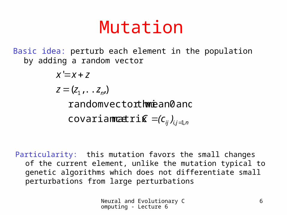
MutationBasic idea: perturb each element in the population by adding a random
vector
,ni,jij
n
)(cC
zzz
zxx
1
1
matrix covariance
and 0mean th vector wirandom
) ..., ,(
'
Particularity: this mutation favors the small changes of the current element, unlike the mutation typical to genetic algorithms which does not differentiate small perturbations from large perturbations
Neural and Evolutionary Computing - Lecture 6
7
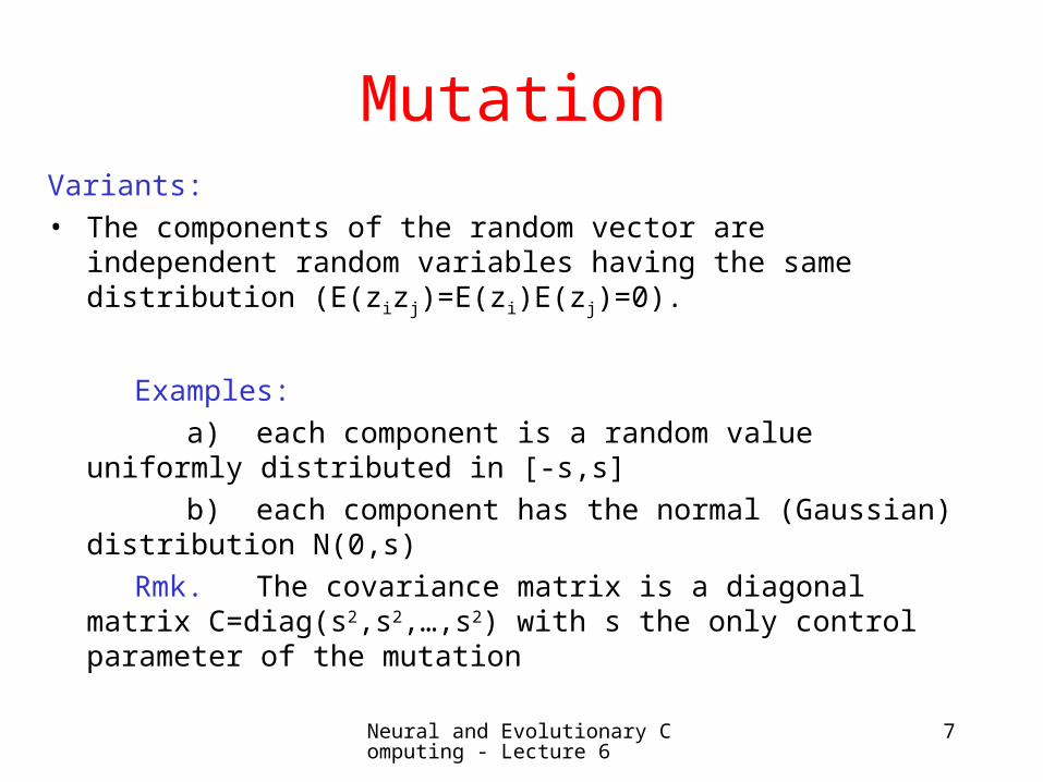
MutationVariants:• The components of the random vector are independent random
variables having the same distribution (E(zizj)=E(zi)E(zj)=0).
Examples:
a) each component is a random value uniformly distributed in [-s,s]
b) each component has the normal (Gaussian) distribution N(0,s)
Rmk. The covariance matrix is a diagonal matrix C=diag(s2,s2,…,s2) with s the only control parameter of the mutation
Neural and Evolutionary Computing - Lecture 6
8
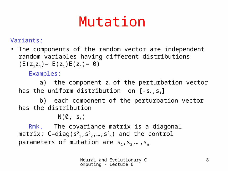
MutationVariants:• The components of the random vector are independent random
variables having different distributions (E(zizj)= E(zi)E(zj)= 0)
Examples:
a) the component zi of the perturbation vector has the uniform distribution on [-si,si]
b) each component of the perturbation vector has the distribution
N(0, si)
Rmk. The covariance matrix is a diagonal matrix: C=diag(s21,s2
2,…,s2
n) and the control parameters of mutation are s1,s2,…,sn
Neural and Evolutionary Computing - Lecture 6
9
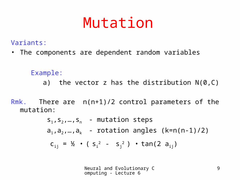
MutationVariants:• The components are dependent random variables
Example:
a) the vector z has the distribution N(0,C)
Rmk. There are n(n+1)/2 control parameters of the mutation:
s1,s2,…,sn - mutation steps
a1,a2,…,ak - rotation angles (k=n(n-1)/2)
cij = ½ • ( si2 - sj
2 ) • tan(2 aij)

Neural and Evolutionary Computing - Lecture 6
10
Mutation
Variants
[Hansen, PPSN 2006]
Neural and Evolutionary Computing - Lecture 6
11
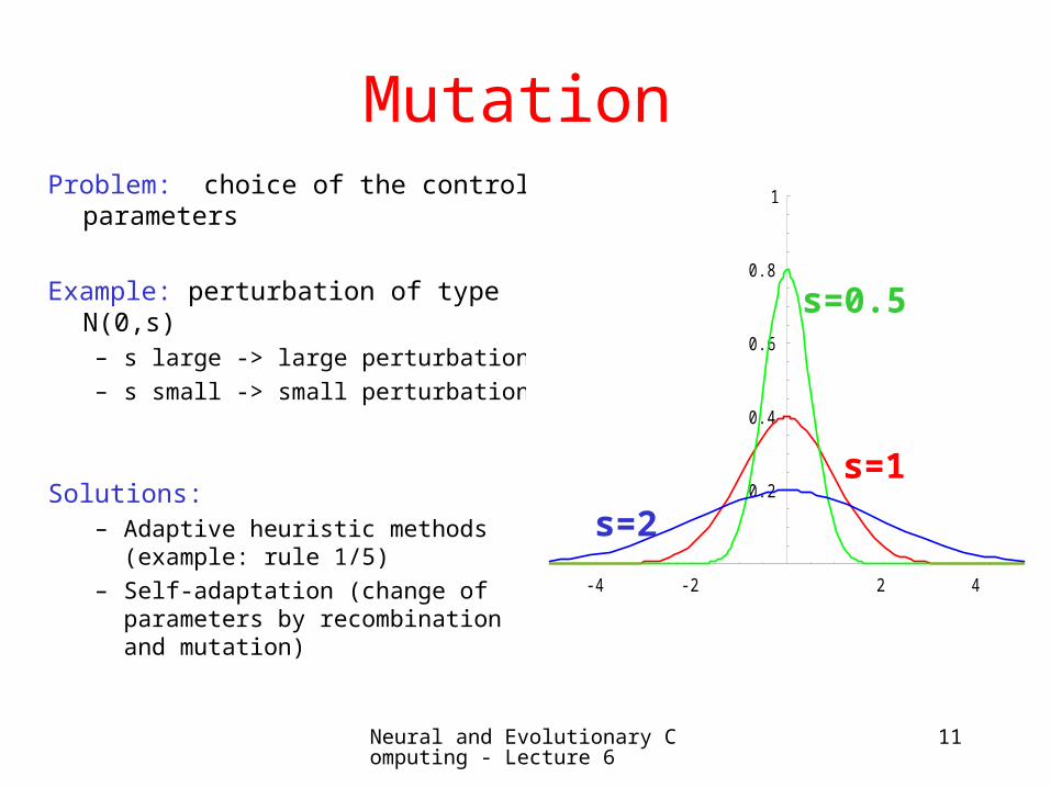
MutationProblem: choice of the control
parameters
Example: perturbation of type N(0,s)– s large -> large perturbation
– s small -> small perturbation
Solutions:– Adaptive heuristic methods
(example: rule 1/5)
– Self-adaptation (change of parameters by recombination and mutation)
-4 -2 2 4
0.2
0.4
0.6
0.8
1
s=0.5
s=1
s=2

Neural and Evolutionary Computing - Lecture 6
12
Mutation1/5 rule.
This is an heuristic rules developed for ES having independent perturbations characterized by a single parameter, s.
Idea: s is adjusted by using the success ration of the mutation
The success ratio:
ps= number of mutations leading to better configurations /
total number of mutations
Rmk. 1. The success ratio is estimated by using the results of at least n mutations (n is the problem size)
2. This rule has been initially proposed for populations containing just one element
Neural and Evolutionary Computing - Lecture 6
13
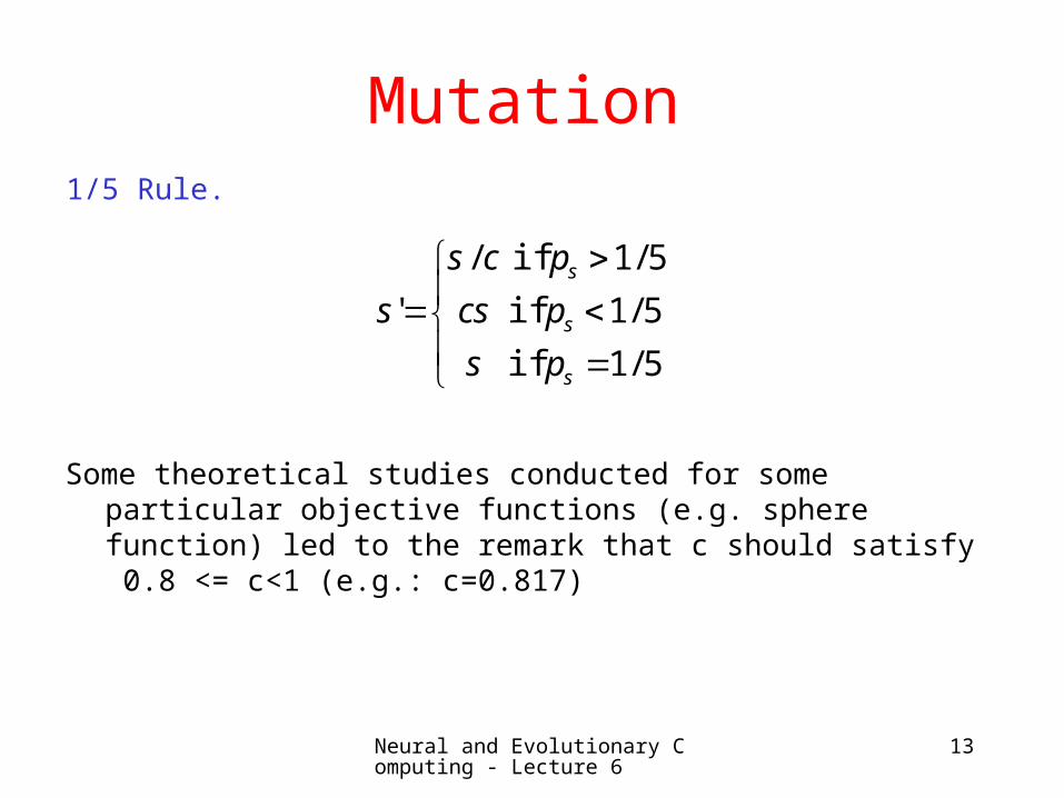
Mutation 1/5 Rule.
5/1 if
5/1 if
5/1 if /
'
s
s
s
p
p
p
s
cs
cs
s
Some theoretical studies conducted for some particular objective functions (e.g. sphere function) led to the remark that c should satisfy 0.8 <= c<1 (e.g.: c=0.817)

Neural and Evolutionary Computing - Lecture 6
14
MutationSelf-adaptation
Idea: • Extend the elements of the population with components corresponding to
the control parameters• Apply specific recombination and mutation operators also to control
parameters• Thus the values of control parameters leading to copmpetitive individuals
will have higher chance to survive
),....,,,...,,,...,(
),...,,,...,(
),,...,(
2/)1(111
11
1
nnnn
nn
n
aassxxx
ssxxx
sxxxExtended population elements
Neural and Evolutionary Computing - Lecture 6
15
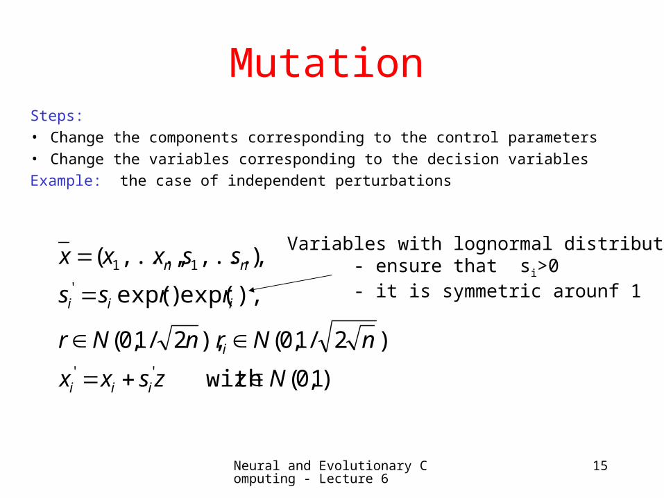
MutationSteps: • Change the components corresponding to the control parameters• Change the variables corresponding to the decision variables
Example: the case of independent perturbations
)1,0( with
)2/1,0(),2/1,0(
),exp()exp(
),...,,,...,(
''
'
11
Nzzsxx
nNrnNr
rrss
ssxxx
iii
i
iii
nn
Variables with lognormal distribution - ensure that si>0 - it is symmetric arounf 1
Neural and Evolutionary Computing - Lecture 6
16
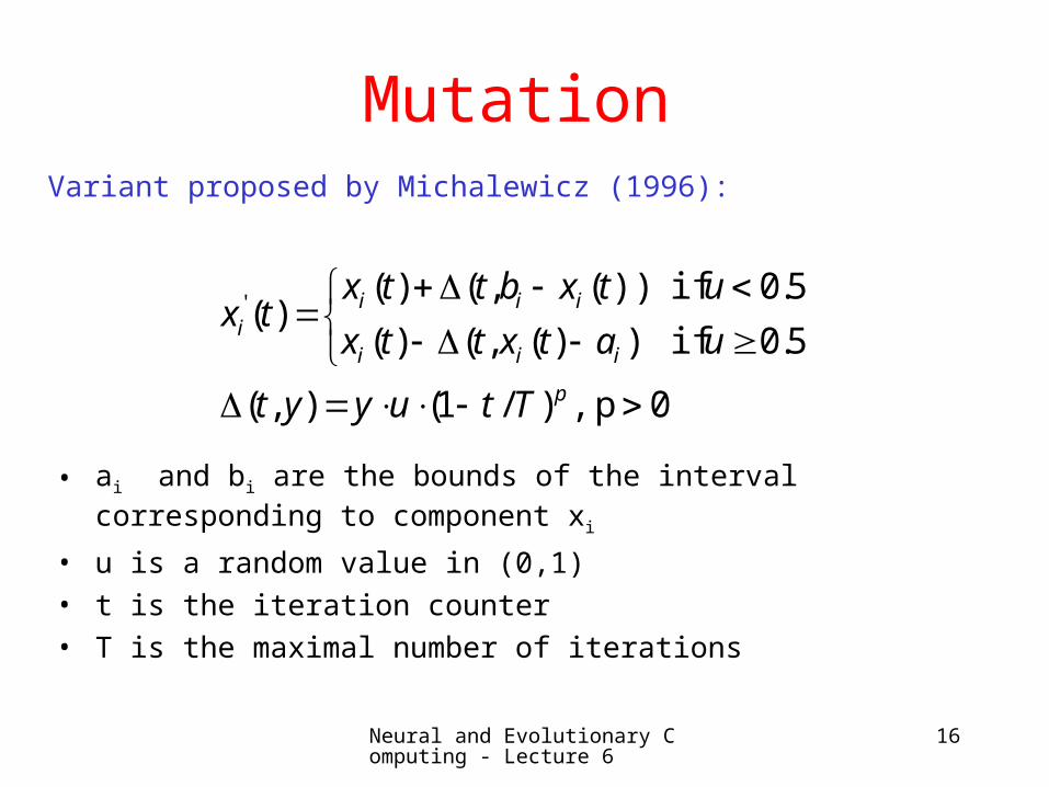
MutationVariant proposed by Michalewicz (1996):
0p ,)/1(),(
5.0 if))(,()(
5.0 if))(,()()('
p
iii
iiii
Ttuyyt
uatxttx
utxbttxtx
• ai and bi are the bounds of the interval corresponding to component xi
• u is a random value in (0,1)• t is the iteration counter• T is the maximal number of iterations

Neural and Evolutionary Computing - Lecture 6
17
MutationCMA – ES (Covariance Matrix Adaptation –ES) [Hansen, 1996]
Neural and Evolutionary Computing - Lecture 6
18
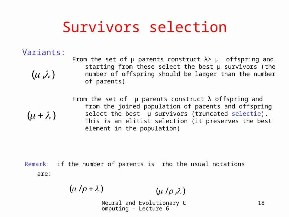
Survivors selection
Variants:
),(
)(
From the set of μ parents construct λ> μ offspring and starting from these select the best μ survivors (the number of offspring should be larger than the number of parents)
From the set of μ parents construct λ offspring and from the joined population of parents and offspring select the best μ survivors (truncated selectie). This is an elitist selection (it preserves the best element in the population)
Remark: if the number of parents is rho the usual notations are:
)/( ),/(
Neural and Evolutionary Computing - Lecture 6
19
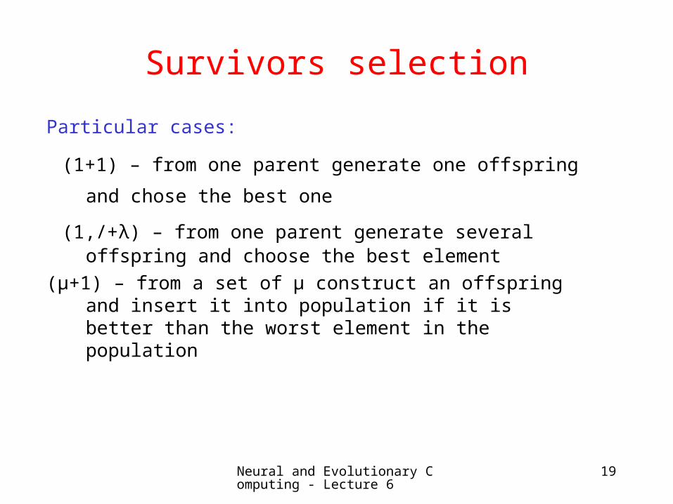
Survivors selection
Particular cases:
(1+1) – from one parent generate one offspring and chose the
best one (1,/+λ) – from one parent generate several offspring and
choose the best element
(μ+1) – from a set of μ construct an offspring and insert it into population if it is better than the worst element in the population
Neural and Evolutionary Computing - Lecture 6
20
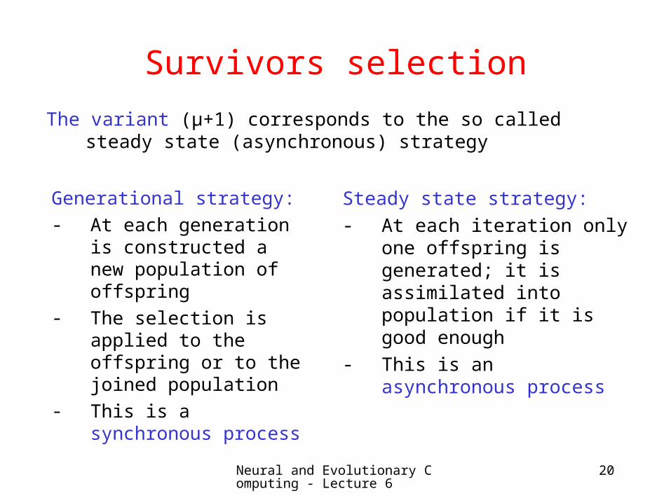
Survivors selection
The variant (μ+1) corresponds to the so called steady state (asynchronous) strategy
Generational strategy:- At each generation is
constructed a new population of offspring
- The selection is applied to the offspring or to the joined population
- This is a synchronous process
Steady state strategy:- At each iteration only one
offspring is generated; it is assimilated into population if it is good enough
- This is an asynchronous process
Neural and Evolutionary Computing - Lecture 6
21
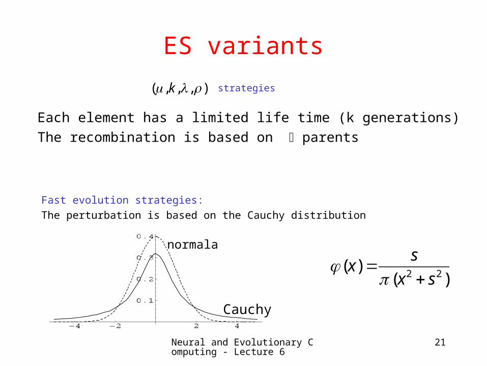
ES variants
strategies ),,,( k
)()(
22 sx
sx
Each element has a limited life time (k generations)
The recombination is based on parents
Fast evolution strategies:
The perturbation is based on the Cauchy distribution
normala
Cauchy
Neural and Evolutionary Computing - Lecture 6
22
Analysis of the behavior of ES
Evaluation criteria:
Effectiveness:- Value of the objective function
after a given number of evaluations (nfe)
Success ratio:- The number of runs in which
the algorithm reaches the goal divided by the total number of runs.
Efficiency:- The number of evaluation
functions necessary such that the objective function reaches a given value (a desired accuracy)

Neural and Evolutionary Computing - Lecture 6
23
Summary
Encoding Real vectors
Recombination Discrete or intermediate
Mutation Random additive perturbation (uniform, Gaussian, Cauchy)
Parents selection Uniformly random
Survivors selection (,) or (+)
Particularity Self-adaptive mutation parameters