neural computation - university of edinburghhomepages.inf.ed.ac.uk/mvanross/ln_all.pdf · neural...
TRANSCRIPT

Neural Computation
Mark van Rossum1
Lecture Notes for the MSc/DTC module.Version 06/072
1AcknowledgementMy sincere thanks to David Sterratt for providing the old course, figures, and tutorials on which thiscourse is based. Typeset using LYX, of course.
2January 5, 2007

1
Introduction: Principles of Neural Computation
The brain is a complex computing machine which is evolving to give the “fittest” output to agiven input. Neural computation has as goal to describe the function of the nervous system inmathematical terms. By analysing or simulating the resulting equations, one can better understandits function, research how changes in parameters would effect the function, and try to mimic thenervous system in hardware or software implementations.
Neural Computation is a bit like physics or chemistry. However, approaches developed in thosefields not always work for neural computation, because:
1. Physical systems are best studied in reduced, simplified circumstances, but the nervoussystem is hard to study in isolation. Neurons have a narrow range of operating conditions(temperature, oxygen, presence of other neurons, ion concentrations, ... ) under which theywork. Secondly, the neurons form a highly interconnected network. The function of thenervous systems depends on this connectivity.
2. Neural signals are hard to measure. Especially, if disturbance and damage to the nervoussystem is to be kept minimal. Connectivity is also very difficult to determine.
But there are factors which perhaps make study easier:
1. There is a high degree of conservation across species. This means that animals can be usedto gain information about the human brain.
2. The nervous system is able to develop by combining on one hand a limited amount of geneticinformation and, on the other hand, the input it receives. Therefore it might be possible tofind the organizing principles.
3. The nervous system is flexible and robust, which might be helpful in developing models.
Neural computation is still in its infancy which means many relevant questions have not beenanswered. My personal hope is that in the end simple principles will emerge. We will see a fewexamples of that during this course.
More reading
• Although no knowledge of neuroscience is required, there are numerous good neurosciencetext books which might be helpful:(Kandel, Schwartz, and Jessel, 2000; Shepherd, 1994;Johnston and Wu, 1995). Finally, (Bear, Connors, and Paradiso, 2000) has nice pictures.
• There is now also a decent number of books dealing with neural computation:
– (Dayan and Abbott, 2002) High level, yet readable text, not too much math. Widerange of up-to-date subjects.
– (Hertz, Krogh, and Palmer, 1991) Neural networks book; the biological relevance isspeculative. Fairly mathematical. Still superb in its treatment of abstract models ofplasticity.
– (Rieke et al., 1996) Concentrates on coding of sensory information in insects and whatis coded in a spike and its timing.
– (Koch, 1999) Good for the biophysics of single neurons.– (Arbib(editor), 1995) Interesting encyclopedia of computational approaches.– (Churchland and Sejnowski, 1994) Nice, non-technical book. Good on population codes
and neural nets.
• Journal articles cited can usually be found via www.pubmed.org
• If you find typos, errors or unclarity in these lecture notes, please tell me so they can becorrected.

Contents
1 Important concepts 51.1 Anatomical structures in the brain . . . . . . . . . . . . . . . . . . . . . . . . . . . 5
1.1.1 The neocortex . . . . . . . . . . . . . . . . . . . . . . . . . . . . . . . . . . 51.1.2 The cerebellum . . . . . . . . . . . . . . . . . . . . . . . . . . . . . . . . . . 61.1.3 The hippocampus . . . . . . . . . . . . . . . . . . . . . . . . . . . . . . . . 6
1.2 Cells . . . . . . . . . . . . . . . . . . . . . . . . . . . . . . . . . . . . . . . . . . . . 71.2.1 Cortical layers . . . . . . . . . . . . . . . . . . . . . . . . . . . . . . . . . . 8
1.3 Measuring activity . . . . . . . . . . . . . . . . . . . . . . . . . . . . . . . . . . . . 101.4 Preparations . . . . . . . . . . . . . . . . . . . . . . . . . . . . . . . . . . . . . . . 12
2 Passive properties of cells 132.1 Passive neuron models . . . . . . . . . . . . . . . . . . . . . . . . . . . . . . . . . . 132.2 Cable equation . . . . . . . . . . . . . . . . . . . . . . . . . . . . . . . . . . . . . . 15
3 Active properties and spike generation 183.1 The Hodgkin-Huxley model . . . . . . . . . . . . . . . . . . . . . . . . . . . . . . . 18
3.1.1 Many channels . . . . . . . . . . . . . . . . . . . . . . . . . . . . . . . . . . 203.1.2 A spike . . . . . . . . . . . . . . . . . . . . . . . . . . . . . . . . . . . . . . 233.1.3 Repetitive firing . . . . . . . . . . . . . . . . . . . . . . . . . . . . . . . . . 24
3.2 Other channels . . . . . . . . . . . . . . . . . . . . . . . . . . . . . . . . . . . . . . 243.2.1 KA . . . . . . . . . . . . . . . . . . . . . . . . . . . . . . . . . . . . . . . . . 253.2.2 The IH channel. . . . . . . . . . . . . . . . . . . . . . . . . . . . . . . . . . 253.2.3 Ca and KCa channels . . . . . . . . . . . . . . . . . . . . . . . . . . . . . . 253.2.4 Bursting . . . . . . . . . . . . . . . . . . . . . . . . . . . . . . . . . . . . . . 263.2.5 Leakage channels . . . . . . . . . . . . . . . . . . . . . . . . . . . . . . . . . 26
3.3 Spatial distribution of channels . . . . . . . . . . . . . . . . . . . . . . . . . . . . . 263.4 Myelination . . . . . . . . . . . . . . . . . . . . . . . . . . . . . . . . . . . . . . . . 263.5 Final remarks . . . . . . . . . . . . . . . . . . . . . . . . . . . . . . . . . . . . . . . 27
4 Synaptic Input 284.1 AMPA receptor . . . . . . . . . . . . . . . . . . . . . . . . . . . . . . . . . . . . . . 294.2 The NMDA receptor . . . . . . . . . . . . . . . . . . . . . . . . . . . . . . . . . . . 31
4.2.1 LTP and memory storage . . . . . . . . . . . . . . . . . . . . . . . . . . . . 324.3 GABAa . . . . . . . . . . . . . . . . . . . . . . . . . . . . . . . . . . . . . . . . . . 324.4 Second messenger synapses and GABAb . . . . . . . . . . . . . . . . . . . . . . . . 324.5 Release statistics . . . . . . . . . . . . . . . . . . . . . . . . . . . . . . . . . . . . . 334.6 Synaptic facilitation and depression . . . . . . . . . . . . . . . . . . . . . . . . . . . 354.7 Markov description of channels . . . . . . . . . . . . . . . . . . . . . . . . . . . . . 36
4.7.1 General properties of transition matrices . . . . . . . . . . . . . . . . . . . . 374.7.2 Measuring power spectra . . . . . . . . . . . . . . . . . . . . . . . . . . . . 37
4.8 Non-stationary noise analysis . . . . . . . . . . . . . . . . . . . . . . . . . . . . . . 38
2

CONTENTS 3
5 Integrate and fire models 405.1 Models of synaptic input . . . . . . . . . . . . . . . . . . . . . . . . . . . . . . . . . 415.2 Shunting inhibition . . . . . . . . . . . . . . . . . . . . . . . . . . . . . . . . . . . . 425.3 Simulating I&F neurons . . . . . . . . . . . . . . . . . . . . . . . . . . . . . . . . . 43
6 Firing statistics and noise 456.1 Variability . . . . . . . . . . . . . . . . . . . . . . . . . . . . . . . . . . . . . . . . . 456.2 Interval statistics . . . . . . . . . . . . . . . . . . . . . . . . . . . . . . . . . . . . . 456.3 Poisson model . . . . . . . . . . . . . . . . . . . . . . . . . . . . . . . . . . . . . . . 476.4 Noisy integrate and fire neuron . . . . . . . . . . . . . . . . . . . . . . . . . . . . . 476.5 Stimulus locking . . . . . . . . . . . . . . . . . . . . . . . . . . . . . . . . . . . . . 506.6 Count statistics . . . . . . . . . . . . . . . . . . . . . . . . . . . . . . . . . . . . . . 506.7 Neuronal activity In vivo . . . . . . . . . . . . . . . . . . . . . . . . . . . . . . . . 51
7 A visual processing task: Retina and V1 537.1 Retina . . . . . . . . . . . . . . . . . . . . . . . . . . . . . . . . . . . . . . . . . . . 54
7.1.1 Adaptation . . . . . . . . . . . . . . . . . . . . . . . . . . . . . . . . . . . . 557.1.2 Photon noise . . . . . . . . . . . . . . . . . . . . . . . . . . . . . . . . . . . 557.1.3 Spatial filtering . . . . . . . . . . . . . . . . . . . . . . . . . . . . . . . . . . 55
7.2 Primary visual cortex, V1 . . . . . . . . . . . . . . . . . . . . . . . . . . . . . . . . 587.2.1 Reverse correlation . . . . . . . . . . . . . . . . . . . . . . . . . . . . . . . . 597.2.2 The iceberg effect . . . . . . . . . . . . . . . . . . . . . . . . . . . . . . . . 60
8 Coding 628.1 Rate coding . . . . . . . . . . . . . . . . . . . . . . . . . . . . . . . . . . . . . . . . 628.2 Population code . . . . . . . . . . . . . . . . . . . . . . . . . . . . . . . . . . . . . . 638.3 Fisher information . . . . . . . . . . . . . . . . . . . . . . . . . . . . . . . . . . . . 648.4 Information theory . . . . . . . . . . . . . . . . . . . . . . . . . . . . . . . . . . . . 668.5 Correlated activity and synchronisation . . . . . . . . . . . . . . . . . . . . . . . . 68
9 Higher visual processing 709.1 The importance of bars and edges . . . . . . . . . . . . . . . . . . . . . . . . . . . 709.2 Possible roles of intra-cortical connections . . . . . . . . . . . . . . . . . . . . . . . 719.3 Higher visual areas . . . . . . . . . . . . . . . . . . . . . . . . . . . . . . . . . . . . 71
9.3.1 Sparse coding and representation . . . . . . . . . . . . . . . . . . . . . . . . 739.3.2 Connectivity and computation . . . . . . . . . . . . . . . . . . . . . . . . . 75
9.4 Plasticity . . . . . . . . . . . . . . . . . . . . . . . . . . . . . . . . . . . . . . . . . 75
10 General approach to networks 7710.1 Rate approximation . . . . . . . . . . . . . . . . . . . . . . . . . . . . . . . . . . . 7710.2 Single neuron with recurrence . . . . . . . . . . . . . . . . . . . . . . . . . . . . . . 78
10.2.1 Two recurrent rate neurons . . . . . . . . . . . . . . . . . . . . . . . . . . . 7910.3 Many neurons: Chaotic dynamics and Hopfield net . . . . . . . . . . . . . . . . . . 8010.4 Single recurrent layer . . . . . . . . . . . . . . . . . . . . . . . . . . . . . . . . . . . 81
11 Spiking neurons 8311.1 Many layers of spiking neurons: syn-fire or not . . . . . . . . . . . . . . . . . . . . 8311.2 Spiking recurrent networks . . . . . . . . . . . . . . . . . . . . . . . . . . . . . . . 8411.3 Spiking working memory . . . . . . . . . . . . . . . . . . . . . . . . . . . . . . . . . 8511.4 Spiking neurons: Attractor states . . . . . . . . . . . . . . . . . . . . . . . . . . . . 86
12 Making decisions 8812.1 Motor output . . . . . . . . . . . . . . . . . . . . . . . . . . . . . . . . . . . . . . . 89

CONTENTS 4
13 Hebbian Learning: Rate based 9313.1 Rate based plasticity . . . . . . . . . . . . . . . . . . . . . . . . . . . . . . . . . . . 9413.2 Covariance rule . . . . . . . . . . . . . . . . . . . . . . . . . . . . . . . . . . . . . . 9613.3 Normalisation . . . . . . . . . . . . . . . . . . . . . . . . . . . . . . . . . . . . . . . 9713.4 Oja’s rule . . . . . . . . . . . . . . . . . . . . . . . . . . . . . . . . . . . . . . . . . 9713.5 BCM rule . . . . . . . . . . . . . . . . . . . . . . . . . . . . . . . . . . . . . . . . . 9813.6 Multiple neurons in the output layer . . . . . . . . . . . . . . . . . . . . . . . . . . 9913.7 ICA . . . . . . . . . . . . . . . . . . . . . . . . . . . . . . . . . . . . . . . . . . . . 10013.8 Concluding remarks . . . . . . . . . . . . . . . . . . . . . . . . . . . . . . . . . . . 100
14 Spike Timing Dependent Plasticity 10214.1 Implications of spike timing dependent plasticity . . . . . . . . . . . . . . . . . . . 10414.2 Biology of LTP and LTD . . . . . . . . . . . . . . . . . . . . . . . . . . . . . . . . 10414.3 Temporal difference learning . . . . . . . . . . . . . . . . . . . . . . . . . . . . . . . 10614.4 Final remarks . . . . . . . . . . . . . . . . . . . . . . . . . . . . . . . . . . . . . . . 107
Bibliography 108

Chapter 1
Important concepts
1.1 Anatomical structures in the brain
We briefly look at some common structures in the brain.
1.1.1 The neocortex
The neocortex is the largest structure in the human brain. The neocortex is the main structureyou see when you remove the skull. Cortex means bark in Greek, and indeed, the cortex lieslike a bark over the rest of the brain, Fig 1.1. It is in essence a two-dimensional structure a fewmillimetres thick.
The human cortical area is about 2000cm2 (equivalent to 18x18 inch). To fit all this area intothe skull, the cortex is folded (convoluted) like a crumbled sheet of paper. In most other mammals(except dolphins) the convolution is less as there is less cortex to accommodate. Because it is solarge in humans, it is thought that it is important for the higher order processing unique tohumans.
Functionally, we can distinguish roughly in the cortex the following parts: 1) In the back thereis the occipital area, this area is important for visual processing. Removing this part will lead toblindness, or loss of a part of function (such as colour vision, or motion detection). A very largepart (some 40%) of the human brain is devoted to visual processing, and humans have comparedto other animals a very high visual resolution.
2) The medial part. The side part is involved in higher visual processing, auditory processing,and speech processing. Damage in these areas can lead to specific deficits in object recognition orlanguage. More on top there are areas involved with somato-sensory input, motor planning, andmotor output.
3) The frontal part is the “highest” area. The frontal area is important for short term orworking memory (lasting up to a few minutes). Planning and integration of thoughts takes placehere. Removal of the frontal parts (frontal lobotomy) makes peoples into zombies without longterm goals or liveliness. Damage to the pre-frontal has varied high-level effects, as illustrated inFig. 1.2.
In lower animals, the layout of the nervous system is more or less fixed. In insects the layout isalways the same: if you study a group of flies, you find the same neuron with the same dendritictree in exactly the same place. But in mammals the precise layout of functional regions in thecortex can vary strongly between individuals. Left or right-handedness and native language willalso be reflected in the location of functional areas. After a stroke other brain parts can take overthe affected part’s role. Especially in young children who have part of there brain removed, sparedparts of the cortex can take over many functions, see e.g.(Battro, 2000).
Lesions of small parts of the cortex can produce very specific deficits, such as a loss of colourvision, a loss of calculation ability, or a loss of reading a foreign language. fMRI studies confirmthis localisation of function in the cortex. This is important. It shows that computations are
5

CHAPTER 1. IMPORTANT CONCEPTS 6
Figure 1.1: Left: Dissected human brain, seen from below. Note the optic nerve, and the radiationto the cortex.Right: The cortex in different animals. Note the relatively constant thickness of the cortex acrossspecies. From (Abeles, 1991).
distributed over the brain (unlike a conventional computer, where most computations take placein the CPU). Similarly, long-term memory seems distributed over the brain.
1.1.2 The cerebellum
Another large structure in the brain is the cerebellum (literally the small brain). The cerebellumis also a highly convolved structure. The cerebellum is a beautiful two-dimensional structure. Thecerebellum contains about half of all the neurons in the brain. But its function is less clear. Thecerebellum is involved in precise timing functions. People without a cerebellum apparently functionnormally, until you ask them to dance or to tap a rhythm, in which they will fail dramatically.
A typical laboratory timing task is classical conditioning (see below). Here a tone sounds and 1second later an annoying air-puff is given into the eye. The animal will learn this association aftersome trials, and will then close its eye some time after the tone, right before the puff is coming.The cerebellum seems to be involved in such tasks and has been a favourite structure to model.
1.1.3 The hippocampus
The hippocampus (Latin for sea-horse) is a structure which lies deep in the brain. The hippocam-pus is sometimes the origin of severe epilepsy. Removal of the hippocampus, as the famous H.M.case, leads to (antero-grade) amnesia. That is, although events which occurred before removal arestill remembered, new memories are not stored. Therefore, it is assumed that the hippocampusworks as an association area which processes and associates information from different sources

CHAPTER 1. IMPORTANT CONCEPTS 7
Figure 1.2: Pre-frontal damage. Patients are asked to draw a figure; command in upper line,response below. From (Luria, 1966).
before storing it.In rats some hippocampal cells are so-called place cells. When the rat walks in a maze, such
a cell is active whenever the rat visits a particular location. The cells thus represent the locationof the rat. Interference with the hippocampus will lead to a deteriorated spatial memory in rats.
Also much studied in the hippocampus are its rhythms: the global activity in the hippocampusshows oscillations. The role of these oscillations in information processing is not known.
1.2 Cells
Like most other biological tissue, the brain consists of cells. One cell type in the brain are theso-called glial cells. These cells don’t do any computation, but provide support to the neurons.They suck up the spilt over neuro-transmitters, and others provide myelin sheets around the axonsof neurons.
More important for us are the neurons. There are some 1011 neurons in a human brain. Thebasic anatomy of the neurons is shown in Fig. 1.4: Every neuron has a cell body, or soma, containsthe nucleus of the cell. The nucleus is essential for the cell, as here the protein synthesis takesplace making it the central factory of the cell. The neuron receives its input through synapses onits dendrites (dendrite: Greek for branch). The dendritic trees can be very elaborate and oftenreceive more than 10,000 synapses.
Neurons mainly communicate using spikes, these are a brief (1ms), stereotypic excursions ofthe neuron’s membrane voltage. Spikes are thought to be mainly generated in the axon-hillock,a small bump at the start of the axon. From there the spike propagates along the axon. Theaxon can be long (up to one meter or so when it goes to a muscle). To increase the speed ofsignal propagation, long axons have a myelination sheet around them. The cortical regions areconnected to each other with axons. This is the white matter, because the layer of fat gives theneurons a white appearance, see Fig. 1.1. The axon ends in many axon terminals (about 10.000of course), where the connection to next neurons in the circuit are formed, Fig. 1.4. The action

CHAPTER 1. IMPORTANT CONCEPTS 8
Figure 1.3: Amnesia in a patient whose hippocampus was damaged due to a viral infection. From(Blakemore, 1988).
potential also propagates back into the dendrites. This provides the synapses with the signal thatan action potential was fired.
A basic distinction between neurons is between the excitatory and inhibitory ones, dependingon whether they release excitatory or inhibitory neurotransmitter. (The inhibitory neurons Ipersonally call “neuroffs”, but nobody else uses this term. Yet...). There are multiple sub-types ofboth excitatory and inhibitory neurons. How many is not well known. As genetic markers becomemore refined, more and more subtypes of the neurons are expected to appear. It is not clear ifand how these different subtypes have different computational roles.
Finally, in reading biology one should remember there are very few hard rules in biology: Thereare neurons which release both excitatory and inhibitory neurotransmitter, there are neuronswithout axons, not all neurons spike, etc...
1.2.1 Cortical layers
A sample of cortex beneath 1 mm2 of surface area will contain some 100.000 cells. After applyinga stain, a regular lay-out of the cells becomes visible. (When one looks at an unstained slice ofbrain under the microscope one does not see much). There is a variety of stains, see Fig. 1.5. Asis shown, the input and output layers arranged in a particular manner. This holds for corticalareas with functions a diverse as lower and higher vision, audition, planning, and motor actions.Why this particular layout of layers of cells is so common and what its computational function is,is not clear.
The connectivity within the cortex is large (about 100.000 km of fibres). Anatomically, thecortex is not arranged like a hierarchical, feed-forward network. Instead, a particular area receives

CHAPTER 1. IMPORTANT CONCEPTS 9
Figure 1.4: Sketch of the typical morphology of a pyramidal neuron. Right: Electron micrographof a neuron’s cell body. From (Shepherd, 1994).
not only feed-forward input from lower areas, but also many lateral and feedback connections. Thefeedback connections are usually excitatory and non-specific. The role of the feedback connectionsis not clear. They might be involved in attentional effects.

CHAPTER 1. IMPORTANT CONCEPTS 10
Figure 1.5: Left: Layers in the cortex made visible with three different stains. The Golgi stain(left) labels the soma and the thicker dendrites (only a small fraction of the total number of cells islabelled). The Nissl stain shows the cell bodies. The Weigert stain labels axons. Note the verticaldimension is one or two millimetres. From (Abeles, 1991). Right: approximate circuitry in thelayers. From (Shepherd, 1994)..
1.3 Measuring activity
Many ways have been developed to measure neural activity.
• EEG (electro encephalogram) and ERP (event related potential) measure the potential onskull. This has very poor spatial resolution, but temporal resolution is good. Non-invasive.Good for behavioural reaction times, e.g. (Thorpe, Fize, and Marlot, 1996).
• fMRI (functional magnetic resonance imaging) measures increased blood oxygenation level.The signal is related to neural activity in a not fully understood manner. It seems to correlatebetter to synaptic activity than to spike activity(Logothetis et al., 2001). Resolution: about1mm, 1 minute. Non-invasive. Good for global activity and localization studies in humans.
• Extracellular electrodes: When a tungsten electrode is held close enough to a firing cell,the cell’s spikes can be picked up. Alternatively, the slow components of the voltage canbe analysed, this is called the field potential and corresponds to the signal from ensemblesof synapses from the local neighbourhood of cells. Extracellular recordings can be donechronically in awake animals. A newer trend is to use many electrodes at once (either in anarray, or arranged in tetrodes). Limitations: no access to precise synaptic current, difficultto control stimulation, need to do spike sorting (an electrode receives usually signals from acouple of neurons, which is undesirable; the un-mixing is called spike sorting)

CHAPTER 1. IMPORTANT CONCEPTS 11
Figure 1.6: A setup to measure extracellular activity. After a band-pass filter the spikes can beclearly extracted from the small electrical signal. Electrodes can remain implanted for years.
Figure 1.7: Patch-clamp recording. The inside of the cell is connected to the pipette. This allowsthe measurement of single channel openings (bottom trace).
• Intracellular: Most intracellular recording are now done using the patch clamp technique.A glass pipette is connected to the intracellular medium, Fig. 1.7. From very small currents(single channel) to large currents (synaptic inputs and spikes) can be measured. Secondlythe voltage and current in the cell can be precisely controlled. Access to the intracellularmedium allows to wash in drugs that work from the inside of the cell. However, the accesscan also lead to washout (the dilution of the cell’s content). Limitations: hard in vivo (dueto small movements of animal even under anaesthesia), and limited recording time (up to 1hour).
• A relatively new method is to use optical imaging. The reflectance of the cortical tissuechanges slightly with activity, and this can be measured. Alternatively, dyes sensitive to Ca

CHAPTER 1. IMPORTANT CONCEPTS 12
or voltage changes can be added, and small activity changes can be measured.
1.4 Preparations
In order to study the nervous system under controlled conditions various preparations have beendeveloped. Most realistic would be to measure the nervous system in vivo without anaesthesia.However, this has both technical and ethical problems. Under anaesthesia the technical problemsare less, but reliable intracellular recording is still difficult. And, of course, the anaesthesia changesthe functioning of the nervous system.
A widely used method is to prepare slices of brains, about 1/2 mm thick. Slices allow foraccurate measurements of single cell or few cell properties. However, some connections will besevered, and it is not clear how well the in vivo situation is reproduced, as the environment(transmitters, energy supply, temperature, modulators) will be different.
Finally, it is possible to culture the cells from young brain. The neurons will by themselvesform little networks. These cultures can be kept alive for long times. Also here the relevance toin vivo situations is not always clear.
More reading: Quantitative anatomy (Braitenberg and Schuz, 1998), neuro-psychological case studies (Sacks, 1985; Luria, 1966)

Chapter 2
Passive properties of cells
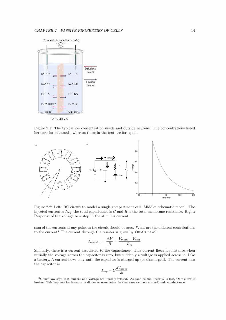
A living neuron maintains a voltage drop across its membrane. One commonly defines the voltageoutside the cell as zero. At rest the inside of the cell will then be at about -70mV (range -90..-50mV). This voltage difference exist because the ion concentrations inside and outside the cell aredifferent. The main ions are K+(potassium, or kalium in many languages), Cl−(chloride), Na+
(sodium), and Ca2+ (calcium).1
Consider for instance for Na, the concentration outside is 440mM and inside it is only 50mM(squid axon). If the cell membrane were permeable to Na, it would flow in. First, because of theconcentration gradient (higher concentration outside than inside), second, because of the attractionof the negative membrane to the positive Na ions. Because of these two forces, Na influx doesnot stop when the voltage across the membrane is zero. Only if the voltage across the membranewould be +55 mV, net Na inflow would stop. This +55mV is called the reversal potentialof Na. Likewise K has a reversal potential of -75mV (outside 20 mM and inside 400mM), and Clof -60mV (outside 500mM and inside 50mM). The reversal potential can be calculated from theNernst equation
Vrev =58mV
zlog10
[X]outside
[X]inside
which follows from the condition that diffusive and electrical force should cancel at equilibrium.The valency of the ion is represented by z.
However, at rest the Na channels are largely closed and only very little Na will flow into the cell.2 The K and Cl channels are somewhat open, together yielding a resting potential of about -70mV.By definition no net current flows at rest (else the potential would change). The concentrationgradient of ions is actively maintained with ion-pumps and exchangers. These proteins move ionsfrom one side of the membrane to the other at the expense of energy.
2.1 Passive neuron models
If one electrically stimulates a neuron sufficiently it will spike. But before we will study the spikingmechanism, we first look at the so-called passive properties of the cell. We model the cell by anetwork of passive components: resistors and capacitors. This approximation is reasonable whenthe cell is at rest and the membrane voltage is around the resting voltage. Most active elementsonly become important once the neuron is close to its firing threshold.
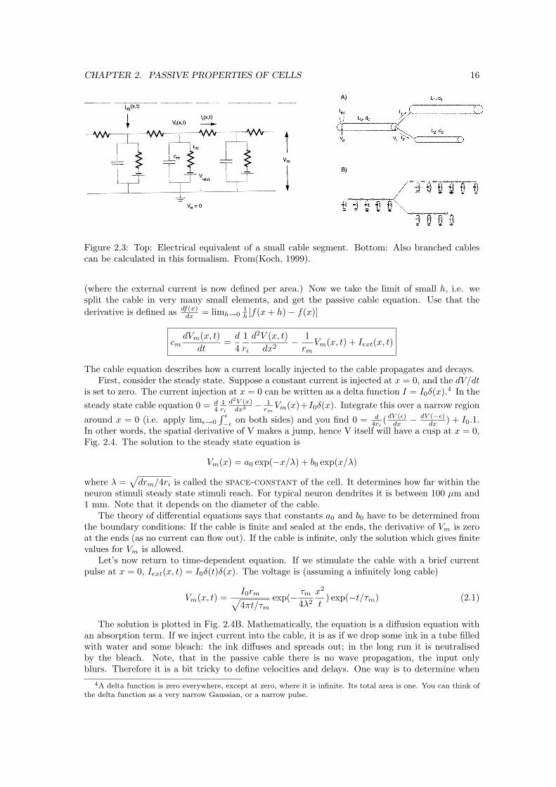
The simplest approximation is a passive single compartment model, shown in Fig. 2.2a. Thismodel allows the calculate the response of the cell to an input. Kirchhoff’s law tells us that the
1For those familiar with electronics: In electronics, charge is mostly carried by electrons. Here, all ions insolution carry charge, so we have at least 4 different charge carriers, all of them contributing to the total currentin the cell.
2When many ions contribute to the potential the Goldman-Hodgkin-Katz voltage equation should be used tocalculate the potential (Hille, 2001).
13
CHAPTER 2. PASSIVE PROPERTIES OF CELLS 14
Figure 2.1: The typical ion concentration inside and outside neurons. The concentrations listedhere are for mammals, whereas those in the text are for squid.
−50 0 50 100 150Time (ms)
0
0.2
0.4
0.6
0.8
1
Vol
tage
Figure 2.2: Left: RC circuit to model a single compartment cell. Middle: schematic model. Theinjected current is Iinj , the total capacitance is C and R is the total membrane resistance. Right:Response of the voltage to a step in the stimulus current.
sum of the currents at any point in the circuit should be zero. What are the different contributionsto the current? The current through the resistor is given by Ohm’s law3
Iresistor =∆V
R=
Vmem − Vrest
Rm
Similarly, there is a current associated to the capacitance. This current flows for instance wheninitially the voltage across the capacitor is zero, but suddenly a voltage is applied across it. Likea battery, A current flows only until the capacitor is charged up (or discharged). The current intothe capacitor is
Icap = CdVmem
dt3Ohm’s law says that current and voltage are linearly related. As soon as the linearity is lost, Ohm’s law is
broken. This happens for instance in diodes or neon tubes, in that case we have a non-Ohmic conductance.

CHAPTER 2. PASSIVE PROPERTIES OF CELLS 15
It is important to note that no current flows when the voltage across the capacitor does not changeover time. (Altenatively, you describe the capacitor using a complex impedance).
Finally we assume an external current is injected. As stated the sum of the currents shouldbe zero. We have to fix the signs of the currents first: we define currents flowing away from thepoint to be negative. Now we have −Iresistor − Icap + Iext = 0. The circuit diagram thus leads tothe following differential equation for the membrane voltage.
CdVm(t)
dt= − 1
Rm[Vm(t)− Vrest] + Iinj(t)
In other words, the membrane voltage is given by a first order differential equation. It is alwaysa good idea to study the steady state solutions of differential equations first. This means that weassume Iext to be constant and dV/dt = 0. We find for the membrane voltage V∞ = Vrest+RmIext.If the current increases the membrane voltage (Iext > 0) it is called de-polarising; if it lowersthe membrane potential it is called hyper-polarising.
How rapidly is this steady state approached? If the voltage at t=0 is V0, one finds by substitu-tion that V (t) = V∞ + [V0 − V∞] exp(−t/τm). So, the voltage settles exponentially. The productτm = RmC is the time constant of the cell. For most cells it is between 20 and 50ms, but we willsee later how it can be smaller under spiking conditions. The time-constant determines how fastthe subthreshold membrane voltage reacts to fluctuations in the input current. The time-constantis independent of the area of the cell. The capacitance is proportional to the membrane area(1µF/cm2), namely, the bigger the membrane area the more charge it can store.
It is useful to define the specific resistance, or resistivity, rm as
rm = ARm
The units of rm are therefore Ω.cm2. The resistance is inversely proportional to membrane area(some 50kΩ.cm2), namely, the bigger the membrane area the more leaky it will be. The productof membrane resistance and capacitance is independent of area. It is also useful to introduce theconductance through the channel, the conductance is the inverse of the resistivity g = 1/R.The larger the conductance, the larger the current. Conductance is measured in Siemens (symbolS).
Note, this section dealt with just an approximation of the behaviour of the cell. Such anapproximation has to be tested against data. It turns out to be valid for small perturbations ofthe potential around the resting potential, but at high frequencies corrections to the simple RCbehaviours exist (Stevens, 1972).
2.2 Cable equation
The above model lumps together the cell into one big soma. But neurons have extended struc-tures (dendrites and axons) which are not perfectly coupled, therefore modelling the cell as asingle compartment has only limited validity. The first step towards a more realistic model is tomodel the neuron as a cable. A model for a cable is shown in Fig. 2.3. One can think of it asmany cylindrical compartments coupled to each other with resistors. The resistance between thecables is called axial resistance. The diameter of the cylinder is d, its length is called h. Nowthe resistance between the compartments is 4rih/(πd2), where ri is the intracellular resistivity(somewhere around 100Ω.cm). The outside area of the cylinder is πhd. As a result the membraneresistance of a single cylinder is rm/(πhd). The capacitance of the cylinder is cmπhd.
The voltage now becomes a function of the position in the cable as well. Consider the voltageat the position x, V (x, t) and its neighbouring compartments V (x + h, t) and V (x − h, t). Forconvenience we measure the voltage w.r.t. Vrest. Again we apply Kirchoff’s law and we get
cmdVm(x, t)
dt= − 1
rmVm(x, t) +
d
4h2
1ri
[V (x + h, t)− 2V (x, t) + V (x− h, t)] + Iext(x, t)
CHAPTER 2. PASSIVE PROPERTIES OF CELLS 16
Figure 2.3: Top: Electrical equivalent of a small cable segment. Bottom: Also branched cablescan be calculated in this formalism. From(Koch, 1999).
(where the external current is now defined per area.) Now we take the limit of small h, i.e. wesplit the cable in very many small elements, and get the passive cable equation. Use that thederivative is defined as df(x)
dx = limh→01h [f(x + h)− f(x)]
cmdVm(x, t)
dt=
d
41ri
d2V (x, t)dx2
− 1rm
Vm(x, t) + Iext(x, t)
The cable equation describes how a current locally injected to the cable propagates and decays.First, consider the steady state. Suppose a constant current is injected at x = 0, and the dV/dt
is set to zero. The current injection at x = 0 can be written as a delta function I = I0δ(x).4 In thesteady state cable equation 0 = d
41ri
d2V (x)dx2 − 1
rmVm(x)+I0δ(x). Integrate this over a narrow region
around x = 0 (i.e. apply limε→0
∫ ε
−εon both sides) and you find 0 = d
4ri(dV (ε)
dx − dV (−ε)dx ) + I0.1.
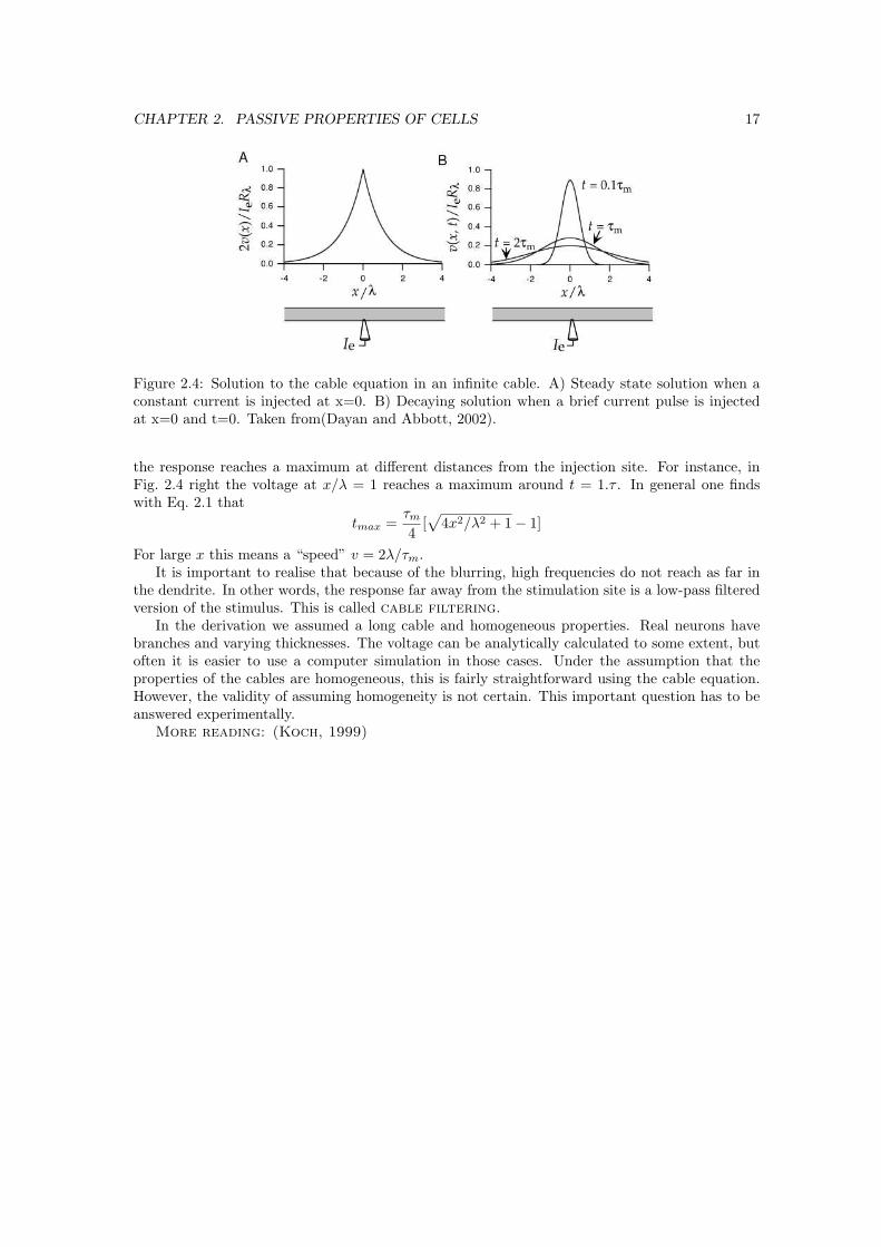
In other words, the spatial derivative of V makes a jump, hence V itself will have a cusp at x = 0,Fig. 2.4. The solution to the steady state equation is
Vm(x) = a0 exp(−x/λ) + b0 exp(x/λ)
where λ =√
drm/4ri is called the space-constant of the cell. It determines how far within theneuron stimuli steady state stimuli reach. For typical neuron dendrites it is between 100 µm and1 mm. Note that it depends on the diameter of the cable.
The theory of differential equations says that constants a0 and b0 have to be determined fromthe boundary conditions: If the cable is finite and sealed at the ends, the derivative of Vm is zeroat the ends (as no current can flow out). If the cable is infinite, only the solution which gives finitevalues for Vm is allowed.
Let’s now return to time-dependent equation. If we stimulate the cable with a brief currentpulse at x = 0, Iext(x, t) = I0δ(t)δ(x). The voltage is (assuming a infinitely long cable)
Vm(x, t) =I0rm√4πt/τm
exp(− τm
4λ2
x2
t) exp(−t/τm) (2.1)
The solution is plotted in Fig. 2.4B. Mathematically, the equation is a diffusion equation withan absorption term. If we inject current into the cable, it is as if we drop some ink in a tube filledwith water and some bleach: the ink diffuses and spreads out; in the long run it is neutralisedby the bleach. Note, that in the passive cable there is no wave propagation, the input onlyblurs. Therefore it is a bit tricky to define velocities and delays. One way is to determine when
4A delta function is zero everywhere, except at zero, where it is infinite. Its total area is one. You can think ofthe delta function as a very narrow Gaussian, or a narrow pulse.
CHAPTER 2. PASSIVE PROPERTIES OF CELLS 17
Figure 2.4: Solution to the cable equation in an infinite cable. A) Steady state solution when aconstant current is injected at x=0. B) Decaying solution when a brief current pulse is injectedat x=0 and t=0. Taken from(Dayan and Abbott, 2002).
the response reaches a maximum at different distances from the injection site. For instance, inFig. 2.4 right the voltage at x/λ = 1 reaches a maximum around t = 1.τ . In general one findswith Eq. 2.1 that
tmax =τm
4[√
4x2/λ2 + 1− 1]
For large x this means a “speed” v = 2λ/τm.It is important to realise that because of the blurring, high frequencies do not reach as far in
the dendrite. In other words, the response far away from the stimulation site is a low-pass filteredversion of the stimulus. This is called cable filtering.
In the derivation we assumed a long cable and homogeneous properties. Real neurons havebranches and varying thicknesses. The voltage can be analytically calculated to some extent, butoften it is easier to use a computer simulation in those cases. Under the assumption that theproperties of the cables are homogeneous, this is fairly straightforward using the cable equation.However, the validity of assuming homogeneity is not certain. This important question has to beanswered experimentally.
More reading: (Koch, 1999)

Chapter 3
Active properties and spikegeneration
We have modelled a neuron with passive elements. This is a reasonable approximation for sub-threshold effects and might be useful to describe the effect of far away dendritic inputs on thesoma. However, an obvious property is that most neurons produce action potentials (also calledspikes). Suppose we inject current into a neuron which is at rest (-70mV). The voltage will startto rise. When the membrane reaches a threshold voltage (about -50mV), it will rapidly depolariseto about +10mV and then rapidly hyper-polarise to about -70 mV. This whole process takes onlyabout 1ms. The spike travels down the axon. At the axon-terminals it will cause the release ofneurotransmitter which excites or inhibits the next neuron in the pathway.
From the analysis of the passive properties, it seems that in order to allow such fast eventsas spikes, the time-constant of the neuron should be reduced. One way would be the reduce themembrane capacitance, but this is biophysically impossible. The other way is to dramaticallyincrease the conductance through the membrane, this turns out to be the basis for the spikegeneration. The magnificent series of papers of Hodgkin and Huxley in 1952 explains how thisworks (Hodgkin and Huxley, 1952).
3.1 The Hodgkin-Huxley model
The membrane of neurons contains voltage-gated ion-channels, Fig. 3.1. These channels letthrough only one particular type of ion, typically Na or K, with a high selectivity. For instancethe channel for Na is called a Na-channel. Due to an exquisite mechanism that relies on conforma-tional changes, the open probability of the channel depends on the voltage across the membrane.When an action potential initiates, the following events happen: 1) close to the threshold voltage afew Na channels start to open. 2) Because the sodium concentration is higher outside the cell (its
Figure 3.1: Voltage gated channels populate the cell membrane. The pores let through certainions selectively, and open and close depending on the membrane voltage.
18

CHAPTER 3. ACTIVE PROPERTIES AND SPIKE GENERATION 19
reversal potential is +40mV), the sodium starts to flow in, depolarising the cell. 3) This positivefeedback loop will open even more Na channels and the spike is initiated. 4) However, rapidlyafter the spike starts, sodium channels close again and now K channels open. 5) The K ions startsto flow out the cell, hyper-polarising the cell, roughly bringing it back to the resting potential.
We now describe this in detail. Consider a single compartment, or a small membrane patch.As before, in order to calculate the membrane potential we collect all currents. In addition tothe leak current and capacitive current, we now have to include Na and K currents. Let’s firstconsider the sodium current. The current (per area) through the sodium channels is
INa(V, t) = gNa(V, t)[V (t)− V revNa ] (3.1)
The current is proportional to the difference between the membrane potential and the Na rever-sal potential. The current flow will try to make the membrane potential equal to the reversalpotential.12
The total conductance through the channels is given by the number of open channels
gNa(V, t) = g0Na ρNaPopen(V, t)
where g0na is the open conductance of a single Na channel (about 20 pS), and ρNa is the density
of Na channels per area. The Na channel’s open probability turns out to factorise as
Popen(V, t) = m3(V, t)h(V, t)
where m and h are called gating variables. Microscopically, the gates are like little binary switchesthat switch on and off depending on the membrane voltage. The Na channel has 3 switches labelledm and one labelled h. In order for the sodium channel to conduct all three m and the h have tobe switched on. The gating variables describe the probability that the gate is in the ’on’ or ’off’state. Note that the gating variables depend both on time and voltage; their values range between0 and 1. The gating variables evolve as
dm(V, t)dt
= αm(V )(1−m)− βm(V )m (3.2)
dh(V, t)dt
= αh(V )(1− h)− βh(V )h
Intermezzo Consider a simple reversible chemical reaction in which substance A is turned into sub-stance B.
[A]βα
[B]
the rate equation for reaction is: d[A]/dt = −β[A]+α[B]. Normalising without loss of generality suchthat [A] + [B] = 1, we have: d[A]/dt = α(1 − [A]) − β[A]. This is very similar to what we have forthe gating variables. The solution to this differential equation is exponential, like for the RC circuit. Ifat time 0, the concentration of A is [A]0, it will settle to
[A](t) = [A]∞ + ([A]0 − [A]∞) exp(−t/τ)
where the final concentration [A]∞ = α/(α + β), and the time-constant τ = 1/(α + β). (Check foryourself)
1The influx of Na will slightly change the reversal potential. Yet the amount of Na that flows in during a singleaction potential causes only a very small change in the concentrations inside and outside the cell. In the long run,ion pumps and ion exchangers maintain the correct concentrations.
2There a small corrections to Eq. 3.1 due to the physical properties of the channels, given by the Goldman-Hodgkin-Katz current equation (Hille, 2001).

CHAPTER 3. ACTIVE PROPERTIES AND SPIKE GENERATION 20
Figure 3.2: Left: The equilibrium values of the gating variables. Note that they depend on thevoltage. Also note that the inactivation variable h, switches off with increasing voltage, whereasmswitches on. Right: The time-constants by which the equilibrium is reached. Note that m is byfar the fastest variable. From(Dayan and Abbott, 2002).
The interesting part for the voltage gated channel is that the rate constants depend on thevoltage across the membrane. Therefore, as the voltage changes, the equilibrium shifts and thegating variables will try to establish a new equilibrium. The equilibrium value of the gatingvariable is
m∞(V ) =αm(V )
αm(V ) + βm(V )
and the time-constant isτm(V ) =
1αm(V ) + βm(V )
Empirically, the rate constants are (for the squid axon as determined by Hodgkin and Huxley)
αm(V ) =25− V
10[e0.1(25−V ) − 1](3.3)
βm(V ) = 4e−V/18
αh(V ) = 0.07e−V/20
βh(V ) =1
1 + e0.1(30−V )
In Fig. 3.2 the equilibrium values and time-constants are plotted.Importantly, the m opens with increasing voltage, but h closes with increasing voltage. The
m is called an activation variable and h is an inactivating gating variable. The inactivation causesthe termination of the Na current. Because the inactivation is much slower than the activation,spikes can grow before they are killed.
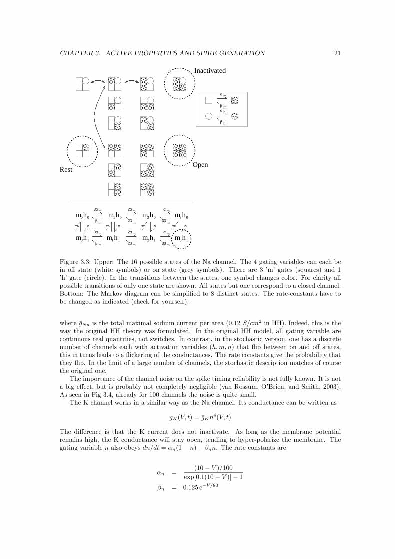
We can write down a Markov state diagram for a single Na channel. There are 4 gates in total(3 m’s, and 1 h), which each can be independently in the up or down state. So in total there are24 = 16 states, where one of the 16 states is the open state, Fig 3.3 top. However, in the diagramit makes no difference which of the m gates is activated, and so it can be reduced to contain 8distinct states, Fig. 3.3 bottom.
3.1.1 Many channels
The channels that carry the current open and close stochastically. The Markov diagrams are usefulwhen we think of microscopic channels and want to simulate stochastic fluctuations in the current.However, when there is a large number of channels in the membrane, it is possible to average allchannels. We simply obtain
gNa(V, t) = gNam3(V, t)h(V, t) (3.4)
CHAPTER 3. ACTIVE PROPERTIES AND SPIKE GENERATION 21
m hm h m h m h
α
β
m
m
β
h
h
α
αβ
hh
m hm hm hm h
αβ
hh
αβ
hh
αβ
hhβ
m
m
3α
β
m
m
3α
m
m
2α
2β
α m
m3β
m
m
2α
2β
α m
m3β
0 0
0
0 0 0
1 1 1 11
1 2
2 3
3
Open
Inactivated
Rest
Figure 3.3: Upper: The 16 possible states of the Na channel. The 4 gating variables can each bein off state (white symbols) or on state (grey symbols). There are 3 ’m’ gates (squares) and 1’h’ gate (circle). In the transitions between the states, one symbol changes color. For clarity allpossible transitions of only one state are shown. All states but one correspond to a closed channel.Bottom: The Markov diagram can be simplified to 8 distinct states. The rate-constants have tobe changed as indicated (check for yourself).
where gNa is the total maximal sodium current per area (0.12 S/cm2 in HH). Indeed, this is theway the original HH theory was formulated. In the original HH model, all gating variable arecontinuous real quantities, not switches. In contrast, in the stochastic version, one has a discretenumber of channels each with activation variables (h,m, n) that flip between on and off states,this in turns leads to a flickering of the conductances. The rate constants give the probability thatthey flip. In the limit of a large number of channels, the stochastic description matches of coursethe original one.
The importance of the channel noise on the spike timing reliability is not fully known. It is nota big effect, but is probably not completely negligible (van Rossum, O’Brien, and Smith, 2003).As seen in Fig 3.4, already for 100 channels the noise is quite small.
The K channel works in a similar way as the Na channel. Its conductance can be written as
gK(V, t) = gKn4(V, t)
The difference is that the K current does not inactivate. As long as the membrane potentialremains high, the K conductance will stay open, tending to hyper-polarize the membrane. Thegating variable n also obeys dn/dt = αn(1− n)− βnn. The rate constants are
αn =(10− V )/100
exp[0.1(10− V )]− 1
βn = 0.125 e−V/80

CHAPTER 3. ACTIVE PROPERTIES AND SPIKE GENERATION 22
Figure 3.4: Top: State diagram for the K channel. Bottom: the K current for a limited numberof channels. Left: 1 channel; right 100 channels. The smooth line is the continuous behaviour.Taken from (Dayan and Abbott, 2002).
Figure 3.5: Spike generation in a single compartment Hodgkin-Huxley model. The cell is stimu-lated starting from t = 5ms. Top: voltage trace during a spike. Next: Sum of Na and K currentthrough membrane (stimulus current not shown). Bottom 3: the gating variables. Note how mchanges very rapidly, followed much later by h and n. From (Dayan and Abbott, 2002).
As can be seen in Fig. 3.2, the K conductance is slow. This allows the Na to raise the membranepotential before the K kicks in and hyper-polarizes the membrane.
CHAPTER 3. ACTIVE PROPERTIES AND SPIKE GENERATION 23
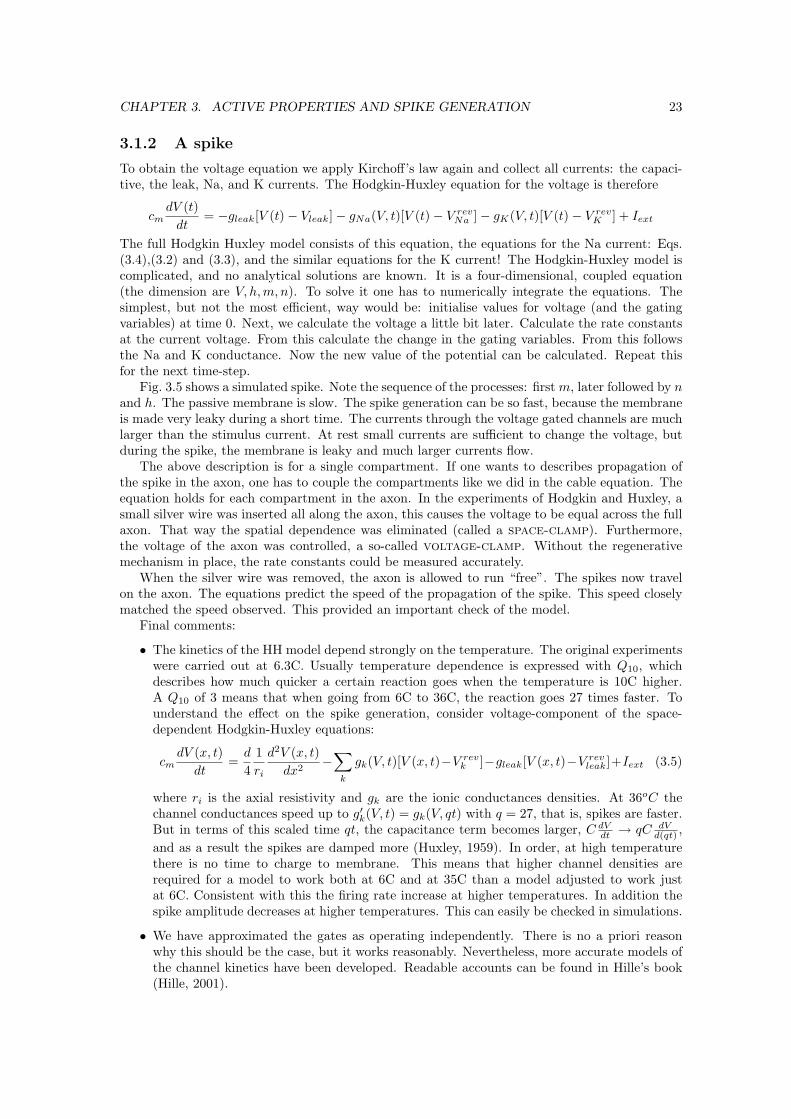
3.1.2 A spike
To obtain the voltage equation we apply Kirchoff’s law again and collect all currents: the capaci-tive, the leak, Na, and K currents. The Hodgkin-Huxley equation for the voltage is therefore
cmdV (t)
dt= −gleak[V (t)− Vleak]− gNa(V, t)[V (t)− V rev
Na ]− gK(V, t)[V (t)− V revK ] + Iext
The full Hodgkin Huxley model consists of this equation, the equations for the Na current: Eqs.(3.4),(3.2) and (3.3), and the similar equations for the K current! The Hodgkin-Huxley model iscomplicated, and no analytical solutions are known. It is a four-dimensional, coupled equation(the dimension are V, h,m, n). To solve it one has to numerically integrate the equations. Thesimplest, but not the most efficient, way would be: initialise values for voltage (and the gatingvariables) at time 0. Next, we calculate the voltage a little bit later. Calculate the rate constantsat the current voltage. From this calculate the change in the gating variables. From this followsthe Na and K conductance. Now the new value of the potential can be calculated. Repeat thisfor the next time-step.
Fig. 3.5 shows a simulated spike. Note the sequence of the processes: first m, later followed by nand h. The passive membrane is slow. The spike generation can be so fast, because the membraneis made very leaky during a short time. The currents through the voltage gated channels are muchlarger than the stimulus current. At rest small currents are sufficient to change the voltage, butduring the spike, the membrane is leaky and much larger currents flow.
The above description is for a single compartment. If one wants to describes propagation ofthe spike in the axon, one has to couple the compartments like we did in the cable equation. Theequation holds for each compartment in the axon. In the experiments of Hodgkin and Huxley, asmall silver wire was inserted all along the axon, this causes the voltage to be equal across the fullaxon. That way the spatial dependence was eliminated (called a space-clamp). Furthermore,the voltage of the axon was controlled, a so-called voltage-clamp. Without the regenerativemechanism in place, the rate constants could be measured accurately.
When the silver wire was removed, the axon is allowed to run “free”. The spikes now travelon the axon. The equations predict the speed of the propagation of the spike. This speed closelymatched the speed observed. This provided an important check of the model.
Final comments:
• The kinetics of the HH model depend strongly on the temperature. The original experimentswere carried out at 6.3C. Usually temperature dependence is expressed with Q10, whichdescribes how much quicker a certain reaction goes when the temperature is 10C higher.A Q10 of 3 means that when going from 6C to 36C, the reaction goes 27 times faster. Tounderstand the effect on the spike generation, consider voltage-component of the space-dependent Hodgkin-Huxley equations:
cmdV (x, t)
dt=
d
41ri
d2V (x, t)dx2
−∑
k
gk(V, t)[V (x, t)−V revk ]−gleak[V (x, t)−V rev
leak]+Iext (3.5)
where ri is the axial resistivity and gk are the ionic conductances densities. At 36oC thechannel conductances speed up to g′k(V, t) = gk(V, qt) with q = 27, that is, spikes are faster.But in terms of this scaled time qt, the capacitance term becomes larger, C dV
dt → qC dVd(qt) ,
and as a result the spikes are damped more (Huxley, 1959). In order, at high temperaturethere is no time to charge to membrane. This means that higher channel densities arerequired for a model to work both at 6C and at 35C than a model adjusted to work justat 6C. Consistent with this the firing rate increase at higher temperatures. In addition thespike amplitude decreases at higher temperatures. This can easily be checked in simulations.
• We have approximated the gates as operating independently. There is no a priori reasonwhy this should be the case, but it works reasonably. Nevertheless, more accurate models ofthe channel kinetics have been developed. Readable accounts can be found in Hille’s book(Hille, 2001).

CHAPTER 3. ACTIVE PROPERTIES AND SPIKE GENERATION 24
0 10 20 30I (pA)
0
20
40
60
80
100
F (
hz)
K_noise/FI.datNA_K_noise/FI.datNa_noise/FI.datno_noise/FI.dat
Figure 3.6: FI curve for the Hodgkin Huxley model. Also shown the effect of channel noise on theFI curve. This a small (100µm2) patch, so channel noise is substantial.
Figure 3.7: The effect of KA currents on spike generation.
3.1.3 Repetitive firing
When the HH model is stimulated with the smallest currents no spikes are produced. For slightlybigger currents, a single spike is produced. When the HH model is stimulated for a longer time,multiple spikes can be produced in succession. Once the current is above threshold, the morecurrent, the more spikes. The firing frequency vs. input current (the FI-curve) shows a sharpthreshold. In more elaborate neuron models and in physiology one finds often a much more linearFI curve, usually without much threshold (i.e. firing frequencies can be arbitrary low). Noise isone way to smooth the curve, see Fig. 3.6, but additional channel types, and the cell’s geometrycan also help.
3.2 Other channels
Although the Na and K channels of the HH model are the prime channels for causing the spike,many other channel types are present. The cell can use these channels to modulate its input-output relation, regulate activity its activity level, and make the firing pattern history dependent(by adaptation).

CHAPTER 3. ACTIVE PROPERTIES AND SPIKE GENERATION 25
Figure 3.8: Spike frequency adaptation. Left: Normal situation, a step current is injected intothe soma, after some 100ms spiking stops. Right: Noradrenaline reduces the KCa current, thuslimiting the adaptation.
3.2.1 KA
The KA current (IA) is a K current that inactivates at higher voltages. This seems a bit counter-productive as one could expect that the higher the membrane voltage, the more important it is tocounteract it with a K current.
The effect of KA current on the firing is as follows: Suppose the neuron is at rest and astimulus current is switched on. At first the KA currents still are active, they keep the membranerelatively hyper-polarized. As the KA channels inactivate, the voltage increases and the spike isgenerated. The KA current can thus delay the spiking. Once repetitive spiking has started, thesame mechanism will lower the spike frequency to a given amount of current.
3.2.2 The IH channel.
The IH channel carries a mainly K current. But the channel also lets through Na and thereforeits reversal potential is at about -20mV. Interestingly, the channel only opens at hyper-polarized(negative) membrane voltages. Because it activates slowly (hundreds of ms), it can help to toinduce oscillations: If the neuron is hyper-polarized it will activate after some delay, depolarisingthe cell, causing spikes, next, Ih will deactivate and as other currents such as KCa (below) willhyper-polarize the cell, and spiking stops. Now the whole process can start over again.
3.2.3 Ca and KCa channels
Apart from K and Na ions, also Ca ions enter the cell through voltage-gated channels. A largeinflux occurs during a spike. There is a large variety of Ca channels. One important role for the Cachannel is to cause Ca influx at the pre-synaptic terminal, as we will see below. But also in the restof the cell, the Ca signal appears as an important activity sensor. As the Ca concentration at restis very low, the Ca concentration changes significantly during periods of activity (this contrastsNa, which does not change much during activity). In the long run, the Ca is pumped out of thecell again. The time-constant of the extrusion is some 50 ms. This makes the Ca concentration anactivity sensor.3One important conductance in the cell are the so-called Ca-activated K channels(or KCa channels). These channels all require internal Ca to open, but in addition some have avoltage dependence. The KCa currents cause spike frequency adaptation. As the internal Caconcentration builds up, the KCa current becomes stronger hyper-polarising the cell, the spikingbecomes slower or stops altogether, Fig. 3.8.
From a theoretical point of view adaptation is interesting: In first approximation it is a high-pass filtering effect. But it is not purely a linear high-pass filtering of the firing rates. If thatwere the case, cells responding with a low firing rate would adapt as much as fast firing cells.But because adaptation depends on the amount of Ca that flows in, fast firing cells adapt more
3The large fluctuations in Ca concentration require a special treatment. Buffers and the diffusion of Ca insidethe cell should be taken into account. More details in(Koch, 1999; de Schutter and Smolen, 1998).

CHAPTER 3. ACTIVE PROPERTIES AND SPIKE GENERATION 26
strongly (see (Liu and Wang, 2001) for a mathematical model). The precise consequences remainto be examined.
Most excitatory neurons have strong spike frequency adaptation (inhibitory ones much lessso). On many levels one can observe that the brain likes change: When an image is projectedsteadily on the retina, the percept disappears after a few minutes. (By continuously making eye-movements, known as saccades, this effect does not occur in daily life.) Also on the single celllevel changes usually have a larger effect on the output than steady state conditions.
3.2.4 Bursting
Some cells, for example in the thalamus, show bursting behaviour. In a burst, a few spike aregenerated in a short time. The burst often continues after the stimulation is stopped. Ca channelsare thought to be important for burst generation. The computational role of bursts is not clear.
3.2.5 Leakage channels
You might not be surprised that also the leak conductance is partly mediated through a channel.These are mainly Cl channels without much voltage dependence. Without any channels themembrane would have a very high resistivity.
3.3 Spatial distribution of channels
As the knowledge of neurons becomes more refined, more channels are being discovered. Thereappears to be a great variety of K channels in particular. Different voltage gated channels populatenot only different types of neurons but also different locations of the neuron. It used to be thoughtthat the dendrites where largely passive cables, but more recently one has observed active channelson the dendrites. Thick dendrites can be patched, and differential distributions of channels havebeen found (Hoffman et al., 1997). Active dendrites can reduce the attenuation of distal inputson the soma, and also can support back-propagating spikes which are important for plasticity.
The standard picture for activity in a cortical neuron is as follows: Synaptic input arrives inthe dendrites. Signals travel subthreshold (i.e. without causing a spike) to the soma. It is possiblethat the EPSPs activate or deactivate some currents; this can lead to a boosting of the EPSP.Once enough input has been collected, a spike is generated in the axon-hillock. It now appearsthat Na channels at the axon hillock have a lower threshold than Na channels on the rest of theneuron (Colbert and Pan, 2002). This elects the axon-hillock as the prime spike generation site.The spike travels down the axon, and also back into the dendrite. The back-propagation actionpotential (BAP) is probably not full-fledged and can have a substantial Ca component.
3.4 Myelination
Axons that have to transmit their spikes over large distances are covered with a sheet of myelin.This highly insulating layer, reduces both the leak and the capacitance by a factor of about 250,speeding up the propagation. The myelin covering is interrupted ever so often along the axon.At these nodes one finds a very high density of sodium and potassium channels that boost thespike. For unmyelinated axons the propagation speed is about 1m/s and proportional to
√d, while
for myelinated fibers the speed is about 50 m/s (and proportional to d. The actual speed is acomplicated reflection of the parameter, but can be found numerically. The proportionality to thediameter can be found using dimensional considerations.

CHAPTER 3. ACTIVE PROPERTIES AND SPIKE GENERATION 27
3.5 Final remarks
Another refinement the experiments are starting to show is that the channels do not have fixedproperties. Instead they are modulated, both by from the outside and the inside. The neuronthus has ways to change it excitability, probably not only globally (Desai, Rutherford, and Turri-giano, 1999), but also locally (Watanabe et al., 2002), thus giving inputs at particular locationspreference. This change of neural properties by changing the channels complements the change insynaptic strength (plasticity) discussed below and has been explored only very sparsely.
A major problem for modellers remains to put all these channel types in the neuron model.For the physiologist it is a lot of work to extract all the parameters the modeller would like toknow. The rate constants are particularly difficult to extract from the data. This is easy to seefor the Na channel: the only thing which is easy to measure is the kinetics of one open state.If we assume independent gates, the problem is still tractable, but if we drop the independenceassumption of the gating variables we have many more rate constants. Secondly, channels canbe modulated (changes in sensitivity for instance) by internal mechanisms and neuro-modulatorssuch as dopamine and acetylcholine. The modulation of voltage gated channels allows neurons tochange its excitability. The variety of voltage gated channels might also be tuned to make theneuron more sensitive to a particular temporal input. (It is interesting to think about learningrules for the channel composition.)
Second challenge for the modeller is that the distribution of the channels on the neurons isvery hard to determine experimentally. And finally, there is large heterogeneity between neurons.As a result it will be very hard to come up with a precise, gold-standard model of ’the neuron’.It is hoped that it will be possible to address these questions in the near future.
On the other hand when we drop our quest for the standard model, perhaps the modellingsituation is not that depressing: The spikes are usually quite robust (you can try parameter vari-ation in the tutorials) and the spikes are an all-or-none event. So that models are not sensitive toslightly incorrect parameter settings.
More Reading: For mathematical aspects of biophysics (Koch, 1999; Johnstonand Wu, 1995),everything about channels including an excellent review of the work of Hodgkinand Huxley, see (Hille, 2001).

Chapter 4
Synaptic Input
So far we have studied artificially stimulated neurons, which responded because we injected acurrent into them. But except for primary sensory neurons, input comes from other cells in thebrain. Synaptic contacts communicate the spikes in axon terminals of the pre-synaptic cell tothe dendrites of the post-synaptic cell. The most important are chemical synapses, in whichtransmission is mediated by a chemical, called a neuro-transmitter.
Another type of connection between neuron are the so called gap-junctions, also calledelectrical synapses. These synapses are pore-proteins, i.e. channels, and provide a directcoupling of small molecules and ions (and hence voltage!) between cells. Although gap junctionsare abundant in some brain areas, their function is less clear. One clear role for gap-junctionsexists in the retina where they determine the spatial spread of electric activity. At different lightlevels, dopamine regulates the gap junction conductivity and hence the spatial filtering of thesignal (see below for adaptation). Another role has been implied in the synchronization of spikesin hippocampal inter-neurons (ref). We will not consider gap-junctions any further and follow thecommon convention that by synapse we mean actually a chemical synapse.
Figure 4.1: Left: Schematic of a chemical synapse. Right top: Electron micrograph of a (chemical)synapse. Right bottom: Electron micrograph of an electrical synapse or gap-junction.
28

CHAPTER 4. SYNAPTIC INPUT 29
Because synapses are the main way neurons communicate and how the networks dynamicallychange, it is important to know their behavior.
4.1 AMPA receptor
We look in detail at the AMPA receptor, which is the main excitatory synapse type in the brain.On the pre-synaptic side of the synapse we find a pool of vesicles, Fig. 4.1. Suppose a spike isgenerated in the soma of the pre-synaptic cell and travels along the axon. When the spike arrivesat the axon terminal, the spike in the membrane voltage causes the opening of voltage gated Cachannels (discussed in last chapter). The Ca flows into the terminal and triggers the release of oneor a couple of vesicles. The vesicles are little balls filled with neurotransmitter. When released, thevesicle membrane fuses with the cell membrane the neurotransmitter goes into the extracellularspace. The transmitter diffuses into the synaptic cleft and binds to the synaptic receptors on thepost-synaptic side.1
Above we saw that the excitability of neurons is due to voltage-gated channels. Synaptic inputto cells is mediated through channels as well: synaptic channels. Synaptic channels are openedwhen they bind neurotransmitter. Like the voltage-gated channels, these channels let through ionsselectively. On the post-synaptic side excitatory synapses have channels that let through both Kand Na; the reversal potential is about 0mV. Inhibitory synapses contain mostly Cl channels, withreversal of -60mV. Unlike the voltage-gated channels important for spike generation, the openingand closing of these channels does not depend on membrane voltage but instead on the bindingof neurotransmitter to the channel.
The excitatory transmitter is the amino-acid glutamate, Glu (you can buy glutamate in Chinesesupermarkets under the name MSG, mono-sodium glutamate). The diffusion across the cleft isvery fast. Binding and opening of the AMPA channel are also fast so that the dynamics of theresponse are largely determined by the unbinding of transmitter from the receptor. In Fig. 4.2 weshow an approximate state diagram for the AMPA receptor (these state diagrams are difficult tomeasure, the shown version fits the data well but is probably not the final word). Few remarks arein order. The transition in the state diagram in the rightward direction depend on the presence oftransmitter (cf. the voltage-gated channels where the voltage changed the transition rates). Twoglutamate molecules are needed to open the channel. This is called cooperativity. If the glutamateconcentration is far from saturation, the probability of opening will therefore be quadratic in theglutamate concentration. Secondly, the AMPA receptor has desensitised states. These becomesmost apparent when a long lasting puff of glutamate is delivered to the synapse with a pipette.The initial current is large, but the current desensitises and reduces to a lower steady state value.The same might occur in vivo when the synapse is stimulated repeatedly.
The jump in transmitter concentration is very brief (about 1ms). The time course of thesynapse is mainly determined by the time-constant of Glu unbinding from the synapse. Model anddata are shown in Fig. 4.3. The whole process can reasonably modelled by a single exponentialwith a time constant of 3 to 5 ms, which we call here τAMPA. We thus have for the current,assuming a pulse of Glu at t = 0,
IAMPA = g(t) (V revAMPA − Vmem) ≈ g0e−t/τAMP A(V rev
AMPA − Vmem)
where V revAMPA is the AMPA reversal potential, which is about 0mV. The g0 is the synapse’s peak
conductance. The peak conductance is depends on a number of factors we discuss below.Like the voltage-gated channels, the channel openings and closings are stochastic events; they
occur randomly. Using patch-clamp recording these fluctuations can be measured, and the singlechannel conductance has been determined and is about 10-100 pS for most channel types (Hille,2001). The number of receptors is usually somewhere between 10 and a few hundred per synapsefor central synapses.
1The distinction pre- and post-synaptic is useful when talking about synapses. However, note this term doesnot distinguish cells; most neurons are post-synaptic at one synapse, and pre-synaptic at another synapse.
CHAPTER 4. SYNAPTIC INPUT 30
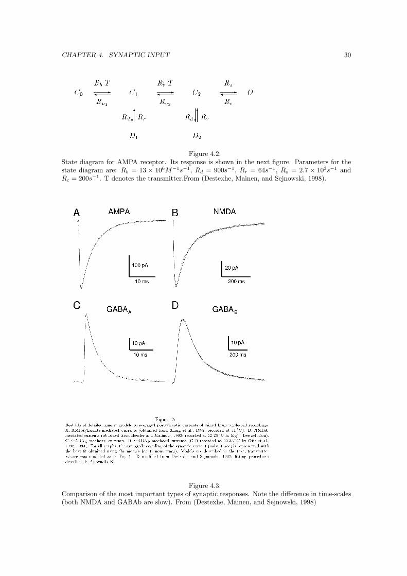
Figure 4.2:State diagram for AMPA receptor. Its response is shown in the next figure. Parameters for thestate diagram are: Rb = 13 × 106M−1s−1, Rd = 900s−1, Rr = 64s−1, Ro = 2.7 × 10³s−1 andRc = 200s−1. T denotes the transmitter.From (Destexhe, Mainen, and Sejnowski, 1998).
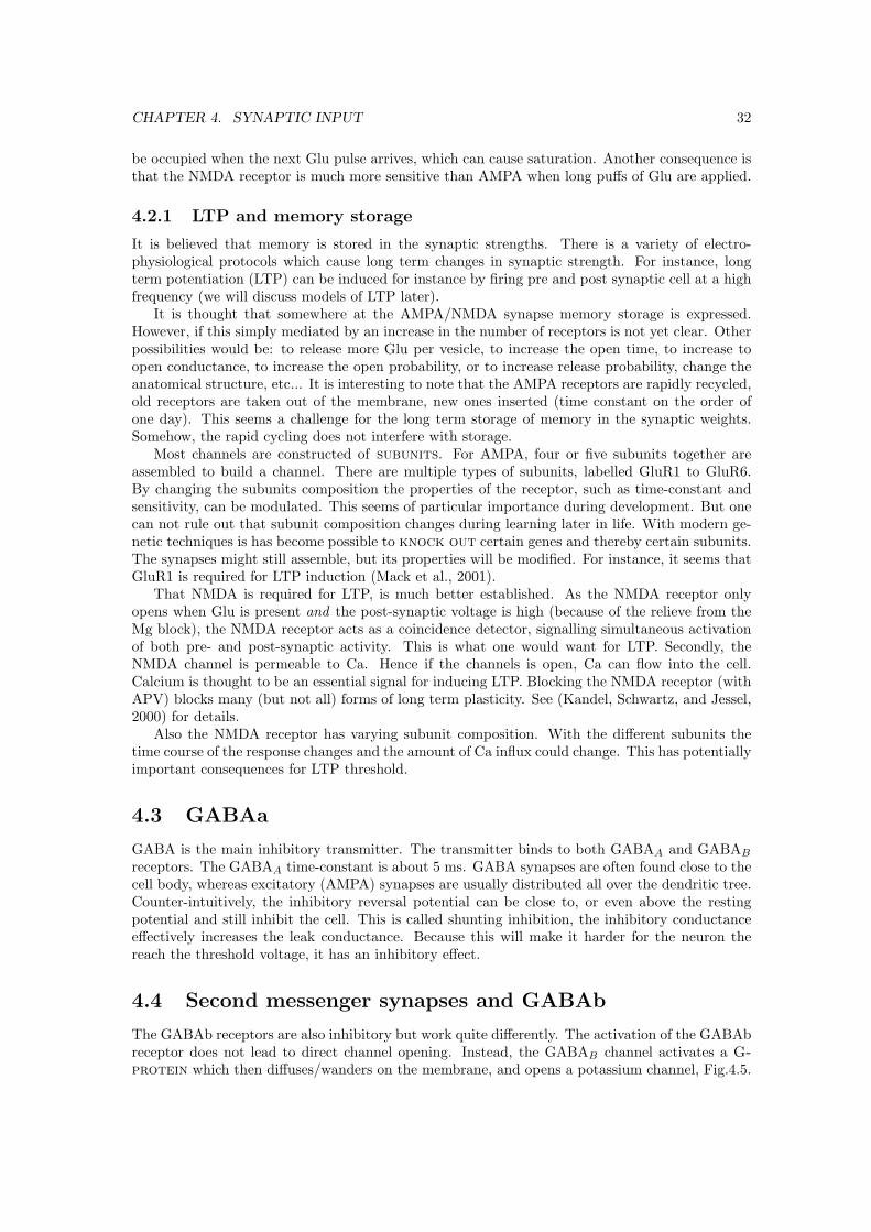
Figure 4.3:Comparison of the most important types of synaptic responses. Note the difference in time-scales(both NMDA and GABAb are slow). From (Destexhe, Mainen, and Sejnowski, 1998)

CHAPTER 4. SYNAPTIC INPUT 31
Figure 4.4: NMDA response is non-linear when Mg is present (which is normally the case).From(Koch, 1999).
4.2 The NMDA receptor
Like the AMPA receptor, the NMDA receptor opens in the presence of glutamate. Commonly, onefinds the AMPA and NMDA receptor at the same synapse. However, there are a few importantdifferences:
1) The current through the NMDA channel depends non-linearly on the voltage, Fig. 4.4. Thereason for this is Mg block. At voltages close to the resting potential an extracellular Mg ionblocks the pore of the NMDA channels. At higher membrane voltages, the attraction from themembrane potential on the Mg ion is less strong. The block is partly relieved and current canflow (the current shows short flickers). Alternatively, one can remove all Mg from the solution andthe block is absent, Fig. 4.4. An important consequence is that the post-synaptic current dependson the post-synaptic cell voltage. This makes NMDA a coincidence detector, only opening whenpre-synaptic activity is combined with post-synaptic activity. This will turn out to be importantfor plasticity, Chap. 14. The Mg-block can be fitted to
B(V ) =1
1 + exp(−0.062V )[Mg]/3.57
2) The time course of the NMDA current is much longer than AMPA, Fig. 4.3. The NMDAresponse comes on, after the AMPA response has largely decayed. It decays back with a time-constant of some 100ms. This long time-constant has helped modellers to build networks whichhave slow dynamics. The slower dynamics help to stabilise attractor states, see Chap. 10.
3) The difference in the dynamics is caused by a much slower unbinding of Glu from the receptor(the binding of Glu to the receptor is similar). As a result, and some NMDA receptors can still
CHAPTER 4. SYNAPTIC INPUT 32
be occupied when the next Glu pulse arrives, which can cause saturation. Another consequence isthat the NMDA receptor is much more sensitive than AMPA when long puffs of Glu are applied.
4.2.1 LTP and memory storage
It is believed that memory is stored in the synaptic strengths. There is a variety of electro-physiological protocols which cause long term changes in synaptic strength. For instance, longterm potentiation (LTP) can be induced for instance by firing pre and post synaptic cell at a highfrequency (we will discuss models of LTP later).
It is thought that somewhere at the AMPA/NMDA synapse memory storage is expressed.However, if this simply mediated by an increase in the number of receptors is not yet clear. Otherpossibilities would be: to release more Glu per vesicle, to increase the open time, to increase toopen conductance, to increase the open probability, or to increase release probability, change theanatomical structure, etc... It is interesting to note that the AMPA receptors are rapidly recycled,old receptors are taken out of the membrane, new ones inserted (time constant on the order ofone day). This seems a challenge for the long term storage of memory in the synaptic weights.Somehow, the rapid cycling does not interfere with storage.
Most channels are constructed of subunits. For AMPA, four or five subunits together areassembled to build a channel. There are multiple types of subunits, labelled GluR1 to GluR6.By changing the subunits composition the properties of the receptor, such as time-constant andsensitivity, can be modulated. This seems of particular importance during development. But onecan not rule out that subunit composition changes during learning later in life. With modern ge-netic techniques is has become possible to knock out certain genes and thereby certain subunits.The synapses might still assemble, but its properties will be modified. For instance, it seems thatGluR1 is required for LTP induction (Mack et al., 2001).
That NMDA is required for LTP, is much better established. As the NMDA receptor onlyopens when Glu is present and the post-synaptic voltage is high (because of the relieve from theMg block), the NMDA receptor acts as a coincidence detector, signalling simultaneous activationof both pre- and post-synaptic activity. This is what one would want for LTP. Secondly, theNMDA channel is permeable to Ca. Hence if the channels is open, Ca can flow into the cell.Calcium is thought to be an essential signal for inducing LTP. Blocking the NMDA receptor (withAPV) blocks many (but not all) forms of long term plasticity. See (Kandel, Schwartz, and Jessel,2000) for details.
Also the NMDA receptor has varying subunit composition. With the different subunits thetime course of the response changes and the amount of Ca influx could change. This has potentiallyimportant consequences for LTP threshold.
4.3 GABAa
GABA is the main inhibitory transmitter. The transmitter binds to both GABAA and GABAB
receptors. The GABAA time-constant is about 5 ms. GABA synapses are often found close to thecell body, whereas excitatory (AMPA) synapses are usually distributed all over the dendritic tree.Counter-intuitively, the inhibitory reversal potential can be close to, or even above the restingpotential and still inhibit the cell. This is called shunting inhibition, the inhibitory conductanceeffectively increases the leak conductance. Because this will make it harder for the neuron thereach the threshold voltage, it has an inhibitory effect.
4.4 Second messenger synapses and GABAb
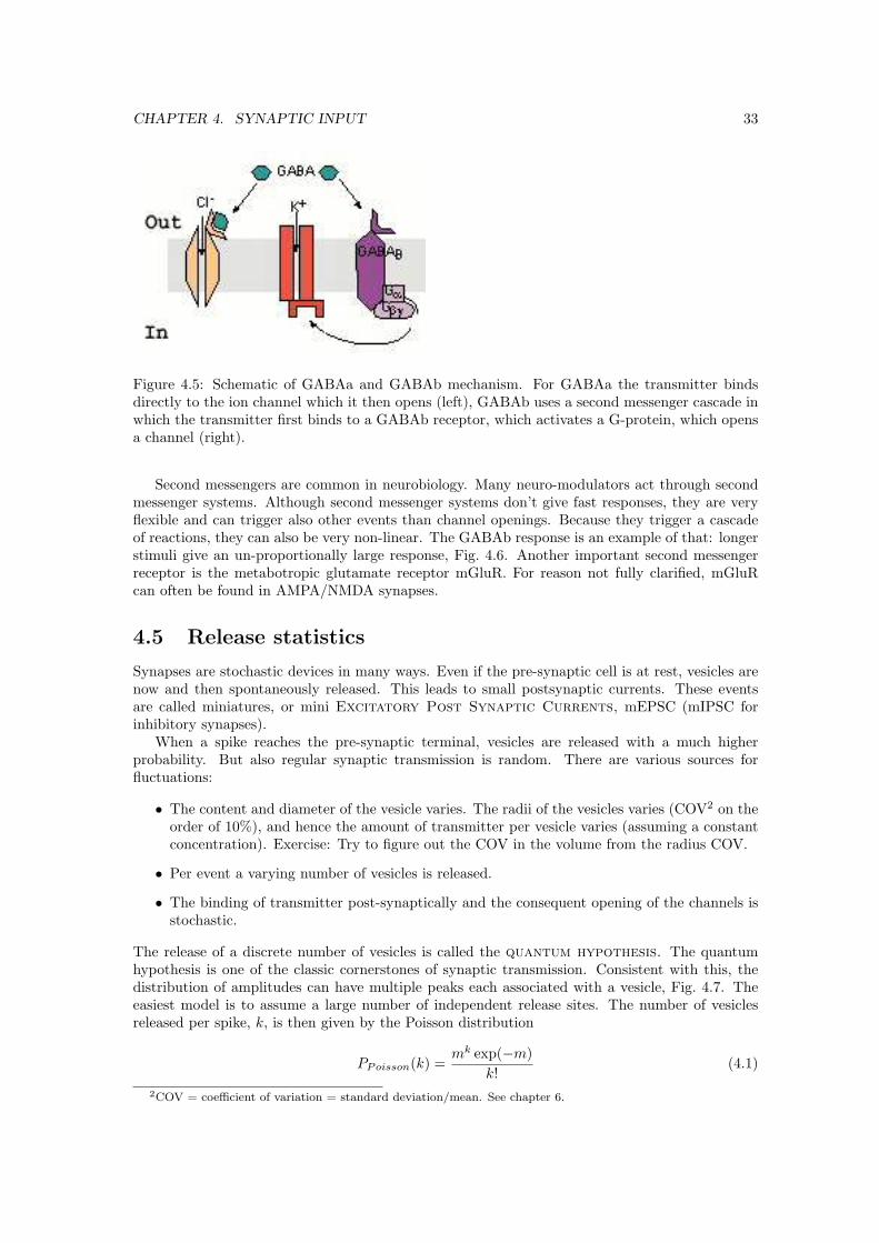
The GABAb receptors are also inhibitory but work quite differently. The activation of the GABAbreceptor does not lead to direct channel opening. Instead, the GABAB channel activates a G-protein which then diffuses/wanders on the membrane, and opens a potassium channel, Fig.4.5.
CHAPTER 4. SYNAPTIC INPUT 33
Figure 4.5: Schematic of GABAa and GABAb mechanism. For GABAa the transmitter bindsdirectly to the ion channel which it then opens (left), GABAb uses a second messenger cascade inwhich the transmitter first binds to a GABAb receptor, which activates a G-protein, which opensa channel (right).
Second messengers are common in neurobiology. Many neuro-modulators act through secondmessenger systems. Although second messenger systems don’t give fast responses, they are veryflexible and can trigger also other events than channel openings. Because they trigger a cascadeof reactions, they can also be very non-linear. The GABAb response is an example of that: longerstimuli give an un-proportionally large response, Fig. 4.6. Another important second messengerreceptor is the metabotropic glutamate receptor mGluR. For reason not fully clarified, mGluRcan often be found in AMPA/NMDA synapses.
4.5 Release statistics
Synapses are stochastic devices in many ways. Even if the pre-synaptic cell is at rest, vesicles arenow and then spontaneously released. This leads to small postsynaptic currents. These eventsare called miniatures, or mini Excitatory Post Synaptic Currents, mEPSC (mIPSC forinhibitory synapses).
When a spike reaches the pre-synaptic terminal, vesicles are released with a much higherprobability. But also regular synaptic transmission is random. There are various sources forfluctuations:
• The content and diameter of the vesicle varies. The radii of the vesicles varies (COV2 on theorder of 10%), and hence the amount of transmitter per vesicle varies (assuming a constantconcentration). Exercise: Try to figure out the COV in the volume from the radius COV.
• Per event a varying number of vesicles is released.
• The binding of transmitter post-synaptically and the consequent opening of the channels isstochastic.
The release of a discrete number of vesicles is called the quantum hypothesis. The quantumhypothesis is one of the classic cornerstones of synaptic transmission. Consistent with this, thedistribution of amplitudes can have multiple peaks each associated with a vesicle, Fig. 4.7. Theeasiest model is to assume a large number of independent release sites. The number of vesiclesreleased per spike, k, is then given by the Poisson distribution
PPoisson(k) =mk exp(−m)
k!(4.1)
2COV = coefficient of variation = standard deviation/mean. See chapter 6.
CHAPTER 4. SYNAPTIC INPUT 34
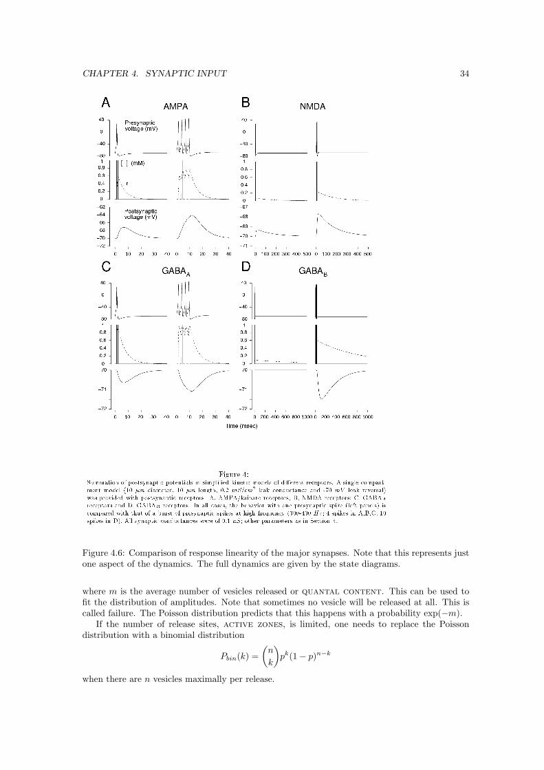
Figure 4.6: Comparison of response linearity of the major synapses. Note that this represents justone aspect of the dynamics. The full dynamics are given by the state diagrams.
where m is the average number of vesicles released or quantal content. This can be used tofit the distribution of amplitudes. Note that sometimes no vesicle will be released at all. This iscalled failure. The Poisson distribution predicts that this happens with a probability exp(−m).
If the number of release sites, active zones, is limited, one needs to replace the Poissondistribution with a binomial distribution
Pbin(k) =(
n
k
)pk(1− p)n−k
when there are n vesicles maximally per release.

CHAPTER 4. SYNAPTIC INPUT 35
Figure 4.7: Distribution of synaptic response amplitudes averaged over many trials. The differenthumps are thought to correspond to the release of different numbers of vesicles. This illustratesthe quantum hypothesis. From (Stricker, 2002).
Most of these models were developed in squid and neuromuscular junctions, where the distri-butions are clear. In central synapses (such as in hippocampus or cortex), results are less clear,for review see (Stricker, 2002). It has been suggested that a single vesicle could fully saturate thepost-synaptic receptors. This would render the above analysis invalid.
4.6 Synaptic facilitation and depression
As we saw, the transmission of synapses is not reliable. The probability for synaptic transmissionat central synapses is about 0.1-0.5. But this release probability is not constant and is subject tothe recent history of the synapse.
As the pre-synaptic cell is stimulated, Ca enter the terminal, causing the release of vesicles(or not). When now a second stimulus is given while the Ca concentration is still enhanced, therelease probability will larger. This effect is called paired-pulse facilitation.
However, if stimulation persists, the readily releasable pool of vesicles will exhaustcausing a decrease in the release probability, we say that the synapse is depressed. The depressionmakes the synapse sensitive to transient inputs. Mathematically, and maybe functionally as well,depression is a bit like spike-frequency adaptation.
A simple way to model synaptic depression or facilitation is with two terms. One term describesthat in the absence of activity the release probability settles to its default value
τdepressdprel(t)
dt= p∞rel − prel(t)
The second term describes that every time a vesicle is released the release probability is reducedwith a fixed amount

CHAPTER 4. SYNAPTIC INPUT 36
Figure 4.8: Schematic of the effect of synaptic depression. Two excitatory neurons P1 (only firingafter a delay) and P3 (continuously firing) provide input to P2. Because of depression, only thetransients of the input are transmitted. Synapses onto inhibitory neurons (I) are thought to bemore likely to facilitate. The response of I is therefore strongly supra-linear in the firing rate ofP3. From comment in Science on(Abbott et al., 1997).
if release prel = prel − α
This should be supplemented with the requirement that the release probability should of not beallowed to go below zero. For more models, see(Varela et al., 1997; Dayan and Abbott, 2002). Theresult is a strong non-linearity in the transfer function, dependent on the history of the synapse.Recently, the functional roles of depression are starting to be realised, e. g. (Carandini, Heeger,and Senn, 2002).
The unreliable transmission also opens the possibility that the release probability can be sys-tematically regulated. There was some evidence for that LTP not only changed synaptic strengthbut also the temporal pattern of release (Markram and Tsodyks, 1996), inspiring a lot of models,however, experimental evidence has failed to accumulate.
Final remark: two neurons might use more than one synaptic contact to contact each other.In the cortex a typical number seems to be between 1 and 10 synaptic contacts per connection.Of course, these synapses are proportionally more reliable and stronger.
4.7 Markov description of channels
Like the voltage gated channels, the synaptic channels can be written with state diagrams. Thesestate, or Markov diagrams, are a convenient method to analyze the channels. And we will see howthey can help to derive the kinetics and channel properties from physiological recordings. TheMarkov diagrams can also be used to accurately simulate the synapses.
The Markov diagrams are directly related to the power spectrum and the autocorrelation ofthe channel openings. To illustrate this consider a simple state diagram
CkTα
C ′k′Tα′
O
The first binding of transmitter T move the channel from closed state C to a second closed stateC ′; binding of another T opens the channel. We can write the state of the channel as a vector~s(t) = (C, C ′, O). The entries in the vector are the probability to find a certain channel in that

CHAPTER 4. SYNAPTIC INPUT 37
state, or, when measuring populations of channels the average number of channels in that state.The dynamics of the channel can then be written as
d~s
dt= W.~s
where W is a transition matrix between the different states. (This formalism is also called masterequation and is closely related to the Chapman Kolmogorov equation.) For our example it is
W =
−kT α 0kT −k′T − α α′
0 k′T −α′
The W matrix has always at least one zero eigenvalue and the corresponding eigenvector is thesteady state. In this case ~s∞ ∝ (αα′, α′kT, kk′T 2). The open probability in this steady state isfound by normalising such that the sum of the probabilities is 1 (i.e.
∑3i=1 si = 1). In this case it
is O∞ = kk′T 2/(αα′+α′kT +kk′T 2). For small concentration of transmitter, the open probabilityis proportional to the transmitter concentration squared. Then there is an intermediate regime,and for large concentration, O∞ = 1, i.e. the receptor is saturated.3
The other two eigenvalues of the transition matrix tell us to how quick the system settles tothe steady state. The general solution can be written as
~s(t) = ~s∞ + c1~s1eλ1t + c2~s2eλ2t
where λi is eigenvalue i and ~si is the corresponding eigenvector. The constants c1 and c2 aredetermined by the solution at time 0, such that ~s(0) = ~s∞ + c1~s1 + c2~s2.
The average of many channels will tend to the steady state, but a single channel will randomlyfluctuate, it will fluctuate around the equilibrium.
4.7.1 General properties of transition matrices
The matrix W has to obey certain properties to be a valid transition matrix. First, the totalprobability has to be conserved d
Ps
dt = 0, this implies that d~n.~sdt = ~n.W.~s = 0, for all ~s, which
means the sum of every column of W has to be zero.Secondly, W has to fulfil the detailed balance condition. It says that in equilibrium the prob-
ability to go around any loop in the diagram in the clockwise direction equals the probability incounter-clockwise direction. Without this condition there would be a constant rotation of occupa-tion numbers in equilibrium. (In diagrams without loops the detailed balance condition is alwaysupheld). In equations it means that for all i, j
wijsequilj = wjis
equili
You check easily check this is true for the Na-channel state diagram shown above by calculationclockwise and counter clockwise loop probabilities. Detailed balance is a requirement from statis-tical physics. Without it, we still have a proper Markov process, but one which can not describea physical process.
4.7.2 Measuring power spectra
Suppose we measure the random openings of a single synaptic channel while transmitter is con-stantly present. In general two quantities are important in characterising any sort of fluctuation:
3In physiology one often defines the effective dose, symbol Kd, EC50, or K0.5. WhenT = Kd the open probabilityis 50%. One encounter fits to the relation
O =1
1 + (Kd/T )n
where n is called the Hill-coefficient. It expresses the cooperativity of binding. Note that this relation will not givea perfect fit in our case.
CHAPTER 4. SYNAPTIC INPUT 38
1. The probability density function (PDF), also called probability distribution. In thiscase it is simple: the channel is either open or closed. The probability whether the channelis open is determined by the amount of transmitter present. With multiple channels theprobability distribution becomes a binomial distribution.
2. The other thing to know is how fast the fluctuations change over time, how often does thechannel switch per second. This is expressed in the autocorrelation function. As weshall see, it is closely related to the power spectrum.
The autocorrelation function of a signal S(t) is defined as
c(t′) = limT→∞
1T
∫ T
0
S(t)S(t + t′) dt
For most processes c(t′) decays for long t′, in other words, the process looses its memory. For thesimplest Markov scheme with two-states (C O), c(t′) decays exponentially. Namely, c(t′) =c e−|t|/τ , we call τ the correlation time. In the case of our three-state synaptic channel, thecorrelation is the sum of two exponentials with time-constants 1/λ1 and 1/λ2.
The Fourier transform of the signal is defined as s(f) =∫ T
0S(t)e−2πiftdt. The power-
spectrum gives how much power the fluctuations generate at each frequency. The power-spectrumw is given by
w(f) = limT→∞
2T|s(f)|2
The Wiener-Khinchin theorem says that the power-spectrum and the autocorrelation are relatedthrough a Fourier transform
w(f) = 4∫ ∞
0
c(t) cos 2πft dt
c(t) =∫ ∞
0
w(f) cos 2πft df
(Easy proof by filling in the definitions).Each exponential in the autocorrelation function will lead to a Lorentzian power spectrum,
which is defined as
w(f) =w(0)
1 + (2πf/λ)2+ c.δ(0)
with λ = 1/τ . The additional delta function term comes from the mean of the signal. It is usuallyremoved by subtracting the mean of the signal. In our three state channel, we have two non-zeroeigenvalues and the spectrum is a sum of two Lorentzians. By applying a constant transmitterconcentration one can measure a long stretch of fluctuating data, measure its power-spectrum,and fit the time constants. The number of Lorentzians in the spectrum gives the minimal numbernumber of states necessary to describe the kinetics. Also the single channel conductance can beextracted from the power spectrum. This is called stationary noise analysis. The largerthe single channel conductance, the large the fluctuations. The above technique requires thetransmitter concentration T to be constant. It can thus be applied in case a long lasting puff oftransmitter is applied.
This method can also be applied to voltage gated channels (under voltage clamp). However,with the patch-clamp technique is has becomes possible to measure the individual currents directlyand this often provides better data.
4.8 Non-stationary noise analysis
The stochastic nature of the channel openings can also be used to infer the unitary conductanceof the channels. Suppose we measure a collection of channels over many trials, the stimulation

CHAPTER 4. SYNAPTIC INPUT 39
Figure 4.9: Left: Non stationary noise analysis as applied the the sodium channels. A repeatedstep current leads to an average response. The size of the fluctuations around it are dependent onthe unitary conductance.Right: The resulting parabola when variance is plotted versus the mean. From (Hille, 2001)
protocol determines the open probability of the channel as a function of time. Let’s call the openprobability at any time p(t). The stimulus can be either a voltage step for voltage gated channels,or transmitter jump for synaptic channels. The average current, averaged over many trials is
〈I(t)〉 = i0Np(t)
where i0 is the unitary channel current and N the number of channels. The variance will be
〈δI(t)2〉 = i20Np(t)(1− p(t))= i0〈I(t)〉 − 〈I(t)〉2/N
The last equation shows that the channel’s unitary can be extracted from plotting the varianceversus the mean, Fig. 4.9. In addition the number of channels can be extracted.
Good models for synaptic kinetics can be found in (Destexhe, Mainen, and Se-jnowski, 1998), more on Markov diagrams in (Johnston and Wu, 1995).
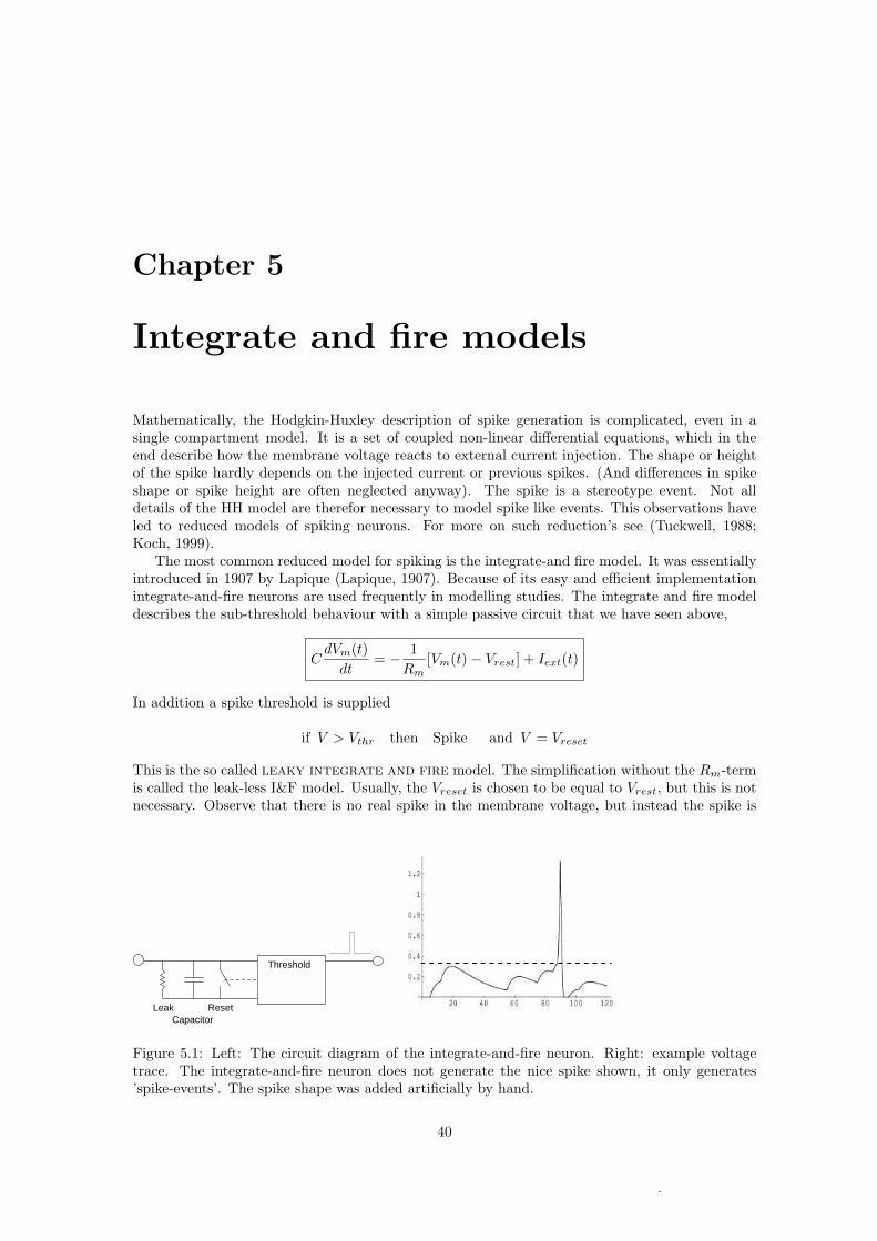
Chapter 5
Integrate and fire models
Mathematically, the Hodgkin-Huxley description of spike generation is complicated, even in asingle compartment model. It is a set of coupled non-linear differential equations, which in theend describe how the membrane voltage reacts to external current injection. The shape or heightof the spike hardly depends on the injected current or previous spikes. (And differences in spikeshape or spike height are often neglected anyway). The spike is a stereotype event. Not alldetails of the HH model are therefor necessary to model spike like events. This observations haveled to reduced models of spiking neurons. For more on such reduction’s see (Tuckwell, 1988;Koch, 1999).
The most common reduced model for spiking is the integrate-and fire model. It was essentiallyintroduced in 1907 by Lapique (Lapique, 1907). Because of its easy and efficient implementationintegrate-and-fire neurons are used frequently in modelling studies. The integrate and fire modeldescribes the sub-threshold behaviour with a simple passive circuit that we have seen above,
CdVm(t)
dt= − 1
Rm[Vm(t)− Vrest] + Iext(t)
In addition a spike threshold is supplied
if V > Vthr then Spike and V = Vreset
This is the so called leaky integrate and fire model. The simplification without the Rm-termis called the leak-less I&F model. Usually, the Vreset is chosen to be equal to Vrest, but this is notnecessary. Observe that there is no real spike in the membrane voltage, but instead the spike is
ResetLeakCapacitor
Threshold
Figure 5.1: Left: The circuit diagram of the integrate-and-fire neuron. Right: example voltagetrace. The integrate-and-fire neuron does not generate the nice spike shown, it only generates’spike-events’. The spike shape was added artificially by hand.
40

CHAPTER 5. INTEGRATE AND FIRE MODELS 41
an event.Although the integrate-and-fire model appears linear and simple, it actually is not. Thisis due to the threshold and subsequent reset.
The F/I curve of the I&F neuron is easily calculated: Suppose Vreset = Vrest, and the neuronis driven by a current Istim. Let’s assume the neuron has fired at t = 0. Its membrane potential isVrest. When will the next spike occur? When is the threshold voltage reached? The voltage willbehave as V (t) = Vrest + IstimRm [1− exp(−t/τm)]. Solving for t gives
f = 0 (if Istim < Vth/Rm)
f =−1
τm log(1− Vth/(IstimRm))
This curve looks quite like the Hodgkin-Huxley one (Fig. 3.6). There is a threshold, too small inputcurrent will not evoke any spikes. For currents above threshold, there is a curved F/I relation,like in Fig. 3.6.
For large stimuli, f ≈ Istim/(CmVthr), that is, the frequency is linear in the input current. Italso becomes independent of the leak resistance. This is because the leak current is in this casenegligible comparable to the stimulus current. There is no maximal rate as the spikes (whichare infinitely thin) can be right after each other. Real neurons show saturation at high stimulusfrequencies due to the refractory period. This can be easily introduced in the model by clampingthe membrane to the resting potential during the refractory period. Exercise: Calculate the F/Icurve in that case.
Spike frequency adaptation, Fig. 7.3, can be included in integrate and fire model without mucheffort. Hereto we introduce an extra variable in the model which represents the Ca concentration.Every time a spike occurs, the Ca concentration jumps up with fixed amount. In between spikesit decays with a time-constant of, say, 50ms. This represents the pump continuously active toremove the Ca. The Ca can be coupled to a simple KCa-like current, such as
IKca = gKCa[Ca](V revK − V )
where gKCa is the strength of the feedback, [Ca] is the calcium concentration.These extensions to the integrate-and-fire model are useful and easy to do in simulations, but
make analytical treatment often much harder. In case of the adaptation, the description of theneuron becomes two dimensional (both V and [Ca] are needed to specify the state of a neuron),instead of one dimensional (just V ).
5.1 Models of synaptic input
When dealing with integrate and fire models, it does not always make sense to have very elaboratesynapse models based on ligand binding and Markov diagrams. Instead, one usually takes synapticcurrents that are simple functions of time. The simplest choice to take the synaptic current a deltafunction, which will cause the membrane potential to make an instantaneous jump.
Isyn = I0δ(ti) ⇒ ∆V = RinI0
More realistic is an exponential current, to describe for instance an AMPA synapse.
Isyn = I0 exp(−t/τsyn) ⇒ ∆V = I0Rinτsyn
τm − τsyn[e−t/τm − e−t/τsyn ] (5.1)
The resulting voltage is a difference of exponentials, the rise time of the voltage is roughly givenby τsyn, the decay by τm (assuming τsyn ¿ τm). The voltage trace is shown in Fig. 5.2. Asone can see the time-constant of the cell determines the time for membrane to settle back to theequilibrium, but the rise can be much faster. In other words, the synaptic time-constant is moreimportant than the membrane time-constant for the firing dynamics. For example, in the extremecase of a non-leaky I&F neuron one has τm = ∞, but the neuron can definitely react faster thanthat.

CHAPTER 5. INTEGRATE AND FIRE MODELS 42
5 10 15 20 25 30
0.025
0.05
0.075
0.1
0.125
0.15
0.175
Figure 5.2: Effect of exponentially decaying synaptic current on the membrane potential. Mem-brane potential vs. time in ms. Parameters: τsyn = 2ms. Upper curve:τm = 50ms, lower curve:τm = 10ms.
0.5 1 1.5 2 2.5 3
-70
-60
-50
-40
-30
-20
-10
Figure 5.3: Effect on inhibition. Left: a passive model. The membrane voltage as a function ofexcitatory input in a non-spiking, passive model for three levels of inhibition, gi = 0.1, 1, and 3(upper curve to lower curve). Parameters:Vrest = Vinh = −70,Vexc = 0,gl = 0.1. Right: Howperfect divisive and subtractive inhibition would look like in theory. Right plot from (Holt, 1998).
Another way synapse model often used is an alpha-function:Isyn = I0 t/τsyn exp(−t/τsyn).Such currents can be used to mimic cable filtered synaptic input.
Inhibitory inputs can be modelled with a negative current. More realistically, an inhibitoryconductance is used. (For excitatory synapses it makes virtually no difference whether the input ismodelled as a conductance or a current as the membrane potential is always far from the excitatoryreversal potential).
5.2 Shunting inhibition
An important question is how excitation and inhibition inputs are combined in a cell. In particularin spatially extended models, this is a difficult question. However, here we concentrate on a singlecompartment model. What is the effect of inhibition in these simple models? Consider a single,passive compartment with both excitatory ge with zero reversal potential and inhibitory input gi
with reversal potential Vinh.
CdV (t)
dt= −gl(V (t)− Vrest)− ge(V (t)− Vexc)− gi(V (t)− Vinh)

CHAPTER 5. INTEGRATE AND FIRE MODELS 43
Figure 5.4: The effect of shunting inhibition in a spiking model cells can be more subtractive thandivisive. From (Holt, 1998).
The steady state voltage of the compartment is given by the solution to C dVdt = 0, or
V∞ =glVrest + geVexc + giVinh
gl + ge + gi
Usually the excitatory reversal potential Vexc is around 0mV . The inhibitory reversal potentialVinh
is about the resting potential. This is called shunting inhibition: the inhibition does not hyper-polarize the neuron but instead forces the membrane potential toward the resting potential. Forstrong inhibition (gi À ge, gl), the difference between resting potential and steady state voltage is∆V ≈ ge(Vexc − Vinh)/gi, see Fig. 5.3. The effect of the inhibition is thus roughly divisive if oneconsiders passive neuron models.
However, in spiking neurons shunting inhibition acts rather in a subtractive than divisive man-ner(Holt and Koch, 1997), as is shown in Fig. 5.4. This effect happens both in I&F neurons as inmore realistic models. The reason why the steady state argument does not hold, is that the neuronnever reaches a steady state when it is firing. If Vinh is exactly Vrest the inhibitory conductancejust effectively increase the leak conductance. The F/I curve is as above but with rescaled Rm.When the inputs are not constant but fluctuating (noisy) the story is more complicated and theinhibition can under some circumstances act divisively (Mitchell and Silver, 2003).
5.3 Simulating I&F neurons
To simulate I&F neurons we can write a straight-forward computer program to do so. Here we giveexample code of an integrate and fire neuron embedded in a network. The synapses are modelledhere as exponentially decaying conductances.
The starting point is the total current into the neuron. First we collect all input current. Withg(k, l) we denote the input conductances from neurons k to neuron l. For simplicity we considerone type of synapses between the neurons. We have
i_total = i_external_stimulusforall inputs
i_total += input_g(k,l)*(v_rev_syn - v)
The voltage is given by Cm dV/dt = −(V −Vrest)/Rm+I. Insert the definition of the derivativedV (t)/dt = [V (t + δt)− V (t)]/δt or
V (t + δt) = V (t) + δt/τm [−(V (t)− Vrest) + I.Rm]

CHAPTER 5. INTEGRATE AND FIRE MODELS 44
where τm = RmCm. In code:
v += dt/tau*(-v+vrest+i_total*rm)
Next, we have to detect spiking. A spike will reset the potential but will also provide input toother neurons receiving input from it, labelled m.
if (v > vthr)v=vresetforall m
input_g(l,m) += synaptic_weight(l,m) % a simple update model for input to other cells
We have to update (decay) the synaptic conductances. When the synaptic conductances aremodelled as exponential synapses, the corresponding differential equation for the conductance isτsyndg(t)/dt = −g(t).
forall synapses (k, l)input_g(k,l) -= dt/tau_syn*input_g(k,l)
Given that in a network there are usually many more synapses than neurons, the synapticcalculations will take the most time. If all synapses have the same time-constant, a simple buteffective speed-up is to collect all incoming synaptic conductance into a single conductance. Nowone only needs to decay the sum of the conductances instead of the individual ones.
A note about time-steps and integration.
In the current integration scheme spikes occur always on the time-step. A too large time-step willincorrectly prevent jitter in the spike times. Especially in large recurrent networks, this can leadto spurious synchronisation. This can be avoided by taking small enough time-steps. In addition,better algorithms calculate the precise firing time by interpolating between the time-steps.
The numerical integration used is called the Euler scheme. Higher order integration routines aworthwhile, although the simplicity of the Euler scheme is attractive for more details see (Hanselet al., 1998).

Chapter 6
Firing statistics and noise
6.1 Variability
In the previous chapters we have developed models for firing of the neurons. Now one can measurethe firing properties of neurons in vivo, and see how they match the models, or lead to refinementof the models. One of the most obvious aspects of neural activity not present in the models so faris the large variability, so here we look at computational considerations about that.
Suppose one has found a cell which reacts to certain visual feature, such as a white bar on ablack background, or maybe a face. When we present the same stimulus over and over again tothe neuron, its spike-train shows quite a bit of variability, see Fig. 6.1. One common explanationis that this variability is due to noise. Another possibility is that for every repetition the nervoussystem perceives the stimulus differently, leading to a different response. Something like: ”Hey, anew face”, “Here it is again”, “And yet again”, and finally “It’s boring”. A more formal way tostate this is to say that the internal state of the organism is important. This could potentially bea serious concern. By checking whether firing rates and patterns remain similar throughout theexperiment one can control for this. In early sensory cells, such as in the retina, one would notexpect such effects. Anesthesia might also partly relieve this problem, although that introducesother problems.
Alternatively, the neural code might not be well stimulus locked, but could use very precisetiming between neurons. Also in that case fluctuations might not corresponds necessarily to noise.This could easily happen in neurons further removed from the sensory system.
Although these possibilities are worth more study both experimentally and theoretically, oneusually interprets all variability as noise and a certain portion of the variability is certainly noise.Therefore responses are commonly averaged over trails and by binning the spikes the Post Stim-ulus Time Histogram (PSTH) is produced. This PSTH gives the average temporal responseprofile to the stimulus. Note that although signals might be obvious in the PSTH, the nervoussystem itself does not have access to the many trials and has to rely on other information, suchas combining the responses from multiple neurons.
6.2 Interval statistics
Various statistical measures have been introduced to measure the variability of spike trains. Onecommon measure is the inter-spike interval (ISI) distribution, PISI(t). From this distributionwe can determine the average and variance of the ISI. The following equations are valid for anyprobability distribution. The mean is given by
〈t〉 =∫
dt PISI(t)t
45
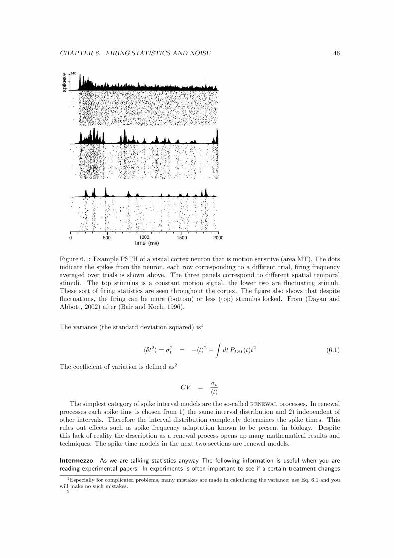
CHAPTER 6. FIRING STATISTICS AND NOISE 46
Figure 6.1: Example PSTH of a visual cortex neuron that is motion sensitive (area MT). The dotsindicate the spikes from the neuron, each row corresponding to a different trial, firing frequencyaveraged over trials is shown above. The three panels correspond to different spatial temporalstimuli. The top stimulus is a constant motion signal, the lower two are fluctuating stimuli.These sort of firing statistics are seen throughout the cortex. The figure also shows that despitefluctuations, the firing can be more (bottom) or less (top) stimulus locked. From (Dayan andAbbott, 2002) after (Bair and Koch, 1996).
The variance (the standard deviation squared) is1
〈δt2〉 = σ2t = −〈t〉2 +
∫dt PISI(t)t2 (6.1)
The coefficient of variation is defined as2
CV =σt
〈t〉The simplest category of spike interval models are the so-called renewal processes. In renewal
processes each spike time is chosen from 1) the same interval distribution and 2) independent ofother intervals. Therefore the interval distribution completely determines the spike times. Thisrules out effects such as spike frequency adaptation known to be present in biology. Despitethis lack of reality the description as a renewal process opens up many mathematical results andtechniques. The spike time models in the next two sections are renewal models.
Intermezzo As we are talking statistics anyway The following information is useful when you arereading experimental papers. In experiments is often important to see if a certain treatment changes
1Especially for complicated problems, many mistakes are made in calculating the variance; use Eq. 6.1 and youwill make no such mistakes.
2

CHAPTER 6. FIRING STATISTICS AND NOISE 47
some mean property of the cell. Therefore it is important how reliable the estimate of the mean is.This quantity is called the standard error σM and is given by σM = σ/
√N . By measuring enough
data, the standard error can usually be made arbitrarily small, whereas σ usually tends to a fixed valuewhen enough data are measured. The means from the two conditions can be compared using a t-test.The resulting p value indicates how likely it was that the effect occurred due to a random coincidence(testing an hypothesis). The lower the standard errors, the more significant the result, values below5% (p<0.05) are considered significant and publishable. Note, that the lack of a significant result doesnot mean that there is no effect...
6.3 Poisson model
The presence of irregularity in neural activity has lead to a number of noise models for neurons.The simplest model for spike generation is a Poisson process. (The prime example of a Poissonprocess is radio active decay). In a homogeneous Poisson process the probability for a spike isidentical at every time. Suppose the rate of the Poisson process is λ = 1/τ . What is the distributionof inter spike intervals? Divide the inter-spike interval in many small steps of duration ∆t. Theprobability to spike after time tisi is given by
P (tisi = n ∆t) = (1− ∆t
τ)n−1 ∆t
τ=
∆t
τexp[(n− 1) log(1− ∆t
τ)]
≈ ∆t
τexp(−tisi/τ)
We have to normalise this expression such that∫∞0
dtisiP (tisi) = 1, and we find
PPoisson(tisi) =1τ
exp(−tisi/τ)
In other words, the intervals are exponentially distributed. The mean interval is τ and the varianceis τ2. In the Poisson process the probability for an event is constant (there is no time-scale intrinsicto the Poisson process). Therefore the autocorrelation function is a constant plus a δ function atzero. As a result the power-spectrum is flat as well with a δ function at zero.
Of course, the spike rate of a neuron usually changes when a stimulus is presented/removedor the stimulus fluctuates, as in Fig. 6.1. A rate-modulated Poisson process can be used to modelthis. In that case at every instant the firing probability is calculated from a rate λ(t). This willof course destroy the exponential distribution of inter-spike intervals.
The Poisson process is only a rough approximation for the firing of real neurons. Althoughreasonably correct for low firing rates, the Poisson approximation goes wrong for higher rates.When the instantaneous rate is high, a Poisson model can fire twice in rapid succession. However,a real neuron’s membrane potential will have to climb up from reset to threshold voltage. Inaddition, refractory mechanisms prevent a rapid succession of spikes in real neurons. As a resultreal neurons fire less fast and also more reliable (Berry and Meister, 1998). Nevertheless, thePoisson model is an easy benchmark for neural firing.
6.4 Noisy integrate and fire neuron
In the Poisson process the intervals are exponentially distributed. This is a reasonable approxi-mation for neurons with low firing rates (for instance background firing). The inter-spike intervaldistribution of real neurons with higher firing rates is usually a skewed Gaussian-like distribution(Note, that mathematically the ISI distribution can never be strictly Gaussian as negative intervalsdo not exist).
There are various noise models which can be inserted to give realistic variability in the firing.One can, for instance, make the threshold fluctuate, chose a random reset potential, or inject a noisecurrent in the neuron. When we supply a constant noise term to the leak-less integrate and fire

CHAPTER 6. FIRING STATISTICS AND NOISE 48
Voltage
Short intervalslittle spread
Long intervalshigh spread
Threshold
P(isi)
isi
P(isi)
isi
Time
Figure 6.2: Noisy integrate and fire neuron. Different sample paths from rest to threshold. Forstrong stimuli (right 2 traces) the slope is steep and the variations in the spike timing is small.For weak stimuli (left 2 traces) the slope is shallow and noise accumulates. The shape of theinter-spike interval histograms sketched on top is like those observed in physiology.
thrVV
P(V) P(V)
V
Figure 6.3: Cartoon of the Fokker-Planck approach. Left: Situation shortly after the neuron hasfired. The Fokker-Planck equation collects all loss and gain term to P (V ) at each voltage (solidarrows loss terms, dashed arrows gain terms). Right: Later situation: the distribution is spreaddue to the noise, and its mean has shifted toward the threshold due to the stimulus current. Whenthe probability reaches threshold, the neuron fires (open arrow).
neuron, one obtains reasonably realistic firing statistics. Simplifying such that Vreset = Vrest = 0,and C = 1 the governing equation is
dV
dt= Istim + Inoise(t)
and of course, as before the neuron spikes and resets when it reaches the threshold.The problem is now to determine when the neuron will fire, given that V (t = 0) = 0. The
noise term is easy to simulate, from trial to trial the neuron will take different paths to thethreshold, Fig. 6.2. Analytical treatment is possible: The voltage obeys a diffusion equation as wewill see shortly (Gerstein and Mandelbrot, 1964). We assume that the noise term has zero mean〈Inoise〉 = 0, and its variance is 〈Inoise(t)Inoise(t′)〉 = σ2δ(t− t′).3
The spike-timing can be calculated using a Fokker-Planck equation. Consider the distributionof possible voltages P (V, t). The Fokker-Planck equation simply collects the contributions whichchange this distribution, as is shown schematically in Fig. 6.3.
P (V, t + ∆t) = P (V, t) +∫
dV ′T (V ′, V )P (V ′, t)− P (V, t)∫
dV ′T (V, V ′)
3This is so called white noise; its power-spectrum is flat, i.e. it contains all possible frequencies.
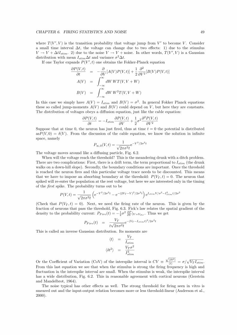
CHAPTER 6. FIRING STATISTICS AND NOISE 49
where T (V ′, V ) is the transition probability that voltage jump from V ′ to become V . Considera small time interval ∆t, the voltage can change due to two effects: 1) due to the stimulusV → V + ∆tIstim. 2) due to the noise V → V + noise. In other words, T (V ′, V ) is a Gaussiandistribution with mean Istim∆t and variance σ2∆t.
If one Taylor expands P (V ′, t) one obtains the Fokker-Planck equation
∂P (V, t)∂t
= − ∂
∂V[A(V )P (V, t)] +
12
∂2
∂V 2[B(V )P (V, t)]
A(V ) =∫ ∞
−∞dW WT (V, V + W )
B(V ) =∫ ∞
−∞dW W 2T (V, V + W )
In this case we simply have A(V ) = Istim and B(V ) = σ2. In general Fokker Planck equationsthese so called jump-moments A(V ) and B(V ) could depend on V , but here they are constants.The distribution of voltages obeys a diffusion equation, just like the cable equation:
∂P (V, t)∂t
= −Istim∂P (V, t)
∂V+
12σ2 ∂2P (V, t)
∂V 2
Suppose that at time 0, the neuron has just fired, thus at time t = 0 the potential is distributedasP (V, 0) = δ(V ). From the discussion of the cable equation, we know the solution in infinitespace, namely
P∞,0(V, t) =1√
2πσ2te−V 2/2σ2t
The voltage moves around like a diffusing particle, Fig. 6.2.When will the voltage reach the threshold? This is the meandering drunk with a ditch problem.
There are two complications: First, there is a drift term, the term proportional to Istim (the drunkwalks on a down-hill slope). Secondly, the boundary conditions are important. Once the thresholdis reached the neuron fires and this particular voltage trace needs to be discounted. This meansthat we have to impose an absorbing boundary at the threshold: P (VT , t) = 0. The neuron thatspiked will re-enter the population at the rest voltage, but here we are interested only in the timingof the first spike. The probability turns out to be
P (V, t) =1√
2πσ2t
(e−V 2/2σ2t − e−(2VT−V )2/2σ2t
)eIstimV/σ2−I2
stimt/2σ2
(Check that P (VT , t) = 0). Next, we need the firing rate of the neuron. This is given by thefraction of neurons that pass the threshold, Fig. 6.3. Fick’s law relates the spatial gradient of thedensity to the probability current: PFire(t) = − 1
2σ2 ∂P∂V |V =Vthr
. Thus we get
PFire(t) =VT
t√
2πσ2te−(VT−Istimt)2/2σ2t
This is called an inverse Gaussian distribution. Its moments are
〈t〉 =VT
Istim
〈δt2〉 =VT σ2
I3stim
Or the Coefficient of Variation (CoV) of the interspike interval is CV ≡√〈δt2〉〈t〉 = σ/
√VT Istim.
From this last equation we see that when the stimulus is strong the firing frequency is high andfluctuation in the interspike interval are small. When the stimulus is weak, the interspike intervalhas a wide distribution, Fig. 6.2. This in reasonable agreement with cortical neurons (Gersteinand Mandelbrot, 1964).
The noise typical has other effects as well. The strong threshold for firing seen in vitro issmeared out and the input-output relation becomes more or less threshold-linear (Anderson et al.,2000).

CHAPTER 6. FIRING STATISTICS AND NOISE 50
0 500 1000
0 500 10000
10
20
30T
rial
0 500 1000
0 500 1000
Figure 6.4: Left: Noisy integrate and fire neuron stimulated with a DC current (bottom panel),responses (top) are shown trial-to-trial. After few spikes, spikes are not stimulus locked. Right:Stimulation with a fluctuating current, leads to much more precise spiking; the firing locks to thestimulus.
6.5 Stimulus locking
Another interesting effect of noisy I&F neurons is that their timing precision seems to depend noonly on the stimulus strength but also on the presence of transients in the stimulus (Bryant andSegundo, 1976; Mainen and Sejnowski, 1995). This is shown in Fig. 6.4. From the spiking patternin the left panel, one would not expect that the neurons could spike so reliable as they do in theright panel. Transients in the stimulus can synchronise and lock the firing. This effect appears tobe even stronger for real neurons probed with current injections. Note the similarity with in vivoneurons, Fig. 6.1.
6.6 Count statistics
The interval statistics is one way to measure spiking variability. Alternatively, one can count thenumber of spikes and calculate its statistical properties. Suppose one counts the spikes occurringin a window of duration T , one repeats the experiment and measures the mean and variance inthe count. The Fano factor is defined as
F (T ) =σ2
N (T )µN (T )
For a Poisson process, see Eq. 4.1, the mean count is T/τ , and the variance is T/τ as well, so theFano factor is 1 for all T . (It is important to distinguish the count statistics and interval statisticsespecially for the Poisson process). The behaviour for large T is revealing: most simple neuronmodels converge to fixed values for long T, however real neurons show often a steady increase inthe Fano factor for long times (seconds), Fig. 6.5. This could either mean that slow variationsin for instance excitability occur, or that the firing has a fractal structure (Lowen et al., 2001).(Exercise: Try to create a cell model with such a Fano factor as in Fig. 6.5).

CHAPTER 6. FIRING STATISTICS AND NOISE 51
Figure 6.5: The Fano factor of the spike count for an experiment like in Fig. 6.1. The flat linecorresponds to a Poisson process. From (Buracas et al., 1998).
6.7 Neuronal activity In vivo
A neuron in vivo continuously receives synaptic inputs. How much? In a resting, awake stateneurons fire at an average rate of about 3Hz. Cortical neurons have about 10.000 synapses. Aconnection between two neurons involves on the average about five synapses. Maybe each synapseis 50% reliable. This means that a neuron receives input at a frequency of 3 × 10.000/5/2Hz =3000Hz. Now suppose for a moment that all these inputs are excitatory. Two problems arise:
• Because there are so many synapses, the fluctuations in the input are averaged out. Thereforeone would expect the post-synaptic neuron to fire very regular. Note, that this will be thecase despite all synaptic and channel noise sources we have encountered.
• A single input depolarises the cell with about 0.1 mV. Maybe some 20..200 inputs are requiredto fire the cell. The total excitation will cause the cell to fire at very high rates, even thoughis just receives background input.
The solution to the riddle is not fully clear yet, but the following factors are believed to beimportant:
• The input is not accurately described by uncorrelated processes, as often a considerableamount of correlation is present. The presence of correlations effectively reduce the numberof independent inputs, and as a result firing is more irregular (Stevens and Zador, 1998).
• The excitatory input is balanced by inhibitory inputs. This will reduce the net drive, andat the same time increase the noise. In addition, because the inhibition is a conductance(and not just a current), the effective leak of the cell is increased (see Section 5.2). Thetypical background activity can reduce the input resistance with some 80%, reducing thetime-constant of cells to about 5 ms, and the electrotonic length will become shorter as well(Pare et al., 1998). All reduce the integration of synaptic inputs in the cell. Completelybalanced models have been proposed, in which the mean input remains constant, insteadthe fluctuations drive the activity (Shadlen and Newsome, 1998).
• Geometry and active properties of real neurons might be important as well.
Two final remarks on this issue: 1) With some simple estimates the approximate behaviour of aneuron was calculated. The realisation that this is not consistent with data, is a nice example ofneural computational thinking (Shadlen and Newsome, 1998; Holt et al., 1996).

CHAPTER 6. FIRING STATISTICS AND NOISE 52
2) It shows that it is not only necessary to have an accurate model of the cell at rest, but thatan effective model for the cell in vivo is as important.
More reading on statistical description of neurons: (Tuckwell, 1988)
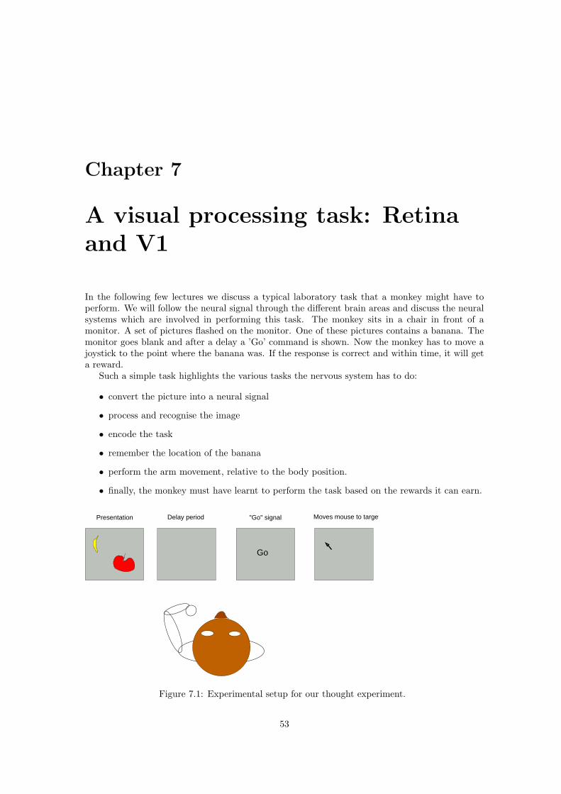
Chapter 7
A visual processing task: Retinaand V1
In the following few lectures we discuss a typical laboratory task that a monkey might have toperform. We will follow the neural signal through the different brain areas and discuss the neuralsystems which are involved in performing this task. The monkey sits in a chair in front of amonitor. A set of pictures flashed on the monitor. One of these pictures contains a banana. Themonitor goes blank and after a delay a ’Go’ command is shown. Now the monkey has to move ajoystick to the point where the banana was. If the response is correct and within time, it will geta reward.
Such a simple task highlights the various tasks the nervous system has to do:
• convert the picture into a neural signal
• process and recognise the image
• encode the task
• remember the location of the banana
• perform the arm movement, relative to the body position.
• finally, the monkey must have learnt to perform the task based on the rewards it can earn.
Go
"Go" signalPresentation Delay period Moves mouse to target
Figure 7.1: Experimental setup for our thought experiment.
53
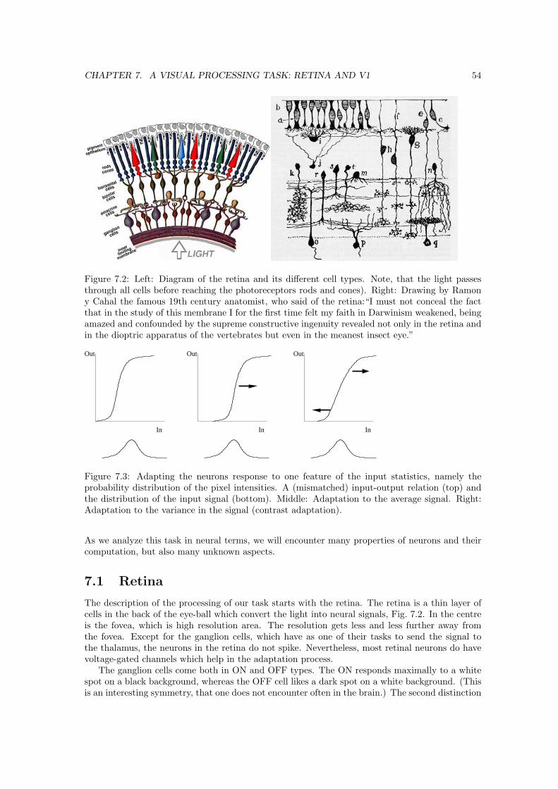
CHAPTER 7. A VISUAL PROCESSING TASK: RETINA AND V1 54
Figure 7.2: Left: Diagram of the retina and its different cell types. Note, that the light passesthrough all cells before reaching the photoreceptors rods and cones). Right: Drawing by Ramony Cahal the famous 19th century anatomist, who said of the retina:“I must not conceal the factthat in the study of this membrane I for the first time felt my faith in Darwinism weakened, beingamazed and confounded by the supreme constructive ingenuity revealed not only in the retina andin the dioptric apparatus of the vertebrates but even in the meanest insect eye.”
In
Out
In
Out
In
Out
Figure 7.3: Adapting the neurons response to one feature of the input statistics, namely theprobability distribution of the pixel intensities. A (mismatched) input-output relation (top) andthe distribution of the input signal (bottom). Middle: Adaptation to the average signal. Right:Adaptation to the variance in the signal (contrast adaptation).
As we analyze this task in neural terms, we will encounter many properties of neurons and theircomputation, but also many unknown aspects.
7.1 Retina
The description of the processing of our task starts with the retina. The retina is a thin layer ofcells in the back of the eye-ball which convert the light into neural signals, Fig. 7.2. In the centreis the fovea, which is high resolution area. The resolution gets less and less further away fromthe fovea. Except for the ganglion cells, which have as one of their tasks to send the signal tothe thalamus, the neurons in the retina do not spike. Nevertheless, most retinal neurons do havevoltage-gated channels which help in the adaptation process.
The ganglion cells come both in ON and OFF types. The ON responds maximally to a whitespot on a black background, whereas the OFF cell likes a dark spot on a white background. (Thisis an interesting symmetry, that one does not encounter often in the brain.) The second distinction

CHAPTER 7. A VISUAL PROCESSING TASK: RETINA AND V1 55
is between the cells in the M- and P- pathway. The P have a fine spatial resolution, are slow andsome are colour selective. The M cells encompass larger receptive fields and therefore have a lowerspatial resolution, but they are faster. The M and P pathway are processed more or less in parallelin the retina, LGN and cortex.
7.1.1 Adaptation
The retina works over a very large range of possible light intensities: a sunny day is about1010
times brighter than a starlit night. The dynamic range of the output (which is defined the ratiothe strongest and weakest perceptible signal) is about 100 (assuming rate coding with firing ratesranging from a few to 200 Hz). So adaptation is required. (Opening and closing the pupil onlycontributes a small bit to the total adaptation).
The principle of adaptation is shown in Fig. 7.3. Adaptation can be understood as chang-ing the input/output relation of cell such that the dynamic range of the cell is optimally used.Adaptation seems to be implemented at many levels in the retina, from the photoreceptor to theganglion circuit. There are both global mechanisms (mediated through neuro modulators such asdopamine), and local mechanisms.
Contrast adaptation also occurs in the retina, but its mechanisms are less well known. Apartfrom biophysical mechanisms in the cells, adaptation can be achieved with a centre-surroundcircuit (a Mexican hat profile). The output of such a circuit subtracts the surround from thecentre. It is easy to see that this circuit will not react to changes in mean light level, instead it isa local contrast detector. The centre-surround structure is ubiquitous in the nervous system, notonly in the visual system, but also in the somato sensory and auditory system.
7.1.2 Photon noise
In detecting the signal, the retina has to deal with the photon noise. Most light sources emitphotons according to a Poisson process. The photon noise is most clear at night; the image thatone sees has a snowy pattern superimposed on it. This is the photon noise. Indeed, the retinacan almost see single photons. And the retina works close to the physical limits in obtaining thisperformance(Bialek, 1987).
Even in dimly lit rooms, photon noise is discernible. This provides a good reason why thepupil should not do all adaptation. That would limit the number of photons impinging on thephotoreceptors, increasing the relative noise. Rather the gain in the system is reduced at higherlight levels. At low light levels one obvious way to reduce the photon noise is to average the signaleither temporally or spatially, but of course this will come at the cost of reducing resolution.
7.1.3 Spatial filtering
The question what is the best (linear) filter to process the image is can be answered using in-formation theory. Here we discuss this argument for the spatial filtering (van Hateren, 1992;Atick and Redlich, 1992; Barlow and Levick, 1965).
The argument is that one tasks of the retina is to remove redundancies in the signal, perhapsbecause the optic nerve has only limited capacity, or because the nervous systems can not processall incoming information. Redundancy can be removed by de-correlating the signal, such that itsautocorrelation function is just a δ-function. That means there is no correlation, except at zero.From our discussion of correlations and power-spectra, we know that this correlation functioncorresponds to flat (’white’) spectrum. This means that the most informative coding will whitenthe spectrum of the output.
Remarkably, the spectrum of visual inputs is not white! The spectrum of natural imagesbehaves as 1/f2
spat, that means that natural image have a tendency to have much more lowfrequency components than high frequencies (you are encouraged to check this with Matlab).Whitening the signal would mean to multiply the signal with f2
spat, i.e. high pass filtering.1
1There is a cut-off somewhere: it would not make sense to increase spatial frequencies which are beyond the eye

CHAPTER 7. A VISUAL PROCESSING TASK: RETINA AND V1 56
−
+
−
−− −
+
+
+
+
a) On−center b) Off−center
+
−−
+
−
+
−
+
−
+
Figure 7.4: Left: Receptive fields of retinal ganglion cells can be modelled by a difference ofGaussians. This yields a bandpass spatial filtering.Right: Spatial transfer function of the retina at different mean light intensities (lowest curve:lowest light level). At low light levels the transfer function is low-pass; at higher light levels itbecomes band-pass. From (Atick and Redlich, 1992).
However, when the signal is corrupted with photon noise, this filtering would be catastrophic,as the noise has a flat power-spectrum. Therefore multiplying the signal plus noise with f2
spat
would cause most bandwidth would be taken up by noise. Instead there is a trade-off betweenwhitening and getting too much noise, Fig. 7.5.
Therefore at normal light levels the resulting spatial filter has a Mexican hat, or centre-surroundprofile. Its centre collects signals from neighbouring cells, thus doing a low-pass filter to reducehigh frequency noise. The inhibition removes partly low-frequency components in the input. Theresult is a bandpass filter. In contrast, at low light levels the optimal filter is purely low-pass,Fig. 7.4.
The idea of removing correlation (redundancies) in the visual signal before sending it on thecortex dates back to Barlow(Barlow, 1958). The typical images are also redundant in time andcolor-space(Buchsbaum and Gottschalk, 1983). Redundancy reduction is a compression algorithm,a bit like JPEG compression. This sort of information reduction is probably going on at manystages in the brain. Our retina sends some 106 axons, with maybe some 10 bits/sec each. Yet,consciously we process much less information (estimate are about 100 bits/sec).
These properties of the input are so called second order statistics, as the calculation of thecorrelation uses terms such as 〈I(x)I(x + ∆x)〉. It is unclear yet if similar principles can be usedfor higher level (smarter) stages of processing. In principle, higher order statistics could yieldadditional compression tricks. Natural images might have a 1/f2
spat power-spectrum, but have
maximal resolution. The resolution of the eye is determined by lens scatter and the number of ganglion cells in theretina.
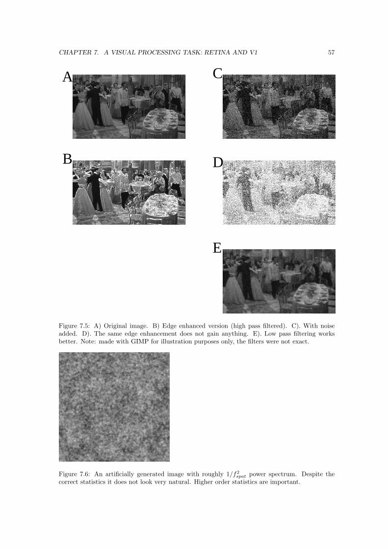
CHAPTER 7. A VISUAL PROCESSING TASK: RETINA AND V1 57
A C
D
E
B
Figure 7.5: A) Original image. B) Edge enhanced version (high pass filtered). C). With noiseadded. D). The same edge enhancement does not gain anything. E). Low pass filtering worksbetter. Note: made with GIMP for illustration purposes only, the filters were not exact.
Figure 7.6: An artificially generated image with roughly 1/f2spat power spectrum. Despite the
correct statistics it does not look very natural. Higher order statistics are important.
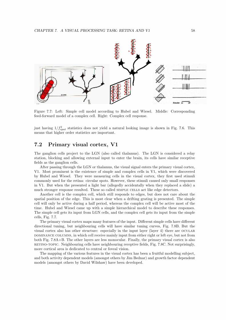
CHAPTER 7. A VISUAL PROCESSING TASK: RETINA AND V1 58
Figure 7.7: Left: Simple cell model according to Hubel and Wiesel. Middle: Correspondingfeed-forward model of a complex cell. Right: Complex cell response.
just having 1/f2spat statistics does not yield a natural looking image is shown in Fig. 7.6. This
means that higher order statistics are important.
7.2 Primary visual cortex, V1
The ganglion cells project to the LGN (also called thalamus). The LGN is considered a relaystation, blocking and allowing external input to enter the brain, its cells have similar receptivefields as the ganglion cells.
After passing through the LGN or thalamus, the visual signal enters the primary visual cortex,V1. Most prominent is the existence of simple and complex cells in V1, which were discoveredby Hubel and Wiesel. They were measuring cells in the visual cortex, they first used stimulicommonly used for the retina: circular spots. However, these stimuli caused only small responsesin V1. But when the presented a light bar (allegedly accidentally when they replaced a slide) amuch stronger response resulted. These so called simple cells act like edge detectors.
Another cell is the complex cell, which still responds to edges, but does not care about thespatial position of the edge. This is most clear when a drifting grating is presented. The simplecell will only be active during a half period, whereas the complex cell will be active most of thetime. Hubel and Wiesel came up with a simple hierarchical model to describe these responses.The simple cell gets its input from LGN cells, and the complex cell gets its input from the simplecells, Fig. 7.7.
The primary visual cortex maps many features of the input. Different simple cells have differentdirectional tuning, but neighbouring cells will have similar tuning curves, Fig. 7.8B. But thevisual cortex also has other structure: especially in the input layer (layer 4) there are oculardominance columns, in which cell receive mainly input from either right or left eye, but not fromboth Fig. 7.8A+B. The other layers are less monocular. Finally, the primary visual cortex is alsoretino-topic. Neighbouring cells have neighbouring receptive fields, Fig. 7.8C. Not surprisingly,more cortical area is dedicated to central or foveal vision.
The mapping of the various features in the visual cortex has been a fruitful modelling subject,and both activity dependent models (amongst others by Jim Bednar) and growth factor dependentmodels (amongst others by David Wilshaw) have been developed.
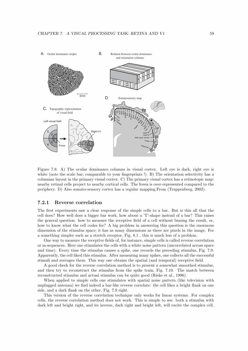
CHAPTER 7. A VISUAL PROCESSING TASK: RETINA AND V1 59
lefteye
lefteye
righteye
righteye
5mm
A. Ocular dominance stripes B. Relation between ocular dominance
and orientation columns
1
2
3
4
5
6
1
2
3
456
Left visual field
Right V1
Fovea
C. Topographic representation
of visual field
D. Somatosensory map
Genitals
Toes
Foot
Leg
Hip
Teeth, gums, and jaw
Tongue
Lower lipUpper lip
Face
Nos
eEyeThu
mb
Inde
x
Mid
dleRin
g
Fin
gers
Litt
le
Hand
Wri
st
Fore
arm
Elb
ow
Arm
Should
er
Hand
Neck
Tru
nk
abdominal
Figure 7.8: A) The ocular dominance columns in visual cortex. Left eye is dark, right eye iswhite (note the scale bar; comparable to your fingerprints !). B) The orientation selectivity has acolumnar layout in the primary visual cortex. C) The primary visual cortex has a retinotopic map:nearby retinal cells project to nearby cortical cells. The fovea is over-represented compared to theperiphery. D) Also somato-sensory cortex has a regular mapping.From (Trappenberg, 2002).
7.2.1 Reverse correlation
The first experiments saw a clear response of the simple cells to a bar. But is this all that thecell does? How well does a bigger bar work, how about a ’T’-shape instead of a bar? This raisesthe general question: how to measure the receptive field of a cell without biasing the result, or,how to know what the cell codes for? A big problem in answering this question is the enormousdimension of the stimulus space; it has as many dimensions as there are pixels in the image. Fora something simpler such as a stretch receptor, Fig. 8.1 , this is much less of a problem.
One way to measure the receptive fields of, for instance, simple cells is called reverse correlationor m-sequences. Here one stimulates the cells with a white noise pattern (uncorrelated across spaceand time). Every time the stimulus causes a spike, one records the preceding stimulus, Fig. 7.9.Apparently, the cell liked this stimulus. After measuring many spikes, one collects all the successfulstimuli and averages them. This way one obtains the spatial (and temporal) receptive field.
A good check for the reverse correlation method is to present a somewhat smoothed stimulus,and then try to reconstruct the stimulus from the spike train, Fig. 7.10. The match betweenreconstructed stimulus and actual stimulus can be quite good (Rieke et al., 1996).
When applied to simple cells one stimulates with spatial noise pattern (like television withunplugged antenna) we find indeed a bar-like reverse correlate: the cell likes a bright flank on oneside, and a dark flank on the other, Fig. 7.9 right.
This version of the reverse correlation technique only works for linear systems. For complexcells, the reverse correlation method does not work. This is simple to see: both a stimulus withdark left and bright right, and its inverse, dark right and bright left, will excite the complex cell.
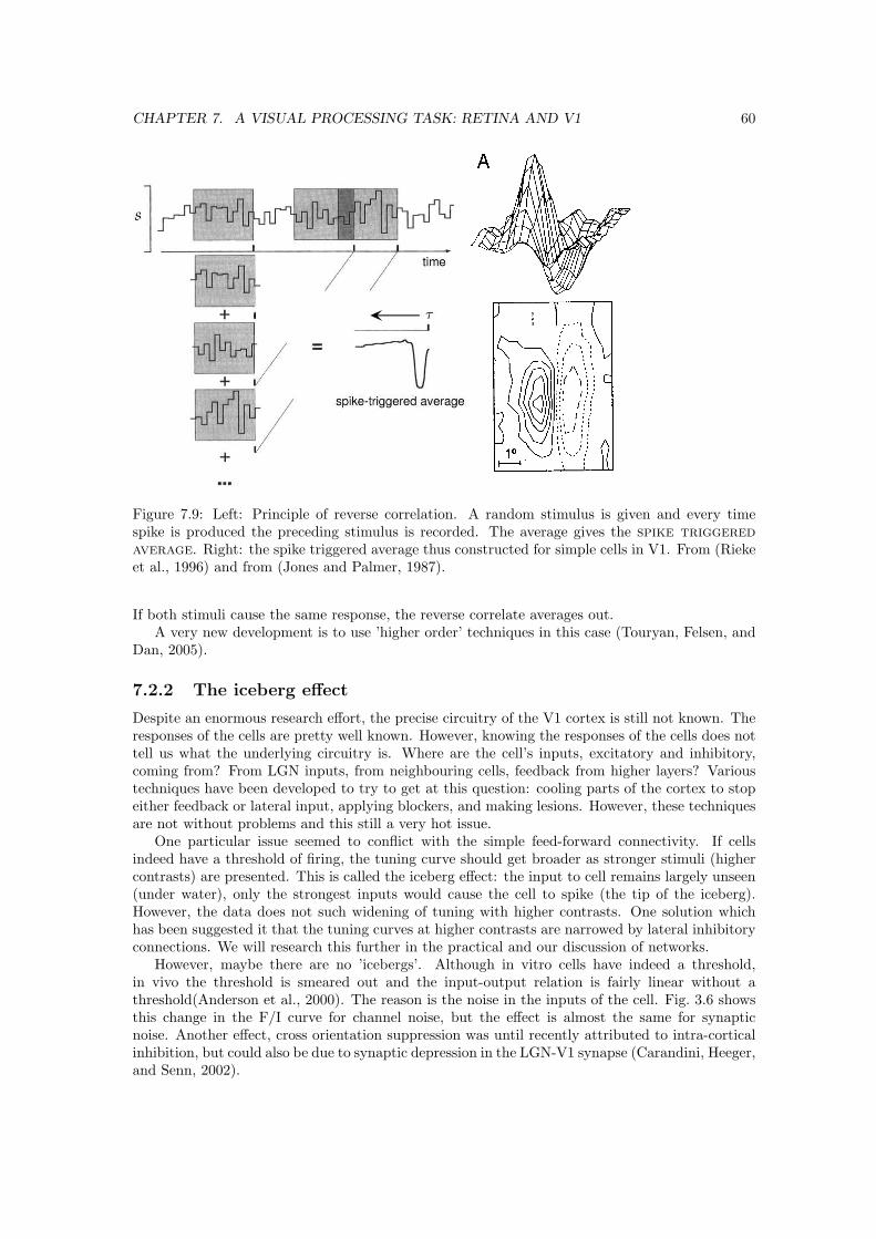
CHAPTER 7. A VISUAL PROCESSING TASK: RETINA AND V1 60
Figure 7.9: Left: Principle of reverse correlation. A random stimulus is given and every timespike is produced the preceding stimulus is recorded. The average gives the spike triggeredaverage. Right: the spike triggered average thus constructed for simple cells in V1. From (Riekeet al., 1996) and from (Jones and Palmer, 1987).
If both stimuli cause the same response, the reverse correlate averages out.A very new development is to use ’higher order’ techniques in this case (Touryan, Felsen, and
Dan, 2005).
7.2.2 The iceberg effect
Despite an enormous research effort, the precise circuitry of the V1 cortex is still not known. Theresponses of the cells are pretty well known. However, knowing the responses of the cells does nottell us what the underlying circuitry is. Where are the cell’s inputs, excitatory and inhibitory,coming from? From LGN inputs, from neighbouring cells, feedback from higher layers? Varioustechniques have been developed to try to get at this question: cooling parts of the cortex to stopeither feedback or lateral input, applying blockers, and making lesions. However, these techniquesare not without problems and this still a very hot issue.
One particular issue seemed to conflict with the simple feed-forward connectivity. If cellsindeed have a threshold of firing, the tuning curve should get broader as stronger stimuli (highercontrasts) are presented. This is called the iceberg effect: the input to cell remains largely unseen(under water), only the strongest inputs would cause the cell to spike (the tip of the iceberg).However, the data does not such widening of tuning with higher contrasts. One solution whichhas been suggested it that the tuning curves at higher contrasts are narrowed by lateral inhibitoryconnections. We will research this further in the practical and our discussion of networks.
However, maybe there are no ’icebergs’. Although in vitro cells have indeed a threshold,in vivo the threshold is smeared out and the input-output relation is fairly linear without athreshold(Anderson et al., 2000). The reason is the noise in the inputs of the cell. Fig. 3.6 showsthis change in the F/I curve for channel noise, but the effect is almost the same for synapticnoise. Another effect, cross orientation suppression was until recently attributed to intra-corticalinhibition, but could also be due to synaptic depression in the LGN-V1 synapse (Carandini, Heeger,and Senn, 2002).
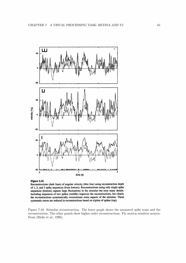
CHAPTER 7. A VISUAL PROCESSING TASK: RETINA AND V1 61
Figure 7.10: Stimulus reconstruction. The lower graph shows the measured spike train and thereconstruction. The other panels show higher order reconstructions. Fly motion sensitive neuron.From (Rieke et al., 1996).
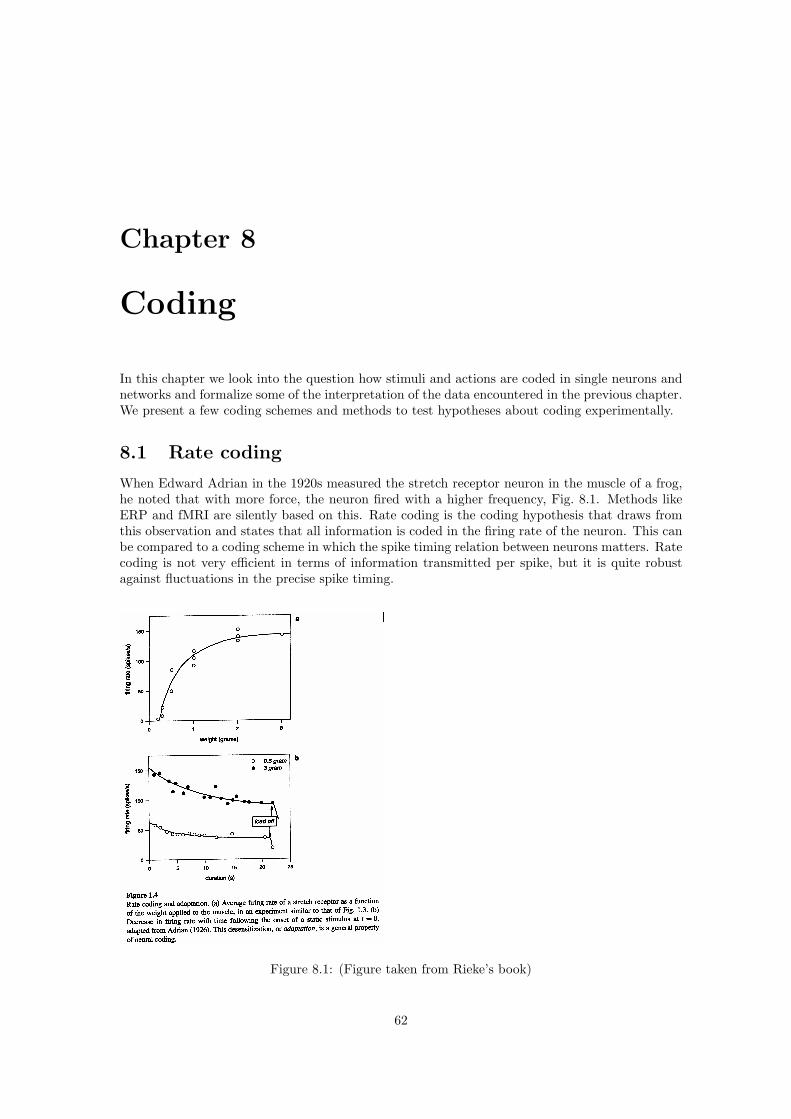
Chapter 8
Coding
In this chapter we look into the question how stimuli and actions are coded in single neurons andnetworks and formalize some of the interpretation of the data encountered in the previous chapter.We present a few coding schemes and methods to test hypotheses about coding experimentally.
8.1 Rate coding
When Edward Adrian in the 1920s measured the stretch receptor neuron in the muscle of a frog,he noted that with more force, the neuron fired with a higher frequency, Fig. 8.1. Methods likeERP and fMRI are silently based on this. Rate coding is the coding hypothesis that draws fromthis observation and states that all information is coded in the firing rate of the neuron. This canbe compared to a coding scheme in which the spike timing relation between neurons matters. Ratecoding is not very efficient in terms of information transmitted per spike, but it is quite robustagainst fluctuations in the precise spike timing.
Figure 8.1: (Figure taken from Rieke’s book)
62

CHAPTER 8. CODING 63
Figure 8.2: Population coding. Left: four cells with their tuning curves. The centres of the tuningcurves are different, but they overlap. Middle: When a single bar is presented, all neurons respond,but with different amplitudes. Right: Hyper-acuity. The location of the bar can be estimated witha accuracy better than the distance between the neurons. The stimulus must have been locatedslightly to the right of the second neuron (because the third neuron is more active than the firstneuron).
A slightly unrelated characteristic of the data shown, is that the relation between firing rateand force is not linear. Instead, the firing rate codes roughly the log of the force. As a resulterrors in the force estimate will be proportional to the force itself (assuming additive, fixed noise).In other words, ∆F/F is constant; the percentage error, rather than the absolute error is fixed.This is called Weber’s law.
8.2 Population code
When a stimulus is presented to our monkey usually not just one, but a whole ensemble of neuronsbecomes active. We have already encountered an example of this effect, namely the simple cells inV1. Because the V1 neurons have a wide tuning curves (Fig.10.6) many neurons will respond whena bar is presented. This distribution of activity over multiple neurons is called population coding(Paradiso, 1988). This might at first seem a wasteful scheme: wouldn’t it be more convenient iffor a given stimulus only a few finely tuned neurons reacted? But population coding has someinteresting advantages.
In Fig. 8.2 we show a example of population coding. Four neurons have overlapping tuningcurves. When a stimulus is presented all neurons respond, albeit with different amplitudes. Al-though the neuron with the highest activity most clearly signals the location of the bar, the otherneurons contribute as well. One advantage is almost immediately evident: a population code isrobust against failure of neurons. In case a neuron fails the rough position of the stimulus canstill be estimated; the information might be distorted but is not completely lost. Similarly, giventhat the response from a single neuron is noisy, using multiple neurons in parallel can speed upprocessing as it reduces the need for long averaging times. Because the neurons have slightlydifferent tuning curves, this parallel processing is not redundant.
Another interesting property of population codes is hyper-acuity. Hyper-acuity means thatthe position of the stimulus can be estimated more finely than the distance between the neurons.Fig. 8.2(right) shows why hyper-acuity can occur. Because the third neuron reacts a bit strongerthan the first neuron we know that the stimulus was slightly toward the third neuron (right ofthe second neuron). Hyper-acuity in our visual system was directly illustrated using Vernier lines:When one is presented with two co-linear line segments which are slightly displaced, one candiscriminate very small displacements. Displacements that projected onto the retina are less thanthe distance between two photoreceptors. This was puzzling at first. However, it turn it turnsout that the lens blurs the image just so much that strip of a few photoreceptors wide will beactivated by even the thinnest line, so that the photoreceptors and subsequent retinal circuitry
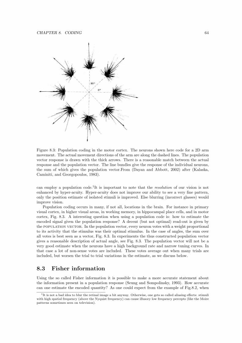
CHAPTER 8. CODING 64
Figure 8.3: Population coding in the motor cortex. The neurons shown here code for a 2D armmovement. The actual movement directions of the arm are along the dashed lines. The populationvector response is drawn with the thick arrows. There is a reasonable match between the actualresponse and the population vector. The line bundles give the response of the individual neurons,the sum of which gives the population vector.From (Dayan and Abbott, 2002) after (Kalaska,Caminiti, and Georgopoulos, 1983).
can employ a population code.1It is important to note that the resolution of our vision is notenhanced by hyper-acuity. Hyper-acuity does not improve our ability to see a very fine pattern,only the position estimate of isolated stimuli is improved. Else blurring (incorrect glasses) wouldimprove vision.
Population coding occurs in many, if not all, locations in the brain. For instance in primaryvisual cortex, in higher visual areas, in working memory, in hippocampal place cells, and in motorcortex, Fig. 8.3. A interesting question when using a population code is: how to estimate theencoded signal given the population response? A decent (but not optimal) read-out is given bythe population vector. In the population vector, every neuron votes with a weight proportionalto its activity that the stimulus was their optimal stimulus. In the case of angles, the sum overall votes is best seen as a vector, Fig. 8.3. In experiments the thus constructed population vectorgives a reasonable description of actual angle, see Fig. 8.3. The population vector will not be avery good estimate when the neurons have a high background rate and narrow tuning curves. Inthat case a lot of non-sense votes are included. These votes average out when many trials areincluded, but worsen the trial to trial variations in the estimate, as we discuss below.
8.3 Fisher information
Using the so called Fisher information it is possible to make a more accurate statement aboutthe information present in a population response (Seung and Sompolinsky, 1993). How accuratecan one estimate the encoded quantity? As one could expect from the example of Fig.8.2, when
1It is not a bad idea to blur the retinal image a bit anyway. Otherwise, one gets so called aliasing effects: stimuliwith high spatial frequency (above the Nyquist frequency) can cause illusory low frequency percepts (like the Moirepatterns sometimes seen on television).

CHAPTER 8. CODING 65
the neurons are noise-free, the accuracy of the estimate is in principle infinite. The question istherefore: given a certain noise-level in the neurons, what the highest accuracy one can achieve.
Suppose we have a large population of N neurons that encode for an angle θ. For conveniencewe suppose that they all have tuning curves which only differ in their centrefi(θ) = A exp[cos(θ−θi)/w2].
The error in the angle estimate can be calculated using the Fisher information2, which is givenby
IF = −∫
drP (r|θ)∂2 log P (r|θ)∂θ2
=∫
drP (r|θ)(
∂ log P (r|θ)∂θ
)2
The Cramer-Rao bound says that it is not possible to estimate the original stimulus with a varianceless than the inverse Fisher information (for a so-called unbiased estimator3), that is
σ2θ ≥ 1/IF
This inequality hold not only for angles, but for any encoded quantity. Suppose the noise onthe neurons is Gaussian, the probability for a certain responseri from neuron i is P (ri|θ) =
1√2πσ
exp[−(ri−fi(θ))2/2σ2]. When the neurons are independent, the full probability is: P (r|θ) =∏N
i=1 P (ri|θ). Hence
IF = −∫
dr1dr2...drnP (r1|θ)P (r2|θ)..P (rn|θ)n∑
i=1
∂2[−(ri − fi(θ))2/2σ2]∂θ2
= − 1σ2
n∑
i=1
∫driP (ri|θ)
(rif
′′i (θ)− fi(θ)f ′′i (θ)− f
′2i (θ)
)
=1σ2
n∑
i
f′2i (θ)[
∫driP (ri|θ)]− f ′′i (θ)
∫driP (ri|θ)[ri − fi(θ)]
=1σ2
n∑
i=1
f′2i (θ)
There are various things to note: the more noise (σ2), the less Fisher information; the moreneurons, the more information. The information is proportional to the derivative on the tuningfunction squared. This means that there is no information when the derivative is zero, i.e. whenthe stimulus is right in the centre of the neuron’s receptive field (!) or when the neuron fires hardlyat all. Instead, most information is provided by neurons in the flanks. This makes sense, if wemove the stimulus slightly, neurons which show a big change in response are most informative.This does not mean we can simply remove the un-informative neurons, because with anotherstimulus these neurons might become important.
The calculation can be extended to include correlations in the noise sources. Correlationin general reduces the accuracy, as fluctuations in one neuron will not average out against thefluctuations in another neuron. One basically finds that correlations with a range comparable tothe tuning curve are most deteriorating. Short range and infinite range correlations can be filteredout (Sompolinsky et al., 2002). Another interesting extension is to see what happens if the neuralresponses have Poisson noise instead of Gaussian noise (Snippe, 1996).
The next question is how to read out the code, such that one reaches the Cramer-Rao bound.If the estimator is able to reach the Cramer-Rao bound one has done the best possible. Variousmethods have been developed such as Bayesian estimates and maximum likelihood methods, see(Dayan and Abbott, 2002) for a recent overview.
However, it is good to realise that except at the motor output the nervous system itself does notneed to ’read out’ the population code. Instead, it computes with it. How that differs from regular
2The Fisher information is not an information measure in the strict sense (bits). It is related though, for detailssee (Brunel and Nadal, 1998).
3an unbiased estimator estimates the angle correctly when given enough trials. A counter example is an estimatorwhich always estimates the angle to be 0, of course the variance is in that case very low (but the estimate is useless).
CHAPTER 8. CODING 66
computation is not fully clear. One proposed scheme is to use Radial Basis Functions (RBF)(Hertz, Krogh, and Palmer, 1991; Pouget and Sejnowki, 1997). One variant of thiscoding scheme is as follows: Suppose one wants to calculate a function f(A,B) of the variablesA and B (A and B might for instance represent the head direction and the eye direction). Atypical transformation is to calculate the sum of these angles. When quantities are populatedcoded, already a simple sum is actually a non-linear operation. Using radial basis functions sucha sum is calculated as follows: One first creates a 2-dimensional layer with an activity equal tothe (outer) product of the population activity in A and B, i.e. f(x, y) = fA(x).fB(y). Next, aprojection from this layer to an output layer implements the output function. Under the quitegeneral conditions this allows for the calculation of arbitrary functions.
8.4 Information theory
In the previous section we implicitly assumed that the neurons use a rate code: the response wasmeasured in their firing rate. Although such rate coding is not in conflict with experimental data,various efforts have been made to see if the firing rate is the whole story, or if neurons also codeinformation differently.
Already a single neuron could in theory pack an enormous amount of information in itsspiketrain when it would fire very precisely. A stupid example is a neuron fires at times t =1.0072, 2.0069, 3.0076, 4.0080, 5.0033s. One might think the neuron just fires at a frequency of1 Hz but it is somewhat noisy. But instead the neuron sends a secret message in the last digits(“HELP!” in ASCII). Without knowing this neurons coding scheme it would have been difficultto decipher this spike train. When many neurons are active this issue is even more complicated.This problem is known as discovering the neural code.
Using information theory it is in principle possible to measure the amount of information in asignal without knowing the coding it uses, or imposing a coding scheme. It is therefore a very cleanway to answer questions about coding. Nevertheless, one should keep in mind that informationtheory does not imply that all information present is actually used.
Suppose we have a response r that can take n values, value r has a probability p(r). Informationis defined as (Shannon and Weaver, 1949)
H = −n∑
r=1
p(r) log2 p(r)
When dealing with a spiketrain, the response will be a discretized spiketrain, such as r =(0, 1, 0, 0, 1). When we split the total time T in bins of length ∆t there are n = 2T/∆t possi-ble responses. If the response pattern is always the same, one p(r) is one while the others arezero. In that case the information is zero. Indeed such a response would not be very informative.Instead, when all probabilities are equal (p(r) = 1/n), information is maximal,H = log2(n). Inthat case the response itself is very informative, we could not have predicted the response withmuch certainty. Information is also called entropy. High entropy corresponds to having a richresponse ensemble.
However, the richness in the response could just be noise. We want to know the informationthat the response provides about the stimulus, this is called the mutual information. We needto subtract the noise part. The noise part can be measured by repeating the stimulus over andover, and measuring the fluctuations in the neural response (see our discussion on spike statisticsfor problems with stimulus repetition). We write the stimulus as s, and the response as r. Thenoise part is for given s and its average are, respectively,4
Hnoise(s) = −∑
r
P (r|s) log2 P (r|s)
Hnoise =∑
s
Hnoise(s)P (s) = −∑r,s
P (s)P (r|s) log2 P (r|s)
4With P (r|s) we denote the probability for response r given a stimulus s.
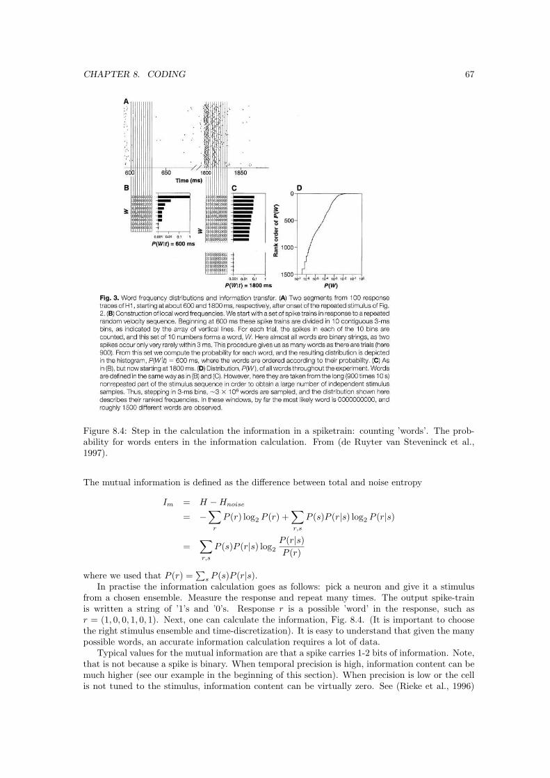
CHAPTER 8. CODING 67
Figure 8.4: Step in the calculation the information in a spiketrain: counting ’words’. The prob-ability for words enters in the information calculation. From (de Ruyter van Steveninck et al.,1997).
The mutual information is defined as the difference between total and noise entropy
Im = H −Hnoise
= −∑
r
P (r) log2 P (r) +∑r,s
P (s)P (r|s) log2 P (r|s)
=∑r,s
P (s)P (r|s) log2
P (r|s)P (r)
where we used that P (r) =∑
s P (s)P (r|s).In practise the information calculation goes as follows: pick a neuron and give it a stimulus
from a chosen ensemble. Measure the response and repeat many times. The output spike-trainis written a string of ’1’s and ’0’s. Response r is a possible ’word’ in the response, such asr = (1, 0, 0, 1, 0, 1). Next, one can calculate the information, Fig. 8.4. (It is important to choosethe right stimulus ensemble and time-discretization). It is easy to understand that given the manypossible words, an accurate information calculation requires a lot of data.
Typical values for the mutual information are that a spike carries 1-2 bits of information. Note,that is not because a spike is binary. When temporal precision is high, information content can bemuch higher (see our example in the beginning of this section). When precision is low or the cellis not tuned to the stimulus, information content can be virtually zero. See (Rieke et al., 1996)

CHAPTER 8. CODING 68
for a good treatment of coding, reconstruction and information theory.
8.5 Correlated activity and synchronisation
In our discussion of population coding we considered the firing of neurons as independent. However,this need not be the case in general.
Suppose one measures the spike count over a few hundred ms in response to some stimulus.Repeated over many trials one finds a certain mean count and some variation. However, thisvariation is not independent from cell to cell: if cell A is firing at a higher frequency than normal,cell B is likely to be more active as well. This is called noise correlation. It could simply bedue to both neurons receiving the same noisy input. A typical values for the correlation coefficientfor neuron which have a similar receptive field is r = 0.2 (for 200ms time-bins) (Zohary, Shadlen,and Newsome, 1994). If fluctuations were independent between neurons they could be averageout by collecting signal from many neurons. However, the presence of correlations will limit theamount of averaging one can do, and thus worsens the stimulus estimate (decrease in the Fisherinformation).5
However, tight correlation could also signal something and in some cases precise correlatedfiring was found between neurons. This synchronisation does not need to be stimulus locked,so only if one measures two neurons simultaneously one has a chance to observe it. Singer andco-workers have proposed that synchronisation might be help for solving the binding problem.
The binding problem is the following: suppose our monkey observes a banana on the lefton the screen, and an apple on the right. The neural processing streams for form and locationare separated. How does the nervous system know that the banana is left? It seems that thebrain could easily confuse the stimulus attributes. However, we seldom have such experiences inlife. Similarly, when an moving object is partially occluded, how does the nervous system knowthat disjunct parts can correspond to the same object when shape and motion are processed indifferent brain regions? This is called the binding problem (a whole issue of Neuron was dedicatedto it, good reading). Synchrony could provide a tag to the neural signal, labelling features whichbelong to the same object. In our example all banana attributes (left, yellow, banana) would spikesynchronously, solving the binding problem.
The data in Fig. 8.5 show that under some conditions, peaks arise in the cross-correlationbetween neurons, even though the neurons are far apart. The cross-correlation is defined inanalogy with the autocorrelation. The cross-correlation between spiketrain 1 and spiketrain 2 is
C12(τ) = limT→∞
∫ T
0
dt s1(t)s2(t + τ)
where si(t) is the discretized spiketrain from neuron i.The peak in the cross-correlation is usually quite small, so that it can not not carry much
information. On the other hand if many neurons synchronise, synchrony might provide a verypowerful stimulus to a downstream neuron. Synchronised input to a neuron is often much moreeffective in firing it than uncorrelated input. Using synchronisation is an elegant way to solve thebinding problem. However, evidence is conflictive and precise conditions for synchrony are stilldebated.
In principle information theory techniques can be used to estimate the amount of informationcarried by synchronous spikes, this can help to estimate the importance of synchronous spikes,e.g. (Oram et al., 2000).
5There are very recent theoretical studies which challenge this view...

CHAPTER 8. CODING 69
Figure 8.5: Left: A. Autocorrelation of two cells. B: The cross-correlation shows a peak, despite theneurons being millimetres apart. Right: Data from the same paper, showing that the correlationdepends on the stimulus: disjunct stimuli do not cause synchrony.Left figure from (Dayan andAbbott, 2002) after (Engel, Konig, and Singer, 1991)(?). Right from (Engel, Konig, and Singer,1991)

Chapter 9
Higher visual processing
In this chapter we discuss how the visual cortex further processes the image that is presented tothe monkey. How does the monkey recognise the banana? The answer to this question is notknown yet, but we discuss some interesting properties of the visual cortex.
9.1 The importance of bars and edges
We have seen that retina and LGN cells respond to spots, simple cells in the primary visual cortexrespond to edges, and complex cells respond to bars independent of their spatial phase. Edgesof objects are indeed important in image processing and object recognition. Or from a moreinformation theoretic point of view, edges contain a lot of information: Instead of describing animage using intensity, using just edges can be much more efficient. As a consequence line drawingsare meaningful, Fig. 9.1.
However, although edges are important, it does not mean the visual system throws awayintensity completely. The contrast inverted image in Fig. 9.1 is much less informative, for instanceit becomes hard to guess the emotion in the faces. This means there might be cells which dorespond to intensity; this could be done by a small number of cells. Alternatively, the sign orphase of the edge (dark to light vs. light to dark) is important.
There are interesting problems here: How well can one reconstruct an image from the responsesof the simple cells? Why is making good line drawings so difficult, both for humans and computers?
Figure 9.1: Line drawings by Van Dyck. Top: originals. Below: inverted images. A lot of thesubtlety is lost. If the cortex would interpret the image using only complex cell responses, it wouldbe hard to explain such effects.
70

CHAPTER 9. HIGHER VISUAL PROCESSING 71
Figure 9.2: Attention increases the neuron’s response. Upper curves are with attention (the neuronfires more), lower curves without attention. Left for area MST (a higher motion area) neurons,right for V4 (higher visual area). From (Treue, 2001).
In a line rendering junctions of edges are of special importance. Junctions tell you which objectis in front of which. In contrast, straight or slightly curved lines can be interpolated, and aretherefore somewhat less informative.
9.2 Possible roles of intra-cortical connections
We have discussed that the original Hubel Wiesel feed-forward model, Fig. 7.7, is roughly correctat least when simple stimuli are presented. We encounter at an old, but intriguing question:what is the role of the many lateral and feedback connections? Most input to a cortical neuronis from lateral and feedback connections and only 20% is due to direct feedforward input. Onerole of the feedback is thought to be attentional effects. With smart experiments one can changethe attentional state of a neuron. One can ask the monkey to detect a small change in a visualstimulus, without allowing it to change its eye-position. Neurons show a stronger response (+20%)when attention is directed to their receptive field, Fig. 9.2. Attention is an interesting phenomenonbecause it has to be a feedback effect.
Also contextual effects might be mediated through lateral or feedback connections. Usuallyfairly simple stimuli are presented in studying the visual system, but when more complex stimuliare presented sometimes effects of parts of the image which fall outside the receptive field areobserved (von der Heydt, Peterhans, and Baumgartner, 1984). An example is shown in Fig. 9.3.We have seen that in lower visual areas there is usually a centre-surround layout of the receptivefield, however for higher order stimuli the story is more complex. The response of the cells can benon-linear, as in the figure, so that the interpretation in terms of linear filters is fraud.
These effects are difficult to study: The stimulus space is gigantic: you should think of alldifferent 1000x1000 pixels colour images one can construct... Such a large stimuli space makes itdifficult to see which stimulus is optimal for a neuron and how stimuli interact. Secondly, andrelated to the first point, the shown contextual effect only appear for certain (low) contrasts. Butthese contextual effects might very well be important in explaining certain aspects of perception,Fig. 9.3, right.
9.3 Higher visual areas
From the primary visual cortex the visual signal goes to higher order areas. There seem to betwo main pathways: one involved with the location of the object (the ’where’ pathway or dorsalpathway). The other pathway is concerned with the identity of the object (the ’what’ pathway ortemporal pathway). In our task, both pathways will be important. The monkey has to recognisethe object and know its location. How precisely this information is linked is not known (see 8).Here we will look into the ’what’ pathway.

CHAPTER 9. HIGHER VISUAL PROCESSING 72
Figure 9.3: Contextual effects in V1. Left: non-linear interaction of centre stimuli and its context.The response to both centre and co-linear segment is much stronger than either parts alone.Right: The interactions in the vertical direction of the grey scale plots are excitatory, in thepercept they lead to line completion. The interactions in the horizontal direction are inhibitory(parallel lines). Perceptually such interaction can cause pop-out of connected structures (B andC). From (Kapadia, Westheimer, and Gilbert, 2000).
In the early visual system the receptive fields are simple, and in the higher visual areas theybecome more complex. This suggests there is a hierarchical stack of processing layers (perhapssome 10 stages) in which the image is processed more and more until in the end a grandmother cellpops up. The speed by which visual images are processed is very quick. Even complicated naturalscenes are processed very fast: categorisation whether an image contains an animal or not is donein some 150 ms (Thorpe, Fize, and Marlot, 1996). Of course, we knew this result approximatelyfrom daily life, but this figure stresses the computational demands in visual processing.
The anatomy indicates that there is no strict hierarchy in the processing stages, instead manycross and feedback connections exist. On the other hand man-made simple object recognitionmodels often operate exclusively in a feed-forward mode (Fukushima, 1980; Riesenhuber andPoggio, 1999). It seems that there is in principle no operation that a recurrent net could do thata feed-forward net could not do (given an arbitrary set of time delays). Therefore the question isperhaps: ’how do recurrent connections make the network more efficient?’,
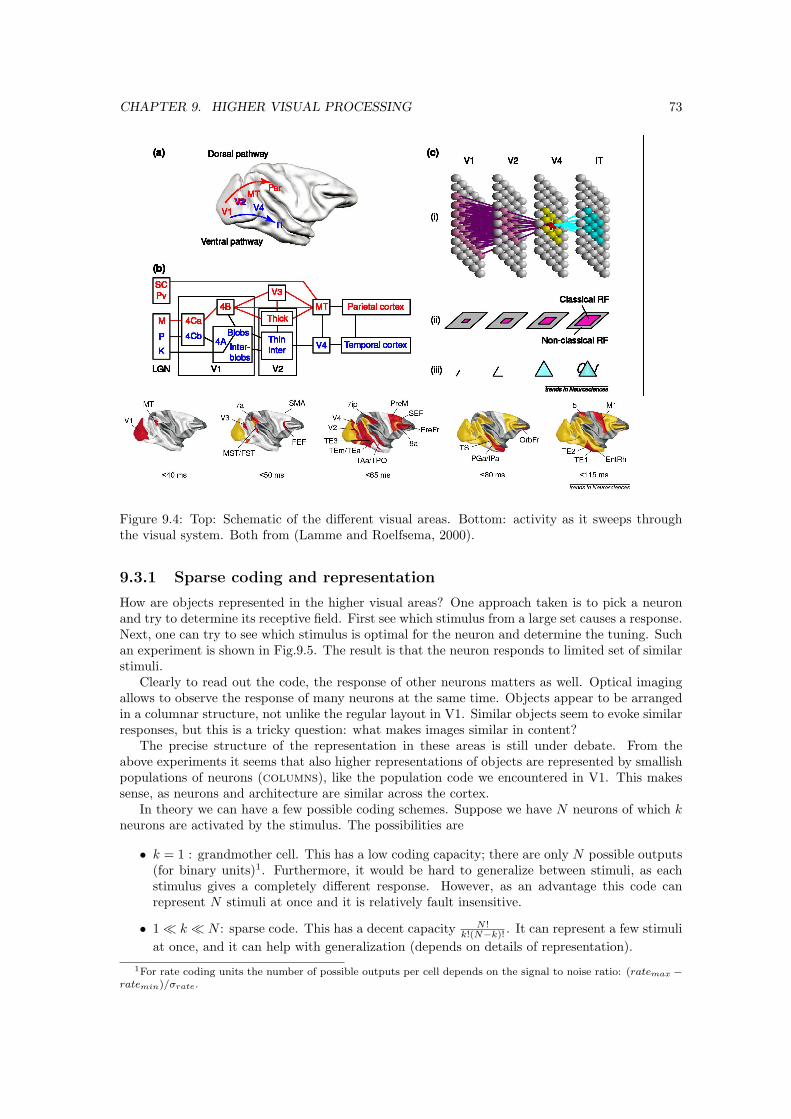
CHAPTER 9. HIGHER VISUAL PROCESSING 73
Figure 9.4: Top: Schematic of the different visual areas. Bottom: activity as it sweeps throughthe visual system. Both from (Lamme and Roelfsema, 2000).
9.3.1 Sparse coding and representation
How are objects represented in the higher visual areas? One approach taken is to pick a neuronand try to determine its receptive field. First see which stimulus from a large set causes a response.Next, one can try to see which stimulus is optimal for the neuron and determine the tuning. Suchan experiment is shown in Fig.9.5. The result is that the neuron responds to limited set of similarstimuli.
Clearly to read out the code, the response of other neurons matters as well. Optical imagingallows to observe the response of many neurons at the same time. Objects appear to be arrangedin a columnar structure, not unlike the regular layout in V1. Similar objects seem to evoke similarresponses, but this is a tricky question: what makes images similar in content?
The precise structure of the representation in these areas is still under debate. From theabove experiments it seems that also higher representations of objects are represented by smallishpopulations of neurons (columns), like the population code we encountered in V1. This makessense, as neurons and architecture are similar across the cortex.
In theory we can have a few possible coding schemes. Suppose we have N neurons of which kneurons are activated by the stimulus. The possibilities are
• k = 1 : grandmother cell. This has a low coding capacity; there are only N possible outputs(for binary units)1. Furthermore, it would be hard to generalize between stimuli, as eachstimulus gives a completely different response. However, as an advantage this code canrepresent N stimuli at once and it is relatively fault insensitive.
• 1 ¿ k ¿ N : sparse code. This has a decent capacity N !k!(N−k)! . It can represent a few stimuli
at once, and it can help with generalization (depends on details of representation).
1For rate coding units the number of possible outputs per cell depends on the signal to noise ratio: (ratemax −ratemin)/σrate.
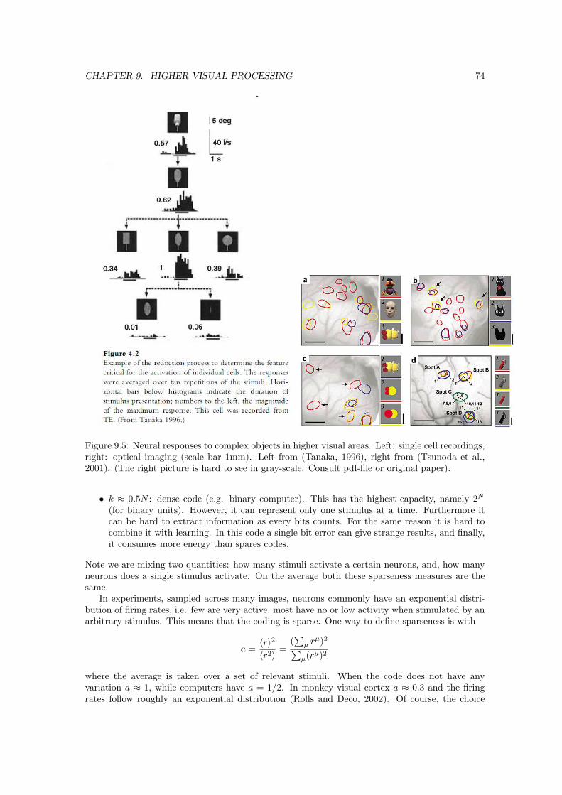
CHAPTER 9. HIGHER VISUAL PROCESSING 74
Figure 9.5: Neural responses to complex objects in higher visual areas. Left: single cell recordings,right: optical imaging (scale bar 1mm). Left from (Tanaka, 1996), right from (Tsunoda et al.,2001). (The right picture is hard to see in gray-scale. Consult pdf-file or original paper).
• k ≈ 0.5N : dense code (e.g. binary computer). This has the highest capacity, namely 2N
(for binary units). However, it can represent only one stimulus at a time. Furthermore itcan be hard to extract information as every bits counts. For the same reason it is hard tocombine it with learning. In this code a single bit error can give strange results, and finally,it consumes more energy than spares codes.
Note we are mixing two quantities: how many stimuli activate a certain neurons, and, how manyneurons does a single stimulus activate. On the average both these sparseness measures are thesame.
In experiments, sampled across many images, neurons commonly have an exponential distri-bution of firing rates, i.e. few are very active, most have no or low activity when stimulated by anarbitrary stimulus. This means that the coding is sparse. One way to define sparseness is with
a =〈r〉2〈r2〉 =
(∑
µ rµ)2∑µ(rµ)2
where the average is taken over a set of relevant stimuli. When the code does not have anyvariation a ≈ 1, while computers have a = 1/2. In monkey visual cortex a ≈ 0.3 and the firingrates follow roughly an exponential distribution (Rolls and Deco, 2002). Of course, the choice

CHAPTER 9. HIGHER VISUAL PROCESSING 75
of stimulus ensemble is crucial here. In these experiments the code was also independent: eachneuron contributes comparable number of bits. There was not much redundancy, i.e. each extraneuron helped to further identify the face.
This representation of sensory information can be compared to a dictionary in our writtenlanguage. There is a trade-off in our language between having a large dictionary of very precisewords where a single word can say all, or a smaller dictionary with less precise words in whichmore words are needed. In this analogy the receptive fields of the neurons are the words in thedictionary, the stimuli (sentences or stories) are represented by a combination of neurons (words).(Also compare to our discussion of hyper-acuity.)
Another reason why sparse representations are used might be related to minimising energyconsumption. The brain demands some 20% of the body’s total oxygen and energy at rest (about20 watts). Some models include this constraint to help to explain the observed representations(Stemmler and Koch, 1999).
So the consensus is that the coding in the brain is Sparse and distributed. The fact thatthe code is sparse and distributed still leaves many possibilities (check for yourself). It would bepossible that the neurons have some random, yet sparse code. This appears not to be the case:1) for each stimulus, the neurons represent some stimulus feature consistently. (Although this isharder to verify in higher areas)2) nearby neurons have similar tuning properties.3) the information is the neurons is not redundant (see above), because the responses are inde-pendent and partly overlapping.
9.3.2 Connectivity and computation
How do the activity patterns in the visual cortex help us in understanding the computations?Unfortunately, knowing the activity patterns in the cortex, does not tell us how the computationsare implemented, or, in other words, how the cells are wired up. This is maybe the most challengingquestion in neurophysiology: how to extract computation from activity. (This is like the problemwith fMRI data.) A few techniques are currently used to measure the inputs to cells:
• Intracellular recording in vivo. This in principle allows to measure both excitatory andinhibitory inputs to a certain cell. However, technical problems, such as a bad space-clampmake this difficult.
• Multi-unit extracellular recording. In principle cross-correlations between neurons can beused to figure out connections. However, without more information correlations are hard tointerpret. Suppose two cells are found to have a strong correlation. Is this because theyreceive common input, or does one provide input to the other? In addition, stationarity canbe a problem and can cause spurious correlations.
• Anatomy can be very useful as well, but it is very labour intensive.
9.4 Plasticity
The visual cortex is remarkably plastic and has an enormous storage capacity. After passivelywatching thousands of images, people can tell which one they have seen and which ones theydidn’t when tested later. All this information must be stored somewhere, most likely in visualcortex.
Indeed, the response of the neurons changes as monkeys becomes familiar with images, evenwhen the monkeys have to do nothing but passively view them (Erickson, Jagadeesh, and Desi-mone, 2000). In another experiment monkeys were trained to do image pairing tasks. It was foundthat cells pick up rather the pairing between the images rather than similarities in the shape of theimages (Sakai and Miyashita, 1991). These experiments show that the representation of objects

CHAPTER 9. HIGHER VISUAL PROCESSING 76
is in a constant state of flux. It is surprising that the changes can be large, and do not lead thedegradation of older memories.
More reading: (Rolls and Deco, 2002)
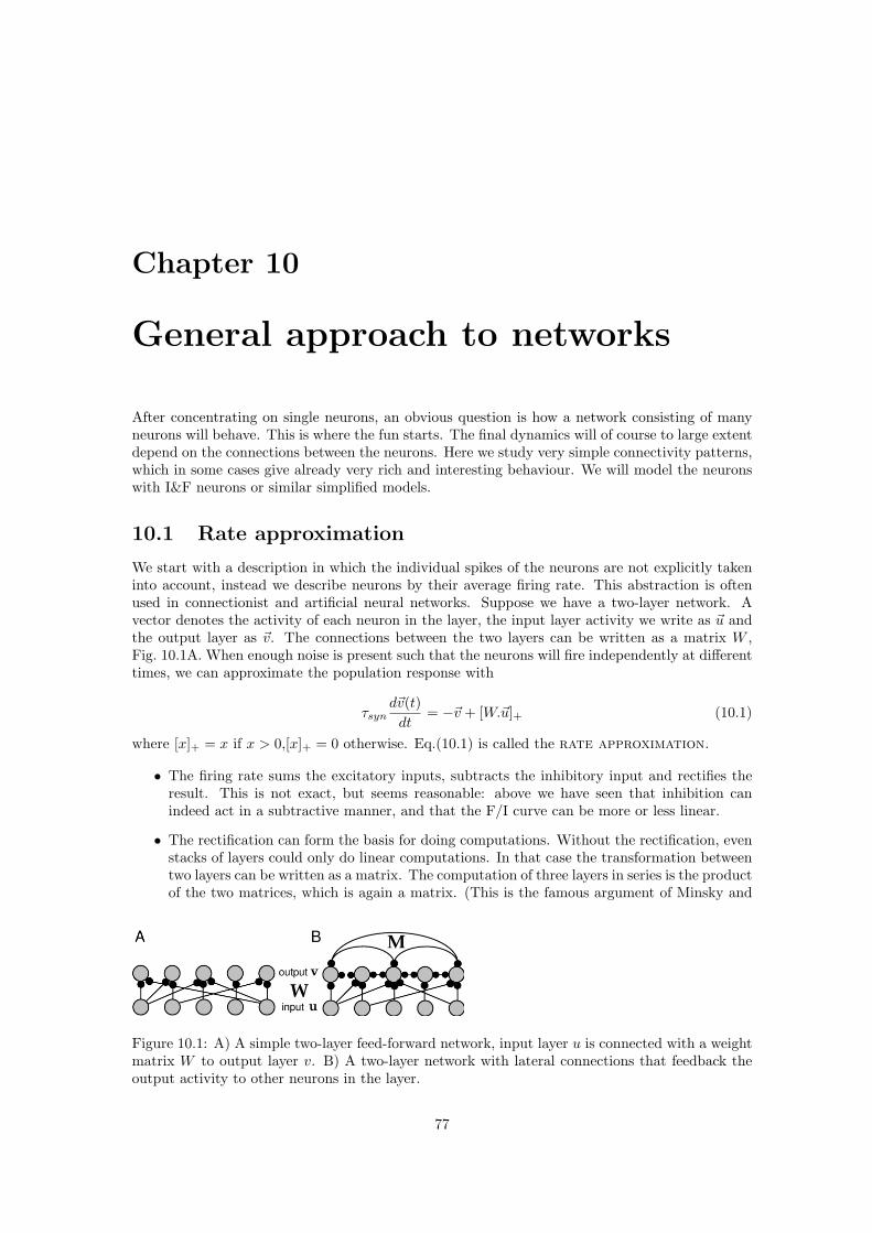
Chapter 10
General approach to networks
After concentrating on single neurons, an obvious question is how a network consisting of manyneurons will behave. This is where the fun starts. The final dynamics will of course to large extentdepend on the connections between the neurons. Here we study very simple connectivity patterns,which in some cases give already very rich and interesting behaviour. We will model the neuronswith I&F neurons or similar simplified models.
10.1 Rate approximation
We start with a description in which the individual spikes of the neurons are not explicitly takeninto account, instead we describe neurons by their average firing rate. This abstraction is oftenused in connectionist and artificial neural networks. Suppose we have a two-layer network. Avector denotes the activity of each neuron in the layer, the input layer activity we write as ~u andthe output layer as ~v. The connections between the two layers can be written as a matrix W ,Fig. 10.1A. When enough noise is present such that the neurons will fire independently at differenttimes, we can approximate the population response with
τsynd~v(t)dt
= −~v + [W.~u]+ (10.1)
where [x]+ = x if x > 0,[x]+ = 0 otherwise. Eq.(10.1) is called the rate approximation.
• The firing rate sums the excitatory inputs, subtracts the inhibitory input and rectifies theresult. This is not exact, but seems reasonable: above we have seen that inhibition canindeed act in a subtractive manner, and that the F/I curve can be more or less linear.
• The rectification can form the basis for doing computations. Without the rectification, evenstacks of layers could only do linear computations. In that case the transformation betweentwo layers can be written as a matrix. The computation of three layers in series is the productof the two matrices, which is again a matrix. (This is the famous argument of Minsky and
Figure 10.1: A) A simple two-layer feed-forward network, input layer u is connected with a weightmatrix W to output layer v. B) A two-layer network with lateral connections that feedback theoutput activity to other neurons in the layer.
77
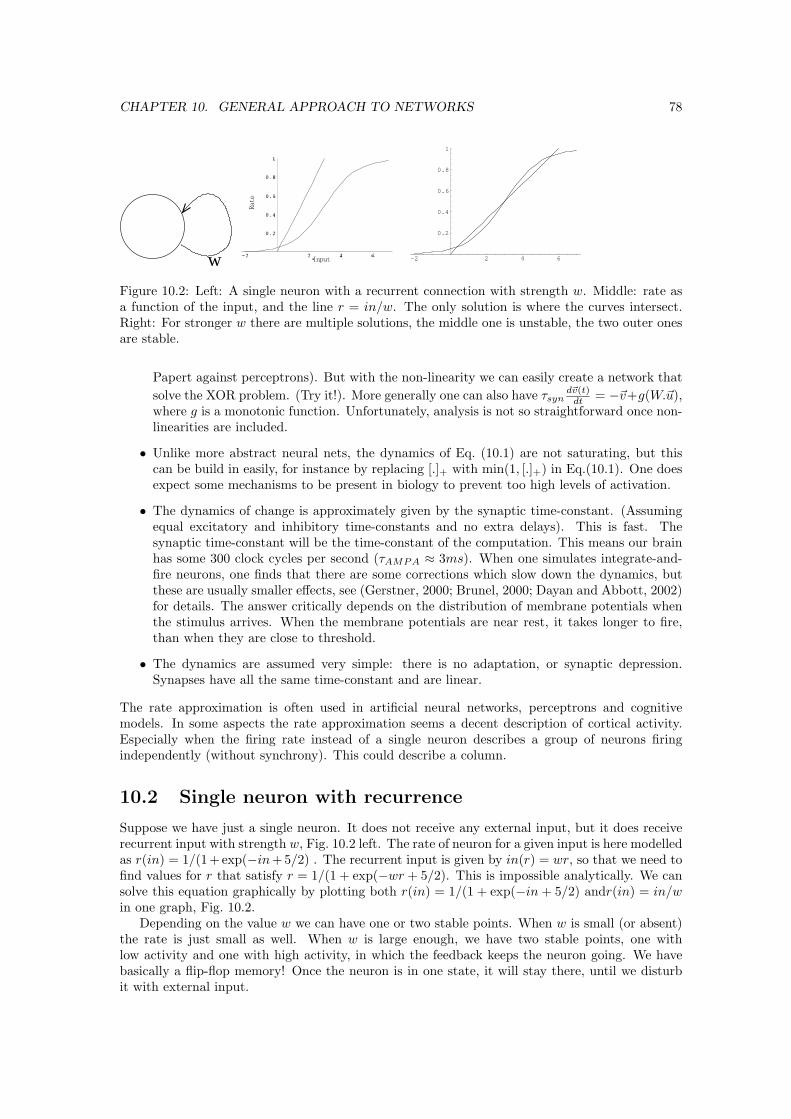
CHAPTER 10. GENERAL APPROACH TO NETWORKS 78
w -2 2 4 6
0.2
0.4
0.6
0.8
1
Figure 10.2: Left: A single neuron with a recurrent connection with strength w. Middle: rate asa function of the input, and the line r = in/w. The only solution is where the curves intersect.Right: For stronger w there are multiple solutions, the middle one is unstable, the two outer onesare stable.
Papert against perceptrons). But with the non-linearity we can easily create a network thatsolve the XOR problem. (Try it!). More generally one can also have τsyn
d~v(t)dt = −~v+g(W.~u),
where g is a monotonic function. Unfortunately, analysis is not so straightforward once non-linearities are included.
• Unlike more abstract neural nets, the dynamics of Eq. (10.1) are not saturating, but thiscan be build in easily, for instance by replacing [.]+ with min(1, [.]+) in Eq.(10.1). One doesexpect some mechanisms to be present in biology to prevent too high levels of activation.
• The dynamics of change is approximately given by the synaptic time-constant. (Assumingequal excitatory and inhibitory time-constants and no extra delays). This is fast. Thesynaptic time-constant will be the time-constant of the computation. This means our brainhas some 300 clock cycles per second (τAMPA ≈ 3ms). When one simulates integrate-and-fire neurons, one finds that there are some corrections which slow down the dynamics, butthese are usually smaller effects, see (Gerstner, 2000; Brunel, 2000; Dayan and Abbott, 2002)for details. The answer critically depends on the distribution of membrane potentials whenthe stimulus arrives. When the membrane potentials are near rest, it takes longer to fire,than when they are close to threshold.
• The dynamics are assumed very simple: there is no adaptation, or synaptic depression.Synapses have all the same time-constant and are linear.
The rate approximation is often used in artificial neural networks, perceptrons and cognitivemodels. In some aspects the rate approximation seems a decent description of cortical activity.Especially when the firing rate instead of a single neuron describes a group of neurons firingindependently (without synchrony). This could describe a column.
10.2 Single neuron with recurrence
Suppose we have just a single neuron. It does not receive any external input, but it does receiverecurrent input with strength w, Fig. 10.2 left. The rate of neuron for a given input is here modelledas r(in) = 1/(1+exp(−in+5/2) . The recurrent input is given by in(r) = wr, so that we need tofind values for r that satisfy r = 1/(1 + exp(−wr + 5/2). This is impossible analytically. We cansolve this equation graphically by plotting both r(in) = 1/(1 + exp(−in + 5/2) andr(in) = in/win one graph, Fig. 10.2.
Depending on the value w we can have one or two stable points. When w is small (or absent)the rate is just small as well. When w is large enough, we have two stable points, one withlow activity and one with high activity, in which the feedback keeps the neuron going. We havebasically a flip-flop memory! Once the neuron is in one state, it will stay there, until we disturbit with external input.
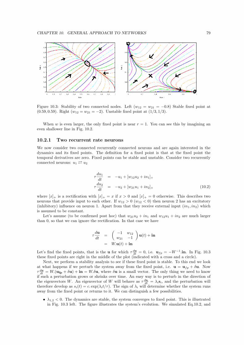
CHAPTER 10. GENERAL APPROACH TO NETWORKS 79
Figure 10.3: Stability of two connected nodes. Left (w12 = w21 = −0.8) Stable fixed point at(0.59, 0.59). Right (w12 = w21 = −2). Unstable fixed point at (1/3, 1/3).
When w is even larger, the only fixed point is near r = 1. You can see this by imagining aneven shallower line in Fig. 10.2.
10.2.1 Two recurrent rate neurons
We now consider two connected recurrently connected neurons and are again interested in thedynamics and its fixed points. The definition for a fixed point is that at the fixed point thetemporal derivatives are zero. Fixed points can be stable and unstable. Consider two recurrentlyconnected neurons: u1 À u2
τdu1
dt= −u1 + [w12u2 + in1]+
τdu2
dt= −u2 + [w21u1 + in2]+ (10.2)
where [x]+ is a rectification with [x]+ = x if x > 0 and [x]+ = 0 otherwise. This describes twoneurons that provide input to each other. If w12 > 0 (w12 < 0) then neuron 2 has an excitatory(inhibitory) influence on neuron 1. Apart from that they receive external input (in1, in2) whichis assumed to be constant.
Let’s assume (to be confirmed post hoc) that w21u2 + in1 and w12u1 + in2 are much largerthan 0, so that we can ignore the rectification. In that case we have
τdudt
=( −1 w12
w21 −1
)u(t) + in
= W.u(t) + in
Let’s find the fixed points, that is the u for which τ dudt = 0, i.e. ufp = −W−1.in. In Fig. 10.3
these fixed points are right in the middle of the plot (indicated with a cross and a circle).Next, we perform a stability analysis to see if these fixed point is stable. To this end we look
at what happens if we perturb the system away from the fixed point, i.e. u = ufp + δu. Nowτ du
dt = W.(ufp + δu) + in = W.δu, where δu is a small vector. The only thing we need to knowif such a perturbation grows or shrinks over time. An easy way is to perturb in the direction ofthe eigenvectors W . An eigenvector of W will behave as τ dsi
dt = λisi, and the perturbation willtherefore develop as si(t) = c. exp(λit/τ). The sign of λi will determine whether the system runsaway from the fixed point or returns to it. We can distinguish a few possibilities.
• λ1,2 < 0. The dynamics are stable, the system converges to fixed point. This is illustratedin Fig. 10.3 left. The figure illustrates the system’s evolution. We simulated Eq.10.2, and
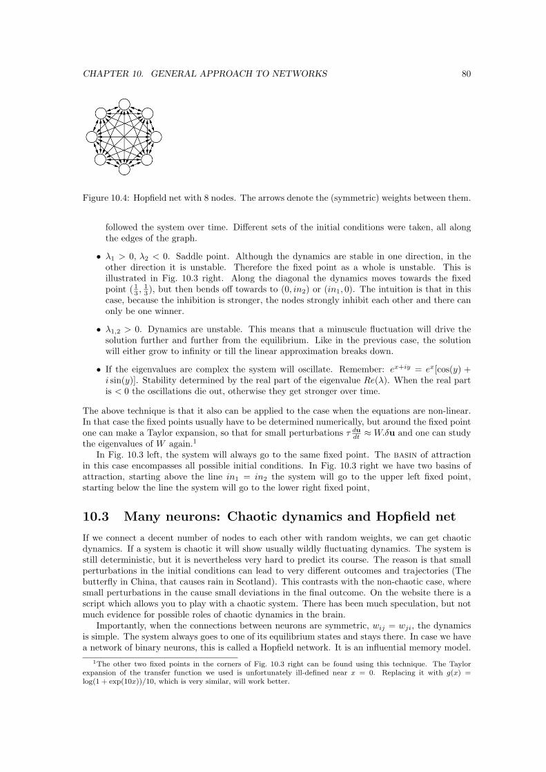
CHAPTER 10. GENERAL APPROACH TO NETWORKS 80
Figure 10.4: Hopfield net with 8 nodes. The arrows denote the (symmetric) weights between them.
followed the system over time. Different sets of the initial conditions were taken, all alongthe edges of the graph.
• λ1 > 0, λ2 < 0. Saddle point. Although the dynamics are stable in one direction, in theother direction it is unstable. Therefore the fixed point as a whole is unstable. This isillustrated in Fig. 10.3 right. Along the diagonal the dynamics moves towards the fixedpoint ( 1
3 , 13 ), but then bends off towards to (0, in2) or (in1, 0). The intuition is that in this
case, because the inhibition is stronger, the nodes strongly inhibit each other and there canonly be one winner.
• λ1,2 > 0. Dynamics are unstable. This means that a minuscule fluctuation will drive thesolution further and further from the equilibrium. Like in the previous case, the solutionwill either grow to infinity or till the linear approximation breaks down.
• If the eigenvalues are complex the system will oscillate. Remember: ex+iy = ex[cos(y) +i sin(y)]. Stability determined by the real part of the eigenvalue Re(λ). When the real partis < 0 the oscillations die out, otherwise they get stronger over time.
The above technique is that it also can be applied to the case when the equations are non-linear.In that case the fixed points usually have to be determined numerically, but around the fixed pointone can make a Taylor expansion, so that for small perturbations τ du
dt ≈ W.δu and one can studythe eigenvalues of W again.1
In Fig. 10.3 left, the system will always go to the same fixed point. The basin of attractionin this case encompasses all possible initial conditions. In Fig. 10.3 right we have two basins ofattraction, starting above the line in1 = in2 the system will go to the upper left fixed point,starting below the line the system will go to the lower right fixed point,
10.3 Many neurons: Chaotic dynamics and Hopfield net
If we connect a decent number of nodes to each other with random weights, we can get chaoticdynamics. If a system is chaotic it will show usually wildly fluctuating dynamics. The system isstill deterministic, but it is nevertheless very hard to predict its course. The reason is that smallperturbations in the initial conditions can lead to very different outcomes and trajectories (Thebutterfly in China, that causes rain in Scotland). This contrasts with the non-chaotic case, wheresmall perturbations in the cause small deviations in the final outcome. On the website there is ascript which allows you to play with a chaotic system. There has been much speculation, but notmuch evidence for possible roles of chaotic dynamics in the brain.
Importantly, when the connections between neurons are symmetric, wij = wji, the dynamicsis simple. The system always goes to one of its equilibrium states and stays there. In case we havea network of binary neurons, this is called a Hopfield network. It is an influential memory model.
1The other two fixed points in the corners of Fig. 10.3 right can be found using this technique. The Taylorexpansion of the transfer function we used is unfortunately ill-defined near x = 0. Replacing it with g(x) =log(1 + exp(10x))/10, which is very similar, will work better.

CHAPTER 10. GENERAL APPROACH TO NETWORKS 81
attractor state
attractor basin
ener
gy
state xsta
te y
Figure 10.5:Left: Whenever the network starts in a state close enough to an attractor, it will ’fall in the hole’and reach the attractor state.Middle: Multiple attractor are present in the network, each with their own basin of attraction.Each corresponds to a different memory.Right: Pattern completion in a Hopfield network. The network is trained on the rightmost images.Each time the leftmost (distorted) input is given, the network evolves via the intermediate stateto the stored state. These different image can all be stored in the same network. From Hertz.
The Hopfield network can store multiple binary patterns with a simple learning rule. The weightbetween node i and j should be set according to the rule wij =
∑µ pµ
i pµj , where pµ
i is a binary bit(±1) representing entry i for pattern µ.
Each stored pattern will correspond to a stable fixed point, or attractor state, see Fig. 10.5.However, the storage capacity of the network is limited. As we increase number of stored patterns,the memories states becomes unstable. Stable mixed states appear. At the critical amount ofstorage, performance decreases suddenly. The network will still equilibrate, but it will end up inspurious attractor states rather than in the memory states it was suppose to find. The numbersof patterns we can store is proportional to the number of nodes, nstored = αn where α is calledthe capacity. Simulation and statistical physics gives αcn = 0.138n. Hence a network with 100nodes can store about 14 patterns. Many more details can be found in (Hertz, Krogh, and Palmer,1991).
This is called an auto-associative memory: Presenting a partial stimulus leads to a recallof the full memory, see Fig. 10.5. Auto-associative memories are very different from computermemory (a bit like Google ...).
10.4 Single recurrent layer
We return to slightly simpler architectures. The next complication one can consider is to allowlateral or recurrent connections, Fig. 10.1. The equation for v becomes
τdv
dt= −v + [W.u + M.v]+
where M is the matrix describing the recurrent connections. An interesting application of thismodel has been to explain contrast invariant tuning curves(Ben-Yishai, Bar-Or, and Sompolinsky,1995). Although as mentioned above, there is now doubt that this is the correct model explainingcontrast invariant tuning curves, it is still worth a study.

CHAPTER 10. GENERAL APPROACH TO NETWORKS 82
Figure 10.6: Recurrent model of simple cells in V1. Left: input to the network, which can be veryweakly tuned. Middle: The network output is strongly tuned. Right: experimental data from V1.Figure from (Dayan and Abbott, 2002).
The model describes a population of simple cells with their preferred angle θ = −π/2...π/2.Rather than specifying u and W , the network receives an input h (i.e. h = W.u), which isparameterised as
h(θ) = Ac[1 + ε(−1 + cos(2θ))]
where A describes the amplitude, c the stimulus contrast, and ε the amount of tuning of theinput. We label the neurons v with the angular variable θ. The lateral interaction is describedwith two parameters λ0, which describes uniform inhibition and λ1 which gives the strength oftuned excitation. So the full equation is (the sum can be written as an integral):
τdv(θ)
dt= −v(θ) +
[h(θ) +
∫ π/2
−π/2
dθ′
π−λ0 + λ1cos(2θ − 2θ′) v(θ′)
]
+
If the network were linear, the output of the network would smoothly depend on the input param-eters. However, in this model, because of the rectification, excitation is not always counteractedby the uniform inhibition: a silent neuron can not inhibit... The effect is that when the input isweakly tuned (or not tuned at all!), the output of the network can be much sharper, amplifyingthe differences in the input, Fig. 10.6.
Importantly, the width of the tuning curves becomes almost independent of the input ’sharp-ness’. This way the recurrent model explains the iceberg effect.2
2Note, that the firing threshold in this model is zero, unlike in the discussion of the iceberg effect above, section7.2.2. This does not change the behaviour of the model.
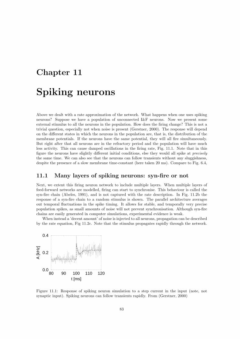
Chapter 11
Spiking neurons
Above we dealt with a rate approximation of the network. What happens when one uses spikingneurons? Suppose we have a population of unconnected I&F neurons. Now we present someexternal stimulus to all the neurons in the population. How does the firing change? This is not atrivial question, especially not when noise is present (Gerstner, 2000). The response will dependon the different states in which the neurons in the population are, that is, the distribution of themembrane potentials. If the neurons have the same potential, they will all fire simultaneously.But right after that all neurons are in the refractory period and the population will have muchless activity. This can cause damped oscillations in the firing rate, Fig. 11.1. Note that in thisfigure the neurons have slightly different initial conditions, else they would all spike at preciselythe same time. We can also see that the neurons can follow transients without any sluggishness,despite the presence of a slow membrane time-constant (here taken 20 ms). Compare to Fig. 6.4,
11.1 Many layers of spiking neurons: syn-fire or not
Next, we extent this firing neuron network to include multiple layers. When multiple layers offeed-forward networks are modelled, firing can start to synchronise. This behaviour is called thesyn-fire chain (Abeles, 1991), and is not captured with the rate description. In Fig. 11.2b theresponse of a syn-fire chain to a random stimulus is shown. The parallel architecture averagesout temporal fluctuations in the spike timing. It allows for stable, and temporally very precisepopulation spikes, as small amounts of noise will not prevent synchronisation. Although syn-firechains are easily generated in computer simulations, experimental evidence is weak.
When instead a ’decent amount’ of noise is injected to all neurons, propagation can be describedby the rate equation, Fig 11.2c. Note that the stimulus propagates rapidly through the network.
80 90 100 110 120t [ms]
0.0
0.2
0.4
A [k
Hz]
Figure 11.1: Response of spiking neuron simulation to a step current in the input (note, notsynaptic input). Spiking neurons can follow transients rapidly. From (Gerstner, 2000)
83

CHAPTER 11. SPIKING NEURONS 84
Figure 11.2: Propagation of a current stimulus through a layered feed-forward network. a) Archi-tecture of the network: 10 layers with 20 integrate-and-fire neurons per layer (5 neurons shown),all-to-all connectivity. b) Syn-fire behaviour: without noise the neurons strongly synchronise. c)But if the neurons are noisy, firing rates can propagate rapidly through layered networks withoutmuch distortion. From (van Rossum, Turrigiano, and Nelson, 2002).
The speed of the propagation helps to explain why one can do such fast processing of, for instance,visual stimuli. The tendency to synchronise is counteracted by the noise and by the synapses whichact as a filter between the layers, removing sharp transients.
It might be possible that in vivo a subset of neurons propagates information using a syn-firemode, whereas the population as a whole appears to be asynchronous. This could have interestingcomputational effects. The existence of such situations would be very hard to verify as one has tomeasure the possibly very small subset of neurons.
11.2 Spiking recurrent networks
Above we dealt with a feed-forward network, the other extreme of modelling is a recurrent networkreceiving constant input (the real brain should be somewhere between these two approaches...)What happens to such a recurrent network, does any interesting activity emerge? When neuronsare connected in an all-to-all fashion and little or no noise is present, the network easily settlesinto a state of global high frequency oscillation or complete quiescence. (Easy to simulate). Thismight relevant in the study of epilepsy or dead, respectively, but it does not reflect the normalstate of the brain.
More realistically, the probability for connections between two arbitrarily chosen neurons issmall. This is called a sparsely connected network. Secondly, inhibition should be incorporated.Interestingly, these networks have a whole range of possible stable states, including a randomlyfiring low-activity state (van Vreeswijk and Sompolinsky, 1996).
The possible states can be analysed by a Fokker-Planck equation for the membrane potential,much like we have seen for the noisy integrate and fire neuron. But here the firing rate of thenetwork is fed back into the network: a self-consistent approach (Brunel, 2000). This way one canfind the conditions for an asynchronous state. The oscillation regimes can be found by perturbing

CHAPTER 11. SPIKING NEURONS 85
Figure 11.3: Possible states of activity in a recurrent network of I&F neurons.From (Brunel, 2000).
the asynchronous state. These studies can then be confirmed in simulations.In Fig. 11.3 the various possible states of a sparse, recurrent network are shown. The x-axis
gives the ratio between recurrent inhibition and recurrent excitation, the y-axis represent the ex-ternal input to the network. When recurrent inhibition is weak, oscillatory high activity statesdevelop. When inhibition is strong enough however (on the right side in the figure), chaotic firingoccurs. The global activity, which shows up in EEGs or field potentials, can still be oscillatory,but individual neurons don’t fire every cycle (top right). This is much like what is seen in hip-pocampal rhythms. The state AI could correspond to cortical activity, with neurons showing lowasynchronous background activity.
11.3 Spiking working memory
In our task the monkey has to remember where the banana was, i.e. it needs a working memory.There are cells in the pre-frontal cortex which fire selectively during such working memory tasks.An example of such a cell is shown in Fig. 11.4. Note that this cell is most active in the absenceof the stimulus, this is presumably due to recurrent input. When the monkey has to rememberthe spatial location of the banana, the cells show a tuning related to the location. But given theflexible role of the pre-frontal cortex, the encoding is probably much more general than that.
Networks with persistent activity need recurrent excitation. As one starts to model suchnetworks (for instance with I&F neurons) one finds that is not easy to have a memory statewhich has relatively low activity, and no synchronisation. One can achieve such by applying theobservations above: having large, sparsely connected networks with excitation and inhibition andincluding enough external noise. As the time-constant for the dynamics is typically given by the

CHAPTER 11. SPIKING NEURONS 86
Figure 11.4: Working memory in pre-frontal cortex. A stimulus was presented (onset and offsetmarked by the two leftmost vertical bars). The monkey had to remember this location for twoseconds. After this the monkey had to make an eye-movement (final bar). The neurons have (inthis case) a spatial tuning function. From(Funahashi, Bruce, and Goldman-Rakic, 1998).
synaptic time-constant, using a lot of NMDA will help to stabilise the network. See (Compte etal., 2000) for a recent model of a working memory network.
As is, the task the money performs could in principle be done by an advanced computer visionsystem, if we program it correctly. One of the interesting issues is how the monkey learns how topay attention to the banana and remember its location. If we would change the task to reward onlymovements to red objects, the monkey could learn this, and the cells in the working memory wouldencode different information. How this interaction between reward, attention, and the dynamicchange in pathway works is not known. It is good to look back at Chapter 1, Fig. 1.2 for examplesof pre-frontal damage.
11.4 Spiking neurons: Attractor states
In the above networks, the activity settles dynamically into a memory state where activity persistsin some neurons, although the stimulus is only transiently present. The final state of the network iscalled an attractor state. Attractor states can be seen as memory states. The best known exampleis the Hopfield net. In the Hopfield network memories are stored in attractor states. When anincomplete memory is presented, the network state will (hopefully) relax into the attractor state,and the memory is retrieved. Whether this is how associative memory really works is not known.
The analysis of spiking recurrent networks can be extended to include several point attrac-tors (discrete memories). This can be achieved by creating subpopulations in the network, whichhave stronger connections among themselves (w+ in Fig. 11.5) than connections between subpop-ulations (w−). To represent ’unknown’ or non-memorized input, one can create a point attractorwith a large basin of attraction corresponding to spontaneous activity, Fig. 11.5. Once activityreaches a point attractor state, it will be very stable (assuming adaptation is absent!).
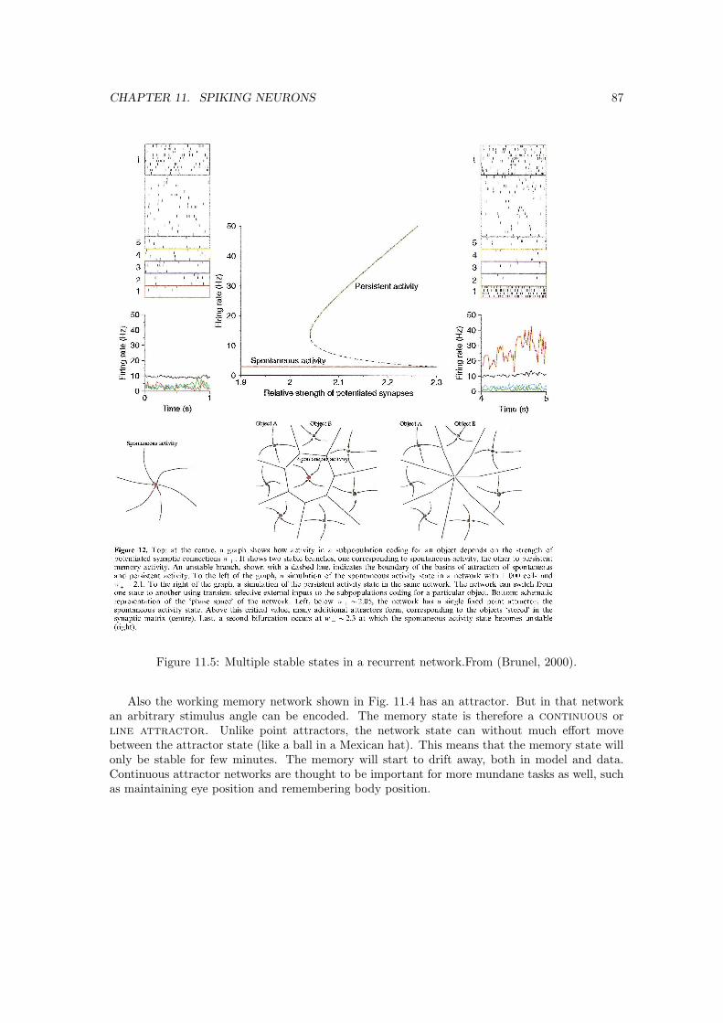
CHAPTER 11. SPIKING NEURONS 87
Figure 11.5: Multiple stable states in a recurrent network.From (Brunel, 2000).
Also the working memory network shown in Fig. 11.4 has an attractor. But in that networkan arbitrary stimulus angle can be encoded. The memory state is therefore a continuous orline attractor. Unlike point attractors, the network state can without much effort movebetween the attractor state (like a ball in a Mexican hat). This means that the memory state willonly be stable for few minutes. The memory will start to drift away, both in model and data.Continuous attractor networks are thought to be important for more mundane tasks as well, suchas maintaining eye position and remembering body position.

Chapter 12
Making decisions
In many instances a task involves making a decision: an eye-movement, a bar press, or a reportto the researcher. And also in real life decisions need to be made. Also our monkey has to decidewhere to move the joystick. It is therefore important to know how the decision is made and howerrors in the decision relate to the underlying quantities.
The most simple case for a decision with noise is a yes/no decision between Gaussian distributedquantities with an equal standard deviation. The errors in the decision are called false positives(saying yes when the answer was no) and false negatives (saying no when the answer is yes). Theerror rates will depend on the width of the distribution and their distance. By changing thethreshold, the trade-off between false positives and false negatives can be changed. This way onecreates the so called receiver operator characteristic, or roc curve.
The variability in the quantities can either come from the stimulus (for instance when thestimulus is very dim and photon noise matters) or from the nervous system itself (for instancewhen you try to decide to go left or right in a forgotten road). Many stimuli have been developedin which the error can be systematically varied, for instance one can make the stimulus very dim.
Another interesting stimulus is the random moving dots stimulus, Fig. 12.2. In area MT ofthe monkey there are neurons which respond to the (local) motion in their receptive field. Forinstance, the stimulus in the right panel can be a very effective stimulus for such a neuron whenthe motion is in the direction of the neuron’s preferred motion, whereas the stimulus in the leftcauses a much less vigorous response. By changing the coherence of the stimulus, the difficulty
positivesfalse
negativesfalse
x
P(x)
Figure 12.1: Left: principle of deciding between two quantities. Right: ROC curve of the randommoving dots stimulus, described below (the numbers indicate the coherence of the stimulus). Inthe graph 1− β is the false negative rate, α is the false positive rate.
88

CHAPTER 12. MAKING DECISIONS 89
Figure 12.2: Moving random dot stimulus. Left no net motion is apparent. Right: the net motionis apparent. In the middle the nervous system is more challenged.
of the task can be changed and the neural responses varies accordingly. Recording the neuronwhile at the same time measuring actual performance, it was found that the performance of asingle (!) neuron already matched the behaviour of the monkey (Newsome, Britten, and Movshon,1989; Britten et al., 1992). (Note, in these studies it is interesting to study both correct and falseresponses).
How does a certain stimulus and the corresponding firing of a neuron lead to a decision?The neurons in the higher brain regions seem to accumulate evidence until they reach a certainthreshold, Fig. 12.3. Also in psychology there are models for the integration of evidence (Ratcliffand Rouder, 1998). How do noise, error rate and reaction time relate? Integration of signal in thepresence of noise is something we have encountered before: the noisy integrate and fire neuron.Indeed such models give reasonable fits to the distribution of response times. This section is oneof the few cases where human psychology and neuroscience have become closely entangled.
Making decisions is also closely related to rewards. If the decision leads to punishment themonkey should better try something else next time. Recommended reading on the relation toreward (Schall, Stuphorn, and Brown, 2002) and the rest of the special issue of Neuron, Oct.2002.
The activity of the decision neurons (if there are such neurons), reflect not only the integrationof evidence but also the size and probability of the rewards (Platt and Glimcher, 1999). Thismeans that when multiple alternatives for action are available, the neurons can directly competewith each other and the one with highest (expected) reward will win, without the need for adeciding arbiter.
It seems reasonable to assume that decision making involves a close to optimal weighting ofthe evidence. How this is exactly done, is not clear. Many computational challenges remain:how to make good integrators from neurons, how to implement learning, how is the thresholdimplemented, are but a few.
12.1 Motor output
In the final stage of our task our monkey will have to produce motor output. The neurons in themotor cortex are a good example of population codes, e.g. Fig. 8.3. A check of the coding ofthe motor cortex is provided by experiments in which a computer cursor is directly controlled byneural activity (Wessberg et al., 2000). A multi-electrode array is implanted in the monkey’s motorcortex. Suppose the cursor is controlled by a joystick. First the receptive field of the neurons aremeasured during a experimental phase where the arm moves a joystick freely. Next, link betweenthe cursor and the joystick is broken (without the monkey being told), instead the spike ratesof the neurons are used to move the cursor. With tens of neurons a bit unreliable, but usable,motor command can be constructed, Fig. 12.4. Interestingly, with training and visual feedback,the animal can improve performance, and thus steer the responses of the recorded neurons (Taylor,Helms Tillery, and Schwartz, 2002). This means that learning can directly affect the coding inthe motor cortex.

CHAPTER 12. MAKING DECISIONS 90
It is also remarkable that the simplest rate decoding mechanism gives good performance. Soa rate coding scheme accounts for a major part of the information. Although one could arguethat in motor cortex there is no place for more complicated coding schemes, as the output is sendfairly directly to the muscles. At least it seems we are out of the woods. These experiments havepotentially important clinical applications: paralysed patients could potentially control artificiallimbs with brain signals through chronically implanted electrodes.

CHAPTER 12. MAKING DECISIONS 91
Figure 12.3: Left: Climbing of a neural response to threshold. This neuron (in the so-calledfrontal eye field) initiates an eye-movement. The time at which the neuron reaches threshold hasa fixed latency to the eye-movement, and does not have a fixed latency to the stimulus onset. Thisshows that the reaching of threshold is strongly coupled to making the movement. From (Schall,Stuphorn, and Brown, 2002).Right: From (Platt and Glimcher, 1999)..
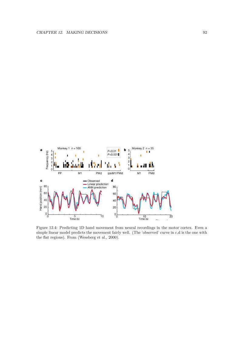
CHAPTER 12. MAKING DECISIONS 92
Figure 12.4: Predicting 1D hand movement from neural recordings in the motor cortex. Even asimple linear model predicts the movement fairly well. (The ’observed’ curve in c,d is the one withthe flat regions). From (Wessberg et al., 2000).
Chapter 13
Hebbian Learning: Rate based
One of the characteristics of the nervous system is that it is not a fixed structure, but it is in aconstant state of change. This plasticity takes places at many different levels and timescales:
1. Development: young brains develop, part by themselves, part helped by sensory signals.This development often goes one way, and damage can only partly be repaired.
2. Throughout life memories are stored, new procedures are invented and stored, new motortasks are learnt. One assumes that such memories are stored in the synaptic weights.
3. Finally, on short time scales (milliseconds to minutes) neurons adapt, especially in the sen-sory systems. This is generally done by biophysical mechanisms and feedback loops.
All these three adaptation mechanisms are a hallmarks of neural computation. Here we focus onthe second form of plasticity, long term synaptic plasticity. It is generally believed that there is notenough genetic information to specify all 1014 synaptic connections and their strengths, insteadsome limited set of rules might be at work. The most famous rule for learning is Hebbian learning.In 1949 Hebb, who was mainly thinking of reverberating loops, stated that:
“When an axon of cell A is near enough to excite cell B or repeatedly or consistently takespart in firing it, some growth or metabolic change takes place in one or both cells such that A’sefficiency, as one of the cells firing B, is increased.”
This remained an unproven theory for a long time, and changes in neural excitability andgenes where also considered as possible memory storage sites. But evidence for Hebbian learninghas now been found in many places in the brain. What remains less clear is whether Hebbianlearning, as we shall shortly describe it, explain all forms of learning. Neuro-psychological casestudies show that different memory systems exist. The different situations quickly mentionedabove under 2) are all processed in different ‘memory systems’. It is not clear if all use the sameHebbian mechanism. In human memory one distinguishes:
Implicit memory Examples: motor learning, pattern completion. These tasks can be learnedby amnesiacs. Their performance improves, but they will not remember learning it. Implicitmemory has different modalities like explicit memory has (motor, visual, etc.).
Explicit memory The opposite of implicit memory. This is the type of memory that is moreintuitive. It can be divided in two sorts.Semantic memory: Factual knowledge about the world.Episodic memory: Personal events memory. This is the answer to the question “Where wereyou when JFK was killed?”The medial temporal lobe is thought to be the storage site for these episodic memories.
In all learning networks we present input and look how the output of the network develops. We candistinguish supervised from unsupervised learning. In supervised learning we have a certain task
93

CHAPTER 13. HEBBIAN LEARNING: RATE BASED 94
Figure 13.1: Hippocampal plasticity. First, LTP is induced by high frequency extracellular stim-ulation, and 10 minutes later it is partly reversed by low frequency stimulation.From (Dayan andAbbott, 2002).
that we want the network to perform, feedback is given to the network whether the performancewas correct. A good example is a feed-forward network with back-propagation. These networkscan in principle be taught any function between input and output. Essential is the presence ofa hidden layer and some non-linearity in the transfer function. One can argue that supervisedalgorithms are nothing more but a fancy way of curve fitting an input-output relation. This istrue, but the supervised algorithms remain an interesting and inspiring subject.
On an abstract level the brain is certainly able to do supervised learning. However, we willconcentrate mainly on unsupervised learning. Hebbian learning is unsupervised when cell B doesnot receive a feedback signal. Here we research variants of Hebb’s learning rule and see how thenetwork and synaptic weights develop under these rules.
13.1 Rate based plasticity
Experimentally, long term potentiation (LTP) was discovered in hippocampal slice (Bliss andLomo, 1973). A example is shown in Fig. 13.1. LTP can be induced in a number of ways: byhigh frequency extracellular stimulation, by providing input while depolarising the post-synapticmembrane potential, or by inducing pre- and postsynaptic spikes. In the figure one sees that LTPusually decreases partly after induction, but the remainder is known to persist for months!
Although other brain regions show similar plasticity, hippocampus has remained the preferredsystem for studying LTP and its counterpart LTD (long term depression). The hippocampus isan associative shorter term storage in which information is thought to be stored for days or weeks,before it is transferred to the cortex (many details are unknown). In the hippocampus LTP is easyto induce. Furthermore, in the hippocampus the input path and synapses are clearly separatedwhich makes extracellular experiments easier. Testing of hippocampal memory formation can bedone in the Morris water-maze, in which the rat has to remember the location of a submergedplatform in milky water. It can do that by remembering landmarks. In the hippocampus there isfairly good evidence that interfering with LTP, worsens the rat’s performance, see e.g. (Riedel etal., 1999).
Mathematically we describe Hebbian learning as follows. Suppose, there are N inputs neurons,which we label with i = 1..N . The pre-synaptic neurons all connect to one post-synaptic neuron.In the simplest rate approximation, the post-synaptic activity y equals the weighted sum of the
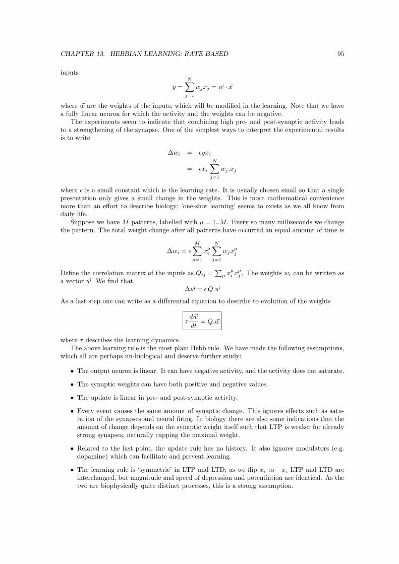
CHAPTER 13. HEBBIAN LEARNING: RATE BASED 95
inputs
y =N∑
j=1
wjxj = ~w · ~x
where ~w are the weights of the inputs, which will be modified in the learning. Note that we havea fully linear neuron for which the activity and the weights can be negative.
The experiments seem to indicate that combining high pre- and post-synaptic activity leadsto a strengthening of the synapse. One of the simplest ways to interpret the experimental resultsis to write
∆wi = εyxi
= εxi
N∑
j=1
wj .xj
where ε is a small constant which is the learning rate. It is usually chosen small so that a singlepresentation only gives a small change in the weights. This is more mathematical conveniencemore than an effort to describe biology; ’one-shot learning’ seems to exists as we all know fromdaily life.
Suppose we have M patterns, labelled with µ = 1..M . Every so many milliseconds we changethe pattern. The total weight change after all patterns have occurred an equal amount of time is
∆wi = ε
M∑µ=1
xµi
N∑
j=1
wjxµj
Define the correlation matrix of the inputs as Qij =∑
µ xµi xµ
j . The weights wi can be written asa vector ~w. We find that
∆~w = ε Q.~w
As a last step one can write as a differential equation to describe to evolution of the weights
τd~w
dt= Q.~w
where τ describes the learning dynamics.The above learning rule is the most plain Hebb rule. We have made the following assumptions,
which all are perhaps un-biological and deserve further study:
• The output neuron is linear. It can have negative activity, and the activity does not saturate.
• The synaptic weights can have both positive and negative values.
• The update is linear in pre- and post-synaptic activity.
• Every event causes the same amount of synaptic change. This ignores effects such as satu-ration of the synapses and neural firing. In biology there are also some indications that theamount of change depends on the synaptic weight itself such that LTP is weaker for alreadystrong synapses, naturally capping the maximal weight.
• Related to the last point, the update rule has no history. It also ignores modulators (e.g.dopamine) which can facilitate and prevent learning.
• The learning rule is ‘symmetric’ in LTP and LTD; as we flip xi to −xi LTP and LTD areinterchanged, but magnitude and speed of depression and potentiation are identical. As thetwo are biophysically quite distinct processes, this is a strong assumption.

CHAPTER 13. HEBBIAN LEARNING: RATE BASED 96
Figure 13.2: Hebbian learning of a neuron with two inputs. A) Two inputs which have strongnegative correlation (each point represents a sample from the input distribution). The inputs arezero-mean. After learning with the plain Hebb rule the weight vector aligns with the data. B)When the data are not zero-mean, the weight vector aligns with the mean. C) In that case thecovariance rule aligns with the data. From (Dayan and Abbott, 2002) and (Hertz, Krogh, andPalmer, 1991).
It is a good exercise to try to investigate variants of the above learning rule for which theseassumptions no longer hold. The effect of many assumptions is unclear.
The correlation matrix Q is a special matrix: It is symmetric and it is positive semi-definite,which means that its eigenvalues are larger or equal than zero. From our discussion of Markov-diagrams we know how the weights are going to evolve:
~w(t) =∑
k
ck ~wkeλkt/τ
where λk is the k-th eigenvalue, with eigenvector ~wk. The coefficients ck are to be solved from theinitial condition −→w (0) =
∑k ck
−→w k. Because the eigenvalues are larger than zero, the weights willrun off to infinity. The reason for this divergence is a positive feedback: when a set of synapsesbecomes potentiated, their weights increase, which causes even more post-synaptic activity, whichpotentiates the synapses even further, etc. As a simple example, suppose that there are threeindependent patterns (0, 0, 10Hz), (0, 20Hz, 0) and (30Hz, 0, 0). The correlation matrix is
proportional to
900 0 00 400 00 0 100
with eigenvalues 900, 400, and 100. When all the weights
are non-zero to start with, the first synapse will eventually become the biggest. More generally,the learning will pick out the pattern which causes most post-synaptic activity, either because theactivity at one input is high or because many inputs are simultaneously active (i.e. correlated).
13.2 Covariance rule
Realistic neurons can only have positive firing rates. If we therefore apply the above rule torate based neurons, synapses can only get potentiated and never be depressed which is of courseproblematic as its leads to higher and higher activity. One can introduce a covariance learningrule (Sejnowski, 1976)
wi = ε(xi − 〈xi〉)(y − 〈y〉)
where 〈xi〉 = 1M
∑µ xµ
i is the activity averaged over the patterns. This is nothing more than theabove rule, but now with Q the covariance matrix Qij =
∑µ(xµ
i − 〈x〉)(xµj − 〈x〉). According to
this rule, the synapse now becomes weaker, if either input or output are below average. Ratheroddly, if both input and output are below average, the synapse becomes stronger as well. Thislatter condition can be removed without much consequences.

CHAPTER 13. HEBBIAN LEARNING: RATE BASED 97
As stated, the learning picks out the inputs with the strongest correlation. These inputs areable to fire the post synaptic cell most and will therefore be enhanced. The unsupervised learningrules perform a principal component analysis on the data. (Below we discuss how to extractmore than one principal component). Principal component analysis projects the data along theeigenvectors of the correlation matrix with the largest eigenvalues, Fig. 13.2. Describing the datathis way is an efficient compression method, we can have many more input dimensions than outputneurons and still have a decent description of the original input. This situation could occur invision. An image has a very high dimension: each pixel is a separate dimensions (to describe animage you need a vector with as many elements as pixels). As we have seen in our discussion ofvisual processing there are many regularities in natural images which can be used to describe themmore succinctly. For instance, neighbouring pixels will be positively correlated. The unsupervisedlearning rules pick up such regularities because they are driven by input correlations.
13.3 Normalisation
As one simulates the above rules, it soon becomes clear that the synaptic weights and the post-synaptic activity run off to un-biologically large values. One can stop learning after a certaintime, or normalisation condition have to be imposed. The precise way one normalises the learning,however, turns out to be of crucial importance for the final weights.
The easiest way is to incorporate a hard limit for each synaptic weight. For instance, 0 < w <wmax. This can already have interesting effects on the dynamics, see Fig. 13.3.
Two other simple ways to constrain the synaptic weight are multiplicative and subtractivescaling. In the first we normalise with a second term which is proportional to the weight itself, inthe second we subtract a constant factor:
τdw
dt= Q.w − γ(w)w(t) = Q.w − [
n.Q.w
n.w]w Multiplicative
= Q.w − ε(w)n = Q.w − [n.Q.w
n.n]n Subtractive
where n is the unit vector, n = (1, 1, 1, ...). You can easily check that in both cases d(n.w)/dt = 0,that is the sum of weights
∑i wi is constant.1Normalisation schemes automatically cause compe-
tition between the synaptic weights: one synapse can only win because the other gets reduced.The subtractive scheme is more competitive than the multiplicative scheme (see Practical). See(Miller and MacKay, 1994) for an full analysis of these schemes.
In biology evidence for homeostasis of synaptic weights has been found (Turrigiano et al.,1998). On long time scales a neuron will try to make sure that it’s activity is not too low or toohigh. It does this by both scaling its synaptic weight (in a multiplicative manner it seems) andby changing the densities of voltage gated channels.
One has introduced the terms hetero-synaptic LTD and homo-synaptic LTD. In hetero-synaptic LTD, synapses depress in the absence input to that synapse (maybe concurrently with thestrengthening of a stimulated input). In homo-synaptic LTD, low pre-synaptic activity is required.With the inclusion of these normalization mechanisms the learning is no longer homo-synaptic(affecting a single synapse only), but hetero-synaptic (a stimulus causes change in not only theassociated synapse, but changes many synapses of the cell).
13.4 Oja’s rule
Oja introduced a rule which automatically picks out the principal component in the inputs andnormalises it. This rule is (Oja, 1982)
∆wi = ε(xiy − wiy2)
1This way of writing the normalisation rules is useful for further analysis. If you just want to simulate learning,it is easier to determine the net weight change at each simulation step and adjust the weights so that their sumremains the same.
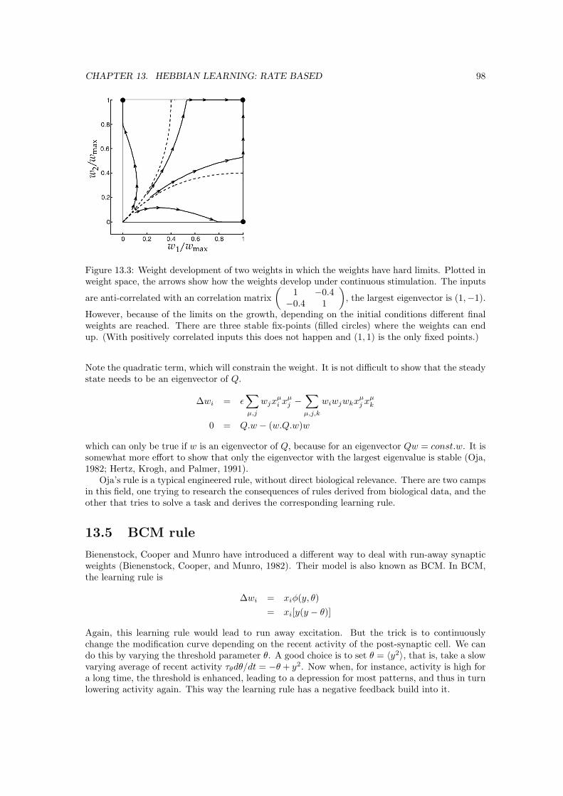
CHAPTER 13. HEBBIAN LEARNING: RATE BASED 98
Figure 13.3: Weight development of two weights in which the weights have hard limits. Plotted inweight space, the arrows show how the weights develop under continuous stimulation. The inputs
are anti-correlated with an correlation matrix(
1 −0.4−0.4 1
), the largest eigenvector is (1,−1).
However, because of the limits on the growth, depending on the initial conditions different finalweights are reached. There are three stable fix-points (filled circles) where the weights can endup. (With positively correlated inputs this does not happen and (1, 1) is the only fixed points.)
Note the quadratic term, which will constrain the weight. It is not difficult to show that the steadystate needs to be an eigenvector of Q.
∆wi = ε∑
µ,j
wjxµi xµ
j −∑
µ,j,k
wiwjwkxµj xµ
k
0 = Q.w − (w.Q.w)w
which can only be true if w is an eigenvector of Q, because for an eigenvector Qw = const.w. It issomewhat more effort to show that only the eigenvector with the largest eigenvalue is stable (Oja,1982; Hertz, Krogh, and Palmer, 1991).
Oja’s rule is a typical engineered rule, without direct biological relevance. There are two campsin this field, one trying to research the consequences of rules derived from biological data, and theother that tries to solve a task and derives the corresponding learning rule.
13.5 BCM rule
Bienenstock, Cooper and Munro have introduced a different way to deal with run-away synapticweights (Bienenstock, Cooper, and Munro, 1982). Their model is also known as BCM. In BCM,the learning rule is
∆wi = xiφ(y, θ)= xi[y(y − θ)]
Again, this learning rule would lead to run away excitation. But the trick is to continuouslychange the modification curve depending on the recent activity of the post-synaptic cell. We cando this by varying the threshold parameter θ. A good choice is to set θ = 〈y2〉, that is, take a slowvarying average of recent activity τθdθ/dt = −θ + y2. Now when, for instance, activity is high fora long time, the threshold is enhanced, leading to a depression for most patterns, and thus in turnlowering activity again. This way the learning rule has a negative feedback build into it.
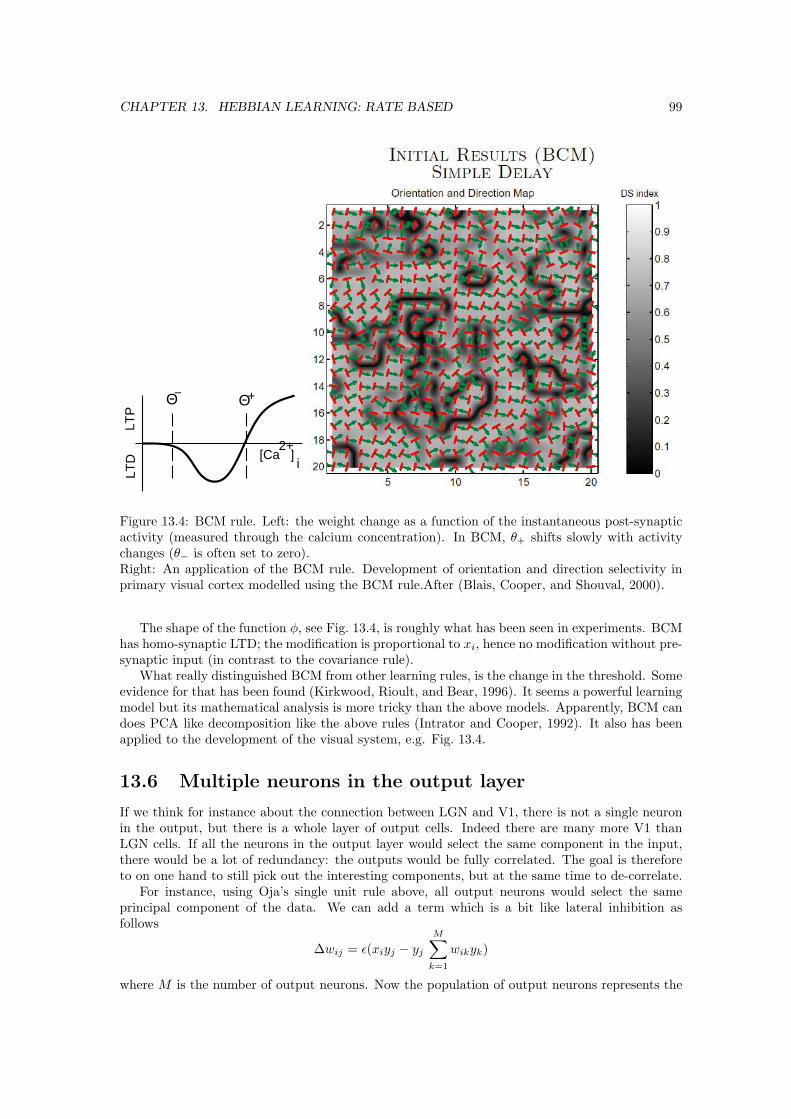
CHAPTER 13. HEBBIAN LEARNING: RATE BASED 99
Θ− Θ+
LTD
LTP
2+i
[Ca ]
Figure 13.4: BCM rule. Left: the weight change as a function of the instantaneous post-synapticactivity (measured through the calcium concentration). In BCM, θ+ shifts slowly with activitychanges (θ− is often set to zero).Right: An application of the BCM rule. Development of orientation and direction selectivity inprimary visual cortex modelled using the BCM rule.After (Blais, Cooper, and Shouval, 2000).
The shape of the function φ, see Fig. 13.4, is roughly what has been seen in experiments. BCMhas homo-synaptic LTD; the modification is proportional to xi, hence no modification without pre-synaptic input (in contrast to the covariance rule).
What really distinguished BCM from other learning rules, is the change in the threshold. Someevidence for that has been found (Kirkwood, Rioult, and Bear, 1996). It seems a powerful learningmodel but its mathematical analysis is more tricky than the above models. Apparently, BCM candoes PCA like decomposition like the above rules (Intrator and Cooper, 1992). It also has beenapplied to the development of the visual system, e.g. Fig. 13.4.
13.6 Multiple neurons in the output layer
If we think for instance about the connection between LGN and V1, there is not a single neuronin the output, but there is a whole layer of output cells. Indeed there are many more V1 thanLGN cells. If all the neurons in the output layer would select the same component in the input,there would be a lot of redundancy: the outputs would be fully correlated. The goal is thereforeto on one hand to still pick out the interesting components, but at the same time to de-correlate.
For instance, using Oja’s single unit rule above, all output neurons would select the sameprincipal component of the data. We can add a term which is a bit like lateral inhibition asfollows
∆wij = ε(xiyj − yj
M∑
k=1
wikyk)
where M is the number of output neurons. Now the population of output neurons represents the

CHAPTER 13. HEBBIAN LEARNING: RATE BASED 100
first M principal components. Another method is Sanger’s rule, which roughly does the samething (Hertz, Krogh, and Palmer, 1991).
Introducing lateral interaction between the neurons to induce competition is of much moregeneral use. Inhibitory interactions reduce the redundancy between the neurons. This is calledcompetitive learning.
In contrast excitatory interactions help to form populations of neurons coding the same stimulusproperties. This decreases the noise associated to a single neuron spike train, increasing reliabilityand reducing integration times. Excitatory interactions do not seem necessary for noiseless, rate-based model neurons. However, when the neurons are noisy, such interactions help to average thesignal. In addition they might perhaps be useful if you want to create population codes with ratebased neurons.
13.7 ICA
PCA uses only first and second order statistics which means it contains only terms suchas 〈xixj〉,〈x2
i 〉. This is because it is based on the correlation matrix. PCA analysis works there-fore best on Gaussian distributed variables. Now the sum of many random numbers tends to aGaussian, so it seems not a bad assumption. (see also the remarks about Fig. 7.6).
However, suppose that we are dealing with a signal in which many variables are mixed and wewant to disentangle them. One way is to make linear combinations of inputs that are explicitly notGaussian distributed, as these combinations are likely to be independent. This can be formulated interms of information theory. This leads to so an extension of PCA, called independent componentanalysis (ICA), see (Bell et al., 1997) (nice read).
The derivation (for noiseless neurons) goes as follows: suppose we have a set of neuron whichhave a sigmoid non-linearity. We can now maximise the mutual information of the output aboutthe input by changing the synaptic weights. For a single neuron this leads to the weights (and anoffset) to be such that the full output range of the neuron is used (much like the retinal adaptationwe described). For multiple neurons the learning rule will de-correlate inputs. A learning rulewhich does this is
∆wij =cof(wji)detW
+ xi(1− 2yj)
where cof(wij) is (−1)i+j times the determinant of the weight matrix W with row i and columnj removed. However, it is not so clear how this would be implemented biologically, as it is a verynon-local rule.
ICA is a more powerful technique than PCA, for instance, it allows the de-mixing of mixedsignals. Suppose that three microphones each record in a room in which three persons are allspeaking simultaneously. The signal of the microphones will be strongly correlated. How can wedisentangle the voices. This is called the cocktail party problem. Applying the ICA algorithmwill de-mix the signals and split the output into the 3 distinct sound sources. Whether this islike what the brain does in auditory processing is not clear, but it is a useful algorithm for signalprocessing such as EEGs. It can also predict reasonably realistic V1 receptive fields, Fig. 13.5.
13.8 Concluding remarks
There is a deep link between information processing and mathematical models of unsupervisedlearning (Linsker, 1992). It would be nice if there were more direct experimental evidence thatshowed that this is what biological Hebbian learning does. It would be interesting to know if thecortex’s goal is to maximise mutual information and that Hebbian learning is just a way to dothat.
Many models can reproduce some organisation structure in the primary visual cortex: mono-ocular dominance columns, orientation columns or simple cell receptive fields. And curiously,from a biological point of view the structure in V1 is perhaps more related to development than

CHAPTER 13. HEBBIAN LEARNING: RATE BASED 101
Figure 13.5: Receptive fields that result from doing PCA on natural images. From(van Haterenand van der Schaaf, 1998).
to learning... It is not so clear how to proceed to construct learning models that do higher levelvision. Not many models have reached beyond V1 and explained the emergence of, say, a face cell.In addition, most models have build in rules and constraints which make sense when formulatingthe model, but have not much experimental support from biology.

Chapter 14
Spike Timing DependentPlasticity
In the previous chapter we looked at plasticity using average firing rates. Recent experiments withother plasticity protocols show that the timing of the spikes turns out to be of critical importancein the induction of LTP and LTD. Using patch clamp recording the pre- and post-synaptic eventcan be precisely timed. Such an experiment is shown in Fig. 14.1. If the pre-synaptic activityprecedes the post-synaptic spike (and the input thus helps to induce the post-synaptic spike),the synapse is strengthened, but if the input lags behind the post-synaptic spike, the synapseis depressed. Thus the modification depends on the precise spike sequence. Note that this inremarkable agreement with Hebb’s statement which implies that the pre-synaptic activity helpsto cause the post-synaptic activity. The surprising part is the LTD condition. It is not clear yetwhether all forms of the rate-based activity can be analysed in terms of this timing dependentplasticity.
Suppose we have one pre-synaptic from neuron i and one post-synaptic spike from neuron j.The simplest way to model this plasticity is to model the plasticity window as an exponentialfunction, and to update the synaptic weight according to
∆wij = A+ exp(−|ti − tj |/τ+) (if ti < tj)= A− exp(−|ti − tj |/τ−) (if tj < ti)
where ti is the pre-synaptic spike-time and tj the post-synaptic spike-time, and A+, A−, τ−, and
pre
post
pre
post
LTP
LTD
1 st∆
Figure 14.1: Left: Protocol for measuring spike time dependent plasticity. Right: Experimentaldata. Changes in synaptic strength after pairing pre- and post-synaptic spikes with 60 repetitionsof pairings at 1Hz. From(Bi and Poo, 1998).
102
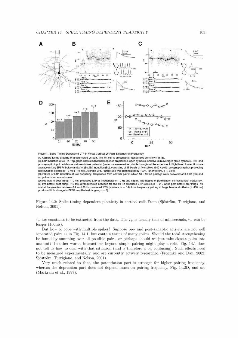
CHAPTER 14. SPIKE TIMING DEPENDENT PLASTICITY 103
Figure 14.2: Spike timing dependent plasticity in cortical cells.From (Sjostrom, Turrigiano, andNelson, 2001).
τ+ are constants to be extracted from the data. The τ+ is usually tens of milliseconds, τ− can belonger (100ms).
But how to cope with multiple spikes? Suppose pre- and post-synaptic activity are not wellseparated pairs as in Fig. 14.1, but contain trains of many spikes. Should the total strengtheningbe found by summing over all possible pairs, or perhaps should we just take closest pairs intoaccount? In other words, interactions beyond simple pairing might play a role. Fig. 14.1 doesnot tell us how to deal with that situation (and is therefore a bit confusing). Such effects needto be measured experimentally, and are currently actively researched (Froemke and Dan, 2002;Sjostrom, Turrigiano, and Nelson, 2001).
Very much related to that, the potentiation part is stronger for higher pairing frequency,whereas the depression part does not depend much on pairing frequency, Fig. 14.2D, and see(Markram et al., 1997).

CHAPTER 14. SPIKE TIMING DEPENDENT PLASTICITY 104
−40 −20 0 20 40 60−80
−60
−40
−20
0
20
Time (ms)
Vo
ltag
e (m
V)
−40 −20 0 20 40 60−80
−60
−40
−20
0
20
Time (ms)
Vo
ltag
e (m
V)
−20 −10 0 10 200
0.2
0.4
0.6
0.8
1
Relative latency
wa/w
max
0 5 10 15 200
0.2
0.4
0.6
0.8
1
Time jitter
wa/w
max
A B
C D
Figure 14.3: Spike timing dependent plasticity prefers early and reliable input. A) Post-synapticspiketrain in response to periodic burst before training. B) After training the neuron respondsearlier to the same input. C) Correspondingly, inputs with the shortest latencies are potentiatedmost. D) In another simulation different jitters were given to the inputs, the inputs with the leastjitter were potentiated.
14.1 Implications of spike timing dependent plasticity
What makes this learning rule different from the rate based learning? We first consider the casethat the inputs have not particular temporal pattern. Again the post-synaptic neuron will pickout the correlated inputs. The rule will pick up correlations on the order of the LTP window, i.e.some 20 ms. Tightly correlated inputs will be potentiated. (Higher order interactions, such asdependence of post-synaptic activity might modify this picture).
As in the rate based case, precautions have to be taken against run away synaptic weights.Either hard bounds can be introduced (Song, Miller, and Abbott, 2000), or the learning rules canbe made converging, a bit like in Oja’s rule (van Rossum, Bi, and Turrigiano, 2000).
Temporal structure of the inputs will be of course important in these learning rules. If westimulate with repeating patterns, the post-synaptic neuron will potentiate the earliest inputs.The reason is that an early input will never come after the post-synaptic spike, and therefore willnot undergo depression. The selection of fastest inputs can be used to shorten navigation routeson a map (Blum and Abbott, 1996). In addition inputs with little jitter are selected above inputswith more jitter, Fig. 14.3D.
Also in a network setting these plasticity models are interesting. They predict an interestingeffect in which the lateral connections at first teach the neighbouring neurons, Fig. 14.4. Thelateral interactions disappear later, their output lags behind feed-forward input, and thus theseconnections are removed.
14.2 Biology of LTP and LTD
Another interesting question is how these time-windows are biophysically engineered. The LTPpart can be roughly understood as follows: 1) synaptic input arrives, opening both fast AMPA and

CHAPTER 14. SPIKE TIMING DEPENDENT PLASTICITY 105
Figure 14.4: Formation of columns and maps under STDP. A) Network diagram. Two layers aresimulated. The input layer contained neurons that fire Poisson trains at different rates and thenetwork layer contained integrate-and-fire neurons. Every neuron in the input layer is randomlyconnected to one fifth of the neurons in the network layer and all the neurons in the network layerare recurrently connected. All synaptic connections are governed by STDP. Input correlations areintroduced by moving a Gaussian hill of activity along the input layer. The Gaussian hill is centredon a random input neuron for a period of time and then shifted to another random location at theend of the period. The length of the period is chosen from an exponential distribution and the timeconstant is similar to the time window of STDP. B) First stage of column formation. Seed placedin the forward connections creates a correlated group of network neurons. C) Second stage ofcolumn formation. Correlated group of networks neurons send out connections to other neuronsin the network. D) Third stage of column formation. Transfer of information from recurrentlayer to feed-forward layer. E) Last stage of column formation. Recurrent connections weakenas feed-forward connections become well formed. F) Receptive fields of two network neurons.G. Feed-forward synaptic strengths define a column. Dark dots represent strong synapses. Thehorizontal stripe indicates that the network neurons have similar input connections, I.e.. receptivefields. H. When short range excitatory and global inhibitory recurrent connections are introducedin the network layer, a map forms in the feed-forward connection. The diagonal bar reflects theprogression of receptive field centres as we move across the sheet of network neurons. After(Songand Abbott, 2001).
slow NMDA receptors. 2) the EPSP propagates sub-threshold to the soma. 3) a spike is generated4) the spike travels not only down the axon, but also back-propagates into the dendrites. The back-propagation spike arriving at the synapse releases the voltage-dependent Mg block. 4) Ca flowsinto the synapse (both through NMDA channels and through voltage dependent Ca channels). 5)The Ca influx leads to the induction of LTP. (The buildup of calcium provides a possible reasonwhy higher pairing frequencies give more LTP).
If this were the full story one might expect a longer LTP window than typically observed,
CHAPTER 14. SPIKE TIMING DEPENDENT PLASTICITY 106
namely a time window that is roughly similar to the NMDA time-constant (check for yourself).A recent study suggest that the EPSP from the synaptic input inactivates the KA current onthe dendrite (Watanabe et al., 2002). When the back-propagated spike follows the input rapidlyenough, the spike can easily back-propagate as the KA is still inactivated. But when the back-propagated spike has a longer delay, the KA current is de-inactivated and could stop the back-propagation. This could help to explain the short LTP windows (τ+).
The next question is of course how the Ca influx leads to LTP. As we briefly mentioned inour discussion of synapses, there are multiple ways the synapse could potentially be modified tochange its strength. There is some evidence that right after LTP the AMPA receptors are putin a phosphorilated state which gives them a higher conductance than normal, un-phosphorilatedAMPA receptors. Some 40 minutes (?) after induction, new receptors are inserted and thephosphorilated ones go back to an un-phosphorilated state. Now the synapse is in a naive stateagain but with a higher conductance as there are more receptors. However, the sequence of eventscausing LTP is not known yet, and different systems might show different LTP mechanisms.
About LTD there is less known: it is mostly believed that a low level Ca influx causes LTD.But the spatial- temporal profile of Ca concentration might very well matter as well.
14.3 Temporal difference learning
So far we have dealt with unsupervised learning on the ’input-side’ of the brain and have seenthat it can extract some interesting features about the data. However, learning supposedly alsoaffects behaviour depending on whether the behaviour is rewarded or not. A classical experimentalparadigm to test this is called classical conditioning: Pavlov and his dogs that started to salivatejust after hearing the bell.
Sutton and Barto introduced an algorithm, temporal difference learning, to deal withthis situation (Sutton and Barto, 1998; Dayan and Abbott, 2002) (see also www-anw.cs.umass.edu/˜rich).This algorithm tries to predict the future reward, which can then be used to control behaviour.
Suppose the animal gets a stimulus u(t), which is followed later by a reward r(t). In temporaldifference learning, one tries to predict the total future reward v(t) from the stimulus. The totalfuture reward is given by the convolution of the stimulus with a weight vector w(t)
v(t) =t∑
t′=0
w(t′)u(t− t′)
Note, that the weights each correspond to a different delay from the stimulus, so a neural imple-mentation requires something like delay lines. A very efficient algorithm to learn the weight vectoris the temporal difference rule:
∆w(t′) = ε∑
t
δ(t)u(t′ − t)
δ(t) = r(t) + v(t + 1)− v(t)
Recently, experimental evidence for reward prediction cells has been found, Fig. 14.5. Theneurons release dopamine in response to reward, but like Pavlov’s dogs, after learning they arealready active at stimulus presentation. Precisely how these neurons interact with learning andchange the behaviour of the animal is not yet clear.
We have discussed a monkey that mostly sits passively and gets rewards (or not). But temporaldifference learning can also be used to guide behaviour as it predicts the reward of a certain action,even if the reward follows much later. This learning method has been successfully applied to teachcomputers (and perhaps humans) to play backgammon and similar games.

CHAPTER 14. SPIKE TIMING DEPENDENT PLASTICITY 107
Figure 14.5: Left: During learning the δ-signal shifts to earlier times. After learning it respondsto the stimulus, not to the reward. Right: A) Cells which before learning respond to the actualreward, respond after learning to the stimulus. B) Absence of the expected reward reduces thefiring rate.From (Dayan and Abbott, 2002), experiments from Schultz and co-workers.
14.4 Final remarks
Whether the above plasticity rules describe learning as we know it remains largely an open ques-tion. The best evidence is that spatial memory in rats is dependent on LTP in the hippocampus,however for other memory systems the case is less clear. For a good review see e.g.(Martin andMorris, 2002).

Bibliography
Abbott, L. F., J. A. Varela, K. Sen, and S. B. Nelson (1997). Synaptic depression and cortical gain control.Science 275: 220–224.
Abeles, M. (1991). Corticonics: neural circuits of the cerebral cortex. Cambridge University Press, Cambridge.
Anderson, J. S., I. Lampl, D. C. Gillespie, and D. Ferster (2000). The contribution of noise to contrastinvariance of orientation tuning in cat visual cortex. Science 290: 1968–1972.
Arbib(editor), M. (1995). The handbook of brain theory and neural networks. MIT press, Cambridge, MA.
Atick, J. J. and A. N. Redlich (1992). What does the retina know about natural scenes. NeuralComp. 4: 196–210.
Bair, W. and C. Koch (1996). Temporal precision of spike trains in extrastriate cortex of the behaving macaquemonkey. Neural Comp. 8: 1185–1202.
Barlow, H. B. (1958). Temporal and spatial summation in human vision at different background intensities.J. Physiol. 141: 337–350.
Barlow, H. B. and W. R. Levick (1965). The mechanism of directionally selective units in rabbit’s retina. J.Physiol. 178: 477–504.
Battro, A. M. (2000). Half a brain is enough. The story of Nico. Cambridge University Press, Cambridge.
Bear, M., B. W. Connors, and M. A. Paradiso (2000). Neuroscience: Exploring the Brain. Lippincott, Williamsand Wilkins.
Bell, C. C., V. Z. Han, Y. Sugawara, and K. Grant (1997). Synaptic plasticity in cerebellum-like structuredepends on temporal order. Nature 387: 278–281.
Ben-Yishai, R., R. L. Bar-Or, and H. Sompolinsky (1995). Theory of orientation tuning in visual cortex. Proc.Natl. Acad. Sci. 92: 3844–3848.
Berry, M. J. and M. Meister (1998). Refractoriness and neural precision. J. Neurosci. 18: 2200–2211.
Bi, G.-q. and M.-m. Poo (1998). Synaptic modifications in cultured hippocampal neurons: dependence onspike timing, synaptic strength, and postsynaptic cell type. J. Neurosci. 18: 10464–10472.
Bialek, W. (1987). Physical limits to sensation and perception. Annu Rev Biophys Biophys Chem 16: 455–78.
Bienenstock, E. L., L. N. Cooper, and P. W. Munro (1982). Theory for the development of neuron selectivity:orientation specificity and binocular interaction in visual cortex. J. Neurosci. 2: 32–48.
Blais, B. A., L. N. Cooper, and H. Shouval (2000). Formation of direction selectivity in natural sceneenvironments. Neural Comp. 12: 1057–1066.
Blakemore, C. (1988). The mind machine. BBC books.
Bliss, T.V.P. and T. Lomo (1973). Long-lasting potentiation of synaptic transmission in the dentate area ofthe anaesthetized rabbit following stimulation of the perforant path,. J. Physiol. 232: 331–56.
Blum, K. I. and L. F. Abbott (1996). A model of spatial map formation in the hippocampus of the rat. NeuralComp. 8: 85–93.
Braitenberg, V. and A. Schuz (1998). Statistics and geometry of neuronal connectivity. Springer.
Britten, K. H., M. N. Shadlen, W. T. Newsome, and J. A. Movshon (1992). The analysis of visual motion:a comparison of neuronal and psychophysical performance. J. Neurosci. 12: 4745–4765.
Brunel, N. (2000). Dynamics of networks of randomly connected excitatory and inhibitory spiking neurons.Journal of Physiology-Paris 94: 445–463.
108

BIBLIOGRAPHY 109
Brunel, N. and J.-P. Nadal (1998). Mutual information, Fisher information, and population coding. NeuralComp. 10: 1731–1757.
Bryant, H. L. and J. P. Segundo (1976). Spike initiation by transmembrane current: a white-noise analysis.J. Physiol. 260: 279–314.
Buchsbaum, G. and A. Gottschalk (1983). Trichromacy, opponent colours coding and optimum colour infor-mation transmission in the retina. Proc. R. Soc. London B 220: 89–113.
Buracas, G. T., A. M. Zador, M. R. DeWeese, and T. D. Albright (1998). Efficient discrimination of temporalpatters by motion sensitive neurons in primate visual cortex. Neuron 20: 959–969.
Carandini, M., D. J. Heeger, and W. Senn (2002). A synaptic explanation of suppression in visual cortex. J.Neurosci. 22: 10053–10065.
Churchland, P. S. and T. J. Sejnowski (1994). The Computational Brain. MIT Press.
Colbert, C. M. and E. Pan (2002). Ion channel properties underlying axonal action potential initiation inpyramidal neurons. Nat. Neurosci. 5: 533–548.
Compte, A., N. Brunel, P. S. Goldman-Rakic, and X. J. Wang (2000). Synaptic mechanisms and networkdynamics underlying spatial working memory in a cortical network model. Cerebral Cortex 10: 910–923.
Dayan, P. and L. F. Abbott (2002). Theoretical Neuroscience. MIT press, Cambridge, MA.
de Ruyter van Steveninck, R. R., G. D. Lewen, S. P. Strong, R. Koberle, and W. Bialek (1997). Reproducibilityand variability in neural spike trains. Science 275: 1805–1809.
de Schutter, E. and Paul Smolen (1998). Calcium dynamics in large neuronal models. In Koch, C. andI. Segev, editors, Methods in neuronal modeling, 2nd ed., pp. 211–250. MIT Press, Cambridge.
Desai, N. S., L. C. Rutherford, and G. G. Turrigiano (1999). Plasticity in the intrinsic electrical properties ofcortical pyramidal neurons. Nat. Neurosci. 2: 515–520.
Destexhe, A., Z. F. Mainen, and T. J. Sejnowski (1998). Kinetic models of synaptic transmission. In Koch,C. and I. Segev, editors, Methods in neuronal modeling (2nd ed.). MIT Press, Cambridge.
Engel, A. K., O. Konig, and W. Singer (1991). Direct physiological evidence for scene segmentation bytemporal coding. Proc. Natl. Acad. Sci. 88: 9136–9140.
Erickson, C. A., B. Jagadeesh, and R. Desimone (2000). Clustering of perirhinal neurons with similar propertiesfollowing visual experience in adult monkeys. Nat. Neurosci. 3: 1143–8.
Froemke, R.C. and Y. Dan (2002). Spike-timing-dependent synaptic modification induced by natural spiketrains. Nature 416: 433–8.
Fukushima, K. (1980). Neocognitron: A self-organising multi-layered neural network. Biol. Cy-bern. 20: 121–136.
Funahashi, S., C. J. Bruce, and P. S. Goldman-Rakic (1998). Mnemonic encoding of visual space in themonkey’s dorsolateral prefrontal cortex. J. Neurophysiol. 61: 1464–1483.
Gerstein, G. L. and B. Mandelbrot (1964). Random walk models for the spike activity of a single neuron.Biophys. J. 4: 41–68.
Gerstner, W. (2000). Population dynamics of spiking neurons: Fast transients, asynchronous state, andlocking. Neural Comp. 12: 43–89.
Hansel, D., G. Mato, C. Meunier, and L. Neltner (1998). On numerical simulations of integrate-and-fire neuralnetworks. Neural Comp. 10: 467–483.
Hertz, J., A. Krogh, and R. G. Palmer (1991). Introduction to the theory of neural computation. Perseus,Reading, MA.
Hille, B. (2001). Ionic Channels of excitable membranes. Sinauer, Sunderland, MA.
Hodgkin, A. L. and A. F. Huxley (1952). A quantitative description of membrane current and its applicationto conduction and excitation in nerve. J. Physiol. 117: 500–544.
Hoffman, D. A., J. C. Magee, C. M. Colbert, and D. Johnston (1997). K+ channel regulation of signalpropagation in dendrites of hippocampal pyramidal neurons. Nature 387: 869–875.
Holt, G. (1998). A Critical Reexamination of Some Assumptions and Implications of Cable Theory in Neuro-biology. Ph.D. diss., Caltech.

BIBLIOGRAPHY 110
Holt, G. and C. Koch (1997). Shunting inhibition does not have a divisive effect on firing rates. NeuralComp. 9: 1001–1013.
Holt, G. R., W. R. Softky, C. Koch, and R. J. Douglas (1996). Comparison of discharge variability in vitroand in vivo in cat visual neurons. J. Neurophysiol. 75: 1806–1814.
Huxley, A. F. (1959). Ion movements during nerve activity. Annals of the New York Academy of Sci-ences 81: 221–246.
Intrator, N. and L. N. Cooper (1992). Objective function formulation of the bcm theory of visual corticalplasticity. Neural Netw. 5: 3–17.
Johnston, D. and S. Wu (1995). Foundations of cellular Neurophysiology. MIT Press, Cambridge, MA.
Jones, J. and L. Palmer (1987). The two-dimensional spatial structure of simple receptive fields in cat striatecortex. J. Neurophysiol. 58: 1187–1211.
Kalaska, J. F., R. Caminiti, and A. P. Georgopoulos (1983). Cortical mechanisms related to the direction oftwo-dimensional arm movements: Relations in parietal area 5 and comparison with motor cortex. Exp. BrainRes. 51: 247–260.
Kandel, E. R., J. H. Schwartz, and T. M. Jessel (2000). Principles of Neural science. McGraw Hill, New York.
Kapadia, M. K., G. Westheimer, and C. D. Gilbert (2000). Spatial distribution of contextual interactions inprimary visual cortex and in visual perception. J. Neurophysiol. 84: 2048–2062.
Kirkwood, A., M. C. Rioult, and M. F. Bear (1996). Experience-dependent modification of synaptic plasticityin visual cortex. Nature 381: 526–528.
Koch, C. (1999). Biophysics of computation. Oxford University Press, New York.
Lamme, V. A. and P. R. Roelfsema (2000). The distinct modes of vision offered by feedforward and recurrentprocessing. Trends Neurosci. 23: 571–9.
Lapique, L. (1907). Recherches quantitatives sur l’excitation electrique de nerfs traitee comme une polarization.J. Physiol. Pathol. Gen. 9.
Linsker, R. (1992). Local synaptic learning rules suffice to maximise mutual information in a linear network.Neural Comp. 4: 691–704.
Liu, Y. H. and X. J. Wang (2001). Spike-frequency adaptation of a generalized leaky integrate-and-fire modelneuron. J. Comp. Neurosci. 10: 25–45.
Logothetis, N.K., J. Pauls, M. Augath, T. Trinath, and A. Oeltermann (2001). Neurophysiological investigationof the basis of the fmri signal. Nature 412: 150–7.
Lowen, S. B., T. Ozaki, E. Kaplan, B. E. Saleh, and M. C. Teich (2001). Fractal features of dark, maintained,and driven neural discharges in the cat visual system. Methods 24: 377–94.
Luria, A. (1966). Higher Cortical function in man. Plenum.
Mack, V., N. Burnashev, K.M. Kaiser, A. Rozov, V. Jensen, O. Hvalby, P. H. Seeburg, B. Sakmann, andR. Sprengel (2001). Conditional restoration of hippocampal synaptic potentiation in glur-a-deficient mice.Science 292: 2501–4.
Mainen, Z. F. and T. J. Sejnowski (1995). Reliability of spike timing in neocortical neurons. Sci-ence 268: 1503–1506.
Markram, H., J. Lubke, M. Frotscher, and B. Sakmann (1997). Regulation of synaptic efficacy by coincidenceof postsynaptic APs and EPSPs. Science 275: 213–215.
Markram, H. and M Tsodyks (1996). Redistribution of synaptic efficacy between neocortical pyramidalneurons. Nature 382: 807–810.
Martin, S. J. and R. G. Morris (2002). New life in an old idea: the synaptic plasticity and memory hypothesisrevisited. Hippocampus 12: 609–36.
Miller, K. D. and D. J. C. MacKay (1994). The role of constraints in Hebbian learning. NeuralComp. 6: 100–126.
Mitchell, S. J. and R. A. Silver (2003). Shunting inhibition modulates neuronal gain during synaptic excitation.Neuron 8: 433–445.
Newsome, W. T., K. H. Britten, and J. A. Movshon (1989). Neuronal correlates of a perceptual decision.Nature 341: 52–54.

BIBLIOGRAPHY 111
Oja, E. (1982). A simplified neuron model as a principal component analyzer. J. Math. Biol. 15: 267–273.
Oram, M. W., N. G. Hatsopoulos, B. J. Richmond, and J. P. Donoghue (2000). Excess synchrony in themotor cortical neurons provides redundant direction information with thtat from coarse temporal measures.J. Neurophysiol. 86: 1700–1716.
Paradiso, M. A. (1988). A theory for the use of visual orientation information which exploits the columnarstructure of striate cortex. Biol. Cybern. 58: 35–49.
Pare, D., E. Shink, H. Gaudreau, A. Destexhe, and E. J. Lang (1998). Impact of spontaneous synaptic activityon the resting properties of cat neocortical pyramidal neurons in vivo. J. Neurophysiol. 79: 1450–1460.
Platt, M. L. and P. W. Glimcher (1999). Neural correlates of decision variables in parietal cortex. Sci-ence 400: 233–238.
Pouget, A. and T. J. Sejnowki (1997). Spatial transformations in the parietal cortex using basis functions. J.Cogn. Neurosci. 9: 222–237.
Ratcliff, R. and J. N. Rouder (1998). Modeling response times for two-choice decisions. PsychologicalScience 9: 347–356. maybe other ratcliff papers are better.
Riedel, G., J. Micheau, A. G. Lam, E. Roloff, S.J Martin, H. Bridge, L. Hoz, B. Poeschel, J. McCulloch,and R.G. Morris (1999). Reversible neural inactivation reveals hippocampal participation in several memoryprocesses. Nat. Neurosci. 2: 898–907.
Rieke, F., D. Warland, R. Steveninck, and W. Bialek (1996). Spikes: Exploring the neural code. MIT Press,Cambridge.
Riesenhuber, M. and T. Poggio (1999). Hierarchical models of object recognition in cortex. Nat. Neu-rosci. 2: 1019–1025.
Rolls, E. T. and G. Deco (2002). Computational neuroscience of vision. Oxford.
Sacks, O. (1985). The man who mistook his wife for a hat and other clinical tales. Summit Books, New York.
Sakai, K. and Y. Miyashita (1991). Neural organization for the long-term memory of paired associates.Nature 354: 152–157.
Schall, J. D., V. Stuphorn, and J. W. Brown (2002). Monitoring and control of action by the frontal lobes.Neuron 36: 309–322.
Sejnowski, T. J. (1976). Statistical constraints on synaptic plasticity. J. theor. Biol. 69: 385–398.
Seung, H. S. and H. Sompolinsky (1993). Simple models for reading neuronal population codes. Proc. Natl.Acad. Sci. 90: 10749–10753.
Shadlen, M. N. and W. T. Newsome (1998). The variable discharge of cortical neurons: Implications forconnectivity, computation, and information coding. J. Neurosci. 18: 3870–3896.
Shannon, C. E. and W. Weaver (1949). The mathematical theory of communication. Univeristy of IllinoisPress, Illinois.
Shepherd, G. M. (1994). Neurobiology. Oxford, New York.
Sjostrom, P.J., G.G. Turrigiano, and S.B. Nelson (2001). Rate, timing, and cooperativity jointly determinecortical synaptic plasticity. Neuron 32: 1149–1164.
Snippe, H. P. (1996). Parameter extraction from population codes: a critical assessment. NeuralComp. 8: 511–529.
Sompolinsky, H., H. Yoon, K. Kang, and M. Shamir (2002). Population coding in neuronal systems withcorrelated noise. Phys. Rev E 64: 51904.
Song, S. and L.F. Abbott (2001). Column and map development and cortical re-mapping through spike-timingdependent plasticity. Neuron 32: 339–350.
Song, S., K. D. Miller, and L. F. Abbott (2000). Competitive Hebbian learning through spike-timing-dependentsynaptic plasticity. Nat. Neurosci. 3: 919–926.
Stemmler, M. and C. Koch (1999). How voltage-dependent conductances can adapt to maximize the infor-mation encoded by neuronal firing rate. Nat. Neurosci. 2: 512–527.
Stevens, C. F. (1972). Interferences about membrane properties from electrical noise measurements. Biophys.J. 12: 1028–1047.

BIBLIOGRAPHY 112
Stevens, C. F. and A. M. Zador (1998). Input synchrony and the irregular firing of cortical neurons. Nat.Neurosci. 1: 210–217.
Stricker, C. (2002). Central synaptic integration: Linear after all? News Physiol. Sci 17: 138–143.
Sutton, R. S. and A. G. Barto (1998). Reinforcement Learning: An Introduction. MIT Press, Cambridge.
Tanaka, K. (1996). Inferotemporal cortex and object vision. Annu Rev Neurosci 19: 109–139.
Taylor, D. M., S. I. Helms Tillery, and A. B. Schwartz (2002). Direct cortical control of 3d neuroprostheticdevices. Science 296: 1829.
Thorpe, S., D. Fize, and C. Marlot (1996). Speed of processing in the human visual system. Na-ture 381: 520–522.
Touryan, J., G. Felsen, and Y. Dan (2005). Spatial structure of complex cell receptive fields measured withnatural images. Neuron 45: 781–791.
Trappenberg, T. P. (2002). Fundamentals of computational neuroscience. Oxford.
Treue, S. (2001). Neural correlates of attention in primate visual cortex. Trend in Neurosc. 24: 295–300.
Tsunoda, K., Y. Yamane, M. Nishizaki, and M. Tanifuji (2001). Complex objects are represented in macaqueinferotemporal cortex by the combination of feature columns. Science 4: 832–838.
Tuckwell, H. C. (1988). Introduction to theoretical neurobiology. Cambridge University Press, Cambridge.
Turrigiano, G. G., K. R. Leslie, N. S. Desai, L. C. Rutherford, and S. B. Nelson (1998). Activity-dependentscaling of quantal amplitude in neocortical neurons. Nature 391: 892–896.
van Hateren, J. H. (1992). Real and optimal neural images in early vision. Nature 360: 68–70.
van Hateren, J. H. and A. van der Schaaf (1998). Independent component filters of natural images comparedwith simple cells in primary visual cortex. Proc. Roc. Soc. B 265: 359–366.
van Rossum, M. C. W., G.-q. Bi, and G. G. Turrigiano (2000). Stable Hebbian learning from spike timingdependent plasticity. J. Neurosci. 20: 8812–8821.
van Rossum, M. C. W., B. J. O’Brien, and R. G. Smith (2003). The effects of noise on the timing precisionof retinal ganglion cells. J. Neurophysiol. 89: 2406–2419.
van Rossum, M. C. W., G. G. Turrigiano, and S. B. Nelson (2002). Fast propagation of firing rates throughlayered networks of noisy neurons. J. Neurosci. 22: 1956–1966.
van Vreeswijk, C. and H. Sompolinsky (1996). Chaos in neuronal networks with balanced excitatory andinhibitory activity. Science 274: 1724–1726.
Varela, J. A., K. Sen, J. Gibson, J. Fost, L. F. Abbott, and S.B. Nelson (1997). A quantitative description ofshort-term plasticity at excitatory synapses in layer 2/3 of rat primary visual cortex. J. Neurosci. 17: 7926–7940.
von der Heydt, R., E. Peterhans, and G. Baumgartner (1984). Illusory contours and cortical neuron responses.Science 224: 1260–2.
Watanabe, S., D. A. Hoffman, M. Migliore, and D. Johnston (2002). Dendritic k+ channels contributeto spike-timing dependent long-term potentiation in hippocampal pyramidal neurons. Proc. Natl. Acad.Sci. 99: 8366–8371.
Wessberg, J., C. R. Stambaugh, J.D. Kralik, P. D. Beck, M. Laubach, J. K. Chapin, J. Kim, S. J. Biggs,M. A. Srinivasan, and M. A. Nicolelis (2000). Real-time prediction of hand trajectory by ensembles of corticalneurons in primates. Nature 408: 361–368.
Zohary, E., M. N. Shadlen, and W. T. Newsome (1994). Correlated neuronal discharge rate and its implicationsfor psychophysical performance. Nature 370: 140–144.