Neural Trees: Using Neural Networks as an Alternative to Binary Comparison in Classical Search Trees

Douglas Santry, NetApp

Abstract Binary comparison, the basis of the venerable B Tree, is perhaps the most successful operator for indexing data on secondary storage. We introduce a different technique, called Neural Trees, that is based on neural networks. Neu-ral Trees increase the fan-out per byte of a search tree by up to 40% compared to B Trees. Increasing fan-out reduces memory demands and leads to increased cacheability while decreasing height and media accesses. A Neural Tree also permits search path layout policies that divorce a key’s val-ue from its physical location in a data structure. This is an advantage over the total ordering required by binary com-parison, which totally determines the physical location of keys in a tree. Previous attempts to apply machine learning to indices are based on learning the data directly, which renders insertion too expensive to be supported. The Neural Tree is a hybrid scheme using a tree of small neural net-works to learn search paths instead of the data directly. Neural Trees can efficiently handle a general read/write workload. We evaluate Neural Trees with weeks of traces from production storage and SPC1 workloads to demon-strate their viability.

1. Introduction The problem of indexing data on persistent secondary stor-age (storage) is as old as storage itself. Once data are writ-ten to storage they must be found again to be of any use; it must be indexed. Indexing storage arises in many ways. Blocks that contain file data must be indexed. A file system must map a logical file block number to a physical disk ad-dress to retrieve the data that it contains [16]. Another ex-ample is mapping a key (or object) to a file in a local file system [9, 15] for an online object/value store. In both cas-es, and countless other applications the B1 Tree [2] has been employed with immense success [6]. The B tree can be the basis of an inode, a table for a database – the list is endless.

The B Tree is successful because it is provably optimal for binary comparison search while accounting for the media that it is stored on. It is a balanced search tree that is tuna-ble with respect to secondary storage accesses. The block size, B, parameterizes the tree such that one can trade off memory consumption and the number of media accesses required to perform a search. The number of media access-

1 In this paper B Tree refers to the entire family of B Tree variations such as the B+, B* trees etc.

es is logB(N), and the number of comparisons is logB(N) · log2(B) = log2(N), thus the number of comparisons required is optimal. While the B Tree is optimal for reading it can perform badly when updating and inserting. This is be-cause, owing to binary comparison, the value of a key total-ly determines its physical location in the tree, which leads to random media accesses that require expensive seeks.

More recent work has argued that the B Tree is just an ex-tremum in the spectrum of the Bε tree [4]. The parameter, 0 ≤ ε ≤ 1, determines how much space in a B Tree block is reserved for keys. Bε space is used for keys and B - Bε is used as a buffer to amortize write cost over multiple key updates (updates percolate down a tree). For ε = 1 the en-tire node is used for keys, a B Tree. When ε = 0 we get the write optimized Cache Oblivious Look-ahead Array (CO-LA) [3, 4]. The COLA can write very quickly, approaching the streaming bandwidth of a disk, but the COLA pays for efficient updates with poor search performance. Search time suffers dramatically requiring log2(N) media transfers and log2(N)2 comparisons. At both ends of the Bε spectrum it is the fact that the values of the keys determine the physi-cal location in the data structure that dictates performance. Log Structured Merge Trees (LSM) [13] suffer from a simi-lar problem and typically require ancillary data structures to support search efficiently. In summary, search based on the binary comparison operator has a lower-bound of log2(N) while dictating the physical structure of the data.

The contributions of this paper are as follows. In §3 we describe how to use neural networks to build search trees that can physically place data based on policy. We further show how training with paths, instead of data, yields trees that can handle generic read/write workloads. We also show that this simultaneously increases the information density in a page, which results in lower memory usage and media accesses compared to binary comparison. Neural Trees have been implemented and in §4 we evaluate them with real storage workloads demonstrating their fitness for purpose.

2. A Brief Aside on Neural Networks There is not sufficient space in this paper for a proper intro-duction to neural networks, nor is one required to under-stand this work. The curious reader is directed to [5]. We merely mention the characteristics of neural networks that are salient for an understanding of Neural Trees.

A neural network is a programmable function, y = f(x; w), that is parameterized by its weights, w. Neural networks can be trained to learn almost any function [1, 7, 11]. A neural network consists of a connected set of “neurons”, the connections between the neurons are weighted. Two factors determine the function they provide, the architecture of the network and the weights on the connections. The values of the weights determine whether f is sine, ex – whatever. The trick is to find the weights that give the desired function. The process of finding the weights is called training. Once a neural network has been trained it is ready for use as a function and is called a model.

Figure 1: Mean training time in microseconds as a function of the number of interior nodes. The ribbon is standard deviation. The x-axis goes up to 17, the largest number of nodes in the hidden layer.

What makes neural networks interesting is that they are specified empirically. Instead of specifying the desired function based on some natural law and integrating, the de-sired function is specified explicitly with a set of vectors, S = { (x1, y1), … , (xN, yN) }. S is called the training set. Thus, a neural network can be a completely user defined function. Training ensures that f(xi; w) = yi.

The process of training can be notoriously very time con-suming and resource intensive (GPU/CPU/RAM). The fewer the weights and training examples, the faster training converges. For large training sets and complicated func-tions, such as natural language comprehension and deep learning, training times can be hours and even days, even with many GPUs. Neural Trees use shallow learning, tiny training sets and small neural networks (a single hidden layer with between 2 and 17 perceptions, SLP, see Figure 1

for training times). The neural networks used in Neural Trees often require less than a millisecond to train running on a commodity CPU. Once trained, Neural Tree models require tens of floating-point multiplications and additions to be used – perfectly manageable on a modern CPU – to compute values. No special hardware is required.

3. Neural Trees In this section we present Neural Trees. Neural Trees index data like B Trees. Their design, and the trade-offs involved, are described. We begin with a high-level description and then descend into the details of their functioning.

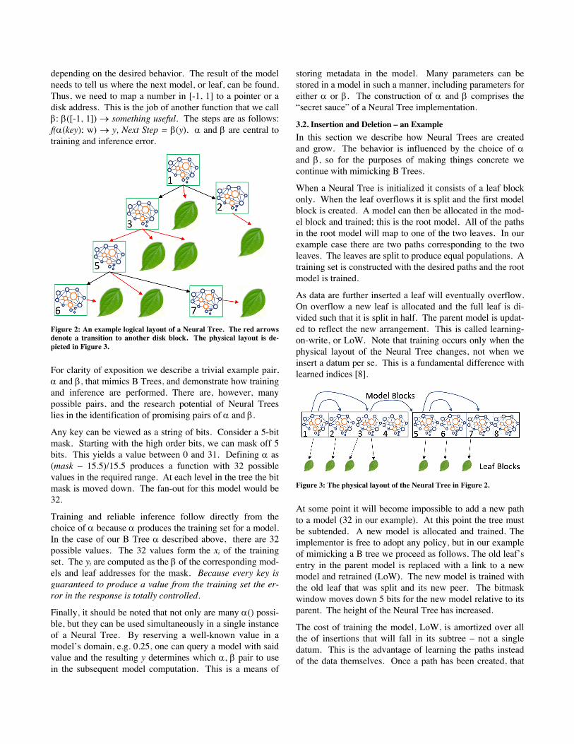
Abstractly, a Neural Tree is a tree of hierarchically arranged models (trained neural networks). Interior nodes in the tree are models, the leaves are data. The role of a model is to map a key to the next model in the tree, or a leaf (terminus). A search starts in the root model and progresses down to a leaf. At each step in the search a model maps the key to the next model in the tree. Where a B Tree would perform a binary search in a block to find the next block in the tree, a Neural Tree computes the next step from a model. Models may have heterogeneous descendants, that is, a single model may point to both leaves and deeper models (see Figure 2).

There are two kinds of physical blocks backing a Neural Tree: leaves and model blocks. A leaf looks the same as a B+ Tree leaf, it is a sorted array of keys and their values. A model block contains an array of neural networks (both trained and raw). It is essentially an array of C float of weights. There many individual models stored in a single model block; they are not necessarily related. Unlike B Trees, node transitions do not necessarily require loading a new block.

The models can be thought of like a switch in a network. Switches route packets based on tables; they are totally pro-grammable. The models in a Neural Tree route queries to the correct leaf based on how they are programmed (speci-fied by the training set), thus we have divorced the physical location of a value from its key that the binary comparison operator requires. Learned Indices (LI) [8] learn the data directly. This makes LI better suited to read-only workloads as inserting a datum requires retraining.

3.1. How to Use a Model The crux of Neural Trees is the model. To understand how the models work we need to examine them somewhat clos-er.

A model, f(; w), maps the search key to the next model. Neural networks work best with ranges and domains of the form [-1, 1] (see [5]). Keys, however, are rarely so restrict-ed. Therefore, the first task for a model is to map the key to the required domain. This is the job of a function we call a: a(key) ® [-1, 1]. The function, a(), can take many forms

depending on the desired behavior. The result of the model needs to tell us where the next model, or leaf, can be found. Thus, we need to map a number in [-1, 1] to a pointer or a disk address. This is the job of another function that we call b: b([-1, 1]) ® something useful. The steps are as follows: f(a(key); w) ® y, Next Step = b(y). a and b are central to training and inference error.

Figure 2: An example logical layout of a Neural Tree. The red arrows denote a transition to another disk block. The physical layout is de-picted in Figure 3. For clarity of exposition we describe a trivial example pair, a and b, that mimics B Trees, and demonstrate how training and inference are performed. There are, however, many possible pairs, and the research potential of Neural Trees lies in the identification of promising pairs of a and b.

Any key can be viewed as a string of bits. Consider a 5-bit mask. Starting with the high order bits, we can mask off 5 bits. This yields a value between 0 and 31. Defining a as (mask – 15.5)/15.5 produces a function with 32 possible values in the required range. At each level in the tree the bit mask is moved down. The fan-out for this model would be 32.

Training and reliable inference follow directly from the choice of a because a produces the training set for a model. In the case of our B Tree a described above, there are 32 possible values. The 32 values form the xi of the training set. The yi are computed as the b of the corresponding mod-els and leaf addresses for the mask. Because every key is guaranteed to produce a value from the training set the er-ror in the response is totally controlled.

Finally, it should be noted that not only are many a() possi-ble, but they can be used simultaneously in a single instance of a Neural Tree. By reserving a well-known value in a model’s domain, e.g. 0.25, one can query a model with said value and the resulting y determines which a, b pair to use in the subsequent model computation. This is a means of

storing metadata in the model. Many parameters can be stored in a model in such a manner, including parameters for either a or b. The construction of a and b comprises the “secret sauce” of a Neural Tree implementation.

3.2. Insertion and Deletion – an Example In this section we describe how Neural Trees are created and grow. The behavior is influenced by the choice of a and b, so for the purposes of making things concrete we continue with mimicking B Trees.

When a Neural Tree is initialized it consists of a leaf block only. When the leaf overflows it is split and the first model block is created. A model can then be allocated in the mod-el block and trained; this is the root model. All of the paths in the root model will map to one of the two leaves. In our example case there are two paths corresponding to the two leaves. The leaves are split to produce equal populations. A training set is constructed with the desired paths and the root model is trained.

As data are further inserted a leaf will eventually overflow. On overflow a new leaf is allocated and the full leaf is di-vided such that it is split in half. The parent model is updat-ed to reflect the new arrangement. This is called learning-on-write, or LoW. Note that training occurs only when the physical layout of the Neural Tree changes, not when we insert a datum per se. This is a fundamental difference with learned indices [8].

Figure 3: The physical layout of the Neural Tree in Figure 2. At some point it will become impossible to add a new path to a model (32 in our example). At this point the tree must be subtended. A new model is allocated and trained. The implementor is free to adopt any policy, but in our example of mimicking a B tree we proceed as follows. The old leaf’s entry in the parent model is replaced with a link to a new model and retrained (LoW). The new model is trained with the old leaf that was split and its new peer. The bitmask window moves down 5 bits for the new model relative to its parent. The height of the Neural Tree has increased.

The cost of training the model, LoW, is amortized over all the of insertions that will fall in its subtree – not a single datum. This is the advantage of learning the paths instead of the data themselves. Once a path has been created, that

is, a subtree trained, insertion can take place beneath it without modifying the models further as it is the path that is relevant, not the individual data. In the steady state, just as for B Trees, the structure of a Neural Tree is quite stable so LoW is a rare event.

Deletion in this Neural Tree is the same as for a B Tree: the entry is looked up and then deleted in the leaf. If the dele-tion creates an empty leaf, then the leaf is removed from the parent model and the leaf block can be released; removing a leaf triggers a LoW. If removal of the leaf results in a mod-el with a single path, then the model is released, and the leaf is attached to the model’s parent. This process is applied recursively until a model with multiple paths is encountered with LoW percolating up the tree.

3.3. Media Access Planning The performance of indexing on storage is sensitive to the number of media accesses. Neural Trees have two mecha-nisms to organize physical media accesses. We now exam-ine them.

A Neural Tree is a logical hierarchy of models. The models are physically stored in arrays in model blocks; neighboring models in an array need not have any relationship. Each step in a Neural Tree search does not necessarily involve a media access. An I/O is required if the next model resides in another model block. Laying out a search path, that is, distributing the models over the physical model blocks, is one means of controlling the media access patterns. Alloca-tion of models in the model blocks is an important way of controlling the access patterns. An implementation is free to adopt any policy to meet its desiderata.

Reverting to our concrete example of mimicking a B Tree, this would be achieved by employing a policy that packs model subtrees into the same model block. Once a model block is full, every time the Neural Tree is subtended out of said model block, we start a new model block. Thus, model blocks represent disjoint subtrees.

The second means of controlling access is with the models themselves. Short circuit search paths that jump multiple levels can be programmed into the models. For example, if locality is identified in a workload then a short circuit from the root model to the subtree containing the subset of blocks comprising the “hot” data can be made. Both model place-ment and short circuiting can be used in conjunction.

3.5. Model Size Recall that for a B Tree, assuming keys and pointers are the same size, N keys ordered by binary comparison requires 2N+1 space for a fan out of N + 1. One of the byproducts of Neural Trees is higher information density to increase the fan-out. A common value for B in implementations of B Trees is 4k. In a 4k page Neural Trees can store a maxi-

mum of 22 models, which yields a fan-out of 32·22=704. A B Tree page, assuming 32-bit keys and pointers (1024 inte-gers or floats), has a fan out of ~500, resulting in a 40% improvement. The arithmetical advantage for Neural Trees only improves if the keys or pointers are larger. This is a dramatic increase in information density.

Figure 4: Mean read times overlaid on mean write times. An obvious question is why model blocks do not contain one large model. Small models were chosen for two rea-sons. Most importantly, small models can be trained quick-ly. Small models with few training examples can be made ready on appropriate time scales for a read/write system; LoW is in the write-path.

Small models also afford the opportunity to employ training techniques that are known to converge very quickly, but do

not scale to deep learning domains. We implemented Le-venberg-Marquardt training for neural networks [12]. This is a second-order trainer that does not scale to the massive problems found in deep-learning. In our experiments LM was between 100x to 1000x faster than RPROP+, a common scalable trainer. Moreover, Levenberg-Marquardt tech-niques made Neural Trees feasible.

4. Evaluation We have implemented Neural Trees, and their ancillary neu-ral network training code. In this section we demonstrate that the Neural Tree data structure is feasible. The basis for comparison is a high-performance B* Tree implementation and a Neural Tree mimicking a B+ Tree (as described above). The experiments were performed on a 2018 Mac-Book Pro with an i9 clocked at 2.9 GHz. Storage consisted of an external Seagate 2TB SRD00F1 disk attached with USB.

Two workloads were chosen to drive the experiments. We used SPC1 [14] and file system traces available for down-load from SNIA [10]. The traces consist of virtual machines (VM) running on virtual desktop infrastructure (VDI) col-lected by Fujitsu. The traces are comprised of 6 LUNs over 28 days. The full characterization and analysis of the traces are available in [10]. In all of the experiments file caching was turned off and the system calls used were lseek/read/write. Every read went to the device (where it may have been cached). Writes were synchronous and the F_FULLFSYNC flag was respected by the device.

Figure 4 depicts the results of microbenchmarks. The y-axis is µs and the x-axis is tree height. The bars are read time (red) overlaid on write time (cyan). For both reading and writing Neural Trees are competitive with B Trees. Neural Trees are at most 3% slower for writing at height 1. For the rest of the micro-ops they are 1% slower. SPC1 and the traces are very similar. Excepting writing at height 1, Neu-ral Trees are within 1% of B Trees. At height 1 LoW is adding more variance to the write path. As it becomes rarer LoW appears more like tail-latency in device I/O. This just becomes noise as the tree increases in height.

The next experiment is op-time as a function of keys in the tree (Figure 5). The x-axis is logarithmic. Despite being ~1% slower in practice Neural Trees are very competitive owing to their fan-out. Height is not a quantum number for real trees. In practice they grow from one height to the next by increasing bushiness. The increased fan-out of the Neu-ral Tree means that mean path length is shorter for a given number of items in the tree. Moreover, as N increases, the probability of going down a shorter path in a Neural Tree versus a B Tree increases and the gap between mean ∆t widens (the gap is linear, only the x-axis is logarithmic).

Figure 5: Operation time as a function of population. Note that the plots naturally group by operation, not tree type.

5. Conclusion We presented Neural Trees, a data structure that is based on neural networks instead of binary comparison. Neural Trees were shown to be competitive with B Trees for basic opera-tions when programmed to mimic their behavior. They are, however, fundamentally different. The mechanism of speci-fying search paths empirically opens up new vistas for searching and indexing. The idea of routing tables for search paths is a potentially very powerful. Our future re-search will examine new ways of searching for data, includ-ing temporal, ontological and metric propinquity. Finding the a/b pairs that permit data placement that is totally policy based is a promising research direction.

7. Bibliography [1] Balázs Csanád Csáji. Approximation with Artificial Neural Networks, Faculty of Sciences; Eötvös Loránd Uni-versity, Hungary, 2001 [2] Bayer, R.; McCreight, E. Organization and maintenance of large ordered indices, Boeing Scientific Research Librar-ies, July 1970 [3] Bender, M. A., Farach-Colton, M., Fineman, J. T., Fo-gel, Y. R., Kuszmaul, B. C., and Nelson, J. Cache-oblivious streaming B-trees. In Proceedings of the ACM symposium on Parallelism in algorithms and architectures (SPAA) (2007), pp. 81–92. [4] Bender, M. A., Farach-Colton, M., Jannen, W., Johnson, R., Kuszmaul, B. C., Porter, D. E., Yuan, J., and Zhan, Y. An introduction to Be -trees and write-optimization, login; Magazine 40, 5 (Oct 2015), 22–28. [5] Charu C. Aggarwal. Neural Networks and Deep Learn-ing: A Textbook 1st ed, 2018 Edition, Springer, ISBN 3319944622 [6] Comer, Douglas (June 1979). The Ubiquitous B-Tree, Computing Surveys, 11 (2): pages 123–137 [7] Cybenko, G. Approximations by superpositions of sig-moidal functions, Mathematics of Control, Signals, and Systems, 2(4), pages 303–314, 1989 [8] Kraska T. and Beutel A., The Case for Learned Index Structures, In SIGMOD’18, June 10-15, 2018, Houston, TX, USA [9] Lakshman A, Malik P. Cassandra: a decentralized struc-tured storage system. ACM SIGOPS Operating Systems Re-view, 2010 [10] Lee, Chunghan and Kumano, Tatsuo and Matsuki, Tatsuma and Endo, Hiroshi and Fukumoto, Naoto and Sugawara, Mariko. Understanding Storage Traffic Charac-teristics on Enterprise Virtual Desktop Infrastructure, In Proceedings of the 10th ACM International Systems and Storage Conference (SYSSTOR ’17) [11] Leshno M, Lin, Vladimir Ya.; Pinkus, Allan; Schock-en, Shimon (January 1993). Multilayer feedforward net-works with a nonpolynomial activation function can approx-imate any function, Neural Networks volume 6 pages 861–867 1993, Elsevier [12] Martin T. Hagan and Mohammad B. Menhaj, Training Feedforward Networks with the Marquardt Algorithm, IEEE

Transactions on Neural Networks, Vol. 5, No. 6, November 1994 [13] O’Neil, P., Cheng, E., Gawlic, D., and O’Neil, E. The log-structured merge-tree (LSM-tree). Acta Informatica 33, 4 (1996), pages 351–385. [14] S. Daniel and R. E. Faith. A portable, open-source implementation of the SPC-1 workload. In Proceedings of the IEEE International Workload Characterization Sympo-sium, 2005 [15] Sage A. Weil and Scott A. Brandt and Ethan L. Miller and Darrell D. E. Long and Carlos Maltzahn. Ceph: A scal-able, high-performance distributed file system, In Proceed-ings of the 7th Symposium on Operating Systems Design and Implementation (OSDI) [16] A. Sweeney, D. Doucette, W. Hu, C. Anderson, M. Nishimoto, and G. Peck. Scalability in the XFS File Sys-tem. In Proceedings of the 1996 USENIX Technical Confer-ence, 1996