Neuro-Adaptive Motion Control with

Velocity Observer in Operational Space

Formulation

Dandy B. Soewandito Denny Oetomo ∗ Marcelo H. Ang, Jr. †

November 15, 2010

Abstract

In this paper, an online neuro-adaptive motion control with velocity observer is devel-

oped and validated in real-time experiment using a 6 DOF PUMA 560 robot. The controller

is constructed for the operational space formulation, such that dynamic terms and the gen-

eralized force descriptions in this algorithm are expressed in the task space. The proposed

strategy assumes no prior knowledge of the robot dynamics, and is formulated without as-

suming the availability of joint velocity feedback. As such, the controller takes only position

feedback. This is an important feature as industrial robots are often fitted only with joint

displacement sensors, not joint rate sensors. Stability analysis of the algorithm is analysed

and presented in the paper. Real-time experiments on a 6 degrees of freedom (DOF) PUMA

560 manipulator were carried out to evaluate the effectiveness of the proposed NN adaptive

control strategy with velocity observer and to compare the performance with the conven-

tional inverse-dynamics control and a similar NN adaptive strategy using filtered velocity

feedback, obtained through the backward difference of the displacement feedback. It should

be noted that the experimental platform, PUMA 560, provides only joint displacement feed-

back through its joint mounted encoders. The results shows a comparable results between

the proposed strategy and the inverse dynamics control law, without the need to perform

dynamics identification procedures.

∗Denny Oetomo is with the Department of Mechanical Engineering, The University of Melbourne, VIC 3010,

Australia. doetomo@unimelb.edu.au†Dandy B. Soewandito and Marcelo H. Ang, Jr. are with the Department of Mechanical Engineering, National

University of Singapore, Singapore 117576. altec 1@yahoo.com, mpeangh@nus.edu.sg

1

1 Introduction

1.1 Motivation

Robotics motion control is a topic that still undergoes a lot of research studies. The advancement

in various technologies has meant higher requirements imposed on the performance of motion

control strategies on robotic manipulators. It is well established that model-based (computed

torque or inverse dynamics) control provides an excellent tracking performance. Theoretically,

the availability of the exact dynamic model and parameters of the robotic manipulator allows

us to compensate for the robot dynamics, providing us with the ultimate tracking performance

of the robot. In practice, however, it is not possible to obtain the exact model and parameter

values of the dynamics of a robotic manipulator. It has also been shown that robot parameter

identification by physical experimentation is tedious and error prone [1,2]. Despite the difficulty

in establishing the dynamic model, inverse dynamic control is still one of the best performing

strategy given that a reasonably accurate model of the manipulator dynamics is obtained.

In this paper, the controller strategy is formulated within the operational (or task) space frame.

End-effector motion control in task space provides the natural spatial frames of human-related

tasks to the formulation of control strategies. It is desired to address the issue of achieving a

motion control performance equivalent to the inverse dynamic control without the tedious effort

of dynamic identification process. To do so, an online Neural Networks (NN ) adaptive control

strategy is proposed. This paper attempts to provide a thorough review of the relevant work

in this area and to provide the online neuro-adaptive strategy that can be implemented within

operational space formulation. The algorithm is also formulated considering the practical issue of

industrial robots being equipped with only joint displacement feedback and not joint rate sensors.

Theoretical study in the form of stability analysis of the controller is provided to support the

fundamental claim of the effectiveness of the strategy. The result is a motion control algorithm

capable of quick implementation and online adaptation, without the need for any prior knowledge

of the manipulator dynamics, implementable on industrial robots with no joint rate feedback, and

capable of achieving performance equivalent to that of a well-tuned inverse-dynamic controller.

1.2 Review of Robotic Adaptive Control Strategies

1.2.1 Linearity-In-Parameter Adaptive Control

Early work in adaptive control strategy was carried out by exploiting the linearity-in-parameter

(LIP) property of robot dynamic model, in which the least-square-estimation procedure can be

employed to identify the robot dynamic parameters [3–9]. This method is often referred as the

indirect adaptive control which consists of the off-line identification stage and the model-based

control stage.

Later, the off-line identification was deemed to be impractical, for any changes in the dynamics,

the identification procedures need to be carried out again. For this reason, some researchers

[10–14] proposed direct LIP adaptive controllers (without parameter identification). The direct

adaptive control with on-line identification was established in [14].

Recent experimental studies using indirect methods on higher (>= 6) DOF robots were shown

in [15–17]. There are relatively few studies reported in the literature on redundant robots with

more than 6 DOFs, as the expressions of robot dynamic model become extremely complex. A

recent example further assumed the robot dynamic model to be a linear system model; where

for ease of parameter identification, it includes only joint friction model [18].

The main challenges in the use of LIP are:

1. The implementation of LIP requires the explicit dynamic model. It is well established

that the complexity of robot dynamic model increases exponentially with the degrees of

freedom of the manipulator. These models can be simplified such that the parameters can

be reduced into a minimum set of base (lumped) parameters [19–24]. The simplification

procedure is carried out by manually and not automated.

2. Regression matrices used in direct adaptive control with identification [14] require the

availability of joint velocities and accelerations, which are often not available in industrial

robots. Obtaining these variables through filtering often produces noisy signals. Several

algorithms were proposed to avoid calculating the joint accelerations, as in [25–29].

3. The need for optimal (exciting) trajectories in order to make the parameters converge

rapidly. The optimal trajectories are those that excite all possible dynamics of the manip-

ulator. It is also often described as dynamically rich trajectories. Derivation of optimal

trajectories generator algorithm were proposed by [30–33].

Extension to operational space in direct method can be shown to be more complex as further

transformations are required to obtain the operational space matrices and vectors [34, 35] from

the joint space dynamics. One must derive a separate linear dynamic model in operational

space, should one use the direct approach. Note that this extension can still be done indirectly

by performing parameter estimation in joint space (either using on-line or off-line method), then

employing model-based control in operational space.

In view of the challenges discussed above in the use of LIP techniques, alternative techniques

that can offer a more straight forward estimation of the manipulator dynamics, an automated

procedure (less manual efforts to derive the dynamic models and identify the parameter values),

and less dependence on variables that are not usually measured in standard industrial robots are

desirable.

1.2.2 Neural Networks Adaptive Control

Subsequently, Linear-in-Parameter Neural Networks strategy (LPNN, or two-layer NN) with

Lyapunov stability analysis was proposed for nonlinear system identification [36, 37] and for

robotic control [38,39], where suitable basis functions, for example: radial basis function (RBF),

needs to be selected beforehand. In practice, this constraint is difficult to satisfy.

To overcome this problem, a three-layer joint space NN adaptive robot motion control was pro-

posed by Lewis et. al. [40, 41]. It contained several interesting characteristics: (1) the proposed

strategy does not have strong constraints and was also shown to have a satisfactory performance,

(2) the formulation was developed based upon a well known joint space LIP adaptive robotic

controller proposed by Slotine and Li’s [13, 14], (3) off-line learning is not needed and the neu-

ral networks are initialised with zero weights and (4) a Lyapunov analysis can be performed to

show bounded stability for both the tracking errors and NN weight errors. These characteristics

made the strategy very attractive for practical implementation. However, the work was only

validated through a simulated study of a 2 DOF robot in joint space. Therefore, the formulation

of this strategy into operational (task) space framework with real-time implementation results

on a 6DOF industrial robot is of great interest.

This early work [40] was followed by various attempts in NN adaptive compliant motion control

[42–44], based-upon [45], where the knowledge of contact surface geometry was required. More

recent neuro-adaptive control studies, where the contact surface normal direction is required,

attempted to adaptively accommodate the contact surface geometry through impedance control

[46,47] and compliant motion based approach [48,49].

Another NN adaptive strategy for compliant motion on unknown contact geometry was presented

in [50], utilising an additional vision feedback to carry out the task. All these algorithms were

mainly validated through simulated robots of up to 3 DOFs. Only [42] was validated through

real-time experiment of a real 2 DOF robot.

1.3 Contributions of this Paper

In view of the state-of-the-art strategies discussed, this paper aims to present the following

contributions:

• To provide an overview of the adaptive motion control for robotic manipulators;

• To extend the formulation of NN adaptive robotic motion control strategy into the opera-

tional space frame;

• To improve the suitability of the technique for implementation on industrial robots, by

formulating the control strategy such that it does not assume the availability of joint velocity

feedback;

• To perform stability analysis of the NN adaptive motion control in operational space frame

to provide the theoretical support of the effectiveness of the proposed control strategy;

• To provide experimental validation of the proposed NN strategy on a 6 DOF robot (without

joint velocity feedback). This would also serve to provide experimental validations on the

similar NN techniques covered in the literature, which have generally been validated only

through simulated studies of low DOF robots.

In our preliminary study, the original NN adaptive joint space strategy in [40] was extended the

operational space free motion [51]. The simulated performance was found to be comparable with

that of model-based control. However, performance on real-time experimentation using a 6 DOF

PUMA 560 robot, was found to be inferior to the simulated equivalent. Note that physically the

PUMA 560 does not have joint velocity sensor. Therefore, in practice, the joint velocity signals

are generally estimated through backward difference algorithm of the displacement feedback,

followed by an appropriate low pass filter (LPF). Consequently, only the estimated operational

space velocities are available.

Therefore, in this paper, an NN adaptive motion control in operational space with velocity

observer is proposed to overcome the absence of an actual velocity signal in real robots. Stability

analysis of the proposed strategy is presented and real-time experimentation was performed on a

PUMA 560 robot, with comparison to the performance of a well-tuned inverse dynamics control

and an NN adaptive strategy using filtered velocity feedback (as presented in [51]). This paper

is organized as follows: Section 2 presents the end-effector motion dynamics, Section 3 defines

the properties of the end-effector dynamics that would be utilised in the later sections, Section

4 formulates the proposed NN adaptive motion control with velocity observer, Section 5 shows

the computation to obtain the estimated operational space coordinates, Section 6 presents the

NN adaptive control using filtered velocities, Section 7 discusses the computational cost of the

proposed NN adaptive controller - observer, and Section 8 presents the results of the realtime

implementation of the: (i) the proposed NN adaptive motion control with velocity observer, (ii)

the Lagrangian inverse dynamics motion control, as presented in [20], and (iii) the NN motion

control using filtered velocity.

2 End-effector Dynamics

The task space dynamics of a non-redundant manipulator in the operational space can be ex-

pressed as

Mx(q)x+Bx(q, q)x+ gx(q) + τx(q, q) = F (1)

where x ∈ ℜm and q ∈ ℜn denote the operational and joint space coordinates, respectively. Note

that for a non-redundant manipulator, the number of joints (n) of the manipulator equals the

degrees of freedom of the task (m), m = n. The vector F ∈ ℜm denotes the generalized forces in

the operational space. The operational space matrices and vectors: Mx(q) ∈ ℜm×m, Bx(q, q) ∈

ℜm×m, gx(q) ∈ ℜm and τx(q, q) ∈ ℜm denote the inertia, Coriolis/centrifugal, gravity and joint

friction terms expressed in operational space, respectively, for a non-redundant manipulator in

non-singular configuration. These operational space dynamic terms can be obtained from the

joint space equivalents as [35]:

Mx(q) = J−T(q) M(q) J−1(q) (2)

Bx(q, q) = [J−T(q) B(q, q)−Mx(q) J(q, q)] J−1(q) (3)

gx(q) = J−T(q) g(q) (4)

τx(q, q) = J−T(q) τ fric(q) (5)

where J(q) is the basic Jacobian and M(q) ∈ ℜn×n, B(q, q) ∈ ℜn×n, g(q) ∈ ℜn and τ fric(q) ∈

ℜn are the inertia, Coriolis/centrifugal, gravity and joint friction dynamics terms, expressed in

joint space. Joint friction vector τ fric(q) was defined as in [52]

τ fric(q) = τ visq+[τ cou + τ stiexp

(−τdecq2)]sgn(q) (6)

where sgn(q) = +1,−1, 0 if q = positive, negative and zero, respectively and τ vis, τ cou, τ sti, and

τ dec ∈ ℜn are the viscous friction, coulomb friction, static friction (stiction) and Stribeck effect,

respectively.

3 Properties of the End-Effector Dynamics

The following properties of the end effector dynamics are utilised in developing the proposed

algorithm. Unless otherwise specified, all vector/matrix norms are defined as 2-norm (Frobenius

norm).

Property 3.1 The operational space kinetic energy matrix Mx(q) ∈ ℜm×m is symmetric and

positive definite matrix, hence all its eigenvalues are positive. This is due to (2), valid for all

non-singular configurations, and the fact that joint space kinetic energy M(q) > 0. It follows

from Rayleigh-Ritz theorem [53] that any positive definite matrix A satisfies Am ≤ ∥A∥ ≤ AM ,

where Am, AM > 0 denote the minimum and maximum eigenvalues of A, respectively. Therefore

Mx(q(t)) along t ≥ 0 is lower-bounded and upper-bounded by its global minimum and maximum

eigenvalues, respectively, as:

Mx,m ≤ ∥Mx(q(t))∥ ≤ Mx,M , t ≥ 0 (7)

where Mx,m = min(λmin(Mx(q(t)))) > 0 and Mx,M = max(λmax(Mx(q(t)))) > 0, where λmin(·)

and λmax(·) denote the minimum and maximum eigenvalue operators, respectively.

Property 3.2 The operational space Coriolis and centrifugal matrix can be expressed as a func-

tion of q and x since

Bx(q, x) = [J−T(q)B(q, x)−Mx(q)J(q, x)]J−1(q). (8)

Note, B(q, x) and J(q, x) as functions of q and x can be obtained directly by using the fact

q = J−1(q) x into B(q, q) and J(q, q), respectively.

Property 3.3 The operational space Coriolis and centrifugal matrix Bx(q, x) can be shown to

be upper-bounded

∥Bx(q, x)∥ ≤ Bx,M ∥x∥ ≤ Bx,M xM (9)

where Bx,M , xM are positive scalar constants. The upper bound (9) can be obtained directly

from the joint space properties ∥B(q, q)∥ ≤ BM ∥q∥ [54] and ∥J(q, q)∥ ≤ JM ∥q∥ [55] and the

relationship q = J−1(q) x. Note that BM , JM are positive scalar constants.

Property 3.4 The operational space gravity vector gx(q) (4) is upper-bounded:

∥gx(q)∥ ≤ gM < ∞ (10)

Property 3.5 Joint friction forces, τ fric(q) (5), are bounded in magnitude

∥τ visq∥ ≤ τvisM qM (11)

∥τ cousgn(q)∥ ≤ τcouM (12)

∥τ stiexp(−τdecq

2)sgn(q)∥ ≤ τstiM (13)

Property 3.6 For non-redundant robot, Mx(q)−2Bx(q, q) is a skew-symmetric matrix [56,57],

hence given an operational space vector z ∈ ℜm, it satisfies

zT(Mx(q)− 2Bx(q, q)

)z = 0. (14)

Using Property 3.2, it can also be written as

zT(Mx(q)− 2Bx(q, x)

)z = 0. (15)

Property 3.7 It can be shown that for a non-redundant robot, given any two operational space

vectors y, z ∈ ℜm, Bx(q, x) satisfies [55]

Bx(q,y)z = Bx(q, z)y. (16)

4 NN Adaptive Motion Controller with Velocity Observer

Formulation

4.1 NN Adaptive Motion Controller-Observer

In this section, an NN adaptive motion controller with velocity observer is proposed. It is based

the controller observer design reported in [58]. The structure is shown in Fig. 1. The control

law is defined as:

F = Mx(q)F∗motion + Bx(q, x0)xr + gx(q) + τx(q, ˙q) (17)

In (17), a relationship (·) = (·) − (·) is defined where (·) is the error dynamics, (·) is the actual

dynamics, (·) is the estimated dynamics, which will be estimated through NN. The following

terms are defined as

xr = xd +Λ1(xd − x) (18)

x0 = ˙x−Λ2x (19)

F∗motion = xr +Λ1(r1 + r2) (20)

with the following terms to obtain F∗motion defined as

xr = xd +Λ1(xd − ˙x) (21)

r1 + r2 = xr − x0. (22)

It follows from (22) that

r1 + r2 = (xr − x) + (x− x0) (23)

where it can be defined that

r1 = xr − x = e+Λ1e+Λ1x (24)

r2 = x− x0 = ˙x+Λ2x. (25)

Note: Λ1,Λ2 ∈ ℜm×m are positive diagonal matrices, e = xd−x and e = xd−x are defined as the

position and velocity tracking errors, respectively, and xd, xd and xd are the desired operational

space trajectories. The estimated position and velocity errors, x = x− x and ˙x = x− ˙x, denote

the differences between the actual and estimated position x, x and the actual and estimated

velocity x, ˙x, respectively. The computation to obtain x and x will be given on Section 5.

Before we carry on, notice that unlike the NN controller as in [40] and model-based observer-

controller [58] which are using the term Kvr, our proposed controller uses only estimated NNs

and omits the term Kvr as in [40, 58], where Kv is a positive diagonal matrix. It can be shown

as in [53], that Kv ≡ Mx(q)Λ. Our intention is that the performance of our NN controller does

not rely on the term Kvr.

Now, combining the robot dynamics (1) and the proposed controller (17), and taking into account

the first derivative of (24) and Property 3.2, a general closed-loop dynamics is obtained as:

Mx(q)r1 =−Mx(q)Λ1 (r1 + r2)−Bx(q, x0)xr

+Bx(q, x)x+ τx(q, q)− τx(q, ˙q) + η(26)

where the uncertainties of the system, η, expressed as

η = Mx(q)F∗motion + Bx(q, x0)xr + gx(q) + τx(q, ˙q). (27)

From Property 3.5, it is shown that

τx(q, q)− τx(q, ˙q) = J−T[τvis ˙q+ τcou(sgn(q)− sgn( ˙q))

+ τ stiexp(−τdecq

2)sgn(q)− τ stiexp(−τdec ˙q2)sgn( ˙q)].

(28)

The general closed-loop dynamics (26) is rearranged into the controller closed-loop dynamics

(Section 4.2) and the observer closed-loop dynamics (Section 4.3) for stability analysis.

4.2 Controller closed-loop dynamics

Using (24), (25) and Property 3.7, the terms Bx(q, x0)xr −Bx(q, x)x in (26) can be rearranged

such that

Bx(q, x0)xr −Bx(q, x)x

= Bx(q, x− r2)(r1 + x)−Bx(q, x)x

= Bx(q, x)r1 −Bx(q, xr)r2.

(29)

Substituting (29) into the general closed-loop dynamics (26) yields the controller closed-loop

dynamics:

Mx(q)r1 =−Mx(q)Λ1(r1 + r2)−Bx(q, x)r1

+Bx(q, xr)r2 + τx(q, q)− τx(q, ˙q) + η(30)

4.3 Observer closed-loop dynamics

A velocity observer, to obtain the estimated velocity ˙x, is proposed (based upon [58] Section

III.A, where the term involving the inverse of the kinetic matrix is omitted) as follows:

˙x = z+ (lD +Λ2) x (31)

z = xr + (lD ·Λ2)x (32)

where lD = diag(lD,ii > 0) ∈ ℜm×m, ˙x, z are computable and z is obtained by integrating z.

Combining the first derivative of (31) with (32) and taking into account the first derivative of

(24) and also the knowledge of x− ˙x, result the observer closed-loop dynamics in:

¨x+ (lD +Λ2) ˙x+ (lD ·Λ2)x = −(xr − x) = −r1. (33)

Substituting (25) and its derivative into the left-hand-side (LHS) of (33) and multiplying both

sides with Mx(q), yield

Mx(q)r2 +Mx(q)lDr2 = −Mx(q)r1. (34)

Using (24), (25) and Property 3.7, the term Bx(q, x0)xr−Bx(q, x)x in (26) can be manipulated

such that= Bx(q, x0)(r1 + x)−Bx(q, x0 + r2)x

= Bx(q, x0)r1 −Bx(q, x)r2.(35)

Substituting (35) into (26), then into the observer closed-loop dynamics (34) yields:

Mx(q)r2 =− (Mx(q)lD −Mx(q)Λ1)r2 +Mx(q)Λ1r1

−Bx(q, x)r2 +Bx(q, x0)r1 − (τx(q, q)− τx(q, ˙q))− η.(36)

It can be shown that the model-based controller - observer in [58], where η = 0, achieves local

asymptotic stability.

4.4 Three-Layer Neural Networks

As shown in Fig. 2, a general three-layer neural network is defined such that N1, N2 and N3

are the number of neurons in layer 1, layer 2, layer 3, respectively. Vector z ∈ ℜN1 is the NN

input-layer vector, σ ∈ ℜN2 is the NN hidden-layer vector and u ∈ ℜN3 is the NN output-layer

vector. vkl is the first-to-second layer weights, with l = 1, . . . , N1 as the input-layer index and

k = 1, . . . , N2 as the hidden-layer index; θk is the threshold offset, and wik is second-to-third

layer weights for an output vector, with i = 1, . . . , N3 as the output-layer index. Function σ(·) is

defined to be differentiable throughout, such as sigmoid and hyperbolic functions. In this paper,

sigmoid function σ(s) = 1/(1 + exp−(a×s)) is selected. Therefore each element of output vector

u can be expressed as

ui =

N2∑k=1

wik σk

(N1∑l=1

vklzl + θk

); i = 1, . . . , N3. (37)

Equation (37) can be written in a simplified manner in vector-and-matrix form as in [59] as

u = WT σ(VTz

)(38)

with W ∈ ℜN3×N2 ,V ∈ ℜN2×N1 . Note N3 can be determined from the robot DOF, therefore

for non-redundant manipulator with 6 DOF, then N3 = n = 6. Also, the addition of the scalar

θk, in (38), has been included in the VTz term. This can be done by appending the vector θT

(where each element is θk) as the first row of V and an element containing ‘1’at the beginning

of vector z. If NN output is considered as a matrix, then each element of U ∈ ℜN3×N4 is

uij =

N2∑k=1

wijk σk

(N1∑l=1

vklzl + θk

);

i = 1, . . . , N3, j = 1, . . . , N4

(39)

where wijk with i = 1, . . . , N3, j = 1, . . . , N4 are the output-layer indices. Similarly, (39) can be

written in a vector-and-matrix form as

U = WT σ(VTz

)(40)

where now W ∈ ℜN3×N4×N2 ,V ∈ ℜN2×N1 . For a non-redundant manipulator with 6 DOF,

N4 = N3 = m = 6.

4.5 Uncertainties η in NN terms

By the definition of error dynamics (·) = (·)− (·), the uncertainties η in (27) can be written as

η =(Mx(q)− Mx(q)

)F∗

motion +(Bx(q, x0)− Bx(q, x0)

)xr

+ (gx(q)− gx(q)) + (τx(q, ˙q)− τx(q, ˙q)).

(41)

From NN theory, given an adequate number of hidden layer nodes N2, a three layer NNs with

ideal weights is capable of approximating any function [60, 61]. In practice, however, there

are only limited number of hidden layer nodes, thus the dynamics terms Mx(q), Bx(q, x0),

gx(q), and τx(q, ˙q), for a given number of neurons, can be described by three-layer NNs with

constant optimum weights Vp,Wp and approximation error εp, with the subscript p = M,B, g, τ

representing the individual dynamical terms:

Mx(q) = WTM σM (VT

M zM ) + εM (42)

Bx(q, x0) = WTB σB(V

TB zB) + εB (43)

gx(q) = WTg σg(V

Tg zg) + εg (44)

τx(q, ˙q) = WTτ στ (V

Tτ zτ ) + ετ (45)

Similarly, the estimated dynamics terms Mx(q), Bx(q, x0), gx(q), and τx(q, ˙q) are described

by the estimated weights Vp,Wp, with subscript p = M,B, g, τ .

It is clear that Mx(q) and gx(q) can be shown to be bounded by Properties 3.1 and 3.4, re-

spectively. Using Property 3.3, the boundedness of Bx(q, x0) depends on x0 (19), which in turn

depends on ˙x, x and x in (19): note x is directly bounded by the workspace. The estimated

velocity, ˙x, can be assumed to be bounded, ∥ ˙x∥ ≤ ˙xM , since in the implementation it is possible

to set − ˙xM ≤ ˙x ≤ ˙xM . This implies that ∥x∥ is bounded since it is obtained from ˙x (see Sec-

tion 5. Computation of Estimated Operational Space Coordinates). Therefore ∥x0∥ is bounded.

The boundedness of τx(q, ˙q) can be shown by using Property 3.5 and the fact that ∥J−1(q)∥ is

bounded for non-singular configuration and ˙x is bounded, implying ˙q is bounded. Therefore, the

optimum weights Wp,Vp and the approximation error εp (with subscript p = M,B, g, τ) from

(42)-(45), are also upper-bounded.

For ease of analysis in later sections, an upper-bounded matrix Z = diag[W,V] can be defined

as follows

∥Z∥ =√∥W∥2 + ∥V∥2 ≤ ZM (46)

where ZM is a positive scalar constant, W = diag[WM ,WB,Wg,Wτ ] and V = diag[VM ,VB ,

Vg,Vτ ].

Now, for ease of presentation, the following generic NN expressions are defined:

Lp = (WTp σp(V

Tp zp)

Lp = (WTp σp(V

Tp zp)

Lp = Lp − Lp;

(47)

where Lp, Lp, and Lp represent the optimum, estimated, and error, of the respective terms.

Hence, using the generic NN expressions, the uncertainties (41) can be written as

η = (LM − LM )F∗motion + (LB − LB)xr + (Lg − Lg) + (Lτ − Lτ ) + ε (48)

where the total approximation error ε = εMF∗motion+ εBxr + εg + ετ (since the actual dynamics

are bounded). To compute η (48), it is necessary to compute the generic form Lp − Lp, which

can be manipulated, as follow

Lp − Lp = WTp σ(V

Tp zp)− WT

p σ(VTp zp)

= WTp σ(V

Tp zp)− WT

p σ(VTp zp)−WT

p σ(VTp z) +WT

p σ(VT zp)

= WTp σ(V

Tp zp) +WT

p

(σ(VT

p zp)− σ(VTp zp)

) (49)

From (49), first, we need to compute the error of the sigmoid function as:

σ = σ(VTz)− σ(VTz). (50)

From the Taylor series expansion

σ(x)∣∣x=x

= σ(x) +dσ(x)

dx(x− x) +O(x− x) (51)

where O(x− x) denotes the higher order terms (x, x are dependent variables).

Note that σ′(k) = dσ(k)dk

∣∣k=k

, and because σ is differentiable, σ′ exists. Hence σ(VTz)∣∣VTz=VTz

in (50) can be written as

σ(VTz) = σ(VTz) + σ′(VTz)VTz+O(VTz) (52)

To simplify the notations, it is defined that σ = σ(VTp z), σ = σ(VTz), and σ = σ + σ.

Therefore, using (52), σ (50) can be rewritten as:

σ = σ(VTz)− σ(VTz) = σ′VTz+O(VTz

). (53)

The substitution of (53) into (49) yields

Lp − Lp = WTp σp +WT

p σp

= WTp σp +WT

p

[σ′

pVTp zp +O(VT

p zp)]

= WTp σp + (WT

p + WTp )[σ′

pVTp zp +O(VT

p zp)] (54)

Using the general expression (54), the uncertainties η in (48) can be written as

η = ξ +w. (55)

This division is needed because only ξ term can be manipulated by the weight updates˙W,

˙V as

will be shown in Section 4.6. The term ξ is defined as

ξ =(WT

M σM

)F∗

motion +(WT

BσB

)xr + WT

g σg + WTτ στ

+(WT

M σ′MVT

MzM

)F∗

motion +(WT

Bσ′BV

TBzB

)xr

+ WTg σ

′gV

Tg zg + WT

τ σ′τ V

Tτ zτ

(56)

and the “whole”NN errors ζ is defined as

ζ =(WT

M σ′MVT

MzM

)F∗

motion +(WT

Bσ′BV

TBzB

)xr + WT

g σ′gV

Tg zg + WT

τ σ′τ V

Tτ zτ

+(WT

M O(VTMzM )

)F∗

motion +(WT

B O(VTBzB)

)xr

+WTg O(VT

g zg) +WTτ O(VT

τ zτ ) + ε

(57)

It can be shown that ζ and ξ possess upper-bounds that are useful for the stability analysis in

Section 4.6. To prove this, we need the boundedness of the generic expression (54)

∥Lp − Lp∥ = ∥WTp ∥ ∥σ(VT

p zp)∥+ ∥WTp ∥∥(σ(VT

p zp)− σ(VTp zp)∥ (58)

It is shown that the boundedness of expressions in (54) depends solely on W and V because:

• The optimum weights Wp,Vp and approximation error εp are upper-bounded.

• σ and σ are bounded for differentiable functions like sigmoid, tanh, RBF functions.

From the definition of the NN weight errors, W = W − W, we have

∥W∥ ≤ ∥W∥+ ∥W∥ (59)

The boundedness of the NN weight errors W in (59) depends solely on the boundedness of the

weight estimate W, since ∥W∥ is upper-bounded. Note that although ∥W∥ is positive, W is

not necessarily a positive definite matrix; i.e. its eigenvalues could be negative, zero or positive.

Therefore Rayleigh-Ritz theorem is not applicable since the minimum and maximum positive

eigenvalues do not exist.

However, it can be shown that the boundedness of W can be achieved by simply combining the

Frobenius norm definition and limiting W in the implementation. From the norm definition of

∥W∥, for a 3D output matrix U ∈ ℜN3×N4×N2 (for a 2D output matrix N4 = 1):

∥W∥ =

√√√√ N3∑i

N4∑j

N2∑k

w2ijk. (60)

In the implementation, W and V can be limited as follows:

if (∥W∥ > WM ), then ˙wijk = 0, and

if (∥V∥ > VM ), then ˙vkl = 0(61)

with WM > 0 and VM > 0, then the upper-bounds are

∥W∥ ≤WM

∥V∥ ≤VM .(62)

Since ∥W∥ ≤ ∥W∥+ ∥W∥ and ∥V∥ ≤ ∥V∥+ ∥V∥ therefore

∥W∥ ≤ WM ;

∥V∥ ≤ VM

(63)

with WM > 0 and VM > 0.

Furthermore, it follows that the overall estimated NN weights, Z, and NN weight errors, Z, are

to be upper bounded as

∥Z∥ ≤ ZM (64)

∥Z∥ ≡ ∥Z∥+ ∥Z∥ ≤ ZM + ZM ≡ ZM (65)

with ZM > 0, ZM > 0.

Substituting (63) into (58), results in the generic expression ∥Lp − Lp∥ in (58) being upper-

bounded by

∥Lp − Lp∥ ≤ (Lp)M . (66)

where (Lp)M > 0. Combining the uncertainties η in (55) with (66), and also exploiting F∗motion

(20) and xr in (22), we can obtain:

∥η∥ ≤ (LM )M ∥F∗motion∥+ (LB)M ∥xr∥+ (Lg)M + (Lτ )M + εM

≤ (LM )M (∥xr∥+Λ1(∥r1∥+ ∥r2∥)) + (LB)M (∥r1∥+ ∥r2∥+ ∥x0∥)

+ (Lg)M + (Lτ )M + εM

(67)

Addressing the boundedness of the terms in (67): (i) x0 defined in (19) depends on ˙x, x and x

(which have been shown to be bounded in previous page), and (ii) xr defined in (21) depends on

xd, xd,xd, ˙x, and x, and is therefore bounded as the desired trajectories xd, xd,xd are bounded

by design, x is bounded by the workspace and ˙x is bounded by limitation in the implementation.

Therefore η can be shown as

∥η∥ ≤ C0 + C1 (∥r1∥+ ∥r2∥). (68)

where C0, C1 > 0. Since η = ξ + ζ, then the following inequalities are true

∥ξ∥ ≤ C0 + C1 (∥r1∥+ ∥r2∥) (69)

∥ζ∥ ≤ C0 + C1 (∥r1∥+ ∥r2∥). (70)

4.6 Stability Analysis

For the end-effector motion controller (17) and observer (31), (32), let the NN weight updates

be provided as

˙wMij= FMij

(σM (r1,i + r2,i) F∗motionj − κ wMij

) (71)

˙vMk= GMk

(zM σ′Mk

(m∑i=1

m∑j=1

wMijk(r1,i + r2,i) F

∗motionj)− κ vMk

) (72)

˙wBij = FBij (σB (r1,i + r2,i) xrj − κ wBij ) (73)

˙vBk= GBk

(zB σ′Bk

(

m∑i=1

m∑j=1

wBijk(r1,i + r2,i) xrj)− κ vBk

) (74)

˙wgi = Fgi(σg (r1,i + r2,i)− κ wgi) (75)

˙vgk = Ggk(zg σ′gk

(

m∑i=1

wgik (r1,i + r2,i))− κ vgk) (76)

˙wτi = Fτi(στ (r1,i + r2,i)− κ wτi) (77)

˙vτk = Gτk(zτ σ′τk

(

m∑i=1

wτ ik(r1,i + r2,i))− κ vτk) (78)

where κ is a positive constant, the estimated NN weight updates: ˙wMij ∈ ℜN2 , ˙vMk∈ ℜN1,M , ˙wBij ∈

ℜN2 , ˙vBk∈ ℜN1,B , ˙wgi ∈ ℜN2 , ˙vgk ∈ ℜN1,g , ˙wτi ∈ ℜN2 , ˙vτk ∈ ℜN1,τ are all column vector, and

the adaptive gains: F−1Mij

∈ ℜN2×N2 , . . . ,F−1τi ∈ ℜN2×N2 and G−1

Mk∈ ℜN1,M×N1,M , . . . ,G−1

τk∈

ℜN1,τ×N1,τ are all positive diagonal matrices. The following indices are defined: i, j = 1, . . . ,m

are output-layer indices, k = 1, . . . , N2 is the hidden-layer index. To simplify the implementation,

the hidden-node size N2 is set the same for all dynamic parameters, while N1,M , N1,B , N1,g, N1,τ

are the respective input-node sizes.

Proposition 4.1 Let y = [rT1 rT2 ]T. With the assumptions that:

1. the controller gain Λ1 and the observer gain lD meet the conditions

Λ1,m >C1

Mx,m(79)

lD,m >Mx,M Λ1,M + 3 C1

Mx,m(80)

where C1 > 0, Λ1,m = min(Λ1), Λ1,M = max(Λ1), Mx,m = min(λmin(Mx(t))), Mx,M =

min(λmax(Mx(t))) and lD,m = min(lD);

2. yM , the upper-bound constraint of y, and, ZM , the upper-bound of the estimated NN

weights, Z, satisfy

yM > by (81)

ZM >

√((τfric)M + 3 C0)2

4 κ Ψm(82)

where C0, κ > 0, (τfric)M is the upper-bound of ∥τx(q, q)− τx(q, ˙q)∥, Ψm = min(Ψ) with

Ψ is to be defined in (99), and by is to be defined in (103); and

3. both initial conditions of y and Z satisfy

∥y(0)∥ < yM (83)

∥Z(0)∥ < ZM (84)

where ZM is the upper-bound of the NN weight errors, Z;

then using the proposed motion control (17), the observer (31) – (32) and the NN weight updates

(71)-(78), it can be shown by Lyapunov’s Extension Theorem [62] that as t → ∞, the errors ∥r1∥,

∥r2∥ and ∥W∥, ∥V∥ will be bounded by an enclosing boundary S, which is defined by V (y, Z) < 0.

Proof 4.1 The chosen Lyapunov function candidate for the closed-loop error dynamics (30) and

(36), with the uncertainties η (41), is

V (r1, r2, Z) =1

2rT1 Mx(q)r1 +

1

2rT2 Mx(q)r2

+1

2

m∑i=1

m∑j=1

wTMij

F−1Mij

wMij + . . .+1

2

m∑i=1

wTτi F−1

τi wτi

+1

2

N2∑k=1

vTMk

G−1Mk

vMk+ . . .+

1

2

N2∑k=1

vTτk

G−1τk

vτk

(85)

where the NN weight errors: wMij ∈ ℜN2 , vMk∈ ℜN1,M , wBij ∈ ℜN2 , vBk

∈ ℜN1,B , wgi ∈ ℜN2 ,

vgk ∈ ℜN1,g , wτi ∈ ℜN2 , vτk ∈ ℜN1,τ are all column vectors.

The closed-loop error dynamics (30), (36), Property 3.6 are substituted into (85), with the ex-

pressions η (41), ξ (56) and ∥ζ∥ ≤ C0 + C1(∥r1∥+ ∥r2∥) (70), to obtain

V (r1, r2, Z) ≤− rT1 Mx(q)Λ1r1 − rT2 (Mx(q)lD −Mx(q)Λ1)r2

+ rT1 Bx(q, xr)r2 + rT2 Bx(q, x0)r1

+ (rT1 − rT2 ) (τx(q, q)− τx(q, ˙q))

+ C0∥r1∥+ C0∥r2∥+ C1∥r1∥2

+ 2 C1∥r1∥∥r2∥+ C2∥r1∥2 +ψ

(86)

where the lump parameter ψ in (86) is defined as

ψ =m∑i=1

m∑j=1

wTMij

(F−1

Mij

˙wMij + σM (r1,i − r2,i) F∗motionj

)

+

N2∑k=1

vTMk

(G−1Mk

˙vMk+ zM σ′

Mk(

m∑i=1

m∑j=1

wMijk(r1,i − r2,i) F

∗motionj))

+m∑i=1

m∑j=1

wTBij

(F−1

Bij

˙wBij + σB (r1,i − r2,i) xrj

)

+

N2∑k=1

vTBk

(G−1Bk

˙vBk+ zB σ′

Bk(

m∑i=1

m∑j=1

wBijk(r1,i − r2,i) xrj))

+

m∑i=1

wTgi

(F−1

gi˙wgi + σg (r1,i − r2,i)

)+

N2∑k=1

vTgk

(G−1

gk˙vgk + zg σ

′gk(

m∑i=1

wgik (r1,i − r2,i))

)

+m∑i=1

wTτi

(F−1

τi˙wτi + στ (r1,i − r2,i)

)+

N2∑k=1

vTτk

(G−1

τk˙vτk + zτ σ

′τk(

m∑i=1

wτ ik(r1,i − r2,i))

).

(87)

Using ξ (56), it can be demonstrated that ψ (87) is made up of ˙W, ˙V and (r1 − r2)T ξ. It is

desired to cancel (r1− r2)T ξ with ˙W, ˙V. However, only (r1+ r2) can be calculated through state

feedback (see (22)), hence only rT1 ξ can be canceled by ˙W, ˙V. With the weight updates˙W,

˙V

( (71) – (78)), and taking into consideration (69), the lump parameter of interest ψ in (87) can

be expressed as:

ψ = κm∑i=1

m∑j=1

wTMij

wMij + . . .+ κ

N2∑k=1

vTτkvτk − 2 rT2 ξ

≤− κ∥Z∥2 + κ∥Z∥ZM + 2 C0∥r2∥+ 2 C1∥r1∥∥r2∥+ 2 C1∥r2∥2.

(88)

Note that − ˙W =˙W, since W = W − W and W is constant.

Equation (88) is obtained by combining all the inner products

⟨W,W⟩ =m∑i=1

m∑j=1

wTMij

wMij + . . .+m∑i=1

wTτiwτi (89)

⟨V, V⟩ =N2∑k=1

vTMk

vMk+ . . .+

N2∑k=1

vTτkvτk (90)

⟨Z, Z⟩ = ⟨V, V⟩+ ⟨W,W⟩ (91)

where Z = Z− Z, and therefore

⟨Z, Z⟩ = ⟨Z,Z⟩ − ∥Z∥2 ≤ ∥Z∥∥Z∥ − ∥Z∥2

≤ ∥Z∥ZM − ∥Z∥2.(92)

The substitution of ψ (88) into V (r1, r2, Z) (86), yields

V (r1, r2, Z) ≤− rT1 (Mx(q)Λ1)r1 − rT2 (Mx(q)lD −Mx(q)Λ1)r2

+ rT1 Bx(q, xr)r2 + rT2 Bx(q, x0)r1

+ (rT1 − rT2 ) (τx(q, q)− τx(q, ˙q))

+ C0∥r1∥+ 3 C0∥r2∥+ C1∥r1∥2 + 4 C1∥r1∥∥r2∥+ 3 C1∥r2∥2

− κ∥Z∥2 + κ∥Z∥ZM

(93)

The terms in (93) can be analysed for its boundedness:

The first two terms, using Property 7, can be written as:

−rT1 Mx(q)Λ1r1 ≤−Mx,m Λ1,m∥r1∥2 (94)

−rT2 (Mx(q)lD −Mx(q)Λ1)r2 ≤− (Mx,mlD,m −Mx,MΛ1,M )∥r2∥2

where Λ1,m,Λ1,M ,Mx,m,Mx,M , lD,m are as defined in (79) and (80).

The next terms, by Property 3.3, can be written as:

∥rT1 Bx(q, xr)r2∥+ ∥rT2 Bx(q, x0)r1∥ ≤∥r1∥∥r2∥Bx,M (∥r1∥+ ∥r2∥+ 2xM ). (95)

This is due to the facts xr = r1 + x in (24) and x0 = x− r2 in (25).

The final term τx(q, q)− τx(q, ˙q) can be shown to be bounded by

∥τx(q, q)− τx(q, ˙q)∥ ≤ (τfric)M (96)

which is obtained from (28), Property 3.5 and the following observations:

1. ∥J−Tτ visJ−1 ˙x∥ is bounded because τ vis is bounded (as shown in (11)), ∥J−1∥ is bounded

for non-singular configuration of the manipulator and it was assumed that ∥ ˙x∥ is bounded.

2. ∥τ cou(sgn(q)−sgn( ˙q))∥ is bounded because τ cou is shown to be bounded in (12) and because

(sgn(qi)− sgn( ˙qi)) is bounded.

3. ∥τ sti(exp(−τdecq

2)sgn(q) − exp(−τdec˙q2)sgn( ˙q))∥ is bounded because τ sti is shown to be

bounded in (13) and because both sgn(·) and exp−|a| are bounded.

Substituting (94)–(96) into V (r1, r2, Z) in (93), we have

V (r1, r2, Z) ≤− (Mx,m Λ1,m − C1) ∥r1∥2

− (Mx,mlD,m −Mx,MΛ1,M − 3 C1) ∥r2∥2

+ ∥r1∥∥r2∥ [Bx,M (∥r1∥+ ∥r2∥+ 2xM ) + 4 C1]

+ ((τfric)M + C0) ∥r1∥+ ((τfric)M + 3 C0) ∥r2∥

− κ∥Z∥2 + κ∥Z∥ZM .

(97)

With the definition of yT =[rT1 rT2

], the gradient of Lyapunov function V (r1, r2, Z) (97) can

be written as

V (y, Z) ≤− yTΨy

+

(τfric)M + C0 0

0 (τfric)M + 3 C0

y

− κ∥Z∥2 + κ∥Z∥ZM ,

(98)

where

Ψ =

(Mx,mΛ1,m − C1) − 12p

− 12p (Mx,mlD,m −Mx,MΛ1,M − 3C1)

(99)

p = Bx,M (∥r1∥+ ∥r2∥+ 2xM ) + 4 C1. (100)

The matrix Ψ (99) is positive definite if

p < 2√

(Mx,m Λ1,m − C1)(Mx,mlD,m −Mx,M Λ1,M − 3 C1); (101)

where the right-hand side is positive due to (79) and (80). Equation (98) can therefore be written

as

V (y, Z) ≤−Ψm

[∥y∥ − (τfric)M + 3 C0

2Ψm

]2

− κ

[∥Z∥ − ZM

2

]2

+((τfric)M + 3 C0)

2

4Ψm+

κZ2M

4

(102)

Hence, V (y, Z) < 0, as depicted in Fig. 3, if

∥y∥ >

√((τfric)M + 3 C0)2

4Ψ2m

+κZ2

M

4Ψm(103)

+(τfric)M + 3 C0

2Ψm≡ by, or

∥Z∥ >

√((τfric)M + 3 C0)2

4κΨm+

Z2M

4+

ZM

2≡ bZ (104)

Applying the Lyapunov’s Extension Theorem [62], then as t → ∞, the errors ∥y∥ and ∥Z∥ can

be shown to be bounded within S, as follows:

From Fig. 3, it can be seen that if the errors were allowed to start within the boundary of S, i.e.

∥y(0)∥ < by and ∥Z(0)∥ < bZ < ZM , and traverse their course towards the enclosing boundary

S, then as the errors reach the boundary, it will not leave the boundary (of S), as the V (y, Z) is

decreasing (i.e. V (y, Z) < 0). Now, suppose the errors start at outside the boundary of S then

they tend to go to the equilibrium since V (y, Z) is decreasing. However, they cannot go to the

equilibrium, but only up to entering the boundary of S and once they enter the boundary of S,

we have already shown that they are bounded.

Using bounded-input-bounded-output (BIBO) property, it can be shown that a bounded r2 in (25),

yields bounded outputs ˙x and x. Bounded input r1 together with x in (24) yield limt→∞

e, e that are

bounded.

The next part of the proof is to demonstrate the necessity of hypothesis yM > by in (81) and

ZM >√

((τfric)M+ 3 C0)2

4 κ Ψmin (82), as follows:

• The error y can be shown to be upper-bounded by combining (101) and the definition of p

in (100):

∥r1∥+ ∥r2∥ < 2(1/Bx,M [√α− 4 C1]− xM ) (105)

where α = (Mx,m Λ1,m −C1)(Mx,mlD,m −Mx,M Λ1,M − 3 C1) > 0 due to hypothesis (79)

and (80), and it is still true that

∥y∥ =√∥r1∥2 + ∥r2∥2 <

√2(1/Bx,M [

√α− 4 C1]− xM ) ≡ yM

(106)

where the right-hand side of (106) can be defined as the upper-bound of y. The last equation

signifies the need of hypothesis yM > by in (81); since y, in its course towards the enclos-

ing boundary S, cannot violate the constraint yM , otherwise, the Lyapunov’s Extension

Theorem is no longer applicable.

• The error Z, in its course towards the enclosing boundary S, cannot violate ZM , otherwise

the Lyapunov’s Extension Theorem is no longer applicable. In other words, ZM in (65)

must satisfy

ZM ≡ ZM + ZM > bZ, (107)

Therefore, it can be shown that if the following is satisfied

ZM + ZM >

√((τfric)M + 3 C0)2

4κΨm+ ZM > bZ (108)

in other words,

ZM >

√((τfric)M + 3 C0)2

4κΨm(109)

then ZM > bZ is also satisfied.

Further, the initial condition ∥y(0)∥ can be less or greater than by, however in order to comply

with the Lyapunovs Extension Theorem, it must be less than yM . Similarly, ∥Z(0)∥ must be less

than ZM . The last part of the proof is to demonstrate hypotheses ∥y(0)∥ < yM in (83) and

∥Z(0)∥ < ZM in (84) are to be satisfied in practical implementation:

1. In the implementation, it is possible to set ∥y(0)∥ to be as small as possible. As ∥y∥ =√∥r1∥2 + ∥r2∥2, obtaining as small ∥y(0)∥ as possible can be achieved through:

• From (25), r2(0) = ˙x(0) + Λ2x(0): it is acceptable to assume that the end-effector

starts from stationary. Setting ˙x(0) = x(0) = 0 results in ˙x(0) = 0. Setting the initial

estimate of x equal to the actual end-effector pose, i.e. x(0) = x(0), results in zero

estimation error x(0) = 0. Hence, r2(0) = 0.

• From (24), r1(0) = xd(0) − x(0) + Λ1e(0) + Λ1x(0) + Λie(0)∆t: as in the previous

point, x(0) = 0. The initial point of the desired trajectory can be set equal to the

initial end-effector pose i.e. xd(0) = x(0) = 0, xd(0) = x(0), resulting in e(0) = 0

and e(0) = 0. Hence r1(0) = 0.

Therefore,

∥y(0)∥ = 0 < by < yM . (110)

2. By definition Z = Z− Z, therefore it is possible to initialize the estimated NN weights with

zeroes, ∥Z(0)∥ = 0, therefore we can have

∥Z(0)∥ = ∥Z∥ ≤ ZM < bZ < ZM . (111)

It can be seen that the initial conditions, ∥y(0)∥ and ∥Z(0)∥, start within the boundary of S.

5 Estimation of the Operational Space Error

For the proposed controller observer, x = x − x needs to be computed. However, estimated

state x cannot be directly obtained by integrating the operational space estimated velocities ˙x

obtained from (31).

First, the estimated joint velocity for non-redundant manipulator is given by

˙q = J−1(q) ˙x (112)

Estimated joint velocity ˙q is integrated to get the estimated joint positions, q. Forward kine-

matics is computed to obtain the estimated end-effector pose x ≡ T(q), which consists of the

estimated position xp ∈ ℜ3 and orientation xr ∈ ℜ9, in full 3 dimension space, of the end-effector

x =

xp

xr

. (113)

The positional estimated errors, xp, can be calculated as

xp = xp − xp, (114)

and the orientation estimated errors, δϕ, can be computed as

δϕ = −1

2([s1×] s1 + [s2×] s2 + [s3×] s3) (115)

using the actual orientation xr =[sT1 (q) sT2 (q) sT3 (q)

]Tand estimated orientation xr =[

sT1 (q) sT2 (q) sT3 (q)]T

. The cross product operator [s×], is a 3 × 3 skew-symmetric matrix

defined as

[s×] =

0 −sz sy

sz 0 −sx

−sy sx 0

(116)

given a 3×1 vector s =(sx sy sz

)T. The close form expression of the position and orientation

estimated error can be written as

x =[xTp δϕT

]T. (117)

6 NN Adaptive Motion Controller using Filtered Velocity

In this section, we present an NN adaptive motion controller using filtered velocity, as a more

conventional comparison to the proposed strategy. The formulation is similar to (17), only this

time filtered velocity signals, ˙q and ˙x, are used as in the real-time experiment, as follows:

F = Mx(q)F∗motion + Bx(q, ˙x)xr + gx(q) + τx(q, ˙q) (118)

where xr and F∗motion are defined as

xr = xd +Λe (119)

F∗motion = x′

r +Λr (120)

with the following terms to obtain F∗motion defined as

x′r = xd +Λ(xd − ˙x) (121)

r = xr − ˙x = xr − x+ ˙x. (122)

where Λ ∈ ℜm×m is a positive diagonal matrix, e = xd − x is the operational space position

tracking error. The velocity estimation error is defined between the actual and estimated (filtered)

velocity, as ˙x = x− ˙x. And, from the first derivative of (122) and (121), we can have the following

relationships

x′r − x = xr − x+Λ ˙x = ˙r− ¨x+Λ ˙x. (123)

The weight updates are introduced as follows

˙wMij = FMij (σM ri F∗motionj − κ∥r∥wMij ) (124)

˙vMk= GMk

(zM σ′Mk

(

m∑i=1

m∑j=1

wMijkri F

∗motionj)− κ∥r∥vMk

) (125)

˙wBij = FBij (σB ri xrj − κ∥r∥wBij ) (126)

˙vBk= GBk

(zB σ′Bk

(

m∑i=1

m∑j=1

wBijkri xrj)− κ∥r∥vBk

) (127)

˙wgi = Fgi(σg ri − κ∥r∥wgi) (128)

˙vgk = Ggk(zg σ′gk

(m∑i=1

wgik ri)− κ∥r∥vgk) (129)

˙wτi = Fτi(στ ri − κ∥r∥wτi) (130)

˙vτk = Gτk(zτ σ′τk

(m∑i=1

wτik ri)− κ∥r∥vτk) (131)

The Lyapunov stability analysis of the NN motion control strategy using filtered backward dif-

ference joint velocity estimation did not manage to guarantee the boundedness of the system

dynamics. Experimentation on the strategy with filtered backward difference strategy had been

shown to provide inferior performance compared to the simulated implementation with the as-

sumption of perfect knowledge of joint velocity feedback [51]. This is in contrast with the strategy

proposed in this paper where boundedness is guaranteed through the use of velocity observer.

Performance comparison will be given in Section 8.

7 Computational Cost

In this section, the computational cost of the proposed NN adaptive strategy is compared with the

classical inverse dynamics strategy. The total computational cost of the proposed NN adaptive

strategy can be shown to be about 163800 arithmetic computations. Inclusive in the presented

number are the weight updates and the final computation to obtain the generalized operational

space forces (the final computation between of the inertia and the Coriolis/centrifugal matrices

and F∗motion, xr, respectively, plus the gravity and joint friction vectors).

The inverse dynamics strategy using dynamics by Armstrong et al. [1] requires 305 arithmetic

operations (down from 1165 operations by eliminating 1% non-significant terms). The time for

deriving and simplify the model only, without physical identification, requires five weeks time [1].

Note that, elimination of common expressions (common-subexpression-elimination (CSE)) was

performed manually.

On the other side, the proposed NN adaptive strategy does not need the dynamics derivation and

its required simplification procedure. We can see this as convenience comes with a cost. There-

fore, the proposed NN adaptive strategy relies on the computer’s speed. It can be shown that

today’s PC is quite fast and cheap enough. For instance, our presented method is implemented

on a PC with a single-core 32-bit Pentium IV 3.2GHz using Windows XP (which is relatively

cheap in the year 2010).

8 Experimentation and Performance Evaluation

In this section, the proposed NN motion control with velocity observer (17), (31)-(32) is im-

plemented in real-time experiment on a 6 DOF PUMA 560 manipulator, which does not have

velocity feedback sensors. For comparison purpose, the following controllers were also imple-

mented: (i) the Lagrangian dynamics motion control (without friction compensation) as in the

original operational space formulation [34], which serves as a benchmark and (ii) the NN motion

control using conventional filtered velocity (118). The NN motion control with filtered velocity is

error Lagrangian

dynamics

NN controller w/

filtered velocity

NN controller w/

velocity observer

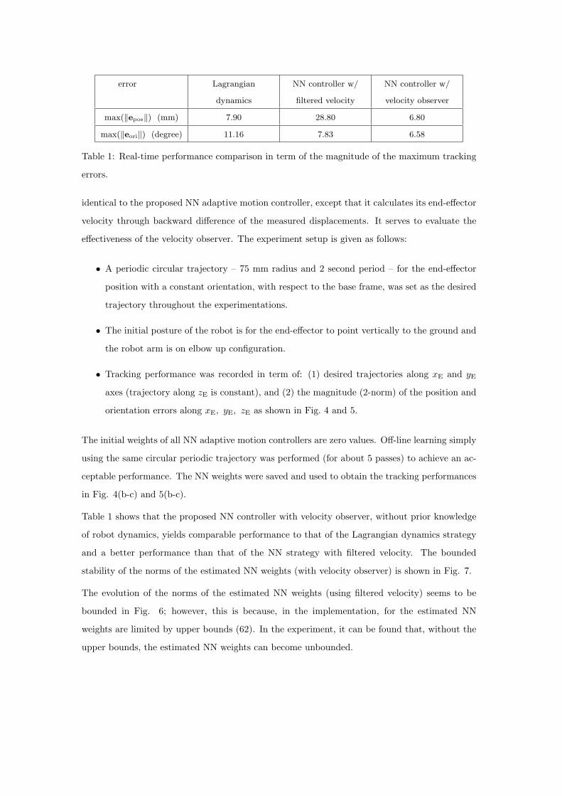
max(∥epos∥) (mm) 7.90 28.80 6.80

max(∥eori∥) (degree) 11.16 7.83 6.58

Table 1: Real-time performance comparison in term of the magnitude of the maximum tracking

errors.

identical to the proposed NN adaptive motion controller, except that it calculates its end-effector

velocity through backward difference of the measured displacements. It serves to evaluate the

effectiveness of the velocity observer. The experiment setup is given as follows:

• A periodic circular trajectory – 75 mm radius and 2 second period – for the end-effector

position with a constant orientation, with respect to the base frame, was set as the desired

trajectory throughout the experimentations.

• The initial posture of the robot is for the end-effector to point vertically to the ground and

the robot arm is on elbow up configuration.

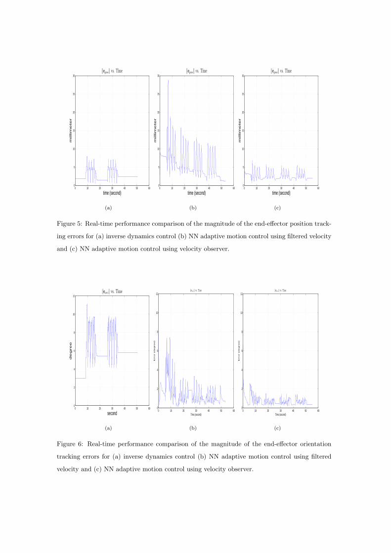
• Tracking performance was recorded in term of: (1) desired trajectories along xE and yE

axes (trajectory along zE is constant), and (2) the magnitude (2-norm) of the position and

orientation errors along xE, yE, zE as shown in Fig. 4 and 5.

The initial weights of all NN adaptive motion controllers are zero values. Off-line learning simply

using the same circular periodic trajectory was performed (for about 5 passes) to achieve an ac-

ceptable performance. The NN weights were saved and used to obtain the tracking performances

in Fig. 4(b-c) and 5(b-c).

Table 1 shows that the proposed NN controller with velocity observer, without prior knowledge

of robot dynamics, yields comparable performance to that of the Lagrangian dynamics strategy

and a better performance than that of the NN strategy with filtered velocity. The bounded

stability of the norms of the estimated NN weights (with velocity observer) is shown in Fig. 7.

The evolution of the norms of the estimated NN weights (using filtered velocity) seems to be

bounded in Fig. 6; however, this is because, in the implementation, for the estimated NN

weights are limited by upper bounds (62). In the experiment, it can be found that, without the

upper bounds, the estimated NN weights can become unbounded.

9 Discussions and Future Works

In this paper, the NN adaptive operational space motion formulation with velocity observer (17),

was derived and validated through real-time experiment.

The proposed strategy yielded a comparable performance to that of the Lagrangian dynamics

strategy. It also produced better performance than the NN motion control using filtered velocity

(118). Therefore, the outcome of the study is cost-effective and practical for real-time robotic

implementation, compared to the Lagrangian dynamic strategy, in term of without the need of

deriving and identifying Lagrangian dynamics.

The immediate future work is to extend the strategy from motion control only to the unified

force and motion control strategy in operational space framework.

References

[1] B. Armstrong, O. Khatib, and J. Burdick, “The explicit dynamic model and inertial param-

eters of the PUMA 560 arm,” in Proc. IEEE Int. Conf. Robot. Autom., San Francisco, CA,

USA, Apr.7–10, 1986, pp. 510–518.

[2] R. S. Jamisola, Jr., M. H. Ang, Jr., T. M. Lim, O. Khatib, and S. Y. Lim, “Dynamics

identification and control of an industrial robot,” in Proc. 9th Int. Conf. Adv. Robot., Tokyo,

Japan, Oct. 25–27, 1999, pp. 323–328.

[3] C. H. An, C. G. Atkeson, and J. M. Hollerbach, “Estimation of inertial parameters of rigid

body links of manipulators,” in Proc. 24th IEEE Conf. on Decision and Control, vol. 24,

no. 1, Dec. 1985, pp. 990 – 995.

[4] M. Gautier, “Identification of robots dynamics,” in Proc. IFAC Symp. on Theory of Robots,

Vienne, 1986, pp. 351–356.

[5] P. K. Khosla and T. Kanade, “Parameter identification of robot dynamics,” in Int. IEEE

Conf. on Decision and Control, vol. 24, no. 1, Dec. 1985, pp. 1754 – 1760.

[6] P. K. Khosla, “Estimation of robot dynamics parameters: Theory and application,” Robotics

Institute, Pittsburgh, PA, Tech. Rep. CMU-RI-TR-87-08, March 1987.

[7] F. Caccavale and P. Chiacchio, “Identification of dynamic parameters and feedforward con-

trol for a conventional industrial manipulator,” Control Engineering Practice, vol. 2, no. 6,

pp. 1039 – 1050, Dec. 1994.

[8] G. Antonelli, F. Caccavale, and P. Chiacchio, “A systematic procedure for the identification

of dynamic parameters of robot manipulators,” Robotica, vol. 17, no. 4, pp. 427 – 435, July

– Aug. 1999.

[9] W. Khalil, M. Gautier, and P. Lemoine, “Identification of the payload inertial parameters

of industrial manipulators,” in Proc. IEEE Int. Conf. Robot. Autom., Kobe, Japan, Apr.

10-14, 2007, pp. 4943 – 4948.

[10] J. J. Craig, P. Hsu, and S. S. Sastry, “Adaptive control of mechanical manipulators,” in

Proc. IEEE Int. Conf. Robot. Autom., San Francisco, CA, Apr.7–10, 1986, pp. 190–195.

[11] R. H. Middleton and G. C. Goodwin, “Adaptive computed torque control for rigid link

manipulators,” Syst. Contr. Lett., vol. 10, no. 1, pp. 9–16, Jan. 1988.

[12] R. Ortega and M. Spong, “Adaptive motion control of rigid robots: A tutorial,” in Proc.

IEEE Conf. on Decision and Control, vol. 2, Austin, TX, USA, Dec.7 – 9, 1988, pp. 1576–

1584.

[13] J.-J. E. Slotine and W. Li, “On the adaptive control of robot manipulators,” Int. Journal

of Robotics Research, vol. 6, no. 3, pp. 49–59, Fall 1987.

[14] ——, “Adaptive robot control: A new perspective,” in Proc. of the 26th IEEE Conf. on

Decision and Control, vol. 26, no. 1, Dec. 1987, pp. 192 – 198.

[15] N. A. Bompos, P. K. Artemiadis, A. S. Oikonomopoulos, and K. J. Kyriakopoulos, “Mod-

eling, full identification and control of the mitsubishi PA-10 robot arm,” in IEEE/ASME

Int. Conf. on Adv. Intel. Mechatronics (AIM2007), Sept.4 - 7, 2007, pp. 1–6.

[16] J. Swevers, W. Verdonck, and J. De Schutter, “Dynamic model identification for industrial

robots,” IEEE Control Systems Magazine, vol. 27, no. 5, pp. 58 – 71, Oct. 2007.

[17] N. D. Vuong, M. H. Ang, Jr., and Y. Li, “Dynamic model identification for industrial

manipulator subject to advanced model based control,” in Proc. 4th Conf. on HNICEM,

Manila, Philippines, Mar. 12 - 16, 2009.

[18] P. M. La Hera, U. Mettin, S. Westerberg, and A. S. Shiriaev, “Modeling and control of

hydraulic rotary actuators used in forestry cranes,” in Proc. IEEE Int. Conf. Robot. Autom.,

Kobe, Japan, May 12-17, 2009, pp. 1315–1320.

[19] W. Khalil, J.-F. Kleinfinger, and M. Gautier, “Reducing the computational burden of the

dynamic models of robots,” in Proc. IEEE Int. Conf. Robot. Autom., vol. 3, Apr. 1986, pp.

525 – 531.

[20] W. Khalil and J.-F. Kleinfinger, “Minimum operations and minimum parameters of the

dynamic models of tree structure robots,” IEEE J. Robot. Autom., vol. RA-3, no. 6, pp. 517

– 526, Dec. 1987.

[21] M. Gautier and W. Khalil, “A direct determination of minimum inertial parameters of

robots,” in Proc. IEEE Int. Conf. Robot. Autom., vol. 3, Apr. 24 – 29, 1988, pp. 368 – 373.

[22] ——, “Direct calculation of minimum set of inertial parameters of serial robots,” in Proc.

IEEE Int. Conf. Robot. Autom., vol. 6, no. 3, June 1990, pp. 368 – 373.

[23] W. Khalil and F. Bennis, “Symbolic calculation of the base inertial parameters of closed-loop

robots,” Int. Journal of Robotics Research, vol. 14, no. 2, pp. 112 – 128, Apr. 1995.

[24] W. Khalil and E. Dombre, Modeling, identification and control of robots, 3rd ed. London:

Hermes Penton Science, 2002.

[25] P. Hsu, M. Bodson, S. Sastry, and B. Paden, “Adaptive identification and control for manip-

ulators without using joint accelerations,” in Proc. IEEE Int. Conf. Robot. Autom., vol. 4,

Mar. 1987, pp. 1210 – 1215.

[26] Z. Lu, K. B. Shimoga, and A. A. Goldenberg, “Experimental determination of dynamic

parameters of robotic arms,” J. of Robotic Syst., vol. 10, no. 8, pp. 1009–1029, Dec. 1993.

[27] M. Gautier and W. Khalil, “An efficient algorithm for the calculation of the filtered dynamic

model of robots,” in Proc. IEEE Int. Conf. Robot. Autom., vol. 1, Apr. 22 – 28, 1996, pp.

323 – 328.

[28] M. Gautier, A. Janot, and P. O. Vandanjon, “Didim: A new method for the dynamic

identification of robots from only torque data,” in Proc. IEEE Int. Conf. Robot. Autom.,

Kobe, Japan, May 19-23, 2008, pp. 2122 – 2127.

[29] A. Janot, P. O. Vandanjon, and M. Gautier, “Identification of robots dynamics with the

instrumental variable method,” in Proc. IEEE Int. Conf. Robot. Autom., Kobe, Japan, May

12-17, 2009, pp. 1762–1767.

[30] M. Gautier and W. Khalil, “Exciting trajectories for the identification of base inertial pa-

rameters of robots,” in Proc. 30th IEEE Conf. on Decision and Control, vol. 1, Dec. 11-13,

1991, pp. 494 – 499.

[31] M. Gautier, “Optimal motion planning for robot’s inertial parameters identification,” in

Proc. 31st IEEE Conf. on Decision and Control, vol. 1, Dec. 16-18, 1992, pp. 70 – 73.

[32] C. Presse and M. Gautier, “New criteria of exciting trajectories for robot identification,” in

Proc. IEEE Int. Conf. Robot. Autom., vol. 3, May 2-6, 1992, pp. 907 – 912.

[33] M. M. Olsen, J. Swevers, and W. Verdonck, “Maximum likelihood identification of a dynamic

robot model: Implementation issues,” Int. Journal of Robotics Research, vol. 21, no. 2, pp.

89 – 96, Feb. 2002.

[34] O. Khatib, “A unified approach for motion and force control of robot manipulators: The

operational space formulation,” IEEE J. Robot. Autom., vol. RA-3, no. 1, pp. 43–53, Feb.

1987.

[35] L. Sciavicco and B. Siciliano, Modelling and Control of Robot Manipulators, 2nd ed. London:

Springer-Verlag, 2000.

[36] R. M. Sanner and J.-J. E. Slotine, “Stable adaptive control and recursive identification using

radial gaussian networks,” in Proc. of the 30th IEEE Conf. on Decision and Control, vol. 3,

Dec. 11 – Dec. 13, 1991, pp. 2116 – 2123.

[37] G. A. Rovithakis and M. A. Christodoulou, “Neural network controller characteristics with

regard to adaptive control,” IEEE Trans. Syst., Man, Cybern., vol. 24, no. 3, pp. 400 – 412,

Mar. 1994.

[38] S. S. Ge, Z.-L. Wang, and Z.-J. Chen, “Adaptive static neural network control of robots,”

in Proc. of the IEEE Conf. on Industrial Technology, vol. 3, Dec. 5 – Dec. 9, 1994, pp. 240

– 244.

[39] F. L. Lewis, K. Liu, and A. Yesildirek, “Neural net robot controller with guaranteed tracking

performance,” IEEE Trans. Neural Networks, vol. 6, no. 3, pp. 703–715, May 1995.

[40] F. L. Lewis, A. Yesildirek, and K. Liu, “Multilayer neural-net robot controller with guaran-

teed tracking performance,” IEEE Trans. Neural Networks, vol. 7, no. 2, pp. 388–399, Mar.

1996.

[41] F. L. Lewis, S. Jagannathan, and A. Yesildirek, Neural Network Control of Robot Manipu-

lators and Nonlinear Systems, 1st ed. Philadelphia, PA: Taylor and Francis, 1998.

[42] S. Hu, M. H. Ang, Jr, and H. Krishnan, “Neural network controller for constrained robot

manipulators,” in Proc. IEEE Int. Conf. Robot. Autom., vol. 2, San Francisco, CA, May

2000, pp. 1906–1911.

[43] C. M. Kwan, A. Yesildirek, and F. L. Lewis, “Robust force/motion control of constrained

robots using neural network,” in Proc. 33rd IEEE Conf. on Decision and Control 1994,

vol. 2, Lake Buena Vista, Florida, USA, Dec. 14 – 16, 1994, pp. 1862–1867.

[44] C. C. Cheah, Y. Zhao, and J.-J. E. Slotine, “Adaptive jacobian motion and force tracking

control for constrained robots with uncertainties,” in Proc. IEEE Int. Conf. Robot. Autom.,

Orlando, FL, USA, May 15 – May 19, 2006, pp. 2226–2231.

[45] N. H. McClamroch and D. Wang, “Feedback stabilization and tracking of constrained

robots,” IEEE Trans. Automat. Contr., vol. AC-33, no. 5, pp. 419–426, May 1988.

[46] Z. Doulgeri and Y. Karayiannidis, “An adaptive force regulator for a robot in compliant

contact with an unknown surface,” in Proc. IEEE Int. Conf. Robot. Autom., Barcelona,

Spain, Apr. 18 – Apr. 22 2005, pp. 2685–2690.

[47] Y. Karayiannidis and Z. Doulgeri, “An adaptive law for slope identification and force position

regulation using motion variables,” in Proc. IEEE Int. Conf. Robot. Autom., Orlando, FL,

May 15 – May 19 2006, pp. 3538–3543.

[48] Y. Karayiannidis, G. Rovithakis, and Z. Doulgeri, “A neuro-adaptive controller for the

force/position tracking of a robot manipulator under model uncertainties in compliance and

friction,” in 14th Mediterranean Conference on Control and Automation, 2006, 2007, pp.

1–6.

[49] ——, “Force/position tracking for robotic manipulator in compliant contact with a surface

using neuro-adaptive control,” Automatica, vol. 43, no. 7, pp. 1281–1288, July 2007.

[50] Y. Zhao, C. C. Cheah, and J.-J. E. Slotine, “Adaptive vision and force tracking control of

constrained robots with structural uncertainties,” in Proc. IEEE Int. Conf. Robot. Autom.,

Roma, Italy, Apr. 10 – Apr. 14, 2007, pp. 2349–2354.

[51] D. B. Soewandito, D. N. Oetomo, and M. H. Ang, Jr., “The operational space formulation

with neural-network adaptive motion control,” in Proc. Int. Fed. of Automat. Contr. (IFAC)

World Congress 2008, Seoul, Korea, July 6 – July 11, 2008, pp. 12 775–12 780.

[52] Q. H. Xia, S. Y. Lim, M. H. Ang, Jr, and T. M. Lim, “Adaptive joint friction compensation

using a model-based operational space velocity observer,” in Proc. IEEE Int. Conf. Robot.

Autom., vol. 3, New Orleans, LA, USA, Apr. 26 – May 1, 2004, pp. 3081–3086.

[53] J.-J. E. Slotine and W. Li, Applied Nonlinear Control, 1st ed. Englewood Cliffs, NJ: Prentice

Hall, 1991.

[54] S. Nicosia and P. Tomei, “Robot control by using only joint position measurements,” IEEE

Trans. Automat. Contr., vol. AC-35, no. 9, pp. 1058–1061, Sept. 1990.

[55] Q. H. Xia, S. Y. Lim, M. H. Ang, Jr., and T. M. Lim, “An operational space observer-

controller for trajectory tracking, Tech. Rep. SIMTech AT/02/014/PM, 2002.

[56] J.-J. E. Slotine and W. Li, “Adaptive manipulator control: Parameter convergence and

task-space strategies,” in Proc. American Cont. Conf., June10 – 12, 1987, pp. 828 – 835.

[57] F. L. Lewis, C. T. Abdallah, and D. M. Dawson, Control of Robot Manipulators, 1st ed.

NY: MacMillan, 1993.

[58] H. Berghuis and H. Nijmeijer, “A passivity approach to controller-observer design for

robots,” IEEE Trans. Robot. Autom., vol. 9, no. 6, pp. 740–754, Dec. 1993.

[59] S. S. Ge, T. H. Lee, and C. J. Harris, Adaptive neural network control of robotic manipulators.

River Edge, NJ: World Scientific, 1998.

[60] P. J. Werbos, “Backpropagation: Past and future,” in Proc. IEEE Int. Conf. Neural Net-

works, vol. 1, San Diego, CA, USA, July 24 – July 27, 1988, pp. 343–353.

[61] G. V. Cybenko, “Approximation by superpositions of a sigmoidal function,” Mathematics

of Control, Signals, and Systems, vol. 2, no. 4, p. v, 1989.

[62] J. P. LaSalle, “Some extensions of liapunov’s second method,” IRE Trans. Circuit Theory,

vol. 7, no. 4, pp. 520–527, Dec. 1960.

xd, xd,xd

x

F Fwd

Kin.

NN

controller

observer

Robotq

NN

weight

updates

x

Figure 1: The structure of the operational space NN motion NN controller-observer.

σ1(·)z1

z2 σ2(·)

zN1

σ3(·)

σN2(·)

.

.

.

.

.

.

v1N1

v11

v12

v2N1

v21

v22

v3N1

v31v32

vN2N1

vN21vN22

u1

u2

u3

uN3

.

.

.

w1N2

w11

w12

w13

w2N2

w21

w22

w23

w3N2

w31w32

w33

wN3N2

wN31

wN32

wN33

θ1

θ2

θ3

θN2

Figure 2: Three-layer NN structure (with output vector).

(ζfriction+3C0)ψm

V < 0

‖y‖

‖Z‖

by

V >=< 0

bZZM ZM

yM

S

Figure 3: V (y, Z) regions of the NN adaptive motion control with velocity observer.

0 1 2 3 4 5 6 7 80.15

0.2

0.25

0.3

Reference Trajectory in XY plane

time(s)

X D

ispl

acem

ent

0 1 2 3 4 5 6 7 8

0.5

0.55

0.6

0.65

time(s)

Y D

ispl

acem

ent

Figure 4: The reference trajectory for the effector position

0 10 20 30 40 50 600

5

10

15

20

25

30

millim

ete

r

time (second)

‖epos‖ vs. Time

(a)

0 10 20 30 40 50 600

5

10

15

20

25

30

millim

ete

r

time (second)

‖epos‖ vs. Time

(b)

0 10 20 30 40 50 600

5

10

15

20

25

30

millim

ete

r

time (second)

‖epos‖ vs. Time

(c)

Figure 5: Real-time performance comparison of the magnitude of the end-effector position track-

ing errors for (a) inverse dynamics control (b) NN adaptive motion control using filtered velocity

and (c) NN adaptive motion control using velocity observer.

0 10 20 30 40 50 600

2

4

6

8

10

12

degree

second

‖eori‖ vs. Time

(a)

0 10 20 30 40 50 600

2

4

6

8

10

12

Error (

degree)

Time (second)

‖eori‖ vs. Time

(b)

0 10 20 30 40 50 600

2

4

6

8

10

12

Error (

degree)

Time (second)

‖eori‖ vs. Time

(c)

Figure 6: Real-time performance comparison of the magnitude of the end-effector orientation

tracking errors for (a) inverse dynamics control (b) NN adaptive motion control using filtered

velocity and (c) NN adaptive motion control using velocity observer.

0 20 40 600

2

4

6

8

10

12‖WM ‖, ‖VM‖ vs. Time

Time (second)

‖WM ‖

‖VM‖

0 20 40 600

0.2

0.4

0.6

0.8

1‖WV ‖, ‖VV ‖ vs. Time

Time (second)

‖WV ‖

‖VV ‖

0 20 40 600

1

2

3

4

5

6

7‖Wg‖, ‖Vg‖ vs. Time

Time (second)

‖Wg‖

‖Vg‖

0 20 40 600

1

2

3

4

5

6

7‖Wτ ‖, ‖Vτ‖ vs. Time

Time (second)

‖Wτ ‖

‖Vτ‖

Figure 7: Real-time norm history of the estimated NN weights of the NN motion controller with

filtered velocity.

0 20 40 600

2

4

6

8

10

12‖WM ‖, ‖VM‖ vs. Time

Time (second)

‖WM ‖

‖VM‖

0 20 40 600

0.2

0.4

0.6

0.8

1‖WV ‖, ‖VV ‖ vs. Time

Time (second)

‖WV ‖

‖VV ‖

0 20 40 600

1

2

3

4

5

6

7‖Wg‖, ‖Vg‖ vs. Time

Time (second)

‖Wg‖

‖Vg‖

0 20 40 600

1

2

3

4

5

6

7‖Wτ ‖, ‖Vτ‖ vs. Time

Time (second)

‖Wτ ‖

‖Vτ‖

Figure 8: Real-time norm history of the estimated NN weights of the NN motion controller with

velocity observer.