KYBERNETIKA — VOLUME 29 (1993), NUMBER 1, PAGES 3 0 - 4 7

NEURODYNAMIC ADAPTIVE CONTROL SYSTEMS

JULIO C. PROANO, JAN T. BIALASIEWICZ AND EDWARD T. WALL

Precision adaptive control has been accomplished using a neural network to generate the required system dynamics, given the desired input and output. That is, an artificial neural network has been designed and incorporated into an adaptive control system to function as a synthesizer of a dynamic plant which senses and continually reduces, in a learning sense, the system error. This approach is called neurodynamic adaptive control since the system dynamics are modeled by an adaptive neural topology.

1. INTRODUCTION

The concept of a neural network can be traced back to the early 1940's. About thirty years ago engineers and scientists began to use this approach in an attempt to model static and simple dynamic problems. In this paper it is shown that neurodynamics and advances in adaptive learning systems are at a state of development where a synthesis of these principles leads to a significant advance in on-line adaptive control systems for control design and off-line model synthesis.

Neural network models of the brain or nervous system have been studied for many years. Initially, they were of primary interest to physiologists, biologists, psycholo­gists, etc., primarily to understand the behavior of the brain and nervous system. In recent years, modeling techniques have been extended and developed in an effort to improve the technology of signal and control processes. The term neurodynamics has been chosen to identify the learning process which is accomplished within this control system.

The approach developed makes use of a class of feedback dynamic neural .nets described by a system of nonlinear difference equations. The solutions of these equations must converge to a bounded region of state space. If the model is a gradient system, i.e., a system that contains no stable limit cycles and has at least one equilibrium state, then its stable trajectories will enter or exit from selected equilibrium states. System applications such as identification, estimation, pattern recognition, etc., essentially become special cases of this normalized gradient system.

For control system applications this research has been limited to systems of linear difference equations, so that accurate adaption and learning laws may be developed for on-line use, using the neural system concept. Thus providing an adaptive control system for standard application.

Neurodynamic Adaptive Control Systems 31

The neurodynamic adaptive model has been successfully tested in three modes of operation: off-line learning mode, on-line learning mode and normal mode. First, the plant is modeled by the neurodynamic system using input and output data as shown in Figure 1. This training or learning process is done off-line until the neurodynamic system adjusts its own parameters to reproduce the input-output pair sequences. Second, once this process is completed satisfactorily, this model can be put in the control loop of the plant (refer to the inverse dynamics control example), in which it will operate in normal execution model. Finally, the complete control of the plant is obtained by adding a duplicate (parameter-wise) neurodynamical system in parallel to the plant which operates in on-line learning mode as shown in Figure 2. Any significant change of the dynamics of the plant is sensed by the latter system and the result is the almost instantaneous changes of its parameters. The two neurodynamic systems (one in normal execution mode and the other in on-line learning mode) share the values of their parameters, and the result is a self-adapting control system.

REFERENCE MODEL

(PLANT)

NHJRODYNAMC

ADAPTIVE SYSTEM

PLANT ou tput

G(s)

4 4

N в u r o d y п a m i c

(on-llnв lвarnśng

N в u r o d y п a m i c

(on-llnв lвarnśng

N в u r o d y п a m i c

(on-llnв lвarnśng

F i g . 1. Neurodynamic adaptive model. F i g . 2. Inverted dynamics control system.

2. NEURODYNAMIC ADAPTIVE SYSTEM

The neurodynamic adaptive system behaves like a synthesizer that evaluates the performance of a dynamic system using multilayer neural network topology. A multilayer dynamic neural network was chosen to implement the system because of its potential for supplementing the dynamics.

The use of a discrete representation of the behavior of a physical system was adopted to introduce the time dimension into the neural network structure. This discrete implementation of the model of a system requires a delay network. This additional subnetwork has been implemented by a neural structure [1] and by shift registers.

The basic research part of the present study is the application of multilayer neural networks to the simulation of the dynamics of physical systems. The most relevant properties for control systems compensation by neural networks can be enumer­ated as follows. The first is the instantaneous performance using simple computing

32 J.C. PROANO, J .T. BIALASIEWICZ AND E.T. WALL

elements. The second is the partial immunity to system crash if some elements mal­function, which is known as the property of continuous domain memory and redun­dancy. Third, and most important, is the parallel processing behavior of multilayer topology, which is particularly exploited in this research.

3. ARCHITECTURE

The topological structure of the dynamic neural network synthesizer, shown in Fig­ure 3, is based on two main developments in the areas of adaptive filters and neural networks, Madaline network developed by Widrow [2], [11] and the delta rule or backpropagation method originally developed by Werbos [9], [10]. The applications of the backpropagation method in neural networks were originated by the paper by Rumelhart, Hinton, and Williams [3]. Windrow's contributions to the field are summarized in [11]. A new recursive prediction error algorithm for the training of feedforward layered network with better convergence properties than the classical backpropagation algorithm is proposed in [12]. Improved learning algorithms are also reported in [17].

Fig. 3. Topological structure of the dynamic neural network synthesizer.

The optimization of parameters of the neural network is accomplished by gradient descent to optimize the values of the weights that interconnect the different layers of the neural network. The present approach goes a step further, and optimizes three other parameters directly related to the slope, threshold value, and saturation level of the activation function of each neuron or processing element. In addition, it updates the learning rate coefficient according to the total error. Thus the learning in this neurodynamic architecture is an extended version of the delta rule.

In the following derivation, it is important to recognize the local character of optimization process. The computation of the updated values of the parameters of the neural network is local to each processing unit. This property makes the overall

Neurodynamic Adaptive Control Systems 33

system a parallel computational structure suitable for hardware implementation with on-line adaptation capabilities.

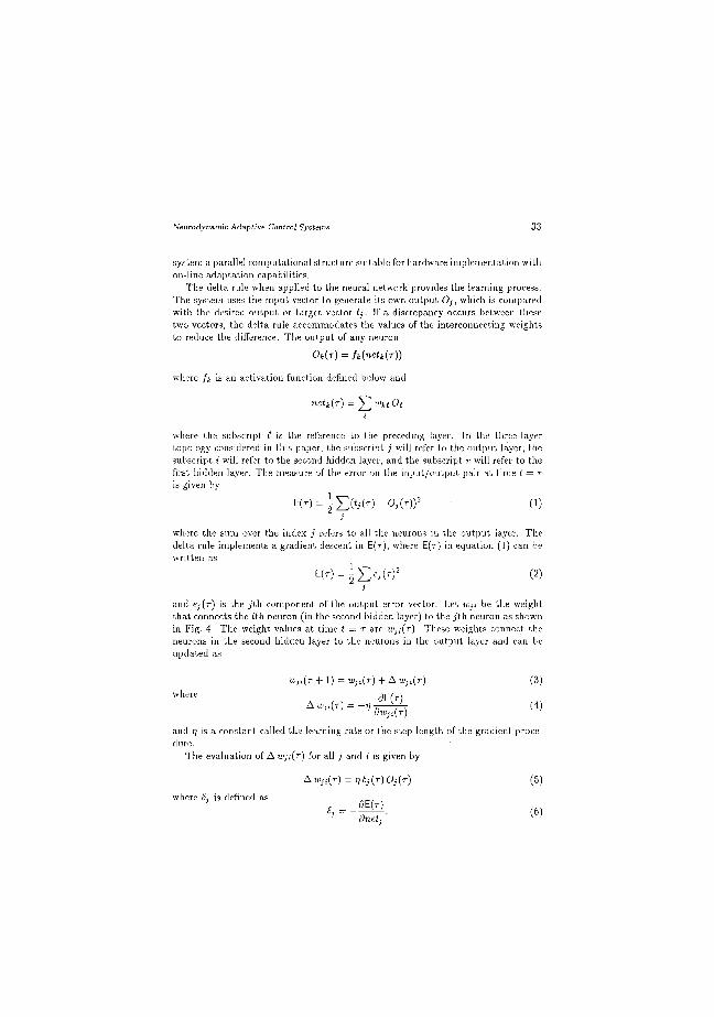
The delta rule when applied to the neural network provides the learning process. The system uses the input vector to generate its own output Oj, which is compared with the desired output or target vector tj. If a discrepancy occurs between these two vectors, the delta rule accommodates the values of the interconnecting weights to reduce the difference. The output of any neuron

Ok(r) = fk(netk(r))

where fk is an activation function defined below and

netk(r) = ] P wkt Ot l

where the subscript £ is the reference to the preceding layer. In the three-layer topology considered in this paper, the subscript j will refer to the output layer, the subscript i will refer to the second hidden layer, and the subscript r will refer to the first hidden layer. The measure of the error on the input/output pair at time t = r is given by

E(T)^E(^T)-°i(r))2 o) 3

where the sum over the index j refers to all the neurons in the output layer. The delta rule implements a gradient descent in E(T) , where E(T) in equation (1) can be written as

E(r) = ^ X > M 2 (2) 3

and e ;(r) is the j th component of the output error vector. Let Wji be the weight that connects the *th neuron (in the second hidden layer) to the j th neuron as shown in Fig. 4. The weight values at time t = r are WJJ(T). These weights connect the neurons in the second hidden layer to the neurons in the output layer and can be updated as

Wji(r+\) = wji(r)+Awji{T) (3) where d£, x

and i] is a constant called the learning rate or the step length of the gradient proce­dure.

The evaluation of A Wji(r) for all j and i is given by

Awji(T) = r1SJ(T)Oj(T) (5)

where 6; is defined as

«' = - * £ W

34 J.C. PROANO, J.T. BIALASIБWICZ AND E.T. WALL

Fig. 4. Interconnections in the multilayer neural network.

This procedure is extended to all layers of the network. The approximation capa­bilities of neural network architectures have been investigated by many authors. Interesting results are presented by Cybenko [15]. In Hornik [13] it is rigorously es­tablished that standard multilayer feedforward networks with one hidden layer using arbitrary squashing or activation functions are capable of approximating any Borel measurable function from one finite-dimensional space to another to any desired de­gree of accuracy, provided sufficiently many hidden units or neurons are available. Farther results on approximation capabilities are reported by Hornik in [14].

4. THE EXTENDED DELTA RULE

The extended delta rule is based on the consideration of a semilinear activation function fk for the neuron uk that belongs to any layer of the neural network.

The generalized activation function fk of the neuron uk is a sigmoidal function that depends on the following parameters:

(i) Measure of the slope of the sigmoid in the linear region ak

(ii) Threshold value hk

(iii) Saturation level Kk-

Such a function is given by

/ - K l ~ exP(-®k(netk + hk)) Jk k l + exp(-ak(netk + hk)) ['>

and

Neurodynamic Adaptive Control Systems 35

or in a more compact form

fk = Kk tanh [y(ne.fc + hk)] • (8)

The parameters a;-, a,- and a r of the sigmoidal function in equation (7) at time i = r can be updated as „. . . . . .

« i ( T + l ) = cvj-W + A a ^ T ) , (9)

a ; ( r + l ) = a t ( r ) +Aa , ; ( r ) , (10)

a r ( r + l ) = « r ( r ) + A a r ( r ) , (11)

W l l 6 r e A 9 j = n6Jnetj (12)

A a,; = n6fneti (13)

A a r = i)6rnetr (14)

6J = {tj-Ofif? (15)

*" = I>«y.ff (16) i

6? = ^SiWirf? (17) k

, u A i dfk h = ^ dn^' ( 1 8 )

This approach is extended to the other two parameters hk and Kk. The parameters hj, hi and hr of the sigmoidal function in equation (7) at time

t = T can be updated as , , , , ,

A ; ( T + 1 ) = / ! j(r) + A/ l j ( r ) (19)

A,(r + 1) = A,-(T) + A A . ( T ) (20)

/ i r ( r + l ) = /i r(r) + A / V ( r ) (21) where „ , ,

A hj = n Sj (22)

Ahi = rj6i (23)

A Ar = n 6r (24)

63 = (tj-OrffJaj (25)

6i = ^SjWjiftai (26)

j

6r = "£6i UHrf? Or (27)

The parameters Kj, A',- and Kr of the sigmoidal function (7) at time t = r can be updated as , s ,

KJ(T+1) = KJW + AK^T) (28)

Ki(T+l) = Ki(T) + AKi(T) (29)

Kr(T+l) = A'r(r) + A K r ( r ) (30)

and

36 J.C. PROANO, J .T. BIALASIEWICZ AND E.T. WALL

where A Kj

Д KІ

A Kr

чSïírKf1

Ji

Цбфlí-1.

(31)

(32)

(33)

5. DYNAMICS OF THE NEURON STRUCTURE

The dynamics introduced in the multilayer neural network structure is the most im­portant component of the neurodynamic adaptive synthesizer (NDAS) architecture. It provides the memory feature that transforms a static neural net into a dynamic neural net. This dynamics is essential in the development of control system models, compensators, estimators, etc..

Definition. Memory-type elements are elements whose input-output characteris­tics are not unique in a static sense but are unique if initial pairs of input-output values plus the entire histories of inputs are specified [4].

Since the output for a memory-type device depends on the entire input histo­ry, the input-output relationship for the memory device can best be represented mathematically by a specific functional

Fig. 5. Active-memory neuron. Fig. 6. Passive-memory neuron.

Two types of memory structures for the neuron have been investigated: active-memory type and passive-memory type. The neural implementation of these two types of memory-elements are shown in Figs. 5 and 6. In the literature on nonlinear control systems, active-memory elements and passive-memory elements have mostly been studied in the context of response to sinusoidal inputs.

Neurodynamic Adaptive Control Systems 37

Definition. A memory element is called active if over one cycle of the input, the characteristic is traversed in such a way that a nonzero area is encircled in a clockwise direction [4].

Definition. A memory element is called passive if over one cycle of input, the characteristic is traversed in such a way that a nonzero area is encircled in a coun­terclockwise direction [4].

An important feature of passive-memory elements in nonlinear systems is that the area enclosed by the element characteristic is a measure of the energy dissipated during each cycle. On the other hand, the area enclosed by the active element characteristic represents the energy supplied by this element to the system in each cycle.

These two concepts are fundamental in the performance of the neurodynamic adaptive synthesizer. The feedback uses the necessary delay to produce the memory effect in the hysteresis in Figs. 5 and 6. The basic equations for the active and passive memory structure of an arbitrary neuron uk, are respectively

ofcí>) = fk(netk(T)-K;lOk(T-\))

Ofc(r) = fk(netk(T) + I<;1 Ok(T - 1))

(34) (35)

Input

Fig. 7. Effect of changes in the values of the parameter a for the active-memory neuron.

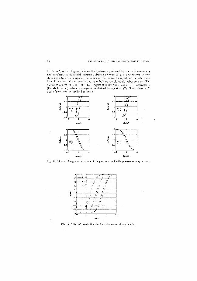
Figure 7 shows the hysteresis produced by the active-memory neuron where the sigmoidal function is defined by equation (7). The different curves show the effect of changes in the values of the parameter a, where the saturation level K is con­stant and normalized to unit, and the threshold value to zero. The values a are:

38 J.C. PROANO, J .T. BIALASIEW1CZ AND E.T. WALL

2; 1.5; —2; —1.5. Figure 8 shows the hysteresis produced by the passive-memory neuron where the sigmoidal function is defined by equation (7). The different curves show the effect of changes in the values of the parameter a, where the saturation level K is constant and normalized to unit, and the threshold value to zero. The values of a are: 2; 1.5; —2; —1.5. Figure 9 shows the effect of the parameter h (threshold value), where the sigmoid is defined by equation (7). The values of K and O' have been normalized to unity.

Input

F i g . 8. Effect of changes in the values of the parameter a for the passive-memory neuron.

—-.-. /""", -•'"" У

Һ - o // •'/

— _-_, II ІI II //

І..JJ ІJ 1 • // // II II // /

V ii

-J / 1/ _ - - - - / , _ r - - " " _ _ - ^

Fig . 9. Effect of threshold value h on the neuron characteristic.

Neurodynamic Adaptive Control Systems 39

6. COMPUTER SIMULATION EXAMPLES

Example 1. Single-degree of a positional controller for a robotic arm. This is a third-order system with the transfer function

T(s) = 75

s 3 + 7s2 + ЗOs + 75'

_ o.в --•• -;

/Г\! I i

- T(s)

NdAS

І L._ Error

i 0 0.5 1 1.5 2 2.5 3 3.5

Time [sec.]

Fig. 10. Step response of the third-order positional controller in a robot arm and its neurodynamic model.

Fig. 11. Illustration of the noise rejection ability of the neurodynamic model

40 J .C. PROANO, J .T. BIALASIEWICZ AND E.T. WALL

The Hemodynamic model was trained to follow the behavior of this system. Fig­ure 10 shows the result of off-line learning. The solid line is the step response of T(s) and the dashed line represents the step response of the neurodynamic model. It can be seen that the difference in the performance of the real system and its neu­rodynamic model is practically negligible. The noise rejection characteristic of this model is illustrated by Figure 11. The step input plus noise shown in this figure pro­duces the response shown by a. light line. It can be compared to the noise-free step response1 of the system model, shown by a solid line. The extremely low sensitivity of the neurodynamic model to noise is to be noted.

An analysis of the. structure of the neuron weights after the completion of learning shows that the neurodynamic model may be used as a state estimator or observer and the states can be defined by the set of outputs of all neurons. However, it has been found by experiment that a sufficient reduced set of states exists [5]. In the recent paper, it- has been shown by Soloway and Bialasiewicz [16] that using Volterra expansion the output of a neural network can be represented as a linear combination of the first and higher order impulse responses, determined by the weights of the trained network. This expansion can be truncated and its term can be used as a finite-dimensional estimate of the state vector.

Example 2. Design of a simplified vertical channel landing condition autopilot. The state model after linearization, as specified in [6] is

0 1 0 0 0 KiK2C K2Cmg K2Cmde

0 1 K3Cla KiCae 0 0 0 - 2 0

x +

Based upon an altitude of 500 feet, an approach speed of about 260 knots and typical values for the various stability derivatives, the A matrix is evaluated to be:

A =

0 1 0 0 0 -.856 -2.737 -0.812 0 1 -.521 -0.77 0 0 0 20

It is now possible using conventional state-variable techniques to obtain the open-loop transfer function of the vertical airplane channel as

GЉ) = -164.24(5+ .495)

ф + 20) (s + .69 + j 1.65) (s + .69 - j 1.65)'

The goal is to show that using the neurodynamic simulator a close approximation to the inverse dynamics l/Gp(s) is obtained, which when cascaded with the plant Gp(s), produces an overall dynamics such that the system performance is satisfac­tory. For simplicity, in the simulation, the velocity controller was developed for the plant transfer function G(s) which is Gp(s) without integration. Figure 12 shows the undesirable performance of the uncompensated plant. To illustrate the high accuracy of the neurodynamic model, its step response (solid line), and also the. step

Neurody Adaptive Control Systems 41

response of the plant (dashed line) are shown together in Fig. 13. To develop a neurodynamic compensator with the transfer function which approximates 1/G(s), a step input is applied to the plant. The inverse dynamics of the plant is learned by the neurodynamic model by inverting the input and output when operating in the learning mode. The performance of the developed inverted dynamics in the form of the unit step response is shown in Fig. 14. Also, the approximate inverted dy­namics were used as a compensator cascaded with the plant. The step responses of the uncompensated plant (dashed line) and the compensated plant (solid line) are shown for comparison in Fig. 15. The significant improvement in performance is to be noted. In Fig. 16 the performance of the neurodynamic inverted compensator is compared with the performance of a compensator that uses state-variable feedback. It is seen that the system with the neurodynamic compensator is much faster with a slightly higher overshoot. This can be improved with a longer off-line learning process. The neurodynamic compensator is faster than the state-variable feedback design due to the difference in performance of the two systems. The neurodynamic compensator is a highly nonlinear system that optimizes the overall performance, driving the parameters in a nonlinear fashion.

Time [sec]

F i g . 12. Plant performance before compensation.

42 J.C. PROANO. J.T. BIALASIEWTCZ AND E.T. WALL

-0 .5

NdAS resp. Desired resp. Error

6

Time [ s e c ]

Fig. 13. Step response ol ilii- plani and its neurodynamic model.

1.2

0.2 Һ

Input

NdAS resp.

0 2 4 6 8 10

Time [ s e c ] Fig. 14. Step response of the approximate inverted dynamics.

Neurodynamic Adaptive Control Systems 43

/--,

/ \ P laa t resp.

ì \ Ctгl. Syst. resp.

| ^ \ 1 / \ " 11 \ / '

Fin;. 15. Step response of the uncompensated and compensated plant.

X<^:

/ /

Time [sec] Fig. 16. Step responses illustrating the performance of the neurodynamic inverted dynamics compensator and the compensator designed using state space approach.

E x a m p l e 3. Application to attitude control of a flexible spacecraft. In general this is a problem of feedback control of bending modes in flexible systems. In theory, such systems required an infinite number of elastic modes to completely de­scribe their behavior. However, they are usually modeled by large finite-dimensional systems. The fundamental problem of feedback control of flexible systems is to pre­cisely control a high dimensional system with a smaller dimensional controller, since

44 J .C. PROANO, J .T. BIALASIБWICZ AND E.T. WALL

on-board computer limitations and modelling errors restrict the control to a few critical modes. This restriction can be removed by the application of a controller based on a neurodynamic simulator. One possibility is the use of an inverted dynam­ics controller. In order to show that the neurodynamic system is capable of accurate modelling of the dynamic of flexible structures, an example with the following pole locations is given.

- 0 . 5 ± j

-0.5 ± j 2

- 1 . 0 ± j l . 5

- 1 . 5 ± j 2 . 5 .

This corresponds to the normalized transfer function

60.43 гo) = s 2 ± 9 . 5 s 7 + 39.25s6+114.6s5 + 223.06s4 + 321.90s3 + 305.05s2 + 194.71s + 60.43'

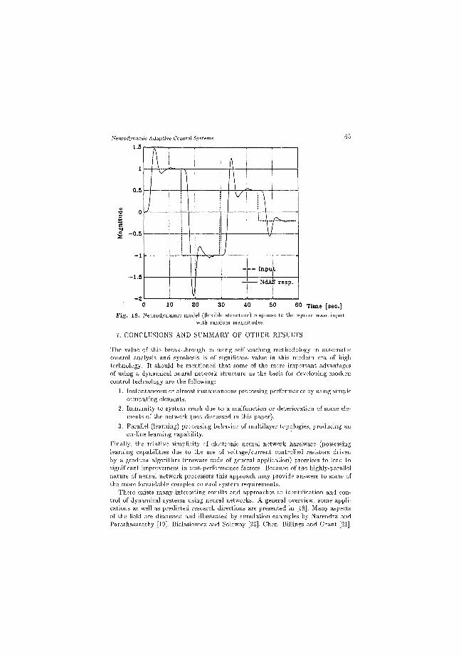
The neurodynamic model trained with this plant performs almost exactly as the plant. This is shown in Figure 17 in which the step responses of both the plant and its neurodynamic model can be seen to be almost identical. Figure 18 shows the neurodynamic model response with a square wave input signal and a random magnitude. j a

4 6 8 10 12 14

Time [ s e c ]

Fig. 17. Step responses of the plant (flexible structure) and its neurodynamic model.

Neurodynmnic Adaptive Control System

1.5

45

-0.5

-1 .5

60 Time [ sec ] Fig . 18 . Neurodynamic model (flexible structure) response to the square wave input

with random magnitudes.

7. CONCLUSIONS AND SUMMARY OF OTHER RESULTS

The value of this break-through in using self-teaching methodology in automatic control analysis and synthesis is of significant value in this modern era of high technology. It should be mentioned that some of the more important advantages of using a dynamical neural network structure as the basis for developing modern control technology are the following:

1. Instantaneous or almost instantaneous processing performance by using simple computing elements.

2. Immunity to system crash due to a malfunction or deterioration of some ele­ments of the network (not discussed in this paper).

3. Parallel (learning) processing behavior of multilayer topologies, producing an on-line learning capability.

Finally, the relative simplicity of electronic neural network hardware (possessing learning capabilities due to the use of voltage/current controlled resistors driven by a gradient-algorithm firmware code of general application) promises to lead to significant improvement in cost-performance factors. Because of the highly-parallel nature of neural network processors this approach may provide answers to some of the more formidable complex control system requirements.

There exists many interesting results and approaches to identification and con­trol of dynamical systems using neural networks. A general overview, some appli­cations as well as predicted research directions are presented in [18]. Many aspects of the field are discussed and illustrated by simulation examples by Narendra and Parathasarathy [19], Bialasiewicz and Soloway [20], Chen, Billings and Grant [21],

46 J.C. PROANO, J.T. BIALASIEWICZ AND E. T. WALL

Poloycarpou and Ioannou [22], and Bialasiewicz and Ho [23]. Stochastic, neural adapt ive control a lgor i thms are presented in [24], [25], [26], [27] and i l lustrated by s imulat ion resul ts .

In spi te of numerous interest ing s imulat ion results and some applicat ion a t t e m p t s , the relevance of research on neural identifiers and controllers is still open to deba te . Al though encouraging results have been obta ined, the development of sound theo­retical bases is still required for the applicabil i ty of neural networks to real control problems. T h e first achievements genera ted a lot of exci tement . However, the key to the future of neural networks lies in high-quali ty long- term basic and applied re­search, not in creat ing "new" a lgor i thms and generat ing endless s imulat ion results .

(Received December 5, 1989.)

REFERENCES

[1] M.I. Jordan: Altractor dynamics and parallelism in a connectionist sequential ma­chine. In: Proc. Eighth Annual Conf. of the Cognitive Science Society, Hillsdale, N . J . 1986.

[2] B. Widrow and R. Winter: Neural nets for adaptive filtering and adaptive pattern recognition. IEEE Computer Magazine, March 1998.

[3] D. Rumelhart, D. Hinton and G. Williams: Learning internal representations by error propagation. In: Parallel Distributed Processing (D. Rummelhart and F.McClelland, eds.), Vol. 1, The MIT Press, 1986.

[4] J .C . Hsu and A. V. Meyer: Modern Control Principles and Applications. McGraw-Hill, N. Y. 1968.

[5] J . T . Bialasiewicz, J .C . Proano and E. T. Wall: Implementation of intelligent controller using neural network state estimator. In: Proc. Fourth IEEE International Symposium on Intelligent Control, Sept. 1989.

[6] J. W. Weinstein and J. L. Melsa: Design of a simplified vertical channel landing control autopilot using state-variables. 1970 SWIEEECO Record, IEEE Catalog No. 70C5-SWIECO.

[7] B. Bavarian: Introduction to neural networks for intelligent control. IEEE Control Systems Magazine, April 1988, 3-7.

[8] D. Psaltis, A. Sideris and A. A. Yamamura: A multilayered neural network controller. IEEE Control Systems Magazine, April 1988, 17-21.

[9] P. J. Werbos: Backpropagation through time: What it does and how to do it. Proc. IEEE 75(1990), 9, 1550-1560.

[10] P .J . Werbos: Beyond Regression: New Tools for Prediction and Analysis in the Be­havioral Sciences. Ph .D . Dissertation, Committee on Appl. Math., Harvard Univ., Cambridge, Mass. 1974.

[11] B. Widrow and M. A. Lehr: 30 years of adaptive neural networks: Perception, rnadaline and backpropagation. In: Proc. IEEE 75(1990), 9, 1415-1442.

[12] S. Chen, C .F . N. Cowan, S. A. Billings and P.M. Grant: Parallel recursive prediction error algorithm for training layered neural networks. Internat. J. Control 51 (1990), 6, 1215-1228.

[13] K. Hornik: Multilayer feedforward networks are universal approximators. Neural Net­works Z (1989), 2, 359-366.

[14] K. Hornik: Approximation capabilities of multilayer feedforward networks. Neural Networks 4 (1991), 251-257.

[15] G. Cybenko: Approximation by superpositions of a sigmoidal function. Math. Control Signals Systems 2 (1989), 303-314.

Neurodynamic Adaptive Control Systems 47

[16] D. Soloway and J . T . Bialasiewicz: Neural network modeling of nonlinear systems based on Volterra series extension of a linear model. In: Proc. 7th IEEE Intl. Sympo­sium on Intelligent Control, Glasgow, Scotland, 1992.

[17] C. Batur, H. Zhang, J. Padovan and V. Kasparian: Davidon least square based neural network learning algorithms. ACC, 1992, 973-977.

[18] T . W . Miller, R. S. Sutton, III and P.J . Werbos (eds.): Neural Network for Control. MIT Press, Cambrdige, Mass. 1990.

[19] K. S. Narendra and K. Parathasarathy: Identification and control of dynamical systems using neural networks. IEEE Trans. Neural Networks 1 (1990), 4-27.

[20] J . T . Bialasiewicz and D. Soloway: Neural network of dynamical systems In: Proc. 5th IEEE Intl. Symposium on Intelligent Control, Philadelphia, 1990, 500-505.

[21] S. Chen, S.A. Billings and P.M. Grant: Nonlinear system identification using neural networks. J. Control 51 (1990), 6, 1191-1214.

[22] M.M. Polycarpou and P. A. Ioannou: Modeling, identification and stable adaptive control of continuous-time nonlinear dynamical systems using neural networks. 1992, ACC, 36-40.

[23] J . T . Bialasiewicz and T. T. Ho: Neural adaptive identification and control. In: Proc. 1991 Intl. Conf. on Artificial Neural Networks in Engineering. St. Louis, Missouri, 1991.

[24] T . T . Ho, H.T . Ho, J . T . Bialasiewicz and E .T . Wall: Stochastic neural direct adap­tive control. In: Proc. 6th IEEE Intl. Symposium on Intelligent Control, Arlington, Virginia, 1991.

[25] T . T . Ho, H.T . Ho and J . T . Bialasiewicz: Stochastic neural adaptive control for non­linear time varying systems. In: Proc. 1991 Intl. Conf. on Artificial Neural Networks in Engineering. St. Louis, Missouri, 1991.

[26] T . T . Ho, S. T. Ho, J. T. Bialasiewicz and E. T. Wall: Stochastic neural adaptive control using state space innovations model. In: Proc. 1991 IJCNN, Singapore, 1991.

[27] T . T . Ho, H .T . Ho and L.T. Ho: Stochastic neural adaptive control for time varying linear systems based on Newton and gradient optimizations. 1992, ACC, 51-55.

Dr. Julio C. Proano, Dr. Jan T. Bialasiewicz, Dr. Edward T. Wall, University of Colorado at Denver, Department of Electrical Engineering, Campus Box 110, P. O. Box 173364, Denver, Colorado 80217-3364. U.S.A.