neutral interstellar helium parameters based on ibex-lo

arX

iv:1

202.

0415

v1 [

astr

o-ph

.GA

] 2

Feb

201

2

Neutral interstellar helium parameters based on IBEX-Lo

observations and test particle calculations

M. Bzowski1, M.A. Kubiak1, E. Mobius2, P. Bochsler2,3, T. Leonard2, D. Heirtzler2,

H. Kucharek2, J.M. Soko l1, M. H lond1, G.B. Crew4, N.A. Schwadron2, S.A. Fuselier5,

D.J. McComas6,7

ABSTRACT

Because of its high ionization potential and weak interaction with hydrogen, Neutral Inter-stellar Helium is almost unaffected at the heliospheric interface with the interstellar mediumand freely enters the solar system. This second most abundant species provides some of thebest information on the characteristics of the interstellar gas in the Local Interstellar Cloud.The Interstellar Boundary Explorer (IBEX) is the second mission to directly detect NISHe. Wepresent a comparison between recent IBEX NISHe observations and simulations carried out us-ing a well-tested quantitative simulation code. Simulation and observation results compare wellfor times when measured fluxes are dominated by NISHe (and contributions from other speciesare small). Differences between simulations and observations indicate a previously undetectedsecondary population of neutral helium, likely produced by interaction of interstellar helium withplasma in the outer heliosheath. Interstellar neutral parameters are statistically different fromprevious in situ results obtained mostly from the GAS/Ulysses experiment, but they do agreewith the local interstellar flow vector obtained from studies of interstellar absorption: the newly-established flow direction is ecliptic longitude 79.2◦, latitude −5.1◦, the velocity is ∼ 22.8 kms−1,and the temperature is 6200 K. These new results imply a markedly lower absolute velocity ofthe gas and thus significantly lower dynamic pressure on the boundaries of the heliosphere anddifferent orientation of the Hydrogen Deflection Plane compared to prior results from Ulysses. Adifferent orientation of this plane also suggests a new geometry of the interstellar magnetic fieldand the lower dynamic pressure calls for a compensation by other components of the pressurebalance, most likely a higher density of interstellar plasma and strength of interstellar magneticfield.

Subject headings: ISM: atoms – ISM: clouds – ISM: kinematics and dynamics – Sun: heliosphere – Sun:

UV radiation

1Space Research Centre PAS, Warsaw, Poland2Space Science Center & Department of Physics, Uni-

versity of New Hampshire, Durham NH, USA3Physikalisches Institut, University of Bern, Bern,

Switzerland4Haystack Observatory, Massachusetts Institute of

Technology, Westford MA, USA5Lockheed Martin, Space Physics Lab, 3251

Hanover Street, Palo Alto, CA 94304, USA;[email protected]

6Southwest Research Institute, San Antonio TX, USA7University of Texas in San Antonio, San Antonio TX,

USA

1. Introduction

The Sun is moving through a surroundingwarm, partially ionized interstellar cloud (Fahr1968; Blum & Fahr 1970; Bertaux & Blamont1971; Holzer & Axford 1971; Axford 1972) calledthe Local Interstellar Cloud (LIC). Because theSun emits a supersonic stream of solar windplasma (primarily protons and electrons with anembedded magnetic field), it inflates a bubble,called the heliosphere, which effectively shields outthe LIC plasma from a region ∼ 100 AU around

1

http://arxiv.org/abs/1202.0415v1

the Sun. In contrast, neutral interstellar helium(NISHe) atoms penetrate freely through the he-liospheric interface and since He has a high ion-ization potential and low cross section for chargeexchange with solar wind protons, almost all ofthese atoms are able to reach Earth’s orbit. Thus,NISHe is an important source of information onthe physical state of the LIC.

Experimental studies of NISHe began withsounding rockets (Paresce et al. 1973, 1974b,a)and advanced to spacecraft (Weller & Meier 1974).These early studies focused on the characteristicpattern of UV emissions from neutral interstellarhelium and hydrogen and yielded the first esti-mates of the density, inflow direction, bulk ve-locity, and temperature of the neutral interstellargas. The discovery by Mobius et al. (1985) of theHe+ pickup ions in the solar wind (i.e., ions thatresult from ionization of neutral interstellar gasin the inner heliosphere) created a new methodfor analyzing the neutral component of interstel-lar gas by in-situ pick-up ion measurements inthe solar wind. A third analysis method – di-rect in situ measurements of the incoming NISHeatoms with a neutral particle detector – was suc-cessfully implemented by Witte et al. (1992) inthe GAS experiment on board the Ulysses space-craft. Analysis of GAS/Ulysses measurementsby Witte et al. (1993), capped by Witte (2004);Witte et al. (2004), created a benchmark set ofNISHe gas parameters. The density was deter-mined to be 0.015±0.0028 cm−3, flow (downwind)direction (in J2000 coordinates) ecliptic longitude75.2◦ ± 0.5◦ and latitude −5.2◦ ± 0.2◦, velocity26.3 ± 0.4 km s−1, temperature 6300 ± 340 K. Aresume of measurements of the NISHe gas withthe use of various techniques can be found inRucinski et al. (2003) and Mobius et al. (2004).

The most recent attempt at reaching consen-sus values of the NISHe flow parameters (priorto the launch of the IBEX mission) was per-formed by a team organized by the Interna-tional Space Science Institute (ISSI) in Bern,Switzerland (Mobius et al. 2004). This consen-sus development involved parallel analysis of di-rect observations of NISHe flow by GAS/Ulysses(Witte 2004), observations of the He+ pickup ionsby SWICS/Ulysses and SWICS/ACE and NO-ZOMI (Gloeckler et al. 2004), and measurementsof the backscattered heliospheric He I glow from

EUVE (Vallerga et al. 2004) and UVCS/SOHO(Lallement et al. 2004). The consensus set of pa-rameters that emerged from this study was: den-sity n = 0.0148 ± 0.0020 cm−3, flow direction inthe J2000 ecliptic coordinates (longitude, latitude)λ = 75.38◦ ± 0.56◦, β = −5.31◦ ± 0.28◦1, flow ve-locity v = 26.24 ± 0.45 km s−1, and temperatureT = 6306 ± 390 K.

The IBEX mission was launched in 2008 to dis-cover the global interaction between the solar windand the interstellar medium (McComas et al.2009b,a). Part of this discovery is based onground-breaking new measurements of interstellarneutral gas. The main goal of interstellar neutralgas studies with IBEX is to discover and ana-lyze neutral interstellar oxygen and its expectedsecondary population coming from the outer he-liosheath. Initial results on this topic were re-ported by Mobius et al. (2009b) and are expandedby Bochsler et al. (2012b). However, interstellaroxygen is highly processed (“filtered”) at the he-liospheric boundary. Therefore, drawing mean-ingful conclusions about this interstellar species ispossible only after critical evaluation of the flowof NISHe gas, which is a topic of this paper aswell as some other papers in this special issue(Mobius et al. 2012; Lee et al. 2012).

The Science Team of the Interstellar Bound-ary Explorer (IBEX) mission (McComas et al.2009b) present a series of articles by Mobius et al.(2012); Bochsler et al. (2012b); Lee et al. (2012);Saul et al. (2012); H lond et al. (2012), includingalso this paper, on results from measurements ofNISHe gas and other neutral interstellar species.These neutral species were measured in 2009 and2010 by the IBEX-Lo sensor (Fuselier et al. 2009)on board the IBEX spacecraft. The other papersin the series focus on analytic modeling of heliumparameters (Lee et al. 2012), measurements ofoxygen and neon (Bochsler et al. 2012b), and hy-drogen (Saul et al. 2012), and determining the ac-curate spacecraft pointing critical for all interstel-lar neutral studies (H lond et al. 2012). This paperand its companion paper (Mobius et al. 2012) fo-cus on NISHe measurements. Mobius et al. (2012)provide a detailed description of the geometryand other details of observations and discuss the

1Which corresponds to the inflow (upwind) direction λ =255.4◦, β = 5.31◦.

2

data selection for analysis. In particular, theydefine the select ISM flow observation times asused throughout this series of papers. They fur-ther discuss the flow parameters of NISHe basedon comparison of the data with the approximateanalytical model by Lee et al. (2012). We providea detailed description of NISHe simulations per-formed using the Warsaw Test Particle Model andcompare them with NISHe measurements. Bothpapers demonstrate evidence that the flow param-eters of the NISHe gas are significantly differentthan previously thought and that, surprisingly, asecondary population of the helium gas seems tobe present at Earth’s orbit.

We begin the paper with a detailed descrip-tion of the model used to understand and analyzethe results. We discuss experimental and obser-vational aspects of the modeling pipeline (“thingsthat must be taken into account”), the WarsawTest Particle Model of the flow of NISHe gas in theheliosphere, relevant heliospheric conditions dur-ing observations and how these conditions are ac-counted for in the modeling. Then we discuss thedata selection we did specifically for this study: weshow which IBEX orbits were used in the analy-sis, how we identify the component of the primarypopulation of NISHe gas in the observed signalprocessed by the IBEX-Lo collimator, what rolevarious miscellaneous observational effects play,and what bias they introduce into results if unac-counted for. After these simulation details, datapreparation for fitting of the NISHe gas flow pa-rameters is discussed. We finish these preparatorysections by presentation of the fitting method usedand demonstrate the results of the analysis. Weclose with an extended discussion of notable con-sequences for the physics of the heliosphere thatresult from the finding that the NISHe parametersare different than previously reported. Finally, weshow evidence on the existence of a significant sec-ondary helium population.

2. Model of the gas flow

The goal of the numerical model used in thisstudy is to simulate measurements of the flux ofNISHe gas by the IBEX-Lo instrument in such away that these simulation results are directly com-parable with the measurements. Hence, the modelsimulates the NISHe flux for each of the IBEX or-

bits for which measurements were available (dur-ing the 2009 and 2010 measurement campaigns).In the following we discuss from the top down thespecifics of how the geometrical, instrumental, andorbital conditions are introduced into the model;the simulation process used to obtain flux valuesas they would be observed in each orbit; the coreof the simulation pipeline that calculates angulardistribution of the flux of the NISHe gas flow in theinner heliosphere; and the heliospheric conditionsadopted for the modeling.

2.1. Specifics taken into account

To achieve the highest possible realism and fi-delity of the simulations, the simulation pipelineaccurately addressed all relevant geometry, timingand instrumental aspects, including the following.

– The Visible sky Strip. IBEX-Lo observes astrip on the sky almost exactly perpendicu-lar to the IBEX rotation axis. The field ofview (FOV) of IBEX-Lo was defined in thesimulation program according to the FOVspecification for IBEX-Lo (Fuselier et al.2009) and, in a separate study (H lond et al.2012), it was verified that the pointing ofIBEX-Lo indeed agrees with its specifiedpointing in the spacecraft system to betterthan 0.15◦. The spin axis of IBEX is closeto the ecliptic during science operations andpointed < 1◦ above (Fig. 1). For each orbitthe Visible Strip of sky viewed by the sensorwas calculated based on the exact pointingof the IBEX spin axis determined by theIBEX Science Operations Center (ISOC)(Schwadron et al. 2009) and illustrated inFig. 1.

– Collimator shape and transmission function.Transmission function T (ρ, θ) of the collima-tor was adopted from pre-launch calibration(Fuselier et al. 2009); its shape is shown inFig. 2. The value of the transmission func-tion at a given location within the FOV ofthe sensor, described by the polar coordi-nates (ρ, θ) relative to the boresight axis ofthe collimator, corresponds to the percent-age of the flux that is able to enter the sensorat a given area element sin ρ dρ dθ. The fieldof view of the low-angular resolution por-tion of the collimator of IBEX-Lo is hexago-

3

nal in shape (Fuselier et al. 2009) and its ar-rangement relative to the sky strip scannedduring spacecraft rotation is shown in Fig.3. The profiles of the transmission functionfrom the boresight to the corner and to theside of the hexagonal base were fitted withthe third and second order polynomials, re-spectively. Both the shape of the collimatortransmission function and its arrangement inthe spacecraft reference system were exactlysimulated in the program.

– Positions and velocity of Earth relative tothe Sun. We used the ephemeris obtainedfrom the SPICE-based program developedand operated by the (ISOC) (Acton 1996;Schwadron et al. 2009). These include ac-tual solar distances and ecliptic longitudesof Earth as well as Earth velocity vectorsrelative to the Sun for all dates for whichsimulations were performed.

– Velocity vectors of the IBEX satellite rela-tive to Earth. They were taken from thesame SPICE-based program source as for theEarth orbit; together with the Earth infor-mation these spacecraft velocity vectors wereused to calculate the state vectors of IBEXrelative to the Sun for the simulations.

– Selection of observations. We use the ob-servations selected from the IBEX-Lo dataset with data drop-outs, spacecraft pointingknowledge problems, and other spacecraftand sensor conditions that affect overall fluxand direction removed (see Mobius et al.(2012) for a detailed description of the selectISM flow observation times).

The simulation pipeline accepts as input: pa-rameters of the NISHe gas in the LIC, energy lim-its of the incoming atoms in the spacecraft iner-tial frame to be adopted as flux integration bound-aries, parameters that describe heliospheric condi-tions (time series of the photoionization rate andsolar wind density and velocity averaged over Car-rington rotations), the number of the orbit forwhich the simulation is to be performed (i.e., datesand times of the simulation), the spin axis point-ing for the orbit, the list of select ISM flow ob-servation times for the orbit from Mobius et al.

æ ææ æ

ææ æ æ

æ

æ

æ

æ

ææ

æ1313 14141515 1616 1717

1818 1919 2020

6161

6363

6464

65656666 6767

6868

290 300 310 320 330 340 3500.2

0.4

0.6

0.8

1.0

1.2

ecliptic longitude

eclip

ticla

titud

e

IBEX spin axis pointing during NISHe flow observations

Fig. 1.— Ecliptic J2000 coordinates of the IBEXspin axis during the two NISHe measurementscampaigns: 2009 (blue) and 2010 (red). The orbitnumbers are shown at the corresponding points.

(2012), and the state vectors of the IBEX space-craft relative to the Sun for the observations. Itreturns collimator-averaged fluxes of the NISHegas as function of IBEX spin angle averaged bythe selected times and the collimator transmissionfunction. The simulation pipeline product can bedirectly compared with the observed count ratesfor the given orbit after linear scaling. In the sim-ulations carried out for this study, the integrationboundaries were adopted from zero to infinity, soeffectively the integration was over the full energyrange of the incoming NISHe atoms. As discussedby Mobius et al. (2012), such an approach is validbecause IBEX-Lo actually does not measure in-coming He atoms directly, rather it detects H, O,and C atoms sputtered off the conversion surface,so He atoms of all relevant energies contribute sig-nificantly to the sputtered H signal collected bythe energy steps 1, 2, and 3 (energy passbands be-tween 0.01 and ∼ 0.075 keV) of IBEX-Lo. Detailsof calibration of the IBEX-Lo instrument for de-tection of H, He, and O atoms are provided bySaul et al. (2012) and Bochsler et al. (2012b).

2.2. Simulation of NISHe flux for a single

orbit

The core of the simulation program calculatesthe flux of NISHe relative to the IBEX spacecraftlocated at a point r relative to the Sun, travelingat a velocity v at a time t for a line of sight deter-mined by ecliptic coordinates (λLOS, βLOS). Thispart of the simulation set is described in the fol-lowing section. Here we discuss simulations of the

4

-10-8-6-4-2 0 2 4 6 8 10

190 192

194 196

198 200

202 204

206 208

210

0 0.1 0.2 0.3 0.4 0.5 0.6 0.7 0.8 0.9

1

Tra

nsm

issi

on

pro

babi

lity

CornerBase

signal seen by collimatorbase line of hexagon

corner line of hexagonperimeter of collimator

angle across the scan strip

spin phase

Tra

nsm

issi

on

pro

babi

lity

Fig. 2.— Transmission function of the IBEX-Locollimator as used in the simulation program. Thetransmission function is the probability of trans-mission for an atom that goes through the colli-mator at an angle ρ off the boresight axis, at anazimuth angle θ. The base of the field of view ishexagonal and the transmission function is calcu-lated as a linear interpolation between the trans-mission at one of the corner lines (magenta in theplot) and the adjacent base line (green). The an-gle ρ goes along the radial lines, examples of whichare the magenta and green lines, θ goes counter-clockwise from the polar line.

NISHe flux averaged over the IBEX-Lo collimatorFOV and select ISM flow observation times in agiven orbit.

The simulation pipeline is organized as fol-lows. With the select ISM flow observation timestransformed into Julian days, a series of dates athalves of full Julian days that straddle and fillin the selected intervals is determined. Subse-quently, the Visible Strip is determined based onthe spin axis pointing for the given orbit and co-ordinates of its boundaries in the ecliptic refer-ence system are calculated. The Visible Strip isthen transformed into heliographic reference sys-tem (HGI, Franz & Harper (2002)) and mappedon a grid of equal-area, equi-distant pixels whoseboundaries and centers in the heliographic coordi-nates are adopted following the HealPix scheme(Gorski et al. 2005) with the resolution param-eter N = 64, which corresponds to 49152 pix-els for the whole sky. Thus the angular resolu-tion of the Visible Strip coverage is better than1 deg2. Centers of these pixels make the simula-

-10

-8

-6

-4

-2

0

2

4

6

8

10

190 195 200 205 210 215 220

angl

e ac

ross

the

scan

str

ip

spin phase

signal from the sky

signal seen by collimatorperimeter of collimator

base line of hexagon

central line15deg

Fig. 3.— Geometry of the collimator relative tothe Visible Strip of the sky. The limits of theinstantaneous field of view are drawn in the thickmagenta line forming a hexagon. Green crossesmark the centers of the sky pixels at which theNISHe flux is calculated. Blue symbols mark thesky pixels within the collimator field of view ata given instant. The collimator scans the VisibleStrip along the center line, constantly changing itsspin angle. The collimator polar angle ρ is countedfrom the boresight along polar line (e.g., the cyanline shown in the figure) and the azimuthal angleθ goes counterclockwise from the polar line.

tions mesh (λLOS, βLOS).

The Visible Strip does not change during oneorbit, so during all select ISM flow observationtimes in a given orbit the instrument is looking atthe same portion of the sky. The simulations arecarried out for all pixel centers within the VisibleStrip for all select ISM flow observation times ina given orbit in the inertial frame of the IBEXspacecraft. The inertial frame is determined bythe IBEX velocity vector v relative to the Sun,which is obtained from the ISOC.

With the detailed map of the NISHe flux withinthe Visible Strip for a given day, we calculate theflux transmitted through the collimator. We do soby sliding the collimator boresight along the spinangle ψ in 1-degree steps (see Fig. 3), integratingthe flux as convolution of the transmission func-

5

tion T (ρ, θ) with the flux FHe(ρ(ψ), θ(ψ)):

FHe,coll(ψ) =

2π∫

θ=0

ρ1(θ)∫

ρ=0

T (ρ, θ)

FHe(ρ(ψ), θ(ψ)) sin ρ dρ dθ (1)

where FHe (ρ (ψ) , θ (ψ)) is the flux calculated at(ρ, θ) for a given spin phase angle ψ of the col-limator boresight and ρ1 (θ) describes the hexag-onal boundary of the field of view. For a differ-ent boresight ψ the same flux element will be lo-cated differently relative to the boresight directionand consequently will contribute to the collimator-averaged flux with a different weight. In practice,the collimator FOV was divided into regions of ap-proximately equal areas distributed symmetricallyaround the boresight at a series of (ρi, θj). The in-tegration over the FOV was in fact a summationof the flux with appropriate weights:

FHe,coll (ψ) =

Ni∑

i=1

Nj∑

j=1

Nij∑

k=1

T (ρi, θj)

FHe (ρik, θjk) sij/Nij (2)

where i marks the radial and j the azimuthal in-dex of the mesh, sij is the unity-normalized areaof the i, j field and k counts from 1 to Nij the pix-els at (ρik, θjk) in the (i, j)-th field, in which thefield-averaged FHe flux is calculated. Since the sijfields are equal-area, the number of sky pixels perintegration field is approximately constant, whichadds to the numerical stability of the calculationscheme.

Following the procedure described in the pre-ceding paragraphs, we obtain a series of collimator-integrated fluxes for given days, which subse-quently are time-averaged over the select ISM flowobservation times. The result of this averaging istaken as the simulation result for a given set ofparameters of NISHe gas for a given orbit. Theprocedure of calculating the collimator- and orbit-averaged flux was repeated for all orbits withinthe 2009 and 2010 observation seasons.

2.3. Model of NISHe flux in the inner he-

liosphere

In the inertial frame of IBEX, the flux of NISHegas FHe (λ, β, r, t) that goes into the ecliptic-

coordinates direction (λ, β) at the location de-scribed by the heliocentric vector r at a time t iscalculated by

FHe (λ, β, r, t) =

∞∫

0

vHe,scfHe (vHe,ecl, r, t)

e (λ, β) v2He,scdvHe,sc, (3)

where vHe,sc is the magnitude of the He atom ve-locity vector vHe,sc in the inertial frame of thespacecraft, e (λ, β) is the unity vector pointing to-ward (λ, β), and fHe (vHe,ecl, r, t) is the distribu-tion function of the NISHe gas for time t and solarframe-velocity vHe,ecl at the location specified bythe solar-frame radius vector r. Assuming thatthe flow of the NISHe gas in the Local InterstellarCloud is constant, the distribution function fHe atr is time dependent only because of variations inthe helium ionization rate.

The transition from the spacecraft inertialframe to the solar inertial frame is done by asimple vector subtraction: with the IBEX solar-inertial velocity vIBEX (t) the relation between theIBEX-inertial vHe,sc and solar-inertial vHe,ecl ve-locities is:

vHe,ecl (t) = vHe,sc − vIBEX (t) (4)

The conversion to the solar-inertial frame duringthe integration specified in Eq. (3) is done sepa-rately for each value of vHe,sc and the calculationof the local distribution function fHe is performedin the solar-inertial frame.

The model of neutral interstellar gas flow inthe inner heliosphere, used to calculate the mapsof NISHe flux at Earth orbit, is a derivative ofthe Warsaw Test Particle Model developed sincethe mid 1990s (Rucinski & Bzowski 1995). Pre-vious versions, as well as its development history,are found in Tarnopolski & Bzowski (2008b). Re-cent applications of this code in interpreting mea-surements of neutral interstellar hydrogen in theinner heliosphere are discussed by Bzowski et al.(2008, 2009) and its use in interpreting interstellarhelium measurements by Gloeckler et al. (2004).Predictions of neutral interstellar deuterium fluxat IBEX, obtained using the model, can be foundin Tarnopolski & Bzowski (2008a). Details of test-particle calculations of NISHe in the inner helio-sphere are in Rucinski et al. (2003).The model was

6

used by Mobius et al. (2009b) to verify the detec-tion by IBEX of the NISHe atoms.

In order to be used in the determination of theflow parameters of the NISHe gas from IBEX-Loobservations, the model had to be modified. Modi-fication to the model was done in three main areas:(1) atom dynamics, (2) inertial frame, and (3) ion-ization rate as function of time and location in theheliosphere.

The first modification was the most straight-forward: since the resonance radiation pressureforce acting on the neutral He atoms in the helio-sphere is practically negligible, the radiation pres-sure module in the code could be switched off.The atoms now move solely under the 1/r2 so-lar gravity force. This change greatly simplifiedthe requirements for the atom tracking module.Nevertheless, this module still had to maintain itsability to accurately link the time on orbit withthe locus on orbit and the current sophisticatedRunge-Kutta tracking scheme was not replaced tosave on the development time and maintain suffi-cient homogeneity of the code in view of plannedfuture applications of the model to interstellar hy-drogen analysis. A version of the code with thefull radiation pressure module installed was usedto calculate the predictions of the neutral inter-stellar H signal discussed later on in the paper.

Since the calculation of the NISHe flux needs tobe done in the IBEX spacecraft inertial frame, theinput direction in space and speed of the atom areformulated in the moving frame and transformedto the solar frame. Therefore, initial values of theatom velocity are taken relative to the Sun, not tothe spacecraft. The integration over speed, whichreturns the flux relative to the spacecraft from agiven direction in space, is performed in the space-craft reference frame, but parameters of the inte-grand function are converted to the solar inertialframe in the heliographic reference system. Thischange to the solar HGI frame is needed becausethe ionization rate model, which is used to calcu-late the survival probability of the atom, uses thesolar equator as the natural reference plane.

The transformation from the spacecraft-inertialframe to the solar-inertial frame requires onlyspecifying the velocity vector of the spacecraft atthe desired moment of time. No further assump-tions need to be made, which facilitates adoptionof various spacecraft velocity vectors in the calcu-

lation scheme.

The ionization rate, which is discussed ingreater detail in the following section, is time-dependent. We determine all the quantities rele-vant for the calculation of the net ionization rateas a function of time by interpolating betweenCarrington-period averaged quantities. Thus themodel is fully time-dependent and uses currentbest parameters obtained directly from measure-ments, which adds to the accuracy of the results.

2.4. Heliospheric conditions: ionization of

NISHe gas

Helium has the highest first ionization potentialof all elements (27.587 eV) and hence the ioniza-tion losses of the NISHe gas in the heliosphere arerelatively low. Where IBEX makes its measure-ments (at 1 AU), as much as 70% of the atomsfrom the original population are able to survive(Rucinski et al. 2003). Nevertheless, ionizationhas to be taken into account in the analysis be-cause it modifies the shape of the observed heliumbeam. Ionization changes the apparent velocitydistribution of the NISHe beam because it morereadily removes slower atoms from the ensemblethan faster ones and thus the mean velocity vec-tor of the remaining distribution differs from theconditions when no ionization is operating (thiseffect is much more pronounced for hydrogen andwas discussed in this context by Lallement et al.(1985) and Bzowski et al. (1997)). The selectiveionization results in a change in the ecliptic longi-tude at which the maximum of the NISHe beamis observed by a few tenth of a degree and, if un-accounted for, biases the derived speed and lon-gitude of the flow direction. Similarly, this effectreduces the width of the beam somewhat, whichif neglected, leads to an underestimation of thetemperature.

Heliospheric conditions that affect the flowof the NISHe gas in the inner heliosphere wereextensively discussed by McMullin et al. (2004).The dominant ionization process is solar pho-toionization, which varies throughout the so-lar cycle from about 5.5 × 10−8 s−1 at mini-mum to ∼ 1.5 × 10−7 s−1 at maximum. In thepresent study, following Bochsler et al. (2012a)(in preparation), we adopted the cross section af-ter Samson et al. (1994); Verner et al. (1996) andwe directly integrated the spectra obtained from

7

2005 2006 2007 2008 2009 2010 20115.´10-8

5.5´10-8

6.´10-8

6.5´10-8

7.´10-8

7.5´10-8

8.´10-8

time @yrD

ioni

zatio

nra

te@s-

1 D

Carrington-averaged photoion. rate of He at 1 AU

Fig. 4.— Time series of Carrington period-averages of the photoionization rate of neutralhelium at a distance of 1 AU from the Sun.They are calculated (Bochsler et al. 2012a, inpreparation) based on direct integration of thesolar spectrum as measured by TIMED/SEEexperiment (Woods et al. 2005) and calibratedwith the CELIAS/SEM observations (Judge et al.1998), using the photoionization cross section fromVerner et al. (1996). Two pairs of vertical linesmark the time intervals of the NISHe flow obser-vations by IBEX-Lo in 2009 and 2010.

TIMED/SEE (Woods et al. 2005). We verified theagreement of the results with the measurementsfrom CELIAS/SEM (Judge et al. 1998). As seenin Fig. 4, measurements of the NISHe flow in the2009 season followed a prolonged period of verylow solar activity and very stable photoionizationrate. In contrast, measurements in the 2010 sea-son occurred during a period of increasing activity,with the photoionization rate higher by 15% thanduring the preceding measurement season.

As pointed out by Auchere et al. (2005a,b), thephotoionization rate of helium appears to varyweakly with heliolatitude, with the polar rateprobably being about 80% – 85% of the equatorialrate. This latitudinal variation was accounted forby implementing the following relation:

βph (φ) = βph (0)√

aβphsin2 φ+ cos2 φ (5)

where aβphis the latitudinal “flattening” param-

eter adopted to be 0.8. In test simulations weverified, however, that this flattening has a smalleffect on the expected NISHe flux in the helio-spheric tail region, and practically no effect at theinterval of ecliptic longitudes where IBEX mea-surements were taken. The weakness of this effect

1 2 3 4 5

5.´10-9

1.´10-8

1.5´10-8

2.´10-8

2.5´10-8

3.´10-8

3.5´10-8

distance @AUD

adju

sted

ioni

zatio

nra

te@s-

1 D

Electron ionization rate of He adjusted to 1 AU

Fig. 5.— Electron-impact ionization rate of he-lium for the 2009 season (red) and 2010 season(green), adjusted to 1 AU by r2.

can be easily explained by the fact that the tra-jectories of NISHe atoms detected by IBEX-Lo re-main close to the ecliptic throughout their travelfrom the LIC to Earth’s orbit and therefore neverexperience the ionization rates relevant for higherlatitudes.

Another ionization process of neutral heliumis ionization by impact of solar wind electrons.The importance of this ionization process forNISHe in the heliosphere was first pointed outby Rucinski & Fahr (1989, 1991). As discussedby McMullin et al. (2004), who used more recentmeasurements of solar wind electrons, this rateclose to the ecliptic plane at 1 AU from the Sunis equal to about 2 × 10−8 s−1, i.e., it is at anappreciable level of ∼ 30% of the photoionizationrate, but due to the rapid cooling of the solarwind electrons it falls off with solar distance muchfaster than 1/r2, i.e., faster than the drop-off ofthe photoionization rate.

We expanded the electron-ionization modelused by McMullin et al. (2004) assuming thethermal behavior of solar wind electrons as con-forming to the core + halo model (Pilipp et al.1987). Following the approach adopted byBzowski (2008) to develop an electron ioniza-tion rate model for hydrogen, we used the so-lar wind electron temperature and density mea-surements by Scime et al. (1994); Issautier et al.(1998); Maksimovic et al. (2000) and implementedthe model by Rucinski & Fahr (1989, 1991), wherethe cross section for electron impact ionization byLotz (1967) is convolved with the Maxwellian dis-tribution function separately for the core and halo

8

temperatures, assuming the radial dependence ofthe temperatures and the proportions between thecore and halo population densities as compiledby Bzowski (2008). The total electron densitywas implemented as tied to the density of solarwind protons (enhanced by the doubled averagealpha particle abundance). The radial behavior ofthereby obtained ionization rates for the 2009 and2010 seasons is presented in Fig. 5. The electron-impact ionization is important only in the finalphase of a NISHe atom flight before detection byIBEX, when its distance from the Sun is close to1 AU. One has to note, however, that becauseIBEX measures only atoms near their perihelia,i.e., those which travel nearly tangentially to the1 AU circle around the Sun, the influence of elec-tron impact ionization is stronger than when theyare observed at ecliptic longitudes in the upwindhemisphere.

The least significant ionization process for neu-tral helium in the inner heliosphere is charge ex-change with solar wind particles: protons and al-phas (Rucinski et al. 1996, 1998; McMullin et al.2004). While significantly less intense, we includethis process for completeness. The instantaneouscharge exchange rate is defined by McMullin et al.(2004) in their Equations 2, 3, and 4, from the for-mula:

βHe,cx (t) = np (t) |vHeENA − vSW|[2αασHe,α (|vHeENA − vSW |)

+σHe,p (|vHeENA − vSW|)] (6)

where |vHeENA − vSW| is the relative speed be-tween a He atom at vHeENA and the radially ex-panding solar wind at vSW (t), αalpha ≈ 0.04 is atypical abundance of solar wind alphas relative toprotons, np(t)) is the local proton density takenfrom the OMNI-2 compilation of solar wind ob-servations (King & Papitashvili 2005), and σHe,p,σHe,α are the charge exchange cross sections forthe reaction given by Eq. (2) and a sum of reac-tions given by Eq. (3) and (4) by McMullin et al.(2004)). The net rate from the three charge ex-change processes that were taken into account is∼ 2.6 × 10−9 s−1 regardless of the activity phase,which is of the order of 4% of the typical photoion-ization rate. Thus typically the rate of charge ex-change losses is less than the uncertainty in thephotoionization rate. We implemented it only tomake sure that we do not miss a sudden increase

in total ionization rate due to possible high fluxevents in the solar wind (like Coronal Mass Ejec-tions, CMEs), when the solar wind density mayincrease by an order of magnitude.

3. Initial insights from modeling of NISHe

flow

Before deciding which of the many effectsshould be taken into account in the simulationpipeline we carried out a study of the expectedbehavior of the NISHe signal and its dependenceon various aspects of the measurement process.

3.1. Orbit selection for the analysis

Since IBEX-Lo is able to observe heliumonly indirectly, via sputtering products fromthe conversion surface, which include H atoms(Mobius et al. 2009a,b; Mobius et al. 2012; Saul et al.2012), we determined from the simulation inwhich orbits the flux expected from the NISHeflow should exceed the flux expected from neutralinterstellar hydrogen. We compared collimator-averaged total NISHe fluxes expected assum-ing the prior consensus NISHe flow parameters(Mobius et al. 2004), which are very close tothe parameters obtained by Witte (2004) fromUlysses, with the neutral interstellar hydrogenflux in Energy Step 2 (center energy 27 eV) of theIBEX-Lo detector (Fuselier et al. 2009). For thiscomparison, we assumed that the population ofinterstellar hydrogen at IBEX is a mixture of theprimary population of interstellar hydrogen and asecondary component due to charge exchange withthe heated and compressed plasma in front of theheliopause (Malama et al. 2006). We used the pa-rameters of the two populations as determined byBzowski et al. (2008) based on pickup ion mea-surements on Ulysses (Gloeckler et al. 2008).

9

1

10

100

1000

10000

100000

1e+06

180 200 220 240 260 280 300 320 340

flux

spin_angle

011.orbitH pr 02.chanH sc 02.chan

He pr 00.chan

1

10

100

1000

10000

100000

1e+06

180 200 220 240 260 280 300 320 340

flux

spin_angle


He pr 00.chan

1

10

100

1000

10000

100000

1e+06

180 200 220 240 260 280 300 320 340

flux

spin_angle


He pr 00.chan

1

10

100

1000

10000

100000

1e+06

180 200 220 240 260 280 300 320 340

flux

spin_angle


He pr 00.chan

1

10

100

1000

10000

100000

1e+06

180 200 220 240 260 280 300 320 340

flux

spin_angle


He pr 00.chan

1

10

100

1000

10000

100000

1e+06

180 200 220 240 260 280 300 320 340fl

uxspin_angle


He pr 00.chan

1

10

100

1000

10000

100000

1e+06

180 200 220 240 260 280 300 320 340

flux

spin_angle


He pr 00.chan

1

10

100

1000

10000

100000

1e+06

180 200 220 240 260 280 300 320 340

flux

spin_angle


He pr 00.chan

1

10

100

1000

10000

100000

1e+06

180 200 220 240 260 280 300 320 340

flux

spin_angle


He pr 00.chan

1

10

100

1000

10000

100000

1e+06

180 200 220 240 260 280 300 320 340

flux

spin_angle


He pr 00.chan

1

10

100

1000

10000

100000

1e+06

180 200 220 240 260 280 300 320 340

flux

spin_angle


He pr 00.chan

1

10

100

1000

10000

100000

1e+06

180 200 220 240 260 280 300 320 340

flux

spin_angle


He pr 00.chan

Fig. 6.— Simulated collimator-averaged flux of neutral interstellar helium (blue) integrated over all energies,compared with the primary (red) and secondary (green) populations of neutral interstellar hydrogen at IBEXorbits 11 through 22, integrated over the energy range corresponding to the IBEX-Lo energy step 2.

10

As shown in Fig. 6, in orbit 11 the helium sig-nal dominates and the only appreciable NISH flux(2 orders of magnitude lower than the He flux) isfrom the secondary population. The dominanceof He over H increases from orbit 11 to 17, butthe intensity of the primary H population gradu-ally increases and in orbit 17 it exceeds the peakintensity of the secondary hydrogen. However, Hefluxes are still significantly higher than the com-bined hydrogen fluxes. Starting in Orbit 14, thewings of the H signal become wider than the wingsfrom He, but these wings are more than 3 orders ofmagnitude lower than the peak of the He flux. Thesituation changes in Orbit 20, when the hydro-gen primary population is only a few times weakerthan He and thus might appear as an extra compo-nent in the total signal. The secondary hydrogenwings should be at a level of ∼ 1% of the He peak.In orbit 21 (when IBEX is viewing the nose of theheliosphere), H exceeds He and in Orbit 22 H be-comes dominant. The observation of interstellarH is discussed by Saul et al. (2012).

Even though a change in the solar wind or in-terstellar parameters may change details, the ba-sic conclusion is that the best orbits to study theNISHe flow are orbits 13 through 19 – 20 and theirequivalent during the second ISN season for IBEX(see Fig. 1; further justification is provided in thedata selection section). Since the NISHe popula-tion is highly peaked and at the peaks it exceedsthe H populations by more than 3 orders of mag-nitude, it is appropriate to analyze the Gaussiancores of the signal as due solely to the NISHe flow.Since the NISH flow should be mostly visible at thewings and since it is expected to consist of at least2 populations, making the signal fairly complex,we decided to remove these non-Gaussian wingsfrom the NISHe analysis.

3.2. Collimator-averaged signal as func-

tion of spin phase

To differentiate the signal from background,secondary populations, and other potential bi-asing, we investigated in greater detail how thecollimator-averaged signal would appear if we as-sume no background or secondaries and furtherassume that the NISHe gas distribution function

in the LIC is the purely Maxwellian function:

fHe,Maxw (v) = n0

( mHe

2πkT

)3/2

exp[

−mHe

2kT(v − vB)

2]

(7)

with the density n0, temperature T and a shift inphase space by the bulk velocity vB. We furtherassume that instantaneous observations with highspin-phase resolution are performed during variousorbits in one observation season at the momentswhen the ecliptic longitude of the spin axis of theIBEX satellite is precisely equal to the ecliptic lon-gitude of the Sun. We will refer to such conditionsas the Exact Sun-Pointing (ES) conditions.

Simulations performed for a number of param-eter sets that covered the expected range of theparameters of the NISHe gas in the LIC suggestthat at the orbits where the helium signal is ex-pected to be the strongest (i.e., from orbit 13 to 20and the equivalent ones during the later seasons)the observed count rate as function of spin angleψ can be approximated by a Gaussian core:

Fobs (ψ) = f0 exp

[

−(

ψ − ψ0

σ

)2]

(8)

with elevated wings. This is illustrated in Fig. 7for 3 selected orbits and 3 different parameter sets.The parameters of the Gaussians (peak height f0,peak width σ and spin angle of the peak ψ0) de-pend on the choice of parameters of the NISHe gasin the LIC, but the feature of a Gaussian core andelevated non-Gaussian wings is always present.The Gaussian core is a result of convolution ofthe true Gaussian signal with the near-Gaussiantransmission function of the collimator. Fits ofthe Gaussian function to the simulation resultsshowed that residuals of the fits within the Gaus-sian core region were below 1%. Outside the Gaus-sian core region, whose span in the spin angle var-ied with assumed bulk velocity and temperature,the elevated non-Gaussian wings were visible inthe residuals as power-law increase in the residualsmagnitudes. They were present for the collimator-integrated flux values FHe (ψ) . 0.01FHe (ψmax),where ψmax is the spin phase angle of the peakflux, as illustrated in Fig. 7.

11

220 240 260 280 300 3200.1

10

1000

105

spin angle

fluxHc

m2

ssrL-

1

Simulated flux, orbit 14

220 240 260 280 300 3200.1

10

1000

105

spin angle

fluxHc

m2

ssrL-

1


220 240 260 280 300 3200.1

10

1000

105

spin angle

fluxHc

m2

ssrL-

1


Fig. 7.— Examples of simulated flux of the NISHe flow for IBEX-Lo during orbits 14 (before the passage ofthe flux maximum – left-hand panel), 16 (at the orbit when the maximum of flux appears, middle panel), and18 (after the passage through the flux maximum, right-hand panel). The dotted lines represent simulationsresults, solid lines represent fits of the simulations to the Gausian formula in Eq. (8). A wide range ofparameters for the NISHe gas were used for the simulations to demonstrate that, regardless of the parameterchoice, the simulated NISHe beam observed by IBEX-Lo is composed of a Gaussian core and non-Gaussianwings. Specifically, the parameter sets shown are the following: λ = 75.4◦, β = −5.31◦, v = 26.4 km s−1,T = 6318 K (red), λ = 75.4◦, β = −5.31◦, v = 18.744 km s−1, T = 10000 K (green), λ = 79.0◦, β = −5.20◦,v = 22.0 km s−1, T = 6318 K (blue).

220 240 260 280 300 3200.1

10

1000

105

spin angle

fluxHc

m2

ssrL-

1


220 240 260 280 300 3200.1

10

1000

105

spin angle

fluxHc

m2

ssrL-

1


220 240 260 280 300 3200.1

10

1000

105

spin angle

fluxHc

m2

ssrL-

1


Fig. 8.— Effect of the width of the binning in spin phase of the simulated NISHe flux at orbits 14 (leftpanel), 16 (middle panel), and 18 (right panel). Red dots are simulation results averaged over the select ISMflow observation times with the flux binned at 1◦ resolution and thick blue dots are for simulations binned6◦. The lines are the Gaussian formula given in Eq (8) fitted to the simulations.

12

1e-05

0.0001

0.001

0.01

0.1

1

60 80 100 120 140 160 180 200 220

norm

alis

ed p

eak

heig

ht

ecliptic longitude of Earth

Peak height 2009

ES, this workST, this work

ST, WitteES, Witte

Data 1e-05

0.0001

0.001

0.01

0.1

1

60 80 100 120 140 160 180 200 220

norm

alis

ed p

eak

heig

ht


Peak height 2010


ST, WitteES, Witte

Data

263.5

264

264.5

265

265.5

266

266.5

267

110 120 130 140 150 160 170

spin

ang

le o

f pe

ak


Spin angle of peak 2009


ST, WitteES, Witte

Data 264

264.5

265

265.5

266

266.5

267

110 120 130 140 150 160 170

spin

ang

le o

f pe

ak




ST, WitteES, Witte

Data

7

8

9

10

11

12

13

14

15

16

17

110 120 130 140 150 160 170

peak

wid

th


Peak width 2009ES, this workST, this work

ST, WitteES, Witte

Data

7

8

9

10

11

12

13

14

15

16

110 120 130 140 150 160 170

peak

wid

th


Peak width 2010ES, this workST, this work

ST, WitteES, Witte

Data

Fig. 9.— Parameters of the NISHe beam: peak height (upper row), peak position (middle row), and peakwidth (lower row) during the 2009 season (left column) and 2010 season (right column). Beam parametersfor the Exact Sun-Pointing longitude of the spin axis (the ES best fit case, red) differ from beam parametersaveraged over select ISM flow observation times (best fit case, green). The simulations in the ES and selectISM flow times cases are shown for comparison as dotted purple and blue lines, respectively. Cyan dots witherror bars show beam parameters of the data averaged over the select ISM flow observation times. Peakheights are normalized to values for the 16-th and 64-th orbits for the 2009 and 2010 seasons, respectively.Step-like features in the peak heights visible during the 2009 seasons both in the observations and simulationsare due to characteristics of the spin axis pointing.

13

We also found that for orbits earlier than 12(and equivalent in 2010) the simulated collimator-averaged signal increasingly deviates from theGaussian shape with the decrease of Earth’s eclip-tic longitude. The flux profiles as function of spinangle become increasingly asymmetric relative tothe peak even though the Maxwellian distributionfunction in the LIC is assumed, as shown by theblue line in the upper left panel of Fig. 6 (orbit11). Despite the non-Gaussianity of the profiles,their peaks are well defined and can be easily com-pared with observations. Such comparisons werein fact done and used as basis to formulate the hy-pothesis that the excess signal observed by IBEXat these Earth’s longitude interval is due to anadditional population of neutral He in or near theheliosphere.

We further verified that binning data into 6◦

bins does not remove the Gaussian character ofthe signal, as shown in Fig. 8. Similarly, averag-ing of the signal over the entire duration of theselect ISM flow observation times maintains theGaussian shape, but the parameters of the Gaus-sians (peak height, peak width and peak location)are changed, as illustrated in Fig. 9, where simu-lations performed for the ES conditions are com-pared with simulations performed for the actualselect ISM flow observation intervals.

The reason for the differences between the se-lect ISM flow observation times and ES beam pa-rameters is that because the spin axis of the space-craft, which is never aligned with the Sun, doesnot change during an orbit (Scherrer et al. 2009;H lond et al. 2012), the beam of the NISHe gas,which in the solar inertial frame is invariant rela-tive to the distant stars, wanders through the FOVof the sensor, changing gradually its angular size,peak location, and height. This effect is especiallyvisible in the orbits before or after orbits 16 and64 and is illustrated in Figs 10, 11, and 12. Thesefigures demonstrate the importance of an exact de-termination of select ISM flow observation times inorder to have a faithful representation of the datain the simulations. These figures also demonstratewhy Mobius et al. (2012) had to extrapolate theirobservations to the ES conditions for the compar-ison with their analytic model.

If the select ISM flow observation times ex-tended over the entire orbit, then IBEX-Lo wouldhave observed daily fluxes marked by the thin

250 255 260 265 270 275 2800

50 000

100 000

150 000

200 000

250 000

300 000

350 000

spin angleco

llim

ator-

aver

aged

fluxHc

m2

ssrL-

1

Simulated daily and time-averaged fluxes, Orbit 14

ES

sel-times aver.

orbit-aver.

sel.times

daily

Fig. 10.— Simulated collimator-averaged flux ofNISHe gas at IBEX-Lo, Orbit 14. Thin lines corre-spond to the flux at midnight for each day duringorbit Science Operations. The gray color marksthe days outside the select ISM flow observationtimes, green marks the days within these times.The flux systematically decreases with time overthe orbit. Thick blue line marks the average fluxover the entire duration of Science Operations andthe thick red line marks the average flux over theselect ISM flow observation times only. The thickpurple line marks the flux for the instant whenthe ecliptic longitude of the spin axis is exactlyequal to the longitude of the Sun (the ES con-ditions). The parameters of the NISHe gas fromWitte (2004) were used in the simulations.

lines, which, when averaged, would equal the thickblue lines. However, these times do not extendover the entire orbit. In Fig. 10, the flux of theincoming interstellar He atoms is most intense dur-ing the first days of the orbit and with time thebeam moves away from the field of view of thecollimator. Since the select ISM flow observationtimes cover the last portion of the orbit, a loweraverage flux is observed, as illustrated with thethick red line. However, the spin axis pointed to-ward the Sun at the beginning of the orbit, so theflux relevant for the ES conditions, marked withthe thick purple line, is much higher than the fluxactually measured.

14

ES

sel-times aver.

orbit-aver.

sel.times

daily

250 255 260 265 270 275 2800

100 000

200 000

300 000

400 000

500 000

600 000

700 000

spin angle

colli

mat

or-

aver

aged

fluxHc

m2

ssrL-

1


Fig. 11.— Simulated collimator-averaged flux ofNISHe gas at IBEX-Lo, Orbit 16. The color/linestyle code and the parameter set used in the sim-ulations are the same as in Fig. 10.

During orbit 16 (Fig. 11) IBEX observed thepeak NISHe flux. The select ISM flow observationtimes occur during the ∼ 3 days at the beginningof the orbit. However, since this is the peak fluxand the NISHe beam is directed into the sensor,the flux varies little with time and the observedmean flux is very similar to the flux averaged overthe entire Science Operations for this orbit. Thusin Fig. 11 the ES flux (purple), the observed av-erage flux (red) and the orbit average flux (blue)are very similar.

In Orbit 18 (Fig. 12) IBEX is beyond the peakNISHe flux and viewing the beam edge. For thisorbit, select ISM flow observation times occurredduring the first ∼ 5 days of Science Operations.The beam moves into the field of view near themiddle of the orbit, but IBEX views the beamwhen it is off the peak and the average flux islower for the selected times than for the full orbit.The spin axis pointed exactly to the Sun at thebeginning of the orbit, so the flux at the ES time islower than the flux averaged over the Select Timesand lower than the flux averaged over the entireorbit.

From this analysis we conclude that the por-tions of the observed count rates that are Gaussian

ES

sel-times aver.

orbit-aver.

sel.times

daily

250 255 260 265 270 275 2800

100 000

200 000

300 000

400 000

500 000

spin angleco

llim

ator-

aver

aged

fluxHc

m2

ssrL-

1


Fig. 12.— Simulated collimator-averaged flux ofNISHe gas at IBEX-Lo, Orbit 18. The color/linestyle code and the parameter set used in the sim-ulations are identical as in Fig. 10. The flux sys-tematically increases with time.

in shape correspond to the NISHe population fromthe LIC and the portions that cannot be fittedby a Gaussian must correspond to something dif-ferent, probably another source of neutral heliumin or near the heliosphere. In either case, thesenon-Gaussian components are eliminated from theanalysis of the NISHe population for now. We alsoconclude that care must be taken to accurately re-produce the flux observed during select ISM flowobservation times, especially for orbits that are notnear the peak flux.

3.3. Role of spin axis pointing, IBEX or-

bital motion, and ellipticity of Earth’s

orbit

Finally, before starting the parameter fittingprocedure, we discuss miscellaneous effects thatshould be included in the simulations. These ef-fects are listed at the beginning of Section 2.

The ellipticity of Earth’s orbit results in a smalldeflection of the direction of the Earth velocityvector from the right angle to the Earth radiusvector, which slightly modifies the aberration ofthe NISHe beam. Further, an additional changein the aberration and relative velocity of the beam

15

and the detector is caused by the small radial com-ponent of the Earth’s velocity (on the order of1 km s−1). Also of the order of a few km s−1 is theproper motion of IBEX relative to the Earth. Inthe simulations we used actual Earth ephemeris,which accounts for the Earth location. The totalvelocity vector of the spacecraft plus the Earth isaccounted for by using the proper motion of thesatellite along its orbit and the total velocity vec-tor of the Earth.

As shown in Fig. 13, the IBEX motion rela-tive to the Earth has its strongest effect on thepeak height of the observed NISHe beam. Onlythe peak height effect exceeds the measurementuncertainty. The effect on peak width is, under-standably, negligible, and the effect on peak spinangle is comparable to the measurement uncer-tainty. Since the effect on the magnitude of theflux cannot be neglected, the satellite proper mo-tion was included in the simulations. The velocityvector of the spacecraft in the inertial frame ofthe Sun was taken as a vector sum of the Earthvelocity relative to the Sun and IBEX’s velocityabout the Earth, and was calculated using thesoftware developed by the ISOC (Schwadron et al.2009) based on the SPICE toolkit (Acton 1996).It should be noted that the aberration effect isstronger during the ES time for each orbit, be-cause that occurs during the ascent of IBEX toapogee when the spacecraft speed is still substan-tial and therefore the effect is also to be taken intoaccount in the analysis by Mobius et al. (2012).

The simulations shown in Fig. 13 were done forthe NISHe flow parameters established in this pa-per based on fitting of the model with all the ef-fects included. It is not surprising then that thesimulations without the IBEX orbital velocity fitthe data less well. Since we know that IBEX ismoving in its orbit and we know from Fig. 13 thatthe influence of this effect on the observed fluxes issmall, but not negligible, we include these effectsin the simulations.

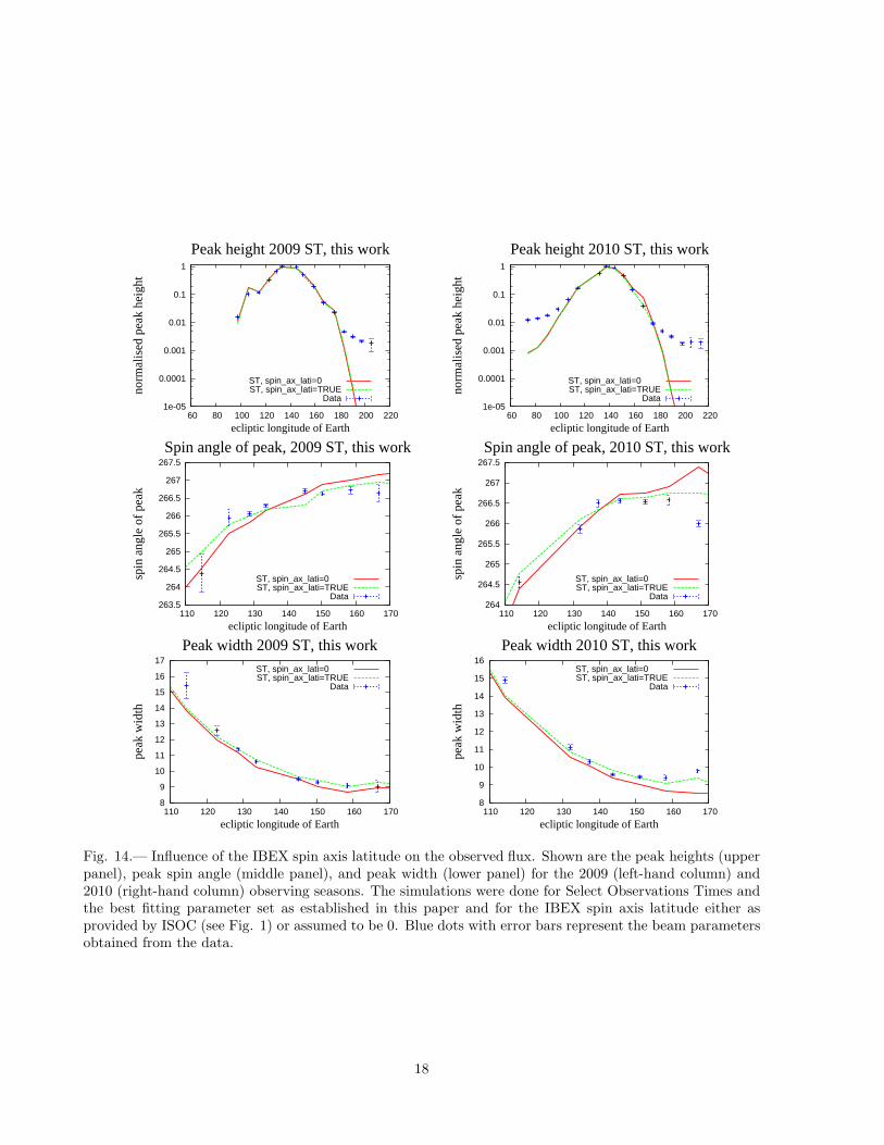
The small tilt of the spin axis out of the eclipticalso affects the observed flux because it excludes asmall portion of the beam while accepting a differ-ent part compared to the situation when the spinaxis is exactly in the ecliptic plane. This effectis especially pronounced in early orbits before thecrossing of the ISM flow peak (Fig. 14). Both thewidth and spin phase of the peak maximum are

affected with offsets clearly larger than the errorbars. In contrast, the peak height is only weaklyaffected.

The exact magnitude of the effects discussed inthis section depend on the details and are chal-lenging to plan in advance, i.e., on the actual se-lect ISM flow observation times, which are deter-mined by a combination of operational aspects,stochastic backgrounds, particle events, actual re-alizations of spin-axis repointing maneuvers, etc.We decided that instead of attempting to correctthe observations for all of these issues, it was bet-ter to simply include them in the simulation. Weemphasize that the magnitude of various effectscan vary depending on the adopted parameter setand also from orbit to orbit. This supports thedecision to complicate the simulation pipeline forthe sake of fidelity of the model rather than try tocorrect the observations.

16

0.1

1

110 120 130 140 150 160 170

norm

alis

ed p

eak

heig

ht


Peak height Earth 2009

VI.eq.VEVI.ne.VE

Data

0.1

1

110 120 130 140 150 160 170

norm

alis

ed p

eak

heig

ht


Peak height Earth 2010

VI.eq.VEVI.ne.VE

Data

263.5

264

264.5

265

265.5

266

266.5

267

110 120 130 140 150 160 170

spin

ang

le o

f pe

ak



VI.eq.VEVI.ne.VE

Data 264

264.5

265

265.5

266

266.5

267

110 120 130 140 150 160 170

spin

ang

le o

f pe

ak



VI.eq.VEVI.ne.VE

Data

8

9

10

11

12

13

14

15

16

17

110 120 130 140 150 160 170

peak

wid

th


Peak width 2009VI.eq.VEVI.ne.VE

Data

9

10

11

12

13

14

15

16

110 120 130 140 150 160 170

peak

wid

th


Peak width 2010VI.eq.VEVI.ne.VE

Data

Fig. 13.— Illustration of the effect of the proper motion of IBEX on the simulated observations of NISHegas for the select ISM flow observation times for 2009 (left column) and 2010 (right column). Shown arepeak heights (upper panel), peak spin angle (middle panel), and peak width (lower panel). The resultsof simulations performed assuming the actual IBEX velocity relative to the Sun are in green, while thesimulations for the IBEX velocity assumed to be equal to the Earth velocity are in red. Observed values arethe blue dots with error bars. The exact magnitude of this proper motion effect depends on the durationof the select ISM flow observation times and their position on the orbit. Shown are simulations for theparameters of the NISHe flow as established in this paper.

17

1e-05

0.0001

0.001

0.01

0.1

1

60 80 100 120 140 160 180 200 220

norm

alis

ed p

eak

heig

ht


Peak height 2009 ST, this work

ST, spin_ax_lati=0 ST, spin_ax_lati=TRUE

Data 1e-05

0.0001

0.001

0.01

0.1

1

60 80 100 120 140 160 180 200 220

norm

alis

ed p

eak

heig

ht


Peak height 2010 ST, this work


Data

263.5

264

264.5

265

265.5

266

266.5

267

267.5

110 120 130 140 150 160 170

spin

ang

le o

f pe

ak


Spin angle of peak, 2009 ST, this work


Data 264

264.5

265

265.5

266

266.5

267

267.5

110 120 130 140 150 160 170

spin

ang

le o

f pe

ak


Spin angle of peak, 2010 ST, this work


Data

8

9

10

11

12

13

14

15

16

17

110 120 130 140 150 160 170

peak

wid

th


Peak width 2009 ST, this workST, spin_ax_lati=0 ST, spin_ax_lati=TRUE

Data

8

9

10

11

12

13

14

15

16

110 120 130 140 150 160 170

peak

wid

th


Peak width 2010 ST, this workST, spin_ax_lati=0 ST, spin_ax_lati=TRUE

Data

Fig. 14.— Influence of the IBEX spin axis latitude on the observed flux. Shown are the peak heights (upperpanel), peak spin angle (middle panel), and peak width (lower panel) for the 2009 (left-hand column) and2010 (right-hand column) observing seasons. The simulations were done for Select Observations Times andthe best fitting parameter set as established in this paper and for the IBEX spin axis latitude either asprovided by ISOC (see Fig. 1) or assumed to be 0. Blue dots with error bars represent the beam parametersobtained from the data.

18

4. Data

Observations used in this analysis are discussedby Mobius et al. (2012) and the ground calibra-tion of the IBEX-Lo instrument by Mobius et al.(2009a); Bochsler et al. (2012b); Saul et al. (2012).We used data collected in Energy Step 2 (centerenergy 27 eV) of IBEX Lo (hydrogen). The hy-drogen atoms that are observed were sputtered offthe conversion surface of the IBEX-Lo instrumentby the incoming NISHe atoms. The fact that theobserved signal is actually due to helium was ver-ified by comparing the H to O ratio observed inflight with the ratio observed in laboratory cali-bration using a neutral helium beam of the sameenergy as the NISHe beam.

To compare with simulations, counts ck accu-mulated at an orbit k during select ISM flow obser-vation times ∆Tki in the 6◦ bins were convertedinto averaged count rates dk using the followingrelation:

dk = 8 × 60ck

Nk∑

i=1

∆Tki

(9)

where the sum in the denominator is the totallength of the Nk intervals of select ISM flow obser-vation times at the k-th orbit and the 8×60 factorreflects the fact that IBEX-Lo observes at 8 energychannels (thus 1 channel is active for 1/8-th of thetime) and each of the 60 6◦ bins is observed during1/60-th of the time.

The data counts are subject to the Poissonstatistics with uncertainties of square root of thetotal counts registered in a given data bin. Statis-tical errors in counts are converted into the errorsin count rates using Eq. (9).

Before starting the search for flow parametersof NISHe we performed data selection based on in-sight obtained from the modeling. Analysis of theexpected NISHe beam peak heights as function ofthe ecliptic longitude of IBEX showed that for noreasonable set of parameters we are able to repro-duce the peak heights in the orbits before Orbit60 during the 2010 season. Orbits 11 and 12 fromthe 2009 season showed a similar behavior as il-lustrated in the upper-right panel of Fig.14. Thuswe concluded that the flux observed at these or-bits must have a strong component different fromthe NISHe gas and removed these orbits for later,separate analysis. Similarly, profiles of the count

rates from orbits 21 and 69 could not be fitted anda similar conclusion was adopted, supported bythe predicted presence of a component from neu-tral interstellar hydrogen, confirmed by Saul et al.(2012). Consequently, we were left with orbits 13–20 from the 2009 season and 60, 61, and 63–68from the 2010 season. Regrettably, there are nodata from orbit 62 because of a spacecraft reset.

In the data from these orbits, based on the pre-diction that the observed NISHe beams should beGaussian in shape, we fitted Gaussian functionsdefined in Eq. (8) and removed the non-Gaussianwings. The original data and the portion left forthe analysis are shown in Fig. 15 for the 2009 sea-son and 16 for the 2010 season. The fitted Gaus-sian functions are also shown in the figure.

19

220 240 260 280 300 320

0.10

0.50

0.20

0.30

0.15

spin angle

coun

trat

e@H

zD

NISHe count rate, orbit 11

220 240 260 280 300 320

0.05

0.10

0.50

1.00

5.00

spin angleco

untr

ate@H

zD


220 240 260 280 300 320

0.05

0.10

0.50

1.00

5.00

spin angle

coun

trat

e@H

zD


220 240 260 280 300 320

0.05

0.10

0.50

1.00

5.00

10.00

spin angle

coun

trat

e@H

zD


220 240 260 280 300 320

0.050.10

0.501.00

5.0010.00

spin angle

coun

trat

e@H

zD


220 240 260 280 300 3200.01

0.1

1

10

spin angleco

untr

ate@H

zD


220 240 260 280 300 3200.01

0.1

1

10

spin angle

coun

trat

e@H

zD


220 240 260 280 300 320

0.050.10

0.501.00

5.0010.00

spin angle

coun

trat

e@H

zD


220 240 260 280 300 320

0.05

0.10

0.50

1.00

5.00

10.00

spin angle

coun

trat

e@H

zD


220 240 260 280 300 320

0.02

0.05

0.10

0.20

0.50

1.00

2.00

spin angle

coun

trat

e@H

zD


220 240 260 280 300 320

0.01

0.02

0.05

0.10

0.20

0.50

1.00

spin angle

coun

trat

e@H

zD


220 240 260 280 300 320

0.010

0.100

0.050

0.020

0.200

0.030

0.015

0.150

0.070

spin angle

coun

trat

e@H

zD


Fig. 15.— Count rates averaged over the select ISM flow observation times, observed by IBEX-Lo in EnergyStep 2 for orbits 11 through 22 in 2009. Blue dots with error bars mark the portion of the data that fitsa Gaussian well. The fitted Gaussians are drawn in blue lines. Red dots show data that do not fit to theGaussian and have been excluded from the analysis. The data from Orbits 11, 21, and 22 are all excludedfrom analysis as explained in the text and consequently are drawn in red. The orbits used in the NISHeparameter search are 13 through 20.

20

220 240 260 280 300 320

0.10

0.50

0.20

0.30

0.15

spin angle

coun

trat

e@H

zD


220 240 260 280 300 320

0.10

1.00

0.50

0.20

0.30

0.15

0.70

spin angleco

untr

ate@H

zD


220 240 260 280 300 320

0.02

0.05

0.10

0.20

0.50

1.00

2.00

spin angle

coun

trat

e@H

zD


220 240 260 280 300 320

0.1

0.2

0.5

1.0

2.0

5.0

spin angle

coun

trat

e@H

zD


220 240 260 280 300 320

0.050.10

0.501.00

5.0010.00

spin angle

coun

trat

e@H

zD


220 240 260 280 300 3200.01

0.1

1

10

spin angleco

untr

ate@H

zD


220 240 260 280 300 3200.01

0.1

1

10

spin angle

coun

trat

e@H

zD


220 240 260 280 300 320

0.050.10

0.501.00

5.0010.00

spin angle

coun

trat

e@H

zD


220 240 260 280 300 320

0.05

0.10

0.50

1.00

5.00

spin angle

coun

trat

e@H

zD


220 240 260 280 300 320

0.02

0.05

0.10

0.20

0.50

1.00

spin angle

coun

trat

e@H

zD


220 240 260 280 300 3200.010

0.100

0.050

0.020

0.200

0.030

0.015

0.150

0.070

spin angle

coun

trat

e@H

zD


Fig. 16.— Count rates averaged by select ISM flow observation times, observed by IBEX-Lo in Energy Step2 for IBEX orbits 58 through 69 during 2010. As for Fig. 15, blue dots with error bars mark the portion ofthe data that fits a Gaussian shape well. The fitted Gaussians are drawn in blue lines. Red dots show datathat do not fit to the Gaussian and have been excluded from the analysis. The data from Orbits 58, 59, and69 are all excluded from analysis as explained in the text and consequently are drawn in red. The orbitsused in the NISHe parameter search are 60 through 68.

21

5. Parameter fit for the NISHe flow

5.1. Method

The goal of our analysis is to determine the flowdirection, velocity, and temperature of the neu-tral interstellar helium gas in the Local InterstellarCloud ahead of the heliosphere. We accomplishedthis by fitting simulations of the NISHe flux to thedata, with the ecliptic longitude and latitude of in-flow direction, inflow speed, and gas temperaturein the LIC as free parameters. Optimizing a multi-parameter model fit to data usually involves select-ing a merit function whose free parameters are thefitted model parameters, and finding its minimumin the multi-dimensional parameter space. Collo-quially speaking, the merit function describes the“distance” of the model predictions from the datain the observation N -space and searching for thebest parameters requires finding the parameter setfor which this distance is minimum.

A well tested and widely used method of fit-ting parameters of a model to a data set is themaximum likelihood method. In this method, themerit function is the likelihood function. To useit, one needs to know probability distributionsfp,i (xp,i, di,p) of all the data points di, param-eterized by the model parameters p. In principle,probability distributions for different data pointscan be described by different probability distribu-tion functions, but in our case we assume that forall data points they are identical, i.e., for all i,fp,i (xp,i, di,p) = fp (xp,i, di,p).

With these definitions we calculate the condi-tional probability Pi that if the model with a givenparameter set p is correct, then our experiment incase i provides measurement di, given by the for-mula:

Pi (xp,i) = fp (xp,i, di,p) (10)

The series xp,i is the series of model predictions ofthe measurements for parameters p. The proba-bility P that our series of N measurements returnsa series of results di, i = 1, . . . , N is, of course, aproduct of all N probabilities Pi:

P (xp,1, . . . , xp,N , d1, . . . , dN ) =

N∏

i=1

Pi =

=N∏

i=1

fp (xp,i, di,p) (11)

Fitting the parameters p is equivalent to findingthe parameters pbest for which absolute maximumof P is achieved. Finding this absolute maximumis the basis of the maximum likelihood method.Remaining details determine how to best accom-plish the goal and the mathematical methods toapply depend on the nature of the problem onhand.

The IBEX-Lo detector actually counts incom-ing NISHe atoms in 6◦ spin angle bins, so thenumber of atoms in each bin is subject to Poissonstatistics. Hence we immediately have estimatesof the measurement errors according to:

σi =√

di (12)

But the counts are relatively high and in this casethe Poisson statistics asymptotically transformsinto the Gaussian. Thus the likelihood functionin Eq. (11) becomes:

P (xp,1, . . . , xp,N , d1, . . . , dN ) =

=

N∏

i=1

(

1√πσi

exp

[

−(

di − xp,iσi

)2])

(13)

which we must maximize. Since all the probabili-ties are positive numbers, we can take natural log-arithm of both sides of this equation and obtain:

ln [P (xp,1, . . . , xp,N , d1, . . . , dN )] =

=

N∑

i=1

[

ln

(

1√πσi

)

−(

di − xp,iσi

2)]

. (14)

Since for a given measurement series the first termunder the logarithm in the sum in Eq. (14) isa constant, we can remove it because our goal isto find the parameter set for which the likelihoodfunction will be maximum, and not the maximumvalue itself. Thus we define the following meritfunction −L (p):

− L (p) = −N∑

i−1

(

di − xp,iσi

)2

(15)

which takes negative values. We can omit the mi-nus signs and then instead of maximizing the termat the right-hand side we have to minimize it. Theparameter set p for which function L(p) is mini-mal will not change when we divide it by the num-ber of degrees of freedom in the problem, equal to

22

N − np, where np is the number of parameters inthe parameter set p. In our case np = 4. Dividingby the number of degrees of freedom converts thisfunction into the chi-squared function and enablesdirect comparison of the quality of approximationbetween data series with different numbers of de-grees of freedom. Effectively, the merit functionin the form

L (p) =1

N − np

N∑

i−1

(

di − xp,iσi

)2

(16)

is the mean distance between data and simulationsin the measurements N -space, normalized by thenumber of degrees of freedom and by the uncer-tainties of the measurements.

The simulations return count rates of NISHeatoms, while the observations are total counts ac-cumulated during the select ISM flow observationtimes. We had to make the two quantities com-patible and the choice was either to convert themodel count rate into total counts or to convertthe counts into the average count rate by dividingthe counts and their errors by the duration of theselect ISM flow observation times. We decided toadopt the second solution for practical reasons: re-calculation could be done only once, and anotherselection would require converting all of the simu-lation cases, adding an unnecessary computationalburden.

Although extensive pre-launch calibrationswere conducted on the sensor (Fuselier et al. 2009;Mobius et al. 2012), we chose to avoid possiblesystematic changes in the observation conditionsdue to changes in the instrument functions fromyear to year by comparing observations and simu-lations separately for the 2009 and 2010 seasons.

From the simulations, we knew that count rateprofiles as function of spin angle should be Gaus-sian. For each season we selected a reference orbitand fitted its data with a Gaussian function speci-fied in Eq. (8). The fitted peak height f0 from thereference orbit was used as scaling factor for allthe data points from that season. Effectively, thisreturned observed count rates relative to the fit-ted peak value at the reference orbit. To facilitatecomparison, simulated count rates were scaled us-ing a similar procedure. As the reference orbits weselected those with the highest count rates: Orbit16 in 2009 and Orbit 64 in 2010.

Having brought simulations and observations tothe common scale, we could look for the minimumof the 4-parameter function given by Eq. (16).This function is purely numerical, because sim-ulations results xi (p) used to evaluate the meritfunction L are purely numerical. In such a sit-uation, calculating derivatives in the parameterspace is problematic. Hence the numerical methodused to minimize this function used finite differ-ences instead of derivatives of the merit function inthe parameter space. In addition, since individualsimulations are very time consuming, the numberof evaluations of the merit function had to be keptas low as possible. We decided to adapt the quasi-Newton method suggested by Press et al. (2007).

In this method, a starting point pstart in theparameter space is adopted and then, using finite-differences to approximate partial derivatives, thegradient of the merit function is calculated. Thegradient provides the direction of the slope of themerit function in the parameter space. This di-rection is sampled by calculation of a number ofpoints p1, . . . ,pn and a minimum at a point ploc

along this direction is estimated from a parabolafit to the sampled points. The ploc that is found bythis method becomes a new starting point. Thisiteration continues until the change in the magni-tude of the function being minimized is consideredsufficiently small. The final parameter set is thenretrieved as pbest. It is essential in this methodto specify initial steps in all coordinates of the pa-rameter space such that the magnitudes of partialderivatives are similar.

5.2. Calculations

Following this method, we computed χ2 (meritfunction) values defined in Eq. (16) for various setsp of flow direction longitude λ, latitude β, veloc-ity v and temperature T , starting from the val-ues reported by Witte (2004). Resulting from thesimulations were five-dimensional “landscapes” ofχ2 (λ, β, v, T ). To find the best-fitting set of pa-rameters pbest, we performed numerical minimiza-tions of χ2 (λ, β, v, T ) function separately on ob-servations from each of the two seasons and col-lectively on combined observations from both sea-sons.

The minimizations were performed on a mesh offlow longitudes λ, with the longitude fixed and lat-itude, speed, and temperature being free param-

23

eters. The values of the 3 free parameters in thesimulations were selected by the algorithm basedon the local gradient of the minimized functionand hence they are not on a regular mesh. Therobustness of the minima of χ2 values for all theλ mesh points was checked by restarting the min-imization algorithm from the parameter set thealgorithm had reported as optimum, until no fur-ther improvements could be obtained. Usually,such a restart of the procedure did not result in asignificant reduction of χ2.

After the absolute solution pbest was found, weextended the simulations on a regular grid of pa-rameters centered at the best solution pbest in or-der to check on the covariance of parameters andto better illustrate the acceptable parameter re-gion. This mesh regularization resulted in a verysmall correction of the best fitting parameter set.The improvement in χ2 value was only ∼ 0.001with the changes in parameters of ∼ 50 K in tem-perature and ∼ 0.1 km s−1 in the flow velocity.

During the minimization process we performedsimulations using a total of about 4000 sets of theNISHe gas parameters. The minimization algo-rithm kept track of its own steps, so that results ofsimulations for individual parameter sets could beused in as many minimization processes as needed.

The values of the merit function χ2 minimizedfor the mesh values of the flow direction λ areshown in Fig. 17. The results of the minimizationperformed separately on the data from 2009 and2010 (red and green, respectively) are consistentwith each other and with the results of the mini-mization performed collectively on the data from2009 and 2010 (blue). They are presented and dis-cussed in greater detail in the following section.

6. Results

The fitting procedure results in a new set ofthe parameters of neutral interstellar helium inthe LIC, which differs from the previously ob-tained by Mobius et al. (2004); Witte (2004);Gloeckler et al. (2004); Vallerga et al. (2004). Thedownwind direction of the NISHe gas in the LICbest fitting to the data is longitude λ = 79.2◦

, latitude β = −5.12◦. The bulk speed isv = 22.756 km s−1 and the temperature T = 6165K.

The flow parameters fitted separately to the ob-

æ

æ

æ

æ

æ

ææææ

ææ

ææ

æ

æ

æ

æ

æ

à

à

à

à

à

à

ààà

à à

à à à à

à

à

à

ì

ì

ì

ìì

ììì ì ì

ì

ìì

ì

ì

ì

ì

ì

70 75 80 854

6

8

10

12

14

16

ecliptic longitude of flow

Χ2

valu

e

Χ2 value as function of ecl.long. of flow direction

Fig. 17.— Values of χ2 statistic defined in Eq. (16)shown as function of ecliptic longitude of the flowdirection of the NISHe gas obtained as a result ofour fitting procedure. The statistics of the fits per-formed separately for the observation campaigns2009 and 2010 are shown in red (dots) and green(squares), respectively; the statistic for the fittingperformed collectively on the data from both cam-paigns is shown in blue (diamonds). The value ofχ2 for the parameter set obtained by Witte (2004)is 143.9.

servations from the 2009 season are λ = 79.2◦, β =−5.06◦, v = 22.831 kms−1, T = 6094 K and tothe observations from the 2010 season λ = 79.2◦,β = −5.12◦, v = 22.710 kms−1, T = 6254 K. It isclear that the solutions obtained separately fromthe two seasons are consistent with each other andwith the solution obtained for the two seasons col-lectively.

The values of χ2 calculated for the two seasonstogether and separately are shown in Fig. 17 asfunction of the downwind longitude. The qualityof the fits for each orbit can be assessed in Fig. 18for the 2009 season and in Fig. 19 for the 2010season; it is apparent that the quality of our fit ismuch better than the solution from Witte (2004).Contributions from individual orbits to the totalχ2 value for the 2009 and 2010 seasons are pre-sented in Fig. 20.

24

æ

æ

æ

æ

æ

æ

æ

æ

æ

æ

æ

æ

æ

æ

250 255 260 265 270 275 2800.00

0.02

0.04

0.06

0.08

0.10

0.12

0.14

spin angle

cntr

ate

norm

tom

axor

b.16

Orbit 13, Χ2 = 0.951633

æ

æ

æ

æ

æ

æ

æ

æ

æ

æ

æ

æ

æ

æ

250 255 260 265 270 275 2800.0

0.1

0.2

0.3

0.4

spin angle

cntr

ate

norm

tom

axor

b.16

Orbit 14, Χ2 = 1.53427

æ

æ

æ

æ

æ

æ

æ

ææ

æ

æ

æ

æ

æ

æ

æ

250 260 270 2800.0

0.2

0.4

0.6

0.8

1.0

spin angle

cntr

ate

norm

tom

axor

b.16

Orbit 15, Χ2 = 1.87246

æ

æ

æ

æ

æ

æ

æ

æ

ææ

æ

æ

æ

æ

æ

æ

æ

æ

240 250 260 270 2800.0

0.2

0.4

0.6

0.8

1.0

spin angle

cntr

ate

norm

tom

axor

b.16

Orbit 16, Χ2 = 0.76817

æ

æ

æ

æ

æ

ææ

æ

æ

æ

æ

æ

255 260 265 270 275 2800.0

0.2

0.4

0.6

0.8

1.0

spin angle

cntr

ate

norm

tom

axor

b.16

Orbit 17, Χ2 = 0.506227

æ

æ

æ

æ

æ

ææ

æ

æ

æ

æ

æ

255 260 265 270 275 2800.0

0.1

0.2

0.3

0.4

0.5

0.6

spin angle

cntr

ate

norm

tom

axor

b.16

Orbit 18, Χ2 = 0.231777

æ

æ

ææ

æ

ææ

æ

æ

æ

æ

æ

255 260 265 270 275 2800.00

0.05

0.10

0.15

0.20

0.25

spin angle

cntr

ate

norm

tom

axor

b.16

Orbit 19, Χ2 = 0.968228

æ

æ æ

æ

æ

ææ

æ

260 265 270 2750.00

0.02

0.04

0.06

0.08

0.10

spin angle

cntr

ate

norm

tom

axor

b.16

Orbit 20, Χ2 = 0.653293

Fig. 18.— Comparison of count rates of NISHe atoms observed by IBEX-Lo for orbits 13 through 20 duringthe 2009 NISHe observation campaign (blue dots with error bars) with the simulated count rates calculatedfor the set of parameters best fitting to the data from both seasons (red lines) and for the parameter setsuggested by Witte (2004) (gray lines). Both observations and simulations are normalized to their respectivepeak values at Orbit 16, as discussed in the text. The value of χ2 at the given orbit for the best case is listedin the headers.

25

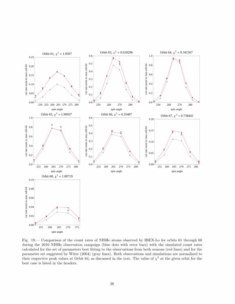
æ

æ

æ

æ

æ

æ

æ

æ

æ

æ

æ

æ

æ

æ

250 255 260 265 270 275 2800.00

0.05

0.10

0.15

0.20

0.25

spin angle

cntr

ate

norm

tom

axor

b.64

Orbit 61, Χ2 = 1.9507

æ

æ

æ

æ

æ

æ

æ

ææ

æ

æ

æ

æ

æ

æ

æ

250 260 270 2800.0

0.1

0.2

0.3

0.4

0.5

0.6

spin angle

cntr

ate

norm

tom

axor

b.64

Orbit 63, Χ2 = 0.618296

æ

æ

æ

æ

æ

æ

æ

ææ

æ

æ

æ

æ

æ

æ

æ

250 260 270 2800.0

0.2

0.4

0.6

0.8

1.0

spin angle

cntr

ate

norm

tom

axor

b.64

Orbit 64, Χ2 = 0.341567

æ

æ

æ

æ

æ

ææ

æ

æ

æ

æ

æ

255 260 265 270 275 2800.0

0.2

0.4

0.6

0.8

1.0

spin angle

cntr

ate

norm

tom

axor

b.64

Orbit 65, Χ2 = 1.90937

æ

æ

æ

æ

æ

ææ

æ

æ

æ

æ

æ

255 260 265 270 275 2800.0

0.1

0.2

0.3

0.4

0.5

0.6

spin angle

cntr

ate

norm

tom

axor

b.64

Orbit 66, Χ2 = 0.35487

æ

æ

æ

æ

æ

ææ

æ

æ

æ

æ

æ

255 260 265 270 275 2800.00

0.05

0.10

0.15

0.20

spin angle

cntr

ate

norm

tom

axor

b.64

Orbit 67, Χ2 = 0.738441

æ

æ

ææ

æ

æ

æ

ææ

æ

255 260 265 270 2750.00

0.02

0.04

0.06

0.08

0.10

spin angle

cntr

ate

norm

tom

axor

b.64

Orbit 68, Χ2 = 1.00719

Fig. 19.— Comparison of the count rates of NISHe atoms observed by IBEX-Lo for orbits 61 through 68during the 2010 NISHe observation campaign (blue dots with error bars) with the simulated count ratescalculated for the set of parameters best fitting to the observations from both seasons (red lines) and for theparameter set suggested by Witte (2004) (gray lines). Both observations and simulations are normalized totheir respective peak values at Orbit 64, as discussed in the text. The value of χ2 at the given orbit for thebest case is listed in the headers.

26

Inspection of Figs 17, 18, 19, and 20 shows thatcontributions of various orbits to χ2 vary appre-ciably among the orbits and that χ2 (λ) exhibitshumps and traces of secondary minima. We triedto identify the causes of non-smooth features in χ2

curves. The obvious candidates were the strongestcontributors to χ2 total. Therefore we repeatedminimizations without Orbits 14 and 15 for the2009 season and without orbit 65 for the 2010 sea-son.

The results of this procedure are shown inFig. 21. Removing Orbits 14 and 15 eliminates thehump seen in χ2 vs λ plots about λ = 82◦, and re-moving Orbit 65 results in a lowering of minimumvalues and shifting position toward greater λ, eventhough it does not remove the correlation of the χ2

values from individual orbits with the angular sep-aration of the Earth from the position of the peakflux, shown in Fig. 20. Thus, the source of theunexpected features in the χ2 vs λ plots was iden-tified. However, inspection of the observations,select ISM flow observation times, and the entiremeasurement process for these orbits did not re-veal any reasons why the quality of the data fromthese orbits should be suspect. Hence there is noobvious reason to reject the three orbits. Instead,we adopted the size of the irregularities as an in-dicator of the uncertainty in χ2 values and usedit to constrain the regions of acceptable values ofthe gas flow parameters.

To this end, we selected χ2 = 8.7 value asthe upper limit, we used all the points that re-turn χ2 ≤ 8.7 and we plotted blue contours sur-rounding the geometric location of those simula-tion points in two-parameter cuts of the χ2 spacein Fig. 22. They form well-defined regions in thetwo-parameter sub-spaces. We consider these re-gions as regions of acceptable values of NISHe gasparameters.

To be acceptable, the components (λ, β, v, T ) ofa parameter set p must be within the acceptableregions in all panels of Fig. 22 with no exceptions.Even one exception invalidates a given solution.The acceptable values of the flow longitude varyfrom 75.2◦ to 83.6◦, but there are only limitedranges of the other parameters possible for a givenvalue of the flow longitude. Similarly, the accept-able velocities range from ∼ 20 to 25.5 km s−1, butfor a given velocity value only a narrow range ofthe remaining parameters is acceptable. It is clear,

for example, that the solution for the NISHe flowparameters obtained by Witte (2004), shown asthe smaller of the two error bar crosses in Fig. 22,is outside the region permitted by our analysis. Ifwe take the flow longitude identical as obtained byWitte (2004), then the gas temperature must be ina narrow range about 8000 K, and velocity mustbe ∼ 25.5 km s−1, both outside the error space.Thus we conclude that our solution differs fromthe solution obtained by Witte (2004) and fromthe consensus solution from Mobius et al. (2004)on a statistically significant level.

By contrast, the LIC flow vector that Redfield & Linsky(2008) obtained from a careful analysis of all avail-able lines of sight toward nearby stars agrees withour solution. These error bars, which appear largeon the scale of the figures, intersect the acceptableregion in all panels.

We also show approximate contours for a fewother select levels of χ2, as indicated in the upperleft panel of Fig. 22. A level of 7.29 corresponds tothe depth of the secondary minimum in χ2 space(cf. Fig. 17); the secondary minimum is then plot-ted as a tiny dot. We plot two contours betweenthe values of the primary and secondary minimumin the χ2 space, to better illuminate the 3D shapebetween the two minima. We also show two con-tours outside the acceptable region: they are forthe χ2 levels above 35 and above 80. While thesampling of these regions in the χ2 space is muchsparser, we are confident we have not missed anysignificant secondary minimum. The figure illus-trates how deep the valley is in the χ2 space.

27

1313

1414

1515

1616

1717

1818

1919

2020

120 130 140 150 1600.0

0.5

1.0

1.5

2.0


Χ2

cont

ribu

tion

Χ2 contributions from orbits

6161

6363

6464

6565

6666

6767

6868

120 130 140 150 1600.0

0.5

1.0

1.5

2.0


Χ2

cont

ribu

tion

Χ2 contributions from orbits

Fig. 20.— Contributions to χ2 values from the individual orbits during the 2009 (left) and 2010 seasons(right). The horizontal axes show the mean ecliptic longitudes of Earth for individual orbits, calculatedas averages over the select ISM flow observation time intervals. The numbers on the points indicate orbitnumbers.

70 75 80 854

6

8

10

12

14

16

ecl. long. of flow

Χ2

valu

e

Χ2 value as function of ecl.long. of flow direction,

Orbit 14 & 15 dropped

70 75 80 854

6

8

10

12

14

16

ecl. long. of flow

Χ2

valu

e

Χ2 value as function of ecl.long. of flow direction,

Orbit 65 dropped

Fig. 21.— Values of χ2 for the 2009 (left) and 2010 seasons (right) with the contributions from orbits 14and 15 and 65 removed, shown as green lines. Red lines are repeated from Fig. 17 for comparison.

28

7.1

7.29

7.29

7.8

7.8

8.3

8.3

8.7

-5.6 -5.4 -5.2 -5.0 -4.8 -4.619

20

21

22

23

24

25

26

Β

v

v vs Β

76 78 80 8219

20

21

22

23

24

25

26

Λ

v

v vs Λ

76 78 80 824000

5000

6000

7000

8000

Λ

T

T vs Λ

19 20 21 22 23 24 25 264000

5000

6000

7000

8000

v

TT vs v

-5.6 -5.4 -5.2 -5.0 -4.8 -4.64000

5000

6000

7000

8000

Β

T

T vs Β

76 78 80 82-5.6

-5.4

-5.2

-5.0

-4.8

-4.6

Λ

Β

Β vs Λ

Fig. 22.— Parameters of the NISHe flow that yield χ2 values below the limit of 8.7 (inside the blue contour and including the darker contours), shown in

cuts through the two-parameter sub-spaces of the 4D parameter space. The best-fit solution is indicated by the black cross-hairs, while the solution obtained

by Witte (2004) is marked with the smaller error bar cross. The yellow and orange points are the solutions obtained separately for the 2009 and 2010 seasons.

The larger error bar cross (only fragments visible in some of the panels) marks the LIC flow vector from Redfield & Linsky (2008). χ2 values for the contours

are indicated in the upper left panel; the values for the two lightest contours, from which the darker one makes the background in v vs β, T vs β, and β vs

λ panels, are 30 and 87. Note that the boundaries of the two lightest panels are very approximate because of the sparse coverage of theses regions of the 4D

χ2 space.

29

Fig. 23.— Comparison of analytic results obtained by Mobius et al. (2012) with the results from this paper.Shown are relations between the flow direction and flow latitude (upper left panel), inflow velocity (lower leftpanel), and gas temperature (lower right panel). Upper right panel presents χ2 values as function of the flowdirection that corresponds to the simulation points used in the remaining panels; basically it is a repetitionof Fig. 17. The temperature panel shows a relation which assumes that all events are transmitted by thedata system (upper line), along with two relations that assume a rate-dependent data loss in the transferto the data system, whose magnitude is currently not well known yet. The system loading-related loss ismodeled like a characteristic dead time of 1.2 ms (middle line) and 5 ms (lower line) (Mobius et al. 2012).

30

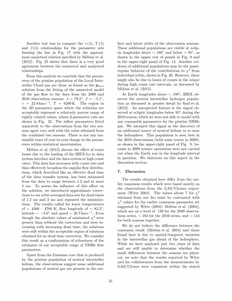
Another test was to compare the v (λ), T (λ)and β (λ) relationships for the parameter setsforming the line in Fig. 17 with the approxi-mate analytical relation specified by Mobius et al.(2012). Fig. 23 shows that there is a very goodagreement between the numerical and analyticalrelationships.

From this analysis we conclude that the param-eters of the pristine population of the Local Inter-stellar Cloud gas are those as found as the pbest

solution from the fitting of the numerical modelof the gas flow to the data from the 2009 and2010 observation seasons: λ = 79.2◦, β = −5.1◦,v = 22.8 km s−1, T = 6200 K. The region inthe 4D parameter space where the solutions areacceptable represent a relatively narrow range oftightly related values, whose 2-parameter cuts areshown in Fig. 22. The inflow parameters fittedseparately to the observations from the two sea-sons agree very well with the value obtained fromthe combined two seasons. There is not any rea-sonable trace of year-to-year change in the param-eters within statistical uncertainties.

Mobius et al. (2012) discuss the effect of countlosses due to the loading of the IBEX-Lo to datasystem interface and the data system at high countrates. This data loss increases with count rate andthus effectively broadens the angular flow distribu-tions, which described like an effective dead timeof the data transfer system, has been estimatedfrom the data to range between 1.2 and at most5 ms. To assess the influence of this effect onthe solution, we introduced approximate correc-tions to our orbit-averaged data sets for dead timesof 1.2 ms and 3 ms and repeated the minimiza-tions. The results called for lower temperaturesof ∼ 4300 – 4700 K, flow longitude of ∼ 82.2◦,latitude ∼ −5.0◦ and speed ∼ 20.7 km s−1. Eventhough the absolute values of minimized χ2 weregreater than without the correction and were in-creasing with increasing dead time, the solutionswere still within the acceptable region of solutionsobtained for no dead time correction. We considerthis result as a confirmation of robustness of theestimates of our acceptable range of NISHe flowparameters.

Apart from the Gaussian core that is producedby the pristine population of neutral interstellarhelium, the observations suggest some additionalpopulations of neutral gas are present in the ear-

liest and latest orbits of the observation seasons.These additional populations are visible at eclip-tic longitudes above ∼ 180◦ and below ∼ 95◦, asshown in the upper row of panels in Fig. 9 andin the upper-right panel of Fig. 14. Another evi-dence of additional populations may be the quasi-regular behavior of the contributions to χ2 fromindividual orbits, shown in Fig. 20. However, thesemight also be due to losses of counts in the sensorduring high count rate intervals, as discussed byMobius et al. (2012).

At Earth longitudes above ∼ 180◦, IBEX ob-serves the neutral interstellar hydrogen popula-tion as discussed in greater detail by Saul et al.(2012). An unexpected feature is the signal ob-served at ecliptic longitudes below 95◦ during the2010 season, which we were not able to model withany reasonable parameters for the pristine NISHegas. We interpret this signal as the discovery ofan additional source of neutral helium in or nearthe heliosphere. This population is seen best inthe 2010 observations (with some traces in 2009),as shown in the upper-right panel of Fig. 9, be-cause in 2009 science operations were not carriedout when the Earth was in the longitude intervalin question. We elaborate on this aspect in thediscussion section.

7. Discussion

The results obtained here differ from the ear-lier consensus results which were based mostly onthe observations from the GAS/Ulysses experi-ment (Witte 2004). The values about 7 for χ2

obtained from our fits must be contrasted withχ2 values for the earlier consensus parameter setsuggested by Witte (2004); Mobius et al. (2004),which are on a level of 139 for the 2009 observa-tions series, ∼ 164 for the 2010 series, and ∼ 144for both seasons together.

We do not believe the difference between theconsensus result (Mobius et al. 2004) and thosefound here is due to spatial/temporal variationin the interstellar gas ahead of the heliosphere.While we have analyzed just two years of dataand are still unable to determine whether thesmall differences between the seasons are physi-cal, we note that the results reported by Witteand his collaborators from the measurements byGAS/Ulysses were consistent within the stated

31

uncertainties starting from the first report byWitte et al. (1993) and through the last ones byWitte et al. (2004); Witte (2004). In our opinion,it is highly unlikely that an abrupt change in thegas parameters at the entrance to the heliosphericinterface occurred during the ∼ 6 years betweenthe end of GAS observations and beginning of theIBEX observations, with no changes during theearlier and later times. Additional evidence sup-porting this position is the fact that the signal weobserve is compatible with a Maxwellian distribu-tion with a small addition of the extra popula-tion we discovered, which we believe is due to pro-cesses operating within the heliospheric interfacerather than within the interstellar gas. A near-Maxwellian distribution suggests a particle distri-bution in quasi-thermal equilibrium. The spatialscale of the near-equilibrium conditions must becomparable to at least the length of Sun’s paththrough the interstellar gas since the beginningof Ulysses observations, i.e., since 1990. For aspeed of the Sun relative to the gas 5 AU/y, thisis only ∼ 100 AU, i.e., shorter than the mean freepath for charge exchange reaction in this environ-ment. Charge exchange is the interaction mostlyresponsible for equilibrating the neutral compo-nent with the ionized component, which in turnis interrelated with disturbances in the local mag-netic field. This suggests that the Sun is likely in alocal region of space that is homogeneous on spa-tial scales at least on the order a few hundred ofAU. Based on spectroscopic observations of inter-stellar matter lines along sightlines toward stars inthe Hyades, Redfield & Linsky (2001) concludedthat inhomogeneities in the LIC are on a spatialscale of 105 AU.

Information on interstellar gas in the Galacticneighborhood of the Sun is available mostly fromobservations of interstellar absorption lines in thespectra of nearby stars, reviewed very recently byFrisch et al. (2009, 2011). This information is de-rived from interpretation of absorption profiles col-lected from the lines of sight to nearby and moredistant stars, i.e., at spatial scales from a few toa hundred parsecs from the Sun. The interstellarabsorption scale is thus longer from the distancescale of our measurements by more than 3 orders ofmagnitude, which makes direct comparisons chal-lenging. Indeed, the classical interpretation ofinterstellar lines of sight calls for an assumption

that the gas is composed of separate clouds withsome temperature and a certain level of turbulence(Redfield & Linsky 2004, the ξ factor). The linesare typically fitted with a number of componentsfeaturing Voigt profiles with different parameters,until a satisfactory agreement of the observed andfitted shape is obtained (see, e.g., Lallement et al.1995; Linsky et al. 2000; Redfield & Linsky 2004).

The Sun seems to be within an old remnantof a series of supernova explosions (see discus-sion in Redfield & Linsky 2000; Fuchs et al. 2009;Frisch et al. 2011) and modeling of such rem-nants suggests the material is expected to beturbulent and fragmented at many spatial scales(Breitschwerdt et al. 2009). Spectroscopic mea-surements analyzed by Frisch et al. (2002) suggestthat the Sun might be still in one of the complexof local interstellar clouds called the Local Cloud,but quite close to its boundary, which might bebetween the Sun and the nearest star α Cen. Thiscloud is expected to have a velocity relative to theSun about 25 km s−1, compatible with the resultsfrom GAS/Ulysses. The adjacent cloud, the so-called G-cloud (Lallement et al. 1995) is expectedto be a few km/s faster. Frisch et al. (2002) donot rule out that the Sun might be within a gra-dient of the gas velocity between the two clouds.More recent analysis by Redfield & Linsky (2008),based on a more extensive observations material,suggests that the flow vector of the Local Cloud(converted to the J2000 ecliptic coordinates) is v =23.84±0.90 km s−1, λ = 78.5◦±3◦, β = −7.8◦±3◦,which (within the error bars) is in a very goodagreement with our findings. Also the tempera-tures agree well: their 7500±1300 K (plus the mi-croturbulence parameter ξ = 1.62 ± 0.75 km s−1)with our 6200 K.

Another source of information on the kinemat-ics of the interstellar material just outside the he-liosphere might be interstellar dust. Interstellardust grains were unambiguously identified on anumber of spacecraft in the inner and outer helio-sphere (for review see Kruger & Grun 2009) andthe direction of inflow seemed to be in a verygood agreement with the helium inflow directionwe have obtained: downwind ecliptic longitudeof 79◦ ± 20◦ and latitude −8◦ ± 3◦ (Frisch et al.1999). This is in better agreement with our resultthan with the consensus result from Mobius et al.(2004). However, after 2005 the direction of inflow

32

changed by ∼ 30◦ southward (Kruger et al. 2007)due to a still unexplained phenomenon, whichquestions the direct usability of the inflow direc-tion of interstellar dust for the studies of kinemat-ics of the very local interstellar material.

The fact that our observations suggest thatmultiple solutions for the flow vector of the NISHegas are almost equally possible is not surprising.Already very early determinations of the NISHeflow vector based on EUV observations of theneutral helium glow (Chassefiere et al. 1988a,b)suggested many possible solutions, with either aslower speed and lower temperature, or a higherspeed and higher temperature, just as our re-sults do. The range of velocities they reported iscompatible with ours, but their temperatures arehigher by ∼ 2000 K than ours. Also Witte et al.(1993) seem to suggest the existence of an “al-ley” in χ2 space, but never expanded on this intheir subsequent papers. Hence our result is notin conflict with the bulk of the prior knowledge,even though it is statistically significantly differ-ent from the solution obtained from GAS/Ulysses;in contrast, our results are in very good agree-ment with the results of a recent and highly so-phisticated study of the local gas kinematics byRedfield & Linsky (2008).

The most pronounced and possibly far-reachingresult is, in our opinion, the new flow veloc-ity: ∼ 22.8 km s−1 as compared with the earlier26.4 km s−1. This is a reduction of ∼ 15%, whichresults in a decrease in the ram pressure the inter-stellar gas exerts on the heliosphere by ∼ 25%.

The size of the heliosphere is a result of the pres-sure balance between the outward pressure of thesolar wind, and of the inward pressure from the Lo-cal Interstellar Cloud material. The componentsof the inward and outward pressures have beenextensively discussed in the literature (see, e.g.,Fahr et al. (2000); Baranov (2009)) and includeram and thermal pressure of the solar wind ther-mal core and pickup ions, magnetic field pressureand pressure of the anomalous and Galactic com-ponents of cosmic rays. While the main pressurecomponents from the core of the solar wind at thetermination shock are known from in situ measure-ments of the solar wind (Richardson et al. 2008;Burlaga et al. 2008), the pressure from pickupions and the components of the inward pressurefrom the LIC are known only indirectly, mostly

from modeling based on the limited observationsavailable. The LIC pressure components includemostly the ram pressure of the ionized component,mediated by the interaction with various neutralcomponents, and supposedly the pressure from theexternal magnetic field. Thermal pressure plays aminor role. The change in the ram pressure atthe LIC side must result in a change in the magni-tudes of the other pressure components, to the firstapproximation without a change in the net pres-sure. Since the distance to the termination shock,known from the distances of the Voyagers crossings(Stone et al. 2005; Burlaga et al. 2008) and mod-eling of the heliospheric size in the presence of anexternal magnetic field (Pogorelov & Zank 2006;Pogorelov et al. 2009; Grygorczuk et al. 2011), isspecifically driven by the ram pressure and exter-nal magnetic field, the reduction in the LIC ve-locity will require recalculation of the present he-liospheric models and is likely to change the es-timates of the external field as well as the pro-portion between the primary and secondary pop-ulations of neutral interstellar hydrogen in the he-liosphere and their bulk velocity and temperatureinside the termination shock. These changes inturn will affect the pickup ion production in thesolar wind and the pickup ion supply to the innerheliosheath, again changing the pressure balancein the heliosphere, because of the very importantrole of pickup ions for the thermal pressure in thisregion.

The change in the longitude of the flow direc-tion by 3.8◦, from 75.4◦ to 79.2◦, is seeminglysmall, but it has a notable effect on the orien-tation of the Hydrogen Deflection Plane (HDP)suggested by Lallement et al. (2005). By defi-nition, the HDP is the plane that contains theinflow vectors of neutral interstellar hydrogen andhelium as observed in the inner heliosphere. It isbelieved that the flow vector of helium is practi-cally unaffected by the interactions going on atthe heliospheric interface. However, the flow ofhydrogen should be strongly disturbed. Since anexternal magnetic field is supposed to introducea distortion of the heliosphere from axial symme-try, the direction of the H flow should be differentfrom the direction of He. The discovery of a differ-ence between the flow directions of He and H sug-gested that the heliosphere is indeed distorted andthe most obvious cause is action of the external

33

magnetic field. Lallement et al. (2005) surmisedthat the external magnetic field vector may bein the HDP, a suggestion that obtained mixedsupport from the heliospheric modeling com-munity (Pogorelov et al. 2009; Izmodenov et al.2005a; Izmodenov & Alexashov 2006; Zank et al.2009). But if indeed the external B vector islocated in the HDP, as the more recent simula-tions suggest, then the new inflow direction ofthe NISHe gas reported in this paper, togetherwith a refined direction of the H flow reportedby Lallement et al. (2010), suggest a new geom-etry of the magnetic field in the LIC near theheliosphere. The magnetic field vector should belocated in the HDP determined by the normal di-rection (λ = 357.51◦, β = 58.51◦), while the nor-mal obtained from the previous estimates of theflow vectors by Witte (2004) and Lallement et al.(2005, 2010) is λ = 349.52◦, β = 32.29◦. Eventhough the error bars for both these determina-tions are big, the difference is significant and equalto ∼ 21◦.

Comparison of our extensive simulations withmeasurements suggests that a secondary popula-tion of neutral helium must be present at Earthorbit because, despite the fact that the simula-tions covered a very wide range of interstellar gasparameters values, we were unable to reproducecount rate profiles observed at orbits before 13during the 2009 campaign and before 60 duringthe 2010 campaign, as illustrated in the upper rowof Figs 9 and 14. In particular it is clear thatpeak heights observed during the 2010 season atecliptic longitudes lower than ∼ 95◦ are not re-produced well by the simulations performed withparameters best fit to Orbits 61 to 68. In fact,we were unable to fit these observations with anyparameter set from the ∼ 4000 tried. A similarsituation happens for the orbits corresponding toEarth longitudes greater than ∼ 180◦. In this casewe interpret the excess signal as due to interstellarhydrogen, as suggested by the simulations shownin Fig. 6. The H signal is discussed in greater de-tail by Saul et al. (2012).

Earlier studies (Muller & Zank 2003, 2004) sug-gested a possible secondary population of neutralhelium from the charge exchange between the He+

ions and H atoms in the outer heliosheath at alevel of about 1% of the primary. In these stud-ies the only source of the secondary He population

was the charge exchange reaction between the in-terstellar He+ ions and neutral H in the outer he-liosheath. In contrast, we believe that such a pop-ulation could come from charge exchange betweenneutral interstellar He atoms and interstellar He+

ions within the piled up and heated plasma in theouter heliosheath. In the following we will qualita-tively assess whether such a hypothesis is justified.

The ionic state of the interstellar He gas inthe LIC is thought to be 0.611 He, 0.385 He+,and 0.00436 He++, as obtained by Slavin & Frisch(2008) as one of results of a research program Di-

agnostic of interstellar hydrogen by an ISSI Work-ing Group “Interstellar Hydrogen in the Helio-sphere” (see Richardson et al. (2008); Bzowski et al.(2008); Pryor et al. (2008) for other results fromthis campaign). The plasma in the outer he-liosheath is compressed, slowed down and heated,as all modern heliospheric models suggest (Muller et al.2008). An illustration of the gas parametersalong the upwind direction can be found, e.g.,in Izmodenov et al. (2005b). The plasma densityincreases from the interstellar value of 0.06 cm−3

to ∼ 0.14 cm−3 and the temperature from ∼ 6000K to ∼ 35000 K. The typical plasma bulk speedin the outer heliosheath along the upwind direc-tion is just ∼ 4 km s−1 sunward, while the primarycomponents of both H and He maintain their in-terstellar speed. The plasma pile up results in anet difference in bulk velocities between the twointeracting components, which adds to the typicalrelative speed of He atoms with respect to theions.

Assuming the ionization state of the gas doesnot change in the outer heliosheath relative to theunperturbed LIC, we can calculate the density ofthe He+ and He++ ions in the heliosheath by mul-tiplying the densities from the LIC by the typi-cal plasma compression factor 0.14/0.06 = 2.33.The base number for this calculation is the den-sity of neutral interstellar He in the LIC equal to0.015 cm−3 (Witte 2004). The reaction rates de-fined as:

β = ntargetvrelσcx (vrel) (17)

will critically depend on the relative speed be-tween the colliding partners. For the temperature35000 K, the mean speed of He atoms and ionswill be

uT,He =

√

8kT

πmHe= 13.6 km s−1 (18)

34

in the reference frame co-moving with the gas. Si-multaneously, the most probable speed of neutralHe at 6300 K will be 5.8 km s−1 and most probablespeed of protons at 35000 K will be 27.1 km s−1.

The process of filtration of the primary popula-tion and simultaneous production of the secondaryhas a kinetic character and thus here we are onlyable to crudely assess reaction rates in order to de-termine which potential processes must be takeninto account and which can be neglected. To thatend, we approximate the relative velocity of thecolliding partners by means of harmonic sum oftheir bulk and thermal velocities:

vrel, 12 =

√

|vB1 − vB2|2 + u2T1 + u2T2 (19)

where vB is the bulk velocity of collision partners1, 2 and uT is the most probable speed given byEq. (18). We assume here that the primary com-ponents of both He and H flow along the upwindline in the outer heliosheath maintaining theiroriginal unperturbed temperature and velocity of6165 K and 22.756 kms−1, while the secondarycomponents have the temperature and bulk ve-locity of the ambient plasma within the outer he-liosheath, adopted here as 35000 K and 4 km s−1,respectively. Based on these numbers and on thecalculations of the thermal velocities presentedabove it is clear that the relative velocity betweenthe collision partners in the outer heliosheath willbe less than 100 km s−1. Accordingly, in Fig. 24we show the cross sections for potentially relevantcharge exchange reactions for the relative veloci-ties below 100 km s−1 (Phaneuf et al. 1987).

The loss rates of the primary population fromvarious reactions in the upwind direction are listedin Table 1. Losses of the primary He atoms in theouter heliosheath due to the charge exchange reac-tion between He and He+ are by far the strongest,larger by 2 orders of magnitude than the lossesfrom solar photoionization.

The gain reactions for the secondary componentof neutral He in the outer heliosheath are detailedin Table 2. Also in this case the He+ + He chargeexchange reaction dominates.

Thus from this simplified, qualitative analysisit follows that the main source of losses of thesecondary population of interstellar helium in theouter heliosheath is charge exchange between theHe+ and neutral interstellar He. It is also the main

source of the secondary population of neutral Heproduced in the outer heliosheath. The secondaryloss mechanism is solar photoionization; the re-maining reactions are unimportant. Details, how-ever, strongly depend on particulars such as theexact ionization state of helium in the interstellargas, the temperature and density of the materialin the outer heliosheath, the bulk speed and tem-perature of interstellar gas etc. Discussion of theseaspects is outside the scope of this paper, we onlymention that the parameter values we used in thisestimate were consequently adopted in agreementwith the results from the coordinated Diagnostic

of interstellar hydrogen ISSI program and thus weconsider them as realistic.

With the estimates on the typical reaction rateson hand, we can make an order-of-magnitude esti-mate of the percentage losses of the primary popu-lation along the upwind direction. We stress thatthis is just an order of magnitude estimate thatwe make to check if the unexpected helium pop-ulation we have observed can potentially be ex-plained as the secondary population of interstellarHe; comprehensive modeling is needed in order toobtain estimates suitable for comparison with ourobservations.

The order-of-magnitude estimate of the produc-tion of the secondary population of He along thestagnation line in the outer heliosheath can be ob-tained from the “optical density” against losses,calculated as:

τHe, gain = 1 − exp

(

−50AU

vB,HeβHe, loss

)

≃ 0.1 (20)

Hence we conclude that the production of sec-ondary neutral He component in the outer helio-sphere may be much more intense than previouslythought and the hypothesis that IBEX discoveredthe secondary population of neutral interstellar Hethat comes up in the outer heliosheath is plausible.

8. Summary and conclusions

In this study, we performed an extensive mod-eling campaign to identify the best observing con-ditions and features of the expected signal fromthe NISHe gas measured by the IBEX-Lo detectorand to check which elements must be included inthe simulations used to establish the parameters ofthe flow of the NISHe gas in the Local InterstellarCloud.

35

1005020 30 7010-26

10-24

10-22

10-20

10-18

10-16

relative speed @km�sD

cros

sse

ctio

n@c

m2 D

Charge transfer cross sections

between He atoms and I�S ions

6. He+ + He ® He + He+

5. He+ + H ® He + H+

4. H+ + He ® H- + He++

3. He + H+ ® HENA + HePUI+

2. He + ΑSW ® HePUI+ + HeSW

+

1. He + ΑSW ® HePUI++ + HeENA

Fig. 24.— Cross sections for charge exchange reactions between hydrogen and helium atoms and ions asfunction of collision speed (Phaneuf et al. 1987). PUI denotes pickup ions, ENA energetic neutral atoms (incontrast to the atoms with energies close to typical energies of the neutral interstellar gas), SW is short forsolar wind.

We showed that if the distribution function ofthe NISHe gas in the LIC is Maxwellian, then thecount rates of the neutral He atoms observed byIBEX-Lo as function of spin angle of the IBEXspacecraft should feature Gaussian cores.

We identified the range of Earth ecliptic longi-tudes where the helium signal is expected to dom-inate over the signal from neutral interstellar hy-drogen: from ∼ 110◦ to ∼ 170◦, which correspondsto orbits 13 through 20 and 61 through 68.

In order to maintain maximum fidelity of thesimulations, the exact solar distances and veloc-ity vectors of both the Earth and IBEX space-craft, the exact correspondence between the selectISM flow observation times and times for whichthe simulations are done, and the true shape ofthe collimator aperture and transmission functionmust all be included. Simplifications of these as-pects cause inaccuracies that reduce the quality of

the fits to unacceptable levels. H lond et al. (2012,this issue) showed that since the boresight of theIBEX-Lo sensor matches the value provided byIBEX attitude control system to ∼ 0.1◦, no furthercorrections for the viewing geometry are needed inthe modeling.

Based on these results, we analyzed direct mea-surements of the flow of neutral interstellar he-lium gas at Earth orbit obtained from the IBEX-Lo experiment onboard the Interstellar BoundaryExplorer, performed during two observation cam-paigns at the beginning of 2009 and 2010. By nu-merical fitting of a model of the gas flow and mea-surement process to the data, we determined theflow vector and temperature of the neutral heliumgas in the Local Interstellar Cloud immediately infront of the heliosphere. The flow vector differsfrom the previously measured, being ∼ 3.8 km s−1

slower and 3.8◦ greater in ecliptic longitude; the

36

Table 1: Losses rates of the primary population of He in the outer heliosheath and other relevant parameters.

reaction rel.speed (km s−1) σ(

cm2)

density(

cm−3)

rate (s−1)

He + αSW → He+PUI + He+SW 23.9 3.6 × 10−20 0.00025 2.1 × 10−17

He + αSW → He++PUI + HeENA 23.9 4.6 × 10−16 0.00025 2.7 × 10−13

He+ + He → He + He+ 23.9 2.0 × 10−15 0.035 1.7 × 10−10

He + He+ → HeENA + He+PUI 33.5 2.6 × 10−22 0.14 1.2 × 10−16

He+ + He → He− + He++ 33.5 1.0 × 10−25 0.14 4.8 × 10−20

photoion.@ 150 AU 4.4 × 10−12

Table 2: Gain rates for the secondary neutral He population in the outer heliosheath and other relevantparameters.

reaction rel.speed (km s−1) σ(

cm2)

density(

cm−3)

rate (s−1)

He + αSW → He++PUI + HeENA 23.9 4.6 × 10−16 0.00025 2.7 × 10−13

He+ + H → He + He+ 25.8 8.1 × 10−18 0.035 7.3 × 10−13

He+ + He → He + He+ 23.9 2.0 × 10−15 0.035 1.7 × 10−10

gas inflow direction is 79.2◦, latitude −5.1◦, veloc-ity 22.8 km s−1 and temperature 6200 K. The un-certainties of the parameters are correlated witheach other and the acceptable ranges are shown inFig. 22. We estimate that the normal to the Hy-drogen Deflection Plane differs by ∼ 21◦ from theprevious determination and points toward eclip-tic (longitude, latitude) λ = 357.5◦, β = 58.5◦.These new findings are in a very good agreementwith the conclusions from a recent sophisticatedstudy of gas kinematics in the Local InterstellarMedium and hence should drive major revisions inthe state-of-the-art models used to represent ourheliosphere.

A comparison of the best model with the mea-surements indicates that IBEX also observed anew source of neutral helium in or near the helio-sphere. A preliminary and rough estimate basedon the prior knowledge of the interstellar condi-tions and on the plasma parameters in the outerheliosheath suggests that much more of the pri-mary interstellar He may be transformed intothe neutral secondary population than previouslythought, mostly due to the charge exchange be-tween the neutral He atoms and interstellar He+

ions, and that the secondary population of He maybe appreciably more abundant. We hypothesizethat IBEX discovered this population.

Acknowledgments: M.B. and M.A.K. wish to

thank Mr J. Kurek and Dr. M. Denis for theirtechnical and engineering assistance with the SRCPAS computer cluster used for the simulations.The use of the solar EUV data from CELIAS/SEMand TIMED/SEE and of the solar wind datafrom the OMNI-2 series is gratefully acknowl-edged. The authors from the SRC PAS weresupported by the Polish Ministry for Science andHigher Education grants NS-1260-11-09 and N-N203-513-038. This work was supported by theInterstellar Boundary Explorer mission as a partof NASA’s Explorer Program.

REFERENCES

Acton, C. H. 1996, Pl. Sp. Sci., 44, 65

Auchere, F., Cook, J. W., Newmark, J. S., Mc-Mullin, D. R., von Steiger, R., & Witte, M.2005a, ApJ, 625, 1036

Auchere, F., McMullin, D. R., Cook, J. W., &et al. 2005b, in ESA SP-592: Solar Wind11/SOHO 16, Connecting Sun and Heliosphere,ed. B. Fleck, T. H. Zurbuchen, & H. Lacoste,327–329

Axford, W. I. 1972, in The Solar Wind, ed.J. M. W. C. P. Sonnet, P. J. Coleman, NASASpec. Publ. 308, 609

Baranov, V. B. 2009, Space Sci. Rev., 143, 449

37

Bertaux, J. L., & Blamont, J. E. 1971, A&A, 11,200

Blum, P., & Fahr, H. J. 1970, Space Research, 12,1569

Bochsler, P., Bzowski, M., Didkovsky, L.,Kucharek, H., Soko l, J. M., & Woods, T. 2012a,in preparation, 00, 00

Bochsler, P., et al. 2012b, ApJS, 198, 13

Breitschwerdt, D., de Avillez, M. A., Fuchs, B., &Dettbarn, C. 2009, Space Sci. Rev., 143, 263

Burlaga, L. F., Ness, N. F., Acuna, M. H., Lep-ping, R. P., Connerney, J. E. P., & Richardson,J. D. 2008, Nature, 454, 75

Bzowski, M. 2008, A&A, 488, 1057

Bzowski, M., Fahr, H. J., Rucinski, D., & Scherer,H. 1997, A&A, 326, 396

Bzowski, M., Mobius, E., Tarnopolski, S., Izmode-nov, V., & Gloeckler, G. 2008, A&A, 491, 7

—. 2009, Space Sci. Rev., 143, 177

Chassefiere, E., Bertaux, J. L., Lallement, R.,Sandel, B. R., & Broadfoot, L. 1988a, A&A,199, 304

Chassefiere, E., Dalaudier, F., & Bertaux, J. L.1988b, A&A, 201, 113

Fahr, H. J. 1968, Nature, 219, 473

Fahr, H. J., Kausch, T., & Scherer, H. 2000, A&A,357, 268

Franz, M., & Harper, D. 2002, Pl. Sp. Sci., 50, 217

Frisch, P. C., Grodnicki, L., & Welty, D. E. 2002,ApJ, 574, 834

Frisch, P. C., Redfield, S., & Slavin, J. D. 2011,ARA&A, 49, 237

Frisch, P. C., et al. 1999, ApJ, 525, 492

—. 2009, Space Sci. Rev., 146, 235

Fuchs, B., Breitschwerdt, D., de Avillez, M. A., &Dettbarn, C. 2009, Space Sci. Rev., 143, 437

Fuselier, S. A., et al. 2009, Space Sci. Rev., 146,117

Gloeckler, G., Fisk, L. A., Geiss, J., Hill, M. E.,Hamilton, D. C., Decker, R. B., & Krimigis,S. M. 2008, Space Sci. Rev., 143, 163

Gloeckler, G., et al. 2004, A&A, 426, 845

Gorski, K. M., Hivon, E., Banday, A. J., Wandelt,B. D., Hansen, F. K., Reinecke, M., & Bartel-mann, M. 2005, ApJ, 622, 759

Grygorczuk, J., Ratkiewicz, R., Strumik, M., &Grzedzielski, S. 2011, ApJ, 727, L48+

H lond, M., et al. 2012, ApJS, 198, 9

Holzer, T. E., & Axford, W. I. 1971, J. Geo-phys. Res., 76, 6965

Issautier, K., Meyer-Vernet, N., Moncuquet, M.,& Hoang, S. 1998, J. Geophys. Res., 103, 1969

Izmodenov, V., Alexashov, D., & Myasnikov, A.2005a, A&A, 437, L35

Izmodenov, V., Malama, Y., & Ruderman, M. S.2005b, A&A, 429, 1069

Izmodenov, V. V., & Alexashov, D. B. 2006, inAIP Conf. Proc. 858: Physics of the InnerHeliosheath, ed. J. Heerikhuisen, V. Florinski,G. P. Zank, & N. V. Pogorelov, 14–19

Judge, D. L., et al. 1998, Sol. Phys., 177, 161

King, J. H., & Papitashvili, N. E. 2005, J. Geo-phys. Res., 110, 2104

Kruger, H., & Grun, E. 2009, Space Sci. Rev., 143,347

Kruger, H., Landgraf, M., Altobelli, N., & Grun,E. 2007, Space Sci. Rev., 130, 401

Lallement, R., Bertaux, J. L., & Dalaudier, F.1985, A&A, 150, 21

Lallement, R., Ferlet, R., Lagrange, R. M.,Lemoine, M., & Vidal-Madjar, A. 1995, A&A,304, 461

Lallement, R., Quemerais, E., Bertaux, J. L., Fer-ron, S., Koutroumpa, D., & Pellinen, R. 2005,Science, 307, 1447

Lallement, R., Quemerais, E., Koutroumpa, D.,Bertaux, J.-L., Ferron, S., Schmidt, W., &Lamy, P. 2010, Twelfth International SolarWind Conference, 1216, 555

38

Lallement, R., Raymond, J. C., Bertaux, J.-L.,Quemerais, E., Ko, Y.-K., Uzzo, M., McMullin,D., & Rucinski, D. 2004, A&A, 426, 867

Lee, M. A., Mobius, E., Wu, X., & Bzowski, M.2012, ApJS, 198, 10

Linsky, J. L., Redfield, S., Wood, B. E., &Piskunov, N. 2000, ApJ, 528, 756

Lotz, W. 1967, Z. Phys., 206, 205

Maksimovic, M., Gary, S. P., & Skoug, R. M. 2000,J. Geophys. Res., 105, 18337

Malama, Y., Izmodenov, V. V., & Chalov, S. V.2006, A&A, 445, 693

McComas, D. J., et al. 2009a, Science, 326, 959

—. 2009b, Space Sci. Rev., 146, 11

McMullin, D. R., et al. 2004, A&A, 426, 885

Mobius, E., Hovestadt, D., Klecker, B., Scholer,M., & Gloeckler, G. 1985, Nature, 318, 426

Mobius, E., et al. 2004, A&A, 426, 897

—. 2009a, Space Sci. Rev., 146, 149

—. 2009b, Science, 326, 969

Mobius, E., et al. 2012, ApJS, 198, 11

Muller, H. R., Florinski, V., Heerikhuisen, J., Iz-modenov, V. V., Scherer, K., Alexashov, D., &Fahr, H. J. 2008, A&A, 491, 43

Muller, H.-R., & Zank, G. P. 2003, in Ameri-can Institute of Physics Conference Series, Vol.679, Solar Wind Ten, ed. M. Velli, R. Bruno,F. Malara, & B. Bucci, 89–92

Muller, H.-R., & Zank, G. P. 2004, J. Geo-phys. Res., 109, A07104

Paresce, F., Bowyer, S., & Kumar, S. 1973, ApJ,183, L87

—. 1974a, ApJ, 188, L71

—. 1974b, ApJ, 187, 633

Phaneuf, R. A., Janev, R. K., & Pindzola, M. S.1987, Atomic data for fusion, Vol. ORNL-6086/V5 (Oak Ridge, Tenn.: Oak Ridge Na-tional Laboratories)

Pilipp, W. G., Muehlhaeuser, K.-H., Miggen-rieder, H., Montgomery, M. D., & Rosenbauer,H. 1987, J. Geophys. Res., 92, 1075

Pogorelov, N. V., Heerikhuisen, J., Mitchell, J. J.,Cairns, I. H., & Zank, G. P. 2009, ApJ, 695,L31

Pogorelov, N. V., & Zank, G. P. 2006, ApJ, 636,L161

Press, W. H., Teukolsky, S. A., Vetterling, W. T.,& Flannery, B. P. 2007, Chapter 10 (CambridgeUniversity Press)

Pryor, W., et al. 2008, A&A, 491, 21

Redfield, S., & Linsky, J. L. 2000, ApJ, 534, 825

Redfield, S., & Linsky, J. L. 2001, ApJ, 551, 413

—. 2004, ApJ, 613, 1004

—. 2008, ApJ, 673, 283

Richardson, J. D., Liu, Y., Wang, C., & McComas,D. 2008, A&A, 491, 1

Rucinski, D., & Bzowski, M. 1995, A&A, 296, 248

Rucinski, D., Bzowski, M., & Fahr, H. J. 1998,A&A, 334, 337

—. 2003, Ann. Geophys., 21, 1315

Rucinski, D., Cummings, A. C., Gloeckler, G.,Lazarus, A. J., Mobius, E., & Witte, M. 1996,Space Sci. Rev., 78, 73

Rucinski, D., & Fahr, H. J. 1989, A&A, 224, 290

—. 1991, Ann. Geophys., 9, 102

Samson, J. A. R., He, Z. H., Yin, L., & Haddad,G. N. 1994, J. Phys. B: At. Mol. Opt. Phys.,27, 887

Saul, L., et al. 2012, ApJS, 198, 14

Scherrer, J., et al. 2009, Space Sci. Rev., 146, 35

Schwadron, N. A., et al. 2009, Space Science Re-views, 146, 207

Scime, E. E., Bame, S. J., Feldman, W. C., Gary,S. P., & Phillips, J. L. 1994, J. Geophys. Res.,99, 23401

39

Slavin, J. D., & Frisch, P. C. 2008, A&A, 491, 53

Stone, E. C., Cummings, A. C., McDonald, F. B.,Heikkila, B. C., Lal, N., & Webber, W. R. 2005,Science, 309, 2017

Tarnopolski, S., & Bzowski, M. 2008a, A&A, 483,L35

—. 2008b, A&A, 493, 207

Vallerga, J., Lallement, R., Lemoine, M.,Dalaudier, F., & McMullin, D. 2004, A&A, 426,855

Verner, D. A., Ferland, G. J., Korista, T. K., &Yakovlev, D. G. 1996, ApJ, 465, 487

Weller, C. S., & Meier, R. R. 1974, ApJ, 193, 471

Witte, M. 2004, A&A, 426, 835

Witte, M., Banaszkiewicz, M., & Rosenbauer, H.1993, Adv. Sp. Res., 13, (6)121

Witte, M., Banaszkiewicz, M., Rosenbauer, H., &McMullin, D. 2004, Adv. Sp. Res., 34, 61

Witte, M., Rosenbauer, H., Keppler, E., Fahr, H.,Hemmerich, P., Lauche, H., Loidl, A., & Zwick,R. 1992, A&AS, 92, 333

Woods, T. N., et al. 2005, J. Geophys. Res., 110,A01312

Zank, G. P., Pogorelov, N. V., Heerikhuisen,J., Washimi, H., Florinski, V., Borovikov,S., Kryukov, I., & Muller, H. R. 2009,Space Sci. Rev., 146, 295

This 2-column preprint was prepared with the AAS LATEXmacros v5.2.

40

neutral interstellar helium parameters based on ibex-lo

Documents