neutrino phenomenology in a little higgs model …quiralidad derecha es suprimida por el cut-o de la...
TRANSCRIPT

NEUTRINO PHENOMENOLOGY IN ALITTLE HIGGS MODEL WITH GAUGE
SYMMETRY SU(3)c ⊗ SU(4)L ⊗ U(1)X
MASTER OF SCIENCE THESISby
Guillermo Alberto Palacio Cardenas
UNIVERSIDAD NACIONAL DE COLOMBIA-SEDE MEDELLINFacultad de Ciencias
Escuela de FısicaGrupo de Fısica Teorica
Supervisor: Luis A. Sanchez Duque
Medellın, Colombia2013

To my parents.
A mis padres.
i

“A person who never made a mistake never tried anything new”Albert Einstein
ii
AbstractWe carry out a search for possible mechanisms that explain the smallness of neutrino massesin the context of an anomaly-free Little Higgs model with electroweak gauge symmetrySU(4)L ⊗ U(1)X . By the introduction of one neutral right-handed neutrino per generation,it is shown that the leading order contribution to the lightest neutrino masses comes atthe one loop level. The model also leads to small corrections on the Higgs mass, that arenegligible in comparison with the one-loop log-divergent contribution coming from the gaugebosons. Our model leads to unsuppressed Yukawa couplings in the neutral leptonic sector,providing an answer for the observable neutrino masses without fine-tuning of Yukawa cou-plings. The Majorana mass for the new neutral lepton is suppressed by the energy scale∼ 10 TeV which represents the UV cut-off.
iii

ResumenLlevamos a cabo una busqueda de posibles mecanismos para explicar la pequenez de lamasa de neutrinos en el contexto de un modelo Little Higgs libre de anomalıas con simetrıagauge electrodebil SU(4)L ⊗ U(1)X . Introduciendo un neutrino derecho por generacion, semuestra que la contribucion dominante a la masa de neutrinos livianos es dada a orden de unloop. El modelo da lugar a pequenas correciones a la masa del Higgs, las cuales son despre-ciables en comparacion con las contribuciones logaritmicamente divergentes provenientes delos bosones gauge. Adicionalmente no existe supresion sobre los acoples de Yukawa del sectorleptonico neutro, proporcionando una respuesta a las masas observadas para los neutrinossin hacer ajustes sobre los acoples de Yukawa. Las masas de Majorana para el neutrino dequiralidad derecha es suprimida por el cut-off de la teorıa.
iv
AcknowledgementsThe realization of this thesis was possible first of all, to the collaboration of my advisor,Professor Luis Alberto Sanchez Duque, who guided me this two years in this project. Hisenthusiasm made the research effort not only challenging but also enjoyable. He motivatedme to go beyond goals I had set for myself.I thank to my family for their faith in my succession in this research, and for their uncondi-tional support and the lot of patient during this time, especially to my father Alberto whomotive me and inspired me to overcome all the difficulties on the way of life. Thanks goto my friends, Emmanuel Dıaz Puentes, Diego Arley Ospina, Natalia Munera and DanielPardo for their suggestions and support throughout the research.I also thanks to my girlfriend Mari Salinas and friends who have given me moral support inorder to go through all the hard work. This work would be impossible without the generoushelp of my fellow students at Universidad Nacional.I appreciate the scholarship provided to me by the Universidad Nacional de Colombia dur-ing this time and also express my appreciation to the GFIF Journal Club at Universidad deAntioquia for letting me share, explore and update me on the latest theoretical and experi-mental results in particle physics.
v
Content
Introduction 1
1 Models for Neutrino Masses 41.1 Seesaw mechanism . . . . . . . . . . . . . . . . . . . . . . . . . . . . . . . . 6
1.1.1 Type I/III Seesaw . . . . . . . . . . . . . . . . . . . . . . . . . . . . . 91.1.2 Type II Seesaw . . . . . . . . . . . . . . . . . . . . . . . . . . . . . . 10
1.2 Radiative Models . . . . . . . . . . . . . . . . . . . . . . . . . . . . . . . . . 121.2.1 The Zee’s Model . . . . . . . . . . . . . . . . . . . . . . . . . . . . . 121.2.2 The Babu model . . . . . . . . . . . . . . . . . . . . . . . . . . . . . 131.2.3 The Radiative Seesaw Model . . . . . . . . . . . . . . . . . . . . . . . 141.2.4 Neutrinos in the Simplest Little Higgs . . . . . . . . . . . . . . . . . 15
2 Little Higgs Model 192.1 The model . . . . . . . . . . . . . . . . . . . . . . . . . . . . . . . . . . . . . 20
2.1.1 Top Yukawa Coupling . . . . . . . . . . . . . . . . . . . . . . . . . . 232.1.2 Yukawa Lagrangian for the Neutral Leptons . . . . . . . . . . . . . . 25
3 Radiative Neutrino Mass Generation 263.1 Model . . . . . . . . . . . . . . . . . . . . . . . . . . . . . . . . . . . . . . . 263.2 One generation case . . . . . . . . . . . . . . . . . . . . . . . . . . . . . . . 273.3 Radiative Seesaw Mechanism . . . . . . . . . . . . . . . . . . . . . . . . . . 313.4 The three generation case . . . . . . . . . . . . . . . . . . . . . . . . . . . . 40
A Neutrino Loop Calculation 47
B Preprint: Unification of gauge coupling constants 52
Bibliography 68
vi

This page intentionally left blank
vii
Introduction
The understanding of the physics behind neutrinos masses and mixing has been, and stillremains, one of the major focus of research in particle physics. In the Standard Model(SM) neutrinos are massless for two independent reasons: first, the absence of right-handedneutrinos avoids to build a Dirac mass term for neutrinos, and second, as Lepton Number isexactly conserved then a Majorana mass term is forbidden. Despite the SM has been verysuccessful in describing most of elementary particle phenomenology up to energies that hasbeen probed so far, there are both theoretical and experimental reasons that suggest it is notthe ultimate theory of Nature. In addition to the neutrino problem, shortcomings such as thereplications of fermions in Nature and the fact that quadratically divergent corrections to theHiggs boson mass m2
H destabilize the electroweak scale, remain as puzzles to be solved. Evenafter considering the Planck scale as the natural cut-off of the SM, the current experimentaldata suggest that the SM remains valid up to ∼ 5 TeV [1], however, in order to avoid largeradiative corrections to the Higgs mass, new physics is expected at or below ∼ 1 TeV. Thislatter issue is known as the little hierarchy problem. Such an inconvenience has been one ofthe motivations to look for new physics beyond the SM.Supersymmetric extensions of the SM [2] arise as theories in which the dangerous radiativecontributions to the Higgs mass are cancelled between the SM particles and their super-partners. Additionally, lead to gauge coupling unification and also account for a dark mattercandidate in the Universe when R-parity conservation is imposed. Despite of the theoreticalsuccess of Supersymmetry (SUSY), nothing new has been found in the Large Hadron Collider(LHC) until now and, with the current lower limit1 on the sparticles masses [3], if SUSY is afundamental symmetry of Nature, fine-tuning is required to stabilize the electroweak scale.
A theory that provides an answer for both the little hierarchy problem and the replication offermions in Nature is the Simplest Little Higgs Model (SLHM)2 based on the approximateglobal [SU(4)/SU(3)]4 symmetry [6]. In such a model, the Higgs arises as a Pseudo-Nambu-Goldstone Boson(PNGB) after the spontaneous breaking of the global [SU(4)] symmetry.In order to trigger the Electroweak Symmetry Breaking (EWSB), a special breaking pattern
1Many of the supersymmetry searches rely on the missing energy signature as an indication of new physics.The analysis of the data accumulated until now is still ongoing.
2Little Higgs models have also a high degree of fine-tuning, what leaves SUSY and this new approach onthe same ground. An analysis of fine-tuning in LH models has been carried out [4], and a strong critiqueagainst LH models was done by H. Georgi [5].
1
2 Introduction
called collective symmetry breaking is implemented [7]. The one-loop quadratic divergencesto the squared Higgs mass m2
H are cancelled between particles of the same spin, and thetwo-loop divergences are negligible. In this SLHM the SU(2)L ⊗ U(1)Y electroweak gaugesymmetry is extended to SU(4)L ⊗ U(1)X [6]. This electroweak extension can provide anexplanation for the replication of fermions in Nature when the cancellation of anomalies takesplace between families [8] (this is achieved by embedding the two first generations of quarksinto the anti-fundamental representation of SU(4)L while the third generation of quarks andall the three generations of leptons are embedded into the fundamental representation).Neutrino physics is one of the most rapidly developing areas of particle physics. Solar [9–12],atmospheric[13, 14] and reactor experiments [15–18] have shown compelling evidences thatsupport the idea of neutrino oscillations (neutrinos transform one into another). If such aphenomenon happens the neutrinos must be massive particles, and models to explain theirmasses and mixing are required. As a first attempt, in 1979 Steven Weinberg built up, inthe context of the SM, the unique non-renormalizable dimension five effective operator [19]which potentially could explain the tiny value of neutrino masses assuming, first, that leptonnumber is not conserved and, second, that neutrino masses appear as low energy effects of ahigh energy scale associated to one (or several) unknown field(s)3. The tree-level realizationof the Weinberg operator yields to the well-known seesaw mechanisms. The Type I [20],Type II [21], and Type III [22] seesaw mechanisms corresponds to the inclusion of a right-handed neutrino, a scalar triplet and a fermion triplet, respectively. Even thought the TypeI seesaw mechanism gives an explanation for the masses of neutrinos, such a theory predictsthe existence of new particles far beyond the electroweak scale with energies ∼ 1015 GeV, tooheavy to be observed experimentally with any (current and future) accelerators. There arealso different scenarios where the neutrinos acquire their mass radiatively: loop suppressionfactors and a natural Yukawa coupling allow to explain the smallness of neutrino massesin comparison with the charged leptons and, in addition, new heavy fields with energies atthe TeV scale are predicted, what makes this kind of scenarios testable in the forthcomingexperiments [See for instance Refs [23–27]].With the recent measurement of θ13 at more than 5 σ C.L. by DAYA-BAY [28] and RENO [29]collaborations, a new window for a better understanding of neutrino mixing is open, as wellas the possibility of testing CP violation in the lepton sector.Taking into consideration the success of the approximate global [SU(4)/SU(3)]4 non-linearsigma model both in describing physics at low-energies and in providing a solution to thetwo theoretical difficulties of the SM mentioned above, the exploration of neutrino massesand mixing is the next step.This thesis is organized as follows. In Chapter I, some of the best known mechanismsstudied in literature for neutrino mass generation are reviewed. A general introduction ofthe Simplest Little Higgs Models based on the global [SU(4)/SU(3)]4 symmetry is given inChapter II. In Chapter III, the mechanism for neutrino mass generation in the context of thisSLH Model is studied. Finally, the conclusions are outlined in Chapter IV. Two appendices
3Depending whether this new interaction has a tree- or loop-level realization

Introduction 3
are also included; the first one contains the mathematical details of the loop calculationsassociated to the analysis in Chapter III, while in the second one a study of the issue of gaugecoupling unification in the SU(3)c ⊗ SU(4)L ⊗ U(1)X and the SU(4)c ⊗ SU(2)L ⊗ U(1)Xextensions of the SM is presented. This last study was done in parallel to the main goal ofthis thesis.
Chapter 1
Models for Neutrino Masses
Solar, atmospheric and reactor neutrino experiments have indicated that neutrinos do havemasses. Since the birth of the Standard Model (SM) the quest for the understanding theneutrino began and by now it is well known from the current experimental data that onlythe left-handed (LH) neutrinos νL (as well as right-handed (RH) antineutrinos νL) are pro-duced in weak interaction processes. In the SM neutrinos are massless due to the absenceof RH neutrinos νR. However, if RH neutrinos (as well as LH antineutrinos νR) exist inNature, their interaction with matter should be much weaker than the weak interaction ofleft-handed neutrinos. As a consequence, RH neutrinos would not feel weak interactionsand also do not possess color charge, then they must transform as a singlet under the SMGSM = SU(3)C ⊗ SU(2)L ⊗ U(1)Y gauge group. In other words, it means that they havenot gauge interaction1. If in addition to the SM particle content it is assumed the existenceof hypothetical new fields (right-handed neutrinos, a 4th generation of fermions, new scalarsetc.), these could play a crucial role in the neutrino mass generation (all models that includemassive neutrinos, are of this type).
For any Dirac particle ψ, a mass term is given by [30]:
− LDMass = mψψ
= m(ψLψR + ψRψL), (1.1)
where the relation ψ = ψL +ψR, has been used. However such a term is not invariant underGSM , and therefore forbidden. The way to explain the mass generation in the SM relies inthe Higgs Mechanism [31–33], where a single Higgs doublet H = (H+
1 , H01 )T is responsible
for generating all fermion masses through Yukawa couplings. All known fermions (exceptneutrinos) acquire masses after the electroweak spontaneous symmetry breaking (EWSB)takes place:
1They would not couple to the weak W±, Z0, gluons and photon bosons.
4

5
SU(3)C ⊗ SU(2)L ⊗ U(1)Yv ∼ 256 GeV−→ SU(3)C ⊗ U(1)Q. (1.2)
The interaction between fermions and the fundamental scalar, known as the Yukawa inter-action has the form:
− LY uk = λψRH†ψL + h.c, (1.3)
being λ the Yukawa coupling that measures the strength of the interaction between the scalarand the fermion. When the Higgs acquire a vacuum expectation value, 〈H〉 = v/
√2, the
previous equation becomes
− LY uk = λv√2ψRψL + h.c, (1.4)
Comparing Eq. (1.1) with Eq. (1.4), we find that after the EWSB, the fermion ψ acquirea mass: mD = (λv)/
√2. However this mass term require the existence both of the right-
handed and the left-handed components of the fermion field ψ. This mass term is calleda Dirac mass term. This mechanism generates a mass term for each fermion in the SM,except for the neutrino because there are not right-handed neutrinos in the SM. Do RHneutrinos exist in Nature?; many extensions of the SM provides an answer to the neutrinopuzzle as well as many other shortcomings (electroweak hierarchy problem, dark matter,gauge couplings unification, etc.) just by extending either the fermion or the scalar particlecontent. Since a Majorana, ψ, particle can be its own antiparticle, it must have zero electriccharge [34]. This implies that ψc = ψ (here, c stands for the charge conjugation operator),where the phase term has been neglected. We can write again Eq. (1.1) for a Majorana field,in the next form
− LMMass =1
2mψcψ + h.c., (1.5)
this is called a Majorana mass term.At this stage, neutrinos can be either Dirac or Majorana particles. However in the StandardModel [34].
• Dirac mass terms are forbidden due to the absence of right-handed neutrinos.
• If lepton number conservation is imposed, then Majorana mass term is also forbidden.
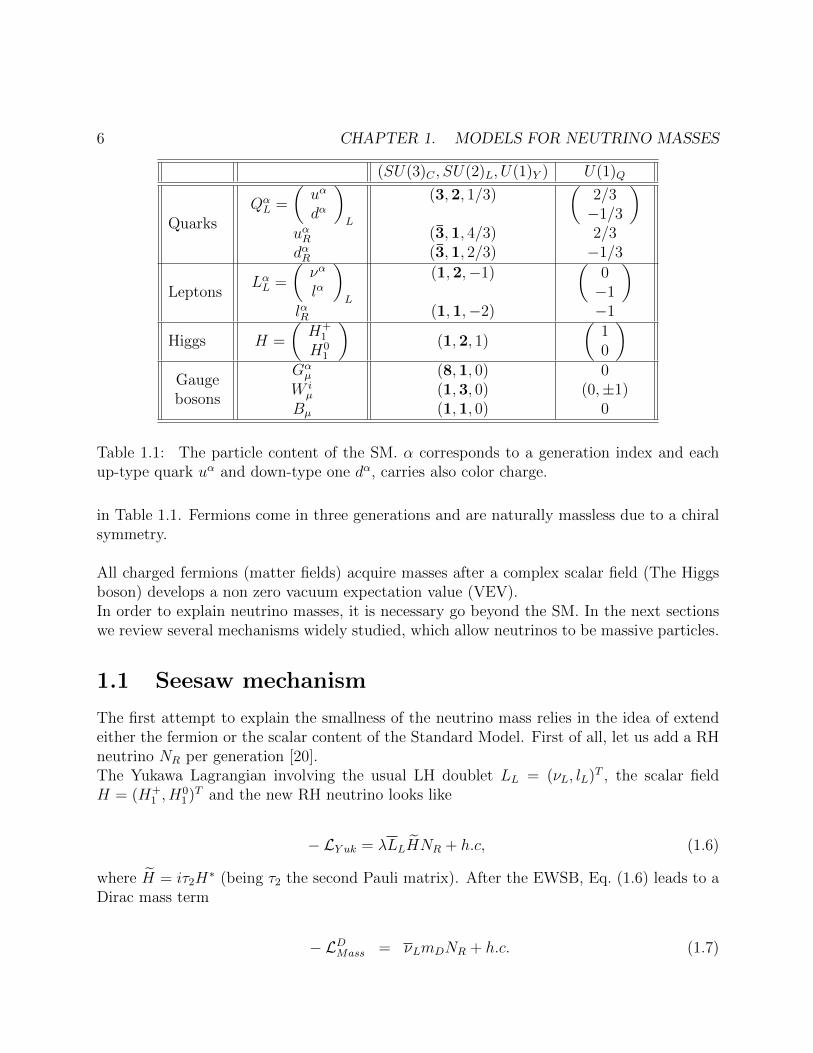
The field content of the SM consists of three types of particles: fermions (spin-1/2 fields),gauge bosons (spin-1 fields), and scalars (spin-0 fields). The particle content is summarized
6 CHAPTER 1. MODELS FOR NEUTRINO MASSES
(SU(3)C , SU(2)L, U(1)Y ) U(1)Q
QuarksQαL =
(uα
dα
)
L
uαRdαR
(3,2, 1/3)
(3,1, 4/3)(3,1, 2/3)
(2/3−1/3
)
2/3−1/3
LeptonsLαL =
(να
lα
)
L
lαR
(1,2,−1)
(1,1,−2)
(0−1
)
−1
Higgs H =
(H+
1
H01
)(1,2, 1)
(10
)
Gaugebosons
Gαµ
W iµ
Bµ
(8,1, 0)(1,3, 0)(1,1, 0)
0(0,±1)
0
Table 1.1: The particle content of the SM. α corresponds to a generation index and eachup-type quark uα and down-type one dα, carries also color charge.
in Table 1.1. Fermions come in three generations and are naturally massless due to a chiralsymmetry.
All charged fermions (matter fields) acquire masses after a complex scalar field (The Higgsboson) develops a non zero vacuum expectation value (VEV).In order to explain neutrino masses, it is necessary go beyond the SM. In the next sectionswe review several mechanisms widely studied, which allow neutrinos to be massive particles.
1.1 Seesaw mechanism
The first attempt to explain the smallness of the neutrino mass relies in the idea of extendeither the fermion or the scalar content of the Standard Model. First of all, let us add a RHneutrino NR per generation [20].The Yukawa Lagrangian involving the usual LH doublet LL = (νL, lL)T , the scalar fieldH = (H+
1 , H01 )T and the new RH neutrino looks like
− LY uk = λLLHNR + h.c, (1.6)
where H = iτ2H∗ (being τ2 the second Pauli matrix). After the EWSB, Eq. (1.6) leads to a
Dirac mass term
− LDMass = νLmDNR + h.c. (1.7)
1.1. SEESAW MECHANISM 7
being mD = λv/√
2. Now, as pointed out before, we can also add a Majorana mass term forNR,
− LMMass =1
2N cRmRNR + h.c.. (1.8)
Denoting nL = (νL, NcR)T , the full Lagrangian is written as
LMass = LMMass + LDMass
=1
2ncLMnL, (1.9)
where
M =
(0 mD
mTD mR
). (1.10)
After diagonalization we find
m2,1 =1
2
(mR ±
√m2R + 4m2
D
). (1.11)
If we demand that m1 is comparable to the charged leptons masses then, in order to explainthe low experimental upper limit on the neutrino mass, m2 must be close to the GUT scale.This means m2 ∼ 1015 GeV. With this mechanism, the smallness of neutrino masses is aconsequence of the heaviness of the right-handed neutrinos. Such a mechanism is called thetype I seesaw mechanism.There exist three realizations of the seesaw mechanism at tree-level [23] which are shown inFig 1.1. These are based on the fact that two SU(2) doublets can be decomposed into asinglet and a triplet (2⊗ 2 = 3⊕ 1).In 1979 Weinberg proved that the symmetries of the SM allow only one (unique) dimension-five effective operator [19]:
LΛ =1
2fαβ
(LcLαH
∗)(H†LLβ
)+ h.c., (1.12)
where fαβ is a coefficient suppressed by an energy scale Λ (associated to the existence ofnew heavy fields) and its calculation depends of the degree of realization of the operator(depending whether the realization is either at tree-level or at loop-level).The seesaw mechanisms (type I [20], type II [21] and type III [22]) are the three realizationsof the dimension-five effective operator at tree-level. This effective theory has an analogy

8 CHAPTER 1. MODELS FOR NEUTRINO MASSES
N N
L
H
L
H
λTνN λνN ∆
L L
H H
λ∆
µ∆
Σ Σ
L
H
L
H
λTνΣλνΣ
Figure 1.1: The three realizations of the seesaw mechanism: Type I (left), Type II (in themiddle) and Type III (right). The massive particle exchanged corresponds to a fermionsinglet NR ∼ (1,1, 0), a scalar triplet ∆ ∼ (1,3,−2) and a fermion triplet Σ ∼ (1,3, 0),respectively.
with the four-fermion point interaction proposed by Fermi in the early 30’s to explain theβ-decay. This proposal describes, at low energies, the weak interaction without W± or Zbosons. In Fig. 1.2 we show both cases: on the left the Fermi’s four-point interaction, andon the right the Feynman diagram associated to the effective operator given in Eq. (1.12).To date we know that the intermediate particles responsible for the weak interaction (and,as a consequence, for the β-decay) are the W± or Z bosons; however is still experimentallyunknown if there exist a heavy field that mediates the interaction drawn on the right ofFig. 1.2. If we assume that the realization of the Weinberg operator is at tree-level, thenthere exist only three different types of fields that could mediate the interaction, these areshown in the Feynman diagram in Fig. 1.1.
In what follows, we discuss briefly each one of the tree-level realizations of the Weinbergeffective Lagrangian.
n
p+
e−
νe
L
H
L
H
Figure 1.2: Effective four-point theories: Fermi’s four-point diagram (left), Weinberg’s four-point diagram (right)

1.1. SEESAW MECHANISM 9
1.1.1 Type I/III Seesaw
We can compute the “effective mass”2 directly from the Feynman diagram or by using theeffective Lagrangian.
LΛ =1
2fαβ
(LcLαH
∗)(H†LLβ
)+ h.c.. (1.13)
After the EWSB, the Higgs field acquires a non-zero VEV: 〈H〉 = v/√
2, the previousequation becomes:
LΛ =1
2(Mν)αβνcLνL, (1.14)
with
(Mν)αβ = fαβv2, (1.15)
that is, a Majorana mass. A simple evaluation shows that, in order to obtain mν < 1 eV,then (fαβ)−1 > 1015 GeV. However, what is fαβ?; with the aim of giving an answer, let usconsiderer the most general Yukawa Lagrangian already written in Eq. (1.9) for the type Iseesaw.
− Lyuk = λLLHNR +1
2N cRmRNR + h.c. (1.16)
After the EWSB, and in matrix form:
− Lyuk =1
2
(νL N c
R
)( 0 mD
mTD mR
)(νcLNR
)+ h.c. (1.17)
Now if mD << mR, by block diagonalization we obtain:
MνL ' −mDm−1R mT
D,
MNR ' mR. (1.18)
From Eq. (1.15) and Eq. (1.18), we find that fαβ has the form:
fαβ = −1
2
λλT
mR
, (1.19)
2I give it this name because it comes from an effective Lagrangian.

10 CHAPTER 1. MODELS FOR NEUTRINO MASSES
is found that in order to obtain MνL ∼ 1 eV, mR ∼ 1015 for Yukawa couplings O(λ) ∼ 1.The same procedure should be done for the type III seesaw. By introducing a fermion tripletΣR ∼ (1,3, 0) to the SM, the most general Yukawa Lagrangian involving this new field andthe neutrino has the form
− Lyuk = LLλΣ
(−→Σ .−→τ
)H +
1
2
−→ΣcmΣ
−→Σ + h.c. (1.20)
After the EWSB and in matrix form the previous equation yields:
− Lyuk =1
2
(νL Σc
3
)( 0 mD
mTD mΣ3
)(νcLΣ3
)+ h.c., (1.21)
with−→Σ = (Σ1,Σ2,Σ3). This mechanism leads to the same result of type I seesaw after
we block diagonalize the mass matrix. Besides, adding a fermion triplet instead a fermionsinglet, yields additional phenomenology. For instance, this model predicts the existence oftwo charged fermions Σ+ ≡ (Σ1−iΣ2)/
√2 and Σ− ≡ (Σ1 +iΣ2)/
√2 with masses M(Σ+,Σ−) >
100.8 GeV [3] (lower experimental bound on its mass). The fact that they have interactionwith the gauge bosons, can lead to new processes like Σ± → l±ν.
1.1.2 Type II Seesaw
Including the scalar triplet ∆ ∼ (1,3, 2):
∆ =
(∆+/√
2 ∆++
∆0 −∆+/√
2
), (1.22)
the relevant Lagrangian is written as:
− L∆ =(LLλ∆∆LL + h.c.
)+ V (H,∆), (1.23)
with
V (H,∆) = m2∆tr∆∆†+ (µ∆H
†∆†H + h.c.). (1.24)
In order to guarantee Lepton Number (LN) conservation in Eq. (1.23), we assign LN = −2to ∆, but this implies the LN is violated explicitly by the µ-term in Eq. (1.24).After the EWSB, and allowing to the scalar triplet to develop a non-vanishing VEV in theneutral direction 〈∆〉 = v∆, the term relevant for neutrino masses given in Eq. (1.23) acquiresthe form:
1.1. SEESAW MECHANISM 11
− LMass = λ∆v∆νcLνL, (1.25)
then
Mν = 2λ∆v∆. (1.26)
From Eq. (1.24), after the two scalars acquire a non-zero VEV and ensuring a minimumvalue for V (H,∆), we find
v∆ = −µ∆v2
4m2∆
, for m∆ >> mH . (1.27)
Taking into account the two previous equations, the expression for the neutrino mass lookslike
Mν = −λ∆µ∆v2
2m2∆
, (1.28)
Doing a comparison between this result and the outcome from the effective dimension-fiveoperator in Eq. (1.12), we find:
fαβ = −λ∆µ∆
m2∆
. (1.29)
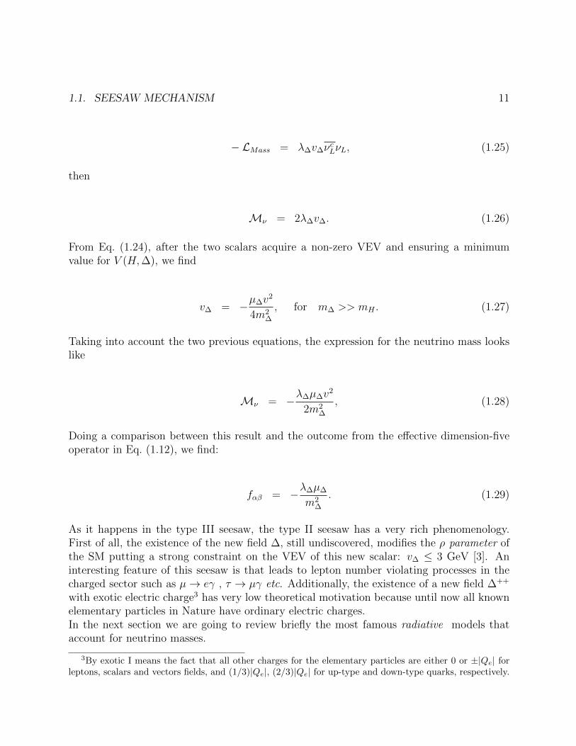
As it happens in the type III seesaw, the type II seesaw has a very rich phenomenology.First of all, the existence of the new field ∆, still undiscovered, modifies the ρ parameter ofthe SM putting a strong constraint on the VEV of this new scalar: v∆ ≤ 3 GeV [3]. Aninteresting feature of this seesaw is that leads to lepton number violating processes in thecharged sector such as µ→ eγ , τ → µγ etc. Additionally, the existence of a new field ∆++
with exotic electric charge3 has very low theoretical motivation because until now all knownelementary particles in Nature have ordinary electric charges.In the next section we are going to review briefly the most famous radiative models thataccount for neutrino masses.
3By exotic I means the fact that all other charges for the elementary particles are either 0 or ±|Qe| forleptons, scalars and vectors fields, and (1/3)|Qe|, (2/3)|Qe| for up-type and down-type quarks, respectively.

12 CHAPTER 1. MODELS FOR NEUTRINO MASSES
1.2 Radiative Models
One of the greatest mysteries yet to be unravelled in the SM is associated to the hierar-chy between the masses of all known fermions. All charged fermions acquire mass throughYukawa couplings with the Higgs boson after the EWSB takes place, however the neutrinoremains massless in the SM. The type I seesaw mechanisms discussed previously lead nat-urally to a massive neutrino by the introduction of heavy fields (at the GUT scale) withmasses around 1015 GeV, making these theories very difficult (with rare decays under specialconditions) to be tested in colliders. Neutrino masses, however, could be originated from aradiative mechanism. This kind of scenario are very attractive due, first, to the ability ofthis type of model to explain the smallness of the neutrino mass as a consequence of loopfactors suppression in the Yukawa couplings and, second, to the prediction of the existenceof new particles that can be found at the Large Hadron Collider (LHC) in the coming years.
In what follows we review the most famous radiative neutrino mass models in the literature.
1.2.1 The Zee’s Model
ν ν
χ−
LL LcL
H+1
〈φ〉
〈H〉Figure 1.3: One-loop diagram in the Zee model
An interesting mechanism to generate masses for neutrinos is given by the Zee model [26] inwhich the masses are generated at one-loop order. In this model the scalar sector of the SMis extend. In addition to the Higgs doublet H = (H+
1 , H01 )T , it is included another doublet
scalar field φ ∼ (1,2, 1) and an SU(2)L singlet(scalar) χ(+) ∼ (1,1, 2). [The numbers in theparentheses stand for the quantum numbers (SU(3)C , SU(2)L, U(1)Y )]
The relevant Lagrangian of the Zee model is:
1.2. RADIATIVE MODELS 13
LZee = LLαhαβLLβχ(+) + µχ(+)H†φ+ h.c., (1.30)
where only the SM doublet H couples to leptons and the SU(2)L singlet χ(+) carries leptonnumber −2 in order to ensure lepton number conservation in the Yukawa sector. Fermi-Dirac statistic makes the coupling hαβ an antisymmetry matrix, which implies a neutrinomass matrix with zeros in its diagonal. The Zee model allows to generate Majorana massfor the neutrino at one-loop order. The relevant Feynman diagram is shown in Fig. 1.3. Inthis model the neutrino mass matrix has the form:
Mν ∼
0 hµe(m2µ −m2
e) hτe(m2τ −m2
e)hµe(m
2µ −m2
e) 0 hτµ(m2τ −m2
µ)hτe(m
2τ −m2
e) hτµ(m2τ −m2
µ) 0
. (1.31)
This model has a rich phenomenology: processes that lead to LFV such as µ → eγ, τ →eµ, etc, are allowed and the existence of the new scalar field φ can be looked for at theLHC. However, the original version of Zee model does not match with the experimentaldata: predicts a maximum value for the solar neutrino mixing angle θ(θ12), and does notreproduce the spectrum of neutrino masses. For these reasons the simplest version of Zeemodel has been rule out [35]. However, a general version of Zee model [36], in where, bothscalar doublets couple to leptons is still a viable model for neutrino masses and mixing.
1.2.2 The Babu model
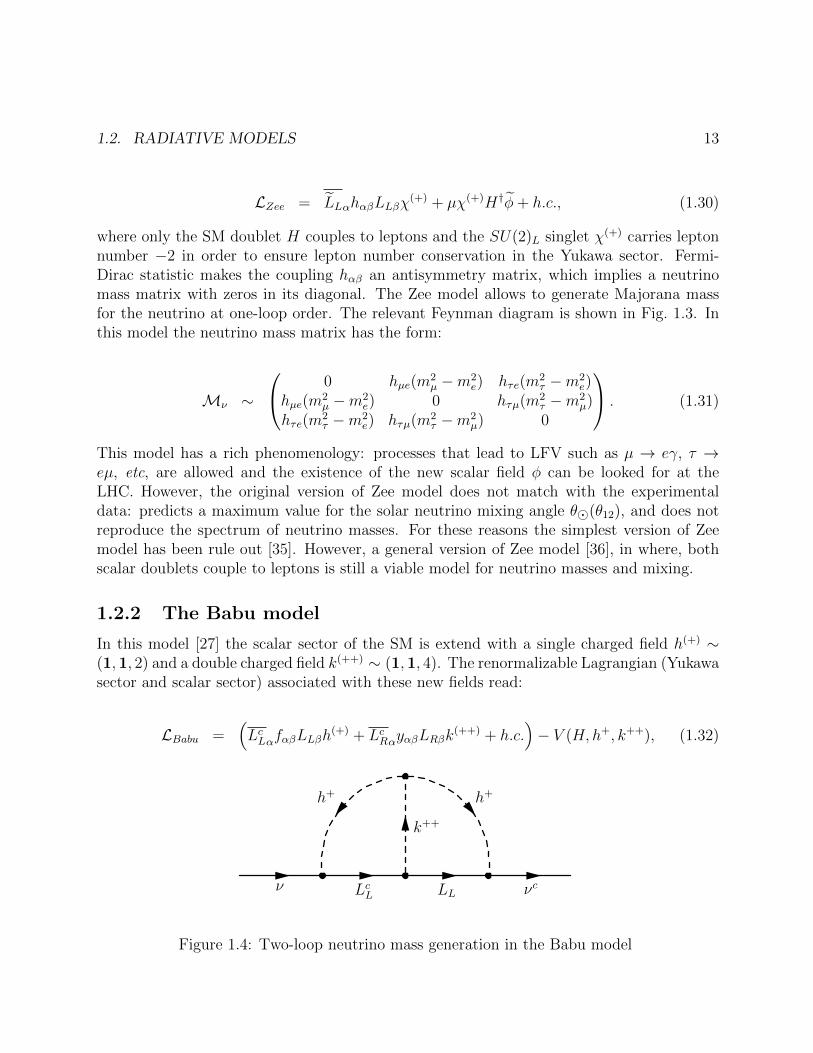
In this model [27] the scalar sector of the SM is extend with a single charged field h(+) ∼(1,1, 2) and a double charged field k(++) ∼ (1,1, 4). The renormalizable Lagrangian (Yukawasector and scalar sector) associated with these new fields read:
LBabu =(LcLαfαβLLβh
(+) + LcRαyαβLRβk(++) + h.c.
)− V (H, h+, k++), (1.32)
ν
h+h+
LcL LL
k++
νc
Figure 1.4: Two-loop neutrino mass generation in the Babu model
14 CHAPTER 1. MODELS FOR NEUTRINO MASSES
with the potential term given by:
V (H, h+, k++) = µh−h−k++ + h.c. (1.33)
Fermi statistic implies antisymmetry of fαβ and symmetry of yαβ. The new trilinear inter-action shown in Eq. (1.33) violates lepton number by two units. Small Majorana neutrinomasses contributions appear at two-loop level as it is shown in Fig. 1.4.The neutrino masses are calculated from the Feynman diagram, and the mass matrix hasthe form:
Mαβ = 8µfαγy′γδmγmδIγδ(y†)γβ, (1.34)
with y′αβ = ζy
′αβ where ζ = 1 for α = β and ζ = 2 for α 6= β, being m(γ,δ) the charged lepton
masses.The term Iγβ is a two-loop integral
Iγδ =
∫d4p
(2π)4
∫d4q
(2π)4
1
(p2 −m2h)
1
(p2 −m2γ)
1
(q2 −m2h)
1
(q2 −m2δ)
1
(p− q)2 −m2k). (1.35)
This integral has been evaluated in Ref. [37].Because det(Mν) = 0, the model matches with the current experimental data [3], andpredicts one of the neutrinos to be massless. The Babu model also leads to decay processesthat violate lepton number such as µ → eee, τ → µµµ which occurs at tree-level via k(++)
exchange.
1.2.3 The Radiative Seesaw Model
An interesting model that can account for neutrino masses and also provides a dark mattercandidate in the Universe is the so-called Radiative Seesaw [38]. This model is based onthe two-Higgs Doublet (2HDM) model [39] where, in addition to the Standard Model gaugegroup GSM is assumed an exact discrete Z2 symmetry, and a minimal particle extension: ahypothetical new scalar doublet and three right-handed neutrinos. Under SU(3)C⊗SU(2)L⊗U(1)Y ⊗ Z2, the new particle content transforms as:
η = (η+, η0)T ∼ (1,2, 1,−), NRα ∼ (1,1, 0,−), (1.36)
The new particles, i.e. NRα and the scalar doublet (η+, η0)T are odd under Z2. The remainingparticles of the SM are even under Z2.The relevant Lagrangian reads:
1.2. RADIATIVE MODELS 15
να νβNγ
η0η0
〈H〉 〈H〉
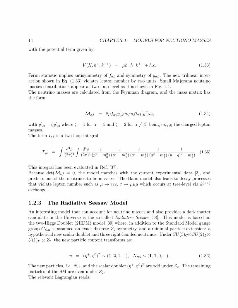
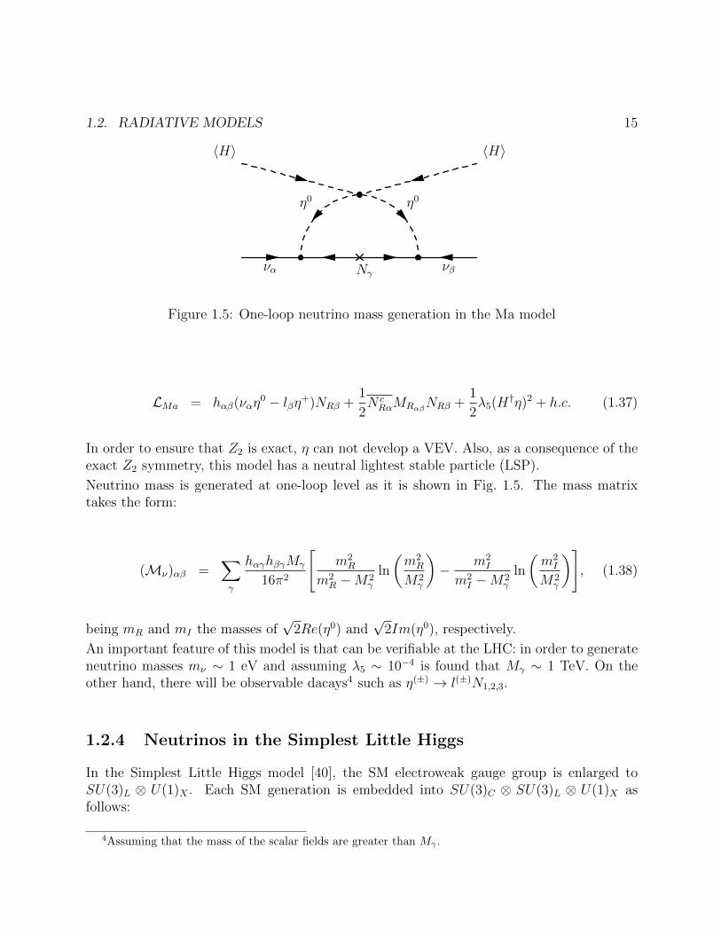
Figure 1.5: One-loop neutrino mass generation in the Ma model
LMa = hαβ(ναη0 − lβη+)NRβ +
1
2N cRαMRαβNRβ +
1
2λ5(H†η)2 + h.c. (1.37)
In order to ensure that Z2 is exact, η can not develop a VEV. Also, as a consequence of theexact Z2 symmetry, this model has a neutral lightest stable particle (LSP).
Neutrino mass is generated at one-loop level as it is shown in Fig. 1.5. The mass matrixtakes the form:
(Mν)αβ =∑
γ
hαγhβγMγ
16π2
[m2R
m2R −M2
γ
ln
(m2R
M2γ
)− m2
I
m2I −M2
γ
ln
(m2I
M2γ
)], (1.38)
being mR and mI the masses of√
2Re(η0) and√
2Im(η0), respectively.
An important feature of this model is that can be verifiable at the LHC: in order to generateneutrino masses mν ∼ 1 eV and assuming λ5 ∼ 10−4 is found that Mγ ∼ 1 TeV. On theother hand, there will be observable dacays4 such as η(±) → l(±)N1,2,3.
1.2.4 Neutrinos in the Simplest Little Higgs
In the Simplest Little Higgs model [40], the SM electroweak gauge group is enlarged toSU(3)L ⊗ U(1)X . Each SM generation is embedded into SU(3)C ⊗ SU(3)L ⊗ U(1)X asfollows:
4Assuming that the mass of the scalar fields are greater than Mγ .

16 CHAPTER 1. MODELS FOR NEUTRINO MASSES
QαL = (uα, dα, Uα)TL ∼ (3, 3, 1/3),
dcα ∼ (3∗, 1, 1/3), ucα ∼ (3∗, 1,−2/3), U cα ∼ (3∗, 1,−2/3),
ψαL = (−iνα,−ilα, Nα)TL ∼ (1, 3,−1/3), (1.39)
lcα ∼ (1, 1, 1), ncα ∼ (1, 1, 0),
where α corresponds to a generation index. The symmetry breaking is triggered by theVEVs of two triplets φ1,2 (of a global [SU(3)]2 symmetry) which transform as (3,−1/3)under SU(3)L ⊗ U(1)X :
φ1 → eiθ cotβ/f
00f1
,
φ2 → e−iθ tanβ/f
00f2
, (1.40)
where tan β = f1/f2, f =√f 2
1 + f 22 , and θ has the matrix form
θ =η√2
+
0 0 H01
0 0 H+1
H01 H−1 0
. (1.41)
For the sake of simplicity identical VEVs for both triplets are assumed (f1 = f2 ∼ f).Masses for the neutral leptons arise from the interactions of the form (considering just onegeneration):
− Lyuk = λνφ†1ψLn
c + h.c. (1.42)
This Lagrangian respects the global [SU(3)]2 symmetry and does not generate radiativecontribution to the Higgs mass m2
h. In the basis (ν,N, nc), the mass matrix takes the form:
M =
0 0 −λνv0 0 λνfλνv λνf 0
, (1.43)
where v is the VEV of the SU(2) Higgs doublet H, and f is the scale at which the twocondensate sigma fields develop VEV. At this stage the lightest neutrino remains massless,however it can acquire mass when one-loop level contribution are taken into account.
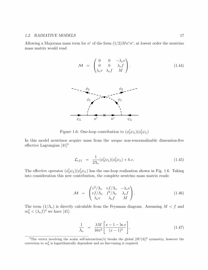
1.2. RADIATIVE MODELS 17
Allowing a Majorana mass term for nc of the form (1/2)Mncnc, at lowest order the neutrinomass matrix would read
M =
0 0 −λνv0 0 λνfλνv λνf M
. (1.44)
ψL ψL
φ1
nc nc
φ1
φ2φ2
Figure 1.6: One-loop contribution to (φ†2ψL)(φ†2ψL)
In this model neutrinos acquire mass from the unique non-renormalizable dimension-fiveeffective Lagrangian [41]5
Leff =1
2Λν
(φ†2ψL)(φ†2ψL) + h.c. (1.45)
The effective operator (φ†2ψL)(φ†2ψL) has the one-loop realization shown in Fig. 1.6. Takinginto consideration this new contribution, the complete neutrino mass matrix reads:
M =
v2/Λν vf/Λν −λνvvf/Λν f 2/Λν λνfλνv λνf M
. (1.46)
The term (1/Λν) is directly calculable from the Feynman diagram. Assuming M < f andm2h < (λνf)2 we have [41]:
1
Λν
=λM
16π2
[x− 1− lnx
(x− 1)2
], (1.47)
5The vertex involving the scalar self-interaction(λ) breaks the global [SU(3)]2 symmetry, however thecorrection to m2
h is logarithmically dependent and no fine-tuning is required.

18 CHAPTER 1. MODELS FOR NEUTRINO MASSES
with x = m2h/(λνf)2 and λ the Higgs quartic coupling.
After diagonalizing Eq. (1.44), the lightest neutrino acquire mass which is given by
mν ' v2 λM
4π2f 2ln
((λνf)2
m2h
). (1.48)
A interesting feature of this model is that neutrino mass depends only logarithmically on theYukawa coupling constant, and predicts the existence of a yet to be observed right-handedneutrino with Majorana mass at the KeV scale6.
6Demanding mν ∼ 1 eV.
Chapter 2
Little Higgs Model
Even with the remarkable success of the Standard Model (SM), there are theoretical reasonsfor believing that it is not the ultimate theory. One of the greatest mysteries still to besolved concerns the fact that the mass-squared parameter for the Higgs m2
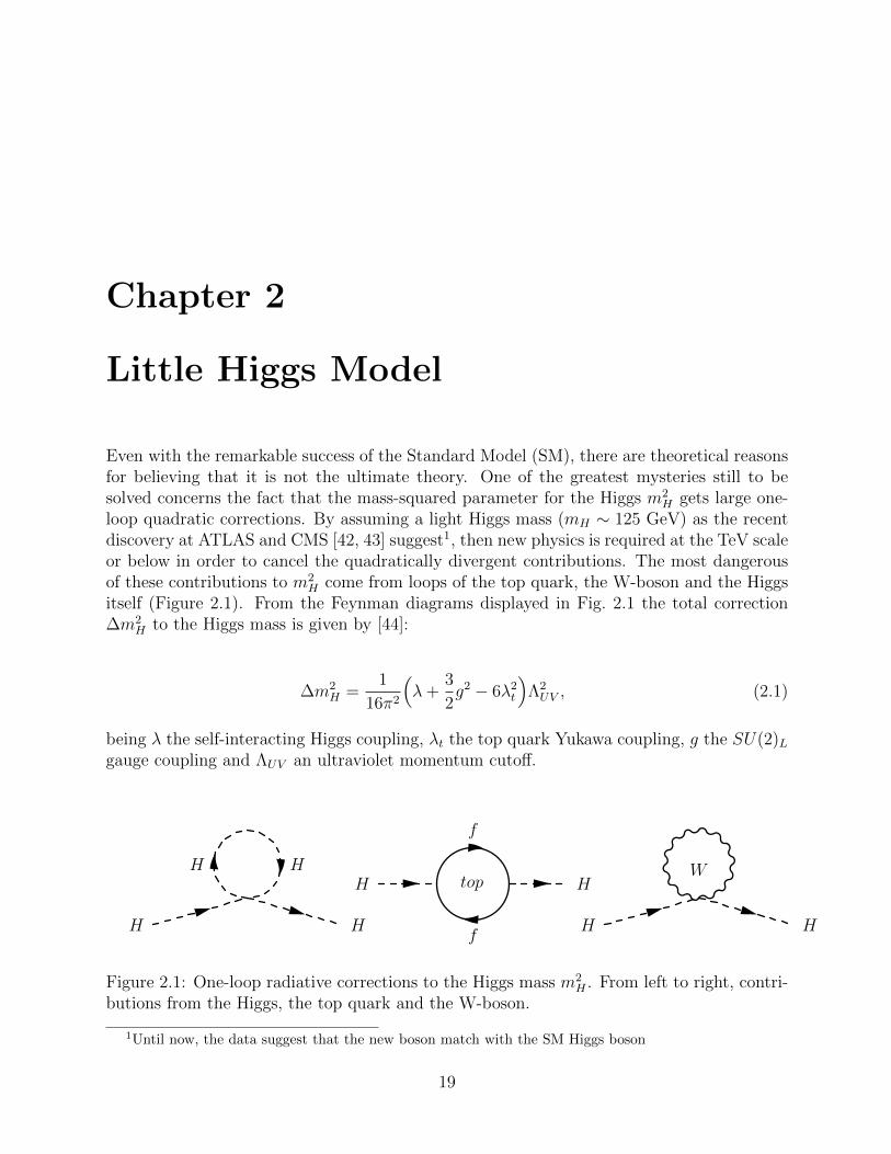
H gets large one-loop quadratic corrections. By assuming a light Higgs mass (mH ∼ 125 GeV) as the recentdiscovery at ATLAS and CMS [42, 43] suggest1, then new physics is required at the TeV scaleor below in order to cancel the quadratically divergent contributions. The most dangerousof these contributions to m2
H come from loops of the top quark, the W-boson and the Higgsitself (Figure 2.1). From the Feynman diagrams displayed in Fig. 2.1 the total correction∆m2
H to the Higgs mass is given by [44]:
∆m2H =
1
16π2
(λ+
3
2g2 − 6λ2
t
)Λ2UV , (2.1)
being λ the self-interacting Higgs coupling, λt the top quark Yukawa coupling, g the SU(2)Lgauge coupling and ΛUV an ultraviolet momentum cutoff.
HH
H H
f
f
H Htop
H H
W
Figure 2.1: One-loop radiative corrections to the Higgs mass m2H . From left to right, contri-
butions from the Higgs, the top quark and the W-boson.
1Until now, the data suggest that the new boson match with the SM Higgs boson
19
20 CHAPTER 2. LITTLE HIGGS MODEL
Assuming that the SM is valid up to MPlanck ∼ 2× 10¹⁸ GeV, a scale at which gravitationaleffects spoil the renormalizability of the theory, then what protects the Higgs mass fromradiative corrections?. These corrections push up the Higgs mass to energies far beyondits bare mass destabilizing the electroweak symmetry breaking scale. This shortcoming isknown as the hierarchy problem. From an experimental point of view, the current datasuggest that SM, including radiative corrections, is a successful theory up to 5 TeV, scale atwhich, is expected that a fundamental theory should manifest in Nature (The UV comple-tion of the SM) [47]. This scale is still too high, and radiative corrections to the Higgs masswould require fine-tuning. On the other hand, from a theoretical point of view, in order tostabilizes the electroweak scale, then new physics (elusive particles that are expected to befound in the current- and forthcoming experiments) is required at ∼ 1 TeV. This issue isknown as the little hierarchy problem [1, 47].Several solutions [2, 7, 49, 50] have been intensively studied in the last decade, one isSupersymmetry (SUSY) in which the quadratic divergences to the Higgs mass comingfrom particles and sparticles cancel between each other. Also are the Little Higgs Mod-els(LHMs) [7, 45, 46, 48, 51] in which the Higgs is thought as a Pseudo-Nambu GoldstoneBoson (PNGB), massless at tree-level, which is allowed to acquire small mass radiatively. Inthis latter framework the radiative contributions to the Higgs mass are cancelled betweenparticles of the same spin.
The trick behind Little Higgs models, the so-called (collective symmetry breaking), lies in factthat no single coupling explicitly breaks the global symmetry. The Higgs mass is protectedby a global symmetry which is spontaneously broken. After the breaking the Higgs arises asa massless PNGB, and acquires mass logarithmically at one-loop order or quadratically attwo-loop order (this latter contribution is negligible).
The Little Higgs model based on the approximate [SU(4)/SU(3)]4 global symmetry has astrong theoretical motivation because of its ability to reproduce the low-energy phenomenol-ogy with a set of minimal parameters and to generate the Higgs quartic self-coupling withoutfine-tuning (unlike the model based on the approximate [SU(3)/SU(2)]2 in which fine-tuningis required). Recently a study was carried out in order to determinate whether the Higgs-likeparticle discovered at CERN is the pseudo-Goldstone Boson of the Little Higgs Models ornot [52]. By now the Simplest Little Higgs model [53] matchs with the current experimentaldata. In what follows we described briefly the Simplest Little Higgs (SLH) Model based onthe approximate [SU(4)/SU(3)]4 global symmetry.
2.1 The model
In the SLH Model based on the SU(4) global symmetry, the electroweak SU(2)L⊗U(1)Y SMgauge group is enlarged to SU(4)L⊗U(1)X [6, 53]. This symmetry group has been proposedas an electroweak extension of the SM [54] and, among its features, the most remarkable
2.1. THE MODEL 21
Table 2.1: Anomaly-free fermion content.
QiL =
diuiUiDi
L
dciL uciL U ciL Dc
iL
[3, 4∗, 16] [3∗, 1, 1
3] [3∗, 1,−2
3] [3∗, 1,−2
3] [3∗, 1, 1
3]
Q3L =
u3
d3
D3
U3
L
uc3L dc3L Dc3L U c
3L
[3, 4, 16] [3∗, 1,−2
3] [3∗, 1, 1
3] [3∗, 1, 1
3] [3∗, 1,−2
3]
LαL =
ν0eα
e−αE−αn0α
L
e+αL E+
αL
[1, 4,−12] [1, 1, 1] [1, 1, 1]
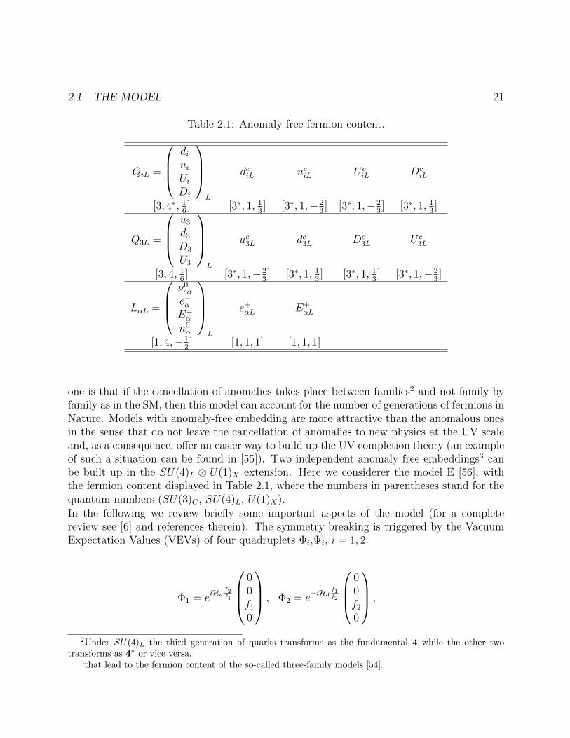
one is that if the cancellation of anomalies takes place between families2 and not family byfamily as in the SM, then this model can account for the number of generations of fermions inNature. Models with anomaly-free embedding are more attractive than the anomalous onesin the sense that do not leave the cancellation of anomalies to new physics at the UV scaleand, as a consequence, offer an easier way to build up the UV completion theory (an exampleof such a situation can be found in [55]). Two independent anomaly free embeddings3 canbe built up in the SU(4)L ⊗ U(1)X extension. Here we considerer the model E [56], withthe fermion content displayed in Table 2.1, where the numbers in parentheses stand for thequantum numbers (SU(3)C , SU(4)L, U(1)X).
In the following we review briefly some important aspects of the model (for a completereview see [6] and references therein). The symmetry breaking is triggered by the VacuumExpectation Values (VEVs) of four quadruplets Φi,Ψi, i = 1, 2.
Φ1 = eiHd f2f1
00f1
0
, Φ2 = e
−iHd f1f2
00f2
0
,
2Under SU(4)L the third generation of quarks transforms as the fundamental 4 while the other twotransforms as 4∗ or vice versa.
3that lead to the fermion content of the so-called three-family models [54].

22 CHAPTER 2. LITTLE HIGGS MODEL
Ψ1 = eiHu f4f3
000f3
, Ψ2 = e
−iHu f3f4
000f4
. (2.2)
These sigma model fields transform under SU(4)L ⊗ U(1)X as Φ1 ∼ (4, 1/2),Φ2 ∼ (4, 1/2), Ψ1 ∼ (4,−1/2), Ψ2 ∼ (4,−1/2);with
Hd =1
f12
0 00 0
hd00
h†d 0 00 0 0 0
, Hu =
1
f34
0 00 0
00
hu
0 0 0 0h†u 0 0
, (2.3)
being f 2ij = f 2
i + f 2j . Additionally, hd and hu are SU(2) doublets with hypercharges 1/2 and
−1/2, respectively, and acquire VEVs:
〈hd〉 =1√2
(0vd
)and 〈hu〉 =
1√2
(vu0
). (2.4)
At low-energies this model reproduce one Two-Higgs-Doublet Model (2HDM). One of themain features of this model (unlike the one based on global SU(3) symmetry) is that it allowsto generate automatically (at tree-level) a self-interacting quartic coupling for the scalar fieldwhich stabilizes the Higgs VEV.
Ψ1
Ψ2 Ψ2
Ψ1
Φi(Ψi) Φi(Ψi)
Φ1
Φ2 Φ2
Φ1
Figure 2.2: Gauge boson contribution to the Higgs potential
2.1. THE MODEL 23
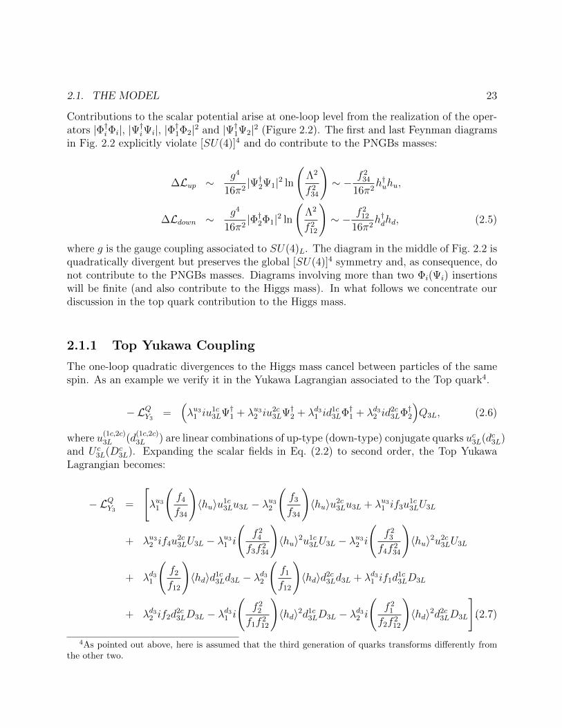
Contributions to the scalar potential arise at one-loop level from the realization of the oper-ators |Φ†iΦi|, |Ψ†iΨi|, |Φ†1Φ2|2 and |Ψ†1Ψ2|2 (Figure 2.2). The first and last Feynman diagramsin Fig. 2.2 explicitly violate [SU(4)]4 and do contribute to the PNGBs masses:
∆Lup ∼g4
16π2|Ψ†2Ψ1|2 ln
(Λ2
f 234
)∼ − f 2
34
16π2h†uhu,
∆Ldown ∼g4
16π2|Φ†2Φ1|2 ln
(Λ2
f 212
)∼ − f 2
12
16π2h†dhd, (2.5)
where g is the gauge coupling associated to SU(4)L. The diagram in the middle of Fig. 2.2 isquadratically divergent but preserves the global [SU(4)]4 symmetry and, as consequence, donot contribute to the PNGBs masses. Diagrams involving more than two Φi(Ψi) insertionswill be finite (and also contribute to the Higgs mass). In what follows we concentrate ourdiscussion in the top quark contribution to the Higgs mass.
2.1.1 Top Yukawa Coupling
The one-loop quadratic divergences to the Higgs mass cancel between particles of the samespin. As an example we verify it in the Yukawa Lagrangian associated to the Top quark4.
− LQY3=
(λu3
1 iu1c3LΨ†1 + λu3
2 iu2c3LΨ†2 + λd3
1 id1c3LΦ†1 + λd3
2 id2c3Lֆ2
)Q3L, (2.6)
where u(1c,2c)3L (d
(1c,2c)3L ) are linear combinations of up-type (down-type) conjugate quarks uc3L(dc3L)
and U c3L(Dc
3L). Expanding the scalar fields in Eq. (2.2) to second order, the Top YukawaLagrangian becomes:
− LQY3=
[λu3
1
(f4
f34
)〈hu〉u1c
3Lu3L − λu32
(f3
f34
)〈hu〉u2c
3Lu3L + λu31 if3u
1c3LU3L
+ λu32 if4u
2c3LU3L − λu3
1 i
(f 2
4
f3f 234
)〈hu〉2u1c
3LU3L − λu32 i
(f 2
3
f4f 234
)〈hu〉2u2c
3LU3L
+ λd31
(f2
f12
)〈hd〉d1c
3Ld3L − λd32
(f1
f12
)〈hd〉d2c
3Ld3L + λd31 if1d
1c3LD3L
+ λd32 if2d
2c3LD3L − λd3
1 i
(f 2
2
f1f 212
)〈hd〉2d1c
3LD3L − λd32 i
(f 2
1
f2f 212
)〈hd〉2d2c
3LD3L
].(2.7)
4As pointed out above, here is assumed that the third generation of quarks transforms differently fromthe other two.

24 CHAPTER 2. LITTLE HIGGS MODEL
hu(hd)
u3L(d3L)
U c3L(U c
3L)
hu(hd)
hu(hd)
U3L(D3L)
hu(hd)
U3L(D3L)
hu(hd)
u3L(d3L)
uc3L(dc3L)
hu(hd)
Figure 2.3: Top(Bottom) contribution to the Higgs mass.
In the mass eigenstates basis the previous equation acquires the form
− LQY3= λu3〈hu〉uc3Lu3L + λU3u3〈hu〉U c
3Lu3L +λU3
2MU3
〈hu〉2U c3Lu3L
+ λd3〈hd〉dc3Ld3L + λD3d3〈hd〉Dc3Ld3L +
λD3
2MD3
〈hd〉2Dc3Ld3L, (2.8)
where
λu3 =λu3
1 λu32 f34√
2MU3
, λU3u3 =
[(λu3
1 )2 − (λu32 )2]f3f4
√2f34MU3
, λU3 =(λu3
1 f4)2 + (λu32 f3)2
2f 234
λd3 =λd3
1 λd32 f12√
2MD3
, λD3d3 =
[(λd3
1 )2 − (λd32 )2]f1f2
√2f12MD3
, λD3 =(λd3
1 f2)2 + (λd32 f1)2
2f 212
,(2.9)
MU =√
(λu31 f3)2 + (λu3
2 f4)2 and MD =√
(λd31 f1)2 + (λd3
2 f2)2.
The couplings between the up-type (down-type) Higgs and the top (bottom) quarks inEq. (2.8) do not contribute to the Higgs mass due to a miraculous cancellation of thequadratic divergences. In Fig. 2.3 we display the one loop diagrams involving these in-teractions. The quadratic divergences coming from the first and last diagrams are cancelledby the contribution from the diagram in the middle. Contributions at two-loop level (fromthe top quark and gauge bosons) to the Higgs mass are also present, but are negligible.5
5Under the assumption that the ultraviolet cutoff is ∼ 10 TeV.
2.1. THE MODEL 25
2.1.2 Yukawa Lagrangian for the Neutral Leptons
With the particle content of the model under consideration it is not possible to generatemasses for neutral leptons unless we introduce right-handed neutrinos NR ∼ (1,1, 0) in themodel. The most general gauge invariant Yukawa Lagrangian looks like:
− LneutroY = λ1NαRΨ†1LβL + λ2NαRΨ†2LβL + h.c,
where α and β are generation indexes. This Lagrangian does not respect the global [SU(4)]4
symmetry and, as a consequence, also gives contribution to the PNGBs masses. Two solu-tions to this problem have been proposed: the first one is to assume only a Yukawa coupling:forbidding, for example, λ2 and leaving the interaction that involves λ1
6; the second one isassuming that the global [SU(4)]4 symmetry is approximate [57]. In this case there exist astrong suppression on the coupling λ2 << 1 while λ1 remains unsuppressed. In this waythe contribution to the PNGBs coming from the leptonic sector remains negligible due tothe smallness of λ2. In this scenario the collective symmetry breaking is achieved only whenλ2 → 0. This latter alternative is the option that is explored in this thesis. Further detailsconcerning the generation of neutrino masses will be considered in Chapter 3.
6This idea is applied by Lee [58] and F. del Aguila et al. [41] to generate masses in the Kaplan-Schmaltzmodel [53]
Chapter 3
Radiative Neutrino Mass Generation
3.1 Model
As pointed out in Chapter 2, the Simplest Little Higgs model based on the approximate[SU(4)/SU(3)]4 global symmetry “solve” the electroweak hierarchy problem (little hierarchyproblem) of the SM. The key of these theories is the implementation of the so-called collectivesymmetry breaking, which avoids large radiative corrections at one loop level to the Higgsmass. The Schmaltz’s model [40] has been extended to the approximate [SU(4)/SU(3)]4 non-liner sigma model [6], with the new top quark partners cancelling the divergences comingfrom the ordinary quark top. The quadratic divergences at one loop order to the Higgs massare suppressed, and at two loops are negligible. In this work, we are going to considerera more generic version of the Simplest Little Higgs model, known as the minimal littlehiggs model already studied in [57] for the [SU(3)/SU(2)]2 non-liner sigma model. Here, itis assumed that the global SU(4) symmetry which protects the Higgs mass is approximate.Then the Higgs mass receives quadratic divergences at one loop, but these new contributionsare negligible mainly by the suppression imposed by the global symmetry on the new Yukawainteractions. Assuming an anomaly free embedding in the SU(4)L⊗U(1)X gauge symmetry,we have the following lepton content1
LαL =(− iν0
eα,−ie−α , E−α , n0α
)TL∼ (1,4,−1/2), e+
αL ∼ (1,1, 1), E+αL ∼ (1,1, 1), (3.1)
with α being a generation index and the numbers inside the parentheses correspond to theway the lepton field transform under SU(3)C ⊗ SU(4)L ⊗ U(1)X (3-4-1 symmetry).
1Exactly the same lepton content displayed in Table 2.1, where a −i phase is included in the SM leptondoublet.
26
3.2. ONE GENERATION CASE 27
The scalar sector in the model is given by,
Φ1 = eiHd f2f1
00f1
0
, Φ2 = e
−iHd f1f2
00f2
0
, (3.2)
Ψ1 = eiHu f4f3
000f3
, Ψ2 = e
−iHu f3f4
000f4
. (3.3)
These sigma model fields transform under the SU(4)L ⊗ U(1)Y symmetry as Φ1 ∼ (4, 1/2),Φ2 ∼ (4, 1/2), Ψ1 ∼ (4,−1/2), Ψ2 ∼ (4,−1/2).The model studied in [6] does not provide a mechanism for neutrino mass generation. As afirst step, following the idea behind the seesaw mechanisms we extend the particle contentof the model but keeping in mind that it is forbidden to break the anomaly-free structureof the model. The most simple choice is to add a right-handed neutrino N0
iR ∼ (1,1, 0) pergeneration. Since neutrinos do not possess electric charge, they can be Majorana particles.
3.2 One generation case
The Yukawa Lagrangian for neutral leptons is given by:
− Lyuk = λnNRΨ†1LL + λmNRΨ†2LL + h.c. (3.4)
Assuming that LL ∼ (4, 1, 1, 1), Ψ1 ∼ (4, 1, 1, 1) and Ψ2 ∼ (1, 4, 1, 1) underSU(4)1⊗SU(4)2⊗SU(4)3⊗SU(4)4([SU(4)]4), we note that the coupling λn is unsuppressed,but λm is suppressed by the global symmetry, therefore, we impose the hierarchy conditionλn >> λm.After the Spontaneous Symmetry Breaking (SSB) takes place, the scalar fields develop aVEV, which is expressed by:
〈Ψ1〉 = eiβ1A
000f3
, 〈Ψ2〉 = e−iβ2A
000f4
, (3.5)
with

28 CHAPTER 3. RADIATIVE NEUTRINO MASS GENERATION
β1 =f4
f3
vµ
f34
√2
, β2 =f3
f4
vµ
f34
√2
and A =
0 0 0 10 0 0 00 0 0 01 0 0 0
. (3.6)
From here on we are going to do some mathematical procedure that will allow us to writedown the Yukawa Lagrangian in terms of the neutrino mixing angle.Expanding the exponential function
eiβ1A = 1 + iβ1A+1
2!(iβ1)2A2 +
1
3!(iβ1)3A3 + ... (3.7)
Is easy to show that:
Am =
C, m oddA, m even.
(3.8)
where
C =
1 0 0 00 0 0 00 0 0 00 0 0 1
. (3.9)
From Eq. (3.7), and using the results from Eq. (3.8)
eiβ1A = 1 + iA[β1 −
1
3!β3
1 +1
5!β5
1 −1
7!β7
1 ± ...]
+ C[− 1
2!β2
1 +1
4!β4
1 −1
6!β6
1 ∓ ...]
= 1− C + iA sin β1 + C cos β1
=
cos β1 0 0 i sin β1
0 1 0 00 0 1 0
i sin β1 0 0 cos β1
. (3.10)
In order to calculate the masses of the neutrinos at tree-level, going from weak eigenstates tomass eigenstates, we need to compute the VEV of the scalar fields, which can be evaluateddirectly using the calculation of eiβ1A. After such a calcutation is obtained:
〈Ψ1〉† = e−iβ1A(0 0 0 f3
)=(−if3 sin β1 0 0 f3 cos β1
), (3.11)
3.2. ONE GENERATION CASE 29
〈Ψ2〉† = eiβ2A(0 0 0 f4
)=(if4 sin β2 0 0 f4 cos β2
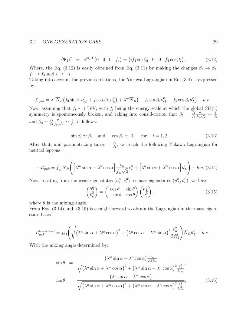
). (3.12)
Where, the Eq. (3.12) is easily obtained from Eq. (3.11) by making the changes β1 → β2,f3 → f4 and i→ −i.Taking into account the previous relations, the Yukawa Lagrangian in Eq. (3.4) is expressedby:
− Lyuk = λnNR
(f3 sin β1ν
0eL + f3 cos β1n
0L
)+ λmNR
(− f4 sin β2ν
0eL + f4 cos β1n
0L
)+ h.c.
Now, assuming that fi ∼ 1 TeV; with fi being the energy scale at which the global SU(4)symmetry is spontaneously broken, and taking into consideration that β1 = f4
f3
νµf34
√2∼ 1
fi
and β2 = f3
f4
νµf34
√2∼ 1
fi, it follows:
sin βi ' βi and cos βi ' 1, for i = 1, 2. (3.13)
After that, and parametrizing tanα = f3
f4, we reach the following Yukawa Lagrangian for
neutral leptons
− Lyuk = f34NR
([λm sinα− λn cosα
] vµ
f34
√2ν0e +
[λn sinα + λm cosα
]n0L
)+ h.c. (3.14)
Now, rotating from the weak eigenstates (n0L, ν
0e ) to mass eigenstates (n0
L, ν0e ), we have
(n0L
ν0e
)=
(cos θ sin θ− sin θ cos θ
)(n0L
ν0e
), (3.15)
where θ is the mixing angle.From Eqs. (3.14) and (3.15) is straightforward to obtain the Lagrangian in the mass eigen-state basis
− Ltree−levelyuk = f34
(√(λn sinα + λm cosα
)2+(λn cosα− λm sinα
)2 v2µ
2f 234
)NRn
0L + h.c.
With the mixing angle determined by:
sin θ =
(λm sinα− λn cosα
) vµ√2f34√(
λn sinα + λm cosα)2
+(λm sinα− λn cosα
)2 v2µ
2f234
,
cos θ =
(λn sinα + λm cosα
)√(
λn sinα + λm cosα)2
+(λm sinα− λn cosα
)2 v2µ
2f234
, (3.16)

30 CHAPTER 3. RADIATIVE NEUTRINO MASS GENERATION
and the mass-term from the Yukawa Lagrangian in Eq. (3.16) is:
mN = f34
(√(λn sinα + λm cosα
)2+(λn cosα− λm sinα
)2 v2µ
2f 234
). (3.17)
In order to compare the latter expression with the neutrino mass reported in [58], we must toexpand and suppress completely either λn or λm. For instance, making λm = 0 and λn 6= 0is reproduced the results in Ref. [58].
At this stage, two heavy neutrinos acquire masses of the order of the mass term given inEq. (3.17), but the SM neutrino (the lightest neutrino) remains massless (this results holdseven if we considerer the three generations of fermions).From now on, we will concentrate in the study of another mechanism to generate neutrinomasses. As a first attempt we explore the so-called radiative seesaw mechanism.
From Eq. (3.14), we can write down the Lagrangian in matrix form (where the super-indexin the neutral leptons had been suppressed):
− LTree−levelyuk =1
2
(νceL ncL NR
)M
νeLnLN cR
+ h.c., (3.18)
with M, the tree-level mass matrix which is given by:
M =
00[
λm sinα− λn cosα]vµ√2
00
f34
[λn sinα+ λm cosα
]
[(λm)† sinα− (λn)† cosα
]vµ√2
f34
[(λn)† sinα+ (λm)† cosα
]
0
(3.19)
.
If we introduce a Majorana mass term for the right-handed neutrino NR, then we must toadd to the tree-level Lagrangian the term 1
2MNRN
cR+h.c , being M the mass of the particle.
At the lowest order the neutrino mass has the structure
M =
00[
λm sinα− λn cosα]vµ√2
00
f34
[λn sinα+ λm cosα
]
[(λm)† sinα− (λn)† cosα
]vµ√2
f34
[(λn)† sinα+ (λm)† cosα
]
M
(3.20)
Diagonalizing this last matrix it is found that the SM neutrino remains massless. In order togive it a non-zero mass, we are going to introduce a dimension-five effective operator, whichare a generalization of the Weinberg operator in the SM [19].

3.3. RADIATIVE SEESAW MECHANISM 31
3.3 Radiative Seesaw Mechanism
In order to explain the smallness of neutrino mass in nature, we can introduce higher di-mensional operators which will automatically generate tiny neutrino masses. The MinimalLittle Higgs Model based on an electroweak symmetry SU(4)L ⊗ U(1)X can be thought asan effective theory that is valid up to an energy scale Λ.The Lagrangian is written as:
Lyuk = Ltree−levelyuk + Lloop−levelyuk (3.21)
.After expanding Lloop−level, it follows:
Lyuk = Ltree−levelyuk + L5 + L6 + . . . (3.22)
In the SM the Weinberg’s dimension-five effective operator [19] provides an answer for neu-trino masses puzzle (this operator violate lepton number, and, neutrinos are Majorana par-ticles).
L5 =1
ΛO5 with O5 ∼ LLHH
Here,we are going to build up all the possible effective operators of dimension d = 5 in ourmodel:
O5 ⊃
(LcLΨ∗1)(Ψ†1LL), (LcLΨ∗2)(Ψ†2LL), (LcLΨ∗1)(Ψ†2LL), (LcLΨ∗2)(Ψ†1LL)
(3.23)
All of these terms generate one-loop contributions2 (see Fig. 3.1).From the dimension-five effective operator we have that the effective Lagrangian is givingby:
L5 =2∑
i,j
1
2Λij
(LcLΨ∗i
)(Ψ†jLL
)
=1
2Λ11
(LcLΨ∗1
)(Ψ†1LL
)+
1
2Λ22
(LcLΨ∗2
)(Ψ†2LL
)+
1
2Λ12
(LcLΨ∗1
)(Ψ†2LL
)+
1
2Λ21
(LcLΨ∗2
)(Ψ†1LL
),
2These effective operator differ slightly from studied in [41], where is not clear the Lorentz invariance ofthe effective operator.

32 CHAPTER 3. RADIATIVE NEUTRINO MASS GENERATION
LcL
Ψj(Ψi)
ncR
Ψi(Ψj)
nRLL
Ψ†i (Ψ†j)
Ψ†j(Ψ†i )
Figure 3.1: One loop contribution to(LcLΨ∗i
)(Ψ†jLL
)
where the relation Λ12 = Λ21 is used3.Let us label Λ11 = Λmm, Λ22 = Λnn and Λ12 = Λmn, where we have implicitly taken intoaccount the dependence of Λij on the Yukawa couplings λn and λm (see, for instance, theFeynman diagram in Appendix A).
Let us compute the contribution to the mass matrix from each effective Lagrangian.After the SSB, Eq. (3.24) becomes:
L5 =1
2Λ11
LcL〈Ψ∗1〉〈Ψ1〉†LL +1
2Λ22
LcL〈Ψ∗2〉〈Ψ2〉†LL
+1
2Λ12
LcL〈Ψ∗1〉〈Ψ2〉†LL +1
2Λ21
LcL〈Ψ∗2〉〈Ψ1〉†LL.
Using the results obtained in Eqs. (3.11) and (3.12), we get
1
2Λnn
LcL〈Ψ∗2〉〈Ψ2〉†LL =1
2Λnn
(f 2
4β22ν
ceLνeL + f 2
4β2νceLneL + f 24β2nceLνeL + f 2
4nceLneL
),
1
2Λmm
LcL〈Ψ∗1〉〈Ψ1〉†LL =1
2Λmm
(f 2
3β21ν
ceLνeL − f 2
3β1νceLneL − f 23β1nceLνeL + f 2
3nceLneL
),
1
2Λnm
LcL〈Ψ∗1〉〈Ψ2〉†LL =1
2Λnm
(− f3f4β1β2νceLνeL − f3f4β1νceLneL + f3f4β2nceLνeL + f3f4nceLneL
),
1
2Λnm
LcL〈Ψ∗2〉〈Ψ1〉†LL =1
2Λnm
(− f3f4β1β2νceLνeL − f3f4β1νceLneL + f3f4β2nceLνeL + f3f4nceLneL
).
3Is straightforward proof that Λ12 = Λ21, from the symmetry properties of the Feynman diagram displayedin Fig. 3.1.
3.3. RADIATIVE SEESAW MECHANISM 33
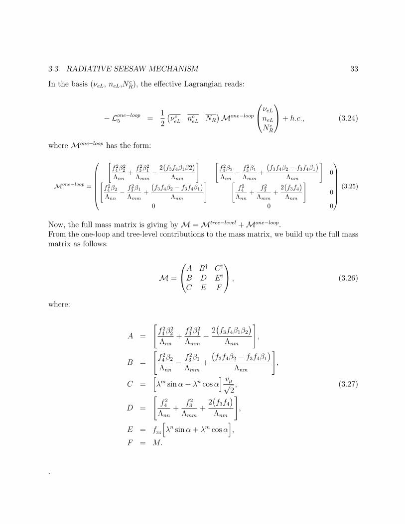
In the basis (νeL, neL,N cR), the effective Lagrangian reads:
− Lone−loop5 =1
2
(νceL nceL NR
)Mone−loop
νeLneLN cR
+ h.c., (3.24)
where Mone−loop has the form:
Mone−loop =
[f24β
22
Λnn+f23β
21
Λmm− 2
(f3f4β1β2
)
Λnm
] [f24β2Λnn
− f23β1Λmm
+
(f3f4β2 − f3f4β1
)
Λnm
]0
[f24β2Λnn
− f23β1Λmm
+
(f3f4β2 − f3f4β1
)
Λnm
] [f24
Λnn+
f23Λmm
+2(f3f4
)
Λnm
]0
0 0 0
(3.25)
Now, the full mass matrix is giving by M =Mtree−level +Mone−loop.From the one-loop and tree-level contributions to the mass matrix, we build up the full massmatrix as follows:
M =
A B† C†
B D E†
C E F
, (3.26)
where:
A =
[f 2
4β22
Λnn
+f 2
3β21
Λmm
− 2(f3f4β1β2
)
Λnm
],
B =
[f 2
4β2
Λnn
− f 23β1
Λmm
+
(f3f4β2 − f3f4β1
)
Λnm
],
C =[λm sinα− λn cosα
] vµ√2, (3.27)
D =
[f 2
4
Λnn
+f 2
3
Λmm
+2(f3f4
)
Λnm
],
E = f34
[λn sinα + λm cosα
],
F = M.
.
34 CHAPTER 3. RADIATIVE NEUTRINO MASS GENERATION
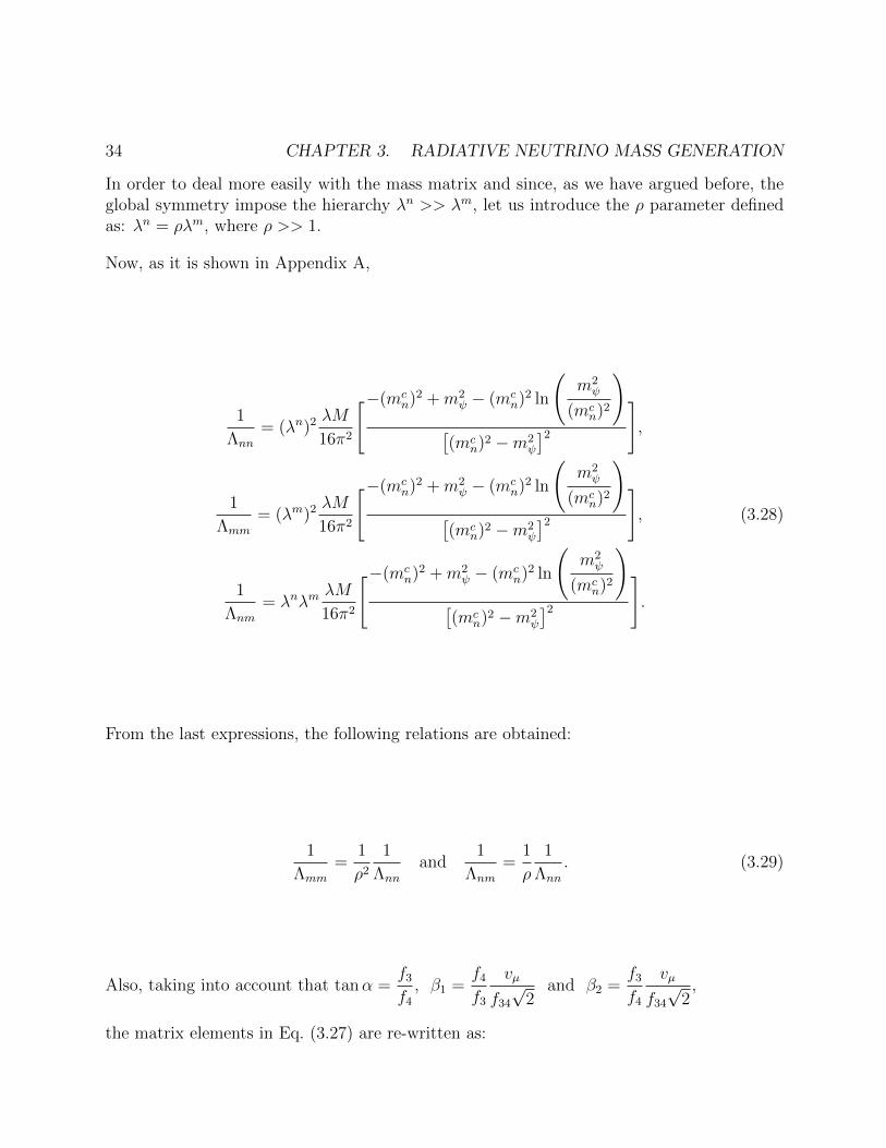
In order to deal more easily with the mass matrix and since, as we have argued before, theglobal symmetry impose the hierarchy λn >> λm, let us introduce the ρ parameter definedas: λn = ρλm, where ρ >> 1.
Now, as it is shown in Appendix A,
1
Λnn
= (λn)2 λM
16π2
[−(mcn)2 +m2
ψ − (mcn)2 ln
(m2ψ
(mcn)2
)
[(mc
n)2 −m2ψ
]2
],
1
Λmm
= (λm)2 λM
16π2
[−(mcn)2 +m2
ψ − (mcn)2 ln
(m2ψ
(mcn)2
)
[(mc
n)2 −m2ψ
]2
], (3.28)
1
Λnm
= λnλmλM
16π2
[−(mcn)2 +m2
ψ − (mcn)2 ln
(m2ψ
(mcn)2
)
[(mc
n)2 −m2ψ
]2
].
From the last expressions, the following relations are obtained:
1
Λmm
=1
ρ2
1
Λnn
and1
Λnm
=1
ρ
1
Λnn
. (3.29)
Also, taking into account that tanα =f3
f4
, β1 =f4
f3
vµ
f34
√2
and β2 =f3
f4
vµ
f34
√2,
the matrix elements in Eq. (3.27) are re-written as:
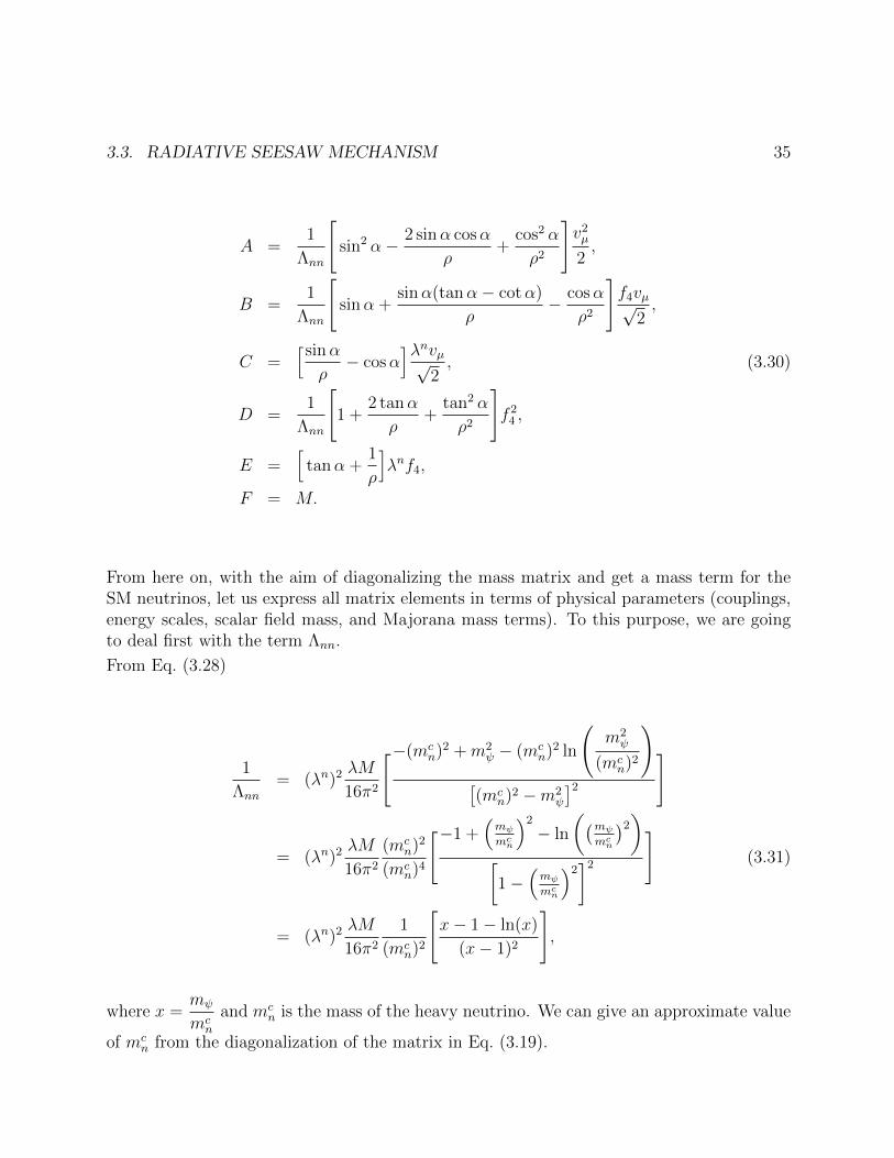
3.3. RADIATIVE SEESAW MECHANISM 35
A =1
Λnn
[sin2 α− 2 sinα cosα
ρ+
cos2 α
ρ2
]v2µ
2,
B =1
Λnn
[sinα +
sinα(tanα− cotα)
ρ− cosα
ρ2
]f4vµ√
2,
C =[sinα
ρ− cosα
]λnvµ√2, (3.30)
D =1
Λnn
[1 +
2 tanα
ρ+
tan2 α
ρ2
]f 2
4 ,
E =[
tanα +1
ρ
]λnf4,
F = M.
From here on, with the aim of diagonalizing the mass matrix and get a mass term for theSM neutrinos, let us express all matrix elements in terms of physical parameters (couplings,energy scales, scalar field mass, and Majorana mass terms). To this purpose, we are goingto deal first with the term Λnn.
From Eq. (3.28)
1
Λnn
= (λn)2 λM
16π2
[−(mcn)2 +m2
ψ − (mcn)2 ln
(m2ψ
(mcn)2
)
[(mc
n)2 −m2ψ
]2
]
= (λn)2 λM
16π2
(mcn)2
(mcn)4
[−1 +(mψmcn
)2
− ln
((mψmcn
)2)
[1−
(mψmcn
)2]2
](3.31)
= (λn)2 λM
16π2
1
(mcn)2
[x− 1− ln(x)
(x− 1)2
],
where x =mψ
mcn
and mcn is the mass of the heavy neutrino. We can give an approximate value
of mcn from the diagonalization of the matrix in Eq. (3.19).
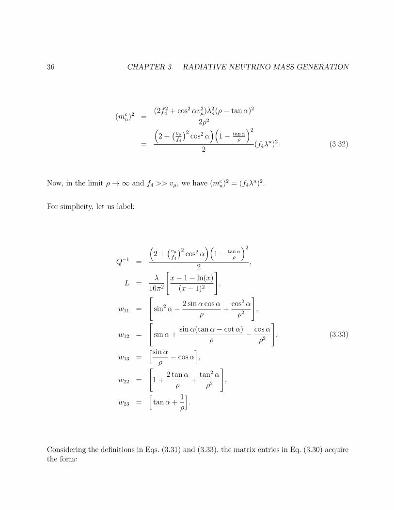
36 CHAPTER 3. RADIATIVE NEUTRINO MASS GENERATION
(mcn)2 =
(2f 24 + cos2 αv2
µ)λ2n(ρ− tanα)2
2ρ2
=
(2 +
(vµf4
)2cos2 α
)(1− tanα
ρ
)2
2(f4λ
n)2. (3.32)
Now, in the limit ρ→∞ and f4 >> vµ, we have (mcn)2 = (f4λ
n)2.
For simplicity, let us label:
Q−1 =
(2 +
(vµf4
)2cos2 α
)(1− tanα
ρ
)2
2,
L =λ
16π2
[x− 1− ln(x)
(x− 1)2
],
w11 =
[sin2 α− 2 sinα cosα
ρ+
cos2 α
ρ2
],
w12 =
[sinα +
sinα(tanα− cotα)
ρ− cosα
ρ2
], (3.33)
w13 =[sinα
ρ− cosα
],
w22 =
[1 +
2 tanα
ρ+
tan2 α
ρ2
],
w23 =[
tanα +1
ρ
].
Considering the definitions in Eqs. (3.31) and (3.33), the matrix entries in Eq. (3.30) acquirethe form:

3.3. RADIATIVE SEESAW MECHANISM 37
A =1
2LQw11M
(vµf4
)2
,
B =1√2LQw12M
(vµf4
),
C =1√2w13
(λnvµ
), (3.34)
D = LQw22M,
E = w23
(λnf4
),
F = M.
and the mass matrix is given by:
M =
1
2LQw11M
(vµf4
)21√2LQw12M
(vµf4
)1√2w13
(λnvµ
)
1√2LQw12M
(vµf4
)LQw22M w23
(λnf4
)
1√2w13
(λnvµ
)w23
(λnf4
)M
. (3.35)
Extracting f4 and introducing the parameters a = vνf4
and b = Mf4
, where the hierarchyimposes that a << 1 , b << 1, we have:
M = f4
1
2LQw11a
2b1√2LQw12ab
1√2w13aλ
n
1√2LQw12ab LQw22b w23λ
n
1√2w13aλ
n w23λn b
, (3.36)
where wij ∼ Q ' 1 for i, j = 1, 2. We perform the calculations of M eigenvalues to thirdorder in perturbation theory. The mass for the lightest neutrino reads:
mνe = LQ(1
2w11 −
w12w13
w23
+1
2
w213w22
w223
)a2bf4. (3.37)
Expanding Eq. (3.37) and keeping only terms O(1/ρ), we reach:
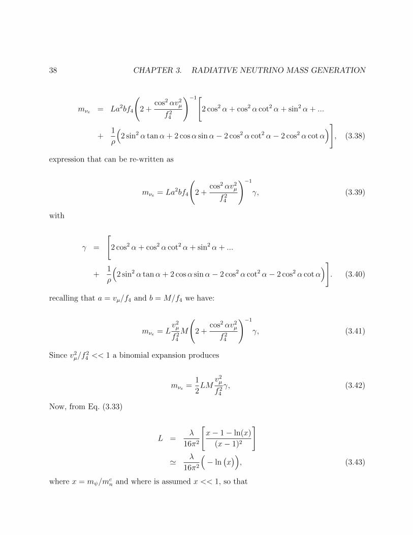
38 CHAPTER 3. RADIATIVE NEUTRINO MASS GENERATION
mνe = La2bf4
(2 +
cos2 αv2µ
f 24
)−1[2 cos2 α + cos2 α cot2 α + sin2 α + ...
+1
ρ
(2 sin2 α tanα + 2 cosα sinα− 2 cos2 α cot2 α− 2 cos2 α cotα
)], (3.38)
expression that can be re-written as
mνe = La2bf4
(2 +
cos2 αv2µ
f 24
)−1
γ, (3.39)
with
γ =
[2 cos2 α + cos2 α cot2 α + sin2 α + ...
+1
ρ
(2 sin2 α tanα + 2 cosα sinα− 2 cos2 α cot2 α− 2 cos2 α cotα
)]. (3.40)
recalling that a = vµ/f4 and b = M/f4 we have:
mνe = Lv2µ
f 24
M
(2 +
cos2 αv2µ
f 24
)−1
γ, (3.41)
Since v2µ/f
24 << 1 a binomial expansion produces
mνe =1
2LM
v2µ
f 24
γ, (3.42)
Now, from Eq. (3.33)
L =λ
16π2
[x− 1− ln(x)
(x− 1)2
]
' λ
16π2
(− ln
(x)), (3.43)
where x = mψ/mcn and where is assumed x << 1, so that

3.3. RADIATIVE SEESAW MECHANISM 39
mνe =λM
32π2ln
(mcn
mψ
)γv2µ
f 24
, (3.44)
Taking back the γ definition given in Eq. (3.40), we finally get
mνe =λM
32π2ln
(mcn
mψ
)[2 cos2 α + cos2 α cot2 α + sin2 α + ...
+1
ρ
(2 sin2 α tanα + 2 cosα sinα− 2 cos2 α cot2 α− 2 cos2 α cotα
)]v2µ
f 24
(3.45)
Let us compare our results with the ones in [41]. Before going on, three remarks must bedone:
• In [41], the VEV of the Higgs-like field is written as 〈h0〉 = (0, v)T , which differs from
our notation where 〈hµ〉 =1√2
(vµ, 0)T .
• Also in [41], the tree-level Lagrangian contains a VEV for the scalar field that is writtenas 〈φ†1〉 = (−〈h†〉, f), being f the scale at which the global symmetry breaks down,while in our case 〈ψ†1〉 = (±〈h†〉, 0, β(1,2)f).
• The coupling λm is absent in [41], which means ρ→∞.
Then, with the goal of doing a direct comparison4, vµ =√
2vDµ and f sin βi ∼ 1 for i = 1, 2,which in our notation means f3/f4 = f3/f34 = f4/f34 ∼ 1. This implies sinα = cosα =tanα = 1.With the clarifications above, the neutrino mass is given by:
mνe =λM
32π2ln
(mcn
mψ
)[1 + 2 + 1
](√2vDµ
)2
f 24
=λM
4π2ln
(mcn
mψ
)vDµ
2
f 24
, (3.46)
that exactly coincides with the result in [41].
4With vDµ we refers to the value vµ used in [41]
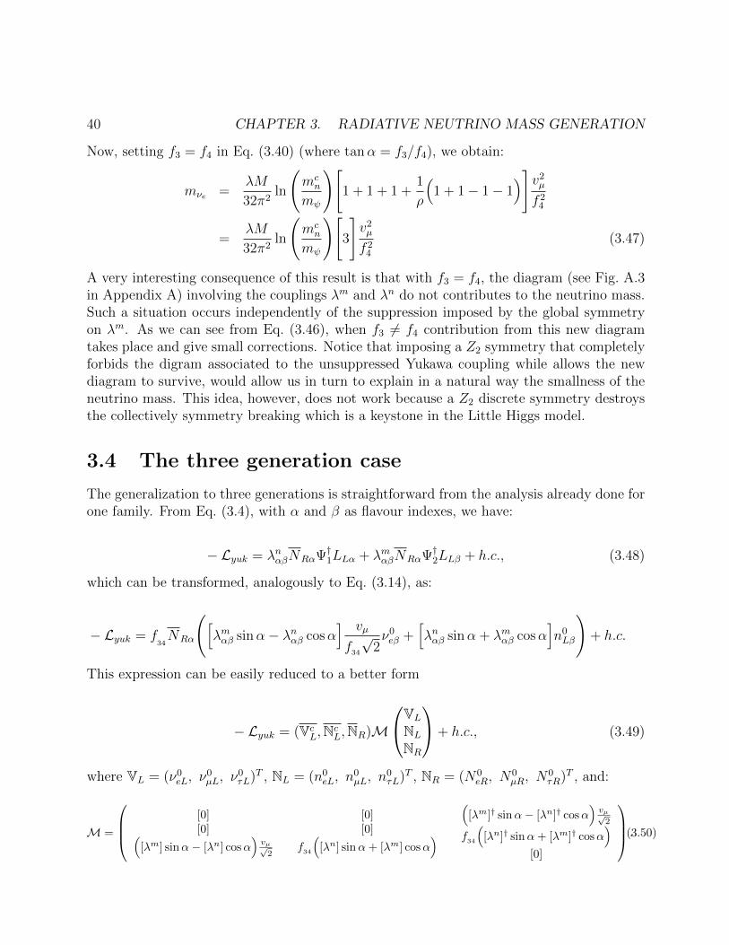
40 CHAPTER 3. RADIATIVE NEUTRINO MASS GENERATION
Now, setting f3 = f4 in Eq. (3.40) (where tanα = f3/f4), we obtain:
mνe =λM
32π2ln
(mcn
mψ
)[1 + 1 + 1 +
1
ρ
(1 + 1− 1− 1
)]v2µ
f 24
=λM
32π2ln
(mcn
mψ
)[3
]v2µ
f 24
(3.47)
A very interesting consequence of this result is that with f3 = f4, the diagram (see Fig. A.3in Appendix A) involving the couplings λm and λn do not contributes to the neutrino mass.Such a situation occurs independently of the suppression imposed by the global symmetryon λm. As we can see from Eq. (3.46), when f3 6= f4 contribution from this new diagramtakes place and give small corrections. Notice that imposing a Z2 symmetry that completelyforbids the digram associated to the unsuppressed Yukawa coupling while allows the newdiagram to survive, would allow us in turn to explain in a natural way the smallness of theneutrino mass. This idea, however, does not work because a Z2 discrete symmetry destroysthe collectively symmetry breaking which is a keystone in the Little Higgs model.
3.4 The three generation case
The generalization to three generations is straightforward from the analysis already done forone family. From Eq. (3.4), with α and β as flavour indexes, we have:
− Lyuk = λnαβNRαΨ†1LLα + λmαβNRαΨ†2LLβ + h.c., (3.48)
which can be transformed, analogously to Eq. (3.14), as:
− Lyuk = f34NRα
([λmαβ sinα− λnαβ cosα
] vµ
f34
√2ν0eβ +
[λnαβ sinα + λmαβ cosα
]n0Lβ
)+ h.c.
This expression can be easily reduced to a better form
− Lyuk = (VcL,Nc
L,NR)M
VL
NL
NR
+ h.c., (3.49)
where VL = (ν0eL, ν
0µL, ν
0τL)T , NL = (n0
eL, n0µL, n
0τL)T , NR = (N0
eR, N0µR, N
0τR)T , and:
M =
[0][0](
[λm] sinα− [λn] cosα)vµ√2
[0][0]
f34
([λn] sinα+ [λm] cosα
)
([λm]† sinα− [λn]† cosα
)vµ√2
f34
([λn]† sinα+ [λm]† cosα
)
[0]
.(3.50)

3.4. THE THREE GENERATION CASE 41
Here [λm] and [λn] are 3 × 3 matrices (where the family indexes have been omitted5), and[0] are also 3 × 3 matrices with all the entries equal to zero.Now, in the study of the one-generation case the parameter ρ = λn/λm 1 makes explicitthe suppression on λm due to the global symmetry. Since in the present case we are dealingwith matrices, we are going to assume that [λm]αβ = [ε]αγ[λ
m]γβ being εαβ << 1. Let us alsoassume that [ε] is diagonal with all the non-zero entries equal, then [ε] = ρ[1], with [1] theidentity matrix.After some simplifications the mass matrix take the form:
M =
[0][0](
[ε sinα− cosα)vµ√
2[λn]
[0][0](
tanα + ε)f4[λn]
(ε sinα− cosα
)vµ√
2[λn]†(
tanα + ε)f4[λm]†
[0]
.(3.51)
Let us now call U the unitary matrix that diagonalizes M
MDiag = U†MU, (3.52)
where
U =
cos θ[1] sin θ[1] [0]− sin θ[1] cos θ[1] [0]
[0] [0] [1]
[1] [0] [0][0] VL [0][0] [0] VR
[1] [0] [0][0] −1√
2[1] 1√
2[1]
[0] 1√2[1] 1√
2[1]
. (3.53)
The mixing angles are given by Eq. (3.16), and can be re-written in terms of the trigonometricexpressions wij in Eq. (3.33) where we have defined ρ = ε−1
sin θ =a√2
w13√w2
23 + (w213)a
2
2
, cos θ =w23√
w223 + (w2
13)a2
2
.
The matrices VL and VR allow to diagonalize [λn].
V†R[λn]VL =
λn1 0 00 λn2 00 0 λn3
. (3.54)
Assuming that the eigenvalues of [λn] are real, Eq. (3.54) yields:
5That is, the matrix entries of [λm] are [λm]αβ

42 CHAPTER 3. RADIATIVE NEUTRINO MASS GENERATION
V†L[λn]†VR =
λn1 0 00 λn2 00 0 λn3
.
After some calculations, the diagonal mass matrix in Eq. (3.52) take the form
MDiag =
[0] [0] [0][0] δ1 [0][0] [0] δ2
, (3.55)
where
δ1 = −(
(ε sinα− cosα)vµ√
2sin θ + (tanα + ε)f4 cos θ
)diag(λn1 , λ
n2 , λ
n3 ).
δ2 =
((ε sinα− cosα)
vµ√2
sin θ + (tanα + ε)f4 cos θ
)diag(λn1 , λ
n2 , λ
n3 ). (3.56)
Finally we have
MDiag =
diag(0, 0, 0)−diag(MN1,MN2,MN3)
diag(MN1,MN2,MN3)
, (3.57)
with
MNi =
√w2
23 + w213
a2
2(f4λ
ni ). (3.58)
At tree-level the UPMNS mixing matrix6 is given by Eq. (3.53). We can also write down the
mass eigenstates (VL, NL, NCR)T as a linear combination of weak eigenstates (VL,NL,NC
R)T :
VL
NL
NCR
=
cos θ[1] sin θ[1] [0]− sin θ[1] cos θ[1] [0]
[0] [0] [1]
[1] [0] [0][0] VL [0][0] [0] VR
[1] [0] [0][0] −1√
2[1] 1√
2[1]
[0] 1√2[1] 1√
2[1]
VL
NL
NCR
=
cos θ[1] −VL√2
sin θ VL√2
sin θ
− sin θ[1] −VL√2
cos θ VL√2
cos θ
[0] 1√2VR
1√2VR
VL
NL
NCR
(3.59)
6Pontecorvo-Maki-Nakagawa-Sakata mixing matrix of the nine neutral leptons
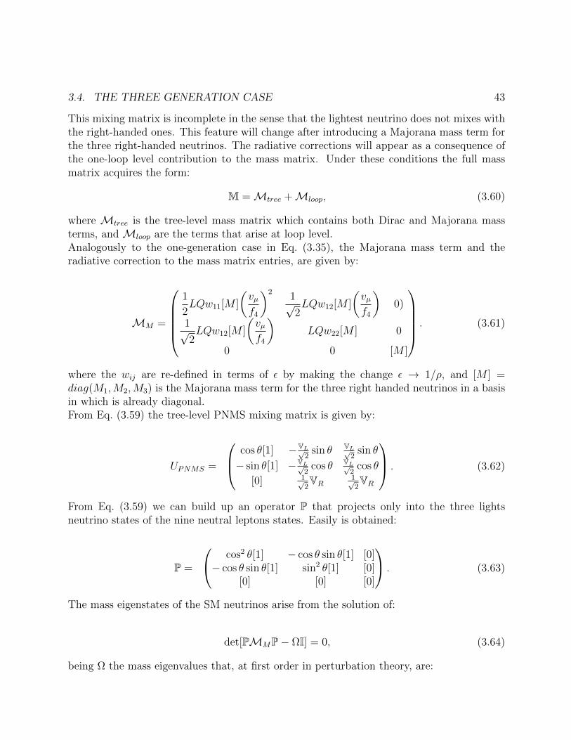
3.4. THE THREE GENERATION CASE 43
This mixing matrix is incomplete in the sense that the lightest neutrino does not mixes withthe right-handed ones. This feature will change after introducing a Majorana mass term forthe three right-handed neutrinos. The radiative corrections will appear as a consequence ofthe one-loop level contribution to the mass matrix. Under these conditions the full massmatrix acquires the form:
M =Mtree +Mloop, (3.60)
where Mtree is the tree-level mass matrix which contains both Dirac and Majorana massterms, and Mloop are the terms that arise at loop level.Analogously to the one-generation case in Eq. (3.35), the Majorana mass term and theradiative correction to the mass matrix entries, are given by:
MM =
1
2LQw11[M ]
(vµf4
)21√2LQw12[M ]
(vµf4
)0)
1√2LQw12[M ]
(vµf4
)LQw22[M ] 0
0 0 [M ]
. (3.61)
where the wij are re-defined in terms of ε by making the change ε → 1/ρ, and [M ] =diag(M1,M2,M3) is the Majorana mass term for the three right handed neutrinos in a basisin which is already diagonal.From Eq. (3.59) the tree-level PNMS mixing matrix is given by:
UPNMS =
cos θ[1] −VL√2
sin θ VL√2
sin θ
− sin θ[1] −VL√2
cos θ VL√2
cos θ
[0] 1√2VR
1√2VR
. (3.62)
From Eq. (3.59) we can build up an operator P that projects only into the three lightsneutrino states of the nine neutral leptons states. Easily is obtained:
P =
cos2 θ[1] − cos θ sin θ[1] [0]− cos θ sin θ[1] sin2 θ[1] [0]
[0] [0] [0]
. (3.63)
The mass eigenstates of the SM neutrinos arise from the solution of:
det[PMMP− ΩI] = 0, (3.64)
being Ω the mass eigenvalues that, at first order in perturbation theory, are:
44 CHAPTER 3. RADIATIVE NEUTRINO MASS GENERATION
Ωk = LQ(1
2w11 −
w12w13
w23
+1
2
w213w22
w223
)a2Mk. (3.65)
This latter expression is exactly the same that was previously found for the one-generationcase.

Conclusions
In this work we have explored a mechanism for neutrino mass generation in a slight variationof the Simplest Little Higgs Model based on the approximate [SU(4)/SU(3)]4 global sym-metry. Since the highest scale of the theory is of the order of 10 TeV, and as the type I-likeseesaw mechanism is not enough for neutrino mass generation, it was explore an alternativethat allows the right-handed neutrino mass be at or below the TeV scale and account forneutrino masses. In this Little Higgs Model we have shown that one loop diagrams involvingtwo scalar 4-plets naturally lead to small Majorana masses for the neutral leptons, includedthe SM neutrinos. We have found that the masses for the lightest neutrinos depend log-arithmically on the Yukawa couplings, leading to unsuppressed Yukawa couplings with atheoretical cut-off of up to 10 TeV. The latter result is similar to the obtained by [41], butis also different in the sense that applies for a SLHM based on a different electroweak gaugesymmetry, and is also more generic for two independent reasons: first, the global symmetrythat protects the Higgs mass is assumed to be approximate in the neutral lepton sector, thenan small (negligible) quadratic divergent contribution to the Higgs mass arises at one loopand, second, as the scalar fields VEV’s are different, the neutrino masses also receive con-tributions from the operator (LcLΨ∗i )(Ψ
†jLL). The analysis done in this thesis yields masses
for the heavy Majorana neutrinos of the order of KeV; the light neutrino mass hierarchy(normal or inverted) is exactly the same for the heavy neutral leptons.An analysis for the three generation case was also done. The results differ slightly fromthe ones in the one-generation case. Further exploration on the neutral lepton mixing arerequired in order to restrict the heavy leptons masses by using the currently known dataon neutrino oscillations. On the other hand, the study of various decay modes of the heavyneutral leptons could lead to restrictions on the mixing between the heavy and light neutrinos.The origin of the Majorana mass for the right-handed neutrinos could be justified after tobuild up the UV completion of the model.High precision experiments as WMAP soon will provide an answer for the number of neutri-nos (active plus sterile) in Nature. Also, with the future International Linear Collider (ILC),the mass hierarchy of the heavy neutral leptons can be revealed. We expect that in the nextcoming years the experiments give us better insights of the nature of neutral leptons.
45

Appendices
46

Appendix A
Neutrino Loop Calculation
LcL
Ψ2
ncR
Ψ1
nRLL
Ψ†1
Ψ†2
Figure A.1: One loop-contribution to(LcLΨ∗2
)(Ψ†2LL
).
From this diagram
i
Λnn
= (−iλ)(iλn)2(−iM)
∫d4k
(2π)4
i
(p− k)2 −m2
i
(p− k)2 −m2
i
(/k)−mnc
i
(−/k)−mnc.(A.1)
The result must be independent of the momentum of the incoming lepton (LL), so we canset this momentum to zero without loss of generality1. The propagator for the Majorananeutrino in momentum space is given by:
Sf =i
/k −mnc
=i(/k +mnc)
k2 −m2nc, (A.2)
1A non-zero momentum only shifts /p but not the neutrino mass
47

48 APPENDIX A. NEUTRINO LOOP CALCULATION
where we have used the field equation in momentum space (/k −mnc)ψ = 02.Making p = 0, Eq. (A.1) becomes:
i
Λnn
= −λ(λn)2M
∫d4k
(2π)4
1
[k2 −m2]21
k2 −m2nc. (A.3)
In order to solve the integral we introduce the Feynman parameters [30]
1
a21a2...an
= n!
∫ 1
0
x1dx1dx2...dxna1x1 + a2x2...anxn
δ(
1−n∑
i=1
xi
), (A.4)
Using this identity the loop integral (A.3) becomes
i
Λnn
= −λ(λn)2M
∫d4k
(2π)42
∫ 1
0
xdxdy[(k2 −m2)x+ (k2 −m2
nc)y]3 δ(1− (x+ y)). (A.5)
After using the δ function we have
i
Λnn
= −2λ(λn)2M
∫d4k
(2π)4
∫ 1
0
xdx[(k2 −m2)x+ (k2 −m2
nc)(1− x)]3
= −2λ(λn)2M
∫d4k
(2π)4
∫ 1
0
xdx[(k2 −m2)x+ k2 −m2
nc − x(k2 −m2nc)]3
= −2λ(λn)2M
∫d4k
(2π)4
∫ 1
0
xdx[k2 − x(m2 −m2
nc)−m2nc
]3 .
Performing now the Wick rotation k0 → ik0e we can transform the integration over a 4D-
Euclidean space3. So, k2 = kµkµ = k02 − −→k 2 = −k0e
2 − −→k 2 = −k2e . Changing dk0 → idk0
e
and k2 → −k2e the loop integral acquires the form
i
Λnn
= −2iλ(λn)2M
∫d4ke(2π)4
∫ 1
0
xdx[− k2
e − x(m2 −m2nc)−m2
nc
]3
= 2iλ(λn)2M
∫d4ke(2π)4
∫ 1
0
xdx[k2e − x(m2 −m2
nc)−m2nc
]3 . (A.6)
2Here ψ is a Dirac field3A integral defined in a 4D hypersphere
49
Let us now consider the integral:
∫d4k
(2π)4
1
(k2 + c2)3. (A.7)
In general, the volume of a sphere of radius k in D-dimensional Euclidean space is given by
Vd(k) = Cdkd, where Cd = π
d2
Γ( d2
+1), being Γ the gamma function which is defined by
Γz =
∫ ∞
0
e−ttz−1dt. (A.8)
For a 4-dimensional Euclidean space we have:
V =π2k4
2,
dV = 2π2k3dk, (A.9)
dk4 = 2π2k3dk,
Using the previous result, Eq. A.7 yields
∫d4k
(2π)4
1
(k2 + c2)3=
∫ ∞
0
2π2k3dk
(2π)4
1
(k2 + c2)3
=
∫ ∞
0
2dkk3
16π2(k2 + a2)3
=
∫ ∞
0
(2kdk)k2
16π2(k2 + a2)3(A.10)
=
∫ ∞
0
(dk2)k2
16π2(k2 + a2)3.
Using the fact that
∫ ∞
0
tm−1dt
(t+ c2)n=
1
(c2)(n−m)
Γ(m)Γ(n−m)
Γ(n), (A.11)
and setting m = 2 and n = 3, Eq. (A.10) becomes equal to Eq. (A.11). It is now straight-forward the calculation of the 4-dimensional integral
∫d4k
(2π)4
1
(k2 + c2)3=
1
32π2c2. (A.12)

50 APPENDIX A. NEUTRINO LOOP CALCULATION
With this result we can solve the 4-dimensional integral over ke in Eq. (A.6). We get
i
Λnn
=iλ(λn)2M
16π2
∫ 1
0
xdx[x(m2 −m2
nc) +m2nc
] , (A.13)
Let us, for simplicity, label a = m2−m2nc and b = m2
nc , and to make the change of variables,u = ax+ b. After some direct calculations we obtain
i
Λnn
=iλ(λn)2M
16π2a2
[a− bln
(ab
+ 1)]. (A.14)
Finally the loop calculation yields the expression
i
Λnn
=iλ(λn)2M
16π2
[m2 −m2nc −m2
nc ln
(m2
m2nc
)
(m2 −m2nc)
2
]. (A.15)
For the other one-loop diagrams the calculation is similar. The first one is
LcL
Ψ1
ncR
Ψ2
nRLL
Ψ†2
Ψ†1
Figure A.2: One loop-contribution to(LcLΨ∗1
)(Ψ†1LL
).
In this case the loop contribution is given by
i
Λmm
=iλ(λm)2M
16π2
[m2 −m2nc −m2
nc ln
(m2
m2nc
)
(m2 −m2nc)
2
]. (A.16)
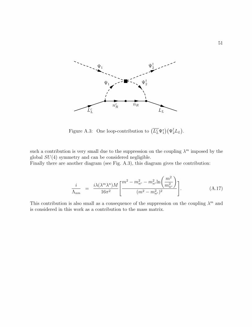
51
LcL
Ψ1
ncR
Ψ1
nRLL
Ψ†2
Ψ†2
Figure A.3: One loop-contribution to(LcLΨ∗1
)(Ψ†2LL
).
such a contribution is very small due to the suppression on the coupling λm imposed by theglobal SU(4) symmetry and can be considered negligible.Finally there are another diagram (see Fig. A.3), this diagram gives the contribution:
i
Λnm
=iλ(λmλn)M
16π2
[m2 −m2nc −m2
nc ln
(m2
m2nc
)
(m2 −m2nc)
2
]. (A.17)
This contribution is also small as a consequence of the suppression on the coupling λm andis considered in this work as a contribution to the mass matrix.
Appendix B
Preprint: Unification of gaugecoupling constants
In this appendix is included a work that is still under construction associated to the unifi-cation of gauge coupling in two gauge extensions of the Standard Model.
52
May 5, 2013 17:16 WSPC/INSTRUCTION FILE paper
International Journal of Modern Physics Ac© World Scientific Publishing Company
GAUGE COUPLINGS UNIFICATION IN THE 3-4-1 AND 4-2-1
EXTENSIONS OF THE STANDARD MODEL
GUILLERMO PALACIO∗ and LUIS A. SANCHEZ†
Escuela de Fısica, Universidad Nacional de Colombia, A.A 3840,
Medellın Colombia∗[email protected]†[email protected]
Received Day Month Year
Revised Day Month Year
We examine the gauge couplings unification of the SU(3)C ⊗ SU(4)L ⊗ U(1)X andSU(4) ⊗ SU(2)L ⊗U(1)X extensions of Standard Model (SM). Based on the Renormal-
ization Group Equations (RGEs), we compared the behaviour of the couplings constants
with the energy scale and is shown in which cases is possible to achieve unificationdepending on the model under consideration.
Keywords: unification; Renormalization Group Equation; electroweak extension; color
extension.
PACS numbers:11.10Hi, 11.10.Gh, 11.15.-q , 11.15.Ex, 11.15.-q, 12.40.-y, 12.60.-i
1. Introduction
The Standard Model (SM) of elementary particles physics remains as the best theory
which, at present, explain almost all physical processes in Nature. Is based on gauge
group GSM = SU(3)C ⊗ SU(2)L ⊗ U(1)Y which breaks down to SU(3)C ⊗ U(1)Qafter the Spontaneous Symmetry Breaking(SSB) take place. Recently, the CMS and
ATLAS collaboration at CERN announced the discovery of a scalar particle1,2 that
seems to be the Higgs boson of the SM with a mass around 126 GeV; addition-
ally new measurements in the ratio of the branching fractions R(D(∗)) = Br(B →D(∗)τ−ντ )/Br(B → D(∗)l−νl)(where l is either e or µ) reported by BaBar collab-
oration3 are in not accordance with SM predictions; giving us a strong clue of new
physics beyond the electroweak scale. From a theoretical point of view there are
also reasons to believe that the SM is not the final theory. Lots of question remains
unanswered such as the electroweak hierarchy problem, neutrino masses, electric
charge quantization, the unification of gauge couplings. Among all the theories that
go beyond the SM one of the best perspectives is the unification idea, where in
principle all the fundamental forces between elementary particles (strong, weak and
electromagnetic) are different manifestations of the same fundamental interaction
involving a single coupling strength4. This idea makes sense when all the gauge
1
May 5, 2013 17:16 WSPC/INSTRUCTION FILE paper
2 Guillermo Palacio and Luis A. Sanchez.
couplings constants meet in a single point at some energy scale.
Since the birth of the SM, SU(5) was proposed as the first attempt to unify all the
fundamental interactions in Nature4. When the SM gauge group GSM is embedded
into SU(5) new interesting phenomenology appear, and the model itself is able to
go further and explain charge quantization, introduces a new symmetry in Nature
at high energies which consist in B-L5 conservation, add news intermediate vector
bosons called lepto-quarks which allow for a quark transforms into a lepton and,
as as a consequence, lead to the proton decay. However SU(5) is rule out because
their theoretical prediction are in not agreements with the experimental data, in
particular the place where all the couplings constants meet is an entire region, and
not a single point. As a requirement for embed the GSM into an Unification Group
GGUT we must guarantee that all the low-energy generators be normalized in the
same way, leading to a well-normalized structure to the hypercharge operator, and
such normalization will depends completely of choice of the GUT groupa.
With the aim of solve the SM puzzles, it has to be extended in different ways,
specifically the quest for unification require the inclusion of additional particle con-
tent that modifies the Callan-Symanzik β-functions leading to the unification of
gauge couplings. Several attempts have been done, such as; a polychromatic exten-
sion 6, the inclusion of vector-like particles7,8 with masses between 1 − 100 TeV ,
and the inclusion of a color sextet scalar at the TeV scale and a lepton triplet9 .
Other theories beyond the SM include the possibility of extending either the elec-
troweak or color sector. Electroweak extensions has been widely study and the
most famous are the models with gauge group SU(3)C ⊗ SU(3)L ⊗ U(1)X10 and
SU(3)C ⊗ SU(4)L ⊗ U(1)X11 known as the 331 and 341 extension, respectively.
The other scenario concerns to the possibility of extend the color group, where
SU(3)C is considered as a low-energy remnant symmetry of a larger group GC . In
Ref. 12 it was shown that in order to reproduce the low-energy phenomenology and
assuming that GC is a simple group which breaks down to SU(3)C by introducing
only one colored Higgs multiple, then the only possible choices are GC = SU(k)
for k = 4, 5. An analysis of the Renormalization Group Equations (RGEs) for the
331 extension was done13 and was shown in which cases there are unification of
gauge coupling constants. Here, by analysing the RGEs, we carry out a study of
the running of gauge coupling constants in: The 341 extension, such extension can
account for the number of generations of fermions when cancellation of anomalies
take places between families and not family by family as in the SM, and to the
SU(4)⊗ SU(2)L ⊗ U(1)X color extension. In this paper we do not pretend to em-
bed the extensions into a GUT group; then for a sake of simplicity, we introduce a
free parameter to define the well-normalize hypercharge generator at the different
scales of energy and explore the possibility of unification at some energy scale.
This letter is organized as follows. In section 2 we review how evolves the couplings
constants at one loop order. In section 3 we introduce the 341 extension, establish
aFor instance, you can review the SU(5) gauge theory in Ref. 5

May 5, 2013 17:16 WSPC/INSTRUCTION FILE paper
Gauge Couplings Unification in the 341 and 421 Extensions of the Standard Model 3
the matching condition and evaluate the unification of gauge couplings for two dif-
ferent models. In section 4 we review the 421 color extension, evaluate the matching
condition and carry out an analysis on the running of couplings constants, finally
our conclusion is outline in section 5.
2. Evolutions of Couplings Constants
The evolution of the running couplings constants at one-loop order is given by the
Renormalization Group Equations (RGEs), and can be written as
1
αi(µ2)=
1
αi(µ1)− bi
2πln
(µ2
µ1
), (1)
with αi ≡ g2i4π and bi the coefficients which depend on the particle content of the
model under consideration. They are the coefficient of the β-function in the Callan-
Symanzik equation14, and are given by15
bi =2
3
∑
f
TRi(f) +1
3
∑
s
TRi(s)−11
3C2i(G). (2)
Here the summations over TRi(f), TRi(s) and C2i(G) are the contribution to the
bi coming from Weyl fermions, scalars and gauge bosons respectively. TRi are the
Dynking indexb and C2(G) is the quadratic Casimir for the adjoint representation.
For fundamental representations of SU(N) we have: TR = 12 and C2(G) = d(R) =
N , being d(R) the dimension of the representation. For the abelian group U(1) is
clear that: C2(G) = 0 and TR =∑Y 2, with Y , the hypercharge generator. Given
the situation of have particle content in the 2nd rank antisymmetry irreducible
representation of SU(N), then TR = (N − 2)/2 and to the 2nd rank symmetry
irreducible representation, TR = (N + 2)/2.
3. SU(3)C ⊗ SU(4)L ⊗ U(1)X extension
The gauge theory based on SU(3)C ⊗ SU(4)L ⊗ U(1)X( hereafter 341) is an elec-
troweak extension which arises as an alternative in the quest for new physics beyond
the SM. This extension has a stronger theoretical motivation based on its ability to
explain the replication of fermions in the Nature when anomaly cancellation take
place between families. Also increase the amount of known fermions, what bring a
new phenomenology still under exploration. By Demanding particle content with-
out exotic electric charge 20, there are in principle few realistic models, the so called
one-family models(three-family model) where the cancellation of anomalies take
place family by family(between families) which are the phenomenological accepted
bThese coefficients are group theory factors, and do not dependent on the spin of particles

May 5, 2013 17:16 WSPC/INSTRUCTION FILE paper
4 Guillermo Palacio and Luis A. Sanchez.
models.
In the 341 extension, the electroweak sector of the SM SU(2)L ⊗ U(1)Y is en-
larged to SU(4)L ⊗ U(1)X17,18, and the following symmetry breaking pattern is
assumed:
3− 4− 1V ′−→ 3− 3− 1
V−→ 3− 2− 1v+v′−→ 3− 1, (3)
where 3-1 refers to the SU(3)C ⊗ U(1)Q symmetry.
The scalar sector responsible for the patter breaking given in Eq. (3) is expressed
by:
⟨φT1⟩
=⟨(φ01, φ
+1 , φ
′+1 , φ
′01
)⟩= (v, 0, 0, 0) ∼ [1, 4∗, 1/2] ,
⟨φT2⟩
=⟨(φ−2 , φ
02, φ′02 , φ
′−2
)⟩= (0, v′, 0, 0) ∼ [1, 4∗,−1/2] ,
⟨φT3⟩
=⟨(φ−3 , φ
03, φ′03 , φ
′−3
)⟩= (0, 0, V, 0) ∼ [1, 4∗,−1/2] ,
⟨φT4⟩
=⟨(φ04, φ
+4 , φ
′+4 , φ
′04
)⟩= (0, 0, 0, V ′) ∼ [1, 4∗, 1/2] . (4)
Where we impose the hierarchy condition V ∼ V ′ >> v ∼ v′ ' 174 GeV.
3.1. Matching conditions
The charge generator in the 341 extension is written as a linear combination of the
diagonal generators17.
Q = T3L +1√3bT8L +
1√6cT15L +X
341I4, (5)
where TiL = λiL/2, being the λiL the Gell-Mann matrices for SU(4)L normalized
as Tr(λiλj) = 2δij , I4 = Dg(1, 1, 1, 1) is the diagonal 4 × 4 matrix, and b and c are
free parameter to be chosen according to the model under consideration11. Using
the Gell-Mann Nishijima formula Q = T3L+Y , the SM hypercharge can be written
as
Y =1√3bT8L +
1√6cT15L +X341I4. (6)
In order to achieve unification the hypercharges must be well-normalized. Let us
assume that Y = aY and X341
= dX341
, here a and d ensures the well-normalization
of the hypercharges. Finally the hypercharge is written as
aY =1√3bT8L +
1√6cT15L + dX341 , (7)
assuming that all the generator are normalized in the same way, it follows
a2 =b2
3+c2
6+ d2. (8)
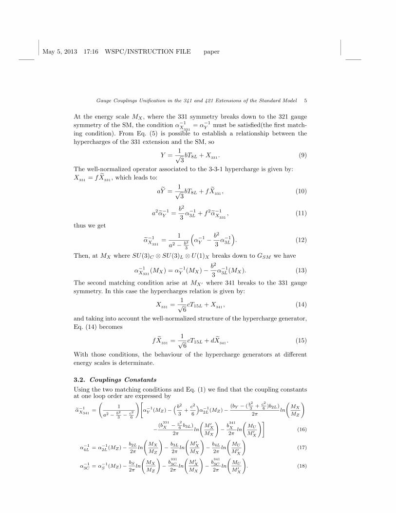
May 5, 2013 17:16 WSPC/INSTRUCTION FILE paper
Gauge Couplings Unification in the 341 and 421 Extensions of the Standard Model 5
At the energy scale MX , where the 331 symmetry breaks down to the 321 gauge
symmetry of the SM, the condition α−1X331= α−1Y must be satisfied(the first match-
ing condition). From Eq. (5) is possible to establish a relationship between the
hypercharges of the 331 extension and the SM, so
Y =1√3bT8L +X331 . (9)
The well-normalized operator associated to the 3-3-1 hypercharge is given by:
X331
= fX331
, which leads to:
aY =1√3bT8L + fX
331, (10)
a2α−1Y =b2
3α−13L + f2α−1X331
, (11)
thus we get
α−1X331
=1
a2 − b2
3
(α−1Y −
b2
3α−13L
). (12)
Then, at MX where SU(3)C ⊗ SU(3)L ⊗ U(1)X breaks down to GSM we have
α−1X331(MX) = α−1Y (MX)− b2
3α−13L (MX). (13)
The second matching condition arise at MX′ where 341 breaks to the 331 gauge
symmetry. In this case the hypercharges relation is given by:
X331
=1√6cT15L +X
341, (14)
and taking into account the well-normalized structure of the hypercharge generator,
Eq. (14) becomes
fX331
=1√6cT15L + dX
341. (15)
With those conditions, the behaviour of the hypercharge generators at different
energy scales is determinate.
3.2. Couplings Constants
Using the two matching conditions and Eq. (1) we find that the coupling constantsat one loop order are expressed by
α−1X341
=
(1
a2 − b2
3− c2
6
)[α−1Y (MZ) −
( b23
+c2
6
)α−12L (MZ) −
(bY − ( b2
3+ c2
6)b2L)
2πln
(MX
MZ
)
−(b
331
X − c2
6b3L)
2πln
(M ′XMX
)− b
341
X
2πln
(MU
M ′X
)](16)
α−14L = α−1
2L (MZ) − b2L
2πln
(MX
MZ
)− b3L
2πln
(M ′XMX
)− b4L
2πln
(MU
M ′X
)(17)
α−13C = α−1
S (MZ) − bS
2πln
(MX
MZ
)− b
331
3C
2πln
(M ′XMX
)− b
341
3C
2πln
(MU
M ′X
). (18)
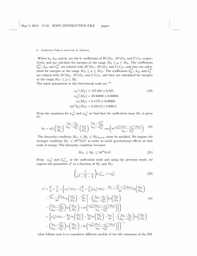
May 5, 2013 17:16 WSPC/INSTRUCTION FILE paper
6 Guillermo Palacio and Luis A. Sanchez.
Where bS , b2L and bY are the bi coefficients of SU(3)C , SU(2)L and U(1)Y respec-
tively, and are calculate for energies at the range MZ ≤ µ ≤ MX . The coefficients
b331
3C , b3L and b331
X are related with SU(3)C , SU(3)L and U(1)X , and they are calcu-
lated for energies at the range MX ≤ µ ≤ MX′ . The coefficients b341
3C , b4L and b341
X
are related with SU(3)C , SU(4)L and U(1)X , and they are calculated for energies
at the range MX′ ≤ µ ≤MU .
The input parameters at the electroweak scale are 19
α−1Y (MZ) = 127.934± 0.027, (19)
α−12L (MZ) = 29.56938± 0.00068,
αs(MZ) = 0.1172± 0.00068,
sin2 θw(MZ) = 0.23113± 0.00015.
From the equations for α−13C and α−14L we find that the unification mass MU is givenby:
MU = M ′X
(MX
MZ
)− b2L − bS
b4L − b341
3C
(M ′XMX
)− b3L − b331
3C
b4L − b341
3C exp
(2πα−12L (MZ) − α−1
S (MZ)
b4L − b341
3C
)(20)
The hierarchy condition MX′ ≤MU ≤MPlanck, must be satisfied. We impose the
stronger condition MU ≤ 1018GeV in order to avoid gravitational effects at that
scale of energy. The hierarchy condition becomes
MX′ ≤MU ≤ 1018GeV. (21)
From α−14L and α−1X341at the unification scale and using the previous result, we
express the parameter a2 as a function of Mx and Mx′
(1
a2 − b2
3 − c2
6
)α−1X341
= α−14L , (22)
a2 =b2
3+c2
6+
α−1Y (MZ) −
( b23
+c2
6
)α−12L (MZ) −
(bY − ( b2
3+ c2
6)b2L)
2πln
(MX
MZ
)
−b331
X − c2
6b3L
2πln
(M ′XMX
)− b
341
X
2π
[−(b2L − bS
b4L − b341
3C
)ln
(MX
MZ
)(23)
−(b3L − b
331
3C
b4L − b341
3C
)ln
(MX′
MX
)+ 2π
(α−12L (MZ) − α−1
S (MZ)
b4L − b341
3C
)]
×α−12L (MZ) − b2L
2πln
(MX
MZ
)− b3L
2πln
(M ′XMX
)− b4L
2π
[−(b2L − bS
b4L − b341
3C
)ln
(MX
MZ
)
−(b3L − b
331
3C
b4L − b341
3C
)ln
(MX′
MX
)+ 2π
(α−12L (MZ) − α−1
S (MZ)
b4L − b341
3C
)]−1
what follows now is to considerer different models of the 341 extension of the SM.

May 5, 2013 17:16 WSPC/INSTRUCTION FILE paper
Gauge Couplings Unification in the 341 and 421 Extensions of the Standard Model 7
3.3. Application I: One-Family model
Here we considerer the Model D11 in which the cancellation of chiral anomalies take
place family by family. By demanding models without exotic electric charge there
are few possibilities of values that can be taken by b and c in the electric charge
operator given in Eq. (5). In particular by fixing b = 1 and c = 1 a set of models is
reach, among them, the so-called model D.
Its fermion content is
ψ1L = (e−, ν0e , N0, N ′0)TL ∼ (1, 4∗,−1/4),
ψ2L = (E−0 , N01 , N
02 , N
03 )TL ∼ (1, 4∗,−1/4),
ψ3L = (N04 , E
+1 , e
+, E+2 )TL ∼ (1, 4∗, 3/4),
QL = (u, d,D,D′)TL ∼ (3, 4,−1/12),
ucL ∼ (3∗, 1,−2/3), dcL ∼ (3∗, 1, 1/3), DcL ∼ (3∗, 1, 1/3),
D′cL ∼ (3∗, 1, 1/3), E−2L ∼ (1, 1,−1)
(24)
there are other two generations which are copies of the first one.
Due to the patter breaking, before obtain the particle content of the SM, first we
must considerer as intermediate step the 331 extension. From Eq. (14) is possible
by making a hypercharge analysis, identify which model is reach in the SU(3)C ⊗SU(3)L⊗U(1)X extension when the Model D of SU(3)C ⊗SU(4)L⊗U(1)X breaks
down to it. Such model called as Model A21 and is also an one-family model, with
the next fermion content.
ψ1L = (e−, ν0e , N0)TL ∼ (1, 3∗,−1/3),
ψ2L = (E−0 , N01 , N
02 )TL ∼ (1, 3∗,−1/3),
ψ3L = (N04 , E
+1 , e
+)TL ∼ (1, 3∗, 2/3),
QL = (u, d,D)TL ∼ (3, 3, 0),
ucL ∼ (3∗, 1,−2/3), dcL ∼ (3∗, 1, 1/3), DcL ∼ (3∗, 1, 1/3)
(25)
By using the expression to calculate the coefficients bi giving in Eq. (2) , and taking
into consideration the quantum number assigned for each representation in this
model, at energies below of MX the coefficients take the next form:
bY =20
9Ng +
1
6NH ,
b2L =4
3Ng +
1
6NH −
22
3, (26)
bS =4
3Ng − 11,
where Ng is the number of families, NH the number of scalar doublets in SU(2)L.
Here at low energies, the 341 extension leads to a two Higgs double model, then
May 5, 2013 17:16 WSPC/INSTRUCTION FILE paper
8 Guillermo Palacio and Luis A. Sanchez.
NH = 2.
For energies in the range MX ≤ µ ≤MX′ the bi’s coefficient are giving by:
b331
X =8
3Ng +
2
3,
b3L = 2Ng +1
2− 11, (27)
b331
3C = 2Ng − 11.
And finally for energies above the MX′ ,the bi’s are expressed by:
b341
X =62
18Ng +
4
3,
b4L = 2Ng −42
3, (28)
b341
3C =8
3Ng − 11.
Then for the spectrum showed in Eq. (24) we obtain for energies above MX′
(b341
X , b4L, b341
3C
)=(70
6,−8,−4
)(29)
Here b4L < b341
3C and as a consequence, α4L and α3C diverges leading a scenario where
unification of gauge couplings in not accomplish. To solve this threat, we extend the
scalar extension of the model, in an analogous way to the procedure carried out in
Ref. 22, where, by the introduction of an additional scalar field transforming as a 2nd
symmetry representation of SU(4), can explain the smallness of neutrino particle.
Here we considerer a set of m decuplets ∆ ∼ (1, 10, z), being z its hypercharge.
By choosing z = 0, then this new scalar couples only to right-handed neutrinos
NR ∼ (1, 1, 0), which can be added into the model without loss of generality c. The
scalar ∆ modifies the b4L coefficient:
δb4L = 1. (30)
In order to make b4L a little bigger than b341
3C we considerer a set of m = 5. that is, 5
scalar ∆ ∼ (1, 10, 0) are include into the model. The new values of the bi coefficients
are:(b341
X , b4L, b341
3C
)=(70
6,−3,−4
). (31)
For energies in the range MX ≤ µ ≤MX′ where the particle content is the spectrum
showed in Eq. (25) we have:
(b331
X , b3L, b331
3C
)=(26
3,−9
2,−5
)(32)
and(bY , b2L, bS
)=(22
3,−3,−7
). (33)

May 5, 2013 17:16 WSPC/INSTRUCTION FILE paper
Gauge Couplings Unification in the 341 and 421 Extensions of the Standard Model 9
MG
UT
0
1e+17
2e+17
3e+17
4e+17
5e+17
MX' (GeV)0 1e+17 2e+17 3e+17 4e+17 5e+17
Fig. 1. Unification mass as a function of MX
′ .
for energies below MX .
Using the hierarchy condition we plot the allowed interval for MX′ . In Fig. 1,
the solid line represent MU as a function of MX′ and the dashed line represents
the functions MU = MX′ . From this plot we fixed MX′ = 2× 10¹⁷ GeV, which is a
value that match with the hierarchy.
For sake of simplicity, we fixed the scale MX = 1.5×10¹⁶, and obtain an Unification
mass MU ∼ 2.7× 10¹⁷ GeV, at that energy scale the couplings are going to met, as
we are going to show below. The normalization parameter satisfies a2 ≥ 0.5, leading
the next restriction MX′ ≥ 1.1×10¹² GeV and as a consequence the previous choice
for MX′ match perfectly. We found that a2 = 1.83135.
After fixing the free parameter, we evaluate the running couplings constants in
Fig. 2, and as is pointed out above, the unification scale appears at MU ∼ 2.7×10¹⁷
GeV.
cThe right-handed neutrinos do not affect the bi coefficients

May 5, 2013 17:16 WSPC/INSTRUCTION FILE paper
10 Guillermo Palacio and Luis A. Sanchez.
α U-1
20
40
60
80
τ100 10,000 1e+06 1e+08 1e+10 1e+12 1e+14 1e+16 1e+18
F1
F2
F3
F4
F5
F6
F7
F8
F10
Fig. 2. Runnnig of gauge couplings constants .
3.4. Application II: Three-Family model
Let us now considerer a model in which the cancellation of anomalies take place
between families. In Ref. 11, by choosing b = 1 and c = 1 we find two three-family
structures, among them the so called model A with the next spectrum
QiL = (u, d,D,D′)TL ∼ (3, 4,−1/12), uciL ∼ (3∗, 1,−2/3),
dciL ∼ (3∗, 1, 1/3), DciL ∼ (3∗, 1, 1/3), D′ciL ∼ (3∗, 1, 1/3),
Q3L = (d, u, U, U ′)TL ∼ (3, 4∗, 5/12), uc3L ∼ (3∗, 1,−2/3),
dc3L ∼ (3∗, 1, 1/3), U c3L ∼ (3∗, 1,−2/3), U ′c3L ∼ (3∗, 1,−2/3),
ψαL = (e−, ν0e , N0, N ′0)TL ∼ (1, 4∗,−1/4), e+αL ∼ (1, 1, 1).
(34)
In an analogous way to the previous application, in the 331 extension by making a
hypercharge analysis, we identify that model A (in 341 extension) breaks down to
model A in the 331 extension10. Such model is also a three-family model, with the
next fermion content.
May 5, 2013 17:16 WSPC/INSTRUCTION FILE paper
Gauge Couplings Unification in the 341 and 421 Extensions of the Standard Model 11
QiL = (u, d,D)TL ∼ (3, 3, 0), uciL ∼ (3∗, 1,−2/3),
dciL ∼ (3∗, 1, 1/3), DciL ∼ (3∗, 1, 1/3),
Q3L = (d, u, U)TL ∼ (3, 3∗, 1/3), uc3L ∼ (3∗, 1,−2/3),
dc3L ∼ (3∗, 1, 1/3), U c3L ∼ (3∗, 1,−2/3),
ψαL = (e−, ν0e , N0)TL ∼ (1, 3∗,−1/3), e+αL ∼ (1, 1, 1).
(35)
The bi coefficients are calculate by using the expression in Eq. (2) , and taking into
consideration the quantum number assigned for each representation in this model.
At energies below of MX the coefficients take the next form:
bY =20
9Ng +
1
6NH ,
b2L =4
3Ng +
1
6NH −
22
3, (36)
bS =4
3Ng − 11,
where Ng is the number of families, NH the number of scalar doublets in SU(2)L.
Here at low energies, the 341 extension leads to a two Higgs double model, then
NH = 2.
For energies in the range MX ≤ µ ≤ MX′ the bi’s coefficient are (b331
X , b3L, b331
3C ) =
( 263 ,−45/6,−5), Finally for energies above the MX′ ,the bi’s are (b
341
X , b4L, b341
3C ) =
( 343 ,−2,−3) where we also extended the scalar sector of the 341, by adding a set of
8 decuplets ∆ ∼ (1, 10, 0) previously introduced to the one-family case.
4. SU(4) ⊗ SU(2)L ⊗ U(1)X Extension
It is not clear what lies beyond the SM, many models beyond it had been studied
and among them polychromatic extension. In Ref. 12 was considered the possibility
that the SU(3)c color group is a remnant symmetry of SU(4). Here we assume
that the quarks transform under the fundamental representation of SU(4), and the
anomalies cancel in each family as in the SM.
It was realize in Ref. 23 that a Higgs field transforming under the irrep(irreducible
representation) [N(N + 1)/2]S of SU(N) can break SU(N) down to SU(N − 1),
while the antisymmetry irrep [N(N−1)/2]A can breaks SU(N) down to SU(N−2)⊗SU(2). In order to obtain a phenomenologically consistent extension, and assuming
that GC is a simple group; then the simplest realizations are SU(4) and SU(5). For
sake of simplicity here we are considering the extension where GC = SU(4).

May 5, 2013 17:16 WSPC/INSTRUCTION FILE paper
12 Guillermo Palacio and Luis A. Sanchez.
The breaking of the gauge group goes in two stages:
SU(4)⊗ SU(2)L ⊗ U(1)Y ′χ−→ SU(3)C ⊗ SU(2)L ⊗ U(1)Yφ−→ SU(3)C ⊗ U(1)Q (37)
Being χ and φ a Higgs multiplet and the Higgs doublet of the SM transforming as
(10, 1, 1/2) and (1, 2, 1/2) respectively.
4.1. Matching Condition
The electric charge generator is defined as:
Q = T3L +1√6aT15C +
Y′
2I4, (38)
with Tiα = λi/2 (where α stands for L and C), being the λi the generalized Gell-
mann matrices normalized as Tr(λiλj) = 2δij , I4 = Dg(1, 1, 1, 1) and a a free
parameter to be chosen.
Let us label for simplicity X = Y′/2, where X is the hypercharge operator. The
SM hypercharge has the form:
Y =1√6aT15C +X, (39)
assuming the well-normalized hypercharge operator Y = bY and X = fX, the
previous equation becomes
bY =1√6aT15C + fX, (40)
now, considering that the all generators are normalized in the same way, then is
straightforward obtain the next relations:
b2 = f2 +a2
6, (41)
b2α−1Y = f2α−1X +a2
6α−14C . (42)
From Eq. (42) and taking into account Eq. (41) we find out the form of the well-
normalized hypercharge coupling, which takes the form:
α−1X =1
b2 − a2
6
(b2α−1Y −
a2
6α−14C
). (43)
The matching condition arises at MX , when SU(4) breaks down to SU(3)C we must
warranty
α−1X (MX) = α−1Y (MX)− a2
6α−14C(MX), (44)
May 5, 2013 17:16 WSPC/INSTRUCTION FILE paper
Gauge Couplings Unification in the 341 and 421 Extensions of the Standard Model 13
by using Eq. (1), we propose an expansion for α−1X
α−1X = α−1X (MZ)− bY ′
2πln
(MX
MZ
)− bX
2πln
(MU
MX
). (45)
Now, evaluating µ = MX in Eq. (44) and comparing this result with the condition
in Eq. (45), it follows
α−1X (MZ) = α−1Y (MZ)− a2
6α−14C(MZ). (46)
bY ′ = bY −a2
6b3C .
4.2. Couplings Constants
With those conditions and taking into account Eq. (1), the evaluation of the running
couplings at one loop order are giveng by
α−1X =
(1
b2 − a2
6
)[α−1Y (MZ)−
(a26
)α−13C(MZ)
− (bY − a2
6 b3C)
2πln
(MX
MZ
)− bX
2πln
(MU
MX
)](47)
α−12L = α−12L (MZ)− b2L2π
ln
(MX
MZ
)− b2L
′
2πln
(MU
MX
)(48)
α−14C = α−1S (MZ)− bS2πln
(MX
MZ
)− b4C
2πln
(MU
MX
). (49)
Where bS , b2L and bY are the bi coefficients of SU(3)C , SU(2)L and U(1)Y respec-
tively, and are calculate for energies at the range MZ ≤ µ ≤ MX . The coefficients
b4C , b′2L and bX are related with SU(4), SU(2)L and U(1)X , and they are calculated
for energies at the range MX ≤ µ ≤MU .
From Eq. (48) and Eq. (49) we calculate the unification mass
MU = MX
(MX
MZ
)− b2L − bSb′2L − b4C exp
(2πα−12L (MZ)− α−1S (MZ)
b′2L − b4C
)(50)
May 5, 2013 17:16 WSPC/INSTRUCTION FILE paper
14 Guillermo Palacio and Luis A. Sanchez.
Is possible also to calculate the free parameter b2, by using the previous result and
Eqs (47, 48).
b2 =a2
6+
α−1Y (MZ)− a2
6α−13C(MZ)− (bY − a2
6 bS)
2πln
(MX
MZ
)
− bX2π
[−(b2L − bSb′2L − b4C
)ln
(MX
MZ
)+ 2π
(α−12L (MZ)− α−1S (MZ)
b′2L − b4C
)]
×α−12L (MZ)− b2L
2πln
(MX
MZ
)− b
′2L
2π
[−(b2L − bSb′2L − b4C
)ln
(MX
MZ
)
+ 2π
(α−12L (MZ)− α−1S (MZ)
b′2L − b4C
)]−1
4.3. Application III
Making a = 1/2 in the electric charge operator, the fermion content of the 421
extension is
fL = (νe, e−)L ∼ (1, 2,−1), eR ∼ (1, 1,−2), (51)
QL = (u, d)L ∼ (4, 2, 1/2), uR,∼ (4, 1, 5/4), dR ∼ (4, 1,−3/4).
By using Eq. (2) the bi coefficients are calculate to the different scales of energy as
follows: For energies in the range MX < µ < MU
b4C =4
3Ng −
41
3,
b2L =10
6Ng −
43
6, (52)
bX =10
4Ng +
3
8.
Considering that the number of generations Ng = 3 we find the next values for the bicoefficients (b4C , b
′2L, bX) = (−29/3,−13/6, 63/8). On the other hand, for energies in
the range MZ < µ < MX the particle content correspond to the SM, but the scalar
sector is compose only per one doublet Higgs model, and not per two like in the 341
extension. The values of the bi coefficients are (bS , b2L, bY ) = (−7,−19/6, 41/6).
Using the hierarchy condition we plot the allowed interval for MX . In Fig. 3,
the solid line represent MU as a function of MX and the dashed line represents the
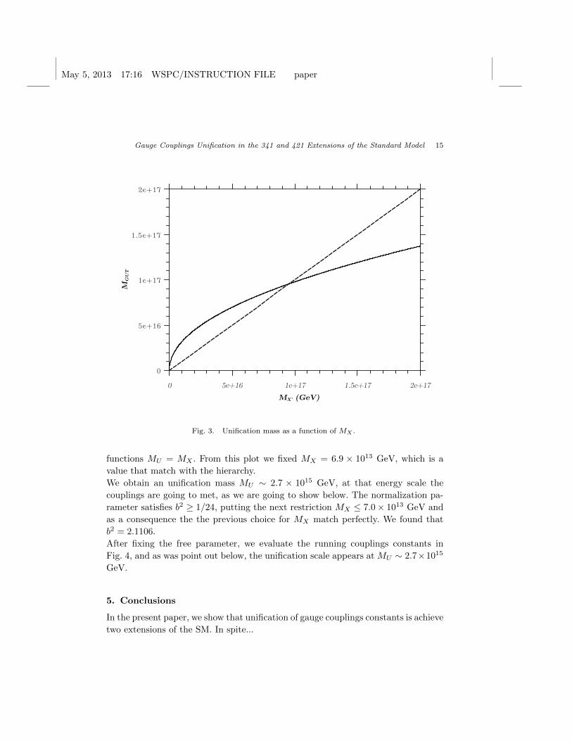
May 5, 2013 17:16 WSPC/INSTRUCTION FILE paper
Gauge Couplings Unification in the 341 and 421 Extensions of the Standard Model 15
MG
UT
0
5e+16
1e+17
1.5e+17
2e+17
MX' (GeV)0 5e+16 1e+17 1.5e+17 2e+17
Fig. 3. Unification mass as a function of MX .
functions MU = MX . From this plot we fixed MX = 6.9 × 10¹³ GeV, which is a
value that match with the hierarchy.
We obtain an unification mass MU ∼ 2.7 × 10¹⁵ GeV, at that energy scale the
couplings are going to met, as we are going to show below. The normalization pa-
rameter satisfies b2 ≥ 1/24, putting the next restriction MX ≤ 7.0× 10¹³ GeV and
as a consequence the the previous choice for MX match perfectly. We found that
b2 = 2.1106.
After fixing the free parameter, we evaluate the running couplings constants in
Fig. 4, and as was point out below, the unification scale appears at MU ∼ 2.7×10¹⁵
GeV.
5. Conclusions
In the present paper, we show that unification of gauge couplings constants is achieve
two extensions of the SM. In spite...
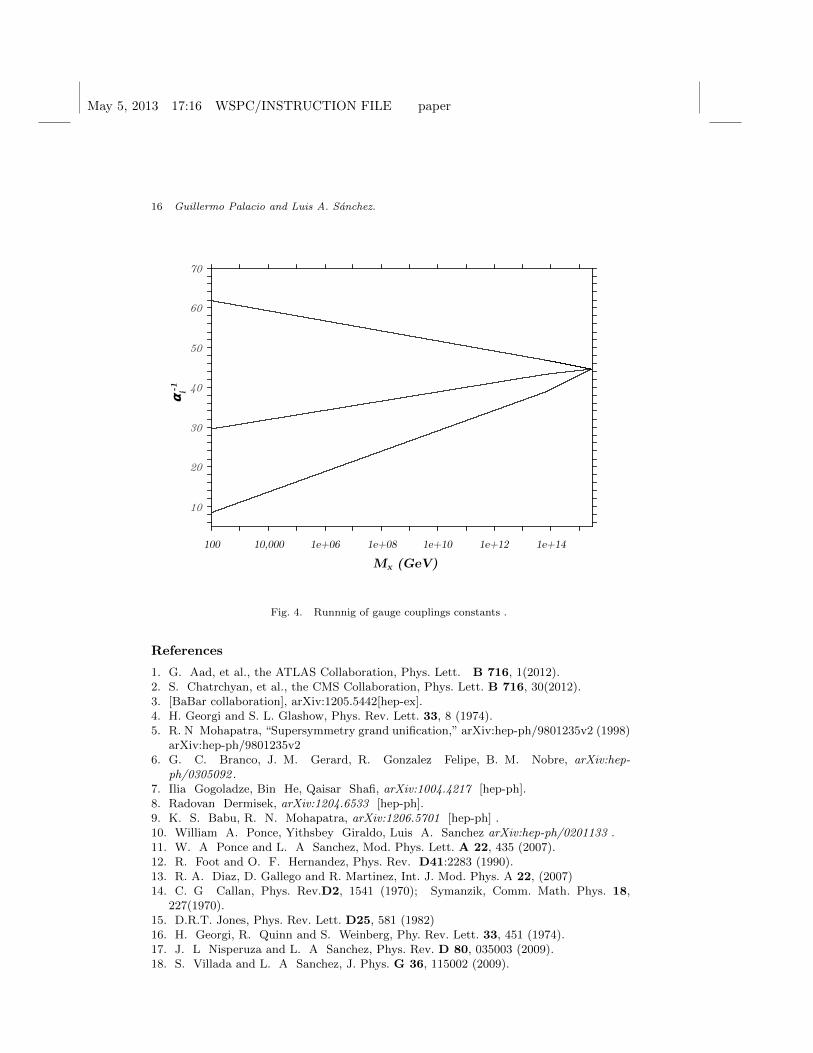
May 5, 2013 17:16 WSPC/INSTRUCTION FILE paper
16 Guillermo Palacio and Luis A. Sanchez.
α i-1
10
20
30
40
50
60
70
Mx (GeV)100 10,000 1e+06 1e+08 1e+10 1e+12 1e+14
F1
F2
F3
F4
F5
F6
F7
Fig. 4. Runnnig of gauge couplings constants .
References
1. G. Aad, et al., the ATLAS Collaboration, Phys. Lett. B 716, 1(2012).2. S. Chatrchyan, et al., the CMS Collaboration, Phys. Lett. B 716, 30(2012).3. [BaBar collaboration], arXiv:1205.5442[hep-ex].4. H. Georgi and S. L. Glashow, Phys. Rev. Lett. 33, 8 (1974).5. R. N Mohapatra, “Supersymmetry grand unification,” arXiv:hep-ph/9801235v2 (1998)
arXiv:hep-ph/9801235v26. G. C. Branco, J. M. Gerard, R. Gonzalez Felipe, B. M. Nobre, arXiv:hep-
ph/0305092 .7. Ilia Gogoladze, Bin He, Qaisar Shafi, arXiv:1004.4217 [hep-ph].8. Radovan Dermisek, arXiv:1204.6533 [hep-ph].9. K. S. Babu, R. N. Mohapatra, arXiv:1206.5701 [hep-ph] .10. William A. Ponce, Yithsbey Giraldo, Luis A. Sanchez arXiv:hep-ph/0201133 .11. W. A Ponce and L. A Sanchez, Mod. Phys. Lett. A 22, 435 (2007).12. R. Foot and O. F. Hernandez, Phys. Rev. D41:2283 (1990).13. R. A. Diaz, D. Gallego and R. Martinez, Int. J. Mod. Phys. A 22, (2007)14. C. G Callan, Phys. Rev.D2, 1541 (1970); Symanzik, Comm. Math. Phys. 18,
227(1970).15. D.R.T. Jones, Phys. Rev. Lett. D25, 581 (1982)16. H. Georgi, R. Quinn and S. Weinberg, Phy. Rev. Lett. 33, 451 (1974).17. J. L Nisperuza and L. A Sanchez, Phys. Rev. D 80, 035003 (2009).18. S. Villada and L. A Sanchez, J. Phys. G 36, 115002 (2009).
May 5, 2013 17:16 WSPC/INSTRUCTION FILE paper
Gauge Couplings Unification in the 341 and 421 Extensions of the Standard Model 17
19. S. Eidelman et, al., “Particle Data Group,” Phys. Lett. B592, 1 (2004).20. William A. Ponce, Diego A. Gutierrez, Luis A. Sanchez, Phys. Rev. D69 055007
(2004).21. L. A. Sanchez, W. A Ponce and R. Martinez, Phys. Rev. D 64, 075013 (2001).22. Robert Foot, Hoang Ngoc Long, Tuan A. Tran, Phys. Rev. D 50:34-38 (1994).23. L. F. Li, Phys. Rev. D 9, 1723 (1974).

Bibliography
[1] R. Barbieri, A. Strumia, The LEP paradox, (2000). [arXiv:hep-ph/0007265].
[2] S. P. Martin, A Supersymmetry primer, (1997). [arXiv:hep-ph/9709356v6 ].
[3] J. Beringer et al.,(Particle Data Group), Phys. Rev. D 86 010001, (2012).
[4] Irene Hidalgo, [arXiv:hep-ph/0505063]
[5] Howard Georgi, Comptes Rendus Physique 8 (2007) 1029-1047.
[6] Oscar A. Macıas, “An anomaly free little higgs model with 3-4-1 gauge symmetry”,MSc thesis, Universidad Nacional de Colombia-Sede Medellın, (2010).
[7] N. Arkani-Hamed, A. G. Cohen and H. Georgi, Phys. Lett. B 513 232 (2001).[arXiv:hep-ph/0105239v4].
[8] L. A. Sanchez, F. A. Perez, William A. Ponce, Eur. Phys. J. C 35, 259 (2004)
[9] R. Davis, Phys. Rev. Lett. 12, 303 (1964).
[10] Y. Fukuda et al., [Kamiokande Collaboration], Phys. Rev. Lett. 77, 1683 (1996).
[11] W. Hampel et al., [GALLEX Collaboration], Phys. Lett. B 447, 127 (1999).
[12] J. N. Abdurashitov et al., [SAGE Collaboration], Phys. Rev. C 60, 055801 (1999).
[13] Y. Fukuda et al., [Super-Kamiokande Collaboration], Phys. Rev. Lett.81, 1158 (1998).
[14] S. Fukuda et al., [Super-Kamiokande Collaboration], Phys. Lett. B539, 179 (2002).
[15] T. Araki et al., [KamLAND Collaboration], Phys. Rev. Lett. 94, 081801 (2005).
[16] M. H. Ahn et al., [K2K Collaboration], Phys. Rev. D 74, 072003 (2006).
[17] P. Adamson et al., [MINOS Collaboration], Phys. Rev. Lett. 107, 181802 (2011).
[18] K. Abe et al., [T2K Collaboration], Phys. Rev. Lett. 107, 041801 (2011).
68
BIBLIOGRAPHY 69
[19] S. Weinberg, Phys. Rev. Lett. 43, 1566 (1979).
[20] R. N. Mohapatra and G. Senjanovic, Phys. Rev. Lett. 44, 912 (1980).
[21] R. N. Mohapatra and G. Senjanovic, Phys. Rev. D 23, 165 (1981).
[22] R. Foot, H. Lew, X-G. He and G. C. Joshi, Z . Phys. C 44, 441 (1989).
[23] E. Ma, Phys. Rev. Lett. 81, 1171 (1998).
[24] F. Bonnet et al., JHEP 07 (2012) 153. arXiv:1204.5862 [hep-ph].
[25] D. Aristizabal Sierra, arXiv:1108.1120 [hep-ph]. (2011)
[26] A. Zee, Phys. Lett.B 93, 389 (1980)
[27] K. S. Babu. Phys. Lett.B 203, 132 (1987)
[28] DAYA-BAY Collaboration, F. An et al., arXiv:1203.1669 [hep-ex]. (2012)
[29] RENO Collaboration, J. Ahn et al., [arXiv:1204.0626 [hep-ex]]. (2012)
[30] Michael E. Peskin, and Dan V. Schroeder “An introduction to quantum field theory”Addison & Wesley (1995).
[31] P. D. B. Collins, A. D. Martin and E. J. Squires, “Particle Physics And Cosmology”,Wiley (1989).
[32] F. Halzen and A. D. Martin, “Quarks And Leptons: An Introductory Course In ModernParticle Physics”, Wiley (1984).
[33] T. P. Cheng and L. F. Li, “Gauge Theory Of Elementary Particle Physics”, Clarendon(1984). (Oxford Science Publications)
[34] R. N. Mohapatra and A. Y. Smirnov, Ann. Rev. Nucl. Part. Sci. 56 (2006) 569,arXiv:hep-ph/0603118.
[35] Xiao-Gang He, Eur. Phys. J. C34 (2004) 371-376 [arXiv:hep-ph/0307172v2]
[36] D. Aristizabal Sierra and D. Restrepo JHEP 0608, 036 (2006) [arXiv:hep-ph/0604012]
[37] K. L. McDonald, B. H. J. McKellar [arXiv:hep-ph/0309270]
[38] Ernest Ma, Phys. Rev. D 73: 077301, (2006). [arXiv:hep-ph/0601225]
[39] T. D. Lee Phys. Rev. D 8 1226, (1973). [arXiv:hep-ph/0307172v2]
[40] M. Schmaltz, JHEP 08 (2004)056. [arXiv:hep-ph/0506063v1] (2005).
70 BIBLIOGRAPHY
[41] F. del. Aguila, M. Masip, J. L. Padilla, “A Little Higgs model of neutrino masses”,[arXiv:hep-ph/0506063v1] (2005).
[42] G. Aad, et al., [ATLAS Collaboration], Phys. Lett. B 716, 1 (2012).
[43] S. Chatrchyan, et al., [CMS Collaboration], Phys. Lett.B 716, 30 (2012).
[44] M. Veltman, Acta. Phys. Pol. B8, (1977) 475.
[45] N. Arkani-Hamed, et al., JHEP 0208, 021 (2002). [arXiv:hep-ph/0206020]
[46] T. Gregoire and J. G. Wacker, JHEP 0208, 019 (2002). [arXiv:hep-ph/0206023]
[47] H. C. Cheng, and I. Low, JHEP 0309, 051 (2003). [arXiv:hep-ph/0308199]
[48] I. Low, W. Skiba and D. Smith, Phys. Rev. D 66, 072001 (2002), [arXiv:hep-ph/0207243].
[49] Gustavo. Burdman, Braz. J. Phys. 37, 506 (2007), [hep-ph/0703194].
[50] L. Vecchi, JHEP 1104: 127, (2011) arXiv:1007.4573 [hep-ph].
[51] M. Schmaltz, [arXiv:hep-ph/0210415].
[52] J. Reuter, M. Tonini [arXiv:1212.5930 [hep-ph]].
[53] D. E. Kaplan and M. Schmaltz, JHEP 0310, 039 (2003), [arXiv:hep-ph/0302049].
[54] W. A. Ponce and L. A. Sanchez, Mod. Phys. Lett. A 22, 435 (2007), [arXiv:hep-ph/0607175]
[55] D. E. Kaplan, M. Schmaltz and W. Skiba Phys. Rev. D7 0 (2004) 075009, [arXiv:hep-ph/0405257v2].
[56] William A. Ponce, Diego A. Gutierrez, and Luis A. Sanchez Phys. Rev. D 69055007,(2004), [arXiv:hep-ph/0312143v3].
[57] R. Barcelo and M. Masip, Phys. Rev.D 78, 095012 (2008), [arXiv:0809.3124 [hep-ph]].
[58] J. Y. Lee, “Neutrinos in the simplest little Higgs model”, [arXiv:hep-ph/0504136],(2005).