neutron capture in low mass asymptotic giant branch stars ... · arxiv:astro-ph/9906266v1 16 jun...
TRANSCRIPT
arX
iv:a
stro
-ph/
9906
266v
1 1
6 Ju
n 19
99
Neutron capture in low mass Asymptotic Giant Branch stars:
cross sections and abundance signatures
Claudio Arlandini1, Franz Kappeler2 and Klaus Wisshak3
Forschungszentrum Karlsruhe, Institut fur Kernphysik, Postfach 3640, D-76021 Karlsruhe,
Germany
Roberto Gallino4
Dipartimento di Fisica Generale, Universita di Torino, I-10125 Torino, Italy
Maria Lugaro5
Department of Mathematics, Monash University, Clayton, Victoria 3168, Australia
Maurizio Busso6
Osservatorio Astronomico di Torino, I-10025 Torino, Italy
and
Oscar Straniero7
Osservatorio Astronomico di Collurania, I-64100 Teramo, Italy
Received ; accepted
1email: [email protected]
2email: [email protected]
3email: [email protected]
4email: [email protected]
5email: [email protected]
6email: [email protected]
7email: [email protected]
– 2 –
ABSTRACT
The recently improved information on the stellar (n, γ) cross sections of
neutron-magic nuclei at N = 82, and in particular of 142Nd, turned out to
represent a sensitive test for models of s-process nucleosynthesis. While these
data were found to be incompatible with the classical approach based on
an exponential distribution of neutron exposures, they provide significantly
better agreement between the solar abundance distribution of s nuclei and the
predictions of models for low mass AGB stars. The origin of this phenomenon
is identified as being due to the high neutron exposures at low neutron density
obtained between thermal pulses when the 13C burns radiatively in a narrow
layer of a few 10−4M⊙. This effect is studied in some detail, and the influence of
the presently available nuclear physics data is discussed with respect to specific
further requests. In this context, particular attention is paid to a consistent
description of s-process branchings in the region of the rare earth elements.
It is shown that - in certain cases - the nuclear data are sufficiently accurate
that the resulting abundance uncertainties can be completely attributed to
stellar modelling. Thus, the s process becomes important for testing the role
of different stellar masses and metallicities as well as for constraining the
assumptions for describing the low neutron density provided by the 13C source.
Subject headings: stars: AGB – stars: evolution – stars: low mass –
nucleosynthesis
– 3 –
1. Introduction
In the last thirty years studies of the slow neutron capture process (s process) have been
pursued either through nucleosynthesis computations in stellar models for the Thermally
Pulsing Asymptotic Giant Branch (TP-AGB) phases of low and intermediate mass stars
(Ulrich 1973; Truran & Iben 1977; Hollowell & Iben 1988; Kappeler et al. 1990; Straniero
et al. 1995; Gallino et al. 1998) or by phenomenological models, mostly by the so-called
classical approach, which were developed with the heuristic intention to provide a possibility
for a ”model-free” description. In this last case, simple analytical expressions are used for
the neutron irradiation and, to first approximation, any time dependence of the physical
parameters is neglected (see e.g. Kappeler, Beer, & Wisshak 1989). For a brief historical
account of s-process analyses see Gallino, Busso, & Lugaro (1997).
For low mass stars, the two descriptions appeared to be compatible within the
respective uncertainties, in particular after the 13C(α, n)16O neutron source was recognized
to play a major role on the AGB (Gallino et al. 1988; Hollowell & Iben 1988). There, the
s process was assumed to occur in convective thermal pulses, the classical analysis was
considered to yield ”effective” conditions characterizing the stellar scenarios (Kappeler et
al. 1990).
This situation changed after it was realized that 13C burns radiatively in the time
interval between two successive convective He-shell instabilities (Straniero et al. 1995).
The interplay of the different thermal conditions for the 13C and 22Ne neutron sources,
both contributing to the nucleosynthesis process, is hardly represented by a single set
of effective parameters like those commonly used by the classical approach. This is
particularly true for the description of the neutron exposure, which is usually simplified by
an exponential distribution. In contrast, present stellar models show that the distribution
of neutron exposures is definitely non-exponential, and actually very difficult to be
– 4 –
described analytically (Arlandini et al. 1995). Any attempt to describe this picture in
a phenomenological way would require to increase the number of free parameters, in
contradiction to the basic reason for such an approach as a model-independent guideline for
stellar calculations.
Despite of the substantial differences between classical approach and the complex
AGB models, the classical analysis is, however, still reproducing the s abundances for the
majority of nuclei between Sr and Bi, simply because two conditions are commonly satisfied
in the mass regions between magic neutron numbers: the respective neutron capture rates
are independent of temperature due to the 1/v-behavior of the (n, γ) cross sections and
are sufficiently large to establish steady flow equilibrium. Consequently, the resulting s
abundances are to good approximation inversely proportional to the Maxwellian averaged
cross sections.
Nevertheless, the differences between classical approach and detailed AGB models
become the more evident the more accurate (n, γ) rates of nuclei involved in s-process
branchings and/or with strong deviations from a 1/v-behavior are becoming available.
A region of the s-process path where this is particularly evident is that involving the
neutron-magic nuclei at N = 82, including the s-only isotope 142Nd. Recent accurate
measurements of the stellar neutron capture cross sections for all stable isotopes in this
area (Wisshak et al. 1998a, 1998b; Voss et al. 1999) revealed a number of significant
discrepancies compared to the older data (see compilations by Bao & Kappeler 1987; Beer,
Voss, & Winters 1992), resulting in a situation where the classical approach implies a large
overproduction of 142Nd for any reasonable parameter set. This problem was already noted
by Guber et al. (1997), but their relatively large cross section uncertainty did not allow any
firm conclusions. At the same time the new data were found to be fully compatible with
the results of the stellar model.
– 5 –
The consequences of this discrepancy will be the subject of the present paper. We
show how the classical model leads to internal inconsistencies, at least near neutron-magic
nuclei, which seem to be the inescapable consequence of this simplifying approach. On
the other hand, stellar models appear increasingly successful in describing the many facets
of the s-abundance patterns, regardless of their much higher complexity. An important
aspect in this discussion will be that average quantities, such as the effective values for the
neutron density and temperature deduced in the classical approach, do not easily relate to
the true features of the stellar scenario. That holds even for the zones of the s-process path
where both models provide a satisfactory reproduction of the solar s abundances. Also
more complex phenomenological models with an increasing number of free parameters lack
a detailed comprehension of the physical conditions at the s-process site.
Finally, we note that the use of the solar s abundances as a constraint for s-process
studies has to be made with caution, since the s process is not a unique event but rather the
result of a complex Galactic evolution mechanism. In particular, the s-process distribution
varies strongly for TP-AGB stars with different metallicity (Busso, Gallino, & Wasserburg
1999; Travaglio et al 1999; Raiteri et al. 1999). Therefore, the comparison with the solar
distribution has to be complemented by direct observations in different types of s-enriched
stars as well by the signatures carried by interstellar grains.
In §2 an overview of the s-process models is presented. In §3 and §4 we discuss the
effect of the new nuclear physics input data on the classical approach and stellar model
calculations, respectively. In §5 the relevance of the uncertainties of some aspects of the
stellar evolution calculations on the s-process nucleosynthesis results are discussed. This is
followed in §6 by an analysis of some relevant branchings of the s-process reaction path.
In §7, we conclude with a presentation of the r-process residuals obtained with the two
approaches and some final remarks in §8.

– 6 –
2. The s-process models
Since the early works (Seeger, Fowler, & Clayton 1965; Clayton & Rassbach 1967;
Clayton & Ward 1974), the process of slow neutron addition in red giants has been
approximated by a phenomenological approach, consisting of an analytical formulation for
the distribution of 〈σ〉i N is products, where N
is is the fractional s abundance of nucleus i and
〈σ〉i = 〈σv〉i /vT is its Maxwellian averaged neutron capture cross section, with vT thermal
velocity. It is known (Clayton 1968) that such a formulation is obtained by adopting a
suitable distribution of neutron exposures ρ(τ), where τ means the time-integrated neutron
flux.
Over the years, this procedure has been particularly successful for the so-called main
s-process component, accounting for s-nuclei between magic neutron numbers N = 50 and
126, i.e. for mass numbers 88 < A < 208. Traditionally, the most common form for ρ(τ)
was an exponential distribution,
ρ(τ) =GN56
⊙
τ0exp(−τ/τ0),
that proved very effective in reproducing the solar system 〈σ〉Ns curve with the fit of only
two parameters: the fraction G of the solar iron abundance that would be required as
a seed, and the mean neutron exposure τ0. The treatment of branchings, as formulated
by Ward, Newman, & Clayton (1976), requires three additional parameters, namely the
temperature, T , the neutron density, nn, and the electron density, ne.
A physical justification for the choice of ρ(τ) seemed to appear when Ulrich (1973)
showed that an exponential distribution of exposures was the natural consequence of
repeated He-shell flashes during the AGB phase. The exponential distribution was shown
to derive simply from the partial overlap of subsequent thermal pulses. With a constant
exposure ∆τ per pulse, and a constant overlap factor r, after N pulses the fraction of

– 7 –
material having experienced an exposure τ = N∆τ is ∼ rN ≡ exp (−τ/τ0), where the the
mean exposure τ0 is defined as τ0 = −∆τ/ ln r.
The pulsed nature of the neutron source was later recognized by the analysis of the
branching at 85Kr (Ward & Newman 1978), and taken into account in more complex
phenomenological approaches (Beer 1991). The classical analysis was found to be a useful
way of describing the s abundances, as it provided an apparently consistent, simple and
straightforward description of the s process, suggesting it to occur in a stellar environment
with physical parameters corresponding to those inferred from this model.
Meanwhile, the knowledge of the last stages of evolution for AGB stars was improved
by a series of investigations originally based on the activation of the 22Ne(α, n)25Mg reaction
in intermediate mass stars (IMS) (e.g. Truran & Iben 1977; Cowan et al. 1980; Busso
et al. 1988), and subsequently emphasizing the importance of the alternative 13C(α,
n)16O reaction in low mass stars (LMS) (Gallino et al. 1988; Hollowell & Iben 1988;
Kappeler et al. 1990). The latter models finally suggested that the main s-process
component results from the interplay of both neutron sources in LMS with masses between
1.5 and 3 M⊙. The present status of this field of research was recently updated on the basis
of revised stellar models, including a self-consistent mixing mechanism for the transport
of freshly synthesized material from the He shell to the stellar surface, the so-called
third dredge-up (TDU) (Straniero et al. 1997). Accordingly, the abundance distributions
considered in the following refer to the composition of the TDU material integrated
over the whole AGB phase and lost by stellar winds. This composition represents the
s-process enrichment of the interstellar medium by the considered model star. This has
to be considered in comparisons with the s-process enhancements observed in chemically
peculiar red giants (Smith & Lambert 1985,1986,1990; Lambert et al. 1995; Busso et al.
1992,1995,1999).
– 8 –
According to the above LMS models, the 13C neutron source is activated under radiative
conditions during the intervals between subsequent He-shell burning episodes. While the
13C reaction provides the bulk of the neutron exposure already at low temperatures (kT
≃ 8 keV) and neutron densities (nn ≤ 107 cm−3), the produced abundances are modified
by the marginal activation of the 22Ne source during the next convective instability, when
high peak neutron densities of nn ≤ 1010 cm−3 are achieved at kT ≃ 23 keV. Though
this second neutron burst represents only a few percent of the total exposure, it suffices
to modify the abundance patterns of several temperature- and neutron-density-dependent
branchings. The time dependence of this second burst is particularly important for defining
the freeze-out conditions for most of these branchings.
Remarkably similar physical conditions are found in AGB models down to a metallicity
slightly lower than 1/2 solar (-0.4 ≤ [Fe/H] ≤ 0) by Gallino et al. (1998). Though
observations in MS and S stars in the solar neighborhood (Smith & Lambert 1990; Busso
et al. 1992) exhibit a spread in the respective s abundances, most Galactic disk AGB stars
in the mass range 1.5 ≤ M/M⊙ ≤ 3 can be considered as suitable sites for reproducing the
main component: while the solar s composition is clearly the product of an average over
Galactic astration processes from various generations of AGB stars with different s-process
efficiencies, according to the initial mass, metallicity, and mass loss mechanism, it is
remarkable that the solar s-abundance distribution lays roughly at the center of the spread
observed in MS and S stars (Busso et al. 1999). The actual neutron capture nucleosynthesis
efficiency in each star depends on the metallicity, the choice of the amount of 13C that is
burnt, and its profile in the intershell region, i.e. on what has become known as the 13C
pocket. In order to model this essential feature, which is controlled by partial proton mixing
below the formal convective envelope border, a detailed hydrodynamical treatment of the
H/He interface is required. Presently available hydrostatic stellar models cannot account
for this phenomenon. Thus, in our computations it is still parameterized in a relatively free

– 9 –
way (see e.g. Gallino et al. 1998; Busso, Gallino, & Wasserburg 1999 for a discussion).
Hence, the AGB nucleosynthesis results presented here, which are shown to account for the
main s-process component, are based on suitable choices for the 13C pocket and metallicity.
They should be considered as the nucleosynthesis pattern of a particular AGB star of the
Galactic disk, whose s-process abundance distribution closely matches the main s-process
component. As said, it is a relatively common occurrence in the Galaxy.
3. The 142Nd cross section and the limits of the classical approach
3.1. New cross sections
The s-process abundance of 142Nd, shielded against a r-process contribution by 142Ce
(Fig. 1), is influenced by two small branchings in the neutron capture path at 141Ce
and 142Pr. Provided the p-process contribution be negligible, the branching probabilities
follow from the comparison of the empirical product 〈σ〉Ns of the stellar neutron capture
cross section and the solar 142Nd abundance with the 〈σ〉Ns systematics in the local mass
region. The expected branching factor is about 5%, so a meaningful analysis was hampered
by the uncertainties in the nuclear physics data, especially by the 9% uncertainty of the
142Nd cross section (Beer et al. 1992). Recently, experimental determinations of the stellar
neutron capture cross sections of 140,142Ce (Kappeler et al. 1996), 141Pr (Voss et al. 1999)
and of all the stable Nd isotopes (Wisshak et al. 1998a, 1998b; Toukan et al. 1995) have
been provided with uncertainties of 1-2% along with new cross section calculations for
the unstable branch point nuclei 141Ce and 142Pr (Kappeler et al. 1996). The significant
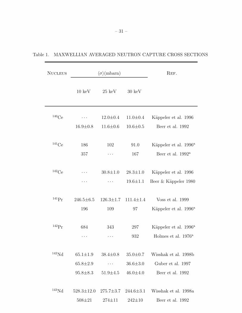
discrepancies with respect to previous data (see Table 1) triggered a detailed s-process
analysis.
EDITOR: PLACE TABLE 1 HERE.

– 10 –
EDITOR: PLACE FIGURE 1 HERE.
The stellar neutron capture cross sections of 142,144Nd were also recently measured by
Guber et al. (1997). While the values agree within the quoted uncertainties at 30 keV, a
serious discrepancy is found for 144Nd at kT ≤ 20 keV. However, this discrepancy had no
effect in the present study. The adopted Ce, Pr, and Nd cross sections were obtained at the
Karlsruhe 3.75 MV Van de Graaff accelerator. The cerium cross sections were measured
with an activation method, while the neodymium and praseodymium experiments were
performed with the Karlsruhe 4π Barium Fluoride (BaF2) detector and the time-of-flight
(TOF) method.
The activation method consists in irradiating a sample in a quasistellar neutron
spectrum, obtained by bombarding a thick metallic Li target with protons of 1912 keV, just
above the reaction threshold. The 7Li(p, n)7Be reaction then yields a continuous energy
distribution with a high energy cutoff at En=106 keV. The resulting neutrons are emitted
in a forward cone of 120◦ opening angle. The angle integrated spectrum closely resembles
a Maxwellian distribution peaked at 25 keV, thus exhibiting almost exactly the shape
required to determine directly the stellar cross section. The samples are placed on the
lithium target, sandwiched between gold foils. The simultaneous activation of the gold foils
serves for normalization, since both the stellar neutron capture cross section of 197Au(n,
γ)198Au (Ratynski & Kappeler 1988) and the decay parameters of 198Au (Auble 1983) are
accurately known. A more detailed description of the method and of the experimental setup
can be found in Beer & Kappeler (1980). After activation, the γ-rays from the decay of the
product nuclei are counted with a high-purity Ge-detector.
As for the TOF experiments, the neutron energies were determined by time of flight,
with the samples being located at a flight path of 79 cm. Adjusting the proton energy
slightly above the reaction threshold a continuous neutron spectrum in the energy range
– 11 –
relevant for the determination of the Maxwellian averaged stellar cross sections, i.e. from
3 to 200 keV, is obtained. Capture events were registered with the Karlsruhe 4π Barium
Fluoride detector via the prompt capture γ-ray cascades. This detector consists of 42
hexagonal and pentagonal crystals forming a spherical shell with 10 cm inner radius and 15
cm thickness. It is characterized by a resolution in γ-ray energy of 7% at 2.5 MeV, a time
resolution of 500 ps, and a peak efficiency of 9% at 1 MeV. A comprehensive description
can be found in Wisshak et al. (1990). Again, the stellar cross sections are calculated using
gold as a standard.
The TOF method represents a universal approach, the only limitation being a minimum
sample mass. On the other hand, the activation technique offers a far superior sensitivity,
since the samples can be placed directly at the neutron production target in a much higher
neutron flux. However, this method can only be applied to cases where the product nucleus
is unstable. Also, the systematic uncertainties are somewhat larger than those typical for
the TOF method.
The cross sections being determined with uncertainties at the 1-2% level, the s-process
abundances are derived with similar accuracy. Therefore, possible p-process contributions
can no longer be neglected. This correction is most important for the s− only nuclei, which
are shielded only against the r-process β-decays. An empirical determination based on the
abundances of local p − only isotopes would suggest a contribution of ∼9% for 142Nd, but
available p-process calculations (Rayet, Prantzos, & Arnould 1990; Prantzos et al. 1990;
Howard, Meyer, & Woosley 1991; Rayet 1991; Howard 1991; Rayet et al. 1995) give lower
values of ∼4%. Such comparably large p-process abundance is plausible, since 142Nd is the
heaviest neutron-magic stable nucleus with N = 82 and is, therefore, favored in a p-process
environment, where the (γ, n) flow is damped at the higher neutron binding energies.
Additionally, 142Nd is enhanced by the decay of its α-unstable p-process progenitors 146Sm,
– 12 –
150Gd, and 154Dy. Another small correction refers to the effect of thermally populated
excited nuclear states. However, such possible enhancements of the (n, γ) cross sections do
not influence the rates used in this discussion.
3.2. The classical approach
142Nd is located immediately at the pronounced precipice of the 〈σ〉Ns curve that is
caused by the small (n, γ) cross sections at N = 82. Hence, its cross section determines
not only the branching analysis, but also the general shape of the s-process distribution,
which is described in the classical approach via the mean exposure, τ0. Since the β-decay
rates of 141Ce and 142Pr are almost independent of the stellar temperature (Takahashi &
Yokoi 1987), these branchings will be completely defined by the effective s-process neutron
density. This parameter can best be determined by means of the s-only pair 148Sm and
150Sm. As the result of three branchings at 147Nd, and 147,148Pm, the first isotope, 148Sm, is
partially bypassed while 150Sm experiences the entire s-process flow. The effective neutron
density is found to be nn = (4.1± 0.6)× 108 cm−3 (Toukan et al. 1995). A more accurate
determination requires an experimental value for the stellar neutron capture cross section
of 147Pm.
Following the concept of Ulrich (1973), classical s-process calculations have been
performed by means of the network code NETZ (Jaag 1990), using a neutron density of
4.1 × 108 cm−3. The adopted thermal energy was kT = 30 keV, according to the analysis
of Wisshak et al. (1995) on the branchings bypassing the s-only isotopes 152,154Gd, which
constrained the s-process temperature to 28 ≤ kT ≤ 33 keV. The electron density ne
= 5.4 × 1026 cm−3 was obtained from a reanalysis of the branching at A = 163 feeding
164Er (Best 1996; Arlandini, Kappeler, & Wisshak 1998). The best fit of the solar
system distribution for the s-nuclei belonging to the main component is obtained for
– 13 –
τ0=(0.296±0.003) [kT/30]1/2 mbarn−1, slightly lower than the previously adopted value of
(0.300±0.009) [kT/30]1/2 mbarn−1 (Kappeler et al. 1990, correctly extrapolating the value
given at kT = 29 keV). Note the significant reduction in the uncertainty of τ0, which is due
the improved cross sections around N = 82. The quality of the fit is evaluated by using
the unbranched s-only nuclei as normalization points, i.e. 100Ru, 110Cd, 116Sn, 122,123,124Te,
150Sm, and 160Dy. The root mean square deviation of their calculated 〈σ〉Ns values from
the respective empirical points is
δ =
1
n
∑
(
〈σ〉N calc − 〈σ〉N emp)2
(〈σ〉N emp)2
1/2
= 6%.
This mean deviation is larger than reported previously (Kappeler et al. 1990), since it
includes 160Dy, whose cross section has been experimentally determined and may well be
influenced by the stellar temperature (Voss et al. 1999). Without 160Dy, this value would
reduce to 4%.
EDITOR: PLACE FIGURE 2 HERE.
Fig. 2 (bottom left panel) shows that the 142Nd is overproduced by ∼12%, despite
the fact that it is partly bypassed by the reaction flow. This overproduction is neither
compatible with the 2% cross section uncertainty at 30 keV, nor with the uncertainty of the
solar abundance, because the abundance ratio between the chemically related rare earth
elements Nd and Sm is known to the 1.8% level (Anders & Grevesse 1989). Furthermore,
the overproduction factor has to be considered as a lower limit, due to the non-negligible
p-process contribution. Accordingly, 142Nd is the first clear evidence that the simple
assumptions of the classical model are not adequate to describe the s process.
Previously, similar difficulties of the classical model were noted already in connection
with the notorious underproduction of 116Sn and the overproduction of the s-only isotope

– 14 –
136Ba (Voss et al. 1994; Wisshak et al. 1996), but in these cases the solar Sn and Ba
abundances were too uncertain to allow for a conclusive argument. Another problem of the
classical approach was related to the overproduction of 86Kr and 87Rb (see e.g. Kappeler
et al. 1990) due to the branching at 85Kr. Even if the contribution from the r process and
from the weak component are neglected, the classical approach yields large overabundances
with respect to the other s nuclei. A possible solution was suggested by the assumption of
a pulsed s process in more complex phenomenological approaches (Ward & Newman 1978;
Beer & Macklin 1989; Beer 1991), constraining the neutron pulse duration to 3 yr ≤ ∆t ≤
20 yr.
3.3. Other phenomenological models
In order to understand if the failure of the classical model may be considered in a more
general way, we analyzed also other parametrized approaches. Seeger, Fowler, & Clayton
(1965), following a suggestion by Clayton et al. (1961), found that the solar s-distribution
can be adequately fitted by a discrete superposition of a limited number (four in their
example) of single neutron exposures. We computed a grid of 50 distributions for single
neutron exposures with ∆τ ranging from 0.03 to 3.50 mbarn−1, assuming a constant neutron
density of 4.1 × 108 cm−3 and varying the irradiation time. The solar distribution of all
s-only isotopes was fitted from Fe to Pb as a weighted sum of four exposures, using a χ2
method. The most promising results fall in two groups, the first consisting of solutions that
are very similar to those obtained with an exponential exposure distribution for the main
component. These cases provide a good overall reproduction of the solar abundances, but
yield strong overproductions of 142Nd and 136Ba. They include also a very small exposure,
which mimics the so-called weak component, representing the s process in massive stars.
This component accounts for most of the s abundances below A = 90. The second group
– 15 –
allowed for an excellent reproduction of all s-only isotopes from Te to Sm, but led to
unavoidable and unacceptable overproductions of more than 10% for all isotopes lighter
than Te or heavier than Sm, including the important normalization points 100Ru and 110Cd.
Therefore, this idea of a superposition of a limited number of single neutron exposures was
found to be no more successful than the classical approach.
A model describing the pulsed burning of two neutron sources with an exponential
distribution of exposures was suggested by Beer (1991) and Beer et al. (1997). Although
the number of free parameters is more than doubled with respect to the classical model, the
fit to the solar main s component is only slightly better, since it does not solve the Sn and
Ba problems, nor is it able to provide consistent constraints on the astrophysical conditions
of the s process.
The same problems are not solved by the model proposed by Goriely (1997), which fits
the solar distribution with a large grid of components, each characterized by a given neutron
irradiation and different constant temperatures and neutron densities. Using an iterative
inversion procedure and without setting any predefined limit to the parameter space, the
solution shows a distribution of exposures that is very close to an exponential law.
4. The new 142Nd cross section: Success for the AGB model
A thorough description of the model and the adopted reaction network can be
found in Gallino et al. (1998). The neutron capture calculations start from evolutionary
computations for low mass stars up to end of the AGB phase, which were made with the
latest version of the FRANEC code (Chieffi & Straniero 1989; Straniero et al. 1997; Chieffi,
Limongi, & Straniero 1998) for a range of initial masses, 1.5 ≤ M⊙ ≤ 3, and metallicities,
-0.4 ≤ [Fe/H] ≤ 0. In addition, the influence of various mass-loss rates was checked as well.
– 16 –
No TDU was found for lower masses. A satisfactory reproduction of the solar distribution
of s isotopes in the range 88 < A < 208 can be obtained for all these stars, since their
physical conditions are quite similar. In this way, the only free parameters of the neutron
capture model, which are the total amount of 13C burnt and its profile in the pocket,
could be constrained. As a general rule it was found that very similar s-process abundance
distributions can be obtained by contemporarily decreasing the metallicity and increasing
the amount of 13C in the pocket by the same factor. The object of this paper is to focus on
the nuclei involved in branchings along the s path, and in particular on the effect of the
142Nd cross section.
EDITOR: PLACE FIGURE 3 HERE.
Following Gallino et al. (1998), we consider the best representation of the main
component obtained for a star of 2 M⊙, Z = 1/2 Z⊙, and a Reimers mass loss rate with η
= 0.75, as a standard case. The general improvement with respect to the classical solution
(Fig. 3) is striking, especially since no fitting procedure was applied. 134,136Ba are now
overproduced by a mere 5%, well compatible with the uncertainties of the neutron capture
cross sections and solar abundances, not requiring any more the large corrections (20%)
to the solar barium advocated by the classical analysis (Voss et al. 1994). Also 116Sn, for
which the classical analysis of Wisshak et al. (1996) suggested a 15% variation to the solar
tin abundance, is now reproduced within the respective uncertainties. In this context, it
is important to note that the meteoritic abundances of Ba and Sn quoted by Anders &
Grevesse (1989) were confirmed by an independent measurement (De Laeter, Rosman, &
Ly 1998). A similar measurement of the Te abundance, which is yet uncertain by 10%
would be important as well.
As already shown by Straniero et al. (1995), the most relevant difference compared
to the classical analysis is actually found in the mass region A < 88. Indeed, all these
– 17 –
nuclei (that are predominantly due to the weak s-component) are produced in much smaller
quantities, even with respect to superseded stellar models, which assumed the convective
burning of 13C. This difference is caused by the very high neutron exposures reached in
the tiny pocket, which favor the production of heavier elements. In particular, at the
s-termination path, 208Pb is produced four times more than in the classical approach.
This has obvious consequences for the branching at 85Kr. The low neutron density of
the 13C neutron release implies that the reaction flow to the neutron-rich nuclei 86Kr and
87Rb is weak, thus avoiding the overproduction of these isotopes that is a severe problem in
the phenomenological approaches and in the old stellar models (Kappeler et al. 1990). In
the present case the contribution from the weaker exposure due to the 22Ne neutron source
is small, because of the small cross section of 85Kr.
The 85Kr branching regulates also the Rb/Sr ratio, which has been measured in AGB
stars showing s-process and carbon enrichments. With the definition [X ] ≡ log10(Xstar) -
log10(X⊙), the average abundance ratio was found to be [Rb/Sr] = -0.80 ± 0.15 (Lambert et
al. 1995, Lambert 1995). Again, the new stellar model calculations are in good agreement
with this stringent constraint.
As for the other significant differences compared to the classical approach, the analysis
of the branchings to 170Yb and 192Pt is hampered by the poor knowledge of the relevant
stellar (n, γ) cross sections, while the branchings to 180Ta (Schumann et al. 1998) and 176Lu
(Doll et al. 1999) remain uncertain because of the complex effect of the stellar temperature
on the population of the respective ground and isomeric states.
In the region around A ∼ 140, two aspects are immediately evident from Fig. 2.
First, the new cross sections improve the situation in the stellar model, from a ∼30%
underproduction of 142Nd to 4%, well compatible with the predicted p-process abundance.
On the other hand, the classical approach is facing the inherent overproduction of 142Nd
– 18 –
discussed in §3.2. The reason for reproducing 142Nd correctly lies in the fact that the cross
section deviates significantly from a 1/v-behavior. Accordingly, the 13C source produces 8%
less 142Nd than the classical approach, which operates at kT = 30 keV. In the subsequent
burst from the 22Ne source relatively high peak neutron densities are reached for about
one year, followed by a rapid freeze-out (Fig. 4, top panel). Due to its rather small cross
section, the abundance of 142Nd itself is depleted by no more than 10% during this phase,
the initial level being rapidly restored during the decline of the neutron density.
EDITOR: PLACE FIGURE 4 HERE.
Secondly, the revised 142Nd and 144Nd cross sections affect the distribution of s
abundances up to A ∼160 by a “propagation effect”. Indeed, during the 13C phase the
neutron exposure is large enough to establish reaction equilibrium, producing an abundance
reservoir at the neutron-magic nuclei. While this equilibrium is practically maintained
during the peak neutron density of the subsequent 22Ne burst, the decline of the neutron
density leads to pronounced freeze-out effects near neutron-magic nuclei. Evidently, the
abundances of the nuclei with the smallest cross sections freeze-out at first, whereas the
isotopes beyond 144Nd are depleted by further neutron captures. This effect causes an
additional abundance difference between 142Nd and 150Sm.
A further increase of this abundance difference results from the fact that the He shell
is enriched in s-process material during the AGB phase due to the overlap of subsequent
He-shell flashes.
The combination of all three effects accounts for the 12% discrepancy in the 142Nd
abundance between the classical approach and the stellar solution.
5. STELLAR EVOLUTION ASPECTS

– 19 –
5.1. Parameters of the stellar models
The presented results are affected by two kinds of uncertainties, those connected with
the neutron capture process itself and those related to the stellar evolutionary calculations.
With respect to the parameters of the stellar model, it was already emphasized that the
amount of primary 13C and its profile in the pocket cannot be obtained through canonical
evolutionary models and have to be, therefore, parameterized. The reasons for the choice of
the adopted profile are described by Gallino et al. (1998).
With the evolution of temperature and density in the 13C pocket provided by
the evolutionary models, the neutron release is determined by the rate of the 13C(α,
n)16O reaction. At low burning temperatures around kT = 8 keV, this rate is rather
uncertain since it is extrapolated from experimental data at higher energies (Denker et al.
1995). Would the rate be substantially lower, part of the 13C nuclei would remain unburned
and engulfed by the successive thermal pulse. In this case, the remaining 13C would be
burnt at higher temperature, substantially affecting the final abundance pattern.
Therefore, test calculations have been performed by reducing the rate of Denker et
al. (1995) by factors of 2 and 10. The results show that also for the extreme case all the
13C would be burnt radiatively due to the progressive increase of temperature and density
in the pocket just prior to the thermal instability. Of course, the time evolution and the
peak value of the neutron density would be different, but these variations would cause no
significant effect on the results.
The rate of the 22Ne(α, n)25Mg reaction exhibits large uncertainties at s-process
temperatures due to the possible existence of a low-lying resonance, which could
substantially enhance the rate (Kappeler et al. 1994). Accordingly, a series of calculations
was performed for the model star, varying the rate from the lower limit, where the possible

– 20 –
contribution of the 633 keV resonance was excluded, to the upper limit, which included this
resonance in toto.
In all calculations, the standard deviation for the set of unbranched normalization
isotopes remains less than 3%, except for the most extreme case. As far as the branchings are
concerned, it has to be stressed that the clear distinction of temperature and neutron density
effects - which is made in the classical approach - makes no sense for the stellar model,
where the time-dependent temperature profile is inherently provided by the evolutionary
code. Accordingly, it depends only on the stellar mass and metallicity and varies with pulse
number. Therefore, an increase in peak temperature implies a corresponding increase in the
peak neutron density, regardless of adopted 22Ne(α, n)25Mg rate.
While the 22Ne(α, n)25Mg rate has no significant impact for the unbranched
normalization isotopes, it governs the abundance patterns in the s-process branchings.
It was found that the branchings represented by the isotope pairs 87Rb/87Sr, 96Zr/96Mo,
134Ba/136Ba, 152Gd/154Gd, and 176Lu/176Hf are most sensitive to the 22Ne(α, n)25Mg rate.
Overall, the 22Ne(α, n)25Mg burst modifies the distribution produced by the first neutron
source, but this remains a ”local” process that does not reach beyond the magic barriers.
Highly non solar patterns were obtained for all isotopes listed above using rates including
more than 50% of the hypothetical 633 keV resonance. These cases yield also unacceptable
values for somewhat less sensitive branchings, like those bypassing 170Yb and 192Pt. As for
142Nd, an increasing 22Ne(α, n)25Mg rate leads to a depletion of this nucleus in the neutron
density maximum, resulting in a progressive decrease of the 142Nd/150Sm ratio.
The best reproduction of the solar branching patterns is obtained with the recommended
rate of Kappeler et al. (1994), after excluding the hypothetical contribution of the 633
kev resonance. Therefore, this rate was considered as a ”standard” choice, although any
value between the lower limit to the recommended value of Kappeler et al. (1994) still
– 21 –
provides satisfactory results. Of course, the intention of this analysis is not to constrain the
22Ne(α, n)25Mg rate, since the fine-tuning is dependent on the model star, but to study the
sensitivity of the results with respect to this uncertain rate.
With the standard choice for the 22Ne(α, n)25Mg rate, the 13C(α, n)16O neutron burst
was investigated by varying the quantity of 13C in the pocket. The best fit to the solar s
abundances was obtained by Gallino et al. (1998) with an average 13C mass fraction of
6 × 10⁻³. A series of test calculations was performed, by keeping the same slope of the
13C pocket as in Gallino et al. (1998) but varying within a factor 1.5 up and down the total
amount of 13C nuclei present in the pocket (and using the standard stellar model for 2 M⊙,
Z = 1/2 Z⊙, η = 0.75), a range that relates to a reasonable representation of the main
component.
As expected, the s-process yields in the investigated range are correlated with
the amount of 13C in the pocket, changing from 40% to 170% compared to the best
representation. Within these limits the s-abundance distribution is fairly well reproduced
over the entire mass range of the main component, except for the extreme cases. Larger
variations than in the present test, however, lead to important deviations. Moreover,
it turned out that the precise reproduction of 134,136Ba abundances constitutes a more
stringent constraint in the above test. Indeed, both nuclei are easily severely overproduced
for low and high values of 13C. Accordingly, this reduces the acceptable 13C values to a range
of ±10% around the best fit case. A similar lower limit is obtained from the significant
overproduction of all isotopes below A ∼ 120.

– 22 –
5.2. Uncertainties due to the evolutionary models
The most crucial points are the mass fractions ∆m dredged up after each thermal
instability and the mass-loss rate. Both problems are somehow related, because the number
of thermal instabilities with TDU is determined by the mass loss rate. According to
Straniero et al. (1997) the TDU ceases when the envelope mass becomes smaller than about
0.5 M⊙. The evolutionary code FRANEC finds TDU for stellar masses above 1.5 M⊙ at
solar metallicity. The efficiency of the phenomenon is still a very debated matter (Frost &
Lattanzio 1996,1998). In the present context, we consider only the uncertainties related to
the FRANEC code.
The determination of ∆m is the most difficult problem for stellar s-process models,
which has a strong impact on Galactic chemical evolution. At present, the concepts for
describing the H-He interface, a very thin zone compared to the mass of the envelope,
exhibit a number of persisting uncertainties. The calculated values for ∆m appear plausible
due to the constraints from stellar observations (Busso, Gallino, & Wasserburg 1999), but
it is certainly difficult to derive the related uncertainties from first principles.
Another problem affecting the final s-process abundance distribution in the envelope
is related to the uncertainty of the choice of the mass loss rate. However, an asymptotic
s-process distribution is reached after a limited number of pulses, so that mass loss
uncertainties affect mainly the total yield of s-processed material, and not much the shape
of the distribution. This last, however, is sensitive to uncertainties in contributions from the
small neutron exposure released by the 22Ne(α, n)25Mg source. Since the maximum bottom
temperature increases from pulse to pulse, affecting the strength of the neutron burst, the
cumulative s-process distribution in the envelope can in fact be influenced by whether the
combined effects of recurrent TDU episodes and mass loss allow the material from the very
last pulses to contribute or not. The TDU efficiency rises rapidly to an almost constant

– 23 –
value until it drops when the envelope mass becomes sufficiently low. The effect of a larger
mass loss rate was, therefore, studied by omitting the three last pulses, which have the
highest temperatures at the bottom of the He burning zone. The resulting effect on the
s-process abundances was negligible. The only noticeable difference of about 8% was found
for 96Zr, which is very sensitive to the neutron density.
5.3. Influence of the initial stellar mass
Though the nucleosynthesis yields of the investigated stars from 1.5 to 3 M⊙ span a
factor of two, the respective abundance distributions are rather similar, an important result
with respect to Galactic evolution. Moderate differences in the s abundances are due to
the higher temperatures reached during the thermal pulses in more massive stars (e.g. in
the 3 M⊙ model). This implies a stronger influence of the 22Ne source, which affects the
contribution of the second burst to the total neutron exposure as well as the abundance
patterns of several branchings.
The effect on the branchings is of the order of 5%, except for 96Zr, which increases by
a factor two, reaching 80% of the average overabundance of the s-only isotopes in the 3
M⊙ star.
6. Relevant branchings in the s-process path
6.1. Nd-Pm-Sm
The abundance of 148Sm is determined by the branchings at 147Nd and 147,148Pm, while
the short lifetimes of 148Nd and 149Pm leave the second s-only samarium isotope, 150Sm,
virtually unbranched. For the involved Nd and Pm branching points, the beta-decay rates

– 24 –
are almost independent of T and ne. Although experimental data for the cross sections of
the unstable Pm isotopes are not yet available, the accurate measurements for Nd (Toukan
et al. 1995) and Sm (Wisshak et al. 1993) isotopes and the accurate solar abundances of
these elements (1.3%, Anders & Grevesse 1989) allow the most constraining determination
of the effective neutron density nn = 4.1 ± 0.6 × 108 cm−3 (Toukan et al. 1995) via the
classical approach. This result is indicated in Fig. 4 (top panel) by the shaded band.
In the stellar model, the mild neutron densities of the 13C source are not sufficient for
the reaction flow to bypass 148Sm, thus producing it abundantly. The opposite situation
prevails, when the neutron density in the second burst reaches up to 1010 cm−3. Then,
148Sm is almost completely bypassed, leading to a strong depletion (Fig. 4, middle panel).
However, during the decline of the neutron density, the branchings to 148Sm are restored.
Eventually, the final value is established during the freeze-out of the abundance pattern.
Thus, in the stellar model this branching depends on the neutron density in a two-fold
way: from the peak neutron density, which causes the initial destruction and explains why
different stellar masses produce small but noticeably different results, and - predominantly
- from the freeze-out of the neutron supply, which determines the final 148Sm/150Sm ratio.
It was pointed out by Cosner, Iben, & Truran (1980) and Kappeler et al. (1982) that
the effective parameters obtained by the classical analysis have to be considered as local
features, which, therefore, could be compared to the freeze-out conditions obtained by the
stellar models. Reasonable agreement was found for the superseded stellar models when
13C was assumed to burn convectively (Kappeler et al. 1990). The most intuitive criterion
for the determination of the freeze-out conditions is to consider the moment in which
the isotopic abundances reach the 90% of their final values. The more complex criterion
proposed by Cosner, Iben, & Truran (1980) was also considered, but with negligible
differences. According to Fig. 4, the neutron density at freeze-out obtained with the present
– 25 –
stellar model is ≈ 1 × 108 cm−3, considerably lower than the phenomenological estimates.
This emphasizes that the effective parameters of the classical approach are certainly not
adequate to describe the dynamical s-process conditions during the AGB phase.
6.2. Sm-Eu-Gd
The abundance of the s-only isotope 152Gd is determined by branchings at 151Sm and
152Eu, while 154Gd is partly bypassed due to a branching at 154Eu. The β-decay rates of
151Sm and 154Eu are extremely sensitive to the temperature, in particular that of 151Sm,
which is enhanced by bound state decays (Takahashi & Yokoi 1987). In both cases, the
effect of the electron density on the stellar decay rates has also to be considered.
Since both the s-only isotopes are partially bypassed, the reaction flow is normalized at
150Sm. This introduces an uncertainty of only 1.3%, since the relative elemental abundances
are well defined in the region of the rare earth elements (Anders & Grevesse 1989). The
main difficulty in determining the effective s-process temperature from these branchings is
due to the rather uncertain p-process contribution to 152Gd. The empirical extrapolation
from neighboring p-only nuclei suggests this contribution to reach ∼30%, whereas the most
recent model calculations yield only a value of ∼12% (Rayet, Prantzos, & Arnould 1990;
Prantzos et al. 1990; Howard, Meyer, & Woosley 1991; Rayet 1991; Howard 1991; Rayet et
al. 1995). Furthermore, a contribution of ∼6% to 152Gd is expected from the s process in
massive stars (Raiteri et al. 1993), even if these calculations need to be updated.
The branchings to 152Gd and 154Gd differ significantly. While ∼90% of the flow is
bypassing 152Gd, which means that fβ is dominated by the β-decay rates rather than by the
neutron capture rates, the branching to 154Gd exhibits the opposite behavior. The neutron
capture cross sections of all stable nuclei have been recently remeasured with considerably

– 26 –
improved accuracy (Wisshak et al. 1993; Wisshak et al. 1995; Jaag et al. 1999). New
calculations have been performed for the branch-point nuclei (Toukan et al. 1995; Jaag
et al. 1999) including an evaluation of the stellar enhancement factors (Jaag et al. 1999).
For the Eu isotopes, these results are found to be significantly different as compared to the
earlier calculations of Holmes et al. (1976) and Harris (1981).
Despite of the remaining uncertainties, the range of possible s-process temperatures
was constrained by the classical analysis, corresponding to thermal energies between kT =
28 and 33 keV (Wisshak et al. 1993).
On the contrary to what happens in the classical scenario, the situation in the stellar
model is rather complex. During the 13C-burning phase, the reaction flow is almost totally
passing through 152Gd, because of the low neutron density and since the lifetime of 151Sm
is strongly reduced already at ∼8 keV. Accordingly, in this phase 154Gd results mainly from
neutron captures on 152Gd and 153Gd, leading to a constant 152Gd/154Gd ratio. Therefore,
it is only during the second neutron burst that the thermometer-like property of these
branchings becomes apparent. Due to the high peak neutron density the reaction flow
essentially bypasses 152Gd, which is almost totally destroyed, and not efficiently restored
during freeze-out so that the final abundance remains relatively small.
154Gd is less depleted during the peak neutron density of the second burst, reaching
about 10% of its abundance prior to the thermal instability (Fig. 4, bottom panel). This
is so because the main reaction flow shifts only from the Gd to the Eu isotopes. During
freeze-out, this shift is reversed, leading to the relatively high value of the final 154Gd
abundance.
– 27 –
6.3. Other branchings
Apart from the two examples discussed in detail, there are a number of other important
branchings along the s-process path, i.e. those to the s-only isotopes 164Er, 176Lu/176Hf,
186Os, and 192Pt. Except for the very complicated case at A = 176, the respective
abundance patterns are well reproduced by the stellar model as can be seen from the regular
overproduction factors of the related s-only nuclei (Fig. 3).
Therefore, it can be concluded, that the very sensitive test via the s-process branchings
has led to another confirmation of the stellar model.
7. r-Residuals
The success of the stellar model in reproducing the s-process pattern of the heavy
elements opens the possibility for decomposing the solar abundance distribution into the
respective s- and r-process components. As far as the p process is concerned, even the
refined s-process analyses based on accurate cross sections are not yet reliable enough to
obtain quantitative estimates for the much smaller p-process yields.
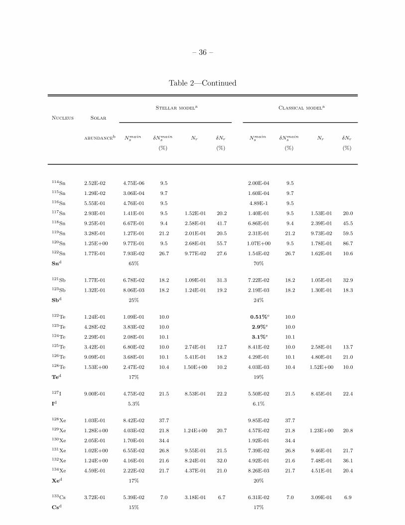
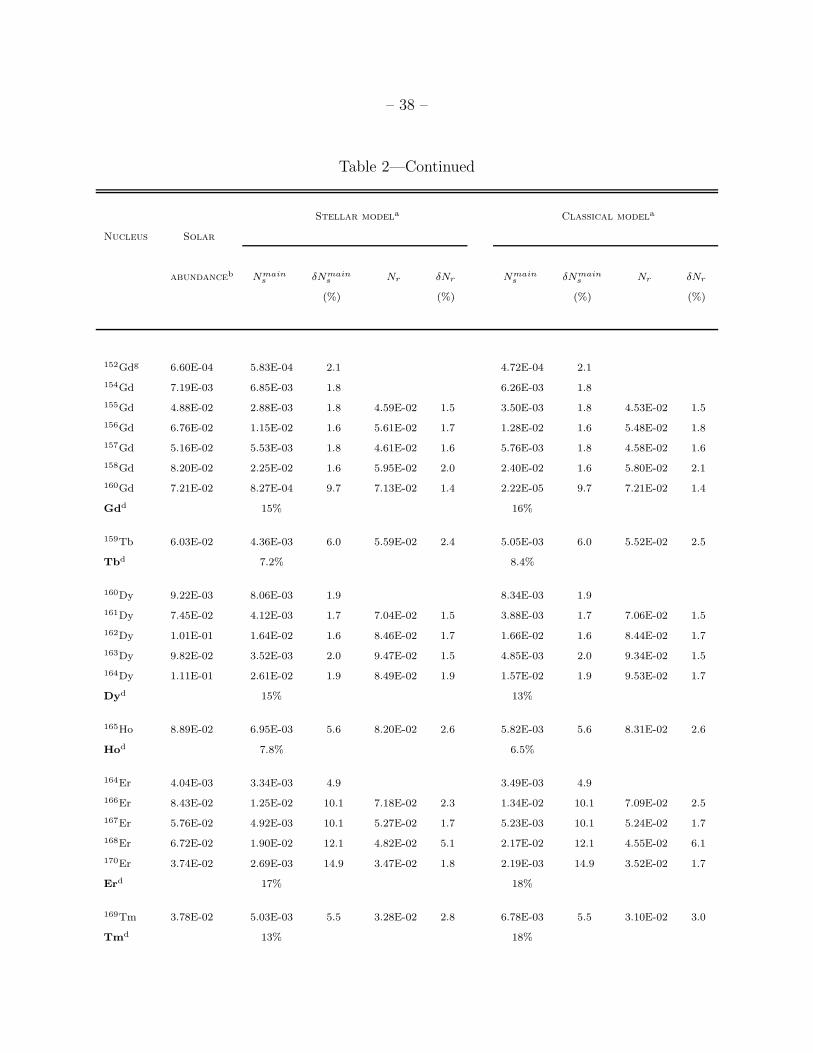
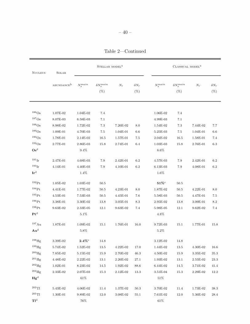
EDITOR: PLACE TABLE 2 HERE.
EDITOR: PLACE FIGURE 5 HERE.
Although the decomposition into s- and r-process components requires a full calculation
for the s abundances integrated over the Galactic evolution, the present stellar model
results appear already to be a reasonable representation of the s-process part (Fig. 3).
Therefore, the residuals Nr = N⊙ - Ns were calculated using the s abundances obtained via
– 28 –
the classical approach and as the arithmetic average of the 1.5 and 3 M⊙ models at Z =
1/2 Z⊙ best reproducing the main component.
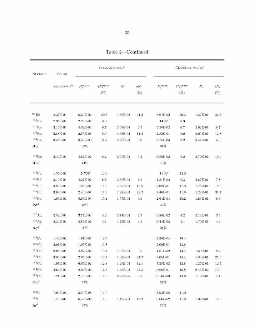
The results are listed in Table 2 for the adopted stellar model (columns 3 to 6) and for
the classical approach (columns 7 to 10). Both calculated s distributions were normalized
using the solar abundance of 150Sm as a reference. Accordingly, the r residuals are expected
to reflect the solar r distribution. The uncertainties δNs and δNr are determined by
the uncertainties of the respective cross sections and solar abundances. Since stellar
spectroscopy often yields elemental abundances the corresponding values are included in
Table 2 for each element by summation over the isotopic data. Relative overabundances in
the calculated distributions with respect to solar are indicated by boldface numbers.
In the mass region of the main component, i.e. between Sr and Tl, the comparison
of both distributions in Fig. 5 shows pretty good agreement. This consistency in the r
residuals is reached since the uncertain abundances of some s-only isotopes are replaced
by the abundances of their r-only isobars. Note, that the r residuals for Pb, and Bi,
are omitted because these isotopes are significantly produced in low metallicity stars (see
Gallino et al. 1998).
In case of the classical model, the r residuals have been complemented below 88Sr
by considering the parameterized weak component of Beer, Walter, & Kappeler (1992).
Though this schematic approach does not relate to any realistic model, it accounts for the
abundances of the respective s-only nuclei and may be useful for comparison with r-process
calculations.
In summary, the r residuals constitute a fairly robust distribution, which can well be
used for comparison with r-process model calculations or astronomical observations.

– 29 –
8. Summary and conclusions
The s abundances for the main component in the mass region 88 < A < 208 were
investigated with updated (n, γ) rates by means of the classical approach and with refined
stellar models for AGB stars in the range between 1.5 and 3 M⊙. Both models were found
to reproduce the ensemble of those s-only isotopes, which are not affected by branchings
in the reaction path, i.e. 100Ru, 110Cd, 116Sn, 122,123,124Te, 150Sm, and 160Dy, with a mean
deviation of a few percent.
However, striking discrepancies between the two models were found for a few isotopes.
The most significant of these refers to 142Nd. The abundance of 142Nd is affected by
branchings in the neutron capture path at 141Ce and 142Pr, which are almost independent
of the s-process temperature and electron density (Takahashi & Yokoi 1987). These
branchings, and consequently the s abundance of 142Nd could be reliably characterized by
means of a complete set of recently reported, accurate (n, γ) cross sections. The significant
revision of the 142Nd cross section eliminated the problem of a persisting underproduction
of this isotope by the stellar models (Gallino et al. 1998). In turn, the new data imply
that the classical model is now producing an inherent overabundance of 142Nd with respect
to the average of the other s-only nuclei, exceeding the respective 1σ-uncertainties by a
factor 6. Similar but less stringent discrepancies were also found earlier for 136Ba (Voss et
al. 1994) and 116Sn (Wisshak et al. 1996). This must be considered as evidence that the
static assumptions for the s-process site, which are implicit for the classical model, are not
realistic. The same argument applies to other phenomenological models.
The stellar models based on recent evolutionary calculations of low mass AGB stars
are found increasingly successful in reproducing the solar distribution of s-nuclei. In the
light of the improved cross sections, these models were found to reproduce the observed s
abundances within the respective cross section and/or abundance uncertainties, despite the

– 30 –
complex scenario and a number of remaining problems. Another example along these lines
are the large abundances in the Kr-Rb-Sr region predicted by the classical approach, which
are incompatible with the additional contributions from the weak component and from the
r process. This problem does not exist in the stellar model, where the s-process production
is much less efficient in this mass region, in full agreement with the low Rb/Sr ratios from
spectroscopic observations (Lambert et al. 1995). This success not only refers to the overall
s distribution but is also confirmed by the proper reproduction of the abundance pattern
of the branchings in the reaction path, which represent a sensitive test for any s-process
model. So far, only a few branchings are determined with sufficient accuracy so that they
can be used to derive sufficiently stringent constraints. Among these are the branchings in
the region of the REE, which all have well defined abundances. In particular, this has been
demonstrated by the branchings characterized by the s-nuclei of neodymium, samarium,
and gadolinium.
In terms of the chemical evolution of the Galaxy the analysis of the s-process yields
from AGB stars of different mass and metallicity (Travaglio et al. 1999; Raiteri et al. 1999)
confirms that the elements heavier than Ba including the large 208Pb abundance - which
required the postulation of a separate strong component in the classical approach (Kappeler,
Beer, & Wisshak 1989) - are naturally produced by AGB stars in the investigated mass
range as anticipated by Gallino et al. (1998). However, a better description of the s
abundances is required in the mass region 88 < A < 130 where the present yields are
somewhat too low. This difference may well be accounted for by the s contributions from
intermediate mass AGB stars (Vaglio et al. 1999; Gallino et al. 1999).
It is a pleasure to thank F.-K. Thielemann and G. J. Wasserburg for stimulating
discussions and suggestions.
This work was partly supported by a grant of italian MURST Cofin 98.
– 31 –
Table 1. MAXWELLIAN AVERAGED NEUTRON CAPTURE CROSS SECTIONS
Nucleus 〈σ〉(mbarn) Ref.
10 keV 25 keV 30 keV
140Ce · · · 12.0±0.4 11.0±0.4 Kappeler et al. 1996
16.9±0.8 11.6±0.6 10.6±0.5 Beer et al. 1992
141Ce 186 102 91.0 Kappeler et al. 1996a
357 · · · 167 Beer et al. 1992a
142Ce · · · 30.8±1.0 28.3±1.0 Kappeler et al. 1996
· · · · · · 19.6±1.1 Beer & Kappeler 1980
141Pr 246.5±6.5 126.3±1.7 111.4±1.4 Voss et al. 1999
196 109 97 Kappeler et al. 1996a
142Pr 684 343 297 Kappeler et al. 1996a
· · · · · · 932 Holmes et al. 1976a
142Nd 65.1±1.9 38.4±0.8 35.0±0.7 Wisshak et al. 1998b
65.8±2.9 · · · 36.6±3.0 Guber et al. 1997
95.8±8.3 51.9±4.5 46.0±4.0 Beer et al. 1992
143Nd 528.3±12.0 275.7±3.7 244.6±3.1 Wisshak et al. 1998a
508±21 274±11 242±10 Beer et al. 1992
– 32 –
Table 1—Continued
Nucleus 〈σ〉(mbarn) Ref.
10 keV 25 keV 30 keV
144Nd 147.0±4.5 88.5±1.7 81.3±1.5 Wisshak et al. 1998b
122.2±5.4 · · · 73.2±6.1 Guber et al. 1997
232±13 123±7 108±6 Beer et al. 1992
aCalculated values

– 33 –
Table 2. S-PROCESS YIELDS AND RESIDUALS FOR THE STELLAR AND THE
CLASSICAL MODEL
Stellar modela Classical modela
Nucleus Solar
abundanceb Nmains
δNmains
Nr δNr Nmains
δNmains
Nr δNr
(%) (%) (%) (%)
63Cu 3.61E+02 2.95E+00 18.6 1.73E+01 18.6
65Cu 1.61E+02 2.04E+00 14.5 9.11E+00 14.5
Cud 1.0% 5.1%
64Zn 6.13E+02 9.21E-01 9.5 4.12E+00 9.5
66Zn 3.52E+02 3.44E+00 9.6 1.42E+01 9.6
67Zn 5.17E+01 7.78E-01 10.7 3.19E+00 10.7
68Zn 2.36E+02 6.78E+00 13.3 2.17E+01 13.3
70Zn 7.80E+00 2.36E-02 50.2 6.57E-3 50.2
Znd 0.9% 3.4%
69Ga 2.27E+01 8.73E-01 11.1 2.85E+00 11.1 6.29E+00c
71Ga 1.51E+01 8.35E-01 9.0 4.25E+00 9.0 0.00E+00c
Gad 4.5% 19%
70Ge 2.44E+01 1.60E+00 11.2 4.37E+00 11.2
72Ge 3.26E+01 2.47E+00 29.7 6.28E+00 29.7 8.12E+00c
73Ge 9.28E+00 4.68E-01 30.8 1.25E+00 30.8 3.66E+00c
74Ge 4.34E+01 2.62E+00 14.7 6.11E+00 14.7 2.50E+01c
76Ge 9.28E+00 5.52E-03 12.6 3.17E-03 12.6 9.28E+00c
Ged 6.0% 15%
75As 6.56E+00 3.02E-01 12.6 5.84E-01 12.6 4.44E+00c
Asd 4.6% 8.9%
76Se 5.60E+00 8.62E-01 8.0 2.21E+00 8.0
77Se 4.70E+00 3.15E-01 30.2 7.27E-01 30.2 2.60E+00c
78Se 1.47E+01 1.57E+00 21.0 3.44E+00 21.0 6.84E+00c
80Se 3.09E+01 2.73E+00 9.4 3.49E+00 9.4 2.41E+01c
82Se 5.70E+00 3.39E-03 50.4 1.82E-03 50.4 5.70E+00c
Sed 8.9% 16%
79Br 5.98E+00 5.22E-01 19.4 9.58E-01 19.4 3.51E+00c
81Br 5.82E+00 5.41E-01 19.4 5.64E-01 19.4 4.36E+00c
Brd 9.0% 14%

– 34 –
Table 2—Continued
Stellar modela Classical modela
Nucleus Solar
abundanceb Nmains
δNmains
Nr δNr Nmains
δNmains
Nr δNr
(%) (%) (%) (%)
80Kr 9.99E-01 1.17E-01 18.9 5.64E-01 18.9
82Kr 5.15E+00 1.91E+00 19.6 3.38E+00 19.6
83Kr 5.16E+00 6.50E-01 19.1 1.12E+00 19.1 3.27E+00c
84Kr 2.57E+01 3.54E+00 21.5 8.21E+00 21.5 1.68E+01c
86Kr 7.84E+00 2.12E+00 18.1 64%e 18.1
Krd 19% 47%
85Rb 5.12E+00 8.36E-01 7.6 2.14E+00 7.6 2.75E+00c
87Rb 2.11E+00 7.46E-01 11.7 66%e 11.7
Rbd 22% 59%
86Sr 2.32E+00 1.09E+00 8.8 1.58E+00 8.8
87Sr 1.51E+00 7.60E-01 8.9 1.12E+00 8.9
88Sr 1.94E+01 1.79E+01 8.1 1.82E+01 8.1 9.06E-01c
Srd 85% 90%
89Y 4.64E+00 4.27E+00 6.6 3.72E-01 100 6.4%e 6.6
Yd 92% 100%
90Zr 5.87E+00 4.24E+00 12.4 1.63E+00 39.7 4.01E+00 12.4 1.86E+00 33.5
91Zr 1.28E+00 1.23E+00 14.8 5.46E-02 100 0.50%e 14.8
92Zr 1.96E+00 1.83E+00 13.7 1.28E-01 100 8.3%e 13.7
94Zr 1.98E+00 8.2%e 7.3 16%e 7.3
96Zr 3.20E-01 1.76E-01 7.3 1.63E-01 7.3
Zrd 83% 82%
93Nb 6.98E-01 5.96E-01 2.4 1.02E-01 16.8 2.0%e 2.4
Nbd 85% 100%
94Mo 2.36E-01 1.53E-03 20.0 8.27E-05 20.0
95Mo 4.06E-01 2.25E-01 6.9 1.81E-01 15.0 2.24E-01 6.9 1.82E-01 14.9
96Mo 4.25E-01 6.1%e 7.1 16%e 7.1
97Mo 2.44E-01 1.43E-01 6.9 1.01E-01 16.4 1.67E-01 6.9 7.72E-02 22.9
98Mo 6.15E-01 4.66E-01 7.5 1.49E-01 32.7 5.52E-01 7.5 6.25E-02 85.3
100Mo 2.46E-01 9.42E-03 21.3 2.37E-01 5.8 0.00E-00 21.3 2.46E-01 5.5
Mod 50% 54%
– 35 –
Table 2—Continued
Stellar modela Classical modela
Nucleus Solar
abundanceb Nmains
δNmains
Nr δNr Nmains
δNmains
Nr δNr
(%) (%) (%) (%)
99Ru 2.36E-01 6.69E-02 50.3 1.69E-01 21.3 6.94E-02 50.3 1.67E-01 22.3
100Ru 2.34E-01 2.23E-01 8.3 11%e 8.3
101Ru 3.16E-01 4.83E-02 6.7 2.68E-01 6.5 5.38E-02 6.7 2.62E-01 6.7
102Ru 5.88E-01 2.53E-01 8.0 3.35E-01 11.3 2.82E-01 8.0 3.06E-01 12.8
104Ru 3.48E-01 9.52E-03 8.2 3.38E-01 5.6 3.75E-03 8.2 3.44E-01 5.5
Rud 32% 37%
103Rh 3.44E-01 4.67E-02 8.2 2.97E-01 9.3 6.50E-02 8.2 2.79E-01 10.0
Rhd 14% 19%
104Pd 1.55E-01 5.7%e 12.0 14%e 12.0
105Pd 3.10E-01 4.27E-02 8.3 2.67E-01 7.8 4.31E-02 8.3 2.67E-01 7.8
106Pd 3.80E-01 1.95E-01 11.9 1.85E-01 18.5 2.02E-01 11.9 1.78E-01 19.5
108Pd 3.68E-01 2.40E-01 11.9 1.28E-01 29.2 2.46E-01 11.9 1.22E-01 31.1
110Pd 1.63E-01 5.93E-03 15.2 1.57E-01 6.9 2.64E-04 15.2 1.63E-01 6.6
Pdd 46% 47%
107Ag 2.52E-01 3.77E-02 4.2 2.14E-01 3.5 3.80E-02 4.2 2.14E-01 3.5
109Ag 2.34E-01 5.86E-02 4.1 1.75E-01 4.1 6.44E-02 4.1 1.70E-01 4.3
Agd 20% 21%
108Cd 1.43E-02 1.61E-05 18.4 2.20E-04 18.4
110Cd 2.01E-01 1.95E-01 13.8 2.00E-01 13.8
111Cd 2.06E-01 4.87E-02 13.4 1.57E-01 9.5 4.61E-02 13.4 1.60E-01 9.2
112Cd 3.88E-01 2.05E-01 14.4 1.83E-01 21.2 2.05E-01 14.4 1.83E-01 21.3
113Cd 1.97E-01 6.85E-02 12.8 1.29E-01 12.1 7.23E-02 12.8 1.25E-01 12.7
114Cd 4.63E-01 2.95E-01 16.8 1.68E-01 34.5 3.68E-01 16.8 9.45E-02 73.0
116Cd 1.21E-01 2.13E-02 14.3 9.97E-02 8.5 9.16E-03 14.3 1.12E-01 7.1
Cdd 52% 57%
113In 7.90E-03 5.59E-08 11.0 3.63E-05 11.0
115In 1.76E-01 6.43E-02 11.8 1.12E-01 12.2 6.66E-02 11.8 1.09E-01 12.6
Ind 35% 36%
– 36 –
Table 2—Continued
Stellar modela Classical modela
Nucleus Solar
abundanceb Nmains
δNmains
Nr δNr Nmains
δNmains
Nr δNr
(%) (%) (%) (%)
114Sn 2.52E-02 4.75E-06 9.5 2.00E-04 9.5
115Sn 1.29E-02 3.06E-04 9.7 1.60E-04 9.7
116Sn 5.55E-01 4.76E-01 9.5 4.89E-1 9.5
117Sn 2.93E-01 1.41E-01 9.5 1.52E-01 20.2 1.40E-01 9.5 1.53E-01 20.0
118Sn 9.25E-01 6.67E-01 9.4 2.58E-01 41.7 6.86E-01 9.4 2.39E-01 45.5
119Sn 3.28E-01 1.27E-01 21.2 2.01E-01 20.5 2.31E-01 21.2 9.73E-02 59.5
120Sn 1.25E+00 9.77E-01 9.5 2.68E-01 55.7 1.07E+00 9.5 1.78E-01 86.7
122Sn 1.77E-01 7.93E-02 26.7 9.77E-02 27.6 1.54E-02 26.7 1.62E-01 10.6
Snd 65% 70%
121Sb 1.77E-01 6.78E-02 18.2 1.09E-01 31.3 7.22E-02 18.2 1.05E-01 32.9
123Sb 1.32E-01 8.06E-03 18.2 1.24E-01 19.2 2.19E-03 18.2 1.30E-01 18.3
Sbd 25% 24%
122Te 1.24E-01 1.09E-01 10.0 0.51%e 10.0
123Te 4.28E-02 3.83E-02 10.0 2.9%e 10.0
124Te 2.29E-01 2.08E-01 10.1 3.1%e 10.1
125Te 3.42E-01 6.80E-02 10.0 2.74E-01 12.7 8.41E-02 10.0 2.58E-01 13.7
126Te 9.09E-01 3.68E-01 10.1 5.41E-01 18.2 4.29E-01 10.1 4.80E-01 21.0
128Te 1.53E+00 2.47E-02 10.4 1.50E+00 10.2 4.03E-03 10.4 1.52E+00 10.0
Ted 17% 19%
127I 9.00E-01 4.75E-02 21.5 8.53E-01 22.2 5.50E-02 21.5 8.45E-01 22.4
Id 5.3% 6.1%
128Xe 1.03E-01 8.42E-02 37.7 9.85E-02 37.7
129Xe 1.28E+00 4.03E-02 21.8 1.24E+00 20.7 4.57E-02 21.8 1.23E+00 20.8
130Xe 2.05E-01 1.70E-01 34.4 1.92E-01 34.4
131Xe 1.02E+00 6.55E-02 26.8 9.55E-01 21.5 7.39E-02 26.8 9.46E-01 21.7
132Xe 1.24E+00 4.16E-01 21.6 8.24E-01 32.0 4.92E-01 21.6 7.48E-01 36.1
134Xe 4.59E-01 2.22E-02 21.7 4.37E-01 21.0 8.26E-03 21.7 4.51E-01 20.4
Xed 17% 20%
133Cs 3.72E-01 5.39E-02 7.0 3.18E-01 6.7 6.31E-02 7.0 3.09E-01 6.9
Csd 15% 17%

– 37 –
Table 2—Continued
Stellar modela Classical modela
Nucleus Solar
abundanceb Nmains
δNmains
Nr δNr Nmains
δNmains
Nr δNr
(%) (%) (%) (%)
134Ba 1.09E-01 1.07E-01 7.1 58%e 7.1
135Ba 2.96E-01 7.75E-02 7.1 2.19E-01 8.9 8.05E-02 7.1 2.15E-01 9.1
136Ba 3.53E-01 0.25%e 7.2 37%e 7.2
137Ba 5.04E-01 3.30E-01 7.3 1.74E-01 23.0 3.67E-01 7.3 1.37E-01 30.4
138Ba 3.22E+00 2.76E+00 6.5 4.59E-01 58.8 18%e 6.5
Bad 81% 92%
139La 4.46E-01 2.77E-01 7.3 1.69E-01 13.1 3.69E-01 7.3 7.71E-02 36.8
Lad 62% 83%
140Ce 1.00E+00 8.36E-01 4.0 1.69E-01 22.3 9.68E-01 4.0 3.66E-02 100
142Ce 1.26E-01 2.79E-02 3.9 9.81E-02 2.5 1.17E-02 3.9 1.14E-01 1.9
Ced 77% 87%
141Pr 1.67E-01 8.13E-02 2.7 8.57E-02 5.3 9.33E-02 2.7 7.37E-02 6.4
Prd 49% 56%
142Nd 2.25E-01 2.08E-01 2.4 12%e 2.4
143Nd 1.00E-01 3.16E-02 1.9 6.84E-02 2.1 3.75E-02 1.9 6.25E-02 2.4
144Nd 1.97E-01 1.00E-01 2.2 9.68E-02 3.5 1.08E-01 2.2 8.93E-02 3.9
145Nd 6.87E-02 1.89E-02 1.7 4.98E-02 1.9 2.20E-02 1.7 4.67E-02 2.1
146Nd 1.42E-01 9.11E-02 1.7 5.09E-02 4.7 9.12E-02 1.7 5.08E-02 4.7
148Nd 4.77E-02 9.05E-03 1.8 3.87E-02 1.7 3.77E-03 1.8 4.39E-02 1.4
Ndd 56% 59%
147Sm 3.99E-02 8.25E-03 1.7 3.17E-02 1.7 8.91E-03 1.7 3.10E-02 1.7
148Sm 2.92E-02 2.82E-02 1.6 1.8%e 1.6
149Sm 3.56E-02 4.45E-03 1.6 3.12E-02 1.5 4.49E-03 1.6 3.11E-02 1.5
150Sm 1.91E-02 1.91E-02 1.6 1.91E-02 1.6
152Sm 6.89E-02 1.58E-02 1.6 5.31E-02 1.8 1.55E-02 1.6 5.34E-02 1.7
154Sm 5.86E-02 4.69E-04 6.6 5.81E-02 1.3 3.18E-04 6.6 5.83E-02 1.3
Smd 29% 30%
151Eu 4.65E-02 3.04E-03 4.3 4.35E-02 1.7 4.29E-03 4.3 4.22E-02 1.8
153Eu 5.08E-02 2.58E-03 10.1 4.82E-02 1.8 3.04E-03 10.1 4.78E-02 1.8
Eud 5.8% 7.5%
– 38 –
Table 2—Continued
Stellar modela Classical modela
Nucleus Solar
abundanceb Nmains
δNmains
Nr δNr Nmains
δNmains
Nr δNr
(%) (%) (%) (%)
152Gdg 6.60E-04 5.83E-04 2.1 4.72E-04 2.1
154Gd 7.19E-03 6.85E-03 1.8 6.26E-03 1.8
155Gd 4.88E-02 2.88E-03 1.8 4.59E-02 1.5 3.50E-03 1.8 4.53E-02 1.5
156Gd 6.76E-02 1.15E-02 1.6 5.61E-02 1.7 1.28E-02 1.6 5.48E-02 1.8
157Gd 5.16E-02 5.53E-03 1.8 4.61E-02 1.6 5.76E-03 1.8 4.58E-02 1.6
158Gd 8.20E-02 2.25E-02 1.6 5.95E-02 2.0 2.40E-02 1.6 5.80E-02 2.1
160Gd 7.21E-02 8.27E-04 9.7 7.13E-02 1.4 2.22E-05 9.7 7.21E-02 1.4
Gdd 15% 16%
159Tb 6.03E-02 4.36E-03 6.0 5.59E-02 2.4 5.05E-03 6.0 5.52E-02 2.5
Tbd 7.2% 8.4%
160Dy 9.22E-03 8.06E-03 1.9 8.34E-03 1.9
161Dy 7.45E-02 4.12E-03 1.7 7.04E-02 1.5 3.88E-03 1.7 7.06E-02 1.5
162Dy 1.01E-01 1.64E-02 1.6 8.46E-02 1.7 1.66E-02 1.6 8.44E-02 1.7
163Dy 9.82E-02 3.52E-03 2.0 9.47E-02 1.5 4.85E-03 2.0 9.34E-02 1.5
164Dy 1.11E-01 2.61E-02 1.9 8.49E-02 1.9 1.57E-02 1.9 9.53E-02 1.7
Dyd 15% 13%
165Ho 8.89E-02 6.95E-03 5.6 8.20E-02 2.6 5.82E-03 5.6 8.31E-02 2.6
Hod 7.8% 6.5%
164Er 4.04E-03 3.34E-03 4.9 3.49E-03 4.9
166Er 8.43E-02 1.25E-02 10.1 7.18E-02 2.3 1.34E-02 10.1 7.09E-02 2.5
167Er 5.76E-02 4.92E-03 10.1 5.27E-02 1.7 5.23E-03 10.1 5.24E-02 1.7
168Er 6.72E-02 1.90E-02 12.1 4.82E-02 5.1 2.17E-02 12.1 4.55E-02 6.1
170Er 3.74E-02 2.69E-03 14.9 3.47E-02 1.8 2.19E-03 14.9 3.52E-02 1.7
Erd 17% 18%
169Tm 3.78E-02 5.03E-03 5.5 3.28E-02 2.8 6.78E-03 5.5 3.10E-02 3.0
Tmd 13% 18%

– 39 –
Table 2—Continued
Stellar modela Classical modela
Nucleus Solar
abundanceb Nmains
δNmains
Nr δNr Nmains
δNmains
Nr δNr
(%) (%) (%) (%)
170Yb 7.56E-03 1.1%e 4.2 6.56E-03 4.2
171Yb 3.54E-02 4.93E-03 3.9 3.05E-02 2.0 6.07E-03 3.9 2.93E-02 2.1
172Yb 5.43E-02 1.65E-02 8.4 3.78E-02 4.3 1.77E-02 8.4 3.66E-02 4.7
173Yb 4.00E-02 8.57E-03 8.5 3.14E-02 3.1 8.92E-03 8.5 3.11E-02 3.2
174Yb 7.88E-02 3.91E-02 9.2 3.97E-02 9.6 4.27E-02 9.2 3.61E-02 11.5
176Yb 3.15E-02 4.28E-03 10.0 2.72E-02 2.4 1.10E-03 10.0 3.04E-02 1.7
Ybd 33% 34%
175Lu 3.57E-02 6.33E-03 4.0 2.94E-02 1.8 5.91E-03 4.0 2.98E-02 1.7
176Lu 1.03E-03 25%e 4.1 83%e 4.1
Lud 20% 19%
176Hf 7.93E-03 7.65E-03 4.8 6.9%e 4.8
177Hf 2.87E-02 5.29E-03 4.9 2.34E-02 2.6 5.14E-03 4.9 2.36E-02 2.5
178Hf 4.20E-02 2.40E-02 3.7 1.80E-02 6.7 2.19E-02 3.7 2.01E-02 5.7
179Hf 2.10E-02 7.74E-03 3.6 1.33E-02 3.7 6.80E-03 3.6 1.42E-02 3.3
180Hf 5.41E-02 4.08E-02 3.4 1.33E-02 13.1 3.71E-02 3.4 1.70E-02 9.6
Hfd 56% 51%
180Ta 2.48E-06 1.21E-06 20.1 17%e 20.1
181Ta 2.07E-02 8.55E-03 2.7 1.22E-02 3.6 8.53E-03 2.7 1.22E-02 3.6
Tad 41% 41%
180W 1.73E-04 8.02E-06 11.6 1.38E-04 11.6
182W 3.50E-02 1.60E-02 7.2 1.90E-02 11.2 1.35E-02 7.2 2.15E-02 9.5
183W 1.90E-02 1.02E-02 7.2 8.76E-03 13.9 1.24E-02 7.2 6.64E-03 19.8
184W 4.08E-02 2.88E-02 7.3 1.20E-02 24.5 2.82E-02 7.3 1.26E-02 23.2
186W 3.80E-02 1.91E-02 7.0 1.89E-02 12.5 8.41E-03 7.0 2.96E-02 6.8
Wd 56% 47%
185Re 1.93E-02 4.78E-03 10.2 1.45E-02 12.9 5.91E-03 10.2 1.34E-02 14.3
187Re 3.51E-02 6.65E-05 10.6 3.50E-02 9.4 1.55E-03 10.6 3.36E-02 9.8
Red 8.9% 14%
– 40 –
Table 2—Continued
Stellar modela Classical modela
Nucleus Solar
abundanceb Nmains
δNmains
Nr δNr Nmains
δNmains
Nr δNr
(%) (%) (%) (%)
186Os 1.07E-02 1.04E-02 7.4 1.06E-02 7.4
187Os 8.07E-03 6.58E-03 7.1 4.99E-03 7.1
188Os 8.98E-02 1.72E-02 7.3 7.26E-02 8.0 1.54E-02 7.3 7.44E-02 7.7
189Os 1.09E-01 4.70E-03 7.5 1.04E-01 6.6 5.25E-03 7.5 1.04E-01 6.6
190Os 1.78E-01 2.14E-02 16.5 1.57E-01 7.5 2.04E-02 16.5 1.58E-01 7.4
192Os 2.77E-01 2.86E-03 15.8 2.74E-01 6.4 1.03E-03 15.8 2.76E-01 6.3
Osd 9.4% 8.6%
191Ir 2.47E-01 4.68E-03 7.9 2.42E-01 6.2 4.57E-03 7.9 2.42E-01 6.2
193Ir 4.14E-01 4.40E-03 7.9 4.10E-01 6.2 6.13E-03 7.9 4.08E-01 6.2
Ird 1.4% 1.6%
192Pt 1.05E-02 1.03E-02 50.5 51%e 50.5
194Pt 4.41E-01 1.77E-02 50.5 4.23E-01 8.0 1.87E-02 50.5 4.22E-01 8.0
195Pt 4.53E-01 7.53E-03 50.5 4.45E-01 7.6 5.58E-03 50.5 4.47E-01 7.5
196Pt 3.38E-01 3.30E-02 13.8 3.05E-01 8.3 2.95E-02 13.8 3.09E-01 8.2
198Pt 9.63E-02 2.33E-05 12.1 9.63E-02 7.4 5.98E-05 12.1 9.62E-02 7.4
Ptd 5.1% 4.8%
197Au 1.87E-01 1.09E-02 15.1 1.76E-01 16.0 9.72E-03 15.1 1.77E-01 15.8
Aud 5.8% 5.2%
198Hg 3.39E-02 2.4%e 14.8 3.12E-02 14.8
199Hg 5.74E-02 1.52E-02 13.5 4.22E-02 17.0 1.44E-02 13.5 4.30E-02 16.6
200Hg 7.85E-02 5.15E-02 15.9 2.70E-02 46.3 4.50E-02 15.9 3.35E-02 35.3
201Hg 4.48E-02 2.22E-02 13.1 2.26E-02 27.1 1.93E-02 13.1 2.55E-02 23.3
202Hg 1.02E-01 8.23E-02 14.5 1.92E-02 88.6 6.44E-02 14.5 3.71E-02 41.4
204Hg 2.33E-02 2.07E-03 15.3 2.12E-02 13.3 3.51E-04 15.3 2.29E-02 12.2
Hgd 61% 51%
203Tl 5.43E-02 4.06E-02 11.4 1.37E-02 50.3 3.70E-02 11.4 1.73E-02 38.3
205Tl 1.30E-01 9.89E-02 12.0 3.08E-02 55.1 7.61E-02 12.0 5.36E-02 28.4
Tld 76% 61%

– 41 –
Table 2—Continued
Stellar modela Classical modela
Nucleus Solar
abundanceb Nmains
δNmains
Nr δNr Nmains
δNmains
Nr δNr
(%) (%) (%) (%)
204Pb 6.11E-02 5.76E-02 9.9 4.83E-02 9.9
206Pbf 5.93E-01 3.43E-01 10.6 1.84E-01 10.6
207Pbf 6.44E-01 4.10E-01 9.4 1.90E-01 9.4
208Pbf 1.83E+00 6.30E-01 8.4 1.81E-01 8.4
Pbd 46% 19%
209Bif 1.44E-01 7.07E-03 13.1 1.37E-01 8.6 4.88E-03 13.1 1.39E-01 8.5
Bid 4.9% 3.4%
aThe abundance distributions are normalized to 150Sm.
bAnders, & Grevesse (1989)
cBetween Cu and Sr the contribution of the weak s component has been considered via the single exposure calculation of
Beer, Walter, & Kappeler (1992). In this region the δNr uncertainties are omitted, since this modification is beyond the scope
of the present paper.
dThe final line for each element denotes the contribution in percent of the main s component to the solar elemental abundance.
ePercent values in boldface denote an overabundance with respect to solar.
fAn important contribution from low metallicity stars is to be expected according to Gallino et al. (1998).
gA contribution of ∼ 6% from the weak s-component is to be expected (Raiteri et al. 1993).
– 42 –
REFERENCES
Anders, E., & Grevesse, N. 1989, Geochim. Cosmochim. Acta, 53, 197
Arlandini, C., Gallino, R., Busso, M., & Straniero, O. 1995, in Stellar Evolution: what
should be done, ed. A. Noels, D. Fraipont-Caro, M. Gabriel, N. Grevesse, & P.
Demarque (Liege: Univ. de Liege), 447
Arlandini, C., Kappeler, F., & Wisshak, K. 1998, Verhandl. DPG , 33, 456
Auble, R. 1983, Nucl. Data Sheets, 40, 301
Bao, Z. Y., & Kappeler, F. 1987, Atom. Data Nucl. Data Tables, 36, 411
Beer, H. 1991, ApJ, 379, 409
Beer, H., Corvi, F., & Mutti, P. 1997, ApJ, 474, 843
Beer, H., & Kappeler, F. 1980, Phys. Rev. C, 21, 534
Beer, H., & Macklin, R. L. 1989, ApJ, 339, 962
Beer, H., Voss, F., & Winters, R. R. 1992, ApJS, 80, 403
Beer, H., Walter, G., & Kappeler, F. 1992, ApJ, 389, 784
Best, J. 1996, Forschungszentrum Karlsruhe Scientific Reports, FZKA 5824 (unpublished)
Busso, M., Gallino, R., Lambert, D. L., Raiteri, C. M., & Smith, V.V. 1992, ApJ, 399, 218
Busso, M., Gallino, R., & Wasserburg, G. J. 1999, ARA&A, in press
Busso, M., Lambert, D. L., Gallino, R., Beglio, L., Raiteri, C. M., & Smith, V. V. 1995,
ApJ, 446, 775
Busso, M., Picchio, G., Gallino, R., & Chieffi, A. 1988, ApJ, 326, 196
– 43 –
Busso, M., Travaglio, C., Gallino, R., Lugaro, M., & Arlandini, C. 1999, in Nuclei in the
Cosmos V, ed. N. Prantzos, & S. Harissopulos (Paris: Editions Frontieres), 227
Chieffi, A., Limongi, M., & Straniero, O. 1998, ApJ, 478, 332
Chieffi, A., & Straniero, O. 1989, ApJS, 71, 47
Clayton, D. D. 1968, Principles of Stellar Evolution and Nucleosynthesis (McGraw-Hill:
New York)
Clayton, D. D., Fowler, W. A., Hull, T. E., & Zimmermann, B. A. 1961, Ann. Phys., 12,
331
Clayton, D. D., & Rassbach, M. E. 1967, ApJ, 148, 69
Clayton, D. D., & Ward, R. A. 1974, ApJ, 193, 397
Cosner, K., Iben, I., Jr., & Truran, J. W. 1980, ApJ, 238, L91
Cowan, J. J., Cameron, A. G. W., & Truran, J. W. 1980, ApJ, 241, 1090
De Laeter, J. R., Rosman, K. J. R., & Ly, C. 1998, Meteoritics & Planet. Sci. Suppl., 33,
A40
Denker, A., Drotleff, H. W., Groβe, M., Knee, H., Kunz, R., Mayer, A., Seidel, R., Soine,
M., Wohr, A., Wolf, G., & Hammer, J. W. 1995, in Nuclei in the Cosmos III, ed.
M. Busso, R. Gallino, & C. M. Raiteri (New York: American Institute of Physics
Press), 255
Doll, C., Borner, H. G., Jaag, S., Kppeler, F., & Andrejtscheff W. 1999, Phys. Rev. C, 59,
492
Frost, C. A., & Lattanzio, J. L. 1996, ApJ, 473, 383
– 44 –
Frost, C. A., & Lattanzio, J. L. 1998, ApJ, 500, 355
Gallino, R., Arlandini, C., Busso, M., Lugaro, M., Travaglio, C., Straniero, O., Chieffi, A.,
& Limongi, M. 1998, ApJ, 497, 388
Gallino, R., Busso, M., & Lugaro, M. 1997, in Astrophysical Implications of the Laboratory
Study of Presolar Materials, ed. T. Bernatowicz & E. Zinner, (Woodbury: American
Institute of Physics Press), 115
Gallino, R., Busso, M., Lugaro, M., Travaglio, C., Arlandini, C., & Vaglio, P. 1999, in Nuclei
in the Cosmos V, ed. N. Prantzos, & S. Harissopulos (Paris: Editions Frontieres),
216
Gallino, R., Busso, M., Picchio, G., Raiteri, C. M., & Renzini, A. 1988, ApJ, 334, L45
Goriely, S. 1997, A&A, 327, 845
Guber, K. H., Spencer, R. R., Koehler, P. E., & Winters, R. R. 1997, Phys. Rev. Lett., 78,
2704
Harris, M. J. 1981, Ap&SS, 77, 357
Hollowell, D. E., & Iben, I., Jr. 1988, ApJ, 333, L25
Holmes, J. A., Woosley, S. E., Fowler, W. A., & Zimmerman, B. A. 1976, Atom. Data Nucl.
Data Tables, 18, 305
Howard, W. M. 1991, private communication
Howard, W. M., Meyer, B. S., & Woosley, S. E. 1991, ApJ, 373, L5
Jaag, S. 1990, Master Thesis, Univ. of Karlsruhe
Jaag, S., & Kappeler, F. 1996, ApJ, 464, 874

– 45 –
Jaag, S., Stoll, H., Wisshak, K., Kappeler, F., Reffo, G., & Rauscher, T. , Phys. Rev. C, in
preparation
Jung, M., et al. 1992, Phys. Rev. Lett., 69, 2164
Kappeler, F., Beer, H., & Wisshak, K. 1989, Rept. Progr. Phys., 52, 945
Kappeler, F., Beer, H., Wisshak, K., Clayton, D. D., Macklin, R. L., & Ward, R. A. 1982,
ApJ, 257, 821
Kappeler, F., Gallino, R., Busso, M., Picchio, G., & Raiteri, C.M. 1990, ApJ, 354, 630
Kappeler, F., Toukan, K. A., Schumann, M., & Mengoni, A. 1996, Phys. Rev. C, 53, 1397
Kappeler, F., Wiescher, M., Giesen, U., Gorres, J., Baraffe, I., El Eid, M., Raiteri, C. M.,
Busso, M., Gallino, R., Limongi, M., & Chieffi, A. 1994, ApJ, 437, 396
Lambert, D. L. 1995, private communication
Lambert, D. L., Smith, V. V., Busso, M., Gallino, R., & Straniero, O. 1995, ApJ, 450, 302
Prantzos, N., Hashimoto, M., Rayet, M., & Arnould, M. 1990, A&A, 238, 455
Raiteri, C. M., Gallino, R., Busso, M., Neuberger, D., & Kappeler, F. 1993, ApJ, 419, 207
Raiteri, C. M., Villata, M., Gallino, R., Busso, M., & Cravanzola, A. 1999, ApJ, 518, L91
Ratynski, W., & Kappeler, F. 1988, Phys. Rev. C, 37, 595
Rayet, M. 1991, private communication
Rayet, M., Arnould, M., Hashimoto, M., Prantzos, N., & Nomoto, K. 1995, A&A, 298, 517
Rayet, M., Prantzos, N., & Arnould, M. 1990, A&A, 227, 271
Schumann, M., Kappeler, F., Bottger, R., & Scholermann H. 1998, Phys. Rev. C, 58, 1790

– 46 –
Seeger, P. A., Fowler, W. A., & Clayton, D. D. 1965, ApJS, 11, 121
Smith, V. V., & Lambert, D. L. 1985, ApJ, 294, 326
Smith, V. V., & Lambert, D. L. 1986, ApJ, 311, 843
Smith, V. V., & Lambert, D. L. 1990, ApJS, 72, 387
Straniero, O., Chieffi, A., Limongi, M., Busso, M., Gallino, R., & Arlandini, C. 1997, ApJ,
478, 332
Straniero, O., Gallino, R., Busso, M., Chieffi, A., Raiteri, C. M., Salaris, M., & Limongi, M.
1995, ApJ, 440, L85
Takahashi, K., & Yokoi, K. 1987, Atom. Data Nucl. Data Tables, 36, 375
Toukan, K. A., Debus, K., Kappeler, F., & Reffo, G. 1995, Phys. Rev. C, 51, 1540
Travaglio, C., Galli, D., Gallino, R., Busso, M., Ferrini, F., & Straniero, O. 1999, ApJ, in
press
Truran, J. W., & Iben, I., Jr. 1977, ApJ, 216, 797
Ulrich, R. K. 1973, in Explosive Nucleosynthesis, ed. D. N. Schramm & W. D. Arnett
(Austin: University of Texas Press), 139
Vaglio, P., Gallino, R., Busso, M., Travaglio, C., Straniero, O., Chieffi, A., Limongi, M.,
Lugaro, M., & Arlandini, C. 1999, in Nuclei in the Cosmos V, ed. N. Prantzos, & S.
Harissopulos (Paris: Editions Frontieres), 223
Voss, F., Wisshak, K., Arlandini, C., Kappeler, F., Kazakov, L., & Rauscher, T. 1999,
Phys. Rev. C, 59, 1154
Voss, F., Wisshak, K., Guber, K., Kappeler, F., & Reffo, G. 1994, Phys. Rev. C, 50, 2582

– 47 –
Ward, R. A., & Newman, M. J. 1978, ApJ, 219, 195
Ward, R. A., Newman, M. J., & Clayton, D. D, 1976, ApJS, 31, 33
Wisshak, K., Guber, K., Kappeler, F., Krisch, J., Muller, H., Rupp, G. & Voss, F. 1990,
Nucl. Instr. Meth. A, 292, 595
Wisshak, K., Guber, K., Voss, F., Kappeler, F., & Reffo, G. 1993, Phys. Rev. C, 48, 1401
Wisshak, K., Voss, F., & Kappeler, F. 1998, Phys. Rev. C, 57, 3452
Wisshak, K., Voss, F., Kappeler, F., Guber, K., Kazakov, L., Kornilov, N., Uhl, M., &
Reffo, G. 1993, Phys. Rev. C, 52, 2762
Wisshak, K., Voss, F., Kappeler, F., Kazakov, L., & Reffo, G. 1998, Phys. Rev. C, 57, 391
Wisshak, K., Voss, F., Theis, C., Kappeler, F., Guber, K., Kazakov, L., Kornilov, N., &
Reffo, G. 1996, Phys. Rev. C, 54, 1541
This manuscript was prepared with the AAS LATEX macros v4.0.

– 48 –
Fig. 1.— The s-process reaction path in the Ce to Nd region, showing the branchings at A
= 141 and 142 that cause part of the reaction flow to partly bypass 142Nd.
Fig. 2.— The s-process overproduction in the 120 < A < 160 region obtained with the
classical approach (left panels) and with the 2 M⊙ ”standard” model at Z = 1/2 Z⊙ (right
panels). The values are normalized to 150Sm. The top panels represent the results with the
old Nd isotopes neutron capture cross sections, while the effect of the new data is plotted in
the bottom panels. The uncertainties on both solar abundances and cross sections are taken
into account.
Fig. 3.— The s-process abundance distribution that best reproduces the solar sistem main
s component, as obtained by the stellar model for a 1.5 M⊙ of Z = 1/2 Z⊙ (”standard
model”) with updated Nd cross sections. The abundances are plotted as overproduction
factors with respect to the solar values, normalized to 150Sm. Circles indicate s-only nuclei.
The uncertainties on both solar abundances and cross sections are taken into account.
Fig. 4.— The evolution of neutron density (top panel, right scale) and of the abundances,
plotted as fractions of mass, of some relevant isotopes during the 142Nd neutron release, for
a typical advanced pulse (pulse 15 of the standard AGB model). The time scale starts at
the moment of bottom temperature reaching 2.5 ×10⁸ K. The effective neutron density, as
derived from the classical approach, is sketched in the top panel by a shaded band. In the
top panel is plotted the evolution of the 142Nd abundance, while the same for 148Sm and
150Sm is found in the middle panel, as for 152Gd and 154Gd in the bottom panel. The arrows
indicate the freeze-out instants, as indicate by the criterion Xfreeze = 0.9Xfinal.
Fig. 5.— The r-process residuals obtained by subtraction of the s-abundances obtained for
the classical and for the stellar model. In this case, as a somewhat closer representation of
the Galactic chemical evolution mechanism, an average of the distributions best reproducing
– 49 –
the main component for the standard 1.5 and 3 M⊙ models at Z = 1/2 Z⊙ is considered.
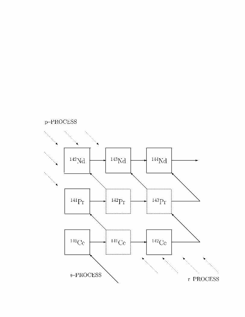
142
Nd
140
Ce
142
Ce
141
Pr
143
Nd
144
Nd
141
Ce
142
Pr
143
Pr
- -
- -
- - -
@
@
@
@
@
@
@
@I
@
@
@
@
@
@
@
@I
@
@
@
@
@
@
@
@I
@
@
@
@
@I
@
@
@
@
@I
@
@
@
@
@I
R R R
R
R
p
p
p
p
p
p
p
p
p
p
p
p
p
p
p
p
p
p
p
p
p
p
p
p
p
p
p
p
p
p
p
p
p
p
p
p
p
p
p
p
p
p
p
p
p
p
p
p
p
p
p
p
p
p
p
p
p
p
p
p
I I I I
p
p
p
p
p
p
p
p
p
p
p
p
p
p
p
p
p
p
p
p
p
p
p
p
p
p
p
p
p
p
p
p
p
p
p
p
p
p
p
p
p
p
p
p
p
p
p
p
p
p
p
p
p
p
p
p
p
p
p
p
r{PROCESS
p{PROCESS
s{PROCESS
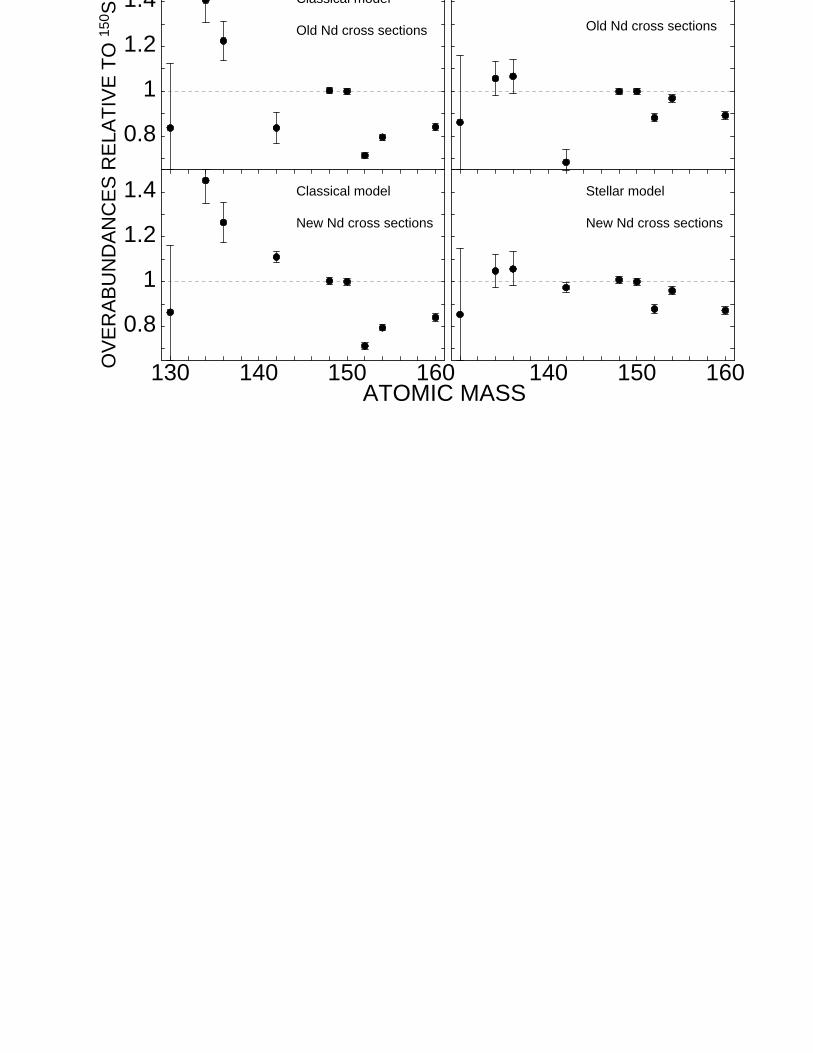
130 140 150 160
0.8
1
1.2
1.4
OV
ER
AB
UN
DA
NC
ES
RE
LAT
IVE
TO
150 S
m
140 150 160ATOMIC MASS
0.8
1
1.2
1.4 Classical model
Old Nd cross sections
Stellar model
Old Nd cross sections
Classical model
New Nd cross sections
Stellar model
New Nd cross sections

50 100 150 200
ATOMIC MASS
10-3
10-2
10-1
100
OV
ER
AB
UN
DA
NC
ES
NO
RM
ALI
ZE
D T
O 15
0
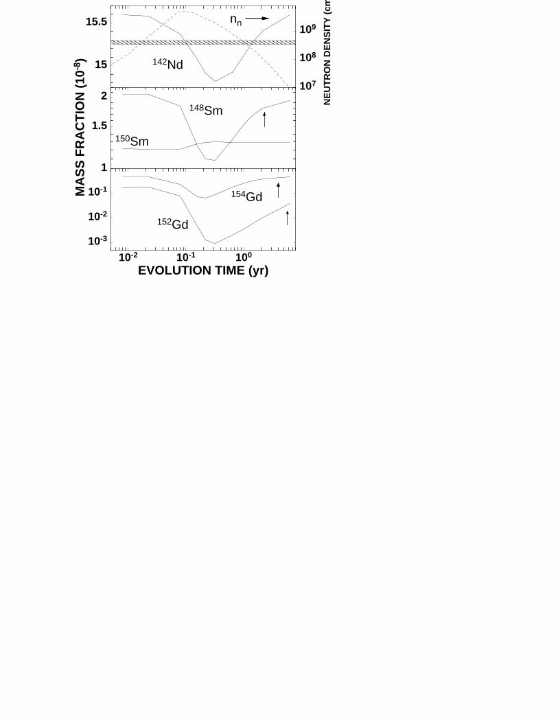
10-2 10-1 100
EVOLUTION TIME (yr)
10-3
10-2
10-1
1
1.5
2M
AS
S F
RA
CT
ION
(10
-8) 15
15.5
107
108
109
NE
UT
RO
N D
EN
SIT
Y (
cm
nn
142Nd
148Sm
150Sm
154Gd
152Gd

100 150 200
10-2
10-1
100
100 150 200MASS NUMBER
10-2
10-1
100
r -
PRO
CE
SS A
BU
ND
AN
CE
S
CANONICAL
STELLAR