New dynamic analysis techniques for structural members subjected to blast loads

Jonathon Dragos Bachelor of Engineering (Civil & Structural) (Hons)

Thesis submitted for the degree of Doctor of Philosophy at The University of Adelaide, Australia

The School of Civil, Environmental and

Mining Engineering

May 2014

i

Contents Abstract ...................................................................................................................................... ii

Statement of Originality ........................................................................................................... iii

List of Publications ................................................................................................................... iv

Acknowledgements .................................................................................................................... v

Introduction and Background .................................................................................................... 1

Chapter 1 - Pressure Impulse Diagrams for Structural Members subjected to Confined Blasts4

Introduction ............................................................................................................................ 4

List of Manuscripts ................................................................................................................ 4

Simplification of Fully Confined Blasts for Structural Response Analysis .......................... 6

Pressure-Impulse Diagrams for an Elastic-Plastic Member under Confined Blasts ............ 38

A New Approach to Derive Normalised Pressure Impulse Curves for Elastic Members ... 59

A New General Approach to Derive Normalised Pressure Impulse Curves ....................... 76

Application of Normalized Pressure Impulse Diagrams for Vented and Unvented Confined Blasts .................................................................................................................................. 106

Chapter 2 - Use of a Numerical Model for developing new Analysis Techniques for Blast Loaded Structural Members ................................................................................................... 130

Introduction ........................................................................................................................ 130

List of Manuscripts ............................................................................................................ 130

A numerically efficient finite element analysis of reinforced concrete members subjected to blasts .............................................................................................................................. 132

A Single Degree of Freedom Approach to incorporate Axial Load Effects on Pressure Impulse Curves for Steel Columns .................................................................................... 154

Interaction between Direct Shear and Flexural Responses for Blast Loaded Reinforced Concrete Slabs using a Finite Element Model ................................................................... 175

Chapter 3 - Conclusion & Future Research ........................................................................... 196

ii

Abstract This thesis contains a number of journal papers which aim to extend, or produce new, analyses techniques for determining the response of structural members subjected to blasts. Within the first portion of the thesis, a new approach is provided which extends upon the concept of the normalised, or non-dimensional, pressure impulse (PI) curve, allowing it to be applied to determine the response of structural members subjected to blasts occurring in vented and unvented confined environments. As a confined blast load is highly irregular, containing multiple peaks and long duration gas pressures, a method for simplifying the confined blast load is proposed. Then, an entirely new general approach for determining normalised PI curves is developed and presented. It is shown that, due to its generality, it can account for any pulse load shape. It is also shown that other curve-fitting techniques typically used to determine normalised PI curves, while being suitable for external blast loads, cannot be applied to the more abstract pulse load shapes associated with confined blast loads. Then, the newly proposed general approach is applied to, and validated for, vented confined blast loads. Furthermore, the entire concept of a PI curve is extended so that an infinitely long duration unvented confined blast load, having an infinite impulse, can be analysed using a PI diagram. A one dimensional (1D) finite element model (FEM) is then adopted for further studies, due to its inherent accuracy and stability despite its numerically efficiency. As the 1D FEM can accurately model the global dynamic response of an entire structural member, it does not suffer from the limitations of more commonly used simplified analysis techniques, such as the single degree of freedom (SDOF) method. Firstly, a segmental moment-rotation model is incorporated into the 1D FEM to accurately analyse the response of reinforced concrete (RC) beams and slabs subjected to blasts. The model, as a whole, can accurately simulate important RC behaviour, such as slipping of steel reinforcement within concrete and softening of concrete in compression, despite being numerically efficient. Furthermore, the 1D FEM is used to determine PI curves for steel columns under various levels of axial loading. This study is then used to validate a newly developed simple SDOF approach for determining PI curves for steel columns under axial loading. Despite the simplicity of the approach, it is shown to accurately account for the new failure mechanism of global instability and PΔ effects, all caused by the axial load. Finally, the 1D FEM is used to undertake a parametric study on RC slabs to determine the influence of the flexural behaviour and geometrical properties on the direct shear response. The results provided in this final study aim to be a starting point for determining more sophisticated simplified methods, such as a new SDOF method or normalised PI curves, for analysing the direct shear response of RC beams and slabs.

iii

Statement of Originality I certify that this work contains no material which has been accepted for the award of any other degree or diploma in my name, in any university or other tertiary institution and, to the best of my knowledge and belief, contains no material previously published or written by another person, except where due reference has been made in the text. In addition, I certify that no part of this work will, in the future, be used in a submission in my name, for any other degree or diploma in any university or other tertiary institution without the prior approval of the University of Adelaide and where applicable, any partner institution responsible for the joint-award of this degree. I give consent to this copy of my thesis when deposited in the University Library, being made available for loan and photocopying, subject to the provisions of the Copyright Act 1968. The author acknowledges that copyright of published works contained within this thesis resides with the copyright holder(s) of those works. I also give permission for the digital version of my thesis to be made available on the web, via the University’s digital research repository, the Library Search and also through web search engines, unless permission has been granted by the University to restrict access for a period of time. …………………………………………………… ………..……………

Jonathon Dragos Date

iv

List of Publications Dragos, J., Wu, C., Oehlers, D.J. (2013). Simplification of fully confined blasts for structural response analysis. Engineering Structures, 56 (2013), 312–326. Dragos, J., Wu, C., Vugts, K. (2013). Pressure-Impulse Diagrams for an Elastic-Plastic Member under Confined Blasts. International Journal of Protective Structures, 4 (2), 143-162. Dragos, J., Wu, C. (2013). A New Approach to Derive Normalised Pressure Impulse Curves for Elastic Members. Journal of Earthquake and Tsunami (Special Issue-IISE 2012), 7 (3), 1350016. Dragos, J., Wu, C. (2013). A new general approach to derive normalised pressure impulse curves. International Journal of Impact Engineering, 62 (2013), 1-12. Dragos, J., Wu, C. (2014). Application of normalised pressure impulse diagrams for vented and unvented confined blasts. Journal of Engineering Mechanics - ASCE, 140 (3), 593–603. Dragos, J., Visintin, P., Wu, C., Oehlers, D. (2014). A numerically efficient finite element analysis of reinforced concrete members subjected to blasts. International Journal of Protective Structures, 5 (1), 65-82. Dragos, J., Wu, C. (2013). A Single Degree of Freedom Approach to incorporate Axial Load Effects on Pressure Impulse Curves for Steel Columns. Tentatively accepted for publication in Journal of Engineering Mechanics - ASCE. Dragos, J., Wu, C. (2014). Interaction between Direct Shear and Flexural Responses for Blast Loaded Reinforced Concrete Slabs using a Finite Element Model. Accepted for publication in Engineering Structures.

v

Acknowledgements My sincerest gratitude goes to Dr Chengqing Wu, whose knowledge in the field of structures response to blasts knows no bounds. For his willingness to provide guidance and assistance, no matter what day of the week it is, I am also extremely grateful for. I would also like to thank Dr Phillip Visintin and Professor Deric Oehlers, who were always willing to provide their expertise when needed. Also, my friends and family deserve my thanks and much more, for their patience and support. Finally, I dedicate this thesis to my partner and soulmate, Stephanie, who has provided me with the confidence and support to complete this thesis to the best of my abilities.

1

Introduction and Background Due to the omnipresent threat of terrorist acts, there exists a need to protect structures and other critical infrastructure from blasts caused by the detonation of explosives. Some examples of this serious threat include the World Trade Centre bombing in 1993, the Oklahoma City bombing in 1996 and, more recently, the Australian Embassy bombing in Jakarta in 2004. As existing infrastructure is not typically designed to withstand the effects of a blast, it is imperative that techniques be developed which can be used by engineers to accurately analyse the response of structures subjected to blasts. For a charge being detonated near a structure, causing a load due to its corresponding shockwave to act on that structure, it is typically the case that only the closest neighbouring structural members, such as a reinforced concrete (RC) or steel column, need to be analysed. This is because the standoff distance from the charge to the target is a key factor influencing the damage caused by a detonated charge. Furthermore, for the protection of critical infrastructure, the analysis of structural walls and barriers needs to be undertaken to ensure safety. Various techniques exist for analysing the entire deflection time history response of structural members, walls and barriers subjected to blast loads. The simplest technique is the single degree of freedom (SDOF) method. This technique converts the entire structural member into a SDOF system, relying on various transformation factors, and only provides the deflection response of the midspan of the member. Many studies have shown that this technique can accurately be used to determine the midspan response of simple beams and slabs subjected to blast loads. However, studies have also shown that in some circumstances the SDOF method cannot accurately account for certain behaviour. For example, the SDOF method cannot account for local material damage failure of RC structural members caused typically by a blast from a charge with an extremely small standoff distance. Also, the SDOF method can only account for a single frequency mode of response. Therefore, in situations where a blast load would incur multiple frequency modes within a structural member response, the SDOF would not be able to accurately simulate this scenario. Furthermore, the assumed shape function used within the SDOF method for a column with fixed and free end support conditions does not reflect that of an actual column, causing the SDOF method to provide erroneous results in this case. Also, the SDOF method has not been thoroughly investigated to confirm whether it can account for other phenomenon which can occur when a structural member is subjected to blasts, such as the support slip response, caused by a vertical direct shear crack adjacent to the supports, of RC beams and slabs subjected to blasts. The most advanced technique for determining the response of structural members subjected to blasts is via a finite element analysis software package which utilises a three dimensional mesh to determine the three dimensional deformations of the structural member over time. Such a technique provides accurate results but is numerically expensive, meaning that it is unsuitable for undertaking large parametric studies, and is not typically used in the design office due to its complexity.

2

In addition to the aforementioned dynamic analysis techniques, pressure impulse (PI) curves are typically used in practice as a preliminary design or analysis tool for quickly determining whether a structural member fails or survives a given blast load. The PI diagram consists of the two most important parameters of a blast load, peak reflected pressure and impulse, as axes on a graph. The PI curve is a plot of the boundary between combinations of these two parameters which cause the structural member in question to fail or survive a given blast load. Although the use of a PI curve is efficient, the determination of a PI curve is quite difficult and time consuming. For this reason, the concept of a normalised, or non-dimensional, PI curve was founded many years ago. A normalised PI curve is a general PI curve which can be converted very quickly to a PI curve corresponding to a given structural member. However, all PI curves are typically determined using SDOF theory, meaning that the limitations of the SDOF method also apply to PI curves. Also, the normalised, or non-dimensional, PI curves found in literature are lacking in generality and, for this reason, can only be applied to structural members subjected to blast loads due to charges being detonated in open and unobstructed environments. In this study, the concept of the normalised PI curve is extended to be applied to blast loads occurring in enclosed environments, such as an underground car park or a bunker, typically denoted as confined blasts. In order to do this, a method for simplifying the confined blast load is provided and is accompanied by a new general approach to determine a normalised PI curve corresponding to any form of confined blast. For further studies, a one dimensional (1D) finite element model (FEM) is developed, which consists of a one dimensional mesh as opposed to the three dimensional mesh of three dimensional finite element software. This was developed to accurately perform dynamic analyses of entire structural members subjected to blasts. The use of the 1D FEM as a numerical model is paramount to these further studies, as it doesn't suffer from the limitations of the SDOF method while still being numerically efficient, as opposed to the three dimensional finite element software. The 1D FEM is then used as a dynamic analysis framework for a new segmental analysis technique which can account for various RC behaviours, such as the cracking of concrete in the tensile region, the sliding of steel reinforcing bars embedded within concrete and the sliding of concrete wedges in the compression region. The 1D FEM is used to show that a new segmental analysis technique can be incorporated within a dynamic analysis model to accurately, but efficiently, determine the blast load response of RC structural members. The 1D FEM is then used to develop a new simple approach to account for the effects of axial load on PI curves for steel columns and to investigate the direct shear response, caused by vertical cracks adjacent to the supports, of RC slabs. This thesis contains a number of manuscripts which have been published in, or accepted in, or submitted to, internationally recognised journals. Each chapter contains an introduction, explaining the aims and how the papers fit together, a list of manuscripts and each manuscript. Within chapter 1, a new approach is provided which extends upon the concept of the normalised, or non-dimensional, PI curve, allowing it to be applied to confined blasts. To do

3

this, a method of simplification is determined which allows the irregular pulse load caused by a confined blast to be converted to a simplified bilinear pulse load. Then, an entirely new general approach to determine a normalised PI curve is developed and presented. This new general approach is then applied to the simplified bilinear pulse load shape, which is equivalent to the actual confined blast load, to demonstrate that normalised PI curves can be used to quickly determine the response of structural members subjected to confined blast loads. Chapter 2 contains three journal papers which each utilises a 1D FEM to extend, or provide new, analysis techniques for determining the response of structural members subjected to blasts. Firstly, a new segmental moment-rotation approach is incorporated into a 1D FEM which is shown to accurately determine the response of RC slabs subjected to blasts, despite its numerical efficiency. Furthermore, with the aid of the 1D FEM, a new simple SDOF approach is developed for determining PI curves for steel columns under constant axial loading. Finally, the 1D FEM is used to undertake a parametric study to investigate the influence of the flexural behaviour and geometrical properties on the direct shear response of reinforced concrete slabs subjected to blast loads.

4

Chapter 1 - Pressure Impulse Diagrams for Structural Members subjected to Confined Blasts Introduction In this chapter, it is shown how the concept of the normalised PI curve can be extended, allowing for the response of structural members subjected to confined blasts to be determined. Firstly, in the paper entitled "Simplification of fully confined blasts for structural response analysis", a method is provided for simplifying the irregular nature of a confined blast load to a bilinear pulse load. Then, within the second publication entitled "Pressure-Impulse Diagrams for an Elastic-Plastic Member under Confined Blasts", a number of normalised PI curves corresponding to this bilinear pulse load are derived, but it is shown that the typical curve-fitting approaches employed in literature cannot be replicated to determine empirical equations for normalised PI curves for any bilinear pulse load. Within the paper entitled "A New Approach to Derive Normalised Pressure Impulse Curves for Elastic Members", a new general approach for determining elastic normalised PI curves is presented, and it is shown that it can be used to accurately determine normalised PI curves corresponding to many different pulse load shapes. Then, within the paper entitled "A new general approach to derive normalised pressure impulse curves", a new general approach for determining normalised PI curves corresponding to any elastic-plastic-hardening structural member subjected to any pulse load shape is presented. Finally, within the paper entitled "Application of normalised pressure impulse diagrams for vented and unvented confined blasts", the new general approach is applied to vented confined blast loads. Also, the entire concept of the PI curve is extended so that PI curves can be used to determine the response of structural members subjected to unvented confined blast loads, which have an infinitely long gas pressure duration. The new approach to determine normalised PI curves is suitable for the purposes of preliminary analysis and design, as it does not require any differential equations to be solved but has the generality to allow for any pulse load shape associated with any type of blast load. List of Manuscripts Dragos, J., Wu, C., Oehlers, D.J. (2013). Simplification of fully confined blasts for structural response analysis. Engineering Structures, 56 (2013), 312–326. Dragos, J., Wu, C., Vugts, K. (2013). Pressure-Impulse Diagrams for an Elastic-Plastic Member under Confined Blasts. International Journal of Protective Structures, 4 (2), 143-162.

5

Dragos, J., Wu, C. (2013). A New Approach to Derive Normalised Pressure Impulse Curves for Elastic Members. Journal of Earthquake and Tsunami (Special Issue-IISE 2012), 7 (3), 1350016. Dragos, J., Wu, C. (2013). A new general approach to derive normalised pressure impulse curves. International Journal of Impact Engineering, 62 (2013), 1-12. Dragos, J., Wu, C. (2014). Application of normalised pressure impulse diagrams for vented and unvented confined blasts. Journal of Engineering Mechanics - ASCE, 140 (3), 593–603.

6

Statement of Authorship Simplification of Fully Confined Blasts for Structural Response Analysis (2013) Engineering Structures, 56 (2013), 312–326 Publication status: Published Dragos, J. (candidate) Developed model and theory, performed all analyses and prepared manuscript. I hereby certify that the statement of contribution is accurate Signed……………………………………………………………………..Date……………… Wu, C. Supervised research, provided critical manuscript evaluation and acted as corresponding author. I hereby certify that the statement of contribution is accurate and I give permission for the inclusion of the paper in the thesis Signed……………………………………………………………………..Date……………… Oehlers, D.J. Provided critical manuscript evaluation. I hereby certify that the statement of contribution is accurate and I give permission for the inclusion of the paper in the thesis

7

Simplification of Fully Confined Blasts for Structural Response Analysis Jonathon Dragos, Chengqing Wu, Deric John Oehlers

Abstract

A blast in a fully confined environment magnifies the blast loading resulting in more serious damage to surrounding structural members. To protect critical infrastructure against confined blasts, the confinement effects need to be fully taken into consideration. In this paper, a procedure to simplify the highly irregular nature of fully confined blast loads was developed for the purpose of being incorporated into a structural response analysis tool such as a Pressure Impulse Diagram. It was found that when the centroid of the simplified confined blast load was close to the centroid of the actual confined blast load, whilst keeping the total impulse the same, the response of a member caused by the simplified confined blast load was similar to that produced by the actual confined blast load. This concept to accurately simplify an irregular confined blast based on structural response was then used to construct the method of simplification. This method of simplification was then tested using a structural response model for the purposes of validation and suitability. A comparison was then made against the current UFC guidelines predictions to assess its accuracy. Keywords: Blast load; Numerical analysis; Structural response 1 Introduction Confined blast loading may occur in many scenarios such as tunnels and subway stations or within car parks and basements of buildings or due to an accidental explosion within an ammunition storage bunker, or even in a building with strong glass panels [1]. As the confinement causes the effects of explosions to be amplified, due to shockwave reflections and long durations of gas overpressure, the severity of damage experienced by critical infrastructure under confined blasts can be much greater [2,3]. Therefore, the consequences of confined blasts on high risk infrastructure need to be taken into account in analysis and design of structures for the safety of people and installations. Research by Hu et al. [4] and Feldgun et al. [5] has shown that there are many parameters which affect the pressure time history at a given pressure gauge due to a given fully confined blast, including the charge size, position, shape and orientation, trigger point of detonation within the charge as well as the shape and size of the confinement. As can be seen in Fig. 1, a typical pressure time history due to a blast in a fully confined environment by Hu et al. [4] and Edri et al. [6] contains an initial pressure peak, corresponding pressure peaks, due to shockwave reflections off the boundary walls, and a gas pressure or quasi static pressure. For the case of a fully confined blast, the quasi static overpressure is assumed to be constant and continues forever as no vents exist for the excess gas to escape.

8

Fig. 1. Typical confined pressure time history by Hu et al. [3] According to Baker et al. [7] for simple one dimensional or two dimensional problems, for example a line charge placed in a cylindrical confinement, the impulse and peak pressure of the subsequent pressure peaks is always half the preceding values, as shown in Fig. 2. In these cases, the pressure time history can be obtained analytically.

Fig. 2. Simplified confined pressure time history proposed by Baker et al. [6] The main limitation of this simplified method [7] is that it cannot be applied to more complex three dimensional problems where the charge is within a confinement of cubic or rectangular shape, imitating that of a typical room in a building or bunker. Also, the simplification above does not take into account gas pressure which can be quite significant in magnitude and duration, as shown by Edri et al. [6]. The most recent guidelines of UFC-3-340-02 [8] use theoretical procedures and an extensive set of experimental data to derive charts to determine the simplified pressure time history based on the confinement geometry, size of charge and position of charge within the confinement, as seen in Fig. 3.

A NOTE:

This figure/table/image has been removed to comply with copyright regulations. It is included in the print copy of the thesis held by the University of Adelaide Library.

A NOTE:

This figure/table/image has been removed to comply with copyright regulations. It is included in the print copy of the thesis held by the University of Adelaide Library.

9

Fig. 3. UFC-3-340-02 [7] idealised confined blast model

It can be seen in Fig. 3 that the UFC simplification takes into account the gas pressure. For a fully confined blast, in which no vents exist, the duration of the gas pressure, tg, is usually much longer than the fundamental periods of the structure's elements [8]. The main limitation of the UFC simplification is that it does not take the effects of charge shape, orientation and point of detonation into consideration. The effects of these parameters were investigated by Hu et al. [4] and were observed to be quite significant. Finally, UFC simplifies the highly irregular multiple pressure peaks that are experienced due to shockwave reflections as a single idealised shock pressure peak. Thus, the accuracy of this simplification needs to be assessed. Fig. 4 shows a comparison between the actual blast and UFC’s predicted pressure time history. It needs to be assessed whether the single pressure peak predicted by UFC is sufficient enough to approximate the multiple pressure peaks of the actual confined blast load.

Fig. 4. UFC prediction and actual confined blast pressure time history

Considerable research has been conducted to investigate the structural response to external blast loadings [9-11]. However, due to the complexity of confined blast loading, little research has been carried out to study the characteristics of structural response under internal blast loading. Only recently the effects of confinement on structural response have been investigated [3]. Azevedo & Alves [12] and Youngdahl [13] have investigated the effects of pulse shape on structural response. Furthermore, Fallah & Louca [14], Krauthammer et al. [15] and Li & Meng [16] have all investigated the effects of pulse shape on pressure impulse (PI) diagrams, which are a useful tool for the quick analysis and design of structural members against blasts. As all of this research corresponds to pulse load shapes associated with external blast loads, none of it can be applied to internal blasts. This is because, in contrast to external blasts, the pressure time history for a confined blast is highly irregular and therefore

0 0

Pres

sure

Time

0

500

1000

1500

2000

2500

0 1 2 3 4 5 6 7 8

Refle

cted

Pre

ssur

e (k

Pa)

Time (ms)

Confined Blast - 1kg Charge

Blast UFC Prediction

Idealized Shock Pressures

Idealized Gas Pressures

tg

10

has no pulse load shape. Therefore, there is a need to derive a method to simplify the confined pressure time history, such that the equivalent simplified pressure time history has a re-occurring pulse load shape. This simplified pressure time history, in comparison to that of the actual blast pressure time history, should cause the same, or more, damage to all structural members to be considered valid. As the simplified pressure time history would correspond to a given pulse load shape, it would then allow a PI diagram to be employed to quickly determine the response of a given structural member against such a confined blast load. Otherwise, a time consuming dynamic response software package of program would need to be utilized to determine the response of that given structural member against the confined blast load. In addition to the above application, another potential purpose for a method for accurately simplifying the pressure time history of a confined blast exists. If a database of confined blast pressure time histories for various charge and confinement properties were to be obtained, experimentally or from a numerical software package, then the proposed method of simplification would be able to be employed to determine new and accurate charts. Similar to the charts for confined blasts provided by UFC guidelines, these charts would provide values for various parameters which can be used to describe a simplified confined pressure time history. These charts would also then eliminate the need for a user to run a numerical software package to determine a confined blast pressure time history. In this study, the concepts to determine the accuracy of a simplified pressure time history are investigated. The most important factors affecting the accuracy of the simplified pressure time history are the total impulse and distribution of impulse, along the time axis, represented by the centroid. With these concepts, the method of simplification of a confined blast pressure time history within a cube or cuboid was derived. The actual confined blast pressure time histories used for development of this simplified method were simulated through the use of a numerical software package such as Autodyn [17]. Through numerical simulation, testing is carried out to determine the accuracy of the method of simplification by subjecting many structural members to both a confined blast pressure time history and its corresponding simplified pressure time history. The developed simplified method is then compared with predictions provided by current UFC guidelines. It was found that the simplified confined blast was accurate and reasonable to be used for structural response analysis. 2 Response of structural members to confined blasts Using the Autodyn software package, pressure time histories for blast events involving charges of cylindrical and spherical shape of up to 1kg were simulated. Also, fully confined environments of cube and cuboid of up to 8m3 in volume were taken into consideration in this study. For charges and confined chamber volumes larger than these values, the methods derived in this study need further testing to be applied with confidence. The simulated confined pressure time history was then applied to a given structural member to study its response. The structural response of members subjected to a given pressure time history was analysed using a finite difference approach [11,18].

11

2.1 Finite difference analysis of structural members To determine the response of a structural member due to a given blast, the finite difference model was used. The finite difference model, based on the work by Krauthammer et al. [18], was developed by Jones et al. [11] and redeveloped by Dragos et al. [19]. Although more comprehensive models exist [20-22], the finite difference method has been proved to be an accurate and fast-running method, suitable for the prediction of the behaviour of one-way spanning structural members (e.g. a reinforced concrete slab) subjected to high intensity, short duration dynamic loads such as those associated with impacts and explosions [18,23]. The finite difference method is used to numerically solve the Timoshenko Beam Equations. The Timoshenko beam equations below allow for deflection of the member due to shear and flexure and also accounts for rotational inertia [24]: 𝜕𝑀𝜕𝑥− 𝑉 = −𝜌𝑚𝐼𝑚

𝜕2𝛽𝜕𝑡2

(1)

𝜕𝑉𝜕𝑥

+ 𝑞 = 𝜌𝑚𝐴𝜕2𝑣𝜕𝑡2

(2)

where: M = bending moment; V = shear force; q = uniformly distributed dynamic transverse load; Im = moment of inertia; A= cross sectional area; ρm = density of member; ν = transverse displacement of the midplane of the beam; β = rotation of the cross section due to bending. To apply the finite difference method, first of all the geometry and material properties of the structural member should be known. Secondly, at the sectional level, the member’s shear stress-strain and moment-curvature relationships should be known. This is why the finite difference method can easily be applied to any structural member, such as a steel beam or a reinforced concrete (RC) slab. For RC members, the finite difference model was modified to take into account the moment-rotation relationship of the plastic hinge region, instead of using the moment-curvature relationship of the member in this region [19]. The moment-rotation and corresponding moment-curvature relationships were developed for various RC members using the methods discussed in Haskett et al. [25] and Dragos et al. [19]. For RC members, all moment-rotation and moment-curvature relationships were of elasto-plastic shape. In this study, elasto-plastic RC members as well as entirely elastic members were tested. 2.2 Effect of confinement on structural response Fig. 5(a) shows an example of a spherical charge placed in the centre of a confinement of cubic shape. Fig. 5(b) shows a cylindrical charge placed in the centre of a confinement of rectangular shape. When the charge is detonated, the pressure time histories recorded at the pressure gauges shown in Fig. 6 are completely different due to the different configurations. Figs. 6(a) and 6(b) show the pressure time histories acting at the pressure gauges shown in the blast configurations in Figs. 5(a) and 5(b), respectively. For both cases, the charge size is 1kg and the volume of the confinement is 8m3.

12

(a) (b)

Fig. 5. Explosions in two confined environments, spherical charge in a cubic room (a) and cylindrical charge in a rectangular room (b)

(a) (b)

Fig. 6. Pressure time histories due to two different confined environments, cubic (a) and rectangular (b)

Figs. 6(a) and 6(b) show that the pressure time history due to a charge in a confined environment can have many pressure peaks, due to shockwave reflections off the adjacent walls, and that the number and size of the pressure peaks is determined based on many parameters. Fig. 6(b), due to the cylindrical charge, has a much greater primary pressure peak and minimal secondary pressure peaks. This is because the majority of the energy is being directed towards the pressure gauge. The main factors contributing to this is the shape of the charge and that the detonator is positioned on the opposite end of the charge, relative to the pressure gauge. However, if the charge was centrally detonated, the magnitude of the primary pressure peak would decrease and the following pressure peaks would increase in magnitude. This is because more of the shockwave energy would be reflected off the surrounding walls before reaching the gauge. Conversely, Fig. 6(a) shows that sometimes the first pressure peak is not always the largest pressure peak due to superposition of shockwave reflections. It also shows that, for complex three dimensional problems, the assumptions made by Baker et al. [7], shown in Fig. 2, do not always remain true. Dragos et al. [26] investigated the effects of confinement on structural response by subjecting a member to both the fully confined and unconfined pressure time histories due to a cylindrical charge. For the confined case, the confinement was a cube of volume 8m3 in which the charge was placed in the centre of the cube. For both cases, the standoff distance

-1000

1000

3000

5000

0 2 4 6 Refle

cted

Pre

ssur

e (k

Pa)

Time (ms)

Confined Blast - 1kg sph chge - cube

-1000

9000

19000

29000

39000

0 1 2 3 Refle

cted

Pre

ssur

e (k

Pa)

Time (ms)

Confined Blast - 1kg cyl chge - rect

Pressure Gauge

Cylindrical Charge

Pressure Gauge

Spherical Charge

13

from the charge to the centre of the member was 1m. Fig. 7(a) and Fig. 7(b) show pressure time histories due to a 0.2kg charge in a confined and unconfined environment, respectively. Fig. 8(a) shows the response of a RC slab subjected to the 0.2kg charge in both the confined and unconfined conditions. In this case the influence factor, which is the ratio of deflection under confined blast to unconfined blast, is approximately 1. Fig. 8(b) shows the response of the same RC slab subjected to a 1kg charge in both the confined and unconfined conditions, for which the influence factor is now 10. It can be seen from Fig. 7 that due to the reflected shockwaves, the duration of the pressures acting on the member, and thus impulse increases significantly.

(a) (b)

Fig. 7. Pressure time history along the length of a member for a 0.2kg charge place in the centre, confined (a) and unconfined (b).

(a) (b)

Fig. 8. Effect of cubic confinement from a, 0.2kg (a) and 1kg (b) charge on a RC slab 3 Simplification of the pressure time history of fully confined blasts 3.1 Concepts of simplification Fig. 9 shows a typical deflection time history of a simply supported structural member subjected to a blast load in which the time to reach the maximum deflection or response time, tmax, is shown. Dragos et al. [26] simplified arbitrary pressure time histories containing multiple peaks by lumping the impulse of the multiple peaks into a single triangular pressure peak, such that its peak pressure was equal to the maximum pressure of the multiple peaks. It was shown that if tmax was greater than 3 times the loading time of the actual load containing

-500

0

500

1,000

1,500

2,000

2,500

3,000

0 1 2 3 4 5 6

Refle

cted

Pre

ssur

e (k

Pa)

Time (ms)

Confined Blast

0

1,000

2,000

3,000

0 0.5 1 1.5 2

Refle

cted

Pre

ssur

e (k

Pa)

Time (ms)

Unconfined Blast

-2

0

2

4

6

0 5 10 15

Defle

ctio

n (m

m)

Time (ms)

Effect of Confinement - 0.2kg charge

Confined Unconfined

-10

10

30

50

70

90

0 5 10 15 20

Defle

ctio

n (m

m)

Time (ms)

Effect of Confinement - 1kg charge

Confined Unconfined

14

multiple peaks, then the simplification would cause almost the same amount of damage as the actual load. It was then shown that if tmax was less than 3 times the loading time of the actual load, then the simplification would cause more damage and could therefore be considered conservative.

Fig. 9. Deflection time history of a typical RC slab subjected to a blast load

To gain a qualitative understanding of this phenomenon, an analysis of Figs. 10 and 11 will be carried out. Fig. 10 shows the blast pressure time history acting at the centre of the wall in a cube of volume 2m3, due to a 1kg spherical charge located in the centre of the cube. It also shows a simplified pressure time history, which is derived by lumping the impulse at a single peak with a peak reflected pressure equal to the maximum pressure of the actual blast. Fig. 11 shows the response of two RC members subjected to both the lumped and actual blast pressure time histories. Fig. 11(a) is that of a member with a shorter response time, approximately 9ms, whereas Fig. 11(b) is that of a member with a longer response time, approximately 23ms.

Fig. 10. Lumped and actual confined pressure time history

0

10

20

30

40

50

0 3 6

Defle

ctio

n (m

m)

Time (ms)

Deflection Time History

-500

500

1500

2500

3500

4500

5500

6500

0 2 4 6 8

Refle

cted

Pre

ssur

e (k

Pa)

Time (ms)

Actual and Lumped P-T History's

Actual Blast Lumped

tmax

tc,b tc,a

15

(a) (b)

Fig. 11. Response of 2 RC members each subjected to both a lumped and actual pressure time history

The key difference between both loads within Fig. 10 is that, although the total impulse of the loads is the same, the distributions of the impulse of the loads, along the time axis, are quite different. The impulse of the lumped pressure time history is heavily concentrated towards a time of 0ms, whereas the impulse of the actual blast pressure time history is more loosely distributed between 0ms and 8ms. To help illustrate this for both loads, the approximate centroids of the distribution of impulse, along the time axis, have been labelled on Fig. 10, where tc,a represents that of the actual blast load and tc,b represents that of the lumped load. It can be seen that for a member with a small response time as in Fig. 11(a), the maximum deflection due to the lumped pressure time history is approximately 80% larger than that from the actual blast. For the member with a large response time in Fig. 11(b), the maximum deflection due to the lumped pressure time history is only approximately 10% larger than that of the actual blast. Although the total impulse of both loads, shown in Fig. 10, are the same, a qualitative reason for this can be deduced by comparing the centroids (tc,a and tc,b) of the loads, with the response time, tmax, of the members in Fig. 11(a) and Fig. 11(b). When tmax is smaller, such as in Fig. 11(a), the centroid of the actual load (tc,a) is much closer to tmax in comparison with that of the simplified load (tc,b). Conversely, when tmax is large, such as in Fig. 11(b), the centroids of the actual and simplified loads are both very small relative to tmax. Therefore, the difference in the centroids is minor, and as the total impulse is the same, the responses of the member subjected to both loads are the same. For such a case, as no on-going gas pressure exists, the blast can be said to be “impulse controlled” which means that the magnitude of the impulse is the main factor which influences the response of the member. As the response time of the member decreases, for example in Fig. 11(a), not only does the total impulse of the simplified load affect its accuracy, but the distribution of its impulse, along the time axis, plays an important role in its accuracy. Therefore, it can be seen that to approximate the actual blast load as accurately as possible, would be to derive a simplified pressure time history which has a distribution of impulse, along the time axis, which is as close as possible to that of the actual blast load, whilst having the same total impulse. As the centroid of the

-10

0

10

20

30

40

50

0 5 10

Defle

ctio

n (m

m)

Time (ms)

Response Comparison - D135 L2

Actual Blast Lumped

0

50

100

150

0 10 20 30 40

Defle

ctio

n (m

m)

Time (ms)

Response Comparison - D135 L4 Actual Blast Lumped

tmax tmax

16

simplified load relative to the centroid of the actual blast can be used to quantitatively gauge the difference in the distribution of impulse, along the time axis, the concept of the centroid will be relied upon to derive a simplified pressure time history for actual confined blast loads. Figs. 12 and 13 show an example of a new simplified pressure time history derived using the concept discussed above. They show a repeat of the above case (Fig. 10 and Fig. 11), with the only difference being that the new simplified load has changed so that its impulse is distributed, along the time axis, in a similar fashion to that of the actual blast, whilst keeping the total impulse the same. As seen in Fig. 12, the centroid of the distribution of impulse, along the time axis, of the new simplified load is now located much closer to that of the actual blast. As seen in Fig. 13, the responses of the same members from Fig. 11 were subjected to both the actual blast load and new simplified load. This was done to determine the increase in accuracy of the new simplified load relative to the actual blast load.

Fig. 12. New simplified and actual confined pressure time history

(a) (b)

Fig. 13. Response of 2 RC members each subjected to both a new simplified and actual confined pressure time history

According to Li & Meng [16], the centroid of a pulse load is a very important geometrical property and this can also be seen to apply in Fig. 13. It can be seen that the response due to the simplified load approximates the response due to the actual load quite well. The responses of the member in Fig. 13(a), with the short response time, differ by only approximately 5%, and the responses of the member in Fig. 13(b), with the large response time, have a negligible difference.

-500

500

1500

2500

3500

4500

5500

6500

0 2 4 6 8

Refle

cted

Pre

ssur

e (k

Pa)

Time (ms)

Actual and Simplified P-T History's

Actual Blast

Simplified

0

5

10

15

20

25

30

0 5 10

Defle

ctio

n (m

m)

Time (ms)

Response Comparison - D135 L2

Actual Blast Simplified

0

50

100

150

0 10 20 30 40

Defle

ctio

n (m

m)

Time (ms)

Response Comparison - D135 L4 Actual Blast Simplified

tc,a & tc,b

17

Figs. 12 and 13 are very important because they show that for a member subjected to the new simplified load, its response is quite reasonable when its response time is equal to or larger than the duration of the load. It can also be seen that the response of a member becomes almost identical as the response time increases. This is due to the fact that, for both pressure time histories seen in Fig. 12, the distribution of impulse along the time axis, and thus the centroid, and total impulse are the same. This is all despite the noticeable differences in the shape of both pressure time histories. It needs to be noted that although the concepts have been shown using simply supported structural members, it was also tested for two-end fixed structural members. Therefore, it applies to structural members regardless of the choice of boundary conditions. This is because the most important factor which determines the accuracy of the simplified pressure time history is the response time. These concepts will be called upon in the following section to derive a simplified pressure time history for fully confined blasts. 3.2 Method of simplification To ascertain an appropriate technique for constructing a simplified confined pressure time history, some understanding of a typical confined pressure time history should be established. This will allow the general shape of the simplified pressure time history to be determined. Fig. 1 displays a typical confined pressure time history derived using Autodyn by Hu et al. [4]. It can be seen to have 4 clearly distinct pressure peaks lying between 0ms and 2ms. Following that, it can be seen to be converging to a constant pressure known as the gas pressure or quasi static pressure (Pqs). The pressure time history can be thought of as having 2 distinct regions, that is the shocks regions, containing the pressure peaks (4 in this case), and the quasi static region, when the primary and secondary shocks have passed and the pressure is converging towards the quasi static pressure. This quasi static pressure arises in fully confined blasts because once the explosive is triggered, the detonation products are converted into gas which increases the overall number of gas molecules in the confined cube, therefore exerting a greater pressure on the walls. As the cube is assumed to be fully confined, none of the extra gas can escape, so the quasi static pressure is assumed to continue to infinity. Due to the above reasons, as can be seen in Fig. 14, the shape of the simplified pressure time history was considered to consist of two distinct regions; a linear descending region to represent the shocks region; and a second region of constant pressure to represent the quasi static pressure. Fig. 14 shows that this choice of shape allows more impulse to be distributed, along the time axis, in the first region, which imitates that of a typical confined blast pressure time history containing large amounts of impulse within its multiple peaks. This also allows the centroid of the simplified pressure time history to be located as close as possible to that of the actual confined pressure time history. Now that the general recurring shape of the simplified pressure time history has been established, the method for deriving the simplified pressure time history based on the actual confined blast pressure time history can be developed. Fig. 14 shows a confined blast pressure time history and also a given simplified pressure time history. From Fig. 14, it can

18

be seen that three parameters require attention. These are the peak reflected pressure (Pr), quasi static pressure (Pqs) and the time at which the quasi static pressure begins (t1). To derive the simplified pressure time history for a given blast, these 3 parameters need to be determined. Pqs, should be equal to the gas pressure so it can either be measured from the actual blast, or calculated using UFC guidelines. That leaves 2 more parameters which have to be determined, Pr and t1.

Fig. 14. Simplified and confined pressure time history

Applying the principles discussed in Section 3.1, but in a more rigorous manner, a method was developed to determine the 2 parameters, Pr and t1. The method relies upon 2 conditions which should be satisfied and act as 2 governing equations used to determine the 2 unknowns, Pr and t1. The first condition is that for a substantially large time, tlarge as seen in Fig. 14, the total impulse of both the simplified and blast pressure time history, from 0 to tlarge, should be equal. The time, tlarge, represents a point in which the pressure of the actual blast has converged to the quasi static pressure. The second condition involves simultaneously manipulating Pr and t1 such that the distribution of impulse, along the time axis, of both the simplified and actual blast pressure time histories are as close as possible. Fig. 15 demonstrates how this is done. As seen in Fig. 15, both the simplified and actual blast pressure time histories are split into many small slices, Δt. For each slice, the absolute difference in the impulse is raised to some power and summated for each slice ranging from 0 to tlarge. The difference in impulse for each slice will be called the impulse error for each slice, EI,i.

0

2000

4000

6000

0 2 4 6 8

Refle

cted

Pre

ssur

e (k

Pa)

time (ms)

Simplified & Typical Confined Pressure Time History

Blast Simplified Pr

Pqs

t1 tlarge

19

Fig. 15. Calculation of impulse error per slice

This summation of errors in impulse raised to some power is the total impulse error, Ei. Its value is indicative of the difference in the distributions of impulse, along the time axis, of the simplified pressure time history and the actual blast pressure time history. Therefore, by minimising the total impulse error, the difference in the distribution of impulse, along the time axis, is minimised. Therefore, Condition 2 requires that the total impulse error, Ei, be minimised. Therefore, the overall method of simplification involves manipulating Pr and t1, such that the total impulse is the same (Condition 1), until the minimum total impulse error is determined (Condition 2). Through testing of this simplified pressure time history, by subjecting many members to this load using the finite difference model, it was found that raising the impulse error of each slice to the power of 2 provided the most accurate results on average. However, it was found that when using a value of 2 the response caused by the simplified load would, on some occasions, be slightly less than the response caused by the corresponding actual blast load. From further testing of other values, it was discovered that raising the impulse error of each slice to the power of 4 provided less accurate results, but it would always provide conservative results. By this, it is meant that the response caused by the simplified would always be equal to, or slightly larger then, the response caused by the corresponding actual blast load. Therefore, raising the impulse of error of each slice to the power of 4 was determined to be the most appropriate value. Eqs. (3) and (4) below outline the conditions which should be satisfied, through manipulation of Pr and t1, to find the simplified pressure time history:

• Condition 1: �𝐼𝑠𝑖𝑚𝑝𝑙𝑖𝑓𝑖𝑒𝑑�0𝑡𝑙𝑎𝑟𝑔𝑒 = [𝐼𝑏𝑙𝑎𝑠𝑡]0

𝑡𝑙𝑎𝑟𝑔𝑒 (3)

• Condition 2: 𝐸𝐼 = min�∑𝐸𝐼,𝑖4� (4) Where the difference in impulse of slice i can be calculated using Eq. (5), which is an application of the trapezoidal rule:

0

500

1000

1500

2000

2500

1.2 1.3 1.4 1.5 1.6

Refle

cted

Pre

ssur

e (k

Pa)

time (ms)

Simplified & Typical Confined Pressure Time History Blast Simplified

Δt

∆I = EI,𝑖

20

𝐸𝐼,𝑖 = ∆𝐼 = �𝑃𝑠(𝑡𝑖)−𝑃𝑠(𝑡𝑖−1)2

− 𝑃𝑏(𝑡𝑖)−𝑃𝑏(𝑡𝑖−1)2

� [𝑡𝑖 − 𝑡𝑖−1] (5)

Where: Ps = reflected pressure of the simplified pressure time history; Pb = reflected pressure of the actual blast pressure time history Determining a simplified pressure time history using this method requires a spreadsheet application in order to input the many data points for each of the actual blast (Pb(ti)) and simplified (Ps(ti)) pressure time histories. Within the spreadsheet, numerical integration can be applied to determine the impulse of each pressure time history from 0 to tlarge. Then, Eq. (5) needs to be used to determine the impulse error of each slice, in which a slice represents the region between ti-1 and ti. Finally, a solver tool is required to manipulate t1 and Pr such that the conditions of Eqs. (3) and (4) are both satisfied. Fig. 14 helps to illustrate that in general, within the shocks region, the simplified pressure time history has a shape which is different to that of an arbitrary confined blast pressure time history. Despite this, its total impulse is equal and its distribution of impulse, along the time axis, is as close as possible to that of the confined blast pressure time history. The simplified pressure time history needs to be validated and it needs to be known when the difference in shape has no effect on the response of the structural member, and when it has a substantial effect on the response of the structural member. 4 Response of RC members to simplified confined blasts Actual confined blast loads for various confined blast scenarios were determined using Autodyn [17] and, for each blast load, its corresponding simplified load was determined. The finite difference model was then used to test the validity of the method of simplification by analysing the response of members to both the simplified and actual confined blast loads. Also, an investigation was undertaken to understand the suitability of simplifying the blast pressure time history. Finally an investigation into the accuracy of the UFC Guidelines predictions of confined pressure time histories was undertaken by comparing the response of members to UFC’s prediction against that of the simplified pressure time history. As the actual blast pressure time history developed using Autodyn was available, the response due to this blast was used as a way of comparing the accuracy of each. All members being tested were slabs with a width of 1000mm. For the RC members, the concrete material was ultra high performance concrete (UHPC) with a compressive and tensile strength of 175MPa and 22MPa, respectively. The steel reinforcement was placed only in the tensile region and had a yield strength of 1750MPa and a diameter or 15mm. The clear cover to the steel reinforcement was 15mm for all cases. For each slab, the number of steel reinforcing bars used was altered, based on the depth, in order to keep the reinforcing ratio constant at a value of approximately 2.5%. For the stiff elastic members, the moment-curvature and moment-rotation relationships were derived from the elastic portions of the corresponding RC members. To produce many structural members with varying response times, tmax, RC member's of varying depths and spans were chosen. This was done as the

21

changes in depth and span produced member's with the greatest difference, and range, of response times. The testing of only simply supported structural member’s have been provided as the manipulation of the boundary conditions, to two-end fixed, only slightly reduced the response time of member’s. 4.1 Testing of simplified confined pressure time histories using FDM The purpose of this is to test how structural members of differing response times, or natural frequency’s, respond to simplified confined loads in comparison to their corresponding actual confined blast loads. Fig. 16 shows the blast pressure time history, and corresponding simplified pressure time history, for a 1kg spherical charge in a confined cube of 8m3. Fig. 17 shows the deflection time history for 2 stiff elastic slabs subjected to both the actual load and simplified loads. Fig. 17(a) is that of a slab with thickness 205mm and span of 4m, where as the slab in the Fig. 17(b) has a thickness of 205mm and span of 2m.

Fig. 16. Simplified and actual confined pressure time history

(a) (b)

Fig. 17. Response of 2 stiff elastic members each subjected to both a simplified and actual confined blast pressure time history

As expected, the response of the slab in Fig. 17(a) due to the simplified load is quite accurate in comparison to that of the actual blast. This is due to the larger response time of approximately 10ms, due to its larger span of 4m. The response of the shorter 2m span slab in Fig. 17(b) is not as accurate, due to its shorter response time, of approximately 2.8ms. To understand why, an analysis of both loads in Fig. 16 needs to be undertaken. To generate the simplified load, the difference in the distribution of impulse, along the time axis, between the

0

500

1000

1500

2000

2500

0 0.5 1 1.5 2 2.5 3 3.5 4 4.5 5 5.5 6 6.5 7 7.5 8 8.5 9

Refle

cted

Pre

ssur

e (k

Pa)

Time (ms)

Confined Simplification for 1kg Spherical Charge

Blast Simplified

0

10

20

0 5 10 15

Def

lect

ion

(mm

)

Time (ms)

Stiff Elastic Response - D205 L4

Blast Simplified

0

0.5

1

1.5

2

0 1 2 3 4

Def

lect

ion

(mm

)

Time (ms)

Stiff Elastic Response - D205 L2

Blast Simplified

Region A

Linear descending region

22

simplified load and the actual load was minimised. Despite this, a noticeable difference in the shapes of the pressure time histories exists between 0ms and 3ms. Within Region A of Fig. 16, it can be seen that the actual blast load contains four pressure peaks whereas the simplified load is equal to the quasi-static pressure. To maintain total impulse compatibility, the additional impulse due to these four pressure peaks was transferred to the linear descending region of the simplified load. This can be seen as, within the linear descending region, the impulse of the simplified load is larger than the impulse of the actual blast load. This causes the simplified load to have more of its impulse distributed closer to time, t = 0, in comparison to the actual blast load. Therefore, the simplified load has a more damaging effect on structural members with shorter response times, such as in Fig. 17(b). Also, in Fig. 17(b), although a difference exists in the response between the simplified and actual loading, the difference in maximum deflection is 33%, and the simplified loading causes a greater deflection, deeming it to be more conservative in this case. In Fig. 17(a), the difference in response is only 4% due to the member having a larger response time. This is because this difference in the distribution of impulse, along the time axis, has less influence on the response of members with larger response times. In Fig. 18, members with the same dimensions as those in Fig. 17 were subjected to the same loads as in Fig. 16. The only difference being that instead of the members being stiff and elastic, they are more typical of RC slabs, having elasto-plastic moment-curvature and moment-rotation relationships. The stiffness of the elastic phase of the members has also been decreased to be more typical of an actual RC slab. The purpose of this is to analyse the effects of increasing the response time of a member by increasing its sectional properties only. Therefore, the responses within Fig. 18(a) will be compared with that of Fig. 17(a) and the response within Fig. 18(b) will be compared with that of Fig. 17(b).

(a) (b)

Fig. 18. Response of 2 RC members each subjected to both a simplified and confined pressure time history

Fig. 18(a), in comparison with Fig. 17(a), clearly displays the effects of a member with a lower stiffness and greater ductility. For Fig. 18(a), the member has entered the plastic region, so its maximum deflection and response time are both much larger than that of Fig. 17(a). This is because for an elasto-plastic member within its plastic region to apply the same

0

20

40

60

80

0 10 20 30

Def

lect

ion

(mm

)

Time (ms)

E-P RC Response - D205 L4

Blast Simplified

0

1

2

3

4

0 1 2 3 4 5

Def

lect

ion

(mm

)

Time (ms)

E-P RC Response - D205 L2

Blast Simplified

23

amount of resistance as a purely elastic member, a larger deflection must occur. For both Fig. 18(b) and Fig. 17(b), the members are in the elastic phase, but the decreased elastic stiffness of the member in Fig. 18(b) causes it to have a greater maximum deflection and response time. The accuracy of the simplified load when applied to the elasto-plastic RC members can be seen to have increased in comparison to that of the stiff elastic members. This can be accredited to the larger response times of the elasto-plastic RC members. In Fig. 18(a), the response time of the member is now 24ms and the difference in response is negligible. In Fig. 18(b), the response time is now approximately 3.5ms and the difference in deflection is less than 10%. Although a difference exists, the simplified load causes a more conservative response then that of the actual blast load. Fig. 19 shows pressure time histories for a 1kg cylindrical charge in a confined cube of 8m3. The charge is oriented such that the shockwave emanating along the vertical axis of the cylindrical charge will reach the surface of the member first. The detonator of the charge is positioned at the end of the charge, such that when the charge is triggered, the detonation products are concentrated towards the position of the gauge. Also, the length to diameter ratio of the charge is 1. The effects of the cylindrical charge shape and detonator position are noticeable as the peak reflected pressure is over three times larger than that of Fig. 16. Fig. 20 shows the deflection time history for 2 elasto-plastic RC slabs subjected to both the actual load and simplified loads. Fig. 20(a) is that of a slab with thickness 135mm and span of 2m, where as the slab in Fig. 20(b) has a thickness of 205mm and span of 1m.

Fig. 19. Simplified and confined pressure time history

(a) (b)

Fig. 20. Response of 2 RC members each subjected to both a simplified and confined pressure time history

0

2000

4000

6000

8000

0 1 2 3 4 5

Refle

cted

Pre

ssur

e (k

Pa)

Time (ms)

Confined Simplification for 1kg Cylindrical Charge

Blast Simplified

0

5

10

15

20

0 2 4 6 8 10

Def

lect

ion

(mm

)

Time (ms)

Response - D135 L2

Blast Simplified

-2

-1

0

1

2

0 2 4

Def

lect

ion

(mm

)

Time (ms)

Response - D205 L1

Blast Simplified

24

Once again, for the member with a larger response time, in Fig. 20(a), the response due to the simplified load is quite similar to the response due to the actual blast load. The difference in the response for this case is 8%, which is quite reasonable, and the simplified load is again more conservative in terms of damage to the member. For the member in Fig. 20(b), its response time is much less, so the error in maximum deflection is 13% at its 3rd oscillation, which is still reasonable. In this case, the simplified load is still conservative. Fig. 21 shows pressure time histories for a 1kg cylindrical charge located in the centre of a confined room of rectangular shape and volume of 8m3. The room has dimensions of 2.8m x 2.0m x 1.4m. The charge is oriented such that the shockwave emanating along the vertical axis of the cylindrical charge will reach the surface of the member first. The pressure time history is that of the gauge placed at the centre of the wall which is closest to the charge (i.e. the centre of the 2.8m x 2.0m wall). In this case, the detonator of the charge is situated at the end of the charge, such that when the charge is triggered, the detonation products are concentrated towards the position of the gauge. The evidence of this can be seen in Fig. 21, which contains a large primary pressure peak in comparison to secondary pressure peaks. Also, the length to diameter ratio of the charge is 1. Fig. 22 shows the deflection time history for two elasto-plastic RC slabs subjected to both the actual load and simplified loads. Fig. 22(a) is that of a slab with thickness 205mm and span of 2m, where as the slab in Fig. 22(b) has a thickness of 135mm with span of 1m.

Fig. 21. Simplified and confined pressure time history

-1000

4000

9000

14000

19000

24000

29000

34000

39000

0 1 2 3 4 5 6 7

Refle

cted

Pre

ssur

e (k

Pa)

Time (ms)

Confined Simplification for 1kg Cylindrical Chg (rectangle)

Blast Simplified

25

(a) (b)

Fig. 22. Response of 2 RC members each subjected to both a simplified and confined pressure time history

Due to the rectangular confinement, the pressure time history in Fig. 21 can be seen to have a pressure peak at 7ms. The simplified load lumps this added impulse into the linear descending region. As most members do not have a response time large enough to experience the pressure peak occurring at 7ms, members experience more impulse when the simplified load is applied. This is why even for the member with a larger response time, in Fig. 22(a), the response due to the simplified load is approximately 15% more conservative. For the member with a shorter response time, as in Fig. 22(b), the response due to the simplified load is approximately 25% more conservative than that due to the actual blast. The important trend to note, from the example above, is that while the simplified pressure time history is not always fully accurate, it will always be conservative in its damage to a given member. So far, no guide has been provided on the choice of the quasi static pressure, Pqs, when determining the simplified pressure time history. In this study, it was simply determined based on observation of the convergence of the actual blast pressure time history. It was found that if the quasi static pressure was chosen to be too large, because the total impulse is kept constant, less impulse would be lumped in the shocks region. This would cause the response of members due to the simplified pressure time history to be less conservative. If the quasi static pressure was chosen to be too small, the response would be more conservative. This should be taken into account when choosing the quasi static pressure. UFC guidelines [8], Hu et al. [4] and Feldgun et al. [5] also provide equations to calculate the quasi static pressure. Alternatively, Edri et al. [6] provides a method for accurately determining the residual gas pressure from the blast pressure time history utilising a parabolic line of best fit. The testing of the simplified blast loads repeatedly show that the larger the response time of the member is, tmax, the more accurate the simplified blast is in comparison to the actual blast. This concept is crucial to the validity of this study. This is because the application of the simplified confined blasts is for PI diagrams. PI diagrams only rely on the behaviour of members at ultimate or failure, when subjected to a blast load. At ultimate, the member undergoes large deflections, causing large response times. This means that at ultimate, the simplified blast load will imitate the actual blast load quite well. This way of thinking, thus,

0

10

20

30

0 2 4 6

Def

lect

ion

(mm

)

Time (ms)

Response - D205 L2

Blast Simplified

-15

-5

5

15

0 5 10

Def

lect

ion

(mm

)

Time (ms)

Response - D135 L1

Blast Simplified

26

increases the confidence in the use of the simplified blast loads to imitate the response of members subjected to confined blasts for use in PI diagrams. On the other hand, as the method requires members to have a large response time, it is more appropriate to apply this simplified method to more massive and ductile structural members, such as steel and RC structural members, as oppose to lighter and stiffer members, such as glass windows panels. 4.2 Effects of resonance on member response Although for many cases the simplified pressure time history is reasonable and conservative, it was necessary to identify the situations in which the simplified load did not produce conservative results. It was found that for blast load scenarios in which the member’s response time was very small, in some special cases the simplified load would cause less damaging deflections then that of the actual blast load. It was found that the simplified load would cause non-conservative deflections when the time at which the peaks of the actual blast load occurred equalled the time in which the member was experiencing a positive velocity. This is when positive is defined as the direction in which the pressure of the blast is acting. Within this section, this scenario will be labelled as constructive interference as the combination of the peaks occurring when the velocity of the member is positive causes enhanced deflections. Conversely, the opposite scenario occurs when the pressure peaks of the actual blast load occur when the member has a negative velocity, and has a negative or no effect on its maximum deflection. This scenario will be labelled as destructive interference. These labels are commonly used in the principle of superposition in wave theory. An example of the effects of resonance can be seen in Fig. 23 and Fig. 24. Fig. 23 shows a blast load which causes interference to two members in particular. It can be seen that its 2nd and 3rd pressure peaks occur at approximately 3ms and 5ms, respectively. Fig. 24(a) shows the response of an elasto-plastic RC member which has a depth of 93mm and a span of 1m, whereas Fig. 24(b) shows the response of the same type of member having a depth of 135mm and a span of 2m.

Fig. 23. Simplified and confined pressure time history

-100

100

300

500

700

900

1100

0 2 4 6 8 10 12 14 16

Refle

cted

Pre

ssur

e (k

Pa)

Time (ms)

Confined Simplification for 100g Spherical Charge

Blast Simplified

27

(a) (b)

Fig. 24. Response of 2 RC members each subjected to both a simplified and confined pressure time history, causing: constructive interference (a) and destructive interference (b)

It can be seen that in Fig. 24(a), due to the member’s relatively short span, its natural frequency is quite high, therefore its response time, tmax, is quite small. It can be seen that the 2nd pressure peak of the blast load in Fig. 23, occurring at 3ms, causes constructive interference at the beginning of the members second oscillation. This causes the maximum deflection of its second oscillation to be approximately 3 times that of its first oscillation. Due to the actual blast load causing constructive interference, it can be seen that the simplified load is not conservative and not reasonable for this case. Due to the larger span of the member in Fig. 24(b), its natural frequency is slightly lower than that of Fig. 24(a). It can be seen that due to its larger response time, the 2nd pressure peak which occurs at 3ms, causes destructive interference during the member’s first oscillation, causing its maximum deflection occurring at 5ms to be hindered. It can be seen that in this case, the original simplified load is conservative, causing more damage than the actual blast. In Fig. 24(a), the 2nd pressure peak occurs when the member is undergoing a positive velocity. However, in Fig. 24(b), the 2nd pressure peak occurs when the member is undergoing a positive velocity. It is known that for an instantaneously applied load, similar to the pressure peak occurring at 3ms in Fig. 23, the change in momentum of that member due to the pressure peak is equal to the impulse of the pressure peak. As momentum has not only a magnitude but a direction, the direction of the momentum, and thus velocity, of the member just before the impulse of the pressure peak is applied determines whether the pressure peak causes a greater or smaller or has minimal effect on the maximum deflection of the member. To combat this, a new conservative simplification method was developed for use when the original simplified method would produce non conservative results due to constructive interference occurring when the actual blast is being applied to the member. The new conservative method involves satisfying Condition 1 from Section 3.2 but also involves satisfying a new second condition. The new second condition is that the peak reflected pressure, Pr, is chosen to be equal to the maximum pressure the actual blast produces. This method distributes the impulse of the shocks region closer to the origin, in comparison to that

-1

0

1

0 2 4 6

Defle

ctio

n (m

m)

Time (ms)

Response - D93 L1

Blast Simplified

-1.6

-0.8

0

0.8

1.6

0 5 10 15

Def

lect

ion

(mm

)

Time (ms)

Response - D135 L2

Blast Simplified

28

of the original simplified method, thus causing members to have a greater deflection, which makes it more conservative. Fig. 25 shows the same blast load as in Fig. 23. It also displays the simplified and the new conservative simplified pressure time histories. As can be seen, its peak reflected pressure is equal to that of the second pressure peak of the actual blast load. Due to this, even though its total impulse is the same as that of the original simplified load, the impulse of the conservative load is distributed much closer to the origin, making it more conservative. Figs. 26(a) and 26(b) show the responses of elasto-plastic RC members with a depth of 93mm, span of 1m and a depth of 135mm, span of 2m, respectively.

Fig. 25. Conservative, simplified and confined pressure time history

(a) (b)

Fig. 26. Response of 2 RC members each subjected to a conservative, simplified and confined pressure time history

It can be seen from Fig. 26, that the actual load causes constructive interference to occur on the 2nd oscillation of both members. This can be seen as the second maximum deflection is much larger than the first maximum deflection for both members. Also, for both members it can be seen that the original simplified load causes non-conservative maximum deflections. On the other hand, as the conservative load has more impulse distributed much closer to the origin, the response of both members due to the conservative load is the same or more damaging than that due to the actual blast load.

-100

100

300

500

700

900

1100

1300

0 2 4 6 8 10 12 14 16

Refle

cted

Pre

ssur

e (k

Pa)

Time (ms)

Confined Simplification for 100g Spherical Charge

Blast Conservative Simplified

-1

0

1

0 2 4 6

Def

lect

ion

(mm

)

Time (ms)

Response - D93 L1

Blast Conservative Simplified

-0.5

0

0.5

0 1 2 3 4

Defle

ctio

n (m

m)

Time (ms)

Response - D135 L1

Blast Conservative Simplified

29

Now that a conservative method of simplification has been established, it needs to be determined when this conservative method should be applied, and when it is safe to use the original method of simplification. From Figs. 24 and 26, it can be seen that the original simplified method is non-conservative when the actual blast causes a member to undergo constructive interference. Therefore, to determine when the conservative method of simplification should be applied, it needs to be determined when an actual blast causes constructive interference. Figs. 27 and 28 illustrate an example which helps to provide an understanding of when constructive and destructive interference occurs for a given confined blast load. Fig. 27 shows a confined blast pressure time history, with 2 important points being labelled. The first is when the second pressure peak occurs, tp,2, and the second being the time corresponding to two thirds of tp,2. Fig. 28 shows a theoretical prediction of the response of 3 elasto-plastic RC members of varying response times when subjected to the blast load. The same points are also labelled in Fig. 28.

Fig. 27. Confined pressure time history

Fig. 28. Response of 3 members displaying the concept of interference

The 3 different members in Fig. 28 each respond differently to the blast load. By observing the response when the second pressure peak occurs, therefore at time equal to tp,2, it can be seen whether constructive, destructive or minimal interference occurs. It can be seen that the

-100

100

300

500

700

900

1100

1300

0 6

Peak

Ref

lect

ed P

ress

ure

(kPa

)

Time (ms)

Confined Pressure Time History

0 6

Def

lect

ion

Time (ms)

Response - Concept of Interference

Constructive Interf. Destructive Interf. Minimal Interf.

𝒕𝒑,𝟐 𝟐𝟑� 𝒕𝒑,𝟐

𝟐𝟑� 𝒕𝒑,𝟐 𝒕𝒑,𝟐

30

member with the shortest response time undergoes constructive interference. This is because the second pressure peak strikes the member when its velocity is becoming positive. The member with the second largest response time undergoes destructive interference. This is because the second pressure peak strikes when its velocity is in the negative direction. It can also be seen that the member with the largest response time undergoes very little interference because the second pressure peak strikes before it has reached its first peak deflection. The example in Fig. 28 also provides, for what response time, constructive, destructive and minimal interference occurs. It shows that when tmax is less than 2/3tp,2, constructive interference can occur. It shows that when tmax is equal to 2/3tp,2, destructive interference will occur and therefore constructive interference will not occur. It also shows that when tmax is larger than 2/3tp,2, minimal interference will occur. The example above allows a conclusion to be made by providing the condition which lets one know when constructive interference may occur, and thus when to apply the conservative method of simplification:

𝑡𝑚𝑎𝑥 < 23𝑡𝑝,2 (6)

The above condition (Eq. (6)) is only to be used as a guide as it relies on many assumptions. It assumes that the first 2 peaks of a blast load contain most of the impulse of all the pressure peaks of the pressure time history. Therefore it assumes that if constructive interference was caused by any of the following pressure peaks then no or little extra damage would occur. It also assumes that the response time is a quarter of the period of the slab. This is only true for members subjected to purely impulse loads, but can be larger or smaller for different types of pressure time histories. In this example, the cyclic loading behaviour for consecutive oscillations of a member was not taken into account. If it were, then its period would become larger and no change would occur to its response time, therefore making the condition above (Eq. (6)) conservative. Although this condition (Eq. (6)) exists, it will rarely be used in the application of PI Diagrams, as PI Diagrams rely on the behaviour of members at ultimate, for which large deflections and large response times occur. As can be seen in Figs. 26(a) and 26(b), the maximum deflection experienced by the 1m span members is 0.9mm and 0.5mm, respectively, due to the actual blast load. These small deflections mean the members were still in the elastic phase. For typical structural members, such as RC and steel members, this is not the phase of response this study is interested in. 4.3 Comparison of simplified confined pressure time history with UFC guidelines The charts provided by the UFC guidelines can be used to directly obtain the parameters Pr, t1, Pqs and tg, which thus forms the simplified confined pressure time history. Therefore, while the simplified pressure time history derived in this study requires the actual blast pressure time history to be derived using a numerical software package, when using the UFC guidelines no numerical software package is required.

31

For given blast scenarios, the simplified pressure time history predicted by UFC is compared with the simplified pressure time history developed in this study. This is done by comparing the accuracy of each simplified method to the actual blast pressure time history developed using Autodyn by subjecting the loads to various members. Fig. 29 shows the pressure time history due to a 1kg spherical charge placed in the centre of a cube of volume 8m3. It also shows the simplified pressure time history obtained using the method from this investigation and UFC’s prediction. Fig. 30 displays the response of two elasto-plastic RC members subjected to all 3 loads. The first member (Fig. 30(a)) is of thickness 205mm and span 2m where as the second member (Fig. 30(b)) is of thickness 135mm and span 2m.

Fig. 29. Comparison of UFC’s predicted confined pressure time history

(a) (b)

Fig. 30. Response of 2 RC members each subjected to a simplified, actual and UFC’s predicted pressure time history

Fig. 29 shows that the first region of the simplified load predicted by UFC is quite reasonable, as it is only slightly larger than that obtained from the simplified load from this study. It also shows that the quasi static pressure obtained from the simplified load predicted by UFC is far too conservative. This is clearly evident when observing the response of the

0

500

1000

1500

2000

2500

0 1 2 3 4 5 6 7 8 9

Refle

cted

Pre

ssur

e (k

Pa)

Time (ms)

UFC Comparison - 1kg spherical - Confined P-T History

Blast Simplified UFC Prediction

0

1

2

3

4

5

6

0 2 4 6

Def

lect

ion

(mm

)

Time (ms)

UFC Comparison - Response - D205 L2

Blast Simplified UFC Predic.

0

10

20

30

40

0 5 10

Def

lect

ion

(mm

)

Time (ms)

UFC Comparison - Response - D135 L2

Blast Simplified UFC Predic.

32

members in Fig. 30. The maximum deflection of the member in Fig. 30(a), due to the UFC predicted load, is approximately 60% larger then that due to the actual blast load. The maximum deflection of the member in Fig. 30(b), due to the UFC predicted load, is approximately 150% larger then that due to the actual blast load. For members with larger response times, such as in Fig. 30(b), more of the impulse due to the quasi static pressure of the load has time to act on the member. As the quasi static pressure due to the UFC predicted load is much too conservative, it has a greater influence on members with larger response times. Fig. 31 shows the pressure time history due to a 1kg cylindrical charge placed in the centre of a confined room of rectangular shape with a volume of 4m3. The dimensions of the confinement are 2m x 1.4m x 1.4m. The pressure time history is due to that acting on the wall which is furthest from the charge. The charge is oriented such that the shockwave emanating along the vertical axis of the cylindrical charge will reach the surface of the member first. In this case, the detonator of the charge is situated at the end of the charge, such that when the charge is triggered, the detonation products are concentrated towards the position of the gauge. The length of diameter ratio of the charge is 1. It also shows the simplified pressure time history obtained using the method from this investigation and UFC’s prediction. Fig. 32 displays the response of two elasto-plastic RC members subjected to all 3 loads. The first member (Fig. 32(a)) is of thickness 205mm and span 2m where as the second member (Fig. 32(b)) is of thickness 135mm and span 2m.

Fig. 31. Comparison of UFC’s predicted confined pressure time history

0

1000

2000

3000

4000

5000

6000

7000

0 1 2 3 4 5 6 7 8 9

Peak

Ref

lect

ed P

ress

ure

(kPa

)

Time (ms)

UFC Comparison - 1kg cyl - Confined P-T History

Blast Simplified UFC Prediction

33

(a) (b)

Fig. 32. Response of 2 RC members each subjected to a simplified, actual and UFC’s predicted pressure time history

When comparing both simplified loads, Fig. 31 shows, once again, that the first region of the simplified load predicted by UFC is quite reasonable and that the quasi static pressure obtained from the simplified load predicted by UFC is far too conservative. This is clearly evident when observing the response of the members in Fig. 32. The response of the member in Fig. 32(a), due to the simplified load predicted by UFC, is quite reasonable up to 2.5ms but from then on is far too conservative. On the other hand, when this member is subjected to the simplified load, its response is conservative from 0.5ms onwards, but due to its quasi static pressure being slightly lower, the overall response is much more reasonable. This shows that the first region of the simplified load is conservative which is expected as it lumps the additional impulse due to secondary pressure peaks into its first region. The member in Fig. 32(b) has a much larger response time. Therefore, the conservative quasi static pressure of the simplified load predicted by UFC has a much more influential effect on this members response as it can be seen that this member fails when subjected to this load. On the other hand, as the simplified load derived in this study has a much more reasonable quasi static pressure, the members response due to this load is more accurate. The details of the blast event corresponding to the blast pressure time history Fig. 33 are identical to that of Fig. 21. In addition to the actual blast pressure time history of this event, Fig. 33 also displays the simplified pressure time history obtained using the method from this investigation and UFC’s prediction. Fig. 34 displays the response of two elasto-plastic RC members subjected to all three loads. The first member, Fig. 34(a), is of thickness 205mm and span 2m where as the second member, Fig. 34(b), is of thickness 93mm and span 1m.

0

5

10

15

0 2 4 6

Def

lect

ion

(mm

)

Time (ms)

UFC Comparison - Response - D205 L2

Blast Simplified UFC Predict.

0

50

100

150

0 5 10 15

Defle

ctio

n (m

m)

Time (ms)

UFC Comparison - Response - D135 L2

Blast Simplified UFC Predict.

34

Fig. 33. Comparison of UFC’s predicted confined pressure time history

(a) (b)

Fig. 34. Response of 2 RC members each subjected to a simplified, actual and UFC’s predicted pressure time history

When comparing both simplified loads, Fig. 33 shows that the UFC predicted simplified load grossly underestimates the peak reflected pressure and impulse in the first region. This is due to the fact that UFC assumes the charge is of spherical shape and does not take into account the effects of different charge shapes and points of detonation. This is clearly evident when observing the response of the members in Fig. 34. Both members, when subjected to the UFC predicted load, grossly underestimate the response compared to when subjected to the actual load. After observation of the response of the member in Fig. 34(b), this underestimation can be seen to be quite dangerous as the member fails when subjected to the actual load, but survives the UFC predicted load. On the other hand, once again the quasi static pressure of the UFC predicted simplified load is seen to be conservative but has little effect on the response due to it being so small compared to the impulse of the first pressure peak. This is because of the geometry of the confinement, as the wall in question is of such close proximity to the charge. The results of Figs. 29 to 34 show that, for regular charges in which the energy of the charge is not extremely directional, the simplified load predicted by UFC is usually reasonable but can be too conservative. This is because, although the first region of the UFC predicted load

-1000

4000

9000

14000

19000

24000

29000

34000

39000

0 2 4 6 8 10

Peak

Ref

lect

ed P

ress

ure

(kPa

)

Time (ms)

UFC Comparison - 1kg cyl - Confined P-T History

Blast Simplified UFC Prediction

0

5

10

15

20

25

30

0 2 4 6

Def

lect

ion

(mm

)

Time (ms)

UFC Comparison - Response - D205 L2

Blast Simplified UFC Predict.

0

20

40

60

80

0 2 4 6

Def

lect

ion

(mm

)

Time (ms)

UFC Comparison - Response - D93 L1

Blast Simplified UFC Predict.

35

is either reasonable or slightly conservative for such cases, the quasi static pressure is usually too conservative. Edri et al. [6] also arrived at the same conclusion after carrying out blast experiments in a rigid fully confined chamber. They found that the gas pressure observed by experiments was consistently lower than that obtained by UFC guidelines. They found that in some experiments, the gas pressure predicted by UFC was up to 50% greater then what was observed. For members with large response times, the quasi static pressure, in which UFC predicted to be up to 60% greater in magnitude then obtained through Autodyn, can have a great influence on the response deeming it to be far too conservative for such a case. All of this is true despite the fact that UFC predicts that the duration of gas pressures for fully confined blast loads is always finite, when it is actually more appropriate to assume it is infinite. For special cases, in which the energy of the blast is highly directional towards the member in question, the UFC predicted load can grossly underestimate the impulse in the first region. An example of such a case was seen in Fig. 33. This was seen to be dangerous as it grossly underestimated the member response in comparison to that caused by the actual blast load. The results also illustrate that the method of simplification presented in this study did not suffer from any of the limitations in which the UFC guidelines predictions suffered from. 5 Conclusion In this study, the concepts required to accurately simplify a complex pressure time history containing multiple peaks have been established. It was found that, for members with larger response times, the total impulse and distribution of impulse, along the time axis, represented by the centroid, were the most important factors which influenced structural response. These concepts were then applied rigorously to develop the method of simplification of a fully confined blast load. The method of simplification was then tested and it was found that for members with larger response times, the simplification method was very accurate and for members with smaller response times, became less accurate but consistently conservative. For this reason, it is suggested that this simplification method be used for analysing the response of more massive and ductile structural members, such as RC and steel structural members. It was also identified when resonance effects, due to the timing of the multiple peaks, occurred which caused the simplified method to yield unconservative results. For such a case, an alternative more conservative method was provided. Finally, a comparison against UFC guidelines predictions was made. It was found that the quasi static pressure predicted by UFC was too conservative. It was also shown that the UFC prediction of the pressure time history due to a highly directional blast can be dangerously unconservative. However, the simplified method within this study did not suffer from any of these limitations. 6 References

[1] Son, J., & Lee, H.J. (2011). Performance of cable-stayed bridge pylons subjected to blast loading. Engineering Structures, vol. 33, no. 4, pp. 1133-1148.

[2] Luccioni, B., Ambrosini, D., & Danesi, R. (2006). Blast load assessment using hydrocodes. Engineering Structures, vol. 28, no. 12, pp. 1736-1744.

[3] Shi, Y., Li, Z., & Hao, H. (2009). Numerical investigation of blast loads on RC slabs from internal explosion. The International Workshop on Structures Response to Impact

36

and Blast Conference, Israel, 15-17 November, CD proceeding [4] Hu, Y., Wu, C., Lukaszewicz, M., Dragos, J., Ren, J., & Haskett, M. (2011).

Characteristics of confined blast loading in unvented structures. International Journal of Protective Structures, vol. 2, no. 1, pp. 21-43.

[5] Feldgun, V.R., Karinski, Y.S., & Yankelevsky, D.Z. (2011). Some characteristics of an interior explosion within a room without venting. Structural Engineering and Mechanics, vol. 38, No. 5, pp. 633-649.

[6] Edri, I., Savir, Z., Feldgun, V.R., Karinski, Y.S., & Yankelevsky, D.Z. (2010). On blast pressure analysis due to a partially confined explosion: 1. Experimental studies. International Journal of Protective Structures, vol. 2, no. 1, pp. 1-20.

[7] Baker, W.E., Cox, P.A., Westine, P.S., Kulesz, J.J., & Strehlow, R.A. (1983). Fundamental Studies in Engineering. Explosion Hazards and Evaluation, vol.5, pp. 238-243, Amsterdam, Oxford, New York: Elsevier.

[8] UFC-3-340-02. (2008). Structures to Resist the Effect of Accidental Explosions. US Department of the Army, Navy and Air Force Technical Manual.

[9] Luccioni, B.M., Ambrosini, R.D., & Danesi, R.F. (2003). Analysis of building collapse under blast loads. Engineering Structures, vol 26, no. 2004, pp. 63-71.

[10] Wu, C., Hao, H., & Lu, Y. (2005). Dynamic response and damage analysis of masonry structures and masonry infilled RC frames to blast ground motion. Engineering Structures, vol. 27, no. 3, pp. 323-333.

[11] Jones, J., Wu, C.Q., Oehlers, D.J., Whittaker, A.S., Sun, W., Marks, S., & Coppola, R. (2009). Finite difference analysis of simply supported RC slabs for blast loadings. Engineering Structures, vol. 31, no. 12, pp. 2825-2832.

[12] Azevedo, R.L., & Alves, M. (2007). A numerical investigation on the visco-plastic response of structures to different pulse loading shapes, Engineering Structures, vol. 30, no. 1, pp. 258-267.

[13] Youngdahl, C.K. (1970). Correlation parameters for eliminating the effect of pulse shape on dynamic plastic deformation. ASME, Journal of Applied Mechanics, vol 37, no. 3, pp. 744-752.

[14] Fallah, A.S., & Louca, L.A. (2006). Pressure-impulse diagrams for elastic-plastic-hardening and softening single-degree-of-freedom models subjects to blast loading. International Journal of Impact Engineering, vol. 34, no. 4, pp. 823-842.

[15] Krauthammer, T., Astarlioglu, S., Blasko, J., Soh, T.B., & Ng, P.H. (2007). Pressure-impulse diagrams for the behavior assessment of structural components. International Journal of Impact Engineering, vol. 35, no. 8, pp. 771-783.

[16] Li, Q.M., & Meng, H. (2002). Pressure-impulse diagram for blast loads based on dimensional analysis and single-degree-of-freedom model. Journal of Engineering Mechanics, vol 128, no. 1, pp. 87-92.

[17] Century Dynamics. (2003). AUTODYN User Manual. Revision 3.0. Century Dynamics, Inc.

[18] Krauthammer, T., Assadi-Lamouki, A., & Shanaa, H.M. (1993). Analysis of impulsively loaded reinforced concrete structural elements – I, Theory. Computers & Structures, vol. 48, no. 5, pp. 851-860.

[19] Dragos, J., Wu, C., Haskett, M., & Oehlers, D.J. (Accepted 2012). Derivation of

37

normalized pressure impulse curves for flexural ultra high performance concrete slabs. Journal of Structural Engineering, ASCE.

[20] Jayasooriya, R., Thambiratnam, D.P., Perera, N.J., & Kosse, V. (2011). Blast and residual capacity analysis of reinforced concrete framed buildings. Engineering Structures, vol. 33, no. 12, pp. 3483-3495.

[21] McConnell, J.R., & Brown, H. (2011). Evaluation of progressive collapse alternate load path analysis in designing for blast resistance of steel columns. Engineering Structures, vol. 33, no. 10, pp. 2899-2909.

[22] Yang, Y., Fallah, Y.S., Saunders, M., & Louca, L.A. (2011). On the dynamic response of sandwich panels with different core set-ups subject to global and local blast loads. Engineering Structures, vol. 33, no. 10, pp. 2781-2793.

[23] Krauthammer, T., Shanaa, H., & Assadi, A. (1994). Response of structural concrete elements to severe impulsive loads. Computers and Structures, 53 (1), 119 – 130.

[24] Weaver, W., & Timoshenko, S.P. (1990). Vibration Problems in Engineering. Fifth Ed. Wiley, New York.

[25] Haskett, M., Oehlers, D.J., Ali, M.S.M., & Wu, C., (2009). Rigid body moment-rotation mechanism for reinforced concrete beam hinges. Engineering Structures, vol. 31, no. 5, pp.1032-1041.

[26] Dragos, J., Hu, Y., Lukaszewicz, M., Ren, J., Wu, C., Oehlers, D.J., & Haskett, M. (2010). Confined Blast Loading and Blast Resistance of Ultra-High Performance Concrete. Final Year Research Report, School of Civil and Environmental Engineering, The University of Adelaide, Australia.

38

Statement of Authorship Pressure-Impulse Diagrams for an Elastic-Plastic Member under Confined Blasts (2013) International Journal of Protective Structures, 4 (2), 143-162. Publication status: Published Dragos, J. (candidate) Supervised research, aided in the development of the model, performed some analyses and completed the preparation of the manuscript. I hereby certify that the statement of contribution is accurate Signed……………………………………………………………………..Date……………… Wu, C. Supervised research, performed critical manuscript evaluation and acted as corresponding author. I hereby certify that the statement of contribution is accurate and I give permission for the inclusion of the paper in the thesis Signed……………………………………………………………………..Date……………… Vugts, K. Derived equations, performed analyses and contributed to writing the draft version of manuscript. I hereby certify that the statement of contribution is accurate and I give permission for the inclusion of the paper in the thesis

Dragos, J., Wu, C. & Vugts, K. (2013). Pressure-Impulse Diagrams for an Elastic-Plastic Member under Confined Blasts. International Journal of Protective Structures, v. 4 (2), pp. 143-162

NOTE:

This publication is included on pages 39 - 58 in the print copy of the thesis held in the University of Adelaide Library.

It is also available online to authorised users at:

http://dx.doi.org/10.1260/2041-4196.4.2.143

59

Statement of Authorship A New Approach to Derive Normalised Pressure Impulse Curves for Elastic Members (2013) Journal of Earthquake and Tsunami (Special Issue ISSE-2012), 7 (3), 1350016 Publication status: Published Dragos, J. (candidate) Developed theory and approach, performed all analyses and prepared manuscript. I hereby certify that the statement of contribution is accurate Signed……………………………………………………………………..Date……………… Wu, C. Supervised research, provided critical manuscript evaluation and acted as corresponding author. I hereby certify that the statement of contribution is accurate and I give permission for the inclusion of the paper in the thesis Signed……………………………………………………………………..Date………………

60

A New Approach to Derive Normalised Pressure Impulse Curves for Elastic Members Jonathon Dragos, Chengqing Wu

Abstract

A Pressure Impulse (PI) diagram is a useful preliminary design tool for structural members against blasts. An extensive amount of investigation has been undertaken to generalise PI curves, using Single Degree of Freedom (SDOF) theory, for elastic structural members. In this study, a new original approach also using SDOF theory, relying on the concept of effective pulse shape, is presented for determining a PI curve for any elastic member. The advantage of this approach is that it can be applied to any given type of blast load. The techniques and equations involved in this approach are outlined. Then, to assess the accuracy of this approach, elastic normalised PI curves generated using the new approach are compared against those obtained using the traditional methods. Finally, this approach is compared against other simplified techniques for determining elastic normalised PI curves. Keywords: Blast Load; Pressure impulse curve; Single degree of freedom (SDOF) model 1 Introduction The single degree of freedom (SDOF) method is the most simplistic method for modelling the response of structural members against blasts [Jones et al., 2009]. The SDOF method models the deflection of a critical point on a structural member, by simplifying this member into an equivalent mass attached to a spring system. Therefore, the method only captures a single mode of response and relies on certain parameters to be obtained such as the equivalent mass and the resistance deflection function of the idealised spring [El-Dakhakkni et al., 2010; Fischer & Haring, 2009; Mays & Smith, 1995]. Despite the methods simplicity, ASCE Guidelines [ASCE, 1997; ASCE, 2008] and the most recent guidelines of UFC-3-340-02 [2008] all recommend the use of the SDOF method for such analyses. A pressure impulse (PI) curve is a useful design tool for determining whether a structural member fails or survives under a given blast load [Abrahamson et al., 1976; Li & Jones, 2005; Ma et al., 2006]. They are typically derived using the SDOF theory, thus, if the parameters used to define the SDOF parameters are accurate, the PI curve will also be accurate. A normalised PI curve represents a family of PI curves which, coupled with a set of expressions for minimum impulse and minimum peak reflected pressure, can be used to quickly determine the PI curve of any given structural member. Li & Meng [2002] and Krauthammer et al. [2007] undertook a dimensional analysis on PI curves for elastic members subjected to different pulse loads corresponding to external blasts. Three pulse load shapes were investigated; exponential, triangular and rectangular. Li & Meng [2002] then used this to investigate, and thus attempted to generalise, the effects of pulse shape on the elastic normalised PI curve. In their approach, they introduced two new parameters which are functions of the shape of the pulse load. These 2 parameters are then used to determine a general function for an elastic normalised PI curve. Campidelli & Viola [2007] then attempted to extend the approach to be more applicable for a wider range of pulse

61

shapes, instead of just exponential, rectangular and triangular. They found that for some other pulse shapes, the errors involved using this method were quite significant. The main limitation of this approach is that within different regions of a PI curve, the shape of the pulse load experienced by the structural member changes. This is due to the relative relationship between the load function and the structural response [Krauthammer et al., 2007]. In this study, the pulse load actually experienced by the structural member, which is related to the structural response, is defined as the effective pulse load. In this paper, the concept of effective pulse load, defined differently to that of Youngdahl [1970], and concepts surrounding the effective pulse load are introduced and discussed. Parameters which define the shape of the effective pulse load, known as the effective pulse shape parameters, are then determined. From this, equations which relate these effective pulse shape parameters to the coordinates of a single point on the elastic normalised PI curve are then presented. These equations are derived based on an extensive database determined using the methods described by Li & Meng [2002]. The database contains coordinates for points on an elastic normalised PI curve for effective pulse loads with various shapes. This technique of determining a point on the elastic normalised PI curve can be repeated, thus forming an entire elastic normalised PI curve. This method will be validated for various pulse load shapes and will be compared against the general function provided by Li & Meng [2002]. 2 Normalised Pressure Impulse Curves A normalised PI curve, as used in this study, can be seen in Fig. 1. It is defined differently to the non-dimensional PI curves used by Krauthammer et al. [2007] and Li & Meng [2002], as it is defined as a PI curve with asymptotes of unity. These asymptotes can be seen as the horizontal and vertical dashed lines in Fig. 1. However, the coordinates of any non-dimensional PI curve can be scaled up or down to form a normalised PI curve. A normalised PI curve can be converted to a PI curve of any given structural member by multiplying the I and Pr axes by Imin and Prmin, respectively. For a given elastic member, the equations for Imin and Prmin can be seen in Eq. (2.1) and Eq. (2.2), respectively.

𝐼𝑚𝑖𝑛 = 𝑦𝑚√𝑀𝑘 (2.1)

𝑃𝑟𝑚𝑖𝑛 =12𝑘𝑦𝑚 (2.2)

Where ym is the maximum deflection, M is the equivalent mass and k is the stiffness.

62

Fig. 1. Normalised PI curve for an elastic member subjected to a triangular pulse load.

Fig. 1 also displays the three different regions, corresponding to the three different response regimes, of the normalised PI curve. These are the impulse controlled region, the dynamic region and the quasi-static region. Fig. 2 displays a typical load time history and response time history for each response regime; impulse controlled (a), quasi-static (b) and dynamic (c).

(a) (b) (c)

Fig. 2. Load-response relationship for three regions of a PI curve; impulse controlled (a), quasi-static (b), and dynamic (c).

For each response regime, the duration of the load, td, and the time to reach maximum deflection, tmax, are also illustrated. In Fig. 2, the importance of providing td and tmax is to understand the relationship between tmax and td, for different points along a normalised PI curve. For a point on the normalised PI curve which is within the impulse controlled region, it can be seen that td is much less than tmax. In contrast, for a point on the normalised PI curve which is within the quasi-static region, it can be seen that td is much larger than tmax. Finally, for a point on the normalised PI curve which is within the dynamic region, it can be seen that td is comparable to tmax. From this, a new parameter can be introduced, τr, as seen in Eq. (2.3):

𝜏𝑟 = 𝑡𝑑 𝑡𝑚𝑎𝑥� (2.3)

0

1

2

3

4

5

0 1 2 3 4 5

P r/P rm

in

I/Imin

Normalised PI Curve

0 0

Forc

e

Time

0 0

Forc

e

Time

0 0

Forc

e

Time

Impulse Controlled

Dynamic Quasi-Static

Load History

Response History Load History

Response History

Load History Response History

tmax td tmax tmax td

63

It can be seen that the magnitude of the parameter, τr, which ranges from 0 to infinity, determines, not only which region, but exactly where along the normalised PI curve a point is located. For each of the examples in Fig. 2, it can be seen that load time history has an exponential pulse shape with duration td. However, between 0 and tmax, it can be seen that the pulse shapes of the load time histories are all quite different. Although for the dynamic case, the load time history from 0 to tmax is exponential, for the quasi-static, the shape of the pulse load from 0 to tmax is almost rectangular. This is because the impulse acting on the member after tmax has no effect on its response and is thus neglected. For the impulse controlled case, the shape of the pulse load from 0 to tmax is also quite different from that of the dynamic case as its centroid, along the time axis, is much close to 0. This observation leads to the concept of the effective pulse load. The effective pulse load is defined as the load time history ranging from 0 to tmax, whereas the pulse load is simply the load time history ranging from 0 to td. Therefore, although the entire normalised PI curve corresponds to a single given pulse shape, each point on the normalised PI curve corresponds to its own effective pulse shape, as is illustrated in Fig. 2. Therefore, it can be seen that the concept of the effective pulse load becomes much more important for determining a single point on the normalised PI curve. In the following sections, a connection between the coordinates of a single point on the elastic normalised PI curve and its corresponding effective pulse shape will be made. 3 Effective Pulse Shape Parameters Before a connection can be made between the effective pulse shape and the coordinates of a point on the elastic normalised PI curve, the unit pulse load and the effective unit pulse load need to be described. Then, equations for parameters which define the shape of the effective unit pulse load are presented. A given pulse load, F(t), with a maximum load of Fo and duration of td, can be can be converted to a unit pulse load, Funit, which has a maximum load of 1 and duration of 1 via Eq. (3.1).

Funit =F(td. t)

Fo (3.1)

Eq. (3.1) can then be converted to the effective unit pulse load, Feff,unit, as seen in Eq. (3.2).

Feff,unit = Funit�t τr� � (3.2) The effective unit pulse load, as seen in Eq. (3.2), is of great importance because it is the unit pulse load such that the response time of the member, tmax, is equal to 1. Now that the effective unit pulse load has been defined, parameters which define the shape of the effective pulse load but are independent of the size and duration of the effective pulse load can be determined. The three parameters are: the effective unit impulse (Ieff,unit); the effective unit

64

centroid in the t-axis (Cx); and the effective unit centroid in the F-axis (Cy), and can be seen in Eq. (3.3), Eq. (3.4) and Eq. (3.5), respectively.

𝐼𝑒𝑓𝑓,𝑢𝑛𝑖𝑡 = � 𝐹𝑒𝑓𝑓,𝑢𝑛𝑖𝑡(𝑡)𝑑𝑡1

0= � 𝐹𝑢𝑛𝑖𝑡�𝑡 𝜏𝑟� �𝑑𝑡

1

0 (3.3)

𝐶𝑥 =∫ 𝑡.𝐹𝑒𝑓𝑓,𝑢𝑛𝑖𝑡(𝑡)𝑑𝑡10

𝐼𝑒𝑓𝑓,𝑢𝑛𝑖𝑡=∫ 𝑡.𝐹𝑢𝑛𝑖𝑡�𝑡 𝜏𝑟� �𝑑𝑡10

𝐼𝑒𝑓𝑓,𝑢𝑛𝑖𝑡 (3.4)

𝐶𝑦 =∫ �𝐹𝑒𝑓𝑓,𝑢𝑛𝑖𝑡(𝑡)�

2𝑑𝑡10

2𝐼𝑒𝑓𝑓,𝑢𝑛𝑖𝑡=∫ �𝐹𝑢𝑛𝑖𝑡�𝑡 𝜏𝑟� ��

2𝑑𝑡1

02𝐼𝑒𝑓𝑓,𝑢𝑛𝑖𝑡

(3.5)

For any τr value, Eq. (3.3), Eq. (3.4) and Eq. (3.5) can be used to determine parameters which define the effective pulse shape corresponding to the given τr value which thus corresponds to a specific position on the normalised PI curve. Finally, two new parameters need to be introduced. Eq. (3.6) is the unit impulse, Iunit, and Eq. (3.7) is the impulse of the load, I. As Iunit is constant for a given type of loading, this means that if Pr and td are known, for a given pulse loading, using Eq. (3.6) and Eq. (3.7), the impulse of the load can be determined.

𝐼𝑢𝑛𝑖𝑡 = � 𝐹𝑢𝑛𝑖𝑡(𝑡)𝑑𝑡1

0 (3.6)

𝐼 = 𝐼𝑢𝑛𝑖𝑡𝑃𝑟𝑡𝑑 (3.7) 4 Normalised Pressure Impulse Curves for Elastic Members As the effective pulse shape parameters have been defined and can be calculated, the aim is now to determine a method for calculating the coordinates of a point on the elastic normalised PI curve, I/Imin and Pr/Prmin, based on these parameters. For the purposes of simplification, the coordinates of a point lying on the elastic normalised PI curve, I/Imin and Pr/Prmin will be labelled Iel and Prel, respectively. Eq. (2.3) can be re-arranged and substituted into Eq. (3.7) to provide an equation for Iel, as seen in Eq. (4.1).

𝐼𝑒𝑙 = 𝐼𝑢𝑛𝑖𝑡𝑃𝑟𝑒𝑙𝜏𝑟𝑡𝑚𝑎𝑥 (4.1) Eq. (4.1) can now be used to establish what functions need to be determined to obtain a point on the elastic normalised PI curve. Iunit is a constant and can be calculated from a known load time history. If one wants to determine a point on the elastic normalised PI curve, a value for τr needs to be selected first. Therefore, based on a given τr value, functions for the parameters, tmax and Prel, need to be determined to find a point on the elastic normalised PI curve. To determine the following functions provided for tmax and Prel within this paper, a database of coordinates for points lying on the elastic normalised PI curve for various effective pulse

65

load shapes was constructed. Li & Meng [2002] and Fallah & Louca [2006] both provide a method for determining a single point on the elastic normalised PI curve for pulse loads with an exponential, triangular or rectangular shape. This same approach was used to determine points along the elastic normalised PI curve for bilinear pulse load shape. As the shape of the bilinear pulse load could easily be manipulated, this allowed an extensive database, consisting of many points corresponding to many different effective pulse shapes, to be constructed. For various effective pulse shapes, in which Cx, Cy and Ieff,unit are quantified, the database provides values for Iel and Prel. Functions provided for tmax and Prel are such that they provide the best fit or correlation between the effective pulse shape parameters and both Iel and Prel within the database. To determine a function for tmax, first the lower and upper bounds in which tmax can take for a response which lies on the normalised PI curve, must be determined. Equations for the lower bound and upper bound can be seen in Eq. (4.2) and Eq. (4.3), respectively. The lower bound of tmax corresponds to a response due to a pure impulse controlled load which thus causes free body vibration and just causes failure. The upper bound of tmax corresponds to a response due to a purely quasi-static (rectangular) load which also just causes failure.

Lower Bound 𝑡𝑚𝑎𝑥 =𝜋

2𝜔 (4.2)

Upper Bound 𝑡𝑚𝑎𝑥 =𝜋𝜔

(4.3)

For a point to lie on the elastic normalised PI curve, ω = 2. Furthermore, this leads to the introduction of a new term, αel. αel ranges from 1 to 2, corresponding to the lower and upper bounds of tmax, and is solely based on the shape of the effective pulse load. tmax, for a response which lies on the elastic normalised PI curve, can now be written as a function of the term αel, as seen in Eq. (4.4).

𝑡𝑚𝑎𝑥 =𝛼𝑒𝑙𝜋

4 (4.4)

After analysis of the constructed database, it was found that the effective pulse shape parameter, Cx, was the main parameter which had influence over the term αel. A function, relating αel and Cx, which provided a good overall fit was determined and can be seen in Eq. (4.5).

𝛼𝑒𝑙 = 1.5 +1𝜋

sin−1�8𝐶𝑥2 − 1� (4.5)

Eq. (4.5) shows that for a purely impulse controlled load, in which Cx = 0, αel = 1. Also, for a purely quasi-static load, in which Cx = 0.5, αel = 2. It should be noted that Eq. (4.5) does not

66

predict αel with full accuracy. However, the errors involved when using the function, in comparison to the database, are typically within 2%. When analysing the database of values for Prel against the effective pulse shape parameters, it was observed that the following function (4.6) was suitable for obtaining Prel.

𝑃𝑟𝑒𝑙 =1

�𝐼𝑒𝑓𝑓,𝑢𝑛𝑖𝑡�𝛽𝑒𝑙

(4.6)

It can be seen that Eq. (4.6) correlates well at the extremes of the elastic normalised PI curve. For example, for an purely impulse controlled pulse load, Ieff,unit → 0 and thus, Prel → infinity. Also, for a purely quasi-static load, Ieff,unit = 1 and thus Prel = 1. It was found that for intermediate values of Ieff,unit, the term βel was observed to be slightly greater than 1, and can be approximated by Eq. (4.7).

𝛽𝑒𝑙 = 1.083 − 1.044𝐼𝑒𝑓𝑓,𝑢𝑛𝑖𝑡�1 − 𝐹𝑒𝑓𝑓,𝑢𝑛𝑖𝑡(1)�𝐶𝑦2 (4.7) Feff,unit(1) can be determined using Eq. (3.2). It should be noted that Eq. (4.6) and Eq. (4.7) do not predict Prel with full accuracy. However, the errors involved when using the functions, in comparison to the database, are typically within 2.5%. Using the functions for Prel and αel, for a given τr value, Iel can then be determined. As Iel and Prel are the coordinates of a point on the elastic normalised PI curve, by iterating through τr values ranging from 0 to infinity, the entire elastic normalised PI curve can thus be obtained for any pulse load. 5 Validation of Elastic Normalised Pressure Impulse Curves The techniques discussed in sections 2, 3 and 4 were then applied to various pulse load shapes. For each τr value ranging from 0 to infinity, Cx, Cy and Ieff,unit were determined using Eq. (3.3), Eq. (3.4) and Eq. (3.5), respectively. Then, for each τr value, the functions presented in section 4 were used to determine its corresponding coordinate on the elastic normalised PI curve, Iel and Prel. By implementing this approach into a simple excel spreadsheet, many points along an elastic normalised PI curve were determined, thus forming the entire curve. Pulse loads associated with external blast loads typically have either a triangular or exponential shape. Fig. 3 displays four pulse loads typically associated with external blasts; triangular (PT), exponential (PE1 and PE2), and rectangular (PR). The elastic normalised PI curves shown in Figs. 4 – 10 each correspond to one of the four pulse load shapes in Fig. 3.

67

Fig. 3. Pulse load shapes; PR: rectangular, PT: triangular, PE1 & PE2: exponential.

All pulse loads seen in Fig. 3 can be described by the general function provided by Li & Meng [2002] and Fallah & Louca [2006]:

F = �Fo �1 − λt

td� exp �−γ t td� �,

0,�0 ≤ t ≤ td

t ≥ td (5.1)

In Eq. (5.1) the various pulse load shapes, seen in Fig. 3, can be formed by manipulating the constants, λ and γ. For a rectangular pulse load shape: λ = 0 and γ = 0. For a triangular pulse load shape: λ = 1 and γ = 0. For the exponential pulse load shape, PE1: λ = 1 and γ = 2.8, whereas for the exponential pulse load shape, PE2: λ = 1 and γ = 6. To illustrate the accuracy of the new approach, elastic normalised PI curves for various pulse load shapes, such as in Fig. 3, determined using the new approach were compared against those determined using the traditional method of solving the governing differential equations such as by Li & Meng [2002]. All points along the elastic normalised PI curves determined using the traditional method contain no errors and were thus used as a benchmark for validation. Fig. 4 presents elastic normalised PI curves for a triangular pulse load shape. The dark dashed curve is that determined using the traditional method of solving the governing differential equations, such as by Li & Meng [2002], whereas the grey curve is that determined using the new approach described in this paper. For a triangular pulse load shape, the elastic normalised PI curve determined using the new approach is quite accurate as the maximum error is 1.6%.

0 0

Pulse Load Shapes

Fo

td

PR

PT PE1

PE2

68

Fig. 4. Elastic normalised PI curves for a triangular pulse load comparing both methods.

Fig. 5 presents elastic normalised PI curves for a rectangular pulse load shape. The grey curve is that determined using the new approach described in this paper, whereas the black points represent various points along the elastic normalised PI curve determined using the traditional method of solving the governing differential equations. The elastic normalised PI curve for a rectangular pulse load shape determined using the new approach is quite accurate, as the maximum error is 3.5%.

Fig. 5. Validation of elastic normalised PI curve for rectangular pulse load shape (PR).

Figs. 6 and 7 present elastic normalised PI curves for the exponential pulse load shapes PE1 and PE2, respectively. For both figures, the grey curve is that determined using the new approach described in this paper, whereas the black points represent various points along the elastic normalised PI curve determined using the traditional method of solving the governing differential equations. The elastic normalised PI curves for both exponential pulse load shapes determined using the new approach are quite accurate as the maximum error for both pulse load shapes is 3.5%.

0

1

2

3

4

0 1 2 3 4

P rel

Iel

Elastic Normalised PI Curves

New Method Traditional Method

0

1

2

3

4

0 1 2 3

P rel

Iel

Elastic Normalised PI Curve - Rectangular

New Method Traditional Method

69

Fig. 6. Validation of elastic normalised PI curve for exponential pulse load shape (PE1).

Fig. 7. Validation of elastic normalised PI curve for exponential pulse load shape (PE2).

Figs. 4 to 7 all demonstrate that the new approach can be used to determine elastic normalised PI curves for pulse load shapes typically associated with external blasts. However, Li & Meng [2002] also developed a set of empirical equations which can be used to determine the function describing the elastic normalised PI curve for any pulse load shape. The general empirical function describing an elastic normalised PI curve for any pulse load shape contains two constants, n1 and n2, which are both functions of a parameter, d. This parameter, d, is a function of both the centroids along the time and force axes, x0 and y0, respectively. Eq. (3.4) and Eq. (3.5) show that the parameters x0 and y0, used by Li & Meng [2002], are equal to the terms Cx and Cy, respectively, for the case in which τr = 1. Li & Meng [2002] determined the expressions for n1 and n2 empirically via a regression analysis. For various pulse load shapes, a comparison was made between the new approach provided in this study and the function provided by Li & Meng [2002]. Fig. 8 provides a comparison between elastic normalised PI curves, for both triangular (PT) and rectangular (PR) pulse loads, determined using both the new approach, seen as the gray

0

1

2

3

4

5

0 1 2 3 4 5

P rel

Iel

Elastic Normalised PI Curve - PE1

New Method Traditional Method

0

1

2

3

4

5

6

0 1 2 3 4 5 6

P rel

Iel

Elastic Normalised PI Curve - PE2

New Method Traditional Method

70

lines, and the function provided by Li & Meng [2002], seen as the black dotted lines. The figure shows that, for both triangular and rectangular pulse loads, the function for determining elastic normalised PI curves is quite accurate and reasonable.

Fig. 8. Elastic normalised PI curves for triangular (PT) and rectangular (PR) pulse load

shapes. Figs. 9 and 10 provide a comparison between elastic normalised PI curves determined using both the new approach, seen as the grey lines, and the function provided by Li & Meng [2002], seen as the black dotted lines, for exponential pulse load shapes, PE1 and PE2, respectively. Fig. 9 demonstrates that, for the exponential pulse load PE1, the function for determining this elastic normalised PI curve is quite accurate and reasonable. However, in Fig. 10, for the exponential pulse load PE2, minor discrepancies can be observed from the dynamic to the Pr controlled regions. For this particular pulse load shape, the function provided by Li & Meng [2002] contains minor errors, approaching a maximum of 8%. Nonetheless, it can still be considered reasonable.

Fig. 9. Elastic normalised PI Curves for exponential pulse load shape (PE1).

0

1

2

3

4

0 1 2 3

P rel

Iel

Elastic Normalised PI Curves - PT & PR

New Method Li & Meng's Approach

0

1

2

3

4

5

0 1 2 3 4 5

P rel

Iel

Elastic Normalised PI Curves - PE1

New Method Li & Meng's Approach

PT PR

71

Fig. 10. Elastic normalised PI Curves for exponential pulse load shape (PE2).

Figs. 8, 9 and 10 all illustrate that, for pulse load shapes corresponding to external blasts typically described using Eq. (5.1), the function provided by Li & Meng [2002] is quite accurate and reasonable. In order to further investigate both the new approach and the general function provided by Li & Meng [2002], comparisons of elastic normalised PI curves were made for more abstract pulse load shapes. In order to accomplish this, elastic normalised PI curves for bilinear descending pulse load shapes were determined, using both the new approach and the function provided by Li & Meng [2002], and compared. Such pulse load shapes can be used to describe a blast in a partially or vented confined environment due to the combination of shorter duration shock pressures and longer duration gas pressures which can simultaneously act on a structural member. The most recent guidelines of UFC-3-340-02 [2008] provide tables which can be used to determine such simplified bilinear pulse loads due to a partially or vented confined blast. Typical bilinear pulse load shapes can be seen in Figs. 11 and 13. Just as the shape of the external blast pulse load, in Eq. (5.1), can be manipulated by adjusting λ and γ, the shape of the bilinear pulse load can be manipulated by adjusting τ and ρ. Fig. 11 presents a bilinear pulse load shape such that τ = 0.3 and ρ = 0.2. This is the pulse load shape which the elastic normalised PI curves in Fig. 12 correspond to. The grey line is the elastic normalised PI curve determined using the new approach. The black dotted line is that determined using the function provided by Li & Meng [2002] and the bold black points represent points along the curve determined using the traditional method of solving the associated differential equations. As the traditional method is the benchmark for comparison, Fig. 12 illustrates that, for this pulse load shape, the new approach contains minimal errors. The function provided by Li & Meng [2002] contains some small errors but can still be considered reasonable as the maximum error does not exceed 9%.

0

1

2

3

4

5

0 1 2 3 4 5

P rel

Iel

Elastic Normalised PI Curves - PE2

New Method Li & Meng's Approach

72

Fig. 11. Bilinear pulse load shape (τ = 0.3, ρ = 0.2).

Fig. 12. Elastic normalised PI curves for bilinear pulse load shape (τ = 0.3, ρ = 0.2).

Fig. 13 presents a bilinear pulse load shape such that τ = 0.15 and ρ = 0.3. This is the pulse load shape which the elastic normalised PI curves in Fig. 14 correspond to. The grey line is the elastic normalised PI curve determined using the new approach. The black dotted line is that determined using the function provided by Li & Meng [2002] and the bold black points represent points along the curve determined using the traditional method of solving the associated differential equations. As the traditional method is the benchmark for comparison, Fig. 14 once again illustrates that, for this pulse load shape, the new approach is accurate. However, the function provided by Li & Meng [2002] contains significant errors, approaching 30%, and cannot be considered reasonable.

0

1

0 1

F/F 0

t/td

Bilinear Pulse Load Shape - τ = 0.3, ρ = 0.2

0

1

2

3

4

5

0 1 2 3 4

P rel

Iel

Elastic Normalised PI Curves - τ=0.3, ρ=0.2

New Method Li & Meng's App Traditional Method

ρ

τ

73

Fig. 13. Bilinear pulse load shape (τ = 0.15, ρ = 0.3).

Fig. 14. Elastic Normalised PI Curves for bilinear pulse load shape (τ = 0.15, ρ = 0.3).

When applying the expressions provided by Li & Meng [2002] to determine the function of an elastic normalised PI curve only the parameter, d, affects this function. The d values for the pulse load shapes in Figs. 11 and 13 are equal to 0.35 and 0.34, respectively. From Figs. 12 and 14, it can be seen that the actual elastic normalised PI curves corresponding to the two pulse load shapes, demonstrated by the grey line or the bold black points, are quite different. This is because the shapes of the pulse loads seen in Figs. 11 and 13 are, in fact, quite different. However, as the d values for both pulse load shapes are almost equal, the function provided by Li & Meng [2002] does not account for this difference. Similarly to the conclusion proposed by Campidelli & Viola [2007], Figs. 4 to 14 all illustrate that, although applying the function provided by Li & Meng [2002] is very simple and efficient, it can only be used to determine elastic normalised PI curves for pulse load shapes associated with external blasts. In contrast, the new approach can accurately determine elastic normalised PI curves for a wide variety of abstract pulse load shapes. 6 Conclusion The concept of effective pulse load, which is the originality in this new approach, was defined. Three parameters which define the shape of the effective pulse load, Cx, Cy and

0

1

0 1

F/F 0

t/td

Bilinear Pulse Load Shape - τ = 0.15, ρ = 0.3

0

1

2

3

4

5

0 1 2 3 4 5

P rel

Iel

Elastic Normalised PI Curves - τ=0.15, ρ=0.3

New Method Li & Meng's App Traditional Method

ρ

τ

74

Ieff,unit, were then introduced and defined mathematically. Using a database, obtained using the methods discussed by Li & Meng [2002], equations were determined which relate the effective pulse shape parameters to a given point on the elastic normalised PI curve. This technique for determining a point on an elastic normalised PI curve is able to be repeated, thus forming an entire elastic normalised PI curve. This new approach for determining an elastic normalised PI curve was validated for various pulse load shapes and compared against the simple function provided by Li & Meng [2002] to determine the limitations of both approaches. References Abrahamson, G.R., & Lindberg, H.E. [1976] "Peak Load - Impulse Characterization of Critical Pulse Loads in Structural Dynamics," Nuclear Engineering and Design, 34(1), 35-46

American Society of Civil Engineers (ASCE). [1997] Design of blast resistant buildings in petrochemical facilities (Reston, VA).

American Society of Civil Engineers (ASCE) [2008] Blast Protection of Buildings (Ballot version 2, Reston, VA).

Campidelli, M., & Viola, E. [2007] "An analytical-numerical method to analyze single degree of freedom models under airblast loading," Journal of Sound and Vibration, 302(1-2), 260-286.

El-Dakhakhni, W.W., Mekky, W.F., & Rezaei, S.H.C. [2010] "Validity of SDOF Models for Analyzing Two-Way Reinforced Concrete Panels under Blast Loading," Journal of Performance of Constructed Facilities, 24(4), 311-325.

Fallah, A.S., & Louca, L.A. [2006] "Pressure-impulse diagrams for elastic-plastic-hardening and softening single-degree-of-freedom models subjects to blast loading," International Journal of Impact Engineering, 34(4), 823-842.

Fischer, K., & Haring, I. [2009] "SDOF response model parameters from dynamic blast loading experiments," Engineering Structures, 31(8), 1677-1686.

Jones, J., Wu, C., Oehlers, D.J., Whittaker, A.S., Marks, S., Coppola, R. [2009] "Finite difference analysis of RC panels for blast effects," Engineering Structures, 31(12), 2825-2832.

Krauthammer, T., Astarlioglu, S., Blasko, J., Soh, T.B., & Ng, P.H. [2007] "Pressure-impulse diagrams for the behavior assessment of structural components," International Journal of Impact Engineering, 35(8), 771-783.

Li, Q.M., & Jones, N. [2005] "Foundation of correlation parameters for eliminating pulse shape effects on dynamics plastic response of structures," Journal of Applied Mechanics, 72(2), 172-176.

Li, Q.M., & Meng, H. [2002] "Pressure-Impulse Diagram for Blast Loads Based on Dimensional Analysis and Single-Degree-of-Freedom Model," Journal of Engineering Mechanics, 128(1), 87-92.

75

Ma, G.W., Shi, H.J., & Shu, D.W. [2007] "P-I diagram method for combined failure modes of rigid-plastic beams," International Journal of Impact Engineering, 34(5), 1081-1094.

Mays, G. C., & Smith, P.D. [1995] Blast Effects on Buildings - Design of Buildings to Optimize Resistance to Blast Loading (Thomas Telford, London).

UFC-3-340-02. [2008] Structures to Resist the Effect of Accidental Explosions (US Department of the Army, Navy and Air Force Technical Manual).

Youngdahl, C.K. [1970] "Correlation parameters for eliminating the effect of pulse shape on dynamic plastic deformation," ASME, Journal of Applied Mechanics, 37(3), 744-752.

76

Statement of Authorship A New General Approach to Derive Normalised Pressure Impulse Curves (2013) International Journal of Impact Engineering, 62 (2013), 1-12 Publication status: Published Dragos, J. (candidate) Developed theory and approach and prepared manuscript. I hereby certify that the statement of contribution is accurate Signed……………………………………………………………………..Date……………… Wu, C. Supervised research, provided critical manuscript evaluation and acted as corresponding author. I hereby certify that the statement of contribution is accurate and I give permission for the inclusion of the paper in the thesis Signed……………………………………………………………………..Date………………

77

A New General Approach to Derive Normalised Pressure Impulse Curves Jonathon Dragos, Chengqing Wu

Abstract

A pressure impulse (PI) diagram is an important tool used for the preliminary design of structural members against blasts. Normalised PI diagrams can be derived using single degree of freedom (SDOF) theory to quickly determine the PI diagram of a given structural member. In order to use PI diagrams for blasts occurring in various confined environments, characterised by irregular shaped pulse loads, an investigation into the effects of pulse shape on a given point on the normalised PI curve is undertaken. Relying on the concept of the effective pulse load, three parameters which define the shape of the effective pulse load are determined. These parameters are then used to derive a method for determining a point on the normalised PI curve for elastic, rigid plastic and elastic plastic hardening structural members. The overall procedure can be iterated to determine many points, thus forming the entire normalised PI curve. Due to the generality of this new approach, it can be applied to structural members subjected to any arbitrary pulse load as long as its response and failure are controlled by its flexural behaviour. Keywords: Blasts; Effective pulse load; Normalised PI diagram; SDOF 1 Introduction The SDOF method is a first order method used to model the response of structural members, such as reinforced concrete (RC), steel members and unreinforced masonry walls, against blasts based on an anticipated response mode [1-3]. Its applications can even be extended to that of structures against sonic booms [4] and aircraft structures against blasts [5]. ASCE Guidelines [6-7] and the most recent guidelines of UFC-3-340-02 [8] all recommend the use of the SDOF method for such analyses. The SDOF method models the deflection of an important point on the structural member, for example the mid span of a simply supported beam, by simplifying it into a lumped mass on a spring type system. Therefore, the method relies on certain parameters, such as the equivalent mass and the resistance deflection (RΔ) function of the idealized spring system [9-11]. Using the SDOF model, pressure impulse (PI) curves for structural members can be determined. Provided that the parameters used in the SDOF model accurately predict the response of a given structural member, the PI curve can be used to quickly determine whether the member fails or survives a given blast [12-14]. Therefore, it can be used as a preliminary design tool for structural members against blasts. A normalized PI curve represents a family of PI curves and can be converted quickly into a PI curve for a given structural member. This is done using expressions for the minimum impulse and the minimum peak reflected pressure asymptotes. For this reason, it is recognized as a useful tool for analysis. Krauthammer et al. [15] and Li & Meng [16] undertook a dimensional analysis on PI curves for elastic members subjected to different pulse loads in order to investigate the effects of pulse shape on the normalized PI curve. This analysis was undertaken for a load function

78

which is typically used for external blasts in which the parameters can be manipulated to form three pulse shapes; exponential, triangular, and rectangular. Li & Meng [16] then attempted to eliminate the effects of pulse shape on the normalised PI curve for elastic members. Two parameters, n1 and n2, were introduced which were empirical functions of the geometric centroid of the pulse load. These parameters were then part of a general hyperbolic function which describes the normalised PI curve for any elastic member subjected to any pulse load shape. This empirical approach for eliminating the effects of pulse shape was proven to be very efficient and accurate for the pulse load shapes tested in the study which are typically associated with external blast loads. However, Campidelli & Viola [17] attempted to extend those empirical equations to be more applicable to a wider range of pulse shapes. They found that for some pulse shapes, the errors involved in those empirical equations were quite significant. This suggests that the empirical approach contains limitations, one of which is that the shape of the pulse load was defined by a single parameter which was labeled d. Another limitation of this empirical approach is that within different regions of a PI curve the shape of the pulse load acting on the structural member, from the time at which the shockwave reaches the member until the time at which the member reaches its maximum deflection, changes. This is due to the relative relationship between the load function and the structural response which is unique for each point along the normalised PI curve [15]. Therefore, by assuming that the shape of the elastic normalised PI curve can be described by a single parameter, d, which is calculated from the pulse load shape, does not take the changing load-response relationships into consideration. Fallah & Louca [2] attempted to extend the studies conducted by Krauthammer et al. [15] and Li & Meng [16] by deriving normalised PI curves, using a dimensional analysis, for an SDOF system with a bilinear resistance deflection (RΔ) function. The bilinear RΔ functions investigated were elastic plastic hardening and elastic plastic softening. Idealising the response of a RC or steel structural member using a bilinear RΔ function is much more appropriate as the yielding and ductility of such a member are taken into account. As done by previous studies, normalised PI curves for such members subjected to pulse loads typically associated with external blasts, that is, exponential, triangular and rectangular shapes, were derived, as they corresponded with that of external blasts. However, for more abstract pulse shapes, the entire approach needs to be repeated and new differential equations need to be solved to derive their associated normalised PI curves. To date, all studies conducted on normalized PI curves have only investigated pulse load shapes corresponding to blasts in an external environment. However, blasts can also occur in a confined or partially confined environment in which shockwave reflections off surrounding walls can occur. This can cause pressure time histories with abstract pulse shapes to act on surrounding structural members. Although there is a high level of variability associated with such blast load scenarios, the most recent guidelines of UFC-3-340-02 [8] claim that it is appropriate to simplify a confined blast pressure time history to a bilinear pulse load. Dragos et al. [18] also support this claim but provide a different technique for obtaining such a simplified bilinear pulse load. Therefore, normalised PI curves derived for these simplified bilinear pulse load shapes will facilitate the quick determination of the response of structural

79

members against confined blasts. However, due to the abstract shapes associated with the simplified bilinear pulse load, a thorough understanding of the effects of pulse shape on the normalized PI curve should be established. In the current study, a new approach for deriving a normalised PI curve for any pulse load shape and any bilinear elastic plastic hardening RΔ function shape is provided. Firstly, the effective pulse load (defined differently to that of Youngdahl [19]), as opposed to the actual pulse load, is investigated and discussed. This is because the concept of the effective pulse load is the foundation of this new approach. Then, by undertaking an approach similar to Li & Meng [16] and Fallah & Louca [2], a database of many points on the normalised PI diagram is determined for various different RΔ functions and effective pulse shapes. Then, parameters which define the shape of an effective pulse load are derived. These parameters, in conjunction with the database of values, are then used as the basis to derive the formulae so as to determine a single point on the elastic and rigid plastic normalised PI curves. Furthermore, using the database, the formulae for determining a single point on the normalised PI curve for a member with a bilinear RΔ curve are also derived. Even though the current study provides a methodology for determining a single point on the normalised PI curve, it can be repeated to find many points, thus forming the entire normalised PI curve. Also, due to the generality of this approach, it can be applied to any pulse load shape. Finally, the overall approach to determine a normalised PI curve utilising a spreadsheet tool with the formulae derived in the current study, is outlined. Such a spreadsheet can be created rather quickly leading to the efficient analysis of structural members against blast load scenarios which generate more abstract pulse load shapes, such as that predicted by UFC guidelines [8] for confined blasts. This approach is more suitable to practicing engineers who do not wish to use a full finite element approach due to its long simulation times and specialised knowledge required. 2 Normalised pressure impulse curves For the purposes of this study, a normalised PI curve, as shown in Fig. 1, is defined as a PI curve with horizontal and vertical asymptotes equal to unity, as seen by the horizontal and vertical dashed lines, respectively. Studies conducted on PI Curves, such as Krauthammer et al. [15] and Li & Meng [16], have shown non-dimensional PI curves for elastic members in which the magnitude of the horizontal and vertical asymptotes are equal to 0.5 and 1, respectively. However, the coordinates of any non-dimensional PI curve can be manipulated to make both of its asymptotes equal to unity, thus forming a normalised PI curve. Fig. 1 shows that the coordinates of any normalised PI curve are I/Imin and Pr/Prmin. To convert a normalised PI curve to a PI curve of a given structural member, the axes, and thus the coordinates, should be multiplied by Imin and Prmin. For a given RΔ curve of a structural member, the equations for Imin and Prmin can be determined using the law of conservation of mechanical energy [2]:

𝐼𝑚𝑖𝑛 = �2𝑀𝐸𝑅 (1)

80

𝑃𝑟𝑚𝑖𝑛 =𝐸𝑅𝑦𝑚

(2)

where: M = equivalent mass; ym = maximum deflection; and ER = strain energy, or: 𝐸𝑅 =∫ 𝑅(𝑦)𝑑𝑦𝑦𝑚0 , in which R(y) = RΔ function.

Fig. 1. Normalised PI curve for elastic member subjected to triangular pulse load.

Fig. 1 also displays the three different regions, or load-response relationships, of the normalised PI curve. The regions are the impulse controlled region, the dynamic region and the quasi-static region. Fig. 2 displays examples of the interaction between the load time history and the deflection time history for all three load-response relationships; impulse controlled (a), dynamic (b) and quasi-static (c). For each load-response relationship, the duration of the load, td, and the time to reach maximum deflection, tmax, are also illustrated.

(a) (b) (c)

Fig. 2. Load-response relationship for three regions of a PI curve; impulse controlled (a), dynamic (b), and quasi-static (c).

The relationship between tmax and td, in Fig. 2, indicates the main notion which distinguishes the three load-response relationships from each other. As shown, for the impulse controlled region, td is much less than tmax; for the dynamic region, td is comparable to tmax; and for the quasi-static region, td is much larger than tmax. From this observation, a new parameter can be introduced, τr, where:

0

1

2

3

4

5

0 1 2 3 4 5

P r/P rm

in

I/Imin

Normalised PI Curve

0 0

0 0

0 0

Impulse Controlled

Dynamic Quasi-Static

Load Time History

Defl Time History

Load Time History

Defl Time History

Load Time History

Defl Time History

tmax td tmax tmax td

81

𝜏𝑟 = 𝑡𝑑 𝑡𝑚𝑎𝑥� (3)

τr is an important parameter, because it determines which load-response relationship, and thus, which region of the PI curve a point is located. Therefore, if τr is much less than 1, the response is impulse controlled. If τr is approximately equal to 1, the response is dynamic and if τr is much larger than 1, the response is quasi-static. Furthermore, each point along the normalised PI curve corresponds to a unique τr value, ranging from 0 to infinity. It can be observed in Fig. 2 that the shape of the pulse load, for all cases, is exponential. However, the shape of the pulse load between 0 and tmax, shown as the shaded regions in Fig. 2, is exponential for the dynamic case only. For the quasi-static case, the shape of the pulse load between 0 and tmax is almost rectangular, as the impulse acting on the system after tmax has no effect on response. Also, for the impulse controlled case, the shape of the pulse load between 0 and tmax is quite different as its centroid, along the time axis, is quite close to 0 relative to tmax. From this observation, the concept of effective pulse arises. The difference between a pulse load and an effective pulse load is that the pulse load is the load which acts from 0 to td. However, the effective pulse load is the part of the load acting during the time in which the member is responding to the load, which is from 0 to tmax. Therefore, although a given PI curve is specific to a given pulse load shape, the effective pulse load shape changes within different regions of the PI curve, as shown in Fig. 2. Thus, the effective pulse load becomes much more important than the pulse load itself for determining a point on a PI curve. All of this is assuming that the maximum deflection occurs at the end of its first response cycle, at tmax, as seen in Fig. 2. The normalised PI curve, shown in Fig. 1, is specific to an elastic system being subjected to a pressure time history which is of triangular shape. Therefore, the shape of the pulse load is triangular. Although all normalised PI curves have asymptotes at unity, the shape of the normalised PI curve can vary. There are two main factors which affect the shape of the normalised PI curve. The first is the shape of the pulse load and the second is the shape of the RΔ function of the member itself. Dimensional studies of the influence of RΔ function shape on normalised PI curves have shown that its effects cannot be ignored [2,20-21]. Fig. 3(a) shows three normalised PI curves of members with differing RΔ function shapes, being elastic, rigid plastic and of typical bilinear shape, subjected to a triangular pulse. The shapes of the three corresponding RΔ functions, elastic, rigid plastic and of typical bilinear shape, can be seen in Fig. 3(b).

82

(a) (b)

Fig. 3. Three normalised PI curves (a) corresponding to three RΔ function shapes (b). In Fig. 3(b), ym is the maximum displacement and Ru is the ultimate resistance. Also, Fig. 3(b) displays the point of yield of the bilinear RΔ function in which y/ym = yel/ym and R/Ru = Ry/Ru. This point has a significant effect on the shape of the bilinear RΔ function and thus has a significant effect on the shape of the normalised PI curve of such a member. However, for any given pulse shape, the elastic and rigid plastic normalised PI curves form the lower and upper boundaries, respectively, of the normalised PI curve for a bilinear RΔ shape, where the point of yield dictates where, relative to the bounds, this curve lies. 3 Analytical solution The general differential equation which is analytically solved in order to determine a point on a PI curve can be seen in Eq. (4):

𝑀�̈� + 𝑅(𝑦) = 𝐹(𝑡) (4) where: R(y) = RΔ function; F(t) = force time history; and M = equivalent mass. As the response times for structural members subjected to blasts are very short, damping has very little effect on the response, and is therefore neglected. In the current study, the load function, F(t) as seen in Fig. 4, is chosen to be a bilinear step function in which the first region F1(t) is linear descending, and the second region F2(t) is of constant force. The peak load is represented by Fo and the duration of the pulse load is represented by td. Two parameters, ρ and τ, can also be observed in Fig. 4, which can be manipulated to alter the shape of the pulse load.

0

1

2

3

4

5

6

0 1 2 3 4

P r/P rm

in

I/Imin

Normalised PI Curves - Triangular Pulse

Elastic

Plastic

Bilinear

0

1

0 1

R/R u

y/ym

Resistance Deflection Functions

Elastic Plastic Bilinear

Point of Yield

yel/ym

Ry/Ru

83

Fig. 4. Bilinear force time history used in SDOF analysis.

The reason for choosing a bilinear pulse load is such that, by manipulating ρ and τ, various pulse shapes can be obtained. This aids in determining various points on the normalised PI diagram due to various pulse shapes. To determine a point on a PI curve, the general differential equation (4) should be solved such that the following initial and final conditions are satisfied: Initial conditions: 𝑦(0) = 0 �̇�(0) = 0 Final conditions: 𝑦(𝑡𝑚𝑎𝑥) = 𝑦𝑚 �̇�(𝑡𝑚𝑎𝑥) = 0 𝑡𝑑 = 𝜏𝑟𝑡𝑚𝑎𝑥 To determine all points along a PI curve, the value of τr is varied from 0 to infinity. However, as the aim is to determine points on a normalised PI diagram corresponding to various effective pulse load shapes, τr is set to equal 1. Therefore, the response time, tmax, is set to equal the duration of the pulse load, td. This ensures that the pulse load chosen is also the effective pulse load acting on the structural member. By setting tmax to equal td means that for a given pulse load, and an effective pulse load, a single point along the PI curve can be determined. It should be noted that the choice of a bilinear load function allows effective pulse loads to be chosen which correspond to various load-response relationships. For example, if the parameters are chosen such that, ρ = 1 & τ = 1, a rectangular effective pulse is chosen. This corresponds to a quasi-static load-response relationship similar to that depicted in Fig. 2(c). On the other hand, if the parameters are chosen such that, ρ = 0 & τ = 0.1, an impulse controlled load-response relationship occurs, similar to that depicted in Fig. 2(a). Therefore, manipulation of the shape of the effective pulse can be used to determine various points along a PI curve. The only difference is that the impulse of the effective pulse load is known, but not the impulse of the actual pulse load. An example of the difference between the effective impulse and the actual impulse can be seen in Fig. 2(c). The shaded region represents the effective impulse which is not equal to the impulse of the actual pulse load. To determine the coordinates of a single point on the PI curve corresponding to a given effective pulse load, the duration and the peak reflected pressure are manipulated such that

0

1

0 1 F/

F o t/td

Bilinear Force Time History

ρ

τ

F1(t) F2(t)

84

the initial and final conditions are satisfied. Once the duration, peak reflected pressure, and thus impulse, are determined, the peak reflected pressure and the impulse are divided by the minimum peak reflected pressure (2), Prmin, and the minimum impulse (1), Imin, respectively. This is carried out to determine where this point lies on a normalised PI diagram. This produces the same results as solving the differential equation (4) in its dimensional form, such as done by Fallah & Louca [2]. From this, a database of coordinates of points of the normalised PI curve corresponding to various effective pulse shapes is determined for elastic, plastic and various bilinear RΔ function shapes. 3.1 Analytical solution for an elastic SDOF model To solve an elastic SDOF model for the bilinear pulse load in Fig. 4, Eq. (4) can be altered to form two differential equations:

𝑀�̈� + 𝑘𝑦 = 𝐹1(𝑡) = 𝐹𝑜 �1 −(1 − 𝜌)𝑡𝜏𝑡𝑑

� (5)

𝑀�̈� + 𝑘𝑦 = 𝐹2(𝑡) = 𝜌𝐹𝑜 (6) To solve Eq. (5) at the intersection of F1 and F2 with time t1 = τ×td, y(t1) and y’(t1) should be determined. y(t1) and y’(t1) then become the initial conditions for part 2, in which Eq. (6) is solved. To be consistent, in part 2 a transformation is undertaken such that t t – t1. Therefore, to determine y and y’ at time tmax, y(tmax – t1) and y’(tmax – t1) should be determined, respectively. To satisfy the final conditions, td, Fo and thus Pr are manipulated. For the elastic case, this cannot be achieved algebraically and so was done using an equation solver. As Pr and td are known, the impulse can be determined. Then, I/Imin and Pr/Prmin are determined. For the elastic case, I/Imin is labeled Iel and Pr/Prmin is labeled Prel. Dimensional studies by Li & Meng [16] on PI curves for elastic SDOF systems subjected to various pulse loads showed that only the shape of the pulse load affects the non-dimensional or normalized PI curve. Therefore, as the shape of the bilinear effective pulse load can be altered by changing ρ and τ, a database of Iel and Prel values can be obtained for varying effective pulse load shapes, seen in Table 1 and Table 2, respectively. Table 1 Database of Iel values corresponding to various bilinear pulse shapes (ρ & τ).

Iel τ\ρ 0 0.2 0.4 0.6 0.8 1

0.02 1.000 1.564 1.569 1.570 1.570 1.579 0.2 1.003 1.369 1.487 1.535 1.557 1.579 0.4 1.015 1.253 1.392 1.485 1.534 1.579 0.6 1.039 1.209 1.339 1.440 1.511 1.579 0.8 1.085 1.215 1.325 1.419 1.499 1.579

1 1.165 1.264 1.352 1.432 1.495 1.579

85

Table 2 Database of Prel values corresponding to various bilinear pulse shapes (ρ & τ).

Prel τ\ρ 0 0.2 0.4 0.6 0.8 1

0.02 126.5 4.975 2.497 1.666 1.250 1.000 0.2 11.92 3.993 2.325 1.621 1.238 1.000 0.4 5.600 3.024 2.040 1.524 1.210 1.000 0.6 3.533 2.386 1.781 1.418 1.175 1.000 0.8 2.543 1.949 1.578 1.324 1.140 1.000

1 2.000 1.666 1.428 1.250 1.111 1.000 3.2 Analytical solution for a rigid plastic SDOF model For a rigid plastic SDOF model, Eq. (4) can be altered to form another two differential equations:

𝑀�̈� + 𝑅𝑢 = 𝐹1(𝑡) = 𝐹𝑜 �1 −(1 − 𝜌)𝑡𝜏𝑡𝑑

� (7)

𝑀�̈� + 𝑅𝑢 = 𝐹2(𝑡) = 𝜌𝐹𝑜 (8) The same process to determine the solutions to Eqs. (5) and (6) are used to determine the solutions to Eqs. (7) and (8) in order to yield I/Imin and Pr/Prmin, which are labelled Ipl and Prpl, respectively. All equations, satisfying the final conditions, can be solved algebraically, allowing Eqs. (9) and (10) to be obtained:

𝐼𝑝𝑙 = �𝜏2 (1 − 𝜌) + 𝜌

𝜏6 (1 − 𝜌)(3 − 2𝜏)

(9)

𝑃𝑟𝑝𝑙 =1

𝜏2 (1 − 𝜌) + 𝜌

(10)

Eqs. (9) and (10) are functions of the parameters ρ and τ only. This means that for the rigid plastic case, only the shape of the effective pulse load affects the coordinates of a point on the normalised PI curve. 3.3 Analytical solution for a bilinear SDOF model The bilinear RΔ function, as shown in Fig. 3(b), is a linear step function and can be described by the following:

𝑅1(𝑦) = 𝑘𝑦 𝑖𝑓 𝑦 < 𝑦𝑒𝑙 (11) 𝑅2(𝑦) = 𝑘2(𝑦 − 𝑦𝑒𝑙) + 𝑅𝑦 𝑖𝑓 𝑦𝑒𝑙 < 𝑦 < 𝑦𝑚 (12)

86

where: yel is the deflection at yield; Ry is the resistance at yield; k is the slope of the first region; and k2 is the slope of the second region. Typically, the first region, R1, is the elastic region and the second region, R2, is the strain hardening or hardening region. It should be noted that in the current study, the case in which k2 is negative is neglected, and thus strain softening is neglected. As the pulse load is also a bilinear step function, 4 cases of the differential equations (4) should be solved for: Case #1: 𝑅(𝑦) = 𝑅1(𝑦) & 𝐹(𝑡) = 𝐹1(𝑡) Case #2: 𝑅(𝑦) = 𝑅2(𝑦) & 𝐹(𝑡) = 𝐹1(𝑡) Case #3: 𝑅(𝑦) = 𝑅1(𝑦) & 𝐹(𝑡) = 𝐹2(𝑡) Case #4: 𝑅(𝑦) = 𝑅2(𝑦) & 𝐹(𝑡) = 𝐹2(𝑡) There are two possible ways in which the model progresses from Case #1 to Case #4. Each progression consists of 3 parts. The chosen progression depends on whether t1 is less then tel, time at which deflection at yield, yel, occurs, or vice versa. Each progression is as follows: Progression #1: Case #1 Case #2 Case #4 Progression #2: Case #1 Case #3 Case #4 As both progressions begin with Case #1, during this case, if tel is less then t1 then Progression #1 should be undertaken. However, if t1 is less then tel then Progression #2 should be undertaken. As for the elastic and rigid plastic SDOF models, when progressing from one case to the next, the final conditions of the current case become the initial conditions for the subsequent case. For this to occur, a transformation of the time variable should be made such that the time at which the current case ends (either tel or t1), should be subtracted from the time variable of the subsequent case. To satisfy all initial and final conditions, the manipulation of 3 parameters should be undertaken, tel (time at which yel is reached), Pr and td. As in the elastic case, due to the difficulty in solving the equations algebraically, an equation solver should be used to simultaneously manipulate all three parameters until all conditions are satisfied. Then, from Pr and td, the impulse can be determined. Finally, I/Imin and Pr/Prmin can then be determined. It was found that, for a given effective pulse shape, the two main factors affecting I/Imin and Pr/Prmin were the ratio of the yield resistance to the ultimate resistance (Ry/Ru) and the ratio of the yield deflection to the ultimate deflection (yel/ym). Fallah & Louca [2] used Buckingham's Pi-theorem to determine two non-dimensional parameters which were said to define the shape of the bilinear RΔ function. The two parameters were the inverse ductility, α, and the hardening/softening index, ψ. Although yel/ym is equal to the inverse ductility used by Fallah & Louca [2], the hardening/softening index is simply a function of both yel/ym and Ry/Ru.

87

Therefore, as both yel/ym and Ry/Ru are non-dimensional, the current approach yields the similar results as Fallah & Louca [2], but is presented differently. For various effective pulse load shapes (ρ and τ), databases of I/Imin and Pr/Prmin values for varying yel/ym and Ry/Ru can be determined. For example, for the effective pulse load shape corresponding to ρ = 0.2 & τ = 0.2, the database of I/Imin and Pr/Prmin for various RΔ function shapes (yel/ym and Ry/Ru) can be seen in the Table 3. Table 3 Database of I/Imin and Pr/Prmin for various RΔ shapes for a given effective pulse shape

ρ=.2,τ=.2 𝑅𝑦𝑅𝑢

\ 𝑦𝑒𝑙𝑦𝑚

0.7 0.4 0.2 0.1 0 Pr/Prmin

0.5 - 3.940 3.820 3.763 3.785

I/Imin - 1.408 1.499 1.559 1.699 Pr/Prmin

0.75 3.975 3.812 3.683 3.631 3.680

I/Imin 1.384 1.495 1.595 1.663 1.854 Pr/Prmin

1 3.873 3.688 3.555 3.507 3.579

I/Imin 1.446 1.575 1.685 1.768 2.003 It should be noted that only elastic plastic hardening RΔ functions are investigated in the current study. This corresponds to the condition, Ry/Ru ≥ yel/ym. It should also be noted that, if Ry/Ru = 1 and yel/ym = 0, then the RΔ function is rigid plastic. Finally, if Ry/Ru = yel/ym, then the RΔ function is elastic. 4 Derivation of equations for normalised PI curves Using the database of I/Imin and Pr/Prmin values, equations are established to determine a single point on the normalised PI curve, for elastic and rigid plastic SDOF systems for any given effective pulse load shape. Therefore, parameters which can define the shape of the effective pulse load should be determined, which are labelled as effective pulse shape parameters. The equations which are established are therefore a function of these effective pulse shape parameters. 4.1 Effective pulse shape parameters To describe the shape of an effective pulse load, three effective pulse shape parameters are defined. However, first both the unit pulse load and the effective unit pulse load are defined in order to eliminate the influence of magnitude and duration. The unit pulse load, an example of which can be seen in Fig. 4, is a pulse load with duration, td = 1 and maximum force, Fo = 1. If F(t) represents the pulse load with duration td, and with maximum load Fo, then Eq. (13) can be used to convert this pulse load to a unit pulse load.

𝐹𝑢𝑛𝑖𝑡 =𝐹(𝑡𝑑 . 𝑡)𝐹𝑜

(13)

88

As can be seen in Fig. 2, the shape of the pulse load acting on the structural member during its response changes based on where along the PI curve the point lies. Therefore, as mentioned previously, the effective unit pulse load is of high importance. If the unit pulse load, duration of 1 and maximum load of 1, is now Funit(t), then the effective unit pulse load can be described by Eq. (14):

𝐹𝑒𝑓𝑓,𝑢𝑛𝑖𝑡 = 𝐹𝑢𝑛𝑖𝑡�𝑡 𝜏𝑟� � (14) where the term τr is described in Eq. (3). As Feff,unit is the effective unit pulse load, Eq. (14) ensures that tmax = 1. This means that it is the unit version of a pulse load which ends at the point in which the structural member reaches its maximum deflection. Fig. 5 illustrates the difference between the unit pulse load and the effective unit pulse load, by displaying the effective pulse load for three different load-response relationships: impulse controlled (Fig. 5(a)); quasi-static (Fig. 5(b)); and dynamic (Fig. 5(c)). These three load-response relationships also correspond to points within the three regions of the normalised PI curve seen in Fig. 1.

(a) (b) (c)

Fig. 5. Three effective unit pulse loads corresponding to the regions; impulse controlled (a), quasi-static (b), and dynamic (c).

In Fig. 5(c), the shape of the effective pulse load matches the shape of the actual pulse load, as τr = 1. However, although for all three cases the actual pulse load is triangular, for the cases seen in Figs. 5(a) and 5(b), the shapes of the effective pulse loads are quite different. Three parameters which define the shape of the effective pulse load will be defined which are functions of the effective unit pulse load. The three parameters are: the effective unit impulse (Ieff,unit); the effective unit centroid in the t-axis (Cx); and the effective unit centroid in the F-axis (Cy), and can be seen in Eqs. (15), (16) and (17), respectively.

𝐼𝑒𝑓𝑓,𝑢𝑛𝑖𝑡 = � 𝐹𝑒𝑓𝑓,𝑢𝑛𝑖𝑡(𝑡)𝑑𝑡1

0= � 𝐹𝑢𝑛𝑖𝑡�𝑡 𝜏𝑟� �𝑑𝑡

1

0 (15)

𝐶𝑥 =∫ 𝑡.𝐹𝑒𝑓𝑓,𝑢𝑛𝑖𝑡(𝑡)𝑑𝑡10

𝐼𝑒𝑓𝑓,𝑢𝑛𝑖𝑡=∫ 𝑡.𝐹𝑢𝑛𝑖𝑡�𝑡 𝜏𝑟� �𝑑𝑡10

𝐼𝑒𝑓𝑓,𝑢𝑛𝑖𝑡 (16)

0

1

0 1

F/F o

t/tmax

Eff Pulse - Impulse Cont

0

1

0 1

F/F o

t/tmax

Eff Pulse - Quasi-Static

0

1

0 1

F/F o

t/tmax

Eff Pulse - Dynamic

89

𝐶𝑦 =∫ �𝐹𝑒𝑓𝑓,𝑢𝑛𝑖𝑡(𝑡)�

2𝑑𝑡10

2𝐼𝑒𝑓𝑓,𝑢𝑛𝑖𝑡=∫ �𝐹𝑢𝑛𝑖𝑡�𝑡 𝜏𝑟� ��

2𝑑𝑡1

02𝐼𝑒𝑓𝑓,𝑢𝑛𝑖𝑡

(17)

For a pure quasi-static load in which the effective pulse load is rectangular and τr = infinity, similar to that in Fig. 5(b), Ieff,unit = 1, Cx = 0.5 & Cy = 0.5. Conversely, for a pure impulse controlled load in which τr = 0, like that in Fig. 5(a), Ieff,unit = 0 & Cx = 0. Just as these extreme load-response relationships form the bounds of the PI curve, They also form the bounds in which the effective pulse shape parameters can take: 0 < Ieff,unit ≤ 1; 0 < Cx ≤ 0.5; and 0 < Cy ≤ 0.5. Finally, the unit impulse can also be defined. This is the impulse of the unit pulse load, and is defined in Eq. (18):

𝐼𝑢𝑛𝑖𝑡 = � 𝐹𝑢𝑛𝑖𝑡(𝑡)𝑑𝑡1

0 (18)

The importance of Eq. (18) is that if the peak reflected pressure and duration of the pulse load are known, its impulse can be determined using Eq. (19):

𝐼 = 𝐼𝑢𝑛𝑖𝑡𝑃𝑟𝑡𝑑 (19) 4.2 Elastic normalised PI curves based on effective pulse shape parameters The aim of this section is to determine formulae to calculate the coordinates of a single point on the elastic normalised PI curve, Iel & Prel, based on the effective pulse shape parameters. To scope out what equations need to be derived, Eq. (3) is re-arranged and substituted into Eq. (19) to yield Eq. (20):

𝐼𝑒𝑙 = 𝐼𝑢𝑛𝑖𝑡𝑃𝑟𝑒𝑙𝜏𝑟𝑡𝑚𝑎𝑥 (20) where Iunit is a constant and can be determined using Eq. (18). Also, this approach requires that τr be chosen and is therefore considered known. As two parameters, Pr and tmax, are unknown, two equations are required to calculate these parameters. For a normalised elastic SDOF system, both Imin and Prmin are equal to 1. From Eqs. (1) and (2), it can then be determined that the angular frequency, ω = 2. When the above mentioned elastic SDOF system is subjected to various effective pulse loads, such that failure occurs at time tmax, tmax lies between π/4 and π/2. Knowing this, Eq. (21) can be used to determine tmax:

𝑡𝑚𝑎𝑥 =𝛼𝑒𝑙𝜋

4 (21)

where αel is a parameter which ranges from 1 to 2, depending on the effective pulse load being applied. Therefore, this parameter is solely a function of the shape of the effective

90

pulse load. When αel = 1, tmax corresponds to its lower bound occurring due to a pure impulse controlled load (τr = 0) which causes free body vibration and causes failure at time tmax. When αel = 2, tmax corresponds to its upper bound which occurs when a purely quasi-static (rectangular, τr = infinity) load acts on the member and causes failure at time tmax. The database of Iel and Prel values determined in section 3.1, corresponding to various effective pulse load shapes, were then used to determine a database of values for αel. Each αel value within the database corresponded to a unique effective pulse load shape, and thus unique effective pulse shape parameters. After an investigation of the influence of the effective pulse shape parameters on αel, it was observed that the effective pulse shape parameter which had the most influence over αel was Cx. A function was then empirically determined which correlated the most with the database of αel values and can be seen in Eq. (22):

𝛼𝑒𝑙 = 1.5 +1𝜋𝑠𝑖𝑛−1�8𝐶𝑥2 − 1� (22)

From Eq. (22), it can be seen that for a purely impulse controlled load in which Cx = 0, αel = 1. Also, for a purely quasi-static load in which Cx = 0.5, αel = 2. Although the function does not predict αel with full accuracy, in comparison to the database the errors involved are typically within 2%. A comparison of the database of Prel values against the effective pulse shape parameters showed that Prel was approximately inversely proportional to Ieff,unit, as can be seen in Eq. (23):

𝑃𝑟𝑒𝑙 =1

�𝐼𝑒𝑓𝑓,𝑢𝑛𝑖𝑡�𝛽𝑒𝑙

(23)

According Eq. (23), it can be seen that for a purely impulse controlled load in which Ieff,unit approaches 0, Prel approaches infinity. Also, for a purely quasi-static load in which Ieff,unit = 1, Prel = 1. A deeper investigation was then undertaken to empirically determine a function for βel. The investigation was done by minimising the absolute errors between Prel determined via Eq. (23) and that determined from the database, which yielded Eq. (24).

𝛽𝑒𝑙 = 1.083 − 1.044𝐼𝑒𝑓𝑓,𝑢𝑛𝑖𝑡�1 − 𝐹𝑒𝑓𝑓,𝑢𝑛𝑖𝑡(1)�𝐶𝑦2 (24) Where Feff,unit(1) represents the value of the effective unit pulse load at t/tmax = 1. Although Eqs. (23) and (24) do not predict Prel with full accuracy, in comparison to the database the errors involved are typically within 2.5%. As functions for Prel and αel have been derived, the coordinates of any point, due to any effective pulse load, on the elastic normalised PI diagram can be determined.

91

4.3 Rigid plastic normalised PI curves based on effective pulse shape parameters Like the elastic case, the aim is to determine a method to calculate the coordinates of a point on the rigid plastic normalised PI curve, Ipl & Prpl, based on the effective pulse shape parameters. Eq. (20) also applies to the rigid plastic case, which yields Eq. (25):

𝐼𝑝𝑙 = 𝐼𝑢𝑛𝑖𝑡𝑃𝑟𝑝𝑙𝜏𝑟𝑡𝑚𝑎𝑥 (25) As for the elastic case, from Eq. (25) it can be observed that two separate equations for two parameters need to be determined, tmax and Prpl. However, in contrast to the elastic case, for the rigid plastic case a purely mathematical approach can be used to determine both Prpl and tmax. The differential equation which needs to be solved can be seen in Eq. (4), such that R(y) = Ru. This can then be re-arranged and integrated to obtain My’ at time t*.

𝑀�̇�(𝑡∗) = � 𝐹(𝑡)𝑑𝑡𝑡∗

0− 𝑅𝑢𝑡∗ (26)

For a point to lie on the PI curve, y’(t* = tmax) = 0. Therefore, this leads to Eq. (27).

𝑅𝑢𝑡𝑚𝑎𝑥 = � 𝐹(𝑡)𝑑𝑡𝑡𝑚𝑎𝑥

0 (27)

It is known that for the normalised case, Ru = 1. Furthermore, as Eq. (27) is simply the effective impulse, the following can be deduced:

𝑡𝑚𝑎𝑥 = 𝐼𝑒𝑓𝑓 = 𝑃𝑟𝑝𝑙𝑡𝑚𝑎𝑥𝐼𝑒𝑓𝑓,𝑢𝑛𝑖𝑡 (28)

→ 𝑃𝑟𝑝𝑙 =1

𝐼𝑒𝑓𝑓,𝑢𝑛𝑖𝑡 (29)

As expected, Eq. (29) agrees with the database of Prpl values determined from Eq. (10). Eq. (26) can be integrated again to determine My at time t*:

𝑀𝑦 = � � 𝐹(𝑡)𝑑𝑡𝑡

0𝑑𝑡

𝑡∗

0−

12𝑅𝑢𝑡∗

2 (30)

Once again, to lie on the PI curve, y(t* = tmax) = ym:

𝑀𝑦𝑚 = � � 𝐹(𝑡)𝑑𝑡𝑡

0𝑑𝑡

𝑡𝑚𝑎𝑥

0−

12𝑅𝑢𝑡𝑚𝑎𝑥

2 (31)

Also, Eq. (27) can be substituted into Eq. (31), and re-arranged, to obtain the following:

92

𝑀𝑦𝑚 = −�𝑡𝑚𝑎𝑥 � 𝐹(𝑡)𝑑𝑡𝑡𝑚𝑎𝑥

0− � � 𝐹(𝑡)𝑑𝑡

𝑡

0𝑑𝑡

𝑡𝑚𝑎𝑥

0� +

12𝑡𝑚𝑎𝑥 � 𝐹(𝑡)𝑑𝑡

𝑡𝑚𝑎𝑥

0 (32)

Eq. (32) is arranged in such a way because the use of integration by parts shows that:

� 𝑡.𝐹(𝑡)𝑑𝑡𝑡𝑚𝑎𝑥

0= 𝑡𝑚𝑎𝑥 � 𝐹(𝑡)𝑑𝑡

𝑡𝑚𝑎𝑥

0− � � 𝐹(𝑡)𝑑𝑡

𝑡

0𝑑𝑡

𝑡𝑚𝑎𝑥

0 (33)

Therefore, by substituting Eq. (33) into Eq. (32), the following can be determined:

𝑀𝑦𝑚 = −� 𝑡.𝐹(𝑡)𝑑𝑡𝑡𝑚𝑎𝑥

0+

12𝑡𝑚𝑎𝑥 � 𝐹(𝑡)𝑑𝑡

𝑡𝑚𝑎𝑥

0 (34)

It is known that for the normalised case, in which Imin = Prmin = 1, Mym = 0.5. It can be seen that the first integral term in Eq. (34) is the centroid along the t-axis of the effective pulse load multiplied by the effective impulse. Also, that the second integral term is the effective impulse. After substitution of the aforementioned terms and some re-arranging, Eq. (35) can be derived.

𝑡𝑚𝑎𝑥 =1

�1 − 2𝐶𝑥 (35)

As expected, when Eq. (35) and Eq. (29) are input into Eq. (25), the values obtained all completely agree with the database of Ipl values determined using Eq. (9). Similar to the elastic case, these equations can be used to determine the coordinates of any point, due to any effective pulse load, on the rigid plastic normalised PI diagram. 5 Normalised PI curves for bilinear SDOF systems Equations to determine a single point on the normalised PI curve for elastic and rigid plastic members have been determined. The focus now shifts to determine such a point for members with a bilinear RΔ function. The aim of this section is to determine I/Imin and Pr/Prmin for members with a bilinear RΔ function subjected to an arbitrary effective pulse load using the extensive database of values obtained in section 3.3, such as in Table 3. An example illustrating the approach that is employed to achieve this goal can be seen in Fig. 6. It assumes that to determine a given point on the normalised PI curve, τr has been chosen and is thus known. From this assumption, the effective pulse load and its corresponding effective pulse shape parameters can be determined. Therefore, its corresponding point on the elastic and rigid plastic normalised PI curves, illustrated as coordinates in Fig. 6, can be determined. From Fig. 6, it can also be seen that, for the same τr value and therefore the same effective pulse load, I/Imin for a member with a bilinear RΔ function always lies between the coordinates of the elastic and rigid plastic cases. This occurs as long as the second region of its RΔ function has a positive slope. Therefore, as long as the condition: k ≥ k2 ≥ 0 holds.

93

Fig. 6. Normalised PI curves for elastic, rigid plastic and bilinear RΔ functions.

The main factors which determine where the coordinates, I/Imin & Pr/Prmin, lie are: Ry/Ru, yel/ym and the effective pulse shape parameters. As the elastic case can be thought of as the lower bound of the bilinear RΔ function, when Ry/Ru = yel/ym, then the point (I/Imin, Pr/Prmin) lies on the point (Iel, Prel). Conversely, as the rigid plastic case can be regarded as the upper bound of the bilinear RΔ function, when Ry/Ru = 1 and yel/ym = 0, then the point (I/Imin, Pr/Prmin) lies on the point (Ipl, Prpl). For all intermediate values of Ry/Ru and yel/ym, the point (I/Imin, Pr/Prmin) lies somewhere between the lower and upper bounds. Therefore, the aim is to derive equations which determine where the point lies, using the extensive database obtained in section 3.3. 5.1 I/Imin for bilinear SDOF systems To begin with, an investigation into the effects of the RΔ function shape (yel/ym & Ry/Ru) on I/Imin for a triangular effective pulse load is undertaken. For this case, Cx = Cy = 1/3 and Ieff,unit = 1/2. From the database, I/Imin values for a triangular effective pulse load can be plotted, as seen in Fig. 7. It shows I/Imin plot against yel/ym for various Ry/Ru values. From Fig. 7, it can be seen that all points lie between Iel and Ipl, the lower and upper bounds.

Fig. 7. Plot of I/Imin against yel/ym and Ry/Ru.

0

1

2

3

4

0 1 2 3

P r/P rm

in

I/Imin

Normalised PI Curves - Triangular Pulse

Elastic

Plastic

Bilinear

1

1.8

0 0.2 0.4 0.6 0.8 1

I/I m

in

yel/ym

I/Imin for bilinear RΔ

Ry/Ru = 0.5

Ry/Ru = 0.75

Ry/Ru = 1

τr = 1

(Iel, Prel) (Ipl, Prpl)

(I/Imin, Pr/Prmin)

Ipl

Iel

I∞

94

Fig. 7 also illustrates another term which needs to be introduced, I∞. This is the value which I/Imin takes when yel/ym = 0, which is the condition in which no elastic region exists or yel = 0. As shown in Fig. 7, it is important to note that I∞ varies based on a given Ry/Ru. For a triangular effective pulse load, it was observed that when Ry/Ru = 0, I∞ = Iel and when Ry/Ru = 1, I∞ = Ipl, which correspond to the elastic and rigid plastic cases, respectively. More importantly, it was observed that I∞ varied linearly between Iel and Ipl, thus leading to Eq. (36):

𝐼∞ = 𝐼𝑒𝑙 + �𝑅𝑦𝑅𝑢� �𝐼𝑝𝑙 − 𝐼𝑒𝑙� (36)

Fig. 7 illustrates that I/Imin varies non-linearly from the coordinates:

�yel ym� , IImin� � = (0, 𝐼∞) (37)

To the coordinates:

�yel ym� , IImin� � = �Ry Ru⁄ , 𝐼𝑒𝑙� (38)

Therefore, a new term is introduced, 𝐼,̅ as seen in Eq. (39):

𝐼 ̅ =𝐼∞ − 𝐼 𝐼𝑚𝑖𝑛⁄𝐼∞ − 𝐼𝑒𝑙

(39)

This term, 𝐼,̅ can be plot against yel/ym to produce Fig. 8:

Fig. 8. Plot of 𝑰� against yel/ym and Ry/Ru.

It can be seen from Fig. 8 that the term, 𝐼,̅ is only a function of yel/ym and Ry/Ru. Therefore, a function, V, which correlated the most with the plots of 𝐼 ̅ in Fig. 8 was obtained and can be seen in Eq. (40):

0

0.2

0.4

0.6

0.8

1

0 0.2 0.4 0.6 0.8 1

Ibar

yel/ym

Ibar vs yel/ym

Ry/Ru = 0.5

Ry/Ru = 0.75

Ry/Ru = 1

95

𝑉 =𝑠𝑖𝑛−1�𝑦𝑒𝑙 𝑦𝑚� �

𝑡𝑎𝑛−1 ��1

�𝑅𝑢 𝑅𝑦⁄ + 1�(𝑦𝑚 𝑦𝑒𝑙⁄ − 1)�

(40)

As this function correlates well with the plots in Fig. 8, it can be said that V = 𝐼.̅ Therefore, Eqs. (36), (39) and (40) can all be combined and re-arranged to provide Eq. (41):

𝐼𝐼𝑚𝑖𝑛� = 𝐼𝑒𝑙 + �

𝑅𝑦𝑅𝑢� �𝐼𝑝𝑙 − 𝐼𝑒𝑙�(1 − 𝑉) (41)

It should be noted that Eq. (41) only applies to the case in which a member is subjected to a triangular effective pulse load. Therefore, the database of I/Imin values for other various effective pulse loads was used to compare against that obtained from Eq. (41). It was observed that, although Iel and Ipl were known for each effective pulse load, Eq. (41) was not accurate enough at determining I/Imin between these two extremes for different effective pulse loads. Therefore, some modifications to this equation had to be made to rectify this difference. It was found that, for some effective pulse loads with large values of Ieff,unit, linear interpolation was not accurate enough for determining I∞. Therefore, to accommodate this scenario, a modification to Eq. (36) was made by introducing a new term, Si. This new term, Si seen in Eq. (42), was empirically determined using the database and is a function of only the effective pulse shape parameters.

𝑆𝑖 = 0.039 �𝐼𝑒𝑓𝑓,𝑢𝑛𝑖𝑡𝐶𝑥0.5 − 𝐶𝑥

� + 0.97 (42)

From Eq. (42), it can be seen that for effective pulse loads corresponding to the impulse controlled region of the PI curve, Si is slightly less than 1. Conversely, for effective pulse loads approaching the quasi-static region of the PI curve, Si is slightly greater than 1. For a triangular effective pulse load, Si = 1. The term, Si, is introduced into Eq. (36) to produce Eq. (43):

𝐼∞ = 𝐼𝑒𝑙 + �𝑅𝑦𝑅𝑢�𝑆𝑖�𝐼𝑝𝑙 − 𝐼𝑒𝑙� (43)

The function V, seen in Eq. (40), correlates quite well with the plots of 𝐼 ̅against yel/ym, seen in Fig. 8, corresponding to that of a triangular pulse load only. However, for other effective pulse load shapes, the function V alone is not sufficient for predicting 𝐼.̅ Therefore, an extra function, Zi, was introduced. This term is to be multiplied by V to alter the shape it takes between the extremes (yel/ym = 0 and yel/ym = Ry/Ru) but have no effect on its value at the extremes and is described by Eq. (44):

96

𝑍𝑖 =𝑘𝑒𝑝 + �1 − 𝑘𝑒𝑝� �

𝑦𝑒𝑙𝑦𝑚�

𝑘𝑒𝑝 + �1 − 𝑘𝑒𝑝� �𝑅𝑦𝑅𝑢�

(44)

where the term, kep, is a function of only the effective pulse shape parameters and is described by Eq. (45):

𝑘𝑒𝑝 =29𝐼𝑒𝑓𝑓,𝑢𝑛𝑖𝑡

𝐶𝑥𝐶𝑦 (45)

The term, kep, ranges from 0.89, for a rectangular effective pulse load, to 1.0, for a triangular effective pulse load. With the two new functions introduced, Si and Zi, the modified equation for determining I/Imin is as follows:

𝐼𝐼𝑚𝑖𝑛� = 𝐼𝑒𝑙 + �

𝑅𝑦𝑅𝑢�𝑆𝑖�𝐼𝑝𝑙 − 𝐼𝑒𝑙�(1 − 𝑉𝑍𝑖) (46)

In Eq. (46), Iel and Ipl, are determined using the equations provided in sections 4.2 and 4.3, respectively. Then, all the other terms describe the influence of the shape of the RΔ function and effective pulse load on I/Imin. Eq. (46) is not completely accurate, but the errors between I/Imin obtained using the equation and that from the database are typically less than 3%. It should be noted that Ipl, Iel and I/Imin, within Eq. (46), can represent either the effective impulse or the actual impulse, although not a combination of both, as they all correspond to the same effective pulse load. However, Si and kep are functions of the effective pulse shape parameters. 5.2 Pr/Prmin for bilinear SDOF systems As was done with I/Imin, an investigation into the effects of the RΔ function shape on Pr/Prmin for a triangular effective pulse load is undertaken first. For this case, Cx = Cy = 1/3 and Ieff,unit = 1/2. As was done previously, the database is used to plot Pr/Prmin against yel/ym for various Ry/Ru values, as seen in Fig. 9.

97

Fig. 9. Plot of Pr/Prmin against yel/ym and Ry/Ru for triangular effective pulse load.

Firstly, Pr∞, which corresponds to the Pr/Prmin value of a member with no elastic region (yel/ym = 0), should be introduced. It can be seen in Fig. 9, that for the case corresponding to a triangular effective pulse load, Prpl = Prel = Pr∞ = 2. It can also be seen that, between the extremes, Pr/Prmin is always less than Prel and Pr∞ by a small amount which is typically less than 7% of Prel and Pr∞. Therefore, what can now be plotted is Prel - Pr/Prmin against yel/ym for various Ry/Ru, as seen in Fig. 10.

Fig. 10. Plot of Prel - Pr/Prmin against yel/ym and Ry/Ru for triangular effective pulse load.

It can be seen that the plot in Fig. 10 is only a function of yel/ym and Ry/Ru. Therefore, a function, YPr, was then empirically determined which correlates quite well with the plot in Fig. 10, and can be seen in Eq. (47):

𝑌𝑃𝑟 =𝑉 �

𝑅𝑦𝑅𝑢

− 𝑦𝑒𝑙𝑦𝑚�

𝐷𝑃𝑟 (47)

Where V can be calculated using Eq. (40) and DPr is approximately 3.7 for the case of a triangular effective pulse load. For other effective pulse load shapes, it was observed that this value changes. From Eq. (47), it can be seen that for the elastic case in which yel/ym = Ry/Ru, Pr/Prmin = Prel. Also, for the rigid plastic case in which yel/ym = 0 and Ry/Ru = 0, Pr/Prmin = Prel = Prpl.

1.8

1.85

1.9

1.95

2

0 0.5 1

P r/P rm

in

yel/ym

Pr/Prmin vs yel/ym

Ry/Ru = 0.5

Ry/Ru = 0.75

Ry/Ru = 1

0

0.02

0.04

0.06

0.08

0.1

0.12

0.14

0 0.2 0.4 0.6 0.8 1

P rel -

Pr/

P rmin

yel/ym

Prel - Pr/Prmin vs yel/ym

Ry/Ru = 0.5

Ry/Ru = 0.75

Ry/Ru = 1

Prpl Prel Pr∞

98

As Eq. (47) was derived based on a member subjected to a triangular pulse load, in which Prel = Prpl = Pr∞ = 2, the equation is not extensive enough to be applied to all effective pulse loads. For other effective pulse loads, it was observed that Prel was not necessarily equal to Prpl. Therefore, Eq. (47) has to be extended to incorporate this and to also incorporate varying Pr∞ values. To accomplish this, an investigation into the effects of RΔ function shape on Pr/Prmin for a bilinear effective pulse load corresponding to ρ = 0.2 & τ = 0.2 is undertaken. For this effective pulse load, Pr/Prmin can be plot against yel/ym, for various Ry/Ru, as seen in Fig. 11. Fig. 11 illustrates that Prel and Prpl are not always equal. It also illustrates that, although Prel forms the upper bound, Prpl does not form the lower bound for Pr/Prmin.

Fig. 11. Plot of Pr/Prmin against yel/ym and Ry/Ru for bilinear effective pulse load.

Fig. 11 also illustrates Pr∞, corresponding to yel/ym = 0, for various Ry/Ru values. It was observed that for this effective pulse load, and for all others, linear interpolation can be used to determine Pr∞, as seen in Eq. (48):

𝑃𝑟∞ = 𝑃𝑟𝑒𝑙 + �𝑅𝑦𝑅𝑢� �𝑃𝑟𝑝𝑙 − 𝑃𝑟𝑒𝑙� (48)

As was done for the triangular effective pulse load case, a plot of Prel - Pr/Prmin against yel/ym for various Ry/Ru values can be constructed, as seen in Fig. 12.

3.4

3.7

4

0 0.2 0.4 0.6 0.8 1

P r/P rm

in

yel/ym

Pr/Prmin vs yel/ym (ρ = τ = 0.2)

Ry/Ru = 0.5 Ry/Ru = 0.75 Ry/Ru = 1

Prpl

Prel

Pr∞

99

Fig. 12. Plot of Prel - Pr/Prmin against yel/ym and Ry/Ru for bilinear effective pulse load.

It can be seen that, although both Figs. 12 and 10 are plotting Prel = Pr/Prmin, they do not correlate at all. This is because in Fig. 10, when yel/ym = 0, Prel - Pr/Prmin = 0. However, in Fig. 12 when yel/ym = 0, Prel – Pr/Prmin ≠ 0. Therefore, Eq. (47) cannot be applied to the plots in Fig. 12 and more manipulation of these plots is required. For the case in which Ry/Ru = 0.5, Fig. 12 illustrates the point in which Pr/Prmin = Pr∞. It also illustrates a linear function, L(yel/ym), which ranges from the coordinates (0, Prel - Pr∞) to (Ry/Ru, 0). Therefore, for any Ry/Ru value the linear function, L(yel/ym), can be described by Eq. (49):

𝐿�𝑦𝑒𝑙 𝑦𝑚� � = (𝑃𝑟𝑒𝑙 − 𝑃𝑟∞) �1 −𝑦𝑒𝑙 𝑦𝑚⁄𝑅𝑦 𝑅𝑢⁄ � (49)

The purpose of this linear function is, for each Ry/Ru value, to plot the difference between the plot in Fig. 12 and its corresponding linear function, L(yel/ym). This is being done in an attempt to obtain similar plots to that in Fig. 10. This new plot is the function, WPr, and can be described by Eq. (50):

𝑊𝑃𝑟 = �𝑃𝑟𝑒𝑙 −𝑃𝑟

𝑃𝑟𝑚𝑖𝑛� � − 𝐿�𝑦𝑒𝑙 𝑦𝑚� � (50)

where the first bracketed function in Eq. (50) represents the plots in Figure13, and the second term is the linear function, L(yel/ym). Now that the function, WPr, has been defined, it can be plot against yel/ym, as seen in Fig. 13.

0

0.5

0 0.5 1

P rel -

Pr/

P rmin

yel/ym

Prel - Pr/Prmin vs yel/ym (ρ = τ = 0.2)

Ry/Ru = 0.5 Ry/Ru = 0.75 Ry/Ru = 1 L(yel/ym)

(0, Prel - Pr∞) (Ry/Ru = 0.5)

100

Fig. 13. Plot of WPr against yel/ym and Ry/Ru for bilinear effective pulse load.

The correlation between Fig. 13 and Fig. 10 is quite noticeable. This is because, for both plots, the functions are equal to 0 at the extremes (yel/ym = 0 and yel/ym = Ry/Ru). It should be noted that the function, WPr seen in Eq. (50), is also being plotted in Fig. 10. However, this plot is for the special case in which L(yel/ym) = 0. It can be seen that the difference between the shapes of the plots in Figs. 10 and 13 are quite large between the extremes. This is because the plots of WPr are influenced by the effective pulse load being considered. This is why the function YPr, seen in Eq. (47), cannot be used to predict WPr for all effective pulse loads, only the case of the triangular effective pulse load. Therefore, to use Eq. (47) to predict WPr, it should be extended to account for the influence of different effective pulse loads. This was achieved by introducing two additional terms which are functions of the effective pulse shape parameters. Eq. (47) contains a term, DPr, which for the case of a triangular effective pulse load, is equal to 3.7. After testing of this value for other effective pulse loads, using the database, an expression for DPr was empirically determined and can be seen in Eq. (51):

𝐷𝑃𝑟 = 1.5 �𝐼𝑒𝑓𝑓,𝑢𝑛𝑖𝑡𝐶𝑥0.5 − 𝐶𝑥

� + 1.95 (51)

Also, a new function was introduced, ZPr, which is to be multiplied by the term, DPr. For a triangular effective pulse load, ZPr = 1, and thus does not exist in Eq. (51). After further testing against the database, it was deemed necessary to add this extra term to modify the shape of WPr, between the extremes, based on the effective pulse load. Therefore, an expression for ZPr was also empirically determined and can be seen in Eq. (52):

𝑍𝑃𝑟 =𝑘𝑒𝑝

8 + �1 − 𝑘𝑒𝑝8� �𝑦𝑒𝑙𝑦𝑚

�

𝑘𝑒𝑝8 + �1 − 𝑘𝑒𝑝

8�(0.1) (52)

where kep is purely a function of the effective pulse shape parameters and can be calculated using Eq. (45).

-0.02

0

0.02

0.04

0.06

0.08

0.1

0.12

0 0.5 1

WPr

yel/ym

WPr vs yel/ym (ρ = τ = 0.2)

Ry/Ru = 0.5

Ry/Ru = 0.75

Ry/Ru = 1

101

Expressions for DPr and ZPr can then be inserted into Eq. (47) to determine the function YPr, seen in Eq. (53):

𝑌𝑃𝑟 =𝑉 �

𝑅𝑦𝑅𝑢

− 𝑦𝑒𝑙𝑦𝑚�

𝐷𝑃𝑟 .𝑍𝑃𝑟 (53)

As the function YPr can be used to predict the plots of WPr for all effective pulse loads, such as in Figs. 10 and 13, YPr and WPr can be considered equal. Therefore, Eqs. (50) and (53) can be combined, together with the expression for Pr∞ in Eq. (48), to determine the overall expression for Pr/Prmin, seen in Eq. (54):

𝑃𝑟𝑃𝑟𝑚𝑖𝑛� = 𝑃𝑟𝑒𝑙 + �𝑃𝑟𝑝𝑙 − 𝑃𝑟𝑒𝑙 −

𝑉𝐷𝑃𝑟 .𝑍𝑃𝑟

� �𝑅𝑦𝑅𝑢

−𝑦𝑒𝑙𝑦𝑚� (54)

In Eq. (54), Prel and Prpl, are determined using the equations provided in sections 4.2 and 4.3, respectively. Then, all the other terms describe the influence of the shape of the RΔ function and effective pulse load on Pr/Prmin. Eq. (54) is not completely accurate, but after testing against the database, it was found that the errors that lie between Pr/Prmin determined using the equation and that from the database are typically within 2%. 6 Technique for constructing a normalised PI curve For a given τr value, the expressions derived in sections 4 and 5 can be used to determine the coordinates of a single point on the normalised PI curve for a member with a bilinear RΔ function subjected to an arbitrary pulse load. The steps showing the parameters which need to be determined are outlined below: 1. Establish τr value 2. Determine Ieff,unit, Cx and Cy (effective pulse shape parameters, section 4.1) 3. Determine Iel & Prel (Point on elastic normalised PI curve, section 4.2)

a. Determine αel → tmax b. Determine Prel c. Determine td → Iel

4. Determine Ipl & Prpl (Point on rigid plastic normalised PI curve, section 4.3) a. Determine tmax b. Determine Prpl c. Determine td → Ipl

5. Determine I/Imin & Pr/Prmin (Point on bilinear RΔ normalised PI curve, section 5) a. Determine terms: kep, Zi, Si, DPr, ZPr & V b. Determine I/Imin c. Determine Pr/Prmin

102

Although, the steps provided only describe the process for determining a single point on the normalised PI curve, the process can be repeated for many chosen τr values, ranging from infinity down to 0. This produces many points, effectively forming the normalised PI curve. Therefore, it is more appropriate to use a spreadsheet application to calculate entire normalised PI curves. The main difficulty in this, is that for every iteration some form of integration needs to be used to determine the effective pulse shape parameters, Ieff,unit, Cx and Cy. This is because for every τr value, the effective pulse shape changes. If the function of the pulse load is defined, and easily integrated, it may be easy to setup equations by hand to determine Ieff,unit, Cx and Cy for every τr value. However, if this is not the case, some other method should be used. As this process is most suitable to a spreadsheet application, a numerical technique for determining Ieff,unit, Cx & Cy, for each τr value has been developed. It can be easily implemented into a spreadsheet application and the method only requires that the unit pulse load, Funit(t), can be typed into the spreadsheet application as a function. To implement this numerical technique, first τr,i needs to be calculated from 0 to m, where m represents the number of points along the normalised PI curve to be calculated. τr,0 should be set to equal infinity, τr,1 should be set to equal some large number, say 200. Then, the following equation can be used to calculate all subsequent τr values:

𝜏𝑟,𝑖 = 𝐴𝜏𝑟,𝑖−1 (55) where the term, A, represents the resolution of the points along the normalised PI curve. Setting A = 0.97 is an appropriate value for it to take. Then, for each τr,i value, Eq. (13) should be used to calculate Funit(1/τr,i), which is labelled Funit,i for simplicity. According to Eqs. (15), (16) and (17), integration needs to be used to calculate Ieff,unit, Cx and Cy, respectively, for each τr value. However, a numerical technique has been constructed to determine Ieff,unit,n, Cx,n & Cy,n for τr,n based on Ieff,unit,n-1, Cx,n-1 & Cy,n-1, respectively. Applying the trapezoidal rule to Eq. (15), an equation for Ieff,unit,n corresponding to τr,n can be determined:

𝐼𝑒𝑓𝑓,𝑢𝑛𝑖𝑡,𝑛 = 𝜏𝑟,𝑛��12�𝐹𝑢𝑛𝑖𝑡,𝑖 + 𝐹𝑢𝑛𝑖𝑡,𝑖−1� �

1𝜏𝑟,𝑖

−1

𝜏𝑟,𝑖−1��

𝑛

𝑖=1

(56)

Then, Eq. (56) can be expanded such that the nth slice is separated from all other slices to provide the following:

103

𝐼𝑒𝑓𝑓,𝑢𝑛𝑖𝑡,𝑛 = 𝜏𝑟,𝑛 �� �12�𝐹𝑢𝑛𝑖𝑡,𝑖 + 𝐹𝑢𝑛𝑖𝑡,𝑖−1� �

1𝜏𝑟,𝑖

−1

𝜏𝑟,𝑖−1��

𝑛−1

𝑖=1

+12�𝐹𝑢𝑛𝑖𝑡,𝑛 + 𝐹𝑢𝑛𝑖𝑡,𝑛−1� �

1𝜏𝑟,𝑛

−1

𝜏𝑟,𝑛−1��

(57)

Then, as:

��12�𝐹𝑢𝑛𝑖𝑡,𝑖 + 𝐹𝑢𝑛𝑖𝑡,𝑖−1� �

1𝜏𝑟,𝑖

−1

𝜏𝑟,𝑖−1��

𝑛−1

𝑖=1

=𝐼𝑒𝑓𝑓,𝑢𝑛𝑖𝑡,𝑛−1

𝜏𝑟,𝑛−1 (58)

Therefore, by substituting Eq. (58) into Eq. (57) leads to the following:

𝐼𝑒𝑓𝑓,𝑢𝑛𝑖𝑡,𝑛 = 𝜏𝑟,𝑛 �𝐼𝑒𝑓𝑓,𝑢𝑛𝑖𝑡,𝑛−1

𝜏𝑟,𝑛−1+

12�𝐹𝑢𝑛𝑖𝑡,𝑛 + 𝐹𝑢𝑛𝑖𝑡,𝑛−1� �

1𝜏𝑟,𝑛

−1

𝜏𝑟,𝑛−1�� (59)

The same technique, of separating out the nth slice from all previous slices as used above, can be applied to Eqs. (16) and (17) to determine Cx,n and Cy,n corresponding to τr,n:

𝐶𝑥,𝑛 =𝜏𝑟,𝑛

2

𝐼𝑒𝑓𝑓,𝑢𝑛𝑖𝑡,𝑛�𝐶𝑥,𝑛−1𝐼𝑒𝑓𝑓,𝑢𝑛𝑖𝑡,𝑛−1

𝜏𝑟,𝑛−12 +

12�𝐹𝑢𝑛𝑖𝑡,𝑛

𝜏𝑟,𝑛+𝐹𝑢𝑛𝑖𝑡,𝑛−1

𝜏𝑟,𝑛−1� �

1𝜏𝑟,𝑛

−1

𝜏𝑟,𝑛−1�� (60)

𝐶𝑦,𝑛 =𝜏𝑟,𝑛

𝐼𝑒𝑓𝑓,𝑢𝑛𝑖𝑡,𝑛�𝐶𝑦,𝑛−1𝐼𝑒𝑓𝑓,𝑢𝑛𝑖𝑡,𝑛−1

𝜏𝑟,𝑛−1+

14�𝐹𝑢𝑛𝑖𝑡,𝑛

2 + 𝐹𝑢𝑛𝑖𝑡,𝑛−12� �

1𝜏𝑟,𝑛

−1

𝜏𝑟,𝑛−1�� (61)

Eq. (59), (60) and (61) are all expressed in such a way for convenience so that only these equations need to be input into the cells of a spreadsheet to calculate Ieff,unit, Cx and Cy for each τr value. In terms of the overall outline provided earlier, Eq. (55) is used in step 1 and Eqs. (59), (60) and (61) are used in step 2. Finally, sections 4.2, 4.3 and 5 are used for steps 3, 4 and 5, respectively. These steps are repeated from τr,0 to τr,m to determine m points along the normalised PI curve. 7 Conclusion A new concept, the effective pulse load, was introduced. Then, using the SDOF model, an entire database of points on the normalised PI diagram for elastic, rigid plastic and elastic plastic hardening structural members corresponding to various effective pulse load shapes was determined. Then, three parameters which define the shape of the effective pulse load were derived. Using the database, the influence of effective pulse load shape on the coordinates of a point on the normalised PI curve for both elastic and rigid plastic members were studied. Furthermore, the database was then used to determine the influence of both the shape of the effective pulse load and the shape of the bilinear RΔ curve on the coordinates of a point on the normalised PI curve. The general procedure to determine a given point on the normalised PI curve for an arbitrary effective pulse shape and RΔ function shape was

104

outlined. A method for iterating through this procedure to determine many points, forming an entire normalised PI curve, was then provided in order for it to be implemented into a spreadsheet application. Although the relationships were developed based on various bilinear pulse loads, as the equations are a function of the effective pulse shape parameters, they can be used to determine normalised PI curves for any pulse load shape. References [1] Abou-Zeid, B.M., El-Dakhakhni, W.W., Razaqpur, A.G. Foo, S. (2011). Modeling the

Nonlinear Behavior of Concrete Masonry Walls Retrofitted with Steel Studs under Blast Loading. Journal of Performance of Constructed Facilities, 25 (5), 411-421.

[2] Fallah, A.S., Louca, L.A. (2006). Pressure-impulse diagrams for elastic-plastic-hardening and softening single-degree-of-freedom models subjects to blast loading. International Journal of Impact Engineering, 34 (4), 823-842.

[3] Jones, J., Wu, C., Oehlers, D.J., Whittaker, A.S., Marks, S., Coppola, R. (2009). Finite difference analysis of RC panels for blast effects. Engineering Structures, 31 (12), 2825-2832.

[4] Crocker, M.J., Hudson, R.R. (1969). Structural response to sonic booms. Journal of Sound and Vibration, 9 (3), 454-468.

[5] Florek, J.R., Benaroya, H. (2004). Pulse-pressure loading effects on aviation and general aircraft structures-review. Journal of Sound and Vibration, 384 (1-2), 421-453.

[6] American Society of Civil Engineers (ASCE). (1997). Design of blast resistant buildings in petrochemical facilities. Reston, VA.

[7] American Society of Civil Engineers (ASCE) (2008). Blast Protection of Buildings. Ballot version 2, Reston, VA.

[8] UFC-3-340-02. (2008). Structures to Resist the Effect of Accidental Explosions. US Department of the Army, Navy and Air Force Technical Manual.

[9] Mays, G. C., Smith, P.D. (1995). Blast Effects on Buildings - Design of Buildings to Optimize Resistance to Blast Loading. Thomas Telford, London.

[10] El-Dakhakhni, W.W., Mekky, W.F., Rezaei, S.H.C. (2010). Validity of SDOF Models for Analyzing Two-Way Reinforced Concrete Panels under Blast Loading. Journal of Performance of Constructed Facilities, 24 (4) 311-325.

[11] Fischer, K., Haring, I. (2009). SDOF response model parameters from dynamic blast loading experiments. Engineering Structures, 31 (8), 1677-1686.

[12] Ma, G.W., Shi, H.J., Shu, D.W. (2007). P-I diagram method for combined failure modes of rigid-plastic beams. International Journal of Impact Engineering, 34 (5), 1081-1-94.

[13] Abrahamson, G.R., Lindberg, H.E. (1976). Peak Load - Impulse Characterization of Critical Pulse Loads in Structural Dynamics. Nuclear Engineering and Design, 34 (1), 35-46

[14] Li, Q.M., Jones, N. (2005). Foundation of correlation parameters for eliminating pulse shape effects on dynamics plastic response of structures. Journal of Applied Mechanics, 72 (2), 172-176.

[15] Krauthammer, T., Astarlioglu, S., Blasko, J., Soh, T.B., Ng, P.H. (2007). Pressure-impulse diagrams for the behavior assessment of structural components. International Journal of Impact Engineering, 35 (8), 771-783.

105

[16] Li, Q.M., Meng, H. (2002a). Pressure-Impulse Diagram for Blast Loads Based on Dimensional Analysis and Single-Degree-of-Freedom Model. Journal of Engineering Mechanics, 128 (1), 87-92.

[17] Campidelli, M., Viola, E. (2007). An analytical-numerical method to analyze single degree of freedom models under airblast loading. Journal of Sound and Vibration, 302 (1-2), 260-286.

[18] Dragos, J., Wu, C., Oehlers, D.J. (2011 submitted). Simplification of Fully Confined Blasts for Structural Response Analysis. Engineering Structures.

[19] Youngdahl, C.K. (1970). Correlation parameters for eliminating the effect of pulse shape on dynamic plastic deformation. ASME, Journal of Applied Mechanics, 37 (3), 744-752.

[20] Li, Q.M., Meng, H. (2002b). Pulse loading shape effects on pressure-impulse diagram of an elastic-plastic, single-degree-of-freedom structural model. Journal of Engineering Mechanics, 44 (9), 1985-1998

[21] Huang, X., Ma, G.W., Li, J.C. (2010). Damage Assessment of Reinforced Concrete Structural Elements Subjected to Blast Loads. International Journal of Protective Structures, 1 (1), 21-43.

106

Statement of Authorship Application of Normalized Pressure Impulse Diagrams for Vented and Unvented Confined Blasts (2013) Journal of Engineering Mechanics, ASCE, 140 (3), 593–603. Publication Status: Published Dragos, J. (candidate) Developed model, performed all analyses and prepared manuscript. I hereby certify that the statement of contribution is accurate Signed……………………………………………………………………..Date……………… Wu, C. Supervised research, provided critical manuscript evaluation and acted as corresponding author. I hereby certify that the statement of contribution is accurate and I give permission for the inclusion of the paper in the thesis Signed……………………………………………………………………..Date………………

107

Application of Normalized Pressure Impulse Diagrams for Vented and Unvented Confined Blasts

Jonathon Dragos, Chengqing Wu

Abstract A pressure impulse (PI) diagram is a useful tool typically used for the preliminary design of structural members against external blasts. Using single degree of freedom (SDOF) theory, numerous studies have been conducted on PI curves for structural members subjected to idealized pulse loads typically associated with free field blasts. However, due to the complex nature of confined blasts, caused by multiple peaks and long-lasting gas pressures, PI curves derived for such pulse loads cannot be applied to confined blasts. As the confinement magnifies the effects of a blast, resulting in more serious damage to surrounding structural members, such effects should be taken into consideration in analysis and design tools. Therefore, in the current study, a new approach for deriving PI curves is applied to confined blasts. First, the approach is used to derive PI curves for pulse loads associated with vented confined blasts. The PI curves derived using the new approach are compared against those using traditional techniques. Then, to determine the response of structural members against unvented confined blasts, in which regular PI curves cannot be used, a new technique is provided. The technique utilizes the concept of the effective pulse load to determine effective PI curves. Keywords: Vented confined blasts; PI curves; Unvented confined blasts; Structural members Introduction The single degree of freedom (SDOF) model is a method for determining the response of structural members, such as beams, columns or slabs made from reinforced concrete or steel, or masonry walls against blasts (Biggs 1964; Urgessa & Maji 2010; Wang et al. 2012). ASCE Guidelines (ASCE 1997; ASCE 2008) and the most recent guidelines of UFC-3-340-02 (2008) all suggest the use of the SDOF method for such analyses against blasts due to its simplicity. The method relies on some important parameters, such as the equivalent mass and the resistance deflection (RΔ) function of a critical point on the member (Morison 2006; Mays & Smith 1995; Fischer & Haring 2009). The SDOF model can be used to generate a pressure impulse (PI) curve for a given structural member. This PI curve can be used as a preliminary design tool against blasts as it allows the quick determination of whether a member fails or survives a given blast (Shi et al. 2008). As a PI curve is specific to a given structural member, a normalized PI curve (Dragos et al. 2012b) is much more useful. It is a general PI curve, which can be used to quickly determine any PI curve for a given structural member. The concept of a PI curve is typically applied to the analysis of structural members against free field blasts. Therefore, a number of studies (Fallah & Louca 2006; Krauthammer et al. 2007; Li & Meng 2002a; Li & Meng 2002b; Ye & Ma 2007) have been conducted to derive normalized PI curves for certain pulse load shapes, triangular, rectangular and exponential, which correspond to free field blast pressure time histories. A recent study by Dragos et al.

108

(2012b) has provided a new general approach to derive normalized PI curves. Within this study, the new approach is introduced, described and a set of expressions are empirically derived which can be used to determine the normalized PI curve for any pulse load shape acting on any structural member with a bilinear elastic plastic hardening RΔ function. Thus, the aim of the current study is to apply these techniques to determine normalized PI curves for structural members against vented and unvented confined blasts, in which the pulse load shapes are quite abstract. The advantage of utilizing a normalized PI curve approach over a SDOF analysis for the preliminary design of structural members against confined blasts is that, while both approaches are quick, the SDOF analysis only provides the response of the member for a single blast event. However, the normalized PI curve provides the limits of all peak reflected pressures and impulses which cause failure. Therefore, this approach can be used to back-calculate to design a suitable structural member which can withstand a given blast loading, which increases the efficiency of preliminary design. There are many scenarios in which confined blast loads can occur. Some examples include: tunnels, subway stations, car parks, basements of buildings, or due to an accidental explosion within an ammunition storage bunker (Hu et al. 2010; Son & Lee 2011). Whereas a free field blast pressure time history consists of a single pressure peak, a confined blast pressure time history, as can be seen in Fig. 1 as the bold function, typically consists of multiple pressure peaks and longer lasting gas pressures. The multiple peaks are caused by shockwave reflections and are dependent on factors such as the geometry of the confining structure and the charge location. The additional gas pressures are caused by the confinement of the explosion products. The rate of alleviation of the gas pressures is dependent on the level of venting. As the confinement causes the effects of explosions to be amplified, the severity of damage experienced by critical infrastructure under confined blasts can be much greater (Feldgun et al. 2011; Shi et al. 2009). Furthermore, studies by Baker et al. (1983) have shown that the presence of combustible materials, mist, dust or gaseous explosive mixtures close to the charge can significantly increase the effects of gas pressure of a confined pressure time history. This can sometimes cause the gas pressure to be the dominant factor of structural damage. For the aforementioned reasons, design and analysis tools for structural response need to be extended to take into account the various types of confined blast events.

Fig. 1. Typical actual and simplified pressure time histories for a confined blast load

109

The most recent guidelines of UFC-3-340-02 (2008) provide design charts which can be used to determine a simplified confined pressure time history. It is supposed that this simplified confined pressure time history will cause the same structural response as its corresponding actual confined blast pressure time history. These charts have been used to determine the dual lined function in Fig. 1 which corresponds to the same blast event. Furthermore, Dragos et al. (2012a) has shown, using a numerical structural response model, that complex confined blast pressure time histories can be simplified in a similar way. They also provide an alternative method for determining such a simplified confined pressure time history. This method has been used to determine the dashed function in Fig. 1, which corresponds to the same blast event. The type and size of the vents determine the duration of the gas pressures of a confined pressure time history. For example, the pressure time history in Fig. 1 was determined from an unvented confined blast event. Therefore, the duration and impulse of the gas pressures can be considered infinite. There are many ways in which a confined pressure time history can be considered unvented. The most ordinary case is a confined blast in which no, or small, vents exist. Also, Larcher et al. (2010) studied the effects of vents, and frangible elements covering such vents, on confined pressure time histories in tubular structures resembling train carriages. They showed that in some cases the frangible elements which cover a vent, such as a window, react too slowly to allow gas pressures to dissipate at a reasonable rate. This is due to the inertia of the frangible element concealing the potential vent. For such confined blast events, in which the frangible elements cause gas pressures with excessively large durations to occur, the associated pressure time histories should also be considered unvented. In the current study, vented and unvented confined blasts will be treated separately. For vented confined blasts the impulse and duration of the associated simplified pulse load can be defined. Therefore, the approach by Dragos et al. (2012b) will be directly applied to derive normalized PI curves for these pulse load shapes. However, as the duration and impulse of simplified pulse loads due to unvented confined blasts are too large to be defined easily, the concept of the PI curve cannot be applied to such cases. Therefore, a new technique for determining member response to such pulse loads will be developed. This new technique relies on the concept of effective pulse load. From this, normalized effective PI diagrams will be derived and a method to use these diagrams for member response will be presented. Normalized Pressure Impulse Curves Fig. 2 illustrates a normalized PI curve for an elastic member subjected to a triangular pulse load. In Fig. 2, it can be seen that two parameters are required to convert the normalized PI curve into a PI curve for a given structural member. These two parameters are Imin and Prmin which can be derived using the conservation of mechanical energy (Fallah & Louca 2006). For the normalized PI curve, in which the vertical and horizontal asymptotes are both unity, the following equations can be used to determine Imin and Prmin:

110

𝐼𝑚𝑖𝑛 = �2𝑀𝐸𝑅 (1)

𝑃𝑟𝑚𝑖𝑛 =𝐸𝑅𝑦𝑚

(2)

where: M = equivalent mass, ym = maximum deflection, ER = strain energy, or: 𝐸𝑅 =∫ 𝑅(𝑦)𝑑𝑦𝑦𝑚0 and R(y) is the RΔ function. Therefore, the term ER represents the area

underneath the RΔ function. Although the normalized PI curve in Fig. 2 corresponds to a given pulse load shape, that is triangular, it does not correspond to a single given effective pulse load shape. The effective pulse load, defined by Dragos et al. (2012b), is the pulse load acting on the structural member from the time at which the shockwave makes contact with the member until the time at which the structural member reaches its maximum deflection, tmax. The term, tmax, is also referred to as the response time of the member. In fact, only at one point along the normalized PI curve, illustrated as point A in Fig. 2, is the shape of the effective pulse load triangular. The effective pulse loads corresponding to three example points in Fig. 2 are illustrated in Fig. 3. At point A, corresponding to Fig. 3(a), it can be seen that the effective pulse load is triangular. This is because at this point along the PI curve the duration of the pulse load, td, is equal to tmax. At point B it can be seen that the point is in the impulse controlled region and this is reflected in the shape of the effective pulse load in Fig. 3(b) as it is truncated along the time axis. It also illustrates that for such a case, td is much less than tmax. At point C it can be seen that the point is in the quasi-static region and this is also reflected in the shape of the effective pulse load in Fig. 3(c) as it is similar to a rectangular pulse load. It also illustrates that for such a case, td is much larger than tmax.

Fig. 2. Normalized PI curve for an elastic member subjected to a triangular pulse load

0

1

2

3

4

5

0 1 2 3 4 5 6

P r/P rm

in

I/Imin

Normalized PI Curve

A (td = tmax)

B

C

111

(a) (b) (c)

Fig. 3. Three effective pulse loads for a triangular pulse load corresponding to the regions; dynamic (a), impulse controlled (b), and quasi-static (c)

From Figs. 2 and 3, it can be seen that the relative load-response relationship between the duration of the pulse load, td, and the response time, tmax, influences the shape of the effective pulse load. The concept of relative load-response relationship was introduced by Krauthammer et al. (2007) and Dragos et al. (2012b) used this concept to determine a parameter, τr, which can be seen in the following equation:

𝜏𝑟 = 𝑡𝑑 𝑡𝑚𝑎𝑥� (3)

The value of the parameter τr, ranging from 0 to infinity, governs the relative load-response relationship. Therefore, it also governs the effective pulse load acting on the member and, thus, governs the region in which a point on the normalized PI curve lies. For example, point A in Fig. 2 corresponds to a τr value which is equal to 1. However, for point B, τr is closer to 0, whereas for point C, τr is very large. The pulse load, F(t), with a peak load of Fo and a duration of td, for a given normalized PI curve is always known. Therefore, for a specific point on the normalized PI curve, and thus a given τr value, the effective unit pulse load, Feff,unit, can be determined, in which three examples can be seen in Fig. 3:

𝐹𝑒𝑓𝑓,𝑢𝑛𝑖𝑡 =

𝐹 �𝑡𝑑 . 𝑡𝜏𝑟� �

𝐹𝑜

(4)

Dragos et al. (2012b) then provided formulae to determine three effective pulse shape parameters, Ieff,unit, Cx and Cy, corresponding to an effective pulse load. Ieff,unit, Cx and Cy are the effective unit impulse and the centroids along the time axis and load axes of the effective unit pulse load, respectively:

0

1

0 1

P/P r

t/tmax

Eff Pulse - td = tmax

0

1

0 1

P/P r

t/tmax

Eff Pulse - Impulse Cont

0

1

0 1

P/P r

t/tmax

Eff Pulse - Quasi Static

112

𝐼𝑒𝑓𝑓,𝑢𝑛𝑖𝑡 = � 𝐹𝑒𝑓𝑓,𝑢𝑛𝑖𝑡(𝑡)𝑑𝑡1

0 (5)

𝐶𝑥 =∫ 𝑡.𝐹𝑒𝑓𝑓,𝑢𝑛𝑖𝑡(𝑡)𝑑𝑡10

𝐼𝑒𝑓𝑓,𝑢𝑛𝑖𝑡 (6)

𝐶𝑦 =∫ �𝐹𝑒𝑓𝑓,𝑢𝑛𝑖𝑡(𝑡)�

2𝑑𝑡10

2𝐼𝑒𝑓𝑓,𝑢𝑛𝑖𝑡 (7)

It is known that the coordinates of a point on the normalized PI curve are governed by the effective pulse load shape, and thus effective pulse shape parameters. Therefore, Dragos et al. (2012b) derived a large database, using the techniques provided by Li & Meng (2002a), which provides coordinates of points on the elastic normalized PI diagram for a wide range of effective pulse load shapes. Within this database, as each point on the normalized PI diagram corresponded to a unique effective pulse load shape, each point also corresponded to a unique combination of effective pulse shape parameters, Ieff,unit, Cx and Cy. From this database, Dragos et al. (2012b) derived a set of semi-empirical expressions which can be used to determine the coordinates of a single point on the elastic normalized PI curve, which are only a function of τr and the effective pulse shape parameters. For a rigid-plastic member, these same expressions were derived by mathematically solving the differential equation of motion of a rigid-plastic SDOF system subjected to an arbitrary pulse load. The coordinates of a point on the elastic normalized PI curve are denoted as Iel and Prel, whereas the coordinates of a point on the rigid-plastic normalized PI curve are denoted as Ipl and Prpl. The following set of equations can be used to determine Iel and Prel, in which Eqs. (8) - (11) are derived empirically based on the aforementioned database.

𝛼𝑒𝑙 = 1.5 +1𝜋𝑠𝑖𝑛−1�8𝐶𝑥2 − 1� (8)

𝑡𝑚𝑎𝑥 =𝛼𝑒𝑙𝜋

4 (9)

𝛽𝑒𝑙 = 1.083 − 1.044𝐼𝑒𝑓𝑓,𝑢𝑛𝑖𝑡�1 − 𝐹𝑒𝑓𝑓,𝑢𝑛𝑖𝑡(1)�𝐶𝑦2 (10)

𝑃𝑟𝑒𝑙 =1

�𝐼𝑒𝑓𝑓,𝑢𝑛𝑖𝑡�𝛽𝑒𝑙

(11)

𝐼𝑒𝑙 = 𝐼𝑢𝑛𝑖𝑡𝑃𝑟𝑒𝑙𝜏𝑟𝑡𝑚𝑎𝑥 (12) The following set of equations can be used to determine Ipl and Prpl:

𝑡𝑚𝑎𝑥 =1

�1 − 2𝐶𝑥 (13)

𝑃𝑟𝑝𝑙 =1

𝐼𝑒𝑓𝑓,𝑢𝑛𝑖𝑡 (14)

𝐼𝑝𝑙 = 𝐼𝑢𝑛𝑖𝑡𝑃𝑟𝑝𝑙𝜏𝑟𝑡𝑚𝑎𝑥 (15) where Iunit is the impulse of the unit pulse load, Funit. Funit corresponds to the pulse load such that the peak load, Fo, and duration, td, of the pulse load are equal to 1:

113

𝐹𝑢𝑛𝑖𝑡 =𝐹(𝑡𝑑 . 𝑡)𝐹𝑜

(16)

𝐼𝑢𝑛𝑖𝑡 = � 𝐹𝑢𝑛𝑖𝑡(𝑡)𝑑𝑡1

0 (17)

Dragos et al. (2012b) also provided expressions to determine a point on the normalized PI curve for a member with a bilinear elastic plastic hardening RΔ function. An example of this RΔ function can be seen in Fig. 4. In Fig. 4, it can be seen that the bilinear RΔ function can be characterized by the deflection and resistance at two points of interest. The deflection and the resistance at yield are denoted as yel and Ry, respectively. The deflection and the resistance at failure are denoted as ym and Ru, respectively.

Fig. 4. Bilinear resistance deflection function

The aforementioned expressions by Dragos et al. (2012b) were derived by investigating the influence of the shape of the bilinear RΔ function on the coordinates of a point on the normalized PI curve for any effective pulse load shape. The expressions rely on the fact that the effective pulse shape parameters, Ieff,unit, Cx and Cy, are known. They also rely on the fact that, for the same effective pulse load, the corresponding coordinates for a point on the elastic and rigid-plastic normalized PI curve, Iel, Prel, Ipl & Prpl, are known. Finally, they rely on the fact that the shape of the bilinear RΔ function is known. Dragos et al. (2012b) define the shape of the RΔ function using the two parameters: yel/ym and Ry/Ru. From Fig. 4 it can be seen that the two parameters, yel/ym and Ry/Ru, define the location of the point of yield relative to the point of failure, thus altering the shape of the bilinear RΔ function. For example, if yel/ym = Ry/Ru, the RΔ function is elastic. Also, if yel/ym = 0 and Ry/Ru = 1, the RΔ function is rigid-plastic. yel/ym is typically dependant on the ductility of the structural member and Ry/Ru is typically dependant on the post elastic hardening properties of the structural member. Similar to the database used to determine Eqs. (8) - (11), Dragos et al. (2012b) also constructed a database which provides coordinates for various points on the normalized PI diagram for various effective pulse load shapes (Ieff,unit, Cx and Cy values) and various bilinear RΔ function shapes (yel/ym and Ry/Ru values). This database was also used to derive a set of

0 0

Resi

stan

ce

Deflection

Bilinear Resistance Deflection Function

yel ym

Ru Ry

Point of Yield

Point of Failure

114

empirical expressions which can be used to determine the coordinates of a point on the normalized PI curve, I/Imin and Pr/Prmin, for a member with a bilinear RΔ function.

𝑉 =𝑠𝑖𝑛−1�𝑦𝑒𝑙 𝑦𝑚� �

𝑡𝑎𝑛−1 ��1

�𝑅𝑢 𝑅𝑦⁄ + 1�(𝑦𝑚 𝑦𝑒𝑙⁄ − 1)�

(18)

𝑘𝑒𝑝 =29𝐼𝑒𝑓𝑓,𝑢𝑛𝑖𝑡

𝐶𝑥𝐶𝑦 (19)

𝑍𝑖 =𝑘𝑒𝑝 + �1 − 𝑘𝑒𝑝� �

𝑦𝑒𝑙𝑦𝑚�

𝑘𝑒𝑝 + �1 − 𝑘𝑒𝑝� �𝑅𝑦𝑅𝑢�

(20)

𝑆𝑖 = 0.039 �𝐼𝑒𝑓𝑓,𝑢𝑛𝑖𝑡𝐶𝑥0.5 − 𝐶𝑥

� + 0.97 (21)

𝐷𝑃𝑟 = 1.5 �𝐼𝑒𝑓𝑓,𝑢𝑛𝑖𝑡𝐶𝑥0.5 − 𝐶𝑥

� + 1.95 (22)

𝑍𝑃𝑟 =𝑘𝑒𝑝

8 + �1 − 𝑘𝑒𝑝8� �𝑦𝑒𝑙𝑦𝑚

�

𝑘𝑒𝑝8 + �1 − 𝑘𝑒𝑝

8�(0.1) (23)

𝐼𝐼𝑚𝑖𝑛� = 𝐼𝑒𝑙 + �

𝑅𝑦𝑅𝑢�𝑆𝑖�𝐼𝑝𝑙 − 𝐼𝑒𝑙�(1 − 𝑉𝑍𝑖) (24)

𝑃𝑟𝑃𝑟𝑚𝑖𝑛� = 𝑃𝑟𝑒𝑙 + �𝑃𝑟𝑝𝑙 − 𝑃𝑟𝑒𝑙 −

𝑉𝐷𝑃𝑟 .𝑍𝑃𝑟

� �𝑅𝑦𝑅𝑢

−𝑦𝑒𝑙𝑦𝑚� (25)

Although Dragos et al. (2012b) provides expressions to determine a single point on the normalized PI curve, the process can be iterated using a simple spreadsheet tool to determine many points along the normalized PI curve, thus forming the entire curve. To determine all points along the normalized PI curve, τr should be varied from 0 to infinity. Then, for each τr value, the coordinates of its corresponding point can be determined using the aforementioned expressions provided by Dragos et al. (2012b). Dragos et al. (2012b) outlines the technique for constructing an entire normalized PI curve in greater detail and provides a numerical technique for determining the effective pulse shape parameters without using any integration. However, although Dragos et al. (2012b) tested the derived expressions against the obtained database for various effective pulse load shapes, they did not use their approach to determine any normalized PI curves. For this reason, this approach will be applied to simplified pulse loads corresponding to vented and unvented confined blasts. In the current study, normalized PI curves will be derived for vented confined blasts. However, as the impulse due to gas pressures is extremely large in unvented confined blasts, normalized effective PI curves will also be derived for such scenarios. Figs. 2 and 3 describe the fundamental difference between a PI diagram and an effective PI diagram. A PI diagram displays all points which just cause failure due to a given pulse load shape. Also, Fig. 3

115

illustrates that the relationship between tmax and td, given by τr, determines the position of a point on the PI diagram. Therefore, to shift from one point to another along the PI curve, the relationship between tmax and td, thus the value of τr, should be adjusted. However, an effective PI diagram follows a different system of rules. The effective PI diagram only displays the points in which td = tmax, such that τr = 1. An example of such a point can be seen as point A in Fig. 2 corresponding to Fig. 3(a). However, to produce a locus of points, thus a failure curve, on an effective PI diagram, such points corresponding to many different effective pulse load shapes need to be determined. Therefore, to traverse from one point to another along a failure curve on an effective PI diagram, the shape of the effective pulse load should be adjusted. The concept of the effective normalized PI curve will allow the use of PI curves to determine the response of structure members against unvented confined blasts. Normalized PI Curves for Vented Confined Blasts Whether UFC-3-340-02 (2008) or other methods are employed, it is typical to simplify a vented confined blast pressure time history to a bilinear descending pulse load, seen in Fig. 5. For a vented confined blast pressure time history, the total duration is finite. This is because the vents allow the additional gas pressures to alleviate at a given rate.

Fig. 5. Simplified vented confined pulse load

From Fig. 5, it can be seen that the shape of the given pulse load can be altered by manipulating the two parameters, ρv and τv. If UFC-3-340-02 (2008) is used to determine the simplified pulse load for a vented confined blast pressure time history, then the following equations can be used to determine ρv and τv:

𝜌𝑣 =𝑃𝑔𝑃𝑟

(26)

𝜏𝑣 =𝑡𝑜𝑡𝑔

(27)

where: Pr is the peak reflected pressure, Pg is the peak gas pressure, t0 is the duration of the reflected pressures and tg is the duration of the gas pressures. However, in Fig. 5 tg is replaced with td as td represents the total duration of the entire pulse load. As any vented confined blast pressure time history can be converted to a simplified pulse load, such as in Fig. 5, the approach provided by Dragos et al. (2012b) can be employed to

0

1

0 1

P/Pr

t/td

Simplified Vented Confined Pulse Load

ρv

τv

116

determine normalized PI curves for any ρv and τv value. These normalized PI curves can be derived for structural members with an elastic, rigid-plastic or bilinear RΔ function. When using this approach, two methods can be used to calculate the effective pulse shape parameters for each τr value. As the pulse load in Fig. 5 is a bilinear step function, the integral formulae provided by Dragos et al. (2012b) can be directly applied to calculate Ieff,unit, Cx and Cy. Conversely, Dragos et al. (2012b) also provided a numerical technique for calculating Ieff,unit, Cx and Cy for each τr value. However, as the pulse load is a bilinear step function and the numerical approach uses the trapezoidal method, the errors involved in this method will be negligible. Traditional techniques for determining points along the normalized PI curve involve solving the associated differential equations of motion for a given pulse load function and RΔ function. Such techniques have been presented by Li & Meng (2002a) for elastic members and by Fallah & Louca (2006) and Dragos et al. (2012b) for members with a bilinear elastic plastic hardening RΔ function. This technique was employed to determine points along the normalized PI curve for the pulse load seen in Fig. 5. As these points contain no errors, they were compared against normalized PI curves determined using the newly developed approach to demonstrate the accuracy of this approach which can be seen in Figs. 6 and 7. In both figures, each of the lines represent normalized PI curves generated using the newly developed approach. On the other hand, the corresponding bold black points represent various points along the normalized PI curve generated using the traditional techniques which were employed by Fallah & Louca (2006). In Fig. 6, a comparison is made for a structural member with a bilinear RΔ function such that yel/ym = 0.2 and Ry/Ru = 0.9. However, the bold line represents a normalized PI curve for a pulse load shape such that ρv = τv = 0.2. Whereas the dotted line represents a normalized PI for a pulse load shape such that ρv = 0.2 and τv = 0.4.

Fig. 6. Validation of normalized PI curves for two simplified vented confined pulse loads

0

1

2

3

4

5

0 1 2 3 4

P r/P rm

in

I/Imin

Normalized PI Curves - yel/ym=0.2 Ry/Ru=0.9

New Method New Method Traditional Meth.

ρv =0.2 & τv =0.2

ρv =0.1 & τv =0.4

117

In Fig. 7, a comparison is made for a structural member subjected to a pulse load shape such that ρv = τv = 0.3. However, the bold line represents a normalized PI curve for a RΔ function such that yel/ym = 0.05 and Ry/Ru = 0.95. Whereas the dotted line represents a normalized PI curve for a RΔ function such that yel/ym = 0.4 and Ry/Ru = 0.7.

Fig. 7. Validation of normalized PI curves for two bilinear RΔ function shapes subjected to a

simplified vented confined pulse load Figs. 6 and 7 illustrate that, even though normalized PI curves for quite abstract pulse shapes have been generated, the accuracy of the newly developed approach still remains high. This can be seen as the errors between the curves generated using the new approach and the points generated using the traditional approach are minimal. To illustrate the versatility of the newly developed approach, normalized PI curves for members with vastly differing pulse load shapes are shown in Figs. 8 and 9. Fig. 8 corresponds to elastic normalized PI curves generated such that the value of τv is held constant, at 0.3, and ρv is adjusted to produce the three curves. The dashed, dotted and bold lines represent normalized PI curves such that ρv is equal to 0.1, 0.25 and 0.5, respectively. Therefore, Fig. 8 demonstrates the influence of the ρv value on the elastic normalized PI curve.

Fig. 8. Three elastic normalized PI curves – fixed τv while varying ρv value

0

1

2

3

4

0 1 2 3

P r/P rm

in

I/Imin

Normalized PI Curves - ρv = τv = 0.3

New Method New Method Traditional Meth.

0

1

2

3

4

5

0 1 2 3 4 5

P rel

Iel

Elastic Normalized PI Curves - τv=0.3

ρv=0.1 ρv=0.25 ρv=0.5

yel/ym=0.05 & Ry/Ru=0.95

yel/ym=0.4 & Ry/Ru=0.7

118

Fig. 9 corresponds to normalized PI curves generated for a RΔ function shape such that yel/ym = 0.5 and Ry/Ru = 0.8. The normalized PI curves are generated for pulse load shapes such that the value of ρv is held constant, at 0.2, and τv is adjusted to produce the three curves. The bold, dotted and dashed lines represent normalized PI curves such that τv is equal to 0.1, 0.2 and 0.4, respectively. Therefore, Fig. 9 demonstrates the influence of the τv value on the normalized PI curve.

Fig. 9. Three normalized PI curves – fixed bilinear RΔ function shape and ρv value while

varying τv value In Fig. 8, the abstract mechanism in which the normalized PI curves due to adjusting ρv should be noted. Also, in Fig. 9, the vast difference in the normalized PI curves should also be noted. Figs. 6 to 9 show that the newly developed approach contains the versatility to be able to accurately determine normalized PI curve for any pulse load shape and any RΔ function shape. This is because it calculates the coordinates of each point based on the effective pulse load, which changes for different points along the normalized PI curve. Despite this, by following the procedures provided by Dragos et al. (2012b), this approach can be easily implemented into a spreadsheet application to determine normalized PI curves for such pulse loads or any other desired pulse load shape. Normalized Effective PI Diagrams for Unvented Confined Blasts As discussed beforehand, there are many ways in which a pressure time history due to a blast in a confined environment can be considered unvented. For such a case, the impulse and duration of the gas pressures can be considered infinite. Therefore, to use a PI curve to determine the member response due to an unvented confined pressure time history is inappropriate as this approach requires that the total impulse is finite and known. Furthermore, to simply assume that the unvented confined blast pulse load corresponds to a point in the quasi-static region of a PI curve is incorrect as this corresponds only to a pulse load which is rectangular from 0 to tmax, as seen in Fig. 3(c). The dashed and dual lined simplified functions in Fig. 1 show that this is not the case. Also, if the duration and impulse of the gas pressures of a vented confined blast are considered large, it would not be a

0

1

2

3

4

5

0 1 2 3 4 5

P r/P rm

in

I/Imin

Normalized PI Curves - ρv = 0.2 - yel/ym = .1 Ry/Ru = .8

τv = 0.1 τv = 0.2 τv = 0.4

119

pragmatic approach to use a regular PI curve. This is because the total impulse would be large and τv, shown in Eq. (27), would approach zero. For such aforementioned cases, utilising an effective PI curve is a much more appropriate and accurate technique for determining member response. Fig. 10(a) shows a simplified unvented confined blast pressure time history. Whether the most recent UFC Guidelines (2008) or alternative methods are used to determine this from an actual unvented confined blast pressure time history, three parameters can be seen to describe it. The three parameters are the peak reflected pressure, Pr, quasi-static/gas pressure, Pqs, and the time at which the quasi-static pressure begins, t1. If UFC guidelines (2008) are used to determine the abovementioned parameters, Pqs is equal to Pg, and t1 is equal to t0. Fig. 10(b) illustrates the response of a structural member, in the form of a deflection time history, subjected to the pressure time history in Fig. 10(a). Fig. 10(b) also illustrates the response time of the member, denoted by tmax. This is the time in which the member reaches its largest deflection.

(a)

(b)

Fig. 10. Simplified unvented confined pressure time history (a) and corresponding deflection time history (b) for a given structural member

In Fig. 10(a), it can be seen that the duration, and thus the impulse of the load, is infinite. However, the actual impulse experienced by the structural member, shown as the shaded region from 0 to tmax, is in fact finite. This impulse is known as the effective impulse and is denoted as Ieff. The excess impulse, Iexcess, is also illustrated in Fig. 10(a) as the unshaded

0

750

1500

0 2 4 Refle

cted

Pre

ssur

e (k

Pa)

Time (ms)

Simplified Unvented Conf PT History

0

10

20

30

40

0 2 4

Def

lect

ion

(mm

)

Time (ms)

Deflection Time History

tmax

tmax

Pqs

Pr

t1

Ieff Iexcess

120

region. This is labeled as the excess impulse as it does not contribute to the structural member in reaching its maximum deflection. Corresponding to the effective impulse is the effective pulse load. This is the pulse load which acts on the structural member from 0 to tmax. The effective impulse can be calculated using Eq. (28):

𝐼𝑒𝑓𝑓 = � 𝑃(𝑡)𝑑𝑡𝑡𝑚𝑎𝑥

0 (28)

The effective pulse load in Fig. 10(a) has been extracted and can be seen in Fig. 11.

Fig. 11. Simplified unvented confined pulse load

It can be seen that two parameters, ρuv and τuv, define the shape of the pulse load in Fig. 11 and can be described by Eqs. (29) and (30). If the pulse load in Fig. 11 is in fact the effective pulse load, then τr = 1, which means that td and tmax are equal and can be used interchangeably.

𝜌𝑢𝑣 =𝑃𝑞𝑠𝑃𝑟

(29)

𝜏𝑢𝑣 =𝑡1𝑡𝑑

(30)

Fig. 12 is used to demonstrate the underlying concept behind an effective PI curve. It illustrates three normalized PI curves corresponding to three different simplified confined pulse load shapes. The pulse shapes of all three curves are such that ρuv = 0.3, but have τuv values of 0.8, 0.4 and 0.2 corresponding to the bold, dashed and dotted lines, respectively. As was done for the normalized PI curve in Fig. 2, for each normalized PI curve, Fig. 12 also illustrates the points in which td = tmax. These are the points of interest, as these are the points in which the actual pulse load shape is equal to the effective pulse load shape. Therefore, for the three pulse load shapes being examined, these three points shown in Fig. 12 are the only points which lie on a normalized effective PI diagram.

0

1

0 1

P/P r

t/td

Simplified Unvented Confined Pulse Load

ρuv

τuv

121

Fig. 12. Normalized PI curves for three simplified unvented confined pulse loads

The approach by Dragos et al. (2012b) allows points along the normalized PI curve to be determined for any effective pulse load shape acting on a member with any bilinear RΔ function. Therefore, this approach is applied to unvented confined blasts by deriving normalized effective PI curves specific to such simplified unvented pulse loads seen in Fig. 11. When a member is subjected to a simplified unvented confined pressure time history, such as in Fig. 10(a), the effective pulse load is dependent on the member response. Therefore, as tmax is not known, the effective pulse load and the shape of the effective pulse load are not known. However, normalized effective PI diagrams for pre-conceived effective pulse load shapes, thus ρuv and τuv values, are derived. These effective PI diagrams for pre-conceived effective pulse load shapes are then used to determine member response. For a given simplified unvented confined blast pressure time history, as seen in Fig. 10(a), typically the peak reflected pressure (Pr) and quasi-static pressure (Pqs) are known. Therefore, the parameter, ρuv, is also known. However, t1 is known but tmax is not known, and thus the parameter τuv is also not known. Therefore, for the case of simplified unvented confined blasts, it is appropriate to plot the set of points corresponding to a constant ρuv value but for τuv values ranging from 0 to 1 on the normalized effective PI diagram. The three effective pulse shape parameters, Ieff,unit, Cx and Cy, need to be calculated to determine a point on the normalized effective PI diagram for each effective pulse load shape. Due to the fundamental difference between an effective PI curve and a regular PI curve, the numerical approach outlined by Dragos et al. (2012b) cannot be used to determine these parameters. However, the integral equations provided by Dragos et al. (2012b) can be used to calculate these parameters analytically. As ρuv and τuv define the shape of the effective pulse load for the simplified pulse load, seen in Fig. 11, the effective pulse shape parameters can be derived as a function of ρuv and τuv.

𝐼𝑒𝑓𝑓,𝑢𝑛𝑖𝑡 =12

(1 − 𝜌𝑢𝑣)𝜏𝑢𝑣 + 𝜌𝑢𝑣 (31)

𝐶𝑥 =𝜏𝑢𝑣2(1 − 𝜌𝑢𝑣) + 3𝜌𝑢𝑣3(1 − 𝜌𝑢𝑣)𝜏𝑢𝑣 + 6𝜌𝑢𝑣

(32)

0

1

2

3

4

5

0 1 2 3

P r/P rm

in

I/Imin

Normalized PI Curves (ρuv = 0.3)

τuv = 0.8 τuv = 0.4 τuv = 0.2

td = tmax

122

𝐶𝑦 =(1 + 2𝜌𝑢𝑣)(1 − 𝜌𝑢𝑣)𝜏𝑢𝑣 + 3𝜌𝑢𝑣2

3(1 − 𝜌𝑢𝑣)𝜏𝑢𝑣 + 6𝜌𝑢𝑣 (33)

As the effective pulse shape parameters for each effective pulse load can be calculated, the coordinates of each point on the elastic normalized effective PI diagram (Ieff,el, Prel), can be determined. It should be noted that, as the effective pulse load is being dealt with, td = tmax. Therefore, in each expression provided by Dragos et al. (2012b), τr = 1. By applying this to many ρuv and τuv values, as seen in Fig. 13, the effective normalized PI diagram for pulse loads, seen in Fig. 11, acting on elastic members can be determined. In Fig. 13, each curve represents the locus of points such that ρuv is kept constant, but τuv is varied from 0 to 1. The ρuv value corresponding to each curve is provided and each symbol seen on each curve represents a given τuv value.

Fig. 13. Elastic normalized effective PI diagram for various simplified unvented confined

pulse load shapes In Fig. 13, it can be seen that the curve corresponding to ρuv = 0 is equal to the normalized PI curve of a triangular pulse load shape acting on an elastic member. This is because when puv = 0 the shape of the effective pulse load is simply a truncated triangular pulse load shape, in which the τuv value represents the ratio of truncation along the time axis. Also, the point in which ρuv = 0 and τuv = 1 in Fig. 13 is equal to the point in which td = tmax for the elastic normalized PI curve in Fig. 2. This is because when ρuv = 0 and τuv = 1, the effective pulse load shape is triangular. According to Dragos et al. (2012b), the differential equations associated with rigid plastic members subjected to simplified confined pulse shapes are able to be solved analytically.

0

1

2

3

4

5

6

7

8

9

10

0.5 0.6 0.7 0.8 0.9 1 1.1 1.2 1.3 1.4 1.5 1.6 1.7 1.8

P rel

Iel

Elastic Normalized Eff PI Diagram

τuv=0.02

τuv=0.1

τuv=0.2

τuv=0.3

τuv=0.5

τuv=1

ρuv = 0 ρuv = 0.1

ρuv = 0.2

ρuv = 0.3

ρuv = 0.4

ρuv = 0.6

ρuv = 1

123

Therefore, the equations for Ieff,pl and Prpl can be provided directly as a function of the parameters ρuv and τuv.

𝐼𝑒𝑓𝑓,𝑝𝑙 = �𝜏𝑢𝑣2 (1 − 𝜌𝑢𝑣) + 𝜌𝑢𝑣

𝜏𝑢𝑣6 (1 − 𝜌𝑢𝑣)(3 − 2𝜏𝑢𝑣)

(34)

𝑃𝑟𝑝𝑙 =1

𝜏𝑢𝑣2 (1 − 𝜌𝑢𝑣) + 𝜌𝑢𝑣

(35)

Similarly for the elastic case, Eqs. (34) and (35) represent the coordinates (Ieff,pl, Prpl) of the effective normalized PI diagram for rigid plastic members subjected to effective pulse loads seen in Fig. 11. Therefore, they represent the points in which td = tmax for all pulse load shapes defined by ρuv and τuv acting on a rigid plastic member. For each ρuv and τuv, the coordinates can be plotted, as seen in Fig. 14. In Fig. 14, each curve represents the locus of points such that ρuv is kept constant, but τuv is varied from 0 to 1. The ρuv value corresponding to each curve is provided and each symbol seen on each curve represents a given τuv value.

Fig. 14. Rigid plastic normalized effective PI diagram for various simplified unvented

confined pulse load shapes Similarly to the elastic case, in Fig. 14, it can be seen that the curve corresponding to ρuv = 0 is equal to the normalized PI curve of a triangular pulse load shape acting on a rigid plastic member. Also similarly to the elastic case, the point in which ρuv = 0 and τuv = 1 in Fig. 14 is equal to the point in which td = tmax for the rigid plastic normalized PI curve for a member subjected to a triangular pulse load.

0

1

2

3

4

5

6

7

8

9

10

0 1 2 3 4 5 6 7 8 9 10 11 12 13

P rpl

Ipl

Rigid Plastic Normalized Eff PI Diagram

τuv=0.02

τuv=0.05

τuv=0.1

τuv=0.2

τuv=0.4

τuv=0.7

ρuv = 0 ρuv = 0.1

ρuv = 0.2

ρuv = 0.3 ρuv = 0.4 ρuv = 0.6

124

This approach can then be used to determine normalized effective PI curves corresponding to a given ρuv value and a given bilinear RΔ function shape. Fig. 15 illustrates effective normalized PI curves corresponding to members with elastic, rigid plastic and bilinear RΔ functions, such that yel/ym = 0.2 and Ry/Ru = 0.9. The curves correspond to effective pulse load shapes such that ρuv = 0.3 and for τuv values ranging from 0 to 1. The three points provided correspond to a τuv value of 0.2.

Fig. 15. Normalized effective PI curves for elastic, rigid plastic and bilinear RΔ function

shapes In Fig. 15, it can be seen that, for ρuv = 0.3, the curve corresponding to the bilinear RΔ function lies between the elastic and rigid plastic curves, which form the lower and upper boundaries, respectively. This is the case for all ρuv values. However, the parameters which define the shape of the bilinear RΔ function, yel/ym and Ry/Ru, determine where the curve lies between these boundaries. For example, if the shape of the bilinear RΔ function is closer to an elastic shape, the point (I/Imin, Pr/Prmin) lies closer to (Iel, Prel). Conversely, if the shape of the bilinear RΔ function is close to a rigid-plastic shape, the point (I/Imin, Pr/Prmin) lies closer to (Ipl, Prpl). Finally, in Fig. 15, the parameters Imin and Prmin are required to convert the normalized effective PI diagram into an effective PI diagram corresponding to a given structural member. Imin and Prmin can be calculated using Eqs. (1) and (2), respectively. Technique for determining member response Now that effective normalized PI diagrams have been derived, the aim is to develop a technique which utilizes these diagrams to determine the response of members against simplified unvented confined pressure time histories, such as in Fig. 10(a). This new approach is quite different from the conventional approach used to determine member response from a regular PI curve. Before the approach is described, some equations corresponding to the simplified unvented confined pressure time history, seen in Fig. 10(a),

0

1

2

3

4

0 1 2 3 4

P r/P rm

in

Ieff/Imin

Normalized Eff PI Diagram (ρuv=0.3)

Elastic Bilinear Plastic

τuv = 0.2

(Iel, Prel) (I/Imin, Pr/Prmin)

(Ipl, Prpl)

Ry/Ru = 0.9 yel/ym = 0.2

125

need to be established. First of all, it should be established that for a given simplified unvented confined pressure time history acting on a member, Pr, Pqs, ρuv and t1 are all known. It should be noted that the duration of the effective pulse load, td, is equal to the response time, tmax. However, this duration, tmax, τuv and thus the effective impulse, Ieff, is not known. Therefore, the following equation for the effective impulse can be derived:

𝐼𝑒𝑓𝑓 = 𝑃𝑟𝑡1 �12

(1 − 𝜌𝑢𝑣) + 𝜌𝑢𝑣 𝜏𝑢𝑣� � (36)

It can be seen that Eq. (36) has been expressed in such a way that all parameters except for τuv are known. Therefore, if tmax or τuv were determined, then the effective impulse could also be determined. Now that the known parameters from a simplified confined pressure time history have been established, the technique for determining member response based on a normalized effective PI diagram can be described. This is described through the use of an example, as seen in Fig. 16. Fig. 16 shows an effective PI diagram such that Imin and Prmin are both unity. This is done for the sake of simplicity. The curve on the effective PI diagram corresponds to a ρuv value of 0.3 and RΔ function parameters of yel/ym = 0.2 and Ry/Ru = 0.9.

Fig. 16. Effective PI curve for a given bilinear RΔ function shape and ρuv value

The first step to determine member response is to obtain all the simplified unvented confined pressure time history parameters and RΔ function parameters. These parameters are: Pr, Pqs, t1, yel/ym and Ry/Ru. This allows the correct curve to be plotted on the normalized effective PI diagram. Next, Imin and Prmin have to be determined, using Eqs. (1) and (2) respectively, to convert the normalized effective PI diagram to the effective PI diagram, as seen in Fig. 16. Then, as shown in Fig. 16, a horizontal line corresponding to the Pr value should be drawn until it intercepts the curve. The τuv value corresponding to this point of interception should be determined and is denoted as τfail. From this point of interception, a vertical line is then drawn down to determine its corresponding Ieff value, denoted as Ieff,fail. The τfail and Ieff,fail values, corresponding to this point of interception, represent the only combination of the

0

1

2

3

0 1 2 3

P r

Ieff

Eff PI Diagram (ρuv=0.3)

Bilinear

τfail

Pr

Ieff,fail

Ry/Ru = 0.9 yel/ym = 0.2

126

unknown τuv and Ieff values to just cause failure for the simplified pressure time history of interest. As the point of interest, with corresponding τfail and Ieff,fail parameters, have been determined, the aim is to use this information to determine the members’ response against the actual simplified pressure time history of interest. The information corresponding to this point of interception is used as a benchmark in which the actual simplified pressure time history of interest is compared against. Fig. 17 illustrates three simplified pressure time histories which all have the same Pr and ρuv values. The bold benchmark pressure time history represents that which just causes failure and thus corresponds to the point of interception in Fig. 16. Therefore, the parameters associated with it are: Ieff,fail and τfail. From these two parameters, it can also be seen that it has associated t1 and tmax values, denoted as t1,fail and tmax,fail, respectively. Eq. (36) can be re-arranged such that t1,fail is the subject, to provide the following:

𝑡1,𝑓𝑎𝑖𝑙 =𝐼𝑒𝑓𝑓,𝑓𝑎𝑖𝑙

𝑃𝑟 �12 (1 − 𝜌𝑢𝑣) + 𝜌𝑢𝑣 𝜏𝑓𝑎𝑖𝑙� �

(37)

Eq. (37) is thus used to determine t1,fail from Ieff,fail, τfail, Pr and ρuv. As the benchmark simplified pressure time history which just causes failure has associated Pr, ρuv and t1,fail values, it can be compared with the actual simplified pressure time history of interest. The simplified pressure time history has a duration, and thus actual impulse, of infinity. Also, the Pr and ρuv values corresponding to both the benchmark and actual simplified pressure time histories are equal. Therefore, a comparison of the actual t1 value, t1,blast, against t1,fail needs to be made to determine the members’ response. As seen in Fig. 17, in addition to the bold benchmark simplified pressure time histories, two extra pressure time histories exist. The simplified pressure time history which is dashed can be seen to have a t1,blast value which is greater than t1,fail, and thus it causes failure as it is more damaging. Conversely, the simplified pressure time history which has dual lines can be seen to have a t1,blast value which is less than t1,fail, and thus it does not cause failure as it is less damaging.

Fig. 17. Three simplified unvented confined pressure time histories demonstrating how the

response is determined

0 0

Refl.

Pre

ssur

e

Time

Simplified Unvented Conf PT History Pr

Pqs

tmax,fail t1,fail

Ieff,fail Fail

Safe

t1,blast t1,blast

Benchmark

127

This logic is the final step in how the effective normalized PI diagram is used to determine a members’ response against a simplified unvented confined blast. The conditions are: 𝐼𝑓 𝑡1,𝑏𝑙𝑎𝑠𝑡 ≥ 𝑡1,𝑓𝑎𝑖𝑙 Member fails due to blast 𝐼𝑓 𝑡1,𝑏𝑙𝑎𝑠𝑡 ≤ 𝑡1,𝑓𝑎𝑖𝑙 Member survives blast

To summarize the approach of using an effective normalized PI diagram to determine member response, firstly the effective normalized PI diagram should be determined. This should contain the failure curve corresponding to the ρuv value which is equal to that of the actual simplified unvented confined pressure time history of interest. The effective normalized PI diagram should then be converted to the effective PI diagram by determining Imin and Prmin for the member in question. A horizontal line should then be drawn on the diagram along the Pr value corresponding to that of the actual simplified pressure time history. At the point where this line intercepts the failure curve, the corresponding Ieff,fail and τfail values should be obtained. The parameters: Pr, ρuv, τfail and Ieff,fail should then be used to determine t1,fail, using Eq. (37). Finally, the above conditions should be used to compare t1,blast with t1,fail to determine whether the member in question survives or fails. Conclusion A new simple approach for deriving normalized PI curves for structural members with a bilinear elastic plastic hardening RΔ function is applied to simplified pulse loads associated with vented and unvented confined blasts. First, the approach is applied to normalized PI curves for pulse loads corresponding to vented confined blast loads, in which the peak reflected pressure and impulse can be defined. These normalized PI curves are then compared against such curves determined using the traditional techniques. The comparison illustrates that the new approach has the accuracy and versatility to handle all pulse load shapes corresponding to vented confined blasts. Then, as the impulse and duration of unvented confined blasts cannot be easily defined, normalized PI curves cannot be applied to determine the structures response against such blasts. Therefore, a new technique relying on the concept of the effective pulse load is established. From this, the method for determining normalized effective PI diagrams is provided. Then, the procedure for using these diagrams to determine the response of structural members against unvented confined blasts is provided. Reference American Society of Civil Engineers (ASCE). (1997). Design of blast resistant buildings in petrochemical facilities. Reston, VA.

American Society of Civil Engineers (ASCE) (2008). Blast Protection of Buildings. Ballot version 2, Reston, VA.

Baker, W.E., Hokanson, J.C., Esparza, E.D., Sandoval, N.R. (1983). Gas Pressure Loads from Explosions within Vented and Unvented Structures. Southwest Research Institute, San Antonio, Texas.

128

Biggs JM. Introduction to structural dynamics. New York, NY: McGraw-Hill Book Company; 1964.

Dragos, J., Wu, C., Oehlers, D.J. (2012a accepted). Simplification of Fully Confined Blasts for Structural Response Analysis. Engineering Structures.

Dragos, J., Wu, C. (2012b submitted). A New General Approach to Derive Normalised Pressure Impulse Curves. International Journal of Impact Engineering.

Fallah, A.S., Louca, L.A. (2006). Pressure-impulse diagrams for elastic-plastic-hardening and softening single-degree-of-freedom models subjects to blast loading. International Journal of Impact Engineering, 34 (4), 823-842.

Feldgun, V.R., Karinski, Y.S., Yankelevsky, D.Z. (2011). Some characteristics of an interior explosion within a room without venting. Structural Engineering and Mechanics, 38 (5), 633-649.

Fischer, K., Haring, I. (2009). SDOF response model parameters from dynamic blast loading experiments. Engineering Structures, 31 (8), 1677-1686.

Hu, Y., Wu, C., Lukaszewicz, M., Dragos, J., Ren, J., & Haskett, M. (2010), Characteristics of Confined Blast Loading in Unvented Structures. International Journal of Protective Structures, 2 (1), 21-43.

Krauthammer, T., Astarlioglu, S., Blasko, J., Soh, T.B., Ng, P.H. (2007). Pressure-impulse diagrams for the behavior assessment of structural components. International Journal of Impact Engineering, 35 (8), 771-783.

Larcher, M., Casadei, F., Solomos, G. (2010). Influence of venting areas on the air blast pressure inside tubular structures like railway carriages. Journal of Hazardous Materials, 183 (1-3), 839-846.

Li, Q.M., Meng, H. (2002a). Pressure-impulse diagram for blast loads based on dimensional analysis and single-degree-of-freedom model. Journal of Engineering Mechanics-ASCE, 128 (1), 87-92.

Li, Q.M., Meng, H. (2002b). Pulse loading shape effects on pressure-impulse diagram of an elastic-plastic, single-degree-of-freedom structural model. International Journal of Mechanical Sciences, 44 (9), 1985-1998.

Mays, G.C., Smith, P.D. (1995). Blast Effects on Buildings - Design of Buildings to Optimize Resistance to Blast Loading. Thomas Telford, London.

Morison, C.M. (2006). Dynamic response of walls and slabs by single-degree-of-freedom analysis – a critical review and revision. International Journal of Impact Engineering, 32 (8), 1214-1247.

Shi, Y., Hao, H., Li, Z. (2008). Numerical Derivation of pressure-impulse diagrams for prediction of RC column damage to blast loads. International Journal of Impact Engineering, 35 (2008), 1213-1227.

129

Shi, Y., Li, Z., Hao, H. (2009). Numerical Investigation of Blast Loads on RC Slabs from Internal Explosion. The International Workshop on Structures Response to Impact and Blast Conference, Israel, 15-17 November, CD proceeding

Son, J., Lee, H.J. (2011). Performance of cable-stayed bridge pylons subjected to blast loading. Engineering Structures, 33 (4), 1133-1148.

UFC-3-340-02. (2008). Structures to Resist the Effect of Accidental Explosions. US Department of the Army, Navy and Air Force Technical Manual.

Urgessa, G.S., Maji, A.K. (2010). Dynamic response of retrofitted masonry walls for blast loading. Journal of Engineering Mechanics-ASCE, 136 (7), 858-864.

Wang, W., Zhang, D., Lu, F. (2012). The influence of load pulse shape on pressure-impulse diagrams of one-way RC slabs. Structural Engineering and Mechanics, 42 (3), 363-381.

Ye, Z.Q., Ma, G.W. (2007). Effects of foam claddings for structure protection against blast loads. Journal of Engineering Mechanics-ASCE, 133 (1), 41-47.

130

Chapter 2 - Use of a Numerical Model for developing new Analysis Techniques for Blast Loaded Structural Members Introduction While the papers in the previous chapter focussed on normalised PI curves for confined blasts, the papers within this chapter will provide new, or extensions to current, dynamic analysis techniques for structural response to blasts. The papers will undertake these studies using a 1D FEM, as this numerical model is both fast-running and provides an accurate dynamic member response. In the first publication entitled "A numerically efficient finite element analysis of reinforced concrete members subjected to blasts", a new segmental moment-rotation approach for determining the static sectional behaviour of RC is incorporated into a 1D FEM. The model provided in this paper is an accurate but fast-running structural response model, which can directly simulate RC behaviour, such as the slip of reinforcing bar from concrete and the softening behaviour of concrete in compression, using partial interaction theory. The second publication, entitled "A Single Degree of Freedom Approach to incorporate Axial Load Effects on Pressure Impulse Curves for Steel Columns", presents a new approach and a simple set of equations which can be employed to determine PI curves for steel columns under constant axial loading subjected to blasts. By comparing results against the 1D FEM, it is shown that this new approach can allow for the new failure mechanism of global instability and can accurately account for the PΔ effects. Finally, in the third publication entitled "Interaction between Direct Shear and Flexural Responses for Blast Loaded Reinforced Concrete Slabs using a Finite Element Model", a parametric study is undertaken using the 1D FEM to investigate the influence of the flexural member response on the direct shear response, being the support slip time history. As the 1D FEM provides the full coupling effect between the flexural and direct shear responses, the study aims to provide some insight into the direct shear response which otherwise cannot be provided by a SDOF method. List of Manuscripts Dragos, J., Visintin, P., Wu, C., Oehlers, D. (2014). A numerically efficient finite element analysis of reinforced concrete members subjected to blasts. International Journal of Protective Structures, 5 (1), 65-82. Dragos, J., Wu, C. (2013). A Single Degree of Freedom Approach to incorporate Axial Load Effects on Pressure Impulse Curves for Steel Columns. Tentatively accepted for publication in Journal of Engineering Mechanics - ASCE.

131

Dragos, J., Wu, C. (2014). Interaction between Direct Shear and Flexural Responses for Blast Loaded Reinforced Concrete Slabs using a Finite Element Model. Accepted for publication in Engineering Structures.

132

Statement of Authorship A numerically efficient finite element analysis of reinforced concrete members subjected to blasts (2013) International Journal of Protective Structures, 5 (1), 65-82. Publication status: Published Dragos, J. (candidate) Performed analyses and jointly contributed to preparation of manuscript. I hereby certify that the statement of contribution is accurate Signed……………………………………………………………………..Date……………… Visintin, P. Performed analyses, jointly contributed to preparation of manuscript and provided further manuscript evaluation. I hereby certify that the statement of contribution is accurate and I give permission for the inclusion of the paper in the thesis

Wu, C. Supervised research and provided critical manuscript evaluation. I hereby certify that the statement of contribution is accurate and I give permission for the inclusion of the paper in the thesis Signed……………………………………………………………………..Date………………

133

Oehlers, D.J. Supervised research and provided critical manuscript evaluation. I hereby certify that the statement of contribution is accurate and I give permission for the inclusion of the paper in the thesis

Dragos, J., Visintin, P., Wu, C. & Oehlers, D.J. (2013). A numerically efficient finite element analysis of reinforced concrete members subjected to blasts. International Journal of Protective Structures, v. 5 (1), pp. 65-82

NOTE:

This publication is included on pages 134 - 153 in the print copy of the thesis held in the University of Adelaide Library.

It is also available online to authorised users at:

http://dx.doi.org/10.1260/2041-4196.5.1.65

154

Statement of Authorship A Single Degree of Freedom Approach to incorporate Axial Load Effects on Pressure Impulse Curves for Steel Columns (2013) Journal of Engineering Mechanics, ASCE Publication status: Tentatively accepted for publication Dragos, J. (candidate) Developed model, theory and approach, performed all analyses and prepared manuscript. I hereby certify that the statement of contribution is accurate Signed……………………………………………………………………..Date……………… Wu, C. Supervised research and provided critical manuscript evaluation. I hereby certify that the statement of contribution is accurate and I give permission for the inclusion of the paper in the thesis Signed……………………………………………………………………..Date………………

155

A Single Degree of Freedom Approach to incorporate Axial Load Effects on Pressure Impulse Curves for Steel Columns

Jonathon Dragos, Chengqing Wu

Abstract

In this paper, the moment-curvature behavior of a steel column under constant axial loading is implemented into a computationally efficient one dimensional finite element approach, utilising Timoshenko Beam Theory, to determine the dynamic response of steel columns subjected to blasts. Then, a new single degree of freedom approach is provided for determining pressure impulse curves for steel columns under constant axial loading. This single degree of freedom approach relies on the newly defined concept of the reduced resistance deflection function to accurately simulate the PΔ effects and the global instability failure mechanism, both caused by the axial load. The aforementioned finite element approach is then used to thoroughly validate the newly proposed single degree of freedom approach for deriving pressure impulse curves. It is shown that, despite its simplicity, the newly proposed single degree of freedom approach provides accurate and reliable results. Keywords: Single degree of freedom method; steel column; blast 1. Introduction The two most widely used methods for analyzing structural members subjected to blasts are the single degree of the freedom (SDOF) method and the Finite Element (FE) method. As the simplest technique, the SDOF method is efficient, easy to implement and is widely referenced in guidelines, such as ASCE guidelines (ASCE 1997; ASCE 2008) and the most recent guidelines of UFC-3-340-02 (2008). Much research has shown that the SDOF method can model the response of steel beams, reinforced concrete beams and masonry walls subjected to blasts (Nassr et al. 2010; Nassr et al. 2012; Urgessa & Maji 2010; Wang et al. 2012). The SDOF method has even been extended to model the response of structural members retrofitted with foam cladding subjected to blasts (Ye and Ma 2007). However, only one study (Nassr et al. 2013) from open sources has been undertaken to determine if the SDOF method can accurately simulate the influence of the PΔ effects, caused by the axial load, when determining the global response of slender steel columns subjected to blasts. Although Nassr et al. (2013) demonstrated, by making comparisons against experimental blast tests, that the SDOF method can model the response of steel columns against blasts, no research has been undertaken to determine whether pressure impulse (PI) curves derived for steel columns using the SDOF method are accurate. Commercially available FE packages, such as LS-DYNA (LSTC 2003), can also be employed to undertake such analyses (Jama et al. 2009; Mutalib and Hao 2010; Shi et al. 2008; Shi et al. 2010; Zhou et al. 2008). The FE approach can allow for multiple modes of response, multiple failure modes, PΔ effects and also both local and global damage. However, such an approach is not ideal for undertaking large parametric studies due to its complexity, numerical expense and the hours of time required to undertake a single simulation.

156

In this paper, the flexural, moment-curvature, behavior of a steel column section is incorporated into a simple one dimensional (1D) FE framework (Bathe 1996). The adopted 1D FE method simulates a dynamic analysis by discretising the member into 1D beam elements and applying Timoshenko Beam Theory (Weaver and Timoshenko 1990). This method is adopted due to its generality, solution accuracy and stability in comparison to other 1D numerical methods for simulating dynamic analyses, such as the finite difference method (Krauthammer et al. 1993; Jones et al. 2009). For example, Dragos et al. (2013a) used the finite difference method to determine pressure impulse curves for reinforced concrete slabs subjected to blasts and found that, on some occasions, numerical instability within the model would cause noticeable errors. However, as only 1D beam elements, instead of a three dimensional mesh, needs to be implemented, the 1D FE method is a computationally efficient but accurate method for performing a dynamic analysis. Therefore, the 1D FE method is suitable for undertaking large parametric studies and can also be used to efficiently derive PI curves for steel columns. With the moment-curvature analysis being incorporated into a 1D FE framework, a case study is undertaken for two typical steel columns in which PI curves are derived for these two steel columns under various levels of axial loading. A new SDOF approach is then outlined for determining PI curves for steel columns. This approach relies on the newly presented concept of the reduced resistance deflection function and also the adopted concept of the normalized, or non-dimensional, PI curve (Li & Meng 2002a; Dragos et al. 2013b). This newly presented SDOF approach is then used to derive PI curves for the steel columns used in the aforementioned case study in order to thoroughly validate the approach. A deeper comparison is also then made to further justify the newly presented concept of the reduced resistance deflection function. 2. Moment-curvature analysis of a section A traditional moment-curvature analysis is used to determine the flexural behavior of a section, as seen in Fig. 1. A linear strain profile over the depth of the section was assumed as by Euler Bernoulli Theory (Timoshenko and Gere 1961), as seen in Fig. 1(b). The curvature, χ, can be determined as the slope of this function. From the steel stress-strain relationship, the stresses and forces along the depth can be determined, as seen in Figs. 1(c) and 1(d), respectively. For a given compressive strain acting on the extreme compressive fibre, corresponding to point A in Fig. 1(b), the curvature was altered, thus altering the neutral axis, until equilibrium was achieved. For this case, equilibrium corresponded to the condition in which the sum of the forces equated to the axial load, Pa. For a section in equilibrium, the sum of the moment due to each of the forces corresponds to the resisting moment, M. This process was repeated for various values of strain at the extreme compressive fibre, A, to produce many points, thus forming the moment-curvature relationship. As the axial load, Pa, can be chosen, moment-curvature relationships can be determined for various axial loads.

157

Fig. 1. Moment-curvature analysis for a section

The moment-curvature relationship is a direct input within the FE model (FEM) and is also utilized by the SDOF method to determine the ultimate moment capacity. Therefore, as both approaches utilize the same moment-curvature relationship, the validation of the SDOF approach against the FEM will not be dependent on whether strain rate effects are included within the moment-curvature analysis or not. 3. Finite element model A 1D FE method is used to determine the dynamic response of a steel column subjected to blast loading. The FEM divides the member into several beam elements to which Timoshenko Beam Theory (Weaver and Timoshenko 1990) is applied. Timoshenko Beam Theory is adopted within the FE method as it allows for both flexural and shear deformation, as well as rotational inertia, as seen in Eqs. (1) and (2).

2

2

tIQ

xM

m ∂∂

−=−∂∂ βρ (1)

2

2

tvA

xPq

xQ

ma ∂∂

=∂∂

++∂∂ ρβ

(2)

Where M is the applied bending moment, Q the applied shear force, q the distributed load acting transverse to the beam, Pa the axial load in the column, A the cross sectional area, I the moment of inertia of the beam, ρm the mass density of the beam, β the rotation and v the transverse displacement. The FE method solves Eqs. (1) and (2) in their weak forms. The governing weak form equation can be expressed in matrix form as:

([𝐾] + 𝑃𝑎[𝐾𝐺]){𝛿} + [𝑀]��̈�� = {𝑃} (3)

Where [K] is the stiffness matrix, [KG] is the geometric stiffness matrix, [M] is the mass matrix, {δ} is the displacement vector, {δ } is the acceleration vector, and {P} is the load

(a) cross section (b) strain (c) stress (d) force

M

ε σ P A

χ

Pflange-tens Pweb-tens

Pweb-comp

Pflange-comp

Pa

158

vector. Eq. (3) is solved using the Newmark method at each time interval (Bathe 1996). It should be noted that in Eqs. (2) and (3) Pa is negative, thereby, reducing the stiffness of the steel column via the PΔ effect. Due to the material and geometric non-linearity of this problem, a modified Newton-Raphson method is adopted to update the displacement vector at each time step (Bathe 1996). Each of the terms in Eq. (3) corresponds to the member at a global level. Therefore, at each time interval, the stiffness matrix, geometric stiffness matrix, mass matrix and load vector are first determined at the element level and are used to assemble these matrices and vectors at the global level. A three node isoparametric beam element, having a quadratic shape function, is adopted for its associated stability. Equations for the stiffness matrix, geometric stiffness matrix, mass matrix and load vector at the element level can all be derived using the principle of virtual work. The integration, which is required to determine each matrix and vector, is then undertaken using gauss quadrature (Bathe 1996). To determine the stiffness matrix at each time step, the non-linear curvature dependant flexural rigidity and the linear shear rigidity are required. During loading, the flexural rigidity is determined directly from the moment-curvature relationship. During unloading, a separate linear unloading curve with a slope equal to that of the elastic region of the moment-curvature relationship is assumed. Linear shear stress-strain theory is used to determine the shear rigidity. The shear stress-strain relationship, as in Eq. (4), calculates the shear force, Q, from the shear strain. For this case, it is assumed that the shear stress of the flanges do not contribute to the total shear force

xzwxzw GKAKAQ γσ == (4) Where Aw is the cross sectional area of the web, G is shear stiffness, σxz is shear stress, γxz is shear strain and K is the correction factor which is used to take into account the constant cross sectional shear stress assumption. K = π2⁄12 for rectangular cross sections, as given by Krauthammer et al. (1993), as it is assumed that only the web experiences shear stress. To be consistent with UFC guidelines (UFC-3-340-02 2008), a deformation criterion is used to determine failure of a given section. The deflection at which sectional failure occurs, ys, can be determined from the ultimate support rotation, θu, using the following equation:

𝑦𝑠 = 𝜃𝑢�𝐿 2� � (5)

Where L is the span of the member. Eq. (5) assumes a perfectly plastic deformation shape which is an appropriate assumption for steel beams and columns at deflections approaching ultimate.

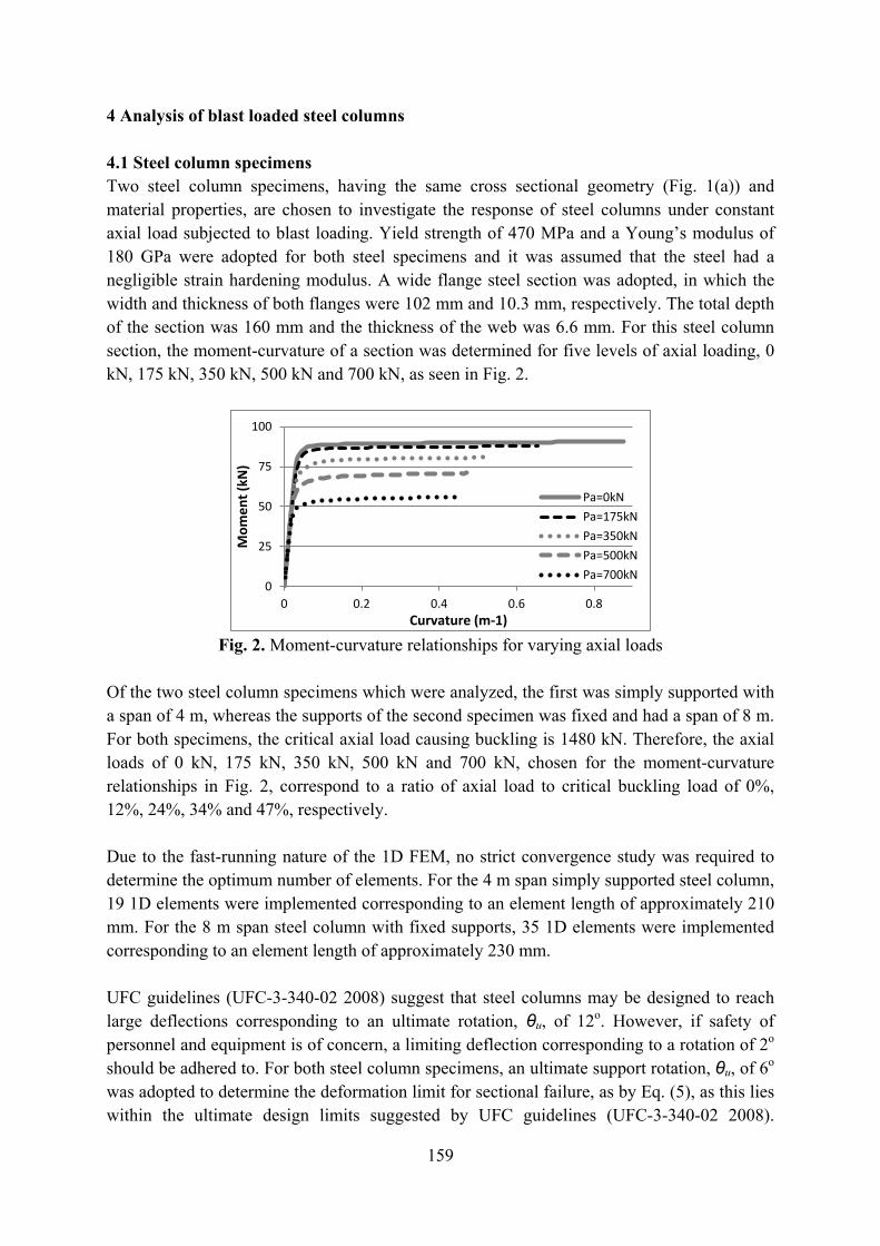
159

4 Analysis of blast loaded steel columns 4.1 Steel column specimens Two steel column specimens, having the same cross sectional geometry (Fig. 1(a)) and material properties, are chosen to investigate the response of steel columns under constant axial load subjected to blast loading. Yield strength of 470 MPa and a Young’s modulus of 180 GPa were adopted for both steel specimens and it was assumed that the steel had a negligible strain hardening modulus. A wide flange steel section was adopted, in which the width and thickness of both flanges were 102 mm and 10.3 mm, respectively. The total depth of the section was 160 mm and the thickness of the web was 6.6 mm. For this steel column section, the moment-curvature of a section was determined for five levels of axial loading, 0 kN, 175 kN, 350 kN, 500 kN and 700 kN, as seen in Fig. 2.

Fig. 2. Moment-curvature relationships for varying axial loads

Of the two steel column specimens which were analyzed, the first was simply supported with a span of 4 m, whereas the supports of the second specimen was fixed and had a span of 8 m. For both specimens, the critical axial load causing buckling is 1480 kN. Therefore, the axial loads of 0 kN, 175 kN, 350 kN, 500 kN and 700 kN, chosen for the moment-curvature relationships in Fig. 2, correspond to a ratio of axial load to critical buckling load of 0%, 12%, 24%, 34% and 47%, respectively. Due to the fast-running nature of the 1D FEM, no strict convergence study was required to determine the optimum number of elements. For the 4 m span simply supported steel column, 19 1D elements were implemented corresponding to an element length of approximately 210 mm. For the 8 m span steel column with fixed supports, 35 1D elements were implemented corresponding to an element length of approximately 230 mm. UFC guidelines (UFC-3-340-02 2008) suggest that steel columns may be designed to reach large deflections corresponding to an ultimate rotation, θu, of 12o. However, if safety of personnel and equipment is of concern, a limiting deflection corresponding to a rotation of 2o should be adhered to. For both steel column specimens, an ultimate support rotation, θu, of 6o was adopted to determine the deformation limit for sectional failure, as by Eq. (5), as this lies within the ultimate design limits suggested by UFC guidelines (UFC-3-340-02 2008).

0

25

50

75

100

0 0.2 0.4 0.6 0.8

Mom

ent (

kN)

Curvature (m-1)

Pa=0kN Pa=175kN Pa=350kN Pa=500kN Pa=700kN

160

Although a simple deformation limit for global instability cannot be provided, the deflection time history results obtained using the FEM can be used to determine whether global instability has caused the steel column to fail prematurely. Figs. 3(a) and 3(b) illustrate example deflection time histories of blast loaded steel columns undergoing sectional failure and failing prematurely due to global instability, respectively. In Fig. 3(a), the 8 m steel column with fixed supports under no axial load has been subjected to a blast load pressure time history with peak reflected pressure of 195 kPa and an almost infinite impulse. Global instability does not occur, but the steel column undergoes sectional failure at a mid-span deflection of 420 mm. However, in Fig. 3(b), the simply supported steel column with a span of 4 m subjected to an axial load of 350 kN has been subjected to a blast load pressure time history with peak reflected pressure of 183 kPa and an almost infinite impulse. Although sectional failure occurs at a mid-span deflection of 210 mm, global instability occurs at a mid-span deflection of 130 mm, causing the member’s acceleration to transition from negative to positive, leading to sectional failure.

(a) (b)

Fig. 3. Deflection time histories demonstrating sectional failure (a) and failure due to global instability (b)

4.2 Pressure impulse curves Due to the generality and numerical efficiency of the FEM, many simulations can be undertaken quickly. Therefore, entire PI curves could be generated in order to fully validate the SDOF approach to derive PI curves for steel columns. Fig. 4 contains PI curves for the 4 m span simply supported steel column, whereas Fig. 5 contains PI curves for the 8 m span steel column with fixed supports. The vertical asymptote of the PI curve represents the resistance of the steel column to impulse controlled blasts, in which the impulse of the blast load is the cause of failure as the duration of the blast load is much less than the quarter period of the member. The horizontal asymptote of the PI curve represents the resistance of the steel column to quasi-static blasts, in which the peak reflected pressure is the cause of failure as the duration of the blast load is much greater than the quarter period of the member. Therefore, as both the horizontal and vertical asymptotes of the PI curves in Figs. 4 and 5 decrease with increasing axial load, they illustrate that the axial load reduces the ability of a steel column to resist both impulse controlled and quasi-static blasts. Each of the PI curves within Figs. 4 and 5 are either represented by a dashed line or a bold line. The failure mechanism of sectional failure is represented by a bold line, whereas the failure mechanism

0

200

400

0 20 40 60

Defle

ctio

n (m

m)

Time (ms)

Deflection Time History

0

100

200

0 20 40 60

Defle

ctio

n (m

m)

Time (ms)

Deflection Time History

sectional failure sectional failure

global instability

161

of global instability is represented by a dashed line, of which examples can be seen in Figs. 3(a) and 3(b), respectively.

Fig. 4. Pressure Impulse Curves for 4m span simply supported steel column for varying axial

loads

Fig. 5. Pressure Impulse Curves for 8m span steel column with fixed supports for varying

axial loads

0

500

1000

1500

0 2000 4000 6000 8000 10000 12000 14000

Peak

Ref

lect

ed P

ress

ure

(kPa

)

Impulse (kPams)

Pressure Impulse Curves (4m span, simply supported)

Pa = 0kN

Pa = 175kN

Pa = 350kN

Pa = 500kN

Pa = 700kN

0

200

400

600

800

0 2000 4000 6000 8000 10000 12000 14000

Peak

Ref

lect

ed P

ress

ure

(kPa

)

Impulse (kPams)

Pressure Impulse Curves (8m span, fixed supports)

Pa = 0kN Pa = 175kN Pa = 350kN Pa = 500kN Pa = 700kN

= global instability = sectional failure

= global instability = sectional failure

162

Within Figs. 4 and 5 it can be observed that for larger axial loads, being 500 kN and 700 kN, failure is governed by global instability, but for smaller and no axial load, sectional failure is the overall failure mechanism. It should also be noted that for some PI curves, such as that corresponding to an axial load of 350 kN in Fig. 4 and those corresponding to axial loads of 175 kN and 350 kN in Fig. 5, the upper portion of these PI curves is bold, whereas the lower portion is dashed. This means that, for these steel column specimens, a blast load with a short duration causes sectional failure, whereas a long duration blast load causes global instability failure. The aforementioned PI curves are especially critical, as the SDOF approach to derive PI curves needs to be able to predict this behavior. 5 Single Degree of Freedom Approach The single degree of freedom approach is the simplest technique for determining a PI curve for a structural member. In particular, many studies have been conducted to derive non-dimensional, or normalized, PI curves which can be used to quickly derive a PI curve for a specific structural member with given properties (Li & Meng 2002a; Krauthammer et al. 2007; Dragos et al. 2013b). Fig. 6 illustrates a typical normalized PI curve. It is generic, such that it applies to any purely elastic structural member subjected to a blast with a triangular pulse load shape. It can be seen in Fig. 6 that both the vertical and horizontal asymptotes correspond to unity. Therefore, to convert this normalized PI curve to a PI curve corresponding to a given structural member, the I/Imin and Pr/Prmin axes need to be multiplied by Imin and Prmin, respectively. Eqs. (6) and (7) can be used to determine Imin and Prmin, respectively, for any structural member with any given resistance deflection (RΔ) function. It should also be noted that many studies have been conducted to derive non-dimensional or normalized PI curves for various pulse load shapes and various RΔ functions, such as elastic, elastic-plastic and elastic-plastic hardening (Li & Meng 2002b; Fallah & Louca 2006; Dragos et al. 2013b; Dragos et al. 2013c).

𝐼𝑚𝑖𝑛 = �2𝑀𝑒𝐸𝑅 (6)

𝑃𝑟𝑚𝑖𝑛 =𝐸𝑅𝑦𝑢

(7)

Where: Me = equivalent mass; yu = ultimate deflection; and ER = strain energy, or:

𝐸𝑅 = � 𝑅(𝑦)𝑑𝑦𝑦𝑢

0 (8)

Where: R(y) = RΔ function.

163

Fig. 6. Normalized PI curve for an elastic member subjected to a triangular pulse load

In order for this approach to be applied to steel columns, extensions need to be made to correctly account for the additional global instability failure mechanism and also to account for the influence of the PΔ effect. This will be done by determining a reduced resistance deflection (RrΔ) function from the original RΔ function. According to Timoshenko and Gere (1961) and Nassr et al. (2013), the general differential equation used to describe the motion of a SDOF system subjected to combined lateral and axial loading is:

𝑀𝑒�̈� + 𝑅(𝑦) = 𝐹(𝑡) +8𝑃𝑎𝐿𝑦 (9)

Where y is the deflection of the mid-span of the column and Pa is the compressive axial load and is positive. The final term in Eq. (9) represents an equivalent lateral load to take into account the influence of the PΔ effects, as it is a function of deflection, y. Eq. (8) can then be re-arranged to form the following:

𝑀𝑒�̈� + 𝑅(𝑦) −8𝑃𝑎𝐿𝑦 = 𝐹(𝑡) (10)

In which Eq. (11) is the reduced resistance deflection, RrΔ, function.

𝑅𝑟(𝑦) = 𝑅(𝑦) −8𝑃𝑎𝐿𝑦 (11)

According to Biggs (1964), and as adopted by UFC guidelines (UFC-3-340-02 2008), an elastic-plastic RΔ function, R(y), can be assumed for steel beams and columns. Therefore, Figs. 7(a) and 7(b) illustrate both the RΔ and RrΔ functions for steel beams and columns with supports which are pinned and fixed, respectively.

0

1

2

3

4

5

0 1 2 3 4 5 6 P r/

P rmin

I/Imin

Normalised PI Curve

164

(a) (b)

Fig. 7. RΔ and RrΔ functions for steel columns: simply supported (a) and fixed supports (b) Figs. 7(a) and 7(b) both illustrate the parameters required to form the RΔ functions for members with pinned and fixed supports. As provided by Biggs (1964), and as adopted by UFC guidelines (UFC-3-340-02 2008), Ru and Ry are the ultimate and yield resistances. ye is the elastic deflection capacity for a beam with pinned supports, whereas yel is the elastic deflection capacity for a beam with fixed supports and yep is the deflection at which plastic behavior begins for a beam with fixed supports. Finally, ys is the deflection capacity at which sectional failure occurs and can be determined using Eq. (5). ye, yel and yep can be determined from the elastic stiffness for simply supported beams, ke, elastic stiffness for beams with fixed supports, kel, and the elastic-plastic stiffness for beams with fixed supports, kep. Also, the trilinear RΔ function for beams with fixed supports, as seen in Fig. 7(b) can be converted to an equivalent bilinear RΔ function by determining an equivalent ye value. This is done by assuming that the equivalent bilinear RΔ function has the same area under its function as the trilinear RΔ function. To determine Imin in Eq. (6) and Prmin in Eq. (7) for steel columns under constant axial loading, Pa, the RΔ function needs to be substituted for the RrΔ function, seen in Eq. (11). Also, the ultimate deflection capacity, yu, needs to be determined. For a beam under no axial load, the ultimate deflection capacity, yu, is equal to the deflection at which sectional failure occurs, ys. However, as the axial load introduces a new failure mechanism, global instability, yu for a steel column is equal to the lesser of the deflection at which global instability (or buckling) occurs, yb, and ys. The deflection at which global instability occurs, yb, differs depending on the duration of the pressure time history. Fig. 8, which contains two example RrΔ functions, is used to illustrate the difference. For an infinitely short duration pressure time history, in which the impulse (Imin) causes failure, global instability occurs at a deflection in which the reduced resistance reaches 0. Therefore, it corresponds to the point in which the RrΔ function intercepts the y-axis, an example of which is illustrated by the point yb,i in Fig. 8. However, for an infinitely long duration pressure time history, in which the peak reflected pressure (Prmin) causes failure, global instability occurs at a slightly smaller deflection. Examples of which can be seen as yb,p in Fig. 8. Fig. 8 also illustrates examples of how the ultimate deflection, yu, should be chosen for determining Imin and Prmin. For RrΔ function 1, the ultimate deflection used to calculate Imin should be determined from ys, but the ultimate deflection used to calculate Prmin

0

Resi

stan

ce (R

)

Deflection (y)

RΔ & RrΔ Fns (simply supported)

0

Resi

stan

ce (R

)

Deflection (y)

RΔ & RrΔ Fns (fixed supports)

Ry Ru Ru

ye ys yel yep ys

RΔ

RrΔ

RΔ

RrΔ

165

should be determined from yb,p. For RrΔ function 2, the ultimate deflection used to calculate Imin should be determined from yb,i, but the ultimate deflection used to calculate Prmin should be determined from yb,p.

Fig. 8. Two typical RrΔ functions

As yb,i corresponds to the point in which the RrΔ function intercepts the y-axis, Eq. (12) can be used to calculate yb,i. This can be compared against ys to determine yu, which can then be used within Eqs. (8) and (6) to determine Imin.

𝑦𝑏,𝑖 =𝑅𝑢𝐿8𝑃𝑎

(12)

The reason why yb,p is not equal to, but less than, yb,i is because it corresponds to the deflection at which the reflected pressure of an infinitely long duration pressure time history surpasses the reduced resistance. yb,p can be obtained mathematically by determining Prmin as a function of y, instead of yu, and then by determining the global maximum of this function Prmin. Eq. (13) provides ER as a function of y.

𝐸𝑅(𝑦) = � 𝑅𝑟(𝑦)𝑑𝑦𝑦

0= � 𝑅𝑢 −

8𝑃𝑎𝑦𝐿

𝑑𝑦𝑦

𝑦𝑒+

12𝑦𝑒 �𝑅𝑢 −

8𝑃𝑎𝑦𝑒𝐿

� (13)

The integral within Eq. (13) can be evaluated to provide Eq. (14).

𝐸𝑅(𝑦) = 𝑅𝑢𝑦 −4𝑃𝑎𝑦2

𝐿−

12𝑅𝑢𝑦𝑒 (14)

Eqs. (7) and (14) can be used to determine Prmin as a function of y.

𝑃𝑟𝑚𝑖𝑛(𝑦) =𝐸𝑅(𝑦)𝑦

= 𝑅𝑢 −4𝑃𝑎𝑦𝐿

−12𝑅𝑢𝑦𝑒𝑦

(15)

0

Resi

stan

ce

Deflection

RrΔ Functions

RrΔ 1

RrΔ 2

yu (Prmin)

yu (Imin)

yb,p

yb,i

ys

166

To determine the global maximum of Prmin, the deflection at which the first derivative of Eq. (15) is zero needs to be obtained.

𝑑𝑃𝑟𝑚𝑖𝑛(𝑦)𝑑𝑦

= −4𝑃𝑎𝐿

+12𝑅𝑢𝑦𝑒𝑦2

= 0 (16)

Therefore, the solution to Eq. (16) is the deflection at which global instability occurs for an infinitely long duration pressure time history, yb,p, as seen in Eq. (17).

𝑦𝑏,𝑝 = �𝑅𝑢𝑦𝑒𝐿

8𝑃𝑎 (17)

It should also be noted that if yb,p, as in Eq. (17), is substituted for yu in Eqs. (8) and (7), Prmin(yb,p) equates to Rr(yb,p). Eqs. (12) and (17) apply to both the simply supported and fixed supports case in which the RrΔ functions are bilinear and trilinear, respectively. For the case of fixed supports, the trilinear RrΔ function needs to be converted to an equivalent bilinear RrΔ function by calculating an equivalent ye. To determine Imin, as in Eq. (6), the appropriate load-mass factor, KLM, also needs to be chosen to determine the equivalent mass, Me. From preliminary tests, it was found that the KLM factor corresponding to a uniformly distributed load acting on a beam with a purely plastic deformation shape provided the most suitable results. For either a beam or column with either pinned or fixed supports, a KLM factor of 0.66 is most suitable. In addition to calculating Imin and Prmin, an appropriate normalized or non-dimensional PI curve also needs to be chosen to determine the actual PI curve corresponding to a given steel column specimen. From testing, it was found that the axial load had a negligible effect on the shape of the normalized PI curve required to form an accurate PI curve. The only factors which needed to be considered when choosing an appropriate normalized PI curve were the shape of the pulse load and the inverse ductility, ye/yu. 6. Validation of Single Degree of Freedom Approach In order to validate the SDOF approach, PI curves determined using this approach are compared against those determined using the FEM. The previous steel column specimens analyzed using the FEM are analyzed using the SDOF approach to determine the same PI curves seen in Figs. 4 and 5. In order to determine the RΔ and RrΔ functions, the ultimate moment, Mu, elastic flexural rigidity, EI, and span, L, are required. The elastic flexural rigidity and span are known, but the ultimate moment for each level of axial loading was determined using Fig. 2. Figs. 9(a) and 9(b) illustrate the RrΔ functions for both steel column specimens, the 4 m span simply supported and 8 m span steel member with fixed supports,

167

respectively. For each specimen, sectional failure was assumed to occur when a support rotation of 6o was reached.

(a)

(b)

Fig. 9. RrΔ functions for 4 m simply supported (a) and 8 m span steel column with fixed supports (b)

Figs. 9(a) and 9(b) both show that, for an infinitely long duration load, instability is the cause of failure for all axial load levels except that corresponding to 0 kN. The Figures also show that, for an infinitely short duration load, instability is the cause of failure for the 500 kN and 700 kN axial load levels, whereas sectional failure occurs for all other levels of axial load. It can also be seen that the larger the magnitude of the axial load, the lesser the strain energy, Er, is. To determine PI curves for each of the RrΔ functions in Figs. 9(a) and 9(b), Imin and Prmin were calculated and the inverse ductility of each RrΔ function was used to obtain the normalized PI curve corresponding to a triangular pulse load shape. Figs. 10 and 11 illustrate PI curves for both steel column specimens, the 4 m span simply supported and 8 m span steel member with fixed supports, respectively. For each of the figures, the actual PI curves

0

50

100

150

200

0 50 100 150 200

Resi

stan

ce (k

N)

Deflection (mm)

RrΔ Functions (4m span - simply supported)

Pa = 0kN Pa = 175kN Pa = 350kN Pa = 500kN Pa = 700kN yu (Prmin) yu (Imin)

0

50

100

150

200

0 100 200 300 400

Resi

stan

ce (k

N)

Deflection (mm)

RrΔ Function (8m span - fixed supports)

Pa = 0kN Pa = 175kN Pa = 350kN Pa = 500kN Pa = 700kN yu (Prmin) yu (Imin)

168

represent that obtained using the SDOF approach, where as the bold points represent points on the PI curve determined using the FEM, seen in Figs. 4 and 5.

Fig. 10. Validation of pressure impulse curves for 4m span simply supported steel column for

varying axial loads

Fig. 11. Validation of pressure impulse curves for 8m span steel column with fixed supports

for varying axial loads It can be seen that the differences between the PI curves determined using the SDOF approach and the FEM are negligible for the simply supported column, seen in Fig. 10.

0

500

1000

1500

0 2000 4000 6000 8000 10000 12000 14000

Peak

Ref

lect

ed P

ress

ure

(kPa

)

Impulse (kPa ms)

Pressure Impulse Curves (4m span - simply supported)

Pa = 0kN

Pa = 175kN

Pa = 350kN

Pa = 500kN

Pa = 700kN

FEM

0

500

1000

0 2000 4000 6000 8000 10000 12000 14000

Peak

Ref

lect

ed P

ress

ure

(kPa

)

Impulse (kPams)

Pressure Impulse Curves (8m span - fixed supports) Pa = 0kN

Pa = 175kN

Pa = 350kN

Pa = 500kN

Pa = 700kN

FEM

169

However, the differences between the PI curves in Fig. 11 are noticeable but not significant. The reason for this slight difference is because the RΔ function for a steel member with fixed supports is trilinear but when determining the normalized PI curves, it was assumed that the RΔ functions were bilinear. It should be noted that, despite the slight but noticeable differences within Fig. 11, the errors are within 6%. Tables 1 and 2 show the calculated Imin and Prmin values determined using both the SDOF approach and the FEM for both steel specimens.

Table 1. Comparison of Imin and Prmin values for 4 m span simply supported steel column

Pa (kN) Prmin (kPa) Imin (kPams)

SDOF FEM % Error SDOF FEM % Error 0 368.5 (s) 361.2 (s) 2.0 4851.2 (s) 4910.4 (s) 1.2

175 271.4 (i) 268.5 (i) 1.1 4138.4 (s) 4197.6 (s) 1.4 350 190.1 (i) 183.0 (i) 3.9 3072.4 (s) 3147.2 (s) 2.4 500 130.9 (i) 123.9 (i) 5.6 2030.7 (i) 2113.4 (i) 3.9 700 72.8 (i) 68.5 (i) 6.2 1148.0 (i) 1185.0 (i) 3.1

Note: (s) = sectional failure, (i) = global instability failure

Table 2. Comparison of Imin and Prmin values for 8 m span steel column with fixed supports

Pa (kN) Prmin (kPa) Imin (kPams)

SDOF FEM % Error SDOF FEM % Error 0 187.7 (s) 195.0 (s) 3.8 4896.5 (s) 4840.0 (s) 1.2

175 138.9 (i) 145.0 (i) 4.2 4192.1 (s) 4126.7 (s) 1.6 350 96.9 (i) 100.7 (i) 3.7 3128.7 (s) 3102.7 (s) 0.8 500 68.0 (i) 69.4 (i) 2.1 2108.8 (i) 2078.3 (i) 1.5 700 38.9 (i) 39.4 (i) 1.1 1206.6 (i) 1165.0 (i) 3.6

Note: (s) = sectional failure, (i) = global instability failure The importance of Tables 1 and 2, is that they demonstrate that the errors associated with the SDOF approach when determining Imin and Prmin are minimal. They also demonstrate that, for each case, the SDOF approach was able to accurately predict which failure mechanism was the cause of failure. Various factors contribute to the errors within Tables 1 and 2, such as the choice of ultimate moment, Mu, the choice of the load-mass factor, KLM, and the fact that the SDOF approach assumes a bilinear or trilinear RΔ function. In order to make a deeper comparison, the PI curve corresponding to an axial load of 350 kN in Fig. 4 was extracted and can be seen in Fig. 12(a). Fig. 12(b) illustrates three deflection time histories, determined using the FEM, of the steel column subjected to three blast loads corresponding to points A, B and C, on the PI curve seen in Fig. 12(a). Point A corresponds to an infinitely short duration blast load, point B corresponds to a blast load in which the duration is comparable with the quarter period of the member, whereas point C corresponds to an infinitely long duration blast load. The deflection time histories in Fig. 12(b) can be

170

compared against the RrΔ function in Fig. 9(a), corresponding to an axial load of 350 kN, to further verify the SDOF approach.

(a)

(b)

Fig. 12. Pressure impulse curve (a) and three corresponding deflection time histories (b) for 4m span simply supported steel column with 350kN axial load

Each of the deflection time histories in Fig. 12(b) illustrates that sectional failure occurs at a deflection of approximately 205 mm. However, the deflection time history in Fig. 12(b) corresponding to point C demonstrates that global instability is the cause of failure for this blast load, occurring at a deflection of approximately 110 mm, whereas the deflection time histories corresponding to points A and B demonstrate that for these blast loads, sectional failure is the overall failure mechanism. These results correspond well with the associated RrΔ function seen in Fig. 9(a), as according to this function, for an infinitely long duration blast load, global instability is the cause of failure and occurs at a deflection of 108 mm. Also, for an infinitely short duration blast load, sectional failure is the controlling failure mechanism and occurs at a deflection of 209 mm. In order to analyze the deflection at which global instability occurs for a given steel column subjected to blasts with various durations, the PI curve corresponding to a 700 kN axial load seen in Fig. 4 was extracted and can be seen in Fig. 13(a). Fig. 13(b) illustrates three deflection time histories, determined using the FEM, of the steel column subjected to three blast loads corresponding to points A, B and C, on the PI curve seen in Fig. 13(a). The deflection time histories in Fig. 13(b) can be compared against the RrΔ function in Fig. 9(a), corresponding to an axial load of 700 kN, to further verify the SDOF approach.

0

500

1000

0 5000 10000 15000 20000

Pr (k

Pa)

Impulse (kPams)

Pressure Impulse Curve

0

100

200

0 10 20 30 40 50

Defle

ctio

n (m

m)

Time (ms)

Deflection Time Histories

Point A Point B Point C

global instability sectional failure

Point C Point B Point A

171

(a)

(b)

Fig. 13. Pressure impulse curve (a) and three corresponding deflection time histories (b) for 4m span simply supported steel column with 700kN axial load

Each of the deflection time histories in Fig. 13(b) illustrates that sectional failure occurs at a deflection of approximately 205 mm, however, the cause of failure for each deflection time history is global instability. While for the deflection time histories corresponding to Points A and B, global instability occurs at a deflection of approximately 75 mm, for the deflection time history corresponding to Point C, global instability occurs at a deflection of approximately 55 mm. This corresponds to a deflection which is approximately 25% less than that for blast loads corresponding to points A and B in Fig. 13(a). This demonstrates that for an infinitely long duration blast load, global instability occurs at a smaller deflection then for a shorter duration blast load. These results also correspond well with the associated RrΔ function seen in Fig. 9(a), as according to this function, for an infinitely long duration blast load, global instability occurs at a deflection of 70 mm. Also, for an infinitely short duration blast load, global instability occurs at a deflection of 49 mm. Figs. 10 - 13 all demonstrate that the SDOF approach can accurately predict the behaviors seen using the FEM. In addition to this, by being able to determine the appropriate RrΔ function, it also explains why the observed behavior occurs. Nassr et al. (2013) undertook a study on steel columns under axial loads subjected to blasts. One conclusion of this study was that, while the axial load severely affects the pressure asymptote (Prmin), it has less effect on the impulsive asymptote (Imin). The SDOF approach provided in the current study explains why this is so, as it can be seen in Figs. 9(a) and 9(b) that, for an infinitely long duration blast

0

200

400

600

800

0 2000 4000 6000 8000

Pr (k

Pa)

Impulse (kPams)

Pressure Impulse Curve

0

50

100

150

200

0 20 40 60

Defle

ctio

n (m

m)

Time (ms)

Deflection Time Histories

Point A Point B Point C

global instability sectional failure

Point C Point B

Point A

172

load, global instability occurs at a much lower deflection in comparison to that for an infinitely short duration blast load. The approach can also accurately predict which failure mechanism will control failure, and why it is the cause of failure. Therefore, despite its simplicity, it is a very useful approach. So far, all PI curves shown in the current study have corresponded to a blast pulse load shape which is triangular. In order to further verify the SDOF approach, the blast pulse load shape was modified to be exponential. The function provided by Li & Meng (2002a) for a free-air blast pulse load shape, with parameters; γ = 4, and λ = 1 were adopted to define the exponential blast pulse load. For this exponential pulse load shape, the SDOF approach was used to determine a new PI curve for the simply supported 4 m span steel columns under a 350 kN axial load. This was done by determining a new normalized PI curve for the exponential pulse load from studies such as Dragos et al. (2013b) or Li & Meng (2002a). The FEM was then modified to determine points along the same PI curve. Fig. 14 provides PI curves for the simply supported 4 m span steel columns under a 350 kN axial load subjected to both a triangular and exponential pulse load shape. The actual curves represent that obtained using the SDOF approach, whereas the bold points represents points determined using the FEM.

Fig. 14. Pressure impulse curves for 4m span simply supported steel column with 350 kN

axial load Fig. 14 illustrates the significant difference between PI curves corresponding to triangular and exponential pulse load shapes. However, Fig. 14 also shows that, despite this difference, the SDOF approach can accurately account for the influence of different pulse load shapes on the PI curve. Conclusion A numerically efficient structural response model for determining the global response of steel columns against blast loads was developed by incorporating a moment-curvature analysis

0

200

400

600

800

1000

1200

0 2000 4000 6000 8000 10000

Peak

Ref

lect

ed P

ress

ure

(kPa

)

Impulse (kPa ms)

PI Curves (4m span - simply supported)

FEM Exp Pulse Load (SDOF) Tri Pulse Load (SDOF)

173

into a 1D FE framework. The FEM was then used to determine PI curves for two steel column specimens under various levels of axial loading, taking into account two failure mechanisms, sectional failure and global instability and the influence of the PΔ effects. A simple SDOF approach was then presented, relying on the newly proposed concept of the reduced resistance deflection function, to be used in conjunction with normalized, or non-dimensional, PI curves, to determine PI curves for steel columns. It is shown that the reduced resistance deflection function can be used to determine which failure mechanism will cause failure for each of the quasi-static and impulse controlled asymptotes of a PI curve. Then, the SDOF approach is thoroughly validated against PI curves determined using the aforementioned FEM. It is shown that the SDOF approach for determining PI curves can accurately account for the influence of the PΔ effects, can predict the failure mechanism causing failure, can reasonably estimate the deflection at which global instability occurs, and can also accurately determine PI curves corresponding to different blast pulse load shapes. References 1. American Society of Civil Engineers (ASCE) (1997). Design of blast resistant buildings

in petrochemical facilities. Reston, VA. 2. American Society of Civil Engineers (ASCE) (2008). Blast Protection of Buildings.

Ballot version 2, Reston, VA. 3. Bathe, K.J. (1996). Finite Element Procedures, Prentice Hall, USA. 4. Biggs, J.M. (1964). Introduction to structural dynamics. McGraw-Hill Book Company,

USA. 5. Dragos, J., Wu, C., Haskett, M., Oehlers, D.J. (2013a). Derivation of normalized

pressure impulse curves for flexural ultra high performance concrete slabs. Journal of Structural Engineering, ASCE, 139 (6), 875-885.

6. Dragos, J., Wu, C. (2013b). A new general approach to derive normalised pressure impulse curves. International Journal of Impact Engineering, 62 (2013), 1-12.

7. Dragos, J., Wu, C. (accepted 2013c). Application of normalized pressure impulse diagrams for vented and unvented confined blasts. Journal of Engineering Mechanics, ASCE.

8. Fallah, A.S., Louca, L.A. (2006). Pressure-impulse diagrams for elastic-plastic-hardening and softening single-degree-of-freedom models subjects to blast loading. International Journal of Impact Engineering, 34 (4), 823-842.

9. Jama, H. H., Bambach, M. R., Nurick, G. N., Grzebieta, R. H., Zhao, X. L. (2009). Numerical modelling of square tubular steel beams subjected to transverse blast loads. Thin-Walled Structures, 47 (12), 1523-1534.

10. Jones, J., Wu, C., Oehlers, D.J., Whittaker, A.S., Marks, S., Coppola, R. (2009). Finite difference analysis of RC panels for blast effects. Engineering Structures, 31 (12), 2825-2832.

11. Krauthammer, T., Assadi-Lamouki, A., Shanaa, H.M. (1993). Analysis of Impulsively Loaded Reinforced Concrete Structural Elements – I. Theory. Computers & Structures, 48 (5), 851-860.

174

12. Krauthammer, T., Astarlioglu, S., Blasko, J., Soh, T.B., Ng, P.H. (2007). Pressure-impulse diagrams for the behavior assessment of structural components. International Journal of Impact Engineering, 35 (8), 771-783.

13. Li, Q.M., Meng, H. (2002a). Pressure-Impulse Diagram for Blast Loads Based on Dimensional Analysis and Single-Degree-of-Freedom Model. Journal of Engineering Mechanics, 128 (1), 87-92.

14. Li, Q.M., Meng, H. (2002b). Pulse loading shape effects on pressure-impulse diagram of an elastic-plastic, single-degree-of-freedom structural model. International Journal of Mechanical Sciences, 44 (9), 1985-1998.

15. Livermore Software Technology Corporation (LSTC). (2003). LS-DYNA Keyword User’s Manual. Version 970. Non Linear Dynamic Analysis of Structures in Three Dimensions. LSTC, Livermore, USA.

16. Mutalib, A.A., Hao, H. (2010). Development of P-I diagrams for FRP strengthened RC columns. International Journal of Impact Engineering, 38 (2011), 290-304.

17. Nassr, A.A., Razaqpur, A.G., Tait, M.J., Campidelli, M., Foo, S. (2010). Measured versus Predicted Response of Steel Beams under Blast Load. First International Conference of Protective Structures, Manchester, UK.

18. Nassr, A.A., Razaqpur, A.G., Tait, M.J., Campidelli, M., Foo, S. (2012). Experimental Performance of Steel Beams under Blast Loading. Journal of Performance of Constructed Facilities, 25 (5), 600-619.

19. Nassr, A.A., Razaqpur, A.G., Tait, M.J., Campidelli, M., Foo, S. (2013). Strength and stability of steel beam columns under blast load. International Journal of Impact Engineering, 55 (2013), 34-48.

20. Shi, Y., Hao, H., Li, Z. (2008). Numerical Derivation of pressure-impulse diagrams for prediction of RC column damage to blast loads. International Journal of Impact Engineering, 35 (2008), 1213-1227.

21. Shi, Y., Li, Z., Hao, H. (2010). A new method for progressive collapse analysis of RC frames under blast loading. Engineering Structures. 32 (6), 1691-1703.

22. Timoshenko, S.P., Gere, J.M. (1961). Theory of elastic stability. Mcgraw-Hill Inc., USA. 23. UFC-3-340-02. (2008). Structures to Resist the Effect of Accidental Explosions. US

Department of the Army, Navy and Air Force Technical Manual. 24. Urgessa, G.S., Maji, A.K. (2010). Dynamic response of retrofitted masonry walls for

blast loading. Journal of Engineering Mechanics-ASCE, 136 (7), 858-864. 25. Wang, W., Zhang, D., Lu, F. (2012). The influence of load pulse shape on pressure-

impulse diagrams of one-way RC slabs. Structural Engineering and Mechanics, 42 (3), 363-381.

26. Weaver, W., Timoshenko, S.P. (1990). Vibration Problems in Engineering. Fifth Ed. Wiley, New York.

27. Ye, Z.Q., Ma, G.W. (2007). Effects of foam claddings for structure protection against blast loads. Journal of Engineering Mechanics-ASCE, 133 (1), 41-47.

28. Zhou, X.Q., Kuznetsov, V.A., Hao, H., Waschl, J. (2008). Numerical prediction of concrete slab response to blast loading. International Journal of Impact Engineering, 35 (2008),1186–1200.

175

Statement of Authorship Interaction between Direct Shear and Flexural Responses for Blast Loaded Reinforced Concrete Slabs using a Finite Element Model (2014) Engineering Structures Publication status: Accepted for publication Dragos, J. (candidate) Developed model, performed all analyses and prepared manuscript. I hereby certify that the statement of contribution is accurate Signed……………………………………………………………………..Date……………… Wu, C. Supervised research and provided critical manuscript evaluation. I hereby certify that the statement of contribution is accurate and I give permission for the inclusion of the paper in the thesis Signed……………………………………………………………………..Date………………

176

Interaction between Direct Shear and Flexural Responses for Blast Loaded Reinforced Concrete Slabs using a Finite Element Model

Jonathon Dragos, Chengqing Wu

Abstract

In this paper, both the moment-curvature flexural behavior and the direct shear behavior are incorporated into a numerically efficient one dimensional finite element model, utilizing Timoshenko Beam Theory, to determine the member and direct shear response of reinforced concrete slabs subjected to blasts. The model is used to undertake a case study to demonstrate the flexural member response behavior during the direct shear response and is then used to carry out a parametric study to better understand the interaction of the flexural member response and the direct shear response. This is done by comparing pressure impulse curves corresponding to direct shear failure for reinforced concrete slabs with varying depth, span and support conditions. The results aim to provide insight to facilitate the development of more accurate simplified methods for determining the direct shear response of blast loaded reinforced concrete members, such as the single degree of freedom method. Keywords: Blast load; Structural response; Numerical analysis; Direct shear 1. Introduction The single degree of freedom (SDOF) method is a first order method, typically used to determine the response of structural members subjected to blasts. Due to its relative accuracy, despite its simplicity, it is widely referenced in guidelines such as the most recent guidelines of UFC 3-340-02 [1] and ASCE guidelines [2-3] for undertaking simple analyses. It was first introduced as a method to determine the flexural response of steel and reinforced concrete (RC) beams and slabs subjected to blasts [4] but has since been extended to account for additional behaviors, failure mechanisms and types of structural members. For example, Park and Krauthammer [5] and Nassr et al. [6] extended the SDOF method to account for the P-Δ effects associated with axial loads acting on columns. Krauthammer [7] and Astarlioglu et al. [8] extended the SDOF method to account for both the flexural and the tensile membrane behaviors in a single analysis technique. The SDOF method has also been extended to determine the response of masonry walls [9-10] and even for determining the response RC beams and slabs retrofitted with foam cladding [11] subjected to blasts. According to many studies, it has been observed experimentally that a RC structural member can undergo shear failure at the supports, commonly referred to as direct shear failure [7,12]. This failure mechanism occurs due to a high amplitude blast loading caused by the detonation of a charge which is in close proximity to the RC specimen. Therefore, much effort has been invested to extend the SDOF method for determining the direct shear response of RC members subjected to blasts. For example, Krauthammer et al. [12] and Krauthammer et al. [13] developed a SDOF approach which analyses the direct shear and flexural responses separately using two differential equations. Although the equations governing the direct shear and flexural responses are not directly coupled, the shear force which drives the direct shear response is determined based on the loading, total inertial force and the distribution of inertial

177

forces at each time step during the flexural member response. Low and Hao [14] also utilized a similar SDOF approach in which the direct shear response is determined separately from the flexural member response, but is determined based on the loading, inertial force of the member, and the deflection profile of the member which is calculated from the flexural response. Although such SDOF methods have been developed, no research has been undertaken to thoroughly validate these methods. Also, very little research has been conducted to determine how the response of the member itself, being the flexural response, influences the direct shear response. Furthermore, studies have been conducted on rigid-plastic beams having both rigid-plastic direct shear behavior and rigid-plastic flexural behavior [15-16] in which a fully coupled analytical approach was used to determine both the direct shear and midspan flexural deflection responses. However, as this can only be applied to rigid-plastic beams, with rigid-plastic direct shear slip and moment-rotation relationships for shear and rotational hinges, respectively, they cannot be applied directly to RC or steel specimens. In this paper, the flexural behavior of a RC cross-section and the direct shear slip behavior are both incorporated into a one-dimensional (1D) finite element model (FEM). The 1D FEM simulates a dynamic analysis by discretizing the member into 1D beam elements and applying Timoshenko Beam Theory [17]. Although other more comprehensive models exist [18-20], the 1D FEM is adopted due to its numerical efficiency, making it a suitable model for undertaking large parametric studies. However, despite its numerical efficiency it has advantages over other numerical techniques, such as the finite difference method [21-23], due to its generality, solution accuracy and stability [24]. The flexural behavior is determined using a regular moment-curvature analysis and the direct shear slip behavior is determined using the proposed model by Krauthammer et al. [12], based on the research conducted by Hawkins [25], Mattock [26], and Walraven and Reinhardt [27]. Also, artificial shear springs are implemented into the 1D FEM to account for the direct shear slip response at the support. The moment-curvature analysis, direct shear model and 1D FEM are first described and a case study is undertaken to investigate the RC flexural member response during the very short timescale at which the direct shear response occurs. Then, due to the numerical efficiency of the 1D FEM, a parametric study is undertaken to investigate the influence of the depth, span and support conditions on the direct shear response. This investigation is undertaken by comparing pressure impulse (PI) curves corresponding to direct shear failure. Then, a loose comparison between the results of the parametric study and the analytical solutions by Ma et al. [16] on rigid-plastic beams is made. Finally, a small comparison is made between two direct shear models which identifies the effect of the softening region of the direct shear model on the direct shear PI curve. The aim of the current study is to investigate the influence of the flexural behavior and geometric properties on the direct shear response and failure of RC slabs. By doing this, the investigation endeavors to provide some insight into the structural dynamics mechanisms and their effects, which need to be accounted for when modeling the direct shear response of RC slabs using an SDOF approach or other simplified approaches.

178

2. Moment-curvature analysis of a section A traditional moment-curvature analysis is used to determine the flexural behavior of a cross-section, as seen in Fig. 1. As seen in Fig. 1(b), a linear strain profile over the depth of the section was assumed as by Euler Bernoulli Theory [28], in which the curvature, χ, can be determined as the slope of this function. From the linear strain profile, Popovics' compressive concrete stress strain relationship [29] was used to determine the concrete compressive stress and the stress in the reinforcing bars were determined from a typical steel stress strain relationship, to form the stress profile in Fig. 1(c). From the stress profile, the force profile in Fig. 1(d) can also be determined. For a given compressive strain acting on the extreme compressive fiber, corresponding to point a in Fig. 1(b), the curvature was altered until equilibrium was achieved. It should be noted that, adjusting the curvature, while keeping the curvature at point a constant, causes a shift in the position of the neutral axis. For this case, equilibrium corresponded to the condition in which the sum of the forces, seen in Fig. 1(d), equated to zero. For a section in equilibrium, the sum of the moment due to each of the forces corresponds to the resisting moment, M. To plot a single point on the moment-curvature relationship, for a given value of strain at the extreme compressive fiber, a, equilibrium was first determined and then the curvature, χ, and resisting moment, M, were plotted. This process was repeated for various values of strain at the extreme compressive fiber, a, to produce many points, thus forming the moment-curvature relationship.

Fig. 1. Moment-curvature analysis for a RC section 3. Direct shear slip function The support slip, due to a vertical crack forming at the support, is governed by the direct shear force - slip function. The functions being utilized within this model, seen in Fig. 2, are fully outlined by Krauthammer et al. [12]. The entire function provided by Krauthammer et al. [12] consists of a tri-linear ascending region, a linear softening region and a constant shear force region, which remains constant until failure is reached. According to Krauthammer et al. [12], the behavior of the third constant shear force region is based on a model only applicable to large deformations of a well anchored bar embedded in concrete and will therefore be ignored in this study. Fig. 2(a) shows the tri-linear ascending region of the direct shear slip function, whereas Fig. 2(b) shows both the ascending and the softening regions of

(a) cross section (b) strain (c) stress (d) force

M

ε σ P a

χ

Preinf-tens

Pcon-comp Preinf-comp

179

the direct shear slip functions. The yield shear force, Vy, ultimate shear force, Vu, and slope of the softening region, ks, in Figs. 2(a) and 2(b) can all be determined using the equations provided in Krauthammer et al. [12]. In Fig. 2(a), the ultimate support slip at which failure occurs, yv,u, is equal to 0.6 mm. In Fig. 2(b), the ultimate support slip at which failure occurs, yv,u, can be calculated based on the slope of the softening region, ks, and the ultimate shear force, Vu.

(a) (b)

Fig. 2. Direct shear slip function without softening region (a) and with softening region (b) The parametric study within section 6 will utilize only the ascending region of the direct shear slip function, seen in Fig. 2(a), whereas the study in section 7 will utilize both the ascending and softening regions of the direct shear slip function, seen in Fig. 2(b). 4. Finite element model To determine the dynamic response of a RC beam or slab subjected to blast loading, a 1D finite element method is utilized. The FEM divides the member into several beam elements to which Timoshenko Beam Theory [17] is applied. Timoshenko Beam Theory is adopted as it allows for both flexural and shear deformation, as well as rotational inertia, as seen in Eqs. (1) and (2).

2

2

tIQ

xM

m ∂∂

−=−∂∂ βρ (1)

2

2

tvAq

xQ

m ∂∂

=+∂∂ ρ (2)

Where: M = applied bending moment, Q = applied shear force, q = distributed load acting transverse to the beam, A = cross sectional area, I = moment of inertia of the beam, ρm = mass density of the beam, β = rotation and v = transverse displacement. The finite element method solves Eqs. (1) and (2) in their weak forms. The governing weak form equation can be expressed in matrix form as seen in Eq. (3):

0 0

Shea

r for

ce -

V

Support slip - yy

Direct shear slip function - ascending

0 0

Shea

r for

ce -

V Support slip - yy

Direct shear slip function - softening

0.1m

0.3m

yv,u = 0.6mm yv,u

Vu

Vy

Vu

Vy

0.6mm

ks 1

180

[𝐾]{𝛿} + [𝑀]��̈�� = {𝑃} (3)

Where: [K] = stiffness matrix, [M] = mass matrix, {δ} = displacement vector, {δ } = acceleration vector and {P} = load vector. Eq. (3) is solved at each time interval using the Newmark method [30]. Due to the material non-linearity of the problem, a modified Newton-Raphson method is adopted to update the displacement vector at each time step [30]. Each of the terms in Eq. (3) corresponds to the member at a global level. Therefore, at each time interval, the stiffness matrix, mass matrix and load vector need to be determined at the element level and are used to assemble these matrices and vectors at the global level. A three node isoparametric beam element, having a quadratic shape function, is adopted for its associated stability. Equations for the stiffness matrix, geometric stiffness matrix, mass matrix and load vector at the element level can all be derived using the principle of virtual work. The integration, which is required to determine each matrix and vector, is then undertaken using gauss quadrature [30]. To determine the stiffness matrix at each time step, the non-linear curvature dependant flexural rigidity and the linear shear rigidity are required. During loading, the flexural rigidity is determined directly from the moment-curvature relationship. During unloading, a separate linear unloading curve is assumed. The slope of the unloading curve is assumed to be equal to that of the elastic region of the moment-curvature relationship, corresponding to an analysis in which the tensile region of the concrete section is cracked. To account for the translational slip occurring at the supports, governed by the non-linear direct shear slip function, a simple two-node interfacial element is required which acts as a transverse spring. The same approach to include a transverse spring was applied by Wu and Shiekh [24], however, this was applied to include a rotational spring to represent the plastic hinge region at the midspan of a beam. In the current study, the adopted two-node interfacial element has no length and is situated between the support and the end of the specimen, on both ends, allowing the ends of the specimen to deflect. At each time step, the non-linear stiffness of the two-node interfacial element, representing the transverse spring, needs to be determined. During loading, the translational stiffness of the two-node interfacial element is determined directly from the non-linear direct shear slip function. During unloading, a separate linear unloading curve with a slope equal to that of the elastic region of the function, seen as the slope of the region which is less than 0.1 mm in Fig. 2(a), is assumed. When a RC specimen is subjected to a blast load, the strain rate effects cause the material to have a slightly larger resisting stress [31-32]. The main technique to account for such effects in a numerical analysis is by increasing the moment-curvature relationship and direct shear slip function by applying a Dynamic Increase Factor (DIF). Whether strain rate effects are implemented within the model will have little effect on the outcomes of the parametric study. For this reason, it was decided not to include strain rate effects within the overall model.

181

Linear shear stress-strain theory is used to determine the shear rigidity along the span of the member between the supports. The shear stress-strain relationship, as in Eq. (4), calculates the shear force, Q, from the shear strain.

xzxz KAGKAQ γσ == (4) Where: G = shear stiffness, σxz = shear stress, γxz = shear strain and K = correction factor, which is used to take into account the constant cross sectional shear stress assumption. K = π2⁄12 for rectangular cross sections, as given by Krauthammer et al. [23]. To be consistent with UFC guidelines [1], a midspan deformation criterion is used to determine flexural failure of the RC specimen. The midspan deflection at which flexural failure occurs, yf,u, can be determined from the ultimate support rotation, θu, using the following equation:

𝑦𝑓,𝑢 = 𝜃𝑢�𝐿 2� � (5)

Where: L = span of the member. Eq. (5) assumes a perfectly plastic deformation shape which is an appropriate assumption for RC slabs at deflections approaching ultimate. 5 Dynamic analysis of blast loaded reinforced concrete slabs 5.1 Reinforced concrete specimens A total of six RC specimens were analyzed within the investigation. The concrete and steel material properties of all six RC specimens are the same. However, the depth, span and support conditions were altered to produce six difference RC specimens. The concrete had a compressive strength of 50 MPa with an assumed strain of 0.005 corresponding to the maximum compressive stress. The steel had a yield strength of 600 MPa and a Young's modulus of 200 GPa with a negligible strain hardening modulus. For each specimen, compression reinforcement was utilized in amount equal to the tension reinforcement. Finally, a unit width of 1 m was adopted for each specimen. Table 1 outlines the varying properties of the six RC specimens.

Table 1. List of RC specimens used within investigation Specimen Code

Depth (mm)

Span (m)

Support conditions

Reinforcing Ratio (%)*

L1 D400 400 1 Pinned 2.4 L2 D400 400 2 Pinned 2.4 L4 D400 400 4 Pinned 2.4 L2 D200 200 2 Pinned 2.4 L2 D100 100 2 Pinned 2.4 L2 D400 F 400 2 Fixed 2.4

*Note: Reinforcing ratio corresponds to total of compression and tension reinforcement

182

Due to the fast-running nature of the 1D FEM, no strict convergence study was required to determine the optimum number of elements. Element lengths of approximately 100 mm were implemented as it was found that using elements of smaller length had negligible effect on the results. The time steps adopted ranged from 10-7 s to 10-4 s. For determining the overall mid-span deflection time history response, governed mostly by the flexural behavior, usage of a time step less than 10-4 s had minimal effect on the results. However, determination of the support slip time history, governed mostly by the direct shear slip function, required the use of a smaller time step to obtain accurate results. For determining the support slip response, a time step ranging from 10-6 to 10-7 was utilized. Section 4-25 of UFC guidelines [1] suggests that for a RC specimen containing stirrups, it may be designed to reach an ultimate midspan deflection, yf,u, corresponding to an ultimate support rotation, θu, of 6o. However, it is also stated that with enough lateral restraint of the steel reinforcement, tensile membrane action can occur, allowing the specimen to be designed to reach an ultimate midspan deflection corresponding to an ultimate support rotation, θu, of 12o. According to section 4-25 of UFC guidelines, at a support rotation of 6o flexural response would cease and the tensile membrane action would govern the response. However, in order to provide a conservative but simplified analysis, UFC guidelines assume that the flexural behavior governs the response from 0o to 12o support rotation. For these reasons, an ultimate midspan deflection corresponding to an ultimate support rotation of 12o was adopted to signify flexural failure and the tensile membrane action was ignored. Furthermore, the flexural behavior is assumed to provide moment resistance up until flexural failure. It should also be noted that direct shear failure is signified by the support slip, yv, reaching the ultimate support slip, yv,u, seen on the direct shear slip functions in Fig. 2. 5.2 Response of reinforced concrete specimens The specimen L2 D400 was subjected to a blast load pressure time history having a peak reflected pressure of 62000 kPa and an Impulse of 10340 kPams. As the pulse shape of the pressure time history was triangular, the duration was 0.334 ms. Figs. 3(a) and 3(b) illustrate both the midspan deflection time histories and the support slip time histories, respectively, of L2 D400 subjected to the aforementioned blast load. The midspan deflection and support slip time histories are denoted as the flexural and direct shear responses, respectively. This is because the midspan deflection time history is used to determine if flexural failure occurs and the support slip time history is used to determine if direct shear failure occurs. In Fig. 3(a), the grey line corresponds to the midspan deflection, whereas the dashed line corresponds to the difference between the midspan deflection and the support slip. Therefore, as the dashed line corresponds to the midspan deflection caused purely due to flexural deformation, it is denoted as the flexural midspan deflection time history. In Fig. 3(b), the black line corresponds to the support slip deformation whereas the dashed line corresponds to the plastic, or permanent, support slip deformation. Fig. 4 illustrates four deflection profiles which correspond to the four bold black points in Figs. 3(a) and 3(b), occurring at 0.1 ms, 0.2 ms, 0.3 ms and 0.4 ms.

183

(a) (b)

Fig. 3. Midspan deflection (a) and support slip (b) time histories for blast loaded RC slab

Fig. 4. Beam deflection profiles for a blast loaded RC slab

Fig. 4 illustrates that the beam deflection profile in no way represents the beam deflection profile typically caused by a static uniformly distributed load. This is despite the fact that the blast load being applied is uniformly distributed. During the very early phase of response, the center portion acts as a free moving body of mass. Also, in addition to the movement of the supports due to support slip, hinge zones can be seen to form near the supports. These hinge zones, which can be seen to propagate towards the midspan of the beam, are regions of extreme curvature. The analytical studies conducted by Li and Jones [15] and Ma et al. [16] all predict various deflection and velocity profiles for blast loaded rigid-plastic beams which are dependent on the pulse load, shear strength, bending moment strength and geometrical properties of the beam. The deflection profiles seen in Fig. 4 reflect that of the fourth deflection profile predicted by Ma et al. [16] seen in Model IV, in which shear hinges form at the supports and dynamic bending hinge zones form at the supports and propagate towards the midspan. As the direct shear strength of the beam in the neutral position is zero, as opposed to a rigid-plastic beam, shear hinges will always form. Also, the entire direct shear response occurs during a timescale which is typically an order of magnitude smaller than the flexural response. Therefore, the deflection profile during the direct shear response will always reflect that seen in Fig. 4, in which the bending hinge zones are in the process of transitioning to the midspan.

0

1

2

3

4

5

0 0.1 0.2 0.3 0.4 0.5 0.6

Defle

ctio

n (m

m)

Time (ms)

Midspan deflection time history

y(L/2,t) flexural y(L/2,t)

0

0.2

0.4

0.6

0 0.1 0.2 0.3 0.4 0.5 0.6

Defle

ctio

n (m

m)

Time (ms)

Support slip time history

y(0,t)

plastic y(0,t)

0

1

2

3

Defle

ctio

n - y

(x) -

mm

Span - x

Total beam deflection along span

t=0.1ms t=0.2ms t=0.3ms t=0.4ms

184

The deflection profiles seen in Fig. 4 all illustrate that the flexural member response during the direct shear response timescale is quite complex and is likely to have some influence on the direct shear response. Therefore, any dynamic response model in which the direct shear and flexural member responses are treated completely independent is not suitable for investigating the influence of the flexural member response and geometrical properties on the direct shear response. Furthermore, while a coupled SDOF method can allow for the flexural response of the member to influence the direct shear response, the SDOF method is not able to account for the deflection profiles seen in Fig. 4, containing moving hinge zones. Therefore, such a method is also not suitable for carrying out this investigation. Also, as the analytical studies by Li and Jones [15] and Ma et al. [16] are all conducted on rigid-plastic beams, with rigid-plastic direct shear and flexural behavior, these studies cannot directly be applied to RC specimens with non-linear direct shear and flexural behavior. As the 1D FEM can simulate the complex deflection profiles occurring during the entire response and can incorporate non-linear direct shear and flexural behavior, the 1D FEM is employed to carry out this investigation. 6 Pressure impulse curves for direct shear failure The 1D FEM is used to determine PI curves for both direct shear failure and flexural failure. Each PI curve, corresponding to each failure criteria, can be overlaid on the same PI axes to produce the entire PI failure envelope. It should be noted that each PI curve or PI failure envelope corresponds to that of the beam being subjected to a triangular pulse load. Although the entire PI failure envelope can be determined, the study will more deeply investigate the PI curves corresponding to direct shear failure, an example of which can be seen in Fig. 5.

Fig. 5. PI curve showing Prmin and Imin

Fig. 5 also illustrates the two asymptotes which are characteristics of every PI curve. The horizontal asymptote is the minimum peak reflected pressure, Prmin, and the vertical asymptote is the minimum impulse, Imin. For a fully uncoupled analysis, in which it is assumed that the member acts as a rigid body and thus has no influence on the direct shear response, Imin,v and Prmin,v can be determined for the direct shear PI curve using Eqs. (6) and (7), respectively. The use of Imin,v and Prmin,v represent that the values correspond to the direct shear PI curve.

𝐼𝑚𝑖𝑛,𝑣 = �2𝐸𝑣𝑀 𝐿2⁄ (6)

0

100

200

0 12000 24000

Peak

refle

cted

pre

ssur

e (M

Pa)

Impulse (kPa ms)

PI curve

Imin

Prmin

185

𝑃𝑟𝑚𝑖𝑛,𝑣 =𝐸𝑣𝑦𝑣,𝑢𝐿

(7)

Where: M = total mass; yv,u = ultimate deflection of direct shear slip function; L = span of beam; and Ev = strain energy of direct shear slip function, or:

𝐸𝑣 = � 𝑉(𝑦𝑣)𝑑𝑦𝑣𝑦𝑣,𝑢

0 (8)

Where: V(yv) = direct shear slip function. It should also be noted that, while Imin,v and Prmin,v represent the vertical and horizontal asymptotes, respectively, of the direct shear PI curve, Imin,f and Prmin,f represent the vertical and horizontal asymptotes, respectively, of the flexural PI curve. The following parametric study will focus on determining PI failure envelopes and direct shear PI curves using the 1D FEM, which do account for the influence of the flexural response on the direct shear PI curves. 6.1 Influence of depth on direct shear PI curve Three RC specimens of varying depths, L2 D100, L2 D200 and L2 D400, were analyzed using the 1D FEM. Fig. 6 illustrates PI failure envelopes corresponding to the three aforementioned RC specimens.

Fig. 6. PI failure envelopes for RC specimen with varying depths

In Fig. 6, the flexural failure criterion is represented by a bold line and the direct shear failure criterion is represented by a dotted line. This Figure demonstrates that as the depth of the specimen increases, the direct shear PI curve has a greater influence on the total PI failure envelope. For the RC specimen with a depth of 100mm, L2 D100, the direct shear PI curve has no influence on the total PI failure envelope as both Imin,v and Prmin,v for the direct shear PI curve are greater than Imin,f and Prmin,f for the flexural PI curve, respectively. Fig. 7 illustrates the direct shear PI curves for the same RC specimens.

0

20000

40000

60000

80000

100000

0 5000 10000 15000 20000

Peak

refle

cted

pre

ssur

e (k

Pa)

Impulse (kPa ms)

PI failure envelopes

L2 D400 L2 D200 L2 D100

186

Fig. 7. Direct shear PI curves for RC specimen with varying depths

Fig. 7 demonstrates that as the depth increases, the asymptotes Prmin,v and Imin,v both increase, as expected. The factors influencing the increase in Prmin,v and Imin,v are most likely to be the mass, flexural rigidity before yielding, yield moment and the strain energy of the direct shear slip function. Table 2 provides Prmin,v and Imin,v determined using both the 1D FEM and the uncoupled analysis, using Eqs. (6), (7) and (8).

Table 2. Comparison of Imin and Prmin values for RC specimens with varying depths Depth (mm)

Prmin,v (kPa) Imin,v (kPams) Uncoupled FEM % Diff. Uncoupled FEM % Diff.

400 5039 34300 581 2469 7355 198 200 2519 27440 989 1234 4854 293 100 1260 18982 1407 617 3137 408

Table 2 reveals the extreme influence which the flexural response and behavior have on the direct shear response. It shows that the inclusion of the flexural response in a fully coupled analysis, being the 1D FEM, can increase Prmin,v and Imin,v by up to an order of magnitude. Not only does this demonstrate the extreme influence which the flexural response has on the direct shear response, it also demonstrates the sensitivity to which the flexural response influences the direct shear response. This is shown by the fact that, as the flexural rigidity before yielding and yield moment increases, the difference between the fully coupled analysis (1D FEM) and the uncoupled analysis also increases. 6.2 Influence of span on direct shear PI curve Fig. 8 shows PI failure envelopes corresponding to three RC specimens of varying span, L1 D400, L2 D400 and L4 D400.

0

50000

100000

150000

200000

250000

0 5000 10000 15000 20000

Peak

refle

cted

pre

ssur

e (k

Pa)

Impulse (kPa ms)

Direct shear PI curves L2 D400 L2 D200 L2 D100

187

Fig. 8. PI failure envelopes for RC specimen with varying spans

In Fig. 8, the flexural failure criterion is represented by a bold line and the direct shear failure criterion is represented by a dotted line. This figure illustrates that, although the asymptotes of the flexural PI curve, Imin,f and Prmin,f, increase with decreasing span, the span has no influence on the portion of the PI curve controlled by direct shear failure. Fig. 9 provides the isolated direct shear PI curves, allowing a deeper investigation of the direct shear PI curves for varying spans.

Fig. 9. Direct shear PI curves for RC specimen with varying spans

Fig. 9 demonstrates that the span has no influence on the direct shear PI curve. The significance of this result is highlighted by Table 3 which provides Prmin,v and Imin,v determined using both the 1D FEM and the uncoupled analysis, using Eqs. (6), (7) and (8).

Table 3. Comparison of Imin and Prmin values for RC specimens with varying span Span (m)

Prmin,v (kPa) Imin,v (kPams) Uncoupled FEM % Diff. Uncoupled FEM % Diff.

4 2519 34100 1254 1746 7357 321 2 5039 34300 581 2469 7355 198 1 10077 34570 243 3491 7360 111

0

20000

40000

60000

80000

100000

120000

0 5000 10000 15000 20000 25000 30000

Peak

refle

cted

pre

ssur

e (k

Pa)

Impulse (kPa ms)

PI failure envelopes

L1 D400 L2 D400 L4 D400

0

50000

100000

150000

200000

250000

0 5000 10000 15000 20000

Peak

refle

cted

pre

ssur

e (k

Pa)

Impulse (kPa ms)

Direct shear PI curves

L1 D400 L2 D400 L4 D400

188

According to the uncoupled analysis in Table 3, Prmin,v is inversely proportional to the span of the member and Imin,v is inversely proportional to the square root of the span of the member. This major discrepancy of the influence of span on the direct shear PI curve, between the uncoupled analysis and the 1D FEM, highlights the importance of correctly accounting for the influence of the flexural behavior on the direct shear response. 6.3 Influence of support conditions on direct shear PI curve Fig. 10 shows PI failure envelopes corresponding to two RC specimens, L2 D400 and L2 D400 F. Both specimens have the same geometrical and material properties, however, L2 D400 is simply supported whereas L2 D400 F has supports which are fixed. It should be noted that, as it is assumed that the support conditions have no influence on the direct shear slip function, the direct shear slip function for both specimens are the same.

Fig. 10. PI failure envelopes for RC specimen with pinned and fixed supports

In Fig. 10, the flexural failure criterion is represented by a bold line and the direct shear failure criterion is represented by a dotted line. It shows that the asymptotes of the flexural PI curve, Imin,f and Prmin,f, are greater for the RC specimen with fixed supports, as expected. However, it also illustrates that the asymptotes of the direct shear PI curve, Imin,v and Prmin,v, are greater for the simply supported RC specimen. This observation is more clearly illustrated in Fig. 11, which shows three direct shear PI curves. The black and the dark grey direct shear PI curves correspond to the RC specimens with pinned and fixed supports, respectively. The additional light grey direct shear PI curve corresponds to an artificially produced RC specimen with the same direct shear slip function but with infinite flexural rigidity.

0

20000

40000

60000

80000

0 5000 10000 15000 20000 25000 30000

Peak

refle

cted

pre

ssur

e (k

Pa)

Impulse (kPa ms)

PI failure envelopes L2 D400 Pinned L2 D400 Fixed

189

Fig. 11. Direct shear PI curves for RC specimen with pinned supports, fixed supports and

infinite flexural rigidity Fig. 11 demonstrates the large influence which the support conditions pose on the asymptotes, Prmin,v and Imin,v, which are larger for the specimen with pinned supports in comparison to the specimen with fixed supports. It also demonstrates that the asymptotes for the RC specimens with pinned and fixed supports are much larger than that for the rigid specimen. Table 4 provides Prmin,v and Imin,v determined using both the 1D FEM and the uncoupled analysis, using Eqs. (6), (7) and (8).

Table 4. Comparison of Imin and Prmin values for RC specimens with pinned supports, fixed supports and infinite flexural rigidity

Beam Type

Prmin,v (kPa) Imin,v (kPams) Uncoupled FEM % Diff. Uncoupled FEM % Diff.

Pinned 5039 34300 581 2469 7355 198 Fixed 5039 20800 313 2469 6596 167 Rigid 5039 5096 1.1 2469 2490 0.9

Table 4 not only reveals the large influence which the support conditions pose on the direct shear response, but also demonstrates that the uncoupled analysis cannot account for varying support conditions. 6.4 Comparison against rigid-plastic beams Ma et al. [16] derived separate closed form solutions for both direct shear and flexural PI curves for rigid plastic beams. The derived closed form solutions correspond only to beams with a rigid-plastic direct shear slip function and rigid-plastic moment-rotation relationship for hinges. In order to derive such solutions, five deflection and velocity profiles were assumed based on pre-defined rotational hinge locations. Closed form solutions for five models were developed, where each of the five models correspond to a given pre-defined deflection and velocity profile. The choice of which model to use depends on the relationship between the loading and the properties of the beam.

0

50000

100000

150000

0 5000 10000 15000 20000

Peak

refle

cted

pre

ssur

e (k

Pa)

Impulse (kPa ms)

Direct shear PI curves L2 D400 Pinned L2 D400 Fixed L2 D400 Rigid

190

The study by Ma et al. [16] applies only to rigid-plastic beams, whereas this study is conducted on beams with a non-linear moment-curvature relationship and a tri-linear direct shear slip function. However, a loose comparison between the closed form solutions by Ma et al. [16] and this parametric study can still be performed. As established in section 5.2, the deflection profile of Model IV most closely reflects the typical deflection profile seen using the 1D FEM, seen in Fig. 4, during the direct shear response. Therefore, the closed form solutions corresponding to Model IV will be compared against the parametric study. According to Ma et al. [16], Eq. (9) describes a direct shear PI curve for a simply supported rigid plastic beam of unit width corresponding to the velocity profile assumed in Model IV.

1.6𝑚𝐷𝛾𝑣𝐼2

+1𝑝0

=3𝐿ℎ

4𝑉0𝑣 (9)

Where: m = mass per unit length (= ρD); D = depth of beam; γv = average shear strain; Lh = half span of beam; I = impulse; po = peak reflected pressure. v is the dimensionless ratio of shear to bending strength, as seen in Eq. (10).

𝑣 =𝑉0𝐿ℎ2𝑀0

(10)

Where: V0 = direct shear strength; and M0 = bending moment strength. According to Ma et al. [16], the ultimate support slip, yv,u, can be described by Eq. (11).

𝑦𝑣,𝑢 = 0.8𝐷𝛾𝑣 (11)

After substituting Eqs. (10) and (11) into Eq. (9) and replacing m with ρD, Eq. (12) can be determined.

2𝜌𝐷𝑦𝑣,𝑢

𝐼2+

1𝑝0

=3𝑀0

2𝑉02 (12)

According to the asymptotic behavior of a PI curve, seen in Fig. 5, as I infinity, p0 Prmin,v. Therefore, if the first term in Eq. (12) is removed, p0 can be replaced by Prmin,v to produce Eq. (13). Also, as p0 infinity, I Imin,v. Therefore, if the second term in Eq. (12) is removed, I can be replaced by Imin,v to produce Eq. (14).

𝑃𝑟𝑚𝑖𝑛,𝑣 =2𝑉02

3𝑀0 (13)

𝐼𝑚𝑖𝑛,𝑣 = �4𝑉02𝜌𝐷𝑦𝑣,𝑢

3𝑀0 (14)

191

It should be noted that Eqs. (13) and (14) correspond only to simply supported rigid plastic beams. However, M0 in Eqs. (13) and (14) can be replaced by 2M0 to produce Prmin,v and Imin,v for rigid plastic beams with fixed support, seen in Eqs. (15) and (16), respectively.

𝑃𝑟𝑚𝑖𝑛,𝑣 =𝑉02

3𝑀0 (15)

𝐼𝑚𝑖𝑛,𝑣 = �2𝑉02𝜌𝐷𝑦𝑣,𝑢

3𝑀0 (16)

Table 3 demonstrates that, according to the 1D FEM, as the depth of the beam increases both Prmin,v and Imin,v increase. According to Eqs. (13) and (14), for a rigid plastic beam, as long as an increase in depth corresponds to an increase in the ratio 𝑉02 𝑀0⁄ , an increase in depth would also correspond to an increase in Prmin,v and Imin,v. However, other than this, no further comparison can be made on the influence of depth on Prmin,v and Imin,v. Within Table 4 it can be seen that, according to the 1D FEM, the span of the beam has no influence on both Prmin,v and Imin,v. Eqs. (13) and (14) demonstrate the same pattern for a rigid-plastic beam. According to Eqs. (13) and (14), the span also has no influence on Prmin,v and Imin,v for a rigid plastic beam. This agreement further indicates that, for a typical RC beam or slab, the span of the beam has no influence on the direct shear response. Table 5 demonstrates that, according to the 1D FEM, both Prmin,v and Imin,v are larger for a simply supported beam in comparison to a beam with fixed supports. According to Eqs. (15) to (16), for a rigid plastic beam this is also true. According to the 1D FEM, Prmin,v for a simply supported beam is larger than that for a beam with fixed supports by a factor of 1.65, whereas for a rigid plastic beam this factor is 2. Also, according to the 1D FEM, Imin,v for a simply supported beam is larger than that for a beam with fixed supports by a factor of 1.12, whereas for a rigid plastic beam this factor is 1.41. Although an exact quantitative agreement cannot be made between the 1D FEM and the rigid plastic beam, they both agree that Prmin,v and Imin,v is larger for a simply supported beam in comparison to a beam with fixed supports. 7. Inclusion of softening within direct shear behavior As seen in Figs. 2(a) and 2(b), the inclusion of the softening region to the direct shear slip function greatly increases its support slip capacity, yv,u, and strain energy, Ev. Slab L1 D400 will be investigated to determine the effects of including the softening region of the direct shear slip function on the PI failure envelope and direct shear PI curve. Whereas if only the ascending region of the direct shear slip function is considered, yv,u is equal to 0.6 mm, for the case in which the softening region has been included, the ultimate support slip, yv,u, increases to 8.6 mm. Fig. 12 illustrates both PI failure envelopes whereas Fig. 13 illustrates both direct shear PI curves. In both figures, it should be noted that '(s)' represents the analysis in which the softening region of the direct shear slip function has been included.

192

Fig. 12. PI failure envelopes for RC specimen with and without softening in direct shear slip

function

The flexural PI curves in Fig. 12, represented by the bold lines, overlap, indicating that the inclusion of softening within the direct shear slip function has no influence on the flexural PI curve. However, a large difference between the two PI failure envelopes is evident. While the influence of the direct shear PI curve on the total PI failure envelope for L1 D400 can be clearly seen by the black dotted curve, when softening is included the direct shear PI curve has no influence on the total PI failure envelope. This means that, for the case in which softening is included, the asymptotes of the direct shear PI curve, Prmin,v and Imin,v, are both larger than the asymptotes of the flexural PI curve, Prmin,f and Imin,f, respectively. In Fig. 13, the direct shear PI curves of both specimens are isolated to observe the influence of the softening region of the direct shear slip function on the direct shear PI curve.

Fig. 13. Direct shear PI curves for RC specimen with and without softening in direct shear

slip function As seen in Fig. 13, inclusion of the softening region of the direct shear slip function greatly increases Imin,v, but only slightly increases Prmin,v. A conceptual reason for this is because Imin is more dependent on the total strain energy, Ev, which is largely increased, whereas Prmin is more dependent on the ultimate direct shear resistance, Vu, which is unchanged.

0

20000

40000

60000

80000

100000

120000

0 10000 20000 30000 40000

Peak

refle

cted

pre

ssur

e (k

Pa)

Impulse (kPa ms)

PI failure envelopes

L1 D400

L1 D400 (s)

0

50000

100000

150000

200000

250000

0 10000 20000 30000 40000 50000

Peak

refle

cted

pre

ssur

e (k

Pa)

Impulse (kPa ms)

Direct shear PI curves

L1 D400

L1 D400 (s)

193

It can also be seen that, allowing for direct shear failure in an analysis of PI failure envelopes for RC specimens will have no effect on the overall result if both Imin,v and Prmin,v are larger than Imin,f and Prmin,f, respectively. Fig. 12 provides an example which illustrates that this definitely can be true for some cases. However, it should be noted that without determining the direct shear PI curve, allowing for a comparison against the flexural PI curve to be made, one will never know if this is the case or not. Therefore, it can be deduced that determination of the direct shear PI curve is imperative for determining the total PI failure envelope of a RC specimen subjected to blasts. Conclusion The moment-curvature flexural behavior of a RC section and the direct shear slip behavior of RC were incorporated into a 1D FEM to determine the flexural member response and direct shear response of RC slabs subjected to blasts. A case study was undertaken which illustrated the deflection profiles of the member during the direct shear response, which were seen to contain moving bending hinge zones propagating towards the midspan. Then, to gain a better understanding of the influence of the flexural member response on the direct shear response, a parametric study was undertaken by determining PI failure envelopes and direct shear PI curves for RC slabs with varying depth, span and support conditions. It was seen that the asymptotes of the direct shear PI curve were 100% to 1500% larger than that determined using an over-simplified analysis which assumed that the member moved as a rigid body. Some significant results were obtained, including the fact that the span of the RC member has no effect on the direct shear PI curve and that the direct shear PI curve corresponding to a simply supported RC member was larger than that corresponding to the same member with fixed supports. Loose comparisons made against analytical solutions for determining direct shear PI curves for rigid-plastic beams by Ma et al. [16] demonstrated very similar patterns as those found in the parametric study. Finally, the effects of including the softening region of the direct shear behavior on the direct shear PI curve were investigated to find that the vertical asymptote was largely increased whereas the horizontal asymptote was only slightly increased. The investigations undertaken in this study are provided as a starting point for the development of more simplified techniques for determining the direct shear response or direct shear PI curves for RC slabs and beams which more accurately account for the influence of the flexural member response. Such techniques could include the empirical development of normalized, or non-dimensional, PI curves or an enhanced SDOF method. Acknowledgements The research presented in this paper jointly supported by the ARC Discovery Grant DP140103025 and the National Science Foundation of China under Grant 51278326 is gratefully acknowledged. References 1. UFC-3-340-02. (2008). Structures to Resist the Effect of Accidental Explosions. US

Department of the Army, Navy and Air Force Technical Manual.

194

2. American Society of Civil Engineers (ASCE) (2010). Design of blast resistant buildings in petrochemical facilities, 2nd Ed., Reston, VA.

3. American Society of Civil Engineers (ASCE) (2011). Blast protection of buildings. ASCE/SEI 59-11, Reston, VA.

4. Biggs, J.M. (1964). Introduction to structural dynamics. McGraw-Hill Book Company, USA.

5. Park, J.Y., Krauthammer, T. (2011). Pressure impulse diagrams for simply-supported steel columns based on residual load-carrying capacities. Structural Engineering and Mechanics, 39 (2), 287-301.

6. Nassr, A.A., Razaqpur, A.G., Tait, M.J., Campidelli, M., Foo, S. (2013). Strength and stability of steel beam columns under blast load. International Journal of Impact Engineering, 55 (2013), 34-48.

7. Krauthammer, T. (1984). Shallow-buried RC box-type structures. Journal of Structural Engineering, ASCE, 110 (3), 637-651.

8. Astarlioglu, S., Krauthammer, T., Morency, D., Tran, T.P. (2013). Behavior of reinforced concrete columns under combined effects of axial and blast-induced transverse loads. Engineering Structures, 55 (October 2013), 26-34.

9. Abou-Zeid, B.M., El-Dakhakhni, W.W., Razaqpur, A.G. Foo, S. (2011). Modeling the Nonlinear Behavior of Concrete Masonry Walls Retrofitted with Steel Studs under Blast Loading. Journal of Performance of Constructed Facilities, 25 (5), 411-421.

10. Urgessa, G.S., Maji, A.K. (2010). Dynamic response of retrofitted masonry walls for blast loading. Journal of Engineering Mechanics-ASCE, 136 (7), 858-864.

11. Ye, Z.Q., Ma, G.W. (2007). Effects of foam claddings for structure protection against blast loads. Journal of Engineering Mechanics-ASCE, 133 (1), 41-47.

12. Krauthammer, T., Bazeos, N., Holmquist, T.J. (1986). Modified SDOF analysis of RC box-type structures. Journal of Structural Engineering, 112 (4), 726-744.

13. Krauthammer, T., Shahriar, S., Shanaa, H.M. (1990). Response of reinforced concrete elements to severe impulsive loads. Journal of Structural Engineering, ASCE, 116 (4), 1061-1079.

14. Low, H.Y., Hao, H. (2001). Reliability analysis of reinforced concrete slabs under explosive loading. Structural Safety, 23 (2), 157-178.

15. Li, Q.M., Jones, N. (1995). Blast Loading of Fully Clamped Beams with Transverse Shear Effects. Mechanics of Structures and Machines, 23 (1), 59-86.

16. Ma, G.W., Shi, H.J., Shu, D.W. (2007). P-I diagram method for combined failure modes of rigid-plastic beams. International Journal of Impact Engineering, 34 (5), 1081-1-94.

17. Weaver, W., Timoshenko, S.P. (1990). Vibration Problems in Engineering. Fifth Ed. Wiley, New York.

18. Yang, Y., Fallah, Y.S., Saunders, M., & Louca, L.A. (2011). On the dynamic response of sandwich panels with different core set-ups subject to global and local blast loads. Engineering Structures, 33 (10), 2781-2793.

19. McConnell, J.R., & Brown, H. (2011). Evaluation of progressive collapse alternate load path analysis in designing for blast resistance of steel columns. Engineering Structures, 33 (10), 2899-2909.

195

20. Jayasooriya, R., Thambiratnam, D.P., Perera, N.J., & Kosse, V. (2011). Blast and residual capacity analysis of reinforced concrete framed buildings. Engineering Structures, 33 (12), 3483-3495.

21. Dragos, J., Wu, C., Oehlers, D.J. (2013). Simplification of fully confined blasts for structural response analysis. Engineering Structures, 56 (2013), 312–326.

22. Jones, J., Wu, C.Q., Oehlers, D.J., Whittaker, A.S., Sun, W., Marks, S., & Coppola, R. (2009). Finite difference analysis of simply supported RC slabs for blast loadings. Engineering Structures, 31 (12), 2825-2832.

23. Krauthammer, T., Assadi-Lamouki, A., Shanaa, H.M. (1993). Analysis of Impulsively Loaded Reinforced Concrete Structural Elements – I. Theory. Computers & Structures, 48 (5), 851-860.

24. Wu, C., Sheikh, H. (2013). A finite element modelling to investigate the mitigation of blast effects on reinforced concrete panel using foam cladding. International Journal of Impact Engineering, 55 (2013), 24-33.

25. Hawkins, N.M. (1974). The strength of stud shear connections. Civil Engineering Transactions, Institute of Engineers, Australia, 39-45.

26. Mattock, A.H. (1974). Effect of Aggregate Type on Single Direction Shear Transfer Strength in Monolithic Concrete. University of Washington, Department of Civil Engineering.

27. Walraven, J.C, and Reinhardt, H.W. (1981). Theory and experiments on the mechanical behaviour of cracks in plain and reinforced concrete subjected to shear loading. Heron, 26 (1A).

28. Timoshenko, S.P., Gere, J.M. (1961). Theory of elastic stability. Mcgraw-Hill Inc., USA. 29. Popovics S. (1973) A numerical approach to the complete stress–strain curves for

concrete. Cement Concrete Research, 3 (5), 583–599. 30. Bathe, K.J. (1996). Finite Element Procedures, Prentice Hall, USA. 31. Bischoff, P.H., Perry, S.H. (1991). Compressive behaviour of concrete at high strain

rates. Materials and Structures. 24 (6), 425–450. 32. Davies, E.D.H., Hunter, S.C. (1963). The dynamic compression testing of solids by the

method of the split Hopkinson pressure bar. Journal of the Mechanics and Physics of Solids, 11 (3), 155-179.

196

Chapter 3 - Conclusion & Future Research Within this thesis, a new approach for determining normalised PI curves for structural members against vented and unvented confined blasts has been proposed. Firstly, a method was provided which can be used to simplify the highly irregular nature of a confined blast load, containing multiple peaks and long duration gas pressures. Then, a new general approach for determining normalised PI curves has been presented, which can be applied to any blast loading with any associated pulse load shape. Finally, this newly developed approach was then applied to confined blast loads to provide a simple method for determining accurate normalised PI curves specifically for vented and unvented confined blasts. A 1D FEM was then adopted with the aim of extending, or developing new, analysis techniques for determining the response of structural members subjected to blasts. A new segmental moment-rotation approach, which can accurately determine the behaviour of a RC section, was incorporated into the 1D FEM to provide a new accurate, but fast-running, structural response model for blasts. The 1D FEM was also used to determine PI curves for blast loaded steel columns under axial loading. These results were used to validate a newly developed simple SDOF approach which can be used to determine PI curves for steel columns under axial loading. This newly developed approach was shown to have the ability to accurately simulate the new failure mechanism of global instability and the PΔ effects, both caused by the axial load acting on the steel column when subjected to blasts. Finally, through a parametric study, the 1D FEM was used to investigate the influence of the flexural behaviour and geometric properties of a RC slab on its direct shear response. The investigation illustrated the complex way in which the flexural member response influenced the direct shear response and acted as a starting point for further studies with the eventual aim being the development of simple techniques for accurately determining the direct shear response of RC slabs and beams. From this thesis stems many ideas for further research. As the segmental moment-rotation approach develops the ability to accurately determine the sectional behaviour of more non-conventional types of structural members, such as that of reinforced ultra high performance concrete beams and RC columns confined by fibre reinforced polymer wraps, such models can also be incorporated into the 1D FEM to accurately simulate the behaviour of these structural members subjected to blasts. Furthermore, the SDOF method and 1D FEM have only been applied to one-way spanning structural members within the current thesis. However, the majority of RC slabs are two-way spanning. Therefore, future research could involve determining the accuracy of using a SDOF method or 1D FEM to simulate the response of two-way spanning RC slabs and also coming up with solutions for the cases which such methods do not accurately simulate two-way spanning behaviour. Also, the SDOF method and 1D FEM models cannot account for interactions between the shockwave and the structural member response. For example, for a steel I-section column, reflection and rarefaction, caused by the interaction between the column and the shockwave, can influence the structures response which cannot be accounted for by the SDOF method and 1D FEM.

197

Therefore, further research could involve the development of a 1D FEM which can account for the coupling effects of the shockwave and the structures response. Alternatively, a simple set of empirical equations could be derived to allow the SDOF method to account for such effects. Furthermore, the 1D FEM can also be extended to model the dynamic response of entire two dimensional and three dimensional skeletal frame structures subjected to blasts. As the SDOF method can only be applied to structural members, the 1D FEM would most likely be one of the most numerically efficient approaches available for determining the blast load response of a frame structure. Finally, by continuing the investigation of the direct shear response of RC slabs and beams subjected to blasts using the 1D FEM, simplified equations can be developed to efficiently determine direct shear PI curves for such members. Such equations would be very valuable for the purposes of preliminary analysis and design.