new dynamical r moon orbital and r m … · comparison with inpopxx/dexxx tides on earth tides...
TRANSCRIPT

Software Features
Physical Dynamical Model
Some Applications
NEW DYNAMICAL RELATIVISTIC MODELING OF THE MOON
ORBITAL AND ROTATIONAL MOTION DEVELOPED BY POLAC(PARIS OBSERVATORY LUNAR ANALYSIS CENTER)
A. Bourgoin, C. Le Poncin-Lafitte, S. Bouquillon, G. Francou,
M.-C. Angonin
SYRTE-LNE Observatoire de Paris, UMR 8630, France
October, 30th 2014
A. Bourgoin, C. Le Poncin-Lafitte, S. Bouquillon, et. al. 19th INTERNATIONAL WORKSHOP ON LASER RANGING

Software Features
Physical Dynamical Model
Some Applications
Summary
1 Software Features
Numerical Integration
Fitting the Numerical Solution
2 Physical Dynamical Model
The Main Problem
List of effects
Comparison with INPOPXX/DEXXX
3 Some Applications
Improvement of the Semi-Analytical ELP Theory
Test of Gravity in Weak Field
A. Bourgoin, C. Le Poncin-Lafitte, S. Bouquillon, et. al. 19th INTERNATIONAL WORKSHOP ON LASER RANGING
Software Features
Physical Dynamical Model
Some Applications
Numerical Integration
Fitting the Numerical Solution
Numerical Integration
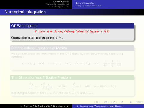
ODEX Integrator
E. Hairer et al., Solving Ordinary Differential Equation I, 1993
Optimized for quadruple precision (10−32).
Dimensionless Equations of Motion
We compute forces and momentums in the ICRS (Solar System Barycenter) by substitutingvariables :
r −→ rc χ and t −→ tc τ , then, d2r = rc d
2χ and1
dt2=
1
t2c
×1
dτ 2.
The Dimensionless 2 Bodies Problem
d2χ
dτ 2= −
µt2
c
r3c
χ
‖χ‖3, we put :
µt2
c
r3c
= 1 with µ = G(MT + ML)
Identifying to Kepler 3rd law : µ = n2a3, we find tc = 1/n and rc = a.
A. Bourgoin, C. Le Poncin-Lafitte, S. Bouquillon, et. al. 19th INTERNATIONAL WORKSHOP ON LASER RANGING

Software Features
Physical Dynamical Model
Some Applications
Numerical Integration
Fitting the Numerical Solution
Numerical Integration
ODEX Integrator
E. Hairer et al., Solving Ordinary Differential Equation I, 1993
Optimized for quadruple precision (10−32).
Dimensionless Equations of Motion
We compute forces and momentums in the ICRS (Solar System Barycenter) by substitutingvariables :
r −→ rc χ and t −→ tc τ , then, d2r = rc d
2χ and1
dt2=
1
t2c
×1
dτ 2.
The Dimensionless 2 Bodies Problem
d2χ
dτ 2= −
µt2
c
r3c
χ
‖χ‖3, we put :
µt2
c
r3c
= 1 with µ = G(MT + ML)
Identifying to Kepler 3rd law : µ = n2a3, we find tc = 1/n and rc = a.
A. Bourgoin, C. Le Poncin-Lafitte, S. Bouquillon, et. al. 19th INTERNATIONAL WORKSHOP ON LASER RANGING

Software Features
Physical Dynamical Model
Some Applications
Numerical Integration
Fitting the Numerical Solution
Fitting the Numerical Solution
Observables
The dynamical model is fitted to an ephemeride (INPOPXX, ELPXX, DEXXX). Several
possibilities for the minimisation of observables :
‖EM‖eph−‖EM‖int
‖0 − MephMint‖T(φ, θ, ψ)eph−T(φ, θ, ψ)int or cosϕeph−cosϕint
with cosϕ = cosφ cosψ+sinφ sinψ cos (π−θ).
Fit of the solution to LLR datas thanks CAROLL.
Least-Squares Method
g(x) =1
2‖f (x) − y‖
2∈ R
+=⇒ g
′(x) = 0
where e.g. y = ‖EM‖epht and f (x) = ‖EM‖int
t with t = 0, · · · , tfin. If x0 is a closed solution of x, wehave δx = x − x0 and approximating g by it Taylor expansion give
δx = {Tf′(x0) · f
′(x0)}−1 · {T
f′(x0) · [y − f (x0)]}
where f ′(x0) is the partial derivative matrix.
A. Bourgoin, C. Le Poncin-Lafitte, S. Bouquillon, et. al. 19th INTERNATIONAL WORKSHOP ON LASER RANGING

Software Features
Physical Dynamical Model
Some Applications
Numerical Integration
Fitting the Numerical Solution
Computation of Matrix f ′(x)
Initial Solution Vector
x = T(p1, · · · , pm, χ1, · · · , χ3, χ1, · · · , χ3). p physical parameters vector, χ dimensionless positionvector and χ dimensionless velocity vector.
Numerically
∂f (x)
∂xk=
f (x1, · · · , x
k+ǫ, · · · , xm+6) − f (x
1, · · · , xk−ǫ, · · · , x
m+6)
2ǫ+ o(ǫ2)
From the Variation’s Equation
l = 1, · · · ,m+6 et i = 1, · · · , 3 we can integrate the 6×(m+6) following equations :
d
dt
(
∂χi
∂xl
)
= Xil
d
dt
(
Xil
)
=3∑
k=1
∂Ai
∂χk
∂χk
∂xl+
3∑
k=1
∂Ai
∂χk
∂χk
∂xl+
m∑
k=1
∂Ai
∂pk
∂pk
∂xl
where A = χ(x) = χ(p,χ, χ) is the dimensionless Earth-Moon acceleration vector.
A. Bourgoin, C. Le Poncin-Lafitte, S. Bouquillon, et. al. 19th INTERNATIONAL WORKSHOP ON LASER RANGING

Software Features
Physical Dynamical Model
Some Applications
The Main Problem
List of effects
Comparison with INPOPXX/DEXXX
Summary
1 Software Features
Numerical Integration
Fitting the Numerical Solution
2 Physical Dynamical Model
The Main Problem
List of effects
Comparison with INPOPXX/DEXXX
3 Some Applications
Improvement of the Semi-Analytical ELP Theory
Test of Gravity in Weak Field
A. Bourgoin, C. Le Poncin-Lafitte, S. Bouquillon, et. al. 19th INTERNATIONAL WORKSHOP ON LASER RANGING

Software Features
Physical Dynamical Model
Some Applications
The Main Problem
List of effects
Comparison with INPOPXX/DEXXX
Modeling
Main Problem
Earth, Moon and Sun are considered as ponctual masses. Sun describes a keplerian ellipse, theecliptic, around the Earth-Moon barycenter.
Restricted Planetary Perturbations
Situation is the same as before, and planetary perturbations are considered. Planets and Plutodescribe keplerian ellipses around Sun.
Forced Planetary Perturbations
Only the Earth-Moon vector is integrated. Planetary perturbations are directly taken from anexisting planetary ephemeride at each time step.
N Bodies Problem
We compute the Newtonian interactions between all planets, Moon, Sun and Pluto.
A. Bourgoin, C. Le Poncin-Lafitte, S. Bouquillon, et. al. 19th INTERNATIONAL WORKSHOP ON LASER RANGING
Software Features
Physical Dynamical Model
Some Applications
The Main Problem
List of effects
Comparison with INPOPXX/DEXXX
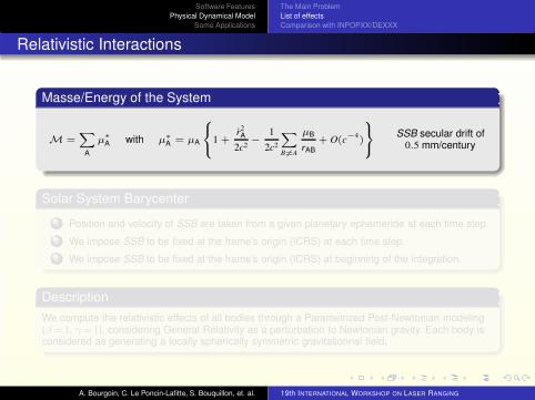
Relativistic Interactions
Masse/Energy of the System
M =∑
A
µ∗A with µ∗
A = µA
1 +r2
A
2c2−
1
2c2
∑
B6=A
µB
rAB
+ O(c−4)
SSB secular drift of0.5 mm/century
Solar System Barycenter
1 Position and velocity of SSB are taken from a given planetary ephemeride at each time step.
2 We impose SSB to be fixed at the frame’s origin (ICRS) at each time step.
3 We impose SSB to be fixed at the frame’s origin (ICRS) at beginning of the integration.
Description
We compute the relativistic effects of all bodies through a Parametrized Post-Newtonian modeling(β=1, γ=1), considering General Relativity as a perturbation to Newtonian gravity. Each body isconsidered as generating a locally spherically symmetric gravitationnal field.
A. Bourgoin, C. Le Poncin-Lafitte, S. Bouquillon, et. al. 19th INTERNATIONAL WORKSHOP ON LASER RANGING

Software Features
Physical Dynamical Model
Some Applications
The Main Problem
List of effects
Comparison with INPOPXX/DEXXX
Earth Figure
Spherical Harmonic
The Earth is no more considered as a ponctual mass but as an axisymmetric body. We consideronly zonal harmonics up degree 4 (J2, J3, J4).
Earth Nutations and Precession Motion
Earth precession motion is forced with P03 solution (Capitaine et al., 2003).
Earth nutations are forced with SOFA’s routines (Standards Of Fundamental Astronomy)http ://www.iausofa.org/
A. Bourgoin, C. Le Poncin-Lafitte, S. Bouquillon, et. al. 19th INTERNATIONAL WORKSHOP ON LASER RANGING

Software Features
Physical Dynamical Model
Some Applications
The Main Problem
List of effects
Comparison with INPOPXX/DEXXX
Tides
Love’s Hypothesis
Each harmonic corresponding to the variations of the potential of a body (Earth e.g.) at its surface(r′ =R, ϕ′,λ′) is proportional to the same harmonic of the potential of a perturber (Moon or Sune.g.).
∆ψ(R, ϕ′,λ′) =
+∞∑
n=2
n∑
m=0
∆ψnm(R, ϕ′,λ′) =
+∞∑
n=2
n∑
m=0
knmVnm(R, ϕ′,λ′)
Dissipation
The deformation of a body is not immediate, the response is related to its internal structure andproduces dissipation. It leads to a time delay (τnm) between the bulge and the perturber direction.So, the deformation due to a perturber at time t is due to its position at time t − τnm.
A. Bourgoin, C. Le Poncin-Lafitte, S. Bouquillon, et. al. 19th INTERNATIONAL WORKSHOP ON LASER RANGING
Software Features
Physical Dynamical Model
Some Applications
The Main Problem
List of effects
Comparison with INPOPXX/DEXXX
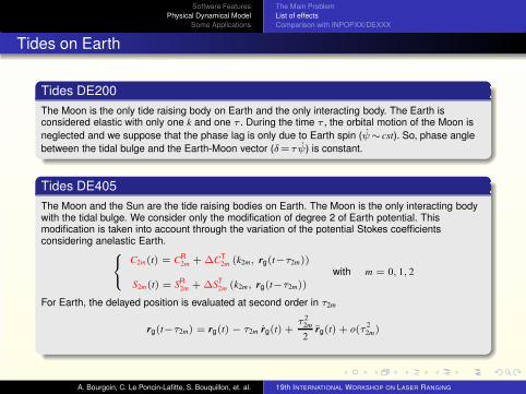
Tides on Earth
Tides DE200
The Moon is the only tide raising body on Earth and the only interacting body. The Earth isconsidered elastic with only one k and one τ . During the time τ , the orbital motion of the Moon is
neglected and we suppose that the phase lag is only due to Earth spin (ψ∼ cst). So, phase angle
between the tidal bulge and the Earth-Moon vector (δ=τψ) is constant.
Tides DE405
The Moon and the Sun are the tide raising bodies on Earth. The Moon is the only interacting bodywith the tidal bulge. We consider only the modification of degree 2 of Earth potential. Thismodification is taken into account through the variation of the potential Stokes coefficientsconsidering anelastic Earth.
C2m(t) = CR2m + ∆CT
2m (k2m, rg(t−τ2m))
S2m(t) = SR2m + ∆ST
2m (k2m, rg(t−τ2m))
with m = 0, 1, 2
For Earth, the delayed position is evaluated at second order in τ2m
rg(t−τ2m) = rg(t) − τ2m rg(t) +τ 2
2m
2rg(t) + o(τ
2
2m)
A. Bourgoin, C. Le Poncin-Lafitte, S. Bouquillon, et. al. 19th INTERNATIONAL WORKSHOP ON LASER RANGING

Software Features
Physical Dynamical Model
Some Applications
The Main Problem
List of effects
Comparison with INPOPXX/DEXXX
Moon Potential
Spherical Harmonic
The Moon is also considered as an extended body. We consider all harmonics up degree 4 (Cnm
and Snm with n=2→4 and m=0→n).
Non-Rigid Moon
The Moon is considered as an elastic body. We consider deformations due to tidal effects (Earthand Sun are the tide raising bodies) and spin. ω represents the spin velocity vector of the Moonexpressed in the frame rotating with Moon.
C2m(t) = CR2m + ∆CT
2m (kM, rg(t−τM)) + ∆CS2m (kM, ω(t−τM))
S2m(t) = SR2m + ∆ST
2m (kM, rg(t−τM)) + ∆SS2m (kM, ω(t−τM))
with m = 0, 1, 2
For Moon, rg(t−τM) and ω(t−τM) are computed by RK4 integration between t and t − τM.
A. Bourgoin, C. Le Poncin-Lafitte, S. Bouquillon, et. al. 19th INTERNATIONAL WORKSHOP ON LASER RANGING

Software Features
Physical Dynamical Model
Some Applications
The Main Problem
List of effects
Comparison with INPOPXX/DEXXX
Moon Librations
Euler Angles
Moon’s orientation (RM) can be identified in the ICRS (RICRS) thanks to Euler angles.
eNex
ey
ezeZ
eX
eY
φ ψ
θ
Euler Equations of Motion
We integrate T(φ, θ, ψ) = f (ω, φ, θ, ψ, φ, θ, ψ) by computing ω.
ω = I−1.{
∑
N ext − I.ω − ω×I.ω}
Moon inertia matrix is time varying I(t) and depends on C2m(t) and S2m(t).
A. Bourgoin, C. Le Poncin-Lafitte, S. Bouquillon, et. al. 19th INTERNATIONAL WORKSHOP ON LASER RANGING

Software Features
Physical Dynamical Model
Some Applications
The Main Problem
List of effects
Comparison with INPOPXX/DEXXX
DE405-Integration without fit
A. Bourgoin, C. Le Poncin-Lafitte, S. Bouquillon, et. al. 19th INTERNATIONAL WORKSHOP ON LASER RANGING

Software Features
Physical Dynamical Model
Some Applications
The Main Problem
List of effects
Comparison with INPOPXX/DEXXX
DE405-Integration without fit
A. Bourgoin, C. Le Poncin-Lafitte, S. Bouquillon, et. al. 19th INTERNATIONAL WORKSHOP ON LASER RANGING

Software Features
Physical Dynamical Model
Some Applications
The Main Problem
List of effects
Comparison with INPOPXX/DEXXX
DE405-Integration without fit
A. Bourgoin, C. Le Poncin-Lafitte, S. Bouquillon, et. al. 19th INTERNATIONAL WORKSHOP ON LASER RANGING

Software Features
Physical Dynamical Model
Some Applications
Improvement of the Semi-Analytical ELP Theory
Test of Gravity in Weak Field
Summary
1 Software Features
Numerical Integration
Fitting the Numerical Solution
2 Physical Dynamical Model
The Main Problem
List of effects
Comparison with INPOPXX/DEXXX
3 Some Applications
Improvement of the Semi-Analytical ELP Theory
Test of Gravity in Weak Field
A. Bourgoin, C. Le Poncin-Lafitte, S. Bouquillon, et. al. 19th INTERNATIONAL WORKSHOP ON LASER RANGING
Software Features
Physical Dynamical Model
Some Applications
Improvement of the Semi-Analytical ELP Theory
Test of Gravity in Weak Field
ELP
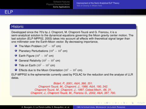
Historic
Developped since the 70’s by J. Chapront, M. Chapront-Touze and G. Francou, it is asemi-analytical solution to the dynamical equations governing the Moon gravity center motion. Thelast solution (ELP-MPP02, 2003) takes into account all effects with theoretical signal larger thanone millimeter over the Earth-Moon vector. By decreasing importance,
The Main Problem (108 − 10
9 cm)
Planetary Perturbations (104 − 10
5 cm)
Earth Figure (104 − 10
5 cm)
General Relativity (102 − 10
3 cm)
Tide on Earth (102 − 10
3 cm)
Effects due to the Moon Orientation (101 − 10
2 cm).
ELP-MPP02 is the ephemeride currently used by POLAC for the reduction and the analyse of LLRdatas.
Bidart, P., 2001, A&A, 366, 351.Chapront-Touze, M., Chapront, J., 1988, A&A, 190, 342.
Chapront-Touze, M., Chapront, J., 1997, Celest.Mech., 66, 31.Chapront, J., Chapront-Touze, M., Francou G., 2002, A&A, 387, 700.
A. Bourgoin, C. Le Poncin-Lafitte, S. Bouquillon, et. al. 19th INTERNATIONAL WORKSHOP ON LASER RANGING

Software Features
Physical Dynamical Model
Some Applications
Improvement of the Semi-Analytical ELP Theory
Test of Gravity in Weak Field
ELP Solution
Reference Plane (Centered on Earth, parallel to ecliptic)
•
•
•Earth
Moon
Sun
G
x (γ′2000
)
y
z
w3
w2 ω′
w1
v′
•
•
•
SE
M
G
D = w1 − v′
F = w1 − w3
l = w1 − w2
l′ = v′ − ω′
Solution to the Main Problem
∑
i1,··· ,i4
[Ai1,··· ,i4 +∑
j
Bi1,··· ,i4j δx
0
j ].
{
cos
sin
}
(
i1D + i2F + i3l + i4l′)
Ai1,··· ,i4 and Bi1,··· ,i4j
are numerical coefficients and δx0
j are literal variations of the constants used
for the construction of the solution.
A. Bourgoin, C. Le Poncin-Lafitte, S. Bouquillon, et. al. 19th INTERNATIONAL WORKSHOP ON LASER RANGING

Software Features
Physical Dynamical Model
Some Applications
Improvement of the Semi-Analytical ELP Theory
Test of Gravity in Weak Field
Main Limitations
Comparison with INPOP08
In his pure semi-analytical form it does not reach a millimetric precision. The RMS over +100/-100years after fitting to INPOP08 gives
∆V =1.56 mas ∆U=0.56 mas ∆r=71 cm
Explanations
Slow convergence of Poisson series (e.g. planetary effects).
Truncation of series for their computation.
Implicit physical parameters impossible to fit.
Implicit physical parameters impossible to update.
Solutions with Numerical Integration
Comparing Numerical to semi-analytical, effect by effect, can provide the true precision of aseries.
Replacing a too slow convergent series by its numerical counterpart (e.g. planetary effects).
A. Bourgoin, C. Le Poncin-Lafitte, S. Bouquillon, et. al. 19th INTERNATIONAL WORKSHOP ON LASER RANGING

Software Features
Physical Dynamical Model
Some Applications
Improvement of the Semi-Analytical ELP Theory
Test of Gravity in Weak Field
Testing Metric Theories of Gravity
Principle
Be able to simulate observables in different theories of gravity. Compute equations of motion from agiven metric theory.
Weak Field
gαβ = ηαβ + hαβ with |hαβ|≪1 and ηαβ Minkowski metric tensor : η00 = 1 ; η0i = 0 ; ηij = −δij
Geodesics Equation
Expressed in function of the coordinate time x0 = ct :
d2xi
dx02= −Γi
αβ
dxα
dx0
dxβ
dx0+ Γ0
αβ
dxα
dx0
dxβ
dx0
dxi
dx0
A. Bourgoin, C. Le Poncin-Lafitte, S. Bouquillon, et. al. 19th INTERNATIONAL WORKSHOP ON LASER RANGING

Software Features
Physical Dynamical Model
Some Applications
Improvement of the Semi-Analytical ELP Theory
Test of Gravity in Weak Field
Testing Metric Theories of Gravity
Equations of motion
xi= −
c2
2∂ih00 −
c2
2hik∂kh00 +
c2
2∂0h0i +
c
2∂0h00 x
i
+ c∂0hik xk + c(∂kh0i − ∂ih0k)x
k + ∂kh00 xkx
i
+ (∂mhik −1
2∂ihkm)x
kx
m + O(c−4).
with xi = dxi/dt. Knowing hαβ et hαβ,γ we can deduce the equations of motion in any metric theoryof gravity which can be expressed under the form gαβ = ηαβ + hαβ . Actually, hαβ = h′αβ + δhαβ
where h′αβ corresponds to General Relativity and δhαβ to the alternative theory.
A. Hees et al., Radioscience simulations in general relativity and in alternative theories of gravity,2012, Classical and Quantum Gravity
A. Bourgoin, C. Le Poncin-Lafitte, S. Bouquillon, et. al. 19th INTERNATIONAL WORKSHOP ON LASER RANGING

Software Features
Physical Dynamical Model
Some Applications
Improvement of the Semi-Analytical ELP Theory
Test of Gravity in Weak Field
Thank you for your attention !
A. Bourgoin, C. Le Poncin-Lafitte, S. Bouquillon, et. al. 19th INTERNATIONAL WORKSHOP ON LASER RANGING