new evidence on the local fiscal multiplier and employment

New Evidence on the Local Fiscal Multiplier and Employment

from Military Construction Spending

Emily Zheng∗

Texas A&M University

Abstract

This paper takes advantage of the 2005 Base Realignment and Closure process to

analyze the effect of government spending on local economic conditions. Exploiting

variation in the timing and amount of construction funding provided across counties,

my analyses yield an estimated cost per job of $65,000 per year and a local fiscal

multiplier of 1.21. Analyses of neighboring counties show little evidence of spillover

effects. To further explore the mechanisms underlying these results, I investigate the

effects of government spending on migration and show that the funding has positive

effects on in-migration, but these effects are too small to explain the main results.

Keywords: Government spending; cost per job; local fiscal multiplier

JEL classification: E62, H30, H50, R23

∗Department of Economics, Texas A&M University, 3035 Allen Building, College Station, TX 77843.Email: [email protected] I would like to thank Jason Lindo, Mark Hoekstra, Jonathan Meer, StevenPuller, Fernando Luco, Sarah Zubairy, Laura Dague along with seminar and conference participants at TexasA&M University for helpful comments. All errors are my own.

1 Introduction

One cannot overemphasize the need to better understand the effects of government spending.

Is government spending really effective at stimulating the economy? How much does it cost to

create a job? And, how large is the multiplier? Motivated by beliefs that the fiscal multiplier

is relatively large, the federal government passed the American Recovery and Reinvestment

Act (ARRA) to stimulate the economy in 2009 at a cost of more than $800 billion (Romer

and Bernstein, 2009). Many other countries adopted similar policies in response to the Great

Recession, the worst economic downturn since the 1930s. However, economists and policy

makers still have not reached a consensus on the effectiveness of government spending.

The debate arises partly because theoretical models offer contradictory predictions. Sim-

ple neoclassical models usually yield a small multiplier (typically less than 0.5) while New

Keynesian models can yield predictions larger than 2 (Ramey, 2011a). Difficulty in mea-

suring the counterfactual in the macroeconomy only adds to the debate. To tackle this

problem, a recent stream of the empirical literature utilizes cross-sectional variation to esti-

mate the income multiplier and cost per job. However, this line of empirical evidence also

offers a wide range of estimates for the cost per job ($25,000–$125,000) and the local income

multiplier (0.4–2.2). This wide range of estimates may be due to differential effects of gov-

ernment spending across different periods of time, across different places or to heterogeneous

treatment effects across various types of government spending (Feyrer and Sacerdote, 2011).

This paper offers new evidence on the effectiveness of government spending. It is the first

to estimate the cost per job and the local multiplier associated with construction spending.1

It is also the first paper to examine the effects of the $25 billion Base Realignment and

1A couple of studies have investigated the effects of public highway spending on economic outcomes.Leduc and Wilson (2013) studies the impulse response of state output to the Federal-Aid Highway Program,a program to fund construction, maintenance, and other improvements on a large array of public roads.Pereira (2000) examines the effects of public infrastructure investment on output using a structural VARand aggregate U.S. data.

1

Closure (hereafter, BRAC) military construction program on local economies.2 As such, it

is quite relevant to the ongoing discussions about the Department of Defense’s proposal of

another BRAC in the near future.

In order to estimate the effect of government spending on local economies, I exploit vari-

ation in the timing and amount of construction funding provided by the 2005 BRAC across

counties with military bases. The BRAC process realigned and closed some military instal-

lations to improve military efficiency and effectiveness.3 A BRAC Commission was created

to provide an objective and non-partisan analysis of military installations. It then produced

a final, non-amendable recommendation list. The commission gave priority to military value

during its selection process, and commissioners recused themselves from participation in

matters related to installations in their home states. Thus, to some extent, the funding

awarded to each county most likely was motivated by military considerations and plausibly

was unrelated to local economies.

My analysis identifies the causal effect of the stimulus on local economies under the

identifying assumption that, changes in local economic conditions would have been the same

across military counties absent the 2005 BRAC funding. Using county-level economic data

from the Bureau of Economic Analysis’ Regional Economic Accounts and a novel dataset

that contains 2005 BRAC construction funding information, I find an estimated cost per

job of $65,000 and a local fiscal multiplier—the change in local per capita income produced

by a one dollar change in per capita government spending—of 1.21. These estimates are

robust to various model specifications and the empirical strategy passes falsification exercises.

Furthermore, my industry-specific analysis reveals especially large effects on the construction

2Lee (2016) also studies the effects of 2005 BRAC on local economies, but he focuses on the effects ofpersonnel relocation as opposed to construction funding. As shown in Section 4 of this paper, the observedeffects are driven by construction funding, not personnel relocation. This paper explicitly examines theidentifying assumption and explores the treatment effects dynamics, which are not feasible for Lee (2016) asit only uses one year of pre-treatment data (2005) and one year of post-treatment data (2011).

3I restrict the analysis to counties that did not experience any closure during the process in order tobetter investigate the effects of government stimulus, excluding disinvestment.

2

industry, which is consistent with the nature of the program.

Traditional Keynesian model usually yields a larger prediction on multiplier when the

economy is in slack; that is, when some factors of production are in idle. In this case, counties

in slack may benefit more from government spending compared to other counties. To test

this hypothesis, I use unemployment rate as a measure of “slack” in an economy and divide

the funded counties into counties with higher and lower unemployment rates. Results from

this analysis provide mixed evidence. The estimates suggest larger effects on income for

counties with higher unemployment rates. However, the effects on emploment are larger for

counties with lower unemployment rates.

To further understand the regional impacts of government spending, I extend the analysis

to directly measure the extent to which there are spillovers across neighboring counties. I find

little evidence of any likely spillover effects. Furthermore, I investigate the extent to which

there are spillovers on the construction industry for nearby counties, since the construction

industry is directly affected by the program. These estimates are uniformly positive and

larger, providing suggestive evidence that the BRAC funding leads to higher employment

for construction workers nearby but has no effect on income for those workers.

In order to speak to the mechanisms at work, I also examine the extent to which the

BRAC stimulus affects in-migration and out-migration. What if government spending at-

tracts many high-ability migrants and they take the employment opportunities and drive

up the average income? In this case, local residents may not gain from increased govern-

ment funding because the benefits of the stimulus instead accrue to migrants. My analysis

suggests that government spending has positive effects on in-migration and no effects on

out-migration to the funded and nearby counties. However, the effects on migration are too

small to explain the main results. This suggests that residents of the funded counties do

benefit from the government spending.

It is important to note that the multiplier estimated in this paper is local, as opposed

3

to the extensively studied national multiplier (Ramey and Shapiro, 1998; Fatas and Mihov,

2001; Blanchard and Perotti, 2002; Ramey, 2011b; Mountford and Uhlig, 2009; Barro and

Redlick, 2009; Zubairy, 2014). Estimating the local multiplier does not inform us directly

about the magnitude of the national multiplier, which has been the focus of the literature and

is of great policy concern. Indeed, spillovers and migration are more likely to occur within

a country rather than across country borders (Dupor, 2016). When a stimulus does lead

to spillovers, or attracts migration, the local multipliers may be larger or smaller than the

national multiplier depending on the direction and magnitude of the effects. For instance, if

there are positive spillovers across counties, then the local multiplier will not fully capture

the effects of government spending and thus will be smaller than the national multiplier.

On the other hand, if government spending attracts many migrants who take employment

opportunities and drive up average income, then the local multiplier will be larger than

the national multiplier. The fact that there is not a one-to-one mapping between local and

national multipliers does not negate the policy relevance of local parameters. State and local

governments spend over 3 trillion dollars every year, and the effects of regional spending are

certainly of interest to local policy makers and residents. Thus, while this paper is only

informative about national stimulus, it provides a direct estimate of the effectiveness of

regional investment.

The rest of the paper is organized as follows. In the next section I discuss related lit-

erature. Section 3 provides some background on the 2005 Base Realignment and Closure.

Section 4 describes the methodology and data used to analyze the causal impact of gov-

ernment spending on local economics. Section 5 presents empirical results of my analyses.

Section 6 concludes and provides a discussion of the implications of the results.

4

2 Related Literature

For decades, macroeconomists have tried to model and estimate the national fiscal multiplier,

a parameter that summarizes the effects of government spending at the national level. Yet,

there is still considerable debate over its magnitude. The debate arises in part because

theoretical models offer contradictory predictions.4 Simple neoclassical models often yield

a small multiplier (usually smaller than 0.5); Baxter and King (1993) find that temporary

spending financed by a distortionary tax could lead to a multiplier as small as -2.5. New

Keynesian models, on the other hand, yield a wide range of predictions, depending crucially

on the monetary policy. Less responsive monetary policy, such as the case of “zero lower

bound,” could yield a multiplier as large as 2.3 (Eggertsson, 2001, 2011; Eggertsson et al.,

2003).5 Difficulty in measuring the counterfactual only adds to the debate. To tackle this

problem, this line of literature employs two major approaches. The first is to use a structural

VAR model, which relies on structural assumptions and small changes in the assumptions can

lead to large differences in the estimated multiplier (Blanchard and Perotti, 2002; Caldara

and Kamps, 2012). The second approach uses military spending associated with wars as

potentially exogenous shocks (Barro and Redlick, 2011; Ramey and Shapiro, 1998; Ramey,

2011b; Fisher and Peters, 2010). However, major episodes of war are rare, and other fiscal

policies, patriotism, or capacity constraints that occur during the war could confound the

estimates.

A recent stream of the empirical literature uses cross-sectional variation to estimate the

local income multiplier and cost per job.6 A number of these studies have used variation in the

geographic distribution of funds under the ARRA. Chodorow-Reich, Feiveson, Liscow, and

4Ramey (2011a) provides a thorough review of the leading theories on the effects of government spendingand related empirical work.

5At the zero lower bound, the nominal interest rate is held constant while inflation drives the real interestrate down (Ramey, 2011a).

6See Chodorow-Reich (2016) for a thorough review on this line of literatures.

5

Woolston (2012) use state-level formula-driven variation in the allocation of ARRA Medicaid

spending; they estimate a cost per job of around $25,000 and a local income multiplier of

about 2. Wilson (2012) uses a similar approach to estimate the overall employment effects

of the total ARRA spending, but finds a state-level cost per job of around $125,000 per

year. The reason for differences in results between these two papers may be that medical

spending and other types of expenditures have differents effects on the economy. Feyrer

and Sacerdote (2011) also use state-level variation in the allocation of ARRA funding; they

estimate a cost per job of $107,000 with an implied income multiplier from 0.5 to 1. They also

suggest that the overall results mask considerable variation for different types of spending.

Support programs for low income households and infrastructure spending are found to be

highly expansionary while grants to states for education do not appear to have created any

additional jobs.

Other studies have explored different sources of variation to estimate these parameters.

Serrato and Wingender (2016) use variation in federal spending that is induced by the

fact that much direct federal spending, and transfer programs to a local area depend on

population estimates which are exogenously “shocked” after each Decennial Census. They

estimate a county-level cost per job of $30,000 per year and income multiplier of 1.7 to 2.

Shoag (2013, 2010) uses differences in returns to state pension funds as “windfall” shocks

to state spending; he estimates a state-level income multiplier of 2.2 and a cost per job of

around $35,000 per year. Fishback and Kachanovskaya (2010) use variation across states in

federal spending during the Great Depression and estimate an income multiplier of 1.1 and no

significant effect on employment. Clemens and Miran (2012) use state spending cuts induced

by institutional rules on budget deficits to estimate a spending multiplier of 0.4. Nakamura

and Steinsson (2014) use regional variation in military procurement spending to estimate

a local multiplier of 1.5. Their theoretical model relates the estimated local multiplier to

the traditional national multiplier; and their estimates fit well with an open economy New

6

Keynesian model in which consumption and labor are complements. Finally, Acconcia,

Corsetti, and Simonelli (2014) use province-level variation in the temporary contractions in

local public spending directed at combatting the Mafia in Italy to estimate a local multiplier

of 1.5.7 Overall, this line of literature offers a wide range of estimates for cost per job

($25,000–$125,000) and the income multiplier (0.4–2.2).

This paper complements the existing literature by providing the first estimates of cost

per job and local multiplier based on a military construction program. This is of particular

significance if heterogeneous treatment effects across various types of government spending

may explain why we observe such a wide range of empirical estimates. Moreover, it provides

guidance to policy makers as to how limited funding should be allocated across various

types of expenditures. Furthermore, I use a recent spending episode (2006–2011) which is

relevant to current policy if the effects of public spending vary across periods. In addition,

this research adds to the literatures on the effects of the BRAC process on various outcomes

(Hultquist and Petras, 2012; Freedman and Owens, 2014; Carlson, 2014; Hooker and Knetter,

2001). Because the Department of Defense is proposing another round of the BRAC in the

near future and a sizable amount of money is at stake, it is valuable that this paper sheds

light on the stimulus benefits of the program itself.

3 Base Realignment and Closure

Base Realignment and Closure (BRAC) is a congressionally authorized process that the

Department of Defense has used to reorganize its base structure. Its goal is to more efficiently

and effectively support the armed forces and to enhance operational readiness. The Defense

Authorization Amendments and Base Closure and Realignment Act, enacted on October

7Dinerstein, Hoxby, Meer, and Villanueva (2014) uses an instrumental variable approach to investigatehow stimulus-motivated federal funding directed to universities affects the economies of the counties in whichthe institutions are located, but they find little evidence of a stumulus effect, which could be due to the factthat only a small fraction of the funding “stuck where they hit”.

7

24, 1988, provided the basis for implementation of the 1988 BRAC recommendations. On

November 5, 1990, President George H. W. Bush signed the Defense Base Closure and

Realignment Act of 1990, an attempt to isolate political influence from military activity.

This act established an independent commission, the Defense Base Closure and Realignment

Commission, to ensure a timely, independent, and fair process for closing and realigning U.S.

military installations. Since then, there have been four additional BRACs in 1991, 1993,

1995, and 2005. The 2005 BRAC cost around 35 billion dollars, more than the sum of the

previous 4 BRACs, and thus provides a good opportunity for examining the local effects of

stimulus.

On May 13, 2005, the Department of Defense issued the initial recommendation list

for the 2005 Base Realignment and Closure. An independent panel of nine commissioners

was created to provide an objective and non-partisan review and analysis of that list. It

then produced a final non-amendable recommendation list.8 During this selection process,

the commission followed eight selection criteria and it gave priority to military value.9 To

enhance the impartiality and integrity of the BRAC process, commissioners recused them-

selves from participation in matters related to installations in their home states.10 President

George W. Bush approved the 2005 BRAC commission’s recommendation on September 15,

2005 with a statutory deadline of September 15, 2011. Given the process by which decisions

were made, it is likely that the funding awarded to each county was motivated by military

considerations and not local economic conditions. I provide graphical evidence and conduct

a robustness check to support this hypothesis in Section 4. First, I show that funded and

8The 2005 BRAC commission consists of Anthony J. Principi, James H. Bilbray, Philip Coyle, HaroldW. Gehman, Jr., James V. Hansen, T. Hill, Lloyd W. Newton, Samuel K. Skinner, Sue E. Turner.

9See Appendix A.1 for a full list of selection criteria.10Four commissioners have recused themselves from participation in matters relating to installations in

their home states. Commissioners Coyle and Gehman recused themselves because of their participation inBRAC-related activity in California and Virginia respectively. Commissioners Bilbray and Hansen recusedthemselves because of their long-time representation in the Congress and other public offices of Nevada andUtah respectively.

8

non-funded military counties did not have divergence in economic conditions prior to the

first year of funding. Then, I perform a robustness check to show that the estimates are

robust to the exclusion of states that were connected to the 2005 BRAC Commission; that

is, the estimates remain robust after I drop states in which any of the commissioners were

born or have worked.

The 2005 BRAC cost over 35 billion dollars; military construction alone cost around

25 billion dollars. Figure 1 presents the geographic distribution of the average annual per

capita construction funding across the United States. The mean of the average annual per

capita funding is roughly $122 for the funded counties. Almost every state has counties

that received construction funding. In addition to funding construction across the nation,

the 2005 BRAC relocated around 200,000 military and civilian personnel. The average net

change in direct jobs was a net loss of 27 jobs per installation throughout the process (Lee,

2016). In Section 4, I conduct a robustness check and show that the main results are not

due to personnel relocation. This is not surprising, as net personnel change only accounts

for a tiny portion of county population.

4 Data and Methodology

4.1 Data

The 2005 Base Realignment and Closure construction funding data come from the 2013

Base Realignment and Closure Commission Execution Report. It provides an overview of

the costs and savings for each the Department of Defense Component throughout the six-

year BRAC implementation period (2006–2011). It also lists detailed annual construction

funding information at the installation level. I geocode and aggregate this information into

county-level funding information. To distinguish between the effects of personnel relocation

9

and construction funding, I obtain county-level annual personnel counts for the years 2002

through 2011 from the U.S. Base Structure Reports. This administrative report is published

annually by the Department of Defense, and lists annual installation-level personnel counts

for installations of at least ten acres and at least $10 million in “Plant Replacement Value.”11

The personnel counts include military personnel, federal civilian employees and other non-

military personnel, such as contractor personnel. I geocode and aggregate these personnel

counts to county-level counts.

The data on county-level economic activity come from the Bureau of Economic Analysis’

(BEA) Regional Economic Accounts. These data provide a wealth of economic statistics at

the county level, including per capita income and employment.12 The dataset comes from a

variety of administrative sources. Employment and wage data are from the Bureau of Labor

Statistics’ Quarterly Census of Employment and Wages (QCEW) . It reports on workers

covered by the state Unemployment Insurance (UI) program and federal workers covered

by the Unemployment Compensation for Federal Employees (UCFE) program. The BEA

then adjusts these data for employment and wages not covered, or not fully covered, by

these programs to provide more comprehensive measures of income and employment. The

Regional Economic Accounts also have annual information on economic activity for large

industries, such as construction and manufacturing, at the county level.

To further investigate whether migrants drive the main results, I use county-level mi-

gration data from the Internal Revenue Service (IRS) Statistics of Income. The IRS tracks

inflows and outflows based on address changes of individual tax filers. I use these data

11I use 2003–2012 Base Structure Reports because reports published in year t+1 would provide informationon the personnel counts in year t. After 2012, the annual report changes format and stops listing personnelcounts at the base level. “Plant Replacement Value” represents the Military Service or Washington Head-quarter Service calculated cost to replace the current physical plant (facilities and supporting infrastructure)using today’s construction cost (labor and materials) and standards (methodologies and codes).

12BEA reports data on a calendar year basis, whereas Department of Defense reports funding on a fiscalyear basis. For instance, fiscal year 2005, begins on October 1, 2004 and ends on September 30, 2005. Imatch fiscal year directly with calendar year in the empirical analysis. This matching procedure should yielda relatively conservative estimate.

10

to construct measures of the number of individuals and households moving into and out

of a particular county and to evaluate how the 2005 BRAC construction funding affects

in-migration and out-migration.

Table 1 presents summary statistics based on these data. County-level per capita income

and employment average around $33,000 and 120,000 across treatment and control counties

respectively over the sample period. Construction employment accounts for around 6% of

all employment in these counties. Military personnel account for about 1.24% of the overall

population in those counties, more than the U.S. average of around 0.78%.13

4.2 Methodology

To identify the effects of government spending on local economies, I exploit variation in the

timing and amount of BRAC construction funding across counties. Specifically, I estimate

the following model:

Yit = α + βperCapitaFundingit + µi + ηt +Xit + δst + uit

where i indicates counties, t indicates years, and s indicates states. In this model, Yit is

a measure of the county economic condition; Xit refers to county-level time-varying demo-

graphic controls, including population, percentage Hispanic, African American, and female;

and δst represents state-by-year fixed effects.14 The county and year fixed effects are captured

by µi and ηt, respectively. The county fixed effects control for county-level time-invariant

characteristics and year fixed effects controls for nationwide economic shocks in any year.

Moreover, I also include state-by-year fixed effects to capture state-level economic shocks in

any given year. The inclusion of state-by-year fixed effects allows counties in different states

13Currently, there are 1.4 million active military personnel and 1.1 million reserve personnel in the UnitedStates.

14The county-level demographic data come from the U.S. Census Bureau.

11

to follow different trajectories and account for differential shocks by state over time. In this

case, the crucial assumption is that in the absence of the 2005 BRAC construction funding,

changes in economic condition would have been the same across all military counties in the

same state. The variable of interest is perCapitaFundingit, which measures 2005 BRAC

construction funding at year t in county i.

Noted that while the BRAC report provides data on funding awarded, information on

when the funding was spent is not available. Thus, I assume that all funding received by

a county was spent linearly beginning in the year of receipt. That is, perCapitaFundingit

equals zero prior to the receipt of any funding for county i and equals FundingitPopulationi,2005

for years

after the initial funding receipt.15 I make that assumption for two reasons. First, according

to the Department of Defense’s policy, military construction funding can remain available

for up to five years. Second, most installations completed their projects in 2011, even though

the Department of Defense distributed most of the funding between 2007 and 2009, and few

counties received funding in 2011 (Lee, 2016).16 The estimate of β identifies the causal effect

of 2005 BRAC funding under the identifying assumption that, in the absence of the BRAC

construction funding, the change in outcomes across counties would have been the same.

Finally, standard errors are clustered at the state level to allow for arbitrary correlation of

the error term at the state level across counties and years.

In reality, counties with military installations are likely to be systematically different from

15Each BRAC construction project should be at least 35-percent design complete to request fundingfrom the Department of Defense, which generates variation in the timing of counties’ first funding receipt.And Fundingit is defined as TotalFundingi

2011−firstyearoffundingreceipt+1ifor years after the initial funding receipt. I

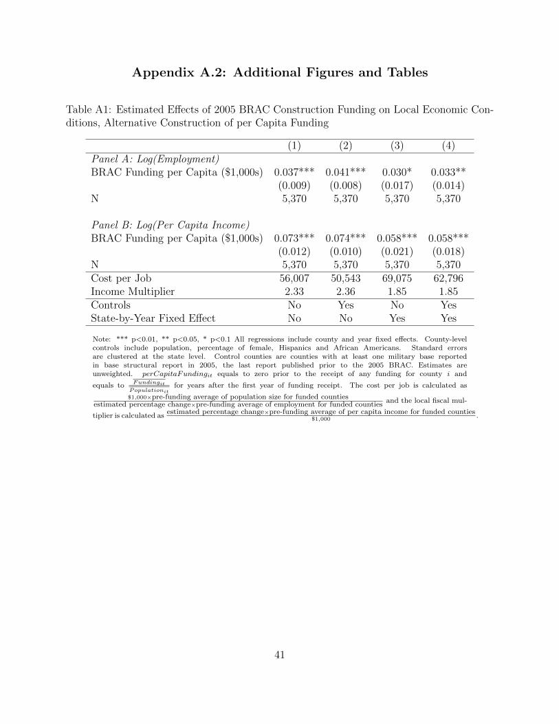
use population counts in 2005 to generate the treatment variable because population could be affected bygovernment spending and 2005 is the last year prior to the BRAC construction program. I also presentestimates where perCapitaFundingit equals zero prior to the receipt of any funding for county i and equalsFundingit

Populationitfor years after the first year of funding receipt in Appendix Table A1. The results are robust to

this exercise.16Another assumption could be that each individual funding awarded to a county at a given year is spent

equally between that year and 2011. For instance, County A receive M million dollars in 2008 and N milliondollars in 2010, so spending for County A would be M

4 million dollars in 2008 and 2009, and M4 + N

2 milliondollars in 2010 and 2011. The results are robust to this alternative assumption of spending pattern and areshown in Appendix Table A2.

12

counties that do not have installations. For this reason, I restrict my sample of unfunded

counties to those with at least one military installation in the 2005 Base Structure Report, the

administrative report on military installations that is published annually by the Department

of Defense.17 I further restrict the overall sample to counties that did not experience any

closure during the 2005 BRAC to better investigate the effects of government spending,

excluding disinvestment. The sample period is 2002–2011 for the main analysis. I use 2002

because it is the first year after the completion of the previous BRAC and 2011 because it is

the statutory deadline for completion of the 2005 BRAC. When I explore treatment effects

over time, I extend the sample period through 2013 to investigate whether the funding has

lingering effects.

5 Results

In this section, I begin by presenting my main results. They are followed by robustness

checks verifying that these results are robust under alternative identification strategies, to

the exclusion of states linked to the 2005 BRAC Commission, and that they are not driven by

personnel relocation. Then, I test the hypothesis that the effects of government spending are

larger during periods of slack and examine the heterogeneous treatment effects of government

spending across high and low unemployment counties. Next, I extend my analysis to explore

the extent to which there are spillovers on the nearby counties. Finally, I examine the effects

on migration to investigate whether migrants are responsible for the main results.

5.1 Main Results

Table 2 presents my main results with Panel A showing the estimated effects on employment

and Panel B on income. Column 1 shows estimates from the baseline specification, simply

17I use the 2005 report because it is the last one published prior to the 2005 BRAC.

13

controlling for county and year fixed effects. The results from this specification suggest

that a $1,000 increase in annual per capita BRAC construction funding would increase

employment by 3.6%, or roughly 5,100 jobs.18 This implies a cost per job of approximately

$57,563, because it takes roughly 279 million dollars ($1,000 per capita spending multiplied

by 278,884, which is the pre-funding population average for funded counties) to create these

jobs. Similarly, the estimate implies that a $1,000 increase in annual per capita BRAC

funding would increase per capita income by 5.6%. Multiplying this number by $31,891—

the pre-funding average of per capita income in the funded counties—yields an increase of

roughly $1,790. This estimate implies a fiscal multiplier of 1.79.

Column 2 adds county-level time-varying demographic controls to the model. Adding

these covariates may be over-controlling, because county-level demographic characteristics

could be affected by government spending and thus a causal path between local stimulus

and economic conditions. So it is unclear whether the estimates in Column 2 are superior to

those in Column 1. Nonetheless, the results change little after adding these controls. These

estimates imply a cost per job of $54,533, and a fiscal multiplier of 1.59.

In Column 3, I present the results of a specification in which I control for county, year,

and state-by-year fixed effects. Adding state-by-year fixed effects to the model controls

for statewide economic shocks. The estimates from this specification suggest that a $1,000

increase in annual per capita funding would increase employment by 3.0% and per capita

income by 4.5%, implying an estimated cost per job of around $69,075 and income multiplier

of 1.44. Finally, in Column 4 I present a specification in which I control for state-by-year fixed

effects and county-level time-varying controls. The results change little, with an estimated

cost per job of approximately $64,795 and an income multiplier of 1.21. To summarize, the

estimates in Table 2 provide strong evidence that the BRAC construction funding had a

18This number is calculated by multiplying 3.8% by 134,580, the pre-funding average of employment forfunded counties.

14

significant impact on employment and income for funded counties, and these estimates are

robust to various model specifications.

As an additional way to estimate the effects of government spending on local economies,

I investigate the dynamic responses of economic conditions to 2005 BRAC construction

funding. To do that, I interact average per capita funding with a set of indicator variables

that correspond to 1, 2, 3, 4 years prior to the first year of funding receipt, the first year

of funding receipt, and 1, 2, 3, 4, 5-or-more years after the first year of funding receipt. As

in Column 4 of Table 2, I continue to control for county, year, state-by-year fixed effects

and county-level time-varying demographic characteristics. Figure 1 plots the coefficient

estimates and 95% confidence intervals from this analysis. None of the coefficient estimates

for the years leading up to the funding receipt are statistically significant at the 5% level,

supporting the common trends assumption. Furthermore, the estimates for years after the

first year of funding receipt provide some evidence that the effects on employment and income

are concentrated in the short term and it fades away once the funding is discontinued.

Finally, because the construction industry is directly affected by BRAC, we might expect

there to be larger effects on this industry. I investigate this hypothesis and present the

results in Table 3. Estimates from this industry-specific analysis are uniformly larger than

the main results, suggesting that BRAC construction funding does have an especially large

effect on the construction industry. Results from the specification where I control for county,

year, state-by-year fixed effects and county-level time-varying demographic characteristics

indicate that a $1,000 increase in per capita funding increases construction employment by

10.8% and personal income by 13.8%.19 Compared with the main results—a 6.8% increase in

overall employment and 3.8% increase in per capita income—these estimates are consistent

with the hypothesis that the BRAC funding has a larger impact on the construction industry.

19BEA publish personal income as opposed to per capita income for large industries and population countsby industry is unavailable, so I focus on personal income instead of per capita income in the industry-specificanalysis.

15

5.2 Robustness Checks

This section presents several tests to check the robustness of the main results. I begin by

presenting results where I drop all unfunded counties from the analysis and only use variation

in the timing and amount of funding among funded counties. Next, I extend the analysis to

explore the extent to which dropping states linked to the 2005 BRAC Commission affects the

results. Finally, I investigate whether the effects are driven by military personnel relocation

or the stimulus.

In Table 4, I present the estimates based only on funded counties. This estimation strat-

egy compares counties receiving lower levels of construction funding per capita to counties

that receive more funding per capita. Each column in Table 4 follows the same specification

as Table 2. The estimates are similar to those presented in Table 2; Column 4 indicates a

3.4% increase in employment and a 3.9% increase in per capita income for a $1,000 increase

in annual per capita funding. That implies a cost per job of around $60,948 and an income

multiplier of 1.24. The estimates remain robust when I use an alternative source of variation,

lending further support to the main results.

In Section 3, I discussed the institutional background of the 2005 BRAC program, arguing

that political factors played a small role in the BRAC process and that funding was mainly

motivated by military considerations. The analysis above supports this argument: it shows

no evidence of economic divergence prior to the receipts of BRAC construction funding. None

of the coefficient estimates for the years leading up to the funding award are statistically

significant. However, this does not rule out the possibility that commissioners may have

voted in favor of their connected states and that political factors may affect the BRAC

process in a significant way. It is important to note that this sort of behavior would only

bias the estimates if it was related to expected economic outcomes.

In any case, to address this concern, I conduct a robustness check by dropping states

16

where any of the commissioners were born or had worked at any time throughout their ca-

reer.20 If the estimates change substantially after dropping those counties, then it would raise

concerns about political involvement during the BRAC process. The estimates presented in

Table 5 remain close to those shown in Table 2: estimates from Column 4 imply a cost per

job of around $64,582 and a local fiscal multiplier of 1.19, This suggests little evidence of

political manipulation that is systematically related to economic conditions.21

Because military personnel were relocated during 2005 BRAC process, the main results

could be driven by more military personnel moving to the funded counties. To address this

concern, I include logged military personnel counts as a covariate in my analysis. I present

the estimates in Table 6. When I control for military personnel, the estimated effects of

BRAC construction funding change little. Estimates from Column 4 imply a cost per job

of approximately $57,166 and an income multiplier of 1.21. Furthermore, the estimates on

logged personnel counts are small and never statistically significant, reassuring us that the

main effects indeed are driven by funding, not personnel relocation. This finding is consistent

with the fact that the number of military personnel in a county only accounts for a small

portion of the population, and on average there is only a net loss of 27 jobs per installation

throughout the process (Lee, 2016).22

Overall, these robustness checks indicate that the main results are robust under alter-

native identification strategies. Also, we observe little political manipulation related to

economic conditions during the BRAC process, which lends further support to the iden-

tification strategy. Also, the main results are driven by the funding, not by relocation of

military personnel. All of this evidence supports an interpretation of the main results as

20I drop the following states in this analysis: Arizona, California, Georgia, Hawaii, Illinois, Maryland,Mississippi, Nebraska, Nevada, New York, Ohio, South Carolina, Texas, Utah, Virginia, Washington.

21The estimated cost per job is calculated as $1,000×258,4713.5%×140,167 , and the local fiscal multiplier is calculated as

$33,070×3.6%$1,000 .

22The estimated cost per job is calculated as $1,000×343,1233.8%×167,397 , and the local fiscal multiplier is calculated as

$32,672×3.7%$1,000 .

17

cost per job and income multiplier.

5.3 Heterogeneous Effects

The traditional Keynesian model implies larger multipliers when the economy is in slack; that

is, when some production factors are in idle.23 This theoretical prediction implies that we

shall observe larger effects on income and employment for counties that have idle productive

capacity. If so, government spending may have a redistributional effect in addition to its

stimulating effects: areas in slack would benefit more from the same amount of government

spending than other areas. In this section, I investigate this issue by examining the degree to

which the effects of BRAC funding on income and employment differ by the amount of slack

in the local economy as measured by the unemployment rate. Specifically, I divide the funded

counties into two groups based on their unemployment rates in the year of 2005, the last

year prior to any counties receiving the BRAC construction funding. Table 7 presents results

from this analysis. Panel A presents the results for counties with higher unemployment

rates while Panel B for those with lower unemployment rates in 2005. Conttracted to the

theoretical prediction, the point estimates for employment effects are larger for counties

with lower unemployment rates, which could be due to the fact that counties with lower

unemployment rates in the sample are more likely to be larger counties with more job

opportunities. The effects on income, on the other hand, provide some evidence to support

the slack hypothesis—economies in slack seems to gain more from federal spending. The

estimated multiplier for counties with lower unemployment rates is smaller relative to the

counties with higher unemployment rates and less robust to alternative model specifications.

23Empirical evidence from the macroeconomics literature yields contrasting results on whether governmentspending multipliers are larger during periods of slack. Auerbach and Gorodnichenko (2012) and Fazzari,Morley, and Panovska (2015) find evidence of larger multipliers during periods of slack, while Ramey andZubairy (forthcoming), Owyang, Ramey, and Zubairy (2013), and Crafts and Mills (2013) do not observehigher multipliers during times of slack.

18

5.4 Spillover Effects

To further examine the effects of the BRAC construction funding, I consider the impact

on neighboring counties.24 This extension of the baseline analysis helps to capture the

total regional impact of the stimulus; government spending may create externalities for

neighboring counties that did not directly receive BRAC funding. Positive spillovers across

counties would suggest that the main analyses understate the total regional effects of the

BRAC funding. Spillovers might arise, for example, if some construction materials are

purchased from neighboring counties: this increase in demand for input would have positive

effects on those counties. On the other hand, if we find negative spillovers on nearby counties,

then the main results may overstate the regional impact of the stimulus. For example, if

the BRAC funding leads to higher wages and attracts migrants from neighboring counties,

then decreases in population could have negative effects on businesses in those counties,

ultimately resulting in negative spillovers.

In order to estimate the spillover effects, I define neighboring counties as the 10 nearest

counties based on highway distance between county centroids for every county in the main

analysis.25 Comparing counties near the funded counties to those near the unfunded military

counties, my results are shown in Table 8. None the estimates are significant and there is little

evidence of spillovers. The estimates are precise enough to rule out effects on employment

on the order of 1% at the 5 percent significance level for a $1,000 increase in per capita

funding. Also the estimates on per capita income can rule out meaningful negative impact

smaller than -0.6% at the 5 percent level.

Because the construction industry is directly affected, it is likely that the BRAC funding

would lead to higher demand for construction workers in the funded counties, and would also

drive up the income and employment for construction workers in the nearby counties. For

24Serrato and Wingender (2016) also finds little evidence of spillovers across neighboring counties.25The County-to-County Distance data are from the Center for Transportation Analysis.

19

this reason, I also explore the spillover effects on the construction industry specifically. These

results are shown in Table 9. The effects on employment are not robust across specifications,

but the signs are uniformly positive, suggesting potential positive spillovers on employment

in the construction industry.

5.5 Are Migrants Responsible for the Effects?

Are migrants are responsible for the main effects on employment and income?26 If govern-

ment spending does not lead to changes in migration, it would suggest that the effects we

observe for the funded counties are likely driven by local residents, who benefit from increased

government funding through higher incomes and more job opportunities. On the other hand,

if government funding leads to higher wages and thus attracts many high-ability migrants,

the observed effects on employment and income could be mainly driven by migrants. If this

is the case, then the benefits of government spending accrue to the migrants instead of the

local residents. To explore this question, I use IRS migration data and separately investigate

the effects on in-migration and out-migration.

Table 10 shows the results of this analysis. The results suggest that government spend-

ing has a positive impact on in-migration to the funded counties, but little effect on out-

migration. The estimate from a specification where I control for county, year, state-by-year

fixed effects and county-level time-varying demographic characteristics indicate that a $1,000

increase in annual BRAC funding per capita attracts around 1,000 additional migrants.27

Given the average population size of the funded counties (200,000), these additional migrants

are not likely to have created an increase in per capita income of 4% as estimated in the main

results. Similarly, because a $1,000 increase in per capita funding could increase employment

26Serrato and Wingender (2011) finds positive migration effects of government spending, and Shoag (2010)find little evidence of migration effects.

27This number is calculated as 6.7% × 13, 807.22, the pre-funding average of in-migrations for the fundedcounties.

20

by more than 5,000 as calculated from the main results, the observed effects on employment

are unlikely to be driven by migrants to the funded counties.

BEA measure employment and income based on place of work, but IRS migration files

measure migration pattern based on change of addresses, a place of residence measure. So

it is possible that migrants move to counties near funded counties and take the employment

opportunities in the funded counties. To investigate this hypothesis, I examine the impact

of the BRAC funding on migration for the nearby counties. Similar to my analysis on the

spillover effects, I define neighboring counties as the 10 nearest counties based on highway

distance between county centroids. Table 11 presents the results from this analysis. The

results show that the stimulus has a positive effect on in-migration to the neighboring coun-

ties, but no effects on out-migration. The estimates on in-migration shows that a $1,000

increase in annual BRAC funding attracts around 2,000 additional migrants to the ten near-

est counties.28 Combining these results with those on the funded counties, a $1,000 increase

in annual BRAC funding attracts around 3,000 additional migrants in total. However, the

effect on migration is still too small to have created an increase in per capita income of 4%

and an additional 5,000 jobs for the funded counties. Thus, local residents do benefit from

the stimulus.

6 Discussion and Conclusion

In this paper, I exploit variation across counties in the timing and amount of construction

funding provided by the 2005 BRAC to estimate the effects of government spending on local

economic conditions. My analysis yields an estimated cost per job of approximately $65,000

and a local fiscal multiplier of around 1.21, and these estimates are robust to various model

specifications. Furthermore, an industry-specific analysis finds especially large effects on

28This number is calculated as 10 × 2.6% × 78, 00, where 78,00 is the pre-funding average of in-migrationfor each of the nearby counties.

21

the construction industry, which is consistent with the nature of the spending. To better

understand the regional impact of the BRAC funding, I directly estimate spillover effects on

neighboring counties. I find little evidence of spillovers; however, there is suggestive evidence

of positive spillovers on construction employment for neighboring counties.

To test traditional Keynesian prediction that economies with higher amount of slack

would gain more from government spending, I investigate if counties with higher unemploy-

ment rates benefit more from the stimulus. Results from this analysis are mixed. While the

effects on income are larger for counties with higher unemployment rates, implying a larger

multiplier for those counties, the effects on employment are larger for counties with lower

unemloyment rates.

Finally, to better understand how stimulus affects relocation decision, I also examine the

effects of government spending on in-migration and out-migration. Government spending

potentially could attract more in-migration into the funded areas, so the main estimated

effects could be driven mainly by migrants. My analysis shows that government spending

has positive effects on in-migration to funded counties and their neighboring counties but no

effects on out-migration. In any case, the migration effects are too small to bring about the

results I observe in the main analyses. Thus we can conclude that residents of the funded

counties do benefit from the government spending.

This paper complements the existing literature on the regional impacts of stimulus by

estimating the effects of a quite recent military construction program. The magnitude of the

estimated cost per job falls in the middle of the distribution on the employment effects of

government spending. Still, the income effects I estimate are modest compared to estimates

based on other stimulus programs. I therefore conclude that government spending, especially

construction spending, could play a significant role in creating jobs and increasing income.

Because the construction industry is usually one of the hardest-hit during economic down-

turns (Hadi, 2011), and my results suggest especially large effects for this sector, it seems

22

that government investment in construction could effectively mitigate economic slowdowns.

Furthermore, heterogeneous treatment effect analysis shows that this program has a larger

income effects on counties with higher unemployment rates. Thus, to the extent that the

federal government wants to redistribute resources to counties with more slack, the BRAC

construction program provides an attractive approach for its impact on those counties and

the fact that it allows the federal government to directly engage in stimulating the economy.

23

References

Acconcia, A., G. Corsetti, and S. Simonelli (2014): “Mafia and Public Spending:Evidence on the Fiscal Multiplier from a Quasi-Experiment,” The American EconomicReview, 104(7), 2185–2209.

Auerbach, A. J., and Y. Gorodnichenko (2012): “Measuring the Output Responsesto Fiscal Policy,” American Economic Journal: Economic Policy, 4(2), 1–27.

Barro, R. J., and C. J. Redlick (2009): “Macroeconomic Effects from GovernmentPurchases and Taxes,” Discussion paper, National Bureau of Economic Research.

(2011): “Macroeconomic Effects From Government Purchases and Taxes*.,” Quar-terly Journal of Economics, 126(1).

Baxter, M., and R. G. King (1993): “Fiscal Policy in General Equilibrium,” The Amer-ican Economic Review, pp. 315–334.

Blanchard, O., and R. Perotti (2002): “An Empirical Characterization of the DynamicEffects of Changes in Government Spending and Taxes on Output,” Quarterly Journal ofEconomics, pp. 1329–1368.

Caldara, D., and C. Kamps (2012): “The Analytics of SVARs: A Unified Framework toMeasure Fiscal Multipliers,” Working Paper.

Carlson, K. (2014): “Red Alert: Prenatal Stress and Plans to Close Military Bases,”Available at SSRN 2448337.

Chodorow-Reich, G. (2016): “Geographic Cross-Sectional Fiscal Multipliers: What HaveWe Learned?,” Discussion paper.

Chodorow-Reich, G., L. Feiveson, Z. Liscow, and W. G. Woolston (2012): “DoesState Fiscal Relief during Recessions Increase Employment? Evidence from the AmericanRecovery and Reinvestment Act,” American Economic Journal: Economic Policy, pp.118–145.

Clemens, J., and S. Miran (2012): “Fiscal Policy Multipliers on Subnational GovernmentSpending,” American Economic Journal: Economic Policy, pp. 46–68.

Crafts, N., and T. C. Mills (2013): “Rearmament to the Rescue? New Estimates ofthe Impact Of ”Keynesian” Policies in 1930s’ Britain,” The Journal of Economic History,73(04), 1077–1104.

Dinerstein, M. F., C. M. Hoxby, J. Meer, and P. Villanueva (2014): “Did theFiscal Stimulus Work for Universities?,” in How the Financial Crisis and Great RecessionAffected Higher Education, pp. 263–320. University of Chicago Press.

24

Dupor, B. (2016): “Local and Aggregate Fiscal Policy Multipliers,” FRB St. Louis WorkingPaper, (2016-4), 2015–269.

Eggertsson, G. (2001): “Real Government Spending in a Liquidity Trap,” .

Eggertsson, G. B. (2011): “What Fiscal Policy Is Effective at Zero Interest Rates?,”in NBER Macroeconomics Annual 2010, Volume 25, pp. 59–112. University of ChicagoPress.

Eggertsson, G. B., et al. (2003): “Zero Bound on Interest Rates and Optimal MonetaryPolicy,” Brookings Papers on Economic Activity, 2003(1), 139–233.

Fatas, A., and I. Mihov (2001): “The Effects of Fiscal Policy on Consumption andEmployment: Theory and Evidence,” .

Fazzari, S. M., J. Morley, and I. Panovska (2015): “State-Dependent Effects of FiscalPolicy,” Studies in Nonlinear Dynamics & Econometrics, 19(3), 285–315.

Feyrer, J., and B. Sacerdote (2011): “Did the Stimulus Stimulate? Real Time Esti-mates of the Effects of the American Recovery and Reinvestment Act,” Discussion paper,National Bureau of Economic Research.

Fishback, P. V., and V. Kachanovskaya (2010): “In Search of the Multiplier forFederal Spending in the States during the Great Depression,” Discussion paper, NationalBureau of Economic Research.

Fisher, J. D., and R. Peters (2010): “Using Stock Returns to Identify GovernmentSpending Shocks,” The Economic Journal, 120(544), 414–436.

Freedman, M., and E. G. Owens (2014): “Your Friends and Neighbors: LocalizedEconomic Development and Criminal Activity,” Review of Economics and Statistics, (0).

Hadi, A. (2011): “Construction employment peaks before the recession and falls sharplythroughout it,” Monthly Labor Review, 134(4), 24–27.

Hooker, M. A., and M. M. Knetter (2001): “Measuring the Economic Effects ofMilitary Base Closures,” Economic Inquiry, 39(4), 583–598.

Hultquist, A., and T. L. Petras (2012): “An Examination of the Local EconomicImpacts of Military Base Closures,” Economic Development Quarterly, 26(2), 151–161.

Leduc, S., and D. Wilson (2013): “Roads to Prosperity or Bridges to Nowhere? Theoryand Evidence on the Impact of Public Infrastructure Investment,” NBER MacroeconomicsAnnual, 27(1), 89–142.

Lee, J. (2016): “The Regional Economic Effects of Military Base Realignments and Clo-sures,” Defence and Peace Economics, pp. 1–18.

25

Mountford, A., and H. Uhlig (2009): “What Are the Effects of Fiscal Policy Shocks?,”Journal of applied econometrics, 24(6), 960–992.

Nakamura, E., and J. Steinsson (2014): “Fiscal Stimulus in a Monetary Union: Evi-dence from US Regions,” The American Economic Review, 104(3), 753–792.

Owyang, M. T., V. A. Ramey, and S. Zubairy (2013): “Are Government SpendingMultipliers Greater During Periods of Slack? Evidence from Twentieth-Century HistoricalData,” The American Economic Review, 103(3), 129–134.

Pereira, A. M. (2000): “Is all public capital created equal?,” Review of Economics andStatistics, 82(3), 513–518.

Ramey, V. A. (2011a): “Can government purchases stimulate the economy?,” Journal ofEconomic Literature, 49(3), 673–685.

(2011b): “Identifying Government Spending Shocks: It’s all in the Timing,” TheQuarterly Journal of Economics, 126(1), 1–50.

Ramey, V. A., and M. D. Shapiro (1998): “Costly Capital Reallocation and the Effects ofGovernment Spending,” in Carnegie-Rochester Conference Series on Public Policy, vol. 48,pp. 145–194. Elsevier.

Ramey, V. A., and S. Zubairy (forthcoming): “Government Spending Multipliers inGood Times and in Bad: Evidence from US Historical Data,” Journal of Political Econ-omy.

Romer, C., and J. Bernstein (2009): “The job impact of the American recovery andreinvestment plan,” .

Serrato, J. C. S., and P. Wingender (2011): “Estimating the Incidence of GovernmentSpending,” Discussion paper, Mimeo, November.

(2016): “Estimating Local Fiscal Multipliers,” University of California at Berkeley,mimeo.

Shoag, D. (2010): “The Impact of Government Spending Shocks: Evidence on the Multi-plier from State Pension Plan Returns,” Working Paper, Harvard University.

(2013): “Using State Pension Shocks to Estimate Fiscal Multipliers since the GreatRecession,” The American Economic Review, 103(3), 121–124.

Wilson, D. J. (2012): “Fiscal spending jobs multipliers: Evidence from the 2009 AmericanRecovery and Reinvestment Act,” American Economic Journal: Economic Policy, pp.251–282.

Zubairy, S. (2014): “On Fiscal Multipliers: Estimates from a Medium Scale DSGE Model,”International Economic Review, 55(1), 169–195.

26

Figure 1: Geographic Distribution of Annual BRAC Funding per Capita

27

Figure 2: Estimated Effects of 2005 BRAC Construction Funding Over Time

Logged Employment Logged per Capita Income

Note: Data to generate these figures are from BEA. These figures present the coefficient estimates from a modelthat includes county fixed effects, year fixed effect, state-by-year fixed effects and county-level time-varyingcontrols. County-level controls include population, percentage of female, Hispanics and African Americans.Standard errors are clustered at the state level. Control counties are counties with at least one military basereported in base structural report in 2005, the last report published prior to the 2005 BRAC. Estimates areunweighted.

28

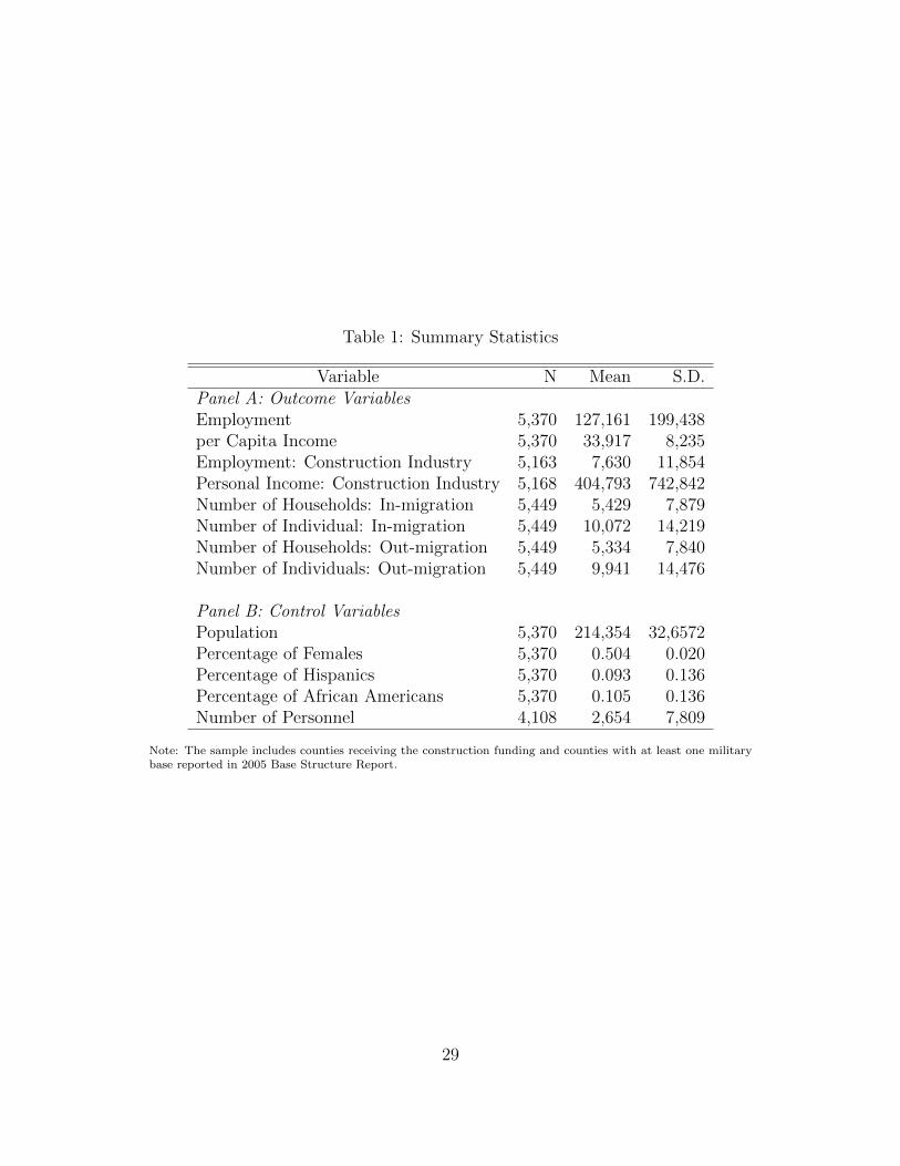
Table 1: Summary Statistics

Variable N Mean S.D.Panel A: Outcome VariablesEmployment 5,370 127,161 199,438per Capita Income 5,370 33,917 8,235Employment: Construction Industry 5,163 7,630 11,854Personal Income: Construction Industry 5,168 404,793 742,842Number of Households: In-migration 5,449 5,429 7,879Number of Individual: In-migration 5,449 10,072 14,219Number of Households: Out-migration 5,449 5,334 7,840Number of Individuals: Out-migration 5,449 9,941 14,476

Panel B: Control VariablesPopulation 5,370 214,354 32,6572Percentage of Females 5,370 0.504 0.020Percentage of Hispanics 5,370 0.093 0.136Percentage of African Americans 5,370 0.105 0.136Number of Personnel 4,108 2,654 7,809

Note: The sample includes counties receiving the construction funding and counties with at least one militarybase reported in 2005 Base Structure Report.

29

Table 2: Estimated Effects of 2005 BRAC Construction Funding on Local Economic Condi-tions

(1) (2) (3) (4)Panel A: Log(Employment)BRAC Funding per Capita ($1,000s) 0.036*** 0.038*** 0.030** 0.033***

(0.007) (0.007) (0.013) (0.009)N 5,370 5,370 5,370 5,370

Panel B: Log(Per Capita Income)BRAC Funding per Capita ($1,000s) 0.056*** 0.050** 0.045*** 0.038***

(0.019) (0.020) (0.011) (0.012)N 5,370 5,370 5,370 5,370Cost per Job 57,563 54,533 69,075 64,795Income Multiplier 1.79 1.59 1.44 1.21Controls No Yes No YesState-by-Year Fixed Effect No No Yes Yes

Note: *** p<0.01, ** p<0.05, * p<0.1 All regressions include county and year fixed effects.County-level controls include population, percentage of female, Hispanics and African Amer-icans. Standard errors are clustered at the state level. Control counties are counties withat least one military base reported in base structural report in 2005, the last report pub-lished prior to the 2005 BRAC. Estimates are unweighted. The cost per job is calculated as

$1,000×pre-funding average of population size for funded countiesestimated percentage change×pre-funding average of employment for funded counties

and the local fiscal mul-

tiplier is calculated asestimated percentage change×pre-funding average of per capita income for funded counties

$1,000.

30

Table 3: Estimated Effects of 2005 BRAC Construction Funding on the Construction Indus-try

(1) (2) (3) (4)Panel A: Log(Employment)Annual BRAC Funding per Capita 0.139*** 0.138*** 0.111*** 0.108***

(0.027) (0.024) (0.036) (0.033)Observations 5,163 5,163 5,163 5,163Panel B: Log(Personal Income)Annual BRAC Funding per Capita 0.203*** 0.202*** 0.142** 0.138***

(0.038) (0.036) (0.053) (0.049)N 5,168 5,168 5,168 5,168Controls No Yes No YesState-by-Year Fixed Effect No No Yes Yes

Note: *** p<0.01, ** p<0.05, * p<0.1 . All regressions include county and year fixed effects. County-levelcontrols include population, percentage of female, Hispanics and African Americans. Standard errors are clus-tered at the state level. Control counties are counties with at least one military base reported in base structuralreport in 2005, the last report published prior to the 2005 BRAC. Estimates are unweighted.

31

Table 4: Estimated Effects of 2005 BRAC Construction Funding on Local Economic Condi-tions, Restricting Analysis to Funded Counties


(0.009) (0.007) (0.015) (0.008)N 1,250 1,250 1,250 1,250



Note: *** p<0.01, ** p<0.05, * p<0.1 These estimates utilize variation in the timing and amount offunding awarded within funded counties to estimate the results. All regressions include county and year fixedeffects. County-level controls include population, percentage of female, Hispanics and African Americans.Standard errors are clustered at the state level. Estimates are unweighted. The cost per job is calculated as




$1,000.

32

Table 5: Estimated Effects of 2005 BRAC Construction Funding on Local Economic Condi-tions: Omitting States linked to the 2005 BRAC Commission

(1) (2) (3) (4)Panel A: Log(Employment)BRAC Funding per Capita ($1,000s) 0.032*** 0.031*** 0.034*** 0.035***

(0.008) (0.006) (0.010) (0.008)N 3,390 3,390 3,390 3,390

Panel B: Log(Per Capita Income)BRAC Funding per Capita ($1,000s) 0.050** 0.042** 0.045*** 0.036***


Note: *** p<0.01, ** p<0.05, * p<0.1 All regressions include county and year fixed effects. County-levelcontrols include population, percentage of female, Hispanics and African Americans. Standard errors areclustered at the state level. Control counties are counties with at least one military base reported in basestructural report in 2005, the last report published prior to the 2005 BRAC. Estimates are unweighted. Countiesin state linked to the 2005 BRAC Commission are dropped from the analysis. The cost per job is calculated as




$1,000.

33

Table 6: Are the Estimated Effects Driven by Personnel Relocation?

(1) (2) (3) (4)Panel A: Log(Employment)BRAC Funding per Capita ($1,000s) 0.037*** 0.038*** 0.038*** 0.038***

(0.007) (0.007) (0.008) (0.007)Logged(Personnel) -0.001 -0.002 -0.002 -0.003

(0.002) (0.001) (0.002) (0.002)N 4,108 4,108 4,108 4,108


(0.018) (0.018) (0.012) (0.013)Logged(Personnel) 0.002 0.002 0.002 0.002

(0.002) (0.001) (0.002) (0.002)N 4,108 4,108 4,108 4,108Cost per job 58,710 57,166 57,166 57,166Income Multiplier 1.70 1.47 1.44 1.21Controls No Yes No YesState-by-Year Fixed Effect No No Yes Yes

Note: *** p<0.01, ** p<0.05, * p<0.1 All regressions include county and year fixed effects. County-level controls include population, percentage of female, Hispanics and African Americans, and naturallog of military personnel counts. Standard errors are clustered at the state level. Control countiesare counties with at least one military base reported in base structural report in 2005, the last re-port published prior to the 2005 BRAC. Estimates are unweighted. The cost per job is calculated as




$1,000.

34

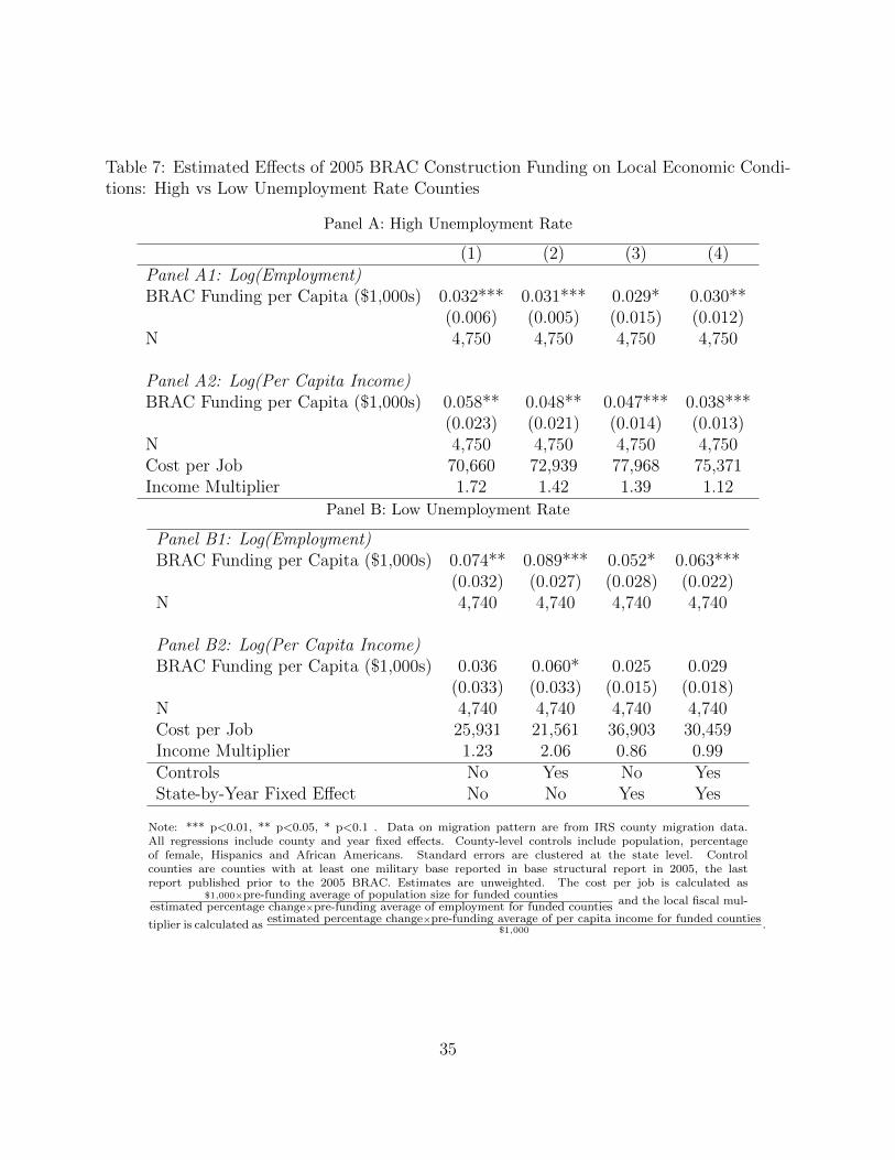
Table 7: Estimated Effects of 2005 BRAC Construction Funding on Local Economic Condi-tions: High vs Low Unemployment Rate Counties

Panel A: High Unemployment Rate

(1) (2) (3) (4)Panel A1: Log(Employment)BRAC Funding per Capita ($1,000s) 0.032*** 0.031*** 0.029* 0.030**

(0.006) (0.005) (0.015) (0.012)N 4,750 4,750 4,750 4,750

Panel A2: Log(Per Capita Income)BRAC Funding per Capita ($1,000s) 0.058** 0.048** 0.047*** 0.038***

(0.023) (0.021) (0.014) (0.013)N 4,750 4,750 4,750 4,750Cost per Job 70,660 72,939 77,968 75,371Income Multiplier 1.72 1.42 1.39 1.12

Panel B: Low Unemployment Rate

Panel B1: Log(Employment)BRAC Funding per Capita ($1,000s) 0.074** 0.089*** 0.052* 0.063***

(0.032) (0.027) (0.028) (0.022)N 4,740 4,740 4,740 4,740

Panel B2: Log(Per Capita Income)BRAC Funding per Capita ($1,000s) 0.036 0.060* 0.025 0.029


Note: *** p<0.01, ** p<0.05, * p<0.1 . Data on migration pattern are from IRS county migration data.All regressions include county and year fixed effects. County-level controls include population, percentageof female, Hispanics and African Americans. Standard errors are clustered at the state level. Controlcounties are counties with at least one military base reported in base structural report in 2005, the lastreport published prior to the 2005 BRAC. Estimates are unweighted. The cost per job is calculated as




$1,000.

35

Table 8: Spillover Effects of 2005 BRAC Construction Funding on Neighboring Counties

(1) (2) (3) (4)Panel A: Log(Employment)BRAC Funding per Capita ($1,000s) -0.001 0.000 -0.008 -0.006

(0.010) (0.010) (0.006) (0.006)N 24,010 24,010 24,010 24,010

Panel B: Log(Per Capita Income)BRAC Funding per Capita ($1,000s) 0.013 0.012 0.012 0.010


Note: *** p<0.01, ** p<0.05, * p<0.1 . All regressions include county and year fixed effects. County-levelcontrols include population, percentage of female, Hispanics and African Americans. Standard errors are clus-tered at the state level. Control counties are counties with at least one military base reported in base structuralreport in 2005, the last report published prior to the 2005 BRAC. Estimates are unweighted. Nearby countiesare selected according to highway distance.

36

Table 9: Spillover Effects of 2005 BRAC Construction Funding on Construction Industry

(1) (2) (3) (4)Panel A: Log(Employment)BRAC Funding per Capita ($1,000s) 0.033 0.031 0.030** 0.031**

(0.021) (0.020) (0.014) (0.013)N 21,951 21,951 21,951 21,951

Panel B: Log(Personal Income)BRAC Funding per Capita ($1,000s) 0.048 0.045 0.030 0.031


Note: *** p<0.01, ** p<0.05, * p<0.1 . All regressions include county and year fixed effects. County-levelcontrols include population, percentage of female, Hispanics and African Americans. Standard errors are clus-tered at the state level. Control counties are counties with at least one military base reported in base structuralreport in 2005, the last report published prior to the 2005 BRAC. Estimates are unweighted. Nearby countiesare selected according to highway distance.

37

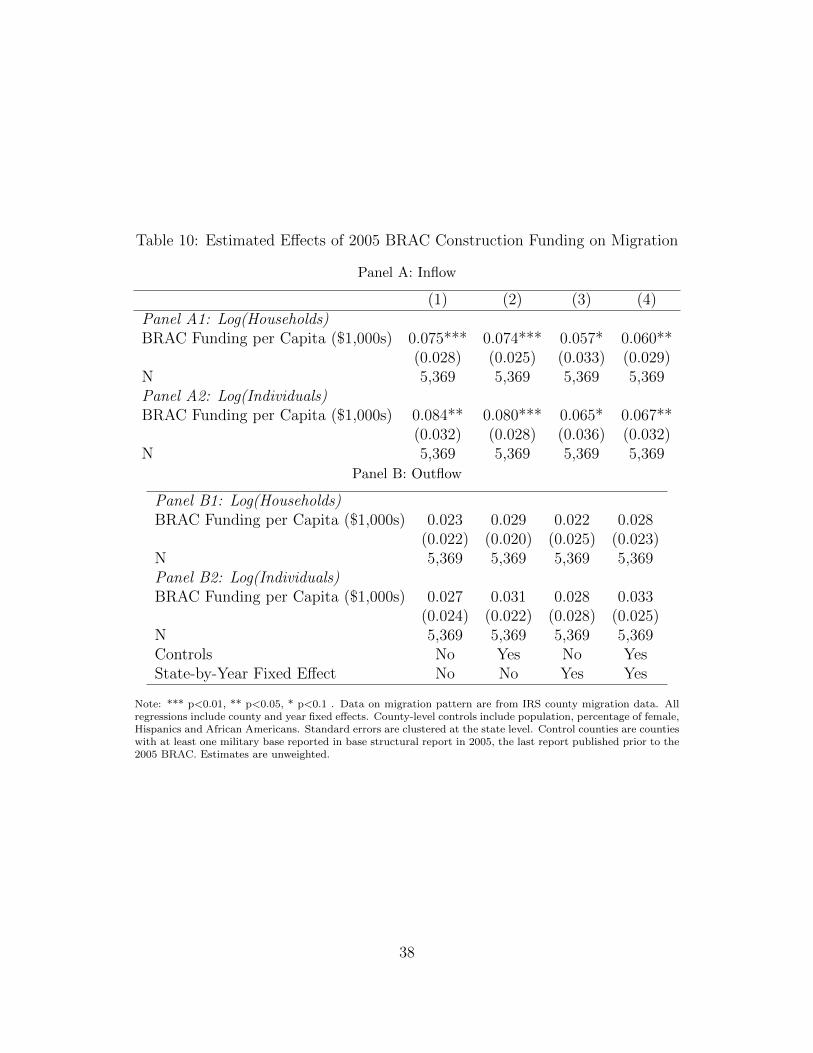
Table 10: Estimated Effects of 2005 BRAC Construction Funding on Migration

Panel A: Inflow

(1) (2) (3) (4)Panel A1: Log(Households)BRAC Funding per Capita ($1,000s) 0.075*** 0.074*** 0.057* 0.060**

(0.028) (0.025) (0.033) (0.029)N 5,369 5,369 5,369 5,369Panel A2: Log(Individuals)BRAC Funding per Capita ($1,000s) 0.084** 0.080*** 0.065* 0.067**

(0.032) (0.028) (0.036) (0.032)N 5,369 5,369 5,369 5,369

Panel B: Outflow

Panel B1: Log(Households)BRAC Funding per Capita ($1,000s) 0.023 0.029 0.022 0.028

(0.022) (0.020) (0.025) (0.023)N 5,369 5,369 5,369 5,369Panel B2: Log(Individuals)BRAC Funding per Capita ($1,000s) 0.027 0.031 0.028 0.033


Note: *** p<0.01, ** p<0.05, * p<0.1 . Data on migration pattern are from IRS county migration data. Allregressions include county and year fixed effects. County-level controls include population, percentage of female,Hispanics and African Americans. Standard errors are clustered at the state level. Control counties are countieswith at least one military base reported in base structural report in 2005, the last report published prior to the2005 BRAC. Estimates are unweighted.

38

Table 11: Spillover Effects of 2005 BRAC Construction Funding on Migration for Neighbor-ing Counties

Panel A: Inflow

(1) (2) (3) (4)Panel A1: Log(Households)BRAC Funding per Capita ($1,000s) 0.026** 0.023* 0.017* 0.017*

(0.012) (0.013) (0.010) (0.009)N 23,980 23,980 23,980 23,980Panel A2: Log(Individuals)BRAC Funding per Capita ($1,000s) 0.035** 0.031** 0.026** 0.025**

(0.014) (0.015) (0.013) (0.012)N 23,980 23,980 23,980 23,980

Panel B: Outflow

Panel B1: Log(Households)BRAC Funding per Capita ($1,000s) 0.012 0.014 -0.002 0.002

(0.010) (0.010) (0.013) (0.012)N 24,078 24,078 24,078 24,078Panel B2: Log(Individuals)BRAC Funding per Capita ($1,000s) 0.016 0.016 -0.000 0.003


Note: *** p<0.01, ** p<0.05, * p<0.1 . Data on migration pattern are from IRS county migration data. Allregressions include county and year fixed effects. County-level controls include population, percentage of female,Hispanics and African Americans. Standard errors are clustered at the state level. Control counties are countieswith at least one military base reported in base structural report in 2005, the last report published prior to the2005 BRAC. Estimates are unweighted.

39

Appendix A.1: Selection Criteria

In selecting military installations for closure or realignment, the Department of Defense, giv-

ing priority consideration to military values, the first four criteria listed below, will consider:

Military Value

1. The current and future mission capabilities and the impact on operational readiness of

total force of the Department of Defense, including the impact on joint warfighting, training,

and readiness.

2. The availability and condition of land, facilities, and associated airspace (including

training areas suitable for maneuver by ground, naval, or air forces throughout a diversity

of climate and terrain areas and staging areas for the use of the Armed Forces in homeland

defense missions) at both existing and potential receiving locations.

3. The ability to accommodate contingency, mobilization, surge, and future total force

requirements at both existing and potential receiving locations to support operations and

training.

4. The cost of operations and the manpower implications.

Other Considerations

5. The extent and timing of potential costs and savings, including the number of years,

beginning with the date of completion of the closure or realignment, for the savings to exceed

the costs.

6. The economic impact on existing communities in the vicinity of military installations.

7. The ability of the infrastructure of both the existing and potential receiving commu-

nities to support forces, missions, and personnel.

8. The environmental impact, including the impact of costs related to potential environ-

mental restoration, waste management, and environmental compliance activities.

40

Appendix A.2: Additional Figures and Tables

Table A1: Estimated Effects of 2005 BRAC Construction Funding on Local Economic Con-ditions, Alternative Construction of per Capita Funding

(1) (2) (3) (4)Panel A: Log(Employment)BRAC Funding per Capita ($1,000s) 0.037*** 0.041*** 0.030* 0.033**

(0.009) (0.008) (0.017) (0.014)N 5,370 5,370 5,370 5,370

Panel B: Log(Per Capita Income)BRAC Funding per Capita ($1,000s) 0.073*** 0.074*** 0.058*** 0.058***


Note: *** p<0.01, ** p<0.05, * p<0.1 All regressions include county and year fixed effects. County-levelcontrols include population, percentage of female, Hispanics and African Americans. Standard errorsare clustered at the state level. Control counties are counties with at least one military base reportedin base structural report in 2005, the last report published prior to the 2005 BRAC. Estimates areunweighted. perCapitaFundingit equals to zero prior to the receipt of any funding for county i and

equals to FundingitPopulationit

for years after the first year of funding receipt. The cost per job is calculated as




$1,000.

41

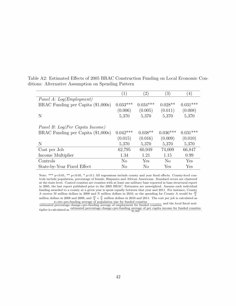
Table A2: Estimated Effects of 2005 BRAC Construction Funding on Local Economic Con-ditions: Alternative Assumption on Spending Pattern


(0.006) (0.005) (0.011) (0.008)N 5,370 5,370 5,370 5,370



Note: *** p<0.01, ** p<0.05, * p<0.1 All regressions include county and year fixed effects. County-level con-trols include population, percentage of female, Hispanics and African Americans. Standard errors are clusteredat the state level. Control counties are counties with at least one military base reported in base structural reportin 2005, the last report published prior to the 2005 BRAC. Estimates are unweighted. Assume each individualfunding awarded to a county at a given year is spent equally between that year and 2011. For instance, CountyA receive M million dollars in 2008 and N million dollars in 2010, so the spending for County A would be M

4

million dollars in 2008 and 2009, and M4

+ N2

million dollars in 2010 and 2011. The cost per job is calculated as$1,000×pre-funding average of population size for funded counties

estimated percentage change×pre-funding average of employment for funded countiesand the local fiscal mul-


$1,000.

42

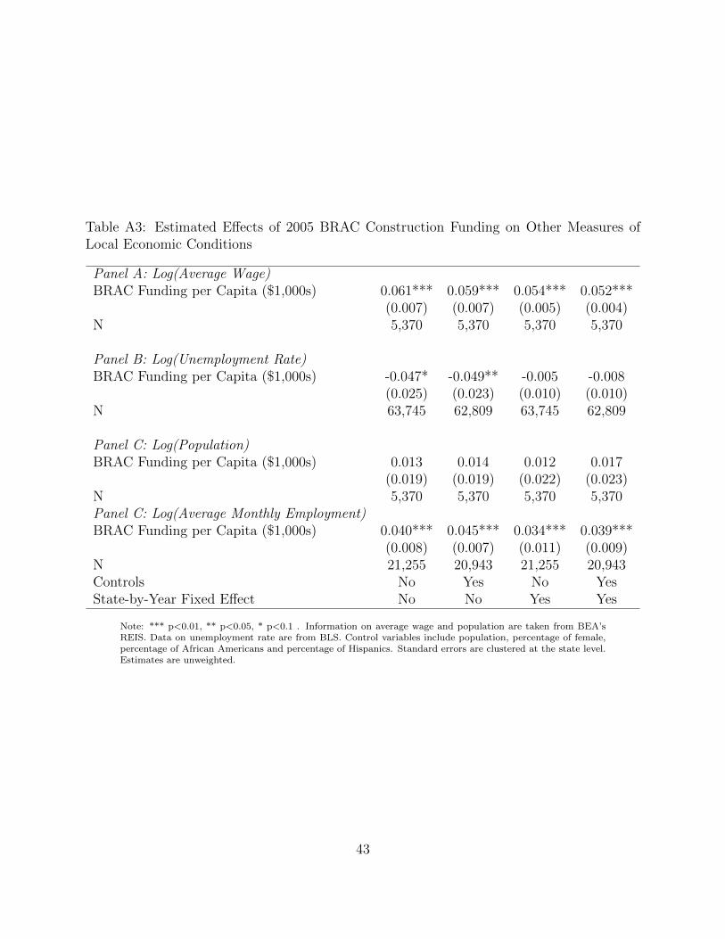
Table A3: Estimated Effects of 2005 BRAC Construction Funding on Other Measures ofLocal Economic Conditions

Panel A: Log(Average Wage)BRAC Funding per Capita ($1,000s) 0.061*** 0.059*** 0.054*** 0.052***

(0.007) (0.007) (0.005) (0.004)N 5,370 5,370 5,370 5,370

Panel B: Log(Unemployment Rate)BRAC Funding per Capita ($1,000s) -0.047* -0.049** -0.005 -0.008

(0.025) (0.023) (0.010) (0.010)N 63,745 62,809 63,745 62,809

Panel C: Log(Population)BRAC Funding per Capita ($1,000s) 0.013 0.014 0.012 0.017

(0.019) (0.019) (0.022) (0.023)N 5,370 5,370 5,370 5,370Panel C: Log(Average Monthly Employment)BRAC Funding per Capita ($1,000s) 0.040*** 0.045*** 0.034*** 0.039***


Note: *** p<0.01, ** p<0.05, * p<0.1 . Information on average wage and population are taken from BEA’sREIS. Data on unemployment rate are from BLS. Control variables include population, percentage of female,percentage of African Americans and percentage of Hispanics. Standard errors are clustered at the state level.Estimates are unweighted.

43

new evidence on the local fiscal multiplier and employment

Documents