NEW GRAPHICS DESIGNS FOR

THE ELEMENTS, ISOTOPES AND PARTICLES

PERIODIC CIRCLE OF THE ELEMENTS

The idea that matter consists of indivisible atoms, each a member of a sequence of unique elements, begins in 1808 with the son of an English weaver. John Dalton, whose talents as an experimentalist were somewhat dubious, perceived that the laws governing the proportioning of chemical compounds could be explained plainly by the concept of atoms from one particular element combining with the atoms peculiar to a different one. Remarkably, to the 20 elementary substances which were known in his day, he was able to assign each with a characteristic property called its atomic weight.

2

As more and more elements were discovered, it became clear that many of them were chemically similar, although of very different atomic weights. Sodium and potassium, for example, are both soft and highly reactive; they decompose in water, giving off hydrogen. And copper and silver are each lustrous, malleable and good conductors. By 1869 the list of known elements had grown to 63, and a chemist at the University of St. Petersburg, Dmitry Mendeleyev, found a method for linking their similarities. By grouping the elements into a recurrent pattern of periods and families, he helped confirm the validity of Dalton’s atomic hypothesis, and predicted successfully the existence and properties of many as yet undiscovered elements.

Mendeleyev’s Periodic Table began as a set of playing cards, with the elements and atomic weights on their faces, which he would shuffle around as if in a game, and his friends had a nickname for this curious new version of solitaire- “Patience”. With that personal quality, and a knowledge of every nuance of the elements’ behavior, Mendeleyev uncovered the property of periodicity- namely, that the elements, when arranged in order of their atomic weights, have such similar characteristics when aligned in certain regular and recurring intervals, they may be grouped formally into families. There was an inherent structure within the design of Nature, a pattern in the atomic progression.

This was Mendeleyev’s great intuition, and he materialized it by stacking his playing cards in columns of seven. These gave our contemporary family arrangements, with the inert gases, not discovered until 25 years later, completing our modern octets. His crowning insight was to recognize that there were gaps- or missing family members- in the progression of atomic weights. Accordingly, he predicted a number of new elements, such as ekaboron, which would lie between calcium and titanium, and its subsequent discovery ten years later as scandium led to the widespread acceptance of the periodic system.

3

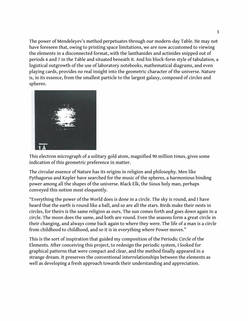
The power of Mendeleyev’s method perpetuates through our modern-day Table. He may not have foreseen that, owing to printing space limitations, we are now accustomed to viewing the elements in a disconnected format, with the lanthanides and actinides snipped out of periods 6 and 7 in the Table and situated beneath it. And his block-form style of tabulation, a logistical outgrowth of the use of laboratory notebooks, mathematical diagrams, and even playing cards, provides no real insight into the geometric character of the universe. Nature is, in its essence, from the smallest particle to the largest galaxy, composed of circles and spheres.

This electron micrograph of a solitary gold atom, magnified 90 million times, gives some indication of this geometric preference in matter.

The circular essence of Nature has its origins in religion and philosophy. Men like Pythagorus and Kepler have searched for the music of the spheres, a harmonious binding power among all the shapes of the universe. Black Elk, the Sioux holy man, perhaps conveyed this notion most eloquently.

“Everything the power of the World does is done in a circle. The sky is round, and I have heard that the earth is round like a ball, and so are all the stars. Birds make their nests in circles, for theirs is the same religion as ours. The sun comes forth and goes down again in a circle. The moon does the same, and both are round. Even the seasons form a great circle in their changing, and always come back again to where they were. The life of a man is a circle from childhood to childhood, and so it is in everything where Power moves.”

This is the sort of inspiration that guided my composition of the Periodic Circle of the Elements. After conceiving this project, to redesign the periodic system, I looked for graphical patterns that were compact and clear, and the method finally appeared in a strange dream. It preserves the conventional interrelationships between the elements as well as developing a fresh approach towards their understanding and appreciation.

4

5

7

Essentially, the elements are here registered within circles instead of squares, and the periods are laid out in an array of concentric circles. Every family of elements align in columns radiating from the center of the chart. Atomic numbers increase in a counterclockwise spiral and, for fine-tuning, the “s”-, “f”-, “d”- and “p”-block elements are placed within their periodic circles according to the relative energy of their valence orbitals.

The open space in the middle gives an opportunity for visual enhancement, and a bit of color helps distinguish the various families. It is my deep hope that this circular presentation will find its way into our schools and research facilities. The image is visually stimulating, with enough serenity to encourage creative scientific thought, whether young or old. Its openness, continuity and color enhance the processes of recognition and memory.

Those praises sung, I’d like to turn now to the customary positioning of the elements lutetium (71) and lawrencium (103), and express the opinion that they belong with the transition metals, rather than the rare-earth or actinide series. This may seem like a technicality, a minor question of categorization, but I noticed a discrepancy in their placement, and subsequently learned that a good deal of confusion had accompanied the history of the rare-earths, from the first fractional precipitations of the Swedish chemist, Carl Mosander, in 1842, up until 1914, when Harold Moseley, a British physicist, established a clear and unambiguous relationship between X-ray emission spectra and atomic number (any element’s unique number of protons). Mendeleyev’s original Table made no provision for a lanthanide series, and two of the elements he knew of- erbium and a substance called didymium- were later found to be conglomerates of even more elements. In fact, before the end of that century, more than 70 claims had been made for the discovery of a new rare-earth.

The trouble stemmed from the lanthanides’ nearly homogeneous chemical properties- they are predominantly trivalent, form hexagonal crystals, are never found as the free metal, but rather as oxides, and their ions replace each other with ease, so they’re simply found always as mixtures. And the slightest trace of impurity may give rise to an outstanding color or fluorescence. Laborious fractionation procedures were resorted to, and lutetium was the last of the sequence to be isolated, in 1907. Somewhat curiously, the least abundant of the rare-earths, thulium, is today believed to be more common than silver or gold.

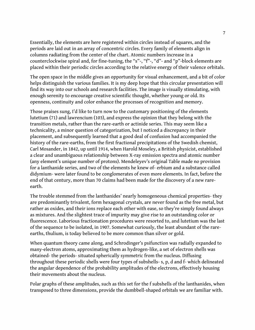
When quantum theory came along, and Schrodinger’s psifunction was radially expanded to many-electron atoms, approximating them as hydrogen-like, a set of electron shells was obtained- the periods- situated spherically symmetric from the nucleus. Diffusing throughout these periodic shells were four types of subshells- s, p, d and f- which delineated the angular dependence of the probability amplitudes of the electrons, effectively housing their movements about the nucleus.

Polar graphs of these amplitudes, such as this set for the f subshells of the lanthanides, when transposed to three dimensions, provide the dumbbell-shaped orbitals we are familiar with.

8

Here is an artist’s rendition of the orbital arrangement around iron, silver, and the rare-earth europium.

It is well worth remembering that exact solutions to Schrodinger’s equations are quite hopeless. Only hydrogen and helium have been determined, and the psifunction for an element like lanthanum, for example, with 57 electrons, has 171 spatial variables, 1596 Coulombic repulsion terms (called shielding), plus each of the electrons’ spin effects. So the quantum model, for electronic configurations, was compelled to resort to the simplification that the orbitals structure out a mathematical phase space around nuclei that are spherical (as of the single proton in hydrogen), sketching a ghosthouse of preferential energy levels. To build atoms, electrons are pictured as being added one by one to the stablest orbital available, so that

the energy of their aggregate is at a minimum, with Wolfgang Pauli’s exclusion principle allowing only two electrons per orbital.

In general, along the lanthanide and actinide series, the f orbitals fill up before the d’s, which characterize the transition metals. But these differently-shaped orbital sets are considered as shielded from the positive nucleus by differing amounts, via the core of electrons beneath them. Accordingly, rather than filling up sequentially into the 14 available slots in the f orbitals, for a few of these elements it is energetically favorable for electrons to enter d orbitals first.

9

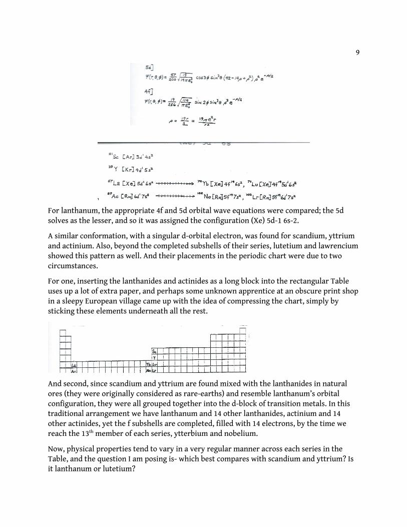
For lanthanum, the appropriate 4f and 5d orbital wave equations were compared; the 5d solves as the lesser, and so it was assigned the configuration (Xe) 5d-1 6s-2.

A similar conformation, with a singular d-orbital electron, was found for scandium, yttrium and actinium. Also, beyond the completed subshells of their series, lutetium and lawrencium showed this pattern as well. And their placements in the periodic chart were due to two circumstances.

For one, inserting the lanthanides and actinides as a long block into the rectangular Table uses up a lot of extra paper, and perhaps some unknown apprentice at an obscure print shop in a sleepy European village came up with the idea of compressing the chart, simply by sticking these elements underneath all the rest.

And second, since scandium and yttrium are found mixed with the lanthanides in natural ores (they were originally considered as rare-earths) and resemble lanthanum’s orbital configuration, they were all grouped together into the d-block of transition metals. In this traditional arrangement we have lanthanum and 14 other lanthanides, actinium and 14 other actinides, yet the f subshells are completed, filled with 14 electrons, by the time we reach the 13th member of each series, ytterbium and nobelium.

Now, physical properties tend to vary in a very regular manner across each series in the Table, and the question I am posing is- which best compares with scandium and yttrium? Is it lanthanum or lutetium?

10

Despite many strong similarities, four basic properties- melting point, density, specific heat capacity, and enthalpy of fusion- when matched beside the trends of the d-block elements above them, show lutetium correspondent with the elements hafnium and tantalum, while lanthanum is decidedly out of sync. It belongs in the f-block, with its periodic counterpart, actinium. Of course, this is only a bookkeeping issue, but serves to present a bit of atomic theory, which will be explored from here on.

Just as the psifunction obtains a set of shells for electron configuration, we have a nucleon wave function to particularize the shell-like arrangement of protons and neutrons in the various nuclei. Their energy, with numerical increase, distributes along several clusters punctuated by significant gaps- the magic numbers, which mark regions of greater nuclear stability, through the tendency of nucleons to seek to fill shells, the more harmonious assemblies of geometrized energy. Nuclei with magic numbers of neutrons are less prone to beta-decay.

Doubly-magic nuclei, with full shells for both protons and neutrons, are exceptionally stable.

11

This kind of quantum wizardy, coupled with our knowledge of the elements’ half-lives, has led to some interesting prospects for the production of superheavy elements.

Here is a map of nuclear stability, due to Glenn Seaborg, where the elements spread out like a mountain range, rising in accord with their half-life, over a sea of instability. The magic numbers generate a succession of ridges, and we speculate as to whether any island peaks of stability might extend beyond the latest synthetics, which only exist in microseconds.

The soft fusion reactions, pioneered by Yuri Oganessian, have successfully produced a full fourth row of transition metals, up to element 112, but only a few atoms at a time, using charged-particle accelerators. In this technique doubly-magic lead, or singly-magic bismuth, is bombarded with an ionic proton source- usually the highest stable isotope of one of the primary transition metals. Plutonium has also been fused with sulfur by this method.

These transactinides, as they are called, currently lack enough neutrons to assume more than quasi-stable arrangements, which points toward an important limitation of the soft fusion technique. For Nature seems to require a strict proportionality between protons and neutrons for stability. Beyond element 50, the necessary ratio lies within a narrow band that is almost exactly linear; the neutron/proton ratio rises by 0.005 per element. So while curium-243, for example, the lightest stable isotope of element 96, has a ratio of 1.53, element 110 needs a ratio above 1.6, say ununnilium-286, to attain similar stability, with perhaps 284 having a half-life measurable in days. Soft fusion produces only 273, an insufficiency of 12 to 16 neutrons, a shortage trending across the new transactinide series. The general reason for this is that any marriage between two stable isotopes produces unstable children; the smaller parent will be unable to boost their fusion product up to the higher neutron/proton ratio needed for long-living arrangements of heavier nuclei.

As regards the synthesis of further elements, speculation centers on elements 114 and 126, the next magic numbers for protons and neutrons. This enlarged version of the Periodic Circle extends out to element 218. Element 114 would constitute a chemical analogue of lead, while 126 is a member of a new electronic shell, the g-block, called the superactinide series.

12

As these idealized reactions show, the upper limits achievable via soft fusion, which marries stable ions together, usually the highest stable isotopes of the elements concerned, falls well short of the desired neutron number for stability.

In these explorations into the superheavy realm, the $64,000 question remains- can we produce a usable superisotope? One avenue to ponder is whether the fusion of two unstable isotopes might beget a viable offspring- whether parents with half-lives of one minute might coalesce to create an element lasting perhaps one year. In this type of nuclear genetics, four candidates- tin-132, radon-228, radium-234 and uranium-242 - are inordinately neutron-rich, with neutron/proton ratios ranging from 1.63 to 1.66.

13

A sampling of possible marriages, with the appropriate partner, suggests that this means of adding in the dozen or so neutrons required for stability is a sound possibility, up to a limit at about element 114. But the success of this “fusion of unstables” depends upon the technology for manipulating them, say by particle accelerators, and on the physics of the fusion itself. For a rule of thumb regarding nuclei is that they seek to become spherical, deforming toward the ellipsoidal as they become overladen with neutrons. And the suggestion being made here is that a pair of egg-shaped, unstable nuclei might, by fusion, create a stable, more spherical element.

What is the actual shape of nuclei? A remarkable correlation seems to exist between the magic numbers, generated by the shells of the nucleon wave function, and the geodesic geometries investigated by Buckminster Fuller. He felt that the tetrahedron, rather than the cube, ought to be used as our fundamental measure of volume and space. When we look in particular at the doubly-magic nuclei, the notion arises that protons and neutrons may actually interlink like a latticework, completely analogous to the crystals that form between atoms at a larger level.

Helium-4, the alpha particle so prominent in radioactive decay, forms a tetrahedron with four equilateral triangles as faces. The optimum arrangement, in terms of volume and energy distribution, might arise by a slight overlap in the packing of the contributing protons’ and neutrons’ spheres. Oxygen-16, in a similar fashion, may be viewed as a tetrahedral lattice of four tetrahedral, or alpha particles.

More striking is the disposition of calcium for assuming the shape of an icosahedron, a 12-part hexagonal lattice, like a multifaceted jewel having 20 triangular faces, with each member meshed to five others in the webwork. This jewel and its components may rotate, vibrate, and rearrange internally to give off effects such as radioactivity. Carbon, zirconium, platinum and plutonium are among the other elements correlating to this icosahedral structure, with higher multiple possible at mass numbers 288 and 336, compatible for elements 110 and 126.

14

A 13-part lattice, the cuboctahedron, with 6 square and 8 triangular faces, constitutes a favorable arrangement for the most stable forms of chromium, palladium, doubly-magic lead and mendelevium. Element 118, at mass number 312, would have the next compatible nucleon ratio in this cuboctahedral sequence.

So it is not only the magic numbers, but the mass numbers of “Fuller lattices” as well, that deserve our consideration in the search for superheavy elements. It is likely that each isotope has an ideal geometry, and their abundance of configurations calls for computer matching schemes of the myriad combinations at hand regarding parent elements and nuclear shapes. The Periodic Circle lends itself to this task, as a conceptual backdrop and easy-to-follow organizer. And if we ever do arrive at these titanic elements, they may somehow resemble this geodesic dome.

THE SPIRAL OF ISOTOPES

We owe the image of isotopes, from the early years of this century, to the English chemist Frederick Soddy. From studies of the “emanations” of radioactive thorium, with Ernest Rutherford at McGill University, Soddy realized that the elements occur as varieties of themselves, with differing atomic masses, but nearly identical chemical properties. The development of the mass spectrograph enabled precise separation of individual isotopes. And with the discovery of the neutron in 1932, the contributing components of the atomic masses could be accounted for.

While it is its unique number of protons that characterizes any particular element, its nucleus may accommodate a significant range of neutrons. The geometry of nuclear forces determines the stability and half-life of these proton-neutron arrangements. Today we have identified over 2900 of such distinct atomic forms- the isotopes- and have further classified them into isobars (isotopes of different elements with the same mass number), isotones (isotopes with the same number of neutrons) and isomers (isotopes with the same nuclear components but differing configurations and radiative properties).

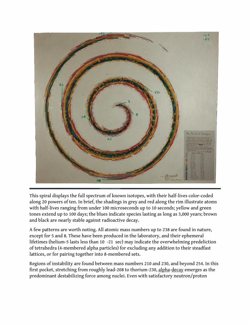
This spiral displays the full spectrum of known isotopes, with their half-lives color-coded along 20 powers of ten. In brief, the shadings in grey and red along the rim illustrate atoms with half-lives ranging from under 100 microseconds up to 10 seconds; yellow and green tones extend up to 100 days; the blues indicate species lasting as long as 3,000 years; brown and black are nearly stable against radioactive decay.

A few patterns are worth noting. All atomic mass numbers up to 238 are found in nature, except for 5 and 8. These have been produced in the laboratory, and their ephemeral lifetimes (helium-5 lasts less than 10 -21 sec) may indicate the overwhelming predeliction of tetrahedra (4-membered alpha particles) for excluding any addition to their steadfast lattices, or for pairing together into 8-membered sets.

Regions of instability are found between mass numbers 210 and 230, and beyond 254. In this first pocket, stretching from roughly lead-208 to thorium-230, alpha-decay emerges as the predominant destabilizing force among nuclei. Even with satisfactory neutron/proton

16

ratios, the geometries comprised by these numbers of nucleons are structurally unfavorable, and typically they cascade radioactively downward into a stable form of lead or bismuth. At a minimum, at mass number 217, there are no isotopes lasting longer than 10 seconds. And while many stable assemblies occur in the procession along the heavier isotopes (curium-247, for instance, has a half-life of over 15 million years), spontaneous fission begins to compete with alpha decay in breaking them apart. This self-splitting, arising when the electrostatic repulsion of protons overcomes the strong force’s attractive binding of nucleons, becomes the limiting factor in the formation of superheavy clusters.

The elements exhibit a fairly normal distribution in terms of their permutations as isotopes- rhodium (45) on up through francium (87) have at least 30 each, and the “champion” is indium (49) with 65. Similarly, there are 10 or more isobars (proportional to the width of the Spiral) for each mass number between 73 and 204, and 15 or more between 116 and 152. Among the isotones (which have the same number of neutrons) is a regular dispersion as well. Isotones with 39 to 121 neutrons have at least 15 isotopes each, with a peak of 39 isotopes at isotone number 79.

Strictly speaking, all isotopes are radioactive. Given enough time, perhaps billions of years, even the most stable nuclear geometry known- iron-56 - will eventually rearrange itself and emit energy. In every atom of matter, the protons, neutrons and electrons are in a real sense tensilely suspended in space, and an ongoing interplay between the electrostatic and the nuclear (strong & weak) forces ultimately disrupts their assemblies, transforming one isotope into another, with the release of alpha, beta and gamma rays. Even a neutron, when sufficiently isolated, decomposes into a proton and electron, with a half-life of only 10.3 minutes. And since the origin of radioactivity is within the nucleus itself, the process of decay is considered as independent of all other external conditions, such as temperature, pressure, magnetism and gravitation.

Because each particular isotope displays a distinctive decay rate, radioactivity may be regarded as an exponential process. The number of atoms expected to decompose within a given infinitesimal time period (dN/dt) is proportional to the number of atoms present (N):

Where N 0 is the number of atoms initially present at time zero, t ½ is the half-life, e is the logarithmic constant 2.71828…, and lambda, the decay constant, is unique and determinable for every isotope.

This principle, that each radioactive atom decays at a distinctive and invariable rate into daughter nuclei, forms the basis for the dating methods used in geology. The age of mineral samples may be accurately determined from as little as one nanogram of the radioisotopes

17

existing naturally in their crystal structure. A familiar technique uses a pair of uranium isotopes, which continuously produce lead via a multistep decay sequence, a cascade that produces various intermediary radioisotopes, along with the emission of several alpha (helium ions) and beta (electrons or positrons) particles.

The relative abundance of the two pairs allows for comparison and correlation of the estimates for the age of our Earth, regarded today as about 4.6 billion years old. These results depend upon the decay rate, however, and are only true as far as this rate remains constant over time.

Before challenging this constancy of decay, which time and again has been empirically verified, since radiation scintillations were first counted by Hans Geiger in 1908, let us briefly review the modern theory of radioactivity.

The quantum model of alpha disintegration pictures the alpha particle existing as a separate ingredient within the nucleus itself. In wave mechanics, this alpha packet has a nonvanishing probability of entering regions of negative kinetic energy, “forbidden” to macroscopic entities. Such a region, a Coulomb barrier, exists around the nucleus because of electrostatic repulsion between resident protons and any hypothetically-approaching alpha particles. But there is an infinitesimal “tunneling” probability that an alpha packet might burrow its way out of the nucleus, on through the Colomb barrier and out into the surrounding space. And the overwhelming number of natural nuclear oscillations (10 22 per second) arising from the close confinement of energy-endowed protons and neutrons yields the slim but definite probability (10 -38 for U-235) that one will escape.

When emission intensities are measured, alpha disintegration displays sharp, discontinuous energy spectra as well as a methodical dependence upon atomic number (Z), particularly among isotopes bearing even numbers of protons and neutrons. The emission energy is related to the decay constant via:

So that the alpha energy release, proportionate to expulsion velocity, increases directly with an isotope’s decay constant, or inversely with its lifetime.

18

Beta-decay comprises an entirely distinct phenomenon, wherein the emitted electrons or positrons exhibit a smooth, continuous energy spectrum, completely independent of atomic number. This nonquantized distribution seemed to violate the law of conservation of energy, until Pauli proposed in 1931 that a new particle, the neutrino, could share out the released energy. In this way the beta particle, coupled with its neutrino partner, emanates in discrete units of h, Planck’s constant.

Beta-minus decay involves the transmutation of a neutron into a proton, with the ejection of and electron and antineutrino.

It is considered as falling under the province of the weak force, as fundamental as gravitation, electromagnetism, and the strong force attracting nucleons together.

Half-lives of nuclei undergoing beta-emission depend upon the “degree of forbiddenness” of the transformation, a measure of the compatibility, or overlap, of the nucleon wave functions before and after the decay. The constant for beta-minus decay may be approximated via:

So the beta decay rate is found to increase directly according to the energy emitted, but balanced, in an intricate manner, by the degree of mismatch of the initial and final nucleon wave functions. Experimentally, allowed transformations are observed to have half-lives inversely proportional to the square-root of the energy, and hence the velocities, of the ejected electron and antineutrino.

Quite curiously, it was discovered by C.S. Wu in 1957 that beta-transitions involving the axial components violated the law of parity, or spatial inversion- the emitted particles spin with a preferential “handedness”, directed along the direction of flight, and the mirror image of this process simply does not happen. This is in point-blank disagreement with the

19

conduct of the other fundamental physical forces, all of which are symmetric with respect to inversion, and as with other physical laws, symmetry implies conservation of energy. A long and tortuous analysis of this predicament evolved into electroweak theory in the 1970’s, after the introduction of exchange bosons (W and Z) for carrying electroweak force, a new quantum number (weak isospin), and an appeal to the concept of “spontaneous symmetry breaking”, akin to the magnetic phase transitions induced by temperature in superconductors. Different particles are here regarded as actually of one type, transposing into different states at low enough energies. While successful predictively, it is fair to regard this theory as philosophically incomplete.

It is worth remembering that most of the experiments in nuclear physics neglect considerations of gravity, applying the approximations of special relativity (a “flat” space-time metric) to give constancy to the inertial frames of the laboratory. And nearly all such inquiries take place on the Earth’s surface, within a homogeneous gravitational field, dominated by the Sun. The solar mass is calculated as being 328,912 times greater than that of the Earth-Moon system.

This approach is substantially justified, as for instance, when the electrical repulsion of two electrons is compared with the gravitational attraction between their miniscule masses. Irrespective of their mutual distance, the gravity is weaker by a factor of 10 -43. It is in the great enormity of astronomical matter that gravity plays its dominant role in the universe.

Which brings one to wonder whether, were physics experiments performed far off in space, would their outcomes be the same as on Earth? Is it valid to extend our local results into other regions, where the inertial frame of reference might be quite different?

Our pillar of reason in this arena is the spectroscope, used to probe the atmosphere of stars, the recession of distant galaxies, the concentration of interstellar plasma, and the temperature gradient of the universe. Very specific spectral lines, signatory of each individual isotope, of a strength correspondent with the source’s temperature, have been employed over the whole of the electromagnetic band to map out the vastness of space. One example- arising due to the proton’s “nonpointlike” distribution of charge- is hydrogen’s hyperfine splitting line, at 1,420,405,751,800+/-0.028 cycles/sec, long used by radiotelescopes to determine the velocities and densities of cosmic gas. Spectroscopy is an exceedingly exact science, and the red-shifts displayed by heavenly bodies demonstrate convincingly that we live in an expanding universe.

An observational parameter, the Hubble constant, allows us to estimate this rate of expansion. A modern value of H 0 = 75 km/sec-megaparsec yields an enlargement of 7.7% per billion years. Also, due to the gravitational pull of the constituent masses on each other, the expansion is gradually slowing down, decelerating by a factor of perhaps 1/10 every billion years. So, this cosmological information lets us postulate that 4.6 billion years ago, at the time of the Earth’s formation, our Cosmos was only 61% its present size. At the time of

20

the extinction of the dinosaurs, estimated geologically at 65 million years, it was about 99.4%.

If we consider this “compression” as occurring uniformly throughout the earlier universe, and the total amount of matter as having remained the same, it follows that an equivalent gravitational force was exerted across a smaller distance, in the past as compared with today. Consequently, in response to the greater gravity felt, heavenly bodies moved faster, then than now, throughout space. In particular, the Earth would have revolved around the Sun more quickly in the earlier universe.

Geophysically, it is well-accepted that the earth’s daily rotation rate is slowing, perhaps by 20 seconds every million years. Equally, if we imagine a celestial sphere, just enclosing the Sun-Earth system, condensed to 99.4% its original size, with our own planet that much closer to its star, using Newton’s laws, it revolves about 1.2% faster than previous, and along a tighter orbital path. So that a period for one revolution becomes 99.2% that of the original, and thus a “year” at the end of the dinosaur age lasted perhaps 358 days- an orbit that loses a day every million years. This sets their demise a bit close to us, at 64.4 of our modern “years” ago. Similar computations for the creation of the Earth, when the period might have been a mere 85 days, give an age of only 2.6 billion years.

So that the further we look back in time, the more it compresses, due to the greater effective gravity. In this sense does the expansion of the universe bestow a nonlinearity upon the flow of time. Envisioning the span of years that return us to the dinosaurs, or further, is not so much like pacing out steps across the Great Plains, but rather, it is more like climbing into the Rocky Mountains. Every step grows smaller, and the trail to the summit only steepens.

And it is fair to wonder whether gravity might exert a profound effect on the stability of the elements themselves- indeed, whether there is a certain range of gravitational pressure within which any atom retains or distorts its basic form; whether radioactivity, considered as a movement of the entire nucleus towards a more spherically-shaped equilibrium- and attributed, in beta-decay, to the action of the weak force- might in actuality be ascribed to the influence of gravity, at this subatomic level, as it alters the permeability of space; and whether the known decay rates, assumed to be constant, and the basis of our geological arrow through time, might in fact change in accord with gravitation.

According to relativity, any event, or “world-point” (x,y,z,t) in four dimensions, may be represented in relation to its past and future light cones, whose boundaries delimit the speed of light. Events located within the cones may affect or be influenced by one another, in “real” time, while those on the outside are lost, in a causal sense, in “imaginary” time, where signals must travel faster than light to connect.

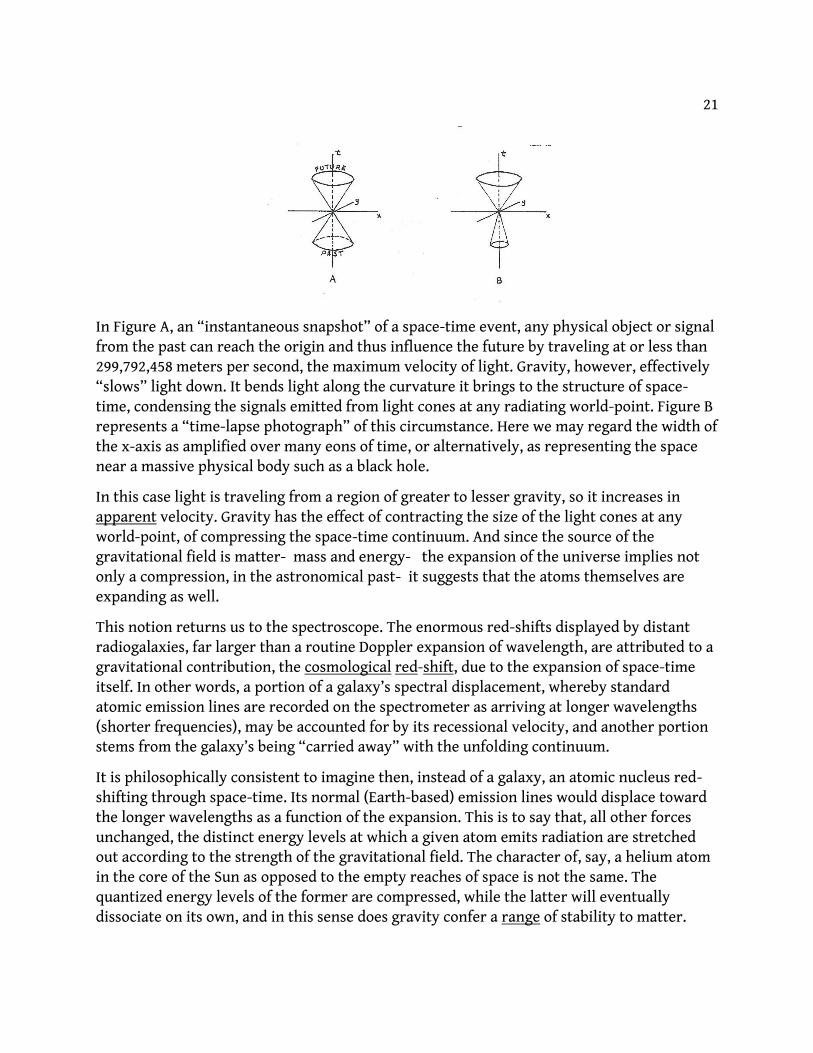
21

In Figure A, an “instantaneous snapshot” of a space-time event, any physical object or signal from the past can reach the origin and thus influence the future by traveling at or less than 299,792,458 meters per second, the maximum velocity of light. Gravity, however, effectively “slows” light down. It bends light along the curvature it brings to the structure of space-time, condensing the signals emitted from light cones at any radiating world-point. Figure B represents a “time-lapse photograph” of this circumstance. Here we may regard the width of the x-axis as amplified over many eons of time, or alternatively, as representing the space near a massive physical body such as a black hole.

In this case light is traveling from a region of greater to lesser gravity, so it increases in apparent velocity. Gravity has the effect of contracting the size of the light cones at any world-point, of compressing the space-time continuum. And since the source of the gravitational field is matter- mass and energy- the expansion of the universe implies not only a compression, in the astronomical past- it suggests that the atoms themselves are expanding as well.

This notion returns us to the spectroscope. The enormous red-shifts displayed by distant radiogalaxies, far larger than a routine Doppler expansion of wavelength, are attributed to a gravitational contribution, the cosmological red-shift, due to the expansion of space-time itself. In other words, a portion of a galaxy’s spectral displacement, whereby standard atomic emission lines are recorded on the spectrometer as arriving at longer wavelengths (shorter frequencies), may be accounted for by its recessional velocity, and another portion stems from the galaxy’s being “carried away” with the unfolding continuum.

It is philosophically consistent to imagine then, instead of a galaxy, an atomic nucleus red-shifting through space-time. Its normal (Earth-based) emission lines would displace toward the longer wavelengths as a function of the expansion. This is to say that, all other forces unchanged, the distinct energy levels at which a given atom emits radiation are stretched out according to the strength of the gravitational field. The character of, say, a helium atom in the core of the Sun as opposed to the empty reaches of space is not the same. The quantized energy levels of the former are compressed, while the latter will eventually dissociate on its own, and in this sense does gravity confer a range of stability to matter.

22

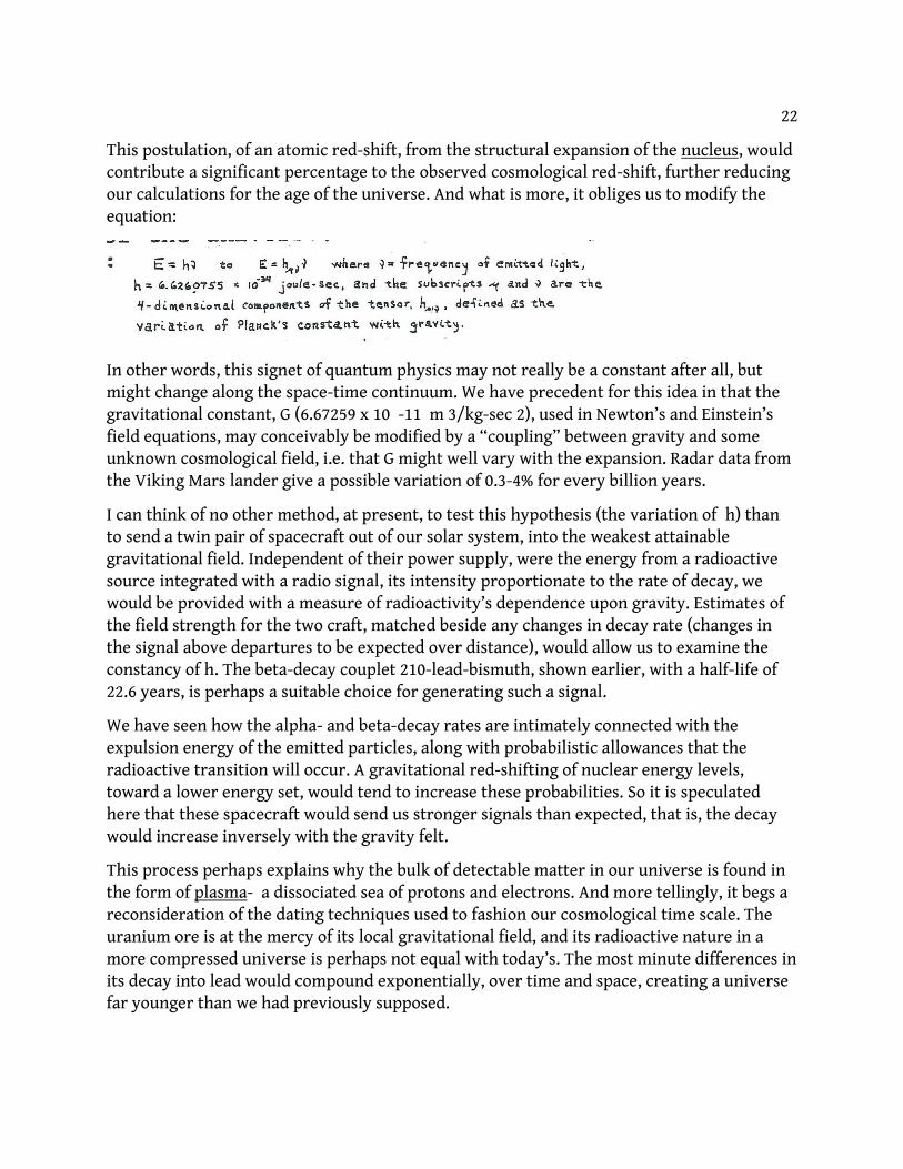
This postulation, of an atomic red-shift, from the structural expansion of the nucleus, would contribute a significant percentage to the observed cosmological red-shift, further reducing our calculations for the age of the universe. And what is more, it obliges us to modify the equation:

In other words, this signet of quantum physics may not really be a constant after all, but might change along the space-time continuum. We have precedent for this idea in that the gravitational constant, G (6.67259 x 10 -11 m 3/kg-sec 2), used in Newton’s and Einstein’s field equations, may conceivably be modified by a “coupling” between gravity and some unknown cosmological field, i.e. that G might well vary with the expansion. Radar data from the Viking Mars lander give a possible variation of 0.3-4% for every billion years.

I can think of no other method, at present, to test this hypothesis (the variation of h) than to send a twin pair of spacecraft out of our solar system, into the weakest attainable gravitational field. Independent of their power supply, were the energy from a radioactive source integrated with a radio signal, its intensity proportionate to the rate of decay, we would be provided with a measure of radioactivity’s dependence upon gravity. Estimates of the field strength for the two craft, matched beside any changes in decay rate (changes in the signal above departures to be expected over distance), would allow us to examine the constancy of h. The beta-decay couplet 210-lead-bismuth, shown earlier, with a half-life of 22.6 years, is perhaps a suitable choice for generating such a signal.

We have seen how the alpha- and beta-decay rates are intimately connected with the expulsion energy of the emitted particles, along with probabilistic allowances that the radioactive transition will occur. A gravitational red-shifting of nuclear energy levels, toward a lower energy set, would tend to increase these probabilities. So it is speculated here that these spacecraft would send us stronger signals than expected, that is, the decay would increase inversely with the gravity felt.

This process perhaps explains why the bulk of detectable matter in our universe is found in the form of plasma- a dissociated sea of protons and electrons. And more tellingly, it begs a reconsideration of the dating techniques used to fashion our cosmological time scale. The uranium ore is at the mercy of its local gravitational field, and its radioactive nature in a more compressed universe is perhaps not equal with today’s. The most minute differences in its decay into lead would compound exponentially, over time and space, creating a universe far younger than we had previously supposed.

23

THE CIRCLE OF SUBATOMIC PARTICLES

The prolific surge of particle physics in this century has led to the detection of hundreds of new components of matter. An advances in the technology of accelerators and bubble chambers promise even further discoveries as scientists probe the inner workings of the atom. Their noblest dream is to confirm a theory for the fundamental forces, unifying general relativity and quantum mechanics.

Yet no adequate system is at hand for relating and referencing these subnuclear entities. The student or researcher is left to fish through a pile of mathematics-style compendiums for information.

The Circle of Subatomic Particles is the first comprehensive guide to the 336 known particles, i.e. all subnuclear matter and antimatter composed of quarks. By graphing them according to their characteristic mass, electrical charge, and quantum spin- the three properties that uniquely define each particle as a physical entity- this concise visual display serves as a simple and time-saving reference system for identifying the individual particles and families, their quark composition, decay modes, resonance patterns, and clustering effects at various energies and spins. And all of this information is made available at a glance.

Essentially, the design is a circular energy map coordinated by mass, charge and spin. The particles, plotted according to their mass in megaelectronvolts, are color-coded into their various families and individually arrayed as incrementally-sized circles, expanding along a scale of 1 to 10, which allows easy identification of their quark content. A larger size indicates a heavier quark composition.

In the legend are sketched the 3 evolutions of quarks (up, charm, top- down, strange, bottom), while the types of subatomic particles are grouped as to generation, class, and quark content.

An assemblage of three quarks classifies a particle as a baryon, and these populate the right-hand side of the chart. Quark-antiquark systems, called mesons, inhabit the left. The positive, neutral, and negative permutations of each delineate six sectors.

Spin defines a particle’s internal angular momentum. It is not so much a revolving about a definite axis, but more like a whirling dispersion, a “preferentiality” as to directional orientation. Quantum laws for matter entities, such as quarks, require their spin to be half-integer (1/2, 3/2, 5/2, etc.) multiples of Planck’s constant, divided by 2 pi. Thus the baryons, via the addition of 3 quark spins, have their spin values measured by halves, while the mesons are in whole numbers.

So the possible spins subdivide the six sectors, with the values increasing in a clockwise manner- excepting for the positive mesons, where spin increases counterclockwise. This is to signify that they are the antimatter counterparts of the negative mesons- duplicates of

25

mass and spin, but with opposite charge. Every baryon also has its own antibaryon- composed of 3 antiquarks- and the entire right-hand side of the design may be flipped over, mentally, to give the set of antimatter baryons. In this way does every known particle find a home on the chart. And the bull’s-eye hints at an even deeper level of reality.

The quarks are believed to be congealed points of energy, like the electron, less than 10 -18 meters across. They carry 1/3 or 2/3 of the electron’s fundamental unit of electrical charge. Quarks orbit one another, clustering in either pairs or triplets, and at preferred energy levels are detectable as matter. Some of the most ephemeral resonances, with lifetimes less than 10 -23 seconds, would only travel, at the speed of light, barely further than their own diameter.

A further property, colour charge, has been ascribed to explain why quarks never occur uncombined. Colour was first introduced for theoretical reasons, since the exclusion principle requires an antisymmetric wave function for a grouped state, say, of two electrons occupying one atomic orbital, or of three quarks assembling into one baryon. Assigning the colour quantum numbers red, blue or green to any quark (or the corresponding anticolour to antiquarks) enables the permutations of each compositional triplet to be distinguished. And also, only “white” states are allowed to exist as free particles. For baryons, this means each member quark has a different colour charge, while mesons match up a colour with its anticolour. Altogether, with 12 flavours having 3 possible colours, there are 36 varieties of quarks, and their myriad combinations and energy properties are the theme of quantum chromodynamics.

Excepting the proton and electron, all free particles eventually decay into lighter ones. Or, their constituent quarks might merge and annihilate, creating energy. The empty space on this chart may be regarded as an energy field of “virtual” matter, condensing into real matter at preferred values. Although some of the slices in this “subatomic pie” are slightly squeezed, for graphic clarity, it presents an able picture for theoreticians to visualize what exists in this realm. There are, unfortunately, very few regular patterns, and the hope of classical physicists- among them Albert Einstein- that these new particles will resolve as special solutions of unified field equations is seemingly impossible.

For most of this century, physics has endured two resoundingly successful yet diametrically opposed “truths”. Quantum mechanics has produced lasers, superconductors and microchips via a world description embracing probabilities, strong & weak nuclear forces, parity violation, “virtual” and antiparticles, atomic orbitals and structured sets of nuclear energy levels. General relativity has given us curved space-time, the red-shift and bending of light, black holes and an expanding universe by means of a 4-dimensional system of partial differential equations, covariant and nonlinear, that describe the world in terms of everywhere-continuous fields.

26

One speaks for a fundamental discreteness in the very texture of space-time, the other for an unbroken continuum. Neither theory implies the scope of the other, and an unshakeable principle lives in the heart of each.

Werner Heisenberg presented the uncertainty principle in 1927. Noting that the concepts as then applied to particles and waves (e.g. velocity, frequency, amplitude, field strengths) were originally derived from everyday experience, he realized these ideas soon became inadequate when carried over to atomic phenomena such as electrons. An inherent indeterminism accompanies any characterization of microcosmic entities and events, in which the customary concepts reach their meaning’s limit. At best, we are only able to perceive the generalized effects of sequential measurements, as probabilities instead of certainties.

Heisenberg deduced the eloquent equations that describe this

predicament. Any use of the concepts “position” and “momentum”, or “energy” and “time” are necessarily limited in accuracy- the most precise knowledge of either pair may not be smaller than Planck’s constant, else these ideas become meaningless.

It is often commented that uncertainty means there is a bottom limit to the precision of our measuring instruments, or the measurement act itself, or that one photon from a light source irretrievably alters the experimental target, beyond accurate knowability. But the imprecision and unapprehensibility arise from within the mystery of the matter/energy event itself. The electron does not possess, as a observable quality, position or velocity, but rather the property of “probability”- a specific likelihood of positional extent when linked within a given range of momenta. Its mass/energy content and the space-time it occupies are uncertain, within these probabilistic bounds. We may only obtain average values, for energy or position, by examining a collection of probabilities.

According to uncertainty, any particle occupies a volume in phase space, a 6-dimensional configuration interval of position and momentum. In phase space “exist” the “virtual” particles, for exceedingly short distances and times, where they may break the law of conservation of energy- otherwise confirmed for every interaction between atoms and radiation. So that this physical maxim, deterministic in the macrouniverse, becomes ambiguous at the subatomic level. Here we have a hint of processes without a causal nexus connecting them- a given effect not necessarily produced from a given cause.

Uncertainty is intimately related to the finite time required for the emission of light, as though it were implanted in the photon at its conception. An atom sends out a light signal because radiation progresses in the direction of increasing entropy- the thermodynamically

27

irreversible arrow of dissipation. About 10 -8 seconds is needed (or once every 10 14 nuclear oscillations) for photons, when created, to overcome the resistance from local fields and radiate away into space. This tenuous suspension of the light event, arising as the balance of matter and energy, with their interwoven forces, seeks havens of equilibrium against inevitable dissolution, is enough to generate the probabilistic ambiguity. It is as if, at our local world-point, the uncertainty principle expresses the essential relation between the time coordinate and space coordinates of space-time.

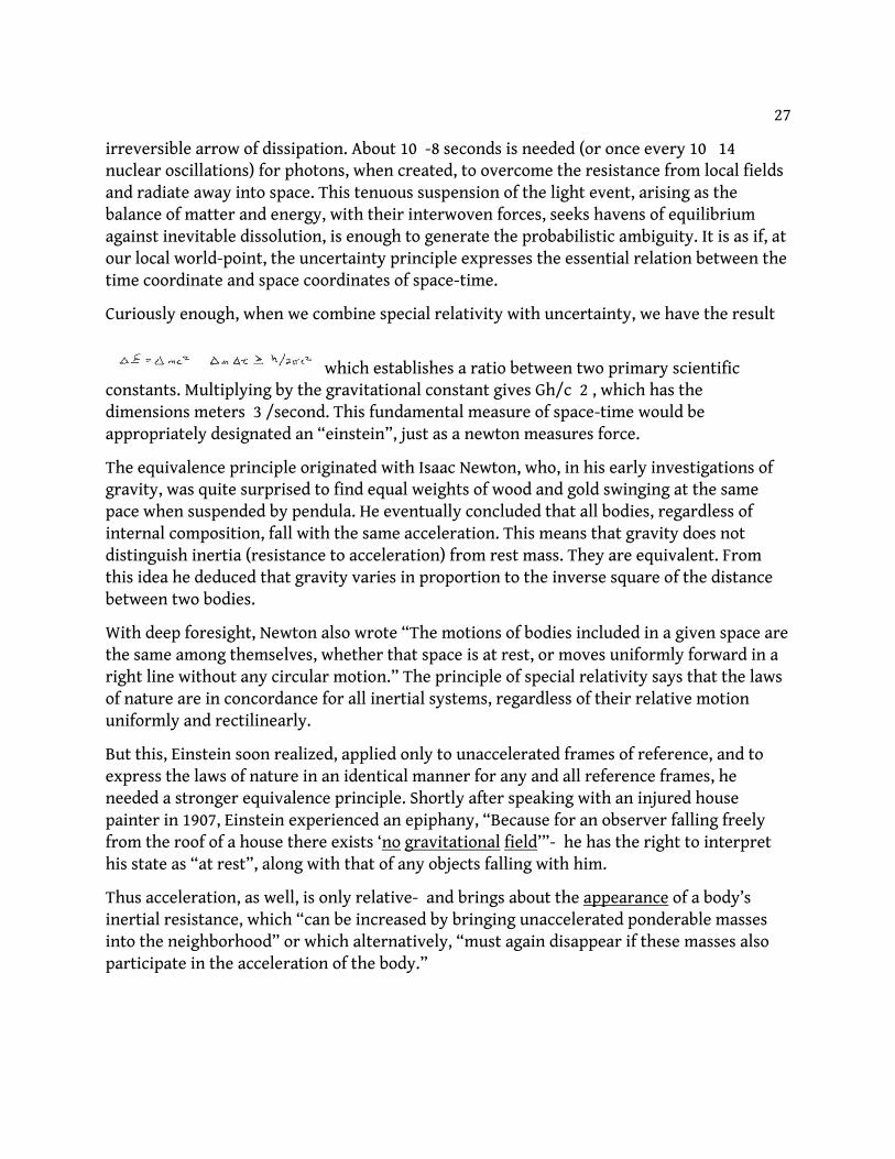
Curiously enough, when we combine special relativity with uncertainty, we have the result

which establishes a ratio between two primary scientific constants. Multiplying by the gravitational constant gives Gh/c 2 , which has the dimensions meters 3 /second. This fundamental measure of space-time would be appropriately designated an “einstein”, just as a newton measures force.

The equivalence principle originated with Isaac Newton, who, in his early investigations of gravity, was quite surprised to find equal weights of wood and gold swinging at the same pace when suspended by pendula. He eventually concluded that all bodies, regardless of internal composition, fall with the same acceleration. This means that gravity does not distinguish inertia (resistance to acceleration) from rest mass. They are equivalent. From this idea he deduced that gravity varies in proportion to the inverse square of the distance between two bodies.

With deep foresight, Newton also wrote “The motions of bodies included in a given space are the same among themselves, whether that space is at rest, or moves uniformly forward in a right line without any circular motion.” The principle of special relativity says that the laws of nature are in concordance for all inertial systems, regardless of their relative motion uniformly and rectilinearly.

But this, Einstein soon realized, applied only to unaccelerated frames of reference, and to express the laws of nature in an identical manner for any and all reference frames, he needed a stronger equivalence principle. Shortly after speaking with an injured house painter in 1907, Einstein experienced an epiphany, “Because for an observer falling freely from the roof of a house there exists ‘no gravitational field’”- he has the right to interpret his state as “at rest”, along with that of any objects falling with him.

Thus acceleration, as well, is only relative- and brings about the appearance of a body’s inertial resistance, which “can be increased by bringing unaccelerated ponderable masses into the neighborhood” or which alternatively, “must again disappear if these masses also participate in the acceleration of the body.”

28

The gravitational field is always acting as a free-falling laboratory. Measurements performed locally in this frame are independent of the frame’s position, time and motion. A system with “no gravitational field” is completely equivalent, as a physical framework, to one accelerating in any manner whatsoever.

The far-reaching conclusion is that space-time and matter/energy influence and even determine one another, and in the higher density regions the geometry is not Euclidean. There gravity begins to diverge from the inverse-square, becoming nonlinear. The field is self-generating in the sense that its force acts on one of its sources, the matter/energy.

Similar to the notion that uncertainty qualifies the contrast between the time and space coordinates, the equivalence principle is suggested here as descriptive of the four space-time axes, when viewed in their whole. We know from special relativity, due to the non-simultaneity of events (since signals travel no faster than light), that space and time have

opposite signs in the continuum metric and self-evidently different properties. Uncertainty is regarded then as the “best fit” at the juncture (of width h) of time and space; equivalence retains the continuity of the 4-dimensional web, even infinitesimally across this “junction”, preserving the thread of causality.

This distinction propagates into the mathematics of either theory. As the existence of quanta make space and time discontinuous, a natural expression for quantum states is realized in the Hamiltonian, an energy matrix of probability amplitudes that modulate over time. QM is linear; the variables in its equations are reducible to the first or zeroth power. This enables superposition of states, for any time sought, by addition or multiplication. Its Achilles’ heel is that some arbitrary gauge- a basis for differentiating the matrix- must be chosen when partitioning space-time. So it becomes a refined system of sets- atomic and without gravity.

General relativity maintains there is no objective rational division of the continuum. Its equations are nonlinear, involving second derivatives, and are only solved approximately- or else by plugging in values for the 10 curvature components of the tensor field. As such, it lends itself to the calculus of variations, particularly the Lagrangian action (i.e. energy-time) density integral of matter, charge, and their fields. The final analyses, however, dead-end at a pseudotensor for the gravitational energy, nontransformable to other coordinate systems, notably the atomic realm. The reason is that gravitation cannot be “localized”, because it draws off both matter/energy and space-time, which interact mutually.

In order to make progress toward a unified field theory, it may become necessary to give up the idea that electrical charge is quantized. It might be so only in appearance, at distances greater than 10 -15 meters- somewhere outside the nucleus. Like Newton’s gravity, Coulomb’s law of electrostatics may eventually diverge from the inverse-square.

29

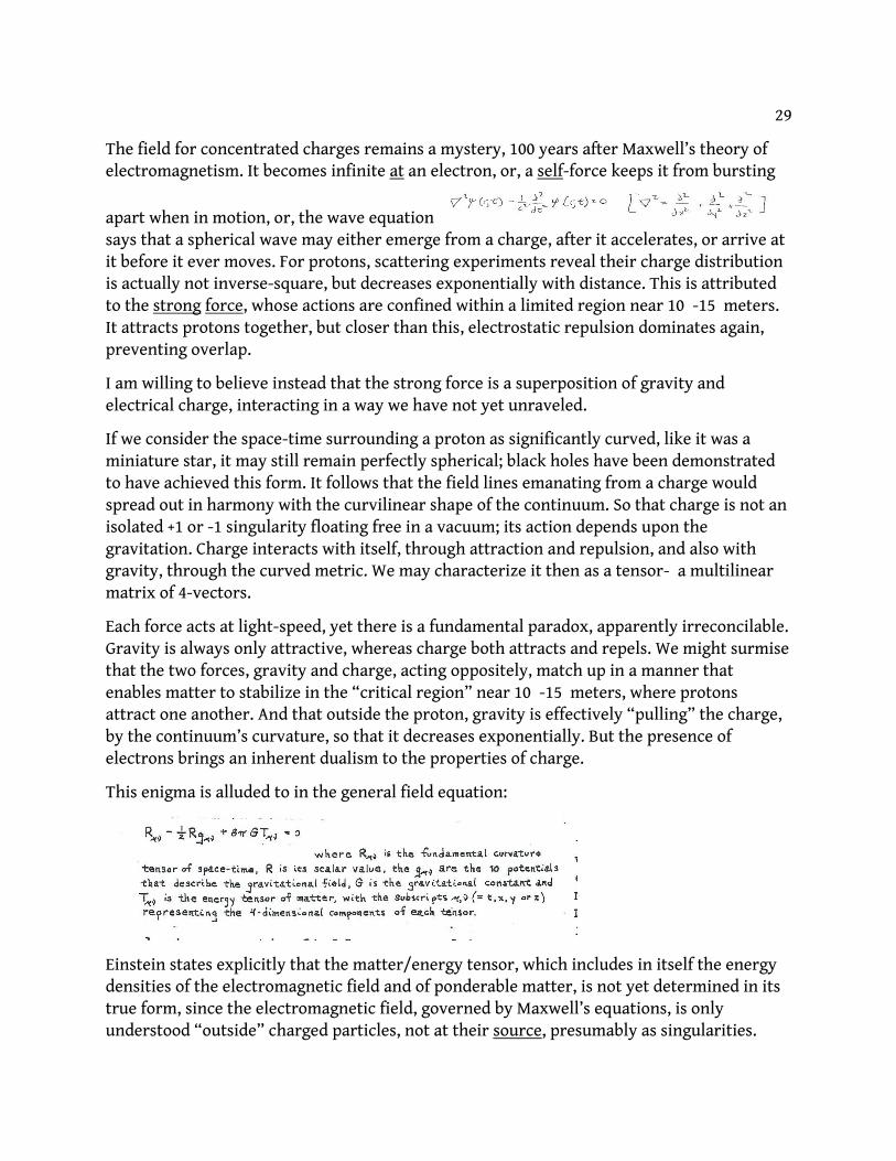
The field for concentrated charges remains a mystery, 100 years after Maxwell’s theory of electromagnetism. It becomes infinite at an electron, or, a self-force keeps it from bursting

apart when in motion, or, the wave equation says that a spherical wave may either emerge from a charge, after it accelerates, or arrive at it before it ever moves. For protons, scattering experiments reveal their charge distribution is actually not inverse-square, but decreases exponentially with distance. This is attributed to the strong force, whose actions are confined within a limited region near 10 -15 meters. It attracts protons together, but closer than this, electrostatic repulsion dominates again, preventing overlap.

I am willing to believe instead that the strong force is a superposition of gravity and electrical charge, interacting in a way we have not yet unraveled.

If we consider the space-time surrounding a proton as significantly curved, like it was a miniature star, it may still remain perfectly spherical; black holes have been demonstrated to have achieved this form. It follows that the field lines emanating from a charge would spread out in harmony with the curvilinear shape of the continuum. So that charge is not an isolated +1 or -1 singularity floating free in a vacuum; its action depends upon the gravitation. Charge interacts with itself, through attraction and repulsion, and also with gravity, through the curved metric. We may characterize it then as a tensor- a multilinear matrix of 4-vectors.

Each force acts at light-speed, yet there is a fundamental paradox, apparently irreconcilable. Gravity is always only attractive, whereas charge both attracts and repels. We might surmise that the two forces, gravity and charge, acting oppositely, match up in a manner that enables matter to stabilize in the “critical region” near 10 -15 meters, where protons attract one another. And that outside the proton, gravity is effectively “pulling” the charge, by the continuum’s curvature, so that it decreases exponentially. But the presence of electrons brings an inherent dualism to the properties of charge.

This enigma is alluded to in the general field equation:

Einstein states explicitly that the matter/energy tensor, which includes in itself the energy densities of the electromagnetic field and of ponderable matter, is not yet determined in its true form, since the electromagnetic field, governed by Maxwell’s equations, is only understood “outside” charged particles, not at their source, presumably as singularities.

30

A singularity carrying charge produces infinite energy, or alternatively, waves dually incoming and exiting. In the mathematics, these difficulties are usually evaded by dealing instead with charged matter as a continuous distribution, to both evaluate the electromagnetic field and confirm that the conservation of electricity holds precisely, even in curved space-time. Yet for uncharged matter, conservation of energy is admittedly only approximate, since the gravitational field acts on matter, and itself has inherent energy. So that energy may “disappear” into space-time, reappearing “later”.

If we dispense with the idea that charge is quantized- localized within point particles- we arrive at a similar conclusion for charged matter, namely that conservation of its electromagnetic energy is approximate as well, valid only for regions greater than roughly 10 -15 meters, where Maxwell’s equations remain accurate.

This postulate finds support in a process discussed earlier, in the analysis of gravity and radioactivity- parity violation in beta-decay. Whereas electromagnetic interactions combine purely vectorial contributions, some beta transitions engage axial (i.e. spin) components, and the radiated particles exhibit a selected handedness. Neutrinos, for instance, are always produced as left-handed. But axial energy is only partially conserved experimentally, attributed in QM to the strong force altering the “spin portion” of the weak force. Whatever the explanation, energy disappears from the reaction, whether into the “virtual” particles of uncertainty or relativity’s space-time web.

The point of view chosen here is that charge mirrors gravity; charge produces electromagnetism, which interacts with gravity, which interacts with matter and the space-time continuum. Effectively, one force may transform into the other.

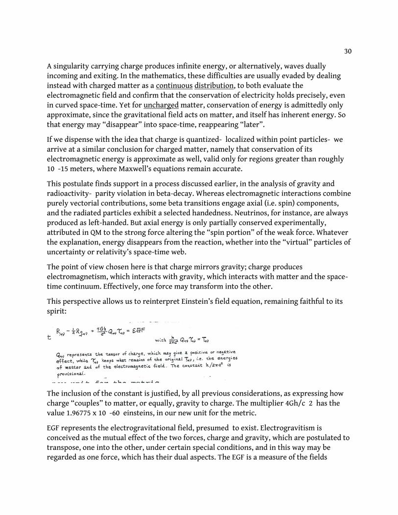
This perspective allows us to reinterpret Einstein’s field equation, remaining faithful to its spirit:

The inclusion of the constant is justified, by all previous considerations, as expressing how charge “couples” to matter, or equally, gravity to charge. The multiplier 4Gh/c 2 has the value 1.96775 x 10 -60 einsteins, in our new unit for the metric.

EGF represents the electrogravitational field, presumed to exist. Electrogravitism is conceived as the mutual effect of the two forces, charge and gravity, which are postulated to transpose, one into the other, under certain special conditions, and in this way may be regarded as one force, which has their dual aspects. The EGF is a measure of the fields

31

gravity plus ponderable matter of any charge, and these two sources interact, each with the other and the space-time continuum. A local minimum may be assigned for the region near 10 -15 meters, where matter equilibrates- here the forces of charge are counteracted to near exactness by gravitation, with the net result being a spherical equipotential surface- the proton.

A careful distinction needs to be made between electromagnetism and charge. The charge density (Q tt), currently considered equal to the number of electrons in a unit volume, includes as well the residual forces (self-forces holding the electrons together, and nonradiating atomic orbitals) which do not release radiation. Charge is a 4-dimensional pressure, and electromagnetic waves are one of its effects.

The propagation of radiation, regarded on the one hand as corpuscles, and on the other as a dispersion in waves, or some blend of the two, its bifold nature suggests an affiliation with the essential dualism of the space-time continuum. If we look upon the spatial components as working toward corpuscularity, with the time contribution lending fluctuations, the actions of gravity seem to compress space while enlarging time, with charge acting in the opposite sense. So seen, charge aims for radiation’s spherocity, whereas gravitation tends toward the dissolution of this form. In the course of radiation’s propagation there is a continual exchange between the two types of energy.

Through this looking glass, a particle with dualistic properties, the photograviton, emerges as the “carrier” of electrogravitational force. It embodies the attributes for both carriers for gravity and electromagnetism, with the further concept that the graviton composes a central void within the photon. Effectively, the photon portion comprises the 3-dimensional space coordinates, leaving the graviton to occupy the “volume” expressed by the 4th coordinate, time. As the properties of the continuum it encounters wax and wane, the photograviton is imagined to undergo oscillatory-like expansions and contractions of its inner and outer “membranes”- the gravitonic “void” and photonic “envelope”- and so transport the energy of electrogravitism.

The subatomic outlook is greatly simplified by claiming the proton and electron only as the fundamental particles, mediated by photogravitons (which, by the way, are perhaps identical to neutrinos), with the neutron arising as their primary resonance form. But what of quarks? I am convinced that they are not separable entities, existing in their own right, in the same way that a room is only real when four walls are around it.

If a pair of protons were resonant with one electron, three up (+2/3 charge) and three down (-1/3 charge) quarks may be derived, capable of forming one proton and one neutron. The fractional charges lead me to believe that, for the up quark phenomenon, only two of the three available space-time coordinates are involved, while the down quark entails one space and the one time coordinate. So that quarks only “exist” in two of the four dimensions.

32

The whole of the subatomic panorama, then, might be viewed as a diffraction pattern for the space-time continuum. Their reduction to constituent quarks, whose overlap begets tangible mass/energy particles, helps illuminate the continuum’s “texture” at our local world-point.

The quantum vs. relativity debate will undoubtedly continue for many more years, but it is the opinion of this essay that Einstein’s general theory has been abandoned prematurely by particle physics, that he may yet have the last word. And the possibility is presented that localized accumulations of charge- perhaps condensed to a greater degree than currently known- may effectively counteract gravity.

Richard Gilbride

West Tisbury, Massachusetts

June 7, 1998