new keynesian macroeconomics and the term structure€¦ · wu (2008), who also append a term...

GEERT BEKAERT

SEONGHOON CHO

ANTONIO MORENO

New Keynesian Macroeconomics and the Term

Structure

This article complements the structural New Keynesian macro frameworkwith a no-arbitrage affine term structure model. Whereas our methodology isgeneral, we focus on an extended macro model with unobservable processesfor the inflation target and the natural rate of output that are filtered frommacro and term structure data. We find that term structure information helpsgenerate large and significant parameters governing the monetary policytransmission mechanism. Our model also delivers strong contemporaneousresponses of the entire term structure to various macroeconomic shocks. Theinflation target shock dominates the variation in the “level factor” whereasmonetary policy shocks dominate the variation in the “slope and curvaturefactors.”

JEL codes: E31, E32, E43, E52, G12Keywords: monetary policy, inflation target, term structure of

interest rates, Phillips curve.

STRUCTURAL NEW KEYNESIAN MODELS, featuring dynamic ag-gregate supply (AS), aggregate demand (IS), and monetary policy equations are be-coming pervasive in macroeconomic analysis. In this article, we complement thisstructural macroeconomic framework with a no-arbitrage term structure model.

We benefited from the comments of two referees, the editor, Pok-Sang Lam, Glenn Rudebusch, AdrianPagan, and seminar participants at Columbia University, Carleton University, the Korea DevelopmentInstitute, the University of Navarra, the University of Rochester (Finance Department), Tilburg University,the National Bank of Belgium, the Singapore Management University, the 2004 meeting of the Societyfor Economic Dynamics in Florence, the 2005 Econometric Society World Congress in London, the 2005European Finance Association annual meeting in Moscow, and the 2006 EC2 Conference in Rotterdam.

GEERT BEKAERT is a Professor at the Graduate School of Business, Columbia Univer-sity (E-mail: [email protected]). SEONGHOON CHO is an Assistant Professor at the Schoolof Economics, Yonsei University, Korea (E-mail: [email protected]). ANTONIO MORENO isan Assistant Professor at the Department of Economics, University of Navarra, Spain (E-mail: [email protected]).

Received November 9, 2007; and accepted in revised form August 19, 2009.

Journal of Money, Credit and Banking, Vol. 42, No. 1 (February 2010)C© 2010 The Ohio State University

34 : MONEY, CREDIT AND BANKING

Our analysis overcomes three deficiencies in previous work on New Keynesianmacro models. First, the parsimony of such models implies very limited informationsets for both the monetary authority and the private sector. The critical variables inmost macro models are the output gap, inflation, and a short-term interest rate. It iswell known, however, that monetary policy is conducted in a data-rich environment.Consequently, lags of inflation, the output gap and the short-term interest rate do notsuffice to adequately forecast their future behavior. Recent research by Bernanke andBoivin (2003) and Bernanke, Boivin, and Eliasz (2005) collapses multiple observ-able time series into a small number of factors and embeds them in standard vectorautoregressive (VAR) analyses. Instead, we use term structure data. Under the nullof the expectations hypothesis, term spreads embed all relevant information aboutfuture interest rates. Additionally, a host of studies have shown that term spreads arevery good predictors of future economic activity (see, e.g., Harvey 1988, Estrellaand Mishkin 1998, Ang, Piazzesi, and Wei 2006) and of future inflation (Mishkin1990, Stock and Watson 2003). In our proposed model, the conditional expectationsof inflation and the detrended output are a function of the past realizations of macrovariables and of unobserved components that are extracted from term structure datathrough a no-arbitrage pricing model.

Second, the additional information from the term structure model transforms aversion of a New Keynesian model with a number of unobservable variables into a verytractable linear model that can be efficiently estimated by maximum likelihood (MLE)or the general method of moments (GMM). Hence, the term structure informationhelps recover important structural parameters, such as those describing the monetarytransmission mechanism, in an econometrically convenient manner.

Third, incorporating term structure information leads to a simple VAR in macrovariables and term spreads but the reduced-form model for the macro variables isa dynamically rich process with both autoregressive and moving average compo-nents. This is important because one disadvantage of most structural New Keynesianmodels is the absence of sufficient endogenous persistence. We generate additionalchannels of persistence by introducing unobservable variables in the macro model andthen identify their dynamics using the arbitrage-free term structure model and termspreads.

The approach set forth in this paper also contributes to the term structure literature.In this literature it is common to have latent factors drive most of the dynamics ofthe term structure of interest rates. These factors are often interpreted ex post aslevel, slope, and curvature factors. A classic example of this approach is Dai andSingleton (2000), who construct an arbitrage-free three factor model of the termstructure (other examples include Knez, Litterman, and Scheinkman 1994, Pearsonand Sun 1994). While the Dai and Singleton (2000) model provides a satisfactoryfit of the data, it remains silent about the economic forces behind the latent factors.In contrast, we construct a no-arbitrage term structure model where all the factorshave a clear economic meaning. Apart from inflation, detrended output, and the short-term interest rate, we introduce two unobservable variables in the underlying macromodel. Whereas there are many possible implementations, our main application hereintroduces a time-varying inflation target and the natural rate of output. Consequently,

GEERT BEKAERT, SEONGHOON CHO, AND ANTONIO MORENO : 35

we construct a five-factor affine term structure model that obeys New Keynesianstructural relations.

Our main empirical findings are as follows. First, the model matches the persistencedisplayed by the three macro variables despite being nested in a parsimonious VAR(1)for macro variables and term spreads. Second, in contrast to previous MLE or GMMestimations of the standard New Keynesian model, we obtain large and significantestimates of the Phillips curve and real interest rate response parameters. Third, ourmodel exhibits strong contemporaneous responses of the entire term structure to thevarious structural shocks in the model.

Our article is part of a rapidly growing literature exploring the relation between theterm structure and macroeconomic dynamics. Kozicki and Tinsley (2001) and Ang andPiazzesi (2003) were among the first to incorporate macroeconomic factors in a termstructure model to improve its fit. Evans and Marshall (2003) use a VAR frameworkto trace the effect of macroeconomic shocks on the yield curve whereas Dewachterand Lyrio (2006) assign macroeconomic interpretations to standard term structurefactors. Our paper differs from these articles in that all the macro variables obey a setof structural macro relations. This facilitates a meaningful economic interpretationof the term structure dynamics, relating them to macroeconomic shocks or “deep”parameters characterizing the behavior of the private sector or the monetary authority.

Two related studies are Hordahl, Tristani, and Vestin (2006) and Rudebusch andWu (2008), who also append a term structure model to a New Keynesian macromodel. Our modeling approach is quite different however. First, our pricing kernelis consistent with the IS equation, whereas in these two papers, it is exogenouslydetermined. Because standard linearized New Keynesian models display constantprices of risk, this implies that our model’s term premiums do not vary through timeby construction. While there is some evidence of time-variation in term premiums,we find it useful to examine how incorporating term structure data in a familiar settingaffects standard structural parameters and macro dynamics. Imposing the restrictionthat the expectations hypothesis accounts for most of the variation in long rates appearsreasonable too. Second, these two articles add a somewhat arbitrary lag structureto the supply and demand equations, whereas we analyze a standard optimizingsticky price model with endogenous persistence. While this modeling choice mayadversely affect our ability to fit the data dynamics, it generates a parsimonious statespace representation for the macroeconomic and term structure variables, with a clearstructural interpretation.

Another related article is Wu (2006). He formulates and calibrates a structuralmacro model with adjustment costs for pricing and only two shocks (a technologyshock and a monetary policy shock). Wu then gauges the fit of the model relative to thedynamics implied by an auxiliary standard term structure model based exclusively onunobservables. Instead of following this indirect approach, we estimate a structuralmacroeconomic model that directly implies an affine term structure model with fiveobservable and interpretable factors.

The remainder of the paper is organized as follows. Section 1 describes the structuralmacroeconomic model, whereas Section 2 outlines how to combine the macro modelwith an affine term structure model. Section 3 discusses the data and the estimation


methodology employed. Section 4 analyzes the macroeconomic implications whileSection 5 studies the term structure implications of our model. Section 6 concludes.

1. A NEW KEYNESIAN MACRO MODEL WITH UNOBSERVABLE STATEVARIABLES

We present a standard New Keynesian model featuring AS, IS, and monetary policyequations with two additions. First, we assume the existence of a natural rate of outputthat follows a persistent stochastic process. Second, the inflation target is assumed tovary through time according to a persistent linear process. The monetary authoritiesreact to the output gap that is the deviation of output from the natural rate of output.We allow for endogenous persistence in the AS, IS, and monetary policy equations.In what follows, we describe each equation in turn and describe the model solution.In Bekaert, Cho, and Moreno (2005) we describe the microfoundations of the ASand IS equations. Related theoretical derivations can be found in Clarida, Galı, andGertler (1999) or Woodford (2003).

1.1 The IS Equation

A standard intertemporal IS equation is usually derived from the first-order con-ditions for a representative agent with power utility as in the original Lucas (1978)economy. Standard estimation approaches have experienced difficulty pinning downthe risk aversion parameter, which is at the same time an important parameter under-lying the monetary transmission mechanism. Another discomforting feature impliedby a standard IS equation is that it typically fails to match the well-documented per-sistence of output. We derive an alternative IS equation from a utility maximizingframework with external habit formation similar to Fuhrer (2000). In particular, weassume that the representative agent maximizes:

Et

∞∑s=t

ψ s−tU (Cs ; Fs) = Et

∞∑s=t

ψ s−t

[FsC1−σ

s − 1

1 − σ

], (1)

where Ct is the composite index of consumption, Ft represents an aggregate de-mand shifting factor, ψ denotes the time discount factor, and σ is the inverse of theintertemporal elasticity of substitution. We specify Ft as follows:

Ft = Ht Gt , (2)

where Ht is an external habit level; i.e., the agent takes Ht as exogenously given, eventhough it may depend on past consumption. Gt is an exogenous aggregate demandshock that can also be interpreted as a preference shock. Following Fuhrer (2000), weassume that Ht = Cη

t−1, where η measures the degree of habit dependence on the pastconsumption level. It is this assumption that delivers endogenous output persistence.

Imposing the resource constraint (Ct = Yt , with Yt output) and assuming log-normality, the Euler equation for the interest rate yields a Fuhrer-type IS equation:


yt = αI S + µEt yt+1 + (1 − µ)yt−1 − φ(it − Etπt+1) + εI S,t , (3)

where yt is detrended log output and it is the short-term interest rate. The parameterφ measures the response of detrended output to the real interest rate; φ = 1

σ+ηand

µ = σφ.The IS shock, εI S,t = φ ln Gt , is assumed to be independently and identicallydistributed with homoskedastic variance σ 2

I S .

1.2 The AS Equation (Phillips Curve)

Building on the Calvo (1983) pricing framework with monopolistic competition inthe intermediate good markets, a forward-looking AS equation can be derived, linkinginflation to future expected inflation and the real marginal cost. By assuming that thefraction of price setters that does not adjust prices optimally, indexes their prices topast inflation, we obtain endogenous persistence in the AS equation. Moreover, wefollow Woodford (2003) assuming the real marginal cost to be proportional to theoutput gap. Consequently, we obtain a standard New Keynesian AS curve relatinginflation to the output gap:

πt = δEtπt+1 + (1 − δ)πt−1 + κ(yt − yn

t

) + εASt , (4)

where πt is inflation, ynt is the natural rate of detrended output that would arise

in the case of perfectly flexible prices, and yt − ynt is the output gap;1 εASt is an

exogenous supply shock, assumed to be independently and identically distributedwith homoskedastic variance σ 2

AS . The parameter κ captures the short-run trade-off between inflation and the output gap and (1 − δ) characterizes the endogenouspersistence of inflation.

In practice, structural estimates of the Phillips curve based on output gap measuresseem less successful than those based on marginal cost (see Galı and Gertler 1999).However, whereas in most studies an exogenously detrended output variable servesas the output gap measure in the AS equation, our output gap measure is endogenousand filtered through macro and term structure information. We let the natural ratefollow an AR(1) process:

ynt = λyn

t−1 + εyn ,t , (5)

where εyn ,t can be interpreted as a negative markup shock with standard deviationσyn .2

1. The output gap is measured as the percentage deviation of detrended output with respect to thenatural rate of output. Both detrended output and the natural rate of output are measured as percentagedeviations with respect to a linear trend. Therefore, the means of the output gap, detrended output, and thenatural rate of output are 0.

2. In a previous version of the paper (Bekaert, Cho, and Moreno 2005), we used the utility function in(1) and a simple production technology to derive an AS equation that provided an explicit link between themarginal cost and the current and past output gap, and also yielded a process for the natural rate of outputendogenously. While some of the versions of the structural model converged, it proved very difficult toestimate.


1.3 The Monetary Policy Rule

We assume that the monetary authority specifies the nominal interest rate target, i∗t ,

as in the forward-looking Taylor rule proposed by Clarida, Galı, and Gertler (1999):

i∗t = [

ıt + β(Etπt+1 − π∗

t

) + γ(yt − yn

t

)], (6)

where π∗t is a time-varying inflation target and ıt is the desired level of the nominal

interest rate that would prevail when Etπt+1 = π∗t and yt = yn

t . We assume that ıt isconstant.3 Note that β measures the long-run response of the interest rate to expectedinflation, a typical measure of the Fed’s stance against inflation.

We further assume that the monetary authority sets the short-term interest rate as aweighted average of the interest rate target and a lag of the short-term interest rate tocapture the tendency by central banks to smooth interest rate changes:

it = ρit−1 + (1 − ρ) i∗t + εM P,t , (7)

where ρ is the smoothing parameter and εM P,t is an exogenous monetary policy shock,assumed to be i.i.d. with standard deviation, σM P . The resulting monetary policy rulefor the interest rate is given by

it = αM P + ρit−1 + (1 − ρ)[β(Etπt+1 − π∗

t

) + γ(yt − yn

t

)] + εM P,t , (8)

where αM P = (1 − ρ)ı .

1.4 Inflation Target π∗t

We close our model by specifying a stochastic process for the inflation target,π∗

t . Little is known about how the monetary authority sets the inflation target.Hordahl, Tristani, and Vestin (2006) assume an AR(1) process for the inflationtarget. Gurkaynak, Sack, and Swanson (2005) specify it as a weighted average ofthe past inflation target and past inflation rates. While their specification is empiri-cally supported to some extent, we deem it plausible that the central bank takes thelong-run inflation expectations of the private sector into account in a forward-lookingmanner. Therefore, we define π L R

t as the conditional expected value of a weightedaverage of all future inflation rates.

π L Rt = (1 − d)

∞∑j=0

d j Etπt+ j , (9)

with 0 ≤ d ≤ 1. This equation can be succinctly written as

π L Rt = d Etπ

L Rt+1 + (1 − d)πt , (10)

3. We estimated alternative model specifications with a time-varying ıt in Bekaert, Cho, and Moreno(2005) and the main results in the article are not altered.


When d equals 0, π L Rt collapses to current inflation, when d approaches 1, long-run

inflation approaches unconditional expected inflation. We assume that the monetaryauthority anchors its inflation target around π L R

t , but smooths it with past inflation,so that:

π∗t = ωπ∗

t−1 + (1 − ω)π L Rt + επ∗,t . (11)

We view επ∗,t as an exogenous shift in the policy stance regarding the long termrate of inflation or the target, and assume it to be i.i.d. with standard deviation σπ∗ .Substituting out π L R

t in equation (11) using equation (10), we obtain

π∗t = ϕ1 Etπ

∗t+1 + ϕ2π

∗t−1 + ϕ3πt + επ∗,t , (12)

where ϕ1 = d1+dω

, ϕ2 = ω1+dω

and ϕ3 = 1 − ϕ1 − ϕ2. In Bekaert, Cho, and Moreno(2005) we also estimated a backward-looking inflation target process similar to thatof Gurkaynak, Sack, and Swanson (2005), producing results qualitatively similar tothe ones we present further.

1.5 The Full Model

Bringing together all the equations, we have a five-variable system with threeobserved and two unobserved macro factors:

πt = δEtπt+1 + (1 − δ)πt−1 + κ(yt − yn

t

) + εASt (13)

yt = αI S + µEt yt+1 + (1 − µ)yt−1 − φ(it − Etπt+1) + εI S,t (14)

it = αM P + ρit−1 + (1 − ρ)[β

(Etπt+1 − π∗

t

) + γ(yt − yn

t

)] + εM P,t (15)

ynt = λyn

t−1 + εyn ,t (16)

π∗t = ϕ1 Etπ

∗t+1 + ϕ2π

∗t−1 + ϕ3πt + επ∗,t . (17)

Our macroeconomic model can be expressed in matrix form as

Bxt = α + AEt xt+1 + J xt−1 + Cεt , (18)

where xt = [πt yt it ynt π∗

t ]′ and εt = [εAS,t εI S,t εM P,t εyn ,t επ∗,t ]′. α is a 5 × 1vector of constants and B, A, J , and C are appropriately defined 5 × 5 matrices.The rational expectations (RE) equilibrium can be written as a first-order VAR:

xt = c + �xt−1 + �εt . (19)

Hence, the implied model dynamics are a simple VAR subject to a set of nonlinearrestrictions. Note that � cannot be solved analytically in general. We solve for �


numerically using the QZ method (see Klein 2000, Cho and Moreno 2008). Once �

is solved for, � and c follow straightforwardly.As the Appendix shows, the reduced-form representation of the vector of observable

macro variables is very similar to a VARMA(3,2) process. By adding unobservables,we potentially deliver more realistic joint dynamics for inflation, the output gap, andthe interest rate, and overcome the lack of persistence implied by previous studies.

2. INCORPORATING TERM STRUCTURE INFORMATION

We derive the term structure model implicit in the IS curve that we presented inSection 1. This effort results in an easily estimable linear system in observable macrovariables and term spreads.

2.1 Affine Term Structure Models with New Keynesian Factor Dynamics

Affine term structure models require linear state variable dynamics and a linearpricing kernel process with conditionally normal shocks (see Duffie and Kan 1996).For the state variable dynamics implied by the New Keynesian model in equation(19) to fall in the affine class, we assume that the shocks are conditionally normallydistributed, εt ∼ N (0, Dt−1). The pricing kernel process Mt+1 prices all securitiessuch that:

Et [Mt+1 Rt+1] = 1. (20)

In particular, for an n-period bond, Rt+1 = Pn−1,t+1

Pn,twith Pn,t the time t price of an

n-period zero-coupon bond. If Mt+1 > 0 for all t, the resulting returns satisfy theno-arbitrage condition (Harrison and Kreps 1979). In affine models, the log of thepricing kernel is modeled as a conditionally linear process. Consider, for instance:

mt+1 = ln(Mt+1) = −it − 1

2�′

t Dt�t − �′tεt+1. (21)

Here, �t = �0 + �1xt , where �0 is a 5 × 1 vector and �1 is a 5 × 5 matrix. First,setting Dt = D, we obtain a Gaussian price of risk model. Dai and Singleton (2002)study such a model and claim that it accounts for the deviations of the expectationshypothesis observed in U.S. term structure data. An alternative model sets �t = � andεt ∼ N (0, Dt−1) with Dt = D0 + D1diag(xt ), where diag(xt ) is the diagonal matrixwith the vector xt on its diagonal. This model introduces heteroskedasticity of thesquare root form and has a long tradition in finance (see Cox, Ingersoll, and Ross1985). Finally, setting �t = �0 and Dt = D results in a homoskedastic model.

All three of these models imply an affine term structure. That is, log bond prices arean affine function of the state variables. The maturity-dependent coefficients followrecursive equations. The three models have different implications for the behaviorof term spreads and holding period returns. First, the homoskedastic model implies


that the expectations hypothesis holds: there may be a term premium but it does notvary through time. Both the Gaussian prices of risk model and the square root modelimply time-varying term premiums. Second, our model includes inflation as a statevariable and the real pricing kernel (the kernel that prices bonds perfectly indexedagainst inflation) and inflation are correlated. It is this correlation that determines theinflation risk premium. If the covariance term is constant, the risk premium is constantover time and this will be true in a homoskedastic model.

The kernel model implied by the IS curve derived above fits in the homoskedasticclass. It is possible to modify the pricing framework into one of the two other models,but we defer this to future work. Bekaert, Hodrick, and Marshall (2001) show thata model with minimal variation in the term premium suffices to match the evidenceregarding the expectations hypothesis for the U.S. Moreover, the current practiceof using linear regressions to infer the properties of term premiums almost surelyleads to the overestimation of their variability (see Bekaert, Wei, and Xing 2007 forsimulation evidence).

2.2 The Term Structure Model Implied by the Macro Model

Because our derivation of the IS curve assumed a particular preference structure, thepricing kernel is given by the intertemporal consumption marginal rate of substitutionof the model. That is:

mt+1 = ln ψ − σ yt+1 + (σ + η)yt − ηyt−1 + (gt+1 − gt ) − πt+1. (22)

The no-arbitrage condition holds by construction. In a log-normal model, pricing aone period bond implies

Et [mt+1] + 0.5Vt [mt+1] = −it . (23)

For our particular model, (21) holds with �, a vector of prices of risk entirely restrictedby the structural parameters,

�′t = �′ = [1 σ 0 0 0]� − [0 (σ + η) 0 0 0] . (24)

Logarithmic bond prices and hence, bond yields (yn,t = −ln(Pn,t )n ), are an affine func-

tion of the state variables:

yn,t = −an

n− b′

n

nxt . (25)

The recursive formulas for an and bn can be constructed using equations (19)–(22).4

Term spreads are also an affine function of the state variables:

4. They are: an = an−1 + b′n−1c + 0.5b′

n−1�D�′bn−1 − �′ D�′bn−1 and b′n = −e′

3 + b′n−1�, respec-

tively.


spn,t = −an

n−

(bn

n+ e3

)′xt , (26)

where spn,t ≡ yn,t − it is the spread between the n-period yield and the short rate.This model provides a particularly convenient form for the joint dynamics of themacro variables and the term spreads. Let zt = [πt yt it spn1,t spn2,t ]

′, where n1

and n2 refer to two different yield maturities for the long-term bond in the spread.Then

xt = c + �xt−1 + �εt (27)

zt = Az + Bz xt , (28)

where

Az =

03×1

−an1

n1

−an2

n2

, Bz =

I3 03×2

−(

bn1

n1+ e3

)′

−(

bn2

n2+ e3

)′

.

Using xt = B−1z (zt − Az), we find

zt = az + �z zt−1 + �zεt , (29)

where

�z = Bz�B−1z

�z = Bz�

az = Bzc + (I − Bz�B−1z )Az,

In other words, the macro variables and the term spreads follow a first-order VARwith complex cross-equation restrictions. This feature also differentiates our methodfrom previous work in the literature. Because equation (29) consists of observedmacro and term spread data, we can directly estimate it employing exactly two termspreads. Once the model is estimated, we can back out the natural rate of output andthe inflation target using equation (28).

3. DATA AND ESTIMATION

In this section, we first describe the data used in the estimation of our macro financemodel. Then we present the general estimation methodology employed.


3.1 Data Description

The sample period is from the first quarter of 1961 to the fourth quarter of 2003.We measure inflation with the CPI (collected from the Bureau of Labor Statistics)but check robustness using the GDP deflator, from the National Income and ProductAccounts (NIPA). Detrended output is measured as the output deviation from a lineartrend. We also estimated the model with quadratically detrended output, producingqualitatively similar results. The results are by and large similar across alternativedetrending methods. Output is real GDP from NIPA. We use the 3-month T-bill rate,taken from the Federal Reserve of St. Louis database, as the short-term interest rate.Finally, our analysis uses term-structure data at the 1-, 3-, 5-, and 10-year maturitiesfrom the CRSP database.5 We use the 3- and 5-year spreads directly in the estimationand use additional term spreads to test the model ex post. Consequently, we do notuse measurement error in the estimation and do not rely on a Kalman filter to extractthe unobservables from the data.

3.2 Estimation Methodology

Because our macro finance model implies a first-order VAR on zt with com-plex cross-equation, nonlinear restrictions, we first verify that the BIC criterion in-deed selects a first-order VAR among unconstrained VARs of lag-lengths 1 through5. We perform the estimation on de-meaned data, zt = zt − E zt with E zt thesample mean of zt . The structural parameters to be estimated are therefore θ =(δ κ σ η ρ β γ λ ω d σAS σI S σM P σyn σπ∗ )′. Assuming normal errors, it is straight-forward to write down the likelihood function for this problem and produce full infor-mation likelihood (FIML) estimates. However, to accommodate possible deviationsfrom the strong normality and homoskedasticity assumptions underlying maximumlikelihood, we use a two-step GMM estimation procedure based on Hansen (1982).To do so, rewrite the model in the following form:

zt = �z zt−1 + �zεt = �z zt−1 + �z�ut , (30)

where ut = �−1εt ∼ (0, I5) and � = diag([σAS σI S σM P σyn σπ∗ ]′), i.e., �2 =D.

To construct the moment conditions, consider the following vector valued pro-cesses:

h1,t = ut ⊗ zt−1 (31)

h2,t = vech(ut u′t − I5) (32)

5. The 10-year zero-coupon yield was constructed splicing two series. We use the McCulloch andKwon series up to the third quarter of 1987; from the fourth quarter of 1987 to the end of the sample,we use the 10-year zero-coupon yield estimated using the method of Svensson (2004). We thank RefetGurkaynak for kindly providing this second part of the series.


ht = [h′1,t h′

2,t ]′, (33)

where vech represents an operator stacking the elements on or below the principlediagonal of a matrix. The model imposes E[ht ] = 0. The 25 h1,t moment conditionscapture the feedback parameters; the 15 h2,t moment conditions capture the structureimposed by the model on the variance–covariance matrix of the innovations. Ratherthan using an initial identity matrix as the weighting matrix, which may give riseto poor first-stage estimates, we use a weighting matrix implied by the model undernormality. That is under the null of the model, the weighting matrix must be

W = (E[ht h′t ])

−1. (34)

Using normality and the error structure implied by the model, it is then straightforwardto show that the optimal weighting matrix is given by

W =

I ⊗ 1

T

T∑t=1

zt−1 z′t−1 025×15

015×25 I15 + vech(I5)vech(I5)′

−1

. (35)

This weighting matrix does not depend on the parameters. Then we minimize thestandard GMM objective function:

Q = (E[ht ])′W (E[ht ]), (36)

where E[ht ] = 1T

∑Tt=1 ht . This gives rise to estimates that are quite close to what

would be obtained with maximum likelihood. Given these estimates, we produce asecond-stage weighting matrix allowing for heteroskedasticity and five Newey–West(Newey and West 1987) lags in constructing the variance–covariance matrix of theorthogonality conditions. We iterate this system until convergence. This estimationproved overall rather robust with parameter estimates varying little after the firstround.

4. MACROECONOMIC IMPLICATIONS

4.1 Structural Parameter Estimates

In order to assess the fit of the model, we first comment on the standard GMM testof the overidentifying restrictions, which follows a χ2 distribution with 25 degreesof freedom because there are 40 moment conditions but only 15 parameters. We findthat the test fails to reject the model at the 5% level when five Newey–West lags areused in the construction of the weighting matrix (the p-value is 26.3%). While themodel is not rejected either with four Newey–West lags (the p-value is 9.4%), it isrejected when only three Newey–West lags are used (the p-value is 1.3%). This initself suggests that the orthogonality conditions still display substantial persistence.


TABLE 1

GMM ESTIMATES OF THE STRUCTURAL PARAMETERS

Std error

Parameter Estimate GMM Bootstrap

δ 0.611 (0.010) (0.031)κ 0.064 (0.007) (0.022)σ 3.156 (0.466) (1.632)η 4.294 (0.470) (1.383)ρ 0.723 (0.028) (0.083)β 1.525 (0.148) (0.251)γ 0.001 (0.047) (0.020)λ 0.958 (0.006) (0.026)ω 0.877 (0.013) (0.031)d 0.866 (0.014) (0.041)σAS 1.249 (0.053) (0.123)σI S 0.671 (0.033) (0.055)σM P 2.177 (0.119) (0.287)σyn 1.380 (0.115) (0.817)σπ∗ 0.730 (0.059) (0.723)

Std errorImpliedparameter Estimate GMM Bootstrap

µ 0.424 (0.013) (0.026)φ 0.134 (0.017) (0.029)ϕ1 0.500 (0.003) (0.007)ϕ2 0.492 (0.003) (0.005)ϕ3 0.008 (0.002) (0.003)

NOTE: The second column reports the parameter estimates for our macro-finance model. The third and fourth columns list the GMM standarderrors of the structural parameters and those obtained through the bootstrap procedure described in the text.

Nevertheless, the model fits the autocorrelograms of the data series very well (notreported).

The second to fourth columns in Table 1 show the parameter estimates of themodel and their GMM and bootstrap standard errors.6 The bootstrap analysis willprove useful in generating standard errors for a number of model-implied statis-tics. A first important finding is the size and significance of κ , the Phillips curveparameter. As Galı and Gertler (1999) point out, previous studies fail to obtain rea-sonable and significant estimates of κ with quarterly data. Galı and Gertler do obtainlarger and significant estimates using a measure for marginal cost replacing the out-put gap. Our estimates of κ , using the output gap and term spreads, are even largerthan those obtained by Galı and Gertler. Using the (larger) standard error from thebootstrap, κ remains statistically significantly different from zero. We estimate the

6. We bootstrap from the 172 observations on the vector of structural standard errors (εt ) with replace-ment and re-create a sample of artificial data using the estimated parameter matrices (�, �) and historicalinitial values. For each replication, we create a sample of 672 observations, discard the first 500 and retainthe last 172 observations to create a sample of length equal to the data sample. We then reestimate the modelwith these artificial data and replicate this process 1,000 times to create the small-sample distributions ofthe parameters. Because we identified some serial correlation in the residuals, we also perform a blockbootstrap using Kunsch’s rule with a block length of 7, as explained in Hall, Horowitz, and Jing (1995).The implied small-sample distributions are very similar to the ones presented in the paper.


forward-looking parameter in the AS equation to be close to 0.61, consistent withprevious studies.

When structural models are estimated with techniques such as GMM or MLE, theyoften give rise to large estimates of σ rendering the IS equation a rather ineffectivechannel of monetary policy transmission. Two examples are Ireland (2001) and Choand Moreno (2006). Lucas (2003) argues that the curvature parameter in the represen-tative agent’s utility function consistent with most macro and public finance modelsshould be between 1 and 4. While the Lucas statement does not strictly apply to mod-els with habit persistence, in our multiplicative habit model σ still represents localrisk aversion. Our estimation yields a small (slightly larger than 3) and significantestimate of σ , although its significance is more marginal using bootstrapped standarderrors. Smets and Wouters (2003) and Lubik and Schorfheide (2004) find small esti-mates of σ using Bayesian estimation techniques. Rotemberg and Woodford (1998)and Boivin and Giannoni (2006) also find small estimates of σ but they modify theestimation procedure toward fitting particular impulse responses. Our model exhibitslarge habit persistence effects, as the habit persistence parameter, η, is close to 4.Other studies have also found an important role for habit persistence (Fuhrer 2000,Boldrin, Christiano, and Fisher 2001).7 In summary, the parameter estimates for theAS and IS equations imply that our model delivers large economic effects of monetarypolicy on inflation and output.

Why do we obtain large and significant estimates of κ and φ? Two channels seem tobe at work. First, expectations are based on both observable and unobservable macrovariables. Therefore, an important variable in the AS equation, such as expected in-flation, is directly affected by the inflation target. As a result, changes in the inflationtarget shift the AS curve. As we show below in variance decompositions, the infla-tion target shock contributes significantly to variation in the inflation rate. Similarly,the natural rate shock significantly contributes to the dynamics of detrended output.Second, our measure of the output gap is different from the usual detrended outputand contains additional valuable information extracted from the term structure. Forinstance, the first-order autocorrelation of the implied output gap is 0.92, which issmaller than 0.96, the first-order autocorrelation of linearly detrended output. ThePhillips curve coefficients found in previous studies reflect the weak link betweendetrended output and inflation in the data and the large difference in persistence be-tween these two variables. In our model, even though κ is rather large, the relationshipbetween inflation and the output gap is still not strongly positive because the inflationtarget also moves the AS curve. In sum, the presence of both the inflation target and thenatural rate of output in the AS equation implies a significantly positive conditionalco-movement between the output gap and inflation, even though the unconditionalcorrelation between them remains low as it is in the data. The unobservables are also

7. Our habit persistence parameter is not directly comparable to that derived by Fuhrer (2000). Thereis, however, a linear relationship between them: η = (σ − 1)h, where h is the Fuhrer habit persistenceparameter. Our implied h is close to 2, larger than in previous studies, and violating a theoretical boundin Fuhrer. This implies that µ < 0.5, as in Boivin and Giannoni (2006), for instance. Imposing h ≤ 1significantly worsens the fit of the empirical model.


critical in fitting the relative persistence of the output gap and inflation. Similarly, theφ parameter still fits the dependence of detrended output on the real interest rate, butthe real interest rate is now an implicit function of all the state variables, includingthe natural rate of output.

The estimates of the policy rule parameters are similar to those found in the lit-erature. The estimated long-run response to expected inflation is larger than 1. Theresponse to the output gap is always close to 0 and insignificantly different from0. Finally, the smoothing parameter, ρ, is estimated to be 0.72, similar to previousstudies.

The two unobservables are quite persistent, but clearly stationary processes. Thenatural rate of output’s persistence is close to 0.96, while the weight on the pastinflation target in the inflation target equation is 0.88. Furthermore, the weight oncurrent inflation in the construction of the long-run inflation target (1 − d) is closeto 0.15. Finally, the five shock standard deviations are significant, with the monetarypolicy shock standard deviation larger than the others. There has been some evidencepointing toward a structural break in the β parameter (see, e.g., Clarida, Galı, andGertler 1999, Lubik and Schorfheide 2004). The large estimate of σM P may reflectthe absence of such a break in our model.

4.2 Output Gap and Inflation Target

One important feature of our analysis is that we can extract two economicallyimportant unobservable variables from the observable macro and term structure vari-ables. The output gap is of special interest to the monetary authority, as it plays acrucial role in the monetary transmission mechanism of most macro models. Smetsand Wouters (2003) and Laubach and Williams (2003) also extract the natural rate ofoutput for the European and U.S. economies from theoretical and empirical models,respectively. An important difference between our work and theirs is that we use termstructure information to filter out the natural rate, whereas they back it out of puremacro models through Kalman filter techniques. The dynamics of the inflation targetare particularly important for the private sector, as the Federal Reserve has neverannounced targets for inflation and knowledge of the inflation target would be usefulfor both real and financial investment decisions.

The top panel in Figure 1 shows the evolution of the output gap implied by themodel. Several facts are worth noting. Before 1980, the output gap stayed above zerofor most of the time. A positive output gap is typically interpreted as a proxy forexcess demand. A popular view is that a high output gap made inflation rise throughthe second half of the 70s. Our output gap graph is consistent with that view. However,right before 1980, the output gap becomes negative. The aggressive monetary policyresponse to the high inflation rate is responsible for this sharp decline. After this, theoutput gap remains negative for most of the time up to 1995. This negative outputgap was mainly caused by a surge in the natural rate of output, which remains abovetrend well into the mid-1990s. Finally, the output gap grows during the mid-1990sand starts to fall around 2000, coinciding with the latest recession in our sample.


66 71 76 81 86 91 96 01−10

−5

0

5

10

Per

cent

66 71 76 81 86 91 96 01−15

−10

−5

0

5

10

Per

cent

OUTPUT GAP

NATURAL RATE

FIG. 1. Output Gap and Natural Rate of Output.

NOTES: The top panel shows the output gap implied by the New Keynesian model for our sample period: 1961:1Q–2003:4Q.The bottom panel shows the filtered natural rate of output.

The bottom panel in Figure 1 analogously presents the natural rate of output impliedby the model. Note that, first, there is a steady upward trend in the natural ratethroughout the 1960s. While it is possible that the natural rate did increase during thatperiod, we think that the linear filtering of output overstates this growth. Second, thenatural rate falls around 1973 and the late 1970s. While the natural rate is exogenousin our setting, this may reflect the side effects of the productivity slow-down broughtabout by oil price increases. Third, the natural rate stayed high throughout most ofthe 1980s. Fourth, the natural rate did fall coinciding with the recession of the early1980s, but it remained above trend during the rest of the 1980s. In the early 1990s itfell below trend and has stayed close to trend since the mid-1990s.

Figure 2 focuses on the inflation target. The top panel shows the filtered infla-tion target.8 The bottom panel shows the CPI inflation series for comparison. Three

8. Because we estimate the model with demeaned data, we add the mean of inflation back to the actualinflation target. This procedure is consistent with our model, where the mean of the inflation target coincideswith that of inflation.


66 71 76 81 86 91 96 01−5

0

5

10

15

20

Per

cent

66 71 76 81 86 91 96 010

5

10

15

20

Per

cent

FIG. 2. Inflation Target and Inflation.

NOTES: The top panel shows the inflation target implied by the New Keynesian model for our sample period: 1961:1Q–2003:4Q. The bottom panel shows the CPI inflation rate.

well-differentiated sections can be identified along the sample. In the first one, theinflation target grows steadily up to the early 1980s. Private sector expectations seemto have built up through the 1960s and 1970s contributing to the progressive increasein inflation. In the second one, the inflation target remains high for about 5 years.Finally, since the mid-1980s, the inflation target declines and remains low for the restof the sample, tracking inflation closely.9

4.3 Implied Macro Dynamics

In this section, we characterize the dynamics implied by the structural model usingstandard impulse response and variance decomposition analysis. Figure 3 shows theimpulse response functions of the five macro variables to (one standard deviation)

9. Notice that the inflation target turns negative at the end of the sample. This occurs because theimplied regression coefficient of the inflation target on the short-term interest rate is positive (1.58) andthe interest rate rapidly declined during the last years of our sample. However, we also computed a 95%confidence interval for the implied inflation target process using the bootstrapped parameter estimates andconditioning on the observed macro and term structure information. The inflation target is not significantlydifferent from zero at the 5% level at the end of the sample.


0 20 40−2

0

2

4

π

εAS

0 20 40−1

−0.5

0

0.5

y

0 20 40−0.5

0

0.5

1

i

0 20 40−1

0

1

yn

0 20 40−0.1

0

0.1

π*

0 20 40−1

0

1

2

εIS

0 20 40−1

0

1

2

0 20 40−0.5

0

0.5

1

0 20 40−1

0

1

0 20 40−0.5

0

0.5

0 20 40−4

−2

0

2

εMP

0 20 40−4

−2

0

2

0 20 40−4

−2

0

2

0 20 40−1

0

1

0 20 40−1

−0.5

0

0 20 40−1

0

1

εy

n

0 20 40−1

0

1

2

0 20 40−1

0

1

0 20 40−2

0

2

4

0 20 40−0.5

0

0.5

1

0 20 400

1

2

3

επ

*

0 20 40−1

0

1

2

0 20 400

1

2

0 20 40−1

0

1

0 20 40−5

0

5

Quarters

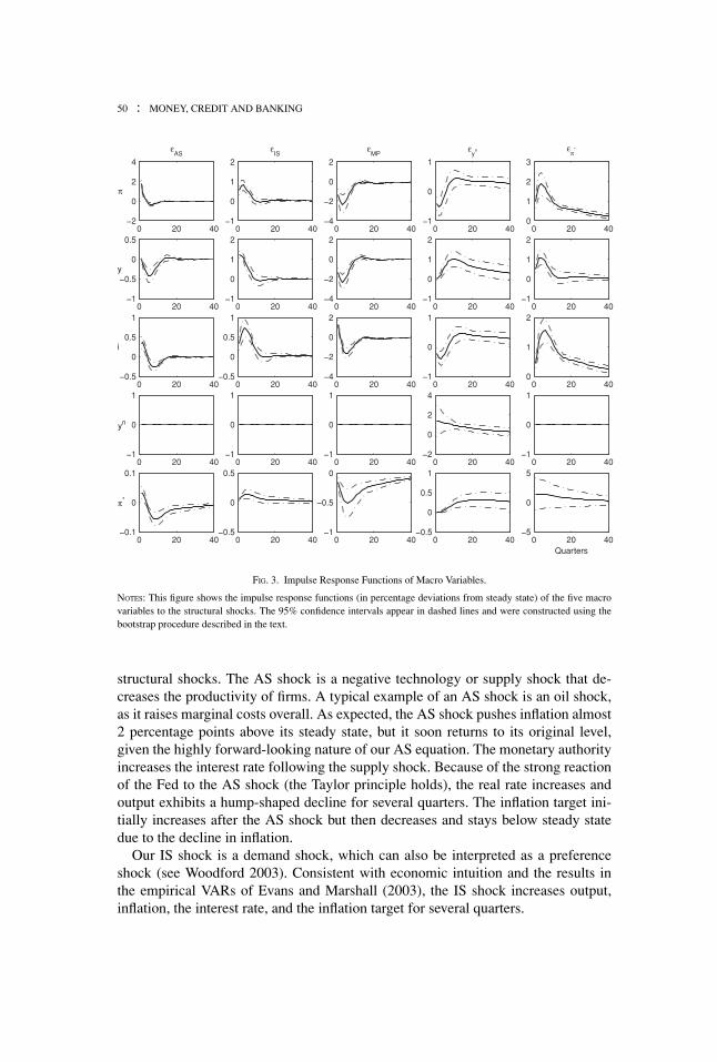
FIG. 3. Impulse Response Functions of Macro Variables.

NOTES: This figure shows the impulse response functions (in percentage deviations from steady state) of the five macrovariables to the structural shocks. The 95% confidence intervals appear in dashed lines and were constructed using thebootstrap procedure described in the text.

structural shocks. The AS shock is a negative technology or supply shock that de-creases the productivity of firms. A typical example of an AS shock is an oil shock,as it raises marginal costs overall. As expected, the AS shock pushes inflation almost2 percentage points above its steady state, but it soon returns to its original level,given the highly forward-looking nature of our AS equation. The monetary authorityincreases the interest rate following the supply shock. Because of the strong reactionof the Fed to the AS shock (the Taylor principle holds), the real rate increases andoutput exhibits a hump-shaped decline for several quarters. The inflation target ini-tially increases after the AS shock but then decreases and stays below steady statedue to the decline in inflation.

Our IS shock is a demand shock, which can also be interpreted as a preferenceshock (see Woodford 2003). Consistent with economic intuition and the results inthe empirical VARs of Evans and Marshall (2003), the IS shock increases output,inflation, the interest rate, and the inflation target for several quarters.


The monetary policy shock reflects shifts to the interest rate unexplained by thestate of the economy. Given our strong monetary transmission mechanism and, anal-ogous to the results obtained in the structural model of Christiano and Eichenbaum(2005), a contractionary monetary policy shock yields a decline of both output andinflation. The inflation target also declines, reinforcing the contractionary effect ofthe monetary policy shock on inflation and output. The interest rate increases follow-ing the monetary policy shock, but after three quarters it undershoots its steady-statelevel. This undershooting is related to the strong endogenous decrease of output andinflation to the monetary policy shock. As we show further, this reaction of the short-term interest rate to the monetary policy shock has implications for the reaction ofthe entire term structure to the monetary policy shock.

A standard microeconomic mechanism for our natural rate shock is an increasein the number of firms, which decreases the wedge between prices and the marginalcost (a negative markup shock) and increases output. In other words, a natural rateshock shifts the AS curve down and, not surprisingly, we see that an expansive naturalrate shock increases output and lowers inflation. Through the monetary policy rule,the interest rate follows initially a similar path to inflation, decreasing substantially.Eventually, inflation rises above steady state again and so does the interest rate,both overshooting their steady state during several periods. As a result, the inflationtarget, which partially reflects expected inflation, rises above steady-state almostimmediately. Notice how output converges toward its natural level after 10 quartersfollowing the natural rate shock and moves in parallel with it from then onward.

An expansionary inflation target shock is an exogenous shift in the preferences ofthe Fed regarding its monetary policy goal. Because the inflation target is a long-termpolicy objective, a positive inflation target shock is akin to a persistent expansionarymonetary policy shock. As a result, output and inflation exhibit a strong hump-shapedincrease in response to the target shock. This response is larger than that estimatedby Rudebusch and Wu (2008) and Diebold, Rudebusch, and Aruoba (2006), whoexplicitly model a level factor instead of the inflation target. Notice that in our setup,the strong response of inflation to a target shock is due to the relation between theinflation target, inflation expectations and inflation.

Figure 4 shows the variance decompositions at different horizons for the five macrovariables in terms of the five structural shocks. The variance decompositions show thecontribution of each macroeconomic shock to the overall forecast variance of each ofthe variables at different horizons. Inflation is mostly explained by the AS shock atshort horizons. However, at medium- and long-run horizons inflation dynamics aremostly driven by the monetary policy shock and the inflation target shock. Short-runoutput dynamics are mostly due to the IS and monetary policy shocks. The naturalrate shock has a growing influence on output dynamics as the time horizon advances,reflecting the fact that in the long-run output tends to its natural level. Interest ratedynamics are dominated by the monetary policy shock at short horizons whereas inthe long-run the inflation target shock has more influence. Given that the monetaryauthority is responsible for both the monetary policy and inflation target shocks, ourresults reveal monetary policy to be a key driver of macro dynamics. Smets and


0 5 10 15 20 25 30 35 400

0.2

0.4

0.6

0.8

π

0 5 10 15 20 25 30 35 400

0.2

0.4

0.6

0.8

y

0 5 10 15 20 25 30 35 400

0.2

0.4

0.6

0.8

i

Quarters

ASISMPy

n

π*

FIG. 4. Variance Decompositions for the Macro Variables.

NOTES: This figure shows the variance decomposition at different time horizons for the macro variables in terms of thefive structural macro shocks. The variance decomposition of a variable at quarter h represents the percentage of the h-stepforecast variance explained by each shock.

Wouters (2003) also find monetary policy shocks to play a key role in explainingmacro dynamics in the euro area.

5. TERM STRUCTURE IMPLICATIONS

5.1 Model Fit for Yields

Our model represents a five-factor term structure model with three observed andtwo unobserved variables. Dai and Singleton (2000) claim that a model with threelatent factors provides an adequate fit with the data. To investigate how well ourmodel fits the complete term structure, we examine its fit with respect to the yields(1 year and 10 year) not used in the estimation. The difference between the actualand model-predicted yields can be viewed as measurement error and should not betoo variable if the model fits the data well. We find that the measurement error forthe 1- and 10-year yields is 45 and 54 basis points (annualized), respectively. Whilethis is significantly different from zero, the fit is reasonable given the parsimoniousstructural nature of our model.


Q1−61 Q1−80 Q4−032

4

6

8

10

12

14

16

y 4

DATAMODEL

Q1−61 Q1−80 Q4−032

4

6

8

10

12

14

16

y 40

DATAMODEL

Q1−61 Q1−80 Q4−032

4

6

8

10

12

14

16

y 4

DATAVAR(3)

Q1−61 Q1−80 Q4−032

4

6

8

10

12

14

16y 40

DATAVAR(3)

FIG. 5. Fit for Yields.

NOTES: This figure graphs the fit of the 1- (y4) and 10-year yields (y40) implied by our macro-finance model (on the left)and those implied by a VAR(3) (on the right) for our sample period: 1961:1Q–2003:4Q. Each graph also plots the actualtime series (in bold).

We also compare the fit of our model to that of a pure macro model in the threeobservable macro variables. We generate yields under the null of the expectationshypothesis, using a VAR(3) for the three variables. Such a VAR can be shown to fitthe macro data very well. In Figure 5, the left-hand side graphs plot the 1- and 10-year yields and their predicted values from the structural model, and the right-handside depicts the yields implied by the VAR(3) macro model. The fit of the VAR(3)is visibly worse for the 10-year yield, but similar for the 1-year yield. Indeed, theimplied measurement error standard deviations of the one and 10-year yields are 45and 169 basis points, respectively.

5.2 Structural Term Structure Factors

It is standard to label the three factors that are necessary to fit term structure dy-namics as the level, the slope, and the curvature factors. We measure the level as theequally weighted average of the 3-month rate, 1-year, and 5-year yields; the slope asthe 5-year to 3-month spread; and the curvature as the sum of the 3-month rate and


0 20 40−0.4

−0.2

0

0.2

0.4

εAS

Level

0 20 40−0.2

0

0.2

0.4

0.6

0.8

εIS

0 20 40−2

−1.5

−1

−0.5

0

0.5

εMP

0 20 40−0.5

0

0.5

1

εy

n

0 20 400

0.5

1

1.5

2

επ

*

0 20 40−0.6

−0.4

−0.2

0

0.2

0.4

Slope

0 20 40−0.8

−0.6

−0.4

−0.2

0

0.2

0 20 40−3

−2

−1

0

1

2

0 20 40−0.2

0

0.2

0.4

0.6

0.8

0 20 40−1.5

−1

−0.5

0

0.5

1

0 20 40−0.4

−0.2

0

0.2

0.4

Curvature

0 20 40−1

−0.5

0

0.5

0 20 40−0.5

0

0.5

1

1.5

2

0 20 40−0.2

0

0.2

0.4

0.6

0.8

0 20 40−1.5

−1

−0.5

0

Quarter

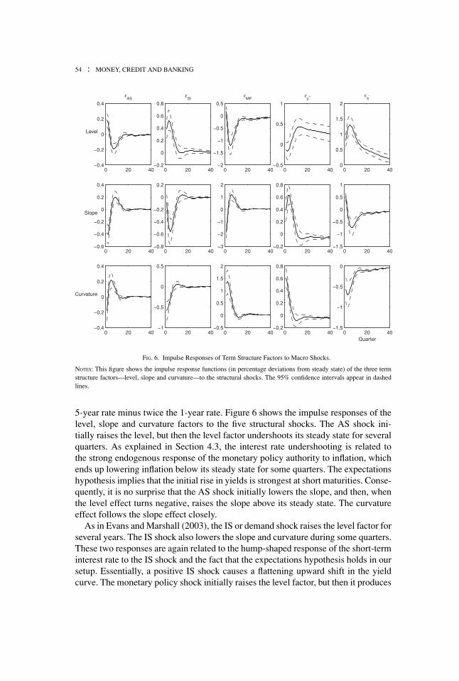
FIG. 6. Impulse Responses of Term Structure Factors to Macro Shocks.

NOTES: This figure shows the impulse response functions (in percentage deviations from steady state) of the three termstructure factors—level, slope and curvature—to the structural shocks. The 95% confidence intervals appear in dashedlines.

5-year rate minus twice the 1-year rate. Figure 6 shows the impulse responses of thelevel, slope and curvature factors to the five structural shocks. The AS shock ini-tially raises the level, but then the level factor undershoots its steady state for severalquarters. As explained in Section 4.3, the interest rate undershooting is related tothe strong endogenous response of the monetary policy authority to inflation, whichends up lowering inflation below its steady state for some quarters. The expectationshypothesis implies that the initial rise in yields is strongest at short maturities. Conse-quently, it is no surprise that the AS shock initially lowers the slope, and then, whenthe level effect turns negative, raises the slope above its steady state. The curvatureeffect follows the slope effect closely.

As in Evans and Marshall (2003), the IS or demand shock raises the level factor forseveral years. The IS shock also lowers the slope and curvature during some quarters.These two responses are again related to the hump-shaped response of the short-terminterest rate to the IS shock and the fact that the expectations hypothesis holds in oursetup. Essentially, a positive IS shock causes a flattening upward shift in the yieldcurve. The monetary policy shock initially raises the level factor, but then it produces


a strong hump-shaped negative response on the level. This is again related to theundershooting of the short-term interest rate after a monetary policy shock. The slopeinitially decreases after the monetary policy shock but then it increases during severalquarters. The initial slope decline happens because a monetary policy shock naturallyshifts up the short end of the yield curve, while it lowers the medium and long partof the yield curve, through its effect on inflationary expectations. The subsequentslope increase arises because the short rate undershoots after a few quarters. Finally,the curvature of the yield curve increases for 10 quarters after the monetary policyshock.

The natural rate shock, which is essentially a positive supply shock, not surpris-ingly induces an initial decline in the level of the yield curve. After 4 quarters, thelevel exhibits a persistent increase, mimicking the response of the short-term rateto the natural rate shock. Both the slope and the curvature factors increase after thenatural rate shock for 10 quarters. As Figure 3 shows, the natural rate shock raisesthe future expected short-term rates whereas it lowers the current short rate. Sincethe expectations hypothesis holds in our setup, that implies that the spread increases.Figure 8 on p. 57 corroborates this intuition.

Finally, the inflation target shock has a very pronounced positive effect on thelevel of the yield curve. This effect has to do with the strong persistent hump-shapedresponse of the interest rate to the target shock. It also makes the slope initiallyincrease, but after three or four quarters the response becomes negative. Thus, thetarget shock ends up having a stronger positive effect on short term rates than on longrates.10 Finally, the curvature declines after the inflation target shock during severalperiods.

To complement the impulse response functions, Figure 7 shows the variance de-compositions of the three factors at different time horizons. The inflation target shockexplains more than 50% of the variation in the level of the term structure at all timehorizons and over 75% at short horizons. Ang, Piazzesi, and Wei (2008) also findthat inflation factors account for a large part of the variation of nominal yields at bothshort and long horizons. After the fifth quarter, the monetary policy shock explainsaround 25% of the level dynamics. In the short-run, the IS shock explains around15%, whereas in the long-run, it is the natural rate shock that explains around 15%of the variation in the level factor.

The monetary policy shock is the dominant factor behind the slope dynamics at allhorizons, as it primarily affects the short end of the yield curve. This fact is especiallyevident at short horizons, where almost 90% of the slope variance is explained by themonetary policy shock. The inflation target shock, which has a dominant effect at thelong end of the yield curve gains importance at longer horizons. The IS shock andthe natural rate shock explain each around 10% of the slope dynamics at virtually allhorizons.

10. Rudebusch and Wu (2008) obtain the opposite reaction of the spread to their level shock. This isprobably related to the fact that they incorporate a time-varying risk premium in the term structure whereaswe maintain the expectations hypothesis throughout.


0 5 10 15 20 25 30 35 400

0.2

0.4

0.6

0.8

Leve

l

0 5 10 15 20 25 30 35 400

0.2

0.4

0.6

0.8

1

Slo

pe

0 5 10 15 20 25 30 35 400

0.2

0.4

0.6

0.8

Cur

vatu

re

Quarters

ASISMPy

n

π*

FIG. 7. Variance Decompositions for the Term Structure Factors.

NOTES: This figure shows the variance decomposition of the term structure factors in terms of the five structural macroshocks. The variance decomposition of a variable at quarter h represents the percentage of the h-step forecast varianceexplained by each shock.

The variance decomposition of the curvature factor yields similar results to the slopefactor, with the monetary policy shock being the dominant factor again, explainingaround 60% of the curvature factor dynamics at all horizons. Finally, it is worthwhilenoting that the AS shock influence on the dynamics of the term structure is overallvery small.

An implication of our study is that the inflation target shock drives much of timevariation of the level, as Figure 7 shows, whereas the monetary policy shock drivesboth the slope and curvature factors. These results are consistent with the those inRudebusch and Wu (2008), where the unobservable variables are directly labeledlevel and slope.

5.3 “Endogenous” Excess Sensitivity

Our model can shed light on an empirical regularity that has received much attentionin recent work, the excess sensitivity of long term interest rates. Gurkaynak, Sack, andSwanson (2005) show a particularly intriguing empirical failure of standard structuralmodels: they fail to generate significant responses of forward interest rates to any


0 10 20 30 40−0.2

0

0.2

0.4

0.6

εAS

0 10 20 30 400

0.2

0.4

0.6

0.8

1

εIS

0 10 20 30 40−2

−1

0

1

2

εMP

0 10 20 30 40−1

−0.5

0

0.5

εy

n

Maturity

0 10 20 30 400

0.5

1

1.5

2

επ

*

Maturity

FIG. 8. Contemporaneous Responses of Yields to Macro Shocks.

NOTES: This figure shows the contemporaneous responses of yields of different maturities to the five structural macroshocks. The 95% confidence bands appear in dashed lines and were constructed using the bootstrap procedure describedin the text.

macroeconomic and monetary policy shock. However, in the data, U.S. long-termforward interest rates react considerably to surprises in macroeconomics data releasesand monetary policy announcements. They use a model with a slow-moving inflationtarget to better match these empirical facts. We now show that our model yields astrong contemporaneous response of the term structure to several macro shocks.

Figure 8 shows the contemporaneous responses of the entire term structure to ourfive structural shocks. The AS shock shifts the short end of the yield curve but hasvirtually no effect on yields of maturities beyond 10 quarters. Our model predicts along-lasting response of bond yields to the IS shock and the shocks to the unobservablemacro variables. The IS shock produces an upward shift in the entire term structurebut affects more strongly the yields of maturities close to 1 year, leading to a hump-shaped response. The IS and natural rate shocks have inverse but symmetric effects on


the term structure. While the IS shock shifts the term structure upward, the natural rateshifts the term structure downward for maturities up to 5 years. This is to be expectedas the IS shock is a demand shock, whereas the natural rate shock is essentially asupply shock.

The monetary policy shock shifts the short end of the curve upward but it has anegative, if small, contemporaneous effect on yields of maturities of five quarters andhigher. Gurkaynak, Sack, and Swanson (2005) also show this pattern, but in theirexercise, the monetary policy shock starts having a negative effect on bond rates at alonger maturities. Our result is again due to the interest rate undershooting in responseto the monetary policy shock. Since the expectations hypothesis holds, future expecteddecreases in short-term rates imply declines of medium and long-term rates. Finally,the inflation target shock produces a very persistent, strong, and hump-shaped positiveresponse of the entire term structure. As agents perceive a change in the monetaryauthority’s stance, they adjust their inflation expectations upward so that interest ratesincrease at all maturities.

Note that the sensitivity of long rates to the inflation target, the natural rate, and theIS shocks remains very strong even at maturities of 10 years. Ellingsen and Soderstrom(2004) and Gurkaynak, Sack, and Swanson (2005) show that their structural macromodels can explain the sensitivity of long rates to structural macroshocks. While theirmodels use several lags of the macro variables in the AS, IS and inflation target equa-tions to generate additional persistence, our model can account for the variability ofthe long rates with a parsimonious VAR(1) specification. More importantly, whereasEllingsen and Soderstrom stress the importance of the monetary policy shock, inour model the IS shock and the shocks to the unobservable macro variables are muchmore important in explaining the sensitivity of the long rates than the monetary policyshock is.

6. CONCLUSIONS

The first contribution of our paper is to use a no-arbitrage term structure model tohelp identify a standard New Keynesian macro model with additional unobservablefactors. Whereas there are many possible implementations of our framework, in thisarticle we introduce the natural rate of output and time-varying inflation target in anotherwise standard model.

From a macroeconomic perspective, our contribution is that we use term structureinformation to help identify structural macroeconomic and monetary policy param-eters and at the same time match the persistence of the key macro variables. From afinance perspective, our contribution is that we derive a no-arbitrage tractable termstructure model where all the factors obey New Keynesian structural relations.

Our key findings are as follows. First, our structural estimation identifies a largePhillips curve parameter and a large response of output to the real interest rate. Second,the inflation target shock accounts for most of variation in the level factor whereasthe monetary policy shocks dominate the variation in slope and curvature factors.


There are a number of avenues for future work. First, the finance literature hasstressed the importance of stochastic risk aversion in helping to explain salient featuresof asset returns (see Campbell and Cochrane 1999, Bekaert, Engstrom, and Grenadier2006). Dai and Singleton (2002) show how time-varying prices of risk play a criticalrole in explaining deviations of the expectations hypothesis for the U.S. term structure.However, their model has no structural interpretation. Piazzesi and Swanson (2004)find risk premiums in federal funds futures rates that appear countercyclical. A follow-up paper will explore the effect of stochastic risk aversion on our findings. Second,Diebold, Rudebusch, and Aruoba (2006) find that macro factors have strong effectson future movements in interest rates and that the reverse effect is much weaker.Our model actually fits this pattern of the data, but we defer a further analysis of thestructural origin of these interactions to future work.

APPENDIX

We now derive the VARMA(3, 2) type representation of the three observable macrovariables implied by the dynamics of the five state variables. For simplicity, we workwith a demeaned system.

Let x1,t = [πt yt it ]′ and x2,t = [ynt π∗

t ]′. Let vt = �εt be the vector of the fivereduced-form errors. Using the lag operator L, the reduced-form model can be decom-posed as x1,t = �11Lx1,t + �12Lx2,t + v1,t and x2,t = �21Lx1,t + �22Lx2,t + v2,t .Note that both v1,t and v2,t are functions of all five structural shocks. The taskis then to substitute out x2,t in the first equation in terms of x1,t and v2,t asx2,t = (I2 − �22L)−1(�21Lx1,t + v2,t ), where (I2 − �22L)−1 can be expressed as

(I2 − �22L)−1 = (1 − ωnn L)(1 − ωpp L) − ωnpωpn L2)−1

×([

(1 − ωpp L) ωnp L

ωpn L (1 − ωnn L)

])

= d(L)−1(I2 − BL),

where �22 = [ ωnn ωnp

ωpn ωpp], B = [ ωpp −ωnp

−ωpn ωnn], d(L) = 1 − b1L + b2L2, b1 = ωpp +

ωnn, b2 = ωppωnn − ωpnωnp. Therefore, x1,t can be expressed as a linear functionof its lags and the reduced-form residual vectors as

x1,t = �1x1,t−1 + �2x1,t−2 + �3x1,t−3 + �0εt + �1εt−1 + �2εt−2,

where �1 = b1 I3 + �11, �2 = −b2 I3 − b1�11 + �12�21, �3 =b2�11 − �12 B�21,

�0 = [I3 03x2]�, �1 = [−b1 I3 �12]�, �2 = [b2 I3 −�12 B]�.


LITERATURE CITED

Ang, Andrew, Geert Bekaert, and Min Wei. (2008) “The Term Structure of Real Rates andExpected Inflation.” Journal of Finance, 63, 797–849.

Ang, Andrew, and Monika Piazzesi. (2003) “A No-Arbitrage Vector Autoregression of TermStructure Dynamics with Macroeconomic and Latent Variables.” Journal of Monetary Eco-nomics, 50, 745–87.

Ang, Andrew, Monika Piazzesi, and Min Wei. (2006) “What Does the Yield Curve Tell Usabout GDP Growth?” Journal of Econometrics, 131, 359–403.

Bekaert, Geert, Seonghoon Cho, and Antonio Moreno. (2005) “New-Keynesian Macroeco-nomics and the Term Structure.” NBER Working Paper No. 11340.

Bekaert, Geert, Eric Engstrom, and Steven R. Grenadier. (2006) “Stock and Bond Returns withMoody Investors.” NBER Working Paper No. 12248.

Bekaert, Geert, Robert J. Hodrick, and David A. Marshall. (2001) “Peso Problem Explanationsfor Term Structure Anomalies.” Journal of Monetary Economics, 48, 241–70.

Bekaert, Geert, Min Wei, and Yuhang Xing. (2007) “Uncovered Interest Rate Parity and theTerm Structure.” Journal of International Money and Finance, 26, 1038–69.

Bernanke, Ben, and Jean Boivin. (2003) “Monetary Policy in a Data-Rich Environment.”Journal of Monetary Economics, 50, 525–46.

Bernanke, Ben, Jean Boivin, and Piotr Eliasz. (2005) “Measuring Monetary Policy: A FactorAugmented Autoregressive (FAVAR) Approach.” Quarterly Journal of Economics, 120,387–422.

Boivin, Jean, and Marc Giannoni. (2006) “Has Monetary Policy Become More Effective?”Review of Economics and Statistics, 88, 445–62.

Boldrin, Michele, Lawrence J. Christiano, and Jonas Fisher. (2001) “Asset Returns and theBusiness Cycle.” American Economic Review, 91, 149–66.

Calvo, Guillermo. (1983) “Staggered Prices in a Utility Maximizing Framework.” Journal ofMonetary Economics, 12, 383–98.

Campbell, John Y., and John H. Cochrane. (1999) “By Force of Habit: A Consumption-BasedExplanation of Aggregate Stock Market Behavior.” Journal of Political Economy, 107, 205–51.

Cho, Seonghoon, and Antonio Moreno. (2006) “A Small-Sample Analysis of theNew-Keynesian Macro Model.” Journal of Money, Credit and Banking, 38, 1461–81.

Cho, Seonghoon, and Antonio Moreno. (2008) “The Forward Method as a Solution Refinementin Rational Expectations Models.” Mimeo, Yonsei University and University of Navarra.

Christiano, Lawrence J., and Martin Eichenbaum. (2005) “Nominal Rigidities and the Dy-namic Effects of a shock to Monetary Policy.” Journal of Political Economy, 113, 1–45.

Clarida, Richard H., Jordi Galı, and Mark Gertler. (1999) “The Science of Monetary Policy:A New Keynesian Perspective.” Journal of Economic Literature, 37, 1661–1707.

Cox, John, Jonathan Ingersoll, and Stephen Ross. (1985) “A theory of term structure of interestrates.” Econometrica, 53, 385–408.

Dai, Qiang, and Kenneth J. Singleton. (2000) “Specification Analysis of Affine Term StructureModels.” Journal of Finance, 55, 531–52.


Dai, Qiang, and Kenneth J. Singleton. (2002) “Expectation Puzzles, Time-Varying Risk Premia,and Affine Models of the Term Structure.” Journal of Financial Economics, 63, 415–41.

Dewachter, Hans, and Marco Lyrio. (2006) “Macro Factors and the Term Structure of InterestRates.” Journal of Money, Credit and Banking, 38, 119–40.

Diebold, Francis X., Glenn D. Rudebusch, and S. Boragan Aruoba. (2006) “The Macroeconomyand the Yield Curve.” Journal of Econometrics, 131, 309–39.

Duffie, Darrell, and Rui Kan. (1996) “A Yield-Factor Model of Interest Rates.” MathematicalFinance, 6, 379–406.

Ellingsen, Tore, and Ulf Soderstrom. (2004) “Why Are Long Rates Sensitive to MonetaryPolicy?” Mimeo, Stockholm School of Economics and IGIER.

Estrella, Arturo, and Frederic S. Mishkin. (1998) “Predicting U.S. Recessions: Financial Vari-ables as Leading Indicators.” Review of Economics and Statistics, 80, 45–61.

Evans, Charles L., and David A. Marshall. (2003) “Economic Determinants of the NominalTreasury Yield Curve.” Working Paper, Federal Reserve of Chicago.

Fuhrer, Jeffrey C. (2000) “Habit Formation in Consumption and Its Implications for Monetary-Policy Models.” American Economic Review, 90, 367–89.

Galı, Jordi, and Mark Gertler. (1999) “Inflation Dynamics.” Journal of Monetary Economics,44, 195–222.

Gurkaynak, Refet T., Brian Sack, and Eric Swanson. (2005) “The Sensitivity of Long-TermInterest Rates to Economic News: Evidence and Implications for Macroeconomic Models.”American Economic Review, 95, 425–36.

Hall, Peter, Joel L. Horowitz, and Bing-Yi Jing. (1995) “On Blocking Rules for the Bootstrapwith Dependent Data.” Biometrika, 82, 561–74.

Hansen, L. P. (1982) “Large Sample Properties of Generalized Method of Moments Estimators.”Econometrica, 50, 1029–54.

Harrison, J. Michael, and David Kreps. (1979) “Martingales and Arbitrage in Multi-PeriodSecurities Markets.” Journal of Economic Theory, 20, 381–408.

Harvey, Campbell R. (1988) “The Real Term Structure and Consumption Growth.” Journal ofFinancial Economics, 22, 305–33.

Hordahl, Peter, Oreste Tristani, and David Vestin. (2006) “A Joint Econometric Model ofMacroeconomic and Term Structure Dynamics.” Journal of Econometrics, 131, 405–44.

Ireland, Peter N. (2001) “Sticky-Price Models of the Business Cycle: Specification and Stabil-ity.” Journal of Monetary Economics, 47, 3–18.

Klein, Paul. (2000) “Using the Generalized Schur Form to Solve a Multivariate Linear RationalExpectations Model.” Journal of Economics Dynamics and Control, 24, 1405–23.

Knez, Peter J., Robert Litterman, and Jose A. Scheinkman. (1994) “Explorations into FactorsExplaining Money Market Returns.” Journal of Finance, 49, 1861–82.

Kozicki, Sharon, and Peter A. Tinsley. (2001) “Shifting Endpoints in the Term Structure ofInterest Rates.” Journal of Monetary Economics, 47, 613–52.

Laubach, Thomas, and John C. Williams. (2003) “Measuring the Natural Rate of Interest.”Review of Economics and Statistics, 85, 1063–70.

Lubik, Thomas A., and Frank Schorfheide. (2004) “Testing for Indeterminacy: An Applicationto U.S. Monetary Policy.” American Economic Review, 94, 190–217.

Lucas, Robert E. (1978) “Asset Prices in an Exchange Economy.” Econometrica, 46, 1426–46.


Lucas, Robert E. (2003) “Macroeconomic Priorities.” American Economic Review, 93, 1–14.

Mishkin, Frederic S. (1990) “The Information of the Longer Maturity Term Structure aboutFuture Inflation.” Quarterly Journal of Economics, 55, 815–28.

Newey, Whitney K., and Kenneth D. West. (1987) “A Simple, Positive Semi-Definite, Het-eroskedasticity and Autocorrelation Consistent Covariance Matrix.” Econometrica, 55, 703–08.

Pearson, Neil D., and Tong-Shen Sun. (1994) “Exploiting the Conditional Density Functionin Estimating the Term Structure: An Application to the Cox, Ingersoll and Ross Model.”Journal of Finance, 49, 1279–1304.

Piazzesi, Monika, and Eric Swanson. (2004) “Futures Prices as Risk-Adjusted Forecasts ofMonetary Policy.” Journal of Monetary Economics, 55, 677–91.

Rotemberg, Julio J., and Michael Woodford. (1998) “An Optimization-Based EconometricFramework for the Evaluation of Monetary Policy: Expanded Version.” NBER WorkingPaper No. T0233.

Rudebusch, Glenn D., and Tao Wu. (2008) “A Macro-Finance Model of the Term Structure,Monetary Policy, and the Economy.” Economic Journal, 118, 906–26.

Smets, Frank, and Raf Wouters. (2003) “An Estimated Dynamic Stochastic General Equilib-rium Model of the Euro Area.” Journal of the European Economic Association, 1, 1123–75.

Stock, James, and Mark W. Watson. (2003) “Understanding Changes in International BusinessCycle Dynamics.” NBER Working Paper No. 9859.

Svensson, Lars E. O. (2004) “Estimating and Interpreting Forward Interest Rates: Sweden1992–1994.” Center for Economic Policy Research Discussion Paper 1051.

Woodford, Michael. (2003) Interest and Prices: Foundations of a Theory of Monetary Policy.Princeton, NJ: Princeton University Press.

Wu, Tao. (2006) “Macro Factors and the Affine Term Structure of Interest Rates.” Journal ofMoney, Credit and Banking, 51, 1847–75.

Copyright of Journal of Money, Credit & Banking (Blackwell) is the property of Blackwell Publishing Limited

and its content may not be copied or emailed to multiple sites or posted to a listserv without the copyright

holder's express written permission. However, users may print, download, or email articles for individual use.

new keynesian macroeconomics and the term structure€¦ · wu (2008), who also append a term...

Documents