new methods for data analysis of complex chemical systems...

New Methods for Data Analysis of Complex

Chemical Systems with Practical

Applications for Atmospheric Studies

Diogo de Jesus Medeiros

Submitted in accordance with the requirements for the degree of Doctor of

Philosophy

The University of Leeds

School of Chemistry

August 2019

The candidate confirms that the work submitted is their own, except where

work which has formed part of jointly authored publications has been included.

The contribution of the candidate and the other authors to this work has been

explicitly indicated below. The candidate confirms that appropriate credit has

been given within the thesis where reference has been made to the work of

others.

The work in Chapter 3 of the thesis has appeared in publication as follows:

Exploring the features on the OH + SO2 potential energy surface using theory

and testing its accuracy by comparison to experimental data.

Medeiros, D. J.; Blitz, M. A.; Seakins, P. W.

Physical Chemistry Chemical Physics

Volume 20, Issue 13. 2018

I was responsible for undertaking the theoretical ab initio calculations and

performing the analysis of the experimental data obtained from previous

studies. Dr. Mark Blitz provided experimental data from previous studies

which were used in the analysis. He also provided important scientific

discussions about the SO2 chemistry which collaborated to the work. Prof.

Paul W. Seakins supervised the analysis and provided scientific guidance with

respect to understanding of the obtained results.

The work in Chapter 4 of the thesis has appeared in publication as follows:

Kinetics of the reaction of OH with isoprene over a wide range of temperature

and pressure including direct observation of equilibrium with the OH Adducts

Medeiros, D. J.;Blitz, M. A.;James, L.;Speak, T. H.;Seakins, P. W.

The Journal of Physical Chemistry A

Volume 122, Issue 37. 2018

I was responsible for performing all the experimental measurements as well as

the analysis of the data, including theoretical calculations and fits. I have also

written the publication. Leanne James have helped collecting information

about the temperature dependence of the CH4 + OH reaction from the

literature during her Masters. This reaction was used to check how well

defined our temperature measurements were. Thomas Speak helped with

collection of some experimental traces. He also provided insightful verbal

discussions on the role of a Hydrogen abstraction in that chemical system. Dr.

Mark Blitz and Prof. Paul W. Seakins supervised the analysis and provided

scientific guidance with respect to understanding of the obtained results. They

have provided critical thinking of the obtained results and proofreading.

This copy has been supplied on the understanding that it is copyright material

and that no quotation from the thesis may be published without proper

acknowledgement

The right of Diogo de Jesus Medeiros to be identified as Author of this work

has been asserted by him in accordance with the Copyright, Designs and

Patents Act 1988.

ACKNOWLEDGMENTS

The conclusion of this work is an event that brings great happiness to my life.

Before any consideration, I can not fail to highlight the direct and definitive

contribution of my parents, Izaltina Maria de Jesus Medeiros and Joel

Medeiros in my academic formation. I had the pleasure of having parents who

showed me from an early age the value of knowledge in the life of the human

being. For all the dedication and sacrifice you have undertaken through the

education of your two children, I make it a point to eternally register your full

names in this work, symbolizing the fact that without your teachings I would

never have succeeded.

It is hard to translate into words the value of working with people as bright and

yet as simple and fun as Paul and Mark. Thank you immensely for the

opportunity to work alongside you and for all the teachings that have been

handed down to me during these four years. Time has gone by in the blink of

an eye, and it seems like only yesterday that I arrived in Leeds for the first time

to find Paul waiting for me at Leeds Bradford Airport. Thank you for having

been so supportive and patient during my time in Leeds. I have a deep pride in

being able to say that I have had you as my supervisors!

Trev, Lisa, Dwayne, Daniel and Lavinia: Thank you for all the constructive

discussions we had during meetings over these four years. Thank you for the

opportunity to have worked with each of you.

My fiancee Isabelle: The support you have given me over the PhD is

something I will never forget. In that time you proved that the distance

between two continents is nothing when love is true. Thank you for all the

wonderful moments we have lived through these four years and for making me

a better person.

My brother Diego: I always remember the example he set when passing a

college entrance exam in the 2000s making me believe that I could too. The

lesson that setting an example can change the world is something I learned

from you.

Tom, Freja, and Alex: Thanks for the company at lunchtime for those days

when, for some reason, I did not have a Subway. It was a great pleasure to

work alongside you and I already miss your company.

I would also like to thank all the other comrades in the Heard and Dainton

groups, with whom the coexistence in this period was a very enriching

experience.

AGRADECIMENTOS

A conclusão do presente trabalho é um acontecimento que traz grande

felicidade à minha vida. Antes de qualquer consideração, não posso deixar de

destacar a contribuição direta e definitiva dos meus pais, Izaltina Maria de

Jesus Medeiros e Joel Medeiros na minha formação acadêmica. Tive o prazer

de ter pais que me mostraram desde cedo o valor do saber na vida do ser

humano. Por toda dedicação e safrifício que vocês se submeteram pela

educação dos seus dois filhos, eu faço questão de registrar seus nomes por

completo nesse trabalho, simbolizando o fato de que sem os seus ensinamentos

eu jamais teria conseguido.

É difícil traduzir em palavras o valor de trabalhar com pessoas tão brilhantes e

ao mesmo tempo tão simples e divertidas como Paul e Mark. Agradeço

imensamente pela oportunidade de trabalhar ao seu lado e por todos os

ensinamentos que me foram passados ao longo desses quatro anos. O tempo

passou num piscar de olhos, e parece que foi ontem que cheguei em Leeds pela

primeira vez para encontrar Paul me esperando no aeroporto. Obrigado por me

apoiar e serem tão pacientes durante meu período em Leeds. Eu tenho um

orgulho profundo de poder dizer que tive vocês como meus supervisores!

Trev, Lisa, Dwayne, Daniel e Lavinia: obrigado pelas discussões construtivas

que tivemos durante reuniões que tivemos ao longo desses quatro anos.

Agradeço a oportunidade de ter trabalhado com cada um de vocês.

Minha noiva Isabelle: o apoio que você me dedicou ao longo do doutorado é

algo da qual nunca irei me esquecer. Nesse tempo você provou que a distância

entre dois continentes não é nada quando o amor é verdadeiro. Obrigado por

todos os momentos maravilhosos que vivemos nesses quatro anos e por me

fazer uma pessoa melhor.

Meu irmão Diego: eu lembro bem que o seu exemplo ao ser aprovado em um

vestibular nos anos 2000 me fez acreditar que eu também seria capaz. A lição

de que um exemplo pode mudar o mundo eu aprendi com você.

Tom, Freja e Alex: obrigado pela companhia no almoço nos dias em que eu,

por algum motivo, não comi um sanduiche do Subway. For um grande prazer

trabalhar ao lado de vocês e eu já sinto falta da sua companhia.

Gostaria de agradecer também a todos os demais companheiros dos grupos

Heard e Dainton, com quem a conviviência nesse período foi uma experiência

bastante engrandecedora.

ABSTRACT

The hydroxyl radical, OH, is the most important oxidizing agent in the

troposphere during daylight periods. This radical, which is predominantly

produced from the photolysis of ozone initiates the gas-phase oxidation of the

vast majority of volatile organic compounds emitted in the atmosphere.

This thesis is focused on the development and exploitation of useful methods

of analysis for the study of atmospherically-relevant processes via direct OH

measurements. However, the flexibility of the technique makes it also suitable

for the study of high temperature combustion-related chemistry. For example,

OH recycling can be an important process for the high temperature oxidation

of ethers, a class of oxygenated species often used as fuel additives. Such

methods provide the necessary tools for the exploration of complex competing

processes, stretching the limits of the conventional bimolecular analysis for

measuring rate coefficients. Among them, a new method based on Master

Equation calculations via global analysis allows the direct analysis of the

temporal evolution of OH radicals undergoing temperature and pressure

dependent processes. Such unprecedented analysis can not only provide

mechanistic information, but also enables a robust evaluation of the

thermochemistry of elementary reactions. The method is very useful in

situations where a reaction of interest cannot be isolated from competing

processes, as required by conventional analysis techniques. For example, for

the high temperature oxidation of alkenes which involve both an OH addition

and a hydrogen abstraction mechanism, the global technique is capable of

discriminating and quantifying the contribution of each channel.

The reaction of OH radicals with sulphur dioxide (SO2) was investigated via

classical Master Equation analysis. The role of a weakly bound pre-reaction

complex formation (~7.2 kJ mol-1

) was tested and a comparison of Leeds

experimental data with the literature was undertaken. The results indicated that

the pre-reaction complex formation is not significant under atmospheric

conditions and much of literature data may have been influenced by secondary

chemistry associated with SO2 photolysis. A transition state submerged below

the reagents (-1.0 kJ mol-1

) was required to describe the Leeds measurements,

which appear to be more consistent than the rest of the literature. The analysis

of high temperature equilibration data (OH + SO2 ⇄ HO-SO2), allowed the

enthalpy of reaction to be determined (110.5 ± 6.6 kJ mol-1

). This experimental

determination is in excellent agreement with the highest-level theoretical

predictions found in the literature (~111.5 kJ mol-1

).

The OH + isoprene reaction in the absence of oxygen was explored over a

wide range of temperatures (298-794 K) and pressures (~60-1500 Torr). At

high enough temperatures (T > 700 K), direct observations of the established

isoprene + OH ⇄ isoprene-OH equilibrium were collected. The study also

generated unprecedented rate coefficients which were subsequently employed

for the study of OH recycling in the presence of O2. The equilibration data

were exploited via a bi-exponential analysis of both experimental and Master

Equation-simulated traces and used for the determination of the well-depth for

OH addition to carbon C1 (153.5 ± 6.2 kJ mol-1

), which is in excellent

agreement with our theoretically-derived estimate (154.1 kJ mol-1

). This

experimental value, however, is dependent on the level of theory at which the

vibrational modes of the involved species are treated. The equilibration data

also indicated a significant OH loss in the system, incompatible with the

reaction of OH with its precursor or diffusion. This process was rationalized as

a competing hydrogen abstraction, which interfered in the non-exponential

equilibration traces. A global analysis of the data was capable of extracting

information about both the OH addition

(kaddition∞

= (9.5 ± 1.2) × 10-11

(T

298 K)

-1.33 ± 0.32

cm3 molecule

-1 s

-1) and the

abstraction channel, (kabstraction∞

= (1.3 ± 0.3) × 10-11

exp (-3.61 kJ mol

-1

RT) cm

3

molecule-1

s-1

). With respect to the OH addition, a comparison with previous

investigations suggests that only our measurements at T >700 K were in the

fall-off region, contradicting some literature studies.

A new method of analysis via a global multi-temperature, multi-pressure

fitting procedure was developed and used for the study of the ethylene + OH

reaction. The method relied on the Master Equation modelling of the OH

addition, and a subsequent incorporation of new consumption and formation

terms to the rate laws of the involved species. With effect, the simulated traces

become comparable to experimental observations and a direct trace analysis is

possible. The reaction of OH with ethylene was studied over a range of

temperatures (563 – 723 K) and pressures (~60 - 220 Torr), which included

pressure dependent data, to test the limits of this global direct trace analysis.

Excellent descriptions of OH traces were obtained when the Master Equations

were modified to incorporate a hydrogen abstraction and a unimolecular loss of

the adduct. A simultaneous fit of 96 traces where direct ethylene + OH ⇄

adduct equilibration was observed enabled the determination of the well-depth

of the adduct (111.8 ± 0.20 kJ mol-1

). This value is in excellent agreement with

our theoretical prediction (111.4 kJ mol-1

), calculated at the

CCSD(T)/CBS//M06-2X/ aug-cc-pVTZ level of theory. The high pressure

limiting rate coefficient for the OH addition extracted from the experimental

traces by this technique (kaddition∞ (T)=(8.13 ± 0.86)×10-12 (

T

298 K)-0.99 ± 0.18

cm-3

molecule-1

s-1

), is in very good agreement with the IUPAC recommendation for

the 100 - 500 K temperature range (k1a∞ (T)=9×10

-12(

T

300 K)-0.85

cm-3

molecule-1

s-1

). Furthermore, the experimentally derived abstraction rate coefficients

kabstraction(T) = 3.5 ± 0.75 × 10-11

exp (-26.2 ± 1.3 kJ mol

-1

RT) cm

-3 molecule

-1 s

-1 are in

excellent agreement with previous investigations. The method proved to be

robust enough to discriminate and quantify the competing processes

influencing the shapes of the experimental OH profiles.

This novel analysis was employed for the study of LIM1, a promising

mechanism for the description of OH recycling via isoprene peroxy chemistry.

Experiments were undertaken at elevated temperatures (400 <T<600 K) and

large concentrations of O2 were employed ([O2]~1017

molecules cm-3

) so as to

promote the recycling to the millisecond timescale, compatible with direct

experimental techniques for OH detection. Rate coefficients measured in the

absence of O2 were incorporated to help constrain the analysis of the data. The

LIM1 mechanism proved to be capable of accurately describing non-

exponential traces collected under such experimental conditions. The OH

recycling involves crucial hydrogen shifts, whose barriers were adjusted in

unison to provide a good fit to the data. However, very small modifications

were necessary for this purpose (~ 2 kJ mol-1

). The incorporation of these

findings in an atmospheric model enabled the description of approximately

50% of the OH concentration measured in a field campaign performed in a

Borneo rainforest, an environment dominated by biogenic volatile organic

compounds emissions.

Finally, the thesis concludes in Chapter 7 with a summary of the results of

each experimental chapter including suggestions for further areas of study.

xiii

TABLE OF CONTENTS

Chapter 1. An Introduction to the Atmospheric Chemistry of OH and relevant

experimental techniques ................................................................................................ 1

Overview of the chapter ............................................................................................. 3

1.1 THE ATMOSPHERIC CYCLE OF HOx ........................................................... 5

1.2 DIRECT AND INDIRECT KINETIC STUDIES ............................................. 11

1.2.1 - Direct Measurements .................................................................................... 12

1.2.2 – Details about Atmospheric Simulation Chambers ....................................... 18

1.2.3 – The Indirect Relative-Rate method. ............................................................. 20

1.3 SUMMARY AND CONCLUSIONS ................................................................ 25

1.4 REFERENCES .................................................................................................. 27

Chapter 2. Experimental Instruments and Theoretical Methods ........................... 31

Overview of the chapter ........................................................................................... 33

2.1 EXPERIMENTAL METHODOLOGY ................................................................. 35

2.1.1 - Fluorescence Assay by Gas Expansion – FAGE .......................................... 35

2.1.2 - FAGE Calibration ......................................................................................... 39

2.1.3 - Laser Flash Photolysis Experiments with Detection by Laser Induced

Fluorescence (LFP-LIF) .......................................................................................... 41

2.2 THEORETICAL METHODS ............................................................................... 48

2.2.1 - The Lindemann Theory ................................................................................ 48

2.2.1.1 The Lindemann Theory From an Unimolecular Perspective ....................... 49

2.2.1.2 The Lindemann Theory From a Bimolecular Perspective ........................... 51

2.2.2 - Master Equation Calculations with MESMER ............................................. 53

2.3 REFERENCES ...................................................................................................... 60

Chapter 3. The Role of the Pre-reaction Complex in the OH + SO2 Reaction ..... 63


3.1 LITERATURE BACKGROUND OF THE OH + SO2 REACTION ................ 67

3.2 AB INITIO AND MASTER EQUATION CALCULATIONS .......................... 70

3.3 RESULTS AND DISCUSSION ........................................................................ 72

3.4 SUMMARY AND CONCLUSIONS ................................................................ 87

3.5 REFERENCES .................................................................................................. 88

xiv

Chapter 4. Kinetics of the Reaction of OH with Isoprene over a Wide Range of

Temperatures and Pressures ......................................................................................... 91


4.1 INTRODUCTION ................................................................................................. 95

4.2 METHODOLOGY .............................................................................................. 100

4.2.1 - Laser flash photolysis experiments with detection by laser induced

Fluorescence (LFP-LIF) ......................................................................................... 100

4.2.2 - Computational Methods: Ab initio Calculations and Master Equation (ME)

Modelling ............................................................................................................... 102

4.3 DATA ANALYSIS .............................................................................................. 105

4.3.1 - Single Exponential Traces .......................................................................... 105

4.3.2 - High Temperature Equilibrium Traces ....................................................... 107

4.4 RESULTS AND DISCUSSION .......................................................................... 112

4.4.1 - Ab initio calculations .................................................................................. 112

4.4.2 - Rate Coefficients for the OH + Isoprene Reaction, R1 .............................. 115

4.4.3 - The Abstraction Channel R1b .................................................................... 121

4.4.4 - Interpretation of OH + Isoprene ⇄ Adducts Equilibria .............................. 124

4.4.5 - Master Equation Modelling and Comparison with Literature .................... 127

4.4.6 - Analytical Representation of Pressure and Temperature for k1a, k-1a,C1, and

k-1a,C4 ....................................................................................................................... 133

4.5 SUMMARY AND CONCLUSIONS .................................................................. 136

4.6 REFERENCES .................................................................................................... 138

Chapter 5. Kinetics of the reaction of ethylene with OH radicals: developing a global

Master Equation-based, raw-trace fitting technique .................................................. 145

Overview of the chapter ......................................................................................... 147

5.1 INTRODUCTION ............................................................................................... 149

5.2 METHODOLOGY .............................................................................................. 159

5.2.1 - Experimental details ................................................................................... 159

5.2.2 - Supporting Ab Initio Calculations .............................................................. 161

5.2.3 - Modifying the full Master Equation transition matrix ................................ 163

5.2.4 - Augmentation of the Bartis-Widom scheme .............................................. 168

5.2.5 - Accounting for hydrogen abstraction and C2H4-OH loss in the BW scheme

............................................................................................................................... 170

5.2.6 - A more programmatic view of the model parameters ................................ 173

5.2.7 - Pre-weighting of experimental data ............................................................ 177

5.3 RESULTS AND DISCUSSION .......................................................................... 181

xv

5.3.1 - Interpretation of the ethylene + OH ⇄ HO-C2H4 data. .............................. 181

5.3.2 - Literature comparison of the OH addition and hydrogen abstraction ........ 185

5.4 SUMMARY AND CONCLUSIONS .................................................................. 193

5.5 REFERENCES .................................................................................................... 194

Chapter 6. Investigation of the Isoprene + OH Reaction in the Presence of Oxygen to

Confirm the Leuven Isoprene Mechanism 1. ............................................................. 197


6.1 INTRODUCTION ........................................................................................... 201

6.2 AB INITIO CALCULATIONS ........................................................................ 211

6.3 RESULTS AND DISCUSSION ...................................................................... 211

6.3.1 – Analysis of non-exponential traces ............................................................ 211

6.3.2 - Numerical integration coupled with a global fit ......................................... 215

6.3.3 – Augmented-ME analysis ........................................................................... 227

6.4 SUMMARY AND CONCLUSIONS .............................................................. 232

6.5 REFERENCES ................................................................................................ 234

Chapter 7. Conclusions and Further Work ................................................................ 233


CHAPTER 3 - The Role of the Pre-reaction Complex in the OH + SO2 Reaction

............................................................................................................................... 237

CHAPTER 4 - Kinetics of the Reaction of OH with Isoprene over a Wide Range of

Temperature and Pressures .................................................................................... 239

CHAPTER 5 - Kinetics of the reaction of ethylene with OH radicals: developing a

global Master Equation-based, raw-trace fitting technique ................................... 242

CHAPTER 6 - Investigation of the Isoprene + OH Reaction in the Presence of

Oxygen to Confirm the Leuven Isoprene Mechanism 1 ........................................ 245

REFERENCES ...................................................................................................... 249

APPENDIX 1 ............................................................................................................ 251

APPENDIX 2 ............................................................................................................ 257

APPENDIX 3 ............................................................................................................ 263

APPENDIX 4 ............................................................................................................ 281

xvi

LIST OF FIGURES

Figure 1.1 – The generic representation of the HOx cycling in the atmosphere.

Processes involving NOx are highlighted in red. ........................................................... 6

Figure 1.2 – Schematic representation of the tests, incorporation and refinement of

atmoshperic models. .................................................................................................... 12

Figure 1.3 - Typical first order decay of OH in the presence of an excess of trans 1,4-

dimethylcyclohexane (DMC). The red line is a single-exponential fit to the data,

which provides a pseudo-first-order rate coefficient for the experimental conditions. T

= 298 K and p = 84 Torr, [DMC] = 1.6 × 1013

molecule cm-3

. ................................... 14

Figure 1.4 – Plot of the pseudo-first-order rate coefficients versus the concentration of

the excess reagent (trans 1,4 dimethylcyclohexane). T = 298 K, p = 84 Torr. ............ 15

Figure 1.5 – Relative rate plot for the reaction of trans 1,4-dimethylcyclohexane with

OH competing with the reaction of cyclohexane with OH. ......................................... 23

Figure 2.1 – OH electronic transitions. On the left-hand side, the off-resonant

approach and the right-hand side shows the resonant fluorescence detection. ............ 37

Figure 2.2 – Lateral section of the FAGE instrument attached to HIRAC. Figure

reproduced from Winiberg (2014).9 ............................................................................. 38

Figure 2.3 – Schematic representation of the high pressure instrument. Upper scheme

shows the full apparatus and the lower evidences the interface between the high

pressure and detection cells. Figure reproduced from Stone et al.30

............................ 42

Figure 2.4 – High-pressure LPF-LIF instrument used in our experiments. For more

images of the apparatus please refer to Appendix 1. ................................................... 44

Figure 2.5 - Single exponential decay obtained from the reaction between isoprene

(1.00 × 1014

molecules cm-3

) and OH radical at 298 K and 2 atm. Low pressure FAGE

cell kept at 1 Torr and sampling distance of 5 mm away from the pinhole.

Measurements were averaged after 4 scans. Points represented for negative times were

probed prior to OH precursor photolysis. The error in the pseudo-first order rate

coefficient is quoted at 2σ. ........................................................................................... 45

Figure 2.6 - Bimolecular plot for the reaction of isoprene with OH radicals at 298 K

and 2 atm. Low pressure FAGE cell kept at 1 Torr and sampling distance of 5 mm.

Error bars quoted at 2σ................................................................................................. 46

Figure 2.7 - Schematic representation of the Lindemann method for pressure-

dependent processes from (a) unimolecular and (b) bimolecular perspectives. .......... 48

Figure 2.8 - The pressure dependence of a generic rate constant as described by the

Lindemann mechanism. ............................................................................................... 50

Figure 2.9 - Generic schematic of the processes involved in Master Equation

modelling. .................................................................................................................... 54

xvii

Figure 3.1 - Potential energy diagram for the OH + SO2 reaction. Relative energies

were calculated at the CCSD(T)/CBS//M06-2X level of theory. A more detailed

description of the calculations is provided later in the chapter. ................................... 68

Figure 3.2 - Potential energy diagram for the OH + SO2 reaction, where a van der

Waals complex, vdW, is formed before proceeding over the transition-state, TS, to

form the hydroxysulfonyl radical, HOSO2. The energies of the stationary states are

those calculated in this work, with zero point energies added. Also included is

OH(v=1) + SO2 reaction, which initially forms a “hot” vdW(**) that either re-

dissociates back to reagents or undergoes intramolecular energy redistribution (IVR)

to vdW(*), which does not significantly re-dissociate to OH(v=1) + SO2; the two thick

arrows indicate that these processes are in competition. The Boltzmann energy

distribution of the vdW is illustrated; it resides mostly above the binding energy of

this complex. ................................................................................................................ 71

Figure 3.3 - The result of the ME fit to the full dataset. a - Blitz et al.9, 11

b – Wine et

al.12

. The y=x line is presented in red. High temperature reverse coefficients by Blitz

et al.9 were suppressed from the figure for illustrative purposes. ................................ 76

Figure 3.4 - The result of the Master Equation fit to the experimental measurements of

Wine et al. 12

. The y=x line is presented in red. ........................................................... 78

Figure 3.5 - The result of the ME fit to the experimental measurements of Blitz et al.9,

11 and those of Wine et al.

12 in argon. The y=x line is presented in red. High

temperature reverse coefficients by Blitz et al.9 were suppressed from the figure for

illustrative purposes. .................................................................................................... 79

Figure 3.6 – A comparison of the estimates of the high pressure limiting rate

coefficients obtained with the use of model H with the previous predictions by Long

et al. and Blitz et al. ..................................................................................................... 86

Figure 4.1 - The rotational torsions described with the hindered rotor approximation

(curved arrows) for isoprene (top left), the isoprene-OH adduct 1 (top right) and the

adduct rising from OH addition to carbon 4 (bottom). Grey, red and white spheres

represent carbon, oxygen and hydrogen atoms respectively. The structure of the higher

energy adducts formed following OH addition at carbons 2 and 3 are presented as

Cartesian coordinates in Appendix 3. The hindered rotor potential for the rotational

torsion of adduct 1 depicted with a red curved arrow is presented in Figure 4.2. ..... 104

Figure 4.2 – The hindered rotor potential for the rotational torsion indicated by a red

curved arrow in Figure 4.1. The energies are relative to that of the lowest energy

conformer (ϕ = 123.2°), whose image is presented in Figure 4.1 and Cartesian

coordinates are available in Appendix 3. ................................................................... 104

Figure 4.3 - Bimolecular plot for Reaction 1 at T = 406 K and p = 2 atm of N2. The

inset shows a typical single exponential decay, generated with [C5H8] = 1.00 × 1014

molecule cm-3

and [O2] = 7.70 × 1018

molecule cm-3

. The points presented in the inset

were averaged after 4 scans. Error bars and uncertainties in the bimolecular plot are at

the 2σ level. Red circles represent data acquired in the presence of oxygen and black

squares represent data in absence of O2. .................................................................... 106

xviii

Figure 4.4 – Residual plot for the single exponential fit of trace presented in Figure

4.3 at T = 406 K and p = 2 atm of N2, [C5H8] = 1.00 × 1014

molecule cm-3

and [O2] =

7.70 × 1018

molecule cm-3

. ......................................................................................... 106

Figure 4.5 - Example of a non-exponential trace acquired at T = 729 K, p = 130 Torr

N2 and [isoprene] = 2.3×1014

molecule cm-3

. The inset shows the same decay trace

with a logarithmic scale for the OH signal. The long-time decay of OH shows that

there is a significant process by which OH is lost from the system (modelled as k1b).

The green lines shows fits of equation E7 to the data where the abstraction was

suppressed and the red lines represent fits where the abstraction was considered. ... 109

Figure 4.6 - Residual plot of the green fit presented in Figure 4.5, where the

contribution of the competing hydrogen abstraction is supressed from the model. ... 110

Figure 4.7 – Residual plot of the red fit presented in Figure 4.5, where the contribution

of the competing hydrogen abstraction is included in the model. .............................. 110

Figure 4.8 - Examples of fits of non-exponential traces acquired at T >725 K and p ~

100 Torr. .................................................................................................................... 111

Figure 4.9 - The potential energy diagram for the OH addition to isoprene. Relative

energies were calculated at the CCSD(T)/CBS//M06-2X/6-311++G(3df,2p) level and

include zero point energy corrections. ....................................................................... 112

Figure 4.10 - Comparison of experimental measurements using the high pressure

instrument (black squares), measurements at the high pressure limit with a

conventional low-pressure instrument (blue triangles) and at the fall-off region (red

circles). The dotted line shows the IUPAC recommendation for the temperature

dependence of the isoprene + OH reaction, the dashed line shows our best estimate for

the high pressure limit k1∞, which was obtained from a ME from this work and

selected data as will be discussed in section 4.4.5. The continuous line represents k1∞

as obtained based purely on our measurements. Errors are statistical at the 2σ level.

................................................................................................................................... 116

Figure 4.11 - The change in the m/z = 71 and m/z = 83 Da peaks at room temperature

when the excimer laser is OFF (black line, no OH radicals generated) and ON (red

line). [C5H8] = 5.3 × 1013

molecule cm-3

, [O2] = 1.2 × 1019

molecule cm-3

, T = 298 K, p

= 1200 Torr. The mass m/z = 71 Da peak corresponds to methyl vinyl ketone (MVK)

and methacrolein (MACR, 2 methylprop 2 enal) and the peak m/z = 83 corresponds to

2-methylene-3-butenal. .............................................................................................. 123

Figure 4.12 - Correlation plot for experimental data points from all the data in Table 3

and the calculated rate coefficients generated by MESMER by allowing the well-

depth, A<ΔE>d,M, A and n to be floated. The resulting parameters are shown in the

second column of Table 4.6. ...................................................................................... 129

Figure 4.13 - Correlation plot for experimental data points from selected data in Table

4 (see text) and the calculated rate coefficients generated by MESMER by allowing

the well-depth, A<ΔE>d,M, A and n to be floated. The resulting parameters are shown

in the ‘selected data’ column of Table 4.6. ................................................................ 131

Figure 4.14 - Fits of the Troe formalism to MESMER-simulated rate coefficients

where N2 was implemented as the buffer gas at various temperatures. Markers

xix

represent MESMER-simulated rate coefficients and the lines of the same colour are

the Troe fits to the data. ............................................................................................. 135

Figure 5.1 - Comparison of experimental recommendations for the ethylene + OH

from different investigations. Red circles represent the recommendation from the

review by Baulch et al.31

, blue open triangles refer to the work of Tully16

, pink

diamonds refer to the work of Liu et al.30

, olive triangles correspond to the report of

Vasu et al.35

, cyan triangles refer to the work of Westbrook et al.32

, orange stars

correspond to the study of Srinivasan et al.34

, light green triangles refer the work of

Bhargava and Westmoreland.33

................................................................................. 156

Figure 5.2 - Internal rotations described with the hindered rotor approach for the

C2H4-OH adduct. ....................................................................................................... 162

Figure 5.3 - Example of an OH trace recorded at ~610 K and ~110 Torr of N2 using a

conventional LFP-LIF instrument (open circles). [C2H4] = 9.5 × 1014

molecule cm-3

.

The red line shows a Master Equation simulation under the same experimental

conditions and the black line depicts a single exponential fit to the data. ................. 164



molecule cm-3

.


conditions and the black line depicts a single exponential fit to the data. The blue line

represents a ME fit in which the transition matrix was altered to incorporate kloss the

sum of the pseudo-first order loss due to reaction of OH with its precursor and

diffusion. .................................................................................................................... 166

Figure 5.5 - Matrix formulation of the OH + Ethylene addition reaction as simplified

via the Bartis-Widom approach. ................................................................................ 169

Figure 5.6 - Matrix formulation of the OH + Ethylene addition reaction as simplified

via the Bartis-Widom approach, modified to incorporate kloss. ............................... 169

Figure 5.7 - Flow chart of the fitting based on BW rate coefficients followed by ODE

modification. .............................................................................................................. 176

Figure 5.8 - Example of a bi-exponential fit to an OH trace related to the OH + C2H4

reaction. T = 610 K p = 110 Torr and [C2H4] = 9.5 × 1014

molecule cm3. Points

averaged after 4 scans. ............................................................................................... 178

Figure 5.9 - Residual plot of the bi-exponential fit presented in Figure 5.8. T = 610 K

p = 105 Torr and [C2H4] = 9.5 × 1014

molecule cm3. Points averaged after 4 scans. 179


conventional LFP-LIF instrument (black squares). [C2H4] = 9.5 × 1014

molecule cm-3

.


conditions and the black line depicts a single exponential fit to the data. The blue line

represents a ME fit in which the transition matrix was altered to incorporate kloss the

sum of the pseudo-first order loss due to reaction of OH with its precursor and

diffusion. .................................................................................................................... 182

Figure 5.11 - Examples of augmented ME fits for multiple traces under significantly

different experimental conditions. The dashed line represents y=0 for a better

reference. ................................................................................................................... 183

xx


from different investigations. Pink triangles represent the IUPAC recommendation for

the temperature dependence of the high-pressure limiting rate coefficient of the

ethylene + OH reaction in the 100-500 K temperature range

(k1a∞

=9×10-12(T

300 K)-0.85

cm3 molecule

-1 s

-1). Black squares represent the

recommendation of this work based on the best fit parameters reported in Table 5.2.

Open markers represent pressure dependent rate coefficients and filled markers are

estimates of k1a∞

. .......................................................................................................... 186


from different investigations. Red circles represent the recommendation from the


, blue open triangles refer to the work of Tully 16

, pink

diamonds refer to the work of Liu et al.30

, olive triangles correspond to the report of

Vasu et al.35

, cyan triangles refer to the work of Westbrook et al.32

, orange stars

correspond to the study of Srinivasan et al.34

, light green triangles refer the work of

Bhargava and Westmoreland33

and finally, black squares are the recommendation

based on the best fit parameters reported in Table 5.2. .............................................. 187

Figure 5.14 – The temperature dependence of H-abstraction and OH-addition rate

coefficients at 100 Torr of He. ................................................................................... 189

Figure 5.15 – List of k3’ values obtained from the augmented BW-ME fit as a function

of temperature. ........................................................................................................... 190

Figure 5.16 – Experimental traces collected at ~610 K and ~110 Torr with the use of

different precursors. While blue triangles and red crosses were collected with the use

of H2O-H2O2, the black squares represent a trace collected with urea-H2O2. ............ 192

Figure 6.1 – The Leuven Isoprene Mechanism as proposed by Peeters et al.13

......... 203

Figure 6.2 - The Leuven Isoprene Mechanism 1 as proposed by Peeters et al.3 ........ 204

Figure 6.3 - Simulations of LIM1 under various temperatures. [O2] = 1 × 1018

molecule cm-3

. These simulations were all done with the aid of the computational

package Kintecus.22

.................................................................................................... 210

Figure 6.4 - An example of a non-exponential decay, generated for [C5H8] ≈ 1.00 ×

1014

molecule cm-3

, 1019

O2 cm-3

, 540 K and 2 atm. The data were averaged after 10

scans. The blue line represents a bi-exponential curve fitted to the data while the red

line represents a single exponential curve fit. The green line represents the average for

the background OH signal. ........................................................................................ 212

Figure 6.5 - The residuals plot for the single exponential fit presented in Figure 6.4.

................................................................................................................................... 212

Figure 6.6 - The residuals plot for the bi-exponential fit presented in Figure 6.4. .... 213

Figure 6.7 – Energy barriers of the hydrogen shifts being modified in unison, as

implemented in the fitting procedures. ...................................................................... 217

Figure 6.8 - Examples of LIM1 fits to the data for various experimental conditions.

................................................................................................................................... 220

Figure 6.9 – Comparison of the various models implemented when fitting a trace

generated at 584 K and 124 Torr of N2. [C5H8] ~ 4×1013

molecule cm-3

, [O2] ~ 1×1017

molecule cm-3

. The red line shows a single-exponential fit to the data. .................... 222

xxi

Figure 6.10 – MCM atmospheric simulations of the OP3 campaign against the actual

OH measurements for various models. Error bars represent the 28% uncertainty

associated with the OH measurements undertaken during the OP3 field campaign.4 224

Figure 6.11 - Sources of OH in the atmospheric simulations of the LIM1-BR-linked

and Teng et al. models included in Figure 6.10. ........................................................ 225

Figure 6.12 - Potential energy diagram for the Leuven Isoprene Mechanism 1 used in

the current analysis. Depicted energetics represent effective barriers that account for

tunnelling from the work of Peeters et al. Energies in kJ mol-1

. ................................ 227

Figure 6.13 – Fits of the vibration-only model and a model which incorporate a total

of 40 hindered-rotors to describe corresponding rotational torsions. ........................ 230

xxii

LIST OF TABLES

Table 3.1 – Comparison of theoretical calculations for the OH + SO2 reaction. All the

energies include zero-point corrections and are relative to OH + SO2. The table also

includes an experimental measurement by Blitz et al.9 ............................................... 73

Table 3.2 - Master Equation fits to the experimental data, where <ΔEdown> = <ΔEd,

M>× (T/298)m. ............................................................................................................... 80

Table 4.1 - Experimental Determinations of k1 from Single Exponential Decays ..... 105

Table 4.2 - Experimental conditions, number of OH + C5H8 ⇌ HOC5H8 equilibrium

traces and obtained rate coefficients .......................................................................... 111

Table 4.3 - Theoretically calculated well-depths for the isoprene + OH reaction with

respect to the additions at carbons 1 and 4. All well-depths are corrected for zero-point

energies ...................................................................................................................... 113

Table 4.4 - Comparison of Experimental Determinations of k1 ................................. 118

Table 4.5 - Comparison of Experimental and calculated k-1a. Uncertainty at 1σ. ....... 126

Table 4.6 - Returned parameters from MESMER fits to this work and the literature

data using a two-adduct model and accounting for H abstraction with all data given an

equal uncertainty of 10%. <ΔE>d,M = A<ΔE>d,M × (T/298)mc

........................................ 132

Table 4.7 - Returned parameters from MESMER fits to this work and the literature

data and accounting for H abstraction with our higher temperature data given the

uncertainties reported in Table 2. <ΔE>d,M = A<ΔE>d,M × (T/298)m ............................. 132

Table 4.8 - Troe fit parameters to MESMER-simulated rate coefficients, for different

buffer gases. ............................................................................................................... 134

Table 5.1 - List of experimental conditions, the chemically significant eigenvalue and

the lowest internal energy redistribution eigenvalue. Eigenvalues were obtained with

the ME parameters presented in Table 5.2. ................................................................ 181

Table 5.2 – List of optimized parameter for the augmented ME fit. Uncertainties

quoted as 2 ................................................................................................................. 183

Table 6.1 – List of experimental conditions at which OH traces were collected for the

isoprene + OH reaction in the presence of O2. ........................................................... 214

Table 6.2 – Best-fit parameters for both BR-Linked and BR-free fitting procedures.

Errors quoted at 2σ ..................................................................................................... 219

Table 6.3 - Best-fit parameters for both Vibration-only and Hindered Rotor fitting

procedures. Errors quoted at 2σ ................................................................................. 229

Table 6.4 - Calculated rate coefficients for the H shifts extrapolated to 298 K and 760

Torr. ........................................................................................................................... 229

xxiii

LIST OF ABBREVIATIONS

B3LYP Becke, Three-Parameter, Lee-Yang-Parr Exchange-Correlation

Functional

BR Branching Ratio

BW Bartis-Widom Analysis

CBS Complete Basis Set Limit

CCSD(T) Coupled Cluster Calculations With Single, Double And

Pertubative Triple Excitations

CHEX Cyclohexane

CI Configuration Interaction

CORR Correlation

CPM Channel Photomultiplier

CSE Chemically Significant Eigenvalue

DF Discharge Flow

DFT Density Functional Theory

di-HPCARP Dihydroperoxycarbonyl Peroxy

DMC trans 1,4-Dimethylcyclohexane

EGME Energy Grained Master Equation

EUPHORE European Photoreactor

FAGE Fluorescence Assay By Gas Expansion

FTIRS Fourier Transform Infrared Spectroscopy

GC Gas Chromatography

HF Hartree Fock

HIRAC Highly Instrumented Reactor For Atmospheric Chemistry

HPALD Hydroperoxycarbonyl Aldehyde

IERE Internal Energy Relaxation Eigenvalue

ILT Inverse Laplace Transformation

IUPAC International Union Of Pure And Applied Chemistry

IVR Internal Vibrational Energy Redistribution

LFP Laser Flash Photolysis

LFP-LIF Laser Flash Photolysis-Laser Induced Fluorescence

LIF Laser Induced Fluorescence

LIM Leuven Isoprene Mechanism

LIM1 Leuven Isoprene Mechanism 1

xxiv

MCM Master Chemical Mechanism

ME Master Equation

MESMER Master Equation Solver For Multi-Energy Well Reactions

MS Mass Spectrometric Detection

Nd-YAG Neodymium-Doped Yttrium Aluminium Garnet

ODEs Ordinary Differential Equations

PLP-CRDS Pulsed Laser Photolysis-Cavity Ring-Down Spectroscopy

PLP-LIF Pulsed Laser Photolysis-Laser Induced Fluorescence

PLP-RF Pulsed Laser Photolysis – Resonance Fluorescence

PMP4(SDTQ) Møller-Plesset Perturbation Theory With Single, Double, Triple

And Quadruple Excitations And Spin Projection

PTR-MS Proton-Transfer Reaction Mass Spectrometry

PTR-TOF-MS Proton-Transfer Reaction Time Of Flight Mass Spectrometry

QCISD(T) Quadratic Configuration Interaction With Single, Double And

Pertubative Triple Excitations

RF Resonance Fluorescence

roQCISD(T) Restricted Open-Shell Quadratic Configuration Interaction With

Single, Double And Pertubative Triple Excitations

RR Relative Rate

RRKM Rice–Ramsperger–Kassel–Marcus Theory

TS Transition State

TST Transition State Theory

UCPH Quartz Photochemical Reactor

vdW van der Waals Pre-Reaction Complex

VOC Volatile Organic Compound

YAG Yttrium Aluminium Garnet

ZPE Zero-Point Energy

1

Chapter 1

Chapter 1. An Introduction to the

Atmospheric Chemistry of OH and

relevant experimental techniques

3

Chapter 1

Overview of the chapter

The first chapter of this thesis is focused on the chemistry of the most

important atmospheric oxidizer during the daylight period: the hydroxyl

radical (OH). This molecule which is often referred to as the detergent of the

atmosphere is responsible to initiate the oxidation of the vast majority of

volatile organic compounds (VOCs) in the gas-phase. For this reason, the

reactions of VOCs with OH are of great importance for atmospheric studies.

After an introduction regarding the atmospheric chemistry of OH, with

considerations about alternative important radicals (NO3 and Cl atoms), the

fundamental differences of direct and indirect kinetic measurements are

discussed to provide a familiarization with the nuances of such approaches. A

pragmatic description of how direct measurements (vastly used in the

experimental work of this thesis) are implemented for monitoring the temporal

evolution of OH radicals. The use of simulation chambers to study

atmospherically relevant reactions is discussed and demonstrated. Relative-rate

experiments are presented in the context of the reactions of cyclohexanes with

OH radicals for an elucidative presentation of an indirect measurement of a

rate coefficient. Even though all the experimental work undertaken for the

current thesis was based on direct radical observations with laser-based

techniques, in many occasions the results of previous chamber studies need to

be either incorporated into the analysis, or addressed in the discussion section.

These needs justify a discussion about the nuances of such apparatus in a more

detailed manner, so as to elucidate the limitations and nuances of the

technique. Finally, a lifetime calculation based on the bimolecular rate

coefficients obtained with both the direct and indirect methods is

demonstrated.

5

Chapter 1

1.1 THE ATMOSPHERIC CYCLE OF HOx

The OH radical, often referred to as the atmospheric detergent, is the primary

oxidizing agent in the atmosphere during daylight periods. The reaction with

OH is responsible to initiate the oxidation of the vast majority of volatile

organic compounds (VOC) released in the atmosphere.1 During sunlight

periods, its production is dominated by the photolysis of ozone (R1) to produce

an excited oxygen atom, denoted as O(1D); followed by the reaction of this

atom with water vapour available in the atmosphere (R2), giving rise to two

molecules of OH radicals.

O3 + hv

λ < 340 nm → O2 + O(

1D)

R1

O(1D) + H2O → 2 OH R2

The main sinks of OH in the troposphere are the reactions with carbon

monoxide (CO) and methane (CH4,) which account for approximately 40%

and 15% of the total OH sink flux respectively.2 As will be discussed later in

the chapter, these numbers are very dependent of the environments considered;

in remote environments such processes can account to nearly 100% of the OH

sink.3 Furthermore, the reactions with OH are the main removal process for

these greenhouse gases from the atmosphere, which denotes that the

implications of the OH chemistry into radiative forcing are of primary

importance.

In polluted environments, characterized by the presence of large concentrations

of nitrogen oxides (NOx), the reaction of HO2 radicals with NO (R3) and the

photolysis of nitrous acid (HONO) (R4) are also important sources of OH

radicals.4-5

Studies indicate that at early times in the morning, immediately

after sunrise, the photolysis of HONO, whose concentration is built up during

the night-time period, can become the primary precursor responsible for OH

production, despite only accounting for as much as 20% of the OH formation

on a 24-hour basis.4, 6

6

Chapter 1

HO2 + NO → OH + NO2 R3

HONO + hv

λ < 400 nm → OH + NO

R4

Alternative sources of OH radicals include formaldehyde and hydrogen

peroxide photolysis2, 4

, alkene ozonolysis via Criegee intermediate formation7,

and the oxidation of atmospherically important VOCs such as isoprene.8-10

Figure 1.1 shows a generic representation of the HOx cycle in the atmosphere.

Figure 1.1 – The generic representation of the HOx cycling in the atmosphere. Processes

involving NOx are highlighted in red.

For a good understanding of the OH cycle, an instructive example will be

considered. As previously discussed, OH is mostly produced via O3 photolysis

followed by the reaction of the formed O(1D) atoms with water vapour. The

hydroxyl radical is now available to react with an organic pollutant. For the

sake of the understanding, a simple alkane will be assumed as an example

(VOC= H3C-CH3). The reaction of ethane with the OH radical proceeds via a

7

Chapter 1

hydrogen abstraction, leading to the formation of an alkyl radical

(R= H3C-ĊH2) which rapidly reacts with O2 to form a peroxy radical

(RO2= H3C-C(O2)H2). The fate of peroxy radicals is determined by three

typical competing paths: (I) reactions with NO (adjacent red arrows in

Figure 1.1), (II) isomerization to form a hydroperoxide specie (QOOH) and

(III) reaction with another peroxy radical. The relative importance of each

channel can vary however, depending on whether a clean or polluted

environment is being considered.

In a polluted environment, in the presence of large concentrations of the NO,

typically in the order of tens of parts per billion (~1011

-1012

molecule cm-3

), the

peroxy radical will predominantly be consumed via its reaction with NO to

form an alkoxy radical (RO= H3C-C(O)H2). To a lesser extent, the RO2 + NO

reactions can lead to the generation of nitrites (RO2NO), whose prompt

isomerization can give rise to a nitrate (RONO2). For example, while the

nitrate yield for the n-hexyl peroxy + NO reaction was measured to be 0.14 ±

0.02, the yields for the corresponding reactions of NO with n-heptyl and

n-octyl peroxys are 0.18 ± 0.02 and 0.22 ± 0.03, respectively.11-12

In pristine environments, however, the fate of peroxy radicals is primarily

dictated by two competing processes: (I) a bimolecular reaction with another

available RO2 to form the alkoxy radical (RO= H3C-C(O)H2); and (II) an

internal hydrogen shift to form a hydroperoxide specie, which can potentially

photolyze to reform OH radicals. The lack of importance of the NO reactions

in this case is justified by the significantly lower concentrations of NO in clean

environments. For example, while concentrations of NO as high as 1 × 1012

molecule cm-3

have been measured during the summer of 2012 in central

London,13

measurements in the order of 109 molecule cm

-3 of NO were

measured in a rainforest of Borneo during the OP3 field campaign.14

The

significant difference of several orders of magnitudes in these numbers and the

multiple competing processes presented in Figure 1.1 evidence how the

atmospheric chemistry driven in clean and polluted environments can differ

substantially from a mechanistic point of view. The isomerization of peroxy

8

Chapter 1

radicals in pristine environments has been the focus of many studies where

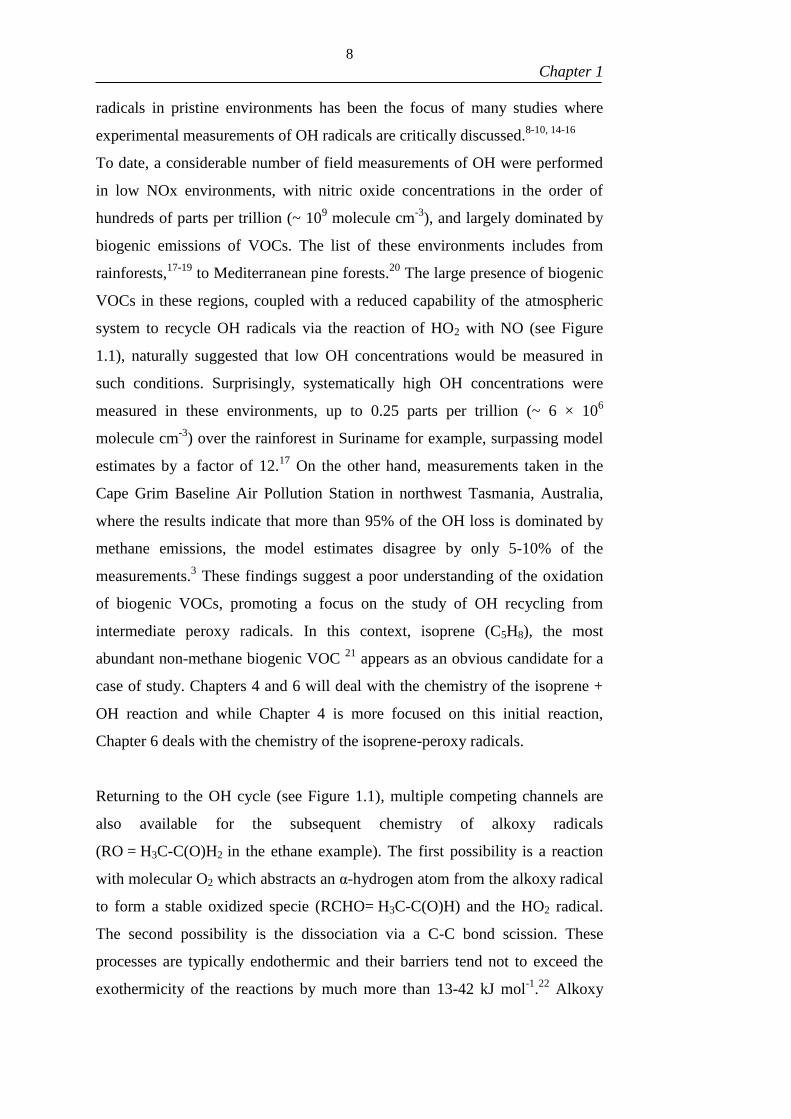
experimental measurements of OH radicals are critically discussed.8-10, 14-16

To date, a considerable number of field measurements of OH were performed

in low NOx environments, with nitric oxide concentrations in the order of

hundreds of parts per trillion (~ 109 molecule cm

-3), and largely dominated by

biogenic emissions of VOCs. The list of these environments includes from

rainforests,17-19

to Mediterranean pine forests.20

The large presence of biogenic

VOCs in these regions, coupled with a reduced capability of the atmospheric

system to recycle OH radicals via the reaction of HO2 with NO (see Figure

1.1), naturally suggested that low OH concentrations would be measured in

such conditions. Surprisingly, systematically high OH concentrations were

measured in these environments, up to 0.25 parts per trillion (~ 6 × 106

molecule cm-3

) over the rainforest in Suriname for example, surpassing model

estimates by a factor of 12.17

On the other hand, measurements taken in the

Cape Grim Baseline Air Pollution Station in northwest Tasmania, Australia,

where the results indicate that more than 95% of the OH loss is dominated by

methane emissions, the model estimates disagree by only 5-10% of the

measurements.3 These findings suggest a poor understanding of the oxidation

of biogenic VOCs, promoting a focus on the study of OH recycling from

intermediate peroxy radicals. In this context, isoprene (C5H8), the most

abundant non-methane biogenic VOC 21

appears as an obvious candidate for a

case of study. Chapters 4 and 6 will deal with the chemistry of the isoprene +

OH reaction and while Chapter 4 is more focused on this initial reaction,

Chapter 6 deals with the chemistry of the isoprene-peroxy radicals.

Returning to the OH cycle (see Figure 1.1), multiple competing channels are

also available for the subsequent chemistry of alkoxy radicals

(RO = H3C-C(O)H2 in the ethane example). The first possibility is a reaction

with molecular O2 which abstracts an α-hydrogen atom from the alkoxy radical

to form a stable oxidized specie (RCHO= H3C-C(O)H) and the HO2 radical.

The second possibility is the dissociation via a C-C bond scission. These

processes are typically endothermic and their barriers tend not to exceed the

exothermicity of the reactions by much more than 13-42 kJ mol-1

.22

Alkoxy

9

Chapter 1

radicals can also isomerize to form a hydroxy-substituted alkyl radical (ROH),

in a process which tend to proceed via 1-5-H shifts.22

Finally, the produced HO2 radicals can react with NO to reform OH radicals to

close the cycle illustrated in Figure 1.1. For the same reasons discussed for the

peroxy radicals, this final reaction is much more dominant for polluted

atmospheres. As will be discussed in Chapter 6, however, even at relatively

low NOx concentrations the HO2 + NO reaction cannot be ruled out or

ignored, as it can, in percentage terms, be relevant.

Despite the fact that considerably different chemical paths can be undertaken

depending on the discussed atmospheric conditions, having an average

estimate of the global OH concentration is highly desirable since it can provide

means to estimate the lifetimes of pollutants. OH is an extremely reactive

specie, and as a consequence, has an atmospheric lifetime of less than a

second. In the late 1970s, Singh et al. demonstrated that the tropospheric

concentration of OH could be estimated from the lifetimes of the now banned

industrial solvent methylchloroform (CH3CCl3).23-24

They have used

atmospheric measurements of CH3CCl3 available along with an industrial

inventory of methylchloroform to estimate its lifetime (τ). Aware of the fact

that CH3CCl3 was predominantly removed via its reaction with OH and

assuming a constant CH3CCl3 concentration throughout the troposphere, the

concentration of OH was estimated (0.41 × 106 molecule cm

-3) from the

CH3CCl3 lifetime and the bimolecular rate coefficient for the mentioned

reaction (E1). The literature typically reports tropospheric mean concentrations

of OH in the order of (0.3-3) × 106 molecules cm

-3 for a 24-hour period.

25-26

[OH] = 1

τ × kOH + CH3CCl3

E1

The initial reactions of OH with VOCs can proceed via two main notable

mechanisms: (I) by the means of an electrophilic addition to an available π

bond or (II) via a hydrogen abstraction process, as exemplified in the case of

10

Chapter 1

ethane. The first channel is naturally important for the oxidation of alkenes and

dienes in general, while the abstraction mechanism is important for saturated

hydrocarbons. During the night, however, when the OH concentrations are

rapidly reduced, so is the importance of the chemistry of this specie. During

this time, nitrate (NO3) chemistry increases in relevance.1, 27-28

While NO3 is

heavily photolyzed to NO2 and a ground state oxygen atom O(3P) during the

day, its concentration can rapidly increase after sunset. However, as NO3

additions to double bonds are typically slower than the OH counterparts,28

the

definition of a dominating process during darkened periods is directly

compromised to the relative concentrations of OH and NO3. At night, NO3

concentrations can be several orders of magnitude larger than the OH.27-28

In the marine boundary layer however, Cl atoms tend to have a key role in the

oxidation of VOCs.29

Reactions between suspended solid particles of NaCl and

nitrogenated species such as NO2 and N2O5 can ultimately lead to the

formation of ClNO and Cl2 (R5-R7), species which absorb actinic ultraviolet

radiation (λ>290 nm).29

Photolysis of these species lead to the formation of

atomic chlorine, which can in turn, initiate the oxidation process of available

VOCs. Reactions of Cl atoms are typically at least an order of magnitude faster

than the corresponding OH reactions.30

Very low ambient Cl concentrations

are predicted in the literature ([Cl] < 1× 105 molecule cm

-3),

31 indirectly

derived from measurements of Cl precursors and products of its reactions with

available hydrocarbons, since no reliable method of direct quantification of this

specie is available. 30

2NO2(s) + NaCl(g) → ClNO(g) + NaNO3(s) R5

N2O5(g) + NaCl(g) → ClNO2(g) + NaNO3(s) R6

ClNO2(g) + NaCl(g) → Cl2(g) + NaNO3(s) R7

11

Chapter 1

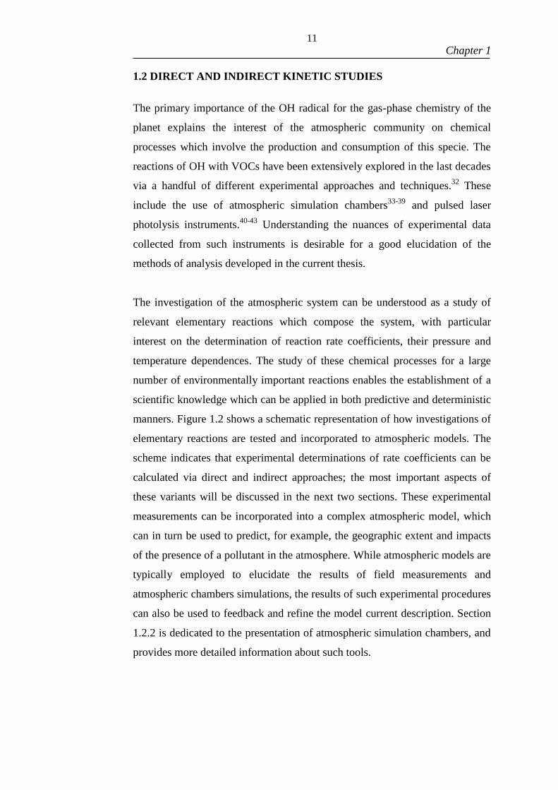
1.2 DIRECT AND INDIRECT KINETIC STUDIES

The primary importance of the OH radical for the gas-phase chemistry of the

planet explains the interest of the atmospheric community on chemical

processes which involve the production and consumption of this specie. The

reactions of OH with VOCs have been extensively explored in the last decades

via a handful of different experimental approaches and techniques.32

These

include the use of atmospheric simulation chambers33-39

and pulsed laser

photolysis instruments.40-43

Understanding the nuances of experimental data

collected from such instruments is desirable for a good elucidation of the

methods of analysis developed in the current thesis.

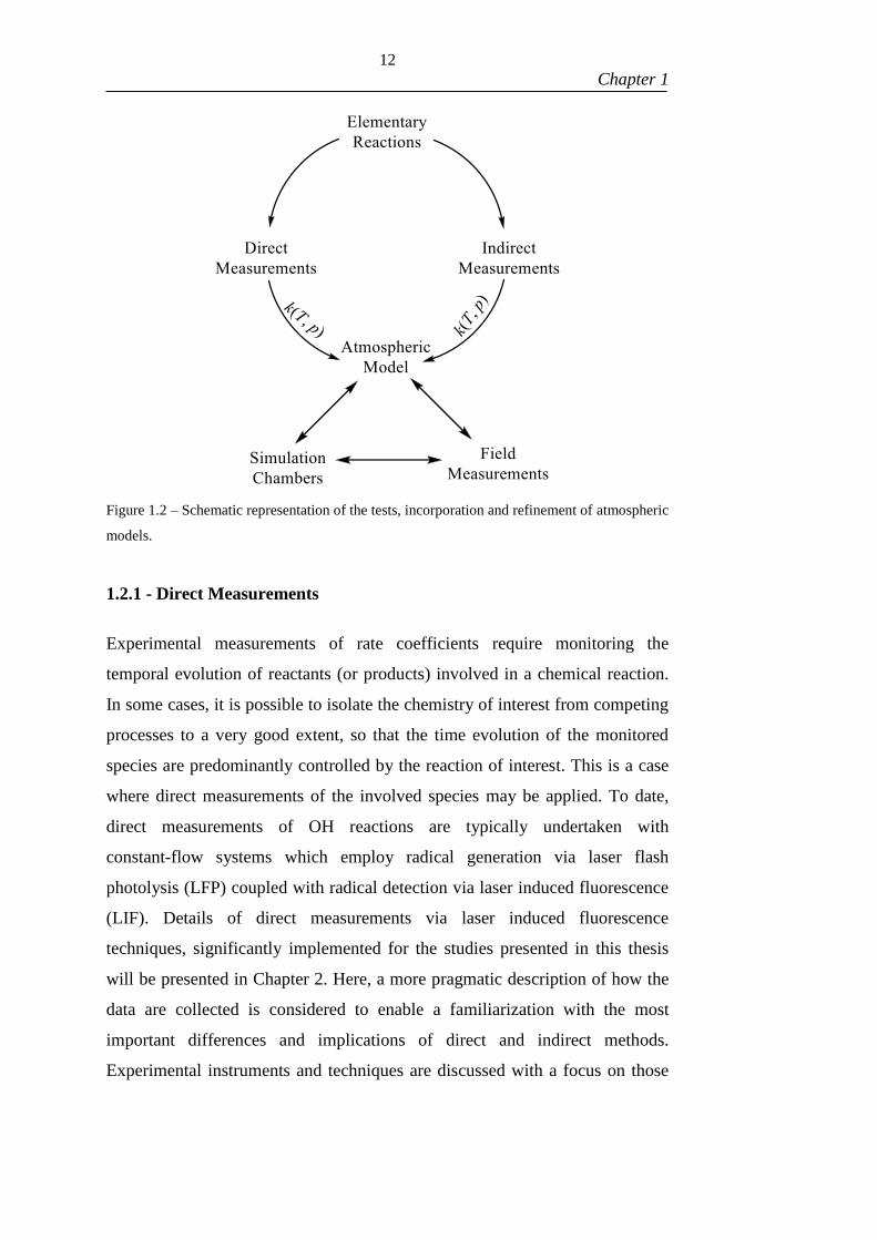
The investigation of the atmospheric system can be understood as a study of

relevant elementary reactions which compose the system, with particular

interest on the determination of reaction rate coefficients, their pressure and

temperature dependences. The study of these chemical processes for a large

number of environmentally important reactions enables the establishment of a

scientific knowledge which can be applied in both predictive and deterministic

manners. Figure 1.2 shows a schematic representation of how investigations of

elementary reactions are tested and incorporated to atmospheric models. The

scheme indicates that experimental determinations of rate coefficients can be

calculated via direct and indirect approaches; the most important aspects of

these variants will be discussed in the next two sections. These experimental

measurements can be incorporated into a complex atmospheric model, which

can in turn be used to predict, for example, the geographic extent and impacts

of the presence of a pollutant in the atmosphere. While atmospheric models are

typically employed to elucidate the results of field measurements and

atmospheric chambers simulations, the results of such experimental procedures

can also be used to feedback and refine the model current description. Section

1.2.2 is dedicated to the presentation of atmospheric simulation chambers, and

provides more detailed information about such tools.

12

Chapter 1

Figure 1.2 – Schematic representation of the tests, incorporation and refinement of atmospheric

models.

1.2.1 - Direct Measurements

Experimental measurements of rate coefficients require monitoring the

temporal evolution of reactants (or products) involved in a chemical reaction.

In some cases, it is possible to isolate the chemistry of interest from competing

processes to a very good extent, so that the time evolution of the monitored

species are predominantly controlled by the reaction of interest. This is a case

where direct measurements of the involved species may be applied. To date,

direct measurements of OH reactions are typically undertaken with

constant-flow systems which employ radical generation via laser flash

photolysis (LFP) coupled with radical detection via laser induced fluorescence

(LIF). Details of direct measurements via laser induced fluorescence

techniques, significantly implemented for the studies presented in this thesis

will be presented in Chapter 2. Here, a more pragmatic description of how the

data are collected is considered to enable a familiarization with the most

important differences and implications of direct and indirect methods.

Experimental instruments and techniques are discussed with a focus on those

13

Chapter 1

employed for the various studies undertaken in this thesis, presented in

Chapters 3-6.

As indicated previously, by isolating the chemistry of interest to a good extent,

the time-dependent evolution of the involved species will contain information

about the desired process. The experimental apparatus used for direct

measurements in this thesis typically consisted of a heatable metal tube in

which a constant flow of reagents is fed with a carrier gas with the aid of mass-

flow controllers. For the generation of OH radicals, the photolysis of a

precursor such as hydrogen peroxide is necessary and can be done with the use

of ~248 nm radiation. The generated OH radicals can be detected via, as

discussed previously, laser induced fluorescence techniques whose basis and

principles will be discussed in detail in Chapter 2. The necessary reactant

time-profile can be constructed by varying the time delay between the radical

generation and its detection, i.e., the time by which OH radicals are consumed

by the reaction of interest is the time available between their generation and

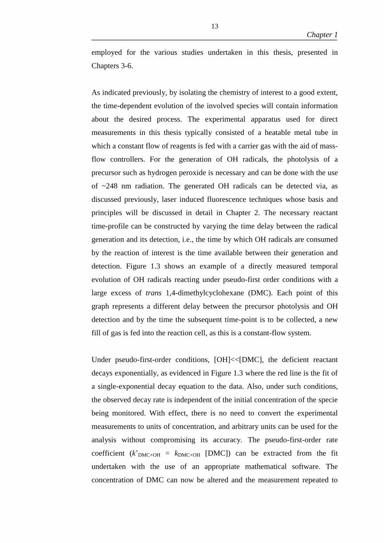
detection. Figure 1.3 shows an example of a directly measured temporal

evolution of OH radicals reacting under pseudo-first order conditions with a

large excess of trans 1,4-dimethylcyclohexane (DMC). Each point of this

graph represents a different delay between the precursor photolysis and OH

detection and by the time the subsequent time-point is to be collected, a new

fill of gas is fed into the reaction cell, as this is a constant-flow system.

Under pseudo-first-order conditions, [OH]<<[DMC], the deficient reactant

decays exponentially, as evidenced in Figure 1.3 where the red line is the fit of

a single-exponential decay equation to the data. Also, under such conditions,

the observed decay rate is independent of the initial concentration of the specie

being monitored. With effect, there is no need to convert the experimental

measurements to units of concentration, and arbitrary units can be used for the

analysis without compromising its accuracy. The pseudo-first-order rate

coefficient (k’DMC+OH = kDMC+OH [DMC]) can be extracted from the fit

undertaken with the use of an appropriate mathematical software. The

concentration of DMC can now be altered and the measurement repeated to

14

Chapter 1

yield another pseudo-first-order rate coefficient. Finally, the bimolecular rate

coefficient of the DMC + OH reaction can be obtained from the slope of a plot

of the pseudo-first-order rate coefficients versus the concentration of DMC

used for each trace, as demonstrated in Figure 1.4.

0 5 10 15 20

0

1

2

3

4

5

6

OH

Sig

nal

/ A

rbit

rary

Un

its

t / 10-3 s

k'DMC+OH

= 310 10 s-1

Figure 1.3 - Typical first order decay of OH in the presence of an excess of trans 1,4-

dimethylcyclohexane (DMC). The red line is a single-exponential fit to the data, which

provides a pseudo-first-order rate coefficient for the experimental conditions. T = 298 K and

p = 84 Torr, [DMC] = 1.6 × 1013

molecule cm-3

.

15

Chapter 1

0 2 4 6 8 10 12

0

200

400

600

800

1000

1200

1400

1600

k'D

MC

+O

H /

s-1

[DMC] / 1013

molecule cm-3

kDMC+OH = (1.16 0.08) 10-11

cm3 molecule

-1 s

-1

Figure 1.4 – Plot of the pseudo-first-order rate coefficients versus the concentration of the

excess reagent (trans 1,4 dimethylcyclohexane). T = 298 K, p = 84 Torr. Increased error bars

at high DMC concentrations probably caused by a slight shift of the probe wavelength during

the experiment.

As indicated by the small uncertainty derived for the bimolecular rate

coefficient (kDMC+OH = (1.16 ± 0.08) × 10-11

cm3 molecule

-1 s

-1), direct

measurements represent a very good option in terms of precision. With good

experimental control, the measurements also tend to have very good accuracies

given the fact that the chemistry of interest is observed directly. These aspects

make this approach an excellent alternative.

Very unstable species are monitored during the execution of the direct

approach, and potential interferences can arise from the presence of stable

contaminants, such as other hydrocarbons, which would compete for the OH

radicals available. In which case, the chemistry of interest would not be well

isolated; the OH time-dependent profiles would contain information about the

two competing processes and appropriately accounting for the contribution of

the contaminant to the decays is of primary importance.

Despite being very reliable and precise, direct measurements have their most

important limitation related to the timescale of the experiments. For example,

16

Chapter 1

the OH recycling from the oxidation of biogenic VOCs such as isoprene,

which is a hot topic in terms of atmospheric chemistry discussed in section 1.1,

is of the order of hundreds of seconds.8-9

Therefore, the millisecond window of

the direct experiments is not suitable for the study of this process under

atmospheric conditions. However, this recycling can be scaled to the

millisecond timeframe if high O2 concentrations are employed to promote the

peroxy formation, in combination with high temperatures to enhance the

hydrogen shifts of ~90 kJ mol-1

, required to regenerate OH according to

theoretical predictions.8 As the experimental apparatus used in this case are

typically consisted of simple stainless steel tubes, the instruments tend to be

small, facilitating a temperature control which can be accomplished with the

use of heating coils. For this thesis, temperatures as high as 790 K were

reached with a conventional laser flash photolysis-laser induced fluorescence

instrument, when studying the initial reaction of OH with isoprene, as

presented in Chapter 4.

As discussed in section 1.1 of the current chapter, at low temperatures the

reactions of OH with alkenes and dienes such as isoprene proceed via an

addition mechanism to a double bond to form an adduct (VOC-OH). At high

enough temperatures, however, a direct equilibration between the OH/VOC

and the OH-VOC adducts is observed, as the adducts begin to unimolecularly

fall apart back to reagents. As will be demonstrated in detail in Chapters 3, 4

and 5 for the OH + SO2, isoprene and ethylene reactions respectively, such

measurements impose significant constraints to the thermochemistry of the

reaction. If this is not the focus of the study however, it can become a

significant interference for the OH measurements. Taking the isoprene peroxy

study as an example, if the initial isoprene-OH adducts are too short lived, the

peroxy formation can be deficient for an investigation of the peroxy-involved

recycling. For this reason, even though direct measurements enable a good

flexibility in terms of achievable temperatures, the experiments need to be

well-planned to make sure the most efficient and useful set of experimental

data is generated.

17

Chapter 1

Executing experiments at non-atmospheric conditions means that an

appropriate extrapolation of the results to more atmospherically-relevant

conditions is a crucially important and challenging task. A global modelling

approach to the problem, in which all the experimental data are analysed as a

whole can help enhance the amount of information extracted from direct

measurements and improve the consistency of the analysis. For example, while

the temperature dependence of a chemical process can be invisible if only one

experimental measurement is to be compared, the analysis of a collection of

data representing a considerable range of temperatures can potentially be

capable of providing this information. Furthermore, if a consistent Arrhenius

formulation is defined for a rate coefficient in the model, in a global analysis,

this will have an effect in the modelling of all experimental data which will be

tested as its adequacy to adopt this formulation, enhancing therefore the

consistency of the obtained results. In Chapter 5, a new and robust global

technique to model pressure and temperature-dependent reactions based on

Master Equation calculations44

allows both an evaluation of the

thermochemistry of chemical reactions and a mechanistic assessment. The

technique will be subsequently applied in Chapter 6 to help elucidate the

chemistry of isoprene peroxys, whose data was generated with direct high

temperature (T > 400 K), high O2 (> 1 × 1017

molecule cm-3

) detection.

As introduced previously, direct measurements are typically undertaken with

constant-flow instruments, a fact which reduces potential issues related to

heterogeneous chemistry influencing the experiments. As will be discussed in

the next sections, this is a significant drawback for the use of atmospheric

simulation chambers, which makes their use for the study of long-lived

hydroperoxides in general a difficult task.

18

Chapter 1

1.2.2 – Details about Atmospheric Simulation Chambers

The atmosphere is a complex system directly influenced by countless physical

and chemical, natural and anthropogenic processes. Its composition depends

not only on physical-chemical processes but also on meteorological and

geographic factors, while many other parameters and their effects are still

unknown (photochemical sinks, the role of aerosols, etc). As a simple example,

the averaged concentration of chlorine atoms in the marine boundary layer of

the North Atlantic can increase from 3.3 × 104 Cl cm

-3 at dawn to 6.5 × 10

4 Cl

cm-3

at noontime45

while the concentrations above the Antarctic Ocean was

estimated around 720 Cl cm−3

.46

The atmospheric chemistry driven in these

locations is affected by temperature and pressure, which makes the

comprehension of field studies a challenging task. In this context, controlled

experiments are essential for aiding the elucidation of field measurements,

providing valuable insights in both kinetic and mechanistic research.

Simulation chambers represent suitable tools for this purpose.

Atmospheric simulation chambers can be made of several distinct materials.

Examples of commonly implemented materials include Teflon, as used in the

EUPHORE outdoor chamber47

in Valencia; steel, as used in the Highly

instrumented Reactor for Atmospheric Chemistry (HIRAC)48

housed in Leeds

and quartz/glass, as implemented in the UCPH reactor49

, located in

Copenhagen.

Large outdoor chambers (~200 m3) are commonly made of Teflon. In these

chambers, the experiments are performed under ambient conditions, and the

use of direct solar radiation to initiate the chemistry is implemented,

preventing issues inherent to artificial light sources. On the other hand, the

progress of the experiments can be interrupted due to meteorological aspects,

such as wind, clouds, storms, etc. Teflon is a relatively cheap material when

compared to steel and quartz, which represents an important advantage for its

use. Since the walls are malleable, the chamber can be built in nearly spherical

shape, reducing the surface to volume ratio. Although small Teflon chambers

can be encapsulated in a temperature-controlled box, the Teflon bag does not

19

Chapter 1

allow pressure control and heterogeneous chemistry on the surface can be an

issue. The HONO formation from reactions between NO2 and H2O on the

surface is an example of undesirable effect observed in this type of reactor.50-51

Metal chambers are the most versatile in terms of instrumentation. Because of

their rigid structure, amendments can be made in order to include new ports,

flanges and windows. Moreover, additional detection equipment can be fused

to its surface improving the detection capabilities. Due to the intrinsic

characteristics of metal chambers, pressure and temperature manipulation is

possible: the walls not only have relevant thermal conductivity, favouring heat

exchange, but they can support pressures as low as a fraction of a millibar. The

construction cost of metal chambers is definitely an issue, and for this reason

they tend to be small (3-2000 L) when compared to Teflon bags. It is likely

that reactions on the walls of metal chambers will occur at a considerable rate,

thereby, quantitative assessments of these removal processes are very

important for a proper understanding of the experimental results. Hydrogen

peroxide is known to significantly decompose on stainless steel surfaces,52

and

this effect is likely to occur for other hydroperoxides.

Custom chambers made of quartz and glass also have the versatility to cover a

range of temperatures with the aid of an external shelter for temperature

control. Their fragility and cost of construction are limiting, therefore, this type

of chamber also tends to be small (0.5-3000 L). Artificial radiation can be

emitted through the walls of the chamber, which allows the photolysis lamps to

be held outside the reaction cell, enabling a more homogeneous distribution of

light. Furthermore, it prevents significant temperature fluctuations inside the

reaction cell, an unwanted effect frequently observed in metal chambers,

caused by the natural warming of the lamps. The construction project of a

chamber presupposes a good knowledge of the experiments that will be

conducted with the same. A good choice of the base material is an essential

step for the development of a suitable methodology that fits the scientific

purposes.

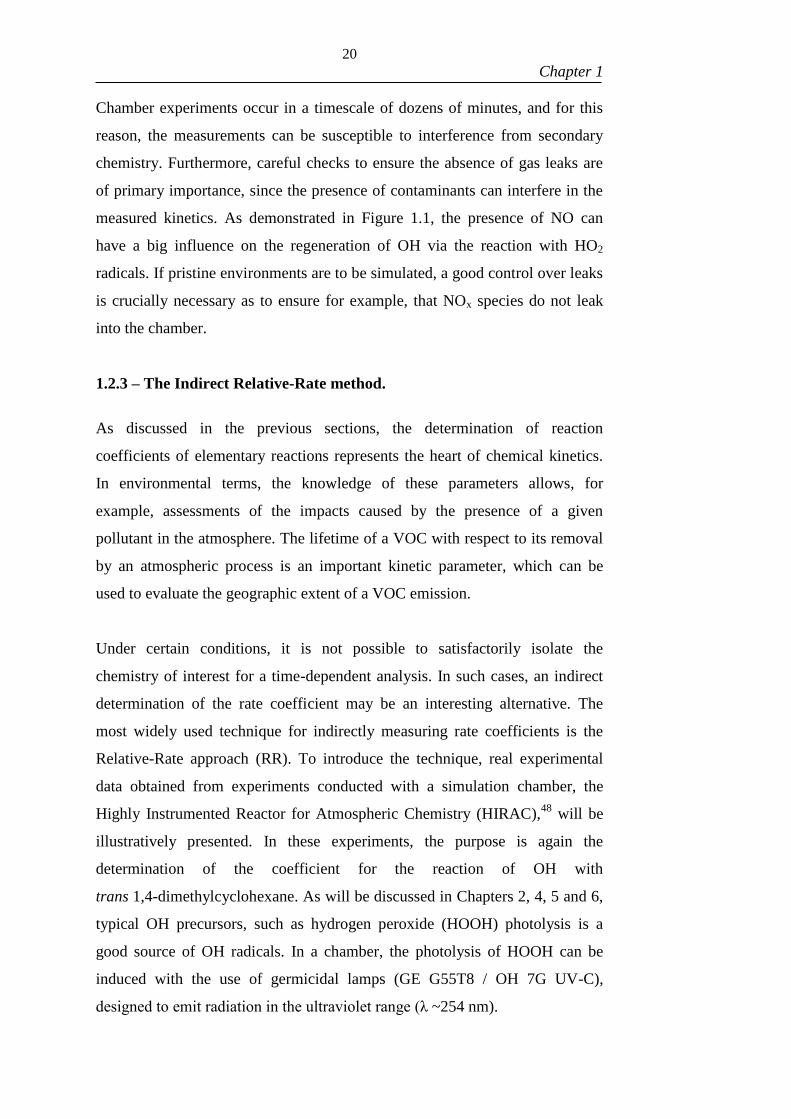
20

Chapter 1

Chamber experiments occur in a timescale of dozens of minutes, and for this

reason, the measurements can be susceptible to interference from secondary

chemistry. Furthermore, careful checks to ensure the absence of gas leaks are

of primary importance, since the presence of contaminants can interfere in the

measured kinetics. As demonstrated in Figure 1.1, the presence of NO can

have a big influence on the regeneration of OH via the reaction with HO2

radicals. If pristine environments are to be simulated, a good control over leaks

is crucially necessary as to ensure for example, that NOx species do not leak

into the chamber.

1.2.3 – The Indirect Relative-Rate method.

As discussed in the previous sections, the determination of reaction

coefficients of elementary reactions represents the heart of chemical kinetics.

In environmental terms, the knowledge of these parameters allows, for

example, assessments of the impacts caused by the presence of a given

pollutant in the atmosphere. The lifetime of a VOC with respect to its removal

by an atmospheric process is an important kinetic parameter, which can be

used to evaluate the geographic extent of a VOC emission.

Under certain conditions, it is not possible to satisfactorily isolate the

chemistry of interest for a time-dependent analysis. In such cases, an indirect

determination of the rate coefficient may be an interesting alternative. The

most widely used technique for indirectly measuring rate coefficients is the

Relative-Rate approach (RR). To introduce the technique, real experimental

data obtained from experiments conducted with a simulation chamber, the

Highly Instrumented Reactor for Atmospheric Chemistry (HIRAC),48

will be

illustratively presented. In these experiments, the purpose is again the

determination of the coefficient for the reaction of OH with

trans 1,4-dimethylcyclohexane. As will be discussed in Chapters 2, 4, 5 and 6,

typical OH precursors, such as hydrogen peroxide (HOOH) photolysis is a

good source of OH radicals. In a chamber, the photolysis of HOOH can be

induced with the use of germicidal lamps (GE G55T8 / OH 7G UV-C),

designed to emit radiation in the ultraviolet range (λ ~254 nm).

21

Chapter 1

The RR technique is based on the intercomparison of the temporal evolution of

the molecule of interest and a reference as they compete for a common reactant

when well-mixed in the chamber. In this case, the reference will compete with

the DMC for OH radicals, generated by HOOH photolysis at ~254 nm

(R8-R10).

HOOH + hv λ~254 nm → 2 OH

R8

DMC + OH k9 → products

R9

reference + OH kR → products

R10

Having reactions R9 and R10 rate coefficients k9 and kR respectively, the rate

laws for each component in the chamber are given by equations E2 and E3.

d[DMC]

dt= − k9[OH][DMC] E2

d[reference]

dt= − kR[OH][reference] E3

Dividing equation E2 by equationE3, followed by an algebraic rearrangement

gives:

d[DMC]

[DMC]=

k9

kR

×d[reference]

[reference]

E4

∫d[DMC]

[DMC]

[DMC]t

[DMC]0

= k9

kR

×∫d[reference]

[reference]

[reference]0

[reference]0

E5

ln([DMC]

t

[DMC]0

)= k9

kR

ln([reference]

t

[reference]0

) E6

Thus, a plot of ln([DMC]0/[DMC]t) versus ln([reference]0/[reference]t)

(e.g. Figure 1.5) provides a gradient that represents a ratio between the two rate

coefficients (see Equation E6). By employing a reference for which the rate

22

Chapter 1

coefficient for its reaction with OH radicals is known, the other one can be

easily calculated as the product of the ratio with the reference rate coefficient.

In this case, the reference chosen was cyclohexane (CHEX), and the rate

coefficient for its reaction with OH was taken from the literature

(kR = kOH+CHEX = (6.97 ± 1.4) × 10-12

cm3 molecule

-1 s

-1).

53 It is worth

highlighting that ratios of the concentrations of the species being monitored are

implemented in equation E6. Experimental measurements of the monitored

species can be undertaken with a range experimental techniques, which include

for example gas chromatography (GC), Fourier transform infrared

spectroscopy (FTIRS) and Proton-transfer reaction time of flight mass

spectrometry (PTR-MS). The measurements with one of such techniques will

yield signals which correspond to a concentration of the specie. Even though a

calibration procedure would be necessary in order to convert those signals into

concentration units, since these signals are proportional to the concentrations,

the ratio of the signals at different times is equal to the ratios of the

concentrations. For this reason, it is common practice to incorporate direct

measured signals, in any units associated with the implemented technique, into

equation E6, as demonstrated in equation E7. It is worth also highlighting the

fact the OH concentration does not need to be known during the RR

measurements, which represents an advantage since the aforementioned

experimental methods used to monitor species are well-stablished and

commercially available. In economic terms, these methods are advantageous

compared to laser-based methods.

ln(SDMC, t

SDMC, 0

)= k9

kR

ln(Sreference, t

Sreference, 0

) E7

In order to obtain accurate results, kR must be accurately known and the

reference should not be reactive to the specie of interest, in this case, DMC. In

contrast to the direct measurements, since this indirect technique relies on the

monitoring of stable species, other radicals that can be produced from the

subsequent reactions may interfere in the measurements. For example, given

the timescale of several minutes for these experiments, if a significant

concentration of HO2 radicals is built in the chamber from secondary reactions,

23

Chapter 1

these radicals can start competing with OH radicals for the VOCs.

Furthermore, if kHO2 + VOC × [HO2] becomes comparable to kOH+VOC × [OH], the

observed relative rates are now influenced by the relative ratio of

kHO2 + VOC / kHO2 + REF. For this reason, a good mechanistic knowledge of the

system is of primary importance. The amount of HOOH used can be increased

for example, providing a greater concentration of OH radicals in the chamber

and hopefully diminishing the importance of undesirable side reactions.

However, such procedures need to be done with care, as not to consume the

VOCs so quickly that not enough measurements can be taken before they are

completely removed. The use of multiple references can also help reinforce the

reliability of chamber measurements.

0.00 0.05 0.10 0.15 0.20 0.25

0.0

0.1

0.2

0.3

0.4

0.5

ln([

DM

C] 0

/ [

DM

C])

ln([REF]0 / [REF])

k9 / k

R = 2.02 0.02

Figure 1.5 – Relative rate plot for the reaction of trans 1,4-dimethylcyclohexane with OH

competing with the reaction of cyclohexane with OH.

As discussed previously, the ratio between the rate coefficients (k9/kR) is the

gradient of the corresponding kinetic plot. Using the previously mentioned

value of kR ((6.97 ± 1.4) × 10-12

cm3 molecule

-1 s

-1), k9 is calculated to be

(1.41 ± 0.28) × 10-11

cm3 molecule

-1 s

-1. This value agrees well with that

obtained with the direct measurements presented previously ((1.16 ± 0.08) ×

10-11

cm3 molecule

-1 s

-1), but includes a much greater uncertainty, due to the

24

Chapter 1

propagation of errors which incorporates the uncertainty of the reference rate

coefficient and the slope of the graph. In contrast, direct measurements do not

require such procedures.

Finally, using an estimate for the global OH concentration of 1×106

molecules∙cm-3

as recommended by Prinn et al.,54

a mean rate coefficient

based on both, the direct and indirect measurements

((1.28 ± 0.15)× 10-11

cm3 molecule

-1 s

-1), the lifetime of

trans 1,4 dimethylcyclohexane is estimated to be of approximately 2.2 hours.

In the context of the isoprene + OH reaction, which is the focus of two

chapters of the current thesis, the use of chambers as an experimental approach

for such investigations would be extremely difficult. The chemistry of isoprene

peroxy radicals involves the formation of long lived hydroperoxy species,

which are likely to undergo severe heterogeneous chemistry on wall surfaces.

Furthermore, the large number of products in this case can make their

discrimination and quantification via analytical techniques a very challenging

task. Control of leaks would be of primary importance, as very low NO

concentrations (< 100 ppt) would need to be employed in the experiments.

Considering the discussed advantages and drawbacks of both direct and

indirect measurements, the experimental measurements undertaken for the

production of the work presented in the current thesis have made use of the

direct approach. This approach is more adequate for an application of the

global technique developed in Chapter 4, since the chemistry of interest can be

isolated to a better extent when compared to the use of simulation chambers.

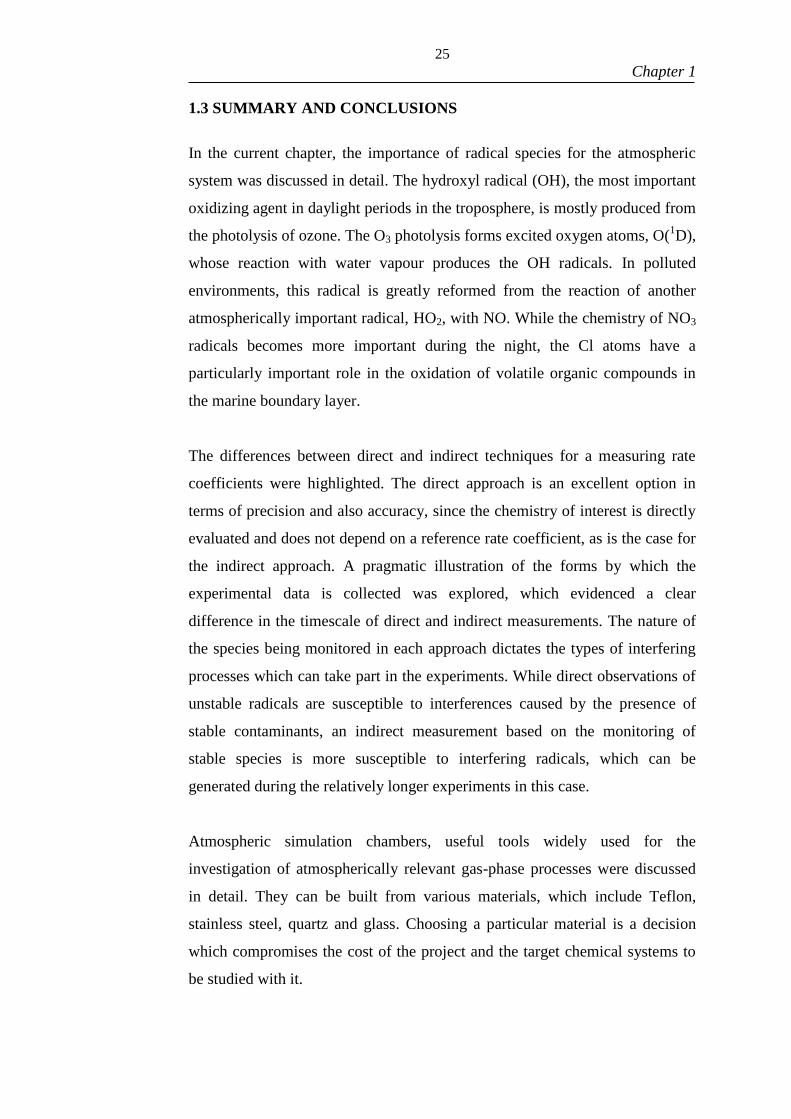
25

Chapter 1

1.3 SUMMARY AND CONCLUSIONS

In the current chapter, the importance of radical species for the atmospheric

system was discussed in detail. The hydroxyl radical (OH), the most important

oxidizing agent in daylight periods in the troposphere, is mostly produced from

the photolysis of ozone. The O3 photolysis forms excited oxygen atoms, O(1D),

whose reaction with water vapour produces the OH radicals. In polluted

environments, this radical is greatly reformed from the reaction of another

atmospherically important radical, HO2, with NO. While the chemistry of NO3

radicals becomes more important during the night, the Cl atoms have a

particularly important role in the oxidation of volatile organic compounds in

the marine boundary layer.

The differences between direct and indirect techniques for a measuring rate

coefficients were highlighted. The direct approach is an excellent option in

terms of precision and also accuracy, since the chemistry of interest is directly

evaluated and does not depend on a reference rate coefficient, as is the case for

the indirect approach. A pragmatic illustration of the forms by which the

experimental data is collected was explored, which evidenced a clear

difference in the timescale of direct and indirect measurements. The nature of

the species being monitored in each approach dictates the types of interfering

processes which can take part in the experiments. While direct observations of

unstable radicals are susceptible to interferences caused by the presence of

stable contaminants, an indirect measurement based on the monitoring of

stable species is more susceptible to interfering radicals, which can be

generated during the relatively longer experiments in this case.

Atmospheric simulation chambers, useful tools widely used for the

investigation of atmospherically relevant gas-phase processes were discussed

in detail. They can be built from various materials, which include Teflon,

stainless steel, quartz and glass. Choosing a particular material is a decision

which compromises the cost of the project and the target chemical systems to

be studied with it.

26

Chapter 1

This chapter also demonstrated the importance of accurate measurements of

bimolecular rate coefficients and atmospheric estimates of important radicals

such as OH, NO3 and Cl for assessing extension of the impact of a pollutant in

the atmosphere. An example of a lifetime calculation based on rate coefficients

measured by the means of the relative-rate method was demonstrated.

The next chapter presents the experimental and theoretical techniques by

which three atmospherically important OH reactions were studied in the

current thesis (OH + SO2, isoprene (C5H8) and ethylene (C2H4)). The

experimental part of Chapter 2 deals with pulsed laser photolysis instruments,

their principles and applications. From this sense, the contents of Chapter 2 are

not only a presentation of the techniques by which new experimental data was

collected and treated, but represents a continuation of the atmospheric

methods, partially introduced in Chapter 1. A good understanding of both

chamber techniques and pulsed laser photolysis methods will greatly clarify

the reasons behind the particular choice of the laser-based procedure.

27

Chapter 1

1.4 REFERENCES

1. Finlayson-Pitts, B. J.; Pitts, J. N., Chemistry of the Upper and Lower Atmosphere :

Theory, Experiments, and Applications. Academic Press: San Diego, California, USA.

London, UK., 2000.

2. Lelieveld, J.; Gromov, S.; Pozzer, A.; Taraborrelli, D. Global Tropospheric Hydroxyl

Distribution, Budget and Reactivity. Atmospheric Chemistry and Physics 2016, 16, 12477-

12493.

3. Sommariva, R. et al. OH and HO2 Chemistry in Clean Marine Air During SOAPEX-

2. Atmospheric Chemistry and Physics 2004, 4, 839-856.

4. Alicke, B. et al. OH Formation by HONO Photolysis During the Berlioz Experiment.

Journal of Geophysical Research 2003, 108, 8247.

5. Lee, J. D. et al. Detailed Budget Analysis of HONO in Central London Reveals a

Missing Daytime Source. Atmospheric Chemistry and Physics 2016, 16, 2747-2764.

6. Ramazan, K. A.; Syomin, D.; Finlayson-Pitts, B. J. The Photochemical Production of

HONO During the Heterogeneous Hydrolysis of NO2. Physical Chemistry Chemical Physics

2004, 6, 3836-3843.

7. Stone, D.; Au, K.; Sime, S.; Medeiros, D. J.; Blitz, M.; Seakins, P. W.; Decker, Z.;

Sheps, L. Unimolecular Decomposition Kinetics of the Stabilised Criegee Intermediates

CH2OO and CD2OO. Physical Chemistry Chemical Physics 2018, 20, 24940-24954.

8. Peeters, J.; Muller, J. F.; Stavrakou, T.; Nguyen, V. S. Hydroxyl Radical Recycling in

Isoprene Oxidation Driven by Hydrogen Bonding and Hydrogen Tunneling: The Upgraded

LIM1 Mechanism. Journal of Physical Chemistry A 2014, 118, 8625-8643.

9. Crounse, J. D.; Paulot, F.; Kjaergaard, H. G.; Wennberg, P. O. Peroxy Radical

Isomerization in the Oxidation of Isoprene. Physical Chemistry Chemical Physics 2011, 13,

13607-13613.

10. Fuchs, H. et al. Experimental Evidence for Efficient Hydroxyl Radical Regeneration

in Isoprene Oxidation. Nature Geoscience 2013, 6, 1023.

11. Arey, J.; Aschmann, S. M.; Kwok, E. S. C.; Atkinson, R. Alkyl Nitrate, Hydroxyalkyl

Nitrate, and Hydroxycarbonyl Formation from the NOx−Air Photooxidations of C5−C8 n-

Alkanes. The Journal of Physical Chemistry A 2001, 105, 1020-1027.

12. Lohr, L. L.; Barker, J. R.; Shroll, R. M. Modeling the Organic Nitrate Yields in the

Reaction of Alkyl Peroxy Radicals with Nitric Oxide. 1. Electronic Structure Calculations and

Thermochemistry. The Journal of Physical Chemistry A 2003, 107, 7429-7433.

13. Whalley, L. K. et al. Understanding in Situ Ozone Production in the Summertime

through Radical Observations and Modelling Studies During the Clean Air for London Project

(Clearflo). Atmospheric Chemistry and Physics 2018, 18, 2547-2571.

14. Stone, D. et al. Isoprene Oxidation Mechanisms: Measurements and Modelling of OH

and HO2 over a South-East Asian Tropical Rainforest During the OP3 Field Campaign.

Atmospheric Chemistry and Physics 2011, 11, 6749-6771.

15. Paulot, F.; Crounse, J. D.; Kjaergaard, H. G.; Kürten, A.; St. Clair, J. M.; Seinfeld, J.

H.; Wennberg, P. O. Unexpected Epoxide Formation in the Gas-Phase Photooxidation of

Isoprene. Science 2009, 325, 730-733.

16. Hansen, R. F.; Lewis, T. R.; Graham, L.; Whalley, L. K.; Seakins, P. W.; Heard, D.

E.; Blitz, M. A. OH Production from the Photolysis of Isoprene-Derived Peroxy Radicals:

Cross-Sections, Quantum Yields and Atmospheric Implications. Physical Chemistry Chemical

Physics 2017, 19, 2332-2345.

17. Martinez, M. et al. Hydroxyl Radicals in the Tropical Troposphere over the Suriname

Rainforest: Airborne Measurements. Atmospheric Chemistry and Physics 2010, 10, 3759-

3773.

28

Chapter 1

18. Whalley, L. K. et al. Quantifying the Magnitude of a Missing Hydroxyl Radical

Source in a Tropical Rainforest. Atmospheric Chemistry and Physics 2011, 11, 7223-7233.

19. Lelieveld, J. et al. Atmospheric Oxidation Capacity Sustained by a Tropical Forest.

Nature 2008, 452, 737-740.

20. Carslaw, N. et al. OH and HO2 Radical Chemistry in a Forested Region of North-

Western Greece. Atmospheric Environment 2001, 35, 4725-4737.

21. Goldstein, A. H.; Galbally, I. E. Known and Unexplored Organic Constituents in the

Earth's Atmosphere. Environmental Science & Technology 2007, 41, 1514-1521.

22. Orlando, J. J.; Tyndall, G. S.; Wallington, T. J. The Atmospheric Chemistry of

Alkoxy Radicals. Chemical Reviews 2003, 103, 4657-4690.

23. Singh, H. B. Atmospheric Halocarbons: Evidence in Favor of Reduced Average

Hydroxyl Radical Concentration in the Troposphere. Geophysical Research Letters 1977, 4,

101-104.

24. Singh, H. B. Preliminary Estimation of Average Tropospheric HO Concentrations in

the Northern and Southern Hemispheres. Geophysical Research Letters 1977, 4, 453-456.

25. Hewitt, C. N.; Harrison, R. M. Tropospheric Concentrations of the Hydroxyl Radical -

a Review. Atmospheric Environment 1985, 19, 545.

26. Lawrence, M. G.; Jöckel, P.; von Kuhlmann, R. What Does the Global Mean OH

Concentration Tell Us? Atmospheric Chemistry and Physics 2001, 1, 37-49.

27. Russell, A. G.; Cass, G. R.; Seinfeld, J. H. On Some Aspects of Nighttime

Atmospheric Chemistry. Environmental Science & Technology 1986, 20, 1167-1172.

28. Brown, S. S.; Stutz, J. Nighttime Radical Observations and Chemistry. Chemical

Society Reviews 2012, 41, 6405-6447.

29. Finlayson-Pitts, B. J. Chlorine Atoms as a Potential Tropospheric Oxidant in the

Marine Boundary Layer. . Research on Chemical Intermediates 1993, 19.

30. Young, C. J. et al. Chlorine as a Primary Radical: Evaluation of Methods to

Understand Its Role in Initiation of Oxidative Cycles. Atmospheric Chemistry and Physics

2014, 14, 3427-3440.

31. Riedel, T. P. et al. Nitryl Chloride and Molecular Chlorine in the Coastal Marine

Boundary Layer. Environmental Science & Technology 2012, 46, 10463-10470.

32. Pilling, M. J.; Seakins, P. W., Reaction Kinetics. Oxford University Press: Oxford,

1995.

33. Bräuer, P. et al. Development of a Protocol for the Auto-Generation of Explicit

Aqueous-Phase Oxidation Schemes of Organic Compounds. Atmospheric Chemistry and

Physics Discussions 2019, 2019, 1-52.

34. Di Biagio, C. et al. Complex Refractive Indices and Single Scattering Albedo of

Global Dust Aerosols in the Shortwave Spectrum and Relationship to Iron Content and Size.

Atmospheric Chemistry and Physics Discussions 2019, 2019, 1-42.

35. Jiang, X.; Tsona, N. T.; Jia, L.; Liu, S.; Zhang, H.; Xu, Y.; Du, L. Secondary Organic

Aerosol Formation from Photooxidation of Furan: Effects of NOx and Humidity. Atmospheric

Chemistry and Physics Discussions 2019, 2019, 1-26.

36. Kaltsonoudis, C.; Jorga, S. D.; Louvaris, E.; Florou, K.; Pandis, S. N. A Portable Dual

Smog Chamber System for Atmospheric Aerosol Field Studies. Atmos. Meas. Tech. Discuss.

2018, 2018, 1-25.

37. Kari, E. et al. Dual Effect of Anthropogenic Emissions on the Formation of Biogenic

Soa. Atmos. Chem. Phys. Discuss. 2019, 2019, 1-35.

38. Massabò, D. et al. ChAMBRe: A New Atmospheric Simulation Chamber for Aerosol

Modelling and Bio-Aerosol Research. Atmos. Meas. Tech. 2018, 11, 5885-5900.

29

Chapter 1

39. Theodoritsi, G. N.; Pandis, S. N. Simulation of the Chemical Evolution of Biomass

Burning Organic Aerosol. Atmos. Chem. Phys. Discuss. 2018, 2018, 1-30.

40. Stone, D.; Blitz, M.; Ingham, T.; Onel, L.; Medeiros, D. J.; Seakins, P. W. An

Instrument to Measure Fast Gas Phase Radical Kinetics at High Temperatures and Pressures.

Review of Scientiifc Instruments 2016, 87, 054102.

41. Medeiros, D. J.; Blitz, M. A.; James, L.; Speak, T. H.; Seakins, P. W. Kinetics of the

Reaction of OH with Isoprene over a Wide Range of Temperature and Pressure Including

Direct Observation of Equilibrium with the OH Adducts. The Journal of Physical Chemistry A

2018, 122, 7239-7255.

42. Vakhtin, A. B.; Murphy, J. E.; Leone, S. R. Low-Temperature Kinetics of Reactions

of OH Radical with Ethene, Propene, and 1-Butene. The Journal of Physical Chemistry A

2003, 107, 10055-10062.

43. Tully, F. P. Laser Photolysis/Laser-Induced Fluorescence Study of the Reaction of

Hydroxyl Radical with Ethylene. Chemical Physics Letters 1983, 96, 148-153.

44. Glowacki, D. R.; Liang, C. H.; Morley, C.; Pilling, M. J.; Robertson, S. H. MESMER:

An Open-Source Master Equation Solver for Multi-Energy Well Reactions. Journal of

Physical Chemistry A 2012, 116, 9545-9560.

45. Wingenter, O. W.; Kubo, M. K.; Blake, N. J.; Smith, T. W.; Blake, D. R.; Rowland,

F. S. Hydrocarbon and Halocarbon Measurements as Photochemical and Dynamical Indicators

of Atmospheric Hydroxyl, Atomic Chlorine, and Vertical Mixing Obtained During Lagrangian

Flights. Journal of Geophysical Research-Atmospheres 1996, 101, 4331-4340.

46. Wingenter, O. W.; Blake, D. R.; Blake, N. J.; Sive, B. C.; Rowland, F. S.; Atlas, E.;

Flocke, F. Tropospheric Hydroxyl and Atomic Chlorine Concentrations, and Mixing

Timescales Determined from Hydrocarbon and Halocarbon Measurements Made over the

Southern Ocean. Journal of Geophysical Research-Atmospheres 1999, 104, 21819-21828.

47. Brockmann, K. J.; Kriesche, V.; Etzkorn, T.; Volkamer, R.; Wirtz, K. The European

Photoreactor Euphore: A Technical Description. Proceedings of Eurotrac Symposium '96 -

Transport and Transformation of Pollutants in the Troposphere, Vol 2 1997, 457-461.

48. Glowacki, D. R. et al. Design of and Initial Results from a Highly Instrumented

Reactor for Atmospheric Chemistry (HIRAC). Atmospheric Chemistry and Physics 2007, 7,

5371-5390.

49. Nilsson, E. J. K.; Eskebjerg, C.; Johnson, M. S. A Photochemical Reactor for Studies

of Atmospheric Chemistry. Atmospheric Environment 2009, 43, 3029-3033.

50. Medeiros, D. J.; Pimentel, A. S. New Insights in the Atmospheric HONO Formation:

New Pathways for N2o4 Isomerization and NO2 Dimerization in the Presence of Water.

Journal of Physical Chemistry A 2011, 115, 6357-6365.

51. Schlosser, E. et al. Technical Note: Formal Blind Intercomparison of OH

Measurements: Results from the International Campaign Hoxcomp. Atmospheric Chemistry

and Physics 2009, 9, 7923-7948.

52. Lin, C. C.; Smith, F. R.; Ichikawa, N.; Baba, T.; Itow, M. Decomposition of

Hydrogen Peroxide in Aqueous Solutions at Elevated Temperatures. International Journal of

Chemical Kinetics 1991, 23, 971-987.

53. Atkinson, R. Kinetics of the Gas-Phase Reactions of OH Radicals with Alkanes and

Cycloalkanes. Atmospheric Chemistry and Physics 2003, 3, 2233-2307.

54. Prinn, R. G.; Weiss, R. F.; Miller, B. R.; Haung, J.; Alyea, F. N.; Cunnold, D. M.;

Fraser, P. J.; Hartley, D. E.; Simmonds, P. G. Atmospheric Trends and Lifetime of Ch3ccl3 and

Global OH Concentrations. Science 1995, 269, 187-192.

31

Chapter 2

Chapter 2. Experimental Instruments

and Theoretical Methods

33

Chapter 2


The relevant experimental and theoretical methods used to investigate

atmospherically significant reactions throughout the thesis are presented in this

chapter. Methods are split into two distinct groups: section 2.1 presents the

experimental techniques used to collect kinetic data for a number of

atmospherically important reactions; section 2.2 presents the principles of

theoretical methods by which the experimental data were analysed. This

chapter will serve as basic introduction, covering the most important methods,

the subsequent chapters will also include concise experimental sections, with

additional, particular and important experimental or theoretical information.

35

Chapter 2

2.1 EXPERIMENTAL METHODOLOGY

As discussed in Chapter 1, direct radical measurements represent a useful and

reliable approach for the study of elementary reactions. In the current work,

direct measurements of hydroxyl radicals were undertaken in order to study

various atmospherically important processes, such as the reactions of OH with

SO2 (Chapter 3), isoprene (C5H8, Chapters 4 and 6) and ethylene (C2H4,

Chapter 5). While the experimental data were predominantly collected with the

use of the conventional low pressure (p < 200 Torr) Laser Flash Photolysis-

Laser Induced Fluorescence (LFP-LIF) technique, a recently developed high-

temperature (TMAX ~750 K), high pressure (pMAX ~5 atm) instrument was

employed in many occasions to expand the experimental horizon. The OH

detection in the high pressure instrument is based on a particular laser induced

procedure, namely the Fluorescence Assay by Gas Expansion (FAGE).1 To

enable a good understanding of experimental measurements, sections 2.1.1 and

2.1.2 will present the FAGE technique and the basis of laser-induced

fluorescence methods. Once the principles are properly introduced, section

2.1.3 presents the LFP-LIF technique in the context of both the low and high

pressure instruments.

2.1.1 - Fluorescence Assay by Gas Expansion – FAGE

Fluorescence Assay by Gas Expansion (FAGE) 1 is a widely implemented

technique for the detection of radical species. FAGE is a laser-induced

fluorescence method (LIF), particularly important for the detection of

atmospherically relevant radical species such as OH and HO2. With a detection

limit for the monitoring of OH in the 106-10

7 molecule cm

-3 range,

2 the

technique is suitable for field measurements since, as discussed in Chapter 1,

the low OH concentrations in pristine environments are often in this range and

higher concentrations are generated in polluted atmospheres. The technique is

currently being adapted for CH3O/CH3O2 detection, and the recent results

obtained from laboratory tests by Onel et al. are promising.3 FAGE is based on

specific rovibrational transitions, induced by excitation pulses and the return of

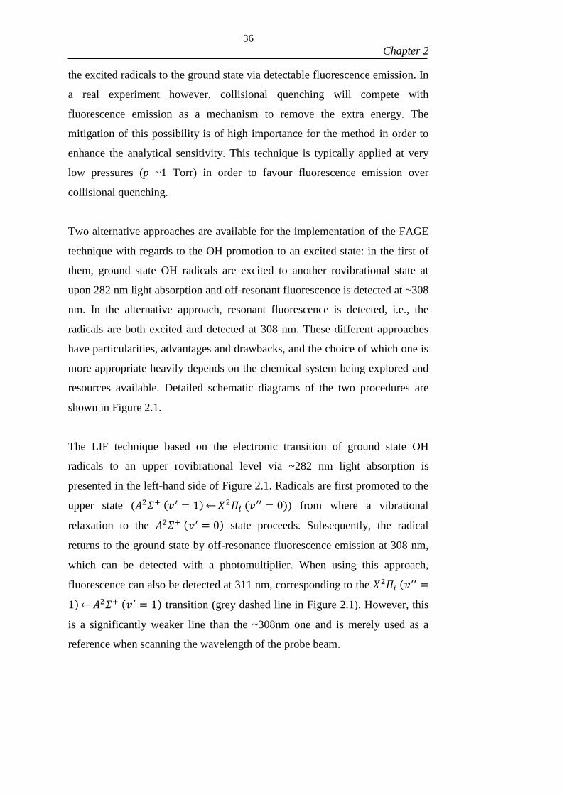
36

Chapter 2

the excited radicals to the ground state via detectable fluorescence emission. In

a real experiment however, collisional quenching will compete with

fluorescence emission as a mechanism to remove the extra energy. The

mitigation of this possibility is of high importance for the method in order to

enhance the analytical sensitivity. This technique is typically applied at very

low pressures (p ~1 Torr) in order to favour fluorescence emission over

collisional quenching.

Two alternative approaches are available for the implementation of the FAGE

technique with regards to the OH promotion to an excited state: in the first of

them, ground state OH radicals are excited to another rovibrational state at

upon 282 nm light absorption and off-resonant fluorescence is detected at ~308

nm. In the alternative approach, resonant fluorescence is detected, i.e., the

radicals are both excited and detected at 308 nm. These different approaches

have particularities, advantages and drawbacks, and the choice of which one is

more appropriate heavily depends on the chemical system being explored and

resources available. Detailed schematic diagrams of the two procedures are

shown in Figure 2.1.

The LIF technique based on the electronic transition of ground state OH

radicals to an upper rovibrational level via ~282 nm light absorption is

presented in the left-hand side of Figure 2.1. Radicals are first promoted to the

upper state (𝐴2𝛴+ (𝑣′ = 1) ⃪ 𝑋2𝛱𝑖 (𝑣′′ = 0)) from where a vibrational

relaxation to the 𝐴2𝛴+ (𝑣′ = 0) state proceeds. Subsequently, the radical

returns to the ground state by off-resonance fluorescence emission at 308 nm,

which can be detected with a photomultiplier. When using this approach,

fluorescence can also be detected at 311 nm, corresponding to the 𝑋2𝛱𝑖 (𝑣′′ =

1) ⃪ 𝐴2𝛴+ (𝑣′ = 1) transition (grey dashed line in Figure 2.1). However, this

is a significantly weaker line than the ~308nm one and is merely used as a

reference when scanning the wavelength of the probe beam.

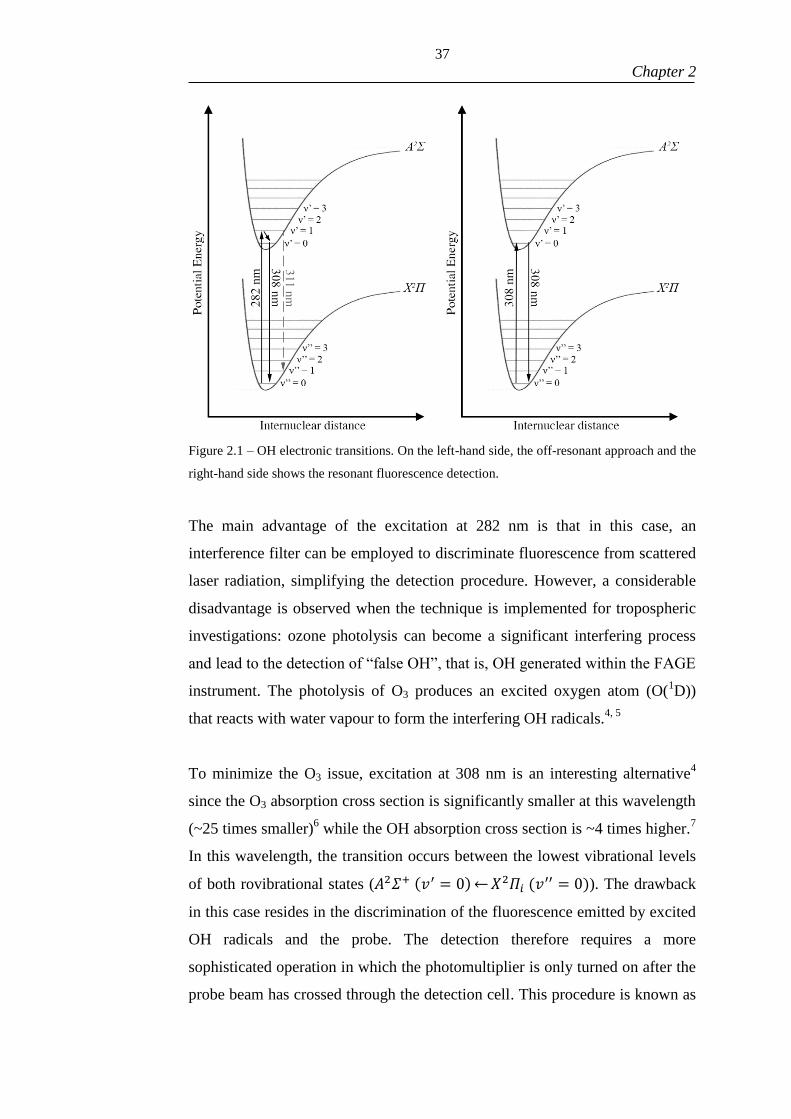
37

Chapter 2

Figure 2.1 – OH electronic transitions. On the left-hand side, the off-resonant approach and the

right-hand side shows the resonant fluorescence detection.

The main advantage of the excitation at 282 nm is that in this case, an

interference filter can be employed to discriminate fluorescence from scattered

laser radiation, simplifying the detection procedure. However, a considerable

disadvantage is observed when the technique is implemented for tropospheric

investigations: ozone photolysis can become a significant interfering process

and lead to the detection of “false OH”, that is, OH generated within the FAGE

instrument. The photolysis of O3 produces an excited oxygen atom (O(1D))

that reacts with water vapour to form the interfering OH radicals.4, 5

To minimize the O3 issue, excitation at 308 nm is an interesting alternative4

since the O3 absorption cross section is significantly smaller at this wavelength

(~25 times smaller)6 while the OH absorption cross section is ~4 times higher.

7

In this wavelength, the transition occurs between the lowest vibrational levels

of both rovibrational states (𝐴2𝛴+ (𝑣′ = 0) ⃪ 𝑋2𝛱𝑖 (𝑣′′ = 0)). The drawback

in this case resides in the discrimination of the fluorescence emitted by excited

OH radicals and the probe. The detection therefore requires a more

sophisticated operation in which the photomultiplier is only turned on after the

probe beam has crossed through the detection cell. This procedure is known as

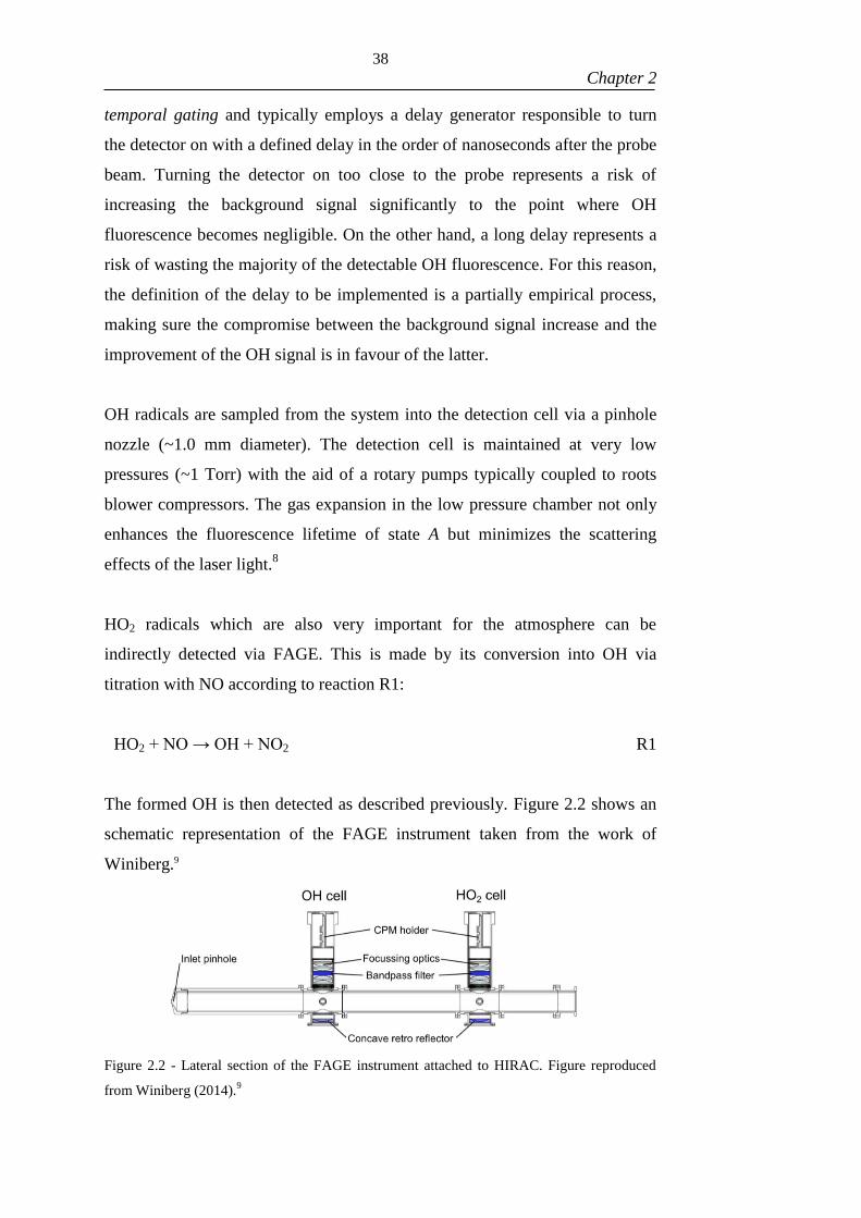
38

Chapter 2

temporal gating and typically employs a delay generator responsible to turn

the detector on with a defined delay in the order of nanoseconds after the probe

beam. Turning the detector on too close to the probe represents a risk of

increasing the background signal significantly to the point where OH

fluorescence becomes negligible. On the other hand, a long delay represents a

risk of wasting the majority of the detectable OH fluorescence. For this reason,

the definition of the delay to be implemented is a partially empirical process,

making sure the compromise between the background signal increase and the

improvement of the OH signal is in favour of the latter.

OH radicals are sampled from the system into the detection cell via a pinhole

nozzle (~1.0 mm diameter). The detection cell is maintained at very low

pressures (~1 Torr) with the aid of a rotary pumps typically coupled to roots

blower compressors. The gas expansion in the low pressure chamber not only

enhances the fluorescence lifetime of state A but minimizes the scattering

effects of the laser light.8

HO2 radicals which are also very important for the atmosphere can be

indirectly detected via FAGE. This is made by its conversion into OH via

titration with NO according to reaction R1:


The formed OH is then detected as described previously. Figure 2.2 shows an

schematic representation of the FAGE instrument taken from the work of

Winiberg.9

Figure 2.2 - Lateral section of the FAGE instrument attached to HIRAC. Figure reproduced

from Winiberg (2014).9

39

Chapter 2

2.1.2 - FAGE Calibration

As discussed in Chapter 1, there are situations where the concentration of OH

radicals do not need to be determined. For example, under pseudo-first order

conditions in which OH is consumed exponentially in time, the concentration

of OH radicals do not need to be known for a kinetic evaluation, as

demonstrated in Chapter 1. For this reason, in such cases, the LIF signal does

not need to be converted into units of concentrations, and arbitrary units of OH

can be employed, implying a good level of simplicity to the collection of

useful data and its posterior analysis.

In other cases however, the concentrations of OH radicals may need to be

known. This is the case, for example, when second order kinetics are being

investigated or when the concentration of the radicals are the main subject of

study. The technique is typically used in field and chamber investigations10-13

with the objective of determining the temporal concentration of OH in the days

of study, far from the simplicity of the pseudo-first order conditions. In such

cases, the FAGE technique requires instrumental calibration. For this reason, a

good understanding of the calibration of the technique is desirable for a better

understanding of the accuracy of atmospheric OH measurements.

The standard calibration method for OH and HO2 detection using vacuum

ultra-violet (VUV) photolysis of water vapour is presented in the following.14-

17 The method consists in the construction of a calibration curve that relates the

FAGE signal normalized to the laser power (SOH / counts s-1

mW-1

) to known

OH radical concentrations produced from water vapour photolysis. Equation

E1 presents this relation considering the OH radical.

SOH = COH[OH] E1

Here, COH is the sensitivity or calibration factor, with units of counts cm3

molecule-1

s-1

mW-1

. This factor is affected by several parameters related to the

employed equipment and experimental conditions. An extensive discussion of

these parameters is presented by Faloona et al. 11

and Creasey et al.18, 19

40

Chapter 2

The water-vapour photolysis generates an OH radical and a hydrogen atom that

subsequently reacts with molecular oxygen to yield one molecule of the HO2

radical. The reactions are:

H2O + hv(184.9 nm) → OH + H∙ R2

H∙ + O2 → HO2 R3

As observed, the water vapour photolysis produces equal amounts of OH and

HO2. Being the water vapour concentration known via the use of calibrated

mass flow controllers, the amount of radicals produced can be obtained from

the following expression:

[OH] = [HO2] = [H2O]vap σH2O 184.9 nm ΦOH F184.9 nm Δt E2

Here, [H2O]vap is the water vapour concentration, σH2O is the absorption cross

section of water at 184.9 nm, ΦOH is the quantum yield for the

photodecomposition of the radical (ΦOH=1), F184.9 nm is the photon flux of

184.9 nm light and Δt is the exposure time of the air to the radiation.

Two distinct methodologies are available in the literature for the measurement

of the F184.9 nm Δt product. The first one, described by Stevens et al.8, uses a

calibrated phototube for the measurement of F184.9nm while Δt is estimated from

the volumetric flow rate and the structural geometry of the flow tube. The

second method uses a chemical actinometer to produce O3 or NO directly from

O2 and N2O photolysis at 184.9 nm respectively. Then, these products are

directly measured with value using commercial gas analysers. Winiberg et al.

present a complete description of the FAGE instrumentation attached to

HIRAC.9

41

Chapter 2

2.1.3 - Laser Flash Photolysis Experiments with Detection by Laser

Induced Fluorescence (LFP-LIF)

Chemical processes involving free radicals are extremely important for

combustion processes20, 21

and planetary atmospheres.22, 23

In kinetic

investigations, laser flash photolysis is a widely used technique for the

generation of radicals, whose consumption can be monitored to allow the

determination of reaction coefficients. The combination of this method with

the real-time monitoring of radical concentrations by laser induced

fluorescence (LIF) spectroscopy has been successfully implemented for the

determination of kinetic parameters of several atmospherically relevant

reactions and development of new radical detection methods.24-27

The LIF

monitoring procedure is very selective, allowing for example the

discrimination between isotope hydroxyl radicals (16

OH and 18

OH) and its

detection limit reaches values below 106 molecule cm

-3.15

Despite high levels

of selectivity and sensitivity, LIF spectroscopy is generally performed at low

pressures (<400 Torr) due to the high collisional quenching of excited states of

radicals at high pressures (particularly by O2). However, in some cases,

experimental measurements at elevated pressures are desirable. At elevated

temperatures, the high-pressure limit of barrierless reactions can be quite

elevated as will be demonstrated in Chapter 4 for the study of the isoprene +

OH reaction.

The majority of the kinetic studies presented in Chapters 4 and 5 for the

reactions of OH with isoprene and ethylene respectively, were performed with

the use of conventional low-pressure (p~100 Torr) laser flash photolysis and

detection of OH radicals by laser-induced fluorescence (LFP-LIF).28, 29

Additionally, high pressure measurements (p > 760 Torr) were undertaken

using a recently developed instrument, capable of operating at pressures up to

5 atm and temperatures as high as 750 K. Given the high degree of similarity

between a conventional LPF-LIF instrument and the high pressure one being

discussed, the latter is presented in detail while its major differences are

highlighted in the text. Figure 2.3 presents a schematic representation of this

apparatus and Figure 2.4 shows a photograph thereof.

42

Chapter 2

Figure 2.3 - Schematic representation of the high pressure instrument. Upper scheme shows

the full apparatus and the lower evidences the interface between the high pressure and

detection cells. Figure reproduced from Stone et al.30

The 6-way cross stainless steel (304L grade) reactor has a high pressure zone,

where the reaction occurs, and a low pressure detection cell, where OH

radicals are probed. A glass liner of approximately 20 cm long is placed in the

reaction cell, in order to reduce the exposure of the chemicals to the metal

surface. The high pressure section is 1 m long and 19 mm in internal diameter.

OH radicals are generated by pulsed excimer laser photolysis of H2O2 (R4) at

248 nm using a Lambda Physik, Compex 200 laser operating on KrF.

H2O2 + hv(248 nm) → 2 OH R4

Even though the majority of the experiments employed H2O2 as the precursor

of OH radicals, in the study of isoprene presented in Chapter 4, tert-butyl

hydroperoxide ((CH3)3COOH) photolysis (R5) was implemented in a limited

number of experiments to ensure the observable kinetics were independent of

the precursor used.

43

Chapter 2

(CH3)3COOH + hv(248 nm) → OH + (CH3)3CO R5

The excimer laser produces a beam with dimensions 24 mm length × 12 mm

width which is expanded to occupy the entire volume of the reaction cell and

to generate a roughly uniform distribution of radicals in the high pressure zone.

The pulses are generated with adjustable frequency (usually between 1 and 10

Hz) and the laser fluence is approximately 15 mJ cm-2

, or ~1.87 × 1016

photons

cm-2

. All experiments presented in the current thesis were performed under low

concentrations of OH precursors (typically 1 × 1015

molecule cm-3

) so that

undesirable effects such as mitigation of the excimer radiation and side

reactions are avoided. Considering a ~1 × 10-19

cm2 molecule

-1 absorption

cross section for H2O2 at 248 nm (based on IUPAC recommendation of 7.69 ×

10-20

cm2 molecule

-1 at 250 nm), the initial OH concentration is estimated to be

lower than 3.75 × 1012

molecule cm-3

.

The excimer beam enters the high pressure reaction cell through a quartz

window, parallel to the gas flow and perpendicular to the probe radiation. The

sampling from the high pressure cell to the detection region is made through a

pinhole nozzle fixed on a flat plate located inside a pressure-sealed chamber.

About 1.2 slm flows into the detection cell while all remaining gas is pumped

by an Edwards rotary-pump (model 210 ED660). A valve connected to the

discharge pipe allows control of the pressure in the reaction cell, which is

measured using a capacitance manometer. In contrast to this instrument, in a

conventional LPF-LIF setup, the pinhole does not exist and the reaction is

probed within the reaction cell, which is typically kept at lower pressures

(p<400 Torr) to avoid collisional quenching of rovibrationally excited radicals,

enhancing the collected fluorescence. For this reason, a conventional LPF-LIF

instrument requires only one pump that is used to maintain a low pressure

throughout the reaction cell, while the high pressure one requires a dedicated

pump for the detection cell.

44

Chapter 2

A heating coil (Watlow, WATROD tubular heater) coupled around the reaction

cell (located within a pressure-sealed chamber for the high pressure

instrument) is used for temperature control by varying the voltage applied to

the heater. In our studies, temperatures between 298 K and 794 K have been

achieved when considering the reactions of OH with isoprene and ethylene.

Three thermocouples (Omega, K-type thermocouples) distributed in the

reaction cell are used to monitor the temperature.

Figure 2.4 - High-pressure LPF-LIF instrument used in our experiments. For more images of

the apparatus please refer to Appendix 1.

A rotary pump (Edwards 210 ED660) backed supercharger pump

(EUROSERV) is responsible for maintaining the low pressure (~ 1 Torr) in the

detection cell. A dye laser (Spectron Laser Systems) operating on Rhodamine-

6-G dye is pumped by the 532 nm radiation produced by an Nd:YAG laser

(Spectron Laser Systems) to generate the probe radiation at 282 nm. The

radicals undergo an electronic transition (OH A2Σ (v = 1) ← X

2Π (v = 0))

caused by the probe beam, and these in turn emit fluorescence at ~308 nm

when returning to the ground state. A channel photomultiplier (CPM, Perkin-

Elmer C1943P), mounted perpendicularly to both probe and excimer beams

detects the off-resonant fluorescence at 308 nm after it has passed through an

interference filter (Barr Associates, 308 ± 5 nm).

45

Chapter 2

The time delay between the excimer and probe beams is controlled by a delay

generator (BNC DG535). A temporal profile of the OH signal is built up by the

variation of the delay after the photolysis pulse. Each trace consists of 200

points, which are typically averaged between 5 and 10 times. The fluorescence

is also measured at 20 additional points prior to photolysis allowing the

measurement of the baseline of the OH signal. As an example Figure 2.5

shows a typical exponential decay, obtained from the isoprene + OH reaction

at 298 K and 2 atm.

-200 0 200 400 600 800 1000

0

10

20

30

40

50

60

OH

Sig

nal

/ A

rbit

raty

un

its

t / µs

kVOC+OH

[VOC] = 11330 ± 240 s-1

Figure 2.5 - Single exponential decay obtained from the reaction between isoprene (1.00 × 1014

molecules cm-3

) and OH radical at 298 K and 2 atm. Low pressure FAGE cell kept at 1 Torr

and sampling distance of 5 mm away from the pinhole. Measurements were averaged after 4

scans. Points represented for negative times were probed prior to OH precursor photolysis. The

error in the pseudo-first order rate coefficient is quoted at 2σ.

The fluorescence is acquired by the photomultiplier and subsequently stored by

a computer. The concentration of the substrate (isoprene or ethylene) is

maintained in large excess (determined via measurements from calibrated mass

flow controllers and measurement of the total pressure) and hence effectively

constant during the scans. Under these pseudo-first order conditions, the

observed traces have the form of an exponential decay; hence the pseudo-first

46

Chapter 2

order rate coefficient k’VOC+OH can be extracted from a fit to an exponential

decay equation (E3).

[OH]=[OH]0e-k'VOC+OHt E3

where the pseudo-first order rate coefficient k’VOC+OH is denoted with a prime

and is equal product of the bimolecular rate coefficient kVOC+OH (no prime) and

the concentration of the VOC (kVOC+OH [VOC]). A bimolecular plot

((kVOC+OH [VOC]) versus [VOC]) allows the estimation of the bimolecular rate

coefficient, kVOC+OH, from the gradient of the resulting straight line. An

example of a bimolecular plot for the isoprene + OH reaction 298 K and 2 atm

is shown in Figure 2.6. The gradient of the blue line represents the rate

coefficient of this reaction under the mentioned conditions.

0.0 0.5 1.0 1.5 2.0 2.5

0

5000

10000

15000

20000

25000

k'O

H+

Iso

pre

ne /

s-1

[Isoprene] / 1014

molecule cm-3

kOH+VOC

=(1.01 ± 0.10)

cm3 molecule

-1 s

-1

Figure 2.6 - Bimolecular plot for the reaction of isoprene with OH radicals at 298 K and 2 atm.

Low pressure FAGE cell kept at 1 Torr and sampling distance of 5 mm. Error bars quoted at

2σ.

The intercept of the bimolecular plot, 1360 ± 680 s-1

in the case of Figure 2.6,

represents the limit in which OH is lost due to other processes rather than then

47

Chapter 2

the reaction with the VOC. This includes the reaction of OH with precursor

and diffusional losses. The combination of these two things can also be

measured from an experiment performed in the absence of the VOC. As

demonstrated in Figure 2.6, the intercept of the bimolecular plot in this case

agrees well with the experimentally determined value (1200 ± 40 s-1

).

The reaction of OH radicals with alkenes and dienes, at least at low

temperatures, proceeds via electrophilic addition to an available double bond.

Under atmospheric conditions, these processes are typically pressure

independent, but at high enough temperatures (more relevant in the context of

combustion chemistry, T > 600 K), significant competing chemical processes

can occur. Not only the OH addition can become pressure dependent, but

chemistry such as hydrogen abstractions and decomposition of intermediates

can become significant so that they need to be accounted for. This is

particularly true for the cases of the OH + isoprene and OH + ethylene,

reactions explored in Chapters 4 and 5 respectively. These mechanistic

changes can lead to significant deviations from a simple exponential decay of

the deficient reagent under pseudo-first order conditions, requiring more

complex strategies for analysing the corresponding experimental data. The

thesis will present different approaches to deal with relevant chemical

processes in terms of gas-phase chemistry. All of these techniques rely, to

some extent, on pressure-dependent processes and master equation modelling

thereof. For this reason, the principles of these two things are presented in the

following, prior to the result chapters.

48

Chapter 2

2.2 THEORETICAL METHODS

2.2.1 - The Lindemann Theory

The Lindemann theory is the simplest mechanism of unimolecular reaction

rates and its comprehension will aid the understanding of the OH + SO2,

isoprene and ethylene reactions covered in Chapters 3, 4 and 5 respectively.

For this reason, a brief description of the theory is provided here. Initially, the

method will be presented with its original formulation, following a

unimolecular point of view. Subsequently, a bimolecular perspective of the

method is presented, which is more contextualized with the bimolecular

reactions investigated in the thesis. Figure 2.7 illustrate the fundamental

differences between the two, which will be discussed in the following.

Figure 2.7 - Schematic representation of the Lindemann method for pressure-dependent

processes from (a) unimolecular and (b) bimolecular perspectives.

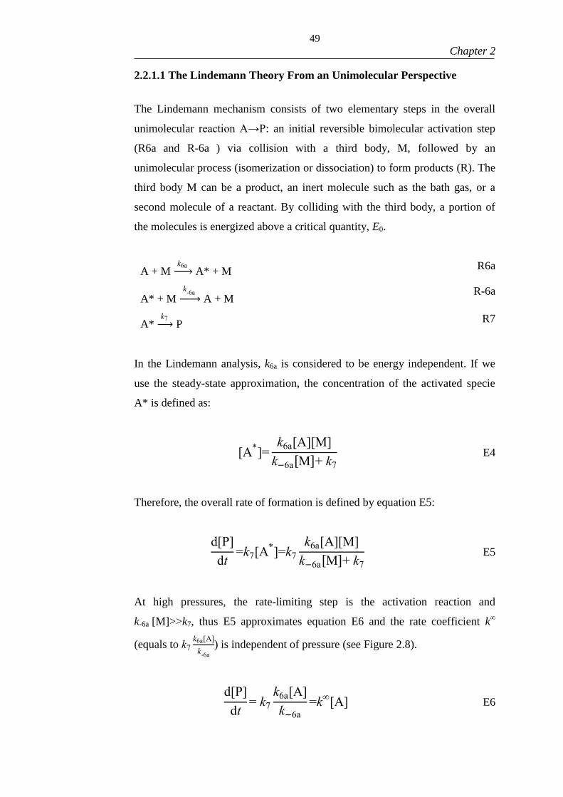
49

Chapter 2

2.2.1.1 The Lindemann Theory From an Unimolecular Perspective

The Lindemann mechanism consists of two elementary steps in the overall

unimolecular reaction A→P: an initial reversible bimolecular activation step

(R6a and R-6a ) via collision with a third body, M, followed by an

unimolecular process (isomerization or dissociation) to form products (R). The

third body M can be a product, an inert molecule such as the bath gas, or a

second molecule of a reactant. By colliding with the third body, a portion of

the molecules is energized above a critical quantity, E0.

A + M k6a → A* + M

R6a

A* + M k-6a

→ A + M R-6a

A* k7 → P

R7

In the Lindemann analysis, k6a is considered to be energy independent. If we

use the steady-state approximation, the concentration of the activated specie

A* is defined as:

[A*]=k6a[A][M]

k−6a[M]+ k7

E4

Therefore, the overall rate of formation is defined by equation E5:

d[P]

dt=k7[A*]=k7

k6a[A][M]

k−6a[M]+ k7

E5

At high pressures, the rate-limiting step is the activation reaction and

k-6a [M]>>k7, thus E5 approximates equation E6 and the rate coefficient k∞

(equals to k7k6a[A]

k-6a

) is independent of pressure (see Figure 2.8).

d[P]

dt= k7

k6a[A]

k−6a

=k∞

[A] E6

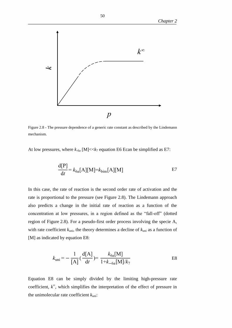
50

Chapter 2

Figure 2.8 - The pressure dependence of a generic rate constant as described by the Lindemann

mechanism.

At low pressures, where k-6a [M]<<k7 equation E6 Ecan be simplified as E7:

d[P]

dt= k6a[A][M]=kbim[A][M] E7

In this case, the rate of reaction is the second order rate of activation and the

rate is proportional to the pressure (see Figure 2.8). The Lindemann approach

also predicts a change in the initial rate of reaction as a function of the

concentration at low pressures, in a region defined as the “fall-off” (dotted

region of Figure 2.8). For a pseudo-first order process involving the specie A,

with rate coefficient kuni, the theory determines a decline of kuni as a function of

[M] as indicated by equation E8:

kuni =−1

[A](

d[A]

dt)=

k6a[M]

1+k−6a[M]/k7

E8

Equation E8 can be simply divided by the limiting high-pressure rate

coefficient, k∞, which simplifies the interpretation of the effect of pressure in

the unimolecular rate coefficient kuni:

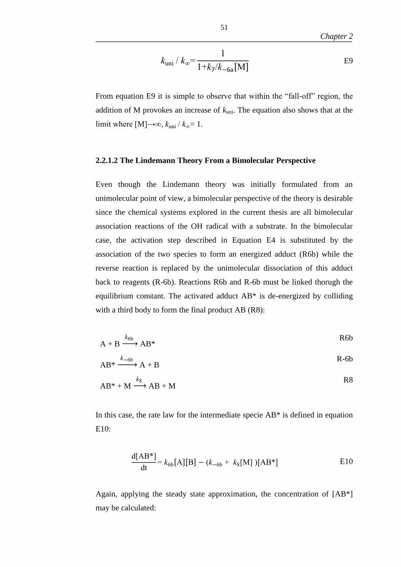
51

Chapter 2

kuni / k∞=1

1+k7/k−6a[M] E9

From equation E9 it is simple to observe that within the “fall-off” region, the

addition of M provokes an increase of kuni. The equation also shows that at the

limit where [M]→∞, kuni / k∞= 1.

2.2.1.2 The Lindemann Theory From a Bimolecular Perspective

Even though the Lindemann theory was initially formulated from an

unimolecular point of view, a bimolecular perspective of the theory is desirable

since the chemical systems explored in the current thesis are all bimolecular

association reactions of the OH radical with a substrate. In the bimolecular

case, the activation step described in Equation E4 is substituted by the

association of the two species to form an energized adduct (R6b) while the

reverse reaction is replaced by the unimolecular dissociation of this adduct

back to reagents (R-6b). Reactions R6b and R-6b must be linked thorugh the

equilibrium constant. The activated adduct AB* is de-energized by colliding

with a third body to form the final product AB (R8):

A + B k6b → AB*

R6b

AB* k−6b → A + B

R-6b

AB* + M k8 → AB + M

R8

In this case, the rate law for the intermediate specie AB* is defined in equation

E10:

d[AB*]

dt= k6b[A][B] − (k−6b + k8[M] )[AB*] E10

Again, applying the steady state approximation, the concentration of [AB*]

may be calculated:

52

Chapter 2

[AB*]=k6b[A][B]

k−6b + k8[M]

E11

The rate of formation of the product AB is then formulated in an analogous

way to that presented previously for the unimolecular case:

d[AB]

dt=k8[AB*][M]=k8

k6b[A][B][M]

k−6b+ k8[M] E12

As a consequence, at high enough pressures, the association reaction is rate-

limiting step, k8[M]>>k-6b and therefore:

d[AB]

dt=k6b[A][B] E13

Finally, at low pressures, the rate law is now linked via the equilibrium

constant of the bimolecular association and the unimolecular decomposition of

the adduct back to reagents as defined by equation E14:

d[AB]

dt=k8

k6b[A][B][M]

k−6b

E14

53

Chapter 2

2.2.2 - Master Equation Calculations with MESMER

The computational package MESMER31

, extensively used in all the analysis

presented in this thesis, implements the energy grained master equation

(EGME) theoretical approach to describe the macroscopic kinetics of a

reaction system; where the behaviour of each isomer is treated at an energy-

resolved level. The high number of rovibrational states of these isomers in

polyatomic molecules makes their time-revolved treatment computationally

impossible. To work around this issue, states of similar energy are grouped

into grains as to simplify the problem to a feasible, yet reliable level. This

robust method allows the exploration of potential energy surfaces via

modelling of the experimental conditions, which may include the use of

different bath gases and wide temperature ranges. The technique is also used in

a predictive manner, by the extrapolation of experimental measurements to a

range of conditions (T, p) of particular interest. The thermochemistry of

particular reactions, such as the OH addition to isoprene (C5H8), can be

evaluated at high temperatures with relative ease when compared to low

temperature measurements and the use of the ME approach in such cases is

appropriate. Chapters 4 and 5 will present the use of alternative ME

approaches in order to extrapolate high temperature measurements results to

room temperature for the isoprene + OH and C2H4 + OH reactions

respectively. A description of the EGME method is therefore provided in order

to simplify the understanding of the multiple analytical strategies implemented

throughout the thesis.

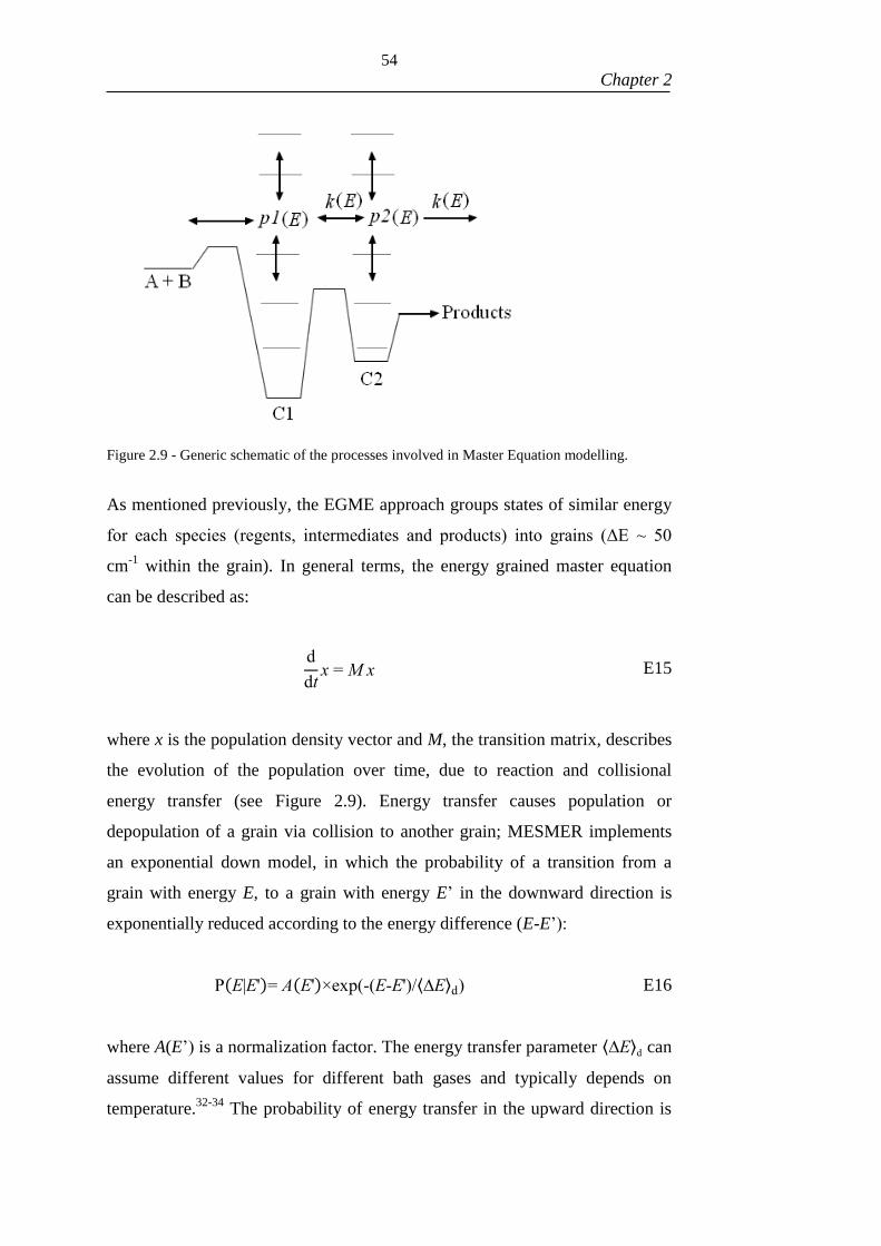
54

Chapter 2

Figure 2.9 - Generic schematic of the processes involved in Master Equation modelling.

As mentioned previously, the EGME approach groups states of similar energy

for each species (regents, intermediates and products) into grains (ΔE ~ 50

cm-1

within the grain). In general terms, the energy grained master equation

can be described as:

d

dtx = M x E15

where x is the population density vector and M, the transition matrix, describes

the evolution of the population over time, due to reaction and collisional

energy transfer (see Figure 2.9). Energy transfer causes population or

depopulation of a grain via collision to another grain; MESMER implements

an exponential down model, in which the probability of a transition from a

grain with energy E, to a grain with energy E’ in the downward direction is

exponentially reduced according to the energy difference (E-E’):

P(E|E')= A(E')×exp(-(E-E')/⟨∆E⟩d) E16

where A(E’) is a normalization factor. The energy transfer parameter ⟨∆E⟩d can

assume different values for different bath gases and typically depends on

temperature.32-34

The probability of energy transfer in the upward direction is

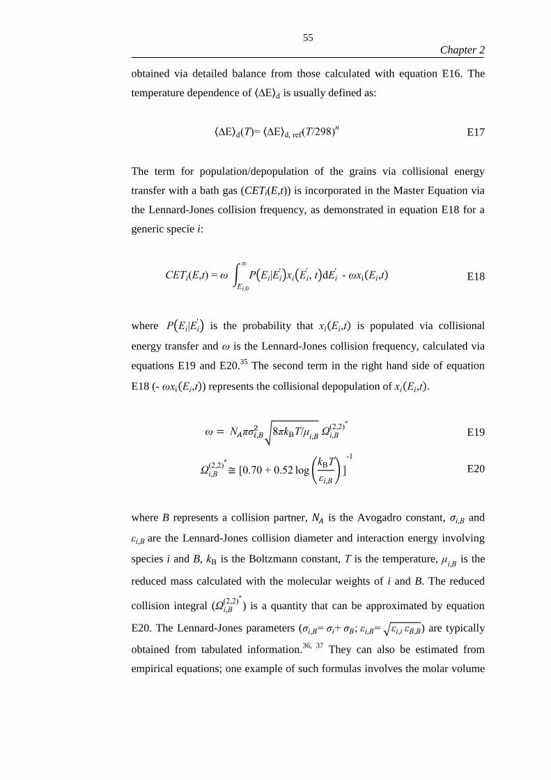
55

Chapter 2

obtained via detailed balance from those calculated with equation E16. The

temperature dependence of ⟨∆E⟩d is usually defined as:

⟨∆E⟩d(T)= ⟨∆E⟩d, ref(T/298)n E17

The term for population/depopulation of the grains via collisional energy

transfer with a bath gas (CETi(E,t)) is incorporated in the Master Equation via

the Lennard-Jones collision frequency, as demonstrated in equation E18 for a

generic specie i:

CETi(E,t) = ω ∫ P(Ei|Ei')xi(Ei

' , t)dEi'

∞

Ei,0

- ωxi(Ei,t) E18

where P(Ei|Ei') is the probability that xi(Ei,t) is populated via collisional

energy transfer and ω is the Lennard-Jones collision frequency, calculated via

equations E19 and E20.35

The second term in the right hand side of equation

E18 (- ωxi(Ei,t)) represents the collisional depopulation of xi(Ei,t).

ω = N𝐴πσ𝑖,𝐵2√8πkBT/μ

i,B Ωi,B

(2,2)*

E19

Ωi,B(2,2)

*

≅ [0.70 + 0.52 log(kBT

εi,B

) ]

-1

E20

where B represents a collision partner, 𝑁𝐴 is the Avogadro constant, 𝜎i,B and

εi,B are the Lennard-Jones collision diameter and interaction energy involving

species i and B, kB is the Boltzmann constant, T is the temperature, μi,B

is the

reduced mass calculated with the molecular weights of i and B. The reduced

collision integral (Ωi,B(2,2)

*

) is a quantity that can be approximated by equation

E20. The Lennard-Jones parameters (σi,B= σi+ σB; εi,B= √εi,i εB,B) are typically

obtained from tabulated information.36, 37

They can also be estimated from

empirical equations; one example of such formulas involves the molar volume

56

Chapter 2

at melting point (Vm) and the boiling temperature (Tb) of the pure substance

(E21-E22).35

2

3N𝐴

πσ𝑖3 = 2.3 Vm E21

εi/kB ≅ 1.18 Tb E22

Although more accurate energy transfer models such as the double exponential

model are available, single-channel unimolecular reaction rates seem to be

strongly dependent on the average rate of energy transfer rather than on the

exact features of models for collision frequency. 38, 39

In the case of a chemical process with a well-defined transition state, chemical

reaction between grains can be accounted for with microcanonical rate

constants (k(E)) calculated via RRKM theory.38

According to this theory, the

microcanonical rate coefficients are calculated from the related potential

energy surface with the use of equation E23.

k(E)=W(E)

h ρ(E) E23

where W(E) is the sum of rovibrational states at the defined transition state

structure, h is the Planck constant and ρ(E) is the density of rovibrational states

of the intermediate isomer.

For a barrierless process on the other hand, if the high pressure limiting rate

constant is known, an Inverse Laplace Transformation (ILT)39

procedure can

be implemented for obtaining the microcanonical rate constants. The ILT

algorithm allows their determination from a fit of the available limiting high

pressure rate coefficients, which may have been determined experimentally or

theoretically. The procedure uses a modified Arrhenius formalism, as

described by equation E24.

k∞

(T) = A∞

×exp(-Ea∞/RT)×(T/298)n∞

E24

57

Chapter 2

where A∞

is the pre-exponential factor, Ea∞ is the activation energy and n∞ is a

parameter that allows the adjustment of the curvature of k∞

(T) as a deviation

from the classic Arrhenius description. The accuracy of the k(E) obtained from

this procedure is highly dependent on how well defined the Arrhenius

parameters are, and therefore, reactions with large energetic barriers will

naturally require k∞

(T) to be known for a large temperature range. This

technique is recommended for association reactions.

Equation E15 represents a set of coupled differential equations relating the

grains of the involved species and its solution has the form of equation E25:

x = U eɅtU-1x(0) E25

where U is a matrix of eigenvectors obtained by the diagonalization of M, Ʌ is

the vector of corresponding eigenvalues and x(0) contains the initial conditions

for each grain. From the solution of the ME with a total of N eigenmodes, the

population density of the ith well can be obtained:

xi(E,t)=∑ cij(E)eɅjt

N

j=0

E26

From equation E26, xi(E,t) is the population density of the ith well, at time t

and with energy E. The expansion coefficient cij is dependent on the jth

eigenvector of the transition matrix, the energy E and the initial conditions. Λj

is the jth eigenvalue of M, with eigenvalues organized in ascending order of

absolute values. The integration of xi(E,t) over E yields the temporal evolution

of the species:

Xi(t) =∫ xi(E,t)dE

∞

E0i

=∑ aijeɅjt

N

j=0

E27

where Xi(t) and E0i are the population fraction and the ground-state energy of

the specie i, and the amplitudes aij is defined as in equation E28:

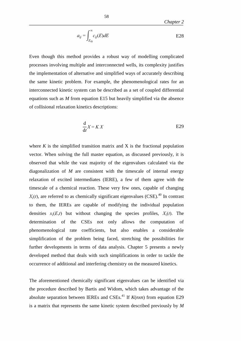
58

Chapter 2

aij =∫ cij(E)dE

∞

E0i

E28

Even though this method provides a robust way of modelling complicated

processes involving multiple and interconnected wells, its complexity justifies

the implementation of alternative and simplified ways of accurately describing

the same kinetic problem. For example, the phenomenological rates for an

interconnected kinetic system can be described as a set of coupled differential

equations such as M from equation E15 but heavily simplified via the absence

of collisional relaxation kinetics descriptions:

d

dtX = K X E29

where K is the simplified transition matrix and X is the fractional population

vector. When solving the full master equation, as discussed previously, it is

observed that while the vast majority of the eigenvalues calculated via the

diagonalization of M are consistent with the timescale of internal energy

relaxation of excited intermediates (IERE), a few of them agree with the

timescale of a chemical reaction. These very few ones, capable of changing

Xi(t), are referred to as chemically significant eigenvalues (CSE).40

In contrast

to them, the IEREs are capable of modifying the individual population

densities xi(E,t) but without changing the species profiles, Xi(t). The

determination of the CSEs not only allows the computation of

phenomenological rate coefficients, but also enables a considerable

simplification of the problem being faced, stretching the possibilities for

further developments in terms of data analysis. Chapter 5 presents a newly

developed method that deals with such simplifications in order to tackle the

occurrence of additional and interfering chemistry on the measured kinetics.

The aforementioned chemically significant eigenvalues can be identified via

the procedure described by Bartis and Widom, which takes advantage of the

absolute separation between IEREs and CSEs.41

If K(nxn) from equation E29

is a matrix that represents the same kinetic system described previously by M

59

Chapter 2

(E15), then the diagonalization of K provides a solution to the reduced number

of interconnected differential equations being discussed. However, in order to

be valid, this solution must be equal (to a numerical precision) to the solution

of the full Master Equation. The solution of K yields n eigenvalues and n

eigenvectors and by definition, the CSEs obtained from K must be equal to the

ones coming from the diagonalization of M. Hence, the elements of the

diagonalized form of K can be algebraically determined using the CSEs

selected from M and the corresponding Xi(t) which was calculated from the full

ME.

The phenomenological rate coefficient kc,i associated with a hypothetical c → i

reaction can be obtained from equation E29:42

kc,i= ∑ aijɅjajl-1

NCSE

j=0

E30

where the NCSE is the number of chemically significantly eigenvalues, aij is the

amplitude associated with species i and j calculated with equation E28.

For the separation of IEREs and CSEs, a critical ratio that separates the largest

CSE and the lowest IERE is considered. MESMER uses a critical ratio of 0.1,

i.e., a reliable separation is considered when CSEs and IEREs are separated by

at least an order of magnitude. Finally, the rate coefficients calculated via the

Master Equation followed by the Bartis-Widom procedure can be compared to

experimental measurements and used to optimize the potential energy surface

with the aid of a minimization algorithm, such as the Levenberg-Marquardt

procedure.43-45

The Master Equation calculations require additional molecular parameters such

as vibrational frequencies and rotational constants, which were calculated via

theoretical calculations. Details on these calculations will be presented in each

chapter, prior to a discussion of the corresponding results.

60

Chapter 2

2.3 REFERENCES

1. Heard, D. E. Annual Review of Physical Chemistry 2006, 57 (1), 191-216.

2. Heard, D. E.; Pilling, M. J. Chemical Reviews 2003, 103 (12), 5163-5198.

3. Onel, L.; Brennan, A.; Seakins, P. W.; Whalley, L.; Heard, D. E. Atmos. Meas. Tech.

2017, 10 (10), 3985-4000.

4. Stone, D.; Whalley, L. K.; Heard, D. E. Chemical Society Reviews 2012, 41 (19),

6348-6404.

5. Smith, G. P.; Crosley, D. R. Journal of Geophysical Research: Atmospheres 1990, 95

(D10), 16427-16442.

6. Sander, S. P.; Friedl, R. R.; DeMore, W. B.; Golden, D. M.; Kurylo, M. J.; Hampson,

R. F.; Huie, R. E.; Moortgat, C. K.; Ravishankara, A. R.; Kolb, C. E.; Molina, M. J. Chemical

Kinetics and Photochemical Data for Use in Atmospheric modelling; Pasadena, California,

2000.

7. McGee, T. J.; McIlrath, T. J. Journal of Quantitative Spectroscopy & Radiative

Transfer 1984, 32 (2), 179-184.

8. Stevens, P. S.; Mather, J. H.; Brune, W. H. J. Geophys. Res.-Atmos. 1994, 99 (D2),

3543-3557.

9. Winiberg, F. A. F. Characterisation of FAGE apparatus for HOx detection and

application in an environmental chamber. University of Leeds, Leeds, 2014.

10. Crounse, J. D.; Paulot, F.; Kjaergaard, H. G.; Wennberg, P. O. Physical Chemistry

Chemical Physics 2011, 13 (30), 13607-13613.

11. Martinez, M.; Harder, H.; Kubistin, D.; Rudolf, M.; Bozem, H.; Eerdekens, G.;

Fischer, H.; Klüpfel, T.; Gurk, C.; Königstedt, R.; Parchatka, U.; Schiller, C. L.; Stickler, A.;

Williams, J.; Lelieveld, J. Atmospheric Chemistry and Physics 2010, 10 (8), 3759-3773.

12. Stone, D.; Evans, M. J.; Edwards, P. M.; Commane, R.; Ingham, T.; Rickard, A. R.;

Brookes, D. M.; Hopkins, J.; Leigh, R. J.; Lewis, A. C.; Monks, P. S.; Oram, D.; Reeves, C.

E.; Stewart, D.; Heard, D. E. Atmospheric Chemistry and Physics 2011, 11 (13), 6749-6771.

13. Whalley, L. K.; Stone, D.; Dunmore, R.; Hamilton, J.; Hopkins, J. R.; Lee, J. D.;

Lewis, A. C.; Williams, P.; Kleffmann, J.; Laufs, S.; Woodward-Massey, R.; Heard, D. E.

Atmospheric Chemistry and Physics 2018, 18 (4), 2547-2571.

14. Aschmutat, U.; Hessling, M.; Holland, F.; Hofzumahaus, A., A tunable source of

Hydroxyl (OH) and Hydroperoxy (HO2) radicals: in the range between 106 and 10

9 cm

-3. In

Physico-Chemical Behaviour of Atmospheric Pollutants, Restelli, G. A. a. G., Ed. European

Comission, Brussels: 1994; pp 811-816.

15. Heard, D. E.; Pilling, M. J. Chemical Reviews 2003, 103, 5163-5198.

16. Schultz, M.; Heitlinger, M.; Mihelcic, D.; Volzthomas, A. J. Geophys. Res.-Atmos.

1995, 100 (D9), 18811-18816.

17. Winiberg, F. A. F.; Smith, S. C.; Bejan, I.; Brumby, C. A.; Ingham, T.; Malkin, T. L.;

Orr, S. C.; Heard, D. E.; Seakins, P. W. Atmospheric Measurement Techniques 2015, 8, 523-

540.

18. Creasey, D. J.; Halford-Maw, P. A.; Heard, D. E.; Pilling, M. J.; Whitaker, B. J. J.

Chem. Soc.-Faraday Trans. 1997, 93 (16), 2907-2913.

19. Faloona, I. C.; Tan, D.; Lesher, R. L.; Hazen, N. L.; Frame, C. L.; Simpas, J. B.;

Harder, H.; Martinez, M.; Di Carlo, P.; Ren, X. R.; Brune, W. H. J. Atmos. Chem. 2004, 47

(2), 139-167.

20. Dooley, S.; Curran, H. J.; Simmie, J. M. Combust. Flame 2008, 153 (1-2), 2-32.

21. Zador, J.; Taatjes, C. A.; Fernandes, R. X. Prog. Energy Combust. Sci. 2011, 37 (4),

371-421.

22. Cody, R. J.; Romani, P. N.; Nesbitt, F. L.; Iannone, M. A.; Tardy, D. C.; Stief, L. J. J.

Geophys. Res.-Planets 2003, 108 (E11), 16.

23. Moses, J. I., Photochemistry in giant-planet atmospheres. Astronomical Soc Pacific:

San Francisco, 2000; Vol. 212, p 196-206.

24. Miyazaki, K.; Nakashima, Y.; Schoemaecker, C.; Fittschen, C.; Kajii, Y. Review of

Scientific Instruments 2013, 84 (7).

25. Michael, J. V.; Keil, D. G.; Klemm, R. B. Journal of Chemical Physics 1985, 83,

1630-1636.

26. Campuzano-Jost, P.; Williams, M. B.; D'Ottone, L.; Hynes, A. J. J. Phys. Chem. A

2004, 108 (9), 1537-1551.

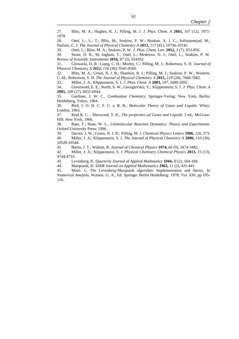
61

Chapter 2

27. Blitz, M. A.; Hughes, K. J.; Pilling, M. J. J. Phys. Chem. A 2003, 107 (12), 1971-

1978.

28. Onel, L.; L., T.; Blitz, M.; Seakins, P. W.; Bunkan, A. J. C.; Solimannejad, M.;

Nielsen, C. J. The Journal of Physical Chemistry A 2013, 117 (41), 10736-10745.

29. Onel, L.; Blitz, M. A.; Seakins, P. W. J. Phys. Chem. Lett. 2012, 3 (7), 853-856.

30. Stone, D. B., M; Ingham, T.; Onel, L.; Medeiros, D. J.; Onel, L.; Seakins, P. W.

Review of Scientific Instruments 2016, 87 (5), 054102.

31. Glowacki, D. R.; Liang, C. H.; Morley, C.; Pilling, M. J.; Robertson, S. H. Journal of

Physical Chemistry A 2012, 116 (38), 9545-9560.

32. Blitz, M. A.; Green, N. J. B.; Shannon, R. J.; Pilling, M. J.; Seakins, P. W.; Western,

C. M.; Robertson, S. H. The Journal of Physical Chemistry A 2015, 119 (28), 7668-7682.

33. Miller, J. A.; Klippenstein, S. J. J. Phys. Chem. A 2003, 107, 2680-2692.

34. Greenwald, E. E.; North, S. W.; Georgievskii, Y.; Klippenstein, S. J. J. Phys. Chem. A

2005, 109 (27), 6031-6044.

35. Gardiner, J. W. C., Combustion Chemistry. Springer-Verlag: New York, Berlin,

Heidelberg, Tokyo, 1984.

36. Bird, J. O. H. C. F. C. a. R. B., Molecular Theory of Gases and Liquids. Wiley:

London, 1963.

37. Reid R. C. ; Sherwood, T. K., The properties od Gases and Liquids. 2 ed.; McGraw-

Hill: New York, 1966.

38. Baer, T.; Hase, W. L., Unimolecular Reaction Dynamics: Theory and Experiments.

Oxford University Press: 1996.

39. Davies, J. W.; Green, N. J. B.; Pilling, M. J. Chemical Physics Letters 1986, 126, 373.

40. Miller, J. A.; Klippenstein, S. J. The Journal of Physical Chemistry A 2006, 110 (36),

10528-10544.

41. Bartis, J. T.; Widom, B. Journal of Chemical Physics 1974, 60 (9), 3474-3482.

42. Miller, J. A.; Klippenstein, S. J. Physical Chemistry Chemical Physics 2013, 15 (13),

4744-4753.

43. Levenberg, K. Quarterly Journal of Applied Mathmatics 1944, II (2), 164-168.

44. Marquardt, D. SIAM Journal on Applied Mathematics 1963, 11 (2), 431-441.

45. Moré, J., The Levenberg-Marquardt algorithm: Implementation and theory. In

Numerical Analysis, Watson, G. A., Ed. Springer Berlin Heidelberg: 1978; Vol. 630, pp 105-

116.

63

Chapter 3

Chapter 3. The Role of the Pre-reaction

Complex in the OH + SO2 Reaction

65

Chapter 3


As discussed in the previous Chapter, the Master Equation (ME) method is a

powerful and versatile approach used to deal with kinetic systems of

interconnected wells. It allows the exploration of these kinetic systems at an

energy-resolved level, and is widely employed for the majority of studies of

pressure dependent processes in this thesis. The technique also allows the

extrapolation of experimental results, often obtained under experimental

conditions that do not necessarily reflect their final practical application. In this

chapter, the results of Master Equation modelling undertaken to better

understand the chemistry of the OH + SO2 reaction, a process of primary

importance for the atmosphere, are presented. The relevance of a pre-reaction

complex to understand experimental measurements of k1(T,p) available in the

literature, for a wide range of temperature (260 – 580 K), pressure (13-695

Torr) and bath gases (He,N2,Ar,SF6) is investigated. The theoretical

calculations indicate that the pre-reaction complex is weakly bound (~7.2 kJ

mol-1

) and all the ME fits point to a lack of importance for the complex

formation. The reaction appears to be predominantly controlled by the inner

transition state, which according to our best ME model, is submerged under the

starting reactants (~-1.0 kJ mol-1

), supporting a slight negative temperature

dependence of k1∞(T). Only a portion of the measurements explored could be

reconciled, and a brief discussion of possible interferences affecting these

measurements is provided. The enthalpy of the reaction (ΔR1H0K = 110.5 kJ

mol-1

), obtained with the ME fits, is in excellent agreement with theoretical

predictions available in the literature. This chapter presents a classic example

of ME modelling where experimental rate coefficients are used to enable a

critical assessment of the related potential energy surface diagram and its

understanding will serve as a basis for the next chapters where more complex

fitting strategies are employed.

67

Chapter 3

3.1 LITERATURE BACKGROUND OF THE OH + SO2 REACTION

The reaction of sulphur dioxide, SO2, with OH radicals (R1) is of primary

importance in the atmosphere. It leads to the formation of a key intermediate,

the hydroxysulfonyl radical (HOSO2), which can further react with O2 and

H2O (R2-R3)1-2

to give sulfuric acid (H2SO4). Sulfuric acid can readily

promote nucleation and represents an important precursor for aerosols in the

atmosphere.1 It is also directly related to the occurrence of acid rain, which

implicates health, environmental and economic consequences.3

OH + SO2 + M → HOSO2 + M R1

HOSO2 + O2 → SO3 + HO2 R2

SO3 + H2O → H2SO4 R3

Alternatively, SO2 from the gas phase can dissolve into water droplets,

particles, clouds and fogs in the atmosphere and be oxidized within the

aqueous phase by species such as O3, O2 and H2O2.4 Strongly acidic fogs can

be formed due to evaporation of water from the droplets (pH~1.7)5 and

because of their sufficiently small size (< 1 μm),6 they represent a considerable

health concern. They can be efficiently inhaled, cause irritation of the

respiratory tract and be particularly harmful to those suffering from respiratory

diseases such as asthma.4, 7

It is estimated that around 50,000 people die every

year in the United Kingdom as a result of respiratory diseases caused by air

pollution, such as particulate matter, ozone and NO2;8 this number denotes the

importance of understanding chemical reactions involved in particulate

formation.

Reaction R1 has been explored recently in experimental investigations with

particular interest on determining both the high pressure limit (k1∞(T))

9-10, and

pressure dependent (k1(T, p)) rate coefficients for a wide range of conditions.11-

12 These studies indicate difficulties in the determination of reliable kinetic

parameters of this reaction. The existence of a van der Waals pre-reaction

complex has been postulated10

in order to rationalize the small high pressure

limiting rate coefficients k1∞

that were measured by Blitz et al.,10

since much

68

Chapter 3

faster coefficients would be expected for a simple barrierless reaction to form

HOSO2. With the complex, reaction R1 is now split into two processes, a

barrierless formation of the complex (R1,vdW) and the subsequent product

(HOSO2) formation via a transition state (R1,TS).

where k1,vdW is the rate coefficient for the pre-reaction complex formation and

k1,TS is the rate coefficient for product formation. Figure 3.1 shows a schematic

representation of the related potential energy surface against the reaction

coordinate.

Figure 3.1 - Potential energy diagram for the OH + SO2 reaction. Relative energies were

calculated at the CCSD(T)/CBS//M06-2X level of theory. A more detailed description of the

calculations is provided later in the chapter.

After these previous studies were published, 9-13

the postulated pre-reaction

complex has been identified via theoretical calculations by Miriyala et al.14

The theoretical level at which the electronic energies were calculated by

Miriyala et al. is relatively low (MP2(full)/aug-cc-pVTZ) when compared to

the beyond-CCSDT correlation energy calculations reported by Donald G.

OH + SO2 k1,vdW → HO―OSO R1,vdW

HO―OSO k1,TS → HOSO2

R1,TS

69

Chapter 3

Truhlar’s group13

for the rest of the potential energy surface (excluding the

pre-reaction complex). From the work of Long et al.,13

the authors predict k1∞

to be 1.25×10-12

cm3 molecule

-1 s

-1 at 298 K, significantly higher compared to

the experimental value of (7.2 ± 3.3)×10-13

cm3 molecule

-1 s

-1 reported by Blitz

et al.11

However, the main difference between these two studies is related to

the temperature dependence of k1∞; while the work by Long et al. reports a

barrier of 1.1 kJ mol-1

for R113

, the experimental results do not indicate an

increase of k1∞ with increasing temperature, and a negative activation energy

has been assigned.11

The study of Blitz et al.11

has also indicated that only a combination of their

data with a portion of those reported by Wine et al.12

could be reconciled,

suggesting that SO2 photolysis may have interfered significantly in the

measurements of many flash photolysis studies found in the literature.15-18

In this chapter, the reconciled data from Blitz et al.11

was coupled with high

temperature dissociation measurements (k-1(T,p)),9 where OH was observed to

be in equilibrium with SO2. An attempt to describe the total dataset, which also

includes measurements by Wine et al.12

, via Master Equation (ME) modelling

and mathematical fitting is performed. A list of all the data used in this

analysis is presented in Table 1 of Appendix 2. The recently identified pre-

reaction complex is incorporated in the analysis and an attempt to further

refine the related potential energy surface is presented. Since the

phenomenological rate coefficients can be directly calculated via the ME, this

case represents the simplest fitting strategy implemented throughout the thesis,

where adjustable parameters are optimised to provide a good match between

experimental values of k1(T,p) and the phenomenological rate coefficients

calculated via ME. Alternative, and more complex, strategies will be required

to analyse other systems in the following chapters, such as the reaction of

isoprene with OH radicals at elevated temperatures. A good understanding of

the procedure used for the OH + SO2 case will help introduce the analysis of

the subsequent chapters. Although simplistic compared to the subsequent

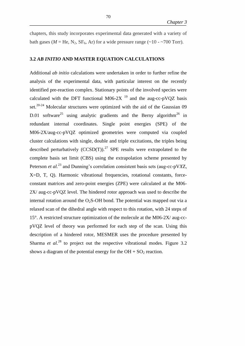
70

Chapter 3

chapters, this study incorporates experimental data generated with a variety of

bath gases (M = He, N2, SF6, Ar) for a wide pressure range (~10 - ~700 Torr).

3.2 AB INITIO AND MASTER EQUATION CALCULATIONS

Additional ab initio calculations were undertaken in order to further refine the

analysis of the experimental data, with particular interest on the recently

identified pre-reaction complex. Stationary points of the involved species were

calculated with the DFT functional M06-2X 19

and the aug-cc-pVQZ basis

set.20-24

Molecular structures were optimized with the aid of the Gaussian 09

D.01 software25

using analytic gradients and the Berny algorithm26

in

redundant internal coordinates. Single point energies (SPE) of the

M06-2X/aug-cc-pVQZ optimized geometries were computed via coupled

cluster calculations with single, double and triple excitations, the triples being

described perturbatively (CCSD(T)).27

SPE results were extrapolated to the

complete basis set limit (CBS) using the extrapolation scheme presented by

Peterson et al.23

and Dunning’s correlation consistent basis sets (aug-cc-pVXZ,

X=D, T, Q). Harmonic vibrational frequencies, rotational constants, force-

constant matrices and zero-point energies (ZPE) were calculated at the M06-

2X/ aug-cc-pVQZ level. The hindered rotor approach was used to describe the

internal rotation around the O2S-OH bond. The potential was mapped out via a

relaxed scan of the dihedral angle with respect to this rotation, with 24 steps of

15°. A restricted structure optimization of the molecule at the M06-2X/ aug-cc-

pVQZ level of theory was performed for each step of the scan. Using this

description of a hindered rotor, MESMER uses the procedure presented by

Sharma et al.28

to project out the respective vibrational modes. Figure 3.2

shows a diagram of the potential energy for the OH + SO2 reaction.

71

Chapter 3

Figure 3.2 - Potential energy diagram for the OH + SO2 reaction, where a van der Waals

complex, vdW, is formed before proceeding over the transition-state, TS, to form the

hydroxysulfonyl radical, HOSO2. The energies of the stationary states are those calculated in

this work, with zero point energies added. Also included is OH(v=1) + SO2 reaction, which

initially forms a “hot” vdW(**) that either re-dissociates back to reagents or undergoes

intramolecular energy redistribution (IVR) to vdW(*), which does not significantly re-

dissociate to OH(v=1) + SO2; the two thick arrows indicate that these processes are in

competition. The Boltzmann energy distribution of the vdW is illustrated; it resides mostly

above the binding energy of this complex.

All the ME modelling was performed with the aid of the computational

package MESMER.29

The inverse Laplace transformation (ILT) method was

implemented to describe the complex formation (R1,vdW ) and RRKM rate

theory30

was used for the subsequent reaction over the transition state (R1,TS ).

For the first step, even though there are no measurements available for this rate

coefficient, this reaction is expected to be close to the gas kinetic collision

frequency. Barrierless reactions typically present a negative temperature

dependence, which can be reasonably described in the form of equation E1 :

k1,vdW =A × (T

298 K)

n

E1

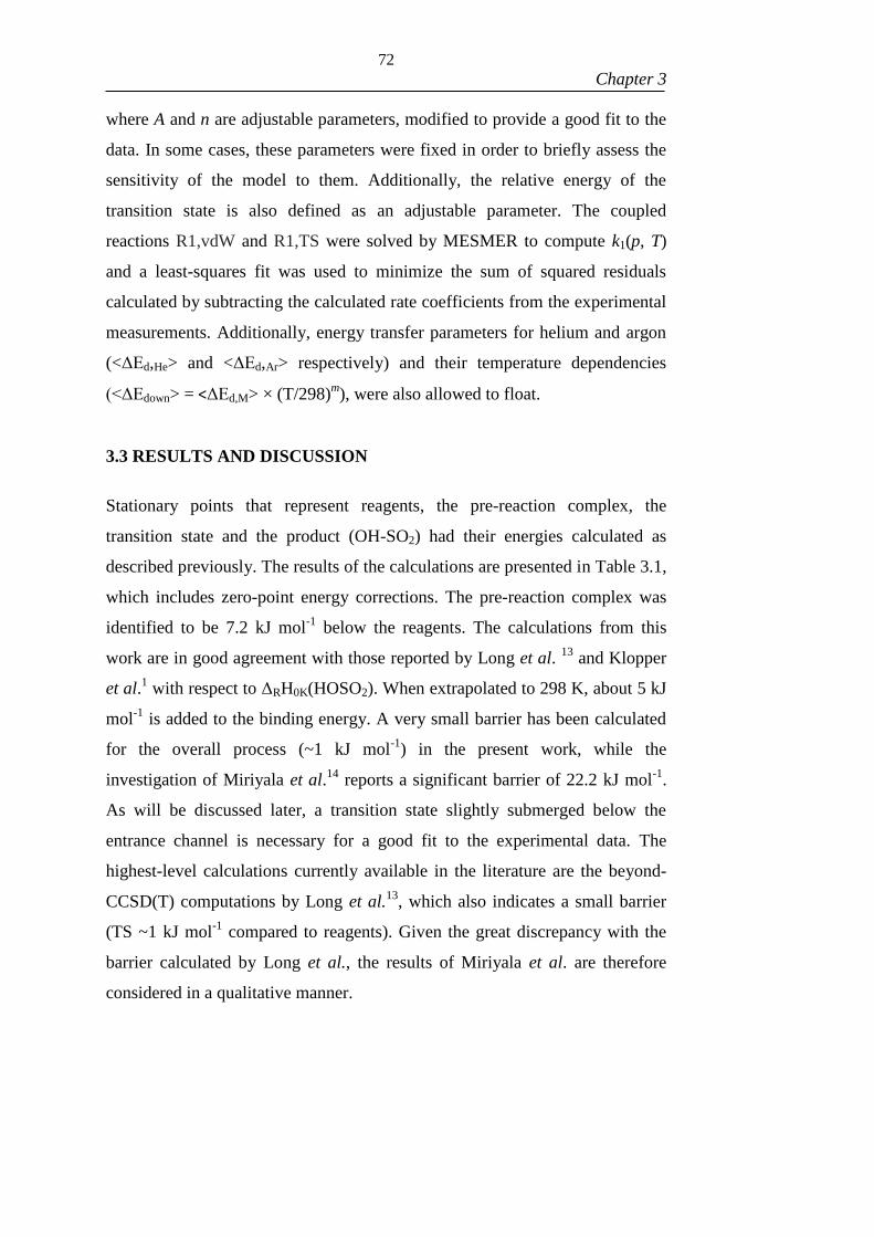
72

Chapter 3

where A and n are adjustable parameters, modified to provide a good fit to the

data. In some cases, these parameters were fixed in order to briefly assess the

sensitivity of the model to them. Additionally, the relative energy of the

transition state is also defined as an adjustable parameter. The coupled

reactions R1,vdW and R1,TS were solved by MESMER to compute k1(p, T)

and a least-squares fit was used to minimize the sum of squared residuals

calculated by subtracting the calculated rate coefficients from the experimental

measurements. Additionally, energy transfer parameters for helium and argon

(<ΔEd,He> and <ΔEd,Ar> respectively) and their temperature dependencies

(<ΔEdown> = <ΔEd,M> × (T/298)m), were also allowed to float.

3.3 RESULTS AND DISCUSSION

Stationary points that represent reagents, the pre-reaction complex, the

transition state and the product (OH-SO2) had their energies calculated as

described previously. The results of the calculations are presented in Table 3.1,

which includes zero-point energy corrections. The pre-reaction complex was

identified to be 7.2 kJ mol-1

below the reagents. The calculations from this

work are in good agreement with those reported by Long et al. 13

and Klopper

et al.1 with respect to ΔRH0K(HOSO2). When extrapolated to 298 K, about 5 kJ

mol-1

is added to the binding energy. A very small barrier has been calculated

for the overall process (~1 kJ mol-1

) in the present work, while the

investigation of Miriyala et al.14

reports a significant barrier of 22.2 kJ mol-1

.

As will be discussed later, a transition state slightly submerged below the

entrance channel is necessary for a good fit to the experimental data. The

highest-level calculations currently available in the literature are the beyond-

CCSD(T) computations by Long et al.13

, which also indicates a small barrier

(TS ~1 kJ mol-1

compared to reagents). Given the great discrepancy with the

barrier calculated by Long et al., the results of Miriyala et al. are therefore

considered in a qualitative manner.

73

Chapter 3

Table 3.1 – Comparison of theoretical calculations for the OH + SO2 reaction. All the energies

include zero-point corrections and are relative to OH + SO2. The table also includes an

experimental measurement by Blitz et al.9

vdW /

kJ mol-1

TS /

kJ mol-1

ΔRH0K(HOSO2)

/ kJ mol-1

ΔRH298K(HOSO2)

/

kJ mol-1

Miriyala et al.

2017 14

-17.6 22.2 -109.2

This study

2019 -7.2 1.2 -110.9

Klopper et al.

2008 1

-109.4 -114.7 ± 3

Long et al.

2017 13

1.1 -111.5

Somnitz (2004) 31

-103.6

Blitz et al. (2003)9

(Experimental) -113 ± 6

In a previous study of Blitz et al.,10

rate coefficients for the removal of

vibrationally excited hydroxyl radicals (OH( > 0)) in the presence of SO2

(R1() ) have been measured, which allowed the determination of k1∞

.

OH(>0) + SO2 → HOSO2** R1()

In reaction R1() , the nascent product HOSO2**(vdW**) is indicated with

two stars to denote additional internal energy from the vibrationally excited

OH. While HOSO2** can react in different ways, and since it is unlikely that

the formation of OH(=0) from it is significant, the measured removal rate

coefficient represents k1∞. This is known as the proxy method for determining

the high pressure limiting rate coefficient, first introduced by Smith.32

The

importance of the van der Waals complex is that it can potentially influence the

energy transfer between the reagents.

74

Chapter 3

In the study of Blitz et al.,10

the measured k1(>0) were faster than k1∞ for the

same experimental conditions. In order to enable significant energy

redistribution within the vdW complex, its lifetime would need to be

considerably long (~1-100 picoseconds). A sufficiently long lifetime would

provide a proxy for the high pressure limit rate coefficient for the formation of

the pre-reaction complex, which should be close to the gas kinetic collision

frequency (~10-10

cm-3

molecules-1

s-1

) (see Table 3.2 for estimates of the rate

coefficients for vdW formation, calculated via ME modelling). However, not

only does the analysis of Blitz et al. indicate much smaller k1(>0) than the gas

kinetic collision frequency, but the rate coefficients also increase with the level

of excitation, being higher for more the elevated vibration levels. This implies

a short lifetime for the complex, which suggests that the re-distribution of the

additional energy of vdW** by its vibrational modes would occur partially

throughout the complex (see Figure 3.2 for OH(=1) + SO2). Internal

vibrational energy redistribution (IVR) usually occurs on a femto-picosecond

timescale33 and our ME calculations indicates that the lifetime of the vdW

complex above T=250 K is of approximately a picosecond. As illustrated in

Figure 3.2, the Boltzmann distribution of the vdW, formed from the reaction of

OH(=0) with SO2 is mostly above the transition state to products. Even

though the k1(>0) rate coefficients measured by Blitz et al. are qualitatively

consistent with the potential energy surface depicted in Figure 3.2 and deserve

good attention in the future, this chapter will focus on the data related to

OH(=0) + SO2. The investigation the k1(>0) provides, however, estimates

for k1∞(T)(=0) which will be used later on in the chapter for a comparison

with the obtained results.

As reaction R1 consists of two steps, it is safer to assume that the measured

kinetic data are related to the total OH loss rather than OH reacting with SO2 to

give HOSO2. For this reason, in the MESMER fitting, the literature data have

been assigned as the total removal of OH. For the equilibrium measurements

of Blitz et al.9, the calculated total loss of HOSO2 was regressed to best fit k-

1(T,p). The phenomenological rate coefficients, which are measured

experimentally,34

correspond to eigenvalues of the transition matrix M

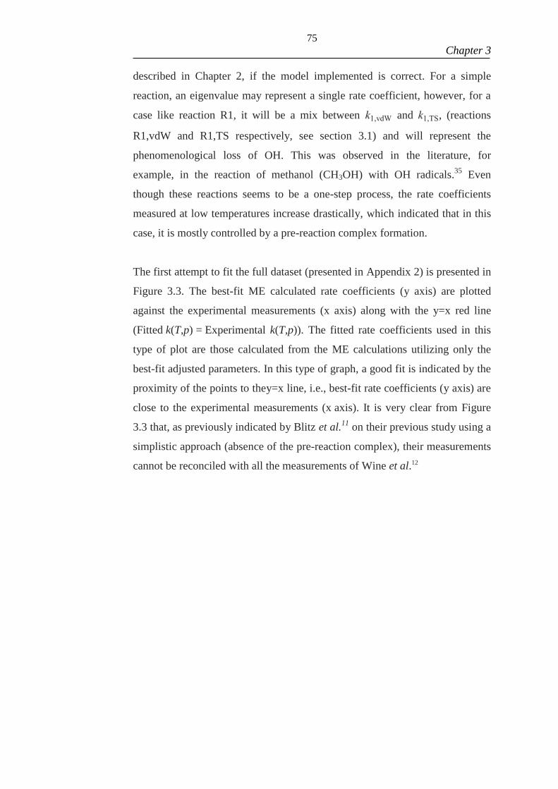
75

Chapter 3

described in Chapter 2, if the model implemented is correct. For a simple

reaction, an eigenvalue may represent a single rate coefficient, however, for a

case like reaction R1, it will be a mix between k1,vdW and k1,TS, (reactions

R1,vdW and R1,TS respectively, see section 3.1) and will represent the

phenomenological loss of OH. This was observed in the literature, for

example, in the reaction of methanol (CH3OH) with OH radicals.35

Even

though these reactions seems to be a one-step process, the rate coefficients

measured at low temperatures increase drastically, which indicated that in this

case, it is mostly controlled by a pre-reaction complex formation.

The first attempt to fit the full dataset (presented in Appendix 2) is presented in

Figure 3.3. The best-fit ME calculated rate coefficients (y axis) are plotted

against the experimental measurements (x axis) along with the y=x red line

(Fitted k(T,p) = Experimental k(T,p)). The fitted rate coefficients used in this

type of plot are those calculated from the ME calculations utilizing only the

best-fit adjusted parameters. In this type of graph, a good fit is indicated by the

proximity of the points to they=x line, i.e., best-fit rate coefficients (y axis) are

close to the experimental measurements (x axis). It is very clear from Figure

3.3 that, as previously indicated by Blitz et al.11

on their previous study using a

simplistic approach (absence of the pre-reaction complex), their measurements

cannot be reconciled with all the measurements of Wine et al.12

76

Chapter 3

0.0 0.2 0.4 0.6 0.8 1.0 1.2

0.0

0.2

0.4

0.6

0.8

1.0

1.2

Blitz et al. (He) a

Wine et al. (He) b

Wine et al. (Ar) b

Wine et al. (N2)

b

Wine et al. (SF6)

b

y=x

Fit

ted

k(T

,p)

/ 1

0-1

2 c

m3 m

ole

cule

-1 s

-1

Experimental k(T,p) / 10-12

cm3 molecule

-1 s

-1

Figure 3.3 - The result of the ME fit to the full dataset. a - Blitz et al.9, 11

b – Wine et al.12

. The

y=x line is presented in red. High temperature reverse coefficients by Blitz et al.9 were

suppressed from the figure for illustrative purposes.

The systematic deviation of a good portion of data from the y=x line as

observed in Figure 3.3 suggests a fundamental problem with some data. A

careful inspection of the results show that while the experimental data reported

by Wine et al. indicates a ΔR1H0K value of ~ -102 mol-1

, the data by Blitz et al.

9, 11 incorporated in the fit suggest a much deeper value, of approximately -111

kJ mol-1

. Both the data sets were further analysed individually and will be

discussed in the following, but it is worth highlighting that such differences

have a significant impact on the predicted pressure-dependent rate coefficients.

For example, Wine et al. have measured a rate coefficient of 1 × 10-12

cm3

molecule-1

s-1

at 300 K and 500 Torr of SF6. However, in order to agree to the

measurements of Blitz et al., a rate coefficient of about 6 × 10-13

cm3 molecule

-

1 s

-1 would be necessary. As the measurements by Blitz et al. indicate a deeper

ΔR1H0K of -111 kJ mol-1

, this would imply faster rate coefficients, but an

opposite effect is observed. For this reason, it is postulated that the

measurements by Wine et al. were affected by fast interfering processes, which

significantly competed with the OH + SO2 reaction.

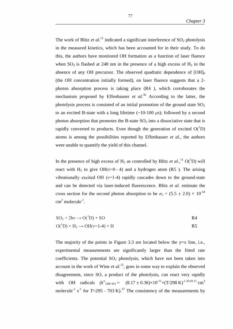
77

Chapter 3

The work of Blitz et al.11

indicated a significant interference of SO2 photolysis

in the measured kinetics, which has been accounted for in their study. To do

this, the authors have monitored OH formation as a function of laser fluence

when SO2 is flashed at 248 nm in the presence of a high excess of H2 in the

absence of any OH precursor. The observed quadratic dependence of [OH]0

(the OH concentration initially formed), on laser fluence suggests that a 2-

photon absorption process is taking place (R4 ), which corroborates the

mechanism proposed by Effenhauser et al.36

According to the latter, the

photolysis process is consisted of an initial promotion of the ground state SO2

to an excited B-state with a long lifetime (~10-100 μs); followed by a second

photon absorption that promotes the B-state SO2 into a dissociative state that is

rapidly converted to products. Even though the generation of excited O(1D)

atoms is among the possibilities reported by Effenhauser et al., the authors

were unable to quantify the yield of this channel.

In the presence of high excess of H2 as controlled by Blitz et al.,11

O(1D) will

react with H2 to give OH(ν=0 - 4) and a hydrogen atom (R5 ). The arising

vibrationally excited OH (ν=1-4) rapidly cascades down to the ground-state

and can be detected via laser-induced fluorescence. Blitz et al. estimate the

cross section for the second photon absorption to be σ2 = (5.5 ± 2.0) × 10-18

cm2 molecule

-1.

SO2 + 2hν → O(1D) + SO R4

O(1D) + H2 → OH(ν=1-4) + H R5

The majority of the points in Figure 3.3 are located below the y=x line, i.e.,

experimental measurements are significantly larger than the fitted rate

coefficients. The potential SO2 photolysis, which have not been taken into

account in the work of Wine et al.12

, goes in some way to explain the observed

disagreement, since SO, a product of the photolysis, can react very rapidly

with OH radicals (k∞

OH+SO = (8.17 ± 0.36)×10-11

×(T/298 K)-1.35±0.11 cm

3

molecule-1

s-1

for T=295 – 703 K).37

The consistency of the measurements by

78

Chapter 3

Wine et al. were submitted to another test, by removing all the data points

corresponding to the measurements of Blitz et al.9, 11

and re-attempting the fit;

the result of this new attempt is presented in Figure 3.4. The poor fit is an

indication that the rate coefficients reported by Wine et al. are internally

inconsistent

0.0 0.2 0.4 0.6 0.8 1.0 1.2

0.0

0.2

0.4

0.6

0.8

1.0

1.2

Wine et al. (He)

Wine et al. (Ar)

Wine et al. (N2)

Wine et al. (SF6)

y=x

Fit

ted

k(T

,p)

/ 1

0-1

2 c

m3 m

ole

cule

-1 s

-1

Experimental k(T,p) / 10-12

cm3 molecule

-1 s

-1

Figure 3.4 - The result of the Master Equation fit to the experimental measurements of Wine et

al. 12

. The y=x line is presented in red.

Even though this result raises questions regarding the validity of these

experimental measurements, further attempts to reconcile at least a portion of

their measurements with those of Blitz et al. were undertaken. By doing so, a

good agreement could only be obtained when their data where Ar is the bath

gas is combined with the measurements by Blitz et al. The result of this

combination is a much better fit (R2=0.93), as depicted in Figure 3.5.

.

79

Chapter 3

0.0 0.5 1.0 1.5 2.0 2.5 3.0 3.5 4.0

0.0

0.5

1.0

1.5

2.0

2.5

3.0

3.5

4.0

Blitz et al. (He)a

Wine et al. (Ar)b

y=x

Fit

ted

k1(T

,p)

/ 1

0-1

2 c

m3 m

ole

cule

-1 s

-1

Experimental k1(T,p) / 10

-12 cm

3 molecule

-1 s

-1

Figure 3.5 - The result of the ME fit to the experimental measurements of Blitz et al.9, 11

and

those of Wine et al. 12

in argon. The y=x line is presented in red. High temperature reverse

coefficients by Blitz et al.9 were suppressed from the figure for illustrative purposes.

From this point, this dataset (presented in Figure 3.5) is considered to be the

basis for exploring the potential energy diagram related to the OH+SO2

reaction. A number of parameters were floated during the fitting exercises, and

in some occasions, some of these parameters were kept fixed to test the

sensitivity of the experimental data to these parameters. The list of floated

parameters are presented in Table 3.2 and they include: the enthalpy of

reaction ΔR1H0K, the energy transfer parameters for helium and argon and their

temperature dependence, <ΔEd,He>, <ΔEd,Ar> and m respectively (see Table

3.2), the pre-exponential factor and the temperature dependence of the van der

Waals complex (R1,vdW ) and finally, the energy of the transition state

relative to the reagents.

80

Chapter 3

Table 3.2 - Master Equation fits to the experimental data, where <ΔEdown> = <ΔEd, M>× (T/298)m.

ΔR1H0K / kJ mol-1

<ΔEd,He> × (T/298)m /cm

-1 <ΔEd,Ar>×(T/298)

0.5 /cm

-1 ILT

(a)= A ×(T/298 )

n TS/kJ mol

-1 χ

2/pts

(b)

Vibration

Model A -114.4 ± 0.8 208 ± 28 1.0 fixed 185 ± 15

(1.4 ± 3.1)× 10-10

-0.99 ± 0.23 1.54 -0.87 ± 3.05

Vibration

Model B -114.4± 0.8 208 ± 29 1.0 fixed 185 ± 16

1.4 × 10-10

fixed -1.00 ± 0.23 1.54

-0.87 fixed

Hindered

Model C -110.5 ± 0.8 145 ± 17 1.0 fixed 127 ± 9

(1.4 ± 3.5)× 10-10

-0.99 ± 0.20 1.31

-0.87 ± 2.01

Hindered

Model D -110.5 ± 0.8 145 ± 17 1.0 fixed 127 ± 9

1.4 × 10-10

fixed -0.99 ± 0.20 1.31

-0.87 fixed

Hindered

Model E -110.5 ± 6.6 145 ± 37 1.00 ± 1.94 127 ± 32

1.4 × 10-10

fixed -0.99 ± 0.21 1.31

-0.87 fixed

Model F -114.3 ± 0.8 1343 ± 422 1.0 fixed 274 ± 14 1.4 × 10

-10fixed

1.1 fixed 4.98 -0.87 fixed

Model G -111.5 fixed 697 ± 109 1.0 fixed 312 ± 14 1.4 × 10

-10fixed

1.1 fixed 5.86 -0.87 fixed

ILT(TS)

Model H -109.1 ± 6.6 120 ± 30 0.76 ± 1.83 116 ± 30

5.76 ± 0.77× 10-13

1.15

-0.84 ± 0.27

(a)Units are cm3 molecule

-1 s

-1. (b)

Weighted by uncertainties in the rate coefficients. Number of points equals 36.

81 Chapter 3

Table 3.2 presents the results of the fits of the different variants of the model

depicted in Figure 3.2 to the experimental data along with the goodness of fit

(χ2/pts). A total of eight variants were constructed, and their details are now

discussed. In variant A, all the vibrational modes of all the species are

described as harmonic oscillators. From the fit, the rate coefficient for the

formation of the van der Waals complex is very fast but ill-defined

(k1,vdW = (1.4 ± 3.1) × 10-10

cm3 molecule

-1 s

-1). On the other hand, the energy

of the transition state (relative to OH + SO2) is submerged below the reactants

(-0.38 ±0.16 kJ mol-1

) and well-defined, diverging from the ab initio estimates

(see table 3.1) which indicates a slightly positive barrier. From these results

and according to model A, reaction R1 is predominantly controlled by the

inner (submerged) transition state. Model B is very similar to A, but maintains

the pre-exponential factor of the pre-reaction complex formation fixed. The

two models indicate a slightly negative energy of the transition state, which

contrasts with ab initio predictions, however, the absolute difference is small

(~ 2 kJ mol-1

). This submerged TS implies that the overall rate coefficient will

present a negative temperature dependence, in contrast to the positive

dependence reported in the work of Long et al. No significant variation is

observed in the returned parameters when model B is compared to model A

and the impact of fixing the mentioned parameter on the uncertainties of them

is negligible. This is an evidence that the vdW complex formation and its

parameters are not strongly correlated to the other ones. Both the models return

-114.4 kJ mol-1

for ΔR1H0K.

The use of rigid harmonic rotors, as implemented in models A and B can lead

to inaccurate calculations of the density of states of the species involved in the

model. This effect can have a severe impact on the entropy of the reaction,

ΔRS, something that propagates to significant changes in the returned ΔR1H0K.

As will be evidenced in the following chapter where the chemistry of isoprene

is explored, much better agreement between experimental measurements and

theoretical predictions of the thermochemistry of that reaction is obtained

when the hindered rotor approach is used to describe low frequency vibrations

with considerable degrees of anharmonicity (ν ≤350 cm-1

) of the involved

82 Chapter 3

species, when compared to an analogous vibration-only model. The relevant

degrees of anharmonicity of some of these low vibrational modes (typically

bends and torsional vibrations) can be better described via the implementation

of the hindered rotor approach. A low vibrational mode can be visually

inspected and when this mode corresponds to a clear rotational torsion, the

implementation of a hindered rotor description is considered. Although the

anharmonicity of bends and coupled modes are admittedly important, the

results obtained in chapters 3 and 4 of this thesis indicate a very good

agreement between thermochemical parameters obtained from ab initio

calculations and experimental determinations when rotational torsions are

treated with the hindered rotor approach and the remaining modes are

described as harmonic vibrations.

The subsequent model variants (C-H) will implement this approach to describe

a small torsional vibration (ν=309 cm-1

) around the OH─SO2 bond of the

product. Thus, model C is analogous to model A, but includes the mentioned

hindered rotor description. As expected based on the result of model A, k1,vdW

remains ill-defined (k1,vdW = (1.4 ± 3.5) × 10-10

cm3 molecule

-1 s

-1) and when

this parameter is fixed (model D), no relevant change is observed in the

returned parameters or their uncertainties. This leads to the same conclusion

reported when models A and B were compared: the pre-reaction complex does

not play an important role in the kinetics. However, the inclusion of a hindered

rotor provoked a significant change in the returned ΔR1H0K (-110.5 ± 0.8 kJ

mol-1

) when D is compared to the analogous vibration-only model B (-114.4±

0.8 kJ mol-1

). This variation of 3.9 kJ mol-1

arises mainly because the entropy

of reaction calculated with model D (ΔSR1,298 K = -142.8 J k-1

mol-1

) is lower

than that when model B is the one of choice (ΔSR1,298 K = -150.4 J K-1

mol-1

).

The value obtained from model D represents the best experimental

measurement of ΔR1H0K obtained in this work, which is in excellent agreement

with the theoretical predictions by Klopper et al.1 Long et al.13 and the

calculations undertaken in this investigation (see Table 3.1).

83 Chapter 3

Despite the good agreement, the returned ΔR1H0K values are dependent on the

energy transfer parameters of helium. The equilibrium measurements of Blitz

et al.9, performed in helium, impose strong constrains on the thermochemistry

of the reaction, justifying the dependence of ΔR1H0K for the energy transfer

parameters of that bath gas. While in the previously discussed models, the

temperature dependence of <ΔEd,He>, m, has been set to 1.0, which is

consistent with measurements for different systems38

, model E has that

temperature dependence as an additional adjustable parameter. This attempt

returns unity as a result, however, according to its uncertainty the parameter is

ill-defined. With effect, having m adjusted has caused the uncertainties of the

other parameters to increase significantly. The uncertainties obtained with

model E probably represents a more realistic estimate of the current accuracy

of ΔR1H0K. The correlation between m and ΔR1H0K was found to be close to

unity, where the enthalpy of reaction increases with m. For this reason,

additional experimental measurements of k1(T,p), preferably at elevated

temperatures (T > 300 K) to promote pressure dependence are desirable in

order to indicate a preferable theoretical investigation with confidence.

From Table 3.2 it is noticed that even for model, E, where uncertainties are

greater than in the other cases, the transition state is submerged even when the

uncertainties are considered (-0.99 ± 0.21 kJ mol-1

), indicating that the

accuracy of the ab initio calculations currently available are not superior to 1

kJ mol-1

. Although the agreement observed is a considerable achievement, the

small discrepancy significantly influences the prediction of rate coefficients at

room temperature. Also, significant correlation coefficients between the energy

transfer parameters <ΔEd,He,Ar> and ΔR1H0K (ρcorr>0.8) are observed. However,

the ab initio estimations of ΔR1H0K presented in table 3.1 give some support to

the obtained ΔR1H0K. The values for the energy transfer parameter <ΔEd,He>

obtained from the ME fits (~150 cm-1

) are similar to those estimated in

chapters 4 and 5 for the reactions of OH with isoprene and ethylene

respectively, and also agree with the values previously reported in the work of

Blitz et al.11

84 Chapter 3

The derived uncertainties of the adjustable parameters indicate the level of

precision in which these parameters are known based on the experimental data.

Usually, the process by which a rate coefficient is extracted from the

experimental data involves the use of a fit of an analytical equation suitable to

describe the system. This is the case of the exponential decay equation

employed for the analysis of first order processes, as presented in Chapter 2.

Nonetheless, when the complexity of the problems is enhanced, more variables

tend to be introduced as a response and more steps tend to be undertaken

before the solutions can be obtained. This effect can eventually become a

compromise to the precision of derived solutions, given that errors need to be

propagated and a certain degree of interdependence between the various

variables can be developed. For this reason, reducing the number of necessary

transformations of the data is an interesting strategy from the point of view of

data analysis. The reaction currently being studied is a great example to show

how a very small error, in the order of 1 kJ mol-1

is the threshold between a

good and a bad agreement to theoretical predictions. The development and

exploitation of more accurate techniques can potentially also calibrate the

accuracy of theoretical calculations, which for binding energies, is typically

believed to be of the order of a few kcal mol-1

.

Attempts to fit the data by fixing the TS relative energy and ΔR1H0K to the

theoretical values calculated by Long et al. were made in models F and G.

While in model F the TS energy is fixed to 1.1 kJ mol-1

and ΔR1H0K is an

adjustable parameter, in model G ΔR1H0K is fixed to -111.5 kJ mol-1

. Model F

shows that by fixing the barrier to 1.1 kJ mol-1

it is not possible to obtain a

good fit to the data as evidenced by the fact that the goodness of fit is increased

by a factor of ~3.8 when compared to the previous models (C-E). Model G

provides a similarly poor fit: when ΔR1H0K is also fixed to the aforementioned

theoretical value the goodness of fit is increased by a factor of ~4.5 when

compared to previous models (C-E). These results reinforce the understanding

that above 250 K, the OH + SO2 reaction is mainly controlled by the inner

transition state (TS in Figure 3.2), diminishing the importance of the pre-

reaction complex. All the modelling presented so far assumes the transition

85 Chapter 3

state structure is unchanged as the temperature varies. This is a reasonable

approximation over large barriers, and even though this is not the case for the

current work, where the barrier from the vdW complex to the TS is 8.2 kJ

mol-1

, the fact that the pre-reaction complex is unimportant for the chemistry

eliminates any burden for the use of this approximation. For barrierless

processes or processes with small barriers (Ea ≤ 4 kJ mol-1

) the transition state

can change with temperature and generally becomes more similar to the adduct

structure as temperature is increased.39

Finally, the reaction has been treated using a one-transition state approach via

an inverse Laplace transformation k1∞×(T/298)

n to calculate the microcanonical

rate coefficients (model H). The parameter n allows flexibility to account for a

possible change of the inner TS with temperature and the result of this fit is

presented on the last row of Table 3.2. The negative temperature dependence

obtained (n=-0.83) is aligned with the results of the previous method where the

TS was found to be submerged under the starting reactants. Figure 3.6 shows a

comparison between the high pressure limiting rate coefficients calculated with

model H and the predictions of k1∞(T) by Long et al.

13 and Blitz et al.

11

86 Chapter 3

200 300 400 500 600 700 800

0.0

0.5

1.0

1.5

2.0

2.5

Long et al.

Blitz et al.

This workk 1(

)

10

-12 c

m3 m

ole

cule

-1 s

-1

T / K

Figure 3.6 – A comparison of the estimates of the high pressure limiting rate coefficients

obtained with the use of model H with the previous predictions by Long et al. 13

and Blitz et

al.11

87 Chapter 3


The current chapter presented an example of a classic Master Equation analysis

in which experimental measurements of the OH + SO2 reaction were used to

enable an assessment of the potential energy surface related to this chemical

process. The investigation made use of experimental data covering a wide

range of temperatures (260 – 580 K), pressures (13 -695 Torr) and carrier

gasses (He, N2, Ar, SF6) highlighting the versatility of the ME method. A

weakly bound (~7.2 kJ mol-1

) pre-reaction complex formation was identified,

but this was found to be unimportant as the chemistry appears to be controlled

by an inner transition state. The results of ME fits to the experimental data

show that the transition state is slightly submerged (~ -1.0 kJ mol-1

) below the

starting reagents (OH + SO2), causing a slightly negative temperature

dependence, as observed for barrierless processes in general. Furthermore, the

enthalpy of reaction derived from the ME analysis (~110.5 ± 6.6 kJ mol-1

) is in

excellent agreement with theoretical estimates available in the literature.

Since the chapter provided that a real application of the ME method, its

contents will serve the basis of the more complex analysis strategies required

to analyse the chemistry of isoprene and ethylene, covered in Chapters 4 and 5

respectively. While the analysis of the current chapter purely based on fits

involving experimentally derived rate coefficients, the analysis implemented in

the next chapter (4) also involves the exploration of species profiles calculated

via the Master Equation.

88 Chapter 3

3.5 REFERENCES

1. Klopper, W.; Tew, D. P.; Gonzalez-Garcia, N.; Olzmann, M. Heat of Formation of the

HOSO2 Radical from Accurate Quantum Chemical Calculations. J Chem Phys 2008, 129,

114308.

2. Mai, T. V. T.; Duong, M. V.; Nguyen, H. T.; Huynh, L. K. Ab Initio Kinetics of the

HOSO2 + 3O2 → SO3 + HO2 Reaction. Physical Chemistry Chemical Physics 2018, 20, 6677-

6687.

3. Singh, A.; Agrawal, M. Acid Rain and Its Ecological Consequences. J Environ Biol

2008, 29, 15-24.

4. Finlayson-Pitts, B. J.; Pitts, J. N., Jr., Chemistry of the Upper and Lower Atmosphere:

Theory, Experiments and Applications. Academic Press: San Diego, CA, 2000.

5. Jacob, D. J.; Hoffmann, M. R. A Dynamic Model for the Production of H+ NO3

−, and

SO42−

in Urban Fog. Journal of Geophysical Research: Oceans 1983, 88, 6611-6621.

6. Ganor, E.; Levin, Z.; Pardess, D. Determining the Acidity and Chemical Composition

of Fog, Haze and Cloud Droplets in Israel. Atmospheric Environment. Part A. General Topics

1993, 27, 1821-1832.

7. Goldstein, I. F.; Weinstein, A. L. Air Pollution and Asthma: Effects of Exposures to

Short-Term Sulfur Dioxide Peaks. Environmental Research 1986, 40, 332-345.

8. Neslen, A. Europe Escalates Action against Uk for Breaching Air Pollution Limits

06/02/2017. https://www.theguardian.com/environment/2017/feb/06/european-commission-

escalates-action-uk-breaching-air-pollution-limits (accessed 23/02/2017).

9. Blitz, M. A.; Hughes, K. J.; Pilling, M. J. Determination of the High-Pressure

Limiting Rate Coefficient and the Enthalpy of Reaction for OH + SO2. The Journal of Physical

Chemistry A 2003, 107, 1971-1978.

10. Blitz, M. A.; Salter, R. J.; Heard, D. E.; Seakins, P. W. An Experimental Study of the

Kinetics of OH/OD(ν = 1,2,3) + SO2: The Limiting High-Pressure Rate Coefficients as a

Function of Temperature. The Journal of Physical Chemistry A 2017, 121, 3175-3183.

11. Blitz, M. A.; Salter, R. J.; Heard, D. E.; Seakins, P. W. An Experimental and Master

Equation Study of the Kinetics of OH/OD + SO2: The Limiting High-Pressure Rate

Coefficients. The Journal of Physical Chemistry A 2017, 121, 3184-3191.

12. Wine, P. H.; Thompson, R. J.; Ravishankara, A. R.; Semmes, D. H.; Gump, C. A.;

Torabi, A.; Nicovich, J. M. Kinetics of the Reaction OH + SO2 + M → HOSO2 + M.

Temperature and Pressure Dependence in the Fall-Off Region. The Journal of Physical

Chemistry 1984, 88, 2095-2104.

13. Long, B.; Bao, J. L.; Truhlar, D. G. Reaction of SO2 with OH in the Atmosphere.

Physical Chemistry Chemical Physics 2017, 19, 8091-8100.

14. Miriyala, V. M.; Bhasi, P.; Nhlabatsi, Z. P.; Sitha, S. Formation of a Pre-Reaction

Hydrogen-Bonded Complex and Its Significance in the Potential Energy Surface of the OH +

SO2→ HOSO2 Reaction: A Computational Study. Journal of Theoretical and Computational

Chemistry 2017, 16, 1750046.

15. Lee, Y. Y.; Kao, W. C.; Lee, Y. P. Kinetics of the Reaction OH + SO2 in He, N2, and

O2 at Low Pressure. The Journal of Physical Chemistry 1990, 94, 4535-4540.

16. Leu, M. T. Rate Constants for the Reaction of Hydroxyl with Sulfur Dioxide at Low

Pressure. The Journal of Physical Chemistry 1982, 86, 4558-4562.

17. Martin, D.; Jourdain, J. L.; Le Bras, G. Discharge Flow Measurements of the Rate

Constants for the Reaction OH + SO2 + He and HOSO2 + O2 in Relation with the Atmospheric

Oxidation of Sulfur Dioxide. The Journal of Physical Chemistry 1986, 90, 4143-4147.

18. Paraskevopoulos, G.; Singleton, D. L.; Irwin, R. S. Rates of OH Radical Reactions.

The Reaction OH + SO2 + N2. Chemical Physics Letters 1983, 100, 83-87.

http://www.theguardian.com/environment/2017/feb/06/european-commission-escalates-action-uk-breaching-air-pollution-limits


89 Chapter 3

19. Zhao, Y.; Truhlar, D. G. The M06 Suite of Density Functionals for Main Group

Thermochemistry, Thermochemical Kinetics, Noncovalent Interactions, Excited States, and

Transition Elements: Two New Functionals and Systematic Testing of Four M06-Class

Functionals and 12 Other Functionals. Theoretical Chemistry Accounts 2008, 120, 215-241.

20. Dunning, T. H. Gaussian-Basis Sets for Use in Correlated Molecular Calculations .1.

The Atoms Boron through Neon and Hydrogen. Journal of Chemical Physics 1989, 90, 1007-

1023.

21. Kendall, R. A.; Dunning, T. H.; Harrison, R. J. Electron-Affinities of the 1st-Row

Atoms Revisited - Systematic Basis-Sets and Wave-Functions. Journal of Chemical Physics

1992, 96, 6796-6806.

22. Woon, D. E.; Jr., T. H. D. Gaussian Basis Sets for Use in Correlated Molecular

Calculations. III. The Atoms Aluminum through Argon. J Chem Phys 1993, 98, 1358-1371.

23. Peterson, K. A.; Woon, D. E.; Dunning, T. H. Benchmark Calculations with

Correlated Molecular Wave Functions. IV. The Classical Barrier Height of the H+H2→H2+H

Reaction. J Chem Phys 1994, 100, 7410-7415.

24. Wilson, A. K.; van Mourik, T.; Dunning, T. H. Gaussian Basis Sets for Use in

Correlated Molecular Calculations. Vi. Sextuple Zeta Correlation Consistent Basis Sets for

Boron through Neon. Journal of Molecular Structure: THEOCHEM 1996, 388, 339-349.

25. Frisch, M. J. et al., Gaussian 09, Revision D.01. Wallingford CT, 2009.

26. Li, X. S.; Frisch, M. J. Energy-Represented Direct Inversion in the Iterative Subspace

within a Hybrid Geometry Optimization Method. Journal of Chemical Theory and

Computation 2006, 2, 835-839.

27. Raghavachari, K.; Trucks, G. W.; Pople, J. A.; Headgordon, M. A 5th-Order

Perturbation Comparison of Electron Correlation Theories. Chemical Physics Letters 1989,

157, 479-483.

28. Sharma, S.; Raman, S.; Green, W. H. Intramolecular Hydrogen Migration in

Alkylperoxy and Hydroperoxyalkylperoxy Radicals: Accurate Treatment of Hindered Rotors.


29. Glowacki, D. R.; Liang, C. H.; Morley, C.; Pilling, M. J.; Robertson, S. H. MESMER:

An Open-Source Master Equation Solver for Multi-Energy Well Reactions. Journal of

Physical Chemistry A 2012, 116, 9545-9560.

30. Baer, T.; Hase, W. L., Unimolecular Reaction Dynamics: Theory and Experiments.

Oxford University Press: 1996.

31. Somnitz, H. Quantum Chemical and Dynamical Characterization of the Reaction OH

+ SO2 → HOSO2 over an Extended Range of Temperature and Pressure. Physical Chemistry

Chemical Physics 2004, 6, 3844-3851.

32. Smith, I. W. M. The Collision Dynamics of Vibrationally Excited Molecules.

Chemical Society Reviews 1985, 14, 141-160.

33. Glowacki, D. R.; Reed, S. K.; Pilling, M. J.; Shalashilin, D. V.; Martinez-Nunez, E.

Classical, Quantum and Statistical Simulations of Vibrationally Excited HOSO2: IVR,

Dissociation, and Implications for OH + SO2 Kinetics at High Pressures. Physical Chemistry


34. Blitz, M. A.; Hughes, K. J.; Pilling, M. J.; Robertson, S. H. Combined Experimental

and Master Equation Investigation of the Multiwell Reaction H+SO2. Journal of Physical

Chemistry A 2006, 110, 2996-3009.

35. Shannon, R. J.; Blitz, M. A.; Goddard, A.; Heard, D. E. Accelerated Chemistry in the

Reaction between the Hydroxyl Radical and Methanol at Interstellar Temperatures Facilitated

by Tunnelling. Nature Chemistry 2013, 5, 745.

36. Effenhauser, C. S.; Felder, P.; Huber, J. R. Two-Photon Dissociation of Sulfur

Dioxide at 248 and 308 nm. Chemical Physics 1990, 142, 311-320.

90 Chapter 3

37. Blitz, M. A.; McKee, K. W.; Pilling, M. J. Temperature Dependence of the Reaction

of OH with SO. Proceedings of the Combustion Institute 2000, 28, 2491-2497.


C. M.; Robertson, S. H. Reanalysis of Rate Data for the Reaction CH3 + CH3 → C2H6 Using

Revised Cross Sections and a Linearized Second-Order Master Equation. Journal of Physical

Chemistry A 2015, 119, 7668-7682.

39. Greenwald, E. E.; North, S. W.; Georgievskii, Y.; Klippenstein, S. J. A Two

Transition State Model for Radical-Molecule Reactions: A Case Study of the Addition of OH

to C2H4. Journal of Physical Chemistry A 2005, 109, 6031-6044.

91

Chapter 4

Chapter 4. Kinetics of the Reaction of

OH with Isoprene over a Wide Range of

Temperatures and Pressures

93

Chapter 4


This chapter focuses on exploring the addition reaction of the hydroxyl radical

to isoprene, C5H8, via laser flash photolysis (LFP). The OH radicals were

monitored via laser induced fluorescence (LIF) over a wide range of

temperature (298 - 794 K) and pressures of nitrogen ranging from 50 to 1670

Torr. Above 700 K, regeneration of OH from decomposition of the HOC5H8

adducts has been observed: the OH decays were no longer single exponentials

and a more robust approach is required for a proper elucidation of the problem.

Also, an abstraction mechanism is tentatively identified and its contribution to

the measured kinetics is assessed.

A versatile and simple approach is applied to explore an important

phenomenon in the atmospheric chemistry of alkenes: radical recycling from

multiple intermediate species. This strategy relies on master equation

calculations of the corresponding potential energy diagram, which were

supported by ab initio calculations. The solution of the master equation (ME)

calculations consisted of OH profiles which can be compared to experimental

traces via their respective fits to an appropriate analytical equation. In the

current study, a bi-exponential equation was used since is capable of

incorporating not only the recycling rate coefficients but also competing

irreversible losses of OH.

The literature data for the isoprene + OH reaction have been significantly

extended with the results of the kinetic measurements presented in this chapter,

which were also incorporated in a scientific paper published in 2018.

Measurements undertaken using the new high pressure system described in

Chapter 2 are used to complement the investigation.

95

Chapter 4

4.1 INTRODUCTION

Biogenic sources are responsible for the great majority of the atmospheric

emissions of volatile organic compounds (~1150 Tg C/yr), accounting for

more than 90% of the total emissions.1 Isoprene, C5H8, is the most abundant

biogenic hydrocarbon emission.2-3

It reacts rapidly with the OH radical

(R1, k298 K = 1.0 × 10-10

cm3 molecule

-1 s

-1)4 and can lead to significant local air

quality issues in the presence of nitrogen oxides (NOx), via ozone formation.5

OH + C5H8 → Products R1

In low NOx/high isoprene environments such as forests, it was expected that

ambient [OH] would be low since there is a rapid loss route for OH with

isoprene, but no obvious route for OH recycling. However, field campaigns in

a variety of such environments which includes boreal forests6, Mediterranean

pine forests,7 and rain forests

8-9 have measured surprisingly high

concentrations of the hydroxyl radical, with discrepancies observed for the

measured:modelled [OH] being up to 10:1.8 These measurements suggest the

existence of an efficient mechanism for OH regeneration; the implications of a

higher concentration of ambient OH on the lifetime of methane, and therefore

on radiative forcing, are important.10

Multiple mechanisms11

describing OH production from RO2 + HO2 reactions12

and epoxide formation from OH + isoprene-OH adducts13

have been recently

explored as attempts to explain the observed [OH] discrepancy. Even though

these processes provide some enhancement of OH levels, they are incapable of

significantly reducing the gap between measurement and model. At present,

the most promising mechanism for OH regeneration is the Leuven Isoprene

Mechanism, proposed by Peeters and co-workers.14-15

Under low NOx

conditions the OH-isoprene-O2 radical formed in reactions R1-R2, can undergo

radical-radical reactions, radical uptake or photolysis16

combined as R3.

Alternatively the peroxy radical can isomerize to form a hydroperoxycarbonyl

(HPALD) species (R4) which can in turn photolyse to give OH (R5).

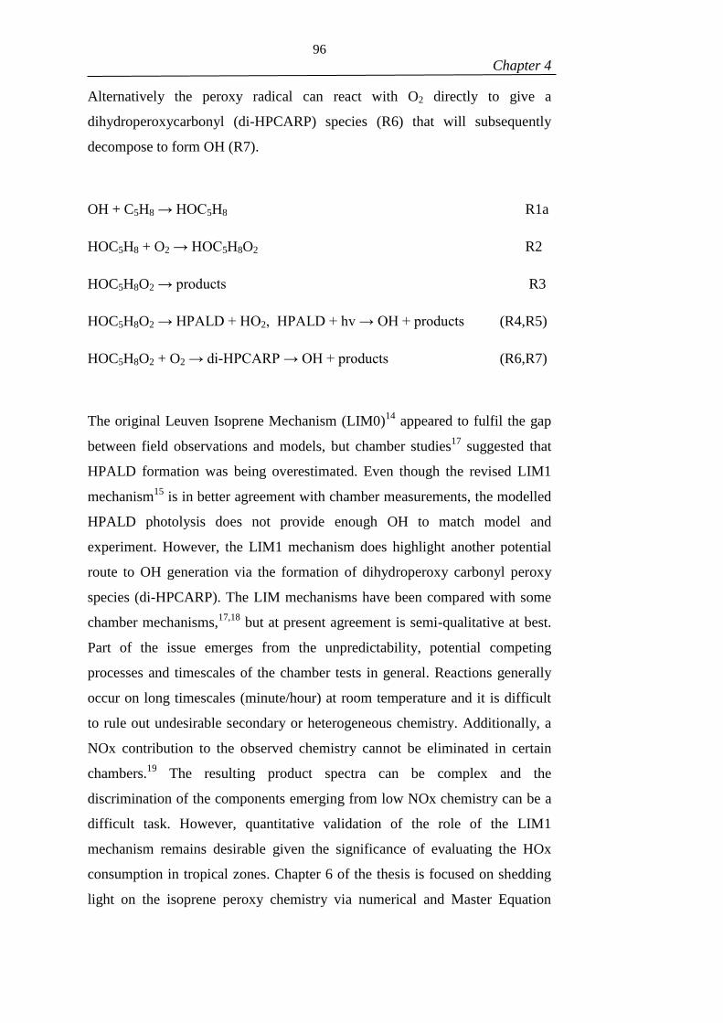
96

Chapter 4

Alternatively the peroxy radical can react with O2 directly to give a

dihydroperoxycarbonyl (di-HPCARP) species (R6) that will subsequently

decompose to form OH (R7).

OH + C5H8 → HOC5H8 R1a

HOC5H8 + O2 → HOC5H8O2 R2

HOC5H8O2 → products R3

HOC5H8O2 → HPALD + HO2, HPALD + hv → OH + products (R4,R5)

HOC5H8O2 + O2 → di-HPCARP → OH + products (R6,R7)

The original Leuven Isoprene Mechanism (LIM0)14

appeared to fulfil the gap

between field observations and models, but chamber studies17

suggested that

HPALD formation was being overestimated. Even though the revised LIM1

mechanism15

is in better agreement with chamber measurements, the modelled

HPALD photolysis does not provide enough OH to match model and

experiment. However, the LIM1 mechanism does highlight another potential

route to OH generation via the formation of dihydroperoxy carbonyl peroxy

species (di-HPCARP). The LIM mechanisms have been compared with some

chamber mechanisms,17,18

but at present agreement is semi-qualitative at best.

Part of the issue emerges from the unpredictability, potential competing

processes and timescales of the chamber tests in general. Reactions generally

occur on long timescales (minute/hour) at room temperature and it is difficult

to rule out undesirable secondary or heterogeneous chemistry. Additionally, a

NOx contribution to the observed chemistry cannot be eliminated in certain

chambers.19

The resulting product spectra can be complex and the

discrimination of the components emerging from low NOx chemistry can be a

difficult task. However, quantitative validation of the role of the LIM1

mechanism remains desirable given the significance of evaluating the HOx

consumption in tropical zones. Chapter 6 of the thesis is focused on shedding

light on the isoprene peroxy chemistry via numerical and Master Equation

97

Chapter 4

modelling of LFP-LIF data and provides a critical assessment of the LIM1

mechanism.

An alternative experimental approach to chamber studies is to monitor OH

recovery on millisecond timescales at higher temperatures utilizing direct

methods.20

Under these approaches, heterogeneous processes are diminished

while NOx contributions can be rigorously eliminated. However, in order to

favour the isomerization so that it is observable on the millisecond timescale,

high temperatures are necessary. As a consequence, the use of elevated

temperatures demands high oxygen concentrations to guarantee a significant

HOC5H8O2 concentration as reaction R2 reaches equilibrium. Quenching of the

fluorescence signal at the resulting high pressures and concentrations of O2

make conventional OH monitoring via laser induced fluorescence (LIF)21

difficult. However, with the use of the recently developed high pressure

instrument based on the FAGE technique, described in Chapter 2, such

measurements are possible. OH temporal profiles become multi-exponential

under the mentioned experimental conditions, with rapid preliminary OH loss

via reaction R1 followed by OH recycling. The recycling manifests in the

experimental traces as a visible change in the decay rate. Recycling parameters

can be extracted from such profiles more accurately if the initial OH decay can

be constrained to previously measured rate coefficient values for reaction R1,

but little high temperature literature data were available prior to the current

study, with no data above 420 K. The rate coefficient, k1, falls monotonically

over the range 250 – 420 K with increasing temperature, which is consistent

with an addition process. The highest reported measurements are at

410 - 420 K.22-24

The bimolecular view of the Lindemann mechanism for pressure dependent

processes presented in Chapter 2 is very useful for the understanding of the

chemistry of the OH + isoprene reaction. At low temperatures, reaction R1

occurs by means of a pressure dependent addition mechanism to the terminal

carbons (C1 and C4) due to a competition between the stabilization by

collisions with the bath gas, M, and the dissociation of the chemically activated

98

Chapter 4

HOC5H8 adduct (HOC5H8*) back to reactants (R-1a). This predominant route

is favoured by the formation of stabilized allylic radicals. At elevated

temperatures (T > 700 K), a hydrogen abstraction from the methyl (R1b) which

also forms an allylically stabilized radical, may contribute significantly.25

Even

though no previous studies of the abstraction channel of the isoprene + OH

reaction are available, this mechanism has been explored for similar species.25-

26 For example, the reaction of 2-methylpropene, an alkene that contains both

allylic and vinylic hydrogens, with OH radicals was investigated in the

theoretical work by Sun and Law.25

Their canonical variational transition-state

theory calculations27

suggest abstraction rate coefficients as fast as ~3.0 × 10-12

cm3 molecule

-1 s

-1 at 750 K.

OH + C5H8 M ↔ HOC5H8

(R1a,R–1a)

OH + C5H8 k1b → C5H7 + H2O (R1b)

At high pressures, the rate limiting step is isoprene + OH association (R1a) and

the high pressure limiting rate coefficient, , is equal to k1a. For such a large

system with a strongly bound adduct, the high pressure limit is reached at low

absolute pressures. However, at elevated temperatures the dissociation back to

reagents becomes competitive with collisional stabilization and the reaction

can exhibit a pressure dependence. The equilibrium constant characterized by

the competition between the adduct formation and unimolecular decomposition

can be linked in terms of the thermodynamics of the system, as indicated in

Equation E1.

k1a

k−1a

= K = e−∆G0

RT E1

The previous work on the kinetics of the OH + isoprene reaction indicates

excellent agreement. The IUPAC recommendation for the room temperature

rate coefficient of 1.0 × 10-10

cm3 molecule

-1 s

-1 is reported with errors of

~15%.4 The available measurements were undertaken via direct LFP methods

1k

99

Chapter 4

and also via the relative rate approach using different reference reactions. Even

though the high pressure limit of reaction R1 appears to be reached at 50 – 100

Torr at room temperature, some controversy regarding the onset of the pressure

independent region still remains. While Singh and Li28

(1 – 3 Torr He),

Chuong and Stevens24

(2-6 Torr He) and Dillon et al.29

(5 – 200 Torr N2 and

air) do not report a pressure dependence at such low pressures, two

measurements from the same research group, McGivern et al.30

(0.5 – 20 Torr

Ar) and Park et al. (2 – 8 Torr Ar) tested positive for this dependence. No

evidence of any role for the abstraction reaction at room temperature has been

reported in these studies.

The work of Hynes and co-workers31-32

appears as an exception to the general

consensus on . They have carried out two studies on the isoprene + OH

reaction, which included in situ measurements of isoprene concentrations, but

the measured room temperature rate coefficient is approximately 20% lower

than the IUPAC recommendation. The reason for the disagreement between

the work of Hynes and co-workers and the other studies (a selection of which

are presented in Table 1) is not fully elucidated, however, recent measurements

of the isoprene absorption cross section by Dillon et al.29

shed some light on

the observed discrepancies.

The objectives of the work presented in this chapter are: (I) to further

characterise the high pressure apparatus by comparison with the room

temperature rate coefficient for the OH + isoprene reaction, (II) to generate

new data on reaction R1 at the higher temperatures required to observe OH

recycling on a millisecond timescale (450 - 794 K), (III) to experimentally

define a value for the well depth of the HOC5H8 adduct via an innovative

analytical approach based on ME calculations, (IV) to investigate whether

there is evidence for OH abstraction from isoprene and finally (V) to use the

MESMER programme33

to compare previous measurements of reaction R1

obtained from the literature.34

1k

100

Chapter 4

4.2 METHODOLOGY

4.2.1 - Laser flash photolysis experiments with detection by laser induced

Fluorescence (LFP-LIF)

Isolated kinetic studies for the reactions of isoprene with OH were performed

with the use of laser flash photolysis and detection of OH radicals by laser-

induced fluorescence (LFP-LIF)35-36

using both a conventional low pressure

pressures (p = 50 – 150 Torr) LFP-LIF instrument and a recently developed

instrument, capable of operating at high pressures (~5 atm maximum pressure)

and temperatures (~ 750K maximum temperature). Additional details on the

operation of these apparatus can be found in the literature.37

Experiments were

carried out under conditions where OH was lost by a simple pseudo-first-order

process and also at sufficiently high temperatures such that direct equilibration

between OH/VOC and the OH-VOC adducts was observed. Such experiments

provide strong constraints on the thermochemistry of the reactions.38

A mixture of OH precursor, H2O2 (50% (w/w) Sigma Aldrich), isoprene

(Sigma Aldrich, >99%) and nitrogen bath gas were flowed through the reaction

cell. OH radicals were generated along the flow tube by pulsed excimer laser

(Lambda Physik, Compex 200) photolysis at 248 nm. Alternatively, a limited

number of experiments implemented a YAG laser (Quantel, Q-smart laser) at

266 nm to generate OH radicals from H2O2 photolysis. These 266 nm

experiments represent a good check to ensure the independence of the

measured kinetics to the potential photolysis of isoprene.

In the high-pressure setup, isoprene/N2 mixtures were manometrically made up

in stainless steel high-pressure cylinders of 10 litres and left to mix 48 hours

before use. In the low-pressure instrument, isoprene was prepared as a diluted

mixture (~10%) in N2 stored in 5 litre darkened bulbs. The concentration of

isoprene in the reactor was determined by the composition of the isoprene/N2

mixture, the flow rates measured with calibrated mass flow controllers, and the

total pressure in the corresponding reactor.

101

Chapter 4

As described in Chapter 2, while the high pressure instrument employs a low-

pressure detection cell, in the conventional LFP-LIF instrument the flowing

gas is probed within the reaction cell. In both cases, OH is interrogated by a

pulsed beam from a Spectron dye laser operating on the dye rhodamine,

pumped by a YAG laser. Experiments were typically performed with a

repetition rate of 5 Hz, although checks were undertaken to ensure the

observed kinetics were independent of this rate. As another instrumental check,

tertiary-butyl hydroperoxide was used as the OH precursor in a limited number

of measurements at 298 K to verify whether the measured coefficients are

independent of the implemented precursor.

Proton-transfer reaction time of flight mass spectrometry (Kore Technology,

Series I PTR-TOF-MS), was implemented for a tentative detection of the

product of the allylic hydrogen abstraction during a few experiments. For this

purpose, the exhaust gas from the high pressure apparatus was vented to

atmospheric pressure and subsequently sampled into the PTR-TOF-MS

spectrometer.

As indicated previously, all the analysis presented in this thesis relies to some

degree on Master Equation modelling. These calculations require information

about the species involved, including vibrational frequencies, rotational

constants and relative potential energies. This information was obtained via

theoretical computations, and the main details of the calculations are presented

below, prior to a discussion of the measured rate coefficients.

102

Chapter 4

4.2.2 - Computational Methods: Ab initio Calculations and Master

Equation (ME) Modelling

Structures of reactants and products were computed with the modern DFT

functional M06-2X39

and a large basis set (6-311++G(3df,2p)).40

Structure

optimizations were carried out using the Gaussian 09 D.01 programme suite41

,

with the use of analytical gradients and the Berny algorithm42-43

in redundant

internal coordinates. High performance coupled cluster calculations with

single, double and triple excitations, the latter treated perturbatively

(CCSD(T)),44

were implemented to calculate single point energies of

M06-2X/6-311++G(3df,2p) optimized geometries. For a more accurate

evaluation of the potential energy surface (PES), the single point energies were

extrapolated to the complete basis set limit (CBS) using the extrapolation

scheme presented by Helgaker et al.45

and Truhlar’s calendar basis sets (Jun-

cc-pVXZ, X=D,T,Q).46-47

These basis set variations are constructed by

removing diffuse functions from the analogue fully augmented basis set

(aug-cc-pVXZ). More specifically, the Jun-cc-pVXZ basis sets remove the

diffuse functions from H and He atoms and also remove the highest angular

momentum diffuse functions from all the other atoms. A slight deviation from

the original formulation of the calendar basis sets is considered by Gaussian 09

since by default, s and p diffuse functions are always introduced. In the

extrapolation scheme presented by Helgaker et al., the Hartree-Fock (HF) and

the correlation energies are extrapolated separately, according to equations E2

and E3. The employed Hartree-Fock extrapolation scheme was originally

presented by Feller et al.48

HF(X)=HFCBS + b×exp(-cX) E2

ECORR(X)=ECORR(CBS) + αX -3

E3

where HF(X) is the Hartree-Fock energy calculated with the jun-cc-pVXZ

basis set. X is the cardinal number for the corresponding basis set (2=D, 3=T,

4=Q). The CBS limit extrapolated Hartree-Fock energy (HFCBS), b and c are

parameters obtained from solving the 3×3 system of HF equations. ECORR(X) is

the correlation energy calculated at the CCSD(T)/Jun-cc-pVXZ level of theory.

103

Chapter 4

ECORR(CBS) corresponds to the CBS limit correlation energy and α is a floated

parameter.

Zero-point energies, force-constant matrices, vibrational frequencies and

rotational constants, required inputs for the ME calculations were computed at

the M06-2X/6-311++G(3df,2p) level as expensive CCSD(T) calculations

would be computationally prohibitive.49

However, the use of the M06-2X

functional coupled with an extensive basis set has been considered appropriate

for the study of the isoprene + OH reaction in the presence of O215

, and the

photolysis of important products of this reaction, such as HPALDs.50

Harmonic vibrational frequencies were corrected with a scaling factor of

0.983, following the recommendation for a similar methodology (M06-2X/6-

311++G(d,p)).51

The calculated enthalpies of reaction with respect to the OH

additions to carbons C1 and C4, presented in section 4.4.1, were used for a

comparison with experimental determinations presented in section 4.4.5.

The approximation of the harmonic oscillator was used for the majority of the

vibrational frequencies in the calculation of the densities of states. However,

due to the structures of the stabilized allylic radicals, a few vibrational

frequencies of isoprene, and the resulting adducts, are better represented by the

hindered rotor approximation. For example, the >C1=C2< double bond in the

isoprene structure has a single-bond analogue in the product structure, which

provides an augmented torsional degree of freedom to the molecule, with

respect to this bond. Figure 4.1 shows all the torsions that were described with

the hindered rotor approximation for both isoprene and the two most stable

isoprene-OH adducts considered in the analysis. The descriptions of these

hindered rotors were obtained through 360° relaxed scans of the dihedral angle

respective to the specific rotation, with steps of 15°. Restricted optimizations at

the M06-2X/6-311++G(3df,2p) level were applied at each step. In order to

avoid inconsistencies in the number of degrees of freedom of species in the

ME calculations, the description of a hindered rotor requires the removal of a

corresponding vibrational frequency. MESMER uses the projection method

proposed by Sharma et al.52

to define the mode related to the internal rotation.

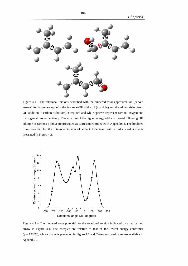
104

Chapter 4

Figure 4.1 - The rotational torsions described with the hindered rotor approximation (curved

arrows) for isoprene (top left), the isoprene-OH adduct 1 (top right) and the adduct rising from

OH addition to carbon 4 (bottom). Grey, red and white spheres represent carbon, oxygen and

hydrogen atoms respectively. The structure of the higher energy adducts formed following OH

addition at carbons 2 and 3 are presented as Cartesian coordinates in Appendix 3. The hindered

rotor potential for the rotational torsion of adduct 1 depicted with a red curved arrow is

presented in Figure 4.2.

-250 -200 -150 -100 -50 0 50 100 150

0

2

4

6

8

10

12

14

Rel

ati

ve p

ote

nti

al

ener

gy

/ k

J m

ol-1

Rotational angle () / degrees

Figure 4.2 – The hindered rotor potential for the rotational torsion indicated by a red curved

arrow in Figure 4.1. The energies are relative to that of the lowest energy conformer

(ϕ = 123.2°), whose image is presented in Figure 4.1 and Cartesian coordinates are available in

Appendix 3.

105

Chapter 4

4.3 DATA ANALYSIS

4.3.1 - Single Exponential Traces

At temperatures below 650 K, OH reacted under pseudo-first-order conditions

via a simple removal process; in this regime, the concentration of OH as a

function of time is given by:

[OH]t=[OH]

0e−k1

't E4

where k1' is the pseudo-first-order rate coefficient given by:

k1' = k1[C5H8] + k1st E5

Here k1 is the bimolecular rate coefficient for reaction R1 and k1st represents

the rate coefficient for the loss processes due to diffusion and reaction of OH

with the constant concentration of precursor, kp. As the OH LIF signal is

proportional to [OH], the [OH] in E4 can be replaced by the OH LIF signal and

the resulting exponential fit (inset to Figure 4.3) to the LIF data, returns k1'.

Under these conditions, a plot of k1' vs [C5H8] should give a straight line, as

shown in Figure 4.3, where the gradient is k1 and the intercept is the sum of the

first order loss processes. The resulting k1 rate coefficients are summarised in

Table 4.1, where N2 was implemented as the bath gas for all measurements.

Table 4.1 - Experimental Determinations of k1 from Single Exponential Decays

T / K p / Torr k1 × 1011

/ cm3

molecule-1

s-1 a

T / K p / Torr k1 × 1011

/ cm3

molecule-1

s-1 a

298 1290 9.90 ± 0.14 473 99 4.98 ± 0.36

298 1365 10.01 ± 0.12 475 1394 5.61 ± 0.50

298 96b

10.60 ± 0.36 477 128 5.3 ± 1.0

298 56 10.40 ± 0.32 478 114 6.12 ± 0.36

337 57 8.28 ± 0.22 508 1673 5.7 ± 1.2

406 1367 6.68 ± 0.54 533 132 4.91 ± 0.24

417 1497 7.2 ± 1.6 540 141 5.27 ± 0.36

418 1418 6.24 ± 0.34 564 1350 4.74 ± 0.44

426 103 5.56 ± 0.26 573 51 4.4 ± 1.1

433 1546 6.0 ± 1.5 618 1536 3.99 ± 0.46

472 99 5.81 ± 0.86 630 1373 4.71 ± 0.56

a – Errors are 2. b – Data where p<150 Torr were recorded on the low pressure, conventional

LFP/LIF apparatus. Other data were from the high pressure apparatus.

106

Chapter 4

0.0 0.2 0.4 0.6 0.8 1.0 1.2

0

10000

20000

30000

40000

50000

60000

70000

80000

-200 0 200 400 600 800 1000

2

4

6

8

10

k1(O

2) = (6.1 0.2) 10

-11 cm

3 molecule

-1 s

-1

Absence of O2

Presence of O2

k' / s

-1

[Isoprene] / 1015

molecule cm-3

k1(no O

2) = (5.8 0.3) 10

-11 cm

3 molecule

-1 s

-1

OH

Sig

na

l / A

rbri

tra

ry U

nit

s

Time / s

Figure 4.3 - Bimolecular plot for Reaction 1 at T = 406 K and p = 2 atm of N2. The inset shows

a typical single exponential decay, generated with [C5H8] = 1.00 × 1014

molecule cm-3

and [O2]

= 7.70 × 1018

molecule cm-3

. The points presented in the inset were averaged after 4 scans.

Error bars and uncertainties in the bimolecular plot are at the 2σ level. Red circles represent

data acquired in the presence of oxygen and black squares represent data in absence of O2.

Figure 4.4 – Residual plot for the single exponential fit of trace presented in Figure 4.3 at T =

406 K and p = 2 atm of N2, [C5H8] = 1.00 × 1014

molecule cm-3

and [O2] = 7.70 × 1018

molecule cm-3

.

0 250 500 750 1000

-1

0

1

OH

Sig

nal

/ A

bri

trar

y U

nit

s

t / 10-6 s

107

Chapter 4

The bimolecular rate coefficients included in Figure 4.3 show that, considering

the uncertainties, no significant difference is observed with the addition of O2

to the system. Furthermore, the small errors evidence the good quality of

experimental data collected for this work.

4.3.2 - High Temperature Equilibrium Traces

At high enough temperatures (T >700 K), the rates of decomposition of the

OH-C5H8 adducts (R-1a) become comparable with that of the forward addition

of OH to isoprene and the OH decays become multi-exponential in nature (see

Figure 4.5 for an example). The obtained equilibrium traces were analysed by

fitting to the chemical scheme S4.1:

S4.1

where C5H8-OH represents the OH-isoprene adducts. As will be reported in

section 4.4.4, additions to the C2 and C3 carbons are negligible and can be

ignored. A kinetic scheme incorporating two adducts would be a tri-

exponential decay, but if the properties of the adducts are similar, then the

decays can be well approximated by a biexponential decay. As expected, the

experimental data were not better fitted with a tri-exponential equation, so our

data were analysed based on models derived from Scheme S1; the role of both

adducts 1 and 4 is assessed via MESMER modelling in Section 4.4.

The analytical solution of the temporal evolution of the OH concentration in

scheme S4.1 is described by the bi-exponential equation E6:

108

Chapter 4

OH(t)=OH0(-k

'

OH - λ

-

λ+-λ-

(exp(λ+t) - exp(λ-t))+ exp(λ-t)) + b E6

where λ-,+=-(k'

OH+k3)±√(k'OH+k3)

2 – 4(k

'OH k3-k

'1a×k

-1a)

2, k

'OH= k

'1a+ k

'D, and

k3= k-1a. k'1a is the pseudo-first order rate coefficient for the addition channel

of reaction R1, k'D is the sum of the pseudo-first order OH losses besides

addition, kD = k1st + k1b', where k1st is the sum of the OH reaction with the

precursor (kp[H2O2]) and diffusion, (which is small compared to kp[H2O2]).

k'1b is the rate coefficient of the hydrogen abstraction channel of reaction R1

and is equal to k1b [C5H8]. b is equal to the signal when no OH is present. For

each temperature and pressure, k1st was measured prior to the OH-trace

acquisition with added isoprene; k1st was fixed to its measured value in the data

fitting procedure. b was determined for each trace by recording points before

time zero.

Over the temperature range 729 – 794 K, a total of 28 traces were recorded that

exhibited equilibrium behaviour. Figure 4.5 clearly demonstrates non-single

exponential behaviour at 729 K and 130 Torr of N2. The red line is a fit using

equation E6 to the data, and as can be seen, it provides an excellent description

of OH temporal behaviour. From equation E6, is the numerically larger

reciprocal time constant and is approximately equal to k'1 and the smaller

reciprocal time constant, is approximately equal to kD + k'1b. In Figure 4.5,

the green line is the significantly poorer fit when the abstraction channel, k'1b,

is set to zero. It is evident that abstraction, or some other loss process, is

required in order to describe the chemistry of the system; this abstraction

channel is discussed in Sections 4.4.3 and 4.4.4. Therefore, the parameters k1a,

k-1a and k1b along with the initial OH signal are required to provide a good fit

to the data

In order to reliably determine the parameters, all the equilibrium traces were

simultaneously analysed via a global non-linear multi-temperature least-

squares fit procedure, using the OriginPro 2016 software.53

For the global

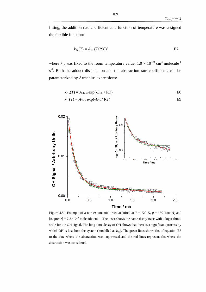
109

Chapter 4

fitting, the addition rate coefficient as a function of temperature was assigned

the flexible function:

k1a(T) = A1a (T/298)n

E7

where k1a was fixed to the room temperature value, 1.0 × 10-10

cm3 molecule

-1

s-1

. Both the adduct dissociation and the abstraction rate coefficients can be

parameterized by Arrhenius expressions:

k-1a(T) = A-1a × exp(-E-1a / RT) E8

k1b(T) = A1b × exp(-E1b / RT) E9

Figure 4.5 - Example of a non-exponential trace acquired at T = 729 K, p = 130 Torr N2 and

[isoprene] = 2.3×1014

molecule cm-3

. The inset shows the same decay trace with a logarithmic

scale for the OH signal. The long-time decay of OH shows that there is a significant process by

which OH is lost from the system (modelled as k1b). The green lines shows fits of equation E7

to the data where the abstraction was suppressed and the red lines represent fits where the

abstraction was considered.

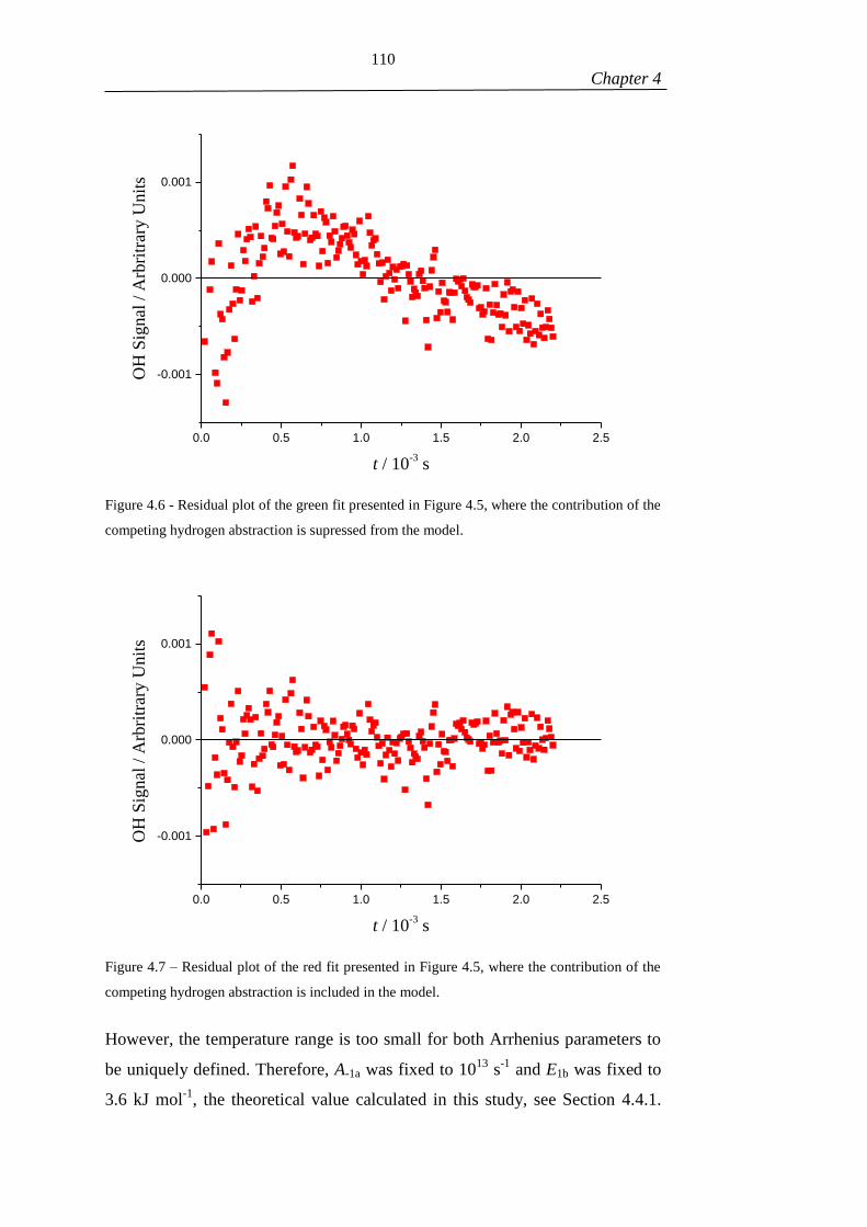
110

Chapter 4

Figure 4.6 - Residual plot of the green fit presented in Figure 4.5, where the contribution of the

competing hydrogen abstraction is supressed from the model.

Figure 4.7 – Residual plot of the red fit presented in Figure 4.5, where the contribution of the

competing hydrogen abstraction is included in the model.

However, the temperature range is too small for both Arrhenius parameters to

be uniquely defined. Therefore, A-1a was fixed to 1013

s-1

and E1b was fixed to

3.6 kJ mol-1

, the theoretical value calculated in this study, see Section 4.4.1.

0.0 0.5 1.0 1.5 2.0 2.5

-0.001

0.000

0.001

OH

Sig

nal

/ A

rbri

trar

y U

nit

s

t / 10-3 s

0.0 0.5 1.0 1.5 2.0 2.5

-0.001

0.000

0.001

OH

Sig

nal

/ A

rbri

trar

y U

nit

s

t / 10-3 s

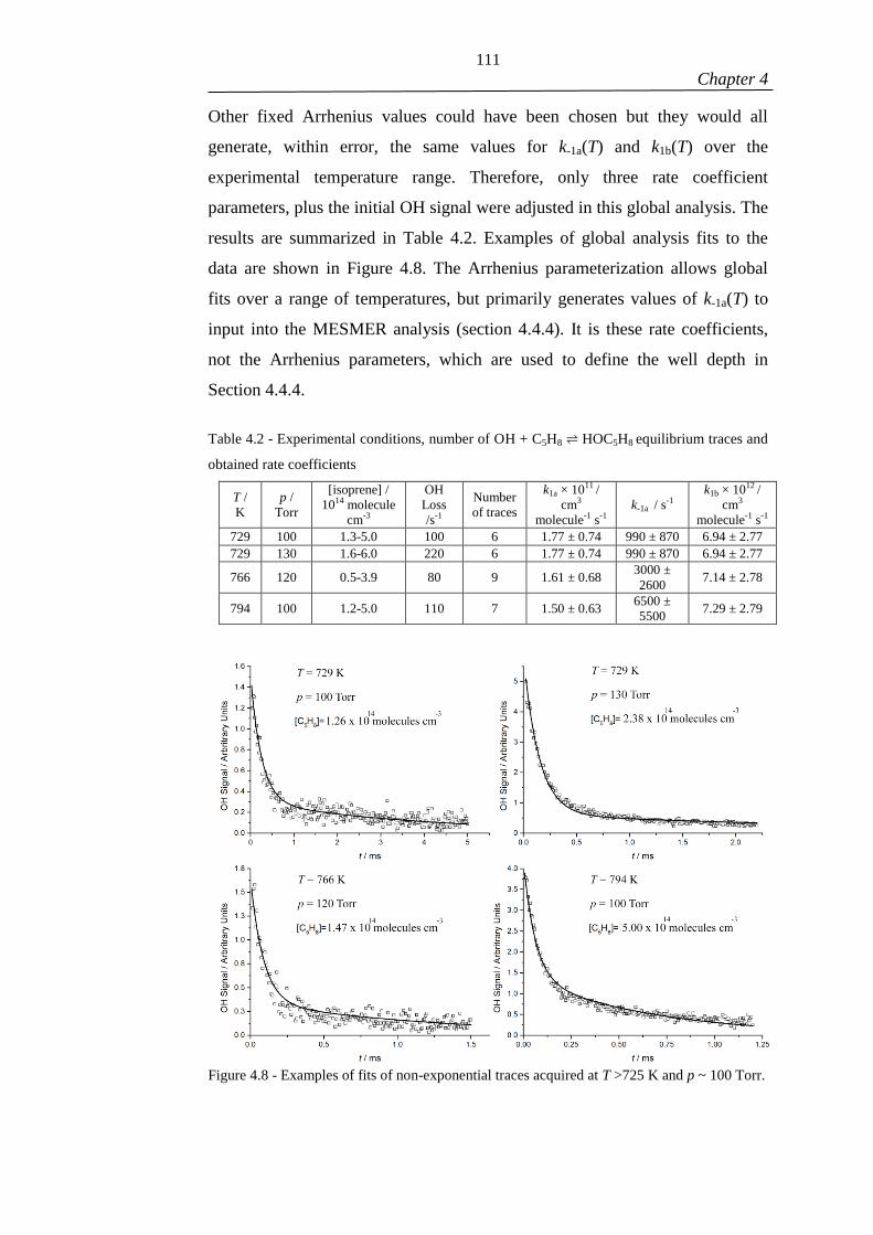
111

Chapter 4

Other fixed Arrhenius values could have been chosen but they would all

generate, within error, the same values for k-1a(T) and k1b(T) over the

experimental temperature range. Therefore, only three rate coefficient

parameters, plus the initial OH signal were adjusted in this global analysis. The

results are summarized in Table 4.2. Examples of global analysis fits to the

data are shown in Figure 4.8. The Arrhenius parameterization allows global

fits over a range of temperatures, but primarily generates values of k-1a(T) to

input into the MESMER analysis (section 4.4.4). It is these rate coefficients,

not the Arrhenius parameters, which are used to define the well depth in

Section 4.4.4.

Table 4.2 - Experimental conditions, number of OH + C5H8 ⇌ HOC5H8 equilibrium traces and

obtained rate coefficients

T /

K

p /

Torr

[isoprene] /

1014 molecule

cm-3

OH

Loss

/s-1

Number

of traces

k1a × 1011 /

cm3

molecule-1 s-1

k-1a / s-1

k1b × 1012 /

cm3

molecule-1 s-1

729 100 1.3-5.0 100 6 1.77 ± 0.74 990 ± 870 6.94 ± 2.77

729 130 1.6-6.0 220 6 1.77 ± 0.74 990 ± 870 6.94 ± 2.77

766 120 0.5-3.9 80 9 1.61 ± 0.68 3000 ±

2600 7.14 ± 2.78

794 100 1.2-5.0 110 7 1.50 ± 0.63 6500 ±

5500 7.29 ± 2.79

Figure 4.8 - Examples of fits of non-exponential traces acquired at T >725 K and p ~ 100 Torr.

112

Chapter 4


4.4.1 - Ab initio calculations

Figure 4.9 shows the potential energy surface for OH addition and H-

abstraction from isoprene at the CCSD(T)/CBS//M06-2X/6-311++G(3df,2p)

level of theory. OH addition to C2 or C3 carbons produces adducts with

significantly higher energies as there is no allylic stabilization of the resulting

radicals. The energy difference between the C1 and C4 adducts is

approximately 10 kJ mol-1

(in good agreement with previous literature, see

Table 4.3) and small compared to the total well depth. Whilst Table 3 shows

that there is some variation in the absolute well-depths from various ab initio

calculations, the energy difference between the two lowest energy adducts is

very consistent at (10.1 ± 0.4) kJ mol-1

. In the subsequent MESMER analysis

assessing the role of both adducts, the energy difference is fixed to our

calculated value (10.1 kJ mol-1

), but the absolute well depth of the C1 adduct is

allowed to float. The barrier for the abstraction reaction is calculated to be 3.6

kJ mol-1

.

Figure 4.9 - The potential energy diagram for the OH addition to isoprene. Relative energies

were calculated at the CCSD(T)/CBS//M06-2X/6-311++G(3df,2p) level and include zero-point

energy corrections.

113

Chapter 4

Table 4.3 - Theoretically calculated well-depths for the isoprene + OH reaction with respect to

the additions at carbons 1 and 4. All well-depths are corrected for zero-point energies

Methodology Reference

Well-depth

adduct C1 /

kJ mol-1

Well-depth

adduct C4 /

kJ mol-1

Energy

Difference

between

adducts/

kJ mol-1

CCSD(T)/CBS//M06-2X/6-

311++G(3df,2p) This work 154.1 144.0 10.1

CCSD(T)/6-311G**//

B3LYP/6-31G Lei et al.

54 145.6 135.1 10.5

roQCISD(T)/6-31++G**//

B3LYP/6-311++G**

Greenwald et

al.55

156.1

a 146.4 9.7

PMP4-(SDTQ)/6-311G**//

MP2/6-311G**+∆ZPE/

B3LYP/6-31G**

Stevens et

al.56

158.6 148.1 10.5

CBS-APNO Peeters et

al.14

163.2 153.6 9.6

a –including basis set correction at the roMP2 level of theory

The CCSD(T) method implemented in this work is known for accurately

computing molecular properties and energies44, 49, 57

and is often referred to as

“Gold Standard” of computational chemistry.58

Our calculated well-depth

differs from that obtained by Lei et al.54

by 8.5 kJ mol-1

, who have

implemented a similar methodology. The use of smaller basis sets for the

calculations of single point energies and structural optimizations as a

computational constraint (6-311G** 59-66

and 6-31G64, 67-75

respectively)

contributes to the observed well-depth discrepancy. London dispersion forces

which are accounted for at the M06-2X level, and neglected by the B3LYP 76-

79 functional also contribute to the discrepancy.

Greenwald et al.55

, have applied the restricted open-shell quadratic

configuration interaction (CI) technique, with perturbative triple excitations44,

80 to study the isomeric branching of the isoprene + OH reaction. In this

correlated method, quadratic terms are included in the configuration

coefficients to correct for size consistency. The authors have done a very

114

Chapter 4

careful study when obtaining the stationary structures of the four possible

isoprene-OH adducts. They have located 58 different local minima for the

adducts at the B3LYP/6-311++G** level, and implemented the lowest energy

conformations in subsequent roQCISD(T) computations. The

roQCISD(T)/6-31++G**// B3LYP/6-311++G** methodology was validated

against previous calculations on the ethylene-OH case, where the well-depth

was calculated to within ~3.35 kJ mol-1

.55, 81

They also report that the relative

well-depths obtained at the PMP4(SDTQ)/6-311G**// B3LYP/6-311++G**

level of theory are qualitatively aligned with those computed at the superior

roQCISD(T)/6-31++G**//B3LYP/6-311++G** level.

Stevens et al.56

have used the less computationally demanding fourth-order

Møller-Plesset perturbation theory with single, double, triple and quadruple

excitations and spin projection (PMP4(SDTQ)) to investigate the OH addition

to isoprene. In the Møller-Plesset perturbation theory, the Hartree-Fock

wavefunction is corrected for electron correlation by a combination with

configurational functions, originated from single, double, triple, etc.

excitations.82-83

In their study, PMP4(SDTQ)/6-311G** single point energies

computed for MP2/6-311G** optimized structures were subsequently

corrected with zero-point energies calculated at the B3LYP/6-31G** level.

Their calculations show a well-depth only 2.51 kJ mol-1

deeper than that

reported by Greenwald et al.

Peeters et al. have employed the Complete Basis Set method CBS-APNO84

to

compute electronic energies while investigating the regeneration of HOx in the

oxidation of isoprene.14

The authors have verified that the CBS-APNO method

systematically overestimated the well-depth of the CH2=CH‒ĊH2 + O2 and for

this reason, a correction of 4.18 kJ mol-1

has been applied. This fact suggests

that the reported isoprene + OH well-depth might also be slightly

overestimated by the CBS-APNO method.

115

Chapter 4

4.4.2 - Rate Coefficients for the OH + Isoprene Reaction, R1

Figure 4.3 shows an example of a typical experimental decay (inset) and

bimolecular plot obtained at 406 K and 2 atm of nitrogen bath gas. Checks

were carried out to ensure that the rate coefficients were invariant (within

experimental error) of laser energy density (15 – 50 mJ cm-2

) or repetition rate

(1 – 10 Hz). Below 400 K, the addition of oxygen had no effect on the

measured rate coefficient for reaction R1 as can be seen from Figure 4.3.

Experiments in the presence of oxygen at temperatures > 450 K, where OH

recycling was observed, will be presented in a subsequent chapter focused on

the validation of the LIM1 mechanism.

A major issue when sampling the monitored species prior to detection, is

whether the transit time from the sampling pinhole to detection influences the

kinetic measurements.21, 85-87

In this study room temperature pseudo-first-order

rate coefficients of up to 70,000 s-1

are in excellent agreement with the

literature data. At higher first order rate coefficients, the influence of transport

can be observed, but can potentially be accounted for with a biexponential

analysis.85

None of the measurements reported in this study required such

corrections, i.e. transport is effectively instantaneous on the timescales of the

chemical reaction. The analysis of the exponential decays is inset a few points

to allow for the ~20 μs transport time.

Figure 4.10 illustrates the observed temperature dependence of k1 from 298 –

794 K. In addition to varying the temperature, the pressure was also varied to

ensure that measurements were always being made at the high pressure limit,

i.e. that the observed bimolecular rate coefficients correspond to k1∞. No

evidence for any pressure dependence was observed from 50 – 1670 Torr for

the 298 – 650 K temperature range and these observations were consistent with

the modelling discussed in the subsequent sections. Measurements performed

at T ≥725 K and p ~100 Torr are located in the fall-off region. For example, at

794 K, with k1a, 794K = (1.50 ± 0.63) × 10-11

cm3 molecule

-1 s

-1, our

measurements are ~40% lower than our best estimate for k1a∞

at that

temperature (2.49 × 10-11

cm3 molecule

-1 s

-1).

Excellent agreement is observed

116

Chapter 4

between the measurements performed with the high and low-pressure

instruments, as evidenced by the proximity of the black and blue triangles in

Figure 4.10.

A least-squares fit to the combined experimental data from both apparatus of

the form k1∞

= A (T

298 K)−n

gives:

k1∞

= (10.4 ± 0.4) × 10-11

(T

298 K)−1.34 ± 0.12

cm3 molecule

-1 s

-1 E10

where errors are at the 2σ level. The negative temperature dependence is

consistent with previous literature and is dominated by the addition reaction;

however, this work considerably extends the range of temperatures studied. A

full discussion on the values of k1 is presented in Section 4.5.

Figure 4.10 - Comparison of experimental measurements using the high pressure instrument

(black squares), measurements at the high pressure limit with a conventional low-pressure

instrument (blue triangles) and at the fall-off region (red circles). The dotted line shows the

IUPAC recommendation for the temperature dependence of the isoprene + OH reaction, the

dashed line shows our best estimate for the high-pressure limit k1∞, which was obtained from a

ME from this work and selected data as will be discussed in section 4.4.5. The continuous line

represents k1∞ as obtained based purely on our measurements. Errors are statistical at the 2σ

level.

117

Chapter 4

As can be seen from Table 4.4, the room temperature rate coefficients for

reaction R1 are in excellent agreement with the IUPAC recommendation and

the bulk of the experimental literature providing evidence that the new

apparatus works well and can generate reliable rate coefficients.

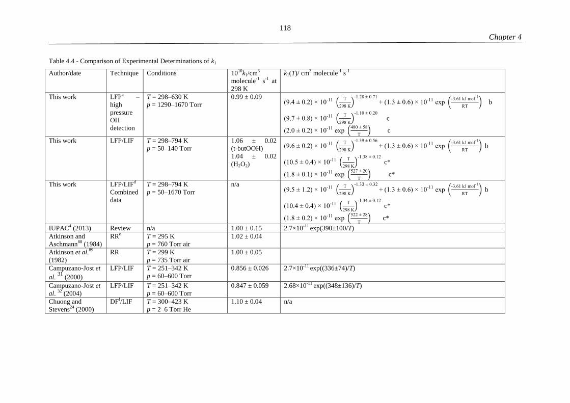
118

Chapter 4

Table 4.4 - Comparison of Experimental Determinations of k1

Author/date Technique Conditions 1010

k1/cm3

molecule-1

s-1

at

298 K

k1(T)/ cm3 molecule

-1 s

-1

This work LFPa –

high

pressure

OH

detection

T = 298–630 K

p = 1290–1670 Torr

0.99 ± 0.09 (9.4 ± 0.2) × 10-11 (

T

298 K)

-1.28 ± 0.71

+ (1.3 ± 0.6) × 10-11 exp (-3.61 kJ mol

-1

RT)

b

(9.7 ± 0.8) × 10-11 (T

298 K)

-1.10 ± 0.20

c

(2.0 ± 0.2) × 10-11 exp (480 ± 58

T)

c

This work LFP/LIF T = 298–794 K

p = 50–140 Torr

1.06 ± 0.02

(t-butOOH)

1.04 ± 0.02

(H2O2)

(9.6 ± 0.2) × 10-11 (T

298 K)

-1.39 ± 0.56

+ (1.3 ± 0.6) × 10-11 exp (-3.61 kJ mol

-1

RT) b

(10.5 ± 0.4) × 10-11 (T

298 K)

-1.38 ± 0.12

c*

(1.8 ± 0.1) × 10-11 exp (527 ± 20

T)

c*

This work LFP/LIFd

Combined

data

T = 298–794 K

p = 50–1670 Torr

n/a (9.5 ± 1.2) × 10-11 (

T

298 K)

-1.33 ± 0.32

+ (1.3 ± 0.6) × 10-11 exp (-3.61 kJ mol

-1

RT) b

(10.4 ± 0.4) × 10-11 (T

298 K)

-1.34 ± 0.12

c*

(1.8 ± 0.2) × 10-11 exp (522 ± 28

T) c*

IUPAC4 (2013) Review n/a 1.00 ± 0.15 2.7×10

-11 exp(390±100/T)

Atkinson and

Aschmann88

(1984)

RRe

T = 295 K

p = 760 Torr air

1.02 ± 0.04

Atkinson et al.89

(1982)

RR T = 299 K

p = 735 Torr air

1.00 ± 0.05

Campuzano-Jost et

al. 31

(2000)

LFP/LIF T = 251–342 K

p = 60–600 Torr

0.856 ± 0.026 2.7×10-11

exp((336±74)/T)

Campuzano-Jost et

al. 32

(2004)

LFP/LIF T = 251–342 K

p = 60–600 Torr

0.847 ± 0.059 2.68×10-11

exp((348±136)/T)

Chuong and

Stevens24

(2000)

DFf/LIF T = 300–423 K

p = 2–6 Torr He

1.10 ± 0.04 n/a

119

Chapter 4

Chuong and

Stevens (2002)90

DF/LIF T = 300 K

p = 100-150 Torr Ar

1.08 ± 0.05

Dillon et al.91

(2017)

LFP/LIF T = 241–356 K

p = 5–200 Torr (N2 or air)

0.93 ± 0.04 (1.93±0.08)×10-11

exp((446±12)/T)

Edney et al.92

(1986)

RR T = 297 K

p = 1 atm air

1.01 ± 0.02

Gill and Hites93

(2002)

RR T = 298–363 K

p = 1 atm He

1.01 ± 0.19 2.54×10-11

exp((409±42)/T)

Hites and Turner23

(2009)

RR/MSg

T = 323–413 K

p = 1 atm

n/a 4.0×10-11

exp((249±20)/T)

Iida et al.94

(2002) RR T = 298 K

p = 760 Torr air

1.04 ± 0.04

Karl et al.95

(2004) GC / LIFh

T = 294 K

p = 760 Torr air

1.00 ± 0.12

Kleindienst et al.22

(1982)

FP/RF T = 297– 23 K

p = 50–200 Torr Ar

0.93 ± 0.15 2.36×10-11

exp((409±28)/T)

McGivern et al.30

(2000)

LFP/LIF T = 295 K

p = 0.5–20 Torr Ar

0.99 ± 0.05

McQuaid et al.96

(2002)

RR T = 298 K

p = 760 Torr air

1.11 ± 0.23

Ohta 97

(1983) RR T = 297 K

p = 760 Torr air

0.990 ± 0.027

Park et al.98

(2004) LFP/LIF T = 279 – 336 K

p = 1-8 Torr

1.08 ± 0.19

(3.49±0.46) ×10-11

exp((366±40)/T)

Poppe et al.99

(2007)

LIF / MS /

GCh

T = 295 K

p = 760 Torr

1.02 ± 0.09

Singh and Li28

(2007)

RR/DF/

MS

T = 240 – 340

p = 1-3 Torr He

1.04 ± 0.19 2.3×10-11

exp((444±27)/T)

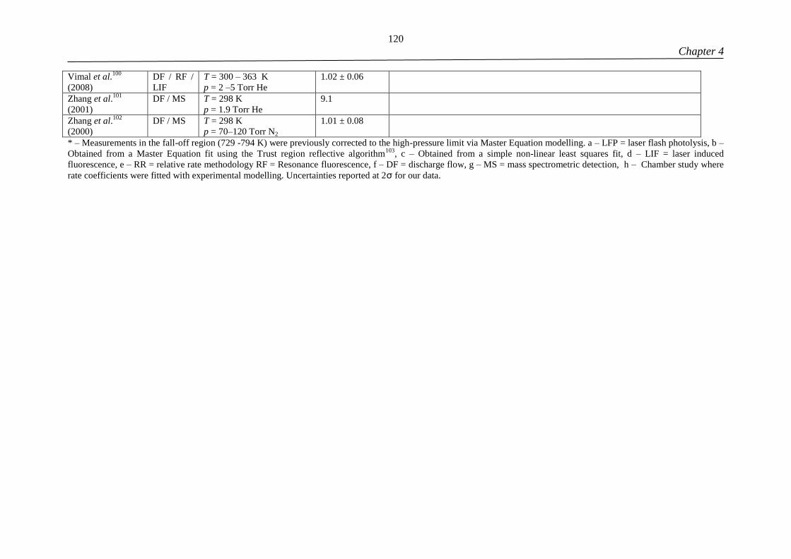
120

Chapter 4

Vimal et al.100

(2008)

DF / RF /

LIF

T = 300 – 363 K

p = 2 –5 Torr He

1.02 ± 0.06

Zhang et al.101

(2001)

DF / MS T = 298 K

p = 1.9 Torr He

9.1

Zhang et al.102

(2000)

DF / MS T = 298 K

p = 70–120 Torr N2

1.01 ± 0.08

* – Measurements in the fall-off region (729 -794 K) were previously corrected to the high-pressure limit via Master Equation modelling. a – LFP = laser flash photolysis, b –

Obtained from a Master Equation fit using the Trust region reflective algorithm103

, c – Obtained from a simple non-linear least squares fit, d – LIF = laser induced

fluorescence, e – RR = relative rate methodology RF = Resonance fluorescence, f – DF = discharge flow, g – MS = mass spectrometric detection, h – Chamber study where

rate coefficients were fitted with experimental modelling. Uncertainties reported at 2σ for our data.

121

Chapter 4

4.4.3 - The Abstraction Channel R1b

From Figure 4.5, the fact that the green line fit (no abstraction) to the data is a

much worse fit than the red line fit (with abstraction) is a strong evidence that

there is another loss process for OH in reaction R1. Abstraction is invoked to

explain this behaviour as it is has been observed in many other OH + alkene

reactions and our calculations predict an abstraction barrier consistent with

both our observations and those of other studies, see below. A good example is

the reaction between OH and C2H4, where the abstraction becomes measurably

significant above 650 K, and is characterized with a (24.9 ± 1.2) kJ mol-1

barrier to abstraction.104-105

This reaction will be used as a test case in Chapter

5, where a new analysis method based on modifications to the ME transition

matrix is presented. When compared to the ethylene case, the barrier to H-

abstraction at the CH3 group in the present system is expected to be much

lower as the electron delocalization of the resulting allylic radical, C5H7, leads

to resonant stabilization, absent in the ethylene case.

The energy barrier of the allylic H abstraction from isoprene was theoretically

explored with the aid of the Gaussian 09 D.01 software at the

CCSD(T)/CBS//M06-2X/6-311++G(3df,2p) level of theory (see Figure 4.9).

The calculated energetic barrier is equal to 3.6 kJ mol-1

, consistent with an

allylic abstraction having a lower barrier than a vinylic abstraction. As

evidenced from the red line fit to the data in Figure 4.5, incorporation of

abstraction, k1b, produces good fits to the experimental kinetic traces (also see

global analysis traces, Figure 4.8). Abstraction reactions with barriers can be

described using an Arrhenius description, and in the analysis of the equilibrium

kinetic data - see Section 4.3.2 - the abstraction rate coefficient, k1b, was

modelled with equation E11. It was noted that over the temperature range of

the experiments k1b and E1b were not uniquely pinpointed; many sets of

Arrhenius parameters could reproduce k1b. Therefore, in this data analysis E1b

was fixed to our theoretical value, 3.6 kJ mol-1

, and returned:

122

Chapter 4

k1b = (1.3 ± 0.6) × 10-11 exp (

-(3.6 ± 3.5) kJ mol-1

RT) cm

3 molecule

-1 s

-1. E11

This fixed value of E1b provided the best fit to the data, but it is acknowledged

other combinations of Arrhenius parameters can also provide an equal fit to the

data. As an exercise, E1b was floated, but bounded very close to our calculated

value, so that essentially, the value is unchanged. The returned uncertainty of

3.5 kJ mol-1

(2 provides an estimate of how well E1b is known. Using E11, k1

can be divided up into k1a and k1b for all the temperatures carried out in this

study. Summaries of k1a and k1b are given in the Appendix 3, in Tables A3.2

and A3.3.

While it is acknowledged that there are significant errors in extrapolating E11

to room temperature, the results suggest that ~3 ± 2% of the R1 occurs via

abstraction at 298 K, k1b(298 K) = 3.1 × 10-12

cm3 molecule

-1 s

-1. Atkinson et

al. have predicted negligible hydrogen abstraction from the OH + isoprene

reaction at room temperature, with an estimate for the upper limit of the

branching ratio of 1%.106

However, the ability of previous experiments to

observe abstraction were probably not any better than 5%, so the present

estimate of ~3 ± 2% does not contradict previous studies. It is noted that OH

abstraction from 3-methyl-1-butene has been verified in a chamber study107

and product analysis reveals that the allylic H abstraction accounts for 5-10%

of the overall OH reaction. Also, while no previous study has observed

abstraction via R1, studies on the isoprene + Cl reaction indicate significant

abstraction at room temperature (~15%).108

The stable product of Cl

abstraction at the CH3 site, 2-methylene-3-butenal, was tentatively identified

via atmospheric pressure ionization mass spectrometry.108

In our high pressure apparatus, the total pressure is considerably greater than 1

atmosphere. This means that it is straightforward to exhaust the reaction gas

mixture from our time-resolved experiments into the proton-transfer mass

spectrometer, where the stable products can be analysed; the transfer time is a

few seconds. The peak related to the mass of 2-methylene-3-butenal (m/z = 83)

was monitored in the 298-473 K temperature range, in the presence of [O2] (>

123

Chapter 4

1 × 1018

molecule cm-3

) to promote the oxidation of the potential allylic radical

formed upon H abstraction. Figure 4.11 shows the variation of the m/z = 83

peak at room temperature, before and after the excimer laser is fired (5 Hz).

Both the spectra were collected in the presence of H2O2, which means that

when the laser is fired, the isoprene + OH chemistry is initiated. The observed

promotion of peak m/z = 83 when the laser is fired corroborates the occurrence

of abstraction via the allylic hydrogen. The promotion was also verified to be

independent of isoprene concentration, which indicates that photolysis of

isoprene is unlikely to be causing the observed effect.

71.0 71.2

0

200

400

600

800

1000

1200

82.8 83.0 83.2 83.4

0

20

40

60

80

100

Nu

mbe

r o

f co

un

ts

Mass / Da

Laser OFF

Laser ON

Nu

mbe

r o

f co

un

ts

Mass / Da

Laser OFF

Laser ON

Figure 4.11 - The change in the m/z = 71 and m/z = 83 Da peaks at room temperature when the

excimer laser is OFF (black line, no OH radicals generated) and ON (red line). [C5H8] = 5.3 ×

1013

molecule cm-3

, [O2] = 1.2 × 1019

molecule cm-3

, T = 298 K, p = 1200 Torr. The mass

m/z = 71 Da peak corresponds to methyl vinyl ketone (MVK) and methacrolein

(MACR, 2-methylprop-2-enal) and the peak m/z = 83 corresponds to 2-methylene-3-butenal.

The stable products of the addition channel, R1a, in the presence of O2 are

expected to be methyl vinyl ketone and methacrolein, formed via HOC5H8O2

self-reaction.109

These products have identical mass and were observed with

the proton-transfer mass spectrometer (m/z = 71) in much larger amounts

compared to 2-methylene-3-butenal, see Figure 4.11. This result is evidence of

MVK MACR

124

Chapter 4

direct abstraction, R1b, that is small, but not negligible at room temperature.

The ratio of the peak areas (am/z = 83 / am/z = 71) ~ 0.07, is consistent with the

reduced abstraction branching ratio if one assumes the molecules to have

similar PTR-TOF-MS sensitivities. The fact that the laser on:off ratios are

different for the different masses is justified by the fact that while the am/z = 83

signal is, in absolute terms, about an order of magnitude smaller than the

am/z = 71 one. Therefore, the background signal represents a larger portion of

the area under the red line for the am/z = 83 signal.

4.4.4 - Interpretation of OH + Isoprene ⇄ Adducts Equilibria

The isoprene molecule has four potential sites of OH addition as illustrated in

Figure 4.9, however, a two-adduct model was adopted in the ME calculations.

Additions to the terminal carbons are believed to be dominant since they lead

to the formation of stabilized allylic radicals.110

Additions at C1 and C4, which

account together for more than 90% of the total additions98, 110

were therefore

selected for implementation in our analysis. A ME calculation including the

four possible additions reveals that the equilibrium fractions of the radicals

generated from additions to carbons 2 and 3, together, account for less than

0.1% at 729 K. The significant equilibrium fractions of adducts 1 and 4 (~65%

and ~35% respectively) justifies why in the analysis only these two adducts are

considered.

In the analysis of the experimental data, see Section 4.3.2, only one well was

considered when determining the adduct dissociation rate coefficient, (k-1a,expt).

However, the current ME model considers two adducts (1 and 4) leading to the

calculation of two individual recycling coefficients, corresponding to the

decomposition of each intermediate being modelled. This creates a problem:

how to compare these two modelled recycling coefficients with an

experimental one obtained via a bi-exponential fit? Formally speaking, the two

adduct model leads to tri-exponential theoretical OH decays, but is was

verified that to a very good approximation these decays can be modelled by a

biexponential equation, and when fitted with equation E6 yields k-1a,calc. In the

analysis, the parameters of the ME are adjusted in order that k-1a,calc best fits k-

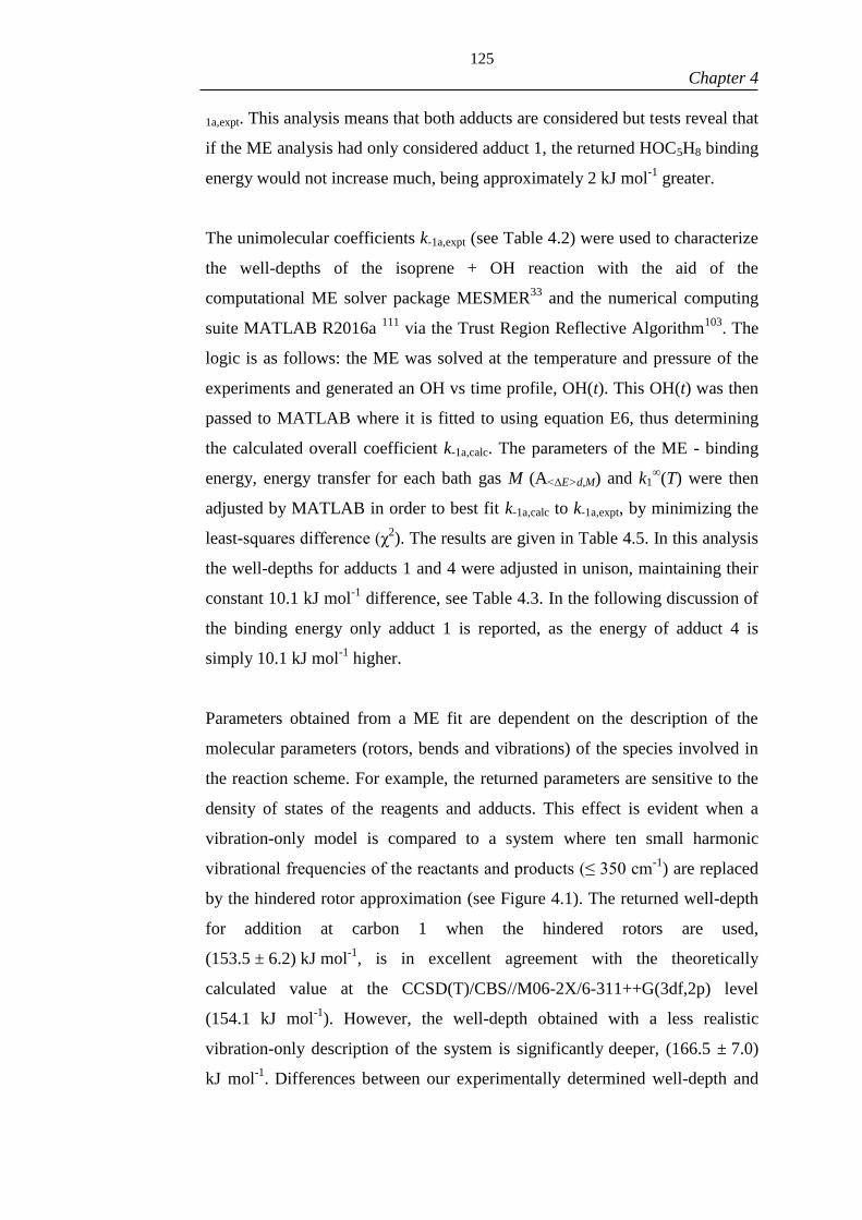
125

Chapter 4

1a,expt. This analysis means that both adducts are considered but tests reveal that

if the ME analysis had only considered adduct 1, the returned HOC5H8 binding

energy would not increase much, being approximately 2 kJ mol-1

greater.

The unimolecular coefficients k-1a,expt (see Table 4.2) were used to characterize

the well-depths of the isoprene + OH reaction with the aid of the

computational ME solver package MESMER33

and the numerical computing

suite MATLAB R2016a 111

via the Trust Region Reflective Algorithm103

. The

logic is as follows: the ME was solved at the temperature and pressure of the

experiments and generated an OH vs time profile, OH(t). This OH(t) was then

passed to MATLAB where it is fitted to using equation E6, thus determining

the calculated overall coefficient k-1a,calc. The parameters of the ME - binding

energy, energy transfer for each bath gas M (A<ΔE>d,M) and k1∞(T) were then

adjusted by MATLAB in order to best fit k-1a,calc to k-1a,expt, by minimizing the

least-squares difference (χ2). The results are given in Table 4.5. In this analysis

the well-depths for adducts 1 and 4 were adjusted in unison, maintaining their

constant 10.1 kJ mol-1

difference, see Table 4.3. In the following discussion of

the binding energy only adduct 1 is reported, as the energy of adduct 4 is

simply 10.1 kJ mol-1

higher.

Parameters obtained from a ME fit are dependent on the description of the

molecular parameters (rotors, bends and vibrations) of the species involved in

the reaction scheme. For example, the returned parameters are sensitive to the

density of states of the reagents and adducts. This effect is evident when a

vibration-only model is compared to a system where ten small harmonic

vibrational frequencies of the reactants and products (≤ 350 cm-1

) are replaced

by the hindered rotor approximation (see Figure 4.1). The returned well-depth

for addition at carbon 1 when the hindered rotors are used,

(153.5 ± 6.2) kJ mol-1

, is in excellent agreement with the theoretically

calculated value at the CCSD(T)/CBS//M06-2X/6-311++G(3df,2p) level

(154.1 kJ mol-1

). However, the well-depth obtained with a less realistic

vibration-only description of the system is significantly deeper, (166.5 ± 7.0)

kJ mol-1

. Differences between our experimentally determined well-depth and

126

Chapter 4

theoretical values obtained at the different levels of theory presented range

from 0.6 to 9.7 kJ mol-1

. Our best estimate of the binding energy, based purely

on the measurements of this work is (153.5 ± 6.2) kJ mol-1

and is given in

Table 4.5.

Table 4.5 - Comparison of Experimental and calculated k-1a. Uncertainty at 1σ.

T / K k-1a,expt / s-1

k-1a,calc / s-1

Adduct 1 Well-

depth / kJ mol-1

729 990 ± 870 1180

153.5 ± 6.2 766 3000 ± 2600 3160

794 6500 ± 5500 6000

The importance of the allylic hydrogen abstraction in the returned well-depths

has also been explored in this investigation. If direct abstraction is neglected,

then a unimolecular loss from the generic adduct presented in scheme S1 needs

to be invoked (R8) to account for the slope observed at longer times of the

equilibrium traces:

C5H8-OH k R → Loss (R8)

From Scheme S4.1, the solution is now given by k3= k-1a + kR, where the slope

of the slow decay of the equilibrium traces, λ-, is approximately equal to kR. If

the abstraction route is supressed, i.e. k1b = 0, kR can provide an equally good

fit to the data, but this reaction scheme skews k-1a, which is the crucial

parameter required to assign the binding energy of the adduct, C5H8-OH. For

instance, at the highest temperature, 794 K, the value of k-1a from Table 4.5 is

6500 ± 5500 s-1

. However, if the highest temperature data are analysed with kR,

the returned value for k-1a is 4810 ± 4200 s-1

. This lower values of k-1a increases

the binding energy of the adduct by 3.8 kJ mol-1

. Even though it is

acknowledged that the experimental observations can be equally described

using kR, there is no evidence for R8. Our theoretical calculations have

identified the direct abstraction channel, R1b, see Figure 4.9. In addition, R8

predicts negligible abstraction at room temperature but R1b predicts 3%; our

proton transfer mass spectrometer observes the abstraction product at room

temperature, see Figure 4.11 and Section 4.4.3. Therefore, the direct

abstraction channel, R1b, is the favoured explanation of the slow decay, λ-.

127

Chapter 4

Potential interference from radical-radical reactions (R+O2 does not happen to

any extent at these high temperatures) could also contribute to OH loss from

the equilibrium system, but is considered unlikely using the following

reasoning. The typical precursor concentration employed in the more sensitive

equilibrium experiments (~1 × 1014

molecule cm-3

, calculated from OH

removal in the absence of isoprene), the laser energy density (~15 mJ cm-2

or

~2 × 1016

photons cm-2

), the precursor cross-section (~1 × 10-19

cm2

molecule-1

for H2O2) and the quantum yield, (2 for OH production from H2O2) is

~ 4 × 1011

molecule cm-3

. If R + R is equal to 10-10

cm3

molecule-1

s-1

(upper

limit) then this implies a k1b ~40 s-1

, which is much lower than experimentally

observed k1b. In some experiments with varying [OH] but similar [C5H8] and

temperature, no significant change in the kinetic parameters were observed.

Additionally, at T = 766 K the photolysis wavelength was changed to 266 nm

(fourth harmonic from Quantel, Q-smart laser, ~ 10 mJ / pulse). Any minor

photolysis of isoprene at 248 nm that could contribute to the radical pool and

hence secondary chemistry, will be significantly reduced with this longer

wavelength photolysis. The 266 nm data are wholly consistent with the other

data, which is further evidence that little additional chemistry is occurring,

other than that given by scheme S1.

4.4.5 - Master Equation Modelling and Comparison with Literature

In this section the master equation modelling package MESMER, described

previously, has been used to compare various experimental values of k1 with a

particular emphasis in determining the onset of pressure dependence. The

complete data set of temperature and pressure dependent rate coefficients (187

values) from the references in Table 4.4 were fitted with the aid of MATLAB

R2016a via the Trust Region Reflective Algorithm, in an analogous procedure

to that described in the previous section. The only difference in the analysis

that now MESMER also returns the forward isoprene + OH rate coefficients

(k1a) to MATLAB. A 10% uncertainty was assigned for all the rate coefficients

considered in this analysis. The fitting parameters were: the adduct well depth,

A<ΔE>d,M for the relevant bath gases used, and the high pressure limiting values

of A1a, C1, A1a, C4 and n in the same format as equation E7. The pre-exponential

128

Chapter 4

factors for additions to carbons 1 and 4 were linked to maintain their constant

ratio (A1a, C1 / A1a, C4 ~ 1.5).30

The vibrational and rotational constants of

isoprene and the OH-C5H8 adducts were calculated at the M06-2X/6-

311++G(3df,2p) level of theory. Lennard Jones parameters were obtained from

the work of Dibble et al.112

and Lei et al.54

A comparison of the complete

experimental and fitted data is shown in Figure 4.12 and the resulting

parameters are presented in Table 4.6.

The proximity of most data points to the y = x line is expected from the

IUPAC evaluation, where most studies are in excellent agreement. Three

studies clearly stand out from the trend from this quantitative analysis; the low

pressure measurements of Chuong and Stevens using discharge flow with OH

detection by LIF, McGivern et al. using laser flash photolysis and LIF

detection and the higher pressure LFP/LIF studies of Campuzano-Jost et al.

Both of the low pressure measurements have been superseded by further,

higher pressure measurements from the same research groups90, 98, 101

which are

in good agreement with the IUPAC evaluation and the y = x line of this

comparison. However, other low pressure, discharge flow/LIF studies from

Stevens’ group, Vimal et al.100

, at 363 K point to some potentially interesting

properties of the OH/isoprene system in comparison to OH/butadiene at low

pressures. Over the pressure range of 1-6 Torr of helium at 363 K, the OH +

isoprene reaction is reported to show some pressure dependence (as does the

study of Singh and Li under similar conditions), however, under identical

conditions, the reactions of OH with the smaller butadiene and 1-butene

molecules (which would be expected to demonstrate greater fall-off

behaviour), show no pressure dependence. Vimal et al.100

used molecular

dynamics simulations to investigate whether differences in the mechanism of

internal energy distribution in isoprene and 1,3-butadiene could explain the

lack of pressure dependence in 1,3 butadiene. Although their calculations

suggested differences in the mechanisms of IVR between the two compounds,

they reported that further studies were required to identify whether such

differences in IVR mechanisms could account for the varying pressure

129

Chapter 4

dependence. Our ME simulations suggest that at 363 K, the high-pressure limit

should be reached at 0.4 Torr of He.

0.0 0.2 0.4 0.6 0.8 1.0 1.2 1.4

0.0

0.2

0.4

0.6

0.8

1.0

1.2

1.4 This work

Kleindest et al. 1982

Campuzano-Jost et al. 2004

Campuzano-Jost et al. 2000

Chuong and Stevens 2000

Hites and Turner 2009

Singh et al. 2007

Park et al. 2004

McGivern et al. 2000

Atkinson 1982

Ohta et al. 1983

Atkinson and Aschmann 1984

Edney et al. 1986

McQuaid et al. 2002

Gill and Hites 2002


Poppe et at. 2007

Zhang et al. 2001

Zhang et al. 2000

Vimal and Stevens 2008

Karl et al. 2004

Iida et al. 2002

Dillon et al. 2017

k1

a, C

alc (

T,p

) /

10

-10 c

m3 m

ole

cu

le-1 s

-1

k1a, Exp

(T,p) / 10-10

cm3 molecule

-1 s

-1

Figure 4.12 - Correlation plot for experimental data points from all the data in Table 3 and the

calculated rate coefficients generated by MESMER by allowing the well-depth, A<ΔE>d,M, A and

n to be floated. The resulting parameters are shown in the second column of Table 4.6.

The work of Singh and Li 28 reports a pressure dependence of 1k at 340 K over

the 1 – 3 Torr pressure range of He. Their equivalent measurements of k1a∞

at 1

and 2 Torr ((7.21 ± 0.65) × 10-11

and 8.16 × 10-11

cm3 molecule

-1 s

-1

respectively, corrected for abstraction with equation E11) are in good

agreement with the set of selected studies presented previously, with ME

predicted values of 7.92 × 10-11

and 7.98 × 10-11

cm3 molecule

-1 s

-1 respectively.

However, the rate coefficient measured at 3 Torr (9.26 × 10-11

cm3 molecule

-1

s-1

) is ~16% higher than the current calculations predict (8.00 × 10-11

cm3

molecule-1

s-1

). The simulations suggest that, in helium at 340 K, the high-

pressure limit should be reached at 0.2 Torr.

It is not easy to explain the discrepancy between the Campuzano-Jost et al.31-32

values and the remaining studies; Campuzano-Jost et al. recognised, but were

130

Chapter 4

unable to rationalize, the difference in their value of k1 and other literature

data. A number of checks were carried out by Campuzano-Jost et al. but they

were unable to identify the origin of the discrepancy. Given the high value of

the rate coefficient k1, it is very unlikely that radical-radical processes could

influence the OH decays and the invariance of the rate coefficients with

photolysis laser power suggests such secondary chemistry plays no role in OH

decays. Rate coefficients lower than the expected value can be an indication of

recycling reactions,113-114

but the invariance of our measured rate coefficients

at low temperatures with large concentrations of oxygen at least rules out

oxygen leaks as a possible route to OH recycling in the Campuzano-Jost et al.

experiments. Given the good agreement in the temperature dependence of k1

with other measurements, the simplest explanation is some systematic error in

determining isoprene concentrations in the reaction cell. That explanation is

supported by the recent studies of Dillon et al.91

who determined UV

absorption cross sections for isoprene which are approximately 10% greater

than those of Campuzano-Jost et al. and in good agreement with another

determination by Martins et al.115

Dillon et al. re-evaluated the Campuzano-

Jost data using their new cross sections, generally bringing the Campuzano-

Jost et al. data in closer agreement to the IUPAC evaluation.

Removing the data sets from Campuzano-Jost et al., Chuong and Stevens,

Vimal et al. and McGivern et al. produces a much better fit (as shown in

Figure 4.13 and Table 4.6) with χ2 being reduced from 601.34 (~3.22 per

point) for the complete data set to 56.53 for the selected data set of 115 data

points (~0.49 per point). χ2 =0.49 implies that the data is on average within 6%

of the fitted value. The resulting best fit parameters in the form of E8 are

A1a = 9.52 ×10-11

cm3 molecule

-1 s

-1 and n1a

∞ = -1.39. Studies represented in

Figure 4.13 are the preferred ones (including this work), and are referred to as

‘Selected Data’.

The returned parameters from the fittings where uncertainties were assigned as

10% of the measured coefficients are summarised in Table 4.6. It contains the

returned parameters from considering the complete dataset and the selected

131

Chapter 4

data. While the k1a data at high temperatures, where equilibria is observed, has

much larger than 10% error, it is consistent with the selected data, under this

10% error criteria.

0.0 0.2 0.4 0.6 0.8 1.0 1.2 1.4

0.0

0.2

0.4

0.6

0.8

1.0

1.2

1.4 This work

Kleindest et al. 1982

Hites and Turner 2009

Singh et al. 2007

Park et al. 2004

Atkinson 1982

Ohta et al. 1983

Atkinson and Aschmann 1984

Edney et al. 1986

McQuaid et al. 2002

Gill and Hites 2002


Poppe et at. 2007

Zhang et al. 2001

Zhang et al. 2000

Karl et al. 2004

Iida et al. 2002

Dillon et al. 2017

k1a, C

alc (

T,p

) /

10

-10 c

m3 m

ole

cu

le-1 s

-1

k1a, Exp

(T,p) / 10-10

cm3 molecule

-1 s

-1

Figure 4.13 - Correlation plot for experimental data points from selected data in Table 4 (see

text) and the calculated rate coefficients generated by MESMER by allowing the well-depth,

A<ΔE>d,M, A and n to be floated. The resulting parameters are shown in the ‘selected data’

column of Table 4.6.

The returned well-depth is virtually unaffected by which data are used as the

well depth is almost exclusively determined by the high temperature data in

this study. The other parameters associated with the fit: A<ΔE>d,M , A1a and n1a

are more dependent on the data set used. For each dataset used, fitted

parameters are reported with either all possibilities of A<ΔE>d,M floated or with

some fixed. Varying the degree of flexibility in fitting A<ΔE>d,M makes little

difference to the returned values of A and n∞; these parameters are mainly

dependent on the datasets considered in the analysis.

132

Chapter 4

Table 4.6 - Returned parameters from MESMER fits to this work and the literature data using a two-adduct model and accounting for H abstraction with all data given an

equal uncertainty of 10%. <ΔE>d,M = A<ΔE>d,M × (T/298)mc

All Data Selected Data

Well depth, E/kJ mol-1

153.1 153.1 152.9 154.0 153.6 153.6

A<ΔE>d / cm-1

He(m=1.00)

Ar (m=0.50)

N2 (m=0.25)

150 (Fixed) 150 (Fixed) 100 150 (Fixed) 150 (Fixed) 100

250 (Fixed) 250 (Fixed) 250 250 (Fixed) 250 (Fixed) 100

200 (Fixed) 200 190 200 (Fixed) 150 150

A × 1011 / cm3 molecule

-

1 s

-1 8.32 8.33 8.34 9.55 9.52 9.52

𝑛∞ -1.45 -1.45 -1.45 -1.44 -1.39 -1.39

χ2 per point 3.31 3.31 3.22 0.56 0.49 0.49

Table 4.7 - Returned parameters from MESMER fits to this work and the literature data and accounting for H abstraction with our higher temperature data given the

uncertainties reported in Table 2. <ΔE>d,M = A<ΔE>d,M × (T/298)m

This work

Two adduct model

This work

One adduct model (C1) Selected Data

Well depth, E/kJ mol-1 153.7 ± 5.9 153.5 ± 6.2 156.0 ± 3.9 156.0 ± 4.2 153.6 ± 4.9 153.4 ± 5.1 153.2 ± 5.0

A<ΔE>d / cm-1

He(m=1.00)

Ar (m=0.50)

N2 (m=0.25)

n/a n/a n/a n/a 150 (Fixed) 150 (Fixed) 100 ± 350

n/a n/a n/a n/a 250 (Fixed) 250 (Fixed) 100 ± 340

200 (Fixed) 150 ± 110 200 (Fixed) 150 ± 70 200 (Fixed) 150 ± 90 150 ± 90

A × 1011 / cm3 molecule

-1

s-1

9.53 ± 0.64 9.47 ± 0.65 9.46 ± 0.41 9.46 ± 0.42 9.46 ± 0.14 9.46 ± 0.14 9.47 ± 0.16

𝑛∞ -1.35 ± 0.15 -1.33 ± 0.16 -1.33 ± 0.10 -1.32 ± 0.10 -1.34 ± 0.07 -1.33 ± 0.07 -1.33 ± 0.07

χ2 per point 0.50 0.48 0.49 0.48 0.42 0.41 0.41

133

Chapter 4

The analysis was also performed with the use of a single-adduct model; the

results for this case are also included in Table 4.7. Little variation is observed

in the returned parameters, with the well-depths varying by 2.5 kJ mol-1

. This

small change is justified by the reduced equilibrium fraction of adduct 4

(~35%) compared to adduct 1 (~65%) and the small energetic difference to

adduct 1 (~10 kJ mol-1

). Finally, the last three columns of Table 7 shows

results, including uncertainties, obtained from fits where the selected data was

incorporated, and the uncertainties of our high temperature measurements

(T > 720 K) were appropriately set as those of Table 4.2.

4.4.6 - Analytical Representation of Pressure and Temperature for k1a,

k-1a,C1, and k-1a,C4

In order to provide analytical representations for the present master equation

calculations, the output from our MESMER equations have been fitted using a

Troe formalism:

k1a(T,[M])=k1a,0(T)[M]

1+k1a,0(T)[M]

k1a∞ (T)

F(x)

E12

k-1a, C1(T,[M]) = k1a(T,[M])× (RT)-1

× exp(ΔHC1⊖

/RT) × exp(-ΔSC1⊖

/R) E13

k-1a, C4(T,[M]) = k1a(T,[M])× (RT)-1

× exp(ΔHC4⊖

/RT) × exp(-ΔSC4⊖

/R)] E14

where [M] is the concentration of the buffer gas, k1a,0(T) is the low-pressure

termolecular rate coefficient, k1a∞ (T) is the high-pressure limit rate coefficient,

and F(x) is the collision broadening factor. The collision broadening factor -

F(x) - is calculated according to the formulation of Troe and Ushakov116

, see

Appendix 3. It is worth mentioning that if the standard broadening factor for

atmospheric studies of 0.6is used,30,54

without a temperature dependence, a

poor fit is produced. k-1a, C1 and k-1a, C4 are the decomposition rate coefficients

for adducts 1 and 4, respectively, and are related to k1a via E13 and E14 using

their thermodynamic parameters: HC1, SC1 and HC4 SC4

134

Chapter 4

A global non-linear least-squares fit to the MESMER data using the Troe

formalism was carried out, where k0(T) and k1a∞ (T) were defined according to

equations E7a and E7b respectively.

k0(T) = A0 × (T/298)n cm

6 molecule

-2 s

-1

E7a

k1a∞(T) = A1a × (T/298)

m cm

3 molecule

-1 s

-1 E7b

A0, A1a, n and m, and F(x)( FcentA, FcentB, 𝑥0 and b), HC1,C4 SC1,C4 were

adjusted to provide a good fit to the simulated pressure dependent coefficients

k1a(T,[M]). The results are given in Table 4.8, and these fits to the MESMER

data are shown in Figure 4.14, where N2 was defined as the bath gas.

Additional Troe fits where helium and argon were simulated as the buffer

gases are also given in Table 4.8.

Table 4.8 - Troe fit parameters to MESMER-simulated rate coefficients, for different buffer

gases.

N2 He Ar

A1a / 10-11

cm3 molecule

-1 s

-1 9.5 9.6 9.5

n -1.26 -1.30 -1.30

A0 / 10-21

cm6 molecule

-2 s

-1 1.68 1.10 1.43

m -14.08 -12.50 -13.27

b 0.08 0.08 0.08

x0 0.90 0.88 0.90

FcentA 0.10 0.11 0.13

FcentB -0.0012 -0.0012 -0.0009

ΔHC1⊖ / J mol

-1 154043 154308 154512

ΔSC1⊖

/ J mol-1

K-1

108.9 109.3 109.6

ΔHC4⊖ / J mol

-1 147251 147495 147696

ΔSC4⊖

/ J mol-1

K-1

102.8 103.1 103.5

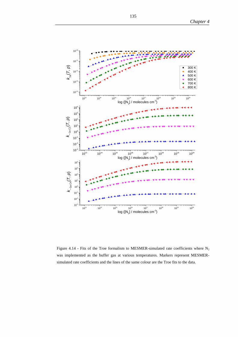
135

Chapter 4

1013

1014

1015

1016

1017

1018

1019

1020

10-14

10-13

10-12

10-11

10-10

1013

1014

1015

1016

1017

1018

1019

1020

10-3

10-2

10-1

100

101

102

103

104

1013

1014

1015

1016

1017

1018

1019

1020

10-3

10-2

10-1

100

101

102

103

104

300 K

400 K

500 K

600 K

700 K

800 K

k1a(T

, p

)

log ([N2] / molecules cm

-3)

k

1a

C1(T

, p)


-3)

k

1a

C4(T

, p)


-3)

Figure 4.14 - Fits of the Troe formalism to MESMER-simulated rate coefficients where N2

was implemented as the buffer gas at various temperatures. Markers represent MESMER-

simulated rate coefficients and the lines of the same colour are the Troe fits to the data.

136

Chapter 4


Measurements of the rate coefficient for the reaction of OH with isoprene, k1,

made around room temperature using a new apparatus for high pressure studies

are in good agreement with the extensive literature data, hence validating this

new apparatus.

Above 700 K the OH temporal profiles exhibit biexponential behaviour,

consistent with the establishment of the OH + C5H8 ⇌ adduct equilibrium. The

experimental adduct dissociation data, k-1a, were fitted to using a master

equation model where the adduct binding energy was adjusted. This analysis

determined a well depth of (153.5 ± 6.2) kJ mol-1

for adduct 1, C1, and

(143.4 ± 6.2) kJ mol-1

for adduct 4, C4. This value is in agreement with the

present ab initio calculations (well depth for C1 adduct = 154.1 kJ mol-1

) on

the R1 potential energy surface. However, it is noted that the well depth

determined from the experimental data is dependent on how the internal modes

of reagents and adducts are treated, and only when the low vibrations are

treated as hindered rotor does experiment and theory show agreement. The

approach based on the species profiles used to explore multiple recycling

proved to be useful in this study and may be used in analogous situations.

The analysis of the > 700 K equilibrium data required an additional minor, but

significant abstraction channel, R1b. Our ab initio calculations have identified

this direct abstraction channel and the proton transfer mass spectrometer

provides evidence that this channel is operating even at room temperature:

k1b = (1.3 ± 0.3) × 10-11

exp (-3.61 kJ mol

-1

RT) cm

3 molecule

-1 s

-1.

Our experimental data on reaction k1, together with the extensive literature data

on this reaction, have been assessed using master equation analysis with the

MESMER programme. This analysis indicates that there is no pressure

dependence in the pressure range of the literature data, contradicting some

previous studies. A selected dataset was then used to provide our

recommended value for k1a(T,[M]). A Troe parametrization of k1a(T,[M])

137

Chapter 4

provides an analytical form of our MESMER analysis. The temperature range

for OH + isoprene studies has been significantly extended to ~800 K with a

high pressure limit recommendation of:

k1∞

= (9.5 ± 0.2) × 10-11 (

T

298 K)

-1.33 ± 0.07

+ (1.3 ± 0.3) × 10-11

exp (-3.61 kJ mol

-1

RT).

Chapter 4 introduced an extra layer of complexity when compared to Chapter

3, by the need of the computation of overall OH recycling coefficients, derived

from contributions of multiple OH recycling species. This was accomplished

by analysing the Master Equation-simulated OH profiles, whose shape is

influenced by all the modelled C5H8-OH adducts. In contrast, in the classic ME

analysis exemplified in Chapter 3, adjustable parameters were floated to

provide a good fit to experimentally determined rate coefficients, which

corresponded to an eigenvalue of the ME.

In Chapter 5, a new method of analysis which expands the horizons of ME

calculations will developed. The reaction of ethylene with OH radicals will be

used as a test case due to its simplicity, atmospheric relevance and wide

previous literature coverage. The method incorporates additional pieces of

chemistry in the ME in order to enable a direct comparison of Master

Equation-simulated traces and raw experimental profiles. This adds another

layer of complexity to the problem as the experimental traces contain pressure

and temperature dependent information about multiple competing process in

which OH is involved. Nonetheless, as will be discussed, a direct raw-trace

fitting not only allows an accurate evaluation of the thermochemistry of a

chemical process, but also represents a critical mechanistic assessment.

138

4.6 REFERENCES

1. Goldstein, A. H.; Galbally, I. E. Known and Unexplored Organic Constituents in the

Earth's Atmosphere. Environmental Science & Technology 2007, 41, 1514-1521.

2. Hantson, S.; Knorr, W.; Schurgers, G.; Pugh, T. A. M.; Arneth, A. Global Isoprene

and Monoterpene Emissions under Changing Climate, Vegetation, CO2 and Land Use.

Atmospheric Environment 2017, 155, 35-45.

3. Guenther, A.; Karl, T.; Harley, P.; Wiedinmyer, C.; Palmer, P. I.; Geron, C. Estimates

of Global Terrestrial Isoprene Emissions Using Megan (Model of Emissions of Gases and

Aerosols from Nature). Atmospheric Chemistry and Physics 2006, 6, 3181-3210.

4. IUPAC Evaluated Kinetic Data. http://iupac.pole-ether.fr/index.html (accessed

February).

5. Utembe, S. R.; Jenkin, M. E.; Derwent, R. G.; Lewis, A. C.; Hopkins, J. R.; Hamilton,

J. F. Modelling the Ambient Distribution of Organic Compounds During the August 2003

Ozone Episode in the Southern Uk. Faraday Discussions 2005, 130, 311-326.

6. Tan, D. et al. HOx Budgets in a Deciduous Forest: Results from the Prophet Summer

1998 Campaign. Journal of Geophysical Research-Atmospheres 2001, 106, 24407-24427.






Nature 2008, 452, 737-740.

10. Saunois, M. et al. The Global Methane Budget 2000-2012. Earth System Science

Data 2016, 8, 697-751.

11. Seakins, P. W.; Blitz, M. A., Developments in Laboratory Studies of Gas-Phase

Reactions for Atmospheric Chemistry with Applications to Isoprene Oxidation and Carbonyl

Chemistry. In Annual Review of Physical Chemistry, Vol 62, Leone, S. R.; Cremer, P. S.;

Groves, J. T.; Johnson, M. A., Eds. Annual Reviews: Palo Alto, 2011; Vol. 62, pp 351-373.

12. Winiberg, F. A. F. et al. Direct Measurements of OH and Other Product Yields from

the HO2 + CH3C(O)O2 Reaction. Atmospheric Chemistry and Physics 2016, 16, 4023-4042.

13. Paulot, R.; Crounse, J. D.; Kjaergaard, H. G.; Kurten, A.; St. Clair, J. M.; Seinfeld, J.


Isoprene. Science (Washington, D. C., 1883-) 2009, 325, 730 - 733.

14. Peeters, J.; Nguyen, T. L.; Vereecken, L. HOx Radical Regeneration in the Oxidation

of Isoprene. Physical Chemistry Chemical Physics 2009, 11, 5935-5939.




16. Hansen, R. F.; Lewis, T. R.; Graham, L.; Whalley, L. K.; Seakins, P. W.; Heard, D.

E.; Blitz, M. A. OH Production from the Photolysis of Isoprene-Derived Peroxy Radicals:

Cross-Sections, Quantum Yields and Atmospheric Implications. Physical Chemistry Chemical

Physics 2017, 19, 2341-2354.



13607-13613.


in Isoprene Oxidation. Nature Geoscience 2013, 6, 1023-1026.

http://iupac.pole-ether.fr/index.html

139

19. Seakins, P. W. A Brief Review of the Use of Environmental Chambers for Gas Phase

Studies of Kinetics, Chemical Mechanisms and Characterisation of Field Instruments. The

European Physical Journal, Web of Conferences 2010, 9, 143-163.

20. Eskola, A. J.; Carr, S. A.; Shannon, R. J.; Wang, B.; Blitz, M. A.; Pilling, M. J.;

Seakins, P. W.; Robertson, S. H. Analysis of the Kinetics and Yields of OH Radical

Production from the CH3OCH2 + O2 Reaction in the Temperature Range 195-650 K: An

Experimental and Computational Study. Journal of Physical Chemistry A 2014, 118, 6773-

6788.

21. Stone, D.; Blitz, M.; Ingham, T.; Onel, L.; Medeiros, D. J.; Seakins, P. W. An

Instrument to Measure Fast Gas Phase Radical Kinetics at High Temperatures and Pressures.

Review of Scientific Instruments 2016, 87, 054102.

22. Kleindienst, T. E.; Harris, G. W.; Pitts, J. N. Rates and Temperature Dependences of

the Reaction of OH with Isoprene, Its Oxidation-Products, and Selected Terpenes.

Environmental Science & Technology 1982, 16, 844-846.

23. Hites, R. A.; Turner, A. M. Rate Constants for the Gas-Phase Beta-Myrcene Plus OH

and Isoprene Plus OH Reactions as a Function of Temperature. International Journal of


24. Chuong, B.; Stevens, P. S. Kinetic Study of the OH Plus Isoprene and OH Plus

Ethylene Reactions between 2 and 6 Torr and over the Temperature Range 300-423 K. Journal

of Physical Chemistry A 2000, 104, 5230-5237.

25. Sun, H.; Law, C. K. Kinetics of Hydrogen Abstraction Reactions of Butene Isomers

by OH Radical. The Journal of Physical Chemistry A 2010, 114, 12088-12098.

26. Smith, G. P. Laser Pyrolysis Studies of OH Reaction Rates with Several Butenes at

1200 K. International Journal of Chemical Kinetics 1987, 19, 269-276.

27. D G Truhlar, a.; Garrett, B. C. Variational Transition State Theory. Annual Review of

Physical Chemistry 1984, 35, 159-189.

28. Singh, S.; Li, Z. Kinetics Investigation of OH Reaction with Isoprene at 240-340 K

and 1-3 Torr Using the Relative Rate/Discharge Flow/Mass Spectrometry Technique. Journal

of Physical Chemistry A 2007, 111, 11843-11851.

29. Dillon, T. J.; Dulitz, K.; Gross, C. B. M.; Crowley, J. N. Temperature Dependent Rate

Coefficients for the Reactions of the Hydroxyl Radical with the Atmospheric Biogenics

Isoprene, alpha-pinene and delta-3-carene. Atmospheric Chemistry and Physics Discussions

2017, 17, 15137-15150.

30. McGivern, W. S.; Suh, I.; Clinkenbeard, A. D.; Zhang, R. Y.; North, S. W.

Experimental and Computational Study of the OH-Isoprene Reaction: Isomeric Branching and

Low-Pressure Behavior. Journal of Physical Chemistry A 2000, 104, 6609-6616.

31. Campuzano-Jost, P.; Williams, M. B.; D'Ottone, L.; Hynes, A. J. Kinetics of the OH-

Initiated Oxidation of Isoprene. Geophysical Research Letters 2000, 27, 693-696.

32. Campuzano-Jost, P.; Williams, M. B.; D'Ottone, L.; Hynes, A. J. Kinetics and

Mechanism of the Reaction of the Hydroxyl Radical with h8-isoprene and d8-isoprene:

Isoprene Absorption Cross Sections, Rate Coefficients, and the Mechanism of Hydroperoxyl

Radical Production. Journal of Physical Chemistry A 2004, 108, 1537-1551.

33. Glowacki, D. R.; Liang, C. H.; Morley, C.; Pilling, M. J.; Robertson, S. H.

MESMER: An Open-Source Master Equation Solver for Multi-Energy Well Reactions.



C. M.; Robertson, S. H. Reanalysis of Rate Data for the Reaction CH3 + CH3 → C2H6 Using

Revised Cross Sections and a Linearized Second-Order Master Equation. Journal of Physical

Chemistry A 2015, 119, 7668-7682.

35. Onel, L.; Blitz, M.; Seakins, P. W.; Bunkan, A. J. C.; Solimannejad, M.; Nielsen, C. J.

Gas Phase Reactions of OH with Methyl Amines in the Presence or Absence of Molecular

140

Oxygen. An Experimental and Theoretical Study. Environmental Science and Technology

2013, Submitted.

36. Onel, L.; Blitz, M. A.; Seakins, P. W. Direct Determination of the Rate Coefficient

for the Reaction of OH Radicals with Monoethanol Amine (MEA) from 296 to 510 K. Journal

of Physical Chemistry Letters 2012, 3, 853-856.

37. Onel, L.; Blitz, M. A.; Breen, J.; Rickardcd, A. R.; Seakins, P. W. Branching Ratios

for the Reactions of OH with Ethanol Amines Used in Carbon Capture and the Potential

Impact on Carcinogen Formation in the Emission Plume from a Carbon Capture Plant.


38. Seakins, P. W.; Pilling, M. J.; Niiranen, J. T.; Gutman, D.; Krasnoperov, L. N.

Kinetics and Thermochemistry of R+HBr ↔ RH+Br Reactions - Determinations of the Heat of

Formation of C2H5, i-C3H7, sec-C4H9, and t-C4H9. Journal of Physical Chemistry 1992, 96,

9847-9855.





40. Frisch, M. J.; Pople, J. A.; Binkley, J. S. Self-Consistent Molecular-Orbital Methods

.25. Supplementary Functions for Gaussian-Basis Sets. Journal of Chemical Physics 1984, 80,

3265-3269.


42. Peng, C. Y.; Ayala, P. Y.; Schlegel, H. B.; Frisch, M. J. Using Redundant Internal

Coordinates to Optimize Equilibrium Geometries and Transition States. Journal of

Computational Chemistry 1996, 17, 49-56.



Computation 2006, 2, 835-839.

44. Raghavachari, K.; Trucks, G. W.; Pople, J. A.; Headgordon, M. A 5th-Order

Perturbation Comparison of Electron Correlation Theories. Chemical Physics Letters 1989,

157, 479-483.

45. Helgaker, T.; Klopper, W.; Koch, H.; Noga, J. Basis-Set Convergence of Correlated

Calculations on Water. Journal of Chemical Physics 1997, 106, 9639-9646.

46. Papajak, E.; Zheng, J.; Xu, X.; Leverentz, H. R.; Truhlar, D. G. Perspectives on Basis

Sets Beautiful: Seasonal Plantings of Diffuse Basis Functions. Journal of Chemical Theory

and Computation 2011, 7, 3027-3034.

47. Kendall, R. A.; Dunning, T. H.; Harrison, R. J. Electron-Affinities of the 1st-Row

Atoms Revisited - Systematic Basis-Sets and Wave-Functions. Journal of Chemical Physics

1992, 96, 6796-6806.

48. Feller, D. The Use of Systematic Sequences of Wave-Functions for Estimating the

Complete Basis Set, Full Configuration-Interaction Limit in Water. Journal of Chemical

Physics 1993, 98, 7059-7071.

49. Ramabhadran, R. O.; Raghavachari, K. Extrapolation to the Gold-Standard in

Quantum Chemistry: Computationally Efficient and Accurate CCSD(T) Energies for Large

Molecules Using an Automated Thermochemical Hierarchy. Journal of Chemical Theory and

Computation 2013, 9, 3986-3994.

50. Liu, Z.; Nguyen, V. S.; Harvey, J.; Muller, J. F.; Peeters, J. Theoretically Derived

Mechanisms of HPALD Photolysis in Isoprene Oxidation. Physical Chemistry Chemical

Physics 2017, 19, 9096-9106.

51. Alecu, I. M.; Zheng, J.; Zhao, Y.; Truhlar, D. G. Computational Thermochemistry:

Scale Factor Databases and Scale Factors for Vibrational Frequencies Obtained from

Electronic Model Chemistries. Journal of Chemical Theory and Computation 2010, 6, 2872-

2887.

141




53. OriginLab Originpro, Northampton, MA.

54. Lei, W. F.; Zhang, R. Y.; McGivern, W. S.; Derecskei-Kovacs, A.; North, S. W.

Theoretical Study of Isomeric Branching in the Isoprene-OH Reaction: Implications to Final

Product Yields in Isoprene Oxidation. Chemical Physics Letters 2000, 326, 109-114.


Transition State Model for Radical−Molecule Reactions: Applications to Isomeric Branching

in the OH−Isoprene Reaction. The Journal of Physical Chemistry A 2007, 111, 5582-5592.

56. Stevens, P. S.; Seymour, E.; Li, Z. J. Theoretical and Experimental Studies of the

Reaction of OH with Isoprene. Journal of Physical Chemistry A 2000, 104, 5989-5997.

57. Řezáč, J.; Šimová, L.; Hobza, P. CCSD[T] Describes Noncovalent Interactions Better

Than the CCSD(T), CCSD(TQ), and CCSDT Methods. Journal of Chemical Theory and

Computation 2013, 9, 364-369.

58. Řezáč, J.; Hobza, P. Describing Noncovalent Interactions Beyond the Common

Approximations: How Accurate Is the “Gold Standard,” CCSD(T) at the Complete Basis Set

Limit? Journal of Chemical Theory and Computation 2013, 9, 2151-2155.

59. Wachters, A. J. H. Gaussian Basis Set for Molecular Wavefunctions Containing

Third‐Row Atoms. The Journal of Chemical Physics 1970, 52, 1033-1036.

60. Hay, P. J. Gaussian Basis Sets for Molecular Calculations. The Representation of 3d

Orbitals in Transition‐Metal Atoms. The Journal of Chemical Physics 1977, 66, 4377-4384.

61. Krishnan, R.; Binkley, J. S.; Seeger, R.; Pople, J. A. Self‐Consistent Molecular

Orbital Methods. XX. A Basis Set for Correlated Wave Functions. The Journal of Chemical

Physics 1980, 72, 650-654.

62. McLean, A. D.; Chandler, G. S. Contracted Gaussian Basis Sets for Molecular

Calculations. I. Second Row Atoms, Z=11–18. The Journal of Chemical Physics 1980, 72,

5639-5648.

63. Raghavachari, K.; Trucks, G. W. Highly Correlated Systems. Excitation Energies of

First Row Transition Metals Sc–Cu. The Journal of Chemical Physics 1989, 91, 1062-1065.

64. Binning, R. C.; Curtiss, L. A. Compact Contracted Basis Sets for Third-Row Atoms:

Ga–Kr. Journal of Computational Chemistry 1990, 11, 1206-1216.

65. McGrath, M. P.; Radom, L. Extension of Gaussian‐1 (G1) Theory to Bromine‐Containing Molecules. The Journal of Chemical Physics 1991, 94, 511-516.

66. Curtiss, L. A.; McGrath, M. P.; Blaudeau, J. P.; Davis, N. E.; Jr., R. C. B.; Radom, L.

Extension of Gaussian‐2 Theory to Molecules Containing Third‐Row Atoms Ga–Kr. The

Journal of Chemical Physics 1995, 103, 6104-6113.

67. Rassolov, V. A.; Ratner, M. A.; Pople, J. A.; Redfern, P. C.; Curtiss, L. A. 6-31g*

Basis Set for Third-Row Atoms. Journal of Computational Chemistry 2001, 22, 976-984.

68. Rassolov, V. A.; Pople, J. A.; Ratner, M. A.; Windus, T. L. 6-31g* Basis Set for

Atoms K through Zn. The Journal of Chemical Physics 1998, 109, 1223-1229.

69. Blaudeau, J.-P.; McGrath, M. P.; Curtiss, L. A.; Radom, L. Extension of Gaussian-2

(G2) Theory to Molecules Containing Third-Row Atoms K and Ca. The Journal of Chemical

Physics 1997, 107, 5016-5021.

70. Francl, M. M.; Pietro, W. J.; Hehre, W. J.; Binkley, J. S.; Gordon, M. S.; DeFrees, D.

J.; Pople, J. A. Self‐Consistent Molecular Orbital Methods. XXIII. A Polarization‐Type Basis

Set for Second‐Row Elements. The Journal of Chemical Physics 1982, 77, 3654-3665.

71. Gordon, M. S. The Isomers of Silacyclopropane. Chemical Physics Letters 1980, 76,

163-168.

142

72. Hariharan, P. C.; Pople, J. A. Accuracy of AHn Equilibrium Geometries by Single

Determinant Molecular Orbital Theory. Molecular Physics 1974, 27, 209-214.

73. Hariharan, P. C.; Pople, J. A. The Influence of Polarization Functions on Molecular

Orbital Hydrogenation Energies. Theoretica chimica acta 1973, 28, 213-222.

74. Hehre, W. J.; Ditchfield, R.; Pople, J. A. Self—Consistent Molecular Orbital

Methods. XII. Further Extensions of Gaussian—Type Basis Sets for Use in Molecular Orbital

Studies of Organic Molecules. The Journal of Chemical Physics 1972, 56, 2257-2261.

75. Ditchfield, R.; Hehre, W. J.; Pople, J. A. Self‐Consistent Molecular‐Orbital Methods.

IX. An Extended Gaussian‐Type Basis for Molecular‐Orbital Studies of Organic Molecules.

The Journal of Chemical Physics 1971, 54, 724-728.

76. Becke, A. D. Density‐Functional Thermochemistry. III. The Role of Exact Exchange.


77. Lee, C.; Yang, W.; Parr, R. G. Development of the Colle-Salvetti Correlation-Energy

Formula into a Functional of the Electron Density. Physical Review B 1988, 37, 785-789.

78. Vosko, S. H.; Wilk, L.; Nusair, M. Accurate Spin-Dependent Electron Liquid

Correlation Energies for Local Spin Density Calculations: A Critical Analysis. Canadian

Journal of Physics 1980, 58, 1200-1211.

79. Stephens, P. J.; Devlin, F. J.; Chabalowski, C. F.; Frisch, M. J. Ab Initio Calculation

of Vibrational Absorption and Circular Dichroism Spectra Using Density Functional Force

Fields. The Journal of Physical Chemistry 1994, 98, 11623-11627.

80. Pople, J. A.; Head-Gordon, M.; Raghavachari, K. Quadratic Configuration-Interaction

- a General Technique for Determining Electron Correlation Energies. Journal of Chemical

Physics 1987, 87, 5968-5975.




82. Cremer, D. Møller–Plesset Perturbation Theory: From Small Molecule Methods to

Methods for Thousands of Atoms. Wiley Interdisciplinary Reviews: Computational Molecular

Science 2011, 1, 509-530.

83. Pople, J. A.; Head-Gordon, M.; Raghavachari, K. Corrections to Correlations

Energies Beyond Fourth Order Moller-Plesset (MP4) Perturbation Theory. Contributions of

Single, Double, and Triple Substitutions. International Journal of Quantum Chemistry 1988,

34, 377-382.

84. Ochterski, J. W.; Petersson, G. A.; Jr., J. A. M. A Complete Basis Set Model

Chemistry. V. Extensions to Six or More Heavy Atoms. The Journal of Chemical Physics

1996, 104, 2598-2619.

85. Baeza-Romero, M. T.; Blitz, M. A.; Goddard, A.; Seakins, P. W. Time-of-Flight

Mass Spectrometry for Time-Resolved Measurements: Some Developments and Applications.

International Journal of Chemical Kinetics 2012, 44, 532-545.

86. Taatjes, C. A. How Does the Molecular Velocity Distribution Affect Kinetics

Measurements by Time-Resolved Mass Spectrometry? International Journal of Chemical

Kinetics 2007, 39, 565-570.

87. Moore, S. B.; Carr, R. W. Molecular Velocity Distribution Effects in Kinetic Studies

by Time-Resolved Mass-Spectrometry. International Journal of Mass Spectrometry and Ion

Processes 1977, 24, 161-171.

88. Atkinson, R.; Aschmann, S. M. Rate Constants for the Reaction of OH Radicals with

a Series of Alkenes and Dialkenes at 295 K. International Journal of Chemical Kinetics 1984,

16, 1175-1186.

89. Atkinson, R.; Aschmann, S. M.; Winer, A. M.; Pitts, J. N. Rate Constants for the

Reaction of OH Radicals with a Series of Alkanes and Alkenes at 299 ± 2 K. International

Journal of Chemical Kinetics 1982, 14, 507-516.

143

90. Chuong, B.; Stevens, P. S. Measurements of the Kinetics of the OH-Initiated

Oxidation of Isoprene. Journal of Geophysical Research-Atmospheres 2002, 107, 4162.

91. Dillon, T. J.; Dulitz, K.; Gross, C. B. M.; Crowley, J. N. Temperature Dependent Rate

Coefficients for the Reactions of the Hydroxyl Radical with the Atmospheric Biogenics

Isoprene, alpha-pinene and delta-3-carene. Atmospheric Chemistry and Physics 2017, 17,

15137-15150

92. Edney, E. O.; Kleindienst, T. E.; Corse, E. W. Room-Temperature Rate Constants for

the Reaction of OH with Selected Chlorinated and Oxygenated Hydrocarbons. International


93. Gill, K. J.; Hites, R. A. Rate Constants for the Gas-Phase Reactions of the Hydroxyl

Radical with Isoprene, alpha- and beta-pinene, and Limonene as a Function of Temperature.


94. Iida, Y.; Obi, K.; Imamura, T. Rate Constant for the Reaction of OH Radicals with

Isoprene at 298 ± 2 K. Chemistry Letters 2002, 31, 792-793.

95. Karl, M. et al. Kinetic Study of the OH-Isoprene and O3-Isoprene Reaction in the

Atmosphere Simulation Chamber, Saphir. Geophysical Research Letters 2004, 31, 4.

96. McQuaid, J. B.; Stocker, D. W.; Pilling, M. J. Kinetics of the Reactions of OH with 3-

methyl-2-cyclohexen-1-one and 3,5,5-trimethyl-2-cyclohexen-1-one under Simulated

Atmospheric Conditions. International Journal of Chemical Kinetics 2002, 34, 7-11.

97. Ohta, T. Rate Constants for the Reactions of Diolefins with OH Radicals in the Gas-

Phase - Estimate of the Rate Constants from Those for Monoolefins. Journal of Physical

Chemistry 1983, 87, 1209-1213.

98. Park, J.; Jongsma, C. G.; Zhang, R. Y.; North, S. W. OH/OD Initiated Oxidation of

Isoprene in the Presence of O2 and NO. Journal of Physical Chemistry A 2004, 108, 10688-

10697.

99. Poppe, D.; Brauers, T.; Dorn, H. P.; Karl, M.; Mentel, T.; Schlosser, E.; Tillmann, R.;

Wegener, R.; Wahner, A. OH-Initiated Degradation of Several Hydrocarbons in the

Atmosphere Simulation Chamber Saphir. J. Atmos. Chem. 2007, 57, 203-214.

100. Vimal, D.; Pacheco, A. B.; Iyengar, S. S.; Stevens, P. S. Experimental and Ab Initio

Dynamical Investigations of the Kinetics and Intramolecular Energy Transfer Mechanisms for

the OH+1,3-butadiene Reaction between 263 and 423 K at Low Pressure. Journal of Physical

Chemistry A 2008, 112, 7227-7237.

101. Zhang, D.; Zhang, R. Y.; Church, C.; North, S. W. Experimental Study of

Hydroxyalkyl Peroxy Radicals from OH-Initiated Reactions of Isoprene. Chemical Physics

Letters 2001, 343, 49-54.

102. Zhang, R. Y.; Suh, I.; Lei, W.; Clinkenbeard, A. D.; North, S. W. Kinetic Studies of

OH-Initiated Reactions of Isoprene. J. Geophys. Res. Atmos. 2000, 105, 24627-24635.

103. Moré, J. J.; Sorensen, D. C. Computing a Trust Region Step. SIAM Journal on

Scientific and Statistical Computing 1983, 4, 553-572.

104. Baulch, D. L. et al. Evaluated Kinetic Data for Combustion Modelling. Journal of

Physical and Chemical Reference Data 1992, 21, 411-734.

105. Tully, F. P. Hydrogen-Atom Abstraction from Alkenes by OH, Ethene and 1-butene.

Chemical Physics Letters 1988, 143, 510-514.

106. Atkinson, R.; Aschmann, S. M.; Tuazon, E. C.; Arey, J.; Zielinska, B. Formation of 3‐Methylfuran from the Gas‐Phase Reaction of OH Radicals with Isoprene and the Rate

Constant for Its Reaction with the OH Radical. International Journal of Chemical Kinetics

1989, 21, 593-604.

107. Atkinson, R.; Tuazon, E. C.; Aschmann, S. M. Products of the Gas‐Phase Reaction of

the OH Radical with 3‐methyl‐1‐butene in the Presence of NO. International Journal of


144

108. Nordmeyer, T.; Wang, W.; Ragains, M. L.; Finlayson‐Pitts, B. J.; Spicer, C. W.;

Plastridge, R. A. Unique Products of the Reaction of Isoprene with Atomic Chlorine: Potential

Markers of Chlorine Atom Chemistry. Geophysical Research Letters 1997, 24, 1615-1618.

109. Jenkin, M. E.; Young, J. C.; Rickard, A. R. The MCM V3.3.1 Degradation Scheme

for Isoprene. Atmospheric Chemistry and Physics 2015, 15, 11433-11459.

110. Peeters, J.; Boullart, W.; Pultau, V.; Vandenberk, S.; Vereecken, L. Structure-Activity

Relationship for the Addition of OH to (Poly)Alkenes: Site-Specific and Total Rate Constants.


111. MATLAB and Optimization Toolbox Release R2016a. Natwick : Math Works Inc.:

2016.

112. Dibble, T. S. Isomerization of OH-Isoprene Adducts and Hydroxyalkoxy Isoprene

Radicals. Journal of Physical Chemistry A 2002, 106, 6643-6650.

113. Papadimitriou, V. C.; Karafas, E. S.; Gierczak, T.; Burkholder, J. B. CH3CO + O2 +

M (M = He, N2) Reaction Rate Coefficient Measurements and Implications for the OH Radical

Product Yield. Journal of Physical Chemistry A 2015, 119, 7481-7497.

114. Baeza-Romero, M. T.; Glowacki, D. R.; Blitz, M. A.; Heard, D. E.; Pilling, M. J.;

Rickard, A. R.; Seakins, P. W. A Combined Experimental and Theoretical Study of the

Reaction between Methylglyoxal and OH/OD Radical: OH Regeneration. Physical Chemistry


115. Martins, G. et al. Valence Shell Electronic Spectroscopy of Isoprene Studied by

Theoretical Calculations and by Electron Scattering, Photoelectron, and Absolute

Photoabsorption Measurements. Physical Chemistry Chemical Physics 2009, 11, 11219-

11231.

116. Troe, J.; Ushakov Vladimir, G. Representation of “Broad” Falloff Curves for

Dissociation and Recombination Reactions. Zeitschrift für Physikalische Chemie 2014, 228, 1-

10.

145

Chapter 5

Chapter 5. Kinetics of the reaction of

ethylene with OH radicals: developing

a global Master Equation-based, raw-

trace fitting technique

147

Chapter 5


The current chapter focuses on the development of a novel strategy to explore

experimental traces via a global multi-temperature, multi-pressure fitting

procedure which relies on Master Equation (ME) calculations from the

corresponding potential energy surface. A new transition matrix is constructed

as a modification of the original ME, via the inclusion of intrinsic formation

and consumption terms such as diffusional losses, reactions with radical

precursors, unimolecular losses of intermediate species and side reactions. The

method is presented in the context of the ethylene + OH reaction due to its

simplicity and wide previous literature coverage. This technique reduces the

number of mathematical transformations necessary when conventionally

converting experimental traces into rate coefficients with propagated errors and

subsequent implementation in ME fits (see Chapter 2 for an example of a

classic ME fit). A global raw-trace fit, with a large number of experimental

profiles covering a wide range of temperature and pressures, not only allows a

good assessment of the thermochemistry of the reactions involved, but also

represents a test of the mechanism implemented. Systematic inconsistencies

observed in the fits can provide insightful information regarding potentially

missing pieces of chemistry. The OH abstraction from ethylene at elevated

temperatures is used to exemplify the last assertion.

149

Chapter 5

5.1 INTRODUCTION

Ethylene, also known as ethene (C2H4), is the simplest possible alkene. It is

extensively used in the manufacture of polymers of wide applicability, such as

polyethylene (PE)1, polyvinyl chloride (PVC) and polyethylene terephthalate

(PET). It is also a precursor of ethylene glycol, an industrially important

compound, largely used in the production of detergents and surfactants.2-3

Ethylene is employed in agriculture as a fruit ripening hormone4; and also

plays additional important roles in the development of plants, influencing not

only their growth, but also seed germination, flowering, root stretching and sex

determination.5

The traditional understanding suggests that global emissions of ethylene to the

atmosphere are dominated by biogenic sources, accounting for approximately

75% of the total emissions.6-7

In one year, 8-25 Tg of ethylene were estimated

in the past to be emitted into the troposphere from natural sources.5 Plant

emissions are believed to account for the majority of natural emissions, with

small contributions from soil (~3 Tg) and ocean (~1 Tg).5, 8

Emissions of

ethylene by vegetation can be significantly enhanced via the “ethylene stress”

phenomenon (~10-400 times), which can be provoked by agents of different

nature, including (i) physical (high temperature, freezing, mechanical damage,

etc), (ii) chemical (ozone, sulfur dioxide) or (iii) biotic (insect wounding,

pathological infection) factors.8

The most significant anthropogenic sources of ethylene include industry,

biomass burning and traffic. More recent estimates9 attempt to discriminate the

ethylene emissions from biomass burning as these can have both a human and

natural causes. According to these evaluations, in one year, 2.7 Tg of ethylene

are emitted into the troposphere from natural sources.6, 9

, while 1.05 Tg/yr and

5.35 Tg/yr of ethylene are believed to be emitted from anthropogenic sources

and biomass burning respectively.6, 9

However, these estimates, are based on a

compilation of data from 1997 and do not reflect a decline of industrial and

traffic emissions observed since 1994.10

150

Chapter 5

When released in the atmosphere, the gas-phase oxidation, predominantly

initiated by the reaction with hydroxyl radicals (R1) is the major removal

process for ethylene.11

Ethylene has a relatively short lifetime with respect to

the removal by OH radicals (τ ~ 6 – 30 h) and represents a significant

atmospheric OH sink.11-12

The C2H4 + OH reaction is also relevant for

combustion chemistry.11, 13

OH + C2H4 k1 → Products R1

At low temperatures (T ≤ 500 K) the ethylene + OH reaction proceeds mostly

via a pressure-dependent OH addition to the π-bond. Under such temperatures,

the collisional stabilization of the chemically activated C2H4-OH* adduct (R2)

competes with the unimolecular decomposition of the C2H4-OH* adduct (R-

1a):

OH + C2H4 k1a , k

-1a

↔ HOC2H4* (R1a, R-1a)

HOC2H4* + M

k2 → HOC2H4 + M (R2)

At elevated temperatures (T > 600 K), however, the abstraction of a hydrogen

atom becomes significant and eventually turns into the major channel of this

reaction14-16

:

C2H4 + OH k1b → H2O + C2H3 (R1b)

Previous studies of the ethylene + OH reaction were carried out via diverse

techniques, among them direct measurements using Pulsed Laser Photolysis –

Laser Induced Fluorescence (PLP-LIF)17-18

, Pulsed Laser Photolysis –

Resonance Fluorescence (PLP-RF)19-20

; Pulsed Laser Photolysis-Cavity Ring-

Down Spectroscopy (PLP-CRDS)11

and indirect measurements using the

relative rate method (RR).21-22

IUPAC recommends k1∞

=(9.0×10-12

)×(T

300 K)-0.85

for the high pressure limit rate coefficients in the 100-500 K temperature

151

Chapter 5

range. This recommendation is based on the work of Vakhtin et al.17

, which is

in good agreement with the measurements by Fulle et al.23

Nielsen et al.24

and

Lloyd et al.25

The temperature and pressure dependencies of the ethylene + OH reaction

have been extensively explored in previous investigations. Even though the

bulk of the experimental literature is focused on temperatures above 298 K, the

studies of Vakhtin et al.,17 and Cleary et al.

11 have covered lower temperatures.

Vakhtin et al. 17 have studied the reaction in the 96 – 296 K temperature range

and 0.2 – 100 Torr of N2 via PLP-LIF using a pulsed Laval nozzle apparatus.

Using the Troe formalism26

, they have extrapolated their pressure dependent

measurements to the high pressure limit, giving a temperature dependence in

the form of k1a∞

=(8.7 ± 0.7)×10-12

×(T

300 K)-0.85 ± 0.11

cm3 molecule

-1 s

-1. These

results were later questioned by the theoretical study of Greenwald et al.18

and

the experimental investigation by Cleary et al.11

Greenwald was unable to

obtain a good agreement between the high pressure rate coefficients reported

by Vakhtin and the bulk of the previous literature investigations. However, a

good agreement is observed when the pressure dependent rate coefficients

measured by Vakhtin et al. are compared to estimates for the same

experimental conditions, computed via Master Equation (ME) modelling.27-28

The authors conclude that the disagreement observed for the high pressure

coefficients could be caused by an inappropriate extrapolation of k1a(T,p), since

Vakhtin’s measurements were performed at very low pressures, far from the

onset of the high pressure limit.

Cleary et al., on the other hand, have investigated the C2H4 + OH reaction via

PLP-LIF, exploring the 200 – 400 K temperature range, in pressures ranging

from 5 to 600 Torr of He and N2. They also performed additional

measurements via PLP-CRDS at 100-760 Torr of SF6. They utilized the

MESMER package27

to optimize the energy transfer parameter (<ΔE>d, M

), the

pre-exponential factor and the temperature dependence of R1a, in the form of

equation E1, using a large set of k1a(T, p).

152

Chapter 5

k1a∞

=A×(T

298 K)n

E1

The best-fit parameters were then used to calculate the pressure dependent

coefficients at the experimental conditions of Vakhtin et al. Their procedure

significantly underestimated the values reported by Vakhtin and the authors

suggest that a more dramatic negative temperature dependence of k1a∞

could

reduce the discrepancy. They also acknowledged that the theoretical level at

which the system was described in their own study may be inappropriate. They

have treated the problem as a single well system, and in contrast, a two

transition state model was employed in the work of Greenwald et al, who as

described previously, managed to reconcile the literature measurements.

The kinetic isotope effect of this reaction has been explored by Liu et al.15

in

the 343 – 1173 K temperature range and has provided insightful mechanistic

information. In their work OH radicals were generated via electron beam pulse

radiolysis of water and detected via resonance absorption. This temperature

range covers a regime where OH addition dominates, but also those where the

dissociation back to reagents competes with the addition, as well as conditions

at which the H-abstraction is likely the most important process. Between 343

K and 563 K, no difference was observed between OH + C2H4 and OH + C2D4

(kOH+C2H4 = kOH+C2D4 = 1.65 × 10-12

exp(480/T) cm3 molecule

-1 s

-1) reactions as

well as between reactions OD + C2H4 and OD + C2D4 (kOD+C2H4 = kOD+C2D4 =

1.35 × 10-12

exp(480/T) cm3 molecule

-1 s

-1). However, as the rate coefficients

indicate, the OH pairs are 22% faster than the OD ones, suggesting a secondary

isotope effect, consistent with an OH/OD addition mechanism where no O-H

or C-H bonds are formed or broken.29

In the fall-off regime, statistical-weight

effects for the hot adducts (OH-C2H4* or OH-C2D4

*) back to reagents would

justify a reverse isotope effect. In the high pressure limit however, R2 should

dominate and the ratio between kOH+C2H4 and kOH+C2D4 gets close to the unity.

The experiments by Liu et al. were performed at 1 atm of argon and given the

lack of isotope effect between kOH+C2H4 and kOH+C2D4 (and kOD+C2H4 and

kOD+C2D4), the high pressure limit assumption was made in this temperature

range. These results have also been compared to estimates via conventional

153

Chapter 5

transition state theory (TST), showing a very good agreement. Internal isotope

scrambling is considered unimportant under their experimental conditions

since it would not only mean a primary isotope effect, which as discussed

previously has not been detected, but because no relevant OH signal has been

detected in OD + C2H4 experiments. Above 720 K, the authors have

determined a positive activation energy of approximately 5 kcal mol-1

. In this

case, while a primary isotope effect is observed between OH + C2H4 and OH +

C2D4, a secondary effect is detected between the OH + C2H4 and OD + C2H4

reactions. These results are consistent with an abstraction mechanism and were

also verified and confirmed via a classic TST calculation. They observed small

systematic under prediction of the experimental rate coefficients which was

partially justified by the lack of quantum mechanical tunnelling effects in the

theoretical calculations. While the primary isotope effect is caused by the

difference in activation energies (H or D abstraction), the secondary one is due

to statistical-weight effects.

At elevated temperatures, where the abstraction chemistry should start to

dominate, two conflicting studies covering relatively wide temperature ranges

are found in the literature: measurements via electron beam pulse radiolysis of

water coupled with resonance absorption detection of OH by Liu et al.(1987)30

(T = 343 - 1173 K) and the PLP-LIF measurements by Tully (1988)16

(T = 650 – 901 K). A literature review published by Baulch et al.31

a few years

later, in 1992, recommends the measurements reported Tully. The rate

coefficients reported by Liu et al. are systematically greater than those

presented by Tully, and is suggested by the last that this was partially caused

by the large C2H4 concentrations employed by Liu et al. in their study.

According to Tully, this caused the time span of experimental traces to be too

short in order to clearly discriminate the abstraction channel from the OH

addition. Tully has investigated the fact that non-exponential OH traces were

collected at the temperatures of his work, and making the assumption that the

chemistry is dominated by the H abstraction, accounted for the deviations from

exponential behaviour as diffusional losses. According to his work, the

abstraction is the dominating channel above the temperature of 650 K.

154

Chapter 5

Liu et al. 30

on the other hand have fitted simple exponential equations to their

measurements to extract pseudo-first order rate coefficients and calculate the

second order rate coefficients k1(T, p) from bimolecular plots, although their

experimental data clearly shows non-exponential behaviour at 603 K. From the

measured rate coefficients and using a steady state approximation of the

excited C2H4-OH*, the temperature dependence of the abstraction coefficients

were obtained as well as those related to the addition ones. According to their

results, the abstraction only dominates the chemistry above 748 K. However, a

direct comparison to the measurements by Tully can be misleading given that

the experiments were done at different pressures and buffer gases: while Tully

covered the 100-350 Torr pressure range using He for ~90% of their

measurements, Liu et al. employed argon as the buffer gas and a unique

pressure of 760 Torr. It is important to note that the definition of a region

where the abstraction dominates depends on the pressure dependence of the

addition reaction.

The chemistry of C2H4 at elevated temperatures (T>900 K) is of particular

interest for combustion chemistry.32-33

The simplicity of this alkene is

attractive for the prediction of the chemistry of larger hydrocarbons. A

satisfactory understanding of the high temperature chemistry of C2H4 could

potentially translate into improvements of the current combustion models. The

vinyl radical formed from the hydrogen abstraction from ethylene is also

interesting for the combustion of hydrocarbons in general.33

Moreover,

ethylene is a common intermediate specie in the combustion of large

hydrocarbons reinforcing the importance of the sub-mechanism of the ethylene

oxidation.32

Due to this evident applicability to combustion systems,

measurements of the H-abstraction rate coefficients above 900 K were in

general obtained from mechanistic fits of complex reactive systems like

flames. This was the case for the work of Westbrook et al.32

and Bhargava and

Westmoreland.33

Such complex models naturally introduce heavily significant

errors in the estimates, and for this reason, these studies will covered in a less

detailed manner.

155

Chapter 5

The work of Westbrook et al.32

was performed in a jet-stirred reactor between

1003-1253 K. Measurements of H2, C2H4, CH4 and CO2 were collected as a

function of the reactor temperature and, using a numerical combustion model,

the authors estimated rate coefficients which agree with the previously

discussed measurements of Tully. However, this agreement is based on a very

poor fit of their model to their measurements. Even though the authors do not

quote errors for their estimates, it is important to note that they will be very

significant. Nonetheless, their recommendation for the abstraction rate

coefficient is k1b= 3.32×10-11

exp(-2897 K

T) cm

3 molecule

-1 s

-1.

Similarly, estimates by Bhargava and Westmoreland33

were based on

mechanistic fits of laminar flame data. Molecular beam mass spectrometry was

undertaken to monitor the composition of a flame enriched with C2H4/O2 in the

1400-1800 K temperature range. A total of 42 individual species were mapped

and the model fits have provided a modified Arrhenius temperature

dependence for k1b= 9.182×10-19

T2.31exp(-1459 K

T) cm

3 molecule

-1 s

-1.

Srinivasan et al.34

have investigated the reaction in the 1463-1931 K

temperature range using shock tube experiments and direct OH detection via

multi-pass absorption spectrometry. The authors recommend a temperature

dependence in the form of k1b= (10.2 ± 5.8)×10-10

exp(-(7411 ± 871) K

T) cm

3

molecule-1

s-1

. They also acknowledge that the work of Bhargava and

Westmoreland33

, based on complex mechanistic fit to laminar flame data

surprisingly agrees to their measurements, despite the complexity with laminar

flame data.

A study by Vasu et al.35

in which shock tube experiments were undertaken in

order to study the abstraction in the ~970-1440 K temperature range was

published in 2010. Experiments were performed in pressures between 1520

and 7600 Torr of argon. Their OH traces collected via absorption spectroscopy

were fitted with a natural gas combustion mechanism from where k1b was

obtained. The authors provide a comparison with the previous literature, and

156

Chapter 5

their measurements agree well with the shock tube study by Srinivasan et al.34

,

the jet-stirred reactor measurements of Wetstbrook et al.32

and the results of

Bhargava and Westmoreland33

based on molecular-beam mass spectrometry.

Their recommended Arrhenius formulation for the abstraction is

k1b= 3.4×10-18

T2.745exp(-1115 K

T) cm

3 molecule

-1 s

-1. A summary of the high

temperature data on R1 is presented in Figure 5.1.

600 800 1000 1200 1400 1600 1800 2000

0.01

0.1

1

10

Baulch et al. (Review)(1992)

Tully (1988)

Liu et at. (1987)

Vasu et al. (2010)

Westbrook et al.(1988)

Srinivasan et al.(2007)

Bhargava and Westmoreland. (1998)k 1b(T

) /

10

-11 c

m3 m

ole

cule

-1 s

-1

T / K

Figure 5.1 - Comparison of experimental recommendations for the ethylene + OH from

different investigations. Red circles represent the recommendation from the review by Baulch

et al.31

, blue open triangles refer to the work of Tully16

, pink diamonds refer to the work of Liu

et al.30

, olive triangles correspond to the report of Vasu et al.35

, cyan triangles refer to the work

of Westbrook et al.32

, orange stars correspond to the study of Srinivasan et al.34

, light green

triangles refer the work of Bhargava and Westmoreland.33

The structural and chemical simplicity of the ethylene case makes the study of

this reaction a benchmark for testing and validating analytical methods and

theoretical calculations.14, 36-37

For example, in the case of relatively simple

dienes such as isoprene and 1,3-butadiene, multiple OH addition sites are

available. The description of concurrent unimolecular decompositions of the

157

Chapter 5

various possible adducts, with different enthalpies of formation and molecular

properties make the analysis of such molecules more complicated when

compared to the ethylene example.

Equilibrium traces, observed due to the competition between reactions R1a and

R-1a, or analogue reactions for similar systems, can be used for a

characterization of the equilibrium constant via analytical equations.38

Under

pseudo-first order conditions, the temporal profile of the OH radical can be

described by a simple exponential equation, however, when the decomposition

of the rising adduct becomes significant, the OH traces become

multi-exponential in nature. For this reason, a more robust and versatile

equation, capable of accurately describing the OH recycling is required. One

must however, be aware of the implications of the use of a more versatile

equation, with additional fitting parameters when describing temporal profiles.

For example, the flexibility of the bi-exponential equation, which is commonly

employed to describe radical recycling in chemical systems,39-40 allows the

description of non-exponential features with some ease. However, an

inadvertent single trace analysis using this equation can easily suppress the

existence of other relevant chemical processes, given the capability of this

formulation to provide a good fit even when the chemistry of the system is not

fully accounted for. This is the case because the large number of extra

parameters can compensate the lack of the description of a real process in the

model. For example, in the case of ethylene, the negligence of the hydrogen

abstraction in competition with the addition of OH to describe experimental

traces generated at elevated temperatures (T > 600 K) may lead to an

overestimation of the addition reaction. Despite this fact and given the

versatility of the fitting equation, it is possible that a “good” fit is obtained,

with a low least-squares difference (χ2), so that conclusions based only on the

goodness of the fit are questionable.

A global fit of a big collection of experimental data is a reliable and

computationally feasible way of testing the ability of a candidate model to

describe the experimental observations. In this form of fitting, a few key

158

Chapter 5

parameters of the system are defined as functions of local variables, which

relate to and are valid only for one unit of analysis, in this work, an

experimental trace. For example, in a global analysis, the pseudo-first order

rate coefficient of the reaction of ethylene with OH is obtained through the

product of the bimolecular reaction coefficient (global variable) with the

concentration of the excess reagent (local variable, exclusive of a single trace).

Alternatively, if multiple temperatures are to be analysed, the bimolecular rate

coefficients can be defined in the form of a simple Arrhenius parametrization,

where both the pre-exponential factor and the activation energy are defined as

global parameters. Global parameters are shared by all the units of analysis,

and in this example, used to calculate bimolecular rate coefficients at a given

temperature. The establishment of these relationships imposes links that help

constrain the analysis, so that experimental traces generated under the same

experimental conditions are "forced" to have a pseudo-first order rate

coefficient proportionally-related to the corresponding ethylene concentrations.

In a global analysis, the inability to describe a group of experimental traces

may indicate an incomplete understanding of the chemistry involved, and can

provide valuable insights for a satisfactory elucidation of the problem. In the

ethylene example, the non-inclusion of the hydrogen abstraction in the model

would probably result in a contrast between good fits for traces where OH

addition dominates the chemistry, and poor fits where the abstraction becomes

important. A systematic characteristic of traces where a poor fit is obtained

may also provide new insights about the missing piece of the chemistry. An

example will be explored later on in this chapter when analysing non-

exponential traces obtained at elevated temperatures for the ethylene + OH

reaction.

Despite being robust and versatile, global analysis requires extra care in data

processing, and the complexity of the chemical system is rapidly translated

into more complicated computational programming. The definition of multiple

reaction constants as a function of other variables such as the temperature, the

appropriate input of the experimental conditions of each trace and the adequate

159

Chapter 5

linking of adjustable parameters are examples of tasks that make a global

analysis a difficult procedure. The non-triviality of the computation of

pressure-dependent rate coefficients makes the global analysis of traces

generated under various pressures of different bath gases even more

challenging.

In this study a new procedure to analyse the kinetics of pressure and

temperature dependent reactions, through a direct global fit of a chemical

model to the raw experimental traces is presented. The method represents a

step forward in the ability to analyse relatively complex kinetic problems, and

allows not only the determination of thermochemical and kinetic parameters,

but also a mechanistic evaluation of the system. The unprecedented analysis of

the ethylene + OH reaction yields a remarkable agreement with theoretical

calculations, where a discrepancy between predictions and measurements are

in the order of 1 kJ mol-1

, thus providing an excellent testbed of this method of

data fitting.

5.2 METHODOLOGY

5.2.1 - Experimental details

Experiments were carried out using a conventional laser flash photolysis

instrument where OH radicals were monitored in situ by laser induced

fluorescence.40-41

Detailed descriptions of the operation of such type of

apparatus are provided in Chapter 2 and therefore only a succinct description is

presented here. Ethylene (Air Products, 99.6%), the OH precursor (H2O2, 50%

(w/w) Sigma Aldrich) and the carrier gas (N2, BOC oxygen free) were flowed

into the LPF-LIF instrument. Typical experimental pressures ranged from 50

to 250 Torr of N2. Hydrogen peroxide was delivered through a temperature

stabilized glass bubbler, and its concentration in the reaction cell was estimated

based on its vapour pressure and the controlled flow rates. The initial OH

concentration was estimated to be ~ 4 × 1012

molecule cm-3

, for the typical

H2O2 concentration (~ 1 × 1015

molecule cm-3

), laser fluence (~15 mJ cm-2

or

~2 × 1016

photons cm-2

), crossection of the precursor at 248 nm (~1 × 10-19

cm2

160

Chapter 5

molecule-1

for H2O2)42

and quantum yield, (2 for OH production from H2O2).

Ethylene was prepared as a diluted mixture in nitrogen and stored in a 2 L

glass bulb. Its concentration in the reaction cell (~1 × 1015

– ~1 × 1016

molecule cm-3

) was determined manometrically.

Under first-order conditions near room temperature, as discussed on many

occasions in the previous chapters, the OH profiles have the form of an

exponential decay, described by equation E2.

tk

t e '

0]OH[]OH[ E2

k’ represents the pseudo-first-order rate constant, defined as:

k’ = k1[C2H4] + kloss E3

Here k1 is the bimolecular rate constant for reaction R1 and kloss represents the

rate coefficient for the losses due to diffusion and reaction of OH with its

precursor. In this work, however, experiments were conducted at sufficiently

high temperatures (T ≥ 560 K) such that the equilibrium between OH/ethylene

and the OH-C2H4 adduct was established. Previous studies show that the

thermochemistry of the reaction is significantly sensitive to such

measurements.38, 43

Non-exponential experimental traces obtained at such

conditions were treated using a new analytical approach, which involves the

description of pressure-dependent reactions via Master Equation modelling.

For this reason, and to guarantee a good understanding of the method, the next

section (5.2.1) is dedicated to details of the ab initio calculations that gave

support for the ME modelling of the OH addition to ethylene. Once the ME

method is properly introduced, the analysis method is presented in more detail

in the following sections (5.2.2-5.2.7).

161

Chapter 5

5.2.2 - Supporting Ab Initio Calculations

Molecular structures and properties of the relevant species were computed with

the M06-2X density functional theory method and the aug-cc-pVTZ version of

Dunning’s correlation consistent basis sets. Redundant internal coordinates

were optimized using the Berny algorithm with the aid of the Gaussian 09

D.01 computational suite. Force-constant matrices, rotational constants,

harmonic vibrational frequencies and zero-point energies required for ME

calculations were all calculated with the M06-2X/aug-cc-pVTZ methodology.

High performance coupled cluster calculations with single, double and triple

excitations, the triples described iteratively (CCSD(T)), were undertaken for a

more accurate estimate of the single point energies of the

M06-2X/aug-cc-pVTZ stationary points. The single point energies were

extrapolated to the complete basis set limit (CBS) using the aug-cc-pVXZ basis

sets (X=2,3,4) and a mixed Gaussian/exponential extrapolation scheme as

proposed by Peterson et al.44

:

2)1()1()( XX

cbs BeAeEXE E4

where )(XE is the total energy calculated with the respective aug-cc-pVXZ

basis set, cbsE is the complete basis set extrapolation of the total energy, A and

B are proportionality constants. A set of three equations containing three

variables ( cbsE , A and B) is obtained from the use of three basis-sets, as

presented in the following:

2)12()12()2( BeAeEE cbs E5

2)13()13()3( BeAeEE cbs E6

2)14()14()4( BeAeEE cbs E7

The unique mathematical solution of this set of equations yields the complete

basis set extrapolation of the electronic energy ( cbsE ), and the constants A and

162

Chapter 5

B. The enthalpy of formation of the adduct, ΔRH0K(C2H4-OH), was calculated

with this methodology and its value of 111.4 kJ mol-1

will later on be used for

a comparison against an experimental determination. This will provide some

insight on the accuracy of the novel analytical method being used.

As detailed in the context of the isoprene + OH reaction in Chapter 4, the

hindered rotor approximation was also implemented here for the description of

two internal rotations of the C2H4-OH adduct, related to small harmonic

vibrational frequencies (< 350 cm-1

). Figure 5.2 shows the rotations described

with the hindered rotor approach. The potential was constructed through a

relaxed scan of the dihedral angle respective to the rotation, with steps of 15°.

A partial structure optimization was performed at the end of every step, until a

360° coverage was obtained. In possession of the force constant matrix and the

hindered rotor potentials, MESMER applies the procedure described by

Sharma et al.45

to project out the modes related to the internal rotations. If

easily identifiable, the modes can be directly indicated to MESMER along with

a list of harmonic vibrational frequencies.

Figure 5.2 - Internal rotations described with the hindered rotor approach for the C2H4-OH

adduct.

163

Chapter 5

5.2.3 - Modifying the full Master Equation transition matrix

As discussed previously, the direct analysis of experimental traces in a global

fashion represents a robust alternative not only for obtaining kinetic

parameters, but also, testing a candidate chemical mechanism. The analysis

will be presented in the context of the ethylene + OH reaction, but its use can

be easily extended for the study of other gas-phase reactions. The global

method is based on the coupling of four main steps which will be described

below. For illustrative and simplicity purposes, examples of fits to single traces

will be displayed, even though a global procedure is being applied. Unless

stated otherwise, the bimolecular rate constants used in the model were defined

as a function of temperature. After a more generic description of the method, a

more programmatic view with a focus on the implementation thereof is

provided.

The first step of the method (I) consisted of a Master Equation modelling of

the pressure-dependent reactions involved, with the definition of the

conventional ME transition matrix as covered in Chapter 2. In our context, this

is the case of the OH addition, while the abstraction is taken to be pressure-

independent. The solution of the ME problem ultimately leads to the

computation of modelled traces which one could, in theory, consider for a

direct comparison to experimental ones. However, the comparison using a

simulated trace at the current stage will neglect unavoidable competing

processes such as OH losses due to various other channels. To clarify this

assertion, Figure 5.3 shows a comparison between an experimental trace

obtained for the OH + C2H4 reaction at ~610 K and ~110 Torr of N2, and the

corresponding ME simulation. It is important to notice that this simulation

considers only the equilibrium established between the OH addition and the

unimolecular decomposition of the C2H4-OH adduct. The figure also includes

an attempt to fit the trace using a single exponential equation (E2), represented

by the black line.

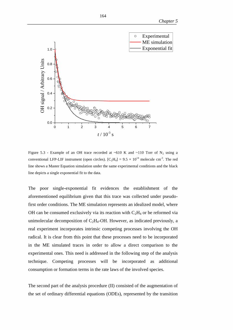
164

Chapter 5

0 1 2 3 4 5 6 7

0.0

0.2

0.4

0.6

0.8

1.0

Experimental

ME simulation

Exponential fit

OH

sig

nal

/ A

rbit

rary

Un

its

t / 10-3 s



molecule cm-3

. The red

line shows a Master Equation simulation under the same experimental conditions and the black

line depicts a single exponential fit to the data.

The poor single-exponential fit evidences the establishment of the

aforementioned equilibrium given that this trace was collected under pseudo-

first order conditions. The ME simulation represents an idealized model, where

OH can be consumed exclusively via its reaction with C2H4 or be reformed via

unimolecular decomposition of C2H4-OH. However, as indicated previously, a

real experiment incorporates intrinsic competing processes involving the OH

radical. It is clear from this point that these processes need to be incorporated

in the ME simulated traces in order to allow a direct comparison to the

experimental ones. This need is addressed in the following step of the analysis

technique. Competing processes will be incorporated as additional

consumption or formation terms in the rate laws of the involved species.

The second part of the analysis procedure (II) consisted of the augmentation of

the set of ordinary differential equations (ODEs), represented by the transition

165

Chapter 5

matrix constructed in step 1, to incorporate new formation or consumption

terms related to additional processes. These additional processes, such as the

measurable OH loss due to its reaction with the precursor and due to diffusion,

are not going to be treated as a function of internal energy. It is common

practice of PLF-LIF experiments to measure kloss (see equation E3) prior to the

execution of an experiment involving the chemistry of interest. Due to its

simplicity, this loss will be used as a first example of a process to be

incorporated to the current transition matrix. The value of kloss of the OH trace

presented in Figure 5.3 was measured to be ~100 s-1

. This means that an

additional consumption term is added as a constant loss to all the OH grains

modelled via the ME, which will perturb the shape of the ME simulation

presented in that figure. It is important to emphasize that this loss, which was

experimentally measured in the absence of C2H4, is not being treated as a

function of energy, but is simply spanned throughout all the grains of OH to

impose an overall loss of that specie. Since the reaction of OH with its

precursor does not influence the chemistry of interest (C2H4 + OH) beyond

representing an alternative loss of OH, a ME model that incorporates explicitly

the OH + H2O2 reaction would not present any feasible advantage, and would

merely increase the computational costs. This fact justifies the incorporation of

a simple constant loss term in the transition matrix to account for kloss.

Once the transition matrix has been altered as described in step II, the third

step can be undertaken (III) which consists of solving the new set of ODEs

using the same procedure as discussed in detail in Chapter 2. Figure 5.4 depicts

the fits presented previously along with the last one which incorporates kloss.

166

Chapter 5

0 1 2 3 4 5 6 7

0.0

0.2

0.4

0.6

0.8

1.0

Experimental

ME simulation

ME simulation with kloss

Exponential fit

OH

sig

nal

/ A

rbit

rary

Un

its

t / 10-3 s



molecule cm-3

. The red


line depicts a single exponential fit to the data. The blue line represents a ME fit in which the

transition matrix was altered to incorporate kloss the sum of the pseudo-first order loss due to

reaction of OH with its precursor and diffusion.

At the current stage it is clear that even though the inclusion of kloss has moved

the simulation in the correct direction, i.e., it has introduced a visible slope to

the simulated trace (note the difference between the red and blue lines); it is

evident that this was not sufficient to provide a good comparison to the

experimental measurements. As indicated previously, this figure is a

representative example from a total of 96 traces being fitted simultaneously. A

careful inspection of all the traces indicates a systematic overestimation of the

recycling by the model, as denoted by the blue line being on top of the black

open markers. From this point, it seems logical to postulate that one or more

significant processes are competing for and removing OH radicals from the

system, given this systematic overestimation.

167

Chapter 5

Two main candidates stand out as potential interferences: the first is a

hydrogen abstraction, which as discussed in the introductory section, is known

to be of significant importance for the chemistry of this reaction at elevated

temperatures. The second is a possible loss of the C2H4-OH adduct, via for

example, its reaction with O2. Even though oxygen was not added intentionally

in any of these experiments, H2O2 can potentially decompose to give O2 and it

is difficult to rule out the presence of small amounts of this gas in the system.

This will be discussed further later on in this chapter, but an important thing

can be noticed with regards to these two potential interfering channels: the H

abstraction is a bimolecular process that involves ethylene. Therefore, its effect

must scale appropriately with changes in the concentration of ethylene. On the

other hand, the concentration of the adduct is limited by the deficient reactant,

OH, and for this reason should be independent of the C2H4 concentration. This

is where a global analysis stands out as being superior and more robust when

compared to a single-trace analysis: these systematic aspects can be simply

assessed in a global fashion by imposing a relationship between model

parameters, such as bimolecular rate constants and their temperature

dependencies. From this point, one can pick a piece of chemistry of preference,

alter the transition matrix as explained previously in step II, solve the system

again and proceed with another comparison.

If one assumes, for example, the loss of the adduct to be the missing piece of

chemistry to be tested, and if this loss is known or easily measurable, then the

problem is analogous to the case of the incorporation of kloss. On the other

hand, if this loss is not known, then this aspect leads to the fourth step of this

analysis procedure, which is (IV) the definition of adjustable parameters

followed by a mathematical minimization in order to obtain a good agreement

between the solution of the ODEs and the experimental observations.

Typical adjustable parameters include: temperature dependencies of rate

coefficients, energy transfer parameters for pressure-dependent steps and

enthalpies of formation. This technique is being incorporated into the

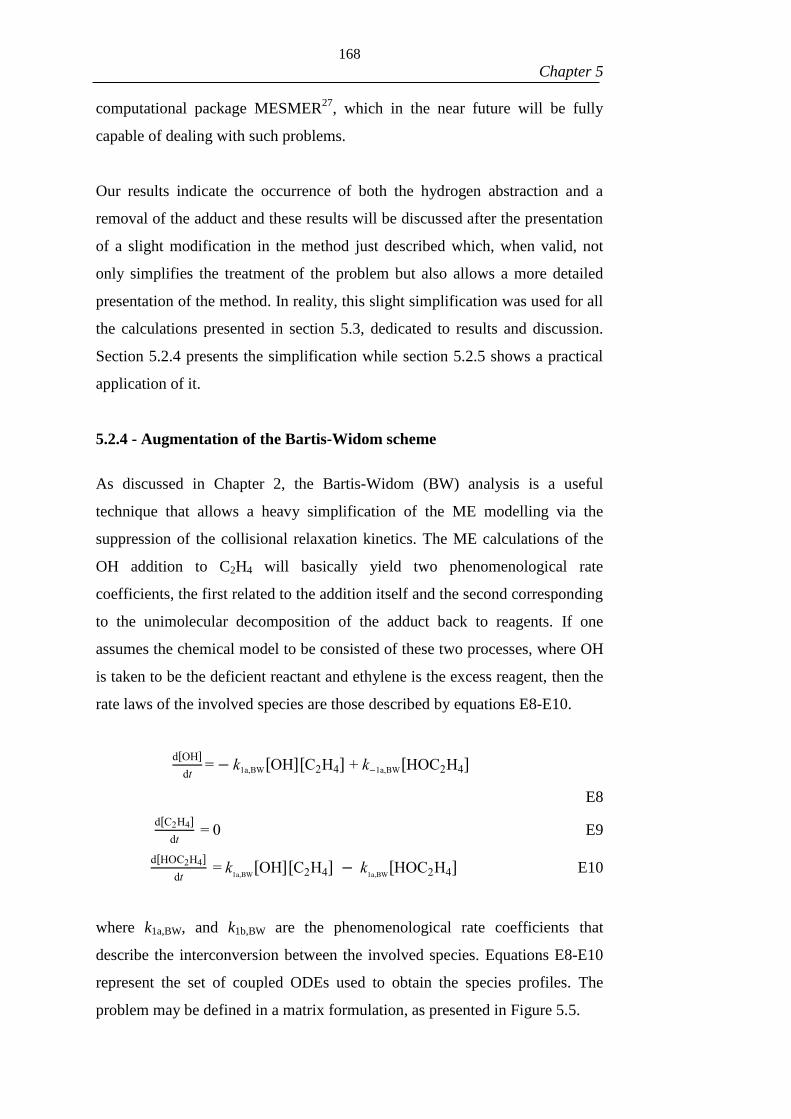
168

Chapter 5

computational package MESMER27

, which in the near future will be fully

capable of dealing with such problems.

Our results indicate the occurrence of both the hydrogen abstraction and a

removal of the adduct and these results will be discussed after the presentation

of a slight modification in the method just described which, when valid, not

only simplifies the treatment of the problem but also allows a more detailed

presentation of the method. In reality, this slight simplification was used for all

the calculations presented in section 5.3, dedicated to results and discussion.

Section 5.2.4 presents the simplification while section 5.2.5 shows a practical

application of it.

5.2.4 - Augmentation of the Bartis-Widom scheme

As discussed in Chapter 2, the Bartis-Widom (BW) analysis is a useful

technique that allows a heavy simplification of the ME modelling via the

suppression of the collisional relaxation kinetics. The ME calculations of the

OH addition to C2H4 will basically yield two phenomenological rate

coefficients, the first related to the addition itself and the second corresponding

to the unimolecular decomposition of the adduct back to reagents. If one

assumes the chemical model to be consisted of these two processes, where OH

is taken to be the deficient reactant and ethylene is the excess reagent, then the

rate laws of the involved species are those described by equations E8-E10.

d[OH]

dt= − k1a,BW[OH][C2H4] + k−1a,BW[HOC2H4]

E8

d[C2H4]

dt = 0 E9

d[HOC2H4]

dt = k

1a,BW[OH][C2H4] − k1a,BW

[HOC2H4] E10

where k1a,BW, and k1b,BW are the phenomenological rate coefficients that

describe the interconversion between the involved species. Equations E8-E10

represent the set of coupled ODEs used to obtain the species profiles. The

problem may be defined in a matrix formulation, as presented in Figure 5.5.

169

Chapter 5

Figure 5.5 - Matrix formulation of the OH + Ethylene addition reaction as simplified via the

Bartis-Widom approach.

where Xi’ represents the rate of specie i, indexes 1 and 3 refers to OH and the

C2H4-OH adduct respectively. As the concentration of C2H4 (i = 2) is taken to

be constant, it was incorporated into k’1a,BW which is equal to the product

k1a,BW × [C2H4] and its rate law was therefore not included in the matrix

scheme. The simplified transition matrix K as presented in Figure 5.5 can also

be modified to account for kloss or any other competing processes in analogy to

the case presented for the full ME. The modified BW-transition matrix

accounting for kloss is presented in Figure 5.6.

Figure 5.6 - Matrix formulation of the OH + Ethylene addition reaction as simplified via the

Bartis-Widom approach, modified to incorporate kloss.

The boundary conditions for these ODEs are the initial concentrations of the

species: as X1(0) = 1, X3(0) = 0. From this point the problem may either be

solved algebraically or via a numerical integration procedure. The main

advantage of the use of the BW transition matrix relies on its simplicity, which

allows its transportation to alternative software such as MATLAB46

, enabling a

wide range of mathematical treatment to the data. This versatility is also

translated into more freedom, for example, to link adjustable parameters. The

main disadvantage of this approach is that, unlike the direct modification of the

full ME, it relies on the numerical separation of the chemically significant

eigenvalues (CSE) from those related to internal energy relaxation (IERE).

170

Chapter 5

Therefore, in the case where the CSEs are not clearly separated, the BW

transition matrix may not be accurate enough to be used and the species

profiles are not reliable enough. It is important to clarify that in the present

study this has not been observed, i.e., a separation of more than one order of

magnitude was observed for all the experimental conditions explored in the

current thesis. This aspect will be discussed in the Results and Discussion

section (5.3).

Due to its validity and simplicity, the experimental data have been in reality

explored via the use of the BW transition matrix. To improve the quality of the

fits, as exemplified in Figure 5.4, the transition matrix was modified to

incorporate a competing H-abstraction and unimolecular losses of the

C2H4-OH adduct. Even though this adduct loss might be occurring via a

bimolecular channel (via O2 reaction for example), the use of a unimolecular

parameter provides an estimate of how fast this process occurs compared to the

recycling of OH. Furthermore, if one assumes an educated guess for the

bimolecular rate coefficient of the C2H4-OH + O2 reaction, an estimate the

concentration of O2 getting into the reaction cell can be obtained.

5.2.5 - Accounting for hydrogen abstraction and C2H4-OH loss in the BW

scheme

At low temperatures, the chemistry of the OH addition represents the bulk of

the mechanism that defines the experimental observations. However, in a real

high temperature experiment (T>500 K), as discussed previously, competing

loss processes of the involved species also play a significant roles that will

interfere in experimental measurements. For a typical laser flash photolysis-

laser induced fluorescence experiment, on a millisecond timescale,

heterogeneous chemistry is negligible and a better control over possible

contaminants is obtained. However, OH radicals are lost via reaction with the

precursor and small leaks combined with O2 generation from H2O2

decomposition can potentially introduce sufficient O2 to consume a significant

amount of the HO-C2H4 specie. In the previous section it was demonstrated

that chemistry represented by reactions R1a and R-1a is not sufficient for a

171

Chapter 5

direct comparison between simulated profiles and raw experimental OH traces.

Therefore, accounting for the hydrogen abstraction and the additional loss

processes of OH and the C2H4-OH species (R1b, Rloss, R3) need to be

incorporated in the ME simulated traces:

C2H4 + OH klb → H2O +·C2H3 (R1b)

OH kloss → Loss (Rloss)

C2H4-OH k3 → Loss (R3)

The existence of the process represented by R3 was identified by Diau et al. 38

,

who have studied the OH + C2H4 reaction in the 544-673 K temperature range

and 278-616 Torr of He using PLP-LIF. They report significant C2H4-OH

losses which increased with temperature, k3= (8.8-1.5

+25)×109 exp(

-10400-400

+1600

T) s

-1,

but were unable to define the mechanistic pathway responsible. The authors

have also measured the rate coefficients for the formation (k1a) and

decomposition (k-1a) of the C2H4-OH adduct at elevated temperatures via a

bi-exponential analysis. Their estimates for the enthalpy of formation of the

adduct (126.78 ± 3.35 kJ mol-1

) and entropy change ((12.93 ± 0.41) 10-2

kJ K-

1 mol

-1) were extracted from a van’t Hoff plot using the equilibrium constants

measured at various temperatures.

In the current thesis, reactions R1b, Rloss and R3 were introduced in the set of

equations E8, E9 and E10 as simple consumption terms for the involved

species, and at least one additional ODE is necessary to describe the evolution

of the products of the abstraction: H2O and C2H3. The chemical path behind the

loss of the C2H4-OH specie is unknown at first, but the importance of this

consumption term in our measurements was explored by defining it as a fitted

parameter. The abstraction rate coefficient is defined as an Arrhenius equation

to account for its temperature dependence since a significant temperature range

was covered. To elucidate the necessary alterations, the modified set of

equations due to the inclusion of reactions R1b, Rloss and R3 is presented in the

following:

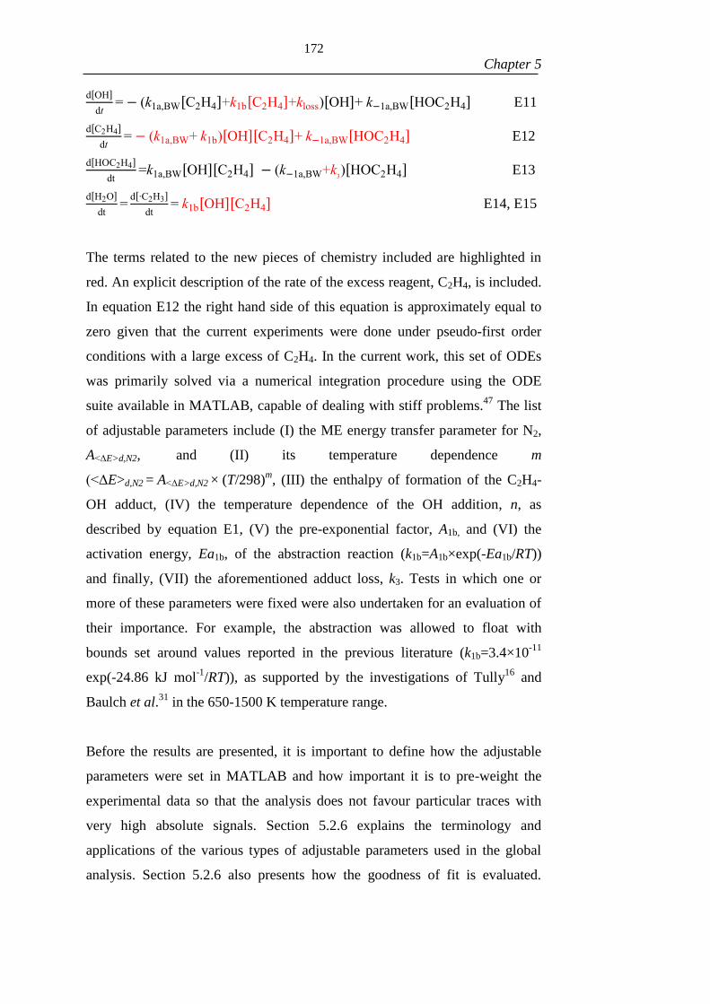
172

Chapter 5

d[OH]

dt= − (k1a,BW[C2H4]+k1b[C2H4]+kloss)[OH]+ k−1a,BW[HOC2H4] E11

d[C2H4]

dt= − (k1a,BW+ k1b)[OH][C2H4]+ k−1a,BW[HOC2H4] E12

d[HOC2H4]

dt=k1a,BW[OH][C2H4] − (k−1a,BW+k

3)[HOC2H4] E13

d[H2O]

dt=

d[∙C2H3]

dt= k1b[OH][C2H4] E14, E15

The terms related to the new pieces of chemistry included are highlighted in

red. An explicit description of the rate of the excess reagent, C2H4, is included.

In equation E12 the right hand side of this equation is approximately equal to

zero given that the current experiments were done under pseudo-first order

conditions with a large excess of C2H4. In the current work, this set of ODEs

was primarily solved via a numerical integration procedure using the ODE

suite available in MATLAB, capable of dealing with stiff problems.47

The list

of adjustable parameters include (I) the ME energy transfer parameter for N2,

A<ΔE>d,N2, and (II) its temperature dependence m

(<ΔE>d,N2 = A<ΔE>d,N2 × (T/298)m, (III) the enthalpy of formation of the C2H4-

OH adduct, (IV) the temperature dependence of the OH addition, n, as

described by equation E1, (V) the pre-exponential factor, A1b, and (VI) the

activation energy, Ea1b, of the abstraction reaction (k1b=A1b×exp(-Ea1b/RT))

and finally, (VII) the aforementioned adduct loss, k3. Tests in which one or

more of these parameters were fixed were also undertaken for an evaluation of

their importance. For example, the abstraction was allowed to float with

bounds set around values reported in the previous literature (k1b=3.4×10-11

exp(-24.86 kJ mol-1

/RT)), as supported by the investigations of Tully16

and

Baulch et al.31

in the 650-1500 K temperature range.

Before the results are presented, it is important to define how the adjustable

parameters were set in MATLAB and how important it is to pre-weight the

experimental data so that the analysis does not favour particular traces with

very high absolute signals. Section 5.2.6 explains the terminology and

applications of the various types of adjustable parameters used in the global

analysis. Section 5.2.6 also presents how the goodness of fit is evaluated.

173

Chapter 5

Section 5.2.7 explains why it is primarily important to pre-weight the

experimental traces in order to avoid undesirable biases in the analysis.

5.2.6 - A more programmatic view of the model parameters

As indicated previously global analysis is a very robust, consistent and

versatile analysis technique, suitable for the exploitation of large amounts of

data. In a global procedure, fitting operations of multiple traces are brought

together in order to provide the best overall agreement of the model to the

complete data set. During the procedure, a limited number of parameters,

which may be fixed or floated, are shared by all the individual fits. These

parameters, referred to as global parameters, will directly influence the model

prediction of every single trace, and therefore tend to have a greater impact on

the overall goodness of fit. For example, the pre-exponential factor and energy

of activation of the abstraction reaction are shared by all traces being analysed.

The bimolecular abstraction rate coefficient, used to construct a model

prediction, is always obtained based on these two parameters and the

corresponding temperature. Moreover, if a trace i has a temperature T1 and a

trace j was collected at temperature T2, then k1b(T1) = A1b × exp(-Ea1b/RT1) and

k1b(T2)=A1b×exp(-Ea1b/RT2). Note that both are calculated based on the

aforementioned global variables. This aspect imposes a constraint that

reinforces the kinetic consistency of the results obtained in the global fitting

procedure. For example, for a well-defined energy barrier, if T1>T2, then not

only is k1b(T1) greater than k1b(T2) but both are linked via a kinetically

consistent Arrhenius formulation.

On the other hand, there are model parameters that can cause interferences

exclusively in individual model predictions and hence, tend to have a smaller

impact on the overall goodness of fit. These are referred to as local variables

or local parameters. In each trace, the initial fluorescence signal from the OH

radicals (t=0) collected by a photomultiplier is very uncertain, and for this

reason it is common practice to have it as an adjustable parameter. This

parameter, however, is not linked or related in any way to the initial OH

concentration of the other traces or the other listed parameters, and represents

174

Chapter 5

therefore an example of a local parameter. Despite the less significant direct

impact on the quality of the global adjustment, local variables can eventually

cause slight variations on the returned optimized parameters, especially when

inappropriate guesses and bounds are set. In this case, the optimization

algorithm might try to compensate the effect of this bad guess with significant

changes in the other parameters. This issue can be minimized if a large number

of traces are considered, making the identification of outliers a simpler task.

A third and final category of parameters is often useful and need to be

addressed here: these are the local-global parameters. Similarly to the case of

global parameters, these ones are shared by two or more traces, but not by the

totality of the data set as it is the case for the global ones. Examples of local

global parameters are kloss and k3. This is justified for kloss, for example,

because this loss is typically kept constant throughout an experiment

performed at a given temperature and pressure. Once the temperature and

pressure are set, OH traces are collected in the course of a few hours depending

on the quality of the signal being acquired. Given that the H2O2 flow was

stable, all traces collected during this course of experiments will therefore

share the same kloss. However, if new experiments are performed with a

different OH precursor or at different temperatures and pressures, it is likely

that the value of kloss will change as well. Moreover, if new traces at

significantly higher temperatures are to be collected, it might be necessary to

increase the H2O2 flow because this high temperature can potentially enhance a

thermal decomposition of H2O2, changing kloss for the next set of traces. As a

general rule, each trace collected in the same day, under the same experimental

conditions is assumed to have the same kloss.

Analogously, if one postulates that the adduct loss occurs unimolecularly, it is

also reasonable to assume this loss should be the same for the traces generated

under the same experimental conditions. On the other hand, if a reaction with

O2 is invoked, this assumption would remain appropriate (a shared k3 per

experimental condition) since O2 is likely to be produced primarily via the

decomposition of the OH precursor, whose concentration is maintained

175

Chapter 5

constant via the use of calibrated mass-flow controllers. With these aspects

presented, the implementation of both kloss and k3 as local-global parameters is

justified. The main difference between these two relies on the fact that, while a

list of kloss values, related to each set of experiments, can be easily measured

and fed into the fitting procedure as fixed values, the list of k3 (one for each T,

p and day) is floated by the optimization algorithm in order to provide a good

fit to the whole set of experimental data. The need to define local-global

parameters and their complex linking is an example of an advantage of the use

of the BW analysis supported by an external piece of software such as

MATLAB. Figure 5.7 presents a flow chart of the procedure based on the BW

analysis supported by MATLAB.

Figure 5.7 - Flow chart of the fitting based on BW rate coefficients followed by ODE

modification.

176

Chapter 5

As observed, the objective function to be minimized is the overall sum of

squared residuals χ2, as a measure of the goodness of fit. For n experimental

traces, χ2

is calculated as defined by equations E16 and E17:

χi2 =∑ (y

j,calc− y

j,exp)2ki

j=1 E16

χ2 =∑ χi2n

i=1 E17

where χi2 is the sum of squared residuals associated to the ith experimental

trace, ki is the number of points of the ith trace, yj,exp

is the jth point within

experimental trace i and yj,calc

is the corresponding model prediction. The

overall χ2 is then calculated as a summation of all χi2. The unweighted linear

combination presented in equation E17 raises a slight concern regarding the

importance attributed to each individual trace during the minimization

procedure. This aspect that will be covered in the subsequent section where it

is explained how the data are weighted to prevent this issue.

5.2.7 - Pre-weighting of experimental data

In LPF-LIF experiments, the OH induced fluorescence is typically collected by

a photomultiplier whose voltage control enables the enhancement of the total

signal being collected. However, this increase also leads to an increase of

background counts, so that a voltage increase does not necessarily translate

into an improvement of the signal/noise ratio. Increasing the voltage can be

useful, for example, for tuning the wavelength of the probe if this has shifted

away from the peak of the ~282 nm excitation line, a common effect observed

when the temperature of the room varies during the course of an experiment.

Varying the photomultiplier voltage also alters the absolute scale of the OH

signal being collected, and this difference needs to be addressed to avoid

unfairly favouring the high signal traces when minimizing χ2. Traces with

larger absolute OH signals will tend to have a greater impact on the sum of

squared residuals, causing the optimization algorithm to “focus” on getting

these traces right, while traces with lower absolute signals will tend to be

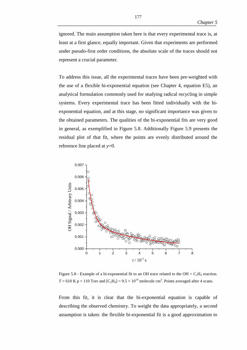
177

Chapter 5

ignored. The main assumption taken here is that every experimental trace is, at

least at a first glance, equally important. Given that experiments are performed

under pseudo-first order conditions, the absolute scale of the traces should not

represent a crucial parameter.

To address this issue, all the experimental traces have been pre-weighted with

the use of a flexible bi-exponential equation (see Chapter 4, equation E5), an

analytical formulation commonly used for studying radical recycling in simple

systems. Every experimental trace has been fitted individually with the bi-

exponential equation, and at this stage, no significant importance was given to

the obtained parameters. The qualities of the bi-exponential fits are very good

in general, as exemplified in Figure 5.8. Additionally Figure 5.9 presents the

residual plot of that fit, where the points are evenly distributed around the

reference line placed at y=0.

0 1 2 3 4 5 6 7 8

0.000

0.001

0.002

0.003

0.004

0.005

0.006

0.007

OH

Sig

nal

/ A

rbit

rary

Un

its

t / 10-3

s

Figure 5.8 - Example of a bi-exponential fit to an OH trace related to the OH + C2H4 reaction.

T = 610 K p = 110 Torr and [C2H4] = 9.5 × 1014

molecule cm3. Points averaged after 4 scans.

From this fit, it is clear that the bi-exponential equation is capable of

describing the observed chemistry. To weight the data appropriately, a second

assumption is taken: the flexible bi-exponential fit is a good approximation to

178

Chapter 5

the best possible fit of a suitable model to the data. This assumption means that

the χi2 value obtained for this bi-exponential fit is a good approximation to the

lowest possible sum of squared residuals, and will be referred to as χi,min2 . If

one then divides the points of the experimental trace by the squared root of this

number, i.e., χi,min

, and attempts another fit, then the new sum of squared

residuals (χi,new2 ) can be calculated in an analogous manner to that previously

presented:

χi,new2 = ∑ (

yj,calc

−yj,exp

χi,min

)2

ki

j=1 =1

χi,min2∑ (y

j,calc− y

j,exp)2ki

j=1 E18

0 1 2 3 4 5 6 7 8

0.000

OH

Sig

nal

/ A

rbit

rary

Unit

s

t / 10-3

s

0

Figure 5.9 - Residual plot of the bi-exponential fit presented in Figure 5.8. T = 610 K p = 105

Torr and [C2H4] = 9.5 × 1014

molecule cm3. Points averaged after 4 scans.

From equation E18, it is clear that at the limit where ∑ (yj,calc

− yj,exp

)2ki

j=1

approximates χi,min2 , χ

i,new2 is unity. This eliminates the issue associated to the

existence of traces with significantly different signal heights. Note that

independent of the height, a trace has a chance to add a total of one to the

overall χi2 if its fit resembles the corresponding bi-exponential one. If the new

179

Chapter 5

fit is not as good as the corresponding bi-exponential, then

∑ (yj,calc

- yj,exp

)2ki

j=1 > χi,min2 and therefore χ

i,new2 > 1. The bi-exponential equation

was used in this chapter, but for other systems, other appropriate equations (tri-

exponentials, tetra-exponentials, etc) can also be used to fit experimental data

in order to determine the weight associated with each individual trace. If no

appropriate analytical equation is available, the traces can also be fitted with a

numerical solution of a reaction scheme, allowing the estimation of χi,min

. It is

important to inspect the resulting fits that generate the individual χi,min

to make

sure the model function (analytical or numeric) is capable of successfully

describing all the traces under analysis and no bias towards a certain group of

traces is inadvertently introduced. For example, new chemical processes can be

turned on at elevated temperatures, and the lack of description of these

processes in the model function can lead to elevated χi,min

(poor fit) to the

traces where this new piece of chemistry is important. As a result, the elevated

χi,min

would imply undesirable lower weights for these traces. For this reason,

the inspection of the resulting fits of the weighting procedure described in this

section is crucial.

In summary, as indicated by the left-hand side of equation E19, a weighted

sum of squared residuals (χi,new2 ) can be obtained calculated as a moderate

average of χi2, where the weight corresponds to 1/χ

i,min2 . A good fit is obtained

when χi,new2 associated with a trace is close to unity, and the new global sum of

squared residuals χnew2 is therefore close to the total number of traces (one per

trace). This weighting procedure was applied to all traces prior to the execution

of the ME global described in detail in sections 5.2.3-5.2.6.

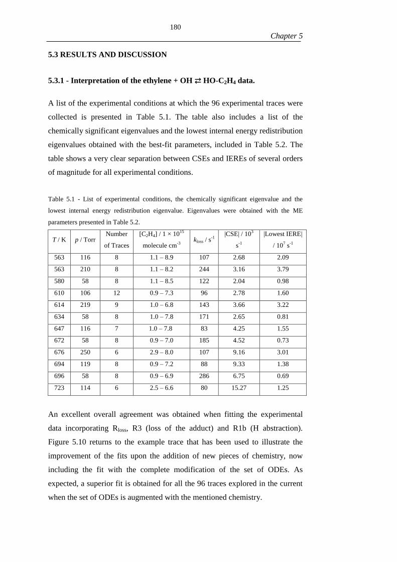
180

Chapter 5


5.3.1 - Interpretation of the ethylene + OH ⇄ HO-C2H4 data.

A list of the experimental conditions at which the 96 experimental traces were

collected is presented in Table 5.1. The table also includes a list of the

chemically significant eigenvalues and the lowest internal energy redistribution

eigenvalues obtained with the best-fit parameters, included in Table 5.2. The

table shows a very clear separation between CSEs and IEREs of several orders

of magnitude for all experimental conditions.

Table 5.1 - List of experimental conditions, the chemically significant eigenvalue and the

lowest internal energy redistribution eigenvalue. Eigenvalues were obtained with the ME

parameters presented in Table 5.2.

T / K p / Torr Number

of Traces

[C2H4] / 1 × 1015

molecule cm-3

kloss / s

-1

|CSE| / 103

s-1

|Lowest IERE|

/ 107 s

-1

563 116 8 1.1 – 8.9 107 2.68 2.09

563 210 8 1.1 – 8.2 244 3.16 3.79

580 58 8 1.1 – 8.5 122 2.04 0.98

610 106 12 0.9 – 7.3 96 2.78 1.60

614 219 9 1.0 – 6.8 143 3.66 3.22

634 58 8 1.0 – 7.8 171 2.65 0.81

647 116 7 1.0 – 7.8 83 4.25 1.55

672 58 8 0.9 – 7.0 185 4.52 0.73

676 250 6 2.9 – 8.0 107 9.16 3.01

694 119 8 0.9 – 7.2 88 9.33 1.38

696 58 8 0.9 – 6.9 286 6.75 0.69

723 114 6 2.5 – 6.6 80 15.27 1.25

An excellent overall agreement was obtained when fitting the experimental

data incorporating Rloss, R3 (loss of the adduct) and R1b (H abstraction).

Figure 5.10 returns to the example trace that has been used to illustrate the

improvement of the fits upon the addition of new pieces of chemistry, now

including the fit with the complete modification of the set of ODEs. As

expected, a superior fit is obtained for all the 96 traces explored in the current

when the set of ODEs is augmented with the mentioned chemistry.

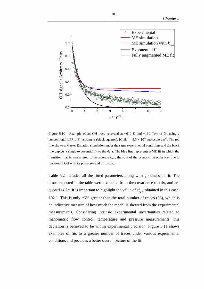
181

Chapter 5

0 1 2 3 4 5 6 7

0.0

0.2

0.4

0.6

0.8

1.0

Experimental

ME simulation

ME simulation with kloss

Exponential fit

Fully augmented ME fit

OH

sig

nal

/ A

rbit

rary

Un

its

t / 10-3 s


conventional LFP-LIF instrument (black squares). [C2H4] = 9.5 × 1014

molecule cm-3

. The red


line depicts a single exponential fit to the data. The blue line represents a ME fit in which the

transition matrix was altered to incorporate kloss, the sum of the pseudo-first order loss due to

reaction of OH with its precursor and diffusion.

Table 5.2 includes all the fitted parameters along with goodness of fit. The

errors reported in the table were extracted from the covariance matrix, and are

quoted as 2σ. It is important to highlight the value of χnew2 obtained in this case:

102.1. This is only ~6% greater than the total number of traces (96), which is

an indicative measure of how much the model is skewed from the experimental

measurements. Considering intrinsic experimental uncertainties related to

manometric flow control, temperature and pressure measurements, this

deviation is believed to be within experimental precision. Figure 5.11 shows

examples of fits to a greater number of traces under various experimental

conditions and provides a better overall picture of the fit.

182

Chapter 5

Table 5.2 – List of optimized parameter for the augmented ME fit. Uncertainties quoted as 2

Parameter Optimized value

ΔHC2H4-OH 111.8 ± 0.2 kJ mol-1

A1a (8.13 ± 0.86)×10-12

cm3 molecule

-1 s

-1

n1a -0.99 ± 0.18

A1b (3.50 ± 0.75)×10-11

cm3 molecule

-1 s

-1

Ea1b 26.2 ± 1.3 kJ mol-1

A<ΔE>d,N2 234 ± 32 cm-1

m (Energy transfer)** 0.11 ± 0.15

X2/ntraces 1.06

k1a∞

=A1a(T

298 K)n1a

; k1b∞

=A1bexp(-Ea1b

RT); <ΔE>

d,N2=A<ΔE>d,N2

(T

298 K)m

0.0 0.2 0.4 0.6 0.8 1.0

0.0

0.2

0.4

0.6

0.8

1.0

p = 105 Torr, T = 610 K, [C2H

4] = 2.78 x 10

15 molecule cm

-3

p = 210 Torr, T = 563 K, [C2H

4] = 3.16 x 10

15 molecule cm

-3

p = 115 Torr, T = 647 K, [C2H

4] = 2.93 x 10

15 molecule cm

-3

p = 60 Torr, T = 634 K, [C2H

4] = 9.88 x 10

14 molecule cm

-3

OH

Sig

nal

/ A

rbit

raty

Un

its

t / 10-3 s

0

Figure 5.11 - Examples of augmented ME fits for multiple traces under significantly different

experimental conditions. The dashed line represents y=0 for a better reference.

The enthalpy of formation determined for the C2H4-OH adduct

((111.8 ± 0.2) kJ mol-1

) is in excellent agreement with the theoretically

determined value of ΔH0K,C2H4-OH of 111.4 kJ mol-1

. This remarkably good

agreement is accompanied with a relatively small uncertainty associated with

the experimental determination. When compared to the uncertainty quoted in

Chapter 4 for the isoprene-OH well depth for example (~5 kJ mol-1

), it is

183

Chapter 5

postulated that the raw-trace global fitting procedure improves the precision of

the parameters by imposing constraints to the fitted variables, such as the

temperature dependence of bimolecular rate coefficients, reducing the degrees

of freedom of the optimization. Furthermore, larger data sets employed

covering wide ranges of experimental conditions (T and p) tend to be sensitive

to a greater number of adjustable parameters. For example, while the activation

energy of a process would be invisible in a single trace analysis, a trend

comprised in a combination of them can provide information about this

parameter.

Another advantage of the current method of analysis is the absence of the use

of analytical equations to extract rate coefficients from the traces, as is the case

in a classic ME fit. In the traditional procedure, experimental traces are

converted into rate coefficients before being fed into the ME fitting. Recycling

rate coefficients can be extracted from bi-exponential fits with some simplicity.

If for example, however, a temperature dependence is imposed for this rate

coefficient (k-1a(T) = A-1a × exp(-Ea

-1a

RT)), the uncertainties of the obtained

parameters A-1a and Ea-1a would require to be appropriately propagated for a

calculation of k-1a(T). The complexity of multi-exponential equations can

rapidly make the suitable computation of these uncertainties a difficult task.

While the uncertainties obtained with the current method are largely controlled

by the signal:noise ratio of the experimental OH traces, in a classic analysis the

uncertainties are additionally dependent on the form by which a rate coefficient

is extracted.

The bi-exponential formulation typically requires the incorporation of 3-5

parameters to describe recycling data. This includes the forward and backward

rate coefficients and the various additional experimental losses from the

system. This large number of parameters provide a great flexibility for fitting

data, but represents a compromise to the fact that good fits may be obtained

even when the chemistry being studied is not sufficiently understood. If an

important piece of chemistry is missing, the remaining parameters are

sometimes sufficient to compensate this effect and provide a good fit to the

184

Chapter 5

data. The current method takes advantage of the global links to avoid this

issue.

5.3.2 - Literature comparison of the OH addition and hydrogen

abstraction

The parameters related to k1a∞

and k1b∞

were used for a comparison with

literature investigations of the corresponding reactions. While the equation

related to the OH addition was compared to the studies of Zellner and

Lorenz20

, Fulle et al.23

, Vakhtin et al.17

, Diau et al.38

and Liu et al.48

, the

abstraction high pressure limiting coefficient was compared against a literature


and the measurements of Tully 16

, Liu et al.30

, Vasu

et al.35

, Westbrook et al.32

, Srinivasan et al.34

and Bhargava and

Westmoreland.33

The respective comparisons are presented in Figures 5.12 and

5.13.

In the context of the OH addition and except for the work of Fulle et al.23

,

where the high pressure limiting rate coefficients for reaction R1a were

observed to be temperature independent, k1a∞

falls monotonically with

increasing temperatures in the depicted range. In the investigation of Fulle et

al., k1a∞

was obtained from an extrapolation of measurements in the fall-off

region between 300 and 800 K with the use of the Troe formalism (see Chapter

4 for an example of the use of such formulation). Even though pressures

ranged from 1 to 150 bar, a very limited number of points was employed in

each fit. The fact that the measurements were analysed separately, as per

temperature, raises concerns with respect to the internal consistency of the

measurements. It is not trivial to rationalize why their k1a∞

values are

independent of temperature for such a large temperature range

185

Chapter 5

100 200 300 400 500 600 700 800

0.3

0.5

1

3

1

Current work

IUPAC recommendation

Liu et al. (1989)

Diau et al. (1992)

Zellner and Lorenz (1984)

Fulle et at. (1997)

Vakhtin et al. (2003)

k 1a(T

) /

10

-11 c

m3 m

ole

cule

-1 s

-1

T / K


different investigations. Pink triangles represent the IUPAC recommendation for the

temperature dependence of the high-pressure limiting rate coefficient of the ethylene + OH

reaction in the 100-500 K temperature range (k1a∞

=9×10-12(T

300 K)-0.85

cm3 molecule

-1 s

-1). Black

squares represent the recommendation of this work based on the best fit parameters reported in

Table 5.2. Open markers represent pressure dependent rate coefficients and filled markers are

estimates of k1a∞

.

Zellner and Lorenz20

have explored this reaction in the 296-524 K temperature

range and pressures between 3 and ~100 Torr of argon, where a pressure

dependence was identified. Their high pressure limiting rate coefficients were

estimated via a simple Lindemann extrapolation (see Chapter 2 for a

description of the Lindemann mechanism). As indicated previously, estimates

based on such extrapolations will naturally enhance errors in the high pressure

limiting rate coefficients. Their recommended equation for k1a∞ tends to be

greater than our recommendation.

186

Chapter 5

600 800 1000 1200 1400 1600 1800 2000

0.01

0.1

1

10

Current work

Baulch et al. (Review)(1992)

Tully (1988)

Liu et at. (1987)

Vasu et al. (2010)

Westbrook et al.(1988)

Srinivasan et al.(2007)

Bhargava and Westmoreland. (1998)

k 1b(T

) /

10

-11 c

m3 m

ole

cule

-1 s

-1

T / K


different investigations. Red circles represent the recommendation from the review by Baulch

et al.31

, blue open triangles refer to the work of Tully 16

, pink diamonds refer to the work of

Liu et al.30

, olive triangles correspond to the report of Vasu et al.35

, cyan triangles refer to the

work of Westbrook et al.32

, orange stars correspond to the study of Srinivasan et al.34

, light

green triangles refer the work of Bhargava and Westmoreland33

and finally, black squares are

the recommendation based on the best fit parameters reported in Table 5.2.

The measurements of Vakhtin et al.17

, used in in the development of the

IUPAC recommendation, were also obtained from an extrapolation of

pressure-dependent rate coefficients in the 96-296 K temperate range and

pressures ranging from 0.2 to 100 Torr of N2. Such extrapolations require a

very large number of measurements for a more accurate determination of the

parameters. While 12 pressures were evaluated at 296 K, only one pressure

was employed at 96 K, 110 K and 165 K investigated, heavily limiting the

accuracy of the extrapolated rate coefficients. If the current results are

extrapolated to the conditions of their work, a very good agreement is

observed, with deviations smaller than 10%.

Measurements by Diau et al.38

were treated via a bi-exponential analysis of

equilibrium traces collected at temperatures between 544 and 673 K and

pressures between ~280 and 615 Torr of He. The authors do not provide a

187

Chapter 5

pressure-dependent treatment to their data, but recognize that traces with T <

590 K and pressures above 500 Torr are more likely to be closer to the high

pressure limit. Considering only this subset of their data, they report an

equation for k1a∞ = (4 ± 3)×10

-13exp(

9.98 kJ mol-1

RT). Our best estimate for k1a at

590 K and 615 Torr of He (3.5×10-12

cm3 molecule

-1 s

-1) is about 16% lower

than our estimated high pressure limiting rate coefficient under the same

temperature, 4.1×10-12

cm3 molecule

-1 s

-1, which suggests that even the

selected subset of their data was within the fall-off region.

In the work of Liu et al.48

measurements were undertaken at a relatively high

pressure (760 Torr of Ar). Compared to helium, argon promotes energy

transfer more efficiently49

, therefore reaching the high pressure limit faster

than in helium. Even though the authors do not provide a proper pressure

dependent treatment of their measurements, and our results indicate that their

measurements at 590 K are not at the high pressure limit, being 13% lower

than our estimate of k1a∞

.

In terms of the abstraction channel, Figure 5.13 shows a good agreement

between the current work and the recommendations reported by Tully16

and

Vasu et al.35

Despite this fact, a ME simulation at the lowest pressure

employed in the work of Tully (to disfavour the addition) (~100 Torr) and 650

K indicates that k1a(T,p) = 3.6 × 10-12

cm3 molecule

-1 s

-1 is still more than an

order of magnitude faster than the abstraction channel

k1b = 2.7 × 10-13

cm3 molecule

-1 s

-1. Additional master equation simulations

indicate that for 100 Torr of He, the H-abstraction just overcomes the OH

addition at around 840 K, as depicted in Figure 5.14. The measurements of Liu

et al.30

for the abstraction coefficient are found to be systematically higher than

our current measurements.

188

Chapter 5

800 820 840 860 880

0.65

0.70

0.75

0.80

0.85

0.90

0.95

1.00

k1a

(T,100 Torr of He)

k1b

(T)k

/ 10

-12 c

m3 m

ole

cule

-1 s

-1

T / K

Figure 5.14 – The temperature dependence of H-abstraction and OH-addition rate coefficients

at 100 Torr of He.

The energy transfer parameter related to the OH addition need to be addressed.

The value of A<ΔE>d,N2 (234 ± 32 cm-1

) is in agreement with the one obtained

for the work of isoprene + OH presented in Chapter 4 (150 ± 90). The

temperature dependence of this parameter, m, is ill-defined as denoted by the

large uncertainty reported. A test was performed by fixing the energy transfer

parameter at the value of 0.25, but no significant variation on the returned

parameters or χnew2 was observed.

189

Chapter 5

560 580 600 620 640 660 680 700 720 740

0

200

400

600

800

1000

1200

k 3 /

s-1

T / K

Figure 5.15 – List of k3’ values obtained from the augmented BW-ME fit as a function of

temperature.

Omitted from Table 5.2, the list of the fitted k3 values is presented in Figure

5.15 as a function of the temperature at which the corresponding OH traces

were collected. This figure is an attempt to identify a potential relationship

between the temperature in the reaction and the chemical process responsible

for k3. According to conventional oxidation pathways for β-hydroxyalkyl

radicals, the O2 addition to a radical is likely to be the main removal process

involved.50-51

Even though no experimental measurements of the C2H4-OH +

O2 reaction are available, the literature reports rate coefficients for β-

hydroxyalkyl radicals + O2 reactions in the 10-11

– 10-12

cm3 molecule

-1 s

-1

range.51

Considering the largest k3’ (the prime is used to denote a pseudo-first

order rate coefficient) value obtained (780 s-1

) and a slow C2H4-OH + O2

bimolecular rate coefficient of 1×10-12

, the largest concentration of O2

introduced in the reaction cell is estimated to be ~7.8×1014

molecule cm-3

.

Estimates undertaken by other personnel using the same instrumental setup,

based on well-skipping reactions in the diethyl ether + OH reaction oxidation

suggest an oxygen concentration around 2 × 1014

molecule cm-3

which does

not seem to vary significantly with temperature.52

190

Chapter 5

Addition reactions are typically barrierless processes and for this reason,

generally present a negative temperature dependence, something that is not

evident from Figure 5.15. This fact reinforces the importance of the definition

of k3’ as a local-global parameter. For example, since the potential O2

contamination is not being controlled, measurements generated at 723 K could

have a larger k3’ simply because more O2 was introduced in those experiments.

As O2 production is likely to come from H2O2 decomposition, the fact that

H2O2 in the delivery vessel gets concentrated with time means that no

relationship can be attributed to k3’ values determined in different days of

experiment. The delivery vessel where the precursor is stored also can run out

of liquid and needs to be topped up eventually, again, altering the

concentration of the OH precursor being delivered and potentially, altering O2

contamination. Nonetheless, the figure shows that, except for the highest

temperature explored, parameters are reasonably well-defined, given the size

of the error bars, quoted as 2σ.

A quick evaluation of the impact of the use of an alternative OH precursor is

finally considered for shedding a little bit of light on the nature of k3’.

Urea-H2O2 ((NH2)2CO-H2O2, ALFA AESAR, 97%) is a commercially

available solid, verified to successfully serve as a source of gas-phase H2O2,53

as first demonstrated by Ludwig et al.54

The authors have used time-resolved

mass spectrometry to study the reaction of C2H5 radicals with HO2 and urea-

H2O2 was implemented as a precursor of gas-phase H2O2 and subsequently,

HO2 was produced via 193 nm photolysis. The precursor was introduced in a

thermostated flask to control the H2O2 concentration via its vapour pressure,

which depends on the temperature of the flask. The authors acknowledge that

beyond 328 K small amounts of H2O and O2 were detected, and for this reason

they have kept the thermostated flask below this temperature.

Figure 5.16 shows OH traces collected under the same experimental conditions

(T~610 K and p= 110 Torr) but with the use of the two OH precursors: H2O-

H2O2 (blue triangles) and urea-H2O2 (red crosses).

191

Chapter 5

0.0 0.5 1.0 1.5 2.0 2.5 3.0

0.000

0.002

0.004

0.006

0.008

0.010

Urea-H2O

2

H2O-H

2O

2

H2O-H

2O

2, [O2] = 9.31015 molecule cm-3

OH

Sig

nal

/ A

rbit

rary

Un

its

t / 10-3

s

Figure 5.16 – Experimental traces collected at ~610 K and ~110 Torr with the use of different

precursors. While blue triangles and red crosses were collected with the use of H2O-H2O2, the

black squares represent a trace collected with urea-H2O2.

A very clear difference is observed between the blue triangles and black

squares, an indication that the concentration of O2 when urea-H2O2 is used is

much greater when compared to the alternative precursor. As a final test, a

flow of O2 was introduced in the H2O-H2O2 experiment ([O2] = 9.3 × 1015

molecule cm-3

), giving rise to the trace represented by red crosses. This new

trace very similarly resembles the urea-H2O2 one, an effect that corroborates

with the postulation of O2 removal being the cause of k3’.

192

Chapter 5


In summary, a new method for analysing temperature and pressure dependent

experimental data via a global raw-trace analysis has been presented and tested

against a large number of complex OH traces associated with the ethylene +

OH reaction. The structure, assumptions and implementation of the method

were discussed in detail. The augmentation of the phenomenological ordinary

differential equations, the heart of the method, have also allowed a systematic

evaluation of the mechanism that governs the experimental observations,

enhancing the reliability of the thermochemical parameters obtained from the

fitting procedure. OH traces were collected under a wide range of pressures

(~60 - 220 Torr) and temperatures (563 – 723 K) to ensure significant chemical

differences are present in each trace. Remarkably, the fits are found be skewed

only 6% from the corresponding experimental measurements in average.

Nonetheless, a comparison of the predicted high pressure limiting rate

coefficients for the OH addition with previous literature investigations shows

that due to the lack of appropriate pressure dependency treatments on the

previous investigations a significant inconsistency of the literature with respect

to the OH addition is observed. For the abstraction reaction on the other hand,

good agreement with the work of Tully16

is obtained. An excellent agreement

is observed between a theoretical prediction of the C2H4-OH well-depth

(111.4 kJ mol-1

) and the experimental determination (111.8 ± 0.20 kJ mol-1

).

The subsequent chapter of the current thesis deals with radical recycling from

the OH + isoprene reaction will take advantage of the current method to

exploit this atmospherically relevant chemical process. The chapter will inherit

the basis of the method described here, as well as their assumptions and

programmatic implementation.

193

Chapter 5

5.5 REFERENCES

1. Benham, E.; McDaniel, M., Ethylene Polymers, HDPE. In Encyclopedia of Polymer

Science and Technology, 4th

ed.; John Wiley & Sons, Inc.: 2002.

2. Proceedings of the 3rd World Conference on Detergents Global Perspectives. Cahn,

A., Ed. AOCS Press: Champaign, Ill. :, 1994.

3. Handbook of Detergents, Part F: Production. In Surfactant Science Series, Zoller, U.;

Sosis, P., Eds. CRC Press 2008; Vol. 142.

4. Barry, C. S.; Giovannoni, J. J. Ethylene and Fruit Ripening. Journal of Plant Growth

Regulation 2007, 26, 143.

5. Sabljic, A., Environmental and Ecological Chemistry. 1st ed.; EOLSS Publishers Co

Ltd: 2009; Vol. 2.

6. Morgott, D. A. Anthropogenic and Biogenic Sources of Ethylene and the Potential for

Human Exposure: A Literature Review. Chemico-Biological Interactions 2015, 241, 10-22.

7. Sawada, S.; Totsuka, T. Natural and Anthropogenic Sources and Fate of Atmospheric

Ethylene. Atmospheric Environment (1967) 1986, 20, 821-832.

8. Reactive Hydrocarbons in the Atmosphere. 1st ed.; Hewitt, C. N., Ed. Academic

Press: 1999.

9. Olivier, J.; Peters, J.; Granier, C.; OPetron, G.; Muller, J. F.; Wallens, S. Present and

Future Surface Emissions of Atmospheric Compounds; 2003.

10. Hakola, H.; Hellén, H.; Laurila, T. Ten Years of Light Hydrocarbons (C2–C6)

Concentration Measurements in Background Air in Finland. Atmospheric Environment 2006,

40, 3621-3630.

11. Cleary, P. A.; Romero, M. T. B.; Blitz, M. A.; Heard, D. E.; Pilling, M. J.; Seakins, P.

W.; Wang, L. Determination of the Temperature and Pressure Dependence of the Reaction

OH+C2H4 from 200-400 K Using Experimental and Master Equation Analyses. Physical

Chemistry Chemical Physics 2006, 8, 5633-5642.

12. Sander, S. P. et al. Chemical Kinetics and Photochemical Data for Use in

Atmospheric Studies; Jet Propulsion Laboratory: Pasadena, 2003.

13. Gas-Phase Combustion Chemistry. 2nd

ed.; Gardiner, W. C., Jr., Ed. Springer: New

York, 2000.




15. Liu, A.; Mulac, W. A.; Jonah, C. D. Kinetic Isotope Effects in the Gas-Phase

Reaction of Hydroxyl Radicals with Ethylene in the Temperature Range 343-1173 K and 1-

Atm Pressure. The Journal of Physical Chemistry 1988, 92, 3828-3833.

16. Tully, F. P. Hydrogen-Atom Abstraction from Alkenes by OH, Ethene and 1-butene.

Chemical Physics Letters 1988, 143, 510-514.

17. Vakhtin, A. B.; Murphy, J. E.; Leone, S. R. Low-Temperature Kinetics of Reactions

of OH Radical with Ethene, Propene, and 1-Butene. The Journal of Physical Chemistry A

2003, 107, 10055-10062.

18. Tully, F. P. Laser Photolysis/Laser-Induced Fluorescence Study of the Reaction of

Hydroxyl Radical with Ethylene. Chemical Physics Letters 1983, 96, 148-153.

19. Atkinson, R.; Perry, R. A.; Pitts, J. N., Jr. Rate Constants for the Reaction of OH

Radicals with Ethylene over the Temperature Range 299–425 °K. The Journal of Chemical

Physics 1977, 66, 1197-1201.

194

Chapter 5

20. Zellner, R.; Lorenz, K. Laser Photolysis/Resonance Fluorescence Study of the Rate

Constants for the Reactions of Hydroxyl Radicals with Ethene and Propene. The Journal of

Physical Chemistry 1984, 88, 984-989.

21. Klein, T.; Barnes, I.; Becker, K. H.; Fink, E. H.; Zabel, F. Pressure Dependence of the

Rate Constants for the Reactions of Ethene and Propene with Hydroxyl Radicals at 295 K. The

Journal of Physical Chemistry 1984, 88, 5020-5025.

22. Atkinson, R.; Aschmann, S. M.; Winer, A. M.; Pitts, J. N., Jr. Rate Constants for the

Reaction of OH Radicals with a Series of Alkanes and Alkenes at 299 ± 2 K. International


23. Fulle, D.; Hamann, H. F.; Hippler, H.; Jansch, C. P. The High Pressure Range of the

Addition of OH to C2H2 and C2H4. Berichte Der Bunsen-Gesellschaft-Physical Chemistry


24. Nielsen, O. J.; Jørgensen, O.; Donlon, M.; Sidebottom, H. W.; O'Farrell, D. J.;

Treacy, J. Rate Constants for the Gas-Phase Reactions of OH Radicals with Nitroethene, 3-

Nitropropene and 1-Nitrocyclohexene at 298 K and 1 Atm. Chemical Physics Letters 1990,

168, 319-323.

25. Lloyd, A. C.; Darnall, K. R.; Winer, A. M.; Pitts, J. N. Relative Rate Constants for

Reaction of the Hydroxyl Radical with a Series of Alkanes, Alkenes, and Aromatic

Hydrocarbons. The Journal of Physical Chemistry 1976, 80, 789-794.

26. Troe, J. Theory of Thermal Unimolecular Reactions at Low Pressures. I. Solutions of

the Master Equation. The Journal of Chemical Physics 1977, 66, 4745-4757.

27. Glowacki, D. R.; Liang, C. H.; Morley, C.; Pilling, M. J.; Robertson, S. H.

MESMER: An Open-Source Master Equation Solver for Multi-Energy Well Reactions.


28. Pilling, M. J.; Robertson, S. H. Master Equation Models for Chemical Reactions of

Importance in Combustion. Annual Review of Physical Chemistry 2003, 54, 245-275.

29. Johnson, M. S.; Feilberg, K. L.; Hessberg, P. v.; Nielsen, O. J. Isotopic Processes in

Atmospheric Chemistry. Chemical Society Reviews 2002, 31, 313-323.

30. Liu, A.; Mulac, W. A.; Jonah, C. D. Pulse Radiolysis Study of the Reaction of OH

Radicals with C2H4 over the Temperature Range 343–1173 K. International Journal of


31. Baulch, D. L. et al. Evaluated Kinetic Data for Combustion Modelling. Journal of

Physical and Chemical Reference Data 1992, 21, 411-734.

32. Westbrook, C. K.; Thornton, M. M.; Pitz, W. J.; Malte, P. C. A Kinetic Study of

Ethylene Oxidation in a Well-Stirred Reactor. Symposium (International) on Combustion

1989, 22, 863-871.

33. Bhargava, A.; Westmoreland, P. R. Measured Flame Structure and Kinetics in a Fuel-

Rich Ethylene Flame. Combustion and Flame 1998, 113, 333-347.

34. Srinivasan, N. K.; Su, M. C.; Michael, J. V. Reflected Shock Tube Studies of High-

Temperature Rate Constants for OH + C2H2 and OH + C2H4. Physical Chemistry Chemical

Physics 2007, 9, 4155-4163.

35. Vasu, S. S.; Hong, Z.; Davidson, D. F.; Hanson, R. K.; Golden, D. M. Shock

Tube/Laser Absorption Measurements of the Reaction Rates of OH with Ethylene and

Propene. The Journal of Physical Chemistry A 2010, 114, 11529-11537.


Transition State Model for Radical−Molecule Reactions: Applications to Isomeric Branching

in the OH−Isoprene Reaction. The Journal of Physical Chemistry A 2007, 111, 5582-5592.

37. Buczek, A.; Kupka, T.; Broda, M. A.; Żyła, A. Predicting the Structure and

Vibrational Frequencies of Ethylene Using Harmonic and Anharmonic Approaches at the

Kohn–Sham Complete Basis Set Limit. Journal of Molecular Modeling 2016, 22, 42.

195

Chapter 5

38. Diau, E. W. G.; Lee, Y. P. Detailed Rate Coefficients and the Enthalpy Change of the

Equilibrium Reaction OH + C2H4 ⇄ HOC2H4 over the Temperature-Range 544-673-K.

Journal of Chemical Physics 1992, 96, 377-386.

39. Onel, L.; Blitz, M.; Seakins, P. W.; Bunkan, A. J. C.; Solimannejad, M.; Nielsen, C. J.

Gas Phase Reactions of OH with Methyl Amines in the Presence or Absence of Molecular

Oxygen. An Experimental and Theoretical Study. The Journal of Physical Chemistry A 2013,

117, 10736–10745.

40. Onel, L.; Blitz, M. A.; Seakins, P. W. Direct Determination of the Rate Coefficient

for the Reaction of OH Radicals with Monoethanol Amine (MEA) from 296 to 510 K. Journal

of Physical Chemistry Letters 2012, 3, 853-856.

41. Onel, L.; Blitz, M. A.; Breen, J.; Rickardcd, A. R.; Seakins, P. W. Branching Ratios

for the Reactions of OH with Ethanol Amines Used in Carbon Capture and the Potential

Impact on Carcinogen Formation in the Emission Plume from a Carbon Capture Plant.


42. Atkinson, R.; Baulch, D. L.; Cox, R. A.; Crowley, J. N.; Hampson, R. F.; Hynes, R.

G.; Jenkin, M. E.; Rossi, M. J.; Troe, J. Evaluated Kinetic and Photochemical Data for

Atmospheric Chemistry: Volume I - Gas Phase Reactions of Ox, HOx, NOx and SOx Species.


43. Seakins, P. W.; Pilling, M. J.; Niiranen, J. T.; Gutman, D.; Krasnoperov, L. N.

Kinetics and Thermochemistry of R+HBr = RH+Br Reactions - Determinations of the Heat of

Formation of C2H5, i-C3H7, sec-C4H9, and t-C4H9. Journal of Physical Chemistry 1992, 96,

9847-9855.

44. Peterson, K. A.; Woon, D. E.; Jr., T. H. D. Benchmark Calculations with Correlated

Molecular Wave Functions. IV. The Classical Barrier Height of the H+H2→H2+H Reaction.




The Journal of Physical Chemistry A 2010, 114, 5689-5701.

46. MathWorks, I., MATLAB and Optimization Toolbox Release R2016a. Natwick : Math

Works Inc.: 2016.

47. Shampine, L. F.; Reichelt, M. W. The MATLAB ODE Suite. SIAM Journal on

Scientific Computing 1997, 18, 1-22.

48. Liu, A.; Jonah, C. D.; Mulac, W. A. The Gas-Phase Reactions of Hydroxyl Radicals

with Several Unsaturated Hydrocarbons at Atmosphere Pressure. International Journal of

Radiation Applications and Instrumentation. Part C. Radiation Physics and Chemistry 1989,

34, 687-691.




50. Orlando, J. J.; Tyndall, G. S.; Wallington, T. J. The Atmospheric Chemistry of

Alkoxy Radicals. Chemical Reviews 2003, 103, 4657-4690.

51. Miyoshi, A.; Matsui, H.; Washida, N. Rates of Reaction of Hydroxyalkyl Radicals

with Molecular Oxygen. The Journal of Physical Chemistry 1990, 94, 3016-3019.

52. Potter, D., Oxygen Concentration Generated in Conventional LFP-LIF Instrument

Based on Well-Skipping Reactions in the Diethyl Ether + OH System. Private

Communication.

53. Hong, Z.; Farooq, A.; Barbour, E. A.; Davidson, D. F.; Hanson, R. K. Hydrogen

Peroxide Decomposition Rate: A Shock Tube Study Using Tunable Laser Absorption of H2O

near 2.5 μm. The Journal of Physical Chemistry A 2009, 113, 12919-12925.

54. Ludwig, W.; Brandt, B.; Friedrichs, G.; Temps, F. Kinetics of the Reaction C2H5 +

HO2 by Time-Resolved Mass Spectrometry. The Journal of Physical Chemistry A 2006, 110,

3330-3337.

196

Chapter 5

197

Chapter 6

Chapter 6. Investigation of the

Isoprene + OH Reaction in the

Presence of Oxygen to Confirm the

Leuven Isoprene Mechanism 1.

199

Chapter 6


In this chapter the chemistry of the isoprene + OH reaction in the presence of

O2 is explored experimentally via laser flash photolysis-laser induce

fluorescence experiments. Experiments were under taken at relatively high

temperatures (T > 400 K) following predictions obtained via numerical

simulations of the most promising atmospheric mechanism for oxidation of

isoprene: the Leuven Isoprene Mechanism, version 1 (LIM1).

The background of this reaction is discussed in section 6.1, while details of

supporting ab initio calculations are presented in section 6.2. The OH

recycling is evidenced in section 6.3.1 via simple single and bi-exponential fits

to the data and a brief residual analysis.

The collection of OH traces was initially explored via a global fitting

procedure based on numerical simulations of the LIM1. Section 6.3.2 shows

the results of this analysis, in which effects of pressure-dependence and well-

skipping were neglected. The best-fit parameters were used for an assessment

of the amospheric impact by simulating the atmospheric conditions of the OP3

Borneo campaign.

The assumptions of no well-skipping and pressure dependence are tested in the

following section, 6.3.3, which employs an augmented-ME analysis, as

described in Chapter 5 in the context of the ethylene + OH reaction.

201

Chapter 6

6.1 INTRODUCTION

The introduction of Chapter 4 dealt with the atmospheric chemistry of isoprene

and its importance to the Earth’s atmosphere. Given that the current chapter is

focused on the same reaction, but under different experimental conditions, the

reader is referred to Chapter 4 for the context and background. A good

understanding of the current chapter depends also on the analytical method

presented in Chapter 5. The method will be used to exploit this complex

chemical system to identify and quantify OH recycling which, as discussed,

has been the focus a controversy in the literature in the last decades.1-5

As discussed in Chapter 4, the atmospheric chemistry of isoprene is complex

and highly dependent on the subchemistry of peroxy radicals (HO-RO2). In

polluted environments, characterized by large concentrations of nitrogen

oxides, these radicals will primarily react with nitric oxide to yield hydroxyl

alkoxy radicals (HO-RO) and nitrogen dioxide (R1).

6 Moreover, NO2 is also

produced from the reaction between NO and HO2 radicals (R2), an important

process in the chemistry of polluted atmospheres, given that this reaction can

reform large amounts of OH radicals.6 In the presence of light, NO2 is

photolysed to give nitric oxide and a ground state oxygen atom, O(3P), (R3)

which will react with molecular O2 (R4) to produce tropospheric ozone. The

list of negative implications of tropospheric O3 formation includes damage to

crops and natural vegetation.7 When inhaled, O3 can cause irritation of the

respiratory tract, reducing lung function and worsening respiratory diseases

such as asthma.8 Ozone is also implicated as an important factor for the

temperature rise in Northern Hemisphere extratropics.9 Recently, the European

Comission has sent a warning to the United Kingdom to comply with

European environmental legislation on air quality. The UK has been in breach

of the NO2 limits since 2010 and it is estimated that around 50,000 people die

every year in the country as a result of respiratory deseases caused by air

pollution, such as particulate matter, ozone and NO2.10

202

Chapter 6

HOCH2C(O2)(CH3)CH=CH2 + NO → HOCH2C(O)(CH3)CH=CH2 + NO2 R1


NO2 + hv ( λ<430 nm) → NO + O(3P) R3

O(3P) + O2 → O3 R4

In pristine environments, HO-RO2 radicals were observed to react with HO2

and form hydroperoxides (HO-ROOH) which can subsequently react with OH

radicals to generate isoprene epoxides.11

These epoxides are believed to serve

as precursors of secondary organic aerosols.11

Due to isoprene’s high emission

rates, and rapid reaction with OH radicals, it was expected that isoprene would

consume considerable amounts of these radicals. Given the reduction of the

importance of reaction R2 under clean atmospheres, this combination should in

theory, translate into low concentrations of hydroxyl radicals in such

environments. However, a large discrepancy has been noticed between current

models estimates and the OH concentrations measured in several campaigns

performed in known isoprene-abundant pristine regions. As discussed in

Chapter 4, the ratio of approximately 0.1 is often observed between model

estimates and actual measurements of OH.5, 12

These comparisons evidence

significant OH radical propagation from isoprene oxidation and reinforce the

need of a reliable and validated model to describe the isoprene HO-RO2

chemistry.

In order to elucidate these radical-recycling processes, Peeters et al. proposed a

mechanism based on theoretical calculations. The mechanism named The

Leuven isoprene mechanism (LIM), presented new pathways for regeneration

of OH involving peroxy radicals.13

Figure 6.1 shows a simplified scheme of

the mechanism, with respect to the OH addition to carbon C1 of the isoprene

chain (Case 1). An analogous scheme regarding the OH addition to carbon C4

(Case 2) is also available in the original publication. From this point,

references to Case 1 relate to the mechanism involving the OH addition to

carbon C1 and Case 2 corresponds to the OH addition to carbon C4.

203

Chapter 6

As observed in Figure 6.1, the essential steps for the regeneration of hydroxyl

radicals from isoprene oxidation include (1) rapid interconversion of δ-

hydroxy and β-hydroxy-isoprenylperoxy radicals, (2) the direct propagation of

OH by isomerization of β-OH-isoprenyl-peroxy radicals (1,5-H shift) followed

by decomposition to the Prod I and subsequently OH, formaldehyde and

methylvinyl ketone (MVK), (3) the formation of hydroperoxy-methylbutenals

(HPALDs) by rapid isomerization of Z-δ-OH-isoprenyl-peroxy radicals (1,6-

Hshift) and finally, (4) HPALD photolysis to give OH. It is worth mentioning

that in the case of OH addition to carbon C4, the co-product of OH and

formaldehyde from the 1,5-H shift is methacrolein (MACR).

Figure 6.1 – The Leuven Isoprene Mechanism as proposed by Peeters et al.13

Despite its recognised importance when presented to the atmospheric

community, the original LIM, often referred to as LIM0, significantly

overestimated the production of hydroperoxy-methylbutenals (HPALDs),

species which can photolytically generate OH, as indicated by the work of

Crounse et al.3, 14

Furthermore, isoprene chemistry has also been explored by

Fuchs et al.1 in an atmospheric simulation chamber study, in which the authors

attempted to use LIM0 to describe experimental measurements of OH and HO2

radicals. Their results show that the mechanism was too generous when

204

Chapter 6

predicting these two species, with OH and HO2 overestimated by factors of 4

and 2 respectively. Despite the fact that the rate of the isoprene oxidation was

overestimated by the model, it ended up underestimating the formation of

methyl vinyl ketone and methacrolein, products of the 1,5-H shifts. This is

justified by the fact that the model was dominated by the 1,6-H shift chemistry,

evidencing that the assigned rate coefficient for the 1,6-H shift

(k1-6H ~0.64 s-1

at 298 K) was too fast when compared to the 1,5-H shifts

(k1-5H ~0.002 s-1

at 298 K).

Figure 6.2 - The Leuven Isoprene Mechanism 1 as proposed by Peeters et al.3

The mechanism proposed by Peeters et al. was later upgraded and presented in

a second publication3 where the rate coefficients for the important processes

have been re-evaluated at a higher theoretical level. The upgraded version, now

named LIM1 and illustrated in Figure 6.2, takes into account the London

dispersion effect, important for hydrogen-bonded structures such as those in

the intermediate isomerization steps. To account for tunnelling effects, Peeters

et al. have implemented the asymmetric Eckart-barrier approximation, which

205

Chapter 6

matches well the small curvature tunnelling factors for similar H-shifts in n-

propylperoxy radicals at 300 K.15

The 1,6-H shifts of both Cases 1 and 4 are

believed to occur predominantly via hydrogen tunnelling (>99 %) and

according to the authors, the LIM1 mechanism is theoretically more reliable

for describing the OH recycling. A new path following these 1,6-H shifts is

now included, which leads to the formation of dihydroperoxy-carbonyl peroxy

radicals (di-HPCARPs), species that can thermally decompose to regenerate

OH. Figure 6.2 shows a simplified scheme of LIM1, corresponding again to

the addition to carbon C1. Quantitatively speaking, the rate coefficients for the

1,5-H shift in Case 1 as calculated by LIM1 are much slower k1,5-H ~6.5×10-

4 s

-1 when compared to the prediction of LIM0, k1,5-H ~2.0×10

-3 s

-1. The rate

coefficients for the 1,6-H shift have not seen much change, k1,-6H being reduced

from ~0.64 to ~0.52 s-1

at 298 K, which does not help improve the

underestimation of MVK and MACR observed by Fuchs et al.1

In LIM1, the most stable peroxy radicals in both addition cases are the β-OH

peroxys, which can proceed via the 1,5-H shifts to regenerate OH. These

radicals are more stable than the also important Z-δ-OH peroxys by

approximately 10 kJ mol-1

. Despite being less stable, Z-δ-OH peroxys can

undergo multiple paths to regenerate OH, namely via HPALD and

di-HPCARP dissociation. For this reason, if the chemistry of isoprene

predominantly follows the 1,6-H shifts, the more significant potential to

explain the discrepancy of current atmospheric models when predicting OH in

pristine environments is compromised. On the other hand, if most of the

chemistry follows the 1,5-H shift, this scenario diminishes the importance of

isoprene chemistry in the OH cycle in pristine environments. For this reason,

understanding the importance of each peroxy radical in the isoprene reaction

chain is crucial for shedding light on the atmospheric chemistry of pristine

environments.

In an investigation published in 2017, the research group headed by Paul

Wennberg (Teng et al.16

) attempted to assess the relative populations of

HO-RO2 radicals in the isoprene oxidation via measurements of

206

Chapter 6

HO-RO2-specific nitrate formation in the presence of NO. The mechanism

behind the nitrate formation includes a couple of steps: the NO addition to the

peroxy radicals forming a hot nitrite (HO-RO2NO*) (R5), followed by a

prompt isomerization to give a nitrate HO-RONO2 (R6). The fate of hot

nitrites also include collisional stabilization (R7) and prompt dissociation to

give an activated alkoxy radical and NO2 (R8).17

Theoretical and master

equation (ME) calculations by Zhang et al.17

indicate that the dissociation is

the most energetically favourable path and previous experimental studies

suggest small ratios for the nitrate formation, between 4 and 12%.18-19

HO-RO2 + NO →HO-RO2NO* R5

HO-RO2NO* → HO-RONO2 R6

HO-RO2NO* M → HO-RO2NO R7

HO-RO2NO*→ HO-RO* + NO2 R8

The experiments by Teng et al.16

were performed in a Teflon chamber, where

the isoprene oxidation was initiated via its reaction with OH, which was

generated via the photolysis of methyl nitrite (CH3ONO). By adding large

enough concentrations of NO, it is expected that the nascent population of HO-

RO2 radicals will be rapidly intercepted by NO, forming, among other

products, isomer-specific nitrates, whose distribution should be kinetically

determined and correspond to the HO-RO2 population distribution. On the

other hand, if small amounts of NO are added, i.e., the lifetimes of the peroxy

radicals are long enough; their relative populations intercepted by NO are

defined by the thermodynamics of the system, favouring the formation of the

nitrates corresponding to the most stable β-OH peroxy radicals. Moreover, the

population of isomer-specific nitrates should therefore reflect this

thermodynamically defined population. This assumption ignores the possibility

of interconversion between nitrates, from their formation to detection,

something that was, in fact, acknowledged by the authors of that work. The

nitrates were separated by gas-chromatography and detected via chemical

ionization mass spectrometry. They recognize that the β-OH nitrates appear to

207

Chapter 6

be converted to the less important E-δ-OH ones within the chromatographic

column. The authors claimed to have applied corrections to account for such

interconversions, even though details about these corrections are not provided

either in the publication or the supplementary information of that work. The β-

OH nitrates were also verified to undergo hydrolysis in the column, and the

authors have therefore tried as far as possible to prevent water from getting

trapped in the column.

Furthermore, the extra energy of a possible hot nitrate formation could in

theory, provoke a re-scrambling of the molecule structure, which would rule

out the correspondence between the relative populations of nitrates and

HO-RO2 radicals. This possibility does not seem to have been considered by

the authors. Additionally, the reactions between the different peroxy radicals

with NO were all assumed to have identical rate coefficients (8.6 × 10−12

cm3

molecule−1

s−1

) and nitrate yields (13 ± 2%). This identical yield assumption is

based on a test where isoprene is oxidized in competition to references such as

1-hexene and methylpropene.16

The ratio between the concentrations of

isoprene-nitrates and reference-nitrates were observed to be independent of the

concentration of NO, which should, in theory, alter the isoprene HO-RO2

populations. It is important to reinforce however, that if hot isoprene-nitrates

isomerize upon formation, the assumption that the nitrate distribution depicts

the peroxy distribution cannot be supported.

The presented aspects raise questions regarding the accuracy of their

measurements, suggesting that the results of the study should be considered

predominantly in a qualitative manner. The authors propose modifications to

the rate coefficients of LIM1, including the HO-RO2 decompositions back to

reagents and H-shifts, to better suit their nitrate distributions. Their results

suggest that for NO concentrations such that the lifetime of the peroxy radicals

are greater than 10 s, the β-OH-peroxy radicals, the most thermodynamically

favourable β-OH-peroxy radicals account for approximately 95% of the pool

of HO-RO2 radicals. Even though HO2 concentrations were not reported in the

work of Teng et al., the chamber work of Fuchs et al.,1 in which very low

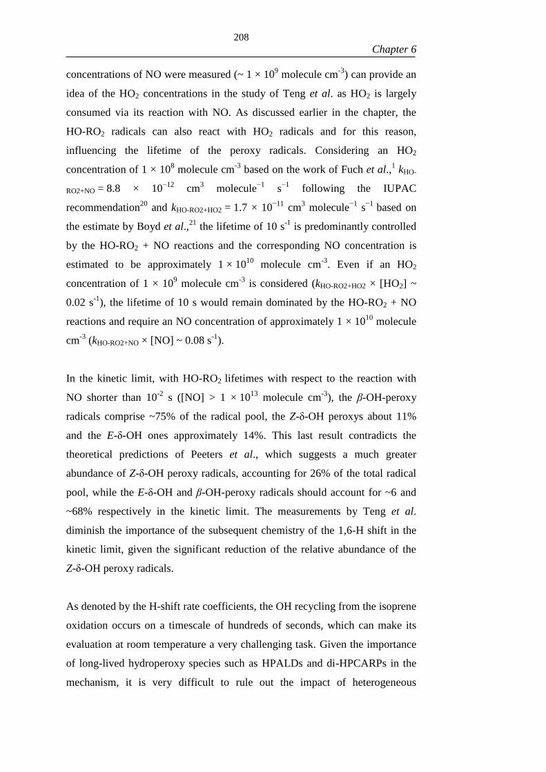
208

Chapter 6

concentrations of NO were measured (~ 1 × 109 molecule cm

-3) can provide an

idea of the HO2 concentrations in the study of Teng et al. as HO2 is largely

consumed via its reaction with NO. As discussed earlier in the chapter, the

HO-RO2 radicals can also react with HO2 radicals and for this reason,

influencing the lifetime of the peroxy radicals. Considering an HO2

concentration of 1 × 108 molecule cm

-3 based on the work of Fuch et al.,

1 kHO-

RO2+NO = 8.8 × 10−12

cm3 molecule

−1 s

−1 following the IUPAC

recommendation20

and kHO-RO2+HO2 = 1.7 × 10−11

cm3 molecule

−1 s

−1 based on

the estimate by Boyd et al.,21

the lifetime of 10 s-1

is predominantly controlled

by the HO-RO2 + NO reactions and the corresponding NO concentration is

estimated to be approximately 1 × 1010

molecule cm-3

. Even if an HO2

concentration of 1 × 109 molecule cm

-3 is considered (kHO-RO2+HO2 × [HO2] ~

0.02 s-1

), the lifetime of 10 s would remain dominated by the HO-RO2 + NO

reactions and require an NO concentration of approximately 1 × 1010

molecule

cm-3

(kHO-RO2+NO × [NO] ~ 0.08 s-1

).

In the kinetic limit, with HO-RO2 lifetimes with respect to the reaction with

NO shorter than 10-2

s ([NO] > 1 × 1013

molecule cm-3

), the β-OH-peroxy

radicals comprise ~75% of the radical pool, the Z-δ-OH peroxys about 11%

and the E-δ-OH ones approximately 14%. This last result contradicts the

theoretical predictions of Peeters et al., which suggests a much greater

abundance of Z-δ-OH peroxy radicals, accounting for 26% of the total radical

pool, while the E-δ-OH and β-OH-peroxy radicals should account for ~6 and

~68% respectively in the kinetic limit. The measurements by Teng et al.

diminish the importance of the subsequent chemistry of the 1,6-H shift in the

kinetic limit, given the significant reduction of the relative abundance of the

Z-δ-OH peroxy radicals.

As denoted by the H-shift rate coefficients, the OH recycling from the isoprene

oxidation occurs on a timescale of hundreds of seconds, which can make its

evaluation at room temperature a very challenging task. Given the importance

of long-lived hydroperoxy species such as HPALDs and di-HPCARPs in the

mechanism, it is very difficult to rule out the impact of heterogeneous

209

Chapter 6

chemistry in chamber investigations such as the work by Fuchs et al.1 As

discussed in the previous chapters, laser flash photolysis-laser induced

fluorescence experiments on a millisecond timescale represent a good

alternative in terms of control over heterogeneous interference and

contaminants. However, the timescale of the OH recycling at low temperatures

(T~298 K) remains an issue. It is theoretically possible, however, to promote

the chemistry of the OH recycling on the millisecond timescale, compatible

with LFP-LIF experiments, if high enough temperatures are employed. Under

such conditions, the crucial isomerization steps are promoted, greatly reducing

the time span of the OH recycling.

On the other hand, the implementation of high temperatures also means an

enhancement of the dissociation of the intermediate peroxy radicals back to

reagents and the establishment of equilibrium between peroxy formation and

unimolecular decomposition. Moreover, the results of such high temperature

experiments have their immediate application under significantly different

conditions. For this reason, their translation to more atmospherically relevant

conditions requires a robust and reliable procedure, using a validated model.

To help promote the peroxy formation, one can consider implementing very

large O2 concentrations. This effect was explored in the current work, initially

via simple numerical simulations of LIM1. Figure 6.3 shows the results of such

simulations, where large O2 concentrations were set ([O2] ~ 1 × 1019

molecule

cm-3

) and temperatures above 400 K were considered. The depicted

simulations were undertaken with the aid of the Kintecus chemical modelling

software.22

Under the pseudo-first order conditions simulated, the deficient

reactant (OH) should decay exponentially, as discussed on many occasions in

the previous chapters.

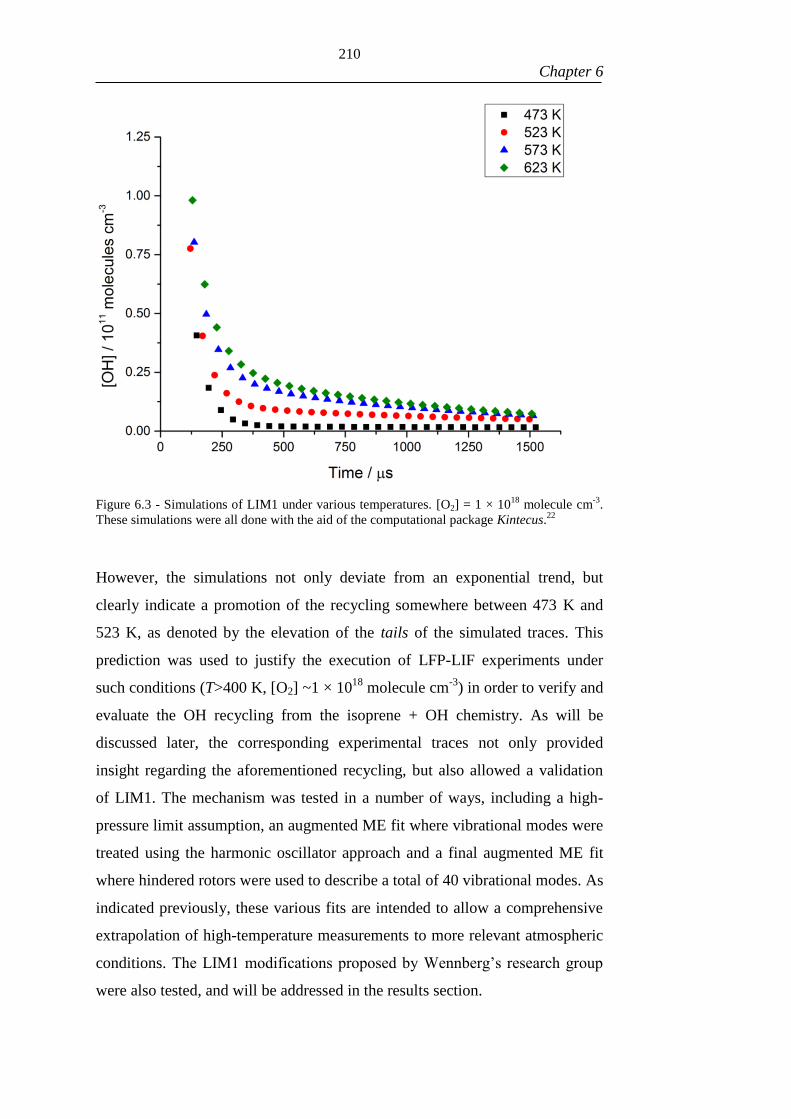
210

Chapter 6

Figure 6.3 - Simulations of LIM1 under various temperatures. [O2] = 1 × 1018

molecule cm-3

.

These simulations were all done with the aid of the computational package Kintecus.22

However, the simulations not only deviate from an exponential trend, but

clearly indicate a promotion of the recycling somewhere between 473 K and

523 K, as denoted by the elevation of the tails of the simulated traces. This

prediction was used to justify the execution of LFP-LIF experiments under

such conditions (T>400 K, [O2] ~1 × 1018

molecule cm-3

) in order to verify and

evaluate the OH recycling from the isoprene + OH chemistry. As will be

discussed later, the corresponding experimental traces not only provided

insight regarding the aforementioned recycling, but also allowed a validation

of LIM1. The mechanism was tested in a number of ways, including a high-

pressure limit assumption, an augmented ME fit where vibrational modes were

treated using the harmonic oscillator approach and a final augmented ME fit

where hindered rotors were used to describe a total of 40 vibrational modes. As

indicated previously, these various fits are intended to allow a comprehensive

extrapolation of high-temperature measurements to more relevant atmospheric

conditions. The LIM1 modifications proposed by Wennberg’s research group

were also tested, and will be addressed in the results section.

211

Chapter 6

As discussed in the previous chapters, ME calculations require a number of

molecular parameters, and therefore, the details of ab initio calculations

undertaken are outlined in the following, prior to the presentation of the

results.

6.2 AB INITIO CALCULATIONS

The methodology implemented in the current chapter is basically the same as

described in Chapter 3 and therefore, only a brief description is provided.

Stationary structures of reagents, intermediates and products were computed

with the DFT functional M06-2X23

and a large basis set (6-311++G(3df,2p))24

,

as implemented in the work of Peeters et al.3 Optimizations were carried out

with the aid of the Berny algorithm25-26

available in the Gaussian 09 D.01

programme suite.27

The minimization used redundant internal coordinates and

analytical gradients. The potential energy surface used in section 6.3.3 (see

Figure 6.12) have employed the calculations reported in the work of Peeters et

al.,3 which gave support to the implementation of LIM1 in the numerical and

ME models.


6.3.1 – Analysis of non-exponential traces

As discussed in Chapter 4, the addition of O2 to LFP-LIF experiments of the

isoprene + OH reaction did not provoke any significant observable changes up

to 460 K. Above this temperature however, a deviation from the expected

single exponential decays was observed. An example of such traces, generated

at 540 K and 2 atm of N2 is shown in Figure 6.4, where a single exponential

(orange line) and a bi-exponential curve (red line) were fitted to the depicted

trace. The green line represents the baseline, calculated as the average of the

background signal, which was probed before the excimer beam crosses through

the reaction cell (negative delay). The decay of the OH signal clearly shows a

delay, not returning to the original background levels. The depicted curve,

which resembles a bi-exponential decay, denotes the existence of one or more

212

Chapter 6

channels by which OH radicals are regenerated. The residual plots for the fits

are presented in Figure 6.5 and Figure 6.6.

0 2 4 6 8 10

-0.2

0.0

0.2

0.4

0.6

0.8

1.0

1.2

1.4

1.6

OH

/ A

rbit

raty

Un

its

t / 10-3 s

0

Figure 6.4 - An example of a non-exponential decay, generated for [C5H8] ≈ 1.00 × 1014

molecule cm-3

, 1019

O2 cm-3

, 540 K and 2 atm. The data were averaged after 10 scans. The blue

line represents a bi-exponential curve fitted to the data while the red line represents a single

exponential curve fit. The green line represents the average for the background OH signal.

Figure 6.5 - The residuals plot for the single exponential fit presented in Figure 6.4.

-2.5 0.0 2.5 5.0 7.5 10.0 12.5

-0.2

0.0

0.2

0.4

0.6

Re

sid

ua

l / A

rbitra

ry U

nits

t / 10-3 s

213

Chapter 6

Figure 6.6 - The residuals plot for the bi-exponential fit presented in Figure 6.4.

Significant changes are observed on the residuals of the single exponential fit,

where a transition from a model underestimation to a model overestimation is

found at near t=0. The residuals indicate another shift back to an

underestimation somewhere between 2.5 and 5.0 ms. These shifts between

underprediction and overprediction indicate that the use of the single-

exponential equation is not appropriate to describe the observed kinetics The

more balanced distribution around zero observed for the residuals of the

bi-exponential fit suggest a better suitability of this model, again, denoting the

existence of significant OH recycling.

Such non-exponential traces were ultimately analysed with the novel method

presented in detail in Chapter 5 where LIM1 was modelled via the ME

approach and modified to incorporate the H-abstraction explored in Chapter 4.

However, the high-pressure limit assumption was initially made and LIM1 was

implemented in a simpler fitting exercise, where all the rate coefficients

involved were assumed to be pressure independent. Moreover, these rate

coefficients and their temperature dependencies were taken directly from the

work of Peeters et al.3 These results will be discussed in the following, prior to

the presentation of the ME treatment. The extrapolation of the obtained results

-2.5 0.0 2.5 5.0 7.5 10.0 12.5

-0.50

-0.25

0.00

0.25

0.50

Re

sid

ua

l / A

rbitra

ry U

nits

t / 10-3 s

214

Chapter 6

to atmospheric conditions is of primary importance to enable an assessment of

the impact of this recycling in current atmospheric models predictions. The use

of various approaches to analyse the data will shed light into the extrapolation

procedure, attributing more confidence to the obtained results.

Table 6.1 – List of experimental conditions at which OH traces were collected for the isoprene

+ OH reaction in the presence of O2.

T / K p / Torr kloss / s-1

ntraces

420 1404 1362 4

477 1404 1480 8

478 134 396 5

480 125 234 21

498 1404 1458 8

513 162 31 8

543 140 334 10

543 140 335 12

550 1366 1693 8

584 124 89 10

A total of 94 traces were analysed, comprising temperatures between 420 and

585 K and pressures between ~125 and ~1400 Torr. Table 6.1 contains the

complete list of conditions along with the number of traces collect under each

one of them. In this table kloss refers to the loss of OH due to diffusion and

reaction with the precursor, measured in the absence of isoprene. Even though

traces at 420 K do not present observable recycling, their inclusion in the

analysis help constrain the optimized parameters. For example, if the recycling

is unreasonably facilitated by the optimization algorithm, the simulations of

traces generated 420 K could present recycling, something that would need to

be addressed by the algorithm. These traces can help define for example, lower

limits of recycling-related energy barriers.

As discussed in Chapter 4, temperatures above 700 K would be necessary for

the decomposition of the isoprene-OH adducts to be comparable to the forward

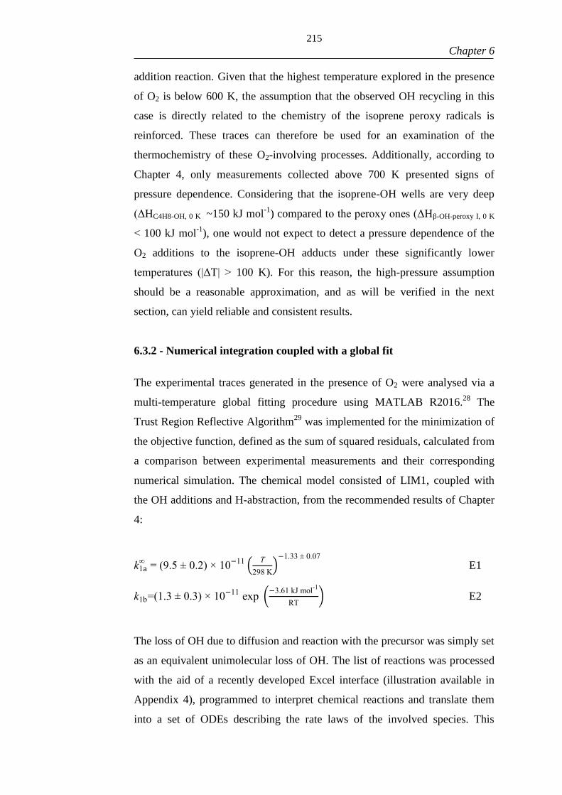
215

Chapter 6

addition reaction. Given that the highest temperature explored in the presence

of O2 is below 600 K, the assumption that the observed OH recycling in this

case is directly related to the chemistry of the isoprene peroxy radicals is

reinforced. These traces can therefore be used for an examination of the

thermochemistry of these O2-involving processes. Additionally, according to

Chapter 4, only measurements collected above 700 K presented signs of

pressure dependence. Considering that the isoprene-OH wells are very deep

(ΔHC4H8-OH, 0 K ~150 kJ mol-1

) compared to the peroxy ones (ΔHβ-OH-peroxy I, 0 K

< 100 kJ mol-1

), one would not expect to detect a pressure dependence of the

O2 additions to the isoprene-OH adducts under these significantly lower

temperatures (|ΔT| > 100 K). For this reason, the high-pressure assumption

should be a reasonable approximation, and as will be verified in the next

section, can yield reliable and consistent results.

6.3.2 - Numerical integration coupled with a global fit

The experimental traces generated in the presence of O2 were analysed via a

multi-temperature global fitting procedure using MATLAB R2016.28

The

Trust Region Reflective Algorithm29

was implemented for the minimization of

the objective function, defined as the sum of squared residuals, calculated from

a comparison between experimental measurements and their corresponding

numerical simulation. The chemical model consisted of LIM1, coupled with

the OH additions and H-abstraction, from the recommended results of Chapter

4:

k1a∞

= (9.5 ± 0.2) × 10−11 (

T

298 K)−1.33 ± 0.07

E1

k1b=(1.3 ± 0.3) × 10−11

exp (−3.61 kJ mol

-1

RT) E2

The loss of OH due to diffusion and reaction with the precursor was simply set

as an equivalent unimolecular loss of OH. The list of reactions was processed

with the aid of a recently developed Excel interface (illustration available in

Appendix 4), programmed to interpret chemical reactions and translate them

into a set of ODEs describing the rate laws of the involved species. This

216

Chapter 6

interface also allows the definition of adjustable parameters such as the pre-

exponential factors or activation energies of the involved bimolecular rate

coefficients. Every rate coefficient was described in the form of a modified

Arrhenius equation, which also contains a term related to quantum mechanical

tunnelling. Equation E3 generically shows this formulation with respect to a

generic reaction i.

ki=Ai× (T/298 K)ni × exp (

Eai

RT) × exp (

Qi

T3) E3

This equation is versatile enough to allow the incorporation of barrierless

reactions such as the OH and O2 additions and processes with well-defined

activation energies as the previously studied hydrogen abstraction. The last

factor in the equation was used by Peeters et al. to account for quantum

mechanical tunnelling of the 1,6-H shift reactions. For example, in Case 1,

their recommended equation for this process is presented in Equation E4.

k1-6-H, Case 1 = 3.556×1010

× exp (−71.41 kJ mol

-1

RT)× exp (

1.0265×108 K3

T3 ) E4

This equation does not contain the (T/298 K)ni term, something that can be

programmatically implemented by setting ni to zero. Analogously, any other

term in equation E3 can be turned off by simply setting the corresponding

temperature dependence parameter to zero. The aforementioned interface also

requires the temperature at which each trace was generated and the initial

concentration of the involved species. Once everything is provided, a

MATLAB script is generated, containing a code to numerically integrate the

set of ODEs for each experimental condition, compare the results with

experimental measurements and minimize the objective function. Appendix 4

contains an example of a MATLAB script used to fit 6 traces using LIM1. The

list of adjustable parameters includes a scaling factor for the pre-exponential

factor of all the isoprene-OH + O2 reactions, so that their ratios are maintained

unchanged. An attempt to include an adjustable temperature dependence for

these reactions was made, but the returned parameters were ill-defined, i.e., the

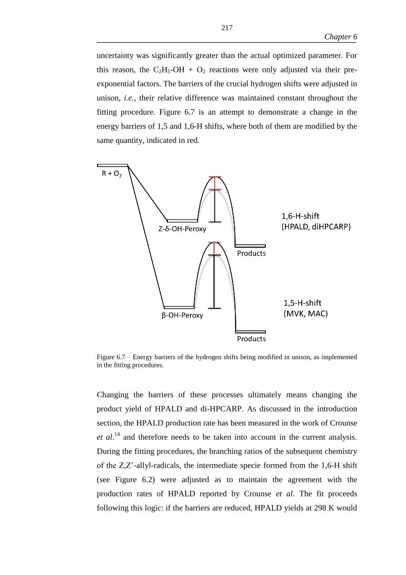
217

Chapter 6

uncertainty was significantly greater than the actual optimized parameter. For

this reason, the C2H5-OH + O2 reactions were only adjusted via their pre-

exponential factors. The barriers of the crucial hydrogen shifts were adjusted in

unison, i.e., their relative difference was maintained constant throughout the

fitting procedure. Figure 6.7 is an attempt to demonstrate a change in the

energy barriers of 1,5 and 1,6-H shifts, where both of them are modified by the

same quantity, indicated in red.

Figure 6.7 – Energy barriers of the hydrogen shifts being modified in unison, as implemented

in the fitting procedures.

Changing the barriers of these processes ultimately means changing the

product yield of HPALD and di-HPCARP. As discussed in the introduction

section, the HPALD production rate has been measured in the work of Crounse

et al.14

and therefore needs to be taken into account in the current analysis.

During the fitting procedures, the branching ratios of the subsequent chemistry

of the Z,Z’-allyl-radicals, the intermediate specie formed from the 1,6-H shift

(see Figure 6.2) were adjusted as to maintain the agreement with the

production rates of HPALD reported by Crounse et al. The fit proceeds

following this logic: if the barriers are reduced, HPALD yields at 298 K would

218

Chapter 6

naturally increase and disagree with the measurements by Crounse et al. To

avoid this consequence, the branching ratio of the HPALD channel is reduced

proportionally as to re-establish the agreement, redirecting the chemistry to the

di-HPCARP channel. The necessary branching ratios were mapped out as a

function of the H-Shift barriers with the much appreciated collaboration of Dr

Lisa Whalley, using an atmospheric model based on the Master Chemical

Mechanism (MCM) version 3.2.30

The MCM is a near-explicit chemical

mechanism dedicated to describe the gas-phase tropospheric chemistry of

volatile organic compounds and in this analysis has been modified to

incorporate the chemistry of LIM1. The model has incorporated the NOx

conditions of the Borneo OP3 field campaign2, 4

, a work in which the

discrepancy between measured and modelled OH was approximately a factor

of 2. At room temperature, a branching ratio of approximately 25% for the

HPALD channel and consequently, 75% for the di-HPCARP channel, is

required if the barriers of the H shifts are assumed to be those as reported by

Peeters et al., guaranteeing a good agreement with the HPALD measurements

by Crounse et al. The branching ratios were mapped out for a maximum

change of approximately 5 kJ mol-1

, a reasonable range for the adjustment of

the barriers. The mapped branching ratio with respect to the HPALD channel,

utilized in this work can be calculated from equation E5:

BRHPALD = 4.3160×10

-7

× (Ea1-5-H shift

/ R)2 -7.8937×10

-3

×(Ea1-5-H shift

/ R) + 36.187 E5

where BRHPALD is the branching ratio for the HPALD channel (in %), Ea1-5-H

shift is the assigned activation energy for the 1-5-H shift of Case 1 and R is the

gas constant with the appropriate units. It is important to reinforce that the

activation energies of the remaining H shifts are linked to this one during the

fitting procedures, as to maintain their relative energy differences intact, as

illustrated in Figure 6.7. This fitting procedure is referred to as BR-linked, to

denote the fact that the branching ratio is linked to the adjustable barriers via

equation E5.

219

Chapter 6

Finally, a fit where the aforementioned branching ratio was set as an

independent adjustable parameter was also undertaken. In this case, Equation

E5 is not considered and the branching ratio is freely allowed to assume any

value between 0 and 100 %. This fitting procedure is referred to as BR-free to

analogously indicate that the Z,Z’-allyl-radical + O2 → HPALD branching

ratio is a global variable, programmatically independent of the other

parameters. Table 6.2 shows the resulting parameters of the two fits along with

uncertainties quoted at 2σ. The table also includes the sum of squared residuals

χ2 divided by the total number of traces (94), as a measure of the goodness of

each fit. Figure 6.8 exemplifies the fits of multiple traces, generated under

various experimental conditions.

Table 6.2 – Best-fit parameters for both BR-Linked and BR-free fitting procedures. Errors

quoted at 2σ

Parameter BR-Linked BR-free Peeters et al. 3

C5H8-OH + O2

Scaling Factor 3.00 ± 1.46 3.00 ± 1.62 1.00

1-5-H shift

barrier / kJ mol-1

81.31 ± 0.17 80.48 ± 0.28 81.03

BRHPALD 0.27* 0.37 ± 0.03 0.50

χ2 /ntraces 1.17 1.16 -

*- Calculated with equation E5 during the fit.

Before the results are discussed, it is important to highlight an aspect of the

recommended LIM1 H-shift rate coefficients. Peeters et al. have incorporated

the tunnelling contribution to the 1,5-H shifts as effective reductions of the

classic Arrhenius barriers. For example, their theoretical calculations indicate

an activation energy of 89.08 kJ mol-1

for the 1,5-H shift in case1, but the

corresponding recommended equation for this rate coefficient

k1-5H-shift = 1.038 × 1011

× exp(-9746.4 K / T) employs an effective barrier of

81.03 kJ mol-1

. The fitting procedures are directly adjusting the equations of

the rate coefficients, which mean that effective barriers are being adjusted.

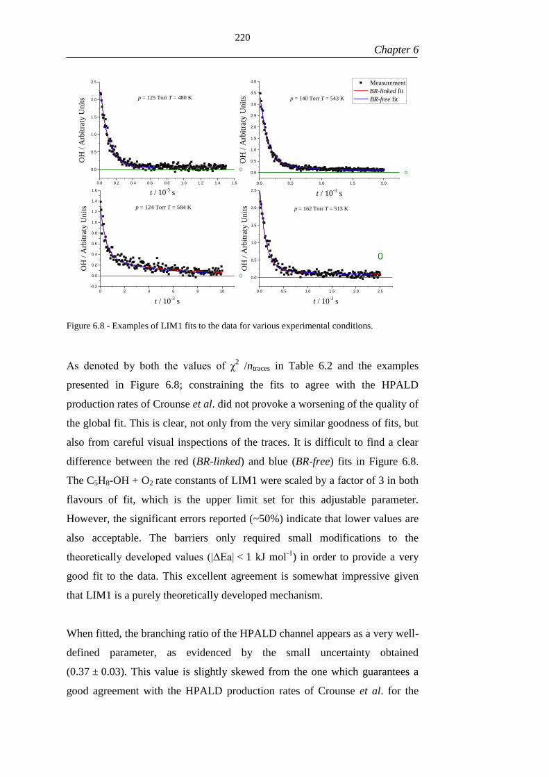
220

Chapter 6

0.0 0.2 0.4 0.6 0.8 1.0 1.2 1.4 1.6

0.0

0.5

1.0

1.5

2.0

2.5

0.0 0.5 1.0 1.5 2.0

0.0

0.5

1.0

1.5

2.0

2.5

3.0

3.5

4.0

0 2 4 6 8 10

-0.2

0.0

0.2

0.4

0.6

0.8

1.0

1.2

1.4

1.6

0.0 0.5 1.0 1.5 2.0 2.5

0.0

0.5

1.0

1.5

2.0

2.5

p = 140 Torr T = 543 K

OH

/ A

rbit

raty

Un

its

0

p = 125 Torr T = 480 K

t / 10-3 s

p = 124 Torr T = 584 K

Measurement

BR-linked fit

BR-free fit

OH

/ A

rbit

raty

Un

its

t / 10-3

s

0

p = 162 Torr T = 513 K

OH

/ A

rbit

raty

Un

its

t / 10-3 s

0

OH

/ A

rbit

raty

Un

its

t / 10-3 s

0

Figure 6.8 - Examples of LIM1 fits to the data for various experimental conditions.

As denoted by both the values of χ2 /ntraces in Table 6.2 and the examples

presented in Figure 6.8; constraining the fits to agree with the HPALD

production rates of Crounse et al. did not provoke a worsening of the quality of

the global fit. This is clear, not only from the very similar goodness of fits, but

also from careful visual inspections of the traces. It is difficult to find a clear

difference between the red (BR-linked) and blue (BR-free) fits in Figure 6.8.

The C5H8-OH + O2 rate constants of LIM1 were scaled by a factor of 3 in both

flavours of fit, which is the upper limit set for this adjustable parameter.

However, the significant errors reported (~50%) indicate that lower values are

also acceptable. The barriers only required small modifications to the

theoretically developed values (|ΔEa| < 1 kJ mol-1

) in order to provide a very

good fit to the data. This excellent agreement is somewhat impressive given

that LIM1 is a purely theoretically developed mechanism.

When fitted, the branching ratio of the HPALD channel appears as a very well-

defined parameter, as evidenced by the small uncertainty obtained

(0.37 ± 0.03). This value is slightly skewed from the one which guarantees a

good agreement with the HPALD production rates of Crounse et al. for the

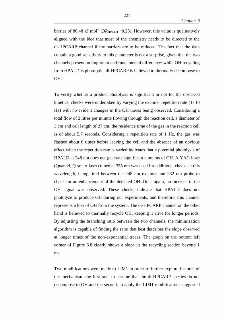
221

Chapter 6

barrier of 80.48 kJ mol-1

(BRHPALD ~0.23). However, this value is qualitatively

aligned with the idea that most of the chemistry needs to be directed to the

di-HPCARP channel if the barriers are to be reduced. The fact that the data

contain a good sensitivity to this parameter is not a surprise, given that the two

channels present an important and fundamental difference: while OH recycling

from HPALD is photolytic, di-HPCARP is believed to thermally decompose to

OH.3

To verify whether a product photolysis is significant or not for the observed

kinetics, checks were undertaken by varying the excimer repetition rate (1- 10

Hz) with no evident changes in the OH traces being observed. Considering a

total flow of 2 litres per minute flowing through the reaction cell, a diameter of

3 cm and cell length of 27 cm, the residence time of the gas in the reaction cell

is of about 5.7 seconds. Considering a repetition rate of 1 Hz, the gas was

flashed about 6 times before leaving the cell and the absence of an obvious

effect when the repetition rate is varied indicates that a potential photolysis of

HPALD at 248 nm does not generate significant amounts of OH. A YAG laser

(Quantel, Q-smart laser) tuned at 355 nm was used for additional checks at this

wavelength, being fired between the 248 nm excimer and 282 nm probe to

check for an enhancement of the detected OH. Once again, no increase in the

OH signal was observed. These checks indicate that HPALD does not

photolyze to produce OH during our experiments, and therefore, this channel

represents a loss of OH from the system. The di-HPCARP channel on the other

hand is believed to thermally recycle OH, keeping it alive for longer periods.

By adjusting the branching ratio between the two channels, the minimization

algorithm is capable of finding the ratio that best describes the slope observed

at longer times of the non-exponential traces. The graph on the bottom left

corner of Figure 6.8 clearly shows a slope in the recycling section beyond 1

ms.

Two modifications were made to LIM1 in order to further explore features of

the mechanism: the first one, to assume that the di-HPCARP species do not

decompose to OH and the second, to apply the LIM1 modifications suggested

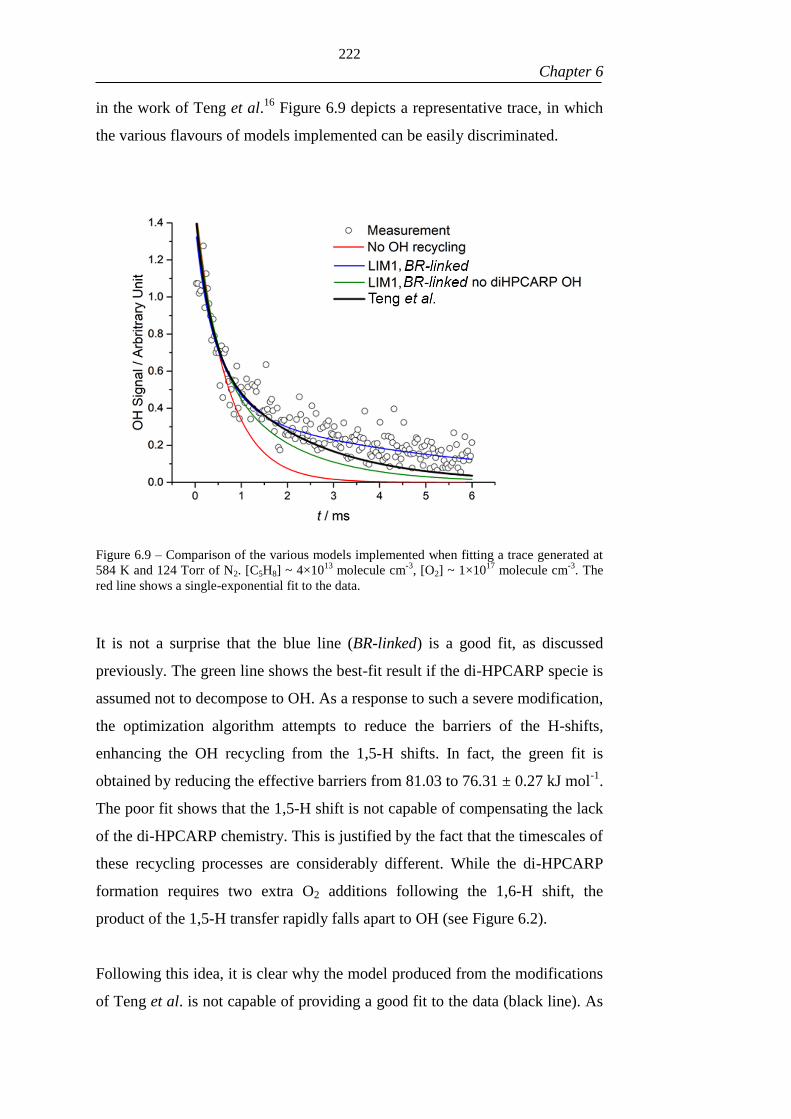
222

Chapter 6

in the work of Teng et al.16

Figure 6.9 depicts a representative trace, in which

the various flavours of models implemented can be easily discriminated.

Figure 6.9 – Comparison of the various models implemented when fitting a trace generated at

584 K and 124 Torr of N2. [C5H8] ~ 4×1013

molecule cm-3

, [O2] ~ 1×1017

molecule cm-3

. The

red line shows a single-exponential fit to the data.

It is not a surprise that the blue line (BR-linked) is a good fit, as discussed

previously. The green line shows the best-fit result if the di-HPCARP specie is

assumed not to decompose to OH. As a response to such a severe modification,

the optimization algorithm attempts to reduce the barriers of the H-shifts,

enhancing the OH recycling from the 1,5-H shifts. In fact, the green fit is

obtained by reducing the effective barriers from 81.03 to 76.31 ± 0.27 kJ mol-1

.

The poor fit shows that the 1,5-H shift is not capable of compensating the lack

of the di-HPCARP chemistry. This is justified by the fact that the timescales of

these recycling processes are considerably different. While the di-HPCARP

formation requires two extra O2 additions following the 1,6-H shift, the

product of the 1,5-H transfer rapidly falls apart to OH (see Figure 6.2).

Following this idea, it is clear why the model produced from the modifications

of Teng et al. is not capable of providing a good fit to the data (black line). As

223

Chapter 6

discussed in the introduction section, the modifications greatly reduce the

importance of the Z-δ-OH peroxy radicals and consequently, that of the di-

HPCARP channel. The change is not as severe as completely turning off the

OH recycling from this channel (green line), and this is why its fit is located

between the blue (LIM1 BR-linked) and the green lines (No di-HPCARP OH).

In the fit of the Teng et al. model, the barriers are increased by 1.71 ± 0.26 kJ

mol-1

. By enhancing the abundance of the β-OH-peroxy radicals, a significant

enhancement of the recycling at earlier times, compared to those of the di-

HPCARP channel is caused, which is rapidly translated into an overestimation

of the recycling at early times. This effect is diminished by the optimization

algorithm by increasing the barriers of the H shifts. Because the 1,6-H shift

barriers are also increased (they are all moved in unison), the recycling at

longer times is affected, presenting a prolific slope in the numerically

integrated traces.

Additionally to these fits, the resulting parameters of the LIM1-BR-linked and

Teng et al. models were incorporated in MCM atmospheric simulations of the

OP3 Borneo campaign in order to evaluate the impact of these results in an

atmospheric model. Figure 6.10 shows the results of these simulations

compared to the experimental OH measurements in one of the days of the OP3

campaign.

224

Chapter 6

Figure 6.10 – MCM atmospheric simulations of the OP3 campaign against the actual OH

measurements for various models. Error bars represent the 28% uncertainty associated with the

OH measurements undertaken during the OP3 field campaign.4

The blue line represents a model that does not incorporate LIM1 and the figure

clearly indicates an improvement of the OH prediction when the

LIM1-BR-linked parameters are incorporated (green line). The reduced

importance of the Z-δ-OH-peroxy radicals and enhancement of less important

E-δ-OH peroxy radicals in the work of Teng et al. contributes to the observed

reduction of the predicted OH when this model is used. As presented in Figure

6.2, the chemistry of the E-δ-OH isomers does not lead to OH regeneration.

The area under the red line (Teng et al.) represents ~50% the area under the

black line (measurements) and the area under the green line (LIM1-BR-linked)

represents ~60% of the measurement area. The unmodified MCM 3.2 accounts

for ~45% of the measurement area.

Finally, the OH data of the LIM1-BR-linked and Teng et al. models were

further consolidated as to identify the sources from which the modelled OH is

being generated. The pie charts presented in Figure 6.11 show that even for the

pristine environment of Borneo ([NO]average~ 1× 109 molecule cm

-3), the

reaction of NO with HO2 radicals is still the most important process for OH

0.0

0.5

1.0

1.5

2.0

2.5

3.0

3.5

00:00:00 06:00:00 12:00:00 18:00:00 00:00:00

[OH

] /

10

6 m

ole

cule

s cm

-3

Time / hh:mm:ss

OH measurement LIM1 BR-linked + MCM 3.2

Teng et al. + MCM 3.2 MCM 3.2

225

Chapter 6

generation, accounting for more than 40% in the case of the LIM1-BR-linked

model and more than 50% if the Teng et al. MCM model is employed.

Figure 6.11 - Sources of OH in the atmospheric simulations of the LIM1-BR-linked and Teng

et al. models included in Figure 6.10.

The chemistry of non-isoprene related species accounts for approximately 30%

of the total OH in both models. Ozone photolysis and OH recycling from

alternative available species such as monoterpenes are examples of processes

accounted for as Other in these pie charts. The OH generated from the isoprene

chemistry is split into three sources: (I)1,5-H shifts, where OH is a co-product

of formaldehyde and methyl vinyl ketone (case 1) and methacrolein (case 2);

(II) photolysis of HPALD and (III) thermal decomposition of di-HPCARP.

While the isoprene chemistry is responsible for more than 20% of the total OH

44.42%

2.50%

16.16% 3.10%

33.82%

LIM1-BR-linked

HO2+NO

1,5-H-Shift

di-HPCARP

HPALD

Other

54.87%

3.95% 6.15%

2.20%

32.82%

Teng et al.

HO2+NO

1,5-H-Shift

di-HPCARP

HPALD

Other

226

Chapter 6

when the LIM1-BR-linked model is considered, this value is reduced to 12.3%

when the Teng et al. variant is assumed. The greater importance of the

di-HPCARP specie in the LIM1-BR-linked model is an interesting feature,

given that the di-HPCARP decomposition also gives rise to dihydroperoxy-

carbonyl radicals, which according to Peeters et al., could photolyze to further

reform OH.3 However, the fact that these dihydroperoxy-carbonyl radicals can

also react with OH means that the net budget in this case is controlled by the

competition between this reaction and the photolytic process. Either way, the

larger di-HPCARP chemistry contribution for the modelled OH in the case of

LIM1-BR-linked represents a greater potential for further improving the

correspondence between current atmospheric model predictions and measured

OH, as exemplified in Figure 6.10.

This section demonstrated that, by making the high-pressure limit assumption,

LIM1 successfully described the kinetics of the isoprene + OH reaction in the

presence of O2 at elevated temperatures (400 K<T<600 K). The model was

capable of describing the experimental traces in a robust multi-temperature fit.

Results also indicated that there is enough room in the fits to constrain the

procedures as to force an agreement to the production rates of HPALDs

reported by Crounse et al.14

without compromising the overall goodness of fit.

The fits were capable of identifying distinct OH recycling processes in the

mechanism, based on their timescales. This is consistent with the formation

and thermal decomposition of di-HPCARP species, as theoretically predicted

in the work of Peeters et al.3 The atmospheric impacts of the optimized

parameters were evaluated by simulating the atmospheric conditions

comprised at the OP3 Borneo campaign, being LIM1 capable of describing up

to 60% of the total OH measured in that field work.

227

Chapter 6

6.3.3 – Augmented-ME analysis

In order to enable the use of the ME-based fitting strategy presented in Chapter

5, the LIM1 was modelled via the Master Equation approach and augmented

with a hydrogen abstraction, as described in Chapter 4 and the OH loss due to

diffusion and reaction with the precursor. Figure 6.12 shows the potential

energy diagram of LIM1 with respect to the OH addition to carbon C1 as

implemented in the Master Equation calculations. As indicated in that Figure,

effective barriers from the work of Peeters et al. were used as first guesses, but

were subsequently adjusted in unison, in the same fashion presented in the

previous section.

Figure 6.12 - Potential energy diagram for the Leuven Isoprene Mechanism 1 used in the

current analysis. Depicted energetics represent effective barriers that account for tunnelling

from the work of Peeters et al. Energies in kJ mol-1

.

For the 1,5-H shifts, the rate coefficients were obtained directly from the ME

calculations. For the 1,6-H shifts however, the ME computations did not

include any tunnelling corrections but these were posteriorly incorporated via

the recommendations of Peeters et al. Equation E4 showed their

recommendation for the 1,6-H shift in Case 1, and Equation E6 now shows the

corresponding correction for Case 2. The parts highlighted in red are the

tunnelling corrections recommended by Peeters et al. It is important to mention

however, that the barriers incorporated in the exponential terms highlighted in

blue were also modified by Peeters et al. in order to best describe their

predictions of k1-6-H, Case 1 and k1-6-H, Case 2 . In order to estimate the tunnelling

factors of these processes and their temperature dependences, the authors have

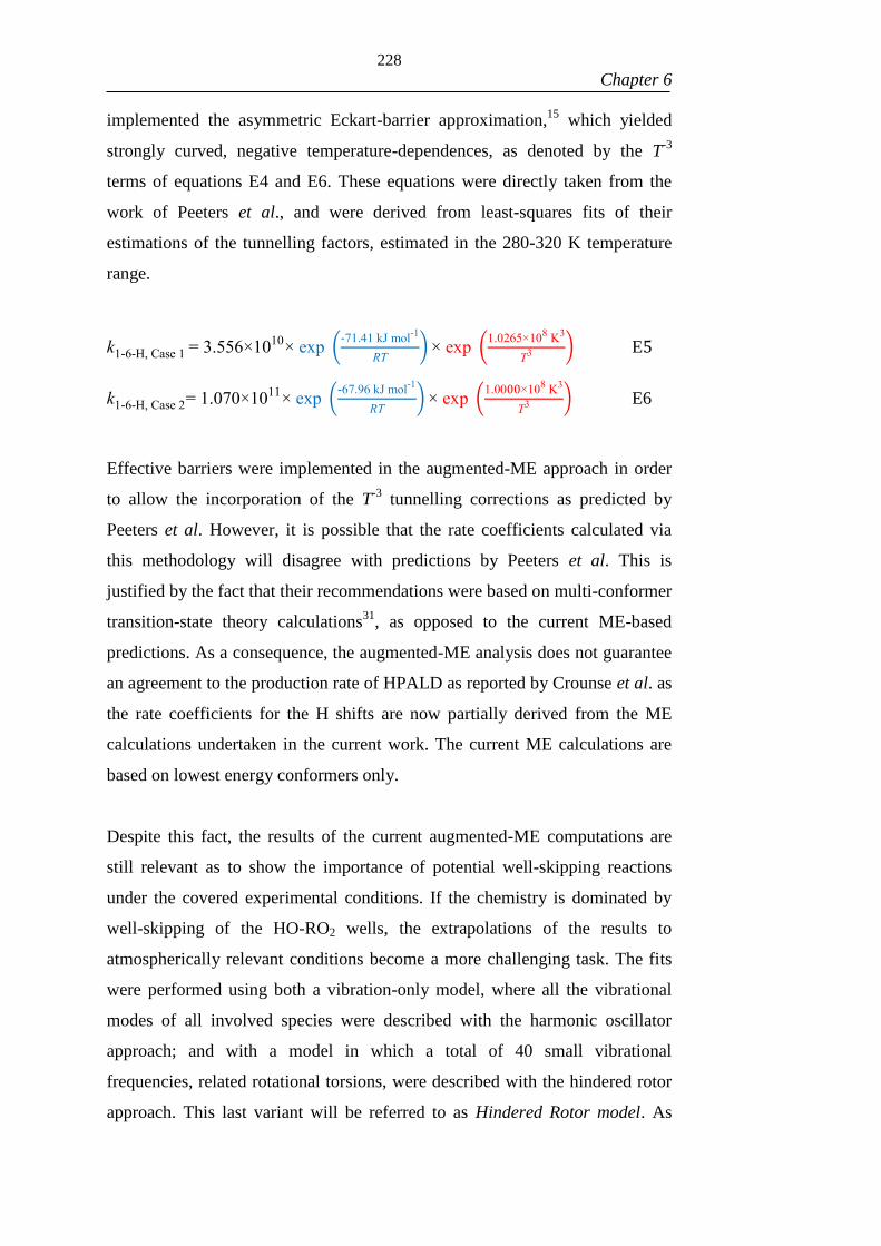
228

Chapter 6

implemented the asymmetric Eckart-barrier approximation,15

which yielded

strongly curved, negative temperature-dependences, as denoted by the T-3

terms of equations E4 and E6. These equations were directly taken from the

work of Peeters et al., and were derived from least-squares fits of their

estimations of the tunnelling factors, estimated in the 280-320 K temperature

range.

k1-6-H, Case 1 = 3.556×1010

× exp (-71.41 kJ mol

-1

RT)× exp (

1.0265×108 K3

T3 ) E5

k1-6-H, Case 2= 1.070×1011

× exp (-67.96 kJ mol

-1

RT)× exp (

1.0000×108 K3

T3 ) E6

Effective barriers were implemented in the augmented-ME approach in order

to allow the incorporation of the T-3

tunnelling corrections as predicted by

Peeters et al. However, it is possible that the rate coefficients calculated via

this methodology will disagree with predictions by Peeters et al. This is

justified by the fact that their recommendations were based on multi-conformer

transition-state theory calculations31

, as opposed to the current ME-based

predictions. As a consequence, the augmented-ME analysis does not guarantee

an agreement to the production rate of HPALD as reported by Crounse et al. as

the rate coefficients for the H shifts are now partially derived from the ME

calculations undertaken in the current work. The current ME calculations are

based on lowest energy conformers only.

Despite this fact, the results of the current augmented-ME computations are

still relevant as to show the importance of potential well-skipping reactions

under the covered experimental conditions. If the chemistry is dominated by

well-skipping of the HO-RO2 wells, the extrapolations of the results to

atmospherically relevant conditions become a more challenging task. The fits

were performed using both a vibration-only model, where all the vibrational

modes of all involved species were described with the harmonic oscillator

approach; and with a model in which a total of 40 small vibrational

frequencies, related rotational torsions, were described with the hindered rotor

approach. This last variant will be referred to as Hindered Rotor model. As

229

Chapter 6

discussed in Chapter 4, the change in the density of states caused by the

augmentation of the degrees of freedom of the species is better captured with

the use of the latter approach. The best-fit parameters of the augmented-ME

fits are presented in Table 6.3, and Table 6.4 shows the 298 K extrapolated rate

coefficients for the 1,5 and 1,6-H shifts calculated from the best-fit parameters

in Table 6.3. Figure 6.13 exemplifies fits of both the vibration-only and

Hindered Rotor models to a representative OH trace generated at T=584 K and

p=125 Torr.

Table 6.3 - Best-fit parameters for both Vibration-only and Hindered Rotor fitting procedures.

Errors quoted at 2σ

Parameter Vibration-only Hindered Rotors Peeters et al. 3

C5H8-OH + O2

Scaling Factor 0.20 ± 0.16 0.20 ± 0.11 1.00

1-5-H shift barrier /

kJ mol-1

86.33 ± 0.08 82.50 ± 0.17 81.03

BRHPALD 0.76 0.36 0.50

χ2 /ntraces 1.32 1.22 -

Table 6.4 - Calculated rate coefficients for the H shifts extrapolated to 298 K and 760 Torr.

Vibration

Only

Hindered

Rotors

High-Pressure

Assumption Peeters et al.

Case 1 1-5 H shift 1.34×10

-3 2.13×10

-3 5.80×10

-4 6.50×10

-4

1-6 H shift 3.33 1.44 0.46 0.52

Case 2 1-5 H shift 3.00×10

-3 5.41×10

-3 1.03×10

-3 1.20×10

-3

1-6 H shift 51.93 7.28 5.11 5.70

Rate coefficients in s-1

.

230

Chapter 6

0.0 0.5 1.0 1.5 2.0 2.5 3.0 3.5 4.0

0.0

0.2

0.4

0.6

0.8

1.0

1.2

1.4

Data

Vibration-only

Hindered RotorsO

H /

Arb

itra

ry U

nit

s

t / 10-3 s

Figure 6.13 – Fits of the vibration-only model and a model which incorporate a total of 40

hindered-rotors to describe corresponding rotational torsions.

Table 6.4 also includes the 298 K rate coefficients extrapolated from the results

presented in section 6.3.2 when making the high-pressure limit assumption

(High-Pressure Assumption). The original recommended values by Peeters et

al. are included in the final column of that table for reference. According to

this table, the vibration-only model heavily overestimates the values

recommended by Peeters et al., justifying the significantly larger barrier

obtained when this model was incorporated (86.33 kJ mol-1

), as an attempt to

compensate this effect. Analogously, in section 6.3.2 when LIM1 was

modified to incorporate the recommendations from the work of Teng et al.16

,

the chemistry of the 1,5-H shift was significantly enhanced. To compensate

this effect, the optimization algorithm attempted to increase the barriers,

affecting the capability of the model to describe the recycling at longer times

(see Figure 6.9). Here, a similar effect is observed, as depicted in Figure 6.13,

when the vibration-only model is adopted. The significant overestimation of

the OH recycling leads to an increase of the barriers, which are all linked,

provoking a poor fit over the sections of the traces where the di-HPCARP

chemistry is important.

231

Chapter 6

The model which incorporated the hindered rotors is more aligned with the

predictions by Peeters et al. although the rate coefficients are systematically

higher. As pointed out before, the estimations of Peeters et al. were computed

via Transition-State Theory calculations which took into account a

combination of multiple conformers of the involved intermediate species,

while the current Master Equation calculations are purely based on the lowest

energy conformers. This fact certainly goes some way into explaining the

observed discrepancy. The hindered-rotor model is expected to overestimate

the HPALD production by approximately a factor of 3, based on a comparison

of the simulated production rates of HPALD between this model and the High-

pressure assumption variant, presented in section 6.3.2.

At the most extreme experimental conditions covered in this work, 584 K and

~125 Torr, the Hindered Rotor model predicts that the largest possibility of

well-skipping occurs over the 15-H shift in Case 2. In this case, the products of

the 1-5 H shifts can be formed directly from the reactions of the cis and trans

conformations of the C5H8-OH adducts with O2 (see Figure 6.2), as indicated

by reactions R9 and R10.

cis-OH-adduct 2 + O2 → Prod II R9

trans-OH-adduct 2 + O2 → Prod II R10

However, even for the mentioned experimental conditions, the ME calculations

indicate that the well-skipping contribution is small, representing less than 4%

of the reactions of the aforementioned C5H8-OH adducts with O2. The vast

majority of these O2 reactions proceed via the formation of the β-OH-peroxy

radical, followed by the corresponding 1,5-H shift. For the other possibilities

of well-skipping, including skipping over the Z-δ-OH peroxy radicals, these

account for approximately 1% of the total C5H8-OH reactions with O2. No

signs of pressure dependence under the covered experimental conditions were

predicted in the ME calculations.

232

Chapter 6

As indicated by the Hindered Rotor results, very small adjustments to the

effective energy barriers and C5H8-OH + O2 reactions are sufficient to provide

a good fit of a ME-based model to the collection of OH traces. This is aligned

with the results of section 6.3.2, where a small change of approximately 2 kJ

mol-1

in the H-transfer barriers was necessary. Well-skipping over the peroxy

radicals was found to be of minor importance even at the experimental

conditions where these reactions are most likely to potentially influence the

kinetics (T ~584 K, p ~125 Torr). Therefore, this section reinforces the

suitability of the analysis presented in section 6.3.2, in which the well-skipping

possibility was ignored and the chemistry was assumed to be pressure-

independent. The current work was capable of demonstrating OH recycling

from isoprene-peroxy chemistry, and proved the suitability of LIM1 to

describe the mentioned recycling. Given the variety of tests and experimental

compatibility, the current work represents an appropriate validation of the

Leuven Isoprene Mechanism 1. Further explorations of the LIM1 can provide

valuable insight regarding the remaining missing OH.


In Chapter 6, the OH recycling observed for the reaction of isoprene with OH

radicals in the presence of O2 for temperatures between 460 K and 584 K was

elucidated with the aid of the Leuven Isoprene Mechanism 1.3 A variety of fits

were undertaken in order to extract as much information as possible from the

experimental measurements.

Initially, the high-pressure limit assumption was made and LIM1 was explored

via numerical simulations of the reaction scheme. The mechanism was not

only capable of qualitatively predicting OH recycling at the aforementioned

temperatures, but also provided a very accurate description of the experimental

observations, requiring small changes to the activation energies employed in

the model (|ΔEa| ~2 kJ mol-1

). The analysis also showed that there is sufficient

flexibility in the data in order to constrain the fits so that the production rate of

HPALDs, important products of the isoprene oxidation, agrees with the

previous measurements of Crounse et al.14

The modifications to LIM1

233

Chapter 6

recommended in the work of Teng et al.16

based on RO2-specific nitrate

measurements were also adopted, but in this case the fits to the data became

significantly poorer. A discussion of potential sources of error in the

measurements of Teng et al. is provided, which helps rationalize the

disagreement.

The impact of these findings were assessed in an atmospheric model that

simulated the atmospheric conditions of the OP3 Borneo campaign2, 4

, showing

that via the incorporation of the optimized LIM1 model, it is possible to

describe up to ~60% of the measured OH in a day of that field work. The

results of this modelling shows that a model based on the recommendations of

Teng et al. is also capable of explaining the majority of the OH. However the

chemistry of the dihydroperoxy-carbonyl peroxy radicals (di-HPCARPs) is

significantly diminished, reducing the possibility of further improvements of

the OH agreement via subsequent isoprene chemistry.

The novel method presented in Chapter 5 was incorporated for the analysis of

LIM1, being the algorithm augmented with the H-abstraction explored in

Chapter 4 and the OH loss due to diffusion and reaction with the precursor.

The results show that the use of a vibration-only model heavily overestimated

the rate coefficients for the crucial H-shifts taking place in the mechanism,

when compared to the original predictions by Peeters et al. Even though a

model that incorporates 40 hindered rotors among the various intermediate

species provides a better agreement to the original LIM1 values, the rate

coefficients are overestimated by factors varying from ~1.25 to ~4.5. Finally,

the possibility of well-skipping for the reactions of the isoprene-OH adducts

with O2 over the various peroxy radicals was explored. These reactions appear

to be unimportant even at the highest temperature comprised in this work (584

K), reinforcing the validity of the best-fit parameters obtained with the

pressure-independent analysis.

234

Chapter 6

6.5 REFERENCES


in Isoprene Oxidation. Nature Geoscience 2013, 6, 1023.

2. Edwards, P. M. et al. OH Reactivity in a South East Asian Tropical Rainforest During

the Oxidant and Particle Photochemical Processes (OP3) Project. Atmospheric Chemistry and

Physics Discussions 2013, 13, 5233-5278.











London, UK., 2000.

7. Benjamin S. Felzer, T. C., John M. Reilly, Jerry M. Melillo, Xiaodong Wang Impacts

of Ozone on Trees and Crops. Comptes Rendus Geoscience 2007, 339, 784–798.

8. Weschler, C. J. Ozone's Impact on Public Health: Contributions from Indoor

Exposures to Ozone and Products of Ozone-Initiated Chemistry. Environmental health

perspectives 2006, 114, 1489-1496.

9. Shindell, D.; Faluvegi, G.; Lacis, A.; Hansen, J.; Ruedy, R.; Aguilar, E. Role of

Tropospheric Ozone Increases in 20th-Century Climate Change. Journal of Geophysical

Research-Atmospheres 2006, 111.

10. Neslen, A. Europe Escalates Action against Uk for Breaching Air Pollution Limits

06/02/2017. https://www.theguardian.com/environment/2017/feb/06/european-commission-

escalates-action-uk-breaching-air-pollution-limits (accessed 23/02/2017).

11. Paulot, F.; Crounse, J. D.; Kjaergaard, H. G.; Kurten, A.; St. Clair, J. M.; Seinfeld, J.


Isoprene. Science 2009, 325, 730-733.

12. Bela, M. M. et al. Ozone Production and Transport over the Amazon Basin During the

Dry-to-Wet and Wet-to-Dry Transition Seasons. Atmospheric Chemistry and Physics 2015, 15,

757-782.

13. Peeters, J.; Nguyen, T. L.; Vereecken, L. HOx Radical Regeneration in the Oxidation

of Isoprene. Physical Chemistry Chemical Physics 2009, 11, 5935-5939.



13607-13613.

15. Zhang, F.; Dibble, T. S. Impact of Tunneling on Hydrogen-Migration of the n-

propyperoxy Radical. Physical Chemistry Chemical Physics 2011, 13, 17969-17977.

16. Teng, A. P.; Crounse, J. D.; Wennberg, P. O. Isoprene Peroxy Radical Dynamics.

Journal of the American Chemical Society 2017, 139, 5367-5377.

17. Zhang, D.; Zhang, R.; Park, J.; North, S. W. Hydroxy Peroxy Nitrites and Nitrates

from OH Initiated Reactions of Isoprene. Journal of the American Chemical Society 2002,

124, 9600-9605.

18. Tuazon, E. C.; Atkinson, R. A Product Study of the Gas-Phase Reaction of Isoprene

with the OH Radical in the Presence of NOx. Int. J. Chem. Kinet. 1990, 22, 1221-1236.



235

Chapter 6

19. O'Brien, J. M.; Czuba, E.; Hastie, D. R.; Francisco, J. S.; Shepson, P. B.

Determination of the Hydroxy Nitrate Yields from the Reaction of C2−C6 Alkenes with OH in

the Presence of NO. The Journal of Physical Chemistry A 1998, 102, 8903-8908.

20. Iupac Task Group on Atmospheric Chemical Kinetic Data Evaluation. Data Sheet

Roo_50. http://iupac.poleether.fr 2010.

21. Boyd, A. A.; Flaud, P.-M.; Daugey, N.; Lesclaux, R. Rate Constants for RO2 + HO2

Reactions Measured under a Large Excess of HO2. The Journal of Physical Chemistry A 2003,

107, 818-821.

22. Ianni, J. C. Kintecus, Windows Version 6.80. www.kintecus.com.





24. Frisch, M. J.; Pople, J. A.; Binkley, J. S. Self-Consistent Molecular-Orbital Methods

.25. Supplementary Functions for Gaussian-Basis Sets. Journal of Chemical Physics 1984, 80,

3265-3269.

25. Peng, C. Y.; Ayala, P. Y.; Schlegel, H. B.; Frisch, M. J. Using Redundant Internal

Coordinates to Optimize Equilibrium Geometries and Transition States. Journal of

Computational Chemistry 1996, 17, 49-56.



Computation 2006, 2, 835-839.


28. MathWorks, I., MATLAB and Optimization Toolbox Release R2016a. Natwick : Math

Works Inc.: 2016.

29. Moré, J. J.; Sorensen, D. C. Computing a Trust Region Step. SIAM Journal on

Scientific and Statistical Computing 1983, 4, 553-572.

30. The Master Chemical Mechanism (MCM) Version 3.2. http://mcm.leeds.ac.uk/MCM.

31. Vereecken, L.; Peeters, J. The 1,5-H-Shift in 1-Butoxy: A Case Study in the Rigorous

Implementation of Transition State Theory for a Multirotamer System. The Journal of


http://iupac.poleether.fr/

http://www.kintecus.com/

http://mcm.leeds.ac.uk/MCM

237

Chapter 7

Chapter 7. Conclusions and Further

Work

239

Chapter 7


The hydroxyl radical (OH), is the most important oxidizing agent in the

atmosphere.1 The reaction with OH initiates the oxidation of the vast majority

of volatile organic compounds (VOC) in the atmosphere,1 and for this reason,

understanding the chemistry of this radical is crucial for the development of

more reliable and accurate atmospheric models. The focus of the thesis was the

development of reliable methods of analysis, capable of evaluating the kinetics

and thermodynamics of atmospherically important processes, and providing

accurate parameters which can be incorporated for the improvement of

atmospheric models.

Direct experimental measurements collected for the reactions of OH with SO2,

ethylene and isoprene were treated in a number of ways, which included (I) a

classic Master Equation analysis, in which experimental measurements

correspond to an eigenvalue of the Master Equation and (II) a bi-exponential

analysis of ME-simulated traces to derive overall recycling coefficients from

the contributions of multiple recycling species, which was used to determine

the well-depth of the isoprene-OH adducts. (III) A global multi-temperature

multi-pressure analysis of raw traces was derived, in which the Master

Equation is modified to incorporate the necessary pieces of chemistry to enable

a direct comparison to experimental traces. (IV) An alternative approach which

takes advantage of the use of phenomenological rate coefficients to enable a

heavy simplification of the problem was also derived. The use of a small

number of phenomenological rate coefficients attributes sufficient flexibility to

the method, so that the communication with alternative software becomes

facile. This approach was used for the study of the reaction of OH with

ethylene, and has yielded an enthalpy of formation for the C2H4-OH adduct

whose agreement to a theoretical prediction is of the order of 1 kJ mol-1

.

Furthermore, the chemistry of the OH addition was successfully discriminated

from the hydrogen abstraction, yielding well-defined kinetic parameters for

both processes.

241 Chapter 7

CHAPTER 3 - The Role of the Pre-reaction Complex in the OH + SO2

Reaction

The chemistry of the atmospherically important OH + SO2 reaction has been

investigated in Chapter 3. This reaction is directly linked to the occurrence of

acid rain, a phenomena with significant environmental, economic and health

implications.2

A controversy with respect to the high-pressure limiting rate coefficients for

this reaction has been observed among literature studies. Recent high-level

theoretical calculations indicate a small activation energy (~1.1 kJ mol-1

) for

the reaction.3 On the other hand, experimental measurements by Bltiz et al.

4-6

contrarily indicate very small high-pressure limiting rate coefficients for a

reaction believed to be nearly barrierless.

In Chapter 3, experimental measurements of the OH + SO2 reaction from

previous studies by Blitz et al.4, 6

and Wine et al.7 were submitted to a Master

Equation (ME) procedure, to verify if their data were compatible. With this,

the chapter provided an example of a classic ME procedure, in which the

experimental measurements were fitted to an eigenvalue of the Master

Equation. A recently discovered weakly-bound pre-reaction complex was

incorporated in the model to have its importance evaluated. The results

indicated that it is not possible to reconcile all the experimental measurements

by Blitz et al. and Wine et al. Furthermore, the experimental data by Wine et

al. appears to be internally inconsistent, since the measurements with the

various bath gases employed in their work (He, N2, Ar, SF6) could not be

reproduced via ME modelling. If, on the other hand, the data by Blitz et al. is

assumed to be correct, a reasonable internal agreement is observed, suggesting

that this set of data is more reliable. The argon data from Wine et al. is the

only dataset which agrees with the measurements of Blitz et al., and for this

reason, were incorporated for an analysis of the potential energy surface of the

reaction. The pre-reaction complex was observed to be unimportant as the

chemistry is dominated by the transition state. A good fit to the measurements

of Blitz et al. however, could only be obtained with a slightly submerged

242 Chapter 7

transition state with respect to reagents (~-1.0 kJ mol-1

). For this reason,

theoretical predictions by Long et al.3 which indicated a slightly positive

barrier for the process, deviate from the ME predictions. This positive barrier

implies a positive temperature dependence, something not supported by

experimental evidence. However, an excellent agreement is observed for the

experimentally derived enthalpy of reaction (110.5 ± 6.6 kJ mol-1

) when

compared to the theoretically derived prediction by Long et al. (111.5 kJ mol-

1).

Future work – OH + SO2

The results presented in the chapter clearly indicate the need of additional

experiments for the OH + SO2 reaction. This is evident from the fact that the

measurements by Wine et al. which were verified to be internally inconsistent

were incorporated in the IUPAC recommendation for low-pressure rate

coefficients of the OH + SO2 reaction.8 Blitz et al.

6 highlight the fact that SO2

photolysis is highly significant at 248 nm, and gives rise to very reactive

species ( O(1D) and SO), which can significantly influence the observed

kinetics. While the SO2 + OH high pressure limiting rate coefficient is around

2 × 10-12

cm3 molecule

-1 s

-1,

4 the reaction of SO with OH is much faster

k∞

OH+SO = (8.17 ± 0.36)×10-11

cm3 molecule

-1 s

-1.9 For this reason, additional

experiments must appropriately account for this interference. Additional

measurements for this reaction at elevated temperatures (T > 300 K) to

promote pressure dependence are desirable in order to indicate a preferable.

These measurements can also help further elucidate the role of the transition

state in this reaction and its energetic position with respect to the reagents.

243 Chapter 7

CHAPTER 4 - Kinetics of the Reaction of OH with Isoprene over a Wide

Range of Temperature and Pressures

In Chapter 4, direct measurements of the rate coefficient for the reaction of OH

with isoprene, k1, were made for wide temperature (298 - 794 K) and pressure

ranges (50-1670 Torr). The work presented in this chapter includes the

definition of the temperature dependence for the OH + isoprene reaction, a

discrimination between the mechanisms by which this reaction occurs, the

determination of the enthalpy of formation of the isoprene-OH adduct, a

pressure dependent treatment via ME calculations necessary for measurements

above 700 K, and an assessment of the available literature covering this

reaction. The measurements of this chapter significantly expanded the

temperature by which the rate coefficients for this reaction is known, since

prior to the execution of this work, no data above 420 K were available.

Above 700 K the OH temporal profiles exhibit non-exponential behaviour,

consistent with the establishment of the OH + C5H8 ⇌ adduct equilibrium. The

rate coefficients for the dissociation were extracted from such traces via a

bi-exponential analysis. This data however are a product of the combination of

the dissociation of multiple isoprene-OH adducts, and inputting this

information in a ME fitting is difficult. In Chapter 3, dissociation rate

coefficients associated with one simple reaction were directly compared an

eigenvalue of the ME. In this case however, an equivalent overall dissociation

rate coefficient calculated theoretically was obtained via a bi-exponential

analysis of ME simulated traces. These traces were influence by the two most

important OH additions in the isoprene system (C1 and C4), being therefore

compatible with the experimentally determined value. This analysis

determined an enthalpy of formation of (153.5 ± 6.2) kJ mol-1

for adduct 1, C1,

and (143.4 ± 6.2) kJ mol-1

for adduct 4, C4, which are in excellent agreement

with undertaken ab initio-based predictions (well depth for C1 adduct = 154.1

kJ mol-1

). These parameters however, were verified to vary depending on the

level of treatment of the internal modes of reagents and products. To obtain

these values, low vibrational frequencies related to rotational torsions were

described via the Hindered Rotor approach. If harmonic oscillators are

244 Chapter 7

assumed however, the returned well-depths become significantly deeper,

(166.5 ± 7.0 kJ mol-1

for C1 and 156.9 ± 7.0 kJ mol-1

for C4).

The equilibrium data required the incorporation of a minor abstraction channel

to describe the measurements and the product of this reaction was tentatively

identified via proton transfer reaction mass spectrometry, where an observed

response in m/z = 83 Da is consistent with the formation of

2-methylene-3-butenal. This specie is expected to be the stable product of the

abstraction. Our experiments suggested an abstraction coefficient of

kabstraction = (1.3 ± 0.3) × 10-11

exp (-3.61 kJ mol

-1

RT).

Finally, rate coefficients measured from this work were coupled with previous

measurements for a literature assessment. The procedure was the same as

implemented for the literature assessment undertaken in Chapter 3, and the

results showed that only our measurements at T > 700 K were in the fall-off

region, contradicting some previous studies. A recommendation for the

temperature dependence of the high pressure limiting rate constant based on

the results of the literature assessment and the determinations of the abstraction

channel is:

kisoprene+OH∞

= (9.5 ± 0.2) × 10-11 (

T

298 K)

-1.33 ± 0.07

+ (1.3 ± 0.3) × 10-11

exp (-3.61 kJ mol

-1

RT)

.

245 Chapter 7

Future Work

The lack of measurements of this reaction on temperatures above 400 K

suggests that more measurements in this temperature range are needed. This

study was part of a more complete investigation of oxidation of isoprene, with

a focus on the chemistry of the isoprene peroxy radicals. As verified in Chapter

6, high temperature measurements are a good alternative for evaluating the

chemistry of isoprene and potentially other similar OH recycling species. For it

to be possible however, the rate coefficients for the starting reactions need to

be known to a good accuracy at these temperatures in order to enable a proper

analysis of the data. For this reason, more isoprene + OH measurements above

420 K are desirable. In the 420 – 700 K temperature range, experiments

performed at 100 Tor of N2 are independent of pressure.

Measurements at even higher temperatures (T > 800 K) would enable a more

accurate determination of the importance of abstraction channel. Also, the lack

of theoretical studies on the isoprene + OH abstraction reaction in the literature

represents a good opportunity for further work. The product with mass m/z =

83 Da needs to be identified with more confidence. Spectroscopic techniques

could be of great help in this case, and a study of the kinetic isotope effect can

provide valuable insights in the matter. The study of other similar and

symmetric VOCs such as dimethyl butadiene would reduce the number of

possible adducts and simplify the analysis.

Finally, the technique of analysing ME simulated traces for the study of

equilibration data needs to be thoroughly tested. An obvious candidate would

be the reaction of OH with butadiene, given its structural similarity to isoprene,

but the absence of allylic hydrogens. In this case, longer non-exponential traces

would be expected as an effect of the diminishment of the importance of the

competing abstraction. This means that, in theory, the enthalpy of formation of

the butadiene-OH adducts could be determined more accurately. A very good

comparison to theoretical determinations of this value could be undertaken,

and enabling an assessment of the quality of theoretical calculations.

246 Chapter 7

CHAPTER 5 - Kinetics of the reaction of ethylene with OH radicals:

developing a global Master Equation-based, raw-trace fitting technique

In Chapter five, a new method for analysing temperature and pressure

dependent experimental data via a global raw-trace analysis has been

presented. In contrast to the techniques presented in Chapters 3 and 4, in this

case, the ME transition matrix is altered to incorporate important experimental

processes, in order to enable a direct comparison of the simulated traces to the

experimental time profiles. The Master Equation transition matrix represents a

set of coupled ordinary differential equations (ODEs), and the method

basically introduces new formation and consumption terms inside them. While

the potentially pressure-dependent processes are dealt with at an energy-

grained level, the additional processes such as a hydrogen abstraction are

accounted for by these simple consumption or formation terms, which may be

set as constants or adjustable parameters. An alternative and interesting

approach is presented, in which the phenomenological rate coefficients,

obtained from the chemically significant eigenvalues are used to model the

problem, granting a great simplification of it. The heavily simplified set of

ODEs can incorporate the necessary consumption and formation terms in a

similar manner to their incorporation to the full-ME. Their simplicity however,

provides enough flexibility in other to establish data processing with

alternative software.

In Chapter 5, MATLAB was used to control the global non-linear

optimizations undertaken for the analysis of a large number of complex OH

traces associated with the ethylene + OH reaction. A global procedure

represents a good option to guarantee the consistency of the results, by

imposing reasonable relationships between the measurements from kinetic

point of view. For example, for traces generated at the same temperature and

pressure, the pseudo-first order rate coefficients employed in each trace are

calculated from the same bimolecular rate coefficient. The concentrations of

the excess reagents were manometrically controlled during the experiments

and therefore, a clear kinetic relationship between the fits of multiple traces

was imposed. The ethylene + OH reaction was chosen due to its simplicity and

247 Chapter 7

wide previous literature coverage. The augmented ME analysis was capable of

describing a total of 96 experimental traces simultaneously, to an excellent

accuracy, being the fits skewed approximately 6% of the best possible flexible

bi-exponential fits to the data. OH traces were collected under a wide range of

pressures (~60 - 220 Torr) and temperatures (563 – 723 K) to promote the

direct of equilibration between the reagents and the ethylene-OH adduct and

the hydrogen abstraction, enhancing the complexity of the data being analysed.

While the addition chemistry was treated at ME level, the abstraction was

introduced to the set of ODEs that represented the simplified Master Equation.

Following the results of Chapter 4, a couple of low frequency vibrations of the

ethylene-OH adduct were described with the hindered rotor description. Again,

an excellent agreement is observed between a theoretical prediction of the

C2H4-OH well-depth (111.4 kJ mol-1

) and an experimental determination

(111.8 ± 0.20 kJ mol-1

).

Future Work

The promising results of this chapter suggest that the technique needs to be

tested for increasing levels of complexity. Again, butadiene + OH would a

good test, representing a complexity between the isoprene case, explored in

Chapter 6, and the ethylene case, explored in Chapter 5. Alkenes such as

propene and butane can be used for a test of the consistency of the results when

more favourable abstraction channels are studied. The technique has an

obvious application for the discrimination of competing processes, and for this

reason, the study of the atmospheric chemistry of alkenes and dienes in general

can make use of it. Nonetheless, the method can be used for the study of

radical recycling for evaluations of enthalpies of formation and energy barriers.

As discussed in the chapter, the high temperature kinetics of the reactions of

hydrocarbons with OH are important parameters in the construction of

complex combustion models. In this context, the high temperature oxidation of

oxygenated species used as fuel additives such as dimethyl, diethyl and

diisopropyl ethers, initiated by the reaction with OH are relevant processes.10-11

248 Chapter 7

In these systems, internal hydrogen shifts to form hydroperoxy species tend to

be ignored by the atmospheric community due to their large barriers (>70 kJ

mol-1

). At high temperatures however (T~650 K), these hydrogen shifts

become more important.10

The developed method of analysis can be employed

for the study of such processes, in which the chemistry of the O2 addition and

hydrogen shifts are treated with a ME approach and competing processes are

incorporated as consumption and loss terms to the set of ODEs. Furthermore,

with an effective dataset, it is probably possible to assess the barriers of the

hydrogen shifts, providing important information to combustion models.

The technique can also be adapted for the application in chamber studies,

which could potentially enable a more reliable treatment of such experiments.

249 Chapter 7

CHAPTER 6 - Investigation of the Isoprene + OH Reaction in the

Presence of Oxygen to Confirm the Leuven Isoprene Mechanism 1

Chapter 6 is focused on shedding light on the discrepancy of the concentrations

of OH between those estimated with atmospheric current models and field

measurements undertaken in pristine environments dominated by biogenic

emissions. In a number of environments, including from rainforests to

Mediterranean pine forests12

the model predictions significantly

underestimated the measured OH concentrations.13-15

At the same time, a very

good understanding of the chemistry of remote environments, where the

atmospheric chemistry of OH is dominated by the reactions with methane and

carbon monoxide suggests a poor understanding of the oxidation processes of

biogenic VOCs. The oxidation of the most abundant VOC is believed to

regenerate OH radicals, so as to explain the missing OH. In this context, the

Leuven Isoprene Mechanism 1 (LIM1)16

appears as the most promising

mechanism which attempts to describe the OH recycling from the chemistry of

isoprene peroxy radicals.

Direct high O2 (>1017

molecule cm-3

), high temperature (400 K < T < 600 K)

monitoring of OH were undertaken in order to promote the OH recycling to a

timescale suitable for the execution of laser flash photolysis-laser induced

fluorescence experiments. At high temperatures, crucial hydrogen shifts

involved in the OH regeneration are promoted and high oxygen concentrations

are employed as to promote the peroxy formation, which will equilibrate with

it unimolecular decomposition. Under pseudo-first-order conditions, non-

exponential OH time profiles indicated OH recycling from isoprene peroxy

chemistry. As discussed in Chapter 4, in the absence of O2 and at temperatures

below 650 K, OH decayed exponentially.

A total of 96 traces were initially fitted with LIM1, where a remarkably good

agreement was observed, and the necessary changes of the barriers of the

hydrogen shifts reported in the LIM1 publication in the order of 2 kJ mol-1

.

The fits were constrained as to respect the product yield of hydroperoxy

250 Chapter 7

aldehydes (HPALDs) measured by Crounse et al.17

without compromising the

quality of the fits.

An attempt to use the model modifications suggested by Teng et al. 18

based on

measurements of peroxy-specific nitrates cased the fits to become significantly

poorer. The modifications suggested by Teng et al. diminish the importance of

a channel by which OH is regenerated at longer timescales, via the formation

of dihydroperoxy-carbonyl peroxy radicals (di-HPCARPs), and the

experimental data appears to be sensitive to this recycling.

The best-fit parameters were incorporated in an atmospheric model based on

the Master Chemical Mechanism,19

to evaluate the impact of these findings in

the experimental measurements of OH undertaken during the Borneo OP3 field

campaign.20

Upon incorporation of the new barriers, a significant improvement

was obtained for the description of the temporal concentration of OH during a

day of the campaign which was analysed. In this case, more than 50% of the

OH peak concentration was successfully described by the model. If the

modifications by Teng et al. are incorporated, similar total OH predictions are

obtained. However, a closer look at the modelled data shows that while the

isoprene chemistry is responsible for more than 20% of the total OH when the

LIM1 is incorporated with the obtained best-fit parameters, this value is

reduced to 12.3% when the Teng et al. modifications are assumed, diminishing

the importance of the isoprene chemistry for the OH chemistry in pristine

environments.

Finally, the novel ME-based method of analysis developed in Chapter 5 was

used for a further elucidation of the results. The LIM1 mechanism was

modelled via the ME, and the system was augmented with the inclusion of the

hydrogen abstraction reaction studied in Chapter 5, and experimental losses

such as the reaction of OH with its precursor. Both a vibration-only model and

an alternative model with the incorporation of 40 hindered rotor descriptions

were employed. The hindered rotor model overpredicts the rate coefficients for

the hydrogen shifts calculated by Peeters et al. in the LIM1 publication by

251 Chapter 7

factors between 1.25 and 4.5. This discrepancy is partially derived from the

fact that Peeters et al. employed a multi-conformer transition state theory

calculation for the determinations of their rate coefficients In contrast, the

undertaken ME model incorporated only the lowest energy conformers.

Finally, the method was used to evaluate the possibility of the occurrence of

significantly interfering well-skipping reactions under the experimental

conditions of the study, but these were found to be unimportant even at the

highest temperature comprised in the work (584 K).

Future work

Given the success of the LIM1 mechanism to describe the observed kinetics at

high temperatures for the isoprene + OH reaction in the presence of O2, further

theoretical evaluations of the potential energy surface of these processes are

highly desirable and encouraged. For example, a theoretical estimate of the

branching ratios of the HPALD and di-HPCARP channels would provide

further information about the mechanism, and reinforce the results of

atmospheric models. The work of Peeters et at. suggests a value of 50% for

each channel, but recognizes that the di-HPCARP channel might be favoured

over the HPALD alternative.

Additional chamber studies with a focus on the detection and quantification of

the products of the di-HPCARP channel are also necessary for a good

understanding and further elucidation of the isoprene oxidation. However,

these experiments require a very good control over NOx presence and

heterogeneous interference. Quartz chambers are probably more appropriate

for the execution of such experiments, as these tend to suffer less from

heterogeneous processes on the walls when compared to metal and Teflon

chambers.

The exploration of such experiments with a real-time detection of OH via the

FAGE technique for example can provide valuable OH temporal information

which can be analysed with the LIM1 to elucidate the mechanism. A quick

simulation of the LIM1 mechanism indicates that at elevated temperatures as

252 Chapter 7

high as 323 K, the thermal decomposition of di-HPCARPs may be enhanced in

a detectable level in a chamber, from which the yield of di-HPCARPs may be

derived. The good limit of detection of the FAGE technique

(106-10

7 molecules cm

-3) seems appropriate for this task.

253

REFERENCES



London, UK., 2000.

2. Singh, A.; Agrawal, M. Acid Rain and Its Ecological Consequences. J Environ Biol

2008, 29, 15-24.

3. Long, B.; Bao, J. L.; Truhlar, D. G. Reaction of SO2 with OH in the Atmosphere.


4. Blitz, M. A.; Hughes, K. J.; Pilling, M. J. Determination of the High-Pressure

Limiting Rate Coefficient and the Enthalpy of Reaction for OH + SO2. The Journal of Physical

Chemistry A 2003, 107, 1971-1978.

5. Blitz, M. A.; Salter, R. J.; Heard, D. E.; Seakins, P. W. An Experimental Study of the

Kinetics of OH/OD(ν = 1,2,3) + SO2: The Limiting High-Pressure Rate Coefficients as a

Function of Temperature. The Journal of Physical Chemistry A 2017, 121, 3175-3183.




7. Wine, P. H.; Thompson, R. J.; Ravishankara, A. R.; Semmes, D. H.; Gump, C. A.;

Torabi, A.; Nicovich, J. M. Kinetics of the Reaction OH + SO2 + M → HOSO2 + M.

Temperature and Pressure Dependence in the Fall-Off Region. The Journal of Physical

Chemistry 1984, 88, 2095-2104.

8. Atkinson, R.; Baulch, D. L.; Cox, R. A.; Crowley, J. N.; Hampson, R. F.; Hynes, R.

G.; Jenkin, M. E.; Rossi, M. J.; Troe, J. Iupac Task Group on Atmospheric Chemical Kinetic

Data Evaluation – Data Sheet I.A4.86 Sox15. Atmospheric Chmistry and Physics 2004, 4,

1461.

9. Blitz, M. A.; McKee, K. W.; Pilling, M. J. Temperature Dependence of the Reaction

of OH with SO. Proceedings of the Combustion Institute 2000, 28, 2491-2497.

10. Wang, S.; Wang, L. The Atmospheric Oxidation of Dimethyl, Diethyl, and

Diisopropyl Ethers. The Role of the Intramolecular Hydrogen Shift in Peroxy Radicals.


11. Orlando, J. J. The Atmospheric Oxidation of Diethyl Ether: Chemistry of the C2H5–

O–Ch(O˙)CH3 Radical between 218 and 335 K. Physical Chemistry Chemical Physics 2007,

9, 4189-4199.



13. Martinez, M. et al. Hydroxyl Radicals in the Tropical Troposphere over the Suriname

Rainforest: Airborne Measurements. Atmospheric Chemistry and Physics 2010, 10, 3759-

3773.




Nature 2008, 452, 737-740.






13607-13613.

254

18. Teng, A. P.; Crounse, J. D.; Wennberg, P. O. Isoprene Peroxy Radical Dynamics.

Journal of the American Chemical Society 2017, 139, 5367-5377.

19. The Master Chemical Mechanism (MCM) Version 3.2. http://mcm.leeds.ac.uk/MCM.




http://mcm.leeds.ac.uk/MCM

255

Appendix 1

APPENDIX 1

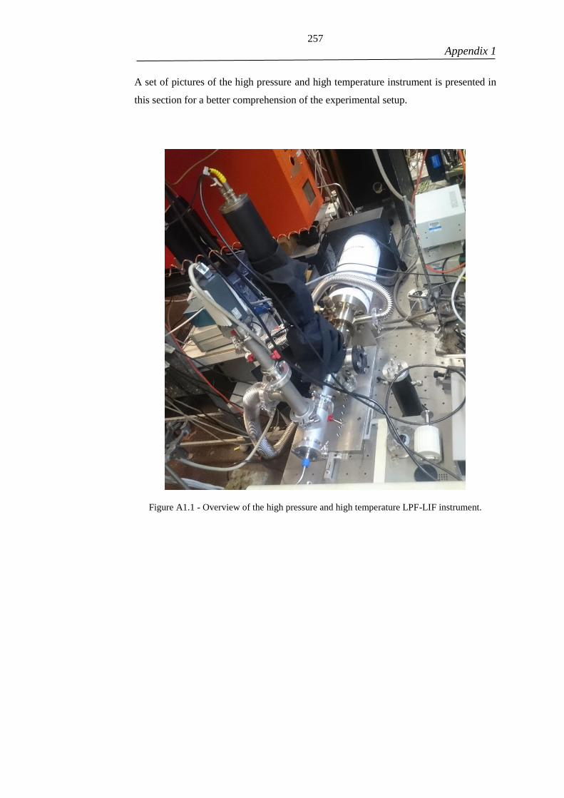
257 Appendix 1

A set of pictures of the high pressure and high temperature instrument is presented in

this section for a better comprehension of the experimental setup.

Figure A1.1 - Overview of the high pressure and high temperature LPF-LIF instrument.

258 Appendix 1

Figure A1.2 - The high pressure LPF -LIF instrument. View of the window from which the

probe beam enters the reaction cell.

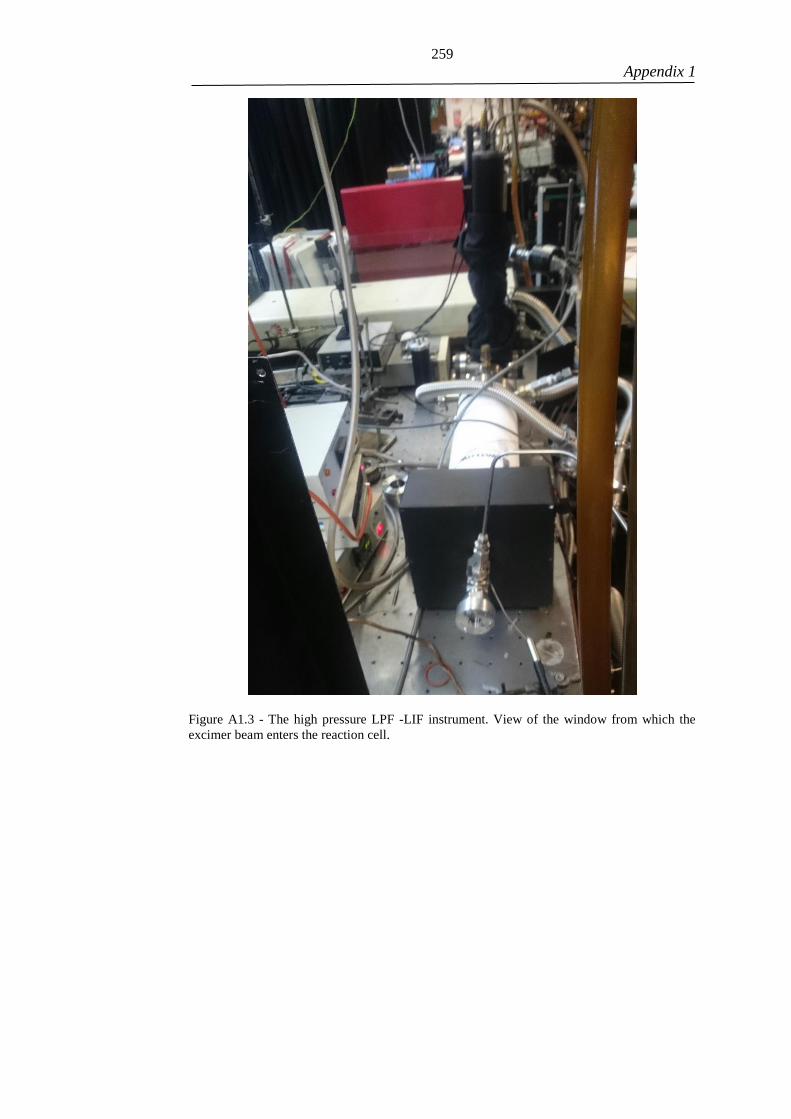
259 Appendix 1

Figure A1.3 - The high pressure LPF -LIF instrument. View of the window from which the

excimer beam enters the reaction cell.

261

Appendix 2

APPENDIX 2

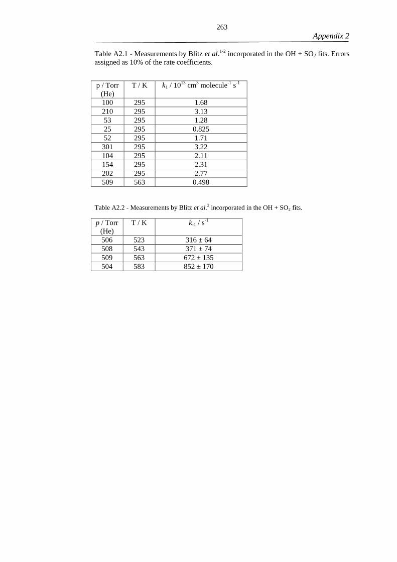
263 Appendix 2

Table A2.1 - Measurements by Blitz et al.1-2

incorporated in the OH + SO2 fits. Errors

assigned as 10% of the rate coefficients.

p / Torr

(He)

T / K k1 / 1013

cm3 molecule

-1 s

-1

100 295 1.68

210 295 3.13

53 295 1.28

25 295 0.825

52 295 1.71

301 295 3.22

104 295 2.11

154 295 2.31

202 295 2.77

509 563 0.498

Table A2.2 - Measurements by Blitz et al.

2 incorporated in the OH + SO2 fits.

p / Torr

(He)

T / K k-1 / s-1

506 523 316 ± 64

508 543 371 ± 74

509 563 672 ± 135

504 583 852 ± 170

264 Appendix 2

Table A2.3 - Measurements by Wine et al.3 incorporated in the OH + SO2 fits. Errors

assigned as 10% of the rate coefficients. Helium used as the bath gas.

p / Torr

(He)

T / K k1 / 1013

cm3 molecule

-1

s-1

16 300 0.467

31 300 0.69

62 300 1.03

124 300 1.44

249 300 2.11

497 300 3.4

Table A2.4 - Measurements by Wine et al. incorporated in the OH + SO2 fits. Errors

assigned as 10% of the rate coefficients. Argon used as the bath gas.

p / Torr

(Ar)

T / K k1 / 1013

cm3 molecule

-1

s-1

16 300 0.491

31 300 0.775

62 300 1.21

124 300 1.58

249 300 2.34

497 300 3.39

13 260 0.821

19 360 0.279

22 420 0.226

27 260 1.18

37 360 0.435

44 420 0.353

54 260 1.67

75 360 0.622

87 420 0.49

108 260 2.36

149 360 0.959

174 420 0.722

215 260 3.65

298 360 1.34

348 420 1.09

431 260 5.46

597 360 1.85

696 420 1.58

265 Appendix 2


assigned as 10% of the rate coefficients. N2 used as the bath gas.

p / Torr

(Ar)

T / K k1 / 1013

cm3 molecule

-1

s-1

16 300 1.13

31 300 1.81

62 300 2.89

124 300 4.17


assigned as 10% of the rate coefficients. SF6 used as the bath gas.

p / Torr

(Ar)

T / K k1 / 1013

cm3 molecule

-1

s-1

16 300 1.92

31 300 2.9

62 300 4.38

124 300 5.22

249 300 7.17

497 300 10

13 260 2.96

19 360 1.29

22 420 1.07

27 260 3.7

37 360 2.18

44 420 1.51

54 260 6.04

75 360 2.86

87 420 2.19

108 260 7.52

149 360 4.38

174 420 3.9

215 260 9.5

298 360 5.83

348 420 4.91

431 260 12.4

597 360 7.45

696 420 7.16

1. Blitz, M. A.; Salter, R. J.; Heard, D. E.; Seakins, P. W. An Experimental Study of the Kinetics of OH/OD(ν = 1,2,3) + SO2: The Limiting High-Pressure Rate Coefficients as a Function of Temperature. The Journal of Physical Chemistry A 2017, 121, 3175-3183. 2. Blitz, M. A.; Hughes, K. J.; Pilling, M. J. Determination of the High-Pressure Limiting Rate Coefficient and the Enthalpy of Reaction for OH + SO2. The Journal of Physical Chemistry A 2003, 107, 1971-1978. 3. Wine, P. H.; Thompson, R. J.; Ravishankara, A. R.; Semmes, D. H.; Gump, C. A.; Torabi, A.; Nicovich, J. M. Kinetics of the Reaction OH + SO2 + M → HOSO2 + M. Temperature and Pressure Dependence in the Fall-Off Region. The Journal of Physical Chemistry 1984, 88, 2095-2104.

267

Appendix 2

APPENDIX 3

269 Appendix 3

Table A3.1 Experimental Determinations of k1 at high pressure.

T / K p / Torr k1 × 1011

/ cm3

molecule-1

s-1

k1a × 1011

/ cm3

molecule-1

s-1

k1b × 1011

/ cm3

molecule-1

s-1

300 1290 9.90 ± 0.07 9.59 0.31

300 1365 10.01 ± 0.06 9.70 0.31

406 1367 6.68 ± 0.27 6.23 0.45

417 1497 7.24 ± 0.80 6.78 0.46

418 1418 6.24 ± 0.17 5.78 0.46

433 1546 5.99 ± 0.77 5.51 0.48

475 1394 5.61 ± 0.25 5.09 0.52

508 1673 5.67 ± 0.63 5.12 0.55

564 1350 4.74 ± 0.22 4.14 0.60

618 1536 3.99 ± 0.23 3.35 0.64

630 1373 4.71 ± 0.28 4.06 0.65

Table A3.2 Experimental Determinations of k1 at low pressure.

T / K p / Torr k1 × 1011

/ cm3

molecule-1

s-1

k1a × 1011

/ cm3

molecule-1

s-1

k1b × 1011

/ cm3

molecule-1

s-1

300 96 10.60 ± 0.18 10.29 0.31

300 56 10.40 ± 0.16 10.09 0.31

337 57 8.28 ± 0.11 7.92 0.36

426 103 5.56 ± 0.13 5.09 0.47

472 99 5.81 ± 0.43 5.29 0.52

473 99 4.98 ± 0.18 4.46 0.52

477 128 5.30 ± 0.5 4.78 0.52

478 114 6.12 ± 0.18 5.60 0.52

533 132 4.91 ± 0.12 4.33 0.58

540 141 5.27 ± 0.18 4.69 0.58

573 51 4.40 ± 0.53 3.79 0.61

729 115 2.46 ± 0.79 1.74 0.72

766 122 2.32 ± 0.73 1.58 0.74

794 100 2.23 ± 0.69 1.48 0.75

270 Appendix 3

Table A3.3 Wavenumbers of isoprene calculated at the M06-2X/6-311++G(3df,2p)

level of theory.

Mode # Wavenumber

cm-1

1 160.16

2 239.94

3 291.65

4 407.99

5 434.42

6 532.67

7 650.83

8 795.58

9 806.46

10 953.58

11 964.35

12 971.95

13 1012.56

14 1041.92

15 1069.27

16 1088.48

17 1323.80

18 1342.80

19 1412.71

20 1439.66

21 1460.97

22 1489.90

23 1506.10

24 1687.26

25 1737.33

26 3039.57

27 3097.70

28 3139.52

29 3142.24

30 3144.79

31 3153.72

32 3229.56

33 3232.20

271 Appendix 3

Table A3.4 Cartesian coordinates for the isoprene structure optimized at the M06-

2X/6-311++G(3df,2p) level of theory.

Atom x y z

C 0.517499 -0.099008 -0.000001

C 0.636141 1.397503 -0.000001

C -0.826523 -0.688292 0.000001

C 1.588187 -0.892823 -0.000002

C -1.964262 -0.000256 0.000002

H 0.149241 1.824206 -0.878950

H 1.679931 1.704179 -0.000002

H 0.149243 1.824207 0.878949

H -0.862185 -1.773179 0.000001

H 2.592606 -0.490543 -0.000003

H 1.485503 -1.970615 -0.000002

H -2.921377 -0.502828 0.000003

H -1.979219 1.081832 0.000002

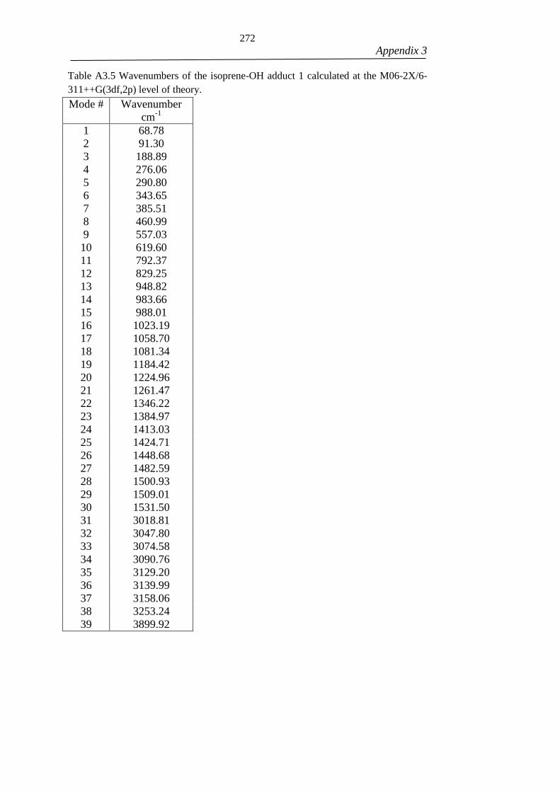
272 Appendix 3

Table A3.5 Wavenumbers of the isoprene-OH adduct 1 calculated at the M06-2X/6-

311++G(3df,2p) level of theory.

Mode # Wavenumber

cm-1

1 68.78

2 91.30

3 188.89

4 276.06

5 290.80

6 343.65

7 385.51

8 460.99

9 557.03

10 619.60

11 792.37

12 829.25

13 948.82

14 983.66

15 988.01

16 1023.19

17 1058.70

18 1081.34

19 1184.42

20 1224.96

21 1261.47

22 1346.22

23 1384.97

24 1413.03

25 1424.71

26 1448.68

27 1482.59

28 1500.93

29 1509.01

30 1531.50

31 3018.81

32 3047.80

33 3074.58

34 3090.76

35 3129.20

36 3139.99

37 3158.06

38 3253.24

39 3899.92

273 Appendix 3

Table A3.6 Cartesian coordinates for the isoprene-OH adduct 1 structure optimized at

the M06-2X/6-311++G(3df,2p) level of theory.

Atom x y z

C -0.061504 0.054587 0.186191

C -0.134746 1.545617 0.087286

C -1.183972 -0.750765 0.030269

C 1.274368 -0.549102 0.484202

C -2.456837 -0.298647 -0.210810

H -0.603420 1.863619 -0.846627

H 0.860221 1.984055 0.132720

H -0.736071 1.960634 0.901837

H -1.034215 -1.823355 0.114307

H 1.659247 -0.169221 1.434847

H 1.189995 -1.636968 0.568826

H -3.281214 -0.987056 -0.319880

H -2.676562 0.756401 -0.297081

O 2.257516 -0.188746 -0.476030

H 1.938040 -0.448276 -1.343532

274 Appendix 3



Mode # Wavenumber

cm-1

1 106.32

2 174.05

3 259.21

4 294.04

5 307.28

6 331.62

7 370.98

8 424.52

9 440.53

10 531.94

11 585.8

12 709.11

13 759.09

14 906.37

15 971.95

16 981.09

17 997.35

18 1035.68

19 1046.41

20 1059.46

21 1219.74

22 1276.72

23 1320.46

24 1332.8

25 1390.31

26 1440.77

27 1449.42

28 1484.68

29 1498.46

30 1725.07

31 3045.16

32 3131.01

33 3134.61

34 3141.25

35 3153.24

36 3157.31

37 3235.13

38 3271.41

39 3871.44

275 Appendix 3

Table A3.8 Cartesian coordinates for the isoprene-OH adduct 2 structure optimized at

the M06-2X/6-311++G(3df,2p) level of theory.

Atom x y z

C -0.37849 -0.04503 0.01455

C -1.08250 1.31214 0.13623

C 0.98250 0.03261 0.67001

C -1.19259 -1.11985 0.66009

C 2.13367 0.02912 0.01922

H -0.50463 2.06361 -0.40171

H -2.07902 1.24430 -0.29887

H -1.16851 1.60633 1.18155

H 0.96553 0.10686 1.75377

H -2.09707 -1.44568 0.16572

H -0.99690 -1.44237 1.67179

H 3.07562 0.09504 0.54607

H 2.16526 -0.02640 -1.06122

O -0.27700 -0.28568 -1.38160

H 0.08010 -1.17026 -1.50490

276 Appendix 3



Mode # Wavenumber

cm-1

1 68.31

2 171.05

3 218.73

4 239.44

5 275.55

6 344.76

7 369.92

8 428.95

9 460.95

10 570.59

11 602.91

12 756.89

13 820.00

14 915.54

15 961.48

16 972.18

17 1029.97

18 1070.82

19 1074.20

20 1155.86

21 1228.48

22 1313.40

23 1321.43

24 1387.17

25 1408.70

26 1453.88

27 1456.57

28 1480.00

29 1500.30

30 1741.98

31 2972.11

32 3045.69

33 3105.81

34 3138.02

35 3140.62

36 3179.40

37 3223.41

38 3300.20

39 3898.05

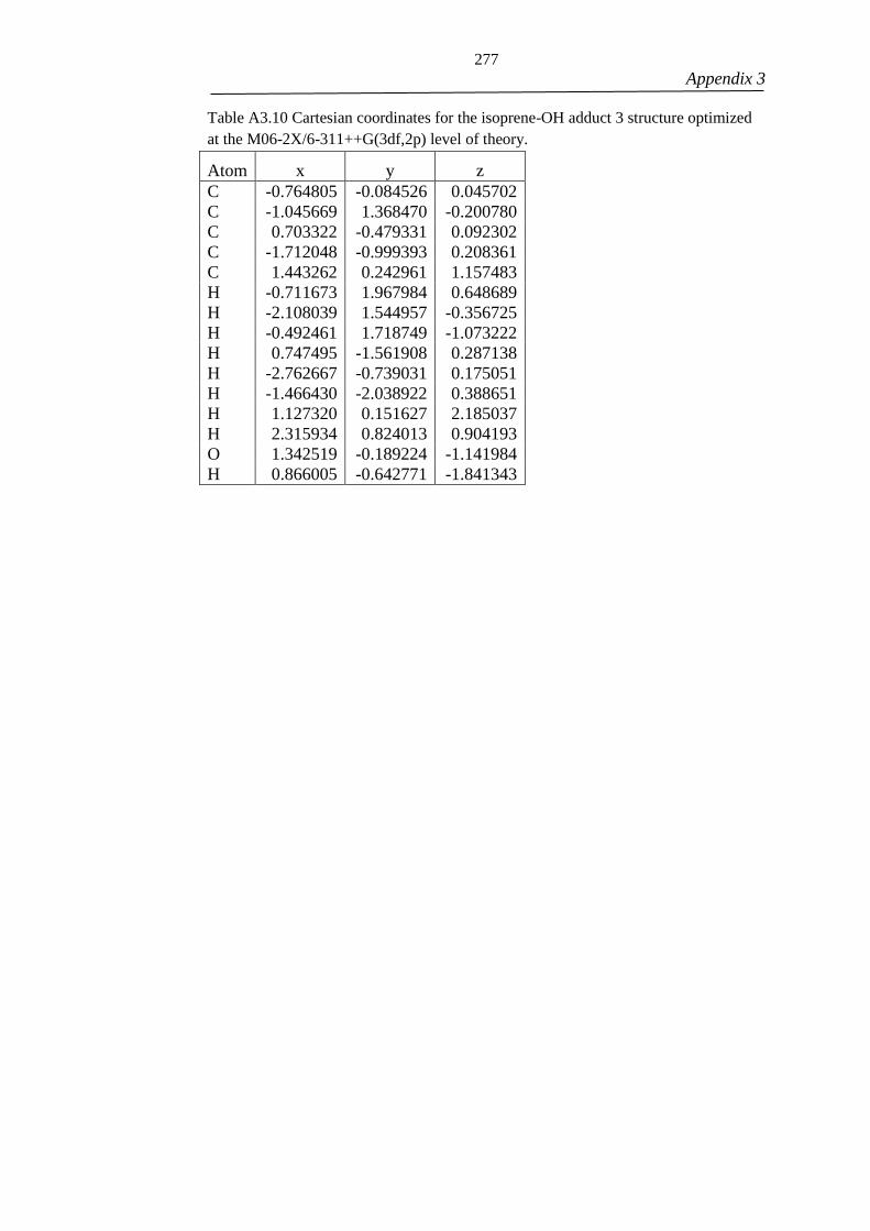
277 Appendix 3

Table A3.10 Cartesian coordinates for the isoprene-OH adduct 3 structure optimized

at the M06-2X/6-311++G(3df,2p) level of theory.

Atom x y z

C -0.764805 -0.084526 0.045702

C -1.045669 1.368470 -0.200780

C 0.703322 -0.479331 0.092302

C -1.712048 -0.999393 0.208361

C 1.443262 0.242961 1.157483

H -0.711673 1.967984 0.648689

H -2.108039 1.544957 -0.356725

H -0.492461 1.718749 -1.073222

H 0.747495 -1.561908 0.287138

H -2.762667 -0.739031 0.175051

H -1.466430 -2.038922 0.388651

H 1.127320 0.151627 2.185037

H 2.315934 0.824013 0.904193

O 1.342519 -0.189224 -1.141984

H 0.866005 -0.642771 -1.841343

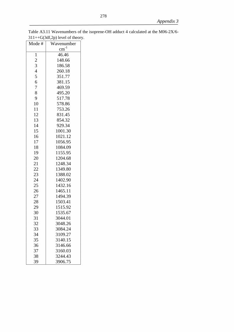
278 Appendix 3



Mode # Wavenumber

cm-1

1 46.46

2 148.66

3 186.58

4 260.18

5 351.77

6 381.15

7 469.59

8 495.20

9 517.78

10 578.86

11 753.26

12 831.45

13 854.32

14 929.34

15 1001.30

16 1021.12

17 1056.95

18 1084.09

19 1155.95

20 1204.68

21 1248.34

22 1349.80

23 1388.02

24 1402.90

25 1432.16

26 1465.11

27 1494.39

28 1503.41

29 1515.92

30 1535.67

31 3044.01

32 3048.26

33 3084.24

34 3109.27

35 3140.15

36 3146.66

37 3160.03

38 3244.43

39 3906.75

279 Appendix 3

Table A3.12 Cartesian coordinates for the isoprene-OH adduct 4 structure optimized


Atom x y z

C 1.054407 -0.121719 0.020786

C 1.335098 1.357966 -0.109674

C -0.239831 -0.575430 0.261110

C 2.093406 -1.016361 -0.093371

C -1.453661 0.274514 0.415823

H 0.756064 1.800155 -0.921557

H 2.389288 1.531036 -0.315008

H 1.076387 1.892490 0.804794

H -0.403063 -1.644302 0.352990

H 3.104796 -0.685199 -0.280082

H 1.922319 -2.080036 0.000876

H -1.235458 1.321352 0.186586

H -1.817361 0.238126 1.446681

O -2.537437 -0.198153 -0.371105

H -2.230000 -0.302219 -1.274480

280 Appendix 3

Table A3.13 Wavenumbers of the transition state of the abstraction, calculated at the

M06-2X/6-311++G(3df,2p) level of theory.

Mode # Wavenumber

cm-1

1 968.22i

2 82.86

3 112.79

4 160.63

5 260.62

6 299.77

7 365.28

8 406.36

9 426.57

10 534.62

11 624.6

12 751.97

13 793.76

14 822.77

15 948.19

16 966.99

17 982.52

18 988.81

19 1017.1

20 1045.71

21 1086.37

22 1229.27

23 1324.86

24 1332.55

25 1372.84

26 1427.46

27 1445.01

28 1460.35

29 1491.7

30 1679.48

31 1724.59

32 3077.27

33 3144.03

34 3151.09

35 3152.95

36 3159.93

37 3234.54

38 3242.34

39 3777.41

281 Appendix 3

Table A3.14 Cartesian coordinates for the transition state of the abstraction, optimized


Atom x y z

C -0.866548 -0.209943 0.082766

C 0.113942 -1.009598 0.861568

C -0.583557 1.212196 -0.151368

C -1.974055 -0.760098 -0.422726

C 0.503126 1.856023 0.267683

H 0.387106 -0.550582 1.811174

H 1.118250 -1.064873 0.271301

H -0.197227 -2.041572 1.001644

H -1.335491 1.750901 -0.719147

H -2.202219 -1.807362 -0.276288

H -2.681628 -0.17146 -0.992614

H 0.644842 2.906421 0.054388

H 1.282236 1.360846 0.833916

O 2.244360 -0.852557 -0.592818

H 1.871807 -0.093342 -1.069373

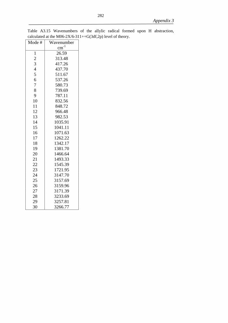
282 Appendix 3

Table A3.15 Wavenumbers of the allylic radical formed upon H abstraction,

calculated at the M06-2X/6-311++G(3df,2p) level of theory.

Mode # Wavenumber

cm-1

1 26.59

2 313.48

3 417.26

4 437.70

5 511.67

6 537.26

7 580.73

8 739.69

9 787.11

10 832.56

11 848.72

12 966.48

13 982.53

14 1035.91

15 1041.11

16 1071.63

17 1262.22

18 1342.17

19 1381.70

20 1466.64

21 1493.33

22 1545.39

23 1721.95

24 3147.70

25 3157.69

26 3159.96

27 3171.39

28 3233.69

29 3257.81

30 3266.77

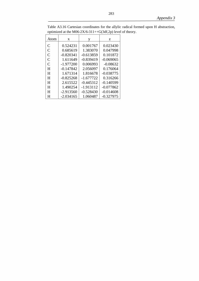
283 Appendix 3

Table A3.16 Cartesian coordinates for the allylic radical formed upon H abstraction,

optimized at the M06-2X/6-311++G(3df,2p) level of theory.

Atom x y z

C 0.524231 0.001767 0.023430

C 0.685619 1.383070 0.047998

C -0.820341 -0.613859 0.101872

C 1.611649 -0.839419 -0.069065

C -1.977200 0.006993 -0.08632

H -0.147842 2.056097 0.176064

H 1.671314 1.816678 -0.038775

H -0.825268 -1.677722 0.316266

H 2.615522 -0.445312 -0.140599

H 1.490254 -1.913112 -0.077862

H -2.913560 -0.528430 -0.014608

H -2.034165 1.060487 -0.327975

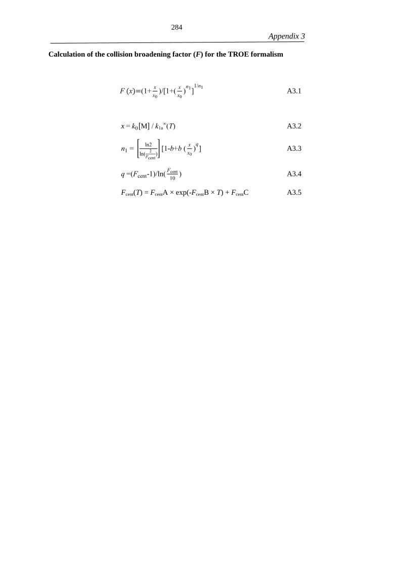
284 Appendix 3

Calculation of the collision broadening factor (F) for the TROE formalism

F (x)=(1+x

x0)/[1+(

x

x0)n1

]1/n1

A3.1

x = k0[M] / k1a∞(T) A3.2

n1 = [ln2

ln(2

Fcent)] [1-b+b (

x

x0)q] A3.3

q =(Fcent-1)/ln(Fcent

10) A3.4

Fcent(T) = FcentA × exp(-FcentB × T) + FcentC A3.5

285

Appendix 4

APPENDIX 4

287 Appendix 4

Figure A4.1 The excel interface used to generate a MATLAB script which solves the

chemical problem defined. The figure shows a simplified version of the Leuven

Isoprene Mechanism 1 which supresses the di-HPCARP channels.

288 Appendix 4

function [ b, fval, exitflag, output, solutions ] = pfo()

clc;

clear all;

close all;

data=importdata('/home/home02/cmddjm/MESMER/Mesmer4.1-

source/examples/matlab_ethylene_12112018/Exp_data.txt');

data2=importdata('/home/home02/cmddjm/MESMER/Mesmer4.1-

source/examples/matlab_ethylene_12112018/Weights.txt');

data3=importdata('/home/home02/cmddjm/MESMER/Mesmer4.1-

source/examples/matlab_ethylene_12112018/Loss_rate.txt');

tspan1=data(:,1);

Ca_data1=data(:,2);

tspan1(~any(~isnan(tspan1), 2),:)=[];

Ca_data1(~any(~isnan(Ca_data1), 2),:)=[];

s1=size(tspan1);

tspan1=tspan1/1e3;

tspan2=data(:,3);

Ca_data2=data(:,4);



s2=size(tspan2);

tspan2=tspan2/1e3;

tspan3=data(:,5);

Ca_data3=data(:,6);



s3=size(tspan3);

tspan3=tspan3/1e3;

tspan4=data(:,7);

Ca_data4=data(:,8);



s4=size(tspan4);

tspan4=tspan4/1e3;

tspan5=data(:,9);

Ca_data5=data(:,10);



s5=size(tspan5);

tspan5=tspan5/1e3;

tspan6=data(:,11);

Ca_data6=data(:,12);



s6=size(tspan6);

289 Appendix 4

tspan6=tspan6/1e3;

Ca_data1=Ca_data1/data2(1);






s0=0;

tspan=[tspan1;tspan2;tspan3;tspan4;tspan5;tspan6;];

Ca_data=[Ca_data1;Ca_data2;Ca_data3;Ca_data4;Ca_data5;Ca_data6];

parguess=[1.98466996809536,1.64722346293468,1.07981103615226,1.24810314998

381,1.16948206026735,1.56841012973971,-110,0.822,-0.35,1,1,221,0.26,400];

ub=[3.77087293938119,3.1297245795759,2.05164096868929,2.37139598496924,2.2

2201591450796,2.97997924650545,-100,0.86,1.35,1.1,1.1,400,0.95,2000];

lb=[0.198466996809536,0.164722346293468,0.107981103615226,0.1248103149983

81,0.116948206026735,0.156841012973971,-135,0.78,-1.35,0.9,0.9,100,0.05,0];

global contador_global;

global last_call;

global save_print;

global arquivo_aberto;

global contcoeff;

global ratecoeffs;

contador_global=0;

last_call=[-999999999999 -999999999999 -999999999999 -999999999999];

function [output] = myfunc2(paras,tspan)

%Primeiro resolve o Mesmer

% persistent arquivo_aberto;

% persistent contcoeff;

% persistent ratecoeffs;

arquivo_aberto=false;

if(last_call(1,1) ~= paras(7) || last_call(1,2) ~= paras(8) || last_call(1,3) ~= paras(9) ||

last_call(1,4) ~= paras(12) || last_call(1,5) ~= paras(13))

%Editar o arquivo com os novos parametros e rodar

% Read txt into cell A

tmpName=tempname;

290 Appendix 4

tmpName=tmpName(5:end);

FulltmpName = ['/home/home02/cmddjm/MESMER/Mesmer4.1-

source/examples/matlab_ethylene_12112018/',tmpName,'.xml'];

copyfile('/home/home02/cmddjm/MESMER/Mesmer4.1-

source/examples/matlab_ethylene_12112018/Ethylene_MATLAB_updated_96_traces

_12112018.xml',[FulltmpName]);

fid = fopen(FulltmpName,'r');

i = 1;

tline = fgetl(fid);

A{i} = tline;

while ischar(tline)

i = i+1;

tline = fgetl(fid);

A{i} = tline;

end

fclose(fid);

patternyy='<molecule id="ethylene_OH"';

for i = 1:numel(A)

control=~isempty(strfind(A{i},patternyy));

if control==true

break;

end

end

patternyy='dictRef="me:ZPE"';

for i = i:numel(A)


if control==true

break;

end

end

%paras(1)=3.25e-12;

variavel_definida=[' <scalar units="kJ/mol">' num2str(paras(7)) '</scalar>'];

A{i+1} = sprintf('%s',variavel_definida);

%A{i+1} = sprintf(' <scalar units="kJ/mol">-150.690685 dIOGO</scalar>');

patternyy='me:ExponentialDown';

for i = i:numel(A)


291 Appendix 4

if control==true

break;

end

end

%paras(1)=3.25e-12;

variavel_definida=[' <me:deltaEDown bathGas="N2" units="cm-1">'

num2str(paras(12)) '</me:deltaEDown>'];


variavel_definida=[' <me:deltaEDownTExponent bathGas="N2"

referenceTemperature="298">' num2str(paras(13)) '</me:deltaEDownTExponent>'];


%A{i+1} = sprintf(' <scalar units="kJ/mol">-150.690685 dIOGO</scalar>');

patternyy='reactionList';

for i = i:numel(A)


if control==true

break;

end

end

%reaction 1

patternyy='<reaction id="R1">';

for i = i:numel(A)


if control==true

break;

end

end

patternyy='<me:preExponential';

for i = i:numel(A)


if control==true

break;

end

end

variavel_definida=[' <me:preExponential units="cm3molecule-1s-1">' num2str(1E-

11*paras(8)) '</me:preExponential>'];

A{i} = sprintf('%s',variavel_definida);

patternyy='<me:nInfinity>';

for i = i:numel(A)


if control==true

break;

292 Appendix 4

end

end

variavel_definida=[' <me:nInfinity>' num2str(paras(9)) '</me:nInfinity>'];

A{i} = sprintf('%s',variavel_definida);

fid = fopen(FulltmpName, 'w');

for i = 1:numel(A)

if A{i+1} == -1

fprintf(fid,'%s', A{i});

break

else

fprintf(fid,'%s\n', A{i});

end

end

fclose(fid);

temporario='Mesmer is running';

% temporario=[num2str(contador_global),' param(1)=',num2str(paras(1)),'

param(2)=',num2str(paras(2)),' param(3)=',num2str(paras(3))];

disp(temporario);

%contador_global=contador_global+1;

%uma vez o arquivo editado, roda-lo e extrair informacoes pertinentes

command=['mesmer -N ',tmpName(2:end),'.xml',' -o ',tmpName(2:end),'.out'];

[status, cmdout]=system(command);

temporario='Mesmer has finished a calculation';

% temporario=[num2str(contador_global),' param(1)=',num2str(paras(1)),'

param(2)=',num2str(paras(2)),' param(3)=',num2str(paras(3))];

disp(temporario);

%copyfile /home/home02/cmddjm/MESMER/Mesmer4.1-

source/examples/matlab_ethylene_12112018//mesmer_out.xml;

%se o arquivo for ser aberto pela primeira vez, contar o numero de

%coeficientes de reacao.

if arquivo_aberto==false

fileID = fopen(['/home/home02/cmddjm/MESMER/Mesmer4.1-

source/examples/matlab_ethylene_12112018/',tmpName,'.out']);

line=fgetl(fileID);

%indicar que o arquivo foi aberto e buscar o numero de coeficientes

arquivo_aberto=true;

patternyy='me:rateList';

control=~isempty(strfind(line,patternyy));

293 Appendix 4

while control==false

line=fgetl(fileID);


end

patternyy='fromRef';

control=false;


line=fgetl(fileID);


end

%essa linha ja contem o primeiro rate coefficient

contcoeff=1;


control=false;


contcoeff=contcoeff+1;

line=fgetl(fileID);


end

contcoeff=contcoeff-1;

fclose(fileID);

end

%aqui ja se sabe o numero de constantes, guardado em contcoeff

fileID = fopen(['/home/home02/cmddjm/MESMER/Mesmer4.1-

source/examples/matlab_ethylene_12112018/',tmpName,'.out']);

line=fgetl(fileID);

%indicar que o arquivo foi aberto e buscar o numero de coeficientes

arquivo_aberto=true;




line=fgetl(fileID);


end


control=false;


line=fgetl(fileID);


end

%essa linha ja contem o primeiro rate coefficient

patternyy='analysis';

control=false;

294 Appendix 4

control2=false;

control3=false;

ratecoeffs=[];

ratecoeffscomplete=[];

counter=1;


patternyy='<me:rateList ';

control2=~isempty(strfind(line,patternyy));

if control2==true

ratecoeffscomplete=[ratecoeffscomplete ratecoeffs];

ratecoeffs=[];


control3=false;

while control3==false

line=fgetl(fileID);

control3=~isempty(strfind(line,patternyy));

end

counter=counter+1;

control2=false;

end

key1=strfind(line,'>');

key2=strfind(line,'<');

[m,n] =size(key1);

[m2,n2] =size(key2);

if(n<2 || n2<2)

line=fgetl(fileID);



continue

end

key1=key1(1)+1;

key2=key2(2)-1;

line=str2double(line(key1:key2));

ratecoeffs=[ratecoeffs;line];

line=fgetl(fileID);



end

ratecoeffs=[ratecoeffscomplete ratecoeffs];

fclose(fileID);

delete([tmpName(2:end),'.out']);

295 Appendix 4

delete([tmpName(2:end),'.log']);

delete([tmpName(2:end),'.test']);

delete([tmpName(2:end),'.xml']);

%removendo valores muito pequenos do array

indices_neg=find(ratecoeffs<1e-10);

ratecoeffs(indices_neg)=0;

end

A1_=ratecoeffs(1,:)/1e15;

Ea1_=0;

n1_=0;

V1_=0;

A2_=ratecoeffs(2,:);

Ea2_=0;

n2_=0;

V2_=0;

A3_=data3;

Ea3_=0;

n3_=0;

V3_=0;

A4_=0;

Ea4_=0;

n4_=0;

V4_=0;

A5_=0;

Ea5_=0;

n5_=0;

V5_=0;

A6_=3.4e-11*paras(10);

Ea6_=2990*paras(11);

n6_=0;

V6_=0;

OH1=paras(1);

OH2=paras(2);

OH3=paras(3);

OH4=paras(4);

OH5=paras(5);

OH6=paras(6);

function f=ode(t,y)

f(1,1)=-(A1_(int64(y(6)))*exp(-

Ea1_/y(5))*((y(5)/298)^n1_)*(exp(V1_/(y(5))^3)))*y(2)*y(1)+(A2_(int64(y(6)))*exp

(-Ea2_/y(5))*((y(5)/298)^n2_)*(exp(V2_/(y(5))^3)))*y(3)-(A3_(int64(y(6)))*exp(-

Ea3_/y(5))*((y(5)/298)^n3_)*(exp(V3_/(y(5))^3)))*y(1)+(A4_*exp(-

Ea4_/y(5))*((y(5)/298)^n4_)*(exp(V4_/(y(5))^3)))*y(3)*y(2)-(A6_*exp(-

Ea6_/y(5))*((y(5)/298)^n6_)*(exp(V6_/(y(5))^3)))*y(2)*y(1);

f(2,1)=-(A1_(int64(y(6)))*exp(-

Ea1_/y(5))*((y(5)/298)^n1_)*(exp(V1_/(y(5))^3)))*y(2)*y(1)+(A2_(int64(y(6)))*exp

(-Ea2_/y(5))*((y(5)/298)^n2_)*(exp(V2_/(y(5))^3)))*y(3)-(A4_*exp(-

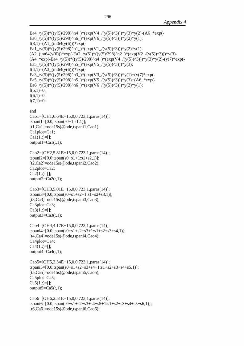
296 Appendix 4

Ea4_/y(5))*((y(5)/298)^n4_)*(exp(V4_/(y(5))^3)))*y(3)*y(2)-(A6_*exp(-

Ea6_/y(5))*((y(5)/298)^n6_)*(exp(V6_/(y(5))^3)))*y(2)*y(1);

f(3,1)=(A1_(int64(y(6)))*exp(-

Ea1_/y(5))*((y(5)/298)^n1_)*(exp(V1_/(y(5))^3)))*y(2)*y(1)-

(A2_(int64(y(6)))*exp(-Ea2_/y(5))*((y(5)/298)^n2_)*(exp(V2_/(y(5))^3)))*y(3)-

(A4_*exp(-Ea4_/y(5))*((y(5)/298)^n4_)*(exp(V4_/(y(5))^3)))*y(3)*y(2)-(y(7)*exp(-

Ea5_/y(5))*((y(5)/298)^n5_)*(exp(V5_/(y(5))^3)))*y(3);

f(4,1)=(A3_(int64(y(6)))*exp(-

Ea3_/y(5))*((y(5)/298)^n3_)*(exp(V3_/(y(5))^3)))*y(1)+(y(7)*exp(-

Ea5_/y(5))*((y(5)/298)^n5_)*(exp(V5_/(y(5))^3)))*y(3)+(A6_*exp(-

Ea6_/y(5))*((y(5)/298)^n6_)*(exp(V6_/(y(5))^3)))*y(2)*y(1);

f(5,1)=0;

f(6,1)=0;

f(7,1)=0;

end

Cao1=[OH1,6.64E+15,0,0,723,1,paras(14)];

tspani1=[0.0;tspan(s0+1:s1,1)];

[t1,Ca1]=ode15s(@ode,tspani1,Cao1);

Ca1plot=Ca1;

Ca1(1,:)=[];

output1=Ca1(:,1);

Cao2=[OH2,5.81E+15,0,0,723,1,paras(14)];

tspani2=[0.0;tspan(s0+s1+1:s1+s2,1)];


Ca2plot=Ca2;

Ca2(1,:)=[];

output2=Ca2(:,1);

Cao3=[OH3,5.01E+15,0,0,723,1,paras(14)];

tspani3=[0.0;tspan(s0+s1+s2+1:s1+s2+s3,1)];


Ca3plot=Ca3;

Ca3(1,:)=[];

output3=Ca3(:,1);

Cao4=[OH4,4.17E+15,0,0,723,1,paras(14)];

tspani4=[0.0;tspan(s0+s1+s2+s3+1:s1+s2+s3+s4,1)];


Ca4plot=Ca4;

Ca4(1,:)=[];

output4=Ca4(:,1);

Cao5=[OH5,3.34E+15,0,0,723,1,paras(14)];

tspani5=[0.0;tspan(s0+s1+s2+s3+s4+1:s1+s2+s3+s4+s5,1)];


Ca5plot=Ca5;

Ca5(1,:)=[];

output5=Ca5(:,1);

Cao6=[OH6,2.51E+15,0,0,723,1,paras(14)];

tspani6=[0.0;tspan(s0+s1+s2+s3+s4+s5+1:s1+s2+s3+s4+s5+s6,1)];


297 Appendix 4

Ca6plot=Ca6;

Ca6(1,:)=[];

output6=Ca6(:,1);

output=[output1;output2;output3;output4;output5;output6];

last_call=[paras(7) paras(8) paras(9) paras(12) paras(13)];

temporario=[num2str(contador_global),' param(97)=',num2str(paras(7)),'

param(98)=',num2str(paras(8)),' param(99)=',num2str(paras(9)),'



param(104)=',num2str(paras(14))];

disp(temporario);

contador_global=contador_global+1;

save('matlab2.mat');

end

scaling=[];

for i=1:104

scaling=[scaling 0.025];

end

options=optimoptions('lsqcurvefit','MaxIterations',10,'Display','iter','TolFun',1e-

6,'TolX',1e-6,'FinDiffRelStep',scaling,'UseParallel',true);

[x,resnorm,residual,exitflag,output,lambda,jacobian]=lsqcurvefit(@myfunc2,parguess

,tspan, Ca_data, lb, ub, options);

fit=myfunc2(x,tspan);

ci=nlparci(x,residual,'jacobian',jacobian);

save('matlab.mat');

end

new methods for data analysis of complex chemical systems...

Documents