FERMILAB-PUB-13-310-T

MITP/13-047

New Physics in B → K∗µµ?

Wolfgang Altmannshofera and David M. Straubb

a Fermi National Accelerator Laboratory, P.O. Box 500, Batavia, IL 60510, USAbPRISMA Cluster of Excellence & Mainz Institute for Theoretical Physics,

Johannes Gutenberg University, 55099 Mainz, Germany

E-mail: waltmann@fnal.gov, david.straub@uni-mainz.de

Recent experimental results on angular observables in the rare decay B → K∗µ+µ−

show significant deviations from Standard Model predictions. We investigate thepossibility that these deviations are due to new physics. Combining all relevantdata on b→ s rare decays, we show that a consistent explanation of most anomaliescan be obtained by new physics contributing simultaneously to the semi-leptonicvector operator O9 and its chirality-flipped counterpart O′9. A partial explana-tion is possible with new physics in O9 or in dipole operators only. We studyin detail the implications for models of new physics, in particular the minimalsupersymmetric standard model, models with partial compositeness and genericmodels with flavour-changing Z ′ bosons. In all considered models, contributionsto B → K∗µ+µ− of the preferred size imply a spectrum close to the TeV scale.We stress that measurements of CP asymmetries in B → K∗µ+µ− could providevaluable information to narrow down possible new physics explanations.

Contents

1. Introduction 21.1. Effective Hamiltonian . . . . . . . . . . . . . . . . . . . . . . . . . . . . . . . . 21.2. Observables . . . . . . . . . . . . . . . . . . . . . . . . . . . . . . . . . . . . . . 3

2. Anatomy of new physics effects and fit to the data 32.1. Confronting the data . . . . . . . . . . . . . . . . . . . . . . . . . . . . . . . . . 42.2. Preliminary considerations . . . . . . . . . . . . . . . . . . . . . . . . . . . . . . 62.3. Trying to reduce the tension in S4 . . . . . . . . . . . . . . . . . . . . . . . . . 72.4. Effects in individual Wilson coefficients . . . . . . . . . . . . . . . . . . . . . . 82.5. Effects in two Wilson coefficients . . . . . . . . . . . . . . . . . . . . . . . . . . 8

3. Implications for models of new physics 123.1. Flavour-changing neutral gauge boson . . . . . . . . . . . . . . . . . . . . . . . 123.2. The Minimal Supersymmetric Standard Model . . . . . . . . . . . . . . . . . . 153.3. Models with partial compositeness . . . . . . . . . . . . . . . . . . . . . . . . . 183.4. Expectations for CP Asymmetries . . . . . . . . . . . . . . . . . . . . . . . . . 21

1

arX

iv:1

308.

1501

v3 [

hep-

ph]

20

Nov

201

3

4. Conclusions 23

A. Data averages 24

B. Loop functions 25

1. Introduction

Rare B decays mediated by the flavour-changing neutral b→ s transition are sensitive probesof physics beyond the Standard Model (SM), being loop and CKM-suppressed in the SM. In theLHC era, particular interest lies on exclusive semi-leptonic and leptonic decays, since they canbe measured more readily in a hadron collider environment. The decay B → K∗(→ Kπ)µ+µ−

plays a special role since the angular distribution of its four-body final state gives access tonumerous observables sensitive to new physics (NP). Since, for a neutral B decay, the flavourcan be tagged by measuring the charges of the final-state mesons, it is also straightforwardto measure CP asymmetries in the angular distribution, some of which are not suppressed bysmall strong phases [1]. All of this makes this decay mode a unique laboratory to test the size,chirality structure and CP phase of the FCNC transition in the SM and beyond, as has beendiscussed extensively in the literature (see e.g. [2–16] for recent studies).

After initial measurements of branching ratio and angular observables at B factories [17,18]and the Tevatron [19–21], recent measurements by LHCb, ATLAS and CMS [22–25] haveadded a wealth of new data. In particular, the recent measurement presented by the LHCbcollaboration [23] shows several significant deviations from the SM expectations. While it isconceivable that these anomalies are due to statistical fluctuations or underestimated theoryuncertainties – for recent reappraisals of various sources of uncertainty, see [26–30] – here weinvestigate the possibility that they are due to new physics. Finding a consistent explanationin terms of new physics is highly non-trivial since all the observables in B → K∗µ+µ− – manyof which are in agreement with SM expectations – as well as other decays like Bs → µ+µ−,B → Kµ+µ− or B → Xsγ, depend on the same short-distance Wilson coefficients, such thata global analysis of model-independent constraints is required. We perform such analysis,building on our previous work [8, 12], with refinements detailed below. Very recently, ref. [31]appeared, that also performs a model independent analysis of B → K∗µ+µ− anomalies. Wewill compare our findings in the conclusions.

Our paper is organized as follows. In sections 1.1 and 1.2 below, we define the relevanteffective Hamiltonian and briefly discuss the observables in B → K∗µ+µ−. In section 2,we perform a model independent analysis of NP effects in b → s transitions, identifying theWilson coefficients whose modification can lead to a consistent explanation of the experimentalobservations. In section 3, we discuss three concrete NP models: a model with a heavy neutralgauge boson (Z ′), the MSSM, and models with partial compositeness. Section 4 contains ourconclusions.

1.1. Effective Hamiltonian

The effective Hamiltonian for b→ s transitions can be written as

Heff = −4GF√2VtbV

∗ts

e2

16π2

∑i

(CiOi + C ′iO′i) + h.c. (1)

2

and we consider NP effects in the following set of dimension-6 operators,

O(′)7 =

mb

e(sσµνPR(L)b)F

µν , O(′)9 = (sγµPL(R)b)(¯γµ`) , O

(′)10 = (sγµPL(R)b)(¯γµγ5`) . (2)

We ignore scalar or pseudoscalar operators, since they are numerically irrelevant for the B →K∗µ+µ− decay. In models modifying O

(′)7 , typically also the chromomagnetic penguin operator

O(′)8 is modified. However, since it enters the decays considered below only via operator mixing

with O(′)7 , its discussion is redundant. As in our previous studies, in our numerical analysis we

consider NP effects to C(′)7 at a matching scale of 160 GeV.

1.2. Observables

In general, the angular distribution of B → K∗µ+µ− contains 24 observables [32], expressedas angular coefficients of a three-fold differential decay distribution, that are functions of thedilepton invariant mass squared q2. However, setting the lepton mass to zero (which is jus-tified at the current level of experimental precision) and neglecting effects of the scalar andpseudoscalar operators (which is well-motivated for B → K∗µ+µ− due to the absence of largeenhancements in Bs → µ+µ−) one is left with 18 independent observables. A convenient basisfor these 18 observables, reducing theoretical uncertainties and separating CP-violating fromCP-conserving effects was suggested in [32]. Instead of the angular coefficients of the B andB decay, one considers their sum or difference, normalized to the differential decay rate,

Si =(Ii + Ii

)/d(Γ + Γ)

dq2, Ai =

(Ii − Ii

)/d(Γ + Γ)

dq2. (3)

Binned observables, defined as ratios of q2 integrals of numerator and denominator, are denotedas 〈Si〉[a,b] and 〈Ai〉[a,b].

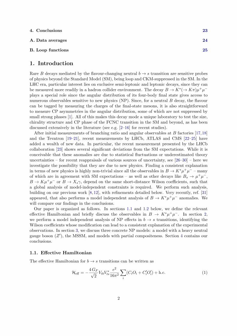
Only some of these angular observables are sensitive to new physics effects in the operators(2) though. In addition to the differential decay rate – which is subject to sizable theory un-certainties – there are mainly five CP-averaged angular observables and three CP-asymmetriesthat can receive significant NP contributions. We list them in table 1 and compare them toother conventions used in the literature. We also compare our conventions to the set of “opti-mized” observables suggested in [16]. These observables correspond to the Si and Ai dividedby a function of the K∗ longitudinal polarization fraction FL(q2) and are constructed to re-duce the dependence on hadronic form factors. In the last two columns, we list the Wilsoncoefficients that can lead to visible NP effects in the observables in question. Here one hasto distinguish between the low q2 region, q2 . 8 GeV2, and the high-q2 region, q2 & 14 GeV2.The intermediate region is unreliable due to the presence of charmonium resonances.

2. Anatomy of new physics effects and fit to the data

The methodology of our global analysis of constraints on Wilson coefficients is based on ourtwo previous studies [8, 12] and described there in detail. Here we only list the changes inthe experimental input data and theoretical calculations with respect to [12]. On the theoryside, we use the recent lattice calculation of B → K form factors at high q2 by the HPQCDcollaboration [33, 34], which strongly reduces theoretical uncertainties. On the experimentalside, we now additionally include

3

Here [32] [1] [16] LHCb [22,23] sens. at low q2 sens. at high q2

FL −Sc2 FL FL C7,9, C′9,10 C ′9,10

AFB34S

s6 AFB −AFB −AFB C7, C9 C9,10, C

′9,10

S3 S312FT P1 S3 C ′7,10 C ′9,10

S4 S412FLT P

′4 −S4 C7,10, C

′7,10 C ′9,10

S5 S5 FLT P′5 S5 C7,9, C

′7,9,10 C9, C

′9,10

A7 A7 −23A

D7 −FLT P ′6CP C7,10, C

′7,10 –

A8 A8 −23A

D8 −1

2FLT P′8

CP C7,9, C′7,9,10 C ′9,10

A9 A923A9 A9 C ′7,10 C ′9,10

P ′4 −2P ′4

P ′5 P ′5

Table 1: Dictionary between different notations for CP averaged angular coefficients and CPasymmetries in B → K∗µ+µ−, where FLT ≡

√FLFT and FT = 1− FL. The last two

columns show the Wilson coefficients the observables are most sensitive to both atlow q2 and high q2.

• updates of the angular analysis of B0 → K∗0µ+µ− by LHCb [22, 23], ATLAS [24] andCMS [25],

• an update of BR(B+ → K+µ+µ−)1 by LHCb [37],

• the recent measurements of BR(Bs → µ+µ−) by CMS [38] and LHCb [39].

Recently, the LHCb collaboration also found an unexpectedly large contribution of a charmo-nium resonance in the high dilepton invariant mass region of the decay B+ → K+µ+µ− thatmakes up ∼ 20% of the B+ → K+µ+µ− signal yield [40]. To be conservative, we treat thisresult by adding an additional relative theoretical uncertainty of 20% to all high-q2 observables,both in B → Kµ+µ− and in B → K∗µ+µ−, since the latter decay could be affected as well.This mars the improvement due to the B → K lattice form factors mentioned above and itwill be important to resolve this issue in the future.

2.1. Confronting the data

Averaging all available data on B → K∗µ+µ−, we can confront them with our SM predictions.Figure 1 shows our differential and binned SM predictions (light blue bands and purple boxes)together with the combined experimental data (black crosses) for the observables AFB, FL, S3,S4, and S5. Our error estimates were described in detail in [12], the only change being the

1We do not use the LHCb measurement of BR(B0 → K0µ+µ−) [35], which has larger error bars. Note thatthis measurement is on the low side compared to the charged decay, which is hard to accommodate even inthe presence of new physics [36]. We do not average the B+ → K+µ+µ− data with B factory or CDF dataeither, since they have a numerically negligible impact.

4

à

à

à

5 10 15 20-0.6

-0.4

-0.2

0.0

0.2

0.4

q2 @GeV2D

AF

B

C7NP=-0.1 , C7

'=-0.2

C9NP=-1.5 , C9

'=1.5

C9NP=-2 , C10

' =-1

à

à à

5 10 15 200.0

0.2

0.4

0.6

0.8

1.0

q2 @GeV2D

FL

C7NP=-0.1 , C7

'=-0.2

C9NP=-1.5 , C9

'=1.5

C9NP=-2 , C10

' =-1

à à

à

5 10 15 20

-0.4

-0.2

0.0

0.2

0.4

q2 @GeV2D

S 3

C7NP=-0.1 , C7

'=-0.2

C9NP=-1.5 , C9

'=1.5

C9NP=-2 , C10

' =-1

à

à

à

5 10 15 20

-0.4

-0.2

0.0

0.2

0.4

q2 @GeV2D

S4

C7NP=-0.1 , C7

=-0.2

C9NP=-1.5 , C9

=1.5

C9NP=-2 , C10

=-1

à

à

à

5 10 15 20

-0.4

-0.2

0.0

0.2

0.4

q2 @GeV2D

S 5

C7NP=-0.1 , C7

'=-0.2

C9NP=-1.5 , C9

'=1.5

C9NP=-2 , C10

' =-1

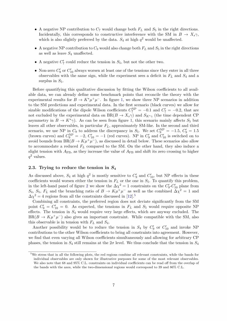
Figure 1: The CP averaged angular observables AFB, FL, S3, S4, and S5 as a function of thedi-muon invariant mass squared q2. Differential (binned) SM predictions are shownwith light blue bands (purple boxes). The combined experimental data is representedby the black crosses. The black, brown, and red curves correspond to NP scenariosthat reproduce the value of S5 at low q2 measured by LHCb.

5

additional relative uncertainty at high q2 as discussed in section 2.1.2

Confronting theory and experiment, we observe three discrepancies:

• A deficit in FL at low q2, mostly driven by the recent ATLAS measurement and to alesser extent by BaBar data. As the ATLAS and BaBar data in the [1, 6] GeV2 bin differsubstantially from the LHCb, CMS, Belle and CDF results, we use the PDG averagingmethod to combine the data, i.e. we rescale the uncertainty of the weighted averageby a factor of

√χ2. Doing so, we still find a discrepancy with the SM prediction at a

significance of 1.9σ in the [1, 6] GeV2 bin (see appendix A for more details).

• A preference for an anomalously low value of S4 at high q2, measured only by LHCb.We find a significance of 2.8σ in the [14.18, 16] GeV2 bin.

• A preference for an opposite sign in S5 at low q2, also measured only by LHCb. We finda significance of 2.4σ in the [1, 6] GeV2 bin.3

We note that the significance of the tension in S5 is substantially increased when consideringonly the [4.3, 8.68] GeV2 bin [23]. However, we consistently stick to the [1, 6] GeV2 bin in thelow-q2 region to be conservative.

Using the alternative basis of observables suggested in [16], we obtain a tension of 2.1σ in P ′4in the [14.18, 16] GeV2 bin and of 2.6σ in P ′5 in the [1, 6] GeV2 bin. We stress that the increasedsignificance in the case of P ′5 compared to S5 is not due to a reduced theory uncertainty. Infact, using our error estimates, we obtain a relative uncertainty of 13% in the low-q2 bin inboth cases. Rather, due to its normalization containing FL, P ′5 feels both the tensions in S5

and FL discussed separately above. In the case of P ′4, the alternative normalization does leadto a reduced theory uncertainty with our choice of high-q2 form factors.

We now turn to the discussion of new physics effects explaining the above tensions.

2.2. Preliminary considerations

Before turning to the numerical analysis, it is instructive to make some analytical considerationsas to which Wilson coefficients have to be modified to explain the tensions in the data. Animmediate observation is that all three tensions occur in CP-averaged observables, so there isno need to invoke non-standard CP violation, i.e. the Wilson coefficients can be kept real.

To get an analytical understanding of the dependence of the relevant observables on theWilson coefficients, we can derive approximate expressions, valid for small NP contributions,neglecting interference terms between NP effects in different coefficients. We find4

〈FL〉[1,6] ' +0.77 + 0.25CNP7 + 0.05CNP

9 − 0.04C ′9 + 0.04C ′10 , (4)

〈S4〉[14.18,16] ' +0.29 − 0.02C ′9 + 0.03C ′10 , (5)

〈S5〉[1,6] ' −0.14− 0.59CNP7 − 0.49C ′7 − 0.09CNP

9 − 0.03C ′9 + 0.10C ′10 . (6)

We can now qualitatively discuss the impact of NP effects in individual Wilson coefficientson the three anomalies.2We note that our treatment of form factors at high q2 is based on the extrapolation of light-cone sum

rule calculations [41] done in [42], which leads to particularly large uncertainties in FL compared to otherapproaches.

3Experimental results for S4 and S5 in the [1, 6] GeV2 region are not available yet. We therefore translate theresults on P ′4 and P ′5 using the measured value of FL and get 〈S4〉[1,6] = 0.14± 0.08 , 〈S5〉[1,6] = 0.10± 0.10 .

4We stress the different sign of our definition of S4 with respect to LHCb, see table 1.

6

• A negative NP contribution to C7 would change both FL and S5 in the right directions.Incidentally, this corresponds to constructive interference with the SM in B → Xsγ,which is also slightly preferred by the data. S4 at high q2 would be unaffected.

• A negative NP contribution to C9 would also change both FL and S5 in the right directionsas well as leave S4 unaffected.

• A negative C ′7 could reduce the tension in S5, but not the other two.

• Non-zero C ′9 or C ′10 always worsen at least one of the tensions since they enter in all threeobservables with the same sign, while the experiment sees a deficit in FL and S4 and asurplus in S5.

Before quantifying this qualitative discussion by fitting the Wilson coefficients to all avail-able data, we can already define some benchmark points that reconcile the theory with theexperimental results for B → K∗µ+µ−. In figure 1, we show three NP scenarios in additionto the SM predictions and experimental data. In the first scenario (black curves) we allow forsizable modifications of the dipole Wilson coefficients CNP

7 = −0.1 and C ′7 = −0.2, that arenot excluded by the experimental data on BR(B → Xsγ) and SK∗γ (the time dependent CPasymmetry in B → K∗γ). As can be seen from figure 1, this scenario mainly affects S5 butleaves all other observables, in particular FL, approximately SM-like. In the second and thirdscenario, we use NP in C9 to address the discrepancy in S5. We set CNP

9 = −1.5, C ′9 = 1.5(brown curves) and CNP

9 = −2, C ′10 = −1 (red curves). NP in C ′9 and C ′10 is switched on toavoid bounds from BR(B → Kµ+µ−), as discussed in detail below. These scenarios also allowto accommodate a reduced FL compared to the SM. On the other hand, they also induce aslight tension with AFB, as they increase the value of AFB and shift its zero crossing to higherq2 values.

2.3. Trying to reduce the tension in S4

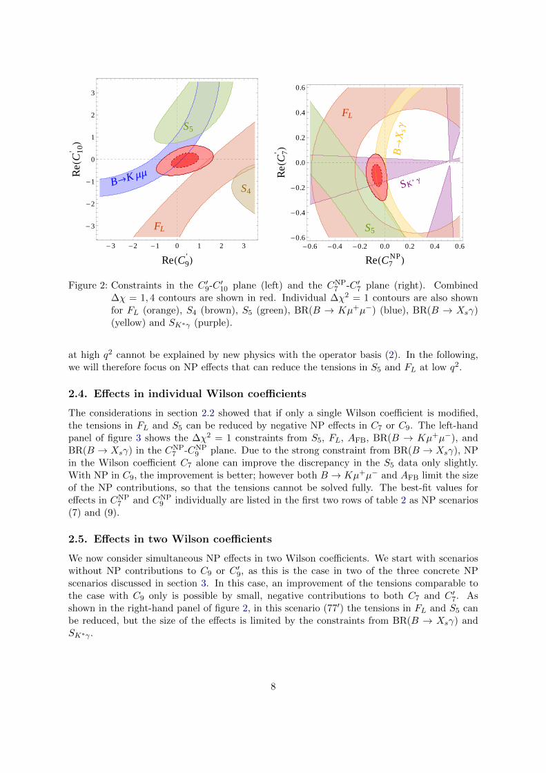
As discussed above, S4 at high q2 is mostly sensitive to C ′9 and C ′10, but NP effects in thesecoefficients would worsen either the tension in FL or the one in S5. To quantify this problem,in the left-hand panel of figure 2 we show the ∆χ2 = 1 constraints on the C ′9-C ′10 plane fromS4, S5, FL and the branching ratio of B → Kµ+µ− as well as the combined ∆χ2 = 1 and∆χ2 = 4 regions from all the constraints discussed in [12].5

Combining all constraints, the preferred region does not deviate significantly from the SMpoint C ′9 = C ′10 = 0. As expected, the tensions in FL and S5 would require opposite NPeffects. The tension in S4 would require very large effects, which are anyway excluded. TheBR(B → Kµ+µ−) also gives an important constraint. While compatible with the SM, alsothis observable is in tension with FL and S4.

Another possibility would be to reduce the tension in S4 by C ′9 or C ′10 and invoke NPcontributions to the other Wilson coefficients to bring all constraints into agreement. However,we find that even varying all Wilson coefficients simultaneously and allowing for arbitrary CPphases, the tension in S4 still remains at the 2σ level. We thus conclude that the tension in S4

5We stress that in all the following plots, the red regions combine all relevant constraints, while the bands forindividual observables are only shown for illustrative purposes for some of the most relevant observables.We also note that 68 and 95% C.L. constraints on individual coefficients can be read off from the overlap ofthe bands with the axes, while the two-dimensional regions would correspond to 39 and 86% C.L.

7

-3 -2 -1 0 1 2 3

-3

-2

-1

0

1

2

3

ReHC9'L

ReHC

10'L

FL

S4

S5

B®K ΜΜ

-0.6 -0.4 -0.2 0.0 0.2 0.4 0.6-0.6

-0.4

-0.2

0.0

0.2

0.4

0.6

ReHC7NPL

ReHC

7' L

FL

S5

SK* Γ

B®

XsΓ

Figure 2: Constraints in the C ′9-C ′10 plane (left) and the CNP7 -C ′7 plane (right). Combined

∆χ = 1, 4 contours are shown in red. Individual ∆χ2 = 1 contours are also shownfor FL (orange), S4 (brown), S5 (green), BR(B → Kµ+µ−) (blue), BR(B → Xsγ)(yellow) and SK∗γ (purple).

at high q2 cannot be explained by new physics with the operator basis (2). In the following,we will therefore focus on NP effects that can reduce the tensions in S5 and FL at low q2.

2.4. Effects in individual Wilson coefficients

The considerations in section 2.2 showed that if only a single Wilson coefficient is modified,the tensions in FL and S5 can be reduced by negative NP effects in C7 or C9. The left-handpanel of figure 3 shows the ∆χ2 = 1 constraints from S5, FL, AFB, BR(B → Kµ+µ−), andBR(B → Xsγ) in the CNP

7 -CNP9 plane. Due to the strong constraint from BR(B → Xsγ), NP

in the Wilson coefficient C7 alone can improve the discrepancy in the S5 data only slightly.With NP in C9, the improvement is better; however both B → Kµ+µ− and AFB limit the sizeof the NP contributions, so that the tensions cannot be solved fully. The best-fit values foreffects in CNP

7 and CNP9 individually are listed in the first two rows of table 2 as NP scenarios

(7) and (9).

2.5. Effects in two Wilson coefficients

We now consider simultaneous NP effects in two Wilson coefficients. We start with scenarioswithout NP contributions to C9 or C ′9, as this is the case in two of the three concrete NPscenarios discussed in section 3. In this case, an improvement of the tensions comparable tothe case with C9 only is possible by small, negative contributions to both C7 and C ′7. Asshown in the right-hand panel of figure 2, in this scenario (77′) the tensions in FL and S5 canbe reduced, but the size of the effects is limited by the constraints from BR(B → Xsγ) andSK∗γ .

8

-0.6 -0.4 -0.2 0.0 0.2 0.4 0.6

-3

-2

-1

0

1

2

3

ReHC7NPL

ReHC

9NP

L

FL

AFB

S5

B®K ΜΜ

B®

XsΓ

-0.6 -0.4 -0.2 0.0 0.2 0.4 0.6

-3

-2

-1

0

1

2

3

ReHC7'L

ReHC

9NP

LFL

AFBS5

B®K ΜΜ

S K*

Γ

Figure 3: Constraints in the CNP7 -CNP

9 plane (left) and the C ′7-CNP9 plane (right).

-3 -2 -1 0 1 2 3

-3

-2

-1

0

1

2

3

ReHC9NPL

ReHC

9' L

FL

S4

S5

AFB

B®K

ΜΜ

-3 -2 -1 0 1 2 3

-3

-2

-1

0

1

2

3

ReHC9NPL

ReHC

10'L

FL

AFB

S5

B®

KΜΜ

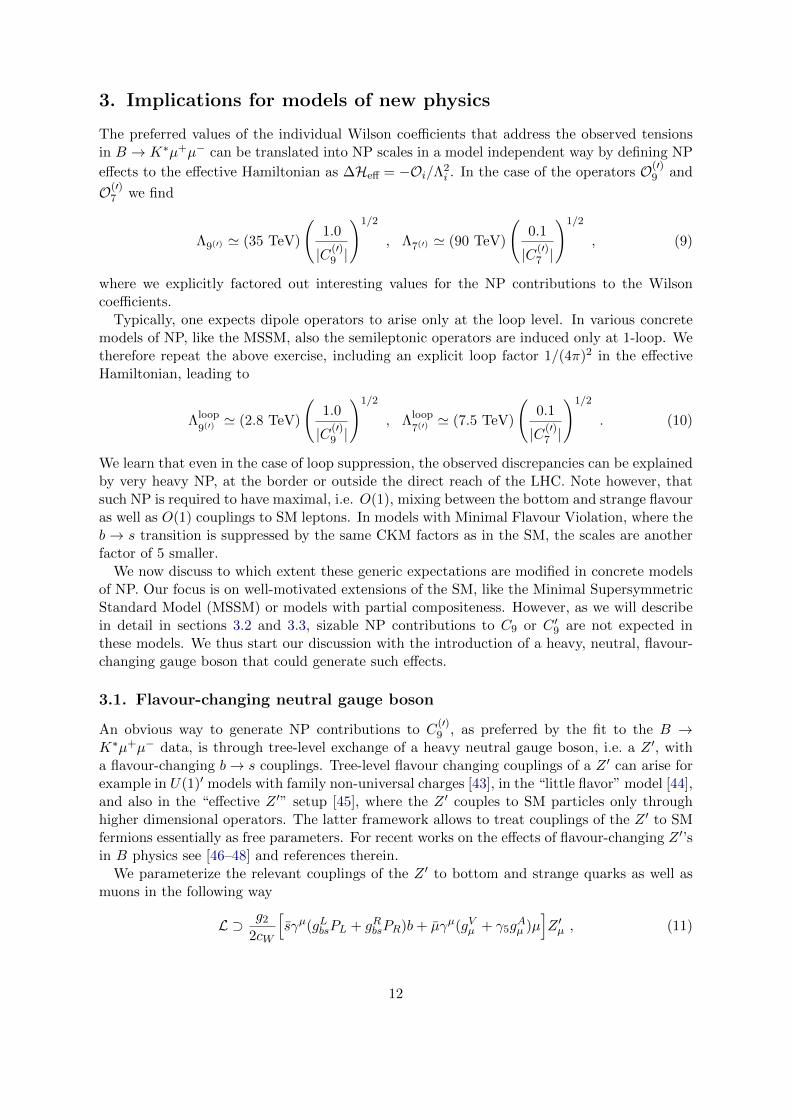
Figure 4: Constraints in the CNP9 -C ′9 plane (left) and the CNP

9 -C ′10 plane (right).

9

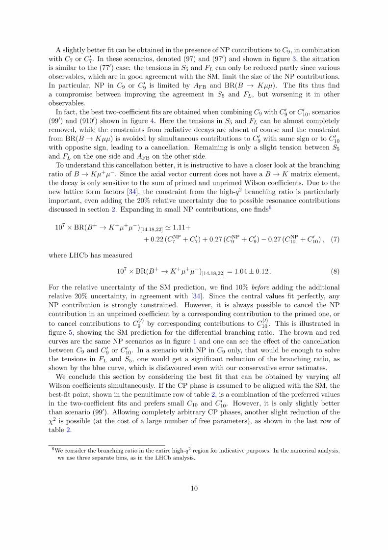
A slightly better fit can be obtained in the presence of NP contributions to C9, in combinationwith C7 or C ′7. In these scenarios, denoted (97) and (97′) and shown in figure 3, the situationis similar to the (77′) case: the tensions in S5 and FL can only be reduced partly since variousobservables, which are in good agreement with the SM, limit the size of the NP contributions.In particular, NP in C9 or C ′9 is limited by AFB and BR(B → Kµµ). The fits thus finda compromise between improving the agreement in S5 and FL, but worsening it in otherobservables.

In fact, the best two-coefficient fits are obtained when combining C9 with C ′9 or C ′10, scenarios(99′) and (910′) shown in figure 4. Here the tensions in S5 and FL can be almost completelyremoved, while the constraints from radiative decays are absent of course and the constraintfrom BR(B → Kµµ) is avoided by simultaneous contributions to C ′9 with same sign or to C ′10

with opposite sign, leading to a cancellation. Remaining is only a slight tension between S5

and FL on the one side and AFB on the other side.To understand this cancellation better, it is instructive to have a closer look at the branching

ratio of B → Kµ+µ−. Since the axial vector current does not have a B → K matrix element,the decay is only sensitive to the sum of primed and unprimed Wilson coefficients. Due to thenew lattice form factors [34], the constraint from the high-q2 branching ratio is particularlyimportant, even adding the 20% relative uncertainty due to possible resonance contributionsdiscussed in section 2. Expanding in small NP contributions, one finds6

107 × BR(B+ → K+µ+µ−)[14.18,22] ' 1.11+

+ 0.22 (CNP7 + C ′7) + 0.27 (CNP

9 + C ′9)− 0.27 (CNP10 + C ′10) , (7)

where LHCb has measured

107 × BR(B+ → K+µ+µ−)[14.18,22] = 1.04± 0.12 . (8)

For the relative uncertainty of the SM prediction, we find 10% before adding the additionalrelative 20% uncertainty, in agreement with [34]. Since the central values fit perfectly, anyNP contribution is strongly constrained. However, it is always possible to cancel the NPcontribution in an unprimed coefficient by a corresponding contribution to the primed one, or

to cancel contributions to C(′)9 by corresponding contributions to C

(′)10 . This is illustrated in

figure 5, showing the SM prediction for the differential branching ratio. The brown and redcurves are the same NP scenarios as in figure 1 and one can see the effect of the cancellationbetween C9 and C ′9 or C ′10. In a scenario with NP in C9 only, that would be enough to solvethe tensions in FL and S5, one would get a significant reduction of the branching ratio, asshown by the blue curve, which is disfavoured even with our conservative error estimates.

We conclude this section by considering the best fit that can be obtained by varying allWilson coefficients simultaneously. If the CP phase is assumed to be aligned with the SM, thebest-fit point, shown in the penultimate row of table 2, is a combination of the preferred valuesin the two-coefficient fits and prefers small C10 and C ′10. However, it is only slightly betterthan scenario (99′). Allowing completely arbitrary CP phases, another slight reduction of theχ2 is possible (at the cost of a large number of free parameters), as shown in the last row oftable 2.

6We consider the branching ratio in the entire high-q2 region for indicative purposes. In the numerical analysis,we use three separate bins, as in the LHCb analysis.

10

à

à

à

à

5 10 15 200.0

0.1

0.2

0.3

0.4

q2 @GeV2D

dB

R�dq

2@10

-7

GeV

2 D

C9NP=-1.5 , C9

'=1.5

C9NP=-2 , C10

' =-1

C9NP=-1.5

Figure 5: The branching ratio of B+ → K+µ+µ− as a function of the di-muon invariant masssquared q2. Differential (binned) SM predictions are shown with light blue bands(purple boxes). The experimental data is represented by the black crosses. The blue,brown, and red curves correspond to NP scenarios that reproduce the value of S5

at low q2 measured by LHCb. At high q2, the darker shaded region and the purpleboxes show the error estimates with lattice form factors before adding an additional20% relative uncertainty to account for the effect of charmonium resonances. Ourfull uncertainty is shown by the lighter shaded region with dashed borders.

Scenario CNP7 C ′7 CNP

9 C ′9 CNP10 C ′10 ∆χ2(SM)

(7) −0.07±0.04 3.4

(9) −0.8±0.3 4.3

(77′) −0.06±0.04 −0.1±0.1 4.7

(97) −0.05±0.04 −0.6±0.3 6.0

(97′) −0.1±0.1 −0.7±0.3 5.5

(99′) −1.0±0.3 +1.0±0.5 8.3

(910′) −1.0±0.3 −0.4±0.2 7.0

Real −0.03 −0.11 −0.9 +0.7 −0.1 −0.2 10.8

Complex +0.03+0.09i

−0.23−0.23i

−1.9+1.2i

+1.2+3.3i

+1.6−0.1i

+1.0+1.6i 14.1

Table 2: Best-fit values and reduction in the total χ2 with respect to the SM fit when varyingindividual Wilson coefficients, pairs of coefficients or all coefficients simultaneously.In all but the last case, we assume the coefficients to be real. We omit cases where∆χ2(SM) < 4 (except the C7 case) or where one of the coefficients has a best-fit valueof 0. For the one- and two-coefficient fits, we also give the 1σ fit ranges.

11

3. Implications for models of new physics

The preferred values of the individual Wilson coefficients that address the observed tensionsin B → K∗µ+µ− can be translated into NP scales in a model independent way by defining NP

effects to the effective Hamiltonian as ∆Heff = −Oi/Λ2i . In the case of the operators O(′)

9 and

O(′)7 we find

Λ9(′) ' (35 TeV)

(1.0

|C(′)9 |

)1/2

, Λ7(′) ' (90 TeV)

(0.1

|C(′)7 |

)1/2

, (9)

where we explicitly factored out interesting values for the NP contributions to the Wilsoncoefficients.

Typically, one expects dipole operators to arise only at the loop level. In various concretemodels of NP, like the MSSM, also the semileptonic operators are induced only at 1-loop. Wetherefore repeat the above exercise, including an explicit loop factor 1/(4π)2 in the effectiveHamiltonian, leading to

Λloop

9(′)' (2.8 TeV)

(1.0

|C(′)9 |

)1/2

, Λloop

7(′)' (7.5 TeV)

(0.1

|C(′)7 |

)1/2

. (10)

We learn that even in the case of loop suppression, the observed discrepancies can be explainedby very heavy NP, at the border or outside the direct reach of the LHC. Note however, thatsuch NP is required to have maximal, i.e. O(1), mixing between the bottom and strange flavouras well as O(1) couplings to SM leptons. In models with Minimal Flavour Violation, where theb→ s transition is suppressed by the same CKM factors as in the SM, the scales are anotherfactor of 5 smaller.

We now discuss to which extent these generic expectations are modified in concrete modelsof NP. Our focus is on well-motivated extensions of the SM, like the Minimal SupersymmetricStandard Model (MSSM) or models with partial compositeness. However, as we will describein detail in sections 3.2 and 3.3, sizable NP contributions to C9 or C ′9 are not expected inthese models. We thus start our discussion with the introduction of a heavy, neutral, flavour-changing gauge boson that could generate such effects.

3.1. Flavour-changing neutral gauge boson

An obvious way to generate NP contributions to C(′)9 , as preferred by the fit to the B →

K∗µ+µ− data, is through tree-level exchange of a heavy neutral gauge boson, i.e. a Z ′, witha flavour-changing b→ s couplings. Tree-level flavour changing couplings of a Z ′ can arise forexample in U(1)′ models with family non-universal charges [43], in the “little flavor” model [44],and also in the “effective Z ′” setup [45], where the Z ′ couples to SM particles only throughhigher dimensional operators. The latter framework allows to treat couplings of the Z ′ to SMfermions essentially as free parameters. For recent works on the effects of flavour-changing Z ′’sin B physics see [46–48] and references therein.

We parameterize the relevant couplings of the Z ′ to bottom and strange quarks as well asmuons in the following way

L ⊃ g2

2cW

[sγµ(gLbsPL + gRbsPR)b+ µγµ(gVµ + γ5g

Aµ )µ

]Z ′µ , (11)

12

where we kept both vector and axial-vector coupling to muons for completeness. Integratingout the Z ′ leads to

e2

16π2(V ∗tsVtb)

{CNP

9 , C ′9, CNP10 , C

′10

}=

m2Z

2m2Z′

{gLbsg

Vµ , g

Rbsg

Vµ , g

Lbsg

Aµ , g

Rbsg

Aµ

}. (12)

As the Z ′ contribution is not loop suppressed and the flavour-changing couplings gL,Rbs can inprinciple be of order 1, very heavy Z ′ can accommodate a CNP

9 ∼ −1. It is interesting to notefrom eq. (12) that the scenarios (9) and (99′) of table 2 can be realized with a single Z ′, butnot scenario (910′), since one always has CNP

9 C ′10 = CNP10 C

′9.

In addition to the contributions to the b → sµµ transition, the flavour-changing Z ′ willnecessarily induce also effects in Bs mixing at the tree level. The effects in the Bs massdifference ∆Ms can be written as

∆Ms

∆MSMs

' 1 +m2Z

m2Z′

[(gLbs)

2 + (gRbs)2 − 9.7(gLbs)(g

Rbs)]( g2

2

16π2(V ∗tsVtb)

2S0

)−1

, (13)

where the SM loop function is S0 ' 2.3. To arrive at (13), we took the matching scaleto be 1 TeV and used the hadronic matrix elements collected in [48]. The contributions areparticularly large if both left- and right-handed couplings are present, due to the larger hadronicmatrix elements of the generated Bs mixing operators with a left-right chirality structure. Fromthe experimental side, the mass difference ∆Ms is measured with very high precision [49, 50].Uncertainties in the SM prediction, stemming mainly from the limited precision of the hadronicmatrix elements and CKM factors, allow for O(10%) NP contributions to this observable. Fora given Z ′ mass, this limits the allowed size of the flavour-changing couplings gL,Rbs significantly.

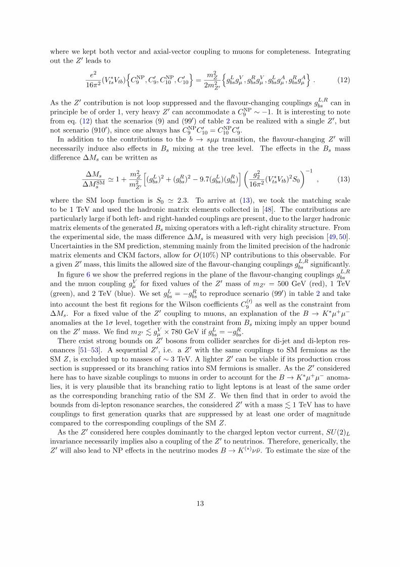
In figure 6 we show the preferred regions in the plane of the flavour-changing couplings gL,Rbs

and the muon coupling gVµ for fixed values of the Z ′ mass of mZ′ = 500 GeV (red), 1 TeV

(green), and 2 TeV (blue). We set gLbs = −gRbs to reproduce scenario (99′) in table 2 and take

into account the best fit regions for the Wilson coefficients C(′)9 as well as the constraint from

∆Ms. For a fixed value of the Z ′ coupling to muons, an explanation of the B → K∗µ+µ−

anomalies at the 1σ level, together with the constraint from Bs mixing imply an upper boundon the Z ′ mass. We find mZ′ . gVµ × 780 GeV if gLbs = −gRbs.

There exist strong bounds on Z ′ bosons from collider searches for di-jet and di-lepton res-onances [51–53]. A sequential Z ′, i.e. a Z ′ with the same couplings to SM fermions as theSM Z, is excluded up to masses of ∼ 3 TeV. A lighter Z ′ can be viable if its production crosssection is suppressed or its branching ratios into SM fermions is smaller. As the Z ′ consideredhere has to have sizable couplings to muons in order to account for the B → K∗µ+µ− anoma-lies, it is very plausible that its branching ratio to light leptons is at least of the same orderas the corresponding branching ratio of the SM Z. We then find that in order to avoid thebounds from di-lepton resonance searches, the considered Z ′ with a mass . 1 TeV has to havecouplings to first generation quarks that are suppressed by at least one order of magnitudecompared to the corresponding couplings of the SM Z.

As the Z ′ considered here couples dominantly to the charged lepton vector current, SU(2)Linvariance necessarily implies also a coupling of the Z ′ to neutrinos. Therefore, generically, theZ ′ will also lead to NP effects in the neutrino modes B → K(∗)νν. To estimate the size of the

13

0.0 0.2 0.4 0.6 0.8 1.0 1.2 1.40.0

0.5

1.0

1.5

2.0

2.5

3.0

gbsL ´ 100 = -gbs

R ´ 100

gΜV

500 GeV

1 TeV

mZ '= 2 TeV

Figure 6: Preferred values for the Z ′ vector couplings to muons (gVµ ) and Z ′ flavour-changing

b → s couplings (gL,Rbs ), taking into account the best fit values for C9 and C ′9 aswell as constraints from Bs mixing. We set gRbs = −gLbs. The red/green/blue regionscorrespond to Z ′ masses of mZ′ = 500/1000/2000 GeV. The solid (dashed) contoursindicate 1σ and 2σ regions, respectively. Note the normalization of the Z ′ couplingsin eq. (11).

14

bL sLH±

tR

γµ µ

(a)

bL sLtR

H±

γµ µ

(b)

bL,R sL,RbL,R sL,R

g

γµ µ

(c)

bL sLtL cL

W±

γµ µ

(d)

bL sLbL sL

W W

ℓµ µ

(e)

Figure 7: Example Feynman diagrams for MSSM contributions to C9 and C ′9. Charged Higgsphoton penguin (a), Higgsino photon penguin (b), gluino photon penguin (c), chargedWino photon penguin (d), and Wino box (e). In the case of the photon penguins,the photon has to be attached to all charged particles in the loop.

expected effects, we neglect possible SU(2)L breaking corrections and work in the limit7

gAµ = gRµ − gLµ = 0 , gLν = gLµ =1

2gVµ . (14)

Using the results in [54], we find that CNP9 ' −1 implies a slight enhancement of the branching

ratios BR(B → K∗νν) and BR(B → Kνν) of the order of 15%. It will be challenging to reachsuch a precision at Belle II [55].

3.2. The Minimal Supersymmetric Standard Model

It is well known, that in the MSSM, large NP contributions to the dipole Wilson coefficientsC7 and C ′7 can arise easily in large regions of parameter space. On the other hand, as wewill show explicitly, the vector coefficients C9 and C ′9 remain to a good approximation SM-likethroughout the viable MSSM parameter space, even if we allow for completely generic flavourmixing in the squark sector.

3.2.1. SUSY contributions to C(′)9

Contributions to C9 and C ′9 can come from (i) Z penguins, (ii) photon penguins, and (iii)box diagrams. Example Feynman diagrams for the most important contributions are shown

7Note that, given the present uncertainties in the B → K∗µ+µ− data, a sizable axial-vector coupling to leptonscannot be excluded yet. Allowing for non-zero axial-vector couplings to leptons, could either enhance orsuppress couplings to neutrinos.

15

in figure 7.

(i) Z penguin contributions to the axial-vector coefficients C10 and C ′10 can be sizable incorners of parameter space with large flavour-changing trilinear couplings [54, 56]. Z penguincontributions to C9 and C ′9, however, are suppressed by the accidentally small vector couplingof the Z to charged leptons ∝ 1− 4s2

W ' 0.08 and therefore negligible.

(ii) Photon penguin contributions to C9 and C ′9 are induced by charged Higgs, Higgsino,and gaugino loops. For charged Higgs loops shown in diagram (a) of figure 7 we find

CH±

9 ' − m2t

m2H±

1

24(cotβ)2 fH

±9

(m2t

m2H±

). (15)

The loop function can be found in appendix B and is normalized such that fH±

9 (1) = 1. Thecharged Higgs loops are strongly suppressed by (cotβ)2. Even for extremely small tanβ ∼ 1,we find that this contribution does not exceed |CH±9 | . 0.05 for any value of the charge Higgsmass mH± > 100 GeV. Charged Higgs contributions to the right-handed coefficient C ′9 aresuppressed by the strange quark mass and also negligible.

Contributions from Higgsino loops are shown in diagram (b) of figure 7 and lead to

CH±

9 ' 7

72

m2t

m2tR

f H±

9

(|µ|2m2tR

). (16)

The loop function f H±

9 is reported in the appendix B and normalized such that for a Higgsino

that is degenerate with the right-handed stop, |µ| ' mtR, one has f H

±9 (1) = +1. The loop

function remains positive for a wide range of Higgsino and stop masses. A negative sign forCH

±9 , as required to address the discrepancies in B → K∗µ+µ−, can only be obtained for

heavy Higgsino masses |µ| & 5mtR. This region of parameter space implies f H

±9 � 1 and CH

±9

is completely negligible.Evaluating gluino loops (diagram (c) of figure 7), we find contributions to both C9 and C ′9

(V ∗tsVtb){C g9 , C

′ g9

}' − 8

135

g2s

g22

m2W

m2d

{(δLbs), (δ

Rbs)}f g9

(m2g

m2d

), (17)

where for simplicity we assume a common mass md for all down-type squarks and the loop

function, that can be found in the appendix B, is normalized such that f g9 (1) = 1. The phase

of C g9 and C ′ g9 is set by the phase of the squark mixing δLbs and δRbs, that are free parameters.Despite the enhancement by the strong coupling constant and the possible enhancement byO(1) squark mixing angles, we find that this contribution is negligible. Sizable contributions|C g9 | & 0.5 are only possible for extremely light squarks and gluinos of order 200 GeV that arecompletely excluded by direct searches. Similar conclusions can be drawn for neutral Wino andBino loops, that, compared to the gluino loops, are further suppressed by small electro-weakgauge couplings.

Finally there are charged Wino loops that can induce photon penguins. We find

(V ∗tsVtb) CW9 ' −

1

45

m2W

m2d

(δLbs) fW9

(m2W

m2d

), (18)

16

where the loop function given in the appendix B. For a degenerate spectrum, fW9 (1) = 1,and the contribution is again negligible. For a large hierarchy between the Wino and down-type squark masses mW � md, however, the contribution is enhanced by a large logarithm

fW9 (x)x→0−−−→ −30 log(m2

W/m2

d). The large logarithm arises from the diagram where the photon

attaches to the light charged Wino in the loop (see diagram (d) of figure 7) and is thereforeabsent in the neutral gaugino loops discussed above. Despite the large logarithm, we find thatappreciable contributions of the order of |CW9 | & 0.5 are only possible for maximal squarkmixing δLbs ∼ O(1), Winos close to the LEP bound mW ∼ 100 GeV and bottom and strangesquarks with a mass of md ∼ 400 GeV. Such light squarks are not only in tension with strongbounds from direct searches for sbottoms [57, 58], but in combination with the O(1) squarkmixing would generically also lead to too large contributions to other well measured flavourobservables, like Bs mixing.

(iii) Box contributions to C9 and C ′9 are again induced by charged Higgs, Higgsino, andgaugino loops. Charged Higgs boxes and Higgsino boxes are suppressed by the tiny muonYukawa coupling and thus completely negligible. For the contribution from Wino boxes (dia-gram (e) of figure 7) we find

(V ∗tsVtb) Cbox9 ' 1

s2W

5

192

m2W

m2d

(δLbs) fbox9

(m2

˜

m2d

,m2W

m2d

). (19)

The loop function fbox9 is given in the appendix B. In the limit of degenerate Wino, slepton and

down-type squark masses mW = m˜ = md, the loop function reduces to fbox9 (1, 1) = 1. For an

approximate degenerate SUSY spectrum, we find again tiny contributions Cbox9 � 0.1 even for

down-squarks as light as 500 GeV and assuming maximal squark mixing δLbs ∼ O(1). The sameconclusion holds for the Bino boxes and mixed Wino-Bino boxes that are further suppressedby the small hypercharge gauge coupling. For a hierarchical spectrum, i.e. if both Winos andsleptons are light compared to the squarks, mW ,m˜� md, the box contributions get enhancedby large logarithms log(mW /md), log(m˜/md). Assuming for simplicity m˜ = mW , we find

fbox9 (x, y)

x,y→0−−−−→ −12 log(m2˜/m

2d). Similar to the charge Wino photon penguins discussed

above, maximal squark mixing, Winos and leptons close to the LEP bound ∼ 100 GeV aswell as light bottom and strange squarks with a mass of md ∼ 500 GeV are required to reach|Cbox

9 | & 0.5. Such a region of parameter space is strongly disfavored by direct searches [57,58],and other flavour constraints. Analogous comments apply to Bino and mixed Wino-Bino boxeswith a hierarchical spectrum.

3.2.2. SUSY contributions to C(′)7

Sizable contributions to the dipole operators, on the other hand, can be generated in variousways in the MSSM. We discuss them separately in the following, keeping in mind that theycould also be present simultaneously. If the charged Higgs boson is light, it can contributesignificantly to the Wilson coefficient C7. At one loop one finds

CH±

7 ' − 7

36

m2t

m2H±

fH±

7

(m2t

m2H±

), (20)

with the loop function given in the appendix B. In (20) we neglected a term that is proportionalto (cotβ)2 and only relevant for very small tanβ. The function fH

±7 is always positive, and

17

therefore the charged Higgs loop always interferes constructively with the SM contributionCSM

7 ∼ −0.31. A charged Higgs contribution of CH±

7 ' −0.07, as in scenario (7) of table 2,corresponds to a charged Higgs mass of m2

H± ' 500 GeV.Large contributions to C7 can also arise from Higgsino–stop loops. The leading term reads

CH±

7 ' 5

72

m2t

m2tR

µAtm2tR

tanβ f H±

7

(|µ|2m2tR

). (21)

The sign of CH±

7 is determined by sign(µAt), and the loop function, that can be found in

the appendix, is normalized such that f H±

7 (1) = 1. Note that GUT-scale boundary conditionstypically lead to constructive interference of the chargino and SM contributions if µ is negative.For illustration we now work in the limit where the right-handed stop and the Higgsino areapproximately degenerate mtR

' |µ|. Assuming also a sizable trilinear coupling At ' mtR, the

right magnitude of CH±

7 as in scenario (7) of table 2, can be achieved with light stops withmass mtR

∼ 500 GeV and a moderate tanβ ∼ 10. For large values of tanβ ∼ 50, stops can beas heavy as 1.2 TeV.

Note that the charged Higgs and Higgsino contributions do not require any flavour structurebeyond the SM CKM matrix. They only contribute to the left-handed dipole coefficient C7. Ifthere is non-trivial squark mixing, also gaugino contributions can become relevant and generateboth C7 (gluino, Wino, and Bino) and C ′7 (gluino and Bino). Due to the large strong couplingconstant, gluino contributions are typically dominant. The leading gluino contributions read

(V ∗tsVtb){C g7 , C

′ g7

}' − 2

45

g2s

g22

m2W

m2d

µmg

m2d

tanβ{δLbs, δ

Rbs

}f g7

(m2g

m2d

). (22)

The above expression assumes a common down-type squark mass m2d. For approximately

degenerate gluinos and down-type squarks one has f g7 (1) = 1. In regions of parameter spacewhere the Higgsino mass is sizable, |µ| ∼ md, squark mixing is of O(1), |δLbs| ' 0.3, |δRbs| ' 0.5,and tanβ is large, tanβ ∼ 50, down squarks and gluinos at ∼ 2 TeV lead to interesting valuesfor the Wilson coefficients C g7 ' −0.06 and C ′ g7 ' −0.10 as in scenario (77’) of table 2.

3.2.3. Summary: MSSM

In summary, we systematically discussed all possible 1-loop contributions to C9 and C ′9 in theMSSM and found that even allowing for generic O(1) squark mixing, C9 and C ′9 remain to agood approximation SM-like. The tensions in the B → K∗µ+µ− data can therefore only besoftened slightly by modifications of the dipole Wilson coefficient C7 and C ′7, that can arise ina variety of MSSM models with a TeV scale spectrum.

3.3. Models with partial compositeness

Next to supersymmetry, the most well-motivated class of models solving the gauge hierar-chy problem are models with a composite Higgs boson or extra-dimensional models dual tofour-dimensional composite Higgs models. In all these models, generating fermion masses with-out generating excessive FCNCs requires, from the 4D perspective, the mechanism of partialcompositeness, giving mass to fermions by linear mixing with composite operators. A simplesetup to obtain approximate results in this framework is given by the two-site description of

18

b

s

µ+

µ−

Z

(a)

b

s

µ+

µ−

ρ

(b)

b

s

ρ

µ+

µ−

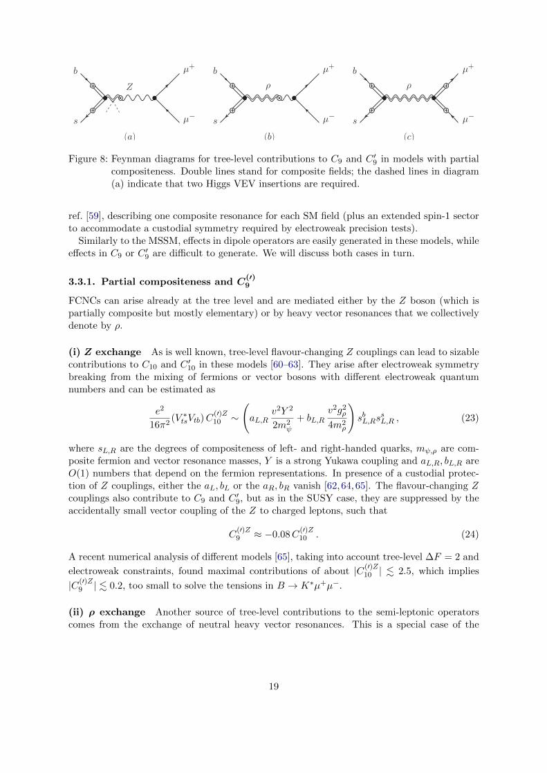
(c)

Figure 8: Feynman diagrams for tree-level contributions to C9 and C ′9 in models with partialcompositeness. Double lines stand for composite fields; the dashed lines in diagram(a) indicate that two Higgs VEV insertions are required.

ref. [59], describing one composite resonance for each SM field (plus an extended spin-1 sectorto accommodate a custodial symmetry required by electroweak precision tests).

Similarly to the MSSM, effects in dipole operators are easily generated in these models, whileeffects in C9 or C ′9 are difficult to generate. We will discuss both cases in turn.

3.3.1. Partial compositeness and C(′)9

FCNCs can arise already at the tree level and are mediated either by the Z boson (which ispartially composite but mostly elementary) or by heavy vector resonances that we collectivelydenote by ρ.

(i) Z exchange As is well known, tree-level flavour-changing Z couplings can lead to sizablecontributions to C10 and C ′10 in these models [60–63]. They arise after electroweak symmetrybreaking from the mixing of fermions or vector bosons with different electroweak quantumnumbers and can be estimated as

e2

16π2(V ∗tsVtb)C

(′)Z10 ∼

(aL,R

v2Y 2

2m2ψ

+ bL,Rv2g2

ρ

4m2ρ

)sbL,Rs

sL,R , (23)

where sL,R are the degrees of compositeness of left- and right-handed quarks, mψ,ρ are com-posite fermion and vector resonance masses, Y is a strong Yukawa coupling and aL,R, bL,R areO(1) numbers that depend on the fermion representations. In presence of a custodial protec-tion of Z couplings, either the aL, bL or the aR, bR vanish [62, 64, 65]. The flavour-changing Zcouplings also contribute to C9 and C ′9, but as in the SUSY case, they are suppressed by theaccidentally small vector coupling of the Z to charged leptons, such that

C(′)Z9 ≈ −0.08C

(′)Z10 . (24)

A recent numerical analysis of different models [65], taking into account tree-level ∆F = 2 and

electroweak constraints, found maximal contributions of about |C(′)Z10 | . 2.5, which implies

|C(′)Z9 | . 0.2, too small to solve the tensions in B → K∗µ+µ−.

(ii) ρ exchange Another source of tree-level contributions to the semi-leptonic operatorscomes from the exchange of neutral heavy vector resonances. This is a special case of the

19

flavour-changing Z ′ discussed above, so we can use the same notation. For the flavour-changingcoupling, one expects

g2

2cWgL,Rbs ∼ gρ sbL,RssL,R (25)

and we stress that it is non-zero even in the limit of vanishing Higgs VEV, in contrast tothe Z-mediated contribution. For the coupling to muons, one has to distinguish betweentwo contributions. In the first case, diagram (b) of figure 8, the coupling proceeds through anadmixture to ρ of an elementary Z boson. In that case, the vector and axial vector couplings ofthe ρ are equal to the vector and axial vector couplings of the SM Z to muons. Consequently,

also here the contributions to C(′)9 are strongly suppressed. In the second case, shown in

diagram (c) of figure 8, the ρ directly couples to the composite component of the muons. Inthis case, the couplings depend on the degrees of compositeness of left- and right-handed muonsand can be different from the Z couplings,

gVµ ∼ gρ[(sµL)2 + (sµR)2

], gAµ ∼ gρ

[(sµL)2 − (sµR)2

]. (26)

Due to the lightness of the muon, it is expected to be mostly elementary and the abovecouplings should be strongly suppressed. They could only be sizable in the extreme case whereone chirality of muons has a large degree of compositeness. Then however, one has gVµ ' ±gAµ ,since the product sµLs

µR has to be tiny. In other words, it is not possible to obtain a sizable

contribution to C9 without at the same time generating a large correction to C10, which isdisfavoured by the data.

To quantify the last statement, we can make a fit to the data as in section 2, but fixingCNP

9 = ±CNP10 . In the case of equal sign, we find ∆χ2 = 0.8, so no significant improvement. In

the case of opposite sign (corresponding to a composite µR), we find ∆χ2 = 2.3 for CNP9 = −0.3,

corresponding to a very small improvement. For C ′9 = ±C ′10, the improvement is even smaller.

3.3.2. Partial compositeness and C(′)7

Dipole operators are generated at the one loop level in partial compositeness [66–69]. Thedominant contribution typically comes from a diagram with a Higgs and a heavy, vector-likefermion in the loop, since the large fermion mass lifts the chirality suppression of the amplitude.One can write it generically as

(V ∗tsVtb)mbC(′)7 ∼ sbR,LssL,R

v3 Y Y Y√2m2

ψ

1

12fh7

(m2ψ

m2h

), (27)

where we suppressed the flavour structure and a model-dependent O(1) overall factor. Here, Yis a “wrong-chirality” Yukawa coupling in the strong sector. A similar contribution also comesfrom loops with a W or Z boson instead of the Higgs. In the flavour-anarchic model, one canestimate

sbRssL

v3 Y Y Y√2m2

ψ

∼ (V ∗tsVtb)mbv2Y Y

m2ψ

, sbLssR

v3 Y Y Y√2m2

ψ

∼ ms

(V ∗tsVtb)

v2Y Y

m2ψ

. (28)

Since ms/(mbV2ts) ≈ 15, one generically expects larger contributions to C ′7 than to C7. Taking

for example Y ∼ Y ∼ 3 and mψ ∼ 1 TeV, one finds |C7| ∼ 0.05, |C ′7| ∼ 0.7. We stress howeverthat these estimates are subject to sizable corrections since we neglected various O(1) factorsthroughout.

20

3.3.3. Summary: partial compositeness

To summarize, in models with partial compositeness one generically expects NP contributionsto C7 and C ′7 that are of the right size to reproduce scenario (77′) above and thus ameliorate thetensions in B → K∗µ+µ−. Generating a sizable contribution to C9 or C ′9, which is required tofully remove the tensions, requires a large degree of compositeness for one chirality of muons aswell as a cancellation between several contributions to C10 and/or C ′10. Whether such scenariois viable when taking into account constraints on the lepton sector is an interesting questionfor future study.

3.4. Expectations for CP Asymmetries

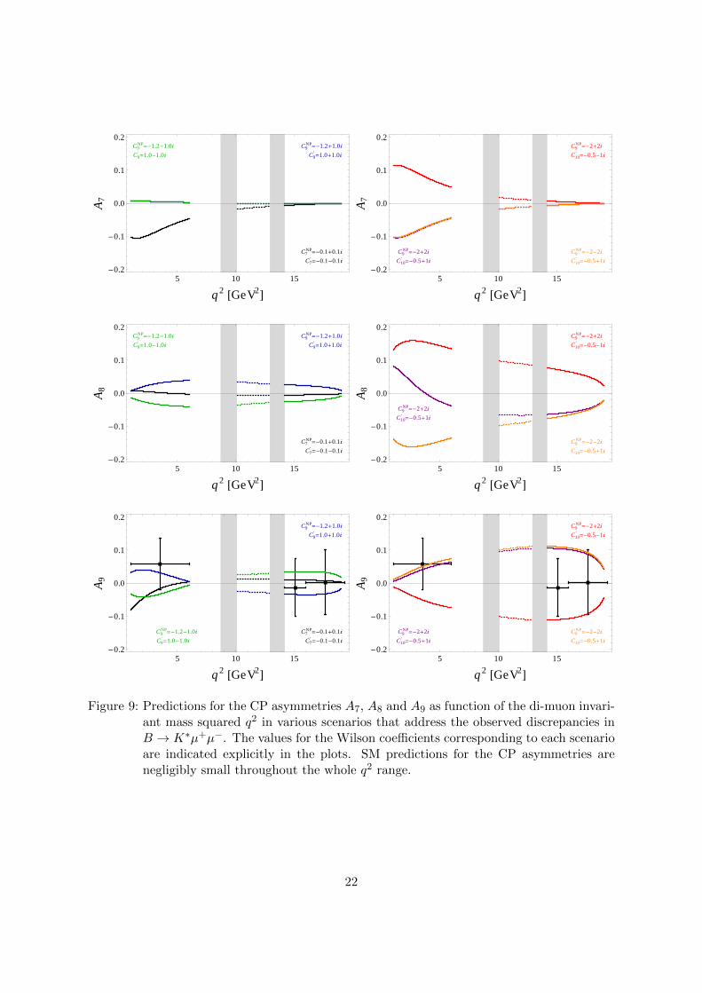
Although all the tensions in the data occur in CP-averaged observables and we thereforestressed above that NP effects required to remove them may be aligned in phase with theSM, this is mostly due to the fact that few CP asymmetries have been measured to a goodprecision and the imaginary parts of the Wilson coefficients are still poorly constrained (cf. [12]).Generically however, without imposing additional restrictions on new sources of CP violation,most of the discussed NP contributions to the Wilson coefficients are expected to be complex.Under the generic assumption that the imaginary parts are of the same order as the real parts,we can derive generic expectations for the CP asymmetries A7, A8 and A9, in the consideredscenarios that address the tensions in the data.8

We provide simple approximate expressions for the T-odd CP asymmetries at low q2

〈A7〉[1,6] '− 0.44 Im(CNP7 ) + 0.44 Im(C ′7) + 0.07 Im(CNP

10 )− 0.07 Im(C ′10) ,

〈A8〉[1,6] '+ 0.25 Im(CNP7 ) + 0.23 Im(C ′7) + 0.04 Im(CNP

9 ) + 0.02 Im(C ′9)− 0.06 Im(C ′10) ,

〈A9〉[1,6] '+ 0.12 Im(C ′7) + 0.04 Im(C ′10) . (29)

The plots in figure 9 show the q2 distributions of the CP asymmetries A7, A8 and A9 invarious NP scenarios. The black curves in the plots on the left hand side correspond to thescenario with non-zero C7 and C ′7 of figure 1, modified to include imaginary parts of the Wilsoncoefficients that are not excluded by the data on SK∗γ (the time dependent CP asymmetryin B → K∗γ) and ACP(b → sγ) (the direct CP asymmetry in B → Xsγ). Measurements ofA7 and A9 at low q2 are sensitive to such a scenario. The green and blue curves in the plotson the left hand side are similar to the scenario with non-zero C9 and C ′9 of figure 1. Here,imaginary parts of O(1) with different signs are switched on. Moderate effects in A8 and A9

at the level of ∼ 5% are expected in this case. Finally, the purple, red and orange curves inthe plots on the right hand side correspond to a scenario where the tensions in B → K∗µ+µ−

are explained by NP in C9 and C ′10. The shown choices of the imaginary parts lead to sizableeffects in all three CP asymmetries of the order of 10%–15%.

We stress again that the currently observed tensions in B → K∗µ+µ− are all confined toCP-averaged observables that are hardly sensitive to CP phases. It is therefore not possibleto predict the sign or the exact size of the expected CP asymmetries Nevertheless, the genericexamples shown in figure 9 demonstrate that precise measurements of the CP asymmetrieswould allow to further narrow down possible NP explanations.

8We explicitly checked that in all cases discussed below and shown in fig 9, the presence of imaginary partsdoes not worsen the agreement with the data significantly.

21

5 10 15-0.2

-0.1

0.0

0.1

0.2

q2 @GeV2D

A7

C7NP=-0.1+0.1ä

C7'=-0.1-0.1ä

C9NP=-1.2+1.0ä

C9'=1.0+1.0ä

C9NP=-1.2-1.0ä

C9'=1.0-1.0ä

5 10 15-0.2

-0.1

0.0

0.1

0.2

q2 @GeV2D

A7

C9NP=-2+2ä

C10' =-0.5+1ä

C9NP=-2+2ä

C10' =-0.5-1ä

C9NP=-2-2ä

C10' =-0.5+1ä

5 10 15-0.2

-0.1

0.0

0.1

0.2

q2 @GeV2D

A8

C7NP=-0.1+0.1ä

C7'=-0.1-0.1ä

C9NP=-1.2+1.0ä

C9'=1.0+1.0ä

C9NP=-1.2-1.0ä

C9'=1.0-1.0ä

5 10 15-0.2

-0.1

0.0

0.1

0.2

q2 @GeV2D

A8

C9NP=-2+2ä

C10' =-0.5+1ä

C9NP=-2+2ä

C10' =-0.5-1ä

C9NP=-2-2ä

C10' =-0.5+1ä

à

à

à

5 10 15-0.2

-0.1

0.0

0.1

0.2

q2 @GeV2D

A9

C7NP=-0.1+0.1ä

C7'=-0.1-0.1ä

C9NP=-1.2+1.0ä

C9'=1.0+1.0ä

C9NP=-1.2-1.0ä

C9'=1.0-1.0ä

à

à

à

5 10 15-0.2

-0.1

0.0

0.1

0.2

q2 @GeV2D

A9

C9NP=-2+2ä

C10' =-0.5+1ä

C9NP=-2+2ä

C10' =-0.5-1ä

C9NP=-2-2ä

C10' =-0.5+1ä

Figure 9: Predictions for the CP asymmetries A7, A8 and A9 as function of the di-muon invari-ant mass squared q2 in various scenarios that address the observed discrepancies inB → K∗µ+µ−. The values for the Wilson coefficients corresponding to each scenarioare indicated explicitly in the plots. SM predictions for the CP asymmetries arenegligibly small throughout the whole q2 range.

22

4. Conclusions

Confronting predictions for B → K∗µ+µ− angular observables with recent measurements byATLAS, CMS and LHCb, we pointed out three discrepancies at the 2–3σ level, namely inthe observables FL and S5 at low q2 and in the observable S4 at high q2. We performed amodel-independent analysis taking into account all relevant constraints, finding in particularthat

1. the tension in S4 cannot be resolved by NP contributions and is therefore likely dueto statistical fluctuations or underestimated errors (with the resonance contributionsmentioned in section 2 a possible source for the latter);

2. the tension in S5 and FL can be reduced by a negative NP contribution to the Wilsoncoefficient C9 only, but measurements of BR(B → Kµ+µ−) and AFB prevent a completesolution;

3. allowing simultaneous NP contributions to two Wilson coefficients, there are variouspossibilities summarized in table 2. The best fit is obtained with simultaneous NPcontributions to C9 and C ′9 with opposite sign. Modifying the dipole operator coefficientsC7 and C ′7 only, the tensions can be reduced.

Very recently, a model independent analysis of B → K∗µ+µ− appeared [31], that has asimilar scope as our section 2. The overall picture of our findings agrees with it, but there aresome notable differences in the strategies. For example,

• we use the Si, Ai basis instead of the observables suggested in [16]. It is reassuring thatboth approaches lead to similar results.

• we include ATLAS and BaBar data for B → K∗µ+µ−, which turns out to be importantfor the significance of the tension in FL.

• we do not observe a tension in AFB (or the alternative observable P2) at low q2. Also here,averaging all available experiments has a notable impact, as discussed in appendix A.

• we include the B → Kµ+µ− data. In spite of our inflated error bars at high q2, theconstraint turns out to be relevant and is crucial for limiting the allowed size of |CNP

9 |,explaining why we find that NP contributions in C9 only cannot reduce the tensions inS5 and FL completely.

In addition to the model-independent analysis, we also studied the implications of the resultsfor models of new physics. A naive dimensional estimate points towards a NP scale of severaltens of TeV in the case of tree-level NP, or several TeV in the case of loop-level NP. In concretewell motivated models, like the MSSM or models with partial compositeness, as well as inmodels with flavour-changing Z ′ bosons, we find that new particles are typically required atthe order of ∼ 1 TeV:

• Models with flavour-changing Z ′ bosons can accommodate large NP in C9 and C ′9. How-ever, taking into account bounds from Bs mixing, we find that the Z ′ bosons have tobe light, of the order of few TeV at most. The strong bounds from searches for di-jetand di-lepton resonances at the LHC imply that for Z ′ masses around 1 TeV, the Z ′

couplings to first generation quarks have to be at least one order of magnitude smallerthan the corresponding couplings of the SM Z boson.

23

• We showed that throughout the viable MSSM parameter space, contributions to C9 arewell below the values preferred by the model independent fit to the available data ofb→ s decays. The tensions in B → K∗µ+µ− can only be softened slightly in the MSSM,

by NP contributing to the dipole operators O(′)7 . Such contributions can be generated

in various ways: charged Higgs bosons with masses around 500 GeV; stops at or below1 TeV; or gluinos and down-type squarks as heavy as 2 TeV, if generic squark flavourmixing is considered.

• In models with partial compositeness, the tensions can also be softened by one-loop con-tributions to the dipole operators. Appreciable contributions to C9 can be generated attree level from heavy vector exchange but would require a significant degree of compos-iteness of one chirality of muons. The question whether such a scenario is viable deservesfurther study. In any case, it would also lead to sizable contributions to C10 that wouldhave to be cancelled by Z-mediated contributions.

Generically, most of the discussed NP explanations of the B → K∗µ+µ− anomalies canalso lead to sizable CP asymmetries in B → K∗µ+µ−, as shown in the examples of figure 9.Improved results on the CP asymmetries A7, A8, and A9 as well as on the CP averagedobservables FL, AFB, S3, S4, S5 and on other processes like B → Kµ+µ− will be extremelyuseful to confirm the deviations currently observed, to establish the presence of new physics inb→ s transitions, and to pin down its properties.

Acknowledgements

We thank Christoph Bobeth for illuminating discussions and Nicola Serra for useful correspon-dence. Fermilab is operated by Fermi Research Alliance, LLC under Contract No. De-AC02-07CH11359 with the United States Department of Energy. The research of D.S. is supportedby the Advanced Grant EFT4LHC of the European Research Council (ERC), and the Clusterof Excellence Precision Physics, Fundamental Interactions and Structure of Matter (PRISMA– EXC 1098). The research of W.A. was supported in part by Perimeter Institute for Theo-retical Physics. Research at Perimeter Institute is supported by the Government of Canadathrough Industry Canada and by the Province of Ontario through the Ministry of EconomicDevelopment & Innovation.

A. Data averages

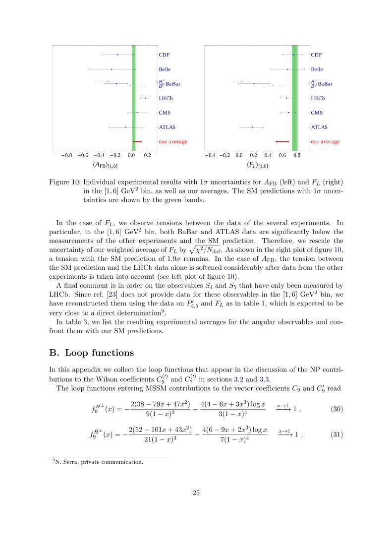
In this appendix we give more details on how we obtain the averages of experimental mea-surements of B → K∗µ+µ− observables [17, 18, 21–25] used in this analysis. As in [12], wefirst symmetrize asymmetric statistical and/or systematic errors and then perform a weightedaverage of the symmetrized individual results. While in many cases the obtained averages aredominated by the LHCb results, the averaging procedure leads to important shifts in the ob-servables FL and AFB in the [1, 6] GeV2 bin. This is illustrated in the plots of figure 10. In thecase of the BaBar B → K∗µ+µ− data at low q2, the results for the charged and neutral modesshow a significant difference. We therefore first average the charged and neutral mode resultsof BaBar, using the PDG averaging method, i.e. rescaling the uncertainty by a factor of

√χ2.

We then use this average and combine it with the available data from the other experiments.

24

-0.8 -0.6 -0.4 -0.2 0.0 0.2

CDF

Belle

B+

BaBarB0

LHCb

CMS

ATLAS

our average

XAFB\@1,6D-0.4 -0.2 0.0 0.2 0.4 0.6 0.8

CDF

Belle

B+

BaBarB0

LHCb

CMS

ATLAS

our average

XFL\@1,6D

Figure 10: Individual experimental results with 1σ uncertainties for AFB (left) and FL (right)in the [1, 6] GeV2 bin, as well as our averages. The SM predictions with 1σ uncer-tainties are shown by the green bands.

In the case of FL, we observe tensions between the data of the several experiments. Inparticular, in the [1, 6] GeV2 bin, both BaBar and ATLAS data are significantly below themeasurements of the other experiments and the SM prediction. Therefore, we rescale theuncertainty of our weighted average of FL by

√χ2/Ndof. As shown in the right plot of figure 10,

a tension with the SM prediction of 1.9σ remains. In the case of AFB, the tension betweenthe SM prediction and the LHCb data alone is softened considerably after data from the otherexperiments is taken into account (see left plot of figure 10).

A final comment is in order on the observables S4 and S5 that have only been measured byLHCb. Since ref. [23] does not provide data for these observables in the [1, 6] GeV2 bin, wehave reconstructed them using the data on P ′4,5 and FL as in table 1, which is expected to be

very close to a direct determination9.In table 3, we list the resulting experimental averages for the angular observables and con-

front them with our SM predictions.

B. Loop functions

In this appendix we collect the loop functions that appear in the discussion of the NP contri-

butions to the Wilson coefficients C(′)9 and C

(′)7 in sections 3.2 and 3.3.

The loop functions entering MSSM contributions to the vector coefficients C9 and C ′9 read

fH±

9 (x) = −2(38− 79x+ 47x2)

9(1− x)3− 4(4− 6x+ 3x3) log x

3(1− x)4

x→1−−−→ 1 , (30)

f H±

9 (x) = −2(52− 101x+ 43x2)

21(1− x)3− 4(6− 9x+ 2x3) log x

7(1− x)4

x→1−−−→ 1 , (31)

9N. Serra, private communication.

25

Observable q2 SM prediction Experiment Pull

〈FL〉[1, 6] 0.77± 0.04 0.59± 0.08 1.9

[14.18, 16] 0.37± 0.19 0.31± 0.06 0.3

[16, 19] 0.34± 0.24 0.31± 0.05 0.1

〈AFB〉[1, 6] 0.03± 0.02 0.07± 0.05 0.9

[14.18, 16] −0.41± 0.12 −0.47± 0.04 0.4

[16, 19] −0.35± 0.13 −0.36± 0.04 0.1

〈S3〉[1, 6] −0.00± 0.01 0.03± 0.07 0.4

[14.18, 16] −0.14± 0.08 0.03± 0.09 1.4

[16, 19] −0.22± 0.10 −0.21± 0.09 0.1

〈S4〉[1, 6] 0.10± 0.02 0.14± 0.10 0.4

[14.18, 16] 0.29± 0.04 −0.07± 0.11 2.8

[16, 19] 0.31± 0.07 0.16± 0.10 1.1

〈S5〉[1, 6] −0.14± 0.02 0.10± 0.10 2.4

[14.18, 16] −0.35± 0.08 −0.38± 0.13 0.2

[16, 19] −0.26± 0.09 −0.28± 0.09 0.2

Table 3: SM predictions confronted with experimental averages of B → K∗µ+µ− angular ob-servables in the three q2 bins. The pull is defined as

√∆χ2. Details and references

are given in the text.

f g9 (x) =5(1− 5x+ 13x2 + 3x3)

3(1− x)4+

20x3 log x

(1− x)5

x→1−−−→ 1 , (32)

fW9 (x) = −10(22− 38x+ 7x2 + 3x3)

3(1− x)4− 10(3− 9x2 + 4x3) log x

(1− x)5

x→1−−−→ 1 , (33)

fbox9 (x, y) =

12(x− 2y + xy)

(1− x)(y − x)(1− y)2− 12x2 log x

(1− x)2(x− y)2+

12y(2x− y + y2) log y

(x− y)2(1− y)3

x,y→1−−−−→ 1 .

(34)The loop functions that are relevant for the MSSM contributions to the dipole coefficients

C7 and C ′7 read

fH±

7 (x) =3(5x− 3)

7(1− x)2+

6(3x− 2)

7(1− x)3log x

x→1−−−→ 1 , (35)

f H±

7 (x) =6(7x− 13)

5(1− x)3+

12(2x2 − 2x− 3)

5(1− x)4log x

x→1−−−→ 1 , (36)

f g7 (x) =10(1 + 10x+ x2)

(1− x)4+

60x(1 + x)

(1− x)5log x

x→1−−−→ 1 . (37)

The function entering the Higgs loop contribution to C7 and C ′7 in models with partialcompositeness reads

fh7 (x) =x(x2 − 4x+ 2 log(x) + 3)

(x− 1)3

x→∞−−−→ 1 . (38)

26

References

[1] C. Bobeth, G. Hiller, and G. Piranishvili, CP Asymmetries in B → K∗(→ Kπ)¯ andUntagged Bs, Bs → φ(→ K+K−)¯ Decays at NLO, JHEP 0807 (2008) 106,[arXiv:0805.2525].

[2] C. Bobeth, G. Hiller, and D. van Dyk, The Benefits of B → K∗l+l− Decays at LowRecoil, JHEP 1007 (2010) 098, [arXiv:1006.5013].

[3] A. K. Alok, A. Datta, A. Dighe, M. Duraisamy, D. Ghosh, et al., New Physics inb→ sµ+µ−: CP-Conserving Observables, JHEP 1111 (2011) 121, [arXiv:1008.2367].

[4] A. K. Alok, A. Datta, A. Dighe, M. Duraisamy, D. Ghosh, et al., New Physics inb→ sµ+µ−: CP-Violating Observables, JHEP 1111 (2011) 122, [arXiv:1103.5344].

[5] S. Descotes-Genon, D. Ghosh, J. Matias, and M. Ramon, Exploring New Physics in theC7-C ′7 plane, JHEP 1106 (2011) 099, [arXiv:1104.3342].

[6] C. Bobeth, G. Hiller, and D. van Dyk, More Benefits of Semileptonic Rare B Decays atLow Recoil: CP Violation, JHEP 1107 (2011) 067, [arXiv:1105.0376].

[7] D. Becirevic and E. Schneider, On transverse asymmetries in B → K∗l+l−, Nucl.Phys.B854 (2012) 321–339, [arXiv:1106.3283].

[8] W. Altmannshofer, P. Paradisi, and D. M. Straub, Model-Independent Constraints onNew Physics in b→ s Transitions, JHEP 1204 (2012) 008, [arXiv:1111.1257].

[9] C. Bobeth, G. Hiller, D. van Dyk, and C. Wacker, The Decay B → Kl+l− at LowHadronic Recoil and Model-Independent ∆B = 1 Constraints, JHEP 1201 (2012) 107,[arXiv:1111.2558].

[10] J. Matias, F. Mescia, M. Ramon, and J. Virto, Complete Anatomy ofBd → K∗0(→ Kπ)l+l− and its angular distribution, JHEP 1204 (2012) 104,[arXiv:1202.4266].

[11] F. Beaujean, C. Bobeth, D. van Dyk, and C. Wacker, Bayesian Fit of Exclusive b→ s ¯

Decays: The Standard Model Operator Basis, JHEP 1208 (2012) 030,[arXiv:1205.1838].

[12] W. Altmannshofer and D. M. Straub, Cornering New Physics in b→ s Transitions,JHEP 1208 (2012) 121, [arXiv:1206.0273].

[13] D. Becirevic, E. Kou, A. Le Yaouanc, and A. Tayduganov, Future prospects for thedetermination of the Wilson coefficient C ′7γ , JHEP 1208 (2012) 090, [arXiv:1206.1502].

[14] S. Descotes-Genon, J. Matias, M. Ramon, and J. Virto, Implications from cleanobservables for the binned analysis of B → K ∗ µ+µ− at large recoil, JHEP 1301 (2013)048, [arXiv:1207.2753].

[15] C. Bobeth, G. Hiller, and D. van Dyk, General Analysis of B → K(∗)`+`− Decays atLow Recoil, Phys. Rev. D87 (2013) 034016, [arXiv:1212.2321].

27

[16] S. Descotes-Genon, T. Hurth, J. Matias, and J. Virto, Optimizing the basis ofB → K∗`+`− observables in the full kinematic range, JHEP 1305 (2013) 137,[arXiv:1303.5794].

[17] BELLE Collaboration, J.-T. Wei et al., Measurement of the Differential BranchingFraction and Forward-Backword Asymmetry for B → K(∗)l+l−, Phys.Rev.Lett. 103(2009) 171801, [arXiv:0904.0770].

[18] BaBar Collaboration, J. Lees et al., Measurement of Branching Fractions and RateAsymmetries in the Rare Decays B → K(∗)l+l−, Phys.Rev. D86 (2012) 032012,[arXiv:1204.3933].

[19] CDF Collaboration, T. Aaltonen et al., Observation of the Baryonic Flavor-ChangingNeutral Current Decay Λb → Λµ+µ−, Phys.Rev.Lett. 107 (2011) 201802,[arXiv:1107.3753].

[20] CDF Collaboration, T. Aaltonen et al., Measurements of the Angular Distributions inthe Decays B → K(∗)µ+µ− at CDF, Phys.Rev.Lett. 108 (2012) 081807,[arXiv:1108.0695].

[21] CDF Collaboration, Updated Branching Ratio Measurements of Exclusive b→ sµ+µ−

Decays and Angular Analysis in B → K(∗)µ+µ− Decays , . CDF public note 10894.

[22] LHCb Collaboration, R. Aaij et al., Differential branching fraction and angular analysisof the decay B0 → K∗0µ+µ−, arXiv:1304.6325.

[23] LHCb Collaboration, R. Aaij et al., Measurement of form-factor independentobservables in the decay B0 → K∗0µ+µ−, arXiv:1308.1707.

[24] ATLAS Collaboration, Angular Analysis of Bd → K∗0µ+µ− with the ATLASExperiment, . ATLAS-CONF-2013-038, ATLAS-COM-CONF-2013-043.

[25] CMS Collaboration, Angular analysis and branching ratio measurement of the decayB0 → K∗0µ+µ−, . CMS-PAS-BPH-11-009.

[26] A. Khodjamirian, T. Mannel, A. Pivovarov, and Y.-M. Wang, Charm-loop effect inB → K(∗)`+`− and B → K∗γ, JHEP 1009 (2010) 089, [arXiv:1006.4945].

[27] M. Beylich, G. Buchalla, and T. Feldmann, Theory of B → K(∗)l+l− decays at high q2:OPE and quark-hadron duality, Eur.Phys.J. C71 (2011) 1635, [arXiv:1101.5118].

[28] D. Becirevic and A. Tayduganov, Impact of B → K∗0`+`− on the New Physics search in

B → K∗`+`− decay, Nucl.Phys. B868 (2013) 368–382, [arXiv:1207.4004].

[29] J. Matias, On the S-wave pollution of B → K∗l+l− observables, Phys.Rev. D86 (2012)094024, [arXiv:1209.1525].

[30] S. Jger and J. M. Camalich, On B → V ll at small dilepton invariant mass, powercorrections, and new physics, JHEP 1305 (2013) 043, [arXiv:1212.2263].

[31] S. Descotes-Genon, J. Matias, and J. Virto, Understanding the B → K∗µ+µ− Anomaly,arXiv:1307.5683.

28

[32] W. Altmannshofer, P. Ball, A. Bharucha, A. J. Buras, D. M. Straub, et al., Symmetriesand Asymmetries of B → K∗µ+µ− Decays in the Standard Model and Beyond, JHEP0901 (2009) 019, [arXiv:0811.1214].

[33] C. Bouchard, G. P. Lepage, C. Monahan, H. Na, and J. Shigemitsu, The rare decayB → Kll form factors from lattice QCD, arXiv:1306.2384.

[34] C. Bouchard, G. P. Lepage, C. Monahan, H. Na, and J. Shigemitsu, Standard Modelpredictions for B → Kll with form factors from lattice QCD, arXiv:1306.0434.

[35] LHCb Collaboration, R. Aaij et al., Measurement of the isospin asymmetry inB → K(∗)µ+µ− decays, JHEP 1207 (2012) 133, [arXiv:1205.3422].

[36] J. Lyon and R. Zwicky, Isospin asymmetries in B → (K∗, ρ)γ/l+l− and B → Kl+l− inand beyond the Standard Model, arXiv:1305.4797.

[37] LHCb Collaboration, R. Aaij et al., Differential branching fraction and angular analysisof the B+ → K+µ+µ− decay, JHEP 1302 (2013) 105, [arXiv:1209.4284].

[38] CMS Collaboration, S. Chatrchyan et al., Measurement of the B0s → µ+µ− branching

fraction and search for B0 → µ+µ− with the CMS Experiment, arXiv:1307.5025.

[39] LHCb Collaboration, R. Aaij et al., Measurement of the B0s → µ+µ− branching fraction

and search for B0 → µ+µ− decays at the LHCb experiment, arXiv:1307.5024.

[40] LHCb Collaboration, R. Aaij et al., Observation of a resonance in B+ → K+µ+µ−

decays at low recoil, arXiv:1307.7595.

[41] P. Ball and R. Zwicky, Bd,s → ρ, ω, K∗, φ decay form-factors from light-cone sum rulesrevisited, Phys.Rev. D71 (2005) 014029, [hep-ph/0412079].

[42] A. Bharucha, T. Feldmann, and M. Wick, Theoretical and Phenomenological Constraintson Form Factors for Radiative and Semi-Leptonic B-Meson Decays, JHEP 1009 (2010)090, [arXiv:1004.3249].

[43] P. Langacker and M. Plumacher, Flavor changing effects in theories with a heavy Z ′

boson with family nonuniversal couplings, Phys.Rev. D62 (2000) 013006,[hep-ph/0001204].

[44] S. Sun, D. B. Kaplan, and A. E. Nelson, Little flavor: A model of weak-scale flavorphysics, arXiv:1303.1811.

[45] P. J. Fox, J. Liu, D. Tucker-Smith, and N. Weiner, An Effective Z ′, Phys.Rev. D84(2011) 115006, [arXiv:1104.4127].

[46] V. Barger, L. L. Everett, J. Jiang, P. Langacker, T. Liu, et al., b→ s Transitions inFamily-dependent U(1)′ Models, JHEP 0912 (2009) 048, [arXiv:0906.3745].

[47] A. Dighe and D. Ghosh, How large can the branching ratio of Bs → τ+τ− be ?,Phys.Rev. D86 (2012) 054023, [arXiv:1207.1324].

29

[48] A. J. Buras, F. De Fazio, and J. Girrbach, The Anatomy of Z ′ and Z with FlavourChanging Neutral Currents in the Flavour Precision Era, JHEP 1302 (2013) 116,[arXiv:1211.1896].

[49] CDF Collaboration, A. Abulencia et al., Measurement of the B0s − B0

s OscillationFrequency, Phys.Rev.Lett. 97 (2006) 062003, [hep-ex/0606027].

[50] LHCb Collaboration, R. Aaij et al., Precision measurement of the B0s -B0

s oscillationfrequency with the decay B0

s → D−s π+, New J.Phys. 15 (2013) 053021,

[arXiv:1304.4741].

[51] CMS Collaboration, Search for Narrow Resonances using the Dijet Mass Spectrum with19.6 fb−1 of pp Collisions at

√s = 8 TeV, . CMS-PAS-EXO-12-059.

[52] CMS Collaboration, Search for Resonances in the Dilepton Mass Distribution in ppCollisions at

√s = 8 TeV, . CMS-PAS-EXO-12-061.

[53] ATLAS Collaboration, Search for high-mass dilepton resonances in 20 fb−1 of ppcollisions at

√s = 8 TeV with the ATLAS experiment, . ATLAS-CONF-2013-017,

ATLAS-COM-CONF-2013-010.

[54] W. Altmannshofer, A. J. Buras, D. M. Straub, and M. Wick, New strategies for NewPhysics search in B → K∗νν, B → Kνν and B → Xsνν decays, JHEP 0904 (2009) 022,[arXiv:0902.0160].

[55] T. Aushev, W. Bartel, A. Bondar, J. Brodzicka, T. Browder, et al., Physics at Super BFactory, arXiv:1002.5012.

[56] E. Lunghi, A. Masiero, I. Scimemi, and L. Silvestrini, B → Xsl+l− decays in

supersymmetry, Nucl.Phys. B568 (2000) 120–144, [hep-ph/9906286].

[57] CMS Collaboration, S. Chatrchyan et al., Search for supersymmetry in hadronic finalstates with missing transverse energy using the variables αT and b-quark multiplicity inpp collisions at

√s = 8 TeV, arXiv:1303.2985.

[58] ATLAS Collaboration, Search for direct third generation squark pair production in finalstates with missing transverse momentum and two b-jets in

√s = 8 TeV pp collisions

with the ATLAS detector, . ATLAS-CONF-2013-053.

[59] R. Contino, T. Kramer, M. Son, and R. Sundrum, Warped/composite phenomenologysimplified, JHEP 0705 (2007) 074, [hep-ph/0612180].

[60] K. Agashe, G. Perez, and A. Soni, B-factory signals for a warped extra dimension,Phys.Rev.Lett. 93 (2004) 201804, [hep-ph/0406101].

[61] G. Burdman, Constraints on the bulk standard model in the Randall-Sundrum scenario,Phys.Rev. D66 (2002) 076003, [hep-ph/0205329].

[62] M. Blanke, A. J. Buras, B. Duling, K. Gemmler, and S. Gori, Rare K and B Decays in aWarped Extra Dimension with Custodial Protection, JHEP 0903 (2009) 108,[arXiv:0812.3803].

30

[63] M. Bauer, S. Casagrande, U. Haisch, and M. Neubert, Flavor Physics in theRandall-Sundrum Model: II. Tree-Level Weak-Interaction Processes, JHEP 1009 (2010)017, [arXiv:0912.1625].

[64] K. Agashe, R. Contino, L. Da Rold, and A. Pomarol, A Custodial symmetry for Z → bb,Phys.Lett. B641 (2006) 62–66, [hep-ph/0605341].

[65] D. M. Straub, Anatomy of flavour-changing Z couplings in models with partialcompositeness, arXiv:1302.4651.

[66] K. Agashe, A. Azatov, and L. Zhu, Flavor Violation Tests of Warped/Composite SM inthe Two-Site Approach, Phys.Rev. D79 (2009) 056006, [arXiv:0810.1016].

[67] O. Gedalia, G. Isidori, and G. Perez, Combining Direct & Indirect Kaon CP Violation toConstrain the Warped KK Scale, Phys.Lett. B682 (2009) 200–206, [arXiv:0905.3264].

[68] M. Blanke, B. Shakya, P. Tanedo, and Y. Tsai, The Birds and the Bs in RS: The btosγpenguin in a warped extra dimension, JHEP 1208 (2012) 038, [arXiv:1203.6650].

[69] N. Vignaroli, ∆F = 1 constraints on composite Higgs models with LR parity, Phys.Rev.D86 (2012) 115011, [arXiv:1204.0478].

31