234 TRANSPORTATION RESEARCH RECORD 1449

New Predictive Modeling Techniques for Pavements

YING-HAUR LEE AND MICHAEL I. DARTER

Statistical regression algorithms have been utilized extensively in pavement engineering for more than three decades. Multiple linear regression, stepwise regression, and nonlinear regression techniques are the most popular ones for pavement predictive modeling. The advantages, the deficiencies, and the limitations of these regression techniques are reviewed. To minimize these problems, the projection pursuit regression (PPR) introduced by Friedman and Stuetzle (1981) was selected to assist in the proper selection of functional forms. Through the use of local smoothing techniques, the PPR attempts to model the response surface as a sum of nonparametric functions of projections of the explanatory variables. The projected terms are es­sentially two-dimensional curves that can be graphically represented, easily visualized, and properly formulated. As a result a two-step pre­dictive modeling approach is proposed and demonstrated in a case study for the prediction of the edge stress of a pavement slab. It is also demonstrated that statistical regression techniques should not be used alone to obtain a more reliable and comprehensive predictive model. The importance of subject-related engineering knowledge, the principles of dimensional analysis, the proper selecton of functional forms, and applicable engineering boundary conditions are considered essential and are also demonstrated. A comparison of the predictive models previously developed and the proposed approach to ''predic­tion" and "extrapolation" clearly shows the preference of the pro­posed approach and the promising features of the PPR algorithm.

Statistical regression techniques have been utilized extensively in predicting complicated pavement performance indicators for more than three decades. Multiple linear regression, stepwise regression, and nonlinear regression techniques are the most popular ones among transportation engineers. Undoubtedly, regression analysis is a very important statistical tool for many sciences. This paper starts with a review of the advantages and the limitations of these currently used regression techniques. Some specific problems in the selection of proper functional forms and the violation of some embedded statistical assumptions 'by use of these techniques are discussed.

Traditional parametric regression techniques such as linear and nonlinear regressions require the imposition of a parametric form on the functions and then obtaining the parameter estimates af­terward. In situations in which little knowledge about the shape and the form of a function exists, several new nonparametric re­gression techniques developed over the past 10 years have grad­ually gained popularity. Without imposing an unjustified para­metric assumption, nonparametric regression techniques strive to estimate the actual functional form that best fits the data through the use of scatter plot smoothers (J).

The alternating conditional expectation (ACE) algorithm de­veloped by Breiman and Friedman (2) for optimal transformation

Y.-H. Lee, Department of Civil Engineering, Tamkang University, E725, #151, Ying-Chuan Road, Tamsui, Taipei, Taiwan 25137, Republic of China. M. I. Darter, Department of Civil Engineering, University of Illi­nois, NCEL #1212, 205 North Mathews Avenue, Urbana, Ill. 61801.

of multiple regression and correlation does an excellent job in maximizing the squared multiple correlation, R2 (1-3). By using the same alternative backfitting procedures for variable transfor­mations as used in the ACE algorithm, Tibshirani ( 4) introduced the additivity and variance stabilization (AVAS) algorithm, which tries to achieve the constant error variance assumption of regres­sion (1,4). Both techniques provide an invaluable tool in sug­gesting proper transformations of variables. However, neither the ACE nor the AVAS algorithm is capable of modeling interactions between the explanatory variables. The variable interactions must be explicitly specified in the assumed model form.

Consequently, the projection pursuit regression (PPR) intro­duced by Friedman and Stuetzle (5) and Friedman ( 6) is selected because of its ability to handle variable interactions. As a result a two-step predictive modeling approach is proposed and dem­onstrated in a case study for the prediction of concrete pavement edge stress owing to the finite slab length effect. · The demonstration is based on a comparison between the pre­vious modeling approaches from the zero-maintenance study (7), a stress analysis procedure (8), and the proposed methodology. The importance of incorporating subject-related engineering knowledge such as the use of the principles of dimensional anal­ysis and the proper selection of functional forms is demonstrated. The proposed modeling procedure illustrates how to select a proper functional form through the use of the PPR as well as the aid of graphical representation and visual inspection. Nonlinear regression is used to obtain the parameter estimates for the spec­ified functional forms. The proper selection of initial parameter estimates is also discussed to guarantee convergence of the iter­ative nonlinear regression routines. The applications of the re­sulting predictive models to "prediction" and "extrapolation" are also discussed.

MULTIPLE REGRESSION

Multiple regression is one of the most time-honored and widely used regression techniques for the study of linear relationships among a group of measurable variables. Suppose there exists a true model to describe the relationship between response variables (y's) and explanatory variables (or predictors, x's) (9-11):

y; = xf~ + E; (i = 1, ... , n) (1)

where xf is the ith row of the (n X p) matrix X of the column of l's if an intercept and the explanatory variables are included. The superscript T denotes the transpose of the column vector X;. ~ is a p X 1 vector of unknown regression coefficients, and p and n are the number of parameter estimates in the model and the total number of observations, respectively.

Lee and Darter

The basic assumptions are usually that the random errors (e's) are mutually uncorrelated and normally distributed with zero mean and constant variance and are additive and independent of the

expectation function. For any arbitrary 13 value of ~. the residuals

r;(~) can be determined by the following expression:

(i = 1, ... , n) (2)

On the basis of the above assumptions multiple regression tries

to find a set of parameters ~ such that the sum of the squared residuals given in Equation 3 is minimized, which is also best known as the least-squares (LS) method.

RSS(~) = L [r~(~)] = ri(~) + r~(~) + · · · + r~(~) (3) i=l

The LS method is best known and most frequently adopted because of its simple structure, elegant LS theory, fast computa­tion time, as well as its estimators, which can be obtained explic­itly from the data and are interpretable to its user.

As far as variable selection is concerned, all-subset regression and stepwise regression techniques are often utilized for automatic variable selection for preliminary and exploratory analyses of lin­ear relationships among a group of important variables.

ALL-SUBSET REGRESSION AND STEPWISE REGRESSION

All-subset regression procedure finds all possible combinations of variables in the model when the set of candidate variables is not too large. To select the "best" subset of variables, different mea­surements including the coefficient of determination (R2

), adjusted R2

(adj-R2), and the Cp statistics due to Mallows have been proposed

(11,12). The Mallows Cp statistic can be defined as follows:

RSS C=-.+2p-n

P s2. (4)

where RSS represents the residual sum of squares of the regres­sion, p is the number of parameters, and s2 is the estimate of the residual variance from the full regression model. According to Draper and Smith (12), a regression model with "a low CP value about equal to p'' is preferred such that the model fits the actual data better with the least number of parameters (11,12).

Stepwise regression uses a forward selection or a backward elimination procedure that iteratively adds or deletes one explan­atory variable at a time to find the ''best'' subset of significant independent variables in the model (13). However, this procedure does not necessarily produce the ''best'' subset among a group of candidate variables. The first variable added or deleted may not necessarily be the best or the worst overall. It is quite possible that the first variable selected by forward selection becomes un­necessary in the presence of the other variables entered afterward or vice versa. In other words, forward selection and backward elimination techniques may result in totally different subsets of variables with similar summary statistics. ''It is unlikely that there is a single best subset, but rather several equally good ones,'' as observed by Gorman and Toman (14).

235

In comparison with the high computational cost of all-subset regression, stepwise regression is one of the most popular tech­niques used in transportation research because of its fast compu­tation, simplicity of use, and capability in progressively adding or dropping variables in a regression model. It is expected that some latent or lurking variables may be included in a regression model.

Because of the ease of use and the efficiency of computation, stepwise regression may be easily abused in some respects if one fails to recognize possible physical interpretations on the param­eter estimates and the embedded basic assumptions. A very long regression model with dozens of parameter estimates may be the typical result of a stepwise regression that fits the data very well but with no comprehensive engineering insight into the data an­alyzed. Often, some applicable engineering boundary conditions are violated as well.

NONLINEAR REGRESSION

Practical real-world problems are often found to be nonlinear in nature. Because of its favorable feature of handling a complicated nonlinear model, nonlinear regression has been widely used as a modeling technique for pavement research. In addition, some ap­plicable boundary conditions may be incorporated into the spec­ified nonlinear model form and the parameter estimates may have their own physical meanings as well. However, nonlinear models are more difficult to specify and develop than linear models.

Suppose there exists a true model that best describes the rela­tionship between response variables (y's) and explanatory varia­bles (x's) (10,15):

Yi = F(13, X;) + E; (i = 1, ... , n) (5)

where F(l3, x;) is a nonlinear function based on the predictors X;.

13 is a p X 1 vector of unknown regression coefficients to be estimated, and n is the total number of observations. Similar to linear regressions, the disturbance (or error) term is usually as­sumed to be additive, mutually uncorrelated, and normally dis­tributed with zero mean and constant variance. For any arbitrary

13 value of ~. the residuals r;(~) are

r;(~) = y; - F(~, x;) (i = 1, ... , n) (6)

Unlike linear regressions whose parameters can be explicitly es­timated by a closed-form expression, nonlinear regressions must

use an iterative routine to find the best parameter estimates (~) such that the sum of the squared residuals as given in Equation 3 is minimized.

Before carrying out a nonlinear regression, engineers must first assume a feasible descriptive (or conceptual) model form with the most important parameters prespecified on the basis of previous experience and engineering knowledge. In a two-dimensional fac­tor space the model form can be determined as easily as it can be visualized in a scatter plot. Subsequently, reliable parameter es­timates may be obtained.

The situation is quite different for the case of multidimensional (three or higher) factor space, where the data trend and the pos­sible interactions among candidate variables cannot be easily iden­tified. Unfortunately, real engineering problems most likely belong to the latter case, in which higher dimensions are concerned and

236

the true functional forms are rarely known to engineers. Thus, the proper selection of a plausible functional form from a multidi­mensional factor space provides a real challenge for pavement engineers.

Guessing initial parameter estimates for a multidimensional model is also a very time-consuming process. It is not uncommon that the resulting model does not converge or contains insignifi­cant parameter estimates, with poor initial parameter estimates and an improper model form. In addition, parameter estimates are sometimes toward the wrong direction of their physical interpre­tations, and they may depend heavily on the initial starting values as well. Specifying bounds for some parameters is not uncommon, although the final resulting model may eventually reach the as­sumed bounds but without achieving the specified convergence criterion. Thus, "some models are difficult to fit, and there is no guarantee that the procedure will be able to fit the model suc­cessfully'' (1 O,p.576).

Furthermore, even w&en parameter estimates are successfully obtained, the assumption of constant error variance is frequently violated, as indicated by residual analyses. This problem, which is probably due to improper selection of the model form, is often unrecognized, and there is no quick remedy for this situation.

Thus, it is very dangerous to develop such a nonlinear model without acquiring more knowledge of the complicated relation­ships between the predictors and the dependent varia~le. The pre­diction based on an inadequate model specification is also very questionable.

PROJECTION PURSUIT REGRESSION

Unlike the ACE and the AVAS algorithms previously discussed, the projection pursuit regression introduced by Friedman and Stuetzle (5) and Friedman (6) is capable of modeling interactions between predictor variables when suggesting nonparametric trans­formations to improve the fit. This algorithm is an exploratory nonlinear regression technique that tries to model the response surface (y's) as a sum of nonparametric functions of projections of the predictor variables (x's) through the use of super smoothers (5,6). Assume there exists a true model given as follows (16, Vol. 2):

Mo

Y = Y + L J3m<l>m(a~x) + E (7) m=l

where X is equal to (Xi. X 2 , ••• , Xpf and denotes the vector of predictor variables and y is the expected value (or mean) of the response variable. The "projection" part of the "projection pur­suit regression'' indicates that the vector of predictors, x, is pro­jected onto the direction vectors, am, to get the lengths of the projection a-::,X, where m = 1, ... , M 0 • The "pursuit" part indi­cates that an optimization technique is used to find the best di­rection vectors, am. <l>m(a-::,X) stands for the unknown nonparametric transformation functions of the projected lengths a-::,X to be esti­mated.Eis the random error. Notice that <l>m has been standardized to have zero mean and the unity variance given in the following expression:

E[ <l>~(a~x)] = 1

(m = 1, ... , Mo) (8)

TRANSPORI'AT/ON RESEARCH RECORD 1449

The PPR algorithm strives to minimize the mean squared resid­uals, E[r2

], over all possible combinations of J3m, <l>m, and am values. This algorithm first performs a forward stepwise fitting procedure starting with a single term and ending up with Mmax terms. Super­smoother is used to estimate the conditional expectation functions. After having fitted the Mmax term model in a forward stepwise man­ner, a backward stepwise procedure is followed and stopped with an Mmin term model. Notice that Mmax and Mmin are the user-specified maximum and minimum number of terms in the model, respec­tively. The relative importance of each term can be measured by the absolute value of J3m as well. The expectation function of the squared residuals is given as follows:

(9)

Conceptually, the explanatory variables x's are projected onto the direction vectors ai. ai. ... , am, to find good nonlinear trans­formations <l>i. <1>2 , ••• , <l>m for the multidimensional response surface. In other words, the response surface is broken down into a series of smooth projected terms adding all together. Thus, the largest trend in the factor space is captured as the first projected term <l>i. and the residuals become the sources for additional pro­jections afterward. More technical details about the development process, the application, and the demonstration on modeling in­teractions of the PPR algorithm can be found elsewhere (5,6,16).

PROPOSED TWO-STEP MODELING APPROACH

The proper selection of regression techniques is one of the most important factors in the success of prediction modeling. Since most of the regression algorithms currently available do not di­rectly consider interaction effects during the modeling process, the interaction terms must be subjectively determined prior to per­forming a regression analysis. With the multidimensional pave­ment engineering problems in mind, several unresolved deficien­cies are frequently identified in the use of stepwise regression and nonlinear regression. These include problems in the selection of correct functional form, violations of the embedded statistical as­sumptions, and failure to satisfy some engineering boundary con­ditions as previously discussed.

The projection pursuit regression, however, appears to have the most favorable features in handling these problems. As a result a two-step regression analysis procedure is proposed herein to better find the correct functional form and to better fit the response sur­face as well.

1. With the help of the PPR a multidimensional response sur­face is broken down into the sum of several smooth projected curves that are graphically representable in two dimensions. Plau­sible functional forms and applicable boundary conditions may then be easily identified and specified through visual inspection or engineering knowledge of the physical relationships to model these individual projected curves separately.

2. Traditional parametric regression techniques such as linear and nonlinear regressions are then utilized for these purposes with higher confidence in the parameter estimates.

The overall regression statistics and the goodness of fit often clearly show the advantages of the proposed two-step modeling

Lee and Darter

approach over the traditional counterparts. The S-PLUS statistical package (16-19), which has been widely used by statisticians, was selected for the analysis due because of the availability of this new regression technique.

EDGE STRESS DUE TO LOADING AND FINITE SLAB LENGTH EFFECTS: CASE STUDY

Since transverse cracking is one of the major structural distresses in jointed concrete pavements, the determination of the maximum bending stress at the longitudinal edge (midway between the trans­verse joints) is very crucial in any mechanistic or mechanistic­empirical design procedures.

However, the theoretical Westergaard edge stress solution (20) based on an infinite slab assumption may not be well suited for the actual finite slab size conditions. To assess the effect of a finite slab length, a series of finite-element (FE) runs are often per­formed. Unfortunately, the FE model cannot be easily imple­mented as a part of a design procedure because of the required running time.

Several attempts in edge stress prediction that proved to be very successful in the past are reviewed and discussed below. The basic concepts behind those analysis procedures were to design and per­form a full factorial of FE runs under various combinations of different conditions. Statistical regression techniques were utilized to develop predictive models for different situations. The predic­tive equations were then used as alternatives for design purposes with sufficient accuracy in estimating stresses.

To demonstrate the proposed two-step predictive modeling pro­cedures, the following case study was performed. The purpose of this case study was to demonstrate the advantages of incorporating dimensional analysis and selecting proper functional forms for the predictive models analyzed. Three different approaches are dis­cussed in the following sections:

1. Use arbitrary but ''best'' linear combinations of individual variables with interaction terms for regression;

2. Introduce as many mechanistic variables as possible on the basis of engineering knowledge, and also find the ''best'' linear combinations of these variables with interaction terms for regres­sion; and

3. Introduce as many mechanistic variables (or clusters of vari­ables) as before, and also try to find the best functional forms on the basis of the proposed two-step predictive modeling procedures.

Principles of Dimensional Analysis

According to Westergaard (20,21), the closed-form stress solution due to a circular edge loading on a semi-infinite slab over a dense liquid foundation on the basis of medium-thick plate theory is given as follows:

3(1 + µ)P [ Eh3

cr = 'TT(3 + µ)h2 log,, l00ka4 + 1.84

4µ 1 - µ a] - - + -- + 1.18(1 + 2µ)-3 2 I

(10)

where

cr = theoretical Westergaard edge stress (FL - 2),

P = total applied wheel load (F), a= radius of the applied circular load (L), E = elastic modulus of the concrete slab (FL - 2

),

h = slab thickness (L ), µ=slab Poisson's ratio, k = modulus of subgrade reaction (FL-3

), and

237

I = radius of relative stiffness of the slab subgrade system (L) given by

v Eh3 I =12(1 - µ 2)k (11)

[Note that the basic dimensions are abbreviated as length (L) and force (F).]

Through the use of the principles of dimensional analysis, the above stress equation may be reduced to the following equation form in which both sides of the equation are dimensionless (22,23).

(12)

Therefore, the above normalized stress equation (crh2IP) is simply a function of the dominating variable, all, representing the com­bination effect of the input parameters, namely E, h, k, and a, for constant µ (usually µ = 0.15).

To account for the finite slab length effect, Ioannides et al. (21) introduced a normalized length term, LI I, when comparing FE results with the theoretical Westergaard solution. Similarly, a nor­malized width term, W/l, was introduced to account for the effect of finite slab width. Note that L and W represent slab length and slab width, respectively. However, it is also recognized that the finite slab width effect (Wll) is not as significant as the other two dimensionless p(!rameters (i.e., a/I and Lil), as suggested by ear­lier investigators (8,23).

An adjustment (or multiplication) factor may be introduced to account for the theoretical difference between the Westergaard so­lution (cr) and the results from the FE model by using only these two dimensionless factors (all and Lil). The adjustment factor (R) is defined by the following expression:

cr- (a L) R =-;:=fl' I (13)

where cr; is the edge stress determined by the FE model. The advantages of using the principles of dimensional analysis

to derive the above formulation are evident. They can be very helpful in identifying the governing dependent and independent variables (or clustered variables) of a given relationship. In ad­dition, they may also help to reduce the number of factorial FE runs needed for the analysis. The above formulation is not only easy to comprehend but is also dimensionally correct. Thus, the resulting edge stress from FE studies ( cr;) can be determined by multiplying the theoretical Westergaard solution and the adjust­ment factor (R) together, if it is properly formulated.

238

Use of Arbitrary Linear Combination of Variables

The analysis of edge stress due to different axle loads, slab lengths, slab thicknesses, foundation supports, thermal gradients, and edge supports was initially studied by Darter (7). A large full factorial of FE runs was performed to determine the edge stresses for different conditions, and subsequently separate predictive models were developed. For the case of loading only, an 18-kip single axle loading was applied on the following factorial pave­ment sections:

1. Slab length L = 15, 20, 25, and 30 ft; 2. Slab thickness h = 8, 10, and 14 in.; 3. Foundation support k = 50, 200, and 500 pci; and 4. Edge support ES = 0, 12, 36, and 60 in.

where other pertinent input parameters are

E = 5 X 106 psi lblin2,

W= 12 ft, µ = 0.15, and

loaded area per wheel= 12 X 15 in.2•

The results of these FE runs were directly used to derive a re­gression model for edge stress (<h) prediction.

Stepwise regression procedure was utilized to pick the ''best'' linear combinations of individual variables including interaction terms during the modeling process. The slab length (L) was not proved to affect the edge stress prediction significantly and thus was excluded from the model. The proposed-predictive model for single axle load without the loss of edge support (ES = 0) is given as follows:

load ( h3

(J = -- . 17.35783 - 0.05388 . -L 18 • h2 k

h3

) + 7.41722 • loglO k (14)

Using Equation 14 to predict the actual calculated edge stresses from the above FE runs, a fairly good agreement is observed.

However, this model does not contain the elastic modulus of the concrete slab (E) and the finite slab length (L) because of the limitations of the factorial runs conducted. The variables included in this model are numerically significant, but they are not the actual dominating factors with correct dimensions. Thus, the ap­plicability of using this equation beyond the ranges of the data for which the model was originally developed such as different E values and other shorter slabs is very questionable.

Introducing Mechanistic Variables (Clustered Variables)

The analysis of edge stress was further studied by Salsilli-Murua (8). The concept of equivalent single axle radius (ESAR) was utilized for analyzing different load configurations including dual wheels, tandem gears, and tridem gears. The effects of slab sizes, widened outer lanes or tied shoulders, subbase and subgrade lay­ers, and thermal curling were also analyzed separately. Through the use of the principles of dimensional analysis, a series of small

TRANSPORI'ATION RESEARCH RECORD 1449

factorial FE runs covering most practical engineering conditions were performed and separate predictive models were developed.

As previously discussed, the effects of wheel loading and finite slab length can be best represented by two dimensionless factors: all and Lil. Thus, only a minimum number of factorial FE runs on the basis of these two factors were performed. The adjustment (or multiplication) factor (R) as defined in Equation 13 was also introduced for edge stress prediction. Note that the Westergaard solution (a) for infinite slab condition is approximated by the resulting ILLI-SLAB edge stress (a"") for Lil = 7.0 herein when calculating the adjustment factor (R = aJaoo).

A multiple stepwise regression procedure was utilized again because of its favorable feature of progressively adding and drop­ping variables in a regression model. The proposed predictive model is given as follows:

R = 0.582282 - 0.533078(7) + 0.181706(7)

- 0.019824(7)' + 0.109051( 7)(7) (15)

Statistics: N = 12, R2 = 0.996, SEE = 0.0028, CV= 0.29 percent Limits: 3 ::; Lil ::; 5, 0.05 ::; all ::; 0.3 N is number of datum points, R2 is the coefficient of determi­

nation, SEE is the standard error of estimates, and CV is the co­efficient of variation).

His work has repeatedly demonstrated the advantages of using dimensional analysis to discover the underlying dominating fac­tors for the analysis. In addition, the proposed predictive model not only has fairly good agreement with the data analyzed, but it may also be applied to a wide range of input parameters (i.e., E, h, k, and a). This model is also dimensionally correct. The pre­diction of edge stress is simply a matter of multiplying the theo­retical Westergaard solution by the predicted R value on the basis of this model.

Nevertheless, the conclusions should be restricted to the ranges of the data for which the model was originally developed. This is also true for any regression technique chosen to develop such a predictive model. Besides, a reasonable doubt is raised as to the adequacy of the functional form, especially when an asymptotic trend of the relationship between R and Lil is observed. This as­ymptotic trend could not be captured simply because of the mul­tiple stepwise regression technique chosen. Thus, the usefulness of the model beyond the specified limits is highly questionable.

Selecting Proper Functional Forms

The importance of incorporating subject-related engineering knowledge into the modeling process, as has been done in the previous example in identifying dominating clustered variables, cannot be overemphasized. In addition, the selection of proper functional forms to satisfy some applicable engineering boundary conditions is a crucial component of a successful predictive model. The proposed two-step modeling approach was adopted herein to illustrate this point. The following factorial ILLI-SLAB runs were performed:

all: 0.05, 0.1, 0.2, and 0.3 and Lil: 2.0, 2.5, 3.0, 3.5, 4.0, 4.5, 5.0, 6.0, and 7.0.

Lee and Darter

Note that W!l was set to 7.0 for all runs. The FE grids were generated according to the recommendations of loannides (24, pp. 187-188) to provide sufficient accuracy. The pertinent input parameters and the results of these factorial runs are presented in Table 1. A three­dimensional perspective plot providing a very clear picture of the relationship among R, a/l, and Lil is shown in Figure 1.

TABLE 1 ILLI-SLAB Runs on Slab Size Effects

a/l Lil c a p

0.05 2.0 2.5 1. 995 1250 39.89 0.05 2.5 2.5 1.995 1250 39.89 0.05 3.0 2.5 1.995 1250 39.89 0.05 3.5 2.5 1. 995 1250 39.89 0.05 4.0 2.5 1. 995 1250 39.89 0.05 4.5 2.5 1. 995 1250 39.89 0.05 5.0 2.5 1. 995 1250 39.89 0.05 6.0 2.5 1.995 1250 39.89 0.05 7.0 2.5 1.995 1250 39.89 0.10 2.0 .5. 0 2.821 2500 28.21 0.10 2.5 5.0 2.821 2500 28.21 0.10 3.0 5.0 2.821 2500 28.21 0.10 3.5 5.0 2.821 2500 28.21 0.10 4.0 5.0 2.821 2500 28.21 0.10 4.5 5.0 2.821 2500 28.21 0.10 5.0 5.0 2.821 2500 28.21 0.10 6.0 5.0 2.821 2500 28.21 0.10 7.0 5.0 2.821 2500 28.21 0.20 2.0 10.0 5.642 10000 28.21 0.20 2.5 10.0 5.642 10000 28.2~

0.20 3.0 10.0 5.642 10000 28.2:!. 0.20 3.5 10.0 5.642 10000 28.21 0.20 4.0 10.0 5.642 10000 28.21 0.20 4.5 10.0 5.642 10000 28.21 0.20 5.0 10.0 5.642 10000 28.21 0.20 6.0 10.0 5.642 10000 28.21 0.20 7.0 10.0 5.642 10000 28.21 0.30 2.0 10.0 5.642 10000 18.81 0.30 2. 5 10.0 5.642 10000 18.81 0.30 3.0 10.0 5.642 10000 18.81 0.30 3.5 10.0 5.642 10000 18.81 0.30 4.0 10.0 5.642 10000 18.81 0.30 4.5 10.0 5.642 10000 18.81 0.30 5.0 10.0 5.642 10000 18.81 0.30 6.0 10.0 5.642 10000 18.81 0.30 7.0 10.0 5.642 10000 18.81

a =radius of loaded area, in.

239

Because the relationship is a nonlinear three-dimensional sur­face, a nonlinear regression model may be better suited for this prediction purpose than an arbitrarily selected linear or polynomial model form. But, what kinds of functional forms to be used in the model and how to choose a proper one remain unanswered.

The proposed two-step modeling approach is aimed at search-

L w E k h a

79.79 279.26 5 200 10.59 40.868 99.74 279.26 5 200 10.59 43.559

119.68 279.26 5 200 10.59 45.458 139.63 279.26 5 200 10.59 46.744 159.58 279.26 5 200 10.59 47.536 179.52 279.26 5 200 10.59 47.973 199.47 279.26 5 200 10.59 48.180 239.37 279.26 5 200 10.59 48.287 279.26 279.26 5 200 10.59 48.293

56.42 197.47 4 300 8.23 100.494 70.52 197.47 4 300 8.23 109.154 84.63 197.47 4 300 8.23 115. 240 98.73 197.47 4 300 8.23 119.399

112.84 197.47 4 300 8.23 121.952 126.94 197.47 4 300 8.23 123.347 141.05 197.47 4 300 8.23 123.999 169.26 197.47 4 300 8.23 124.304 197.47 197.47 4 300 8.23 124.311

56.42 197.47 3 400 9.97 178.536 70.52 197.47 3 400 9.97 201.014 84.63 197.47 3 400 9.97 216.928 98.73 197.47 3 400 9.97 227.837

112. 84 197.47 3 400 9.97 234.529 126.94 197.47 3 400 9.97 238.158 141.05 197.47 3 400 9.97 239.822 169.26 197.47 3 400 9.97 240.510 197.47 197.47 3 400 9.97 240.443

37.61 131. 64 2 500 7.16 251.011 47.02 131.64 2 500 7.16 292.598 56.42 131. 64 2 500 7.16 322.461 65.82 131.64 2 500 7.16 342.758 75.23 131.64 2 500 7.16 355.316 84.63 131. 64 2 500 7.16 362.178 94.03 131.64 2 500 7.16 365.327

112.84 131. 64 2 500 7.16 366.408 13.1.64 131.64 2 500 7.16 365.845

c = load dimensions are c x c, except those cases with c = 2.5 use 2c x c instead, in. 1 = radius of relative stiffness, in. h =slab thickness, in. E = elastic modulus of concrete, *Hf psi k = modulus of subgrade reaction, pci L = slab length, in. W = slab width, in. P = total applied load, lb a = edge bending stress, psi

The tire pressure was held constant at 100 psi for all the runs. Note: 1 inch= 2.54 cm, 1 psi= 6.89 kPa, 1 pci = 0.27 MN/m3

, 1 lb= 0.454 kg.

240

en ci

Ii<: CXl ci

I'-: 0

FIGURE 1 Slab size effect: three-dimensional plot.

ing for a series of two-dimensional projected curves first to ease these important modeling decisions. First, the PPR technique was utilized to determine the direction vectors for all and L /l and the suggested single-term nonlinear transformation <l>1(aix) by using only those datum points within the specified limits of Equation 15. The results of this PPR trial are given in the following equations:

R = 0.9667 + 0.0330<1>1(ATXl) (16)

ATXl = -08945~ + 0.447lfl . l (17)

A graphical representation of this PPR trial is shown in Figure 2. The first two plots are the scatter plots of the one-to-one rela­tionships of R versus all and Lil. The next plot shows the resulting first PPR projected term versus the length of the projection, that is, <l>1(aix) versus aix. Notice that aix is represented by the axis label ATXl, whereas <l>1(ATXl) is represented by the axis label "1st Projected Term" in this plot. The goodness-of-fit of this PPR model including a plot of the predicted versus actual values and a plot of the residual versus predicted values is displayed in the last two plots. If this curve is properly modeled and the above two equations are used, fairly good predictions with a relatively high R2 of 0.995 may be obtained.

Thus, the task was reduced to simply finding a feasible model for this projected curve. An asymptotic trend was clearly identified through visual inspection. Therefore, an asymptotic nonlinear model with two to three (or at most four) parameters may describe this curve adequately. The following four-parameter equation form was selected to offer the maximum flexibility in the modeling process:

(18)

The nonlinear regression technique was then used to obtain the parameter estimates. The first derivative of this equation form with respect to each parameter was also provided to help the iterative regression routine converge faster. The starting value of each pa­rameter was carefully chosen so that a 1 and a4 were large negative values, for example, -4.0, and a1 was the minimum possible

TRANSPORTATION RESEARCH RECORD 1449

value of <1>1. Since a2 and a3 were still undecided, two small pos­itive values, for example, 0.01, were chosen as their starting points. The following equation satisfies the convergence criteria even with many other different starting values:

<l>1(ATXl) = -5.5869 (19)

1 + ~~~~~~~~~-0. 1473 + 0.2627ATXi-5·1659

The overall statistics for the prediction of R (or rr;/rroo) because of the slab length effect by using Equations 16, 17, and 19 are summarized as follows:

Statistics: N = 20, R2 = 0.994, SEE= 0.0027, CV= 0.28 percent Limits: 3 ::;; L 11 ::;; 5, 0.05 ::;; all ::;; 0.3

To illustrate how the three-dimensional response surface (Fig­ure 1) might be broken down into the sum of a series of two­dimensional curves, the PPR algorithm was utilized again to ob­tain a two-term model and a three-term model as shown in Figures 3 and 4, respectively. By analogy, the axis labels "ATX2" and '' ATX3'' represent a~x and arx, respectively, whereas the axis labels "2nd Projected Term" and "3rd Projected Term" represent <l>2(ATX2) and <l>3(ATX3) in Equation 7, respectively. The other plots are similar to the plots defined in Figure 2.

As an example, the results of the two-term PPR model are given in the following equations:

R = 0.9667 + 0.0330<1>1(ATXl) + 0.00210<1>2(ATX2) (20)

ATXl a L

-0.89451 + 0.4471 / (21)

ATX2 0.99707 + 0.077877 (22)

The second projected term contributes little to the prediction of R, since its coefficient is very small when compared with the coefficient of the first projected term (i.e., (32 = 0.0021, whereas (31 = 0.0330). The third projected term also contributes very little to the accuracy of the prediction when compared with the first one and the second one, and thus the associated equations for the three-term model are not presented herein. In fact, the use of only one or two projected curves can adequately describe this three­dimensional response surface, as suggested by these figures.

The plausible model forms suggested by these PPR trials are an asymptotic nonlinear model for the first projected curve, a second-degree polynomial for the second projected curve, and a third-degree polynomial for the third projected curve if necessary. Of course, some piecewise linear and nonlinear curves may also be formulated for these purposes without much loss of generality.

Prediction and Extrapolation

From the above demonstration, it is evident that using different regression procedures may result in totally different predictive models, but with excellent agreement with the same set of data.

Lee and Darter

a: ~ 0

SI c)

8 c)

CD O! • 0

:§: c)

a: ct c)

SI c)

8 c)

i c)

0.05 0.10 0.15 0.20 0.25 0.30 3.0 3.5

a/I

a :

:§l ~ c)

c)

li . c)

§ 0

.ii

"i Cl gi

.e Ji! u.. c) I

a:

~ 0 c) c)

8 c)

8 q i c)

0.88 0.92 0.96 1.00 0.88 0.92

R

FIGURE2 Slab size effect: one-term PPR model.

Under the umbrella of statistical regression analysis, they are all feasible solutions of the targeted problem as long as the conclu­sions are restricted to the range of the data. In other words "ex- , trapolation beyond the range of the data'' is never considered feasible with statistical regression analysis procedures.

However, it is also recognized that "extrapolation" is often necessary in actual engineering practice because of the limited

241

..... ..

0

E CD t-

I -~ Cl. ';'"

~

4.0 4.5 5.0 1.2 1.4 1.6 1.8 2.0 2.2

L/I ATX1

0.96 1.00

Fitted

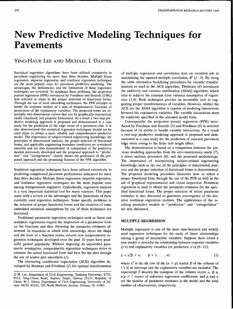
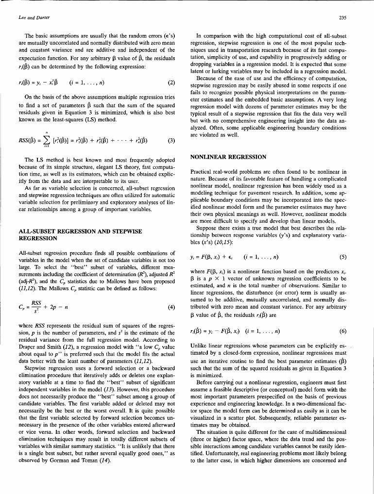
resources available and technical limitations. To judge which equation is preferable, both Equations 15 and 16 were checked by plotting the predicted versus the actual R values within the specified data ranges as displayed by the symbol ''o'' in Figures S(a) and 5(b), respectively. It is clearly shown that both equations result in very good predictions within the range of the data from which they were originally developed. In addition, Figures S(a)

242

~ ~

s co CJ)

ci ci

~ 8 0 ci

a: 3i a: 3i ci ci

Sl Sl ci ci

8 8 ci ci

:B :B ci ci

0.05 0.10 0.15 0.20 0.25 0.30 3.0 3.5

11/l

0 ~ C\i

co ~ CJ)

ci

"' C> OI ci

~ ~ "i in "i ., -l ci .t:< OI

LL ci ll. "O c (\I

0 ci (\I

CJ)

ci

in

9 Sl 0

~ .. co co ci

0.3 0.4 0.5 0.6 0.7 0.88

ATX2

FIGURE 3 Slab size effect: two-term PPR model.

and 5(b) present the results when extrapolating beyond the spec­ified limits by using these two models and the data from all of the 36 FE runs, respectively. These datum points, as displayed by the symbol '' *'' in the graphs, clearly show the difference.

Extrapolation by using Equation· 15 results in totally unaccept­able predictions outside the specified limits as shown in Figure 5( a). However, this problem is less pronounced as shown in Fig-

0.92

TRANSPORTATION RESEARCH RECORD 1449

..

0

E

.! "O y ·e-ll. ';-a;

4.0 4.5 5.0 1.2 1.4 1.6 1.8 2.0 2.2

Lil ATX1

in

8 ci

0

0 0 ci

in

§ ci

0 ci

in g 0

9

0

8 9

in

8 9

0.96 1.00 0.88 0.92 0.96 1.00

A Fitted

ure 5(b) when using Equation 16. In fact, the extrapolation of Lil greater than 5.0 provides excellent agreements with the actual data, since the functional form was properly selected to be as­ymptotic such that the predicted R values are very close to unity, as they should be. Nevertheless, some discrepancies still exist when extrapolating Equation 16 to smaller Lil values, that is, Lil < 3.0, which generally result in smaller R values.

Lee and Darter

~ ~

3! 8l 0 0

~ <D O>

0 0

v v a: O> a: O>

0 0

~ N O>

0 0

8 ~ 0 0

f8 :B 0 0

0.05 0.10 0.15 0.20 0.25 0.30 3.0 3.5

a/I

N

N

E E

~ ~ "i

"O 0 . 02)

tS 0 .!R. ·[ e a.. a..

~ "E ":- -(')

N

0

~

.· ";"

... 0.3 0.4 0.5 0.6 0.8

ATX2

§ 0

0.88 0.92 0.96 1.00

Fitted

FIGURE 4 Slab size effect: three-term PPR model.

This result may be explained by the fact that the first parameter [ai. or the minimum possible value of <l>1(ATXl)] of Equation 19 was estimated to be -5.5869, such that Equation 16 will never result in a value below 0.7823. This approximation is acceptable for the ranges of data that were used to develop Equations 16, 17, and 19. However, it may not be as accurate when extrapolating too far away from this specified range. If the minimum possible

..

243

0

E 02)

I-"O

02)

.i e ":-a.. ~

~

4.0 4.5 5.0 1.2 1.4 1.6 1.8 2.0 2.2

L/1 ATX1

8 ...: ,, co O> 0

.. ~ 0

"O v 02) O> .E 0 LL.

N O> 0

0 O> 0

co co 0

1.0 1.2 1.4 0.88 0.92 0.96 1.00

ATX3 R

value of R is known, this boundary condition may also be imposed on the predictive model. Thus, better agreement with the data can be obtained even in the case of extrapolation.

In summary, this case study not only demonstrates the benefits of using mechanistic variables through the use of the principles of dimensional analysis but it also emphasizes the importance of selecting proper functional forms. Correct functional forms pro-

244 TRANSPORTATION RESEARCH RECORD 1449

~

(a)

~ c:::i

~

] ~ c:i

u ] ""' ~

U"> co c:i

a.7a a.75 a.ea a.es a.ea a.95 "1.aa

Actual R

~

(b)

~ c:i

~

] u ~ ] <=>

""' ~

~ c:::i

a.7a a.75 a.ea a.es 0.9a a.95 "1.aa

Actual R

FIGURE 5 Extrapolated prediction plots using (a) existing model; (b) new model.

vide more comprehensive insights into the performance of the predictive model and may also lead to reasonable results even when extrapolation beyond the range of the data is required. It can be concluded that proper functional form is also a very crucial component in the success of a modeling process. The proper se­lection of functional forms to satisfy some applicable physical boundary conditions and subject-related engineering knowledge are the best supplements to statistical regression algorithms.

CONCLUSIONS

Several traditional linear and nonlinear regression techniques that have been widely adopted in pavement research were reviewed. Their advantages and limitations were discussed. Application of these regression techniques to practical engineering problems of­ten shows the deficiencies in the selection of proper functional forms, the violation of some embedded statistical assumptions,

,r

/

·-._

\ \

\') \

Lee and Darter

and failures to satisfy some applicable engineering boundary conditions.

Through the use of projection pursuit regression technique, a two-step predictive modeling approach was proposed in an at­tempt to minimize these problems. The proposed modeling ap­proach was demonstrated in a case study for edge stress prediction owing to the finite slab length effect. Without imposing an unjus­tified parametric assumption, the PPR provides a unique routine for breaking down higher-dimensional engineering problems into a series of sensible projected curves. By doing so the individual projected curves may be formulated separately with better choices of feasible functional forms as well as possible boundary condi­tions. Not only did the demonstration reemphasize the advantages of using the principles of dimensional analysis but it also illus­trated the importance of the proper selection of functional forms. Correct functional form provides more comprehensive insights into the performance of the predictive equation and may also lead to reasonable results even when extrapolation beyond the range of the data is required.

The demonstration was based on the data from the theoretical FE solutions in which no erroneous data are expected. As for applying the PPR to field or laboratory data with some possible errors, the promising features of the PPR algorithm are also help­ful for identifying any extremely strange behavior because of data errors. Engineering knowledge of the physical mechanism of the problem may be applied in identifying the possible bad datum points as well.

It is also believed that only through the application of both engineering and statistical knowledge and techniques will a more theoretically correct predictive equation be developed. If properly developed it may also be applied beyond the range of the data. Nevertheless, the conclusions should be restricted to the range of the data.

ACKNOWLEDGMENTS

This research work was partially sponsored by the Illinois De­partment of Transportation under the project titled Implementation of Illinois Pavement Feedback System, for which different modem regression techniques were utilized for predictive model devel­opment. The authors would like to express much appreciation to James Hall, Illinois Department of Transportation, for valuable assistance in this project.

REFERENCES

1. Hastie, T. J., and R. J. Tibshirani. Generalized Additive Models. Monographs on Statistics and Applied Probability 43. Chapman & Hall, 1990.

2. Breiman, L., and J. H. Friedman. Estimating Optimal Transformations for Multiple Regression and Correlation (with Discussion). Journal of the American Statistical Association, Vol. 80, 1985, pp. 580-619.

245

3. Buja, A Remarks on Functional Canonical Variates, Alternating Least Squares Methods and ACE. Annals of Statistics, Vol. 18, No. 3, 1990, pp. 1032-1069.

4. Tibshirani, R. Estimating Transformations for Regression via Additiv­ity and Variance Stabilization. Journal of the American Statistical As­sociation, Vol. 83, 1987, pp. 394-405.

5. Friedman, J. H., and W. Stuetzle. Projection Pursuit Regression. Jour­nal of the American Statistical Association. Vol. 76, 1981, pp. 817-823.

6. Friedman, J. H. SMART User's Guide. Technical Report No. 1. LCS, Department of Statistics, Stanford University, Stanford, Calif., 1984.

7. Darter, M. L Design of Zero-Maintenance Plain Jointed Concrete Pavement, Vol. /. Development of Design Procedures. FHWA Report FHWA-RD-77-111. FHWA, U.S. Department of Transportation, June 1977.

8. Salsilli-Murua, R. A Calibrated Mechanistic Design Procedure for Jointed Plain Concrete Pavements. Ph.D. thesis. University of Illinois, Urbana, 1991.

9. SAS User's Guide: Basics, Version 5 edition. SAS Institute, Inc., 1985.

10. SAS User's Guide: Statistics, Version 5 edition. SAS Institute, Inc., 1985.

11. Weisberg, S. Applied Linear Regression, 2nd ed. Wiley Series in Prob­ability and Mathematical Statistics. John Wiley & Sons, Inc., New York, 1985.

12. Draper, N. R., and H. Smith. Applied Regression Analysis, 2nd ed. Wiley Series in Probability and Mathematical Statistics. John Wiley & Sons, Inc., New York, 1981.

13. Rousseeuw, P. J., and AM. Leroy. Robust Regression and Outlier Detection. Wiley Series in Probability and Mathematical Statistics. John Wiley & Sons, Inc., New York, 1987.

14. Gorman, J. W., and R. J. Toman. Selection of Variables for Fitting Equations to Data. Technometrics, Vol. 8, 1966, pp. 27-51.

15. Bates, D. M., and D. G. Watts. Nonlinear Regression Analysis and Its Applications. Wiley Series in Probability and Mathematical Statistics. John Wiley & Sons, Inc., New York, 1988.

16. S-PLUS User's Manual, Vol. 1 and Vol. 2. Statistical Sciences, Inc., Seattle, Wash., Nov. 1991.

17. S-PLUS Reference Manual. Statistical Sciences, Inc., Seattle, Wash., Nov. 1991.

18. Chambers, J.M., and T. J. Hastie. Statistical Models in S. Wadsworth & Brooks/Cole Computer Science Series. AT&T Bell Laboratories, 1992.

19. Becker, R. A., J.M. Chambers, and AR. Wilks. The New S Language-A Programming Environment for Data Analysis and Graphics. The Wadsworth & Brooks/Cold Computer Science Series. AT&T Bell Laboratories, 1988.

20. Westergaard, H. M. New Formulas for Stresses in Concrete Pave­ments of Airfields. Transactions, ASCE, Vol. 113, pp. 425-444, 1948. Also in Proceedings, ASCE,Vol. 73, No. 5, May 1947.

21. Ioannides, AM., M. R. Thompson, and E. J. Barenberg. The Wester­gaard Solutions Reconsidered. In Transportation Research Record 1043, TRB, National Research Council, Washington, D.C., 1985.

22. Tayabji, S. D., and D. J. Halpenny. Thickness Design of Roller­Compacted Concrete Pavements. In Transportation Research Record 1136, TRB, National Research Council, Washington, D.C., 1987.

23. loannides, AM., and R. A Salsilli-Murua. Temperature Curling in Rigid Pavements: An Application of Dimensional Analysis. In Trans­portation Research Record 1227, TRB, National Research Council, Washington, D.C., 1989.

24. Ioannides, A M. Analysis of Slabs-on-Grade for a Variety of Loading and Support Conditions. Ph.D. thesis. University of Illinois, Urbana, 1984.

Publication of this paper sponsored by Task Force on Statistical Methods in Transportation.