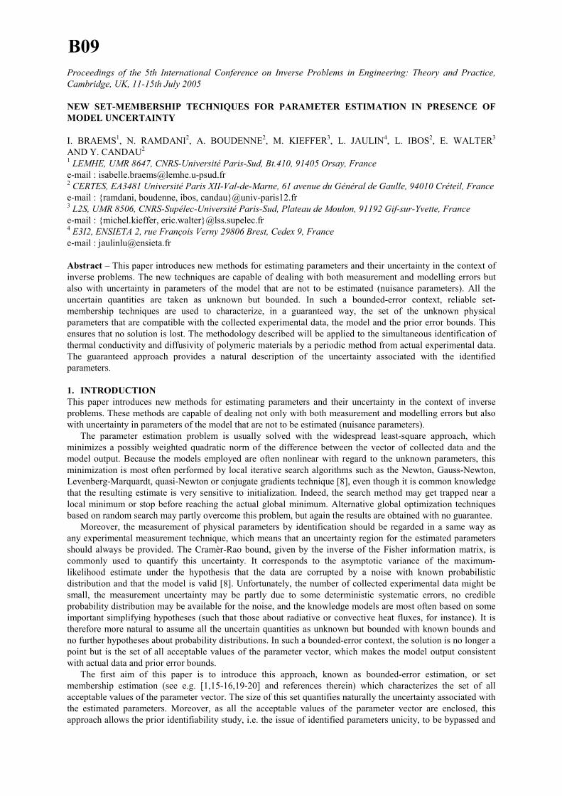
Proceedings of the 5th International Conference on Inverse Problems in Engineering: Theory and Practice,Cambridge, UK, 11-15th July 2005

NEW SET-MEMBERSHIP TECHNIQUES FOR PARAMETER ESTIMATION IN PRESENCE OFMODEL UNCERTAINTY

I. BRAEMS1, N. RAMDANI2, A. BOUDENNE2, M. KIEFFER3, L. JAULIN4, L. IBOS2, E. WALTER3

AND Y. CANDAU2

1 LEMHE, UMR 8647, CNRS-Université Paris-Sud, Bt.410, 91405 Orsay, Francee-mail : isabelle.braems@lemhe.u-psud.fr2 CERTES, EA3481 Université Paris XII-Val-de-Marne, 61 avenue du Général de Gaulle, 94010 Créteil, Francee-mail : {ramdani, boudenne, ibos, candau}@univ-paris12.fr3 L2S, UMR 8506, CNRS-Supélec-Université Paris-Sud, Plateau de Moulon, 91192 Gif-sur-Yvette, Francee-mail : {michel.kieffer, eric.walter}@lss.supelec.fr4 E3I2, ENSIETA 2, rue François Verny 29806 Brest, Cedex 9, Francee-mail : jaulinlu@ensieta.fr

Abstract – This paper introduces new methods for estimating parameters and their uncertainty in the context ofinverse problems. The new techniques are capable of dealing with both measurement and modelling errors butalso with uncertainty in parameters of the model that are not to be estimated (nuisance parameters). All theuncertain quantities are taken as unknown but bounded. In such a bounded-error context, reliable set-membership techniques are used to characterize, in a guaranteed way, the set of the unknown physicalparameters that are compatible with the collected experimental data, the model and the prior error bounds. Thisensures that no solution is lost. The methodology described will be applied to the simultaneous identification ofthermal conductivity and diffusivity of polymeric materials by a periodic method from actual experimental data.The guaranteed approach provides a natural description of the uncertainty associated with the identifiedparameters.

1. INTRODUCTIONThis paper introduces new methods for estimating parameters and their uncertainty in the context of inverseproblems. These methods are capable of dealing not only with both measurement and modelling errors but alsowith uncertainty in parameters of the model that are not to be estimated (nuisance parameters).

The parameter estimation problem is usually solved with the widespread least-square approach, whichminimizes a possibly weighted quadratic norm of the difference between the vector of collected data and themodel output. Because the models employed are often nonlinear with regard to the unknown parameters, thisminimization is most often performed by local iterative search algorithms such as the Newton, Gauss-Newton,Levenberg-Marquardt, quasi-Newton or conjugate gradients technique [8], even though it is common knowledgethat the resulting estimate is very sensitive to initialization. Indeed, the search method may get trapped near alocal minimum or stop before reaching the actual global minimum. Alternative global optimization techniquesbased on random search may partly overcome this problem, but again the results are obtained with no guarantee.

Moreover, the measurement of physical parameters by identification should be regarded in a same way asany experimental measurement technique, which means that an uncertainty region for the estimated parametersshould always be provided. The Cramèr-Rao bound, given by the inverse of the Fisher information matrix, iscommonly used to quantify this uncertainty. It corresponds to the asymptotic variance of the maximum-likelihood estimate under the hypothesis that the data are corrupted by a noise with known probabilisticdistribution and that the model is valid [8]. Unfortunately, the number of collected experimental data might besmall, the measurement uncertainty may be partly due to some deterministic systematic errors, no credibleprobability distribution may be available for the noise, and the knowledge models are most often based on someimportant simplifying hypotheses (such that those about radiative or convective heat fluxes, for instance). It istherefore more natural to assume all the uncertain quantities as unknown but bounded with known bounds andno further hypotheses about probability distributions. In such a bounded-error context, the solution is no longer apoint but is the set of all acceptable values of the parameter vector, which makes the model output consistentwith actual data and prior error bounds.

The first aim of this paper is to introduce this approach, known as bounded-error estimation, or setmembership estimation (see e.g. [1,15-16,19-20] and references therein) which characterizes the set of allacceptable values of the parameter vector. The size of this set quantifies naturally the uncertainty associated withthe estimated parameters. Moreover, as all the acceptable values of the parameter vector are enclosed, thisapproach allows the prior identifiability study, i.e. the issue of identified parameters unicity, to be bypassed and

B09

potentially unidentifiable parameters to be estimated. It makes it also possible to deal with ill-posed problems.This technique has been developed in the fields of control and signal processing and has been recently used inelectrochemistry [3] and robot localization [14].

The second aim of this paper is to deal with the fact that the knowledge-based model involves other uncertainparameters than those to be estimated. Usually, these parameters, to be called nuisance parameters from now on,are assumed to be known. In fact, they are uncertain as they correspond to imprecise measurement, insufficientknowledge or strong modelling simplification. Obviously, this uncertainty can be expected to affect both theidentified parameters and their uncertainty. In order to take into account this disturbance, Fadale [9] hasproposed an extended maximum-likelihood estimator in which the above nuisance parameters are modelled asnormal random variables with known variance. The uncertainty associated which the identified parameters isthen derived from the asymptotic variance of the estimator. The use of the asymptotic variance with fewexperimental data has already been criticized above. In addition, the prior distribution of the nuisance parametersis not always known, except for the optimistic case where they are actually measured in repeated experiments. Inthe general case, only a range of values is available. Last, characterizing uncertainty by random variables maynot be a valid approach as modelling error may induce systematic errors which cannot be taken into account bystochastic variables. Consequently, the uncertainty in the nuisance parameters will be also characterized byintervals in the following. We shall show that set-membership estimation can reliably account for this type ofuncertainty.

This method has been investigated for the first time by the authors for the guaranteed identification ofthermal parameters within a periodic experimental procedure applied to a test sample with known thermalproperties [5-6]. In this paper, the technique is used with a new experimental system [2] and for thecharacterization of the thermal transport properties of a Polyvinilidene Fluoride (PVDF) sample from actualdata.

Section 2 details the framework of bounded-error set estimation. Section 3 introduces basic tools of intervalanalysis and constraint propagation techniques to be used for reliable set estimation with algorithms presented inSection 4. The method is illustrated in Section 5 with the simultaneous estimation of thermal conductivity anddiffusivity of a polymeric sample material via a periodic method and actual experimental data.

2. SET-MEMBERSHIP ESTIMATIONIn the sequel two types of parameters will be distinguished. The parameters of interest, i.e., those to beidentified, are in the parameter vector p. The other non-essential parameters are gathered in a vector q called thenuisance parameter vector. It is assumed that p ΠP and q ΠQ ,where P and Q are known prior domains.

Let e be the model output error e = y Рf(p,q), where y is the vector of the collected data and f(.,.) thecorresponding model output. In bounded-error estimation (or set-membership estimation), one looks for the setof all parameter vectors such that the error stays within some known feasible domain E, i.e., e ΠE (see [16,19]and the references therein). The set estimate then contains all values of the parameter vector that are acceptable,i.e., consistent with the model and the collected data y, given what is deemed an acceptable error. The size of thisset quantifies the uncertainty associated with the estimated parameters.

Assume first that the value q* taken by the nuisance parameter vector q is known. The set C to be estimatedis the set of all the acceptable parameter vectors p

( ){ }, , *= ∈ ∈C P Yp f p q (1)

where Y = y – E. Characterizing C is a set-inversion problem, as (1) can be rewritten as( )1−

= ∩C Y Pg (2)where g(.) = f(.,q*). It can be solved in a guaranteed way using the algorithm SIVIA [10,13], see Section 3.

Suppose now that q* is unknown. One may of course choose to estimate the set( ) ( ){ }, | ,= ∈ × ∈S P Q Yp q f p q (3)

which can again be seen as a set-inversion problem. However, characterizing S will be much more difficult thanestimating C, since the dimension of S is larger than that of C and the volume of S may be very large.

An alternative simpler approach is to characterize the set Π of all the acceptable parameter vectors p underthe assumption that q belongs to its prior domain, i.e.,

( ){ }| , ,Π = ∈ ∃ ∈ ∈P Q Yp q f p q (4)

The estimation of the acceptable values of q is then given up to simplify computation. While C is a cut of S,Π is the projection of S onto the p-space (see Figure 1)

Π =PSproj (5)

Remark 1. The inclusion C Ã Π, illustrates the fact that when q is uncertain, the uncertainty on p increases.

B092

The basic tools for the characterization of Π will now be presented.

p1

S

p2

q

P

�

q*

C

Q

Figure 1. The sets to be characterized.

3. INTERVAL ANALYSISInterval analysis was initially developed to account for the quantification errors introduced by the floating pointrepresentation of real numbers with computers and was extended to validated numerics [13,17,18]. A realinterval ,a a a[ ] = [ ] is a connected and closed subset of R. The set of all real intervals of R is denoted by IR.Real arithmetic operations are extended to intervals [17]. Consider an operator � Œ {+ , - , * , § } and [a] and [b]two intervals. Then

[ ] [ ] [ ] [ ]{ },= ∈ ∈� �a b x y x a y b (6)

Consider : →R Rn mf ; the range of this function over an interval vector [a] is given by:

[ ]( ) ( ) [ ]{ }| ∈f a f x x a��� (7)

The interval function [f] from IRn to IRm is an inclusion function for f if

[ ] [ ]( ) [ ] [ ]( ),∀ ∈ ⊆IRna f a f a (8)

An inclusion function of f can be obtained by replacing each occurrence of a real variable by thecorresponding interval and each standard function by its interval counterpart. The resulting function is called thenatural inclusion function. The performances of this inclusion function depend on the formal expression for f.

3.1 Constraints satisfaction problem, contractorsConsider n variables xi ∈ R, i ∈ {1,2,…,n}, linked by nf relations of the form

1 2( , , , ) 0=…j nf x x x (9)and where each variable xi is known to belong to a prior interval domain [xi]0 ; define the vector

T1 2 = ( , , , )… nx x xx and the function T

1 2 = ( , , , )…

fnf f ff x x x x( ) ( ) ( ) ( ) , then eqn. (9) can be written as a constraintsatisfaction problem CSP [13] :

H : = , ∈f x 0 x x 0( ) [ ] (10)Interval vectors containing the solution of CSP can be evaluated using contractors. An operator CH is a

contractor for the CSP H defined by (10) if, for any box [x] in [x]0, it satisfiesa) the contractance property : [ ]( ) [ ]⊂HC x x

b) and the correctness property : [ ]( ) [ ]∩ = ∩HC x xS S

where ∩ is the intersection of two boxes and S the solution set for H. A possible way for solving the CSPdefined by (10) is to design a function Ψ such that:

( ) ( )= ⇔ = Ψf x 0 x x (11)According to the fixed-point theorem and using (11), if the series 1[ ] ([ ] )k k+

= Ψx x converges towards [ ]∞

x ,

B093

then [ ]∞

x shall contain the solution of H. Several point solvers such as the Newton method, the Gauss-Seidel orthe Krawczyk operators have been extended to intervals, and are used to solve efficiently even non-linear CSPs[13,17-18]. However, they remain limited to problems where the number of constraints is equal to the number ofvariables.

When the number of constraints and the number of variables are different, one can use another contractorrelying on interval propagation techniques. These techniques combine the constraint propagation techniquesclassically used in the domain of artificial intelligence [7] and interval analysis. They have been brought toautomatic control in [12], for solving set inversion problems in a bounded-error context. The algorithm used forconstraint propagation is based on the interval extension of the local Waltz filtering [7,12]. In fact, therelationships (9) between the variables can be viewed as a network where the nodes are connected with theconstraints. In order to spread the consequences of each node throughout the network, the main idea is to dealwith a local group of constraints and nodes and then record the changes in the network. Further deductions willmake use of these changes to make further changes. The inconsistent values for the variable vector are thusremoved. If the network exhibits no cycles, then optimal filtering can be achieved by performing only oneforward and one backward propagation: this is known as the forward-backward contractor [7,12-13,17-18].

3.2 Set inversion via interval analysisConsider the problem of determining a solution set for the unknown quantities u defined by:

( ) [ ]{ } [ ]( )1| −

= ∈ Ψ ∈ = Ψ ∩u u y yS U U (12)

where [y] is known a priori, U is an a priori search set for u and ψψψψ a nonlinear function not necessarilyinvertible in the classical sense. Since (12) involves computing the reciprocal image of ΨΨΨΨ, it is a set inversionproblem which can be solved using SIVIA (Set Inversion Via Interval Analysis). SIVIA [10-11] is a recursivealgorithm which explores all the search space without losing any solution. This algorithm makes it possible toderive a guaranteed enclosure of the solution set S as follows

⊆ ⊆S S S (13)The inner enclosure S consists of the boxes that have been proved feasible. To prove that a box [u] is

feasible it is sufficient to prove that Ψ ⊆u y[ ]([ ]) [ ] . If, on the other hand, it can be proved thatΨ ∩ =∅u y[ ]([ ]) [ ] , then the box [u] is unfeasible. Otherwise, no conclusion can be reached and the box [u] is

said undetermined. It is then bisected and tested again until its size reaches a threshold ε > 0 to be tuned by theuser. Such a termination criterion ensures that SIVIA terminates after a finite number of iterations. The outerenclosure S is defined by

= ∪∆S S S (14)where ∆S is an uncertainty layer given by the union of all the undetermined boxes (with their widths not largerthan ε ).

3.3 Set projection via interval analysisWhen only Π is to be characterized, one can use another algorithm called PROJECT [4-6,12]. This algorithmcomputes inner and outer approximations Π and Π of the set Π defined by (4). As only the p-space ispartitioned, the memory and computational time required are much smaller than for a full characterization of S.Obviously, the main difference between PROJECT and SIVIA lies in the tests to be implemented. In SIVIA, theouter approximation [g]([p]) is directly used to test the acceptability of all elements of [p]. Here, to characterizeΠ , [p] will be said acceptable if there exists q ∈Q such that f ⊆p q Y[ ]([ ], ) . Feasible point finders then requirespecific approaches. In order to allow consideration of higher dimensions, the procedure implemented inPROJECT uses contractors (see [12] for details). As only the p-space is partitioned, the memory andcomputational time required are much smaller than for a full characterization of S.

4. APPLICATION

4.1 Experimental procedureThe experimental procedure under analysis hereafter is devoted to the measurement of the thermal properties ofmaterials: the thermal diffusivity a and the thermal conductivity λ of a sample are measured simultaneously witha so-called periodic method, using multi-harmonic heating signals [2]. The experimental set-up is shown onFigure 2. The sample under study is held between metallic plates. A thermal grease layer ensures good thermalexchanges between the elements. The front side of the first metallic plate, made of brass, is also fixed to a

B094

5B37

5B37

Poweramplifier

5B49

Turbomolecularpump

Primary pumpPC with

multifunction analogI/O card

Copper

Sample

BrassThermoelectric

cooler

Grease

Figure 2. The experimental set-up.

-0.025 -0.02 -0.015 -0.01 -0.005 0 0.005 0.01 0.015-0.18

-0.16

-0.14

-0.12

-0.1

-0.08

-0.06

-0.04

-0.02

0

0.02

Figure 3. The experimental data. Dots: Nyquist plot of experimental transfer function HS(j⋅2πf),f ∈ { 2.5, 5, 10, 20, 40} mHz, 20 trials. Boxes: Sets of acceptable outputs.

heating device. The rear side of the second metallic plate, made of copper, is in contact with air at ambienttemperature. The set-up is put in a high vacuum environment in order to reduce heat transfer by convection.

The excitation voltage of the thermoelectric cooling device is a sum of five sinusoidal signals. The resultingsignal is expressed as follows

( ) ( )5

10

1sin 2 2n

nn

V t V f tπ−

=

= ⋅ ⋅∑ (15)

where f0 = 2.5 mHz is the fundamental frequency, Vn is a partial voltage amplitude and t is the time.An amplifier device feeds the thermoelectric cooler and is controlled by an analogical voltage provided by an

I/O card via a signal conditioning block (Analog Devices, 5B49). The signal provided by two thermocouplesfixed on the front and rear plates is amplified and low-pass filtered with conditioning modules (Analog Devices,5B37). All conditioning modules are connected to a multifunction acquisition card (NI-6035E) controlled by aLabview application.

To estimate thermal conductivity and diffusivity, it is desirable to explore a large frequency range. In ourcase, the use of a sum of five sinusoidal signals allows us to obtain five times more information from oneexperiment and reduces its duration. Moreover, it is required to have large signal amplitudes for a better signal-

T rear

T front

B095

to-noise ratio. However, the increase in amplitude is limited by the power of the generator and by the operatingtemperature of the thermoelectric cooling system. Generally, the temperature data obtained show a drift of themean temperature of both front and rear plates (typically a few degrees). The signal mean value is subtractedfrom experimental data values to get the temperature variations only. After this rough signal correction,experimental data are taken as the following frequency response

( )( )

( )

ω

ω

ω

=

rearS

front

T jH j

T j(16)

where the temperature spectra are given by the Fourier transform of the time-history signals, and where Treardenotes the temperature of the rear metallic plate and Tfront the one of the front plate, see Figure3. Error boundson the values taken by the experimental transfer function at the five angular frequencies ωi are calculated prior tothe identification, from measurements repeated 20 times in order to assess variability. The experimental data aregiven in Figure 3. The X-axis represents the real part of the transfer function whereas the Y-axis represents theimaginary part ; the depicted dots are the actual experimental data whereas the boxes are the prior feasibledomains for model output at the five frequencies.

4.2 Physical modelThe system under study is modelled with quadrupoles (two-port transfer functions). The quadrupole method iswell known and extensively used in thermal science [21]. A quadrupole Z(s) is defined by

( )( ) ( )

( ) ( )

cosh sinh

sinh cosh

τ τ

τ

τ

τ τ

=

Rs sss

s s sR

Z (17)

where 2 aτ δ= , R δ λ= , δ is the material thickness and s is the Laplace variable. For the particular case ofthe grease layer, which is assumed with no inertia, the relationship uses the resistance only and becomes

( )10 1

=

RsZ (18)

The model transfer function is then given by

( )( )

( ), =

rear

front

T sH s

T sp (19)

where the front temperature is given by (the s symbol being removed, for convenience)

0

0ϕ

=

frontBrass Gre Sample Gre Copp

front

T ThT

Z Z Z Z Z (20)

and the rear temperature is given by

0_

0ϕ

=

rearCopp half

rear

T ThTZ (21)

where h is a constant coefficient modelling surface heat exchanges with the fluid, and where T0 is thetemperature of the rear face of the copper plate. The nuisance parameters and their uncertainties are given inTable 1. The sample thickness belongs to [1.95 , 2.05] 10-3m.

Table 1. Nuisance model parameters.Material Parameters Scale Nominal

valueUncertaintyinterval

Diffusivity, a 10-6 m2.s-1 34.0 [33 , 35]Conductivity, λ W.m-1.K-1 112.5 [100 , 125]

Brass plateFront side

Brass thermocouple – sample interface distance 10-3 m 5.0 [4.225 , 5.775]Diffusivity, a 10-6 m2.s-1 115.5 [114 , 117]Conductivity, λ W.m-1.K-1 395.5 [389 , 402]Copper thermocouple – sample interface distance 10-3 m 4.5 [3.725 , 5.275]

Copper plateRear side

Thickness 10-3 m 9.0 [8.89 , 9.01]Grease Thermal resistance 10-6 K.m2.W-1 115.0 [80 , 150]Fluid Surface heat exchange coefficient W.m-2.K-1 5 [5 , 10]

B096

5. RESULTSIn this section, two cases are studied. First, the parameters are estimated while assuming the nuisance parametersperfectly known, then the latter are assumed uncertain. In both cases, the prior search space for the parameters istaken as:

[ ]1, 30τ ∈p s1/2 and 410 , 5− ∈ pR m2.K.W-1 (22)

5.1 Bounded-error identification with set inversion, nuisance parameters assumed knownIn 2 s on a Pentium IV 1.7 Ghz, SIVIA with a contractor derives the inner and outer approximations plotted inFigure 4. Since the inner approximation C is not empty, we have proved that the problem under study admits asolution : it is possible to find acceptable values for the thermal diffusivity and conductivity that are consistentwith the modelling hypotheses and the prior feasible domains for model output at the five frequencies.

The projection of the outer approximation C onto the parameter axes provides an outer approximation of theuncertainty interval associated with each of the identified parameters

88.167 10 8.3%−

= ⋅ ±a m2.s-1 (23)and 0.201 4.6%λ = ± W.m-1.K-1 (24)

Compare (23)-(24) with the estimated parameters given by classical least square estimation, i.e.88.767 10a −

= ⋅ m2.s-1 (25)and 0.179λ = W.m-1.K-1 (26)

The reader can see that the identified value for the diffusivity parameter a as obtained with set inversion isconsistent with the one given by least squares. However, the identified values for the conductivity parameter λobtained with both methods differ significantly. In order to explain this result, we have checked both identifiedmodels outputs: we found that the output of the model identified with least squares is not included in the priorbounds for experimental data at the lowest frequency, which is possible because this was not the purpose of leastsquares estimation. To the contrary, the output of the model obtained by set inversion is indeed included in theprior bounds for experimental data as was required by the bounded-error estimation technique.

Figure 4. Inner approximation (dark boxes) and outer approximation of posterior feasible set C.(Light grey boxes form the uncertainty layer ∆C)

5.2 Bounded-error identification with set projection, nuisance parameters assumed uncertainNow assume the nuisance parameters are uncertain. In 300 s on a Pentium IV 1.7 Ghz, PROJECT derives theinner and outer approximations plotted in Figure 5. The large thickness of the uncertainty layer is due to thepessimism of the contractors and inclusion functions employed, which limits the quality of the results.

The projection of the outer approximation Π onto the parameter axes provides an outer approximation of theuncertainty interval associated with each of the identified parameters

88.13 10 22%−

= ⋅ ±a m2.s-1 (27)and 0.205 15%λ = ± W.m-1.K-1 (28)

Rp ( m2KW-1)

( )τ

12sp

B097

As expected, the uncertainty in the nuisance parameters leads to much larger uncertainties in the identifiedparameters.

Figure 5. Inner approximation (dark boxes) and outer approximation of posterior feasible set Π.(Light grey boxes form the uncertainty layer ∆Π).

6. CONCLUSIONSIn this paper we have addressed the problem of reliable parameter estimation in presence of model uncertaintyresulting from nuisance parameters.

In the first part of this paper, we assumed that the nuisance parameter vector was accurately known.Assuming that the errors on model output were bounded with known bounds and no further hypotheses aboutprobability distributions, we have shown that estimating the parameters in such a framework is a set inversionproblem. The algorithm SIVIA has been used with data taken from an actual experimental thermal set-up. Thenew method generates inner and outer approximations for the solution set which provides a simple and reliableevaluation of the estimation uncertainty.

In the second part of this paper, we have addressed the problem of estimating the feasible parameter set whenthe nuisance parameter are uncertain. We have shown that estimating the parameters in this framework amountsto projecting the solution set onto the space of the parameters of interest. We characterized this projection withthe algorithm PROJECT. The volume of this projected set is larger than the one derived when the nuisanceparameters are assumed accurately known: taking into account uncertainty increases the uncertainty associatedwith the estimation. One is now capable of accounting for bounded uncertainty in nuisance parameters in areliable and guaranteed way.

REFERENCES

1. G. Belforte, B. Bona and V. Cerone, Parameter estimation algorithms for a set-membership description ofuncertainty. Automatica (1990) 26, 887-898.

2. A. Boudenne, L. Ibos, E. Gehin and Y. Candau, A simultaneous characterization of thermal conductivityand diffusivity of polymer materials by a periodic method. J. Phys. D: Appl. Phys. (2004) 37, 132-139.

3. I. Braems, F. Berthier, L. Jaulin, M. Kieffer and E. Walter, Guaranteed estimation of electrochemical

Rp ( m2KW-1)0.008 0.012

7.9

6.4

( )τ

12sp

B098

parameters by set inversion using interval analysis. J. Electroanal. Chem. (2001) 495, 1-9.

4. I. Braems, Méthodes Ensemblistes Garanties pour l'Estimation de Grandeurs Physiques, PhD dissertation,Université Paris-Sud, Orsay, France, 2002.

5. I. Braems, L. Jaulin, M. Kieffer, N. Ramdani and E. Walter, Reliable parameter estimation in presence ofuncertainty, 13th IFAC Symposium on System Identification, Rotterdam, SYSID 2003, pp. 1856-1861.

6. I. Braems, N. Ramdani, M. Kieffer and E. Walter, Caractérisation garantie d'un dispositif de mesure degrandeurs thermiques. APII-Journal Européen des Systèmes Automatisés (2003) 37, 1129-1143.

7. E. Davis, Constraint propagation with interval labels, Artificial Intelligence (1987) 32, 281-331.

8. P. Eykhoff, System Identification, John Wiley and Sons, New York, 1979.

9. T.D. Fadale, A.V. Nenarokomov and A.F. Emery, Uncertainties in parameter estimation: The inverseproblem. Int. J. Heat Mass Transfer (1995) 38, 511-518.

10. L. Jaulin and E. Walter, Guaranteed nonlinear parameter estimation from bounded-error data via intervalanalysis. Math. Comput. Simul. (1993) 35, 123-137.

11. L. Jaulin and E. Walter, Set inversion via interval analysis for nonlinear bounded-error estimation.Automatica (1993) 29, 1053-1064.

12. L. Jaulin, I. Braems and E. Walter, Interval methods for nonlinear identification and robust control, In 41stIEEE Conference on Decision and Control, Las Vegas, 2002, pp. 4676-4681.

13. L. Jaulin, M. Kieffer, O. Didrit and E. Walter, Applied Interval Analysis, Springer-Verlag, London, 2001.

14. M. Kieffer, L. Jaulin, E. Walter and D. Meizel, Robust autonomous robot localization using intervalanalysis. Reliable Computing (2000) 6, 337-362.

15. M. Milanese and A. Vicino, Estimation theory for nonlinear models and set membership uncertainty.Automatica (1991) 27, 403-408.

16. M. Milanese, J. Norton, H. Piet-Lahanier and E. Walter, (Eds.) Bounding Approaches to SystemIdentification, Plenum Press, New York, 1996.

17. R. E. Moore, Interval Analysis, Prentice-Hall, Englewood Cliffs, 1966.

18. A. Neumaier, Interval Methods for Systems of Equations, Cambridge University Press, Cambridge, 1990.

19. J. P. Norton, (Ed.) Special Issue on Bounded-Error Estimation: Issue 2. Int. J. Adaptive Control SignalProcessing (1995) 9, 1-132.

20. E. Walter, (Ed.) Special Issue on Parameter Identification with Error Bounds. Math. Comput. Simul.(1990) 32, 447-607.

21. H. Wang, A. Degiovanni and C. Moyne, Periodic thermal contact: a quadrupole model and an experiment.Int. J. Thermal Sci. (2002) 41, 125-135.

B099