new statistical methods in risk assessment by probability...
TRANSCRIPT
New statistical methods in risk assessment
by probability bounds
Victoria Montgomery
A thesis presented for the degree of
Doctor of Philosophy
Department of Mathematical Sciences
Durham University
UK
February 2009

Dedication
To Willem for his love and support
ii
New statistical methods in risk assessment by
probability bounds
Victoria Montgomery
Abstract
In recent years, we have seen a diverse range of crises and controversies concerning
food safety, animal health and environmental risks including foot and mouth disease,
dioxins in seafood, GM crops and more recently the safety of Irish pork. This has
led to the recognition that the handling of uncertainty in risk assessments needs
to be more rigorous and transparent. This would mean that decision makers and
the public could be better informed on the limitations of scientific advice. The
expression of the uncertainty may be qualitative or quantitative but it must be well
documented. Various approaches to quantifying uncertainty exist, but none are
yet generally accepted amongst mathematicians, statisticians, natural scientists and
regulatory authorities.
In this thesis we discuss the current risk assessment guidelines which describe the
deterministic methods that are mainly used for risk assessments. However, proba-
bilistic methods have many advantages, and we review some probabilistic methods
that have been proposed for risk assessment. We then develop our own methods
to overcome some problems with the current methods. We consider including var-
ious uncertainties and looking at robustness to the prior distribution for Bayesian
methods. We compare nonparametric methods with parametric methods and we
combine a nonparametric method with a Bayesian method to investigate the effect
of using different assumptions for different random quantities in a model. These
new methods provide alternatives for risk analysts to use in the future.

Declaration
I declare that the research presented in this thesis is, to the best of my knowledge,
original. Where other work is quoted, due reference has been made.
Copyright © 2009 Victoria Montgomery
The copyright of this thesis rests with the author. No quotations from it should be
published without the author’s prior written consent and information derived from
it should be acknowledged.
iv

Acknowledgements
Firstly I would like to thank Professor Frank Coolen for being an excellent su-
pervisor. His enthusiasm, untiring support and calm advice throughout this project
made this research much more productive and enjoyable. I would also like to ac-
knowledge the help I received from Dr. Peter Craig and Professor Michael Goldstein.
I am grateful for their interest in my research.
My thanks also go to the members of the risk analysis team at CSL, York. In
particular Dr. Andy Hart, who gave unfailing support and advice throughout the
project.
Thank you to the members of Durham Probability and Statistics Department
for being there and helping when asked.
However the greatest thanks is reserved for my family and partner: Willem for
his enduring love and support throughout the highs and lows of my research, my
gran for her love, support and never-ending chocolate supply, my sister for listening
to me stressing for hours on end, my dad for providing endless cups of tea and my
mum for her constant editing and unwavering belief in me.
v

Contents
Abstract iii
Declaration iv
Acknowledgements v
1 Introduction 1
1.1 Motivation . . . . . . . . . . . . . . . . . . . . . . . . . . . . . . . . . 1
1.2 Outline of Thesis . . . . . . . . . . . . . . . . . . . . . . . . . . . . . 6
1.3 Collaborators . . . . . . . . . . . . . . . . . . . . . . . . . . . . . . . 7
2 Statistical methods for risk assessment 8
2.1 Introduction . . . . . . . . . . . . . . . . . . . . . . . . . . . . . . . . 8
2.2 Risk assessment of chemicals . . . . . . . . . . . . . . . . . . . . . . . 9
2.3 Current EU guidance . . . . . . . . . . . . . . . . . . . . . . . . . . . 11
2.4 Data sets for risk assessment . . . . . . . . . . . . . . . . . . . . . . . 13
2.5 Species sensitivity distributions . . . . . . . . . . . . . . . . . . . . . 14
2.6 Variability and uncertainty . . . . . . . . . . . . . . . . . . . . . . . . 15
2.6.1 Description of variability and uncertainty . . . . . . . . . . . . 15
2.6.2 Types of uncertainty . . . . . . . . . . . . . . . . . . . . . . . 16
2.6.3 Modelling variability and uncertainty . . . . . . . . . . . . . . 17
2.6.4 Example . . . . . . . . . . . . . . . . . . . . . . . . . . . . . . 18
2.7 Bayesian methods . . . . . . . . . . . . . . . . . . . . . . . . . . . . . 20
2.7.1 Credible or posterior intervals and regions . . . . . . . . . . . 21
2.7.2 Example of hpd region for the Normal distribution . . . . . . 21
2.7.3 Prior distributions . . . . . . . . . . . . . . . . . . . . . . . . 22
vi
CONTENTS vii
2.7.4 Bayesian posterior predictive distribution . . . . . . . . . . . . 23
2.7.5 Robustness to the prior distribution . . . . . . . . . . . . . . . 24
2.7.6 Bayesian methods for left-censored data . . . . . . . . . . . . 25
2.7.7 Bayesian pointwise method . . . . . . . . . . . . . . . . . . . . 25
2.8 Frequentist confidence methods . . . . . . . . . . . . . . . . . . . . . 26
2.9 Nonparametric Predictive Inference (NPI) . . . . . . . . . . . . . . . 27
2.9.1 Hill’s A(n) . . . . . . . . . . . . . . . . . . . . . . . . . . . . . 28
2.9.2 Lower and Upper probabilities . . . . . . . . . . . . . . . . . . 29
2.9.3 M function . . . . . . . . . . . . . . . . . . . . . . . . . . . . 29
2.10 Probability Boxes (p-boxes) . . . . . . . . . . . . . . . . . . . . . . . 30
2.10.1 Nonparametric p-boxes . . . . . . . . . . . . . . . . . . . . . . 30
2.10.2 Parametric p-boxes . . . . . . . . . . . . . . . . . . . . . . . . 31
2.10.3 Discussion . . . . . . . . . . . . . . . . . . . . . . . . . . . . . 32
2.11 Dependence between random quantities . . . . . . . . . . . . . . . . . 33
2.11.1 Copulas . . . . . . . . . . . . . . . . . . . . . . . . . . . . . . 33
2.11.2 Dependency bounds . . . . . . . . . . . . . . . . . . . . . . . 34
2.12 Monte Carlo Simulation . . . . . . . . . . . . . . . . . . . . . . . . . 35
2.12.1 One-Dimensional Monte Carlo Simulation . . . . . . . . . . . 36
2.12.2 Two-Dimensional Monte Carlo Simulation . . . . . . . . . . . 36
2.13 Alternative methods . . . . . . . . . . . . . . . . . . . . . . . . . . . 37
2.13.1 Bootstrapping . . . . . . . . . . . . . . . . . . . . . . . . . . . 37
2.13.2 Worst-case analysis . . . . . . . . . . . . . . . . . . . . . . . . 39
2.13.3 Interval analysis . . . . . . . . . . . . . . . . . . . . . . . . . . 39
2.13.4 Fuzzy arithmetic . . . . . . . . . . . . . . . . . . . . . . . . . 40
2.13.5 Sensitivity analysis . . . . . . . . . . . . . . . . . . . . . . . . 40
2.14 Conclusion . . . . . . . . . . . . . . . . . . . . . . . . . . . . . . . . . 41
3 Bayesian Probability Boxes 42
3.1 Introduction . . . . . . . . . . . . . . . . . . . . . . . . . . . . . . . . 42
3.2 Bayesian p-box method . . . . . . . . . . . . . . . . . . . . . . . . . . 44
3.2.1 Forming a Bayesian p-box . . . . . . . . . . . . . . . . . . . . 44
3.2.2 Choosing Θs(α) . . . . . . . . . . . . . . . . . . . . . . . . . . 45
CONTENTS viii
3.2.3 Example: Exponential Distribution . . . . . . . . . . . . . . . 45
3.2.4 Different credibility levels . . . . . . . . . . . . . . . . . . . . 47
3.2.5 Robustness to the prior distribution . . . . . . . . . . . . . . . 48
3.3 Normal and Lognormal distributions . . . . . . . . . . . . . . . . . . 50
3.3.1 Bayesian P-boxes for the Normal distribution . . . . . . . . . 50
3.3.2 Justification . . . . . . . . . . . . . . . . . . . . . . . . . . . . 51
3.3.3 Example: Lognormal distribution with small n . . . . . . . . . 53
3.4 Validating Bayesian p-boxes . . . . . . . . . . . . . . . . . . . . . . . 54
3.5 Generalisations . . . . . . . . . . . . . . . . . . . . . . . . . . . . . . 56
3.5.1 Robustness to the prior distribution for µ . . . . . . . . . . . . 56
3.5.2 Example: A robust Normal Bayesian p-box . . . . . . . . . . . 57
3.5.3 Robustness to the prior distribution for µ and σ . . . . . . . . 60
3.5.4 Example: A robust (µ, σ) Normal Bayesian p-box . . . . . . . 61
3.5.5 Imprecise data . . . . . . . . . . . . . . . . . . . . . . . . . . 63
3.5.6 Example: Normal Bayesian p-boxes for imprecise data . . . . 64
3.6 Comparison of different methods . . . . . . . . . . . . . . . . . . . . 65
3.6.1 Example: Comparing methods for small n . . . . . . . . . . . 66
3.6.2 Example: Comparing methods for larger n . . . . . . . . . . . 69
3.7 Dependence . . . . . . . . . . . . . . . . . . . . . . . . . . . . . . . . 70
3.7.1 Example: Combining random quantities . . . . . . . . . . . . 71
3.8 Conclusion . . . . . . . . . . . . . . . . . . . . . . . . . . . . . . . . . 73
4 Nonparametric predictive assessment of exposure risk 76
4.1 Introduction . . . . . . . . . . . . . . . . . . . . . . . . . . . . . . . . 76
4.2 Nonparametric Predictive Inference . . . . . . . . . . . . . . . . . . . 77
4.2.1 Example: NPI for a single random quantity . . . . . . . . . . 78
4.2.2 Example: NPI for the Exposure Model . . . . . . . . . . . . . 79
4.2.3 NPI for left-censored data . . . . . . . . . . . . . . . . . . . . 80
4.3 Case Study: Benzene Exposure . . . . . . . . . . . . . . . . . . . . . 82
4.3.1 The data . . . . . . . . . . . . . . . . . . . . . . . . . . . . . . 82
4.3.2 NPI lower and upper cdfs . . . . . . . . . . . . . . . . . . . . 84
4.4 Exploring dependence for NPI by simulation . . . . . . . . . . . . . . 87

CONTENTS ix
4.4.1 Varying n . . . . . . . . . . . . . . . . . . . . . . . . . . . . . 88
4.4.2 Varying µz and σz . . . . . . . . . . . . . . . . . . . . . . . . 92
4.4.3 Discussion . . . . . . . . . . . . . . . . . . . . . . . . . . . . . 96
4.5 Computational issues . . . . . . . . . . . . . . . . . . . . . . . . . . . 97
4.6 The effect of different sample sizes . . . . . . . . . . . . . . . . . . . . 98
4.7 Imprecise data . . . . . . . . . . . . . . . . . . . . . . . . . . . . . . . 100
4.8 Comparison to Bayesian methods . . . . . . . . . . . . . . . . . . . . 102
4.9 Robust NPI . . . . . . . . . . . . . . . . . . . . . . . . . . . . . . . . 105
4.9.1 Example: Robust NPI lower and upper cdfs . . . . . . . . . . 105
4.10 Conclusion . . . . . . . . . . . . . . . . . . . . . . . . . . . . . . . . . 107
5 Combining NPI and Bayesian methods 109
5.1 Introduction . . . . . . . . . . . . . . . . . . . . . . . . . . . . . . . . 109
5.2 The NPI-Bayes hybrid method . . . . . . . . . . . . . . . . . . . . . . 111
5.3 Predicting exposure using the NPI-Bayes hybrid method . . . . . . . 114
5.3.1 Data sets . . . . . . . . . . . . . . . . . . . . . . . . . . . . . 115
5.3.2 Calculating exposure . . . . . . . . . . . . . . . . . . . . . . . 117
5.3.3 Sampling variation . . . . . . . . . . . . . . . . . . . . . . . . 119
5.3.4 Larger sample sizes . . . . . . . . . . . . . . . . . . . . . . . . 121
5.4 Robustness . . . . . . . . . . . . . . . . . . . . . . . . . . . . . . . . 125
5.4.1 Robustness for the Normal distribution . . . . . . . . . . . . . 125
5.4.2 Diagram showing how to include robustness for the Exposure
Model . . . . . . . . . . . . . . . . . . . . . . . . . . . . . . . 126
5.5 Examples: NPI-Bayes robust hybrid method . . . . . . . . . . . . . . 127
5.5.1 Case (BXr, BYr, BZr) . . . . . . . . . . . . . . . . . . . . . . 127
5.5.2 Case (NXr, NYr, NZr) . . . . . . . . . . . . . . . . . . . . . . 129
5.5.3 Comparing all the cases . . . . . . . . . . . . . . . . . . . . . 129
5.6 Combining NPI with Bayesian 2D MCS . . . . . . . . . . . . . . . . . 131
5.7 Conclusions . . . . . . . . . . . . . . . . . . . . . . . . . . . . . . . . 132
6 Conclusions and Future Research 135
6.1 Conclusions . . . . . . . . . . . . . . . . . . . . . . . . . . . . . . . . 135

CONTENTS x
6.2 Topics for future research . . . . . . . . . . . . . . . . . . . . . . . . . 137
6.2.1 Uncertainty about correlations . . . . . . . . . . . . . . . . . . 137
6.2.2 Bayesian p-boxes for other distributions . . . . . . . . . . . . 138
6.2.3 More realistic models . . . . . . . . . . . . . . . . . . . . . . . 139
Appendix 140
A Distributions used in this thesis . . . . . . . . . . . . . . . . . . . . . 140
Bibliography 142

Chapter 1
Introduction
This chapter offers an explanation of the motivation for this thesis and introduces
the particular areas of risk assessment that are discussed later in the thesis. It
also provides an outline of the focus of subsequent chapters and introduces the
collaborators for the project.
1.1 Motivation
Recent years have seen a diverse range of crises and controversies concerning food
safety, animal health and environmental risks, e.g. the safety of Irish pork, dioxins in
seafood, foot and mouth disease and GM crops. These crises have led to increased
recognition of the need for improvement in risk assessment, risk management and
risk communication. It is important to improve the handling of uncertainty in
risk assessment, so that decision makers and the public are better informed on the
limitations of scientific advice. Codex, which is the international forum for food
safety issues, annually adopts new working principles for risk analysis. These in-
clude, “Constraints, uncertainties and assumptions having an impact on the risk
assessment should be explicitly considered at each step in the risk assessment and
documented in a transparent manner. Expression of uncertainty or variability in risk
estimates may be qualitative or quantitative, but should be quantified to the extent
that is scientifically achievable.” (Codex, 2007). Various approaches to quantifying
uncertainty exist, but none of them are yet generally accepted amongst mathemati-
1
1.1. Motivation 2
cians, statisticians, natural scientists and regulatory authorities.
In this thesis we introduce new methods for two specific areas of risk assessment.
One is ecotoxicological risk assessment (e.g. protection of ecosystems from pesti-
cides) and the other is food safety risk assessment (e.g. protection of humans from
food additives and contaminants). We discuss current guidelines for risk assessment
for ecosystems and for human dietary exposure. Both are based on deterministic
approaches in which a conservative exposure estimate is compared with a threshold
value. Deterministic methods are methods where point values are used to represent
random quantities, rather than probabilistic methods which assume a distribution
for each random quantity. The difficulty with probabilistic methods is that decision
makers may not fully understand the results and the effect of assumptions made in
the methods may not be clear. Probabilistic methods present results as a distribu-
tion or as bounds on distributions. They may produce results where the majority of
the distribution or the bounds on the distribution fall below a safe threshold. This
can make it difficult to determine if the chemical is safe enough to be licensed. There
are also many uncertainties in risk assessments that are ignored because it is not
easy to include them in an analysis, for example, because appropriate methodology
has not yet been developed or because there is not enough information available to
choose distributions.
There are many agencies working in the area of pesticides and food safety risk
assessment. These include regulatory bodies and research agencies who consider
which methods should be used and how reliable current methods are. As we are in
the UK, we focus on the EU legislation and on the guidance provided by the UK
Chemicals Regulation Directorate (CRD). On behalf of the UK government, the
CRD of the Health and Safety Executive (HSE) implements European and National
schemes to assess the risks associated with biocides, pesticides and plant protec-
tion products. These schemes are used to ensure that potential risks to people
and the environment from these substances are properly controlled. The CRD are
the UK Competent Authority (CA) regulating chemicals, pesticides, biocides and
detergents and are authorised to act on behalf of ministers. As the CA for the
UK, they are authorised to carry out work under programmes such as the Biocidal

1.1. Motivation 3
Products Directive (BPD)1, the REACH (Registration, Evaluation, Authorisation
and Restriction of Chemicals) regulation and Plant Protection Products directives
and regulations. They also have ongoing regulatory responsibilities under the UK
Control of Pesticides Regulations (CoPR). Each European Union Member State has
the responsibility of establishing their own CA and is responsible for implement-
ing the Directives into their national legislation. In UK law this is through the
Biocidal Products Regulations 2001 (BPR)2 and the Biocidal Products Regulations
(Northern Ireland) 20013 and corresponding legislation for pesticides. The CRD is
responsible for representing the UK and making recommendations at the Commis-
sion of the European Communities (CEC’s) and Standing Committee on Biocides
(SCB) and the Standing Committee on Plant Health (SCPH) as well as examin-
ing the recommendations proposed by other EU Member States. The CRD works
closely with the Department of the Environment, Food and Rural Affairs (Defra).
Defra is responsible for strategic policy for pesticides, chemicals and detergents.
Further information can be found on the CRD website (www.pesticides.gov.uk) or
the biocides area of the HSE website (http://www.hse.gov.uk/biocides/about.htm).
There are also advisory groups such as the European Food Safety Agency (EFSA).
They work in collaboration with national authorities and stakeholders to provide ob-
jective and independent scientific advice and clear communication on various risks
based on the most up-to-date scientific information and knowledge available. EFSA
was set up in January 2002, following a series of food crises in the late 1990s, to
provide an independent source of scientific advice and communication for risks in
several areas including food safety, animal health and welfare and plant protection.
Their aim is to improve EU food safety, to ensure that consumers are protected
and to try to restore and then maintain confidence in the EU food supply. EFSA
is responsible for producing scientific opinions and advice to direct EU policies and
legislation and to support the European Commission, European Parliament and EU
member states in taking effective risk management decisions.
1http://eurlex.europa.eu/LexUriServ/LexUriServ.do?uri=CELEX:31998L0008:EN:NOT2http://www.opsi.gov.uk/si/si2001/20010880.htm3http://www.opsi.gov.uk/sr/sr2001/20010422.htm
1.1. Motivation 4
Currently the deterministic methods used in risk assessment use safety or uncer-
tainty factors to include uncertainty in the risk assessment. Frequently these factors
are used for various uncertain extrapolation steps and it is often difficult to assess
which factor is used for which extrapolation. For example, when using rat data to
predict toxicity for humans, the current method would divide the toxicity value by
an overall factor of 1000 which should account for several extrapolation steps, e.g.
species-to-species extrapolation, within species extrapolation and short-term expo-
sure to long-term exposure. Often the overall extrapolation factor is interpreted as
the product of these three extrapolation steps, hence the assumption that a factor
of 10 is used for each of them. However, this assumption cannot be justified based
on the literature. Other factors may be applied if there are other uncertainties,
for example, lab-to-field extrapolation. Unfortunately it is not clear whether these
factors of 10 are too conservative or not conservative enough. A discussion of the
deterministic method is given by Renwick (2002). The factors are not transparent in
the sense that it is not clear which uncertainties they represent and the uncertainties
included vary between assessments. Probabilistic methods that take variability and
uncertainty (explained in Section 2.6.1) into account will provide more information
on the distribution of risk. Therefore they can be a better representation of the risk
distribution than the point estimate from a deterministic risk assessment.
The aim of this research is to provide new methods which quantify uncertainty
to provide decision makers with a more transparent and realistic description of the
risks to individuals or populations. To do this, we consider a new method that can
include various uncertainties, Bayesian probability boxes (p-boxes), and a method
that does not require strong distributional assumptions, nonparametric predictive
inference (NPI). We also provide a method that allows analysts to mix Bayesian
methods with NPI.
Bayesian probability boxes, presented in Chapter 3, were developed because of
the advantages of the probability bounds analysis framework. These advantages
include easily interpreted output, methodology that allows us to assume nothing
about dependence between random quantities and methodology for sensitivity anal-
ysis. Currently p-boxes for distributions with more than one parameter fail to

1.1. Motivation 5
take parameter dependence into account. Therefore we developed a Bayesian p-box
method because Bayesian methods can include parameter dependence.
In Chapter 4, we look at nonparametric predictive inference (NPI) as this method
has not been implemented in exposure risk assessment before. It has useful charac-
teristics, such as only making Hill’s assumption and not having to assume a distri-
bution. In contrast, Bayesian methods require the choice of a prior distribution and
a distribution for the data.
In Chapter 5, we present a new hybrid method that allows us to combine random
quantities modelled by NPI with random quantities modelled by Bayesian methods.
This is useful when we have different levels of information about each random quan-
tity in the model. We show that NPI can be combined with the Bayesian posterior
predictive distribution and Bayesian two-dimensional Monte Carlo Simulation (2D
MCS).
In this thesis we make several contributions to knowledge. These include de-
veloping the Bayesian p-box to represent variability and uncertainty for random
quantities for ecotoxicological risk assessment. Bayesian p-boxes are useful as they
can use tools from the general probability bounds framework. These tools include
combining random quantities without making assumptions about dependence and
sensitivity analysis by pinching p-boxes to a single distribution and seeing how this
affects the output. We illustrate how NPI can be used for exposure assessment for
food safety risk assessment as it has not been implemented in this field before and it
has the advantage of not having to assume a parametric distribution. We propose a
method that combines Bayesian methods with NPI as they have not been combined
in a model before. This allows analysts to make different levels of assumptions about
random quantities in the model. For example, analysts may only be prepared to
assume Hill’s assumption, A(n), which is weaker than a parametric distributional as-
sumption. These methods have been developed or implemented specifically for the
ecotoxicological or food safety risk assessments. However they may be applicable
in many other types of risk assessment. For example, p-boxes are currently used in
the fields of reliability and engineering and NPI has applications in areas such as
survival analysis.

1.2. Outline of Thesis 6
1.2 Outline of Thesis
In this thesis we aim to add to the methods available for risk assessment. We be-
gin in Chapter 2 by discussing the current state of risk assessment and the various
uncertainties that need to be considered, when appropriate, in risk assessment. We
explain why methods that model variability and uncertainty separately are used
when answering questions about population risk. We provide an overview of several
methods that are currently available. We look both at methods that model variabil-
ity and uncertainty separately and those that do not. We explain the advantages
and disadvantages of several of the methods and provide a simple exposure model
(Section 2.2) which we focus on throughout the thesis. The use of this model allows
us to illustrate methods clearly.
One of our main contributions to the literature is a new method called Bayesian
p-boxes, which models variability and uncertainty separately to look at the risk to
populations including parameter uncertainty. We present this in Chapter 3, and pro-
vide an illustration of how it works for two different distributions. We look at two
different classes of prior distributions to include robustness to the prior distribution
in the analysis and show how fixed measurement uncertainty can be incorporated
in the analysis. We compare Bayesian p-boxes to other methods and show that a
Bayesian p-box produces bounds that take parameter uncertainty and the depen-
dence between parameters into account. We also illustrate the results of combining
Bayesian p-boxes using the method by Williamson and Downs (1990), which allows
us to make no assumptions about dependence between random quantities. The
majority of this research will appear as Montgomery et al. (In press).
In Chapter 4, we illustrate how nonparametric predictive inference (NPI) can
be used for exposure assessment by forming NPI lower and upper cumulative dis-
tribution functions (cdfs) for exposure. NPI can incorporate left-censored data in
the analysis which is useful because left-censoring is a common occurrence with
concentration data sets. We investigate how NPI lower and upper cdfs are affected
by strongly and weakly correlated data sets and how known measurement uncer-
tainty can be included in an NPI analysis. We compare NPI with another predic-
tive method, the Bayesian posterior predictive distribution, where NPI compares

1.3. Collaborators 7
favourably because it includes interval uncertainty and makes no distributional as-
sumptions. Then we consider an ad hoc method to form robust NPI lower and upper
cdfs.
In Chapter 5 we develop a hybrid method that allows us to combine random
quantities modelled by NPI and random quantities modelled by Bayesian posterior
predictive distributions. We illustrate this method and investigate the effect of
sampling variation and sample size using a simple exposure model. A robust hybrid
method is presented where we include robustness for each random quantity in the
model. We also illustrate a method of combining 2D Monte Carlo Simulation with
NPI. Papers based on Chapters 4 and 5 and aimed at both the risk assessment and
statistics literatures are in preparation.
In Chapter 6 we sum up the results of this thesis and the contribution we have
made to the area of risk assessment. We also suggest some areas that we think would
be useful for future research, including combining random quantities using uncertain
correlations, forming Bayesian p-boxes for other distributions, and developing the
methods we have considered for more realistic models.
Appendix A contains the specific parameterisations for all the distributions used
in this thesis. All computations were performed using Matlab (Release 2006b, The
Mathworks).
1.3 Collaborators
This thesis is the result of a collaboration between Durham University and the Risk
Analysis team at Central Science Laboratory in York. Central Science Laboratory
is a government agency that is dedicated to applying science for food safety and
environmental health. The Risk Analysis team specialises in quantitative risk as-
sessment for environment, agriculture and food safety. Their main work is to develop
and implement probabilistic approaches for risk assessment. They also undertake
consultancy work and contribute to international expert committees.

Chapter 2
Statistical methods for risk
assessment
2.1 Introduction
In this chapter we introduce two different types of risk assessment, food safety and
ecotoxicological (pesticide) risk assessment and statistical methods that are cur-
rently used for different parts of a risk assessment. We have investigated these due
to the recognised need, by policy makers and analysts, that the handling of uncer-
tainty in risk assessment must be improved. This is a consequence of previous health
scares (e.g. dioxins in seafood, GM crops, etc). It is also important to communicate
the limitations of scientific advice to decision makers and the public in a transparent
way. There are difficulties with terminology in risk assessment, as users and analysts
often interchange the use of the terms ‘random quantities’, ‘variables’ and ‘parame-
ters’ and frequentist confidence intervals are often interpreted as Bayesian credible
intervals. Therefore it is important to communicate exactly what the results from a
particular approach show and which uncertainties have been taken into account to
arrive at those results.
We begin by explaining the different parts of a risk assessment for chemicals
(Section 2.2) and introduce a specific exposure model that we will use throughout
the thesis to illustrate various methods. In Section 2.3, we discuss the current EU
guidance for plant protection products and food safety risk assessment and describe
8

2.2. Risk assessment of chemicals 9
some of the data sets that are available for effects assessment and exposure as-
sessment (both assessments are explained in Section 2.2). In exposure assessment,
there is the added difficulty of left-censored data sets for concentration, which is dis-
cussed in Section 2.4. For the effects assessment for ecotoxicological risk assessment,
we consider species sensitivity distributions (Section 2.5) to describe the variation
between different species’ sensitivities to various chemicals.
When a risk manager wants to make a decision about a population, an important
concept is the separate modelling of variability and uncertainty (both defined in
Section 2.6.1). A population is defined as the group of individuals or entities to
which a distribution refers. We discuss some important types of uncertainty and
provide an example that explains why analysts and risk managers want to model
variability and uncertainty separately when considering a population.
In Sections 2.7 - 2.12, several methods for risk assessment are briefly explained,
all of which are implemented in the thesis. These include Bayesian methods, non-
parametric predictive inference (NPI), probability bounds analysis and methods for
dealing with dependence between random quantities. Some of these methods model
variability and uncertainty separately and would thus be useful for questions about
populations, while others, e.g. NPI and the Bayesian posterior predictive distri-
bution, do not model variability and uncertainty separately. These methods are
important for decision making if the interest is in an individual randomly selected
from the population. In Section 2.13, we also look at some alternative methods
which have been used in risk assessment but not in the research reported in this
thesis.
2.2 Risk assessment of chemicals
Chemicals are tested to assess their risk to a population or to an individual. If risk
managers deem the risk to be small enough, the chemical will be licensed and can
be used. Risk assessments are performed in different ways depending on their in-
tended purpose and other factors such as available data and resources. Van Leeuwen
and Hermens (1995) define risk assessment as a process which entails the following

2.2. Risk assessment of chemicals 10
elements: hazard identification, effects assessment, exposure assessment and risk
characterisation.
Hazard identification is the process of determining if a substance can cause
adverse health effects in organisms. It also includes investigating what those effects
might be. It involves evaluating data on the types of possible health effects and
looking at how much exposure will lead to environmental damage or diseases. Data
may be available from laboratory or field studies.
Effects Assessment is the determination of the relationship between the mag-
nitude of exposure to a substance and the severity or frequency of occurrence, or
both, of associated adverse health effects. One chemical may produce more than
one type of dose-response relationship, for example, a high dose over a short time
period may be fatal, but a low dose over a long time period may lead to effects such
as cancer. The data available are usually laboratory data. Extrapolation factors
are sometimes used when only surrogate data sets are available, e.g. if we want to
look at the effect of a particular exposure on humans but we only have data for
tests done on rats. In human risk assessment, the variations in exposure routes (e.g.
dermal absorption, inhalation or ingestion) and variation in the sensitivity of differ-
ent individuals to substances may be considered. A discussion of species-to-species
extrapolation and other research needs in environmental health risk assessment is
provided by Aitio (2008).
Exposure Assessment is the evaluation of the likely intake of substances.
It involves the prediction of concentrations or doses of substances to which the
population of interest may be exposed. Exposure can be assessed by considering
the possible exposure pathways and the rate of movement and degradation of a
substance. A simple exposure model that we consider throughout the thesis is:
Exposure =Concentration× Intake
Bodyweight(2.1)
where exposure is measured in µg/kg bw/day, concentration in µg/kg, intake in

2.3. Current EU guidance 11
kg/day and bodyweight in kg. As stated by Crocker (2005), in the context of birds’
exposure to pesticides, if we assume that the only exposure pathway is through food,
the simplest estimated theoretical exposure is the food intake rate multiplied by con-
centration of the pesticide and divided by the bodyweight of the bird. There are
several other factors affecting birds, such as the proportion of food items obtained
from a field that has been sprayed with pesticide, and these can be incorporated to
make a more detailed model. Similarly for human risk assessment there are com-
plicated exposure models available, where analysts are trying to combine different
exposure pathways, for an example see Brand et al. (2007). However, as our aim in
this thesis is to explore different methodologies, we restrict attention to the simple
model (2.1), where we only consider the exposure pathway from food or drink via
the random quantity Intake. From here on we will refer to model (2.1) as the Ex-
posure Model.
Risk Characterisation is the assessment of the probability of occurrence of
known or potential adverse health effects in a population, together with their ef-
fects, due to an actual or predicted exposure to a substance. It is based on hazard
identification, effects assessment and exposure assessment and aims to include vari-
ability and uncertainty.
2.3 Current EU guidance
The above steps for risk assessment for chemicals have been implemented at the EU
level. Currently under EU legislation, risk assessments for plant protection prod-
ucts are mainly deterministic. Probabilistic methods are mentioned as a refinement
option in the current EU guidance documents on assessing environmental risks of
pesticides (European Commission, 2002a,c). These documents recognise the poten-
tial usefulness of probabilistic methods, but they also express reservations about the
lack of reliable information for specifying distributions of random quantities, about
the validity of assumptions, and about the lack of officially endorsed statistical
methods.

2.3. Current EU guidance 12
In deterministic modelling for exposure assessment, point estimates, either mean
values or worst-case values chosen by experts, are used for each different random
quantity in an exposure model. The resulting point estimate is assumed to be a
conservative estimate of exposure. The endpoint of the risk assessment for birds,
wild mammals, aquatic organisms and earthworms is the Toxicity-Exposure-Ratio
(TER), which is the ratio of the measure of effects and an exposure value. The
measure of effects is the toxicity value that is relevant for the assessment. This may,
for example, be an LD50, which is the concentration at which a chemical kills 50%
of the individuals in the tested population. Alternatively it may be a no-effect level,
which is the highest concentration at which the chemical causes no toxicological
effects. The exposure value is the value calculated using the deterministic values
mentioned previously. The risk is considered acceptable if the TER is greater than a
chosen threshold value. If this is not the case, the pesticide is not acceptable unless
it can be shown by higher tier risk assessment, e.g. probabilistic risk assessment or
field studies, that the substance is likely to have a low risk.
For food safety risk assessment a similar framework is used where a conserva-
tive deterministic exposure assessment is carried out and compared to a threshold
toxicity value. However approaches used in the EU to assess exposure vary in de-
tail between different types of chemicals and foods which are controlled by different
parts of legislation. An overview of the approaches used in different areas is given
by EFSA (2005).
For exposure assessments in both types of risk assessment, it is common to
use conservative point estimates as inputs to an exposure model, as the aim is to
protect the whole population including the individuals most at risk. However, when
conservative assumptions are made for several random quantities, the compounding
effect is frequently not quantitatively understood (Frey, 1993). These assumptions
may lead to so-called hyperconservativism, where several conservative assumptions
are made and compound each other to create a level of conservatism that is extreme
(Ferson, 2002).

2.4. Data sets for risk assessment 13
2.4 Data sets for risk assessment
In ecotoxicological effects assessment, we may be faced with data sets containing
as few as one or two observations for toxicity, or there may only be surrogate data
available. When modelling these data, the small sample size leads to several of the
uncertainties that will be discussed in Subsection 2.6.2. These uncertainties include
uncertainty about the distribution that the data have come from, extrapolation
uncertainty and measurement uncertainty.
One of the main databases of toxicity data is the ECOTOX database1, provided
by the US environmental protection agency (USEPA). Another is the e-toxbase2,
provided by the Netherlands National Institute of Public Health and the Environ-
ment (RIVM). These provide chemical toxicity information for both aquatic and
terrestrial species. They contain toxicity values for test endpoints, which include
the concentration at which half of the tested population experiences an effect such
as behavioural changes, effects on growth, mortality etc. and the highest measured
concentration at which no effects are observed (NOEC). The records contain specific
information such as the chemical name, toxic mode of action, species name and test
endpoint. There are generally very few observations available for new chemicals that
are tested in order to be licensed and there are generally more data available for
aquatic species than for terrestrial species.
Consider the number of observations available in the AQUIRE database (the
aquatic section of the ECOTOX database) for various chemicals for aquatic species.
There are 4127 chemicals, of which 1742 have only been tested on one species, 185
have been tested on more than 25 species, and of these, 71 have been tested on more
than 50 species.
In food safety risk assessment there tends to be more data available as data
are collected for every day of a short (e.g. between 1 and 4 days) or long (e.g.
around 7 days) survey on the intake of food for hundreds or thousands of people.
However, there are often problems with the data including measurement uncertainty
1http://cfpub.epa.gov/ecotox/2http://www.e-toxbase.com/default.aspx

2.5. Species sensitivity distributions 14
and missing values, where e.g. some intakes of food are not recorded. The relatively
short length of the food surveys leads to issues with extrapolation for predictions for
individuals over longer time spans. An example of a dietary database is the UK Data
Archive Study No. 3481 − National Diet, Nutrition and Dental Survey of Children
Aged 1.5 − 4.5 years, 1992 − 19933. This is a 4 day survey for 1717 individuals
giving information such as their age, sex, weight, height and their consumption of
different types of food and drink.
For the exposure assessment for a food safety risk assessment there is concentra-
tion data available about chemicals in different food types. A problem that often
occurs with concentration data is that there are observations that are only recorded
as less than a specific limit. When the concentration of a chemical is measured,
there is often a positive limit of detection (LOD) below which the equipment can-
not measure. The measured concentrations of the chemical which fall below the
LOD will be recorded as less than the LOD. Some methods can easily incorporate
left-censored data including Bayesian methods (Section 2.7), NPI (Section 2.9) and
bootstrap methods (Subsection 2.13.1).
2.5 Species sensitivity distributions
Species sensitivity distributions (SSDs) are used in effects assessment to describe
the distribution of the variation in toxicity of a compound between species. There
are biological differences between living organisms and these mean that different
species will respond in different ways to compounds at varying concentrations. We
can model these differences using an SSD. The SSD is formed from a sample of tox-
icity data for different species, for example, the No Observed Effect Concentrations
(NOEC). An SSD is often represented by the cumulative distribution function (cdf)
of a distribution that is fitted to the data. This may be a parametric distribution
or the empirical distribution function for the data. For a detailed account of the
theory and application of SSDs, see Posthuma et al. (2002).
As toxicity data sets tend to be small there is a lot of uncertainty about the
3http://www.esds.ac.uk/findingdata/snDescription.asp?sn=3481&key=coding

2.6. Variability and uncertainty 15
distribution that is fitted to the data. However, in some cases other information may
be available to suggest a particular distribution. When parametric distributions are
fitted to the data sample, there may also be uncertainty about the parameters of
the SSD. In practice, uncertainty about the parameters of the chosen distribution
can be included in the analysis to provide lower and upper bounds on the SSD. To
include parameter uncertainty, the SSD may be formed in many ways including the
use of a Bayesian p-box (Chapter 3), the Bayesian pointwise method (Subsection
2.7.7) or a nonparametric p-box (Subsection 2.10.1).
2.6 Variability and uncertainty
In this section variability and uncertainty that may be present in a risk assessment
are explained and discussed. In Subsection 2.6.4, we illustrate with an example, why
variability and uncertainty need to be modelled separately when the population is
of interest.
2.6.1 Description of variability and uncertainty
The definitions below are taken from Burmaster and Wilson (1996).
Variability represents heterogeneity or diversity in a well-characterised popu-
lation which is usually not reducible through further measurement or study. For
example, different people in a population have different body weights, no matter
how carefully we weigh them.
Uncertainty represents ignorance about a poorly characterised phenomenon
which is sometimes reducible through further measurement or study. For example,
the analyst may be able to reduce his or her uncertainty about the volume of wine
consumed in a week by different people through a survey of the population.

2.6. Variability and uncertainty 16
It is possible to reduce variability in some situations. For example, if government
advice is to eat 500g of fish a week and people follow that advice, the variability in
the amount of fish consumed in a week may reduce.
2.6.2 Types of uncertainty
There are many uncertainties that may need to be accounted for in a risk assess-
ment. A selection of uncertainties relevant to the problems addressed in this thesis
is explained here.
Parameter uncertainty refers to the uncertainty about parameters of input
distributions for a model. For every random quantity in the model for which we
assume a parametric distribution, we must choose values or a distribution for the
parameter(s). Common statistical methods for fitting distributions to data include
the maximum likelihood method or the method of moments (Rice, 1995). However,
these choose a single parameter value for the distribution and ignore any uncertainty
about that value. Bayesian methods (Section 2.7) and parametric p-boxes (Subsec-
tion 2.10.2) can be used to express parameter uncertainty.
Uncertainty about dependence may refer to dependence between observable
random quantities or dependence between parameters of a distribution. In many
risk analyses there is no information available about the relationships between all
the random quantities in the model and therefore many analyses assume indepen-
dence between random quantities, e.g. Fan et al. (2005); Havelaar et al. (2000). This
assumption may lead to some uncertainty not being captured in the results of the
analysis. This is discussed and illustrated in Section 3.7. If analysts have enough
information about dependence, they can incorporate it into the analysis using meth-
ods such as copulas (Subsection 2.11.1). Dependence between the parameters of a
distribution can be included in a Bayesian framework whereas it is not included
in methods such as parametric p-boxes. The importance of including dependence
between parameters is discussed in Section 3.6.
2.6. Variability and uncertainty 17
Data uncertainty can arise from measurement errors, censoring (see Section
2.4) or extrapolation uncertainty (explained in Effects Assessment in Section 2.2),
or all three. Measurement errors include human error and inaccuracy of measuring
equipment and may be presented as an interval within which the datapoint falls.
We consider measurement errors in Subsection 3.5.5 and Section 4.7.
Model uncertainty refers to the fact that the models that we use to analyse
phenomena do not fully describe the real world. Two different models may explain
observed behaviour equally well, yet may produce significantly different predictions.
The performance of models can be tested by comparing the results with observa-
tions from laboratory experiments or field studies. Model uncertainty may refer to
choosing the distribution of a random quantity. This can be difficult, because if the
data set is small, almost any distribution will fit, and if the data set is large, often no
standard distributions, such as the Normal, Gamma or Exponential distributions,
will fit.
2.6.3 Modelling variability and uncertainty
In the literature it is stated that variability and uncertainty should be considered
separately (Burmaster and Wilson, 1996; Frey, 1993; Vose, 2001). The motivation
for this appears to be that decision makers and analysts want to see which has more
influence on the results. Also, they may find it more useful to have estimates of the
proportion or number of people that will be affected, together with a measure of the
uncertainty of that estimate, rather than an estimate of the probability that a ran-
dom individual is affected. Modelling variability and uncertainty separately provides
a clearer picture of how much uncertainty surrounds the output for a population.
These methods, which we refer to as 2D methods, can be used to identify important
random quantities with large uncertainty or variability or both, which may have a
large effect on the overall risk. A case study providing motivation for modelling
variability and uncertainty separately in exposure risk assessments is given by Frey
(1993). Modelling variability and uncertainty separately helps to identify further
data collection needs, as uncertainty can usually be reduced by more data collection

2.6. Variability and uncertainty 18
whereas variability cannot. However, gathering more information may be useful
in quantifying the variability correctly. The separate modelling of variability and
uncertainty helps the risk manager in deciding whether it is better to collect more
data on the risk or act immediately to reduce it.
Modelling variability and uncertainty separately is important when risk managers
want to make a decision about a population. When dealing with a population, if
variability and uncertainty are not modelled separately it can lead to assessments
where sensitive individuals may be put at risk. We illustrate this in the next section
by implementing a one-dimensional method which mixes variability and uncertainty
and comparing it to a two-dimensional method that models variability and uncer-
tainty separately.
2.6.4 Example
We explore the use of two Bayesian methods, one which mixes variability and uncer-
tainty, which we call method A, and one which models variability and uncertainty
separately, which we call method B. These methods allow us to illustrate the need
to model variability and uncertainty separately for a population.
Assume that we have the following data {1, 1, 1, 2, 3, 4, 5, 5, 10, 23} in µg/kg for
concentration of benzene in different cans of soft drink. We assume that the con-
centrations follow a Lognormal distribution. We use the same non-informative
p(µ, σ) = 1σ
prior for both method A and method B, where µ and σ are the pa-
rameters for the Normal distribution assumed for the log10 of the data.
Using method A we can predict a concentration value for a random can from
the population of cans by integrating over the posterior distribution. This leads to
a Student t-distribution with location parameter y, scale parameter(1 + 1
n
) 12 s and
n−1 degrees of freedom (Gelman et al., 1995). We can plot the cdf for this Student
t-distribution after transforming the values back to the original scale. This is shown
in red in Figure 2.1.
In method B we first need to look at what is variable and what is uncertain.
Each can of drink has a different concentration of benzene in it due to the natural
variability in the concentration of benzene between cans. We do not know the

2.6. Variability and uncertainty 19
parameters of the Lognormal distribution, so these are treated as uncertain. We
model this parameter uncertainty by sampling 1,000 values for the parameters σ
and µ|σ, so we have (µi, σi), i = 1, ..., 1, 000. The cdfs for each (µi, σi) pair can be
plotted. Then if we want e.g. 95% limits on the concentration, we calculate 2.5th
and 97.5th percentiles pointwise at 1,000 values between 0 and 1 (i.e. by taking
horizontal slices through the 1,000 cdfs). This then provides the 95% pointwise
bounds shown in Figure 2.1.
Figure 2.1: Method A (red) and 95% pointwise bounds from method B (black)
0 20 40 60 80 1000
0.2
0.4
0.6
0.8
1
Concentration (µg / kg)
Cum
ulat
ive
Pro
babi
lity
As indicated by the arrows in Figure 2.1, we can see that the 90th percentile
when using method A is 14.97 µg/kg, whereas for method B the 90th percentile
is between 1.00 and 74.22 µg/kg with 95% probability. So method B shows that
the concentration in the can of drink can be as high as 74.22 µg/kg at the 90th
percentile given the 95% limits on the 90th percentile. A concentration of 14.97
µg/kg may be relatively safe, leading a risk manager to declare the cans of drink
safe for consumption without being aware that the 90th percentile could be as high
as 74.22 µg/kg, which may be high enough to be of concern. Therefore, to make
sure that we are protecting a population and in particular, the sensitive individuals
in the population, it is important to model variability and uncertainty separately.
We consider the 90th percentile and the 95% level of credibility for method B. The
choice of percentile to consider, i.e. the level of protection required, and the level of
confidence or credibility about that percentile are risk management decisions.

2.7. Bayesian methods 20
These decisions may involve social, economic, ethical, political and legal considera-
tions that are outside the scope of the scientific estimation of risk.
2.7 Bayesian methods
In this section we discuss Bayesian methods and introduce some concepts that are
important for later chapters in this thesis. A basic introduction to Bayesian statistics
is given by Lee (2004), while a guide to Bayesian data analysis is given by Gelman
et al. (1995). Bayesian methods are very versatile and can be used in many ap-
plications, such as in meat quality analysis (Blasco, 2005) and cost-effectiveness
analysis from clinical trial data (O’Hagan and Stevens, 2001). An overview of
Bayesian methodology and applications is presented by Berger (2000) and O’Hagan
and Forster (2004). Two case studies illustrating Bayesian inference in practice are
given by O’Hagan and Forster (2004) and many applications of Bayesian statistics
are illustrated by Congdon (2001).
Bayesian methods involve choosing a parametric model, M(X|θ), where M rep-
resents the model, X is the random quantity of interest and θ represents the pa-
rameters. Then a prior distribution, p(θ), needs to be selected for each parameter.
The likelihood function, L(θ|x), is p(x|θ) where p(x|θ) is a function of θ for given
X. We then use Bayes Theorem to multiply the prior distribution(s) with the like-
lihood function for the chosen model to give a posterior distribution. This allows
any prior information that we have about a random quantity to be included in the
analysis via the prior distribution. It also naturally models the joint distribution of
the parameters. An advantage of Bayesian methods is that additional observations
can be used to update the output. Once a joint probability distribution for all ob-
servable and unobservable quantities has been chosen, posterior distributions and
Bayesian posterior predictive distributions (see Subsection 2.7.4) can be calculated.
The Bayesian posterior predictive distributions for Normal and Lognormal distribu-
tions are well known for specific priors (Gelman et al., 1995). When distributions
do not have closed-form solutions, Markov Chain Monte Carlo (MCMC) methods
2.7. Bayesian methods 21
can be implemented using software like WinBUGS (1990), so we can make inferences
by sampling from the posterior distribution.
2.7.1 Credible or posterior intervals and regions
A 100(1−α)% Bayesian credible or posterior interval for a random quantity X is the
interval that has the posterior probability (1−α) that X lies in the interval (Gelman
et al., 1995). There are different types of credible interval, including a central interval
of posterior probability which for a 100(1−α)% interval is the range of values between
the α2
and 1−α2
percentiles. Another way of summarising the posterior distribution
is by considering the highest posterior density (hpd) interval (or hpd region in
higher dimensions). This set contains 100(1− α)% of the posterior probability, and
the posterior density within the interval is never lower than the density outside the
interval. The central posterior interval is identical to the hpd interval if the posterior
distribution is unimodal and symmetric. If the posterior distribution is multimodal,
the central posterior interval may contain areas of low pdf values whereas the hpd
region will consist of several intervals. When the posterior distribution is integrated
over these intervals, they will contain 100(1 − α)% of the probability. Therefore
the hpd intervals provide more information about the posterior distribution than
the credible interval as they indicate that the posterior distribution is multimodal
which the credible interval does not. If Θ represents multiple parameters, then the
hpd space is a subset of the joint posterior parameter space for all parameters in Θ.
Next we show an example of an hpd region for the Normal distribution.
2.7.2 Example of hpd region for the Normal distribution
To find the hpd region for a Normal distribution with parameters µ and σ we
can follow the steps by Box and Tiao (1973). We start with the non-informative
prior, p(µ, σ) = 1σ, and find the posterior distribution for µ and σ. Each contour
p(µ, σ|data) = c is a curve in the (µ, σ) plane, where c > 0 is a suitable constant.
2.7. Bayesian methods 22
The density contour is given by
−(n + 1)ln(σ)− ((n− 1)s2 + n(µ− y)2)
2σ2= d (2.2)
where n is the sample size, y is the sample mean, s is the sample standard deviation
and d is a function of c. The posterior probability contained in this contour can be
calculated by integrating the posterior pdf over the contour. An example of an hpd
region for the Lognormal distribution is illustrated in Subsection 3.3.3. For large
samples a χ2 approximation can be used to approximate the hpd region (see Box
and Tiao (1973) for more details). This approximation is needed to form Bayesian
p-boxes for large n, as discussed in Section 3.6.2.
2.7.3 Prior distributions
Bayesian analyses are often criticised because a prior distribution has to be chosen
and may lead to biased posterior distributions that do not produce results consistent
with the data. If information is available about the random quantity of interest then
it is useful to try and incorporate this into the prior distribution. However, it is often
the case that analysts assume a non-informative prior to try and avoid biasing the
analysis.
One choice of prior distribution is a conjugate prior distribution. These have
the advantage that they lead to a posterior distribution with the same distribution
family as the prior distribution. For example, the Normal distribution is conjugate
to itself for µ when σ2 is known, so combining a Normal prior distribution with
the Normal likelihood function leads to a Normal posterior distribution. Similarly
the Gamma distribution is the conjugate prior for one parameterisation of the Ex-
ponential distribution (see Appendix A). The advantages of conjugate families are
discussed by Gelman et al. (1995). These advantages include that they can often
be put in analytic form and they simplify computations. There are infinitely many
subjective prior distributions and a selection are discussed by O’Hagan and Forster
(2004). Distributions that integrate to 1 are called proper distributions whereas
those that do not are called improper distributions. However if the data dominates

2.7. Bayesian methods 23
the analysis, it is possible that an improper prior can lead to a proper posterior
distribution (Gelman et al., 1995).
There are also objective priors such as reference priors and Jeffrey’s prior which
are discussed by O’Hagan and Forster (2004). A review of methods for constructing
’default’ priors is given by Kass and Wasserman (1996). Default priors are intended
to make the prior choice as automatic as possible. Box and Tiao (1973) discuss
non-informative priors and how to check if prior distributions are non-informative
in different scenarios.
It is also possible to choose a prior distribution using expert elicitation. There is
much discussion about how best to elicit distributions from experts and the pitfalls
that face analysts trying to get such information (O’Hagan, 1998; Kadane and Wolf-
son, 1998). Difficulties may arise when experts disagree and their opinions need to
be combined in some way. Some applications of expert elicitation in risk assessment
are given by Krayer von Krauss et al. (2004), Walker et al. (2001) and Walker et al.
(2003).
2.7.4 Bayesian posterior predictive distribution
The Bayesian posterior predictive distribution for a future observation y is given by:
p(y|data) =
∫θ
p(y|θ, data)p(θ|data) dθ
(2.3)
where θ represents the parameters of the distribution and the data are assumed to be
independent and identically distributed. For the Normal distribution, with a non-
informative prior, p(µ, σ) = 1σ, the Bayesian posterior predictive distribution can
be shown to be a Student t-distribution with location parameter y, scale parameter(1 + 1
n
) 12 s and n − 1 degrees of freedom (Gelman et al., 1995). Therefore we can
sample from this distribution to produce predictions for a random individual in a
population. The posterior predictive distribution can also be used to predict for any
number of future observations.
2.7. Bayesian methods 24
The Bayesian posterior predictive distribution can also be used to check that the
chosen distribution for the data set is a plausible model. We can do this by taking
a sample from the Bayesian posterior predictive distribution and comparing it with
the observed data set. If the sample does not resemble the observed data then we
would know that the model (here, choice of distribution) or the prior distribution is
not appropriate (Gelman et al., 1995). We would then need to investigate why this
was the case, for example, it may be due to some surprising features of the data or
due to a lack of knowledge about the random quantity.
2.7.5 Robustness to the prior distribution
Robustness to the prior distribution can be achieved by using classes of prior distri-
butions to see how sensitive the results of an analysis are to the prior distributions
that are used. There are several classes of prior distributions available and some
are discussed by Berger (1990). These include the conjugate class, classes with
approximately specified moments, neighbourhood classes and density ratio classes.
The class of all distributions is not useful because this produces vacuous posterior
distributions. Berger (1985) introduces the ε-contamination class and Berger and
Berliner (1986) recommend using this class when investigating posterior robustness
for several reasons. Firstly, it is natural to specify an initial prior and then adjust it
by ε after more thought or discovering new information. Therefore we should include
the priors that differ by ε in the analysis. Secondly, this class is easy to work with
and flexible through the choice of the class of contaminations (Berger and Berliner,
1986). Robust Bayesian analysis involves minimising and maximising over the class
of prior distributions. As explained by Berger (1990), often we need to find a low
dimensional subclass of prior distributions which contains the minimising or max-
imising prior distribution. Optimisation can then be carried out numerically over
this smaller subclass. Examples for different criteria are given by Berger (1990).
Robust Bayesian analysis has been conducted in many areas, such as on the
linear regression model by Chaturvedi (1996). In this model an ε-contamination
class of priors is used, where the starting prior is a g-prior distribution with specific
parameters. The g-prior distribution is a form of conjugate prior distribution for

2.7. Bayesian methods 25
the parameters in a linear regression model developed by Zellner (1986). Bayesian
robustness of mixture classes of priors was investigated by Bose (1994). Clearly,
robust Bayesian analysis can be useful in risk assessment as it would provide an
indication of how sensitive the output is to the prior distributions and therefore
may show how robust a decision based on the results can be. Robustness and
choices for the class of prior distributions are also discussed by O’Hagan and Forster
(2004).
2.7.6 Bayesian methods for left-censored data
In a Bayesian framework censored data can be accounted for via the likelihood
function. Where this is a closed form solution, we can sample from the relevant
distribution. However if this is not the case or we want to model variability and
uncertainty separately, censoring can be dealt with using data augmentation (Tanner
and Wong, 1987). To use the method for a Lognormal distribution, we take the log of
the data and then assume initial values for the parameters of a Normal distribution.
There are two steps. First we sample k values from the tail below the LOD, where
k is the number of censored values. Secondly, we sample a value for µ and a value
for σ from the joint posterior distribution based on the original data above the LOD
and the data we sampled in the first step. Both these steps can be repeated several
times to obtain samples of the posterior distribution of the parameters.
2.7.7 Bayesian pointwise method
Aldenberg and Jaworska (2000) devised a method for dealing with uncertainty
about specific percentiles of a (Log)Normal distribution, we will refer to this as
the Bayesian pointwise method. The Bayesian pointwise method is used to describe
posterior uncertainty around percentiles of a (Log)Normal distribution and uses
pointwise bounds on cdfs to represent uncertainty. The width of the bounds at each
percentile depends only on the shape of a non-central t-distribution with (n−1) de-
grees of freedom scaled by 1√n
(Aldenberg and Jaworska, 2000). When n is small this
distribution is very skewed, so wide intervals are observed at high and low percentiles.

2.8. Frequentist confidence methods 26
At the median, there are narrower credible intervals. As n increases, the skewness
in the non-central t-distribution quickly reduces, producing narrower bounds. This
method can only be used for (Log)Normal distributions. For more complex models
with several random quantities, distributions other than (Log)Normal distributions
and non closed-form posterior distributions, two-dimensional Monte Carlo Simula-
tion (see Subsection 2.12.2) could be used. Aldenberg and Jaworska (2000) also
display the median distribution which is found by calculating the 50th percentile
of the possible cdfs horizontally at several percentiles. An example of the Bayesian
pointwise output with the median distribution and credible intervals for each per-
centile is given in Section 3.6.
2.8 Frequentist confidence methods
The frequentist alternative to a p% credible region is a p% confidence region. This
has the interpretation that in a large number of repeated trials m, (m →∞), the true
values of the parameters would fall in the p% confidence region mp100
times. As with
the Bayesian methods, visualising and plotting confidence regions is difficult when
working with more then three parameters. In Burmaster and Thompson (1998),
maximum likelihood estimation is used to fit parametric distributions to data. Point
estimates of parameters are obtained and used to produce joint confidence regions
using standard methods (e.g. Mood et al. (1974); Cox and Snell (1989)). Both a χ2
approximation and the standard Taylor series approximation are used to illustrate
approximate confidence regions. The confidence regions differ depending on which
approximation is used but as n → ∞, where n is the sample size, the confidence
regions will converge. This is similar to the Bayesian credible region which will
differ depending on the prior distribution that is chosen for the parameters. As
n → ∞, generally the likelihood function of the data will dominate and the prior
distribution will have less influence. The maximum likelihood method is illustrated
for both the Normal and Beta distributions in Burmaster and Thompson (1998) and
an assumption that the parameters of both the Normal distribution and the Beta
distribution are distributed according to a Multivariate Normal distribution is made.

2.9. Nonparametric Predictive Inference (NPI) 27
The Bayesian framework allows the choice of other distributions for the parameters
via the prior distribution and the likelihood function. There are other methods
available such as given by Bryan et al. (2007), who construct confidence regions
of expected optimal size, and Evans et al. (2003) who consider a hybrid Bayesian-
frequentist confidence region with the frequentist coverage properties. The Bayesian
framework allows more flexibility as it can include prior information using the prior
distribution which the frequentist methods cannot. The frequentist method however
has the advantage that there is no need to choose a prior distribution if there is
no information available a priori. In this thesis, for illustration, we use Bayesian
credible regions and thus illustrate the Bayesian p-box. However different p-boxes
could be constructed in the same way as for the Bayesian p-box by using different
regions such as the ones illustrated by Burmaster and Thompson (1998), Evans et al.
(2003) and Bryan et al. (2007). These would produce frequentist p-boxes with the
interpretation that p% of the time, where p is some chosen confidence level, the true
distribution would fall within the p-box.
2.9 Nonparametric Predictive Inference (NPI)
Nonparametric Predictive Inference (NPI) is a method that provides lower and up-
per probabilities for the predicted value(s) of one or more future observation(s) of
random quantities. NPI is based on Hill’s assumption A(n), explained in Subsection
2.9.1, and uses interval probability to quantify uncertainty (Coolen, 2006). It is
an alternative to robust Bayes-like imprecise probability methods (Walley, 1991).
NPI has been presented for many applications including comparison of proportions
(Coolen and Coolen-Schrijner, 2007), adaptive age replacement strategies (Coolen-
Schrijner et al., 2006) and right-censored data (Coolen and Yan, 2004). Due to its
use of A(n) in deriving the lower and upper probabilities, NPI fits into a frequentist
framework of statistics, but can also be interpreted from a Bayesian perspective
(Hill, 1988; 1993). Other advantages of NPI include that it is consistent within in-
terval probability theory (Augustin and Coolen, 2004), in agreement with empirical
probabilities, exactly calibrated in the sense of Lawless and Fredette (2005), and it

2.9. Nonparametric Predictive Inference (NPI) 28
allows the analyst to study the effect of distribution assumptions in other methods.
NPI makes only few assumptions, one of which is that the data are exchangeable,
so inferences do not depend on the ordering of the data. There is also an underlying
assumption that there is a uniform distribution of the intervals between the data
points but without further specification on how the probabilities are distributed
within these intervals. NPI has never been implemented before in the area of expo-
sure assessment but as it can provide predictive probability bounds for the exposure
of an individual without making an assumption about the distribution that the data
have come from, it seems useful to implement it. Therefore we present an NPI anal-
ysis for exposure assessment on the simple Exposure Model (Section 2.2) in Chapter
4, to explain how it can be implemented and to illustrate the advantages of using a
nonparametric method.
2.9.1 Hill’s A(n)
Nonparametric Predictive Inference (Section 2.9) is based on the assumption A(n),
proposed by Hill (1968) for prediction when there is very vague prior knowledge
about the form of the underlying distribution of a random quantity. Let x(1), ..., x(n)
be the order statistics of data x1, ..., xn, and let Xi be the corresponding random
quantities prior to obtaining the data, so that the data consist of the realised values
Xi = xi, i = 1, ..., n. Then the assumption A(n) is defined as follows (Hill, 1993):
1. The observable random quantities X1, ... , Xn are exchangeable.
2. Ties have probability 0, so p(xi = xj) = 0,∀ i 6= j
3. Given data xi, i = 1, .., n, the probability that the next observation, Xn+1 falls
in the open interval Ij = (x(j−1), xj) is 1n+1
, for each j = 1, ..., n + 1, where we
define x(0) = −∞ and x(n+1) = ∞
For nonnegative random quantities, we define x(0) = 0 instead and similarly if
other bounds for the values are known. Hill’s A(n) can be adjusted to include ties
(Hill, 1988) by assigning the probability c−1n+1
to the tied data point, where c is the
number of times the value is present in the data set and n is the sample size. In the
2.9. Nonparametric Predictive Inference (NPI) 29
NPI framework, a repeated value can be regarded as a limiting situation where the
interval between the repeated observations is infinitesimally small, but can still be
considered as an interval to which we can assign the probability 1n+1
.
2.9.2 Lower and Upper probabilities
As explained in Augustin and Coolen (2004), we can find lower and upper bounds
for the probability of Xn+1 ∈ B given the intervals I1, ..., In+1 and the assumption
A(n), where B is an element of B and B is the Borel σ-field over R. The Borel
σ-field is the set consisting of all sets of intervals on the real line. The lower bound
is then L(Xn+1 ∈ B) = 1n+1
|{j : Ij ⊆ B}| and the upper bound is U(Xn+1 ∈ B) =
1n+1
|{j : Ij ∩ B 6= ∅}|, where | · | denote absolute values. The lower bound only
takes into account the probability mass that must be in B, which only occurs with
probability mass 1n+1
per interval Ij when the interval Ij is completely contained
within B. The upper bound takes into account any probability mass that could be
in B, which occurs with probability mass 1n+1
per interval Ij if the intersection of
the interval Ij and B is nonempty. The NPI lower and upper cdfs for Xn+1 can then
be calculated by taking B = (−∞, x], where x ∈ (x(0), x(n+1)). Subsection 4.2.3
explains how we can form NPI lower and upper cdfs for left-censored data.
2.9.3 M function
One useful tool for representing the probability mass on intervals for NPI is an M
function which is a Dempster-Shafer structure. A Dempster-Shafer structure can
represent the partial specification of a probability distribution on intervals with no
restrictions as to where the probability mass falls in the interval. For example,
instead of a discrete probability mass function over the real-line with probabilities
for each point, a Dempster-Shafer structure might give a probability mass that
corresponds to an interval rather than a point value (Ferson et al., 2004). The
masses must sum to one and the sets containing non-zero mass are called focal
elements. This structure can be represented using the notation of the M function
for a random quantity, say X. The probability mass assigned for a random quantity

2.10. Probability Boxes (p-boxes) 30
X to an interval (a, b) can be denoted by MX(a, b). It is important to note that the
intervals to which positive M function values are assigned can overlap.
2.10 Probability Boxes (p-boxes)
In ecotoxicological risk assessment there is often a lack of information available to
quantify random quantities and the uncertainty around them. Probability bounds
analysis incorporates established results on bounding distributions and random
quantities by, e.g. Chebyshev (1874) and Markov (1886), with modern computa-
tional methods to solve two common problems: (1) not knowing the exact input
distributions, and (2) not knowing dependencies between the inputs. The idea of
p-boxes is that the output p-box will contain all possible output distributions that
could result from the input distributions, assuming the distributions of the random
quantities actually lie in their respective p-boxes (Ferson and Tucker, 2003). They
may be nonparametric or parametric as discussed next.
2.10.1 Nonparametric p-boxes
Some p-boxes do not need a large amount of information, for example some types can
be constructed based on the minimum, maximum, mean or variance of the data or a
combination of these. Nonparametric p-boxes may have confidence levels associated
with them, such as the 95% Kolmogorov-Smirnov (KS) confidence limits introduced
below, or they may be formed assuming 100% confidence. For more information on
nonparametric p-boxes see Ferson et al. (2003).
Methods based on the maximum and minimum values do not model sampling
uncertainty separately, where sampling uncertainty is the uncertainty that arises
from only having one small sample from a larger population. For example, if a
second sample was taken the empirical distribution for the first sample would not
be the same as for the second sample. It is similar to parameter uncertainty (see
Subsection 2.6.2), but it is termed sampling uncertainty here because we have no
specific distribution and no parameters. Kolmogorov-Smirnov (KS) confidence limits
(Kolmogorov, 1941; Smirnov, 1939), can be used to include sampling uncertainty.

2.10. Probability Boxes (p-boxes) 31
These bounds rely on the calculation of the one-sample Kolmogorov-Smirnov critical
statistic D(α, n) for confidence level 100(1 − α)% and sample size n. Kolmogorov
proved that these confidence limits can be used for entire distributions and Smirnov
produced a formula to calculate D(α, n). KS confidence limits are distribution-free
bounds for the empirical cdf, so they are bounds on a probability distribution as a
whole. Miller (1956) improved the formulation for D(α, n) and provided extensive
tables of D(α, n) values. The KS confidence limits are frequentist bounds that
have the interpretation that they will totally enclose the true empirical distribution
function in 95% of a given number of trials. An example to illustrate KS confidence
limits for a random sample including and excluding measurement uncertainty is
given by Ferson et al. (2003). In theory, the left tails of the KS limits continue to
negative infinity and the right tails of the KS limits continue to positive infinity. In
practice these may be truncated at reasonable values that depend on the data or
any other available information.
An example of KS confidence limits is shown in Section 3.6. The advantage of
KS confidence limits is that no distribution has to be assumed. A disadvantage of
the KS confidence limits, which it shares with other nonparametric methods, is that
for small n, the bounds are often too wide to be of practical use. However if there
is no other information available then these infinite tails are useful because they
express this lack of knowledge to risk managers.
2.10.2 Parametric p-boxes
For parametric models where the distribution is specified, but the parameter esti-
mates are only described by intervals, probability bounds can be calculated (Ferson
et al., 2003). This works well for single parameter distributions, assuming there is
some justification for the choice of interval for the parameter. However for distribu-
tions with more than one parameter, the method proposed by Ferson et al. (2003)
does not include the dependence between the parameters. For example, if we as-
sume that a random quantity X has a Normal distribution, to create a parametric
p-box for X we need to choose intervals for µ and σ. Assume we choose the intervals
µ ∈ [µl, µu] and σ ∈ [σl, σu], then the Normal p-box is constructed by taking the

2.10. Probability Boxes (p-boxes) 32
envelope of the four Normal distributions, N(µl, σ2l ), N(µl, σ
2u), N(µu, σ
2l ), N(µu, σ
2u).
This leads to a Normal p-box as shown in Figure 2.2.
Figure 2.2: Normal p-box
−10 −5 0 5 10 15 20 250
0.2
0.4
0.6
0.8
1
X
Cum
ulat
ive
Pro
babi
lity
N(
µl, σ2
u
)
N(
µl, σ2
l
)
N(
µu, σ2
l
)
N(
µu, σ2
u
)
In Section 3.6 we use 95% frequentist confidence intervals to form the Normal
p-box as is done by Aughenbaugh and Paredis (2006). Therefore we will call this the
frequentist Normal p-box to distinguish between the Bayesian p-boxes introduced
in Chapter 3 and this type of p-box that is formed using frequentist confidence
intervals. As a consequence of ignoring the dependency between parameters, the
frequentist parametric p-boxes may lead to wider or narrower bounds than necessary
at some percentiles, although this depends on how the intervals for the parameters
are chosen. This is discussed in Subsection 3.6.1 where we compare the Bayesian
Normal p-box, developed in Chapter 3, which does include parameter dependence
with the frequentist Normal p-box. In Subsection 3.6.1 we briefly mention some
frequentist approximations which could be used to improve the frequentist Normal
p-box by including parameter dependence.
2.10.3 Discussion
There are some problems with both nonparametric and frequentist parametric p-
boxes, such as where to truncate the p-box and not knowing the probability of any of
the distributions within the p-box. Advantages of p-boxes are that there is a method
for combining p-boxes for different random quantities without assuming anything
about the dependence between random quantities (explained in Section 2.11) and
they are useful tools for sensitivity analysis as explained further by Ferson and

2.11. Dependence between random quantities 33
Tucker (2006), who consider pinching the p-boxes for each random quantity in the
model to single distributions and then looking at the effect on the output. They also
compare combining the p-boxes for the random quantities assuming independence
with p-boxes based on no assumptions about dependence. Numerical examples
of the use of p-boxes for ecotoxicological risk assessment, effects assessments, and
discussion of issues such as truncation, are given by Ferson (2002) and Ferson and
Tucker (2003). P-boxes have been used for species sensitivity distributions (Dixon,
2007a) and for uncertainty propagation for salinity risk models (Dixon, 2007b).
2.11 Dependence between random quantities
In this section we discuss dependence between random quantities and how this can
be included in a risk assessment. We first look at copulas which are used to include
known correlations between random quantities and we then look at the case where
we make no assumption about dependence. It is common in risk assessments to
assume independence between random quantities, e.g. Fan et al. (2005); Havelaar
et al. (2000) and Chow et al. (2005). We include the explanation of copulas to aid
the understanding of Frechet bounds which are important for the method developed
by Williamson and Downs (1990). This method enables the derivation of bounds
for the combination of random quantities whilst making no assumptions about the
dependence between them. It is useful to consider these bounds and then compare
them with the bounds formed under the assumption of independence, to see how
much the assumption of independence influences the results. Ferson et al. (2004)
discuss dependence in probabilistic modelling including copulas, Frechet bounds and
the method developed by Williamson and Downs. We briefly explain these methods
here.
2.11.1 Copulas
Copulas are used as a general way of representing various types of dependence in
models. For an introduction to copulas see Nelsen (2002), while an introduction to
copulas in risk assessment is given by Haas (1999). Sklar’s Theorem (Sklar, 1959)

2.11. Dependence between random quantities 34
underlies most applications of copulas. The theorem states that if we have a joint
distribution function F for n random quantities then there exists a copula C which
joins the marginal distributions of the random quantities to form the joint distri-
bution function. For example, for any bivariate distribution, F (x, y), let G(x) and
H(y) be the marginal probability distributions. Then there exists a copula C such
that F (x, y) = C(G(x), H(y)). Also, if the marginal distributions are continuous,
the copula function is unique.
There are many families of copulas available, such as Normal (Gaussian) copulas
which are derived from the bivariate Normal distribution using Sklar’s Theorem
and can cover the entire range of correlation from -1 to 1. The family of bivariate
Gaussian copulas is parameterised by the linear correlation matrix(
1 ρρ 1
), where ρ is
the rank correlation. As we only use the Gaussian copula in this thesis, we do not
elaborate on the other families here.
2.11.2 Dependency bounds
When we have very little or no information about dependencies between the random
quantities in a model, it may be useful to compute bounds on the results of an
analysis without making an assumption about any of the dependencies. If we have
two marginal cdfs, F and G with finite positive variances and we have the set Π ≡
Π(F, G) of all cdfs H on R2, then contained within Π are two cdfs that correspond
to the maximum and minimum correlation (Whitt, 1976). This was discovered by
Frechet (1951) and Hoeffding (1940) who showed that the lower bound for all copulas
is W (u, v) = max(u + v − 1, 0) for two random quantities U and V and the upper
bound for all copulas for two random quantities is min(u, v). These are often referred
to as Frechet bounds or Frechet-Hoeffding limits.
Williamson and Downs (1990) explain how Frechet bounds can be used to com-
bine probability boxes with no assumption about dependence. Ferson et al. (2004)
state that if the p-box for a random quantity X is [FX , FX ] and the p-box for a
random quantity Y is [F Y , F Y ], where F represents the lower cdf and F represents
the upper cdf, then the p-box for X+Y , without any assumptions about dependence
between X and Y , can be written as:

2.12. Monte Carlo Simulation 35
FX+Y (z) = supz=x+y
max(FX(x) + F Y (y)− 1, 0)
FX+Y (z) = infz=x+y
min(FX(x) + F Y (y), 1)
There are similar formulas for subtraction, multiplication and division, given by
Ferson et al. (2004). Williamson and Downs (1990) provide algorithms for efficient
calculation of these limits. This method can be used for any type of p-box and is
implemented in Section 3.7 to combine Bayesian p-boxes with no assumptions about
dependence. It can also be used to combine other types of bounds, such as those
produced in the Bayesian pointwise method or in a 2D Monte Carlo Simulation
(Section 2.12.2). This allows a comparison between making no assumption about
dependence and assuming independence which may provide useful information to
decision makers. However, they contain all possible dependencies and cannot exclude
dependencies so they may not be useful if, for example, it is known that there is no
negative correlation between the two random quantities.
Ferson et al. (2004) show the Frechet bounds on conjunctions of events. For
example, using the Frechet inequality, max(0, a + b − 1) ≤ P(A ∩ B) ≤ min(a, b),
where a = P(A) and b = P(B), we can calculate the interval of probability that A
and B occur. This can be generalised to the multivariate case, giving max(0, a1 +
a2 + ...+an− (n− 1)) ≤ P(A1∩A2∩ ...∩A3) ≤ min(a1, a2, ...an). We use this result
to combine p-boxes in Section 3.7.
2.12 Monte Carlo Simulation
Monte Carlo simulation (MCS) is one of several techniques currently employed to
carry out risk assessments. In the 1940s MCS, originated at Los Alamos from the
work of Ulam, von Neumann and Fermi, as a random sampling technique for solving
difficult deterministic equations (Ulam, 1976; Cullen and Frey, 1999). An overview
of the history of Monte Carlo Simulation is given by Rugen and Callahan (1996).
Since then Monte Carlo methods have continued to evolve and due to advances in

2.12. Monte Carlo Simulation 36
computing they can now be used in many applications. Two-dimensional Monte
Carlo simulation (2D MCS) is used in a wide range of applications including human
health risk assessment, (Burmaster and Wilson, 1996; Glorennec, 2006; Pouillot
et al., 2007), avian risk assessment, (Hart et al., 2007), environmental flood risk
assessment, (Lindenschmidt et al., 2008) and microbial risk assessment (Miconnet
et al., 2005; Vicari et al., 2007).
2.12.1 One-Dimensional Monte Carlo Simulation
One-Dimensional Monte Carlo simulation (1D MCS) is a method which provides
predictive results for a random individual from a population. There are different
implementations of one-dimensional Monte Carlo Simulation (1D MCS) of which one
is given by Frey (1993), who states that each input random quantity is assigned a
distribution based on observed data values. Assigning a distribution is usually done
by using maximum likelihood methods or the method of moments. The model is then
run for many iterations using sampled values from the input distributions for each
random quantity. Typically anything from 100 to 10,000 iterations are made giving
a set of sample values for a random quantity of interest. The number of iterations
used is generally determined by the analyst using trial and error by looking at the
output after each run and checking it is consistent with all the previous runs. If it
is, then the number of iterations is considered sufficient. The number of iterations
required will depend on the complexity of the model and the sampling technique
used.
2.12.2 Two-Dimensional Monte Carlo Simulation
Two-dimensional Monte Carlo simulation (2D MCS) is an extension of Monte Carlo
simulation. In 2D MCS there are two loops (as opposed to just one in MCS) allowing
variability and uncertainty to be modelled separately. The variability is modelled in
the inner loop and the uncertainty in the outer loop. An introduction to modelling
variability and uncertainty separately and for setting up a 2D MCS in a classical

2.13. Alternative methods 37
framework is given by Burmaster and Wilson (1996).
2D MCS can be implemented in a Bayesian framework because it assumes that
the distribution parameters are uncertain. However, the advantage of a Bayesian
2D MCS has not always been recognised and non-Bayesian versions have been im-
plemented. In these non-Bayesian versions, distributions for the parameters are
selected by analysts and dependencies between the parameters are often ignored.
In the Bayesian framework, prior distributions are assigned for parameters of the
random quantities and then updated using the data. This accounts for parame-
ter uncertainty and the dependencies between parameters, so we only describe a
Bayesian 2D MCS in this thesis.
Bayesian 2D MCS can produce bounds on the output of a particular model at
any credible level and it takes into account parameter uncertainty for each random
quantity in the model. Some advantages of Monte Carlo methods are listed by Vose
(2001). These include the availability of software to implement the procedure and
that it can be used as a sensitivity analysis by making adjustments to the model
and then comparing the results from each adjustment to see the effect of changes.
Model uncertainty (Subsection 2.6.2) can also be included by setting up different
models and comparing or enveloping the results from each of them. Also, 2D MCS
can be implemented with copulas (explained in Subsection 2.11.1) to take account of
any known correlations between the random quantities in the model. Problems with
2D MCS have been described by Ferson (1996), including difficulties with assigning
input distributions and dealing with unknown correlations.
2.13 Alternative methods
In this section we provide a brief overview of some methods that have been used for
risk assessment but are not used further in this thesis.
2.13.1 Bootstrapping
Introductions to bootstrapping are presented by Davison and Hinkley (1997), Efron
and Tibshirani (1993), Vose (2001) and many others. Bootstrapping is a compu-

2.13. Alternative methods 38
tationally intensive approach to statistical inference. It is commonly used to find
confidence intervals for particular parameters, such as the mean, when sampling
from an approximate distribution such as the commonly used empirical distribution
of the data set. Generally one can sample many times with replacement from the
observed data set to get new data sets of the same size and then calculate the statis-
tic of interest for each sample. We can sample with or without replacement and we
can sample smaller or larger size data sets from the whole data set if desired.
Bootstrapping is a useful alternative to parametric methods which require strong
assumptions about the distribution of the data. However, in exposure risk assess-
ment we are often interested in the tails of distributions and resampling from the
data set that we have can never provide information on more extreme values than
those observed. To deal with this, a parametric model can be fitted to the data and
then random samples can be drawn from this distribution, but this does not account
for uncertainty about the parameter values themselves. Bootstrap methods can also
be used to deal with censored data as illustrated by Zhao and Frey (2004).
Bootstrapping has also been used for species sensitivity distributions (SSDs)
(Section 2.5) as illustrated by Grist et al. (2002) and Verdonck et al. (2001). Grist
et al. (2002) illustrate their method of a bootstrap regression for estimation of SSDs
for the aquatic environment. They use the empirical distribution function (edf)
so each observation has a probability of 1n. They point out that with their choice
of edf, at least n = 20 is necessary for a 5th percentile to exist as the minimum
percentile of the edf is 100n
. Therefore, with data sets less than 20, which is a common
situation for toxicity in birds and mammals, no 5th percentile can be calculated.
Even with a sample of 20, bootstrapping may not capture the 5th percentile in
the confidence limits. Therefore, it appears that bootstrapping should not be used
on small samples. However the coverage of bootstrap confidence intervals can be
improved by using a bias corrected or bias corrected accelerated confidence interval,
explained by Efron and Tibshirani (1993), Grist et al. (2002) and Vose (2001).

2.13. Alternative methods 39
2.13.2 Worst-case analysis
One approach for ecotoxicological risk assessment is worst-case analysis, which works
by recognising there is uncertainty about the values of random quantities but does
not model this uncertainty explicitly. The uncertainty is accounted for by selecting
values in such a way that it is believed that the overall risk estimate will be conser-
vative. The EU guidance for birds and mammals (European Commission, 2002b)
contains an example where worst-case analysis is used for part of the model. The
approach has been criticised by Frey (1993) because the compounding effect of using
several conservative estimates is often not understood. Ferson (2002) asserts that
another problem is that the conservatism is unquantified and inconsistent among
different assessments. As the levels of conservatism for different analyses are un-
known, they cannot be compared for decision making purposes. Worst-case analysis
can be used as a screening assessment to see if further refinement is required. A com-
parison of worst-case analysis and a probabilistic assessment is given by Vermeire
et al. (2001).
2.13.3 Interval analysis
This method uses intervals to describe the possible values that a random quantity can
take. These intervals can then be manipulated using the rules of interval arithmetic.
Ferson et al. (2007) discuss data with interval uncertainty including descriptions of
the basic operations, addition, subtraction, division and multiplication. It is possible
to compute bounds on all elementary mathematical operations. If a random quantity
is repeated in the analysis, the uncertainty for the random quantity is added for each
repetition leading to suboptimal bounds, where the optimal bounds are the tightest
possible bounds given the inputs. When there are no repeated random quantities
in the model, interval analysis is guaranteed to yield the optimal bounds given the
inputs (Moore, 1966). Therefore if possible, it is better to manipulate the model so
random quantities only occur once.
The advantage of interval analysis is that it can deal with any kind of uncertainty
and provide bounds given the data. If the input random quantities lie within their

2.13. Alternative methods 40
intervals and we combine the intervals in the correct way it can be guaranteed
that the true result will lie in the output interval. Unfortunately the intervals
become more conservative as more mathematical operations are performed and as
they become wider they give less information on the result. So this method suffers
from hyperconservatism. There is also no indication of which values are more or
less likely in the interval so if the decision is based on a threshold value, interval
analysis would only indicate which decision to make if the threshold value does
not lie in the interval. Interval analysis for risk assessments can be performed in
RiskCalc software4. Details of methodology with examples of applications are given
by Ferson et al. (2007). Applications of interval analysis in engineering are given by
Moller and Beer (2008).
2.13.4 Fuzzy arithmetic
Fuzzy numbers are a generalisation of interval analysis where we have an interval
and we have a membership function which describes our beliefs about the interval
in which the value of the random quantity falls. Arithmetic operations can be
performed on fuzzy numbers by using interval arithmetic for each possibility level
between 0 and 1. Details of a comparison between a frequentist 2D MCS and fuzzy
2D MCS are given by Kentel and Aral (2005). In the 2D fuzzy Monte Carlo, they
assign membership functions for the mean and standard deviation. The membership
functions must be chosen by an analyst or expert and the dependencies between
parameters are not taken into account by the fuzzy method. A posterior distribution
automatically takes into account the dependence between parameters and therefore
it appears that 2D MCS in a Bayesian framework is preferable to the 2D fuzzy MCS.
2.13.5 Sensitivity analysis
A sensitivity analysis is often considered the most straightforward approach to deter-
mine which random quantities in the model have the most influence on the output.
It also provides an indication of the range of possible outputs. The main criticism of
4http://www.ramas.com/riskcalc.htm
2.14. Conclusion 41
this method is that as the number of random quantities increases the complexity of
considering all possible scenarios becomes cumbersome and computationally inten-
sive. A good overview of techniques for sensitivity analysis is presented by Saltelli
et al. (2000). There are methods that vary correlation coefficients, e.g. Ma (2002),
but Ferson and Hajagos (2006) show that varying correlation coefficicents is not
sufficient to include all possible dependencies in the sensitivity analysis. Sensitivity
analysis for p-boxes has been explored by Ferson and Tucker (2006). They show
how p-boxes can be pinched to a precise distribution to see what effect this has on
the output.
2.14 Conclusion
This chapter has provided an insight into some of the methods that are currently
being used for risk assessment, as well as some important definitions and explana-
tions required for Chapters 3, 4 and 5. It also provided motivation for the methods
developed and implemented later in the thesis.

Chapter 3
Bayesian Probability Boxes
3.1 Introduction
In this chapter we introduce Bayesian probability boxes (p-boxes) which can be used
to express variability and uncertainty in risk assessment. As explained in Subsec-
tion 2.10.2, frequentist parametric p-boxes are useful as they can include different
types of uncertainty, but unfortunately the way that they are constructed ignores
dependence between parameters. Bayesian methods can easily deal with dependence
between parameters and therefore it is natural to look at a Bayesian way of forming
a p-box. The Bayesian p-box can also easily be displayed together with the modal
distribution. The modal distribution is the distribution with the mode of the pos-
terior distribution as its parameters. For example, for the Normal distribution with
non-informative priors for µ and σ, the posterior is a unimodal distribution. The
mode (µm, σm) is the peak of this unimodal distribution and therefore the modal
distribution is N(µm, σ2m). Bayesian methods also have the advantages that they
can deal with censored data, be updated if more data are obtained and incorporate
expert opinion or other evidence through prior distributions.
The proposed Bayesian method takes a distribution-wise approach, as opposed
to the Aldenberg and Jaworska (2000) pointwise method that was explained in Sub-
section 2.7.7. In ecotoxicological risk assessment, when the risk manager is making
decisions on questions about a population, it is generally agreed that variability
and uncertainty need to be modelled separately to ensure the whole population is
42

3.1. Introduction 43
considered (Subsection 2.6.3). The Bayesian posterior predictive distribution does
not do this so we illustrate the Bayesian posterior predictive distribution in this
chapter, together with the Bayesian p-box, to show the difference between the two
methods. Bayesian methods all require distributions to be chosen and therefore it
is interesting to compare the results with nonparametric p-boxes which do not re-
quire a distribution to be chosen. One such nonparametric p-box is formed using
the Kolmogorov-Smirnov confidence limits (Subsection 2.10.1) and is illustrated as
a comparison to the other methods which assume a particular distribution.
In Section 3.2 we introduce the Bayesian p-box method, apply it to the basic
case of the Exponential distribution and consider robustness of the output to the
chosen prior distribution. Section 3.3 considers the more complicated case of the
Normal and Lognormal distributions while Section 3.5 looks at including robust-
ness with respect to the prior distribution(s) and how to deal with imprecise data
sets. In Section 3.6, five methods, namely the Bayesian p-box, the frequentist p-
box, Kolmogorov-Smirnov confidence limits, a Bayesian pointwise method and the
Bayesian posterior predictive distribution, will be illustrated and compared for two
different sample sizes. In Section 3.7 we look at combining Bayesian p-boxes in a
basic Exposure Model (Section 2.2) and investigate the effect of the frequently used
assumption of independence between random quantities by comparing it to a case
where no assumption is made about dependence. In Section 3.8 we discuss all the
methods previously mentioned and their usefulness in risk assessment.
Any credibility level can be chosen and evaluated, although throughout this
chapter the focus will be on the 95% credibility level. In ecotoxicological risk assess-
ment the percentile of interest is frequently the 5th percentile, whereas in human
exposure risk assessment the analysts tend to choose their own percentile (e.g. the
97.5th, 99th or 99.9th percentile). For illustrative purposes we will focus on the 5th
percentile for ecotoxicological risk assessment and look at several percentiles (50th,
90th and 99th) for human exposure risk assessment in this chapter.
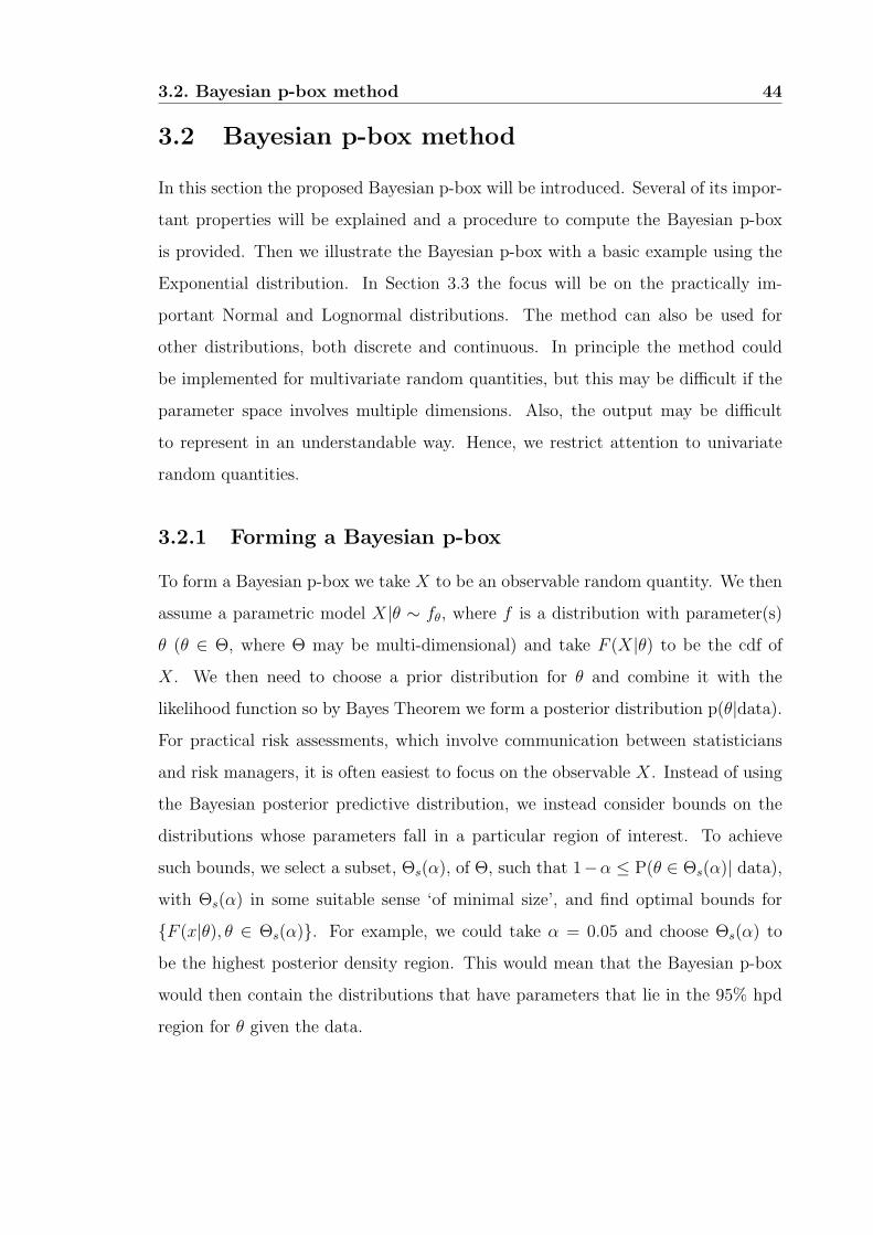
3.2. Bayesian p-box method 44
3.2 Bayesian p-box method
In this section the proposed Bayesian p-box will be introduced. Several of its impor-
tant properties will be explained and a procedure to compute the Bayesian p-box
is provided. Then we illustrate the Bayesian p-box with a basic example using the
Exponential distribution. In Section 3.3 the focus will be on the practically im-
portant Normal and Lognormal distributions. The method can also be used for
other distributions, both discrete and continuous. In principle the method could
be implemented for multivariate random quantities, but this may be difficult if the
parameter space involves multiple dimensions. Also, the output may be difficult
to represent in an understandable way. Hence, we restrict attention to univariate
random quantities.
3.2.1 Forming a Bayesian p-box
To form a Bayesian p-box we take X to be an observable random quantity. We then
assume a parametric model X|θ ∼ fθ, where f is a distribution with parameter(s)
θ (θ ∈ Θ, where Θ may be multi-dimensional) and take F (X|θ) to be the cdf of
X. We then need to choose a prior distribution for θ and combine it with the
likelihood function so by Bayes Theorem we form a posterior distribution p(θ|data).
For practical risk assessments, which involve communication between statisticians
and risk managers, it is often easiest to focus on the observable X. Instead of using
the Bayesian posterior predictive distribution, we instead consider bounds on the
distributions whose parameters fall in a particular region of interest. To achieve
such bounds, we select a subset, Θs(α), of Θ, such that 1−α ≤ P(θ ∈ Θs(α)| data),
with Θs(α) in some suitable sense ‘of minimal size’, and find optimal bounds for
{F (x|θ), θ ∈ Θs(α)}. For example, we could take α = 0.05 and choose Θs(α) to
be the highest posterior density region. This would mean that the Bayesian p-box
would then contain the distributions that have parameters that lie in the 95% hpd
region for θ given the data.

3.2. Bayesian p-box method 45
3.2.2 Choosing Θs(α)
For the purposes of this chapter, the highest posterior density (hpd) interval or
region (Subsection 2.7.1) for the parameter(s) of the distribution is used as Θs(α).
If the parametric distribution is not symmetric and unimodal, then the hpd interval
displays more important features of the posterior distribution than a credible interval
(Chen et al., 2001). If the posterior density is continuous and unimodal then the
hpd interval or region is a compact set as it is closed and bounded. As shown in Box
and Tiao (1973), it may occur that the 100(1−α)% credible region is identical to the
100(1− α)% confidence region in frequentist statistics, although the interpretation
is different. This is, for example, the case for some specific non-informative prior
distributions if the same sufficient statistic is used in both classical and Bayesian
approaches (Turkkan and Pham-Gia, 1997). There has been some discussion as to
whether the hpd region is appropriate, as it is not invariant under reparameterisation
(Bernardo and Smith, 1994). Other regions, such as Bernardo’s lowest posterior loss
region (Bernardo, 2005), which is invariant under reparameterisation, could be used
instead. In fact any subset of the parameter space Θ that is closed and bounded and
has a specific posterior probability could be used to construct Bayesian p-boxes.
3.2.3 Example: Exponential Distribution
Suppose that components of a machine are stress-tested, their lifetimes are measured
in days and that these lifetimes follow an Exponential distribution with parameter
λ, where λ is the distribution mean. Assume that a sample, x1, x2, ..., xn, of n = 30
such lifetimes is available, with sample mean 16.72 days and standard deviation 17.21
days. Consider the case α = 0.05 and find Θs(0.05), here the 95% hpd interval for
λ. If λ ∈ [c1, c2], then Θs(0.05) is derived by calculating values of c1 and c2 such
that the integral of the posterior distribution between c1 and c2 is equal to (1− α)
and the value of the posterior probability density function is equal at c1 and c2.

3.2. Bayesian p-box method 46
We define the prior probability density function to be:
p(λ|a, b) ∝ λ(a−1)exp (−λb) (3.1)
and multiply this by the likelihood function for the Exponential distribution to find
the corresponding posterior probability density function:
p(λ|x1, ...xn, a, b) ∝ λ(a+n)−1exp
(−λ
(b +
n∑i=1
xi
))(3.2)
Θs(0.05) for λ (c1 = 0.0392 and c2 = 0.0816) is illustrated in Figure 3.0.1 where
we use a non-informative Gamma prior distribution with shape parameter a = 0.001
and inverse scale parameter b = 1000. p(λ|x, a, b) represents the posterior probability
density given the shape and inverse scale parameters, a and b, and the data x.
Maximising and minimising the Exponential distribution over Θs(0.05) is equivalent
to plotting the Exponential distributions with λ equal to the endpoints of Θs(0.05)
due to the monotonicity of the Exponential cdf with respect to λ. This leads to the
Exponential Bayesian p-box shown in Figure 3.0.2.
Figure 3.1: Example for the Exponential distribution
0.02 0.04 0.06 0.08 0.10
5
10
15
20
25
30
35
λ
p(λ|
x, a
, b)
3.0.1 Posterior distribution of λ withΘs(0.05) (shown by the arrow)
0 50 100 1500
0.2
0.4
0.6
0.8
1
Component life (days)
Cum
ulat
ive
prob
abili
ty
3.0.2 95% Exponential Bayesian p-box
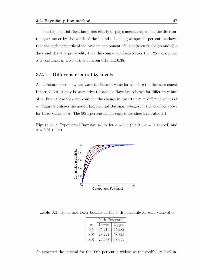
3.2. Bayesian p-box method 47
The Exponential Bayesian p-box clearly displays uncertainty about the distribu-
tion parameter by the width of the bounds. Looking at specific percentiles shows
that the 90th percentile of the random component life is between 28.2 days and 58.7
days and that the probability that the component lasts longer than 25 days, given
λ is contained in Θs(0.05), is between 0.13 and 0.38.
3.2.4 Different credibility levels
As decision makers may not want to choose a value for α before the risk assessment
is carried out, it may be attractive to produce Bayesian p-boxes for different values
of α. From these they can consider the change in uncertainty at different values of
α. Figure 3.1 shows the nested Exponential Bayesian p-boxes for the example above
for three values of α. The 90th percentiles for each α are shown in Table 3.1.
Figure 3.1: Exponential Bayesian p-box for α = 0.5 (black), α = 0.05 (red) andα = 0.01 (blue)
0 50 100 1500
0.2
0.4
0.6
0.8
1
Component life (days)
Cum
ulat
ive
prob
abili
ty
Table 3.1: Upper and lower bounds on the 90th percentile for each value of α
90th Percentileα Lower Upper0.5 35.219 45.2820.05 28.227 58.7250.01 25.538 67.055
As expected the interval for the 90th percentile widens as the credibility level in-

3.2. Bayesian p-box method 48
creases. Nested Bayesian p-boxes are useful to consider how much the uncertainty
increases as the credibility level increases.
3.2.5 Robustness to the prior distribution
A common criticism of Bayesian methods is that the prior distribution may influence
the posterior results of an analysis. We illustrated the use of a non-informative
prior distribution in Subsection 3.2.3. One can also consider using a class of prior
distributions to study robustness with respect to the prior distribution. To do this
for the Exponential case, we need to choose bounds for a and b. The posterior
distribution is a Gamma distribution with parameters a + n and b +∑n
i=1 xi. Now
suppose a priori that it is believed that the expected value of the random quantity
of interest is approximately E. Then we could, for example, choose a class of prior
distributions by taking s small, a ∈ (1+ε, s+1), where ε = 1e−15 and b ∈(
12Es
,∞).
Then as λ has a Gamma distribution, 1λ
has an Inverse-Gamma distribution, with
parameters a and θ = 1b, and thus θ ∈ (0, 2Es). The expected value of 1
λis θ
(a−1). So
when a = 1+ε, the expected value of 1λ
is in the interval(0, 2Es
ε
)and when a = 1+s,
the expected value of 1λ
is in the interval (0, 2E) which both seem reasonable as 1λ
is the mean of the Exponential distribution.
Let us consider two examples in which we use the same robustness criteria as
described above(a ∈ (1 + ε, s + 1) and b ∈
(1
2Es,∞))
, and the same value of s, but
with two different sample sizes.
1. Choose s = 2, E = 30 and randomly generate a sample of size 10 from an
Exponential distribution with λ = 120
. This yields∑n
i=1 xi = 273.11.
2. Choose s = 2, E = 30 and randomly generate a sample of size 100 from an
Exponential distribution with λ = 120
. This yields∑n
i=1 xi = 2034.99.
We split a into 20 equally spaced values including the endpoints and b into 20
equally spaced values including the endpoints. Taking the envelope of the possible
distributions, by using the endpoints of Θs(0.05), we find the 95% robust Exponen-
tial Bayesian p-boxes for these two examples. The 95% robust Exponential Bayesian

3.2. Bayesian p-box method 49
p-boxes are compared with 95% Exponential Bayesian p-boxes formed using a non-
informative gamma prior distribution with a = 0.001 and b = 1000 as before, in
Figures 3.2.1 and 3.2.2.
Figure 3.3: Comparison of Robust 95% Exponential Bayesian p-box (red) and 95%Exponential Bayesian p-box (blue)
0 50 100 150 200 2500
0.2
0.4
0.6
0.8
1
X
Cum
ulat
ive
Pro
babi
lity
3.2.1 Small sample: n = 10,∑ni=1 xi = 273.11
0 50 100 150 200 2500
0.2
0.4
0.6
0.8
1
X
Cum
ulat
ive
Pro
babi
lity
3.2.2 Larger sample: n = 100,∑ni=1 xi = 2034.99
It is clear that the inferences from a smaller data set are more influenced by the
choice of prior distribution resulting in wider bounds. Additional data lead to a more
peaked likelihood function which has a stronger influence on the inferences leading to
narrower bounds. The Exponential Bayesian p-box, formed using a non-informative
prior distribution, is enclosed within the Exponential p-box using the class of prior
distributions in both cases. The endpoints of the hpd intervals, c1 and c2, for the
non-informative prior distribution are enclosed within the interval of c1r and c2r,
where c1r and c2r are the endpoints of the robust hpd interval, in both cases. As
the Exponential Bayesian p-box is formed using these endpoints, the robust cases
will enclose the non-informative Exponential Bayesian p-boxes for these examples.
Including robustness to the prior distribution describes a little more uncertainty
which is indicated by the width of the bounds. As the sample size increases, both
uncertainty about λ and the influence of the prior distribution decrease. Thus, there
is not a large difference between the width of the bounds using the robust class of
prior distributions or the non-informative conjugate prior distribution for n = 100.
For these data sets which were randomly generated we used 30 as an estimate of E.
In practice, this value would need to be chosen by an expert or based on information

3.3. Normal and Lognormal distributions 50
available about the random quantity prior to data collection.
In this section we have introduced the procedure to form a Bayesian p-box and
illustrated it for the Exponential distribution. We have shown the possible benefit
of producing Exponential p-boxes for different credibility levels and that the method
can include robustness to the prior distributions. In the next section we consider how
to form a Bayesian p-box for the more complicated case of the Normal distribution.
3.3 Normal and Lognormal distributions
In this section the derivation of a Bayesian p-box for the Normal and Lognormal
distributions is discussed. The Lognormal distribution is frequently used in risk as-
sessments, in particular for assessment of the magnitude of effects by estimating the
proportion of species for which exposure to a chemical exceeds some threshold level
(e.g. LD50 or NOEC). To describe the variation in these threshold levels between
species, a species sensitivity distribution (see Section 2.5) is often used. As this is
frequently assumed to be Lognormal (EFSA, 2005), the illustrative example shown
in Subsection 3.3.3 is for the Lognormal distribution.
3.3.1 Bayesian P-boxes for the Normal distribution
We assume that a random quantity X has a Normal distribution with parameters
µ and σ. Box and Tiao (1973) present the equation of the joint hpd region for
parameters µ and σ assuming locally uniform prior distributions for µ and ln(σ).
In this case Θs(α) is the hpd region containing the (µ, σ) pairs with 100(1 − α)%
posterior probability. We find the hpd region by evaluating the double integral:
∫R
p(µ, σ|data) dµ dσ (3.3)
where the region R is given by: h(µ, σ) =−(n+1)ln(σ)− 12σ2 [(n−1)s2+n(µ−y)2] ≥ d,
where y is the sample mean, s is the sample standard deviation and d is a constant.
To do this, we integrate numerically over R at different values of d until we find
the region, Θs(α), that contains 100(1 − α)% probability. Then we find the (µ, σ)

3.3. Normal and Lognormal distributions 51
pairs from Θs(α) that optimise the Normal cdf, and use these to find bounds on
the distribution of the random quantity X. So we need to calculate the (µ, σ) pairs
that optimise the function g = Φ(
x−µσ
), where Φ(·) is the standard Normal cdf. It
is clear that the Normal cdf is maximised (minimised) by maximising (minimising)(x−µ
σ
), with fixed x ∈ R, µ ∈ R and σ > 0.
If X ∼ N(µ, σ2), then Θs(α) is a strictly convex set defined by g(µ, σ) ≥ d,
where d is a fixed constant, and it is closed and bounded. Therefore the gradient
of the boundary of the set, that we call the contour, is continuous and constantly
changing everywhere. The (µ, σ) pairs found by tracing the contour, where Θs(α) =
d, maximise and minimise the cdf of X for all x, justification is given in Subsection
3.3.2. We can then form the Bayesian p-box by plotting the value of the cdf at each
x given the values of each optimal (µ, σ) pair from the contour.
The parameters µ and σ are location and scale parameters respectively and
this result generalises to other location-scale distributions, such as the Student t-
distribution and the Cauchy distribution, as long as the derived region, Θs(α), is
closed and bounded. This result allows the use of an efficient algorithm for the
computations involved in the derivation of such Bayesian p-boxes. Suppose that
(µ1, σ1) maximises the cdf (over Θs(α), and hence this point is on its boundary) at
a particular value of x, say x1. To find the maximum of the cdf at a point close to
x1, we only need to search the values of (µ, σ) on the boundary of Θs(α) that are
close to (µ1, σ1). Alternatively to speed up computation we can split the contour
into several (µ, σ) pairs to give an approximate Bayesian p-box.
3.3.2 Justification
We first show that the values of µ and σ that maximise (minimise) f = x−µσ
are
on the contour. To maximise f , one needs to minimise σ. The smallest values of
σ possible in Θs(α) at any µ will fall on the contour. Similarly to minimise f , one
needs to maximise σ and the maximum σ values possible at any µ will fall on the
contour.
Consider the contour h(µ, σ) = d. An example of a possible contour and the
resulting Bayesian p-box is shown in Figures 3.3.1 and 3.3.2 to aid understanding.

3.3. Normal and Lognormal distributions 52
The blue half of the contour corresponds to the resulting blue maximum bound for
the Bayesian p-box and similarly the red half corresponds to the resulting minimum
bound. This is a closed strictly convex set and therefore the gradient of the contour
is different at all points, changes continuously and takes all directions.
Figure 3.3: Example of a possible contour and the resulting Bayesian p-box
0.2 0.4 0.6 0.8 1 1.2 1.4 1.6
0
0.5
1
1.5
2
σ
µ
3.3.1 Possible contour
-5 0 5 100
0.1
0.2
0.3
0.4
0.5
0.6
0.7
0.8
0.9
1
Log10
Concentration (µg / kg)C
umul
ativ
e P
roba
bilit
y
3.3.2 95% Normal Bayesian p-box withmodal distribution (black)
Standard optimisation theory states that the gradient of the function f must be
a negative multiple of the gradient of the contour where the contour optimises the
function e.g. Boas (1983). Consider optimising the function f = x−µσ
with respect
to the contour h(µ, σ) = d. Then ∇(f) = −λ∇h(µ, σ), where λ is a constant and
∇(f) =
(µ−x)σ2
−1σ
(3.4)
The first term of the vector is a continuous function of x. For x ∈ R, it is clear from
∇h(µ, σ) = ∇(f)−λ
that:
x → −∞ : ∇h(µ, σ) →
−∞1
λσ
(3.5)
x → µ : ∇h(µ, σ) →
0
1λσ
(3.6)
x →∞ : ∇h(µ, σ) →
∞1
λσ
(3.7)

3.3. Normal and Lognormal distributions 53
so the gradient changes continuously with x. The gradient of the function h that
optimises f must follow the above pattern as x increases. Therefore it is clear
that the contour optimises f . To see which half of the contour is maximising f we
consider the contour h(µ, σ) ≤ d − ε, where ε is a small positive constant. This
contour will be larger as it contains more probability. Again we consider the edge
of the contour at h(µ, σ) = d− ε. As we move from the contour h(µ, σ) = d to the
contour h(µ, σ) = d − ε, we find that the values of µ increase for the upper half of
the contour and decrease at the lower half of the contour for given σ. This leads to
an increase in f = x−µσ
for the lower half of the contour and a decrease in f for the
upper half of the contour. Therefore the upper half of the contour is minimising f
and the lower half of the contour is maximising f .
3.3.3 Example: Lognormal distribution with small n
To illustrate the Bayesian p-box method, consider the No Observed Effect Concen-
tration (NOEC) of Cadmium (µg Cd/g) of seven soil organisms data (Table 3.2)
from Van Straalen and Denneman (1989), also used by Aldenberg and Jaworska
(2000).
Table 3.2: NOEC for toxicity of Cadmium (µg Cd/g) of soil organisms.
Species 1 2 3 4 5 6 7NOEC values 0.97 3.33 3.63 13.50 13.80 18.70 154.00log10 (NOEC) -0.013 0.522 0.560 1.130 1.140 1.272 2.188
Assuming that the data come from a Lognormal distribution, Log10(data) follows
a Normal distribution. Let us consider using the non-informative prior, p(µ, σ) = 1σ,
and take α = 0.05. Θs(0.05), the 95% hpd region, is found by numerical integration,
and is shown in Figure 3.4.1, where the mode of the posterior distribution is also
indicated. Maximising and minimising the Normal cdf over Θs(0.05) leads to the
95% Normal Bayesian p-box shown in Figure 3.4.2. The uncertainty about the
variability is indicated by the width of the bounds. The modal distribution, i.e. the
distribution with the mode of the posterior distribution as its parameters, is also
shown.
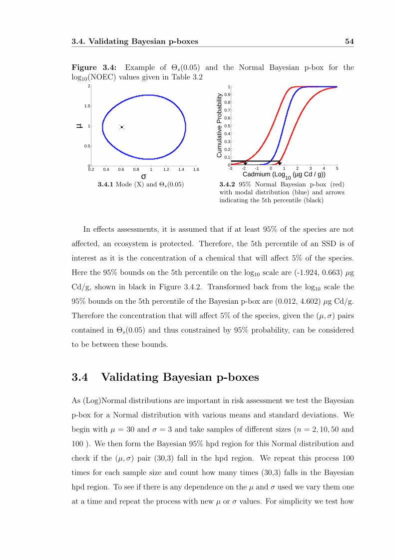
3.4. Validating Bayesian p-boxes 54
Figure 3.4: Example of Θs(0.05) and the Normal Bayesian p-box for thelog10(NOEC) values given in Table 3.2
0.2 0.4 0.6 0.8 1 1.2 1.4 1.60
0.5
1
1.5
2
σ
µ
3.4.1 Mode (X) and Θs(0.05)
-3 -2 -1 0 1 2 3 4 50
0.1
0.2
0.3
0.4
0.5
0.6
0.7
0.8
0.9
1
Cadmium (Log10
(µg Cd / g))
Cum
ulat
ive
Pro
babi
lity
3.4.2 95% Normal Bayesian p-box (red)with modal distribution (blue) and arrowsindicating the 5th percentile (black)
In effects assessments, it is assumed that if at least 95% of the species are not
affected, an ecosystem is protected. Therefore, the 5th percentile of an SSD is of
interest as it is the concentration of a chemical that will affect 5% of the species.
Here the 95% bounds on the 5th percentile on the log10 scale are (-1.924, 0.663) µg
Cd/g, shown in black in Figure 3.4.2. Transformed back from the log10 scale the
95% bounds on the 5th percentile of the Bayesian p-box are (0.012, 4.602) µg Cd/g.
Therefore the concentration that will affect 5% of the species, given the (µ, σ) pairs
contained in Θs(0.05) and thus constrained by 95% probability, can be considered
to be between these bounds.
3.4 Validating Bayesian p-boxes
As (Log)Normal distributions are important in risk assessment we test the Bayesian
p-box for a Normal distribution with various means and standard deviations. We
begin with µ = 30 and σ = 3 and take samples of different sizes (n = 2, 10, 50 and
100 ). We then form the Bayesian 95% hpd region for this Normal distribution and
check if the (µ, σ) pair (30,3) fall in the hpd region. We repeat this process 100
times for each sample size and count how many times (30,3) falls in the Bayesian
hpd region. To see if there is any dependence on the µ and σ used we vary them one
at a time and repeat the process with new µ or σ values. For simplicity we test how

3.4. Validating Bayesian p-boxes 55
often the true µ and σ values fall in the hpd region, as then the true distribution
will fall in the 95% Bayesian p-box. The results from 100 simulations for various µ
and σ values are shown in Table 3.3.
Table 3.3: Results for 100 simulations
µ σ n Success out of 100
30
3
2 9810 9850 97100 98
5
2 9610 9950 99100 99
7
2 9610 9850 98100 99
9
2 9510 9850 99100 98
20 3
2 9510 9750 98100 98
40 3
2 9510 9950 99100 99
50 3
2 9810 9750 98100 100

3.5. Generalisations 56
It is clear that there is some sampling variation so some samples lead to hpd
regions where the parameters of the true distribution are not included. However
generally the Bayesian p-box includes the true distribution in most of the simu-
lations, even for n as small as 2 and therefore seems a reasonably robust method
to use. The method is not affected by the change of µ and σ as we would expect
because the method takes the sample mean and standard deviation into account.
For small samples the size of the hpd region increases, resulting in a wide Bayesian
p-box, which leads to the n = 2 case producing good results.
3.5 Generalisations
Two topics which are of practical interest are robustness with respect to the prior
distribution and imprecision in the data. In effects assessments, sample sizes may
be as small as 2, so any prior distribution can have a large influence on the posterior
distribution. Therefore it is useful to consider robustness with respect to the influ-
ence of the prior distribution. Robustness for the Normal distribution with respect
to the prior distribution(s) for µ and σ is considered in Subsections 3.5.1 and 3.5.3.
For a detailed introduction to robust Bayesian analysis we refer to Berger (1990).
In practice, data sets may be given as interval data, for example when an indication
of measurement uncertainty is given. A straightforward method for including such
imprecision in data in the analysis is presented in Subsection 3.5.5.
3.5.1 Robustness to the prior distribution for µ
To investigate robustness with respect to the prior distribution for µ, we consider
a class of Normal prior distributions for µ given values of σ. We will call this the
interval class of prior distributions. The resulting Bayesian p-box will be called the
‘robust Normal Bayesian p-box’. Keeping the non-informative prior distribution for
σ, p(σ) = 1σ, a Normal class of prior distributions for µ|σ is chosen:
{p(µ, σ) : p(µ, σ) ∼ N
(a,
σ2
n
); a ∈ [c, v]
}(3.8)

3.5. Generalisations 57
and the prior interval for the mean, a, is chosen to be between constants c and v.
Calculating the posterior distribution, and repeating the previous steps, as in Box
and Tiao (1973) and Subsection 2.7.2, leads to the equation of a density contour:
−(n + 2)ln(σ)− 1
2σ2
((n− 1)s2 +
n
2(x− a)2 + 2n
(µ−
(a + x
2
))2)
= d (3.9)
To find Θs(0.05), integrate the posterior distribution over different regions to
find the region enclosing 95% probability. To perform the integration, values for c
and v must be chosen. Here c and v are the prior limits on the mean of µ that
should be chosen by an expert or based on available evidence.
3.5.2 Example: A robust Normal Bayesian p-box
We have a small data set (n = 3) sampled from a Normal distribution with mean
100 and standard deviation 15. The sample statistics are x = 96.83 and s = 8.58
and we take the interval a ∈ [66, 116]. We split this interval by taking 20 equally
spaced values, ai, i = 1, ..., 20, including the endpoints for illustrative purposes and
this produces the regions Θs(ai)(0.05). Figure 3.5.1 shows these regions and the
variation in their shape as the range of σ changes at different values of a. As the
interval for a is longer below x there will be larger contours at lower µ values than
there will be at higher µ values. This can clearly be seen in Figure 3.5.1. This is
because, as the prior value that we specify for the mean moves further away from
the sample mean, the values for µ in the posterior will be lower. Therefore σ has to
increase for the sample to be able to come from a distribution with such a low value
for µ. The larger σ values will contribute mostly to the lower tail of the maximum
(left) bound, but also slightly to the upper tail of the minimum (right) bound of
the robust Normal Bayesian p-box. If the interval had been longer above x, then
the larger contours that we see at lower µ values would have instead been at higher
µ values. These larger σ values would mostly contribute to the upper tail of the
minimum (right) bound but also slightly to the lower tail of the maximum (left)
bound of the robust Normal Bayesian p-box.

3.5. Generalisations 58
We also look at a larger sample (n = 50) from a Normal distribution with mean
100 and standard deviation 15. The sample statistics are x = 96.48 and s = 13.54
and we take the interval a ∈ [66, 116]. Figure 3.5.2 shows the regions Θs(ai)(0.05) for
this data set where the interval a is again split by taking 20 equally spaced values
including the endpoints.
Figure 3.5: Examples of Θs(ai)(0.05) for both data sets
0 20 40 60 8040
60
80
100
120
140
σ
µ
3.5.1 Example of Θs(ai)(0.05) for n = 3, x =
96.83 and s = 8.58
10 15 20 25 30 3570
80
90
100
110
120
σ
µ
3.5.2 Example of Θs(ai)(0.05) for n = 50,
x = 96.48 and s = 13.54
To approximate the robust Normal Bayesian p-box for both data sets, we can
take many values of a (20 equally spaced values including the endpoints in this
example), maximise and minimise over the 100(1 − α)% contours by taking 100
(µ, σ) pairs from the boundary of each contour, and plot the envelope of all these
distributions. Figure 3.6.1 shows the 95% robust Normal Bayesian p-box and the
95% Normal Bayesian p-box, using a non-informative prior, p(µ, σ) = 1σ, for the
n = 3 example. Figure 3.6.2 shows the 95% robust Normal Bayesian p-box and the
95% Normal Bayesian p-box for the n = 50 example.

3.5. Generalisations 59
Figure 3.6: Robust Normal Bayesian p-boxes
-50 0 50 100 150 2000
0.2
0.4
0.6
0.8
1
X
Cum
ulat
ive
Pro
babi
lity
3.6.1 Robust 95% Normal Bayesian p-boxfor n = 3, x = 96.83 and s = 8.58 (blue)with 95% Normal Bayesian p-box (red) andmodal distribution (dashed)
-50 0 50 100 150 2000
0.2
0.4
0.6
0.8
1
X
Cum
ulat
ive
Pro
babi
lity
3.6.2 Robust 95% Normal Bayesian p-boxfor n = 50, x = 96.48 and s = 13.54 (blue)with 95% Normal Bayesian p-box (red) andmodal distribution (dashed)
We can see here that the larger data set leads to more certainty about the
parameters and therefore a narrower p-box. It is helpful that the graphical display
of any type of p-box allows an intuitive assessment of the uncertainty based on
the width of the bounds. In Figures 3.7.1 and 3.7.2, we show the contour for each
data set using the same non-informative prior as we used previously, p(µ, σ) = 1σ,
alongside the contours for the robust 95% Normal Bayesian p-boxes.
Figure 3.7: Θs(ai)(0.05) for the robust cases and using a non-informative prior
0 20 40 60 8040
60
80
100
120
140
σ
µ
3.7.1 For n = 3, x = 96.83 and s = 8.58, ro-bust case (black) and non-informative case(red)
10 15 20 25 30 3575
80
85
90
95
100
105
110
115
120
σ
µ
3.7.2 For n = 50, x = 96.48 and s = 13.54,robust case (black) and non-informativecase (red)

3.5. Generalisations 60
These regions show that the 95% Bayesian p-box should be contained within
both robust 95% Normal Bayesian p-boxes. We can see this is true in Figures 3.6.1
and 3.6.2. Also, Figure 3.6.1 shows that for the n = 3 case, the larger contours at
lower µ values lead to the extra width at the bottom of the maximum (left) bound
and the top of the minimum (right) bound of the robust 95% Normal Bayesian p-
box. The narrower range of σ values for larger n leads to the narrower limits on the
robust 95% Normal Bayesian p-box in Figure 3.6.2.
3.5.3 Robustness to the prior distribution for µ and σ
To study robustness with respect to the prior distribution for µ and σ together, we
choose a set of prior distributions for both parameters. We will call the result the
‘robust (µ, σ) Normal Bayesian p-box’. Consider an interval on σ and a class of
Normal prior distributions on µ given values of σ. So the joint prior distribution is
as follows: {p(µ, σ) ∼ N
(a,
σ2x
n
): a ∈ {µl, µu}, σx ∈ {σl, σu}
}(3.10)
where µl, µu, σl and σu are the chosen prior limits for µ and σ respectively. Calcu-
lating the posterior distribution, and repeating the steps as in Box and Tiao (1973)
and Subsection 2.7.2 for this new posterior distribution, leads to density contour:
−ln(σx)− nln(σ)− n
2σ2x
(µ− a)2 − 1
2σ2
((n− 1)s2 + n (x− µ)2) = d
To find Θs(α), integrate over the posterior distribution to find the region enclos-
ing 100(1 − α)% probability. Values for µl, µu, σl and σu must be chosen by an
expert based on available evidence.
For the numerical integration it is necessary to calculate the normalising constant
k. Unfortunately this can only be derived numerically so the following results are
again approximations. The lack of an exact normalising constant causes problems
with numerical integration so the standard Matlab function, contour, is used to
obtain numerical approximations to the contours. Contour allows the user to specify
a grid of values for two random quantities (here µ and σ) and plot corresponding

3.5. Generalisations 61
contours at different heights (here at different heights of the posterior distribution).
3.5.4 Example: A robust (µ, σ) Normal Bayesian p-box
We consider a data set of size 10 (n = 10), randomly sampled from a Normal
distribution with mean 100 and standard deviation 15. The sample statistics are
x = 98.40 and s = 9.51. Now consider the intervals from µl = 94 to µu = 102, and
from σl = 8 to σu = 11. We need to find all the contours for each prior combination
of µ and σ.
An example is shown in Figure 3.8.1, where the prior interval σx is split into four
equal parts and the prior interval a is split into three equal parts, both including
the endpoints, so the contours can be seen more clearly. We denote the different
combinations of σx and a by ri, i = 1, ..., 12, as there are 12 combinations of a and
σx. Figure 3.8.2 shows the resulting Θs(ri)(0.05) where the prior interval for σ is
split into five equal parts and the prior interval for µ is split into ten equal parts
(For this case, i = 1, ..., 50).
Figure 3.8: Examples of Θs(ri)(0.05) for n=10, x = 98.40 and s = 9.51
6 8 10 12 1492
94
96
98
100
102
104
σ
µ
3.8.1 µl = 94, µu = 102, σl = 8, σu = 11
6 8 10 12 14 1692
94
96
98
100
102
104
σ
µ
3.8.2 µl = 94, µu = 102, σl = 8, σu = 11

3.5. Generalisations 62
We see that the range for σ is wider for the contours where a is close to the
mean of the data than for the contours where a moves away from the mean. For
larger values of a the range for σ will increase again. To see this, consider the 95%
highest posterior regions for σx = 8, with a = 98.5, 99.5, 100.5, 101.5 and 104, shown
in Figure 3.9.
Figure 3.9: 95% hpd regions for σx = 8 and a = 98.5 (blue), 99.5 (green), 100.5(red), 101.5 (yellow) and 104 (black)
6 8 10 12 14 1694
96
98
100
102
104
106
σ
µ
Figure 3.9 shows that the lowest contour (where a = 98.5) has the second largest
range of σ values. This is because there is agreement between the prior value for
µ (i.e. a) and the data mean (x) which leads to the posterior values for µ being
close to the mean value of the data. Therefore there is low probability at higher and
lower values of µ as both the likelihood function and the prior distribution suggest
that µ should be around the mean. For the other contours the value of a leads to a
conflict between the prior value of µ and the mean of the data. The conflict leads
to more µ values having higher posterior probabilities and therefore being included
in the hpd region. This leads to a posterior distribution that is not symmetrical
about the mean. As a increases, the hpd region becomes less and less symmetrical
about the mean, leading to narrower ranges of σ. However, eventually the range of
σ starts to increase again. Figure 3.9 shows the highest contour (where a = 104)
has the largest range of σ values. This is because the mean of the data and the
prior value a assigned for µ are far apart and therefore the posterior distribution
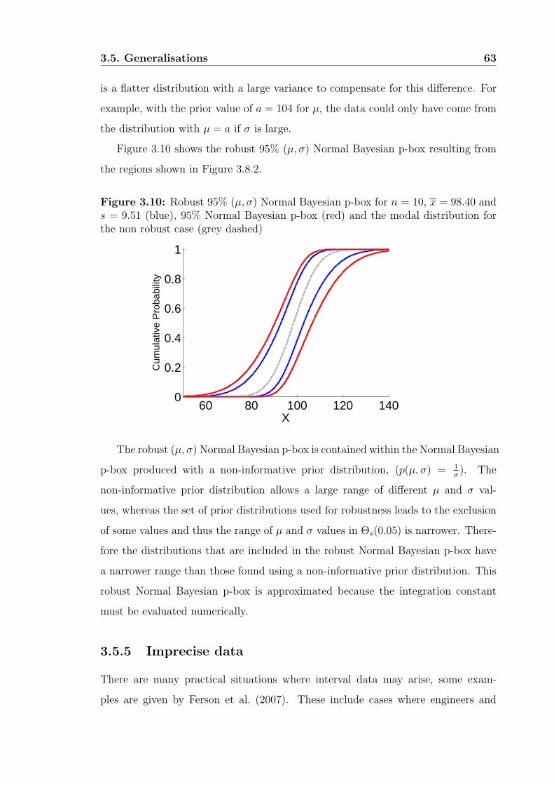
3.5. Generalisations 63
is a flatter distribution with a large variance to compensate for this difference. For
example, with the prior value of a = 104 for µ, the data could only have come from
the distribution with µ = a if σ is large.
Figure 3.10 shows the robust 95% (µ, σ) Normal Bayesian p-box resulting from
the regions shown in Figure 3.8.2.
Figure 3.10: Robust 95% (µ, σ) Normal Bayesian p-box for n = 10, x = 98.40 ands = 9.51 (blue), 95% Normal Bayesian p-box (red) and the modal distribution forthe non robust case (grey dashed)
60 80 100 120 1400
0.2
0.4
0.6
0.8
1
X
Cum
ulat
ive
Pro
babi
lity
The robust (µ, σ) Normal Bayesian p-box is contained within the Normal Bayesian
p-box produced with a non-informative prior distribution, (p(µ, σ) = 1σ). The
non-informative prior distribution allows a large range of different µ and σ val-
ues, whereas the set of prior distributions used for robustness leads to the exclusion
of some values and thus the range of µ and σ values in Θs(0.05) is narrower. There-
fore the distributions that are included in the robust Normal Bayesian p-box have
a narrower range than those found using a non-informative prior distribution. This
robust Normal Bayesian p-box is approximated because the integration constant
must be evaluated numerically.
3.5.5 Imprecise data
There are many practical situations where interval data may arise, some exam-
ples are given by Ferson et al. (2007). These include cases where engineers and

3.5. Generalisations 64
other scientists report the uncertainty associated with calibration of their measur-
ing equipment with an interval, gross ignorance where we have no data about a
random quantity so we assign theoretical limits, and when numbers are rounded to
significant digits. Here we consider the case where data have been provided with an
indication of the measurement uncertainty surrounding the values.
Suppose that a data set, x1, x2, ..., xn, has a particular measurement uncertainty
stated, {−ε, +δ}, for ε, δ > 0. This means that the actual value corresponding to a
reported measurement xi is only known to be in the interval [xi − ε, xi + δ] and all
values have the same measurement error. To find the ‘lowest’ Normal distribution
(i.e. shifted furthest to the left) that could describe the data, we can take all the
values xi − ε, and to find the highest Normal distribution that could describe the
data we would take all the values xi + δ. This follows Manski (2003), where it is
stated that if y is observed to lie in [y−, y+], then the distribution P (y+) is a feasible
value of P (y) and stochastically dominates all other feasible values of P (y). This
means that the cdf of P (y+) is less than or equal to the cdf of P (y) at any value
y. This is the case as P (y+) has the same shape as P (y) but it is moved further to
the right. Similarly the distribution P (y−) is stochastically dominated by all other
feasible values of P (y), as the cdf of P (y) is less than or equal to the cdf of P (y−)
because the cdf of P (y−) is the cdf of P (y) shifted to the left.
3.5.6 Example: Normal Bayesian p-boxes for imprecise data
A random sample of size n = 40 is taken from a Normal distribution with mean
100 and standard deviation 15. The sample statistics are x = 102.31 and s = 13.90.
Consider very substantial data imprecision specified by δ = ε = 10. The procedure
presented in Subsection 3.3.1 can be used to form a contour using numerical inte-
gration for each extreme case of values (i.e. taking all values xi − ε or xi + δ) and
the original data set. These are presented in Figure 3.11.1. We adjust the values
by either adding δ to all the values or subtracting ε from all the values so that
the sample standard deviation, s, remains the same. Therefore the contours are all
the same shape and only the location of the data set is adjusted by ε or δ. So it
is only necessary to calculate the contour for the original data set and maximise
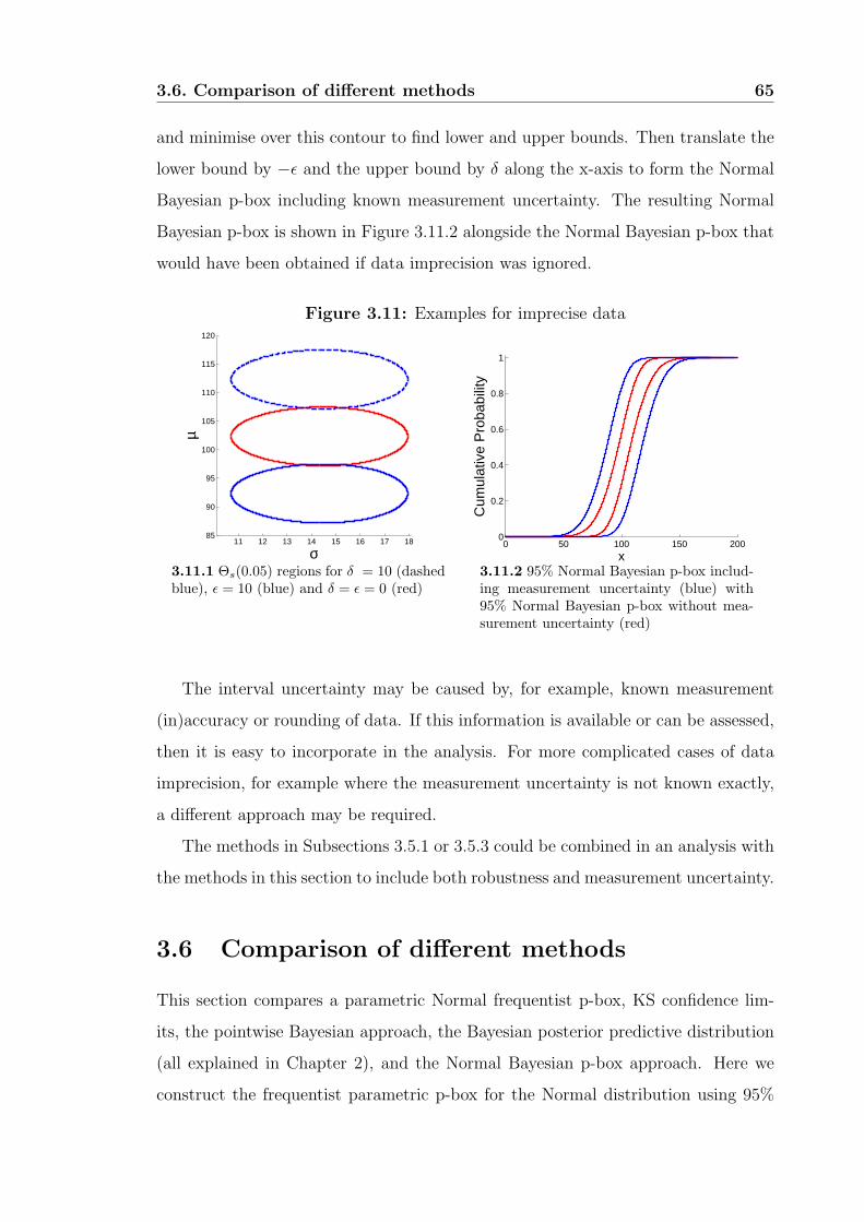
3.6. Comparison of different methods 65
and minimise over this contour to find lower and upper bounds. Then translate the
lower bound by −ε and the upper bound by δ along the x-axis to form the Normal
Bayesian p-box including known measurement uncertainty. The resulting Normal
Bayesian p-box is shown in Figure 3.11.2 alongside the Normal Bayesian p-box that
would have been obtained if data imprecision was ignored.
Figure 3.11: Examples for imprecise data
11 12 13 14 15 16 17 1885
90
95
100
105
110
115
120
σ
µ
3.11.1 Θs(0.05) regions for δ = 10 (dashedblue), ε = 10 (blue) and δ = ε = 0 (red)
0 50 100 150 2000
0.2
0.4
0.6
0.8
1
x
Cum
ulat
ive
Pro
babi
lity
3.11.2 95% Normal Bayesian p-box includ-ing measurement uncertainty (blue) with95% Normal Bayesian p-box without mea-surement uncertainty (red)
The interval uncertainty may be caused by, for example, known measurement
(in)accuracy or rounding of data. If this information is available or can be assessed,
then it is easy to incorporate in the analysis. For more complicated cases of data
imprecision, for example where the measurement uncertainty is not known exactly,
a different approach may be required.
The methods in Subsections 3.5.1 or 3.5.3 could be combined in an analysis with
the methods in this section to include both robustness and measurement uncertainty.
3.6 Comparison of different methods
This section compares a parametric Normal frequentist p-box, KS confidence lim-
its, the pointwise Bayesian approach, the Bayesian posterior predictive distribution
(all explained in Chapter 2), and the Normal Bayesian p-box approach. Here we
construct the frequentist parametric p-box for the Normal distribution using 95%
3.6. Comparison of different methods 66
frequentist confidence intervals for µ and σ (Aughenbaugh and Paredis, 2006).
3.6.1 Example: Comparing methods for small n
For small n, consider a typical data set for avian risk assessment for pesticides. In
the European Council Directive 91/414/EEC, it is stated that the acute oral toxicity
of an active substance must be determined for either a quail species or the mallard
duck. There are typically two species available and the same two are generally
used. Suppose that for a certain pesticide, toxicity tests were conducted on these
species resulting in median lethal doses (LD50 in mg/kg bw) of 400 (quail) and
2000 (mallard). It is assumed that these two data points come from a Lognormal
distribution. The bounds from each method at the 5th percentile are shown in Table
3.4. Figures 3.12.1 and 3.12.2 present the results of the different methods with 95%
confidence or credibility levels. In Figure 3.12.2, the modal distribution is omitted so
that the median can be clearly seen. The Bayesian posterior predictive distribution
gives a 5th percentile of 1.971 mg/kg bw on the log10 scale. In the current legislation
for birds, European Commission (2002b), the toxicity-exposure ratio (TER) is found
by taking the lowest data point and dividing by an exposure value. This is then
compared with a threshold level of 10. So when the TER > 10, the chemical is
considered safe. Rearranging the equation shows us that the chemical is considered
to be safe if exposure is less than 40 mg/kg bw. On the log10 scale this equates to
1.6 mg/kg bw. This suggests that the current approach is not conservative when
compared to the results for the probabilistic methods shown in Table 3.4, because it
is not below their lower limits. However it is more conservative than the posterior
predictive distribution on the log10 scale (1.971 mg/kg bw). However the approaches
shown in Table 3.4 all envelope the current method which indicates that a safe level
could be much lower than implied by the current approach.

3.6. Comparison of different methods 67
Table 3.4: Comparison of bounds on 5th percentile in log10 (mg/kg bw)
Lower Upper95% parametric Normal frequentist p-box -27.43 7.0395% Normal Bayesian p-box approach -14.99 3.9595% KS confidence limits - ∞ 3.301095% pointwise Bayesian approach -23.03 2.82
Figure 3.12: Examples for a small sample size
-30 -25 -20 -15 -10 -5 0 5 10 15 20 25 300%
10%
20%
30%
40%
50%
60%
70%
80%
90%
100%
log10
Dose (mg / kg bw)
Per
cent
age
of S
peci
es
3.12.1 95% parametric Normal frequen-tist p-box (red), 95% Normal Bayesianp-box (blue), modal disribution (blackdashed), Bayesian posterior predictivedistribution (red dotted)
-30 -25 -20 -15 -10 -5 0 5 10 15 20 25 300%
10%
20%
30%
40%
50%
60%
70%
80%
90%
100%
log10
Dose (mg / kg bw)
Per
cent
age
of S
peci
es
3.12.2 95% Normal Bayesian p-box(blue), 95% KS confidence limits(black dashed), 95% pointwise Bayesianmethod (green), median distribution(green dotted) and data (black dots)
The values in Table 3.4 appear to be similar because they are given on a log10
scale, but there are actually large differences between the methods. The Normal
frequentist p-box method gives wider bounds than the other methods at high and
low percentiles. This may be due to the fact that the subspace of Θ in the Normal
frequentist p-box method is a rectangle between the smallest and largest µ and σ
pairs, whereas in the Normal Bayesian p-box method it is a strictly convex set,
here oval-shaped, where the dependence of µ and σ is taken into account. This
indicates that ignoring the dependence between parameters leads to wider bounds
at the higher and lower percentiles than when dependence is taken into account. If
narrower confidence intervals for µ and σ had been chosen, so the rectangular sub-
space of Θ was enclosed in the Bayesian oval, the Normal frequentist p-box would
fall within the Normal Bayesian p-box. At the 50th percentile, it is clear that the
Normal frequentist p-box is narrower than the other methods because of the way
it is constructed, ignoring dependence between µ and σ. If the frequentist Normal

3.6. Comparison of different methods 68
p-box was constructed using, for example, a joint confidence region for µ and σ, as
described in Burmaster and Thompson (1998), it may provide bounds closer to the
Bayesian p-box bounds as the joint confidence region is designed to take dependen-
cies between µ and σ into account. However both confidence regions described in
Burmaster and Thompson (1998) use approximations. One uses a χ2 approximation
which may not be appropriate for small n, the other uses a Taylor series approxi-
mation and it is not clear what effect these approximations will have on the output.
The KS confidence limits are based on no assumptions about distribution shape and
are very wide to include the large sampling uncertainty due to the small sample size.
The lower limit is −∞, although there may be practical reasons to bound this at a
particular value.
The lower and upper bounds according to the Bayesian pointwise method are
lower, at the 5th percentile, than those based on the Normal Bayesian p-box. This
is because in the former method the uncertainty is estimated about the percentile,
irrespective of the rest of the distribution, and a scaled non-central t-distribution
is used to calculate the bounds. The Normal Bayesian p-box takes the whole dis-
tribution into account when finding the bounds as it takes the (µ, σ) pairs from
the 100(1 − α)% hpd region, whereas the pointwise method finds the α2
and (1−α)2
-
percentiles of the scaled non-central t-distribution at each percentile.
The 5th percentile of the Bayesian posterior predictive distribution is a predic-
tion for a random individual and produces a single line rather than upper and lower
bounds. The Bayesian posterior predictive distribution would be appropriate when
a random species is of interest, or it can be used for checking the underlying as-
sumptions of the model (Lee, 2004). This can be done by simulating samples from
the Bayesian posterior predictive distribution and comparing these samples with the
observed data set. If there are large differences between them this may indicate that
the chosen model is not appropriate (Gelman et al., 1995).
Clearly which method should be used depends on whether the specific percentile
or the whole distribution is of interest. In practice, it will often be useful to present
methods together to get a better picture of the uncertainty and variability involved.

3.6. Comparison of different methods 69
However, the results and the differences between the methods would need to be
clearly communicated to risk managers to avoid confusion.
3.6.2 Example: Comparing methods for larger n
We consider a larger data set (n = 50) sampled from a Normal distribution with
mean 200 and standard deviation 20. The sample statistics are x = 194.71 and
s = 18.75. For this n, an approximate Normal Bayesian p-box may be formed by
finding Θs(α) using a χ2 approximation, and maximising and minimising over this.
The results from all the methods (assuming α = 0.05) are shown in Figures 3.13.1
and 3.13.2.
Figure 3.13: Examples for n = 50
100 150 200 250 3000
0.1
0.2
0.3
0.4
0.5
0.6
0.7
0.8
0.9
1
x
Cum
ulat
ive
Pro
babi
lity
3.13.1 95% Normal frequentist p-box(red), 95% approximate (χ2) NormalBayesian p-box (blue dashed), Bayesianposterior predictive distribution (dottedred) and data (black dots)
100 150 200 250 3000
0.1
0.2
0.3
0.4
0.5
0.6
0.7
0.8
0.9
1
x
Cum
ulat
ive
Pro
babi
lity
3.13.2 95% Normal Bayesian p-box(blue), 95% KS confidence limits(black dashed), 95% Bayesian pointwisemethod (green dashed), median distri-bution (green dotted) and data (blackdots)
The Normal frequentist p-box is slightly wider than the Bayesian methods at
lower and higher percentiles and narrower at the median, although there is not a large
difference. The χ2 approximation results are close to the Normal Bayesian p-box. As
n increases to infinity the bounds will converge to the true distribution (assuming
the true distribution was Normal). The Bayesian pointwise method bounds are
now enclosed within the Normal Bayesian p-box. These narrower pointwise bounds
are due to the shape of the scaled non-central t-distribution with n − 1 degrees
of freedom. This becomes more peaked and less skewed as n increases and so the
percentiles enclosing 95% become narrower. KS confidence limits are particularly

3.7. Dependence 70
useful when there is no reason to assume any specific distribution, as they provide
limits on the empirical distribution function. The Bayesian posterior predictive
distribution indicates a prediction for a random individual and is contained within
all the other p-boxes shown here. To illustrate the uncertainties involved it is again
useful to represent the results from several methods. If a decision is to be made
about a population, then methods that form bounds on variability should be used.
If a decision is about a random individual from a population then predictive methods
should be implemented.
The computation of frequentist parametric p-boxes is not affected by large n, as
it only requires intervals for the input parameters. A large n does not cause prob-
lems with computation of KS confidence limits because it is a simple calculation
based on n and α. The Bayesian posterior predictive distribution is not affected by
large n as it uses the sufficient sample statistics. The Bayesian pointwise method
becomes slower as n increases and as the number of percentiles evaluated increases.
However, even for n = 1000, finding the bounds on 1000 percentiles using the point-
wise Bayesian method only takes around 45 seconds on a computer with a 1.6Ghz
Intel Pentium processor with 1 Gb of RAM. For large samples (say n > 300) the
time taken to calculate the Normal Bayesian p-box using numerical integration can
become prohibitive and the normalising constant becomes large, which complicates
the calculations. In such cases, Θs(α) can be easily formed using a χ2 approxi-
mation, as shown by Box and Tiao (1973), and this can then be used to form an
approximate Normal Bayesian p-box.
3.7 Dependence
The use of Bayesian p-boxes for more complex models with multiple random quan-
tities is not straightforward. In principle the Bayesian p-box could be used for any
random quantity or model, but practically it may be difficult to implement. To cal-
culate Bayesian p-boxes for a more complex model, for example the simple Exposure
Model (Section 2.2), requires the calculation of a multi-dimensional posterior distri-
bution and derivation of the corresponding Θs(α). If the posterior distribution has

3.7. Dependence 71
more than three dimensions, we would need to find a mode and integrate outwards
equally in all directions to find the 100(1− α)% hpd space.
A useful tool in probability bounds analysis is the possible combination of differ-
ent p-boxes using Frechet bounds, which are computed using a method by Williamson
and Downs (1990). This method enables the analyst to combine bounds, such as
the pointwise bounds, Bayesian p-boxes, frequentist parametric p-boxes and KS
confidence limits when nothing is assumed about dependence between the random
quantities. As sometimes little is known about the dependence between random
quantities, it is useful to visualise these bounds and compare them to the bounds
produced under the assumption of independence, which is often used by default. In
many risk assessments the assumption of independence is used, for example by Fan
et al. (2005), Chow et al. (2005) and Havelaar et al. (2000), because of a lack of
methods that can deal with unknown dependence. In the following example we il-
lustrate the Williamson and Downs method by combining Bayesian p-boxes without
making any assumption about dependence. This method may be a way forward for
applying Bayesian p-boxes in more complicated models. However, this will provide
no information on the modal distribution and only provides a range of values for the
probability contained within the final Bayesian p-box, as explained and illustrated
in the example below.
3.7.1 Example: Combining random quantities
This example compares the Bayesian p-box formed for the Exposure Model assuming
independence between the random quantities, with the Bayesian p-box formed using
the Williamson and Downs method (1990). We consider the exposure of young
children between 1.5 and 4 years old to benzene in soft drinks with simulated data
sets. We take a sample of size 100 from a Normal distribution with mean 20 kg
and standard deviation 2 kg for their bodyweight and with mean 1 kg/day and
standard deviation 0.2 kg/day for their intake. A sample of size 100 is taken from
a Lognormal distribution with mean 4.48 µg/kg and standard deviation 5.87 µg/kg
for concentration. The sufficient sample statistics for bodyweight are: x = 20.16 kg,
s = 2.01 kg; intake: x = 0.49 kg/day, s = 0.10 kg/day; and Log10(concentration):

3.7. Dependence 72
x = 0.42 µg/kg, s = 0.40 µg/kg.
The methods described previously are used to calculate the Normal Bayesian p-
boxes for each random quantity. Here we calculate 98.3% Normal Bayesian p-boxes
so that when we assume independence the final probability within the Bayesian
p-box will be 0.9833 ≈ 0.95. Then these Bayesian p-boxes are combined both by
assuming independence (which we call the BI p-box) and by using Frechet bounds
in the method by Williamson and Downs (which we call the BF p-box). The results
are shown in Figures 3.14.1 and 3.14.2. Figure 3.14.2 is on a log10 scale to show the
differences between the methods more clearly.
Figure 3.14: 95% BI p-box (red) and between 94.91 and 98.3% BF p-box (blue)
0 0.5 1 1.5 2 2.5 3 0
0.2
0.4
0.6
0.8
1
Exposure (µg / kg bw / day)
Cum
ulat
ive
Pro
babi
lity
3.14.1 Linear Scale
0.0001 0.001 0.01 0.1 1 10 0
0.2
0.4
0.6
0.8
1
Exposure (µg / kg bw / day)
Cum
ulat
ive
Pro
babi
lity
3.14.2 Log10 Scale
The probability within the BF p-box is between 94.91% and 98.3%. These
values are calculated using Frechet bounds on the probability. The lower and upper
bounds for P (A1 & A2 & A3) (where & indicates the conjunction of events) are [max
(0, a1 + a2 + a3− 2), min(a1, a2, a3)] for three events as explained in Subsection
2.11.2, where a1, a2, a3 are the probabilities for the events. In this example the
probabilities are the credible levels of the random quantities (e.g. 0.95 for 95%).
The 10th, 50th and 90th upper and lower percentiles for both Bayesian p-boxes are
given in Table 3.5.
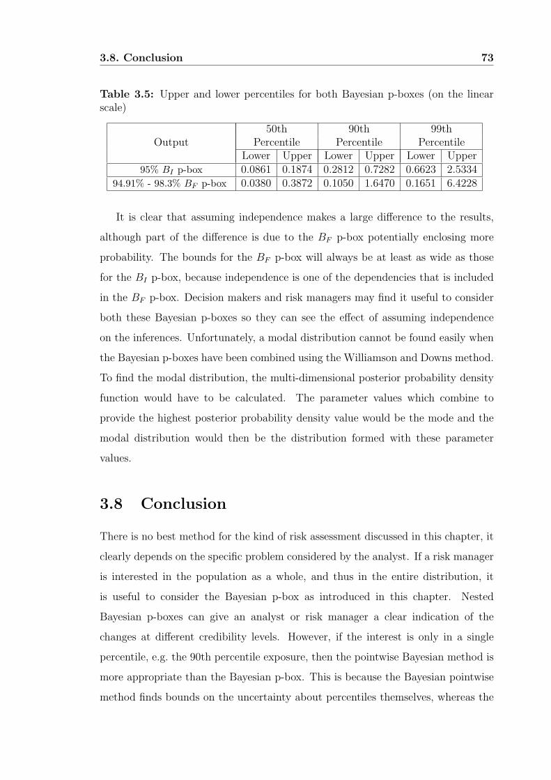
3.8. Conclusion 73
Table 3.5: Upper and lower percentiles for both Bayesian p-boxes (on the linearscale)
50th 90th 99thOutput Percentile Percentile Percentile
Lower Upper Lower Upper Lower Upper95% BI p-box 0.0861 0.1874 0.2812 0.7282 0.6623 2.5334
94.91% - 98.3% BF p-box 0.0380 0.3872 0.1050 1.6470 0.1651 6.4228
It is clear that assuming independence makes a large difference to the results,
although part of the difference is due to the BF p-box potentially enclosing more
probability. The bounds for the BF p-box will always be at least as wide as those
for the BI p-box, because independence is one of the dependencies that is included
in the BF p-box. Decision makers and risk managers may find it useful to consider
both these Bayesian p-boxes so they can see the effect of assuming independence
on the inferences. Unfortunately, a modal distribution cannot be found easily when
the Bayesian p-boxes have been combined using the Williamson and Downs method.
To find the modal distribution, the multi-dimensional posterior probability density
function would have to be calculated. The parameter values which combine to
provide the highest posterior probability density value would be the mode and the
modal distribution would then be the distribution formed with these parameter
values.
3.8 Conclusion
There is no best method for the kind of risk assessment discussed in this chapter, it
clearly depends on the specific problem considered by the analyst. If a risk manager
is interested in the population as a whole, and thus in the entire distribution, it
is useful to consider the Bayesian p-box as introduced in this chapter. Nested
Bayesian p-boxes can give an analyst or risk manager a clear indication of the
changes at different credibility levels. However, if the interest is only in a single
percentile, e.g. the 90th percentile exposure, then the pointwise Bayesian method is
more appropriate than the Bayesian p-box. This is because the Bayesian pointwise
method finds bounds on the uncertainty about percentiles themselves, whereas the

3.8. Conclusion 74
Bayesian p-box takes the parameter values from the 100(1 − α)% hpd region and
then produces bounds based on the distributions with these parameters.
There are many uncertainties that need to be accounted for in risk analyses
including choice of distribution, parameter uncertainty and assumptions on depen-
dence between random quantities. Bayesian p-boxes can deal with the uncertainty
of distribution shape by forming separate p-boxes for each possible input distribu-
tion. The envelope of all the Bayesian p-boxes can then be taken. The Normal
Bayesian p-box includes parameter dependence and parameter uncertainty in the
bounds. Robustness can, in principle, be included, but computations may be cum-
bersome for many distributions. Also the modal distribution can be displayed, as
illustrated in examples in this chapter. To account for uncertainty about the depen-
dence between random quantities, the Williamson and Downs method, as mentioned
in Section 3.7, can be used on any type of p-box to compare the effect of dependence
assumptions. The Bayesian p-box method is versatile in that it can use any strictly
convex bounded region of the posterior parameter space to form a Bayesian p-box,
using the procedures described in this chapter. A disadvantage of Bayesian methods
is that a distributional assumption has to be made.
The KS confidence limits bound the empirical distribution function and make no
assumption about distribution shape. Using these limits or other nonparametric p-
boxes (Subsection 2.10.1) would be useful in situations where an analyst prefers not
to assume a particular distribution. However for small sample sizes these usually lead
to wide bounds. The Normal frequentist p-box neglects parameter dependence, and
therefore it does not seem reasonable to use these bounds except when alternatives
cannot be used because no data are available. A disadvantage of both the Normal
frequentist p-box and the KS confidence limits is that they give no indication of how
likely any of the distributions within the bounds are.
The Bayesian p-boxes introduced in this chapter provide a means of character-
ising variability and uncertainty in risk assessment, while avoiding simplistic and
often invalid assumptions of independence between parameters. Bayesian p-boxes
can contribute to addressing the need for information about the degree of variabil-
ity and uncertainty in risk estimates (Codex, 2007; Madelin, 2004). This allows risk

3.8. Conclusion 75
managers to take account of the range of possible outcomes in decision-making. In
particular, this is useful for support of risk managers in judging when the degree
of uncertainty is sufficient to justify precautionary action (European Commission,
2000).

Chapter 4
Nonparametric predictive
assessment of exposure risk
4.1 Introduction
Nonparametric Predictive Inference (NPI) is a method that provides lower and up-
per probabilities for the predicted value(s) of one or more future observation(s) of
random quantities. NPI is introduced with references to applications of NPI in
Section 2.9. In this chapter we present NPI lower and upper cdfs for the simple
Exposure Model that was introduced in Section 2.2. This is the first use of NPI for
this type of risk assessment. Currently many of the methods used in exposure risk
assessment use parametric probability distributions. Here we consider the applica-
tion of NPI to assess the exposure of a random individual to a chemical without
making any distributional assumptions.
In Section 4.2 we explain how to calculate NPI lower and upper cdfs for random
quantities and briefly consider NPI for censored data sets. We explore calculating
exposure values for a random individual using the simple Exposure Model for a case
study in Section 4.3. Section 4.4 explores how strongly and weakly correlated data
affect the NPI lower and upper cdfs by using simulations. We discuss difficulties in
computation in Section 4.5 and the effect of different sample sizes in Section 4.6.
76

4.2. Nonparametric Predictive Inference 77
We show how to include known measurement uncertainty in an analysis in Section
4.7. Section 4.8 compares NPI with the Bayesian posterior predictive distribution
and in Section 4.9 we propose an ad hoc method for robust NPI.
4.2 Nonparametric Predictive Inference
As discussed in Section 2.9, NPI is based on the assumption, A(n), proposed by Hill
(1968) for making predictions when there is very vague a priori knowledge about the
form of the underlying distribution of a random quantity. The NPI framework is
particularly useful because it provides a probability that the predicted value of the
next observation of a random quantity will fall in various intervals. NPI also has
the advantage that it does not require any further assumptions to be added. NPI
includes uncertainty by using interval probability and does not use any information
other than that provided by the data. Therefore it gives the best possible bounds
without making any assumptions other than A(n) for each random quantity.
In risk assessments for food safety, risk managers could be interested in the
distribution for a random individual’s exposure to a chemical or the exposure dis-
tribution of a population to a chemical. As introduced in Section 2.2, a simple way
to calculate exposure is by the Exposure Model:
Exposure =Intake × Concentration
Bodyweight
NPI provides predictive probabilities for an individual. Although we do not
consider it further in this thesis, NPI could be used if individuals would like to
predict their own exposure. This can be done by taking their own intakes of a
food type, their own bodyweight and a data set of concentrations for a particular
chemical in the food type. The NPI lower and upper probabilities based on their own
data can then be formed following the procedure presented in Subsection 4.2.2. The
probability in the intervals between the calculated exposure values for one person
will then be [(nc+1)(ni+1)(nbw+1)]−1, where nc is the size of the concentration data
set, ni is the size of the intake data set and nbw is the size of the bodyweight data
set (which is 1), assuming there are no ties in any of the data sets and no ties in the

4.2. Nonparametric Predictive Inference 78
exposure values that are calculated. Combining these lower and upper probabilities
leads to NPI lower and upper cdfs for the individual’s exposure. This could easily be
extended to take concentrations of a chemical in multiple food types into account.
Next we look at an example of calculating NPI for one random quantity and then
an example for calculating NPI lower and upper cdfs for Exposure.
4.2.1 Example: NPI for a single random quantity
To calculate the tightest lower and upper bounds on the cumulative distribution
function (cdf) of a random quantity corresponding to the assumption A(n), we form
lower and upper cdfs (F and F respectively) for the probability that the next value
will fall in the intervals formed by the observed values. As a brief example, suppose
we have an ordered data set {2, 2, 4, 5, 6} for positive random quantities Xi, i = 1, ..5.
Following A(5), the lower and upper cdfs can be calculated as explained in Subsection
2.9.2 where the set B is (−∞, x]. where x ∈ (0,∞). The M function for X6 is:
MX6(0, 2) = 1/6 MX6(4, 5) = 1/6MX6 (2) = 1/6 MX6(5, 6) = 1/6MX6(2, 4) = 1/6 MX6(6,∞) = 1/6
The lower and upper cdfs for X6 can be plotted as shown in Figure 4.1. The
final value of the lower cdf for X6, FX6(x), is 5
6, for x > x5.
Figure 4.1: NPI lower and upper cdfs
0 5 100
0.2
0.4
0.6
0.8
1
X
Cum
ulat
ive
Pro
babi
lity

4.2. Nonparametric Predictive Inference 79
As n tends to ∞, the NPI lower and upper cdfs converge to the empirical distri-
bution function of the data. The cdf of the empirical distribution function, Fe, will
always lie in [FXn+1(x), FXn+1(x)] for all x, where n is the number of observations.
4.2.2 Example: NPI for the Exposure Model
Now we look at calculating NPI lower and upper cdfs for the Exposure Model that
was described in Section 2.2. Assume we have ordered observations x1, x2, for the
random quantities X1 and X2 respectively. Then nx = 2 is the total number of
observations and we have intervals (0, x1), (x1, x2), (x2,∞). Assuming A(2), the
probability that the next observation falls in any of these intervals is 1nx+1
= 13.
Assume we also have ordered observations y1, y2, y3 for random quantities Y1, Y2,
and Y3 respectively and ny = 3 is the total number of observations. This leads to
intervals (0, y1), (y1, y2), (y2, y3), (y3,∞) and assuming A(3), the probability that the
next observation falls in any of these intervals is 1ny+1
= 14. Taking the product
of the intervals for the random quantities X3 and Y4, leads to 12 intervals each
with probability 112
, assuming there are no ties, for the random quantity that we
call XYnew. We combine the intervals by multiplying the minimum values of each
interval for X3 with the minimum values of each interval for Y4 and the maximum
values of each interval for X3 with the maximum values of each interval for Y4. For
example to multiply (x1, x2) with (y1, y2), we multiply x1 with y1 and x2 with y2
to form the interval (x1y1, x2y2). Notice that this is the widest the interval can be,
as combining the other endpoints, e.g. y2 with x1 will always produce values that
fall in this interval due to their ordering. Now assume we have ordered observations
z1, z2 for random quantities Z1 and Z2 respectively. Assuming A(2), the probability
that the next observation falls in any of the intervals (0, z1), (z1, z2), (z2,∞) is 13.
Combining the random quantities X3, Y4 and Z3 in the Exposure Model leads to
36 intervals each with probability 136
assuming there are no ties. The M function
for the predicted value of the next observation, XYZ new
, is shown below, where expj
represents the jth ordered value that forms the intervals for XYZ new
, and j = 1, ..., 34.

4.2. Nonparametric Predictive Inference 80
MXYZ new
(0, exp1) = 1/36
MXYZ new
(expj, expj+1) = 1/36
MXYZ new
(exp35, ∞) = 1/36
The NPI lower and upper cdfs are formed as explained in Subsection 2.9.2.
4.2.3 NPI for left-censored data
The distribution of probability mass for a data set with left-censored values (ex-
plained in Section 2.4) can also be represented using M functions. It is often the
case with concentration data that there is a limit of detection (LOD) below which
concentration of chemicals cannot be measured. This leads to left-censored data
where some values are reported as < LOD. The censoring will be between 0 and the
LOD because concentration cannot be negative.
Example: NPI lower and upper cdfs for left-censored data
Assume that the LOD is 1 and we have an ordered data set {x1, x2, x3, x4} for
concentration and x1 is a censored value that is between 0 and 1. The uncertainty
about the value of x1 can be represented by overlapping intervals in the M function,
which takes into account that the censored value may be 0, or any value between
0 and 1. So the partial description of probability mass for a new observation X5,
based on A(4), can be represented as below:
MX5(0 , 1) = 1/5 MX5(x3, x4) = 1/5MX5(0, x2) = 1/5 MX5(x4, ∞) = 1/5MX5(x2, x3) = 1/5
The NPI lower and upper cdfs calculated from this M function will describe the
tightest possible bounds given the information we have available and A(4). Figure
4.2 shows the NPI lower and upper cdfs for this example.

4.2. Nonparametric Predictive Inference 81
Figure 4.2: NPI lower and upper cdfs for X5
0 2 4 60
0.2
0.4
0.6
0.8
1
X
Cum
ulat
ive
Pro
babi
lity
NPI upper cdfNPI lower cdf
There is a problem that if, for example, the censored value happened to be 0.2,
then the intervals (0, 0.2) and (0.2, x2) should each have probability mass 15
rather
than the probability masses assigned to the intervals in the previous M function.
However, without knowing anything more than the censored value is less than 1,
the tightest bounds given A(4) and the censoring are represented by the M function
given previously. The bounds will enclose the possible lower and upper cdfs that
would correspond to all possible values of x1.
We are interested in the exposure of individuals to a particular chemical. Al-
though it is informative to see how much uncertainty in the exposure is caused by
the censored concentration values, often the risk associated with exposure is based
on upper tail exposures. This is because higher exposures to chemicals are generally
more harmful than low exposures. Since the left-censored concentration values only
contribute to the lower tail of the exposure distribution, they are generally consid-
ered to be less important in risk assessments. However if the LOD is large, or the
safe exposure level is very low, the censoring may contribute substantially making
it useful to be able to form such lower and upper cdfs for a random individual.
4.3. Case Study: Benzene Exposure 82
4.3 Case Study: Benzene Exposure
In this section we show how to calculate NPI lower and upper cdfs for the Exposure
Model where we have data for the exposure of young children to benzene in soft
drinks. We have data for each of the three non-negative random quantities, concen-
tration, intake and bodyweight. A description of the data sets that we will use for
the analysis is given in Subsection 4.3.1. We calculate the NPI lower and upper cdfs
for exposure for a random individual, for two different cases and then we compare
them. First we consider the case where we calculate NPI lower and upper cdfs for
exposure for a random individual, for the three random quantities separately. Then,
for the second case, we combine each individual’s bodyweight with their average
intake and treat this as one random quantity which we call IR. We then calculate
the NPI lower and upper cdfs for exposure for a random individual, using the two
random quantities, concentration and IR.
4.3.1 The data
Concentration data for benzene in soft drinks were obtained from the Food Stan-
dards Agency Survey from March 20061. Out of 150 samples, 109 were below the
Limit Of Detection (LOD) of 1 µg/kg. Assuming A(150), the probability of the next
observation of benzene concentration falling in the interval (0, 1) is 122151
. Usually the
probability of X151 falling in the interval (0, 1) would be 109151
but here the lowest
measured datum that is not censored is equal to the LOD. Therefore there is a
probability of 110151
that X151 falls in the interval (0, 1). The concentration data is
given in Table 4.1.
1http://www.food.gov.uk/science/surveillance/fsisbranch2006/fsis0606

4.3. Case Study: Benzene Exposure 83
Table 4.1: Concentration data
Data value Frequency Data value Frequency< 1 109 7 41 13 8 12 13 9 13 3 10 14 3 23 15 1
Intake and bodyweight data were obtained from the UK Data Archive Study No.
3481. National Diet, Nutrition and Dental Survey of Children Aged 1.5 - 4.5 years
(1992 - 1993)2. It is a 4 day survey of 1717 children giving information about their
weight, food and drink intake and other covariates such as age, height, region and
social class. Only individuals with no missing values (i.e. individuals with intake
values for every day of the survey and a recorded bodyweight) were used in the
analysis. We excluded 23 individuals, whose bodyweights were not recorded, leaving
us with data for 1694 individuals. Omitting these individuals from the analysis may
lead to bias, particularly if they all had large or small bodyweights. Also, if they
were heavy consumers of soft drinks then their exposure may be higher than the
exposure of the general population. However their average intakes of drink were
between 0.025 kg/day and 0.418 kg/day compared with the minimum of 0 kg/day
and maximum of 1.239 kg/day for all the other individuals, so it is unlikely that
they would lead to higher exposures than individuals that are included unless they
have very small bodyweights.
As an illustration of the use of NPI in risk assessment we include non-consumers
in the analysis and consider the average intake over the 4 days of the survey. We can
only make inferences about the random quantities that we have data for. Therefore
the conclusions reached can only be predictions for the average exposure for a ran-
dom individual on the particular four days of the survey. They cannot provide any
information about the exposure of an individual for the rest of the year.
As we have bodyweight and average intake values for each individual it is possible
to treat bodyweight and average intake as separate random quantities and generate
2http://www.esds.ac.uk/findingdata/snDescription.asp?sn=3481&key=coding

4.3. Case Study: Benzene Exposure 84
NPI lower and upper cdfs based on this assumption. This is presented in the next
section. However, it is generally believed that bodyweight and average intake are
dependent on each other. Therefore we also consider using IR as a random quantity.
This loses some information as we no longer separate the random quantities, average
intake and bodyweight, but it does naturally include dependencies between these
random quantities. The differences caused by using IR are discussed in Subsection
4.3.2. We use the average intake over the 4 days of the survey throughout this
chapter so for ease of presentation we will henceforth refer to this as ‘intake’.
4.3.2 NPI lower and upper cdfs
In this example we derive NPI lower and upper cdfs for exposure for a random
individual using the data sets that were described in the previous section. We
compare the results of treating all three random quantities separately, which we
will call the ‘independent case’, and using the IR, which we will call the ‘dependent
case’. It is interesting to look at both cases, although using IR has the advantage
that it takes dependencies between intake and bodyweight into account. For the
situation where all the random quantities are assumed to be independent, we first
calculate the NPI lower and upper cdfs for the exposure as described in Subsection
4.2.2. In the second situation we calculate the IR and then calculate the NPI lower
and upper cdfs on the product of concentration and IR.
To calculate the NPI lower and upper cdfs for exposure for a random individual,
we first add a minimum and a maximum to each data set. For concentration and
intake, zero and ∞ are appropriate. However for bodyweight we use 1e-15 and ∞
as we cannot divide by zero.
For the independent case, we have ties at 135 bodyweight values and 1194 intake
values, both from an original sample size of 1694. The tied values from the original
data set and their frequency of occurrence are stored and the correct probability is
assigned to the tied values themselves or to the intervals if the value is not tied.
Working with the tied values speeds up computation and avoids problems with
computer memory (computational issues are discussed in Section 4.5). First we
look at a scatterplot of bodyweight and intake to see if there appears to be any

4.3. Case Study: Benzene Exposure 85
correlation between them. The scatterplot is shown in Figure 4.3.
Figure 4.3: Scatterplot of Intake versus Bodyweight
0 10 20 30 40 500
0.2
0.4
0.6
0.8
1
1.2
1.4
Bodyweight (kg)
Inta
ke (
kg)
The scatterplot does not show any obvious correlation between bodyweight and
intake. To check the strength of correlation we consider Spearman’s rank correlation
coefficient which ranges between -1 and 1, where -1 indicates a very strong negative
correlation and 1 indicates a very strong positive correlation. Around zero indicates
very weak correlation. Spearman’s rank correlation coefficient is -0.0071, indicating
a weak negative correlation between bodyweight and intake. The weak correlation
suggests that there is no strong dependence between the random quantities.
Figure 4.4.1 shows the NPI lower and upper cdfs for exposure for a random
individual for both cases. Part of the upper tail is displayed in more detail in Figure
4.4.2 to show the differences between the two cases. It is clear that the dependent
case resembles a step function more closely than the independent case. This is due
to the smaller number of exposure values generated in the dependent case which
leads to fewer steps with larger jumps at many values. The independent case has
many more exposure values so it appears to be much smoother, but it is still a step
function, with small jumps at several values.

4.3. Case Study: Benzene Exposure 86
Figure 4.4: NPI lower and upper cdfs for a random individual
0 0.1 0.2 0.3 0.40
0.2
0.4
0.6
0.8
1
Exposure (µg / kg bw / day)
Cum
ulat
ive
Pro
babi
lity
4.4.1 NPI lower and upper cdfs for theindependent case (blue line) and the de-pendent case (red line) on a linear scale
0.02 0.04 0.06
0.84
0.86
0.88
0.9
0.92
0.94
0.96
Exposure (µg / kg bw / day)
Cum
ulat
ive
Pro
babi
lity
4.4.2 A close up of part of the NPI lowerand upper cdfs for the independent case(blue line) and the dependent case (redline)
There is not much difference between the results from the independent and de-
pendent cases. There are small differences at some exposure values and neither set of
NPI lower and upper cdfs is enclosed within the other. One observable difference is
that the final value of the lower cdf for independence (0.9922) is lower than the final
value of the lower cdf for the dependent case (0.9928). The difference in the final
value of the lower cdfs might be informative for an individual and may be useful for
risk managers to see how much dependence is influencing the results. The difference
is due to the larger number of data values combined in the independent case where
bodyweight and intake are combined separately. In the dependent case intake is
divided by bodyweight and then the resulting values combined with concentration
values leading to fewer exposure values. Therefore in the M function for exposure
for a random individual, Mexp, there is a larger probability mass in M(3)exp(expN ,∞)
(where M(i)exp(expN ,∞) represents the M function value for the interval between the
highest exposure value and∞ for exposure for a random individual, calculated using
i random quantities) than in M(2)exp(expN ,∞).

4.4. Exploring dependence for NPI by simulation 87
For the case where we use IR the final value of the lower cdf is given by
1− (nc + 1 + nIR)
(nc + 1)(nIR + 1)= 0.9928 (4.1)
as M(2)exp(expN ,∞) = (nc+1+nIR)
(nc+1)(nIR+1), where nc is the concentration sample size (here
150) and nIR is the IR sample size (here 1694). Similarly in the independent case
M(3)exp(expN ,∞) = ((nc+1+nint)nbw+(nc+1)(nint+1))
(nc+1)(nint+1)(nbw+1)so the final value of the lower cdf in
this case is
(1− ((nc + 1 + nint)nbw + (nc + 1)(nint + 1))
(nc + 1)(nint + 1)(nbw + 1)
)= 0.9922 (4.2)
where nbw is the bodyweight sample size (here 1694) and nint is the intake sample
size (here 1694) and as before nc is the concentration sample size (here 150).
4.4 Exploring dependence for NPI by simulation
We keep X (in µg / kg) as a fixed sample from a Lognormal distribution with
mean, µx = 1.5 and standard deviation, σx = 2.8. We consider the effect of varying
the correlation between Y (in kg /day), which we assume to have a Lognormal
distribution with mean, µy = 1.27 and standard deviation, σy = 1.03 and Z (in kg),
which we assume to have a Normal distribution with mean, µz = 30, and standard
deviation, σz = 3. We consider 1000 simulations for two values of n (50 and 100) and
we vary ρ between -1 and 1. The exposure percentiles are estimated by taking very
large samples (1,000,000) from the relevant distributions and combining them as in
the simple Exposure Model. Then we take the 10th, 50th and 90th percentiles for
comparison purposes and call them the true exposure percentiles. We compare the
10th, 50th and 90th percentiles from the independent and dependent NPI methods
with the true exposure percentiles. We count how many times the true exposure
percentiles fall in the intervals generated by the dependent and independent NPI.

4.4. Exploring dependence for NPI by simulation 88
We also consider whether the NPI methods over- or underestimate the true exposure
percentile.
4.4.1 Varying n
In this section we consider two different values of n and then compare how well NPI
predicts for 1000 samples for each of these n. The results for n = 50 are shown in
Table 4.2. The results for n = 100 are shown in Table 4.3.
Table 4.2: Results from 1000 simulations when n = 50
ρ MethodPercentile
10th 50th 90th
1 DependentSuccess 719 351 350
Underestimates 233 256 1Overestimates 48 393 649
0.5 DependentSuccess 651 348 360
Underestimates 273 246 9Overestimates 76 406 631
0 DependentSuccess 654 365 380
Underestimates 278 218 8Overestimates 68 417 612
-0.5 DependentSuccess 655 375 404
Underestimates 287 220 8Overestimates 58 405 588
-1 DependentSuccess 582 308 396
Underestimates 336 258 26Overestimates 82 434 578
1 IndependentSuccess 478 571 172
Underestimates 522 138 0Overestimates 0 291 828
0.5 IndependentSuccess 617 560 278
Underestimates 383 151 0Overestimates 0 289 722
0 IndependentSuccess 759 549 422
Underestimates 240 144 0Overestimates 1 307 578
-0.5 IndependentSuccess 871 567 592
Underestimates 126 144 0Overestimates 3 289 408
-1 IndependentSuccess 857 461 679
Underestimates 130 195 6Overestimates 13 344 315

4.4. Exploring dependence for NPI by simulation 89
Table 4.3: Results from 1000 simulations when n = 100
ρ MethodPercentile
10th 50th 90th
1 DependentSuccess 687 351 269
Underestimates 206 221 4Overestimates 107 428 727
0.5 DependentSuccess 673 337 280
Underestimates 225 217 6Overestimates 102 446 714
0 DependentSuccess 653 352 284
Underestimates 244 189 4Overestimates 103 459 712
-0.5 DependentSuccess 629 340 283
Underestimates 271 208 6Overestimates 100 452 711
-1 DependentSuccess 546 273 329
Underestimates 339 241 28Overestimates 115 486 643
1 IndependentSuccess 348 498 49
Underestimates 652 126 0Overestimates 0 376 951
0.5 IndependentSuccess 626 489 156
Underestimates 372 129 0Overestimates 2 382 844
0 IndependentSuccess 777 488 310
Underestimates 212 120 1Overestimates 11 392 689
-0.5 IndependentSuccess 865 487 541
Underestimates 97 146 3Overestimates 38 367 456
-1 IndependentSuccess 784 394 653
Underestimates 98 187 30Overestimates 118 419 317
Generally the 10th percentile is captured best by both methods regardless of
n. The general trend for the dependent case is that as ρ decreases from 1 to -1,
the dependent method captures the 10th percentile less often. The trend is less
clear in the independent case as the 10th percentile is captured more often as ρ
decreases from 1 to 0 but increases for ρ = −0.5 and decreases again for ρ = −1.
As n increases the percentage of times that the 10th percentile is captured, by both
methods, decreases slightly. This is probably due to the narrowing of the intervals

4.4. Exploring dependence for NPI by simulation 90
in the NPI lower and upper cdfs because of the larger data samples used. Both
methods appear to underestimate the 10th percentile more than they overestimate
it, for both n, except for the independent case where ρ = −1 and n = 100. Here the
overestimates are slightly higher than the underestimates. This is probably due to
the gradient of the exposure distribution when ρ is negative as discussed later.
The 50th percentile is captured between 27.3 and 37.5% of the time for the
dependent method and between 39.4 and 57.1% of the time for the independent
method. There is the same general trend as with the 10th percentile, that as n
increases the percentage of times that the 50th percentile is captured decreases
slightly. There is a general trend in the independent case that as ρ decreases from 1
to -1, the 50th percentile is captured fewer times, although again ρ = −0.5 performs
better than ρ = −1. For the dependent case the results are similar for different
values of ρ although ρ = −1 leads to the lowest percentage of times that the 50th
percentile is captured. Again this is probably due to the gradient of the exposure
distribution at different values of ρ. Generally the 50th percentile is overestimated
more than it is underestimated.
The 90th percentile is captured between 26.9 and 40.4% of the time for the
dependent case whereas it is captured between 4.9 and 67.9% of the time by the
independent case. For the dependent case there is a general trend that the 90th
percentile is captured more often as ρ decreases from 1 to -1, regardless of n. However
for n = 50 there is a decrease from 40.4% for ρ = −0.5 to 39.6% for ρ = −1.
This decrease does not occur when n = 100 so it is probably due to sampling
variation. Both the dependent and independent methods generally overestimate the
90th percentile, particularly the independent case which does not underestimate
the 90th percentile for most of the results in this example. The cases where the
independent method does underestimate the 90th percentile are generally at negative
rank correlations. This is explained by the gradient of the exposure distribution for
negative values of ρ as discussed below.
When ρ = 1, the gradient of the exposure distribution at low percentiles is lower
than the gradient of the exposure distribution when ρ = −1. At higher percentiles
this is reversed and the gradient of the exposure distribution when ρ = 1 is higher

4.4. Exploring dependence for NPI by simulation 91
than the gradient when ρ = −1. This means that the exposure distribution when
ρ = −1 is much flatter and spread out than the exposure distribution for ρ = 1. The
exposure distributions for each value of ρ are shown in Figure 4.5.1 on a log scale.
Figure 4.5.2 shows a close up of the lower half of the distributions. The independent
NPI tends to underestimate the 10th percentile and overestimate the 90th percentile.
This is because it allows every combination of values for X, Y and Z ignoring any
dependency between them. Therefore the smallest values are divided by the largest
values and the largest values are divided by the smallest values regardless of the
specified rank correlation. This leads to a flat distribution where the values are
spread out.
In the dependent case this does not happen because, for example, if ρ = 1, then
the smallest value of Y will be divided by the smallest value of Z and the largest
value of Y will be divided by the largest value of Z. Similarly for ρ = −1, the
smallest value of Y will be divided by the largest value of Z etc. Therefore there
are fewer values in the dependent case and there are less extreme values compared
to the independent case. The independent case appears to perform better on the
negative correlation than the positive correlation. This is probably because the lower
predictions for the 10th percentile and higher predictions for the 90th percentile
mean the NPI upper and lower cdfs do not increase steeply. Therefore the cdf more
closely resembles that of the cdf when ρ = −1 than the cdf when ρ = 1.
The dependent case appears to be an improvement on the independent case for
positive correlations, but not for the zero rank correlation. As the dependent case
is taking the rank correlation into account, we would expect the dependent case to
be better than the independent case for correlated data but not for uncorrelated
data (i.e. when ρ = 0). However we would also expect the dependent case to
perform better for the negative correlations which it does not appear to do. The
dependent case considers fewer values as it only uses the data for X and YZ, whereas
the independent case uses all the data for X, Y and Z separately. Therefore the
dependent case not performing as well as the independent case may be due to the
independent case having cdfs that more closely resemble the cdf of the case with
negative correlation. The dependent case has less values with higher probability and

4.4. Exploring dependence for NPI by simulation 92
grows more steeply, which is closer to the positive correlation case.
Figure 4.5: Exposure distributions with various values for ρ
10-3
10-2
10-1
100
0
0.2
0.4
0.6
0.8
1
Exposure (µg / kg bw / day)
Cum
ulat
ive
Pro
babi
lity
ρ = 1ρ = 0.5ρ = 0ρ = -0.5ρ = -1
4.5.1 Exposure distribution with vary-ing ρ
10-2
0.05
0.1
0.15
0.2
0.25
0.3
0.35
0.4
Exposure (µg / kg bw / day)
Cum
ulat
ive
Pro
babi
lity
ρ = 1ρ = 0.5ρ = 0ρ = -0.5ρ = -1
4.5.2 Close-up of exposure distributionwith varying ρ
4.4.2 Varying µz and σz
In this section we only consider samples of size 50 and we take ρ = 1 and ρ = −1.
We vary σz first while keeping µz fixed and then we consider the case where we fix
σz and vary µz.
Varying σz
We begin by keeping µz fixed at 30, while taking σz to be 5 and 7. The results for
ρ = 1 are shown in Table 4.4 and the results for ρ = −1 are shown in Table 4.5. We
re-use the results from Table 4.2 above where σz = 3.

4.4. Exploring dependence for NPI by simulation 93
Table 4.4: Results from 1000 simulations with σz = 3, 5 and 7 and ρ = 1
σz MethodPercentile
10th 50th 90th
3 DependentSuccess 719 351 350
Underestimates 233 256 1Overestimates 48 393 649
5 DependentSuccess 787 389 342
Underestimates 180 237 0Overestimates 33 374 658
7 DependentSuccess 546 397 228
Underestimates 450 280 1Overestimates 4 323 771
3 IndependentSuccess 478 571 172
Underestimates 522 138 0Overestimates 0 291 828
5 IndependentSuccess 232 630 41
Underestimates 768 83 0Overestimates 0 287 959
7 IndependentSuccess 95 618 20
Underestimates 905 128 0Overestimates 0 254 980
For ρ = 1 we can see that increasing σz from 5 to 7 leads to lower success rates
for the 10th and 90th percentiles for the dependent case. The 50th percentile for
both cases was fairly consistent because the 50th percentile does not depend on σz
as much as the tails of the distribution do. The independent case shows a very clear
decrease in success rates for the 10th and 90th percentiles as σz varies from 3 to 7.
Also the 10th percentile is always underestimated and the 90th percentile is always
overestimated (in this example). This is expected because as we saw earlier the NPI
independent case combines every possible combination of all the data values. As
σz increases, the spread of exposure values increases leading to flatter NPI lower
and upper cdfs. At the same time, as σz increases, the true exposure distribution
becomes a steeper distribution. Therefore we would expect that the independent
case performs better for smaller σz. The dependent case performs better than the
independent case. This is probably because it takes the rank correlation into account
so the NPI lower and upper cdfs do not become as flat as in the independent case.
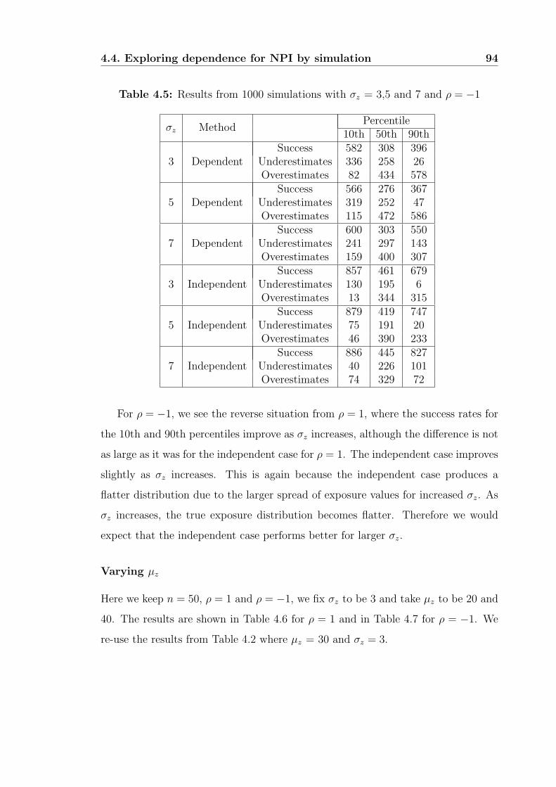
4.4. Exploring dependence for NPI by simulation 94
Table 4.5: Results from 1000 simulations with σz = 3,5 and 7 and ρ = −1
σz MethodPercentile
10th 50th 90th
3 DependentSuccess 582 308 396
Underestimates 336 258 26Overestimates 82 434 578
5 DependentSuccess 566 276 367
Underestimates 319 252 47Overestimates 115 472 586
7 DependentSuccess 600 303 550
Underestimates 241 297 143Overestimates 159 400 307
3 IndependentSuccess 857 461 679
Underestimates 130 195 6Overestimates 13 344 315
5 IndependentSuccess 879 419 747
Underestimates 75 191 20Overestimates 46 390 233
7 IndependentSuccess 886 445 827
Underestimates 40 226 101Overestimates 74 329 72
For ρ = −1, we see the reverse situation from ρ = 1, where the success rates for
the 10th and 90th percentiles improve as σz increases, although the difference is not
as large as it was for the independent case for ρ = 1. The independent case improves
slightly as σz increases. This is again because the independent case produces a
flatter distribution due to the larger spread of exposure values for increased σz. As
σz increases, the true exposure distribution becomes flatter. Therefore we would
expect that the independent case performs better for larger σz.
Varying µz
Here we keep n = 50, ρ = 1 and ρ = −1, we fix σz to be 3 and take µz to be 20 and
40. The results are shown in Table 4.6 for ρ = 1 and in Table 4.7 for ρ = −1. We
re-use the results from Table 4.2 where µz = 30 and σz = 3.

4.4. Exploring dependence for NPI by simulation 95
Table 4.6: Results from 1000 simulations with µz = 20, 30 and 40 and ρ = 1
µz MethodPercentile
10th 50th 90th
20 DependentSuccess 745 367 338
Underestimates 228 248 4Overestimates 27 385 658
30 DependentSuccess 719 351 350
Underestimates 233 256 1Overestimates 48 393 649
40 DependentSuccess 666 341 360
Underestimates 295 231 6Overestimates 39 428 634
20 IndependentSuccess 255 608 75
Underestimates 745 102 0Overestimates 0 290 925
30 IndependentSuccess 478 571 172
Underestimates 522 138 0Overestimates 0 291 828
40 IndependentSuccess 529 545 246
Underestimates 471 143 0Overestimates 0 312 754
Table 4.7: Results from 1000 simulations with µz = 20, 30 and 40 and ρ = −1
µz MethodPercentile
10th 50th 90th
20 DependentSuccess 559 298 396
Underestimates 341 276 39Overestimates 100 426 565
30 DependentSuccess 582 308 396
Underestimates 336 258 26Overestimates 82 434 578
40 DependentSuccess 581 293 375
Underestimates 328 263 23Overestimates 91 444 602
20 IndependentSuccess 891 434 753
Underestimates 80 212 19Overestimates 29 354 228
30 IndependentSuccess 857 461 679
Underestimates 130 195 6Overestimates 13 344 315
40 IndependentSuccess 838 468 615
Underestimates 156 180 2Overestimates 6 352 383

4.4. Exploring dependence for NPI by simulation 96
We would not expect that increasing µz would have a large influence on the
results because increasing µz only affects the location of the exposure distribution.
This is particularly true for the dependent case because there is little variance in
the results as µ increases for both values of ρ. It is also the case for the independent
case when ρ = −1, where there are only small differences in the number of successes
for each percentile at different values of µz. The results for the independent case
are better for ρ = −1 than for ρ = 1, whereas for the dependent case the results
are better for ρ = 1. This was expected given the results discussed previously.
For ρ = 1, the success rate of the 10th and 90th percentiles for the independent
case improves as µz increases. This is probably due to the NPI lower and upper
cdfs becoming steeper and therefore closer to the true exposure distribution as µz
increases.
4.4.3 Discussion
In this example, i.e. for a division, we have seen that the dependent case appears to
perform better for positive rank correlations, whereas the independent case appears
to perform better for negative correlations and correlations equal to zero. Varying
σz and varying µz also affected the results in the ways described above. We have
counted how many intervals overestimated or underestimated the true percentiles
but not given an indication of how much they over- or underestimate by. Generally,
the independent case underestimated the 10th percentile, or overestimated the 90th
percentile by more than the dependent case. This is because the independent case
does not account for the specified correlation so it produces flatter distributions.
We would not expect predictive methods to produce exact predictions based
on samples such as those used in these examples. If we used different predictive
methods, e.g. the Bayesian posterior predictive distribution, the results would be
dependent on distributional assumptions and how well the sample represents the
distribution that it has been sampled from. As seen in Chapter 5, both NPI and the
Bayesian posterior predictive distribution can produce good predictions and poor
predictions depending on the samples and the distributions that are sampled from.
4.5. Computational issues 97
Here we used 1,000 simulations to try and allow for sampling variation. Sampling
variation will strongly affect the NPI results for small samples because it only uses
the samples and an assumption of A(n) for the analysis. For larger samples there
will be less effect from sampling variation (as illustrated in Chapter 5), but the
NPI intervals become narrower. Therefore the NPI lower and upper cdfs for smaller
samples may perform better (as we saw in our example) because the intervals are
wider and include more uncertainty about the exposure percentiles so it is more
likely that they will enclose the true percentiles.
4.5 Computational issues
In this section we briefly discuss some computational problems that arise when
modelling NPI with large data sets. The large number of values in the intake and
bodyweight data sets described in Subsection 4.3.1 led to problems with computer
memory as we needed to store all the possible combinations of all the values of all
three data sets. As the data sets were nc = 150, nint = 1694 and nbw = 1694 in
length (and adding a minimum or maximum depending on which cdf we consider)
this leads to (nc + 1)(nint + 1)(nbw + 1) = 433, 826, 775 values for each cdf. These
need to be stored along with the cumulative probabilities for each interval so that
we can plot the NPI lower and upper cdfs. One way in which we solved this problem
was by looking for repeated values in the data sets. Fortunately there were only 135
tied bodyweight values which made it possible to calculate NPI lower and upper
cdfs for exposure for a random individual in the way explained below.
When there are repeated values in the data sets we can speed up the calculation
by counting the number of tied values and then only using one in the calculation.
This means that instead of having (nc + 1)(nint + 1)(nbw + 1) values to consider for
each cdf we only have to calculate (Tc + 1)(Tint + 1)(Tbw + 1) where Tc, Tint and
Tbw are the number of tied values in the data sets for concentration, intake and
bodyweight respectively. Eliminating repeated values can be done at each stage so
the calculation is only done with the minimum possible number of values.
4.6. The effect of different sample sizes 98
The probabilities for each interval are calculated based on the number of repeated
values that occur in the data sets.
If it is the case that even after checking for repeated values, the data sets are still
too large, it is still possible to calculate NPI lower and upper cdfs. It can be done
by calculating all the values and counting how many are less than various threshold
values. This eliminates problems with storing many values but it only becomes
accurate by using a large number of threshold values. Several threshold values are
needed because the smaller the interval between the threshold values, the closer to
the actual lower and upper cdfs the results will be. However, as we would only use
this method when there are very large data sets, it gives a good approximation for
lower numbers of threshold values. Using many threshold values makes the method
slow, but when the data sets are so large that there is no other method available, it
gives a useful approximation. A relatively quick approximation can be made using
the histc function in Matlab, which counts the number of values in each interval
between threshold values. However it is only fast for smaller numbers of threshold
values (e.g. for 1000 threshold values for the data sets in the case study (Section
4.3), it took approximately 3.5 minutes on a computer with a 1.6Ghz Intel Pentium
processor with 1 Gb of RAM).
4.6 The effect of different sample sizes
In this section we look at how taking different sample sizes affects the NPI lower and
upper cdfs. For simplicity we consider a case without censoring in the concentration
data set and look at the effect of sample size on the NPI lower and upper cdfs for
exposure for a random individual, again using the Exposure Model. For comparison
we keep the size of the concentration data set at nc = 100 and sample different
size data sets for intake and bodyweight. The concentration data set is sampled
from a Lognormal distribution with mean 9.02 µg/kg and standard deviation 66.07
µg/kg. We sample intake from a Lognormal distribution with mean 1.13 kg/day and
standard deviation 0.60 kg/day and sample bodyweight from a Normal distribution
with mean 30 kg and standard deviation 3 kg. Again these distributions are chosen

4.6. The effect of different sample sizes 99
so the samples resemble the data sets that we have for young children. We consider
samples of size 10, 30, 50 and 100. The results are shown on the linear scale in Figure
4.6.1 and on the log scale in Figure 4.6.2.
Figure 4.6: NPI lower and upper cdfs using different sample sizes
0 1 2 3 40
0.2
0.4
0.6
0.8
1
Exposure (µg / kg bw / day)
Cum
ulat
ive
Pro
babi
lity
n = 10n = 30n = 50n = 100
4.6.1 Linear scale
10-4
10-2
1000
0.2
0.4
0.6
0.8
1
Exposure (µg / kg bw / day)
Cum
ulat
ive
Pro
babi
lity
n = 10n = 30n = 50n = 100
4.6.2 Log10 scale
Figures 4.6.1 and 4.6.2 show that, as the sample size increases, the uncertainty
reduces so the NPI lower and upper cdfs get narrower. This is to be expected because
including more observations in NPI leads to less uncertainty about variability and
therefore narrower bounds. The general shape remains the same for the values of
n shown here. The NPI lower and upper cdfs for the smaller values of n do not
entirely enclose the NPI lower and upper cdfs for other sample sizes. This is due to
variation between samples. We briefly investigate the effect of sampling variation
for a sample of size 10 and a sample of size 100 below. For each sample size we take
5 different samples and plot the NPI lower and upper cdfs on a log10 scale in Figures
4.7.1 and 4.7.2 respectively.

4.7. Imprecise data 100
Figure 4.7: NPI lower and upper cdfs for 5 different samples from each sample size
10-4
10-2
1000
0.2
0.4
0.6
0.8
1
Exposure (µg / kg bw / day)
Cum
ulat
ive
Pro
babi
lity
4.7.1 n = 10
10-4
10-2
100
0.2
0.4
0.6
0.8
1
Exposure (µg / kg bw / day)
Cum
ulat
ive
Pro
babi
lity
4.7.2 n = 100
As we expected Figures 4.7.1 and 4.7.2 show that there is more sampling variation
when we consider a sample of size 10 than there is for a sample of size 100. This
can be seen as the distance between the NPI lower and upper cdfs for the sample
size of 10 is larger than the distance between the NPI lower and upper cdfs for the
sample size of 100.
4.7 Imprecise data
In practice, data sets may be given as interval data, such as when an indication
of measurement uncertainty is given as discussed in Subsection 3.5.5. An example
of how to calculate NPI lower and upper cdfs with measurement uncertainty is
presented here.
Suppose that the maximum measurement error of some apparatus used to mea-
sure the concentration of benzene in soft drinks is known. There may of course also
be human error but we ignore that here. Assume that the maximum measurement
error is δ = 0.3. Then we can form NPI lower and upper cdfs on the concentration
data (the benzene data used in Subsection 4.3.1) by considering the values yi = xi+δ
and zi = xi− δ. Let x(1), x(2), ..., x(n) be the order statistics of data x1, x2, ..., xn and
let Xi be the corresponding pre-data random quantities so the data consist of the
realized values Xi = xi, i = 1, ..., n. Let Yi and Zi be observable random quanti-
ties with observations yi and zi respectively. The cdf for the next random quantity
Yn+1, is the NPI lower cdf because we find the NPI lower cdf by taking the envelope

4.7. Imprecise data 101
of the M functions for Xn+1, Yn+1 and Zn+1. The M function for Yn+1 describes
probability mass at higher concentration values than either of the M functions for
Xn+1 and Zn+1. Therefore the NPI lower cdf for Yn+1 becomes the NPI lower cdf for
Xn+1 including measurement uncertainty. Similarly the upper cdf for Zn+1 forms
the NPI upper cdf as the M function for Zn+1 describes probability mass at lower
concentrations than the M functions for Xn+1 and Yn+1.
The maximum value that the censored values can take is 1, so we take the
censored point including measurement uncertainty to be 1 + δ. One could argue
that we should take the limit to be 1, as if it is above 1 then we assume that the
concentration is high enough to be detected. However if the apparatus can measure
inaccurately up to ±δ, then it is possible that some values recorded as 1 are actually
lower than the limit of detection, and some values recorded as < 1 are actually higher
than 1 so we take 1 + δ to be the maximum value that censored values can take.
The NPI lower and upper cdfs including fixed measurement uncertainty (δ = 0.3)
for the concentration data (see Subsection 4.3.1) are shown with the NPI lower and
upper cdfs for the original concentration data set in Figure 4.8.
Figure 4.8: NPI lower and upper cdfs with fixed measurement uncertainty (red)and for the original data set (blue)
0 5 100
0.2
0.4
0.6
0.8
1
Concentration (µg / kg)
Cum
ulat
ive
Pro
babi
lity
Including the measurement uncertainty leads to NPI lower and upper cdfs that
increase at different values of concentration. We can see from Figure 4.8 that the
measurement uncertainty leads to more uncertainty around the original data values,

4.8. Comparison to Bayesian methods 102
but for the values that are not within ±δ of an observed data value the lower and
upper probabilities remain the same.
If information on measurement uncertainty is provided with data as a constant,
it is easy to incorporate into the NPI lower and upper cdfs as shown here. We can
combine such NPI lower and upper cdfs that incorporate measurement uncertainty
with other NPI lower and upper cdfs for other random quantities. This is illustrated
next with the original data sets (see Subsection 4.3.1) for bodyweight, intake and
concentration. We form two sets of NPI lower and upper cdfs for exposure for a
random individual, one set with no measurement uncertainty and one set with fixed
measurement uncertainty (δ = 0.3) for the concentration data set. These NPI lower
and upper cdfs are shown in Figure 4.9.
Figure 4.9: NPI lower and upper cdfs with fixed measurement uncertainty (red)and no measurement uncertainty (blue)
0 0.05 0.1 0.15 0.20
0.2
0.4
0.6
0.8
1
Exposure (µg / kg bw / day)
Cum
ulat
ive
Pro
babi
lity
As shown in Figure 4.9, the NPI lower and upper cdfs including measurement
uncertainty enclose the NPI lower and upper cdfs for the original data set. The
difference in the width of NPI lower and upper cdfs is simply due to the size of δ.
4.8 Comparison to Bayesian methods
NPI focuses on predicting a future observation for a random quantitiy or a com-
bination of random quantities. We therefore begin by comparing it to a Bayesian

4.8. Comparison to Bayesian methods 103
posterior predictive distribution, where a prediction is obtained for a random indi-
vidual. To calculate the Bayesian posterior predictive distribution, it is necessary
to choose a prior distribution and a likelihood function. Independence is assumed
between random quantities in many analyses because it is difficult to choose a joint
distribution that describes the (unknown) dependence accurately. We calculate the
Bayesian posterior predictive distributions for the random quantities concentration
and IR, where we assume that both random quantities have a Lognormal distribu-
tion. Then we take 10,000 random samples from their Bayesian posterior predictive
distributions and calculate the product. We calculate the NPI lower and upper cdfs
on the product of concentration and IR. The results from both methods are shown
in Figures 4.10.1 and 4.10.2.
Figure 4.10: Comparison of the Bayesian posterior predictive distribution (blackdots) and NPI lower and upper cdfs (red lines)
0 0.1 0.2 0.3 0.4 0.50
0.2
0.4
0.6
0.8
1
Exposure (µg / kg bw / day)
Cum
ulat
ive
Pro
babi
lity
4.10.1 Linear scale
10-3
10-2
10-1
1000
0.2
0.4
0.6
0.8
1
Exposure (µg / kg bw / day)
Cum
ulat
ive
Pro
babi
lity
4.10.2 Log10 scale
The results of the Bayesian posterior predictive distributions are above the NPI
lower and upper cdfs at around 0.1 µg/kg bw/day, leading to a less conservative in-
dication of exposure than the NPI cdfs. It is less conservative in the sense that the
Bayesian bounds indicate that, for example, the 99th percentile exposure is lower
than indicated by NPI. The differences between the NPI and Bayesian results are
due to the distributional assumptions made for the Bayesian posterior predictive
distribution. The Bayesian method makes the assumptions that the IR and the
concentration data are Lognormally distributed. The censored values in the concen-
tration data set were dealt with using data augmentation (see Section 2.7.6) for the
Bayesian posterior predictive distribution.

4.8. Comparison to Bayesian methods 104
Figures 4.10.1 and 4.10.2 show that distributional assumptions have an effect on
the final exposure distribution, and may lead to overestimates or underestimates of
exposure for different percentiles, depending on the distributional assumption used.
NPI is nonparametric and therefore does not share this problem of the influence of
a distributional assumption. This is useful, particularly as there are many problems
with fitting distributions to data sets, e.g. if the data set is small almost any dis-
tribution will fit, and if the data set is large, often no standard distributions such
as Normal or Lognormal distributions will fit. NPI performs best on medium to
large data sets. For small data sets there is often little information available which
leads to large uncertainty, as indicated by the width between the lower and upper
cdfs. The NPI lower and upper cdfs are very far apart at zero and low exposure
values, due to the censoring included in the concentration and the presence of non-
consumers who have an intake of zero. At larger exposure values the bounds get
closer together again as the censored values only contribute to the lower tail. It is
not surprising that the NPI lower and upper cdfs and the Bayesian posterior pre-
dictive methods differ as they are quite extreme cases; one assumes a specific, fully
specified distribution and the other only assumes A(n).
We briefly consider the situation where we assume independence between all
three random quantities. For the Bayesian method we assume Lognormal distri-
butions for bodyweight, intake and concentration and combine them by randomly
sampling 10,000 values for each random quantity from their Bayesian posterior pre-
dictive distribution. We then combine the values as in the Exposure Model to
produce predictions for exposure. We find NPI lower and upper cdfs as previously
described. The results for these methods are shown in Figures 4.11.1 and 4.11.2.

4.9. Robust NPI 105
Figure 4.11: Comparison of the Bayesian posterior predictive distribution (blackdots) and NPI lower and upper cdfs (blue lines)
0 0.1 0.2 0.3 0.4 0.50
0.2
0.4
0.6
0.8
1
Exposure (µg / kg bw / day)
Cum
ulat
ive
Pro
babi
lity
4.11.1 Linear scale
10-3
10-2
10-1
1000
0.2
0.4
0.6
0.8
1
Exposure (µg / kg bw / day)
Cum
ulat
ive
Pro
babi
lity
4.11.2 Log10 scale
The NPI lower and upper cdfs for the three separate random quantities are
smoother than the NPI lower and upper cdfs for the product of concentration and
IR because of the larger number of exposure values calculated. The small changes
in the Bayesian predictions are due to the new assumptions about the distributions
of the input random quantities which lead to the Bayesian predictions now lying
between the NPI lower and upper cdfs. There is still the large difference that we
saw before in the NPI lower and upper cdfs near zero due to the censored values
and non-consumers in the analysis.
4.9 Robust NPI
In this section we consider an ad hoc method for which the theoretical foundation
requires further investigation. We call this method robust NPI and illustrate an
example here. We will explore the use of the method as part of a robust model in
Chapter 5.
4.9.1 Example: Robust NPI lower and upper cdfs
In a Bayesian analysis we include robustness by considering different parameter
values for distributions. As we have no parameters for NPI, one option we have is to
assign the probability 1n+1
to the intervals as before, but spread the 1n+1
probability
over the intervals on either side of every interval. This is an ad hoc method which
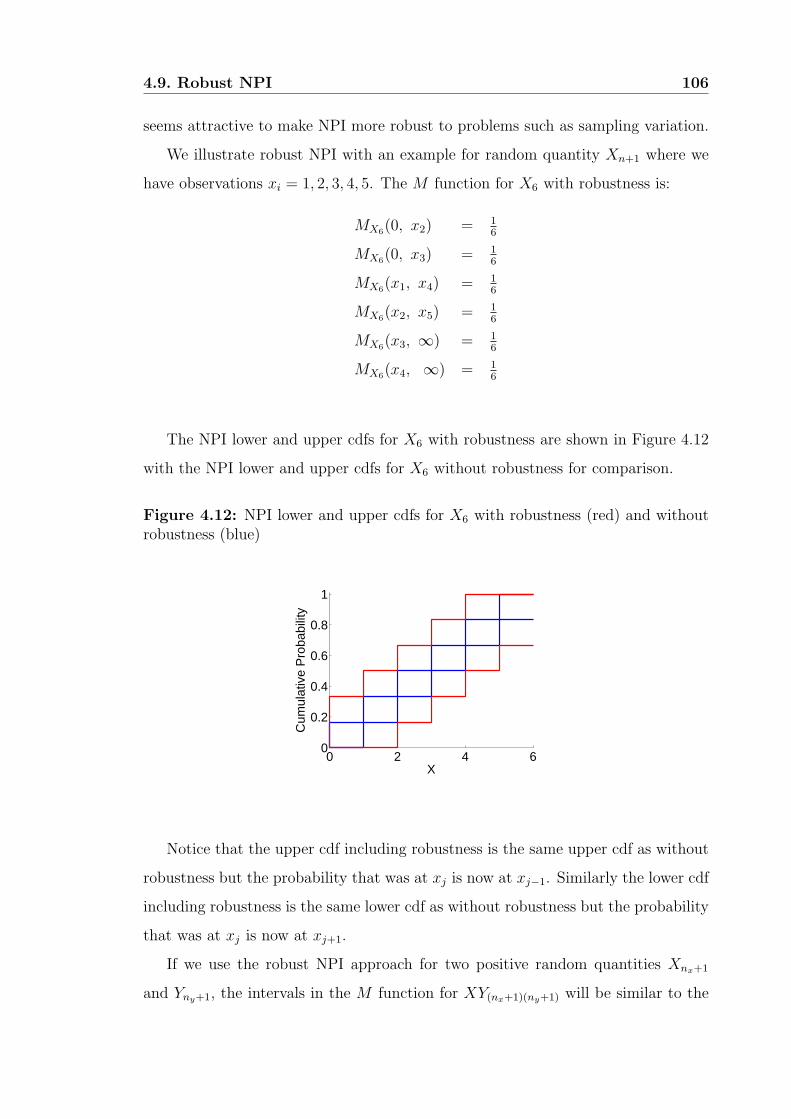
4.9. Robust NPI 106
seems attractive to make NPI more robust to problems such as sampling variation.
We illustrate robust NPI with an example for random quantity Xn+1 where we
have observations xi = 1, 2, 3, 4, 5. The M function for X6 with robustness is:
MX6(0, x2) = 16
MX6(0, x3) = 16
MX6(x1, x4) = 16
MX6(x2, x5) = 16
MX6(x3, ∞) = 16
MX6(x4, ∞) = 16
The NPI lower and upper cdfs for X6 with robustness are shown in Figure 4.12
with the NPI lower and upper cdfs for X6 without robustness for comparison.
Figure 4.12: NPI lower and upper cdfs for X6 with robustness (red) and withoutrobustness (blue)
0 2 4 60
0.2
0.4
0.6
0.8
1
X
Cum
ulat
ive
Pro
babi
lity
Notice that the upper cdf including robustness is the same upper cdf as without
robustness but the probability that was at xj is now at xj−1. Similarly the lower cdf
including robustness is the same lower cdf as without robustness but the probability
that was at xj is now at xj+1.
If we use the robust NPI approach for two positive random quantities Xnx+1
and Yny+1, the intervals in the M function for XY(nx+1)(ny+1) will be similar to the

4.10. Conclusion 107
M function for a standard NPI analysis except the intervals will be wider. For
example, the interval that would be (xy1, xy2) in standard NPI will now be (0, xy3)
and the interval that was (xy2, xy3) will now be (xy1, xy4) etc, where xyk is the kth
ordered value for XY . Similarly for three random quantities, as we have in the
Exposure Model, the intervals will be wider when using robust NPI than when we
use standard NPI. To incorporate more robustness for any of the random quantities
we could assign 1n+1
probability over two intervals either side of every interval etc.
This may be appropriate for small sample sizes.
Any theoretical properties for the robust method used for NPI need investigation
but it seems a sensible approach to indicate the uncertainty about the predicted value
of the next observation. As n increases, these robust NPI lower and upper cdfs will
converge to the empirical distribution, as the NPI lower and upper cdfs do. However
the convergence will be slower. Also we can see that robust NPI makes sense when
we have one observation as it produces the output that the next observation has a
probability between 0 and 1 of falling in the interval (−∞,∞). This statement is
true given our current state of information and is more cautious about predictions
than the NPI method.
4.10 Conclusion
In this chapter we have shown how NPI can be implemented for an exposure risk
assessment including censored data. An example with real data sets has been pre-
sented and we have explored the effect of correlations on the NPI bounds. We briefly
discussed how to solve the computational challenges with implementing NPI either
by only using one of each tied value in the sample or by using a threshold approach.
We looked at the effect of different sample sizes and saw that larger sample sizes
lead to less uncertainty about the next observation and therefore the NPI lower and
upper cdfs are closer together. Fixed measurement uncertainty can be included in
the NPI lower and upper cdfs.
We compared the results from an NPI analysis with the Bayesian posterior pre-
dictive distribution, where it compares favourably due to the fact that no assumption

4.10. Conclusion 108
is needed about the distribution and that NPI includes interval uncertainty due to
the assumption A(n). We saw that the assumptions necessary in the Bayesian frame-
work led to differing results, whereas the NPI results were similar for both two and
three random quantities in the exposure model. The main difference was the final
probability of the NPI lower cdf due to the sample sizes, as discussed in Subsection
4.3.2. We introduced an ad hoc method where we included robustness for NPI. This
helps to make NPI more robust to sampling variation and may be useful for small
sample sizes because it introduces more uncertainty about the predicted value of the
next observation. So in this chapter we have shown that NPI can be applied in the
field of exposure risk assessment even when there is censored data. It is also useful
when we want to avoid making distributional assumptions and has the potential to
be made robust for smaller sample sizes.

Chapter 5
Combining NPI and Bayesian
methods
5.1 Introduction
In this chapter we present a hybrid method that can be used to combine nonpara-
metric predictive inference (NPI) with Bayesian methods. This hybrid method,
which we will call the NPI-Bayes hybrid method, will be useful in practice when
we want to combine random quantities for which we make different assumptions
based on the level of information available. If we do not have enough information to
justify the assumption of a particular distribution, we can implement NPI for that
random quantity and combine it with other random quantities for which we have
enough evidence available to make distributional assumptions. As the majority of
methods used in probabilistic risk assessments require distributional assumptions,
it is interesting to compare nonparametric methods such as NPI with distributional
methods, such as the Bayesian posterior predictive distribution. The NPI-Bayes
hybrid method allows us to combine and compare these methods.
In Section 5.2 we explain how the NPI-Bayes hybrid method works and illustrate
it with an example. We implement the NPI-Bayes hybrid method for the simple
Exposure Model (Section 2.2) with different assumptions made about each random
quantity in the model in Section 5.3. We consider the case where all the random
quantities are modelled by NPI and another case where all the random quantities
109

5.1. Introduction 110
are modelled by Bayesian posterior predictive distributions. We also consider all the
other possible combinations (e.g. one random quantity represented by NPI and two
by Bayesian posterior predictive distributions, etc.) using the NPI-Bayes hybrid
method. For the simple Exposure Model we use simulated data sets to describe
the exposure of young children to benzene from soft drinks. We then compare the
results for all the different combinations of NPI and the Bayesian posterior pre-
dictive distribution for the random quantities using the NPI-Bayes hybrid method.
Throughout this chapter we assume (Log)Normality for the random quantities that
are described using the Bayesian posterior predictive distribution. However it would
be possible to implement the NPI-Bayes hybrid method when assuming other distri-
butions by sampling from the corresponding posterior predictive distributions. We
also consider how sampling variation and sample size affect the results by simulating
multiple samples, of two different sizes, for each random quantity in the Exposure
Model and comparing the results.
In Section 5.4 we show how the NPI-Bayes hybrid method can be adapted to
include robustness to the prior distribution for the random quantities for which
we use a Bayesian posterior predictive distribution. For these random quantities,
robustness to the prior distribution is implemented for two different classes of prior
distributions and compared with the Bayesian method when we use a non-infomative
prior distribution. Next we provide an algorithm for incorporating robustness in
the NPI-Bayes hybrid method. In Section 5.5 we present two examples including
robustness for the Exposure Model, one where robust Bayesian methods are used
for all the random quantities and one where robust NPI is used for all the random
quantities. Then all the different possible combinations are compared by looking
at their 10th, 50th and 90th percentiles. In Section 5.6 we show that NPI can be
combined with two-dimensional Monte Carlo simulation (2D MCS) using an example
with the Exposure Model.

5.2. The NPI-Bayes hybrid method 111
5.2 The NPI-Bayes hybrid method
In this section we explain the NPI-Bayes hybrid method for combining NPI and a
Bayesian posterior predictive distribution. Assume that we have nx observations xi,
where i = 1, ..., nx, for random quantities Xi and that these observations come from
a Normal distribution. We also have ny observations yj, j = 1, ..., ny, for positive
random quantities, Yj. As we have no further information about the Yj we choose to
use NPI for Yny+1. To apply the NPI-Bayes hybrid method we assume independence
between the Xi and Yj.
The Bayesian posterior predictive distribution for the Xi with a non-informative
prior, p(µ, σ2) = 1σ2 , is a scaled Student t-distribution with (nx − 1) degrees of
freedom, location parameter x and scale parameter
√(1 + ( 1
nx)sx
), where x is the
sample mean, sx is the sample standard deviation and nx is the number of ob-
servations of X (Gelman et al., 1995). We invert the cdf at np percentiles of the
Student t-distribution between 0 and 1 and assign each value probability pi = 1np
.
By inverting the cdf we capture the range of values for the Xi.
We want to find bounds on the prediction for the next observation, XYnew. To
do this we use the following algorithm.
1. Take np values, which we denote vi, i = 1, ..., np, by inverting the Student
t-distribution with nx − 1 degrees of freedom, location parameter x and scale
parameter
√(1 + ( 1
nx)sx
)at np percentiles.
2. Take the set of ordered observed values for Yj, j = 1, ..., ny, and add ∞ so
we have ny + 1 values, call this set L (this leads to the values that form the
intervals for the lower cdf for xynew).
3. Take the set of ordered observed values for Yj and add 0 so we have ny + 1
values, call this set U (this will lead to the values that form the intervals for
the upper cdf for xynew).
4. Find all the intervals between the ordered values (viyj)k for FXYnew(xy) by
multiplying the values vi from the Student t-distribution, with the set L, where
k = 1, ..., np(ny + 1), i = 1, ..., np and j = 1, ..., ny.
5.2. The NPI-Bayes hybrid method 112
5. Similarly find all the intervals between the ordered values (viyj)k for FXYnew(xy)
by multiplying the values vi with the set U, with i, j and k as before.
6. The probability on the intervals between each viyj value is 1np(ny+1)
7. Plot FXYnew(xy) and FXYnew(xy)
The combinations of (viyj) for the lower and upper cdfs will be the same, apart
from the infinities generated for the lower cdf and the zeroes generated for the upper
cdf. Therefore it is only necessary to combine the values from the scaled Student
t-distribution with the observed values for Yj once. We can describe the resulting
probabilities using an M function. We order all the values viyj and call them b and
use the index r to denote their place in the ordering.
MXYnew(0, b1) = 1/np(ny + 1)
MXYnew(br, br+1) = 1/np(ny + 1)
MXYnew(b(np(ny+1)−1), ∞) = 1/np(ny + 1)
for r = 1, ..., (np(ny + 1)− 2).
We now illustrate the NPI-Bayes hybrid method using an example where we use
the NPI approach for one random quantity and use the Bayesian posterior predictive
distribution for the other random quantity.
Take Y > 0 and assume that we have observations [1,2,3] for the Yj, j = 1, ..., 3.
We assume A(3) for Y4 and therefore the M function is as follows:
MY4(0, 1) = 1/4
MY4(1, 2) = 1/4
MY4(2, 3) = 1/4
MY4(3, ∞) = 1/4
Generally we would only recommend using NPI for medium to large samples, but
for illustrative purposes we use it for small n here. We take a sample of 20 values,
xi, i = 1, ..., 20 for the Xi from a Normal distribution with mean 5 and standard

5.2. The NPI-Bayes hybrid method 113
deviation 0.2. The sample mean, x = 5.00 and the sample standard deviation, sx =
0.17. Then we invert the cdf of the Student t-distribution at 5000 percentiles. We
can see that the probability for each interval will be 14(5000)
as each of the 5000 vi
values for the Xi have probability 1np
which is 15000
and each Y4 value has probability
14
of falling in each of the intervals shown in the M function. We then proceed as
with a NPI analysis to find the lower and upper cdfs. An example is shown in Figure
5.1.
Figure 5.1: Example of NPI-Bayes hybrid method
0 5 10 15 200
0.2
0.4
0.6
0.8
1
XY
Cum
ulat
ive
Pro
babi
lity
The influence of the Yj is very clear in the four different parts of the lower and
upper cdfs obtained. This is because of the small sample size that was used in this
example. The final value of the lower cdf will be 34
because the probability that
the random quantity falls in an interval between the largest finite value for XYnew
and ∞ will be 1ny+1
. If we instead had 50 observations, and thus Yj, j = 1, ..., 50,
(sampled from a Normal distribution with mean 2 and standard deviation 0.2) and
we again use NPI for the Yj and model the Xi as before, we would get results as
shown in Figure 5.2. The final value of the lower cdf will now be 5051
.

5.3. Predicting exposure using the NPI-Bayes hybrid method 114
Figure 5.2: Combining NPI and Bayesian posterior predictive distribution for alarger sample size for Y
0 5 10 15 200
0.2
0.4
0.6
0.8
1
XY
Cum
ulat
ive
Pro
babi
lity
So we have shown that the NPI-Bayes hybrid method allows us to combine NPI
and the Bayesian posterior predictive distribution for different random quantities.
Our example is for the Normal distribution and can be used when an analyst assumes
a Normal or Lognormal distribution. However the Bayesian posterior predictive
distribution for any distribution could be combined with NPI in a similar way if it is
possible to sample from the Bayesian posterior predictive distribution. In the next
section we show how we can apply the NPI-Bayes hybrid method to the Exposure
Model.
5.3 Predicting exposure using the NPI-Bayes hy-
brid method
We consider the simple Exposure Model described in Section 2.2:
Exposure =X × Y
Z(5.1)
where X is concentration, Y is intake and Z is bodyweight. We begin by simulating
5.3. Predicting exposure using the NPI-Bayes hybrid method 115
a sample from a (Log)Normal distribution for each random quantity. We look
at how well NPI and the Bayesian posterior predictive distribution describe the
(Log)Normal distributions that we have taken the samples from. Then we calculate
exposure by combining NPI for some random quantities and the Bayesian posterior
predictive distribution for other random quantities. We compare the results for each
of these combinations. We will use the following notation for the different possible
combinations: NX indicates that the NPI approach was used for the random quan-
tities Xi and BX that the Bayesian posterior predictive distribution was used for
the random quantities Xi. Similarly we use NY, BY, NZ and BZ.
5.3.1 Data sets
To illustrate the NPI-Bayes hybrid method for calculating exposure, we need to
have a sample for each random quantity in the model. In this example we choose
distributions for each random quantity so that the data sets resemble those from
Section 4.3 which described young children’s exposure to benzene in soft drinks.
We simulate 20 concentration (x) values from a Lognormal distribution with mean
1.4993 µg/kg and standard deviation 1.6749 µg/kg, 20 intake (y) values from a
Lognormal distribution with mean 1.2776 kg/day and standard deviation 1.0159
kg/day and 20 bodyweight (z) values from a Normal distribution with mean 30 kg
and standard deviation 3 kg. The ordered samples are:
X 0.1703 0.1828 0.3059 0.4278 0.4439 0.4994 0.5459 0.6037,
0.6118 0.8656 0.8700 0.9074 1.175 1.471 1.472 1.569,
2.346 2.663 4.036 12.12
Y 0.2758 0.3199 0.4195 0.4397 0.4815 0.5377 0.6922 0.6997,
0.7477 0.7675 0.8732 0.9954 1.130 1.174 1.348 1.403,
1.629 1.632 1.653 2.769
Z 25.86 25.93 26.58 26.65 26.93 28.61 28.83 28.98,
29.37 30.95 31.11 31.51 32.12 32.18 33.11 33.57,
34.66 35.59 35.87 36.34
Figures 5.3.1, 5.3.2 and 5.3.3 show the NPI lower and upper cdfs, the cdf of the

5.3. Predicting exposure using the NPI-Bayes hybrid method 116
Bayesian posterior predictive distribution given the assumption of (Log)Normality,
the cdf of the distribution that each data set was sampled from and the empirical cdf
for each random quantity. We display the distributions from which the data were
sampled so we can see how closely the results from the different methods resemble
these distributions. However, in a real-life risk assessment it is unlikely that we
would know which distributions the data were sampled from and the data probably
would not have come from a random sampling process.
Figure 5.3: NPI lower and upper cdfs (blue lines), Bayesian posterior predictivedistribution (red line), empirical cdf of the data (green) and distribution that thedata were sampled from (black line) for each random quantity
0 5 100
0.2
0.4
0.6
0.8
1
Concentration (µg / kg)
Cum
ulat
ive
Pro
babi
lity
5.3.1 Concentration (X)
0 1 2 3 40
0.2
0.4
0.6
0.8
1
Intake (kg / day)
Cum
ulat
ive
Pro
babi
lity
5.3.2 Intake (Y )
20 25 30 35 400
0.2
0.4
0.6
0.8
1
Bw (kg)
Cum
ulat
ive
Pro
babi
lity
5.3.3 Bodyweight (Z)
Figure 5.3.1 shows that for this sample of concentration values, the Bayesian
posterior predictive cdf overestimates the concentration at high percentiles (above
about the 80th percentile) but it is very close to the cdf of the distribution that the
data were sampled from at lower percentiles. The NPI lower and upper cdfs are
generally close to the cdf of the distribution that the data were sampled from except
at very high percentiles. Figure 5.3.2 shows that the Bayesian posterior predictive

5.3. Predicting exposure using the NPI-Bayes hybrid method 117
cdf underestimates intake for most percentiles of the cdf of the distribution that the
data were sampled from. The NPI lower and upper cdfs are close to or enclose the
cdf of the distribution from which the data were sampled for most percentiles. The
large intervals in the upper tail of the NPI lower and upper cdfs for concentration
and intake, are due to fewer data points being sampled from the tails than from
the middle of the distributions that the data were sampled from. Figure 5.3.3
shows that the Bayesian posterior predictive cdf overestimates the bodyweight for
low percentiles and is close to the upper tail of the cdf of the distribution from
which the data were sampled. The NPI lower and upper cdfs enclose the cdf of the
distribution from which the data were sampled in the lower and upper tails and
predicts values that are higher for the middle percentiles. Generally we tend to
be more interested in the lower tail because people with smaller bodyweights are
potentially more at risk from exposure to a chemical.
The Bayesian posterior predictive distribution is determined by the mean and
standard deviation of the sample and by the shape of the Student t-distribution
imposed on it because of the Normality assumption. NPI also depends on the values
in the sample but does not make distributional assumptions and the NPI lower and
upper cdfs will always enclose the empirical cdf of the data. Therefore different
samples lead to different results so we explore the effect of sampling variation in
Subsection 5.3.3.
5.3.2 Calculating exposure
We consider all different combinations of random quantities, using the NPI approach
for some random quantities and the Bayesian posterior predictive distribution for
the other random quantities, in the Exposure Model. For ease of presentation,
we display the results of each combination by the 10th, 50th, and 90th percentiles.
These percentiles are either intervals, if they use the NPI approach for some random
quantities, or point values if they only use the Bayesian posterior predictive distri-
bution for all the random quantities. We represent these by plotting the intervals for
each percentile in Figure 5.4 as horizontal lines. We combine the distributions that
the data were sampled from assuming independence between the random quantities

5.3. Predicting exposure using the NPI-Bayes hybrid method 118
and call this the approximate exposure distribution. We show the percentiles of the
approximate exposure distribution as vertical grey lines, so it is clear which inter-
vals include the percentiles of the approximate exposure distribution. Although it
cannot be seen in Figure 5.4, the lower bound for the 10th percentile for the case
(NX, NY, NZ) extends down to 0, and the upper bound for the 90th percentile for
(NX,NY,NZ) extends to ∞.
Figure 5.4: Percentiles for Exposure for combinations of Bayes and NPI
10-3
10-2
10-1
NX, NY, NZ
BX, NY, NZ
NX, BY, NZ
NX, NY, BZ
NX, BY, BZ
BX, NY, BZ
BX, BY, NZ
BX, BY, BZ
10th percentile 50th percentile 90th percentile
Exposure (µg / kg bw / day)
As can be seen from Figure 5.4, the 10th and 50th percentiles of the approximate
exposure distribution do not lie within the corresponding lower and upper cdfs of any
of the cases. However the 90th percentile of the approximate exposure distribution
lies within the lower and upper cdfs of all the cases except (BX, BY, BZ). The lower
and upper cdfs on the 10th and 50th percentiles are all lower than the percentiles of
the approximate exposure distribution. This is due to the combination of the higher
and lower predictions for each random quantity (See Figures 5.3.1, 5.3.2 and 5.3.3).
The higher predictions for bodyweight for middle and low percentiles and the lower
predictions for intake would lead to lower exposure values in general. However when
combined with the higher predictions for upper percentiles for concentration, the
values for the upper percentiles of exposure are larger. This explains why the 90th
percentile of the approximate exposure distribution lies within the lower and upper
5.3. Predicting exposure using the NPI-Bayes hybrid method 119
cdfs of all the cases except (BX, BY, BZ).
The combinations where the NPI approach is used for more random quantities
lead to the widest intervals. Therefore if we were uncertain about the distribution
that the data were sampled from, we would recommend combining all the random
quantities using NPI because we are more likely to capture the percentiles of the
approximate exposure distribution.
5.3.3 Sampling variation
In this section we explore sampling variation by comparing the differences in results
for each of the eight cases, (NX, NY, NZ), (NX, NY, BZ), etc., when we use different
samples for each random quantity in the model.
We simulate 10 samples of size 20 from the Lognormal distributions that we
assigned for concentration and intake and 10 samples of size 20 from the Normal
distribution that we assumed for bodyweight (see Subsection 5.3.1). We combine
these samples to produce 10 different lower and upper cdfs for the 10th, 50th and
90th percentiles of exposure for each of the eight different combinations of random
quantities (NX, NY, NZ), etc. We then compare how the 10th, 50th and 90th
percentiles differ for each case and compare the results between cases. We plot the
results with the percentiles of the approximate exposure distribution (vertical grey
lines) for comparison. The 10th, 50th and 90th percentiles obtained by using the
NPI-Bayes hybrid method for each of the 10 different sets of samples are shown in
Figures 5.5.1 - 5.5.6 and Figures 5.6.1 - 5.6.2. We denote each set of three samples
by Sample 1 to 10 for simplicity in the Figures.

5.3. Predicting exposure using the NPI-Bayes hybrid method 120
Figure 5.5: Percentiles for different samples for each combination
10-3
10-2
10-1
100
Sample 1
Sample 2
Sample 3
Sample 4
Sample 5
Sample 6
Sample 7
Sample 8
Sample 9
Sample 10
10th percentile 50th percentile 90th percentile
Exposure (µg / kg bw / day)
5.5.1 (NX, NY, NZ)
10-3
10-2
10-1
100
Sample 1
Sample 2
Sample 3
Sample 4
Sample 5
Sample 6
Sample 7
Sample 8
Sample 9
Sample 10
10th percentile 50th percentile 90th percentile
Exposure (µg / kg bw / day)
5.5.2 (BX, NY, NZ)
10-3
10-2
10-1
100
Sample 1
Sample 2
Sample 3
Sample 4
Sample 5
Sample 6
Sample 7
Sample 8
Sample 9
Sample 10
10th percentile 50th percentile 90th percentile
Exposure (µg / kg bw / day)
5.5.3 (NX, BY, NZ)
10-3
10-2
10-1
100
Sample 1
Sample 2
Sample 3
Sample 4
Sample 5
Sample 6
Sample 7
Sample 8
Sample 9
Sample 10
10th percentile 50th percentile 90th percentile
Exposure (µg / kg bw / day)
5.5.4 (NX, NY, BZ)
10-3
10-2
10-1
100
Sample 1
Sample 2
Sample 3
Sample 4
Sample 5
Sample 6
Sample 7
Sample 8
Sample 9
Sample 10
10th percentile 50th percentile 90th percentile
Exposure (µg / kg bw / day)
5.5.5 (NX, BY, BZ)
10-3
10-2
10-1
100
Sample 1
Sample 2
Sample 3
Sample 4
Sample 5
Sample 6
Sample 7
Sample 8
Sample 9
Sample 10
10th percentile 50th percentile 90th percentile
Exposure (µg / kg bw / day)
5.5.6 (BX, NY, BZ)

5.3. Predicting exposure using the NPI-Bayes hybrid method 121
Figure 5.6: Percentiles for different samples for each combination
10-3
10-2
10-1
100
Sample 1
Sample 2
Sample 3
Sample 4
Sample 5
Sample 6
Sample 7
Sample 8
Sample 9
Sample 10
10th percentile 50th percentile 90th percentile
Exposure (µg / kg bw / day)
5.6.1 (BX, BY, NZ)
10-3
10-2
10-1
100
Sample 1
Sample 2
Sample 3
Sample 4
Sample 5
Sample 6
Sample 7
Sample 8
Sample 9
Sample 10
10th percentile 50th percentile 90th percentile
Exposure (µg / kg bw / day)
5.6.2 (BX, BY, BZ)
We can see from Figures 5.5.1 - 5.5.6 and Figures 5.6.1 - 5.6.2 that the intervals
for all the percentiles become narrower as we use the NPI approach for fewer ran-
dom quantities. The intervals for the 50th percentile tend to be narrower than the
intervals for the 10th and 90th percentiles. This is due to the lack of data describing
the tails of the distribution, so there is more uncertainty about the higher and lower
percentiles than about the 50th percentile. For the (NX, NY, NZ) case the lower
limit of the 10th percentile for all the samples is 0, and the upper limit for the 90th
percentile for all the samples is ∞. The intervals for this case overlap for different
samples. Therefore using the NPI approach for random quantities is more robust to
sampling variation than the Bayesian method which only produces point estimates
which underestimate or overestimate the percentiles. However, even using the NPI
approach for all the random quantities in the Exposure Model does not lead to the
percentiles of the approximate exposure distribution lying within the lower and up-
per cdfs. This may be due to the small sample size that we used. In the next section
we look at the difference when we use a larger sample size.
5.3.4 Larger sample sizes
In this section we explore the effect of sample size on the percentiles for exposure and
again compare the difference in results for each of the eight cases (NX, NY, NZ), etc.
As before we simulate 10 samples from the Lognormal distributions that we assigned
for concentration and intake and 10 samples from the Normal distribution that we

5.3. Predicting exposure using the NPI-Bayes hybrid method 122
assumed for bodyweight. However, here we take samples of size 100. We combine
these samples for each of the eight different combinations of random quantities to
produce 10 different lower and upper cdfs for the 10th, 50th and 90th percentiles
of exposure. We plot the results with the percentiles of the approximate exposure
distribution (vertical grey lines) for comparison. The 10th, 50th and 90th percentiles
obtained by using the NPI-Bayes hybrid method for each of the 10 different sets of
samples are shown in Figures 5.7.1 - 5.7.4 and Figures 5.8.1 - 5.8.4. We compare
these results with those given in Figures 5.5.1 - 5.5.6 and Figures 5.6.1 - 5.6.2 for
samples of size 20.
Figure 5.7: Percentiles for different samples of size 100
10-2
10-1
Sample 1
Sample 2
Sample 3
Sample 4
Sample 5
Sample 6
Sample 7
Sample 8
Sample 9
Sample 10
10th percentile 50th percentile 90th percentile
Exposure (µg / kg bw / day)
5.7.1 (NX, NY, NZ)
10-2
10-1
Sample 1
Sample 2
Sample 3
Sample 4
Sample 5
Sample 6
Sample 7
Sample 8
Sample 9
Sample 10
10th percentile 50th percentile 90th percentile
Exposure (µg / kg bw / day)
5.7.2 (BX, NY, NZ)
10-2
10-1
Sample 1
Sample 2
Sample 3
Sample 4
Sample 5
Sample 6
Sample 7
Sample 8
Sample 9
Sample 10
10th percentile 50th percentile 90th percentile
Exposure (µg / kg bw / day)
5.7.3 (NX, BY, NZ)
10-2
10-1
Sample 1
Sample 2
Sample 3
Sample 4
Sample 5
Sample 6
Sample 7
Sample 8
Sample 9
Sample 10
10th percentile 50th percentile 90th percentile
Exposure (µg / kg bw / day)
5.7.4 (NX, NY, BZ)

5.3. Predicting exposure using the NPI-Bayes hybrid method 123
Figure 5.8: Percentiles for different samples of size 100
10-2
10-1
Sample 1
Sample 2
Sample 3
Sample 4
Sample 5
Sample 6
Sample 7
Sample 8
Sample 9
Sample 10
10th percentile 50th percentile 90th percentile
Exposure (µg / kg bw / day)
5.8.1 (NX, BY, BZ)
10-2
10-1
Sample 1
Sample 2
Sample 3
Sample 4
Sample 5
Sample 6
Sample 7
Sample 8
Sample 9
Sample 10
10th percentile 50th percentile 90th percentile
Exposure (µg / kg bw / day)
5.8.2 (BX, NY, BZ)
10-2
10-1
Sample 1
Sample 2
Sample 3
Sample 4
Sample 5
Sample 6
Sample 7
Sample 8
Sample 9
Sample 10
10th percentile 50th percentile 90th percentile
Exposure (µg / kg bw / day)
5.8.3 (BX, BY, NZ)
10-2
10-1
Sample 1
Sample 2
Sample 3
Sample 4
Sample 5
Sample 6
Sample 7
Sample 8
Sample 9
Sample 10
10th percentile 50th percentile 90th percentile
Exposure (µg / kg bw / day)
5.8.4 (BX, BY, BZ)

5.3. Predicting exposure using the NPI-Bayes hybrid method 124
The main difference in results between the application with a small sample size
and with a larger sample size is that the intervals for the percentiles are much
narrower. These narrower intervals for NPI are due to the larger sample size which
provides more information about the distribution. Generally the percentiles of the
approximate exposure distribution lie in more intervals, particularly for the (NX,
NY, NZ) case and the cases where the NPI approach is used for two of the random
quantities. The intervals for the 50th percentile still tend to be narrower than those
at the 10th and 90th percentile, although the difference in width is smaller than it
was for the small sample size. The Bayesian posterior predictive distribution does
not capture uncertainty about the estimates for the percentiles and thus can lead
to incorrect results. NPI captures more uncertainty than the Bayesian method due
to NPI’s inclusion of interval uncertainty.
As the sample size increases, the performance of NPI will improve because it
only uses information from the data and distributional assumptions for the data are
not needed. This makes NPI particularly useful if the distribution is unknown or
the data do not follow a standard parametric distribution (e.g. Normal, Lognormal,
etc.). The estimates given by the Bayesian posterior predictive distribution may not
improve as n increases if an incorrect distributional assumption is made. However if
the assumed distribution is the correct distribution, then as n → ∞, the Bayesian
estimates will be closer to the distribution that the data were sampled from. As
we have seen, even with a sample size of 100 there is variation in the results and
the percentiles for the approximate exposure distribution do not always lie within
the lower and upper bounds. Therefore if we are interested in the tails and the
uncertainty about the tails, predictive methods may not be the most appropriate
choice. One solution to include more uncertainty about the tails in the analysis is to
include robustness. In the next section we discuss how to include robustness to the
prior distribution when we use a Bayesian approach for a random quantity and how
to include robustness in the NPI-Bayes hybrid method for the Exposure Model.
5.4. Robustness 125
5.4 Robustness
5.4.1 Robustness for the Normal distribution
In this section we explain how our proposed hybrid method can be combined with
robustness when we use the Bayesian approach for random quantities. We begin
by explaining two different classes of prior distributions, a class of interval prior
distributions for µ that we used in Subsection 3.5.1 and a class of Normal-Gamma
prior distributions. We then explain the algorithm used to include robustness in the
NPI-Bayes hybrid method for the Exposure Model.
Robustness to the prior for µ
To include robustness to the prior for µ, we consider the class of Normal prior
distributions on µ|σ used in Subsection 3.5.1. The corresponding Bayesian posterior
predictive distribution is a Student t-distribution with n − 1 degrees of freedom,
location parameter(
a+x2
)and scale parameter
√(2n+1)
�(n−1)s2+
n(x−a)2
2
�
2n(n−1), where x is
the sample mean, n is the sample size and s is the sample standard deviation. When
we use this class of prior distributions, we will call the resulting bounds the ‘robust
interval posterior predictive box’.
Robustness to prior distribution for (µ, σ)
Another possible class of prior distributions can be obtained by using a conjugate
Normal-Gamma prior. If we assume this prior distribution
p(µ, σ) ∝ 1
σ2
a
exp
[− c
2σ2(µ−m)2 − b
σ2
], −∞ < µ < ∞, σ2 > 0
the Bayesian posterior predictive distribution for the Xi given this conjugate prior
distribution can be shown by basic exercise to be a Student t-distribution with 2a∗−3
degrees of freedom, location parameter m∗ and scale parameter√
2b∗(1+c∗)(c∗(2a∗−3))
, where
a∗ = a + n2, b∗ = b + s2(n−1)
2+ (nd)
2(n+c)(x−m)2, c∗ = c + n, m∗ = cm+nx
c+n. When we use
this class of Normal-Gamma prior distributions, we will call the resulting bounds
the ‘robust Normal-Gamma posterior predictive box’.

5.4. Robustness 126
We now illustrate the algorithm for including robustness in the NPI-Bayes hybrid
method. It is most easily represented with a diagram. In this algorithm we assume
that we want to include robustness for every random quantity. If this is not the case,
an approach combining this algorithm and the algorithm for the original NPI-Bayes
hybrid method can be used instead.
5.4.2 Diagram showing how to include robustness for the
Exposure Model
Choose robust NPI or Bayesian method for each of the three random quantities, X, Y and Z
Robust NPI Robust Bayesian method
Choose class of prior distributions
Interval ClassNormal-Gamma Class
Use robust NPI as explained in Section
4.9
Choose interval for m and split interval into k values
Choose interval for µ and split interval into j values
Find the parameters for the k scaled student-t distributions and invert
each cdf at nppercentiles. Call these xpik, ypik or zpik for i =
1,…, np
Find the parameters for the j scaled student-t
distributions and invert each cdf at np
percentiles. Call these xpij, ypij or zpij for i =
1,…, np
Count how many random quantities are modelled using robust NPI and call this number r
Combine all three random quantities , X, Y and Z using robust NPI as explained in
Section 4.9
If r = 0 If r = 1 If r = 2 If r = 3
Take the envelope of the cdfs for the sets of exposure values to form the robust posterior predictive box
Combine all the values xpig, ypig
and zpig, i = 1,…,np. This
produces np values for exposure. Repeat this
process for all combinations of j
or k for each random quantity.
Combine two sets of values (e.g. ypig and zpig) as in the Exposure Model to produce
np values. For X we use robust NPI and multiply the intervals with the np values.
The intervals have probability 1/np(nx+1).
Repeat this process for all combinations of j or k for Y
and Z
Combine e.g. X and Y as in Section 4.9.
Combine the resulting NPI
intervals with the zpig so each interval has a probability of 1/np(nx+1)(ny+1).
Repeat this process for all combinations
of j or k for Z
where g represents j if the interval class was chosen and k if the Normal
Gamma class was chosen.

5.5. Examples: NPI-Bayes robust hybrid method 127
5.5 Examples: NPI-Bayes robust hybrid method
In this section we look at the results of incorporating robustness into the hybrid
method for the Exposure Model. We compare the results for assuming each of
the previously described classes of prior distributions for the case (BX, BY, BZ)
with each other and with the results when we assume a non-robust, non-informative
prior, p(µ, σ) = 1σ
for all three random quantities. We then show the results for
the (NX, NY, NZ) case where we use robust NPI for all the random quantities.
We compare this with the case where we use NPI without robustness for all three
random quantities. These examples allow us to illustrate the proposed NPI-Bayes
robust hybrid method for the two most extreme cases. We illustrate the approximate
exposure distribution to show how close the combinations are to the percentiles of
the approximate exposure distribution. In the model, we can combine robust and
non-robust random quantities, but for illustration of the method here we concentrate
on the case where we include robustness for all the random quantities. We show the
percentiles for all the other possible combinations of random quantities including
robustness for each random quantity. We use r to denote that we are including
robustness, e.g. BXr indicates that we are using robust Bayesian methods for random
quantity X.
5.5.1 Case (BXr, BYr, BZr)
We consider the case where bodyweight, the log of concentration and the log of
intake are modelled by the robust Bayesian posterior predictive distribution with
the assumption of Normality. We again use the data sets introduced in Subsection
5.3.1. We compare the results from assuming a non-informative prior for all three
random quantities, assuming an interval class of prior distributions for all three
random quantities and assuming a class of Normal-Gamma prior distributions for
all three random quantities. Combinations of different classes of prior distributions
could be considered if desired.
Let µbw, µint and µconc be the intervals for the mean of the prior distribution
for bodyweight, intake and concentration respectively for the interval class of prior

5.5. Examples: NPI-Bayes robust hybrid method 128
distributions. Also, let mbw, mint and mconc be the intervals for the mean of the prior
distribution for bodyweight, intake and concentration respectively for the Normal-
Gamma class of prior distributions. Take µbw and mbw to be 10 equally spaced values
between 25 kg and 35 kg, µint and mint to be 10 equally spaced values between
0.5 kg/day and 1.2 kg/day and µconc and mconc to be 10 equally spaced values
between 0.3 µg/kg and 3 µg/kg. For the Normal-Gamma prior we use parameters
a = c = 10, b = 0.01 for all the random quantities. Figure 5.9 shows the results
for the non-informative prior, the two different classes of prior distribution and the
approximate exposure distribution for comparison.
Figure 5.9: Non-informative posterior predictive distribution (black line), robustinterval posterior predictive box (red line), robust Normal-Gamma posterior predic-tive box (blue line) and approximate exposure distribution (green line)
10-4
10-3
10-2
10-1
100
101
0
0.2
0.4
0.6
0.8
1
Exposure (µg / kg bw / day)
Cum
ulat
ive
Pro
babi
lity
In Figure 5.9 we see that the robust Normal-Gamma posterior predictive box
follows the shape of the approximate exposure distribution for lower percentiles
and encloses the approximate exposure distribution. The robust interval poste-
rior predictive box nearly encloses the approximate exposure distribution, although
it slightly underestimates the lower percentiles of exposure. The non-informative
posterior predictive distribution is only a single line here and underestimates the
approximate exposure distribution for most percentiles until it reaches very high per-
centiles. This is probably due to the shape constraints of the Student t-distributions
used to form the non-informative posterior predictive distribution and the lack of
uncertainty included by the prior distribution.
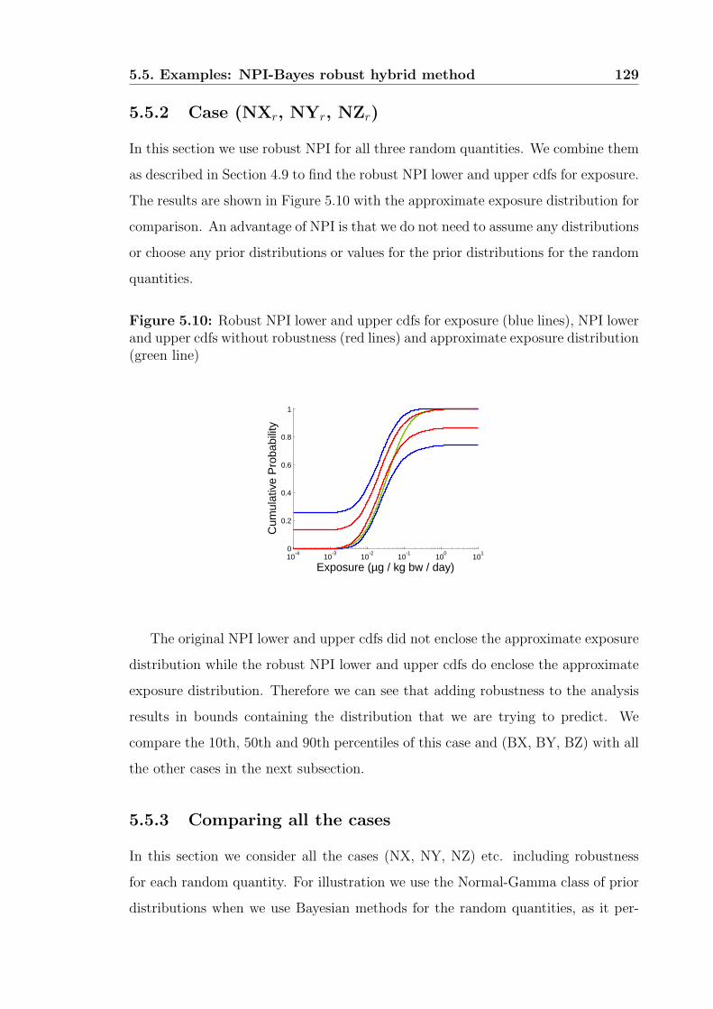
5.5. Examples: NPI-Bayes robust hybrid method 129
5.5.2 Case (NXr, NYr, NZr)
In this section we use robust NPI for all three random quantities. We combine them
as described in Section 4.9 to find the robust NPI lower and upper cdfs for exposure.
The results are shown in Figure 5.10 with the approximate exposure distribution for
comparison. An advantage of NPI is that we do not need to assume any distributions
or choose any prior distributions or values for the prior distributions for the random
quantities.
Figure 5.10: Robust NPI lower and upper cdfs for exposure (blue lines), NPI lowerand upper cdfs without robustness (red lines) and approximate exposure distribution(green line)
10-4
10-3
10-2
10-1
100
101
0
0.2
0.4
0.6
0.8
1
Exposure (µg / kg bw / day)
Cum
ulat
ive
Pro
babi
lity
The original NPI lower and upper cdfs did not enclose the approximate exposure
distribution while the robust NPI lower and upper cdfs do enclose the approximate
exposure distribution. Therefore we can see that adding robustness to the analysis
results in bounds containing the distribution that we are trying to predict. We
compare the 10th, 50th and 90th percentiles of this case and (BX, BY, BZ) with all
the other cases in the next subsection.
5.5.3 Comparing all the cases
In this section we consider all the cases (NX, NY, NZ) etc. including robustness
for each random quantity. For illustration we use the Normal-Gamma class of prior
distributions when we use Bayesian methods for the random quantities, as it per-

5.5. Examples: NPI-Bayes robust hybrid method 130
formed well in the (BX, BY, BZ) case. We take mbw, mint and mconc as before. The
10th, 50th and 90th percentiles are shown in Table 5.1.
Table 5.1: Percentiles for all cases including robustness
Case
10th 50th 90th
Percentile Percentile Percentile
Lower Upper Lower Upper Lower Upper
(NXr, NYr, NZr) 0 0.0087 0.0130 0.0435 0.0655 ∞
(BXr, NYr, NZr) 0 0.0112 0.0121 0.0537 0.0548 ∞
(NXr, BYr, NZr) 0 0.0095 0.0137 0.0377 0.0595 ∞
(NXr, NYr, BZr) 0 0.0089 0.0147 0.0384 0.0655 ∞
(NXr, BYr, BZr) 0.0016 0.0095 0.0151 0.0344 0.0603 0.7663
(BXr, NYr, BZr) 0.0009 0.0115 0.0136 0.0497 0.0570 0.7610
(BXr, BYr, NZr) 0.0009 0.0118 0.0121 0.0490 0.0527 0.6789
(BXr, BYr, BZr) 0.0036 0.0118 0.0139 0.0446 0.0515 0.1760
The 10th, 50th and 90th percentiles for the approximate exposure distribution
are 0.0077, 0.0335 and 0.1455 µg/kg bw/day respectively. We can see that the 10th,
50th and 90th percentiles of the approximate exposure distribution all lie in the
lower and upper bounds for the 10th, 50th and 90th percentiles for all the cases.
Therefore adding robustness to all the random quantities leads to results that again
enclose the 10th, 50th and 90th percentiles of the approximate exposure distribution.
In this section we have seen that it is possible to include robustness when we
use Bayesian methods for random quantities and when we use NPI for random
quantities. We have compared the different cases of combining the random quantities
with the different robust methods. Including robustness is useful as it resulted in all
the cases enclosing the 10th, 50th and 90th percentiles of the approximate exposure
distribution. For the Bayesian case different classes of prior distributions could
be chosen to reflect prior beliefs about the random quantities. For the NPI case
different levels of robustness could be incorporated. For small samples, we could
perhaps assign the probability 1n+1
to two intervals on either side of every interval.

5.6. Combining NPI with Bayesian 2D MCS 131
This would include more robustness to represent the increased uncertainty about
the distribution that the data were sampled from for a small sample.
5.6 Combining NPI with Bayesian 2D MCS
We have illustrated combining NPI with the Bayesian posterior predictive distribu-
tion in this chapter. However it may be the case that we want to combine a predictive
method with a Bayesian 2D method (one that separates variability and uncertainty).
We illustrate a NPI-2D Bayes hybrid method with the Exposure Model. Suppose we
want to calculate exposure based on predictions of the bodyweight of a young child.
Usually to combine a Bayesian posterior predictive distribution with a Bayesian
2D MCS, we would sample from the Bayesian posterior predictive distribution for
bodyweight in the outer loop of a 2D MCS. We would then combine the predicted
value with the values calculated in the inner loop of the 2D MCS.
Here we do not want to choose a distribution for bodyweight so we predict the
bodyweights using NPI. We again use the data sets provided in Subsection 5.3.1. We
use a Bayesian 2D MCS for concentration and intake assuming that both random
quantities are Lognormally distributed. We combine concentration and intake in a
2D MCS with 1000 inner loops and 1000 outer loops to include uncertainty about
the distribution parameters. Then we find NPI lower and upper cdfs for the product
of intake and concentration including parameter uncertainty by using the values that
form the envelope of the 2D MCS output. These NPI lower and upper cdfs can then
be combined with the NPI lower and upper cdfs for bodyweight as done previously
in Section 4.3 to find bounds on exposure. The resulting lower and upper NPI cdfs
are shown in Figure 5.11.

5.7. Conclusions 132
Figure 5.11: NPI lower and upper cdfs for exposure
0 50 1000
0.2
0.4
0.6
0.8
1
Exposure (µg / kg bw / day)
Cum
ulat
ive
Pro
babi
lity
So here we have combined the NPI predictions for the next bodyweight obser-
vation with the 2D MCS results to include parameter uncertainty for concentration
and intake.
5.7 Conclusions
In this chapter we have shown that we can combine NPI and the Bayesian posterior
predictive distribution by using the NPI-Bayes hybrid method and the NPI-Bayes
robust hybrid method. We have also shown that it is possible to combine NPI with
2D Bayesian methods such as 2D MCS. The NPI-Bayes hybrid method is useful
where there are different levels of information available for random quantities. NPI
can be used for random quantities for which we do not have enough information
available to assume a distribution and the Bayesian posterior predictive distribution
or 2D Bayesian MCS can be used for random quantities about which we have more
information. It is common in practice that this situation, where we have lots of in-
formation about some random quantities and less information about other random
quantities, will occur. For example, there is often little information about concen-
tration of chemicals in different food types but lots of information available about
the bodyweights of the population.
We saw in Subsection 5.3.4 that even when using samples with 100 values, the

5.7. Conclusions 133
percentiles of the approximate exposure distribution did not lie in the intervals for all
the cases for all the samples. We would expect that as the sample size, n, increases,
the lower and upper cdfs would converge to the approximate exposure distribution.
Therefore as some of the combinations failed to fully represent the percentiles of
the approximate exposure distribution for n = 100, we added robustness to each
random quantity to improve the hybrid method.
To incorporate robustness we created a new robust hybrid method that can com-
bine random quantities using either robust NPI or the Bayesian posterior predictive
distribution with robustness. We considered two different classes of prior distribu-
tions for the Bayesian posterior predictive distribution, and our method could easily
be adapted to include other possible classes of prior distributions. The Bayesian
part of the NPI-Bayes robust hybrid method could be applied to any distribution
(e.g. Weibull or Exponential distribution), as long as we can sample from the poste-
rior predictive distribution. We can also represent different levels of robustness for
NPI. Including robustness allows us to account for more uncertainty and led to both
cases (NXr, NYr, NZr) and (BXr, BYr, BZr) enclosing the approximate exposure
distribution. Also, all the cases where robustness was included for all the random
quantities produced intervals containing the 10th, 50th and 90th percentiles of the
approximate exposure distribution. This was not the case without robustness. This
indicates that when using predictive methods on smaller samples, the NPI-Bayes ro-
bust hybrid method can represent the uncertainty about the approximate exposure
distribution.
In practice, the NPI-Bayes robust hybrid method allows us to take account of
the information available about random quantities such as intake whilst including
robustness for random quantities such as concentration. It also allows us the option
of not having to assume a distribution for all the random quantities in the model.
We can use a mixture of the NPI-Bayes hybrid method and robust hybrid method to
implement robustness for some random quantities and not for others. If the sample
sizes are large then the hybrid method will provide results close to the approximate
exposure distribution when the random quantities are combined. However if the
sample sizes are small the robust hybrid method will provide better results than

5.7. Conclusions 134
the hybrid method because it is more likely to contain the approximate exposure
distribution in the resulting bounds.
The results from all three of these methods require more investigation as it is
not clear how the resulting bounds should be interpreted. The NPI-Bayes hybrid
method, the NPI-Bayes robust hybrid method and the NPI-2D Bayes hybrid method
introduced in this chapter are useful tools to combine random quantities in practice.
The choice of which method to use and which combination to use will depend on
many factors, such as sample size, whether there is enough information to make
distributional assumptions and whether there are experts available to choose classes
of prior distributions.

Chapter 6
Conclusions and Future Research
This chapter provides a short summary of the main results presented in this thesis,
and discusses important challenges for future research.
6.1 Conclusions
In this thesis we have introduced new methods that add to the choice of methods
available for risk assessment. The appropriate method to use will depend on factors
such as whether the decision is about a population or an individual, how many data
are available and if there is enough information about the random quantities for the
analyst to assume a particular distribution. It also depends on whether the whole
distribution or a percentile for a population is of interest. If the decision maker
would like to estimate the risk based on the whole distribution, Bayesian p-boxes
could be implemented. If the question is about a random individual NPI could be
appropriate, as NPI only assumes A(n) and includes interval uncertainty. If there
are some random quantities in a model about which we do not want to make a
distributional assumption and others that we are prepared to assume distributions
for, then the NPI-Bayes or robust NPI-Bayes hybrid method could be used.
In Chapter 3, we have seen that nested Bayesian p-boxes can give an analyst or
risk manager a clear indication of the changes at different credibility levels. Bayesian
p-boxes should be used instead of frequentist p-boxes when working with distribu-
tions with more than one parameter, particularly for small sample sizes. This is be-
135

6.1. Conclusions 136
cause the frequentist p-boxes ignore dependence between parameters and therefore
do not lead to the tightest possible bounds given the information available. Bayesian
p-boxes can be formed using any subset of the posterior parameter space, as long as
it is closed and bounded. We have shown that the Bayesian p-box method can take
fixed measurement uncertainty and robustness to the prior distribution into account.
We focused on including robustness to the prior distribution for the practically im-
portant cases of the Normal and Lognormal distributions. We have explained how
Bayesian p-boxes can be combined under the assumption of independence or under
no assumptions about dependence using the Williamson and Downs method. It may
be useful to risk managers to see both outputs so they can see how much reduction
in uncertainty there is under the assumption of independence. Bayesian p-boxes can
include distribution uncertainty and model uncertainty by forming Bayesian p-boxes
separately for each distribution or model and then taking the envelope of the results.
Displaying the results from different distributions or models may provide more in-
sight into the risk distribution and provide a clearer picture for the risk manager.
When a risk manager has to make a decision about a population, this method can
be used to illustrate bounds on the distribution of the population.
In Chapter 4, we have shown that NPI provides an alternative method for pre-
dicting the exposure of a random individual to a chemical. For a medium or large
data set, NPI provides a better representation of the exposure than methods such
as the Bayesian posterior predictive distributions due to the inclusion of interval
uncertainty and the lack of distributional assumptions. NPI can be used where we
have left-censored data and known measurement uncertainty and will produce the
tightest possible lower and upper cdfs given this information. We explored the ef-
fect of strong and weak correlations in an example and it seemed that neither of
them strongly influenced the NPI analysis. We also suggested an ad hoc method
to include more uncertainty in the NPI analysis which we called ‘robust NPI’. This
method seems to work well and may provide a way to use NPI for small samples
but requires further investigation.
In Chapter 5, we introduced a NPI-Bayes hybrid method that allows us to com-
bine random quantities where some random quantities are modelled with NPI and

6.2. Topics for future research 137
others are modelled with Bayesian methods. We have shown that NPI can be com-
bined with both one-dimensional methods, such as the Bayesian posterior predictive
distribution and two-dimensional methods such as 2D Monte Carlo Simulation. We
showed how robustness could be incorporated in the hybrid method for both NPI
and the Bayesian posterior predictive distribution methods. Including robustness to
the prior distribution can partially reduce the effect of distributional assumptions, as
including the additional uncertainty increases the chance that the true distribution
will fall within the bounds. However, robustness may also reduce the uncertainty
if narrower ranges are selected for the priors. Further research is required into the
interpretation of the output bounds. NPI is a frequentist method, that is also con-
sistent with the Bayesian framework and it is unclear how to interpret the bounds
when mixing a frequentist and a Bayesian method together.
All methods that we have presented and explored in this thesis help to model the
uncertainties involved more transparently than they currently are in the determin-
istic risk assessments. We have focused on Bayesian methods because they have the
advantage that parameter dependence can be incorporated and the results can be
updated with future observations. NPI has been investigated due to the advantage
of not having to assume a distribution and because it includes interval uncertainty.
As both NPI and Bayesian methods have advantages we then combined them in
a NPI-Bayes hybrid method. Further research is required into extensions of these
methods. We briefly describe possible future research topics in Section 6.2.
6.2 Topics for future research
In this section we discuss possible areas of future research which build on the work
presented in this thesis. All these areas would add to the expansion of quantifying
uncertainty in risk assessments.
6.2.1 Uncertainty about correlations
It is possible to combine various types of bounds, e.g. Bayesian p-boxes, by using the
method presented by Williamson and Downs (1990). We have also briefly introduced

6.2. Topics for future research 138
copulas which are a method of combining random quantities with a fixed correlation.
However when we do not know much about the dependence but we do know that
the random quantities are, for example, definitely not negatively correlated, the
Williamson and Downs method will not be able to exclude this particular correlation.
Further research is needed into excluding known dependencies from the resulting
bounds. If the result of combining two random quantities with a specific correlation
falls completely within the bounds formed using the Williamson and Downs method,
excluding the specific correlation may not have any effect on the outer bounds. If
we knew that there was a range of possible correlations, it may be possible to
combine the bounds assuming various correlations in the interval. If these behave in
a linear way (i.e. the lowest correlation leads to the lowest possible bound and as the
correlation increases the upper bounds increase) then it may be possible to draw a
p-box around the results. Further research into eliciting and modelling dependencies
between random quantities is necessary to make the risk assessments more realistic.
6.2.2 Bayesian p-boxes for other distributions
In this thesis we have presented Bayesian p-boxes for the Exponential and Normal
distributions. Bayesian p-boxes could be formed for other distributions, as long as
we can calculate the highest posterior density or similar region from the posterior
distribution. The region needs to be closed and bounded so we can minimise and
maximise the corresponding cdf over the region to form the lower and upper bounds
on the random quantity. If we had a multi-modal distribution, we could have various
closed and bounded regions. It would in theory be possible to minimise and maximise
the cdf of the distribution over these regions separately and then form multiple p-
boxes to represent the different regions. When these p-boxes are considered all
together they should represent the 100(1 − α)% probability that, for example, the
distribution for a random quantity X falls in the p-boxes. However, if we can only
sample from the posterior distribution, it may not be possible to calculate a highest
posterior density or any other region with a certain credible level. The justification
for the minimum and maximum bounds being formed by the (µ, σ) pairs on the
contour applies to location-scale distributions. However if distributions have more

6.2. Topics for future research 139
than two parameters, it will become more complicated to calculate regions and to
present the results in a meaningful way. It would be interesting and also important
for risk assessment to develop Bayesian p-boxes for other distributions.
6.2.3 More realistic models
Throughout this thesis we have used the simple Exposure Model to illustrate our
methods. It would be beneficial to consider developing the methods for more com-
plicated exposure models or for models in other fields. We have already discussed
developing Bayesian p-boxes for other distributions, but there is also research needed
on combining the Bayesian p-boxes for different random quantities in a model. It
would be useful to research how we could find the hpd region, or a similar region,
from the posterior distribution for several combined random quantities as this would
then allow us to find, for example, 95% bounds on the whole model. NPI could be
used for more complicated models, although more research needs to be done on
how to do this in the most computationally efficient way. As models become more
complicated and include more random quantities it can potentially make it difficult
to store all the possible values on a computer. It would also be useful to look at
combining random quantities with different dependencies which is currently not pos-
sible in the NPI framework. The NPI-Bayes hybrid methods could be used for more
complicated models, although this too will be limited by the computation required
for the random quantities that NPI is used for in the model.

A. Distributions used in this thesis 140
Appendix
A Distributions used in this thesis
Normal distribution
X has a Normal distribution with mean µ and variance σ2, denoted X ∼ N(µ, σ2),
if it has density
p(X) =1
σ√
2πexp
(−(x− µ)2
2σ2
)(−∞ < x < ∞)
As the distribution is symmetric and unimodal, the median and mode are both equal
to the mean. If µ = 0 and σ = 1, X is said to have a Standard Normal distribution.
µ can be referred to as the location parameter and σ can be referred to as the scale
parameter.
Lognormal distribution
X has a Lognormal distribution if it has density
p(X) =1
xσ√
2πexp
(−(log(x)− µ)2
2σ2
)
where µ and σ are the mean and standard deviation of the Normal distribution for
log(X).
Student t distribution
X has a Student t distribution on ν degrees of freedom, denoted X ∼ tµ, if it has
density
p(X) =Γ(ν+1
2)
√πνΓ(ν
2)
(1 +
x2
ν
)− ν+12
The non-central t distribution is a generalisation of Student’s t distribution with a
non-centrality parameter that measures the normalised distance between the true
population mean and the population mean, µ, that we have assumed.

A. Distributions used in this thesis 141
Gamma distribution
X has a two parameter Gamma distribution with parameters a and b, denoted
X ∼ G(a, b), if it has density
p(X) =1
baΓ(a)xa−1exp
(−x
b
)
This is a conjugate prior distribution for the Exponential distribution in Bayesian
statistics.
χ2 distribution
X has a χ2 distribution on ν degrees of freedom, denoted X ∼ χ2ν , if it has density
p(X) =1
2ν2 Γ(
ν2
)x ν−22 exp
(−x
2
)
This is a special case of the Gamma distribution with a = ν2
and b = 2.
Exponential Distribution
X has an Exponential distibution with parameter λ if it has the density
p(X) = λexp (−λx)
Bibliography
Aitio A. (2008). Research needs for environmental health risk assessment. Journal
of Toxicology and Environmental Health Part A, 71 (18): 1254 – 1258
Aldenberg T. and Jaworska J.S. (2000). Uncertainty of the Hazardous Concentration
and Fraction Affected for Normal Species Sensitivity Distributions. Ecotoxicology
and Environmental Safety, 46 (1): 1 – 18
Aughenbaugh J.M. and Paredis C.J.J. (2006). The value of using imprecise prob-
abilities in engineering design. Journal of Mechanical Design, 128 (4): 969 –
979
Augustin T. and Coolen F.P.A. (2004). Nonparametric predictive inference and
interval probability. Journal of Statistical Planning and Inference, 124 (2): 251
– 272
Berger J.O. (1985). Statistical Decision Theory and Bayesian Analysis. New York:
Springer-Verlag, Second Edition
Berger J.O. (1990). Robust Bayesian analysis: sensitivity to the prior. Journal of
Statistical Planning and Inference, 25 (3): 303 – 328
Berger J.O. (2000). Bayesian analysis: A look at today and thoughts of tomorrow.
Journal of the American Statistical Association, 95 (452): 1269 – 1276
Berger J.O. and Berliner L.M. (1986). Robust Bayes and Empirical Bayes Analysis
with ε-contaminated priors. The Annals of Statistics, 14 (2): 461 – 486
Bernardo J.M. (2005). Intrinsic credible regions: An objective Bayesian approach
to interval estimation. Test, 14 (2): 317 – 384
142

BIBLIOGRAPHY 143
Bernardo J.M. and Smith A.F.M. (1994). Bayesian Theory. John Wiley and Sons,
First Edition
Blasco A. (2005). The use of Bayesian statistics in meat quality analyses: a review.
Meat Science, 69 (1): 115 – 122
Boas M.L. (1983). Mathematical Methods in the Physical Sciences. John Wiley and
Sons, Second Edition
Bose S. (1994). Bayesian robustness with mixture classes of priors. The Annals of
Statistics, 22 (2): 652 – 667
Box G.E.P. and Tiao G.C. (1973). Bayesian Inference in Statistical Analysis.
Addison-Wesley, Reading, MA
Brand E., Otte P.F. and Lijzen J.P.A. (2007). CSOIL 2000 an exposure
model for human risk assessment of soil contamination. A model descrip-
tion. Technical report. RIVM, Bilthoven, The Netherlands. Available at
http://rivm.openrepository.com/rivm/bitstream/10029/7382/1/601501022.pdf
Bryan B., , McMahan H.B., Shafer C.M. and Schneider J. (2007). Efficiently com-
puting minimax expected-size confidence regions. In Proceedings of the 24th In-
ternational Conference on Machine Learning, Corvallis, OR
Burmaster D.E. and Thompson K.M. (1998). Fitting second-order parametric dis-
tributions to data using maximum likelihood estimation. Human and Ecological
Risk Assessment, 4 (2): 319 – 339
Burmaster D.E. and Wilson A.M. (1996). An introduction to second-order random
variables in human health risk assessments. Human and Ecological Risk Assess-
ment, 2 (4): 892 – 919
Chaturvedi A. (1996). Robust Bayesian analysis of the linear regression model.
Journal of Statistical Planning and Inference, 50 (2): 175 – 186
Chebyshev P. (1874). Sur les valeurs limites des integrales. Journal de Mathema-
tiques Pures Appliques, Ser 2 (19): 157 – 160
BIBLIOGRAPHY 144
Chen M.H., Shao Q.M. and Ibrahim J.G. (2001). Monte Carlo Methods in Bayesian
Computation. Springer Series in Statistics. New York: Springer-Verlag
Chow T.E., Gaines K.F., Hodgson M.E. and Wilson M.D. (2005). Habitat and
exposure modelling for ecological risk assessment: A case study for the raccoon
on the Savannah River Site. Ecological Modelling, 189 (1 – 2): 151 – 167
Codex (2007). Codex Alimentarius Commission 16th procedural manual. Available
at http://www.codexalimentarius.net/web/procedural manual.stm.
Congdon P. (2001). Bayesian Statistical Modelling. John Wiley and Sons Ltd
Coolen F.P.A. (2006). On nonparametric predictive inference and objective
Bayesianism. Journal of Logic, Language and Information, 15 (1 – 2): 21 –
47
Coolen F.P.A. and Coolen-Schrijner P. (2007). Nonparametric predictive comparison
of proportions. Journal of Statistical Planning and Inference, 137 (1): 23 – 33
Coolen F.P.A. and Yan K.J. (2004). Nonparametric predictive inference with right-
censored data. Journal of Statistical Planning and Inference, 126 (1): 25 – 54
Coolen-Schrijner P., Coolen F.P.A. and Shaw S.C. (2006). Nonparametric adaptive
opportunity-based age replacement strategies. Journal of the Operational Research
Society, 57 (1): 63 – 81
Cox D.R. and Snell E.J. (1989). Analysis of Binary Data. Second Edition, Chapman
and Hall, London, UK
Crocker D.R. (2005). Estimating the exposure of birds and mammals to pesticides
in long-term risk assessments. Ecotoxicology, 14 (8): 833 – 851
Cullen A.C. and Frey H.C. (1999). Probabilistic Techniques in Exposure Assessment.
Plenum Publishing Corporation, New York
Davison A.C. and Hinkley D.V. (1997). Bootstrap Methods and their Application.
Cambridge University Press, Cambridge
BIBLIOGRAPHY 145
Dixon W.J. (2007a). The use of Probability Bounds Analysis for Characterising
and Propagating Uncertainty in Species Sensitivity Distributions. Technical Re-
port Technical Report Series No. 163, Arthur Rylah Institute for Environmental
Research, Melbourne, Australia
Dixon W.J. (2007b). Uncertainty Propagation in Population Level Salinity Risk
Models. Technical Report Technical Report Series No. 164, Arthur Rylah Institute
for Environmental Research, Melbourne, Australia
Efron B. and Tibshirani R.J. (1993). An Introduction to the Bootstrap. Chapman
and Hall, New York
EFSA (2005). Opinion of the scientific committee on a request from EFSA related
to exposure assessments. The EFSA Journal, 249: 1 – 26
European Commission (2000). Communication from The Commission on the pre-
cautionary principle. COM(2000) 1 final. Brussels
European Commission (2002a). Guidance Document on Aquatic Ecotoxicology in
the context of Directive 91/414/EEC. SANCO/3268/2001 Rev. 4 (Final). Brussels
European Commission (2002b). Guidance document on risk assessment for birds
and mammals under council directive 91/414/EEC. SANCO/4145/2000. Brussels,
http://ec.europa.eu/food/plant/protection/evaluation/guidance/wrkdoc19 en.pdf
European Commission (2002c). Guidance document on Terrestrial Ecotoxicology
under Directive 91/414/EEC. SANCO/10329/2002 Rev. 2 (Final). Brussels
Evans S.N., Hansen B.B. and Stark P.B. (2003). Minimax expected measure con-
fidence sets for restricted location parameters. Technical report, University of
California, Berkeley. Tech Report 617
Fan M., Thongsri T., Axe L. and Tyson T.A. (2005). Using a probabilistic approach
in an ecological risk assessment simulation tool: test case for depleted uranium
(du). Chemosphere, 60 (1): 111 – 125

BIBLIOGRAPHY 146
Ferson S. (1996). What Monte Carlo methods cannot do. Human and Ecological
Risk Assessment, 2 (4): 990 – 1007
Ferson S. (2002). RAMAS Risk Calc 4.0 Software. Risk Assessment with Uncertain
Numbers. Lewis Publishers, Boca Raton, Florida
Ferson S. and Hajagos J.G. (2006). Varying correlation coefficients can underes-
timate uncertainty in probabilistic models. Reliability Engineering and System
Safety, 91 (10 – 11): 1461 – 1467
Ferson S., Kreinovich V., Ginzburg L.R., Myers D.S. and Sentz K. (2003). Con-
structing Probability Boxes and Dempster-Shafer structures. Technical Report
SAND2002-4015, Sandia National Laboratories, Albuquerque, New Mexico
Ferson S., Kreinovich V., Hajagos J., Oberkampf W. and Ginzburg L. (2007). Ex-
perimental Uncertainty Estimation and Statistics for Data Having Interval Un-
certainty. Technical Report SAND2007-0939, Sandia National Laboratories, Al-
buquerque, New Mexico
Ferson S., Nelsen R.B., Hajagos J., Berleant D.J., Zhang J., Tucker W.T., Ginzburg
L.R. and Oberkampf W.L. (2004). Dependence in probabilistic modelling,
Dempster-Shafer theory and Probability Bounds Analysis. Technical Report
SAND2004-3072, Sandia National Laboratories, Albuquerque, New Mexico
Ferson S. and Tucker W.T. (2003). Probability Bounds Analysis in Environmental
Risk Assessments. Technical report, Applied Biomathematics, Setauket, New
York. Available at www.ramas.com/pbawhite.pdf
Ferson S. and Tucker W.T. (2006). Sensitivity Analysis using probability bounding.
Reliability Engineering and System Safety, 91 (10 – 11): 1435 – 1442
Frechet M. (1951). Sur les tableaux de correlation dont les marges sont donnees.
Ann. Univ. Lyon, Section A, 9: 53 – 77
Frey H.C. (1993). Separating variability and uncertainty in exposure assessment:
motivations and method. Proceedings of the 86th Annual Meeting (13-18 June
1993, Denver, CO). Air and Waste Management Association, Pittsburgh, PE
BIBLIOGRAPHY 147
Gelman A., Carlin J.B., Stern H.S. and Rubin D.B. (1995). Bayesian Data Analysis.
Chapman and Hall, London
Glorennec P. (2006). Analysis and reduction of the uncertainty of the assessment of
children’s lead exposure around an old mine. Environmental Research, 100 (2):
150 – 158
Grist E.P.M., Leung K.M.Y., Wheeler J.R. and Crane M. (2002). Better boot-
strap estimation of hazardous concentration thresholds for aquatic assemblages.
Environmental Toxicology and Chemistry, 21 (7): 1515 – 1524
Haas C.N. (1999). On modelling correlated random variables in risk assessment.
Risk Analysis, 19 (6): 1205 – 1214
Hart A.D.M., Roelofs W. and Crocker D.R. (2007). Webfram Pesticide Risk Assess-
ment Website. Available at http://www.webfram.com
Havelaar A.H., De Hollander A.E.M., Teunis P.F.M., Evers E.G., Van Kranen H.J.,
Versteegh J.F.M., Van Koten J.E.M. and Slob W. (2000). Balancing the risks and
benefits of drinking water disinfection: Disability adjusted life-years on the scale.
Environmental Health Perspectives, 108 (4): 315 – 321
Hill B.M. (1968). Posterior distribution of percentiles: Bayes’ theorem for sampling
from a population. Journal of the American Statistical Association, 63 (322): 677
– 691
Hill B.M. (1988). De Finetti’s Theorem, Induction, and A(n) or Bayesian nonpara-
metric predictive inference (with discussion). In Bayesian Statistics 3. Edited by
J. M. Bernardo and M. H. DeGroot and D. V. Lindley and A. F. M. Smith ,
Oxford University Press
Hill B.M. (1993). Parametric models for an: Splitting processes and mixtures.
Journal of the Royal Statistical Society B, 55 (2): 423 – 433
Hoeffding W. (1940). Masstabinvariante Korrelationstheorie. Schriften des Matem-
atischen Instituts und des Instituts fur Angewandte Mathematik der Universitat
Berlin, 5: 133 – 144
BIBLIOGRAPHY 148
Kadane J.B. and Wolfson L.J. (1998). Experiences in elicitation. The Statistician,
47 (1): 3 – 19
Kass R.E. and Wasserman L. (1996). The selection of prior distributions by formal
rules. Journal of the American Statistical Association, 91 (435): 1343 – 1370
Kentel E. and Aral M.M. (2005). 2D Monte Carlo versus 2D Fuzzy Monte Carlo
health risk assessment. Stochastic Environmental Research and Risk Assessment,
19 (1): 86 – 96
Kolmogorov A. (1941). Confidence limits for an unknown distribution function. The
Annals of Mathematical Statistics, 12 (4): 461 – 463
Krayer von Krauss M.P., Casman E.A. and Small M.J. (2004). Elicitation of ex-
pert judgements of uncertainty in the risk assessment of herbicide-tolerant oilseed
crops. Risk Analysis, 24 (6): 1515 – 1527
Lawless J.F. and Fredette M. (2005). Frequentist prediction intervals and predictive
distributions. Biometrika, 92 (3): 529 – 542
Lee P.M. (2004). Bayesian Statistics: An introduction. Hodder Arnold, London,
UK. Third Edition.
Lindenschmidt K.E., Huang S.C. and Baborowski M. (2008). A quasi-2D flood mod-
eling approach to simulate substance transport in polder systems for environment
flood risk assessment. Science of the total environment, 397 (1-3): 86 – 102
Ma H.W. (2002). Stochastic multimedia risk assessment for a site with contaminated
groundwater. Stochastic Environmental Research and Risk Assessment, 16 (6):
464 – 478
Madelin R. (2004). The importance of scientific advice in the community decision
making process. Opening address to the Inaugural Joint Meeting of the mem-
bers of the Non-Food Scientific Committees. Directorate General for Health and
Consumer Protection, European Commission, Brussels.

BIBLIOGRAPHY 149
Manski C.F. (2003). Partial Identification of Probability Distributions. New York:
Springer - Verlag
Markov A. (1886). Sur une question de maximum et de minimum proposee par M.
Tchebycheff. Acta Mathematica, 9: 57 – 70
Miconnet N., Cornu M., Beaufort A., Rosso L. and Denis J.B. (2005). Uncertainty
distribution associated with estimating a proportion in microbial risk assessment.
Risk Analysis, 25 (1): 39 – 48
Miller L. (1956). Table of percentage points of Kolmogorov statistics. Journal of
the American Statistical Association, 51 (273): 111 – 121
Moller B. and Beer M. (2008). Engineering computation under uncertainty ca-
pabilities of non-traditional models. Computers & Structures, 86 (10): 1024 –
1041
Montgomery V.J., Coolen F.P.A. and Hart A.D.M. (In press). Bayesian probability
boxes in risk assessment. Journal of Statistical Theory and Practice
Mood A.M., Graybill F.A. and Boes D.C. (1974). Introduction to the Theory of
Statistics. Third Edition, McGraw Hill, New York
Moore R.E. (1966). Interval Analysis. Prentice Hall, Englewood Cliffs, New Jersey
Nelsen R.B. (2002). An Introduction to Copulas. Lecture Notes in Statistics 139,
Springer-Verlag, New York
O’Hagan A. (1998). Eliciting expert beliefs in substantial practical applications.
The Statistician, 47 (1): 21 – 35
O’Hagan A. and Forster J. (2004). Kendall’s Advanced Theory of Statistics. Arnold,
London, UK, Volume 2B, Second Edition
O’Hagan A. and Stevens J.W. (2001). A framework for cost-effectiveness analysis
from clinical trial data. Health Economics, 10 (4): 303 – 315

BIBLIOGRAPHY 150
Posthuma L., Suter II G.W. and Traas T.P. (editors) (2002). Species Sensitivity
Distributions in Ecotoxicology. Lewis Publishers, Boca Raton, Florida
Pouillot R., Miconnet N., Afchain A.L., Delignette-Muller M.L., Beaufort A., Rosso
L., Denis J.B. and Cornu M. (2007). Quantitative risk assessment of listeria
monocytogenes in French cold-smoked salmon: I. Quantitative exposure assess-
ment. Risk Analysis, 27 (3): 683 – 700
Renwick A.G. (2002). Pesticide residue analysis and its relationship to hazard char-
acterisation (adi/arfd) and intake estimations (nedi/nesti). Pest Management
Science, 58 (10): 1073 – 1082
Rice J.A. (1995). Mathematical Statistics and Data Analysis. Wadsworth Inc, Sec-
ond Edition
Rugen P. and Callahan B. (1996). An overview of Monte Carlo, a fifty year perspec-
tive. Human and Ecological Risk Assessment, 2 (4): 671 – 680
Saltelli A., Chan K. and Scott E.M. (editors) (2000). Sensitivity Analysis. John
Wiley and Sons Ltd, Chichester, England
Sklar A. (1959). Fonctions de repartition a n dimensions et leurs marges. Publications
de l’Institut de Statistique de L’Universite de Paris, 8: 229 – 231
Smirnov N. (1939). On the estimation of the discrepancy between empirical curves
of distribution for two independent samples. Bulletin University of Moscow, 2:
3–16
Tanner M.A. and Wong W.H. (1987). The calculation of posterior distributions by
data augmentation. Journal of the American Statistical Association, 82 (398):
528 – 540
Turkkan N. and Pham-Gia T. (1997). Algorithm AS 308: Highest posterior density
credible region and minimum area confidence region: the bivariate case. Journal
of the Royal Statistical Society: Series C (Applied Statistics), 46 (1): 131 – 140

BIBLIOGRAPHY 151
Ulam S.M. (1976). Adventures of a Mathematician. Charles Scribners Sons, New
York
Van Leeuwen C.J. and Hermens J.L.M. (editors) (1995). Risk Assessment of Chem-
icals: An introduction. Kluwer Academic Publishers, Dordrecht
Verdonck F.A.M., Jaworska J., Thas O. and Vanrolleghem P.A. (2001). Determining
environmental standards using bootstrapping, Bayesian and maximum likelihood
techniques: a comparative study. Analytica Chimica Acta, 446: 429 – 438
Vermeire T., Jager T., Janssen G., Bos P. and Pieters M. (2001). A probabilistic
human health risk assessment for environmental exposure to dibutylphthalate.
Human and Ecological Risk Assessment, 7 (6): 1663 – 1679
Vicari A.S., Mokhtari A., Morales R.A., Jaykus L.A., Frey H.C., Slenning B.D.
and Cowen P. (2007). Second-order modeling of variability and uncertainty in
microbial hazard characterization. Journal of food protection, 70 (2): 363 – 372
Vose D. (2001). Risk Analysis. A Quantitative Guide. John Wiley and Sons, Chich-
ester, England, Second Edition
Walker K.D., Catalano P., Hammitt J.K. and Evans J.S. (2003). Use of expert
judgment in exposure assessment: Part 2. Calibration of expert judgments about
personal exposures to benzene. Journal of Exposure Analysis and Environmental
Epidemiology, 13: 1 – 16
Walker K.D., Evans J.S. and Macintosh D. (2001). Use of expert judgment in
exposure assessment Part I. Characterization of personal exposure to benzene.
Journal of Exposure Analysis and Environmental Epidemiology, 11: 308 – 322
Walley P. (1991). Statistical Reasoning with Imprecise Probabilities. Chapman and
Hall, London
Whitt W. (1976). Bivariate distributions with given marginals. The Annals of
Statistics, 4 (6): 1280 – 1289

BIBLIOGRAPHY 152
Williamson R.C. and Downs T. (1990). Probabilistic Arithmetic I: Numerical meth-
ods for calculating convolutions and dependency bounds. Journal of Approximate
Reasoning, 4: 89 – 158
WinBUGS (1990). Computer Program, http://www.mrc-bsu.cam.ac.uk/bugs/
Zellner A. (editor) (1986). On assessing prior distributions and Bayesian regression
analysis with g-prior Distributions. In P.K. Goel and A. Zellner (Eds.), Bayesian
Inference and Decision Techniques. North Holland, Amsterdam
Zhao Y.C. and Frey H.C. (2004). Quantification of variability and uncertainty for
censored data sets and application to air toxic emission factors. Risk Analysis,
24 (4): 1019 – 1034