new techniques for linear arithmetic: cubes and equalities
TRANSCRIPT
HAL Id: hal-01656397https://hal.inria.fr/hal-01656397
Submitted on 5 Dec 2017
HAL is a multi-disciplinary open accessarchive for the deposit and dissemination of sci-entific research documents, whether they are pub-lished or not. The documents may come fromteaching and research institutions in France orabroad, or from public or private research centers.
L’archive ouverte pluridisciplinaire HAL, estdestinée au dépôt et à la diffusion de documentsscientifiques de niveau recherche, publiés ou non,émanant des établissements d’enseignement et derecherche français ou étrangers, des laboratoirespublics ou privés.
New Techniques for Linear Arithmetic: Cubes andEqualities
Martin Bromberger, Christoph Weidenbach
To cite this version:Martin Bromberger, Christoph Weidenbach. New Techniques for Linear Arithmetic: Cubes and Equal-ities. Formal Methods in System Design, Springer Verlag, 2017, 51 (3), pp.433-461. �10.1007/s10703-017-0278-7�. �hal-01656397�

Noname manuscript No.(will be inserted by the editor)
New Techniques for Linear Arithmetic:Cubes and Equalities
Martin Bromberger · Christoph Weidenbach
the date of receipt and acceptance should be inserted later
Abstract We present several new techniques for linear arithmetic constraint solv-ing. They are all based on the linear cube transformation, a method presentedhere, which allows us to efficiently determine whether a system of linear arith-metic constraints contains a hypercube of a given edge length.
Our first findings based on this transformation are two sound tests that findinteger solutions for linear arithmetic constraints. While many complete methodssearch along the problem surface for a solution, these tests use cubes to explorethe interior of the problems. The tests are especially efficient for constraints witha large number of integer solutions, e.g., those with infinite lattice width. Insidethe SMT-LIB benchmarks, we have found almost one thousand problem instanceswith infinite lattice width. Experimental results confirm that our tests are superioron these instances compared to several state-of-the-art SMT solvers.
We also discovered that the linear cube transformation can be used to inves-tigate the equalities implied by a system of linear arithmetic constraints. For thispurpose, we developed a method that computes a basis for all implied equalities,i.e., a finite representation of all equalities implied by the linear arithmetic con-straints. The equality basis has several applications. For instance, it allows us toverify whether a system of linear arithmetic constraints implies a given equality.This is valuable in the context of Nelson-Oppen style combinations of theories.
Keywords Linear Arithmetic · SMT · Integer Arithmetic · Constraint Solving ·Equalities · Combination of Theories
1 Introduction
Polyhedra and the systems of linear arithmetic constraints Ax ≤ b defining themhave a vast number of theoretical and real-world applications [5,19]. It is, therefore,
M. Bromberger - C. WeidenbachMax-Planck-Institut fur Informatik, Campus E1 4, 66123 Saarbrucken, GermanyE-mail: {mbromber,weidenb}@mpi-inf.mpg.de
M. BrombergerGraduate School of Computer Science, Campus E1 3, 66123 Saarbrucken, Germany
2 Martin Bromberger, Christoph Weidenbach
no surprise that the theory of linear arithmetic is one of the most popular andbest investigated theories for satisfiability modulo theories (SMT) solving [14–16].
This paper serves as a collection of our results based on the linear cube trans-formation. On its own, the linear cube transformation allows us to efficiently de-termine whether a system of linear arithmetic constraints contains a hypercubeof a given edge length. We were able to develop several techniques based on thistransformation that allow us to investigate linear arithmetic constraints in variousways. Here, we present our previous results [8,7] on the linear cube transformationin more detail as well as some new applications (e.g., quantifier elimination).
Finding an integer solution for a polyhedron that is defined by a system of linearinequalities Ax ≤ b is a well-known NP-complete problem [25]. This problem hasbeen investigated in different research areas, e.g., in optimization via (mixed) inte-
ger linear programming (MILP) [19] and in constraint solving via satisfiability modulo
theories (SMT) [4,6,11,16]. For commercial MILP implementations, it is standardto integrate preprocessing techniques, heuristics, and specialized tests [19]. Al-though these techniques are not complete, they are much more efficient on theirdesignated target systems of linear inequalities than a complete algorithm alone.
The SMT community is still in the process of developing a variety of specializedtests. A big challenge is to adopt the tests from the MILP community so that theystill fit the requirements of SMT solving. SMT theory solvers have to solve a largenumber of incrementally connected, small systems of linear inequalities. Exploitingthis incremental connection is key for making SMT theory solvers efficient [15]. Incontrast, MILP solvers typically target one large system. The same holds for theirspecialized tests, which are not well suited to exploit incremental connections.
Based on the linear cube transformation, we present two tests tailored forSMT solvers: the largest cube test and the unit cube test [8]. The largest cube testfinds a hypercube with maximum edge length contained in the input polyhedron,determines its rational valued center, and rounds it to a potential integer solution.The unit cube test determines if a polyhedron contains a hypercube with edgelength one, which is the minimal edge length that guarantees an integer solution.Due to computational complexity, we restrict ourselves to those hypercubes thatare parallel to the coordinate axes.
Most SMT linear integer arithmetic theory solvers are based on a branch-and-bound algorithm on top of the simplex algorithm. They search for a solution atthe surface of a polyhedron. In contrast, our tests search in the interior of thepolyhedron. This gives them an advantage on polyhedra with a large number ofinteger solutions, e.g., polyhedra with infinite lattice width [20].
SMT theory solvers are designed to efficiently exchange bounds [14]. This effi-cient exchange is the main reason why SMT theory solvers exploit the incrementalconnection between the different polyhedra so well. Our unit cube test also requiresonly an exchange of bounds. After applying the test, we can easily recover the orig-inal polyhedron by reverting to the original bounds. In doing so, the unit cube testconserves the incremental connection between the different original polyhedra. Wemake a similar observation about the largest cube test.
Equalities are a special instance of linear arithmetic constraints. They areuseful in simplifying systems of arithmetic constraints [16], and they are essentialfor the Nelson-Oppen style combinations of theories [9]. However, they are also anobstacle for our fast cube tests. If a system of linear arithmetic constraints impliesan equality, then it has only a surface and no interior; so our cube tests cannot

New Techniques for Linear Arithmetic 3
explore an interior and will certainly fail. In order to expand the applicabilityof our cube tests, we have to develop methods that find, isolate, and eliminateimplied equalities from systems of linear arithmetic constraints [7].
We can detect the existence of an implied equality by searching for a hyper-cube in our polyhedron. If the maximal edge length of such a hypercube is zero,there exists an implied equality. This test can be further simplified. By turning allinequalities into strict ones, the interior of the original polyhedron remains whilethe surface disappears. If the strict system is unsatisfiable, the original system hasno interior and implies an equality. Based on an explanation of unsatisfiability forthe strict system, the method generates an implied equality as an explanation.
We are also able to extend the above method into an algorithm that computesan equality basis, i.e., a finite representation of all equalities implied by a satisfiablesystem of linear arithmetic constraints. For this purpose, the algorithm repeatedlyapplies the above method to find, collect, and eliminate equalities from our systemof constraints. When the system contains no more equalities, then the collectedequalities represent an equality basis, i.e., any implied equality can be obtainedby a linear combination of the equalities in the basis. The equality basis has manyapplications. If transformed into a substitution, it eliminates all equalities impliedby our system of constraints, which results in a system of constraints with aninterior and, therefore, improves the applicability of our cube tests. The equalitybasis also allows us to test whether a system of linear arithmetic constraints impliesa given equality. We even extend this test into an efficient method that computesall pairs of equivalent variables inside a system of constraints. These pairs arenecessary for the Nelson-Oppen style combination of theories.
While Hillier [17] was aware of the unit cube test, he applied it only to cones(a special class of polyhedra) as a subroutine in a new heuristic. His work nevermentioned applications beyond cones, nor did he prove any structural propertiesconnected to hypercubes. Hillier’s heuristic tailored for MILP optimization lostpopularity as soon as interior point methods [21] became efficient in practice.Nonetheless, our cube tests remain relevant for SMT theory solvers because thereare no competitive incremental interior point methods known.
Also, Bobot et al. discuss relations between hypercubes and polyhedra [4] in-cluding infinite lattice width and positive linear combinations between inequalities.Our largest cube test can also detect these relations because it is, with some minorchanges, the dual of the linear optimization problem of Bobot et al. In contrast tothe linear optimization problem of Bobot et al., our tests are closer to the originalpolyhedron and, therefore, easier to construct. Our cube tests also produce samplepoints and find solutions for polyhedra with finite lattice width.
Another method that provides a sufficient condition for the existence of an in-teger solution is the dark shadow of the Omega Test [26]. The dark shadow is basedon Fourier-Motzkin elimination and its worst case runtime is double exponential.Although not practically advantageous, formulating the unit cube test throughFourier-Motzkin elimination allows us to put the sufficient conditions of the twomethods in relation. Fourier-Motzkin elimination eliminates the variable x from aproblem by combining each pair of inequalities ax ≤ p and q ≤ bx (with a, b > 0)into a new inequality aq − bp ≤ 0. The dark shadow creates a stronger version(aq − bp ≤ a + b − ab) of the combined inequality to guarantee the existence ofan integer solution for x. Formulating the unit cube test through Fourier-Motzkinelimination makes the combined inequality even stronger (aq − bp ≤ −ab). This

4 Martin Bromberger, Christoph Weidenbach
means that the sufficient condition of the dark shadow subsumes the condition ofthe unit cube test. Still, our unit cube test is definable as a linear program and itis, therefore, computable in polynomial time. So the better condition of the darkshadow comes at the cost of being much harder to compute.
There also already exist several methods that find, isolate, and eliminate im-plied equalities [3,27,31,32]. Hentenryck and Graf [32] define unique normal formsfor systems of linear constraints with non-negative variables. To compute a nor-mal form, they first eliminate all implied equalities from the system. To this end,they determine the lower bound for each inequality by solving one linear optimiza-tion problem. Similarly, Refalo [27] describes several incremental methods that useoptimization to turn a satisfiable system of linear constraints in “revised solvedform” into a system without any implied equalities. Rueß and Shankar also usethis optimization scheme to determine a basis of implied equalities [28]. Addition-ally, they present a necessary but not sufficient condition for an inequality to bepart of an equality explanation. During preprocessing, all inequalities not fulfillingthis condition are eliminated, thus, reducing the number of optimization problemstheir method has to compute. However, this preprocessing step might be in itselfexpensive because it relies on a non-trivial fixed-point scheme. The method pre-sented by Telgen [31] does not require optimization. He presents criteria to detectimplied equalities based on the tableau used in the simplex algorithm, but he wasnot able to formulate an algorithm that efficiently computes these criteria. In theworst case, he has to pivot the simplex tableau until he has computed all pos-sible tableaux for the given system of constraints. Another method that detectsimplied equalities was presented by Bjørner [3]. He uses Fourier Motzkin variableelimination to compute linear combinations that result in implied equalities.
Our methods that detect implied equalities do not require optimization, whichis advantageous because SMT solvers are usually not fine-tuned for optimization.Moreover, we defined our methods for a rather general formulation of linear con-straints, which allows us to convert our results into other representations, e.g., thetableau-and-bound representation used in Dutertre and de Moura’s version of thesimplex algorithm (see Section 7), while preserving efficiency. Finally, our methodefficiently searches for implied equalities. We neither have to check each inequal-ity independently nor do we have to blindly pivot the simplex tableau. This alsomakes potentially expensive preprocessing techniques obsolete.
The paper is organized as follows: we start with some preliminary definitionsin Section 2. Then, we define in Section 3 the linear cube transformation (Propo-sition 3) that allows us to efficiently compute whether a polyhedron contains ahypercube of a given edge length by solely changing the bounds of the inequali-ties. Based on this transformation, we develop in Section 4 two tests: the largestcube test and the unit cube test. Both tests find integer solutions for linear arith-metic constraints. For polyhedra with infinite lattice width, both tests always suc-ceed (Lemma 4). Inside the SMT-LIB benchmarks, there are almost one thousandproblem instances with infinite lattice width, and we show the advantage of ourcube tests on these instances by comparing our implementation of the cube testwith several state-of-the-art SMT solvers in Section 5. In Section 6, we show howto investigate equalities with the linear cube transformation. First, we introducean efficient method for testing whether a system of linear arithmetic constraintsimplies a given equality (Section 6.1). Then, we extend the method so that it com-putes an equality basis for our system of constraints (Section 6.2). In Section 7 we

New Techniques for Linear Arithmetic 5
start with an implementation of our methods as an extension of Dutertre and deMoura’s version of the simplex algorithm [14], which is integrated in many SMTsolvers. The implementation generates justifications and preserves incrementality.The efficient computation of an equality basis can then be used in identifyingequivalent variables for the Nelson-Oppen combination of theories. Section 8 con-cludes the paper including a further application of the linear cube transformationto quantifier elimination.
2 Preliminaries
While the difference between matrices, vectors, and their components is alwaysclear in context, we generally use upper case letters for matrices (e.g., A), lowercase letters for vectors (e.g., x), and lower case letters with an index i or j (e.g., bi,xj) as components of the associated vector at position i or j, respectively. The onlyexceptions are the row vectors aTi = (ai1, . . . , ain) of a matrix A = (a1, . . . , am)T ,which already contain an index i that indicates the row’s position inside A. Inorder to save space, we write vectors only implicitly as columns via the transposeoperator ( )T , which turns all rows (b1, . . . , bm) into columns (b1, . . . , bm)T and viceversa. We also abbreviate the n-dimensional origin (0, . . . , 0)T as 0n. Likewise, weabbreviate (1, . . . , 1)T as 1n.
In the context of SMT solvers, we have to deal with strict inequalities aTi x < biand non-strict inequalities aTi x ≤ bi as our constraints, where ai ∈ Qn and bi ∈ Q.A system of constraints is, therefore, just a set of inequalities and the rational so-lutions of this system are exactly those points x ∈ Qn that satisfy all inequalities inthis set. The rational solutions of this system also define a polyhedron in the Qn,where each rational solution is equivalent to a point in the polyhedron. For thisreason, we treat polyhedra and their definitions through a system of inequalities as in-terchangeable. In the case that our system contains only non-strict inequalities, thepolyhedron is even closed convex, which entails two very useful properties: firstly,the closed convex polyhedron has a surface if it is neither empty nor encompassesthe whole Qn; secondly, any supremum hmax = sup{hT x : x ∈ Qn satisfies Ax ≤ b}over a linear objective h ∈ Qn is either hmax = −∞ because there exists no pointsatisfying our constraints, hmax = ∞ because the supremum is unbounded, orthere exists an actual maximum, i.e., there exists an x ∈ Qn that satisfies theconstraints and its cost hT x is equivalent to our supremum hmax.
If we also consider strict inequalities, then our polyhedron is no longer neces-sarily a closed convex set. This means we lose the above properties, which posesa problem when we want to adapt algorithms that originally deal only with non-strict inequalities so they can also deal with strict inequalities. For instance, theclassical dual simplex algorithm [29] returns only rational solutions on the surfaceof the polyhedron defined by Ax ≤ b. It is, therefore, not trivial to adapt theclassical dual simplex algorithm to also handle strict inequalities.
To avoid these problems, we instead model strict inequalities as non-strictinequalities by generalizing the field Q for our inequality bounds bi and variablesxi to Qδ [14].
Lemma 1 ([14]) Let ai ∈ Qn and bi ∈ Q. Then a set of linear arithmetic constraints
S containing strict inequalities S′ = {aT1 x < b1, . . . , aTmx < bm} is satisfiable iff there
6 Martin Bromberger, Christoph Weidenbach
exists a rational number δ > 0 such that Sδ′ = (S ∪ S′δ′) \ S′ is satisfiable for all δ′
with 0 < δ′ ≤ δ, where S′δ′ = {aT1 x ≤ b1 − δ′, . . . , aTmx ≤ bm − δ′}.
As a result of this observation, δ is expressed symbolically as an infinitesimalparameter. This leads to the ordered vector space Qδ that has pairs of rationalsas elements (p, q) ∈ Q×Q, representing p+ qδ, with the following operations:
(p1, q1) + (p2, q2) ≡ (p1 + p2, q1 + q2)a · (p, q) ≡ (a · p, a · q)
(p1, q1) ≤ (p2, q2) ≡ (p1 < p2) ∨ (p1 = p2 ∧ q1 ≤ q2)(p1, q1) < (p2, q2) ≡ (p1 < p2) ∨ (p1 = p2 ∧ q1 < q2) ,
where a ∈ Q [14]. Now we can represent aTi x < bi by aTi x ≤ bi − δ, where ai ∈ Qnand bi ∈ Q. Since we also let the assignments for our variables range over Qδ, thesolutions of our inequalities describe a closed convex polyhedron in the Qnδ andmethods like the classical simplex algorithm are again complete. It is also easyto extract a purely rational solution v′ ∈ Qn from a δ-rational solution v ∈ Qnδof Ax ≤ b. We just have to choose a small enough value δ′ ∈ Q and replace theparameter δ with this value (Lemma 1). Therefore, we call a δ-rational solution justa rational solution. Representing our strict inequalities as non-strict inequalitiesalso allows us to use the second property listed above for closed convex polyhedra:any supremum hmax = sup{hT x : x ∈ Qnδ satisfies Ax ≤ b} over a linear objectiveh ∈ Qn is either hmax = −∞, hmax = ∞, or there exists an actual maximumand not just a limit. This property is especially useful on techniques based onoptimization like the largest cube test (see Section 4.1).
With the δ-rationals, we are now able to formally define a system of con-straints as Ax ≤ b. Ax ≤ b is just an abbreviation for the set of inequalities {aT1 x ≤b1, . . . , a
Tmx ≤ bm}. The row coefficients are given by A = (a1, . . . , am)T ∈ Qm×n,
the variables are given by x = (x1, . . . , xn)T , and the inequality bounds are givenby b = (b1, . . . , bm)T ∈ Qmδ . Moreover, we assume that any constant rows ai = 0n
were eliminated from our system during an implicit preprocessing step. This isa trivial task and eliminates some unnecessarily complicated corner cases. The δ-coefficients qi in the bounds bi = pi+qiδ can take on any value in Qδ. In case qi = 0,the inequality aTi x ≤ bi is equivalent to the non-strict inequality aTi x ≤ pi. In caseqi < 0, the inequality aTi x ≤ bi is equivalent to the strict inequality aTi x < pi. Incase qi > 0, we have no clear interpretation over the actual rationals (comparealso Lemma 1). For instance, the two inequalities x ≤ δ and −x ≤ −δ describea satisfiable system of constraints in Qδ, but there is no clear way of interpret-ing x ≤ δ in Q. Beware also that our linear cube transformation can introducepositive δ-coefficients in the bounds. But since we derive the transformation viaa semantically clear construction, the semantic interpretation over the rationalsis still discernible if the original system has only non-positive δ-coefficients in itsinequality bounds before the transformation.
For the remainder of the paper, we abbreviate with bδi the strict version of agiven bound bi ∈ Qδ. If the bound bi is non-strict, i.e., bi = (pi, 0), then the strictversion is bδi := (pi,−1). Otherwise, the bound bi is already strict, i.e., bi = (pi, qi)with qi < 0, and we just standardize the δ-coefficient to −1, i.e, bδi := (pi,−1).
Since Ax ≤ b and A′x ≤ b′ are just sets, we can write their combination as(Ax ≤ b) ∪ (A′x ≤ b′). A special system of inequalities is a system of equationsDx = c, which is equivalent to the combined system of inequalities (Dx ≤ c) ∪(−Dx ≤ −c). For such a system of equalities, the row coefficients are given by

New Techniques for Linear Arithmetic 7
D = (d1, . . . , dm)T ∈ Qm×n, the variables are given by x = (x1, . . . , xn)T , and theequality bounds are given by c = (c1, . . . , cm)T ∈ Qm.
We denote by PAb = {x ∈ Qnδ : Ax ≤ b} the set of δ-rational solutions to thesystem of inequalities Ax ≤ b and, therefore, the points inside the polyhedron.Similarly, we denote by Ce(z) =
{x ∈ Qnδ : ∀j ∈ 1, . . . , n. |xj − zj | ≤ e
2
}the set of
points contained in the n-dimensional hypercube that is parallel to the coordinateaxes, has edge length e ∈ Qδ (with e ≥ 0), and has center z ∈ Qnδ . For the remainderof this paper, we consider only hypercubes that are parallel to the coordinate axes.For simplicity, we call these restricted hypercubes cubes.
Besides cubes and polyhedra, we use two norms in this paper. The first normwe use is the maximum norm. It is defined by: ‖x‖∞ = max {|x1|, . . . , |xn|}, andwe use it because it is closely related to our definition of cubes Ce(z), i.e., thecondition in the definition of Ce(z) can also be expressed with the maximumnorm:
(‖x− z‖∞ ≤
e2
)⇐⇒
(∀j ∈ 1, . . . , n. |xj − zj | ≤ e
2
). The second norm we
use is the 1-norm, which is defined by: ‖x‖1 = (|x1|+ . . .+ |xn|). We use it inSection 3 to define the linear cube transformation.
Using the maximum norm, we define a closest integer to x as a point x′ ∈ Znwith minimal distance
∥∥x− x′∥∥∞. We also define the operators dxjc and dxc suchthat they describe a closest integer to xj and x, respectively. Formally, this meansthat dxc = (dx1c, . . . , dxnc)T and
dxjc =
{bxjc if xj − bxjc < 0.5 ,dxje if xj − bxjc ≥ 0.5 .
This definition of dxc is also known as simple rounding.
Proposition 1 For x ∈ Qnδ , dxc is a closest integer to x, or formally:
∀x′ ∈ Zn. ‖x− dxc‖∞ ≤∥∥x− x′∥∥∞ .
We say that a polyhedron implies an inequality hT x ≤ g, where h ∈ Qn, h 6= 0n,and g ∈ Qδ, if hT x ≤ g holds for all x ∈ PAb . In the same manner, a polyhedronimplies an equality hT x = g, where h ∈ Qn, h 6= 0n, and g ∈ Q, if hT x = g holdsfor all x ∈ PAb . An equality implied by Ax ≤ b is explicit if the inequalities hT x ≤ gand −hT x ≤ −g appear in Ax ≤ b. Otherwise, the equality is implicit. Polyhedraimplying equalities have only surface points and, therefore, neither an interior nora center. Thus, all cubes that fit into a polyhedron implying an equality dT x = c
with d 6= 0n have edge length zero.In Section 6, we present a method that detects whether a polyhedron implies
an equality at all and returns one such equality. To prove the correctness of thismethod, we use Farkas’ Lemma [5]. But first we have to proof that Farkas’ Lemmaworks with δ-rationals:
Lemma 2 Ax ≤ b is unsatisfiable iff there exists a y ∈ Qm with y ≥ 0m and yTA = 0n
so that yT b < 0, i.e., there exists a non-negative linear combination of inequalities in
Ax ≤ b that results in an inequality yTAx ≤ yT b that is constant and unsatisfiable.
Proof. Let us first consider the case where Ax ≤ b is unsatisfiable. Dutertre andde Moura’s version of the dual simplex algorithm is a complete and correct al-gorithm for determining the satisfiability of a linear arithmetic problem over theδ-rationals [14]. In case the problem is unsatisfiable, the algorithm returns a con-flict explanation, which can be turned, together with the final simplex tableau,into the non-negative linear combination y ∈ Qm we are looking for. Let us now

8 Martin Bromberger, Christoph Weidenbach
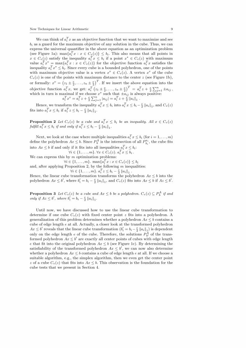
(a) (b) (c)
Fig. 1 a A square (two-dimensional cube) fitting into an inequality aTi x ≤ bi and the cube’s
maximum aTi x∗ for the objective aTi x. b The vertices of an arbitrary square parallel to the
coordinate axes (two-dimensional cube with edge length e and center z). c The transformedpolyhedron Ax ≤ b′ for edge length 1 together with the original polyhedron Ax ≤ b.
consider the case where x ∈ Qnδ is a solution for Ax ≤ b. If x is a solution tothe inequalities in Ax ≤ b, then it is also a solution to any non-negative linearcombination of inequalities in Ax ≤ b.
Our method that detects implied equalities transforms our original polyhedronAx ≤ b into a second polyhedron A′x ≤ b′ that is unsatisfiable if Ax ≤ b impliesan equality. We also show how to extract an equality implied by Ax ≤ b from aminimal set C of unsatisfiable inequalities in A′x ≤ b′. We call an unsatisfiable set Cof inequalities minimal if every proper subset C′ ⊂ C is satisfiable. If a polyhedronAx ≤ b is unsatisfiable, there exists a minimal set C of unsatisfiable inequalitiesso that every inequality in C appears also in Ax ≤ b [14]. We call such a minimalset C an explanation for Ax ≤ b’s unsatisfiability. In case we are investigating aminimal set of unsatisfiable inequalities, we can refine Farkas’ Lemma:
Lemma 3 ([7]) Let C = {aTi x ≤ bi : 1 ≤ i ≤ m} be a minimal set of unsatisfiable
constraints. Let A = (a1, . . . , am)T and b = (b1, . . . , bm)T . Then it holds for every
y ∈ Qm with y ≥ 0n, yTA = 0n, and yT b < 0 that yi > 0 for all i ∈ {1, . . . ,m}.
3 Fitting Cubes into Polyhedra
We say that a cube Ce(z) fits into a polyhedron defined by Ax ≤ b if all pointsinside the cube Ce(z) are solutions of Ax ≤ b, or formally: Ce(z) ⊆ PAb . In orderto compute this, we transform the polyhedron Ax ≤ b into another polyhedronAx ≤ b′. For this new polyhedron, we merely have to test whether the cube’scenter point z is a solution (z ∈ PAb′) in order to also determine whether the cubeCe(z) fits into the original polyhedron. This is a simple test that requires onlyevaluation. We call this entire transformation the linear cube transformation.
We start explaining the linear cube transformation by looking at the case wherethe polyhedron is defined by a single inequality aTi x ≤ bi. A cube Ce(z) fits intothe inequality aTi x ≤ bi if all points inside the cube Ce(z) are solutions of aTi x ≤ bi,or formally: ∀x ∈ Ce(z). aTi x ≤ bi.
New Techniques for Linear Arithmetic 9
We can think of aTi x as an objective function that we want to maximize and seebi as a guard for the maximum objective of any solution in the cube. Thus, we canexpress the universal quantifier in the above equation as an optimization problem(see Figure 1a): max{aTi x : x ∈ Ce(z)} ≤ bi. This also means that all points inx ∈ Ce(z) satisfy the inequality aTi x ≤ bi if a point x∗ ∈ Ce(z) with maximumvalue aTi x
∗ = max{aTi x : x ∈ Ce(z)} for the objective function aTi x satisfies theinequality aTi x
∗ ≤ bi. Since every cube is a bounded polyhedron, one of the pointswith maximum objective value is a vertex xv ∈ Ce(z). A vertex xv of the cubeCe(z) is one of the points with maximum distance to the center z (see Figure 1b),
or formally: xv =(z1 ± e
2 , . . . , zn ±e2
)T. If we insert the above equation into the
objective function aTi x, we get: aTi(z1 ± e
2 , . . . , zn ±e2
)T= aTi z + e
2
∑nj=1±aij ,
which in turn is maximal if we choose xv such that ±aij is always positive:aTi x
v = aTi z + e2
∑nj=1 |aij | = aTi z + e
2 ‖ai‖1 .
Hence, we transform the inequality aTi x ≤ bi into aTi x ≤ bi− e2 ‖ai‖1, and Ce(z)
fits into aTi x ≤ bi if aTi z ≤ bi − e2 ‖ai‖1.
Proposition 2 Let Ce(z) be a cube and aTi x ≤ bi be an inequality. All x ∈ Ce(z)fulfill aTi x ≤ bi if and only if aTi z ≤ bi − e
2 ‖ai‖1.
Next, we look at the case where multiple inequalities aTi x ≤ bi (for i = 1, . . . ,m)define the polyhedron Ax ≤ b. Since PAb is the intersection of all Paibi , the cube fits
into Ax ≤ b if and only if it fits into all inequalities aTi x ≤ bi:∀i ∈ {1, . . . ,m}. ∀x ∈ Ce(z). aTi x ≤ bi .
We can express this by m optimization problems:∀i ∈ {1, . . . ,m}. max{aTi x : x ∈ Ce(z)} ≤ bi
and, after applying Proposition 2, by the following m inequalities:∀i ∈ {1, . . . ,m}. aTi z ≤ bi − e
2 ‖ai‖1 .Hence, the linear cube transformation transforms the polyhedron Ax ≤ b into thepolyhedron Ax ≤ b′, where b′i = bi − e
2 ‖ai‖1, and Ce(z) fits into Ax ≤ b if Az ≤ b′.
Proposition 3 Let Ce(z) be a cube and Ax ≤ b be a polyhedron. Ce(z) ⊆ PAb if and
only if Az ≤ b′, where b′i = bi − e2 ‖ai‖1.
Until now, we have discussed how to use the linear cube transformation todetermine if one cube Ce(z) with fixed center point z fits into a polyhedron. Ageneralization of this problem determines whether a polyhedron Ax ≤ b contains acube of edge length e at all. Actually, a closer look at the transformed polyhedronAx ≤ b′ reveals that the linear cube transformation (b′i = bi− e
2 ‖ai‖1) is dependent
only on the edge length e of the cube. Therefore, the solutions PAb′ of the trans-formed polyhedron Ax ≤ b′ are exactly all center points of cubes with edge lengthe that fit into the original polyhedron Ax ≤ b (see Figure 1c). By determining thesatisfiability of the transformed polyhedron Ax ≤ b′, we can now also determinewhether a polyhedron Ax ≤ b contains a cube of edge length e at all. If we choose asuitable algorithm, e.g., the simplex algorithm, then we even get the center pointz of a cube Ce(z) that fits into Ax ≤ b. This observation is the foundation for thecube tests that we present in Section 4.
10 Martin Bromberger, Christoph Weidenbach
(a) (b) (c)
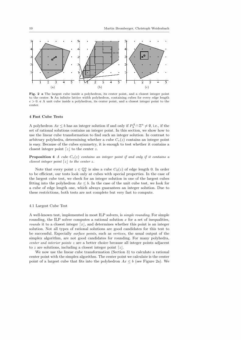
Fig. 2 a The largest cube inside a polyhedron, its center point, and a closest integer pointto the center. b An infinite lattice width polyhedron, containing cubes for every edge lengthe > 0. c A unit cube inside a polyhedron, its center point, and a closest integer point to thecenter.
4 Fast Cube Tests
A polyhedron Ax ≤ b has an integer solution if and only if PAb ∩Zn 6= ∅, i.e., if the
set of rational solutions contains an integer point. In this section, we show how touse the linear cube transformation to find such an integer solution. In contrast toarbitrary polyhedra, determining whether a cube Ce(z) contains an integer pointis easy. Because of the cubes symmetry, it is enough to test whether it contains aclosest integer point dzc to the center z.
Proposition 4 A cube Ce(z) contains an integer point if and only if it contains a
closest integer point dzc to the center z.
Note that every point z ∈ Qnδ is also a cube C0(z) of edge length 0. In orderto be efficient, our tests look only at cubes with special properties. In the case ofthe largest cube test, we check for an integer solution in one of the largest cubesfitting into the polyhedron Ax ≤ b. In the case of the unit cube test, we look fora cube of edge length one, which always guarantees an integer solution. Due tothese restrictions, both tests are not complete but very fast to compute.
4.1 Largest Cube Test
A well-known test, implemented in most ILP solvers, is simple rounding. For simplerounding, the ILP solver computes a rational solution x for a set of inequalities,rounds it to a closest integer dxc, and determines whether this point is an integersolution. Not all types of rational solutions are good candidates for this test tobe successful. Especially surface points, such as vertices, the usual output of thesimplex algorithm, are not good candidates for rounding. For many polyhedra,center and interior points z are a better choice because all integer points adjacentto z are solutions, including a closest integer point dzc.
We now use the linear cube transformation (Section 3) to calculate a rationalcenter point with the simplex algorithm. The center point we calculate is the centerpoint of a largest cube that fits into the polyhedron Ax ≤ b (see Figure 2a). We

New Techniques for Linear Arithmetic 11
determine the center z of this largest cube and the associated edge length e withthe following linear program (LP):
maximize xesubject to Ax+ a′ xe
2 ≤ b, where a′i = ‖ai‖1xe ≥ 0 .
This linear program employs the linear cube transformation from Section 3. Theonly generalization is a variable xe for the edge length instead of a constant valuee. Additionally, this linear program maximizes the edge length as an optimizationgoal. If the resulting maximum edge length is unbounded, the original polyhedroncontains cubes of arbitrary edge length (see Figure 2b) and, thus, infinitely manyinteger solutions. Since the linear program contains all solutions of the originalpolyhedron (see xe = 0), the original polyhedron is empty if and only if the abovelinear program is infeasible. If the maximum edge length is a finite value e, weuse the resulting assignment z for the variables x as a center point and Ce(z) isa largest cube that fits into the polyhedron. From the center point, we round toa closest integer point dzc and determine if it fits into the original polyhedron.If this is the case, we are done because we have found an integer solution forAx ≤ b. Otherwise, the largest cube test does not know whether or not Ax ≤ b hasan integer solution. An example for the latter case, are the following inequalities:3x1 − x2 ≤ 0, −2x1 − x2 ≤ −2, and −2x1 + x2 ≤ 1. These inequalities have exactlyone integer solution (1, 3)T , but the largest cube contained by the inequalities hasedge length e = 3
17 and center point ( 317 ,
32 )T , which rounds to (0, 2)T .
The largest cube test also upholds the incremental advantages of Dutertreand de Moura’s version of the dual simplex algorithm [14]. The only differenceis the extra column a′ xe
2 , which the theory solver can internally create while itis notified of all potential arithmetic literals. Adding this column from the startdoes not influence the correctness of the solution because xe ≥ 0 guarantees thatthe largest cube test is satisfiable exactly when the original inequalities Ax ≤ b
are satisfiable. Even for explanations of unsatisfiability, it suffices to remove thebound xe ≥ 0 to obtain an explanation for the original inequalities Ax ≤ b. Theonly disadvantage is the additional variable xe, which only shrinks the searchspace when it is increased. Therefore, increasing xe can never resolve any conflictsduring the satisfiability search. The simplex solver recognizes this with at leastone additional pivot that sets xe to 0. Hence, adding the extra column a′ xe
2 fromthe beginning has only constant influence on the theory solver’s run-time, and istherefore negligible.
4.2 Unit Cube Test
Most SMT solvers implement a simplex algorithm that is specialized towards fea-sibility and not towards optimization [1,14,16,24]. Therefore, a test based on op-timization, such as the largest cube test, does not fit well with existing implemen-tations. As an alternative, we have developed a second test based on cubes thatdoes not need optimization.
We avoid optimization by fixing the edge length e to the value 1 for allthe cubes Ce(z) we consider (see Figure 2c). We do so because cubes C1(z) ofedge length 1 are the smallest cubes to always guarantee an integer solution,independent of the center point z. A cube with edge length 1 is also called a

12 Martin Bromberger, Christoph Weidenbach
unit cube. To prove this guarantee, we first fix e = 1 in the definition of cubes,C1(z) =
{x ∈ Qnδ : ∀j ∈ 1, . . . , n. |xj − zj | ≤ 1
2
}, and look at the following property
for the rounding operator d.c: ∀zj ∈ Qδ.|dzjc − zj | ≤ 12 . We see that any unit cube
contains a closest integer dzc to its center point z. Furthermore, 1 is the small-est edge length that guarantees an integer solution for a cube with center pointz = (. . . , 12 , . . .)
T . Thus, 1 is the smallest value that we can fix as an edge lengthto guarantee an integer solution for all cubes C1(z).
Our second test tries to find a unit cube that fits into the polyhedron Ax ≤ b
and, thereby, a guarantee for an integer solution for Ax ≤ b. Again, we employ thelinear cube transformation from Section 3 and obtain the linear program:
Az ≤ b′, where b′i = bi − 12 ‖ai‖1 .
In addition to being a linear program without an optimization objective, weonly have to change the row bounds b′i of the original inequalities. In Dutertre andde Moura’s version of the dual simplex algorithm [14], which is implemented inmany SMT solvers [1,14,16,24], such a change of bounds is already part of theframework so that integrating the unit cube test into theory solvers is possiblewith only minor adjustments to the existing implementation. Since our unit cubetest requires only an exchange of bounds, we can easily return to the originalpolyhedron by reverting the bounds. In doing so, the unit cube test upholds theincremental connection between the different original polyhedra.
4.3 Mixed Linear Integer and Rational Arithmetic
We can also extend our cube tests to the theory of mixed linear integer and rationalarithmetic. In this theory, we partition our variables x = (x1, . . . , xn)T into twovectors: the integer variables xZ = (xZ1 , . . . , x
Zk)T and the rational variables xQ =
(xQ1 , . . . , xQl )T . Based on this partitioning, we also split the coefficient matrix A
into two matrices A = (S,R), where S = (s1, . . . , sm)T ∈ Qm×k defines thecoefficients for the integer variables and R = (r1, . . . , rm)T ∈ Qm×l defines thecoefficients for the rational variables. The system has a solution if there exists aninteger assignment for the variables xZ and a rational assignment for the variablesxQ that satisfies our system of inequalities sTi x
Z + rTi xQ ≤ bi (for i = 1, . . . ,m).
Because only integer variables need to be assigned to integer values, tests likesimple rounding should be restricted to integer variables. For instance, if z is arational solution for the overall polyhedron, then simple rounding applies d.c onlyto the components zZ of z that correspond to integer variables. The same holds forour fast cube tests. Instead of looking for hypercubes of the same dimension n asthe number of total variables, we are looking for hypercubes of dimension k thatexpand in the directions that correspond to integer variables, but are flat in thedirections that correspond to rational variables. Such a hypercube of dimension k
with center point z is defined as the set:
F e(z) ={x ∈ Qkδ : ∀j ∈ 1, . . . , k. |xZj − z
Zj | ≤ e
2
}×{zQ}.
We can also modify the linear cube transformation so that we can computewhether a polyhedron SxZ +RxQ ≤ b contains a hypercube F e(z) that is less thanfull dimensional:
Proposition 5 Let F e(z) be a flat cube of dimension k and SxZ + RxQ ≤ b be a
polyhedron. F e(z) ⊆ PAb if and only if SzZ +RzQ ≤ b′, where b′i = bi − e2 ‖si‖1.

New Techniques for Linear Arithmetic 13
Since the hypercube F e(z) only expands in the directions that correspond to in-teger variables, the inequality bounds b′ of the modified linear cube transformationare only influenced by the coefficients of the integer variables. Using Proposition 5,we can now modify our fast cube tests so that they work for mixed linear integerand rational arithmetic. For the largest cube test, we compute the center pointof a largest cube F e(z) that is flat in the directions that correspond to rationalvariables and fits into the polyhedron SxZ + RxQ ≤ b. We determine the center zof this largest cube and the associated edge length e with the following LP:
maximize xesubject to SxZ +RxQ + s′ xe
2 ≤ b, where s′i = ‖si‖1xe ≥ 0 .
From the resulting center point z we receive a candidate mixed integer rationalsolution by applying the rounding operator d.c to the components zZ of z thatcorrespond to integer variables. For the unit cube test, we search for a cube F 1(z)that is flat in the directions that correspond to rational variables, has edge length1, and fits into the polyhedron SxZ +RxQ ≤ b. A linear program that accomplishesthis task is: SxZ +RxQ ≤ b′, where b′i = bi − 1
2 ‖si‖1 .Again, 1 is the smallest value that we can fix as an edge length to guarantee a
mixed rational integer solution for all cubes F 1(z).
5 Experiments
While our tests are useful for many types of polyhedra, the motivation for ourtests stems from a special type of polyhedron, a so-called infinite lattice width
polyhedron [20]. A polyhedron Ax ≤ b has infinite lattice width if for every objectivec ∈ Qn \ {0n}, either its maximum or minimum objective value is unbounded:
∀c ∈ Qn \ {0n}. sup{cT x : x ∈ PAb
}=∞ or inf
{cT x : x ∈ PAb
}= −∞ .
Polyhedra with infinite lattice width seem trivial at first glance because their in-terior expands arbitrarily far in all directions (see Figure 2b). Therefore, a polyhe-dron with infinite lattice width contains an infinite number of integer solutions [20].Nonetheless, many SMT solvers are inefficient on those polyhedra because they usea branch-and-bound approach with an underlying simplex solver [14]. Althoughsuch an approach terminates inside finite a priori bounds [25], it does not explorethe infinite interior, but rather directs the search along the solutions suggestedby the simplex solver: the vertices of the polyhedron. Thus, the SMT solvers con-centrate their search on a bounded part of the polyhedron. This bounded partcontains only a finite number of integer solutions, whereas the complete interiorcontains infinitely many integer solutions. The advantage of our cube tests is thatthey actually exploit the infinite interior because polyhedra with infinite latticewidth contain cubes for every edge length (see Figure 2b). Our tests are, therefore,always successful on polyhedra with infinite lattice width and usually need only asmall number of pivoting steps before finding a solution.
Lemma 4 ([8]) Let Ax ≤ b be a polyhedron. Let a′ ∈ Qm be a vector such that its
components are a′i = ‖ai‖1. Then Ax ≤ b contains a cube Ce(z) for every non-negative
e ∈ Qδ if and only if Ax ≤ b has infinite lattice width.
We have found instances of polyhedra with the infinite lattice width property insome classes of the SMT-LIB benchmarks. These instances are 229 of the 233 dillig

14 Martin Bromberger, Christoph Weidenbach
Benchmark Name CAV-2009 DILLIG PRIME-CONE SLACKS ROTATE#Instances 503 229 19 229 229
Solvers: solved time solved time solved time solved time solved time
SPASS-IQ-0.1+uc 503 22 229 9 19 0.4 229 26 229 9SPASS-IQ-0.1 503 713 229 218 19 0.4 197 95 229 214
ctrl-ergo 503 12 229 5 19 0.4 229 46 24 6760cvc4-1.4 467 12903 206 4146 18 3 152 4061 208 6964
mathsat5-3.13+uc 503 42.37 229 18 19 0.4 229 39 229 21mathsat5-3.13 500 4601 225 2315 19 3.5 181 4573 229 1507yices-2.5.1 469 11403 213 2553 19 0.1 147 5725 180 10073z3-4.4.1 466 682 213 475 19 0.1 158 371 213 473
Fig. 3 Experimental Results
benchmarks designed by Dillig et al. [11], 503 of the 591 CAV-2009 benchmarksalso by Dillig et al. [11], 229 of the 233 slacks benchmarks which are the dilligbenchmarks extended with slack variables [18], and 19 of the 37 prime-cone bench-marks, that is, “a group of crafted benchmarks encoding a tight n-dimensionalcone around the point whose coordinates are the first n prime numbers” [18].The remaining problems (4 from dillig, 88 from CAV-2009, 4 from slacks, and 18from prime-cone) do not have infinite lattice width because they are either tightlybounded or unsatisfiable. For our experiments, we look only at the instances ofthose benchmark classes that actually fulfill the infinite lattice width property.
Using these benchmark instances, we have confirmed our theoretical assump-tions (Lemma 4) in practice. We integrated the unit cube test into our own branch-and-bound solver SPASS-IQ (http://www.spass-prover.org/spass-iq) and ran it onthe infinite lattice width instances; once with the unit cube test turned on (SPASS-
IQ-0.1+uc) and once with the test turned off (SPASS-IQ-0.1 ). For every prob-lem, SPASS-IQ-0.1+uc applies the unit cube test exactly once. This applicationhappens before we start the branch-and-bound approach. We also compared oursolver with state-of-the-art SMT solvers for linear integer arithmetic: cvc4-1.4 [1],mathsat5-3.13 [10], yices2.5.1 [13], and z3-4.4.1 [24]. All these solvers employ abranch-and-bound approach with an underlying dual simplex solver [14]. The onlyexception is mathsat5, which, subsequent to our first publication on the unit cubetest [8], now also performs the unit cube test in advance. That is why we also testmathsat5 once with the unit cube test turned on (mathsat5-3.13+uc) and oncewith the test turned off (mathsat5-3.13).
The solvers had to solve each problem in under 10 minutes. For the exper-iments, we used a Debian Linux server with 32 Intel Xeon E5-4640 (2.4 GHz)processors and 512 GB RAM. Figure 3 lists the results of the different solvers(column one) on the different benchmark classes (row one). Row two lists thenumber of benchmark instances we considered for our experiments. For each com-bination of benchmark class and solver, we have listed the number of instancesthe solver could solve in the given time as well as the total time (in seconds) ofthe instances solved (columns labelled with “solved” and “time”, respectively).
Our solver that employs the unit cube test solves all instances with the ap-plication of the unit cube test and is 25 times faster than our solver without thetest. The SMT theory solvers in their standard setting were not able to solve allinstances within the allotted time. Moreover, our unit cube test was over 100 timesfaster than any state-of-the-art SMT solver without the unit cube test. The resultsfor mathsat5 further support the superiority of the test.

New Techniques for Linear Arithmetic 15
We also compared our test with the ctrl-ergo solver, which includes a subrou-tine that is essentially the dual to our largest cube test [4]. As expected, bothapproaches are comparable for infinite lattice width polyhedra. In order to alsocompare the two approaches on benchmarks without infinite lattice width, we cre-ated the rotate benchmarks by adding the same four inequalities to all infinitewidth instances of the dillig benchmarks. These four inequalities essentially de-scribe a square bounding the variables x0 and x1 in an interval [−u, u]. For a largeenough choice of u (e.g., u = 210), the square is so large that the benchmarks arestill satisfiable and not absolutely trivial for branch-and-bound solvers. To adda challenge, we rotated the square by a small factor 1/r, which resulted in thefollowing four inequalities:
−b · r · r + r ≤ b · r · x0 − x1 ≤ b · r · r − r , and−b · r · r + r ≤ x0 + b · r · x1 ≤ b · r · r − r .
These changes have nearly no influence on SPASS-IQ, and two SMT solvers evenbenefit from the proposed changes. For ctrl-ergo the rotate benchmarks are veryhard because its subroutine detects only infinite lattice width. Without infinitelattice width, ctrl-ergo starts its search from the boundaries of the polyhedroninstead of looking at the polyhedron’s interior. We can even control the number ofiterations (r2) ctrl-ergo spends on the parts of the boundary without any integersolutions if we choose r accordingly (e.g., r = 210). In contrast, we use our cubetests to also extract interior points for rounding. This difference makes our testsmuch more stable under small changes to the polyhedron.
There exist alternative methods for solving linear integer constraints that donot rely on a branch-and-bound approach [6,18]. These have not yet maturedenough to be competitive with our tests or state-of-the-art SMT theory solvers.
Most problems in the linear integer arithmetic SMT-LIB benchmarks withfinite lattice width can be solved without using any actual integer arithmetic tech-niques. A standard simplex solver for the rationals typically finds a rational solu-tion for such a problem that is also an integer solution. Applying the unit cubetest on these trivial problem classes is a waste of time. In the worst case, it dou-bles the eventual solution time. For these examples it is beneficial to first computea general rational solution and to check it for integer satisfiability before apply-ing the unit cube test. This has the additional benefit that rational unsatisfiableproblems are filtered out before applying the unit cube test. The unit cube testis also guaranteed to fail on problems containing boolean variables, i.e., variablesthat are either 0 or 1, unless they are absolutely trivial and describe a unit cubethemselves. Whenever the problem contains a boolean variable, it is beneficial toskip the unit cube test. This is also the reason why we provide no experimentalresults for the theory of mixed linear integer and rational arithmetic, i.e., the fewmixed benchmarks available in the SMT-LIB all contain boolean variables.
6 From Cubes to Equalities
If a polyhedron implies an equality, then it has only surface points and neither aninterior nor a center. There is no way such a polyhedron contains a unit cube anda largest cube has edge length zero and is just a point in the original polyhedron.Equalities are, therefore, a challenge for the applicability of our cube tests.

16 Martin Bromberger, Christoph Weidenbach
There even exist systems of inequalities that imply infinitely many equalities.For instance, the system consisting of the inequalities −2x1+x2 ≤ −2, x1+3x2 ≤ 8,and x1 − 2x2 ≤ −2 has only one rational solution: the point (x1, x2) = (2, 2).Therefore, it implies the equalities −2x1 + x2 = −2 and x1 + 3x2 = 8, and alllinear combinations of those two equalities, i.e., λ1 · (−2x1 +x2) +λ2 · (x1 + 3x2) =λ1 · (−2) + λ2 · 8 for all λ1, λ2 ∈ Q. The above example also points us to anotherfact about equalities: there exists a finite representation of all equalities impliedby a system of inequalities—even if the system implies infinitely many equalities.
One such finite representation is the equality basis for a satisfiable system ofinequalities Ax ≤ b. An equality basis is a system of equalities D′x = c′ such thatall (explicit and implicit equalities) implied by Ax ≤ b are linear combinationsof equalities from D′x = c′. We prefer to represent each equality basis D′x = c′
as an equivalent system of equalities y − Dz = c such that y = (y1, . . . , yny )T
and z = (z1, . . . , znz )T are a partition of the variables in x, D ∈ Qny×nz , andc ∈ Qny . The existence of such an equivalent system of equalities is guaranteedby Gaussian elimination. Moreover, each variable yi appears exactly once in thesystem y − Dz = c, that is to say, yi appears only in the row yi − dTi zi = ci.We choose to represent our equality bases in this manner because this form alsocorrelates to a distinct substitution σD,cy,z that replaces variable yi with ci + dTi z:
σD,cy,z := {yi 7→ ci + dTi z : i ∈ {1, . . . , ny}}.The substitution σD,cy,z is important because it allows us to eliminate all equal-
ities from Ax ≤ b. We simply apply the substitution σD,cy,z to Ax ≤ b and receive anew system A′z ≤ b′ that neither contains the variables y nor implies any equali-ties.1 And the substitution σD,cy,z for the equality basis y−Dz = c has even furtherapplications. For instance, we can directly check whether an equality hT x = g isa linear combination of y − Dz = c and, therefore, implied by both Ax ≤ b andy −Dz = c. We simply apply σD,cy,z to hT x = g and see if it simplifies to 0 = 0. We
even use σD,cy,z for the Nelson-Oppen style combination of theories (see Section 7).
6.1 Finding Equalities
The first step in computing an equality basis for a polyhedron Ax ≤ b is to detectwhether the system contains any equalities. We have already stated a criterionthat detects this:
Lemma 5 ([8]) Let Ax ≤ b be a polyhedron. Then exactly one of the following state-
ments is true: (1) Ax ≤ b implies an equality hT x = g with h 6= 0n, or (2) Ax ≤ b
contains a cube with edge length e > 0.
A cube with positive edge length is enough to prove that there exists no impliedequality. The actual edge length e of this cube is not relevant. Therefore, we canassume that the edge length e is arbitrarily small. We can even assume that ouredge length is so small that we can ignore the different multiples ‖ai‖1 and anyinfinitesimals introduced by strict inequalities. We just have to turn all of ourinequalities into strict inequalities.
1 If we combine the equality basis with a diophantine equation handler [16], then we evenreceive a substitution σ′ that eliminates the equalities in such a way that we can reconstruct aninteger solution from them. The result is a new system of inequalities that implies no equalitiesand has an integer solution if and only if Ax ≤ b has one.
New Techniques for Linear Arithmetic 17
Lemma 6 Let Ax ≤ b be a polyhedron, where ai 6= 0n, bi = (pi, qi), qi ≤ 0, and
bδi = (pi,−1) be the strict versions of the bounds bi for all i ∈ {1, . . . ,m}. Then the
following statements are equivalent: (1) Ax ≤ b contains a cube with edge length e > 0,
and (2) Ax ≤ bδ is satisfiable.
Proof. (1) ⇒ (2): If Ax ≤ b contains a cube of edge length e > 0, then Ax ≤ b− a′is satisfiable, where a′i = e
2 ‖ai‖1. By Lemma 1, we know there exists a δ ∈ Q suchthat Ax ≤ p+ qδ−a′. Now, let δ′ = min{a′i− qiδ : i = 1, . . . ,m}. Since a′i− qiδ ≥ δ
′,it holds that Ax ≤ p − δ′1m. Since qi ≤ 0 and a′i = ‖ai‖1 > 0, it also holds thatδ′ > 0. By Lemma 1, we deduce that Ax < p and, therefore, Ax ≤ bδ holds.
(2) ⇒ (1): If Ax ≤ bδ is satisfiable, then we know by Lemma 1 that there mustexist a δ > 0 such that Ax ≤ p− δ1m holds. Let amax = max{‖ai‖1 : i = 1, . . . ,m},δ′ = δ
2 , and e = δamax
. Then pi − δ = pi − δ′ − e2amax ≤ bi − e
2 ‖ai‖1. Thus, Ax ≤ b
contains a cube with edge length e > 0.
In case Ax ≤ bδ is unsatisfiable, Ax ≤ b contains no cube with positive edgelength and, therefore by Lemma 5, an equality. In case Ax ≤ bδ is unsatisfiable, thealgorithm returns an explanation, i.e., a minimal set C of unsatisfiable constraintsaTi x ≤ b
δi from Ax ≤ bδ. If Ax ≤ b itself is satisfiable, we can extract equalities from
this explanation: for every aTi x ≤ bδi ∈ C, Ax ≤ b implies the equality aTi x = bi.
Lemma 7 Let Ax ≤ b be a satisfiable polyhedron, where ai 6= 0n, bi = (pi, qi), qi ≤ 0,
and bδi = (pi,−1) for all i ∈ {1, . . . ,m}. Let Ax ≤ bδ be unsatisfiable. Let C be a
minimal set of unsatisfiable constraints aTi x ≤ bδi from Ax ≤ bδ. Then it holds for
every aTi x ≤ bδi ∈ C that aTi x = bi is an equality implied by Ax ≤ b.
Proof. Because of transitivity of the subset and implies relationships, we can as-sume that Ax ≤ b and Ax ≤ bδ contain only the inequalities associated withthe explanation C. Therefore, C = {aT1 x ≤ bδ1, . . . , a
Tmx ≤ bδm}. By Lemma 2 and
Ax ≤ bδ being unsatisfiable, we know that there exists a y ∈ Qm with y ≥ 0,yTA = 0n, and yT bδ < 0. By Lemma 2 and Ax ≤ b being satisfiable, we know thatyT b ≥ 0 is also true. By Lemma 3, we know that yk > 0 for every k ∈ {1, . . . ,m}.
Now, we use yT bδ < 0, yT b ≥ 0, and the definitions of < and ≤ for Qδ to provethat yT b = 0 and b = p. Since yT bδ < 0, we get that yT p ≤ 0. Since yT b ≥ 0, weget that yT p ≥ 0. If we combine yT p ≤ 0 and yT p ≥ 0, we get that yT p = 0. FromyT p = 0 and yT b ≥ 0, we get yT q ≥ 0. Since y > 0 and qi ≤ 0, we get that yT q = 0and qi = 0. Since qi = 0, b = p.
Next, we multiply yTA = 0n with an x ∈ PAb to get yTAx = 0. Since yk > 0for every k ∈ {1, . . . ,m}, we can solve yTAx = 0 for every aTk x and get:
aTk x = −∑mi=1,i6=k
(yiykaTi x
).
Likewise, we solve yT b = 0 for every bk to get: bk = −∑mi=1,i6=k
(yiykbi
).
Since x ∈ PAb satisfies all aTi x ≤ bi, we can deduce bk as the lower bound of aTk x:
aTk x = −∑mi=1,i6=k
(yiykaTi x
)≥ −
∑mi=1,i6=k
(yiykbi
)= bk ,
which proves that Ax ≤ b implies aTk x = bk.
Lemma 7 justifies simplifications on Ax ≤ bδ. We can eliminate all inequali-ties in Ax ≤ bδ that cannot appear in the explanation of unsatisfiability, i.e., allinequalities aTi x ≤ bδi that cannot form an equality aTi x = bi that is implied by

18 Martin Bromberger, Christoph Weidenbach
Algorithm 1: EqBasis(Ax ≤ b)Input : A satisfiable system of inequalities Ax ≤ b, where A ∈ Qm×n and b ∈ QmδOutput : An equality basis z −Dy = c for Ax ≤ b
1 l := 1, nz := n, (z1, . . . , znz ) := (x1, . . . , xn), y := ()T , and (y −Dz = c) := ∅2 Remove all rows aTi z ≤ bi from Az ≤ b with ai = 0n and bi = 0
3 while Az ≤ bδ is unsatisfiable (i.e., Az ≤ b contains an equality) do4 Let C be an explanation for Az ≤ bδ being unsatisfiable
5 Select (aTi z ≤ bδi ) ∈ C ; // by Lemma 7, aTi z = bi is implied by Az ≤ b6 Select a variable zk such that aik 6= 0.
7 σ′ := {zk 7→ biaik−
∑nj=1,j 6=k
aijaik
zj}8 z′ := (z1, . . . , zk−1, zk+1, . . . , zn)T , y′ := (y1, . . . , yl, zk)T , l := l + 19 (A′z′ ≤ b′) := (Az ≤ b)σ′
10 (y′ −D′z′ = c′) := (y −Dz = c)σ′ ∪ {zk +∑nj=1,j 6=k
aijaik
zj = biaik}
11 z := z′, y := y′, (Az ≤ b) := (A′z′ ≤ b′), (y −Dz = c) := (y′ −D′z′ = c′)
12 Remove all rows aTi z ≤ bi from Az ≤ b with ai = 0n and bi = 0
13 end14 return y −Dz = c
Fig. 4 EqBasis computes an equality basis
Ax ≤ b. For example, if we have an assignment v ∈ Qnδ such that Av ≤ b is true,then we can eliminate every inequality aTi x ≤ bδi for which aTi v = bi is false. Ac-cording to this argument, we can also eliminate all inequalities aTi x ≤ b
δi that were
already strict inequalities in Ax ≤ b.
6.2 Computing an Equality Basis
We now present the algorithm EqBasis(A′x ≤ b′) (Figure 4) that computes anequality basis for a polyhedron A′x ≤ b′. In a nutshell, EqBasis iteratively detectsand removes equalities from our system of inequalities and collects them in asystem of equalities until it has a complete equality basis. To this end, EqBasis
computes in each iteration one system of inequalities Az ≤ b and one system ofequalities y − Dz = c such that A′x ≤ b′ is equivalent to (y − Dz = c) ∪ (Az ≤b). While the variables z are completely defined by the inequalities Az ≤ b, theequalities y −Dz = c extend any assignment from the variables z to the variablesy. Initially, z is just x, y −Dz = c is empty, and Az ≤ b is just A′x ≤ b′.
In every iteration l of the while loop, EqBasis eliminates one equality aTi z = bifrom Az ≤ b and adds it to y − Dz = c. EqBasis finds this equality based onthe techniques we presented in the Lemmas 6 & 7 (line 3). If the current systemof inequalities Az ≤ b implies no equality, then EqBasis is done and returns thecurrent system of equalities y−Dz = c. Otherwise, EqBasis turns the found equalityaTi z = bi into a substitution σ′ := {zk 7→ bi
aik−∑nj=1,j 6=k
aijaik
zj} (line 7) andapplies it to Az ≤ b (line 9). This has the following effects: (1) the new systemof inequalities A′z′ ≤ b′ implies no longer the equality aTi z = bi; and (2) it nolonger contains the variable zk. Next, we apply σ′ to our system of equalities(line 10) and concatenate the equality zk +
∑nj=1,j 6=k
aijaik
zj = biaik
to the end of
(y − Dz = c)σ′. This has the following effects: (1) the new system of equalitiesy′ − D′z′ = c′ implies aTi z = bi; and (2) the variable zk appears exactly once in

New Techniques for Linear Arithmetic 19
y′ − D′z′ = c′. This means that we can now re-partition our variables so thatz := (z1, . . . , zk−1, zk+1, . . . , zn)T and yl := zk to get two new systems Az ≤ b andy − Dz = c that are equivalent to our original polyhedron (line 11). Finally, weremove all rows 0 ≤ 0 from Az ≤ b because those rows are trivially satisfied butwould obstruct the detection of equalities with Lemma 6.
To prove the correctness of the algorithm, we first need to prove that movingthe equality from our system of inequalities to our system of equalities preservesequivalence, i.e, the systems (Az ≤ b)∪(y−Dz = c) and (A′z′ ≤ b′)∪(y′−D′z′ = c′)are equivalent in line 10.
Lemma 8 Let Az ≤ b be a system of inequalities. Let y − Dz = c be a system of
equalities. Let hT z = g be an equality implied by Az ≤ b with hk 6= 0. Let σ′ := {zk 7→ghk−∑nj=1,j 6=k
hj
hkzj} be a substitution based on this equality. Let y′ := (y1, . . . , yl, zk)T
and z′ := (z1, . . . , zk−1, zk+1, . . . , zn)T . Let (A′z′ ≤ b′) := (Az ≤ b)σ′. Let (y′ −D′z′ = c′) := (y −Dz = c)σ′ ∪ {zk +
∑nj=1,j 6=k
hj
hkzj = g
hk}. Let u ∈ Qny
δ , v ∈ Qnz
δ ,
u′ = (u1, . . . , uny , vk)T , and v′ = (v1, . . . , vk−1, vk+1, . . . , vnz )T . Then (Av ≤ b) ∪(u−Dv = c) is true if and only if (A′v′ ≤ b′) ∪ (u′ −D′v′ = c′) is true.
Proof. First, we create a new substitution σv := {zk 7→ ghk−∑nj=1,j 6=k
hj
hkvj} that
is equivalent to σ′ except that it directly assigns the variables zi to their values vi.Let us now assume that either (Av ≤ b)∪(u−Dv = c) or (A′v′ ≤ b′)∪(u′−D′v′ = c′)is true. This means that hT v = g is also true, either by definition of (Av ≤ b) or
(u′ −D′v′ = c′). But hT v = g is true also implies that vk = ghk−∑nj=1,j 6=k
hj
hkvj is
true. Therefore, σv simplifies to the assignment zk 7→ vk. So (Av ≤ b)∪(u−Dv = c)and (A′v′ ≤ b′) ∪ (u′ − D′v′ = c′) simplify to the same expressions and if onecombined system is true, so is the other.
The algorithm EqBasis(A′x ≤ b′) decomposes the original system of inequalitiesA′x ≤ b′ into a reduced system Az ≤ b that implies no equalities, and an equalitybasis y −Dz = c. The algorithm is guaranteed to terminate because the variablevector z decreases by one variable in each iteration. Note that EqBasis(A′x ≤ b′)
constructs y−Dz = c in such a way that the substitution σD,cy,z is the concatenationof all substitutions σ′ from every previous iteration. Therefore, we also know thatσD,cy,z applied to A′x ≤ b′ results in the system of inequalities Az ≤ b that impliesno equalities. We exploit this fact to prove the correctness of EqBasis(A′x ≤ b′),but first we need two more auxiliary lemmas.
Lemma 9 Let y − Dz = c be a satisfiable system of equalities. Let Ax ≤ b and
A∗x ≤ b∗ be two systems of inequalities, both implying the equalities in y − Dz = c.
Let A′z ≤ b′ := (Ax ≤ b)σD,cy,z and A∗∗z ≤ b∗∗ := (A∗x ≤ b∗)σD,cy,z . Then A′z ≤ b′ is
equivalent to A∗∗z ≤ b∗∗ if Ax ≤ b is equivalent to A∗x ≤ b∗.
Proof. Let Ax ≤ b be equivalent to A∗x ≤ b∗. Suppose to the contrary that A′z ≤ b′is not equivalent to A∗∗z ≤ b∗∗. This means that there exists a v ∈ Qnz
δ suchthat either A′v ≤ b′ is true and A∗∗v ≤ b∗∗ is false, or A′v ≤ b′ is false andA∗∗v ≤ b∗∗ is true. Without loss of generality we select the first case that A′v ≤ b′is true and A∗∗v ≤ b∗∗ is false. We now extend this solution by u ∈ Qny
δ , where
ui := ci + dTi v, so (A′v ≤ b′)∪ (u−Dv = c) is true. Based on the definition of σD,cy,z
and ny recursive applications of Lemma 8, the four systems of constraints Ax ≤ b,

20 Martin Bromberger, Christoph Weidenbach
A∗x ≤ b∗, (A′z ≤ b′)∪ (y−Dz = c), and (A∗∗z ≤ b∗∗)∪ (y−Dz = c) are equivalent.Therefore, (A∗∗v ≤ b∗∗)∪ (u−Dv = c) is true, which means that A∗∗v ≤ b∗∗ is alsotrue. The latter contradicts our initial assumptions.
Now we can also prove what we have already explained at the beginning ofthis section. The equality hT x = g is implied by Ax ≤ b if and only if y −Dz = c
is an equality basis and (hT x = g)σD,cy,z simplifies to 0 = 0. An equality basis isalready defined as a set of equalities y−Dz = c that implies exactly those equalitiesimplied by Ax ≤ b. So we only need to prove that hT x = g is implied by y−Dz = c
if (hT x = g)σD,cy,z simplifies to 0 = 0.
Lemma 10 Let y − Dz = c be a satisfiable system of equalities. Let hT x = g be an
equality. Then y −Dz = c implies hT x = g iff (hT x = g)σD,cy,z simplifies to 0 = 0.
Proof. First, let us look at the case where hT x = g is an explicit equality yi−dTi z =
ci in y −Dz = c. Then (yi − dTi z = ci)σD,cy,z simplifies to 0 = 0 because σD,cy,z maps
yi to dTi z + ci and the variables zj are not affected by σD,cy,z .
Next, let us look at the case where hT x = g is an implicit equality in y−Dz = c.Since both y − Dz = c and (y − Dz = c) ∪ (hT z = g) imply hT z = g and the
equalities in y−Dz = c, both (y−Dz = c)σD,cy,z and ((y−Dz = c)∪ (hT z = g))σD,cy,z
must be equivalent (see Lemma 9). As we stated at the beginning of this proof,
(yi − dTi z = ci)σD,cy,z simplifies to 0 = 0. An equality h′T c = g′ that simplifies to
0 = 0 is true for all v ∈ Qnz
δ . Moreover, only equalities that simplify to 0 = 0 are
true for all v ∈ Qnz
δ . This means (y−Dz = c)σD,cy,z is satisfiable for all assignments
and, therefore, (hT z = g)σD,cy,z must simplify to 0 = 0.
Finally, let us look at the case where hT x = g is not an equality implied byy−Dz = c. Suppose to the contrary that ((y−Dz = c)∪(hT z = g))σD,cy,z is satisfiablefor all assignments. We know based on Lemma 8 and transitivity of equivalencethat (y − Dz = c) ∪ (hT z = g) and (y − Dz = c) ∪ ∅ are equivalent. Therefore,hT z = g is implied by y −Dz = c, which contradicts our initial assumption.
With Lemma 10, we have now all auxiliary lemmas needed to prove that thealgorithm EqBasis is correct:
Lemma 11 Let A′x ≤ b′ be a satisfiable system of inequalities. Let y−Dz = c be the
output of EqBasis(A′x ≤ b′). Then y −Dz = c is an equality basis of A′x ≤ b′.
Proof. Let Az ≤ b be the result of applying σD,cy,z to A′x ≤ b′. Since y − Dz = c
is the output of EqBasis(A′x ≤ b′), the condition in line 3 of EqBasis guaranteesus that Az ≤ b implies no equalities. Let us now suppose to the contrary of our
initial assumptions that A′x ≤ b′ implies an equality h′Tx = g′ that y − Dz = c
does not imply. Since h′Tx = g′ is not implied by y − Dz = c, the output of
(h′Tx = g′)σD,cy,z is an equality hT z = g, where h 6= 0nz . This also implies that
(Az ≤ b)∪ (hT z = g) is the output of ((A′x ≤ b′)∪ (h′Tx = g′))σD,cy,z . By Lemma 9,
Az ≤ b and (Az ≤ b) ∪ (hT z = g) are equivalent. Therefore, Az ≤ b impliesthe equality hT z = g, which contradicts the condition in line 3 of EqBasis and,therefore, our initial assumptions.

New Techniques for Linear Arithmetic 21
7 Implementation and Application
It is not straight forward how to efficiently integrate our method that finds anequality basis into an SMT solver. Therefore, we now explain how to implementour method as an extension of Dutertre and de Moura’s version [14] of the dualsimplex algorithm [2,22]. We choose to specialize this version of the dual simplexalgorithm because it is implemented in most SMT solvers and has all propertiesnecessary for an efficient theory solver: it produces minimal conflict explanations,handles backtracking efficiently, and is highly incremental. Whenever we refer tothe simplex algorithm in this section, we refer to the specific version of the dualsimplex algorithm presented by Dutertre and de Moura [14].
We defined the theory for the equality basis by representing our input con-straints through inequalities Ax ≤ b because inequalities represent the set of so-lutions more intuitively. In the simplex algorithm, the input constraints are rep-resented instead by a so-called tableau Ax = 0m and two bounds li ≤ xi ≤ ui forevery variable xi in the tableau. Therefore, it might seem difficult to efficientlyintegrate our method in the simplex algorithm. The truth, however, is that thetableau-and-bound representation grants us several advantages for the implemen-tation of our equality basis method. For example, we do not have to explicitlyeliminate variables via substitution, but we do so automatically via pivoting.
Later in this Section, we also explain how the integration of our methods in thesimplex algorithm can be used for the combination of theories with the Nelson-Oppen Method. For the Nelson-Oppen style combination of theories inside an SMTsolver [9], each theory solver has to return all valid equations between variablesin its theory. Linear arithmetic theory solvers sometimes guess these equationsbased on one satisfying assignment. Then the equations are transferred accordingto the Nelson-Oppen method without verification. This leads to a backtrack of thecombination procedure in case the guess was wrong and eventually led to a conflict.With the availability of an equality basis, the guesses can be verified directly andefficiently. Therefore, the method helps the theory solver in avoiding any conflictsdue to wrong guesses together with the overhead of backtracking. This comes atthe price of computing the equality basis, which should be negligible because theintegration we propose is incremental and includes justified simplifications.
7.1 The Dual Simplex Algorithm
The input of the simplex algorithm (Figure 5) is a set of equalities Ax = 0m anda set of bounds for the variables lj ≤ xj ≤ uj (for j = 1, . . . , n). If there is no lowerbound lj ∈ Qδ for variable xj , then we simply set lj = −∞. Similarly, if there isno upper bound uj ∈ Qδ for variable xj , then we simply set uj =∞.
We can easily transform a system of inequalities Ax ≤ b into the above formatif we introduce a so-called slack variable si for every inequality in our system. Oursystem is then defined by the equalities Ax−s = 0m, and the bounds −∞ ≤ xj ≤ ∞for every original variable xj and the bounds −∞ ≤ si ≤ bi for every slack variableintroduced for the inequality aTi x ≤ bi. We can even reduce the number of slackvariables if we transform rows of the form aij · xj ≤ cj directly into bounds forxj . Moreover, we can use the same slack variable for multiple inequalities as longas the left side of the inequality is similar enough. For example, the inequalities

22 Martin Bromberger, Christoph Weidenbach
Algorithm 2: pivot(xi, xj)
Input : A basic variable xi and a non-basic variable xj so that aij is non-zeroEffect : Transforms the tableau so xi becomes non-basic and xj basic
1 Let xi =∑k∈N aikxk be the row defining the basic variable xi
2 We rewrite this row as xj = 1aij
xi −∑k∈N\{xj}
aikaij
xk so it defines xj instead
3 foreach xk ∈ N \ {xj} do ajk := −aikaij
;
4 aji := 1aij
5 Substitute xj in all other rows with 1aij
xi −∑k∈N\{xj}
aikaij
xk
6 for xl ∈ B do7 foreach xk ∈ N \ {xj} do alk := alk + aljajk;8 ali := aljaji; alj := 0
9 end10 N = (N ∪ {xi}) \ {xj}; B = (B ∪ {xj}) \ {xi}
Algorithm 3: update(xj , v)
Input : A non-basic variable xj and a value v ∈ QδEffect : Sets the value β(xj) of xj to v and updates the values of all basic variables
1 foreach xi ∈ B do β(xi) := β(xi) + aij(v − β(xj));2 β(xj) := v
Algorithm 4: pivotAndUpdate(xi, xj , v)
Input : A basic variable xi, a non-basic variable xj , and a value v ∈ QδEffect : Pivots variables xi and xj and updates the value β(xi) of xi to v
1 θ :=v−β(xi)aij
2 β(xi) := v; β(xj) := β(xj) + θ3 foreach xk ∈ B \ {xi} do β(xk) := β(xk) + akjθ;4 pivot(xi, xj)
Algorithm 5: Check()
Output : Returns true iff there exists a satisfiable assignment for the tableau and thebounds u and l; otherwise, it returns (false,xi), where xi is the conflictingbasic variable
1 while true do2 select the smallest basic variable xi such that β(xi) < li or β(xi) > ui3 if there is no such xi then return true;4 if β(xi) < li then5 select the smallest non-basic variable xj such that6 (aij > 0 and β(xj) < uj) or (aij < 0 and β(xj) > lj)7 if there is no such xj then return (false,xi) ;8 pivotAndUpdate(xi, xj , li)
9 end10 if β(xi) > ui then11 select the smallest non-basic variable xj such that12 (aij < 0 and β(xj) < uj) or (aij > 0 and β(xj) > lj)13 if there is no such xj then return (false,xi) ;14 pivotAndUpdate(xi, xj , ui)
15 end
16 end
Fig. 5 The functions of the dual simplex algorithm by Dutertre and de Moura [14]
New Techniques for Linear Arithmetic 23
aTi x ≤ bi and −aTi x ≤ ci can be transformed into the equality aTi x − si = 0 andthe bounds −ci ≤ si ≤ bi. SMT solvers typically assign the slack variables duringa preprocessing step with a normalization procedure based on a variable ordering.After the normalization, all terms are represented in one directed acyclic graph(DAG) so that all equivalent terms are assigned to the same node and, thereby, tothe same slack variable. For more details on these simplifications we refer to [14].
The simplex algorithm also partitions the variables into two sets: the set of non-
basic variables N and the set of basic variables B. Initially, our original variablesare the non-basic variables and the slack variables are the basic variables. Thenon-basic variables N define the basic variables over a tableau derived from oursystem of equalities. Each row in this tableau represents one basic variable xi ∈ B:xi =
∑xj∈N aijxj . The simplex algorithm exchanges variables from xi ∈ B and
xj ∈ N with the pivot algorithm. To do so, we also have to change the tableau viasubstitution. All tableaux constructed in this way are equivalent to the originalsystem of equalities Ax = 0m.
The goal of the simplex algorithm is to find an assignment β that maps ev-ery variable xi to a value β(xi) ∈ Qδ that satisfies our constraint system, i.e.,A(β(x)) = 0m and li ≤ β(xi) ≤ ui for every variable xi. The algorithm startswith an assignment β that fulfills A(β(x)) = 0m and lj ≤ β(xj) ≤ uj for ev-ery non-basic variable xj ∈ N . Initially, we get such an assignment through ourtableau. We simply choose a value lj ≤ β(xj) ≤ uj for every non-basic variablexj ∈ N and define the value of every basic variable xi ∈ B over the tableau:β(xi) :=
∑xj∈N aijβ(xj). As an invariant, the simplex algorithm continues to ful-
fill A(β(x)) = 0m and lj ≤ β(xj) ≤ uj for every non-basic variable xj ∈ N andevery intermediate assignment β.
The simplex algorithm finds a satisfiable assignment or an explanation of un-satisfiability through the Check() algorithm. Since all non-basic variables fulfilltheir bounds and the tableau guarantees that Ax = 0m, Check() only looks for abasic variable that violates one of its bounds. If all basic variables xi satisfy theirbounds, then β is a satisfiable assignment and Check() returns true. If Check() findsa basic variable xi that violates one of its bounds, then it looks for a non-basicvariable xj fulfilling the conditions in lines 6 or 12 of Check(). If it finds a non-basicvariable xj fulfilling the conditions, then we pivot xi with xj and update our βassignment so β(xi) is set to the previously violated bound value, which satisfiesour invariant once more. If it finds no non-basic variable fulfilling the conditions,then the row of xi and all non-basic variables xj with aij 6= 0 build an unresolv-able conflict. Hence, Check() has found a row that explains the conflict and it canreturn unsatisfiable. The algorithm terminates due to a variable selection strategycalled Bland’s rule. Bland’s rule is based on a predetermined variable order andalways selects the smallest variables fulfilling the conditions for pivoting.
7.2 Implementation Details
In case of the tableau-and-bound representation, an equality basis simplifies to thetableau Ax = 0m and a set of tightly bounded variables, i.e., a set of variables xjsuch that β(xj) := lj or β(xj) := uj for all satisfiable assignments β. Therefore,one way of determining an equality basis is to find all tightly bounded variables.

24 Martin Bromberger, Christoph Weidenbach
Algorithm 6: Initialize()
Effect : Removes all bounds lk and uk that cannot produce equalities; turns asmany basic variables xi with li = ui into non-basic variables as is possible;the bounds for all variables xk are turned into strict bounds if lk < uk
1 for xk ∈ B ∪N do2 l′k := lk;u′k := uk ; // Remember the original bounds
3 if β(xk) > lk then lk := −∞;4 if β(xk) < uk then uk := +∞;5 if β(xk) = pk + qkδ such that qk 6= 0 then lk := −∞;uk :=∞;
6 end7 for xi ∈ B do8 if li = ui then9 select the smallest non-basic variable xj such that aij is non-zero and lj < uj
10 if there is such an xj then pivot(xi, xj);
11 end
12 end13 for xk ∈ B ∪N do14 if lk < uk then15 if lk 6= −∞ then lk := lk + δ;16 if uk 6= +∞ then uk := uk − δ;17 if lk 6= −∞ and xk ∈ N then update(xk, lk);18 if uk 6= +∞ and xk ∈ N then update(xk, uk);
19 end
20 end
Algorithm 7: FixEqs(xi)
Input : A basic variable xi that explains the conflictEffect : Turns the bounds of all variables responsible for the conflict into equalities
1 for xj ∈ N do2 if lj < uj then3 if β(xi) < li and aij > 0 then uj := u′j ; lj := u′j ; update(xj , uj);
4 if β(xi) < li and aij < 0 then lj := l′j ; uj := l′j ; update(xj , lj);
5 if β(xi) > ui and aij > 0 then lj := l′j ; uj := l′j ; update(xj , lj);
6 if β(xi) > ui and aij < 0 then uj := u′j ; lj := u′j ; update(xj , uj);
7 end
8 end9 if β(xi) > ui then ui := u′i; li := u′i;
10 if β(xi) < li then li := l′i; ui := l′i;
Algorithm 8: FindTBnds()
Effect : Finds as many tightly bounded variables as possibleOutput : false iff the system of linear arithmetic constraints is unsatisfiable
1 if Check() returns (false,xi) then return false;2 Initialize()3 while Check() returns (false,xi) do4 FixEqs(xi)5 end
/* For all variables xk with lk < uk recover their original bounds l′k, u′k */
6 for xk ∈ B ∪N do7 if lk < uk then lk := l′k;uk := u′k;
8 end9 return true
Fig. 6 The functions used to turn our original tableau into a basis of equalities

New Techniques for Linear Arithmetic 25
To find all tightly bounded variables, we present a new extension of the simplexalgorithm called FindTBnds() (Figure 6). This extension uses our Lemmas 6 & 7to iteratively find all bounds lj ≤ xj (xj ≤ uj) that hold tightly for all satisfiableassignments β, and then turns them into explicit equalities by setting uj := lj(lj := uj). But first of all, FindTBnds() determines if our constraint system isactually satisfiable with a call of Check(). If the system is unsatisfiable, then it hasno solutions and implies all equalities. In this case, FindTBnds() returns false.
Otherwise, we get a satisfiable assignment β from Check() and we use thisassignment in Initialize() (Figure 6) to eliminate all bounds that do not holdtightly under β (i.e., β(xi) > li or β(xi) < ui). We know that we can eliminatethese bounds without losing any tightly bounded variables because we only needthe bounds that can be part of an equality explanation, i.e., only bounds thathold tightly for all satisfiable assignments (see Lemma 7). For the same reason,Initialize() eliminates all originally strict bounds, i.e., bounds with a non-zerodelta part.
Next, Initialize() tries to turn as many variables xi with li = ui into non-basic variables. We do so because xi is guaranteed to stay a non-basic variableif li = ui (see lines 6 & 12 of Check). Pivoting like this essentially eliminates thetightly bounded non-basic variable xi and replaces it with the constant value li.There only exists one case when Initialize() cannot turn the variable xi withli = ui into a non-basic variable. This case occurs whenever all non-basic variablesxj with non-zero coefficient aij also have tight bounds lj = uj . In this case, thecomplete row xi =
∑xj∈N aijxj simplifies to xi = li, so it never produces a conflict
and we can also ignore this row.
As its last action, Initialize() turns the bounds of all variables xj with lj <
uj into strict bounds. Since Initialize() transformed these bounds into strictbounds, the condition of the while loop in line 3 of FindTBnds() checks whetherthe system contains another tightly bounded variable (see also Lemma 6). If Checkreturns (false, xi), then the row xi represents an equality explanation and allvariables xj with a non-zero coefficient in the row hold tightly (see Lemma 7).FindTBnds() uses FixEqs(xi) (Figure 6) to turn these tightly bounded variables xjinto explicit equalities by setting lj = uj . After FixEqs(xi) is done, we go back tothe beginning of the loop in FindTBnds() and do another call to Check.
If Check returns true, then the original system of inequalities implies no furthertightly bounded variables (Lemma 6). We exit the loop and revert the bounds ofthe remaining variables xj with lj < uj to their original values. As a result, we havealso reverted to a linear system equivalent to our original constraint system. Theonly difference is that now all tightly bounded variables xi are explicit equalitiesbecause li = ui. Moreover, the tableau Ax = 0m and the non-basic variables thatare tightly bounded represent an equality basis for our original constraint system.The simplex algorithm even represents the current tableau and the tightly boundednon-basic variables in such a way that they also describe a substitution σ for theelimination of equalities: the rows of the tableau map each basic variable xi totheir row definition
∑xj∈N aijxj and the tightly bounded non-basic variables xj ,
i.e., all variables xj with j ∈ N and lj = uj , are mapped to their tight bound lj .
After applying FindTBnds(), we can efficiently find all valid equations betweenvariables as needed for the Nelson-Oppen style combination of theories. For eachvariable xi, we use the substitution σ that we get from the tableau and the tightly

26 Martin Bromberger, Christoph Weidenbach
bounded variables to get a normalized term that represents each variable. If thevariable xi is non-basic and tightly bounded (i.e., li = ui), then the normalizedterm is the constant value li. If the variable xi is non-basic and not tightly bounded(i.e., li 6= ui), then the normalized term is the variable xi itself. If the variable xi
is basic, then the normalized term is(∑
xj∈N ,lj 6=ujaijxj
)+(∑
xj∈N ,lj=ujaij lj
),
where all basic mathematical operations between constant values are replaced bythe results of those operations.
We know from Lemma 10 that xiσ = xkσ simplifies to 0 = 0 if σ is the sub-stitution we get from an equality basis and xi = xk is implied by our constraints.Therefore, both xiσ and xkσ must be represented by the same normalized term ifxi and xk are equivalent. So the equality basis together with a normalization proce-dure has turned semantic equivalence into syntactic equivalence. It is very easy tofind variables xi represented by the same normalized term if we store these termsin a DAG, which most SMT solvers already provide for assigning slack variables.
7.3 Incrementality, Explanations, and Justifications
Note that asserting additional bounds to our system can increase the number oftightly bounded variables. In this case, we have to apply FindTBnds() again tofind all tightly bounded variables and to complete the new equality basis. Wealready mentioned that Check() never pivots a non-basic variable xj into a basicone if lj = uj because of the conditions in the lines 6 & 12 of Check(). So evenif the SMT solver asserts additional bounds for the variables and applies Check()again, the tightly bounded non-basic variables we have computed in the last callto FindTBnds() stay non-basic. Hence, our next application of FindTBnds() does notperform any computations for the tightly bounded variables that were detectedby earlier applications of FindTBnds(). This means that our algorithm to computethe equality basis is highly incremental.
Another important feature of an efficient SMT theory solver is that it producesgood—maybe even minimal—conflict explanations. In a typical SMT solver, a SATsolver based on CDCL (conflict-driven clause learning) selects and asserts a setof theory literals that satisfy the boolean model. Then the theory solvers verifythat the asserted literals that belong to their theory are consistently satisfiable.If the theory solver finds a conflict between the asserted literals, then it returnsa conflict explanation. The SAT solver uses the conflict explanation to start aconflict analysis that determines a good point for back jumping so it can select anew set of theory literals. Naturally, a good conflict explanation greatly enhancesthe conflict analysis and, therefore, the remaining search.
The literals asserted in our simplex based theory solver are bounds for ourvariables.2 Our algorithm FindTBnds() asserts bounds independently of the SATsolver. This leads to problems in the conflict analysis because the conflict expla-nation is no longer comprehensible for the SAT solver. Hence, we have to extend
2 Actually, the literals we assert are full inequalities aTi x ≤ bi. Due to slacking, the left side
of those constraints is abstracted to a slack variable s such that s = aTi x. The definition of
the slack variable s = aTi x is directly stored in the simplex solver and only a bound s ≤ biremains as the literal for the SMT solver.

New Techniques for Linear Arithmetic 27
FindTBnds() so it produces justifications (for the bounds it asserts in FixEqs(xi))that the SAT solver can comprehend and reproduce.
We only need to justify bounds asserted by FixEqs(xi) because all other boundsasserted by FindTBnds() are reverted to their original bounds xk ≥ l′k and xk ≤ u′k.And even in FixEqs(xi), we only have to justify the bounds xk ≤ l′k (xk ≥ u′k) thatmake the tight bounds xk ≥ l′k (xk ≤ u′k) explicit. We also see that the boundsasserted by FixEqs(xi) are just linear combinations of existing bounds if we lookagain at the proof of Lemma 7. The proof also shows that we can derive this linearcombination from the conflict explanation C of the strict system. For instance, ifthe call to Check() from line 3 of FindTBnds() exits in line 7 with (false, xi), thenthe conflict explanation isC = {xi > l′i} ∪ {xj < u′j : j ∈ N and aij > 0} ∪ {xj > l′j : j ∈ N and aij < 0}. [14]If the call to Check() exits instead in line 13 with (false, xi), then the conflictexplanation isC = {xi < u′i} ∪ {xj > l′j : j ∈ N and aij > 0} ∪ {xj < u′j : j ∈ N and aij < 0}. [14]
We receive the set of tightly propagating bounds that we found with the lastcall to Check() if we turn all bounds in C into non-strict bounds:
C′ = {xk ≤ u′k : (xk < u′k) ∈ C} ∪ {xk ≥ l′k : (xk > l′k) ∈ C}.FixEqs(xi) asserts now for every bound (xk ≥ l′k) ∈ C′ the bound xk ≤ l′k. Fromthe proof of Lemma 7, we see that the bound xk ≤ l′k is a linear combination ofthe bounds C′ \ {xk ≥ l′k}. Hence, xk ≤ l′k is implied by the bounds C′ \ {xk ≥ l′k}and, therefore, the clause(∨
(xi≥l′i)∈C′,xi 6=xkxi < l′i
)∨(∨
(xi≤u′i)∈C′ xi > u′i
)∨(xk ≤ l′k
)justifies the asserted bound xk ≤ l′k. Together with the slack variable definitionsstored in the simplex tableau, this clause is a tautology and the SAT solver canlearn it without restrictions. Moreover, all literals in this clause except for xk ≤ l′kare asserted as unsatisfiable in the current model of our SAT solver. Therefore,the SAT solver can assert the literal xk ≤ l′k on its own through unit propagation.
Symmetrically, FixEqs(xi) asserts for every bound (xk ≤ u′k) ∈ C′ the boundxk ≥ u′k and the justification for this bound is the clause:(∨
(xi≥l′i)∈C′ xi < l′i
)∨(∨
(xi≤u′i)∈C′,xi 6=xk
xi > u′i
)∨(xk ≥ u′k
).
But FindTBnds() is not our only method that asserts literals independently ofthe SAT solver. If we use the equality basis computed by FindTBnds() for a Nelson-Oppen style combination of theories, then we also assert equalities xi = xk for allpairs of equivalent variables xi, xk. Hence, we also have to justify these assertionsto the SAT solver.
We get these justifications by looking at the normalized representations ofthe variables xi and xk that are equivalent. The current set of non-basic variablesdefines a basis and, therefore, already on its own a normalized representation for allvariables. Since this normalized representation only depends on the current tableauAx = 0m, it is also independent of any of the asserted bounds. The normalizedrepresentation we use for the Nelson-Oppen style combination is only an extensionof this representation by the tight bounds xj = cj of all tightly bounded non-basicvariables. Therefore, the equality xi = xk is implied by those tight bounds xj = cjthat were actively used to compute this representation.
For instance, if xi and xk are both non-basic, both variables must be tightlybounded so that xi = xk = v. Otherwise, they cannot have the same normalized

28 Martin Bromberger, Christoph Weidenbach
representation. Therefore, xi = v and xk = v imply xi = xk, or as a clause:(xi < v ∨ xi > v) ∨ (xk < v ∨ xk > v) ∨ (xi = xk) .
Next, we look at the case where two basic variables xi and xk are equivalent.But before we give the complete formal justification, let us look at an example.Let the variables x1, x2, x3, x4, x5 be non-basic and the variables x6 and x7 bebasic. In this example, the basic variables are defined by the non-basic variables asfollows: x6 = 2x1−x2 +3x4 and x7 = 2x1−x2 +x5. Moreover, let the variables x2,x3, x4, and x5 be tightly bounded such that x2 = 1, x3 = 0, x4 = 1, and x5 = 3.If we now replace the tightly non-basic variables, in the definitions of x6 and x7we get that both of their normalized representations are 2x1 and we have activelyused the tight bounds x2 = 1, x4 = 1, x5 = 3 to compute this normalization. Hence,x6 = x7 is implied by the tight bounds x2 = 1, x4 = 1, and x5 = 3. The variablesx6 and x7 are also equivalent if we had not asserted that x2 = 1 because thenormalized representation of both variables without x2 = 1 is 2x1 − x2. Hence,x2 = 1 is redundant for the justification and x6 = x7 is also implied by just thetight bounds x4 = 1 and x5 = 3.
To find which tightly bounded variables are redundant, we can just look at thecoefficients. If aij and akj are the same, then any tight bound xj = cj is redundantin the justification. This gives us the following clause as a general justification:(∨
j∈N ,lj=uj ,aij 6=akj ,(akj ,aij) 6=(0,0) xj < lj ∨ xj > uj
)∨ xi = xk (1)
From this clause, we also get the justification for the mixed case, i.e., the casewhere xi is basic and xk non-basic. We simply treat xk as if it were defined asa basic variable by itself (xk = 1 · xk), so akk = 1 and all other akj = 0. If wesimplify these restrictions in the clause justification (1) for the case with two basicvariables, then we receive the following general justification for the mixed case:(∨
j∈N ,lj=uj ,aij 6=0,(j,aij)6=(k,1) xj < lj ∨ xj > uj
)∨ xi = xk
All literals in the above clauses except for xi = xk are asserted as unsatisfiablein the current model of our SAT solver. This holds because these literals containonly tightly bounded variables. Hence, the SAT solver can assert the literal xi = xkon its own through unit propagation. Note also that all justifications we definedare in some sense minimal: each of the above clauses is a tautology and, if weremove one literal from the clause, then it is no longer a tautology. This fact isanother property that enhances any potential conflict analysis.
8 Conclusions
We have presented the linear cube transformation (Proposition 3), which allowsus to efficiently determine whether a polyhedron contains a cube of a given edgelength. Based on this transformation we have created two tests for linear integerarithmetic: the largest cube test and the unit cube test. Our tests can be integratedinto SMT theory solvers without sacrificing the advantages that SMT solvers gainfrom the incremental structure of subsequent subproblems. Furthermore, our ex-periments have shown that these tests increase efficiency on certain polyhedra suchthat previously hard sets of constraints become trivial.
One obstacle for our cube tests are equalities. Resolving these obstacles led toan additional application of the linear cube transformation: investigating equali-ties. Through Lemmas 6 & 7, we have presented a method that efficiently checks
New Techniques for Linear Arithmetic 29
whether a system of linear arithmetic constraints implies an equality at all. Weuse this method in the algorithm EqBasis(Ax ≤ b) to compute an equality ba-sis y − Dz = c, which is a finite representation of all equalities implied by theinequalities Ax ≤ b.
We also presented various applications for the equality basis y−Dz = c. (1) Wecan use the equality basis to eliminate all equalities from Ax ≤ b. It is, therefore,useful as a preprocessing step for our cube tests. (2) We can use the equalitybasis to directly check whether an equality hT x = g is implied by Ax ≤ b. (3) InSection 7, we also use the equality basis to efficiently compute all pairs of equivalentvariables in Ax ≤ b. These pairs are necessary for a backjump-free Nelson-Oppen
style combination of theories.
The results presented in this paper have further applications. For instance, ourmethods for detecting implied equalities are also useful for quantifier elimination.In general, a quantifier elimination (QE) procedure takes a formula ∃y.φ(y), whereφ(y) itself is quantifier-free but may contain extra variables x called parameters, andreturns an equivalent formula φ′ that is quantifier-free. Linear virtual substitution
is a complete QE procedure for the theory of linear rational arithmetic [23]. Iteliminates the variable y by creating a case distinction exploiting the following fact:a linear real arithmetic formula φ(y) is satisfiable if and only if φ(l) is satisfiable,where l is the strictest lower bound (or upper bound) of y, i.e., the smallest valuefor y in any solution to the problem. This value is either represented by one ofthe inequalities in φ(y) containing y or −∞ (+∞). There are only finitely manyinequalities in φ(y), so by a case distinction over all inequalities containing y
satisfiability can be preserved:
∃y.φ(y) ≡ φ(−∞) ∨∨
aiyy+aTi x≤bi in φ(y) with aiy<0
φ(− biaiy
+aTi xaiy
).
This case distinction is the source of the worst-case doubly exponential com-plexity of the procedure in case of quantifier alternations. At the same time, thereare also instances that we can resolve without case distinctions. For instance, ifthe formula φ(y) implies an equality hy ·y+hT x = g where hy 6= 0, then we alreadyknow one guaranteed definition for the strictest lower bound of y:
ghy− hT x
hy.
A quantifier-free formula that is equivalent to the original one is simply:
∃y.φ(y) ≡ φ(ghy− hT x
hy
).
This technique is well-known and integrated in many QE implementations [12,23,30]. Even so, we are unaware of any implementation that makes use of non-explicitequalities for this purpose. This is where our methods that find implicit equalitiescome into play. Our methods are applicable because QE procedures typically keepφ in a disjunctive form and the respective disjuncts contain often only conjunctsof inequalities. This allows us to efficiently search for an equality.
For future research, we plan to implement the methods around the equal-ity basis and investigate their performance for the above mentioned applications.Moreover, we want to work out even more applications for the linear cube trans-formation.
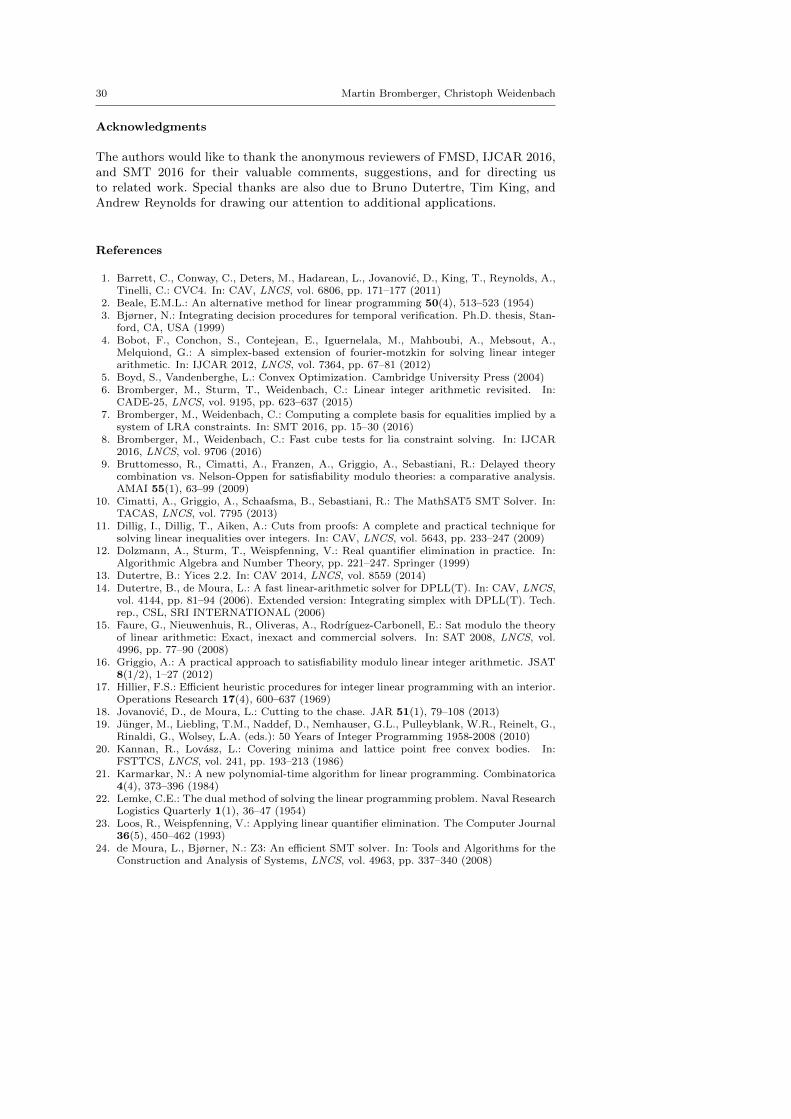
30 Martin Bromberger, Christoph Weidenbach
Acknowledgments
The authors would like to thank the anonymous reviewers of FMSD, IJCAR 2016,and SMT 2016 for their valuable comments, suggestions, and for directing usto related work. Special thanks are also due to Bruno Dutertre, Tim King, andAndrew Reynolds for drawing our attention to additional applications.
References
1. Barrett, C., Conway, C., Deters, M., Hadarean, L., Jovanovic, D., King, T., Reynolds, A.,Tinelli, C.: CVC4. In: CAV, LNCS, vol. 6806, pp. 171–177 (2011)
2. Beale, E.M.L.: An alternative method for linear programming 50(4), 513–523 (1954)3. Bjørner, N.: Integrating decision procedures for temporal verification. Ph.D. thesis, Stan-
ford, CA, USA (1999)4. Bobot, F., Conchon, S., Contejean, E., Iguernelala, M., Mahboubi, A., Mebsout, A.,
Melquiond, G.: A simplex-based extension of fourier-motzkin for solving linear integerarithmetic. In: IJCAR 2012, LNCS, vol. 7364, pp. 67–81 (2012)
5. Boyd, S., Vandenberghe, L.: Convex Optimization. Cambridge University Press (2004)6. Bromberger, M., Sturm, T., Weidenbach, C.: Linear integer arithmetic revisited. In:
CADE-25, LNCS, vol. 9195, pp. 623–637 (2015)7. Bromberger, M., Weidenbach, C.: Computing a complete basis for equalities implied by a
system of LRA constraints. In: SMT 2016, pp. 15–30 (2016)8. Bromberger, M., Weidenbach, C.: Fast cube tests for lia constraint solving. In: IJCAR
2016, LNCS, vol. 9706 (2016)9. Bruttomesso, R., Cimatti, A., Franzen, A., Griggio, A., Sebastiani, R.: Delayed theory
combination vs. Nelson-Oppen for satisfiability modulo theories: a comparative analysis.AMAI 55(1), 63–99 (2009)
10. Cimatti, A., Griggio, A., Schaafsma, B., Sebastiani, R.: The MathSAT5 SMT Solver. In:TACAS, LNCS, vol. 7795 (2013)
11. Dillig, I., Dillig, T., Aiken, A.: Cuts from proofs: A complete and practical technique forsolving linear inequalities over integers. In: CAV, LNCS, vol. 5643, pp. 233–247 (2009)
12. Dolzmann, A., Sturm, T., Weispfenning, V.: Real quantifier elimination in practice. In:Algorithmic Algebra and Number Theory, pp. 221–247. Springer (1999)
13. Dutertre, B.: Yices 2.2. In: CAV 2014, LNCS, vol. 8559 (2014)14. Dutertre, B., de Moura, L.: A fast linear-arithmetic solver for DPLL(T). In: CAV, LNCS,
vol. 4144, pp. 81–94 (2006). Extended version: Integrating simplex with DPLL(T). Tech.rep., CSL, SRI INTERNATIONAL (2006)
15. Faure, G., Nieuwenhuis, R., Oliveras, A., Rodrıguez-Carbonell, E.: Sat modulo the theoryof linear arithmetic: Exact, inexact and commercial solvers. In: SAT 2008, LNCS, vol.4996, pp. 77–90 (2008)
16. Griggio, A.: A practical approach to satisfiability modulo linear integer arithmetic. JSAT8(1/2), 1–27 (2012)
17. Hillier, F.S.: Efficient heuristic procedures for integer linear programming with an interior.Operations Research 17(4), 600–637 (1969)
18. Jovanovic, D., de Moura, L.: Cutting to the chase. JAR 51(1), 79–108 (2013)19. Junger, M., Liebling, T.M., Naddef, D., Nemhauser, G.L., Pulleyblank, W.R., Reinelt, G.,
Rinaldi, G., Wolsey, L.A. (eds.): 50 Years of Integer Programming 1958-2008 (2010)20. Kannan, R., Lovasz, L.: Covering minima and lattice point free convex bodies. In:
FSTTCS, LNCS, vol. 241, pp. 193–213 (1986)21. Karmarkar, N.: A new polynomial-time algorithm for linear programming. Combinatorica
4(4), 373–396 (1984)22. Lemke, C.E.: The dual method of solving the linear programming problem. Naval Research
Logistics Quarterly 1(1), 36–47 (1954)23. Loos, R., Weispfenning, V.: Applying linear quantifier elimination. The Computer Journal
36(5), 450–462 (1993)24. de Moura, L., Bjørner, N.: Z3: An efficient SMT solver. In: Tools and Algorithms for the
Construction and Analysis of Systems, LNCS, vol. 4963, pp. 337–340 (2008)

New Techniques for Linear Arithmetic 31
25. Papadimitriou, C.H.: On the complexity of integer programming. J. ACM 28(4), 765–768(1981)
26. Pugh, W.: The omega test: A fast and practical integer programming algorithm for de-pendence analysis. In: Supercomputing 1991, Supercomputing ’91, pp. 4–13. ACM (1991)
27. Refalo, P.: Approaches to the incremental detection of implicit equalities with the revisedsimplex method. In: PLILP 1998, LNCS, vol. 1490, pp. 481–496 (1998)
28. Rueß, H., Shankar, N.: Solving linear arithmetic constraints. Tech. rep., SRI International,Computer Science Laboratory (2004)
29. Schrijver, A.: Theory of Linear and Integer Programming. John Wiley & Sons, Inc., NewYork, NY, USA (1986)
30. Sturm, T.: Real quadratic quantifier elimination in risa/asir. Tech. rep., ISIS-RM-5E,Fujitsu Laboratories Ltd. (1996)
31. Telgen, J.: Identifying redundant constraints and implicit equalities in systems of linearconstraints. Management Science 29(10), 1209–1222 (1983)
32. Van Hentenryck, P., Graf, T.: Standard forms for rational linear arithmetic in constraintlogic programming. AMAI 5(2), 303–319 (1992)