Lecture Notesin Control and Information Sciences 295

Editors: M. Thoma · M. Morari

SpringerBerlinHeidelbergNewYorkHong KongLondonMilanParisTokyo

Wei Kang Mingqing Xiao Carlos Borges (Eds.)

New Trends in NonlinearDynamics and Control,and their Applications

With 45 Figures

1 3

Series Advisory BoardA. Bensoussan · P. Fleming · M.J. Grimble · P. Kokotovic ·A.B. Kurzhanski · H. Kwakernaak · J.N. Tsitsiklis

EditorsProf. Wei KangProf. Carlos BorgesNaval Postgraduate SchoolDept. of Mathematics93943 Monterey, CAUSA

Prof. Mingqing XiaoSouthern Illinois UniversityDept. of Mathematics62901-4408 Carbondale, ILUSA

ISSN 0170-8643

ISBN 3-540-40474-0 Springer-Verlag Berlin Heidelberg New York

Cataloging-in-Publication Data applied forA catalog record for this book is available from the Library of Congress.Bibliographic information published by Die Deutsche BibliothekDie Deutsche Bibliothek lists this publication in the Deutsche Nationalbibliografie; detailed biblio-graphic data is available in the Internet at <http://dnb.ddb.de>.

This work is subject to copyright. All rights are reserved, whether the whole or part of the mate-rial is concerned, specifically the rights of translation, reprinting, reuse of illustrations, recitation,broadcasting, reproduction on microfilm or in other ways, and storage in data banks. Duplicationof this publication or parts thereof is permitted only under the provisions of the German CopyrightLaw of September 9, 1965, in its current version, and permission for use must always be obtainedfrom Springer-Verlag. Violations are liable for prosecution under German Copyright Law.

Springer-Verlag Berlin Heidelberg New Yorka member of BertelsmannSpringer Science + Business Media GmbH

http://www.springer.de

© Springer-Verlag Berlin Heidelberg 2003Printed in Germany

The use of general descriptive names, registered names, trademarks, etc. in this publication doesnot imply, even in the absence of a specific statement, that such names are exempt from the relevantprotective laws and regulations and therefore free for general use.

Typesetting: Data conversion by the authors.Final processing by PTP-Berlin Protago-TeX-Production GmbH, BerlinCover-Design: design & production GmbH, HeidelbergPrinted on acid-free paper 62/3020Yu - 5 4 3 2 1 0

Preface

The concept for this volume originated at the Symposium on New Trendsin Nonlinear Dynamics and Control, and their Applications. The symposiumwas held October 18-19, 2002, at the Naval Postgraduate School in Monterey,California and was organized in conjunction with the 60th birthday of Profes-sor Arthur J. Krener, a pioneer in nonlinear control theory. The symposiumprovided a wonderful opportunity for control theorists to review major deve-lopments in nonlinear control theory from the past, to discuss new researchtrends for the future, to meet with old friends, and to share the success and ex-perience of the community with many young researchers who are just enteringthe field.

In the process of organizing this international symposium we realized thata volume on the most recent trends in nonlinear dynamics and control wouldbe both timely and valuable to the research community at large. Years of re-search effort have revealed much about the nature of the complex phenomenaof nonlinear dynamics and the performance of nonlinear control systems. Wesolicited a wide range of papers for this volume from a variety of leading re-searchers in the field, some of the authors also participated in the symposiumand others did not. The papers focus on recent trends in nonlinear control re-search related to bifurcations, behavior analysis, and nonlinear optimization.The contributions to this volume reflect both the mathematical foundationsand the engineering applications of nonlinear control theory. All of the papersthat appear in this volume underwent a strict review and we would like totake this opportunity to thank all of the contributors and the referees for theircareful work. We would also like to thank the Air Force Office of ScientificResearch and the National Science Foundation for their financial support forthis volume.

Finally, we would like to exercise our prerogative and thank many of thepeople involved with the symposium at this time. In particular, we would liketo thank Jhoie Passadilla and Bea Champaco, the staff of the Departmentof Applied Mathematics of the Naval Postgraduate School, for their supportin organizing the symposium. Furthermore, we extend our special thanks to

VI Preface

CAPT Frank Petho, USN, whose dedication to the core mission of the Na-val Postgraduate School allowed him to cut through the bureaucratic layers.Without his vision and support the symposium might never have happened.Most importantly, we would like to express our deepest gratitude to the AirForce Office of Scientific Research and the National Science Foundation, forthe financial support which made the symposium possible.

Monterey, California, Wei KangEarly Spring, 2003 MingQing Xiao

Carlos Borges

Contents

Part I Bifurcation and Normal Form

Observability Normal FormsJ-P. Barbot, I. Belmouhoub, L. Boutat-Baddas . . . . . . . . . . . . . . . . . . . 3

Bifurcations of Control Systems: A View from Control FlowsFritz Colonius, Wolfgang Kliemann . . . . . . . . . . . . . . . . . . . . . . . . . . . . . 19

Practical Stabilization of Systems with a Fold ControlBifurcation

Boumediene Hamzi, Arthur J. Krener . . . . . . . . . . . . . . . . . . . . . . . . . . . 37

Feedback Control of Border Collision BifurcationsMunther A. Hassouneh, Eyad H. Abed . . . . . . . . . . . . . . . . . . . . . . . . . . . 49

Symmetries and Minimal Flat Outputs of Nonlinear ControlSystems

W. Respondek . . . . . . . . . . . . . . . . . . . . . . . . . . . . . . . . . . . . . . . . . . . . . . . . 65

Normal Forms of Multi-input Nonlinear Control Systemswith Controllable Linearization

Issa Amadou Tall . . . . . . . . . . . . . . . . . . . . . . . . . . . . . . . . . . . . . . . . . . . . . 87

Control of Hopf Bifurcations for Infinite-DimensionalNonlinear Systems

MingQing Xiao, Wei Kang . . . . . . . . . . . . . . . . . . . . . . . . . . . . . . . . . . . . . 101

Part II System Behavior and Estimation

On the Steady-State Behavior of Forced Nonlinear SystemsC.I. Byrnes, D.S. Gilliam, A. Isidori, J. Ramsey . . . . . . . . . . . . . . . . . . 119

VIII Contents

Gyroscopic Forces and Collision Avoidance with ConvexObstacles

Dong Eui Chang, Jerrold E. Marsden . . . . . . . . . . . . . . . . . . . . . . . . . . . . 145

Stabilization via Polynomial Lyapunov FunctionDaizhan Cheng . . . . . . . . . . . . . . . . . . . . . . . . . . . . . . . . . . . . . . . . . . . . . . . 161

Simulating a Motorcycle DriverRuggero Frezza, Alessandro Beghi . . . . . . . . . . . . . . . . . . . . . . . . . . . . . . . 175

The Convergence of the Minimum Energy EstimatorArthur J. Krener . . . . . . . . . . . . . . . . . . . . . . . . . . . . . . . . . . . . . . . . . . . . . 187

On Absolute Stability of Convergence for Nonlinear NeuralNetwork Models

Mauro Di Marco, Mauro Forti, Alberto Tesi . . . . . . . . . . . . . . . . . . . . . . 209

A Novel Design Approach to Flatness-Based FeedbackBoundary Control of Nonlinear Reaction-Diffusion Systemswith Distributed Parameters

Thomas Meurer, Michael Zeitz . . . . . . . . . . . . . . . . . . . . . . . . . . . . . . . . . 221

Time-Varying Output Feedback Control of a Family ofUncertain Nonlinear Systems

Chunjiang Qian, Wei Lin . . . . . . . . . . . . . . . . . . . . . . . . . . . . . . . . . . . . . . 237

Stability of Nonlinear Hybrid SystemsG. Yin, Q. Zhang . . . . . . . . . . . . . . . . . . . . . . . . . . . . . . . . . . . . . . . . . . . . . 251

Part III Nonlinear Optimal Control

The Uncertain Generalized Moment Problem withComplexity Constraint

Christopher I. Byrnes, Anders Lindquist . . . . . . . . . . . . . . . . . . . . . . . . . 267

Optimal Control and Monotone Smoothing SplinesMagnus Egerstedt, Clyde Martin . . . . . . . . . . . . . . . . . . . . . . . . . . . . . . . . 279

Towards a Sampled-Data Theory for Nonlinear ModelPredictive Control

Rolf Findeisen, Lars Imsland, Frank Allgower, Bjarne Foss . . . . . . . . . 295

High-Order Maximal PrinciplesMatthias Kawski . . . . . . . . . . . . . . . . . . . . . . . . . . . . . . . . . . . . . . . . . . . . . . 313

Contents IX

Legendre Pseudospectral Approximations of Optimal ControlProblems

I. Michael Ross, Fariba Fahroo . . . . . . . . . . . . . . . . . . . . . . . . . . . . . . . . . 327

Minimax Nonlinear Control under Stochastic UncertaintyConstraints

Cheng Tang, Tamer Basar . . . . . . . . . . . . . . . . . . . . . . . . . . . . . . . . . . . . . 343

Observability Normal Forms

J-P. Barbot, I. Belmouhoub, and L. Boutat-Baddas

Equine Commando des Systemes (ECS), ENSEA, 6 Av. du Ponceau, 95014Cergy-Pontoise Cedex, France, barbot@ensea.fr

1 Introduction

One of the first definitions and characterizations of nonlinear observability wasgiven in the well known paper of R. Hermann and A.J. Krener [18], where theconcept of local weak observability was introduced and the observability rankcondition was given. In [18], observability and controllability were studied withthe same tools as those of differential geometry ([33]). Similarly to the linearcase, some direct links between observability and controllability may be found.After this pioneering paper many works on nonlinear observability followed[41, 6]... One important fact, pointed out in the eighties, was the loss of ob-servability due to an inappropriate input. Consequently, the characterizationof appropriate input (universal input) with respect to nonlinear observability([12]) was an important challenge. Since that time, much research has beendone on the design of nonlinear observers. From our point of view, one ofthe first significant theoretical and practical contributions to the subject wasthe linearization by output injection proposed by A.J Krener and A. Isidori[30] for a single output system and by A.J Krener and W. Respondek [31] forthe multi output case (see also X. Xia and W. Gao [45]). From these worksand some other ones, dealing with structural analysis [24, 37, 13, 40, 20, 5]an important literature on nonlinear observer design followed. Different tech-niques were studied: High gain [13, 25]..., Backstepping [23, 39]..., ExtendedLuenberger [7]..., Lyapunov approach [44]..., Sliding mode [42, 11, 46, 36, 3]...,Numerical differentiator [10]... and many other approaches. Some observer de-signs use partially or totally the notion of detectability. This concept will beused and highlighted in this paper in the context of observability bifurcation(see also the paper of A.J Krener and M.Q Xiao [32]).

But what is the observability bifurcation? Roughly speaking this is theloss of the linear observability property at one point or on a submanifold. Itis important to recall that the classical notion of bifurcation is dedicated to

W. Kang et al. (Eds.): New Trends in Nonlinear Dynamics and Control, LNCIS 295, pp. 3–17, 2003.c© Springer-Verlag Berlin Heidelberg 2003

4 J-P. Barbot, I. Belmouhoub, and L. Boutat-Baddas

stability properties. So, H. Poincare [38] introduced the normal form in orderto analyze the stability bifurcation. The main idea behind this concept is tohighlight the influences of the dominant terms with respect to a consideredlocal property (stability, controllability, observability). Moreover, each normalform characterizes one and only one equivalent class. So, the structural pro-perties of the normal form are also the same as those of each system in thecorresponding equivalence class. Thus, if the linear part of the normal formhas no eigenvalue on the imaginary axis, the system behavior is locally givenby this linear part. If some eigenvalues are on the imaginary axis, the linearapproximation does not characterize the local behavior and then higher orderterms must be considered. In [27] A.J Krener has introduced the concepts ofapproximate feedback linearization and approximated integrability (see also[17] around a manifold). After that, W. Kang and A.J Krener introduced in[22] the definition of a normal form with respect to the controllability pro-perty, for this, they introduced a new equivalence relation. This relation iscomposed of a homogenous diffeomorphism, as in the classical mathematicalcontext, and of a homogenous regular feedback. After that many authors wor-ked on the subject of controllability bifurcation [21, 28, 29, 43, 15, 2, 14, 16]...

In this paper, a new class of homogeneous transformations, by diffeomor-phism and output injection, is used in order to study the observability bifur-cation and define an observability normal form (in continuous and discretetime). The usefulness of this theoretical approach is highlighted with two ex-amples of chaotic system synchronization. As a matter of fact, it was shown in[35] by H. Nijmeijer and I. Mareels that the synchronization problem may berewritten and understood as an observer design problem. In the first example,the sliding mode observer efficiency with respect to the observability bifurca-tion is highlighted ([9]). In the second example, a special structure of discretetime observer dedicated to discrete time system with observability bifurcationis recalled ([4]). The paper ends with a conclusion and some perspectives.

2 Some Recalls on Observability

Let us consider the following system:

x = f(x); y = h(x) (1)

where vector fields f : IR n → IR n and h : IR n → IR m are assumed tobe smooth with f(0) = 0 and h(0) = 0. The observability problem arises asfollows : can we estimate the current state x(t) from past observations y(s),s ≤ t , without measuring all state variables? An algorithm that solves thisproblem is called an observer.

Motivated by the consideration that it is always possible to cancel all inde-pendent parts constituted only by the input and the output in the estimatederror, the observer linearization problem was born. Is it possible to find in aneighborhood U of 0 in IR n a change of state coordinates z = θ(x) such thatdynamic (1) is linear driven by non linear output injection:

Observability Normal Forms 5

z = Az − β(y). (2)

where β : IR m → IR n is a smooth vector field. Note that the output injectionterm β(y) is cancelled in the observation error dynamic for system (2). Thediffeomorphism θ must satisfy the first-order partial differential equation:

∂θ

∂x(x)f(x) = Aθ(x)− β(h(x)). (3)

In [30] A.Krener and A. Isidori showed that equation (3) has a solution ifand only if the following two conditions are satisfied:

i) the codistribution spandh, dLfh, ..., dL

n−1f h

is of rank n at 0,

ii)[τ, adkfτ

]= 0 for all k = 1, 3, ..., 2n− 1 where τ is the unique solution

vector fields of[(dh)T , (dLfh)T , ...., (dLn−1

f h)T]T, τ = [0, 0, ....1]T

3 Observability Normal Form

In this paper for the lack of space, we only give the normal form for a systemwith a linear unobservable mode in both continuous and discrete time case.

3.1 Continuous Time Case

Let us consider a nonlinear Single Input Single Output (SISO) system:

ξ = f(ξ) + g(ξ)u; y = Cξ (4)

where, vector fields f, g : U ⊂ IR n −→ IR n are assumed to be real analytic,such that f (0) = 0.

Setting: A = ∂f∂ξ (0) and B = g(0) around the equilibrium point ξe = 0,

the system can be rewritten in the following form:

z = Az +Bu+ f [2](z) + g[1](z)u+O[3] (z, u) ; y = Cz (5)

where: f [2] (z) =[f

[2]1 (z) , ..., f [2]

n (z)]T

and g[1] (z) =[g[1]1 (z) , ..., g[1]n (z)

]T

with for all 1 ≤ i ≤ n, f [2]i (z) and g

[1]i (z) are respectively homogeneous

polynomials of degree 2, respectively 1 in z.

Definition 1.i) The component f [2](z) + g[1](z)u is the quadratic part of system (5).ii) Consider a second system:

x = Ax+Bu+ f [2](x) + g[1](x)u+O[3](x, u); y = Cx (6)

6 J-P. Barbot, I. Belmouhoub, and L. Boutat-Baddas

We say that system (5) whose quadratic part is f [2](z) + g[1](z)u, is Quadra-tically Equivalent Modulo an Output Injection to System (6) whose quadraticpart is f [2](x) + g[1](x)u, if there exists an output injection:

β[2](y) + γ[1](y)u (7)

and a diffeomorphism of the form:

x = z − Φ[2](z) (8)

which carries f [2](z) + g[1](z)u to f [2](x) + g[1](x)u+[β[2](y) + γ[1](y)u

].

Where Φ[2] (z) =[Φ

[2]1 (z) , ......, Φ[2]

n (z)]T

, β[2] (y) =[β

[2]1 (y) , ......, β[2]

n (y)]T

and for all 1 ≤ i ≤ n, Φ[2]i (z) and β[2]

1 (y) are homogeneous polynomial in z

respectively in y of degree two, and γ[1](y) =[γ

[1]1 (y) , ......, γ[1]

n (y)]T

with

γ[1]i (y) is a homogeneous polynomial of degree one in y.

iii) If f [2](x) = 0 and g[1](x) = 0 we say that system (5) is quadraticallylinearizable modulo an output injection.

Remark 1. If(

∂f∂x (0), C

)has one unobservable real mode then one can trans-

form system (4) to the following form:

˙z = Aobsz +Bobsu+ f [2](z) + g[1](z)u+O[3] (z, u)zn = αnzn +

∑n−1i=1 αizi + bnu+ f

[2]n (z) + g

[1]n (z)u+O[3] (z, u)

y = z1 = Cobsz

(9)

with:z = [ z1 · · · · · · zn−1 ]T , z = [zT , zn]T ,

Aobs =

a1 1 0 ... 0a2 0 1 0 ...... 0

...... 0

an−2 0 ... 0 1an−1 0 ... ... 0

, Bobs =

b1......

bn−1

Remark 2. Throughout the paper, we deal with systems in form (9). Moreover,the output is always taken equal to the first state component. Consequently,the diffeomorphism (x = z − Φ[2] (z)) is such that Φ[2]

1 (z) = 0.

Proposition 1. [8] System (5) is QEMOI to system (6), if and only if thefollowing two homological equations are satisfied:

i) AΦ[2](z)− ∂Φ[2]

∂z Az = f[2]

(z)− f [2](z) + β[2] (z1)

ii) −∂Φ[2]

∂z B = g[1](z)− g[1](z) + γ[1](z1)(10)

Observability Normal Forms 7

where ∂Φ[2]

∂z Az :=(

∂Φ[2]1 (z)∂z Az, ......,

∂Φ[2]n (z)∂z Az

)T

and ∂Φ[2]i (z)∂z is the Jacobian

matrix of Φ[2]i (z) for all 1 ≤ i ≤ n.

Using proposition 1 and remark 1 we show the following theorem which givesthe normal form for nonlinear systems with one linear unobservable mode.

Theorem 1. There is a quadratic diffeomorphism and an output injectionwhich transform system (9) in the following normal form:

x1 = a1x1 + x2 + b1u+∑n

i=2 k1ixiu+O[3](x, u)... =

...xn−2 = an−2x1 + xn−1 + bn−2u+

∑ni=2 k(n−2)ixiu+O[3](x, u)

xn−1 = an−1x1 + bn−1u+∑n

j≥i=2 hijxixj + h1nx1xn+

∑ni=2 k(n−1)ixiu+O[3](x, u)

xn = αnxn +∑n−1

i=1 αixi + bnu+ αnΦ[2]n (x) +

∑n−1i=1 αiΦ

[2]i (x)

−∂Φ[2]n

∂x Aobsx+ f[2]n (x) +

∑ni=2 knixiu+O[3](x, u)

(11)

For the proof see [8].

Remark 3.1) If for some index i ∈ [1, n] we have hinxi = 0 then we can recover, at leastlocally, all state components.2) If we have some kin = 0 then with an appropriate choice of input u (uni-versal input [12]) we can have quadratic observability.3) Thus, the local quadratic observability is principally given by the dynamicxn−1. In the case where conditions 1) and 2) are not verified, then we can usecoefficient αn to study the detectability propriety. Then, we have three cases:

a) if αn < 0 then the state xn is detectable,b) if αn > 0 then xn unstable, and consequently undetectable,c) if αn = 0 we can use the center manifold theory in order to analyze sta-

bility or instability of xn and consequently its detectability or undetectability.

Remembering the well known Poincare-Dulac theorem we have:

Remark 4. If Φ[2]n (x) check the following equation:

αnΦ[2]n (x) +

n−1∑i=1

αiΦ[2]i (x) =

∂Φ[2]n

∂xAobsx− f [2]

n (x) + β[2]n (x1) (12)

then quadratic terms in xn are cancelled. Which in general is not the case forarbitrary αn and ai. Nevertheless, this condition is less restrictive than theusual one thanks to the output injection β[2]

n (x1).

8 J-P. Barbot, I. Belmouhoub, and L. Boutat-Baddas

3.2 Discrete Time Case

Now, let us consider a discrete time nonlinear SISO system:

ξ+ = f(ξ, u); y = Cξ (13)

where, ξ is the state of the system and ξ (respectively ξ+) denote ξ(k) (res-pectively ξ(k+ 1)). The vector fields f : U ⊂ IR n+1 −→ IR n and the functionh : M ⊂ IR n −→ IR are assumed to be real analytic, such that f (0, 0) = 0.As for the continuous time case, we only give the observability normal formfor a system with one linear unobservable mode. We apply, as usual, a secondorder Taylor expansion around the equilibrium point.

Thus the system is rewritten as :z+ = Az +Bu+ F [2](z) + g[1](z)u+ γ[0]u2 +O3 (z, u)y = Cz

(14)

withA = ∂f∂x (0, 0),B = ∂f

∂u (0, 0) and where: F [2] (z) =[F

[2]1 (z) , · · · , F [2]

n (z)]T

and g[1] (z) =[g[1]1 (z) , · · · , g[1]n (z)

]T. From (14), we give

Definition 2. The system:

z+ = Az +Bu+ F [2](z) + g[1](z)u+ γ[0]u2 +O3(z, u); y = Cz (15)

is said to be quadratically equivalent to the system:x+ = Ax+Bu+ F [2](x) + g[1](x)u+ γ[0]u2

+β[2](y) + α[1](y)u+ τ [0]u2 +O3 (x, u)y = Cx

(16)

modulo an output injection: β[2](y) + α[1](y)u+ τ [0]u2 (17)

if there exists a diffeomorphism of the form: x = z − Φ[2] (z) (18)

which transforms the quadratic part of (15) into the one of (16).

Remark 5. The output injection (17) is different from the one defined in (7)for the continuous-time case. This is due to the fact that the vector field com-position does not preserve the linearity in “u”; So we are obliged to considerthe term τ [0]u2 in (17).

In the next proposition, we give necessary and sufficient conditions forobservability QEMOI:

Observability Normal Forms 9

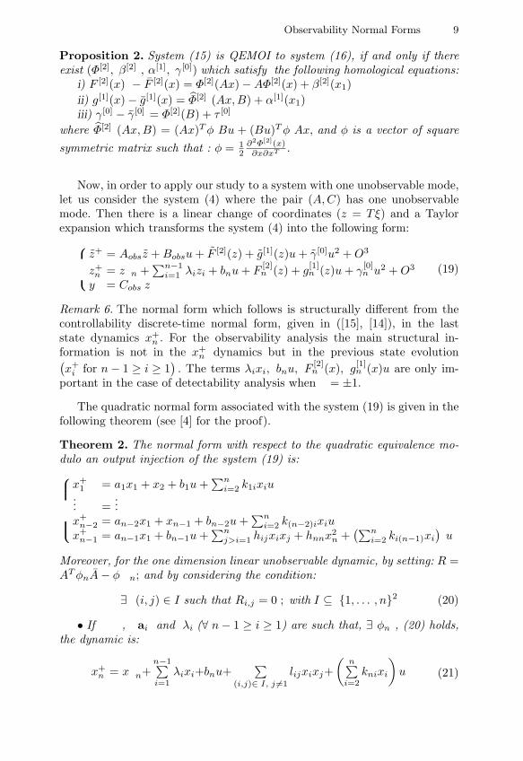
Proposition 2. System (15) is QEMOI to system (16), if and only if thereexist (Φ[2], β[2] , α[1], γ[0]) which satisfy the following homological equations:

i) F [2](x) − F [2](x) = Φ[2](Ax)−AΦ[2](x) + β[2](x1)ii) g[1](x)− g[1](x) = Φ[2] (Ax,B) + α[1](x1)iii) γ[0] − γ[0] = Φ[2](B) + τ [0]

where Φ[2] (Ax,B) = (Ax)Tφ Bu + (Bu)Tφ Ax, and φ is a vector of squaresymmetric matrix such that : φ = 1

2∂2Φ[2](x)∂x∂xT

.

Now, in order to apply our study to a system with one unobservable mode,let us consider the system (4) where the pair (A,C) has one unobservablemode. Then there is a linear change of coordinates (z = Tξ) and a Taylorexpansion which transforms the system (4) into the following form:

z+ = Aobsz +Bobsu+ F [2](z) + g[1](z)u+ γ[0]u2 +O3

z+n = ηzn +∑n−1

i=1 λizi + bnu+ F[2]n (z) + g

[1]n (z)u+ γ

[0]n u2 +O3

y = Cobs z

(19)

Remark 6. The normal form which follows is structurally different from thecontrollability discrete-time normal form, given in ([15], [14]), in the laststate dynamics x+

n . For the observability analysis the main structural in-formation is not in the x+

n dynamics but in the previous state evolution(x+i for n− 1 ≥ i ≥ 1

). The terms λixi, bnu, F

[2]n (x), g[1]n (x)u are only im-

portant in the case of detectability analysis when η = ±1.

The quadratic normal form associated with the system (19) is given in thefollowing theorem (see [4] for the proof).

Theorem 2. The normal form with respect to the quadratic equivalence mo-dulo an output injection of the system (19) is:

x+1 = a1x1 + x2 + b1u+

∑ni=2 k1ixiu

... =...

x+n−2 = an−2x1 + xn−1 + bn−2u+

∑ni=2 k(n−2)ixiu

x+n−1 = an−1x1 + bn−1u+

∑nj>i=1 hijxixj + hnnx

2n +

(∑ni=2 ki(n−1)xi

)u

Moreover, for the one dimension linear unobservable dynamic, by setting: R =ATφnA− η φn; and by considering the condition:

∃ (i, j) ∈ I such that Ri,j = 0 ; with I ⊆ 1, . . . , n2 (20)

• If η , ai and λi (∀ n− 1 ≥ i ≥ 1) are such that, ∃ φn , (20) holds,the dynamic is:

x+n = ηxn+

n−1∑i=1

λixi+bnu+∑

(i,j)∈ I, j =1lijxixj+

(n∑

i=2knixi

)u (21)

10 J-P. Barbot, I. Belmouhoub, and L. Boutat-Baddas

• And if η, ai and λi (∀ (n− 1) ≥ i ≥ 1) are such that for no φn, (20) isverified, the dynamic is:

x+n = ηxn+

∑n−1i=1 λixi+bnu+ (

∑ni=2 knixi)u (22)

Remark 7.• Thanks to the quadratic term kn(n−1)xnu in the normal form describedabove, it is possible with a well chosen input u, to restore observability.• In the normal form, let us consider more closely the observability singula-rity’s (here we consider system without input) by isolating the terms in xnwhich appear in the (n− 1)-th line, as follows:

∑n−1j>i=1 hijxixj+ (

∑ni=1 hinxi)xn; (23)

we can deduce the manifold of local unobservability: Sn =

n∑i=1hinxi = 0

.

4 Unknown Input Observer

In many works, the observer design for a system with unknown input wasstudied [46, 19]... and numerous relevant applications of such approaches weregiven. In this paper we propose to find a new application domain for theunknown input observer design. More precisely, we propose a new type ofsecure data transmission based on chaotic synchronization. For this we haveto recall and give some particular concepts of an observer for a system withunknown input.Roughly speaking, in a linear context, the problem of observer design for asystem with unknown input is solved as follows:Assume an observable system with two outputs and one unknown input suchthat at least one derivative of the output is a function of the unknown input(i.e C1G or C2G different from zero),

x = Ax+Bu+Gω; y1 = C1x; y2 = C2x

Then to design an observer, we have to choose a new output as a compositionof the both original ones, ynew = φ(y1, y2) and find observation error dynamicswhich are orthogonal to the unknown input vector. Unfortunately, this kind ofdesign can not be applied to system with only one output (the case consideredin this paper). Nevertheless, it is possible with a step by step procedure todesign an observer for such a system. Obviously, there are some restrictiveconditions on the system to solve this problem (see [46, 36]). Now, let usconsider the nonlinear analytic system:

x = f(x) + g(x)u; y = h(x) (24)

where vector fields f and g : IR n → IR n and h : IR n → IR m are assumedto be smooth with f(0) = 0 and h(0) = 0. Now, we can give a particular

Observability Normal Forms 11

constraint in order to solve this problem. The unknown input observer designis solvable locally around x = 0 for system (24) if :

• spandh, dLfh, ..., dLn−1f h is of rank n at x = 0,

•(

(dh)T (dLfh)T · · · (dLn−1f h)T

)T

g =(

0 · · · 0 )T (observability mat-

ching condition) with “ ” means a non null term. Sketch of proof: Settingz1 = h, z2 = Lfh,..., zn = Ln−1

f h, we have

z1 = z2; z2 = z3, ..., zn−1 = znzn = f(z) + g(z)u

(25)

Then under classical boundary assumptions, it is possible for the system (25)to design a step by step sliding mode observer such that we recover in finitetime all state components and the unknown input.

Remark 8. In discrete-time the observability matching condition is :

•(

(dh)T (dfoh)T · · · (dfn−1o oh)T

)T

g =(

0 · · · 0 )T

where o denotes the usual composition function and f jo denotes the function

f composed j times.

5 Synchronization of Chaotic Systems

Now we propose new encoding algorithm based on chaotic system synchro-nization but for which we have also an observability bifurcation. Moreover inboth the continuous case and the discrete time case the message is includedin the system structure and the observability matching condition is required.

5.1 Continuous-Time Transmission: Chua Circuit

Here we just give an illustrative example, so let us consider the well knownChua circuit with a variable inductor (see figure 1). The circuit contains linearresistors (R,R0), a single nonlinear resistor (f (v1)), and three linear energy-storage elements: a variable inductor (L) and two capacitors (C1, C2).The state equations for the circuit are as follows:

x1 = −1C1R

(x1 − x2) + f(x1)C1

x2 = 1C2R

(x1 − x2) + x3C2

x3 = −x4 (x2 +R0x3)x4 = σ

(26)

with: y ∆= x1∆= v1, x2

∆= v2, x3∆= i3, x4

∆= 1L(t) , x ∆= (x1, x2, x3, x4)T and

f(x1) = Gbx1 + 0.5(Ga −Gb)(|x1 + E| − |x1 − E|).

12 J-P. Barbot, I. Belmouhoub, and L. Boutat-Baddas

Fig. 1. Chua Circuit with inductance variation.

Moreover x1 is the output and x4 = 1L is the only state component directly

influenced by σ an unknown bounded function. The variation of L is theinformation to pass on the receiver. Moreover, we assume that there exist K1and K2 such that |x4| < K1 and |dx4

dt | < K2, this means that the informationsignal and its variation are bounded.This system has one unobservable real mode and using the linear change ofcoordinates z1 = x1, z2 = x1

C2R+ x2

C1R, z3 = x3

C1C2Rand z4 = x4 we obtain:

z1 = −(C1+C2)C1C2R

z1 + z2 + f(x1)C1

z2 = z3 + f(x1)C1C2R

z3 = z1z4C2

2R− z2z4

C2−R0z3z4

z4 = σ

(27)

Equations (27) are in observability normal form [8] with α = 0 and resonantterms h22 = h23 = 0, h14 = 1

C22R

, h24 = 1C2

and h34 = −R0.Moreover the system verified the observability matching condition [46, 1]

with respect to σ and as non smooth output injection (f(x1)C1

, f(x1)C1C2R

, 0, 0)T .From the normal form (27) we conclude that the observability singularitymanifold is M0 =

z z1C2

2R− z2

C2−R0z3 = 0

, and taking into account this

singularity we can design an observer. Therefore, it is possible to design thefollowing step by step sliding mode observer (here given in the original coor-dinate for the sake of compactness):

dx1dt = 1

C1

(x2−yR −f(y)

)+ λ1sign(y − x1)

dx2dt = 1

C2

(y−x2R +x3

)+ E1λ2sign(x2 − x2)

dx3dt = x4(−x2 −R0x3) + E2λ3sign(x3 − x3)dx4dt = E3λ4sign(x4 − x4)

(28)

with the following conditions:if x1 = x1 then E1 = 1 else E1 = 0, similarly if [x2 = x2 and E1 = 1] thenE2 = 1 else E2 = 0 and finally if [x3 = x3 and E2 = 1] then E3 = 1 elseE3 = 0. Moreover, in order to take into account the observability singularitymanifold M0 respectively (x2 + R0x3 = 0), we set Es = 1 if x2 + R0x3 = 0else Es = 0. And by definition we take:

Observability Normal Forms 13

x2 = x2 + E1C1Rλ1sign(y − x1)x3 = x3 + E2C2λ2sign(x2 − x2)x4 = x4 − E3Es

(x2+R0x3−1+ES))λ3sign(x3 − x3)(29)

Then the observation error dynamics (e = x− x) are:

de1dt = e2

C1R− λ1sign(x1 − x1)

de2dt = e3

C2− λ2sign(x2 − x2)

de3dt = −(x2 +R0x3)e4 − λ3sign(x3 − x3)de4dt = σ − Esλ4sign(x4 − x4)

(30)

The proof of observation error convergence is in [9].

Remark 9. In practice we add some low pass filter on the auxiliary componentsxi and we set Ei = 1 for i ∈ 1, 2, 3, not exactly when we are on the slidingmanifold but when we are close enough. Similarly, Es = 0 when we are closeto the singularity, not only when we are on it.

In order to illustrate the efficiency of the method we chose to transmit thefollowing message: 0.1 sin (100t) . The message was introduced in the Chuacircuit as following: L (t) = L+ 0.1L sin (100t) with: L = 18.8mH.

Fig. 2. x4, x4, Es and the singularity (x2 + R0x3)

In figure (2), if we set Es = 0 on a big neighborhood of the singularitymanifold (x2 +R0x3), we lose for a long time the information on x4. We noticethat the convergence of the state x4 of the observer, towards x4 of the systemof origin (26) depends on the choice of Es (see both first curves of the figure(2)). In order to have good convergence it is necessary to take Es = 0 on avery small neighborhood of the singularity manifold (x2 +R0x3), as we noticeit on both last curves of the figure (2).

But in any case, these simulations confirm that the resonant terms(−x4x2 −R0x4x3) = 0 allow us to obtain the message.

14 J-P. Barbot, I. Belmouhoub, and L. Boutat-Baddas

5.2 Discrete-Time Transmission: Burgers Map

As information such as it appears nowadays is more and more digitized, trea-ted, exchanged, by “thinking” organs; thus we think that is of first importanceto study systems in discrete time. Hereafter, we study the following discretetime chaotic system, known under the name of Burgers Map [26]:

x+

1 = (1 + a)x1 + x1x2

x+2 = (1− b)x2 − x2

1(31)

where a and b are two real parameters. We assume that we can measure thestate x1, so we have y = x1 as output of the system. This system is thenormal form of:

z+1 = (1 + a) z1 + z1z2z+2 = (1− b) (z2 + bz1z2)− z12 (32)

obtained, modulo (−y2), by applying him the change of coordinates x = z −Φ[2] (z) ; where the diffeomorphism Φ[2] is as: Φ[2]

1 (z) = 0 and Φ[2]2 (z) = z1z2.

Encryption: Now let us consider the Burgers map, and let us note thatm represents the message and only y = x1 the output, is transmitted to thereceiver via a public channel. Then, the transmitter will have the form:

x+

1 = (1 + a)x1 + x1x2

x+2 = (1− b)x2 − x2

1 +m(33)

The key of this secure communication consists in the knowledge of theparameters a and b. The fact that the message should be the last informationto reach the system constitutes a necessary and sufficient condition to recoverthe message by the construction of a suitable observer. It is what we call theobservability “Matching Condition”.

Decryption: Now, to decrypt the message we construct the observer:x+

1 = (1 + b) y + y x2

x+2 = (1− a)x2 − y2 (34)

The observer design consists of reconstructing all the linearly unobservablestates (i.e. x2) in the observer, with the knowledge of y.

Reconstruction of x2: For the sake of causality, we extract x2 from e1, atthe iteration (k − 1); which we approximate by x−

2 , so: x−2 = e1

y− ,for y = 0.Consequently, when y = 0 this leads to a singularity. However, we overcomethis problem, by forcing x2 to take the last remembered value when y = 0.

Correction of x−2 : By correction, we mean to replace x2 by x2 in the

prediction equation of x2, then we have: x−2C = (1− b)x− −

2 − (y− −)2.Reconstruction of the message m: We have x−

2 = x−2 = (1 − b)x− −

2 −(y− −)2 + m− −. It is now possible to extract m with 2 delays from e2 as:

Observability Normal Forms 15

e−2 = x−2 − x−

2C = m− −. Which means that e2(k − 1) = m(k − 2). Sowe have to wait two steps (these correspond to the necessary steps to thesynchronization).

The two studied examples consolidate our reflection that the observabi-lity normal form, allows one to simplify the structural analysis of dynamicalsystems, while preserving their structural properties. Hence, thanks to theresonant terms, we were able to recover the observability in the receiver anddo a suitable observer design, with eventually, bifurcations of observability;and properly reconstruct the confidential message.

References

1. Barbot J-P, Boukhobza T, Djemai M (1996) Sliding mode observer for trian-gular input form, in Proceedings of the 35th CDC, Kobe, Japan

2. Barbot J-P, Monaco S, Normand-Cyrot D (1997) Quadratic forms and appro-ximate feedback linearization in discrete time, International Journal of Control,67:567–586

3. Bartolini G, Pisano A, Usai E (200) First and second derivative estimation bysliding mode technique, Int. J. of Signal Processing, 4:167–176

4. Belmouhoub I, Djemai M, Barbot J-P, Observability quadratic normal formsfor discrete-time systems, submitted for publication.

5. Besancon G (1999) A viewpoint on observability and observer design for nonli-near system, Lecture Notes in Cont. & Inf. Sci 244, Springer, pp. 1–22

6. Bestle D, Zeitz M (1983) Canonical form observer design for nonlinear timevarying systems, International Journal of Control, 38:429–431

7. Birk J, Zeitz M (1988) Extended Luenberger observers for nonlinear multiva-riable systems International Journal of Control, 47:1823–1836

8. Boutat-Baddas L, Boutat D, Barbot J-P, Tauleigne R (2001) Quadratic Obser-vability normal form, in Proc. of the 41th IEEE CDC

9. Boutat-Baddas L, Barbot J-P, Boutat D, Tauleigne R (202) Observability bi-furcation versus observing bifurcations, in Proc. IFAC World Congress

10. Diop S, Grizzle JW, Morral PE, Stefanoupoulou AG (1993) Interpolation andnumerical differentiation for observer design, in Proc. of IEEE-ACC, 1329–1335

11. Drakunov S, Utkin V (1995) Sliding mode observer: Tutorial, in Proc. of theIEEE CDC

12. Gauthier J-P, Bornard G (1981) Observability for any u(t) of a class of bilinearsystems, IEEE Transactions on Automatic Control, 26:922–926

13. Gauthier J-P, Hammouri H, Othman S (1992) A simple observer for nonlinearsystems: application to bioreactors IEEE Trans. on Automat. Contr., 37:875–880

14. Gu G, Sparks A, Kang W (1998) Bifurcation analysis and control for model viathe projection method, in Proc. of 1998 ACC, pp. 3617–3621

15. Hamzi B, Barbot JP, Monaco S, Normand-Cyrot D (2001) Nonlinear discrete-time control of systems with a Naimar-Sacker bifurcation, Systems & ControlLetters 44:245–258,

16. Hamzi B, Kang W, Barbot JP (2000) On the control of bifurcations, in Proc.of the 39th IEEE CDC

16 J-P. Barbot, I. Belmouhoub, and L. Boutat-Baddas

17. Hauser J, Xu Z (1993) An approximate Frobenius theorem, in Proc. of IFACWorld Congress (Sydney), 8:43–46

18. Hermann R, Krener AJ (1977) Nonlinear contollability and observability, IEEETransactions on Automatic Control, 22:728–740

19. Hou M, Muller PC (1992) Design of observers for linear systems with unknowinputs, IEEE Transactions on Automatic Control, 37:871–875

20. Hou M, Busawon K, Saif M (2000) Observer design based on triangular formgenerated by injective map, IEEE Trans. on Automat. Contr., 45:1350–1355

21. Kang W (1998) Bifurcation and normal form of nonlinear control system: PartI and II, SIAM J. of Control and Optimization, 36:193–232

22. Kang W, Krener AJ (1992) Extended quadratic controller normal form anddynamic state feedback linearization of nonlinear systems, SIAM J. of Controland Optimization, 30:1319–1337

23. Kang W, Krener AJ Nonlinear observer design, a backstepping approach, per-sonal communication

24. Keller H (1987) Nonlinear Observer design by transformation into a generalzedobserver canonical form International Journal of Control, 46:1915–1930

25. Khalil HK (1999) High-gain observers in nonlinear feedback control, LectureNotes in Cont & Inf Sciences 244, Springer, pp. 249–268

26. Korsch HJ, Jodl HJ (1998) Chaos. A Program Collection for the PC, Springer,2nd edition

27. Krener AJ (1983) Approximate linearization by state feedback and coordinatechange, Systems & Control letters, 5:181–185

28. Krener AJ (1998) Feedback Linearization Mathematical Control Theory, in J-Bailleul and J-C. Willems Eds, pp. 66–98, Math. Cont. Theory, Springer

29. Krener AJ, Li L (2002) Normal forms and bifurcations of discrete time nonlinearcontrol systems, SIAM J. of Control and Optimization, 40:1697–1723

30. Krener AJ, Isidori A (1983) Linearization by output injection and nonlinearobserver, Systems & Control Letters, 3:47–52

31. Krener AJ, Respondek W (1985) Nonlinear observer with linearizable errordynamics , SIAM J. of Control and Optimization, 23:197—216

32. Krener AJ, Xiao MQ (2002) Observers for linearly unobservable nonlinear sy-stems, Systems & Control Letters, to appear.

33. Lobry C (1970) Contolabilite des systemes non lineaires, SIAM J. of Control,pp. 573-605, 1970

34. Nijmeijer H (1981) Observability of a class of nonlinear systems: a geometricapproach, Richerche di Automatica, 12:50–68

35. Nijmeijer H, Mareels IMY (1997) An observer looks at synchronization, IEEETrans. on Circuits and Systems-1: Fundamental Theory and Applications,44:882–891

36. Perruquetti W, Barbot JP (2002) Sliding Mode control in Engineering, M. Dek-ker

37. Plestan F, and Glumineau A (1997) Linearization by generalized input-outputinjection, Systems & Control Letters, 31:115–128

38. Poincare H (1899) Les Methodes nouvelles de la mecanique celeste, GauthierVillard, 1899 Reedition 1987, bibliotheque scientifique A. Blanchard.

39. Robertsson A, Johansson R (1999) Observer backstepping for a class ofnonminimum-phase systems, Proc. of the 38th IEEE CDC

40. Rudolph J, Zeitz M (1994) A Block triangular nonlinear observer normal form,Systems & Control Letters, 23

Observability Normal Forms 17

41. Sussmann HJ (1979) Single input observability of continuous time systems,Math. Systems Theory, 12:371–393

42. Slotine JJ, Hedrick JK, Misawa EA (1987) On sliding observer for nonlinearsystems, ASME J.D.S.M.C, 109:245–252

43. Tall IA, Respondek W (2001) Normal forms and invariants of nonlinear single-input systems with noncontrollable linearization, in IFAC NOLCOS

44. Tsinias J (1989) Observer design for nonlinear systems, Systems & ControlLetters, 13:135–142

45. Xia X, Gao W (1989) Nonlinear observer design by observer error linearization,SIAM J. of Control and Opt., 27:199–213

46. Xiong Y, Saif M (2001) Sliding mode observer for nonlinear uncertain systems,IEEE Transactions on Automatic Control, 46:2012–2017

Bifurcations of Control Systems: A View fromControl Flows

Fritz Colonius1 and Wolfgang Kliemann2

1 Institut fur Mathematik, Universitat Augsburg, 86135 Augsburg, Germany,colonius@math.uni-augsburg.de

2 Department of Mathematics, Iowa State University, Ames IA 50011, U.S.A,kliemann@iastate.edu

1 Introduction

The purpose of this paper is to discuss bifurcation problems for control sy-stems viewing them as dynamical systems, i.e., as control flows. Here openloop control systems are considered as skew product flows where the shiftalong the control functions is part of the dynamics.

Basic results from this point of view are contained in the monograph [8]. Inthe present paper we survey recent results on bifurcation problems-some newresults are included and a number of open problems is indicated. Pertinentresults from [8] are cited if necessary for an understanding.

We consider control systems in Rd of the form

x(t) = f(α, x(t), u(t)), u ∈ U = u : R→ Rm, u(t) ∈ U for t ∈ R, (1)

where the control range U is a subset of Rm and α ∈ A ⊂ R denotes a bi-

furcation parameter. For simplicity we assume that for every initial conditionx(0) = x0 ∈ R

d and every admissible control function u a unique global so-lution ϕα(t, x0, u), t ∈ R, exists. If the dependence on α is irrelevant, wesuppress α in the notation.

As for differential equations, it is relevant to discuss qualitative changesin the system behavior when α is varied. Such problems have found muchinterest in recent years; see e.g. the contributions in this volume or in [7]. Thebifurcation theory developed here concerns open loop control system. Basedon the concept of the associated control flow, changes in the controllabilitybehavior come into focus. It turns out that the difference between controlla-bility and chain controllability (which allows for arbitrarily small jumps) isdecisive for our analysis. Since we discuss open loop systems with restrictedcontrol values, feedback transformations will not be allowed; this is in con-trast to classical concepts of normal forms in control theory. In particular, this

W. Kang et al. (Eds.): New Trends in Nonlinear Dynamics and Control, LNCIS 295, pp. 19–35, 2003.c© Springer-Verlag Berlin Heidelberg 2003

20 F. Colonius and W. Kliemann

is a notable difference to the bifurcation and normal form theory developedrecently by A. Krener and W. Kang; see, in particular, Kang [21].

The contents are as follows: In Section 2 we introduce our framework.Section 3 discusses bifurcation from a singular point, i.e., a point in the statespace that remains fixed under all controls; here also an approach to normalforms is discussed. Section 4 treats bifurcations from invariant control sets.

Notation: For A,B ⊂ Rd the distance of A to B is

dist(A,B) = supa∈A

infb∈B|a− b|

and the Hausdorff distance is dH(A,B) = max (dist(A,B),dist(B,A)). Thetopological closure and interior of a set A are denoted by clA and intA, res-pectively.

2 Control Flows

System (1) may be viewed as a family of ordinary differential equations in-dexed by u ∈ U . Since they are non-autonomous, they do not define a flowor dynamical system. In the theory of non-autonomous differential equationsthere is the classical device to embed such an equation into a flow by conside-ring all time shifts of the right hand side and to include the possible right handsides into the state. In the context of uniformly continuous time dependencethis goes back to Bebutov [3]; more recently, such constructions have been usedextensively by R. Johnson and others in the context of non-autonomous (li-near) control systems (e.g. Johnson and Nerurkar [19]); see also Grune [16] fora different discussion emphasizing numerical aspects. Here, however, we willstick to autonomous control systems and only consider the time-dependencestemming from the control functions. Introduce the shift

(θtu) (τ) = u(t+ τ), τ ∈ R,

on the set of control functions. One immediately sees that the map

Φ : (t, u, x0) → (θtu, ϕ(t, x0, u))

defines a flow Φ on U × Rd: Abbreviating Φt = Φ(t, ·, ·), one has

Φ0 = id and Φt+s = Φt Φs.

Since the state space is infinite-dimensional, additional topological require-ments are needed. We require that U is contained in L∞(R,Rm). This givesa reasonable framework, if U ⊂ R

m is compact and convex and the system iscontrol affine, i.e.,

f(α, x, u) = f0(α, x) +m∑i=1

uifi(α, x). (2)

Bifurcations of Control Systems: A View from Control Flows 21

Then the flow Φ is continuous and U becomes a compact metric space inthe weak∗ topology of L∞(R,Rm) (cp. [8, Lemma 4.2.1 and Lemma 4.3.2]).We refer to system (1) with right hand side given by (2) for some α ∈ A assystem (2)α; similarly, we denote objects corresponding to this system by asuperfix α. We assume that 0 ∈ intU . Throughout this paper we remain inthis framework.

Remark 1. The class of systems can be extended, if-instead of the shift alongcontrol functions-the shift along the corresponding time dependent vectorfields is considered; cp. [10] for a brief exposition.

A control set D is a maximal controlled invariant set such that

D ⊂ clO+(x) for all x ∈ D. (3)

Here O+(x) = ϕ(t, x, u), u ∈ U and t ≥ 0 denotes the reachable set fromx. A control set C is called an invariant control set if clC = clO+(x) forall x ∈ C. Often we will assume that local accessibility holds, i.e., that thesmall time reachable sets in forward and backward time O+

≤T (x) and O−≤T (x),

respectively, have nonvoid interiors for all x and all T > 0. Then intD ⊂ O+(x)for all x ∈ D. Local accessibility holds, if

dimLAf0 +m∑i=1

uifi, (ui) ∈ U(x) = d for all x ∈ Rd. (4)

We also recall that a chain control set E is a maximal subset of the state spacesuch that for all x ∈ E there is u ∈ U with ϕ(t, x, u) ∈ E for all t ∈ R and forevery two elements x, y ∈ E and all ε, T > 0 there are x0 = x, x1, ..., xn = yin R

d, u0, ..., un ∈ U and T0, ..., Tn−1 > T with d(ϕ(Ti, xi, ui), xi+1) < ε.Every control set with nonvoid interior is contained in a chain control set;chain control sets are closed if they are bounded.

Compact chain control sets E uniquely correspond to compact chain re-current components of the control flow via

E = (u, x) ∈ U × Rd, ϕ(t, x, u) ∈ E for all t ∈ R.

Control sets D with nonvoid interior uniquely correspond to maximal topo-logically transitive sets (such that the projection to R

d has nonvoid interior)via

D = cl(u, x) ∈ U × Rd, ϕ(t, x, u) ∈ intD for all t ∈ R.

It turns out that for parameter-dependent systems, control sets and chaincontrol sets have complementary semicontinuity properties; see [9].

Theorem 1. Consider parameter-dependent system (2) and fix α0∈ A.(i) Let Dα0 be a control set with compact closure of (2)α0 , and assume that

22 F. Colonius and W. Kliemann

system (2)α0 satisfies accessibility rank condition (4) on clDα0 . Then for αnear α0 there are unique control sets Dα of (2)α such that the map α −→ clDα

is lower semicontinuous at α = α0.(ii) Let K ⊂ R

d be compact and suppose that for α near α0 the chain controlsets Eα with Eα ∩K = ∅ of (2)α are contained in K. Then α → Eα is uppersemicontinuous at α0 in the sense that

lim supα→α0

Eα =x ∈M, there are αk → α0 and

xαk ∈ Eαk with xαk → x

⊂

⋃Eα0 ,

where the union is taken over the chain control sets Eα0 ⊂ K of (2)α0 .(iii) Let Dα0 be a control set of (2)α0 with α0 ∈ A, and assume that sy-stem (2)α0 satisfies accessibility rank condition (4) on clDα0 . Let Eα be thechain control set containing the control set Dα (given by (i)) and assume thatclDα0 = Eα0 . Then the control sets Dα depend continuously on α at α = α0,

limα→α0

clDα = limα→α0

Eα = clDα0 = Eα0 .

Remark 2. Gayer [14] shows that (i) in the previous theorem remains true if(instead of α–dependence) the control range depends lower semicontinuouslyon a real parameter ρ.

Thus a chain control set which is the closure of a control set with nonvoidinterior depends continuously on parameters. This equivalence of controlla-bility and chain controllability may be interpreted as a structural stabilityproperty of control systems. Hence it is important to study when chain con-trol sets coincide with the closures of control sets.

In order to allow for different maximal amplitudes of the inputs, we con-sider admissible controls in Uρ = u ∈ L∞(R,Rm), u(t) ∈ ρ · U, ρ ≥ 0. It iseasily seen that the corresponding trajectories coincide with the trajectoriesϕρ(t, x, u) of

x(t) = fρ(x(t), u(t)) = f(x(t), ρu(t)), u ∈ U .

Clearly, this is a special case of a parameter-dependent control system asconsidered above. The maximal chain transitive sets E0

i of the uncontrolledsystem are contained in chain control sets Eρ

i of the ρ-system for every ρ >0. Their lifts Eρi are the maximal chain transitive sets of the correspondingcontrol flows Φρ. Every chain transitive set for small positive ρ > 0 is of thisform with a unique E0

i , i = 1, ...,m (see [8]). For larger ρ-values, there mayexist further maximal chain transitive sets Eρ containing no chain transitiveset of the unperturbed system. An easy example is obtained by looking atsystems where for some ρ0 > 0 a saddle node bifurcation occurs in x = f(x, ρ).A more intricate example is [8], Example 4.7.8. Observe that for larger ρ-valuesthe chain control sets may intersect and hence coincide. From Theorem 1 weobtain that the maps

Bifurcations of Control Systems: A View from Control Flows 23

ρ → clDρ and ρ → Eρ (5)

are left and right continuous, respectively. We call (u, x) ∈ U × Rd an inner

pair, if there is T > 0 with ϕ(T, x, u) ∈ intO+(x). The following ρ-inner paircondition will be relevant:

For all ρ′, ρ ∈ [ρ∗, ρ∗) with ρ′ > ρ and all chain control sets Eρ

every (u, x) ∈ Eρ is an inner pair for (2)ρ′.

(6)

By [8, Corollary 4.1.12] the ρ-inner pair condition and local accessibility implythat for increasing families of control sets Dρ and chain control sets Eρ withDρ ⊂ Eρ the number of discontinuity points of (5) is at most countable;they coincide for both maps and at common continuity points clDρ = Eρ.The number of discontinuity points may be dense (without the inner paircondition, there may be “large” discontinuities which persist for all ρ > 0).

Remark 3. The inner-pair condition (6) may appear unduly strong. Howeverit is easily verified for small ρ > 0 if the unperturbed system has a controllablelinearization (more information is given in [8], Chapter 4.) For general ρ > 0the inner pair condition holds, e.g., for coupled oscillators if the number ofcontrols is equal to the degrees of freedom; for this result and more generalconditions see Gayer [14].)

Next we show that the number of discontinuity points with a lower boundon the discontinuity size is finite in every compact ρ-interval. Thus, from apractical point of view, only finitely many may be relevant.

Lemma 1. Consider families of increasing control sets Dρ and chain controlsets Eρ with Dρ ⊂ Eρ.(i) Let ρ0 ≥ 0 and assume that Eρ0 ⊂ clDρ for ρ > ρ0. For every ε > 0 thereis δ > 0 such that for all ρ > ρ0

ρ− ρ0 < δ implies dH(clDρ, Eρ) < ε.

(ii) Let ρ0 > 0 and assume that Eρ ⊂ clDρ0 for ρ < ρ0. For every ε > 0 thereis δ > 0 such that for all ρ < ρ0

ρ0 − ρ < δ implies dH(clDρ, Eρ) < ε.

Proof. (i) Since for all ρ the inclusion clDρ ⊂ Eρ holds, one only has to showthat

dist(Eρ, clDρ) = supd(x, clDρ), x ∈ Eρ) < ε.

Let ε > 0. By right continuity of ρ → Eρ there is δ > 0 such thatdist(Eρ, Eρ0) < ε for all ρ with δ > ρ − ρ0 > 0 and we know thatEρ0 ⊂ clDρ ⊂ Eρ. Thus

24 F. Colonius and W. Kliemann

dist(Eρ, clDρ) = supd(x, clDρ), x ∈ Eρ≤ supd(x,Eρ0), x ∈ Eρ= dist(Eρ, Eρ0) < ε.

(ii) Similarly, left continuity of ρ → clDρ yields for ε > 0 a number δ > 0 suchthat dH(clDρ0 , clDρ) = dist(clDρ0 , clDρ) < ε for all ρ with −δ < ρ − ρ0 < 0and we know that Eρ ⊂ clDρ0 . Thus

dist(Eρ, clDρ) = supd(x, clDρ), x ∈ Eρ≤ supd(x, clDρ), x ∈ clDρ0= dist(clDρ0 , clDρ) < ε.

Proposition 1. Suppose that the ρ-inner pair condition (6) holds on an in-terval [ρ∗, ρ∗] ⊂ [0,∞). Then for every ε > 0 there are only finitely manypoints ρ ∈ [ρ∗, ρ∗] where dH(clDρ, Eρ) ≥ ε.Proof. The inner pair condition guarantees that for all ρ < ρ′ in [ρ∗, ρ∗] onehas Eρ ⊂ clDρ′

; see [8, Section 4.8]. Let ε > 0. By the preceding lemma onefinds for every point ρ0 ∈ [ρ∗, ρ∗] a number δ > 0 such that for all ρ = ρ0 inU(ρ0) := [ρ∗, ρ∗] ∩(ρ0 − δ, ρ0 + δ)

dH(clDρ, Eρ) < ε.

Now compactness implies that [ρ∗, ρ∗] is covered by finitely many of these setsU(ρ0). Only their midpoints ρ0 may have d(clDρ0 , Eρ0) ≥ ε.Remark 4. The same arguments show that the reachable sets enjoy the sameproperties, if their closures are compact and the ρ-inner pair condition holdseverywhere.

3 Bifurcation from a Singular Point

In this section we discuss bifurcation of control sets and chain control sets froma singular point x0. Here the linearized system is a (homogeneous) bilinearcontrol system; the associated control flow is a linear skew product flow overthe base of control functions.

Assume that x0 ∈ Rd remains fixed for all α and for all controls, i.e.,

fi(α, x0) = 0 for i = 0, 1, ...,m. (7)

Then the system linearized with respect to x is

y(t) =

[A0 +

m∑i=1

ui(t)Ai

]y(t), u ∈ U , (8)

Bifurcations of Control Systems: A View from Control Flows 25

where Ai := Dfi(x0). The solutions are y(t, y0, u) = D2ϕ(t, x0, u)(y0) and theassociated linearized control flow has the form

TΦt(x0) : U×Rd → U×R

d, (u, y)→ (θtu, y(t, y0, u)).

Clearly this flow is linear in the fibers u×Rd, since it corresponds to linear

homogeneous differential equations.The singular point is a trivial control set which is invariant. It need not

be a chain control set. The bifurcation from this control set can be analyzedusing the Lyapunov exponents of the linearized system which are given by

λ(u, y0) = lim supt→∞1t

log∥∥y(t, y0, u)

∥∥ . (9)

We note that there are a number of closely related notions for this genera-lization of the real parts of eigenvalues to nonautonomous linear differentialequations. Basic results are given by Johnson, Palmer, and Sell [20]; see [8,Section 5.5] for some additional information.

The following result due to Grunvogel [17] shows that control sets nearthe singular point are determined by the Lyapunov exponents; note that forperiodic controls, the Lyapunov exponents are just the Floquet exponents.

Theorem 2. Consider the control-affine systems (2) with a singular pointx0 ∈ R

d satisfying (7) and assume that the accessibility rank condition (4)holds for all x = x0. Furthermore assume that(i) there are periodic control functions us and uh such that for us the lineari-zed system is exponentially stable, i.e., the corresponding Lyapunov exponentssatisfy

0 > λs1 > ... > λsd,

and for uh the corresponding Lyapunov exponents satisfy

λh1 ≥ ... ≥ λhk > 0 > λhk+1 > ... > λhd ;

(ii) all pairs (uh, x) ∈ U × Rd with x = x0 are strong inner pairs, i.e.,

ϕ(t, x, uh) ∈ intO+(x) for all t > 0.Then there exists a control set D with nonvoid interior such that x0 ∈ ∂D.

Using this result one observes in a number of control systems, e.g., in theDuffing-Van der Pol oscillator [17], that for some α-values the singular pointx0 is exponentially stable for all controls, hence there are no control sets nearx0. Then, for increasing α-values, control sets Dα occur with x0 ∈ ∂Dα. Forsome upper α-value, they move away from x0.

Remark 5. Assumption (i) in Theorem 2 is in particular satisfied, if 0 is in theinterior of the highest Floquet spectral interval (cp. [8]) and the correspondingsubbundle is one-dimensional.

26 F. Colonius and W. Kliemann

Remark 6. Grunvogel [17] also shows that there are no control sets in a neig-hborhood of the origin if zero is not in the interior of the Morse spectrum ofthe linearized system (8). This also follows from a Hartman-Grobman Theo-rem for skew product flows; see Bronstein/Kopanskii [4]. One has to take intoaccount that the spectral condition implies hyperbolicity, since the base spaceU is chain recurrent. Then the use of appropriate cut-off functions yields thedesired local version.

Remark 7. Using averaging techniques, Grammel/Shi [15] considered the sta-bility behavior and the Lyapunov spectrum of bilinear control systems per-turbed by a fast subsystem.

Remark 8. A number of questions remains open in this context: Is the controlset containing the singular point x0 on its boundary invariant? (certainlyit is not closed.) Can one also prove a bifurcation of control sets if otherspectral intervals (instead of the highest interval) contain 0? What happensif the corresponding subbundles are higher dimensional? Is the considerationof periodic controls necessary?

We see that a characteristic of bifurcations from a singular point is thatthere is (at least) one transitional state. Here the control set x0 has alreadysplit into two or more control sets which, however, still form a single chaincontrol set. The bifurcation is complete when also the chain control set hassplit. This should be compared with L. Arnold’s bifurcation pattern for sto-chastic systems [1]; see in particular the discussion in Johnson, Kloeden, andPavani [18].

The Hartman-Grobman Theorem alluded to in Remark 6 gives a topolo-gical conjugacy result. As for differential equations, a natural next step is toclassify the bifurcation behavior by introducing normal forms of nonlinear sy-stems based on smooth conjugacies. Since we discuss open loop systems withrestricted control values, feedback transformations will not be allowed (thusthis is different from classical concepts of normal forms in control theory). Theadmissible transformations have to depend continuously on the control func-tions u in the base space U of the skew product flow. This makes it possible(see [11]) to use methods from normal forms of nonautonomous differentialequations (Siegmund [25]). Then conjugacies eliminate all nonresonant termsin the Taylor expansion without changing the other terms up to the sameorder. We note that there is also related work in the theory of random dyna-mical systems which can be considered as skew product flows with an invariantmeasure on the base space; compare L. Arnold [1].

We consider the control affine system (2) and assume that f0, . . . , fm areCk vector fields for some k ≥ 2. Then the associated control flow Φ is, forfixed u ∈ U , k times continuously differentiable with respect to x. Our no-tion of conjugacies which, naturally, depend on u is specified in the followingdefinition.

Bifurcations of Control Systems: A View from Control Flows 27

Definition 1. Let ϕ : R × U × Rd → R

d and ψ : R × U × Rd → R

d be twocontrol systems of the form (2) with common singular point x0. Then ϕ andψ are said to be Ck conjugate if there exists a bundle mapping

U × Rd (u, x) → (u,H(x, u)) ∈ U × R

d

which preserves the zero section U × 0, such that

(i) x → H(x, u) is a local Ck diffeomorphism (near x0 = 0) for each fixedu ∈ U (with inverse denoted by y → H(y, u)−1),

(ii) (u, x) → H(x, u) and (u, y) → H(y, u)−1 are continuous,

(iii) for all t ∈ R, x ∈ Rd and u ∈ U the conjugacy

ψ(t, u,H(x, u)) = H(θtu, ϕ(t, x, u))

holds.

Next we discuss the Taylor expansions and the terms which are to beeliminated by conjugacies. We rewrite system (2) in the form

x = A(u(t))x(t) + F (x(t), u(t)), (10)

where the nonlinearity is given by

F (x(t), u(t)) = f0(x(t))−A0x(t) +m∑i=1

ui(t)(fi(x(t))−Aix(t)).

In the following we assume that the linearized system is in block diagonalform and that the nonlinearity is Ck-bounded. More precisely we assumeA = diag(A(1), . . . , A(n)) with A(i) : U → R

di×di , d1 + · · · + dn = d and‖Di

xF (x0, u)‖ ≤M for i = 1, . . . , k, u ∈ U , with a constant M > 0.The block diagonalization of the linearized system into the matrices

A(i) corresponds to a decomposition of Rd into di-dimensional subspaces.

Corresponding to the block diagonal structure of A one can write x =(x(1), . . . , x(n)) ∈ R

d and F = (F (1), . . . , F (n)) with the component func-tions F (i) : R

d × U → Rdi . For a multi-index = (1, . . . , n) ∈ N

0 let

|| = 1 + · · ·+ n denote the order and define

DxF = D1

x(1) · · ·Dnx(n)F and x = x(1) · · ·x(1)︸ ︷︷ ︸

1-times

· · ·x(n) · · ·x(n)︸ ︷︷ ︸n-times

.

Now we can expand F (·, u(t)) into a Taylor series at x0

F (x, u(t)) =∑

∈Nn0 : 2≤||≤k

1!D

xF (x0, u(t)) · (x− x0) + o(‖x− x0‖k) ,

28 F. Colonius and W. Kliemann

where ! = 1! · · · n!. For simplicity we assume without loss of generalitythat x0 = 0. We are looking for a condition which ensures the existence of aCk conjugacy which eliminates the j-th component D

xF(j)(0, u(t)) · x of a

summand in the Taylor expansion of F .Let Φ = diag(Φ(1), . . . , Φ(n)) denote the solution of the linearized system

(8), i.e., Φ(i)(t, u)y(i) solves the control system

y(i)(t) = A(i)(u(t))y(i)(t) in Rdi , u ∈ U ,

with Φ(i)(0, u)y(i) = y(i). The nonresonance condition will be based on expo-nential dichotomies: we associate to each Φ(i) an interval Λi = [ai, bi] suchthat for every ε > 0 there is K > 0 with

‖Φ(i)(s, u)−1‖ ≤ Ke−(ai−ε)s and ‖Φ(i)(s, u)‖ ≤ Ke(bi+ε)s (11)

for s ≥ 0, u ∈ U .Remark 9. Condition (11) holds if we define, for the Lyapunov exponents asin (9),

ai = infλ(u, y(i)), (u, y(i)) ∈ U × Rdi, bi = supλ(u, y(i)), (u, y(i)) ∈ U × R

di.

Then [ai, bi] contains the dynamical spectrum of the corresponding systemon R

di and the assertion follows from its properties; see [24] or [8, Section 5.4].

Next we state the normal form theorem for control systems at a singularpoint. It shows that nonresonant terms in the Taylor expansion can be elimi-nated without changing the other coefficients up to the same order. The proofof this theorem is given in [11], where also some first examples are indicated.

For compact setsK1,K2 ⊂ R and integers 1, 2 ∈ Z we define the compactset 1K1 + 2K2 := 1k1 + 2k2 : ki ∈ Ki and we write K1 < K2 iffmaxK1 < minK2 and similarly for K1 > K2.

Theorem 3. Consider a class of Ck control affine systems (2) satisfying theassumptions above. Suppose that to each block an interval Λi is associated withproperty (11). Let = (1, . . . , n) ∈ N

n0 be a multi-index of order 2 ≤ || ≤ k

and assume that for some j the nonresonance condition

Λj <

n∑i=1

iΛi or Λj >

n∑i=1

iΛi

holds. Then there exists a Ck conjugacy between (10) and a system

x = A(u(t))x(t) +G(x(t), u(t)) (12)

which eliminates the j-th Taylor component 1!D

xF

(j)(0, u(t)) ·x belonging tothe multi index and leaves fixed all other Taylor coefficients up to order ||,

Bifurcations of Control Systems: A View from Control Flows 29

Remark 10. This result shows that-under a non-resonance condition-someterms can be eliminated without changing the other terms up to the sameorder. We would like to stress that higher order terms may be changed; noanalysis of terms of arbitrarily high order appears feasible in this context.

Remark 11. The theorem above leads to the problem to find a complete cata-logue of systems of order k without terms which can be eliminated. Such ananalysis must be made for every control range (i.e. for every base flow). It isan interesting question, when different control ranges may lead to the samenormal forms.

Remark 12. The Lyapunov exponents generalize the real part of eigenvalues.The imaginary parts of eigenvalues determine the rotational behavior andhence are also of relevance in describing the bifurcation behavior. For stocha-stic equations (where an ergodic invariant measure on the base space is given),Arnold/San Martin [2] and Ruffino [23] have discussed a corresponding rota-tion number. Another concept is used by Johnson and others for Hamiltonianskew product flows; in particular, the latter is used for a generalization [13] ofa theorem due to Yakubovich who analyzed linear quadratic optimal controlproblems for periodic systems.

4 Bifurcation from Invariant Control Sets

The previous section dealt with bifurcation of control sets from a singularpoint. Other singular scenarios where bifurcation phenomena occur are totallyunexplored. The present section concentrates on the regular situation wherelocal accessibility holds. Bifurcations will be considered for an invariant objectin the state space (not for the more general case of invariant objects for thelifted system in U ×M).

A first question concerns the role of hyperbolicity in this regular context.In the theory of chaotic dynamical systems a classical tool is Bowen’s sha-dowing lemma. It allows one to find close to (ε, T )-chains trajectories of ahyperbolic differential equation or discrete dynamical system. In the contextof control flows, a generalization has been given in Colonius/Du [5]. The re-quired hyperbolicity condition refers to the linearized system given by

x = f(x, u), y = D1f(x, u)y, u ∈ Uρ. (13)

Theorem 4. Suppose that the uncontrolled system x = f(x, 0) is hyperbolicon a compact chain transitive componentM and assume local accessibility forall ρ > 0. Furthermore assume that the chain control set Eρ containing Mhas nonvoid interior. Then for ρ > 0, small enough, Eρ = clDρ for a controlset Dρ with nonvoid interior.

Remark 13. Since control flows are special skew product flows, it may appearnatural to ask if a shadowing lemma for general skew product flows can be

30 F. Colonius and W. Kliemann

used in this context. However, closing the gap between chain controllabilityand controllability also requires to close gaps in the base space. Here, in ge-neral, hyperbolicity which only refers to the fibers cannot be used. Thus theshadowing lemma for general discrete-time skew product flows by Meyer andSell [22] can not be used since it excludes jumps in the base space.

In another direction one can analyze the behavior near a hyperbolic equi-librium of the uncontrolled system. Then a natural question is if the localuniqueness of the equilibrium of the uncontrolled system transfers to thecontrolled system. A positive answer has been given in Remark 6 for thecase of a singular equilibrium. The following result from Colonius/Spadini[12] gives an analogous result in the regular situation. For the formula-tion we need the notion of local control sets: For a subset N ⊂ R

d denoteO+

N (x) = ϕ(T, x, u), T > 0, u ∈ U and ϕ(t, x, u) ∈ N for all 0 ≤ t ≤ T.A subset D ⊂ R

d is called a local control set, if there exists a neighborhoodN of clD such that D ⊂ clO+

N (x) for all x ∈ D and D is maximal with thisproperty.

Consider a parameter-dependent family of control systems

x(t) = f(α, x(t), u(t)), u(t) ∈ ρU, (14)

where α ∈ R, ρ > 0 and U ⊂ Rm is bounded, convex and contains the origin in

its interior. We consider the behavior near an equilibrium of the uncontrolledsystem with α = α0 for small control range.

Theorem 5. Let f : R × Rd × R

m → Rd be a continuous map which is

C1 with respect to the last two variables. Consider a continuous family ofequilibria xα ∈ R

d such that f(α, xα, 0) = 0 and assume that the pair ofmatrices

(D2f(α0, xα0 , 0), D3f(α0, xα0 , 0)

)is controllable and D2f(α0, xα0 , 0)

is hyperbolic. Then there exist ε0 > 0, ρ0 > 0 and δ0 > 0 such that, for all|α− α0| < ε0 and all 0 < ρ < ρ0, the ball B(xα0 , δ0) contains exactly onelocal control set for (14) with parameter value α.

Without hyperbolicity this claim is false. We proceed to a partial genera-lization of Grunvogel’s theorem, Theorem 2. Since we discuss bifurcation froma nontrivial invariant set, here the direction of the unstable manifold will beimportant (it must be directed outward).

For an invariant control set C with nonvoid interior and compact closurewe denote the lift of C by C,

C = cl(u, x) ∈ U × Rd, ϕ(t, x, u) ∈ intC for all t ∈ R.

The linearized flow over C is obtained by restricting attention to solutions of(13) with (u, x, y) ∈ C × R

d. The corresponding Lyapunov exponents are

λ(u, x, y) = lim supt→∞1tlog |D2ϕ(t, x, u)y(t)| .

Bifurcations of Control Systems: A View from Control Flows 31

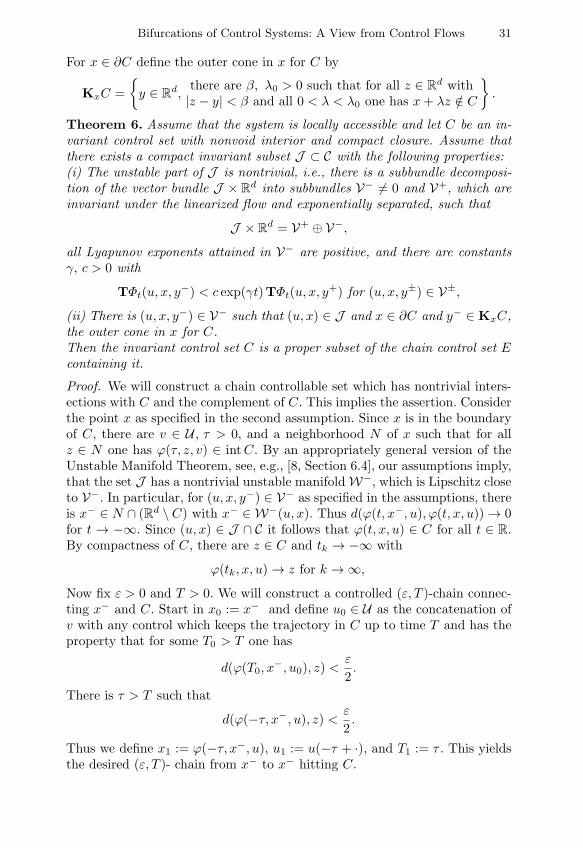
For x ∈ ∂C define the outer cone in x for C by

KxC =y ∈ R

d,there are β, λ0 > 0 such that for all z ∈ R

d with|z − y| < β and all 0 < λ < λ0 one has x+ λz /∈ C

.

Theorem 6. Assume that the system is locally accessible and let C be an in-variant control set with nonvoid interior and compact closure. Assume thatthere exists a compact invariant subset J ⊂ C with the following properties:(i) The unstable part of J is nontrivial, i.e., there is a subbundle decomposi-tion of the vector bundle J × R

d into subbundles V− = 0 and V+, which areinvariant under the linearized flow and exponentially separated, such that

J × Rd = V+ ⊕ V−,

all Lyapunov exponents attained in V− are positive, and there are constantsγ, c > 0 with

TΦt(u, x, y−) < c exp(γt) TΦt(u, x, y+) for (u, x, y±) ∈ V±,

(ii) There is (u, x, y−) ∈ V− such that (u, x) ∈ J and x ∈ ∂C and y− ∈ KxC,the outer cone in x for C.Then the invariant control set C is a proper subset of the chain control set Econtaining it.

Proof. We will construct a chain controllable set which has nontrivial inters-ections with C and the complement of C. This implies the assertion. Considerthe point x as specified in the second assumption. Since x is in the boundaryof C, there are v ∈ U , τ > 0, and a neighborhood N of x such that for allz ∈ N one has ϕ(τ, z, v) ∈ intC. By an appropriately general version of theUnstable Manifold Theorem, see, e.g., [8, Section 6.4], our assumptions imply,that the set J has a nontrivial unstable manifoldW−, which is Lipschitz closeto V−. In particular, for (u, x, y−) ∈ V− as specified in the assumptions, thereis x− ∈ N ∩ (Rd \C) with x− ∈ W−(u, x). Thus d(ϕ(t, x−, u), ϕ(t, x, u))→ 0for t → −∞. Since (u, x) ∈ J ∩ C it follows that ϕ(t, x, u) ∈ C for all t ∈ R.By compactness of C, there are z ∈ C and tk → −∞ with

ϕ(tk, x, u)→ z for k →∞,Now fix ε > 0 and T > 0. We will construct a controlled (ε, T )-chain connec-ting x− and C. Start in x0 := x− and define u0 ∈ U as the concatenation ofv with any control which keeps the trajectory in C up to time T and has theproperty that for some T0 > T one has

d(ϕ(T0, x−, u0), z) <

ε

2.

There is τ > T such that

d(ϕ(−τ, x−, u), z) <ε

2.

Thus we define x1 := ϕ(−τ, x−, u), u1 := u(−τ + ·), and T1 := τ . This yieldsthe desired (ε, T )- chain from x− to x− hitting C.

32 F. Colonius and W. Kliemann

The result above is only a first step, since it does not answer the question,if the gap between the control set D and the chain control set E ⊃ D is dueto the presence of another control set sitting in E. A partial answer is givenin the following result from [10] which shows when the loss of invariance isdue to the merger with a variant control set. We need some preparations. LetK ⊂ R

d be compact and invariant. An attractor for the control flow Φ is acompact invariant set A ⊂ U ×K that admits a neighborhood N such thatA = ω(N) = (u, x) ∈ U × K, there are tk → ∞ and (uk, xk) ∈ N withΦ(tk, uk, xk)→ (u, x). Define for chain recurrent components E , E ′

[E , E ′] = (u, x) ∈ U ×K, ω∗(u, x) ⊂ E and ω(u, x) ⊂ E ′;

here ω∗(u, x) denotes the limit set for t→ −∞. The structure of attractors andtheir relation to chain control sets is described in the following proposition.

Proposition 2. Assume that for every ρ > 0 every chain recurrent componentEρ contains a chain recurrent component E0

i of the unperturbed system. Thenthere is ρ0 > 0 such that for all ρ with ρ0 > ρ > 0 the attractors Aρ of theρ-system are given by

Aρ =⋃

i,j∈J

[Eρj , Eρk]

where the allowed index sets J coincide with those for ρ = 0. The chainrecurrent components Eρi depend upper semicontinuously on ρ and converge forρ→ 0 toward U×E0

i ; all Eρj are different and they have attractor neighborhoodsof the form U ×B with B ⊂ K.

For a set I ⊂ K the invariant domain of attraction is

Ainv(I) =x ∈ K,

if C ⊂ clO+(x) is an invariantcontrol set, then C ⊂ I

. (15)

The invariant domain of attraction is closed and invariant.For simplicity we assume that all control sets are in the interior of K. By

local accessibility, all invariant control sets have nonvoid interiors.We will assume that for all ρ with ρ1 > ρ > 0 the chain control sets Eρ

i

are the closures of control sets Dρi with nonvoid interior; observe that some of

the control sets in the attractor must be invariant, since every point can besteered into an invariant control set. Then Eρ

i = clDρi implies that also the

lifts coincide, i.e., Eρi = Dρi . It follows that the attractors are given by

Aρ =⋃

i,j∈J

[Dρi ,Dρ

j

]. (16)

We will analyze the case where for ρ = ρ1 the set Aρ1 has lost the attractorproperty.

Bifurcations of Control Systems: A View from Control Flows 33

Theorem 7. Consider the control system (2) in Rd and assume that K =

cl intK ⊂ Rd is a compact and connected set which is invariant for the sy-

stem with input range given by ρ1U with ρ1 > 0. Assume that the followingstrong invariance conditions describing the behavior near the boundary of Kare satisfied:(i) For all x ∈ L there is εx > 0 with d(ϕ(t, x, u), ∂K) ≥ εx for all u ∈ U andt ≥ 0.(ii) There is ε0 > 0 such that for all x ∈ clL and u ∈ U

y = limk→∞

ϕ(tk, x, u) ∈ L for tk →∞ implies d(y, ∂K) ≥ ε0. (17)

Consider the invariant sets in Uρ ×KIρ =

⋃i,j∈J

[Dρi ,Dρ

j

],

and assume that they are attractors for ρ < ρ1 and that the projection Iρ1 toR

d of Iρ1 intersects the boundary of its invariant domain of attraction definedin (15), i.e.,

Iρ1 ∩ ∂Ainv(Iρ1) = ∅.

Then every attractor containing Iρ1 contains a lifted variant control set Dρ1

with Dρ1 ∩ Iρ1 = ∅.

This theorem shows that the loss of the attraction property due to increa-sed input ranges is connected with the merger of the attractor with a variantcontrol set Dρ1 . Connections to Input-to-State Stability are discussed in [10].

Remark 14. The abstract Hartman-Grobman Theorem from [4] can also beapplied to the system over an invariant control set. Here, for the linearizedsystem, the base space is the lift of the invariant control set. However, forparameter-dependent systems, this entails that the base space changes withthe parameter. Hence it does not appear feasible to obtain results which yieldconjugacy for small parameter changes. Here, presumably, normal hyperboli-city assumptions are required.

Remark 15. Consider a family of increasing control set Dρ corresponding toincreasing control ranges. Assume that they are invariant for ρ ≤ ρ0 andvariant for ρ > ρ0 Then Gayer [14] has shown that the map ρ → clDρ has adiscontinuity at ρ0. This is a consequence of his careful analysis of the differentparts of the boundary of control sets. This also allows him to describe in detailthe merging of an invariant control set with a variant control set.

Finally we remark that the intuitive idea of a slowly varying bifurcationparameter is made more precise, if the bifurcation parameter actually is sub-ject to slow variations. This leads to concepts of dynamic bifurcations. Thefate of control sets for frozen parameters under slow parameter variations ischaracterized in Colonius/Fabbri [6].

34 F. Colonius and W. Kliemann

References

1. L. Arnold, Random Dynamical Systems, Springer-Verlag, 1998.2. L. Arnold and L. S. Martin, A multiplicative ergodic theorem for rotation num-

bers, J. Dynamics Diff. Equations, 1 (1989), pp. 95–119.3. M. V. Bebutov, Dynamical systems in the space of continuous functions, Dokl.

Akad. Nauk SSSR, 27 (1940), pp. 904–906. in Russian.4. I. U. Bronstein and A. Y. Kopanskii, Smooth Invariant Manifolds and Normal

Forms, World Scientific, 1994.5. F. Colonius and W. Du, Hyperbolic control sets and chain control sets, J. Dy-

namical and Control Systems, 7 (2001), pp. 49–59.6. F. Colonius and R. Fabbri, Controllability for systems with slowly varying pa-

rameters, ESAIM: Control, Optimisation and Calculus of Variations, 9 (2003),pp. 207–216.

7. F. Colonius and L. Grune, eds., Dynamics, Bifurcations and Control, Springer-Verlag, 2002.

8. F. Colonius and W. Kliemann, The Dynamics of Control, Birkhauser, 2000.9. , Mergers of control sets, in Proceedings of the Fourtheenth International

Symposium on the Mathematical Theory of Networks and Systems (MTNS),Perpignan, France, June 19–23 2000, A. El Jai and M. Fliess, eds., 2000.

10. , Limits of input-to-state stability, Systems Control Lett., (2003). to ap-pear.

11. F. Colonius and S. Siegmund, Normal forms for control systems at singularpoints, J. Dynamics Diff. Equations, (2003). to appear.

12. F. Colonius and M. Spadini, Uniqueness of local control sets, 2002. submittedto J. Dynamical and Control Systems.

13. R. Fabbri, R. Johnson, and C. Nunez, On the Yakubovich frequency theorem forlinear non-autonomous processes, Discrete and Continuous Dynamical Systems,(2003). to appear.

14. T. Gayer, Controlled and perturbed systems under parameter variation, 2003.Dissertation, Universitat Augsburg, Augsburg, Germany.

15. G. Grammel and P. Shi, On the asymptotics of the Lyapunov spectrum undersingular perturbations, IEEE Trans. Aut. Control, 45 (2000), pp. 565–568.

16. L. Grune, Asymptotic Behavior of Dynamical and Control Systems under Per-turbation and Discretization, Springer-Verlag, 2002.

17. S. Grunvogel, Lyapunov exponents and control sets, J. Diff. Equations, 187(2003), pp. 201–225.

18. R. Johnson, P. Kloeden, and R. Pavani, Two-step transition in nonautonomousbifurcations: An explanation, Stochastic and Dynamics, 2 (2002), pp. 67–92.

19. R. Johnson and M. Nerurkar, Controllability, Stabilization, and the RegulatorProblem for Random Differential Systems, vol. 136, No. 646 of Memoirs of theAMS, Amer. Math. Soc., 1998.

20. R. A. Johnson, K. J. Palmer, and G. R. Sell, Ergodic properties of linear dyna-mical systems, SIAM J. Math. Anal., 18 (1987), pp. 1–33.

21. W. Kang, Bifurcation and normal form of nonlinear control systems – part Iand part II, SIAM J. Control Optim., 36 (1998), pp. 193–212 and 213–232.

22. K. R. Meyer and G. R. Sell, Melnikov transforms, Bernoulli bundles and almostperiodic perturbations, Trans. Amer. Math. Soc., 129 (1989), pp. 63–105.

23. P. Ruffino, Rotation numbers for stochastic dynamical systems, Stochastics andStochastics Reports, 60 (1997), pp. 289–318.

Bifurcations of Control Systems: A View from Control Flows 35

24. R. J. Sacker and G. R. Sell, A spectral theory for linear differential systems, J.Diff. Equations, 27 (1978), pp. 320–358.

25. S. Siegmund, Normal forms for nonautonomous differential equations, J. Diff.Equations, 14 (2002), pp. 243–258.

Practical Stabilization of Systems with a FoldControl Bifurcation

Boumediene Hamzi1,2 and Arthur J. Krener2

1 INRIA, Domaine de Voluceau, Rocquencourt, BP 105, 78153 Le Chesnay Cedex,France, hamzi@math.ucdavis.edu

2 Department of Mathematics, University of California, One Shields Avenue,Davis, CA 95616, USA, krener@math.ucdavis.edu

1 Introduction

Nonlinear parameterized dynamical systems exhibit complicated performancearound bifurcation points. As the parameter of a system is varied, changesmay occur in the qualitative structure of its solutions around an equilibriumpoint. Usually, this happens when some eigenvalues of the linearized systemcross the imaginary axis as the parameter changes [7].

For control systems, a change of some control properties may occur aroundan equilibrium point, when there is a lack of linear stabilizability at this point.This is called a control bifurcation [21]. A control bifurcation occurs also forunparameterized control systems. In this case, it is the control that plays theparameter’s role in parameterized dynamical systems.

The use of feedback to stabilize a system with bifurcation has been studiedby several authors, and some fundamental results can be found in [1], [2],[3], [6], [16], [8], [17],[11],[12], [10], the Ph.D. theses [13], [21], [22] and thereferences therein.

When the uncontrollable modes are on the imaginary axis, asymptoticstabilization of the solution is possible under certain conditions, but whenthe uncontrollable modes have a positive real part, asymptotic stabilizationis impossible to obtain by smooth feedback [4].

In this paper, we show that by combining center manifold techniques withthe normal forms approach, it is possible to practically stabilize systems witha fold control bifurcation [21], i.e. those with one slightly unstable uncontrolla-ble mode. The methodology is based on using a class C0 feedback to obtain abird foot bifurcation ([20]) in the dynamics of the closed loop system on thecenter manifold. Systems with a fold control bifurcation appear in applicati-ons. For example, in [25] a fold bifurcation appears at the point of passagefrom minimum phase to nonminimum phase.

W. Kang et al. (Eds.): New Trends in Nonlinear Dynamics and Control, LNCIS 295, pp. 37–48, 2003.c© Springer-Verlag Berlin Heidelberg 2003

38 B. Hamzi and A.J. Krener

The paper is divided as follows : in Section §1, we introduce definitionsof ε−Practical Stability, ε−Practical Stabilizability and Practical Stabiliza-bility ; then, in Section §2, we show that a continuous but non differentiablecontrol law permits the practical stabilization of systems with a fold controlbifurcation.

2 Practical Stability and Practical Stabilizability

Practical stability was introduced in [23] and is defined as the convergenceof the solution of a differential equation to a neighborhood of the origin.In this section, we propose definitions for practical stability and practicalstabilizability.

Let us first define class K, K∞ and KL functions.

Definition 1. [18, definitions 3.3, 3.4]

• A continuous function α : [0, a) → [0,∞) is said to belong to class K ifit is strictly increasing and α(0) = 0. It is said to belong to class K∞ ifa =∞ and limr→∞ α(r) =∞.

• A continuous function β : [0, a)× [0,∞)→ [0,∞) is said to belong to classKL if, for each fixed s, the mapping β(r, s) belongs to class K with respectto r; and, for each fixed r, the mapping β(r, s) is decreasing with respectto s and limr→∞ β(r, s) = 0.

Let D ⊂ Rn be an open set containing the closed ball Bε of radius ε

centered at the origin. Let f : D → Rn a continuous function such that

f(0) = 0.Consider the system

x = f(x).

Definition 2. (ε−Practical Stability) The origin is said to be locally ε−practic-ally stable, if there exists an open set D containing the closed ball Bε, a classKL function ζ and a positive constant δ = δ(ε), such that for any initialcondition x(0) with ||x(0)|| < δ, the solution x(t) of (2) exists and satisfies

dBε(x(t)) ≤ ζ(dBε(x(0)), t), ∀t ≥ 0,

with dBε(x(t)) = infρ∈Bε d(x(t), ρ), the usual point to set distance.

Now consider the controlled system

x = f(x, v),

with f : D × U → Rn, f(0, 0) = 0, and U ⊂ R

m a domain that contains theorigin.

Practical Stabilization of Systems with a Fold Control Bifurcation 39

Definition 3. (ε−Practical Stabilizability) The system (2) is said to be locallyε−practically stabilizable around the origin, if there exists a control law v =kε(x), such that the origin of the closed-loop system x = f(x, kε(x)) is locallyε−practically stable.

Definition 4. (Practical Stabilizability) The system (2) is said to be locallypractically stabilizable around the origin, if it is locally ε−practically stabiliz-able for every ε > 0.

If, in the preceding definitions, D = Rn, then the corresponding properties

of ε−practical stability, ε−practical stabilizability and practical stabilizabilityare global, and the adverb “locally” is omitted.

Now, let us reformulate the local ε−practical stability in the Lyapunovframework.

Let V be a function V : D → R+, such that V is smooth on D \ Bε, and

satisfies

x ∈ D =⇒ α1(dBε(x(t))) ≤ V (x) ≤ α2(dBε

(x(t))),

with α1 and α2 class K functions.Such a function is called a Lyapunov function with respect to Bε, if there

exists a class K function α3 such that

V (x) = Lf(x)V (x) ≤ −α3(dBε(x)), for x ∈ D \ Bε.

Proposition 1. The origin of system (2) is ε−practically stable if and onlyif there exists a Lyapunov function with respect to Bε.

Proof. In [24], the authors gave stability results for systems with respect toa closed/compact, invariant set A. In particular, the definition of asymptoticstability and Lyapunov function with respect to A were given. In the casewhere1 A = Bε, asymptotic stability with respect to Bε reduces to our defi-nition of ε−practical stability (definition 2). The proof of our proposition isobtained by applying a local version of [24, Theorem 2.9].

If D = Rn and α1, α2 are a class K∞ functions, the origin is globally

ε−practically stable.

Remark : When ε = 0, we recover the classical definitions of local andglobal asymptotic stability.

3 Systems with a Fold Control Bifurcation

In this section, we apply the ideas of the preceding section to the system (2)when its linearization is uncontrollable at an equilibrium, which we take to1

Bε is a nonempty, compact and invariant set. It is invariant since V is negativeon its boundary ; so, a solution starting in Bε remains in it.

40 B. Hamzi and A.J. Krener

be the origin. Suppose that m = 1 and that the linearization of the system(2) at the origin is (A,B) with

A =∂f

∂ x(0, 0), B =

∂f

∂ v(0, 0),

and

rank([B AB A2B · · · An−1B]) = n− 1.

According to the assumption in (3), the linear system is uncontrollable.Suppose that the uncontrollable mode λ satisfies the following assumptionAssumption : The uncontrollable mode is λ ∈ R≥0.

Let us denote as ΣU , the system (2) under the above assumption. Thissystem exhibits a fold control bifurcation when λ > 0, and, generically, atranscontrollable bifurcation when λ = 0 (see [21]).

From linear control theory [14], we know that there exist a linear changeof coordinates and a linear feedback that put the system ΣU in the followingform

˙z1 = λz1 +O(z1, z2, u)2,˙z2 = A2z2 +B2u+O(z1, z2, u)2,

with z1 ∈ R, z2 ∈ R(n−1)×1, A2 ∈ R

(n−1)×(n−1) and B2 ∈ R(n−1)×1. The

matrices A2 and B2 are given by

A2 =

0 1 0 · · · 00 0 1 · · · 0...

......

. . ....

0 0 0 · · · 10 0 0 · · · 0

, B2 =

00...01

.

To simplify the quadratic part, we use the following quadratic transforma-tions in order to transform the system to its quadratic normal form

[z1z2

]=

[z1z2

]− φ[2](z1, z2), (1)

u = u− α[2](z1, z2, u). (2)

The normal form is given in the following theorem

Theorem 1. [21, Theorem 2.1] For the system ΣU whose linear part is of theform (3), there exist a quadratic change of coordinates (1) and feedback (2)which transform the system to

Practical Stabilization of Systems with a Fold Control Bifurcation 41

z1 = λz1 + βz21 + γz1z2,1 +n∑

j=1

δj z22,j +O(z1, z2, u)3,

z2 = A2z2 +B2u+n−1∑i=1

n∑j=i+2

θji z22,j e

i2 +O(z1, z2, u)3,

with β, γ, δj , θji are constant coefficients, z2,n = u, and ei2 is the ith− unit

vector in the z2−space.

Let us consider the piecewise linear feedback

u = K1(z1)z1 +K2z2 +O(z1, z2)2,

with

K1(z1) =k1, z1 ≥ 0,k1, z1 < 0.

We wish to stabilize the system around the bifurcation point. The con-trollable part can be made asymptotically stable by choosing K2 such thatProperty P: The matrix A2 = A2 +B2K2 is Hurwitz.

Under the feedback (3), the system ΣU has n−1 eigenvalues with negativereal parts, and one eigenvalue with positive real part, the uncontrollable modeλ. Nevertheless, if we view the system ΣU as being parameterized by λ, andby considering λ as an extra-state, satisfying the equation λ = 0, the systemΣU under the feedback (3) possesses two eigenvalues with zero real part andn− 1 eigenvalues in the left half plane.

Theorem 2. Consider the closed-loop system (1)-(3), then there exists a cen-ter manifold defined by z2 = Π(z1, λ) whose linear part is determined by thefeedback (3).

Proof. By considering λ as an extra state, the linear part of the dynamics(1)-(3) is given by

λ = 0,z1 = O(λ, z1, z2)2,z2 = B2K1(z1)z1 + A2z2 +O(z1, z2)2.

λz1 is now considered as a second order term.Let Σk1

(resp. Σk1) be the system (3) when K1(z1) = k1 (resp. K1(z1) =

k1) for all z1. Since the system Σk1(resp. Σk1

) is smooth, and possesses twoeigenvalues on the imaginary axis and n− 2 eigenvalues in the open left halfplane ; then, from the center manifold theorem, in a neighborhood of theorigin, Σk1

(resp. Σk1) has a center manifold W

c(resp. W c).

For Σk1, the center manifold is represented by z2 = Π(λ, z1), for λ and z1

sufficiently small. Its equation is

42 B. Hamzi and A.J. Krener

z2 = A2Π(λ, z1) +B2(k1z1 +K2Π(λ, z1)) +O(z1, z2)2,

=∂ Π(λ, z1)∂ z1

z1 = O(z1, z2)2.

Since λ = 0 and λz1 is a second order term in the enlarged space (λ, z1, z2),then there is no linear term in λ in the linear part of the center manifold.Hence, the linear part of the center manifold is of the form z2 = Π

[1]z1, and

its i−th component is z2,i = Π[1]i z1, for i = 1, · · · , n− 1. Using (3) we obtain

that Π[1]1 = − k1

k2,1and Π

[1]i = 0, for 2 ≤ i ≤ n− 1.

Similarly for Σk1, the center manifold is represented by z2 = Π(λ, z1).

Its linear part is given by z2 = Π [1]z1, whose components are defined byΠ

[1]1 = − k1

k2,1and Π [1]

i = 0, for 2 ≤ i ≤ n− 1.Since A2 has no eigenvalues on the imaginary axis, and k2,1 is the product

of all the eigenvalues of A2, then k2,1 = 0.The center manifolds W

cand W c intersect along the line z1 = 0. Indeed,

since λ = 0, then ∂kΠ(λ,z1)∂ λk

|λ=0,z1=0 = 0 and ∂kΠ(λ,z1)∂ λk

|λ=0,z1=0 = 0, for k ≥ 1.So, Π(λ, z1)|z1=0 = 0 and Π(λ, z1)|z1=0 = 0, for all λ.

Hence, if we slice them along the line z1 = 0 and then glue the part of Wc

for which z1 > 0 with the part of W c for which z1 < 0, along this line, wededuce that in an open neighborhood of the origin, D, the piecewise smoothsystem (3) has a piecewise smooth center manifold Wc. The linear part of thecenter manifold Wc is represented by z2 = Π [1]z1. The i − th component ofz2, z2,i, is given by

z2,i = Π[1]i (z1)z1,

with

Π[1]1 (z1) = −K1(z1)

k2,1and Π [1]

i (z1) = 0, for i ≥ 2.

Using (1) and (3), the reduced dynamics on the center manifold is given

by

z1 =

λz1 + Φ(Π

[1]1 )z21 +O(z31), z1 ≥ 0,

λz1 + Φ(Π [1]1 )z21 +O(z31), z1 < 0,

with Φ the function defined by Φ(X) = β + γX + δ1X2.

The following theorem shows that the origin of the system (3) can be madepractically stable, for small λ > 0, and asymptotically stable if λ = 0.

Theorem 3. Consider system (1) with γ2 − 4βδ1 > 0, then, the piecewiselinear feedback (3) practically stabilizes the system around the origin for smallλ > 0, and locally asymptotically stabilizes the system when λ = 0.

Practical Stabilization of Systems with a Fold Control Bifurcation 43

Proof. See appendix.

If we choose Π[1]1 and Π [1]

1 such that Φ(Π[1]1 ) = −Φ(Π [1]

1 ) = Φ0, the dyna-mics (3) will be of the form

z1 = µz1 − Φ0|z1|z1 +O(z31), (3)

with µ ∈ R a parameter. The equation (3) is the normal form of the bird footbifurcation, introduced by Krener in [20].

If Φ0 > 0, the equation (3) corresponds to a supercritical bird foot bifur-cation. For µ < 0, there is one equilibrium at z1 = 0 which is exponentiallystable. For µ > 0, there are two exponentially stable equilibria at z1 = ± µ

Φ0,

and one exponentially unstable equilibrium at z1 = 0. For µ = 0, there is oneequilibrium at z1 = 0 which is asymptotically stable but not exponentiallystable.

If Φ0 < 0, the equation (3) is an example of subcritical bird foot bifurcation.For µ < 0, there is one equilibrium at z1 = 0 which is exponentially stableand two exponentially unstable equilibria at z1 = ± µ

Φ0. For µ > 0, there is

one exponentially unstable equilibrium at z1 = 0. For µ = 0, there is oneequilibrium at z1 = 0 which is unstable.

Notice that both normal forms are invariant under the transformationz1 → −z1 and so the bifurcation diagrams can be obtained by reflecting theupper or lower half of the bifurcation diagram of a transcritical bifurcation.In both cases the bifurcation diagrams look like the foot of a bird.

In the λ − z1 plane, the dynamics (3) are in the form (3) with Φ0 > 0.A supercritical birdfoot bifurcation appears at (λ, z1) = (0, 0). For λ > 0, wehave 3 equilibrium points : the origin and ±ε (corresponding to the solutionsof z1 = 0). The origin is unstable for λ > 0, and the two other equilibriumpoints are stable (cf. Figure 1). The practical stabilization of the system ismade possible by making the two new equilibrium points sufficiently close tothe origin, i.e. by choosing Φ(Π

[1]1 ) and Φ(Π [1]

1 ) sufficiently large.If a quadratic feedback was used instead of (3), i.e.

u = K1z1 +K2z2 + zT1 Qfbz1 +O(z31),

we can prove that the closed loop dynamics has a center manifold. Moreover,by appropriately choosing K1, the reduced dynamics on the center manifoldwill have the form

z1 = λz1 − Φ1z31 +O(z41),

with Φ1 > 0, by appropriately choosing Qfb.The equation (3) is the normal form of a system exhibiting a supercritical

pitchfork bifurcation. By using a similar analysis as above, we deduce thatthe solution of the reduced dynamics converges to the equilibrium points ε =±√

λΦ1

, and that the closed-loop system (1)-(3) is practically stabilizable.

44 B. Hamzi and A.J. Krener

The reason of the choice of a piecewise linear feedback instead of a quadra-tic feedback is that it is preferable to have a supercritical bird foot bifurcationthan a supercritical pitchfork bifurcation. This is due to the fact that the sta-ble equilibria in a system with a bird foot bifurcation grow like µ not like

õ

as in the pitchfork bifurcation2, and that the bird foot bifurcation is robust tosmall quadratic perturbations, while these transform the pitchfork bifurcationto a transcritical one.

Fig. 1.

4 Appendix

Proof of Theorem 3

Consider the Lyapunov function V (z1) =12z21 , and let ε1 − λ

Φ(Π[1]1 )

and

ε2 − λ

Φ(Π[1]1 )

. Then, from (3), we have

V =

Φ(Π

[1]1 )(z1 − ε1)z21 +O(z41), z1 ≥ 0,

Φ(Π [1]1 )(z1 − ε2)z21 +O(z41), z1 < 0,

• Practical Stabilization for λ > 0By choosing3 Π

[1]1 and Π [1]

1 such that Φ(Π[1]1 ) < 0 and Φ(Π [1]

1 ) > 0, weget ε1 > 0 and ε2 < 0. This choice is always possible since Φ is a secondorder polynomial whose discriminant, γ2− 4βδ1, is positive ; so, Φ takes bothpositive and negative values. In this case, V < 0 for z1 > ε1 and z1 < ε2, andV = 0 for z1 = ε1 or z1 = ε2.2 Let us recall that the normal for of a pitchfork bifurcation is z1 = µz1 − Φ1z

31 ,

with µ ∈ R the parameter.3 This choice is made by fixing the parameters k1 and k1 of the feedback (3) linked

to Π[1]1 and Π

[1]1 through (3).

Practical Stabilization of Systems with a Fold Control Bifurcation 45

In the following, and without loss of generality, we choose Π[1]1 and Π [1]

1

such that Φ(Π[1]1 ) = −Φ(Π [1]

1 ), so ε1 = −ε2 ε, with 0 ≤ ε ≤ r, and r is theradius of Br, the largest closed ball contained in D.

Let Ω1 and Ω2 be two sets defined by Ω1 =]ε,+r] and Ω2 = [−r,−ε[.If z1(0) ∈ Ω1 ∪ Ω2, and since V < 0 on Ω1 ∪ Ω2, then, from (2) and (2),

V satisfies

V ≤ −α3(||z1||) ≤ −α3(α−12 (V )).

Since α2 and α3 are a classK functions, then α3(α−12 ) is also a classK function.

Hence, using the comparison principle in [24, lemma 4.4], there exists a classKL function η such that

V (z1(t)) ≤ η(V (z1(0), t)).

The sets Ω1 = [0, ε] and Ω2 = [−ε, 0] have the property that when asolution enters either set, it remains in it. This is due to the fact that V isnegative definite on the boundary of these two sets. For the same reason, ifz1(0) ∈ Ω1 (resp. z1(0) ∈ Ω2), then z1(t) ∈ Ω1 (resp. z1(t) ∈ Ω2), for t ≥ 0.

Let T (ε) be the first time such that the solution enters Ω1 ∪ Ω2 = Bε.Using (2) and (4), we get that for 0 ≤ t ≤ T (ε),

ε ≤ ||z1(t)|| ≤ α−11 (V (z1(t)) ≤ α−1

1 (η(V (z1(0), t))) ζ(z1(0), t).

The function ζ is a class KL function, since α1 is a class K function and ηa class KL function. Since ζ is a class KL function, then T (ε) is finite. Hence,z1(t) ∈ Ω1 ∪Ω2, for t ≥ T (ε).

Hence, for z1 ∈ Br, the solution satisfies

dBε(z1(t)) ≤ ζ(dBε(z1(0)), t).

So, in Br, the origin is locally ε−practically stable.Now, consider the whole closed-loop dynamics

z1 = λz1 + βz21 + γz1z2,1 +n−1∑i=1

δi z22,i +O(z1, z2)3,

z2 = B2K1z1 + A2z2 +n−1∑i=1

n−1∑j=i+2

θji z22,j e

i2 +O(z1, z2)3.

Let w1 = z1, w2 = z2 −Π [1]z1, and w = (w1, w2)T . Then, the closed-loopdynamics is given by

w1 =

λw1 + Φ(Π

[1]1 )w2

1 + N1(w1, w2), for w1 ≥ 0,λw1 + Φ(Π [1]

1 )w21 + N1(w1, w2), for w1 < 0.

46 B. Hamzi and A.J. Krener

w2 =A2w2 + N2(w1, w2), for w1 ≥ 0,A2w2 + N2(w1, w2), for w1 < 0.

Let

Ni(w1, w2) = Ni(w1, w2), w1 ≥ 0,Ni(w1, w2), w1 < 0,

for i = 1, 2,

with N1(w1, w2) = (γ + 2δ1Π[1]1 )w1w2,1 +

∑n−1i=1 δi w

22,i and N2(w1, w2) =∑n−1

i=1∑n−1

j=i+2 θji w

22,j e

i2.

Since Ni(w1, 0) = 0 and ∂Ni

∂w2(0, 0) = 0 (i = 1, 2), then in the domain

||w||2 < σ, N1 and N2 satisfy

Ni(w1, w2) ≤ κi||w2||, i = 1, 2,

where κ1 and κ2 can be arbitrarily small by making σ sufficiently small.Since A2 is Hurwitz, there exists a unique P such that AT

2 P +PA2 = −I.Let V be the following composite Lyapunov function

V(w1, w2) =12w2

1 + wT2 Pw2.

The derivative of V along the trajectories of the system is given by

V(w1, w2) = π(w1) +w1N1(w1, w2) +wT2 (AT

2 P +PA2)w2 + 2wT2 PN2(w1, w2),

with π(w1) = (λ+ Φ(Π[1]1 )w1)w2

1 for w1 ≥ 0 and π(w1) = (λ+ Φ(Π [1]1 )w1)w2

1for w1 < 0.

For w1 ∈ Ω1 ∪Ω2, then π(w1) ≤ −α3(||w1||) according to (4). Hence

V(w1, w2) < −α3(||w1||) + w1N1(w1, w2) + wT2 (PA2 + PA2)w2 + 2wT

2 PN2(w1, w2),≤ −(−κ1ν + 1 + 2κ2λmax(P ))||w2||+ κ2||w2|| − κ2||w2||,≤ −(−κ1ν − κ2 + 1− 2κ2λmax(P ))||w2||,

with ν = maxw1:w1∈Ω1∪Ω2 ||w1||.By choosing κ1 and κ2 such that κ1ν + κ2(1 + 2λmax(P )) < 1, then

V(w1, w2) < 0.

Hence, for w1 ∈ Ω1 ∪ Ω2, V(w1, w2) < 0. So, there exists a class KLfunction η such that

||w(t)|| ≤ η(||w(0)||, t).

When w1 ∈ Ω1 ∪Ω2, and by considering w1 as an input of the system

w2 = A2w2 +N2(w1, w2),

Practical Stabilization of Systems with a Fold Control Bifurcation 47

we deduce that ||w2|| is bounded, since A2 is Hurwitz. Hence, for w1 ∈ Ω1∪Ω2,there exists ε such that

||w(t)|| ≤ ε.

From (4)-(4) we obtain

dBε(w(t)) ≤ η(dBε(w(0)), t).

So the origin of the whole dynamics is locally ε−practically stable.• Asymptotic Stabilization for λ = 0In this case, generically, we have a transcontrollable bifurcation [17, 21].

Since ε1 = ε2 = 0, the sets Ω1 and Ω2 reduce to the origin. Hence, the originof the reduced closed-loop system is asymptotically stable, since the solutionconverges to Ω1∪Ω2 = 0. We deduce that the origin of the whole closed-loopdynamics is asymptotically stable by applying the center manifold theorem[5].

References

1. Abed, E. H. and Fu J.-H. (1986). Local Feedback stabilization and bifurcationcontrol, part I. Hopf Bifurcation, Systems and Control Letters, 7, 11–17.

2. Abed, E. H. and Fu J.-H. (1987). Local Feedback stabilization and bifurcationcontrol, part II. Stationary Bifurcation, Systems and Control Letters, 8, 467–473.

3. Aeyels, D. (1985). Stabilization of a class of nonlinear systems by a smoothfeedback control, Systems and Control Letters, 5, 289–294.

4. Brockett, R. (1983). Asymptotic Stability and Feedback Stabilization, In R.W. Brockett, R. Milman and H. Sussman Eds., Differential Geometric ControlTheory, Birkhauser.

5. Carr, J. (1981). Application of Centre Manifold Theory, Springer.6. Colonius, F., and W. Kliemann (1995). Controllability and stabilization of one-

dimensional systems near bifurcation points,Systems and Control Letters, 24,87–95.

7. Guckenheimer, J. and P. Holmes (1983). Nonlinear Oscillations, DynamicalSystems, and Bifurcations of Vector Fields, Springer.

8. Gu, G., X. Chen, A. G. Sparks and S. S. Banda (1999). Bifurcation Stabilizationwith Local Output Feedback, Siam J. Control and Optimization, 37, 934–956.

9. Hahn, W. (1967). Stability of Motion, Springer.10. Hamzi, B., J.-P. Barbot, S. Monaco, and D. Normand-Cyrot (2001). Nonlinear

Discrete-Time Control of Systems with a Naimark-Sacker Bifurcation, Systemsand Control Letters, 44, 245–258.

11. Hamzi, B., W. Kang and J.-P. Barbot (2003). Analysis and Control of Hopfbifurcations, Siam J. Control and Optimization, to appear.

12. Hamzi, B. and W. Kang (2003). Resonant Terms and Bifurcations of NonlinearControl Systems with One Uncontrollable Mode, Systems and Control Letters,to appear.

48 B. Hamzi and A.J. Krener

13. Hamzi, B. (2001). Analyse et commande des systemes non lineaires non com-mandables en premiere approximation dans le cadre de la theorie des bifurcati-ons, Ph.D. Thesis, University of Paris XI-Orsay, France.

14. Kailath, T. (1980). Linear Systems, Prentice-Hall.15. Kang, W. and A.J. Krener (1992). Extended Quadratic Controller Normal Form

and Dynamic State Feedback Linearization of Nonlinear Systems, Siam J. Con-trol and Optimization, 30, 1319–1337.

16. Kang, W. (1998). Bifurcation and Normal Form of Nonlinear Control Systems-part I/II, Siam J. Control and Optimization, 36, 193–212/213–232.

17. Kang, W. (2000). Bifurcation Control via State Feedback for Systems with aSingle Uncontrollable Mode, Siam J. Control and Optimization, 38, 1428–1452.

18. Khalil, H.K. (1996). Nonlinear Systems, Prentice-Hall.19. Krener, A. J. (1984). Approximate linearization by state feedback and coordi-

nate change, Systems and Control Letters, 5, 181–185.20. Krener, A. J. (1995). The Feedbacks which Soften the Primary Bifurcation of

MG 3, PRET Working Paper D95-9-11, 181-185.21. Krener, A.J., W. Kang, and D.E. Chang (2001). Control Bifurcations, accepted

for publication in IEEE trans. on Automatic Control.22. Krener, A.J. and L. Li (2002). Normal Forms and Bifurcations of Discrete Time

Nonlinear Control Systems, SIAM J. on Control and Optimization, 40, 1697–1723.

23. Lakshmikantham,V., S. Leela, and A.A. Martynyuk (1990). Practical stabilityof nonlinear systems, World Scientific.

24. Lin, Y., Y. Wang, and E. Sontag (1996). A smooth converse Lyapunov theoremfor robust stability, Siam J. Control and Optimization, 34, 124–160.

25. Szederkenyi, G., N. R. Kristensen, K. M. Hangos and S. Bay Jorgensen (2002).Nonlinear analysis and control of a continuous fermentation process, Computersand Chemical Engineering, 26, 659–670.

Feedback Control of Border CollisionBifurcations

Munther A. Hassouneh and Eyad H. Abed

Department of Electrical and Computer Engineering, and the Institute for SystemsResearch, University of Maryland, College Park, MD 20742 USA,munther, abed@eng.umd.edu,

—Dedicated to Professor Arthur J. Krener on the occasion of his 60thbirthday

Summary. The feedback control of border collision bifurcations is considered.These bifurcations can occur when a fixed point of a piecewise smooth system crossesthe border between two regions of smooth operation. The goal of the control effortin this work is to modify the bifurcation so that the bifurcated steady state is lo-cally attracting. In this way, the system’s local behavior is ensured to remain stableand close to the original operating condition. Linear and piecewise linear feedbacksare used since the system linearization on the two sides of the border genericallydetermines the type and stability properties of any border collision bifurcation. Atwo-dimensional example on quenching of heart arrhythmia is used to illustrate theideas.

1 Introduction

The purpose of this paper is to study the feedback control of border collisionbifurcations (BCBs) in piecewise smooth (PWS) maps. The goal of the controleffort in this work is to modify the bifurcation so that the bifurcated steadystate is locally attracting. In this way, the system’s local behavior is ensuredto remain stable and close to the original operating condition. Another contri-bution of the paper is to summarize some available results on BCBs in moredetail than exists in the literature, and to supply additional results that areuseful for control design.

Continuous piecewise-smooth dynamical systems have been found to un-dergo special bifurcations along the borders between regions of smooth dy-namics. These have been named border collision bifurcations by Nusse andYorke [14], and had been studied in the Russian literature under the nameC-bifurcations by Feigin [9]. Di Bernardo, Feigin, Hogan and Homer [3] intro-duced Feigin’s results in the Western literature.

W. Kang et al. (Eds.): New Trends in Nonlinear Dynamics and Control, LNCIS 295, pp. 49–64, 2003.c© Springer-Verlag Berlin Heidelberg 2003

50 M.A. Hassouneh and E.H. Abed

Border collision bifurcations include bifurcations that are reminiscent ofthe classical bifurcations in smooth systems such as fold and period doublingbifurcations. Despite this resemblance, the classification of border collisionbifurcations is far from complete, and certainly very preliminary in comparisonto the results available in the smooth case. The classification is complete onlyfor one-dimensional discrete-time systems [15, 2]. Concerning two-dimensionalpiecewise smooth maps, Banerjee and Grebogi [1] propose a classification fora class of two-dimensional maps undergoing border-collision by exploiting anormal form. One result on BCB for two-dimensional maps that has beenmentioned but not carefully proved in the literature has recently been provedby the authors in joint work with H. Nusse [13]. This result asserts localuniqueness and stability of fixed points in the case of real eigenvalues in (−1, 1)on both sides of the border. For higher dimensional systems, currently theknown results are limited to several general observations.

It should be noted that work such as that in this paper focusing on mapshas implications for switched continuous-time systems as well. Maps providea concise representation that facilitates the investigation of system behaviorand control design. They are also the natural models for many applications.Even for a continuous piecewise smooth system, a control design derived usingthe map representation can be translated to a continuous controller eitheranalytically or numerically.

There is little past work on control of BCBs; we are aware of the papersby Di Bernardo [4], Di Bernardo and Chen [5] and our work [11, 12]. Thepresent paper summarizes some results in our manuscripts [11, 12] which gofurther than [4, 5] by doing a systematic feedback design approach and byusing a more detailed classification of BCBs. In [11, 12], we consider designof feedbacks that achieve safe BCBs for one-dimensional and two-dimensionaldiscrete-time systems. This could entail feedback on either side of the borderor on both sides. Sufficient conditions for stabilizing control gains are foundanalytically.

This paper is organized as follows. In Sect. 2, we summarize results onBCBs in one-dimensional maps and discuss the available results in two-dimensional PWS maps. In Sect. 3, we develop feedback control laws for BCBsin one-dimensional maps. In Sect. 4, the results are applied to a model that hasbeen used in studies of cardiac arrhythmia. In Sect. 5, we collect concludingremarks and mention some problems for future research.

2 Background on Border Collision Bifurcations

In this section, relevant results on BCBs are recalled (including one whoseproof has just been reported [13]). We begin with results on BCBs in one-dimensional (1-D) maps followed by the result on BCBs in two-dimensional(2-D) maps proved in [13]. Since the 1-D case is well understood, we are able togive a detailed description of the possible scenarios in this case. The discussion

Feedback Control of Border Collision Bifurcations 51

of the 2-D case is more brief in that the focus is only on stating the neededresult from [13].

2.1 BCBs in One-Dimensional PWS Maps

The presentation below on BCBs in one-dimensional maps closely follows [15,2], with only cosmetic modifications. See [15, 2] for more details.

Consider the 1-D PWS map

xk+1 = f(xk, µ) (1)

where x ∈ , µ is a scalar bifurcation parameter, and f(x, µ) takes the form

f(x, µ) =g(x, µ), x ≤ xbh(x, µ), x ≥ xb (2)

Since the system is one-dimensional, the border is just the point xb. The mapf : × → is assumed to be PWS: f depends smoothly on x everywhereexcept at xb, where it is continuous in x. It is also assumed that f dependssmoothly on µ everywhere. Denote by RL and RR the two regions in statespace separated by the border: RL := x : x ≤ xb and RR := x : x ≥ xb.

Let x0(µ) be a path of fixed points of f ; this path depends continuously onµ. Suppose also that the fixed point hits the boundary at a critical parametervalue µb: x0(µb) = xb. Below, conditions are recalled for the occurrence ofvarious types of BCBs from xb for µ near µb.

The normal form for the PWS map (1) at a fixed point on the borderis a piecewise affine approximation of the map in the neighborhood of theborder point xb, in scaled coordinates [15, 2, 3]. The state and parametertransformations occurring in the derivation of the normal form are needed inapplying control results derived for systems in normal form to a system inoriginal coordinates. In the interest of brevity, these transformations are notrecalled here.

The 1-D normal form is [2]

xk+1 = G1(xk, µ) =axk + µ, xk ≤ 0bxk + µ, xk ≥ 0 (3)

where a = limx→x−b

∂f(x,µb)∂x and b = limx→x+

b

∂f(x,µb)∂x . Suppose that |a| =

1 and |b| = 1. The normal form map G1(·, ·) can be used to study localbifurcations of the original map f(·, ·) [15, 2]. Note that the original map (2)is not necessarily piecewise affine.

Denote by x∗R and x∗

L the fixed points of the system near the border tothe right (x > xb) and left (x < xb) of the border, respectively. Then in thenormal form (3), x∗

R = µ1−b and x∗

L = µ1−a . For the fixed point x∗

R to actuallyoccur, we need µ

1−b ≥ 0 which is satisfied if and only if µ > 0 and b < 1 or

52 M.A. Hassouneh and E.H. Abed

µ < 0 and b > 1. Similarly, for x∗L to actually occur, we need µ

1−a ≤ 0 whichis satisfied if and only if µ < 0 and a < 1 or µ > 0 and a > 1.

Various combinations of the parameters a and b lead to different kinds ofbifurcation behavior as µ is varied. Since the map G1 is invariant under thetransformation x→ −x, µ→ −µ, a b, it suffices to consider only the casea ≥ b.

The possible bifurcation scenarios are summarized in Fig. 1. Sample bifur-cation diagrams for border collision pair bifurcation (similar to saddle nodebifurcation in smooth maps) and period doubling BCB in PWS 1-D maps aredepicted in Figs. 2 and 3, respectively. In these figures, a solid line represents astable fixed point whereas a dashed line represents an unstable fixed point. Allthe results pertain to system (3). Detailed descriptions of these bifurcationscan be found in [11].

−ab =

aa+1

b =

a−1C2

B2

B1

a

b

B2−1

+1

+1−1

C1

A2

C3

C1

B3

A2

A1 B1

B3

C2ab =1

a = b

ab =−1

ab =−1C3

Fig. 1. The partitioning of the parameter space into regions with the same qua-litative phenomena. The numbers on different regions refer to various bifurcationscenarios (associated parameter ranges are clear from the figure). Scenario A1: Per-sistence of stable fixed points (nonbifurcation), Scenario A2: Persistence of unstablefixed points, Scenario B1: Merging and annihilation of stable and unstable fixedpoints, Scenario B2: Merging and annihilation of two unstable fixed points pluschaos, Scenario B3: Merging and annihilation of two unstable fixed points, ScenarioC1: Supercritical border collision period doubling, Scenario C2: Subcritical bordercollision period doubling, Scenario C3: Emergence of periodic or chaotic attractorfrom stable fixed point.

The following results give detailed statements relating stability of the fixedpoint at criticality with the nature of the BCB that occurs. These results,though not difficult to obtain, haven’t previously been stated explicitly inthis detail.

Feedback Control of Border Collision Bifurcations 53

µ>0

Unstable chaotic orbit for µ>0

Growing chaotic attractor for

0

0

0

0

0

x

x

x

0

(a)

(b)

(c)

µ

Fig. 2. Bifurcation diagrams for Scenarios B1-B3. (a) A typical bifurcation diagramfor Scenario B1. (b) A typical bifurcation diagram for Scenario B2. (c) A typicalbifurcation diagram for Scenario B3.

0

0

µ

x

0

0

µ

x

(a)

(b) unstable period-2 orbit

stable period-2 orbit

Fig. 3. Typical bifurcation diagrams for Scenarios C1 and C2. (a) Supercriticalperiod doubling border collision (Scenario C1, b < −1 < a < 1 and −1 < ab < 1)(b) Subcritical period doubling border collision (Scenario C2, b < −1 < a < 0 andab > 1).

Proposition 1 The origin of (3) at µ = 0 is asymptotically stable if and onlyif any of (i)-(iii) below holds(i) −1 < a < 1 and −1 < b < 1(ii) 0 < a < 1 and b < −1 or 0 < b < 1 and a < −1(iii) −1 < a < 0, b < −1 and ab < 1 or −1 < b < 0, a < −1 and ab < 1.The origin of (3) at µ = 0 is unstable iff any of (iv)-(vi) below holds(iv) −1 < a < 1 and b > 1 or −1 < b < 1 and a > 1(v) −1 < a < 0, b < −1 and ab > 1 or −1 < b < 0, a < −1 and ab > 1(vi) |a| > 1 and |b| > 1.

54 M.A. Hassouneh and E.H. Abed

Proof (cases (i)-(iii)): Consider the piecewise quadratic Lyapunov function

V (xk) =p1x

2k, xk ≤ 0

p2x2k, xk > 0 (4)

where p1 > 0 and p2 > 0. Clearly, V is positive definite. To show asymptoticstability of the origin of (3) at criticality (µ = 0), we need to show thatthe forward difference ∆V := V (xk+1)− V (xk) is negative definite along thetrajectories of (3) for all xk = 0. There are two cases:Case 1: xk < 0

∆V =p1(x2

k+1 − x2k), xk+1 < 0

p2x2k+1 − p1x2

k, xk+1 > 0

=p1x

2k(a2 − 1), xk+1 < 0

x2k(p2a2 − p1), xk+1 > 0 (5)

Case 2: xk > 0

∆V =p2(x2

k+1 − x2k), xk+1 > 0

p1x2k+1 − p2x2

k, xk+1 < 0

=p2x

2k(b2 − 1), xk+1 > 0

x2k(p1b2 − p2), xk+1 < 0 (6)

It remains to show that ∆V < 0 for all xk = 0 in (i)-(iii).(i) −1 < a < 1 and −1 < b < 1: Choose p1 = p2 := p > 0. From (5), it followsthat ∆V = px2

k(a2−1) < 0 and from (6) it follows that ∆V = px2k(b2−1) < 0.

Thus ∆V < 0 ∀xk = 0.(ii) 0 < a < 1 and b < −1 (the proof for the symmetric case 0 < b < 1and a < −1 is similar and therefore omitted): Since 0 < a < 1, if xk < 0then xk+1 = axk < 0. From (5), ∆V = p1x

2k(a2 − 1) < 0. Since b < −1, if

xk > 0 then xk+1 = bxk < 0. From (6), ∆V = x2k(p1b2 − p2) < 0 if and only

if p2 > p1b2 > 0. Thus, choosing p1 > 0 and p2 > p1b

2 results in a positivedefinite V and a negative definite ∆V .(iii) −1 < a < 0, b < −1 and ab < 1 (the proof for the symmetric case−1 < b < 0, a < −1 and ab < 1 is similar and therefore omitted): Since−1 < a < 0, if xk < 0 then xk+1 = axk > 0. From (5),∆V = x2

k(p2a2−p1) < 0if and only if p1 > p2a

2. Since b < −1, if xk > 0 then xk+1 = bxk < 0.From (6), ∆V = x2

k(p1b2 − p2) < 0 if and only if p1 < p2b2 . Thus, p1 and p2

must be chosen such that p2a2 < p1 <p2b2 . Clearly, any p2 > 0 works. For

p1 > 0 to exist, we need 1b2 > a

2 which is satisfied since ab < 1 by hypothesis.Proof (cases (iv)-(vi)): It suffices to show that no matter how close theinitial condition is to the origin, the trajectory of (3) diverges.(iv) −1 < a < 1 and b > 1 (the proof for the symmetric case −1 < b < 1and a > 1 is similar and therefore omitted): Let x0 = ε > 0. Then, x1 = bε,x2 = b2ε and xk = bkε. As k →∞, xk →∞ no matter how small ε is.

Feedback Control of Border Collision Bifurcations 55

(v) −1 < a < 0, b < −1 and ab > 1 (the proof for the symmetric case−1 < b < 0, a < −1 and ab > 1 is similar and therefore omitted): Letx0 = ε > 0. It is straightforward to show that x2k = (ab)kε. Since ab > 1,x2k →∞ as k →∞, for any fixed ε.(vi) This is an easy exercise and is omitted.

The assertions of the next proposition follow from relating the stabilityof the fixed point at criticality as given in Proposition 1 with the ensuingbifurcation for different regions in the (a, b) parameter space as shown inFig. 1.

Proposition 2 1) If the fixed point of system (3) is asymptotically stable atcriticality (i.e., at µ = 0), then the border collision bifurcation is supercriticalin the sense that no bifurcated orbits occur on the side of the border where thenominal fixed point is stable and the bifurcated solution on the unstable sideis attracting.2) If the fixed point of system (3) is unstable at criticality, then the bordercollision bifurcation is subcritical in the sense that no bifurcated orbits occuron the side of the border where the nominal fixed point is unstable and thebifurcated solution on the stable side is repelling.

2.2 BCBs in Two-Dimensional PWS Maps

Consider a two-dimensional PWS map that involves only two regions ofsmooth behavior:

f(x, y, µ) =fA(x, y, µ), (x, y) ∈ RA

fB(x, y, µ), (x, y) ∈ RB(7)

Here, µ is the bifurcation parameter and RA and RB are regions of smoothbehavior. Since the system is two-dimensional, the border is a curve separatingthe two regions of smooth behavior and is given by x = h(y, µ). The mapf : 2 × → 2 is assumed to be PWS: f depends smoothly on (x, y)everywhere except at the border where it is continuous in (x, y). It is alsoassumed that f depends smoothly on µ everywhere, and the Jacobian elementsare finite at both sides of the border.

Let (x0(µ), y0(µ)) be a path of fixed points of f ; this path depends conti-nuously on µ. Suppose also that the fixed point hits the border at a criticalparameter value µb.

It has been shown [14, 1] that a normal form for the two-dimensional PWSsystem (7) in the neighborhood of a fixed point on the border takes the form

56 M.A. Hassouneh and E.H. Abed

(xk+1yk+1

)= G2(xk, yk, µ) =

(τA 1−δA 0

)

︸ ︷︷ ︸JA

(xkyk

)+

(10

)µ, xk ≤ 0

(τB 1−δB 0

)

︸ ︷︷ ︸JB

(xkyk

)+

(10

)µ, xk ≥ 0

(8)

where τA is the trace and δB is the determinant of the limiting Jacobianmatrix JA of the system at a fixed point in RA as it approaches the border.Similarly, τB is the trace and δB is the determinant of the Jacobian matrixJB of the system evaluated at a fixed point in RB near the border. System (8)undergoes a variety of border collision bifurcations depending on the valuesof the parameters τA, δA, τB and δB .

As mentioned previously, only a few results are available on BCBs in two-dimensional systems. Next, we state one result that will be needed in thecontrol design of our paper [12], as well as in Sect. 4, in which we considercontrol of a 2-D model of cardiac arrhythmia.

Proposition 3 [13] (Sufficient Condition for Nonbifurcation in 2-D PWSMaps) If the eigenvalues of the Jacobian matrices on both sides of the borderof a two dimensional PWS map are real in (−1, 1), then a locally unique andstable fixed point on one side of the border leads to a locally unique and stablefixed point on the other side of the border as µ is increased (decreased) throughzero.

3 Feedback Control of Border Collision Bifurcations

In this section, control of BCBs in PWS maps of dimension one and two isconsidered. The fact that the normal form for BCBs contains only linear termsin the state leads us to seek linear feedback controllers to modify the system’sbifurcation characteristics. The linear feedback can either be applied on oneside of the border and not the other, or on both sides of the border. Bothapproaches are considered below. The issue of which approach to take and withwhat constraints is a delicate one. There are practical advantages to applyinga feedback on only one side of the border, say the stable side. However, thisrequires knowledge of where the border lies, which is not necessarily the casein practice.

The purpose of pursuing stabilizing feedback acting on both sides of theborder is to ensure robustness with respect to model uncertainty. This is donebelow by investigating the use of simultaneous stabilization as an option —that is, controls are sought that function in exactly the same way on bothsides of the border, while stabilizing the system’s behavior. Not surprisingly,the conditions for existence of simultaneously stabilizing controls are morerestrictive than for the existence of one sided controls.

Feedback Control of Border Collision Bifurcations 57

Due to space limitations, we only discuss static feedback and do not includedetails for the 2-D case. Results on the 2-D case and on washout filter-aidedfeedback (a form of dynamic feedback) can be found in [12] and [11]. It isimportant to emphasize that although the control results are based on thenormal form, the results can be easily applied to general PWS maps by keepingtrack of the associated transformations to and from normal form.

3.1 Control of BCB in 1-D Maps Using Static Feedback

Consider the one-dimensional normal form (3) for a BCB, repeated here forconvenience:

xk+1 =axk + µ, xk ≤ 0bxk + µ, xk ≥ 0 (9)

Below, the control schemes described above are considered for the system (9),with a control signal u included in the dynamics as appropriate.

Method 1: Control Applied on One Side of Border.

In the first control scheme, the feedback control is applied only on one sideof the border. Suppose that the system is operating at a stable fixed pointon one side of the border, locally as the parameter approaches its criticalvalue. Without loss of generality, assume this region of stable operation isx : x < 0— that is, assume −1 < a < 1. Since the control is applied onlyon one side of the border, the linear feedback can be applied either on theunstable side or the stable side of the border.

Method (1a): Linear Feedback Applied in Unstable Side of theBorder.

Suppose that the fixed point is stable if x∗ ∈ − and unstable if x∗ ∈ +.Applying additive linear state feedback only for x ∈ + leads to the closed-loop system

xk+1 =axk + µ, xk ≤ 0bxk + µ+ uk, xk ≥ 0 (10)

uk = γxk (11)

The following proposition asserts stabilizability of the border collision bifur-cation with this type of control policy.

Proposition 4 Suppose that the fixed point of (9) is stable in − for µ < 0(i.e., |a| < 1) and unstable in + for µ > 0 (i.e., b < −1) or the fixed pointdoes not exist for µ > 0 (i.e., b > 1). Then there is a stabilizing linear feedbackon the right side of the border. That is, a linear feedback exists resulting in astable fixed point to the left and right of the border (i.e., achieving Scenario

58 M.A. Hassouneh and E.H. Abed

A1 of Fig. 1). Indeed, precisely those linear feedbacks uk = γxk with gain γsatisfying

−1− b < γ < 1− b (12)

are stabilizing.

Method (1b): Linear Feedback Applied in Stable Side of the Border.For a linear feedback applied on the stable side of the border to be effectivein ensuring an acceptable bifurcation, it turns out that one must assume thatthe open-loop system supports an unstable fixed point on the right side of theborder. This is tantamount to assuming b < −1. Of course, the assumption−1 < a < 1 is still in force. Now, applying additive linear feedback in thex < 0 region yields the closed-loop system

xk+1 =axk + µ+ uk, xk ≤ 0bxk + µ, xk ≥ 0 (13)

uk = γxk (14)

Note that such a control scheme does not stabilize the unstable fixed point onthe right side of the border for µ > 0. This is because the control has no directeffect on the system for x > 0. All is not lost, however. The next propositionasserts that such a control scheme may be used to stabilize the system to aperiod-2 solution for µ > 0.

Proposition 5 Suppose that the fixed point of (9) is stable in − and isunstable in + (i.e., |a| < 1 and b < −1). Then there is a linear feedback thatwhen applied to the left of the border (i) maintains a stable fixed point to theleft of the border for µ < 0, and (ii) produces a stable period-2 orbit to theright of the border for µ > 0 (i.e., the feedback achieves Scenario C1 of Fig. 1).Indeed, precisely those linear feedbacks uk = γxk with gain γ satisfying

1b− a < γ < −1

b− a (15)

are stabilizing.

Proof: The closed-loop system is given by

xk+1 =

(a+ γ)xk + µ, xk ≤ 0bxk + µ, xk ≥ 0

The fixed point on the left of the border for µ < 0 remains stable if and onlyif |a+ γ| < 1 ⇐⇒ − 1− a < γ < 1− a (16)

The fixed point on the right of the border for µ > 0 remains unstable since thecontrol is applied only in the x < 0 region. The closed-loop system bifurcatesto a period-2 orbit as µ is increased through zero if the fixed point of the

Feedback Control of Border Collision Bifurcations 59

second return map xk+2 for µ > 0, which form a period-2 orbit for the firstreturn map, is stable. That is, if

|(a+ γ)b| < 1 ⇐⇒ 1b− a < γ < −1

b− a (17)

Combining conditions (16) and (17) yields

max

1b− a,−1− a

< γ < min

−1b− a, 1− a

(18)

Since b < −1 < a, condition (18) is equivalent to 1b − a < γ < − 1

b − a whichcompletes the proof.

Method 2: Simultaneous Stabilization.

In this method, the same linear feedback control is applied additively in boththe x < 0 and x > 0 regions. This leads to the closed-loop system

xk+1 =axk + µ+ uk, xk ≤ 0bxk + µ+ uk, xk ≥ 0 (19)

uk = γxk (20)

The result is given in the following proposition the proof of which is straight-forward.

Proposition 6 The fixed points of the closed-loop system (19)-(20) on bothsides of the border can be simultaneously stabilized using linear feedback controluk = γxk if and only if

|a− b| < 2 (21)

Indeed, precisely those linear feedbacks uk = γxk with gain γ satisfying

−1− b < γ < 1− a (22)

are stabilizing.

Next, the case in which |a − b| ≥ 2 is considered. Recall that, because ofsymmetry, a − b ≥ 2 can be assumed to hold. The next proposition assertsthat in this case a simultaneous linear feedback control exists that ensures theborder collision bifurcation is from a stable fixed point to a stable period-2solution (i.e., the feedback achieves Scenario C1, supercritical border collisionperiod doubling).

Proposition 7 Suppose a− b ≥ 2. Then, there is a simultaneous control lawthat renders the BCB in the system (19)-(20) a supercritical border collisionperiod doubling (Scenario C1 of Fig. 1). To achieve this, the control gain mustbe chosen to satisfy

−1 < γ + a < 1 and − 1 < (γ + a)(γ + b) < 1 (23)

A specific class of such control gains is γ = −a+ ε, with ε sufficiently small.

60 M.A. Hassouneh and E.H. Abed

Note that if the system is known on the stable side but is uncertain on theunstable side (with b < −1) the conclusion of Prop. 7 still applies. This hasimportant implications for robustly stabilizing the system.

3.2 Control of BCB in 2-D Maps Using Static Feedback

For the control of BCBs in two dimensional maps, similar ideas are used as inthe case of controlling BCBs in 1-D maps. All the control laws are developedbased on the map linearizations as the fixed point is approached on bothsides of the border. We do not assume the system to be in normal form. Thisalleviates the need to include state transformations in the design of controllaws except for the transformation setting the border to lie on the y-axis.Details on control of BCBs in two-dimensional maps can be found in [12].The control ideas are illustrated in the next section using a two-dimensionalcardiac arrhythmia example.

4 Case Study: Quenching of Alternans in a CardiacConduction Model

In this section, we consider the cardiac conduction model of [16]. The mo-del incorporates physiological concepts of recovery, facilitation and fatigue.It is formulated as a two-dimensional PWS map. Two factors determine theatrioventricular (AV) nodal conduction time: the time interval from the atrialactivation to the activation of the Bundle of His and the history of activationof the node. The model predicts a variety of experimentally observed complexrhythms of nodal conduction. In particular, alternans, in which there is analternation in conduction time from beat to beat, are associated with perioddoubling bifurcation in the theoretical model.

The authors of [16] first define the atrial His interval, A, to be that betweencardiac impulse excitation of the lower interatrial septum to the Bundle of His.(See [16] for definitions.) The model is

(An+1Rn+1

)= f(An, Rn, Hn) (24)

where

f(An, Rn, Hn) =

(Amin +Rn+1 + (201− 0.7An)e−

Hnτrec

Rne− (An+Hn)

τfat + γe− Hnτfat

), for An ≤ 130

(Amin +Rn+1 + (500− 3.0An)e−

Hnτrec

Rne− (An+Hn)

τfat + γe− Hnτfat

), for An > 130

with R0 = γexp(−H0/τfat). Here,H0 is the initialH interval and the parame-ters Amin, τfat, γ and τrec are positive constants. The variable Hn represents

Feedback Control of Border Collision Bifurcations 61

the interval between bundle of His activation and the subsequent activation(the AV nodal recovery time) and is usually taken as the bifurcation parame-ter. The quantity Rn represents a drift in the nodal conduction time, and issometimes taken to be constant. In this paper, we take Rn to be a variableas in [16]. Note that the map f is piecewise smooth and is continuous at theborder Ab := 130ms.

Next, the following parameter values are assumed (borrowed from [16]):τrec = 70ms, τfat = 30000ms, Amin = 33ms, γ = 0.3ms.

4.1 Analysis of the Border Collision Bifurcation

Numerical simulations show that the map (24) undergoes a supercritical pe-riod doubling bifurcation as the bifurcation parameter S := Hn is decreasedthrough a critical value (see Fig. 4). We show that this bifurcation is a super-critical period doubling BCB which occurs as the fixed point of the map hitsthe border Ab = 130.

Let the fixed points of the map (24) be given by (A∗−(S), R∗

−(S)) for An <Ab and (A∗

+(S), R∗+(S)) for An > Ab. Under normal conditions, the fixed

point (A∗−(S), R∗

−(S)) is stable and it loses stability as S is decreased througha critical value S = Sb where A∗

− = Ab. Denote by Rb the value of R∗− at

criticality (S = Sb). Denote by JL the Jacobian of f for An < Ab, JR theJacobian of f for An > Ab and (α1, α2)T the derivative of f with respect to thebifurcation parameter. For the assumed parameter values, Sb = 56.9078ms,Rb = 48.2108ms and

JL =(−0.31208 0.99379−0.001597 0.99379

), JR =

(−1.33223 0.99379−0.001597 0.99379

)

and(α1α2

)=

( −0.69861−0.001607

)

The eigenvalues of JL are λL1 = −0.3109, λL2 = 0.9926 (τL = 0.6817, δL =−0.3086) and those of JR are λR1 = −1.3315, λR2 = 0.9931 (τR = −0.3384and δR = −1.3224). Note that there is a discontinuous jump in the eigenvaluesat the border collision bifurcation. The stability of the period-2 orbit with onepoint in RL := An : An ≤ Ab and the other in RR := An : An > Abis determined, by the eigenvalues of JLR := JLJR. These eigenvalues areλLR1 = 0.4135 and λLR2 = 0.9867. This implies that a stable period-2 orbitis born after the border collision. The occurrence of a supercritical perioddoubling BCB can be also seen from the bifurcation diagram depicted inFig. 4 (a).

4.2 Feedback Control of the Border Collision Period DoublingBifurcation

For the cardiac conduction model, the control is usually applied as a perturba-tion to the bifurcation parameter S [8, 7]. The state An has been used in the

62 M.A. Hassouneh and E.H. Abed

40 45 50 55 60 6540

60

80

100

120

130

140

160

180

S

Rn

A

n

0 500 1000 1500 2000 2500 30000

20

40

60

80

100

120

130

140

160

Beat number n

Rn

A

n

(a) (b)

Fig. 4. (a) Joint bifurcation diagram for An and for Rn for (24) with S as bifurcationparameter and τrec = 70ms, τfat = 30000ms, Amin = 33ms and γ = 0.3ms (b)Iterations of map showing the alternation in An as a result of a supercritical perioddoubling BCB (the parameter values are the same as in (a) with S = 45ms.)

feedback loop by other researchers who developed control laws for this model(e.g., [6, 7]). We use the same measured signal in our feedback design. Below,two control methods are used to quench the period doubling bifurcation, re-placing the period doubled orbit by a stable fixed point. Feedback applied onthe unstable side is considered first, followed by simultaneous control.

Static Feedback Applied on Unstable Side.

It is straightforward to calculate the Jacobians of the closed loop systemwith linear state feedback un = γ1(An − Ab) + γ2(Rn − Rb) applied on theunstable side only (An > Ab) as a perturbation to the bifurcation parameter.The calculated Jacobian for An > Ab involves the control gains (γ1, γ2). ByProp. 3, choosing the control gains such that the eigenvalues are stable and realguarantees that the unstable fixed point is stabilized (i.e., alternan quenchingis achieved). The details are omitted, but can be found in our recent work [10].

Figure 5 (a) shows the bifurcation diagram of the controlled system with(γ1, γ2) = (−1, 0). Note that by setting γ2 = 0, only An is used in the feedback.In practice, the conduction time of the nth beat An, can be measured.

Simultaneous Feedback Control.

Next, a feedback control un = γ1(An − Ab) + γ2(Rn − Rb) is applied onboth sides of the border. The gains are designed to satisfy the assumptions ofProp. 3 for the closed-loop system.

Figure 5 (b) shows the bifurcation diagram of the controlled system with(γ1, γ2) = (−1, 0). Figure 6 (a) shows the effectiveness of the control in quen-ching the period-2 orbit and simultaneously stabilizing the unstable fixedpoint. The robustness of the control law to noise is demonstrated in Fig. 6(b).

Feedback Control of Border Collision Bifurcations 63

45 50 55 60 65120

122

124

126

128

130

132

134

136

138

140

S

An

45 50 55 60 65110

115

120

125

130

135

140

S

An

(a) (b)

Fig. 5. (a) Bifurcation diagram of the controlled system using linear state feedbackapplied in the unstable region with control gains (γ1, γ2) = (−1, 0). (b) Bifurca-tion diagram of the controlled system using simultaneous linear state feedback withcontrol gains (γ1, γ2) = (−1, 0).

0 500 1000 1500 2000 2500 300095

100

105

110

115

120

125

130

135

140

145

Beat number n

An

off on off off on on

0 500 1000 1500 2000 2500 300095

100

105

110

115

120

125

130

135

140

145

Beat number n

An

off on off on off on

(a) (b)

Fig. 6. Iterations of map. Simultaneous linear state feedback control applied at beatnumber n = 500. The control is switched off and on every 500 beats to show theeffectiveness of the controller ( S = 48ms and (γ1, γ2) = (−1, 0)). (a) without noise(b) with zero mean, σ = 0.5ms white Gaussian noise added to S.

5 Concluding Remarks

Feedback control of border collision bifurcations has been studied and appliedto a model of cardiac arrhythmia. It was pointed out that the basic theory ofBCBs is incomplete and needs further development in order for control pro-blems for higher dimensional systems to be adequately addressed. Among themany open problems of interest are the following: a detailed classification ofBCBs in nonscalar maps; bifurcation formulas for BCBs; order reduction prin-ciples for BCBs; exchange of stability / stability of critical systems; relation ofcritical system dynamics to multiple bifurcating attractor phenomenon; Lya-punov function analysis; and Lyapunov-based control design as a means ofcircumventing the need for detailed BCB classification.

64 M.A. Hassouneh and E.H. Abed

Acknowledgments. The authors are grateful to Soumitro Banerjee, HelenaNusse and Priya Ranjan for helpful discussions. This work was supported inpart by the National Science Foundation under Grants ECS-01-15160 andANI-02-19162.

References

1. Banerjee S and Grebogi C (1999), “Border collision bifurcations in two-dimensional piecewise smooth maps,” Physical Review E 59 (4): 4052–4061.

2. Banerjee S, Karthik MS, Yuan GH and Yorke JA (2000), “Bifurcations in one-dimensional piecewise smooth maps- theory and applications in switching sy-stems,” IEEE Transactions on Circuits and Systems-I 47 (3): 389–394.

3. Di Bernardo M, Feigin MI, Hogan SJ and Homer ME (1999), “Local analysis ofC-bifurcations in n-dimensional piecewise smooth dynamical systems,” Chaos,Solitons and Fractals 10 (11): 1881–1908.

4. Di Bernardo M (2000), “Controlling switching systems: a bifurcation approach,”IEEE International Symposium on Circuits and Systems 2: 377–380.

5. Di Bernardo M and Chen G (2000), “Controlling bifurcations in nonsmoothdynamical systems,” In: Chen G and Dong X (eds), Controlling Chaos andBifurcations in Engineering Systems, ch. 18, pp. 391–412, Boca Raton, FL:CRC Press.

6. Brandt ME, Shih HT and Chen G (1997), “Linear time-dely feedback controlof a pathological rhythm in a cardiac conduction model,” Physical Review E56: R1334–R1337.

7. Chen D, Wang HO and Chin W (1998), “Suppressing cardiac alternans: Analy-sis and control of a border-collision bifurcation in a cardiac conduction model,”IEEE International Symposium on Circuits and Systems 3: 635–638.

8. Christini DJ and Collins JJ (1996), “Using chaos control and tracking to sup-press a pathological nonchaotic rhythms in cardiac model,” Physical ReviewE 53: R49–R51.

9. Feigin MI (1970), “Doubling of the oscillation period with C-bifurcations inpiecewise continuous systems,” Prikladnaya Matematika Mechanika 34: 861–869.

10. Hassouneh MA and Abed EH, “Border collision bifurcation control of cardiacalternans,” International Journal of Bifurcation and Chaos, to appear.

11. Hassouneh MA and Abed EH (2002), “Feedback control of border collisionbifurcations in one dimensional piecewise smooth maps,” Tech. Report 2002-26, Inst. Syst. Res., University of Maryland, College Park.

12. Hassouneh MA, Abed EH and Banerjee S (2002), “Feedback control of bordercollision bifurcations in two dimensional discrete time systems,” Tech. Report2002-36, Inst. Syst. Res., University of Maryland, College Park.

13. Hassouneh MA, Nusse HE and Abed EH, in preparation.14. Nusse HE and Yorke JA (1992), “Border-collision bifurcations including ‘period

two to period three’ for piecewise smooth maps,” Physica D 57: 39–57.15. Nusse HE and Yorke JA (1995), “Border-collision bifurcations for piecewise

smooth one-dimensional maps,” Int. J. Bifurcation and Chaos 5: 189–207.16. Sun J, Amellal F, Glass L and Billette J (1995), “Alternans and period-doubling

bifurcations in atrioventricular nodal conduction,” Journal Theoretical Bio-logy 173: 79–91.

Symmetries and Minimal Flat Outputs ofNonlinear Control Systems

W. Respondek

Laboratoire de Mathematiques, INSA de Rouen, Pl. Emile Blondel, 76131 MontSaint Aignan, France, wresp@insa-rouen.fr

1 Introduction

Consider a nonlinear control system of the form

Π : x = F (x, u),

where x ∈ X, a smooth n-dimensional manifold and u ∈ U , a smooth m-dimensional manifold. To the system Π we associate its field of admissiblevelocities

F(x) = F (x, u) : u ∈ U ⊂ TxX.We will say that a diffeomorphism of the state space X is a symmetry of Πif it preserves the field of admissible velocities.

The notion of flatness for the system Π, introduced by Fliess, Levine,Rouchon and Martin [6] formalizes dynamic feedback linearizability of Π by(dynamically) invertible and endogenous feedback. Roughly speaking,Π is flatif we can find m (which is the number of controls) functions, depending on thestate x, the control u and its time-derivatives, whose successive derivatives,with respect to the dynamics of Π, determine all components of the state xand of the control u.

The aim of this paper is to discuss the following general observation rela-ting the notion of symmetries with that of flatness:

A system is flat if and only if it admits a sufficiently large infinite dimensionalgroup of symmetries.

We will make this statement rigorous in the three following cases:- single-input systems;- feedback linearizable systems;- contact systems.

Dedicated to Professor Arthur J. Krener on the occasion of his 60th birthday.

W. Kang et al. (Eds.): New Trends in Nonlinear Dynamics and Control, LNCIS 295, pp. 65–86, 2003.c© Springer-Verlag Berlin Heidelberg 2003

66 W. Respondek

By sufficiently large, we will mean an infinite dimensional group parame-terized by m arbitrary functions of m variables, where m is the number ofcontrols.

In the first part of the paper we will deal with single-input systems thatare not flat, which, as is well known [4], [30], are just systems that are notlinearizable via a static feedback. For such systems, the group of symmetries isvery small. Indeed, as proved by Tall and the author, for an analytic system,which is not feedback linearizable and whose first order approximation aroundan equilibrium is controllable, the group of stationary symmetries (that is,preserving the given equilibrium) contains at most two elements (see [34]) andthe group of non stationary symmetries consists of at most two 1-parameterfamilies (see [33]).

This surprising result follows from the canonical form obtained for single-input systems by Tall and the author [40]. This form completes a normal formobtained by Kang and Krener [19], [18] who proposed to apply to controlsystems a method developed by Poincare for dynamical systems, see e.g., [1].

In the second part of the paper we will deal with feedback linearizablesystems. We will show that in this case the group of local symmetries is pa-rameterized by m arbitrary functions of m variables, where m is the numberof controls. Moreover, we will prove that any local symmetry is a composi-tion of one linearizing diffeomorphism with the inverse of another linearizingdiffeomorphism.

In the third part of the paper, we deal with control systems subject tononholonomic kinematic constraints. We study the class of systems that arefeedback equivalent to the canonical contact system on Jn(R,Rm), that is, tothe canonical contact system for curves. We will describe their symmetries; itturns out that the geometry of such systems, as shown by Pasillas-Lepine andthe author [27], [28], is given by a flag of distributions, whose each membercontains an involutive subdistribution of corank one. This implies that thegeometry of contact systems for curves resembles that of feedback linearizablesystems and, as a consequence, the picture of symmetries is analogous.

Finally, in the fourth part of the paper we will establish relations betweenflatness and symmetries for two classes of systems: feedback linearizable sy-stems and for systems equivalent to the canonical contact system for curves.We introduce the notion of minimal flat outputs and give two main results ofthe paper, Theorems 6 and 7, which say that for those two classes of systemsthe minimal flat outputs determine local symmetries and vice versa. Moreo-ver, for each of those classes of systems, minimal flat outputs have a cleargeometric interpretation: they are functions whose differentials annihilate acertain involutive distribution which describes the geometry of the consideredclass of systems.

The paper is organized as follows. We introduce the notion of a symmetryof a control system in Section 2 and in Section 3 we discuss our results withTall on symmetries of single-input systems. In particular, we recall our cano-nical form in Subsection 3.1 and describe symmetries of the canonical form in

Symmetries and Minimal Flat Outputs of Nonlinear Control Systems 67

Subsection 3.2. We discuss symmetries of feedback linearizable systems in Sec-tion 4 starting by symmetries of linear systems. Section 5 is devoted to contactsystems for curves and their symmetries. We define this class of systems, givea geometric characterization of systems equivalent to the canonical contact sy-stem for curves, define transformations bringing a given system to that form,and, finally, we describe symmetries of the canonical contact system for curvesand symmetries of systems equivalent to that form. Section 6 contains mainresults of the paper, namely two theorems relating symmetries and minimalflat outputs for feedback linearizable systems and systems equivalent to thecanonical contact system for curves.

2 Symmetries

In this section we will introduce the notion of symmetries of nonlinear controlsystems (see also [11], [15], [34], [37]). Let us consider the system

Π : x = F (x, u),

where x ∈ X, a smooth n-dimensional manifold and u ∈ U , a smooth m-dimensional manifold. The map F : X × U −→ TX is assumed to be smoothwith respect to (x, u) and for any value u ∈ U of the control parameter, Fdefines a smooth vector field Fu on X, where Fu(·) = F (·, u).

Consider the field of admissible velocities F associated to the system Πand defined as

F(x) = Fu(x) : u ∈ U ⊂ TxX.We say that a diffeomorphism σ : X −→ X is a symmetry of Π if it preservesthe field of admissible velocities F , that is,

σ∗F = F .Recall that for any vector field f on X and any diffeomorphism y = ψ(x) ofX, we put

(ψ∗f)(y) = Dψ(ψ−1(y)) · f(ψ−1(y)).

A local symmetry at p ∈ X is a local diffeomorphism σ of X0 onto X0,where X0 and X0 are, respectively, neighborhoods of p and σ(p), such that

(σ∗F)(q) = F(q)

for any q ∈ X0.A local symmetry σ at p is called a stationary symmetry if σ(p) = p and

a nonstationary symmetry if σ(p) = p.

Let us consider a single-input control affine system

Σ : x = f(x) + g(x)u,

68 W. Respondek

where x ∈ X, u ∈ U = R and f and g are smooth vector fields on X. Thefield of admissible velocities for the system Σ is the following field of affinelines:

A(x) = f(x) + ug(x) : u ∈ R ⊂ TxX.A specification of the above definition says that a diffeomorphism σ : X −→ Xis a symmetry of Σ if it preserves the affine line field A (in other words, theaffine distribution A of rank 1), that is, if

σ∗A = A.We will call p ∈ X to be an equilibrium point of Σ if 0 ∈ A(p). For any

equilibrium point p there exists a unique u ∈ R such that f(p) = 0, wheref(p) = f(p) + ug(p). By the linear approximation of Σ at an equilibrium p

we will mean the pair (F,G), where F = ∂f∂x (p) and G = g(p).

We will say that Σ is an odd system at p ∈ X if it admits a stationarysymmetry at p, denoted by σ−, such that

∂σ−

∂x(p) = −Id.

3 Symmetries of Single-Input Nonlinearizable Systems

In this section we deal with single-input control affine systems of the form

Σ : x = f(x) + g(x)u,

where x ∈ X, u ∈ R. Our analysis will be local so we can assume thatX = Rn.

Throughout this section we will assume that the point p around which wework is an equilibrium, that is f(p) = 0 and, moreover, that g(p) = 0. It isknown (see [4], [30]) that for single input systems the notions of flatness (seeSection 6 for a precise definition) and feedback linearizability (see Section4.2) coincide. We will prove that if Σ is not feedback linearizable, i.e., notflat, then the group of local symmetries of Σ around an equilibrium p ∈ R

n

is very small. More precisely, the following result of Tall and the author [33],[34] says that if Σ is analytic, then it admits at most two 1-parameter familiesof local symmetries. We will say that σc, where c ∈ (−ε, ε) ⊂ R, is a nontrivial1-parameter analytic family of local symmetries if each σc is a local analyticsymmetry, σc1 = σc2 if c1 = c2, and σc(x) is jointly analytic with respect to(x, c).

Theorem 1. Assume that the system Σ is analytic, the linear approximation(F,G) of Σ at an equilibrium point p is controllable and that Σ is not locallyfeedback linearizable at p. Assume, moreover, that the local feedback transfor-mation bringing Σ into its canonical form ΣCF , defined in the next section, isanalytic at p. Then there exists a local analytic diffeomorphism φ : X0 → R

n,where X0 is a neighborhood of p, with the following properties.

Symmetries and Minimal Flat Outputs of Nonlinear Control Systems 69

(i) If σ is a local analytic stationary symmetry of Σ at p, then either σ = Idor

φ σ φ−1 = −Id.

(ii) If σ is a local analytic nonstationary symmetry of Σ at p, then

φ σ φ−1 = Tc,

where c ∈ R and Tc is either the translation Tc = (x1 + c, x2, . . . , xn)or Tc is replaced by T−

c = Tc (−Id) = (−x1 + c,−x2, . . . ,−xn).(iii) If σc, c ∈ (−ε, ε), is a nontrivial 1-parameter analytic family of local

symmetries of Σ at p, then

φ σc φ−1 = Tc,

where Tc is as above, for c ∈ (−ε, ε).If we drop the assumption thatΣ is equivalent to its canonical formΣCF by ananalytic feedback transformation, then items (i) and (iii) remain valid with thelocal analytic diffeomorphisms φ being replaced by a formal diffeomorphism.

3.1 Canonical Form of Single-Input Systems

The nature of (stationary and nonstationary) symmetries of single-input sy-stems is very transparent when we bring the system into its canonical form.Moreover, our proof of the above theorem, see [34], is also based on trans-forming the formal power series Σ∞ of the system into its canonical formΣ∞

CF . For these two reasons we will recall our canonical form Σ∞CF , which was

obtained in [40] (see also [39]) and which completes the normal form Σ∞NF of

Kang and Krener [18] and [19].Assume that we work around p = 0 ∈ R

n. Together with the system Σ,consider its Taylor series expansion at 0 ∈ R

n:

Σ∞ : ξ = Fξ +Gu+∞∑

m=2

(f [m](ξ) + g[m−1](ξ)u),

where F = ∂f∂ξ (0) and G = g(0).

Consider the Taylor series expansion Γ∞

Γ∞ :x =

∑∞m=1 φ

[m](ξ)

u =∑∞

m=1(α[m](ξ) + β[m−1](ξ)v),

of a feedback transformation Γ

Γ :x = φ(ξ)u = α(ξ) + β(ξ)v.

70 W. Respondek

Following Kang and Krener [18] and [19] (who have adapted for controlsystems Poincare’s method developed for dynamical systems, e.g., [1]), ana-lyze the action of the transformation formal power series Γ∞ on the systemformal power series Σ∞ step by step. This means to analyze how the homo-genous part of degree m of Γ∞ acts on the homogeneous part of degree mof Σ∞. Let the first homogeneous term of Σ∞, which cannot be annihilatedby feedback, be of degree m0. As proved by Krener [20], the degree m0 isgiven by the largest integer such that, for 1 ≤ k ≤ n − 1, all distributionsDk = span g, . . . , adk−1

f g are involutive modulo terms of order m0 − 2.Denote xi = (x1, . . . , xi). The following canonical form was obtained by

Tall and the author in [40] (see also [39]):

Theorem 2. The system Σ∞ is equivalent by a formal feedback Γ∞ to asystem of the form

Σ∞CF : x = Ax+Bv +

∞∑m=m0

f [m](x),

where, for any m ≥ m0,

f[m]j (x) =

n∑i=j+2

x2iP

[m−2]j,i (xi), 1 ≤ j ≤ n− 2

0, n− 1 ≤ j ≤ n;

(1)

additionally, we have∂m0 f

[m0]j∗ (x)

∂xi11 · · · ∂xin−sn−s

= ±1

and, moreover, for any m ≥ m0 + 1,

∂m0 f[m]j∗ (x)

∂xi11 · · · ∂xin−sn−s

(x1, 0, . . . , 0) = 0.

The integers j∗ and (i1, . . . , in−s), where i1 + · · · + in−s = m0, are uniquelydetermined by f [m0] and are defined in [40].

Kang [18] proved that by a successive application of homogeneous feedbacktransformations we can bring all homogeneous terms f [m] for m ≥ m0 to theabove ”triangular” form (1) and simultaneously get g[m] = 0 for m ≥ 1. Aresult of this normalization is the Kang normal form. It turns out that eachhomogeneous term f [m] of the Kang normal form is unique under the actionof homogeneous feedback transformation of degree m but the Kang normalform is not unique under the action of the full feedback group consisting oftransformations Γ∞, see [18], [40]. In fact, for each degree of homogeneity mthere exists a 1-dimensional subgroup of the group of feedback homogeneous

Symmetries and Minimal Flat Outputs of Nonlinear Control Systems 71

transformations of degree m that preserve the ”triangular structure” of theKang normal form and can be used to normalize higher order terms. Theabove canonical form is a result of a normalization coming from the action ofthis small group. It deserves its name: we proved in [40] that two single-inputsystems are equivalent under a formal feedback if and only if their canonicalforms coincide.

If the feedback transformation bringing an analytic system Σ into its ca-nonical form is analytic (and not only formal), then we will denote the corre-sponding analytic canonical form by ΣCF .

3.2 Symmetries of the Canonical Form

Symmetries take a very simple form if we bring the system into its canonicalform. Indeed, we have the following result obtained by Tall and the author(see [34] and [33] for proofs and details):

Proposition 1. Assume that the system Σ is analytic, the linear approxima-tion (F,G) of Σ at an equilibrium point p is controllable and Σ is not locallyfeedback linearizable at p. Assume, moreover, that the local feedback transfor-mation, bringing Σ into its canonical form ΣCF , is analytic at p.

(i) Σ admits a nontrivial local stationary symmetry if and only if the drift

f(x) = Ax+∞∑

m=m0

f [m](x) of the canonical form Σ∞CF satisfies

f(x) = −f(−x),

that is, the system is odd.(ii) Σ admits a nontrivial local nonstationary symmetry if and only if the

drift f(x) of the canonical form Σ∞CF satisfies

f(x) = f(Tc(x)),

that is f is periodic with respect to x1.(iii) Σ admits a nontrivial local 1-parameter family of symmetries if and

only if the drift f(x) of the canonical form Σ∞CF satisfies

f(x) = f(x2, . . . , xn).

The above result describes all symmetries around an equilibrium of anysingle-input nonlinear system that is not feedback linearizable and whose firstorder approximation at the equilibrium is controllable. If we drop the assump-tion that Σ is equivalent to its canonical form ΣCF by an analytic feedbacktransformation, then the ”only if” statements in items (i) and (iii) remainvalid while in the ”if” statements we have to replace local symmetries by for-mal symmetries, that is, by formal diffeomorphisms which preserve the fieldof admissible velocities, see [33] and [35].

72 W. Respondek

4 Symmetries of Feedback Linearizable Systems

In the previous section we proved that the group of symmetries of feedbacknonlinearizable systems around an equilibrium is very small provided that thelinear approximation at the equilibrium is controllable. A natural question isthus what are symmetries of feedback linearizable systems? In this sectionwe will show that symmetries of such systems form an infinite dimensionalgroup parameterized by m arbitrary functions of m variables, where m is thenumber of controls.

We will describe symmetries of linear systems in Brunovsky canonical formand then of feedback linearizable systems. For simplicity we will deal withsystems with all controllability indices equal, the general case is treated in [32].Another description of symmetries of linear systems in Brunovsky canonicalform was given by Gardner et al in [8] and [9].

4.1 Symmetries of Linear Systems

Consider a linear control system in the Brunovsky canonical form with allcontrollability indices equal, say to n+ 1,

Λ :

x0 = x1

...xn−1 = xn

xn = v,

on RN , where dim v = m, dimxj = m, N = (n+ 1)m.

Put π0(x) = x0. For any diffeomorphism µ of Rm we define µ0 : R

N → Rm

byµ0 = µ π0.

Proposition 2. Consider the linear systemΛ in the Brunovsky canonical form.

(i) For any diffeomorphism µ of Rm, the map

λµ =

µ0

LAxµ0

...Ln

Axµ0

is a symmetry of Λ.(ii) Conversely, if σ is a symmetry of Λ, then

σ = λµ,

for some diffeomorphism µ of Rm.

Symmetries and Minimal Flat Outputs of Nonlinear Control Systems 73

Notice that µ0 is a map from RN into R

m depending on the variables x0

only. The transformation λµ : RN → R

N is defined by successive differen-tiating this map with respect to the drift Ax. Item (i) claims that such atransformation is always a symmetry of the linear system Λ (in particular, adiffeomorphism) while item (ii) claims that all symmetries of linear systemsare always of this form.

Remark 1. Clearly, an analogous result holds for local symmetries, that is,if µ is a local diffeomorphism of R

m, then the corresponding λµ is a localsymmetry of Λ and, conversely, any local symmetry of Λ is of the form λµ forsome local diffeomorphism µ.

This local version of the above result will allow us to describe in the nextsection all local symmetries of feedback linearizable systems.

4.2 Symmetries of Feedback Linearizable Systems

Consider a control-affine system of the form

Σ : ξ = f(ξ) +m∑i=1

gi(ξ)ui,

where ξ ∈ Ξ, an N -dimensional manifold, and f and gi for 1 ≤ i ≤ m areC∞-vector fields on Ξ. We will say that Σ is feedback equivalent (or feedbacklinearizable) to a linear system of the form

Λ : x = Ax+Bv,

if there exists a feedback transformation of the form

Γ :x = Φ(ξ)u = α(ξ) + β(ξ)v,

with β(ξ) invertible, transforming Σ into Λ. We say that Σ is locally feedbacklinearizable at ξ0 if Φ is a local diffeomorphism at ξ0 and α and β are definedlocally around ξ0.

Define the following distributions:

G0 = span g1, . . . , gmGj+1 = Gj + [f,Gj ] .

It is well known (see, e.g., [13], [16], [25]) that Σ is, locally at ξ0, feedbackequivalent to a linear system Λ, with all controllability indices equal to n+ 1,if and only if the distributions Gj are involutive and of constant rank (j+1)mfor 0 ≤ j ≤ n.

74 W. Respondek

For any map ϕ : Ξ0 → Rm, where Ξ0 is a neighborhood of ξ0, put

Φϕ =

ϕLfϕ

...Ln

fϕ

.

Note that Φϕ is a map from Ξ0 in RN . If ϕ = (ϕ1, . . . , ϕm) is chosen such that

(Gn−1)⊥ = span dϕ = span dϕ1, . . . , dϕm ,then it is well known (see, e.g., [13], [25]) that Φϕ is a local diffeomorphism ofan open neighborhood Ξϕ of ξ0 onto Xϕ = Φϕ(Ξϕ), an open neighborhood ofx0 = Φϕ(ξ0), and gives local linearizing coordinates for Σ in Ξϕ. To keep thenotation coherent, we will denote by ξ, with various indices, points of Ξϕ, byx, with various indices, points of Xϕ = Φϕ(Ξϕ) ⊂ R

N , and by y, with variousindices, points of π0(Xϕ) ⊂ R

m, where π0 is the projection π0(x) = x0.Combining this result with Proposition 2, we get the following complete

description of local symmetries of feedback linearizable systems with equalcontrollability indices. The notation Diff(Rm; y0, y0) will stand for the fa-mily of all local diffeomorphisms of R

m at y0 transforming y0 into y0 (moreprecisely, all diffeomorphisms germs with the base point y0 and its image y0).

Theorem 3. Let the system § be locally feedback linearizable at ξ0 with equalcontrollability indices. Fix ϕ : Ξ0 → R

m such that (Gn−1)⊥ = span dϕ =span dϕ1, . . . , dϕm.

(i) Let µ ∈ Diff(Rm; y0, y0), where y0 = π0(x0) and y0 = π0(λµ(x0)),such that λµ(x0) ∈ Xϕ. Then

σµ,ϕ = Φ−1ϕ λµ Φϕ

is a local symmetry of Σ at ξ0.(ii) Conversely, if σ is a local symmetry of Σ at ξ0, such that σ(ξo) ∈ Ξϕ,

then there exits µ ∈ Diff(Rm; y0, y0), where y0 = π0(x0), y0 = π0(x0),x0 = Φϕ(σ(ξ0)) such that

σ = σµ,ϕ.

Moreover, σµ,ϕ = Φ−1ϕ λµ Φϕ = Φ−1

ϕ Φµϕ.

The structure of symmetries of feedback linearizable systems is thus sum-marized by the following diagram.

Item (i) states that composing a linearizing transformation Φϕ with asymmetry λµ of the linear equivalent Λ of Σ and with the inverse Φ−1

ϕ weget a symmetry of Σ, provided that the image x0 = λµ(x0) belongs to Xϕ

(otherwise the composition is not defined). Item (ii) asserts that any localsymmetry of a feedback linearizable system is of this form. Moreover, any localsymmetry can be expressed as a composition of one linearizing transformation

Symmetries and Minimal Flat Outputs of Nonlinear Control Systems 75

(Σ, ξ0) (Σ, ξ0)

(Λ, x0)

(Λ, x0)

ΦϕΦϕ Φµϕ

σµ,ϕ

λµ

with the inverse of another linearizing transformation. Indeed, observe thatfor any fixed ϕ, the map Φµϕ, for µ ∈ Diff(Rm; y0, y0), gives a linearizingdiffeomorphism and taking all µ ∈ Diff(Rm; y0, y0) for all y0 ∈ π0(Xϕ), thecorresponding maps Φµϕ provide all linearizing transformations around ξ0.

5 Symmetries of Contact Systems for Curves

In this section we will show that for contact systems for curves, which forma class of systems with nonholonomic kinematic constraints, the group oflocal symmetries exhibits a structure very similar to that of symmetries offeedback linearizable systems. In Section 5.1 we discuss very briefly systemswith nonholonomic kinematic constraints, in Section 5.2 we will define thecanonical contact system for curves and in Section 5.3 we will give a geometriccharacterization of those contact systems. Then we will show in Section 5.4how to transform a system to the canonical contact system for curves. Finally,we will describe in Section 5.5 symmetries of the canonical contact system forcurves and in Section 5.6 symmetries of their equivalents.

5.1 Systems with Nonholonomic Constraints

Consider a mechanical system with nonholonomic kinematic constraints on asmoothN -dimensional manifold Ξ, called the configuration space, and subjectto a set of constraints of the form

J(ξ)ξ = 0,

where ξ(t) ∈ Ξ and J is an s×N smooth matrix of full rank s representing sconstraints put on the velocities of the system.

The rows of J define, in the ξ-coordinate system, s everywhere independentdifferential 1-forms. Denote by I the codistribution spanned by those 1-formsand by D the distribution annihilated by them, that is D⊥ = I. It is clearthat all trajectories of the system, subject to the constraints imposed by J ,are just all trajectories of the control system

76 W. Respondek

ξ =k∑

i=1

gi(ξ)ui,

where k = N − s, the controls ui ∈ R, and g1, . . . , gk are smooth vector fieldson Ξ that locally span D, which will be denoted by

D = span g1, . . . , gk.Two distributionsD and D defined on two manifolds Ξ and Ξ, respectively,

are equivalent if there exists a smooth diffeomorphism ϕ between Ξ and Ξsuch that

(φ∗D)(p) = D(p),

for each point p in Ξ. It is easy to see that two distributions D and D,associated to two control systems

∆ : ξ =k∑

i=1gi(ξ)ui and ∆ : ˙

ξ =k∑

i=1gi(ξ) ui,

are locally equivalent if and only if the corresponding control systems ∆ and∆ are locally feedback equivalent.

5.2 Canonical Contact System for Curves

A nonholonomic control system, with m+ 1 controls,

x =m∑i=0

gi(x)ui,

where x ∈ RN , the controls ui for 0 ≤ i ≤ m take values in R, and g0, . . . , gm

are smooth vector fields on RN , is called the canonical contact system for cur-

ves (or the canonical contact system on Jn(R,Rm), or the Cartan distributionon Jn(R,Rm)) if

g1 = ∂∂xn1

, . . . , gm = ∂∂xnm

g0 = ∂∂x0

0+

m∑i=1

n−1∑j=0

xj+1i

∂

∂xji,

where N = (n+1)m+1 and (x00, x

01, . . . , x

0m, x

11, . . . , x

1m, . . . , x

n1 , . . . , x

nm) are

coordinates on Jn(R,Rm) ∼= RN .

Equivalently, the canonical contact system for curves is a control systemwith k = m+ 1 controls, whose state space is R

N , where N = (n+ 1)m+ 1,given by

x00 = u0 x0

1 = x11u0 · · · x0

m = x1mu0

......

xn−11 = xn1u0 xn−1

m = xnmu0xn1 = u1 xnm = um,

Symmetries and Minimal Flat Outputs of Nonlinear Control Systems 77

whose trajectories are thus subject to s = nm nonholonomic constraints

dx01 − x1

1dx00 = 0 , · · · , dxn−1

1 − xn1dx00 = 0

...dx0

m − x1mdx

00 = 0 , · · · , dxn−1

m − xnmdx00 = 0.

When m = 1, that is in the case of two controls, the canonical contactsystem for curves gives the celebrated Goursat normal form (characterizedoriginally by von Weber in 1898 and studied extensively since then), knownin the control theory as chained form:

x00 = u0x0 = x1u0

...xn−1 = xnu0xn = u1.

Goursat normal form is the canonical contact system on Jn(R,R), that is thecanonical contact system for curves with values in R; there is only one chainof integrators.

Many control systems with nonholonomic mechanical constraints are equi-valent to the canonical contact system. Concrete examples of such systems are:n-trailer, see e.g., [23], [14], [17], [26], [36], [41], the nonholonomic manipulator[38], and multi-steered trailer systems [28], [31], [42], [43] for which m ≥ 2.

The interest of control systems that are equivalent to the canonical contactsystem for curves follows from the fact that for a system that has been trans-formed to that form, important control theory problems like stabilization(using time-varying and discontinuous feedback) and motion planning canbe solved. Canonical contact systems for curves are flat (we will discuss thisissue in Section 6). Moreover, they exhibit, as we show in the next section, abeautiful geometry.

5.3 Characterization of the Canonical Contact System for Curves

The equivalence problem of characterizing distributions (or control-linear sy-stems in other language) that are (locally) transformable to the canonicalcontact form goes back to Pfaff [29] who stated and solved it for contactsystems on J1(R,R) in 1814. For contact systems on J1(Rk,R), that is, 1-jets of R-valued maps, the final answer was obtained by Darboux in 1882 inhis famous theorem [5]. The equivalence to the canonical contact system onJn(R,R), that is, arbitrary jets of R-valued curves, was solved by von Weber[44] in 1898, with important contributions made then by Cartan [3], Gour-sat [10], Kumpera and Ruiz [22], and Murray [24] (we do not study in thispaper the issue of singularities, which has recently attracted a lot of atten-tion). Finally, the equivalence problem for the canonical contact systems on

78 W. Respondek

J1(Rk,Rm), that is, for 1-jets of arbitrary maps, called also Bryant normalform, was solved by Bryant [2].

In this paper we will be interested in systems that are equivalent to thecanonical contact system on Jn(R,Rm) for m ≥ 2, that is, n-jets of curves inR

m (which are studied in [27] and [28]; for related work, see also [21]). Forthe case m = 1, that is, the Goursat normal form, see, e.g., [26].

In order to give our characterization, we need the two following notions.The derived flag of a distribution D is defined by the relations

D(0) = D and D(i+1) = D(i) + [D(i),D(i)], for i ≥ 1.

The Lie flag of a distribution D is defined by the relations

D0 = D and Di+1 = Di + [D0,Di], for i ≥ 1.

The distribution D is said to be regular at a point p if all the elements Di,for i ≥ 0, of its Lie flag are of constant rank in a small enough neighborhoodof p.

The following result characterizing the canonical contact system for curveswas obtained by Pasillas-Lepine and the author in [27] and [28].

Theorem 4. Let m ≥ 2. The control system

∆ : ξ =m∑i=0gi(ξ)ui, (2)

defined on an open subset Ξ of Rm(n+1)+1, is feedback equivalent, in a small

enough neighborhood of any point p in X, to the canonical contact system onJn(R,Rm) if and only if the distribution D = span g0, . . . , gm satisfies thethree following conditions for 0 ≤ i ≤ n:

(i) Each element D(i) of the derived flag has constant rank (i+ 1)m+ 1;(ii) Each D(i) contains an involutive subdistribution Li ⊂ D(i) that has

constant corank one in D(i);(iii) The point p is a regular point for the distribution D;

or, equivalently, the three following conditions:(i)’ D(n) = TΞ;(ii)’ D(n−1) is of constant rank nm + 1 and contains an involutive subdis-

tribution Ln−1 that has constant corank one in D(n−1);(iii)’ D(0)(p) is not contained in Ln−1(p).

Recall that a characteristic vector field of a distribution D is a vector fieldg that belongs to D and satisfies [g,D] ⊂ D. The characteristic distribution ofD is the distribution spanned by all its characteristic vector fields. We denoteby Ci the characteristic distribution of D(i). The geometry of a distribution Dequivalent to the canonical contact system for curves can thus be summarizedby the following incidence relations.

Symmetries and Minimal Flat Outputs of Nonlinear Control Systems 79

D(0) ⊂ D(1) ⊂ · · · ⊂ D(n−2) ⊂ D(n−1) ⊂ D(n) = TΞ∪ ∪ ∪ ∪L0 ⊂ L1 ⊂ · · · ⊂ Ln−2 ⊂ Ln−1‖ ‖ ‖C1 ⊂ C2 ⊂ · · · ⊂ Cn−1∩ ∩ ∩D(1) ⊂ D(2) ⊂ · · · ⊂ D(n−1)

The whole geometry of the problem is encoded in condition (ii). It ischeckable via calculating the Engel rank of each distribution D(i), see [27] fordetails. A comparison of the above the conditions (i)-(iii) and (i)’-(iii)’ impliesthat a lot of geometry of the problem is encoded just in the existence ofone involutive subdistribution Ln−1, which is unique if conditions (i)’-(iii)’ ofTheorem 4 are satisfied and m ≥ 2. Firstly, Ln−1 “knows” about the existenceof all involutive subdistributions Li = Ci+1 whose existence is claimed by (ii).Secondly, Ln−1 “knows” about the regularity of all intersections of D(i) withCi+2 implying that p is regular and that there are no singularities in theproblem (for the issue of singularities see [27] and [28]).

5.4 Transforming into the Canonical Contact System for Curves

In this Section we recall a construction of diffeomorphisms, given in [28] and[31], that bring a system satisfying Theorem 4 to the canonical contact systemfor curves.

Since the distribution Ln−1 is involutive and of corankm+1 (it is of corankone in D(n−1) so of corank m + 1 in TΞ), we can choose smooth functionsψ = (ψ0, ψ1, . . . , ψm), defined in a neighborhood Ξ0 of ξ0, such that

(Ln−1)⊥ = span dψ = span dψ0, dψ1, . . . , dψm.

By condition (iii)’ there exists a vector field g0 ∈ D(0) such that g0(ξ0) /∈Ln−1(ξ0). By a suitable rearranging the functions ψi, we can suppose thatLg0ψ0(ξ0) = 0. Put x0

0 = ψ00 = ψ0 and for 1 ≤ i ≤ m define x0

i = ψ0i = ψi and

xji = ψji =

Lg0ψj−1i

Lg0ψ00,

for 1 ≤ j ≤ n. Define ψj = (ψj1, . . . , ψ

jm)T . For any map ψ : Ξ0 → R

m+1 put

Ψψ =

ψ00ψ0

ψ1

...ψn

.

80 W. Respondek

Proposition 3. Consider the control system ∆ with m ≥ 2 given by (2). Themap Ψψ is a local diffeomorphism of a neighborhood Ξψ of ξ0 and brings ∆into the canonical contact system for curves.

Notice that the structure of Ψψ resembles that of Φϕ. Indeed, we chooseψi’s whose differentials annihilate Ln−1 (like we choose ϕi’s whose differentialsannihilate Gn−1). The difference is that when constructing φj

i for j ≥ 1, wekeep differentiating with respect to the drift f while in order to constructψj

i we have to normalize the Lie derivative with respect to g0 by Lg0ψ00 .

The reason being that in the linearization problem we deal with control affinesystems and the drift f is given by the system. In the problem of transformingto the canonical contact system for curves, a vector field g0 ∈ D(0), satisfyingg0 /∈ Ln−1, is not unique and it is a part of the problem to find the ”right”vector field g0.

Now we will describe all symmetries of systems that can be transformedinto the canonical contact system for curves. The structure of the remainingpart of the section will be the same as that of Section 4 devoted to symmetriesof feedback linearizable systems. We start in Section 5.5 with symmetries ofthe canonical contact system for curves, which from now on will be denoted byCCSn(1,m), and then in Section 5.6 we will describe symmetries of systemsthat are equivalent to CCSn(1,m).

5.5 Symmetries of the Canonical Contact System for Curves

Consider the canonical contact system

CCSn(1,m) : x =m∑i=0

gi(x)ui

on Jn(R,Rm), equipped with coordinates x = (x00, x

01, . . . , x

0m, x

11, . . . , x

nm).

Denote the projections π00(x) = x0

0 and π0(x) = (x01, . . . , x

0m).

Let ν = (ν00 , ν1, . . . , νm) : R

m+1 → Rm+1 be a diffeomorphism of R

m+1

such that Lg0ν00 = 0. Denote ν0 = (ν1, . . . , νm). Put λ0

ν = ν0 (π00 , π

0) andλ0ν,0 = ν0

0 (π00 , π

0). For any 1 ≤ j ≤ n, define

λjν =Lg0λ

j−1ν

Lg0λ0ν,0.

Proposition 4. Consider CCSn(1,m), that is, the canonical contact systemon Jn(R,Rm).

(i) For any diffeomorphism ν of Rm+1 as above, the map

λν =

λ0ν,0λ0ν...λnν

is a symmetry of the canonical contact system for curves CCSn(1,m).

Symmetries and Minimal Flat Outputs of Nonlinear Control Systems 81

(ii) Conversely, if σ is a symmetry of CCSn(1,m), then σ = λν for somediffeomorphism ν of R

m+1.

This description resembles that of symmetries of linear control systems.The difference is the presence of the term Lg0λ

0ν,0 in the definition of λjν . Notice

that x00 = λ0

ν,0(x) defines the new independent variable x00. It follows that the

drift g0 is multiplied by Lg0λ0ν,0. Now in order that λν defines a symmetry,

all components of the drift must be multiplied by the same function, whichexplains the presence of the function Lg0λ

0ν,0 in the denominator.

Clearly, taking local diffeomorphisms ν of Rm+1 we get local symmetries

of the canonical contact system CCSn(1,m).

5.6 Symmetries of Systems Equivalent to the Canonical ContactSystem

Let Ψψ be a local diffeomorphism of a neighborhood Ξψ of ξ0 onto the neig-hborhood Xψ = Ψψ(Ξψ) of x0 = Ψψ(ξ0), described by Proposition 3. We willdenote by ξ, with various indices, points of Ξψ, by x, with various indices,points of Xψ = Ψψ(Ξψ) ⊂ R

N , and by y, with various indices, points of(π0

0 , π0)(Xψ) ⊂ R

m+1, where π00 and π0 are the projections defined in the pre-

vious section. Combining Proposition 3 with 4 we get the following descriptionof local symmetries of systems locally equivalent to CCSn(1,m):

Theorem 5. Let the control system ∆ be locally feedback equivalent at ξ0 tothe canonical contact system on Jn(R,Rm) for m ≥ 2. Fix ψ : Ξ0 → R

m+1

such that (Ln−1)⊥ = span dψ0, . . . , dψm = span dψ.(i) Let ν ∈ Diff(Rm+1; y0, y0), where y0 = (π0

0 , π0)(x0) and y0 =

(π00 , π

0)(λν(x0)), such that λν(x0) ∈ Xψ. Then

σν,ψ = Ψ−1ψ λν Ψψ

is a local symmetry of ∆ at ξ0.(ii) Conversely, if σ is a local symmetry of ∆ at ξ0, such that σ(ξ0) ∈ Ξψ,

then there exits ν ∈ Diff(Rm+1; y0, y0), where y0 = (π00 , π

0)(x0) andy0 = (π0

0 , π0)(x0), x0 = Ψψ(σ(ξ0)) such that

σ = σν,ψ.

Moreover, σν,ψ = Ψ−1ψ λν Ψψ = Ψ−1

ψ Ψνψ.

The structure of local symmetries of systems equivalent to the canoni-cal contact system for curves CCSn(1,m), denoted shortly by CS, is thussummarized by the following diagram.

82 W. Respondek

(∆, ξ0) (∆, ξ0)

(CS, x0)

(CS, x0)

ΨψΨψ Ψνψ

σν,ψ

λν

Item (i) states that composing a normalizing transformation Ψψ with asymmetry λν of CCSn(1,m) and with the inverse Ψ−1

ψ we get a symme-try of ∆. Moreover, any local symmetry can be expressed as a compositionof one normalizing transformation with the inverse of another normalizingtransformation. Indeed, observe that for any fixed ψ, the map Ψνψ, forν ∈ Diff(Rm+1; y0, y0), gives a normalizing diffeomorphism and taking allν ∈ Diff(Rm+1; y0, y0) for all y0 ∈ (π0

0 , π0)(Xψ), the corresponding maps

Ψµψ provide all normalizing transformations around ξ0, that is, transforma-tions bringing locally ∆ into CCSn(1,m).

Above, we have assumed that m ≥ 2. Symmetries of systems equivalentto the Goursat normal form, i.e., the case m = 1, are studied in [26].

6 Symmetries and Minimal Flat Outputs

The smooth nonlinear control system

Π : x = F (x, u),

where x ∈ X, an n-dimensional manifold and u ∈ U , an m-dimensional ma-nifold, is flat at p = (x0, u0, u0, . . . , u

(q)0 ) if there exist a neighborhood O of p

and smooth functions φ1, . . . , φm, where φi = φi(x, u, u, . . . , u(r)), called flatoutputs, defined in a neighborhood of (x0, u0, u0, . . . , u

(r)0 ), such that

x = γ(φ, . . . , φ(q))u = δ(φ, . . . , φ(q))

for some smooth maps γ and δ, along any (x(t), u(t), u(t), . . . , u(q)(t)) ∈ O.The concept of flatness was introduced by Fliess, Levine, Rouchon and

Martin [6] (see also [7], [14], [30]), and it formalizes dynamic feedback linea-rizability of Π by (dynamically) invertible and endogenous feedback

z = g(x, z, v)u = ψ(x, z, v).

Symmetries and Minimal Flat Outputs of Nonlinear Control Systems 83

It is well known that feedback linearizable systems are flat. In fact,the notion of flatness is clearly invariant under invertible static feedbackand thus it is enough to notice that for the linear system Λ the functionsφ1 = x0

1, . . . , φm = x0m are flat outputs. Also systems equivalent to the ca-

nonical contact system for curves CCSn(1,m) are flat. Because of invarianceunder static feedback, it is enough to consider CCSn(1,m) and to observe,by choosing as flat outputs φ0 = x0

0, φ1 = x01, . . . , φm = x0

m, that it is flat atany (x0, u0,0, u0,1, . . . , u0,m) such that u0,0 = 0, where u0,i stands for the i-thcomponent of the nominal control u0. We send the reader to [28] and [31] forinvariant description of the control value to be excluded and for relations withdynamic feedback decoupling.

Let φ1 . . . , φm be flat outputs. It can be proved (see [32]) that then thereexist integers k1, . . . , km such that

span dx1, . . . , dxn, du1, . . . , dum ⊂ span dφ(j)i , 1 ≤ i ≤ m, 0 ≤ j ≤ ki

and if also

span dx1, . . . , dxn, du1, . . . , dum ⊂ span dφ(j)i , 1 ≤ i ≤ m, 0 ≤ j ≤ li,

then ki ≤ li, for 1 ≤ i ≤ m. The m-tuple (k1, . . . , km) will be called thedifferential m-weight of φ = (φ1 . . . , φm) and k =

∑mi=1 ki will be called the

differential weight of φ.

Definition 1. Flat outputs of Π at p = (x0, u0, . . . , u(q)0 ) are called minimal

if their differential weight is the lowest among all flat outputs of Π at p.

6.1 Symmetries and Flat Outputs

The two following theorems describe relations between symmetries and mini-mal flat outputs for, respectively, feedback linearizable systems and for thoseequivalent to the canonical contact system for curves. By Sym(Σ, ξ0) (resp.Sym(∆, ξ0)) we will mean the local group of all local symmetries σ of Σ (resp.∆) at ξ0 such that σ(ξ0) ∈ Ξϕ (resp. at ξ0 such that σ(ξ0) ∈ Ξψ), where Ξϕ

(resp. Ξψ) is the domain of the diffeomorphism Φϕ (resp. Ψψ). In the statementbelow we use the notation of Theorems 3 and 5, in particular, y0 = π0(x0)and y0 = π0(λµ(x0)) (resp. y0 = (π0

0 , π0)(x0) and y0 = (π0

0 , π0)(λν(x0))).

Theorem 6. Let the control-affine system Σ be feedback linearizable at ξ0 ∈ Ξ.The following conditions are equivalent.

(i) (Gn−1)⊥ = span dϕ1, . . . , dϕm around ξ0.(ii) ϕ1, . . . , ϕm are minimal flat outputs of Σ at ξ0.(iii) Sym(Σ, ξ0) = σµ,ϕ : µ ∈ Diff(Rm; y0, y0).

Theorem 7. Let the control-linear system ∆ be feedback equivalent at ξ0 ∈ Ξto the canonical contact system for curves CCSn(1,m), with m ≥ 2. Thefollowing conditions are equivalent.

84 W. Respondek

(i) (Ln−1)⊥ = span dψ0, . . . , dψm around ξ0.(ii) ψ0, . . . , ψm are minimal flat outputs of ∆ at ξ0.(iii) Sym(∆, ξ0) = σν,ψ : ν ∈ Diff(Rm+1; y0, y0).

7 Conclusions

The aim of this paper was to examine relations between two important noti-ons of control systems, those of flatness and symmetries. We have illustratedour general observation that flatness correspond to a big infinite dimensionalgroup of symmetries for three classes of systems. We have shown that systemsof the first class, that is single-input systems that are not flat (equivalently,feedback non linearizable) admit very few local symmetries; namely, aroundequilibria with controllable linearization they admit at most two 1-parameterfamilies of local symmetries. Then we have shown that two classes of flatsystems admit large infinite dimensional group of local symmetries. Namely,static feedback linearizable systems and systems that are static feedback equi-valent to the canonical contact system for curves admit infinite dimensionalgroups of local symmetries parameterized by as many arbitrary functions asis the number of controls. Moreover, for the two last classes, minimal flat ou-tputs determine symmetries and vice versa.

Acknowledgements. The author would like to thank William Pasillas-Lepine and Issa A. Tall for helpful discussions.

References

1. Arnold VI (1988) Geometrical Methods in the Theory of Ordinary DifferentialEquations, Second Edition, Springer-Verlag.

2. Bryant R (1979) Some aspects of the local and global theory of Pfaffian systems.Ph.D. thesis, University of North Carolina, Chapel Hill.

3. Cartan E (1914) Sur l’equivalence absolue de certains systemes d’equationsdifferentielles et sur certaines familles de courbes. Bulletin de la SocieteMathematique de France, 42:12–48. Œuvres completes, Part. II, Vol. 2,Gauthiers-Villars, Paris.

4. Charlet B, Levine J, Marino R (1989) On dynamic feedback linearization, Sy-stems and Control Letters, 13:143–151.

5. Darboux G (1882) Sur le probleme de Pfaff., Bulletin des Sciencesmathematiques, 2(6):14–36,49–68.

6. Fliess M, Levine J, Martin P, Rouchon P (1995) Flatness and defect of nonlinearsystems: Introductory theory and examples, International Journal of Control,61:1327–1361.

7. Fliess M, Levine J, Martin P, Rouchon P (1999) A Lie-Backlund approach toequivalence and flatness of nonlinear systems, IEEE Trans. Automat. Control,44:922–937.

Symmetries and Minimal Flat Outputs of Nonlinear Control Systems 85

8. Gardner RB, Shadwick WF (1990) Symmetry and the implementation of feed-back linearization, Syst. Contr. Lett, 15:25–33.

9. Gardner RB, Shadwick WF, Wilkens GR (1989) Feedback equivalence andsymmetries of Brunovsky normal forms, Contemporary Mathematics, 97:115–130.

10. Goursat E (1905) Sur le probleme de Monge, Bulletin de la SocieteMathematique de France, 33:201–210.

11. Grizzle JW, Marcus SI (1985) The structure of nonlinear systems possessingsymmetries, IEEE Trans. Automat. Control, 30:248–258.

12. Hunt LR, Su R (1981) Linear equivalents of nonlinear time varying systems,In: Proc. MTNS, Santa Monica, CA, pp. 119–123.

13. Isidori A (1995) Nonlinear Control Systems, Third edition, Springer-Verlag,London.

14. Jakubczyk B (1993) Invariants of dynamic feedback and free systems. In Proc.of the European Control Conference EEC’93 , Groningen, pp. 1510–1513.

15. Jakubczyk B (1998) Symmetries of nonlinear control systems and their symbols,Canadian Math. Conf. Proceed., 25:183–198.

16. Jakubczyk B, Respondek W (1980) On linearization of control systems, Bull.Acad. Polon. Sci. Ser. Math., 28:517–522.

17. Jean F (1996) The car with n trailers: Characterization of the singular configu-rations, ESAIM Control, Optimisation, and Calculus of Variations, 1:241–266.

18. Kang W (1996) Extended controller form and invariants of nonlinear controlsystems with single input, J. of Mathem. Systems, Estimation and Control,6:27–51.

19. Kang W, Krener AJ (1992) Extended quadratic controller normal form anddynamic feedback linearization of nonlinear systems, SIAM J. Control and Op-tim., 30:1319–1337.

20. Krener AJ (1984) Approximate linearization by state feedback and coordinatechange, Systems and Control Letters, 5:181–185.

21. Kumpera A, Rubin JL (2002) Multi-flag systems and ordinary differential equa-tions, Nagoya Math. J., 1666:1–27.

22. Kumpera A, Ruiz C (1982) Sur l’equivalence locale des systemes de Pfaff endrapeau. In F. Gherardelli, editor, Monge-Ampere equations and related topics,Instituto Nazionale di Alta Matematica Francesco Severi, Rome, pp. 201–247.

23. Laumond JP (1991) Controllability of a multibody robot, IEEE Trans. Roboticsand Automation, 9:755–763.

24. Murray R (1994) Nilpotent bases for a class of nonintegrable distributions withapplications to trajectory generation for nonholonomic systems, Mathematicsof Control, Signals, and Systems, 7:58–75.

25. Nijmeijer H, van der Schaft AJ (1990) Nonlinear Dynamical Control Systems,Springer-Verlag, New York.

26. Pasillas-Lepine W, Respondek W (2001) On the geometry of Goursat structu-res, ESAIM Control, Optimisation, and Calculus of Variations, 6:119–181.

27. Pasillas-Lepine W, Respondek W (2001) Contact systems and corank one in-volutive subdistributions, Acta Applicandae Mathematicae, 69:105–128.

28. Pasillas-Lepine W, Respondek W (2001) Canonical Contact Systems for Cur-ves: A Survey, In : Contemporary Trends in Geometric Control Theory and Ap-plications, A. Anzaldo, B. Bonnard, J.P. Gauthier et F. Monroy (eds), WorldScientific, Singapore, pp. 77–112.

86 W. Respondek

29. J-F. Pfaff JF (1814-1815) Methodus generalis, aequationes differentiarum par-tialum, nec non aequationes differentiales vulgares, utrasque primi ordinis, in-ter quotcunque variabiles, completi integrandi. Abhandlungen der Koniglich-Preußischen Akademie der Wissenschaften zu Berlin, Mathematische Klasse,pp. 76–136.

30. Pomet JB (1995) A differential geometric setting for dynamic equivalence anddynamic linearization, In Geometry in Nonlinear Control and Differential In-clusions, B. Jakubczyk, W. Respondek, and T. Rzezuchowski (eds.), vol. 32,Banach Center Publications, Warszawa, pp. 319–339.

31. Respondek W (2001) Transforming nonholonomic control system into the ca-nonical contact form, Proc. of the 40th IEEE Conf. on Decision and Control,Orlando, Florida, pp. 1781–1786.

32. Respondek W (2003) Symmetries and minimal flat outputs: linearizable,contact, and extended Goursat systems, in preparation.

33. Respondek W, Tall IA (2001) How many symmetries does admit a nonlinearsingle-input control system around an equilibrium?, Proc. of the 40th IEEEConf. on Decision and Control, Orlando, Florida, pp. 1795–1800.

34. Respondek W, Tall IA (2002) Nonlinearizable single-input control systems donot admit stationary symmetries, Systems and Control Letters, 46:1–16.

35. Respondek W, Tall IA (2003) Symmetries of single-input control systems aro-und equilibria, submitted for publication.

36. Rouchon P, Fliess M, Levine J, Martin P (1993) Flatness and motion planning:the car with n trailers, Proc. of the European Control Conference ECC’93,Groningen, pp. 1518–1522.

37. van der Schaft AJ (1987) Symmetries in optimal control, SIAM J. ControlOptim., 25:245–259.

38. Sørdalen O, Nakamura Y, Chung W (1996) Design and control of a nonholono-mic manipulator, Proc. of Ecole d’ete d’automatique de l’ENSIEG, Grenoble.

39. Tall IA, Respondek W (2000) Normal forms, canonical forms, and invariants ofsingle-input control systems under feedback, Proc. of the 39th IEEE Conf. onDecision and Control, Sydney, pp. 1625–1630.

40. Tall IA, Respondek W (2003) Feedback classification of nonlinear single-inputcontrol systems with controllable linearization: normal forms, canonical forms,and invariants, SIAM J. Control and Optim., 41:1498–1531.

41. Tilbury D, Murray R, Sastry S (1995) Trajectory Generation for the N-trailerProblem Using Goursat Normal Form, IEEE Trans. on Automat. Contr.,40:802–819.

42. Tilbury D, Sastry S (1995) The multi-steering n-trailer system: A case study ofGoursat normal forms and prolongations, International Journal of Robust andNonlinear Control, 5(4):343–364.

43. Tilbury D, Sørdalen O, Bushnell L, Sastry S (1995) A multi-steering trailersystem: Conversion into chained form using dynamic feedback, IEEE Trans.on Robotics and Automation, 11.

44. von Weber E (1898) Zur Invariantentheorie der Systeme Pfaff’scher Gleichun-gen. Berichte Verhandlungen der Koniglich Sachsischen Gesellshaft der Wis-senshaften Mathematisch-Physikalische Klasse, Leipzig, 50:207–229.

Normal Forms of Multi-input NonlinearControl Systems with ControllableLinearization

Issa Amadou Tall1,2

1 Department of Mathematics, University of California, One Shields Avenue,Davis 95616, CA, tall@math.ucdavis.edu

2 Department of Mathematics and Informatics, University Cheikh Anta Diop,Dakar, Senegal

Summary. We study, step by step, the feedback group action on Multi-inputnonlinear control systems with controllable linearization. We construct a normalform which generalizes the results obtained in the single-input case. We illustrateour results by studying the prototype of a Planar Vertical TakeOff and Landingaircraft (PVTOL).

1 Introduction

We consider the problem of transforming the nonlinear control system

Π : ζ = f(ζ, u), ζ(·) ∈ Rn u(·) = (u1(·), · · · , up(·))t ∈ R

p

by a feedback transformation of the form

Υ :x = φ(ζ)u = γ(x, v)

to a simpler form. The transformation Υ brings Π to the system

Π : x = f(x, v) ,

whose dynamics are given by

f(x, v) =∂φ

∂ζ· f(ζ, γ(ζ, v))

∣∣∣ζ=φ−1(x)

.

Research partially supported by AFOSR F49620-01-1-0202

W. Kang et al. (Eds.): New Trends in Nonlinear Dynamics and Control, LNCIS 295, pp. 87–100, 2003.c© Springer-Verlag Berlin Heidelberg 2003

88 I.A. Tall

We will follow a very fruitful approach proposed by Kang and Krener [3, 4, 5].Their idea, which is closely related with the classical Poincare technique forlinearization of dynamical systems (see e.g. [1]), is to analyze the system Πand the feedback transformation Υ step by step and, as a consequence, toproduce a simpler equivalent system Π also step by step.

Although this method produces formal normal forms, the theory develo-ped by Kang and Krener has proved to be very useful in analyzing structuralproperties of nonlinear control systems. It has been used to study bifurcationsof nonlinear systems [6, 7], has led to a complete description of symmetriesaround equilibrium [11, 20], and allowed the characterization of systems equi-valent to feedforward forms [18, 19, 21].

The feedback classification of single-input nonlinear control systems viathis method is almost complete (see [3, 5, 9, 12, 14, 15, 16]), and the aim of thispaper is to deal with the multi-input nonlinear control systems. Preliminaryresults on the quadratic normal form of systems with multiple inputs werederived in [2], in which it is assume that the system is linearly controllable andthe controllability indices equal each other. Preliminary results for two-inputcontrol systems, with controllable mode, has been recently obtained by Talland Respondek [17] and this paper gives a generalization of existing results tomulti-input systems with controllable mode. The case of uncontrollable modeis already obtained and will be addressed in another paper.

In this paper we propose a normal form for multi-input nonlinear con-trol systems with controllable linearization. The normal form presented heregeneralizes, in the case of multi-input systems with controllable mode, thoseobtained in the single-input case [3, 12, 14, 15], and in the two-input case [17].

The paper is organized as following: Section 2 deals with basic definitions.In Section 3, we construct a normal form for multi-input nonlinear controlsystems with controllable linearization. We illustrate our results by studyingthe prototype of a planar vertical takeoff and landing aircraft. In Section 4,we give sketches of proofs of our results. For the details of proofs and theinvariants, we send the reader to the complete version [13].

2 Notations and Definitions

All objects, that is, functions, maps, vector fields, control systems, etc., areconsidered in a neighborhood of 0 ∈ R

n and assumed to be C∞-smooth.For a smooth R-valued function h, defined in a neighborhood of 0 ∈ R

n, wedenote by

h(x) = h[0](x) + h[1](x) + h[2](x) + · · · =∞∑

m=0

h[m](x)

its Taylor series expansion at 0 ∈ Rn, where h[m](x) stands for a homogeneous

polynomial of degree m.

Normal Forms of Multi-input Nonlinear Control Systems 89

Similarly, throughout the paper, for a map φ of an open subset of Rn

into Rn (resp. for a vector field f on an open subset of R

n), we will denoteby φ[m] (resp. by f [m]) the term of degree m of its Taylor series expansionat 0 ∈ R

n, that is, each component φ[m]j of φ[m] (resp. f [m]

j of f [m]) is ahomogeneous polynomial of degree m.

We will denote by H [m](x) the space of homogenous polynomials of de-gree m of the variables x1, . . . , xn and by H≥m(x) the space of formal powerseries of the variables x1, . . . , xn starting from terms of degree m. Similarly,we will denote by R[m](x) the space of homogeneous vector fields whose com-ponents are in H [m](x) and by R≥m(x) the space of formal vector fields powerseries whose components are in H≥m(x).

We consider nonlinear control systems, with multi-input, of the form

Π : ζ = f(ζ, u), ζ(·) ∈ Rn, u(·) = (u1(·), · · · , up(·))t ∈ R

p

around the equilibrium point (0, 0) ∈ Rn × R

p, that is, f(0, 0) = 0, and wedenote by

Π [1] : ζ = Fζ +Gu = Fζ +G1u1 + · · ·+Gpup ,

its linearization at this point, where

F =∂f

∂ζ(0, 0), G1 =

∂f

∂u1(0, 0), · · · , Gp =

∂f

∂up(0, 0) .

We will assume that G1 ∧ · · · ∧Gp = 0, and the linearization is controllable,that is

spanF iGk : 0 ≤ i ≤ n− 1, 1 ≤ k ≤ p = R

n .

Let (r1, · · · , rp), 1 ≤ r1 ≤ · · · ≤ rp = r, be the largest, in the lexicographicordering, p-tuple of positive integers, with r1 + · · ·+ rp = n, such that

spanF iGk : 0 ≤ i ≤ rk − 1, 1 ≤ k ≤ p = R

n . (1)

With the p-tuple (r1, · · · , rp) we associate the p-tuple (d1, · · · , dp) of nonnega-tive integers, 0 = dp ≤ · · · ≤ d1 ≤ r−1, such that r1 +d1 = · · · = rp +dp = r.

Our aim is to give a normal form of feedback classification of such systemsunder invertible feedback transformations of the form

Υ :x = φ(ζ)u = γ(ζ, v) ,

where φ(0) = 0 and γ(0, 0) = 0.Let us consider the Taylor series expansion Π∞ of the system Π, given by

Π∞ : ζ = Fζ +Gu+∞∑

m=2

f [m](ζ, u) (2)

90 I.A. Tall

and the Taylor series expansion Υ∞ of the feedback transformation Υ , given by

Υ∞ :x = φ(ζ) = Tζ +

∞∑m=2

φ[m](ζ)

u = γ(ζ, v) = Kζ + Lv +∞∑

m=2γ[m](ζ, v) .

(3)

Throughout the paper, in particular in formulas (2) and (3), the homogeneityof f [m] and γ[m] will be taken with respect to the variables (ζ, u)t and (ζ, v)t

respectively.We will use an approach proposed by Kang and Krener [3, 4, 5], (see

also [15]), which consists of applying the feedback transformation Υ∞ step bystep.

We first notice that, because of the controllability assumption (1), therealways exists a linear feedback transformation

Υ 1 :x = Tζu = Kζ + Lv

bringing the linear part

Π [1] : ζ = Fζ +Gu = Fζ +G1u1 + · · ·+Gpup

into the Brunovsky canonical form

Π[1]CF : x = Ax+Bv = Ax+B1v1 + · · ·+Bpvp ,

where A = diag(A1, · · · , Ap), B = (B1, · · · , Bp) = diag(b1, · · · , bp), that is,

A =

A1 · · · 0...

. . ....

0 · · · Ap

n×n

, B =

b1 · · · 0...

. . ....

0 · · · bp

n×p

(4)

with (Ak, bk) in Brunovsky single-input canonical forms of dimensions rk, forany 1 ≤ k ≤ p.

Then we study, successively for m ≥ 2, the action of the homogeneousfeedback transformations

Υm :x = ζ + φ[m](ζ)u = v + γ[m](ζ, v)

(5)

on the homogeneous systems

Π [m] : ζ = Aζ +Bu+ f [m](ζ, u) . (6)

Let us consider another homogeneous system

Π [m] : x = Ax+Bv + f [m](x, v) . (7)

Normal Forms of Multi-input Nonlinear Control Systems 91

Definition 1. We say that the homogeneous system Π [m], given by (6), isfeedback equivalent to the homogeneous system Π [m], given by (7), if thereexist a homogeneous feedback transformation Υm, of the form (5), whichbrings the system Π [m] into the system Π [m] modulo terms in R≥m+1(x, v).

The starting point is the following result generalizing that proved by Kang [3].

Proposition 1. The homogeneous feedback transformation Υm, defined by (5),brings the homogeneous system Π [m], given by (6), into the homogeneous sy-stem Π [m], given by (7), if and only if the following relation

[Ax+Bv, φ[m]] +Bγ[m](x, v) = f [m](x, v)− f [m](x, v) (8)

holds.

In the formulae (8), we define the Lie bracket of g and h by[g(x, u), h(x, u)

]=∂h

∂x(x, u) · g(x, u)− ∂g

∂x(x, u) · h(x, u) .

3 Main Results

In this section we will establish our main results. We will give, in Subsec-tion 3.1 below, the normal forms we obtain for general control systems. InSubsection 3.2, we will express those results for control affine systems. In theaffine case, when the distribution generated by the control vector fields is invo-lutive, these vector fields are normalized and the non removable nonlinearitiesgrouped in the drift. When this distribution is not involutive, one of the con-trol vector fields is normalized and the non removable nonlinearities groupedin the drift and the remaining control vector fields. Finally, in Subsection 3.3,we will study an example of the prototype of a Planar Vertical TakeOff andLanding aircraft.

3.1 Non Affine Case

Let 1 ≤ s ≤ p. We denote by

xs = (xs,ds+1, · · · , xs,r)t, xs,r+1 = vs

and we set xs,i = (xs,ds+1, · · · , xs,i)t for any ds + 1 ≤ i ≤ r + 1.For any 1 ≤ s ≤ t ≤ p, and any ds + 1 ≤ i ≤ r + 1, we also denote by

πst,i(x) = (x1,i, · · · , xs,i, xs+1,i−1, · · · , xt−1,i−1, xt,i, xt+1,i−1, · · · , xp,i−1)t ,

where, along the paper, we will take xs,i to be empty for any 0 ≤ i ≤ ds.Our main result for multi-input nonlinear control systems with controllable

linearization is as following.

92 I.A. Tall

Theorem 1. The control system Π∞, defined by (2), is feedback equivalent,by a formal feedback transformation Υ∞ of the form (3), to the normal form

Π∞NF : x = Ax+Bv +

∞∑m=2

f [m](x, v) ,

where for any m ≥ 2, we have

f [m](x, v) =p∑

k=1

r−1∑j=dk+1

fk[m]j (x, v)

∂

∂xk,j, (9)

with,

fk[m]j (x, v) =

∑1≤s≤t≤p

r+1∑i=j+2

xs,ixt,iPk[m−2]j,i,s,t (πs

t,i(x))

+∑

1≤s<t≤p

r+1∑i=j+2

xs,ixt,i−1Qk[m−2]j,i,s,t (πs

t,i−1(x))

(10)

for any 1 ≤ k ≤ p and any dk + 1 ≤ j ≤ r − 1.Above, the functions P k[m−2]

j,i,s,t and Qk[m−2]j,i,s,t stand for homogeneous polyno-

mials of degree m−2 of the indicated variables; P k[m−2]j,i,s,t (resp. Qk[m−2]

j,i,s,t ) beingequal zero for 1 ≤ i ≤ ds (resp. 1 ≤ i ≤ ds + 1 ).

Notice that when p = 1, that is, if we deal with single-input control systems,then the homogeneous polynomials Qk[m−2]

j,i,s,t are zero, and thus the normalform reduces to Kang normal form [3] given by

f[m]j (x, v) =

r+1∑i=j+2

x21,iP

k[m−2]j,i,1,1 (π1

1,i(x)) =r+1∑

i=j+2

x21,iP

k[m−2]j,i (x1,i) .

Since the homogeneous feedback transformations Υm leave invariant the termsof degree less than m, Theorem 1 follows from a successive application ofTheorem 2 below.

Theorem 2. The homogeneous control system Π [m], defined by (6), is feedb-ack equivalent, by a homogeneous feedback transformation Υm of the form (5),to the normal form

Π[m]NF : x = Ax+Bv + f [m](x, v) ,

where for any m ≥ 2, the vector field f [m](x, v) is given by (9)-(10).

The homogeneous polynomials P k[m−2]j,i,s,t and Qk[m−2]

j,i,s,t defined in (10) are the

homogeneous invariants of the normal formΠ[m]NF under homogeneous feedback

transformations Υm. For explicit formulas of homogeneous invariants of thesystem Π [m] under feedback transformations Υm, we send the reader to thecomplete version [13].

Normal Forms of Multi-input Nonlinear Control Systems 93

3.2 Affine Case

In this section we will study, as a particular case, control affine systems, thatis, systems Π of the form

Σ : ζ = f(ζ) + g(ζ)u = f(ζ) + g1(ζ)u1 + · · ·+ gp(ζ)up, ζ ∈ Rn, u ∈ R

p ,

and feedback transformations Υ of the form

Γ :x = φ(ζ)u = α(ζ) + β(ζ)v ,

where, for any ζ ∈ Rn, we have

α(ζ) = (α1(ζ), · · · , αp(ζ))t ∈ Rp, with α(0) = 0 ,

and β(ζ) ∈ Gl(p,R) a p×p invertible matrix, and v = (v1, · · · , vp)t. All entriesof α and β are smooth functions.

The linearly controllable assumption (1) implies

spanadjfgi(0), 0 ≤ j ≤ ri − 1, 1 ≤ i ≤ p

= R

n ,

where the integers 1 ≤ r1 ≤ · · · ≤ rp, satisfying r1 + · · · + rp = n, arecontrollability indices of the controllable linear part. In particular, the distri-bution G = span g1, · · · , gp, spanned by the vector fields g1, · · · , gp, is ofconstant rank p in a neighborhood of 0 ∈ R

n.We study the action of the Taylor series expansion Γ∞ of the transforma-

tion Γ , given by

Γ∞ :x = φ(ζ) = Tζ +

∞∑m=2

φ[m](ζ)

u = α(ζ) + β(ζ)v = Kζ + Lv +∞∑

m=2

(α[m](ζ) + β[m−1](ζ)v

) (11)

on the Taylor series expansion Σ∞ of the system Σ, given by

Σ∞ : ζ = Aζ +Bu+∞∑

m=2

(f [m](ζ) + g[m−1](ζ)u

), (12)

where we assume the linear part to be already in the Brunovsky canonicalform (A,B) defined by (4).

A result, similar to that of Theorem 2, could be deduced for each homo-geneous part of the formal system Σ∞, whose application step by step, leadsto the theorem below.

Due to page limitation, this result is not presented here and could befound in the complete version [13]. However, Theorem 3 could also be seen asa corollary of Theorem 1.

94 I.A. Tall

Theorem 3. The formal system Σ∞, defined by (12), is feedback equivalent,by a formal feedback transformation Γ∞ of the form (11), to the normal form

Σ∞NF : x = Ax+Bv +

∞∑m=2

(f [m](x) + g

[m−1]1 (x)v1 + · · ·+ g

[m−1]p−1 (x)vp−1

),

where for any m ≥ 2, the vector field f [m](x) and the vector fields g[m−1]s (x),

for 1 ≤ s ≤ p− 1, are given by

f [m](x) =p∑

k=1

r−1∑j=dk+1

fk[m]j (x)

∂

∂xk,j,

g[m−1]s (x) =

p∑k=1

r−1∑j=dk+1

gk[m−1]s,j (x)

∂

∂xk,j,

with

fk[m]j (x) =

∑1≤s≤t≤p

r∑i=j+2

xs,ixt,iPk[m−2]j,i,s,t (πs

t,i(x))

+∑

1≤s<t≤p

r∑i=j+2

xs,ixt,i−1Qk[m−2]j,i,s,t (πs

t,i−1(x)) ,

and

gk[m−1]s,j (x) =

p∑t=s+1

xt,rQk[m−2]j,r+1,s,t(π

st,r(x))

for any 1 ≤ k ≤ p, and any dk + 1 ≤ j ≤ r − 1.Moreover, if the formal distribution

G∞ = span

B1 +

∞∑m=2

g[m−1]1 , · · · , Bp +

∞∑m=2

g[m−1]p

is involutive, then the homogeneous polynomials Qk[m−2]j,r+1,s,t are equal zero.

3.3 Example

In this subsection we will illustrate our results by considering the physicalexample described by the prototype of a Planar Vertical TakeOff and Landingaircraft (PVTOL). The equations of motion of the PVTOL (see [10]) aregiven by

x = − sin θu1 + ε2 cos θu2,

y = cos θu1 + ε2 sin θu2 − 1,

θ = u2 ,

Normal Forms of Multi-input Nonlinear Control Systems 95

where (x, y) denotes the position of the center mass of the aircraft, θ the angleof the aircraft relative to the x-axis, ”− 1” the gravitational acceleration andε = 0 the (small) coefficient giving the coupling between the rolling momentand the lateral acceleration of the aircraft. The control inputs u1 and u2 arethe thrust (directed out the bottom of the aircraft) and the rolling moment.

We introduce the variables

ζ1,1 = y, ζ1,2 = y,ζ2,1 = x, ζ2,2 = x,

ζ2,3 = θ, ζ2,4 = θ,w1 = u1 − 1, w2 = u2 .

The equations of motion of the PVTOL become

ζ1,1 = ζ1,2ζ1,2 = cos ζ2,3w1 + ε2 sin ζ2,3w2 + cos ζ2,3 − 1ζ2,1 = ζ2,2ζ2,2 = − sin ζ2,3w1 + ε2 cos ζ2,3w2 − sin ζ2,3ζ2,3 = ζ2,4ζ2,4 = w2 .

(13)

The equilibria of the system is defined by

(ζe1,1, ζe1,2, ζ

e2,1, ζ

e2,2, ζ

e2,3, ζ

e2,4, w

e1, w

e2)t = (c, 0, 0, 0, 0, 0, 0, 0)t ,

where c is any constant. The linearization of the system (13) around theequilibria is given by

ζ1,1 = ζ1,2ζ1,2 = w1

ζ2,1 = ζ2,2ζ2,2 = −ζ2,3 + ε2w2

ζ2,3 = ζ2,4ζ2,4 = w2 .

It is easy to see that the linear system is controllable with controllabilityindices r1 = 2 and r2 = 4, and hence d1 = 2 and d2 = 0.

The change of coordinates given by

x1,3 = ζ1,1 − ε2∫ ζ2,3

0

dtcos t

x1,4 = ζ1,2 + ζ1,2 tan ζ2,3 − ε2

cos ζ2,3ζ2,4

x2,1 = ζ2,1

x2,2 = ζ2,2

x2,3 = − tan ζ2,3x2,4 = −ζ2,4(1 + tan2 ζ2,3) = x2,3

96 I.A. Tall

followed by the feedback

w1 =v1

cos ζ2,1− ε2v2 tan ζ2,1 +

1cos ζ2,1

− 1

v2 = x2,4 = −w2(1 + tan2 ζ2,3)− 2ζ22,4 tan ζ2,3(1 + tan2 ζ2,3)

takes the system into the following one

x1,3 = x1,4x1,4 = v1x2,1 = x2,2 + x1,4x2,3x2,2 = x2,3 − x1,4x2,4 + ε2(1− x2

2,3)x22,4

x2,3 = x2,4x2,4 = v2 .

This system is in normal form (compare with Theorem 3), with

Q2[0]1,4,1,2(x) = 1, P 2[0]

2,4,1,2(x) = −1, P 2[0]2,4,2,2(x) = ε2, P

2[2]2,4,2,2(x) = −ε2x2

2,3 .

4 Proofs of Main Results

The aim of this section is to give sketches of the proofs of Theorems 2 and3. The proof of Theorem 2 is facilitated by the remark stated below. We firstnotice that the homogeneous system Π [m], defined by (6), can be decomposedinto p homogeneous subsystems Πk[m], for 1 ≤ k ≤ p, given by

Πk[m] : ζk = Akζk + bkuk + fk[m](ζ, u) ,

where ζ = (ζ1, · · · , ζp)t, with ζk = (ζk,dk+1, · · · , ζk,r)t.Moreover, the transformation (5) can also be viewed as a composition of p

homogeneous transformations

Υ km :

xk = ζk + φk[m](ζ)xi = ζi if i = kuk = vk + γk[m](ζ, v)ui = vi if i = k

for 1 ≤ k ≤ p.Remark. For any 1 ≤ k ≤ p and any l = k, the homogeneous feedbacktransformation Υ km leaves invariant the homogeneous subsystem Π l[m]. Itthus suffices to study, for a fixed 1 ≤ k ≤ p, the action of the homogeneousfeedback transformation Υ km on the homogeneous subsystem Πk[m].

Normal Forms of Multi-input Nonlinear Control Systems 97

4.1 Sketch of Proof of Theorem 2

Let us consider the homogeneous system Π [m], given by (6), and assume, forthe simplicity of the proof, that the controllability indices are equal, that is,r1 = · · · = rp = r. The details and the case of non equal controllability indicesare given in [13].

Using the remark above, we study the action of the homogeneous feedbacktransformation Υ km on the homogeneous subsystem

Πk[m] :

ζk,1 = ζk,2 + fk[m]1 (ζ, u)

...ζk,r−1 = ζk,r + f

k[m]r−1 (ζ, u)

ζk,r = uk .

(14)

The proof is constructive based on an inductive argument. At each step weconstruct the transformation which annihilates some undesirable terms.

For any 1 ≤ j ≤ r − 1, we represent the homogeneous polynomial fk[m]j

uniquely as follows

fk[m]j (ζ, v) =

∑1≤s≤t≤p

r+1∑i=j+2

ζs,iζt,iPk[m−2]j,i,s,t (πs

t,i(ζ))

+∑

1≤s<t≤p

r+1∑i=j+2

ζs,iζt,i−1Qk[m−2]j,i,s,t (πt

t,i−1(ζ))

+∑

1≤t≤p

r+1∑i=j+2

ζt,iRk[m−1]j,i,t (πt

t,i−1(ζ)) + Sk[m]j,j+1(πp

p,j+1(ζ)) .

The aim is to annihilate all terms of the form

∑1≤t≤p

r+1∑i=j+2

ζt,iRk[m−1]j,i,t (πt

t,i−1(ζ)) + Sk[m]j,j+1(πp

p,j+1(ζ))

while keeping the structure of the other terms (not the terms itself) invariant.The change of variables given by

yk,j = ζk,j −∑

1≤t≤p

∫ ζt,r

0R

k[m−1]j,r+1,t (πt

t,r(ζ))dζt,r , for 1 ≤ j ≤ r − 1

yk,r = ζk,r + Sk[m]r+1 (πp

p,r(ζ))wk = yk,r ,

allows us to annihilate the homogeneous terms∑

1≤t≤p

ζt,r+1Rk[m−1]j,r+1,t (πt

t,r(ζ)) .

98 I.A. Tall

We then apply the feedback

zk,j = yk,j −∑

1≤t≤p

∫ yt,r−1

0R

k[m−1]j,r,t (πt

t,r−1(y))dyt,r−1 , for 1 ≤ j ≤ r − 2

zk,r−1 = yk,r−1 + Sk[m]r (πp

p,r−1(y))zk,r = zk,r−1

vk = zk,r ,

to annihilate the terms of the form∑

1≤t≤p

yt,rRk[m−1]j,r,t (πt

t,r−1(y)) .

Each of these feedback transformations allows us to annihilate undesirableterms and modify the other terms. What is important is that the secondtransformation doesn’t modify the terms

∑1≤s≤t≤p

ys,r+1yt,r+1Pk[m−2]j,r+1,s,t(π

st,r+1(y)) +

∑1≤s<t≤p

ys,r+1yt,rQk[m−2]j,r+1,s,t(π

tt,r(y))

since it only depends on the variables ys,1, · · · , ys,r, for 1 ≤ s ≤ p.We keep applying those transformations and after we get rid to the homo-

geneous terms of the form

∑1≤t≤p

r+1∑i=l+2

ζt,iRk[m−1]j,i,t (πt

t,i−1(ζ)) ,

for some l ≥ j + 1, we then apply a feedback transformation of the form

yk,j = ζk,j −∑

1≤t≤p

∫ ζt,l

0R

k[m−1]j,l+1,t (πt

t,l(ζ))dζt,l , for 1 ≤ j ≤ l − 1

yk,l = ζk,l + Sk[m]l,l+1(πp

p,l(ζ))yk,j+1 = yk,j for l ≤ j ≤ r − 1

vk = yk,r

to annihilate the homogeneous terms

∑1≤t≤p

ζt,l+1Rk[m−1]j,l+1,t (πt

t,l(ζ)) .

At the end, the terms Sk[m]j,j+1(πp

p,j+1(ζ)) present in the jth-component arelinearizable. This ends the sketch of the proof.

Normal Forms of Multi-input Nonlinear Control Systems 99

4.2 Sketch of Proof of Theorem 3

Let us consider a homogeneous system

Σ[m] : ζ = Aζ +Bu+ f [m](ζ, u) = Aζ +Bu+ f [m](ζ) + g[m−1](ζ)u .

Thus, Theorem 2 implies the existence of a feedback transformation

Υm :x = ζ + φ[m](ζ)u = v + γ[m](ζ, v)

which takes the system Σ[m] into the normal form

Σ[m]NF : x = Ax+Bv + f [m](x, v) ,

where the vector field f [m](x, v) is given by (9)-(10). Following Proposition 8,we have

f [m](x, v) = f [m](x, v) +[Ax+Bv, φ[m](x)

]+Bγ[m](x, v) .

For any 1 ≤ s ≤ t ≤ p, we get by differentiation

∂2f [m]

∂vs∂vt(x, v) =

∂2f [m]

∂vs∂vt(x, v) +B

∂2γ[m]

∂vs∂vt(x, v) = B

∂2γ[m]

∂vs∂vt(x, v)

since f [m] is affine with respect to the control. It thus follows that

∂2fk[m]j

∂vs∂vt(x, v) = 0

for any dk + 1 ≤ j ≤ r − 1.This is equivalent of saying that the homogeneous polynomials P k[m−2]

j,r+1,s,tare equal to zero for 1 ≤ k ≤ p and dk + 1 ≤ j ≤ r which means that thetransformation takes the system into its normal form. A successive applicationof this result for m = 2, 3, · · · leads to Theorem 3.

References

1. Arnold VI (1988) Geometrical Methods in the Theory of Ordinary DifferentialEquations, Second Edition, Springer-Verlag, 1988.

2. Kang W (1991) Extended controller normal form, invariants and dynamic feed-back linearization of nonlinear control systems, Ph.D. dissertation, Universityof California at Davis.

3. Kang W (1994) Extended controller form and invariants of nonlinear controlsystems with single input, J. of Mathem. System, Estimation and Control, 4,pp. 253–256.

100 I.A. Tall

4. Kang W (1995) Quadratic normal forms of nonlinear control systems withuncontrollable linearization, Proc. 34th CDC, New Orleans.

5. Kang W, Krener AJ (1992) Extended quadratic controller normal form anddynamic feedback linearization of nonlinear systems, SIAM J. Control and Op-tim., 30, pp. 1319–1337.

6. Kang W (1998) Bifurcation and normal form of nonlinear control systems −parts I and II, SIAM J. Control and Optimization, 36, 193–212 and 213–232.

7. Kang W (2000) Bifurcation control via state feedback for systems with a singleuncontrollable mode, SIAM J. Control and Optimization, 38, 1428–1452.

8. Krener AJ (1984) Approximate linearization by state feedback and coordinatechange, Systems and Control Letters, 5, pp. 181–185.

9. Krener AJ, Normal forms of nonlinear control systems with uncontrollablemode, preprint.

10. Sastry S (1999) Nonlinear Systems: Analysis, Stability, and Control, Springer-Verlag.

11. Respondek W, Tall AI (2001) How many symmetries does admit a nonlinearsingle-input control system around equilibrium, in Proc. of the 40th CDC, pp.1795–1800, Florida.

12. Tall IA (2000) Classification par bouclage des systemes de controles nonlineaires mono-entree: formes normales, formes canoniques, invariants etsymetries. Ph. D. Thesis, INSA de Rouen, France.

13. Tall IA, Normal forms, dual normal forms, and invariants for multi-input non-linear control systems, in preparation.

14. Tall IA, Respondek W (2003) Feedback classification of nonlinear single-inputcontrol systems with controllable linearization: normal forms, canonical forms,and invariants, SIAM Journal on Control and Optimization, 41(5) pp. 1498–1531.

15. Tall IA, Respondek W (2000) Normal forms, canonical forms, and invariantsof single single-input control systems under feedback, Proc. 39th CDC, Sydney,pp. 1625–1630.

16. Tall IA, Respondek W (2001) Normal forms and invariants of nonlinear single-input systems with noncontrollable linearization, NOLCOS’01, Petersburg,Russia.

17. Tall IA, Respondek W (2002) Normal forms of two-inputs nonlinear controlsystems, submitted to Proc. 41th CDC, Las Vegas, USA, pp. 2732–2737.

18. Tall IA, Respondek W, Feedback equivalence to a strict feedforward form fornonlinear single-input systems, to appear in International Journal of Control.

19. Tall IA, Respondek W (2001) Transforming a single-input nonlinear system toa strict feedforward form via feedback, Nonlinear Control in the Year 2000, A.Isidori, F. Lamnabhi-Lagarrigue, and W. Respondek, (eds.), Springer-Verlag,2, pp. 527–542, London, England.

20. Tall IA, Respondek W (2002) Nonlinearizable analytic single-input control sy-stems with controllable linearization do not admit stationary symmetries, Sy-stems and Control Letters, 46 (1), pp. 1–16.

21. Tall IA, Respondek W (2002) Feedback equivalence to feedforward form fornonlinear single-input systems, Dynamics, Bifurcations and Control, F. Colo-nius and L. Grune (eds.), LNCIS, 273, pp. 269–286, Springer-Verlag, BerlinHeidelberg.

Control of Hopf Bifurcations forInfinite-Dimensional Nonlinear Systems

MingQing Xiao1 and Wei Kang2

1 Southern Illinois University, Carbondale, IL 62901, USA, mxiao@math.siu.edu2 Naval Postgraduate School, Monterey, CA 93943, USA, wkang@nps.navy.mil

— Dedicated to Professor Arthur J. Krener on the occasion of his 60thbirthday.

Summary. This paper addresses the problem of local feedback stabilization of Hopfbifurcations for infinite dimensional systems. The systems are nonlinear, in whichthe linearization has a simple conjugate pair of eigenvalues on the imaginary axis. Allother eigenvalues of the system lie strictly in the left half-plane. Using the integralaveraging method, the normal form of nonlinear systems in polar coordinates isderived. Based on the normal form, several nonlinear control laws are derived tostabilize or destabilize the periodic solutions generated by the Hopf bifurcation.

1 Introduction

The study of changes in the qualitative structure of the flow of a differentialequation as parameters are varied is called bifurcation theory. At a givenparameter value, a differential equation is said to have stable orbit structureif the qualitative structure of the flow does not change for sufficiently smallvariations of the parameter. A parameter value for which the flow does nothave stable orbit structure is called a bifurcation value, and the equation issaid to be at a bifurcation point.

Bifurcation phenomena are an inherent behavior of nonlinear systems withgreat physical interest (for example, see [8], [16], [18], [19], [3], [18]). Hopf bi-furcations are found in many complex dynamical systems in scientific andindustrial research, such as in the flutter dynamics of an aircraft wing, in theoscillation of nonlinear circuits, in the surge and stall of aircraft engines, andin the voltage collapse of power transmission networks. For example, a super-critical Hopf bifurcation describes the first stage of transition to turbulence in The research and both authors are supported in part by AFRL.

W. Kang et al. (Eds.): New Trends in Nonlinear Dynamics and Control, LNCIS 295, pp. 101–116, 2003.c© Springer-Verlag Berlin Heidelberg 2003

102 M. Xiao and W. Kang

fluids as postulated by Landau [17], and a subcritical Hopf bifurcation occursfor flows that exhibit an immediate transition behavior [18]. For the super-critical Hopf bifurcation, as the parameter passes a critical value, its stableequilibrium is replaced by a stable limit cycle of small amplitude. Thus thestate of the system stays in a neighborhood of the equilibrium. It exhibits asoft or noncatastrophic stability loss. For the subcritical Hopf bifurcation, theregion of attraction of the equilibrium point is bounded by the unstable cycle,which shrinks as the parameter approaches its critical value. The domain ofattraction disappears and the equilibrium becomes unstable if the parameterpasses through the critical value. This phenomenon leads to a sharp or ca-tastrophic loss of stability. It is important and critical to understand how tocontrol such bifurcations, by either completely suppressing the bifurcation orutilizing it beneficially for some non-traditional, time- or energy-critical, andsafety-guaranteed applications.

The feedback control of the Hopf bifurcation for finite-dimensional nonli-near systems was studied by Abed and Fu [1]. In [2], stationary bifurcations arestudied for systems with a linearization that possesses a simple zero eigenvalue.Liaw and Abed studied the active control of compressors by bifurcation con-trol [20]. Colonius and Kliemann studied the stabilization of one-dimensionalcontrol systems [6]. Using the normal form of nonlinear systems, Kang develo-ped the theory and algorithms of controller design for systems with one or twouncontrollable modes, including both stationary and Hopf bifurcations ([12],[13], [14] and [11]). Gu et al studied the stabilization of bifurcations usingoutput feedback [10]. Wang and Murray studied the feedback stabilizationof steady-state and Hopf bifurcations with a multi-input case [23]. Zaslavskyinvestigated the feedback stabilization of connected nonlinear oscillators withuncontrollable linearization [24]. The existing methods of bifurcation controlare based on the calculation of the first Lyapunov coefficient. The first Lya-punov coefficient is always computable in the finite-dimensional case since itdepends on the solutions of a set of algebraic equations, which are alwayssolvable (see e.g. [16] or [4]). However, for infinite-dimensional systems, thecomputation of the first Lyapunov coefficient may require the solution of corre-sponding boundary-value problems (for example, see section 5.6 of [16]), whichare cumbersome and even formidable in some cases. In this paper, we deve-lop a bifurcation control method for infinite-dimensional nonlinear systemsby using a so called integral averaging method, in which a direct connectionbetween the control feedback and the stability of the periodic solutions isestablished, while the solution of corresponding boundary-value problems isnot required.

2 Preliminaries

Let X be a Hilbert space with inner product < ·, · > and norm ‖ · ‖. Weconsider a nonlinear evolution control system of the form

Control of Hopf Bifurcations for Infinite-Dimensional Nonlinear Systems 103

dx

dt= A(µ)x+ fµ(x, u(x)), (1)

where A(µ) is the generator of an analytic linear semigroup Tµ(t) on X foreach µ in a neighborhood of the origin, U is an open set of X, u : X → Uis a control function, and fµ : D(A(µ)) × U → X is a smooth function withfµ(0, u(0)) = 0andf ′

µ(0, u(0)) = 0 (f ′µ is the Frechet derivative of fµ). Without

loss of generality (e.g. see [4]), we may make the following assumptions forµ ∈ (−δ, δ) with some positive number δ > 0

1. X = X1 ⊕X2, where X1 is two-dimensional and X2 is closed.2. X1 is A(0)-invariant. If A1(µ) is the restriction of A(µ) to X1, then

A1(µ) =[α(µ) −ω(µ)ω(µ) α(µ)

]. (2)

3. Let Sµ(t) be the restriction of Tµ(t) to X2. We assume that X2 is Sµ(t)-invariant at µ = 0. We also assume that there exist positive constants Mand b so that

‖Sµ(t)‖ ≤ Me−bt. (3)

Remark 1. Let P be the projection from X = X1⊕X2 into X1. Then Assump-tion 3 implies that the infinitesimal generator A2(µ) of the semigroup Sµ(t)in X2 is the restriction of the operator (Id− P )A(µ) on X2, where Id standsfor the identity mapping from X to X, and the spectrum of A2(µ) stays inthe left-half plane a uniform positive distance away from the imaginary axisfor small µ.

Lemma 1. Let P be the projection from X = X1 ⊕X2 into X1. Then, thereexist linear and bounded operators

E(µ) : D(A(µ)) ∩X2 → X1

H(µ) : D(A(µ)) ∩X1 → X2

such that for any x = x1 + x2 ∈ D(A(µ)), where x1 ∈ X1 and x2 ∈ X2, wehave the following equalities,

PA(µ)x = A1(µ)x1 + µE(µ)x2 (4)(Id− P )A(µ)x = µH(µ)x1 + (Id− P )A(µ)x2. (5)

Proof. Let x1 ∈ X1, x2 ∈ X2 and x1 + x2 = x ∈ D(A(µ)). Then

PA(µ)x = PA(µ)(x1 + x2) = PA(µ)x1 + PA(µ)x2

and

(Id− P )A(µ)x = (Id− P )A(µ)x1 + (Id− P )A(µ)x2.

104 M. Xiao and W. Kang

According to the definition of P , and the assumptions 2 and 3, the operatorPA satisfies

PA(µ)x2 = 0, (Id− P )A(µ)x1 = 0

at µ = 0. Therefore, we can define the operators E(µ) and H(µ) as follows,

µE(µ) := the restriction of PA(µ) on X2

µH(µ) := the restriction of (Id− P )A(µ) on X1.

Notice that Range(E(µ)) ⊆ X1, thus E(µ) is a compact operator. It mustalso be bounded. Similarly, because the domainD(H(µ)) has finite dimension,H(µ) is compact and bounded.

Let

f1(x1, x2, µ) := Pfµ(x1 + x2, u(x1 + x2))f2(x1, x2, µ) := (Id− P )fµ(x1 + x2, u(x1 + x2)) (6)

and

A2(µ) := the restriction of (Id− P )A(µ) on X2. (7)

According to Lemma 1, the system defined by (1) has the following form,

x1 = A(µ)x1 + µE(µ)x2 + f1(x1, x2, µ)x2 = µH(µ)x1 +A2(µ)x2 + f2(x1, x2, µ). (8)

Remark 2. In the sections that follow, nonlinear feedbacks of quadratic andcubic functions of the following forms are used to control the Hopf bifurcation.For quadratic feedback,

u(x1) = p11x211 + p12x11x12 + p21x12x11 + p22x

222

:= [p11, p12, p21, p22]x21,

(9)

where pij is a constant for 1 ≤ i, j ≤ 2. For cubic feedback control,

u(x1) = p11x311 + p12x

211x12 + p13x12x

211 + p21x

212x11

+p22x212x11 + p23x

322

:= [p11, p12, p13, p21, p22, p23]x31.

(10)

2.1 Integral Averaging Method

In this section, we introduce the integral averaging method for infinite-dimensional nonlinear systems around the point of the Hopf bifurcation. In[5], Chow and Mallet-Paret developed a framework for the integral averagingmethod for the Hopf bifurcation of infinite-dimensional systems based on afinite-dimensional version of the averaging method. Here we complete all de-tails which are needed for our control design in section 3.

Control of Hopf Bifurcations for Infinite-Dimensional Nonlinear Systems 105

Since f1, f2 are sufficiently smooth, we can expand (8) as follows:

x1 = B0(x2, µ) +B1(x2, µ)x1 +B2(x2, µ)x21 + . . . ,

x2 = Γ0(x1, µ) + Γ1(x1, µ)x2 + Γ2(x1, µ)x22 + . . . .

(11)

where Bi(x2, µ) and Γi(x1, µ) are symmetric i-linear operators [15]. Accordingto (8) and Taylor expansions, we may assume

B0(x2, µ) = µE(µ)x2 + F (x2, µ)x22

B1(x2, µ) = A1(µ) +G(x2, µ)x2Γ0(x1, µ) = µH(µ)x1 + J(x1, µ)x2

1Γ1(x1, µ) = A2(µ) +N(x, µ)x1

(12)

where F (·, µ), J(·, µ), G(·, µ) and N(·, µ) are symmetric operators on appro-priate spaces. We shall see that the operators Bj , J , and G determine thestability of the Hopf bifurcation. For further discussion, we denote

G(x2, µ)x2 :=[g11(x2, µ)x2 g12(x2, µ)x2g21(x2, µ)x2 g22(x2, µ)x2

](13)

where gij(·, µ) : X2 → R is an linear operator, and

Bj(x2, µ)xj1 :=[b1j (x1, x2, µ)b2j (x1, x2, µ),

]j = 3, 4, . . .

Next, the integral averaging is applied to the system in polar coordinatesx1 = (r cos θ, r sin θ). System (11) is transformed into the following form,

r = [µE1(θ, µ)x2 + F1(θ, x2, µ)x22] + r[α(µ) +G2(θ, x2, µ)x2] + r2C3(θ, x2, µ)

+r3C4(θ, x2, µ) + . . . ,

θ = 1r [µE1(θ, µ)x2 + F1(θ, x2, µ)x2

2] + [ω(µ) + G2(θ, x2, µ)x2] + rD3(θ, x2, µ)+r2D4(θ, x2, µ) + . . . ,

x2 = Γ0(r, θ, µ) + Γ1(r, θ, µ)x2 + Γ2(r, θ, µ)x22 + Γ3(r, θ, µ)x3

2 + . . .

where E1, E1, F1, F1, G1, G1 are operators which are computed from E,F,Gon appropriate spaces and G2, Cj , Dj , j ≥ 3 are real-valued functions whichhave expressions

G2(θ, x2, µ) = cos2 θg11(x2, µ) + sin θ cos θg12(x2, µ)+ sin θ cos θg21(x2, µ) + sin2 θg22(x2, µ). (14)

and

Cj(θ, x2, µ) = (cos θ)b1j−1([

cos θsin θ

], x2, µ) + (sin θ)b2j−1(

[cos θsin θ

], x2, µ)

Dj(θ, x2, µ) = (cos θ)b2j−1([

cos θsin θ

], x2, µ)− (sin θ)b1j−1(

[cos θsin θ

], x2, µ)

(15)

106 M. Xiao and W. Kang

for j = 3, 4, · · · . To further simplify the system, we scale the above equationsby

r → εr, x2 → εx2, µ→ εµ

and define α1(εµ) := ε−1α(εµ), then

r = ε[α1r + r2C3(θ, εx2, εµ) + µE1(θ, εµ) + F1(θ, εx2, εµ)x22

+rG2(θ, εx2, εµ)x2] + ε2r3C4(θ, εx2, εµ) +O(ε3), (16)

and let ω(0) = ω0, noting ω(εµ) = ω0 + εµω′(0) +O(ε2), then

θ = ω0 + ε[µω′(0) + rD3(θ, εx2, εµ) + µr E1(θ, εµ)x2 + 1

r F1(θ, εx2, εµ)x22

+G2(θ, εx2, εµ)x2] +O(ε2),(17)

and

x2 = A2(εµ)x2 + ε[µH(εµ)x1 + J(εx1, εµ)x21 +N(εx1, εµ)x1x2

+Γ2(εx1, εµ)x22] +O(ε2). (18)

Now, we define some functions for the simplification of the system in polarcoordinates. Let

φ1(r, θ, µ, ε) := − r2

ω0

∫ θ

0C3(s, 0, εµ)ds, (19)

and let w(r, θ, µ, ε) be an element of the dual space ofD (A2(µ))∩X2 satisfyingthe evolution equation

rG2(θ, 0, µ) +∂w

∂θ(r, θ, µ, ε)ω0 + w(r, θ, µ, ε)A2(µ) = 0. (20)

If we define w(r, θ, µ, ε) = rw(θ, µ, ε), then w satisfies

G2(θ, 0, µ) +∂w

∂θ(θ, µ, ε)ω0 + w(θ, µ, ε)A2(µ) = 0. (21)

which is also an evolution equation on the dual space of D(A(µ) ∩ X2). Weshall show that (21) is solvable in next section.

Now we consider the coordinate transformation

r := r + εφ1(r, θ, µ, ε) + εw(r, θ, µ, ε)x2 + ε2φ2(r, θ, µ, ε) (22)

where φ2 is a smooth functional that will be specified later. The transforma-tion (22) has inverse

r = r − εφ1(r, θ, µ, ε) +O(ε‖x2‖) +O(ε2). (23)

Notice that

Control of Hopf Bifurcations for Infinite-Dimensional Nonlinear Systems 107

εdφ1

dt= ε

∂φ1

∂r

dr

dt+ ε

∂φ1

∂θ

dθ

dt

= ε2∂φ1

∂r

(α1(εµ)r + r2C3

)+ ε

∂φ1

∂θ(ω0 + εµω′(0) + εrD3) +O(ε2‖x2‖)

+O(ε‖x2‖2),

and

εd

dt(wx2) = ε

∂w

∂r

dr

dtx2 + ε

∂w

∂θ

dθ

dtx2 + εw

dx2

dt

= ε∂w

∂θω0x2 + εw

(A2(εµ)x2 + ε(µHx1 + Jx2

1))

+O(ε2‖x2‖)+O(ε‖x2‖2),

and

ε2dφ2

dt= ε2

∂φ2

∂r

dr

dt+ ε2

∂φ2

dθ

dθ

dt= ε2

∂φ2

dθω0 +O(ε3).

Now substituting (22) into (16) yields

r = ε[α1(εµ)r + r2C3] + ε[µE1 + rG2]x2 + ε2r3C4 + ε2 ∂φ1∂r (r, θ, µ, ε)[α1(εµ)r

+r2C3]ε∂φ1∂θ (r, θ, µ, ε)[ω0 + εµω′(0) + εrD3] + ε∂w∂θ (r, θ, µ, ε)ω0x2

+εw(r, θ, µ, ε)A2(εµ)x2 + ε2w(r, θ, µ, c)[µH(εµ)x1 + J(εx1, εµ)x21]

+ε2 ∂φ2∂θ (r, θ, µ, ε)ω0 +O(ε‖x2‖2) +O(ε2‖x2‖) +O(ε3)

= ε[α1r + r2C3 + ∂φ1∂θ (r, θ, µ, ε)ω0] + ε[µE1 + rG2 + ∂w

∂θ (r, θ, µ, ε)ω0

+w(r, θ, µ, ε)A2(εµ)]x2 + ε2[r3C4 + ∂φ1∂r (r, θ, µ, ε)(α1r + r2C3)

+∂φ1∂θ (r, θ, µ, ε)(α1ω

′(0) + rD3) + w(r, θ, µ, ε)(µHx1 + Jx21)

−φ1(r, θ, µ, ε)(α1 + 2rC3 + ∂φ21

∂r∂θ (r, θ, µ, ε)ω0) + ∂φ2∂θ (r, θ, µ, ε)ω0]

+O(ε‖x2‖2) +O(ε2‖x2‖) +O(ε3)(24)

where C3, E1, G2, · · · are evaluated at (θ, 0, εµ). According to (19) and (20),the coefficient of ε in (24) can be simplified because the functions φ1 and wsatisfy

r2C3(θ, 0, µε) +∂φ1

∂θ(r, θ, µ, ε)ω0 = 0,

and

rG2 +∂w

∂θ(r, θ, µ, ε)ω0 + w(r, θ, µ, ε)A2(εµ) = 0.

To simplify the coefficient of ε2 in equation (24), we define Φ(r, θ, µ, ε) by thefollowing equation,

108 M. Xiao and W. Kang

r3C4 + ∂φ1∂r (r, θ, µ, ε)(α1r + r3C3) + ∂φ1

∂θ (r, θ, µ, ε)(α1ω′(0) + rD3)

+w(r, θ, µ, ε)(µHx1 + Jx21)− φ1(r, θ, µ, ε)(α1 + 2rC3 + ∂φ2

1∂r∂θ (r, θ, µ, ε)ω0)

+∂φ2∂θ (r, θ, µ, ε)ω0

:= Φ(r, θ, µ, ε)ω0 + ∂φ2∂θ (r, θ, µ, ε)ω0.

(25)

Let

φ2(r, θ, µ, ε) := −∫ θ

0Φ(r, θ, µ, ε)dθ +

θ

2π

∫ 2π

0Φ(r, θ, µ, ε)dθ.

Then the right side of (25) equals

12π

∫ 2π

0Φ(r, θ, µ, ε)dθ.

Notice that O(α1) = O(µ). A direct calculation yields

12π

∫ 2π

0Φ(r, θ, µ, ε)dθ =

r3

2π

∫ 2π

0

[C4(s, 0, εµ)− 1

ω0C3(s, 0, εµ)D3(s, 0, εµ)

]ds

+1

2π

∫ 2π

0w(r, θ, µ, ε)J(0, 0)x2

1dθ +r2α1

2πω0

∫ 2π

0

∫ θ

0C3(s, 0, εµ)dsdθ.

Define κ := κ1 + κ2 and

κ1 :=1

2π

∫ 2π

0

[C4(θ, 0, 0)− 1

ω0C3(θ, 0, 0)D3(θ, 0, 0)

]dθ (26)

κ2 :=1

2π

∫ 2π

0w(θ, 0, 0)J(0, 0)(cos θ, sin θ)2dθ, (27)

and

χ :=1

2πω0

∫ 2π

0

∫ θ

0C3(s, 0, 0)dsdθ, (28)

where C3, C4, D3 are defined by (15), and w is the solution of (21) which willbe discussed in next section. Then the coefficient of ε2 in (24) equals

∫ 2π

0Φ(r, θ, µ, ε)dθ = µα′(0)χr2 + κr3.

To summarize, the system defined by (16),(17), and (18) is transformed intothe following averaged system under the transformation (22),

r = α(εµ)r + ε2µα′(0)χr2 + ε2κr3 +O(ε3), (29)θ = ω0 +O(ε), (30)x2 = A2(εµ)x2 +O(ε), (31)

Control of Hopf Bifurcations for Infinite-Dimensional Nonlinear Systems 109

because of x2 = o(ε). If we let µ = ε, (29)-(31) become

r = ε2(α′(0)r + κr3

)+O(ε3), (32)

θ = ω0 +O(ε), (33)x2 = A2(εµ)x2 +O(ε). (34)

This leads to the infinite-dimensional version of Poincare-Andronov-Hopftheorem:

Theorem 1. The bifurcation curve for periodic orbits of (1) under the newcoordinates is approximately

µ = − κ

α′(0)r2 +O(r3) (35)

as r → 0. The periodic orbit is orbitally asymptotically stable if κα′(0) < 0,and unstable if κα′(0) > 0.

2.2 The Existence of w(θ, µ, ε)

Lemma 2. The operator equation (21) admits a unique solution that is 2π-periodic in θ. The solution can be expressed in the following form

w(θ, µ, ε) = −∞∑

n=−∞gµ2n (A2(µ) + inω0)−1einθ (36)

where gµ2n represents the nth coefficient in the Fourier expansion of G2(θ, 0, µ).

Proof. Notice that the operator equation (21) is in the dual space ofD(A2(µ)).Let x2 ∈ D(A2(µ)), then G2(θ, 0, µ)x2 is in the space L2(0, 2π). Thus it hasFourier series expansion:

G2(θ, 0, µ)x2 :=∞∑

n=−∞gµ2n(x2)einθ, (37)

wheren=∞∑n=−∞

|gµ2n(x2)|2 <∞. Since G2(θ, 0, µ) is linear and bounded,

g2n : D(A2)→ C,

is also a linear bounded functional. Define w(θ, µ, ε) by a Fourier series,

w(θ, µ, ε)(x2) =∞∑

n=−∞wn(µ, ε)(x2)einθ. (38)

Substituting w into (21) yields

110 M. Xiao and W. Kang

wn(µ, ε) (inω0 +A2)x2 = −gµ2n(x2). (39)

According to Hille-Yosida Theorem [21] and Assumption 3, for any complexnumber with Re(λ) > −b, the operator (λI −A2)−1 is bounded on X2. Furt-hermore,

‖(λI −A2)−1‖L(X2) ≤M

Reλ+ b. (40)

In particular, when λ = −inω0, we have

‖(inω0 +A2)−1‖L(X2) ≤M

b. (41)

Hence for any ξ ∈ X2,

|wn(µ, ε)(ξ)| = |gµ2n (inω0 +A2(µ))−1ξ|≤ ‖gµ2n (inω0 +A2(µ))−1‖L(X2)‖ξ‖X2

≤ ‖gµ2n‖L(X2,R)M

b‖ξ‖X2 .

(42)

This inequality implies that the Fourier series (38) converges. It representsthe solution of (21).

3 Feedback Control of Hopf Bifurcations

Recall that we consider the system:

dx

dt= A(µ)x+ fµ(x, u),

where

fµ : D(A(µ))× U → X

is a smooth function in both variables x and u. Without loss of generality weassume

fµ(x, u) = fµ(x) + gµ(x, u)u (43)

with fµ(0) = 0, and dfµ(0) = 0. In this section, we focus on how to change thevalue of the stability indicator κ using state feedbacks. If u = 0, the indicatoris denoted by κ. With a feedback u = u(x), the indicator of the closed-loopsystem is denoted by κ.

Theorem 2. Consider the system (43). Let x1 = (x11, x12). Suppose at µ = 0

Pgµ(0, 0) =[a b

]T = [0 0

]T (44)

Control of Hopf Bifurcations for Infinite-Dimensional Nonlinear Systems 111

where P represents the projection mapping from X = X1 ⊕X2 to X2. Thenthe following feedback control

u(x1) = q1x311 + q2x

312. (45)

is able to change the stability of the periodic solutions of the Hopf bifurcation.Furthermore, the relationship between the control law (45) and the stabilityindicator κ is defined by

κ = κ+38

(aq1 + bq2),

where κ and κ are the stability indicators for the original system with u = 0and the closed-loop system with the feedback (45), respectively.

Proof. At µ = 0, denote

Pgµ(0, 0) =[ab

]. (46)

With the cubic feedback control (44), we have

Pgµ(x1, u(x1))u(x1) =[ab

](q1x3

11 + q2x312) +O(x1)4. (47)

From equation (15) a direct calculation shows

C4(θ, 0, 0) = C4(θ, 0, 0) + (a cos θ + b sin θ)(q1 cos3 θ + q2 sin3 θ)C3(θ, 0, 0) = C3(θ, 0, 0)D3(θ, 0, 0) = D3(θ, 0, 0), (48)

where C3, C4, and D3 are given by (15). Thus we have

κ1 = κ1 +1

2π

∫ 2π

0(a cos θ + b sin θ)(q1 cos3 θ + q2 sin3 θ)dθ

= κ1 +38

(aq1 + bq2). (49)

Now we compute κ2. Note that if x2 = 0 we have

(I − P )gµ(x, u(x1))u(x1) = (I − P )gµ(x1, u(x1))u(x1) = J(x1)x21 (50)

where J is a function of x1. Because u(x1) is cubic in x1, we know thatJ(0) = 0 . Hence we have J(0, 0) = J(0, 0). Moreover, the feedback control(44) does not change G2. Thus κ2 = κ2. Therefore we arrive at

κ = κ1 + κ2 +38

(aq1 + bq2). (51)

Since a and b are not zero simultaneously, the sign of κ can be determined bysuitable choices of q1 and q2.

112 M. Xiao and W. Kang

Remark 3. Assumption (44) implies that the pair (A1(0), Pg0(0, 0)) is con-trollable. In Theorem 3, we will address the case in which the critical eigen-values are not controllable.

Remark 4. Let H3 be the linear vector space consisting of 3th order homo-geneous polynomials of x1. Each p ∈ H3 represents a cubic feedback. Theclosed-loop system admits a normal form (29). Define F , a mapping from H3to , as follows

F(p) = κ.

Then Theorem 2 implies that F is surjective, provided (44) holds. Therefore,one can achieve any given value of κ through a cubic feedback. Note that thecubic feedback control (45) cannot alter the value κ2, which is determined byhigher order modes. Instead, the feedback changes the value of κ by changingthe value of κ1.

If the critical eigenvalues are not controllable, then the feedback must bequadratic in order to control the stability of the Hopf bifurcation.

Corollary 1. Consider the system (43). Suppose that

Pg0(0, 0) =[

00

]. (52)

Suppose that a feedback u(x1) contains cubic and higher degree terms only.Then, in a neighborhood of the origin, the feedback does not change the stabilityof the periodic solutions of (43).

Proof. The assumption (52) implies that C3, D3, C4 cannot be changed bythe feedback u(x1) of cubic and higher degrees. Thus the feedback leaves κ1invariant. From the proof of Theorem 2, we know that the feedback controlu(x1) does not change the functions G2, J and w. Thus κ2 is not changedeither. According to the averaged normal form (29), the value of κ determinesthe stability of the periodic solutions generated by the Hopf bifurcation. The-refore, the stability of (43) is invariant under the nonlinear feedback u(x1) ofcubic and higher degrees.

In order to control the stability of the Hopf bifurcation with uncontrollable cri-tical modes, we must use quadratic feedback because the cubic and higher de-gree terms in a feedback have no influence on the stability. Let x1 = (x11, x12).Recall the general form of a quadratic feedback is

u(x1) = p11x211 + p12x11x12 + p21x12x11 + p22x

222

:= [p11, p12, p21, p22]x21.

According to the discussion in section 2, the above quadratic feedback controlchanges the values of both κ1 and κ2. However, under certain assumptions

Control of Hopf Bifurcations for Infinite-Dimensional Nonlinear Systems 113

given in Theorem 3, the control changes κ2, but not κ1. In this case, anexplicit formula is derived to compute the coefficients in a nonlinear feedbackthat achieves a desired value of κ. Let

(I − P )g0(0, 0) := K

where gµ is defined in (43) and K : U → X2 is a bounded operator.

Theorem 3. Consider the system (43). Suppose

Pgµ(x1 + x2, u)u = β2(x2, u)x21 + β3(x2, u)x3

1 + · · · . (53)

1. Under the feedback (9), the value of κ for the closed-loop system satisfiesthe following equations.

κ = κ1 + κ2, (54)

and

κ2 = κ2 +1

2π

∫ 2π

0w(θ, 0, 0)K[p11, p12, p21, p22](cos θ, sin θ)2dθ, (55)

where pij ∈ R, i, j = 1, 2.2. In the case of either G2(·, 0, 0) = 0 or K = 0, a nonlinear feedback control

of quadratic and higher degrees is not able to change the stability of theHopf bifurcation.

Proof. 1. The condition (53) implies that a quadratic feedback does not changethe terms C3, C4, and D3 defined by (15). Thus κ1 defined by (26) is invariantunder the feedback (9). On the other hand, the feedback (9) changes thecoefficient J in (12). The new coefficient J has the following expression,

J(x1, µ) = J(x1, µ)x21 +K[p11, p12, p21, p22]x2

1.

Meanwhile, the feedback (9) is not able to changeG2. Therefore, the solution of(21) is not changed. Now conclusions (54) and (55) follow from equation (27).2. Condition (53) implies that the feedback (9) cannot change G2. SupposeG2(·, 0, 0) = 0. From (21), w(θ, 0, 0) = 0 in the closed-loop system. Therefore,κ2 = κ2 under the feedback (9). IfK = 0, then obviously k2 = k2 from (55).

We next consider a general case for the quadratic feedback control. Recallthat we assume

fµ(x, u) = fµ(x) + gµ(x, u)u

and

Pg0(0, 0) :=[ab

], (I − P )g0(0, 0) := K. (56)

114 M. Xiao and W. Kang

Notice that gµ is smooth and u is quadratic in x1 = (x11, x12), thus thereexists a symmetric 4-linear operator β(µ) : X4

1 → X1 and a 2 × 2 constantmatrix a = (aij) such that

Pgµ(x1, u(x1))u(x1) =([a11 a12a21 a22

] [x11x12

]+

[ab

])[p11, p12, p21, p22]x2

1

+β(µ)x41,(57)

where u(x1) is a feedback in the form of (9).

Theorem 4. Given a feedback (9). Then we have

κ1 = κ1 +1

2π

∫ 2π

0

(f(a, θ)f(p, θ)− 1

ω0

[C3(θ, 0, 0)(−a sin θ + b cos θ)f(p, θ)

+D3(θ, 0, 0)(a cos θ + b sin θ)f(p, θ) + (a cos θ + b sin θ)(−a sin θ + b cos θ)f2(p, θ)])dθ

and

κ2 = κ2 +1

2π

∫ 2π

0w(θ, 0, 0)Kf(p, θ)dθ

where

f(p, θ) := [p11, p12, p21, p22](cos θ, sin θ)2

f(a, θ) := [a11, a12, a21, a22](cos θ, sin θ)2

and C3, D3 are given in (15).

Proof. Let us put x1 into the following format:

x1 = Pgµ(x, u)u+B0(x2, µ) +B1(x2, µ)x1 +B2(x2, µ)x21 + . . . . (58)

We use the same notations as before for C3, C4, D3, G2, J when u ≡ 0. Thenew C3, C4, D3, G2, J of the closed-loop system under the feedback satisfy thefollowing equations,

C3(θ, 0, 0) = C3(θ, 0, 0) + [a cos θ + b sin θ] f(p, θ)D3(θ, 0, 0) = D3(θ, 0, 0)− [a sin θ − b cos θ] f(p, θ)C4(θ, 0, 0) = C4(θ, 0, 0) + f(a, θ)f(p, θ)G2(θ, 0, 0) = G2(θ, 0, 0)

J(0, 0) = J(0, 0) +K[p11, p12, p21, p22].

Now the proof is straightforward using the formulae for κ1 and κ2.

Control of Hopf Bifurcations for Infinite-Dimensional Nonlinear Systems 115

4 Summary

We now summarize the main results of this paper. Consider the system definedby (1) with (43). Let the feedback u = u(x1) be a function of x1.

1. Cubic feedbacks are able to change κ1, but not κ2. The necessary andsufficient condition for the stabilization under a cubic feedback is

Pg0(0, 0) =[

00

]. (59)

2. If the system satisfies (53), then only a quadratic feedback is able to changethe stability of the system. In this case, the control changes the value ofκ2 only;

3. In general, quadratic feedbacks could make changes to both κ1 and κ2;4. Any nonlinear feedback other than the quadratic and cubic feedback does

not change the stability of the Hopf bifurcation of (43).

References

1. Abed E., Fu J. (1986) Local feedback stabilization and bifurcation control, I.Hopf bifurcation. Systems & Control Letters, 7, pp. 11–17.

2. Abed E., Fu J. (1987) Local feedback stabilization and bifurcation control, II.Stationary bifurcation. Systems & Control Letters, 8, pp. 467–473.

3. Aronson D. G. (1977) The asymptotic speed of propagation of a simple epi-demic. NSF-CBMS Regional Conf. Nonlinear Diffusion Equations, Univ. Hou-ston, Houston, Tex., 1976, pp. 1–23. Res. Notes Math., No. 14, Pitman, London.

4. Carr J. (1981) Applications of Centre Manifold Theory. Springer-Verlag.5. Chow S., Mallet-Paret J. (1977) Integral averaging and bifurcation. Journal of

Differential Equations, 26, pp. 112–159.6. Colonius F., Kliemann W. (1995) Controllability and stabilization of one di-

mensional systems near bifurcation points. Systems and Control Letters, 24,87–95.

7. Crandall M., Rabinowitz P. (1977) The Hopf bifurcation theorem in infinitedimensions. Arch. Rat. Mech. Anal., 67, pp. 53–72.

8. Crandall M., Rabinowitz P. (1980) Mathematical theory of bifurcation. In:Bifurcation Phenomena in Mathematical Physics and Related Topics, edited byC. Bardos and D. Bessis. Reidel: Dordrecht.

9. Iooss G., Joseph D. D. (1980) Elementary Stability and Bifurcation Theory.Springer, New York.

10. Gu G., Chen X., Sparks A., Banda S. (1999) Bifurcation stabilization withlocal output feedback linearization of nonlinear systems. SIAM J. Control andOptimization, 30, 934–956.

11. Hamzi B., Kang W., Barbot J.-P., Analysis and Control of Hopf Bifurcations,SIAM J. on Control and Optimization, to appear.

12. Kang W. (1998) Bifurcation and Normal Form of Nonlinear Control Systems,Part I. SIAM J. Control and Optimization, 1(36), pp. 193–212.

116 M. Xiao and W. Kang

13. Kang W. (1998) Bifurcation and Normal Form of Nonlinear Control Systems,Part II. SIAM J. Control and Optimization, 1(36), pp. 213–232.

14. Kang W. (2000) Bifurcation Control via State Feedback for Systems with aSingle Uncontrollable Mode. SIAM J. Control and Optimization, 38, 1428–1452.

15. Kato T. (1995) Perturbation Theory for Linear Operators. Berlin : Springer.16. Kuznetsov Y. A. (1998) Elements of Applied Bifurcation Theory. Springer,

New York.17. Landau L., Lifshitz E. (1959) Fluid Mechanics. Pergamon, Oxford.18. Marsden J. E., McCracken M. F. (1976) The Hopf Bifurcation and Its Appli-

cations. Springer-Verlag.19. McCaughan F. (1990) Bifurcation analysis of axial flow compressor stability.

SIAM J. of Appl. Math. 50, 1232–1253.20. Liaw D. C., Abed E. H. (1996) Active control of compressor stall inception: a

bifurcation theoretic approach. Automatica, Vol. 32, 109–115.21. Pazy A. (1983) Semigroup of Linear Operators and Applications to Partial

Differential Equations. Springer-Verlag.22. Xiao M., Basar T. (2001) Center manifold of the viscous Moore-Greitzer PDE

model. SIAM Journal of Applied Mathematics, Vol. 61, No. 3, pp. 855–869.23. Wang Y., Murray R. M. (1999) Feedback stabilization of steady-state feedback

and Hopf bifurcations. Proc. of the 38th IEEE CDC, pp. 2431–2437.24. Zaslavsky B. (1996) Feedback stabilization of connected nonlinear oscillators

with uncontrollable linearization. Systems Control Lett., 27, no. 3, 181–185.

On the Steady-State Behavior of ForcedNonlinear Systems

C.I. Byrnes1, D.S. Gilliam2, A. Isidori3, and J. Ramsey4

1 Department of Systems Science and Mathematics, Washington University, St.Louis, MO 63130, chrisbyrnes@seas.wustl.edu

2 Department of Mathematics and Statistics, Texas Tech University,Lubbock, TX 79409, gilliam@math.ttu.edu

3 Dipartimento di Informatica e Sistemistica, Universita di Roma “La Sapienza”,00184 Rome, ITALY, isidori@zach.wustl.edu

4 Boeing, james.ramsey@boeing.com

This paper is dedicated to Art Krener – a greatresearcher, a great teacher and a great friend

1 Introduction

The purpose of this paper is to discuss certain aspects of the asymptotic beha-vior of finite-dimensional nonlinear dynamical systems modeled by equationsof the form

x = f(x,w) (1)

in which x ∈ Rn and w ∈ R

r is an input generated by some fixed autonomoussystem

w = s(w) . (2)

The initial conditions x(0) and w(0) of (1) and (2) are allowed to range oversome fixed sets X and W .

There are several reasons why the analysis of the asymptotic behaviorof systems of this kind is important. Indeed, every periodic function is anoutput of a system (2), so that the study of the asymptotic behavior of (1)– (2) includes the classical problem of determining existence (and possibly Research supported in part by AFOSR, The Boeing Corporation, Institut Mittag-

Leffler, and ONR

W. Kang et al. (Eds.): New Trends in Nonlinear Dynamics and Control, LNCIS 295, pp. 119–143, 2003.c© Springer-Verlag Berlin Heidelberg 2003

120 C.I. Byrnes et al.

uniqueness) of forced oscillations in a nonlinear system. On the other hand,in control theory, an analysis of this kind arises when a system of the form

x = f(x,w, u) (3)

is given, with w still generated by a system of the form (2), and a feedbackcontrol law u = u(x,w) is sought to the purpose of steering to 0 a prescribed“regulated output”

e = h(x,w) , (4)

while keeping all trajectories bounded. In this case, in particular, the interest isin the analysis and design of a system of the form (1) – (2) in which trajectoriesare bounded and asymptotically approach the set

K = (x,w) : h(x,w) = 0 . (5)

A problem of this kind is commonly known as a problem of output regulationor as the generalized servomechanism problem ([2, 6, 7, 8, 13]).

2 Notations and Basic Concepts

Consider an autonomous ordinary differential equation

x = f(x) (6)

with x ∈ Rn, t ∈ R, and let

φ : (t, x) → φ(t, x)

define its flow [10]. Suppose the flow is forward complete. The ω-limit set ofa subset B ⊂ R

n, written ω(B), is the totality of all points x ∈ Rn for which

there exists a sequence of pairs (xk, tk), with xk ∈ B and tk →∞ as k →∞,such that

limk→∞

φ(tk, xk) = x .

In case B = x0 the set thus defined, ω(x0), is precisely the ω-limit set,as defined by G.D.Birkhoff, of the point x0. With a given set B, is it is alsoconvenient to associate the set

ψ(B) =⋃

x0∈B

ω(x0)

i.e. the union of the ω-limits set of all points of B. Clearly, by definition

ψ(B) ⊂ ω(B) ,

but the equality may not hold.

On the Steady-State Behavior of Forced Nonlinear Systems 121

G.D.Birkhoff has shown that, if φ(t, x0) is bounded in positive time, theset ω(x0) is non-empty, compact, invariant, and

limt→∞ dist(φ(t, x0), ω(x0)) = 0 .

More generally, recall that a set A is said to uniformly attract1 a set B underthe flow of (6) if for every ε > 0 there exists a time t such that

dist(φ(t, x), A) ≤ ε, for all t ≥ t and for all x ∈ B.

With the above definitions we immediately obtain the following lemma.

Lemma 1. If B is a nonempty bounded set for which there is a compact setJ which uniformly attracts B (thus, in particular, if B is any nonempty boun-ded set whose positive orbit has a bounded closure), then ω(B) is nonempty,compact, invariant and uniformly attracts B.

3 The Steady-State Behavior

One of the main concerns, if not the main concern, in the analysis and design ofcontrol systems, is the ability of influencing or shaping the response of a givensystem to assigned external inputs. This can be achieved either by open-loop orby closed-loop control, the latter being almost always the solution of choice inthe presence of uncertainties, affecting the control systems itself as well as theexternal inputs to which the response has to be shaped ([1]-[4]). Among variouspossible criteria by means of which responses can be analyzed and classified,a classical viewpoint, dating back to the origins of control theory, is thatbased on the separation between “steady-state” and “transient” responses;the former being viewed as the unique response (if any) to which any actualresponse conforms to as time increases, while the latter is defined as thedifference between actual response and steady-state one. There are severalwell-known strong arguments in support of the important role played by theidea of a steady-state response in system analysis and design. On one hand, ina large number of cases it is actually required, as a design specification, thatthe response of a system asymptotically converge to a prescribed function oftime. This is for instance the case in the so-called “set-point control” problem(which includes the problem of asymptotic stabilization to an equilibriumas a special case), where the response of a controlled system is required toasymptotically converge to a fixed (but otherwise arbitrary or unpredictable)1 Note that, in [10], the property which follows is simply written as

limt→∞

dist(φ(t, B), A) = 0, with the understanding that

dist(B, A) := supx∈B

dist(x, A) = supx∈B

infy∈A

dist(x, y) .

122 C.I. Byrnes et al.

value, and it is also for instance the case when the response of a system isrequired to asymptotically track (or reject) a prescribed periodically varyingtrajectory (or disturbance). On the other hand, as is well-known in linearsystem theory, the ability to analyze and shape the steady-state response tosinusoidally-varying inputs also provides a powerful tool for the analysis and,to a some extent, for the design of the transient behavior.

Traditionally, the idea of a separation between steady-state and transi-ent response stems from the observation that, in any finite-dimensional time-invariant linear system, (i) the forced response to an input which is a poly-nomial or exponential function of time normally includes a term which is apolynomial (of degree not exceeding that of the forcing input) or an exponen-tial function (with an exponent whose rate of change is the same as that of theforcing input) of time, and (ii) if the unforced system itself is asymptoticallystable, this term is the unique function of time to which the actual responseconverges as the initial time tends to −∞ (regardless of what the state of thesystem at the initial time is). In particular, a fundamental property on whicha good part of classical network analysis is based is the fact that, in any finite-dimensional time-invariant asymptotically stable (single-input) linear system

x = Ax+ bu

forced by the harmonic input u(t) = u0 cos(ωt), there is a unique initial con-dition x0 which generates a periodic trajectory of period T = 2π/ω, and thistrajectory is the unique trajectory to which any other trajectory converges asthe initial time t0 tends to −∞. As a matter of fact, using the variation ofparameters formula, it can be immediately checked that the integral formula

x0 = (I − eAT )−1(∫ T

0eA(T−t)b cos(ωt)dt

)u0

provides the unique initial condition x0 from which a forced periodic trajec-tory, of period T = 2π/ω, is generated.

There are various ways in which this elementary result can be extended tomore general situations. For example, if a nonlinear system

x = f(x, u) (7)

has a locally exponentially stable equilibrium at (x, u) = (0, 0), i.e. if f(0, 0) =0, then existence, uniqueness and asymptotic stability of a periodic responseforced by the harmonic input u(t) = u0 cos(ωt), for small |u0|, can be deter-mined via center manifold theory, as explained in more detail in Sect. 4. Inparticular, it can be proven that, under these hypotheses, for small |u0| andsmall ‖x(t0)‖ the forced response of the system always converges, as t0 → −∞,to a periodic response generated from a uniquely determined initial state x0.

Even though we have motivated the interest in the notion of steady stateresponse in the context of problems of analysis and design for control systems,

On the Steady-State Behavior of Forced Nonlinear Systems 123

it should be observed here that the principle inspiring this notion, at least inthe case of sinusoidally varying or periodic inputs, is the same principle whichis behind the investigation of forced oscillations in nonlinear systems, a clas-sical problem with its origin in celestial mechanics. In this respect, however,it must be stressed that for a nonlinear system such as (7), forced by theharmonic input u(t) = u0 cos(ωt), the situation is far more complex thanthose outlined above, with the possibility of one, or several, forced oscillationswith varying stability characteristics occurring. In addition, the fundamentalharmonic of these periodic responses may agree with the frequency of the for-cing term (harmonic oscillations), or with integer multiples or divisors of theforcing frequency (higher harmonic, or subharmonic, oscillations). Despite avast literature on nonlinear oscillations, only for second order systems is theremuch known about existence and stability of forced oscillation and, in par-ticular, which of these kinds of periodic responses might be asymptoticallystable.

In the above, the steady-state responses of time-invariant systems wereintuitively viewed as the limits of the actual responses as the initial time t0tends to −∞. This intuitive concept appears to be conveniently captured inthe notion of ω-limit set of a set, used in the theory of dissipative dynamicalsystems by J.K.Hale and other authors and summarized in Sect. 2. Morespecifically, consider again the composite system (1) – (2), namely the system

x = f(x,w)w = s(w) , (8)

which will be seen as a cascade connection of a driven system (1) and a drivingsystem (2). Suppose that the forward orbit of a bounded set X ×W of initialconditions has a bounded closure. Then (see Lemma 1) the set

SSL = ω(X ×W )

is a well-defined nonempty compact invariant set, which uniformly attractsX ×W . It is very natural to consider as “steady-state behavior” of system(8), or – what is the same – as “steady-state behavior” of system (1) underthe family of inputs generated by (2), the behavior of the restriction of (8) tothe invariant set SSL. The set in question will be henceforth referred to asthe steady state locus of (8) and the restriction of (8) to the invariant set SSLas the steady-state behavior of (8). In the sequel, we will provide a numberof examples illustrating the concept steady state locus in various differentsituations and to discuss some of its properties.

124 C.I. Byrnes et al.

4 Some Examples

4.1 Finite-Dimensional Linear Systems

Consider a linear time-invariant system

x = Ax+Bu

y = Cx+Du(9)

with state x ∈ Rn, input u ∈ R

m, output y ∈ Rp, forced by the input

u(t) = u0 cos(ωt) (10)

in which u0 a fixed vector and ω is a fixed frequency. Writing u(t) = Pw(t),with P =

(u0 0

)and w(t) solution of

w = Sw =(

0 ω−ω 0

)w (11)

with initial condition w(0) = (1 0)T, the forced response x(t) of (9), fromany initial state x(0) = x0, to the input (10) is identical to the response x(t)of the (augmented) autonomous system

x = Ax+BPw

w = Sw(12)

from the initial condition

x(0) = x0, w(0) =(

10

).

To compute the response in question, various elementary methods are availa-ble. In what follows, we choose a geometric viewpoint, which is more suitedto the analysis of broader classes of examples, presented in the next sections.

Assume that all the eigenvalues of the matrix A have negative real part.Since S has purely imaginary eigenvalues, C

n+2 can be decomposed into thedirect sum of two subspaces, invariant for (12),

VA =(In×n

02×n

), VS =

(ΠI2×2

),

in which Π is the unique solution of the Sylvester’s equation

AΠ +BP = ΠS. (13)

By construction x = x−Πw satisfies ˙x = Ax and therefore

limt→∞ x(t) = lim

t→∞[x(t)−Πw(t)] = 0.

On the Steady-State Behavior of Forced Nonlinear Systems 125

On the other hand, since the subspace VS is invariant for (12), if x0 = Πw0the integral curve of

(x(t), w(t)

)of (12) passing through (x0, w0) at time t = 0

is such that x(t) = Πw(t) for all t. This curve is therefore a closed curve andx(t), which is given by

x(t) = Xw(t) = Π

(cos(ωt) sin(ωt)− sin(ωt) cos(ωt)

)w(0) ,

is a periodic solution of period T = 2π/ω. We can in this way conclude that,for any compact set of the form W = w ∈ R

2 : ‖w‖ ≤ r and any compactset X ⊂ R

n, the steady-state locus of (12) is the set

SSL = (x,w) ∈ Rn × R

2 : x = Πw, ‖w‖ ≤ r .Note that Π can easily be computed in the following way. Rewrite (13) in

the form

Π

(0 ω−ω 0

)= AΠ +Bu0

(1 0

).

Split Π as Π =(Π1 Π2

)and multiply both sides on the right by the vector

(1 i)T to obtain

Π1 + iΠ2 = (iωI −A)−1Bu0 .

4.2 Finite-Dimensional Bilinear Systems

We consider now the problem of determining the steady state response, to theforcing input (10), of an arbitrary single-input single-output finite-dimensionalnonlinear system having an input-output map characterized by a Volterra se-ries consisting only of a finite number of terms. To this end, it suffices to showhow the response can be determined in the special case of a Volterra seriesconsisting of one term only, that is the case in which this map is convolutionintegral of the form

y(t) =∫ t

0

∫ τ1

0· · ·

∫ τk−1

0w(t, τ1, . . . , τk)u(τ1) . . . u(τk)dτ1 . . . dτk . (14)

Since our method of determining the steady-state behavior is based onthe use of state space models, we first recall an important result about theexistence of finite dimensional realizations for an input-output map of theform (14).

Proposition 1. The following are equivalent

(i) the input-output map (14) has a finite dimensional nonlinear realization,(ii) the input-output map (14) has a finite dimensional bilinear realization,(iii) there exist matrices A1, A2, . . . Ak, N12, . . . , Nk−1,k, C1 and Bk such that

126 C.I. Byrnes et al.

w(t, τ1, . . . , τk) = C1eA1(t−τ1)N12e

A2(τ1−τ2)N23 · · ·Nk−1,keAk(τk−1−τk)Bk .

(15)

In particular, from the matrices indicated in condition (iii) it is possibleto construct a bilinear realization of the map (14), which has the form

x1 = A1x1 +N12x2ux2 = A2x2 +N23x3u

...xk−1 = Ak−1xk−1 +Nk−1,kxkuxk = Akxk +Bkuy = C1x1 .

(16)

The realization in question is possibly non-minimal, but this is not an is-sue so far as the calculation of the steady-state response is concerned. Forconvenience, set

x =

x1x2...

xk−1xk

, F (x, u) =

A1x1 +N12x2uA2x2 +N23x3u

...Ak−1xk−1 +Nk−1,kxku

Akxk +Bku

(17)

and H(x) = C1x1, with x ∈ Rn, which makes it possible to rewrite system

(16) can be in the form

x = F (x, u)y = H(x) .

Viewing the input (10) as u(t) = Pw(t), with w(t) generated by an exo-system of the form (11), we determine in what follows the structure of thesteady state locus of the composite system

x = F (x, Pw)w = Sw ,

(18)

for initial conditions ranging on a setX×W . To this end, we need the followingpreliminary result (see [13]).

Lemma 2. Let A be an n × n matrix having all eigenvalues with nonzeroreal part and let S be as in (11). Let P denote the set of all homogeneouspolynomials of degree p in w1, w2, with coefficients in R. For any q(w) ∈ Pn,the equation

∂π(w)∂w

Sw = Aπ(w) + q(w) (19)

has a unique solution π(w), which is an element of Pn.

On the Steady-State Behavior of Forced Nonlinear Systems 127

Using this property it is possible to prove the following result (see [13]).

Proposition 2. Let F (x, u) be as in (17) and S as in (11). Assume thatall matrices A1, A2, . . . Ak have eigenvalues with negative real part. Then theequation

∂π(w)∂w

Sw = F (π(w), Pw), π(0) = 0 (20)

has a globally defined solution π(w), whose entries are polynomials, in w1, w2of degree not exceeding k.

By construction, the set (x,w) : x = π(w) where π(w) is the solutionof (20), is a globally defined invariant set for the system (18). Therefore, ifx0 = π(w0) the integral curve

(x(t), w(t)

)of (18) passing through (x0, w0) at

time t = 0 is such that x(t) = π(w(t)) for all t. This curve is then a closedcurve and x(t) is a periodic solution of period T = 2π/ω. Moreover it easyto prove the this set is globally attractive and, in particular, that for anypair (x0, w0), the solution x(t) of (18) passing through (x0, w0) at time t = 0satisfies

limt→∞[x(t)− π(w(t))] = 0 . (21)

We can in this way conclude that, for any compact set of the form W = w ∈R

2 : ‖w‖ ≤ r and any compact set X ⊂ Rn, the steady-state locus of (18) is

the set

SSL = (x,w) ∈ Rn × R

2 : x = π(w), ‖w‖ ≤ r ,

4.3 Finite Dimensional Non-linear Systems

Consider now a nonlinear system modeled by equations of the form

x = f(x, u) (22)

with state x ∈ Rn and input u ∈ R

m, in which f(x, u) is a Ck function, k ≥ 2,of its arguments with f(0, 0) = 0. Let the input function u(t) be as in (10).Therefore, any integral curve of (22) can be seen as the x-component of anintegral curve of the autonomous system

x = f(x, Pw)w = Sw .

(23)

Suppose that the equilibrium x = 0 of x = f(x, 0) is locally exponentiallystable. If this is the case, it is well known that for any ε > 0 there existnumbers δ1 > 0 and δ2 > 0 such that, for any

(x0, w0

) ∈ x : ‖x‖ ≤ δ1 × w : ‖w‖ ≤ δ2

128 C.I. Byrnes et al.

the solution(x(t), w(t)

)of (23) satisfying

(x(0), w(0)

)=

(x0, w0

)satisfies

‖x(t)‖ ≤ ε, ‖w(t)‖ ≤ δ2and therefore the equilibrium (x,w) of (23) is stable in the sense of Lyapunov[9]. It is also known that system (23) has two complementary invariant ma-nifolds through the equilibrium point (x,w) = (0, 0): a stable manifold and a(locally defined) center manifold. The stable manifold is the set of all points(x, 0) such that x belongs to the basin of attraction of the equilibrium x = 0of x = f(x, 0). The center manifold, on the other hand, can be expressed asthe graph of a Ck−1 mapping x = π(w) defined on some neighborhood ofw = 0, for instance a ball of small radius r centered at w = 0. This mappingby definition satisfies

∂π

∂wSw = f(π(w), Pw) (24)

and π(0) = 0.Let

(x(t), w(t)

)be the integral curve of (23) passing through (x0, w0) at

time t = 0. Since the equilibrium (x,w) = (0, 0) of (23) is stable in the sense ofLyapunov and the center manifold in question is locally exponentially attrac-tive, it can be concluded, for r as above, that there exists positive numbersδ, α, λ such that

‖w0‖ ≤ r‖x0 − π(w0)‖ ≤ δ

⇒ ‖x(t)− π(w(t))‖ ≤ αe−λt‖x0 − π(w0)‖ for all t ≥ 0.

In particular, if x0 = π(w0), the integral curve of (23) is a closed curve andx(t) is a periodic solution, of period 2π/ω, of

x = f(x, u0 cos(ωt)) .

We can in this way conclude (as in [13]) that, for any compact set of theform W = w ∈ R

2 : ‖w‖ ≤ r and any compact set of the form X = x ∈R

n : ‖x− π(w)‖ ≤ δ, the steady-state locus of (23) is the set

SSL = (x,w) ∈ Rn × R

2 : x = π(w), ‖w‖ ≤ r .

5 On the Structure of the Steady-State Locus

In Section 3, for a system of the form (8), with initial conditions in a setX × W the forward orbit of which was assumed to be bounded, we havesuggested to define the steady-state behavior as the restriction of the systemin question to the invariant set ω(X ×W ). In this section, we analyze someproperties of this set. This will be done under the additional assumption that

On the Steady-State Behavior of Forced Nonlinear Systems 129

the set W of admissible initial conditions w(0) for (2) is a compact invariantsubset of R

r and that

W = ψ(W ) ,

i.e. that any point of W is in the ω-limit set of some (possibly different) pointof W . This assumption will be henceforth referred to as property of Poissonstability.

In the present context, the assumption that ψ(W ) = W is quite reasonable.This assumption reflects, to some extent, the interest in restricting the classof forcing inputs for (1) to inputs which possess some form of persistency intime. These are in fact the only inputs which seems reasonable to consider inthe analysis of a steady-state behavior. As a matter of fact, if it is assumed,without much loss of generality, that the set W of admissible initial conditionsfor (2) is a closed invariant set, it follows that ψ(W ) ⊂W . To say that ψ(W )is exactly equal to W is simply to say that no initial condition for (2) istrivial from the point of view of the steady-state behavior, because this initialcondition is assumed to be a point in the ω-limit set of some trajectory. Inparticular, it is immediate to check that this assumption is fulfilled when anypoint in W is a recurrent point, i.e. whenever each point in W belongs toits own ω-limit set, as occurs when the exosystem is the classical harmonicoscillator.

Lemma 3. Suppose ψ(W ) = W . Then, for every w ∈ W there is an x ∈ Xsuch that (x, w) ∈ ω(X ×W ).

Proof. To prove the Lemma, let

φ(t, x, w) :=(φx(t, x, w)φw(t, w)

)

denote the flow of (8). Pick w ∈W . By hypothesis there exists w ∈W and asequence of times tk, with tk →∞ as k →∞, such that

limk→∞

φw(tk, w) = w

For any x ∈ X, consider now the sequence φx(tk, x, w). Since φx(tk, x, w)is bounded by assumption, there exists a subsequence θk, with tk → ∞ ask →∞, such that the sequence φx(θk, x, w) converges to some x. By definition(x, w) is a point in ω(X ×W ). $

Thus, if the exosystem is Poisson stable, the steady-state locus is the graphof a (possibly set-valued ) map, defined on the whole setW . Since the notion ofsteady-state locus has been introduced in order to formally define the steady-state response of a nonlinear system to families of forcing inputs, such as thosegenerated by the exosystem (2), there is an obvious interest in considering thespecial case in which the steady-state locus is the graph of a single-valued map

130 C.I. Byrnes et al.

π : W → Rn

w → π(w) .

In this case, in fact, each forcing input produces one and only one steady-stateresponse in (1). More precisely, for every w0 ∈ W , there is one and only onex0 in R

n, namely x0 = π(w0), with the property that the response of (8) fromthe initial condition (x0, w0) remains in the steady-state locus for all times.In this case, we will say that the response x(t) = π(w(t)) = π(φw(t, w0)) isthe steady-state response of (1) to the input (2).

In the examples of Sect. 4, the steady-state locus is the graph of a map,and a (unique) steady-state response can be defined. On the other hand, inmany of the examples in Sect. 6 which follows, multiple steady-state behaviorsare possible, the convergence of the actual response to a specific one beinginfluenced by the initial condition of the driven system.

6 More Examples

Example 1. Consider the system

x = −(3w2 + 3wx+ x2)x+ yy = ax− y (25)

in which a > 0 is a fixed number and w a constant input generated by theexosystem

w = 0 . (26)

For any fixed w, all trajectories of system (25) are ultimately bounded. Infact, consider the positive definite function

V (x, y) =x2

2+y2

2,

for which

V (x, y) =(x y

)(−(3w2 + 3wx+ x2) 1a −1

)(xy

),

is negative (for nonzero (x, y)) if

3w2 + 3wx+ x2 > a . (27)

If 3w2 > 4a, (27) holds for all x and therefore the equilibrium (x, y) = (0, 0)is globally asymptotically stable.

If 3w2 ≤ 4a, system (25) has two additional equilibria, namely the twopoints (x−

w , ax−w ), (x+

w , ax+w ) in which x−

w and x+w are the two real roots of

3w2 + 3wx + x2 = a. Note, in particular, that if 3ω2 = a, one of these two

On the Steady-State Behavior of Forced Nonlinear Systems 131

2 1.5 1 0.5 0 0.5 1 2

1.5

1

0.5

0

0.5

1

2 1.5 1 0.5 0 0.5 1 2

1.5

1

0.5

0

0.5

1

2 1.5 1 0.5 0 0.5 1 2

1.5

1

0.5

0

0.5

1

w =1

2√

3w =

1√3

w =3

2√

3

2 1.5 1 0.5 0 0.5 1 2

1.5

1

0.5

0

0.5

1

2 1.5 1 0.5 0 0.5 1 2

1.5

1

0.5

0

0.5

1

w =2√3

w =5

2√

3

Fig. 1. Steady State Locus

equilibria coincides with the equilibrium at (0, 0), while if 3ω2 = 4a, these two(nonzero) equilibria coincide.

If 3w2 ≤ 4a, (27) holds for all (x,w) but those such for which x ∈ [x−w , x

+w ].

Set now Ωc = (x, y) : V (x, y) ≤ c and, for any w pick any c > 0 such that

(x−w , ax

−w ) ∪ (x+

w , ax+w ) ⊂ int(Ωc) .

By construction, V (x, y) < 0 on the boundary on Ωc and at all points ofR

2 \Ωc. Thus, all trajectories, in finite time, enter the compact set Ωc, whichis positively invariant. Moreover, by Bendixson’s criterion, it is possible todeduce that there are no closed orbits entirely contained in Ωc because

∂

∂x(−(3w2 + 3wx+ x2)x+ y) +

∂

∂y(ax− ε−1y) = −3(x+ w)2 − 1 < 0

at each point of Ωc.From this analysis it is easy to conclude what follows. For any pair of

compact sets

X = (x, y) : max|x|, |y| ≤ r W = w : |w| ≤ r ,the positive orbit of X ×W is bounded. Moreover, for large r, if 3w2 > 4a,the set

132 C.I. Byrnes et al.

-20

2

-2

0

2

-2

0

2

xw

y

Fig. 2. Steady State Locus

SSLw = ω(X ×W ) ∪ (R2 × w) ,i.e. the intersection of ω(X ×W ) with the plane R

2 × w reduces to justone point, namely the point (0, 0, w). On the other hand, if 3w2 ≤ 4a, the setSSLw is a 1-dimensional manifold with boundary, diffeomorphic to a closedinterval of R. Different shapes of these sets, for various values of w, are shownin Fig. 1 and a collection of these curves are depicted as a surface in Fig. 2.

Example 2. Consider now the system

x = y

y = x− x3 − y(−x

2

2+x4

4+y2

2+

14− w

) (28)

in which w is a constant input generated by the exosystem (26). For any fixedw, this system has three equilibria, at (x, y) = (0, 0) and (x, y) = (±1, 0). Weshow now that, for any fixed w, all trajectories of system (28) are ultimatelybounded. In fact, consider the positive semi-definite function

V (x, y) = −x2

2+x4

4+y2

2+

14

which is zero only at the two equilibria (x, y) = (±1, 0) and such that, for anyc > 0, the sets Ωc = (x, y) : V (x, y) ≤ c are bounded. Note that

V (x, y) = −y2(V (x, y)− w) .

If w ≤ 0, V (x, y) ≤ 0 for all (x, y) and therefore, by LaSalle’s invarianceprinciple, all trajectories which start in R

2 converge to the largest invariantset contained in the locus where y = 0, which only consists of the union ofthe three equilibria.

If w > 0, V (x, y) ≤ 0 for all (x, y) in the set (x, y : V (x, y) ≥ w. Thus,again by LaSalle invariance principle, all trajectories which start in the set

On the Steady-State Behavior of Forced Nonlinear Systems 133

w = −18

w =18

w =14

w =12

Fig. 3. Steady State Locus

(x, y : V (x, y) ≥ w converge to the largest invariant set contained in thelocus where either y = 0 or V (x, y) = w. Since the locus V (x, y) = w, theboundary of Ωw, is itself invariant and the two equilibria (x, y) = (±1, 0) arein Ωw, it is concluded that all trajectories which start in R

2 \ Ωw convergeeither to the boundary of Ωw or to the equilibrium (x, y) = (0, 0). On theother hand, the boundary of Ωw, for 0 < w < 1/4 consists of two disjointclose curves while for 1/4 ≥ w it consists of a single closed curve (a “figureeight” for w = 1/4).

From this analysis it is easy to conclude what follows. For any pair ofcompact sets

X = (x, y) : max|x|, |y| ≤ r W = w : |w| ≤ r ,the positive orbit of X ×W is bounded. Moreover, for large r, if w ≤ 0, theset

SSLw = ω(X ×W ) ∪ (R2 × w) ,i.e. the intersection of ω(X ×W ) with the plane R

2 × w is a 1-dimensionalmanifold with boundary, diffeomorphic to a closed interval of R. If 0 < w <

134 C.I. Byrnes et al.

1/4, the set SSLw is the union of a 1-dimensional manifolds diffeomorphicto R and of two disjoint 2-dimensional manifold with boundary, each onediffeomorphic to a closed disc. If 1/4 ≤ w, the set SSLw is a 2-dimensionalmanifold with boundary, diffeomorphic to a closed disc for 1/4 < w, or to a“filled figure eight” for w = 1/4. Different shapes of these sets, for variousvalues of w, are shown in Fig. 3.

Example 3. Consider the system

x = −x3 + u (29)

driven by an input u = w1 generated by the harmonic exosystem (11), inwhich for convenience we set ω = 1.

To establish boundedness of trajectories, observe that the positive definitefunction

V (x) = x2

satisfies

V = −2x4 + 2xw1 ≤ −2|x|(|x|3 − |w1|)from which it is concluded that system (29) is input-to-state stable (see [11];in fact, V < 0 whenever |x| > |w1|1/3). Hence, since w1(t) is always bounded,then also x(t) is always bounded.

For any A > 0, trajectories of (29) – (11) satisfying ‖w(0)‖ = A evolve onthe cylinder

CA = (x,w) : ‖w‖ = A .Using standard arguments based on the method of Lyapunov it is easy to seethat these trajectories in finite time enter the compact set

KA = (x,w) : |x| ≤ 2A1/3, ‖w‖ = Awhich is positively invariant. Hence, by the Poincare-Bendixson Theorem, theω-limit sets of all such trajectories consist of either equilibria, or closed orbits,or open orbits whose α- and ω-limit sets are equilibria. Equilibria clearly canexist only if w0 = 0, in which case there is a unique equilibrium at x = 0.Suppose there is a closed orbit in KA. Since w(t) is a periodic function ofperiod 2π, a simple argument based on uniqueness of solutions shows that theexistence of a closed orbit in KA implies the existence of a nontrivial periodicsolution, of period 2π, of the equation

x(t) = −[x(t)]3 + w1(t) . (30)

Let

φ(t, x, w) :=(φx(t, x, w)φw(t, w)

)

On the Steady-State Behavior of Forced Nonlinear Systems 135

denote the flow of (29) – (11). Existence of a periodic orbit of period 2π isequivalent to the existence of x0 satisfying

x0 = φx(2π, x0, w0) . (31)

Bearing in mind the fact that

dφx

dt(t, x, w) = −[φx(t, x, w)]3 + w1 (32)

take the derivatives of both sides with respect to x, to obtain

ddt

(∂φx

∂x

)(t, x, w) = −3[φx(t, x, w)]2

(∂φx

∂x

)(t, x, w) .

Integration over the interval [0, 2π] yields

∂φx

∂x(2π, x, w) = exp

[∫ 2π

0−3[φx(τ, x, w)]2dτ

]

because

∂φx

∂x(0, x, w) = 1 .

Suppose w0 = 0. Since by hypothesis (x0, w0) produces a nontrivial peri-odic solution of (30), φx(τ, x0, w0) cannot be identically zero, and we deducefrom the previous relation that

0 <∂φx

∂x(2π, x0, w0) < 1 .

Hence, any nontrivial periodic solution of (30) is locally exponentially stable.We conclude from this that (see Sect. 7), for any fixed w0 = 0, there is aunique x0 satisfying (31). This equation implicitly defines a unique functionπ : R

2 → R . This function is smooth on R2 \ 0, but just continuous at

w = 0, where the implicit function theorem cannot be used, because at thispoint we have

∂φx

∂x(2π, 0, 0) = 1. (33)

To show that π(w) in not C1 at w = 0, take the derivatives of both sidesof (32) with respect to w1, to obtain

ddt

(∂φx

∂w1

)(t, x, w) = −3[φx(t, x, w)]2

(∂φx

∂w1

)(t, x, w) + 1 .

Integration over the interval [0, 2π] yields

136 C.I. Byrnes et al.

∂φx

∂w1(2π, x, w) = exp

[−

∫ 2π

03[φx(τ, x, w)

]2

dτ ]∂φx

∂w1(0, x, w)

+∫ 2π

0exp

[−

∫ 2π

τ

3[φx(σ, x, w)]2dσ]dτ.

Now,

∂φx

∂w1(0, x, w) = 0

by definition of φx(t, x, w). Moreover, φx(σ, 0, 0) = 0. Thus, we deduce fromthe relation above that

∂φx

∂w1(2π, 0, 0) = 2π. (34)

Now, observe that, if there was a continuously differentiable map π(w)satisfying

π(w) = φx(2π, π(w), w)

the following would hold

∂π

∂w1=∂φx

∂x(2π, π(w), w)

∂π

∂w1+∂φx

∂w1(2π, π(w), w). (35)

Evaluating this at (π(w), w) = (0, 0) and bearing in mind (33), this wouldyield

∂φx

∂w1(2π, 0, 0) = 0

which contradicts (34).We have in this way found a characterization identical to that described

in Sect. 4.3, in a case, though, in which the equilibrium x = 0 of the drivensystem is not locally exponentially stable. For any compact set of the formW = w ∈ R

2 : ‖w‖ ≤ r and any compact set of X = x ∈ R : |x| ≤ r, thesteady state locus is the a graph of a map

SSL = (x,w) ∈ R× R2 : w = π(w), ‖w‖ ≤ r ,

which is depicted in Fig. 4.

Example 4. Consider the system

x = x− (x+ u)3 + u3 (36)

driven by an input u = w1 generated by the harmonic exosystem (11), inwhich for convenience we set ω = 1.

On the Steady-State Behavior of Forced Nonlinear Systems 137

Fig. 4. Steady State Locus

System (36) is not input-to-state stable, because the equilibrium at (x,w1) =0 is unstable. Nevertheless, trajectories are ultimately bounded. In fact, con-sider the candidate Lyapunov function

V (x) = x2

for which we obtain, after a simple algebra,

V = −2V [x2 + 3xw1 + 3w21 − 1]. (37)

Since

|x| > 2 ⇒ x2 + 3xw1 + 3w21 − 1 > 0

we conclude that V < 0 so long as V > 4.As in the previous example, for any A > 0, trajectories of (36) – (11)

satisfying ‖w(0)‖ = A evolve on the cylinder CA and, as shown by means ofstandard arguments based on the method of Lyapunov, in finite time enterthe compact set

K ′A = (x,w) : |x| ≤ 3, ‖w‖ = A

which is positively invariant. Hence, by Poincare-Bendixson’s Theorem, theω-limit sets of all such trajectories consist of either equilibria, or closed orbits,or open orbits whose α- and ω-limit sets are equilibria. Equilibria clearly canexist only if w0 = 0, and these are the three points at which x = 0,−1,+1.If w0 = 0, there are only closed orbits in K ′

A, which will be analyzed in thefollowing way.

First of all, we observe that the set x = 0 is an invariant set for the system(36) – (11). This set is filled with closed orbits, namely those of the exosystem(11). One may wish to determine the local nature of these closed orbits, by

138 C.I. Byrnes et al.

looking at the linear approximation of the system. Since x(t) = 0 on theseorbits, all that we have to do is to study the local stability properties of theequilibrium x = 0 of the periodically varying system

x = −(x+ w1(t))3 + x+ w31(t) .

The linear approximation about the equilibrium solution x = 0 is theperiodic linear system

xδ(t) = −(3w21(t)− 1)xδ

which is exponentially stable (respectively, unstable) if∫ 2π

0(3w2

1(τ)− 1)dτ > 0 (respectively, < 0).

Recalling that A = ‖w(0)‖, we see that the above condition holds if andonly if 3A2π − 2π > 0, i.e. A >

√2/3. We conclude therefore that, on the

plane x = 0, the closed orbits of (36) – (11) inside the disc of radius A =√

2/3are unstable, while those outside this disc are locally asymptotically stable.

To determine existence and nature of the nontrivial closed orbits, i.e. thosewhich do not lay inside the plane x = 0, we proceed as follows. Integratingthe differential equation (37) we obtain

V (t) = exp[−2

∫ t

0[x2(τ) + 3x(τ)w1(τ) + 3w2

1(τ)− 1]dτ]V (0) .

As before, let

φ(t, x, w) :=(φx(t, x, w)ψw(t, w)

)

denote the flow of (36) – (11) and observe that, since

V (t) = [φt(x,w)]2

the function φx(t, x, w) satisfies

φx(t, x, w) = exp[−

∫ t

0[x2(τ) + 3x(τ)w1(τ) + 3w2

1(τ)− 1]dτ ]φx(0, x, w)

where for convenience we have written x(τ) for φx(τ, x, w), under the sign ofintegral. In particular,

φx(2π, x, w) = exp[−

∫ 2π

0[x2(τ) + 3x(τ)w1(τ) + 3w2

1(τ)− 1]dτ]x.

Along a nontrivial closed orbit, φx(2π, x0, w0) = x0 for some nonzero (x0, w0),i.e.

On the Steady-State Behavior of Forced Nonlinear Systems 139

∫ 2π

0[x2(τ) + 3x(τ)w1(τ) + 3w2

1(τ)− 1]dτ = 0,

and hence

3∫ 2π

0x(τ)w1(τ)dτ = 2π − 3A2π −

∫ 2π

0x2(τ)dτ. (38)

Bearing in mind the fact that

dφx

dt(t, x, w) = −[[φx(t, x, w)]2 + 3φx(t, x, w)w1(t) + 3w2

1(t)− 1]φx(t, x, w)

take the derivatives of both sides with respect to x, to obtain

ddt

(∂φx

∂x

)(t, x, w) = −[3x2(t) + 6x(t)w1(t) + 3w2

1(t)− 1]∂φx

∂x(t, x, w).

Integration over the interval [0, 2π] yields

∂φx

∂x(2π, x, w) = exp[−

∫ 2π

0[3x2(τ) + 6x(τ)w1(τ) + 3w2

1(τ)− 1]dτ ]

because

∂φx

∂x(0, x, w) = 1.

Suppose now that φx(2π, x0, w0) = x0 for some nonzero x0. Using (38) weobtain

∂φx

∂x(2π, x0, w0) = exp[−2π + 3A2π −

∫ 2π

0x2(τ)dτ ].

If A <√

2/3 we have

0 <∂φ2π

∂x(x0, w0) < 1.

We have shown in this way that, for A <√

2/3,

φx(2π, x0, w0) = x0 ⇒ ∂φx

∂x(2π, x0, w0) < 1.

and this proves that, if A <√

2/3, any nontrivial closed orbit is locallyexponentially stable. This completes the analysis for the case A <

√2/3.

Having shown that all trajectories enter the positively invariant set K ′A, in

which there are no equilibria and an unstable closed orbit on the plane x = 0,we conclude that there are two (and, see Sect. 7, only two) nontrivial closedorbits in K ′

A, one occurring in the half space x > 0, the other occurring in thehalf space x < 0.

140 C.I. Byrnes et al.

From this analysis it is easy to conclude what follows. For any pair ofcompact sets

X = (x, y) : max|x|, |y| ≤ r W = w : |w| ≤ r ,

the positive orbit of X ×W is bounded. Moreover, for large r, if A ≥√2/3,

the set

SSLA = ω(X ×W ) ∪ CA ,

reduces to just one closed curve, namely the curve (x,w) : x = 0, ‖w‖ = A.On the other hand, if A <

√2/3, the set SSLA is a 2-dimensional manifold

with boundary, diffeomorphic to a set I × S1, in which I a closed interval ofR. Different shapes of these sets, for various values of A, are shown in Fig. 4.

Fig. 5. Steady State Locus

7 On the Existence and Uniqueness of PeriodicSteady-State Responses

For the purpose of output regulation, we will research the steady-state re-sponse of systems defined by (1)-(2). Since the error should asymptoticallyvanish, stability properties, as well as in the uniqueness, of the steady-stateresponse are important. For these reasons, we are particularly interested inresults, for reasonable classes of systems, which would assert that local stabi-lity implies global uniqueness. In this section, we shall illustrate such a result

On the Steady-State Behavior of Forced Nonlinear Systems 141

for forced oscillations in dissipative systems, following the earlier work of Le-vinson, Pliss, Krasnosel’ski and Hale. Recall, the system

x = f(x, t), f(x, t+ T ) = f(x, t)

is dissipative if there exists R > 0 such that limt→∞ ‖x(t;x0, t0)‖ < R. DefineF : R

n → Rn via F (x0) = x(T ;x0)

For a dissipative system there exists a ball H = x : ‖x‖ < h and a naturalnumber k(a) such that for k > k(a)

F k(H) ⊂ H .

so that by Brouwer’s Fixed Point Theorem there exists a periodic orbit.Control theoretic examples of systems which are dissipative abound and

include systems having a globally exponentially stable equilibrium, forced witha periodic input. More generally, any input-to-state stable system [11], forcedwith a periodic input, is dissipative. For any such system, Lyapunov theoryapplies and there exists a function V satisfying

〈gradV (x), f(x, t)〉 < 0 for ‖x‖ 0 .

In this context, we can adapt the work of Krasnosel’ski [12] to rigorouslyformulate the notion that local stability implies global uniqueness. On thetoroidal cylinder R

n × S1 we have a “Lyapunov can” V −1(−∞, c]. We areinterested in zeros of the “translation field”

ψ(t, τ, x0) = x0 − x(t, τ, x0)

when τ = 0, t = T . In this setting, Krasnosel’ski’s main observations are:

(i) For each s and all x ∈ V −1(c), f(x, s) is nonsingular and ψ(t, s, x) isnonsingular for 0 ≤ t− s ∞.

(ii) f(x, s) and ψ(t, s, x) do not point in the same direction. Therefore, thereis a homotopy

ψ(t, s, x) ∼ −f(x, s)

(iii) ψ(t, s, x) ∼ −f(x, s) for t ≥ s whenever ψ(τ, s, x) = 0 for s ≤ τ ≤ t.(iv) Since V < 0 holds, ψ(t, s, x0) = 0 for t ≥ s.(v) Therefore ψ(T, 0, x) ∼ −f(x, 0).

Thus, for ψ(T, 0, x0) = x0 − x(T, 0, x0) = x0 − P(x0), we have

indV −1(c)(ψ(T, 0, ·)) = indV −1(c)(−f(·, 0))

and by the Gauss-Bonnet Theorem

142 C.I. Byrnes et al.

indV −1(c)(−f) = indV −1(c)(n) = 1

since V −1(−∞, c] is contractible. If all the zeros of ψ are hyperbolic, then thelocal index of ψ near x0 satisfies

indx0(ψ) = sign det(I −DP(x0))

so that by Stokes’ Theorem∑

γ periodicsign det(I −DP(x0)) = +1.

In particular, if x0 is asymptotically stable and hyperbolic

sign det(I −DP(x0)) = 1

and therefore, if each periodic orbit is exponentially orbitally stable

#γ · 1 = 1 or #γ = 1 .

It then follows that the local exponential stability of each periodic orbit impliesglobal uniqueness. We conjecture that this assertion remains valid when theorbits are critically asymptotically stable.

We remark that when uniqueness holds, the steady state-locus will be thegraph of a function π(w) and that invariance, where π is smooth, will becharacterized by a partial differential equation, as in center manifold theory.In the local theory, this pde is often used to find or approximate π. In general,one would expect that π is a viscosity solution.

Finally, we note that the arguments above are reminiscent of averagingand that, indeed, one can use these methods to prove the basic averagingtheorems.

References

1. Byrnes C.I., Isidori A. (1984), A Frequency Domain Philosophy for NonlinearSystems, with Applications to Stabilization and to Adaptive Control, Proc. of23rd IEEE Conf. on Decision and Control, Las Vegas.

2. Isidori A., Byrnes C.I., (1990), Output regulation of nonlinear systems, IEEETrans. Aut. Control, AC-35, 131–140.

3. Byrnes C.I., Isidori A. (1991), Asymptotic stabilization of minimum phase non-linear systems, IEEE Trans. Aut. Control, AC-36, 1122–1137.

4. Byrnes C.I., Isidori A. (2000), Bifurcation analysis of the zero dynamics andthe practical stabilization of nonlinear minimum-phase systems, Asian Journalof Control, 4, 171–185.

5. Byrnes C.I., Isidori A., Willems J.C. (1991), Passivity, feedback equivalence,and the global stabilization of minimum phase nonlinear systems, IEEE Trans.Autom. Contr., AC-36, 1228–1240.

On the Steady-State Behavior of Forced Nonlinear Systems 143

6. Davison E.J. (1976), The robust control of a servomechanism problem for lineartime-invariant multivariable systems, IEEE Trans. Autom. Control, 21, 25–34.

7. Francis B.A. (1977), The linear multivariable regulator problem, SIAM J.Contr. Optimiz., 14, 486–505.

8. Francis B.A., Wonham W.M. (1976), The internal model principle of controltheory, Automatica, 12, 457–465.

9. Hahn W. (1967), Stability of Motion, Springer-Verlag, New York.10. Hale J.K., Magalhaes L.T., Oliva W.M. (2001) Dynamics in Infinite Dimen-

sions, Springer Verlag (New York).11. Sontag E.D. (1995), On the input-to-state stability property, European J.

Contr., 1, 24–36.12. Krasnosel’skii, M.A., Zabreiko, P.P.,(1984) Geometric Methods of Nonlinear

Analysis, Springer-Verlag Berlin Heidelberg New York Tokyo.13. Byrnes, C.I., Delli Priscoli, F., Isidori, A. , (1997) Output Regulation of Un-

certain Nonlinear Systems, Birkhauser, Boston Basel Berlin.

Gyroscopic Forces and Collision Avoidancewith Convex Obstacles

Dong Eui Chang1 and Jerrold E. Marsden2

1 Mechanical & Environmental Engineering, University of California, SantaBarbara, CA 93106-5070, dchang@engineering.ucsb.edu

2 Control & Dynamical Systems, California Institute of Technology, Pasadena, CA91125, marsden@cds.caltech.edu

Summary. This paper introduces gyroscopic forces as an tool that can be used inaddition to the use of potential forces in the study of collision and convex obstacleavoidance. It makes use of the concepts of a detection shell and a safety shell andshows, in an appropriate context, that collisions are avoided, while at the same timeguaranteeing that control objectives determined by a potential function are met.In related publications, we refine and extend the method to include flocking andswarming behavior.

1 Introduction

Goals of the Paper. The purpose of this paper is to make use of the tech-niques of controlled Lagrangians given in [3] and references therein—in parti-cular gyroscopic control forces—in the problem of collision and obstacle avoi-dance. We are also inspired by the work of Wang and Krishnaprasad [9]. Aninteresting feature of gyroscopic forces is that they do not interfere with anyprior use of potential forces, as in the fundamental work on the navigationfunction method of Rimon and Koditschek [8], that may have been set up forpurposes of setting control objectives. In particular, the method avoids theoften encountered difficulty of purely potential theoretic methods in which un-wanted local minima appear. The techniques we develop appear to be efficientand the algorithms provably respect given safety margins.

This paper is a preliminary report on the methodology of gyroscopic forces.We will be developing it further in the future in the context of networksof agents, including underwater vehicles and other systems. Of course theseagents have nontrivial internal dynamics that need to be taken into account,but our view (consistent with methods developed by Steve Morse—see, forinstance, [6]) is that only information concerning a “safety shell” need betransmitted to the vehicle network, and this perhaps only to nearest neighbors,

W. Kang et al. (Eds.): New Trends in Nonlinear Dynamics and Control, LNCIS 295, pp. 145–159, 2003.c© Springer-Verlag Berlin Heidelberg 2003

146 D.E. Chang and J.E. Marsden

rather than all the detailed state information about each agent. Of course sucha hierarchical and networked approach is critical for a strategy of this sort tobe scalable.

Collision avoidance is of course a key ingredient in coordinated control ofvehicles and in particular in the flight control community. We refer to, forexample, [5]. Earlier work, such as [7] introduces “vortical” forces that arereminiscent of, but not the same as, gyroscopic forces studied in the presentpaper. A future goal is to apply the present method to coordinated control ofgroups of underwater vehicles; see, for instance, [1] and references therein.

The present paper was inspired by a Caltech lecture of Elon Rimon andwe thank him for very useful conversations about the subject and his interest.While there remain a number of important results which remain to be provedin the present context, we hope that the work described here will be helpfultowards incorporating gyroscopic forces more systematically into methods ba-sed on potential functions. The techniques are further developed in [4] andapplied to the problem of flocking and swarming behavior.

Gyroscopic Forces. Gyroscopic forces denote forces which do not do anywork. Mathematically, a force Fg defined to be a gyroscopic force if Fg · q = 0where q is a velocity vector. A general class of gyroscopic force Fg have theform

Fg = S(q, q)q (1)

where S is a skew symmetric matrix. There are two useful viewpoints on gy-roscopic forces in the dynamics of mechanical systems. One is that gyroscopicforces create coupling between different degrees of freedom, just like mecha-nical couplings. The other is that gyroscopic forces rotate the velocity vectorjust like a magnetic field acting on a charged particle. The first interpreta-tion regards the matrix S in (1) as an interconnection matrix and the secondinterpretation considers S as an infinitesimal rotation. In this paper, we willtake the second viewpoint and use gyroscopic forces to prevent vehicles fromcolliding with obstacles or other vehicles. In the future, we will also elaborateon the first viewpoint relating the matrix S to the graph of inter-vehicle com-munication links. The first viewpoint was taken in [3] when gyroscopic forceswere introduced into the method of controlled Lagrangian; indeed, gyroscopicforces are very useful in stabilization of mechanical systems.

2 Obstacle Avoidance

The problem of obstacle avoidance is important in robotics and multivehiclesystems. The objective is to design a controller for a robot so that it approa-ches its target point without colliding with any obstacles during the journey.We will employ potential forces, dissipative forces, and gyroscopic forces. Thefirst two forces take care of convergence to the target point and the gyroscopic

Gyroscopic Forces and Collision Avoidance with Convex Obstacles 147

force handles the obstacle avoidance. We will compare our method with thenavigation function method which was developed in [8]. For the sake of easyexposition, we address a particular situation where there is only one obstaclein a plane. Since our algorithm uses only local information around the vehicle,the same control law works for multiple obstacles.

Obstacle Avoidance by Gyroscopic Forces. Suppose that there is a fullyactuated vehicle and an obstacle in the xy-plane. For the purpose of exposi-tion, we assume that the vehicle is a point of unit mass and the obstacle isa unit disk located at the origin. We want to design a feedback control lawto (asymptotically) drive the vehicle to a target point qT = (xT , yT ) withoutcolliding with the obstacle. A detection shell, a ball of radius rdet is given tothe vehicle such that the vehicle will respond to the obstacle only when theobstacle comes into the detection shell. Safety shells can be readily added tothis discussion, as in §3 below; the safety shell itself is designed to not collidewith the obstacle.

The dynamics of the vehicle are given simply by q = u, where q = (x, y)and u = (ux, uy). The control u consists of four parts as follows:

u = Fp + Fd + Fg + v (2)

where Fp is a potential force which assigns to the vehicle a potential functionwith the minimum at the target qT ; Fd is a dissipative force; Fg is a gyroscopicforce; and v is an another control force. We set v to zero unless this additionalcontrol is needed (as remarked later, it may be useful in near-zero velocitycollisions). The three forces, Fp, Fd, and Fg are of the following form:

Fp = −∇V (q), Fd = −D(q, q)q, Fg = S(q, q)q

where V is a (potential) function on R2, the matrix D is symmetric and

positive-definite, and the matrix S is skew-symmetric.We choose the potential function V and the dissipative force Fd as follows:

V (q) =12‖q− qT ‖2, Fd = −2q.

Before we choose a gyroscopic force, let us introduce some definitions. Letd(q) = (dx(q), dy(q)) be the vector from the vehicle position, q, to the nea-rest point in the obstacle. Since the obstacle is convex, the vector d(q) iswell defined. Let d(q) = ‖d(q)‖ be the distance between the vehicle and theobstacle. We now choose the following gyroscopic force Fg

Fg =[

0 −ω(q, q)ω(q, q) 0

]q. (3)

Here, the function ω is defined by

148 D.E. Chang and J.E. Marsden

ω(q, q) =

πVmax

d(q)if [d(q) ≤ rdet] ∧ [d(q)· q > 0] ∧ [det[d(q), q] ≥ 0]

−πVmax

d(q)if [d(q) ≤ rdet] ∧ [d(q)· q > 0] ∧ [det[d(q), q] < 0]

0 otherwise(4)

where Vmax > 0 is a constant and ∧ denotes the logical “and”. The meaningof the function ω is as follows. The vehicle gets turned by the gyroscopic forceonly when it detects an obstacle in the detection shell (d(q) ≤ rdet) and it isheading toward the obstacle (d(q) · q > 0). The role of the gyroscopic force isto rotate the velocity vector (as indicated in (3)). The direction of the rotation(that is, the sign of ω(q, q)) depends on the orientation of the two vectors,d(q) and q, i.e, the sign of det[d(q), q].

The energy E of the vehicle is given by its kinetic plus potential energies:

E(q, q) =12‖q‖2 + V (q). (5)

One checks that the energy is non-increasing in time as follows:

d

dtE(q, q) = q · Fd = −2‖q‖2 ≤ 0. (6)

We now prove, by contradiction, that the vehicle does not collide with theobstacle at nonzero velocity when the initial energy satisfies

E(q(0), q(0)) ≤ 12V 2

max , (7)

where Vmax is the positive constant in (4). Suppose that the vehicle collidedwith the obstacle at time t = tc < ∞ with velocity q(tc) = 0. Take a small∆t > 0 and consider the dynamics in the time interval, I = [tc − ∆t, t−c ].Without loss of generality, we may assume det[d(q), q] ≥ 0 in I. Then, thedynamics are given by

q =[ −2 −ω(q, q)ω(q, q) −2

]q− (q− qT )

with ω(q, q) = πVmax/d(q). One can integrate this ODE for q during I asfollows:

q (t−c ) = e−2∆t

[cos θ(t−c ) − sin θ(t−c )sin θ(t−c ) cos θ(t−c )

]q(tc −∆t) (8)

−∫ t−

c

tc−∆t

e−2(t−c −τ)

[cos(θ(t−c )− θ(τ)) − sin(θ(t−c )− θ(τ))sin(θ(t−c )− θ(τ)) cos(θ(t−c )− θ(τ))

](q(τ)− qT ))dτ ,

where

Gyroscopic Forces and Collision Avoidance with Convex Obstacles 149

θ(t) =∫ t

tc−∆t

ω(q(s), q(s))ds =∫ t

tc−∆t

πVmax

d(q(t))ds. (9)

Since the velocity q(t) is continuous on the time interval I, there is a β > 0such that ‖q(t)‖ > β in I. We can therefore rewrite (8) as

q(t−c ) = e−2∆t

[cos θ(t−c ) − sin θ(t−c )sin θ(t−c ) cos θ(t−c )

]q(tc −∆t) +O(∆t). (10)

because ‖q(t)‖ is bounded during I and ∆t is very small. By (5), (6), (7) andV (q) ≥ 0, we have ‖q(t)‖ ≤ Vmax for t ∈ I. So,

∆t ≥ d(q(tc −∆t))Vmax

. (11)

Since the trajectory is approaching the obstacle during I, one may assumethat

d(q(t)) ≤ d(q(tc −∆t)) (12)

for t ∈ I. It follows from (9), (11) and (12) that

θ(t−c ) ≥ π (13)

Notice that the inequality (13) is independent of ∆t. We can conclude from(10) and (13) that the velocity vector q(t) rotates more than, say, 3π/4 radiansduring the interval [tc−∆t, t−c ] for a small ∆t > 0. However, since we assumedthat the vehicle collided with the obstacle at t = tc with nonzero velocity, thevelocity cannot rotate much during the interval [tc−∆t, t−c ] for a small ∆t > 0by the continuity of q(t). We have reached a contradiction and therefore, thereis no (finite-time) collision of the vehicle with the obstacle at nonzero velocity.

There are two ways that the vehicle may collide with the obstacle: in afinite time or in infinite time. As shown above, a finite-time collision occursonly if

q(tc) = 0 (14)

where tc is the moment of collision. Let us consider the case where there isa time sequence ti ∞ such that q(ti) converges to the obstacle. By (5)and(6),

∫ ∞

0‖q(τ)‖2dτ ≤ 1

2E(0) <∞.

Hence, there exists a time sequence si ∞ such that

limi→∞

q(si) = 0. (15)

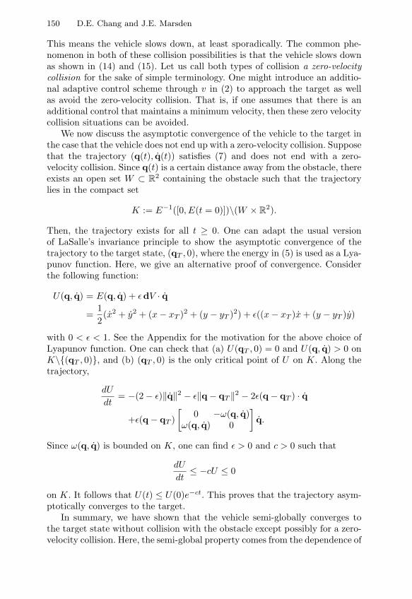
150 D.E. Chang and J.E. Marsden

This means the vehicle slows down, at least sporadically. The common phe-nomenon in both of these collision possibilities is that the vehicle slows downas shown in (14) and (15). Let us call both types of collision a zero-velocitycollision for the sake of simple terminology. One might introduce an additio-nal adaptive control scheme through v in (2) to approach the target as wellas avoid the zero-velocity collision. That is, if one assumes that there is anadditional control that maintains a minimum velocity, then these zero velocitycollision situations can be avoided.

We now discuss the asymptotic convergence of the vehicle to the target inthe case that the vehicle does not end up with a zero-velocity collision. Supposethat the trajectory (q(t), q(t)) satisfies (7) and does not end with a zero-velocity collision. Since q(t) is a certain distance away from the obstacle, thereexists an open set W ⊂ R

2 containing the obstacle such that the trajectorylies in the compact set

K := E−1([0, E(t = 0)])\(W × R2).

Then, the trajectory exists for all t ≥ 0. One can adapt the usual versionof LaSalle’s invariance principle to show the asymptotic convergence of thetrajectory to the target state, (qT , 0), where the energy in (5) is used as a Lya-punov function. Here, we give an alternative proof of convergence. Considerthe following function:

U(q, q) = E(q, q) + εdV · q=

12

(x2 + y2 + (x− xT )2 + (y − yT )2) + ε((x− xT )x+ (y − yT )y)

with 0 < ε < 1. See the Appendix for the motivation for the above choice ofLyapunov function. One can check that (a) U(qT , 0) = 0 and U(q, q) > 0 onK\(qT , 0), and (b) (qT , 0) is the only critical point of U on K. Along thetrajectory,

dU

dt= −(2− ε)‖q‖2 − ε‖q− qT ‖2 − 2ε(q− qT ) · q

+ε(q− qT )[

0 −ω(q, q)ω(q, q) 0

]q.

Since ω(q, q) is bounded on K, one can find ε > 0 and c > 0 such that

dU

dt≤ −cU ≤ 0

on K. It follows that U(t) ≤ U(0)e−ct. This proves that the trajectory asym-ptotically converges to the target.

In summary, we have shown that the vehicle semi-globally converges tothe target state without collision with the obstacle except possibly for a zero-velocity collision. Here, the semi-global property comes from the dependence of

Gyroscopic Forces and Collision Avoidance with Convex Obstacles 151

Vmax on the initial condition given in (7). We may avoid zero-velocity collisionby adding an adaptive scheme. We expect that the set of initial states endingup with zero-velocity collision is small.

Remarks.1. The choice of Vmax satisfying (7) may be conservative. Recall that the

gyroscopic force gets turned on only when an obstacle comes into the detectionshell. So, we can choose a new value of Vmax satisfying E(t = td) ≤ 1

2V2max at

the moment, t = td, when the vehicle detects the obstacle. The proof givenabove is still valid with this update rule of Vmax. In this sense, the abovecollision avoidance algorithm works globally. Moreover, the same control lawworks in the existence of multiple obstacles since our control law is feedbackand the vehicle only uses the local information in its detection shell.

2. One can easily modify the above control algorithm for convex obstacles.When the obstacle is not convex, one needs to add an adaptive scheme. Oneconservative way is to make a convex buffer shell which contains the non-convex obstacle and regard this convex shell as an obstacle. However, thisentails that the vehicle knows the global shape of the obstacle. In reality, thevehicle may only have a local information of the obstacle. In such a case, oneneeds to apply a scheme to find a convex arc (or, surface) which divides thedetection shell so that the vehicle lies on one side and the obstacle on theother side. Then, one regards this convex arc as an obstacle.

For obstacles and bodies with sharp corners and flat surfaces or edges,the algorithm also needs to be modified; this can be done and will appearin forthcoming works of the authors. We illustrate the results of such analgorithm in Figure 1 below.

3. We give an alternative choice of a gyroscopic force, which produces afaster convergence of a vehicle to its target point than that in (3). Assumethat the vehicle has detected an obstacle in its detection shell. In such a case,let us define the function, σqT = σqT (q) as follows:

σqT (q) =

0 if the obstacle does not lie between the two points, q and qT

1 otherwise

where q is the position of the vehicle and qT is the target point of the vehicle.Roughly speaking, the function σqT checks if the vehicle can directly see thetarget. The new gyroscopic force, Fg, is defined by the product of the functionσqT and the old gyroscopic function Fg in (3) as follows:

Fg = σqTFg.

The vehicle switches off the gyroscopic force if the vehicle can directly see thetarget even when there is an obstacle nearby. Simulation studies show thatthis new gyroscopic force gives faster convergence to the target. We expectthat the gyroscopic force Fg reduces the possibility of a zero-velocity collision.

4. If d(q) · q ≈ 0 and there is a measurement error, then the sign of ω(q, q)becomes fragile. In such a case, one can choose a constant sign of ω(q, q) for

152 D.E. Chang and J.E. Marsden

a period. The reason is as follows. The condition, d(q) · q ≈ 0, means thatthe velocity is almost perpendicular to the obstacle. Hence, the direction ofrotation the velocity does not matter much as long as one keeps rotating ituntil the measurement of the direction of velocity becomes relevant to thevector d(q) in a certain way. Another possible option is to choose the signof ω which agrees with the current direction of the potential plus dissipativeforce, −∇V + Fd. Issues such as this are important for robustness.

5. Above, we chose a particular form of potential function, dissipativeforce, and gyroscopic force. However, one can modify the above proof for moregeneral from of V , Fd and Fg. We also assumed that the vehicle is a pointmass. In reality, it has a volume. In this case, the vehicle is equipped withtwo shells around it where the inner shell is the safety shell which containsthe vehicle and the outer shell is the detection shell. In this case, one mustprevent the obstacle from coming into the safety shell. For example, d(q) in(4) should be modified to the distance from the safety shell to the obstacle.

6. One can extend this control algorithm to three dimensions. In such acase, the skew-symmetric matrix S in the gyroscopic force Fg = S(q, q)qshould be an infinitesimal rotation with the axis in parallel to the vectord(q, q)× q when d(q, q)× q = 0. When d(q, q)× q = 0, one just chooses apreferred rotational direction, as in the planar case.

Comparison with the Navigation Function Method. We compare ourmethod with the navigation function method developed in [8]. In the naviga-tion function method, when the vehicle is fully actuated and there are someobstacles, then one first designs a potential function which has maxima on theboundary of obstacles and the minimum at the target point where no otherlocal minima are allowed, but saddle points are allowed in dynamics becausethe stable manifolds of saddle points are measure zero. The control force isthe sum of the potential force from the potential function and a dissipativeforce. Then, the vehicle converges to its target point avoiding collision withobstacles. A caveat in the navigation function method is that the constructionof such a potential function depends on the global topology of the configu-ration space excluding obstacles. In other words, the vehicle must know allthe information of obstacles in advance; of course one could also considerdeveloping a more local formulation of the navigation function methodology.

Our method differs fundamentally from the navigation function method inwhich the potential force is used for both convergence and collision-avoidance.Our method employs a potential force only for convergence and uses a gyros-copic force for collision avoidance. We design our potential function withoutconsidering the configuration of obstacles, so it is easy to choose a potentialfunction. We only use local information inside the detection shell of the vehicleto execute the gyroscopic force. Hence, we need not know all the informationof obstacles in advance. In either method, one must be careful about the(perhaps remote) possibility of zero-velocity collisions. In general, we regardthese two methods as complementary to each other.

Gyroscopic Forces and Collision Avoidance with Convex Obstacles 153

Simulation: One Vehicle + Two Obstacles. Consider the case of onevehicle and two obstacles. One obstacle is a disk of radius 1 located at (0, 0)and the other is a disk of radius 2 centered at (5, 0) (left side of Figure 1).

4 2 0 2 4 6 8 10

4

2

0

2

4

6

ObstacleObstacle

target

-

-

- - 5 4 3 2 1 0 1 2 3 44

3

2

1

0

1

2

3

4

------

-

-

-

Fig. 1. (Left–Vehicle with two obstacles.) The vehicle starts from (−2, −1) with zeroinitial velocity, converging to the target point, (8, 3), avoiding any collisions withobstacles. The shaded disk about the vehicle is the detection shell. (Right–avoidinga flat obstacle.) This shows a simulation result for a modified algorithm suitable forobjects with flat surfaces; the vehicle starts at (−3, −1) and the target is at (2, 0).

The vehicle is regarded as a point of unit mass. It starts from (−2,−1)with initial zero velocity and converges to the target point qT = (8, 3). Weused the following potential function and dissipative force:

V (q) =12‖q− qT ‖2, Fd = −2q.

We used√

10 for Vmax in the gyroscopic force in (3) and (4).The right side of this figure shows that the general methodology, suitably

modified also works for objects with flat surfaces, and sharp corners and edges.As mentioned previously, this will be explained in detail in future publications.

3 Collision Avoidance: Multi-vehicles

We develop a collision-avoidance scheme using gyroscopic forces in the casethat there are multiple vehicles in a plane. For the purpose of illustration, weonly consider two vehicles and we make a remark on how to extend this tomulti-vehicle case.

Collision Avoidance between Two Vehicles. Let us consider the situa-tion where there are two vehicles in a plane and there are no other vehicles or

154 D.E. Chang and J.E. Marsden

obstacles. Each vehicle wants to approach its own target point without colli-ding with the other vehicle. We assume that each vehicle has a finite volumeand two shells around its center. The inner shell is called a safety shell, whichcompletely contains the vehicle. Its radius is denoted by rsaf . The outer shellis a detection shell of thickness rdet. Each vehicle detects the other vehicleonly when the other vehicle comes into the detection shell. Here, a collisionmeans the collision between safety shells.

Let qi = (xi, yi) be the position of the i-th vehicle, and qT,i = (xT,i, yT,i)be the target point of the i-th vehicle, with i = 1, 2. The dynamics of the i-thvehicle are given by qi = ui with ui = (uxi , uyi). The control law consists ofa potential, a dissipative, and a gyroscopic force: u = −∇V + Fd + Fg. Forsimplicity, we will only design a controller for vehicle 1 in the following. Onecan get a controller for vehicle 2 in the similar manner.

Choose the following potential function and dissipative force for vehicle 1:

V1(q1) =12‖q1 − qT,1‖2, Fd,1(q1, q1) = −2q1.

Before we choose a gyroscopic force, let us define a couple of functions. Letd(q1,q2) be the distance between the safety shells of the two vehicles, whichis given by

d(q1,q2) = ‖q1 − q2‖ − rsaf,1 − rsaf,2.Define ϕ : R

2 × R2 → [−π/2, π/2] by

ϕ(v,w) =

the signed angle from v to w if [v ·w ≥ 0] ∧ [‖v‖ · ‖w‖ = 0],0 otherwise

For example, ϕ((1, 0), (1, 1)) = π/4 and ϕ((1, 1), (1, 0)) = −π/4. Define χ :R

2 × R2 → R by

χ(q1,q2) =

1 if d(q1,q2) ≤ rdet,10 otherwise

which checks if vehicle 2 is in the detection shell of vehicle 1. For the positionvectors q1 and q2 of both vehicles, define q21 = q2 − q1, q12 = −q21. Thegyroscopic force Fg,1 of vehicle 1 is given by

Fg,1 = χ(q1,q2)[

0 −ω(q1, q1,q2, q2)ω(q1, q1,q2, q2) 0

]q1 (16)

where the function ω is given by

ω(q1, q1,q2, q2) = f(q1, q1,q2, q2)πVmax

d(q1,q2)

where Vmax is a fixed positive number and the function f is defined by consi-dering four possible cases, C1–C4, as follows:

Gyroscopic Forces and Collision Avoidance with Convex Obstacles 155

C1. If [q21 · q1 ≥ 0] ∧ [q21 · q2 ≥ 0]: vehicle 2 is before and heading awayfrom vehicle 1, then

f(q1, q1,q2, q2) =

1 if ϕ(q21, q1)− ϕ(q21, q2) ≥ 0−1 otherwise

C2. If [q21 · q1 ≥ 0] ∧ [q21 · q2 < 0]: vehicle 2 is before and heading towardvehicle 1, then

f(q1, q1,q2, q2) =

1 if ϕ(q21, q1)− ϕ(q2,q12) ≥ 0−1 otherwise

C3. If [q21 · q1 < 0] ∧ [q21 · q2 < 0]: vehicle 2 is behind and heading towardvehicle 1, then

f(q1, q1,q2, q2) =

1 if ϕ(q12, q1)− ϕ(q12,q2) > 0−1 otherwise

C4. Otherwise (i.e., vehicle 2 is behind and heading away from vehicle 1),

f(q1, q1,q2, q2) = 0.

Notice that vehicle 1 does not turn on the gyroscopic force when vehicle 2 isbehind and heading away from vehicle 1 in the detection shell of vehicle 1.

The energy of each vehicle is given by

Ei(qi, qi) =12‖qi‖2 + Vi(qi)

with i = 1, 2. One can check that each energy function is non-increasing intime.

Suppose that the initial state (qi(0), qi(0)) of each vehicle satisfies

Ei(qi(0), qi(0)) ≤ 12

(Vmax,i)2

with i = 1, 2. We want to show that it cannot happen that the two vehiclescollide with q1 = 0 or q2 = 0 at the moment of collision. We prove thisby contradiction. Suppose that the two vehicles collided at time t = tc withq1(tc) = 0 or q2(tc) = 0. Without loss of generality, we may assume thatq1(tc) = 0. Then, one will reach a contradiction by studying the dynamicsof vehicle 1 during the time interval, [tc −∆t, t−c ] for a small ∆t > 0 just asdone for the case of obstacle avoidance in § 2. One can also show semi-globalconvergence of each vehicle to its target point. The proof is almost identicalto that in § 2. The point is that each vehicle has its own Lyapunov functionwhich is independent of that of the other vehicle. In this sense, the controlscheme given here is a distributed and decentralized control.

156 D.E. Chang and J.E. Marsden

Remarks.1. We have not excluded the possibility of zero-velocity collision. Since this

happens only at low velocity, one can add an adaptive scheme to handle this.2. We give another possible choice of the function, ω, in (16). We do

this from the viewpoint of vehicle 1 as the same procedure applies to othervehicle. Suppose that vehicle 2 is detected and it does not belong to the case,C4, above. Let v12 = q1− q2 be the velocity of vehicle 1 relative to vehicle 2.We regard vehicle 2 as a fixed obstacle located at q2 and compute ω with thealgorithm used for obstacle avoidance in § 2 with this relative velocity v12.

3. We give an ad-hoc extension of the gyroscopic collision avoidance schemeto the case of multiple vehicles. The situation is the same as that of two-vehiclecase except that there are more than two vehicles. Suppose that vehicle Adetected n other vehicles in its detection shell where we have already excludedvehicles which are behind and heading away from vehicle A. Let di, i =1, . . . , n be the distance between the safety shell of vehicle A and that of thei-th vehicle. Let

qCM =1n

n∑i=1

qi

be the mean position of the n vehicles, and

qCM =1n

n∑i=1

qi

the mean velocity of the n vehicles. We now design ω in the gyroscopic forceFg,A = (−ωyA, ωxA) where ω as follows:

ω = fπVmax

mindi | i = 1, . . . nwhere one decides the value of f by applying the algorithm used for thetwo-vehicle case, assuming that there is only one (equivalent) vehicle locatedat qCM with velocity qCM. One needs to modify this in the case that qCMcoincides with the position of vehicle A. The same procedure applies to othervehicles. Simulations show that this ad-hoc scheme works well.

4. If one of the vehicles is “adversarial” then clearly the situation describedabove needs to be modified.

Simulation: Three Vehicles. Figure 2 shows a simulation of three vehicles.The three vehicles are initially located along the circle of radius 2 and they are120 away from one another. The target point of each vehicle is the oppositepoint on the circle. The detection radius is 0.5 and the safety shell was notconsidered for simplicity. We used the control law described above with Vmax =√

2.5. The simulation result is given in Figure 2 where the shaded disks denotedetection shells. One can see that each vehicle switches on the gyroscopic forcewhen it detects other vehicles.

Gyroscopic Forces and Collision Avoidance with Convex Obstacles 157

3 2 1 0 1 2 3 3

2

1

0

1

2

3

-

-

-- - -

Fig. 2. Three vehicles are initially located along the circle, 120 away from oneanother. The target of each vehicle is the opposite point on the circle. The shadeddisks are detection shells

Appendix

One often uses LaSalle’s theorem to prove asymptotic stability of an equili-brium in a mechanical system using an energy function E. Although LaSalle’stheorem is a powerful stability theorem, it normally gives no information onexponential convergence since E is only semidefinite. Here, we show that if theenergy has a minimum at an equilibrium of interest and the system is forcedby a strong dissipative force (and a gyroscopic force), then the equilibrium isexponentially stable. The idea, called Chetaev’s trick, is to add a small crossterm to the energy function to derive a new Lyapunov function. In this appen-dix, we give an intrinsic explanation to Chetaev’s trick. A preliminary workwas done in [2] in a different situation.

Consider a mechanical system with the Lagrangian

L(q, q) = K(q, q)− V (q) =12mij(q)qiqj − V (q)

with q = (q1, . . . , qn) ∈ Rn, and the external force, F = Fd +Fg, where Fd is

a strong dissipation given by

Fd(q, q) = −Rqq, R = RT > 0, (17)

and Fg is a gyroscopic force of the form Fg = S(q, q)q, ST = −S. Herewe assume that the matrix S is bounded in magnitude on a domain we areinterested in. In showing exponential stability, the role of gyroscopic force islittle when the dissipation is strong, i.e., R = RT > 0. Also, one may allow thematrix R to depend on velocity q. Here, we use R

n as a configuration space

158 D.E. Chang and J.E. Marsden

for simplicity. However, all arguments will be made in coordinate-independentlanguage in the following.

Suppose the energy

E(q, q) = K(q, q) + V (q)

has a nondegenerate minimum at the origin, (0, 0) ∈ Rn × R

n: i.e.,

dV (0) = 0,∂2V

∂qi∂qj(0) > 0 (18)

since the kinetic energy is already positive definite in the velocity q. Withoutloss of generality, we assume that V (0) = 0.

Let us review the proof of the asymptotic stability of the origin usingLaSalle’s theorem with E as a Lyapunov function. Consider the invariantsubset M of the set E = −〈q, Rq〉 = 0. Suppose (q(t), q(t)) is a trajectorylying inM. Then, q(t) ≡ 0. Substitution of this into the equations of motionyields dV (q(t)) ≡ 0. By (18), the critical point q = 0 of V is isolated. Itfollows q(t) ≡ 0. Hence, M consists of the origin only. By LaSalle’s theorem,the origin is asymptotically stable.

We now devise a trick to show the exponential stability of the origin.Consider the following function U :

U(q, q) = E(q, q) + εdVqq (19)

=12mij(q)qiqj + V (q) + ε

∂V

∂qiqi

with 0 < ε 1. Notice that the definition of U in (19) is coordinate-independent. For a sufficiently small ε,

dU(0, 0) = 0, D2U(0, 0) > 0 (20)

where D2U is the second derivative of U with respect to (q, q). Hence, U has aminimum at the origin. We will use U as a Lyapunov function. One computes

dU

dt(q, q) = −W (q, q) (21)

where

W (q, q) = 〈Rq, q〉 − ε(∂2V

∂qi∂qjqiqj +

∂V

∂qi(−Γ i

jkqj qk − (m−1dV )i)

)

+ ε∂V

∂qi((m−1Rq)i − (m−1Sq)i)

= R(q, q)− ε(∇qdV )q + εm−1(dV,dV ) + εm−1(Rq,dV )− εm−1(Sq,dV ) (22)

Gyroscopic Forces and Collision Avoidance with Convex Obstacles 159

where ∇ is the Levi-Civita connection of the metric m and Γ ijk are the Chri-

stoffel symbols of ∇. One can check that for a sufficiently small ε > 0

dW (0, 0) = 0, D2W (0, 0) > 0. (23)

By (20) and (23), there exists c > 0 such that d(W − cU)(0, 0) = 0 andD2(W − cU)(0, 0) > 0. Therefore, W − cU ≥ 0 in a neighborhood N of theorigin. This and (21) imply dU

dt ≤ −cU ≤ 0. It follows

U(q(t), q(t)) ≤ U(q(0), q(0))e−ct (24)

on N . This proves the exponential stability of the origin. One can also gofurther by invoking the Morse lemma to find a local chart z = (z1, . . . , z2n)in which the function U becomes U(z) =

∑2ni=1(zi)2. Hence, (24) implies

‖z(t)‖ ≤ ‖z(0)‖e− c2 t where ‖z‖ =

√∑2ni=1(zi)2.

Acknowledgements. We thank Noah Cowan, Sanjay Lall, Naomi Leonard,Elon Rimon, Clancy Rowley, Shawn Shadden, Claire Tomlin, and SteveWaydo for their interest and valuable comments. Research partially supportedby ONR/AOSN-II contract N00014-02-1-0826 through Princeton University.

References

1. Bhatta, P., Leonard, N. (2002) “Stabilization and coordination of underwatergliders”, Proc. 41st IEEE Conference on Decision and Control.

2. Bloch A., Krishnaprasad P.S., Marsden J.E., Ratiu T. (1994) Annals Inst. H.Poincare, Anal. Nonlin., 11:37–90.

3. Chang D.E., Bloch A.M., Leonard N.E., Marsden J.E., Woolsey C. (2002)ESAIM: Control, Optimization and Calculus of Variations, 8:393–422.

4. Chang, D.E., Shadden S., Marsden, J.E. and Olfati-Saber, R. (2003), Collisionavoidance for multiple agent systems, Proc. CDC (submitted).

5. Hwang I., Tomlin C.(2002) “Multiple aircraft conflict resolution under finiteinformation horizon”, Proceedings of the AACC American Control Conference,Anchorage, May 2002, and “Protocol-based conflict resolution for air trafficcontrol”, Stanford University Report SUDAAR-762, July, 2002.

6. Jadbabaie A, Lin J, Morse A.S. (2002) “Coordination of groups of mobile au-tonomous agents using nearest neighbor rules”, Proc. 41st IEEE Conference onDecision and Control, 2953–2958; see also IEEE Trans. Automat. Control (toappear 2003).

7. Kosecka, J., Tomlin C., Pappas, G., Sastry, S. (1997) “Generation of conflictresolution maneuvers for air traffic management”, IROS; see also IEEE Trans.Automat. Control, 1998, 43:509–521.

8. Rimon E., Koditschek D.E. (1992) IEEE Trans. on Robotics and Automation,8(5):501–518.

9. Wang L.S., Krishnaprasad P.S. (1992) J. Nonlinear Sci., 2:367–415.

Stabilization via Polynomial LyapunovFunction

Daizhan Cheng

Institute of Systems Science, Chinese Academy of Sciences, Beijing 100080,P.R.China, dcheng@iss03.iss.ac.cn

1 Introduction

In this paper we summarize some recent results on local state feedback stabi-lization of a nonlinear system via a center manifold approach.

A systematic design procedure for stabilizing nonlinear systems of non-minimum phase, i.e., with unstable zero dynamics, was presented recently in[11]. The basic idea can be described as follows. We first propose some suf-ficient conditions to assure the approximate stability of a dynamic system.Using these conditions and assuming the zero dynamics has stable and centerlinear parts, a method is proposed to design controls such that the dynamicson the designed center manifold of the closed-loop system are approximatelystable. It is proved that using this method, the first variables in each of theintegral chains of the linearized part of the system do not affect the approxi-mation degree of the dynamics on the center manifold. So the first variablesare considered as nominating controls, which can be designed to produce asuitable center manifold. Based on this fact, the concept of injection degree isproposed. According to different kinds of injection degrees certain sufficientconditions are obtained for the stabilizability of systems of non-minimumphase.

To apply this approach a new useful tool, the Lyapunov function with ho-mogeneous derivative (LFHD) has been developed. It assures the approximatestability of a dynamic system. Since the center manifold of a dynamic systemis not easily obtainable but its approximation is easily computable, LFHD isparticularly useful in center manifold approach.

Another important tool is the normal form of nonlinear control systems,which is essential for analyzing the stability of systems. It was shown that [13]the classical normal form is very restrictive because it requires a very strongregularity assumption. In [13] a generalized normal form was proposed. Itis based on point relative degree and point decoupling matrix. Since they

W. Kang et al. (Eds.): New Trends in Nonlinear Dynamics and Control, LNCIS 295, pp. 161–173, 2003.c© Springer-Verlag Berlin Heidelberg 2003

162 D. Cheng

are only defined point-wise, certain regularity requirements can be removed.Moreover, the generalized normal form can be obtained by straightforwardcomputation. So it is convenient in use. Several stabilization results for classi-cal normal forms can be developed to their counterparts for generalized normalforms.

The main purpose of this paper is to summarize some recent developments[11], [9], [13], [14] into a general frame. The paper is organized as follows:Section 2 introduces the LFHD. Some sufficient conditions are presented inSection 3 to assure the negativity of the homogeneous polynomials. Section4 cites some related results from the center manifold theory. The new stabi-lization technique for a class of nonlinear systems of non-minimum phase isintroduced in Section 5. Section 6 is devoted to the generalized normal form ofnonlinear control systems and its applications. In section 7, the stabilizationof systems with different types of center manifolds are reviewed briefly.

2 Lyapunov Function with Homogeneous Derivative

Consider a nonlinear dynamic system

x = f(x), x ∈ Rn, (1)

where f(x) is a smooth vector field. (The degree of smoothness is enoughto assure the existence of following required derivatives.) Let the Jacobianmatrix of f(x) at zero to be Jf (0). It is well known that [15]Lemma 2.1 If Jf (0) is a Hurwitz matrix, then the overall system is asym-ptotically stable at the origin.

Now we may use Taylor expansion on each component fi(x) of f(x), toget the lowest degree (ki) non-vanishing terms as

fi = gi(x) + 0(‖x‖ki+1), i = 1, · · · , n,

where gi is a homogeneous polynomial of degree ki.Definition 2.2 Construct a system as

x = g(x), x ∈ Rn, (2)

where g = (g1, · · · , gn), and gi are defined as above. Then (2) is called theapproximate system of system (1).Remark. It is clear that if Jf (0) is Hurwitz, the approximate system of (1)is

x = Jf (0)x.

As a generalization of Lemma 2.1, it is natural to ask whether the asym-ptotic stability of (2) assures the asymptotic stability of (1)? In fact, the

Stabilization via Polynomial Lyapunov Function 163

Lyapunov function with homogeneous derivative (LFHD), proposed in [11],answers the question partly.Definition 2.3 A positive definite polynomial function V > 0 is called aLFHD of system (2) if its derivative along (2) is a homogeneous polynomial.Definition 2.4 System (1) is said to be approximately stable, if

x = f(x) + r(x)

is asymptotically stable, where r(x) is a disturbance satisfying

r(x) = (r1(x), · · · , rn(x))T

and ri(x) = 0(‖x‖ki+1).Remark. If system (2) is approximately stable, then system (1) is asympto-tically stable.

The following result provides a sufficient condition for system (2) to beapproximately stable.Theorem 2.5 System (2) is approximately stable if there exists a LFHDV (x) > 0 such that the derivative V |(2) < 0.Remark. Assume system (1) is odd leading, i.e., the degrees ki of the com-ponents of its approximate system (2) are all odd. Then we can choose aninteger m such that

2m ≥ maxk1, · · · , kn+ 1.

Setting 2mi = 2m− ki + 1, a LFHD can be constructed as

V (x) =n∑

i=1

pi(xi)2mi , pi > 0, i = 1, · · · , n. (3)

This is the most useful LFHD.Example 2.6 Consider the following system

x = x2 tan(5y − 6x)y = y2 sinh(x3 − y3).

(4)

The approximate system isx = −6x3 + 5x2y

y = −y5 + x3y2.(5)

Choosing V = x4 + 4y2, then we have

V |(5) = 4x3(−6x3 + 5x2y)− 8y6 + 8x3y3

≤ −24x6 + 20( 56x

6 + 16y

6)− 8y6 + 4(x6 + y6)= − 10

3 x6 − 2

3y6 < 0.

So (4) is asymptotically stable at the origin.

164 D. Cheng

3 Negativity of a Homogeneous Polynomial

To use the LFHD method it is important to verify whether an even degreepolynomial is negative definite. As proposed in [11] a basic inequality is usedto estimate the negativity.

∣∣∣∣∣n∏

i=1

xkii

∣∣∣∣∣ ≤n∑

i=1

kik

∣∣xki∣∣ , where k =

n∑i=1

ki. (6)

The proof can be found in [12]. Now for a 2k degree homogeneous polynomialV (x) to be negative definite a necessary condition is that all of the diagonalterms, x2k

i , have negative coefficients. As a sufficient condition for negativitywe can 1. eliminate negative semi-definite (non-diagonal) terms, 2. Use (6)to split cross terms into a sum of diagonal terms. Then check if the resultingpolynomial is negative definite. This method has already been used in Example2.5. The following example demonstrates the details.Example 3.1 Consider

V (x) = −x41 + ax3

1x2 − x21x

22 − x4

2 + x1x2x23 − x4

3.

We have

V ≤ −x41 + ax3

1x2 − x42 + x1x2x

23 − x4

3≤ −x4

1 − x42 − x4

3 + |a|( 34x

41 + 1

4x42) + 1

4x41 + 1

4x42 + 1

2x43

= − 34 (1− |a|)x4

1 − 14 (3− |a|)x4

2 − 12x

43.

It is obvious that V (x) is negative definite as |a| < 1. (A simple algebraictransformation, say x3

1x2 = (λx1)3 · (x2/λ3), can show that as |a| = 1, V is

still negative definite.) Now system (2) can be expressed component-wise as

xi =∑

|S|=ki

aiSxS , i = 1, · · · , n.

where S = (s1, · · · , sn) and

|S| =n∑

i=1

si, xS =n∏

i=1

xsii .

Using the above technique, some sufficient conditions for (2) to be approxi-mately stable are provided in [11].

Denote by

Qi = |S| = ki | sj(j = i) are even and aiS < 0.It represents the set of negative semi-definite terms in ∂V

∂xigi for any LFHD. So

such terms can be skipped when the negativity is tested. Using the above tech-nique, two sufficient conditions for approximate stability of the approximatesystem (2) (same as for (1)) are presented in [11].

Stabilization via Polynomial Lyapunov Function 165

Theorem 3.2 CRDDP( Cross Row Diagonal Dominating Principle) System(2) (equivalently, (1) )is approximately stable at the origin, if there exists aninteger m with 2m > maxk1, · · · , kn, such that

−aidi >∑

|S|=ki,S ∈Qi

|aiS |(si + 2m− ki

2m

)

+n∑

j=1,j =i

∑|S|=kj ,S ∈Qj

|ajS |( si

2m

), i = 1, · · · , n.

(7)

A simpler form, which deals with each row independently, is obtained asCorollary 3.3 DDP(Diagonal Dominating Principle) System (2) (equiva-lently, (1) )is approximately stable at origin if

−aidi >∑

|S|=ki,S ∈Qi

|aiS |, i = 1, · · · , n. (8)

4 Center Manifold Approach

Stabilization is one of the basic and most challenging tasks in control design.The asymptotic stability and stabilization of nonlinear systems has receivedtremendous attention. The center manifold approach has been implementedto solve the problem. Some special non-linear controls are designed to stabilizesome particular control systems. The method used there is basically a case-by-case study [1], [2]. For control systems in canonical form, assume the centermanifold has minimum phase, then a “quasi-linear” feedback can be usedto stabilize linearly controllable variables. We refer to [3], [7], [4], [7], [8] forminimum phase method and its applications.

Our purpose is to apply the techniques developed in Sections 2-3 to thedynamics on center manifold of closed-loop nonlinear control systems to findstabilizing controls without a minimum phase assumption.

We cite some related results of the theory of center manifold here [5].Theorem 4.1 Consider the following system

x = Ax+ p(x, z), x ∈ Rn,

z = Cz + q(x, z), z ∈ Rm,(9)

where Reσ(A) < 0, Reσ(C) = 0, p(x, z) and q(x, z) vanish at zero with theirfirst derivatives. Then there exists an m dimensional invariant sub-manifoldthrough the origin, described by

S = (x, z) | x = h(z), (10)

where h(z) satisfies

166 D. Cheng

∂h(z)∂z

(Cz + q(h(z), z))−Ah(z)− p(h(z), z) = 0. (11)

Theorem 4.2 The dynamics on the center manifold are

z = Cz + q(h(z), z), z ∈ Rm. (12)

System (9) is asymptotically stable, stable, unstable, iff system (12) is asym-ptotically stable, stable, unstable respectively.Theorem 4.3 Assume there exists a smooth function φ(z), such that

∂φ(z)∂z

(Cz + q(φ(z), z))−Aφ(z)− p(φ(z), z) = 0(‖z‖k+1). (13)

Then

‖φ(z)− h(z)‖ = 0(‖z‖k+1). (14)

For convenience, we call Theorem 4.1, Theorem 4.2, and Theorem 4.3 theexistence theorem, equivalence theorem, and approximation theorem respec-tively.

5 Stabilization of Non-minimum Phase NonlinearSystems

Consider an affine nonlinear control systemξ = f(ξ) +

m∑i=1gi(ξ)ui, ξ ∈ R

n

y = h(ξ), y ∈ Rm.

(15)

Assume the decoupling matrix is nonsingular and G = Spangi is involutive,then the system can be converted into a feedback equivalent normal form as[7]

x = Ax+Bv x ∈ R

s

z = q(z, x), z ∈ Rt.

(16)

Without loss of generality, we assume (A,B) is of the Brunovskey canonicalform. That is, the linear part of (16) can be expressed as

xi1 = xi2...xisi−1 = xisixisi = vi, xi ∈ R

si , i = 1, · · · ,m.

Stabilization via Polynomial Lyapunov Function 167

Note thatm∑i=1si = s and s+ t = n. It is well known [7] that if system (16) is

of minimum phase, i.e.,z = q(z, 0)

is asymptotically stable, then the system is stabilizable by linear state feed-back. Now if (16) is of non-minimum phase, [11] proposes a systematic wayto stabilize it. The method, called designing center manifold, can be roughlydescribed as follows: We look for a set of controls of the following form

vi = ai1xi1 + · · ·+ aisix

isi − ai1

t∑j=2

P ij (z), i = 1, · · · ,m. (17)

where P ij (z) are polynomials of degree j, aij are chosen such that the linear

part is Hurwitz. Now we use

xi = φi(z) =

t∑j=2

P ij (z)

0...0

, i = 1, · · · ,m (18)

to approximate the center manifold, say x = h(z). Using Theorem 4.3, it iseasy to see that if

∂φ

∂zq(z, φ(z)) = 0(‖z‖r+1) (19)

then the difference (approximation error) is

‖φ(z)− h(z)‖ = 0(‖z‖r+1),

where φ(z) = (φ1(z), · · · , φm(z)). Next, we consider the approximate dyna-mics on center manifold of the closed-loop system. It is expressed as

zi = qi(z, φ(z)), i = 1, · · · , t. (20)

Denote the approximate system of (20) by

zi = ηi(z), i = 1, · · · , t. (21)

If deg(ηi) = ki are odd, and let k = maxki. Then we have the followingmain result:Theorem 5.1 Assume there exists φ(z) as described above, such that 1. (19)holds; 2.

qi(z, φ(z))− qi(z, φ(z) + 0(‖z‖r+1)) = 0(‖z‖ki+1), i = 1, · · · , t. (22)

168 D. Cheng

3. There exists a LFHD V (z) > 0 such that V |(21) < 0. Then the system (16)is stabilizable by control (17).Remark. 1. In fact, condition 3 assures the approximate stability of (20).Then in the light of condition 1, condition 2 assures the asymptotical stabilityof the true dynamics on center manifold. 2. Of course, condition 3 can bereplaced by saying (21) is approximately stable.

We give a simple example to describe the stabilizing process.Example 5.2 Consider the following system

x1 = x2

x2 = u

z1 = z1 ln(1 + z1)x1 + 3z21z22

z2 = z2x1 + z1z2x1.

(23)

We search for a control having the form

u = −x1 − 2x2 + P2(z) + P3(z),

where deg(P2) = 2, deg(P3) = 3. Then

x = φ(z) =(P2(z) + P3(z)

0

).

A simple computation shows that we can choose P (z) = P2(z) + P3(z) as

P (z) = −3z22 − 2z31 .

The approximate dynamics on the center manifold becomez1 = −2z51 + 3

2z31z

22 + 0(‖z‖6)

z2 = −3z32 + 0(‖z‖4).(24)

Now the approximation error is

∂φ(z)∂z

g(z, φ(z)) = 0(‖z‖4).

Then a straightforward computation shows that

q1(z, φ(z) + 0(‖z‖4))− q1(z, φ(z)) = 0(‖z‖6),q2(z, φ(z) + 0(‖z‖4))− q2(z, φ(z)) = 0(‖z‖5).

The condition (22) is obviously satisfied.Using CRDDP or DDP, Theorem 3.2 or Corollary 3.3 shows that (24) is

approximately stable. Now Theorem 5.1 assures that the control

u = −x1 − 2x2 − 3z22 − 2z31

stabilizes the system (23).

Stabilization via Polynomial Lyapunov Function 169

6 Generalized Normal Form

From previous section one sees that the normal form is essential in the stabi-lization via center manifold approach. But to get Byrnes-Isidori normal form(16), the system (15) should be regular in the sense that the relative degreevector is well defined and the decoupling matrix is nonsingular on a neighbor-hood of the origin. A generalized normal form is proposed in [13], based onthe so called point relative degree vector. Unlike the relative degree vector,the point relative degree vector is always well defined.Definition 6.1 1. For system (15) the point relative degree vector (ρ1, · · · , ρm)is defined as

LgL

kfhi(0) = 0, k < ρi − 1,

LgLρi−1f h(0) = 0, i = 1, · · · ,m. (25)

2. The essential relative degree vector, ρe = (ρe1, · · · , ρem), (the essentialpoint relative degree vector, ρep = (ρep1 , · · · , ρepm )) , for the state equation of(15) is defined as the largest one of relative degree (resp. point relative degree),ρ∗, for all possible auxiliary outputs, which makes the decoupling matrix, W ρe

(resp. W ρep ), non-singular. That is,

‖ρ∗e‖ =m∑i=1

ρ∗ei = max‖ρe‖ |W ρe is nonsingular; (26)

and

‖ρ∗ep‖ =m∑i=1

ρ∗epi = max‖ρep‖ |W ρep is nonsingular. (27)

For system (15) we give two fundamental assumptions:H1. The decoupling matrix is invertible at the origin;H2. g1(0), · · · , gm(0) are linearly independent and Spang(x) is involu-

tive near the origin.Then we can seek a generalized normal form as

zi = Aizi + biui +

(0

αi(z, w)

)+ pi(z, w)u, zi ∈ R

ρi

i = 1, · · · ,mw = q(z, w), w ∈ R

r

yi = zi1, i = 1, · · · ,m,

(28)

where r+m∑i=1ρi = n, αi(z, w) are scalars, pi(z, w) are ρi×mmatrices, q(z, w) is

a r×1 vector field, and (Ai, bi) are Brunovsky canonical form, and pi(0, 0) = 0.

170 D. Cheng

Comparing (28) with (16), the only difference between them is that in (16)gi = (0 · · · 0 di(x, z))T , i = 1, · · · ,m, and in (28) there exist pi(z, w) whichare higher degree input channels. Then we can prove the following:Proposition 6.2 Consider system (15). 1. Assume H1 and H2 and if thesystem has point relative degree vector ρp = (ρ1, · · · , ρm), then there exists alocal coordinate frame such that the system can be converted into the genera-lized normal form (28).

2. Assume H2 and if system (15) has essential point relative degree vectorρep = (ρ1, · · · , ρm), then there exists a local coordinate frame such that thesystem can be converted into the generalized normal state form as the stateequation of (28).Remark. Unlike the classical normal form, the essential point relative degreevector is straightforwardly computable, and then so is the generalized normalform.

Now for the generalized normal form we have some stabilization results,which are parallel to their counterparts for the classical normal form [13].

Observer system (28), for the case of “minimum phase” we assumeH3. αi(0, w)pi(0, w) = 0, i = 1, · · · ,m.Then we have

Proposition 6.3 Assume H3. For the generalized normal state form (stateequation of (28)) if the pseudo-zero dynamics

w = q(0, w) (29)

are asymptotically stable at zero, then (6) is stabilizable by a pseudo-linearstate feedback control.

For the case of non-minimum phase, using the center manifold approachwe have the followingTheorem 6.4 For system (28), assume there exist m homogeneous quadraticfunctions

φ(w) = (φ1(w), · · · , φm(w))

and m homogeneous cubic functions

ψ(w) = (ψ1(w), · · · , ψm(w))

such that the following hold:1. There exists an integer s > 3, such that

L.D.

Lq(φ+ψ,0, · · · , 0︸ ︷︷ ︸

‖ρ‖−m

,w)(φ+ ψ)

≥ s; (30)

L.D.

p(φ+ ψ, 0, · · · , 0︸ ︷︷ ︸

‖ρ‖−m

, w)α(φ+ ψ, 0, · · · , 0︸ ︷︷ ︸‖ρ‖−m

, w)

≥ s. (31)

Stabilization via Polynomial Lyapunov Function 171

2.

L.D.

qi(φ+ ψ, 0, · · · , 0︸ ︷︷ ︸

‖ρ‖−m

, w)

= Li, i = 1, · · · , r. (32)

3.

w = q(φ+ ψ, 0, · · · , 0︸ ︷︷ ︸‖ρ‖−m

, w) (33)

is L = (L1, · · · , Lr) approximately asymptotically stable at the origin, and4.

qi((φ+ ψ + 0(‖w‖s), 0(‖w‖s), · · · , 0(‖w‖s)︸ ︷︷ ︸‖ρ‖−m

, w)

= qi(φ+ ψ, 0, · · · , 0︸ ︷︷ ︸‖ρ‖−m

, w) + 0(‖w‖Li+1), i = 1, · · · , r. (34)

Then the overall system (28) is state feedback stabilizable.Remark. 1. In the above theorem we use only quadratic and cubic functionsfor control design. In fact, higher degree polynomials may also be used. It isnot difficult to generalize the above result to the more general case. 2. Again,the LFHD can be used to test the approximate stability of (33).

7 Other Types of Center Manifolds

In either classical or generalized normal form, the state equations of linearlyuncontrollable variables (z in (16) or w in (28) ) are the key for stabilization.If their linear parts, say ∂q

∂z |(0,0) in (16), have positive real part eigenvalues,the system is not stabilizable. So if the system is stabilizable we have toassume that only the negative and zero real part eigenvalues are allowed. Inthe above discussion, we didn’t consider negative eigenvalues in the linear partof nonlinear state equations. But it is not difficult to include them. In fact,[11] considered systems with both negative and zero eigenvalues.

Next, we assume the linear part of the nonlinear state equations has onlyzero real part eigenvalues. Then this part of the variables will appear in thecenter manifold. We simply denote it by C, which means the linear part is Cz.Now according to the form of C, we say that the system has different typesof center manifolds. The types are defined as follows:

Case 1. Zero center: C = 0Case 2. Multi-fold zero center:

172 D. Cheng

C =

0 1 0 · · · 00 0 1 · · · 0

0 0 0. . . 0

0 0 0 · · · 10 0 0 · · · 0

.

(Of course, we may have more than one such Jordan Block.)Case 3. Oscillatory center:

C =(

0 a−a 0

).

In fact, in the above Sections 4-6 only case 1 is considered.The case when the center manifold is of the type of

C =(

0 10 0

)

was discussed in [9]. It was proved that we are not able to find a LFHD tostabilize the dynamics of this kind of center manifold approximately. A ge-neralized LFHD was introduced to stabilize such systems. The basic idea isto add some cross terms to LFHD and keep its positivity. When the mul-tiplicity of zero is greater than two, we still don’t know how to stabilize itsystematically.

As for the case of an oscillatory center, a standard way is to convert itinto a normal dynamical form, which has a Taylor expansion with the lowestdegree terms of degree greater than or equal to 3. (We refer to [6] for normalform of dynamics. Do not confuse it with the normal forms of control systemsdiscussed is Sections 5-6.) Some recent results were presented in [10].

The method of LFHD can also be used for estimating the region of at-traction of equilibrium points. It can also be used for time-varying systems[14].

8 Conclusion

This paper summarized the method of stabilization of nonlinear affine systemsvia designed center manifold. A few key points in this method are listed asfollows:

• Consider the normal form of a control system (16), the first variables ineach integral chain don’t affect the approximation degree of the centermanifold. So they can be used as nominate controls to design the requiredcenter manifold.

• Lyapunov function with homogeneous derivative (LFHD) can assure theapproximate stability of a dynamic system. This is the key of the method,

Stabilization via Polynomial Lyapunov Function 173

because it is very difficult, if not impossible, to get the precise dynamicson center manifold, but the approximation theorem provides an easy wayto get its approximate dynamics. Then the approximate stability of theapproximate dynamics assures the stability of the true dynamics on centermanifolds.

• Certain easily verifiable conditions, as CRDDP and DDP etc., were deve-loped to check the negativity of the homogeneous derivative of LFHD.

• The method depends on the normal form of nonlinear control systems. Toapply it to more general systems the generalized normal form of nonli-near control systems was introduced. The generalized normal form coversalmost all smooth affine nonlinear control systems.

The method has been extended to treat the cases of multi-zero and oscil-latory centers. But only some special simple cases can be properly handled[9], [10]. The general cases remain for further investigation.

References

1. Aeyels, D. (1985), Stabilization of a class of non-linear systems by a smoothfeedback control, Sys. Contr. Lett. Vol. 5, 289–294.

2. Behtash, S., Dastry D. (1988), Stabilization of non-linear systems with uncon-trollable linearization, IEEE Trans. Aut. Contr., Vol. 33, No. 6, 585–590.

3. Byrnes, C.I., Isidori A. (1984), A frequency domain philosophy for non-linearsystems, IEEE Conf. Dec. Contr. Vol. 23, 1569–1573.

4. Byrnes, C.I., Isidori A., and Willems J.C. (1991), Passivity, feedback equiva-lence, and the global stabilization of minimum phase nonlinear systems, IEEETrans. Aut. Contr. Vol. 36, No. 11, 1228–1240.

5. Carr,J. (1981), Applications of Center Manifold Theory, Springer-Verlag.6. Guchenheimer, J., Holmes, P. (1983), Nonlinear Oscillations, Dynamical Sy-

stems, and Bifurcations of Vector Fields, Springer-Verlag.7. Isidori,A. (1995), Non-linear Control Systems, 3nd ed., Springer-Verlag.8. Nijmeijer, H., van der Schaft A.J. (1990), Non-linear Dynamical Control Sy-

stems, Springer-Verlag.9. Cheng,D. (2000), Stabilization of a class of nonlinear non-minimum phase sy-

stems, Asian J. Control, Vol. 2, No. 2, 132–139.10. Cheng,D., Spurgeon S. (2000), Stabilization of nonlinear systems with oscilla-

tory center, Proc. 19th CCC, Hong Kong, Vol. 1, 91–96.11. Cheng, D., Martin C. (2001), Stabilization of nonlinear systems via designed

center manifold, IEEE Trans. Aut. Contr., Vol. 46, No. 9, 1372–1383.12. Cheng, D. (2002), Matrix and Polynomial Approach to Dynamic Control Sy-

stems, Science Press, Beijing.13. Cheng, D., Zhang L. (2003), Generalized Normal Form and Stabilization of

Nonlinear Systems, Internal J. Control, (to appear)14. Dong, Y., Cheng D., Qin H., New Applications of Lyapunov Function with

Homogeneous Derivative, IEE Proc. Contr. Theory Appl., (accepted)15. Willems, J.L. (1970), Stability Theory of Dynamical Systems, John Wiley &

Sons, New York.

Simulating a Motorcycle Driver

Ruggero Frezza and Alessandro Beghi

Department of Information Engineering, University of Padova, Italy,frezza,beghi@dei.unipd.it

Summary. Controlling a riderless bicycle or motorcycle is a challenging problembecause the dynamics are nonlinear and non-minimum phase. Further difficultiesare introduced if one desires to decouple the control of the longitudinal and lateraldynamics. In this paper, a control strategy is proposed for driving a motorcyclealong a lane, tracking a speed profile given as a function of the arc length of the midlane.

1 Introduction

Driving a bicycle or a motorcycle is a difficult task which requires repeatedlearning trials and a number of bruises. A well known idiom, however, goeslike: Once learnt, one never forgets how to ride a bicycle. Underneath thisapparently trivial guidance task, there lies a complex control problem, that isof interest both for the physics it involves and the applications.

Our specific motivation in dealing with the control of bicycles and mo-torcycles comes from the world of virtual prototyping. Nowadays, all majorcar manufacturers and automotive suppliers employ virtual prototyping soft-wares to cut time and costs in the development of new models. Virtual vehiclesare described by highly detailed mechanical models where all the vehicle com-ponents (chassis, suspensions, tires, powertrain, etc.) are represented so thatthe software can accurately reproduce the very complex behaviour of realvehicles. To be used for testing purposes, the simulation environment has toprovide both a means of describing the interaction between the vehicle and theenvironment (course of road, weather conditions, etc.) and a control systemthat emulates the driver, so that appropriate test maneuvers can be executed.Commercial software systems are available to accomplish all of these tasks(see e.g. [1], [2]). The same software systems can be employed in the field ofmotorcycle manufacturing as far as the modeling part is concerned. However,a satisfactory virtual motorcycle driver that can be used to test the virtual

W. Kang et al. (Eds.): New Trends in Nonlinear Dynamics and Control, LNCIS 295, pp. 175–186, 2003.c© Springer-Verlag Berlin Heidelberg 2003

176 R. Frezza and A. Beghi

vehicle on the desired maneuvers has not yet been developed. This is due tothe fact that driving a motorcycle is a more demanding task than driving acar, and the difficulty obviously lies in keeping the motorcycle upright whilefollowing a desired path. These two goals are often in contrast: In order tolean the motorcycle in the turn, one has first to steer it the opposite way togenerate a centrifugal force that pushes the motorcycle in the right direction.Considering the problem from a control theoretic standpoint, we can say thatthe motorcycle exhibits a non-minimum phase behaviour. As is known, controldesign for nonlinear, non-minimum phase systems is a current research topicin the scientific community (see for instance the recent papers [3, 4, 5, 6, 7].)

The study of guidance systems for bicycles and motorcycles has alreadybeen considered in the literature. In particular, a very nice exposition on thephysics of driving a bicycle is given in [8]. In the control literature, the twoapproaches that are more closely related to what we propose in this paperare due to Von Wissel [9] and Getz [10] who both wrote their Ph.D. the-sis on controlling a riderless bicycle. Getz’s work [10] is about the trajectorytracking problem. The motorcycle is controlled to follow a curve in the planewith a given time parametrization. Von Wissel [9] proposes a solution to thepath planning problem which consists in finding a feasible path avoiding fi-xed obstacles. The solution consists in the choice of optimal precomputedmaneuvers that satisfy the requirements and it is computed by dynamic pro-gramming techniques.

The control problem we consider here is different. The motorcycle mustbe steered inside a lane of given width, and a desired forward velocity is alsoassigned as a function of the arc length of the midlane, so that the problemcannot be stated in the standard terms of trajectory tracking. The proposedcontrol strategy is a kinematic path following control law which decoupleslateral from longitudinal control. The roll angle is controlled by nonlinear statefeedback linearization and a simple proportional, integral and derivative law isadopted for the control of longitudinal velocity. Other marginal control taskshave also been solved in particular situations where the dynamics neglectedin the model become relevant and affect the behaviour of the controller. Onesuch situation happens in heavy braking and during gear shifting.

The paper is organized as follows. In Section 2 the adopted motorcyclemodel is presented, and an analysis of the existing approaches to the problemmotivates the need for a new control strategy. In Section 3, the concept offeasible trajectories and the proposed control scheme are introduced. Simula-tion results are given in Section 4, and some concluding remarks are drawn inSection 5.

2 Model and Traditional Control Approaches

Characteristically, in control, the first tradeoff is in modeling. The model ofthe motorcycle should be rich enough to capture the most relevant dynamical

Simulating a Motorcycle Driver 177

features of the system for control purposes, but simple enough to be able toderive a control law. In this paper, the model is that of a kinematic cart withan inverted pendulum on top, with its mass concentrated at distance c in theforward direction from the rear axle and at height p from the ground (see Fig.1). It is, in principle, the same model used by [9] and [10], even if their controlgoals were different.

Fig. 1. The bicycle model.

There are restrictions on how wheeled vehicles can move on a plane, inthat they cannot slide sideways. Sideways motion can, however, be achievedby maneuvering with combinations of steering actions and forward/reversetranslations. Constraints in the velocity that cannot be integrated into con-straints in the configuration of the vehicle are called “non-holonomic” andthere is a large literature dealing with the representation and control of suchsystems [12, 13, 14, 15, 16].

Let X, Y and θ be the position of the contact point of the rear wheelon the ground and the orientation of the bicycle with respect to an inertialreference frame, then, the kinematic model of the bicycle is

X = cos(θ)vY = sin(θ)v

θ = tan(ϕ)b cos(α)v

.= σv

σ = ν

v = u

(1)

178 R. Frezza and A. Beghi

where ϕ and α are the steering and the roll angle respectively and ν and uare the control actions. The roll angle satisfies

pα = g sin(α) + (1 + pσ sin(α)) cos(α)σv2 + c cos(α)(σv + σv). (2)

Now consider a road described by its width l and a differentiable path Γparameterized by s

Γ = (X(s), Y (s)) s ∈ [s0, s1] ⊂ R ⊂ C1(R2) (3)

in the inertial reference frame. The goal is to drive the motorcycle along theroad at a velocity vr(s) assigned as a function of the arc length of Γ . Clearly,the problem is different than tracking the trajectory Γ (s(t)) where s solves

s = vr(s) s(0) = 0 (4)

even if, in case of no error, the vehicle trajectories are coincident.The bicycle trajectory tracking problem has been dealt with by N. Getz

[17] who applied internal equilibrium control to solve it. In the approachproposed by Getz, an external control law for trajectory tracking in absence ofroll dynamics is first determined. Then, an internal control law that linearizesby state feedback and stabilizes the roll dynamics about a desired trajectoryαd(t) is found. Afterwards, the internal equilibrium roll angle αe is computedor estimated by solving the roll dynamics (2) imposing α = 0 and α = 0and the current value of the external tracking controller. Finally, the internalequilibrium controller is determined by computing an internal control law thattracks the internal equilibrium roll angle along the trajectories that result bythe application of the external control law.

The problem tackled in this paper is different than trajectory tracking andGetz’s controller may not be applied. In the remaining part of this section wederive a new formulation of the model that allows for a better description ofthe lateral control task. Some sort of perceptive referenced frame as describedin Kang et al. [18, 19] is implicit in our derivation.

As a first step, we change reference frame and write the evolution of thereference path Γ in body frame, i.e., as seen by an observer riding the bicycle.The body frame coordinates (x, y) of a point (X,Y ) are

[xy

]=

[cos(θ) sin(θ)− sin(θ) cos(θ)

]([XY

]−

[X0Y0

])(5)

where (X0, Y0) is the current position in the inertial frame of the body frame.The point of coordinates (x, y) moves, therefore, with respect to the bodyframe, with velocity

[xy

]=

[0 σv−σv 0

] [xy

]−

[v0

](6)

Simulating a Motorcycle Driver 179

where the velocity component about the y axis of the body frame is zero dueto the non holonomic constraint. Assume that locally, in a neighborhood ofthe body frame, the reference path Γ may be represented as a function

y = γ(x, t) x ∈ [0, L]. (7)

Clearly, in the moving frame, the representation also evolves in time. Thelocal evolution of the reference path Γ as perceived by an observer sitting onthe vehicle is obtained combining (7) with (6):

∂γ

∂t(x, t) = (−σ(t)x+

∂γ

∂x(x, t)(1− σ(t)γ(x, t)))v(t). (8)

The lateral control goal of following the path Γ consists in choosing bo-unded and continuous controls such that the trajectory of the origin of themoving frame covers the contour Γ , i.e.:

γ(0, t) = 0 ∀t; (x(t), y(t)), t ∈ R+ = Γ. (9)

Since v appears in each term of the right hand side and s = v, one may writethe evolution of γ in terms of the arc length s, decoupling de facto the lateralcontrol task from the longitudinal one.

Now, as in [20], let us introduce the moments ξi(t).= ∂i−1γ/∂ti−1(0, t) for

i = 1, 2, . . . , from (8) we can write

ξ1 = ξ2(1− σξ1)vξ2 = (ξ3 − σ(1 + ξ22 + ξ1ξ3))vξ3(t) = . . .

. (10)

This infinite set of ODE’s is locally equivalent, under appropriate hypotheseson the regularity of Γ , to the PDE (8).

Observe that if the reference path can be generated by a finite dimensionalsystem of differential equations, then the infinite set of ODE’s closes. Forinstance, if the reference path is composed by a combination of line segments,and circular arcs, the equations close with ξ3(t) =

∑Ajδ(t− tj) where the δ

are Dirac’s δ-functions and the tj are the instants at which the path changesfrom a line segment to a circular arc or vice versa.

The first two moments ξ1 and ξ2 code the pose of the bicycle with respectto the reference path. Successive moments are related to the shape of thereference path. The lateral control task consists in regulating to zero thefirst moment ξ1(t), however, if one imposes ξ1(t) = 0 for all t ≥ 0, one seesimmediately that for v(t) = 0, it is necessary that ξ2(t) = 0. If one, then,imposes ξ2(t) = 0 for all t ≥ 0, one obtains the exact tracking controller

σ(t) = ξ3(t). (11)

180 R. Frezza and A. Beghi

3 Exact Tracking Control and Feasible Trajectories

In [20], the stability of a particular MPC for path following in the absenceof roll dynamics was shown. There, the strategy consists in choosing on linean optimal feasible trajectory for the vehicle that, in some sense, fits best thelocal representation of the reference path, as, for instance, a polynomial oforder n

γc(x, t) =n∑

i=2

ai(t)xi (12)

satisfying the boundary conditions

[γc(0, t)∂γc∂x (0, t)

]=

[00

]

γc(L, t)∂γc∂x (L, t)

...∂n−2γc∂xn−2

=

γ(L, t)∂γ∂x (L, t)

...∂n−2γ∂xn−2

. (13)

At time t, the control action is chosen to achieve exact tracking of the currentfeasible trajectory

σ(t) =∂2γc∂x2 (0, t) = 2a2(t)

= 2a2(γ(L, t), . . . , ∂n−2γ/∂xn−2(L, t)) (14)

which is a linear output feedback.The main result of [20] is that the linearization of the closed loop system

governing the evolution of the first two moments ξ1 and ξ2 is[ξ1ξ2

]=

[0 1

− (n−1)(n)L2 − ξ23 −2 (n−1)

L

] [ξ1ξ2

]v (15)

which is stable.While in the absence of roll dynamics the bicycle can follow any trajectory

with smooth curvature bounded in absolute value by σmax = 1/b tan(φmax),in presence of the roll dynamics this is not true anymore. As a matter of fact,substituting the control law (11) in the roll dynamics (2), the bicycle will mostlikely fall down. A question that naturally arises is then: Are there trajectorieswhich may be tracked exactly maintaining the roll angle in a region where thetires are working, for example in the interval I = (−2π/3, 2π/3)?

Definition 1. A trajectory γ(t) with t ∈ [0, T ] which may be exactly trackedkinematically is called feasible if along γ the roll dynamics of the bicycle admita solution with α ∈ I for all t ∈ [0, T ].

Simulating a Motorcycle Driver 181

Do there exist feasible trajectories? The answer is clearly affirmative.Straight lines σ(t) = 0 and circular arcs σ(t) = k are feasible trajectoriesas long as |k| < σmax because the roll dynamics admit an equilibrium so-lution in I. The set of feasible trajectories is, however, much richer and itscharacterization is an interesting vehicle dynamics problem since the ease ofhandling of a bicycle is related to the set of feasible trajectories.

The proposed solution to the lateral control problem is reminiscent ofthe MPC paradigm [21]. An on-line finite horizon optimal control problemis solved by selecting, among all feasible trajectories up to the time horizonT , the one that is closest to the reference path. The bicycle is controlled inorder to follow for one time step the current optimal feasible trajectory andthe whole procedure is iterated.

The bicycle will follow the envelope of the locally optimal feasible trajec-tories. One certainly would like that the resulting bicycle path be “close” insome sense to the reference path Γ which, in general, is not feasible. This is acurve fitting problem. Demonstrating convergence of the control law requires afirst step showing that given a road of arbitrary width l > 0, with Γ satisfyingappropriate bounds on the curvature and on the jerk, there exists a feasibletrajectory fully contained within the road margins. However, characterizingfeasible trajectories is a very difficult problem, and the design of a controlaction ν(t) = σ(t) so that the roll angle stays bounded is still an unansweredquestion.

A simpler approach is that of solving the inverse roll dynamics for σ(t)given a trajectory α(t) that satisfies the constraints on α ∈ I. Because ofthe inertia of the bicycle and its rider, the roll angle typically does not showaggressive dynamics. Therefore, during a short time interval, the roll angletrajectories may be approximated well by smooth functions such as cubicpolynomials

α(t) = α0(T − t)3 + α1(T − t)2t+ α2(T − t)t2 + α3t3. (16)

The coefficients αi for i = 0, 1, 2, 3 have a clear meaning:

α0 = α(0)T 3

α1 = 1T 2

dαdt (0) + 3α0

α2 = 1T 2

dαdt (T )− 3α3

α3 = 1T 3α(T )

. (17)

The first two coefficients are clearly determined by the current state of thebicycle while the remaining two, α2 and α3 are considered optimization pa-rameters. Physical constraints on the roll angle α and its time derivative areeasily considered.

The problem now has been transformed in that of finding, among the ∞2

roll angle trajectories parameterized by α2 and α3 the one that correspondsto a feasible trajectory that best fits the reference path. Due to the bounds

182 R. Frezza and A. Beghi

for physically admissible roll angle and roll rate, the search for the optimaltrajectory is in a compact set. The adopted search algorithm implements anadaptive scheme to automatically refine the grid and gives good computationalperformances.

4 Results

The developed virtual driver has been used to test a number of diffe-rent motorcycle models in the ADAMS [1] environment, ranging from high-performance racing motorcycles to scooters and bicycles. The set of test ma-neuvers has been chosen to be rich enough so that the virtual vehicles havebeen requested to operate in critical situations, such as heavy braking in themiddle of a curve. In all the situations the virtual motorcycle driver behavedsatisfactorily, succeeding in preserving stability and completing the maneuver.

We report here the time evolution of some of the most relevant variables forthe maneuver corresponding to driving on the track of Figure 2 at a constantspeed of 30 m/s. The chicane consists of straight segments connected by curveswith radius equal to 125 m.

Fig. 2. Track used in the simulation. The dot at the beginning of the chicanerepresents the initial position of the motorcycle, and the arrow shows the directionin which the track is covered.

Simulating a Motorcycle Driver 183

The roll angle α and the steering angle ϕ (i.e., the control input) arereported in Figure 3 and Figure 4, respectively. In particular, in Figure 4 onecan clearly see the strong countersteering actions at each curve entrance andexit points. Observe that the steering angle ϕ for this maneuver is the onlycontrol input, since the velocity must be kept constant. The small irregularitiesin the steering angle ϕ(t) are due to the effect of tire slip, which is not modelledbut that is taken care of by the overall controller architecture. The motorcyclelateral acceleration is shown in Figure 5. The distance of the motorcycle fromthe mid lane is shown in Figure 6. It can be seen that the maximum error is onthe order of 0.6 m, which is considered a good result for the given maneuver.

40.030.020.010.00.0

0.0

45.0

35.0

25.0

15.0

5.0

-5.0

-15.0

-25.0

-35.0

-45.0

Time (sec)

An

gle

(d

eg

)

Fig. 3. Roll angle α(t).

5 Conclusions

A new approach to the control of a riderless motorcycle has been proposed,with the aim of designing a virtual motorcycle driver to be used in connec-tion with virtual prototyping software. At the heart of the approach, thatfollows the MPC philosophy, lies the idea of ensuring that the designed tra-jectories, that approximate the assigned reference trajectory, are feasible forthe motorcycle. The choice of the “best” feasible approximating trajectory

184 R. Frezza and A. Beghi

40.030.020.010.00.0

0.0

0.6

0.5

0.4

0.3

0.2

0.1

0.0

-0.1

-0.2

-0.3

-0.4

Time (sec)

An

gle

(d

eg

)

Fig. 4. Steering angle ϕ(t).

40.030.020.010.00.0

0.0

10.0

5.0

0.0

-5.0

-10.0

Time (sec)

Acce

lera

tio

n (

me

ter/

se

c**

2)

Fig. 5. Lateral acceleration.

Simulating a Motorcycle Driver 185

40.030.020.010.00.0

0.0

1.0

0.5

0.0

-0.5

-1.0

Time (sec)

Le

ng

th (

me

ter)

Fig. 6. Distance from mid lane.

is made by searching among an appropriately parameterized set of curves.The proposed controller has been extensively tested in a virtual prototypingenvironment, showing good performance, even with respect to robustness. Anumber of theoretical issues are still open. In particular, a proof of the conver-gence of the trajectory generating MPC-like scheme to a feasible trajectory isstill lacking, and is the object of ongoing research.

Acknowledgments. The authors would like to acknowledge the support ofMechanical Dynamics, Inc, and Dr. Ing. Diego Minen and Luca Gasbarro fortheir invaluable contributions to their understanding of vehicle dynamics.

References

1. Anonymous (1987) ADAMS User’s Guide. Mechanical Dynamics, Inc.2. Anonymous (1997) VEDYNA User’s Guide. TESIS Dynaware GmbH, Munchen3. Hongchao Zhao, Degang Chen (1998), IEEE Transactions on Automatic Con-

trol, 43(8):1170–11744. Huang, J (2000) IEEE Transactions on Automatic Control, 45(3):542–5465. Devasia, S., Paden, B (1998) IEEE Transactions on Automatic Control,

43(2):283–288

186 R. Frezza and A. Beghi

6. Guemghar,K., Srinivasan, B., Mullhaupt, P., Bonvin, D. (2002) Predictive con-trol of fast unstable and nonminimum-phase nonlinear systems. In: Proceedingsof the 2002 American Control Conference, pp. 4764–9

7. Ju Il Lee, In Joong Ha, (2002) IEEE Transactions on Automatic Control.,47(9):1480–6

8. Fajans, J. (2000) Am. J. Phys., 68(t):654–6599. von Wissel, D (1996) DAE control of dynamical systems: example of a riderless

bicycle. Ph.D. Thesis, Ecole Nationale Superieure des Mines de Paris10. Getz, N (1995) Dynamic Inversion of Nonlinear Maps with Applications to

Nonlinear Control and Robotics. Ph.D. thesis, University of California, Berkely11. Getz, N (1994) Control of balance for a nonlinear nonhlonomic non-minimum

phase model of a bicycle. In: Proceedings of the American Control Conference,Baltimore

12. Rouchon P., Fliess M., Levine J., Martin P. (1993) Flatness and motion plan-ning: The car with n trailers. In: Proceedings of the European Control Confe-rence, ECC’93,pp. 1518–1522

13. Fliess M., Levine J., Martin P., Rouchon P. (1995) Design of trajectory stabili-zing feedback for driftless flat systems. In: Proceedings of the European ControlConference, ECC’95, pp. 1882–1887

14. Murray R., Sastry S., IEEE Trans. Automatic Control 38(5):700–71615. Murray R., Li Z., Sastry S. A Mathematical Introduction to Robotic Manipu-

lation. CRC Press Inc.16. Samson C., Le Borgne M., Espiau B. (1991) Robot Control: The Task Function

Approach. Oxford Engineering Science Series, Clarendon Press17. (1995) Internal equilibrium control of a bicycle. In: Proceedings of the IEEE

Conf. on Decision and Control, pp. 4285–428718. Kang W., Xi N. (1999) Non-time referenced tracking control with application in

unmanned vehicle. In: Proceedings IFAC World Congress of Automatic Control,Beijing, China

19. Kang W., Xi N., Sparks A. (2000) Theory and Applications of formation controlin a perceptive referenced frame. In: proceedings of the IEEE Conf. on Decisionand Control

20. Frezza R. (1999) Path following for air vehicles in coordinated flight. In: Pro-ceedings of the 1999 IEEE/ASME Conference on Advanced Intelligent mecha-tronics, Atlanta, Georgia, pp. 884–889

21. Mayne, D.Q., Rawlings, J.B., Rao, C.V., Scokaert, P.O.M. (2000) Automatica,36(6)789–814

The Convergence of the Minimum EnergyEstimator

Arthur J. Krener

Department of Mathematics, University of California, Davis, CA 95616-8633, USA,ajkrener@ucdavis.edu

Summary. We show that under suitable hypothesis that the minimum energy esti-mate of the state of a partially observed dynamical system converges to the truestate. The main assumption is that the system is uniformly observable for any input.

Keywords: Nonlinear Observer, State Estimation, Nonlinear Filtering, MinimumEnergy Estimation, High Gain Observers, Extended Kalman Filter, Uniformly Ob-servable for Any Input.

1 Introduction

We consider the problem of estimating the current state x(t) ∈ Rn of a non-

linear system

x = f(x, u)y = h(x, u)x(0) = x0

(1)

from the past controls u(s) ∈ U ⊂ Rm, 0 ≤ s ≤ t, past observations y(s) ∈

Rp, 0 ≤ s ≤ t and some information about the initial condition x0. The

functions f, h are assumed to be known. We assume that f, h are Lipschitzcontinuous on R

n and satisfy linear growth conditions

|f(x, u)− f(z, u)| ≤ L|x− z||h(x, u)− h(z, u)| ≤ L|x− z||f(x, u)| ≤ L(1 + |x|)|h(x, u)| ≤ L(1 + |x|)

(2)

for some L > 0 and all x ∈ Rn and u ∈ U . We also assume that u(s), 0 ≤ s ≤ t

is piecewise continuous. Piecewise continuous means continuous from the left Research supported in part by NSF DMS-0204390 and AFOSR F49620-01-1-0202.

W. Kang et al. (Eds.): New Trends in Nonlinear Dynamics and Control, LNCIS 295, pp. 187–208, 2003.c© Springer-Verlag Berlin Heidelberg 2003

188 A.J. Krener

with limits from the right (collor) and with a finite number of discontinuitiesin any bounded interval. The symbol | · | denotes the Euclidean norm. Theequations (1) model a real system which probably operates over some compactsubset of R

n. Therefore we may only need (2) to hold on this compact set aswe may be able to extend f, h so that (2) holds on all of R

n.To construct an estimator, we follow an approach introduced by Mortenson

[9] and refined by Hijab [5], [6]. To account for possible inaccuracies in themodel (1), we add deterministic but unknown noises ,

x = f(x, u) + g(x)wy = h(x, u) + k(x)v (3)

where w(t) ∈ Rl, v(t) ∈ R

p are L2[0,∞) functions. The driving noise, w(t),represents modeling errors in f and other possible errors in the dynamics.The observation noise, v(t), represents modeling errors in h and other possibleerrors in the observations. We assume that

|g(x)− g(z)| ≤ L|x− z||k(x)− k(z)| ≤ L|x− z||g(x)| ≤ L|k(x)| ≤ L.

(4)

Note that g(x), k(x) are matrices so |g(x)|, |k(x)| denote the induced Euclideanmatrix norms.

Define

Γ (x) = g(x)g′(x)R(x) = k(x)k′(x)

and assume that there exist positive constantsm1,m2 such that for all x ∈ Rn,

m1Ip×p ≤ R(x) ≤ m2I

p×p. (5)

In particular this implies that k(x) and R(x) are invertible for all x.The initial condition x0 of (1) is also unknown and viewed as another noise.

We are given a function Q0(x0) ≥ 0 which is a measure of the minimal amountof ”energy” in the past that it would take to put the system in state x0 attime 0. We shall assume that Q0 is Lipschitz continuous on every compactsubset of R

n.Given the output y(s), 0 ≤ s ≤ t, we define the minimum discounted

”energy” necessary to reach the state x at time t as

Q(x, t) = infe−αtQ0(z(0)) +

12

∫ t

0e−α(t−s) (|w(s)|2 + |v(s)|2) ds

(6)

where the infimum is over all triples w(·), v(·), z(·) satisfying

The Convergence of the Minimum Energy Estimator 189

z(s) = f(z(s), u(s)) + g(z(s))w(s)y(s) = h(z(s), u(s)) + k(z(s))v(s)z(t) = x.

(7)

The discount rate is α ≥ 0. Notice that Q(x, t) depends on the past controlu(s), 0 ≤ s ≤ t and past output y(s), 0 ≤ s ≤ t.

A minimum energy estimate x(t) of x(t) is a state of minimum discountedenergy given the system (3), the initial energy Q0(z) and the observationsy(s), 0 ≤ s ≤ t,

x(t) ∈ arg minxQ(x, t). (8)

Of course the minimum need not be unique but we assume that there is apiecewise continuous selection x(t). Clearly Q satisfies

Q(x, 0) = Q0(x). (9)

In the next section we shall show that Q(x, t) is locally Lipschitz continuousand it satisfies, in the viscosity sense, the Hamilton Jacobi PDE

0 = αQ(x, t) +Qt(x, t) +Qx(x, t)f(x, u(t)) (10)

+12|Qx(x, t)′|2Γ −

12|y(t)− h(x, u(t))|2R−1

where the subscripts x, t, xi, etc. denote partial derivatives and

|Qx(x, t)|2Γ = Qx(x, t)Γ (x)Qx(x, t)′

|y(t)− h(x, u(t))|2R−1 = (y(t)− h(x, u(t)))′R−1(x)(y(t)− h(x, u(t))).

To simplify the notation we have suppressed the arguments of Γ, R−1 on theleft but they should be clear from context.

In the next section we introduce the concept of a viscosity solution tothe Hamilton Jacobi PDE (10) and show that Q(x, t) defined by (6) is one.Section 3 is devoted to the properties of smooth solutions to (10) and itsrelationship with the extended Kalman filter [4]. The principal result of thispaper is presented in Section 4, that, under suitable hypothesis, any piecewisecontinuous selection of (8) globally converges to the corresponding trajectoryof the noise free system (1) and this convergence is exponential if α > 0. Weclose with some remarks.

2 Viscosity Solutions

The following is a slight modification of the standard definition [2].

Definition 1. A viscosity solution of the partial differential equation (10) isa continuous function Q(x, t) which is Lipschitz continuous with respect to xon every compact subset of R

n+1 and such that for each x ∈ Rn, t > 0 the

following conditions hold.

190 A.J. Krener

1. If Φ(ξ, τ) is any C∞ function such that for ξ, τ near x, t

Φ(x, t)−Q(x, t) ≤ e−α(t−τ) (Φ(ξ, τ)−Q(ξ, τ)) .

then

0 ≥ αΦ(x, t) + Φt(x, t) + Φx(x, t)f(x, u(t))

+12|Φx(x, t)|2Γ −

12|y(t)− h(x, u(t))|2R−1 .

2. If Φ(ξ, τ) is any C∞ function such that for ξ, τ near x, t

Φ(x, t)−Q(x, t) ≥ e−α(t−τ) (Φ(ξ, τ)−Q(ξ, τ)) .

then

0 ≤ αΦ(x, t) + Φt(x, t) + Φx(x, t)f(x, u(t))

+12|Φx(x, t)|2Γ −

12|y(t)− h(x, u(t))|2R−1 .

Theorem 1. The function Q(x, t) defined by (6) is a viscosity solution of theHamilton Jacobi PDE (10) and it satisfies the initial condition (9).

Proof. Clearly the initial condition is satisfied and Q(·, 0) is Lipschitz conti-nuous with respect to x on compact subsets of R

n. We start by showing thatQ(·, t) is Lipschitz continuous with respect to x on compacta. Let K be acompact subset of R

n, x ∈ K, T > 0 and 0 ≤ t ≤ T . Now

Q(x, t) ≤(e−αtQ0(z(0)) +

12

∫ t

0e−α(t−s)|y(s)− h(z(s), u(s))|2R−1 ds

)(11)

where

z = f(z, u)z(t) = x.

By standard arguments, z(s), 0 ≤ s ≤ t is a continuous function of x ∈ K andthe right side of (11) is a continuous functional of z(s), 0 ≤ s ≤ t. Hence thecomposition is bounded on the compact set K and there exists c large enoughso that K ⊂ x : Q(x, t) ≤ c for all 0 ≤ t ≤ T .

Fix x ∈ K and t ∈ [0, T ], given ε > 0 we know that there exists w(s) suchthat

Q(x, t) + ε ≥ e−αtQ0(z(0)) (12)

+12

∫ t

0e−α(t−s) (|w(s)|2 + |y(s)− h(z(s), u(s))|2R−1

)ds

where

The Convergence of the Minimum Energy Estimator 191

z = f(z, u) + g(z)wz(t) = x.

Now∫ t

0|w(s)|2 ds ≤

∫ t

0eαs|w(s)|2 ds

≤ eαt

∫ t

0e−α(t−s)|w(s)|2 ds

≤ 2eαt(c+ ε).

Using the Cauchy Schwarz inequality we also have

∫ t

0|w(s)| ds ≤

(∫ t

01 ds

) 12(∫ t

0|w(s)|2 ds

) 12

≤M

whereM =

(2TeαT (c+ ε)

) 12 .

Notice that this bound does not depend on the particular x ∈ K and 0 ≤ t ≤T , only that w(·) has been chosen so that (13) holds.

Let ξ ∈ K, define ζ(s), 0 ≤ s ≤ t by

ζ = f(ζ, u) + g(ζ)wζ(t) = ξ.

where w(·) is the above. Now for 0 ≤ s ≤ t we have

|ζ(s)| ≤ |ζ(t)|+∫ t

s

|f(ζ(r), u(r))|+ |g(ζ(r))| |w(r)| dr

≤ |ζ(t)|+∫ t

s

L(1 + |ζ(r)|+ |w|) dr

so using Gronwall’s inequality

|ζ(s)| ≤ eLT (|ξ|+ LT + LM) .

Since ξ lies in a compact set we conclude that there is a compact set containingζ(s) for 0 ≤ s ≤ t ≤ T for all ξ ∈ K.

Now

Q(ξ, t) ≤ e−αtQ0(ζ(0))

+12

∫ t

0e−α(t−s) (|w(s)|2 + |y(s)− h(ζ(s), u(s))|2R−1

)ds

so

192 A.J. Krener

Q(ξ, t)−Q(x, t) ≤ ε+ e−αt(Q0(ζ(0))−Q0(z(0))

)(13)

+12

∫ t

0e−α(t−s)|y(s)− h(ζ(s), u(s))|2R−1 ds

−12

∫ t

0e−α(t−s)|y(s)− h(z(s), u(s))|2R−1 ds

Again by Gronwall for 0 ≤ s ≤ t|z(s)− ζ(s)| ≤ e(LT+LM)|x− ξ|.

The trajectories z(s), ζ(s), 0 ≤ s ≤ t lie in a compact set where Q0 and theintegrands are Lipschitz continuous so there exists L1 such that

Q(ξ, t)−Q(x, t) ≤ ε+ L1|x− ξ|.But ε was arbitrary so

Q(ξ, t)−Q(x, t) ≤ L1|x− ξ|.Reversing the roles of (x, t) and (ξ, t) yields the other inequality. We haveshown that Q(·, t) is Lipschitz continuous on K for 0 ≤ t ≤ T .

Next we show that Q(x, t) is continuous with respect to t > 0 for fixedx ∈ K. Suppose x, τ ∈ K. If τ < t, let w(·) satisfy (13) and define

w(s) = w(s+ t− τ)ζ = f(ζ, u) + g(ζ)w

ζ(τ) = x

Then ζ(s) = z(s+ t− τ) and

Q(x, τ) ≤ e−ατQ0(ζ(0))

+12

∫ τ

0e−α(τ−s) (|w(s)|2 + |y(s)− h(ζ(s), u(s))|2R−1

)ds

so

Q(x, τ)−Q(x, t) ≤ ε+ e−ατQ0(z(t− τ))− e−αtQ0(z(0))

−12

∫ t−τ

0e−α(t−s)|w(s)|2 ds

−12

∫ t−τ

0e−α(t−s)|y(s)− h(z(s), u(s))|2R−1 ds

+12

∫ t

t−τ

e−α(t−s) (|y(s+ τ − t)− h(z(s), u(s))|2R−1

−|y(s)− h(z(s), u(s))|2R−1

)ds

The Convergence of the Minimum Energy Estimator 193

Clearly the quantities

e−ατQ0(z(t− τ))− e−αtQ0(z(0)),12

∫ t−τ

0 e−α(t−s)|y(s)− h(z(s), u(s))|2R−1 ds,

12

∫ t

t−τe−α(t−s)

(|y(s+ τ − t)− h(z(s), u(s))|2R−1 − |y(s)− h(z(s), u(s))|2R−1

)ds

all go to zero as t − τ 0. Let χt(s) be the characteristic function of [0, t]and T > 0. For 0 ≤ t− τ ≤ T

12

∫ t−τ

0e−α(t−s)|w(s)|2 ds ≤ 1

2

∫ t−τ

0|w(s)|2 ds

≤ 12

∫ T

0χt−τ (s)|w(s)|2 ds

which goes to zero as t − τ 0 by the Lebesgue dominated convergencetheorem so

limt−τ→0−

Q(x, τ)−Q(x, t) < ε.

If τ > t, let w(·) satisfy (13) and define

w(s) =

0 if 0 ≤ s < τ − tw(s+ t− τ) if τ − t ≤ s ≤ τ

ζ = f(ζ, u) + g(ζ)wζ(τ) = x

Then ζ(s) = x(s+ t− τ) and

Q(x, τ) ≤ e−αtQ0(ζ(0))

+12

∫ τ

0e−α(τ−s) (|w(s)|2 + |y(s)− h(ζ(s), u(s))|2R−1

)ds

so

Q(x, τ)−Q(x, t) ≤ ε+ e−ατQ0(ζ(0))− e−αtQ0(ζ(τ − t))

+12

∫ τ−t

0e−α(τ−s)|y(s)− h(ζ(s), u(s))|2R−1 ds

+12

∫ τ

τ−t

e−α(τ−s) (|y(s)− h(ζ(s), u(s))|2R−1

−|y(s+ t− τ)− h(ζ(s), u(s))|2R−1

)ds

This clearly goes to ε as t− τ 0 so we conclude that

limt−τ→0+

Q(x, τ)−Q(x, t) < ε.

194 A.J. Krener

But ε was arbitrary and we can reverse t and τ so

limτ→t

Q(x, τ) = Q(x, t).

Now by the Lipschitz continuity with respect to x for all x, ξ ∈ K,0 ≤ τ, t ≤ T

|Q(ξ, τ)−Q(x, t)| ≤ |Q(ξ, τ)−Q(x, τ)|+ |Q(x, τ)−Q(x, t)|≤ L1|ξ − x|+ |Q(x, τ)−Q(x, t)|

and this goes to zero as (ξ, τ)→ (x, t). We conclude that Q(x, t) is continuous.Next we show that 1 and 2 of Definition 1 hold. Let 0 ≤ τ < t then the

principle of optimality implies that

Q(x, t) = infe−α(t−τ)Q(z(τ), τ) +

12

∫ t

τ

e−α(t−s) (|w(s)|2 + |v(s)|2) ds

where the infimum is over all w(·), v(·), z(·) satisfying on [τ, t]

z = f(z, u) + g(z)wy = h(z, u) + k(z)vz(t) = x.

(14)

Let Φ(ξ, τ) be any C∞ function such that near x, t

Φ(x, t)−Q(x, t) ≤ e−α(t−τ) (Φ(ξ, τ)−Q(ξ, τ)) . (15)

Suppose w(s) = w, a constant, on [τ, t] and let ξ = z(τ) where v(·), z(·) satisfy(14). For any constant w we have

Q(x, t) ≤ e−α(t−τ)Q(ξ, τ) +12

∫ t

τ

e−α(t−s) (|w|2 + |v(s)|2) ds. (16)

so adding (15, 16) together yields

Φ(x, t) ≤ e−α(t−τ)Φ(ξ, τ) +12

∫ t

τ

e−α(t−s) (|w|2 + |v(s)|2) ds

Recall that u(t) is continuous from the left. Assume t− τ is small then forany constant w

Φ(x, t) ≤ (1− α(t− τ))Φ(x− (f(x, u(t)) + g(x)w)(t− τ))

+12(|w|2 + |y(t)− h(x, u(t))|2R−1

)(t− τ) + o(t− τ)

Φ(x, t) ≤ Φ(x, t)− αΦ(x, t)(t− τ)−Φt(x, t)(t− τ)− Φx(x, t)(f(x, u(t)) + g(x)w)(t− τ)

+12(|w|2 + |y(t)− h(x, u(t))|2R−1

)(t− τ) + o(t− τ)

0 ≥ αΦ(x, t) + Φt(x, t) + Φx(x, t)(f(x, u(t)) + g(x)w)

−12(|w|2 + |y(t)− h(x, u(t))|2R−1

)

The Convergence of the Minimum Energy Estimator 195

We letw = g′(x)Φx(x, t)′

to obtain

0 ≥ αΦ(x, t) + Φt(x, t) + Φx(x, t)f(x, u(t))+ 1

2 |Φx(x, t)|2Γ − 12 |y(t)− h(x, u(t))|2R−1 .

(17)

On the other hand, suppose

Φ(x, t)−Q(x, t) ≥ e−α(t−τ) (Φ(ξ, τ)−Q(ξ, τ)) (18)

in some neighborhood of x, t. Given any ε > 0 and 0 ≤ τ < t there is a w(s)such that

Q(x, t) ≥ e−α(t−τ)Q(ξ, τ) (19)

+12

∫ t

τ

e−α(t−s) (|w(s)|2 + |v(s)|2) ds+ ε(t− τ)

where ξ = z(τ) from (14). Adding (18, 19) together yields for some w(s)

Φ(x, t) ≥ e−α(t−τ)Φ(ξ, τ) +12

∫ t

τ

e−α(t−s) (|w(s)|2 + |v(s)|2) ds+ ε(t− τ),

0 ≥ Φ(x, t)− αΦ(x, t)(t− τ)−Φt(x, t)(t− τ)− Φx(x, t)f(x, u(t))(t− τ)

−∫ t

τ

Φx(x(s), s)g(x(s))w(s) ds

+12

∫ t

τ

|w(s)|2 ds+12|y(t)− h(x, u(t))|2R−1(t− τ)

+o(t− τ) + ε(t− τ).

At each s ∈ [τ, t], the minimum of the right side with respect to w(s)occurs at

w(s) = g′(x(s))Φx(x(s), s)′

so we obtain

0 ≤ αΦ(x, t) + Φt(x, t) + Φx(x, t)f(x, u(t))+ 1

2 |Φx(x, t)|2Γ − 12 |y(t)− h(x, u(t))|2R−1 .

(20)

Note that we have an initial value problem (9) for the Hamilton JacobiPDE (10) and this determines the directions of the inequalities (17, 20).

196 A.J. Krener

3 Smooth Solutions

In this section we review some known facts about viscosity solutions in generaland Q(x, t) in particular. If Q is differentiable at x, t then it satisfies theHamilton Jacobi PDE (10) in the classical sense [2]. There is at most oneviscosity solution to the Hamilton Jacobi PDE (10) [2].

Furthermore [9], [5], if Q is differentiable at (x(t), t) then

0 = Qx(x(t), t). (21)

If, in addition, x is differentiable at t then

d

dtQ(x(t), t) = Qt(x(t), t) +Qx(x(t), t) ˙x(t)

= Qt(x(t), t)

so this and (10) imply that

d

dtQ(x(t), t) = −αQ(x, t) +

12|y(t)− h(x(t), u(t))|2. (22)

Suppose that Q is C2 in a neighborhood of (x(t), t) and x is differentiablein a neighborhood of t. We differentiate (21) with respect to t to obtain

0 = Qxit(x(t), t) +Qxixj (x(t), t) ˙xj(t).

We are using the convention of summing on repeated indices. We differentiatethe Hamilton Jacobi PDE (10) with respect to xi at x(t) to obtain

0 = Qtxi(x(t), t) +Qxjxi(x(t), t)fj(x(t))

+hrxi(x(t), u(t))R−1rs (x(t)) (ys(t)− hr(x(t), u(t)))

so by the commutativity of mixed partials

Qxixj (x(t), t) ˙xj(t) = Qxixj (x(t), t)fj(x(t), u(t))

+hrxi(x(t), u(t))R−1rs (x(t)) (ys(t)− hr(x(t), u(t)))

If Qxx(x(t), t) is invertible, we define P (t) = Q−1xx (x(t), t) and obtain an ODE

for x(t),

˙x(t) = f(x(t), u(t)) + P (t)h′x(x(t), u(t))R−1(x(t)) (y(t)− h(x(t), u(t)))(23)

Suppose that Γ (x), R(x) are constant, f, h are C2 in a neighborhood ofx(t) and Q is C3 in a neighborhood of (x(t), t) then we differentiate the PDE(10) twice with respect to xi and xj at x(t) to obtain

The Convergence of the Minimum Energy Estimator 197

0 = αQxixj (x(t), t) +Qxixjt(x(t), t)+Qxixk(x(t), t)fkxj (x(t), u(t)) +Qxjxk(x(t), t)fkxi(x(t), u(t))+Qxixjxk(x(t), t)fk(x(t), u(t)) +Qxixk(x(t), t)ΓklQxlxj (x(t), t)

−hrxi(x(t), u(t))R−1rs hsxj (x(t), u(t))

+hrxixj (x(t), u(t))R−1rs (ys(t)− hs(x(t), u(t)))

If we set to zero α, the second partials of f, h and the third partials of Q thenwe obtain

0 = Qxixjt(x, t) +Qxixk(x, t)fkxj (x(t), u(t)) +Qxjxk(x(t), t)fkxi(x(t), u(t))

+Qxixk(x(t), t)ΓklQxlxj (x(t), t)− hrxi(x(t), u(t))R−1rs hsxj (x(t), u(t))

and so, if it exists, P (t) satisfies

P (t) = fx(x(t), u(t))P (t) + P (t)f ′x(x(t), u(t))

+Γ − P (t)h′x(x(t), u(t))R−1hx(x(t), u(t))P (t)

(24)

We recognize (23, 24) as the equations of the extended Kalman filter [4]. Baras,Bensoussan and James [1] have shown that, under suitable assumptions, theextended Kalman filter converges to the true state provided that the initialerror is not too large. Their conditions are quite restrictive and hard to verify.Recently Krener [8] proved the extended Kalman filter is locally convergentunder broad and verifiable conditions. There is a typographical error in theproof, the corrected version is available from the web.

4 Convergence

In this section we shall prove the main result of this paper, that is, undercertain conditions, the minimum energy estimate converges to the true state.

Lemma 1. Suppose Q(x, t) is defined by (6) and x(t) is a piecewise conti-nuous selection of (8). Then for any 0 ≤ τ ≤ t

Q(x(t), t) = e−α(t−τ)Q(x(τ), τ) +12

∫ t

τ

e−α(t−s)|y(s)− h(x(s), u(s))|2R−1 ds

Proof. With sufficient smoothness the lemma follows from (22). If Q, x arenot smooth we proceed as follows. Let 0 ≤ si−1 < si ≤ t then

Q(x(si), si) = infe−α(si−si−1)Q(z(si−1), si−1)

+12

∫ si

si−1

e−α(si−s) (|w(s)|2 + |v(s)|2) ds

where the infimum is over all w(·), v(·), z(·) satisfying

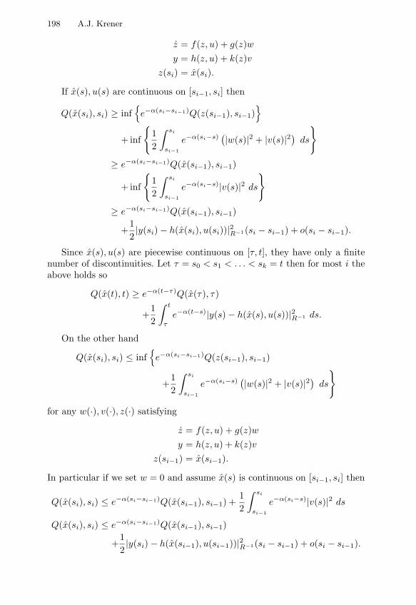
198 A.J. Krener

z = f(z, u) + g(z)wy = h(z, u) + k(z)v

z(si) = x(si).

If x(s), u(s) are continuous on [si−1, si] then

Q(x(si), si) ≥ infe−α(si−si−1)Q(z(si−1), si−1)

+ inf

12

∫ si

si−1

e−α(si−s) (|w(s)|2 + |v(s)|2) ds

≥ e−α(si−si−1)Q(x(si−1), si−1)

+ inf

12

∫ si

si−1

e−α(si−s)|v(s)|2 ds

≥ e−α(si−si−1)Q(x(si−1), si−1)

+12|y(si)− h(x(si), u(si))|2R−1(si − si−1) + o(si − si−1).

Since x(s), u(s) are piecewise continuous on [τ, t], they have only a finitenumber of discontinuities. Let τ = s0 < s1 < . . . < sk = t then for most i theabove holds so

Q(x(t), t) ≥ e−α(t−τ)Q(x(τ), τ)

+12

∫ t

τ

e−α(t−s)|y(s)− h(x(s), u(s))|2R−1 ds.

On the other hand

Q(x(si), si) ≤ infe−α(si−si−1)Q(z(si−1), si−1)

+12

∫ si

si−1

e−α(si−s) (|w(s)|2 + |v(s)|2) ds

for any w(·), v(·), z(·) satisfying

z = f(z, u) + g(z)wy = h(z, u) + k(z)v

z(si−1) = x(si−1).

In particular if we set w = 0 and assume x(s) is continuous on [si−1, si] then

Q(x(si), si) ≤ e−α(si−si−1)Q(x(si−1), si−1) +12

∫ si

si−1

e−α(si−s)|v(s)|2 ds

Q(x(si), si) ≤ e−α(si−si−1)Q(x(si−1), si−1)

+12|y(si)− h(x(si−1), u(si−1))|2R−1(si − si−1) + o(si − si−1).

The Convergence of the Minimum Energy Estimator 199

Therefore since x(s), u(s) are piecewise continuous on [τ, t], with only a finitenumber of discontinuities then

Q(x(t), t) ≤ e−α(t−τ)Q(x(τ), τ)

+12

∫ t

τ

e−α(t−s)|y(s)− h(x(s), u(s))|2R−1 ds.

Definition 2. [3] The system

z = f(z, u) + g(z)wy = h(z, u) (25)

is uniformly observable for any input if there exist coordinates

xij : i = 1, . . . , p, j = 1, . . . , li

where 1 ≤ l1 ≤ . . . ≤ lp and∑li = n such that in these coordinates the system

takes the form

yi = xi1 + hi(u)xi1 = xi2 + fi1(x1, u) + gi1(x1)w

...xij = xij+1 + fij(xj , u) + gij(xj)w

...xili−1 = xili + fi,li−1(xli−1, u) + gi,li−1(xli−1)wxili = fi,li(xli , u) + gi,li(xli)w

(26)

for i = 1, . . . , p where xj is defined by

xj = (x11, . . . , x1,j∧l1 , x21, . . . , xpj). (27)

Notice that in xj the indices range over i = 1, . . . , p; k = 1, . . . , j ∧ li =minj, li and the coordinates are ordered so that right index moves fasterthan the left.

We also require that each fij , gij be Lipschitz continuous and satisfy gro-wth conditions, there exists an L such that for all x, z ∈ R

n, u ∈ U ,

|fij(xj , u)− fij(zj , u)| ≤ L|xj − zj ||gij(xj)− gij(zj)| ≤ L|xj − zj ||fij(xj , u)| ≤ (L+ 1)|xj ||gij(xj)| ≤ L.

(28)

A system as above but without inputs is said to be uniformly observable [3].

200 A.J. Krener

Let

Ai =

0 1 0 . . . 00 0 1 . . . 0

. . .0 0 0 . . . 10 0 0 . . . 0

li×li

A =

A1 0 0

0. . . 0

0 0 Ap

n×n

Ci =[

1 0 0 . . . 0]1×li

C =

C1 0 0

0. . . 0

0 0 Cp

p×n

fi(x, u) =

fi1(x1, u)

...fili(xli , u)

li×1

f(x, u) =

f1(x, u)

...fp(x, u)

n×1

gi(x) =

gi1(x1)

...gili(xli)

li×l

g(x) =

g1(x)

...gp(x)

n×l

(29)

h(u) =[h1(u), . . . , hp(u)

](30)

then (26) becomes

x = Ax+ f(x, u) + g(x)wy = Cx+ h(u) (31)

We recall the high gain observer of Gauthier, Hammouri and Othman [3].Their estimate x(t) of x(t) given x0, y(s), 0 ≤ s ≤ t is given by the observer

˙x = Ax+ f(x, u) + g(x)w + S−1(θ)C ′(y − Cx− h(u))x(0) = x0 (32)

where θ > 0 and S(θ) is the solution of

A′S(θ) + S(θ)A− C ′C = −θS(θ). (33)

It is not hard to see that S(θ) is positive definite for θ > 0 for it satisfies theLyapunov equation

(−A− θ

2I

)′S(θ) + S(θ)

(−A− θ

2I

)= −C ′C

The Convergence of the Minimum Energy Estimator 201

where C,(−A− θ

2I)

is an observable pair and(−A− θ

2I)

has all eigenvaluesequal to − θ

2 .Gauthier, Hammouri and Othman [3] showed that when θ is sufficiently

large, p = 1, u=0 and w(·) is L∞[0,∞) then |x(t)− x(t)| → 0 exponentially ast → ∞. We shall modify their proof to show when θ is sufficiently large, p isarbitrary, u(·) is piecewise continuous and w(·) is L2[0,∞) then |x(t)−x(t)| →0 exponentially as t→∞. The key to both results is the following lemma. Wedefine

|x|2θ = x′S(θ)x.

SinceS(θ) ispositivedefinite, foreachθ > 0,thereexistsconstantsM1(θ), M2(θ)so that

M1(θ)|x| ≤ |x|θ ≤ M2(θ)|x|. (34)

Lemma 2. [3] Suppose g is of the form (29) and satisfies the Lipschitz con-ditions (28). Then there exists a Lipschitz constant L which is independent ofθ such that for all x, z ∈ R

n,

|g(x)− g(z)|θ ≤ L|x− z|θ. (35)

Note that g(x) is an n× l matrix so |g(x)− g(z)|θ denotes the induced operatornorm.

Proof. It follows from (33) that

Sij,rs(θ) =Sij,rs(1)θj+s−1 =

(−1)j+s

θj+s−1

(j + s− 2j − 1

). (36)

Let C = 1M2

1 (1) then

|x|2 ≤ C|x|21.Let σ = max|Sij,rs(1)| then for each constant w ∈ R

l

|g(x)w − g(z)w|2θ ≤∑

(gij(x)w − gij(z)w)′ Sij,rs(1)θj+s−1 (grs(x)w − grs(z)w)

≤ σL2∑ 1

θj+s−1 |xj − zj | |xs − zs| |w|2.

Defineξij =

xijθj, ζij =

zijθj

and ξj, ζ

jas with xj , zj . Then

1θj|xj − zj | ≤ |ξj − ζj |

and so

202 A.J. Krener

|g(x)w − g(z)w|2θ ≤ σL2θ∑|ξ

j− ζ

j| |ξ

s− ζ

s| |w|2

≤ σL2θn2|ξ − ζ|2 |w|2≤ σL2θCn2|ξ − ζ|21 |w|2≤ σL2Cn2|x− z|2θ |w|2

|g(x)− g(z)|2θ ≤ σL2Cn2|x− z|2θ.

Notice that for each u ∈ U , f(·, u) also satisfies the hypothesis of the abovelemma so

|f(x, u)− f(z, u)|θ ≤ L|x− z|θ.Theorem 2. Suppose

• the system (25) is uniformly observable for any input so that it can betransformed to (31) which satisfies the Lipschitz and growth conditions(28),

• u(·) is piecewise continuous,• w(·) is L2[0,∞), i.e., ∫ ∞

0|w(s)|2 ds <∞

• x(t), y(t) are any state and output trajectories generated by system (31)with inputs u(·) and w(·),

• θ is sufficiently large• x(t) is the solution of (32).

Then |x(t)− x(t)| → 0 exponentially as t→∞.

Proof. Let x(t) = x(t)− x(t) then

d

dt|x|2θ = 2x′S(θ) ˙x

= 2x′S(θ)(Ax+ f(x, u)− f(x, u) + (g(x)− g(x))w − S−1(θ)C ′Cx

)

≤ −θ|x|2θ + 2|x|θ |f(x, u)− f(x, u) + (g(x)− g(x))w|θ≤ (−θ + 2L(1 + |w|)) |x|2θ.

Define

β(t, τ) =∫ t

τ

−θ + 2L(1 + |w(s)|) ds.

We choose θ ≥ 5L and τ large enough so that

(∫ ∞

τ

|w(s)|2 ds) 1

2

≤ 1.

The Convergence of the Minimum Energy Estimator 203

Then for t− τ ≥ 1

β(t, τ) = (−θ + 2L)(t− τ) + 2L∫ t

τ

|w(s)| ds

≤ (−θ + 2L)(t− τ) + 2L(∫ t

τ

1 ds) 1

2(∫ t

τ

|w(s)|2 ds) 1

2

≤ (−θ + 2L)(t− τ) + 2L (t− τ)12

(∫ ∞

τ

|w(s)|2 ds) 1

2

≤ −L(t− τ)

By Gronwall’s inequality for 0 ≤ τ < τ + 1 ≤ t

|x(t)|2θ ≤ eβ(t,τ)|x(τ)|2θ≤ e−L(t−τ)|x(τ)|2θ

and we conclude that |x(t)− x(t)| → 0 exponentially as t→∞.

Theorem 3. (Main Theorem) Suppose

• the system (1) is uniformly observable for any input and so without lossof generality we can assume that is in the form

x = Ax+ f(x, u)y = Cx+ h(u) (37)

with A, C, f , h as above,• g(x) has been chosen so that (25) is uniformly observable for any input

and WLOG (25) is in the form (31) with A, C, f , g, h as above,• k(x) has been chosen to satisfy condition (5),• x(t), u(t), y(t) are any state, control and output trajectories generated by

the noise free system (37),• Q(x, t) is defined by (6) with α ≥ 0 for the system

x = Ax+ f(x, u) + g(x)wy = Cx+ h(u) + k(x)v (38)

where Q0(x0) ≥ 0 is Lipschitz continuous on compact subsets of Rn,

• x(t) is a piecewise continuous minimizing selection of Q(x, t), (8).

Then |x(t)−x(t)| → 0 as t→∞. If α > 0 then the convergence is exponential.

Proof. Let x(t) be the solution of the high gain observer (32) with g = 0,driven by u(t), y(t) where x0 = x0 and the gain is high enough to insureexponential convergence,

204 A.J. Krener

|x(t)− x(t)| → 0 as t→∞. (39)

We know that for any T ≥ 0 there exists wT (t) such that the solutionzT (t) of

zT = AzT + f(zT , u) + g(zT )wT

zT (T ) = x(T )

satisfies for 0 ≤ τ ≤ T

e−α(T−τ)Q(zT (τ), τ) + 12

∫ T

τe−α(T−s)

(|wT (s)|2 + |y(s)− CzT (s)− h(u(s))|2R−1

)ds

≤ e−αTT+1 +Q(x(T ), T )

From Lemma 1 we have for 0 ≤ τ ≤ T ,

Q(x(T ), T ) = e−α(T−τ)Q(x(τ), τ)

+12

∫ T

τ

e−α(T−s)|y(s)− Cx(s))− h(u(s))|2R−1 ds.

By the definition (6) of Q since x(s), y(s) satisfy the noise free system (37),

Q(x(τ), τ) ≤ e−ατQ0(x(0)),

so

Q(x(τ), τ) ≤ Q(x(τ), τ) ≤ e−ατQ0(x(0)).

Hence Q(x(T ), T ) is bounded if α = 0 and goes to zero exponentially asT →∞ if α > 0. From the definition (8) of x(τ) we have

Q(x(τ), τ) ≤ Q(zT (τ), τ).

From these we conclude that

12

∫ T

τ

eαs(|wT (s)|2 + |y(s)− CzT (s))− h(u(s))|2R−1

)ds

≤ 1T + 1

+ eατQ(x(τ), τ)

+12

∫ T

τ

eαs|y(s)− Cx(s))− h(u(s))|2R−1 ds

≤ 1T + 1

+Q0(x(0))

and it follows that∫ ∞

0eαs|y(s)− Cx(s))− h(u(s))|2R−1 ds <∞.

The Convergence of the Minimum Energy Estimator 205

Therefore given any ε there is a τ large enough so for all T ≥ τ

12

∫ T

τ

eαs|y(s)− Cx(s))− h(u(s))|2R−1 ds < ε

and

12

∫ T

τ

|wT (s)|2 + |y(s)− CzT (s))− h(u(s))|2R−1 ds (40)

< e−ατ

(1

T + 1+Q0(x0) + ε

).

Let zT (t) be the solution of the following high gain observer for zT (t)driven by u(t), wT (t) and CzT (t),

˙zT = AzT + f(zT , u) + g(zT )wT + S−1(θ)C ′(CzT − CzT )zT (0) = x0 (41)

then the error zT (t) = zT (t)− zT (t) satisfies

˙zT = AzT + f(zT )− f(zT , u) + (g(zT )− g(zT ))w − S−1(θ)C ′CzT

Proceeding as in the proof of Theorem 2 we obtain

d

dt|zT |2θ ≤ β(t, τ)|zT |2θ

where

βT (t, τ) =∫ t

τ

−θ + 2L(1 + |wT (s)|) ds.

We choose θ ≥ 5L and τ large enough so that for any T ≥ τ(∫ T

τ

|wT (s)|2 ds) 1

2

≤ 1.

Then for t− τ ≥ 1

βT (t, τ) = (−θ + 2L)(t− τ) + 2L∫ t

τ

|wT (s)| ds

≤ (−θ + 2L)(t− τ) + 2L(∫ t

τ

1 ds) 1

2(∫ t

τ

|wT (s)|2 ds) 1

2

≤ (−θ + 2L)(t− τ) + 2L (t− τ)12

(∫ T

τ

|wT (s)|2 ds) 1

2

≤ −L(t− τ)

206 A.J. Krener

By Gronwall’s inequality for 0 ≤ τ ≤ T

|zT (T )|2θ ≤ eβT (T,τ)|zT (τ)|2θ≤ e−L(T−τ)|zT (τ)|2θ

and we conclude that |zT (T ) − zT (T )| → 0 exponentially as T → ∞ hencex(T ) = zT (T )→ zT (T ) exponentially.

The last step of the proof is to show x(T ) → zT (T ) (exponentially ifα > 0). Now

d

dt(x− zT ) = Ax+ f(x, u) + S−1(θ)C ′(y − Cx− h(u))

− (AzT + f(zT , u) + g(zT )wT + S−1(θ)C ′(CzT − CzT )

)

=(A− S−1(θ)C ′C

)(x− zT )

+f(x, u)− f(zT , u)− g(zT )wT + S−1(θ)C ′(y − CzT − h(u))

so

d

dt|x− zT |2θ = 2(x− zT )′S(θ)

((A− S−1(θ)C ′C

)(x− zT )

+f(x, u)− f(zT , u)− g(zT )wT + S−1(θ)C ′(y − CzT − h(u)))

≤ −θ|x− zT |2θ + 2|x− zT |θ |f(x, u)− f(zT , u)− g(zT )w|θ+2|x− zT | |C ′ (y − CzT − h(u)

) |≤ (−θ + 2L)|x|2θ + 2LM2(θ)|x− zT |θ |wT |

+2|x− zT | |C ′ (y − CzT − h(u))) |.

We have chosen θ ≥ 5L. Using (28) and (34) we conclude that there is anM3(θ) > 0 such that

|x− zT | |C ′C (x− zT ) | ≤M3(θ)|x− zT |θ |y − CzT − h(u)|R−1

Therefore

d

dt|x− zT |2θ ≤ (−θ + 2L)|x− zT |2θ + 2LM2(θ)|x− zT |θ |wT |

+M3(θ)|x− zT |θ |y − CzT − h(u))|R−1

d

dt|x− zT |θ ≤ −L|x− zT |θ + LM2(θ)|wT |+M3(θ)|y − CzT − h(u)|R−1 .

By Gronwall’s inequality for 0 ≤ τ ≤ t ≤ T

The Convergence of the Minimum Energy Estimator 207

|x(t)− zT (t)|θ ≤ e−L(t−τ)|x(τ)− zT (τ)|θ+

∫ t

τ

e−L(t−s)LM2(θ)|wT | ds

+∫ t

τ

e−L(t−s)M3(θ) |y(s)− CzT (s)− h(u(s))|R−1 ds

≤ e−L(t−τ)|x(τ)− zT (τ)|θ

+LM2(θ)(∫ t

τ

e−2Ls ds

) 12(∫ t

τ

|wT |2 ds) 1

2

+M3(θ)(∫ t

τ

e−2Ls ds

) 12(∫ t

τ

|y(s)− CzT (s)− h(u(s))|2R−1 ds

) 12

≤ e−L(t−τ)|x(τ)− zT (τ)|θ

+LM2(θ)(∫ ∞

τ

e−2Ls ds

) 12(∫ t

τ

|wT |2 ds) 1

2

+M3(θ)(∫ ∞

τ

e−2Ls ds

) 12(∫ t

τ

|y(s)− CzT (s)− h(u(s))|2R−1 ds

) 12

≤ e−L(t−τ)|x(τ)− zT (τ)|θ

+LM2(θ)(

12L

) 12(∫ t

τ

|wT |2 ds) 1

2

+M3(θ)(

12L

) 12(∫ t

τ

|y(s)− CzT (s)− h(u(s))|2R−1 ds

) 12

.

As before, from (40) we see that given any δ we can choose τ large enoughso that for all α ≥ 0 and all τ ≤ t ≤ T we have

|x(t)− zT (t)|θ ≤ e−L(t−τ)|x(τ)− zT (τ)|θ + δ

so we conclude that |x(t)− zT (t)| → 0 as t→∞. In particular,|x(T )− zT (T )| → 0 as t→∞.

If α > 0 then (40) implies that for T = 2τ

|x(T )− zT (T )|θ ≤ e−LT2 |x(

T

2)− zT (

T

2)|θ

+LM2(θ)(

12L

) 12(

2e−αT2

(1

T + 1+Q0(x0) + ε

)) 12

+M3

(1

2L

) 12(

2e−αT2

(1

T + 1+Q0(x0) + ε

)) 12

.

Since we have already shown that |x(T2 )− zT (T

2 )| → 0 as T →∞, we concludethat |x(T )− zT (T )| → 0 exponentially as T →∞.

208 A.J. Krener

5 Conclusion

We have shown the global convergence of the minimum energy estimate tothe true state under suitable assumptions. The proof utilized a high gainobserver but it should be emphasized that the minimum energy estimatoris not necessarily high gain. It is low gain if the discount rate α is smalland the observation noise is substantial, i.e. R(x) is not small relative toΓ (x). It becomes higher gain as the α is increased, Γ (x) is increased or R(x)is decreased. For any size gain, the minimum energy estimator can makeinstantaneous transitions in the estimate as the location of the minimum ofQ(x, t) jumps around.

The principal drawback of the minimum energy estimator is that it requiresthe solution in the viscosity sense of the Hamilton Jacobi PDE (10) that isdriven by the observations. This is very challenging numerically in all but thesmallest state dimensions and the accuracy of the estimate is limited by thefineness of the spatial and temporal mesh. Krener and Duarte [7] have offereda hybrid approach to this difficulty. The solution of (10) is computed on avery coarse grid and this is used to initiate multiple extended Kalman filters(23) which track the local minima of Q(·, t). The one that best explains theobservations is taken as the estimate.

References

1. Baras JS, Bensoussan A, James MR (1988) SIAM J on Applied Mathematics48:1147–1158

2. Evans LC (1998) Partial Differential Equations. American Mathematical So-ciety, Providence, RI

3. Gauthier JP, Hammouri H, Othman S (1992) IEEE Trans Auto Contr 37:875–880

4. Gelb A (1974) Applied Optimal Estimation. MIT Press, Cambridge, MA5. Hijab O (1980) Minimum Energy Estimation PhD Thesis, University of Cali-

fornia, Berkeley, California6. Hijab O (1984) Annals of Probability, 12:890–9027. Krener AJ, Duarte A (1996) A hybrid computational approach to nonlinear

estimation in Proc. of 35th Conference on Decision and Control, 1815–1819,Kobe, Japan

8. Krener AJ (2002) The convergence of the extended Kalman filter. In:Rantzer A, Byrnes CI (eds) Directions in Mathematical Systems Theoryand Optimization, 173–182. Springer, Berlin Heidelberg New York, also athttp://arxiv.org/abs/math.OC/0212255

9. Mortenson RE (1968) J. Optimization Theory and Applications, 2:386–394

On Absolute Stability of Convergence forNonlinear Neural Network Models

Mauro Di Marco1, Mauro Forti1, and Alberto Tesi2

1 Dipartimento di Ingegneria dell’Informazione, Universita di SienaV. Roma 56 - 53100 Siena Italy, dimarco,forti@dii.unisi.it

2 Dipartimento di Sistemi e Informatica, Universita di Firenzev. S. Marta 3 - 50139 Firenze, Italy, atesi@dsi.unifi.it

Summary. This paper deals with a class of large-scale nonlinear dynamical sy-stems, namely the additive neural networks. It is well known that convergence ofneural network trajectories towards equilibrium points is a fundamental dynamicalproperty, especially in view of the increasing number of applications which involvethe solution of signal processing tasks in real time. In particular, an additive neuralnetwork is said to be absolutely stable if it is convergent for all parameters and allnonlinear functions belonging to some specified and well characterized sets, inclu-ding situations where the network possesses infinite non-isolated equilibrium points.The main result in this paper is that additive neural networks enjoy the property ofabsolute stability of convergence within the set of diagonal self-inhibition matrices,the set of symmetric neuron interconnection matrices, and the set of sigmoidal pie-cewise analytic neuron activations. The result is proved by generalizing a method forneural network convergence introduced in a recent paper, which is based on showingthat the length of each forward trajectory of the neural network is finite. The advan-tages of the result in this paper over previous ones on neural network convergenceestablished by means of LaSalle approach are discussed.

1 Introduction

A neural network is a large-scale nonlinear dynamical system obtained bymassively interconnecting in feedback a large number of elementary proces-sing units usually called neurons. The network is aimed at mimicking somefundamental mechanisms of biological neural systems, in order to achieve realtime processing capabilities useful to tackle pattern recognition and optimiza-tion problems [1].

A neural network is said to be convergent, or completely stable, when eachtrajectory converges towards an equilibrium point (a stationary state). Con-vergence is a fundamental property for neural network applications to severalsignal processing tasks [2, 3, 4, 5]. Consider for example the implementation

W. Kang et al. (Eds.): New Trends in Nonlinear Dynamics and Control, LNCIS 295, pp. 209–220, 2003.c© Springer-Verlag Berlin Heidelberg 2003

210 M. Di Marco, M. Forti, and A. Tesi

of a content addressable memory. The pattern corrupted by noise is providedas the initial condition to the neural network, and the process of retrievalof the uncorrupted pattern, which is represented by some stable equilibriumpoint of the network, is achieved during the convergent transient towards thisequilibrium. It is important to note that a convergent behavior is in gene-ral not guaranteed for a neural network. Indeed, oscillatory dynamics, suchas limit cycles, and even complex dynamics, such as chaotic attractors, havebeen observed in simulations and real experiments of some classes of neuralnetworks [2, 3, 6, 7].

A number of methods to investigate convergence of neural network tra-jectories have been developed in the last two decades [1, 3, 8]. Nevertheless,the problem of convergence is far from being completely solved, since severalissues need a much deeper understanding [9]. In particular, one of the mostchallenging issues in current neural network research is to obtain methodsfor studying convergence in situations where the nonlinear dynamical systemmodeling the network is of high order, and, most importantly, it possessesmultiple (possibly non-isolated) equilibrium points.

Within this context, this paper deals with the class of additive neural net-works, which are dynamical systems typically specified by sets of parameters(e.g., the neuron self-inhibitions, the synaptic neuron interconnections, andthe biasing neuron inputs), and sets of nonlinear functions (e.g., the sigmoidalneuron activations) [2, 3]. Specifically, we are interested in the issue of abso-lute stability of convergence, which means roughly speaking that convergenceholds for all neural network parameters, and all nonlinear neuron activations,belonging to specified and well characterized sets. This property represents akind of robustness of convergence with respect to parameter variations andwith respect to the actual electronic implementation of the nonlinearities. Itis worth to point out that an absolutely stable neural network enjoys the inte-resting property of being convergent even in situations, which are encounteredas the parameters are varied, where the network possesses infinite non-isolatedequilibrium points, e.g., when there are entire manifolds of equilibria.

The main result in this paper (Theorem 1) is that additive neural networksenjoy the property of absolute stability of convergence with respect to the setof diagonal self-inhibition matrices, the set of symmetric neuron interconnec-tion matrices, and the set of sigmoidal piecewise analytic neuron activations.The class of symmetric neural networks is central in the literature concerningconvergence of neural networks [2, 4, 5, 10]. Moreover, any neuron activa-tion referred to in specific examples is indeed modeled by piecewise analyticfunctions.

To prove Theorem 1, a method introduced in a recent paper [11] to addressabsolute stability of convergence for the class of standard Cellular NeuralNetworks [5], see also [12], is generalized. The method is based on provinga fundamental limit theorem for the neural network trajectories, accordingto which the total length of each forward trajectory is finite. This in turn

Absolute Stability of Convergence for Neural Networks 211

ensures convergence of each trajectory towards a singleton, independently ofthe structure of the set of the neural network equilibrium points.

The structure of the paper is briefly outlined as follows. In Sect. 2, thepiecewise analytic neural network model which is dealt with in the paperis introduced. Section 3 presents the main results on absolute stability ofconvergence, while Sect. 4 compares the obtained results with some basicexisting results in the literature on neural network convergence. Finally, themain conclusions drawn in the paper are reported in Sect. 5.

Notation.R

n : real n-spaceA = [Aij ] ∈ R

n×n : square matrixA′ : transpose of Aα = diag(α1, · · · , αn) ∈ R

n×n : diagonal matrix with diagonal entries αi,i = 1, · · · , nx = (x1, · · · , xn)′ ∈ R

n : column vector‖x‖2 =

[∑ni=1 x

2i

]1/2 : Euclidean norm of x∇V (x) : gradient of V (x) : R

n → R

2 Piecewise Analytic Neural Networks

Consider the class of additive neural networks described by the differentialequations

x = Ax+ Tg(x) + I (N)

where x = (x1, · · · , xn)′ ∈ Rn is the vector of the neuron states, A ∈ R

n×n

is a matrix modeling the neuron self-inhibitions, and T ∈ Rn×n is the neuron

interconnection matrix. The diagonal mapping g(x) = (g1(x1), · · · , gn(xn))′ :R

n → Rn has components gi(xi) that model the nonlinear input-output ac-

tivations of the neurons, whereas I ∈ Rn is a vector of constant neuron inputs.

Model (N) includes the popular Hopfield neural networks [4], the emergingparadigm of Cellular Neural Networks [5], and several other neural modelsfrequently employed in the literature.

Throughout the paper, some assumptions on the self-inhibition matrix A,the interconnection matrix T , and the activations g, are enforced. In order tostate these assumptions, the next definitions are introduced.

Definition 1 (Diagonal inhibitions DA). We say that A ∈ DA, if and onlyif A = diag(−a1, · · · ,−an) is a diagonal matrix such that ai > 0, i = 1, · · · , n.Definition 2 (Symmetric interconnections TS). We say that T ∈ TS , ifand only if T is symmetric, i.e., T ′ = T . Definition 3 (Sigmoidal piecewise analytic activations GA). We saythat g ∈ GA, if and only if, for i = 1, · · · , n, the following conditions hold:

212 M. Di Marco, M. Forti, and A. Tesi

a) gi is bounded on R;b) gi is piecewise analytic on R, i.e., there exist intervals Λi

j = (λij , λij+1) ⊂

R, j = 1, · · · , pi, with λi1 = −∞, λip =∞, λij+1 > λij, such that gi is analytic

in Λij; moreover, gi ∈ C0(R), and gi is strictly increasing on R, i.e., it results

∞ > M ij > dgi(xi)/dxi > 0 for all xi ∈ Λi

j. Assumption 1 We assume that A ∈ DA, T ∈ TS , and g ∈ GA.

Some comments on the above assumptions are in order. The hypothe-sis of diagonal self-inhibitions is standard for neural networks [4]. Moreo-ver, the set of piecewise analytic activations g ∈ GA is of interest, asit is witnessed by the fact that the most commonly used sigmoidal func-tions are analytic, and they belong to GA. Consider for example the po-pular activation gi(ρ) = (2/π) arctan(λπρ/2) proposed by Hopfield [4] (seeFig. 1(a)), the sigmoidal function gi(ρ) = 1/(1 + e−ρ), the multilevel activa-tions gi(ρ) =

∑ki/(1 + e−η(ρ−θi)) [13], and other activations referred to in

the literature. It is also noted that it is common practice in circuit theory toconstruct a model of a nonlinear function by using piecewise analytic appro-ximations [14] (see Fig. 1(b)-(c)).

The assumption of symmetric interconnections, T ∈ TS , is enforced fortwo main reasons. The first one is that such hypothesis is at the core of themost fundamental results on neural network convergence established in theliterature via LaSalle approach (cf. Sect. 4). The second one, is that symmetrymay be crucial to establish convergence. More specifically, it is known thatwhen the neuron interconnection matrix is largely non-symmetric, the net-work can exhibit oscillatory dynamics, such as limit cycles, and even complexdynamics, such as chaotic attractors [2, 3, 7, 15]. More recent investigationshave also shown that there are special classes of neural networks which un-dergo complex bifurcations, leading to the birth of non-convergent dynamics,even close to some neural network with nominal symmetric interconnections[7, 16].

In this paper, we are interested in absolute stability of convergence (seeDefinition 5) for the class of neural networks (N) where the self-inhibitionsA ∈ DA, the interconnection matrix T ∈ TS , and the neuron activationsg ∈ GA. To define the concept of absolute stability of convergence, let usconsider the set of the equilibrium points of (N), which is given by

E = x ∈ Rn : Ax+ Tg(x) + I = 0. (1)

Under the assumptions A ∈ DA and g ∈ GA it can be shown that E is notempty [17]. Furthermore, it is stressed that the equilibria of (N) may be ingeneral non-isolated, as it is shown in Example 1 below.

Definition 4 ([3]). Given some A, T , g, and I, the neural network (N) issaid to be convergent if and only if, for any trajectory x(t) of (N), there existsx ∈ E such that

Absolute Stability of Convergence for Neural Networks 213

−3 −2 −1 0 1 2 3−1

−0.8

−0.6

−0.4

−0.2

0

0.2

0.4

0.6

0.8

1

ρ

ρg

( )

i

−3 −2 −1 0 1 2 3−1

−0.8

−0.6

−0.4

−0.2

0

0.2

0.4

0.6

0.8

1

ρ

ρg

( )

i

(a) (b)

−3 −2 −1 0 1 2 3

0

0.2

0.4

0.6

0.8

1

ρ

ρg

( )

i

(c)

Fig. 1. Sigmoidal piecewise analytic neuron activations in the class GA. (a) The stan-dard analytic neuron activation gi(ρ) = (2/π) arctan(λπρ/2) proposed by Hopfield(λ = 1); (b) a piecewise analytic approximation of the sigmoidal activation in (a)using polynomials and rational functions (see (4)); (c) sigmoidal piecewise analyticfunction obtained by piecing together two exponential functions (gi(ρ) = (1/2)eρ−1

for ρ ≤ 1; gi(ρ) = 1 − (1/2)e−3(ρ−1) for ρ > 1).

limt→+∞x(t) = x.

The property of convergence, which is frequently referred to in the li-

terature as complete stability, is related to a specific neural network wherethe self-inhibitions A, interconnection matrix T , nonlinear activations g, andinputs I, have been fixed. In this paper we are interested in the stronger pro-perty of absolute stability of convergence, which is related to an entire set ofneural networks, as stated in the next definition.

214 M. Di Marco, M. Forti, and A. Tesi

Definition 5. We say that convergence of (N) is absolutely stable within thesets DA, TS , and GA, if and only if (N) is convergent for any neuron self-inhibition matrix A ∈ DA, any neuron interconnection matrix T ∈ TS , anyneuron activations g ∈ GA, and any neuron input I ∈ R

n. It is worth to remark that the concept of absolute stability of convergence

as in Definition 5 should not be confused with the property of absolute sta-bility defined in previous work [17, 18]. In fact, in those papers the absolutestability refers to neural networks that possess a unique equilibrium point,while in Definition 5 we consider more generally neural networks with multi-ple equilibria, e.g., networks with entire manifolds of equilibrium points.

3 Main Result

The main result on absolute stability of convergence of neural network (N) isas follows.

Theorem 1. Convergence of (N) is absolutely stable within the sets DA, TS ,and GA.

This result includes situations where the neural network (N) possessesinfinite non-isolated equilibrium points, see Example 1 below. In this respect,it differs substantially from existing results on complete stability of (N) in theliterature, as it is discussed in Sect. 4.

Example 1. Consider the second-order neural network

x1 = −x1 + g1(x1)− g2(x2)x2 = −x2 − g1(x1) + g2(x2) (2)

where

g1(ρ) =

14ρ3, |ρ| ≤ 1;

ρ

ρ+ 3, ρ > 1;

ρ

−ρ+ 3, ρ < −1

(3)

and

g2(ρ) =

ρ− 14ρ3, |ρ| ≤ 1;

3ρ3ρ+ 1

, ρ > 1;

3ρ−3ρ+ 1

, ρ < −1.

(4)

Absolute Stability of Convergence for Neural Networks 215

The neural network (2) satisfiesA ∈ DA, T ∈ TS , and g(x) = (g1(x1), g2(x2))′ ∈GA. Moreover, it can be easily verified that the set E of the equilibrium pointsof (2) contains the set E = (x1, x2) ∈ R

2 : x1 = −x2; |x1| ≤ 1, |x2| ≤ 1.Figure 2 reports the trajectories of (2), as obtained with MATLAB, for a

number of different initial conditions. It is seen that each trajectory convergestowards a unique equilibrium point within the set E , in accordance with theresult in Theorem 1.

−2 −1.5 −1 −0.5 0 0.5 1 1.5 2−2

−1.5

−1

−0.5

0

0.5

1

1.5

2

x1

x2

Fig. 2. Phase portrait of neural network (2). The initial conditions are representedby the symbol . The set E of equilibrium points corresponds to the thick solidsegment.

Below, the main steps of the proof of Theorem 1 are outlined. The wholetechnical details can be found in [19].

1. Let us consider the Lyapunov function

W (x) = −12g′(x)Tg(x)− g′(x)I +

n∑i=1

ai

∫ xi

0

dgi(ρ)dρ

ρ dρ (5)

which has been introduced by Hopfield to study the dynamics of (N) [4].The following classic result holds [3, 4].

216 M. Di Marco, M. Forti, and A. Tesi

Property 1 Suppose that A ∈ DA, T ∈ TS , and g ∈ GA. Then, W is astrict Lyapunov function for (N), i.e., it results W(N)(x) = [∇W (x)]′x ≤ 0for all x ∈ R

n, E = x ∈ Rn : W(N)(x) = 0, and W(N)(x) < 0 for

x ∈ Rn\E.

Since the trajectories of (N) are bounded on [0,+∞), Property 1 implies,on the basis of LaSalle invariance principle, that the ω-limit set of eachtrajectory of (N) is contained within the set E of equilibrium points of(N). If in particular E is made up of isolated equilibria, then (N) is con-vergent, due to the connectedness of the ω-limit set. However, when (N)has uncountably many equilibrium points, it cannot be concluded on thebasis of LaSalle approach alone that (N) is convergent. Indeed, there is therisk that a trajectory indefinitely slides over some manifold of equilibria,without converging to a singleton.The previous discussion shows that further argument with respect to La-Salle invariance principle is needed to prove convergence of (N) in thegeneral case of non-isolated equilibrium points. Such an argument, whichis provided in points 2) and 3) below, exploits the basic assumption thatthe neuron nonlinearities g are modeled by piecewise-analytic functions.

2. The existence of a strict Lyapunov function W (see Property 1), togetherwith the hypothesis g ∈ GA (cf. Assumption 1), is exploited in order toestablish a basic property of the neural network trajectories. Namely, itis shown that the length of the trajectories of (N) on the time interval[0,+∞) is necessarily finite.To state this result more formally, let x(t), t ∈ [0,+∞), be some trajectoryof (N). For any t > 0, the length of x(t) on [0, t) is given by

∫ t

0 ‖x(σ)‖2 dσ.The following result can be proved.

Theorem 2. Suppose that A ∈ DA, T ∈ TS , and g ∈ GA. Then, anytrajectory x(t) of (N) has finite length on [0,+∞), i.e.,

L =∫ +∞

0‖x(σ)‖2 dσ = lim

t→+∞

∫ t

0‖x(σ)‖2 dσ < +∞.

Once it has been shown that the total length of x(t) is finite, a standardmathematical argument allows one to conclude the existence of the limitof x(t) as t → +∞, hence convergence of x(t) towards an equilibriumpoint of (N) (see the proof of Corollary 1 in [11]).

3. The proof of Theorem 2 exploits a fundamental inequality established byLojasiewicz for analytic functions, which is reported next.Consider a function F (x) : Γ ⊂ R

n → R, which is analytic in the openset Γ , and assume that the set of critical points of F

C = x ∈ Γ : ∇F (x) = 0is not empty. Then, it possible to give an estimate from below of the normof the gradient of F , in a neighborhood of a critical point x0, as stated inthe next lemma.

Absolute Stability of Convergence for Neural Networks 217

Lemma 1. 1 Suppose that x0 ∈ C. Then, there exists R > 0 and anexponent θ ∈ (0, 1) such that

‖∇F (x)‖2 ≥ |F (x)− F (x0)|θ (6)

for ‖x− x0‖ < R. Lojasiewicz inequality plays a key role to prevent trajectories of (N) fromsliding over some manifold of equilibrium points without converging toa singleton. In fact, the use of such an inequality leads to a direct proofthat the length of each trajectory of (N) is necessarily finite, even whenthe neural network possesses entire manifolds of equilibria. The technicaldetails of the proof of this argument are given in [19]. We conclude this section by noting that the method of proof of Theo-

rem 1 generalizes that previously introduced to analyze absolute stability ofthe standard Cellular Neural Networks [11], and general additive neural net-works with neuron activations modeled by piecewise linear functions [12]. Itis worth to note that the property of finiteness of trajectory length for stan-dard Cellular Neural Networks was directly proved in [11] by exploiting thespecial structure of the piecewise affine vector fields describing the dynamicsof a Cellular Neural Network. Since general piecewise analytic vector fieldsare considered for (N), the specific arguments used in [11] are no longer ap-plicable. As it was noted before, Lojasiewicz inequality is the key additionalmathematical device here employed to extend the proof of finiteness of lengthto the general model (N).

4 Discussion

In this section, we briefly compare the result on absolute stability of conver-gence in Theorem 1 with previous results on convergence of the additive neuralnetwork (N) in the literature [2, 3, 4, 10]. Those results require A ∈ DA, andthe symmetry of the interconnection matrix (T ∈ TS), but are applicable inthe less restrictive case, with respect to Theorem 1, where the neuron non-linearities g only need to be Lipschitz continuous sigmoidal functions. Sinceunder such hypotheses (N) possesses a strict Lyapunov function, the quotedresults on convergence are obtained as a direct application of LaSalle invari-ance principle. It is noted, however, that all those results require the additionalassumption, with respect to Theorem 1, that the equilibrium points of (N)be isolated. This is due to the fact that, as it was discussed before, LaSalleapproach is not suitable to prove convergence in the general case where theequilibrium points are not isolated. Finally, we remark that an additional ma-thematical device used in some of the quoted papers is Sard’s theorem, which1 See, e.g., Theorem 4 in [20].

218 M. Di Marco, M. Forti, and A. Tesi

enables to prove that given specific neuron self-inhibitions A, neuron activati-ons g, and symmetric interconnection matrix T , for almost all neural networkinputs I the equilibrium points are isolated (see, e.g., [10, Theorem 4.1]). Insummary, the results in [2, 3, 4, 10] are basically results on almost absolutestability of convergence. Furthermore, they leave open the issue of convergencefor those parameters where there are non-isolated equilibrium points of (N).2

From the previous discussion it is seen that the result on absolute stabilityof convergence in Theorem 1 actually refers to a more restrictive class ofneural networks with respect to [2, 3, 4, 10]. However, it enjoys the significantadvantage that there is no technical difficulty to verify the hypotheses ofTheorem 1. For comparison, we stress the fact that the notion of almostabsolute stability of convergence is not simple to deal in practice, due totechnical difficulties to establish whether or not a given neural network hasisolated equilibria. Indeed, Sard’s theorem does not specify the critical setfor which there are non-isolated equilibrium points, and there is no generalmethod to find all equilibria of (N) for sigmoidal activations.

There are also other advantages of the property of absolute stability ofconvergence as in Theorem 1, with respect to the weaker notion of almostabsolute stability of convergence. In fact, there are interesting applicationswhere it is required that the neural network (N) be convergent also when itpossesses entire manifolds of equilibrium points. This is the case when thenetwork is used to retrieve a static pattern within a set of uncountably manyequilibrium patterns, as in the problems discussed in [2, Sect. I].

5 Conclusion

The paper has considered a class of additive neural networks where the neu-ron self-inhibitions are modeled by diagonal matrices with negative diagonalelements, the neuron interconnection matrix is symmetric, and the neuronactivations are modeled by sigmoidal piecewise analytic functions. The mainresult is that convergence is absolutely stable within this class, i.e., it holdsfor all parameters and all nonlinear functions defining the considered class,including situations where the neural network possesses infinite non-isolatedequilibrium points. The result has been proved through a generalization of anew method that has been recently introduced to analyze convergence of neu-ral networks. The method is based on showing that the length of each forward2 It is known that a system possessing a strict Lyapunov function and non-isolated

equilibria may in general be non-convergent. A classical example is due to Palisand De Melo [21, Example 3, p. 14]. This corresponds to a planar gradient systemwhere all bounded trajectories have an entire circle of equilibrium point as theω-limit set. Actually, these trajectories show a large-size non-vanishing oscillationin the long-run behavior, without converging to a singleton. It is worth to notethat such a kind of non-convergent dynamics would be highly undesirable for theapplication of neural networks to solve signal processing tasks.

Absolute Stability of Convergence for Neural Networks 219

trajectory of the neural network is necessarily finite. It has also been pointedout that LaSalle approach would be not suitable to address absolute stabilityof convergence for the considered class. Indeed, even in the presence of a strictLyapunov function, LaSalle invariance principle does not imply convergencein the general case of non-isolated equilibrium points.

Future work aims at exploring absolute stability of convergence for largerclasses of neural networks. A possible case of special interest is that of neuralnetworks where the neuron activations are characterized by a threshold valueunder which they are zero. In that case, the energy function of the neural net-work is no more strictly decreasing along the trajectories, and a more generaltechnique than that presented in this paper is required to prove finiteness oftrajectory length for each forward trajectory.

References

1. Grossberg S (1988) Nonlinear neural networks: Principles, mechanisms, andarchitectures. Neural Networks, 1:17–61.

2. Cohen M. A., Grossberg S. (1983) Absolute stability of global pattern formationand parallel memory storage by competitive neural networks. IEEE Trans. Syst.Man Cyber., 13:815–825.

3. Hirsch M. (1989) Convergent activation dynamics in continuous time networks.Neural Networks, 2:331–349.

4. Hopfield J. J. (1984) Neurons with graded response have collective computatio-nal properties like those of two-state neurons. Proc. Nat. Acad. Sci., 81:3088–3092.

5. Chua L. O., Yang L. (1988) Cellular neural networks: Theory. IEEE Trans.Circuits Syst., 35(10):1257–1272, October.

6. Chua L. O. (1997) CNN: A vision of complexity. Int. J. Bifurcation and Chaos,7(10):2219–2425, October.

7. Di Marco M., Forti M., Tesi A. (2000) Bifurcations and oscillatory behavior ina class of competitive cellular neural networks. Int. J. Bifurcation and Chaos,10(6):1267–1293, June.

8. Chua L. O., Wu C. W. (1992) On the universe of stable cellular neural networks.Int. J. Circuit Theory Applicat., 20:497–517.

9. Lemmon M. D., Michel, A. N. (Eds.) (1999) Special section on neural networksin control, identification, and decision making. IEEE Trans. Automat. Contr.,44(11):1993–2057, November.

10. Li J. H., Michel A. N., Porod W. (1988) Qualitative analysis and synthesis ofa class of neural networks. IEEE Trans. Circuits Syst., 35(8):976–986, August.

11. Forti M., Tesi A. (2001) A new method to analyze complete stability of PWLcellular neural networks. Int. J. Bifurcation and Chaos, 11:655–676, March.

12. Forti M. (2002) Some extensions of a new method to analyze complete stabilityof neural networks. IEEE Trans. Neural Networks, 13:1230–1238, September.

13. Bang S. H., Sheu B. J., Chang J. C.-F. (1994) Search of optimal solutions inmulti-level neural networks. In Proc. ISCAS 1994, IEEE Int. Symp. on Circuitsand Systems, volume 6, pages 423–426, London.

220 M. Di Marco, M. Forti, and A. Tesi

14. Chua L. O., Desoer C. A., Kuh E. S. (1987) Linear and Nonlinear Circuits.McGraw-Hill, New York.

15. Chua L. O. (Edt.) (1995) Special issue on nonlinear waves, patterns and spatio-temporal chaos in dynamic arrays. IEEE Trans. Circuits Syst. I, 42(10):557–823, October.

16. Di Marco M., Forti M., Tesi A. (2002) Existence and characterization of limitcycles in nearly symmetric neural networks. IEEE Trans. Circuits Syst. I,49(7):979–992, July.

17. Forti M., Tesi A. (1995) New conditions for global stability of neural networkswith application to linear and quadratic programming problems. IEEE Trans.Circuits Syst. I , 42:354–366.

18. Liang X.-B., Wang J. (2001) An additive diagonal stability condition for abso-lute stability of a general class of neural networks. IEEE Trans. Circuits Syst.I, 48:1308–1317, November.

19. Di Marco M., Forti M., Tesi A. (2002) A method to analyze complete stabilityof analytic neural networks. Technical Report 15, Universita di Siena, Siena,Italy.

20. Lojasiewicz S. (1959) Sur le probleme de la division. Studia Math., T. XVIII:87–136.

21. Palis J. De Melo W. (1982) Geometric Theory of Dynamical Systems. Springer-Verlag, Berlin.

A Novel Design Approach to Flatness-BasedFeedback Boundary Control of NonlinearReaction-Diffusion Systems with DistributedParameters

Thomas Meurer and Michael Zeitz

Institute of System Dynamics and Control Engineering, University of Stuttgart,Pfaffenwaldring 9, 70569 Stuttgart, Germany,meurer,zeitz@isr.uni-stuttgart.de

1 Introduction

Differential flatness has proven to be a very powerful approach for analysisand design of open–loop and stabilizing feedback tracking control for nonlinearfinite–dimensional systems [2, 10, 11]. Thereby, flatness can be interpreted asa generalization of controllability or the possibility to determine the inversemodel, respectively. The flatness approach has been extended to the design ofopen–loop boundary control for infinite–dimensional or distributed parame-ter systems (DPSs) described by partial differential equations (PDEs). Theparameterization of system states and boundary input by a flat output (in-verse system) can be obtained for parabolic DPS by assuming a power seriesexpansion of the solution [5, 6, 7, 8]. Applications concern the linear heatconduction equation [5], rather general nonlinear parabolic PDEs describingdiffusion or heat conduction [8], and nonlinear tubular reactor models [6, 7].Note, that also the case of time–dependent coefficients is treated [8]. In thescope of industrial applications, flatness–based open–loop boundary controlof a solenoid valve modelled by Maxwell’s equations with space–dependentcoefficients is addressed in [12]. Nevertheless, the use of open–loop boundarycontrol is rather limited due to disturbances acting on the system or modeluncertainties. Hence, a closed–loop strategy is desired, trying to cope withthese effects.

This was the motivation of the authors for a flatness–based approach to thedesign of feedback boundary tracking control for linear DPS as illustrated in[9] for the boundary control of a linear heat conduction equation. The results of[9], which allow the exploitation of the full scope of differential flatness for thefeedback boundary control design, are extended in the present contribution

W. Kang et al. (Eds.): New Trends in Nonlinear Dynamics and Control, LNCIS 295, pp. 221–235, 2003.c© Springer-Verlag Berlin Heidelberg 2003

222 T. Meurer and M. Zeitz

to asymptotic tracking control for nonlinear parabolic DPS. This includesmotion planning, inspection of state or input constraints, asymptotic feedbackstabilization, and observer design. The proposed flatness–based procedure isdemonstrated for the boundary control of a nonlinear parabolic distributedparameter model of a reaction–diffusion system.

The paper is organized as follows. The control problem is specified in Sec-tion 2 for a rather general scalar nonlinear reaction–diffusion PDE. The proofof flatness for the considered DPS and the design of flatness–based open–loopcontrol are treated in Section 3 serving as basis for the boundary feedbackcontrol design in Section 4. The performance of open–loop and feedback con-trol is studied in various simulation scenarios in Section 5, followed by someconcluding remarks.

2 Problem Formulation

Consider a scalar reaction–diffusion system modelled by the rather generalnonlinear parabolic PDE

∂x(z, t)∂t

=∂2x(z, t)∂z2

+ ϕ

(x(z, t),

∂x(z, t)∂z

), t > 0, z ∈ (0, 1) (1)

∂x

∂z(0, t) = u(t), t > 0 (2)

∂x

∂z(1, t) = 0, t > 0 (3)

x(z, 0) = x0(z), z ∈ [0, 1] (4)y(t) = x(1, t), t ≥ 0, (5)

where state x(z, t), time t, spatial coordinate z, boundary input u(t), ou-tput variable y(t), and any model parameter are assumed to be perfectlynon–dimensionalized. The nonlinear function ϕ

(x, ∂x∂z

)could describe a tem-

perature–dependent heat source, some kind of chemical reaction following anonlinear reaction rate [13], or nonlinear convection. In Section 3, some re-strictions will be imposed on the class of functions ϕ.

The considered control problem concerns the design of a boundary controlu for a possibly unstable system (1)–(5), in order to realize the transitionbetween the initial stationary profile x0(z) = x1

S(z) and a final stationaryprofile x2

S(z) in finite time T such that y(t ≥ T ) = x2S(1) in the presence of

model errors or exogenous disturbances.For the solution of this control problem, both open–loop and feedback

control will be considered. Therefore, inspired by the flatness property offinite–dimensional nonlinear systems, a flat output will be determined in orderto parameterize the system state x(z, t) as well as boundary input u(t).

Flatness-Based Feedback Boundary Control of Reaction-Diffusion Systems 223

3 Flatness-Based Motion Planning and Open-LoopBoundary Control

The proof of flatness and hence the design of an open–loop control for theconsidered DPS is based on a power series approach as proposed in [5, 6, 7, 8].Similarly, motion planning is addressed based on Gevrey functions [3].

3.1 Flatness of the Nonlinear DPS

In order to analyze the flatness of (1)–(5), a formal power series ansatz forthe state x(z, t) with yet unknown time–varying coefficients an(t) is used, i.e.

x(z, t) =∞∑

n=0

an(t)(1− z)n, (6)

which can be formally differentiated with respect to t and z. The formalpower series ansatz (6) considered throughout this contribution differs fromthe one proposed e.g. in [6, 7, 8], where the ansatz is defined in terms ofthe scaled arguments an(t) = n! an(t). However, the formal approach (6)provides significantly better numerical conditioning for the implementationand simulation of the boundary feedback control design presented in Section4. Inserting (6) into PDE (1) yields

∞∑n=0

(1− z)n [an(t)− (n+ 2)(n+ 1)an+2(t)]

= ϕ

( ∞∑n=0

an(t)(1− z)n, −∞∑

n=0

(n+ 1)an+1(t)(1− z)n).

(7)

This infinite set of nonlinear equations for the series coefficients an(t), n ≥ 0only provides a solution by comparing polynomials in (1− z), if the nonlinearsource term is restricted to functions allowing a power series expansion of thefollowing form

ϕ(x, ∂x∂z

)=

∞∑n=0

ϕn(an+1(t))(1− z)n, (8)

where

an+1(t) = [a0(t), . . . , an+1(t)], (9)

and ϕn(an+1(t)) being smooth with respect to its arguments for any n ∈ N.This condition imposes only weak limitations as will be shown throughoutthis section. As a result, terms of equal order n in the polynomials (1 − z)ncan be arranged in (7)

224 T. Meurer and M. Zeitz

∞∑n=0

(1− z)n [an(t)− (n+ 2)(n+ 1)an+2(t)− ϕn(an+1(t))] = 0,

which yields

an(t)− (n+ 2)(n+ 1)an+2(t)− ϕn(an+1(t)) = 0 ∀n ∈ N. (10)

Eqn. (10) can be evaluated recursively by solving for an+2(t) and consideringthe boundary condition (3) and the output equation (5)

an+2(t) =an(t)− ϕn(an+1(t))

(n+ 2)(n+ 1), a1(t) = 0, a0(t) = y(t). (11)

This recursion allows a parameterized solution for the series coefficients an(t)in terms of the controlled variable y(t) and its time–derivatives y(i)(t), i ≥ 1

an(t) = φn

(y(t), y(t), . . . , y(j)(t)

), j =

n2 n evenn−1

2 n odd.(12)

In general, Eqn. (11) can be efficiently evaluated by use of a computer–algebra–system like Mathematica [14]. Under the formal assumption of se-ries convergence, the state x(z, t) at any point (z, t) and the input u(t) =∂x∂z (0, t) can be determined by substituting (12) into the formal ansatz (6), i.e.

x(z, t) =∞∑

n=0

φn (yn(t)) (1− z)n = Φ(y(t), y(t), . . . ), (13)

u(t) = −∞∑

n=1

nφn (yn(t)) = Ψ(y(t), y(t), . . . ), (14)

where yn(t) = [y(t), . . . , y(n)(t)]. A straightforward comparison of (13), (14)with the definition of differential flatness for finite–dimensional systems [2]illustrates, that the controlled variable y(t) = x(1, t) represents a flat outputfor the infinite–dimensional system (1)–(4), whereby an infinite number oftime–derivatives of the flat output is necessary to parameterize system stateand input.

Note that Eqn. (8) only imposes a rather weak restriction on ϕ(x, ∂x∂z

)since

many nonlinear functions allow at least an asymptotic power series expansion,which can be evaluated by the formal power series ansatz (6) using for exampleCauchy’s product formula. Some technically important examples for ϕ

(x, ∂x∂z

)together with their evaluation using the formal power series ansatz (6) aresummarized below:

• Model of an isothermal tubular reactor concentration x(z, t) with thirdorder reaction

∑3i=1 βixi and linear convection α∂x

∂z

Flatness-Based Feedback Boundary Control of Reaction-Diffusion Systems 225

ϕ(x, ∂x∂z ) = α∂x∂z + β1x+ β2x

2 + β3x3

=∞∑

n=0

[−α(n+ 1)an+1(t) + β1an(t) + β2

n∑p=0

an−p(t)ap(t)+

β3

n∑p=0

an−p(t)p∑

q=0

ap−q(t)aq(t)

](1− z)n

(15)

• Model of a tubular bioreactor concentration x(z, t) with linear convectionα∂x

∂z and Monod kinetics β x1+x [1]

ϕ(x, ∂x∂z ) = α∂x∂z + β x

1+x

≈ α∂x∂z + β

m∑n=0

(−1)nxn+1

=∞∑

n=0

[−α(n+ 1)an+1(t) + β

m∑p=0

(−1)pcnp+1(t)

](1− z)n,

(16)

where cn1 (t) = an(t) and cnp (t) denotes the Cauchy product for xp, p ∈ N

with x from (6). Here, the kinetic function β x1+x is expanded only asym-

ptotically by truncating the series expansion for 11+x at some m ∈ N.

3.2 Convergence of the Formal Solution and Motion Planning

In order to obtain an open–loop boundary control as stated in Section 2, asmooth trajectory yd(t) for the flat output y(t) of class C∞ has to be specifiedconnecting the two stationary profiles x1

S(z) and x2S(z) at z = 1. It follows

directly that yd(0) = x1S(1) and yd(t ≥ T ) = x2

S(1) since the flat outputy(t) completely parameterizes the state (13) and hence the stationary profilesxS(z) = x(z, t→∞). The convergence of the infinite series solutions (13) and(14) has to be ensured by an appropriate choice of the desired trajectory yd(t).Due to the broad class of possible nonlinear source terms, convergence has tobe proven for each given function ϕ

(x, ∂x∂z

)in (1) allowing an expansion given

by (8). Therefore in the remainder of this paper, only the particular functionϕ given by Eqn. (15) will be considered.

In [6], it is shown that (13) and (14) converge for β1,3 = 0 in (15), i.e. asecond order reaction, with unit radius of convergence, if yd(t) : R → R is aGevrey function of class γ ≤ 2, i.e. a C∞ function satisfying

supt∈R

|y(n)d (t)| ≤ m(n!)γ

Rn, ∀n ≥ 0, γ ≤ 2, (17)

where m and R are constants, and if in addition the following inequality issatisfied

226 T. Meurer and M. Zeitz

|α|+ |β2|m+ 2R−1 ≤ 2.

This clearly illustrates the importance of motion planning since the giveninequality combines the physics of the problem given by parameters α and β2with the estimates on the bounds of the chosen desired trajectory. Followinga similar argumentation as in [6], it can be shown, that the open–loop control(14) converges for β1,3 = 0 in (15), i.e. a third order reaction, with unit radiusof convergence, if the desired trajectory yd(t) : R→ R is a Gevrey function ofclass γ ≤ 2 and if in addition the following inequality is satisfied

|α|+ |β1|+ |β2|m+ |β3|m2 + 2R−1 ≤ 2. (18)

Numerical results indicate that also nonlinearities involving powers of order≥ 4 in the state x(z, t) allow the derivation of convergent infinite series ex-pansions for system state and boundary control.

In the following, similar to [5] and [8], motion planning is based on a socalled smooth ’step function’ of Gevrey order γ = 1 + 1

ω

Θω,T (t) =

0 if t ≤ 01 if t ≥ T∫ t0 θω,T (τ)dτ

∫ T0 θω,T (τ)dτ

if t ∈ (0, T )(19)

where θω,T denotes the ’bump function’

θω,T (t) =

0 if t ∈ (0, T )

exp

(−1[

(1− tT ) t

T

]ω)

if t ∈ (0, T ).(20)

Therefore, a desired trajectory being consistent with both the initial and finalstationary profile is realized by

yd(t) = x1S(1) + (x2

S(1)− x1S(1))Θω,T (t), (21)

such that yd(0) = x1S(1) and yd(t ≥ T ) = x2

S(1). As outlined above, theparameters ω and T of (19) have to be chosen appropriately for every desi-red final stationary profile x2

S(z) in order to ensure convergence of the seriesexpansions (13), (14) and satisfy possible state and input constraints. Thisresults in the associated open–loop control ud(t) = Ψ(yd(t), yd(t), . . . ) with|ud(t)| < u similar to results proposed in [6, 7, 8, 12] for other DPS controlproblems. Note however, that for implementation the open–loop control (14)has to be truncated at a certain integer, since it is impossible to compute aninfinite series. Due to this fact and in view of exogenous disturbances, modelerrors or instability, a closed–loop control strategy is needed.

Flatness-Based Feedback Boundary Control of Reaction-Diffusion Systems 227

4 Flatness-Based Feedback Boundary Tracking Control

Based on a re–interpretation of the results for the flatness–based open–loopcontrol design for the DPS (1)–(5) as summarized in Section 3, the design ap-proach originally proposed in [9] for linear flatness–based feedback boundarycontrol is extended to the considered nonlinear problem.

4.1 Flat Design Model for Feedback Boundary Control

As illustrated in the previous section, appropriate motion planning ensuresconvergence of the formal solution (6). Therefore, re–consider Eqn. (7), andsubstitute the abbreviations (8), (9), i.e.

∞∑n=0

(1− z)n [an(t)− (n+ 2)(n+ 1)an+2(t)− ϕn (an+1(t))] = 0. (22)

Under the formal assumption of convergence, the series expansion (14) for theopen–loop control can be truncated at some upper limit 2N, N ∈ N, whichis equivalent to consider only the first 2N − 2 terms of summation in (22)

an(t)− (n+ 2)(n+ 1)an+2(t)− ϕn (an+1(t)) = 0, n ∈ 0, 1, . . . , 2N − 2.(23)

Differing from the previous section where (23) was solved for an+2(t) to obtaina recursion formula, interpret (23) as a set of nonlinear ordinary differentialequations (ODEs) for the coefficients an(t), n = 0, 1, . . . , 2N − 2. Note, sincea1(t) = 0 by boundary condition (3) and hence a(k)

1 (t) = 0, k ∈ N, thecoefficients an(t), n = 1, 3, . . . , 2N−1 can be expressed in terms of an(t), n =0, 2, . . . , 2N − 2 by successively evaluating (23):

a1(t) = 0,a2n+1(t) = θ2n+1 (a0(t), a2(t), . . . , a2n(t)) , n ≥ 1. (24)

In the following an+1(t) denotes (9) with (24) substituted. Therefore, consi-dering 2N − 2 terms in (23) results in the following N nonlinear ODEs

a0(t) = 2a2(t) + ϕ0 (a1(t)) ,a2(t) = 12a4(t) + ϕ2 (a3(t)) ,

...a2N−2(t) = 2N(2N − 1)a2N (t) + ϕ2N−2 (a2N−1(t)) .

(25)

It is essential for the determination of the only unknown coefficient a2N (t) toconsider the inflow boundary condition (2) together with a truncated formalansatz (6), i.e.

228 T. Meurer and M. Zeitz

u(t) =∂x

∂z(0, t) ≈ −

2N−1∑n=0

(n+ 1)an+1(t)

⇒ a2N (t) = − 12N

(u(t) +

2N−2∑n=0

(n+ 1)an+1(t)

), (26)

with a2n+1(t), n ≥ 0 by (24), such that the boundary input u is introducedinto the ODEs (25). As a result, the following state–space representation isobtained for ζ = [ζ1, . . . , ζN ]T with ζn(t) = a2n−2(t), n = 1, 2, . . . , N

ζ =

2ζ212ζ3

...(2N − 2)(2N − 3)ζN

ρ (ζ)

︸ ︷︷ ︸f1(ζ)

+

ϕ0 (ζ1)ϕ2 (ζ1, ζ2)

...ϕ2N−4 (ζ1, . . . , ζN−1)

ϕ2N−2 (ζ)

︸ ︷︷ ︸f2(ϕ(ζ))

+

00...0

−(2N − 1)

︸ ︷︷ ︸b

u(t),

(27)

where ρ(ζ) can be determined from (26) with (24). This input affine nonlinearsystem of finite dimension, allows an interpretation as a generalized controllernormal form due to the obtained triangular structure of f1(ζ) and f2(ϕ(ζ)).In order to further illustrate this, consider a linear reaction–diffusion PDE (1)without convection, i.e. ϕ(x, ∂x∂z ) = βx and follow the procedure above. Thisyields [9]

ζ =

β 2 . . . 0 00 β . . . 0 0...

. . ....

0 0 . . . β (2N − 2)(2N − 3)0 −2(2N − 1) . . . −(2N − 2)(2N − 1)β

︸ ︷︷ ︸A

ζ +

00...0

−(2N − 1)

︸ ︷︷ ︸b

u(t),

where the matrix A shows a characteristic band structure with one–sidedcoupling except for the last row, concluding the interpretation as a generalizedcontroller normal form with flat output ζ1(t).

The initial condition of (27) follows directly from the assumption oftransition between stationary profiles x1

S(z) → x2S(z). Due to this assump-

tion, every desired trajectory connecting x1S(z) and x2

S(z) has to satisfyy(i)(t = 0) = x1

S(1)δi,0, where δi,0 denotes the Kronecker delta. Hence, eva-luation of (12) for t = 0 provides

ζn(0) = a2n−2(0) = φ2n−2(x1S(1), 0, . . . , 0), n = 1, 2, . . . , N. (28)

Flatness-Based Feedback Boundary Control of Reaction-Diffusion Systems 229

System (27) is flat with flat output y(t) = ζ1(t) = a0(t) as can be ea-sily verified by the argumentation given in Section 3. The derived flat finite–dimensional system of ODEs serves as a design model for flatness–based feed-back boundary control for the nonlinear DPS (1)–(5), as will be outlined inthe next section.

4.2 Flatness-Based Feedback Boundary Control with Observer

In order to track the flat output y(t) along an appropriately designed desi-red trajectory yd(t) (see Section 3.2 on motion planning), feedback trackingcontrol [2, 10] is designed based on the flat representation (27), (28).

Flat systems are exactly feedback linearizable [2], such that asymptoticallystable tracking control can be designed by methods of linear control theory– for details, the reader is referred to [2, 10]. Following the flatness–basedfeedback control design approach for finite–dimensional nonlinear systems, astatic feedback control law can be obtained

u = ψ(y, y, . . . , y(N)d − Λ(e)), (29)

where Λ(e) with e =[e, e, . . . , e(N−1)

]can be any type of control, asympto-

tically stabilizing the tracking error e(t) = y(t) − yd(t). Note, that (29) isderived by successive time–differentiations of the flat output y(t) = ζ1(t) upto N–th order and introduction of a new input v = y(N) = y

(N)d − Λ(e). For

the design of Λ(e) consider extended PID–control [4], i.e.

Λ(e) = p0

∫ t

0e1(τ)dτ +

N∑k=1

pkek(t). (30)

The parameters pk, k = 0, . . . , N are assumed to be coefficients of a Hurwitzpolynomial in order to obtain asymptotically stable tracking error dynamicsand can be determined by eigenvalue assignment

λN+1 + pNλN + . . .+ p1λ+ p0 =

N+1∏i=1

(λ− λk). (31)

Note, that the integral part in the extended PID–control is necessary forrobustness purposes [4].

Since full state information is necessary for the implementation of the feed-back control (29)–(31), an observer is needed to estimate the non–measuredstates. This results in the block diagram depicted in Figure 1 for the realiza-tion of the proposed flatness–based feedback boundary tracking control withobserver for nonlinear parabolic DPS governed by (1)–(5). There, all non–measured states are replaced by their estimated counterpart as indicated bythe hat on each affected quantity. For the observer design assume that the

230 T. Meurer and M. Zeitz

!

"# $

% &'

$

$

$

$

Fig. 1. Block diagram of the flatness–based feedback boundary tracking controlscheme with spatial profile estimation for DPS (1)–(5) with yd = [yd, yd, . . . , y

(N)d ].

flat output, i.e. y(t) = ζ1(t) = x(1, t) is measured, such that the followingnonlinear tracking observer can be designed based on model (27), (28)

˙ζ = f1(ζ) + f2(ϕ(ζ)) + bu+ l(t)

(y − ζ1

), ζ(0) = ζ0 (32)

with suitable initial conditions ζ0. The time-varying observer gain vector l(t)can be determined based on a linearization of the observer error dynamicsalong the desired trajectory ζd(t) which is known due to the flatness propertyof the design model [11]. Hence, the gain vector l(t) can be designed using theAckermann–formula for linear time–varying systems [10, 11]. This allows theassignment of suitable eigenvalues λk, k = 1, . . . , N , for the observer errordynamics

λN + pN−1λN−1 + . . .+ p1λ+ p0 =

N∏i=1

(λ− λk). (33)

In addition to state feedback, the designed observer can be used for spatialprofile estimation throughout the transition process. An estimate x(z, t) ofthe spatial profile x(z, t) at time t can be obtained by evaluating the poweransatz (6)

x(z, t) =2N−1∑n=0

an(t)(1− z)n, (34)

where the time–varying coefficients an(t) are replaced by their estimated coun-terparts an(t). These coefficients can be determined directly from the observedstates since first

Flatness-Based Feedback Boundary Control of Reaction-Diffusion Systems 231

a2n−2(t) = ζn(t), n = 1, 2, . . . , N (35)

and second using (24)

a1(t) = 0,a2n+1(t) = θ2n+1 (a0(t), a2(t), . . . , a2n(t)) , n = 1, 2, . . . , N − 1. (36)

5 Simulation Results

In order to illustrate the performance of the proposed flatness–based feedbackcontrol scheme, simulation results are shown for the model of an isothermaltubular reactor concentration x(z, t) (non–dimensionalized) with third orderreaction governed by

∂x(z, t)∂t

=∂2x(z, t)∂z2

+ α∂x

∂z+ β1x+ β2x

2 + β3x3. (37)

For the simulation, PDE (37) with boundary and initial conditions (2)–(4)are discretized using the method–of–lines (MOL) approach with spatial di-scretization ∆z = 0.01. The initial condition and hence the initial profile areassumed to be equal to zero, i.e x0(z) = x1

S(z) = 0. Various parameter setsα, β1, β2, β3 will be considered in the simulation scenarios. Note, that theparameter values are assigned with some kind of arbitrariness, but can beadapted to real physical values. The desired trajectory (21) is parameterizedby x1

S(1) = 0, x2S(1) = 0.5, ω = 1.1, and T = 2.0. Feedback control and

observer are designed for N = 6 in the design model (27). In any scenario, theeigenvalues for feedback control (31) and observer (33) are assigned as follows

λk = −20− 2(k − 1), k = 1, 2, . . . , 7, (38)

λk = −50− 2(k − 1), k = 1, 2, . . . , 6. (39)

For comparison purposes, the series expansion of the open–loop boundarycontrol (14) is also truncated at N = 6 for the MOL simulations.

5.1 Stable Operating Point

At first, simulation results are shown for the parameters α = 0, β1 = −1,β2 = 3, and β3 = −3. For this parameter set, the transition from the initialstationary profile to the final stationary profile remains stable. Simulationresults for applying the open–loop as well as feedback control are depicted inFigure 2. The transition from the initial profile to the final profile is illustratedin Fig. 2, top (left), for the evolution of the controlled state x(z, t) in the(z, t)–domain. The control performance for open–loop and feedback controlonly differs slightly, whereby zero steady state error is only obtained for thefeedback control due to the induced truncation error for the open–loop control.

232 T. Meurer and M. Zeitz

5.2 Model Error

In order to study robustness issues, assume the model parameters in the MOLdiscretized plant differ by 50% from the parameters used for the control design,i.e. α = 0, β1 = −1.5, β2 = 4.5, β3 = −4.5 in the simulation model andα = 0, β1 = −1, β2 = 3, β3 = −3 for the open–loop and feedback controldesign. Simulation results for this scenario are depicted in Figure 3, showingthe applied boundary controls (left) and the obtained control performance(right). These results clearly illustrate the great control performance of theproposed feedback boundary control strategy reaching zero steady state error.

5.3 Unstable Operating Point

Depending on the parameters α and βi, i = 1, 2, 3, the dynamics of (37)might change drastically. Hence by assuming α = 0, β1 = −1, β2 = 3, andβ3 = 3, the transition to the desired final stationary profile has to be sta-bilized. This is illustrated in Figure 4 comparing open–loop and feedbackboundary control. Due to the instability, the open–loop control is no longerapplicable, whereby the flatness–based feedback boundary tracking controlwith observer clearly stabilizes the system providing excellent control perfor-mance.

5.4 Profile Estimation

Finally, the applicability of the proposed approach to profile estimation is il-lustrated by considering the simulation scenarios of Sections 5.2 and 5.3. Theestimated profiles x(z, t) at various times t obtained by evaluating (34) withthe observer data are compared in Figure 5 to the profiles x(z, t) determinedby the MOL–simulation of the controlled DPS (37). In any case, the estima-ted profiles match the exact profiles almost exactly throughout the transitionprocess.

6 Conclusion

This contribution presents an extension of the flatness–based feedback bo-undary tracking control approach introduced in [9] for linear parabolic DPSto scalar nonlinear parabolic reaction–diffusion equations. The approachis based on a re–interpretation of the power–series approach to derive aformal open–loop boundary control by means of a flat output. It provi-des an approximation of the considered nonlinear infinite–dimensional sy-stem by an inherently flat nonlinear finite–dimensional system, which ser-ves as a design model for feedback boundary control and tracking obser-ver.

Flatness-Based Feedback Boundary Control of Reaction-Diffusion Systems 233

00.5

1 01

20

0.2

0.4

0.6

0.8

1

Time tSpace z

x

0 0.5 1 1.5 2 2.5−0.9

−0.8

−0.7

−0.6

−0.5

−0.4

−0.3

−0.2

−0.1

t

u

FBOL

0 0.5 1 1.5 2 2.50

0.1

0.2

0.3

0.4

0.5

0.6

t

x(1,

t)

FBOLDes.

0 0.5 1 1.5 2 2.5−1

−0.5

0

0.5

1

1.5x 10

−3

t

e(t)

FBOL

Fig. 2. Simulation results for open–loop and feedback controlled stable DPS withα = 0, β1 = −1, β2 = 3, and β3 = −3. Top (left): evolution of x(z, t) in (z, t)–domainfor open–loop control; top (right): comparison of open–loop and feedback boundarycontrol; bottom (left): comparison of output y(t) = x(1, t) and desired trajectoryyd(t); bottom (right): comparison of tracking error e(t) = y(t) − yd(t).

0 0.5 1 1.5 2 2.5−1

−0.8

−0.6

−0.4

−0.2

0

t

u

FBOL

0 0.5 1 1.5 2 2.50

0.1

0.2

0.3

0.4

0.5

0.6

t

x(1,

t)

FBOLDes.

Fig. 3. Simulation results for open–loop and feedback controlled stable DPS withmodel error described in Sec. 5.2. Left: comparison of open–loop and feedback bo-undary control; right: comparison of output y(t) = x(1, t) and desired trajectoryyd(t).

Simulation studies illustrate the performance and robustness of the feed-back control scheme when applied to the original DPS involving model errorsand unstable behavior, pointing out the necessity of a closed–loop strategy for

234 T. Meurer and M. Zeitz

0 0.5 1 1.5 2 2.5−0.8

−0.6

−0.4

−0.2

0

0.2

0.4

0.6

t

u

FBOL

0 0.5 1 1.5 2 2.50

0.1

0.2

0.3

0.4

0.5

0.6

t

x(1,

t)

FBOLDes.

Fig. 4. Simulation results for open–loop and feedback controlled unstable DPS withα = 0, β1 = −1, β2 = 3, and β3 = 3. Left: comparison of open–loop and feedbackcontrol; right: comparison of output y(t) = x(1, t) and desired trajectory yd(t).

0 0.2 0.4 0.6 0.8 10

0.1

0.2

0.3

0.4

0.5

0.6

0.7

t1=0.5

t2=0.75

t3=1.0

t4=2.0

z

x(z,

t)

x(z,tj)

∧x(z,t

j)

0 0.2 0.4 0.6 0.8 10

0.1

0.2

0.3

0.4

0.5

0.6

0.7

t1=0.5

t2=0.75

t3=1.0

t4=2.0

z

x(z,

t)

x(z,tj)

∧x(z,t

j)

Fig. 5. Comparison of estimated profile x(z, t) from (34) with the exact profilex(z, t) for simulation scenarios of Section 5.2 (left) and 5.3 (right).

the control of DPS. The proposed approach is completely model based anddirectly provides design rules for feedforward and feedback control as well asfor the observer, establishing an analogy to flatness–based control design forfinite–dimensional systems.

References

1. Delattre C, Dochain D, Winkin, J (2002) Observability analysis of a nonlineartubular bioreactor. Proceedings of the 15th Int. Symposium on MathematicalTheory of Networks and Systems (MTNS), Notre Dame, USA

2. Fliess M, Levine J, Martin P, Rouchon P (1995) Internat. J. Control 61:1327–1361

3. Gevrey M (1918) Annales Scientifiques de l’Ecole Normale Superieure 25:129–190

4. Hagenmeyer V (2001) Nonlinear stability and robustness of an extended PID–control based on differential flatness. Proceedings (CDROM) 5th IFAC Sympo-sium on Nonlinear Control Systems NOLCOS (St. Petersburg, Russia), 179–184

Flatness-Based Feedback Boundary Control of Reaction-Diffusion Systems 235

5. Laroche B, Martin P, Rouchon P (2000). Int. J. Robust Nonlinear Control10:629–643

6. Lynch AF, Rudolph J (2000b) Flatness–based boundary control of a nonli-near parabolic equation modelling a tubular reactor. In Isidori A, Lamnabhi–Lagarrique F, Respondek W (eds) Nonlinear Control in the Year 2000 Vol. 2.Springer

7. Lynch AF, Rudolph J (2000c) Flatness–based boundary control of couplednonlinear PDEs modelling a tubular reactor. Proceedings of the InternationalSymposium on Nonlinear Theory and its Applications NOLTA2000 (Dresden,Germany), 641–644

8. Lynch AF, Rudolph J (2002) Internat. J. Control 75(15):1219–12309. Meurer T, Zeitz M (2002) submitted

10. Rothfuß R, Rudolph J, Zeitz M (1996) Automatica 32:1433–143911. Rothfuß R (1997) Anwendung der flachheitsbasierten Analyse und Regelung

nichtlinearer Mehrgroßensysteme. Fortschr.–Ber. VDI Reihe 8 Nr. 664, VDIVerlag, Dusseldorf

12. Rothfuß R, Becker U, Rudolph J (2000) Controlling a solenoid valve – a dis-tributed parameter approach. Proceedings of the 14th Int. Symposium on Ma-thematical Theory of Networks and Systems (MTNS), Perpignan, France

13. Showalter K (1995) Nonlinear Science Today 4(4):3–1014. Wolfram S (1999) The Mathematica Book. Wolfram Media & Cambridge Uni-

versity Press, 4th edition

Time-Varying Output Feedback Control of aFamily of Uncertain Nonlinear Systems

Chunjiang Qian1 and Wei Lin2

1 Dept. of Electrical Engineering, The University of Texas at San Antonio, SanAntonio, TX 78249, cqian@utsa.edu

2 Dept. of Electrical Engineering and Computer Science, Case Western ReserveUniversity, Cleveland, OH 44106, linwei@nonlinear.cwru.edu

Dedicated to our teacher and friend Art Kreneron the occasion of his 60th birthday

Summary. This paper addresses the problem of global regulation by time-varyingoutput feedback, for a family of uncertain nonlinear systems dominated by a linearlygrowing triangular system. The growth rate of the nonlinearities is not known apriori, and therefore the problem is unsolvable by existing results on this subject.By extending the output feedback design method introduced in [17] to the time-varying case, we explicitly construct a linear time-varying output feedback controllaw that globally regulates all the states of the systems without knowing the growthrate.

1 Introduction and Discussion

Control of nonlinear systems by output feedback is one of the fundamentalproblems in the field of nonlinear control. A major difficulty in solving the ou-tput feedback control problem is the lack of the so-called separation principlefor nonlinear systems. As such, the problem is more challenging and difficultthan its full-state feedback control counterpart. Over the last two decades, anumber of researchers have investigated the output feedback control problemfor nonlinear systems and obtained some interesting results; see, for instance,the papers [2, 15, 20, 13, 3, 18, 1, 16] and [7]–[11] to just name a few. Note thatmost of the aforementioned results only deal with nonlinear systems involving C. Qian’s work was supported in part by the U.S. NSF grant ECS-0239105, UTSA

Faculty Research Award, and Texas Space Grant Consortium. W. Lin’s work was supported in part by the U.S. NSF grants ECS-9875273 and

DMS-0203387.

W. Kang et al. (Eds.): New Trends in Nonlinear Dynamics and Control, LNCIS 295, pp. 237–250, 2003.c© Springer-Verlag Berlin Heidelberg 2003

238 C. Qian and W. Lin

no uncertainties, while fewer of them consider the output feedback controlof uncertain nonlinear systems in which the uncertainties are associated withthe measurable states (e.g. the system outputs). When the uncertainties arerelated to the unmeasurable states, the output control problem becomes muchmore involved. The essential difficulty is that the uncertainties (e.g. unknownparameters or disturbances) associated with the unmeasurable states preventone designing a conventional observer that often consists of a copy of the un-certain system. Such an observer is of course not implementable due to thepresence of the uncertainty.

In this paper, we investigate the output feedback control problem for non-linear systems with uncertainties that are associated with the unmeasurablestates. Specifically, we consider a family of time-varying uncertain systems ofthe form

x1 = x2 + φ1(t, x, u)x2 = x3 + φ2(t, x, u)

...xn = u+ φn(t, x, u), y = x1 (1)

where x = (x1, · · · , xn)T ∈ IRn, u ∈ IR and y ∈ IR are the system state, inputand output, respectively. The uncertain mappings φi : IR × IRn × IR → IR,i = 1, · · · , n, are continuous and satisfy the following condition:

Assumption 2 For i = 1, · · · , n, there is an unknown constant θ ≥ 0 suchthat

|φi(t, x, u)| ≤ θ(|x1|+ · · ·+ |xi|). (2)

In the case when θ is known, Assumption 2 reduces to the condition intro-duced in [18], where a linear state feedback control law was designed to globallyexponentially stabilize the nonlinear system (1). Under the same condition,we showed recently in [17] that global exponential stabilization of (1) can alsobe achieved by a time-invariant dynamic output compensator. The linear ou-tput feedback controller was constructed using a feedback domination designmethod that substantially differs from the so-called separation principle.

When the parameter θ is unknown, the problem of global regulation ofsystems (1) has been studied in the literature and there are some resultsavailable using full state feedback. For instance, the paper [12] proved thatglobal adaptive regulation of systems (1) is solvable via dynamic state feedback(see Corollary 3.11 and Remark 3.12 in [12]). In [19], a time-varying statefeedback control law was proposed to regulate a class of systems (1) undercertain growth/structural conditions. By comparison, global regulation of theuncertain system (1) by output feedback is a far more difficult problem thatreceives much less attention. Only under certain structural assumptions [14, 5](e.g. (1) is in a output-feedback form) and restrictive conditions on θ (e.g.

Time-Varying Output Feedback for Uncertain Nonlinear Systems 239

the bound of θ is known [14]), adaptive regulation was achieved via outputfeedback. However, the problem of how to use output feedback to globallyregulate a whole family of systems (1) remains largely open and unsolved.

The objective of this paper is to prove that under Assumption 2, this openproblem can be solved by time-varying output feedback. To be precise, we shallshow that there exists a Ck(k ≥ 0) time-varying dynamic output compensatorof the form

ξ = M(t)ξ +N(t)y, M : IR→ IRn×n, N : IR→ IRn

u = K(t)ξ, K : IR→ IR1×n (3)

such that all the solutions of the closed-loop system (1)-(3) are globally ulti-mately bounded. Moreover,

limt→+∞(x(t), ξ(t)) = (0, 0).

It must be pointed out that the nonlinear system (1) satisfying Assumption2 represents an important class of uncertain systems that are impossible tobe dealt with by existing output feedback control schemes such as those in[18, 13, 1, 16]. First, the uncertain system (1) includes a family of linearsystems with unknown time-varying parameters θi,j(t)’s as a special case:

x1 = x2 + θ1,1(t)x1

x2 = x3 + θ2,1(t)x1 + θ2,2(t)x2

...xn = u+ θn,1(t)x1 + θn,2(t)x2 + · · ·+ θn,n(t)xny = x1 (4)

where θi,j(t) is a C0 function of t bounded by an unknown constant θ.To the best of our knowledge, none of the existing output feedback control

schemes can achieve global regulation of the time-varying system (4). However,it is easy to verify that Assumption 2 is fulfilled for system (4), and thereforeglobal regulation via time-varying output feedback is possible, according tothe main result of this paper—Theorem 1 in Section 2.

Besides the aforementioned uncertain time-varying linear system, there arealso a number of classes of uncertain nonlinear systems satisfying Assumption2, whose global regulation problem cannot be solved by any output feedbackdesign method in the present literature. For instance, consider the nonlinearlyparameterized system

x1 = x2 +x1

(1− θ1x2)2 + x22

x2 = u+ ln(1 + (x22)θ2)

y = x1 (5)

240 C. Qian and W. Lin

where θ1 ∈ IR and θ2 ≥ 1 are unknown constants. It can be verified that∣∣∣∣

x1

(1− θ1x2)2 + x22

∣∣∣∣ ≤ (1 + θ21)|x1| and∣∣ln(1 + (x2

2)θ2)∣∣ ≤ (2θ2−1)|x2|.

Clearly, system (5) satisfies Assumption 2 with θ = max2θ2−1, 1+θ21, andhence can be handled by the time-varying output feedback approach proposedin this paper. However, since θ1 and θ2 are not known, all the existing outputfeedback design methods including those in [18, 13, 1, 16] and [17] are notapplicable to the nonlinearly parameterized system (5).

In summary, the uncertain system (1) satisfying Assumption 2 encompas-ses a family of uncertain linear/nonlinear systems whose global state regula-tion problem is not solvable by any existing design method. In this paper, wepropose to solve this nontrivial problem by using time-varying output feedback.In particular, we will further exploit the feedback domination design techniqueintroduced in [17] and combine it with the idea of using a time-varying gain.First, we extend the linear high-gain observer in [7, 3, 6] to a time-varying ob-server that does not require any information of the uncertainties of the system.We then use a feedback domination design method to construct a controllerwhose gain is also time-varying. Finally, we prove that a combination of thesetwo designs leads to a solution to the problem of global state regulation viaoutput feedback for the entire family of uncertain systems (1). As alreadydemonstrated in [17], an important feature of our design method is that theprecise knowledge of the nonlinearities or uncertainties of the system needsnot be known (in [17], only θ in Assumption 2 requires to be known). In thepresent work, due to the use of time-varying gains, an additional advantage ofthe proposed time-varying output feedback control scheme is the possibility ofcontrolling the uncertain system (1) without knowing the parameter θ. Thisis a nice “universal” property that allows one to globally regulate an entirelyfamily of uncertain nonlinear systems using a single time-varying dynamicoutput compensator.

2 Time-Varying Output Feedback Control

In this section, we prove that without knowing the parameters θ in (2), it isstill possible to globally regulate a whole family of systems (1) by time-varyingoutput feedback. This is achieved by employing the output feedback designmethod proposed in [17] combined with the idea of the use of time-varyinggains.

Theorem 1. Under Assumption 2, there is a time-varying output feedbackcontroller (3) that solves the global state regulation problem for the uncertainnonlinear system (1).

Proof. The proof is carried out in the spirit of [17] but quite different from[17], due to the design of both time-varying observer and controller. We divide

Time-Varying Output Feedback for Uncertain Nonlinear Systems 241

the proof into two parts. In part 1, we design a linear observer without usingthe information of uncertain nonlinearities. In order to overcome the difficultycaused by the unknown parameter θ, we use a time-varying gain instead ofa constant high-gain in [17]. In part 2 we propose a domination-based designmethod to construct an output controller, achieving global state regulationfor the uncertain system (1). In this part, we again design a time-varying gainto take care of the unknown parameters/uncertainties and to guarantee theconvergence of the closed-loop system.

Part 1 – Design of a Time-Varying Linear Observer:

We begin by introducing the time-varying dynamic output compensator

˙x1 = x2 + La1(x1 − x1)...

˙xn−1 = xn + Ln−1an−1(x1 − x1)˙xn = u+ Lnan(x1 − x1) (6)

where L = t+ 1 is a time-varying gain, aj > 0, j = 1, · · · , n, are coefficientsof the Hurwitz polynomial p(s) = sn + a1s

n−1 + · · · + an−1s + an, and u =u(t, x1, · · · , xn) is a time-varying feedback control law to be determined later.

Let εi = xi−xiLi−1 , i = 1, · · · , n. Then, it is easy to see that

ε = LAε+

φ1(t, x, u)1Lφ2(t, x, u)...

1Ln−1φn(t, x, u)

+

0−ε2 1

L...−(n− 1) 1

Lεn

(7)

where

ε =

ε1ε2...εn

, A =

−a1 1 · · · 0...

.... . .

...−an−1 0 · · · 1−an 0 · · · 0

.

By construction, A is a Hurwitz matrix. Hence, there exists a positive definitematrix P = PT > 0 satisfying

ATP + PA = −I.

Choose the Lyapunov function V (ε) = εTPε. By Assumption 2, it can beshown the existence of an unknown constant Θ ≥ 0 such that

242 C. Qian and W. Lin

V (ε) ≤ −L‖ε‖2 + 2εTP

φ1(t, x, u)φ2(t,x,u)

L...φn(t,x,u)

Ln−1

+ 2‖P‖ (n− 1)

L‖ε‖2

≤ − [L− c1] ‖ε‖2 +Θ‖ε‖(|x1|+ 1

L|x2|+ · · ·+ 1

Ln−1 |xn|),

with c1 = 2‖P‖(n− 1).Since xi = xi + Li−1εi, we have

∣∣∣∣1

Li−1xi

∣∣∣∣ ≤∣∣∣∣

1Li−1 xi

∣∣∣∣ + |εi|, i = 1, · · · , n.

Using this relationship, it is straightforward to show that

V (ε) ≤ −(L−Θ√n− c1)‖ε‖2 +Θ‖ε‖[|x1|+ 1

L|x2|+ · · ·+ 1

Ln−1 |xn|]

≤ −[L−Θ√n− n

2Θ − c1

]‖ε‖2 +Θ

[x2

1

2+x2

2

2L2 + · · ·+ x2n

2L2n−2

].

Part 2 – Design of a Time-Varying Feedback Controller:

Define z = (z1, · · · , zn)T with

z1 = x1, z2 =x2

L, · · · , zn =

xnLn−1 , (8)

and design the controller as

u = −Ln[bnz1 + bn−1z2 + · · ·+ b1zn], (9)

where sn + b1sn−1 + · · · + bn−1s + bn is a Hurwitz polynomial. It is easy to

verify that under new coordinates (8) and controller (9) z-subsystem can berewritten as

z = LBz + Lε1

a1a2...an

−

1L

0z2...

(n− 1)zn

, B =

0 1 · · · 0. . .

0 0 · · · 1−bn −bn−1 · · · −b1

.(10)

With the choice of Lyapunov function U(z) = zTQz, where positive definitematrix Q satisfies

BTQ+QB = −I,the following inequality can be easily proved

Time-Varying Output Feedback for Uncertain Nonlinear Systems 243

U = −L‖z‖2 + 2Lε1zTQ[a1, · · · , an]T − 1L

2zTQ

0z2...

(n− 1)zn

≤ −(L− c3)‖z‖2 + Lc2‖ε‖‖z‖≤ −

(L

2− c3

)‖z‖2 +

Lc222‖ε‖2 (11)

where c2 = 2‖Q‖‖[a1, . . . , an]T ‖ and c3 = 2‖Q‖‖[0, 1, . . . , n − 1]T ‖ are con-stants. Construct

W (ε, z) = c22V (ε) + U(z),

which is positive definite and proper Lyapunov function with respect to (7)-(10). A simple calculation yields

W (ε, z) ≤ −c22(L

2− (√n+

n

2)Θ − c1

)‖ε‖2 −

(L

2− Θc

22

2− c3

)‖z‖2.(12)

From (12), it is clear that all the solutions of the closed-loop system existand are well-defined on the time interval [0,+∞). In addition, it can be con-cluded that there is a constant c > 0 such that

W ≤ −cW, ∀ t ≥ T + 1, T := 2 ·max(√n+n

2)Θ + c1,

Θc222

+ c3.

HenceW (t) ≤ e−c(t−T−1)W (T + 1), ∀t ≥ T + 1.

This implies that there is a constant c > 0 such that for i = 1, · · · , n,|εi| ≤ e−c(t−T−1)/2c, |zi| ≤ e−c(t−T−1)/2c. (13)

This, in turn, implies that

|xi(t)− xi(t)| ≤ (t+ 1)i−1e−c(t−T−1)/2c,

|xi(t)| ≤ (t+ 1)i−1e−c(t−T−1)/2c, ∀t ≥ T + 1. (14)

By the definition of ξi, it follows from (14) that all the states are ultimatelybounded. Moreover,

limt→+∞ xi(t) = 0 and lim

t→+∞xi(t) = 0, i = 1, · · · , n.

Remark 1. It must be noticed that the time-varying controller (9) is globallyultimately bounded. In fact, it follows from (9) and (13) that

|u(t)| = |(t+1)n[bnz1+bn−1z2+· · ·+b1zn]| ≤ (t+1)ne−c(t−T−1)/2c, t ≥ T+1.

244 C. Qian and W. Lin

This, together with the fact that u(t) is bounded on [0, T+1], implies globallyultimate boundedness of u(t). In addition, it is obvious that the controllerconverges to zero as time tends to infinity. By same reasoning, it can be seenthat the term Li(x1−x1) in (6) is globally ultimately bounded and convergentto zero, although L itself is not bounded.

Remark 2. Note that the gain function L(t) in observer and controller is atime-varying function that is unbounded as time tends to infinity. This willcause implementation difficulty in computing the gain L(t) when t is very big.However, as we will see in the simulations of Examples 1 and 3, the trajectorieswill converge to the zero in quite a short time. Therefore, in real application,we can simply saturate the gain L(t) after a certain amount of time.

Remark 3. In contrast to the time-invariant linear observer proposed in [17],in this paper we construct a time-varying linear observer that is substantiallydifferent from the conventional design (as it does not use a copy of the uncer-tain system (1)). The time-varying feedback design, together with Assumption2, enables us to deal with the difficulties caused by the uncertainties or non-linearities of system (1). On the other hand, the use of time-varying gains inconstructing both the observer and controller makes it possible to graduallyeliminate the effects of the unknown parameter θ.

Remark 4. In the proof of Theorem 1, the observer gain L = t + 1 wasused to simplify the proof. Notably, the gain L can be chosen as a slowergrowth function of t. For example, it is not difficult to show that by choosingL = m m

√t+ 1 with m ≥ 1, the following time-varying controller

u = −Ln

(bnx1 + bn−1

x2

L+ · · ·+ b1

xnLn−1

)

still achieves global regulation of (1), where bi’s are the same parameters in(9).

It should be pointed out that the time-varying feedback design methodabove can be easily extended to the more general case where θ in Assump-tion 2 is a time-varying function, not necessarily bounded by an unknownconstant. Indeed, a similar argument shows that global regulation of the un-certain system (1) is still possible by time-varying output feedback, as longas θ(t) ≤ c(1 + tm) for an integer m ≥ 0. Of course, in this case the time-varying gain L(t) used in designing the observer and controller should be ahigher-order function of t instead of a linear function of t.

Theorem 2. Suppose the time-varying nonlinear system (1) satisfies

|φi(t, x, u)| ≤ c(1 + tm)(|x1|+ · · ·+ |xi|), i = 1, · · · , n,where c > 0 is an unknown constant. Then, global state regulation of (1) canbe achieved by the time-varying output feedback controller (3).

Time-Varying Output Feedback for Uncertain Nonlinear Systems 245

Next we discuss some interesting consequences and applications of Theo-rem 1. The first result shows how an output feedback controller can be usedto regulate a family of time-varying linear systems of the form (4). ClearlyAssumption 2 holds for system (4). Therefore, we have:

Corollary 1. For an uncertain time-varying system (4), there is a time-varying linear dynamic output compensator of the form (3) regulating all thestates of (4).

Example 1. As discussed in Section 1, system (5) satisfies Assumption 2.By Theorem 1, system (5) can be globally regulated by linear time-varyingoutput feedback. Choosing the coefficients a1 = a2 = 2 and b1 = b2 = 2, thetime-varying output feedback controller is given by

˙x1 = x2 + 2(t+ 1)(y − x1)˙x2 = u+ 2(t+ 1)2(y − x1)u = −(t+ 1)(2x2 + 2(t+ 1)x1). (15)

The simulation shown in Fig.1 demonstrates the effectiveness of the outputfeedback controller (15).

0 1 2 3 4 5 6−0.5

0

0.5

1

1.5

2

2.5

3

x1

x1

^

Time

0 1 2 3 4 5 6−3

−2

−1

0

1

2

3

4

x2

x2

^

Time

Fig. 1. Transient responses of (5)-(15) with θ1 = 4, θ2 = 5 and (x1(0), x2(0), x1(0),x2(0)) = (1, 2, 3, 4)

246 C. Qian and W. Lin

Example 2. Consider a single-link robot arm system introduced in [4]. Thestate space model can be put into the following form (see [17])

x1 = x2

x2 = x3 − F2(t)J2

x2 − KJ2x1 − mgd

J2(cosx1 − 1)

x3 = x4

x4 = v +K2

J1J2N2x1 − K

J2Nx3 − F1(t)

J1x4

y = x1 (16)

where J1, J2, K, N, m, g, d are known parameters and F1(t) and F2(t) areviscous friction coefficients that may vary continuously with time. In the casewhen F1(t) and F2(t) are bounded by known constants, the problem of globaloutput feedback stabilization was solved in [17]. However, when F1(t) andF2(t) are bounded by unknown constants, the problem of how to use outputfeedback to globally regulate the states of (16) remains unsolved. Observe thatAssumption 2 holds for system (16) because for an unknown θ > 0

| cosx1 − 1| ≤ |x1|,∣∣∣∣F2(t)J2

x2

∣∣∣∣ ≤ θ|x2|,∣∣∣∣F1(t)J1

x4

∣∣∣∣ ≤ θ|x4|.

By Theorem 1, it is easy to construct a time-varying dynamic output feedbackcontroller of the form (6)–(9) achieving global regulation of system (16).

As shown in [17], one can design a single linear output feedback con-troller stabilizing simultaneously a family of nonlinear systems (1) underAssumption 2 with θ being a known constant. This kind of universal pro-perty is still preserved in the present paper. In fact, Theorem 1 indicatesthat there is a single time-varying output feedback controller of the form(3) such that an entire family of systems (1) satisfying Assumption 2 canbe globally regulated. In addition, the time-varying controller (3) requiresonly the output instead of the full-state information of the systems. Thesetwo features make the controller (3) easy to implement and practically ap-plicable, because only one signal (the output) needs to be measured andonly one controller is used for the control of a whole family of uncertainsystems.

For example, it is easy to see that the time-varying output feedback con-troller (15) designed for the planar system (5) also simultaneously regulatethe following uncertain systems in the plane:x1 = x2 + ln(1+u2x2

1θ2)

1+u2θ2

x2 = u+ x2 sin(x2u)y = x1

x1 = x2

x2 = u+ θ(t)1+t2 sinx2

2y = x1, |θ(t)| ≤ θ

x1 = x2 + x1x2 = u+ d(t) ln(1 + x4

2)y = x1, |d(t)| ≤ θ

In the remainder of this section, we discuss how Theorem 1 can be ge-neralized to a class of uncertain nonlinear systems that are perturbed by a

Time-Varying Output Feedback for Uncertain Nonlinear Systems 247

time-varying dynamic system. To be specific, consider the following C0 time-varying system

z = Ψ(t, z)x1 = x2 + φ1(t, z, x, u)x2 = x3 + φ2(t, z, x, u)

...xn = u+ φn(t, z, x, u)y = x1, (17)

where the z-subsystem is an nonautonomous system that is globally uniformlybounded.

Since dynamic behavior of the z-dynamics of (17) cannot affected by thefeedback control u, the best control objective that is achievable is to regulatethe partial state (x1, · · · , xn) of (17). However, due to the presence of theunmeasurable states z and (x2, · · · , xn), global regulation of the x-subsystemusing output feedback is not a trivial problem. In what follows, we illustratehow Theorem 1 can lead to a solution to the problem.

Corollary 2. If the z-subsystem of (17) is globally uniformly bounded withan unknown bound and

|φi(t, z, x, u)| ≤ γ(z)(|x1|+ · · ·+ |xi|), i = 1, · · · , n, (18)

where γ(z) is an unknown C0 function, then there exists a time-varying outputfeedback controller of the form (3) such that all the states (z, x) are globallyultimately bounded. Moreover

limt→+∞(x1(t), · · · , xn(t)) = 0.

Proof. By assumption, ‖z(t)‖ is bounded by an unknown constant θ. This,together with the condition (18), implies that Assumption 2 holds. As a con-sequence, Corollary 2 follows immediately from Theorem 1. The following example demonstrates an interesting application of Corollary 2.

Example 3. Consider the four-dimensional system

z1 = z2

z2 = −z31x1 = x2 + z21 sin(x1)x2 = u+ ln(1 + |x2z2|)y = x1 (19)

Obviously, the z-subsystem is globally stable and hence uniformly boun-ded, although its bound is not precisely known (depends on the initial state

248 C. Qian and W. Lin

(z1(0), z2(0)). In addition, it is easy to verify that |φ1(z1, x1)| ≤ z21 |x1| and| ln(1 + |x2z2|)| ≤ |z2||x2|. As a result, (18) holds. By Corollary 2, one candesign a time-varying output feedback controller to regulate (x1, x2) of (19).Due to the universal property of the proposed output feedback control scheme,we simply adopt the output feedback control law (15) for system (19). Thesimulation results of the closed-loop system (19)-(15) are given in Fig. 2.

0 1 2 3 4 5 6−0.5

0

0.5

1

1.5

2

2.5

3

x1

x1

^

Time

0 1 2 3 4 5 6−3

−2

−1

0

1

2

3

4

x2

x2

^

Time

Fig. 2. Transient responses of (19)-(15) with (z1(0), z2(0), x1(0), x2(0), x1(0),x2(0)) = (1, 2, 1, 2, 3, 4)

3 Conclusion

By integrating the idea of the use of time-varying gains and the output feed-back domination design method introduced in [17], we have explicitly con-structed in this paper a time-varying output feedback controller that achievesglobal state regulation, for a family of uncertain nonlinear systems whoseoutput feedback regulation problem has remained unsolved until now. Theproposed time-varying controller is linear and can simultaneously regulatea whole family of nonlinear systems bounded by any linearly growing tri-angular systems with unknown growth rates. It has also demonstrated, bymeans of examples, that the proposed controller is easy to design and imple-ment.

Time-Varying Output Feedback for Uncertain Nonlinear Systems 249

References

1. Besancon G. (1998) State affine systems and observer-based control, NOL-COS’98. Vol. 2, pp. 399–404.

2. Gauthier J. P., Kupka I. (1992) A separation principle for bilinear systems withdissipative drift, IEEE Trans. Automat. Contr., Vol. 37, pp. 1970–1974.

3. Gauthier J. P., Hammouri H., Othman S. (1992) A simple observer for nonlinearsystems, applications to bioreactors, IEEE Trans. Automat. Contr., Vol. 37,pp. 875–880.

4. Isidori A. (1995) Nonlinear Control Systems, 3rd ed., New York: Springer-Verlag.

5. Krstic M., Kanellakopoulos I., Kokotovic P. K. (1995) Nonlinear and AdaptiveControl Design, John Wiley.

6. Khalil H., Esfandiari F. (1995) Semi-global stabilization of a class of nonli-near systems using output feedback, IEEE Trans. Automat. Contr., Vol. 38,pp. 1412–1415.

7. Khalil H. K., Saberi A. (1987) Adaptive stabilization of a class of nonlinear sy-stems using high-gain feedback, IEEE Trans. Automat. Contr., Vol. 32, pp. 875–880.

8. Krener A. J., Isidori A. (1983) Linearization by output injection and nonlinearobserver, Systems & Control Letters, Vol. 3, pp. 7–52.

9. Krener A. J., Respondek W. (1985) Nonlinear observers with linearizable errordynamics, SIAM J. Contr. Optimiz. Vol. 23, pp. 197–216.

10. Lin W. (1995) Input saturation and global stabilization of nonlinear systems viastate and output feedback, IEEE Trans. Automat. Contr., Vol. 40, pp. 776–782.

11. Lin W. (1995) Bounded smooth state feedback and a global separation principlefor non-affine nonlinear systems, Systems & Control Letters, Vol. 26, pp. 41–53.

12. Lin W., Qian C. (2002) Adaptive control of nonlinearly parameterized systems:the smooth feedback case, IEEE Trans. Automat. Contr., vol. 47, pp. 1249–1266. A preliminary version of this paper was presented in Proc. of the 40thIEEE CDC, Orlando, FL., 4192–4197 (2001).

13. Marino R., Tomei P (1991) Dynamic output feedback linearization and globalstabilization, Systems & Control letters, Vol. 17, pp. 115–121.

14. Marino R., Tomei P. (1993) Global adaptive output feedback control nonlinearsystems, Part II: noninear parameterization, IEEE Trans. Automat. Contr.,Vol. 38, pp. 33–48.

15. Mazenc F., Praly L., Dayawansa W. D. (1994) Global stabilization by outputfeedback: examples and counterexamples, Systems & Control letters, Vol. 23,pp. 119–125.

16. Praly L. (2001) Asymptotic stabilization via output feedback for lower trian-gular systems with output dependent incremental rate, Proc. 40th IEEE CDC,Orlando, FL, pp. 3808–3813.

17. Qian C., Lin W. (2002) Output Feedback Control of a Class of Nonlinear Sy-stems: A Nonseparation Principle Paradigm, IEEE Trans. Automat. Contr.,Vol. 47, pp. 1710–1715.

18. Tsinias J. (1991) A theorem on global stabilization of nonlinear systems bylinear feedback, System & Control Letters, Vol. 17, pp. 357–362.

250 C. Qian and W. Lin

19. Tsinias J. (2000) Backstepping design for time-varying nonlinear systems withunknown parameters, System & Control Letters, Vol. 39, pp. 219–227.

20. Xia X. H., Gao W. B. (1989) Nonlinear observer design by observer error linea-rization, SIAM J. Contr. Optimiz., Vol. 27, pp. 199–216.

Stability of Nonlinear Hybrid Systems

G. Yin1 and Q. Zhang2

1 Wayne State University, Detroit, MI 48202, gyin@math.wayne.edu2 University of Georgia, Athens, GA 30602, qingz@math.uga.edu

Dedicated to Professor Arthur J. Krener on the Occasion of His 60th Birthday

Summary. This work is devoted to stability of nonlinear hybrid systems (or nonli-near systems with regime switching). The switching regime is described by a finite-state Markov chain. Both continuous-time and discrete-time systems are considered.Aiming at reduction of complexity, the system is setup as one with two-time scaleswhich gives rise to a limit system as the jump rate of the underlying Markov chaingoes to infinity. Using perturbed Liapunov function methods, the stability of theoriginal system in an appropriate sense is obtained provided that the correspondinglimit system is stable.

1 Introduction

Stability of nonlinear hybrid systems (or nonlinear systems with regime swit-ching) have drawn much needed attention in recent years. This is becausemany of such systems arise from various applications in estimation, detection,pattern recognition, signal processing, telecommunications, and manufactu-ring among others. In this paper, we often refer to such systems as hybridsystems. Here, by hybrid systems, we mean that the systems under conside-ration are subject to both usual dynamics given by differential or differenceequations as well as by discrete events represented by jump processes. Theresulting systems have the distinct features that instead of one fixed system,one has a number of systems with regime changes modulated by certain jumpprocesses such that among different regimes, the dynamics are quite different.In [6], piecewise multiple Liapunov functions are used to treat stability of bothswitching systems and hybrid systems. In [26] (see also [20]), the authors con-sider invariant sets for hybrid dynamical systems and obtain several stabilityproperties using Liapunov-like functions. Stochastic sequences are consideredin [3] where the stability of stochastic recursive sequences is established whenthe underlying process is not necessarily Markovian; see also [2] for a queueing

W. Kang et al. (Eds.): New Trends in Nonlinear Dynamics and Control, LNCIS 295, pp. 251–264, 2003.c© Springer-Verlag Berlin Heidelberg 2003

252 G. Yin and Q. Zhang

system model with retrials. Additional recent progress in stability of hybridsystems can also be found in [10, 17, 18], among others.

In this paper, we consider both a continuous-time model and a discrete-time model. In the continuous-time model, the underlying system is modeledby a differential equation, while in the discrete-time model, the system underconsideration is governed by a difference equation. Both systems are subjectto random switching. We model the modulating jump process by a Markovchain. Recent study of hybrid systems has indicated that such a formulationis more general and appropriate for a wide variety of applications; see, for ex-ample, feedback linear systems [5], robust linear control [19], Markov decisionproblems [15], portfolio selection problems and nearly optimal controls [32].Due to various modeling considerations, the Markov chain often has a largestate space, which makes it difficult to analyze the stability of the underly-ing systems. To overcome the difficulties, by noting the high contrasts of thetransition rates and introducing a small parameter ε > 0, one can incorporatetwo-time-scale Markov chains into the problem under consideration. For somerecent developments on two-time-scale (or singularly perturbed) Markoviansystems, we refer the reader to [1, 21] among others. Note that the introduc-tion of the small parameter ε > 0 is only a convenient way for the purpose oftime-scale separation. In the previous work, by concentrating on the hierar-chical approach, we accomplish the reduction of complexity by showing thatthe underlying system converges to a limit system in which the coefficientsof the dynamics are averaged out with respect to the invariant measures ofthe Markov chain. Then using the optimal controls of the limit systems asa reference, we construct controls for the original systems and demonstratetheir asymptotic optimality; see for example, [15, 16, 27]. In the aforemen-tioned work, when we deal with the underlying systems, we have focused onthe study of asymptotic properties for ε → 0 and t in a bounded intervalfor continuous-time systems, and ε → 0 and k → ∞, but εk remains to bebounded for discrete-time systems. As alluded to before, in this paper, weexamine the reduction of complexity from a different angle, namely, from astability point of view via a singular perturbation approach. We mainly con-cern ourselves with the behavior of the systems as ε → 0 and t → ∞ for acontinuous-time systems and as ε → 0, k → ∞, and εk → ∞ for a discrete-time system. We show that if the limit system (or reduced system) is stable,then the original system is also stable for sufficient small ε > 0. The approachwe are taking is perturbed Liapunov function method. The Liapunov functionof the limit system is used, and perturbations of the Liapunov functions arethen constructed. We use the limit system to carry out the needed analysis soit is simpler than treating the original system directly. To achieve the reduc-tion of complexity, the original dynamic systems are compared with the limitsystems and then perturbed Liapunov function methods are used to obtainthe desired bounds. Our results indicate that one can concentrates on the pro-perties of much simpler limit systems to make inference about the stability ofthe original more complex systems.

Stability of Nonlinear Hybrid Systems 253

The rest of the paper is arranged as follows. Section 2 presents the resultsfor nonlinear dynamic systems with regime switching in continuous time. Sec-tion 3 proceeds with the development of discrete-time Markov modulatedsystems. The conditions needed are given, whereas the proofs can be found in[4, 29].

2 Continuous-Time Models

Let α(·) = α(t) : t ≥ 0 be a continuous-time Markov chain with state spaceM = 1, . . . ,m and generator Q = (qij) ∈ R

m×m satisfying qij ≥ 0 for i = jand

∑j∈M qij = 0 for each i ∈M. For a real-valued function g(·) defined on

M,

g(α(t))−∫ t

0Qg(·)(α(ς))dς is a martingale,

where for each i ∈M,

Qg(·)(i) =∑j∈M

qijg(j) =∑j =i

qij(g(j)− g(i)). (1)

A generator Q or equivalently its corresponding Markov chain is said to beirreducible if, the system of equations

νQ = 0,m∑i=1

νi = 1 (2)

has a unique solution ν = (ν1, . . . , νm) satisfying νi > 0 for i = 1, . . . ,m.Such a solution is termed a stationary distribution. We consider the case thatthe Markov chain has a large state space, i.e., the cardinality |M| is a largenumber. In various applications, to obtain optimal or nearly optimal controlsof hybrid systems involving such a Markov chain, the computation complexitybecomes a pressing issue due to the presence of a large number of states. Assuggested in [27], the complexity can be reduced by observing that not allof the states are changing at the same rate. Some of them vary rapidly andothers change slowly. To take advantage of the hierarchical structure, thestates can be divided naturally into several classes. To reflect the differentrates of changes, we introduce a small parameter ε > 0 into the system. TheMarkov chain becomes one depending on ε, i.e., α(t) = αε(t). Assume thatthe generator of αε(t) is Qε with

Qε =1εQ+ Q, (3)

where Q and Q are themselves generators. If Q = 0, the generator Qε ischanging at a fast pace, and the corresponding Markov chain varies rapidly.

254 G. Yin and Q. Zhang

The smaller the ε is, the faster the chain varies. If Q = 0, the Markov chainis also subject to weak interactions in addition to the rapid variations dueto Q/ε. Consider the case that the states of the Markov chain are divisibleto a number of classes such that within each class, the transitions take placeat a fast pace, whereas among different classes, the transitions appear lessfrequently. Such a formulation can be taken care of by taking advantage ofthe structure of Q. In this paper, we assume that

Q = diag(Q1, . . . , Ql), (4)

where diag(A1, . . . , Al) is a block diagonal matrix having matrix entriesA1, . . . , Al of appropriate dimensions. LetMi = si1, . . . , simi

, i = 1, 2, . . . , l,denote the state spaces corresponding Qi. Then,M = M1 ∪ · · · ∪Ml. Moreo-ver, we assume that the resulting Markov chain corresponding to each blockQi is recurrent. To proceed, we define an aggregated process αε(t) by

αε(t) = i, when αε(t) ∈Mi, for each i = 1, . . . , l.

That is, we lump all the states in Mi as a “super” state. This idea canbe schematically presented as in the figures. Fig. 1 presents the states inthe original Markov chain, and Fig. 2 depicts the aggregated super-states,represented by the circles, after lumping all the states in Mi together.

Fig. 1. Original Markovian States

Note that in general that the aggregated process αε(·) is no longer Markov.However, this will not concern us since it can be shown that the aggregatedprocess converges weakly to a Markov chain whose generator is an average ofthe slow generator Q with respect to the stationary measures. If l, the numberof classes (or groups) satisfies l m, then working with the limit systemswill substantially reduce the amount of complexity.

Let f(·) : Rn ×M → R

n, σ(·) : Rn ×M → R

n×n, and w(·) be a standardn-dimensional Brownian motion that is independent of αε(·). Let xε(t) be the

Stability of Nonlinear Hybrid Systems 255

Fig. 2. Aggregated Super States

state variable of a switching diffusion at time t ≥ 0, governed by the followingequation:

dxε(t) = f(xε(t), αε(t))dt+ σ(xε(t), αε(t))dwxε(0) = x0, α

ε(0) = α0,(5)

where f(·) and σ(·) are appropriate functions satisfying suitable conditions.This model is motivated by, for example, the price movements in a stockmarket, where xε(t) represents the price of a stock, f(x, α) = f0(x, α)x,σ(x, α) = σ0(x, α)x, and f0(x, α) and σ0(x, α) are the expected apprecia-tion rate and volatility, respectively. The Markov chain describes the markettrends and other economic factors.

A special form of (5) is that σ(·) ≡ 0. That is a system of nonlinearordinary differential equations with regime switching. As ε→ 0, the dynamicsystem is close to an averaged system of switching diffusions. Our interest isto figure out the stability of the dynamic system governed by (5).

Definition 1.. Property (H): For an appropriate function h(·) (either h(·) :R

n ×M → Rn or h(·) : R

n ×M → Rn×n), we say h(·) satisfies property (H)

if for some K > 0 and for each α ∈ M, h(·, α) is continuously differentiable,and |hx(x, α)x| ≤ K(|x|+ 1); h(0, α) = 0 for all α ∈M.

Let V (x, i) be a function. The notation ∂ιV (x, i) is used in this paper: If ι =1, ∂V (x, i) is the gradient; if ι = 2, ∂2V (x, i) is the Hessian; if ι > 2, ∂ιV (x, i)is the usual multi-index notation of mixed partial derivatives. References onmatrix calculus and Kronecker products can be found, for instance in [8],among others.

Definition 2.. Property (V): For each i = 1, . . . , l and for some positiveinteger n0, there is a function V (·, i) that is n0-times continuously differen-tiable with respect to x, |∂ιV (x, i)||x|ι ≤ K(V (x, j) + 1) for 1 ≤ ι ≤ n0 − 1,i, j = 1, . . . , l, and |∂n0V (x, i)| = O(1) (where for 2 ≤ ι ≤ n0, ∂ιV (x, i) deno-tes the ιth derivative of V (x, i)), V (x, i) → ∞ as |x| → ∞, K1(|x|n0 + 1) ≤V (x, i) ≤ K2(|x|n0 + 1).

256 G. Yin and Q. Zhang

Remark 1.. Note that in [4, 29], a global Lipschitz condition was assumed forh(·, α) in property (H). It turns out that this condition can be relaxed byassuming that the associated limit martingale problem has a unique (in thesense of in distribution) solution for each initial condition.

Remark 2.. For the original systems, in order to establish the desired stability,one needs m Liapunov functions. Our results demonstrate that the problemcan be simplified by using l Liapunov functions for the limit system instead.The stability analysis can be done based on a model of much smaller dimen-sion. When l m, the advantage of the singular perturbation approach isparticularly pronounced.

In the analysis to follow, the function V (x, i) is a Liapunov function forthe limit hybrid stochastic differential equation. The growth and smooth con-ditions will be satisfied if V (x, i) is a polynomial of order n0 or has polynomialgrowth of order n0. It follows from this condition that |∂ιV (x, i)|[|f(x, i)|ι +|σ(x, i)|ι] ≤ K(V (x, i) + 1).

For the continuous-time problem, we use the following assumptions.

(C1) For each i = 1, . . . , l, Qi is irreducible.(C2) The functions f(·) and σ(·) satisfy property (H).

Lemma 1.. Assume condition (C1). Then the following assertions hold:

(a) The probability distribution vector pε(t) ∈ R1×m with pε(t) = (P (αε(t) =

sij), i = 1, . . . , l, j = 1, . . . ,mi), satisfies

pε(t) = θ(t)ν +O(ε(t+ 1) + e−κ0t/ε) (6)

for some κ0 > 0 , and θ(t) = (θ1(t), . . . , θl(t)) ∈ R1×l satisfies

dθ(t)dt

= θ(t)Q, θ(0) = p(0)11.

(b) For the transition probability matrix P ε(t), we have

P ε(t) = P (0)(t) +O(ε(t+ 1) + e−κ0t/ε

), (7)

where P (0)(t) = 11Θ(t)ν and

dΘ(t)dt

= Θ(t)Q, Θ(0) = I. (8)

(c) The aggregated process αε(·) converges weakly to α(·) as ε → 0, whereα(·) is a Markov chain generated by Q.

Stability of Nonlinear Hybrid Systems 257

To proceed, we show that the limit of (xε(·), αε(·)) is given by

dx(t) = f(x(t), α(t))dt+ σ(x(t), α(t))dw, (9)

with x(0) = x0, α(0) = α0, where for each i ∈M,

f(x, i) =mi∑j=1

νijf(x, sij),

σ(x, i)σ′(x, i) = Ξ(x, i) =mi∑j=1

νijΞ(x, sij),

where Ξ(x, sij) = σ(x, sij)σ′(x, sij) and z′ denotes the transpose of z foreither a matrix or a vector. In fact, associated with (9), there is a martingaleproblem (see [27, Appendix] and the references therein) with operator

LF (x, i) = F ′x(x, i) +

12

tr[Fxx(x, i)Ξ(x, i)] +QF (x, i), (10)

for any C2 functions F (·, i) with compact support. We need another condition.Note that only uniqueness in the sense of in distribution is needed. We do notrequire the pathwise properties of the solution. Thus the condition is a lotmilder than that of the pathwise counter part. Sufficient conditions may beestablished by using a technique such as in [27, Lemma 7.18].

(U) The martingale problem with operator L given by (10) has a uniquesolution in distribution.

Lemma 2.. Assume (C1), (C2) and (U). Then (xε(·), αε(·)), the solution of(5) converges weakly to (x(·), α(·)) as ε→ 0 where (x(·), α(·)) is the solutionof (9).

Remark 3.. This lemma indicates that associated with the original system,there is a limit process, in which, the system is averaged out with respect tothe stationary measure. Suppose that the system represents a manufacturingsystem. As pointed out in, for example, in [23], the management at the higherlevel of the production decision-making hierarchy can ignore daily fluctuati-ons in machine capacities and/or demand variations by looking at only the“average of the system” to make long-term planning decisions.

Remark 4.. Note that in the above lemma, when σ(·) ≡ 0, under (C1) and(C2), the sequence (xε(·), αε(·)) given in (5) converges weakly to (x(·), α(·))such that x(·) satisfies

d

dtx(t) = f(x(t), α(t)), x(0) = x0, α(0) = α0, (11)

where

f(x, i) =mi∑j=1

νijf(x, sij), for i = 1, 2, . . . , l.

258 G. Yin and Q. Zhang

Remark 5.. The quantity∫ t

0 Iαε(s)=sijds is known as occupation measure ofthe Markov chain since it represents the amount of time the chain spendsin state sij . It is a useful quantity, for instance, we can rewrite xε =f(xε(t), αε(t)) in the variational form as

xε(t) = x0 +l∑

i=1

mi∑j=1

∫ t

0f(xε(s), sij)Iαε(s)=sijds,

which often facilitates the require analysis. Lemma 3 indicates that∫ ∞

0e−tIαε(t)=sijdt

can be approximated by that of the aggregated process∫ ∞

0e−tνijIαε(t)=idt

in the sense that the mean squares error is of the order O(ε) as given in (12).Although there are certain similarities, Lemma 3 is different from that of [27,p.170], since in lieu of working with a finite horizon, infinite time intervals aredealt with. To ensure the integral to be well defined, a discount factor e−t isused in (12).

Lemma 3.. Assume (C1). Then for each i = 1, . . . , l and j = 1, . . . ,mi,

E

[∫ ∞

0e−t(Iαε(t)=sij − νijIαε(t)=i)dt

]2

= O(ε), (12)

where νij denotes the jth component of νi for i = 1, . . . , l and j = 1, . . . ,mi.

Theorem 1.. Assume conditions (C1) and (C2), and suppose that for eachi = 1, . . . , l, there is a Liapunov function V (x, i) satisfying property (V), andhaving continuous mixed partial derivatives up to the order 4 such that

LV (x, i) ≤ −γV (x, i), for some γ > 0,

LV (x, i) = Vx(x, i)f(x, i) +12

tr[Vxx(x, i)Ξ(x, i)] +QV (x, ·)(i),(13)

for i ∈M. Let EV (x0, α0) <∞. Then

EV (xε(t), αε(t)) ≤ e−γtEV (x0, α0)(1 +O(ε)) +O(ε),

i.e., the original system is stable.

Note that QV (x, ·)(i) is the coupling term associated with the switchingMarkov chain. It is the ith component of the column vector

Q(V (x, 1), . . . , V (x, l))′.

To illustrate, let us look at a simple example.

Stability of Nonlinear Hybrid Systems 259

Example 1.. Consider the case of a scalar case for simplicity. Suppose thatn = 1, σ(·) ≡ 0, and that the system (5) becomes

xε(t) = f(xε(t), αε(t)).

Suppose in addition that l = 1. Thus the generator Q is irreducible. In thiscase, the Markov chain αε(·) can be viewed as a fast varying noise process. Inthe limit, it will be replaced by its stationary measure. Thus the limit becomes

x(t) = f(x(t)), f(x) =m∑i=1

νif(x, i).

Suppose that Q = Q =(−1 1

2 −2

)and Q = 0. Then ν = (2/3, 1/3). Let

f(x, 1) = −x and f(x, 2) = lnx. Then V (x) = x2 can be used as a Liapunovfunction for the limit ODE. Theorem 1 implies that the original system is alsostable.

It is worthwhile to note that Markovian property helps to stabilize theunderlying system (see [18]). As a result, it need not be the case that allthe individual components of the system be stable. In fact, as seen in theexample, f(x, 2) = lnx yielding an unstable component. However, the long-run behavior of the system is dominated by the average with respect to ν. Aslong as the averaged system is stable, the original system will be stable. Thisdiscussion carries over to the case that l > 1. In the multi-class case, it neednot be the case that all the components are stable. All we need is that theaveraged system with respect to the stationary measure νi is stable.

3 Discrete-Time Models

In this section, we consider the stability of a discrete-time system. We considera Markov chain αε

k with finite state space M = 1, . . . ,m and transitionprobability matrix

P ε = P + εQ, (14)

where P is a transition probability matrix of a time-homogeneous Markovchain satisfying

P = diag(P 1, . . . , P l), (15)

with each P i, i = 1, . . . , l, being a transition probability matrix of appro-priate dimension, and Q = (qij) is a generator of a continuous-time Markovchain. Such Markov chains are often referred to as nearly completely decom-posable chains. Recent studies have focused on asymptotic properties such asasymptotic expansion of probability vectors [28], asymptotic normality of an

260 G. Yin and Q. Zhang

occupation measure [30], and near-optimal controls of hybrid systems [16]).Similar to the continuous-time models, define an aggregated process αε

k by

αεk = i, when αε

k ∈Mi, for each i = 1, . . . , l.

Define also interpolated process

αε(t) = αεk, for t ∈ [εk, εk + ε).

Let f(·) : Rn×M → R

n, σ(·) : Rn×M → R

n×n be appropriate functionssatisfying suitable conditions and wk be an external random noise independentof αε

k. Let xεk be the state at time k ≥ 0, and

xεk+1 = xεk + εf(xεk, αεk) +

√εσ(xεk, α

εk)wk

xε0 = x0, αε0 = α0.

(16)

As ε → 0, the dynamic system is close to an averaged system of switchingdiffusion. Again, our interest is to figure out the stability of the dynamicsystem governed by (16), which will be carried out using the stability of itslimit system. For the discrete-time problems, we assume:

(D1) P ε, P , and Pi for i ≤ l are transition probability matrices suchthat for each i ≤ l, Pi is aperiodic and irreducible, i.e., for each i, thecorresponding Markov chain is aperiodic and irreducible.(D2) f(·) and σ(·) satisfy property (H).(D3) wk is a sequence of independent and identically distributed randomvariables with zero mean and Ewkw

′k = I, the identity matrix.

Remark 6.. Condition (D2) implies that f(x, α) and σ(x, α) grow at mostlinearly. A typical example of the noise wk is a sequence of Gaussian randomvariables. In fact, in our study, we only need a central limit theorem holds fora scaled sequence of the random noise. Thus the independence condition canbe relaxed considerably by allowing mixing type noise together with certainmoment conditions. Nevertheless, the independence assumption does make thepresentation much simpler. For a hybrid LQ problem with regime switching,conditions (D2)–(D3) are readily verified. The conditions are also verifiedfor certain problems arising from wireless communications such as CDMAsystems.

Lemma 4.. Assume (D1) holds. For each i = 1, . . . , l and j = 1, . . . ,mi,define

πij = ε

∞∑k=0

e−kε[Iαεk=sij − νijIαεk∈Mi]. (17)

Then E(πij)2 = O(ε), i = 1, . . . , l and j = 1, . . . ,mi.

Stability of Nonlinear Hybrid Systems 261

Lemma 5.. Assume conditions (D1)-(D3), and (U). Then the sequence

(xε(·), αε(·)),the solutions of (16), converges weakly to (x(·), α(·)), the solution of (9).

Remark 7.. When σ(·) ≡ 0, the sequence (xε(·), αε(·)) converges weakly to(x(·), α(·)), the solution of (11).

Remark 8.. Similar to the continuous-time problems, the occupation measuresallow us to work with the system with regime switching modulated by theMarkov chain effectively. For example, dealing with (16), we can write it as

xεk+1 = xεk + ε

l∑i=1

mi∑j=1

f(xεk, sij)Iαεk=sij +√ε

l∑i=1

mi∑j=1

σ(xεk, sij)Iαεk=sij.

It indicates that the Markov chain sojourns in a state sij ∈ M for a randomduration, during which the system takes a particular configuration. Then itswitches to si1j1 ∈ M with si1j1 = sij and the system then takes a newconfiguration and so on. A discrete-time version of Lemma 1 asserts that theprobability distribution and the k-step transition probability matrices can beapproximated by means of asymptotic expansions. The leading terms have theinterpretation of total probability. That is, they consist of the probabilities ofjumps among the l groups and the stationary distribution of a given group.

Remark 9.. As observed in Remark 6, if wk is a sequence of Gaussian randomvariables, then the moment condition E|wk|n1 holds for any positive integern1 <∞. Moreover, we can treat correlated random variables of mixing type.However, for notational simplicity, we confine ourselves with the current setup.

Theorem 2.. Assume that (D1)–(D3) hold, that n1 in property (V) satisfiesn0 ≥ 3, and that E|wk|n1 < ∞ for some integer n1 ≥ n0, that LV (x, i) ≤−γV (x, i) for some γ > 0, where the operator is defined by

LV (x, i) = V ′x(x, i)f(x, i)+

12

tr[Vxx(x, i)Ξ(x, i)] +QV (x, ·)(i), (18)

for i ∈M, and that EV (x0, α0) <∞. Then

EV (xεk+1, αεk+1) ≤ e−εγkEV (x0, α0) +O(ε), (19)

i.e., the original system is stable.

Example 2.. Consider a two-state Markov chain αεk ∈ 1, 2 and a scalar

system (16). Suppose that f(x, 1) = −5x, f(x, 2) = 5(x+ (lnx/4)), σ(x, 1) =

(4x)/(x − 1), and σ(x, 2) = cosx and that P =(

1/2 1/23/4 1/4

). Then the limit

system is

262 G. Yin and Q. Zhang

dx = (−x+12

lnx)dt+

(√35

16x2

(x− 1)2+

25

cos2 x

)dw.

The stability of the limit yields that of the original system in the sense asstated in Theorem 2.

To proceed, we further exploit the recurrence of the underlying systems.Instead of (V), we will use a modified condition for the next result.

Definition 3.. Property (V’): For each i = 1, . . . , l, there is a twice conti-nuously differentiable Liapunov function V (x, i) such that

|V ′x(x, i)||x| ≤ K(V (x, i) + 1), for each i, (20)

that minx V (x, i) = 0, that V ′x(x, i)f(x, i) ≤ −c0 for some c0 > 0, and that

V (x, i)→∞ as |x| → ∞.For some λ0 > 0 and λ1 > λ0, define

B0 = x : V (x, i) ≤ λ0, i = 1, . . . , l,B1 = x : V (x, i) ≤ λ1, i = 1, . . . , l.

Let τ0 be the first exit time from B0 of the process xεk, and τ1 be the firstreturn time of the process after τ0. That is,

τ0 = mink : xεk ∈ B0, τ1 = mink ≥ τ0 : xεk ∈ B0.The random time τ1 − τ0 is known as the recurrence time. It is the durationthat the process wanders around from the exit of B0 to return to B0.

Theorem 3.. Consider the system (16). Assume (D1)–(D3) and (V’) aresatisfied. Then for some 0 < c1 < c0,

Eτ0(τ1 − τ0) ≤ Eτ0V (xετ0 , αετ0)(1 +O(ε)) +O(ε)c1

, (21)

where Eτ0 denotes the conditional expectation with respect to the σ-algebraFτ0 .

Remark 10.. The above theorem indicates that for sufficiently small ε > 0,xεk is recurrent in the sense that if xετ0 ∈ B1 −B0, then the conditional meanrecurrence time of τ1 − τ0 has an upper bound [λ1(1 +O(ε)) +O(ε)]/c1.

In addition to the conditional moment bound, we may also obtain theprobability bound of the form for κ > 0,

P(

supτ0≤k<τ1

V (xεk, αεk) ≥ κ∣∣Fτ0

)≤ Eτ0V (xετ0 , α

ετ0+1)(1 +O(ε)) +O(ε)

κ.

Compared with Theorem 2, the growth conditions are much relaxed. Themain reason is: We do not need the moment estimates since we can work withtruncated Liapunov function.

Stability of Nonlinear Hybrid Systems 263

4 Conclusion

Stability of nonlinear switching systems have been considered. Our discussionhas been confined to the case that the Markov chains have only recurrentstates. It is known that for finite state Markov chains (either in continuoustime or discrete time) can either have all recurrent states or include transientstates in addition to recurrent states. The results presented above can beextended to such cases. Detailed development together with verbatim proofscan be found in [4, 29]. For future study, effort may directed to stabilizationof nonlinear dynamic systems with regime switching.

References

1. Abbad M, Filar JA, Bielecki TR (1992) Algorithms for singularly perturbedlimiting average Markov control problems, IEEE Trans. Automat. Control AC-37: 1421–1425.

2. Altman E, Borovkov AA (1997) On the stability of retrial queues, QUESTA,26: 343–363.

3. Altman E, Hordijk A (1997) Applications of Borovkov’s renovation theory tononstationary stochastic recursive sequences and their control, Adv. Appl. Pro-bab., 29: 388–413.

4. Badowski G, Yin G (2002) Stability of hybrid dynamic systems containingsingularly perturbed random processes, IEEE Trans. Automat. Control, 47:2021–2032.

5. Blair WP, Sworder DD (1986) Feedback control of a class of linear discretesystems with jump parameters and quadratic cost criteria, Int. J. Control, 21:833–841.

6. Branicky MS (1998) Multiple Liapunov functions and other analysis tools forswitched and hybrid systems, IEEE Trans. Automat. Control, 43: 475–482.

7. Ethier SN, Kurtz TG (1986) Markov Processes: Characterization and Conver-gence, J. Wiley, New York.

8. Graham A (1981) Kronecker Products and Matrix Calculus with Applications,Ellis Horwood Ltd., Chinchester.

9. Iosifescu M (1980) Finite Markov Processes and Their Applications, Wiley,Chichester.

10. Ji Y, Chizeck HJ (1990) Controllability, stabilizability, and continuous-timeMarkovian jump linear quadratic control, IEEE Trans. Automat. Control, 35:777–788.

11. Krishnamurthy V, Wang X, Yin G (2002) Spreading code optimization andadaptation in CDMA via discrete stochastic approximation, preprint.

12. Kushner HJ (1984) Approximation and Weak Convergence Methods for Ran-dom Processes, with applications to Stochastic Systems Theory, MIT Press,Cambridge, MA.

13. Kushner HJ, Yin G (1997) Stochastic Approximation Algorithms and Applica-tions, Springer-Verlag, New York.

14. LaSalle JP (1979) The Stability of Dynamical Systems, SIAM, Philadelphia,PA.

264 G. Yin and Q. Zhang

15. Liu RH, Zhang Q, Yin G (2001) Nearly optimal control of singularly perturbedMarkov decision processes in discrete time, Appl. Math. Optim., 44: 105–129.

16. Liu RH, Zhang Q, Yin G (2002) Asymptotically optimal controls of hybridlinear quadratic regulators in discrete time, Automatica, 38: 409–419.

17. Mao X (1994) Exponential Stability of Stochastic Differential Equations, MarcelDekker, New York.

18. Mao X (1999) Stability of stochastic differential equations with Markovian swit-ching, Stochastic Process Appl., 79: 45–67.

19. Mariton M, Bertrand P (1985) Robust jump linear quadratic control: A modestabilizing solution, IEEE Trans. Automat. Control, AC-30: 1145–1147.

20. Michel AN, Hu B (1999) Towards a stability theory of general hybrid dynamicalsystems, Automatica, 35: 371–384.

21. Pervozvanskii AA, Gaitsgori VG (1988) Theory of Suboptimal Decisions: De-composition and Aggregation, Kluwer, Dordrecht.

22. Simon HA, Ando A (1961) Aggregation of variables in dynamic systems, Eco-nometrica 29: 111–138.

23. Sethi SP, Zhang Q (1994) Hierarchical Decision Making in Stochastic Manu-facturing Systems, Birkhauser, Boston.

24. Solo V, Kong X (1995) Adaptive Signal Processing Algorithms, Prentice-Hall,Englewood Cliffs, NJ.

25. Tsai CC (1998) Composite stabilization of singularly perturbed stochastic hy-brid systems, Internat. J. Control, 71: 1005–1020.

26. Ye H, Michel AN, Hou L (1998) Stability theory for hybrid dynamical systems,IEEE Trans. Automat. Control, AC-43: 461–474.

27. Yin G, Zhang Q (1998) Continuous-Time Markov Chains and Applications: ASingular Perturbation Approach, Springer-Verlag, New York.

28. Yin G, Zhang Q (2000) Singularly perturbed discrete-time Markov chains,SIAM J. Appl. Math. 61: 834–854.

29. Yin G, Zhang Q (2003) Stability of Markov modulated discrete-time dynamicsystems, to appear in Automatica.

30. Yin G, Zhang Q, Badowski G (2000) Asymptotic properties of a singularlyperturbed Markov chain with inclusion of transient states, Ann. Appl. Probab.10: 549–572.

31. Yin G, Zhang Q, Badowski G (2003) Discrete-time singularly perturbed Markovchains: Aggregation, occupation measures, and switching diffusion limit, Adv.in Appl. Probab. 35: in press.

32. Zhang Q, Yin G (2003) Nearly optimal asset allocation in hybrid stock-investment models, preprint.

The Uncertain Generalized Moment Problemwith Complexity Constraint

Christopher I. Byrnes1 and Anders Lindquist2

1 Washington University, St. Louis, MO, USA, chrisbyrnes@seas.wustl.edu2 Royal Institute of Technology, Stockholm, Sweden, alq@math.kth.se

This paper is dedicated to Arthur Krener – a great researcher, a great tea-cher and a great friend – on the occasion of his 60th birthday. In this workwe study the generalized moment problem with complexity constraints in thecase where the actual values of the moments are uncertain. For example, inspectral estimation the moments correspond to estimates of covariance lagscomputed from a finite observation record, which inevitably leads to statisticalerrors, a problem studied earlier by Shankwitz and Georgiou. Our approachis a combination of methods drawn from optimization and the differentiableapproach to geometry and topology. In particular, we give an intrinsic geo-metric derivation of the Legendre transform and use it to describe convexityproperties of the solution to the generalized moment problems as the mo-ments vary over an arbitrary compact convex set of possible values. This isalso interpreted in terms of minimizing the Kullback-Leibler divergence forthe generalized moment problem.

1 Introduction

Let α0, α1, · · · , αn be a sequence of C2 functions defined on some interval Iof the real line. Given a suitable sequence of complex numbers, c0, c1, · · · , cn,we are interested in moment problems of the form

∫

Iαk(t)Φ(t)dt = ck, k = 0, 1, · · · , n, (1)

for functions Φ ∈ L1+(I), where L1

+(I) is the space of positive functions inL1(I).

In fact, suppose that α0, . . . , αr−1 are real functions and αr, . . . , αn arecomplex-valued functions whose real and imaginary parts, taken together with This research was supported in part by grants from AFOSR, VR, Institut Mittag-

Leffler, and SBC.

W. Kang et al. (Eds.): New Trends in Nonlinear Dynamics and Control, LNCIS 295, pp. 267–278, 2003.c© Springer-Verlag Berlin Heidelberg 2003

268 C.I. Byrnes and A. Lindquist

α0, . . . , αr−1 are linearly independent over R. This is no restriction since apurely imaginary moment condition can always be reduced to a real one. Forsimplicity of exposition, we also assume that α0 = 1. Let P be the real vectorspace that is the sum of the real span of α0, . . . , αr−1 and the complex spanof αr, . . . , αn. Hence, the real dimension of P is 2n− r+ 2. If P+ denotes thesubset of all functions in P that have a positive real part on I, then P+ is anonempty, open, convex subset of dimension 2n− r + 2.

For this moment problem to have a solution it is clearly necessary thatthe sequence c0, c1, · · · , cn is positive in the sense that

〈c, q〉 := Ren∑

k=0

qkck > 0 (2)

for all (q0, q1, · · · , qn) ∈ Rr × C

n−r+1 such that

q :=n∑

k=0

qkαk ∈ P+. (3)

Indeed,

〈c, q〉 =∫

I

[Re

n∑k=0

qkαk

]Φdt > 0,

whenever (3) holds. If C+ denotes the space of positive sequences, then C+ isa nonempty, open, convex subset of dimension 2n− r + 2.

In [3] we considered the problem to find, for each Ψ in some class G+, theparticular solution Φ to the moment problem (1) minimizing the Kullback-Leibler divergence

IΨ (Φ) =∫

IΨ(t) log

Ψ(t)Φ(t)

dt. (4)

Here G+ is the class of functions in L1+(I) satisfying the normalization condi-

tion∫

IΨ(t)dt = 1 (5)

and the integrability conditions∣∣∣∣∫

Iαk

Ψ

Req dt∣∣∣∣ <∞, k = 0, 1, . . . , n, (6)

for all q ∈ P+. If I is a finite interval, (6) of course holds for all Ψ ∈ L1+(I).

In fact, Ψ could be regarded as some a priori estimate, and, as was done in[10] for spectral densities, we want to find the function Φ that is “closest” to Ψin the Kullback-Leibler distance and also satisfies the moment conditions (1).

The Uncertain Moment Problem with Complexity Constraint 269

This notion of distance arises in many applications, e.g., in coding theory [8]and probability and statistics [13, 11, 9]. Note, however, that Kullback-Leiblerdivergence is not really a metric, but, if we normalize by taking c0, c1, · · · , cnin

C+ := c ∈ C+ | c0 = 1 (7)

so that Φ satisfies (5), the Kullback-Leibler divergence (4) is nonnegative, andit is zero if and only if Φ = Ψ .

In [3] we proved that the problem to minimize (4), subject to the momentconditions (1), has a unique solution for each Ψ ∈ G+ and c ∈ C+ and thatthis solution has the form

Φ(t) =Ψ(t)

Req(t) (8)

for some q ∈ P+, which can be determined as the unique minimum in P+ ofthe strictly convex functional

JΨ (q) = 〈c, q〉 −∫

IΨ log (Req(t)) dt. (9)

This ties up to a large body of literature [4, 7, 5, 6, 2, 3, 10] dealing withinterpolation problems with complexity constraints.

In this paper we consider a modified optimization problem in which cis allowed to vary in some compact, convex subset C0 of C+, where C+ ⊂C+ is given by (7). In fact, the moments c1, c2, · · · , cn may not be preciselydetermined, but only known up to membership in C0. The problem at handis then

Problem 1. Find a pair (Φ, c) ∈ L1+(I) × C0 that minimizes the Kullback-

Leibler divergence (4) subject to the moment conditions (1).

We will show that this problem has a unique minimum and that the corre-sponding c lies in the interior of C0 only if Ψ satisfies the moment conditions,in which case the optimal Φ equals Ψ .

An important special case of Problem 1 was solved in [15]. In [15] the uncer-tain covariance extension problem, as a tool for spectral estimation, is noted tohave two fundamentally different kinds of uncertainty. It is now known [3, 10]that the rational covariance extension problem can be solved by minimizingthe Kullback-Leibler divergence (4), where Ψ is an arbitrary positive trigono-metric polynomial of degree at most n, and where the functions α0, α1, . . . , αn

are the trigonometric monomials, i.e, αk(t) = eikt, k = 0, 1, . . . , n. The corre-sponding moments are then the covariance lags of an underlying process.

The uncertainty involving the choice of Ψ is resolved in [15] by choosingΨ = 1. Then minimizing the Kullback-Leibler divergence is equivalent tofinding the maximum-entropy solution, corresponding to having no a priori

270 C.I. Byrnes and A. Lindquist

information about the estimated process, namely the solution to the trigono-metric moment problem maximizing the entropy gain

∫

IlogΦ(t)dt. (10)

The other fundamental uncertainty in this problem arises from the statisticalerrors introduced in estimating the covariance lags from a given finite obser-vation record. This was modeled in [15] by assuming that the true covariancelags are constrained to lie in the polyhedral set

ck ∈ [c−k , c+k ], k = 0, 1, . . . , n. (11)

In this setting, it is shown that the maximal value of (10) subject to themoment conditions is a strictly convex function on the polytope C0 definedby (11) and hence that there is a unique choice of c ∈ C0 maximizing theentropy gain. As will be shown in this paper, this is a special case of ourgeneral solution to Problem 1.

2 Background

The problem described above is related to a moment problem with a certaincomplexity constraint: In [2, 3] we proved that the moment problem (1) withthe complexity constraint (8) has a unique solution. More precisely, we proved

Theorem 1. For any Ψ ∈ G+ and c ∈ C+, the function F : P+ → C+,defined componentwise by

Fk(q) =∫

Iαk(t)

Ψ(t)Req(t)dt, k = 0, 1, . . . , n, (12)

is a diffeomorphism. In fact, the moment problem (1) with the complexityconstraint (8) has a unique solution q ∈ P+, which is determined by c and Ψas the unique minimum in P+ of the strictly convex functional (9).

Note that JΨ (q) is finite for all q ∈ P+. In fact, by Jensen’s inequality,

− log∫

I

Ψ

Req(t)dt ≤∫

IΨ log (Req(t)) dt ≤ log

∫

IReq(t)Ψdt,

where both bounds are finite by (6). (To see this, for the lower bound take k =0; for the upper bound first take q = 1 in (6), and then form the appropriatelinear combination.) In this paper we shall give a new proof of Theorem 1 byusing methods from convex analysis.

As proved in [3], following the same pattern as in [4, 5, 6], the optimizationproblem of Theorem 1 is the dual problem in the sense of mathematical pro-gramming of the constrained optimization problem in the following theorem.

The Uncertain Moment Problem with Complexity Constraint 271

Theorem 2. For any choice of Ψ ∈ G+, the constrained optimization problemto minimize the Kullback-Leibler divergence (4) over all Φ ∈ L1

+(I) subject tothe constraints (1) has unique solution Φ, and it has the form

Φ =Ψ

Req ,

where q ∈ P+ is the unique minimizer of (9). Moreover, for all Φ ∈ L1+(I)

and q ∈ P+,

−IΨ (Φ) ≤ JΨ (q)− 1 (13)

with equality if and only if q = q and Φ = Φ.

3 The Uncertain Moment Problem

We are now a position to solve Problem 1. We shall need the following defini-tion [14, p. 251].

Definition 1. A function f is essentially smooth if

1. int(domf) is nonempty;2. f is differentiable throughout int(domf);3. limk→∞ |∇f(x(k))| = +∞ whenever x(k) is a sequence in int(domf)

converging to the boundary of int(domf).

An essentially smooth function such that int(domf) is convex and f is astrictly convex function on int(domf) is called a convex function of Legendretype.

The optimal point IΨ (Φ) of Theorem 2 clearly depends on c, and hence wemay define a function

ϕ : C+ → R

which sends c to IΨ (Φ), i.e.,

c →∫

IΨ(t) log

Ψ(t)Φ(t)

dt. (14)

We also write q(c) to emphasize that the unique minimizer q in P+ of thefunctional (9) depends on c. Similarly, we write Φ(c) for the unique minimizerof Theorem 2. Then, by Theorem 2,

Φ(c) =Ψ

Req(c) , for all c ∈ C+.

272 C.I. Byrnes and A. Lindquist

Theorem 3. The function ϕ is a convex function of Legendre type. In parti-cular, ϕ is strictly convex, and the problem to minimize ϕ over the compact,convex subset C0 of C+ has a unique solution. The minimizing point c belongsto the interior of C0 only if Ψ satisfies the moment conditions (1), in whichcase

q(c) = 1.

The gradient of ϕ is given by

∇ϕ(c) = −q(c), (15)

and the Hessian is the inverse of the matrix

H(c) :=

[∫

Iαj(t)

Ψ(t)(Req(c)(t))2αk(t)dt

]n

j,k=0

. (16)

The proof of this theorem will be given in Section 5.As an illustration, we can use Newton’s method to solve Problem 1. In fact,

suppose that C0 has an nonempty interior. Then, for any c(0) in the interiorof C0, the recursion

c(ν+1) = c(ν) + λν

[0 00 I

]H(c(ν))q(c(ν)), ν = 0, 1, 2, . . . (17)

will converge to c for a suitable choice of λν keeping the sequence inside C0.This algorithm can be implemented in the following way. For ν = 0, 1, 2, . . . ,the gradient q(c(ν)) is determined as the unique minimum in P+ of the strictlyconvex functional

J(ν)Ψ (q) = 〈c(ν), q〉 −

∫

IΨ log (Req(t)) dt, (18)

and then c(ν+1) is obtained from (17).As an example, consider the special, but important, case that C0 is defined

as the polyhedral set of all c = (c0, c1, · · · , cn) ∈ C+ satisfying (11). TheLagrange relaxed problem is then to minimize

L(c, λ−, λ+) = ϕ(c) +n∑

k=0

λ−(ck − c−k ) +n∑

k=0

λ+(c+k − ck), (19)

where λ−k ≥ 0 and λ+

k ≥ 0, k = 0, 1, . . . , n, are Lagrange multipliers. ByTheorem 3, the Lagrangian has a unique stationary point that satisfies

q(c) = λ+ − λ−. (20)

By the principle of complementary slackness, a Lagrange multiplier can bepositive only when the corresponding constraint is satisfied with equality atthe optimum. In particular, if all components of q(c) are nonzero, c must bea corner point of the polyhedral set C0.

The Uncertain Moment Problem with Complexity Constraint 273

4 A Derivation of the Legendre Transform from aDifferentiable Viewpoint

Suppose U is an open subset of RN , which is diffeomorphic to R

N , and thatF is a C1 map

F : U → RN

with a Jacobian, Jacq(F ), which is invertible for each q ∈ U . A useful formu-lation of the Poincare Lemma is that Jacq(F ) is symmetric for each q ∈ U ifand only if F is the gradient vector, ∇f , for some C2 function

f : U → R,

which is unique up to a constant of integration.

Remark 1. Here, we mean symmetric when represented as a matrix in thestandard basis of R

N , i.e., symmetric as an operator with respect to the stan-dard inner product. We interpret the gradient as a column vector using thisinner product as well.

Alternatively, consider the 1-form

ω =N∑

k=1

Fkdqk,

where Fk and qk denote the kth component of F and q, respectively. To saythat Jacq(F ) is symmetric for all q ∈ U is to say that dω = 0 on U , andtherefore ω = df for an f as above.

More generally,

N∑k=1

(Fkdqk − q∗

kdqk)

= df(q)−N∑

k=1

q∗kdqk

so that

df(q) =N∑

k=1

q∗kdqk ⇔ F (q) = q∗ ⇔ ∇f(q) = q∗. (21)

We now specialize to the strictly convex case, i.e., we suppose that U isconvex and that Jacq(F ) is positive definite for all q ∈ U . Alternatively, wecould begin our construction with a strictly convex C2 function f . In thiscase, we note that (21) is equivalent to

infpf(p)− 〈p, q∗〉 = f(q)− 〈q, q∗〉 ⇔ ∇f(q) = q∗. (22)

274 C.I. Byrnes and A. Lindquist

The left hand side of the equivalence (22) defines a function of q∗, which wedenote by g(q∗), and which we will soon construct in an intrinsic, geome-tric fashion. For now, it suffices to note that, in light of (21), we obtain thefollowing expression for g:

g(q∗) = f((∇f)−1(q∗))− 〈q∗, (∇f)−1(q∗)〉. (23)

In fact, since f is strictly convex, the map F is injective. Since F has aneverywhere nonvanishing Jacobian, by the inverse function theorem, F is adiffeomorphism between U and V := f(U), where V is an open subset of R

N .Since the inverse of a positive definite matrix is positive definite, F−1 hasan everywhere nonsingular symmetric Jacobian, Jacq∗(F−1). Therefore, wemay apply our general construction to find, up to a constant of integration, aunique C2 function

f∗ : V → R

satisfyingN∑

k=1

[F−1]kdq∗k = df∗(q∗

k)

and, more generally,N∑

k=1

([F−1]kdq∗

k − qkdq∗k

)= df∗(q∗

k)−N∑

k=1

qkdq∗k

and consequently

df∗(q∗) =N∑

k=1

qkdq∗k ⇔ F−1(q∗) = q ⇔ ∇f∗(q∗) = q. (24)

Of course, this geometric duality has several corollaries. Fix q0 ∈ U andq∗0 := F (q0) ∈ V . Let q be an arbitrary point in U and denote its image, F (q),

by q∗. Let γ be any smooth oriented curve starting at q0 and ending at q, andconsider γ∗ := F (γ). We may then compute the following path integral as afunction of the upper limit,

f∗(q∗)− f∗(q∗0) =

∫

γ∗df∗(q∗) =

∫

γ∗

N∑k=1

[F−1]k(q∗)dq∗k =

∫

γ

N∑k=1

qkdFk. (25)

Then, integrating by parts, we obtain

f∗(q∗) = f∗(q∗0) +

N∑k=1

qkFk

∣∣∣q

q0−

N∑k=1

∫

γ

Fkdqk

= f∗(q∗0) + 〈q,∇f〉

∣∣∣q

q0−

∫

γ

df

= 〈q,∇f(q)〉 − f(q) + κ,

where

The Uncertain Moment Problem with Complexity Constraint 275

κ := f∗(q0)− 〈q0,∇f(q0)〉+ f(q0)

is a constant of integration for f∗, which we may set equal to zero. Therefore,since q = (∇f)−1(q∗) and q∗ = ∇f(q),

f∗(q∗) = 〈(∇f)−1(q∗), q∗〉 − f((∇f)−1(q∗)),

or, recalling that q is arbitrary,

f∗(q∗) = 〈(∇f)−1(q∗), q∗〉 − f((∇f)−1(q∗))

= −g(q∗).

Remark 2. Since our fundamental starting point assumes that F has a symme-tric everywhere nonsingular Jacobian, the above analysis extends to strictlyconcave functions, the only change being that the infima be replaced by su-prema. Furthermore, since the Hessian of f∗ is the inverse of the Hessian off , it follows that, on any open convex subset of V , f∗ will be strictly convex(strictly concave) whenever f is strictly convex (strictly concave).

Remark 3. These expressions are well-known in convex optimization theory.(See, e.g., [12, 14].) Indeed, since f∗ = −g, (22) yields

f∗(q∗) = supq∈U〈q∗, q〉 − f(q) , (26)

which is referred to as the conjugate function of f . Then, (23) yields

f∗(q∗) = 〈q∗, (∇f)−1(q∗)〉 − f((∇f)−1(q∗)), (27)

which is the Legendre transform of f [12, p. 35].

Remark 4. We have derived the Legendre transform and certain of its pro-perties from a differentiable viewpoint, because the corresponding functionsdefined by the moment problem are in fact infinitely differentiable. In contrast,the trend in modern optimization theory is to assume as little differentiabilityas possible. For example, if f is a strictly convex C1 function, then F is acontinuous injection defined on U and is therefore an open mapping by Brou-wer’s Theorem on Invariance of Domain. Thus it is a homeomorphm betweenU and V . Following [14], one can define the conjugate function via (26) andverify that (27) holds. In particular, the inverse of F is given by a gradient.Far deeper is the situation when f maps U to an open convex set W , andone also wants to show the V = W . Such a global inverse function theoremfor strictly convex C1 functions f is given in the beautiful Theorem 26.5 in[14], under the additional assumption that f is a convex function of Legendretype. Returning to the case of smooth F , a global inverse function theoremcan be proved under the condition that F is proper, in which case F is adiffeomorphism.

276 C.I. Byrnes and A. Lindquist

5 The Main Theorem

Applying the path integration methods of the previous section to the functionF in Theorem 1, we obtain the strictly concave C∞ function f : P+ → R

taking the values

f(q) =∫

IΨ(t) log Req(t)dt. (28)

The function f can be extended to the closure of P+ as an extended real-valued function. In particular, F is a diffeomorphism between P+ and itsopen image in C+.

In this setting,

JΨ (q(c)) = f∗(c), (29)

where q(c) is the minimizer of (9) expressed as a function of c. Accordingto Remark 2, f∗ is strictly concave on any convex subset of F (P+), since fis. (See also [14, page 308] for a discussion about properties of the conjugatefunction f∗ in the concave setting.) We also note that

IΨ (Φ(c)) = 1− JΨ (q(c)), for all c ∈ C+ (30)

by Theorem 2, and hence, in view of (29), the function ϕ : C+ → R, definedin (14), is given by

ϕ(c) = 1− f∗(c), (31)

and consequently ϕ is a strictly convex function on any convex subset ofF (P+). We are now prepared to prove our main result.

Theorem 4. The function F defined in Theorem 1 is a diffeomorphism bet-ween P+ and C+. Moreover, the value function ϕ is a convex function ofLegendre type on C+.

Proof. Since the image of F is an open subset in the convex set C+, it sufficesto prove that it is also closed. To show this, we show that F is proper, i.e.that for any compact subset K of C+, the inverse image F−1(K) is compactin P+. This will follow from the fact that F is infinite on the boundary ofP+, which in turn follows from the following calculation:

∂f

∂qk=

∫

Iαk(t)

Ψ(t)Req(t)dt, k = 0, 1, . . . , n. (32)

Now, t → Req(t) is a smooth, nonnegative function on I. As q tends to theboundary of P+, this function attains a zero on the interval, and hence, sinceα0 = 1 and q is C2, the integral (32) is divergent at least for k = 0. Therefore,F is a diffeomorphism between P+ and C+.

The Uncertain Moment Problem with Complexity Constraint 277

We have already seen that ϕ is a strictly convex function. Therefore itjust remains to show that f is essentially smooth. Clearly, P+ is nonemptyand f is differentiable throughout P+, so conditions 1 and 2 in Definition 1are satisfied. On the other hand, condition 3 is equivalent to properness of F ,which we have already established above.

All that remains to be proven are the identities in Theorem 3. Recallingthat the function F : P+ → C+ in Theorem 1 is given by

F (q) = ∇f(q), (33)

the map ∇ϕ : C+ → P+ is the inverse of the diffeomorphism −F , i.e.,

∇ϕ = −F−1. (34)

Therefore, ∇ϕ sends c to −q(c), which establishes (15). To prove (16), observethat the Hessian

∂2ϕ

∂c2= −∂q

∂c

but, since F (q) = c, this is the inverse of

− ∂F

∂q

∣∣∣∣q=q

,

which, in view of (12), is precisely (16). Clearly, the strictly convex function ϕhas a unique minimum in the compact set C0. The minimizing point c belongsto the interior of C0 only if 〈∇ϕ(c), h〉 = 0 for all h ∈ TcC+, in which case wemust have q(c) = q0 = 1 by (15). This concludes the proof of Theorem 3.

Remark 5. As discussed in Remark 4, one can also deduce this theorem fromTheorem 26.5 in Rockafeller [14], which would imply that F is a homeomor-phism for a C1 strictly convex function f . That F is a diffeomorphism for a C2

function f would then follow from the Inverse Function Theorem. An alter-native route, as indicated in Remark 4 could be based on Brouwer’s Theoremon Invariance of Domain to prove that F is a homeomorphism. Either proofwould of course entail the use of substantial additional machinery not neededin the smooth case. Indeed, this motivated us to develop the self-containedderivation of the Legendre transform and the subsequent proof presented here.

Acknowledgment. We would like to thank J. W. Helton for inquiring aboutthe relationship between our earlier differential geometric proof of Theorem 1and the Legendre transform, which led to the development of Sections 4 and 5.

278 C.I. Byrnes and A. Lindquist

References

1. Akhiezer, N. I. (1965) The Classical Moment Problem and Some Related Que-stions in Analysis, Hafner Publishing, New York.

2. Byrnes C.I., Lindquist A., Interior point solutions of variational problems andglobal inverse function theorems, submitted for publication.

3. Byrnes C.I., Lindquist A. (Dec. 2002) A Convex Optimization Approach toGeneralized Moment Problems, in “Control and Modeling of Complex Systems:Cybernetics in the 21st Century: Festschrift in Honor of Hidenori Kimura on theOccasion of his 60th Birthday”, Koichi Hashimoto, Yasuaki Oishi, and YutakaYamamoto, Editors, Birkhauser Boston.

4. Byrnes C.I., Gusev S.V., Lindquist A. (1999) A convex optimization approach tothe rational covariance extension problem, SIAM J. Control and Optimization37, 211–229.

5. Byrnes C.I., Georgiou T.T., Lindquist A. (2001) A generalized entropy cri-terion for Nevanlinna-Pick interpolation with degree constraint, IEEE Trans.Automatic Control AC-46, 822–839.

6. Byrnes C.I., Georgiou T.T.,Lindquist A. (Nov. 2000) A new approach to spectralestimation: A tunable high-resolution spectral estimator, IEEE Trans. on SignalProcessing SP-49, 3189–3205.

7. Byrnes C.I., Gusev S.V., Lindquist A. (Dec. 2001) From finite covariance win-dows to modeling filters: A convex optimization approach, SIAM Review 43,645–675.

8. Cover T.M., Thomas J.A. (1991) Elements of Information Theory, Wiley.9. Csiszar I. (1975) I-divergence geometry of probability distributions and mini-

mization problems, Ann. Probab. 3, 146–158.10. Georgiou T.T., Lindquist A., Kullback-Leibler approximation of spectral density

functions, IEEE Trans. on Information Theory, to be published.11. Good I.J. (1963) Maximum entropy for hypothesis formulation, especially for

multidimentional contingency tables, Annals Math. Stat. 34, 911–934.12. Hiriart-Urruty J.B., Lemarechal C. (1991) Convex Analysis and Minimization

Algorithms II, Springer-Verlag.13. Kullback S. (1968) Information Theory and Statistics, 2nd edition, New York:

Dover Books, (1st ed. New York: John Wiley, 1959).14. Rockafellar R.T. (1970) Convex Analysis, Princeton University Press, Prince-

ton, NJ.15. Shankwitz C.R., Georgiou T.T. (October 1990) On the maximum entopy me-

thod for interval covariance sequences, IEEE Trans. Acoustics, Speech and Sig-nal processing 38, 1815–1817.

Optimal Control and Monotone SmoothingSplines

Magnus Egerstedt1 and Clyde Martin2

1 School of Electrical and Computer Engineering, Georgia Institute of Technology,Atlanta, GA 30332, USA, magnus@ece.gatech.edu

2 Department of Mathematics and Statistics, Texas Tech University, Lubbock, TX79409, USA, martin@math.ttu.edu

Summary. The solution to the problem of generating curves by driving the outputof a particular, nilpotent single-input, single-output linear control system close togiven waypoints is analyzed. The curves are furthermore constrained by an infinitedimensional, non-negativity constraint on one of the derivatives of the curve. Themain theorem in this paper states that the optimal curve is a piecewise polynomialof known degree, and for the two-dimensional case, this problem is completely solvedwhen the acceleration is controlled directly. The solution is obtained by exploitinga finite reparameterization of the problem, resulting in a dynamic programmingformulation that can be solved analytically.

1 Introduction

When interpolating curves through given data points, a demand that arisesnaturally when the data is noise contaminated, is that the curve should passclose to the interpolation points instead of demanding exact interpolation.This means that outliers will not be given too much attention, which couldotherwise potentially corrupt the shape of the curve. In this paper, we investi-gate this type of interpolation problem from an optimal control point of view,where the interpolation task is reformulated in terms of choosing appropriatecontrol signals in such a way that the output of a given, linear control systemdefines the desired interpolation curve. The curve is obtained by minimizingthe energy of the control signal, and we, furthermore, deal with the outliers-problem by adding quadratic penalties to the energy cost functional. In thismanner, deviations from the data points are penalized in order to producesmooth output curves [5, 14]. The fact that we minimize the energy of thecontrol input, while driving the output of the system close to the interpola-tion points, tells us that the curves that we are producing belong to a class

W. Kang et al. (Eds.): New Trends in Nonlinear Dynamics and Control, LNCIS 295, pp. 279–294, 2003.c© Springer-Verlag Berlin Heidelberg 2003

280 M. Egerstedt and C. Martin

of curves that in the statistics literature is referred to as smoothing splines[14, 15].

However, in many cases, this type of construction is not enough since onesometimes want the curve to exhibit a certain structure, such as monotonicityor convexity. These properties correspond to non-negativity constraints onthe first and second derivative of the curve respectively, and hence the non-negative derivative constraint will be the main focus of this paper. Our maintheorem, Theorem 2, states that the optimal curve is a piecewise polynomialof known degree, and we will show how the corresponding infinite dimensionalconstraint (it has to hold for all times) can be reformulated and solved in afinite setting based on dynamic programming.

That piecewise polynomial splines are the solutions to a number of dif-ferent optimal control problems is a well-known fact [11]. However, in [11],the desired characteristics of the curves were formulated as constraints, whilethis paper investigates how the introduction of least-square terms in the costfunction affects the shape of the curve. Furthermore, in [13] only the opti-mality conditions (necessary as well as sufficient) were studied, but it is ingeneral not straight forward to go from a maximum principle to a numeri-cally tractable algorithm, which is the case in this paper. The problem ofmonotone interpolation has furthermore been extensively studied in the lite-rature. In [8, 9] the problem of exact interpolation of convex or monotone datapoints using monotone polynomials is investigated. Questions concerning exi-stence and convergence of such interpolating polynomials have been studiedin [4, 7, 12]. Those results are in general not constructive in so far as theycan not be readily implemented as a numerical algorithm. In [3], however,a numerical algorithm for producing monotone, interpolating polynomials isdeveloped, even though no guarantees that the monotonicity constraint is re-spected for all times is given. What is different in this paper is first of all thatwe focus exclusively on producing monotone, smoothing curves, i.e. we do notdemand exact interpolation. Secondly, we want our solution to be construc-tive so that it can be implemented as a numerically sound algorithm withguaranteed performance in the case when the curve is generated by a secondorder system. The main contribution in this paper is thus that we show howconcepts, well studied in control theory, such as minimum energy control anddynamic programming, give us the proper tools for shedding some new lighton the monotone smoothing splines problem. The outline of this paper is asfollows: In Sections 2 and 3, we describe the problem and derive some of theproperties that the optimal solution exhibits. We then, in Section 4, showhow the problem can be reparameterized as a finite dimensional dynamic pro-gramming problem. In Section 5, we give the exact solution to the monotoneinterpolation problem when the underlying dynamics is given by a particularsecond order system.

Optimal Control and Monotone Smoothing Splines 281

2 Problem Description

Consider the problem of constructing a curve that passes close to given datapoints, at the same time as we want the curve to exhibit certain monotonicityproperties. In other words, if p(t) is our curve, we want (p(ti) − αi)2, i =1, . . . ,m to be qualitatively small. Here, (t1, α1), . . . , (tm, αm) are the datapoints, with αi ∈ , i = 1, . . . ,m, and 0 < t1 < t2 < . . . < tm ≤ T , forsome given terminal time T > 0. We do not only, however, want to keep theinterpolation errors small. We also want the curve to vary in a smooth way,as well as

p(n)(t) ≥ 0, ∀t ∈ [0, T ], (1)

for some given, positive integer n.Let

A =

0 1 0 · · · 00 0 1 · · · 0

.... . .

...0 0 0 · · · 10 0 0 · · · 0

b =

0...01

c1 =(

1 0 · · · 0)

c2 =(

0 0 · · · 1),

(2)

where A is an n×n-matrix, b is n×1, and c1 and c2 are 1×n. Then, by usingthe standard notation from control theory [2], our problem can be cast as

infu

12

∫ T

0u2(t)dt+

12

m∑i=1

τi(c1x(ti)− αi)2, (3)

subject tox = Ax+ bu, x(0) = 0u ∈ L2[0, T ]c2x(t) ≥ 0, ∀t ∈ [0, T ],

(4)

where τi ≥ 0 reflects how important it is that the curve passes close to aparticular αi ∈ . Here, c1x(t) takes on the role of p(t), and by our particularchoices of A and b in Equation 2, x is a vector of successive derivatives. It isfurthermore clear that by keeping the L2-norm of u small, we get a curve thatvaries in a smooth way.

282 M. Egerstedt and C. Martin

Now, if x = Ax+ bu then x(t) is given by

x(t) = eAtx(0) +∫ t

0eA(t−s)bu(s)ds,

which gives that c1x(ti) can be expressed as

c1x(ti) =∫ ti

0c1e

A(ti−t)bu(t)dt

since x(0) = 0. This expression can furthermore be written as

c1x(ti) =∫ T

0gi(t)u(t)dt,

where we make use of the following linearly independent basis functions:

gi(t) =c1e

A(ti−t)b if t ≤ ti0 if t > ti

i = 1, . . . ,m. (5)

The fact that these functions are linearly independent follows directly fromthe observation that they vanish at different points.

Our infimization over u can thus be rewritten as

infu

12

∫ T

0u2(t)dt+

12

m∑i=1

τi

(∫ T

0gi(t)u(t)dt− αi

)2 , (6)

which is an expression that only depends on u.Since we want c2x(t) to be continuous, we let the constraint space be

C[0, T ], i.e. the space of continuous functions. In a similar fashion as before,we can express c2x(t) as

c2x(t) =∫ t

0c2e

A(t−s)bu(s)ds =∫ t

0f(t, s)u(s)ds.

This allows us to form the associated Lagrangian [10]

L(u, ν) =12

∫ T

0u2(t)dt+

12

m∑i=1

τi

(∫ T

0gi(t)u(t)dt− αi

)2

−∫ T

0

∫ t

0f(t, s)u(s)dsdν(t), (7)

where ν ∈ BV [0, T ] (the space of functions of bounded variations, which isthe dual space of C[0, T ]). The optimal solution to our original optimizationproblem is thus found by solving

max0≤ν∈BV [0,T ]

infu∈L2[0,T ]

L(u, ν). (8)

Optimal Control and Monotone Smoothing Splines 283

3 Properties of the Solution

Lemma 1. Given any triple (A, b, c), where A is an n× n matrix, b is n× 1,and c is 1× n. If x = Ax+ bu, x(0) = 0, then the set of controls in L2[0, T ]that make the solution to the differential equation satisfy

cx(t) ≥ 0, ∀t ∈ [0, T ],

is a closed, non-empty, and convex set.

Proof: We first show convexity. Given two ui(t) ∈ L2[0, T ], i = 1, 2, such that∫ t

0ceA(t−s)bui(s)ds ≥ 0, ∀t ∈ [0, T ], i = 1, 2,

then for any λ ∈ [0, 1] we have∫ t

0ceA(t−s)b(λu1(s) + (1− λ)u2(s))ds ≥ 0, ∀t ∈ [0, T ],

and convexity thus follows.Now, consider a collection of controls, ui(t)∞i=0, where each individual

control makes the solution to the differential equation satisfy cx(t) ≥ 0 ∀t ∈[0, T ], and where ui → u as i→∞. But, due to the compactness of [0, t], wehave that

limi→∞

∫ t

0ceA(t−s)bui(s)ds =

∫ t

0ceA(t−s)bu(s)ds ≥ 0,∀t ∈ [0, T ].

The fact that L2[0, T ], with the natural norm defined on it, is a Banach spacegives us that the limit, u, still remains in that space. The set of admissiblecontrols is thus closed.

Furthermore, since x(0) = 0, we can always let u ≡ 0. This gives that theset of admissible controls is non-empty, which concludes the proof. Lemma 2. The cost functional in Equation 3 is convex in u.

The proof of this lemma is trivial since both terms in Equation 3 arequadratic functions of u.

Lemmas 1 and 2 are desirable in any optimization problem since they arestrong enough to guarantee the existence of a unique optimal solution [10],and we can thus replace inf in Equation 7 with min, which directly allows usto state the following, standard theorem about our optimal control.

Theorem 1. There is a unique u0 ∈ L2[0, T ] that solves the optimal controlproblem in Equation 3.

We omit the proof of this and refer to any textbook on optimization theoryfor the details. (See for example [10].)

284 M. Egerstedt and C. Martin

Lemma 3. Given the optimal solution u0. The optimal ν0 ∈ BV [0, T ], ν0 ≥ 0,varies only where c2x(t) = 0. On intervals where c2x(t) > 0, ν0(T )− ν0(t) isa non-negative, real constant.

Proof: Since ν0(T )−ν0(t) ≥ 0, due to the positivity constraint on ν0, we reducethe value of the Lagrangian in Equation 7 whenever ν0 changes, except whenc2x(t) = 0. But, since ν0 maximizes L(u0, ν), we only allow ν0 to change whenc2x(t) = 0, and the lemma follows.

Now, before we can completely characterize the optimal control solution,one observation to be made is that

c2x(t) =(

0 0 · · · 1)x(t) =

∫ t

0u(s)ds,

i.e. f(t, s) is in fact equal to 1 in Equation 7. This allows us to rewrite theLagrangian as

L(u, ν) =12

∫ T

0u2(t)dt+

12

m∑i=1

τi

(∫ T

0gi(t)u(t)dt− αi

)2

−∫ T

0

∫ t

0u(s)dsdν(t). (9)

By integrating the Stieltjes integral in Equation 9 by parts, we can furthermorereduce the Lagrangian to

L(u, ν) =12

∫ T

0u2(t)dt+

12

m∑i=1

τi(∫ T

0gi(t)u(t)dt− αi)2

−∫ T

0(ν(T )− ν(t))u(t)dt, (10)

which is a more easily manipulated expression.

Definition 1. Let PPk[0, T ] denote the set of piecewise polynomials of degreek on [0, T ]. Let, furthermore, Pk[0, T ] denote the set of polynomials of degreek on that interval.

Theorem 2. The control in L2[0, T ] that minimizes the cost in Equation 3is in PPn[0, T ]. It furthermore changes from different polynomials of degreen only at the interpolation times, ti, i = 1, . . . ,m, and at times when c2x(t)changes from c2x(t) > 0 to c2x(t) = 0 and vice versa.

Proof: Due to the convexity of the problem, and the existence and uniquen-ess of the solution, we can obtain the optimal controller by calculating theFrechet differential of L with respect to u, and setting this equal to zero forall increments h ∈ L2[0, T ].

Optimal Control and Monotone Smoothing Splines 285

By letting Lν(u) = L(u, ν), we get that

δLν(u, h) = limε→0

1ε (Lν(u+ εh)− Lν(u)) =

∫ T

0

(u(t) +

m∑i=1

τi(∫ T

0gi(s)u(s)ds− αi)gi(t)− (ν(T )− ν(t))

)h(t)dt.

(11)

For the expression in Equation 11 to be zero for all h ∈ L2[0, T ] we need tohave that

u0(t) +m∑i=1

τi(∫ T

0gi(s)u0(s)ds− αi)gi(t)− (ν(T )− ν(t)) = 0.

This especially has to be true for ν = ν0, which gives that

u0(t) +m∑i=1

τi(∫ T

0gi(s)u0(s)ds− αi)gi(t)− Cj = 0, (12)

whenever c2x0(t) > 0. Here Cj is a constant. The index j indicates that thisconstant differs on different intervals where c2x0(t) > 0.

Now, the integral terms in Equation 12 do not depend on t, while gi(t) is inPn[0, ti] for i = 1, . . . ,m. This, combined with the fact that ν0(T )−ν0(t) = Cj

if x(t) > 0, directly gives us that the optimal control, u0(t), has to be inPPn[0, T ]. It obviously changes at the interpolation times, due to the shapeof the gi’s, but it also changes if Cj changes, i.e. it changes if c2x0(t) = 0.It should be noted that if c2x0(t) ≡ 0 on an interval, ν0(t) may change onthe entire interval, but since c2x0(t) ≡ 0 we also have that u0(t) ≡ 0 on theinterior of this interval. But a zero function is, of course, polynomial. Thuswe know that our optimal control is in PPn[0, t], and the theorem follows. Corollary 1. If n = 2 then the optimal control is piecewise linear (inPP1[0, T ]), with changes from different polynomials of degree one at the inter-polation times, and at times when c2x(t) changes from c2x(t) > 0 to c2x(t) = 0and vice versa.

4 Dynamic Programming

Based on the general properties of the solution, the idea now is to formulatethe monotone interpolation problem as a finite-dimensional programming pro-blem that can be dealt with efficiently. If we drive the system x = Ax + bu,where A and b are defined in Equation 2, between xi and xi+1 on the timeinterval [ti, ti+1], under the constraint c2x(t) ≥ 0, we see that we must at leasthave

c2xi ≥ 0c2xi+1 ≥ 0D(xi+1 − xi) ≥ 0,

(13)

286 M. Egerstedt and C. Martin

where

D =

1 0 · · · 0 00 1 · · · 0 0...

. . ....

0 0 · · · 1 0

,

and the inequality in Equation 13 is taken component-wise. We denote theconstraints in Equation 13 by

D(xi, xi+1) ≥ 0.

Since the original cost functional in Equation 3 can be divided into oneinterpolation part and one smoothing part, it seems natural to define thefollowing optimal value function as

Si(xi) =min

xi+1|D(xi,xi+1)≥0

Vi(xi, xi+1) + Si+1(xi+1)

+ τi(c1xi − αi)2

Sm(xm) = τm(c1xm − αm)2,

(14)

where Vi(xi, xi+1) is the cost for driving the system between xi and xi+1using a control in PPn[ti, ti+1], while keeping c2x(t) non-negative on the timeinterval [ti, ti+1].

The optimal control problem thus becomes that of finding S0(0), wherewe let τ0 = 0, while α0 can be any arbitrary number. In light of Theorem 2,this problem is equivalent to the original problem, and if Vi(xi, xi+1) couldbe uniquely determined, it would correspond to finding the n ×m variablesx1, . . . , xm, which is a finite dimensional reparameterization of the original,infinite dimensional programming problem.

For this dynamic programming approach to work, our next task becomesthat of determining the function Vi(xi, xi+1). Even though that is typicallynot an easy problem, a software package for computing approximations ofsuch monotone polynomials was developed in [3]. In [8, 9] this problem ofexact interpolation, over piecewise polynomials, of convex or monotone datapoints was furthermore investigated from a theoretical point of view. It isthus our belief that showing that the original problem can formulated as adynamic programming problem involving exact interpolation is a result that isvaluable since it greatly simplifies the structure of the problem. It furthermoretransforms it to a form that has been extensively studied in the literature.

In the following section, we will show how to solve this dynamic pro-gramming problem exactly for a second order system in such a way that thecomputational burden is kept to a minimum. This work was carried out indetail in [6], and we will, throughout the remainder of this paper, refer to thatwork for the proofs. Instead we will focus our attention on the different stepsnecessary for constructing optimal, monotone, cubic splines.

Optimal Control and Monotone Smoothing Splines 287

5 Example – Second Order Systems

If we change our notation slightly in such a way that our state variable isgiven by (x, x), x, x ∈ , the dynamics of the system becomes

x = u.

The optimal value function in Equation 14 thus takes on the form

Si(xi, xi) =min

xi+1≥xi,xi+1≥0

Vi(xi, xi, xi+1, xi+1) + Si+1(xi+1, xi+1)

+ τi(xi − αi)2

Sm(xm, xm) = τm(xm − αm)2.(15)

5.1 Two-Points Interpolation

Given the times ti and ti+1, the positions xi and xi+1, and the correspon-ding derivatives xi and xi+1, the question to be answered, as indicated byCorollary 1, is the following: How do we drive the system between (xi, xi)and (xi+1, xi+1), with a piecewise linear control input that changes betweendifferent polynomials of degree one, only when x(t) = 0, in such a way thatx(t) ≥ 0 ∀t ∈ [ti, ti+1], while minimizing the integral over the square of thecontrol input? Without loss of generality, we, for notational purposes, trans-late the system and rename the variables so that we want to produce a curve,defined on the time interval [0, tF ], between (0, x0) and (xF , xF ).

Assumption 3x0, xF ≥ 0, xF > 0, tF > 0.

It should be noted that if xF = 0, and either x0 > 0 or xF > 0, thenx(t) can never be continuous. This case has to be excluded since we alreadydemanded that our constraint space was C[0, T ]. If, furthermore, xF = x0 =xF = 0 then the optimal control is obviously given by u ≡ 0 on the entireinterval.

One first observation is that the optimal solution to this two-points in-terpolation problem is to use standard cubic splines if that is possible, i.e. ifx(t) ≥ 0 for all t ∈ [0, tF ]. In this well-studied case [1, 13] we would simplyhave that

x(t) =16at3 +

12bt2 + x0t, (16)

where(ab

)=

6t3F

(tF (x0 + xF )− 2xF

tFxF − 1/3t2F (2x0 + xF )

). (17)

288 M. Egerstedt and C. Martin

This solution corresponds to having ν(t) = ν(ti+1), for all t ∈ [ti, ti+1) inEquation 10, and it gives the total cost

I1 =∫ tF

0(at+ b)2dt = 4

(x0t2F − 3xF tF )(x0 + xF ) + 3x2

F + t2F x2F

t3F, (18)

where the subscript 1 denotes the fact that only one polynomial of degree onewas used to compose the second derivative.

0 0.2 0.4 0.6 0.8 1−0.4

−0.2

0

0.2

0.4

0.6

0.8

1

t

dx

dx0

dxF

tM

tF

Fig. 1. The case where a cubic spline can not be used if the derivative has to benon-negative. Plotted is the derivative that clearly intersects x = 0.

However, not all curves can be produced by such a cubic spline if thecurve has to be non-decreasing at all times. Given Assumption 3, the one casewhere we can not use a cubic spline can be seen in Figure 1, and we, fromgeometric considerations, get four different conditions that all need to holdfor the derivative to be negative. These necessary and sufficient conditions are

(i) a > 0(ii) b < 0(iii) x(tM ) < 0(iv) tM < tF ,

(19)

where a and b are defined in Equation 16, and tM is defined in Figure 1.We can now state the following lemma.

Lemma 4. Given Assumption 3, a standard cubic spline can be used to pro-duce monotonously increasing curves if and only if

xF ≥ χ(tF , x0, xF ) =tF3

(x0 + xF −√x0xF ). (20)

Optimal Control and Monotone Smoothing Splines 289

The proof of this follows from simple algebraic manipulations [6], and wenow need to investigate what the optimal curve looks like in the case whenwe can not use standard, cubic splines.

5.2 Monotone Interpolation

Given two points such that xF < χ(tF , x0, xF ), how should the interpolatingcurve be constructed so that the second derivative is piecewise linear, withswitches only when x(t) = 0? One first observation is that it is always possibleto construct a piecewise polynomial path that consists of three polynomialsof degree one that respects the interpolation constraint, and in what followswe will see that such a path also respects the monotonicity constraint.

The three interpolating polynomials are given by

u(t) =

a1t+ b1 if 0 ≤ t < t10 if t1 ≤ t < t2a2(t− t2) + b2 if t2 ≤ t ≤ tF ,

(21)

where(a1b1

)= 6

t31

(t1x0 − 2x1

t1x1 − 2/3t21x0

)

(a2b2

)= 6

(tF−t2)3

((tF − t2)xF − 2(xF − x1)

(tF − t2)(xF − x1)− 1/3(tF − t1)2xF

),

(22)

and where x(t1) = x(t2) = x1 that, together with t1 and t2, is a parameterthat needs to be determined.

Assumption 4x0, xF , xF , tF > 0.

We need this assumption, which is stronger than Assumption 3, in the follo-wing paragraph but it should be noted that if x0 = 0 or xF = 0 we wouldthen just let the first or the third polynomial on the curve be zero.

We now state the possibility of such a feasible three polynomial construc-tion.

Lemma 5. Given (tF , x0, xF , xF ) such that xF < χ(tF , x0, xF ), then a fea-sible, monotone curve will be given by Equation 21 as long as Assumption 4holds. Furthermore, the optimal t1, t2, and x1 are given by

t1 = 3x1x0,

t2 = tF − 3xF−x1xF

,

x1 = x3/20

(x3/20 +x

3/2F )

xF .

(23)

290 M. Egerstedt and C. Martin

The proof is constructive and is based on showing that with the typeof construction given in Equation 21, the optimal choice of t1, t2, x1 gives afeasible curve. We refer the reader to [6] for the details, and we can thusconstruct a feasible path, as seen in Figure 2, by using three polynomialswhose second derivatives are linear.

0 0.1 0.2 0.3 0.4 0.5 0.6 0.7 0.8 0.9 1

0

0.05

0.1

0.15

0.2

x

0 0.1 0.2 0.3 0.4 0.5 0.6 0.7 0.8 0.9 1−0.5

0

0.5

1

t

dx/d

t

Fig. 2. The dotted line corresponds to a standard, cubic spline, while the solid lineshows the three polynomial construction from Lemma 5. Depicted is the positionand the velocity.

Theorem 3 (Monotone Interpolation). Given Assumption 3, the optimalcontrol that drives the path between (0, x0) and (xF , xF ) is given by Equation16 if xF ≥ χ(tF , x0, xF ) and by Equation 21 otherwise.

Proof. The first part of the theorem is obviously true. If we can construct astandard, cubic spline, then this is optimal. However, what we need to show isthat when xF < χ(tF , x0, xF ) the path given in Equation 21 is in fact optimal.

The cost for using a path given in Equation 21 is

I3 =∫ t1

0(a1t+ b1)2dt+

∫ tF

t2

(a2(t− t2) + b2)2dt =4(x3/2

F + x3/20 )2

9xF,

where the coefficients are given in Equation 23. We now add another, arbitrarypolynomial, as seen in Figure 3, to the path as

Optimal Control and Monotone Smoothing Splines 291

u(t) =

a1t+ b1 if 0 ≤ t < t10 if t1 ≤ t < t3a3(t− t3) + b3 if t3 ≤ t < t40 if t4 ≤ t < t2a2(t− t2) + b2 if t2 ≤ t ≤ tF ,

(24)

where 0 < t1 ≤ t3 ≤ t4 ≤ t2 < tF . Furthermore, t3, t4, and x2 = x(t4) (seeFigure 3) are chosen arbitrarily while the old variables, t1, t2 and x1 = x(t1),are defined to be optimal with respect to the new, translated end-conditionsthat the extra polynomials give rise to.

After some straight forward calculations, we get that the cost for this newpath is

I5 =4(x3/2

F + x3/20 )2

9(xF − x2)+

12(x2 − x1)2

(t4 − t3)3, (25)

where the subscript 5 denotes the fact that we are now using five polynomialsof degree one to compose our second derivate. It can be seen that we minimizeI5 if we let x2 = x1 and make t4 − t3 as large as possible. This correspondsto letting t3 = t1 and t4 = t2, which gives us the old solution from Lemma 5,defined in Equation 21.

0 0.2 0.4 0.6 0.8 1−0.2

0

0.2

0.4

0.6

0.8

1

t

dx

dx0

dxF

t1 t2 tFt3 t4

Fig. 3. Two extra polynomials are added to the produced path. Depicted is thederivative of the curve.

5.3 Monotone Smoothing Splines

We now have a way of producing the optimal, monotone path between twopoints, while controlling the acceleration directly. We are thus ready to for-mulate the transition cost function in Equation 15, Vi(xi, xi, xi+1, xi+1), that

292 M. Egerstedt and C. Martin

defines the cost for driving the system between (xi, xi) and (xi+1, xi+1), withminimum energy, while keeping the derivative non-negative.

Based on Theorem 3 we, given Assumption 3, have that1

Vi(xi, xi, xi+1, xi+1) =

4 xi(ti+1−ti)2−3(xi+1−xi)(ti+1−ti)(xi+xi+1)+3(xi+1−xi)2+(ti+1−ti)2x2i+1

(ti+1−ti)3

if xi+1 − xi ≥ χ(ti+1 − ti, xi, xi+1)

4(x3/2i+1+x

3/2i )2

9(xi+1−xi)

if xi+1 − xi < χ(ti+1 − ti, xi, xi+1),

(26)

where t0 = x0 = x0 = 0.If we use this cost in the dynamic programming algorithm, formulated in

Equation 15, we get the results displayed in Figures 4–6, which shows thatour approach does not only work in theory, but also in practice.

0 0.1 0.2 0.3 0.4 0.5 0.6 0.7 0.8 0.9 1

0

0.2

0.4

0.6

0.8

1

x

0 0.1 0.2 0.3 0.4 0.5 0.6 0.7 0.8 0.9 1−0.5

0

0.5

1

1.5

2

2.5

t

dx/d

t

Fig. 4. Monotone smoothing splines with τi = 1000, i = 1, . . . , 5.

1 If xi+1 − xi = xi = xi+1 = 0 then the optimal control is obviously zero, meaningthat Vi(xi, xi, xi+1, xi+1) = 0.

Optimal Control and Monotone Smoothing Splines 293

0 0.1 0.2 0.3 0.4 0.5 0.6 0.7 0.8 0.9 1

0

0.2

0.4

0.6

0.8

1

x

0 0.1 0.2 0.3 0.4 0.5 0.6 0.7 0.8 0.9 1

0

1

2

3

4

t

dx/d

t

Fig. 5. Monotone smoothing splines with τ4 = 10τi, i = 4 (with t4 = 0.8), resultingin a different curve compared to that in Figure 4 where equal importance is givento all of the waypoints.

0 0.1 0.2 0.3 0.4 0.5 0.6 0.7 0.8 0.9 1

0

0.2

0.4

0.6

0.8

1

x

0 0.1 0.2 0.3 0.4 0.5 0.6 0.7 0.8 0.9 1

−1

0

1

2

3

t

dx/d

t

Fig. 6. Smoothing splines, without the monotonicity constraint on the derivative.The curve is produced based on the theory developed in [5, 16].

6 Conclusions

In this paper we propose and analyze the optimal solution to the problem ofdriving a curve close to given waypoints. This is done while the state space of

294 M. Egerstedt and C. Martin

the control system used for generating the curve is constrained by an infinitedimensional non-negativity constraint on one of the derivatives of the curve.

This problem is found to support a finite reparameterization, resultingin a dynamic programming formulation that can be solved analytically forthe second order case. Simulation results furthermore support our claim thatthe proposed solution is not just theoretically sound, but also produces anumerically stable algorithm for computing monotone, smoothing splines.

References

1. Ailon A, Segev R (1988) Driving a linear constant system by piecewise constantcontrol. International Journal of Control 47(3):815–825

2. Brockett RW (1970) Finite dimensional linear systems. John Wiley and Sons,Inc., New York

3. Constantini P (1997) Boundary-valued shape-preserving interpolating splines.ACM Transactions on Mathematical Software 23(2):229–251

4. Darst RB, Sahab S (1983) Approximation of continuous and quasi-continuousfunctions by monotone functions. Journal of Approximation Theory 38:9–27

5. Egerstedt M, Martin CF (1998) Trajectory planning for linear control systemswith generalized splines. Proceedings of the Mathematical Theory of Networksand Systems, Padova, Italy

6. Egerstedt M, Martin CF (2000) Monotone smoothing splines. Proceedings ofthe Mathematical Theory of Networks and Systems, Perpignan, France

7. Ford WT (1974) On interpolation and approximation by polynomials with mo-notone derivatives. Journal of Approximation Theory 10:123–130

8. Hornung U (1980) Interpolation by smooth functions under restrictions on thederivatives. Journal of Approximation Theory 28:227–237

9. Iliev GL (1980) Exact estimates for monotone interpolation. Journal of Appro-ximation Theory 28:101–112

10. Luenberger DG (1969) Optimization by vector space methods. John Wiley andSons, Inc., New York

11. Mangasarian OL, Schumaker LL (1969) Splines via optimal control. Approxi-mation with Special Emphasis on Spline Functions, Schoenberg IJ (Ed.), Aca-demic Press, NY

12. Passow E, Raymon L, Rouler JA (1974) Comotone polynomial approximation.Journal of Approximation Theory 11:221–224

13. Schumaker LL (1981). Spline functions: basic theory. John Wiley and Sons,New York

14. Wahba G (1990) Spline models for observational data. Society for Industrialand Applied Mathematics

15. Wegman EJ, Wright IW (1983) Splines in statistics. Journal of the AmericanStatistical Association 78(382)

16. Zhang Z, Tomlinson J, Martin CF (1997) Splines and linear control theory.Acta Applicandae Mathematicae 49:1–34

Towards a Sampled-Data Theory for NonlinearModel Predictive Control

Rolf Findeisen1, Lars Imsland2, Frank Allgower1, and Bjarne Foss2

1 Institute for Systems Theory in Engineering, University of Stuttgart,Pfaffenwaldring 9, D-70550 Stuttgart, Germany,findeise,allgower@ist.uni-stuttgart.de

2 Department of Engineering Cybernetics, NTNU, 7491 Trondheim, Norway,Lars.Imsland,Bjarne.Foss@itk.ntnu.no

Summary. This paper considers the stability, robustness and output feedback pro-blem for sampled-data nonlinear model predictive control (NMPC). Sampled-dataNMPC here refers to the repeated application of input trajectories that are obtai-ned from the solution of an open-loop optimal control problem at discrete samplinginstants. Specifically we show that, under the assumption that the value functionis continuous, sampled-data NMPC possesses some inherent robustness properties.The derived robustness results have a series of direct implications. For example,they underpin the intuition that small errors in the optimal input trajectory, e.g.resulting from an approximate numerical solution, can be tolerated. Furthermore,the robustness can be utilized to design observer-based semi-globally stable outputfeedback NMPC schemes.

1 Introduction

Model predictive control (MPC), also known as receding horizon control ormoving horizon control, is by now a well established control method. Espe-cially linear MPC, i.e. predictive control for linear systems considering linearconstraints, is widely used in industry; mainly since it allows to handle MIMOsystems and constraints on states and inputs systematically [38]. Motivatedby the success of linear MPC, predictive control of nonlinear systems (NMPC)has gained significant interest over the past decade. Various NMPC strategiesthat lead to stability of the closed-loop have been developed in recent yearsand key questions such as the efficient solution of the occurring open-loopoptimal control problem have been extensively studied (see e.g. [33, 1, 10] forrecent reviews).

In this paper we are interested in stability, robustness, and output feedbackfor continuous time NMPC with sampled measurement information; i.e. we

W. Kang et al. (Eds.): New Trends in Nonlinear Dynamics and Control, LNCIS 295, pp. 295–311, 2003.c© Springer-Verlag Berlin Heidelberg 2003

296 R. Findeisen et al.

consider the stabilization of continuous time systems by repeatedly applyinginput trajectories that are obtained from the solution of an open-loop optimalcontrol problem at discrete sampling instants. In the following we refer to thisproblem as sampled-data NMPC.

In the first part of this paper we briefly review how nominal stability forsampled-data NMPC can be achieved. Based on the nominal stability resultswe show in Section 4 that, under the assumption that the value functionis continuous, the closed-loop using a nominally stable sampled-data NMPCscheme possesses some inherent robustness properties. Some consequences ofthe result are outlined. Expanding the robustness results obtained in Section 4to measurement errors, we consider in Section 5 the output feedback problemfor sampled-data NMPC. Specifically we state conditions on the observer errorthat must be satisfied to achieve semi-global practical stability of the closed-loop.

2 State Feedback Sampled-Data NMPC

We consider the stabilization of time-invariant nonlinear systems of the form

x(t) = f(x(t), u(t)), x(0) = x0 (1)

subject to the input and state constraints: u(t)∈U⊂Rm, x(t)∈X ⊆R

n, ∀t ≥0. With respect to the vector field f :Rn×R

m→Rn we assume that it is locally

Lipschitz continuous and satisfies f(0, 0) = 0. Furthermore, the set U⊂Rm is

compact, X ⊆Rn is connected, and (0, 0)∈X×U .

In sampled-data NMPC an open-loop optimal control problem is solvedat discrete sampling instants ti based on the current state information x(ti).The sampling instants ti are given by a partition π of the time axis.

Definition 1. (Partition) Every series π = (ti), i∈N of (finite) positivereal numbers such that t0 = 0, ti < ti+1 and ti →∞ for i→∞ is called apartition. Furthermore, let π := supi∈N(ti+1−ti) be the upper diameter of πand π := infi∈N(ti+1−ti) be the lower diameter of π.

When the time t and ti occurs in the same setting, ti should be taken as theclosest previous sampling instant ti<t.

In sampled-data NMPC, the input trajectory applied in between the sam-pling instants is given by the solution of the following open-loop optimalcontrol problem:

minu(·)

J(x(ti), u(·)) subject to: ˙x(τ)=f(x(τ), u(τ)), x(ti)=x(ti) (2a)u(τ)∈U , x(τ)∈X τ ∈ [ti, ti + Tp] (2b)x(ti + Tp)∈E . (2c)

Towards a Sampled-Data Theory for Nonlinear Model Predictive Control 297

The bar denotes predicted variables, i.e. x(·) is the solution of (2a) drivenby the input u(·) : [ti, ti + Tp]→U with the initial condition x(ti). The costfunctional J minimized over the control horizon Tp ≥ π > 0 is given by

J(x(ti), u(·)) :=∫ ti+Tp

ti

F (x(τ), u(τ))dτ + E(x(ti + Tp)), (3)

where the stage cost F : X ×U → X is assumed to be continuous, satis-fies F (0, 0) = 0, and lower bounded by a class K function1 αF : αF (‖x‖) ≤F (x, u) ∀(x, u)∈X × U , where ‖ · ‖ denotes the Euclidean vector norm. Theterminal region constraint E and the terminal penalty term E are often usedto enforce stability of the closed-loop [33, 20]. The solution of the optimalcontrol problem (2) is denoted by u(·;x(ti)). It defines the open-loop inputthat is applied to the system until the next sampling instant ti+1:

u(t;x(ti))= u(t;x(ti)), t∈ [ti, ti+1) . (4)

The control u(t;x(ti)) is a feedback, since it is recalculated at each samplinginstant using the new state measurement.

Remark 1. The main idea behind predictive control is to solve the optimalcontrol problem for the current state on-line. Thus, no explicit expression foru(t;x(ti)) is obtained. Note that this is not equivalent to the rather difficulttask of finding a solution to the underlying Hamilton Jacobi Bellman PDE,since only the current state is considered. Typically the resulting dynamicoptimization problem is solved using the so called direct approach, which hasattracted significant research interest in recent years (see e.g. [41, 2, 40, 4, 11,17, 13]). Specifically, it has been established that an on-line solution is possiblefor realistically sized problems even with present-day computing power.

We denote the solution of (1) starting at time t1 from an initial state x(t1),applying an input u : [t1, t2]→R

m by x(τ ;u(·), x(t1)), τ ∈ [t1, t2]. For clarity ofpresentation we limit ourselves to input signals that are piecewise continuousand thus refer to an admissible input as:

Definition 2. (Admissible Input) An input u : [0, Tp]→Rm for a state x0

is called admissible, if it is: a) piecewise continuous, b) u(τ)∈U ∀τ ∈ [0, Tp],c) x(τ ;u(·), x0)∈X ∀τ ∈ [0, Tp], d) x(Tp;u(·), x0)∈E.Furthermore, we often refer to the so-called value function:

Definition 3. (Value function) The value function V (x) is defined as theminimal value of the cost for the state x: V (x) = J(u(·;x);x).

Various sampled-data NMPC schemes that guarantee stability and fit into thegiven setup exist [6, 20, 36, 7, 25, 31, 16]. These schemes differ in the way the1 A continuous function α : [0, ∞) → [0, ∞) is a class K function, if it is strictly

increasing and α(0) = 0.

298 R. Findeisen et al.

terminal penalty term E and (if it appears at all) the terminal region E aredetermined.

We do not assume an explicit controllability assumption on the system.Instead, as often done in NMPC, we derive stability under the assumption ofinitial feasibility of the optimal control problem.

3 Nominal Stability of State Feedback NMPC

The following theorem establishes conditions for the convergence of the closed-loop states to the origin. It is a slight modification of the results given in [20]and [6, 5]. We state it here together with a condensed proof, since it lays thebasis for the robustness considerations in Section 4.

Theorem 1. (Stability of sampled-data NMPC) Suppose that(a) the terminal region E ⊆ X is closed with 0 ∈ E and that the terminal

penalty E(x) ∈ C1 is positive semi-definite(b) ∀x∈E there exists an (admissible) input uE : [0, π]→U such that x(τ) ∈ E

and

∂E

∂xf(x(τ), uE(τ)) + F (x(τ), uE(τ)) ≤ 0 ∀τ ∈ [0, π] (5)

(c) the NMPC open-loop optimal control problem is feasible for t = 0.Then for the closed-loop system (1), (4) x(t)→ 0 for t → ∞, and the regionof attraction R consists of the states for which an admissible input exists.

Proof. As usual in predictive control the proof consists of two parts: in thefirst part it is established that initial feasibility implies feasibility afterwards.Based on this result it is then shown that the state converges to the origin.Feasibility: Consider any sampling instant ti for which a solution exists (e.g.t0). In between ti and ti+1 the optimal input u(τ ;x(ti)) is implemented.Since no model plant mismatch nor disturbances are present, x(ti+1) =x(ti+1; u(τ ;x(ti)), x(ti)). Thus, the remaining piece of the optimal inputu(τ ;x(ti)), τ ∈ [ti+1, ti + Tp] satisfies the state and input constraints. Fur-thermore, x(ti+Tp;x(ti), u(τ ;x(ti)))∈E and we know from assumption (b)of the theorem that for all x ∈ E there exists at least one input uE(·) thatrenders E invariant on [ti + Tp, ti + Tp + π]. Picking any such input we obtainas admissible input for any time ti + σ, σ ∈ (0, ti+1 − ti]

u(τ ;x(ti + σ)) =u(τ ;x(ti)), τ ∈ [ti + σ, ti+Tp]uE(τ − ti − Tp), τ ∈(ti + Tp, ti+Tp + σ] . (6)

Specifically, we have for the next sampling time (σ = ti+1 − ti) thatu(·;x(ti+1)) is a feasible input, hence feasibility at time ti implies feasibilityat ti+1. Thus, if (2) is feasible for t = 0, it is feasible for all t ≥ 0.

Furthermore, if the states for which an admissible input exists converge tothe origin, it is clear that the region of attraction R consists of those points.

Towards a Sampled-Data Theory for Nonlinear Model Predictive Control 299

Convergence: We first show that the value function is decreasing starting froma sampling instant. Remember that the value of V at for x(ti) is given by:

V (x(ti))=∫ ti+Tp

ti

F (x(τ ; u(·;x(ti)), x(ti)), u(τ ;x(ti))dτ

+E(x(ti+Tp; u(·;x(ti)), x(ti))),

and the cost resulting from (6) starting from any x(ti + σ; u(·;x(ti)), x(ti)),σ∈(0, ti+1− ti], using the input u(τ, x(ti + σ)), is given by:

J(x(ti+σ), u(·;x(ti+σ)))=∫ ti+σ+Tp

ti+σ

F (x(τ ; u(·;x(ti+σ)), x(ti+σ)), u(τ ;x(ti+σ)))dτ

+E(x(ti + σ+Tp; u(·;x(ti + σ)), x(ti + σ))).

Reformulation yields

J(x(ti + σ), u(·;x(ti + σ)))=V (x(ti))

−∫ ti+σ

ti

F (x(τ ; u(·;x(ti)), x(ti)), u(τ ;x(ti)))dτ−E(x(ti+Tp; u(·;x(ti)), x(ti)))

+∫ ti+σ+Tp

ti+Tp

F (x(τ ; u(·;x(ti + σ)), x(ti + σ)), u(τ ;x(ti + σ)))dτ

+E(x(ti + σ+Tp; u(·, x(ti + σ)), x(ti + σ))).

Integrating inequality (5) from ti+σ to ti+σ+Tp starting from x(ti + σ) weobtain zero as an upper bound for the last three terms on the right side. Thus,

J(x(ti + σ), u(·, x(ti + σ)))−V (x(ti))≤−∫ ti+σ

ti

F (x(τ ; u(·;x(ti))), u(τ ;x(ti)))dτ.

Since u is only a feasible but not necessarily the optimal input for x(ti + σ),it follows that

V (x(ti + σ))−V (x(ti))≤−∫ ti+σ

ti

F (x(τ ; u(·;x(ti)), x(ti)), u(τ ;x(ti)))dτ, (7)

i.e. the value function is decreasing along solution trajectories starting at asampling instant ti. Especially we have that:

V (x(ti+1))−V (x(ti))≤−∫ ti+1

ti

F (x(τ ; u(·;x(ti)), x(ti)), u(τ ;x(ti)))dτ.

By assumption, this decrease in the value function is strictly positive forx(ti) = 0. Since this holds for all sampling instants, convergence holds si-milarly to [20, 7] by an induction argument and the application of Barbalat’slemma.

300 R. Findeisen et al.

Various ways to determine a suitable terminal penalty term and terminalregion exist. Examples are the use of a control Lyapunov function as terminalpenalty E [25] or the use of a local nonlinear or linear control law to determinea suitable terminal penalty E and a terminal region E [36, 7, 6, 9, 31].

Note that Theorem 1 allows to consider the stabilization of systems thatcan only be stabilized by feedback that is discontinuous in the state [20], e.g.nonholonomic mechanical systems. However, for such systems it is in generalrather difficult to determine a suitable terminal region and a terminal penaltyterm.

In the next section, we examine when and under which conditions thenominal NMPC controller is robust against (small) disturbances. The exami-nation is based on the observation that the decrease of the value functionin (7) is strictly positive. Since for convergence only a (finite) decrease in thevalue function is necessary, one can consider the integral term on the righthand side of (7) as a certain robustness margin.

4 Robustness of State Feedback Sampled-Data NMPC

Several NMPC schemes have been proposed that take uncertainties directlyin the controller formulation into account. Typically these schemes follow agame-theoretic approach and require the on-line solution of a min-max pro-blem (e.g. [28, 30, 8]). In this section we do not consider the design of arobustly stable NMPC controller. Instead we examine if sampled-data NMPCbased on a nominal model possess certain inherent robustness properties withrespect to small model uncertainties and disturbances.

We note that the results derived show similarities to the discrete time re-sults presented in [39]. However, since we consider the stabilization of a conti-nuous time system applying pieces of open-loop input signals, we also have totake the inter-sampling behavior into account. The results are also related tothe robustness properties of discontinuous feedback via sample and hold [26].However, note that we do not consider a fixed input over the sampling time.

Specifically, we consider that the disturbances affecting the system lead tothe following modified system equation:

x = f(x, u) + p(x, u, w) (8)

where f , x and u are the same as in Section 2, where p : Rn×R

m×Rl → R

n

describes the model uncertainty/disturbance, and where w ∈ W ∈ Rl might

be an exogenous disturbance acting on the system. It is assumed that p isbounded over the region of interest, R× U ×W. With regard to existence ofsolutions, we make the following assumption:

Assumption 5 The system (8) has a continuous solution for any x(0) ∈R, any piecewise continuous input u(·) : [0, Tp] → U , and any exogenousdisturbance w(·) : [0, Tp]→W.

Towards a Sampled-Data Theory for Nonlinear Model Predictive Control 301

With respect to the value function V we assume that:

Assumption 6 The value function is continuous.

Assumption 7 There exists a K function αV such that for all x1, x2 ∈ R :V (x1)− V (x2) ≤ αV (‖x1 − x2‖).In the followingΩc denotes level sets of V contained inR, where c > 0 specifiesthe level: Ωc = x∈R|V (x)≤c. Given this definition we furthermore assumethat

Assumption 8 For all compact sets S ⊂R there is at least one level set Ωc

such that S⊂Ωc.

In general there is no guarantee that a stabilizing NMPC schemes satisfies As-sumption 6, especially if state constrains are present. As is well known [34, 20],NMPC can also stabilize systems that cannot be stabilized by feedback thatis continuous in the state. Such feedbacks in general also imply a disconti-nuous value function. Many NMPC schemes, however, satisfy this assumptionat least locally around the origin [7, 9, 33]. Furthermore, NMPC schemes thatare based on control Lyapunov functions [25] without any constraints on thestates and inputs satisfy Assumption 6.

4.1 Stability Definition and Basic Idea

We consider persistent disturbances and the repeated application of open-loopinputs, i.e. we cannot react instantaneously to disturbances. Thus, asympto-tic stability cannot be achieved, and the region of attraction R is in generalnot invariant. As a consequence, we desire in the following only “ultimateboundedness”-results; that the norm of the state after some time becomessmall, and that this should hold on inner approximations of R. Furthermore,we want to show that the bound can be made arbitrarily small depending onthe bound on the disturbance and the sampling time (practical stability), andthat the region of initial conditions where this holds can be made arbitra-rily large with respect to R (semiglobal). In view of Assumption 8 and forsimplicity of presentation, we parameterize these regions with level sets.

Specifically we derive bounds that the maximum allowable disturbanceand sampling time must fulfill such that we converge from any arbitrary levelset of initial conditions Ωc0 ⊂ R in finite time to an arbitrary small (butfixed) set Ωα around the origin without leaving a desired set Ωc ⊂ R withc > c0, compare Figure 1.

The derived results are based on the observation that small disturbancesand model uncertainties lead to a (small) difference between the predictedstate x and the real state x. As will be shown, the influence of the disturbanceon the value function can be bounded by

302 R. Findeisen et al.

R

Ωc0

Ωα

Ωcx(0)

Fig. 1. Set of initial conditions Ωc0 , maximum attainable set Ωc, desired region ofconvergence Ωα and nominal region of attraction R.

V (x(ti+1))−V (x(ti))≤−∫ ti+1

ti

F (x(τ ; u(·;x(ti)), x(ti)), u(τ ;x(ti)))dτ

+ ε(ti+1 − ti, x(ti), w(·)), (9)

where ε corresponds to the disturbance contribution. Thus, if the disturbancecontribution ε(ti+1) “scales” with the size of disturbance (it certainly alsoscales with the sampling time ti+1− ti) one can achieve contraction of thelevel sets, at least at the sampling points.

To bound the minimum decrease in the derivations below, we need thefollowing fact:

Fact 1 For any c > α > 0 with Ωc ⊂ R, Tp > δ > 0 the lower boundVmin(c, α, δ) on the value function exists and is non-trivial for all x0∈Ωc/Ωα:0 < Vmin(c, α, δ) := minx0∈Ωc/Ωα

∫ δ

0 F (x(s;u(·;x0), x0), u(s;x0))ds <∞.

4.2 Additive Disturbances

Considering the additive disturbance p in (8) we can derive the followingTheorem

Theorem 2. Given arbitrary level sets Ωα ⊂ Ωc0 ⊂ Ωc ⊂ R. Furthermore,assume that the additive disturbance satisfies ‖p(x, u, w)‖ ≤ pmax with

αV

(pmax

Lfx

(eLfxπ − 1

)) ≤ min c− c0, Vmin(c, α/4, π), α/2 (10)

where Lfx is the Lipschitz constant of f over Ωc. Then for any x(0)∈Ωc0 theclosed-loop trajectories under the nominal feedback (4) will not leave the setΩc, x(ti) ∈ Ωc0 ∀i ≥ 0, and there exists a finite time Tα such that x(τ)∈Ωα

∀τ ≥ Tα.

Proof. The proof consists of 3 parts. In the first part we establish conditionsthat guarantee that the state does not leave the set Ωc for all x(ti) ∈ Ωc0 .

Towards a Sampled-Data Theory for Nonlinear Model Predictive Control 303

In the second part we establish conditions such that the states converge infinite time to the set Ωα/2. In the last part we derive bounds, such that forall x(ti)∈Ωα/2 the state does not leave the set Ωα.First part (x(ti+τ) ∈Ωc ∀x(ti) ∈Ωc0): We start by comparing the nominal(predicted) trajectory x and the trajectory of the real state x starting fromthe same initial state x(ti)∈Ωc0 . First note that x(ti + τ) and x(ti + τ) canbe written as (skipping the additional arguments the state depends on):

x(ti + τ) = x(ti) +∫ ti+τ

ti

(f(x(s), u(s;x(ti))) + p(x(s), u(s;x(ti)), w(s)))ds

x(ti + τ) = x(ti) +∫ ti+τ

ti

f(x(s), u(s;x(ti)))ds.

This is certainly possible for all times τ ≥ 0 such that x(ti + τ) ∈ Ωc andx(ti + τ)∈Ωc. Subtracting x from x, using the Lipschitz property of f in xinside of Ωc (where Lfx is the corresponding Lipschitz constant), applying thetriangular inequality and partial integration as well as the Gronwall-Bellmaninequality we obtain:

‖x(ti + τ)− x(ti + τ)‖ ≤ pmax

Lfx

(eLfxτ − 1

). (11)

Furthermore, at least as long as x is in Ωc we have that

V (x(ti + τ))− V (x(ti)) ≤ V (x(ti + τ))− V (x(ti + τ))

≤ αV (‖x(ti + τ)− x(ti + τ)‖) ≤ αV

(pmax

Lfx

(eLfxτ − 1

)).

Here we used that V (x(ti + τ))− V (x(ti)) ≤ 0 (see (7)). Thus, if

αV

(pmax

Lfx

(eLfxπ − 1

)) ≤ c− c0 (12)

then x(ti + τ) ∈ Ωc τ ∈ [0, ti+1 − ti], ∀x(ti)∈Ωc0 . Second part (x(ti) ∈ Ωc0

and finite time convergence to Ωα/2): Assume that (12) holds. Note that (12)assures that x(ti + τ) ∈ Ωc, ∀τ ∈ [0, ti+1− ti]. Assuming that x(ti) ∈ Ωα/2 weknow that

V (x(ti+1))− V (x(ti)) = V (x(ti+1))− V (x(ti+1)) + V (x(ti+1))− V (x(ti))

≤ αV

(pmax

Lfx

(eLfxπ − 1

))− Vmin(c, α/2, π).

To achieve convergence to the set Ωα/2 in finite time we need that the righthand side is strictly less than zero. If we require that

αV

(pmax

Lfx

(eLfxπ−1

)) ≤Vmin(c, α/4, π),

304 R. Findeisen et al.

then we achieve finite convergence, since V (x(ti+1))− V (x(ti)) ≤ kdec :=−Vmin(c, α/2, π)+Vmin(c, α/4, π)< 0 as α/4<α/2. Thus, for any x(ti) ∈ Ωc0

we have finite time convergence to the set Ωα/2 for a sampling time tm that

satisfies tm − ti ≤ Tα :=⌈

c−α/2kdec

⌉. We can also conclude that x(ti+1) ∈ Ωc0

for all x(ti) ∈ Ωc0 .Third part (x(ti+1) ∈ Ωα ∀x(ti) ∈ Ωα/2): This is trivially satisfied followingthe arguments in the first part of the proof, assuming that

αV

(pmax

Lfx

(eLfxπ − 1

)) ≤ α/2.

If V is locally Lipschitz over all compact subsets of R, it is possible to replacecondition (10) by the following more explicit one:

pmax ≤ Lfx

LV (eLfxπ − 1)min (c− c0), Vmin(c, α/4, π), α/2 .

Here LV is the Lipschitz constant of V over Ωc.

Remark 2. Calculating the robustness bound is difficult, since in general noexplicit expression for Vmin(c, α/4, π) can be found, nor is it in general pos-sible to calculate the necessary Lipschitz constants or to obtain an explicitexpression for αV . The result is still of value, since it underpins that smalladditive disturbances can be tolerated and it can be utilized for the design ofoutput feedback NMPC schemes.

4.3 Input Disturbances/Optimization Errors

The results can be easily extended to disturbances that directly act on theinput. To do this we have to assume that f is also Lipschitz in u over R×U .One specific case of such disturbances can for example be errors in the optimalinput due to the numerical solution of the optimal control problem.

To simplify the presentation we assume that the disturbed input is given byu(t;x(ti))+v(t), where v(·) is assumed to be piecewise continuous. Followingthe ideas in the first part of the proof of Theorem 2, we obtain

‖x(ti + τ)− x(ti + τ)‖ ≤∫ ti+τ

ti

Lfx‖x(s)− x(s)‖ds+ Lfuvmaxτ,

where Lfu is the Lipschitz constant of f(x, u) with respect to u over Ωc ×U ,and vmax is the maximum input error. Via the Gronwall-Bellman inequality,this gives (11) with pmax exchanged with Lfuvmax. The remainder of the proofstays unchanged, thus we obtain the following result for input disturbances:

Theorem 3. Given the level sets Ωα ⊂Ωc0 ⊂Ωc ⊂R and assuming that theadditive input disturbance satisfies ‖u‖ ≤ umax and that

Towards a Sampled-Data Theory for Nonlinear Model Predictive Control 305

αV

(Lfuvmax

Lfx

(eLfxπ − 1

)) ≤ min (c− c0), Vmin(c, α/4, π), α/2 . (13)

Then for any x(0) ∈ Ωc0 the closed-loop trajectories under the nominal feedb-ack (4) will not leave the set Ωc, x(ti) ∈ Ωc0 ∀i ≥ 0, and there exists a finitetime Tα such that x(τ) ∈ Ωα ∀τ ≥ Tα.

Assuming that V is locally Lipschitz we can obtain, similarly as for Theorem 2,a more explicit bound:

pmax ≤ Lfx

LfuLV (eLfxπ − 1)min (c− c0), Vmin(c, α/4, π), α/2 . (14)

One direct implication of this result is that approximated solutions to theoptimal control problem can in principle be tolerated. Such approximated so-lutions can for example result from the numerical integration of the differentialequations, as considered in [23]. Furthermore, Theorem 3 gives a theoreticalfoundation for the so called real-time iteration scheme, in which only oneNewton step optimization is performed per sampling instant [13].

Note that the result can, similarly to results on robustness properties ofdiscontinuous feedback via sample-and-hold [26], in principle be expanded toother disturbances, e.g. neglected fast actuator dynamics or computationaldelays.

5 Output-Feedback Sampled-Data NMPC

One of the key obstacles for the application of NMPC is that at every samplinginstant ti the system state is required for prediction. However, often not allsystem states are directly accessible. To overcome this problem one typicallyemploys a state observer for the reconstruction of the states. Yet, due to thelack of a general nonlinear separation principle, stability is not guaranteed,even if the state observer and the NMPC controller are both stable.

Several researchers have addressed this question. The approach in [12] de-rives local uniform asymptotic stability of contractive NMPC in combinationwith a “sampled” state estimator. In [29], see also [39], asymptotic stability re-sults for observer based discrete-time NMPC for “weakly detectable” systemsare given. The results allow, in principle, to estimate a (local) region of at-traction of the output feedback controller from Lipschitz constants. In [37] anoptimization based moving horizon observer combined with a certain NMPCscheme is shown to lead to (semi-global) closed-loop stability.

Here we follow and expand the ideas derived in [19, 18, 24], where semi-global stability results for output-feedback NMPC using high-gain observersare derived. In this section we outline explicit conditions on the observererror, allowing to consider different types of observers such as moving horizonobservers, sliding mode observers, observers with a linear error dynamics witharbitrary placeable poles, or observers with a finite time error convergence.

306 R. Findeisen et al.

5.1 Robustness to Estimation Errors

We assume that instead of the real system state x(ti) at every sampling in-stant only a state estimate x(ti) is available. Thus, instead of the optimalfeedback (4) the following “disturbed” feedback is applied:

u(t; x(ti))= u(t; x(ti)), t∈ [ti, ti+1) . (15)

The estimated state x(ti) can be outside the region of attraction R. To avoidfeasibility problems we assume that the input is fixed to an arbitrary, boundedvalue in this case. Similarly to the previous results, we can state that:

Theorem 4. Given the level sets Ωα ⊂Ωc0 ⊂Ωc ⊂R. Furthermore, assumethat the state estimation error satisfies ‖x(ti)− x(ti)‖ ≤ emax, where

αV (eLfxπemax) + αV (emax) ≤ minc− c0, 1

2Vmin(c, α/4, π), α/4

.

Then for any x(0) ∈ Ωc0 the closed-loop trajectories with the feedback (4) willnot leave the set Ωc, x(ti) ∈ Ωc0 ∀i ≥ 0, and there exists a finite time Tα suchthat x(τ) ∈ Ωα ∀τ ≥ Tα.

Proof. The proof follows the ideas of Theorem 2.First part (x(ti+τ)∈Ωc ∀x(ti)∈Ωc0): We consider the difference in the valuefunction between the initial state x(ti) ∈ Ωc0 at a sampling time ti and thedeveloping state x(ti+τ ;x(ti), ux). For simplicity of notation, ux denotes inthe following the optimal input resulting from x(ti) and ux the input thatcorrespond to the real state x(ti). Furthermore, xi = x(ti) and xi = x(ti).By adding and subtracting terms to the difference in the value function, weobtain the following equality

V (x(τ ;xi, ux))−V (xi) = V (x(τ ;xi, ux))− V (x(τ ; xi, ux))+ V (x(τ ; xi, ux))− V (xi) + V (xi)− V (xi). (16)

One way to ensure that xi ∈ Ωc (this also implies that x(τ ; xi, ux) ∈ Ωc) ifxi ∈ Ωc0 is to require that αV (emax) ≤ c − c0. Then the last two terms canbe bounded using αV , which is also possible for the first two terms:

V (x(τ ;xi, ux))−V (xi) ≤ αV (eLfx(τ−ti)‖xi − xi‖)

−∫ τ

ti

F (x(s; xi, ux), ux)ds+ αV (‖xi − xi‖)

From this it follows (since the contribution of the integral is negative) that if

αV (eLfxπemax) + αV (emax) ≤ c− c0 (17)

(which implies αV (emax) ≤ c− c0) then x(ti + τ)∈Ωc ∀τ ∈ (ti+1− ti).

Towards a Sampled-Data Theory for Nonlinear Model Predictive Control 307

Second part (x(ti) ∈ Ωc0 and finite time convergence to Ωα/2): We assumethat (17) holds and that x(ti)∈Ωc0 . Note that (12) assures that x(ti+τ)∈Ωc,∀τ ∈ [0, ti+1− ti]. Assuming that x(ti) /∈Ωα/2 and that αV (emax) ≤ α/4 weknow that x(ti) /∈Ωα/4. Then we obtain from (16) that

V (x(τ ;xi, ux))−V (xi)≤−Vmin(c, α/4, τ−ti)+αV (eLfxπ‖xi−xi‖)+αV (‖xi−xi‖)

Thus we know that if

αV (eLfxπemax) + αV (emax) ≤ 12Vmin(c, α/4, π) and αV (emax) ≤ α/4

that we achieve finite time convergence from any x(ti) ∈ Ωc0 to the set Ωα/2

for a sampling time tm that satisfies tm − ti ≤ Tα :=⌈

c−α/2kdec

⌉. We can also

conclude that x(ti+1) ∈ Ωc0 for all x(ti) ∈ Ωc0 .Third part (x(ti+1) ∈ Ωα ∀x(ti) ∈ Ωα/2): This is trivially satisfied followingthe arguments in the first part of the proof, assuming that

αV (eLfxπemax) + αV (emax) ≤ α/2.

As for Theorem 3 and Theorem 2 it is possible to derive an explicit bound onemax assuming that V is locally Lipschitz:

emax ≤ 1LV (eLfxπ + 1)

min

(c− c0),12Vmin(c, α/4, π), α/4

. (18)

The result allows the design of output feedback NMPC controllers.

5.2 Output Feedback NMPC

Theorem 4 lays the basis for the design of observer based output feedbackNMPC controllers that achieve semi-global practical stability. Semi-globalpractical stability here means that for any given three sets Ωα⊂Ωc0⊂Ωc⊂Rthere exists observer parameters and an upper bound on the maximum sam-pling time π, such that the closed-loop system states will not leave the set Ωc

and converge in finite time to the practical stability region Ωα, where theyremain afterwards.

Achieving the semi-global practical stability requires that the observererror ‖x(ti)− x(ti)‖ can be made sufficiently small. Since the required boundof emax directly depends on c− c0 and on α, as well as on the maximum (π)and minimum (π) sampling time, using fixed NMPC controller parameters (inaddition to the sampling time) requires that the observer has some sort of atuning knob to decrease the maximum observer error emax.

One possibility for such an observer is a high-gain observer, which allowsunder certain further restrictions, that the observer error can be sufficiently

308 R. Findeisen et al.

decreased in a sufficiently short time by increasing the observer gain. Thisapproach has been exploited in [19, 24] for output feedback stabilization ofnonlinear MIMO systems which are uniformly globally observable. We do notgo into details here, and refer to [19] for the sampled-data case.

We note that it is also possible to consider other observers, which allowa sufficient decrease in the observer error. One example are moving horizonobservers with contraction constraint [37], where increase of the contractionrate allows to achieve any desired observer error. Other examples are observerswith linear error dynamics that allows to place the poles of the error dynamicsarbitrarily. Such observers can for example be obtained exploiting certainnormal forms and output injection [3, 27]. Another class of suitable observersare observers that achieve a finite time observer error convergence such assliding mode observers [14] or the approach presented in [15, 35].

6 Conclusions

In this paper we considered the stabilization of nonlinear systems using NMPCwith sampled measurement information. In a first step we reviewed a gene-ric stability result for sampled-data NMPC. Based on this stability result weconsidered the inherent robustness properties of sampled-data NMPC. Speci-fically we showed that NMPC possesses some inherent robustness propertiesto additive disturbances in the differential equations, to input disturbancesand to measurement uncertainties, which could for example be caused by theapplication of a state observer. The robustness to measurement uncertaintyderived here can be used to derive output feedback schemes that achieve semi-global practical stability, that is, for a fast enough sampling frequency andfast enough observer, it recovers up to any desired accuracy the NMPC statefeedback region of attraction (semi-global) and steers the state to any (small)compact set containing the origin (practical stability).

The price to pay is that the value function must be continuous. In gene-ral there is no guarantee that nominally stable NMPC schemes satisfy thisassumption, especially if constraints on the states are present, see [21]. Thus,future research has to focus on either relaxing this condition, or to deriveconditions under which an NMPC scheme does satisfy this assumption, seefor example [22].

References

1. Allgower F, Badgwell TA, Qin JS, Rawlings JB, Wright SJ (1999) Nonlinearpredictive control and moving horizon estimation – An introductory overview.In P.M. Frank, editor, Advances in Control, Highlights of ECC’99, pp. 391–449.Springer.

Towards a Sampled-Data Theory for Nonlinear Model Predictive Control 309

2. Bartlett RA, Wachter A, Biegler LT (2000) Active set vs. interior point strate-gies for model predictive control. In Proc. Amer. Contr. Conf., pp. 4229–4233,Chicago, Il.

3. Bestle D, Zeitz M (1983) Canonical form observer design for non-linear time-variable systems. Int. J. Contr., 38(2):419–431.

4. Biegler L (2000) Efficient solution of dynamic optimization and NMPC pro-blems. In F. Allgower and A. Zheng, editors, Nonlinear Predictive Control, pp.219–244. Birkhauser.

5. Chen H (1997) Stability and Robustness Considerations in Nonlinear ModelPredictive Control. Fortschr.-Ber. VDI Reihe 8 Nr. 674. VDI Verlag, Dusseldorf.

6. Chen H, Allgower F (1998) Nonlinear model predictive control schemes withguaranteed stability. In R. Berber and C. Kravaris, editors, Nonlinear ModelBased Process Control, pp. 465–494. Kluwer Academic Publishers.

7. Chen H, Allgower F (1998) A quasi-infinite horizon nonlinear model predictivecontrol scheme with guaranteed stability. Automatica, 34(10):1205–1218.

8. Chen H, Scherer CW, Allgower F (1998) A robust model predictive controlscheme for constrained linear systems. In 5th IFAC Symposium on Dynamicsand Control of Process Systems, DYCOPS-5, pp. 60–65, Korfu.

9. Chen W, Ballance DJ, O’Reilly J (2000) Model predictive control of nonli-near systems: Computational delay and stability. IEE Proceedings, Part D,147(4):387–394.

10. De Nicolao G, Magni L, Scattolini R (2000) Stability and robustness of nonli-near receding horizon control. In F. Allgower and A. Zheng, editors, NonlinearPredictive Control, pp. 3–23. Birkhauser.

11. de Oliveira NMC, Biegler LT (1995) An extension of Newton-type algorithmsfor nonlinear process control. Automatica, 31(2):281–286.

12. de Oliveira Kothare S, Morari M (2000) Contractive model predictive controlfor constrained nonlinear systems. IEEE Trans. Automat. Contr., 45(6):1053–1071.

13. Diehl M, Findeisen R, Schwarzkopf S, Uslu I, Allgower F, Bock HG, SchloderJ (2002) An efficient approach for nonlinear model predictive control of large-scale systems. Part I: Description of the methodology. Automatisierungstechnik,12:557–567.

14. Drakunov SV (1992) Sliding-mode Observer Based on Equivalent Control Me-thod. In Proc. 31st IEEE Conf. Decision Contr., pp. 2368–2369, Tucson.

15. Engel R, Kreisselmeier G (2002) A continuous–time observer which convergesin finite time. IEEE Trans. Aut. Control, 47(7):1202–1204.

16. Findeisen R, Allgower F (2001) The quasi-infinite horizon approach to nonlinearmodel predictive control. In A. Zinober and D. Owens, editors, Nonlinear andAdaptive Control, Lecture Notes in Control and Information Sciences, pp. 89–105, Berlin, Springer-Verlag.

17. Findeisen R, Diehl M, Uslu I, Schwarzkopf S, Allgower F, Bock HG, SchloderJP, Gilles ED (2002) Computation and performance assesment of nonlinearmodel predictive control. In Proc. 42th IEEE Conf. Decision Contr., Las Vegas.

18. Findeisen R, Imsland L, Allgower F, Foss BA (2002) Output feedback nonlinearpredictive control - a separation principle approach. In Proceedings of 15thIFAC World Congress, Barcelona, Spain.

19. Findeisen R, Imsland L, Allgower F, Foss BA (2003) Output feedback stabi-lization for constrained systems with nonlinear model predictive control. Int.J. of Robust and Nonlinear Control, 13(3-4):211–227.

310 R. Findeisen et al.

20. Fontes FA (2000) A general framework to design stabilizing nonlinear modelpredictive controllers. Syst. Contr. Lett., 42(2):127–143.

21. Grimm G, Messina MJ, Teel AR, Tuna S (2002) Examples when model predic-tive control is nonrobust. (preprint)

22. Grimm G, Messina MJ, Teel AR, Tuna S (2002) Model predictive control: Forwant of a local control Lyapunov function, all is not lost. (preprint)

23. Grune L, Nesic D (2003) Optimization based stabilization of sampled-data non-linear systems via their approximate discrete-time models. To appear in SIAMJ. Contr. Optim.

24. Imsland L, Findeisen R, Bullinger E, Allgower F, Foss BA (2002) A note onstability, robustness and performance of output feedback nonlinear model pre-dictive control. To appear in J. Proc. Contr.

25. Jadbabaie A, Yu J, Hauser J (2001) Unconstrained receding horizon control ofnonlinear systems. IEEE Trans. Automat. Contr., 46(5):776–783.

26. Kellett C, Shim H, Teel A (2002) Robustness of discontinuous feedback viasample and hold. In Proc. Amer. Contr. Conf., pp. 3512–3516, Anchorage.

27. Krener AJ, Isidori A (1983) Linearization by output injection and nonlinearobservers. Syst. Contr. Lett., 3:47–52.

28. Lall S, Glover K (1994) A game theoretic approach to moving horizon con-trol. In D. Clarke, editor, Advances in Model-Based Predictive Control. OxfordUniversity Press.

29. Magni L, De Nicolao G, Scattolini R (2001) Output feedback and trackingof nonlinear systems with model predictive control. Automatica, 37(10):1601–1607.

30. Magni L, Nijmeijer H, van der Schaft AJ (2001) A receding-horizon approachto the nonlinear H∞ control problem. Automatica, 37(5):429–435.

31. Magni L, Scattolini R (2002) State-feedback MPC with piecewise constant con-trol for continuous-time systems. In Proc. 42th IEEE Conf. Decision Contr.,Las Vegas, USA.

32. Martinsen F, Biegler LT, Foss BA (2002) Application of optimization algo-rithms to nonlinear MPC. In Proceedings of 15th IFAC World Congress, Bar-celona, Spain.

33. Mayne DQ, Rawlings JB, Rao CV, Scokaert POM (2000) Constrained modelpredictive control: stability and optimality. Automatica, 26(6):789–814.

34. Meadows ES, Henson MA, Eaton JW, Rawlings JB (1995) Receding hori-zon control and discontinuous state feedback stabilization. Int. J. Contr.,62(5):1217–1229.

35. Menold PH, Findeisen R, Allgower F (2003) Finite time convergent observersfor linear time-varying systems. Submitted to the 11th Mediterranean Confe-rence on Control and Automation MED’03.

36. Michalska H, Mayne DQ (1993) Robust receding horizon control of constrainednonlinear systems. IEEE Trans. Automat. Contr., AC-38(11):1623–1633.

37. Michalska H, Mayne DQ (1995) Moving horizon observers and observer-basedcontrol. IEEE Trans. Automat. Contr., 40(6):995–1006.

38. Qin SJ, Badgwell TA (1996) An overview of industrial model predictive con-trol technology. In J.C. Kantor, C.E. Garcia, and B. Carnahan, editors, FifthInternational Conference on Chemical Process Control – CPC V, pp. 232–256.American Institute of Chemical Engineers.

Towards a Sampled-Data Theory for Nonlinear Model Predictive Control 311

39. Scokaert POM, Rawlings JB, Meadows ES (1997) Discrete-time stability withperturbations: Application to model predictive control. Automatica, 33(3):463–470.

40. Tenny MJ, Rawlings JB (2001) Feasible real-time nonlinear model predictivecontrol. In 6th International Conference on Chemical Process Control – CPCVI, AIChE Symposium Series.

41. Wright SJ (1996) Applying new optimization algorithms to model predictivecontrol. In J.C. Kantor, C.E. Garcia, and B. Carnahan, editors, Fifth Internatio-nal Conference on Chemical Process Control – CPC V, pp. 147–155. AmericanInstitute of Chemical Engineers.

High-Order Maximal Principles

Matthias Kawski

Arizona State University, Tempe, AZ 85287, kawski@asu.edu

— Dedicated to Arthur Krener on his 60th birthday. —

1 Introduction

The High-Order Maximal Principle (HMP) [15] is one of the first amongA. Krener’s many major contributions to modern control theory. While someprecursors had appeared in the literature in earlier years, compare the dis-cussions in [15] and in the abbreviated announcement [14], it was [15] thatbecame the starting point for much research in the next decades, continuingto this day – typical for many of A. Kreners’s path-breaking contributions.

Originally formulated in the early 1970s [14], the HMP underwent a la-borious and lengthy birth process (due to many technical intricacies) until itfinally appeared as a journal article in 1977 [15]. This long delay is in largepart due to the very delicate nature of precise technical conditions that mustbe imposed on needle variations in order to assure that higher-order appro-ximating cones have the convexity properties that are needed for meaningfultests for optimality. It was only in the last year [6], almost 30 years afterthe HMP was first announced, that a counter example was constructed thatauthoritatively demonstrated that these highly technical conditions on thefamilies of control variations cannot be eliminated, even for some of the mostbenign systems. The purpose of this note is to survey some of these recentresults and put them into perspective, demonstrating that even three decadesafter Krener’s original article major discoveries are still made in this researcharea. In particular, we highlight how these recent results demarcate a definiteboundary beyond which any argumentation along the lines of the MaximumPrinciple of optimal control cannot possibly work. This work was partially supported by the National Science Foundation through

the grants DMS 00-72369 and DMS and DMS 01-07666.

W. Kang et al. (Eds.): New Trends in Nonlinear Dynamics and Control, LNCIS 295, pp. 313–326, 2003.c© Springer-Verlag Berlin Heidelberg 2003

314 M. Kawski

The article is organized as follows: After this brief introduction we firstdescribe general features of reachable sets and their boundaries, and some keyideas of the classical approach, followed by a brief review of technical definiti-ons, in particular families of control variations, approximating cones and theassociated high order open mapping principles, and graded structures. Themain focus is on convexity properties of approximating cones to the reachablesets. Next we discuss some recent counter examples, and highlight key aspectsof the construction, pointing out how their features relate to classical theoremsand technical conditions on control variations posed in the past. In the finalsection, we point out some further consequences, speculating about definiteboundaries beyond which the basic paradigm that underlies the MaximumPrinciple can no longer apply.

2 Reachable Sets and Their Boundaries, Pictorially

Much progress has been made in recent years to extend classical optimalcontrol techniques and results to ever more general systems, assuming everweaker technical hypotheses, compare e.g. [21, 22] for a survey of the currentstate of the art, including a detailed discussion of “generalized differentialquotients”. However, this note goes into the opposite direction: Rather thanlooking at the most general systems, we focus on the inherent limitations ofthe basic paradigm underlying any generalization of the Pontryagin MaximumPrinciple (PMP) – even in the case of most regular nonlinear systems. Thus,for the sake of clarity, we may restrict our attention to the well-studied classof analytic systems that are affine in the controls

x = f(x) +m∑

j=1

uj(t)gj(x), x ∈ Rn, u ∈ U ⊆ Rm, (1)

initialized at x(0) = 0 ∈ Rn. The controls u(·) are assumed to be measurableand take values in the set of admissible control values U, a convex compactsubset of Rm containing 0 in its interior. The vector fields are f and gj arereal-analytic. Solution curves are denoted by x(t, u), or simply by x(t) if thecontrol u is clear from the context. By suitably adding the running cost asan additional state, if necessary, one may rephrase a large class of generaloptimization as time-optimal control problems, and we restrict our attentionto the latter.

Departing from the classical calculus of variations, compare e.g. [20], op-timal control starts by considering the set of all solution curves generated bythe system (1). We refer to the union of their graphs as the funnel F(T ) ofreachable sets, also thought of as the disjoint union

F(T ) =⋃

0≤t≤T

t ×R(t) ⊆ Rn+1 (2)

High-Order Maximal Principles 315

of copies of the reachable sets R(t), the sets of all points x(t, u) which can bereached in time t from x(0) along solution curves x(t, u) of (1) correspondingto admissible controls u(·). The funnel F(T ) is readily seen to be a closedset for general classes of systems which include the special case of systems(1) considered here. Thus any trajectory x∗(·) corresponding to an optimalcontrol u∗(·) for time T must lie on the boundary of the reachable sets R(t)for all times 0 ≤ t ≤ T .

Fig. 1. Extremal trajectories and the funnel of reachable sets

Rn R(T )

t

xs(·) xs(T )

x∗ ≡ 0

p(·)p(T )

The Pontryagin Maximum Principle [17] asserts that a necessary conditionfor a control u∗ : [0, T ] → U to be optimal is that there exists an absolutelycontinuous, nontrivial section (x∗, 0) ≡ (x∗, p∗) : [0, T ] → T ∗Rn that is asolution of the Hamiltonian system

x =∂H∗

∂p(x, p) p = −∂H

∗

∂x(x, p) (3)

where H∗(x, p) def= maxu∈U H(x, p, u) is the pointwise maximized “pre-Hamil-tonian” H : T ∗Rn×U → R which in turn is defined by H(x, p, u) = 〈p, f(x)+∑

j ujgj(x)〉. Pictorially, one may think of p∗(·) as an outward normal vectorfield along the trajectory x∗(·), defining at each time t ∈ (0, T ] a supportinghyperplane to (some approximating cones of) the reachable set R(t) at x∗(t).While, in general, the reachable sets R(t) need not be convex, this pictureis nonetheless correct as long as one considers only first order approximatingcones. The HMP and this note are concerned with the problems that arisewhen relaxing this restriction by developing notions of higher order variations.Basically, the PMP asserts that a necessary condition for x∗(T ) to lie on theboundary of R(T ) is that the inner product (dual pairing) of p(T ) with anyfirst order variational vector ξ in an approximating coneK1 is nonpositive. TheHMP extends this condition by requiring that this also holds for all suitablydefined higher order variational vectors ξ ∈ Kk, k ≥ 1 – where, of course, theprecise definition of the cone Kk is the main issue.

It is instructive to consider a simple example in order to clarify certainkinds of lack of convexity or smoothness that do not cause any difficulty,distinguishing these from more problematic situations. Consider the following

316 M. Kawski

two systems in the plane, which are easily seen to be equivalent via the analyticcoordinate change (y1, y2) = (x1, x2 − x2

1) (with analytic inverse).

x1 = ux2 = 3x2

1

y1 = uy2 = 3y2

1 − 2y1ux(0) = 0,|u(·)| ≤ 1 (4)

It is easy to see that all time-optimal controls are piecewise constant with atmost two pieces. The constant controls u ≡ 1 and u ≡ −1 generate the lo-wer boundaries of the reachable sets s → (s, |s3|), and s → (s, |s3| − s2),0 ≤ s ≤ T , respectively, which are also trajectories of the system. Thecontrols with us(t) = ±1 for 0 ≤ t ≤ s and us(t) = ∓1 for s ≤ t ≤ Tsteer to the curves of endpoints s → (2s − T, 2s3 + (T − 2s)3) and s →(2s−T, 2s3 +(T −2s)3− (2s−T )2), respectively. For T/2 ≤ s ≤ T these formthe upper boundaries of the reachable sets, i.e. these controls are optimal.However, if the second piece is longer than the first leg, i.e. if T > 2s > 0then these controls are no longer optimal, and the endpoints of the respectivetrajectories lie in the interior of the reachable sets.

Fig. 2. Harmless lack of convexity of reachable sets

This simple example illustrates several features: Most importantly, the bound-aries are piecewise smooth. It is conceivable that the boundaries of reachablesets of some systems might not have locally finite stratifications, and it wasonly in [2] that the question about their generic subanalyticity was finally re-solved. Outward corners of R(1), like those at the points (±1, 1) and (±1, 0),respectively, clearly pose no problems for characterization via supporting hy-perplanes. The point (0, 0) lies on the boundary of the reachable set for eithersystem, yet the interior of the reachable set of the second system containspoints in each of the four quadrants that are arbitrarily close to (0, 0), i.e.there is no supporting hyperplane of the reachable set that passes through(0, 0). Since these two systems are equivalent up to a simple polynomial coor-dinate change (with polynomial inverse), this makes it clear that one shouldnot directly look for supporting hyperplanes of the reachable sets themsel-ves, but rather for supporting hyperplanes of suitably defined approximatingcones.

Finally, the reachable sets of both systems also exhibit an inward cornerat (0, 1/4). However, this is much less problematic than it may appear at

High-Order Maximal Principles 317

first sight. The reason is that this corner is effectively due to a foldover ofthe reachable sets resulting in conjugate points. Indeed, there are two distinctcontrols u∗ = −u , each switching between the values ±1 and ∓1 at t0 = T/2that steer to this point. The key observation is that for every control u thatis close to u∗ (close to u , respectively) in any reasonable sense (e.g. in the L1

norm), the endpoints of the corresponding trajectory all lie below the curves → (2s− T, 2s3 + (T − 2s)3) (or s → (T − 2s, 2s3 + (T − 2s)3), respectively)near s = T/2. Thus one is naturally led to construct local approximatingcones to the reachable set by restricting the perturbed controls to be closeto the reference control – i.e. in general one does not expect to obtain goodconditions by simply working with all endpoints near the reference endpoint.However, the examples presented later in this note will show that even this isnot enough as it is still possible to have inward corners, even when restrictingall controls to be close in e.g. L1.

3 Control Variations and Approximating Cones

A family of control variations of a reference control u∗, defined on some interval[0, T ] is a (not necessarily continuous) curve s → us : [0, T ] → U in the space

of all admissible controls such that usL1

−→ u0 = u∗ as s 0. We say that sucha family generates ξ ∈ Rn as an k-th order tangent vector to the reachableset R(T ) at x(T, u∗), written ξ ∈ Kk, if

x(T, us) = x(T, u∗) + ‖us − u∗‖kL1ξ + o(‖us − u∗‖kL1). (5)

Also, write Kk = λξ : λ ≥ 0, ξ ∈ k. Note that this cone generally not onlydepends on the endpoint x(T, ·) ∈ R(T ) but also on the choice of the referencecontrol u∗. More specifically, in the example discussed in the preceding section,there are two distinct second cones, each a half plane, at the same point(0, 1/4) – corresponding to the different reference controls u∗ = −u . It iseasy to see that the cones Kkk≥0 form an increasing sequence: Using asuitably reparameterization of the family uss≥0 one finds that if ξ ∈ Kk

then also ξ ∈ Kk+ for all ≥ 0.To be useful as a tool to derive optimality criteria it is highly desirable to

refine the notion of admissible families of control variations so that

• each cone Kk is convex, and• an open mapping theorem is available for the particular class of cones.

The first property allows one to work with just a small, finite, number offamilies of control variations, and still conclude that the cone is large. In theideal case (n+1) well-chosen families of control variations may already sufficeto conclude that the cone has n-dimensional interior, or even that it is thewhole (tangent)-space.

318 M. Kawski

The second desired property makes the cone into an approximating cone: Ifthe cone is the whole space, one wants to be able to conclude that the referenceendpoint x∗(T ) lies in the interior of the reachable set R(T ), and hence u∗

cannot be optimal. Moreover, a desirable property is that even in the casethat the cone is not the whole space, it still has a directional approximationproperty: E.g., for every convex cone C that is contained in the interior of theapproximating cone Kk (plus its vertex 0), there exist some ε > 0 such thatthe reachable set R(T ) contains the intersection (x∗(T ) + C) ∩ Bε(x0) of thecone C with some open ball.

In the case of first order approximating cones, i.e. k = 1, well-known pro-perties of first order derivatives make it relatively simple to establish the twodesired properties, essentially yielding the Pontryagin Maximum Principle.

Another noteworthy special case is that of a stationary reference trajec-tory, i.e. x∗ ≡ 0 and f(0) = 0. In this case it is remarkably simple to constructsuitable cones Kk that have both of these properties, and moreover, even ex-plicitly construct controls steering to any desired target in C∩ Bε(0), startingfrom only a finite number of families of control variations, compare [12] (aspecial case of the general results [8, 9]). What so much simplifies the case ofa stationary reference trajectory x∗ ≡ 0 is the ability to concatenate (append)any control us defined on an interval [0, s] to the zero-control on the interval[0, T − s], to obtain a new control us, now defined on [0, T ], but such thatx(T, us) = x(s, us) ∈ R(s) ⊆ R(T ). It is these families of control variationswith each us defined (or differing from u∗ ≡ 0) only on the interval [0, s] thatprove to be critical in the explicit constructions [12].

In the case of a nonstationary reference trajectory there exists a very richliterature of ever more intricate technical conditions that are imposed on thefamilies of control variations in order to be able to derive both the desiredconvexity results and approximation properties (open mapping theorems).Krener’s original article [15] was just the most prominent starting point in thisseries. Other notable approaches include [5, 7, 8, 9, 13], all the way to [21, 22].Suppose that uss≥0 and vss≥0 are two families of control variations ofthe same reference control u∗ = u0 = v0, generating the tangent vectorsξ ∈ Kk and η ∈ Kk to R(T ) at x(T, u∗), respectively. In order to obtain, forany λ ∈ [0, 1], a new family of control variations wss≥0 that generates (apositive multiple of) (λξ + (1− λ)η) as a k-th order tangent vector, one wouldlike to combine elements from uss≥0 and vss≥0. Conceptually, the mostattractive case is when for sufficiently small s0 > 0 the support of the functions(us − u∗), s < s0 is disjoint from support of the functions (vs − u∗), s < s0,i.e. if Su ∩ Sv = ∅ where

Su =⋃

s<s0

t ∈ [0, T ] : us(t) = u∗(t) and Sv =⋃

s<s0

t ∈ [0, T ] : vs(t) = u∗(t)

(6)

High-Order Maximal Principles 319

In this case, one may define

ws(t) =

uα(λ,s)(t) if t ∈ Su

vβ(λ,s)(t) if t ∈ Sv

u∗(t) else(7)

for suitably chosen reparameterizations α and β. Relying on continuity of theflows, one may reasonably expect that this new family of control variationsmight be shown to generate (λξ + (1− λ)η) as the desired tangent vector.This reasoning is basically sound – but the technical details, depending on theparticular setting, can be formidable. For this scheme to be broadly applicableit is natural to work with families of control variations which are supported onvery small sets, i.e. in above language that e.g. the measure of Su goes to zeroas s0 0. Compare e.g. [16, 17] for the early uses of such needle variations.We formally define a family uss≥0 of the control u∗ : [0, T ] → U to be afamily of needle variations if for each s0 > 0 there exist a finite number N ofclosed intervals I(s0)

i = [a(s0)i , b

(s0)i ] ⊆ [0, T ], i = 1, . . . N such that

us(t) = u∗(t) if s ≤ s0, t ∈N⋃i=1

I(s0)i and

N∑i=1

(b(s0)i − a(s0)

i

)< Cs (8)

and for some constant C > 0.A further special class of needle variations are those whose support is

concentrated at a single point. We define a family of control variations uss ≥0 of u∗, defined on [0, T ] to be a (needle) variation at t0 ∈ [0, T ] if in additionus(t) = u∗(t) for all t ∈ [0, T ]\[t0−s, t0+s]. Note that, with this definition, thevariations employed in [12] for systems with stationary reference trajectoryare needle variations at t0 = 0.

The small, even asymptotically vanishing, support of families of needlevariations much facilitates combining them in order to create new families ofneedle variations that generate convex combinations of tangent vectors.

In order to generate convex combinations of tangent vectors generated bydifferent families of needle variations that have disjoint support (for sufficientlysmall s0 > 0), and may proceed in the manner outlined above. The only dif-ficult case is when the supports of the different families of needle variations,that are to be combined, have nontrivial intersection even for arbitrarily smalls0. A natural strategy is to shift one family of control variations by a smallamount in time, which may even go to zero as s goes to zero, and then com-pose the families in the aforedescribed manner. For example, if u(1)

s s≥0 andu(2)

s s≥0 are two families of control variations of u∗ such that u(1)s (t) = u∗(t)

for all t ∈ [0, T ] \ [t0, a(s)] and u(2)s (t) = u∗(t) for all t ∈ [0, T ] \ [t0, b(s)] for

some functions a(s), b(s) 0, one may define

320 M. Kawski

uλs (t) =

u(1)α(λ,s)(t) if t ∈ [t0, t0 + a(α(λ, s))]

u(2)β(λ,s)(t− a(α(λ, s))) if t ∈ (t0 + a(α(λ, s)),

t0 + a(α(λ, s)) + b(β(λ, s))]u∗(t) else

(9)

where α and β are suitable reparameterizations of the original curves. In ge-neral, one expects that a time-shifted family may generate a different curveof endpoints in R(T ), but if e.g. α(λ, s) −→ 0 sufficiently fast as s −→ 0,it is conceivable that it will generate the same tangent vector. In addition,one also has to be very careful as the two (or more) families of control va-riations may in general have more complicated interactions. However, for along time the general thinking has been that if enough care is taken carefullyspelling out very intricate technical conditions on the admissible families ofcontrol variations, then all such effects due to small, but vanishing time shiftsand nonlinear interactions can be guaranteed to be of even higher order, sothat the new combined family of control variations will indeed generate thedesired convex combination. In this spirit, much of the classical literature,e.g. [3, 5, 7, 8, 9, 15, 13, 21, 22] make specific requirements on the class ofadmissible control variations – a common one being that each variation mustbe moveable by a small amount, i.e. any such translation only causing higherorder perturbations. Progress made over several decades seemed to that even-tually it might be possible to eventually drop all such technical hypotheses asthey appeared to be automatically satisfied for all known systems. Their ex-plicit statement seemed only required to make specific proofs work. However,as we shall discuss in the next section, any such hope has to be abandoned aswithout such conditions one may indeed loose the desired convexity.

On the side we may point out, that the typical open mapping theoremsadapted to the specific cones of higher order tangent vectors rely on topologicalarguments, which require in addition to the above that the convex combination(λ1ξ1 + . . .+ λn+rξn+r) of tangent vectors ξ1, . . . ξn+r ∈ Kk, with (λ1 + . . .+λn+r) = 1 can be generated by continuously parameterized combinations ofthe respective families of control variations. This requirement precludes forexample the intuitive strategy of always choosing the ordering of the shiftedcontrol variations in such a way as to minimize the total sum of all shifts, e.g.not moving the shortest variations at all, etc.

4 Cones of Needle Variations Which Lack Convexity

In this section we shall discuss the construction of a simple, yet very carefullycrafted counterexample showing that cones of tangent vectors generated byneedle variations without additional technical requirements for being movea-ble may indeed lack convexity. The technical details and full calculations maybe found in [6] – here we concentrate on pointing out how this example is con-structed, defying prior expectations that were inspired by generalized notions

High-Order Maximal Principles 321

of continuously differentiable dependence on initial conditions: small perturba-tions of the control variations should only result in small, higher order effectsin the curve of endpoints, and thus not affect the resulting tangent vectors.

Following the technical presentation in [6], we start with a simple poly-nomial system with a stationary reference trajectory x∗ ≡ 0 correspondingto the reference control u∗ ≡ (0, 0). This system with output is easier to ana-lyze, and serves as a preparation for a system with nonstationary referencetrajectory that is the desired counter example.

x1 = u1 |u1(·)| ≤ 1x2 = u2 |u2(·)| ≤ 1x3 = x2

1 x(0) = 0x4 = x2

2 ϕ(x) = (x1, x2, x5, x6)x5 = x4x

21 − x7

1x6 = x3x

22 − x7

2

(10)

The presence of the positive definite terms x21 and x2

2 in the drift vector field fobviously causes a lack of controllability. However, if one considers the imageof the reachable set under the output map ϕ, effectively projecting out thetwo uncontrollable directions x3 and x4, a very intricate picture emerges. Wewrite y = (y1, y2, y3, y4) = ϕ(x) The first two components y1 and y2 are easilylinearly controllable, and we may concentrate on e.g. the slice of the output-reachable set defined by ϕ(R(T )) ∩ y ∈ R4 : y1 = y2 = 0. It is easy tosee that one can reach all points in the first quadrant y3 ≥ 0, y4 ≥ 0 (thatare sufficiently close to the origin) in small time. The standard tool for sucharguments are families of dilations which provide a filtered structure on theset of polynomials that corresponds to different scalings of the control, and thecorresponding iterated integral functionals. For a control u defined on [0, T ]and δ, ε1, ε2 ∈ [0, 1] consider the three-parameter family of controls uδ,ε1,ε2 ,also defined on [0, T ] by uδ,ε1,ε2(t) = u∗(t) = (0, 0) for t ∈ [0, T − δT ] and

uδ,ε1,ε2(T − δt) = (ε1u1(T − t), ε2u2(T − t)) (11)

With this one finds, for example, that the terms on the right hand side of thefifth component of (10) scale like

x4(T − δt, uδ,ε1,ε2) · x21(T − δt, uδ,ε1,ε2) = δ5ε21ε

22 · x2

1(T − t, u) · x4(T − t, u)

x71(T − δt, uδ,ε1,ε2) = δ7ε71 · x7

1(T − t, u) (12)

Thus after one further integration one sees that when letting δ = s 0 andeither holding ε1 = ε fixed, or letting it go to zero with s, the first, positivedefinite term, will necessarily dominate the second one – unless u2 ≡ 0. Onthe other hand, by holding either u2 ≡ 0 or u1 ≡ 0 fixed and, it is possibleto reach points of the forms y(T ) = (0, 0,−cs8, 0) and y(T ) = (0, 0, 0,−cs8),respectively, (for some constant c > 0, using controls supported on intervals

322 M. Kawski

of length at most s). From here it is fairly simple to see that one can reachall points of the form (y(T ) = (0, 0, c1s8, c2s8) with at least one of c1 ≥ 0or c2 ≥ 0 (both sufficiently small) using controls supported on an interval oflength at most s. Next one may show that a vector ξ = (0, 0, ξ3, ξ4) ∈ K8

ϕ

lies in the 8-th order approximating cone if and only if ξ3 ≥ 0 or ξ4 ≥ 0.This means that this cone of tangent vectors generated by needle variationsat t = T is a union of (different, but not complementary) half-spaces, andthus is non-convex.

Using concatenations of the simple needle variations at t = T that generatethe 8-th order tangent vectors (0, 0,−1, 0) and (0, 0, 0,−1) in K8

ϕ one mighttry to generate tangent vectors (0, 0, ξ3, ξ4) to ϕ(R(T ) with both ξ3 < 0and ξ4 < 0. However, it can be shown [6] that any such effort using linearrescaling of the parameterization and shifting the support of either family bythe required amount to make them nonoverlapping, fails. To be precise, forall 8 ≤ k < 38/3 it can be shown that ξ = (0, 0, ξ3, ξ4) ∈ Kk

ϕ if and only ifξ3 ≥ 0 or ξ4 ≥ 0.

Nonetheless, it is still possible to reach points in quadrant by suitablycombining nonlinear reparameterizations of the original families of controlvariations. More specifically if u(3)

s s≥0 and u(4)s s≥0 are the original families

of control variations, supported each on [T − s, T ], then the key is to considercombinations of the form

u(34)s (T − t) =

0 if a(s) + b(s) < tu(3)(T − (t− b(s))) if b(s) < t ≤ a(s) + b(s)u(4)(T − t) if 0 ≤ t ≤ b(s)

(13)

and, this is critical, a(s) = o(s5/3) < s. However, such nonlinear rescalingchanges the order of the tangent vector generated. Here, using control varia-tions that generate (0, 0,−1, 0) and (0, 0, 0,−1) as 8-th order tangent vectorswill generate e.g. (0, 0,−1,−1) only as a tangent vector of order k = (40/3). It

has been shown that indeed K40/3ϕ = R4 and hence this system is small-time

locally output controllable (STLOC).

y3

y4 K6ϕ

y3

y4 Kkϕ

8 ≤ k < 38/3

y3

y4 K403ϕ

Fig. 3. Cross-sections of approximating cones of tangent vectors for system (10)

High-Order Maximal Principles 323

This necessary nonlinear rescaling has some profound consequences. Inparticular, it shows that STLOC is not structurally stable in the desired sense,i.e. such that higher order perturbations w.r.t. a graded structure shall notdestroy controllability of a nominal system. In this specific case, one can showthat the perturbed system

z1 = u1 |u1(·)| ≤ 1z2 = u2 |u2(·)| ≤ 1z3 = z21 z(0) = 0z4 = z22 ϕ(z) = (z1, z2, z5, z6)z5 = z4z

21 − z71 + z101 + z102

z6 = z3z22 − z72 + z101 + z102

(14)

is no longer STLOC. Indeed for any k ≥ 8, a vector (0, 0, ξ3, ξ4) lies in Kkϕ for

system (14) if ξ3 ≥ 0 or ξ4 ≥ 0 (for all sufficiently small times T > 0).In the standard language of research on small-time local controllability,

one might say that the terms z4z21 and z3z22 are the lowest order ones thatprovide accessibility, but are potential obstructions to controllability, while thehigher order terms z71 and z72 are able to neutralize these potential obstruc-tions, providing controllability of (10). Nonetheless the terms z101 + z102 whichby any method of counting are of even higher order, again destroy controllabi-lity. This kind of behavior is completely opposite of the key ideas underlyingnilpotent approximations (constructed from suitable filtrations of the Lie alge-bra generated by the system vector fields and associated families of dilations)that has dominated much of the work on controllability and optimality in the1980s, see [10] for an authoritative survey. Indeed, one may raise the questionwhether it might be possible to construct systems that exhibit infinite suchchains of higher order terms that alternate to provide and destroy controlla-bility. This is closely related to the open question whether controllability isfinitely determined [1].

One might argue that it is not surprising at all that one can construct suchcounterexamples, exhibiting nonconvex cones of tangent vectors generated byneedle variations, by means of nontrivial output maps that project out thosecomponents that otherwise would dominate any such pathological behavior.After all, from [12] it is known that analytic systems with a stationary refe-rence trajectory cannot have such undesirable behavior. Thus we continue bymodifying the above system so that it has a nonstationary reference trajec-tory, yet still is such that the cone of tangent vectors to the reachable set, thatis generated by needle variations as defined above, is not convex. Specificallyconsider the following system which has two additional control, and an addi-tional drift term that lies in the span of the two additional controlled vectorfields. For emphasis we also performed a simple linear coordinate change inthe last two components with c = 0 any nonzero constant.

324 M. Kawski

w1 = u1 |u1(·)| ≤ 1w2 = u2 |u2(·)| ≤ 1w3 = w2

1 + (1 + u3) |u3(·)| ≤ 1w4 = w2

2 + (1 + u4) |u4(·)| ≤ 1w5 = c−1 · (w4w

21 − w3w

22 − w7

1 + w72) w(0) = 0

w6 = w4w21 + w3w

22 − w7

1 − w72 + w10

1 + w102 w∗(t) = ( 0, 0, t, t, 0, 0)

(15)

The critical part in this construction is to align the directions x3 and x4 thatwere projected out in system (10) with the new control vector fields g3 and g4and an additional drift term. A key feature is that the velocity w = 0 lies onthe boundary of the set of all possible velocities – but only at the initial pointw∗(0) = 0 of the reference trajectory. Consequently, this system inherits someof the nice properties of systems with stationary reference trajectory – butonce the system sets along (or near) the reference trajectory it looses muchof this controllability.

w5

w6 w6 = |c · w5|

Kk, k ≥ 8

Fig. 4. Cross-sections of approximating cones of tangent vectors for system (15)

As a result, it is possible to generate each of (0, 0, 0, 0,±1, |c|) ∈ K8 asan 8 − th-order tangent vectors to the reachable set R(T ) at w∗(T ) usingneedle variations of the reference control u∗ ≡ (0, 0, 0, 0) at time t0 = 0, butnot by using needle variations at any time t0 > 0. Following similar technicalarguments as in system (10), it then can be shown that the intersection of thereachable set R(T ) with the hyperplane w ∈ R6 : w1 = w2 = 0, w3 = w4 =T is contained in the union of the two half-spaces defined by w6 ≤ |c|w5,giving the complete picture.

5 Conclusion

In summary, this counter example demonstrates that the highly technicalconditions on needle variations (e.g. that they be “moveable” by not-too-small amounts) are indeed necessary. In other words, we should not expect

High-Order Maximal Principles 325

any future version of a High-order Maximal Principle to be able to eliminatethe kind of technical assumptions that we find in e.g. Krener’s pioneering work[15].The larger the class of admissible control variations is in any theory, thelarger the cone of tangent vectors will be. And larger cones provide strongernecessary conditions. However, this work shows that the natural candidate ofthe largest possible cone generated by needle variations (which works so wellfor stationary reference trajectories) is too large: Due to its lack of convexityit looses its usefulness for any argumentation along the ideas of the PMP andHMP (i.e. based on separating hyperplanes). On the other hand, any theorythat places sufficient restrictions on the admissible control variations for thecones of tangent vectors to be convex will necessarily unable to certify theoptimality or lack of optimality of some controls for even the most benignnonlinear systems, cascades of polynomials.

On a different level, the perturbations introduced in system (14) raise amore worrisome prospect, namely that controllability (here: small-time localcontrollability, “STLC”) may be considerably less structurally stable thanexpected. Much work in the 1980s and early 1990s by many authors was basedon an implicit assumption that nilpotent approximating systems constructedfrom a filtration of the Lie algebra L(f, g1, . . . gm) would be able to capturethe key controllability properties e.g. [4, 10, 18, 19] The system presented in[11] remained for a long time a very isolated counter example that showed thatthe theory was still incomplete. The work discussed here casts a much darkershadow on this approach as apparently much higher order perturbations mayagain destroy the local controllability of the usual nilpotent approximatingsystems. The question whether controllability, and thus also optimality, ofeven the most benign analytic affine control systems is finitely determined,remains open [1].

Another question that remains open is whether reachable of nice, say ana-lytic, systems may have inward cusps (rather than just inward corners). Insuch cases, the reference trajectory might lie on the boundary of the reach-able sets at all times, yet the approximating cones, possibly even by needlevariations, are the entire (tangent) spaces.

References

1. Agrachev A (1999) Is it possible to recognize local controllability in a finite num-ber of differentiations? In: Blondel V, Sontag E, Vidyasagar M, and Willems J(eds) Open Problems in Mathematical Systems and Control Theory. Springer,Berlin Heidelberg New York

2. Agrachev A, Gauthier J.-P. (2001) Annales de l’Institut Henri Poincare; Ana-lyse non-lineaire 18:359–382

3. Bianchini R, Stefani G (1984) Int J Cntrl 39:701–7144. Bianchini R, Stefani G (1990) SIAM J Control Optim 28:903–924

326 M. Kawski

5. Bianchini R (1999) Proc Symposia Pure Math 64:91–101, Birkhauser6. Bianchini R, Kawski M (2003) SIAM J Control Optim (to appear)7. Bressan A (1985) SIAM J Control Optim 23:38–488. Frankowska H (1987), J Math Anal Appl 127:172–1809. Frankowska H (1989), J Optim Theory Appl 60:277–296

10. Hermes H (1991), SIAM Review 33:238–26411. Kawski M (1988) Bull AMS 18:149–15212. Kawski M (1988) An angular open mapping theorem, in: Analysis and Opti-

mization of Systems, Bensoussan A, Lions J L, eds., Lect. Notes in Control andInformation Sciences 111:361–371 Springer, Berlin Heidelberg New York

13. Knobloch H (1981), Higher Order Necessary Conditions in Optimal ControlTheory, Lect. Notes in Control and Information Sciences 34 Springer, BerlinHeidelberg New York

14. Krener A (1973) The high order maximal principle. In: Geometric Methods inSystems Theory, Mayne D and Brockett R (eds) Reidel, Dordrecht (Holland)

15. Krener A (1977) SIAM J Control Optim 15:256–29316. Lee E and Markus L(1967) Foundations of optimal control theory, Wiley, New

York17. Pontryagin L, Boltyanskii V, Gamkrelidze R, Mischenko E (1962) The mathe-

matical theory of optimal processes, Wiley, New York18. Sussmann H (1983), SIAM J Control Optim 21:686–71319. Sussmann H (1987) SIAM J Cntrl Optim 25:158–19420. Sussmman H and Willems J (1997) IEEE Control Systems Magazine 17:32–44.21. Sussmann H (2002) Proc IEEE CDC (to appear)22. Sussmann H (2003) Set-valued Anal (to appear)

Legendre Pseudospectral Approximations ofOptimal Control Problems

I. Michael Ross1 and Fariba Fahroo2

1 Department of Aeronautics and Astronautics, Code AA/Ro, Naval PostgraduateSchool, Monterey, CA 93943, imross@nps.navy.mil

2 Department of Applied Mathematics, Code MA/Ff, Naval Postgraduate School,Monterey, CA 93943, ffahroo@nps.navy.mil

Summary. We consider nonlinear optimal control problems with mixed state-control constraints. A discretization of the Bolza problem by a Legendre pseudos-pectral method is considered. It is shown that the operations of discretization anddualization are not commutative. A set of Closure Conditions are introduced tocommute these operations. An immediate consequence of this is a Covector Map-ping Theorem (CMT) that provides an order-preserving transformation of the La-grange multipliers associated with the discretized problem to the discrete covectorsassociated with the optimal control problem. A natural consequence of the CMTis that for pure state-constrained problems, the dual variables can be easily relatedto the D-form of the Lagrangian of the Hamiltonian. We demonstrate the prac-tical advantage of our results by numerically solving a state-constrained optimalcontrol problem without deriving the necessary conditions. The costates obtainedby an application of our CMT show excellent agreement with the exact analyticalsolution.

1 Introduction

Many problems in control theory can be formulated as optimal control pro-blems [5]. From a control engineer’s perspective, it is highly desirable to obtainfeedback solutions to complex nonlinear optimal control problems. Althoughthe Hamilton-Jacobi-Bellman (HJB) equations provide a framework for thistask, they suffer from well-known fundamental problems [1, 3, 5], such as thenonsmoothness of the value function and the “curse of dimensionality”. Thealternative framework of the Minimum Principle, while more tractable froma control-theoretic point of view, generates open-loop controls if it can besolved at all. The Minimum-Principle approach is also beset with fundamen-tal numerical problems due to the fact that the costates are adjoint to thestate perturbation equations [3]. In other words, the Hamiltonian generates

W. Kang et al. (Eds.): New Trends in Nonlinear Dynamics and Control, LNCIS 295, pp. 327–342, 2003.c© Springer-Verlag Berlin Heidelberg 2003

328 I.M. Ross and F. Fahroo

a numerically sensitive boundary value problem that may produce such wildtrajectories as to exceed the numerical range of the computer [3]. To overcomethis difficulty, direct methods have been employed to solve complex optimalcontrol problems arising in engineering applications [2]. While the theoreti-cal properties of Eulerian methods are widely studied [5, 12], they are notpractical due to their linear (O(h)) convergence rate. On the other hand, col-location methods are practical and widely used [2], but not much can be saidabout the optimality of the result since these methods do not tie the resultingsolutions to either the Minimum Principle or HJB theory. In fact, the popularHermite-Simpson collocation method and even some Runge-Kutta methodsdo not converge to the solution of the optimal control problem [10]. This is be-cause an N th-order integration scheme for the differential equations does notnecessarily lead to an N th-order approximation scheme for the dual variables.That is, discretization and dualization do not necessarily commute [14]. Byimposing additional conditions on the coefficients of Runge-Kutta schemes,Hager[10] was able to transform the adjoint system of the discretized problemto prove the preservation of the order of approximation. Despite this breakt-hrough, the controls in such methods converge more slowly than the statesor the adjoints. This is because, the controls are implicitly approximated toa lower order of accuracy (typically piecewise linear functions) in the discretetime interval.

In this paper, we consider the pseudospectral (PS) discretization of con-strained nonlinear optimal control problems with a Bolza cost functional[6, 8,9]. PS methods differ from many of the traditional discretization methods inthe sense that the focus of the approximation is on the tangent bundle thanon the differential equation[15]. In this sense, they most closely resemble finiteelement methods but offer a far more impressive convergence rate known asspectral accuracy[17]. For example, for smooth problems, spectral accuracyimplies an exponential convergence rate. We show that the discretization ofthe constrained Bolza problem by an N th-order Legendre PS method doesnot lead to an N th-order approximation scheme for the dual variables as pre-viously presumed[7, 9]. However, unlike Hager’s Runge-Kutta methods, noconditions on the coefficients of the Legendre polynomials can be imposed toovercome this barrier. Fortunately, a set of simple “closure conditions,” thatwe introduce in this paper, can be imposed on the discrete primal-dual va-riables so that a linear diagonal transformation of the constrained Lagrangemultipliers of the discrete problem provides a consistent approximation to thediscrete covectors of the Bolza problem. This is the Covector Mapping Theo-rem (CMT). For pure state-constrained control problems, the CMT naturallyprovides a discrete approximation to the costates associated with the so-calledD-form of the Lagrangian of the Hamiltonian[11]. This implies that the or-der of the state-constraint is not a limiting factor and that the interior pointconstraint at the junction of the state constraint is not explicitly imposed.More importantly, the jump conditions are automatically approximated as a

Legendre Pseudospectral Approximations of Optimal Control Problems 329

consequence of the CMT. These sets of results offer an enormously practicaladvantage over other methods and are demonstrated by a numerical example.

2 Problem Formulation

We consider the following formulation of an autonomous, mixed state-controlconstrained Bolza optimal control problem with possibly free initial and ter-minal times:

Problem B

Determine the state-control function pair, [τ0, τf ] τ → x ∈ RNx ,u ∈

RNu and possibly the “clock times,” τ0 and τf , that minimize the Bolza cost

functional,

J [x(·),u(·), τ0, τf ] = E(x(τ0),x(τf ), τ0, τf ) +∫ τf

τ0

F (x(τ),u(τ)) dτ (1)

subject to the state dynamics,

x(τ) = f(x(τ),u(τ)) (2)

end-point conditions,

e(x(τ0),x(τf ), τ0, τf

)= 0 (3)

and mixed state-control path constraints,

h(x(τ),u(τ)) ≤ 0 (4)

Assumptions and Notation

For the purpose of brevity, we will make some assumptions that are oftennot necessary in a more abstract setting. It is assumed the functions E :R

Nx×RNx×R×R→ R, F : R

Nx×RNu → R, f : R

Nx×RNu → R

Nx , e : RNx×

RNx×R×R→ R

Ne , h : RNx×R

Nu → RNh are continuously differentiable with

respect to their arguments. It is assumed that a feasible solution, and hence anoptimal solution exists in an appropriate Sobolev space, the details of whichare ignored. In order to apply the first-order optimality conditions, additionalassumptions on the constraint set are necessary. Throughout the rest of thepaper, such constraint qualifications are implicitly assumed. The Lagrangemultipliers discussed in the rest of this paper are all assumed to be nontrivialand regular. The symbol N(·) with a defining subscript is an element of theNatural numbers N. Nonnegative orthants are denoted by R

Nh+ . The shorthand

h[τ ] denotes h(x(τ),u(τ)). By a somewhat minor abuse of notation, we let hk

330 I.M. Ross and F. Fahroo

denote hN [τk] = h(xN (τk),uN (τk)) where the superscript N denotes the N th

degree approximation of the relevant variables. The same notation holds forall other variables. Covectors are denoted by column vectors than row vectorsto conform with the notion of a gradient as a column vector.

Under suitable constraint qualifications[11], the Minimum Principle isola-tes possible optimal solutions to Problem B by a search for vector-covectorpairs in the primal-dual space. Denoting this as Problem Bλ, it is defined as:

Problem Bλ

Determine the state-control-covector function 4-tuple, [τ0, τf ] τ → x ∈R

Nx ,u ∈ RNu , λ ∈ R

Nx ,µ ∈ RNh+ , a covector ν ∈ R

Ne , and the clock timesτ0 and τf that satisfy Eqs.(2)-(4) in addition to the following conditions:

λ(τ) = −∂L[τ ]∂x

(5)

∂L

∂u= 0 (6)

λ(τ0),λ(τf ) =− ∂Ee

∂x(τ0),∂Ee

∂x(τf )

(7)

H[τ0], H[τf ] =∂Ee

∂τ0,−∂Ee

∂τf

(8)

where L is the D-form of the Lagrangian of the Hamiltonian defined as[11],

L(x,u,λ,µ) = H(x,u,λ) + µTh(x,u) (9)

where H is the (unminimized) Hamiltonian,

H(x,u,λ) = λT f(x,u) + F (x,u) (10)

and µ ∈ RNh+ satisfies the complementarity condition,

µT (τ)h[τ ] = 0 ∀τ ∈ [τ0, τf ] (11)

In the above equations, Ee is defined as

Ee(x(τ0),x(τf ), τ0, τf ,ν) = E(x(τf ),x(τ0), τ0, τf ) + νTe(x(τ0),x(τf ), τ0, τf )(12)

If the path constraint, Eq.(4), is independent of the control (i.e. a purestate constraint), then the costate, λ(τ), must satisfy the jump condition[11],

λ−(τe) = λ+(τe) +(

∂h∂x(τe)

)T

η (13)

Legendre Pseudospectral Approximations of Optimal Control Problems 331

where η ∈ RNh is a (constant) covector which effectively arises as a result of

the implied interior point constraint (with a pure state constraint),

h(x(τe)) = 0 (14)

where τe denotes the entry or exit point of the trajectory. The importantpoint to note about the jump condition, Eq.(13), is that it is derived byexplicitly imposing the constraint, Eq.(14). This is important from a control-theoretic point of view but as will be apparent from the results to follow in theLegendre pseudospectral method, it is not necessary to explicitly impose thisconstraint. In fact, the method automatically determines an approximation tothe covector jump as part of the solution.

3 The Legendre Pseudospectral Method

The Legendre pseudospectral method is based on interpolating functions onLegendre-Gauss-Lobatto (LGL) quadrature nodes[4]. These points which aredistributed over the interval [−1, 1] are given by t0 = −1, tN = 1, and for1 ≤ l ≤ N−1, tl are the zeros of LN , the derivative of the Legendre polynomialof degree N, LN . Using the affine transformation,

τ(t) =(τf − τ0)t+ (τf + τ0)

2(15)

that shifts the LGL nodes from the computational domain t ∈ [−1, 1] to thephysical domain τ ∈ [τ0, τf ], the state and control functions are approximatedby Nth degree polynomials of the form

x(τ(t)) ≈ xN (τ(t)) =N∑l=0

xlφl(t) (16)

u(τ(t)) ≈ uN (τ(t)) =N∑l=0

ulφl(t) (17)

where, for l = 0, 1, . . . , N

φl(t) =1

N(N + 1)LN (tl)(t2 − 1)LN (t)

t− tlare the Lagrange interpolating polynomials of order N . It can be verified that,

φl(tk) = δlk =

1 if l = k0 if l = k

Hence, it follows that xl = xN (τl), ul = uN (τl) where τl = τ(tl) so thatτN ≡ τf . Next, differentiating Eq. (16) and evaluating it at the node points,tk, results in

332 I.M. Ross and F. Fahroo

xN (τk) =dxN

dτ

∣∣∣τ=τk

=dxN

dt

dt

dτ

∣∣∣tk

=2

τf − τ0N∑l=0

Dklxl ≡ 2τf − τ0 dk (18)

where Dkl = φl(tk) are entries of the (N + 1)× (N + 1) differentiation matrixD [4]

D := [Dkl] :=

LN (tk)LN (tl)

. 1tk−tl

k = l

−N(N+1)4 k = l = 0

N(N+1)4 k = l = N

0 otherwise

(19)

This facilitates the approximation of the state dynamics to the following al-gebraic equations

τf − τ02

f(xk,uk)−N∑l=0

Dklxl = 0 k = 0, . . . , N

Approximating the Bolza cost function, Eq.(1), by the Gauss-Lobatto inte-gration rule, we get,

J [XN ,UN , τ0, τf ] = E(x0,xN , τ0, τf ) +τf − τ0

2

N∑k=0

F (xk,uk)wk

whereXN = [x0; x1; . . . ; xN ], UN = [u0; u1; . . . ; uN ]

and wk are the LGL weights given by

wk :=2

N(N + 1)1

[LN (tk)]2, k = 0, 1, . . . , N

Thus, Problem B is discretized by the following nonlinear programming (NLP)problem:

Problem BN

Find the (N+1)(Nx+Nu)+2 vector XNP = (XN ; UN ; τ0, τf ) that minimizes

J(XNP ) ≡ JN = E(x0,xN , τ0, τf ) +τf − τ0

2

N∑k=0

F (xk,uk)wk (20)

subject to

Legendre Pseudospectral Approximations of Optimal Control Problems 333

τf − τ02

f(xk,uk)−N∑l=0

Dklxl = 0 (21)

e(x0,xN , τ0, τf ) = 0 (22)h(xk,uk) ≤ 0 (23)

for k = 0, . . . , N.Problem Bλ can also be discretized in much the same manner. Approxi-

mating the costate by the N th degree polynomial,

λ(τ(t)) ≈ λN (τ(t)) =N∑l=0

λlφl(t) (24)

and letting ΛNP = [λ0; λ1; . . . ; λN ; µ0; µ1; . . . ; µN ; ν0; νf ], we can discretizeProblem Bλ as,

Problem BλN

Find XNP and ΛNP that satisfy Eqs.(21)-(23) in addition to the followingnonlinear algebraic relations:

N∑l=0

Dklλl = −∂Lk

∂xk(25)

∂Lk

∂uk= 0 (26)

λ0,λN =−∂Ee

∂x0,∂Ee

∂xN

(27)

H0, HN =∂Ee

∂τ0,−∂Ee

∂τN

(28)

µTk hk = 0, µk ≥ 0 (29)

for k = 0, . . . , N.

Remark 1. In the case of pure state constraints, it is necessary to determinea priori a switching structure and impose the jump conditions for optimality.Assuming a sufficiently large N , the jump condition can be approximated as,

λ(te) = λ(te+1) +(∂h(xe)∂xe

)T

η (30)

for all points te that are the junction points of the switching structure. Thisis the indirect Legendre pseudospectral method[8] and represents a discretiza-tion of the multi-point boundary value problem. It is obvious that the directmethod (Problem BN ) is far simpler to implement than the indirect method.

334 I.M. Ross and F. Fahroo

This is true of any direct/indirect method[2]. However, unlike the indirectmethod, not much can be said about the optimality or the convergence of thedirect method. The theorem of the next section shows how to get the highperformance of the indirect method without actually implementing it by wayof the significantly simpler implementation of the direct method.

3.1 KKT Conditions for Problem BN

The Lagrangian for Problem BN , can be written as

JN

(XNP , ν, λ, µ) = JN (XNP ) + νTe(x0,xN , τ0, τf )+N∑i=0

(λ

T

i (τf − τ0

2)fi(XNP )− di(XN )+ µT

i hi(XNP ))

(31)

where ν, λi, µi are the KKT multipliers associated with the NLP. UsingLemma 1 below, the KKT conditions may be written quite succinctly in acertain form described later in this section.

Lemma 1. The elements of the Differentiation Matrix, Dik, and the LGLweights, wi, together satisfy the following properties,

wiDik + wkDki = 0 i, k = 1, . . . , N − 1 (32)

For the boundary terms, we have 2w0D00 = −1, and 2wNDNN = 1. Further,∑Ni=0 wi = 2.

For a proof of this, please see [9].

Lemma 2. The LGL-weight-normalized multipliers λk

wk,µk

wksatisfy the same

equations as the discrete costates (Cf. Eq.(25)) at the interior nodes, k =1, . . . N − 1; i.e., we have

∂L

∂xk(xk,uk,

λk

wk,µk

wk) +

N∑i=0

Dki

(λi

wi

)= 0 (33)

Proof: Consider the interior state variables (x1, . . .xN−1). From applying theKKT condition at the interior nodes to Eq.(31), i.e. ∂J

N

∂xk = 0, we have

∂

∂xk

[N∑i=0

λT

i

[τf − τ02

fi − di

]+ µT

i hi

]= −∂J

N

∂xk(34)

Since the functions f ,h, F are evaluated only at the points ti, we have

Legendre Pseudospectral Approximations of Optimal Control Problems 335

∂

∂xk

[N∑i=0

λT

i

(τf − τ0

2fi

)+ µT

i hi +τf − τ0

2Fiwi

]=τf − τ0

2

(∂fk∂xk

)T

λk +

τf − τ02

∂Fk

∂xkwk +

(∂hk

∂xk

)T

µk (35)

For the term involving the state derivatives, a more complicated expression isobtained since the differentiation matrix D relates the different componentsof xk :

∂

∂xk

[N∑i=0

λT

i di

]=

N∑i=0

Dikλi (36)

From Lemma 1, Dik = −wk

wiDki, therefore by putting together Eqs. (35)-(36),

the following is obtained for k = 1, . . . , N − 1 :

τf − τ02

∂Fk

∂xkwk +

τf − τ02

(∂fk∂xk

)T

λk + wk

N∑i=0

Dki

(λi

wi

)+

(∂hk

∂xk

)T

µk = 0

(37)

Dividing Eq. (37) by wk yields the desired result for k = 1, . . . , N − 1.

Lemma 3. The LGL-weight-normalized multipliers λk

wk,µk

wksatisfy the di-

screte first-order optimality condition associated with the minimization of theHamiltonian at all node points:

∂L

∂uk(xk,uk,

λk

wk,µk

wk) = 0 (38)

Proof: Considering the terms that involve differentiation with respect tothe control variables uk in Eq. (31) yields

τf − τ02

(∂fk∂uk

)T

λk +(∂hk

∂uk

)T

µk = −∂JN

∂ukk = 0, . . . , N. (39)

Since

∂JN

∂uk=

(τf − τ0

2

)∂Fk

∂ukwk (40)

dividing Eq.(39) by wk, yields the desired result. Lemma 4. At the final node, the KKT multipliers satisfy the following equa-tion:

336 I.M. Ross and F. Fahroo

wN

(∂L

∂xN(xN ,uN ,

λN

wN,µN

wN) +

N∑i=0

DNiλi

wi

)≡ cN (41)

λN

wN− ∂Ee

∂xN≡ cN (42)

where Ee = Ee(x0,xN , τ0, τN , ν)

Proof: The following KKT condition holds for the last node:

(∂e∂xN

)T

ν +τf − τ0

2

(∂fN∂xN

)T

λN −N∑i=0

DiN λi +(∂hN

∂xN

)T

µN = −∂JN

∂xN

(43)

Using the relationship

DiN = −wN

wiDNi, i = N and 2DNN =

1wN

and adding 2DNN λN = λN

wNto both sides of Eqn (43) and rearranging the

terms, the following is obtained:

τf − τ02

(∂FN

∂xN

)wN+

τf − τ02

(∂fN∂xN

)T

λN+wN

N∑i=0

DNiλi

wi+(∂hN

∂xN

)T

µN =

2DNN λN − ∂E

∂xN−

(∂e∂xN

)T

ν (44)

or

wN

(∂L

∂xN(xN ,uN ,

λN

wN,µN

wN) +

N∑i=0

DNiλi

wi

)=

λN

wN− ∂Ee

∂xN≡ cN .

Corollary 1. The result for the zeroth node (i.e. initial time condition) canbe shown in a similar fashion:

−w0

(∂L

∂x0(x0,u0,

λ0

w0,µ0

w0) +

N∑i=0

D0iλi

wi

)=

λ0

w0+∂Ee

∂x0

≡ c0

Lemma 5. The Lagrange multipliers λi and ν satisfy the condition,

Legendre Pseudospectral Approximations of Optimal Control Problems 337

12

N∑i=0

wiH(xi,ui,

λi

wi

)= −∂Ee

∂τN(45)

12

N∑i=0

wiH(xi,ui,

λi

wi

)=∂Ee

∂τ0(46)

Proof: Applying the KKT condition for the variable, τN , we have,

− ∂E∂τN

− ∂e∂τN

T

ν =

[N∑i=0

λT

i fi2

+Fiwi

2

]=

12

N∑i=0

wi

(Fi +

λT

i

wifi

)

and hence the first part of the lemma. The second part of the lemma followssimilarly by considering the variable τ0.

Collecting all these results, and letting

ΛNP = [λ0; λ1; . . . ; λN ; µ0; µ1; . . . ; µN ; ν0; νf ]

the dualization of Problem BN may be cast in terms of Problem BNλ:

Problem BNλ

Find XNP and ΛNP that satisfy Eqs.(21)-(23) in addition to the followingnonlinear algebraic relations:

∂L

∂uk(xk,uk,

λk

wk,µk

wk) = 0 k = 0, . . . , N (47)

µTk hk = 0, µk ≥ 0 k = 0, . . . , N (48)

∂L

∂xk(xk,uk,

λk

wk,µk

wk) +

N∑i=0

Dki

(λi

wi

)= 0 k = 1, . . . , N − 1 (49)

and

∂L

∂xN(xN ,uN ,

λN

wN,µN

wN) +

N∑i=0

DNiλi

wi=

cN

wN(50)

λN

wN− ∂Ee

∂xN= cN (51)

∂L

∂x0(x0,u0,

λ0

w0,µ0

w0) +

N∑i=0

D0iλi

wi= − c0

w0(52)

λ0

w0+∂Ee

∂x0= c0 (53)

12

N∑i=0

wiH(xi,ui,

λi

wi

)= −∂Ee

∂τN(54)

12

N∑i=0

wiH(xi,ui,

λi

wi

)=∂Ee

∂τ0(55)

338 I.M. Ross and F. Fahroo

where c0 and cN are arbitrary vectors in RNx . The deliberate formulation of

the KKT conditions for Problem BN in the above form facilitates a definitionof Closure Conditions:

Definition 1. Closure Conditions are defined as the set of constraints thatmust be added to Problem BNλ so that every solution of this restricted problemis equivalent to the solution of Problem BλN

From this definition, the Closure Conditions are obtained by simply mat-ching the equations for Problems BNλ to those of Problem BλN . This resultsin,

c0 = 0 (56)cN = 0 (57)

12

N∑i=0

wiH(xi,ui,

λi

wi

)= H0 = HN (58)

The Closure Conditions facilitate our main theorem:

The Covector Mapping Theorem

Theorem 1. There exist Lagrange multipliers λi, µi that are equal to thepseudospectral approximations of the covectors λN (τi),µN (τi) at the shiftedLGL node τi multiplied by the corresponding LGL weight wi. Further, thereexists a ν that is equal to the constant covector ν. In other words, we canwrite,

λN (τi) =λi

wi, µN (τi) =

µi

wi, ν = ν (59)

3.2 Proof of the Theorem

Since a solution, xi, ui, λi, µi, ν, to Problem BλN exists (by assumption),it follows that xi, ui, wiλi, wiµi, ν solves Problem BNλ while automati-cally satisfying the Closure Conditions. Conversely, a solution, xi, ui, λi, µi,ν, of Problem BNλ that satisfies the Closure Conditions provides a solution,

xi, ui,λi

wi,

µi

wi, ν, to Problem BλN .

Remark 2. A solution of Problem BλN always provides a solution to ProblemBNλ; however, the converse is not true in the absence of the Closure Condi-tions. Thus, the Closure Conditions guarantee an order-preserving bijectivemap between the solutions of Problem BNλ and BλN . The commutative dia-gram depicted in Fig.1 captures the core ideas.

Legendre Pseudospectral Approximations of Optimal Control Problems 339

Problem B

Problem B Problem B N

Problem B N

du

aliza

tio

n

du

aliza

tio

n

discretization

(direct)

discretization

(indirect)

convergence

convergence

gap

Covector

Mapping

Theorem

Problem B N

Fig. 1. Commutative Diagram for Discretization and Dualization

Remark 3. The Closure Conditions given by c0 = 0 = cN are a simple re-quirement of the fact that the PS transformed discrete adjoint equations besatisfied at the end points in addition to meeting the endpoint transversa-lity conditions. On the other hand, the condition given by Eq.(58) states theconstancy of the discrete Hamiltonian in a weak form (see Lemma 1).

Remark 4. The Closure Conditions signify the closing of the gap between Pro-blems BNλ and BλN which exist for any given degree of approximation, N .The issue of convergence of Problem BN to Problem B via Problem BλN isdiscussed in Ref.[13].

4 Numerical Example

To illustrate the theory presented in the previous sections, the Breakwellproblem[3] is considered:Minimize

J =12

∫ 1

0u2 dt

subject to the equations of motion

x(τ) = v(τ), v(τ) = u(τ)

the boundary conditions

x(0) = 0, x(1) = 0, v(0) = 1.0, v(1) = −1.0

and the state constraintx(τ) ≤ = 0.1

340 I.M. Ross and F. Fahroo

Figures 2 and 3 demonstrate the excellent agreement between the analy-tical solution[3] and the solution obtained from our Legendre pseudospec-tral method. The solution was obtained for 50 LGL points with the aid ofDIDO[16], a software package that implements our ideas. The cost functionobtained is 4.4446 which agrees very well with the analytic optimal result ofJ = 4

9 = 4.4444. It is apparent that the optimal switching structure is free-constrained-free. The costates corresponding to the D-form of the Lagrangianare shown in Figure 4. Note that the method adequately captures the factthat λv should be continuous while λx should have jump discontinuities givenby,1

λ−x (τj)− λ+

x (τj) =2

92j = 1, 2 τ1 = 3, τ2 = 1− 3

Figure 4 exhibits a jump discontinuity of 22.2189 which compares very wellwith the analytical value of 22.2222.

0 0.1 0.2 0.3 0.4 0.5 0.6 0.7 0.8 0.9 10

0.05

0.1

0 0.1 0.2 0.3 0.4 0.5 0.6 0.7 0.8 0.9 1−1

0

1

position

velocity

Time

Fig. 2. PS states, x and v. Solid line is analytical.

5 Conclusions

A Legendre pseudospectral approximation of the constrained Bolza problemhas revealed that there is a loss of information when a dualization is per-formed after discretization. This information loss can be restored by way ofClosure Conditions introduced in this paper. These conditions also facilitatea spectrally accurate way of representing the covectors associated with thecontinuous problem by way of the Covector Mapping Theorem (CMT). Allthese results can be succinctly represented by a commutative diagram. The1 Ignoring the typographical errors, the costates given in Ref.[3] correspond to the

P -form[11] and exhibit a jump discontinuity in λv as well.

Legendre Pseudospectral Approximations of Optimal Control Problems 341

0 0.1 0.2 0.3 0.4 0.5 0.6 0.7 0.8 0.9 1−7

−6

−5

−4

−3

−2

−1

0

1

Time

Con

trol

, u

Fig. 3. PS control, u. Solid line is analytical.

0 0.1 0.2 0.3 0.4 0.5 0.6 0.7 0.8 0.9 1−50

0

50

0 0.1 0.2 0.3 0.4 0.5 0.6 0.7 0.8 0.9 1−10

0

10

Time

lambdax

lambdav

Fig. 4. Costates, λx and λv from CMT. Solid line is analytical.

practical advantage of the CMT is that nonlinear optimal control problemscan be solved efficiently and accurately without developing the necessary con-ditions. On the other hand, the optimality of the solution can be checked byusing the numerical approximations of the covectors obtained from the CMT.Since these solutions can presently be obtained in a matter of seconds, it ap-pears that the proposed technique can be used for optimal feedback controlin the context of a nonlinear model predictive framework.

References

1. Bellman, R. E. (1957). Dynamic Programming. Princeton University Press,Princeton, NJ.

2. Betts, J. T. (1998). Survey of numerical methods for trajectory optimization.Journal of Guidance, Control, and Dynamics, Vol 21, No. 2, 193–207.

342 I.M. Ross and F. Fahroo

3. Bryson, A.E., Ho, Y.C., (1975). Applied Optimal Control. Hemisphere, NewYork.

4. Canuto, C., Hussaini, M. Y., Quarteroni, A., Zang, T.A. (1988). Spectral Me-thods in Fluid Dynamics. Springer Verlag, New York.

5. Clarke, F. H., Ledyaev, Yu. S., Stern, R. J., Wolenski, P. R. (1998). NonsmoothAnalysis and Control Theory, Springer-Verlag, New York.

6. Elnagar, J., Kazemi, M. A., Razzaghi, M. (1995). The pseudospectral Legen-dre method for discretizing optimal control problems. IEEE Transactions onAutomatic Control, Vol. 40, No. 10, 1793–1796.

7. Elnagar, J., Razzaghi, M. (1997). A collocation-type method for linear quadra-tic optimal control problems. Optimal Control Applications and Methods, Vol.18, 227–235.

8. Fahroo, F., Ross, I. M. (2000). Trajectory optimization by indirect spectralcollocation methods. Proc. AIAA/AAS Astrodynamics Specialist Conference.Denver, CO, 123–129.

9. Fahroo, F.,Ross, I. M. (2001). Costate estimation by a Legendre pseudospectralmethod. Journal of Guidance, Control, and Dynamics, Vol. 24, No. 2, 270–277.

10. Hager, W. W. (2000). Runge-Kutta methods in optimal control and the trans-formed adjoint system. Numerische Mathematik, Vol. 87, pp. 247–282.

11. Hartl, R. F., Sethi, S. P., Vickson, R. G. (1995). A survey of the maximumprinciples for optimal control problems with state constraints. SIAM Review,Vol. 37, No. 2, 181–218.

12. Mordukhovich, B. S., Shvartsman, I. (2002). The approximate maximum prin-ciple for constrained control systems. Proc. 41st IEEE Conf. on Decision anControl, Las Vegas, NV.

13. Ross, I. M., Fahroo, F. (2001). Convergence of pseudospectral discretizationsof optimal control problems. Proc. 40th IEEE Conf. on Decision and Control,Orlando, FL.

14. Ross, I. M., Fahroo, F. (2002). A perspective on methods for trajectory opti-mization,” Proc. AIAA/AAS Astrodynamics Specialist Conference, Monterey,CA, Invited Paper, AIAA-2002-4727.

15. Ross, I. M., Fahroo, F. (2002). Pseudospectral methods for optimal motionplanning of differentially flat systems, Proc. 41st IEEE Conf. on Decision andControl, Las Vegas, NV.

16. Ross, I. M., Fahroo, F., (2002). User’s manual for DIDO 2002: A MATLABapplication package for dynamic optimization,” NPS Technical Report AA-02-002, Department of Aeronautics and Astronautics, Naval Postgraduate School,Monterey, CA.

17. Trefethen, L. N., (2000). Spectral Methods in MATLAB, SIAM, Philadelphia,PA.

Minimax Nonlinear Control under StochasticUncertainty Constraints

Cheng Tang and Tamer Basar

Coordinated Science Laboratory, University of Illinois, 1308 W. Main Street,Urbana, Illinois 61801-2307, USA, cheng, tbasar@control.csl.uiuc.edu

Summary. We consider in this paper a class of stochastic nonlinear systems in strictfeedback form, where in addition to the standard Wiener process there is a norm-bounded unknown disturbance driving the system. The bound on the disturbanceis in the form of an upper bound on its power in terms of the power of the output.Within this structure, we seek a minimax state-feedback controller, namely one thatminimizes over all state-feedback controllers the maximum (over all disturbancessatisfying the given bound) of a given class of integral costs, where the choice of thespecific cost function is also part of the design problem as in inverse optimality.

We derive the minimax controller by first converting the original constrainedoptimization problem into an unconstrained one (a stochastic differential game)and then making use of the duality relationship between stochastic games and risk-sensitive stochastic control. The state-feedback control law obtained is absolutelystabilizing. Moreover, it is both locally optimal and globally inverse optimal, wherethe first feature implies that a linearized version of the controller solves a linearquadratic risk-sensitive control problem, and the second feature says that thereexists an appropriate cost function according to which the controller is optimal.

1 Introduction

There has been considerable research in the past decade on the subject ofoptimal control for system regulation and tracking under various types ofuncertainty. The types of uncertainty include among many others additiveexogenous disturbances, lack of knowledge about the system model, and timevarying dynamics. There are two prominent approaches to such problems, na-mely H∞ control and game theory. In H∞ control, the system consists of botha (deterministic) nominal model and a (deterministic) uncertainty model. Thedesign objective is to achieve a certain form of disturbance attenuation withrespect to the uncertainty. In the game-theoretic approach, the uncertainty Research supported in part by NSF through Grant ECS 02-2J48L.

W. Kang et al. (Eds.): New Trends in Nonlinear Dynamics and Control, LNCIS 295, pp. 343–361, 2003.c© Springer-Verlag Berlin Heidelberg 2003

344 C. Tang and T. Basar

is taken as an adversary whose objective is to counteract whatever actionthe controller takes, e.g. in a standard zero-sum game, the designer acts asa minimizing player while the uncertainty acts as a maximizing player, thusthe name of minimax control. Both approaches have been under intense inve-stigation, with their respective results and connections established clearly in[1].

According to one approach, the uncertainties in the dynamical system arejust random noise. The well-known linear-quadratic-Gaussian (LQG) optimalcontrol problem is just one example, where the uncertainty is modeled as exo-genous (Gaussian) noise. The case of dynamic uncertainty (with the possibi-lity of non-Gaussian noise) can be formulated as a minimax type optimizationproblem, such as the robust version of the linear quadratic regulator (LQR)approach to state feedback controller design given in [14, 15]. More generally,a robust version of the LQG technique was discussed in [11, 12, 16, 17], wherethe concept of an uncertain stochastic system was introduced. Again, the pro-blem is of the minimax type and it involves construction of a controller whichminimizes the worst-case performance, with the system uncertainty satisfyinga certain stochastic uncertainty constraint. This constraint is formulated inthe framework of relative entropy (or Kullback-Leibler divergence measure)by restricting the relative entropy between an uncertainty probability measurerelated to the distribution of the uncertainty input and the reference proba-bility measure. One advantage of such an uncertainty description is that itallows for stochastic uncertainty inputs to depend dynamically on the uncer-tainty outputs. In addition, by making use of the duality relationship betweena stochastic game and the risk-sensitive stochastic control (RSSC) problem[3, 4, 13], it was possible to synthesize the robust LQG controller from theassociated algebraic or differential Riccati equations (from a certain speciallyparameterized RSSC problem). In the infinite horizon case of [17], the un-certainty was described by an approximating sequence of martingales, and itwas shown that H∞ norm-bounded uncertainty can be incorporated into theproposed framework by constructing a corresponding sequence of martinga-les. The controller proposed in such a problem thus guarantees an optimalupper bound on the time-averaged performance of the closed-loop system inthe presence of admissible uncertainties.

A natural though not immediate extension of such a methodology wouldbe to stochastic nonlinear systems, which is the subject of this paper. Here weconsider a particular class of stochastic nonlinear systems in strict-feedbackform, where the uncertainty satisfies a stochastic integral quadratic constraint.The minimax optimization is formulated in the infinite horizon, and the objec-tive is to seek a state-feedback controller which guarantees an optimal upperbound on the time-averaged performance of the closed-loop system in the pre-sence of admissible uncertainties. As in [17], we consider the time-average pro-perties of the system solutions. Therefore, the admissible uncertainty inputsneed not be L2[0,∞)−integrable. Additionally, using the newly developed lo-cally optimal design and stochastic backstepping technique [2, 6], we are able

Minimax Nonlinear Control under Stochastic Uncertainty Constraints 345

to impose additional specifications on the minimax state-feedback controller,namely one that minimizes over all state-feedback controllers the maximum(over all disturbances satisfying a given bound) of a given class of integralcosts, where the choice of the specific cost function is also part of the designproblem as in inverse optimality.

One of the main contributions of this paper is to generalize the earlierconsidered linear-quadratic stochastic minimax optimization problem to sto-chastic nonlinear systems in strict feedback form. The uncertainty input inthe system model is expressed as an integral quadratic one, which is equi-valent to the relative entropy constraint formulated in [16, 17]. Secondly, byconverting the original problem into an unconstrained stochastic differentialgame and RSSC problem, we are able to construct a state-feedback controllaw that is both locally optimal and globally inverse optimal, i.e. in the non-linear system design, we are able to guarantee a desired performance for thelinearized system dynamics, while also ensuring global stability and global in-verse optimality for an a posteriori cost functional of the nonlinear closed-loopsystem.

The organization of the paper is as follows. In the next section, the stocha-stic strict-feedback system and the related infinite-horizon constrained mini-max optimization problem formulation is given, with the notions of local opti-mality and global inverse optimality introduced. In section 3, we illustrate thecomplete procedure of constructing the minimax state-feedback control law.The paper ends with the concluding remarks of section 4, and two appendices.

2 Problem Formulation

Consider the following stochastic system in strict-feedback form:

dx1(t) = [x2(t) + f1(x1(t)) + ξ1(t)]dt+ h′1dwt

......

dxn−1(t) = [xn(t) + fn−1(x[n−1](t)) + ξn−1(t)]dt+ h′n−1dwt

dxn(t) = [fn(x[n](t)) + b(x[n](t))u(t) + ξn(t)]dt+ h′ndwt

(1)

where x = (x1 ... xn)′ ∈ Rn is the state, x[k] = (x1 ... xk)′, 1 ≤ k ≤ n,denotes the subvector from x consisting of its first k components, u is thescalar control input, ξ = (ξ1 ... ξn)′ ∈ Rn is the unknown disturbance input,and w ∈ Rr is a standard vector Wiener process. The underlying probabilityspace is the triple (Ω,F ,P), where the sample space Ω is C([0,∞),Rr), andthe probability measure P is defined as the standard Wiener measure onC([0,∞),Rr). We equip the sample space with a filtration, i.e. a nondecreasingfamily Ft, t ≥ 0 of sub-σ-fields of F : Fs ⊆ Ft ⊆ F for 0 ≤ s < t <∞, which has been completed by including all sets of probability zero. Thisfiltration can be thought of as the filtration generated by the mapping Πt :C([0,∞),Rr)→ Rr, Πt(w(·)) = w(t), t ≥ 0 [3, 17]. Here, the control input u

346 C. Tang and T. Basar

and the uncertainty input ξ are Ft-adapted with their specific structure givenlater in the section. We also assume that the following conditions (on systemdynamics) hold.Assumption 1. The functions fi : Ri → R, i = 1, · · · , n, are C∞ in all theirarguments (or simply are smooth functions), with fi(0) = 0, i = 1, · · · , n. Thenonlinear function b : Rn → R is C2 and b(x) > 0,∀x ∈ Rn. Furthermore,H = (h1 ... hn)′, with HH ′ being positive definite, i.e. HH ′ > 0.

The first part of the conditions above is a standard smoothness assump-tion for this class of nonlinear systems; the condition imposed on fi at x = 0is to assure that the origin is an equilibrium point of the deterministic (un-perturbed) part of the system.

Note that system (1) can also be written compactly as

dx = [f(x) +G(x)u+ ξ]dt+Hdwt (2)

where

f(x) =

x2 + f1(x[1])x3 + f2(x[2])

...fn(x[n])

, G(x) =

0...0

b(x[n])

. (3)

Define the uncertainty output process zi(t) ∈ Rpi , i = 1, ..., L, as

zi(t) = Cix(t) +Diu(t) (4)

where Ci ∈ Rpi×n, Di ∈ Rpi×1, i = 1, ..., L. To facilitate the exposition, weassume that

CTi Di = 0, i = 1, ..., L, (5)

and denote by Gt the filtration generated by the uncertainty output processes,i.e. Gt = σzi(s), 0 ≤ s ≤ t, i = 1, ..., L. Clearly, Gt ⊂ Ft.

Adopting the stochastic uncertainty model in [17], we make the followingassumption.Assumption 2. The disturbance input ξ(t) ∈ Rn is a Gt-adapted process withthe property that

E[exp(

12

∫ t

0|ξ(s)|2ds

)] <∞ (6)

for all t > 0, which further satisfies the following bounds

lim infT→∞

1T

∫ T

0(|zi(s)|2 − |N1/2ξ(s)|2)ds ≥ 0, P-a.s., i = 1, ..., L, (7)

where N := (HH ′)−1.

Minimax Nonlinear Control under Stochastic Uncertainty Constraints 347

Denote by Γ the set of all processes ξ such that Assumption 2 holds andsystem (1) admits a unique solution.

Note that the nonlinear system (1) together with the above assumptionscompletely describe an uncertain stochastic system, in the same way as inrobust control formulation, where ξ, u are taken as input signals and z, y :=x as the outputs. The mapping from uncertainty output z to the uncertainty(or disturbance) input ξ represents the stochastic uncertainty model adoptedby the designer, just as in deterministic H∞ theory. In its current form, thestochastic nonlinear system (1) is driven by both the uncertainty input ξ andthe additive noise input described by the Wiener process wt. This allows forthe modeling of both additive disturbances and unmodeled dynamics, whichmay be the case in many realistic situations, and we interpret ξ as dynamicuncertainty input and w as exogenous uncertainty input. Furthermore, theuncertainty description in the form of stochastic uncertainty constraint (7)allows for the stochastic uncertain input ξ to depend dynamically on theuncertainty output z, which implies that it may depend on the applied controlinput u, thus giving rise to a constrained minimax optimization problem laterin the section.

The above assumption imposes the constraint in the form of a bound onthe power of disturbance in terms of the power of the uncertainty output,which can be regarded as a generalization of standard uncertainty modelsused in the literature, e.g. it was shown in [17] that the standard H∞ norm-bounded linear time-invariant (LTI) uncertainty would satisfy a similar formof constraint, in which case ξ, z are in fact L2[0,∞)-integrable, and it readilyleads to (7). In addition, we note that the uncertainty description in (7) issimilar to the form of integral quadratic constraint (IQC) in deterministicformulations, and the condition (7) imposes an upper bound on the “energy”of the process ξ [14, 18].

With the given dynamic equation (1) under stochastic uncertainty con-straint, the admissible control laws are Ft−adapted state-feedback policiesand are chosen as

u(t) = µ(t, x(t)), µ ∈ U ,where U is the set of all locally Lipschitz continuous state-feedback policies.We now consider the following cost functional

J(µ; ξ) = lim supT→∞

1TE[

∫ T

0

(q(x(s)) + r(x(s))u(s)2

)dt)] (8)

where q(·) and r(·) are some positive definite continuous functions.One of our goals is to obtain a closed-form minimax solution with respect

to J(µ; ξ) subject to the stochastic uncertainty constraint (Assumption 2), i.e.a µ∗ ∈ U such that

infµ∈U

supξ∈Γ

J(µ; ξ) = supξ∈Γ

J(µ∗; ξ). (9)

348 C. Tang and T. Basar

This is a particular type of a stochastic zero-sum game where the control-ler acts as the minimizing player, and the disturbance input ξ acts as themaximizing player. Note that in this constrained stochastic game, the mini-mizing player imposes restrictions on the choice of the strategy available tothe maximizing player through the constraint. This observation reveals a ma-jor difference between the current formulation and the standard game-typeoptimization problem related to the worst-case LQG control design.

It is well-known that such an optimization problem is associated with acorresponding Hamilton-Jacobi-Isaacs (HJI) equation whose solution yieldsthe optimal value of the game, whenever it exists. Such an endeavor is gene-rally not feasible, however, particularly given the nonlinearity of the systemdynamics (1). This infeasibility of solving the HJI equation has motivated thedevelopment of the inverse optimality design.Definition 1. A state-feedback control law µ ∈ U is globally inverse optimalfor the constrained minimax problem (9) if it achieves the optimal value withrespect to the cost function (8) for some positive-definite continuous functionsq(·) and r(·).

Inverse optimality exploits the fact that an HJI equation with given costfunction (8) is only a sufficient condition for achieving optimality and ro-bustness. In the inverse optimal design, the flexibility in the choices of q(·)and r(·) opens up the possibility of a closed-form solution to the HJI equationwithin some loose constraints on the desirable performance. More specifically,the inverse optimal approach enables us to design robust control laws with-out solving an HJI equation directly, but implicitly from an iterative designprocess.

In addition to global inverse optimality for the nonlinear system, we alsowish to achieve a better performance, namely local optimality, for a correspon-ding linearized system with respect to some nonnegative quadratic functionsx′Qx and Ru2 in place of q(·) and r(·)u2 in (8). Toward this end, we rewritesystem (1) as:

dx = [Ax+ f(x) +Bu+ G(x)u+ ξ]dt+Hdwt (10)

where A = fx(0), B = G(0) := ( 0 · · · 0 b0 )′, with obvious definitions for theperturbation terms f , G. Denote the linearized versions of x and u by x andu, respectively. Then, the linearized system is given by

dx = [Ax +Bu + ξ]dt+Hdwt. (11)

Note that (A,B) is a controllable pair by the structure of these matrices.Given a nonnegative-definite Q such that (A,Q) is observable, we considerthe following cost functional

J(µ; ξ) = lim supT→∞

1TE[

∫ T

0(x′Qx+Ru2)dt)]. (12)

Minimax Nonlinear Control under Stochastic Uncertainty Constraints 349

The associated minimax optimization problem here is

infµ∈U

supξ∈Γ

J(µ; ξ) = supξ∈Γ

J(µ∗ ; ξ) (13)

for which we seek to obtain an explicit, closed-form solution. We have thefollowing definition.Definition 2. Consider the stochastic nonlinear system (1) with its linearizeddynamics (11). A globally inverse optimal control law µ ∈ U is locally optimalif its linearized version u(t) = µ(t, x(t)), µ ∈ U , is optimal with respect tothe constrained minimax problem (13), where the cost function is given by(12) with

r(0) = R,∂2q(x)∂x2

∣∣∣∣x=0

= Q, (14)

where R > 0 and Q ≥ 0 are a priori fixed.This type of a control design problem was first introduced in [6] for de-

terministic systems, and then extended to stochastic systems under a risk-sensitive criterion in [2], in both cases without the uncertainty constraint (7).To carry out such a design, normally one first solves the linearized optimiza-tion problem (13), and then applies a nonlinear coordinate transformation toconstruct a globally inverse optimal control law, as well as the non-negativecost terms q(·), r(·)u2, subject to the local optimality condition (14).

To obtain the solution to the constrained minimax problem (9) in thispaper, we first convert it into a formulation in terms of the relative entropy (orthe Kullback-Leibler divergence measure). We then show that this constrainedoptimization problem can be transformed into an unconstrained one, andby making use of the duality relationship between free energy and relativeentropy [3, 4], this problem can be solved via a corresponding risk-sensitivestochastic control (RSSC) formulation. Utilizing a stochastic backsteppingdesign as in [2], we obtain a closed-loop state feedback control law that is bothlocally optimal and globally inverse optimal under the stochastic uncertaintyconstraint.

3 The Main Result

In this section, we present the construction of the state-feedback controllerin two steps. First, using Girsanov’s theorem and a duality relationship, weconvert the original problem into an associated RSSC formulation. Next, astochastic backstepping procedure is applied which leads to the constructionof the desired control law.

Minimax Optimization and the RSSC Problem

Note that Assumption 2 ensures that ξ(t) satisfies a Novikov type condition[7, 8]. Let Σ = −H ′[HH ′]−1. For 0 ≤ T <∞, we define

350 C. Tang and T. Basar

wQ(t) = w(t)−∫ t

0Σξ(s)ds,

and

ζ(t) = exp(∫ t

0ξ′(s)Σ′dw(s)− 1

2

∫ t

0|Σξ(s)|2ds

),

where 0 ≤ t ≤ T . Then, it can be shown that (ζ(t),Ft) defines a continuousFt-adapted martingale with E[ζ(T )] = 1. From Girsanov’s theorem [7, 8],ζ(T ) defines a probability measure QT on the measurable space (Ω,FT ) bythe equation

QT (A) = EPT [1Aζ(T )], ∀A ∈ FT , (15)

where the expectation is under the probability measure PT , the restrictionof the reference probability measure P to (Ω,FT ). From this definition, theprobability measure QT is absolutely continuous with respect to PT , QT PT . Furthermore, (wQ

t ,Ft; 0 ≤ t ≤ T ) is a standard Brownian motion processon (Ω,FT ) and under the probability measure QT .

We further note that with wt being the complete coordinate mappingprocess on Ω, F = B(C[0,∞),Rr), and P the associated Wiener measure on(Ω,F), there is a unique probability measure Q with the property that

Q(A) = E[1Aζ(T )], ∀A ∈ FT , 0 ≤ T <∞, (16)

where the expectation is under the probability measure P. In addition,wQ

t ,Ft; 0 ≤ t < ∞ is a standard Brownian motion process on (Ω,F ,Q)(see section 3.5 of [7], [8]). With the additional condition that ζ(t) is uni-formly integrable, P and Q would be mutually absolutely continuous.

Note that wQt is thus defined for all t ∈ [0,∞), and there are corresponding

probability measures QT ; 0 ≤ T <∞ defined on FT , with the property thatwhen Q is restricted to any FT it agrees with QT , i.e.

QT (A) = E[1Aζ(T )], ∀A ∈ FT .

Furthermore, the following consistency condition holds:

QT (A) = Qt(A), ∀A ∈ Ft, 0 ≤ t ≤ T.Therefore, the family Q0≤T<∞ is consistent, and (16) defines well a finitelyadditive set function Q on the algebra ∪0≤T<∞FT .

We also note that (ζ(t),Ft) is in fact the admissible martingale definedin [17] in terms of the adopted admissible uncertainty model. It is definedvia a sequence of approximating martingales. Here, let τn = inft ≥ 0 :∫ t

0 |ξ(s)|2ds > n and ξn(t) = ξ(t)1t≤τn. Then, the processes

ζn(t) = exp(∫ t

0ξ′n(s)Σ′dw(s)− 1

2

∫ t

0|Σξn(s)|2ds

)

Minimax Nonlinear Control under Stochastic Uncertainty Constraints 351

defines a sequence of approximating martingales, with corresponding proba-bility measures QT

n defined on (Ω,FT ) as

QTn (A) = EPT [1Aζn(τn ∧ T )], ∀A ∈ FT .

Since τn → ∞ with probability one as n → ∞, then ζn(T ) → ζ(T ) withprobability one. This fact together with Assumption 2 implies that QT

n ⇒ QT

as n → ∞. Using the definition of the relative entropy (or the Kullback-Leibler divergence measure) provided in appendix A, and the following explicitexpression (see [3, 4]):

h(QTn ||PT ) = EQTn [

12

∫ T

0|Σξn(s)|2ds] = EQTn [

12

∫ T∧τn

0|Σξ(s)|2ds], (17)

the condition for the finiteness of relative entropy can be readily verified.Lastly, the inequality (7) in Assumption 2 implies the following relationship

lim infT→∞

1T

[12EQTn

∫ T

0|zi(t)|2dt− h(QT

n ||PT )

]≥ 0

for i = 1, ..., L, and for all n, which leads to the third condition of admissiblemartingale definition in [17]. As pointed out earlier in the section, the standardH∞ norm-bounded LTI uncertainty would satisfy Assumption 2, in which caseξ, z are in L2([0,∞),P), and the inequality (7) holds.

Given this new formulation, we use the expectation E[·] as interpretedunder the original probability measure P, whereas EQ[·] to denote the expec-tation under new probability measure Q. The system dynamics can then bedescribed as

dx1 = [x2 + f1(x1)]dt+ h′1dw

Qt

......

dxn−1 = [xn + fn−1(x[n−1])]dt+ h′n−1dw

Qt

dxn = [fn(x[n]) + b(x[n])u]dt+ h′ndw

Qt

(18)

or

dx = [f(x) +G(x)u]dt+HdwQt (19)

where wQt is the standard Brownian motion (under probability measure Q),

and the nonlinear dynamic system is still in strict feedback form. Similarly asin the previous section, the linearized system is given by

dx = [Ax +Bu]dt+HdwQt . (20)

Note that in comparison with (11), it has the same form of stochastic dif-ferential equations (SDEs), with the difference being that we now have the

352 C. Tang and T. Basar

uncertainty probability measure Q, and that the system is driven by a stan-dard Brownian motion process wQ

t .Using the fact that ξ(·) represents admissible uncertainty input associated

with the uncertainty probability measures Q0≤T<∞, and using the explicitexpression for the relative entropy (17), the stochastic uncertainty constraintof Assumption 2 can also be expressed as follows:Assumption 2′. For the uncertainty probability measure Q0≤T<∞ associa-ted with system (18), the following condition holds

lim infT→∞

1T

[EQT (12

∫ T

0|zi(s)|2ds)− h(QT ||PT )] ≥ 0, i = 1, ..., L. (21)

Note that h(QT ||PT ) characterizes a measure of the discrepancy between theprobability measure Q and the reference probability measure P, both definedon the same probability space (Ω,F). Denote by Ξ the set of probabilitymeasures Q such that Assumption 2′ holds, and for 0 ≤ T < ∞, QT PT , h(QT ||PT ) < ∞. The elements of Ξ are called admissible probabilitymeasures. Note that the relative entropy functional is a convex function in Q,which implies that the set Ξ is convex and non-empty.

Therefore, the stochastic system (18) under an admissible probability mea-sure Q corresponds to the uncertain dynamical system (1) with disturbanceinput ξ.

With system (18) and Assumption 2′, we consider the admissible controllaw µ ∈ U and the cost function

JQ(µ) = lim supT→∞

1TEQ[

∫ T

0

(q(x(s)) + r(x(s))u(s)2

)dt)] (22)

where q(·) and r(·) are the same as in (8).The original minimax problem (9) now becomes a constrained minimax

optimization problem (or a stochastic game) with respect to JQ(µ), with theminimax control µ∗ given by

supQ∈Ξ

JQ(µ∗) = infµ∈U

supQ∈Ξ

JQ(µ). (23)

To obtain a solution to the above constrained optimization problem, we applythe stochastic S-procedure (or the Lagrange multiplier principle) as in [9, 16]to obtain an unconstrained minimax optimization problem. Using Lemma B.1of appendix B, in terms of system (18), we define the cost functional

JQλ (µ) = lim sup

T→∞1TEQ[

∫ T

0(q(x(s)) + r(x(s))u(s)2

+L∑

i=1

λi2|zi(s)|2)dt)− (

L∑i=1

λi)h(QT ||PT )](24)

Minimax Nonlinear Control under Stochastic Uncertainty Constraints 353

where λ = (λ1 ... λL) ≥ 0 is a given constant vector of Lagrange multipliers,and Q ∈ P, the set of probability measures Q with the properties that QT PT and h(QT ||PT ) < ∞ for 0 ≤ T < ∞. Since λ is a Lagrange multiplier,one can equivalently have an unconstrained minimax optimization problem

infµ∈U

supQ∈P

JQλ (µ). (25)

Similarly, for the linearized system (20) and Assumption 2′, we considerthe admissible control law µ ∈ U and the cost function

JQ (µ) = lim sup

T→∞1TEQ[

∫ T

0

(x′(s)Qx(s) +Ru(s)2

)dt)] (26)

where Q and R are given in (14). There is also a corresponding constrainedminimax optimization problem (or a stochastic game) with respect to JQ

(µ),with the minimax control µ∗

given by

supQ∈Ξ

JQ (µ∗

) = infµ∈U

supQ∈Ξ

JQ (µ). (27)

Application of Lemma B.1 yields an unconstrained minimax optimization pro-blem

infµ∈U

supQ∈P

JQλ(µ) (28)

with the following cost functional

JQλ(µ) = lim sup

T→∞1TEQ[

∫ T

0(x′(s)Qx(s) +Ru(s)2

+L∑

i=1

λi2|zi(s)|2)dt)− (

L∑i=1

λi)h(QT ||PT )](29)

where λ ≥ 0 and Q ∈ P.Let Vλ denote the optimal value of the constrained minimax problem (25),

and define the set Λ as

Λ := λ : λ ≥ 0 such that Vλ <∞.

Let θ = 2/(∑L

i=1 λi), and associated with system (18), define the followingrisk-sensitive cost function

(λ(µ) = lim supT→∞

2θT

lnEQ

exp[

θ

2

∫ T

0q(t, x(t), u(t);λ)dt)]

(30)

where q(t, x, u;λ) = q(x)+r(x)u2+∑L

i=1λi2 |zi|2. This is a standard RSSC pro-

blem for strict-feedback system (18) under probability measure Q. Similarly,for the linearized system (20), there is a corresponding LEQG cost function

354 C. Tang and T. Basar

(λ(µ) = lim supT→∞

2θT

lnEQ

exp[

θ

2

∫ T

0Q(t, x(t), u(t);λ)dt]

(31)

where Q(t, x, u;λ) = x′(t)Qλx(t) + Rλu(t), Qλ = Q +∑L

i=1λi2 C

′iCi, and

Rλ = R+∑L

i=1λi2 D

′iDi.

Note that in the above RSSC and LEQG problems, the probability measureQ is assumed to be as given, with wQ

t being a standard Brownian motion. Theexpectation in the cost functional (30) is considered under the fixed probabilitymeasure Q. The optimal state-feedback controller µ∗ ∈ U is defined such that

(λ(µ∗) = infµ∈U(λ(µ) (32)

with the optimal value denoted by (∗λ, while the optimal linearized state-

feedback controller µ∗ ∈ U is given by

(λ(µ∗) = infµ∈U

(λ(µ) (33)

with the optimal value denoted by (∗λ. Analogous to the definitions given in

the previous section, one can also define local optimality and global inverseoptimality with respect to the standard RSSC problem, as in [2].

Utilizing the duality relationship between free energy and relative entropyestablished in [3, 4], we arrive at the following conclusion. First, we consi-der the linearized system (11) with stochastic uncertainty input satisfyingAssumption 2.Theorem 1. Consider the linear stochastic system (11)-(7) with associatedminimax cost function (12), as well as the system (20) with associated risk-sensitive cost function (31). Suppose that the set Λ is nonempty. Then, thefollowing relationship holds:

infµ∈U

supξ∈Γ

J(µ; ξ) = infµ∈U

supQ∈Ξ

JQ (µ) = inf

λ∈Λ(∗

λ,

where the optimal control law µ∗ is the minimax optimal control policy,

supξ∈Γ

J(µ∗; ξ) = (∗λ∗ .

Furthermore, the closed-loop system is absolutely stable.The proof of the theorem follows from [17] and is given in appendix B.

Next, the nonlinear stochastic system (1) is considered, and a similar typeconclusion can be arrived at.Theorem 2. Consider the stochastic system (1)-(7) with associated minimaxcost function (8), as well as the system (18) with associated risk-sensitive costfunction (30). Then, the following hold:

(i) Suppose that the set Λ is nonempty, and that λ∗ attains the infimum(in the associated RSSC problem). Let µ∗ be the corresponding optimal controllaw. Then, the following relationship holds:

Minimax Nonlinear Control under Stochastic Uncertainty Constraints 355

infµ∈U

supξ∈Γ

J(µ; ξ) = infµ∈U

supQ∈Ξ

JQ(µ) ≤ supξ∈Γ

J(µ∗; ξ) ≤ infλ∈Λ(∗

λ = infλ∈Λ(λ(µ∗).

Furthermore, the closed-loop system is absolutely stable.(ii) Conversely, if there exists a minimax optimal controller µ ∈ U such

that supξ∈Γ J(µ; ξ) <∞, then the set Λ is nonempty. Moreover, the followingrelationship holds:

infλ∈Λ(∗

λ = infλ∈Λ(λ(µ∗) ≤ sup

ξ∈ΓJ(µ; ξ).

The proof of the theorem follows from [3, 16, 17] and is given in appendixB.

In addition, using the above theorems, we also have the following resultwith regard to the desired local optimality and global inverse optimality ofthe control policy.Theorem 3. Consider the stochastic system (1)-(7) with linearized dynamics(11), and associated minimax cost functions (8)-(12), as well as the system(18) with linearized dynamics (20), and associated risk-sensitive cost functions(30)-(31). The following conclusions hold:

(i) Let the set Λ be nonempty, and the control law µ∗ be locally optimal

with respect to the LEQG problem (31). Then, it is locally optimal with respectto the constrained minimax problem (12), i.e.

infµ∈U

supξ∈Γ

J(µ; ξ) = J(µ∗ ; ξ) = inf

λ∈Λ(λ(µ∗

).

(ii) Let the set Λ be nonempty, and the control law µ∗ be globally inverseoptimal with respect to the RSSC problem (30). Then, it is globally inversesub-optimal with respect to the constrained minimax problem (8), i.e.

infµ∈U

supξ∈Γ

J(µ; ξ) ≤ supξ∈Γ

J(µ∗; ξ) ≤ infλ∈Λ(λ(µ∗).

Furthermore, the closed-loop system is absolutely stable.

Locally Optimal Controller Design

Using Theorem 3 and the stochastic backstepping procedure from [2], wecan now construct a state-feedback controller for the constrained minimaxoptimization problem of section 2. First, the linearized risk-sensitive design isconsidered, and then the backstepping procedure is extended to the nonlinearcase with global inverse optimality.

From standard LEQG theory, since (A,B) is controllable and (A,Qλ) isobservable, there exists a threshold value θ∗

for θ, such that for all θ < θ∗ ,

the LEQG problem (31) admits a unique solution, given by

356 C. Tang and T. Basar

µ∗ (x) = −R−1

λ B′Px (34)

where P is the minimal positive-definite solution of the generalized algebraicRiccati equation (GARE):

A′P + PA− P (BR−1

λ B′ − θHH ′)P +Qλ = 0. (35)

Furthermore, the feedback matrix A−R−1λ BB′P is Hurwitz. For θ > θ∗

, (35)does not admit any nonnegative-definite solution, and the cost is unbounded.For the linearized risk-sensitive design, we let V(x) = x′

Px, and apply acoordinate transformation z = Lx based on a Cholesky decomposition of P ,P = L′∆L, where∆ is a diagonal matrix consisting of the positive eigenvalues,δi’s, of P , and L is a lower triangular matrix. This brings the equation (35)into the form

A′∆+∆A−∆ (BR−1

λ B′ − θHH ′)∆+ Qλ = 0 (36)

where the barred quantities are the corresponding representations in the newcoordinate system with A = LAL−1, H = LH and Qλ = (L′)−1QλL

−1.This gives rise to the transformed subsystem as

dz[i] =

A[i]z[i] +

0...

zi+1

dt+ H[i]dwt (37)

for 1 ≤ i < n, where z[i] = L[i]x[i]. Defining the value function recursively as

V(z[i]) = z′[i]∆[i]z[i] = V(z[i−1]) + δiz

2i , V(z[0]) = 0,

one arrives at the following equation

A′[i]∆[i] +∆[i]A[i] + θ∆[i]H[i]H

′[i]∆[i] + Q[i] = 0.

This iterative process yields a formulation of the linearized dynamics in thenew coordinate system as

dz(t) = (Az(t) +Bul(t))dt+ Hdw(t),

and the optimal linearized control law is given by µl(z) = −R−1λ B′∆z.

For the nonlinear system (in strict feedback form), we follow the samebackstepping procedure, but with the perturbation terms in (1) brought in.The virtual controls are now used to cancel out the nonlinearities and to copewith the second-order terms resulting from Ito differentiation. The transfor-mation zi = φ(x[i]) is now a nonlinear mapping and is given by our choiceof the virtual control law at each step. After the final step, this constructionresults in the lower-triangular diffeomorphism z = Φ(x). The linear part ofthis diffeomorphism is Lx, i.e. z = Lx + Φ(x), where Φ(x) contains only thehigher order terms.

Minimax Nonlinear Control under Stochastic Uncertainty Constraints 357

At each step with i = 1, ..., n, let zi = φi(x[i]) = xi − αi−1(z[i−1]), whereαi−1(z[i−1]) = α[i−1]z[i−1] + αi−1(z[i−1]). Here, the linear term α[i−1]z[i−1]comes directly from the linearized backstepping design, while the nonlineartransformation term α[i−1](·) is yet to be designed. We choose the value fun-ction as Vi = z′

[i]∆[i]z[i] = Vi−1 + δiz2i , the same as in the linearized design.

Then, through the iterative design process, we arrive at the following expres-sion for the z[i]-subsystem by making use of the corresponding results at theprevious (i− 1)-th step, i.e.

dz[i] =

A[i]z[i] + f[i](z[i]) +

0...

xi+1 − αi

dt+ H[i]dwt,

where the nonlinear dynamics f[i] is given by

fi(z[i]) = αi + α[i]Ψ[i](z[i]) + fi(Φ−1[i] )− ∂αi−1

∂z[i−1]f[i−1]

− ∂αi−1

∂z[i−1]

A[i−1]z[i−1] +

0...zi

− 1

2Tr

[∂2αi−1

∂z2[i−1]H[i−1]H

′[i−1]

].

Furthermore, the Ito differential for Vi is then given by

dVi = 2z′[i]∆[i]H[i]dwt +

(Tr[H[i]H

′[i]∆[i]]− θz′

[i]∆[i]H[i]H′[i]∆[i]z[i]

−z′[i]Q[i]z[i] + 2ziδi[fi + (xi+1 − αi)]

)dt.

We select αi to cancel out the nonlinearities, i.e.,

αi = −α[i]Ψ[i](z[i])− fi(Φ−1[i] ) +

∂αi−1

∂z[i−1]f[i−1]

+∂αi−1

∂z[i−1]

A[i−1]z[i−1] +

0...zi

+

12

Tr

[∂2αi−1

∂z2[i−1]H[i−1]H

′[i−1]

].

With such a choice and by letting zi+1 = xi+1 − αi = 0, Vi satisfies thefollowing HJI equation

Viz

(A[i]z[i] + f[i](z[i])

)+θ

4VizH[i]H

′[i]V

′iz + qi(z[i]) +

12

Tr[VizzH[i]H′[i]] = Ji,

(38)

where qi(·) is the nonlinear cost term in the associated RSSC problem forthe z[i]-subsystem, and Ji is a positive constant, representing the optimallong term average risk-sensitive cost. Note the presence of an additional term

358 C. Tang and T. Basar

(1/2)Tr[(∂2αi−1/∂z

2[i−1])H[i−1]H

′[i−1]

]in αi(·), which is a result of the Ito

differentiation rule.With V = z′

[n]∆z[n] = Vn−1 +δnz2n, and after the nonlinear transformationz = φ(x), the original nonlinear dynamics is now described by

dz = (Az + f(z) +Bu)dt+ Hdwt

in the new coordinate system, and the Ito differential of V (z) is given by

dV = 2z′∆Hdwt +(Tr[HH ′∆] + z′∆(Br−1(z)B′

−θHH ′)∆z − z′Qz + 2znδn[fn + u])dt.

To achieve global inverse optimality, we select functions r(z) and qλ(z)through a completion of squares, i.e.

q(z) = z′Qλz + (r−1(z)−R−1λ )δ2nz

2n − 2znδnfn(z) (39)

and

r(z) =

(R−1λ + σ(z))−1 : σ(z) ≥ 0

Rλ : σ(z) < 0

where σ(z) = 2δ−1n η2 − 2q1Q−1

[n−1]δ−1n η′

1 + η1Q−1[n−1]η

′1, and η1, η2 are appro-

priately defined functions. Then, the state-feedback control law

u = µλ(z) = −Rλ−1(z)B′∆z

is globally inverse optimal with respect to the RSSC problem (30). For moredetails of the stochastic backstepping design, we refer to [2].

Note that the diffeomorphism z = Φ(x) is a bijective mapping from thetransformed state z to the original state x, and thus x = Φ−1(z) is bijective.The state-feedback controller

u = µλ(x) = µλ(Φ(x))

applied to system (18) thus achieves both local optimality and global inverseoptimality, with cost terms q(·), r(·). By Theorem 3, it is also globally inverseoptimal with respect to the constrained minimax problem (8).

4 Conclusion

In this paper, we have considered the constrained minimax optimization pro-blem for stochastic nonlinear systems in strict-feedback form. The uncertaintyin the system satisfies stochastic integral quadratic constraints, or can be ex-pressed as a bound on the relative entropy. Using the Girsanov’s theorem andthe duality relationship between stochastic game and RSSC control problem,we have obtained a state-feedback controller that is both locally optimal andglobally inverse optimal.

Minimax Nonlinear Control under Stochastic Uncertainty Constraints 359

Appendix A. Relative Entropy

This appendix presents the definition of relative entropy (or the Kullback-Leibler divergence measure) as well as the duality relationship between freeenergy and relative entropy that is exploited in the paper. The results aretaken from [17]; for more details and proof, we refer to [3, 7, 17].

Let (Ω,F) be a measurable space, and let P(Ω) be the set of probabilitymeasures on (Ω,F).Definition A.1 Given any two probability measures Q,P ∈ P(Ω), the relativeentropy h(Q||P ) of the probability measure Q with respect to the probabilitymeasure P is defined as

h(Q||P ) =

EQ[log

(dQdP

)] if Q P and log

(dQdP

)∈ L1(dQ),

+∞ else.(40)

In the above definition, dQdP is the Radon-Nikodym derivative of the probability

measure Q with respect to the probability measure P [7, 8]. Note that the re-lative entropy is a convex, lower semicontinuous functional of Q. Furthermore,the following Legendre-type duality relationship holds.Lemma A.2 ([3]) Let P ∈ P(Ω) and ψ : Ω → R be a measurable function,denote

E(ψ) = ln(ψP (dω)).

(i) For any Q ∈ P(Ω),

h(Q||P ) = supeψ∈L1(Ω,F,P ), ψ bounded below.

∫ψQ(dω)− E(ψ); (41)

(ii) For any ψ bounded below,

E(ψ) = suph(Q||P )<∞

∫ψQ(dω)− h(Q||P ). (42)

Moreover, if ψeψ ∈ L1(Ω,F , P ), then the supremum in ( 41) is attained at Q∗

given by

dQ∗

dP=

eψ∫eψP (dω)

.

Appendix B.

This appendix presents the proofs of Theorem 1 and 2 in the paper. First,some results on the stochastic S-procedure are given, which will be used laterin the proofs.

360 C. Tang and T. Basar

S-Procedure. Consider the following set of real-valued measurable functio-nals defined on C([0, T ],Rn)×Rn ×Ω → R :

g0(x(·), x0, ω), g1(x(·), x0, ω), . . . , gk(x(·), x0, ω). (43)

Associated with these functionals and the system (1), define the followingfunctional on the set P, the set of probability measures with Q P andh(Q||P ) <∞,

G0(Q) = EQ[g0(x(·), x0, ω)]G1(Q) = EQ[g1(x(·), x0, ω)]− h(Q||P )

...Gk(Q) = EQ[gk(x(·), x0, ω)]− h(Q||P )

where x(·) is the solution to (1) corresponding to the initial condition x(0) =x0, and Q ∈ P.Lemma B.1 (Stochastic S-Procedure [16]) Suppose that system (1) and thefunctionals (43) are such that the following condition is satisfied:G0(Q) ≥ 0 for any Q ∈ P such that G1(Q) ≥ 0, . . . ,Gk(Q) ≥ 0.Then there exist constants τ0 ≥ 0, τ1 ≥ 0, ..., τk ≥ 0,

∑ki=0 τi > 0, such

that, for any probability measure Q ∈ P,

τ0G0(Q) ≥k∑

i=0

τiGi(Q).

Furthermore, if there exists a probability measure Q ∈ P such that

G1(Q) > 0, . . . ,Gk(Q) > 0,

then there exist constants τi, i = 1, ..., L, such that τ0 = 1, and

G0(Q) ≥k∑

i=0

τiGi(Q).

Definition B.2. The stochastic uncertain system (1) (or (11)) with uncer-tainty satisfying (7) is said to be absolutely stable if there exist constants c > 0such that for any admissible uncertainty input ξ(·) ∈ Ξ,

lim supT→∞

1T

[EQT (∫ T

0|x(t)|2dt) + h(QT ||PT )] ≤ c. (44)

Proof of Theorem 1. Given the linear stochastic system (11) with uncertaintysatisfying (7), using Lemma B.1, the constrained minimax optimization pro-blem can be converted into an unconstrained optimization problem (27) in-volving the uncertainty probability measure Q and the Lagrange multiplierλ, i.e.

Minimax Nonlinear Control under Stochastic Uncertainty Constraints 361

supξ∈Γ

J(µ; ξ) = supQ∈Ξ

JQ (µ)

for any µ ∈ U such that the closed-loop system is absolutely stable. Then,following the proof of Theorem 3 in [17], and by utilizing the duality relati-onship of Lemma A.2, there is an associated LEQG problem (λ(µ), withthe optimal µ∗

being a linear state-feedback control law. The conclusion ofthe theorem follows by applying Theorem 4 of [17]. Proof of Theorem 2. The proof of the theorem follows the same line as in proofof Theorem 3 of [17], by making use of the duality relationship of Lemma A.2as well as the stochastic uncertainty constraint (7) of Assumption 2. Acknowledgment. The first author would like to thank Professor RenmingSong for his comments and suggestions in the preparation of this paper.

References

1. Basar T, Bernhard P (1995) H∞-Optimal Control and Related Minimax DesignProblems: A Dynamic Game Approach. Birkhauser, Boston

2. Basar T, Tang C (2000) J. Optimization Theory & Applications 105:521–5413. Dai Pra P, Meneghini L, Runnggaldier R (1996) Math. Control Signals Systems

9:303–3264. Dupuis P, Ellis R(1997) A Weak Convergence Approach to Theory of Large

Deviations. Wiley, New York5. Dupuis P, James M R, Petersen I R (1998) Proceedings of the IEEE Conference

on Decision and Control 3:2365–23706. Ezal K, Pan Z, Kokotovic P V (2000) IEEE Trans. on Automatic Control

45:260–2717. Karatzas I, Shreve S E (1988) Brownian Motion and Stochastic Calculus.

Springer-Verlag, New York8. Oksendal O (1998) Stochastic Differential Equations: An Introduction with

Applications. Springer-Verlag, New York9. Luenberger D G (1969) Optimization by Vector Space Methods, Wiley, New

York10. Pan Z, Basar T (1996) SIAM J. Control Optim. 34:1734–176611. Petersen I R, James M R (1996) Automatica 32:959-97212. Petersen I R, James M R, Dupuis P (2000) IEEE Trans. Automat. Control

45:398–41213. Runolfsson T (1994) IEEE Trans. Automat. Control 39:1551–156314. Savkin A V, Petersen I R (1995) Internat. J. Robust Nonlinear Control 5:119–

13715. Ugrinovskii V A, Petersen I R (1999) SIAM J. Control Optim. 37:1089–112216. Ugrinovskii V A, Petersen I R (1999) Math. Control Signals Systems 12:1–2317. Ugrinovskii V A, Petersen I R (2001) SIAM J. Control Optim. 40:1189–122618. Yakubovich V A (1988) Systems Control Lett. 11:221–228