New York Journal of MathematicsNew York J. Math. 21 (2015) 485–510.

The twistor discriminant locus of theFermat cubic

John Armstrong

Abstract. We consider the discriminant locus of the Fermat cubic un-der the twistor fibration CP3 −→ S4. We show that it has a confor-mal symmetry group of order 72. Using these symmetries we reducethe problem of computing the topology of this discriminant locus to acomputationally feasible problem which we solve using the cylindricalalgebraic decomposition algorithm.

Contents

1. Introduction 485

2. Review of the twistor projection CP3 → S4 487

3. Algebraic properties of the discriminant locus 488

4. The topology of the discriminant locus 490

5. The topology of singular surfaces 492

6. The discriminant locus of the Fermat cubic 494

7. Symmetry of the discriminant locus 501

8. Cylindrical algebraic decomposition of the fundamental domain 506

References 510

1. Introduction

Orientation preserving conformal maps of S4 = R4 ∪ {∞} to itself giverise, via the twistor construction, to projective transformations of the twistorspace CP3. So, in the spirit of Klein’s Erlangen program, one can chooseto consider the classical geometry of CP3 modulo the projective transfor-mations or the twistor geometry of CP3 modulo the orientation preservingconformal maps of S4. In particular instead of classifying algebraic surfacesup to projective transformation, one can instead attempt to classify themup to orientation preserving conformal transformation.

Received April 30, 2015.2010 Mathematics Subject Classification. 53C28.Key words and phrases. Twistor, discriminant locus, Fermat cubic.

ISSN 1076-9803/2015

485

486 JOHN ARMSTRONG

For the sake of brevity, in the rest of this paper, we will redefine con-formal to mean orientation and angle preserving rather than merely anglepreserving.

The defining polynomial equation of a degree d complex surface Σ inCP3 reduces to a polynomial in one variable of degree d on each fibre ofthe twistor fibration. So when restricted to Σ, the twistor fibration givesa d-sheeted cover S4. The branch locus is given by the points where thediscriminant of the polynomial on each fibre vanishes, hence this is calledthe discriminant locus.

The topology of the discriminant locus is an invariant of Σ under theconformal group. Thus understanding the topology of the discriminant locusis a natural question when classifying surfaces modulo the conformal group.

Related to the study of the discriminant locus is the study of twistor lines.If a fibre of the twistor projection is contained in Σ, then the polynomial onthat fibre completely vanishes. Such a fibre is called a twistor line of Σ. Itsprojection onto S4 is a singular point of the discriminant locus.

The classification of nonsingular degree 2 surfaces under conformal trans-formations was completed in [12]. The classification shows that for nonsin-gular degree 2 surfaces there are always either 0, 1, 2 or ∞ fibres of thetwistor fibration lying on the surface and that the topology of the discrimi-nant locus is completely determined by the number of twistor lines.

A study of twistor lines on cubic surfaces was made in [1]. The aim of thispaper is to consider the topology of the discriminant locus on such surfacesand, in particular, to calculate the topology of the discriminant locus forthe Fermat cubic. This is the cubic surface given by the equation

(1.1) z31 + z3

2 + z33 + z3

4 = 0.

A key ingredient in the proof is the observation that the discriminant locushas a surprisingly large conformal symmetry group of order 72. By contrast,the Fermat cubic itself has only 6 conformal symmetries.

The question of computing the topology of the discriminant locus in de-grees d ≥ 2 was raised in [11]. The topology of a projectively, but notconformally, equivalent cubic surface was computed informally in [2]. How-ever, the argument in [2] is not fully rigorous since it depends upon visualexamination of the discriminant locus. This paper contains the first fullyrigorous calculation of the discriminant locus of an irreducible surface ofdegree d ≥ 2.

The structure of the remainder of the paper is as follows.We begin by clarifying our notation and reviewing the twistor fibration

in Section 2. The reader should consult [3] for further background on theTwistor fibration.

In Section 3 we prove the basic algebraic facts about the discriminantlocus. We show in particular how to choose coordinates that significantly

THE TWISTOR DISCRIMINANT LOCUS OF THE FERMAT CUBIC 487

reduce the algebraic complexity of the discriminant locus when it has atwistor line.

In Section 4 we prove some general facts about the topology of the dis-criminant locus. In particular we compute its Euler characteristic, dimensionand orientability and consider its (non)-smoothness properties.

In Section 5 we review the classification of surfaces with isolated singu-larities. The purpose of this is to establish a graphical notation which wecan use to unambiguously describe the topology of a singular surface.

In Section 6 we compute the topology of the discriminant locus of the Fer-mat cubic using a visual inspection. The aim of the remaining two sectionsis to provide a rigorous justification for this computation. In Section 7 weanalyse the symmetries of the discriminant locus which allows us to signifi-cantly simplify the problem. With these simplifications in place, in Section 8we are able to apply the cylindrical algebraic decomposition algorithm tocomplete the proof.

2. Review of the twistor projection CP3 → S4

Let us quickly review the setup.Define two equivalence relations on (H × H) \ {0}, denoted ∼C and ∼H,

by

(q1, q2) ∼H (λq1, λq2) λ ∈ H \ {0}(q1, q2) ∼C (λq1, λq2) λ ∈ C \ {0}

((H×H)\{0})/ ∼C∼= CP3 and ((H×H)\{0})/ ∼H∼= HP 1 ∼= R4∪{∞} ∼= S4.An explicit map from CP3 to ((H×H) \ {0})/ ∼C is given by

[z1, z2, z3, z4]→ [z1 + z2j, z3 + z4j]∼C .

The map π : [q1, q2]∼C −→ [q1, q2]∼H is the twistor fibration.Left multiplication by the quaternion j induces an antiholomorphic invo-

lution of CP3 given by [q1, q2]∼C 7→ [jq1, jq2]∼C . We will call this involutionj, it should be clear from the context whether we are referring to the quater-nion j or to this map. The map j acts on each fibre of π as the antipodalmap.

The group of conformal transformations of S4 is given by the quaternionicMobius transformations acting on the quaternionic projective space on theright. That is for 4 quaternions a, b, c, d we define the associated Mobiustransformation by:

[q1.q2]∼ → [q1a+ q2b, q1c+ q2d]∼.

This can be viewed either as a conformal transformation of S4 or as a fibrepreserving holomorphic map of CP3. Thinking of S4 as H ∪ {∞} we canwrite this map as:

q → (qc+ d)−1(qa+ b).

488 JOHN ARMSTRONG

If we use the notation q = q1 + q2j to split a quaternion into two complexcomponents q1 and q2 then we can explicitly write the projective transfor-mation associated with the Mobius transformation (qc+ d)−1(qa+ b) as:

a1 −a2 b1 −b2a2 a1 b2 b1c1 −c2 d1 −d2

c2 c1 d2 d1

.

Thus a projective transformation arises from a conformal transformation ofS4 if and only if it has the complex conjugation symmetries shown in thematrix above.

Let us give formal definitions of the central notions in this paper:

Definition 2.1. The discriminant locus D of a degree d complex surface Σin CP3 is the set:

{x ∈ S4 : #(π−1(x) ∩X) 6= d}.

Definition 2.2. A twistor line of Σ is a fibre of π which lies entirely withinΣ.

Definition 2.3. When d = 3 we define the set of triple points of Σ to bethe set:

{x ∈ S4 : #(π−1(x) ∩X) = 1}.

3. Algebraic properties of the discriminant locus

We can now state the main algebraic results about the discriminant locus.

Proposition 3.1. With the exception of a possible point at ∞, the dis-criminant locus of a general degree d surface is described by the zero setof a complex valued polynomial of degree 2d(d − 1) in the real coordinatesx = (x1, x2, x3, x4) for S4 = R4∪{∞}. If the surface contains a twistor lineover ∞ this simplifies to a polynomial of degree 2(d− 1)2.

Proof. Let the surface be defined by the equation f(z1, z2, z3, z4) = 0 for ahomogeneous polynomial f of degree d.

Define a map p1 : R4 −→ H by p1(x1, x2, x3, x4) = x1 + x2i + x3j + x4k.Define p2 = j ◦ p1.

Define ψ : R4 × CP1 −→ CP3 by ψ(x, [λ1, λ2]) = [λ1p1(x) + λ2p2(x)].Thinking of S4 as R4 ∪ {∞}, one sees that ψ gives a trivialization of thetwistor fibration away from the point ∞.

Viewing R4 as C×C we can define p1(w1, w2) for complex numbers w1 =x1 + ix2 and w2 = x3 + ix4. So f ◦ p1 is an inhomogeneous polynomial inw1, w2 of degree at most d. Its zero set defines a complex affine curve C1.This affine curve is mapped by p1 to the intersection of the surface f = 0and the affine plane in CP3 defined by the conditions z4 = 0 and z3 6= 0.p1(C1) thus lies inside the degree d curve C2 defined by the intersection off = 0 and the plane z4 = 0.

THE TWISTOR DISCRIMINANT LOCUS OF THE FERMAT CUBIC 489

If C2 is irreducible, we may conclude that f ◦ p1 is of degree exactly d.However if C2 contains the line defined by the conditions z3 = z4 = 0 thenf ◦p1 will be of degree at most d−1. We deduce that f ◦p1 will be of degreeless than d if the surface f = 0 contains the line z3 = z4 = 0. Equivalentlyf ◦ p1 will be of degree ≤ d− 1 if and only if the surface f = 0 contains thetwistor line over ∞.

Using the same argument with a different identification of R4 and C×Cgives the same result for f ◦ p2. Indeed one has this result for any functionf ◦ (λ1p1 + λ2p2) for complex numbers {λ1, λ2} ∈ C2 \ {0}.

We deduce that the function f(x, λ) = f(p1(x) + λp2(x)) is a degree dpolynomial in λ with coefficients of degree d in x (of degree less than dif f = 0 contains the twistor line over ∞). To see this write f(x, λ) =ad(x)λd + ad−1(x)λd−1 + . . . a1(x)λ + a0(x), for some polynomials ai. In-serting the values λ = 0, 1, 2, . . . , d in this expression gives d + 1 linearlyindependent expressions in the ai in terms of the degree d (or d − 1) poly-nomials f(x, ω). Solving these equations allows us to express ai as degree d(or d− 1) polynomials.

Recall that the discriminant of a polynomial of degree d is a polynomialof degree 2(d− 1) in the coefficients. The result now follows. �

For cubic surfaces, the discriminant locus is of degree 12 or, if there is atwistor line, of degree 8.

We will also be interested in the number of triple points of a cubic surface.If we recall that the cubic aω3 + bω2 + cω + d has a triple root if and onlyif b2 − 3ac = 0 and 9ad− bc = 0 we find from the argument above:

Proposition 3.2. The set of triple points of a cubic surface is the zero setof two complex polynomials of degree 6 in x. If there is a twistor line at ∞these simplify to polynomials of degree 4.

We make some remarks.

(i) The discriminant locus is defined by the zero set of a complex valuedpolynomial. Taking real and imaginary parts of this polynomial, thediscriminant locus can be defined by intersection of the zero sets of tworeal valued polynomials.

(ii) It is straightforward to perform this calculation explicitly with a com-puter algebra system to find the explicit polynomials. When one no-tices that a general degree 12 polynomial in 4 variables has 1820 co-efficients and a general degree 8 polynomial in 4 variables has 495 co-efficients then the need for computer algebra in calculations becomesobvious.

(iii) The drop in the degree when one has a twistor line at infinity shouldbe seen as a substantial simplification. Many of the known algorithmsin computational geometry have computational complexity of the ap-

proximate form p(d)cn−1

where p is a polynomial in the degree d ofthe polynomials under consideration, n is the dimension and c is some

490 JOHN ARMSTRONG

constant. Key examples of such algorithms are the computation ofGrobner bases (see [9, 6]) and of cylindrical algebraic decompositions(see [4]).

4. The topology of the discriminant locus

Let us make some general observations about the topology of the discrim-inant locus.

Definition 4.1. The double locus of D denoted D′ is the set of points x inD where f�π−1(x) has a unique double point.

Proposition 4.2. The discriminant locus D of a degree d complex surfaceΣ defined by the equation f = 0, with f a square free polynomial, is compactand of real dimension ≤ 2. The set D′ is a smooth orientable real surface.

Proof. The discriminant locus can locally be written as the zero set of acomplex valued polynomial in the coordinates x. Therefore it is compact.

Write Σ = Σ1 ∪ Σ2 where Σ1 consists of the smooth points of Σ andΣ2 contains the nonsmooth points. Since f is square free, Σ2 has complexdimension of one or less.

A point x0 lies in D\π(Σ2) if and only if at some point z ∈ π−1(x)∩Σ1, thetangent space TzΣ contains the tangent of the twistor fibre at z. Thereforethe restriction of π to Σ1 has rank 2 at z. The Sard–Federer theorem thenimplies that the Hausdorff dimension of D \ π(Σ2) is ≤ 2. Since we areworking in the real algebraic category, Hausdorff dimension and dimensioncoincide. So the real dimension of D is ≤ 2.

Suppose that x0 is a point in D′. Let z be the unique double point off�π−1(x0). As described in the proof of Proposition 3.1, we have a chart

ψ : R4 × C2 → CP3 given by ψ(x, λ) → [p1(x) + λp2(x)]. We assume thischart is centred on z. Suppose that Σ is defined by the polynomial f andconsider the function F (x, λ) = f ◦ψ. F is holomorphic in the λ componentand smooth in the x component. Since z lies in D′ we have that F and∂F∂λ vanish at 0 but that ∂2F

∂λ2does not. Define the map g : R4 × C → C

by g = ∂F∂λ . Σ is tangent to the fibre at z. g∗(

∂∂λ) 6= 0. Therefore when

restricted to TzΣ, the differential g∗ has real rank 2. Note that the factF is holomorphic in λ is the crucial point here. By the implicit functiontheorem g−1(0) ∩ Σ is locally a smooth 2-manifold in a neighbourhood ofz. Since x0 ∈ D′, π is a homeomorphism of a neighbourhood of z onto aneighbourhood of x0. Thus D′ is a smooth 2-manifold.

At z the tangent space TzΣ can be written as the sum of a vertical sub-space V , given by the tangent space of the fibre and a horizontal subspace Hwith π∗ mapping H isomorphically to the tangent space of the discriminantlocus. There is a canonical symplectic form ωV on V given by the pull-backof the Fubini–Study metric onto the fibre. Similarly there is a canonicalsymplectic form ωΣ on TzΣ. So we can say that a nondegenerate two form

THE TWISTOR DISCRIMINANT LOCUS OF THE FERMAT CUBIC 491

ωH is positively oriented if ωV ∧ωH is a positive multiple of ωΣ. This definesan orientation of H and hence an orientation Tx0D′. �

It is quite possible that the dimension of the discriminant locus of a surfaceΣ is strictly less than 2. For example: the discriminant locus of a plane isjust a point; there exist quadrics whose discriminant locus is just a circle([12])). The discriminant locus of a reducible surface is given by the unionof the discriminant loci of the intersections and the image of the intersectionof components under π. This allows one to manufacture singular surfaceswith pathological discriminant loci. For example consider the cubic surfaceconsisting of three planes intersecting in a line. If the line of intersection is atwistor line, the discriminant locus is a single point. If the line of intersectionis not a twistor line, then the discriminant locus is a round sphere and allpoints in the discriminant locus are triple points or twistor lines.

Proposition 4.3. If Σ is a nonsingular complex surface of degree d withd > 2 then its discriminant locus has dimension 2.

Proof. We have already shown that the dimension of the discriminant locusis no greater than 2, so suppose for a contradiction that the discriminantlocus D is 1 (or less) dimensional. Then S4 \ D is simply connected. Therestriction π�Σ\(π−1D) is a d-sheeted cover of S4 \ D with no branch points.

Therefore Σ \ (π−1D) has d connected components. In particular it is dis-connected if d ≥ 2.

If Σ is nonsingular and d > 2 then Σ only contains a finite numberof projective lines (see [5] for a survey of the known bounds). Given apoint x ∈ S4 then π−1(x) is either finite or a projective line. So π−1D hasdimension at most 2. Nonsingular complex surfaces are always connected.So Σ \ (π−1D) is connected.

This is the desired contradiction. �

We next compute the Euler characteristic:

Proposition 4.4. Let Σ be a nonsingular cubic curve. Let T denote the setof triple points of the twistor fibration and D be the discriminant locus. Wehave:

χ(D) = −3− χ(T ).

Proof. Let n denote the number of twistor lines. π�Σ is a 3 sheeted coverof S4 branched over the discriminant locus. There are two points in Σ overeach point in D′, 1 point over each triple point and a copy of CP1 for eachtwistor line. Hence by the additivity of the Euler characteristic:

χ(Σ) = 3χ(S4 \ D) + 2χ(D′) + χ(T ) + nχ(CP1).

All nonsingular cubics are diffeomorphic to CP2#6CP2. So χ(Σ) = 9.

9 = 6− 3χ(D) + 2(χ(D)− χ(T )− n) + χ(T ) + 2n.

492 JOHN ARMSTRONG

The result follows. �

Corollary 4.5. The set D\D′ on a smooth nonsingular surface Σ of degreed is always nonempty if d is odd.

Proof. Suppose that d is odd and that the twistor fibration contains notriple points or twistor lines. The discriminant locus will then be smooth,compact and orientable. So its Euler characteristic must be even.

The Euler characteristic of S4 is even. Hence the Euler characteristic of ad fold cover of S4 branched along the discriminant locus must also be even.In particular the Euler characteristic of Σ must be even.

On the other hand, the Euler characteristic of a degree d complex surfaceis d(6 − d(4 − d)) (This can be proved using the adjunction formula andthe fact that the Euler characteristic is equal to the top Chern number: see[8]). �

In this section we have proved a number of basic topological facts aboutthe discriminant locus, but much remains unanswered. For example canwe obtain bounds on the number of connected components of D or on thenumber of triple points? One can find crude bounds rather easily usingthe Milnor–Thom bound ([10, 13]). This states that the sum of the Bettinumbers of a real algebraic variety in Rm defined as the zero set of a finitenumber of polynomial equations of degree k is less than or equal to

k(2k − 1)m−1.

Thus for a cubic surface the sum of the Betti numbers of D is bounded aboveby 12(23)3 = 146004 and the number of triple points is bounded above by8(15)3 = 27000. One can surely do rather better!

Note that for the related question of the number of twistor lines, we havea sharp bound: there are at most 5 twistor lines. See [1] for a proof and aclassification of cubic surfaces with 5 twistor lines.

5. The topology of singular surfaces

The primary aim of this paper is to compute the topology of the discrimi-nant locus of the Fermat cubic. But what does it actually mean to computethe topology of a space X? The very notion presupposes that one has aclassification theorem for the candidate topologies and one wishes to iden-tify the topology of X within this classification. In order to compute thetopology of the discriminant locus, therefore, we need some classification forthe topology of singular surfaces. Since we expect that for generic cubics,the discriminant locus will have isolated singularities, let us focus on thiscase.

Definition 5.1. A topological space is a real surface with isolated topologicalsingularities if it is homeomorphic to a finite CW-complex built using only 0,1 and 2 cells where precisely two faces meet at any given edge. This ensuresthat along the interior of the edges the space is locally homeomorphic to R2.

THE TWISTOR DISCRIMINANT LOCUS OF THE FERMAT CUBIC 493

A topological singularity is a point on such a surface which is not locallyhomeomorphic to R2. We will sometimes abbreviate this to simply sin-gularity when there is no danger of confusion with the algebraic notion ofsingularity. We empahsise the distinction because we will find in practicethat the triple points of the Fermat cubic are algebraically singular but nottopologically singular.

The topological classification of such spaces is straightforward but perhapsnot very well known. We will show how to classify theses spaces by means ofan associated graph which encodes the topology. See [7] for an alternative,but equivalent, description for the case of surfaces in RP3.

Let us begin by describing the associated graph in some special cases, wewill then explain more formally how to construct the graph.

For a nonsingular compact real surface, the graph consists of a single nodelabelled either Σg or Θc with g ∈ N and c ∈ N+. Σg is the label used for aconnected orientable surface of genus g. Θn is the label used for a connectednonorientable surface with c cross caps.

When n smooth points of a singular real surface are glued together at apoint we add one extra node to the graph representing the glue point. Wejoin this node to the nodes representing the smooth parts of the surface thathave been glued together.

Example 5.2. The surface obtained by choosing two points on a sphere,gluing one point to a torus and the other to a Klein bottle has graph:

Σ1— ◦— Σ0 — ◦— Θ2.

If one takes three points on a sphere and glues them all together, the result-ing surface has graph Σ0 ◦.

Let us now describe in general how to associate a graph Γ∆ to a celldecomposition ∆. The point we wish to emphasize is the algorithmic wayin which one can compute Γ∆ from ∆.

First, we need to understand the topology of the surface at the singu-larities. Given a vertex v of the cell decomposition we can define a graphΓv as follows: add a node to the graph for each edge that ends at v; foreach face in the cell decomposition which has two edges that meet at v inits boundary, connect the corresponding nodes in the Γv. Since two facesmeet at each edge, Γv will consist simply of closed loops. Let nv denote thenumber of loops. If nv 6= 0, the surface is locally homeomorphic to nv discswhose origins have all been glued together with v corresponding to the gluepoint. In the case nv = 0 the surface consists of a single point. Note thatin the case nv = 1, the surface is locally homeomorphic to R2.

We can now define the resolution of a singularity to be the cell decom-position obtained by replacing the vertex with nv vertices each connectedto one of the components of Γv. This construction simply corresponds toungluing the discs.

494 JOHN ARMSTRONG

Given a cell decomposition ∆ we now define the nodes of the graph Γ∆.The nodes of Γ∆ are defined to be the union of two sets N1 and N2. The setof nodes N1 is given by the set of connected components of the topologicalspace ∆ with its vertices removed. By resolving the singularities of eachconnected component, we obtain a compact smooth real surface. We addthe data of its Euler characteristic and orientation to each node in N1.

The nodes N2 for Γ∆ are defined to be the topological singularities. Thatis they correspond to the vertices of ∆ with nv 6= 1. There is no additionaldata associated with these nodes.

The links in Γ∆ are defined as follows: we add one link to the node v ∈ N2

for each connected component of Γv; this link connects the node v to thenode in N1 containing the edges and faces of associated with the connectedcomponent. There are no other links.

With the obvious notion of graph homomorphism for this category ofgraphs, the graph Γ∆ completely classifies the surface up to homeomor-phism. This follows from the classification theorem for closed nonsingularsurfaces.

We can now state the aim of this paper more clearly. It is to computethe graph that encodes the topology of the discriminant locus of the Fermatcubic.

6. The discriminant locus of the Fermat cubic

The discriminant locus defines a surface in R4 ∪ {∞} which we can viewas the world sheet swept out as a curve moves through R3. A first stepto understanding the discriminant locus is to generate an animation of thiscurve. One hopes that by careful study of the resulting curve we should beable to piece together the topology of the surface. We will do this in twostages — firstly we will calculate the topology by a simple visual examinationof the curve. We will then show how the results of this visual examinationcan be rigorously justified.

The ease with which one can comprehend the animation of the discrim-inant locus depends crucially upon the choice of coordinates for R4. Theideal coordinates for viewing the Fermat cubic are not immediately appar-ent. As a preliminary step to choosing good coordinates, let us describe theconformal symmetries of the Fermat cubic. This will surely guide our choiceof coordinates.

The Fermat cubic is defined by the equation

z31 + z3

2 + z33 + z3

4 = 0.

There is an obvious S4 action given by permuting the coordinates. One canalso make transformations such as (z1, z2, z3, z4) 7→ (ω1z1, ω2z2, ω3z3, ω4z4)where each ωi is a cube root of unity. These generate all the projectivesymmetries of the Fermat cubic.

THE TWISTOR DISCRIMINANT LOCUS OF THE FERMAT CUBIC 495

It is easy now to check that the conformal symmetries of the Fermat cubicare generated by

(z1, z2, z3, z4) 7→ (z3, z4, z1, z2),

(z1, z2, z3, z4) 7→ (ωz1, ω2z2, z3, z4),

where ω = e2πi3 . Thus the group of conformal symmetries is isomorphic to

Z3 × Z2.The next observation to make is that the Fermat cubic has three twistor

lines. This is easily checked using the well known explicit description for the27 lines on the Fermat cubic.

If one then chooses coordinates for S4 such that the twistor lines are at(−1, 0, 0, 0), (1, 0, 0, 0) and ∞ then by Proposition 3.1 the equations for thediscriminant locus are equations of degree 8 and the equations for the triplepoints are of degree 4. The equations for the triple points are sufficientlysimple for Mathematica to be able to solve them and it is indeed feasibleto solve them by hand. This demonstrates the practical value of Proposi-tion 3.1.

If we then transform back to the standard coordinates we have:

Lemma 6.1. Identifying S4 with H∪ {∞}, the triple points for the Fermatcubic have coordinates

−1

2j +

√3

2k,

1

2j +

√3

2k, −j, j, −1

2j −√

3

2k,

1

2j −√

3

2k.

The twistor lines for the Fermat cubic lie above the points

−1,1

2+

√3

2i,

1

2−√

3

2i.

Notice that the triple points all lie on a circle and are conformally equiv-alent to the 6 roots of unity. We will exploit the six fold symmetry thissuggests later.

All 9 points lie in the unit sphere, so we can make a quaternionic Mobiustransformation to transform these points so they all lie in the plane x1 = 0.Then, if we produce an animation with time coordinate x1 we will be ableto view all these singular points simultaneously at time x1 = 0.

We make the Mobius transformation is q 7→ (q − k)−1(−q − k). It trans-forms the six triple points to the following points: −(2 +

√3)i, (2 +

√3)i,

−i, i, −(2−√

3)i, (2−√

3)i. Note that they all lie on the j axis. The points

corresponding to the twistor lines are mapped to −√

32 j −

12k, +

√3

2 j −12k

and k. They lie in a circle in the j, k plane.Let us use the notation x′ for these transformed coordinates. In these

coordinates, the animation of the discriminant locus becomes considerablysimpler.

496 JOHN ARMSTRONG

The discriminant locus at time x′1 = 0:

The discriminant locus at time x′1 = 0.02:

Figure 6.1. Three views of the discriminant locus at twodifferent times.

One feature that stands out when using these coordinates is an appar-ent rotation symmetry given by rotating through 120 degrees about the iaxis. This suggests that it might be useful to introduce cylindrical polarcoordinates. We write x′3 = r cos θ and x′4 = r sin θ.

THE TWISTOR DISCRIMINANT LOCUS OF THE FERMAT CUBIC 497

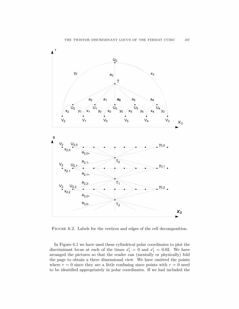
Figure 6.2. Labels for the vertices and edges of the cell decomposition.

In Figure 6.1 we have used these cylindrical polar coordinates to plot thediscriminant locus at each of the times x′1 = 0 and x′1 = 0.02. We havearranged the pictures so that the reader can (mentally or physically) foldthe page to obtain a three dimensional view. We have omitted the pointswhere r = 0 since they are a little confusing since points with r = 0 needto be identified appropriately in polar coordinates. If we had included the

498 JOHN ARMSTRONG

points there would be six vertical lines representing the triple points runningacross the front of the figure at time x′1 = 0.

For each time point we have coloured the plots to indicate which partsof the different views correspond. We have not coloured the view of the(r, θ) plane at time 0.02 as the nontransverse intersections make it difficultto work out how the curves correspond to the other figures. Note that thereis no relationship between the colours used at times x′1 = 0 and x′1 = 0.02.

The first thing to notice about Figure 6.1 is the translation symmetry onthe θ axis (corresponding to 120 degree rotations in the x′ coordinates). Ifone simplifies the expression for the discriminant locus in these coordinatesone obtains an expression only involving θ via the functions cos(3θ) andsin(3θ). This proves the visually apparent symmetry is a genuine symmetryof the discriminant locus.

This is surprising since this symmetry does not arise from the group ofconformal symmetries Z3×Z2 acting on the Fermat cubic. We conclude thatthe discriminant locus is more symmetrical than the Fermat cubic itself. Wewill discover as we continue our study that it has yet more symmetries.

Next note that at small positive x′1 > 0 times the discriminant locusconsists of a number of disjoint loops. We have illustrated this behaviourwith only one time point x′1 = 0.02, but it appears to be true for all positivetimes when one plots an animation. As time progresses, each of these loopsshrinks to a point and then disappears. There is a time symmetry in thesecoordinates which ensures that at small negative times, one similarly sees anumber of disjoint loops which shrink to a point and then disappear as timex′1 decreases.

Since the worldsheet of a loop shrinking to a point and disappearing ishomeomorphic to R2, this suggests that we have found a cell decompositionof the discriminant locus.

The vertices and edges of the cell decomposition are given by the curveat time x′1 = 0. Plotting the curve at this time does indeed show it tobe singular: the singularities are the vertices of our cell decomposition, thesmooth curves are the edges. The worldsheets of the loops at positive andnegative times give the faces of our cell decomposition.

Note that the view of the (x′2, r) plane clearly shows 6 distinct loopsat time t = 0.02. As time progresses these loops shrink to points anddisappear. Taking into account the Z3 symmetry, this gives a total of 18loops for positive times. There is also a time symmetry given by

(x′1, x′2, r, θ) 7→ (−x′1,−x′2, r, θ).

Thus we have identified a cell decomposition with 36 faces.So, by means of visual inspection, we have identified a cell decomposition

of the discriminant locus. We have two tasks remaining: the first is tocompute the topology of the discriminant locus from the cell decomposition;the second is to rigorously justify the existence of the cell decomposition.

THE TWISTOR DISCRIMINANT LOCUS OF THE FERMAT CUBIC 499

The first task is reasonably simple. We postpone the second to the nextsection.

Proposition 6.2. Assuming the cell decomposition of the discriminant locusof the Fermat cubic obtained by visual inspection is correct, its topology isencoded by the graph:

Σ4

Proof. We label the edges and vertices of the cell decomposition as shownin Figure 6.2.

In the top part of Figure 6.2 we have shown how to associate labels forthe edges and vertices seen in the view of the (x′2, r) plane at time x′1 = 0.We have used a more schematic representation of the decomposition thanthat shown in Figure 6.1, but the relationship between the pictures shouldbe obvious. We have used lower case letters to indicate edges. We haveused upper case letters to indicate vertices. We have used indices from 0to 5 to correspond to the approximate rotational symmetry about the point(0, 1) in the (x′2, r) plane. Our numbering starts at the downward pointingvertical and then moves clockwise.

Since the (x′2, r) plane is only two dimensional, some of the edges andvertices of our cell decomposition coincide when viewed in the (x′2, r) plane.We have shown in the lower part of Figure 6.2 how to add a second indexto the edges and vertices to indicate their θ coordinate. In summary thenour edges and vertices can be enumerated as follows:

• Edges ai,j i ∈ {0, 1, 2, 3, 4, 5}, j ∈ {0+, 1−, 1+, 2−, 2+, 0−};• Edges xi,j i ∈ {0, 1, 2, 3, 4, 5}, j ∈ {0, 1, 2};• Edges yi,j i ∈ {0, 1, 2, 3, 4, 5}, j ∈ {0, 1, 2};• Vertices Ui,j i ∈ {0, 1, 2, 3, 4, 5}, j ∈ {0, 1, 2};• Vertices Vi i ∈ {0, 1, 2, 3, 4, 5};• Vertices Tj j ∈ {0, 1, 2}.

Notice that we only have 6 vertices of the form Vi since when r = 0 we mustidentify points that only differ by the value of θ.

We label the faces of our cell decomposition f±i,j with i ∈ {0, 1, 2, 3, 4, 5}and j ∈ {0, 1, 2}. Here the plus or minus indicates whether the face corre-sponds to positive times x′1 > 0 or to negative times. The i index indicatesthe sector of the (x′2, r) plane and the j indicates the values of θ in accor-dance with the conventions used for edges and vertices.

An examination of Figure 6.1 allows us to write down the boundary ofeach face:

∂(f+i,j) = xi,j+1 + ai,(j+1)− + ai+1,j+ + yi,j ,

∂(f−i,j) = xi,j + ai,j+ + ai+1,(j+1)− + yi,j+1.

500 JOHN ARMSTRONG

In the formulae above, arithmetic in indices is performed modulo 6 whenworking with the i indices and modulo 3 when working with the j indices.We will use modular arithmetic for i and j indices for the rest of the proofwithout further comment.

One can see immediately from the above formulae for the faces in ourcell decomposition that precisely two faces meet at each edge. Thus the celldecomposition describes a surface with isolated topological singularities.

We compute the local topology at a vertex v by drawing the graph Γv asdescribed in Section 4. The graph ΓUi,j is:

xi,j

ai,j−

yi−1,j

ai,j+

f+i,j−1f−i−1,j−1

f+i−1,j f−i,j

The graph ΓVi is:

xi,0

yi,1xi,2

yi,0

xi,1 yi,2

f−i,0

f+i,1

f−i,2

f+i,0

f−i,1

f+i,2

The graph ΓTj is:

a0,j+

a1,(j+1)−a2,j+

a3,(j+1)−

a4,j+ a5,(j+1)−

f−0,j

f+1,j

f−2,j

f+3,j

f−4,j

f+5,j

a0,(j+1)−

a1,j+a2,(j+1)−

a3,j+

a4,(j+1)− a5,j+

f+0,j

f−1,j

f+2,j

f−3,j

f+4,j

f−5,j

THE TWISTOR DISCRIMINANT LOCUS OF THE FERMAT CUBIC 501

We deduce that the discriminant locus has precisely three topologicalsingularities T0, T1 and T2 corresponding to the twistor lines. At thesesingularities, the discriminant locus is locally homeomorphic to two discsglued together at a point.

Since the faces f+i,j and f−i,j lie in a connected component component of the

graph ΓVi , these faces can be connected via a path that avoids all vertices.The graph ΓVi also shows that the faces f±i,j1 and f±i,j2 can be connected bysuch a path for all j1 and j2. Similarly the graph of ΓTj shows that the faces

f±i1,j and f±i2,j can be connected by such a path for all i1 and i2. We deducethat all faces can be connected by a path that avoids the singularities.

We know from Proposition 4.2 that discriminant locus is orientable awayfrom the triple points and twistor lines. We deduce from this and the con-siderations above that the topology of the discriminant locus is describedby a graph of the form:

Σg

Our cell decomposition contains 27 vertices, 72 edges and 36 faces so hasEuler characteristic −9. One can alternatively calculate this using Lem-ma 6.1 and Proposition 4.4. The Euler characteristic of the singular surfaceassociated with the graph above is (2− 2g)− 3. So g = 4. �

7. Symmetry of the discriminant locus

The first step towards a rigorous justification of the above results is tofind a simpler expression for the discriminant locus. To do this we need toexploit all of its symmetries.

Assuming that our topological calculation above is correct, one sees thatthe image of the twistor lines on the Fermat cubic’s discriminant locus canbe identified entirely in terms of the geometry of the discriminant locuswithout reference to the Fermat cubic. They are simply the points of thediscriminant locus that are not locally homeomorphic to R2. Thus anyconformal symmetry of the discriminant locus must preserve the 3 pointscorresponding to the twistor lines.

Similarly one can identify the triple points as the points of the discrimi-nant locus that are not smoothly embedded in S4 yet are locally homeomor-phic to R2. Thus any conformal symmetry of the discriminant locus mustpreserve the 6 triple points. We can use this to put a bound on the size ofthe group of conformal symmetries of the discriminant locus of the Fermatcubic.

Lemma 7.1. The group, G, of conformal symmetries that permute the sixtriple points of the Fermat cubic and its three twistor lines is isomorphic toD3 ×D6.

502 JOHN ARMSTRONG

Proof. By Lemma 6.1, we have identified a round 3-sphere in S4 that con-tains all 9 nonsmooth points. It is the unique such sphere, so it too mustbe preserved by any element of G. There is a one to one correspondencebetween conformal symmetries of R4 that leave this 3-sphere fixed and an-gle preserving (but not necessarily orientation preserving) symmetries of the3-sphere.

The six triple points all lie on a hexagon in the unit circle in the planespanned by the quaternions j and k and the three twistor lines lie on anequilateral triangle in the unit circle in the plane spanned by 1 and and i.The symmetry group of a regular n-gon in the plane is Dn. Thus we can finda subgroup D3×D6 of ⊂ O(2)×O(2) ⊂ O(4) acting on R4 which preservesthe twistor lines and triple points. The induced maps on the unit sphere S3

are isometries and hence angle preserving. Thus G contains D3 ×D6.To show that there are no further symmetries, we switch to the x′ coor-

dinates. The unit 3-sphere becomes the hyperplane x′1 = 0 together withthe point at infinity. Let C3 be the unit circle in the x′1 = x′2 = 0 plane con-taining the image of the twistor lines. Let C6 be the line x′1 = x′3 = x′4 = 0containing all 6 triple points.

We can make a further conformal change of coordinates on the threesphere that fixes C3 and C6 but which moves one of the triple points toinfinity and another to zero. In these coordinates, any quaternionic Mobiustransformation that fixes the triple points must be given by a linear map.This map must be conformally equivalent to a unitary map. If this map alsofixes C3 it must be an isometry. Thus the group of transformations that fixC6 and permute C3 is D3.

We can make a conformal transformation of the three spheres that swapsC3 and C6. The argument above then shows that the group of transfor-mations that fix C3 and permute C6 is the dihedral group D6. The resultfollows. �

Lemma 7.2. The discriminant locus of the Fermat cubic is invariant underG.

Proof. Making the coordinate change

x1 = a cosα, x2 = a sinα, x3 = b cosβ, x4 = b sinβ

and simplifying yields the following equations for discriminant locus of theFermat cubic:

(7.1) − 2a3 cos(3β) sin(3α) + (−1 + a6 + 3a4b2 + 3a2b4 + b6) sin(3β) = 0,

(7.2) 1 + 4a6 − 4b6 + a12 + b12 + 6a4b2 − 6a2b4 + 6a10b2 + 6a2b10+

15a8b4 + 15a4b8 + 20a6b6 + 2b6 sin(6β) + 2a6 cos(6α)+

4a3(1 + a6 + b6 + 3a4b2 + 3a2b4) cos(3α) = 0.

THE TWISTOR DISCRIMINANT LOCUS OF THE FERMAT CUBIC 503

The invariance of the discriminant locus under the rotations

Z3 × Z6 ⊂ D3 ×D6

is now manifest.Under the transformation

a 7→ a/(a2 + b2), b 7→ b/(a2 + b2), α 7→ −α, β 7→ β,

these two equations are transformed to nonzero multiples of themselves. Sothe discriminant locus is invariant under this transformation. Similarly it isinvariant under the transformation

a 7→ a/(a2 + b2), b 7→ b/(a2 + b2), α 7→ α, β 7→ −β.Together these transformations generate G. �

Although the coordinates used in the above lemma give the simplest ex-planation for the symmetries of the discriminant locus, the topology seemseasier to understand in the x′ coordinates. This is because all the verticesof the cell decomposition can be viewed at the single time x′1 = 0. It is bycombining the best features of both coordinate systems that we will be ableto certify the topology of the discriminant locus. Therefore, let us considerthe equations for the discriminant locus in the cylindrical polar coordinatesused in the previous section. The equations take form:

p1(r, x′1, x′2) + r6 cos(6θ) + p2(r, x′1, x

′2) sin(3θ) = 0,(7.3)

p3(r, x′1, x′2) + p4(r, x′1, x

′2) cos(3θ) = 0,(7.4)

for some polynomials p1, p2, p3 and p4. So long as p4 6= 0 we can solve forcos(3θ) using Equation (7.4). We can then substitute the resulting valuefor cos(6θ) = 2 cos(3θ)2 − 1 into Equation (7.3) and hence solve for sin(3θ),assuming p2 6= 0.

cos(3θ) = −p3

p4,

sin(3θ) =r6(p2

4 − 2p23)− p2

4p1

p2p24

.

These equations have a unique solution for θ ∈ [0, 2π3 ) so long as the sum of

the squares of the right hand sides is equal to 1. Thus away from the pointswhere p4 = 0 or p2 = 0 we see that the discriminant locus is a triple coverof the surface defined by the equation:

(7.5) p22p

23p

24 + (r6(1− 2p2

3)− p24p1)2 = p2

2p44

and the inequality

(7.6) r ≥ 0.

Excluding the cases where p4 = 0 or p2 = 0, we have reduced our prob-lem from one of considering the intersection of two polynomials in R4 toa problem involving the zero set of a single polynomial in R3. This is a

504 JOHN ARMSTRONG

considerable simplification since the topology of surface defined by a singleequation is much easier to understand than a surface defined by two equa-tions. Having said that, the degree of Equation (7.5) is 44. One also needsto give careful consideration to the situation when p4 = 0 or p2 = 0. Weomit the details, but one can, with the aid of computer algebra, prove allsolutions with p4 = 0 or p2 = 0 in fact satisfy Equation (7.5).

We now make a conformal transformation of Equation (7.5) sending thesix triple points to a circle. We transform to new coordinates ((x, y, t)) asfollows:

r =1− x2 − y2 − t2

x2 + t2 + (1− y)2,

x′1 =2t

x2 + t2 + (1− y)2,

x′2 =2x

x2 + t2 + (1− y)2.

The inequality (7.6) transforms under this coordinate change to the con-dition x2 + y2 + t2 ≤ 1. After this transformation, a D6 symmetry doesindeed become clear. We once again introduce cylindrical polar coordinatesy = R sinφ, u2 = R cosφ. The inequality (7.6) becomes R2 + t2 ≤ 1.Equation (7.5) takes the form:

(7.7)∑

n∈{6,12,18,24}

pn(R, t)R12 cos(nφ)

for appropriate polynomials pn.We write cos(6φ) = Φ for a new coordinate Φ ∈ [−1, 1]. With this

coordinate change (7.5) becomes a quartic in Φ with coefficients that arepolynomials in R and u1. The discriminant locus will be a 3 × 12 = 36sheeted cover of the implicit surface obtained.

It turns out these coefficients are of entirely even degree in both R andt. So we make another simplification and introduce new variables (S, T )with S = R2 and T = t2 with the conditions S ≥ 0 and x ≥ 0. Note thatthis indicates another symmetry of the discriminant locus given by the mapt− > −t.

By means of these algebraic manipulations we have now confirmed thatG preserves the discriminant locus and simultaneously introduced simplercoordinates.

The final change of coordinates is to write Z = S + T and work with thecoordinates (Z,Φ, T ). This final change of coordinates is designed so that(7.6) transforms to the simple condition Z ≤ 1.

In summary then, we have introduced new coordinates (T,Z,Φ) such thatthe discriminant locus is a 72 sheeted cover of the implicit surface defined

THE TWISTOR DISCRIMINANT LOCUS OF THE FERMAT CUBIC 505

by the inequalities:

(7.8) T ≥ 0, 0 ≤ Z ≤ 1, −1 ≤ Φ ≤ 1

and the transformed equation (7.5). The transformed equation will be ofdegree 4 in Φ.

We know from Equation (7.7) that there is a constant factor of R12 thatwe can cancel. After making this cancellation and also the cancellation of aconstant factor, one obtains the equation:

(7.9)

426T 2 − 228ΦT 2 − 6Φ2T 2 + 3792T 3 − 496ΦT 3 − 848Φ2T 3 − 16Φ3T 3 + 7584T 4 + 96ΦT 4 −1056Φ2T 4 − 480Φ3T 4 + 4608T 5 + 1536ΦT 5 + 1536Φ2T 5 − 1536Φ3T 5 + 128T 6 + 1024ΦT 6 +

1792Φ2T 6 − 1024Φ3T 6 + 128Φ4T 6 + 228TZ + 240ΦTZ + 12Φ2TZ + 3936T 2Z + 432ΦT 2Z +

1728Φ2T 2Z + 48Φ3T 2Z + 22944T 3Z − 288ΦT 3Z − 1056Φ2T 3Z + 1440Φ3T 3Z + 31104T 4Z −384ΦT 4Z − 1920Φ2T 4Z + 1920Φ3T 4Z + 8448T 5Z + 4608Φ2T 5Z − 768Φ4T 5Z − 6Z2 − 12ΦZ2 −6Φ2Z2+912TZ2+48ΦTZ2−912Φ2TZ2−48Φ3TZ2+13368T 2Z2+1968ΦT 2Z2+5304Φ2T 2Z2−1440Φ3T 2Z2 + 55344T 3Z2 − 3600ΦT 3Z2 − 3504Φ2T 3Z2 + 3600Φ3T 3Z2 + 47424T 4Z2 −5568ΦT 4Z2 − 10176Φ2T 4Z2 + 3264Φ3T 4Z2 + 1920Φ4T 4Z2 + 4608T 5Z2 + 1536ΦT 5Z2 +

1536Φ2T 5Z2−1536Φ3T 5Z2+16ΦZ3+32Φ2Z3+16Φ3Z3+1872TZ3−1824ΦTZ3−3216Φ2TZ3+

480Φ3TZ3+27168T 2Z3+4176ΦT 2Z3+6336Φ2T 2Z3−6960Φ3T 2Z3+74944T 3Z3−1472ΦT 3Z3−4544Φ2T 3Z3 + 192Φ3T 3Z3 − 2560Φ4T 3Z3 + 31104T 4Z3 − 384ΦT 4Z3 − 1920Φ2T 4Z3 +

1920Φ3T 4Z3 + 24Z4 + 48ΦZ4 + 24Φ2Z4 + 3696TZ4 − 1584ΦTZ4 − 2160Φ2TZ4 + 3120Φ3TZ4 +

35004T 2Z4 + 8808ΦT 2Z4 + 12444Φ2T 2Z4 − 4800Φ3T 2Z4 + 1920Φ4T 2Z4 + 55344T 3Z4 −3600ΦT 3Z4−3504Φ2T 3Z4+3600Φ3T 3Z4+7584T 4Z4+96ΦT 4Z4−1056Φ2T 4Z4−480Φ3T 4Z4−144ΦZ5−288Φ2Z5−144Φ3Z5+4248TZ5−2976ΦTZ5−4344Φ2TZ5+2112Φ3TZ5−768Φ4TZ5+

27168T 2Z5+4176ΦT 2Z5+6336Φ2T 2Z5−6960Φ3T 2Z5+22944T 3Z5−288ΦT 3Z5−1056Φ2T 3Z5+

1440Φ3T 3Z5 + 92Z6 + 184ΦZ6 + 220Φ2Z6 + 256Φ3Z6 + 128Φ4Z6 + 3696TZ6 − 1584ΦTZ6 −2160Φ2TZ6+3120Φ3TZ6+13368T 2Z6+1968ΦT 2Z6+5304Φ2T 2Z6−1440Φ3T 2Z6+3792T 3Z6−496ΦT 3Z6−848Φ2T 3Z6−16Φ3T 3Z6−144ΦZ7−288Φ2Z7−144Φ3Z7 +1872TZ7−1824ΦTZ7−3216Φ2TZ7 +480Φ3TZ7 +3936T 2Z7 +432ΦT 2Z7 +1728Φ2T 2Z7 +48Φ3T 2Z7 +24Z8 +48ΦZ8 +

24Φ2Z8 + 912TZ8 + 48ΦTZ8 − 912Φ2TZ8 − 48Φ3TZ8 + 426T 2Z8 − 228ΦT 2Z8 − 6Φ2T 2Z8 +

16ΦZ9 + 32Φ2Z9 + 16Φ3Z9 + 228TZ9 + 240ΦTZ9 + 12Φ2TZ9 − 6Z10 − 12ΦZ10 − 6Φ2Z10 = 0.

Ugly though this formula is, from a computational complexity viewpoint it isa simplification of Equations (7.1) and (7.2). We started with two degree 12polynomials in 4 variables and have reduced the problem to a single degree12 polynomial in 3 variables. Moreover, the polynomial is of degree 4 in oneof those variables.

A plot of the surface defined by these conditions is shown in Figure 7.1.Since we introduced S = R2 where R is a radial coordinate, one needs toidentify certain points with S = 0. Thus a fundamental domain of G isgiven by an appropriate quotient of Figure 7.1.

We have identified a group of order 72 acting on the discriminant locus.Figure 7.1 represents a fundamental domain of this group action.

The cell decomposition used in the proof of Proposition 6.2 only had 36faces. To obtain the 72 faces associated with G, one divides each face in

506 JOHN ARMSTRONG

0.000

0.002

0.004

0.006

0.0

0.5

1.0

-1.0

-0.5

0.0

0.5

1.0

Figure 7.1. The surface defined by Equations (7.8) and (7.9).

the cell decomposition used earlier into two pieces by introducing new edgesfrom the twistor lines Tj to the triple points Vi. With this understood, theproof of Proposition 6.2 amounts to a computation of the topology of thetiling of the covering space with copies of this fundamental domain.

8. Cylindrical algebraic decomposition of the fundamentaldomain

We now wish to:

(1) Identify the points on Figure 7.1 that correspond to points with nontrivial stabilizer under G and confirm that they split into verticesand edges homeomorphic to [0, 1] as expected.

(2) Show that the Figure 7.1, with the appropriate quotients when S =0, is homeomorphic to the closed unit disc with boundary given bythe points with non trivial stabilizer under G.

If we can complete these tasks we will have rigorously identified a cell de-composition of the discriminant locus.

We begin with the first part. By construction of our coordinate system,the points with non zero stabilizer are points with S = 0, Φ = −1, T = 0,

THE TWISTOR DISCRIMINANT LOCUS OF THE FERMAT CUBIC 507

Φ = 1. Simplifying Equation (7.9) for each of the first three cases oneobtains the following simple equations:

8T 2(3 + 10T + 3T 2)4 = 0(8.1)

8T 2(3 + 3S2 + 10T + 3T 2 + 6S(1 + T ))4 = 0(8.2)

(8.3) 2(1 + Φ)2Z2(−3 + 12Z2 + 46Z4 + 64Φ2Z4

+ 12Z6 − 3Z8 + 8Φ(Z − 9Z3 − 9Z5 + Z7)) = 0.

The first equation has solutions T = 0, Φ ∈ [−1, 1]. The second equationhas the unique solution S = T = 0. The third is quadratic in Φ so isalso easily understood. All of these solutions have in common the fact thatT = 0. So referring back to Figure 6.1 these solutions correspond to theedges shown at time x′1 = 0.

The solutions of the equation Φ = 1 correspond to edges used to split thecell decomposition consisting of 36 faces into one of 72 faces. The equationin this case is a little more complex, but does factor into two cubics in T :

(8.4) 8(1 + 12T + 24T 2 + 16T 3 + 36TZ + 48T 2Z − 6Z2 + 36TZ2 + 24T 2Z2 + 8Z3 + 60TZ3 − 3Z4)×

(24T 2 + 16T 3 + 60TZ + 48T 2Z − 3Z2 + 36TZ2 + 24T 2Z2 + 8Z3 + 36TZ3 − 6Z4 + 12TZ4 + Z6)

= 0.

We need to show that the curve defined by this equation together withthe conditions 0 ≤ Z ≤ 1 and 0 ≤ T ≤ 1 is homeomorphic to [0, 1]. Onecould do this with one’s bare hands, but we will instead discuss how one canuse the “cylindrical algebraic decomposition” algorithm.

Cylindrical algebraic decomposition is a foundational algorithm in com-putational real algebraic geometry. It is an algorithm that allows one todecompose a semi-algebraic set (that is a real set defined by polynomialequalities and inequalities) into pieces called cylindrical sets which are allhomeomorphic to either {0} or Ri for some i. In effect, it computes a CWcomplex that is guaranteed to be homeomorphic to the semi-algebraic set.See [4] for more information.

There is a catch: the running time of cylindrical algebraic decomposition

is of the order (sd)cn−1

where s is the number of equations and inequationsused to define the semi-algebraic set, n is the number of variables, d isthe maximum degree of the polynomials and c is a constant. This doublyexponential running time means that cylindrical algebraic decomposition isonly effective for rather small problems.

Fortunately the semi-algebraic set defined by (8.4) and 0 ≤ Z ≤ 1 and 0 ≤T ≤ 1 is appropriately small and one can perform the cylindrical algebraicdecomposition quickly. The algorithm works inductively by using resultantsto project the equations along each of the coordinate axes to obtain lowerdimensional equations. Thus the specific cylindrical decomposition dependsupon the semi-algebraic set and the ordering of the coordinate axes. For

508 JOHN ARMSTRONG

0.000

0.001

0.002

0.003

0.004

0.0

0.2

0.4

0.6

-1.0

-0.5

0.0

0.5

1.0

Figure 8.1. Cylindrical algebraic decomposition of the fun-damental domain.

this case, if one chooses the order (Z, T ) one obtains a decomposition intothe following three cylindrical sets:

{(0, 0)},{(1, 0)},{(Z, T ) : 0 < Z < 1 and T = rootλ(−3Z2 + 8Z3 − 6Z4 + Z6+

(60Z + 36Z2 + 36Z3 + 12Z4)λ+ (24 + 48Z + 24Z2)λ2 + 16λ3, 3)}.

Here we are using the notation rootλ(p(λ), n) to denote the nth real root ofa polynomial p in the variable λ. We conclude that the semi-algebraic setdefined by Equation (8.4) and 0 ≤ Z ≤ 1 and 0 ≤ T ≤ 1 is homeomorphicto [0, 1] as required.

The final ingredient required to complete the proof is to show that thesemi-algebraic set defined by Equations (7.8) and (7.9) together with theappropriate quotienting when S = 0 is homeomorphic to the closed discand that its boundary consists of the stabilizer just identified. Using Math-ematica we do this by computing the cylindrical algebraic decompositionwith respect to the variable ordering Φ, Z, T . The computation takes sev-eral minutes to run. Notice that our many simplifications of the equationsdefining the discriminant locus are crucial to achieving this. For example

THE TWISTOR DISCRIMINANT LOCUS OF THE FERMAT CUBIC 509

simply failing to introduce the coordinate Z = S + T is enough to preventthe algorithm running to completion on our computers.

Since the cylindrical algebraic decomposition in this case is far too lengthyto print out, we have simply plotted the decomposition in Figure 8.1. Itconsists of six faces. As we saw in the example above, the specific formulaein the cylindrical algebraic decomposition are irrelevant for our purposes.All that matters is the topology implied by the decomposition. Thus thepicture in Figure 8.1 summarises all the key information we need aboutthe cylindrical algebraic decomposition. We conclude that our fundamentaldomain is homeomorphic to 6 closed discs glued as indicated. Hence itis homeomorphic to a disc. Thus the cylindrical algebraic decompositionprovides rigorous confirmation of what was visually obvious in Figure 7.1.

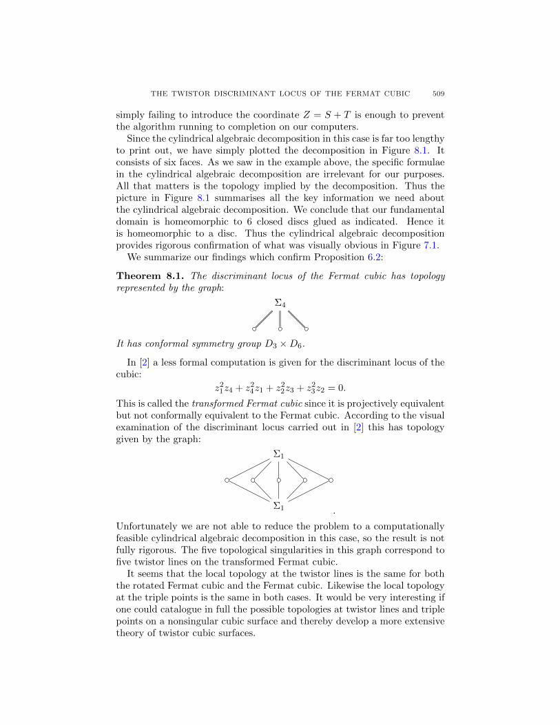
We summarize our findings which confirm Proposition 6.2:

Theorem 8.1. The discriminant locus of the Fermat cubic has topologyrepresented by the graph:

Σ4

It has conformal symmetry group D3 ×D6.

In [2] a less formal computation is given for the discriminant locus of thecubic:

z21z4 + z2

4z1 + z22z3 + z2

3z2 = 0.

This is called the transformed Fermat cubic since it is projectively equivalentbut not conformally equivalent to the Fermat cubic. According to the visualexamination of the discriminant locus carried out in [2] this has topologygiven by the graph:

Σ1

Σ1 .

Unfortunately we are not able to reduce the problem to a computationallyfeasible cylindrical algebraic decomposition in this case, so the result is notfully rigorous. The five topological singularities in this graph correspond tofive twistor lines on the transformed Fermat cubic.

It seems that the local topology at the twistor lines is the same for boththe rotated Fermat cubic and the Fermat cubic. Likewise the local topologyat the triple points is the same in both cases. It would be very interesting ifone could catalogue in full the possible topologies at twistor lines and triplepoints on a nonsingular cubic surface and thereby develop a more extensivetheory of twistor cubic surfaces.

510 JOHN ARMSTRONG

References

[1] Armstrong, John; Povero, Massimiliano; Salamon, Simon. Twistor lines oncubic surfaces. Rend. Sem. Mat. Univ. Pol. Torino. 71 (2012), no. 3–4, 317–338.arXiv:1212.2851.

[2] Armstrong, John; Salamon, Simon. Twistor topology of the Fermat cubic.SIGMA 10 (2014), Paper 061, 12 pp. MR3226989, Zbl pre06334464, arXiv:1310.7150,doi: 10.3842/SIGMA.2014.061.

[3] Atiyah, M. F. Geometry of Yang–Mills fields. Mathematical problems in theoreti-cal physics (Proc. Internat. Conf., Univ. Rome, Rome, 1977), pp. 216–221, LectureNotes in Phys., 80. Springer, Berlin-New York, 1978. MR0518436 (80a:14006), Zbl0435.58001, doi: 10.1007/3-540-08853-9 18.

[4] Basu, Saugata; Pollack, Richard; Roy, Marie-Francoise. Algorithms in realalgebraic geometry. Second edition. Algorithms and Computation in Mathematics,10. Springer-Verlag, Berlin, 2006. x+662 pp. ISBN: 978-3-540-33098-1; 3-540-33098-4. MR2248869 (2007b:14125), Zbl 1102.14041, doi: 10.1007/3-540-33099-2.

[5] Bossiere, Samuel; Sarti, Alessandra. Counting lines on surfaces. Ann. Sc. Norm.Super. Pisa Cl. Sci. (5) 6 (2007), no. 1, 39–52. MR2341513 (2008e:14074), Zbl1150.14013, arXiv:math/0606100.

[6] Dube, Thomas W. The structure of polynomial ideals and Grobner bases. SIAMJ. Comput. 19 (1990), no. 4, 750–773. MR1053942 (91h:13021), Zbl 0697.68051,doi: 10.1137/0219053.

[7] Fortuna, E.; Gianni, P.; Luminati, D. Effective methods to compute the topologyof real algebraic surfaces with isolated singularities. University of Trento, (2005).http://eprints.biblio.unitn.it/844/1/UTM687.pdf.

[8] Griffiths, Phillip; Harris, Joseph. Principles of algebraic geometry. Reprintof the 1978 original. Wiley Classics Library. John Wiley & Sons, 1994.xiv+813 pp. ISBN: 0-471-05059-8. MR1288523 (95d:14001), Zbl 0836.14001,doi: 10.1002/9781118032527.

[9] Mayr, Ernst W.; Meyer, Albert R. The complexity of the word problems forcommutative semigroups and polynomial ideals. Adv. in Math. 46 (1982), no. 3, 305–329. MR0683204 (84g:20099), Zbl 0506.03007, doi: 10.1016/0001-8708(82)90048-2.

[10] Milnor, J. On the Betti numbers of real varieties. Proc. Amer. Math. Soc. 15 (1964),275–280. MR0161339 (28 #4547), Zbl 0123.38302, doi: 10.2307/2034050.

[11] Povero, M. Modelling Kahler manifolds and projective surfaces. Ph.D. thesis, cycleXXI. Politecnico di Torino, 2009.

[12] Salamon, Simon; Viaclovsky, Jeff. Orthogonal complex structures on domainsin R4. Math. Ann. 343 (2009), no. 4, 853–899. MR2471604 (2010b:53132), Zbl1167.32017, arXiv:0704.3422, doi: 10.1007/s00208-008-0293-5.

[13] Thom, Rene. Sur l’homologie des varietes algebriques reelles. Differential andcombinatorial topology , Princeton Univ. Press, Princeton, N.J.,1965. pp. 255–265.MR0200942 (34 #828), Zbl 0137.42503.

(John Armstrong) King’s College London, Strand, London, WC2R 2LSjohn.1.armstrong@kcl.ac.uk

This paper is available via http://nyjm.albany.edu/j/2015/21-22.html.