news, uncertainty and economic fluctuations (no · pdf filenews, uncertainty and economic...
TRANSCRIPT
News, Uncertainty and Economic Fluctuations
(No News Is Good News)
Mario Forni∗
Universita di Modena e Reggio Emilia, CEPR and RECent
Luca Gambetti†
Universitat Autonoma de Barcelona and Barcelona GSE
Luca Sala‡
Universita Bocconi, IGIER and Baffi CAREFIN
Abstract
We formalize the idea that uncertainty is generated by news about future developments
in economic conditions which are not perfectly predictable by the agents. With a simple
model of limited information we show that uncertainty shocks can be obtained as the square
of news shocks. We develop a two-step econometric procedure to estimate the effects of
news and we find highly nonlinear effects. Large news shocks increase uncertainty that
mitigates the effects of good news and amplify the effects of bad news in the short run.
By contrast, small news shocks reduce uncertainty and increase output in the short run.
The Volcker recession and the great recession were exacerbated by the uncertainty effects
of news.
JEL classification: C32, E32.
Keywords: news shocks, uncertainty shocks, imperfect information, structural VARs.
∗The financial support from FAR 2014, Universita di Modena e Reggio Emilia is gratefully acknowledged.
Contact: Dipartimento di Economia Politica, via Berengario 51, 41100, Modena, Italy. Tel. +39 0592056851;
e-mail: [email protected]†Luca Gambetti acknowledges the financial support of the Spanish Ministry of Economy and Competitiveness
through grant ECO2015-67602-P and through the Severo Ochoa Programme for Centres of Excellence in R&D
(SEV-2015-0563), and the Barcelona Graduate School Research Network. Contact: Office B3.1130 Departament
d’Economia i Historia Economica, Edifici B, Universitat Autonoma de Barcelona, Bellaterra 08193, Barcelona,
Spain. Tel. +34 935814569; e-mail: [email protected]‡Corresponding author. Contact: Department of Economics, Universita Bocconi, Via Roentgen 1, 20136,
Milan, Italy. Tel. +39 0258363062; e-mail: [email protected]
1

1 Introduction
News shocks and uncertainty shocks have been in recent years at the heart of the business cycle
debate. In the “news shock” literature, news about future fundamentals affect the current
behavior of consumers and investors by changing their expectations. A partial list of major
contribution in this body of literature includes Beaudry and Portier 2004, 2006, Lorenzoni,
2007, Barski and Sims, 2011. By contrast, in the uncertainty shock literature, exogenous
shocks change the “confidence” of economic agents about their expectations. An increased
uncertainty induces agents to defer private expenditure, thus producing a temporary downturn
of economic activity. A few important contributions in the latter stream of literature include
Bloom, 2009, Rossi and Sekhposyan, 2015, Jurado et al., 2015, Ludvigson et al., 2015, Baker
et al., 2016.
Somewhat surprisingly, uncertainty and news are usually regarded as distinct, if not com-
pletely independent, sources of business cycle fluctuations. But where does uncertainty stem
from? The starting point of the present work is the idea that uncertainty precisely arises from
news. Te definition of uncertainty we focus on in this paper is the forecast error variance. Eco-
nomic agents observe new important events, but usually cannot predict exactly their effects
on economic activity. This increases the forecast error variance, i.e. uncertainty. Moreover
the more important is the event, i.e. Brexit, the higher is the uncertainty originating from
news. To support this idea, we show below, using data from the Michigan Consumers Survey,
that squared-news consumers have access to and the uncertainty measures considered in the
literature are highly and negatively correlated.
In other words, news have both a “first-moment” effect on the expected values of the series
and a “second-moment” effect on their confidence bands. Of course, it is conceivable that some
news affects uncertainty without affecting point forecasts, or vice-versa. But it is quite reason-
able to assume that first-moment and second-moment effects are most often closely related to
each other. If nothing new happens, expectations do not change and uncertainty is low. By
contrast, when important events occur, expectations change substantially (either positively or
negatively) and, given that the true magnitude of the event is unknown, uncertainty increases.
To develop this idea, we propose a simple model where a single long-run shock drives the
output trend. Such “fundamental” shock is the product of two independent factors: an ob-
servable one, which is the “news” shock, and an unobservable one, which produces uncertainty.
The news shock is nothing else than the expected value of the true shock. The unobservable
factor is the percentage deviation of the true shock from the news shock. Owing to this multi-
plicative interaction, expectation errors have a time-varying conditional variance, proportional
to the square of the news shock. Big news (either good or bad) is on average associated to
1

large expectation errors, and therefore large uncertainty.
Output is modeled as the sum of the output trend and a cycle, possibly affected by uncer-
tainty. Hence news shocks are allowed to have both a linear and a quadratic effect on output.
The linear effect is the usual news shock effect, related to expectation changes. The quadratic
effect is an additional effect, related to uncertainty, which has been neglected so far in the news
shock literature.
When the quadratic effect is taken into account, the business-cycle consequences of news
appear more complex than usually believed. First, news shocks below average reduce uncer-
tainty, producing a temporary upturn of economic activity. A zero news shock, for instance,
implies a zero first-moment effect, but a positive uncertainty effect. In this sense, no news is
good news. Second, the response of output to positive and negative news is generally asym-
metric. For small shocks, the uncertainty effect is positive; it therefore mitigates the negative
first moment effect of bad news and reinforces the positive effect of good news. For large
shocks, the asymmetry is reversed. The uncertainty effect is negative; it therefore exacerbates
the negative first moment effect of bad news and reduces the positive impact of good news.
Third, the density distribution of the squared news shock is of course highly skewed, with a
fat tail on the right-hand side. As a consequence, positive uncertainty effects cannot be large,
whereas negative effects can.
In the uncertainty shocks literature, news-related uncertainty is often regarded as “endoge-
nous”, meaning that it is a consequence, rather than a cause, of business cycle fluctuations.
In our model this is not the case: news-driven uncertainty is a genuine, independent source of
business cycle fluctuations.
In the empirical part of the paper, we estimate the US news shock with standard VAR
methods. Then we compute the squared news shock, as well as the associated uncertainty
implied by our model. The squared news shocks peaks in quarters characterized by important
recognizable economic, institutional and political events, such as the the Afghanistan war
and the first oil shock, the monetary policy shocks of the Volcker era, the Lehman Brother
bankruptcy and the subsequent stock market crash. Since large events are mainly negative,
squared news is negatively correlated with news, though correlation is not large (about -
0.20). Squared news uncertainty is highly correlated with existing measures of uncertainty: the
correlation with VXO is about 0.65 and the correlation with the 3-month horizon uncertainty
estimated by Jurado et al., 2015, is about 0.60.
In order to evaluate the business cycle effects of news uncertainty, we include both the
news shock and the related uncertainty into a second VAR, including the variables of interest.
We find that (i) a positive news shock has effects similar to the ones found in the literature,
with a gradual and persistent increase of GDP, consumption and investment; (ii) the squared
2

news shock has a significant negative temporary effect on economic activity peaking after one
quarter; (iii) the squared news shock affects positively and significantly on impact the VXO
index and the risk premium.
The forecast error variance of GDP accounted for by squared news is sizable on average
(about 20% at the 1-year horizon in the benchmark specification). The distribution of squared
news shocks is characterized by a large number of small shocks and a small number of large
shocks. As a consequence, most of the time the effect of square news is relatively small, but in
a few episodes it is not. The historical decomposition of GDP reveals that news uncertainty
explains a good deal of the early 1980s recession as well as the great recession.
The reminder paper is structured as follows: section 2 discuss some evidence about news
and uncertainty; section 3 discuss the theoretical model; section4 presents the econometric
procedure; section 5 presents the empirical results; section 6 concludes.
2 News and uncertainty
News and uncertainty have been considered in the empirical literature as two separate factors
driving economic fluctuations and the link between them has been largely neglected. However
it is plausible to think of uncertainty as originated from news about future developments of
the economy. Moreover, the intuition suggests that the more important is the event reported
by the news the higher should be the uncertainty generated by the news. For instance the
UK leaving Europe is expected generate much more uncertainty that other minor events. In
this first section we provide prima facie descriptive evidence in support of this idea using data
from the Michigan University Surveys of Consumers.
Question A.6 of the Michigan Consumers Survey questionnaire asks: “During the last few
months, have you heard of any favorable or unfavorable changes in business conditions?”.
The answers are summarized into three time series, Favorable News, Unfavorable News, No
Mentions, which express the percentage of responded which select that particular answer.
The “No Mentions” variable takes on large values when most consumers report that they
did not hear relevant news and small values when most people think that there is news worthy
of mention. If our hypothesis is correct, no news should be associated with low uncertainty
and relevant news with high uncertainty, so that No Mentions should be negatively correlated
with existing measures of uncertainty.
A single “Consumers’ News” variable can be constructed simply by taking the difference
between “Favorable News” and “Unfavorable News”. This variable (Figure 1, upper panel)
takes on positive values when most consumers mention good news and negative values when
most consumers mention bad news. The square of this variable, let us say “Consumers’ Squared
3
News” is large when there are more consumers that have heard the same type (positive or
negative) news. Of course this will happen when there are news (either negative or positive)
which are widely perceived as important by consumers. The variable will take small values
when either there are no news or the sign of news is ambiguous, so that negative and positive
mentions compensate each other. If our idea is correct, Consumers’ Squared News should be
positively correlated with uncertainty.
The Consumers’ Squared News variable is plotted in Figure 1, middle panel, together with
the uncertainty measure proposed by Jurado, Ludvigson and Ng, 2015 (3-month horizon, JLN
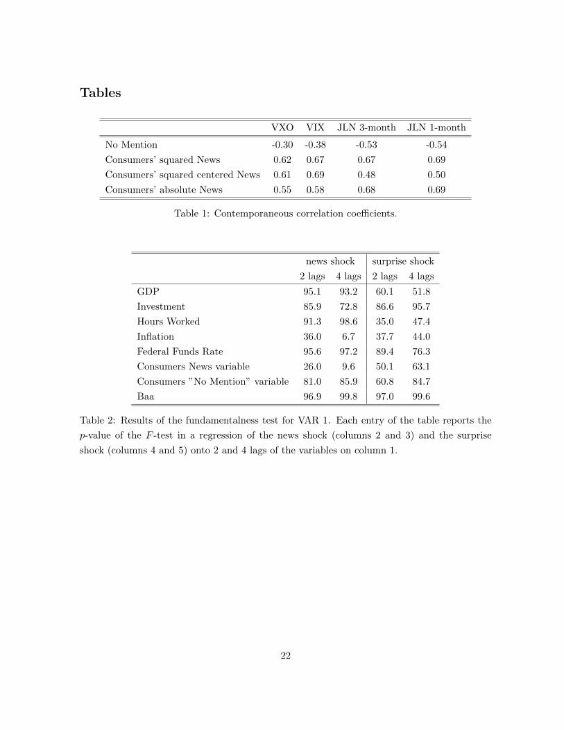
henceforth). The similarity between the two series is really impressive. Table 1 shows the
correlation coefficients of the No Mention variable and the Consumers’ Squared News variable
with the VIX index, the VXO index, the JLN 3-month index and the JLN 1-month index.
As expected, the No Mention variable is negatively correlated with all uncertainty indexes
while the Squared News variable is positively correlated with all uncertainty indexes, with
correlation coefficients ranging from 0.62 to 0.69. Large positive correlations are also obtained
when using absolute values in place of squares or when centering the News variable before
computing squares (last two lines).
In the empirical analysis below we replace the Consumers’ News variable with a news
shock identified by means of a standard structural VAR procedure (where the Consumers’
News variable is not included in the VAR). Again, we find that big news is associated with
large uncertainty.
Why the size of news shocks is so strongly correlated with uncertainty measures? In the
next section we show a simple model producing this implication.
3 Theory
3.1 Toy model
We start off by assuming that Total Factor Productivity (TFP), at, is driven by a structural
shock εt ∼ iid(0, σ2ε) with delayed effects. In the literature this kind of shock is known as
“news” or “anticipated” shock. To begin with, and for illustrative purposes, we assume only
one period of delay
∆at = µ+ εt−1 (1)
but we will generalize the process below. Agents cannot observe εt, but rather can only
observe the events underlying the shock, whose nature is qualitative in most cases: natural
disasters, scientific and technological advances, institutional changes and political events. After
observing such events, in order to take their decisions, agents form an ”estimate” of the shock,
4

which is assumed to simply be the expectation of εt conditional on the available information
set, st = Etεt. We do not explicitly model the agent’s information set, but rather we model
the error made in forecasting the value of the shock. More specifically we assume that the
percentage deviation of εt from st
vt =εt − stst
∼ iid(0, σ2v) (2)
and is independent of st at all leads and lags as well as other information available to the
agents at time t. This simply means that agents tend to make the same error in percentage
terms irrespectively on the value of the expected economic shock and the available information
set. The implication is that the forecast error
εt − st = stvt (3)
is proportional to the expected shock. From the above equation one can see that the covariance
between εt and st is s2t . This means that the larger is the shock εt, the larger will be the expected
shock st and, consequently, the larger will be the forecast error. This assumption captures the
idea that when nothing happens, both εt and st are small and so is the error st − εt. On the
contrary, if important events take place, both εt and st will be large and the expectation error
may be large as well.
We further assume that agents, at time t, perfectly observe at. In this simple version of the
model this implies that even if εt is not known at time t, agents fully learn its realization one
period later when at+1 is observed. In this model the innovation of ∆at with respect to agents’
information set is ut = st−1vt−1.1 The prediction error of ∆at+1 is therefore ut+1 = stvt. We
define uncertainty as the variance of the prediction error. Since vt and st are independent,
Etstvt = stEtvt = 0, whereas the conditional variance is Ets2t v
2t = s2tσ
2v . When nothing
happens, the expected shock will be small and so will be the conditional variance. This means
that agents are more confident about their predictions. On the contrary when facts perceived
as important occur, s2t will be generally large and uncertainty will increase. This prediction
precisely matches the empirical fact presented in the previous section: news which are perceived
as important are positively correlated with uncertanity.
The innovation representation of ∆at and st is then(∆at
st
)=
(1 L
0 1
)(ut
st
)(4)
Notice that ut and st are jointly white noise and orthogonal with variance σ2u = σ2vσ2s and
σ2s respectively.
1In fact ut = ∆at − Et−1∆at = εt−1 − Et−1εt−1 = st−1vt−1.
5
We allow for the presence of other shocks in the economy, collected in the vector wt. Finally
we assume that output yt is given by the sum of its trend at and a stationary cycle ct which
may be affected by the standardized news-uncertainty shock (s2t − σ2s)/σs2 , the standardized
news shock st/σs, as well as the other shocks wt2:
∆yt = ∆at + f(L)(s2t − σ2s)/σs2 + g(L)st/σs + h(L)wt. (5)
with f(1) = g(1) = h(1) = 0. That is we assume that uncertainty has temporary effects on
output like the other cyclical shocks wt.
3.2 A more general model
Let us now consider a more general specification for productivity, i.e.
∆at = µ+ c(L)εt =
∞∑k=1
ckεt−k, (6)
where c(L) is a rational impulse response function in the lag operator L. We assume that
c(0) = 0, so that εt is still a news shock and the general model reduces to the special case of
the previous subsection when c(L) = L.
In this model εt is not completely revealed by observed productivity at time t+ 1 and the
innovation of productivity with respect to agents’ information set is no longer st−1vt−1. The
bivariate MA representation of ∆at and st in the white noise vector (stvt st)′ is(
∆at
st
)=
(c(L) c(L)
0 1
)(stvt
st
). (7)
Without loss of generality, we now assume σ2s = 1, the normalization being absorbed by c(L).
The above representation is non-fundamental, since the determinant of the MA matrix,
c(L), vanishes by assumption for L = 0. This means that present and past values of the
observed variables ∆at and st contain strictly less information than present and past values of
stvt and st.3
On the other hand, stationarity of ∆at and st entails that the two variables have a fun-
damental representation with orthogonal innovations. Such a representation can be found as
follows. Let rj , j = 1, . . . , n, be the roots of c(L) which are smaller than one in modulus and
b(L) =
n∏j=1
L− rj1− rjL
(8)
2We are very loose in terms of economic modeling on purpose. We do not take a stand on what is the true
model behind the data. Actually any stationary model, for instance models of precautionary saving, where
consumers or investors react to uncertainty is compatible with our assumptions.3About fundamentalness see....
6

where rj is the complex conjugate of rj . Then let us consider the representation(∆at
st
)=
(d(L) c(L)
0 1
)(ut
st
), (9)
where d(L) = c(L)/b(L) and
ut = b(L)stvt =
∞∑k=1
bkst−kvt−k. (10)
Since b(L) is a so called “Blasckhe factor” (see e.g. Lippi and Reichlin, 1993, Leeper et al.,
2013) ut has a flat spectral density function and therefore is a white noise process. Moreover,
ut and st are orthogonal at all leads and lags since st and vt are zero mean and independent at
all leads and lags by assumption. Finally, the determinant of the matrix in (9), i.e. c(L)/b(L),
vanishes only for |L| ≥ 1 because of the very definition of b(L). Hence representation (9) is
fundamental and ut is the “surprise” shock, i.e. the new information conveyed by ∆at with
respect to available information, or, in other words, the residual of the projection of ∆at onto
its own past and the present and the past of st.4
By inverting equation (10) we get stvt = ut/b(L) = b(F )ut where F is the forward operator.
As in the previous section, the structural shock εt = st + stvt depends on future innovations,
with the difference that here the shock gets unveiled in the long run, rather than after one
period.
3.3 Prediction error and uncertainty
We assume that agents’ information set Ωt is given by the linear space spanned by the constant
and the present and past values of ut, st and the centered, squared news shock s2t −1 (we recall
that st is unit variance); the expected values are approximated by linear predictions onto Ωt,
denoted by Pt. Note that, while predictions are linear, the information set includes the squared
news shock.
It is seen from equations (9) and (10) that the k-period ahead prediction error of at is given
by
at+k − Ptat+k = Dk(L)ut+k + Ck(L)st+k
= Rk(L)st+kvt+k + Ck(L)st+k, (11)
where Rk(L) = Dk(L)b(L), Dk(L) =∑k−1
h=0DhLk, Ck(L) =
∑k−1h=0ChL
k, Dh =∑h
j=0 dj ,
Ch =∑h
j=0 cj , d(L) = c(L)/b(L).
4Notice that b(L) reduces to L in the special case of the toy model where c(L) = L.
7

We define the k-period-ahead uncertainty Ukt as Pt(at+k−Ptat+k)2, i.e. the linear projection
of the squared error onto Ωt. We show in the Appendix that, if the density distribution of vt
is symmetric,
Ukt = σ2v
∞∑h=0
(Rkk+h)2(s2t−h − 1) + σ2v
k−1∑h=0
(Rkh)2 +k−1∑h=0
C2h. (12)
Uncertainty is the sum of three components. The first term in the right-hand side of the above
equation is the component of uncertainty driven by the demeaned news-uncertainty shock.
Again the larger the perceived shock the larger is the effect on uncertainty. Te intuition is the
same as that discussed in the previous section.
4 The econometric approach
Our econometric approach to estimate the effects of uncertainty consists in a two stage proce-
dure. In the first stage the news shocks is estimated. In the second stage we feed the estimated
news shock and its squared values in a new VAR and we identify the uncertainty shock. The
procedure is relatively simple since amounts at identifying two shocks in two separate VAR
models. ere we apply our framework to news and uncertainty. The procedure however is very
general and can be used in order to study potential non-linearities of any structural shock. Its
advantage, relative to other non-linear approach, is that it is very easy to implement since it
only requires the standard estimation of two linear VARs.
4.1 Step 1
In practice the signal st is not observed by the econometrician. We therefore assume that
there are observable variables, collected in the vector zt, which reveal the signal. In principle
such variables may depend on both st and ut, as well as the additional shocks wt affecting the
business cycle. Therefore we can write the joint representation of ∆at and zt as
(∆at
zt
)=
(d(L) c(L) 0
m(L)σu n(L) P (L)
)ut/σust
wt
, (13)
where m(L) and n(L) are nz × 1 vectors of impulse-response functions, 0 is an nw-dimensional
row vector and P (L) is an nz × nw matrix of impulse response functions and wt is a vector of
orthonormal economic shocks, orthogonal to ut and st, which might potentially includes2t−1σs2
.
Note that, following the usual econometric convention, the shocks are normalized to have unit
variance.
8

Assuming invertibility of (13) we can estimate it by means of a structural VAR (VAR 1).
To identify the news shock st we follow Forni, Gambetti and Sala (2014) and Beaudry et al.
(2016) and we impose the following restrictions: (i) ut is the only one shock affecting at on
impact; (ii) ut and st are the only two shocks affecting at in the long-run. Condition (ii) is
equivalent to maximizing the effect of st on at at the same horizon. This identification scheme
is standard in the news-shock literature and is very similar to the one used in Barski and Sims
(2011).
4.2 Step 2
Having an estimate of st, we compute s2t and the related uncertainty Ukt , according to formula
(12). To evaluate the effects of news —including uncertainty-related effects— on economic
activity, we include both st and s2t (or Ukt ) into a new VAR (VAR 2), aimed at estimating the
impulse response function representation
s2t − 1
st
∆yt
=
σs2 0 0 0
0 1 0 0
f(L) [c(L) + g(L)] d(L)σu h(L)
s2t−1σs2
st
ut/σu
wt
, (14)
where the last row is obtained from equations (5), (5) and (9).
A few remarks are in order. First, as st is iid, then s2t − 1 is also iid and st and s2t − 1 are
jointly white noise. This implies that the OLS estimator of the VAR associated to the above
MA representation will have the standard properties including consistency. Second, if st has
a symmetric distribution, then s2t is also orthogonal to st. In this case identification of st and
s2t can be carried out by means of a standard Cholesky scheme with st and s2t ordered as the
first two variables, the ordering between them being irrelevant. However, in practice it turns
out that the distribution of st is not symmetric, since most of large news is bad news. The
estimated contemporaneous correlation coefficient of st and s2t is about -0.20. This produces an
identification problem: what are the “pure” first moment expectation effect, on the one hand,
and the “pure” second moment uncertainty effect, on the other hand? Below we orthogonalize
the two shocks by imposing a Cholesky scheme with s2t ordered first and st ordered second, as
in (14). By using this scheme, the long-run effects of uncertainty on GDP, consumption and
investment are close to zero, which is in line with our theoretical assumption. As an alternative,
we might identify by directly imposing a zero effect on GDP in the long-run; we do this in
the robustness section, where we also try the Cholesky scheme with st ordered first and s2tordered second. Third, inference of the impulse response functions of the second VAR should
should take into account the estimation uncertainty of st. So in principle for any realization
9

of the shock obtained in the first VAR one should implement a bootstrap in the second VAR.
However in the empirical section we abstract from this complication and we treat st as an
observed series.
4.3 Simulations
We use two simulations to assess our econometric approach. The first simulation is designed as
follows. First we assume that there are two signals, zt = [z1t z2t]′ and that the data generating
process is given by the following MA:∆at
z1t
z2t
=
1 L 0
1 +m1L 1 + n1L 0
1 +m2L 1 + n2L 1 + p2L
ut/σu
sts2t−1σs2
. (15)
Simple MA(1) impulse response functions are chosen for sake of tractability but more compli-
cated processes can be also considered. Using the following values m1 = 0.8, m2 = 1, n1 =
0.6, n2 = −0.6, p1 = 0.2, p2 = 0.4, and assuming [ut st]′ ∼ N(0, I) we generate 2000 artificial
series of length T = 200. For each set of series we estimate a VAR for [∆at z1t z2t]′ and
identify st as the second shock of the Cholesky representation. We define st the estimates of
st obtained from the VAR.
In the second step, using the same 2000 realizations of [ut st s2t ]′ we generate ∆yt from the
equation
∆yt = ut + (1 + (g1 − 1)L− g1L2 + L)st − (1 + (f1 − 1)L− f1L2)s2t − 1
σs2,
we estimate a VAR with [st s2t ∆yt]
′ and apply a Cholesky identification. The first shock is
the news shock the second shock is the uncertainty shock.
The second simulation is similar to the first, the only difference being that the uncertainty
shock has no effects on any of the variable. So the data are generated using the following
processes ∆at
z1t
z2t
=
1 L 0
1 +m1L 1 + n1L 0
1 +m2L 1 + n2L 1 + p2L
ut/σust
wt
(16)
and
∆yt = ut + (1 + (g1 − 1)L− g1L2 + L)st − (1 + (f1 − 1)L− f1L2)wt
where [ut st wt]′ ∼ N(0, I) and the values of the parameters are the same as before.
Results of simulation 1 are reported in Figure 2 while results of simulation 2 are reported
in Figure 3. The left column plots the effects of ∆at, z1t and z2t of the news shock st. The
10
right column reports the responses of ∆yt to the three shocks st,s2t−1σs2
and ∆at. The solid line
is the mean of the 2000 responses, the grey area represent the 68% confidence bands while the
dashed red lines are the true theoretical responses. In both simulations all of the cases our
approach succeeds in correctly estimate the true effects of news and uncertainty shock, the
theoretical responses essentially overlapping with the mean estimated effects.
5 Empirics
5.1 The news shock
Our empirical analysis focuses on quarterly US data covering the time span 1963:Q4-2015:Q2.
Following Beaudry and Portier, 2006, we use total factor productivity (TFP) corrected for
capacity utilization5 as a proxy for the output trend. To reveal news we use six variables:
(a) stock prices (the S&P500 index divided by the GDP deflator), which is the main variable
used to identify news shocks in the literature; (b) the Michigan University confidence index
component concerning business conditions for the next five years (E5Y), whose anticipation
properties are widely discussed in Barsky and Sims, ???; (c) real consumption of nondurables
and services (Consumption), which according to economic theory should anticipate future
income; (d) the 3-month treasury bill secondary market rate (TB3M); (e) the 10-year treasury
constant maturity rate (GS10) and (f) the Moody’s Aaa interest rate. The interest react
readily to news and therefore can in principle be able to reveal them. All data but TFP are
taken from the FRED website.
We estimate a Bayesian VAR with diffuse prior and 4 lags. The series are taken in log-
levels. The identification scheme is the one explained in Subsection 4.1, where the long-run
horizon is 48 quarters (12 years).
To evaluate whether we are neglecting relevant variables in our VAR specification, we use
the testing procedure suggested in Forni and Gambetti, 2014. We regress the news shock as well
as the “surprise” shock onto the past values of seven additional variables, taken one at a time:
real GDP (GDP), real investment plus durable consumption (Investment), hours worked, the
GDP deflator inflation rate (Inflation), the federal funds rate, the Michigan University News
variable described above, and Moody’s Baa bond rate. Then we computed the F -test. Table
2 reports the p-values. For all of the regressions, the null that all coefficients are zero cannot
be rejected. We conclude that VAR 1 include enough information to identify the news shock.
Figure 4 shows the effects of the news shock on the variables in the VAR. The impulse-
response function of TFP exhibits the typical S-shape which is usually found in the literature.
5The source is Fernald’s website. TFP is cumulated to get level data.
11

Stock prices and E5Y jump on impact, as expected, while consumption increases more gradu-
ally. All interest rates reduce on impact, albeit the effect is barely significant. All in all, the
effects of the news shock are qualitatively similar to those found in the previous literature.
In the robustness Section we try alternative specifications for VAR 1.
5.2 Uncertainty: dating of large shocks and comparison with existing mea-
sures
The squared news shock exhibits very large values (larger than average by more than two
standard deviations) in the following 8 quarters:
1972:Q1 (+) Tax Reduction Act, Smithsonian Agreement, Space Shuttle Program
1973:Q2 (-) Mid ’70 Crisis
1974:Q1 (-) Stock Market Oil Embargo Crisis
1982:Q1 (-) Loan Crisis
1990:Q4 (-) Gulf War I (UN Resolution 678), Omnibus Budget Reconciliation Act
2002:Q3 (-) WorldCom Bankruptcy
2008:Q3 (-) Lehman Brothers Bankruptcy
2008:Q4 (-) Stock Market Crash
Most of these dates correspond to recognizable events and/or cycle phases. The sign in bracket
is the sign of the news shock. Most of large news is bad news (7 out of 8); this is the reason
why the news shock and the squared news shock are negatively correlated.
Figure 5 plots four series: the square of the estimated news shock, the corresponding
squared news uncertainty, computed according to formula (12) with k = 3, the VXO and the
uncertainty measure estimated by Jurado, Ludvigson and Ng, 2015, for the 3-month ahead
horizon (JLN3 henceforth). Clearly, the squared news shock and the related uncertainty mea-
sure are positively correlated with both the VXO and the JLN measure.
Table 3 reports the contemporaneous correlation coefficient of the squared news shock and
the related uncertainty U2t and U3
t (see formula (12)), on the one hand, and a few existing
measures of uncertainty: namely, the VXO and the VIX indeces, JLN3 and JLN12. Such
correlations are noticeable high. In particular, the correlation of U3t with the reported measures
ranges between 0.51 and 0.68.
12

5.3 The uncertainty effect of news
Let us now come to the results of VAR 2, where we include the squared news shock and the
news shock estimated with VAR 1, along with real GDP, real consumption of non-durables
and services, real investment plus consumption of durables and hours worked. Identification
is obtained as explained in subsection 4.2.
Results are reported in Figures 6 and 7. The numbers on the vertical axis can be interpreted
as yearly percentage variations. The squared news shock has a significant negative effect on
all variables on impact. The maximum effect on GDP is reached after 4 quarters and is about
-2% in annual terms (-0.5% on a quarterly basis). Afterwards the effects reduces and becomes
approximately zero around the 3-year horizon. By using different identification schemes and
different specifications for VAR 1 we find similar results, the maximal effect on GDP ranging
between -1.5% and -2% at the 1-year horizon (see the robustness section).
As for the news shock, Figure 7 shows that it has a large, permanent, positive effect on
real activity, reaching its maximum after about 2 years. This confirms results already found
in the literature.cit, footnote
Table 3 shows the variance decomposition. The most important finding is that the squared
news shock explains a sizable fraction of output, investment and hours volatility at the 1-year
horizon (22%, 20% and 22%, respectively). The effects on consumption are smaller (about
7%).
We have seen in Figure 3 the uncertainty effect of a standardized squared news shock equal
to 1, i.e. our estimate of f(L), say f(L). To better understand the uncertainty effects of news,
it can be useful to see the uncertainty effects of the news shock itself, when it takes on different
values. To this end we compute
f(L)(s2t − 1)/σs2 ,
for |st| = 0, 0.5, 1, 2 (of course, positive and negative news have the same uncertainty effects in
our framework).
Figure 8 shows the result. A few observations are in order. First, the uncertainty effects
of news may be positive (upper panels). This happens when the centered squared news shock
is negative, that is when −1 < st < 1. No news (or small news) produce a temporary upturn
of economic activity. However, the largest positive effect is obtained when st = 0 (upper-right
panel); such effect is small, the maximum being about 1.2% on a yearly basis.
Second, when the news shock is equal to 1 or -1, that is the news shock in absolute value
is equal to its standard deviation, the innovation of uncertainty is zero and there are no
uncertainty effects (lower-right panel).
Third, a news shock larger than its standard deviation in absolute values produces negative
13

uncertainty effects. Such effects may be very large —much larger than the largest possible
positive effect. For instance, a news shock equal to 2 times its standard deviation (lower-right
panel) produces a maximum GDP decrease around 4% on an yearly basis (1% on a quarter-
on-quarter basis). In the 8 quarters reported in the previous subsection the uncertainty effects
of news were larger or equal to the one depicted here.
To evaluate the total effect of news, including both the expectation, first moment effect
and the uncertainty effect, we computed
f(L)st + f(L)(s2t − 1)/σs2
for st = −2,−1,−0.5, 0.5, 1, 2.
Results are reported in Figure 9. The basic finding here is that the effects of news are
generally asymmetric, but the asymmetry is different for small shocks and large shocks. When
st is small (precisely, smaller than its standard deviation in absolute value), the uncertainty
effect is positive, so that, in the short run, it mitigates the negative first moment effect of
bad news and reinforces the positive effect of good news (upper panels). When |st| = 1, the
uncertainty effect is zero, so that the overall effects of news are symmetric (middle panels).
For large shocks the the asymmetry is reversed. The uncertainty effect is negative; therefore
it exacerbates the negative first moment effect of bad news and mitigates the positive effect of
good news.
5.4 Historical decomposition
Figure 10 compares per-capita GDP (blue solid line) with per-capita GDP cleaned from the un-
certainty effect of news (red dashed line). For a better reading, the sample is broken into three
subperiods: 1965:Q4-1983:Q2 (upper panel), 1983:Q3-1998:Q2 (middle panel) and 1998:Q3-
2015:Q2 (lower panel). The two lines are very far apart during two periods: the final part of
the early 80’s recession and the beginning of the subsequent recovery, on the one hand, and
the second half of the great recession, on the other hand. In both cases the red line is above
the blue line, meaning that the uncertainty effect of news was recessionary. The first period is
characterized by the large negative news shock of 1982:Q1; the second period is characterized
by the two large negative shocks of 2008:Q3 and 2008:Q4.
Figure 11 compares per-capita GDP (blue solid line) with per-capita GDP cleaned from
the overall effect of news, including both the expectation effect and the uncertainty effect (red
dashed line). The sample is broken into three subperiods as before. The main insight here is
that the role of the news shock in driving GDP was large for most of the sample, with the
noticeable exception of Reagan’s recovery and the Great Moderation (middle panel), where the
two lines are relatively close to each other. By looking at the dating of subsection 5.2 it is seen
14

that there is no large news between 1990:Q4 and 2002:Q1, which seems to provide evidence in
favor of Stock and Watson’s “good luck” explanation of the Great Moderation (cit.)
5.5 News uncertainty and financial variables
In order to analyze the effects of news and squared news on financial variables and uncertainty
variables we estimated an additional VAR (VAR 3), where we included again the squared news
shock and the news shock estimated with VAR 1, along with stock prices, the spread between
Baa bonds and ten-year treasury bonds (GS10), which may be regarded as a measure of the
risk premium, the WXO, extended as in Bloom, 2009, and the 3-month JLN uncertainty index.
Results are reported in Figures 12 and 13. The squared news shock (Figure 12) reduces
stock prices and increases the risk premium significantly on impact and at lags 1 and 2. As
expected, the VXO increases significantly in the first year after the shock. The effect on
the JLN index is somewhat more puzzling. The index increase significantly on impact but
afterward it reduces and the reduction is significant at the one-year horizon, albeit at the 68%
level.6
As for the first moment, expectation effects of the news shock (Figure ??, it is seen that
good news have a large, positive and persistent effect on stock prices. Moreover, good news
reduce significantly the risk premium, the VXO index and the JLN index.
Table 6 shows the variance decomposition. The squared news shock explains a sizable
fraction of the forecast error variance of the VXO index at the 4-quarter horizon.
5.6 Robustness
In this subsection we show the results of two robustness exercises. In the former one we keep
fixed the specification of VAR 1 and try alternative identification schemes for VAR 2.
Figure 14 shows the results. The red dashed line is the response obtained with the Choleski
scheme, where the news shock is ordered first and the squared news shock is ordered second.
The blue dotted-dashed line is the estimate obtained by imposing a zero effect of the squared
news shock at the 10-year horizon. The black solid line and the confidence bands are those of
the benchmark identification.
Both of the alternative schemes produce smaller short run uncertainty effects of news,
even if the results are qualitatively similar to the benchmark. The positive long-run effect
on consumption obtained with the alternative identification schemes are somewhat puzzling,
particularly for the recursive ordering with the news shock ordered first (red-dashed line).
6By observing Figure 5, it is seen that the squared news shock is somewhat lagging with respect to the JLN
index in the first half of the 80’s. This could be related to this result, even if of course it is not an explanation.
15

In the latter robustness exercise we keep fixed identification of VAR 1 as well as specification
and identification of VAR 2, and try different specifications for VAR 1. Specification (i)
includes TFP, S&P500, Consumption and TB3M. Specification (ii) includes TFP, Investment
and TB3M (stock prices are excluded).
Figure 15 shows the results. The red-dashed line is the one obtained with specification (i);
the blue dotted-dashed line the one obtained with specification (ii). The black solid line and
the confidence bands are again the point estimate and the confidence bands of the benchmark
case.
The impulse-response functions obtained with both specifications (i) and (ii) are similar to
the benchmark. Notice that specification (ii) is very different from that of the benchmark case
and specification (i), in that it excludes stock prices. Somewhat surprisingly, the correlation
of news-driven uncertainty with VXO, VIX and the JLN uncertainty measure is still high. In
particular the correlation coefficient of U4t and the above uncertainty variables ranges between
0.52 and 0.64.
16

References
[1] Angeletos G., M. and J. La’O (2010), “Noisy Business Cycles”, NBER Chapters, in:
NBER Macroeconomics Annual 24, 319-378.
[2] Barsky, R. and E. Sims (2012), “Information, Animal Spirits, and the Meaning of Inno-
vations in Consumer Confidence”, American Economic Review 102, 1343-77.
[3] Barsky, R. and E. Sims (2011), “News shocks and business cycles”, Journal of Monetary
Economics 58, 273-289.
[4] Baxter, B., L. Graham, and S. Wright (2011), “Invertible and non-invertible information
sets in linear rational expectations models”, Journal of Economic Dynamics and Control
35, pp. 295-311.
[5] Basu, S., L. Fernald and M. Kimball (2006), “Are Technology Improvements Contrac-
tionary?”, American Economic Review, vol. 96(5), pp. 141848.
[6] Beaudry, P. and F. Portier (2004), “Exploring Pigou’s Theory of Cycles”, Journal of
Monetary Economics 51, 1183-1216.
[7] Beaudry, P. and F. Portier (2006), “Stock Prices, News, and Economic Fluctuations”,
American Economic Review 96, 1293-1307.
[8] Beaudry, P., D. Nam and J. Wang (2011), “Do Mood Swings Drive Business Cycles and
is it Rational?”, NBER working paper 17651.
[9] Blanchard O.J., G. Lorenzoni and J.P. L’Huillier (2013), “News, Noise, and Fluctuations:
An Empirical Exploration”, American Economic Review, vol. 103(7), pp. 3045-70,
[10] Chari, V.V., Kehoe, P.J. and E.R. McGrattan (2008), “Are structural VARs with long-run
restrictions useful in developing business cycle theory?”, Journal of Monetary Economics
55, pp. 1337-1352.
[11] Chen, B., Choi, J. and J.C. Escanciano (2015), “Testing for Fundamental Vector Moving
Average Representations”, CAEPR Working Paper No. 022-2015, forthcoming in Quan-
titative Economics.
[12] Christiano, L., C. Ilut, R. Motto and M. Rostagno (2007), Signals: Implications for
Business Cycles and Monetary Policy, mimeo, Northwestern University.
[13] Cochrane, John H. (1994), “Shocks”, Carnegie-Rochester Conference Series on Public
Policy 41, 295-364.
17
[14] Coibion, O. and Y. Gorodnicenko (2012), ”What can survey forecasts tell us about infor-
mational rigidities?”, Journal of Political Economy 120, pp. 116-159.
[15] Den Haan, W.J. and G. Kaltenbrunner (2009). “Anticipated growth and business cycles
in matching models”, Journal of Monetary Economics 56, pp. 309-327.
eds. Boulder: Westview, pp.77-119.
[16] Fernandez-Villaverde, J., J. F. Rubio, T. Sargent and M. Watson (2007), “A, B, C, (and
D)’s for Understanding VARs”, American Economic Review 97, pp. 1021-1026.
[17] Forni, M. and L. Gambetti (2014), “Sufficient information in structural VARs”, Journal
of Monetary Economics 66, pp. 124-136.
[18] Forni, M., Gambetti, L., Lippi, M. and L. Sala (2014),“Noise Bubbles”, Baffi Center
Research Papers no. 2014-160, forthcoming in Economic Journal.
[19] Forni, M., L. Gambetti and L. Sala (2014), “No News in Business Cycles”, The Economic
Journal 124, pp. 1168-1191.
[20] Forni, M., Gambetti, L. and L. Sala (2016), “VAR Information and the Empirical Vali-
dation of Macroeconomic Models”, CEPR Discussion Papers no. 11178.
[21] Forni, M., D. Giannone, M. Lippi and L. Reichlin (2009), “Opening the Black Box:
Structural Factor Models with Large Cross-Sections”, Econometric Theory 25, pp. 1319-
1347.
[22] Giannone, D., and L. Reichlin (2006), “Does Information Help Recovering Structural
Shocks from Past Observations?”, Journal of the European Economic Association 4, pp.
455-465.
[23] Gilchrist, S. and E. Zakrajek (2012), “Credit Spreads and Business Cycle Fluctuations”,
American Economic Review, 102(4), pp. 1692-1720.
[24] Hansen, L.P., and T.J. Sargent (1991), “Two problems in interpreting vector autore-
gressions”, in Rational Expectations Econometrics, L.P. Hansen and T.J. Sargent, eds.
Boulder: Westview, pp.77-119.
[25] Jaimovich, N. and S. Rebelo, (2009), “Can News about the Future Drive the Business
Cycle?”, American Economic Review, 99(4): 1097-1118
[26] Keynes, J.M., (1936), The general theory of employment, interest and money, London:
Macmillan.
18

[27] Kilian, L. (1998), “Small-Sample Confidence Intervals for Impulse Response Functions”,
Review of Economics and Statistics 80, 21830.
[28] Leeper, E. M., Walker, T. B. and Yang, S.-C. S. (2013), “Fiscal Foresight and Information
Flows”, Econometrica, 81: 11151145
[29] Lippi, M. and L. Reichlin (1993), “The Dynamic Effects of Aggregate Demand and Supply
Disturbances: Comment”, American Economic Review 83, 644-652.
[30] Lippi, M. and L. Reichlin (1994), “VAR analysis, non fundamental representation,
Blaschke matrices”, Journal of Econometrics 63, 307-325.
[31] Lorenzoni, G., (2009), “A Theory of Demand Shocks”, American Economic Review, 99,
2050-84.
[32] Lorenzoni, G. (2010). “Optimal Monetary Policy with Uncertain Fundamentals and Dis-
persed Information”, Review of Economic Studies 77, pp. 305-338.
[33] Lucas, R.E., Jr. (1972), “Expectations and the Neutrality of Money”, Journal of Economic
Theory 4, 103-124.
[34] Mankiw G. N. and R Reis (2002), “Sticky Information Versus Sticky Prices: A Proposal
to Replace the New Keynesian Phillips Curve”, Quarterly Journal of Economics 117,
1295-1328.
[35] Mertens, K. and M. O. Ravn (2010), “Measuring the Impact of Fiscal Policy in the Face
of Anticipation: A Structural VAR Approach”, The Economic Journal, vol. 120(544), pp.
393-413.
[36] Pigou, A. C. (1927). “Industrial fluctuations”, London, Macmillan.
[37] Rozanov, Yu. (1967). Stationary Random processes, San Francisco: Holden Day.
[38] Schmitt-Grohe, S. and Uribe, M. (2012), “What’s News in Business Cycles”, Economet-
rica, 80: pp. 27332764.
[39] Sims, C. A. (2003), “Implications of Rational Inattention”, Journal of Monetary Eco-
nomics 50, 665-690.
[40] Woodford M. (2002), “Imperfect Common Knowledge and the Effects of Monetary Pol-
icy”, in P. Aghion, R. Frydman, J. Stiglitz, and M. Woodford, eds., Knowledge, Infor-
mation, and Expectations in Modern Macroeconomics: In Honor of Edmund S. Phelps,
Princeton: Princeton University Press.
19
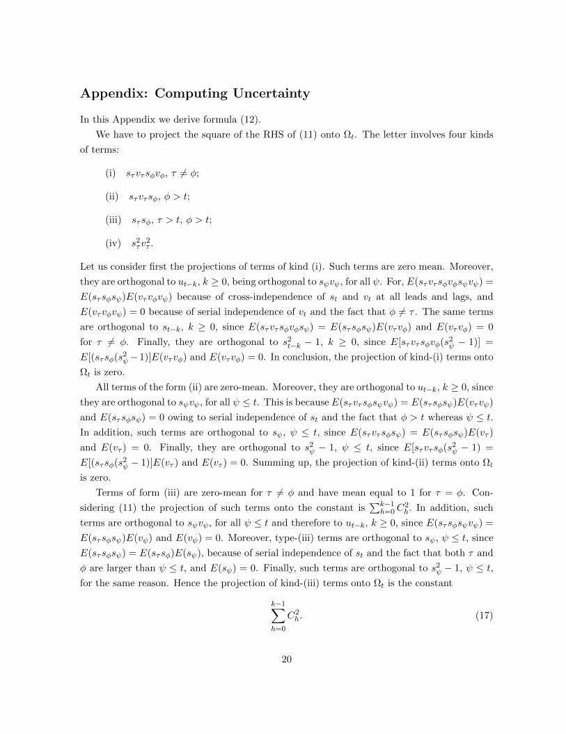
Appendix: Computing Uncertainty
In this Appendix we derive formula (12).
We have to project the square of the RHS of (11) onto Ωt. The letter involves four kinds
of terms:
(i) sτvτsφvφ, τ 6= φ;
(ii) sτvτsφ, φ > t;
(iii) sτsφ, τ > t, φ > t;
(iv) s2τv2τ .
Let us consider first the projections of terms of kind (i). Such terms are zero mean. Moreover,
they are orthogonal to ut−k, k ≥ 0, being orthogonal to sψvψ, for all ψ. For, E(sτvτsφvφsψvψ) =
E(sτsφsψ)E(vτvφvψ) because of cross-independence of st and vt at all leads and lags, and
E(vτvφvψ) = 0 because of serial independence of vt and the fact that φ 6= τ . The same terms
are orthogonal to st−k, k ≥ 0, since E(sτvτsφvφsψ) = E(sτsφsψ)E(vτvφ) and E(vτvφ) = 0
for τ 6= φ. Finally, they are orthogonal to s2t−k − 1, k ≥ 0, since E[sτvτsφvφ(s2ψ − 1)] =
E[(sτsφ(s2ψ−1)]E(vτvφ) and E(vτvφ) = 0. In conclusion, the projection of kind-(i) terms onto
Ωt is zero.
All terms of the form (ii) are zero-mean. Moreover, they are orthogonal to ut−k, k ≥ 0, since
they are orthogonal to sψvψ, for all ψ ≤ t. This is because E(sτvτsφsψvψ) = E(sτsφsψ)E(vτvψ)
and E(sτsφsψ) = 0 owing to serial independence of st and the fact that φ > t whereas ψ ≤ t.
In addition, such terms are orthogonal to sψ, ψ ≤ t, since E(sτvτsφsψ) = E(sτsφsψ)E(vτ )
and E(vτ ) = 0. Finally, they are orthogonal to s2ψ − 1, ψ ≤ t, since E[sτvτsφ(s2ψ − 1) =
E[(sτsφ(s2ψ − 1)]E(vτ ) and E(vτ ) = 0. Summing up, the projection of kind-(ii) terms onto Ωt
is zero.
Terms of form (iii) are zero-mean for τ 6= φ and have mean equal to 1 for τ = φ. Con-
sidering (11) the projection of such terms onto the constant is∑k−1
h=0C2h. In addition, such
terms are orthogonal to sψvψ, for all ψ ≤ t and therefore to ut−k, k ≥ 0, since E(sτsφsψvψ) =
E(sτsφsψ)E(vψ) and E(vψ) = 0. Moreover, type-(iii) terms are orthogonal to sψ, ψ ≤ t, since
E(sτsφsψ) = E(sτsφ)E(sψ), because of serial independence of st and the fact that both τ and
φ are larger than ψ ≤ t, and E(sψ) = 0. Finally, such terms are orthogonal to s2ψ − 1, ψ ≤ t,
for the same reason. Hence the projection of kind-(iii) terms onto Ωt is the constant
k−1∑h=0
C2h. (17)
20

Coming to terms of the form (iv), we have E(s2τv2τ ) = σ2v . Going back to (11) it is seen
that their projection onto the constant is σ2v∑k−1
h=0(Rkh)2. Moreover, such terms are orthogonal
to sψvψ, for all ψ. This is obvious for τ 6= ψ, but is also true for τ = ψ, since in this case
E(s2τv2τsψvψ) = E(s3τv
3τ ) = E(s3τ )E(v3τ ) which is zero since we are assuming that vt has a
symmetric density distribution. As a consequence these terms are orthogonal to ut−k, k ≥ 0.
All such terms are also orthogonal to sψ and s2ψ − 1 for τ 6= ψ, because of independence of st
and vt at all leads and lags and serial independence of st. As for ψ = τ , the projection of s2τv2τ
onto sτ and s2τ − 1, τ ≤ t, is
ΓΣ−1
(sτ
s2τ
),
where
Γ = σ2v
(Es3τ Es4τ − 1
)and
Σ =
(1 Es3τEs3τ Es4τ − 1
).
It is seen that ΓΣ−1 = (0 σv), so that the projection reduces to σ2v(s2t−h − 1). Considering
(11) and the constant term, the projection of type-(iv) terms onto Ωt is
σ2v
∞∑h=0
(Rkk+h)2(s2t−h − 1) + σ2v
k−1∑h=0
(Rkh)2. (18)
Formula (12) is the sum of (18) and (17).
21
Tables
VXO VIX JLN 3-month JLN 1-month
No Mention -0.30 -0.38 -0.53 -0.54
Consumers’ squared News 0.62 0.67 0.67 0.69
Consumers’ squared centered News 0.61 0.69 0.48 0.50
Consumers’ absolute News 0.55 0.58 0.68 0.69
Table 1: Contemporaneous correlation coefficients.
news shock surprise shock
2 lags 4 lags 2 lags 4 lags
GDP 95.1 93.2 60.1 51.8
Investment 85.9 72.8 86.6 95.7
Hours Worked 91.3 98.6 35.0 47.4
Inflation 36.0 6.7 37.7 44.0
Federal Funds Rate 95.6 97.2 89.4 76.3
Consumers News variable 26.0 9.6 50.1 63.1
Consumers ”No Mention” variable 81.0 85.9 60.8 84.7
Baa 96.9 99.8 97.0 99.6
Table 2: Results of the fundamentalness test for VAR 1. Each entry of the table reports the
p-value of the F -test in a regression of the news shock (columns 2 and 3) and the surprise
shock (columns 4 and 5) onto 2 and 4 lags of the variables on column 1.
22

Variable Horizon
Impact 1-Year 2-Years 4-Years 10-Years
TFP 0.0 3.4 3.4 3.6 36.9
S&P500 59.1 66.7 72.6 78.8 77.1
non durables and services 27.4 57.6 68.3 78.6 81.8
TB3M 22.9 8.9 6.6 10.1 28.2
GS10Q 6.3 4.2 8.1 16.9 40.4
Aaa 9.3 8.5 11.6 17.7 39.0
Table 3: Variance decomposition for VAR 1. The entries are the percentage of the forecast
error variance explained by the news shock.
VXO VIX JLN 3-month JLN 12-month
Squared News Shock 0.58 0.59 0.46 0.43
squared news uncertainty k=2 0.62 0.64 0.52 0.48
squared news uncertainty k=3 0.65 0.68 0.56 0.51
Table 4: Contemporaneous correlation coefficients.
Variable Horizon
Impact 1-Year 2-Years 4-Years 10-Years
Squared news shock
Squared News Shock 100.0 90.4 89.0 88.2 87.2
News Shock 7.5 9.0 9.0 9.0 9.0
GDP 9.6 22.4 14.8 9.0 6.0
non durables and services 4.9 7.3 4.2 2.3 1.8
Investment 9.2 19.9 12.2 7.7 6.4
Hours Worked 4.5 22.4 19.5 12.8 8.6
News shock
Squared News Shock 0.0 1.9 3.1 3.2 3.2
News Shock 92.5 87.5 87.2 86.9 86.7
GDP 1.6 19.3 32.5 44.1 51.9
non durables and services 20.9 42.7 52.0 58.6 61.5
Investment 0.2 17.4 28.9 37.2 42.0
Hours Worked 1.6 15.6 28.5 40.7 35.4
Table 5: Variance decomposition for VAR 2. The entries are the percentage of the forecast
error variance explained by the shocks.
23

Variable Horizon
Impact 1-Year 2-Years 4-Years 10-Years
Squared news shock
Squared News Shock 100.0 82.2 76.8 74.1 73.3
News Shock 6.9 7.9 7.9 7.9 7.9
S&P500 7.5 6.3 3.4 2.1 1.3
Spread Baa-GS10 6.0 6.5 6.8 7.0 6.5
VXO extended as in Bloom (2009) 15.7 16.1 13.8 12.8 12.7
JLN uncertainty 6.7 1.9 3.2 3.3 3.4
News shock
Squared News Shock 0.0 1.0 1.0 0.9 1.2
News Shock 93.1 86.0 85.4 85.1 85.1
S&P500 45.8 34.2 28.3 24.1 22.3
Spread Baa-GS10 0.4 1.7 1.5 2.7 4.3
VXO extended as in Bloom (2009) 9.2 7.5 7.3 7.8 7.8
JLN uncertainty 3.5 2.7 1.6 1.7 2.2
Table 6: Variance decomposition for VAR 3. The entries are the percentage of the forecast
error variance explained by the shocks.
24

Figures
25

Figure 1: Plots of (a) the Consumers’ news variable (upper panel); (b) the Consumers’ squared
news variable (middle panel), (c) Jurado, Ludvigson and Ng 3-month uncertainty (lower panel).
26
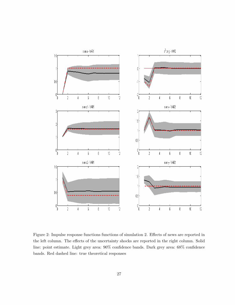
Figure 2: Impulse response functions functions of simulation 2. Effects of news are reported in
the left column. The effects of the uncertainty shocks are reported in the right column. Solid
line: point estimate. Light grey area: 90% confidence bands. Dark grey area: 68% confidence
bands. Red dashed line: true theoretical responses
27

Figure 3: Impulse response functions functions of simulation 2. Effects of news are reported in
the left column. The effects of the uncertainty shocks are reported in the right column. Solid
line: point estimate. Grey area: 68% confidence bands. Red dashed line: true theoretical
responses.
28
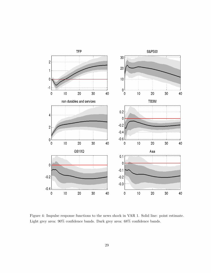
Figure 4: Impulse response functions to the news shock in VAR 1. Solid line: point estimate.
Light grey area: 90% confidence bands. Dark grey area: 68% confidence bands.
29

Figure 5: Plots of (a) the squared news shock (first panel), (b) squared-news uncertainty
(k = 3), (c) VXO, (d) Jurado, Ludvigson and Ng 3-month uncertainty.
30

Figure 6: Impulse response functions to the squared news shock in VAR 2. Solid line: point
estimate. Light grey area: 90% confidence bands. Dark grey area: 68% confidence bands.
31

Figure 7: Impulse response functions to the news shock in VAR 2. Solid line: point estimate.
Light grey area: 90% confidence bands. Dark grey area: 68% confidence bands.
32

Figure 8: The uncertainty effect of the news shock on GDP, for different values of the news
shock (VAR 2). Solid line: point estimate. Light grey area: 90% confidence bands. Dark grey
area: 68% confidence bands.
33

Figure 9: The total reaction of GDP to the news shock, including both the expectation effect
and the uncertainty effect, for different values of the news shock (VAR 2). Solid line: point
estimate. Light grey area: 90% confidence bands. Dark grey area: 68% confidence bands.
34

Figure 10: Historical decomposition of GDP (VAR 2). Blue line: per-capita GDP. Red line:
per-capita GDP minus the uncertainty effects of news.
35

Figure 11: Historical decomposition of GDP (VAR 2). Blue line: per-capita GDP. Red line:
per-capita GDP minus the total effects of news, including the uncertainty effects.
36

Figure 12: Impulse response functions to the squared news shock in VAR 3. Solid line: point
estimate. Light grey area: 90% confidence bands. Dark grey area: 68% confidence bands.
37
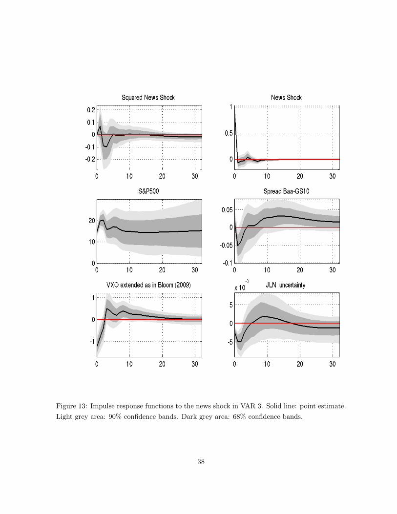
Figure 13: Impulse response functions to the news shock in VAR 3. Solid line: point estimate.
Light grey area: 90% confidence bands. Dark grey area: 68% confidence bands.
38

Figure 14: Robustness: Impulse response functions to the squared news shock with the spec-
ification of VAR 2 and two alternative identification schemes: the recursive scheme with the
news shock ordered first (red dashed line) and a long-run restriction imposing zero effect of
squared news on GDP at the ten-year horizon. The black solid line and the confidence bands
are the point estimate and the confidence bands of the benchmark case.
39

Figure 15: Robustness: Impulse response functions to the squared news shock for different
specifications of VAR 1: (i) TFP, S&P500, Consumption and TB3M (red-dashed line) and (ii)
TFP, Investment and TB3M (blue dotted-dashed line). Identification of both VAR 1 and VAR
2 are unchanged. The black solid line and the confidence bands are the point estimate and the
confidence bands of the benchmark case.
40