.... uNPU_Us

_-_'_ -NEWYORKUNIVERSITY;i..... 2 ......

https://ntrs.nasa.gov/search.jsp?R=19630007463 2020-03-26T21:50:30+00:00Z

NEW YORKUNIVERSITY

College of Engineering

Research Division

INTERACTION BETWEEN THE SOLAR WIND

AND THE GEOMAGNETIC FIELD

by

James Hurley

Project Report

Approved

Arthur Beiser

Project Director

The work described herein was sponsored by the Advanced Research

Projects Agency under Order Nr. 163-61, through the U.S. Army

Signal Research and Development Laboratory under Contract Nr.DA 36-0390SC-87171 and by the National Aeronautics and SpaceAdministration under Grant No. NsG 108-61.

2

ACKNOWLEDGEMENTS

I would llke to express my thanks to Professor

Arthur Beiser for suggesting the problem and for his

assistance throughout the course of the research.

This _ork _as supported in part by the National

Science Foundation, the Advanced Research Projects

Agency of the Defense Department3 and the National

Aeronautical and Space Administration.

3

ii

ABSTRACT

There is nov considerable evidence for the existence of

an interaction between the solar wind and the geomagnetic field.

The solar wind is a highly ionized plasma and as such may well

influence the earth's magnetic field. It is this interaction

that we have studied.

We have limited ourselves to a two dimensional model to

permit an exact solution to be obtained. The plasma wind is

considered as impinging upon an arbitrarily oriented two dimen-

sional magnetic dipole. We find that the field is compressed

by the plasma and essentially confined to form a cavity in the

plasma wind. The thickness of the boundary layer within which

the plasma and field interact is found to be small. We have

determined the equation of this boundary surface and the extent

to which the field is changed by such a confinement.

We have also considered the stability of such a system.

We find that there are certain regions of instability, but for

the part of the surface facing the wind it is stable.

iii

Table of ContentsJ

Introduction .................

Depth of penetration ..............

Reflection from the cavity boundary .........

Definition of the problem ............

Interaction between a plasma wind and the field of an

infinite line current ............

Interaction between a plasma wind and the magnetic

field of a two dimensional dipole .........

Arbitrary angle of incidence ...........

An approximation method .............

Stability ..................

Summary ..................

References ........... . . . . . .

Page

1

3

15

16

19

23

39

42

54

56

5

INTRODUCTION

Recently a great deal of work has been devoted to the problem of

the interaction of the solar wind with the earth's magnetic field. The

solar wind consists of a totally ionized hydrogen plasma continuously

streaming from the sun. The velocity and density in the neighborhood

of the earth are approximately l07 cm/sec, and 100 cm "3 respectively.

These values have been estimated by Biermann and others by observing the

deflection of comet tails in the solar wind. Further evidence of its

existence is the geomagnetic storms accompanying increased solar activity.

The mechanism for this disturbance will be made clear in the work that

follows.

The energy density of this plasma is 1/2 Nmv 2 = 0.83 × l0 -8 ergs/cm 3

where N is the number density of the plasma particles and m the proton

mass. If we approximate the earth's field by a simple dipole the magnetic

field in the equatorial plane is B = 0.35(Ro/R)3 where R ° is the radius of

the earth and 0.35 the earth's field in gauss at the equator. The energy

density of the magnetic field then is B2/8_ = (.35Ro3/R3)2/8_. We see

that the energy density of the field and the energy density of the plasma

wind are equal at approximately 9.1 earth's radii. If the plasma wind

is to have any effect on the earth's field it should be felt at 9.1

earth's radii and beyond.

There is direct experimental evidence for such an interaction. Rocket

studies I indicate that the earth's magnetic field behaves roughly llke a

dipole out to 12-13 earth's radii where it sharply decreases to the field

i A Radial Rocket Survey of the Distant Geomagnetic Field, C.P. Sonett,

D.L. Judge, A.R. Sims, and J.M. Kelso_ Space Technology Laboratories Report

732o,2-13.

g

2,

of interplanetary space (5 × 10-5 gauss).

We wish to describe the nature of the interaction between the plas-

ma wind and the earth's field. In particular we shall show that the wind

compresses the field so that a cavity is formed in the wind. This com-

pression may be seen physically from either macroscopic or microscopic

models.

First let us consider the macroscopic model. The solar plasma has

a high conductivity. Parker I has estimated the mean free path to be of

the order of lO6 km. Now a good conductor behaves diamagnetically.

Any magnetic field which exists initially in the conductor will tend to

persist. If the field is zero initially it will remain zero. This pheno-

menon of diamagnetism may be explained by Lenz's law. If the magnetic

field does change there will be an induced electric field. The induced

currents will flow in such a direction so as to oppose the change in the

field. The greater the conductivity the greater the opposition to change.

Thus if we imagine a plasma streaming toward the dipole from infinity

where the magnetic field is zero the magnetic field must remain zero for

all time in the limit of infinite conductivity, i.e. the magnetic field

in the plasma may not change.

We may also envisage this exclusion of the field from the plasma

from a microscopic picture. Since the mean free paths are so enormous

a particle description is certainly better suited to describe the inter-

action. Charged particles moving in a magnetic field themselves create

magnetic fields. Imagine a uniform magnetic field in the negative half

1E.N. Parker, Interaction of the Solar Wind with the Geomagnetic Field,

Phys. of Flui_s, i, 171 (1958).

7

.

space y < 0 and zero in the positive half space y > 0. Consider a

particle incident on the field-vacuum interface along the y-axis from

y = +_. It will be curved by the magnetic field moving in a semicir-

cular path with center of curvature on the positive or negative x-axis

depending on the sign of the charge. In either case the particle will

decrease the field within its orbit (i.e. within the semicircle) and

increase the field outside. We may now generalize to consider the prob-

lem of a plasma incident on the interface. For sufficiently large num-

bers of particles the magnetic field may be materially reduced within

the region where the particles are turning, and increased beyond this

region. Thus we may speak of a compression of the magnetic field by

the plasma stream. We shall study this problem in more detail later.

In our particle picture we may describe the interaction as follows.

The plasma particles move in straight lines (because of their long mean

free paths), penetrate a short distance into the field3 and are then de-

flected out.

A more rigorous Justification of these statements will follow in

the next section.

DEPTH OF PENETRATION

The problem to be described now has been considered by Dungey I and

2Rosenbluth . Our reason for including it here is partly for complete-

ness and partly because we feel that an important feature of the problem

1J.W. Dungey, Cosmic Electrodynamics (Cambridge University Press, New York

19_8), Sec. 8.3.

M. Rosenbluth, in Magnetohydrodynamics, edited by R. Landshoff (Stanford

University Press, Stanford, California, 19_7).

8

So

has been ignored.

We vould llke to knov how far the plasma will penetrate into the

magnetic field. To this end ve shall investigate the following two

dimensional problem. The magnetic field is constant in the half space

x < 0 and approaches 0 as x approaches infinity. The flel_ is every-

where parallel to the z-axls. The plasma is incident on the field from

x = + _. We assume that all the particles are moving parallel to the

x-axis before encountering the field. We expect the path of the par-

ticles to be curved as they enter the field and be deflected out. The

protons having the greater momentum will penetrate further than the elec-

trons, thereby building up a space charge. The electric field of this

space charge will tend to pull the electrons in with the protons. The

paths of the particles are roughly described in Fig. 1. We observe that

the particle current is responsible for the decay of the magnetic field

in the x-dlrection. The discontinuity in the magnetic field between

x = 0 and x = _ is equal to the total particle current in the y-direction.

The solution of this problem is determined by a self-conslstent

solution of the equations of motions of the particles and Maxwell's equa-

tions. The boundary conditions are that B = Bo at x = 0 and B _ 0 as

x -* _. The electric field must be 0 at x = 0 and approach zero as

x-* + _. Let (Up(X), Vp(X)_ O) be the (x3y, z) components of the outgo-

ing protons. From symmetry we see that the velocity components for the

incoming protons are (-Up3Vp_O). The corresponding velocity components

of the electrons are (Ue,Ve_0) and (-Ue, Ve,O ). Let Up(X) and ne(X ) be

the number density of the incoming and outgoing protons and electrons

respectively. The magnetic field is represented by a vector potential

9

Q

having only a y-component A(x), and the electric field by a scalar poten-

tial _(x). The number density and velocity at x = _ are N and U.

We may integrate the y-component of the equations of motion

eA eAv +--= v ---= o . (i)p me e me

p e

The energy equation gives

2 2 2 2U +V + = U +V - = •p p m e e m

p e

(2)

Particle conservation requires

n u = n u = NU (3)pp ee

Maxwell's equations are

and

d2A -8{e _dx---_ = (npVp neV e ) (4)

d2_ -8_e(np (5)d.x2 = - ne) •

(The currents and charge densities have been doubled to include both in-

coming and outgoing particles. )

The above system of equations apply in region II only. If the elec-

tron terms are dropped we obtain the equations appropriate to region I.

It goes without saying that these equations cannot be solved exactly.

We can however find a valuable first integral. (It is at this point that

we depart from Dungey's analysis.)

I0

.

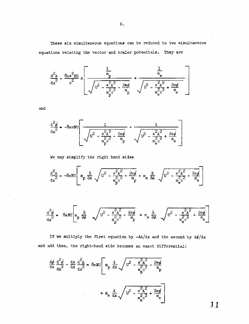
These six simultaneous equations can be reduced to two simultaneous

equations relating the vector and scalar potentials. They are

m

mp + e

e2A2 e2A222 m --_+ m

mc p mc ep e

and

dx2= -8_eNU e% 2 2e_ e2A 2

- --/_" m - 2-r-_+2-_m

mc p mc ep e

We may simplify the right hand sides

---_ - m e _[ - m"_ +m c p m c melIp e d

d__ e2A 2 2e_ +m _) e2A2= 8_NU 2 2 m e _-_ - 2 2 + m

dx 2 mpc p meC e

If we multiply the first equation by -dA/dx and the second by d6/dx

and add them, the right-hand side becomes an exact differential:

J e2A2d__ d___ dAd2A 8_NU d _ 22 m

_2 _ _2 _ _ mpC p

+ me

- _meC + meJ

,

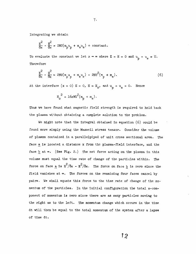
Integrating we obtain

E 2 H 2

- _ = 2NU(mpUp + meUe) + constant.

To evaluate the constant we let x _ _ where E = H = 0 and u = u = U.p e

Therefore

E2 _ 2_(%Up + m u ) - 2_2% + (6)- _= e e me)"

At the interface (x = 0) E = 0_ H = Ho, and u = u = 0. Hencep e

2 16_NU2(mp + me).HO =

Thus we have found what magnetic field strength is required to hold back

the plasma without obtaining a complete solution to the problem.

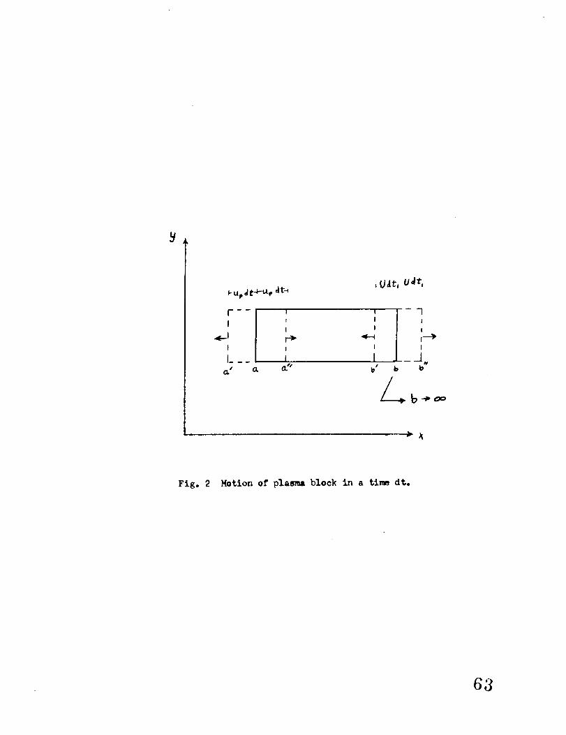
We might note that the integral obtained in equation (6) could be

found more simply using the Maxwell stress tensor. Consider the volume

of plasma contained in a parallelpiped of unit cross sectional area. The

face a is located a distance x from the plasma-fleld interface, and the

face b at _. (See Fig. 2.) The net force acting on the plasma in this

volume must equal the time rate of change of the particles within. The

force on face a is H2/8_ - E2/8_. The force on face b is zero since them

field vanishes at _. The forces on the remaining four faces cancel by

pairs. We shall equate this force to the time rate of change of the mo-

mentum of the particles. In the initial configuration the total x-com-

ponent of momentum is zero since there are as many particles moving to

the right as to the left. The momentum change which occurs in the time

dt will then be equal to the total momentum of the system after a lapse

of time dt.

L72

o

(We have omitted the motion in the y-direction as this would only compli-

cate the picture and is of no interest in calculating the change in the

x-component of momentum.) Those particles which were at the surface a

and moving to the left are at the surface a' after a time dt. Those

moving to the right are located at a" . b' and b" are defined in a simi-

lar way. The change in momentum then is the total momentum of those

particles between a' and b" which were between a and b at time t. There

will be other particles between a' and b" which moved in during the time

dt. These must not be counted. The momentum of the particles between

a" and b' is zero. The momentum of the particles between a' and a" is

-2u dtn m u and the momentum of those between b' and b"p p p p , 2UdtNmpU,

We must add similar expressions for the electrons. Equating F and dp/dt,

E 2 _ 2 2- _ = 2n m u + 2n m u - 9_N(m + m ")U2,

ppp eee -p e

but since n u = n u = NUpp ee

E2 H2

- _ = 2NU(mpUp + meU e) - 2NU2(mp + me)

which we see is eq. (6).

It is not possible to proceed any further with an exact solution.

We would however llke to estimate the rate of decay of the magnetic field,

i.e., how far from the vacuum-plasma interface must we go before the mag-

netic field becomes a small fraction of the vacuum field. It will be

important in our subsequent work that this distance is small compared

to the dimensions of the cavity.

Dungey has presented an approximate solution to this problem. He

assumes that the electron density is everywhere approximately equal to

13

.

the proton density. He has Justified the approximation using the full

set of equations (1,2,3,4_5). In doing so he has overlooked the possi-

bility of an absolute change separation such as would occur in region I.

In this region the electron terms must be omitted from the equations and

hence are not to be included in an estimate of the relative densities.

We will first find an upper limit on the thickness of region I and

then verify that Dungey's solution is valid in region II. Kaving stud-

ied both regions we may then estimate the thickness of the current

sheath.

We return to the integral we found in eq. (6).

E2 = H2 + 16_NU(mpUp + meUe) - 16_NU2(mp + me). (7)

Now at the interface between region I and II

and

u =0e

u <UP

H<HO

X XO O

E = 8_e f np dx >>8_e f

o o

N dx = 8_eNx ° ,

where x is the distance between the plasma-vacuum interface and theO

interface between I and II. Substituting into eq. (7) we find

(8_eNxo)2 << E 2 : H 2 + 16_NUmpUp - 2NU2(mp+ me)

< H 2 + Ib_NU2m-o p - 16xNU2(mp+ me)

= 16_NU2m .P

<

14

lO.

So that

or

m U22 _2__x <<

o 4_e2N(8)

x << 8 meters.o

Where 8 m. is a large distance in laboratory experiments, it is quite

small in comparison wlth the dimensions of the cavity, i0 7 - lO8 m.

We might obtain a better physical insight into this upper limit on

the charge separation by considering how much energy is available in the

plasma stream for charge separation. Let us imagine a block of plasma

of unit cross sectional area and width a moving to the left with a velo-

city U. The plasma block now runs into an army of Maxwell demons who

instantaneously stop all the electrons and allow the protons to pass.

We shall simplify the calculation by assuming that the protons move as

a block, and we ask how far this block will move before coming to rest.

When the protons are at rest the energy stored in the electric field

must equal the initial kinetic energy. If the protons are displaced

a distance x° (see fig. 3.) from the electrons the electric field is

E = 4_eNx O.

Equating the field energy to the kinetic energy

16_2e2N2Xo 2

E2/8 - a = 1/2

so that m U22 __p__X

o 4_Ne 2

which is identical to the upper limit for the change separation obtained

ll.

in eq. (8). (Wehave tacitly assumedthat b >> xo.) The fact that the

numerical coefficient is the sameis of course fortuitous.

Novlet us consider region II. Here we shall showthat Dungey's

solution is quite good. He assumesthat the electron and ion charge

distributions are approximately equal. This assumptionis to be tested

a posteriori. Fromeq. (3) we see that

U _ U •

e p

The y-components of the electron and proton velocities are related by

eq. (1)

mv : -mypp ee

so that IVpl << IVel. We may therefore neglect the proton current in

eq. (4) so that

d2A 8_eNU Ve

_= C m e

(9)

If we now eliminate _ from eq. (2) and substitute for Vp and v e from

eq. (I) we find that

2 e2A 2 U 2mu + =mpp _ p

m ce

(i0)

/mp. We now solve eq. (I0) for uneglecting terms of order me p

for v e mad substitute in eq. (9) remembering that Up = Ue,

eA

d2A 8_ eNU mec

72 e

2mm c

ep

and eq. (I)

(ii)

12

Let

= A/AO

wheremm c2_

2 epAo - 2

e

and

X' = X/X O

whe re2

m c2 e

x -o 8_Ne

Eq. (II) then becomes

Clearly a _ i so we set _ = sin 8. Integrating

x' = - gn(tan 8/4) - 2 cos(@/2) + 6n(_/_ - l) + _/_

For small @

x' = - _n 9/4

or

= _e -Xl

so that

dA -x r

H _ dx---T Do e

The field then will decrease by a factor I/e when x' = l, i.e.

_8_Ne I

meC

x = _ 500 m.

for N = i00 cm-3. This is again much less than the dimensions of the cavity.

17

13

We must now justify the assumption made earlier that the electron

and proton densities are approximately equal. We may do this by calcu-

lating

Now

d2_ -8_e(np n )dx 2= - e'

me (Ue2 2 U2)- ve -

and from eq. (I0)

2 U2 e2A 2 A2Ue = 2 - U2 - U2 --2 = 02 c°s2e

mmc Ae p o

Als o

2V

e

2e2A 2 m A 2 m

2 2=m -_U2c _-_ = _ U2 sin2em e m

e o e

so that 2

m_ < c 4 l_¢__ e os2e + sin2@ _m

e

(12)

(13)

We observe that if m were to equal m the potential would bee p

zero and consequently no charge separation would occur. This is to be

expected. If the particles have the same mass they must penetrate to

equal depths.

Differentiating eq. (13) twice we find

so that

8_NeU2c [ sin2e qd._ (mp me) 7 2 - 2 cos @ c-_ @_Jdx2 =e

n (mp- me)NU22 E sin2@cob__/qn - = 2 - 2 cos @ - _-z_ •e p mc

e

18

14

We see that the plasma is far from neutrality at @ = _/2, i.e. at the

= _ _). Although n and n differ con-point where u = 0 (ne NU/u e ee p

slderably near x = 0 (@ = _/2) the approximation may still be a good

one. We must go back to our calculation of the field decay and investi-

gate what is a reasonable measure of large deviation from neutrality.

In calculating the field from eq. (9) we substituted for ue the

value obtained from eq. (i0) for u assuming that u = u . Let us seep p e

how far n and n must differ before this becomes a poor approximation.e p

Let n - n = 5. Nowp e

or

nu =nupp ee

u = P= + U •

e ne p

We require that

No%r

n - np e <<i.

ne

NU U/cos @n = --e u

e

since

U = U cos @e

from eq. (12). So that

ne - n (mp - me)U 2 (2 cos @ - 2 cos2@ - sin2@)n = 2e m c

e

_ (2 cos @ - cos2@ - i) < .002 or,2%.m ce

19

15

This completes our discussion of the rate of decay of the field in

the stream. We have shown that the region where the field differs appre-

ciably from zero is much smaller than the dimensions of the cavity. (We

shall, in the future, refer to this region as the current sheath.) Since

the mean free path is so large the plasma constituents will behave as

free particles until they reach the cavity boundary where they are reflec-

ted. We shall now consider the problem of the reflection of particles

with an arbitrary angle of incidence.

REFLECTION FROM THE CAVITY BOUNDARY

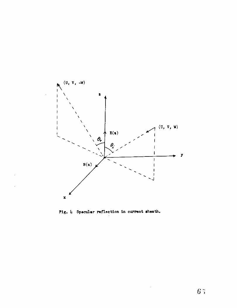
We wish to show now that if the current sheath is small the particles

will be specularly reflected from the sheath. We shall consider charged

particles incident on a magnetic field as above except their velocity com-

ponents at infinity are now (U, V, W). The magnetic and electric fields,

B = B(z) _ and E = E(z) _, approach zero as z _ _. We shall show that

after reflection the velocity components will be (U, V, -W) so that the

angle of incidence is equal to the angle of reflection. (See Fig. 4_)

The fields may be expressed in terms of a vector and scalar potential

A = Ay(Z) and _ = _(z). The path of the particle is determined by the

conservati on laws,

u = u (i_)

v + --v (15)mc

i

2 w2 e__ V2 + W2v + + mc TM (16)

where (u, v, w) are the velocity components at some Intermediate point of

the motion. The constants of the motion in eqs. (14,15,16) have been

16

evaluated at t = - _. We now look at t = + _. Assuming that the field

has sufficient depth that the particle is reflected and not transmitted

then z _ + _ as t _ + _. Eq. (15) requires then that v _ V as t _ + _.

Substituting u = U and v = V in eq. (16) and observing that _(_) = 0

so that

w 2 _ W2

w _+Wt=+_

w = - W •t_

We might generalize this conclusion somewhat to include curved fields

with the proper symmetry. However, for our purposes it will be sufficient

to require that the _eld may be approximated locally by a plane field

whose principle gradient is perpendicular to the field (i.e. within the

orbit of a particle, the field does not vary appreci_le along the field

lines).

DEFINITION OF THE PROBLEM

Let us now return to the problem of physical interest, a plasma wind

blowing on the magnetic field of a dipole. As we have demonstrated , the

plasma constituents will move in straight lines up to the cavity boundary

where they are specularly reflected. The region of interaction (current

sheath) separates the plasma from the field. Since the sheath thickness

is small we may treat it as a boundary surface separating the two domalns.

In the plasma domain we have streaming particles making elastic collisions

with the boundary and in the field domain we have a static magnetic field

g_

17

confined to a cavity by the boundary surface. The equilibrium shape of

the cavity surface will be determined by a condition of pressure balance.

The magnetic pressure within the cawity must balanc_ the pressure of the

plasma wind from without. We may then formulate our idealized problem

as follows :

V x _ ,, 0 (17)

everywhere inside the cavity except at the dipole where

* - M/r3 sin0 $ - 3 cosO

as r-_O.

-@

v. B = 0 (18)

inside the cavity,

Bn = 0 (19)

on the surface, and

B2/8_ = 2Nm_ cos_ (20)

on the surface. Here X is the angle between the normal to the surface and

the direction of the incident wind.

In eq. (17) we neglect all currents within the cavity such as atmos-

pheric currents and currents in the Van Allen belts_ or else we lump them

in with the dipole field. The boundary condition (eq. (19)) is imposed

since the field is zero outside the cavity and the normal component must

be continuous. Eq. (20) expresses the condition of pressure balance, i.e.

we are looking for a steady state solution.

This problem differs in an essential way from the usual boundary

value problem. If the magnetic field were expressed as the gradient of a

18

scalar field, the problemwould be determined by finding a scalar solution

to Laplace's equation having the appropriate singularity at the origin and

satisfying two boundary conditions. Normally one is given the boundary and

one boundary condition. Here the second boundary condition must determine

the boundary.

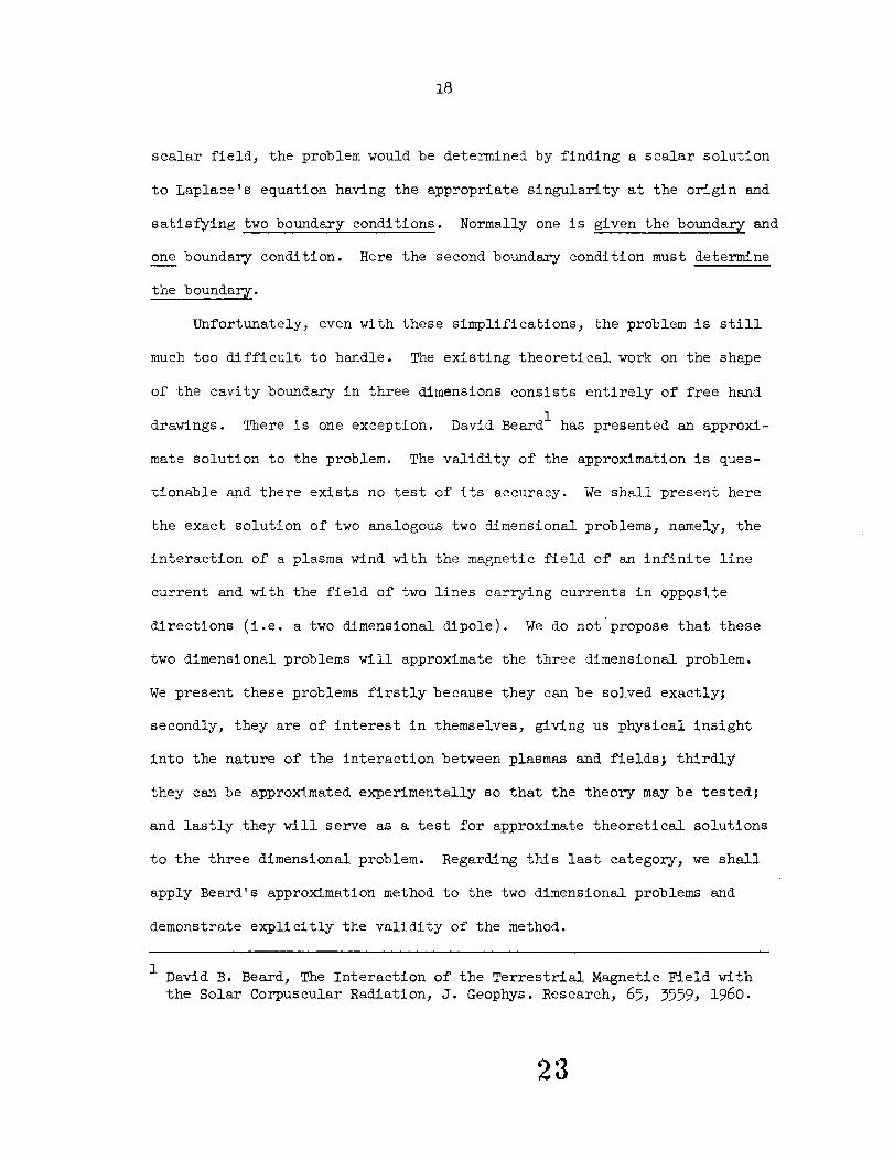
Unfortunately, even with these simplifications, the problem is still

much too difficult to handle. The existing theoretical work on the shape

of the cavity boundary in three dimensions consists entirely of free hand

drawings. There is one exception. David Beard I has presented an approxi-

mate solution to the problem. The validity of the approximation is ques-

tionable and there exists no test of its accuracy. We shall present here

the exact solution of two analogous two dimensional problems, namely, the

interaction of a plasma wind with the magnetic field of an infinite line

current and with the field of two lines carrying currents in opposite

directions (i.e. a two dimensional dipole). We do not propose that these

two dimensional problems will approximate the three dimensional problem.

We present these problems firstly because they can be solved exactly;

secondly, they are of interest in themselves, giving us physical insight

into the nature of the interaction between plasmas and fields; thirdly

they can be approximated experimentally so that the theory may be tested;

and lastly they will serve as a test for approximate theoretical solutions

to the three dimensional problem. Regarding this last category, we shall

apply Beard's approximation method to the two dimensional problems and

demonstrate explicitly the validity of the method.

David B. Beard, The Interaction of the Terrestrial Magnetic Field with

the Solar Corpuscular Radiation, J. Geophys. Research, 65, 3559, 1960.

23

19

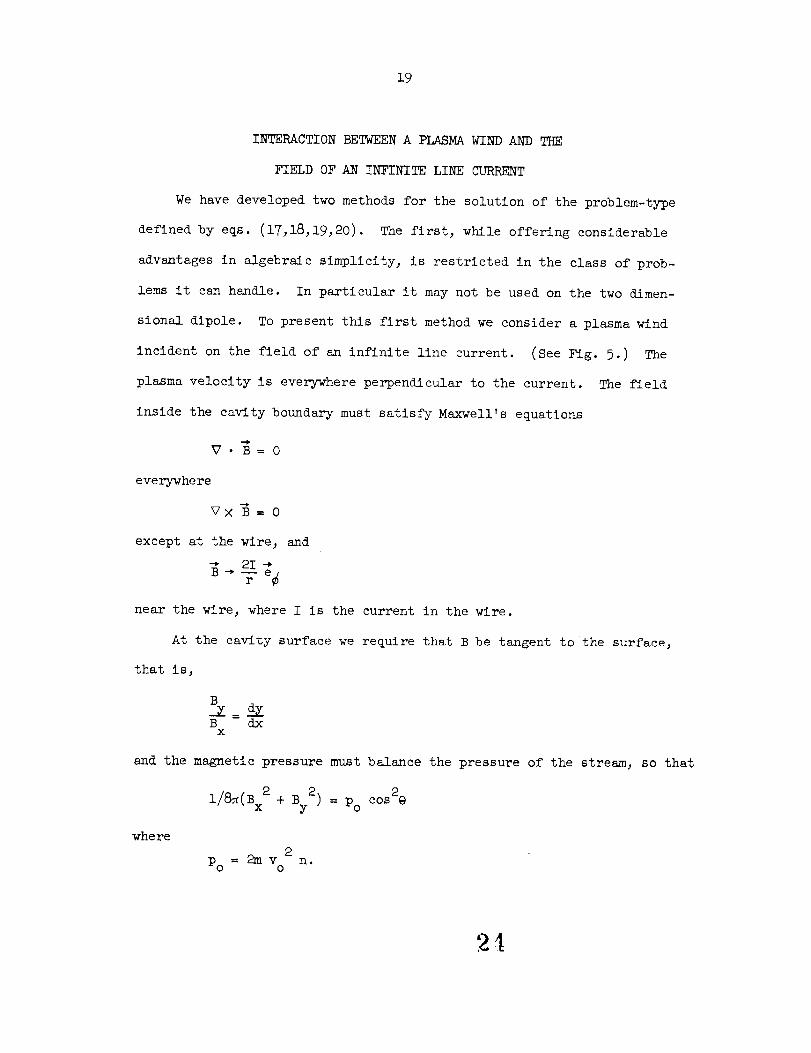
INTERACTION BETWEEN A PLASMA WIND AND THE

FIELD OF AN INFINITE LINE CURRENT

We have developed two methods for the solution of the problem-type

defined by eqs. (17,18,19,20). The firstj while offering considerable

advantages in algebraic simplicity, is restricted in the class of prob-

lems it can handle. In particular it may not be used on the two dimen-

sional dipole. To present this first method we consider a plasma wind

incident on the field of an infinite llne current. (See Fig. 5.) The

plasma velocity is everywhere perpendicular to the current. The field

inside the cavity boundary must satisfy Maxwell's equations

_7. B=0

everywhere

vx =o

except at the wire 3 and

r

near the wire, where I is the current in the wire.

At the cavity surface we require that B be tangent to the surface_

that is,

B_Z =B dxx

and the magnetic pressure must balance the pressure of the stream, so that

2) =i/8_(Bx 2 + By Po c°s2@

where

2

Po = 2m v ° no

2O

We now reformulate the problem in complex notation. Since

_B(z_ z* 12 az' - v •B + ilvx _'_iO,.-"Z

B must be a function of z* where

B=B +IB .x y

The singularity at the wire required that

B-* 2Ii/z* as z _ 0.

To formulate the boundary conditions consider

B-am :_. £s +ilEx £sI.

The imaginary part must be zero (tangency condition).

l

(SxPo)_ cos @ d_

from the condition of pressure balance. Since cos @ = dy/ds we may

state both boundary conditions in the single equation

1

B*_z - (8_Po)_ ay.

Our problem then is to find a complex function B such that

B --_(z*)

B-* 2Ii/z* as z -* 0

and

B*dz,,(8_po)½dy

on the surface.

Let

The real part is

(21)

(22)

(2.5)

We now use the unknown field B to generate a conformal mapplng. 1

w(_.)- 1/i_*

1J.D. Cole and J.H. Huth, Physics of Fluids, 2, 624 (1959).

21

where

W= U+ iV.

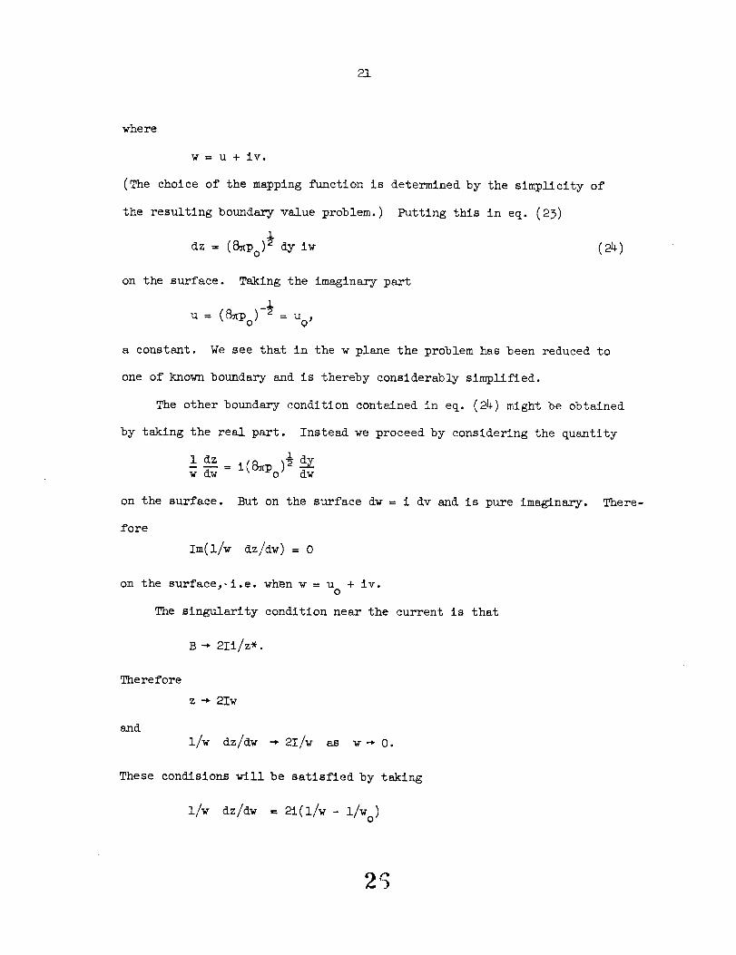
(The choice of the mapping function is determined by the simplicity of

the resulting boundary value problem.) Putting this in eq. (23)

dz = (_po)½dy iw (24)

on the surface. Taking the imaginary part

1

u = (_po)-_= U02

a constant. We see that in the w plane the problem has been reduced to

one of known boundary and is thereby considerably simplified.

The other boundary condition contained in eq. (24) might be obtained

by taking the real part. Instead we proceed by considering the quantity

i dz , _Iw d_= i_8_poJ_dw

There-on the surface.

fore

Im(i/w

But on the surface dw = i dv and is pure imaginary.

dz/dw)= 0

on the surface,-i.e, when w = u + iv.O

The singularity condition near the current is that

Therefore

and

B _ 21i/z*.

z -_ 21w

i/w dz/dw* 21/w as _ o.

These condlsions will be satisfied by taking

I/w dz/dw _ 21(i/w-llwo)

22

where (see Fig. 6)

=w- 2u ."_o o

We find then for z

w - 2u_z = -4I u° &n _ - •

The constant of integration a is determined by the singularity condition.

Let a = -2u . ThenO

z = -4Iu ° _n(l - w/2u o) (25)

and approaches 2Iw as it should.

If we evaluate w in eq. (25) on the surface (w = u ° + iv) we deter-

mine the surface

uc)zs =-4IUo &n _ o (26)

so that

2(% + 2)½

xs = -4IUo _n (27)2u

0

Ys = 4Iu O tan -I v/u o. (28)

which are parametric equations for the boundary surface. These results

are plotted in Fig. 7.

Eq. (25), besides giving us the shape of the cavity boundary, can

be inverted to give us also the magnetic field. Solving for w

_z/4iUo_w = 2u0 1 - e

But

1

27

23

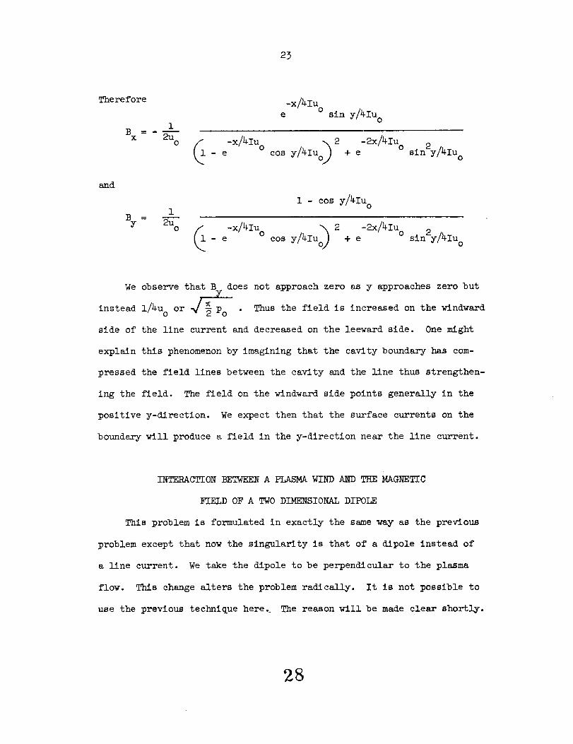
Therefore

1Bx 2u

O

and

1

By=O

-x/41uO

e sin y/41u O

-x/41u° cos y/41Uo_- e

2 -2x/41u °

+ e sin2y/41Uo

i - cos y/41u °

"x/41u° cos y/41Uo_- e

2 - /41u°+ e sln2y/41Uo

We observe that B does not approach zero as y approaches zero but

instead 1/4u ° or _ . Thus the field is increased on the windward

side of the line current and decreased on the leeward side. One might

explain this phenomenon by imagining that the cavity boundary has com-

pressed the field lines between the cavity and the line thus strengthen-

ing the field. The field on the _-Indward side points generally in the

positive y-dlrection. We expect then that the surface currents on the

boundary_lll produce a field in the y-direction near the llne current.

INTERACTION BETWEEN A PLASMA WIND AND THE MAGNETIC

FIELD OF A TWO DIMENSIONAL DIPOLE

This problem is formulated in exactly the same _ay as the previous

problem except that now the singularity is that of a dipole instead of

a line current. We take the dipole to be perpendicular to the plasma

flow. This change alters the problem radically. It is not possible to

use the previous technique here. The reason will be made clear shortly.

28

24

We begin again with the relevant equations,

_7xB-O

everywhere except at the dipole where

2 2B-*2M e ex 4

r

as r _ O. Here M is the dipole moment.

- B = 0

everywhere.

The field must be tangent to the cavity surface so that

B_Z = _YB dxX

and the magnetic pressure must balance the pressure of the stream,

where

Bi +

Po = 2Nmv2"

= Po c°sfiX

Again we find a considerable simplification by expressing these

conditions in complex notation. The two Maxwell's equations become

B = B(z*)

and the two boundary conditions

B* dz = B • ds + i B X ds = (+)

The singularity at the dipole is

2mi

Z

as z-*0.

dy.

(ag)

(30)

(3l)

29

25

The reason for the (+) in eq. (30) can be seen from the geometry of

the field. We have made a rough sketch of this in Figure 8.

If ds is a vector tangent to the surface and the sense is defined

in the usual way (moving along the surface we keep the internal domain

on our left) we see that E'_s (i.e. the real part of B* dz) is negative

between the two neutral points (N) and positive outside.

The magnetic field reverses direction at the neutral points and is

therefore zero there. Since the magnetic pressure is zero the particle

pressure, and hence the slope, must also be zero.

It is this reversal of sign that prevents us from using the previous

method of attack on this problem. If we again used the field to define

a transformation, the transformed boundary shape would no longer be a

plane. This plane was defined by the condition that u = 1/V_o = U o"

This condition becomes in the present case u = + u depending on whether-- O

we are inside or outside of the neutral points and the transformed geometry

would becomeV

Fig. 9.

U

It

gO

26

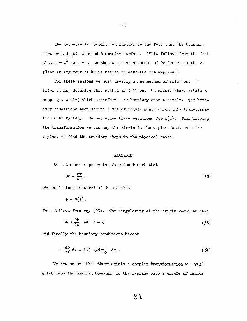
The geometry is complicated further by the fact that the boundary

lies on a double sheeted Riemanian surface. (This follows from the fact

2that w _ z as z _ O, so that where an argument of 2_ described the z-

plane an argument of 4_ is needed to describe the w-plane.)

For these reasons we must develop a new method of solution. In

brief we may describe this method as follows. We assume there exists a

mapping w = w(z) which transforms the boundary onto a circle. The boun-

dary conditions then define a set of requirements which this transforma-

tion must satisfy. We may solve these equations for w(z). Then knowing

the transformation we can map the circle in the w-plane back onto the

z-plane to find the boundary shape in the physical space.

ANALYSIS

We introduce a potential function _ such that

The conditions required of _ are that

¢(z).

This follows from eq. (29). The singularity at the origin requires that

2M¢*i-T as z*o. (33)

And finally the boundary conditions become

We now assume that there exists a complex transformation w = w(z)

which maps the unknown boundary in the z-plane onto a circle of radius

t.;

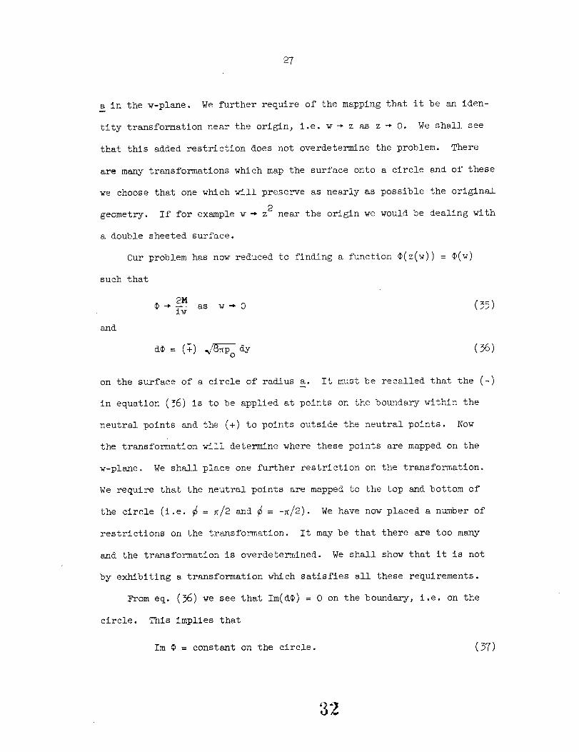
27

a in the w-plane. We further require of the mapping that it be an iden-

tity transformation near the origin, i.e. w _ z as z _ 0. We shall see

that this added restriction does not overdetermine the problem. There

are many transformations which map the surface onto a circle and of these

we choose that one which will preserve as nearly as possible the original

2geometry. If for example w _ z nea_ the origin we would be dealing with

a double sheeted surface.

Our problem has now reduced to finding a function ¢(z(w)) = _(w)

such that

and

@_ 2M- as w_0 (35)iw

de= by

on the surface of a circle of radius a.

(36)

It must be recalled that the (-)

in equation (36) is to be applied at points on the boundary within the

neutra& points and the (+) to points outside the neutral points. Now

the transformation will determine where these points are mapped on the

w-plane. We shall place one further restriction on the transformation.

We require that the neutral points are mapped to the top and bottom of

the circle (i.e. _ = _/2 and _ = -_/2). We have now placed a number of

restrictions on the transformation. It may be that there are too many

and the transformation is overdetermined. We shall show that it is not

by exhibiting a transformation which satisfies all these requirements.

From eq. (36) we see that Im(d¢) = 0 on the boundary, i.e. on the

circle. This implies that

Im ¢ = constant on the circle. (37)

28

Then

or

and

We can see this condition physically in this way. Let ¢ = _ + i_.

dz dz

Since ¢(z) is analytic we may set dz = dx so that

Bx

where we have used the Cauchy-Riemann equations. Therefore

A AB=B e +B e =x x y y

The magnetic field lines then are the family of orthogonal trajectories to

the equipotential surfaces _ = constant. But we know that since _ and

are conjugate functions that _ = constant are the family of lines orthogo-

nal to _ = constant. Therefore the magnetic field lines are coincident

with the family of lines @ = constant. Now on the cavity surface the mag-

netic field lines must be tangential so that the surface is itself a

field llne. Therefore @ = Im ¢ = constant on the surface. We shall choose

this constant to be zero.

We shall attempt now to construct a trial solution for the potential.

2M 2M

¢ ia2 "

Let

asThis choice clearly fulfills the requirement of eq. (35) since w _ z

z _ O. It also satisfies eq, (37) since on the circle w = a ei_ and

33

29

2.M -i_ _ ei_ 4M sin_ = _a e - i-_ : - _-

so that Im ¢ = 0 on the circle.

There remains only to investigate the real part of eq. (36),

_ 4Ma cos_d_=; _ dy.

i,e,

This equation is readily integrated,

- 2 - sin

sin

2 - sin

- _ < ¢ <- _12

_12< ¢ < _12

whe re

aW oY' = 4M Y

We shall find it more convenient to write this equation in this form

2-sin_

y, _'____I _k sin_ (40)

-2-si

We wish now to find a function z' = z'(w) such that z' is propor-

tional to w near the origin and whose imaginary part satisfies eq. (40)

on the boundary. This function will define the transformation from the

z-plane to the w-plane.

31

3O

We shall construct this function piecemeal. Let us break up the

boundary value problem into two parts

y!

sin _ = 211_ 01+ sin _ I-l_!_

Consider the function

FI- 2_ gn 2 2

w2 w3

It is not difficult to show that

Im FI _- 0-I

when evaluated on the boundary.

Also, if

2

w 2!F2 = gn _ +

2i2

w 3

(The variables are defined in Fig. i0. )

then

Im F2 = -i _I S +i

when evaluated on the boundary.

Finally, let

F 3 = i/2(a/w - w/a)

then

F 3 = sin

on the circle.

31

Let us now evaluate the imaginary part of

F3F 2 + 2FI + real constant

on the boundary. We see that it is Just y'. (The addition of a real

constant will not affect this result.) We therefore set

i a w # w2 i Wl 2

z' +-w 3 _ w2 w 3

(4l)

We have chosen the constant so that z' _ 0 as w _ O.

4wm r -._ __

_a

In particular

as w-+ O_ or

16Mz-_ 2 W as W-_ 0 .

Now we assumed that z * w as w _ 0. We therefore choose the radius a

so that the coefficient of w is one, i.e.

2 16Ma = (42)

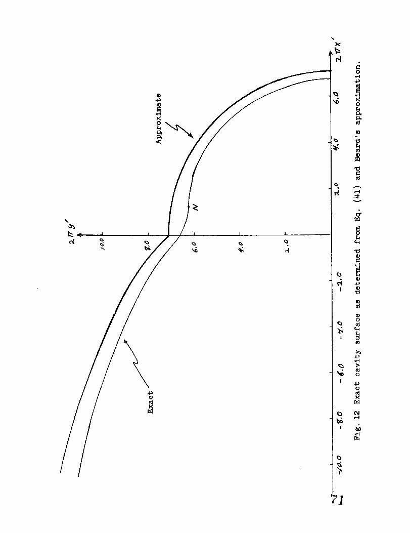
The real part of eq. (41) evaluated on the boundary is

x' i tn (i + c°s _)2 + 2 + I _ii " sln_ (43)= _ COS2_ _ _-stn _ Sn + sin

Eqs. (39) and (43) are parametric equation for the cavity boundary.

This has been plotted in Fig. 12.

31

32

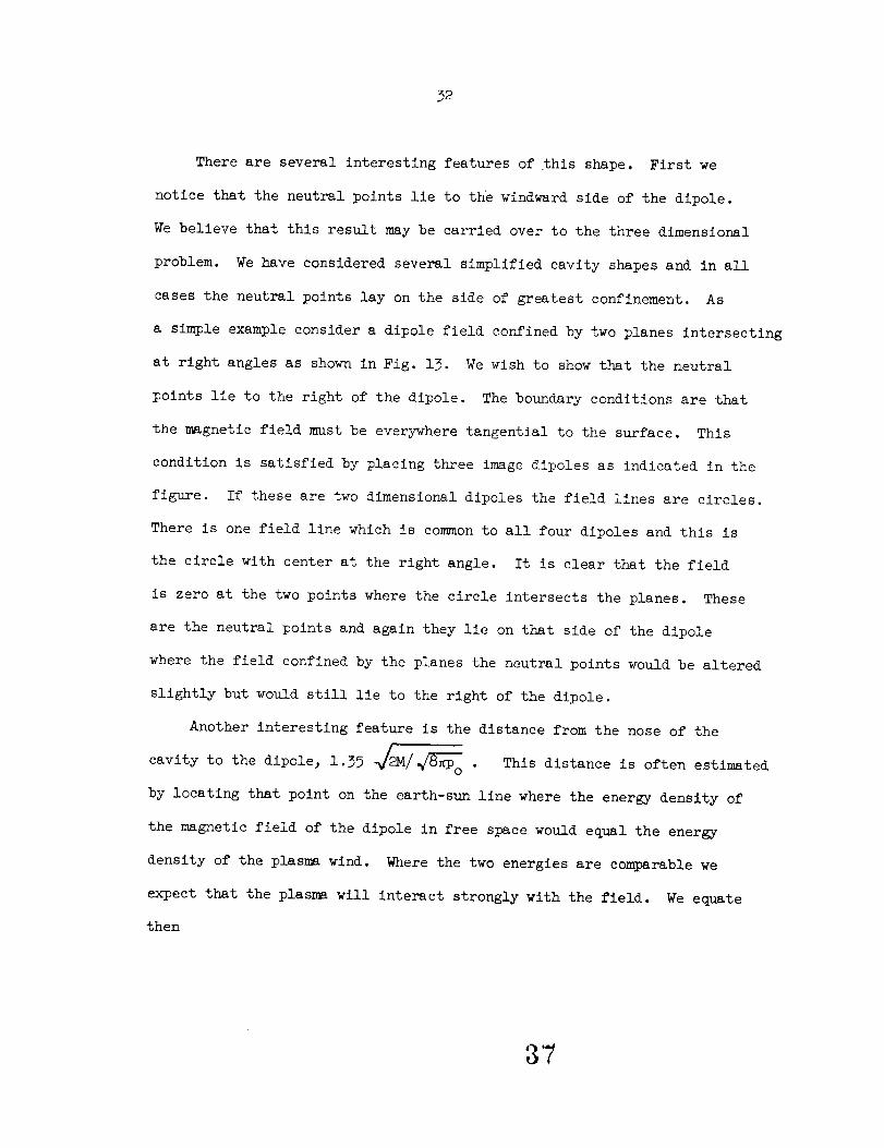
There are several interesting features of this shape. First we

notice that the neutral points lie to the windward side of the dipole.

We believe that this result may be carried over to the three dimensional

problem. We have considered several simplified cavity shapes and in all

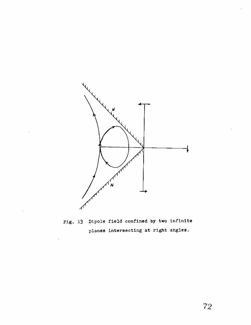
cases the neutral points lay on the side of greatest confinement. As

a simple example consider a dipole field confined by two planes intersecting

at right angles as shown in Fig. 13. We wish to show that the neutral

points lle to the right of the dipole. The boundary conditions are that

the magnetic field must be everywhere tangential to the surface. This

condition is satisfied by placing three image dipoles as indicated in the

figure. If these are two dimensional dipoles the field lines are circles.

There is one field line which is common to all four dipoles and this is

the circle with center at the right angle. It is clear that the field

is zero at the two points where the circle intersects the planes. These

are the neutral points and again they lie on that side of the dipole

where the field confined by the planes the neutral points would be altered

slightly but would still lle to the right of the dipole.

Another interesting feature is the distance from the nose of the

cavity to the dipole, 1.39 /P_M/_ . This distance is often estimated

by locating that point on the earth-sun line where the energy density of

the magnetic field of the dipole in free space would equal the energy

density of the plasma wind. Where the two energies are comparable we

expect that the plasma will interact strongly with the field. We equate

then

37

33

1B2/8_ = _ Nmv2

with

2MB _

2r

and find for the cut off distance

r _ i._i_/_I_o "

We see that the estimate is good to within 5%.

The magnetic field within the cavity may be determined from

eqs. (32,38,41). It is of particular interest to investigate the field

near the dipole. We find that at the commencement of a magnetic storm

(i.e. at a time of increased solar activity) the magnetic fle]d at the

surface of the earth at latitudes below the auroral zone is increased.

We shall now show that the magnetic field due to the currents in the

current sheath of the cavity boundary will enhance the field of the

dipole in the equitorial zone.

If we expand eq. (41) in a power series we find

1 w2 1 w3

z-w-_2-÷3-_+ ....a

Inverting this series we obtain

Now

W=Z+1 z2 1 Z3

3a 92"a

® ,, ].-. _.._.

88

34

or

¢=-- - 3a- 9a a+ ""

and

13" = _ = 2Ri + +a

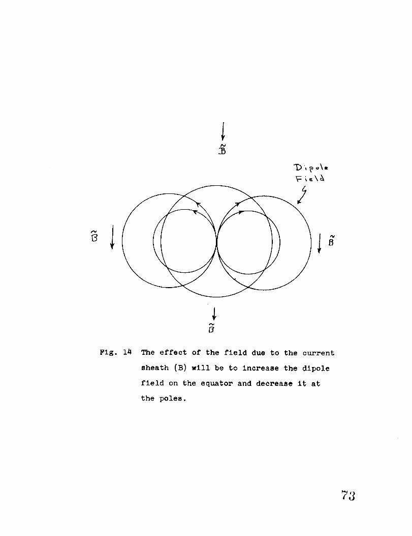
We see that we have a constant field superimposed on the dipole near the

origin. This field is

By = -2M .__7__

0a 2

such a field will enhance the field in the equitorial region and diminish

the field at the poles (see Fig. 14).

We should point out here that we have neglected the temperature of

the plasma wind. Certainly this assumption is valid when the slope of

the cavity wall is far from zero. The pressure of the wind on the boundary

is determined by the normal component of the plasma velocity. When the

slope is small the normal component of the velocity of mass flow may be

comparable with the thermal velocities. We expect then that the leeward

side of the cavity boundary should be pinched do_nwhen the thermal pressure

becomes comparable with the magnetic pressure.

ARBITRARY ANGLE OF INCIDENCE

Certainly the earth's dipole is not in general perpendicular to

the solar wind. It is of interest therefore to investigate the effect

of orientation on the cavity surface.

a9

35

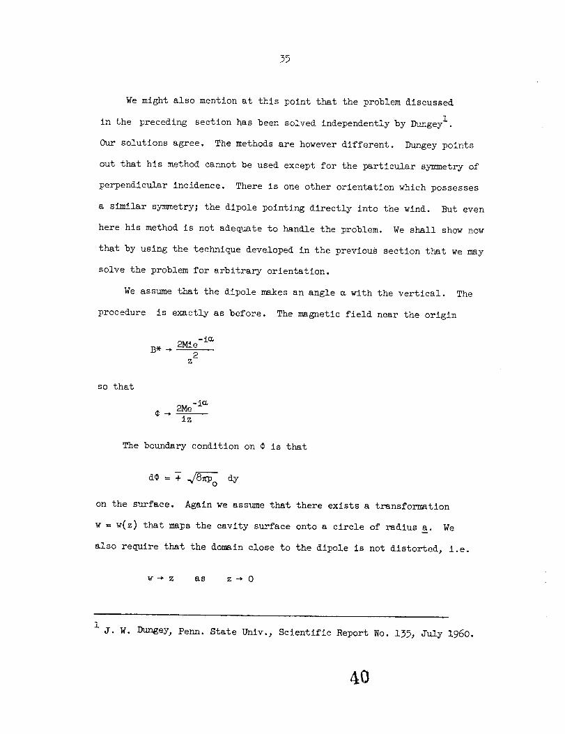
We might also mention at this point that the problem discussed

in the preceding section has been solved independently by Dungey 1.

Our solutions agree. The methods are however different. Ikungey points

out that his method cannot be used except for the particular symmetry of

perpendicular incidence. There is one other orientation which possesses

a similar symmetry; the dipole pointing directly into the wind. But even

here his method is not adequate to handle the problem. We shall show now

that by using the technique developed in the previous section that we may

solve the problem for arbitrary orientation.

We assume that the dipole makes an angle _ with the vertical. The

procedure is exactly as before. The magnetic field near the origin

RMie -i_

2z

so that

2Me- is

iz

The boundary condition on ¢ is that

on the surface. Again we assume that there exists a transformation

w = w(z) that maps the cavity surface onto a circle of radius a. We

also require that the domain close to the dipole is not distorted, i.e.

W-_ Z as z-* 0

iJ. W. Dungey, Penn. State Univ., Scientific Report No. 135, July 1960.

4O

36

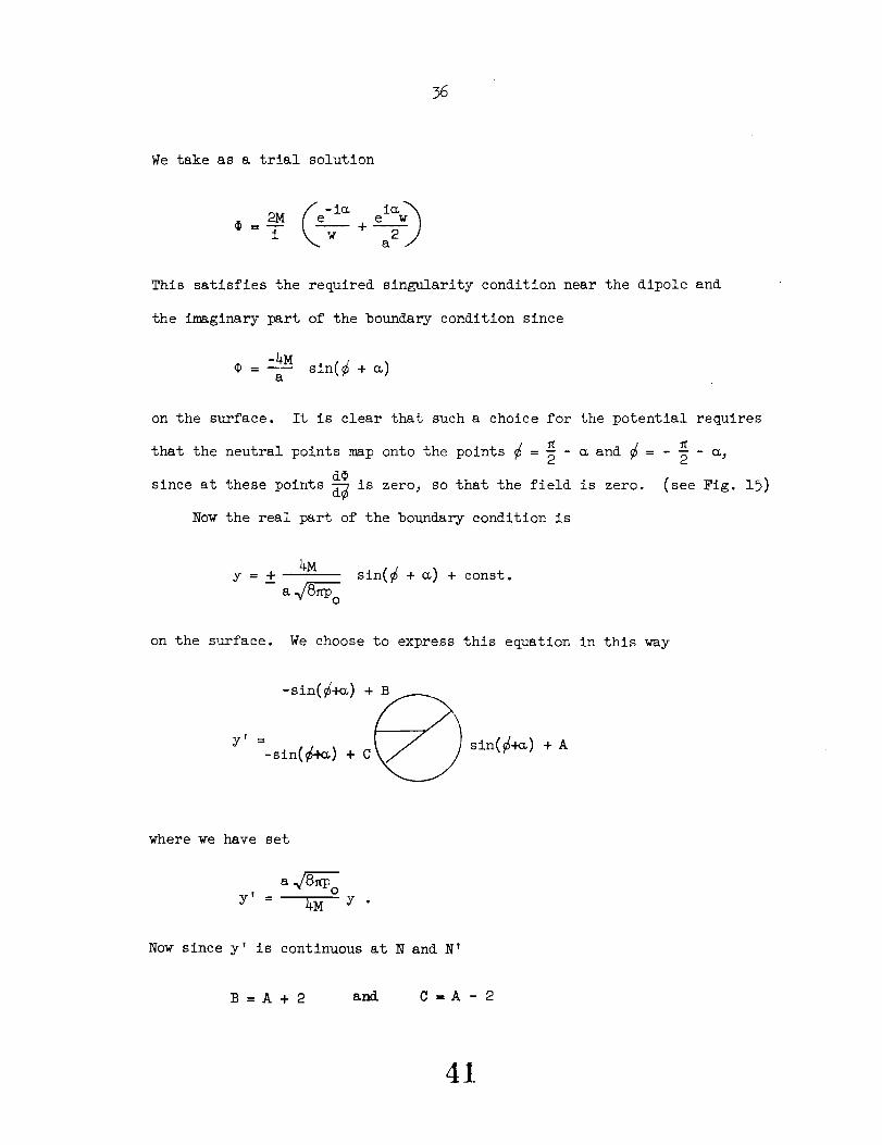
We take as a trial solution

2M -ie i _$=-- i _e +

This satisfies the required singularity condition near the dipole and

the imaginary part of the boundary condition since

¢ _ -4M sin(_ + e)a

on the surface.

that the neutral points map onto the points _ = _ - _ and

d$

since at these points d-_ is zero, so that the field is zero.

Now the real part of the boundary condition is

It is clear that such a choice for the potential requires

(see Fig. 15)

4My=+

-- a 8_O

sin(_ + e) + const.

on the surface. We choose to express this equation in this way

-sin(¢+_) + B

Y' =-sin(_4_) + C_7/ i sin(_+_) + A

where we have set

a 8_-_ °

Y ' - 4M Y "

NOW since y' is continuous at N and N'

B=A + 2 and C =A - 2

4!

37

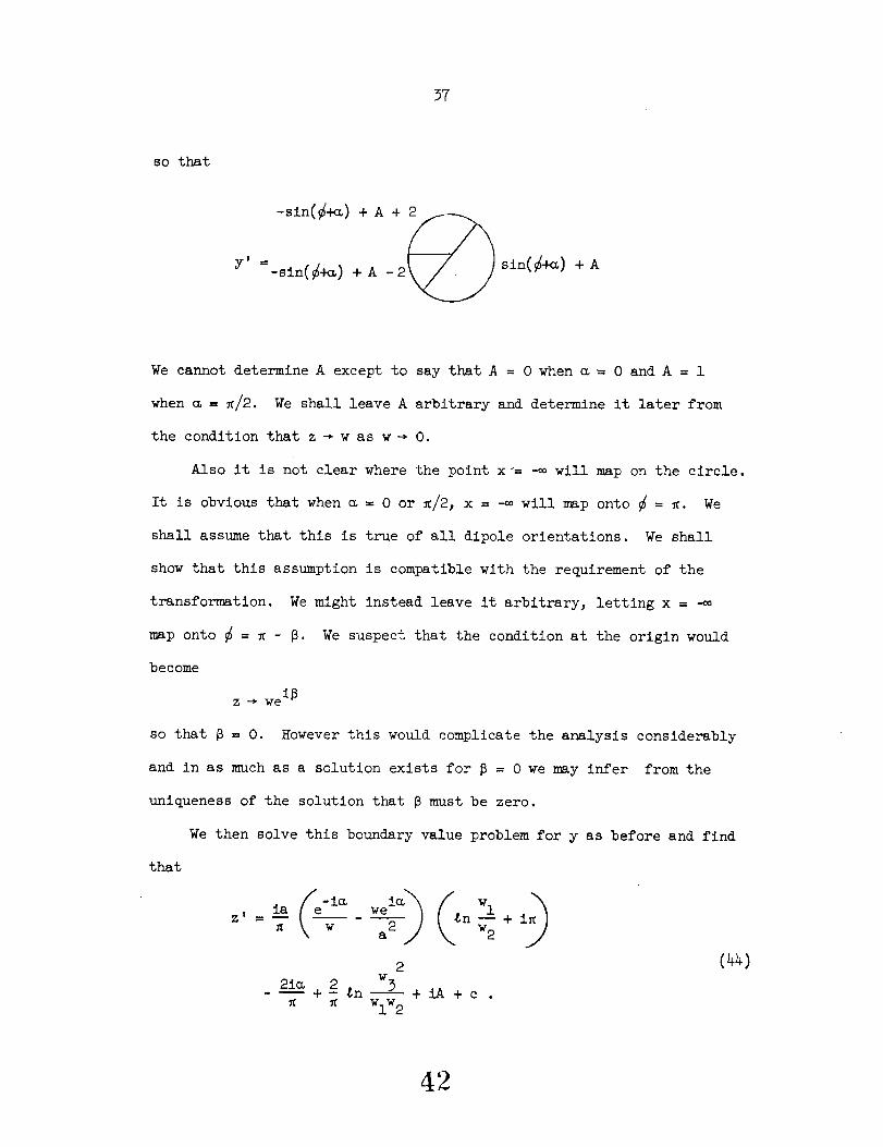
so that

-sln(¢_)+ A + _/_

Y' ---sin(_+_)+ A -2___// sin(_+_)+ A

We cannot determine A except to say that A = 0 when m = 0 and A = i

when _ = _/2. We shall leave A arbitrary and determine it later from

the condition that z _ w as w* 0.

Also it is not clear where the point x_= -_ will map on the circle.

It is obvious that when m = 0 or _/2, x = -0o will map onto _ = _. We

shall assume that this is true of all dipole orientations. We shall

show that this assumption is compatible with the requirement of the

transformation. We might instead leave it arbitrary, letting x = -_

map onto _ = _ - _. We suspect that the condition at the origin would

become

Z _ we i_

so that _ = O. However this would complicate the analysis considerably

and in as much as a solution exists for _ = 0 we may infer from the

uniqueness of the solution that _ must be zero.

We then solve this boundary value problem for y as before and find

that

Z !

ia ie Wl

2

. 2i____+--2 _n w3 + iA + c

_ WlW 2

(44)

where wl, w 2 and w 3 are defined in Fig. 16.

Expandi___ about the origin we find

z' , __4w_ _2 +--2ira+ iA + c_a _

so that A = _ and c = _ . Then

4M 16MZ _ Z t -_ "_

so that

2 16Ma --

as before.

Evaluating eq. (44) on the circle we find the parametric equations

for the cavity boundary,

-_2x'=s -(1 - sin(_+_)) _n _l+sin(_)J + _n k+sln(_+_) J + 1

and

YS = -sin(_) - 2 - sln(_4<_) - --_

43

39

When _ _ 0 these equations reduce to eqs. (39) and (43) as they must.

We have plotted these equations in Figs. 17 and 18 for m = 37° and

: 90°.

AN APPROXIMATIONMETHOD

Recently Beard I has presented an approximate solution to the

problem of the interaction between the scalar wind and the earth's

dipole field. As a test of the method we shall apply it to our two

dimensional problem and compare it with the above solution.

The essential feature of Beard's method is the way in which he

approximates the field. Imagine a plane surface brought in from

infinity compressing the field in front of it. (see Fig. 19) This

problem is easily solved by placing an image dipole at 0'. If the

plane is inclined at an angle m with the dipole at 0 then the image

dipole at 0 w is inclined at an angle 2_. It is clear that the resultant

magnetic field at the plane is Just twice the tangential component of

a single dipole.

Beard assumes that this will be approximately true for a curved

surface as well. The dipole field is

_ 2M sin2 8 er^ 2M cos2 e 8er r

iOp. cit.

4o

(The geometryks defined in Fig. 20.) The tangential componentof the

field then is

2M-_ cos (_+e)

I"

The pressure balance condition at the boundary ks

2Bt

_ Po c°s2X

where

- 4M cos(¢ + e)Bt = +-_

r

so that

cos X = cos(e - _) =4M eos(_ + e)

_8_Por2

(45)

The upper sign ks to be applied outside the nodal points and the lower

within. Let

2 4Mr

o

so that eq. (45) becomes

cos 8 + sin @ -----i dr

r de r2 _os 8 - sin e ir d_

41

wherer is nowmeasuredin units of r .0

that

i drtan _ - r d@

Between the nodal points the solution is

We have made use of the fact

r=l

and outside the nodal points

sin 8r sin 8 = 2

r

This boundary has been plotted in Fig. 12.

It is interesting to note that if there were equal plasma winds

streaming from the right and left the approximate solution would be a

circle of radius r=l. This is also the exact solution. (The reason

for the agreement is that the field of a two dimensional dipole confined

to a cylinder has a magnitude on the surface which is twice the tangential

component of the dipole alone. This is Just Beard's assumption.) If

the wind from the left is cut off, the magnetic field will expand into

this region and the magnetic pressure on the right will drop. The

cavity surface on the right will therefore fall toward %_e dipole and

reach equilibrium at the configuration given by the exact boundary

plotted in Fig. 12.

42

STABILITY

The stability of the cavity surface is a very important question

and also a very difficult one. If one is to makeany progress at all with

the analysis one is forced to makesomerather drastic assumptions.

Considerable effort has been devoted to problems of stability.

Before proceeding with the special features of our problem we shall

describe an important stability requirement for thermal plasmas

confined by a magnetic field. (In our problem there is a net mass

flow in the plasmawind. Weare nowconsidering a plasmaat rest.)

This problem has been investigated by Kruskal and Schwarzschildl,

Rosenbluth2, Grad3 and manyothers. Onecommonfeature of these

treatments is that the surface is stable whenthe center of curvature

of the boundarylies in the magnetic field and unstable whenit lies

in the plasma. Wemaygive qualitative evidence for this conclusion

in this w_y. Weconsider first the case wherethe center of

curvature lies in the plasma. (see Fig. 21) Themagnetic field is

directed into the page. In the equilibrium configuration (solid line)

the magnetic pressure Just balances the plasmapressure, i.e.

B2/8_ = p. The magnetic field increases as weapproach the boundary.

Thus if the boundary is perturbed as indicated by the dotted llne the

field at b will increase and the field at a decrease. If we adjust

the deformation so that the plasmavolume is kept constant the plasma

iM. Druskal and M. Schwarzschild, Proc. Roy. Soc. A223, 348, 1954.

2M. N. Rosenbluth and C. L. Longmire, Annals of Phys. i, 120, 1957.

3 H. Grad, 2d GenevaConf., 31:190.

43

pressure will remain the same. It is clear then that the perturbation

will grow. Let us now consider the other case (Fig. 22). The field

now increases as we move a_ay from the boundary so that in the perturbed

state the field pressure is increased at a and decreased at _. Thus

the surface is stable.

Since it is the latter case that prevails in our problem we might

expect the surface to be stable. There is however a difference. Our

plasma is a wind and not stationary. Further the mean free paths are

too long to apply the continuum plasma equations. Also the magnetic

field is itself imbedded in a plasma. (The earth's atmosphere is

certainly highly ionized at 9 earth's radii.)

Parker I has considered the stability of the interface between the

solar wind and the earth's field and concludes that it is everywhere

unstable. We do not feel that this conclusion necessarily follows

from his analysis. We shall conclude now with a more detailed consider-

ation of Parker's model.

The cavity surface is assumed to be locally plane with a plasma

stream incident on it at an angle @ . See Fig. 23. This system iso

assumed to be in equilibrium with the magnetic pressure of the wind.

The magnetic field below the interface is immersed in an infinitely

conducting, incompressible, invisid plasma. It is further assumed that

this plasma has a scalar pressure and scalar conductivity. The surface

is now perturbed by a traveling wave. The equation of the surface is

i0p. cir.

44

z = _(y,t) = Ae i_wt_y'f_. The _quations of motion together with the

boundary conditions determine a dispersion relation _ = _(k). If a

solution exists for _ complex the surface will be unstable if Im

i_tis negative since e will now grow exponentially. Parker states

that "the field density B remains uniform" under such a perturbation.

This would be true only if the field is directed into the page. Although

such a relative orientation of field lines and wind direction does occur

in the geomagnetic problem (in the equltorlal plane) it does not occur in

our two dimensional problem. However_ even in the equitorial plane of

the geomagnetic fieldj we would suspect that the curvature of the boundary

would have a considerable stabilizing influence.

We shall show now that even if one accepts Parker's model the cavity

surface surrounding the two dimensional dipole will for the most part be

stable. We shall show that there is a critical angle of incidence above

which the surface is stable and below which the surface is unstable.

Because the magnetic field in our two dimensional problem lles in

the plane of incidence of the streaming plasma particles we must

generalize the geometry considered by Parker. In his analysis the field

is perpendicular to the plane of incidence. We shall investigate the

following problem. (see Fig. 23) The equilibrlumboundary lies In the

x-y plane. The incident plasma particles have polar angles @o' _o"

We assume that the surface is perturbed by a traveling wave moving In

the @-directlon. The equation of the perturbed surface Is z = _(y,t).

We shall first consider the case where the magnetic field is perpendicular

to the direction of propagation (in the x-dlrectlon) and secondly parallel

45

to the direction of propagation (y-direction).

Parker has assumedthat the plasmabeneath the boundary is

incompressiblej invisid_ and infinitely conducting. In the unperturbed

state u = O, p = Po and B = Bo. In the perturbed state weassumethat

all of these quantities differ only slightly from their equilibrium values.

Let the increments be denotedby u, 8p, and 6B. Weshall also find it

convenient to introduce a displacement vector _ such that u =1

The equations that apply in such a plasmaare

du_. = -_ + _ ('_)xg

S-g _x(-Zxg)_-=

V'u=O

V-_=O

where D is the plasma density_ _ the fluid velocity_ p the plasma pressure

and d/dr the mobile operator_ + u.V. Neglecting terms of second order

the plasma equations become

a2 -,_p +_ ('_B) × g (46)8t 2 = o

= _(?xgQ) (47)

_._"= o (_8)V.SB = 0

iS. Chandrasekhar_ Plasma Physics (University of Chicago Press 3 1960).

5O

46

Expanding eq. (47) wefind that

(49)

Since B° has only a x-component

_B= Bo_

But _=_(y, z3t) so that

8_ = 0

The magnetic field is unchanged to first order.

It follows then from eq. (46) by taking the curl of both sides that

_X'_=O

We see then that the fluid motion is irrotational. We may therefore

represent the fluid motion by a scalar potential such that u = -_.

Eq. (4_) becomes

-ov_ ---vsp

Integrating

D$ = 5p.

Also since the motion is incompressible

V2¢ = 0 .

(90)

(5l )

51

47

Before one can complete the solution of eqs. (50) and (51) for the

plasma motion one must specify the boundary conditions. The boundary

in our problem is a free boundary and is determined by the condition

that the pressure on the boundary from the plasma wind must balance

the pressure of the plasma below. (The pressure from the plasma below

the boundary is in part due to the particle pressure and in part due

to the magnetic field pressure.) We must now investigate the effect

of the perturbation on the plasma wind pressure.

We consider a small segment of the perturbed boundary as illustrated

in Fig. 2_. The normal to the perturbed surface makes an angle _(y,t)

with the z-axis. We assume that _ is small. Let U be the normal

component of the velocity of the surface. Parker points out that in

the local frame of reference moving with the fluid the electric field will

vanish so that in this frame the particles are specularly reflected.

The pressure then of this moving surface will be

p --2Mm(Vn-U)2

where V is the normal component of the particle velocity and son

V - U is the velocity relative to the surface. The change in pressuren

then is

_P = P-Po = 2Nm[_(Vn-U)2-Vno_ _ 4Nm_no(Vn-Vno)-VnoU ]

to f_rst order in small quantities. V is the normal velocity componentnO

to the unperturbed surface. The change in the wind pressure is then

52

48

sin _ sin m + U cos @o_8p = 4NmV cos _o sin e° o

and since the magnetic pressure does not change this must equal the

change in the plasma pressure below the boundary as given by eq. (50).

We now let

and

5p = A 1 ei(_t+ky)+kz

= A 2 ei(_t+ky)+kz

_(y,t) = A 3 ei(_t+ky)

kzThe z-dependence e has been choosen so that _2¢ = O. The three

constants are determined by two boundary conditions and the equation of

motion of the fluid. The two boundary conditions are that the pressure

below the surface must equal the pressure above and that the boundary

must move with the fluid_ i.e.

on the surface. The equation of motion (eq. (49)) gives

AI/D = i A 2

53

49

and the boundary conditions become

i_A 3 = -kA 2 and _AI = 4NmV2Eik sin 8o cos 8° sin _o A5

(52)

where we have used the fact that

The determinant of the coefficients must be zero so that

i_2 + 4Vk cos 8 _ _ 4V2k2 sin @ cos e sinE 0 E 0 0 0

=0

where we have set the ratio of the densities D/NM = c. Solving for

i_ we find

F /,

iu - 2Vk cos eoll _ -!-I #J1 + e2 tan28 sin2_oc L V_ o

+l

/,

_ #Jl + c2 tan2e

We se_ that i_ will have a positive real part unless

e tan 8o sin _o = 0

5!

5o

or

cos @ = 0O

So that the surface wave will grow except when

or

¢o _

Fortunately _o = 0 or _ in both our two dimensional problems,

the surface is stable with respect to this mode.

so that

Let us now turn to the mode which propagates along the magnetic

field lines. We therefore take the field to be B = BoY. The change

in the magnetic field 5B is no longer zero. From eq. (49)

= (_o.V)_= B° _ (y,,,t)

Now

Vx_ = B° ;_ (_)

and

(_)_ = -B (Bo-_)O O O X( -----Bo

51

so that

2 _2(_)

Vx [(_B) x _o]" Bo aY2 .

But from eq. (45) this is also equal to D_X[ and so

_2

_, _o_ (_×_)-__ × _'

If we again assume that the disturbance is a traveling wave

b 2 _k 2

_y2

and

_2 2

bt 2

so that

2(_i) . k2 _o2

We see then that either

Bo

(53)

or

_7X_=O

I

52

Eq. (53) is Just the dispersion relation for an Alfven wave. If

such a solution exists, i.e. if we can satisfy the boundary conditions

with such a mode, it will be stable since _ is real. As we are looking

for possible unstable modes we shall take _7 x _ = 0, so that we are again

dealing with Irrotational flow. The situation is then as before except

(B2 - Bo2)/8_ , the change in the magnetic pressure, is not zero.that

Here

so that

In the equation of pressure balance we must now add a change in magnetic

pressure so that eq. (51) becomes

B 2k2

o .A I + _ A2 4NmV 2 in e°k 2 kA 2 • _]

cos @O sin _o _- A2 - T cos 8oj

Eliminating the A's and solving for _ we find

r-

i_-- 4Vkcos e tl; tJi_

o L -J_

5"_

53

where

when

c sinx = _ tan @o o

The real part of i_ is positive, and hence the surface is unstable

_/_ +i >i

or when

tan eo[sin Wol >

In our problem _o = _/2 so that instability occurs when 0°

than the critical angle (8o) c where

is greater

tan (00) c = 2/.W/'E"

We might say then that for all angles less than (0o) c the surface will

be stable and for all angles greater than (0o) c the surface will be

stable or unstable depending on the stabilizing influence of the

curvature of the surface which has been neglected.

Unfortunately there is no reliable estimates for the plasma density

as far out as 9 earth's radii. We would suspect however that the

density is quite low so that c is small and the critical angle ~ 90° .

58

54

On the basis of the above calculation we might draw some tentative

conclusions concerning the stability of the surface surrounding the

earth's dipole field. In the azimuthal plane passing through the sun

the surface will be stable over a wide range. In the equitorial plane

however we feel that the stability question can not be answered by

the above analysis. The curvature of the surface will exert a

stabilizing influence which should not be neglected.

SUMMARY

We have shown that a plasma incident on the magnetic field of

an infinite line current or a two dimensional dipole will confine

the field so that it forms a cavity in the wind. The plasma particles

move in straight lines (assuming long mean free paths) and penetrate

a short distance into the field to form a current sheath within which

they are deflected out of the field. We have sho_ that the thickness

of this sheath is small compared to the dimensions of the cavity.

In the steady state the particles will be specularly reflected

from the surface. They will therefore exert a pressure on the surface

which is proportional to the square of the normal velocity component.

The cavity boundary is determined then by the condition that the

magnetic pressure from within the cavity balance the particle pressure

from without. We have calculated the shape of this boundary separating

the plasma wind from the magnetic field of an infinite llne current and

a two dimensional dipole. The analysis also determines the magnetic

field within the cavity.

59

The cavity boundary has been shown to be stable except for those

regions _here the cavity _all is almost parallel to the plasma _ind

direction.

GO

56

REFERENCES

C.P. Sonett, D.L. Judge, A.R. Sims, and J.M. Kelso, A Radial Rocket

Survey of the Distant Geomagnetic Field, Space Technology Labora-tories .Report 7320, 2-13.

E.N. Parker, Interaction of the Solar Wind with the Geomagnetic Field,

Phys. of Fluids, l, 171 (1958).

David B. Beard, The Interaction of the Terrestrial Magnetic Field with

the Solar Corpuscular Radiation, J. Geophys. Research, 65, 3559,1960.

J.D. Cole and J.H. Huth, Physics of Fluids, 2, 624 (1959).

J.W. Dungey, Penn. State Univ., Scientific Report No. 135, July 1960.

S. Chandrasekhar, Plasma Physics (University of Chicago Press, 1960).

GI

+ /

'E"

\

@

J

fJ

G_

Fig. 1 Particle traJecZories In th_ magnetic field.

62

F w

I

t

o. I O.

I

I

r->I

I

I, iI

I __-Jb' b b

A_ b-_oo

Fig. 2 Motion of plasma block in a time dr.

63

|

i

i t

i

+!

I

I

iL

I_- X0_I

!

I

i

[

I --

I

I

I

I

I

I --

l

I

!

Fig. 3 Maximum charge separation compatible

with energy conservation.

GI

I \

I

I

I

I

I

I

I

(Uj V, -W)

X

\

\

\

\

\

\

\

\

\

f

/ I

If

I

"- I

"- i

(U, V, W)

w Y

Fig, h Specular reflection in cur_nt sheath.

Fig. 5 Flow of plasma past a line current.

Gq

v

2u °

Cavi ty

Boundary

U = U 0

U

Fig. 6 @eom_try as transformed by setting

w = I/_B* .

G7

I-I

I I

v_

m

_DOJ

v

qD

0

_ oo_ aJ

J@oaJ

Io

_ L_-

q-q

o(!

G8

\

\_o

,r4

.r4

o

f.4o

cO

_Q

69

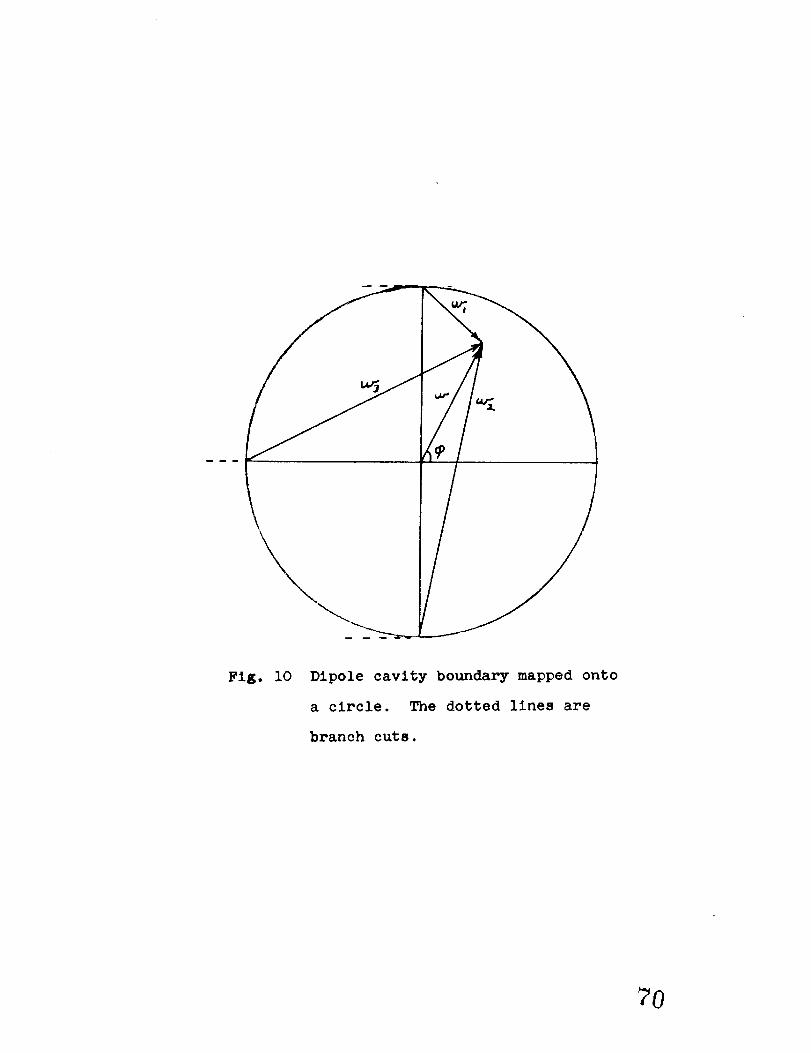
FiE. i0 Dipole cavity boundary mapped onto

a circle. The dotted lines are

branch cuts.

7O

04_

1<

.<

i L... I I

Q <3

4.)

;

_6

o.,-'4

o

'o

c_

NV

E_o

IQ

C.)

I

/

\\

Fig. 13 Dipole field confined by two infinite

planes intersecting at right angles.

72

N

O

B

Fig. 14 The effect of the field due to the current

sheath (B) will be to increase the dipole

field on the equator and decrease it at

the poles.

73

N

Fig. 15 Cavity boundary transformed to a circle.

Fig. 16 Definition of polar vectors used in

Eq. (44). The dotted lines are branch

cuts. _, varies between - 4 and +d -T,

_ between -d and _ -._ and_3between

-_/2 and +_/2.

%

0C---

0

_P0

4_

b-r-I

.r'l

76

4

• )O

oOO_

II

%0

o

cO

77

Fig. 19 Dipole field confined by an infinite plane.

78

C_v_t_

• A

Fig. 20 Segment of cavity boundary.

normal to the surface.

A

n Is a unit vector

79

Fig. 21. Perturbation of equilibrium boundary surface

when the center of curviture lies in the plasma

domain.

Fig. 22 Perturbation of equilibrium boundary surface

when the center of curvlture lies in the field

domain.

V

/7// "-_X

Fig. 23 Plasma wlnd blowing on a surface wave

propagating In the y-dlrectlon.

81

n@

.

Fig. 24 Perturbed element of boundary surface, n is

a unit vector normal to the perturbed surface

and no a unit vector normal to the unperturbed

surface. _ is the displacement of the perturbed

surface element from the unperturbed surface.

_2