!ngs!analyses!with!galaxy! -...

NGS Analyses with Galaxy

1

1 NGS Analyses with Galaxy

Introduction Every living organism on our planet possesses a genome that is composed of one or several DNA (deoxyribonucleotide acid) molecules determining the way the organism is built and maintained. The DNA molecules are divided into sets of discrete sequence stretches which encode for the genetic information that is translated into proteins. Since 1970, researchers have made an effort to develop strategies to “read” the DNA sequence because the knowledge of an individual genome sequence provides deep insights into the biological functions and the evolutionary history of this organism. Moreover, a couple of diseases are caused by genetic disorders that are only diagnosable by studying sequence variations within certain regions on the DNA sequence. A widely applied strategy for DNA sequencing is the “chain-‐termination method” introduced by Frederick Sanger in 1977 (Sanger et al., 1977). The importance of this method over the last 20 years can be explained with its applicability to the machine-‐based automatization of DNA sequencing. This automatization step accelerated the development towards other high-‐throughput sequencing technologies, which eventually, opened the flood-‐gates to an extensive amount of sequence data.

Still, the sequencing of whole genomes turns out to be very challenging and time-‐consuming because only short sequences called reads (<1000 base pairs) can be produced. The genome shotgun sequencing approach, devised by Sanger (Sanger et al., 1982), deals with the problem to reconstruct longer sections of a genome: the idea is to sequence cloned and randomly sampled fragments of the genome to obtain short, overlapping reads. The random sampling and the cloning step ensures to cover each position of the original genome sequence with a sufficient number of reads. Using specialized algorithms, these reads are pieced back together to obtain the final genome sequence. Today, there exists a couple of genome assembly strategies and tools that try to resolve this “jigsaw-‐puzzle” problem efficiently. The genome shotgun strategy has already been successfully applied to many organisms, such as the bacterium Haemophilus influenzae (Fleischmann et al., 1995), the fruit fly Drosophila melanogaster (Fleischmann et al., 1995) and even parts of the human genome (Venter et al., 2001). However, due to some characteristics of the DNA (e.g. repeat regions) and some technical aspects, the assembly problem is far from being solved. For example, the complete reconstruction of a single contiguous sequence in the end of the assembly process sometimes fails and results in DNA fragments resembling a gapped genome

1 Adapted from ‘Putting together a draft genome assembly”, Dan MacLean, The Sainsbury Laboratory and ‘Using Galaxy for NGS Analyses’, Luce Skrabanek


2

sequence. To fill these gaps with sequence data, the fragments need to be ordered and orientated, i.e. they need to be set into the context of the original genome. The Sanger technology dominated the sequencing market for several years. Eventually, since 2005, new (“next-‐generation”) sequencing technologies have been commercially launched which promise to produce much more sequencing data in shorter time and at lower cost compared to the Sanger technology. The development of the Roche 454, Illumina Genome Analyzer and SOLiD platforms (Margulies et al., 2005; Bentley, 2006; Shendure et al., 2005) was enabled by advancements in microfluidics, surface chemistry, and enzymology, and led to a significant increase of diverse (re-‐)sequencing projects. A relatively new research field, called metagenomics, also benefits from the advancements of the new technologies. As a major part of the free-‐living microbes (>99%) is assumed to elude the cultivation under laboratory conditions, new methods are required to enable the direct sequencing of organisms contained in environmental samples. In contrast to the Sanger sequencing, the emerging next-‐generation sequencing technologies avoid library preparation issues and therefore, enable researchers to generate unbiased sequencing data directly from the environment. However, the computational analysis of metagenomic data sets is a challenging task because the initial sequencer output consists of large volumes of short, anonymous reads, i.e. the species origin of a read is unknown. These reads are structured (optionally assembled) and taxonomically classified to gain knowledge about the complex species composition of the studied habitat.

Another focus is given to the functional analysis of the metagenome by detecting coding sequences (genes) on the DNA fragments. These genes are either annotated to known functions and gene products or classified as hypothetical proteins if no homologous sequence can be found in reference databases. Obviously, there is great hope to discover unique biosynthetic capabilities and pathways that are encoded in genomes of still unnoticed ��microbes. For example, striking insights have already been obtained by studying different environments such as seawater (Rusch et al., 2007), soil (Daniel, 2005), air (Tringe et al., 2008) and various biofilms (Tyson et al., 2004). Furthermore, researchers apply metagenomic methods to understand the complexity of the human microbiome that is composed of a large number of microorganisms “whose collective genome contains at least 100 times as many genes as our genome” (Gill et al., 2006). The resulting excess of data is remarkable: For example, the Global Ocean Sampling project sampled water probes in the Atlantic and Pacific and predicted about 6.21 million hypothetical proteins, almost doubling the number of known proteins present in databases at that time (Rusch et al., 2007). Hence, this example points out the need for novel algorithmic approaches and innovative software tools that allow the efficient organization and interpretation of metagenomic data sets. Overall, the advent of next-‐generation sequencing technologies have had a strong bearing on several (new) research fields like the high-‐throughput sequencing of human genomes (personalized medicine), genome assembly, paleogenomics


3

(Hofreiter, 2008) and metagenomics. It will certainly lead to further exciting discoveries and insights, which, until recently, seemed to be hardly achievable. The extraordinary throughput of next-‐generation sequencing (NGS) technology is outpacing our ability to analyze and interpret the data and to cope with this we need systems to help us analyse this data. In this module we will introduce you to the Galaxy interface, a freely available web-‐based platform for the quality control and analysis of NGS and other large-‐scale biological datasets.

1. Getting Started Using Galaxy Before you begin, you will need to create a user account (for free) at Galaxy.

Access the eBiokit server and start Galaxy.

Under the “User” menu, select “Register” to create a new account.

Next, complete the registration form.


4

Finally, you can log into Galaxy with this new account.

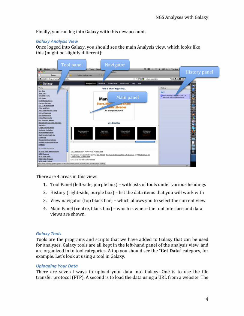
Galaxy Analysis View Once logged into Galaxy, you should see the main Analysis view, which looks like this (might be slightly different):

There are 4 areas in this view:

1. Tool Panel (left-‐side, purple box) – with lists of tools under various headings 2. History (right-‐side, purple box) – list the data items that you will work with

3. View navigator (top black bar) – which allows you to select the current view

4. Main Panel (centre, black box) – which is where the tool interface and data views are shown.

Galaxy Tools Tools are the programs and scripts that we have added to Galaxy that can be used for analyses. Galaxy tools are all kept in the left-‐hand panel of the analysis view, and are organized in to tool categories. A top you should see the “Get Data” category, for example. Let’s look at using a tool in Galaxy.

Uploading Your Data There are several ways to upload your data into Galaxy. One is to use the file transfer protocol (FTP). A second is to load the data using a URL from a website. The

Sunday, September 4, 2011

Tool panel Navigator History panel

Main panel


5

third method is to load a file from your computer. We will use the latter method in this tutorial.

Exercise • Click the Get Data heading in the tool panel and Upload File from the

computer tools.

• The tool interface should replace the splash page in the centre panel, and look like this:

• The tool options are now visible and can be selected.

• Select Choose File and from the drop-‐down box select the file GM12878_rnaseq1.fastqsanger from the folder Module_NGS on your computer.

• Change the File-‐Format pull-‐down menu from ‘Auto-‐detect’ to ‘Fastqsanger’. (Although Galaxy is usually quite good at recognizing formats, it is always safer, if you know the format of your file, not to leave its recognition to chance.)

• Select Execute at the bottom of the tool interface to make the tool run. You should see a helpful message when the tool starts to run.

• When the tool has run, and the data uploaded you should see a green box in the History panel.


6

History items History items are the data that Galaxy is using, and they live in the history in the order that they were created (lower items = older items) and have a number of attributes. Each history item is coloured according to state.

• Green = everything is fine with this data item and it can be used in the tools.

• Yellow = this job is running.

• Red = this job has failed and the data item cannot be used.

• Grey = this job is queued and is waiting to run. History items can be downloaded from the History panel, using icons in the top right of each History item. The eye icon allows you to preview the file contents in the Main Panel; the disk icon allows you to download the file. Galaxy items are never deleted until you explicitly state that they can be, data items, analyses and jobs stay live even after you log-‐out and shut down the machine.

Inspecting History Items Clicking on the name of the history item that we just uploaded (GM12878_rnaseq1.fastqsanger ), will expand it and presents you with summary information and a preview of the data. We are shown that this file is 17.4 MB in size and is in fastq format. The first few lines of the fastq data is shown in the white box.

Upload doneData Upload★ sequencing reads★ reference

Data preparation

Data Quality control

Data Mapping

Data Visualization

Adaptor clipping


Upload in process Data Upload

★ sequencing reads★ reference

Data preparation


Data Mapping

Data Visualization

Adaptor clipping


Uploading2 Illumina read filesmac-18_noad.fastq

mac18red.fastq

2 ref seqPLMV_PC-C40.fasta

peach_chloro.fa

Data Upload★ sequencing reads★ reference

Data preparation


Data Mapping

Data Visualization

Adaptor clipping


� ;OL�[VVS»Z�VW[PVUZ�HYL�UV^�]PZPISL�HUK�JHU�IL�ZLSLJ[LK� ;OPZ�[VVS�OHZ�Q\Z[�HML �̂ HUK�HYL�HSS�KLZJYPILK�PU�[OL�OLSW�H[�[OL�IV[[VT�VM�[OL�ZJYLLU�

� :LSLJ[ &KRRVH�)LOH HUK�MYVT�[OL�KYVW�KVÛ�IV_�ZLSLJ[�[OL�ÄSL VPDOO�JIIÔPJO�ZOV\SK�IL�PU�[OL GDWD MVSKLY�VU�[OL�+LZR[VW�

� :LSLJ[�,_LJ\[L�H[�[OL�IV[[VT�VM�[OL�[VVS�PU[LYMHJL�[V�THRL�[OL�[VVS�Y\U� @V\ZOV\SK�ZLL�H�OLSWM\S�TLZZHNL�ÔLU�[OL�[VVS�Z[HY[Z�[V�Y\U�

� >OLU�[OL�[VVS�PZ�Y\U� HUK�[OL�KH[H�HYL�\WSVHKLK�`V\�ZOV\SK�ZLL�H�NYLLU�IV_PU�[OL�/PZ[VY`�WHULS�

�� /PZ[VY`�P[LTZ/PZ[VY`�P[LTZ�HYL�[OL�KH[H�[OH[�.HSH_`�PZ�\ZPUN� [OL`�SP]L�PU�[OL�OPZ[VY`�PU�[OL�VYKLY[OH[�[OL`�^LYL�JYLH[LK��SV^LY�P[LTZ�$�VSKLY�P[LTZ��HUK�OH]L�H�U\TILY�VM�H[[YPI\[LZ�,HJO�OPZ[VY`�P[LT�PZ�JVSV\YLK�HJJVYKPUN�[V�Z[H[L�

� .YLLU�$�L]LY`[OPUN�PZ�ÄUL�^P[O�[OPZ�KH[H�P[LT�HUK�P[�JHU�IL�\ZLK�PU�[VVSZ�

�


7

Editing attributes for history items If Galaxy makes a mistake with any of our history items, such as giving a file the wrong format, we can alter the attributes manually. This is often useful to give the items a useful name. To alter the attributes of an item, click the pencil icon in the top-‐right corner of the history item.

Exercise

Update the attributes of the GM12878_rnaseq1.fastqsanger dataset that we previously downloaded.

1. Click the pencil icon for the GM12878_rnaseq1.fastqsanger dataset.

2. Change the name of the data set to GM12878 in the Name field.

3. Associate the dataset that we just downloaded with the human hg19 genome in the Database/Build field.

4. Click Save.

2. Using and preparing next-‐generation sequence reads with Galaxy Sequence data is the starting point for most Pathogenomics experiments. The raw sequence data will often be assembled into a rough draft assembly before other analysis can be carried out on it. Assembly is a tricky and labour intensive job. The first task is to quality control our sequence reads to ensure that we are working with the best quality data.

Quality Scores During sequencing it is never possible to determine absolutely which base is found at that position in the process, rather the most likely base out of all the options is called. This uncertainty means that a measure of the quality of the call has been developed, the quality score. The actual number of the quality is generated by a log transformation of the calculated probability of the read being wrong (Ewing et al., 1998). Quality scores generally fall in the range between 0 (very poor confidence in the base called) and 40 (very high confidence in the base called), though there are some practical complications to this scheme (Cock et al., 2010). The sequence reads and the quality scores are usually output from base calls into FASTQ format. The quality scores are provided in a list of characters that encode the scores directly. The FASTQ format encodes the base qualities in single characters based on the ASCII code, a computing convention that assigns a unique number to each of the characters used in computing systems, for example the ! character has the decimal number 33 in the ASCII code. The FASTQ format is complicated by a number of factors, first the codes must be offset since the first 32 characters of the ASCII set represent non-‐printable characters like system alerts and the offset is slightly


8

different depending on the origin of the file. Also the range of numbers that the quality score can fall into differs depending on the provenance of the file, even down to the version of the base-‐calling pipeline that was used. The difficulties in this popular format and how to deal with them are laid out better elsewhere but it is important that nay user of these technologies is aware of the potential for confusion. (Cock et al., 2010).

PHRED scores Quality scores used in the FASTQ format were originally derived from the PHRED program that read DNA sequence trace files. The PHRED program assigns quality scores to each base, according to the following formula:

where Pe is the probability of erroneously calling a base. PHRED puts all of these quality scores into another file called QUAL (which has a header line as in a FASTA file, followed by whitespace-‐separated integers. The lower the integer, the higher the probability that the base has been called incorrectly.

While scores of higher than 50 in raw reads are rare, with post-‐processing (such as read mapping or assembly), scores of as high as 90 are possible.

Solexa scores The Solexa quality scores, which were used in the earlier Illumina pipelines, are calculated differently from the PHRED scores:

FASTQ Paired-‐End Reads All the reads that we use are paired-‐end FASTQ reads, in Sanger Quality scaling. FASTQ format is a multi-‐line description of the read. The first line starts with a @’ and contains the sequence ID. The second line contains the sequence of the read. The third line starts with a ‘+’ and then optionally contains the sequence ID again. Line 4 encodes the quality values as ASCII characters.

@HWI-EAS396\_0001:6:1:11659:1311\#0/1 CCTCGGAGTGGAA…. +HWI-EAS396\_0001:6:1:11659:1311\#0/1 !~@£%%£$%$%^^…

7

Examining and Manipulating FastQ data

Quality Scores The FastQ format provides a simple extension to the FastA format, and stores a simple numeric quality score with each base position. Despite being a “standard” format, FastQ has a number of variants, deriving from different ways of calculating the probability that a base has been called in error, to different ways of encoding that probability in ASCII, using one character per base position.

PHRED scores Quality scores were originally derived from the PHRED program which read DNA sequence trace files. The PHRED program assigns quality scores to each base, according to the following formula: !_!"#$% = !−10!!"#10!(!") where Pe is the probability of erroneously calling a base. PHRED puts all of these quality scores into another file called QUAL (which has a header line as in a FastA file, followed by whitespace-separated integers. The lower the integer, the higher the probability that the base has been called incorrectly. PHRED Quality Score Probability of incorrect base call Base call accuracy 10 1 in 10 90 % 20 1 in 100 99 % 30 1 in 1000 99.9 % 40 1 in 10000 99.99 % 50 1 in 100000 99.999 % While scores of higher than 50 in raw reads are rare, with post-processing (such as read mapping or assembly), scores of as high as 90 are possible.

Solexa scores The Solexa quality scores, which were used in the earlier Illumina pipelines, are calculated differently from the PHRED scores: !!_!"#$%& = !−10!!"#10!( !"

!!!")

7





!!!")

7





!!!")


9

Paired-‐end reads are those in which the reads actually come in pairs with an approximate distance (in nucleotides) between them. This distance, known as the insert-‐size, is set during the sample preparation and refers to the size of DNA fragment cut from the gel for sequencing. The ‘paired-‐ends’ are then sequenced from either side of these fragments and hence if we have paired-‐end sequences of 75 nts from each end of the DNA fragment with a 350 nt gap between them, our insert-‐size will be ~500 nts.

FastQ Conversion Above we loaded the file GM12878_rnaseq1.fastqsanger as fastq format, the “default” FastQ format. Other possible FastQ formats in the pulldown menu are [fastq, fastqcssanger, fastqillumina, fastqsanger, fastqsolexa]. If we want to change the FastQ format we can do that in Galaxy.

Changing between FastQ formats Galaxy is able to interchange between the different FASTQ formats with a tool called FASTQ Groomer, found under the NGS: QC and manipulation tab. Since Galaxy tools are designed to work with the Sanger FASTQ format, it is advisable to convert any FASTQ files in another FASTQ format to Sanger FASTQ. The FASTQ Groomer tool takes as input any file designated as FASTQ format and converts it according to the equations found in Cock et al. NAR 2009.


FastQ Quality Control There are two standard ways of examining FastQ data in Galaxy: using the Summary Statistics method and the FastQC method.

8

FastQ Conversion

Changing between FastQ formats Galaxy is able to interchange between the different FastQ formats with a tool called FASTQ Groomer, found under the NGS: QC and manipulation tab. Since Galaxy tools are designed to work with the Sanger FastQ format, it is advisable to convert any FastQ files in another FastQ format to Sanger FastQ. The FASTQ Groomer tool takes as input any file designated as FastQ format and converts it according to the equations found in Cock et al. NAR 2009.

Description Galaxy format name

ASCII characters Quality score Range Offset Type Range

Sanger standard/Illumina 1.7+ fastqsanger

33 to 126 33 PHRED 0 to 93

Solexa/early Illumina fastqsolexa

59 to 126 64 Solexa -5 to 62

Illumina 1.3+ fastqillumina

64 to 126 64 PHRED 0 to 62

8

FastQ Conversion

Changing between FastQ formats Galaxy is able to interchange between the different FastQ formats with a tool called FASTQ Groomer, found under the NGS: QC and manipulation tab. Since Galaxy tools are designed to work with the Sanger FastQ format, it is advisable to convert any FastQ files in another FastQ format to Sanger FastQ. The FASTQ Groomer tool takes as input any file designated as FastQ format and converts it according to the equations found in Cock et al. NAR 2009.

Description Galaxy format name

ASCII characters Quality score Range Offset Type Range

Sanger standard/Illumina 1.7+ fastqsanger

33 to 126 33 PHRED 0 to 93

Solexa/early Illumina fastqsolexa

59 to 126 64 Solexa -5 to 62

Illumina 1.3+ fastqillumina

64 to 126 64 PHRED 0 to 62


10

Summarizing and visualizing statistics about FastQ reads As with any data, you first need to assure yourself that the data you are about to analyse are of high quality and don’t have any obvious problems. Using Galaxy, we will run a series of diagnostic analyses to look for problems in the sequencing reads.

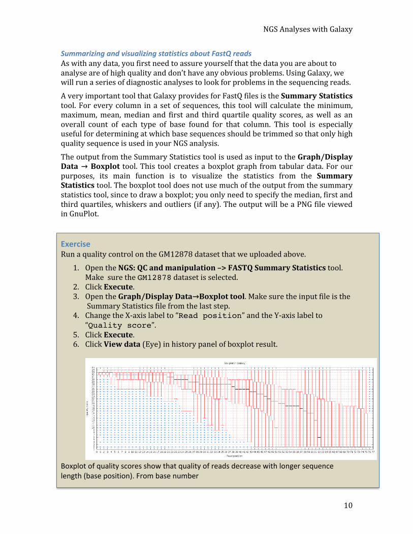
A very important tool that Galaxy provides for FastQ files is the Summary Statistics tool. For every column in a set of sequences, this tool will calculate the minimum, maximum, mean, median and first and third quartile quality scores, as well as an overall count of each type of base found for that column. This tool is especially useful for determining at which base sequences should be trimmed so that only high quality sequence is used in your NGS analysis.

The output from the Summary Statistics tool is used as input to the Graph/Display Data → Boxplot tool. This tool creates a boxplot graph from tabular data. For our purposes, its main function is to visualize the statistics from the Summary Statistics tool. The boxplot tool does not use much of the output from the summary statistics tool, since to draw a boxplot; you only need to specify the median, first and third quartiles, whiskers and outliers (if any). The output will be a PNG file viewed in GnuPlot.

Exercise Run a quality control on the GM12878 dataset that we uploaded above.

1. Open the NGS: QC and manipulation –> FASTQ Summary Statistics tool. Make sure the GM12878 dataset is selected.

2. Click Execute. 3. Open the Graph/Display Data→Boxplot tool. Make sure the input file is the

Summary Statistics file from the last step. 4. Change the X-‐axis label to “Read position” and the Y-‐axis label to

“Quality score”. 5. Click Execute. 6. Click View data (Eye) in history panel of boxplot result.

Boxplot of quality scores show that quality of reads decrease with longer sequence length (base position). From base number


11

Perform Quality Control Diagnostics using FastQC A second tool in Galaxy is the FastQC tool, from Babraham Bioinformatics. It takes as input either a FastQ file, or BAM or SAM files. FastQC bundles into one executable what many of the individual tools available in Galaxy do for specific FastQ formats. FastQC provides information on the following:

Basic Statistics This section gives some simple composition statistics for the input file, including filename, filetype (base calls or colorspace), encoding (which FastQ format), and total number of sequences, sequence length and % GC.

Per Base Sequence Quality This plot shows the range of quality values over all bases at each position (similar to the boxplot from the BoxPlot tool.)

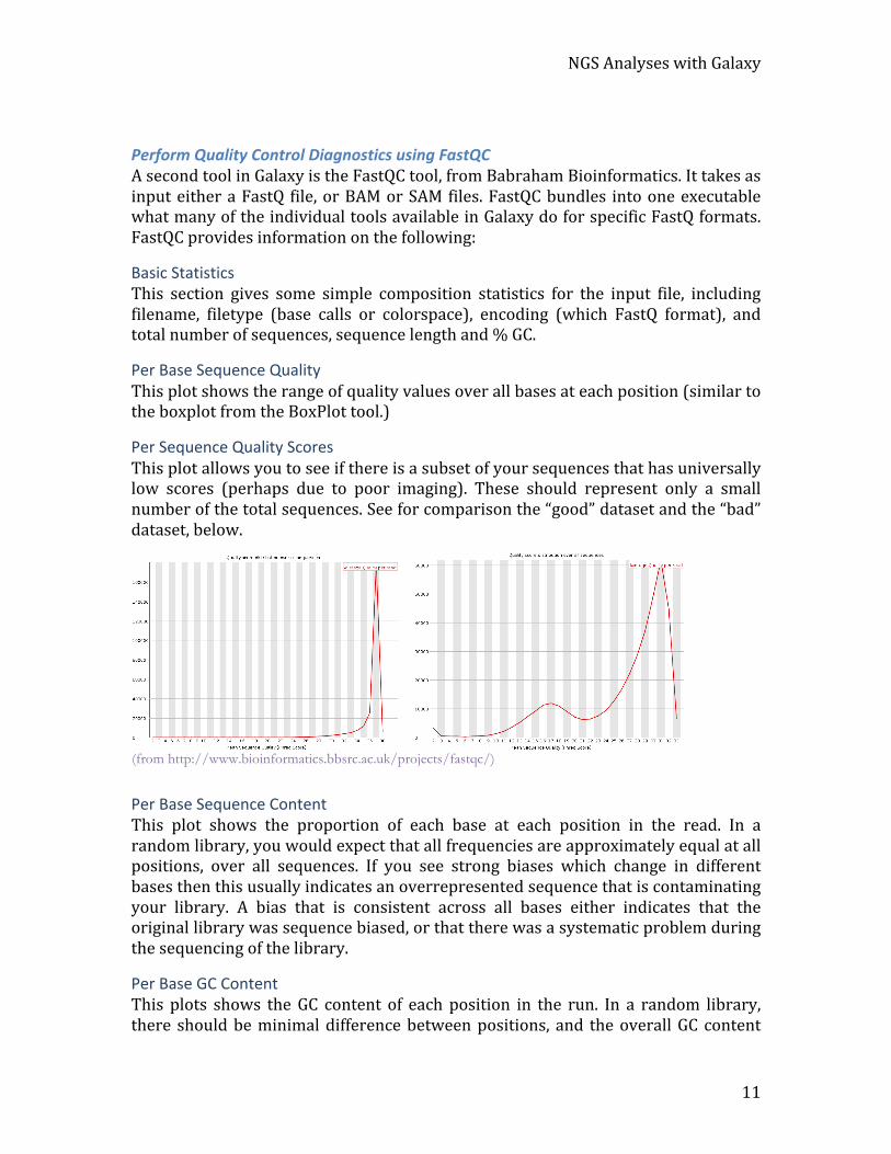
Per Sequence Quality Scores This plot allows you to see if there is a subset of your sequences that has universally low scores (perhaps due to poor imaging). These should represent only a small number of the total sequences. See for comparison the “good” dataset and the “bad” dataset, below.

Per Base Sequence Content This plot shows the proportion of each base at each position in the read. In a random library, you would expect that all frequencies are approximately equal at all positions, over all sequences. If you see strong biases which change in different bases then this usually indicates an overrepresented sequence that is contaminating your library. A bias that is consistent across all bases either indicates that the original library was sequence biased, or that there was a systematic problem during the sequencing of the library.

Per Base GC Content This plots shows the GC content of each position in the run. In a random library, there should be minimal difference between positions, and the overall GC content

10

FastQC quality control Another way of looking at your data to determine the overall quality of your run and to warn you of any potential problems before beginning your analysis is to use the FastQC tool, from Babraham Bioinformatics. It takes as input either a FastQ file, or BAM or SAM files. FastQC bundles into one executable what many of the individual tools available in Galaxy do for specific FastQ formats.

Basic Stat i s t i c s This section gives some simple composition statistics for the input file, including filename, filetype (base calls or colorspace), encoding (which FastQ format), total number of sequences, sequence length and %GC.

Per Base Sequence Quali ty This plot shows the range of quality values over all bases at each position (similar to the boxplot from the BoxPlot tool.)

Per Sequence Quali ty Scores This plot allows you to see if there is a subset of your sequences which has universally low scores (perhaps due to poor imaging). These should represent only a small number of the total sequences. See for comparison the “good” dataset and the “bad” dataset, below.

(from http://www.bioinformatics.bbsrc.ac.uk/projects/fastqc/)

Per Base Sequence Content This plot shows the proportion of each base at each position in the read. In a random library, you would expect that all frequencies are approximately equal at all positions, over all sequences. If you see strong biases which change in different bases then this usually indicates an overrepresented sequence which is contaminating your library. A bias which is consistent across all bases either indicates that the original library was sequence biased, or that there was a systematic problem during the sequencing of the library.

Per Base GC Content This plots shows the GC content of each position in the run. In a random library, there should be minimal difference between positions, and the overall GC content should reflect the GC content of the genome under study. As in the Per Base Sequence Content plot, deviations across all positions could indicate an over-represented sequence. Similarly, if a bias is consistent across all bases, this could either indicate that the original library was sequence biased, or that there was a systematic problem during the sequencing of the library.


12

should reflect the GC content of the genome under study. As in the Per Base Sequence Content plot, deviations across all positions could indicate an over-‐represented sequence. Similarly, if a bias is consistent across all bases, this could either indicate that the original library was sequence biased, or that there was a systematic problem during the sequencing of the library.

Per Sequence GC content This plots the GC content across each sequence and compares it to a modelled GC content plot. In a random library, the plot should look normal and the peak should correspond to the overall GC of the genome under study. A non-‐normal distribution may indicate a contaminated library or biased subset.

Per Base N Content This plots the percentage of base calls that were Ns (i.e., a base call could not be made with certainty) at every position. Ns more commonly appear towards the end of a run.

Sequence Length Distribution This plots the distribution of all read lengths found. Duplicate Sequences This counts the number of times any sequence appears in the dataset and shows a plot of the relative number of sequences with different degrees of duplication. In a diverse library most sequences will occur only once in the final set. A low level of duplication may indicate a very high level of coverage of the target sequence, but a high level of duplication is more likely to indicate some kind of enrichment bias (e.g., PCR over amplification).

Overrepresented Sequences This creates a list of all the sequences that make up more than 0.1% of the total. A normal high-‐throughput library will contain a diverse set of sequences. Finding that a single sequence is very over-‐represented in the set either means that it is highly biologically significant, or indicates that the library is contaminated, or not as diverse as you expected.

Overrepresented Kmers This counts the enrichment of every 5-‐mer within the sequence library. It calculates an expected level at which this k-‐mer should have been seen based on the base content of the library as a whole and then uses the actual count to calculate an observed/expected ratio for that k-‐mer. In addition to reporting a list of hits it will draw a graph for the top 6 hits to show the pattern of enrichment of that k-‐mer across the length of your reads. This will show if you have a general enrichment, or if there is a pattern of bias at different points over your read length. Before running these analyses, we will need to run a pre-‐processing step in Galaxy called FASTQ Groomer. This step will ensure that the data is properly formatted and the quality scores are consistently scaled.


13

Exercise 1. Click on the “NGS: QC and manipulation” link on the menu on the left and

then click on the “FASTQ Groomer” link that will appear when the menu is expanded.

2. Select the GM12878 dataset.

3. Change the “Input FASTQ quality scores type” pull-‐down menu to “Sanger” and then launch the process by

4. Click “Execute”.

After launching the job, you will see the job in your history on the right. A clock will appear next to job until it is complete at which time it will be highlighted in green.


14

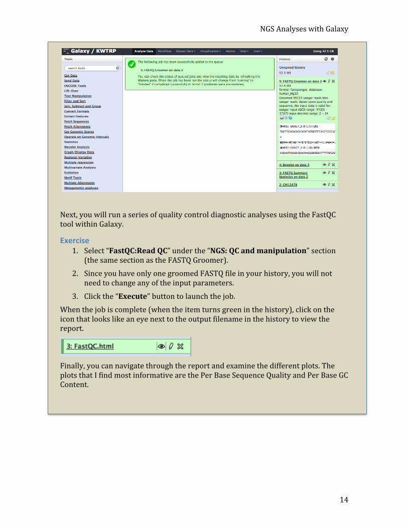
Next, you will run a series of quality control diagnostic analyses using the FastQC tool within Galaxy.

Exercise 1. Select “FastQC:Read QC” under the “NGS: QC and manipulation” section

(the same section as the FASTQ Groomer). 2. Since you have only one groomed FASTQ file in your history, you will not

need to change any of the input parameters.

3. Click the “Execute” button to launch the job. When the job is complete (when the item turns green in the history), click on the icon that looks like an eye next to the output filename in the history to view the report.

Finally, you can navigate through the report and examine the different plots. The plots that I find most informative are the Per Base Sequence Quality and Per Base GC Content.


15

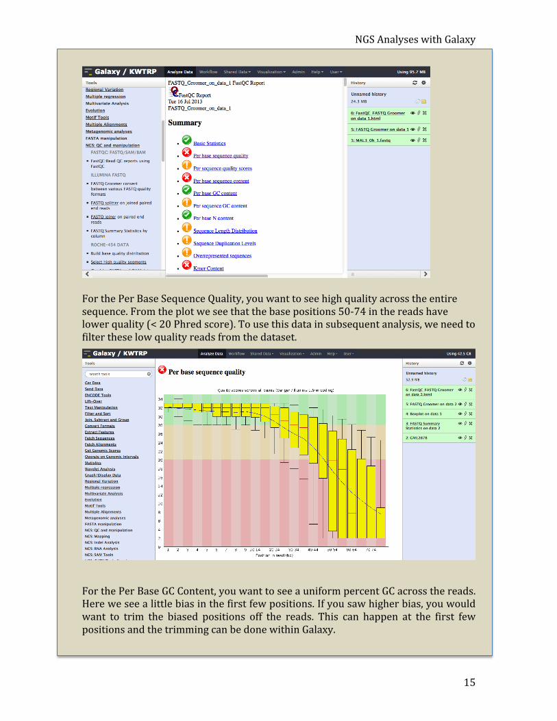
For the Per Base Sequence Quality, you want to see high quality across the entire sequence. From the plot we see that the base positions 50-‐74 in the reads have lower quality (< 20 Phred score). To use this data in subsequent analysis, we need to filter these low quality reads from the dataset.

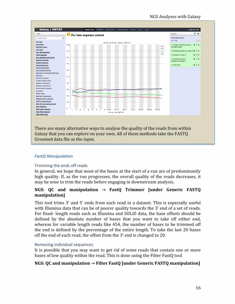
For the Per Base GC Content, you want to see a uniform percent GC across the reads. Here we see a little bias in the first few positions. If you saw higher bias, you would want to trim the biased positions off the reads. This can happen at the first few positions and the trimming can be done within Galaxy.


16

There are many alternative ways to analyse the quality of the reads from within Galaxy that you can explore on your own. All of these methods take the FASTQ Groomed data file as the input.

FastQ Manipulation

Trimming the ends off reads In general, we hope that most of the bases at the start of a run are of predominantly high quality. If, as the run progresses, the overall quality of the reads decreases, it may be wise to trim the reads before engaging in downstream analysis.

NGS: QC and manipulation → FastQ Trimmer [under Generic FASTQ manipulation] This tool trims 3’ and 5’ ends from each read in a dataset. This is especially useful with Illumina data that can be of poorer quality towards the 3’ end of a set of reads. For fixed-‐ length reads such as Illumina and SOLiD data, the base offsets should be defined by the absolute number of bases that you want to take off either end, whereas for variable length reads like 454, the number of bases to be trimmed off the end is defined by the percentage of the entire length. To take the last 20 bases off the end of each read, the offset from the 3’ end is changed to 20.

Removing individual sequences It is possible that you may want to get rid of some reads that contain one or more bases of low quality within the read. This is done using the Filter FastQ tool

NGS: QC and manipulation → Filter FastQ [under Generic FASTQ manipulation]


17

This tool allows the user to filter out reads that have some number of low quality bases and return only those reads of the highest quality. For example, if we wanted to remove from our dataset all reads where the quality of any base was less than 20; we change the Minimum quality box to 20. The “Maximum number of bases allowed outside of quality range” allows us to select how many bases per read must be below our threshold before we discard that read. If we leave this at the default setting of 0, all bases in a read must pass the threshold minimum quality score to be kept.

More complex manipulations The Manipulate FastQ tool in Galaxy also allows much more complex manipulation of FastQ data, whether manipulating the read names, the sequence content or the quality score content. This tool also allows the removal of reads that match some given criteria. NGS: QC and manipulation → Manipulate FASTQ [under Generic FASTQ manipulation] This tool can work on all, or a subset of, reads in a dataset. The subset is selected using regular expressions on the read name, sequence content, or quality score content. If no ‘Match Reads’ filter is added, the manipulation is performed on all reads.

Exercise 1. The GM12878 dataset seems to be a poor quality.

2. Trim the reads in the GM12878 dataset using the Generic FASTQ manipulation → FastQ Trimmer tool. Determine from the boxplot and FastQC figures where the quality of the reads begins to drop off sharply. Calculate how many bases have to be trimmed from the end and use that number as the Offset from 3' end.

3. Using the Generic FASTQ manipulation → Filter FastQ tool, filter out all sequences with any bases that have a quality less than 20. How many sequences do you have left in your dataset?

4. Run another QC (summary statistics and boxplot) on both of the new datasets.


18

Mapping Illumina data with BWA

Mappers There are two mappers available in Galaxy: Bowtie and BWA. The crucial difference between these mappers is that BWA performs gapped alignments, whereas Bowtie does not (although there is a beta version of Bowtie available which does perform gapped alignments, it is not the one available in Galaxy). This, therefore, gives BWA greater power to detect indels and SNPs. Bowtie tends to be much faster, and have a smaller memory footprint, than BWA. BWA is generally used for DNA projects, whereas Bowtie is used for RNA-‐Seq projects since the exonic aligner TopHat uses Bowtie to do the initial mapping of reads.

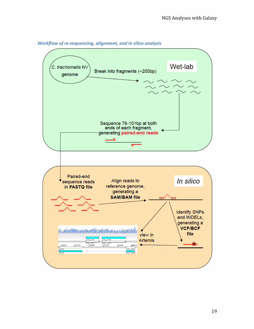
In this portion of the exercise, we will use one of the popular alignment tools for high-‐throughput sequence data, named BWA from the Sanger Institute, to align Illumina reads from a new strain variant of Chlamydia trachomatis (NV) isolated in Sweden against a C. trachomatis reference sequence (L2). Later in another module on SNP analysis, we will be using another aligner, bowtie, to map the reads again. Here, we are using BWA to give you experience of using an aligner in Galaxy.

Aligning reads with BWA [Burrows-‐Wheeler Alignment] Create a new history by clicking the gear icon and selecting Create New. We will be working with the data in the Module_Mapping directory. Our reference sequence for this exercise is a C. trachomatis LGV strain called L2. The sequence file against which you will align your reads is called L2_cat.fasta. This file contains a concatenated sequence in FASTA format consisting of the genome and a plasmid. The forward and the reverse paired-‐end reads of the newly sequenced strain are labelled NV_1.fastq and NV_2.fastq.


19

Workflow of re-‐sequencing, alignment, and in silico analysis


20

Exercise

1. Upload the L2_cat.fasta file as in the previous exercise. (Get Data tool).

2. Select format as fasta format 3. Click Execute

Load the forward and the reverse paired-‐end reads of the newly sequenced strain. The forward and reserve reads are contained in files NV_1.fastq and NV_2.fastq.

1. Upload the two files NV_1.fastq and NV_2.fastq using the Get Data -‐> Upload File tool).

2. Select format as fastqsanger format

3. Click Execute

We will now align the joined forward and the reverse reads against our reference sequence L2

1. Select the NGS:Mapping→Map with BWA for Illumina tool.

2. Select reference genome from the history option and select L2_cat.fasta we uploaded earlier.

3. This library is paired-‐end

4. Select the forward fastq file: NV_1.fastq

5. Select the reverse fastq file: NV_2.fastq 6. Keep rest op settings as is. 7. Click Execute.

Once the job has completed, the result is a single SAM file.


21

The output of either BWA or bowtie is a Sequence Alignment and Mapping (SAM) file that is a massive text file containing every read, the quality for each base and how those reads align to the genome. A more compact format of this file is the Binary Alignment and Mapping (BAM) file. These files are often used as input for other analyses and even visualization (e.g., Artemis). The conversion of these files from SAM to BAM format (or vice versa) is done within the samtools software package that has been incorporated into Galaxy.

SAM [Sequence Alignment/Map] Format The Sequence Alignment/Map (SAM) format is a generic nucleotide alignment format that describes the alignment of query sequences or sequencing reads to a reference sequence. It can store all the information about an alignment that is generated by most alignment programs. Importantly, it is a compact representation of the alignment, and can allow many of the operations on the alignment to be performed without loading the whole alignment into memory. The SAM format also allows the alignment to be indexed by reference sequence position to efficiently retrieve all reads aligning to a locus.

The SAM format consists of a header section and an alignment section.

Header section The header section includes information about the alignment and the program that generated it. All lines in the header section are tab-‐delimited and begin with a “@” character, followed by tag:value pairs, where tag is a two-‐letter string that defines the content and the format of value.

There are five main sections to the header, each of which is optional:

@HD. The header line. If this is present, it must be the first line, and must include: VN: the format version.

@SQ. Includes information about the reference sequence(s). If this section is present, it must include two fields:

SN: the reference sequence name. LN: the reference sequence length.

@RG. Includes information about read groups. These can be present multiple times for multiple read groups. If this section is present, each @RG section must include: ID: the read group identifier. If an RG tag appears anywhere in the alignment section, there should be a single corresponding @RG line with matching ID tag in the header section.


22

@PG. Includes information about the program generating the alignment. Must include: ID: The program identifier. If a PG tag appears anywhere in the alignment section, there should be a single corresponding @PG line with matching ID tag in the header section.

@CO. These are unstructured one-‐line comment lines which can be present multiple times.

Alignment section

Each alignment line has 11 mandatory fields and a variable number of optional fields. These fields always appear in the same order and must be present, but their values can be ‘0’ or ‘*’ (depending on the field) if the corresponding information is unavailable.

Mandatory Alignment Section Fields

FLAG field The FLAG field includes information about the mapping of the individual read. It is a bitwise flag, which is a way of compactly storing multiple logical values as a short series of bits where each of the single bits can be addressed separately.

27

Alignment section Each alignment line has 11 mandatory fields and a variable number of optional fields. These fields always appear in the same order and must be present, but their values can be ‘0’ or ‘*’ (depending on the field) if the corresponding information is unavailable. Mandatory Alignment Section Fields Position Field Description 1 QNAME Query template (or read) name 2 FLAG Information about read mapping (see next section) 3 RNAME Reference sequence name. This should match a @SQ

line in the header. 4 POS 1-based leftmost mapping position of the first

matching base. Set as 0 for an unmapped read without coordinate.

5 MAPQ Mapping quality of the alignment. Based on base qualities of the mapped read.

6 CIGAR Detailed information about the alignment (see relevant section).

7 RNEXT Used for paired end reads. Reference sequence name of the next read. Set to “=” if the next segment has the same name.

8 PNEXT Used for paired end reads. Position of the next read. 9 TLEN Observed template length. Used for paired end reads

and is defined by the length of the reference aligned to. 10 SEQ The sequence of the aligned read. 11 QUAL ASCII of base quality plus 33 (same as the quality

string in the Sanger FASTQ format). 12 OPT Optional fields (see relevant section).


23

FLAG fields

In a run with single reads, the only flags you will see are:

0 None of the bitwise flags have been set. This read has been mapped to the forward strand. 4 The read is unmapped.

16 The read is mapped to the reverse strand. Some common flags that you may see in a paired experiment include:

CIGAR [Concise Idiosyncratic Gapped Alignment Report] String The CIGAR string describes the alignment of the read to the reference sequence. It is able to handle (soft-‐ and hard-‐) clipped alignments, spliced alignments, multi-‐part alignments and padded alignments (as well as alignments in color space). The following operations are defined in CIGAR format:

28

FLAG field The FLAG field includes information about the mapping of the individual read. It is a bitwise flag, which is a way of compactly storing multiple logical values as a short series of bits where each of the single bits can be addressed separately. FLAG fields Hex Binary Description 0x1 00000000001 (1) The read is paired 0x2 00000000010 (2) Both reads in a pair are mapped “properly” (i.e., in the

correct orientation with respect to one another) 0x4 00000000100 (4) The read itself is unmapped 0x8 00000001000 (8) The mate read is unmapped 0x10 00000010000 (16) The read has been reverse complemented 0x20 00000100000 (32) The mate read has been reverse complemented 0x40 00001000000 (64) The read is the first read in a pair 0x80 00010000000 (128) The read is the second read in a pair 0x100 00100000000 (256) The alignment is not primary (a read with split matches

may have multiple primary alignment records) 0x200 01000000000 (512) The read fails platform/vendor quality checks 0x400 10000000000 (1024) PCR or optical duplicate

In a run with single reads, the only flags you will see are: 0 None of the bitwise flags have been set. This read has been mapped to the forward strand. 4 The read is unmapped. 16 The read is mapped to the reverse strand. Some common flags that you may see in a paired experiment include: 69 1 + 4 + 64 The read is paired, is the first read in the pair, and is unmapped. 73 1 + 8 + 64 The read is paired, is the first read in the pair, and it is mapped while

its mate is not. 77 1 + 4 + 8 +

64 The read is paired, is the first read in the pair, but both are unmapped.

133 1 + 4 + 128 The read is paired, is the second read in the pair, and it is unmapped. 137 1 + 8 + 128 The read is paired, is the second read in the pair, and it is mapped

while its mate is not. 141 1 + 4 + 8 +

128 The read is paired, is the second read in the pair, but both are unmapped.

28

FLAG field The FLAG field includes information about the mapping of the individual read. It is a bitwise flag, which is a way of compactly storing multiple logical values as a short series of bits where each of the single bits can be addressed separately. FLAG fields Hex Binary Description 0x1 00000000001 (1) The read is paired 0x2 00000000010 (2) Both reads in a pair are mapped “properly” (i.e., in the

correct orientation with respect to one another) 0x4 00000000100 (4) The read itself is unmapped 0x8 00000001000 (8) The mate read is unmapped 0x10 00000010000 (16) The read has been reverse complemented 0x20 00000100000 (32) The mate read has been reverse complemented 0x40 00001000000 (64) The read is the first read in a pair 0x80 00010000000 (128) The read is the second read in a pair 0x100 00100000000 (256) The alignment is not primary (a read with split matches

may have multiple primary alignment records) 0x200 01000000000 (512) The read fails platform/vendor quality checks 0x400 10000000000 (1024) PCR or optical duplicate

In a run with single reads, the only flags you will see are: 0 None of the bitwise flags have been set. This read has been mapped to the forward strand. 4 The read is unmapped. 16 The read is mapped to the reverse strand. Some common flags that you may see in a paired experiment include: 69 1 + 4 + 64 The read is paired, is the first read in the pair, and is unmapped. 73 1 + 8 + 64 The read is paired, is the first read in the pair, and it is mapped while

its mate is not. 77 1 + 4 + 8 +

64 The read is paired, is the first read in the pair, but both are unmapped.

133 1 + 4 + 128 The read is paired, is the second read in the pair, and it is unmapped. 137 1 + 8 + 128 The read is paired, is the second read in the pair, and it is mapped

while its mate is not. 141 1 + 4 + 8 +

128 The read is paired, is the second read in the pair, but both are unmapped.


24

CIGAR Format Operations

• H can only be present as the first and/or last operation.

• S may only have H operations between them and the ends of the CIGAR string.

• For mRNA-‐to-‐genome alignment, an N operation represents an intron. For other types of alignments, the interpretation of N is not defined.

• Sum of lengths of the M/I/S/=/X operations must equal the length of read.

OPT field The optional fields are presented as key-‐value pairs in the format of TAG:TYPE:VALUE, where TYPE is one of:

29

CIGAR [Concise Idiosyncratic Gapped Alignment Report] String The CIGAR string describes the alignment of the read to the reference sequence. It is able to handle (soft- and hard-) clipped alignments, spliced alignments, multi-part alignments and padded alignments (as well as alignments in color space). The following operations are defined in CIGAR format: CIGAR Format Operations Operation Description M Alignment match (can be a sequence match or mismatch) I Insertion to the reference D Deletion from the reference N Skipped region from the reference S Soft clipping (clipped sequences present in read) H Hard clipping (clipped sequences NOT present in alignment record) P Padding (silent deletion from padded reference) = Sequence match (not widely used) X Sequence mismatch (not widely used)

• H can only be present as the first and/or last operation. • S may only have H operations between them and the ends of the CIGAR string. • For mRNA-to-genome alignment, an N operation represents an intron. For other

types of alignments, the interpretation of N is not defined. • Sum of lengths of the M/I/S/=/X operations must equal the length of read.

Li et al, Bioinformatics (2009) 25 (16): 2078-2079. “The Sequence Alignment/Map format and SAMtools”

29

CIGAR [Concise Idiosyncratic Gapped Alignment Report] String The CIGAR string describes the alignment of the read to the reference sequence. It is able to handle (soft- and hard-) clipped alignments, spliced alignments, multi-part alignments and padded alignments (as well as alignments in color space). The following operations are defined in CIGAR format: CIGAR Format Operations Operation Description M Alignment match (can be a sequence match or mismatch) I Insertion to the reference D Deletion from the reference N Skipped region from the reference S Soft clipping (clipped sequences present in read) H Hard clipping (clipped sequences NOT present in alignment record) P Padding (silent deletion from padded reference) = Sequence match (not widely used) X Sequence mismatch (not widely used)

• H can only be present as the first and/or last operation. • S may only have H operations between them and the ends of the CIGAR string. • For mRNA-to-genome alignment, an N operation represents an intron. For other

types of alignments, the interpretation of N is not defined. • Sum of lengths of the M/I/S/=/X operations must equal the length of read.

Li et al, Bioinformatics (2009) 25 (16): 2078-2079. “The Sequence Alignment/Map format and SAMtools”


25

A Printable character I Signed 32-‐bin integer F Single-‐precision float number Z Printable string H Hex string

The information stored in these optional fields will vary widely with the mapper.

They can be used to store extra information from the platform or aligner. For example, the RG tag keeps the ‘read group’ information for each read, where a read group can be any set of reads that use the same protocol (sample/library/lane). In combination with the @RG header lines, this tag allows each read to be labeled with metadata about its origin, sequencing center and library.

Other commonly used optional tags include: NM:i Edit distance to the reference MD:Z Number matching positions/mismatching base AS:i Alignment score BC:Z Barcode sequence X0:i Number of best hits X1:i Number of suboptimal hits found by BWA XN:i Number of ambiguous bases in the reference XM:i Number of mismatches in the alignment XO:i Number of gap opens XG:i Number of gap extensions XT:A Type of match (Unique/Repeat/N/Mate-‐sw) XA:Z Alternative hits; format: (chr,pos,CIGAR,NM) XS:i Suboptimal alignment score XF: Support from forward/reverse alignment XE:I Number of supporting seeds Thus, for example, we can use the NM:i:0 tag to select only those reads which map perfectly to the reference (i.e., have no mismatches). If we wanted to select only those reads which mapped uniquely to the genome, we could filter on the XT:A:U (where the U stands for “unique”).


26

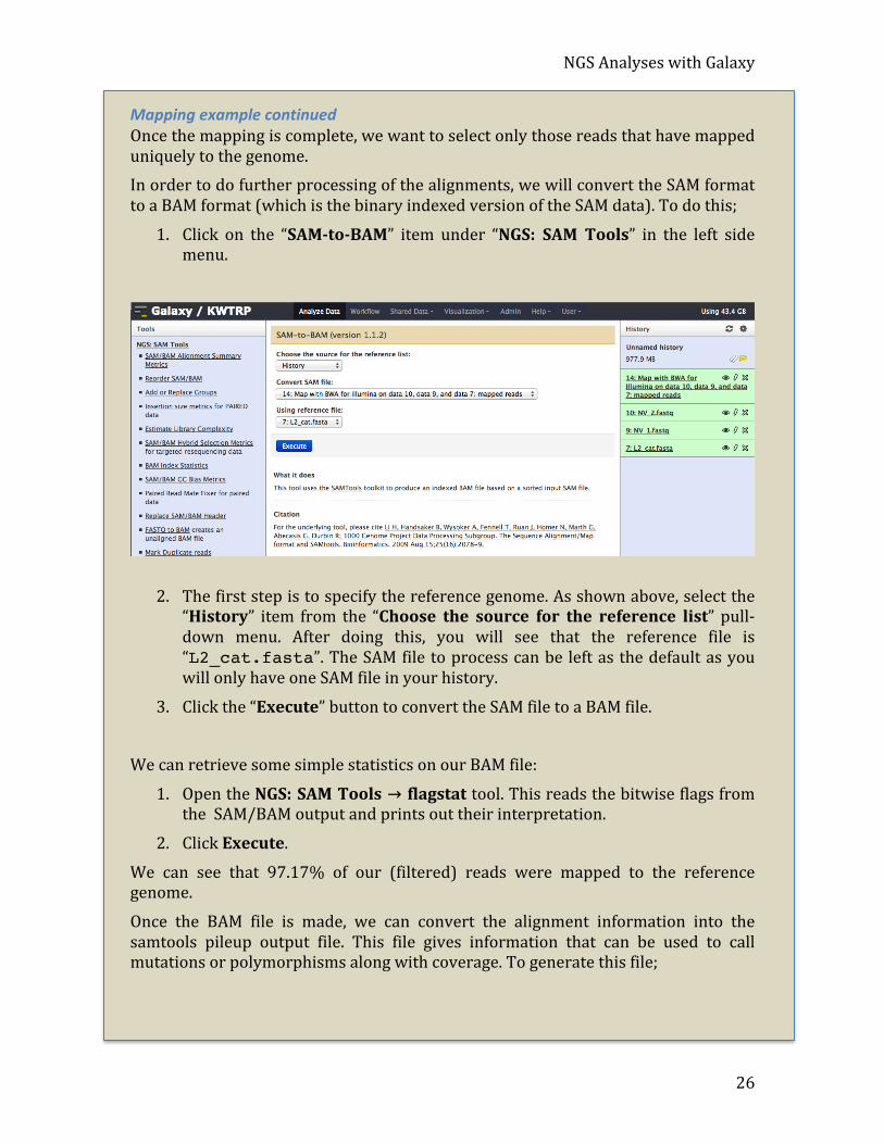
Mapping example continued Once the mapping is complete, we want to select only those reads that have mapped uniquely to the genome. In order to do further processing of the alignments, we will convert the SAM format to a BAM format (which is the binary indexed version of the SAM data). To do this;

1. Click on the “SAM-‐to-‐BAM” item under “NGS: SAM Tools” in the left side menu.

2. The first step is to specify the reference genome. As shown above, select the “History” item from the “Choose the source for the reference list” pull-‐ down menu. After doing this, you will see that the reference file is “L2_cat.fasta”. The SAM file to process can be left as the default as you will only have one SAM file in your history.

3. Click the “Execute” button to convert the SAM file to a BAM file.

We can retrieve some simple statistics on our BAM file:

1. Open the NGS: SAM Tools → flagstat tool. This reads the bitwise flags from the SAM/BAM output and prints out their interpretation.

2. Click Execute.

We can see that 97.17% of our (filtered) reads were mapped to the reference genome.

Once the BAM file is made, we can convert the alignment information into the samtools pileup output file. This file gives information that can be used to call mutations or polymorphisms along with coverage. To generate this file;


27

The SAM and BAM formats are read-‐specific, in that every line in the file refers to a read. We want to convert the data to a format where every line represents a position in the genome instead, known as a pile-‐up.

1. Click on the “Mpileup SNP and indel caller” link under “NGS: SAM Tools” on the menu on the left side of the page. Like the SAM-‐to-‐BAM conversion, we first have to select the L2 genome file (L2_cat.fasta ) as the reference. To do this, select “Use one from the history” from the pull-‐down menu at the top of the page.

2. Make sure the L2 genome file and the recently made BAM file is selected (which should be the case as you have only one FASTA file and one BAM file). Finally, click the “Execute” button to launch the job.

Pileup output


28

Pileup Format Each line in the pileup format includes information on:

1. The reference sequence (chromosome) name. 2. The position in the reference sequence.

3. The reference base at that position (uppercase indicates the positive strand; lowercase the negative strand). An asterisk marks an indel at that position. 4. The number of reads covering that position.

5. The read base at that position. This column also includes information about whether the reads match the reference position or not.

• A “.” stands for a match to the reference base on the forward strand, • A “,” stands for a match on the reverse strand, • “[ACGTN]” for a mismatch on the forward strand and • “[acgtn]” for a mismatch on the reverse strand. • A pattern “\[+-‐][0-‐9]+[ACGTNacgtn]+” indicates there is an insertion (+) or

deletion (-‐) between this reference position and the next reference position. • Finally, a “^” indicates the start of a new, or soft-‐ or hard-‐clipped read,

followed by the mapping quality of the read. • The “$” symbol marks the end of a read segment.

6. The quality scores for each read covering that position. For more detailed information on the pileup format, go to http://samtools.sourceforge.net/pileup.shtml

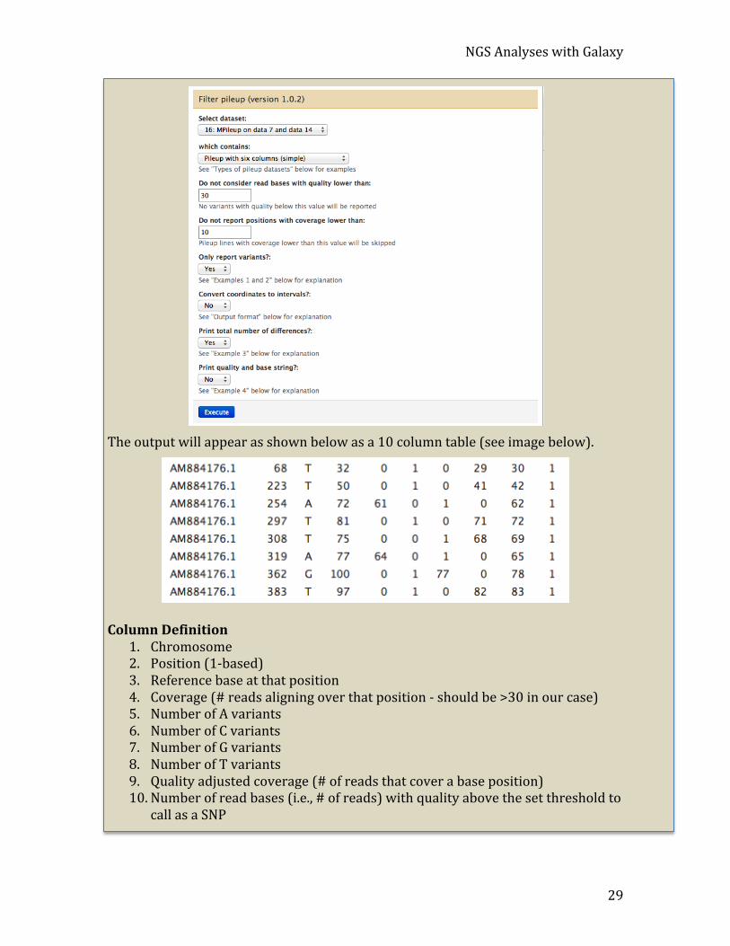
Analyze pileup The pileup file can be filtered in many ways from within Galaxy. The “Filter pileup” tool underneath “NGS: SAM Tools” on the menu on the left can be used to do this. As a demonstration, open the tool;

1. Click NGS: SAM Tools -‐> Filter pileup and run the default filtering that will report variants between the NV genome reads and the reference genome L2. Select Require that a base call must have a quality of at 30 to be considered. Remove all bases covered by fewer than 10 reads and clicking the “Execute” button (See image below).

2. Change the pulldown menus so that:

• the tool reports variants only • coordinates are not converted to intervals • the total number of differences is reported • the quality and base string are not returned (since these will be very large

fields).


29

The output will appear as shown below as a 10 column table (see image below).

Column Definition

1. Chromosome 2. Position (1-‐based) 3. Reference base at that position 4. Coverage (# reads aligning over that position -‐ should be >30 in our case) 5. Number of A variants 6. Number of C variants 7. Number of G variants 8. Number of T variants 9. Quality adjusted coverage (# of reads that cover a base position) 10. Number of read bases (i.e., # of reads) with quality above the set threshold to

call as a SNP


30

We can now remove any positions that is not covered by >20 reads. This will ensure that we are confident that when a SNP is called it is correctly called.

1. Open the Filter and Sort → Filter tool.

2. Use“c10>=20”as the filter condition.

Once the filtering job has completed, you can either examine the results in Galaxy or save the output as a text file. To examine the results in Galaxy, just click the icon that looks like an eye next to the name of the filtering job in your history.

In the image below you will see that the first SNP is reported at position 1430 where the base is a G (Guanine) in the reference genome L2 compared to an A (Adenine) base in the same position in the NV genome and is covered by at least 66 reads.

In a subsequent module we will show you how to visually analyse the same data using Artemis as shown below.

!ngs!analyses!with!galaxy! -...

Documents