SUPPLEMENTARYINFORMATION

Confidencematchingingroupdecision-making

DanBang*,LaurenceAitchison,RaniMoran,SantiagoHerceCastañón,BanafsheRafiee,AliMahmoodi,JenniferY.F.Lau,PeterE.Latham,BahadorBahrami,and

ChristopherSummerfield

*Correspondenceto:danbang.db@gmail.com

SUPPLEMENTARYMETHODS

Computationalmodel

Wedevelopedasimplesignaldetectionmodel(tounderstandhowjointaccuracy(fractionofcorrectjoint decisions) varies with differences between groupmembers’ expertise andmean confidenceand to establish an optimal benchmark against which empirical group performance could becompared(Figure3).Themodelassumesthatthreecognitiveprocessesgovernconfidence: (i) theagentreceivesnoisysensoryevidence,(ii)theagentcomputesaninternalestimateoftheevidencestrengthand(iii)theagentmapstheinternalestimateontoaresponse(decisionandconfidence)byapplyingasetofthresholds.Thelevelofsensorynoisedeterminestheagent’sexpertiseandthesetofthresholdsdeterminestheagent’smeanconfidence.

Modeldescription

We assumed that on each trial an agent receives noisy sensory evidence, 𝑥, sampled from aGaussiandistribution,𝑥 ∈ 𝑁(𝑠, 𝜎().Themean,𝑠, isthedifferenceincontrastbetweenthesecondandthefirstdisplayatthetargetlocation.Assuch,𝑠isdrawnuniformlyfromtheset𝑠 ∈ 𝑆 = {−.15,−.07, −.035, −.015, .015, .035, .07, .15} – the sign of 𝑠 indicates the target display (negative:1st;positive:2nd)and its absolutevalue indicates the contrast added to the target. The standarddeviation,𝜎,describesthelevelofsensorynoiseandisthesameforallstimuli.

Wemodelledtheinternalestimateoftheevidencestrengthastherawsensoryevidence,𝑧 = 𝑥.Theinternal estimate thus ran from largenegative values, indicatingahighprobability that the targetwas inthefirstdisplay,throughvaluesnear0, indicatinghighuncertainty,to largepositivevalues,indicatingahighprobabilitythatthetargetwasintheseconddisplay.Wechosethisformulationformathematical simplicitybutnote thatour analysiswould show the same results for anymodel inwhichtheinternalestimateisamonotonicfunctionofthesensoryevidence,includingprobabilisticestimatessuchas𝑧 = 𝑃(𝑠 > 0|𝑥).

We assumed that the agentmaps the internal estimate onto a response, 𝑟, by applying a set ofthresholds,𝜽.As inourexperiments, theresponses range from-6 to -1and1 to6– thesignof𝑟indicates thedecision (negative:1st;positive:2nd)and itsabsolutevalue indicates theconfidence(𝑐 = |𝑟|).Thethresholds,𝜽,determinetheprobabilitydistributionoverresponses

𝑝> ≡ 𝑃 𝑟 = 𝑖 =

𝑃 𝑧 ≤ 𝜃CD 𝑖 = −6𝑃 𝜃FCG < 𝑧 ≤ 𝜃F𝑃 𝜃CG < 𝑧 ≤ 𝜃G

−6 < 𝑖 ≤ −1, 2 ≤ 𝑖 < 6𝑖 = 1

𝑃 𝑧 > 𝜃J 𝑖 = 6

.

There is no criterion𝜃D, because 𝑟 = 6 corresponds to 𝑧 exceeding 𝜃J. There is a one-to-onerelationshipbetweenthresholdsandprobabilities,soitiseasytofindthethresholdscorrespondingtoagivenresponsedistribution(aswewilldoshortly).

Derivingaccuracyforanagent

Wecalculatedtheaccuracy(fractionofcorrectdecisions)ofanagent,givenalevelofsensorynoise,𝜎,andaresponsedistribution,𝑝>,where𝑖 = ±1,2, … , 6,asfollows.

We first calculated the thresholds,𝜽, that produced the response distribution 𝑝> over the entirestimulusset𝑆 = {−.15, −.07, −.035, −.015, .015, .035, .07, .15}.Inparticular,wefound(usingMATLAB’s‘fzero’function)thresholds𝜃>,where𝑖 = −6, −5, … , −1,1,2, … 5,suchthat

𝑝MMN>

=18

Φ(𝜃> − 𝑠𝜎

)Q∈R

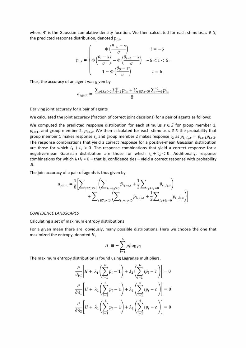
whereΦ istheGaussiancumulativedensityfucntion.Wethencalculatedforeachstimulus,𝑠 ∈ 𝑆,thepredictedresponsedistribution,denoted𝑝>,Q,

𝑝>,Q =

Φ𝜃CD − 𝑠𝜎

𝑖 = −6

Φ𝜃> − 𝑠𝜎

− Φ𝜃>CG − 𝑠

𝜎−6 < 𝑖 < 6

1 − Φ𝜃J − 𝑠𝜎

𝑖 = 6

.

Thus,theaccuracyofanagentwasgivenby

𝑎agent = 𝑝𝑖,𝑠6

𝑖=1 +Q∈R,QZ[ 𝑝𝑖,𝑠−1𝑖=−6Q∈R,Q\[

8

Derivingjointaccuracyforapairofagents

Wecalculatedthejointaccuracy(fractionofcorrectjointdecisions)forapairofagentsasfollows:

We computed the predicted response distribution for each stimulus 𝑠 ∈ 𝑆 for group member 1,𝑝>,Q,G,andgroupmember2,𝑝>,Q,(.We thencalculated foreachstimulus𝑠 ∈ 𝑆 theprobability thatgroupmember1makesresponse𝑖Gandgroupmember2makesresponse𝑖(as𝑝>],>^,Q =𝑝>,Q,G𝑝>,Q,(.Theresponsecombinationsthatyieldacorrectresponseforapositive-meanGaussiandistributionare those for which 𝑖G + 𝑖( > 0. The response combinations that yield a correct response for anegative-mean Gaussian distribution are those for which 𝑖G + 𝑖( < 0. Additionally, responsecombinationsforwhichi1+i2=0–thatis,confidenceties–yieldacorrectresponsewithprobability.5.

Thejoinaccuracyofapairofagentsisthusgivenby

𝑎_`Fab =18

𝑝>],>^,Q>]c>^Z[+12

𝑝>],>^,Q>]c>^d[𝑠∈𝑆,𝑠>0

+ 𝑝>],>^,Q>]c>^\[+12

𝑝>],>^,Q>]c>^d[𝑠∈𝑆,𝑠<0

CONFIDENCELANDSCAPES

Calculatingasetofmaximumentropydistributions

For a givenmean there are, obviously,manypossible distributions.Herewe choose the one thatmaximizedtheentropy,denoted𝐻,

𝐻 ≡ − 𝑝>log𝑝>

D

>dG

ThemaximumentropydistributionisfoundusingLagrangemultipliers,

𝜕𝜕𝑝>

𝐻 +𝜆G 𝑝> − 1D

>dG

+ 𝜆( 𝑖𝑝> − 𝑐D

>dG

= 0

𝜕𝜕𝜆G

𝐻 +𝜆G 𝑝> − 1D

>dG

+ 𝜆( 𝑖𝑝> − 𝑐D

>dG

= 0

𝜕𝜕𝜆(

𝐻 +𝜆G 𝑝> − 1D

>dG

+ 𝜆( 𝑖𝑝> − 𝑐D

>dG

= 0

where𝑐isthemean.Solvingtheseequationsgivesthemaximumentropydistribution,subjecttotheconstraints that the distribution sums to 1, 𝑝> = 1,D

>dG and has the right mean confidence, c,𝑖𝑝> = 𝑐D

>dG and𝑝> ≥ 0. For 𝑐 = 1 the unique distribution that satisfies these constraints is𝑝 =(1,0,0,0,0,0). Similarly, for𝑐 = 6,𝑝 = (0,0,0,0,0,1) is the solution. For any intermediate value forthemean,1 ≤ 𝑐 ≤ 6,thesolutionis

𝑝> =𝑒>l^

𝑒Ml^DMdG

with𝜆(chosenbysolvingtheconstraint

𝑐 =𝑗𝑒Ml^D

MdG

𝑒Ml^DMdG

whichcanbedonewithMATLAB’s“fzero”function.Wetransformedconfidencedistributions(1to6)toresponsedistributions(-6to-1and1to6)byassumingsymmetryaround0.

SUPPLEMENTARYNOTES

Comparingobservedtooptimaljointaccuracy

In Figure 3D, we show that the ratio of the observed joint accuracy to that expected under theoptimal solution,𝑎nop/𝑎`pb, approaches1as the ratioof theaccuracyof the lessaccurategroupmembertothatofthemoreaccurategroupmember,𝑎oFa/𝑎ors,approaches1–apatternwhichisexpectedunderconfidencematching.Thisanalysisis,however,subjecttopotentialconfounds.Ouraimhereistoexplainwhattheseconfoundsareandshowthateachofthemcanberuledout.

First,wemightfindadivergencebetweentheobservedjointaccuracyandthatexpectedundertheoptimalsolutionbecausetheonlysourceofresponsevariationinourmodelissensorynoise;unlikeparticipants,themodelnevermakesresponseerrorsorhas lapsesofattention.Tocorrectforthispotentialmismatch,were-definedjointaccuracyundertheoptimalsolutionas:

𝑎`pb = 𝑎`pb − (𝑎tFb − 𝑎nop)

where𝑎`pbisthemaximumofagivenconfidencelandscapeasbeforeand𝑎tFbisthejointaccuracyderivedundergroupmembers’observedresponsedistributions.Theadditionalterm,(𝑎tFb − 𝑎nop),correctsforany‘overestimation’ofjointaccuracyintroducedbyourmodellingprocedure.Critically,whenre-definingoptimalityas𝑎nop/𝑎`pb,westillobserveapositivecorrelationbetweenoptimalityandthesimilarityofgroupmembers’accuracy(r(80)=.682,p<.001,Pearson).

This analysis, however,may still be subject to twoadditional confounds. First,𝑎`pbmightdivergefrom𝑎nopsimplybecause𝑎`pbwasderivedundermaximumentropydistributions,which–foranygiven mean confidence – usually reduces the number of confidence ties. Second, the level ofoptimality itself, 𝑎nop/𝑎`pb, might be smaller for similar group members, 𝑎oFa/𝑎ors ≈ 1, thandissimilar group members, 𝑎oFa/𝑎ors ≪ 1, due to range effects. For the most dissimilar groupmembers, the difference between the minimum and the maximum value of a given confidencelandscapeisabout.1.Incontrast,forthemostsimilargroupmembers,thedifferencebetweentheminimumandthemaximumvalueofagivenconfidencelandscapeisonlyabout.05.Thus,therewaslessroomforthelattertodeviatefromthejointaccuracyexpectedundertheoptimalsolution.

Wethereforerepeatedtheaboveanalysisbutnowre-definingoptimalityas:

𝑎nop/𝑎`pb = (𝑎orsnab − 𝑎rabF)/(𝑎`pb − 𝑎rabF)

where 𝑎rabF is the minimum value of a confidence landscape and 𝑎orsnab is the value of thelandscape coordinate indexed by group member’s observed mean confidence. First, by using𝑎orsnab insteadof𝑎nop inthenumerator,wecontrolnotonlyformodelmisspecificationbutalsofor the use of maximum entropy distributions. Second, the subtraction of 𝑎rabF in both thenumeratoranddenominatorcontrols forrangeeffects. Importantly, in linewiththeaboveresults,westillfindapositivecorrelationbetweenoptimalityandthesimilarityofgroupmembers’accuracy(r(80)=.469,p<.001,Pearson).

Supplementary Figure1 | Evidence formatchingof confidence variability and confidencedistributions.a,Correlationinconfidencevariability.Theaxesshowthevarianceofgroupmembers’confidence,var(𝑐G)andvar(𝑐().Theresultsindicatethatgroupmembersadaptedtoeachother’sconfidencevariabilityinthesocialtaskonly.Eachdot isagroup.Each line isthebest-fitting lineofarobustregression;becausethesortingofgroupmembers into1and2 isarbitrary,weshowthep-valuefortheslopeofthebest-fitting lineaveragedacross 105 separate regressions, for each randomly re-labelling the members of a group as 1 and 2. b,Convergenceinconfidencevariability.They-axisshowstheabsolutedifferencebetweenthevarianceofgroupmembers’confidence,|var 𝑐G − var 𝑐( |.Theresultsarenotconclusive;inEXP1,EXP5andEXP6,thereareonlytrendstowardsconvergenceinconfidencevariabilityinthesocialtaskcomparedtotheothertasks.Eachblackdotisdataaveragedacrossgroups.Eachcoloureddotisagroup;thelinesconnectgroupdatawhenthesame pairing of group members was used in two conditions. Error bars are 1 SEM. c, Convergence inconfidence distributions. The y-axis shows the Jensen-Shannon divergence,𝐷z{, between group members’confidencedistributions.Theresultsprovidestrongsupportforconvergenceinconfidencedistributionsinthesocialtaskcomparedtotheothertasks,exceptinthecaseofEXP6.InEXP3,thecontinuousconfidencevalueswerediscretisedtotherange1to6instepsof1.Eachblackdotisdataaveragedacrossgroups.Eachcoloureddot is a group; the lines connect group data when the same pairing of group members was used in twoconditions.Errorbarsare1SEM.SeeSupplementaryFigure3forcomplementarypermutation-basedtests.

mem

ber 2

mea

n co

nfid

ence

member 1 mean confidence

a

experiment

diffe

renc

e in

var

ianc

e of

co

nf. [

|var

(c1)-

var(c 2

)|]

b

experiment

diffe

renc

e be

twee

n co

nf. d

istr

ibut

ions

[DJS

]

ct(29)=1.213

p=.235paired

t(9)=1.235 p=.248paired

t(11)=0.986p=.335

two-sample

t(29)=3.656 p=.001

t(9)=3.014 p=.015

t(11)=0.578 p=.569

two-sample

isolatedobservesocial

task

correlation in confidence variabilityn=30

n=30

n=15

n=15 n=10

n=10

n=12

n=12

n=30 n=15 n=15 n=10 n=12 n=30 n=15 n=15 n=10 n=12

SupplementaryFigure2|ResultsfromExperiment1splitbyconditionorder.Thex-axisshowsthecurrentcondition, they-axis shows themeasureof interestand thecolourdenoteswhethergroups firstperformedthe isolated condition (blue) or the social condition (red).We tested the effect of conditionorder using anANOVAwiththemeasureofinterestaswithin-subjectfactor(isolatedversussocial)andtheconditionorderasbetween-subject factor (isolated first versus social first). The interaction between the two factorswas onlysignificantforthedifferencesbetweenthevarianceofgroupmembers’confidence(variance:F1,28=4.160,p=.041;allothers:F1,28<0.700,p>.400.DJS:Jensen-Shannondivergence.

n=30

first condition

Supplementary Figure 3 | Null distributions for permutation testing. We created for each measure ofinterest,𝜗,adistributionunderthenullhypothesis,𝑝(𝜗),byrandomlyrepairingparticipantsandcomputingthemeanofmeasuredvaluesforeachsetofrepairedparticipants(wesimulated106setsintotal).Byaskingwhethertheobservedmeanvalue(redline)foragivenmeasurewassmallerthan95%ofthevaluesfromthenulldistribution(i.e.,p<.05,one-tailed),wecouldtestwhethertheobservedmeanvaluewasspecifictothetruepairingofgroupmembers–wewouldexpectthistobethecaseifitwastheresultofdynamicinteractionbetween group members. The permutation-based approach unequivocally shows that the mean valuesobservedinthesocialtaskarespecifictothetruepairingofgroupmembers.Theplotsshowtheprobabilitydensityfunctionforeachmeasureofinterest.Thedottedlineshowsthemeanofeachnulldistribution.Thep-valueindicatestheproportionofvaluesfromthenulldistributionthatweresmallerthantheobservedmeanvalue.Mean:|𝑐G − 𝑐(|.Variability:|var 𝑐G − var 𝑐( |.DJS:Jensen-Shannondivergence.

D

D

D

D

D

D

D

D

SupplementaryFigure4|Maximumentropydistributions.Thex-axisshowstheconfidencelevels.They-axisshowstheproportionoftimesthateachconfidencelevelisselected.Wetransformedconfidencedistributions(1 to 6) to response distributions (-6 to -1 and 1 to 6) by assuming symmetry around 0.Weonly display asubsetofthemaximumentropydistributions(fullset:1to6instepsof.1).

Supplementary Figure 5 | Comparison between empirical and model psychometric functions. The x-axisshowsthestimulus.They-axisshowstheproportionoftimesthattheseconddisplaywasselectedforagivenvalueofthestimulus.Theplotswerecreatedbyfittingpsychometricfunctionstotheempiricalandthemodeldata.WecomputedR2-valuesacrossparticipants(mean±SD)toevaluatethemodelfits:EXP1-S:R2=.825±.358;EXP2:R2=.892±.089;EXP3:R2=.947±.030;EXP4-I:R2=.844±.135;EXP5-S:R2=.823±.405;EXP6-S:R2= .862 ± .193. Black line: empirical psychometric functions averaged across participants. Red dots: modelpsychometric functions (best fits) averaged across participants; dots only shown for the stimuli used in theexperiments.Shadedarea/errorbarsare1SEM(notvisibleintheseplots).

n=60

n=30

n=20

n=30

n=38

n=24

Supplementary Figure 6 | Comparison between empirical and model response distributions. The x-axisshows the response values (from -6 to 1 and 1 to 6). The y-axis shows the proportion of times that eachresponsewasmade.The titleofeach subplot indicates theexperimentand the stimulus.WecomputedR2-valuesacrossparticipants(mean±SD)toevaluatethemodelfits.EXP1-S:R2=.606±.354;EXP2:R2=.777±.136;EXP3:R2=.838±.078;EXP4-I:R2=.613±.251;EXP5-S:R2=.761±.146;EXP6-S:R2=.635±.206.Thereasonwhytheempiricalandthemodelresponsedistributionsarenotidenticalisthatthemodelwasfittingusing the response distribution observed across all stimuli. Grey: empirical response distributions averagedacrossparticipants.Red:modelresponsedistributions(bestfits)averagedacrossparticipants.Errorbarsare1SEM.

n=60

n=30

n=20

n=30

n=38

n=24

Supplementary Figure 7 | Confidence landscapes. The title of each plot indicates the experiment (E), thegroup(G)andtherangeof jointaccuracies.Theaxesshowthemeanconfidenceoftheworse,𝑐oFa (x-axis),andthebettergroupmember,𝑐ors(y-axis)–withthisdivisiondeterminedbycomparingtheirfittedlevelsofsensory noise. Each mean indexes a maximum entropy distribution associated with a specific meanconfidence.Thegreydotindexesthejointaccuracyexpectedunderthedistributionsassociatedwiththegroupmembers’ observed mean confidence, 𝑎orsnab. The white dot indexes the joint accuracy expected underconfidence matching, 𝑎orb}~, here the pair of confidence distributions associated with the average of thegroup members’ mean confidence. The black dot indexes the joint accuracy expected under the optimalsolution,𝑎`pb.Thevaluesofeachlandscapewerenormalisedtotherange0(blue)to1(red).

Supplementary Figure 8 | Confidence matching in Experiment 4. The plot shows the probability densityfunction over our measure of confidence matching: ∆𝑚 = |𝑐pr�bF}FprabF�`�rbn� − 𝑐pr�ban�| − 𝑐pr�bF}Fprab�`}Fr� − 𝑐pr�ban� .The empirical observations (x-axis) are overlaid,with each dot corresponding to a group. The difference inmean confidence was smaller in the social blocks than prior to interaction ( 𝑐pr�bF}Fprab�`}Fr� − 𝑐pr�ban� <|𝑐pr�bF}FprabF�`�rbn� − 𝑐pr�ban�|:t(151)=-5.066,p<.001,paired).

confidence matching[∆" = |%&'()*+*&',)*-./')01 − %&'(),0(| − %&'()*+*&',)-.+*'/ − %&'(),0( ]

p(∆"

)

SupplementaryFigure9|Serialdependenceinconfidence.a,Mutualinfluence.Theaxesshowtheinfluenceofthepartner’sconfidenceontrial𝑡 − 1ontheparticipant’sconfidenceontrialt.Eachdotisagroup.Thelineisthebest-fittinglineofarobustregression;becausethesortingofgroupmembersinto1and2isarbitrary,weshowthep-value for theslopeof thebest-fitting lineaveragedacross105separateregressions, foreachrandomlyre-labellingthemembersofagroupas1and2.b,Short-rangeserialdependence in isolatedtask.They-axisshowscoefficientsfromalinearregressionencodingthedegreetowhichaparticipant’sconfidenceon trial 𝑡 depended on their partner’s confidence on trial 𝑡 − 5 to 𝑡 − 1 in the social task. We testedsignificancebycomparingthecoefficientspooledacrossparticipantstozero(trial𝑡 − 3 to𝑡 − 1:allt(103)<1.6,allp>.010,one-samplet-test,null:0).Weincludedthestimulusontrial𝑡 − 5to𝑡andtheparticipant’sownconfidenceontrial𝑡 − 5 to𝑡 − 1asnuisancepredictors.Thedata is fromEXP1-I,EXP5-IandEXP6-I.c,Noisyread-out.Weusedourlearningmodel(seeMethods)tosimulatedataunderdifferentdegreesofserialdependence(i.e.,differentadaptationrates,x-axis)andappliedastandardmeasureofmetacognitiveabilitytothedata,meta-d’(seeREFsinmaintext).Thismeasureidentifiesthelevelofsensorynoisethatcorrupts‘first-order’decisionperformance,d’,andthenaskshowmuchmorenoiseisneededtoaccountfor‘second-order’confidence performance,meta-d’. The standard interpretation is that such additional noise reflects a noisyread-out of the first-order information and thus lower metacognitive ability. The plot shows that higheradaptation rates are associated with higher differences between d’ and meta-d’ (y-axis). Importantly, bydesign, there is no noisy read-out in our learning model; only the mapping function is changing. It wouldthereforebewrongtoattributeahigherdifferencebetweend’andmeta-d’toanoisyread-out;theread-outis only noisy from the perspective of the experimenter. In a way, differences between d’ andmeta-d’ canreflecthighermetacognitiveabilitywhen theyaredrivenbydynamic changes to themapping function thatmakesensegiventhecurrentcontext.Inoursimulations,weassumedthatthatapairofagentshadthesamelevels of sensory noise (s = .10); that theirmapping functionswere updated so as tomaintainmaximumentropyoverconfidence;andthat the learning ratewas fixed (𝛼 = .12) forbothagents. Ineachsimulatedexperiment,theagentsperformed160trials,withstimulidrawnasinourtask.Tocontrolforrandomresponsevariationduetosensorynoise,weaveragedacross103simulatedexperiments.

am

embe

r 2in

fluen

ce o

f par

tner

(t-1

)

member 1influence of partner (t-1)

n=82

recent trial

seria

l dep

ende

nce

in tr

ial

conf

iden

ce [a

rbitr

ary

units

]

b

no short-range serial dependence in isolated task

n=104

adaptation rate [!]

nois

y re

ad-o

ut

[met

a-d’

-d’]

high degree of adaptation can be confused with bad

metacognition

c

data condition meanaccuracy(SD) meanconfidence(SD)

GROUP1

participant

isolated .711(.052) 2.697(.613)

ALCL .727(.062) 3.079(.649)

ALCH .717(.068) 3.566(.675)

AHCL .714(.065) 2.659(.538)

AHCH .720(.053) 3.313(.610)

virtualpartner

ALCL .653(.054)*$ 2.427(.092)*$

ALCH .659(.053)*$ 4.582(.096)*$

AHCL .792(.059)*$ 2.417(.069)*$

AHCH .784(.054)*$ 4.572(.097)*$

GROUP2

participant

isolated .715(.042) 2.832(.702)

ALCL .713(.056) 3.121(.776)

ALCH .730(.055) 3.685(.669)

AHCL .726(.045) 2.796(.512)

AHCH .719(.063) 3.412(.646)

virtualpartner

ALCL .639(.046)*$ 2.043(.081)*$

ALCH .666(.051)*$ 4.083(.100)*$

AHCL .800(.033)*$ 2.046(.056)*$

AHCH .789(.041)*$ 4.023(.067)*$

SupplementaryTable1|ManipulationchecksforExperiment4.Thesummarystatisticsareshownseparatelyfor the first and the second group of participants (19 in each group). We used two generic confidencedistributionstospecifytheconfidenceofthecomputer-generatedpartners.Forthefirstgroupofparticipants,we used the following confidence distributions:𝑝�`� = [.35, .27, .15, .11, .08, .04]withmean = 2.42 and𝑝~F�~ = [.04, .08, .11, .15, .27, .35]withmean=4.56–wherethefirstelementcorrespondstoconfidencelevel 1, the second element corresponds to confidence level 2, and so forth. For the second group ofparticipants,weusedthefollowingconfidencedistributions:𝑝�`� = [.44, .30, .14, .06, .02, .04]withmean=2.04and𝑝~F�~ = [.10, .12, .14, .16, .18, .26]withmean=3.86.Thesecondsetofconfidencedistributionsweresetsoastobetterfitthoseofthefirstgroupofparticipants.Weusedpairedt-tests(one-tailed)totestwhetherthedataofparticipantsweresignificantlydifferentfromthatofthevirtualpartners.*:dataofvirtualpartnerssignificantlydifferentfromthatofparticipantsatbaseline(isolatedtask).$:dataofvirtualpartnerssignificantlydifferentfromthatofparticipantsinagivensocialcondition(socialtask).

condition

gender(1=female)

like(0-100)

cooperation(0-100)

moreaccurate(1=yes)

moreconfident(1=yes)

GROUP1

ALCL 0.75 65.25 70.40 0.20 0.13

ALCH 0.26 57.15 69.00 0.25 0.73

AHCL 0.55 72.50 75.10 0.73 0.15

AHCH 0.20 58.00 69.85 0.65 0.90

GROUP2

ALCL 0.65 73.17 67.50 0.33 0.06

ALCH 0.24 61.11 64.83 0.31 0.81

AHCL 0.76 77.89 81.39 0.75 0.14

AHCH 0.24 70.00 76.11 0.72 0.86

COMBINED

ALCL 0.70 69.00 69.03 0.26 0.09

ALCH 0.25 59.03 67.03 0.28 0.76

AHCL 0.65 75.05 78.08 0.74 0.14

AHCH 0.22 63.68 72.82 0.68 0.88

Supplementary Table 2 | Questionnaire data from Experiment 4. Participants were asked to complete aquestionnaire about each partner after each social block. They were asked to indicate: (1) whether theythoughtthepartnerwasmale[0]orfemale[1];(2)howmuchtheylikedthepartner[0-100];(3)howwelltheyperformedasagroup[0-100];(4)whetherthepartnerwasless[0]ormore[1]accuratethantheywere;and(5) whether the partner was less [0] or more [1] confident than they were. The table shows the averageresponses.SeeSupplementaryTable1fordifferencebetweenthefirstandthesecondgroupofparticipants.