Written evidence submitted by NHS England (CSR0107)

NHS Five Year Forward View

Recap briefing for the Health Select Committee on technical modelling and scenarios

Table of contents

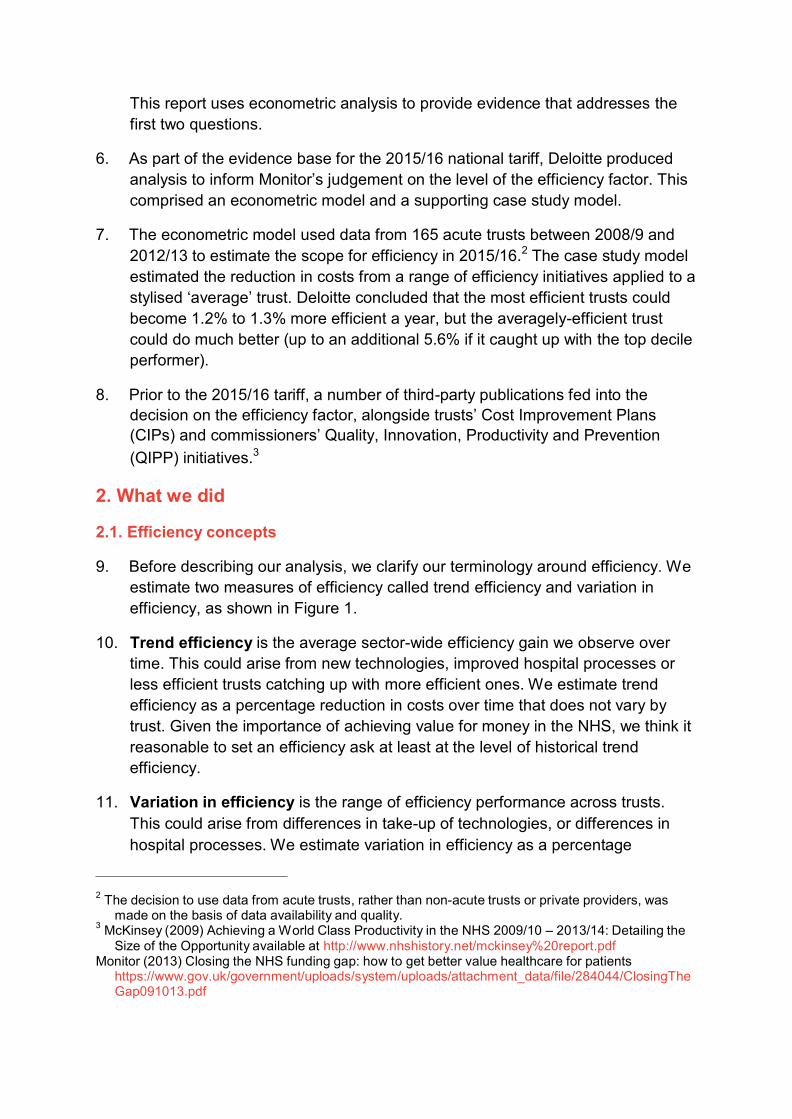
Executive summary

Chapter 1: Introduction

Chapter 2: How was the “£30 billion” 2020 funding gap derived?

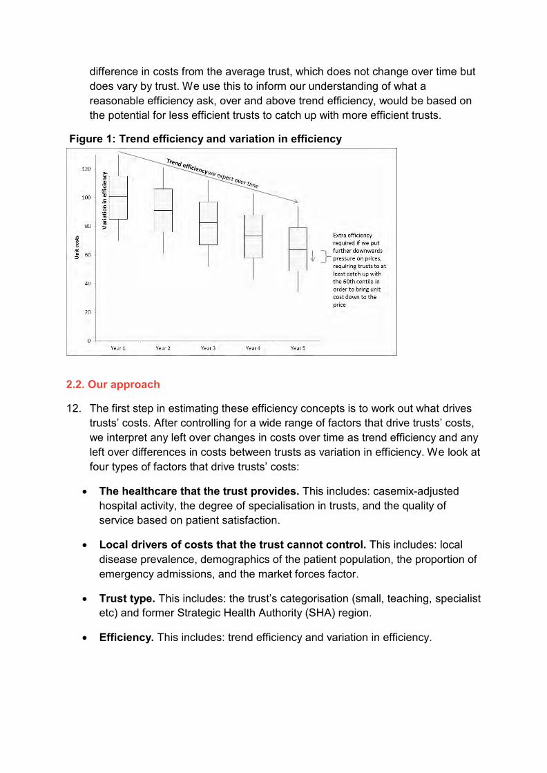
Chapter 3: How were the NHS funding requirements for 2020 estimated at £8 billion to £21 billion?

Chapter 4: What does the NHS Spending Review settlement imply for needed efficiencies (the so-called “£22 billion efficiency requirement”)?

Appendices:

Appendix 1 Worked example – Calculating acute services base case pressures

Appendix 2 2016/17 National Tariff Payment System: A consultation notice Annex B5: Evidence on efficiency for the 2016/17 national tariff

Executive summary At the request of the Health Select Committee, this briefing recaps the modelling undertaken in the lead up to October 2014, when the NHS published the Five Year Forward View (FYFV)1. The FYFV forecast that the NHS would have a £30bn gap in funding by 2020/21 if current demand trends continued, the NHS received flat real terms funding and no further efficiencies were delivered. The weighted average health care demand growth factored into the model was 2.7-2.8% per annum to 2020/21 based upon a 10 year average.

The subsequent Spending Review (SR) modelling of cost pressures and investments remained broadly in line with the modelling conducted a year earlier, as part of the FYFV, with a total potential unmitigated gap of around £30bn by 2020/21.

Three financial scenarios were modelled in the FYFV incorporating different assumptions for demand, efficiency and funding to reduce the £30bn funding gap.

In the first scenario, the £30bn funding gap was reduced to £21bn by 2020/21. This scenario assumed that the NHS delivered its average long run productivity gain of 0.8% a year.

The second scenario presented a residual funding need of £16bn by 2020/21. This scenario would require that the NHS delivers stronger efficiencies of 1.5% a year.

The final scenario required that the NHS received the transition and operating investment needed to move rapidly to the new care models and ways of working described in the FYFV, which in turn might enable demand and efficiency gains worth 2% rising to 3% net each year.

In November 2015, the Government set out the financial settlement for the NHS to 2020/21. Annual funding will rise by £3.8bn above inflation in 2016/17 and £8.4bn above inflation in 2020/21, which equates to NHS funding growing from £101.0bn in 2015/16 to £119.6bn in 2020/21.

While this implies an efficiency requirement of £22 billion by 2020/21, the majority of these efficiencies are not cost reductions per se, but action to moderate the counterfactual rate of spending growth. Furthermore the SR assumes that around £7 billion of the total will be delivered nationally, leaving only £15 billion to be sourced locally, of which under £9 billion would come from conventional provider productivity. This scenario requires a 2% annual efficiency gain from providers; this was partly based on efficiency work produced by NHS Improvement (formerly Monitor), which concluded that this level of efficiency was stretching but achievable.2

1 www.england.nhs.uk/wp-content/uploads/2014/10/5yfv-web.pdf 2 www.gov.uk/government/uploads/system/uploads/attachment_data/file/499476/Annex_B5_ Evidence_on_the_efficiency_factor.pdf

Chapter 1: Introduction In October 2014 the NHS leadership bodies – NHS England, NHS Improvement (formerly Monitor and the NHS Trust Development Authority), Public Health England, Health Education England and the Care Quality Commission – jointly produced the NHS Five Year Forward View (FYFV)3.

The FYFV set out NHS funding scenarios for the period to 2020/21. This technical briefing document summarises the methodology used to derive these scenarios, and describes the subsequent Spending Review (SR) settlement and its efficiency implications. In doing so it answers three questions:

1. How was the so-called 2020 “£30bn funding gap” calculated? (Chapter 2)

2. How were the NHS real terms funding requirements for 2020 estimated at between £8bn and £21bn? (Chapter 3)

3. What does the NHS Spending Review settlement imply for efficiencies (the so-called “£22bn efficiency requirement”) (Chapter 4)

3 www.england.nhs.uk/wp-content/uploads/2014/10/5yfv-web.pdf

Chapter 2: How was the “£30 billion” 2020 funding gap derived?

In summary, the “£30 billion” gap is the difference in 2020/21 between trend demand increases on the one hand, and no real increases in funding or efficiency on the other. So the £30 billion gap could be larger or smaller depending on demand, funding or efficiency. In this chapter we describe the methodology used to calculate the “base case” demand growth pressure.

2.1 Modelling methodology Chart 2.1 presents the map of the financial modelling undertaken. Our modelling focused on the aggregated health expenditure at the following service levels for which we had assessable data and to which we could apply publicly available trends:

• Acute services • MH services • Community services • Continuing Care services • Prescribing services • Specialised services • GP services

Chart 2.1 – Financial modelling map

The financial modelling process was split into three steps.

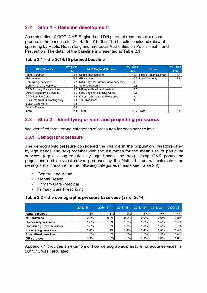
2.2 Step 1 – Baseline development A combination of CCG, NHS England and DH planned resource allocations produced the baseline for 2014/15 – £100bn. The baseline included relevant spending by Public Health England and Local Authorities on Public Health and Prevention. The detail of the baseline is presented at Table 2.1.

Table 2.1 – the 2014/15 planned baseline

CCG Service FY 14/15

£bn

NHS England Service FY 14/15

£bn

Other FY 14/15 £bn

Acute Services 35.5 Specialised services 13.9 Public Health England 0.4 MH services 6.7 GP services 6.8 Local Authority 2.8 Community services 6.7 NHS England Primary Care services 4.6 Continuing Care services 4.0 Secondary dental 0.8 CCG Primary Care services 9.3 Military & Health and Justice 0.5 Other Programme services 1.9 NHS England Running Costs 0.6 CCG Running Costs 1.3 Other Commitments Pressures 1.4 CCG Reserves & Contingency 0.4 s7a Allocations 1.6 Better Care Fund 1.1 Quality Premium 0.2 Total 67.1 Total 30.2 Total 3.2

2.3 Step 2 – Identifying drivers and projecting pressures We identified three broad categories of pressures for each service level:

2.3.1 Demographic pressure The demographic pressure considered the change in the population (disaggregated by age bands and sex) together with the estimates for the mean use of particular services (again disaggregated by age bands and sex). Using ONS population projections and age/cost curves produced by the Nuffield Trust we calculated the demographic pressure for the following categories (please see Table 2.2):

• General and Acute • Mental Health • Primary Care (Medical) • Primary Care Prescribing

Table 2.2 – the demographic pressure base case (as of 2014)

2015/ 16

2016/ 17

2017/ 18

2018/ 19

2019/ 20

2020/ 21

Acute services 1.3% 1.3% 1.5% 1.5% 1.5% 1.4% MH services 0.8% 0.9% 0.9% 0.9% 0.9% 0.8% Community services 1.3% 1.3% 1.5% 1.5% 1.5% 1.4% Continuing Care services 1.3% 1.3% 1.5% 1.5% 1.5% 1.4% Prescribing services 1.4% 1.4% 1.4% 1.4% 1.4% 1.4% Specialised services 1.3% 1.3% 1.5% 1.5% 1.5% 1.4% GP services 1.1% 1.0% 1.0% 1.1% 1.0% 1.0%

Appendix 1 provides an example of how demographic pressure for acute services in 2015/16 was calculated.

2.3.2 Non-demographic pressure

Non-demographic growth pressures include:

• Increasing expectation and demand for healthcare services, • Improving access to care, • Changes in healthcare technology, • Medical practice, • Changes in disease profile, etc.

To approximate the non-demographic pressures we used historic activity trends, and from these we removed the effect of demographic pressure in order to calculate a historic non-demographic trend (please see Table 2.3).

Table 2.3 – the unmitigated non-demographic pressure base case (as of 2014)

2015/ 16

2016/ 17

2017/ 18

2018/ 19

2019/ 20

2020/ 21

Acute services 1.0% 1.0% 1.0% 1.0% 1.0% 1.0% MH services 1.0% 1.0% 1.0% 1.0% 1.0% 1.0% Community services 2.2% 2.2% 2.2% 2.2% 2.2% 2.2% Continuing Care services 1.0% 1.0% 1.0% 1.0% 1.0% 1.0% Prescribing services 3.4% 3.4% 3.4% 3.4% 3.4% 3.4% Specialised services 3.0% 3.0% 2.8% 2.9% 2.9% 2.9% GP services 1.0% 1.0% 1.0% 1.0% 1.0% 1.0%

By way of illustration, appendix 1 explains the steps for calculating the non- demographic pressure for acute services in 2015/16.

Based on the demographic and non-demographic assumptions we calculated the total activity pressure (see table 2.4).

Table 2.4 – the unmitigated combined activity pressure base case (as of 2014)

2015/ 16

2016/ 17

2017/ 18

2018/ 19

2019/ 20

2020/ 21

Acute services 2.4% 2.4% 2.5% 2.5% 2.5% 2.4% MH services 1.8% 1.9% 1.9% 1.9% 1.9% 1.8% Community services 3.6% 3.6% 3.7% 3.7% 3.7% 3.6% Continuing Care services 2.4% 2.4% 2.5% 2.5% 2.5% 2.4% Prescribing services 4.9% 4.8% 4.8% 4.9% 4.9% 4.9% Specialised services 4.4% 4.4% 4.4% 4.4% 4.4% 4.4% GP services 2.1% 2.0% 2.0% 2.1% 2.1% 2.0%

2.3.3 Price pressure

We produced assumptions for the following price pressures:

a. Pay b. Drugs c. High cost drugs d. Non-pay non-drugs e. Devices f. Litigation

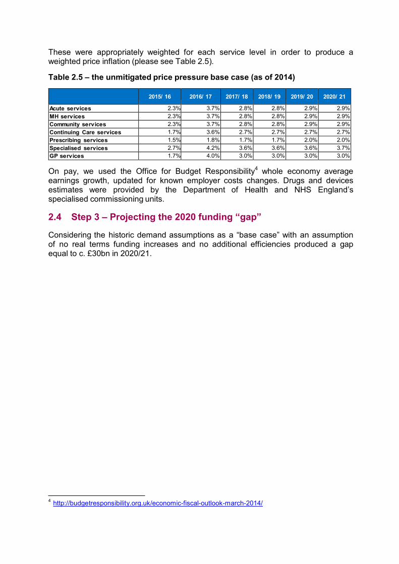
These were appropriately weighted for each service level in order to produce a weighted price inflation (please see Table 2.5).

Table 2.5 – the unmitigated price pressure base case (as of 2014)

2015/ 16

2016/ 17

2017/ 18

2018/ 19

2019/ 20

2020/ 21

Acute services 2.3% 3.7% 2.8% 2.8% 2.9% 2.9% MH services 2.3% 3.7% 2.8% 2.8% 2.9% 2.9% Community services 2.3% 3.7% 2.8% 2.8% 2.9% 2.9% Continuing Care services 1.7% 3.6% 2.7% 2.7% 2.7% 2.7% Prescribing services 1.5% 1.8% 1.7% 1.7% 2.0% 2.0% Specialised services 2.7% 4.2% 3.6% 3.6% 3.6% 3.7% GP services 1.7% 4.0% 3.0% 3.0% 3.0% 3.0%

On pay, we used the Office for Budget Responsibility4 whole economy average earnings growth, updated for known employer costs changes. Drugs and devices estimates were provided by the Department of Health and NHS England’s specialised commissioning units.

2.4 Step 3 – Projecting the 2020 funding “gap” Considering the historic demand assumptions as a “base case” with an assumption of no real terms funding increases and no additional efficiencies produced a gap equal to c. £30bn in 2020/21.

4 http://budgetresponsibility.org.uk/economic-fiscal-outlook-march-2014/

Chapter 3: How were the NHS funding requirements for 2020 estimated at £8 billion to £21 billion?

The NHS Five year Forward View projected that the NHS could need in the range of £8bn to £21bn real terms growth annually by 2020/21, depending on demand and efficiency assumptions. Specifically it described three potential funding scenarios: £8bn, £16bn and £21bn.

The original text is as follows:

“NHS Five Year Forward View, October 2014

It has previously been calculated by Monitor, separately by NHS England, and also by independent analysts, that a combination of a) growing demand, b) no further annual efficiencies, and c) flat real terms funding could, by 2020/21, produce a mismatch between resources and patient needs of nearly £30 billion a year.

So to sustain a comprehensive high-quality NHS, action will be needed on all three fronts. Less impact on any one of them will require compensating action on the other two.

Demand

On demand, this Forward View makes the case for a more activist prevention and public health agenda: greater support for patients, carers and community organisations; and new models of primary and out-of-hospital care. While the positive effects of these will take some years to show themselves in moderating the rising demands on hospitals, over the medium term the results could be substantial. Their net impact will however also partly depend on the availability of social care services over the next five years.

Efficiency

Over the long run, NHS efficiency gains have been estimated by the Office for Budget Responsibility at around 0.8% net annually. Given the pressures on the public finances and the opportunities in front of us, 0.8% a year will not be adequate, and in recent years the NHS has done more than twice as well as this.

A 1.5% net efficiency increase each year over the next Parliament should be obtainable if the NHS is able to accelerate some of its current efficiency programmes, recognising that some others that have contributed over the past five years will not be indefinitely repeatable. For example as the economy returns to growth, NHS pay will need to stay broadly in line with private sector wages in order to recruit and retain frontline staff.

Our ambition, however, would be for the NHS to achieve 2% net efficiency gains each year for the rest of the decade – possibly increasing to 3% over time. This would represent a strong performance – compared with the NHS' own past, compared with the wider UK economy, and with other countries' health systems. It would require investment in new care models and would be achieved by a combination of "catch up" (as less efficient providers matched the performance of the best), "frontier shift"(as new and better ways of working of the sort laid out in

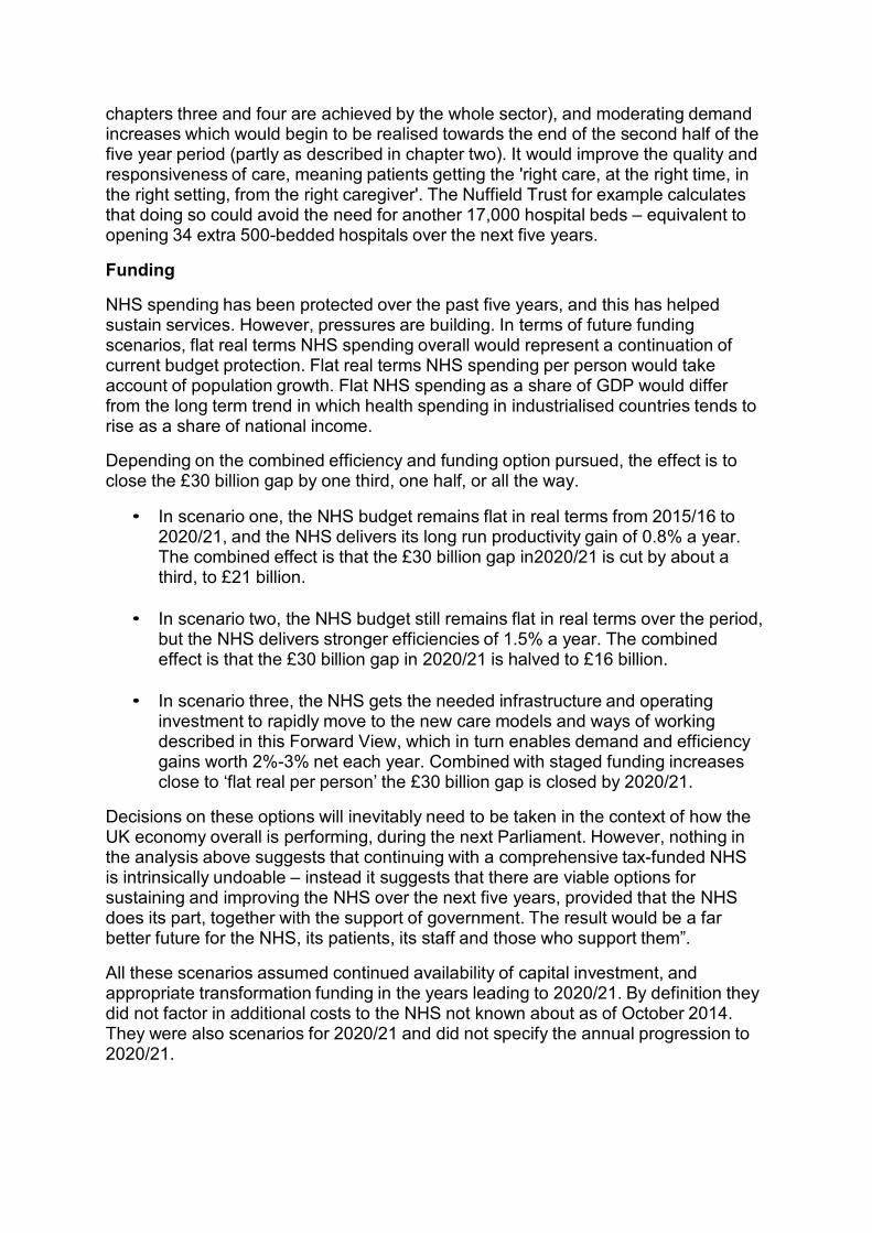
chapters three and four are achieved by the whole sector), and moderating demand increases which would begin to be realised towards the end of the second half of the five year period (partly as described in chapter two). It would improve the quality and responsiveness of care, meaning patients getting the 'right care, at the right time, in the right setting, from the right caregiver'. The Nuffield Trust for example calculates that doing so could avoid the need for another 17,000 hospital beds – equivalent to opening 34 extra 500-bedded hospitals over the next five years.

Funding

NHS spending has been protected over the past five years, and this has helped sustain services. However, pressures are building. In terms of future funding scenarios, flat real terms NHS spending overall would represent a continuation of current budget protection. Flat real terms NHS spending per person would take account of population growth. Flat NHS spending as a share of GDP would differ from the long term trend in which health spending in industrialised countries tends to rise as a share of national income.

Depending on the combined efficiency and funding option pursued, the effect is to close the £30 billion gap by one third, one half, or all the way.

• In scenario one, the NHS budget remains flat in real terms from 2015/16 to 2020/21, and the NHS delivers its long run productivity gain of 0.8% a year. The combined effect is that the £30 billion gap in2020/21 is cut by about a third, to £21 billion.

• In scenario two, the NHS budget still remains flat in real terms over the period,

but the NHS delivers stronger efficiencies of 1.5% a year. The combined effect is that the £30 billion gap in 2020/21 is halved to £16 billion.

• In scenario three, the NHS gets the needed infrastructure and operating

investment to rapidly move to the new care models and ways of working described in this Forward View, which in turn enables demand and efficiency gains worth 2%-3% net each year. Combined with staged funding increases close to ‘flat real per person’ the £30 billion gap is closed by 2020/21.

Decisions on these options will inevitably need to be taken in the context of how the UK economy overall is performing, during the next Parliament. However, nothing in the analysis above suggests that continuing with a comprehensive tax-funded NHS is intrinsically undoable – instead it suggests that there are viable options for sustaining and improving the NHS over the next five years, provided that the NHS does its part, together with the support of government. The result would be a far better future for the NHS, its patients, its staff and those who support them”.

All these scenarios assumed continued availability of capital investment, and appropriate transformation funding in the years leading to 2020/21. By definition they did not factor in additional costs to the NHS not known about as of October 2014. They were also scenarios for 2020/21 and did not specify the annual progression to 2020/21.

Chapter 4: What does the NHS Spending Review settlement imply for needed efficiencies (the so-called “£22 billion efficiency requirement”)?

The Government announced the NHS Spending Review (SR) settlement for the period 2016/17 to 2020/21 as follows:

Table 4.1

Revenue and capital combined 2015-16 2016-17 2017-18 2018-19 2019-20 2020-21 Total (£ million) 100,500 105,975 109,337 111,824 114,929 119,035 Real terms increase on previous year (%)

3.7%

1.3%

0.3%

0.7%

1.3%

Real terms increase on 2015-16 baseline (£ billion)

3.8

5.3

5.8

6.7

8.4

Note: These figures differ from the NHS TDEL figures announced at SR due to a number of technical adjustments, including transfers of functions. The main transfer of function is the move of 0-5 public health services from NHS England to local government. There are a small number of other transfers including the move of the Leadership Academy to Health Education England. To ensure comparability of numbers, in this table £500 million has been removed from the 2015-16 baseline, representing 6 months of funding for 0-5 public health services between 1 April and 30 September 2015 and these other planned transfers.

NHS England had set out five tests that the NHS would use to assess the outcome of the SR relative to the FYFV. In December 2015, NHS England’s Public Board assessment of the SR settlement was as follows5:

“First, our request for a ‘frontloaded’ settlement has been met. £3.8 billion of the overall £8.4bn real terms annual growth will be available to us next year, with an incremental £1.4bn real terms growth added the year after, 2017/18. So three fifths of the extra funding will be available in the first two fifths of the period stretching out to 2020/21.

Second, the need to phase any new ‘deliverables’ requested by Government in line with the ‘U’-shaped profile of our extra SR funding over the five years is on track. Today the Government will lay before Parliament its new Mandate to NHS England - and through us, to the NHS as a whole. This sets some specific requests for 2016/17 and a broader set of goals for 2020/21. We will discuss the Mandate at Item 5 of today’s public board meeting, and are reflecting its contents in the NHS Planning Guidance we will be issuing with our partners in the next few days.

Third, in addition to the available new funding, we argued that the efficiencies needed to provide the NHS with further ‘headroom’ to respond to likely demand could not all come from traditional provider tariff-style efficiency targets. Government, the NHS, and our partners would all need to support a broader range of actions to put the NHS on a sustainable footing. Subsequent to the SR (and indeed subsequent to the writing of the NAO’s report published this week) there is now an agreed cross-system efficiency profile, which will enable NHS England and NHS

5 https://www.england.nhs.uk/wp-content/uploads/2015/12/03.PB_.17.12.15-Chief-Executive- Report.pdf

Improvement to consult on a net tariff efficiency of 2%, as against 3.5%-3.8% this past year.

Fourth, the Forward View called for a radical upgrade in prevention, and support for wider public health measures. Given the funding pressures in the local authority financed public health services and the need for wider government action on obesity and related challenges, we cannot yet conclude that this test has been met. Much hinges on whether the Government’s proposed childhood obesity strategy comprises an effective package of credible actions when it is published in the New Year. Absent this, and other linked action, the NHS will be exposed to patient demand and consequent funding pressures over and above that modelled in the Five Year Forward View assumptions.

Fifth, the Forward View made the obvious point that the level of patient demand on the NHS is partly a function of the availability of social care, particularly for frail older people. The SR makes some welcome moves to hypothecate new funding streams for social care, but the overall funding quantum nationally and the distributional effects across England still imply a widening gap between growing need and available services. If unaddressed this would result in extra demand on GPs, community health services and hospitals over and above the FYFV NHS cost estimates. Our ‘fifth test’ should therefore be regarded as ‘unfinished business’.”

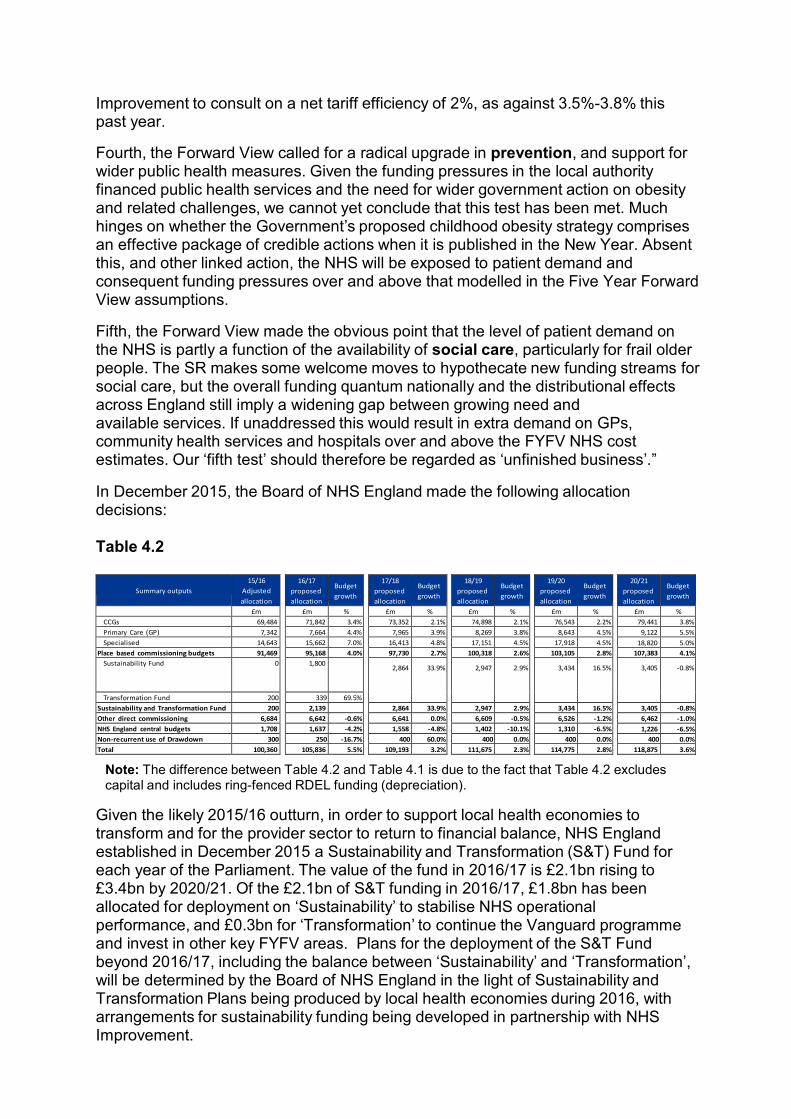
In December 2015, the Board of NHS England made the following allocation decisions:

Table 4.2

Summary outputs

15/16

Adjusted

allocation

16/17

proposed

allocation

Budget

growth

17/18

proposed

allocation

Budget

growth

18/19

proposed

allocation

Budget

growth

19/20

proposed

allocation

Budget

growth

20/21

proposed

allocation

Budget

growth

£m £m % £m % £m % £m % £m %

CCGs 69,484 71,842 3.4% 73,352 2.1% 74,898 2.1% 76,543 2.2% 79,441 3.8%

Primary Care (GP) 7,342 7,664 4.4% 7,965 3.9% 8,269 3.8% 8,643 4.5% 9,122 5.5%

Specialised 14,643 15,662 7.0% 16,413 4.8% 17,151 4.5% 17,918 4.5% 18,820 5.0%

Place based commissioning budgets 91,469 95,168 4.0% 97,730 2.7% 100,318 2.6% 103,105 2.8% 107,383 4.1%

Sustainability Fund 0 1,800 2,864 33.9% 2,947 2.9% 3,434 16.5% 3,405 -0.8%

Transformation Fund 200 339 69.5%

Sustainability and Transformation Fund 200 2,139 2,864 33.9% 2,947 2.9% 3,434 16.5% 3,405 -0.8%

Other direct commissioning 6,684 6,642 -0.6% 6,641 0.0% 6,609 -0.5% 6,526 -1.2% 6,462 -1.0%

NHS England central budgets 1,708 1,637 -4.2% 1,558 -4.8% 1,402 -10.1% 1,310 -6.5% 1,226 -6.5%

Non-recurrent use of Drawdown 300 250 -16.7% 400 60.0% 400 0.0% 400 0.0% 400 0.0%

Total 100,360 105,836 5.5% 109,193 3.2% 111,675 2.3% 114,775 2.8% 118,875 3.6%

Note: The difference between Table 4.2 and Table 4.1 is due to the fact that Table 4.2 excludes capital and includes ring-fenced RDEL funding (depreciation).

Given the likely 2015/16 outturn, in order to support local health economies to transform and for the provider sector to return to financial balance, NHS England established in December 2015 a Sustainability and Transformation (S&T) Fund for each year of the Parliament. The value of the fund in 2016/17 is £2.1bn rising to £3.4bn by 2020/21. Of the £2.1bn of S&T funding in 2016/17, £1.8bn has been allocated for deployment on ‘Sustainability’ to stabilise NHS operational performance, and £0.3bn for ‘Transformation’ to continue the Vanguard programme and invest in other key FYFV areas. Plans for the deployment of the S&T Fund beyond 2016/17, including the balance between ‘Sustainability’ and ‘Transformation’, will be determined by the Board of NHS England in the light of Sustainability and Transformation Plans being produced by local health economies during 2016, with arrangements for sustainability funding being developed in partnership with NHS Improvement.

£bn

The modelling underpinning the SR assumed that the aggregate recurrent provider deficit in 2015/16 would be £1.8bn. In light of the higher deficit now reported for 2015/16, it will be critical in 2016/17 to bring the provider sector back to the planned position through additional efficiencies in order to remain on track to close the funding gap.

4.1 Required level of efficiencies implied by the NHS Spending Review settlement

The majority of the efficiencies are delivered through interventions which, rather than releasing cash, reduce the level of underlying growth we would have expected to see should the intervention not have taken place. This creates an efficiency against the do-nothing/counterfactual growth rate.

However, there are also savings sources which do release cash, such as NHS England’s central programme and administration cost reductions. Changes which affect the amount of income received have equivalent effect.

The chart below shows how these savings are split between nationally delivered and locally delivered, along with an assessment of which have already been secured.

Chart 4.1 – Breakdown of the 2020 £22bn efficiency programme going into 2016/17

25

21.6 6.7

20

15

14.9 1.0 13.9 4.3

In 2016/17 plans

8.6

10

5

0 NHS Efficiencies Of which nationally delivered

To be delivered Of which already locally secured

To be secured Activity related - care redesign - demand offsets

Secondary care NHS provider productivity improvement 2%

1.0

Other commissioner

We should acknowledge that the objective of the 2016/17 operating planning round is to produce plans which contain the savings needed to deliver balance in both commissioning and provider sectors (net of the £1.8bn provider sustainability funding). Assuming successful delivery of the related 2016/17 efficiency requirements, the local efficiencies to be secured for future years reduces to £11bn.

£bn

Chart 4.2 – Expected breakdown of the 2020 £22bn efficiency programme remaining after 2016/17

25

21.6 6.7

20

15

10

14.9 3.7

11.3 4.1

6.3

5

0

NHS Efficiencies Of which nationally delivered

To be delivered

locally

Of which already

secured

To be secured Activity related

- care redesign - demand offsets

Secondary care NHS provider productivity

improvement 2%

0.9

Other

commissioner

4.2 Nationally delivered

We estimate that £6.7bn of efficiencies against the Forward View counterfactual cost growth could be nationally delivered. These include:

• Implementing the government’s 1% public sector pay cap to 2019/20 • Renegotiating the community pharmacy contract with the pharmacy sector,

and a variety of other nationally delivered cost efficiencies • Implementing income generating activities overseen by the Department of

Health as agreed in the SR • Reducing NHS England central budgets and admin costs

This leaves local health economies needing to find around £15bn in efficiencies.

4.3 Efficiencies to be secured by local health economies We already have line of sight to £1bn of efficiencies from Non-NHS provider contracts and CCG running cost reductions.

Per the SR modelling, this would leave £14bn of efficiencies to find over the period. We expect that these will be delivered through achieving the following:

• Activity – Moderating the level of activity growth through care redesign, and interventions such as RightCare and Self Care.

• NHS secondary care provider productivity – Achieving 2% productivity improvements each year across NHS secondary care providers, delivering £8.6bn in savings.

• Other efficiencies – including operational efficiency within other elements of CCG and non-secondary care commissioning.

Provider productivity opportunity

The aggregate underlying provider deficit for 2015/16 was c. £1bn higher than anticipated, creating an additional £1bn efficiency requirement. This higher deficit was in part a product of higher use of agency staff. Therefore as part of plans we are assuming that the NHS can achieve at least a £1.2bn net reduction in agency staff expenditure.

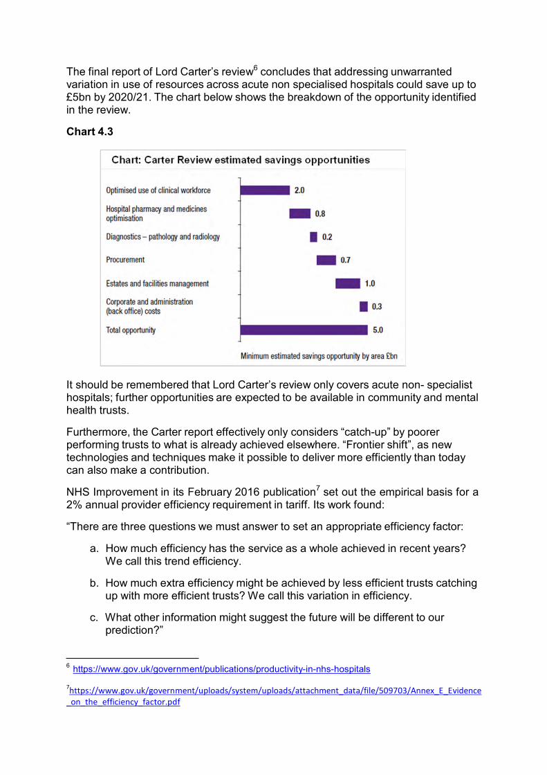
The final report of Lord Carter’s review6 concludes that addressing unwarranted variation in use of resources across acute non specialised hospitals could save up to £5bn by 2020/21. The chart below shows the breakdown of the opportunity identified in the review.

Chart 4.3 It should be remembered that Lord Carter’s review only covers acute non- specialist hospitals; further opportunities are expected to be available in community and mental health trusts.

Furthermore, the Carter report effectively only considers “catch-up” by poorer performing trusts to what is already achieved elsewhere. “Frontier shift”, as new technologies and techniques make it possible to deliver more efficiently than today can also make a contribution.

NHS Improvement in its February 2016 publication7 set out the empirical basis for a 2% annual provider efficiency requirement in tariff. Its work found:

“There are three questions we must answer to set an appropriate efficiency factor:

a. How much efficiency has the service as a whole achieved in recent years? We call this trend efficiency.

b. How much extra efficiency might be achieved by less efficient trusts catching up with more efficient trusts? We call this variation in efficiency.

c. What other information might suggest the future will be different to our prediction?”

6 https://www.gov.uk/government/publications/productivity-in-nhs-hospitals

7https://www.gov.uk/government/uploads/system/uploads/attachment_data/file/509703/Annex_E_Evidence

_on_the_efficiency_factor.pdf

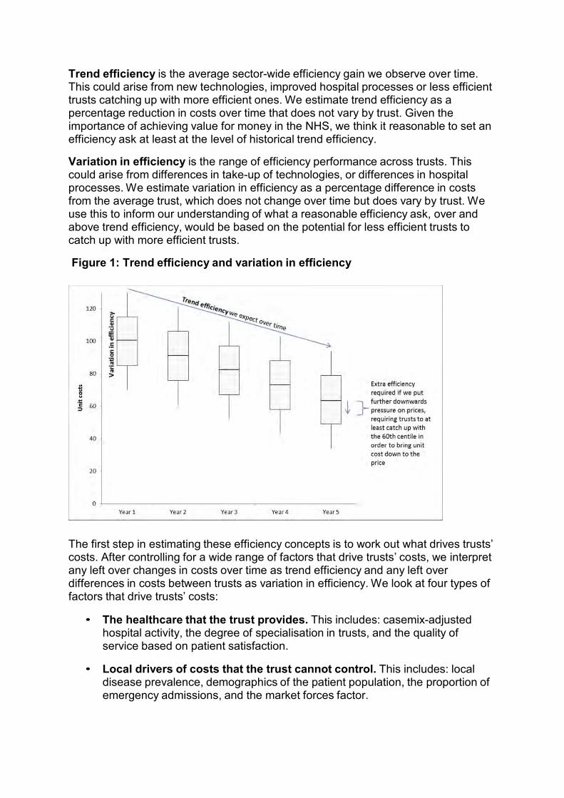
Trend efficiency is the average sector-wide efficiency gain we observe over time. This could arise from new technologies, improved hospital processes or less efficient trusts catching up with more efficient ones. We estimate trend efficiency as a percentage reduction in costs over time that does not vary by trust. Given the importance of achieving value for money in the NHS, we think it reasonable to set an efficiency ask at least at the level of historical trend efficiency.

Variation in efficiency is the range of efficiency performance across trusts. This could arise from differences in take-up of technologies, or differences in hospital processes. We estimate variation in efficiency as a percentage difference in costs from the average trust, which does not change over time but does vary by trust. We use this to inform our understanding of what a reasonable efficiency ask, over and above trend efficiency, would be based on the potential for less efficient trusts to catch up with more efficient trusts.

Figure 1: Trend efficiency and variation in efficiency

The first step in estimating these efficiency concepts is to work out what drives trusts’ costs. After controlling for a wide range of factors that drive trusts’ costs, we interpret any left over changes in costs over time as trend efficiency and any left over differences in costs between trusts as variation in efficiency. We look at four types of factors that drive trusts’ costs:

• The healthcare that the trust provides. This includes: casemix-adjusted hospital activity, the degree of specialisation in trusts, and the quality of service based on patient satisfaction.

• Local drivers of costs that the trust cannot control. This includes: local disease prevalence, demographics of the patient population, the proportion of emergency admissions, and the market forces factor.

• Trust type. This includes: the trust’s categorisation (small, teaching, specialist etc) and former Strategic Health Authority (SHA) region.

• Efficiency. This includes: trend efficiency and variation in efficiency.

We considered four additional pieces of evidence:

• Previous analysis undertaken for Monitor by Deloitte, which suggested one year savings of between 1% and 1.4% are possible if the average trust were to catch up to better-performing trusts.

• Analysis undertaken by the Centre for Health Economics at the University of York of trust-level productivity, which highlights the consistency in trust productivity rankings between 2010/11 and 2012/13.8 Consistent rankings suggest there is not much movement in the variation in efficiency between trusts.

• Health Foundation analysis of trust-level productivity,9 which shows very little

evidence of less productive trusts catching up with more productive trusts. This suggests that the differences in efficiency between trusts tend not to lead to rapid improvement in less efficient trusts.

• Analysis by Monitor, based on the Centre for Health Economics and Health Foundation methods, which supports the idea that there has not been very much narrowing in the distribution of trust efficiency.

The results of our analysis support a range for the efficiency factor of 1.5% to 2.5%, namely trend efficiency of 1.4% plus catch-up of up to 1.1%.

Given the scale of financial challenge that we face in 2016/17, and the current state of provider finances, we recommend that an efficiency factor in the region of 2% is appropriate.”

4.4 Summary Of the so-called “£22bn efficiency requirement”, around £7bn will be delivered nationally, leaving around £15bn to be secured from local efficiencies, of which only £8.6bn relates to provider tariff efficiencies. Furthermore, the majority of these efficiencies are not cost reductions per se but involve slowing the rate of spend and growth.

8 Aragon, Castelli, Gaughan (2015) Hospital Trusts Productivity in the English NHS: Uncovering Possible Drivers

of Productivity Variations Centre for Health Economics Research Paper 117

https://www.york.ac.uk/media/che/documents/papers/researchpapers/CHERP117_hospital_trusts_productivi ty_English_NHS.pdf 9

Lafond, Charlesworth, Roberts (2015) Hospital finances and productivity: in a critical condition? The Health Foundation http://www.health.org.uk/publication/hospital-finances-and-productivity-critical-condition

Appendix 1: Worked example – Calculating acute services base case pressures

Calculating demographic pressures for acute services

Cost Curve Population

5-year age sex bands General & Acute 2015 2016

m_0_4 59.19 1,766,800 1,772,400

m_5_9 39.29 1,697,500 1,725,100

m_10_14 42.70 1,517,800 1,547,900

m_15_19 41.16 1,636,700 1,608,000

m_20_24 38.67 1,834,200 1,816,400

m_25_29 37.26 1,902,100 1,938,900

m_30_34 38.57 1,854,200 1,867,200

m_35_39 44.70 1,723,200 1,761,600

m_40_44 53.71 1,787,600 1,734,100

m_45_49 66.16 1,910,300 1,900,600

m_50_54 81.78 1,876,000 1,900,600

m_55_59 108.58 1,613,000 1,658,500

m_60_64 143.83 1,417,500 1,428,400

m_65_69 190.22 1,461,200 1,466,700

m_70_74 250.48 1,080,300 1,136,000

m_75_79 321.68 830,900 829,100

m_80_84 394.49 576,200 591,300

m_85+ 501.40 463,400 487,600

f_0_4 47.94 1,682,100 1,687,600

f_5_9 33.14 1,619,400 1,644,300

f_10_14 36.71 1,446,400 1,474,000

f_15_19 47.32 1,551,800 1,529,000

f_20_24 49.42 1,763,400 1,739,800

f_25_29 53.51 1,865,400 1,883,700

f_30_34 58.63 1,862,100 1,864,000

f_35_39 68.06 1,727,900 1,768,700

f_40_44 77.98 1,819,900 1,760,800

f_45_49 88.78 1,957,500 1,949,800

f_50_54 104.02 1,919,400 1,949,800

f_55_59 118.85 1,649,700 1,697,900

f_60_64 141.27 1,474,000 1,483,800

f_65_69 177.24 1,547,000 1,554,600

f_70_74 221.62 1,185,100 1,241,300

f_75_79 281.95 973,600 969,600

f_80_84 346.32 758,400 766,300

f_85+ 433.86 861,400 884,400

5,666,082,563 5,742,114,470

Demographic pressure 1.3%

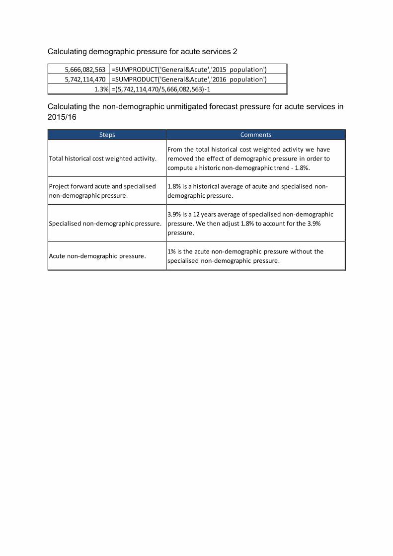
Calculating demographic pressure for acute services 2

5,666,082,563 =SUMPRODUCT('General&Acute','2015 population')

5,742,114,470 =SUMPRODUCT('General&Acute','2016 population')

1.3% =(5,742,114,470/5,666,082,563)-1 Calculating the non-demographic unmitigated forecast pressure for acute services in 2015/16

Steps Comments

Total historical cost weighted activity.

From the total historical cost weighted activity we have

removed the effect of demographic pressure in order to

compute a historic non-demographic trend - 1.8%.

Project forward acute and specialised

non-demographic pressure.

1.8% is a historical average of acute and specialised non-

demographic pressure.

Specialised non-demographic pressure.

3.9% is a 12 years average of specialised non-demographic

pressure. We then adjust 1.8% to account for the 3.9%

pressure.

Acute non-demographic pressure.

1% is the acute non-demographic pressure without the

specialised non-demographic pressure.

Appendix 2

2016/17 National Tariff Payment System: A consultation notice

Annex B5: Evidence on efficiency for the 2016/17 national tariff

.

.

2016/17 National Tariff Payment System: A consultation notice

Annex B5: Evidence on efficiency for the 2016/17 national tariff

11 February 2016

Monitor publication code: IRCP 05/16

Contents

1. Why we modelled efficiency .............................................................................................. 3

1.1. Rationale for setting an efficiency factor .................................................................................. 3 1.2. What we have done in recent years ......................................................................................... 3

2. What we did ...................................................................................................................... 4

2.1. Efficiency concepts................................................................................................................... 4 2.2. Our approach............................................................................................................................ 5

3. What we found .................................................................................................................. 6

3.1. Efficiency results....................................................................................................................... 6 3.2. Sensitivity checks ..................................................................................................................... 7

4. What it means ................................................................................................................... 7

4.1. Recommendation for the 2016/17 efficiency factor .................................................................. 7

Annex 1: Technical details .................................................................................................... 9 1. Background....................................................................................................................... 9

1.1. Purpose .................................................................................................................................... 9 1.1.1. Background to the efficiency factor ............................................................................... 9 1.1.2. Problems due to bad decisions on the efficiency factor ................................................ 9

1.2. What work has been done...................................................................................................... 10 1.2.1. Deloitte model .............................................................................................................. 10 1.2.2. Health Foundation model ............................................................................................ 11 1.2.3. Other NHS benchmarking analyses ............................................................................ 11

2. Method............................................................................................................................ 11

2.1. Econometric models ............................................................................................................... 11 2.1.1. Econometric benchmarking techniques....................................................................... 11 2.1.2. Panel data techniques ................................................................................................. 12 2.1.3. Efficiency concepts ...................................................................................................... 14

2.2. Models .................................................................................................................................... 15 2.2.1. Baseline models .......................................................................................................... 15 2.2.2. Sensitivity check models ............................................................................................. 16

2.3. Model interpretation................................................................................................................ 17 3. Data ................................................................................................................................ 17

3.1. Dataset description................................................................................................................. 17 3.2. Variables................................................................................................................................. 17

3.2.1. Total costs ................................................................................................................... 17 3.2.2. Hospital output ............................................................................................................. 18 3.2.3. Uncontrollable cost drivers .......................................................................................... 19 3.2.4. Trust type ..................................................................................................................... 21

4. Results............................................................................................................................ 22

4.1. Regression results.................................................................................................................. 22 4.2. Efficiency results..................................................................................................................... 25 4.3. Sensitivity checks ................................................................................................................... 25

5. Discussion and conclusions ............................................................................................ 28

5.1. Changes from last year .......................................................................................................... 28 5.2. Interpretation for 2016/17 efficiency factor ............................................................................. 28

1. Why we modelled efficiency

1.1. Rationale for setting an efficiency factor

1. The NHS is a highly valued service and significant element of public spending. It

accounts for around 7% of GDP.1 It is important that we maximise value for money within the NHS, to ensure the very best services for patients and that taxpayers’ money is well spent.

2. In other parts of the economy, we get value for money by shopping around between sellers competing for our business. We then select the product or service that gets us the most gain for the least cost. This puts pressure on firms to adopt the best production processes and most efficient technologies, and to pass reductions in costs on through lower prices. Those that don’t are driven out of business by those that do.

3. In the NHS prices aren’t set by this process between buyers and sellers, so this mechanism is not available. Instead we set many prices centrally, so we need to find a way of driving value for money. The efficiency factor that we apply to the prices we set is how we do this.

4. However, it is difficult to get the efficiency factor right, and there are problems if we get it wrong. If the efficiency factor is set too high, then prices are too low. This can mean that the business of providing healthcare can become unsustainable. If it is set too low, then prices are too high. This can mean that we fail to provide as much healthcare as possible for patients, wasting taxpayers’ money. To avoid these problems it is important to use the best evidence available to help us set the efficiency factor.

1.2. What we have done in recent years 5. There are three questions we must answer to set an appropriate efficiency

factor:

a. How much efficiency has the service as a whole achieved in recent years? We call this trend efficiency.

b. How much extra efficiency might be achieved by less efficient trusts catching

up with more efficient trusts? We call this variation in efficiency.

c. What other information might suggest the future will be different to our prediction?

1 OECD (2015) Focus on health spending available at http://www.oecd.org/health/health- systems/Focus-Health-Spending-2015.pdf

This report uses econometric analysis to provide evidence that addresses the first two questions.

6. As part of the evidence base for the 2015/16 national tariff, Deloitte produced analysis to inform Monitor’s judgement on the level of the efficiency factor. This comprised an econometric model and a supporting case study model.

7. The econometric model used data from 165 acute trusts between 2008/9 and 2012/13 to estimate the scope for efficiency in 2015/16.2 The case study model estimated the reduction in costs from a range of efficiency initiatives applied to a stylised ‘average’ trust. Deloitte concluded that the most efficient trusts could become 1.2% to 1.3% more efficient a year, but the averagely-efficient trust could do much better (up to an additional 5.6% if it caught up with the top decile performer).

8. Prior to the 2015/16 tariff, a number of third-party publications fed into the decision on the efficiency factor, alongside trusts’ Cost Improvement Plans (CIPs) and commissioners’ Quality, Innovation, Productivity and Prevention (QIPP) initiatives.3

2. What we did 2.1. Efficiency concepts

9. Before describing our analysis, we clarify our terminology around efficiency. We

estimate two measures of efficiency called trend efficiency and variation in efficiency, as shown in Figure 1.

10. Trend efficiency is the average sector-wide efficiency gain we observe over time. This could arise from new technologies, improved hospital processes or less efficient trusts catching up with more efficient ones. We estimate trend efficiency as a percentage reduction in costs over time that does not vary by trust. Given the importance of achieving value for money in the NHS, we think it reasonable to set an efficiency ask at least at the level of historical trend efficiency.

11. Variation in efficiency is the range of efficiency performance across trusts. This could arise from differences in take-up of technologies, or differences in hospital processes. We estimate variation in efficiency as a percentage

2 The decision to use data from acute trusts, rather than non-acute trusts or private providers, was

made on the basis of data availability and quality. 3 McKinsey (2009) Achieving a World Class Productivity in the NHS 2009/10 – 2013/14: Detailing the

Size of the Opportunity available at http://www.nhshistory.net/mckinsey%20report.pdf Monitor (2013) Closing the NHS funding gap: how to get better value healthcare for patients

https://www.gov.uk/government/uploads/system/uploads/attachment_data/file/284044/ClosingThe Gap091013.pdf

difference in costs from the average trust, which does not change over time but does vary by trust. We use this to inform our understanding of what a reasonable efficiency ask, over and above trend efficiency, would be based on the potential for less efficient trusts to catch up with more efficient trusts.

Figure 1: Trend efficiency and variation in efficiency

2.2. Our approach

12. The first step in estimating these efficiency concepts is to work out what drives

trusts’ costs. After controlling for a wide range of factors that drive trusts’ costs, we interpret any left over changes in costs over time as trend efficiency and any left over differences in costs between trusts as variation in efficiency. We look at four types of factors that drive trusts’ costs:

The healthcare that the trust provides. This includes: casemix-adjusted hospital activity, the degree of specialisation in trusts, and the quality of service based on patient satisfaction.

Local drivers of costs that the trust cannot control. This includes: local disease prevalence, demographics of the patient population, the proportion of emergency admissions, and the market forces factor.

Trust type. This includes: the trust’s categorisation (small, teaching, specialist etc) and former Strategic Health Authority (SHA) region.

Efficiency. This includes: trend efficiency and variation in efficiency.

13. Figure 2 shows how these factors are related to costs.

Figure 2: Model specification

14. We use statistical methods to unpick the impact of each factor on trusts’ costs.4

This gives us an estimate of the effect of each driver on costs.5 With the estimated impacts in hand, we remove their influence from trusts’ costs and interpret the service-wide reduction in costs over time as trend efficiency, and the long-term differences between trusts’ costs as variation in efficiency.

3. What we found 3.1. Efficiency results

Table 1: Efficiency estimates

Estimate Trend efficiency: 1.4% Variation in efficiency:

median to 60th centile 2.0% median to 70th centile 3.6% median to 80th centile 5.6% median to 90th centile 7.6%

Source: Monitor analysis

15. Our analysis tells us that trusts become 1.4% more efficient each year on average. Around this trend we estimate that there is substantial variation in

4 We adjusted trusts’ costs for inflation in healthcare prices, to ensure we measured them in real terms. We used the inflation cost uplift in the national tariff as our measure of inflation.

5 Our statistical results are in Table 4 on page 25.

efficiency. For example, in order for the average (median) provider to catch up to the 60th centile, it would need to become 2% more efficient on top of this 1.4% (see Table 1). In order for the average provider to catch up to the 90th

centile, it would need to become 7.6% more efficient on top of this 1.4%. 3.2. Sensitivity checks

16. We checked how robust our results were by undertaking a number of sensitivity

checks. Details can be found in section 4.3 below. Our results are robust to these checks.

4. What it means 4.1. Recommendation for the 2016/17 efficiency factor

17. Our estimate of trend efficiency tells us that it is reasonable for the efficiency

factor to be at least 1.4%. At an efficiency factor of 1.4%, the sector would need to continue to achieve efficiencies at the rate it has managed over the last six years in order to maintain its financial position.

18. What our estimates say about how much larger the efficiency factor could be requires careful interpretation, however. This is because it is clear that catch-up opportunities exist, but it is less clear that these opportunities can be realised within the one-year timeframe of the 2016/17 national tariff. So to reach a recommendation on this, we considered four additional pieces of evidence:

Previous analysis undertaken for Monitor by Deloitte, which suggested one year savings of between 1% and 1.4% are possible if the average trust were to catch up to better-performing trusts.

Analysis undertaken by the Centre for Health Economics at the University of York of trust-level productivity, which highlights the consistency in trust productivity rankings between 2010/11 and 2012/13.6 Consistent rankings suggest there is not much movement in the variation in efficiency between trusts.

Health Foundation analysis of trust-level productivity,7 which shows very little evidence of less productive trusts catching up with more productive trusts.

6 Aragon, Castelli, Gaughan (2015) Hospital Trusts Productivity in the English NHS: Uncovering

Possible Drivers of Productivity Variations Centre for Health Economics Research Paper 117 https://www.york.ac.uk/media/che/documents/papers/researchpapers/CHERP117_hospital_trusts_ productivity_English_NHS.pdf

7 Lafond, Charlesworth, Roberts (2015) Hospital finances and productivity: in a critical condition? The Health Foundation http://www.health.org.uk/publication/hospital-finances-and-productivity-critical- condition

This suggests that the differences in efficiency between trusts tend not to lead to rapid improvement in less efficient trusts.

Analysis by Monitor, based on the Centre for Health Economics and Health Foundation methods, which supports the idea that there has not been very much narrowing in the distribution of trust efficiency.

19. The results of our analysis support a range for the efficiency factor of 1.5% to 2.5%, namely trend efficiency of 1.4% plus catch-up of up to 1.1%.

20. Given the scale of financial challenge that we face in 2016/17, and the current

state of provider finances, we recommend that an efficiency factor in the region of 2% is appropriate. This is towards the top end of what has been achieved in recent years and implies the sector needs to increase its efficiency gains by almost 50% above long term trend.

Annex 1: Technical details

1. Background

1.1. Purpose

1.1.1. Background to the efficiency factor

The NHS is a publicly funded system. If it fails to provide healthcare at maximum value for money, that means either more taxpayer funding is needed or less healthcare is provided. It is therefore important to maximise efficiency.8

Price-setting is one of the ways that we promote efficiency. This allows us to align the incentives of providers to provide efficient care, and commissioners to commission the right care. The efficiency factor is our lever for promoting efficiency through the price level. It acts as both an incentive and a signal.

As an incentive it drives efficiency. In other markets we expect producers to pursue technological or process improvements that result in cost reductions so that they can lower prices, increase market share and extract profit. If producers do not keep up with the improvements of their competitors they lose market share and fail. This is less likely to occur in the NHS for two reasons. Firstly, NHS providers do not have the same profit-maximising incentives as other sectors. Secondly, even when costs are lowered, commissioners or patients cannot easily switch towards more efficient providers that pass on the benefits. This is for a number of reasons, including the need for providers to be located sufficiently close to their population and because a large number of services are priced nationally.

As a signal it informs decisions about resource allocation. For commissioners it directly affects the price, which is the cost to them of procuring a service. With these prices, commissioners can decide how best to allocate resources locally. More generally, the efficiency factor represents our judgement of the improvement in efficiency the NHS can and should make. This can be used to aid planning at both the national and local levels.

1.1.2. Problems due to bad decisions on the efficiency factor

Setting the efficiency factor at the right level is challenging. Problems can arise from too high or low a factor:

If it is set too high the business of providing healthcare can become increasingly unsustainable as prices are pushed further below costs. This

8 In economic terms, the efficiency we mean here is productive efficiency, sometimes known as technical efficiency.

could mean we risk incentivising inappropriate cuts to costs that reduce safety, quality or access. Additionally, the more prices diverge from costs the more misleading the signal to commissioners. For example: this could lead commissioners to regard acute care as a relatively cheap way to provide care compared with community-based prevention schemes, and potentially lower overall system efficiency. Furthermore it is possible that the incentive for providers to reduce costs is actually weakened if the efficiency factor is considered to be infeasible.

If it is set too low the commissioning of local services is needlessly restricted due to high prices, leading to less healthcare delivered to patients. The incentives for providers to realise potential efficiencies are blunted, and taxpayers’ money may be wasted.

To avoid setting the efficiency factor too high or too low, we look at a wide range of information when deciding what the level of the efficiency factor should be. To inform this complex regulatory judgement we have updated and amended the econometric evidence Deloitte produced for us last year. Similar to last year, we do not believe data quality is good enough outside of the acute sector to reliably estimate efficiency through econometric means. We therefore restrict our analysis to secondary care.

1.2. What work has been done 1.2.1. Deloitte model

For the 2015/16 national tariff decision on the efficiency factor Deloitte conducted analysis on the scope for efficiency in the NHS.9 This consisted of statistical analysis plus a case study.

The statistical analysis estimated the scope for efficiency in 2015/16 using trust-level data from 2008/09 to 2012/13. By controlling for differences in activity, casemix, quality and other local cost drivers, it estimated that the level of efficiency of the most efficient trust increased at a rate of 1.2% to 1.3% a year. Additionally, the analysis estimated that the 90th centile trust was 5% to 5.6% more efficient than the median trust, while the 60th centile trust was approximately 1% more efficient than the median.

The case study examined the effect that various efficiency levers could have

on the costs of a notional ‘average’ hospital. These levers included increasing the day case rate, shortening length of stay and reducing use of agency staff. It suggested that an average trust could increase its efficiency by between 1% and 1.4% within a year through the efficiency levers identified.

9 Deloitte (2014) Evidence for the 2015/16 national tariff efficiency factor https://www.gov.uk/government/consultations/nhs-national-tariff-payment-system-201516- engagement-documents

Our analysis builds on the Deloitte model. We use additional data for 2013/14 and make a small number of improvements to the method (explained further below).

1.2.2. Health Foundation model In their report “Hospital finances and productivity: in a critical condition?” the Health Foundation presented an analysis of efficiency based on the Deloitte work.10 Using a different set of factors driving cost to those used by Deloitte, the Health Foundation found that annual efficiency improvement averaged 0.4% between 2009/10 and 2013/14. Although this is substantially lower than the Deloitte estimate, the 95% confidence intervals of the two estimates overlap (that is, the intervals within which, with 95% confidence, we can say that the trust estimate lies).

As to catch-up efficiencies the Health Foundation’s analysis suggests there is very little change in the distribution of productivity over time.11

1.2.3. Other NHS benchmarking analyses

The Centre for Health Economics12 at the University of York and the Office of National Statistics (ONS) have both produced estimates of NHS productivity, based on the ratio of outputs to inputs. The CHE estimates suggest that productivity in the English NHS grew at 0.8% a year between 2004/05 and 2012/13.13 This masked substantial volatility, however, with growth ranging from -2.3% to +4.4%. The ONS estimates suggest that productivity growth for the NHS across the UK averaged 1% a year in the same period. The ONS productivity growth estimates are less volatile than those from CHE, ranging from -1.3% to +3.5%.14

2. Method

2.1. Econometric models

2.1.1. Econometric benchmarking techniques

Econometrics is the application of statistics methods to economic data. In our application, it allows us to compare trusts’ costs while controlling for a large number

10 Lafond, Charlesworth, Roberts (2015) Hospital finances and productivity: in a critical condition? The Health Foundation http://www.health.org.uk/publication/hospital-finances-and-productivity-critical- condition

11 Though productivity is a different concept to technical efficiency, the Health Foundation use real costs as the ‘input’ variable in their productivity index, so in this instance the two concepts are similar.

12 Bojke, Castelli, Grašič, Street (2015) Productivity of the English NHS: 2012/13 Update Centre for Health Economics Research Paper 110 https://www.york.ac.uk/media/che/documents/papers/researchpapers/CHERP110_NHS_productivi ty_update_2012-13.pdf

13 Monitor calculations based on published CHE productivity figures, using cost-weighted activity 14 ONS (2015) Public Service Productivity Estimates: Healthcare, 2012

http://www.ons.gov.uk/ons/dcp171766_393405.pdf

of cost drivers. Differences in costs that cannot be explained by these cost drivers using the econometric method are interpreted as efficiency.

Two econometric methods are typically used:

Corrected Ordinary Least Squares (COLS) Stochastic Frontier Analysis (SFA)

Corrected Ordinary Least Squares

In COLS, total cost is regressed on a cost function. It is assumed that the specification accurately captures the underlying cost process, and so the residuals can be interpreted as differences in efficiency. The firm with the smallest residual is said to be operating at the efficient frontier, and all other firms’ efficiency is measured relative to their distance from this frontier. For a standard cost function, the COLS regression is:

𝐶𝑖 = 𝛼 + 𝛽1𝑤𝑖 + 𝛽2𝑦𝑖 + 𝜀𝑖

𝜀𝑖 ~ (0, 𝜎2)

with cost 𝐶𝑖, input price 𝑤𝑖, output 𝑦𝑖, 𝜀𝑖 is interpreted as firm i’s efficiency. Stochastic Frontier Analysis As with COLS, SFA assumes that the process being modelled is a cost function. But SFA does not interpret the whole residual as efficiency. Instead SFA models efficiency as an additional statistical error with a specific probability distribution. Maximum Likelihood estimation is then used to estimate firm-level efficiency. Typically, the efficiency term is restricted to be strictly positive, for instance by using the half-normal or truncated-normal distribution, and is interpreted as a distance from the efficient frontier. For a standard cost function, the SFA model is:

𝐶𝑖 = 𝛼 + 𝛽1𝑤𝑖 + 𝛽2𝑦𝑖 + 𝑢𝑖 + 𝜀𝑖

𝜀𝑖 ~ (0, 𝜎2)

𝑢𝑖 ~ 𝑁+(0, 𝛾2)

with cost 𝐶𝑖, input price 𝑤𝑖, output 𝑦𝑖, and idiosyncratic error 𝜀𝑖, 𝑢𝑖 is interpreted as firm i’s efficiency.

2.1.2. Panel data techniques Because our data consists of repeated observations of trusts over time, the statistical inference drawn from comparing two observations is likely to depend on whether the two observations are from two trusts in the same year, from two years for the same trust, or from two different trusts in two different years. Techniques to isolate these effects are:

Fixed Effects (FE)

Random Effects (RE)

the Mundlak transformation Fixed Effects

Under FE, each trust is modelled as having its own intercept.

Typically this is estimated by subtracting the within-trust mean from the dependent and each independent variable and using Ordinary Least Squares (OLS) on the transformed variables, in order to remove the trust-specific effect. For our purposes, FE has the drawback of subsuming any time-invariant effects in the data into the fixed effects (the α𝑖 trust-level, time invariant effects) rendering them uninterpretable.

As we need to be able to compare trusts to benchmark them, this is an insurmountable obstacle. So FE is not appropriate for our purposes. Random Effects

In RE, each trust is modelled with an additional trust-specific error term. As with FE, this results in each trust having its own specific intercept. But instead of being ‘fixed’ to the sample of data, these intercepts are treated as ‘random’ draws from a normal distribution across the population.15

This RE model can be estimated by Generalised Least Squares (GLS). Unlike the FE model, the RE estimates retain information in the data that varies between trusts but not over time. RE estimates are therefore amenable to econometric

15 We note the difference between RE and SFA is the choice of distribution for the error term. Under

RE this is a normal distribution and therefore symmetric. Under SFA this is a truncated normal distribution and asymmetric. Thus the modelling difference between RE and SFA can be

considered an implicit belief about the underlying efficiency distribution: under SFA there is a long tail of increasingly inefficient trusts, whereas under RE the distribution of the most efficient trusts is mirrored in the distribution of the least efficient trusts.

benchmarking. However, RE estimates are biased if the error term u is not independent of the covariates x.

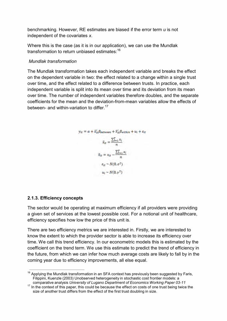
Where this is the case (as it is in our application), we can use the Mundlak transformation to return unbiased estimates:16

Mundlak transformation The Mundlak transformation takes each independent variable and breaks the effect on the dependent variable in two: the effect related to a change within a single trust over time, and the effect related to a difference between trusts. In practice, each independent variable is split into its mean over time and its deviation from its mean over time. The number of independent variables therefore doubles, and the separate coefficients for the mean and the deviation-from-mean variables allow the effects of between- and within-variation to differ.17

2.1.3. Efficiency concepts

The sector would be operating at maximum efficiency if all providers were providing a given set of services at the lowest possible cost. For a notional unit of healthcare, efficiency specifies how low the price of this unit is.

There are two efficiency metrics we are interested in. Firstly, we are interested to know the extent to which the provider sector is able to increase its efficiency over time. We call this trend efficiency. In our econometric models this is estimated by the coefficient on the trend term. We use this estimate to predict the trend of efficiency in the future, from which we can infer how much average costs are likely to fall by in the coming year due to efficiency improvements, all else equal.

16 Applying the Mundlak transformation in an SFA context has previously been suggested by Faris, Filippini, Kuenzle (2003) Unobserved heterogeneity in stochastic cost frontier models: a comparative analysis University of Lugano Department of Economics Working Paper 03-11

17 In the context of this paper, this could be because the effect on costs of one trust being twice the size of another trust differs from the effect of the first trust doubling in size.

Secondly, we are interested to know the extent of variation in efficiency across trusts in the sector. We call this variation in efficiency. Understanding this allows us to set an efficiency factor that is challenging for most trusts but still within the range of variation in efficiency that we see; put differently, this allows us to judge what is a stretching but achievable target.

These concepts of efficiency are related to frontier shift and catch-up efficiency, the terms that Deloitte used in their analysis last year. The efficiency frontier is the maximum possible efficiency a provider can attain. Frontier shift describes how this increases over time, as new technologies and processes make lower production costs possible. In practice, this efficient frontier and its change over time is inferred from those providers with the lowest unit costs. Catch-up efficiency describes the distance providers are from this frontier. Though this conceptual framework is appealing, we think the terms trend efficiency and variation in efficiency better describe what we are estimating:

Trend efficiency (the trend term in our estimation) incorporates the sector- level reduction in unit costs over time, not just the reduction in unit costs of the most-efficient trusts, or the conceptual frontier itself. This means that the trend term also includes historical catch-up efficiency gains.

Variation in efficiency (the trust-level efficiency effects in either the RE or SFA model) estimate the difference in unit costs on average across the whole time period. Some portion of these estimated opportunities for efficiency improvement may be eroded by trusts catching up within the time span. Without making much stronger assumptions in the model it is not possible to model this catch-up.

2.2. Models 2.2.1. Baseline models

Our baseline models are the RE and SFA specifications with the Mundlak transformation. The RE specification assumes that the efficiency effect follows a time-invariant normal distribution across trusts and is estimated by GLS with heteroscedastic-robust standard errors. The SFA specification assumes that the efficiency effect follows a time-invariant truncated normal distribution across trusts and is estimated by MLE. Both specifications use the same dependent and independent variables.

The dependent variable is the natural logarithm of costs deflated by the inflation cost uplift in each year. This is regressed on variables which we group into four categories:

The healthcare that the trust produces. This includes: the natural log of

casemix-adjusted hospital activity, the degree of specialisation in trusts and the quality of service based on patient satisfaction.

Local drivers of costs that the trust cannot control. This includes: local disease prevalence, demographics of the patient population, the proportion of emergency admissions and the market forces factor (MFF).

Trust type. This includes: the trust’s categorisation (small, teaching, specialist etc) and former SHA region.

Efficiency. This includes: trend efficiency and variation in efficiency.

These variables are described in Section 3 below.

2.2.2. Sensitivity check models We check the sensitivity of our results to changes in modelling assumptions. These checks can be grouped into sampling changes and variable changes.

We test the effect of sampling changes by running our analysis with specific subsamples excluded. The changes we make are:

1. to exclude specialist, multi-service and teaching hospitals 2. to exclude trusts that may have less accurate coding. When an activity code is

invalid, using as a proxy those trusts with a greater proportion of activity that is not recognised by grouping software and is therefore coded into the UZ01Z currency18

3. to restrict the sample to those trusts that we observe in every year. We test the effect of changes to the variables in our models in the following ways:

4. Including the number of sites the trust operates across

5. Including the number of acute sites the trust operates across

6. Including the proportion of inpatients from a lower super output area designated

as ‘urban’ by the ONS 7. Deflating costs by the MFF

8. Replacing the health-specific measure of inflation with the GDP deflator.

18 Note, this does not capture activity that is incorrectly coded but falsely recognised under a valid currency.

2.3. Model interpretation

The key estimates of interest in our modelling are of trend efficiency, and variation in efficiency.

Trend efficiency is simply the estimated coefficient on the time trend term. Because the dependent variable is in natural logarithms, this coefficient is the estimated average annual change in real costs measured in percentage terms.

Variation in efficiency is extracted from the efficiency effects themselves. The differences in the efficiency effects are differences in real unit costs between trusts in percentage terms. This ensures that our estimates of the two concepts of efficiency are presented in the same units, namely percentage deviation in real unit costs. We present the variation in efficiency estimates in terms of percentage difference in real costs between the median (50th centile) provider and the 60th, 70th, 80th and 90th

centile providers.

3. Data

3.1. Dataset description We use an unbalanced panel dataset covering 170 trusts across the time period 2008/09 to 2013/14.19 Although our panel of data is unbalanced (that is, has different numbers of trusts across time) entrants, exits and mergers should be related to the level of efficiency of a trust. If so, then excluding them from our sample (to balance it up) would give us a skewed perspective of efficiency in the whole system.20

3.2. Variables 3.2.1. Total costs

Total costs are taken from reference costs. We are modelling the efficiency of the acute sector, so we exclude costs for mental health and community services. We deflate costs by the national tariff’s inflation cost uplift.

19 We do not remove statistically influential observations. This is for three reasons: for dummy variables that relate to a small number of trusts, each trust is likely to exert a relatively large influence on the dummy coefficient; the Mundlak transformation increases the number of covariates substantially, and each additional covariate increases the chance of a type 1 error; those trusts that do exert a significant influence may be of particular interest to us in the stochastic frontier analysis, because their influence may be because they are close to the efficient frontier. For these reasons, we prefer to deal with issues of statistical influence by varying the sample in our sensitivity analyses.

20 We test this decision by re-running our regressions with a reduced balanced panel (that is, using only trusts reporting data for the full time period) as a sensitivity test.

3.2.2. Hospital output

Output is the healthcare that hospitals produce, for which they incur costs. We use a number of output variables to control for the effects of scale and scope in trusts’ production costs.

We measure activity using the reference cost dataset, with casemix adjustment by cost weight. Each currency’s cost weight is calculated each year as the currency’s national average cost relative to the national average cost across all currencies.21

We include an index for the quality of care that trusts produce to account for the additional costs this extra value may require. We extract the percentage of respondents that answered “strongly agree” (or “no” in the case of seeing errors or near misses in the last month) from the relevant questions in the NHS Staff Survey.22 We then use principal component analysis to extract an underlying index of service quality. The questions, and their correlation with the first principal component, are reported in Table 2.23

21 The only change we have made to this calculation is for the currencies that appear in both normal and excess bed days categories (both elective and non-elective). We regroup the costs and activity for these currencies, so that the costs reflect the full cost of the episode (inlier cost plus excess bed day cost) and the activity number reflects the numbers of episodes (number of inlier episodes, as every excess bed day requires a preceding inlier episode).

22 The NHS Staff Survey is an annual questionnaire completed by staff in NHS providers. 23 The first principal component captures 63% of the variation in the trusts’ responses to the identified

questions. This is slightly more than the corresponding principal component used in the Deloitte analysis previously (63% versus 61%).

Table 2: NHS Staff Survey questions and correlation with 1st principal component

Question: Correlation with the 1st

principal component Training keeps me up to date with professional standards 0.72 Effective communication between senior management and staff

0.87

Senior managers where I work are committed to patient care

0.92

I am satisfied about the quality of patient care I give 0.87 Care of patients is my trust’s top priority 0.93 I am able to deliver the patient care I aspire to 0.85 I cannot meet all the conflicting demands on my time at work

-0.51

I have adequate supplies, materials and equipment 0.87 There are enough staff at this trust for me to do my job properly

0.87

If a friend/relative needed treatment, I would be happy with the quality

0.79

Have you seen any errors, near misses or incidents that could have hurt a patient in the last month

0.23

Source: Monitor analysis

Costs may be affected by the degree of specialisation in a trust. To control for this, we construct a specialisation index based on the method employed by Deloitte in previous work for us. We aggregate casemix adjusted activity to the HRG chapter level for each trust. The index measures the divergence of any individual trust HRG activity profile from the national aggregate profile.

where 𝑝𝑖ℎ is the proportion of activity in chapter h for provider i and 𝜑ℎ is the national average activity in chapter h.

3.2.3. Uncontrollable cost drivers

In addition to the cost of healthcare that trusts provide, our modelling needs to account for cost drivers outside of their control. This is necessary to avoid attributing changes in the environment within which trusts operate to our estimate of trend efficiency, or differences between trusts in the nature of uncontrollable cost drivers to our estimates of variation in efficiency.

We control for the effect on costs of local demographics using Hospital Episode Statistics (HES) data. For the inpatient population we calculate the annual percentage who are:

o female

o under the age of 19

o over the age of 75

o from an ethnic minority background.

Our cut-offs for age categories align with the age split used in the national tariff. In addition to these variables, we calculate the average Index of Multiple Deprivation (IMD) overall score across all inpatients for each trust.24

We control for the health of the local area using the disease prevalence reported by GP surgeries through the Quality and Outcome Framework (QOF). We take the disease prevalence across 20 disease categories for each GP surgery and map these proportions to acute trusts based on the proportion of inpatients in each trust coming from each surgery. We then estimate the principal components of disease prevalence, and follow Deloitte in using the first two components in our subsequent regression analysis. Due to changes in the scope of QOF collection we are unable to use disease prevalence for four conditions: the depression 1 indicator, osteoporosis, peripheral arterial disease and cardiovascular disease. The diseases that we consider, and their correlation with the first two principal components, are reported in Table 3.25

We account for the effect of local market forces on costs using the underlying index of the MFF. This controls for unavoidable area-level variation in the cost of staff, land and buildings.

Table 3: Local disease prevalence and correlation with 1st and 2nd principal components

Disease Correlation with first principal Correlation with second component principal component

Coronary heart disease

0.93 -0.22

Stroke or Transient Ischaemic Attacks

0.94 -0.08

Hypertension 0.95 -0.01

24 We prefer the IMD overall score to the alternative health domain because it uses a broader range of data related to deprivation, whereas the health domain is constructed solely from health measures including Years of Potential Life Lost, mood and anxiety disorders, morbidity measures and illness and disability ratios, and we prefer to account for local health through the local disease prevalence.

25 The first principal component explains 67% of the variation in disease prevalence, the second principal component explains 8%. Together, they explain slightly more of the variation in disease

prevalence than the corresponding principal components used in the Deloitte analysis previously (75% versus 70%).

Disease Correlation with first principal Correlation with second component principal component

Diabetes 0.80 0.20 Chronic Obstructive Pulmonary Disease

0.84 -0.10

Epilepsy 0.93 -0.11 Hypothyroidism 0.84 0.17 Cancer 0.77 0.47 Mental health 0.38 0.19 Asthma 0.90 -0.07 Heart Failure 0.91 -0.19 Heart failure due to LVD

0.70 -0.49

Palliative Care 0.58 0.58 Dementia 0.83 0.35 Depression 0.47 -0.67 Chronic Kidney Disease

0.82 -0.07

Atrial Fibrillation 0.88 0.14 Obesity 0.79 -0.21 Learning Disabilities 0.82 0.15 Smoking 0.97 -0.01

Source: Monitor analysis

3.2.4. Trust type To ensure we are fully controlling for differences between trusts associated with the local area or other trust characteristics, we include a set of 1/0 indicator variables (dummies).

The region in which the trust is located is represented by a geographical dummy. Each dummy corresponds to a former SHA area. The regions are:

o East Midlands

o East

o London

o South West

o South East

o North West

o North East

o South

o South Central

o West Midlands

o Yorkshire and the Humber.

We use the trust type dummies as defined in the Estates Return Information Collection.26 Categories include:

o Small acute trust

o Medium acute trust

o Large acute trust

o Teaching acute trust

o Multi-speciality acute trust

o Specialist trust

4. Results

4.1. Regression results The results from the headline RE and SFA models are presented in Table 4 below. Because the models use the Mundlak transformation, we report the estimates based on the within-trust variation and between-trust variation separately, in columns side by side.

Our primary aim is to control for as many relevant factors as possible, to obtain the best possible (unbiased) estimates of ‘trend’ and ‘variation’ (see Section 3.3). This can make interpretation of the other coefficients in our model difficult, but we prefer to over-control for cost drivers and face multi-collinearity than under-control and suffer omitted variable bias. Nevertheless, we make the following observations:

1. Many of our estimated coefficients are similar to the estimates produced for us by Deloitte last year. The significant coefficients on the underlying MFF index, the percentage of inpatients who are female, the percentage of inpatients who are over 75 years old, the first principal component of the disease index, and the dummies relating to multiservice, teaching and specialist (SFA only) trusts for the between-trust variable versions are all close to last year’s coefficient estimates. A substantial number of the coefficients that are not statistically significant in our analysis were not significant last year either, with the exception

26 Available at http://hefs.hscic.gov.uk/ERIC.asp

of the percentage of inpatients from ethnic minorities and a number of the trust type dummies. Two variables that are significant in our analysis were insignificant last year: the percentage of emergency admissions and the quality index. However, when the between-trust and within-trust variables are combined (undoing the Mundlak transformation) these fall back to their previous level of insignificance.

2. The estimated coefficients on the effect of activity on cost (0.95 between trusts and 0.68 within trusts) suggest that the result last year (overall elasticity around 0.8) masked a difference between the within-trust elasticity and the between- trust elasticity. Essentially, this implies the economies of scale we can see across different trusts are much more modest than the economies of scale an individual trust can observe over time.

3. The results of the RE and SFA models are very similar, despite assuming different distributions for the efficiency term and using different estimation techniques (GLS and MLE respectively). The Deloitte analysis last year found the same similarity between the two models. Two possible explanations are:

a. The effect of the efficiency terms are small, so the specific distribution that we assume for them exerts little influence on the estimates of the coefficients.

b. The profile of efficiency across providers is symmetric, so SFA selects a truncation point on the extreme end of the normal distribution, and there is little difference between distributions used under SFA (truncated normal) and RE (normal).

4. There are many more statistically significant coefficients for the variables based on the between-trust variation than those based on the within-trust variation. Our model specification explains more of the variance related to differences in trust costs than changes within a trust’s costs over time.

5. The estimated coefficients in the within-trust columns are noticeably different from those in the between-trust columns. This supports our suspicion that the effect of a cost driver when we consider differences between trusts differs markedly from its effect when we consider changes for an individual trust over time. This is not surprising, as we have observations across many more trusts than time periods. Additionally, the Hausman test for the RE model supports our use of the Mundlak transformation.

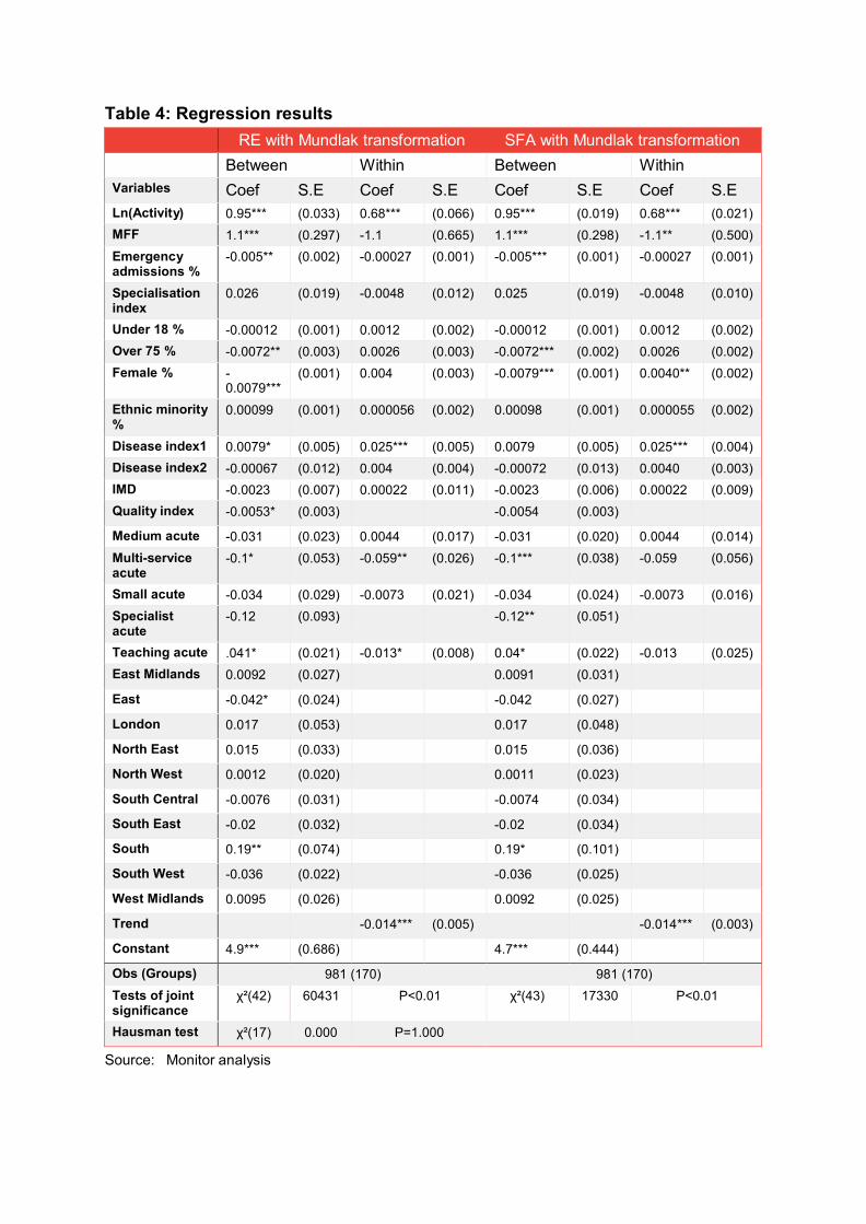
Table 4: Regression results

RE with Mundlak transformation SFA with Mundlak transformation Between Within Between Within

Variables Coef S.E Coef S.E Coef S.E Coef S.E Ln(Activity) 0.95*** (0.033) 0.68*** (0.066) 0.95*** (0.019) 0.68*** (0.021) MFF 1.1*** (0.297) -1.1 (0.665) 1.1*** (0.298) -1.1** (0.500) Emergency admissions %

-0.005** (0.002) -0.00027 (0.001) -0.005*** (0.001) -0.00027 (0.001)

Specialisation index

0.026 (0.019) -0.0048 (0.012) 0.025 (0.019) -0.0048 (0.010)

Under 18 % -0.00012 (0.001) 0.0012 (0.002) -0.00012 (0.001) 0.0012 (0.002) Over 75 % -0.0072** (0.003) 0.0026 (0.003) -0.0072*** (0.002) 0.0026 (0.002) Female % -

0.0079*** (0.001) 0.004 (0.003) -0.0079*** (0.001) 0.0040** (0.002)

Ethnic minority %

0.00099 (0.001) 0.000056 (0.002) 0.00098 (0.001) 0.000055 (0.002)

Disease index1 0.0079* (0.005) 0.025*** (0.005) 0.0079 (0.005) 0.025*** (0.004) Disease index2 -0.00067 (0.012) 0.004 (0.004) -0.00072 (0.013) 0.0040 (0.003) IMD -0.0023 (0.007) 0.00022 (0.011) -0.0023 (0.006) 0.00022 (0.009) Quality index -0.0053* (0.003) -0.0054 (0.003)

Medium acute -0.031 (0.023) 0.0044 (0.017) -0.031 (0.020) 0.0044 (0.014) Multi-service acute

-0.1* (0.053) -0.059** (0.026) -0.1*** (0.038) -0.059 (0.056)

Small acute -0.034 (0.029) -0.0073 (0.021) -0.034 (0.024) -0.0073 (0.016) Specialist acute

-0.12 (0.093) -0.12** (0.051)

Teaching acute .041* (0.021) -0.013* (0.008) 0.04* (0.022) -0.013 (0.025) East Midlands 0.0092 (0.027) 0.0091 (0.031)

East -0.042* (0.024) -0.042 (0.027)

London 0.017 (0.053) 0.017 (0.048)

North East 0.015 (0.033) 0.015 (0.036)

North West 0.0012 (0.020) 0.0011 (0.023)

South Central -0.0076 (0.031) -0.0074 (0.034)

South East -0.02 (0.032) -0.02 (0.034)

South 0.19** (0.074) 0.19* (0.101)

South West -0.036 (0.022) -0.036 (0.025)

West Midlands 0.0095 (0.026) 0.0092 (0.025)

Trend -0.014*** (0.005) -0.014*** (0.003)

Constant 4.9*** (0.686) 4.7*** (0.444)

Obs (Groups) 981 (170) 981 (170) Tests of joint significance

χ²(42) 60431 P<0.01 χ²(43) 17330 P<0.01

Hausman test χ²(17) 0.000 P=1.000

Source: Monitor analysis

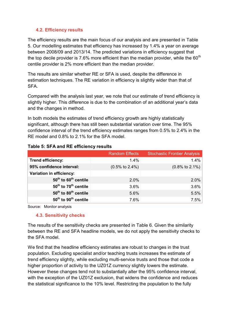
4.2. Efficiency results

The efficiency results are the main focus of our analysis and are presented in Table 5. Our modelling estimates that efficiency has increased by 1.4% a year on average between 2008/09 and 2013/14. The predicted variations in efficiency suggest that the top decile provider is 7.6% more efficient than the median provider, while the 60th

centile provider is 2% more efficient than the median provider. The results are similar whether RE or SFA is used, despite the difference in estimation techniques. The RE variation in efficiency is slightly wider than that of SFA.

Compared with the analysis last year, we note that our estimate of trend efficiency is slightly higher. This difference is due to the combination of an additional year’s data and the changes in method.

In both models the estimates of trend efficiency growth are highly statistically significant, although there has still been substantial variation over time. The 95% confidence interval of the trend efficiency estimates ranges from 0.5% to 2.4% in the RE model and 0.8% to 2.1% for the SFA model.

Table 5: SFA and RE efficiency results

Random Effects Stochastic Frontier Analysis Trend efficiency: 1.4% 1.4% 95% confidence interval: (0.5% to 2.4%) (0.8% to 2.1%) Variation in efficiency:

50th to 60th centile 2.0% 2.0% 50th to 70th centile 3.6% 3.6% 50th to 80th centile 5.6% 5.5% 50th to 90th centile 7.6% 7.5%

Source: Monitor analysis

4.3. Sensitivity checks The results of the sensitivity checks are presented in Table 6. Given the similarity between the RE and SFA headline models, we do not apply the sensitivity checks to the SFA model.

We find that the headline efficiency estimates are robust to changes in the trust population. Excluding specialist and/or teaching trusts increases the estimate of trend efficiency slightly, while excluding multi-service trusts and those that code a higher proportion of activity to the UZ01Z currency slightly lowers the estimate. However these changes tend not to substantially alter the 95% confidence interval, with the exception of the UZ01Z exclusion, that widens the confidence and reduces the statistical significance to the 10% level. Restricting the population to the fully

balanced panel does not alter the trend efficiency estimate, though it does narrow the estimate of variation in efficiency past the 80th centile.

The estimates of both trend efficiency and variation in efficiency are robust to the sensitivity checks on variables, other than those related to inflation. Although it is plausible that the number of sites and the proportion of inpatients from an urban area affect trusts costs, we do not identify any effect.

The largest change to our estimate of trend efficiency is made when we change the way we account for inflation. Replacing our health-specific measure of inflation with the GDP deflator pushes down our estimate to 0.4%, which we note is consistent with the analyses from both the Health Foundation and Deloitte (who also used the GDP deflator as a sensitivity check on their headline models). The choice of variable to control for inflation is important, because any increases in costs due to inflation do not subtract from the rate of efficiency growth. Our measure of health-specific inflation estimates that input prices were 17% higher by the end of a time period compared to the base year. The GDP deflator estimates that input prices were only 11% higher. The difference between these two estimates accounts for the difference in trend efficiency estimates. Our preference is to use the health-specific measure of inflation for two reasons:

1. The inflation trusts faced was higher than that of the economy in general, and represents an uncontrollable cost factor to trusts.

2. Trusts are compensated for inflation (through the inflation cost uplift), and this adjustment of the price level is distinct from the efficiency factor adjustment.

.

Table 6: Sensitivity analysis

1) Exc 2) Exc 3) Exc 4) 1&2&3 5) Exc 6) Exc 7) Inc 8) Inc 9) Inc 10) 11) specialist multi- teaching UZ01Z entrants number number urban % Deflate Deflating

service and of sites of acute by MFF by GDP exiters sites deflator

Trend efficiency: 1.6%*** 1.3%*** 1.7%*** 1.7%*** 1.1%* 1.4%*** 1.4%*** 1.4%*** 1.4%*** 1.4%*** 0.4%

95% CI: 0.6% to 2.5%

0.4% to 2.3%

0.7% to 2.8%

0.6% to 2.8%

-0.04% to 2.1%

0.5% to 2.4%

0.4% to 2.3%

0.5% to 2.4%

0.4% to 2.3%

0.4% to 2.3%

-0.5% to 1.3%

Variation in efficiency:

50th to 60th centile 1.4% 2% 1.5% 0.7% 1.6% 2% 1.8% 1.9% 1.8% 1.7% 2%

50th to 70th centile 2.2% 3.3% 3.7% 1.8% 3.4% 3.4% 3.5% 3.3% 3.3% 3.3% 3.7%

50th to 80th centile 4.3% 5% 5.6% 2.9% 5.3% 4.7% 6.1% 5.8% 5.6% 5.3% 5.6%

50th to 90th centile 5.8% 7.6% 7.1% 4.5% 7% 6.5% 7.8% 7.6% 7.5% 7.3% 7.6%

Observations 864 950 816 668 852 936 981 981 981 981 981

Groups 150 163 144 117 147 156 170 170 170 170 170

Coefficients

Within 0.0004 0.003 0.021

S.E (0.0003) (0.003) (0.016)

Between -0.001 -0.006 -0.005

S.E (0.001) (0.005) (0.005)

Source: Monitor analysis

27 .

5. Discussion and conclusions

5.1. Changes from last year We have estimated a model of trust costs and derived from this estimates of the efficiency trend and variation in English NHS acute trusts. This model is based on a model developed by Deloitte for use as evidence to inform the 2015/16 national tariff. We have updated Deloitte’s model from last year to include data from 2013/14, and made a number of refinements to the method.

We have made the following changes.

Added an extra year’s data (2013/14). This strengthens our confidence in our estimate of the efficiency improvement we see over time and ensures we are using the most up-to-date information (see 3.1).

Changed the age threshold to calculate the proportion of inpatients that are young from under 15 to under 19 years (see 3.2.3).

Included area-level effects (see 3.2.4).

Based our expectation of the profile of activity across chapters (for the specialisation index) on what we actually observe at the national level, rather than using a uniform distribution (see 3.2.2).

Adjusted inpatient cost to reflect the additional cost of excess bed days, but maintain the appropriate number of episodes (see footnote 21).

Reduced the number of diseases covered by the local disease indices due to those that are recorded across all time periods (see 3.2.3).

Moved from the health domain of the IMD to the overall score, in order to more precisely measure deprivation (see footnote 24).

Adapted our specification of the model with the Mundlak transformation to account for the difference across the between-trust and within-trust effects (see 2.1.2).

Retained the full set of observations available by not dispensing with trusts that influence our coefficient estimates (see footnote 19).

Overall, these changes have made relatively little difference to our estimates of efficiency.

5.2. Interpretation for 2016/17 efficiency factor Our interpretation of the evidence presented here could support an efficiency factor between 1.5% and 2.5% as discussed in 4.1. In terms of the historical trend

efficiency, this range spans the upper half of the confidence interval of our estimate. The extent of variation in efficiency suggests that there is sufficient scope for additional catch-up to support efficiency factors greater than trend efficiency. 6 May 2016