ninthlecture gauss - the prince of mathematics · ninthlecture gauss - the prince of mathematics1...
TRANSCRIPT

Ninth Lecture
Gauss - the Prince of Mathematics1
Gauss was born at Brunswick (Braunschweig) in 1777 the son of an uneducatedlaborer and his wife, who could hardly read. Early on he showed remarkableabilities in mathematics. It is said that even at the tender age of three he spottedhis father making a mistake when giving out the renumerations to his staff. Atten he astonished his teacher Buttner by immediately adding an arithmeticseries2. He then got to be tutored by an older student Barthels, who soonrealized he no longer had anything to contribute. His father had no interestin furthering the promising career of his son, but was persuaded to allow it tohappen as the duke of Braunschweig took a personal interest in the prodigy andgave him a stipend to study and in the process Gauss also got quite interested inclassical languages and philology, which he, to the alarm of his father, consideredpursuing, but one thing made him turn to mathematics to which we will returnbelow. He kept a diary with elliptic, not to say laconic, notes from then on fortwenty years. Mathematically he was extremly productive, ideas rushed into hishead with such force that he only had time to attend to a few, and even thosehe did not have time to develop properly and publish, thus he anticipated muchof 19th century mathematics such as the theory of elliptic functions, hyperbolicgeometry, least squares, fast Fourier transform.
Gauss was exceptionally productive and worked in a wide variety of fields,not only mathematics, but also doing empirical as well as theoretical work inAstronomy, Geodesy, Magnetism. It is tempting to compare him with Euler,with whom he shared many characteristics, such as a love and incredible abilityto perform numerical computations as well as an omnivorous taste in all kinds ofmathematics, as well as physics3. But while Euler published almost everythinghe wrote, Gauss did not, as noted above, have time for that, famous for his mottopauca sed matura (few but ripe), he wanted only to present the thoroughlythought out and polished. When it came to computations it is tempting toconclude that Euler did it by brute force like a idiot savant, Gauss could neverresist doing it in a clever way finding short-cuts. The difference is telling whenit came to celestial calculations, what took Euler three days and made him blindin the process, Gauss did in a matter of hours (saving his eye-sight).
As to his personal life, he had no affection for his father Gebhard, whosehonesty and comptence he respected but whose brutality he resented, and thuswas rather relieved than sorry when he died while Gauss was still in his earlythirties. His mother Dorthea (b. Benze) though, who was always very proud ofhim and his achievements, lived on in his home until her death at 97 in 1839.Gauss was married twice and widowed twice and the unions brought three plusthree children of whom five reached adulthood. With one son - Eugene - hequarreled, referred to him as a ’Taugenicht’ (good for nothing). The son earlyon emigrated to America, where he died at the age just short of 85 in 1896, and
1

showed some remarkable talents, including a prodigious memory and capacityfor calculating in his head, as well a mastery of many languages including Sioux4.Another son - Joseph - was of a more docile character and assisted his father insurvey work.
Gauss was not only a swift worker, but also a hard one, unbelievably diligent.Much of that activity taken up by what we now would consider mindless com-putations in celestial mechanics and surveys. However, in whatever activity hefound himself, he turned it to good use, literally transforming everything to goldthat he touched. He took a keen interest in designing telescopes (cf. Newtonwho made himself his own reflecting telescope) and actually made several veryuseful inventions such as the heliotrope very useful for surveying by reflectingsunlight visible as a bright star for many miles. Another, even more remarkableinvention was the first telegraph in 1833 together with his assistant Weber whoexploited the recent discovery of Ørsted as to the connection between electricityand magnetism.
Gauss was fond of literature and read in many languages apart from theClassical ones and his own Native German also in English, French and Danishand after teaching himself Russian in his sixties adding that language as well tohis reading repertoire. As a teacher he was very demanding and few studentsattended his lectures, which he delivered sitting by a table, covered with books,writing in his small and neat handwriting on a small black board put on a stand.He did not want his students to take notes as it impaired their attention. Hispenetrating gaze out of clear blue eyes was legendary and must have terrifiedall but the most intrepid of his students. Eisenstein was his favorite one, buthe died very early and was not to leave the mark he might have been destinedto. Dirichlet and Riemann, both who succeeded him at Gottingen, are his mostfamous ones5.
Gauss was by modern standards a bit short 5′1′′ but of stocky muscularbuild. Of a hypochondrial temperament his health was nevertheless very robust,allowing his demaning working schedule; only during the last year of his life,did his heart start to give up.
The regular 17-gon
As a student Gauss was quite enamoured by classical languages and contem-plated a career in philology, but just short of turning nineteen he discoveredthat the regular 17-gon could be constructed by ruler and compass, meaningthat the cosine for the angle 2π
17 could be obtained by a series of quadratic equa-tions (three in fact, leading to a formula involving nested square roots up tothree levels). So let us warm up with the regular pentagon the construction ofwhich was known already to the Greeks.
Using complex numbers we can express its five vertices as the solutions tothe equation z5 − 1. Those can be expressed by e
2πk5 for k = 0, . . . 4. It has the
obvious solution z = 1 corresponding to k = 0 and factorizing it out the four
2
remaining roots satisfy the equation
z4 + z3 + z2 + z + 1 = 0
Now set w = z+ 1z and note that 1
z = z and hence that w is twice the real part
of z or if z = e2πk5 then w = 2 cos 2πk
5 . This obviously holds for any regularpolygon, given by the solutions to zn − 1 = 0. Now divide the equation withz2 and get z2 + z + 1 + 1
z + 1z2 = 0, As w2 = z2 + 2 + 1
z2 we can rewrite this
as w2 + w − 1 = 0 which can be solves explicitly as w = −1±√5
2 . We note that
for z = e2πk5 k = ±1 cosine must be positive but for k = ±2 it has to be
negative. Hence 2 cos 2πk5 = −1+
√5
2 for k = ±1 while − 1+√5
2 for k = ±2. Thusthe pentagon can be constructed by ruler and compass. Note also that z can besolved by solving the quadratic equation z2−wz+1 = 0 which will of course havetwo conjugate complex roots, the real part given by the cosine and the imaginarypart by the sine of the appropriate angle, after all e
2πk5 = cos 2πk
5 +i sin 2πk5 . Note
also that if we double the angle we get a new solution. As cos 2θ = 2 cos2 θ − 1this translates into w 7→ w2−2 and indeed w+(w2−2) = (w2+w−1)−1 = −1and w(w2 − 2) = w(w2 + w − 1)− (w2 + w) = −1
Now set ω = e2πi17 . This is a 17th root of unity and all the others are given
by ωn for n = 0, 1 . . . 16. Throw away the trivial one n = 0 and the remainingsatisfy the equation
ω16 + · · ·+ 1 = 0
In modern language this is an equation with Galois group Z16 with a generatorT given by ζ 7→ ζ3 for ζ = ωn (n = 1, . . . , 16). In fact if we apply T and itspowers to ω we end up with
ω, ω3, ω9, ω10, ω13, ω5, ω15, ω11, ω16, ω14, ω8, ω7, ω4, ω12, ω2, ω6
Which we can summarize as
[1, 3, 9, 10, 13, 5, 15, 11, 16, 14, 8, 7, 4, 12, 2, 6]
note that the sum is −1Now split this ordered set into two by taking every other element
[1, 9, 13, 15, 16, 8, 4, 2] [3, 10, 5, 11, 14, 7, 12, 6]
Let z1 be the sum of the first eight and z2 the sum of the second eight. Notethat Tz1 = z2 thus z1 + z2 and z1z2 are left invariant by T and hence arein fact integers. Obviously z1 + z2 = −1 as to z1z2 we get a new sum of ωn
where 1 never appears. As there are 64 terms in the product, and every oneof the sixteen terms ωn (n 6= 0) occurs equally often we see that the sum ofthe terms will be −4. Why do the powers of ω appear equally often? Thisactually comes form an important meta-principle which lies at the heart of thewhole investigation, namely that of symmetry which provides the clue to alldiscussions of polynomial equations (and actually beyond). The piint is that
3
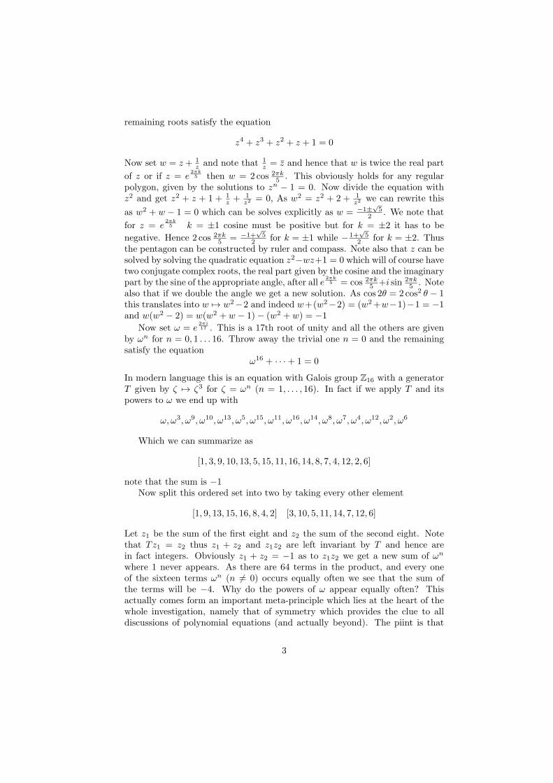
this sum is independent of the sixteen possible choices of ω (of course for therunning discussion be fix ideas by sticking to a particular value of ω namely theone given initially). Thus z1, z2 are the solutions to the quadratic equation
z2 + z − 4 = 0
with solutions −1±√17
2 . Which one is z1? Looking at the figure below where
the points of the first sum are dotted black, we see that z1 =√17−12 and z2 =
−√17+12 .
Now split up the first sum into two by taking everyother thus getting
[1, 13, 16, 4] [9, 15, 8, 2]
Let the first sum be w1 and the second w2. As w1+w2 = z1 and w1w2 consists of sixteen distinct termswe find that w1w2 = −1 hence they are solutions ofthe quadratic
z2 − z1z − 1 = 0
with solutions
w =z1 ±
√
1 +z21
4
2=
√17− 1±
√
34− 2√17
4
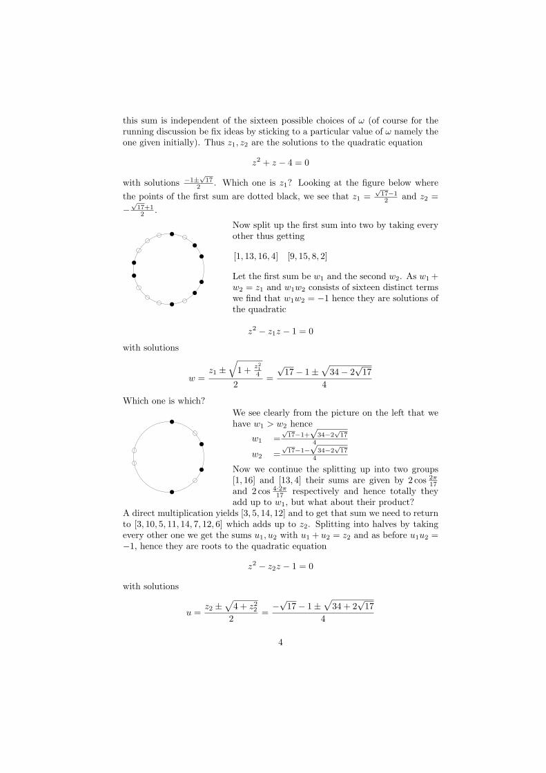
Which one is which?
We see clearly from the picture on the left that wehave w1 > w2 hence
w1 =√17−1+
√34−2
√17
4
w2 =√17−1−
√34−2
√17
4
Now we continue the splitting up into two groups[1, 16] and [13, 4] their sums are given by 2 cos 2π
17and 2 cos 4·2π
17 respectively and hence totally theyadd up to w1, but what about their product?
A direct multiplication yields [3, 5, 14, 12] and to get that sum we need to returnto [3, 10, 5, 11, 14, 7, 12, 6] which adds up to z2. Splitting into halves by takingevery other one we get the sums u1, u2 with u1 + u2 = z2 and as before u1u2 =−1, hence they are roots to the quadratic equation
z2 − z2z − 1 = 0
with solutions
u =z2 ±
√
4 + z222
=−√17− 1±
√
34 + 2√17
4
4
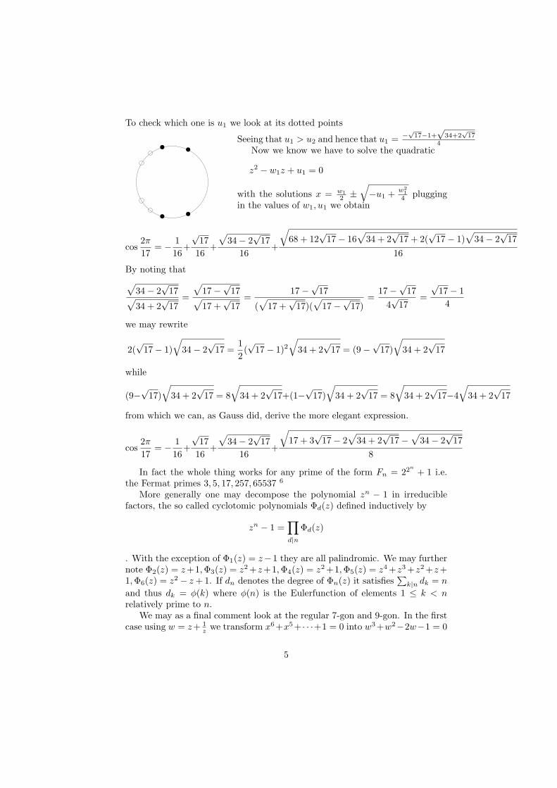
To check which one is u1 we look at its dotted points
Seeing that u1 > u2 and hence that u1 = −√17−1+
√34+2
√17
4Now we know we have to solve the quadratic
z2 − w1z + u1 = 0
with the solutions x = w1
2 ±√
−u1 + w21
4 pluggingin the values of w1, u1 we obtain
cos2π
17= − 1
16+
√17
16+
√
34− 2√17
16+
√
68 + 12√17− 16
√
34 + 2√17 + 2(
√17− 1)
√
34− 2√17
16
By noting that
√
34− 2√17
√
34 + 2√17
=
√
17−√17
√
17 +√17
=17−
√17
(√
17 +√17)(
√
17−√17)
=17−
√17
4√17
=
√17− 1
4
we may rewrite
2(√17− 1)
√
34− 2√17 =
1
2(√17− 1)2
√
34 + 2√17 = (9−
√17)
√
34 + 2√17
while
(9−√17)
√
34 + 2√17 = 8
√
34 + 2√17+(1−
√17)
√
34 + 2√17 = 8
√
34 + 2√17−4
√
34 + 2√17
from which we can, as Gauss did, derive the more elegant expression.
cos2π
17= − 1
16+
√17
16+
√
34− 2√17
16+
√
17 + 3√17− 2
√
34 + 2√17−
√
34− 2√17
8
In fact the whole thing works for any prime of the form Fn = 22n
+ 1 i.e.the Fermat primes 3, 5, 17, 257, 65537 6
More generally one may decompose the polynomial zn − 1 in irreduciblefactors, the so called cyclotomic polynomials Φd(z) defined inductively by
zn − 1 =∏
d|nΦd(z)
. With the exception of Φ1(z) = z−1 they are all palindromic. We may furthernote Φ2(z) = z+1,Φ3(z) = z2+z+1,Φ4(z) = z2+1,Φ5(z) = z4+z3+z2+z+1,Φ6(z) = z2 − z+1. If dn denotes the degree of Φn(z) it satisfies
∑
k|n dk = n
and thus dk = φ(k) where φ(n) is the Eulerfunction of elements 1 ≤ k < nrelatively prime to n.
We may as a final comment look at the regular 7-gon and 9-gon. In the firstcase using w = z+ 1
z we transform x6+x5+ · · ·+1 = 0 into w3+w2−2w−1 = 0
5
which is the third degree equation we need to solve in order to find cos 2π7 . In
the second case the cyclotomic polynomial Φ9(z). We can find it either by
dividing z9 + z8 + · · ·+ 1 by Φ3(z) = z2 + z + 1 or by setting ω = e2π9 (or any
other primitive 9-th root) and look at its six roots ω, ω2, ω4, ω5, ω7, ω8. Thoseare invariant by multiplication by the primitive third roots ω3, ω6 hence Φ6 isa polynomial in z3, in fact a quadratic such, which can be no other than Φ3
and thus Φ6 = z6 + z3 + 1. Proceeding as before we end up with the cubicw3 − 3w + 1 = 0.
Disquistiones Arithmeticae
The book was published in the summer of 1801 when Gauss was twenty-fourbut was written already three years earlier. It contains the results above andis a systematic compendium of elementary number theory and its ramificationsand as such it has provided the basics for number theory ever since. Moreprecisely it starts out with a pedestrian exposition of congruences, introducingstandard notation, including solving linear congruences by the method of con-tinued fractions, intimately related to the Euclidean algorithm, which goes backto Euler and Lagrange. Then there is a discussion of powers and two proofs ofFermat’s little theorem to the effect that ap−1 = 1 if a 6= 0(p) and the relatednotion of primitive elements, which also goes back to Euler. This is incidentallyrelated to periods of decimal expansions of rational numbers, which he also dis-cusses. Then there is a discussion of how to compute the Euler totient usingits restricted multiplicativity, familar to any student of an elementary text innumber theory. The presentation is leisurely and filled with worked out ex-amples, obviously Gauss loved to play around with these and he often prefersto illustrate a general method by a particular example than to formulating it.Things starts to pick up when second degree equations are considered. Crucialis the notion of quadratic reciprocity, which had been conjectured by Euler butfirst proved by Gauss in this work (other attempts had been made by Legen-dre). There are a lots of results of an elementary notion that are not usuallyencountered today. As an example the following theorem: If a is a prime of theform 8n + 1 there will be some prime number p less than 2
√a + 1 such that a
is a non-residue mod p.The bulk of the work is devoted to quadratic forms, especially binary. Given
a quadratic form ax2 + 2bxy + cy2 with integral coefficients what values canit take for integers x, y? He introduced an equivalence between them by usingsubstitutions effected by elements of SL(2,Z) (as well as elements of determinant−1). Such will not change the discriminant D = b2 − ac which hence is aninvariant, but it is not a complete invariant, many inequivalent forms may havethe same invariant, but he showed that there could only be a finite number ofclasses, out of which he singled out a special one x2−Dy2 as the principal (thusany square-free D can occur as a discriminant). Furthermore he introducedan abelian group structure on the classes associated to a given discriminantbefore such notions became explicit. He noted that there was a fundamental
6
difference between positive and negative discriminant, in the latter case therewere only a finite number of solutions to x2+Dy2 = m, while in the positive casex2−Dy2 = m there is an infinite number if there are any. Classical cases such asprimes which are the sum of two squares, or a sum of a square and twice a squareare simple special cases of his analysis, and can be described by congruences.In the case of Pell’s equation x2 −Dy2 = 1 he writes down the general solutiongiven a minimal non-trivial one (x1, y1) in terms of xn+.yn
√D = (x1+y1
√D)n.
An eight chapter had been projected, but it was not printed to keep down costs.A sequel was planned but never written, after all Gauss was severely distractedby other time consuming work. He did, however, later write on biquadraticreciprocity which necessitated a detour into what is now known as Gaussianintegers, namely integers of the form a+ bi where a, b are (rational) integers. Aring which has an Euclidean algorithm and hence is a so called principal idealdomain.
Digression on quadratic forms with negative discriminants
Although Gauss did not present his theory in geometric terms, it has beensuggested (by Felix Klein) that he nevertheless was familiar with it. But beforethis let us recall some basic facts about quadratic equations and quadratic fieldsover the rationals. A quadratic number θ is a number that satisfies an irreduciblequadratic polynomial with rational coefficients, i.e. satisfying an equation7
x2 − px+ q = 0
Given a root θ we can consider all elements of the form η = αθ + β. Theyare closed under addition and multiplication, and each element (except 0 ofcourse) has an inverse. They form a field denoted by Q(θ). This can be viewedas a vector space of dimension 2 over Q. Any element η in the field satisfiesa quadratic equation because the three elements 1, η, η2 cannot all be linearindependent. If we insist that the equation is monic (i.e. starting out withx2) the equation is unique x2 − Px + Q = 0 where P and Q depend on η.By the theory of quadratic equations, it will have two roots (which cannotcoincide because of the condition of irreducibility) and setting the other rootη′ we will have P = η + η′, Q = ηη′8. The coefficient P will be called thetrace of η denoted by Tr(η) and Q will be called the norm of η and be denotedby Nm(η). The trace is additive, and the norm is multiplicative, both areelementary symmetric functions of η, η′. Another symmetric function is thediscriminant D(η) = (η − η′)2, which measures the difference between the tworoots. Being symmetric it can be expressed in P,Q and indeed9
(η − η′)2 = (η + η′)2 − 4ηη′ = P 2 − 4Q
In terms of the discriminant we can write out explicitly the solution to a
quadratic equation x2 − Px + Q = 0 by x = P±√D
2 . By using the proper-ties of the trace and the norm we can compute them for any number η knowingit for θ. In fact
Tr(η) = Tr(αθ + β) = (αθ + β) + (αθ + β) = αTr(θ) + 2β
7

and
Nm(η) = Nm(αθ + β) = (αθ + β)(αθ + β) = α2Nm(θ) + αβTr(θ) + β2
and maybe more interesting
D(η) = Tr(η)2−4Nm(η) = (αTr(θ)+2β)2−4(α2Nm(θ)+αβTr(θ)+β2) = α2D(θ)
Thus elements in the quadratic field have the same discriminant up to asquare, and that is also sufficient to be in the same field, as the formula for theroots show. This is a crucial observation which tells you right away when twoquadratic elements belong to the same field (there is no immediate analogy forfields of higher degrees).
We also have the important notion of integral elements. Those are theones which satisfy a monic equation with integral coefficients. An equivalentformulation is that an element τ is integral iff the subspace that is generatedby integral combinations of 1, τ is closed also under multiplication, i.e. forminga ring. The integral elements of a quadratic form a ring, which is the biggestsubring of the field, with rank two over the integers. An arbitrary element η ofthe field satisfies an equation of form ax2 + bx+ c where (a, b, c) are relativelyprime integers. There is a unique such if we fix the sign of a . We have that a isthe smallest positive integer such that aη is integral. Note that the discriminantof an integral element is obviously an integer. Conversely one may show that ifthe discriminant is an integer, than the element is integral.
We will now restrict to the case of negative discriminant, then the field(from now on referred to as imaginary quadratic and denoted by K or Q(θ)when a generator θ is specified) can be embedded in C in such a way thatthere is a universal conjugation that restricts to the special conjugation for eachquadratic subgroup, namely complex conjugation. Thus we find that Tr(z) =z + z,Nm(z) = zz (making the linear and multiplicative character of the traceand norm respectively immediate). Furthermore we find that D(z) = (z − z)2.By the universality we have that the norm zz is a common quadratic formwhich will play a crucial role in what follows. We also note that any subring Rof the imaginary quadratic consisting of integral elements will form a discretesubgroup or rank two. Any additive subgroup of finite rank will be of rank oneor two, and if closed under multiplication of some ring with complex member,of rank two. Such additive subgroups of the field will be referred to as fractionalideals. (They are just modules of the ring contained in the field.) If they arecontained in the ring they will be ideals. The crucial thing is that fractionalideals may be multiplied and still be fractional ideals. This follows that theproduct is necessarily a subgroup of finite rank over the integers, and hence ofrank two. It follows that R plays the role of the identity in that multiplication.Furthermore to each fractional ideal I we may form the inverse, namely
I−1 = a ∈ K : ab ∈ R ∀b ∈ I
This is easily seen to be a fractional ideal, and more or less by definition wehave I · I−1 = R. So let us now look at the situation a bit more closely.
8

The basic concept is thus that of a lattice. A lattice Λ ⊂ C is a non-denserank-two additive subgroup of the complex numbers, hence it is generated bytwo complex numbers ω1, ω2 such that τ = ω1
ω2is non-real (and if necessary by
switching the ωs can be assumed to have positive imaginary part i.e.belongingto the upper half plane H). On C we have an inner product < ∗ · ∗ > given by< z ·w >= 1
2 (zw+wz) thus note that ‖z‖2 = |z|2 = zz. We are now interestedin lattices such that |ω1|2, < ω1 ·ω2 >, |ω2|2 are all integers (a, b, c)10, then moregenerally
|mω1 + nω2|2 = m2|ω1|2 + 2mn < ω1 · ω2 > +n2|ω2|2 = am2 + 2bmn+ cn2
defines an integral quadratic form. The parallelogram spanned by ω1, ω2 iscalled the fundamental parallelogram.
The fundamental parallelogram is not determined by the lattice, but dependson what basis is chosen. A basis change is affected by a matrix of type M =(
a bc d
)
with detM = ac−bd = ±1. Thus equivalent quadratic forms belong
to the same lattice. Gauss makes a point of distinguishing between forms whichare properly and improperly equivalent depending on whether the determinantis positive or negative, i.e. whether it preserves the orientation of the basisor not. Such transformations preserve the area of the parallelogram (up tosign) and this area can be interpreted as the square root of the discriminant ofthe quadratic form11. We may choose a normalized basis as follows: Pick anelement ω1 with smallest norm, and then ω2 with next to smallest. As −ω2
has the same norm we may choose it such that < ω · ω2 >≥ 0. Hence thatc ≥ b ≥ 0, 0 < a ≤ c, such forms are referred to as reduced. We may alsoclassify the shapes of lattices, saying that two lattices Λ,Λ′ are similar iff thereis λ such that λΛ = Λ′. The shapes are classified by τ = ω2/ω1 where by choice
9
of ordering we can make sure τ belongs to the upper half plane. And if we takeinto account the action of SL(2,Z) we get τ 7→ aτ+b
cτ+d . There is also anotherway we can associate an element of the upper half-plane to a definite quadraticform namely by letting (a, b, c) correspond to the equation az2 + 2bz + c = 0and pick the root τCM with positive imaginary part. This will be referred to asthe CM -point of the quadratic form. Now those turn out to be essentially thesame, in fact setting τ = ω2
ω1we obtain
τ + τ = 2< ω1 · ω2 >
|ω1|2and
τ τ =|ω2|2|ω1|2
hence τ satisfies the quadratic equation az2 − 2bz + c = 0 and hence τ =−τCM
12
Now given a lattice Λ we may consider the complex numbers z such thatzΛ ⊂ Λ. Trivial examples are z an integer, but can there be other complexnumbers? Obviously we are on the look out for lattices that can appear asfractional ideals for some order. The condition is that
zω1 = aω1 + bω2
zω2 = cω1 + dω2
Thus we see that z has to be an eigenvalue of a matrix M =
(
a bc d
)
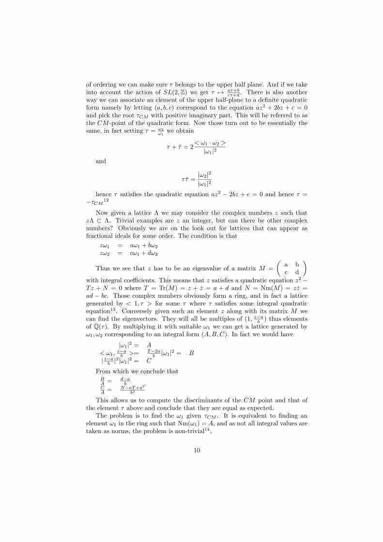
with integral coefficients. This means that z satisfies a quadratic equation z2 −Tz + N = 0 where T = Tr(M) = z + z = a + d and N = Nm(M) = zz =ad − bc. Those complex numbers obviously form a ring, and in fact a latticegenerated by < 1, τ > for some τ where τ satisfies some integral quadraticequation13. Conversely given such an element z along with its matrix M wecan find the eigenvectors. They will all be multiples of (1, z−a
b ) thus elementsof Q(τ). By multiplying it with suitable ω1 we can get a lattice generated byω1, ω2 corresponding to an integral form (A,B,C). In fact we would have
|ω1|2 = A< ω1,
z−ab >= T−2a
b |ω1|2 = B| z−a
b |2|ω1|2 = C
From which we conclude thatBA = d−a
bCA = N−aT+a2
b2
This allows us to compute the discriminants of the CM point and that ofthe element τ above and conclude that they are equal as expected.
The problem is to find the ω1 given τCM . It is equivalent to finding anelement ω1 in the ring such that Nm(ω1) = A, and as not all integral values aretaken as norms, the problem is non-trivial14.
10
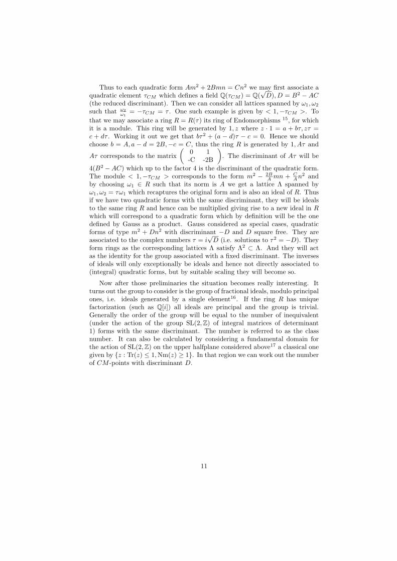
Thus to each quadratic form Am2 + 2Bmn = Cn2 we may first associate aquadratic element τCM which defines a field Q(τCM ) = Q(
√D), D = B2 − AC
(the reduced discriminant). Then we can consider all lattices spanned by ω1, ω2
such that ω2
ω1= −τCM = τ . One such example is given by < 1,−τCM >. To
that we may associate a ring R = R(τ) its ring of Endomorphisms 15, for whichit is a module. This ring will be generated by 1, z where z · 1 = a + bτ, zτ =c + dτ . Working it out we get that bτ2 + (a − d)τ − c = 0. Hence we shouldchoose b = A, a − d = 2B,−c = C, thus the ring R is generated by 1, Aτ and
Aτ corresponds to the matrix
(
0 1-C -2B
)
. The discriminant of Aτ will be
4(B2 −AC) which up to the factor 4 is the discriminant of the quadratic form.The module < 1,−τCM > corresponds to the form m2 − 2B
A mn + CAn
2 andby choosing ω1 ∈ R such that its norm is A we get a lattice Λ spanned byω1, ω2 = τω1 which recaptures the original form and is also an ideal of R. Thusif we have two quadratic forms with the same discriminant, they will be idealsto the same ring R and hence can be multiplied giving rise to a new ideal in Rwhich will correspond to a quadratic form which by definition will be the onedefined by Gauss as a product. Gauss considered as special cases, quadraticforms of type m2 + Dn2 with discriminant −D and D square free. They areassociated to the complex numbers τ = i
√D (i.e. solutions to τ2 = −D). They
form rings as the corresponding lattices Λ satisfy Λ2 ⊂ Λ. And they will actas the identity for the group associated with a fixed discriminant. The inversesof ideals will only exceptionally be ideals and hence not directly associated to(integral) quadratic forms, but by suitable scaling they will become so.
Now after those preliminaries the situation becomes really interesting. Itturns out the group to consider is the group of fractional ideals, modulo principalones, i.e. ideals generated by a single element16. If the ring R has uniquefactorization (such as Q[i]) all ideals are principal and the group is trivial.Generally the order of the group will be equal to the number of inequivalent(under the action of the group SL(2,Z) of integral matrices of determinant1) forms with the same discriminant. The number is referred to as the classnumber. It can also be calculated by considering a fundamental domain forthe action of SL(2,Z) on the upper halfplane considered above17 a classical onegiven by z : Tr(z) ≤ 1,Nm(z) ≥ 1. In that region we can work out the numberof CM -points with discriminant D.
11

The example of Q[√−5]
Above we present the lattice Q[√−5](R) with discriminant 5 (τCM =
√5i)
and area√5 of a fundamental parallelogram, as well as the sub-lattice the
principal ideal I = (1 +√5i)R) whose discriminant will be 6 · 5 = 30. The
corresponding quadratic form will be 6m2 + 30n2 which is not primitive, theprimitive form will correspond to the original lattice R. The quotient R/(1 +√5i) will be cyclic of order 6 and we can add the element 2 to I and get an ideal
J of discriminant −20, which is not principal18. A fundamental parallelogramwill be spanned by 2, 1 +
√5i and the corresponding quadratic form will be
4m2 + 4mn + 6n2 with discriminant −20. The ideal J 2 will be spanned by2, 2(1 +
√5i) and have discriminant −80.
The presentation above is of course not, as already remarked, found in Gausswork, but all the ideas exist there and were to provide inspiration for the alge-braic concepts related to rings and ideals that would be developed during the19th century, especially as it relates to algebraic number theory. Gauss cameup with estimates of class numbers and it was only in the late 60’s when theclassification of all negative discriminants with class number 1 was completed.The short list is given by
D = −1,−2,−3,−7,−11,−19,−43,−67,−163
12

The Fundamental theorem of Algebra
A modern proof of the fundamental theorem of algebra is very simple using theelements of elementary complex function theory. Given any polynomial P (z) itis easy to see that lim|z|7→∞ |P (z)| = ∞ by noting that the leading term will bedominating for large |z|. Thus in particular if P (z) never vanishes then 1/P (z)becomes a bounded entire function which by Liouville must be constant. Thattheorem comes more or less directly from the Cauchy integral formula. In fact wecan make a Fourier expansion of an analytic function f(reiθ) =
∑
n≥0 anrneinθ
and hence anrn = 1
2π
∫ 2π
0e−inθf(reiθ)dθ. If the function is bounded by M
we obtain the estimate |an| ≤ Mrn . this being true for all r implies that an =
0 ∀n > 0 and we are done.Gauss proved this theorem in his thesis (submitted to the University at
nearby Helmstedt) and would during his life produce a number of proofs, noneas slick as the one above, although complex analysis of some form is inevitable.Gauss was also a pioneer of the fundamentals of complex analysis anticipatingCauchy, but kept most of it to himself. In particular he was very clear about thegeometric representation of complex number (now usually referred to as Arganddiagrams) and showed great impatience at mathematicians who abhorred themas mysterious specious.
Celestial Mechanics and Ceres
In 1781 William Herschel discovered a new planet - later called Uranus - whichwas a sensation, as the number of planets had been assumed fixed. Uranuswas a transsaturnian planet. A few years later, in fact on January 1 1801, theItalian astronomer Piazzi discovered another one which was named Ceres, awelcome addition as there had been, according to the empirical law by Bodea gap between Mars and Jupiter but Ceres seemed to fill it19. Only a fewobservations were made before the planet disappeared behind the sun. Afterthat the planet was lost, but Gauss figured out a way of making the mostof the few observations to determine its path. In so doing the planet was thenrediscovered later according to Gauss’ predictions. This made Gauss famous andstarted his association with astronomy and celestial mechanics and in particularfunds were sought given to him for an observatory, which would be built inGottingen. One may speculate as to his motivations. True, Gauss loved tocalculate, as did Euler, but one suspects, as noted in the introduction, thatwhile Euler did it by brute force, Gauss went about it in a clever way not beingable to help himself. Celestial Mechanics had been worked out extensively byLaplace, but his investigations were theoretical in the sense of not being feasiblefor actual numerical work, thus Gauss had to approach the subject from scratchdeveloping a lot of tricks and methods he used with great ingenuity, as well asdeveloping the theory of least squares fundamental to observational work 20 andhitting on fast Fourier transform as a computational tool21 Celestial Mechanicsis not an exact science in the sense that in actual work you need to do a lot of
13
approximations and for that purpose avail yourself of a lot of tricks, thus moreof an art or handicraft than a conceptual science. Although he did have a deepinfluence on celestial work any actual presentation of it tends to be a bit ad hoc
and lack the beauty and simplicity that is the hallmark of pure mathematicsat its best. Thus the work on Ceres was just the beginning, later on he wouldstruggle with new asteroids as a steady stream of them were being discovered,especially Juno and Pallas. The latter even stymied him and in his Nachlaß thepenciled remark Lieber der Tod als ein solches Leben was later found22. It wasgenerally felt at the time that it was a waste of Gauss’ unique talents to havethem squandered on purely observational work and computations.
Easter Formula
As an elementary example of combining simple congruence counting with astron-omy, one can consider the date of Easter, for which Gauss provided a formula.To come up with it you do not need the genius of a Gauss, but anyway it canserve as a distraction23.
A crucial event of the year is the vernal equinox. It is the time when theecliptic (the plane of the orbit of the Earth) crosses the celestial equator (theplane of the equator, or equivalently the plane perpendicular to the axis of ro-tation). At the time night and day is equally long. The time difference betweentwo such events is 365.24 days (known as the tropical year the approximationof which is the basis of the Gregorian calendar, while the Julian makes do withthe cruder but simpler approximation 365.25 thus there being 1461 days in afour year cycle). Now the date of Easter Sunday was decided to be on the firstSunday after the first full Moon after the vernal Equinix. Thus Easter Sundaycan fall at any time between March 22 (The vernal equinox occuring on March21) and April 2524.
First we need to compare with the cycle of the phases of the Moon. TheSynodic period, i.e. the interval between two Full Moons is 29.53 days twelvetimes this is 354.36 which is somewhat short of a full year. However if we take 19years it will to high accuracy correspond to 235 Synodic periods, and everythingwill start over again25. Of course there is no exact relation, over extendedtimes there will be a drift, and besides the Synodic periods vary slightly dueto irregularities of the Moon’s orbit (see endnote below). Thus to assume it beexact means Easter will follow an artificial Moon but not the physical. However,by the time a discrepancy will occur, there will be a slight readjustment ormankind, or whatever has succeeded it, will not care about Easter.
14

0
1
2
3
4
5
6
7
8
9
10
11
12
13
14
15
16
17
18
The Synodic period will hence be divided into 19 parts each the length of1.55421 days of which there will be 7 in the discrepancy between twelve Synodicperiods and one year. Thus after the completion of one year there will be a 7/19th advancement of the phase cycle of the Moon and the Full Moon will hencehave occurred at position −7/19 or equivalently 12/19 in the phase period. Thusif the Full Moon occurred at position 0 one year later it will occur in position12/19 and so on. Thus in the figure above the subsequent occurrences of theFull Moon will be noted.
Assume now that at some reference year the Full Moon occurs on the dayof the Vernal equinox at a leap year. We can then compare the Synodic periodwith actual dates going from March 21 to April 19 plus half a day as below.
21 22 23 24 25 26 27 28 29 30 31 1 2 3 4 5 6 7 8 9 10 11 12 13 14 15 16 17 18 19 20
15
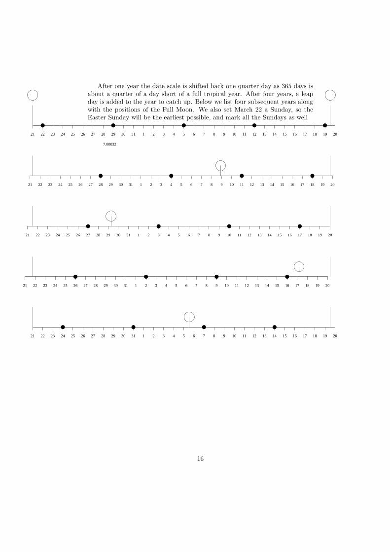
After one year the date scale is shifted back one quarter day as 365 days isabout a quarter of a day short of a full tropical year. After four years, a leapday is added to the year to catch up. Below we list four subsequent years alongwith the positions of the Full Moon. We also set March 22 a Sunday, so theEaster Sunday will be the earliest possible, and mark all the Sundays as well
7.00032
21 22 23 24 25 26 27 28 29 30 31 1 2 3 4 5 6 7 8 9 10 11 12 13 14 15 16 17 18 19 20
21 22 23 24 25 26 27 28 29 30 31 1 2 3 4 5 6 7 8 9 10 11 12 13 14 15 16 17 18 19 20
21 22 23 24 25 26 27 28 29 30 31 1 2 3 4 5 6 7 8 9 10 11 12 13 14 15 16 17 18 19 20
21 22 23 24 25 26 27 28 29 30 31 1 2 3 4 5 6 7 8 9 10 11 12 13 14 15 16 17 18 19 20
21 22 23 24 25 26 27 28 29 30 31 1 2 3 4 5 6 7 8 9 10 11 12 13 14 15 16 17 18 19 20
16
We can then read off the subsequent dates for Easter Sunday, namely April11, April 3, April 23, April 7. One may then continue this by hand (as itwas classically done) and work out subsequent dates. As we see there will be anumber of cycles, in addition of one of length nineteen there will be one of lengthseven giving the week days, which with the every four leap years combine into acycle of twenty-eight. Thus the whole thing will repeat itself in 19·28 = 532 yearswhen the Julian calendar is concerned. We note that there are only about 30possible dates for Easter Sunday, so every date occurs many times, in particularknowing the date for a certain Easter does not help us in determining the dateof the next, although one may of course restrict it to a certain narrower interval.Now what Gauss did was to write down a formula in terms of congruences fordetermining the date for any year. The solution will not be given but offered asa challenge to the reader. It is hard enough for the Julian case, the Gregoriancase adds a further non-trivial complication. Gauss provided formulas for both.The Julian Calendar is still uses in Eastern Orthodox churches. Finally the FullMoon at its height occurs on a certain time moment, and hence one also needsto fix the time zone in order to determine the day of the Full Moon. Whetherit appears late on a Saturday or early the next morning can make a differenceof seven days26.
Non-Euclidean Geometry
As we have seen there were many mathematicians such as Legendre, Lambertand Saccheri who tried to prove the Fifth postulate of Euclid by trying toget a contradiction. No real logical contradiction was achieved, however manyseemingly absurd results27. Now absurdity is not a priori a reason for rejection,and eventually people came to the understanding that it might be possible tocreate a logically consistent geometry by negating the postulate, which can bedone in two ways. Either, using the reformulation of Playfair, that there wereno parallel lines, or that through a point an infinite number of lines could bedrawn parallel, meaning non-intersecting, with a given. Janos Bolyai (1802-1860) was the son of a Hungarian student friend of Gauss and who himselfhad tried in vain to prove the axiom and gave as an advice to his son to stayaway from it. This proved only to be a further incentive and the son eventuallycame to the conclusion that it would be impossible and started to work out theconsequences of such an assumption accepting the apparent absurdities as theypresented themselves. He showed his results to his father, who relayed themto his friend. Gauss replied that he was unable to praise the work, becausedoing so would mean praising himself, as he had already worked it out in hisyouth, but been reluctant to publish it because of the outcry it no doubt wouldcause28. Bolyai was very discouraged by this and more or less dropped out ofmathematics, and the work he had carefully prepared between 1820 and 1823was eventually published as an appendix to a textbook by his father almost tenyears later, but by then Lobachevsky had already published his, but that wassomething Bolyai only would find out almost twenty years later much to his
17

chagrin. Thus to Lobachevsky (1792-56) belongs the honor of priority being outof Gauss’ circle he was not inhibited from going public. Lobachevsky called thisnew geometry, which unlike spherical geometry had no precedence, astral; andthought of it as having definite physical implications. Was that the geometryof the Cosmos? Recall that given a point P outside a line L we may considerthe limiting angle for lines L′ not intersecting L
P
O
L
L’
φ
The larger the distance OP the smaller the angle θ and the greater itsdeviance from π
2 . In Euclidean space a line will extend π in our field of vision(unless we are sighting it in the same direction in which case it will just be apoint) regardless of how far away we are. Not so in hyperbolic space, when it willextend 2θ the further away the smaller (which incidentally gives an intrinsic wayof measuring lengths). We can also think of it as the angular displacement indirection when we look at an object and move, known as parallax. In Euclideanspace objects infinitely far away will show no parallax, not so in Hyperbolicspace, where there will always be a parallax, even for objects infinitely far away.At the time no parallax had been obtained for any stars29 which meant thatphysical space, even if hyperbolic, would be very close to Euclidean space evenwhen astronomical distances were considered.
The most striking thing of hyperbolic space is that the circumference andarea of a a circle increases exponentially with the radius. In fact they are givenby 2π sinh r and π(cosh r − 1) respectively30. For large circles most of the areais concentrated close to the border, and if you want to go to one border pointto another along a geodesic, i.e. a line, you will get back close to the origin.
18

Surveying and Differential Geometry
Gauss was for a long time engaged to make a land survey of the principality ofHanover (in a royal union with Great Britain) to connect with a concomitanteffort by the Danes. This fostered an interest in the geometry of curved surfaces.But let us start from the beginning.
The notion of curvature of a curve is ancient, and can be seen as a change ofchange, and thus closely related to second derivatives. First in the 17th centurydid it get a more precise meaning. Just as a tangent line can be seen as the linethat best fits a curve, but also seen as a line that intersects the curve in twocoinciding points, we can ask the same thing about circles. What is the bestfitted circle, a so called osculating circle, or a circle that intersects the curve inthree points? Through three points there is a unique circle (except if they arecollinear, in which case it is a line, or a circle with an infinite radius). By lettingthe points come together we may hope for a limiting circle, whose radius willbe called the radius of curvature its inverse the curvature, and whose center thecenter of curvature.
PQ
R
C
If the points are P,Q,R the approximate center C of curvature may bethought of as the intersections of the midpoint normals of PQ and PR. Wemay also think of this as the infitesimal intersections of normals. Given a curveat each point P we can think of the line orthogonal to the tangent at P which isthe normal. Thus a curve gives rise to a family of normals. Given a normal NP
at P look at nearby normals at P ′ and their intersections with Np and the limitwhen P ′ → P . Thus to each curve we can associate its involute, the locus ofpoints given by the centers of curvature of the given curve. This was somethingstudied by 18th century mathematicians among them the Bernoullis. Note thatcircles by this definition have constant curvature 1
R where R is the radius of thecircle. The involute in this case degenerates to a single point, the center of thecircle.
Now consider a curve y = f(x) with horizontal tanget at the origin. It canlocally be given as y = ax2 + . . . where a = 1
2f′′(0). If we have a circle of
radius R tangent at the same point, say x2+(y−R)2 = R2 we can write locally
y = R −√R2 − x2 = x2
2R + . . . . By comparison we find the best fit if we choseR such that 1
2R = a i.e. R = 12a or the curvature 1
R = 2a. Thus if the change of
19

the change (the second derivative) is big, the radius of curvature is small, andhence the curvature is big.
P
P
Q
Q
R
R
S
S
We can also see the curvature by considering directly how much the directionof a tangent (or equivalently a normal changes) as we move along the curve. Theangular change dθ along a distance ds of the curve gives rise to a rate of changeof dθ
ds . In the case of a circle this change is constant, in fact if the radius is Runder a complete revolution we have travelled 2πR and undergone a change ofangle given by 2π hence the curvature is 1
R as expected. Note also that we canthink of curvatures with signs, depending on what side of the curve the centerslie on, or whether the change of angle is positive or negative
When it comes to a surface S in R3 we may consider the planes through thenormal at a point P . They give rise to planar sections, each with its curvature atP . Those curvatures will in general vary by the direction, and there will be twodirections of extremal curvatures (taking into account the signs). Those direc-tions are called the principal curvatures, and the directions are perpendicular.This was known to Euler.
20

Example: Consider the saddle-shaped surface S given by z = x2 − y2. Thenormal at the origin is given by the z−axis. The planes containing the normalhave equations ax+by = 0 and there intersections with S are given by parabolas
z = b2−a2
a2+b2 u2. The curvatures vary between 1
2 (a = 0) and − 12 (b = 0) this
gives two orthogonal directions. Note also that for a = ±b the curvatures arezero, as the parabola degenerates into z = 0.
More generally given z = ax2 + 2bxy + cy2 + . . . we may look at the planewith angle θ we then get z = (a cos2 θ+2b cos θ sin θ+c sin2 θ)u2+ . . . the termsax2 + cy2 can be rewritten as a+c
2 (x2 + y2) + a−c2 (x2 − y2) hence we can write
z = (a+c2 + a−c
2 cos 2θ+ b sin 2θ)u2 + . . . or z = (A+B cos(2θ+ θ0))u2 + . . . for
suitable A,B, θ0 namely A = a+c2 , B =
√
(a−c)2
4 + b2 and cos θ0 = a−cB . From
this we see that the max (A+B) and min (A−B) are taken when 2θ+θ0 = ±πhence at orthogonal angles. This was known by Euler.
Now it is customary to speak about the mean curvature as the sum of theprincipal curvatures (due to Sophie Germain), in the above case zero, and thetotal curvature, or the gaussian curvature, as their products, in this case −4.More generally note that the total curvature will be
4(A2 −B2) = 4(ac− b2)
which fits well. The right hand side is positive when the form is definite, andthen the surface lies on one side of the tangent plane, and negative when it isindefinite. When zero it degenerates to zero curvature. Thus we see that for aconvex body, the curvature of its boundary is non-negative.
It is one thing to make up a definition, quite another thing to hit upona fruitful definition, and this turns out to be that in this case. This has todo with Gauss’ crucial idea to think of an intrinsic geometry of the surface.To that concept belongs notions such as geodesics, locally the shortest pathbetween two points. Thus given a surface in three-space there are two kindsof curvatures, one merely accidental having to do how the surface happens tobe bent (extrinsic) and one intrinsic having to do with the surface itself. Anobserver constrained to the surface would have no idea of the former only of thelatter. A cylinder is curved but it can be folded out flat, using no stretching(nor any tearing except at a meridan along which it is cut ), with the geodesicsremaining geodesics, while a sphere cannot be flattend, if no stretching allowedthen it will invariable burst, and a saddle surface when flattened out will crumple(the opposite problem will appear when trying to wrap them both in paper).
21

Another definition of of the gaussian curvature is given by the Gauss map.Consider the unit normals to a small neighborhood U of a point P . They willmap U to an area U ′ on the unit sphere. The larger the quotient A(U ′)/A(U) isthe more the surface bends. The gaussian curvature at a point P is simply thelimit of this when U shrinks to P (note the analogy with the second definition ofthe curvature of a curve). The remarkable thing is not so much that those twodefinitions are equivalent, but that it is invariant under isometric imbeddingsof a surface (i.e. one which does not change distances). Thus there shouldbe an intrinsic definition of curvature, which does not depend on a particularembedding. One way is to look at how the circumferences and areas of circlesdepend on their radii. On a sphere of radius 1 a circle of radius r will be the sameas a Euclidean circle of radius sin r i.e. 2π sin r, while its area (by Archimedes)
will be given by 2π(1 − cos r). For small r we can write 2π(r − r3
6 + . . . ) and
π(r2 − r4
12 + . . . ) From this we are motivated to make the definition
K = 12 limr→0
A0(r)−A(r)
A0(r)
where A0(r) = πr2 is the area of the Euclidean circle of radius r and A(r) thecircle on the surface.
22

Given the surface parametrically (x(u, v), y(u, v), z(u, v)) form and a curveγ(t) = (u(t), v(t)) on it. This forms a space curve given by
Γ(t) = (x(u(t), v(t)), y(u(t), v(t)), z(u(t), v(t)))
to compute its length we need to integrate |Γ′(t)| which will be given by thechain rule as
√
(∂x
∂uu′(t) +
∂x
∂vv′(t))2 + (
∂y
∂uu′(t) +
∂y
∂vv′(t))2 + (
∂z
∂uu′(t) +
∂z
∂vv′(t))2
This motivates us to make the following definition by setting
a = ∂x∂u a′ = ∂x
∂v
b = ∂y∂u b′ = ∂y
∂v
c = ∂z∂u c′ = ∂z
∂v
And then form
E(u, v) = a2 + b2 + c2, F (u, v) = aa′ + bb′ + cc′, G(u, v) = a′2+ b′
2+ c′
2
to which we can associate the innerproduct
E(u, v)dudu′ + F (u, v)(dudv′ + du′dv) +G(u, v)dvdv′
This depends only on the ’interior’ coordinates of the surface, and its lengthcan thus be given by integrating |γ′(t)| but now with respect to the above innerproduct on the surface.
Example: If we consider spherical coordinates, i.e. x = cosu cos v, y =sinu cos v, z = sin v we get the form E = cos2 v, F = 0, G = 1 which illustratesthe fact that the length of a latitudinal circle at v will be scaled by cos v.
23

Digression on Gauss-Bonnet
Gauss noted that for a geodesic triangle ∆ with angles α, β, γ we have
∫∫
∆
K = α+ β + γ − π
which is a generalization of the fact that on a unit sphere, the area of a sphericaltriangle is equal to its angular excess (by noting that areas scale as R2 andcirvature as R−2 this will hold for any sphere).
Now the angular excess is additive, which is easy to see thus there will be afunction K ′ such that
∫∫
∆
K ′ = α+ β + γ − π
and it will simply be the limit of angular excess divided by area. If we can provethat this is equal to gaussian curvature we are done. It is true for spheres andthe hyperbolic plane, and we would be done if we can well approximate surfaceswith those locally.
Now given this we may make a formal calculation. Given a surface X wecan triangulate it into geodesic triangles, and if n0, n1, n2 denotes the number ofvertices, edges and triangles respectively the euler characteristics e(X) is givenby
e(X) = n0 − n1 + n2
Now add all the integrals∫∫
∆K and we get on the lefthand side
∫∫
XK while on
the right hand side we get∑
α α− πn2. The sum of all angles we can rearrangeas to collect them vertice by vertice and than the right hand side becomes2πn0−πn2. Now given n2 triangles the number of edges will become 3
2n2 (eachtriangle give rise to three edges, but then every edge will be counted twice),thus e(X) = n0 − 1
2n2 putting everything together we get Gauss-Bonnet
∫∫
X
K = 2πe(X)
.
24
αβγ
γβ
γβ
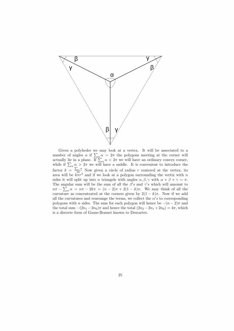
Given a polyheder we may look at a vertex. It will be associated to anumber of angles α if
∑
α α = 2π the polygons meeting at the corner willactually lie in a plane. If
∑
α α < 2π we will have an ordinary convex corner,while if
∑
α α > 2π we will have a saddle. It is convenient to introduce the
factor k =∑
α α
2π Now given a circle of radius r centered at the vertex, itsarea will be kπr2 and if we look at a polygon surrounding the vertix with nsides it will split up into n triangels with angles α, β, γ with α + β + γ = π.The angular sum will be the sum of all the β′s and γ′s which will amount tonπ − ∑
α α = nπ − 2kπ = (n − 2)π + 2(1 − k)π. We may think of all thecurvature as concentrated at the corners given by 2(1 − k)π. Now if we addall the curvatures and rearrange the terms, we collect the α′s to correspondingpolygons with n sides. The sum for each polygon will hence be −(n− 2)π andthe total sum −(2n1−2n0)π and hence the total (2n2−2n1+2n0) = 4π, whichis a discrete form of Gauss-Bonnet known to Descartes.
25

We may now relate excess angular sum with the Gauss curvature definedby the Gauss map. Consider the unit normals ni to the faces fi meeting at afixed vertex. They will correspond to points pi on the unit sphere, which can beseen as the dual of the configurations of the faces meeting at the vertix. Twoadjacent points pi, pj are joined by a gedosic arc cij (meaning part of a greatcircle), the length of that arc corresponds to the angle the faces fi, fj meetalong their edge eij , which incidentally is the angle at which the normals ni, njmeet. One may think of all the vectors v perpendicular to eij between ni, nj asnormals along the edge. In this way we get a polygon on the unit sphere whichwill enclose a region P , corresponding so to speak to all the ’normals’ at thevertex. In order to compute the area of P we need to compute all the anglesformed by two adjacent arcs cij , cjk. Now the edge eij is perpendicular to bothni and nj , thus we see that the sought after angle is related to the angle αj
between eij and ejk (which is the angle of the face fj at the vertex) or moreprecisely to their normals (in the plane spanned by the two edges) thus it willbe given by π − αj . Adding everything up and computing the excess it willturn out to be exactly that of the angular excess of the polygon that encirclesthe vertex. Thus by approximating a surface with a polygon we can prove thetheorem of Gauss above.
26
Hypergeometric Series, the Arithmetic-geometric
mean and Elliptic Functions
Hypergeometric series
Gauss work on the hypergeometric function may not be the most exciting, yet itshows both his concern with rigor as well as his delight in formal manipulationof functions, where we once again may compare him to Euler.
There are various hypergeometric functions according to the number of pa-rameters defined as follows
0F1(a; z) = 1 +
∞∑
n=1
1
a(a+ 1) . . . (a+ n− 1)
zn
n!
1F1(a, b; c; z) = 1 +
∞∑
n=1
a(a+ 1) . . . (a+ n− 1)
b(b+ 1) . . . (b+ n− 1)
zn
n!
2F1(a, b; c; z) = 1 +
∞∑
n=1
a(a+ 1) . . . (a+ n− 1)b(b+ 1) . . . (b+ n− 1)
c(c+ 1) . . . (c+ n− 1)
zn
n!
Many well-known functions are special cases of them, e.g.
log(1 + z) = z2F1(1, 1; 2;−z)(1− z)−a = 2F1(a, 1 : 1 : z)arcsin(z) = z2F1(
12 ,
12 ;
32 ; z
2)
cosh(z) = 0F1(12 ;
z2
4 )
sinh(z) = z0F1(32 ;
z2
4 )arctan(z) = z2F1(
12 , 1;
32 ;−z2)
We can easily spot some formal properties such as
1 + ad0F1(a; z)
dz= −0F1(a+ 1; z)
or
1 +c
ab
d2F1(a, b; c; z)
dz= −2F1(a+ 1, b+ 1; c+ 1; z)
They lend themselves naturally to continued fraction expansions. Morespecifically let f0, f1 . . . be a sequence of analytic functions such that fi−1−fi =kizfi+1 then fi−1
fi= 1 + kiz
fi+1
fii.e. fi
fi−1= 1
1+kizfi+1fi
. Now setting gi =fi−1
fi
we can thus set gi =1
1+kizgi+1we get
g1 =f1f0
=1
1 + k1zg2=
1
1 + k1z1+k2zg3
=1
1 + k1z
1+k2z
1+k3zg4
= . . .
27
leading to the continued fraction
f1f0
=1
1 + k1z
1+k2z
1+k3z
1+...
For the simplest hypergeometric series we may start with the identity
0F1(a− 1; z)−0 F1(a; z) =z
a(a− 1) 0F1(a+ 1; z)
and hence take fi =0 F1(a+ i; z), ki =1
(a+i)(a+i−1) leading to
0F1(a+ 1; z)
a0F1(a; z)=
1
a+ z(a+1)+ z
(a+2)+ z(a+3)+...
With more elaborate identities on may establish
2F1(a+ 1, b; c+ 1; z)
c2F1(a, b; c, z)=
1
c+ (a−c)bz
(c+1)+(b−c−1)(a+1)z
(c+2)+(a−c−1)(b+1)z
(c+3)+(b−c−2)(a+2)z
(c+4)+...
Using 2F1(0, b; c; z) = 1 setting a = 0 and replacing c with c + 1 we obtainthe simpler version
2F1(1, b; c; z) =1
1 + −bz
c+(b−c)z
(c+1)+−c(b+1)z
(c+2)+2(b−c−1)z
(c+3)+−(c+1)(b+2)z
(c+4)+...
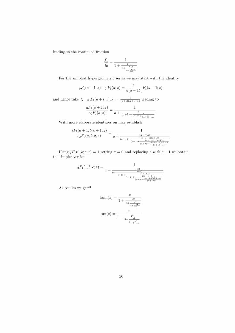
As results we get31
tanh(z) =z
1 + z2
3+ z2
5+ z27+...
tan(z) =z
1− z2
3− z2
5− z27−...
28
The Arithmetic-Geometric Mean
Another thing Gauss played with was the arithmetic-geometric mean (agM)from now on denoted by M(a, b) of two numbers a, b. Assume that 0 < a < band form the geometric mean a1 =
√ab and the arithmetic mean b1 = a+b
2getting two numbers a1, b1 nestled in the former i.e. a < a1 < b1 < b. Proceedinductively producing an, bn. Those number will converge to the agM M(a, b),in fact in view of
b1 − a1 =b21 − a21a1 + b1
=(a− b)2
2(a1 + b1)
and thus inductively
bn+1 − an+1 =b2n+1 − a2n+1
an+1 + bn+1=
(an − bn)2
2(an+1 + bn+1)
we see that the convergence is very fast. More precisely an error of ǫ at one
stage is reduced to an error of ǫ2
4M(a,b) at the next. As an example one may try
to expand M(1 + x, 1− x) in a power series. As the function is symmetric withrespect to its two variables it must be even (x 7→ −x makes no difference) andthus only involving even powers, i.e. being a power series in x2. We also notethat the initial error is bounded by 2x at the second stage it will be boundedby x2 then by 1
4x4 and then by 1
64x8 etc. If we with obvious notation look at
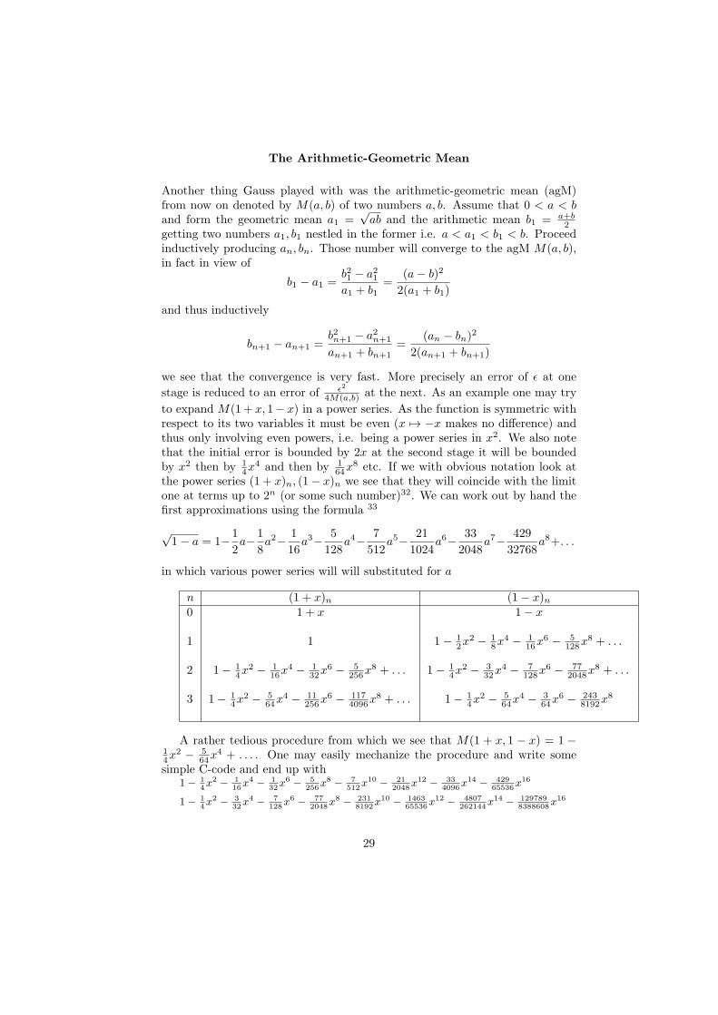
the power series (1 + x)n, (1− x)n we see that they will coincide with the limitone at terms up to 2n (or some such number)32. We can work out by hand thefirst approximations using the formula 33
√1− a = 1−1
2a−1
8a2− 1
16a3− 5
128a4− 7
512a5− 21
1024a6− 33
2048a7− 429
32768a8+. . .
in which various power series will will substituted for a
n (1 + x)n (1− x)n0 1 + x 1− x
1 1 1− 12x
2 − 18x
4 − 116x
6 − 5128x
8 + . . .
2 1− 14x
2 − 116x
4 − 132x
6 − 5256x
8 + . . . 1− 14x
2 − 332x
4 − 7128x
6 − 772048x
8 + . . .
3 1− 14x
2 − 564x
4 − 11256x
6 − 1174096x
8 + . . . 1− 14x
2 − 564x
4 − 364x
6 − 2438192x
8
A rather tedious procedure from which we see that M(1 + x, 1 − x) = 1 −14x
2 − 564x
4 + . . . . One may easily mechanize the procedure and write somesimple C-code and end up with
1− 14x2
−
116x4
−
132x6
−
5256
x8−
7512
x10−
212048
x12−
334096
x14−
42965536
x16
1− 14x2
−
332x4
−
7128
x6−
772048
x8−
2318192
x10−
146365536
x12−
4807262144
x14−
1297898388608
x16
29

1− 14x2
−
564x4
−
11256
x6−
1174096
x8−
34316384
x10−
2135131072
x12−
6919524288
x14−
18470116777216
x16
1− 14x2
−
564x4
−
11256
x6−
2358192
x8−
69332768
x10−
8683524288
x12−
283252097152
x14−
1522109134217728
x16
1− 14x2
−
564x4
−
11256
x6−
46916384
x8−
137965536
x10−
172231048576
x12−
560014194304
x14−
2999717268435456
x16
1− 14x2
−
564x4
−
11256
x6−
46916384
x8−
137965536
x10−
172231048576
x12−
560014194304
x14−
5999435536870912
x16
From this we note some computational mistakes from the hand calculation(Gauss of course did all his calculation by hand, many of them in his head, andonly rarely making mistakes, even when they were very extensive and involved)but more interestingly we note (as expected) that the error of the first pair isx4 of the second pair x8 and the last pair x16 and we can write down
1− 1
4x2− 5
64x4− 11
256x6− 469
16384x8− 1379
65536x10− 17223
1048576x12− 56001
4194304x14+ . . .
The point is not to compute the power series as a computational tool, as thisis not what power series are intended to be used as34, that is in this case effectedmuch more rapidly in the direct way, but to see some pattern and hence to getan independent characterization of it. For that purpose Gauss used anotherapproach. Namely we can write
M(1+2t
1 + t2, 1− 2t
1 + t2=
1
1 + t2M((1+ t)2, (1− t)2) = 1
1 + t2M(1+ t2, 1− t2)
From this Gauss considers the expansion of
1
M(1 + x, 1− x)= 1 +Ax2 +Bx4 + Cx6 + . . .
Setting x = 2t1+t2 we get from the above the identity
1+A(2t
1 + t2)2+B(
2t
1 + t2)4+C(
2t
1 + t2)2+· · · = (1+t2)(1+At4+Bt8+Ct12+. . .
Now we need to identify coefficients and solve for the A,B,C . . . . We can readilywork out A = 1
4 and B = 964 . Through a tour de force Gauss is able to simplify
those equations to 4A = 1, 16B = 9A, 36C = 25B . . . thus finding a closed formfor the expansion of the inverted function
1
M(1 + x, 1− x)=
∞∑
n=0
(
1 · 3 · 5 · 7 · · · · (2n− 1)
2nn!
)2
x2n
30

The Lemniscate and Elliptic integrals and functions
Let us now turn to the lemniscate which was introduced by the Bernoulli broth-ers in the 18th century.
The lemniscate is the locus of points whose product (not the sum) of dis-tances to two given points is constant.
In fact by varying the value of the product we get a whole family ofcurves, known as Cassini’s ovals. They are actually the level curvesof a quartic polynomial, and the leminiscate proper is the one whichpasses through the saddle located half-way between the two referencepoints, where it will have a node. If those are given by (±a, 0) thequartic will be given by
(x2 + y2 + a2)2 − (4a2x2 + a4) = 0
and in the sequel we will find it convenient to set 2a2 = 1 and thelemniscate will cross the x-axis at ±1, 0 given by x2(x2−1) = 0 witha double zero at the origin due to the singularity.
Now it is natural to use the radius vector r =√
x2 + y2 to parametrize thelemniscate. Let us write the equation on the form
(x2 + y2)2 + (x2 + y2)− 2x2 = 0
or x2 = 12 (r
2 + r4) and hence y2 = 12 (r
2 − r4). We get 2xx = (r + 2r3), 2yy =(r − 2r3) thus
x2 + y2 =(r + 2r3)2
r2 + r4+
(r − 2r3)2
r2 − r4=
(1 + 2r2)2
1 + r2+
(1− 2r2)2
1− r2=
1
1− r4
31

Hence the arc length of the lemniscate is given by the integral∫
1√1−r4
in par-
ticular a quarter of the length of the lemniscate is given by the integral
∫ 1
0
dr√1− r4
This integral was well-known during the 18th century (in fact it appearedin a paper by Jacob Bernoulli already in 1691) and had been studied by Eulerand Lagrange among others. Gauss even had a special notation ω for its valuesetting
ω = 2
∫ 1
0
dr√1− r4
computing the value πw numerically to eleven digits he noticed that it coincided
with M(1,√2) = 1.1981402347355922074... He then set out to prove it. One
method was to show that
M(a, b) ·∫ π
2
0
(a2 cos2 φ+ b2 sin2 φ)−12 =
π
2
the key step being that I(a, b) = I(a1, b1) where I is the above integral anda1, b1 occur after the first step in the agM process, noting that (a2n cos
2 φ +
b2n sin2 φ)−
12 converges uniformly to 1
M(a,b)12. He does that by introducing the
variable substitution
sinφ =2a sinφ′
a+ b+ (a− b) sin2 φ′
which will lead to
(a2 cos2 φ+ b2 sin2 φ)−12 dφ = (a21 cos
2 φ′ + b21 sin2 φ′)−
12 dφ′
and he leaves out the details35.Now at the time well-known elliptic integral
F (k,π
2) =
∫ π2
0
(1− k2 sin2 φ)−12 dφ
is related to I(a, b) as follows. Set k = a−ba+b then we have
I(a, b) =1
aF (
2√k
1 + k,π
2)
Furthermore by setting r = cosφ we get
∫ 1
0
dr√1− r4
=
∫ π2
0
(2 cos2 φ = sin2 φ)−12 dφ = I(
√2, 1)
Now impressive as those calculations and manipulations may be, the mostsignificant thing he did was to invert elliptic integrals, in fact the lemniscate
32
integral above, and getting double periodic functions which he denoted by sin-lemn (]sln) and coslem (cl) in analogy with the trigonometric functions. In sodoing he anticipated Abel and Jacobi. More precisely
sl(
∫ x
0
(1− z4)−12 dz) = x
and
cl(ω
2−
∫ x
0
(1− z4)−12 dz) = x
from which will follow identities such as
sl2φ+ cl2φ = sl2φcl2φ = 1
and
sl(φ+ φ′) =slφclφ′ + slφ′clφ
1− slφslφ′clφclφ′
which are actually identities that go back to Euler but in different garb. Further-more he anticipated Jacobi by designing theta functions, in which they could beexpressed as quotients. The periods he computed as 2πG, 2πiG (Note that thelattice generated is up to scale the same as the one of Gaussian integers) where
G =2
π
∫ 1
0
dt√1− t4
=ω
π
Magnetism, Gauss Theorem
Gauss hade already met Wilhelm Weber (184-91) at a meeting in Berlin in 1828(Gauss attended few meetings) and been impressed by him. In 1831 Weberbecame a professor of physics at Gottingen and a co-operation started. Gausshad always been interested in physics, not only astronomy, but until then hiswork had been theoretical, Most importantly in a short paper he had builton the ideas of Maupertuis and d’Alembert on least actions and developed aprinciple of least constrain in which he sought to unify mechanics. With Weberexperimental work began, mostly concerned with magnetism, including (on thesuggestion of the explorer Alexander Humboldt, who in vain tried to enticeGauss to come to Berlin) the mapping of the magnetic field of the Earth, forwhich purpose they even founded a journal. The significance of his work inphysics has been recognized as the unit G of the strength of magnetic fieldsin the now superseeded cgs system36. Mathematically Gauss was a pioneerintroducing potentials and in this context the divergence theorem or Gausstheorem, concerns the integral of the flux of a vector field F across a surface Splays a central role, as all students of mathematics are aware of. Explicitly
∫∫∫
V
(∇ · F)dV =
∫∫
S
(F · n)dS
33

where ∇ ·F = divF = ∂F∂x + ∂F
∂y + ∂F∂z of particular interest being the case when
the divergence vanishes outside the singularities of the field F. In other wordswhen it is the gradient field of a harmonic function, which occurs naturally whengravity or electrical attraction is concerned, because of the inverse square law.
Gaussian distributions and Least Squares
Gauss was very interested in observational astronomy and hence concerned witherror of observations. At every observation there will be mistakes, some randomsome principal. It is the business of theory to rule out the latter, but as to therandom fluctations there is nothing to be done except to expect that they willsomehow cancel out in the long run. Thus we need to make many observationsto determine a quantity, say a1, . . . an what is the ’true’ value x of the observedentity, or better still an x which differ from the values an as little as possible?There is no canonical answer to this question but a natural norm in this caseis the one given by the sum of squares. In other words we want to find x as tomake
∑
n(x − an)2 as small as possible. Differentiating we find the condition
0 =∑
n(x− an) = nx−∑
n an i.e. x = 1n ∼n an. In terms of linear algebra we
can consider the vectors A = (a1, . . . an), I = (1, . . . 1) and seeking to minimize< A − xI · A − xI > under the standard inner product. Geometrically thisamounts to finding the projection of A onto the subspace spanned by I. Thiscan be generalized. Say that we are given a number of dots (an, bn) in the planeand want to find the equation of a line that ’best fits’. Setting the equationof the line as Xx + Y y + Z = 0 where X,Y, Z to be determined we naturallywant to minimize the sum of squares
∑
n(Xan + Y bn + Z)2 or setting A =(an), B = (bn) the squared norm < AX + BY + ZI · AX + BY + ZI >. Anobvious and uninteresting solution is X = 0, Y = 0, Z = 0, uninteresting as itdoes not correspond to a line. It is then natural to normalize (X,Y, Z) suchthat X2 + Y 2 + Z2 = 1. Using the technique of Lagrange multipliers we needto find out when the two gradients are parallel. This leads to the system ofequations
< A ·A > X+ < A ·B > Y+ < A · I > Z = λX< A ·B > X+ < B ·B > Y+ < B · I > Z = λY< A · I > X+ < I ·B > Y+ < I · I > Z = λZ
This can be reformulated as finding the eigenvectors to the linear transfor-mation T whose symmetric matrix is given by
< A ·A > < A ·B > < A · I >< A ·B > < B ·B > < B · I >< A · I > < I ·B > < I · I >
It corresponds to the linear map v 7→< A·v > A+ < B ·v > B+ < C ·v > C.A more natural clarification will appear below in the digression on quadraticforms.
Another normalization may be done by setting y = −1 corresponding tofinding the best linear relation y = Xx + Z giving the values bn when the an
34

are plugged in. In this case we look at the two partials with respect to X andZ setting them zero
< A ·A > X+ < A · I > Z = < A ·B >< A · I > X+ < I · I > Z = < I ·B >
Let us look at the case (1, 1), (3, 4), (2, 5) withA = (1, 3, 2), B = (1, 4, 5), I =(1, 1, 1) We get the matrix
14 23 623 42 106 10 3
and a corresponding cubic characteristic equation
λ3− 59λ2 + 91λ− 25 = 0
You expect three real roots corresponding to the axi of an ellipsoid (incase we have a rotational one you expect one eigenvalue to be double anda corresponding 2-dimensional vector space). In our case we get two smallroots 0.357, 1.22 and a big root 57.423
35

We find the normalized eigenvectors in the three cases and the correspond-ing sum of squares
eigenvalue eigenvector sum of squares
0.357 (0.452,−0.036,−0.891) 0.3571.22 (0.752,−0.523, 0.402) 1.2257.423 (−0.48,−0.852,−0.209) 57.423
Note the curious fact that the sum of the squares equals the correspondingeigenvalues. It could hardly be a coincidence?
As to the second method we only need to solve the system of equations
14X + 6Z = 236X + 3Z = 10
with the solution X = 32, Z = 1
3.
We could also have done it expressing Y as a function of X then therelevant system would have been
42Y + 10Z = 2310Y + 3Z = 6
with the solution Y = 926, Z = 11
13. Those two are plotted below in fat,
along with the three stationary lines from the first method.
We note that the line that has the best fit in the latter case is not the one
close to the fat one.
The first method is mathematically more satisfying or at least elegant, butas we have noted computationally much more complicated. The method canbe vastly generalized, a circle can be given by three linear parameters by x2 +y2+Xx+Y y+Z = 0 while for a general quadric we need six linear parametersthat need to be normalized. More precisely: If the points are given by (an, bn)there will be three quadric monomials a2n, anbn, b
2n two linear ones an, bn and one
contant one 1. Thus we will consider∑
(x1A1+x2A2+x3A3+x4B1+x5B2+x6)2
where Ai, Bi etc are vectors determined by observational data. In general wewill consider
∑
i(∑
k xkAk)2 where the vectors Ak are concocted in various ways
from the data.
36

Digression on Quadrics
To consider a sum of squares
Σ =∑
k
(x1Ak + x2Bk + . . . xnΩn)2
as above is to consider a homogenous quadric in the variables x1, x2 . . . xn. Givenany homogeneous polynomial F (x1, x2 . . . xn) of degree d (i.e. F (tx1, tx2 . . . txn) =tdF (x1, x2 . . . xn)) we can form F0 =
∑
i xi∂F∂xi
and it turns out that F0 = dF arelation named after Euler. It is easy to verify as the relation is obviously linearand it is enough to look at monomials. In our case we have a matrix M whoserows are half of the partials. If we have an eigenvector Ξ = (ξ1, ξ2 . . . xin) onthe unit sphere with eigenvalue λ for the matrix we have
Σ(Xi) =∑
i
ξi(λxi) = λ∑
i
x2i = λ
and we have verified the statement we came across numerically.
To understand it properly we note that any quadric Q gives rise to a gradientvector field on the vector space V (of dimension n)37. As the tangents havecanonical identifications by the underlying linear space itself this gives rise to amap T from V to V . Furthermore the potential being quadratic means that Tis linear (and its matrix is 2M as above). The level surfaces of Q are ellipsoidsand as we put a ballon at the origin and blow it up it will touch the ellipsoidn-times corresponding to its axi. The first it encounter will be the minimal
37

one, and the last the maximal one, which will correspond to the minimum andmaximum respectively of the distance to the origin, for the remaining ones wehave saddles.
Finally we can clarify everything with some more abstract notation. Whatwe have been doing is to create from a given inner product < ∗ · ∗ > a quadraticform < Lv ·Lv > on V where L is a linear map. Now every quadratic form canbe given as < Av, v > where A is a linear map on V (corresponding to the onewe represented by T above and a symmetric matrix M). We can represent A asA = L∗L which becomes symmetric. Now if v with < v ·v >= 1 is a eigenvectorwith respect to A with eigenvalue λ we get
< Lv · Lv >=< Av · v >= λ < v, ·v >= λ
We also note that eigenvectors v, w corresponding to different eigenvalues λ, µwill be orthogonal as
λ < v · w >=< Av · w >=< v ·Aw >= µ < v · w >
Hence the distinct axi of the ellipsoid are orthogonal.
Gaussian distributions
The normal distribution is given by
1√2σ2π
e−(x−µ)2
2σ2
where µ is the expected average and σ2 is the variance (σ is referred to as the
standard deviation). The crucial function is 1√2πe−
12x
2
where the coefficient is
38

chosen to make the integral∫∞−∞
1√2πe−
12x
2
dx = 138. By scaling with 1√2σ
and
translating with µ we get the general case.Say that we want to measure a certain quantity µ then there will be some
observational error. Those errors are the compound of several small errors,sometimes reinforcing each other, sometime canceling each other out. If wemake many observations and take their average we expect that the result willconverge to the true value. We will make this more precise below.
As an example assume that we are tossing a fair coin, meaning that we expecteach face to turn up equally often. Thus if we make n tosses and observe thefrequency of each face we expect that the actual observation will differ slightlyfrom the true value because of error. If we consider all the 2n possible sequencesof head and tails and keep track of how many of those will result in k heads saywe get the binomial distribution with
(
nk
)
such sequences. Now normalize it by
considering k ranging between −n/2 and n/2 by defining φn(k) =(
nk+n/2
)
/2n.
The integral of this step function will be 1 but as n→ ∞ we get that φn(x) → 0spread along an interval of length n. If we scale this interval by a factor 2√
n
thus going from −√n to
√n then we have to scale the function by
√n/2 to
keep the area equal to one. Thus we are looking at ψn(x) = λnφn(λnx) withλn =
√n/2. Using Stirling’s formula
n! ∼√2πnnne−n
we can write down(
2n
n
)
=(2n)!
(n!)2∼
√4πn · 22nn2ne−2n
(2πn)n2ne−2n= 22n
2√π
2π√n
Thus ψ2n(0) =1√2π
and ψn will converge to ψ = 1√2πe−
12x
2 39
In the picture below we see an approximation to the normal distribution bythe binomial.
39
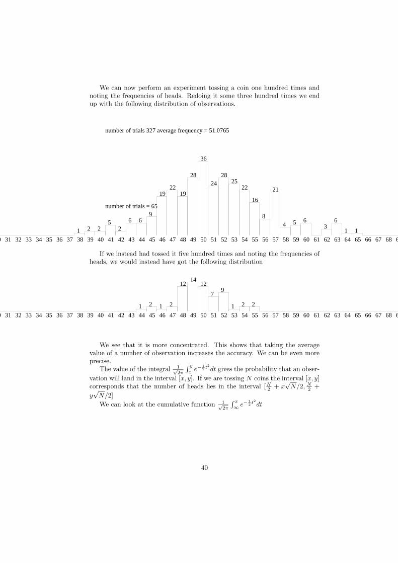
We can now perform an experiment tossing a coin one hundred times andnoting the frequencies of heads. Redoing it some three hundred times we endup with the following distribution of observations.
69686766
1
65
1
64
6
63
3
6261
6
60
5
59
4
58
21
57
8
56
16
55
22
54
25
53
28
52
24
51
36
50
28
49
19
48
22
47
19
46
9
45
6
44
6
43
2
42
5
41
2
40
2
39
1
383736353433323130
number of trials 327 average frequency = 51.0765
If we instead had tossed it five hundred times and noting the frequencies ofheads, we would instead have got the following distribution
6968676665646362616059585756
2
55
2
54
1
53
9
52
7
51
12
50
14
49
12
48
2
47
1
46
2
45
1
444342414039383736353433323130
number of trials = 65
We see that it is more concentrated. This shows that taking the averagevalue of a number of observation increases the accuracy. We can be even moreprecise.
The value of the integral 1√2π
∫ y
xe−
12 t
2
dt gives the probability that an obser-
vation will land in the interval [x, y]. If we are tossing N coins the interval [x, y]corresponds that the number of heads lies in the interval [N2 + x
√N/2, N2 +
y√N/2]
We can look at the cumulative function 1√2π
∫ x
∞ e−12 t
2
dt
40
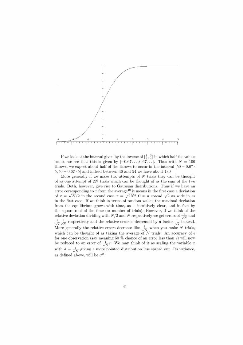
-3 -2 -1 0 1 2 3 4 5
If we look at the interval given by the inverse of [ 14 ,34 ] in which half the values
occur, we see that this is given by [−0.67 . . . , 0.67 . . . ]. Thus with N = 100throws, we expect about half of the throws to occur in the interval [50− 0.67 ·5, 50 + 0.67 · 5] and indeed between 46 and 54 we have about 180
More generally if we make two attempts of N trials they can be thoughtof as one attempt of 2N trials which can be thought of as the sum of the twotrials. Both, however, give rise to Gaussian distributions. Thus if we have anerror corresponding to x from the average40 it means in the first case a deviationof x =
√N/2 in the second case x =
√2N2 thus a spread
√2 as wide in as
in the first case. If we think in terms of random walks, the maximal deviationfrom the equilibrium grows with time, as is intuitively clear, and in fact bythe square root of the time (or number of trials). However, if we think of therelative deviation dividing with N/2 and N respectively we get errors of 1√
Nand
1√2
1√N
respectively and the relative error is decreased by a factor 1√2instead.
More generally the relative errors decrease like 1√N
when you make N trials,
which can be thought of as taking the average of N trials. An accuracy of ǫfor one observation (say meaning 50 % chance of an error less than ǫ) will nowbe reduced to an error of 1√
Nǫ. We may think of it as scaling the variable x
with σ = 1√N
giving a more pointed distribution less spread out. Its variance,
as defined above, will be σ2.
41

Notes
1Why not King of Mathematics? There is no separate English word for the GermanFurst or the Swedish furste which denotes the monarch of a small kingdom, or principality(furstendome), of which Germany was a mosaic.
2The series is usually presented as the sum of the first hundred numbers, most likely it wasmore complicated and that its arithmetic nature was not immediate.
3Both Euler and Gauss made no distinction between pure and applieed mathematics, ev-erything was food for thought, and in the case of Gauss he is said to have quoted King Learto the effect of Thou, nature, art my goddess; to thy laws my services are bound.
4He also left descendants, of whom Eugene and Albert Fawcett lived until the early 1950’s,but neither seem to have left any issue. The longest living grandchild of Gauss was JospehHenry (1855-1956) son of Charles Gauss (1813-79) and born in the Missouri. His daughterJanet Lee (1912-2012) must be the longest surviving great grandchild of Gauss. There arestill great great grandchildren about, all Americans.
5Less spectacular students were Moebius, who nevertheless is a name that pops up repeat-edly and may to most mathematicians be more well-known than Dirichlet. Even more thanthat of Riemann among the general population.
6The case p = 257 was worked out in a dissertation in 1831 involving a sequence of sevenquadratic extensions by Friedrich Julius Richelot (1808-75) a student of Jacobi, whom he latersucceeded at Konigsberg. The construction involved 194 printed pages. Incidentally Richelotwas the father-in-law of the well-known 19th century physicist Kirchoff. Attempts at the caseof p = 65537 involving fifteen quadratic extensions were undertaken by Johann Gustav Hermes(1846-1912) who devoted ten years to the task. The results of his efforts, completed in 1889,remain in some large chest specially designed and made for that purpose at the Gottingenmath department. A shorter report on it was published in 1894, sponsored by Felix Klein.
7 If the polynomial is reducible, it splits up into two linear factors and have two rational(unrelated) roots. To talk about numbers may be a trifle misleading as it is not strictlynecessary, one may look at the ring Q[x]/(x2−px+q) where we will have the rule x2 = px−q,thus in practice (see below) any element can be written as ax+ b with the above rule.
8It turns out that η 7→ η′ is both linear and multiplicative, in fact the one non-trivialautomorphism of a quadratic extension.
9There is some confusion what is a discriminant. If the linear term is even one can factorout the factor 4 in the discriminant, thus 4b2 − 4ac is reduced to b2 − ac as Gauss does in hisdefinition. The confusion is irritating, but not serious, as a discriminant is mostly interestingmod squares anyway.
10Gauss considers integral forms of type ax2 + 2bxy+ cy2 which corresponds to lattices forwhich the restriction of the inner product is integral, which is a strong condition. A weaker,and perhaps more natural condition is that the restriction of the quadratic form is integral.
11Given two vectors ω1, ω2 the area ∆ of the parallelogram spanned by them is given bysin θ|ω1||ω2| from which follows that
∆2 = sin2 θ|ω1|2|ω2|2 = |ω1|2|ω2|2− < ω1 · ω2 >2
as
< ω1 · ω2 >=1
2(ω1ω2 + ω2ω1)
we get
< ω1 · ω2 >2=
1
4(ω2
1ω22 + ω2
2ω21 + 2|ω1|2|ω2|2)
42

hence
∆2 = −1
4(ω1ω2 − ω2ω1)
2 = −D
We also note that given the quadratic form An2+2Bmn+Cm2 its discriminant being B2−ACtranslates into < ω1 · ω2 >2 −|ω1|2|ω2|2 = −D
12To be pedantic, τ = −τCM if we want to insist that τ belongs to the upper half-plane.But in the ensuing discussion we can afford to be a bit sloppy.
13An example of such z is given by z = ω2ω1
as
ω2ω1ω1 = ω2
ω2ω1ω2 = cω1 + dω2
where(ω2
ω1)2 = d
ω2
ω1+ c
is assumed to satisfy an integral quadratic equation. This will of course not be true in general,but whenever we note that c = −Nm(τ), d = Tr(τ)
14What we need to do is given D find t such that the discriminant of the equation x2+tx+ais a square multiple of D i.e. t2 − 4A = k2D. If D = −1 it means that A needs to be thesum of two squares which is not always possible. Note that the norms of elements in Q[i] are
obviously sums of two squares. However we have that D = B2−4ACA2 if B2 − 4AC = −1 we
see that A|B2 + 1 and hence A is a sum of two squares.
15To each quadratic field we may associate the ring of integral elements, namely those whichsatisfy a quadratic equation with integral coefficients and monic. To each quadratic field weget a discriminant by computing the discriminant of different elements, which will all differby a square. This ring will have the property that all its elements leave the lattice Λ invariantunder multiplication. The ring itself will be a rank two lattice spanned by 1, τ whose trace isnot necessarily even, hence it does not necessarily correspond to a quadratic form with evenmiddle term, the kind favored by Gauss. More specifically. The full ring of integral elementswill be elements of the type ατ + β such that their traces and norms are integral. It is easyto compute
Tr(ατ + β) = αTr(τ) + 2β Nm(ατ + β) = α2Nm(τ) + αβTr(τ) + β2
From which we conclude that if D 6= 3(4) then α, β need to be integers, so the ring coincideswith the original. However if D = 3(4) we can also have α = β = 1
2(Z) and hence the ring
is generated by 1, 12(1 + τ) this will be an element with odd trace (and thus not contained in
Gauss study). In general the endomorphism ring will just be a subring of the integral ring,and will be referred to as an order.
16For an ideal generated by α ∈ R we can take ω1 = α, ω2 = ατ and thus the associatedquadratic form will not be primitive, but we can factor out |α|2.
17To be more precise, elements ±M give the same action, as Moebius tranformations, andwe are really looking at PSL(2,Z) known as the modular group Γ
18The ring is not a unique factorization domain, we have (1 +√5i)(1 −
√5i) = 6 = 2 · 3
where all the elements are irreducible. It is this fact that serves as an inspiration for theconstruction of the ideal generated by 2, 1 +
√5i.
19If the unit is 1 A.U. the distances from the sun for the planet p is given by 0.4 + 0.3 · 2mwhere m = ∞ corresponds to Mercury, m = 0 Venus m = 1 the Earth, m = 2 Mars, m = 4Jupiter, m = 5 Saturn and m = 6 Uranus, thus Ceres (and a host of others) would correspondto m = 3, the law breaks down for Neptune.
43

20He anticipated Legendre who resented that Gauss claimed priority, could nothing be leftfor him?
21This was later introduced in 1965 unawares that Gauss had used it a century and a halfearlier.
22’Rather death than such a life’ actually discovered by Felix Klein
23In fact the ancients did it step by step, and as to be seen below this did not require muchmathematical maturity, the Babylonians could have done it had they had occasion to do so.Apparently Gauss became interested in it, as his mother did not know the date of his birth,only the year and that it had been on Ascension Day.
24For some reason the theoretical possibility of April 26 is excluded on an ad hoc basis.
25In the culture of India, having lived through one thousand Full Moons is a significantevent, which we see occurs around the time you turn 75.
26The standard time used nowadays is UTC which has replaced GMT. There was a FullMoon on November on November 14 at 13:52 and one on December 14 at 00:06 this correspondsto 29 days 10 hrs 14 min, the next one will be on January 12 at 11:34 UTC giving 29 days 11hrs 28 min, subsequent periods will be 29 days 11 hrs 59 min, 29 days 14 hrs 21 min 29 days15 hrs 14 min, thus we see that the Synodic period varies rater substantially. The average forthose makes up 29 days 12 hrs 39 min to be compared with the long term average of 29 days12 h 44 min (there is an advantage of having a virtual moon with some regularity comparedto a real one). The first Full Moon after the vernal equinox on 2017 will be on Tuesday April11 at 6:08 UTC making Sunday April 16, the next Easter Sunday. As to a Full Moon in theperiod in 2018 we have to subtract 365.24− 354.36 = 10.88 days from April 11 + 0.25 endingup on March 31 + 0.37 (give or take a few hours because of the irregularity) this will be aSaturday so Easter Sunday on 2018 will be on April 1. Below is shown the sybodic periodscounted from full moon to full moon as well as new moon to new moon for about a yearsworth of phase cycles
7 h
8 h
9 h
10 h
11 h
12 h
13 h
14 h
15 h
16 h
17 h
18 h
29 days + 27One such result was that in a non-euclidean geometry there would be an absolute unit of
length, thus it would not be scale invariant, furthermore there would be a uniform bound onthe areas of triangles, no matter how large.
44

28To another correspondent he wrote that he found Bolyai to be a genius of the first order
29the first one such measured was by Bessel in 1838 of 61 Cygni. Actually a binary star ofhigh magnitude (5.2+6) just discernible to the naked eye. Rather unremarkable until Piazzi(the discoverer of Ceres) noted in 1804 that it had a large proper motion, i.e. that its positionon the celestial square changed rapidly, indicating that it might be a close star. Bessel’sestimate was 10.3 light years, rather close to the modern estimate of 11.4 . Of all starsvisible to the naked eye it has the largest motion amounting to 4′′/year in Right Ascensionand 3′′/year in Declination. At a declination of 40o this amounts to about 4.5′′/year to becompared with that of Barnard’s arrow star of 10”/year.
30Those are analogous to the case of spherical geometry. They were formally producedalready in the 18th century by Lambert.
31Those were known already to Lambert in 1768 and were used by him and Legendre toprove the irrationality of π.
32We can see this in two different ways. Heuristically truncating an expansion starting withthe term xn gives for small values ǫ an error of at least the order of ǫn. If two power seriesstart to differ at that term they will differ by that amount, but if the order of error is ofa higher power, we get a contradiction. Another mathematically more satisfying way is toobserve that the formula above shows that if xn divides the power series an(x)− bn(x) thenx2n divides an+1(x)− bn+1(x).
33Using factorials or (integral) binomial coefficients we can of course put this into closed
form. As Newton pointed out the power series expansion of (1 + a)12 is given as
∑
k
( 12k
)
ak
where the coefficients (k = n+ 1) can be expanded out as
( 12)( 1
2− 1)( 1
2− 2)( 1
2− 3) . . . ( 1
2− n)
(n+ 1)!= (−1)n
1
2n+1
1 · 3 · 5 · · · · (2n− 1)
1 · 2 · 3 . . . (n+ 1)
where in the right hand side the even factors are missing. Filling them in (n− 1) of them weget
1
22n(2n− 1)!
(n+ 1)!(n− 1)!=
1
22n1
n− 1
(2n− 1
n+ 1
)
. We would like to observe that up to the initial negative power of two we have an integer.To show that it is more convenient to use the left hand side. Note that the order of the factorp in (n+ 1)! is given by
⌊n+ 1
p⌋+ ⌊n+ 1
p2⌋+ ⌊n+ 1
p3⌋ . . .
while for the numerator we are only interested in the odd multiples of p and its powers (whichwe can assume to be odd) let us denote their numbers by [n/p] etc. If we can show that[n/q] ≥ ⌊n+1
q⌋ for each odd number q we will be done. Now set n+1 = kq+ r with 0 ≤ r < q
and k = ⌊n+1q
⌋. From this we find 2n − 1 = 2kq + 2r − 3 if 2r − 3 < 0 we will lose an even
multiple of q but this does not matter as we will still have k odd multiples of q left, namelyq, 3q, 5q, . . . (2k − 1)q. We will get an excess when 2r − 3 ≥ q (note that this always happenswhen q > (n+ 1) ) which means that p divides the numerator (q = pn). Recall the list of thefirst few coefficients (note that n correspond to n+ 1 above)
n 1 2 3 4 5 6 7 8num 1 1 1 5 7 21 33 429exp of 2 1 3 4 7 9 10 11 15
We will get a factor of 3 in the denominator when n = 6, 7, 8(9) (or if that is failing whenn = 18, 19, . . . (27) etc) a factor of 5 if n = 4(5), a factor of 7 if n = 5, 6(7) a factor of 11if n = 7, 8, . . . 10(11) and a factor of 13 if n = 8, 9 . . . 12(13) all of which are ratified by theexamples above. As an example we may compute the coefficient for n = 30. Looking at theprimes 5, 7 . . . 53 and the prime powers 9, 27, 25, 49 up to 57 = 2 · 30 − 3 we conclude that
45
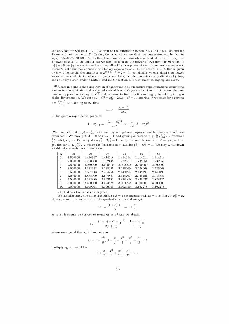
the only factors will be 11, 17, 19 as well as the automatic factors 31, 37, 41, 43, 47, 53 and for49 we will get the factor 7. Taking the product we see that the numerator will be (up tosign) 125280277081421. As to the denominator, we first observe that there will always bea power of n as to the additional we need to look at the power of two dividing n! which is⌊n2⌋+ ⌊n
4⌋+ ⌊n
8⌋+ · · · ≤ n− 1 with equality iff n is a power of two. In general we get n− k
where k is the number of ones in the binary expansion of 2. In the case of n = 30 this is givenby k = 4 hence the denominator is 230+30−4 = 256. In conclusion we can claim that powerseries whose coefficients belong to dyadic numbers, i.e. denominators only divisible by two,are not only closed under addition and multiplication but also under taking square roots.
34A case in point is the computation of square roots by successive approximations, somethingknown to the ancients, and a special case of Newton’s general method. Let us say that wehave an approximation xn to
√A and we want to find a better one xn+1 by adding to xn a
slight disturbance ǫ. We get (xn + ǫ)2 = x2n +2xnǫ+ ǫ2 = A ignoring ǫ2 we solve for ǫ getting
ǫ =A−x2
n2xn
and adding to xn that
xn+1 =A+ x2n2xn
. This gives a rapid convergence as
A− x2n+1 = − (A− x2n)2
4x2n∼ − 1
4A(A− x2n)
2
(We may not that if (A− x2n) > 4A we may not get any improvement but we eventually arerewarded). We may put A = 2 and x0 = 1 and getting successively 3
2, 1712, 577408
. . . fractionspnqn
satisfying the Pell’s equation p2n − 2q2n = 1 readily verified. Likewise for A = 3, x0 = 1 we
get the series 2, 74
9756. . . where the fractions now satisfies p2n − 3q2n = 1. We may write down
a table of successive approximations
A x1 x2 x3 x4 x5 x62 1.500000 1.416667 1.414216 1.414214 1.414214 1.4142143 2.000000 1.750000 1.732143 1.732051 1.732051 1.7320514 2.500000 2.050000 2.000610 2.000000 2.000000 2.0000005 3.000000 2.333333 2.238095 2.236069 2.236068 2.2360686 3.500000 2.607143 2.454256 2.449494 2.449490 2.4494907 4.000000 2.875000 2.654891 2.645767 2.645751 2.6457518 4.500000 3.138889 2.843781 2.828469 2.828427 2.8284279 5.000000 3.400000 3.023529 3.000092 3.000000 3.00000010 5.500000 3.659091 3.196005 3.162456 3.162278 3.162278
which shows the rapid convergence.We can also apply the same procedure to A = 1+x starting with x0 = 1 so that A−x20 = x,
thus x1 should be correct up to the quadratic terms and we get
x1 =(1 + x) + 1
2= 1 +
x
2
as to x2 it should be correct to terms up to x4 and we obtain
x2 =(1 + x) + (1 + x
2)2
2(1 + x2)
=1 + x+ x2
8
1 + x2
where we expand the right hand side as
(1 + x+x2
8)(1− x
2+x2
4− x3
8+x4
16. . . )
multiplying out we obtain
1 +x
2− x2
8+x3
16− x4
32+ . . .
46
where terms up to x4 are indeed correct but the x4 term is not. The next step will be a truemess but the patient reader may convince herself that terms will be correct up to x8 a truly
painful way of obtaining the binomial theorem for (1 + x)12
35Jacobi supplies some of the details. An excellent exposition can be found in The Arithmetic-
Geometric Mean of Gauss by David Cox in L’enseignement Matheematique IIe Serie , TomeXXX -Fascicule 3-4, 1984 from which much of the discussion is lifted.
36cgs standing for centimeter, gram and second. In the more modern SI system one speaksabous Tesla (T) with the conversion 1T = 104G.
37If the quadric is given by x2 + k2y2 we see that for any value of the parameter λ the
curves (x(t), y(t)) = λ(et, ek2t) are integral curves, as the derivatives λ(et, k2ek
2t) have thesame directions as the gradient at any point. The curves are in general transcendental, i.e.not satisfying any algebraic equation, but nevertheless they can be given a simple equation of
type y = µxk2with µ = λk
2−1.
38recall that
(
∫ ∞
−∞e−
12x2dx)(
∫ ∞
−∞e−
12y2dy) =
∫∫
R2e−
12(x2+y2)dxdy =
∫ 2π
0
∫ ∞
0e−
12R2Rdθdr = 2π[−e− 1
2R2
]∞0 = 2π
39We note that setting k = x√2n/2 we have
ψ2n(x) =
√2n
2
1
22n
( 2n
n+ k
)
∼√4πn
√2n · n2n
2 ·√
4π2(n− k)(n+ k) · (n+ k)n+k(n− k)n−k
Now taking the log of (n+kn
)n+k(n−kn
)n−k we get
(n+ k)(k
n− 1
2
k2
n2+ . . . )− (n− k)(
k
n+
1
2
k2
n2+ . . . ) =
2k2
n− 2
1
2
k2
n=k2
n
as k2 = x2 2n4
we get k2
n= 1
2x2 and hence the limit 1√
2πe−
12x2
40If x = 1 in the standard distribution, we talk about one standard deviation. This cor-
responds to the area 1√2π
∫ 1−1 e
− 12x2dx = 0.682689 . . . . More generally this will be true for
any Gaussian distribution, when 1 is replaced by σ one standard deviation. Thus the smallerstandard deviation, the more concentrated around the average is the distribution.
47