UNIVERSITY OF NAPLES FEDERICO II

DEPARTMENT OF AGRICULTURE AGRICULTURAL ECONOMICS AND POLICY GROUP

DOCTORAL THESIS – XXX CYCLE FOOD AND AGRICULTURAL SCIENCES

ECONOMETRIC STUDIES OF FOOD DEPENDENCY IN SOME

DEVELOPING OIL-EXPORTING COUNTRIES.

SUPERVISOR PH.D STUDENT PROF. LUIGI CEMBALO ABDALLAH DJELLA

CO- SUPERVISOR PROF. FABIO GAETANO SANTERAMO

PORTICI, NAPLES (ITALY) - 2017

2

Index

INTRODUCTION……………………………………………………………………………3

1. OIL EXPORT DEPENDENCE ANALYSIS……………………………………………...6

1.1. The paradox of oil dependency in the developing oil-exporting countries…..…………6

1.2. Oil scarcity in the developing oil-rich countries…...…………………………………..20

2. FOOD IMPORT DEPENDENCE ANALYSIS…........…………………………………..22

2.1. Agricultural itinerary of some developing petroleum-exporting countries (Qatar, Saudi

Arabia, United Arab Emirates, Angola, Nigeria and Algeria)...…………………………….22

2.2. The post-petroleum food system in the developing oil-wealth countries…..…………..38

3. STATE OF THE ART IN THE STUDY OF INTERNATIONAL TRADE..…………...41

3.1. The study of international trade ….…………………………………………………….41

3.2. The basic concept of the gravitational model for the study of international trade.…....45

3.3. Economic explanation of the gravitational model …………………………………….46

3.4. The estimation of the gravitational model…..………………………………………....48

3.5. Dimension of the economy …………………………………………………………….49

3.6. Distance ...………………………………………………………………………….....50

3.7. Isolation ….…………………………………………………………………………...52

3.8. Enrichment of the gravitational model ………………………………………………..53

3.9. State of the art on the use of gravitational models in international …..……………...56

3.10. Modeling of commerce barrier ..………………………………………………...…..64

4. ECONOMETRIC ESTIMATION OF FOOD DEPENDENCY...…………………….....74

CONCLUSION…..………………………………………………………………………......79

REFERENCES

3

Introduction

According to the prevailing opinion, natural resources in general and oil in particular, are a

curse rather than a blessing. The growing literature on the “curse of resources” and the

“paradox of plenty” (Karl, 1997) has generated significant causal claims that link the

abundance of resources with dependence on corruption, authoritarianism, economic decline

and violent conflicts. It has often argued that oil-dependent states today are the most unstable

economically, the most authoritarian, and the most tormented by conflicts (Gary & Karl,

2003). Realistically, oil is not the curse but the “oil bad management” or “oil misused” is the

curse in the developing oil wealth countries, paradoxically can see a good example of “oil

control” in developed countries as Norway and Chile. The developing oil wealth countries are

suffering the two curses, internal curse referring to the bad management with no capital

transparency and the external evil relating to violent war.

Kevin Tsui observed how developing oil-rich regimes neglect the non-oil industry and tend

not to undertake necessary institutional enhancements and economic reforms. Consequently,

these systems tend to have stagnant economies and are particularly vulnerable to price

fluctuations of oil products. These structural problems are exacerbated by the high rates of

population growth across the world, as well as by persistent corruption and clientelism that

accompanying the oil-financed patronage. The presence of these economic trends is essential

when evaluating the connection between oil wealth and the regime stability. Given the

carelessness towards industries such as agriculture, Oil-rich governments are forced to

allocate more and more resources to the aid of expensive increasingly food imports, thereby

limiting their ability to finance mechanisms of stabilization of social spending and repression.

Besides the lack of economic growth can force the population to rapid growth dealing with

the growth of unemployment and poverty. Which therefore form the basis for the widespread

discontent and mobilization anti-regime potentially destabilizing. Can it be considered

surprising that, during the Arab Spring, socio-economic complaints were the heart of many

4

anti-regime protests? For sure, in the Arab Spring states where these kinds of problems more

pronounced, The protests built entirely around issues such as poverty and unemployment.

Thus, the socioeconomic roots of many Arab Spring protests indicate that oil wealth can lead

to the instability of the regimes, creating long-term economic problems that lead to popular

mobilizations (Tsui, 2011). Another long-term socio-economic challenge for oil-rich regimes

is the unemployment of the most educated population. When in the 1960's and 70's of the last

century, the revenues generated by the oil were booming, Arab regimes expanded their

citizen’s access to education as part of their oil-financed social expenditure. However, in

many of these states, the lack of economic growth caused the inability to find work or the

underemployment for these educated professionals. This dynamic is a cause of dissatisfaction

among the educated population, which moved by the non-coincidence of its socio-economic

ambitions with the economic reality in which brought the demand for political changes. This

dynamic shows clearly that scholars, jurists, and other professionals play a fundamental role

in launching and supporting anti-regime political mobilizations. The majority of oil-rich

countries is depending on oil revenue sector and also depending to the importation of many

domestic goods like food, this critical situation permit to these kinds of countries covering

their hard dependency of importation by oil revenues. The largest addiction shows entirely in

the agri-food sector imports, nevertheless; many developing oil-wealth countries don’t

investing sufficiently in agricultural areas as one of the important industry because, without

an integrated national economy, there can be not sustainable food security or sovereignty. The

challenge that how can improve the capacity of food production in the society that increases

exponentially, and how can convince the private sector and foreign direct investment to

investing in agriculture as a complicated industry. Particularly, in an arid, semi-arid and desert

area that suffering economic water scarcity, low rainfall, and high temperature.

Economically, in the petro-states, the finance of project depends directly on oil revenues

means the volatility of oil price has a direct and close impact on agricultural investment as

5

well as logistically, these countries need more agricultural technology, machinery, and more

skilled labor in which usually are taken by developed countries. The developing oil-rich

countries possess the two dependencies compared to other world countries; one is positive

regarding the petrodollars budget wealth and another negative related to the great goods

import dependence, particularly, the agri-food. The question that can pose; witch future of

food without oil revenues in the oil-exporting state? Another challenge of these countries is

the agricultural land availability.

The problem of food scarcities not just in the developing countries but all the world where the

population could be around 9 billion by 2060 and how can feed the two extra billion (Bailey

2012). In 2009, according to the FAO estimation, 70% more food in 2050 will be needed. In

the same time, the international food prices are rising continuously. Additionally, some

exporter countries as China and India continue the reduction of its exportation product like

wheat, corn, and rice for secure the high local demands. The food scarcity usually, influences

the developing countries that can see about 785 million of their people undernourishment

(FAO 2015), where the developing countries represent 82% of world population (United

Nation, 2013). The agricultural industry needs more investment in the sector for securing the

food sovereignty of the nations. The FAO administration seeking to promote food production

and security. Especially, in some countries where some crops threatened by the climate

change.

This study permits to explain “the resource curse” in some developing oil exporting countries

that possessing the macroeconomic similarity regarding the oil dependency, and the identical

environmental conditions in which these countries are; Qatar, United Arab Emirates, Saudi

Arabia, Angola, Nigeria, and Algeria.

6

1. Oil export dependence analysis:

The petrodollar states more dependent on hydrocarbons revenues rather than other sectors

where suffering no-economic diversity in which no-oil industry scant. The Oil-GDP variate

between 50 to 90% in these countries. This dependency is a curse for the economic

development that invests in other sectors depending highly to oil revenues where the

challenge how can funding the projects in the era of continuous oil price volatility and how

can protect the budget balance in the long term period or the era of oil scarcity.

1.1. The paradox of oil dependency in the developing oil-exporting countries.

The undeveloped petrodollars state budget is heavily dependent on the fluctuations of the

hydrocarbons price. In fact, changes in the oil price cause fluctuations in national GDP in

which these states most dependent to oil export for formation of their GDP. In parallel,

dependent to importation per secure their domestic consumption of industrial, technological

and agri-food products. The rentier states suffering economic stagnation in many sectors

where the oil dependency destabilized the macroeconomic budget and discourage investment

in no-oil industry, in the same time the economic balance depending to boom and busts of oil

price. From one hand the oil-wealth countries exempt their citizens from taxes and subsiding

many domestic products, and in another hand, the oil encourage a civil war such as in Angola

and Nigeria (Basedau & Lay, 2009) and invasions such as Iraq and Libya, means no peace in

developing oil-producing countries. These violent situation block foreign investment, promote

ethnic tension and create more dictatorial and military regimes. Today the majority of these

economies are in crisis either political or economic. About this critical reality, the founder of

the OPEC Juan Perez Pablo Alfonso said “I call petroleum the devil's excrement. It brings

trouble, waste, corruption, consumption, our public services fall apart, and debt - a debt we

shall have for years.” (The Economist, 2003). Wherever, could see the corruption in these

7

countries where one of the largest oil-producing countries is the most corrupted in the world

as Nigeria ( Karl, 1999). The oil could be the obstacle of development and why the

developing oil wealth economies suffering slow growth, despite possessing sufficient wealth

to investing profitably in all economic sectors. The negative correlation between natural

resources especially hydrocarbon and economic development confirmed by many lecturers.

Therefore, the economic stagnation is the major problem. Many economic studies observed

that the majority of oil-exporting countries suffers the less democracy, institution deficiency,

bureaucracy and chronic political system since the oil discovery. At the same time, the no-oil

producing countries are more democratic rather than some oil-wealth countries. The oil

considered as significant wealthy resources but will be a hell for their country if not well

managed correctly, in parallel the natural resources lead to poverty more than development.

The economic growth linked to natural resources where the economy of developing oil wealth

countries growth slowly than no-natural resources countries (Okpanachi, 2011). The oil

wealth counties don't look to invest in other sectors regardless petroleum sectors like tourism,

services, infrastructure, and agriculture. In reality, there is a modest investment but not

sufficient and efficient regarding its wealth capacities. Eventually, these countries become the

most unstable, growing slower and performed worse rather than those without natural

resources. The dependency to oil-wealth losing the spirit of action, competitiveness and

strategic planning.

This study permits to explain “the resource curse” in some developing oil exporting countries

that possessing the macroeconomic similarity regarding the oil dependency (Graph.1), and

identical environmental conditions in which these countries are; Qatar, United Arab Emirates,

Saudi Arabia, Angola, Nigeria, and Algeria.

The choice of these countries based on the data provided by UN Comtrade where taking into

considerations the states that mostly fuel exports, at the same time highly dependent on agri-

8

food importation. The data permit to find countries in the middle east as Qatar, United Arab

Emirates and Saudi Arabia then others in Africa as Angola, Nigeria and Algeria. These

countries are under the econometric estimation.

Qatar: This “ Small state,” with the minuscule population about 2,32 million, has begun the

gas production since 1949, is the first gas producer in the world, the third largest gas reserves

in the world that estimated by 900 trillion standard cubic feet. The Qatar Petroleum is the

largest gas producer company in the world. The economy of Qatar is very dependent on

hydrocarbon income which represents 61% of GDP, 95% of total exportation and 75% of

budget revenue (Gardan, 2013). In 2015, Qatar gas revenue estimated by $50,52 Billion and

by $64,53 Billion of oil revenues. Fortunately, in the recent years , the non-hydrocarbon GDP

growth notably passing from 44% to 55% of GDP between 2000 and 2011.

The political system in Qatar is monarchic where the Gulf regimes are still monarchic and

tribalism system. The economic system management basing in hydrocarbon resources,

primarily the gas and oil revenues. According to Minister of Development Planning and

Statistics in 2016, the gas price decline has a negative impact on Qatari budget in which the

$0,00

$50.000.000.000,00

$100.000.000.000,00

$150.000.000.000,00

$200.000.000.000,00

$250.000.000.000,00

$300.000.000.000,00

$350.000.000.000,00

$400.000.000.000,00

Saudi Arabia

Nigeria

Qatar

United Arab Emirates

Algeria

Angola

Graph 1. GDP formed by hydrocarbons (Oil+Gas) revenues.Source: UN Comtrade.

9

hydrocarbon production decreased by 2.8% in 2016. Immediately after, in the late of 2015

The government canceled the subsidies for water, electricity, and taxing some other products

and rationalized the public expenditures, at the same time the inflation pass from 3,4 percent

in 2016 to 3,6% in 2017 and continue to increase that will arrive at 3,8% in 2018. Qatar and

all Gulf cooperation council countries (GCC) will apply the value-added taxation at 5% on the

underlying goods price at the beginning of 2018. After the decline of gas and oil price, the

fiscal deficit in 2016 estimated at 7,8 percent of GDP and the liquidity reduced significantly.

Qatar's trade surplus in 2015 fell by half of its value (in 2014) to 2.29% of GDP. This decline

due to the lower of export revenues which shrunk by 39%. Other financial risks include the

realization delay of the main infrastructure projects and increasing the cost of its

implementation. The fiscal balance is also expected to remain in deficit in 2017 and 2018,

although the reduction in expenditure and the moderate increase in hydrocarbon prices will

ease its sharpness in comparison to 2016. The gas production is more important in Qatar than

oil production. Indeed, the value of liquefied natural gas (LNG) exports in 2015 exceeded the

value of all other hydrocarbon products and accounted for about 46% of total export

commodities. Immediately, The Qatar GDP decrease from $210,1 Billion in 2014 to $152,5 B

in 2015. Consequently, the total saving rate reduced from about 75% of total GDP in 2011 to

58,6% in 2015. After the hydrocarbons shock in 2014, the total revenue decrease by 20,7%, at

the same time the income from hydrocarbon decrease by 23.3% in 2015. the investment also

decreased immediately in the same year by 7.19% in which consists mainly from the profits

of Qatar Petroleum. Away from hydrocarbon, Qatar economy based on importation that

accounts for a high demand proportion in 2015 that estimated by 44,3% of final domestic

spending.

Politically, Qatar plays a fundamental role in the middle east but has a political problem with

neighborhood countries in which today suffers the “Business embargo” by the Gulf countries

10

and Egypt that these countries accuse Qatar its responsibility for supporting the terrorism, but

Qatar denied. This embargo has an adverse impact on Qatari gas transportation due to the

closure of sea crossings. According to Reuters news, the Gas price immediately raised by

4,5% but at the same time the Qatari money value “Riyal” decreased by 10%. Furthermore,

many foreign Qatari citizens and businessman should leave the gulf countries. Consequently,

humanitarian crisis and economic losses. The hydrocarbon wealth gives Qatar policy a

leadership post among nations, especially in the GCC regions, this position is an imprecation

for some other leading countries in the middle east as Saudi Arabia and Egypt in which Qatar

disrupt the GCC countries decisions. Especially, the external policies with Iran which are very

conflictual in the Gulf, excepting Qatar. But economically, after The gas discovery in the

northern maritime field of Qatar, the largest liquefied natural gas output, it was a curse for

Iranian gas exportation. For this reason, Iran attempt to increase its production in southern gas

maritime parts field by the realization of a new project with France’s Total in November

2016.

United Arab Emirates (UAE): considered among the prominent members of the Gulf

Cooperation Council (GCC). UAE participates by 24% of Gulf area GDP that estimated for

approximately $348,74 Billion , after Saudi Arabia by 46%, according to trading economics

estimation. The economic situation of UAE as Saudi Arabia, more oil commodity exportation

and more no-oil commodities importation. According to FMI, the UAE heavily dependent on

oil revenue by 45% of GDP that in 2016 produced about 3 million barrels per day, classified

the fifth’s world oil producer by 5,8% of global oil total exportation (IMF, 2016). According

to Organization of Arab Petroleum Exporting Countries (OAPEC), Annual statistical report

2016, the proven oil reserves of UAE at the end of 2015 estimated by 97,8 Billion of barrels

and by 6091 Billion Cubic Meters of proven natural gas reserves, represent 3,10% of total

world’s gas. In 2015 after the oil price crisis, the GDP decreased by 4,7%. At the same time,

11

the gross international reserves declined at $85,4 Billion, passing from 38,1% in 2014 to

20,8% of GDP in 2016, according to CIA World Factbook 2017.

From a critical point of view, despite The UAE is “ less resource cursed ” compared to other

oil exporting countries remains undeveloped countries. Indeed, the UAE’s GDP is among the

highest world’s GDP, but until today the country suffering the mono-economy regime based

on hydrocarbons sectors, away from industrial and technological production. A country as

UAE with its massive exchange reserves could be the leader of no-oil industrialization

investment in the middle east in which the oil dependency remains the long-term challenge of

UAE government.

The political system in UAE commanded by seven monarchical federations in which the

richest alliance is Abu Dhabi and Dubai . These Emirates possess many rentier millionaires,

especially, surround the closed monarchical system. Instead, can see in UAE the paradox of

people wealth or the inequality of the oil-wealth distribution between the seven federations.

According to some political specialist of Al-Jazeera, the UAE possesses two faces, one

brilliant regarding its high social level of life and the rapidity of its business, furthermore,

considered the largest in the middle east about the foreign direct investment. The adverse face

seems in the political assassinations, human right crisis, no freedom of expression and non-

political participation. Recently, the political conflict between the two economic largest

federations, Abu Dhabi by Al Nahyan family and Dubai by Al Maktoum family regarding the

embargo decision against Qatar in which this attitude cost the UAE’s state treasury about $11

Billion, after the withdrawing of money by Qatari businesspeople from UAE’s banks.

Furthermore, some political parties of the Arab world accused the UAE its support of the

Arab spring chaos or “ Arab winter ” ultimately.

12

Saudi Arabia: The world’s oil king is the largest producer of oil in the world, heavily

dependent on oil revenue. The massive budget revenue from oil estimated by 87% dominating

its economy, an account of 45% of GDP and 80 percent of export Earning. The oil production

expected by more than 11,75 million of barrels per day with $637.8 billion of exportation

budget in 2016. The prospective study provides the decline of oil production and GDP of

Saudi Arabia which in the last decade induced economic difficulty and socio-political

challenge (Krimly, 1999). The economic policies of Saudi Arabia are dependent to the

fluctuation of oil price, at the same time, the kingdom’s command the oil price because is the

most prominent member of OPEC countries and possessing the largest proven oil reserves in

the world estimated at the end of 2015 by 258 billion of barrels (IMF, 2016). The greatest

challenge of Saudi Arabia is the oil shock decline where the oil price could continue to

decrease until 2020. Immediately after the oil decline in 2014, the Saudi Arabia register a

deficit balance that estimated by -13,6 % of GDP in 2016. Nevertheless, The investment in

non-hydrocarbon sectors ligated directly to the oil revenues through the petrodollar spending

(IMF, 2015).

Politically, The oil in Saudi Arabia has a regional strategic importance that the petrodollar in

Saudi Arabia’s Sunni inducing war in the middle east, particularly in Yamen. Recently, on

May 2017 the Saudi government hold a military business deal estimated at $400 Billion

which trump’s America. The Saudi political system was spending more for the defense rather

than economic growth aiming to dominate the middle east policies, protecting its system and

confronting the middle east dominance of Iran’s Shiite. The petrodollar in Saudi Arabia

creates the oil-rich Emir in which they control the power of the country and the people.

Consequently, induced the authoritarianism and this domination has an adverse impact on the

democracy and political participation, while that the political system in Saudi Arabia is

monarchic since 1932 from Ibn Saud royal family. Furthermore, by oil-wealth money, the

13

Saudi Arabia promote the Wahhabism or Salafism ideology in the world where 37 years ago

it financed the Taliban groups in Afghanistan for combating against the URSS “ Russia

Federation today ” in favor to the United States. According to one former state department,

about 3 to 4 billion of dollar of donation to Islamic causes financed by Saudi Arabia.

Furthermore, the terrorism index of Saudi Arabia rose strongly in the recent years, passing

from 2,41 in 2010 to 5,4 in 2016, according to trading economics. The oil was also a curse for

the strategic relationship with Saudi Arabia neighborhood countries like Iraq in which after

the UN security council sanctions on Iraq about the invasion of Kuwait in 1990, Saudi Arabia

closed its territory where the Iraqi oil pipeline passing ( McMillan, 2006). Eco-socially, and

according to the official statistics of the Ministry of Social Services, the poverty in Saudi

Arabia registers a high level that estimated by 35%, whereas the poverty line stands at $480

per month. However, the inequality “ Gini coefficient ” record its highest level in 2014 by

25,5%. These value corresponding for nothing to one of the highest GDP in the Gulf countries

and the middle east even in the world, which estimated by $646,44 Billion in 2016 and about

25% of total Arab GDP. In other hand and according to the world bank data, the proportion of

the Saudi Arabia population estimated at 32,83 million in 2016 that is modest when

comparing to the public expenditures and the standard level of living. Inflation also has its

part of the oil curse in Saudi Arabia, continuing to increase since 2000 that arrived at 4,4% in

2016 and expected to increase by the introduction of VAT in 2018 (IMF, 2016). According to

the Saudi Arabia Economy Profile of Index Mundi (2017), The unemployment also registers a

high level of 11,2% in 2016 but the youth ages unemployment arrived to 30% of which 21,4%

male and 57,9% female.

The Saudi Arabia institutional systems are suffering the weakness, clientelism, and

bureaucracy. According to the international budget partnership, the political curse of

monarchic rentier state reflected in the no transparency with no public budget information in

14

which the open budget index is zero out of 100, in parallel no opportunities to engage in the

budget process. In the Saudi Arabia could see many aspects of decadence whether political

stagnation, economic regression, the crisis of mono-economy, the absence of justice, no

media freedom, religious fundamentalism and poverty (Raphaeli, 2005). Despite its wealth,

the world’s oil king remain until today an undeveloped country, although the oil discovery

since 1938.

Angola: Angola is a part of the Gulf of Guinea, One of the largest oil producers in sub-

Saharan Africa, an important member of OPEC countries. This country possessing all natural

resources whether; Oil, gas, diamonds, gold, water resources, and agricultural land. The

hydrocarbons are the first export resources revenue. Angola is more dependent on oil income

more than other African oil exporting countries as Nigeria and Algeria ( De Sà & Belpaire,

2007). According to the U.S energy information administration, Angola oil production in

2015 estimated at 1,8 Million barrels per day, the second largest oil producer in Africa after

Nigeria. Oil production contributes about 75% of government revenue and more than 95% of

export ( IMF, 2015) and according to British Petroleum Statistical Review of World Energy

2016, The proven oil reserves in Angola estimated at 12,7 billion of barrels, equivalent to

9,8% of African oil reserves in which the third largest in Africa. The decline of oil price at

60% in the recent years had a drastic impact on Angolan government revenues. The Angolan

budget record a deficit about 3,5 % of GDP in 2015 and about 6,5% in 2016. Arithmetically,

and according to the World Bank the GDP falling from $126,7 Billion in 2014 to 102,9 in

2015, and then 89,6 in 2016 (IMF, 2017). According to trading economics forecast, the GDP

could continue to decrease arriving until 2020 to 76,78 due to fall in oil price. After the oil

shock in 2014, Angola government followed the policy of austerity through rationalization of

public expenditures, mobilizing non-oil revenues, elimination of subsidies, preserving the

15

export competitiveness, reducing the importation and accelerate the economic diversification

( Mauzima & Gallardo, 2017).

Socioeconomically, the great oil price volatility improves the inflation that rose from 7,3 % in

2014 to 32,4 % in 2016. This terrible growth means that the government could not be capable

controlling the market repercussions in which suffering the inefficient of social policy, no

planning strategy, and deficiency of human economic capital. In the same time, suffering the

chronic poverty in which 54,3% of Angolan people under $1,25 per day, less than global line

poverty at $2 ( Barros, 2012). According to trading economics estimations, Angola possesses

a high public debt estimated at 38% of GDP. In parallel, the government budget registers a

deficit of -4,2 in 2015. Furthermore, rising unemployment at 26 % since 2014 and decrease of

the business confidence index at -34 in 2016. The Angolan situation like Nigeria among the

“extreme resources cursed” or rather “the absolute paradox” that considered as non-

democratic countries with a fragile state apparatus and suffers the no-investment with less

diversified economy. According to International Transparency Organization 2016, the

Angolan corruption perceptions index among the highest in Africa that register a low score

estimated at 18, classified as 164 of world’s rank out of 176 countries. Resultantly, the oil

considered the obstacle of the economic development in Angola.

Angola since its independence from the Portuguese colonization in 1975 suffered civil war

until 2002, between The people's movement for the liberation of Angola (MPLA) and The

National Union for the Total Independence of Angola (UNITA). This Civil War financed by

oil and diamonds exploitation of both parties and by external funding, particularly from the

cold war blocks; Soviet Union block per MPLA finance and Unites State block per UNITA.

The curse of barrels seems on manufacturing destruction, killed about 500,000 people, form 1

million homeless, kidnapping oil industry staff, sabotage of oil companies, interruption of oil

extraction operations and delayed the foreign investment in all sectors, particularly, oil sector

16

by no exploitation of the considerable onshore reserves in Luanda capital’s ( Frynas & Wood,

2001). Additionally, the diamond is the second resources revenues after the oil that during the

violent war conflict, Angola loses its extraordinary dominance as the world's primary

producers, in which the diamond's sector remains under-exploited.

The Angolan “ bloody oil ” induced political, macroeconomic instability and provoke ethnic

conflict in which until today the political situation remains fragile, maybe could be exploded

any time. In the post-conflict period, after the peace agreement, the oil-economy register an

estimable development but the non-mineral sectors remain scant.

Nigeria: Country of the “extreme paradox of plenty.” the giant of Africa, the most populated

(192 million in 2017), one of the highest GDP of Africa and heavily dependent to Oil

revenue. In 2016 Nigeria registers $481,03 Billion of the budget after South Africa. At the

same time, the only country in the word that record a budget deficit with a significant and

high oil revenues. In 2014 the country registered $93,47 Billion of exportation between oil

and gas After the oil shock price. The oil in Nigeria represents 90 to 95% of Nigeria's export

revenues that contributing nearly for 40% of GDP. The Nigerian oil reserve estimated around

more than 37 billion barrels, is the second largest reserve in Africa. Nigeria gas reserve is

over185 trillion cubic feet (Tcf), the largest gas reserve in Africa. The Nigerian oil production

in 2016 varied between 1,7 to 2,1 million barrels per day. Nigeria one of the prominent

member of OPEC countries. The curse of oil in Nigeria primarily is political that between

1960 and 1999 more than $400 billion stole by politicians and rulers (Okpanachi, 2011).

Indeed, all conflicts whether political, economic or social are around the oil where the oil in

Nigeria located with blood. Moreover, the oil created a military conflict with Niger groups

about oil Delta or “ Oil rivers ” the main oil-producing area in Nigeria where the benefit from

oil in favor of Nigerian system and oil producer companies. On the front the delta people

living in the hell of poverty, underdevelopment and pollution since 1960, after the oil

17

discovery and exploitation in which The environmental damage and ecosystem destruction

due to oil spillage. In the beginning of 1992, the oil sabotage leads its extreme level between

oil companies as Shell, Chevron, and the Nigerian National Petroleum Corporation ( NNPC)

against the movement for the emancipation of Niger Delta (MEND). Enormous economic

costs have proven about oil conflict. Exactly, from 1999 to 2007. According to radio Nigeria,

the country lost about $58 billion, about 300,000 barrels of oil wasted each day. The oil-

wealth in Nigeria is the limiting factor of degradation, underdevelopment, and regression. The

instability situation in delta Niger has an impact on raising of world oil price. The Niger Delta

groups formed by three Nigerian states: Bayelsa, Rivers, and Delta. They are the responsible

for the kidnapping of the foreign workers from oil companies between American, European

and Asian people. Between 2006 and 2007, about 120 foreigner workers taken as a hostage,

of which two killed ( Obi, 2009). Oil is a curse for Nigerian people that the income per capita

continuing to decrease rather than other world’s countries where decreased from $3,221 in

2014 to $2,177 in 2016, according to world bank data. In another side, Indonesia has the

similarity to Nigeria in many aspects where the two nations have been experiencing the

colonialism, having a many ethnic, with high population, possessing oil wealth, experience of

military regimes since 1966. In the same time, the income per capita of Indonesia doubled

four-time. Furthermore, Indonesia transformed from a “fragile” to “Asian miracle country”

where Nigeria remain under-development ( Fuady, 2015).

Nigeria today one of the poorest 25 countries where in 1970 was one of the richest 50

countries. Among the highest Gini index in the world by 50.6 that means the suffering the

highest inequality of wealth distribution (Onyeukwu, 2007). From 2015 to 2016, Annual

inflation doubled to 18,6 and according to the Nigerian National Bureau of Statistics,

The total foreign and domestic debt stocks at December 31, 2016, increased to around $11.41

billion.

18

The volatility of oil price has a significant impact on economic investment. In the recent

years, especially three years ago, Nigeria registered a drastic decline in economic balance

where the oil is the only commodity that can control the macroeconomic situation and

financial stability of the country. The oil prices have an impact on business, especially; GDP,

employment rate, consumer price and household consumption. The “ Curse of governance ”

that Nigeria was not capable to manage the oil revenue correctly for the benefit of the all

Nigerian citizens. The Nigerian oil money induces more corruption and clientelism. Although

the developing oil exporting countries suffering from the curse of their resources.

Algeria:The major exportation of Algeria is gas and oil by 90 to 95% of export earnings, 60%

of budget revenues by CIA The world factbook 2017. According to British Petroleum

Statistical Review of World Energy 2017, Algerian proven oil reserves estimated at 12,2

Billion barrels and about 4,5 trillion cubic meters (TCM) or 159,1 trillion cubic feet (TCF) of

proven gas. At the same time, the average of daily oil production in 2016 estimated about

1,57 million barrels and about 91,3 billion cubic meters of Gas production by 7,6% of world’s

total gas production. Algeria among the major’s oil and gas producers in Africa, the 18th

largest global oil exporter and 6th world’s liquefied natural gas (LNG) exporter in which the

second largest natural gas supplier for Europe destination, Approximately for 90 % of its

exportation of natural gas, according to U.S. Energy Information Administration. Algeria

suffers the high volatility of oil budget that reflected adversely on the economic growth and

the project’s investment, especially in oil shock period (Chakouri & Chibi, 2016; Elhannani &

Al, 2016 ). This situation demonstrates the paralyze of non-fuel sectors that make the country

more depending to foreign demands and external market price. Consequently, more inflation

and less competitiveness. Algeria suffers from the “Dutch disease” where the economic

instability is the chronical curse (Akacem & Cachanosky, 2017). Immediately after the oil

price shock in 2014, the GDP declined by 27% passing from 213,98 in 2014 to 156,05 in

19

2016, according to the world bank data. At this period, the inflation raised from 2,92% in

2014 to 6,4% in 2016. The curse of the oil in Algeria is that the government since the oil

discovery investing massively in the hydrocarbons sector at the expense of other sectors, in

which promoting the mon-economic regime. This kind of economy, usually coincides with

government subsidies intervention and no taxation for improving the social level. But after the

drastic budget decline due to oil shock, the Algerian government changed its social policies

by the application of austerity policy in which planning for ambitious fiscal consolidation and

encouragement of no-oil sector for reducing the balance deficit that registered -14% of GDP

in 2016, then aimed to close it to zero by 2019, according to International Monetary Fund

2017.

From a political point of view, Algeria as other developing oil exporting countries suffers a

military authoritarianism, less democracy, one-party government, and corruption. Algeria

remains a fragile country due to a negative response from those seeking a more transparent

society. The serious structural problems that led to instability in the late 1980s of the last

century are still present; High state dependency on oil price volatility; A strong state grip on

economic resources and political power by a small and elitist group whose legitimacy goes

back directly or indirectly to the Algerian revolution against France colonialism. Weak public

institutions stuck in clientele structures, And last but not least, social tensions concerning

identity issues. Algeria since the black gold discovery in 1954 and its independence from

France in 1962 doesn’t make measurable progress on both aspects; political and economic due

to the bad governance. Paradoxically, more defense military spending by oil fund, especially,

amidst and after the black decade of the civil war period, between 1991 and 2000.

Economically, and according to the global competitiveness index (World Economic Forum,

2017) Algeria suffers from the foreign and local investment due to many factors; the

inefficient economic bureaucracy, less access to financing, delayed time to start a business,

20

less quality of infrastructure, policy instability, favoritism in decisions of government

officials, no transparency of government policymakers and corruption.

1.2. Oil scarcity in the developing oil-rich countries:

Oil is not a renewable resource, even in some oil exporting countries with a less proven

hydrocarbon reserves could see a severe scarcity in the next years. At the same time, its oil

productivity could not answer to the foreign demands market and satisfying just its local

necessity. For example; According to the forecasts of British Petroleum, Algeria could shows

a tendency of crude oil decrease production with a drastic estimation, and a significant

reduction of oil reserve by 2035. Some other developing oil exporting countries with a high

proven oil reserves as Saudi Arabia, United Arab Emirates, and Nigeria could satisfy its local

and foreign demands market in a long-term period but the challenge is the future of the

hydrocarbons energy in era of new economy, and the question is; which oil price

competitiveness could be had in front of renewable energy ?. Furthermore, The problematic

will be not just the oil production but the oil price profitability because in oil period crisis the

cost of extraction of some exporting countries sometimes more than oil price.

Could inspire two aspects about the oil scarcity; the oil availability and the oil extinction. The

oil supply in the future could be increased due the increment of the population in which the

demands of energy increase. At the same time, the decline of oil price induce the exporting

countries to reduce the export quantities for increasing the price in which causes less fuel

availability and shortage in the market. Cochet & Perrin in 2009 expected that the oil

production will decrease significantly toward 2020 or 2030. In another side, the oil rarity or

oil extinction, the author observed that the proven oil reserves possess enormous uncertainties

in which the largest oil exporter countries don’t know exactly concerning reserves and

resources and some oil exporting countries could see a severe scarcity in short-term. For this

21

reason, these countries should think in another economic model basing on the diversification

of revenues, if not could have important macro and socioeconomic problems.

In 1996, Uri Noel also observed that non-renewable resources possess two type of scarcity;

Malthusian scarcity referring to the law of diminishing returns of fixed non-renewable

resources and the Ricardian scarcity referring to the diminishing of quality continuously.

Among these two approaches there are four aspects; “Malthusian stock scarcity,” “Malthusian

flow scarcity,” “Ricardian stock scarcity,” and “ Ricardian flow scarcity.” Econometrically,

the index of scarcity according to Smith (1979), Johnson & al (1980) estimated by this model:

IND it = β1i + β2i D20 + β3i D30+ β4i D40 + γ1i t + γ2i t D20 + γ3i t D30+ γ4i t D40

Where INDit represent the index of scarcity in which taking into consideration the relative

price and the unit cost, i represent the natural resources that in our case the non-renewable

resources (Oil and gas), t represents the period, for example between 2020 to 2040 ; β1i β2i

β3i β4i γ1i t γ2i γ3i t γ4i t are parameters to be estimated.

D20 = ( 0 for t ˂ 2020, and 1 for t ≥ 2020),

Where: D30 = ( 0 for t ˂ 2030, and 1 for t ≥ 2030),

D40 = ( 0 for t ˂ 2040, and 1 for t ≥ 2040).

According to the Britain’s Greenest Energy Company about the end of fossil fuels, the oil

could be vanished and decreased drastically until 2052 due to the continuous increment of

world’s consumption in which the annual oil consumption estimated over 11 billion of

barrels. In the same time, the gas could vanish until 2060 and coal until 2088. The developing

oil exporting countries, in the era of post-petroleum could have the no-oil wealthy budget and

22

no-easy domestic energy. Moreover, when the resources become scarce, the local price of

energy will rise tremendously. The developing countries could have more poverty and misery

in time where are still developing at the moment of its “peak in resources capacity.” The

geopolitics of post-scarcity could conduce to the war where the powerful countries could

aiming to find other wealthy resources. Especially, the solar energy in which the largest oil

producing countries are a Saharan area, from the middle east by Saudi Arabia, Iran, Iraq,

United Arab Emirates, Kuwait, and Qatar to Africa by Algeria, Libya, Nigeria and Angola.

Aguilar-Millan & Al About the post-scarcity world of 2050-2075 concluded and said; “ If

humans are inherently a warlike species, a post-scarcity economy will enhance leaders'

ability to create the war over causes that might have seemed trivial during a time when there

was scarcity to worry about...”

2. Food import dependence analysis:

The Agricultural sector in the majority of the developing oil-exporting countries possesses a

considerable limitation, suffering the underinvestment and lower rural area in some of these

countries. These kinds of problems induce to the increment of the food importation in which

the agri-food imports fluctuate by the fluctuation of oil price and oil-GDP where make these

countries affronting a high risk of food insecurity and undernourishment.

2.1 Agricultural itinerary of some developing oil-exporting countries (Qatar, Saudi Arabia, United Arab Emirates Angola, Nigeria and Algeria).

Qatar: Is one of the dry Arab micro-state with a total superficies about 11590 Km2, the

agricultural area represent 6,5% of total area, and the arable land by 1,6% or 25,4% of

farmland, According to World Stat Info. The Persian Gulf surrounds the Qatar peninsula that

means the fisheries sector is fascinating. Fishing, pearling and the date palm cultivation have

a significant role for Qatari budget until the oil discovery in 1939, where remain the principal

agricultural products in Qatar, nevertheless, no others local strategic agri-food products. Qatar

23

among the countries that suffering food insufficiency that covering the shortfall by a massive

importation in which between 2000 to 2015 the food import multiplied for nine-times, passing

from $300 million to $2,9 Billion, According to UN Comtrade. Additionally, the constant

increment of domestic food price. Furthermore, The importation could continue its increase

due to the rise of the world’s population, particularly in the developing countries. Qatar as

desert countries suffers the lower rainfall quantities that estimated less than 75 millimeters (3

inches) per year. At the same time, the highest temperature that arrives some time to 47 C°. In

this critical environmental conditions with the problems of desertification, arable land

deficiency, and water scarcity. Qatar imports about 90% of its local food demand and could

not be able to secure its domestic production. Its principal’s partner in the Gulf countries;

Saudi Arabia, UAE, and Bahrain by 80% of Qatari importation and other nations; India,

Australia, Brazil, Netherland and USA ( Graph 2).

Since 2000, the agricultural share GDP is under 0,4% that continue to decrease, passing from

0,38 in 2001 to 0,16 in 2015. This situation doesn’t bode well for Qatari food sovereignty in

which after the economic and political embargo in July 2017 by Gulf countries, Qatar

suffering the availability of food products in the market and quickly makes a new agricultural

cooperation with other partners as Iran and Turkey to secure its heavy local food demands.

24

Qatar as all Gulf countries suffering from low water renewable resources, while the Qatari

agriculture is very dependent to underground water aquifers; Rus, and Umm er Rhaduma but

threaten by salinized sea water ( Hawey, 2015). The groundwater as the only resources of

fresh water is over-exploited, quality deteriorated, and becoming less favorable for

agricultural usage and expected to expire in few years. Qatar for satisfying its domestic water

demands agricultural or urban realized seawater desalination stations, but adversely these

stations could conduce to more sea water salinization, the Arabic gulf could arrive at the “

Salt peak,” according to some expert. Consequently, water becomes so salty that the

desalinization no longer becoming unfeasible economically and environmentally. In Parallel,

The underground water is fastly depleting due to agricultural misused, wasting, and create

other environmental problems as soil erosion (Osman & Al, 2016). Qatar very preoccupied

with its local food production and water availability, about this reason, the government in

2008 installed “Qatar National Food Security Program (QNFSP)” guided by “Qatar National

Vision (QNV 2030)” that basing to renewable energy. Especially the solar energy for food

and water production with the collaboration of all institutional entities whether governmental

or non-governmental. This program aims to enhance agricultural and fisheries self-

$0,00

$100.000.000,00

$200.000.000,00

$300.000.000,00

$400.000.000,00

$500.000.000,00

Graph 2. Qatar food import partners in 2015.Source: UN Comtrade.

25

productivity, optimization the usage of natural resources, modernization the agricultural

sectors through modern technology, improving agricultural research and training, promoting

the legislation and regulation, and revised its global agricultural policies.

United Arab Emirate: The father of this nation, known as “ The sage of the Arabs ” Sheikh

Zayed Bin Sultan Al-Nahyan said, “ Give me agriculture and I will give you civilization .”

But unfortunately, despite the efforts made, the agricultural field still late due to the

geographic position of this country and environmental conditions in which the UAE is a

desert area with the arid ecosystem, suffering less rainfall, high temperature, strong wind and

desertification as all Gulf countries. The arable land possessed a huge decrease passing from

0,72% in 2000 to 0,45 in 2014. At the same time, the agricultural land estimated about 4,57%

of total area ( 83600 km2 ), according to the world bank. This critical condition makes UAE

more dependent to importation where the agricultural production is insufficient, and

consequently, the volatility of the foreign food price and market speculation. In another side,

the UAE suffers “ The extreme water scarce ” which the water resources are; groundwater by

70%, desalinated with 24% and treated wastewater by 6% in which the water consumed by

agricultural sector about 83% ( Shahin & Salem, 2015). The agricultural GDP less than 4%

that in the last decade see a high decline passing from 2,3 % in 2000 to 0,7% in 2015 where

the Agricultural labor force estimated at 7%, According to the world bank. The UAE imports

about 90% of its food demands, the major partners are; India, USA, Brazil, Saudi Arabia and

Australia (Graph 3).

26

The UAE for secure its food consumption leased agricultural land in Sudan, Morocco, and

Pakistan but the curse that these countries suffering from the climate change impact and

drought ( Sadik & Al, 2014). Fisheries and pearl extraction were significant resources of

income before oil and gas discovery and until today remain popular products with an

important role for food sufficiency in UAE ( Fathelrahman & Al, 2014). The food importation

continues to rise drastically passing from $ 5,4 Billion in 2000 to $ 28,5 Billion in 2015,

fortunately, financed by oil revenues. According to UAE government, The agricultural sectors

in UAE practiced in some area as; Ras Al-Khaimah, Fujairah, Al Ain and Liwa oasis. But its

production suffers from the high costs, Agricultural pest and post-harvest losses due to heat.

Recently, thanks to the late president of UAE Sheikh Zayed bin Sultan Al Nahyan, the

agricultural sectors known a significant modernization. Particularly, by the installation of the

modern irrigation system. The main production in UAE and Gulf countries are; Dates,

Vegetables, Fruits, tobacco and cucurbit crops. The challenge of the food security in the UAE

is the rapid increase of the population that could grow to 10,6 Million in 2030. Consequently,

the rise of the food importation. According to the ministry of economy in 2013, the food

manufacturing distributed between the seven UAE's federations of which; Dubai by 48%,

Sharjah (19%), Ajman (13%), Abu Dhabi (8%), Ras Al-Khaimah (5%), Umm Al-Quwain

$0,00

$500.000.000,00

$1.000.000.000,00

$1.500.000.000,00

$2.000.000.000,00

Graph 3. UAE Food import partners in 2015.Source: UN Comtrade.

27

(4%), and Fujairah with 3%. For combating against desertification, the UAE’s government

installed a program of green area implantation, such as the establishment of forests and

protected area for protecting cities, village, roads, and farms from the shifting sands.

Furthermore, the creation of Zayed international center for agricultural and environmental

research which focuses on the study of the sandy dunes movement and improving the desert

agriculture.

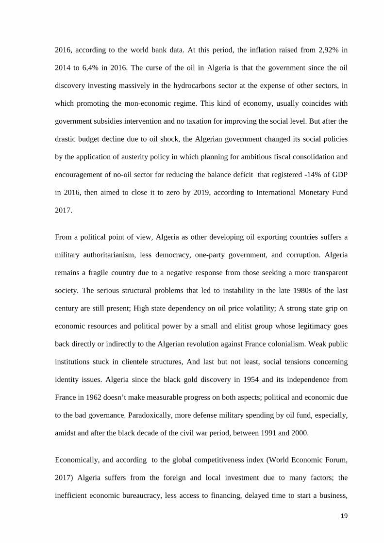
The UAE implied on the impact of the climate change for the long-term food security,

through a program launched by the environmental agency of Abu Dhabi in 2013 known as “

Local, National, and regional climate change (LNRCC) program ”. The program aims to

reduce the risk of climate change and the agricultural productivity shock in National (UAE)

and Regional ( GCC) countries. The climate change will contribute to the rise of the food

price until 84% in 2050, Particularly the core foods as wheat could increase by 34,4%, Rice

about 58,6% and Maize at 72,2% ( Nelson & Al, 2010 ). Econometrically, The constrained

food imports under the climate change could be estimated by this equation:

“ Unconstrained,” for Rmin – Amax ˂ 0 and Amin – Rmax ≥ 0

FIS = “ Partially constrained,” for Rmin – Amax ˂ 0 and Amin – Rmax ≤ 0

“ Constrained,” for Rmin – Amax ≥ 0

Where:

FIS: Food import status.

R min is the minimum required food import volume based on population projections.

R max is the maximum required food import volume based on the maximum population

growth scenario.

A min is the minimum actual food import volume available based on the climate change

scenarios.

28

A max is the maximum actual food import volume available based on the climate change

scenarios.

Saudi Arabia: The kingdom’s arable land estimated at 1,63% (236026 ha) and the

agricultural land about 80,78% (3502000 ha), According to trading economics. The food

imports dependency in 2013 nearly for 80%. The importation increased rapidly passing from

$9,2 Billion in 2000 to $39,6 Billion in 2015. Its primary partners are; India, Brazil, United

Arab Emirates, USA, Egypt, Germany, and France ( Graph 4). Agriculture in Saudi Arabia is

suffering a shortage of rainfall that the average is less than 100 mm/year in normal conditions.

At the same time, the kingdom among the few countries where the temperature in summer

surpasses 50 C°. These climatic conditions make the agricultural sectors limited to some

products as date palm, fodder, barley, wheat, melons, and tomatoes. The agricultural GDP see

also a sharp decline in the last decade that decreased from 5,2% of GDP in 2000 to 2,26% in

2015 that means regression of agricultural local and foreign investment. Furthermore, the less

agricultural labor force that estimated in 2015 by 6,1% of total employment, according to the

world bank.

$0,00

$500.000.000,00

$1.000.000.000,00

$1.500.000.000,00

$2.000.000.000,00

Graph 4. Saudi Arabia food import partners in 2015Source: UN Comtrade.

29

Saudi Arabia as all Gulf and MENA countries suffers the water scarcity and desertification in

which the food commodities could arrive at 100% of importation by 2050. The challenge of

the kingdom’s government is how could secure the food production amidst the threat of water

scarcity where agricultural used about 88% of the total water consummation (Fiaz & Al,

2016). The agriculture water resources coming from conventional resources formed by water

surface by 2,4 Billion Cubic Meter ( Billion m3 ) per year that mainly located in the west, and

groundwater by 2,2 Billion m2 that usually supplied by the infiltration of water surface where

the total renewable water resources about 6 billion m3. The non-conventional water consists

by treated wastewater for 730 Million m3 and sea water desalinization in which the Saudi

Arabia is the largest producer of desalinized water by more than 1 Billion m3/ or 26% of the

total world’s seawater desalination (Ouda, 2013).

Saudi Arabia for securing its long-term food demands installed a project for agricultural land

investment launched in 2009, year after the world food supplies and price crisis, known as

“ King Abdulla’s initiative for agricultural investment abroad ”, aiming to support the staple

commodities; rice, barley, wheat, sugar, corn, green fodders, and animals resources in which

the Saudi star agricultural development in 2010 signed the largest Ethiopian lease agreement

by 10,000 hectares for rice farming, where investing about $2,5 Billion until 2020 and expect

to acquire extra 290,000 hectares until 2060. In Zambia, Saudi Arabia invests around $125

million for pineapple fruit production. In Sudan, The kingdom’s considered the largest renter

of agricultural where 1 million acres approved by Sudanese national assembly in favor to

Saudi Arabia for 99 years of land investment, and for water security three dams should be

constructed in the north of Sudan; The Kajbar, Dal and Al-Shiraik dams by an amount about $

1,7 Billion. Additionally, $500 million for others water and electricity projects. In Pakistan,

Saudi Arabia leased more than 500,000 acres or (1,25 million ha) of land, and approximately

$ 46,2 million of agricultural investment. Privately, by Almarai, the largest dairy company in

30

the middle east, the kingdom’s bought about 1,790 acres in Blythe, California along Colorado

river to grow fodder in which the land cost around $31,8 million. Another 10,000 acres

nearby Vicksburg, Arizona for around $48 million. Saudi Arabia, together with other Gulf

countries, looking for 1 million hectares for wheat production in Australia. In Indonesia, the

Saudi Arabia’s Bin Laden Group invest around $4,3 Billion for 2 million hectares of

farmland. But despite these efforts, some opponents consider these kinds of investments a

new sort of “land grab or neocolonialism .” At the same time, Saudi policy outlooks for more

agricultural land investments in other countries as Turkey, Philippine, Ukraine, Brazil,

Vietnam, and Kazakhstan

Angola: Angola possesses tremendous agricultural potential by approximately 47,5 million

hectares of farmland of which 3,5 million available arable lands, according to World Bank

2015. Notwithstanding, enormous Angolan capacities with the highest rural population in

Africa, Angola exploited only 4 million hectares of its agricultural land that means the

country enable to generate its local resources. Agricultural share GDP about 12% or around

$102 billion of the total budget. Angola in the last years shows a significant enhancement that

the Agri-GDP increased from 4,6% in 2008 to 9,9% in 2015, According to the domestic

authorities. Paradoxically, before this period, and during the civil war, the no-investment and

abandonment of the agricultural sectors induced more dependency on importation and food

aid by United Nations. The Angolan food imports record more than 50% that estimated by

$2,22 billion in 2015. The principal export partners; Portugal, Brazil, South Africa, USA,

Belgium, and Turkey ( Graph 5). In the same time, Angola export some products as; coffee,

sisal, banana, sugar cane, and cotton in which over 90% of local agricultural production by

familiar farmland.

Ecologically, Angola possesses two types of climate; heaviest rainy in the north by up to

1,800mm annually, and warmer particularly in the south. The southern Angolan agriculture

31

suffers from the drought that caused a loss estimated at $242,5 million in 2015, and about

500,000 heads of livestock died in 2016. At the same time, the cereal production registers a

deficit by 40%. However, this grim situation affects the food security of about 1 million

people and could have an impact on more than 400,000 in the future that will suffer the food

deficiency. Furthermore, Angola suffers the climate change.

According to the projections of Intergovernmental Panel on Climate Change (IPCC), the sub-

Saharan countries could have the greatest temperature rise in the world combined

systematically with the high decline of rainfall ( Ringler & Al, 2010). Currently, Angola has

not a problem of water scarcity that possesses 47 rivers basins in which the agricultural

sectors consume about 61,5% of the total water, according to Aquastat FAO.

Recently, Angola for securing its local food sovereignty invested about $2 Billion in the

agricultural industry in 2009, then installed the National development plan ( NDP 2013-17)

by 7,5% of the budget for improving irrigation systems, supporting farm cooperatives and

fisheries industry ( Muzima & Gallardo, 2017). In the same time, the country invests in the

infrastructure for mobilizing the agricultural activities. Furthermore, Angola received about

$0,00

$100.000.000,00

$200.000.000,00

$300.000.000,00

$400.000.000,00

Graph 5. Angola food import partners in 2015.Source: UN Comtrade.

32

$70 million from the World Bank in 2016 to increase smallholder agriculture, technical

competence, and management. In 2013, the Indian government credited about $37 million for

boosting agricultural industrialization in Angola. As well, in October 2015, China by its two

multinationals Hassan and Forever Groups committed to investing a combined amount of

$650 million in Angola’s agriculture aiming to build new firms, and personal training centers

for producing cassava, tomato, Maize, and wheat, according to Forever Green manager Wam

Xan.

Despite these efforts, Angolan people until today suffers from the malnutrition in which

Angola considered the highest world’s under 5 years old mortality rate by 167 death per 1000

live births in 2013, and the Angolan stunting children estimated at 20% in 2012 or around

820,000 child. For minimizing this dramatic situation, the European Union and non-

governmental organizations gave donors to Angolan government for inducing the nutrition

quality and reducing the children mortality in which should be decreased by 10% until 2025,

according to the European Commission.

Nigeria: Nigerian farmland about 85 million hectares in which only 40% cultivated ( Onuka,

2017). Nigeria among the largest producers of some cultures in Africa as; cassava, cocoa

beans, palm oil, palm kernels, groundnuts, bananas, rice, rubber, and sorghum. In 2015 the

agricultural share GDP estimated at 24,18% of total GDP where about 70% of population

engaging in agricultural sector (Odeh, 2011). Agriculture in Nigeria suffering the logistic

problems due to the poor manufacturing, poor transportation, bad food conservation quality,

and bad packaging. Resultantly, Nigerian agriculture suffers from non-sustainability farming.

In 2016, Nigeria spends around $20 Billion for food imports, particularly for the largest

consuming products as; wheat, sugar, rice, dairy products, frozen fish, and vegetables. The

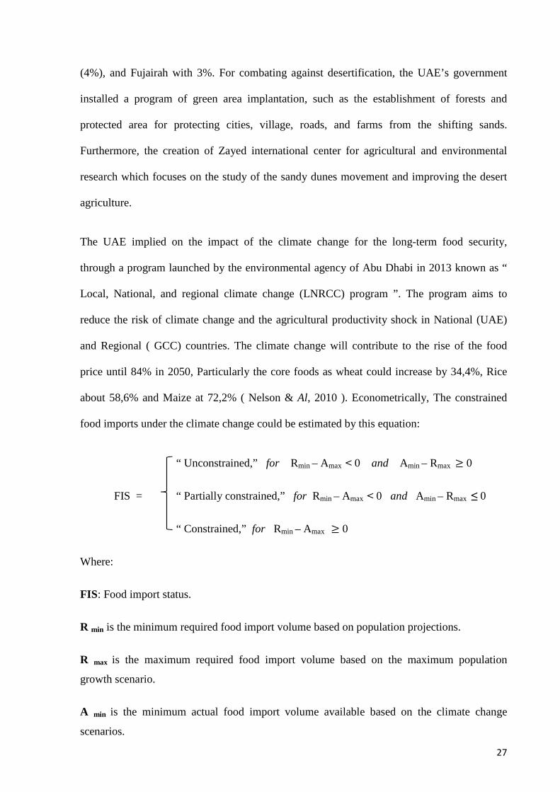
major’s partners are; Asia by 44,6%, European Union (33,6%), Americas (14,1%), Africa

33

(6,5%), and others by 10% ( Graph 6). The total food imports (% of merchandise imports)

estimated at 17,03% in 2014, according to the world bank.

Nigeria possesses a potential of water resources by 267,7 billion cubic meters (BCM) of

surface water and 57,9 BCM per underground water ( Odetola & Etumnu, 2013). But

regrettably, 66 million people have not access to water potable, according to UNICEF. In

2016, the government for reducing the severe water shortage and progressing the water

availability whether agricultural or urban around the all country, implemented 116 water

projects; 41 water supply projects, 38 irrigation projects, and 37 dams, according to the

minister of water resources. But regrettably, 66 million people have not access to water

potable, according to UNICEF.

In Nigeria, The agro-food production in the rainy seasons generally in the favorable agro-

climatic seasons ( Autumn and summer ). For improving the agricultural sectors, Nigerian

government and FAO launched an project of Youth Employment in Agriculture Program

2013-2017 (YEAP) by an amount around $235 million, aiming to implement 750,000 young

farmers and agribusiness entrepreneurs. The FAO’s expertise administration in Nigeria seeks

$0,00

$200.000.000,00

$400.000.000,00

$600.000.000,00

$800.000.000,00

$1.000.000.000,00

$1.200.000.000,00

Graph 6. Nigeria food import partners in 2014.Source: UN Comtrade.

34

to improve nutrition security and public food, support for agricultural policy and regulatory

framework, support for the agricultural transformation agenda (ATA) and promote

employment for youth and women, sustainable management of natural resources, improved

disaster risk reduction, and emergency management ( FAO, 2015). The U.S. Agency for

International Development (USAID) invests nearly $60,5 million for incentivizing the

smallholders farmers toward a new markets by a project called MARKETS II that focused on

cocoa, cassava, rice, sorghum, soybeans, maize and aquaculture (Downie, 2017). Moreover,

the Nigerian richest man in Africa ( by $12,1 Billion of wealth ) planning to invest about $4,5

billion for farming ( $3,8 Billion for sugar and rice, $800 for dairy production). Aiming to

produce 1 million tons of rice per year by cultivation about 350,000 hectares of farmland, and

1,5 million tons of sugar through 200,000 hectares, at the end of 2020. In another side, 500

million liters of milk per year by 2019, according to Bloomberg Markets.

Like the majority of fuel exporting countries, Nigeria before the oil discovery possessed food

self-sufficiency, but after this period, Nigerian people suffered from many crises of nutrition,

Notably, the crisis of 1976, due to the exponential rise of population, and negligence of

agricultural sector. Immediately, in the same year, the government launched the plan of

“Feed Nations” (1976-1979), and strengthened after by the “Green revolution.” In the decade,

exactly in 2001, the government looked for a new ambitious agricultural strategy by “ New

agricultural policy on agriculture.” In which under this policy, there are two pillar programs.

Firstly the program of “ National Economic Employment and Development Strategy” (

NEEDS II 2008-2011), aiming primarily for combating the highest level of poverty in which

112 million of Nigerian people living under the poverty line or about 67,1 % of total

population. The other wider program “ National Food Security Programme NFSP 2008 ”

looking for achievement the national food guaranty by ensuring the availability and

accessibility of quantity, even quality food for all citizens.

35

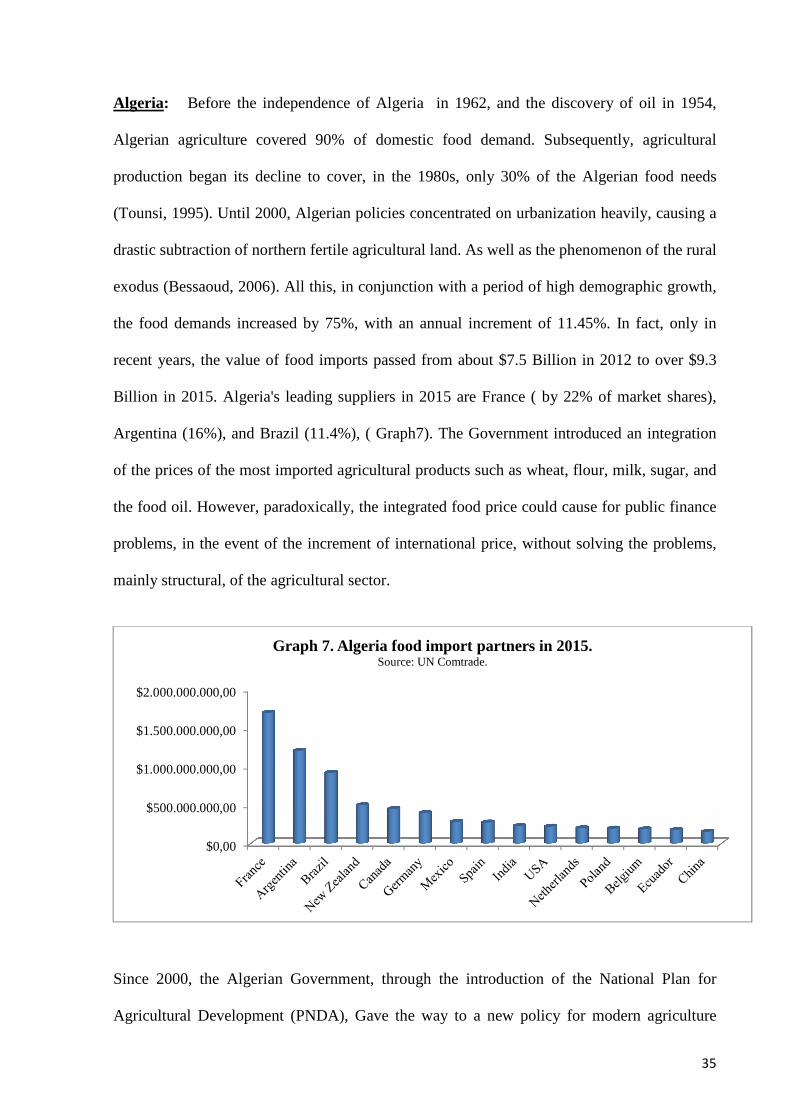
Algeria: Before the independence of Algeria in 1962, and the discovery of oil in 1954,

Algerian agriculture covered 90% of domestic food demand. Subsequently, agricultural

production began its decline to cover, in the 1980s, only 30% of the Algerian food needs

(Tounsi, 1995). Until 2000, Algerian policies concentrated on urbanization heavily, causing a

drastic subtraction of northern fertile agricultural land. As well as the phenomenon of the rural

exodus (Bessaoud, 2006). All this, in conjunction with a period of high demographic growth,

the food demands increased by 75%, with an annual increment of 11.45%. In fact, only in

recent years, the value of food imports passed from about $7.5 Billion in 2012 to over $9.3

Billion in 2015. Algeria's leading suppliers in 2015 are France ( by 22% of market shares),

Argentina (16%), and Brazil (11.4%), ( Graph7). The Government introduced an integration

of the prices of the most imported agricultural products such as wheat, flour, milk, sugar, and

the food oil. However, paradoxically, the integrated food price could cause for public finance

problems, in the event of the increment of international price, without solving the problems,

mainly structural, of the agricultural sector.

Since 2000, the Algerian Government, through the introduction of the National Plan for

Agricultural Development (PNDA), Gave the way to a new policy for modern agriculture

$0,00

$500.000.000,00

$1.000.000.000,00

$1.500.000.000,00

$2.000.000.000,00

Graph 7. Algeria food import partners in 2015.Source: UN Comtrade.

36

(Bessaoud 2006). Between 2001-2004, to ensure the food security of the country through the

PNDA, more than €600 million was disbursed for the relaunch of the agricultural sector, for

promoting farms employment with the improvement of the socio-economic conditions of

farmers, and enhancing the sustainable management of natural resources ( Khiati, 2007).

The PNDA, in 2002, was enlarged to the National Agricultural and Rural Development

Program (PNDAR). This program is looking for ensuring the preservation of natural

resources and aims to revitalize rural areas through the modernization of the agricultural

sector by the improvement of the living conditions of the rural population (Akerkar, 2015).

The main relevant instrument that has adopted for rural development is “Integrated Rural

Development and Projects of Proximity” (PPDRI), it has been set up to strengthen local

development activities, especially from a structural point of view.

In recent years, the Ministry of Agriculture and Rural Development relaunched the

“Agricultural and Rural Renewal Policy” Whereas, from 2008 until 2014, implements more

ambitious policy than the previous programs. In fact, highlights the urgency of revitalizing

Algerian agriculture to ensure food security but also to make it the force for the economic

growth. The first phase of this new policy, which commits the five-year period 2010-2014, is

based on three pillars: The agricultural renewal, rural development, and the program for the

strengthening of human capacity and technical support to producers (PRCHAT) (Maghni,

2013). According to the Ministry of Agriculture, Rural Development and fisheries, the

agricultural renewal could be achieved through the modernization of the agricultural sector to

increase production and productivity. Moreover, the integration of 10 priority products such

as Cereals, raw milk, dried vegetables, potatoes, olive cultivation, industrial tomatoes,

arboriculture, date palms cultivation, red meat, and aviculture. All this will have to go through

the establishment of a regulated market system (SYRPALAC) which has a primary purpose,

the guaranty of the internal supplies of broad consuming products (Cereals, milk, oil,

37

potatoes, tomatoes, and meat) and protecting the farmer’s income. The achievement of this

object requires the implementation of specific measures for the facilitation and protection of

the agricultural activity, such as the possibility for farmers to receive interest-free loans

(RFIG); Strengthening of leasing credit for the purchase of farm machinery and materials;

Insurance to compensate for any reductions in income as a result of natural disasters (FGCA);

Strengthening the communication between actors in rural areas to facilitate the exchange of

skills; Support for the professional organizations; Improvement the mechanisms of food

production, and improvement the security of the agricultural territory.

The “Rural development”, second pillar of the new agrarian reform, based on an innovative

approach, represented by the “ Integrated Rural Development Project” (PPDRI). Rural

development is primarily focusing on disadvantaged areas where the production conditions

are more challenging as mountains, steppes, and Sahara. Also, aiming for more efficient forest

management to facilitate the control of fires. The further goal of rural development is the

involvement in the national economy through the promotion of local resources and typical

products, so far neglected, as a potential source of agricultural export. Rural development

based on five programs, such as protection of river basins; Management and protection of

forest heritage; Combating the desertification; Protection of natural spaces, and development

of the territory.

Finally, the program for strengthening human capacity and technical support to producers

(PRCHAT), is an action mainly aimed at innovation in the agricultural sector, Increasing

investment in research and development, and improving training to facilitate the development

of new technologies and its rapid transfer to farmers. Other goals of the PRCHAT programs

are; Strengthening of the material and human capacities of all institutions and organizations,

enhancement of monitoring and protection services, veterinary, and phytosanitary certification

services for seeds and seedlings.

38

The action plan of the government, scheduled for the five-years 2015-2019, with an annual

appropriation of €2,8 Billion, it provides for the development of infrastructure and the internal

policy for encouraging the national and foreign investments. To achieve, in the next five

years, an annual average growth of the agricultural sector, greater than 13%. This aim could

be achievable through the implementation of technical measures such as the increment of

irrigated surfaces by about one million hectares, reinforcement the mechanization, using of

highly productive propagation material, strengthening olive cultivation areas (from 370,000 to

1 million hectares), developing the infrastructure. Besides, the new program of the Algerian

Government provides the enhancement of the administration, and regional institution for

secure the implementation of agricultural and rural development programs.

Eventually, the strategy of the agri-food industry (IAA program), Promoted by the Ministry of

Industry set as the primary goals, the intensification of the industrial food fabrication, through

the creation of 500 modern companies that must comply with the food safety standards

required by foreign markets (ISO 22000 standards). The IAA strategy also provides for the

establishment of five export consortiums and reduction of the food importation.

2.2. The post-petroleum food system in the developing oil-wealth countries.

The developing oil-wealth countries are unstable economically; therefore, this situation is

risky for their food system and puts in front of a twofold question: In an era of oil scarcity,

what will be the future of the agro-food system?. Also, in a time of post-petroleum, how can

the policymaker diversify revenue? The lack of crude oil means that the government will not

be able to respond to socio-economic challenges in the coming years without implementing a

policy of diversification to maintain the economic balance, what could generate an financial

and social crisis as has happened in the past in some oil-exporting countries.

39

The supply of food has been obtained, for decades, through imports. This trade was financed

almost exclusively by the income from the petroleum industry. But in the era of oil scarcity,

the oil-rich states should be thinking about other economic models for additional revenue to

secure the domestic economy. The agricultural sector could be the proper alternative where

the industrialization sector in the developing countries is limited. About this critical situation,

Awokuse & Xie in 2015 posed this question: Does agriculture matter for economic growth in

developing countries?. The agricultural power could contribute for guarantee the internal food

sovereignty and enhances the national budget. For imagine a new model of development no

longer focusing solely on the extraction of crude oil, an important role could, and should, take

on the agri-food sector.

In our study could see six nations that have many similar macroeconomic and environmental

characteristics that possessing high income from hydrocarbons, but varying between it about

the external food dependency. Could see a direct relationship about oil revenues and volume

of food imports in which, immediately, after the fuel shock price in 2014, the quantity of the

agro-alimentary imports decreased sharply and could continue to drop by the fall of oil price

that means the food security closely ligated to hydrocarbons revenues. In another side, the

figure (Graph 8) represents the similarity trend of the food imports between the six states in

which influenced by the fluctuation of the oil revenues. In the same time, could see a

significant similarity between hydrocarbons revenues trend ( see Graph 1) and food

importation trend.

40

From a critical point of view, many others questions could pose, that how can finance the

agricultural projects in the epoch of fuel paucity?; and how long time the sustainable

agriculture will be dependent on rentier income? For responding to these crucial questions,

the political system forcedly should thinking for a long-term financial strategy, in which has

been absent for decades. Without a diversified economy, it will be difficult to secure the

future food system. The challenge of the oil reserve decline combined with environmental

degradation, and the over-increment of the population don’t predict well for the future of the

world’s food security (Wright, 2009). On the other hand, the additional challenge could be the

biofuel economy in which the farmers could be motivated to investing in the biofuels

production, leaving the farmlands to avoid the sharp food price volatility and the climate

impact. Naylor & Al in 2007 expected the price volatility in the era of biofuel economy in

which the wheat price could fluctuate between (2.5% to 65%), corn (2.5% to 65%), sugar

(-8% to 66%), and soy (-11% to 76%). Moreover, 2 to 2.5 billion world’s people living by $1

to $2 per day under the risk of the food insecurity due to the continuous rise in food price.

$0,00

$5.000.000.000,00

$10.000.000.000,00

$15.000.000.000,00

$20.000.000.000,00

$25.000.000.000,00

$30.000.000.000,00

$35.000.000.000,00

$40.000.000.000,00

$45.000.000.000,00

Saudi Arabia food import

UAE food import

Algeria food import

Nigeria food import

Qatar food import

Angola food import

Graph8: Food importation from 2000 to 2015

41

3. State of the art in the study of international trade

This chapter proposes an analysis of the main economic models formulated for the study of

international trade, some of them constitute the theoretical foundations on which the gravity

model based. It then described how this model works and the how empirical enrichment

proposed over the years. Finally, a review carried out on the insertion of barriers to trade, both

tariffs and not, in the gravity model.

3.1 THE STUDY OF INTERNATIONAL TRADE

Several models try to explain the motives that lead two countries to market among

themselves. The simplest of these is the Ricardo model. In this model, the work is the only

productive factor, and countries differ only in labor productivity in different sectors.

Relatively, the country’s export goods that produce high efficiency and import those which

provide low efficiency. In other words, the production model of a nation determined by its

comparative advantages.

Since resources are scarce, in production there is a trade-off. When used all the working hours

available to produce a higher quantity of the good x, is necessary to give up part of the

production of y. The model explains how trade brings benefit to both nations in two ways;

The first is to think of trade as a method of indirect production. Instead, producing an asset

autonomously, a nation can produce another good and market it with the desired good. The

model shows that every time an asset imported is worth the principle that the “indirect

production” requires less work than direct production. Secondly, the trade increases the

consumption possibilities of a country, which implies a benefit from the trade. The

distribution of benefits from the trade depends on the relative prices of the goods that a certain

nation produces for determine these relative prices, is necessary to refer to the global supply

and demand.

42

In the Ricardian model, the trade leads to an international specialization, where each country

shifts its workforce from the industries where are relatively inefficient towards those where

are relatively more efficient. Since the work is the only productive factor in the model, and

that assumed its mobility without cost between one industry and another, there is no

possibility to be damaged by trade. Consequently, the Ricardian model suggests that not only

all countries could take advantage from commerce, but also every individual should increase

his welfare because the trade does not affect the distribution of income.

However, considering the work as a single production factor leads to limitations, because the

specific resources of the countries not taken into account. There is a theory, initially

developed by Eli Heckscher and Bertil Ohlin, which explains how international trade strongly

influenced by differences in resources between countries. The developed model takes the

model name Heckscher-Ohlin (HO) or Heckscher-Ohlin-Samuelson (HOS), by the name of

the Economist Paul Samuelson. The essence of the model that the trade conditioned by the

difference in the abundance of productive factors between countries, and leads to formulate

four predictions: a) The HO theorem: A country tends to export the good that uses more

intensely, the factor of which is relatively more abundant; b) The price equalization Theorem:

With diversified productions, the international trade equalizes the prices; c) The Stolper-

Samuelson theorem: Keeping the production factors fixed, an increase in the relative price of

an good generates an increase in the real output of the factor, in which used more intensely in

the production of the good in question. In the same time, reduces the output of other factor; d)

The Rybczynski theorem: By keeping the prices of goods fixed, an increase in the assignment

of a productive factor generates a more proportional increase in the production of the good

which uses that factor intensely (at the same time, a reduction in the production of the other

good that uses the increased factor with less intensity).

43

The model with specific factors, developed by Samuelson (1971) and Jones (1971), as the

Ricardian model, assumes an economy that produces two goods and that can distribute the

workforce in two sectors but has the difference to allow the existence of production factors

other than work. Given an economy that produces two goods x and y, which require the use of

two or more production factors, unlike the model of Heckscher-Ohlin, the model with specific

factors foresees that only one factor, the work, can be moved freely between the production of

one of other good. The other factor remains fixed, and for this defined as specific. The

international trade has essential effects on the distribution of profits between nations, and

therefore the actors can profit as losses from the trade. The theory behind the model has

specific factors that the different distribution of profits born for two reasons: The first is that

the production factors cannot be moved instantaneously and without cost from one industry to

another, while the second is that the change in the mix output of a given economy has effects

on the demand for different production factors. The specific factor model allows a distinction

between generic-use factors (which can be moved between sectors) and factors that are

specific to certain uses. In the model, the differences in the level of resources can involve

divers offering curves between nations, and consequently cause international trade.

There is then the monopolistic competition model, which provides for an imperfect

competition where one or more producers sell products that are differentiated from those

competitors who are not perfect substitutes. here are six characteristics that distinguish the

monopolistic competition (Goodwin & Al., 2009; Hirschey., 2000): a) the products between

them are differentiated; b) There are many companies in the market; c) There is the freedom

to enter and exit the market; d) Enterprises take their decisions independently, as they were in

a monopoly situation; e) Companies have market power; f) Sellers and buyers do not have the

perfect information.

44

In the monopolistic competition an enterprise takes as data the prices set by its competitors,

and at the same time ignores the impact of the price of its products on other companies

(Krugman, 2011). In such market, enterprises could have a kind of monopoly in the short term

due to product differentiation, and they can also use this market power to generate profits. In

the long term, with the entry of other companies into the market, the benefits derived from

differentiation decrease by the increase of competition, and companies could not benefit

economic profits. This is because the monopolistic competition model provides for barriers

limiting the entry and exit of the actors, as a result, when the price of the asset exceeds the

average costs, occurs the entry of new companies in the sector, while when the price is less

than average costs occurs an exit. This process of entry and exit leads in the long run to have a

profit of zero.

In the monopolistic competition model, each country will export classes of differentiated

products with other countries. Although the industries of the different states can theoretically

produce different categories of products, as seen from the models of the international trade

occurs in practice a specialization that leads to maximization of the profit. The business of

these products called “Intra Industry Trade”-IIT.

In the monopolistic competition model and the model of (HO) with the continuum of goods

expected the existence of many more assets than factors; This assumption allows the full

specialization in different classes of products between countries. In this case the determinants

of trade can be described through a relatively simple equation called “gravitational equation”

which is described below.

45

3.2 THE BASIC CONCEPT OF THE GRAVITATY MODEL FOR THE STUDY OF

INTERNATIONAL TRADE

The use of the gravity models for the estimation of international trade dates back to 1962,

when Jan Tinbergen began an extensive empirical literature on gravitational equations for the

study of world import-export. Since then, these have been widely used in the analysis of

bilateral flows between different geographic regions.

The theoretical concept that the model refers to the “universal gravitation Law” proposed by

Newton in 1687. In this, it stated that the attractive force between two objects i and j is equal

to

��� = � �����

Where ��� is the attractive force, � � are the masses of the two objects, and Dij is the

distance. G is the universal gravitation constant, which depends on the units of measure of

mass and strength.

In 1962 Tinbergen has, therefore, resumed the same functional formula, applying to

international trade flows. This was also repeatedly used in conjunction with a wide range of

those that can be called "social interactions", including migratory flows, tourism and foreign

direct investment. This new gravitational equation for social interaction can approximate in

the following way:

��� = � �����

��

Where

46

� ��� is the flow from source i to destination j;

� �and � are the size of their economies. If F measured as a cash flow (e.g., Value

of export), usually M measured as gross domestic product (GDP) or gross national

product (GNP) of each region.

� Dij is the distance between the two regions (usually measured between the

respective centres).

Noting that, returning to the previous Newton equation: α = β = 1, and θ = 2.

3.3 ECONOMIC EXPLANATION OF THE GRAVITY MODEL

The gravitational equation can be thought as a schematic representation of the forces of

supply and demand. If i is the country of origin, Mi represents the total amount of an good

that is willing to provide to all its customers, while Mj is the total demand of the country Mj.

The distance acts in terms of transaction costs, imposing trade charges and lowering the level

of equilibrium of trade flows.

Recently (starting from Anderson, 1979) there were several attempts to derive the

gravitational equation formally; then the theoretical bases of Anderson are reported:

If Mi is the total expenditure of the country j for all assets of any source i , and Sij is the

share of Mj expenditure for goods of the country i, then Fij = Sij Mij . Accordingly Sij:

1. Must be between 0 and 1.

2. It should increase if i produce a wide variety of goods (wide ni) and/or produce goods

that perceived as high-quality (large µ).

3. Should decrease with the presence of trade barriers, such as distance, Dij .

In the light of these arguments it is obtained that:

47

��� = ����,��,��∑ ����,��,����

where the g(.) function should be positively correlated with the first two arguments, and

inversely correlated with the distance, for all i ��� ˃ 0.

At this point, necessary a specific form for g ( ). An approach proposed by Bergstrand (1989)

uses the monopolistic competition model of Dixit and Stiglitz (1977), for different but

symmetric companies. This model fixed ��= 1, and makes �� proportional to Mi. A second

approach proposed by Anderson takes a single asset from each country, ��=1, but allows to

enter a parameter of preference ��that can vary between subjects, depending to the constraint

of the market. The differences must also be proportionate to the size of the Mi economy. Both

of these models allow to consider the costs for trade as an exponential function of the

distance.

Allowing the variation of n and �between countries, obtaining that:

���� , ��� = ∑ � ��!/���!�#$%��!&#

Where is the price, and ' indexes the particular substitutable varieties with the elasticity of

substitution given by (. If the goods of a given country are differentiated but of the same

average quality, and subject to the same cost of transport, then it is possible to eliminate the

parameter ' and establish �() = ��� ��/����#$%

The next step is to relate the final price (adjusted with the quality factor) with the price in the

country of origin and the costs of transport between source and destination. The assumption

report as follows: +��/��� = ( �/��),��-

48

The price of Origin +��, is often considered as the FOB price (free on board). In the basic

gravitational model are not considered price differences. This is not totally unrealistic as it

initially might seem (Head, 2003), however it is required that the FOB price varies

proportionally to the quality of the exporting nation's product, in other words that �/�� ≈

/.

It is not possible to observe the number of varieties in each country directly. It is preferable to

use the property of the model Dixit-Stiglitz, means that all companies with the same size. In

this case, �� = �/1where 1 is the size of the enterprise. By imposing this last assumption,

defined as: 2 ≡ 4(( − 1) ≥ 0 obtaining that �() = ��� ��/����#$%

This implies that the market share for exporter i in Country j is: ��� = �,�,��$%8�

where 8� = 1/(∑ 99 ,9�$:. Substituting and adapting the terms, obtaining a very similar

result to the departure equation: ��� = 8� �����

The main difference is that now the term Rj replaces the gravitational constant G. As a result

would have that: 8� = 1/∑ 9 =9 1/ ; <���∗ = � �/ ; ( Dove > represents the

world).

3.4 THE ESTIMATION OF THE GRAVITATIONAL MODEL

The multiplicative nature of the gravitational model involves the possibility of using the

natural logarithm and obtaining a linear relationship between the logarithm of the trade flows

and those of the size of the economy and the distance.

?���� = @?� � + B?� � − 2?�,�� + ?�8� +C��

49

The OLS regression ( Ordinary Least Squares regression ) could estimate the stochastic

equation (including the error term C��) . If the assumptions made previously are accurate, is

reasonable to expect the estimation of @ = B = .

3.5 DIMENSION OF THE ECONOMY

The economic dimension of the exporting and importing country, Mi, Mj are generally

measured as gross domestic product. Generally, the estimated coefficients are not

significantly different from the value of one, but is not normal to obtain predictive estimates

in a wider range, ranging from 0.7 to 1.1. However, it should point out that in the economic

model the empirical formula of the gravitational equation assumes a coefficient equal to one,

consequently, lacking a theoretical interpretation for coefficients that deviate from this value.

There are also other problems that result from the use of logarithms of Mj and Mi as

regressors. The first is high collinearity (Head, 2003), at the moment where is difficult to

imagine the world’s large economy do not trade more, in absolute terms. Secondly, since

export and import are part of GDP, there is always a relationship between ���, �, and �.

Also highlighted by McCallum (1995), which reports a problem of endogeneity in the use of

gravitational models because the dependent variable (the export) is the component of one of

the regressors (GDP). Some studies tried to solve the latter problem by using the instrumental

variables method, for example, inserting the population as an instrument instead of GDP. A

simple solution is to impose unitary elasticity. This involves to moving the term refers to the

income in the left part of the equation. Subtracting ?� � + ?� � − ?� ; on both sides,

getting that:

?�����/���∗ � = ?� ; + ?�8� − 2?�,�� +C��

50

The dependent variable measures the deviation of the current commercial flow from the ideal

one which would occur in the absence of friction. The sum of the first two terms on the right

side estimated as a regression constant; This means that the variation shown as an error. There

are two statistical tests allow to verifying, if the data reject the hypothesis of the absence of

restrictions on trade statistically. One of these is the statistic (t) on the constant, and the other

is the statistic (t) on θ.

3.6 DISTANCE

The distance is always measured using the formula of the “Large Circle.” This formula

approximates the shape of the earth with that of a sphere, calculating the minimum distance

along the surface.

For calculate the distance have to use longitude and latitude of the “economic center” of each

economic study. The distance obtained by the application of the following formula:

,�� = 3962.6HIJKL([LN�O�. LN�O� ] + [JKLO�. JKLO� . cos (T� − T�)])

Where X is the longitude in degrees multiplied by 57.3 to convert it to gradients, and Y is the

latitude multiplied by-57.3 (if measured in west degrees).

In fact, The main problem of this method that, even in the air transport, the distance measured

by the formula of the large circle underestimate the real distance, at the moment, does not

consider that the most trade routes avoid crossing the North Pole. However, for maritime

voyages, not considered the deviations which made compulsory by the presence of emerged

land and ice blocks. Besides, many air and marine routes are drawn taking into account the

presence of vital nerve centers, the so-called “economic hubs.”

51

Moreover, as various international shipping cartels often lead to a low relationship between

cost and travel distance; Finally, the cost of packing, loading and unloading are mostly fixed

costs and, therefore, do not undergo changes with the distance.

Take together; these elements suggest that the distance should have a slight influence on

trade; however, the distance hinders the trade enormously. An analysis conducted by Head

and Disdier on the estimation of the distance in the gravitational models, starting from 595

regressions reported in approximately 35 works, showed how the elasticity value (θ)

concerning the distance is equal to 0.94. That means the doubling of distance trading roughly

to halve. The study sample covered a historical period from 1928 to 1995, and the trading

partners were mostly nations, although some results have been included on the provinces of

Canada.

Leamer and Levinsohn (1994) researched empirical evidence of international trade,

identifying the effect of distance on international trade as “the clearest and most robust

empirical evidence in economics.” An effect of 0.6 found in their study.

On the grounds of this enormous influence of distance on trade, the economists formulated six

main explanations (Head, 2003):

1. The distance is a transport cost proxy. For several authors, shipping costs (transport and

insurance costs) can explain, in large part, the influence of distance;

2. The distance implies a loss of time during shipping. For perishable goods, the probability

of non-alteration is inversely proportional to the time of transport. The meaning of

perishability can interpret in a rather broad manner, including the following risks:

a) Damage or loss of property due to bad weather or ill-treatment;

b) Decomposition and ruin of organic matter;

52

c) Loss of market (the possible buyer becomes unable or no longer willing to make the

payment).

3. Synchronization costs; When businesses combine different inputs into the production

process, there is a need for these inputs to arrive in time to the appearance of

“bottlenecks.” One possibility to get around this problem is to use stores to maintain a

supply of each input, but this approach has several drawbacks (increased costs,

technological obsolescence, changing tastes, and low pressure on quality controls).

Replenish of inputs from neighboring firms then lowers the synchronization costs;

4. Communication costs; According to Paul Krugman (1991), the distance influences the

possibility of personal contacts between suppliers and customers;

5. Transaction costs. The distance can also link to the research costs of commercial

opportunities and the establishment of a fiduciary relationship between two potential

trading partners;

6. Cultural distance; The increase of the geographic distance leads to the increment of the

cultural distance. Cultural differences can prevent trade in different ways, such as

hindering communications, generating misunderstandings, and contrasts in the form of

negotiation.

3.7 ISOLATION

Several jobs implicitly assume Rj is constant between nations and therefore represent the

intercept in the regression equation. On the other hand, Rj is essential, as it reproduces the

alternatives set of each importer. Countries with different suppliers of goods, which are

generally also those with low Rj values, import less from each specific supplier. Some studies

considered variables such as, referring to them, as “isolation.” (remoteness). However, some

of these measures differ from the correct theoretical Rj, which could be problematic. For

53

example, Helliwell (1998) measures isolation as 8U � =∑ ,9�9 / 9. This method makes

the isolation variable very high if includes distant nations ( high ,9�) , and at the same time,

the small dimensions ( low 9). Because in the literature there is usually θ ≈ 1 (Head, 2003),

a better insulation measurement is 1/(∑ 9�9 /,9). In This formula the dimension of very

distant nations becomes irrelevant. The importance of isolation in current trade patterns can

be easily illustrated, comparing trade between Australia and New Zealand with trade between

Austria and Portugal. The distance between the two major cities of the respective couples is

the same: Lisbon-Vienna and Auckland-Cambera, are among them 1430 miles. Moreover, the

product of their GDP is similar, with that of the two oceanic countries that is smaller than

20%. Consequently, excluding isolation, the gravitational model predict that trade between

Austria and Portugal is slightly higher. In fact, in the year in which the analysis refers, trade

between Australia and New Zealand was nine times higher than that between Austria and

Portugal.

3.8 ENRICHMENT OF THE GRAVITATIONAL MODEL

Although the gravitational model provides good results in explaining trade using only the

economic dimension and the distance between two regions, there is an immense commercial

variability that cannot be explained. For this reason over the years many authors have added

other variables, Although not of the same theoretical basis, only because past studies had

shown that contributed to enrich the empirical formulation. The main are:

Income per capita:

Several authors estimate the gravitational model through the logarithm of the income per

capita ?� /VWV of the importer and exporter countries, including also the logarithm of the

total income ?� (Suaré, 2006; Head and Mayer, 2010; Fieler 2011).

54

The idea behind the use of this variable is that countries with high income generally trade

more. Two possible causes of this fact can attributed to a better transport network (internal

roads, ports, airports, etc.), and generally, to the lower tariffs applied by high-income

countries. On the other hand, a clearing effect may be represented by the fact that the latter

tend be more oriented towards the purchase of services, involving a lower level of trade in

goods for a given level of GDP.

The estimated coefficients of the logarithm of GDP per capita show considerable variations

between nations, ranging from a minimum of 0.2 to a maximum of 1.

Adjacency:

Adjacent or contiguous countries are those that share a border. Several studies include a

variable dummy to identify this proximity.

The estimated coefficients are generally close to 0.5, suggesting that trade increases by about

half in case of sharing a border. It is not clear why the adjacency should be considered

important, if already including the distance in the model. One possible explanation is that the

distance of the states based on two points can lead to an overestimation of the same, because

neighboring countries often have large volumes of trade (Head, 2003). A further theory is

that the adjacency tends to provide qualitative information that allows to discriminate the

distance, instead ,which is a purely quantitative information.

Common language and colonial ties:

These variables resume the theory that the impediment to trade exerted by distance is due to

transaction costs caused by the difficulty of communication and cultural differences. As a

result, it is reasonable to expect that countries speak the same language trading more.

55

Empirical evidence strongly confirms this hypothesis. Two countries with the same official

idiom trade two or three times more than those who do not share any language.

A part of this phenomenon due to the fact that there is usually also a common historical past

that has led the two countries to speak the same language. As a result, colonial bonds are also

positively correlated with trade.

By including these variables as a control, allows reducing the effect of the language, which is

usually still high.

Border Effects:

A more recent literature, begun in 1995 by John McCallum, studies why the frontiers of a

country affect trade.

Regarding the Borderless World, K. Ohmae and McKinsey assert that “National frontiers

have actually disappeared and the economic logic that made them useful lines of demarcation

at first.”

McCallum's examination of Canadian trade determinants shows that, in fact, national

boundaries have a significant effect, since the Canadian provinces trade 20 times more with

other Canadian provinces than American provinces, with the same distance and the same

economic size. The practical example reported by the author considers Ontario's expeditions

to British Columbia (BC) and the Washington State. The distance is the same, but in one case

there is the border crossing while another does not.

In the case the borders have an irrelevant effect, the gravitational model predicts that exports

to the BC should be 60% of exports to Washington due to the size of the two economies.

Instead, BC receives from Ontario a quantity of goods 12.6 times higher than Washington.

56

Consequently, in this case, the effect of the border, defined as current trade divided by the

expected one, is 12.6 / 0.6 = 21.

With the establishment of Canada-US Free trade Agreement The trade between these two

nations increased rapidly, and the effect of the borders fell to an average of 12. Instead,

Anderson and Van Wincoop found more content results, showing how the frontiers reduce the

trade by 29% between industrialized countries.

The effects of borders can also be calculated without intra-national trade flows, which are

available only for a few countries. This method, developed by Shang Jin Wei, therefore

requires estimates of intra-national distances. The effects of borders can also be calculated

without intra-national trade flows, which are only available for a few countries.

Evaluation of favorable trade policies:

Countries often establish preferential agreements with the aim of facilitating mutual trade.

The liberalization agreements between different geographically close countries (e.g. European

Common Market, NAFTA) or not, have rapidly increased since the mid-80.

Generally, the Free trade agreements-FTAs increased the trade by 50%, although a study by

Frankel and Rose (2000) reports how the FTAs lead to triple the trade between the countries

that stipulate the agreement.

3.9 STATE OF THE ART ON THE USE OF GRAVITATIONAL MODELS IN INTERNATIONAL

TRADE

Gravitational models widely used to make inference on the effect on international trade in

distance (Disdier, 2008), Common Borders (McCallum, 1995), Tariffs (Baier and Bergstrand,

57

2007), Technical Barriers to trade (Maskus and Al, 2000), fixed costs to trade between nations

(Helpman, Melitz and Rubinstein, 2008), and other costs to trade.

Gravitational equations used for decades thanks to their outstanding empirical performance

but lacked theoretical foundations until Anderson (1979) that proposed these foundations in

the presence of imperfect substitution between goods. The theory explains that in addition to

an influence exerted by the size of their economies, trade between two regions decreases

according to the existing bilateral barriers, the average trade barrier that has towards all other

partners. Consequently, The more significant is the resistance to trade towards all other

regions, the higher is the push to trade towards a given partner. Anderson also introduced the

theoretical foundations for the use of the gravitational model with constant elasticity of

substitution (CES). The replacement elasticity estimated with a regression of the bilateral

flows on the basis of different control variables and a measure of the costs to the trade. The

coefficient of trade costs is then used as a replacement elasticity between the varieties.

Since the end of the 80, there have been numerous applications of this model, both in its

classical form and including new explanatory variables. In particular, gravitational equations

have been widely used to assess the effects of the various national provisions on trade, such as

tariff agreements, exchange rates, but also the importance of other parameters such as

language, ethnicity, and borders.

Further developments shown the consistency of gravitational equations even in the case of

situations characterized by monopolistic competition (Bergstrand, 1989). Deardoff (1998)

also establishes connections between the Heckscher-Ohlin and gravitational models. One of

the most cited works in the use of the gravity model in international trade is McCallum

(1995), which uses a gravitational equation where the bilateral commercial flow depends on

the outputs of both regions, from their distant and whether or not separated from a frontier.

58

McCallum, otherwise , what was done in most of the literature, does not use data on

international trade to estimate the impact of barriers for trade, but uses a combination of intra-

national and international trade data to estimate the effect of the variable “nation” (and

therefore frontier) between the determinants of trade. To insert a dummy variable into the

equation, which assumes the value one, if deals with trade between state provinces and zero if

instead, the business takes place between region and state abroad. The results show that at the

parity of GDP and distance of two geographic regions, the trade considerably more, if are not

separated from a frontier.

Anderson and Van Wincoop (2003) claim that the original model proposed by Tinbergen has

some shortcomings due to the lack of a variable that measures a hypothetical medium-trade

barrier, which named the “multilateral resistance.” In literature is often not considered this

multilateral resistance, or is included in the variable “isolation”, related to the distance

between the two trading partners. The variable isolation does not captures any of the other

trade barriers, and, even if the distance is the only bilateral barrier, its functional form is in

conflict with the theory (Bergstrand, 1989).

The aims are to solve the “border puzzle” of McCallum, estimating in a first phase the

gravitational equation based on what is proposed by McCallum (1995), but adding the

variables of multilateral resistance. Instead, the second step is to perform a comparative

statistic of general equilibrium, removing the border between the United States and Canada to

determine the effects of borders in international trade. It found that borders reducing bilateral

trade with a substantial magnitude. The results of several study, which show a much higher

border effect is attributed to the fact that (i) consider the effect of frontiers by comparing

intra-national trade with the international one, (ii) that the effect of frontiers is large

intrinsically for small nations and (iii) that the not considered variables push the estimation of

the effects of the borders upward. The Results show once again that the use of the

59

gravitational model in its basic form not only increases the estimation of the effect of the

borders but also produces potential inconsistencies in estimating the level of aggregation

between different Business partners.

Also, a similar approach developed by Head and Mayer (2000), which always takes into

account the multilateral resistance in the determination of commercial flows, but differs from

the model of Anderson to use an empirical specification of two steps, instead, of the fixed

effects for the control of the multilateral resistance. In addition, the model of Head and Mayer

allows to modeling the asymmetry in the consumer preferences, which is the traditional

version of gravity are considered equal for all countries and captured by the fixed effects. This

model used by Olper and Raimondi (2008a) to explain the effects of frontiers in the trade in

agri-food products between the United States, Canada, the European Union and Japan, by

detecting the existence of important asymmetries Market access. The results show an essential

role of policies, information costs and cultural proximity in explanation the incidence of the

border, while tariff and non-tariff barriers can able jointly explain 28% of trade reduction.

The multilateral resistance also included by Xiong and Beghin (2011a) on the effect of

European regulation of aflatoxin on African peanut export. It reported as main problems of

the gravitational models the presence of zero to the trade and the heteroscedasticity, which

makes it impossible to interpret as truthful the elasticities provided by the models log-

linearized. Several estimation techniques used for the gravitational model: the Trun-OLS, the

HMR (Helpman-Melitz-Rubinstein) and the maximum likelihood models. The latter are the

PPML (Poisson pseudo-maximun-likelihood) proposed by Silva and Tenreyro (2006) and the

variants proposed by Burger et al. (2009) To adapt to the large dispersion of data resulting

from the presence of zero: The negative binomial pseudo-maximun-likelihood estimator

(NBPML), the zero-inflated Poisson pseudo-maximun-likelihood model (ZINPML) and the

zero-inflated negative Binomial pseudo-maximun-likelihood model (ZINBPML). Their

60

results resulted in believing the model Trun-OLS lower than the others because of its inability

to explain zeros and access to the market, while the most suitable one proved the ZINBPML

followed by the HMR. Their results have led the Trun-OLS model to be inferior to others due

to its inability to explain zero and access to the market, While the most suitable one proved

the ZINBPML followed by the HMR.

A very bright discussion point on gravitational models is the use of OLS estimates. Silva and

Tenreyro (2006) move a critique to the usual practice of interpreting logarithmic patterns

where elasticity estimated through OLS, which can lead to misleading results in the presence

of Heteroscedasticity. Because the expected value of the logarithm of a random variable

depends on the moments of its distribution. Also, if the errors are heteroscedastic, the

transformed errors are correlated with the covariate. A further disadvantage of the use of the

linear logarithmic model that is incompatible with the presence of zero in trade data, which

leads to unsatisfactory solutions to remedy the problem, such as the elimination of Zero from

the sample or additional nonlinear transformations of the dependent variable. The authors

assert that the gravitational models, with constant elasticity generally, should be estimated in

their multiplication form and propose a method of estimation of type pseudo-maximum-

likelihood (PML). This method able to be consistent even in the presence of

heteroscedasticity, providing an optimal solution even to the problems posed by the presence

of zeros in the dependent variable. Comparing the results obtained with the PML and OLS

techniques using the Monte Carlo method, is highlighted that the latter tends to overestimate

the coefficients of GDP (the PML technique signals them lower than the unit, unlike what is

reported in the classical bibliography using the OLS method), as well as the role of colonial

ties and geographical distance (Silva and Tenreyro, 2006).

However, several authors continue to use the OLS, among these Baier and Bergstrand (2009),

employing this method to approximate the costs of international trade using an equation of

61

gravity type. Helpman & Al (2008) Developed a method for estimating international trade of

gravitational models, which allows predicting positive but also nil trade flows between pairs

of countries, and allows the variation of the number of exporters to a determined Nation.

Allows also decomposing the impact of the clutches on trade in intensive and extensive

margins, where the first refers to the volumes marketed by the exporter and the second to the

number of exporters. This model produces a generalized gravitational equation that allows the

selection of companies in the export market and their impact on the marketed volumes.

Subsequently, the two-step estimation procedure developed that uses an equation to select the

trading partners in the first phase and an equation of the trade flows in the second. This

procedure implemented by parametric, semi-parametric and non-parametric, showing that in

all three cases the effects of the restriction on the estimated trade are similar. By acting in this

way, the authors were able to estimate the extensive and intensive trade margins,

demonstrating that the classical estimates lack objectivity and that most of the alterations are

not due to the selection but to the omission of extensive margins. Among the works that

employ a gravitational model for the study of the determinants of international trade, found

Cipollina e Salvatici (2010) who use a gravity model to estimate the effect of the reciprocal

trade agreements (RTAs) in Trade flows between two partner countries, using a meta-analysis

approach. The results obtained made it possible to reject with the standard level of

significance that the RTAs do no effect in the trade. In particular, time estimates of the

relevant parameters obtained from different studies used as single observations for the

Multiple regression analysis models (MRA), adopting the method of the weighted least

squares – WLS, and testing the Robustness and sensitivity of the results. Subsequently, a

focus is on the effects of specific FTAs on trade, using a probit model to identify which

factors contribute to the positive and significant impact that RTAs possessed on bilateral

trade. The study also criticized the use of the fixed-effect model (FEM) for the estimation of

gravity, since there is a part of the literature that demonstrates the inability to summarize high

62

heterogeneity through an estimation of fixed effects. For this reason, a random effect (REM)

model used.

Raimondi and Olper (2010) Use a gravitational model to study the effect of the elimination of

tariffs in 18 agri-food sectors, in a broad sample of developed and developing countries.

Using the CES Monopolistic competition model introduced by Krugman (1980)

complemented by a rich set of international asymmetries as proposed by Lai and Zhu (2004),

that estimated the elasticity of substitution by simulating the consequences of abolishing

duties. The study shows a significant variation in the estimated elasticity, depending on the

model econometrically used, and in particular that the pseudo-maximum-likelihood of

Poisson (PPML) significantly increases their magnitude.

The results indicate that trade liberalization would increase the importance of exports of

foodstuffs, especially for countries with high GDP per capita, with a consequent decrease in

the market share of the developing countries.

The authors emphasize the extent of their study that the fact of having placed attention

exclusively on tariffs which, although particularly important in the agri-food sector, are not

the only barriers that act on trade. Therefore, suggested to consider also the effect of non-tariff

barriers (NTBs), which remain an important challenge for the analysis of trade, assuming as a

more appropriate approach of the CES with a Gravity model.

On the same line Yue, Beghin and Jensen (2006), Xiong and Beghin (2011b) use a constant-

elastic replacement model to incorporate the heterogeneity of the goods into a gravity model.

Also Arkolakis & Al. (2008) and Feenstra (2009) use an CES model to study the benefits of

international trade, by detecting how in the monopolistic competition model the amount of the

trade depends strongly on only two parameters: The percentage change of household

expenditure as a result of the exchange rate trade barriers, and a gravitational estimator of the

63

elasticity of imports on the variable trade barriers. Liu and Yue (2009), broaden the model of

Yue, Beghin and Jensen (2006) by development a methodology to quantify the combined

effect of the two main non-tariff barriers, using an CES model with a factor that can consider

the technical progress for incorporating changes in the quality of goods.

Henderson and Millimet (2008) Underline how, despite the substantial theoretical foundations

on which gravitational models based on bilateral trade, the empirical implementation requires

different assumptions that do not follow the theory directly. Firstly, the unobserved

commercial costs assumed to be a linear logarithmic function of the observable ones.

Secondly, the effects of trade costs considered being constant between pairs of countries.

Maintaining consistency with the theoretical foundations, but removing the constraints

previously described, the gravitational model estimated with non-parametric methods.

Parametric ones offered an equal or superior reliability regarding of sample prediction and

out-of-sample prediction in most cases. Besides, formal statistical tests do not allow to reject

the presence of the constraints, implying higher efficiency of the parametric models. The

conclusion of Henderson and protector is that the gravitational model, with the assumption

that the costs to trade are linear and homogeneous, is a correct representation of the bilateral

trade. The results obtained by excluding zeros, contrary to what was proposed by Silva and

Tenreyro.

Li and Beghin (2011) Perform a meta-analysis to explain the systematic changes in the results

of the estimates the effects of technical regulations on trade, using different methodologies

and methods of sampling the data. The results obtained show that the agri-food industry tends

to be more affected, or less advantageous, by these measures and barriers than what is

happening in other sectors. The results obtained show that the agri-food industry tends to be

more affected, or less advantageous, by these measures and barriers than what is happening in

other sectors. Moreover, does not consider the “multilateral resistance” increases the

64

possibility of inflating the effects of the impediment to trade due to technical regulations.

Otherwise, is not possible to put the endogeneity potential of trade policies into an opposite

effect, and it can lead to the erroneous conclusion that does not reduce trade. Studies using the

MRL (maximum residual limits) tend to detect a more significant impediment to trade than

other measures and lead to apparent effects of policies since its focused on a specific measure.

Other proxy measures tend to generate confusion in results, increasing the likelihood of

inconclusive results and weak policy implications.

3.10 MODELING OF COMMERCE BARRIER

As mentioned the gravity model can be enriched by several variables, including the most

interesting ones are certainly barriers to trade (tariff and non).

Tariff Barriers:

It is often more complicated than it can initially appear in a gravitational model. In fact, few

countries have a single duty for each of the 6-digit HS codes (HS 6) related to the wine in its

different classes, which bottled, sparkling and bulky. The most common is to find differences

in the levy depending on the alcohol degree or other parameters set by the various national

authorities. The presence of different ranks of levy leads to the need to make an association

between them, to obtain an average data that reflects adequately the tax operated by a state

towards each of its suppliers, subjects also face for HS code 6.

Transformation in ad valorem equivalent.

The aggregation of tariffs is, however, a relatively complicated procedure, and there is still no

universally recognized methodology as the most suitable. A first problem that arises when

comparing the tariff profiles of different countries, often is very duties that not expressed as a

65

percentage on the value. Instead, refer to the quantity or other parameters (as can be for

example the grad of alcoholic in the case of wine). Therefore, in these cases is necessary to

calculate the respective AVE (ad valorem equivalent) to have a set of rates comparable to

each other.

The tariffs converted into the respective AVE by dividing the duty through the unit value of

the asset. Therefore, the problem lies in the choice of the unit value, which encompasses

different complications both from a statistical and methodological point of view.

Theoretically, the duties have a more critical impact on goods of the higher unity of value,

and even if the 6-digit HS classification allows to differentiate very well between different

classes of products, however, is not entirely excluded the heterogeneity between it.

The use of the respective unit values can initially seem very interesting, is entirely consistent

with the size of the collected duties, also allows to operate a qualitative differentiation of the

respective trade flows. On the other side, is more sensitive for errors in the estimation of data

provided by the reporting countries, and is not represented if the magnitude of trade is modest.

Calculating the AVE based on the world average of the import proposed by Gibson & Al

(2001) offers better guarantees regarding the robustness of the data, but without considering

the qualitative differences between products to reflect differentiation between partner

countries, while avoiding the excessive volatility of data. Bouët & Al (2008) proposed a

calculation of the AVE based on the average unit value of world export, calculated from a

group of reference countries of which the exporting member belongs. Then, each nation

included in a group of countries with similar characteristics, defined by a hierarchical cluster

analysis based on GDP per capita (concerning purchasing power parity) and commercial

opening. Using the unit value of the reference group offers three main advantages: (i)

considered the differences in the unit value between countries with different qualitative

preferences, (ii) the problems of endogeneity deriving from the push to vary the quality of the

66

products in response to specific tariffs are more content than those that would be working

with bilateral unit values, since the value calculated on world export; (iii) The use of the

group of countries is more robust for estimation errors than the respective unit value; Being

based on the median is not strongly influenced by outliers. However, once all the tariffs

transformed into its consideration, AVE is a second methodological problem, that is to

summarize it correctly in a single representative figure in case there are more sublines within

the C Odice HS 6.

Data aggregation Methodology

The first approach to aggregating tariffs is to use the simple medium to capture the overall

level, and the standard deviation to measure the dispersion seen as the differential of

observations from the arithmetic average. The use of the average tariff without any weighting

offers, however, different disadvantages. The first of these is that the tariffs have incredibly

uneven distributions, and therefore the average cannot be the most suitable summary measure.

In These cases, the mean value may improperly represent the central tendency, and the most

representative measure could be the median. When the tariff profile has a normal distribution,

the average and the median should be very close, otherwise when the distribution is not

homogeneous both the media and the median can provide useful information. Cases recorded

a high average, and a low median (or the opposite) suggest an extremely high (or low)

protectionist level for a few specific product categories, while most of the tariff lines are low

(or high). Also, Anderson and Neary (2003) criticize the use of simple media, considering it

to be free of foundation and reporting two main problems arising from the use of the same:

To equally treat all commodities and sensitivity to any variations in the HS classification. Of

the same opinion Bouët & Al (2008) which consider the simple average without any

theoretical basis, and therefore advise against its use.

67

The most commonly used methodology for aggregating tariffs remains the use of their

weighted average , using the respective import quota valued at the border. The formula for

calculating the weighted average rate is as follows:

XY = ∑ Z[ ∗ X[

Where XY is the tariff share to valorem of the good k and the weight based on the value of

the import of the good Z[ ∗ balancing to the total import.

Z[∗ =

�\]\

∑ �^ ]

While this equation easy to calculate, on the other hand, this measure suffers from the higher

price of the tariff, the higher efficiency of the restriction on trade, depending on the elasticity

at the price of the application ( Anderson & Al., 2003; Bouët, 2008). There is no apparent

solution to this problem (Bouët, 2008). However, many authors proposed different methods of

weighting tariffs. The first of these is Leamer and Levinsohn (1974), which proposes the use

of world import as a weighting measure. However, if on the one hand this solution is able to

solve the problems of endogeneity, on the other it does not allow to consider the specificities

of the different national economies.

Gibson & Al. (2001), working on a large group of nations, converted all tariffs using the unit

value of world trade to the 6-digit HS code level, while Bureau & Al. (2004) moreover, Jank

& Al. (2002) Used the calculated average price, but the average of the last three years on the

8-digit HS code. The first of these two approaches influenced by some tariff spikes that may

be present within the 6-digit HS code, while the latter has the defect of being able to use only

data from specific countries and no the world average. Therefore, the problem of identifying a

robust methodology but that allows at the same time to discern between the peculiarities and

differences of the individual nations.

68

A solution to this problem proposed by Bouët & Al. (2008) In the construction of the

MAcMap database, where once again used for weighting, import of a group of reference

countries. The import of each group of countries then normalized taking into account the size

of each country.

Unfortunately, this approach, as well as other weighting methodologies that use parameters

other than the national import, cannot be used with a higher level of detail than HS code 6,

since HS codes with 8 or more digits differ from country to another, and therefore are not

comparable.

Non-Tariff Barriers:

The inclusion of non-tariff barriers in the gravity model has also a crucial importance in the

estimation, as reported by Raimondi and Olper (2010). The implications of these measures on

market access mechanisms are generally more complex than a traditional barrier based on a

tax levy, mainly because market imperfections being formed (asymmetry of information,

externalities, etc). Therefore, the non-tariff barriers tend to change the consumer information

set and their behaviour, as well as the behaviour of the producers. For these reasons cannot be

easily transformed into a simple tax or equivalent price (Xiong and Beghin, 2011b). In the

literature, different measures proposed and used to identify non-tariff barriers and to estimate

their impact. However, is possible to classify these methodologies into four main groups:

Estimation by frequency and coverage indexes:

Frequency indexes shall only take into account the presence or absence of the non-tariff

barrier in question. These indexes do not provide any further information on the respective

value of the affected products, which can be acquired through the hedging index. The latter is

ideally calculated using the value that the import would have assumed in the absence of the

69

NTBs (Leamer, 1990). However , this value is undetectable and the domestic or worldwide

imports often used as an alternative weight. Despite, this approach suffers from endogeneity

problems: if the barriers to trade actually reduce the transactions, the index is underestimated

(Fontagné & Al. 2008).

Deardoff and Stern (1997), mention two other limits of frequency and coverage indexes; The

first is that do not indicate the deterrent effect that the non-tariff barriers have on the average

of quantity and price, the goods purchased by the importer. Secondly, these indexes do not

provide any indication of the possible effect of barriers on prices, productions and

international trade. Dollar and Kraay (2004) claim that the hedging indexes do not seem to be

able to capture the severity of a non-tariff barrier.

The frequency and coverage indexes used in several studies: Nogués, Olechowski and

Winters, (1986), analyse the impact of NTBs on the import of sixteen industrialised countries

for the years 1981-1983, finding that non-tariff barriers influence more than 27% of the global

import and more than 34% of import from developing countries. Other authors and institution

who used these indexes are: OECD 1995; Fontagné, von Kirchbach and Mimouni, 2005).

Estimation of the quantitative impact:

When trying to quantify the NTBs, a fairly used technique which cannot be explained by the

tariffs. A typical methodological approach is to rely on the residues of the trade determinants,

inserted in the econometric regressions of the trade flows.

This method uses models for estimating commercial flows (mainly gravitational models) in

which the information on non-tariff barriers included as explanatory variables. The

comparison between the expected commercial flow in the absence of NTBs and the current

70

one provides information on trade restrictions operated by these barriers. Frequency or

coverage indices usually do the insertion of barriers to trade in the model.

Critically, this approach justifies the trend of the trade from what the model can explain,

using a set of political effects including the NTBs, while the model may not be able to explain

all commercial flows, even in the absence of domestic regulations and other factors falling

under the frontier effects. When focus on specific products and related trade flows between

nations, the estimate becomes so sensitive to the assumptions made by the model (Beghin and

Bureau, 2001).

Leamer (1990) and Harrigan (1993) Use this method to determine the impact of NTBs on

trade in 1983. The results obtained by Leamer show how trade barriers reduced the export of

South America to major industrialized countries, while Harrigan conclude are that tariffs and

transport costs between OECD members, significantly operate higher restriction than non-

tariff barriers.

Otsuki & Al. (2001) Use a gravitational model to explain the determinants of trade between

nations and to determine the effect of the European standard on aflatoxin of African export.

Their results show that the new and more restrictive regulations seem to be the main barriers

to the export of dried fruit. Xiong and Beghin (2011a) move two criticisms to the study of

Otsuki & Al. (2001); The first is the time variation of the standard set by law, which makes its

effect not distinguishable from the multilateral resistance of which it has already spoken. The

second derives from zero elimination, which limits the economic interpretation of the model.

Moenius (2004) based on this approach to study the impact on trade of bilaterally recognized

(shared) and country-specific standards. Its analysis, operated on 471 production sectors in 12

countries for the period 1980-95, shows the existence of a positive influence of the shared

standards, while for specific ones the results vary depending on the sector.

71

Henry de Fraham and Vancauteren (2006), studying the process of integrating European

technical regulations into the agri-food industry, highlight how harmonization helped to raise

trade within the European Union. Finally, Fontagné & Al (2005) use the quantity-impact

measures to estimate the effect of SPS and TBT on trade in fresh and processed foodstuffs,

showing a significant or positive impact on most goods.

Jayasinghe, Beghin, and Mama (2010) use the gravity model with constant elasticity of

substitution to incorporate intermediate demand for maize seeds and to calculate the tariff

equivalent of SPS regulations.

Heien and Sims (2000) use a gravitational model to study the Free Trade Agreement (FTA)

between Canada and the United States and its effect on wine export. The study attempts to

quantify the impact of the reduction of wine export restrictions from the United States to

Canada. The methodology foresees an initial estimate of the demand function for wines

exported from the USA to Canada. Using data from the period before the FTA, therefore, the

elasticities found by the estimated model, used for predict the percentage variation of the

import, based on the historical variation of three variables: Price in Canadian dollars,

replacement price in Canadian dollars, real wage and annual income. The difference between

real and expected imports attributed to two remaining factors: tariffs and non-tariff barriers.

An increase in imports of 10% calculated as a result of the removal of tariff barriers and 17%

of non-tariffs.

Price-wedged Estimate

This approach based on the idea that NTBs can be estimated based on its impact on the

domestic price in comparison with a reference price. The primary use of this method is to

obtain a given AVE (ad valorem equivalent) of non-tariff barriers, directly comparable with

tariffs. Since the price that would have with the total absence of barriers is not observable, the

72

effect of the price, also known as "price weight" is usually obtained by simple comparison

between the domestic the domestic and world price in the presence of NTBs.

There are several limitations reported by several authors of this methodology; Among these,

the principal is that the measure of NTBs implicitly as AVE, is valid only below the

assumption that the imported goods are perfect substitutes. There is a possibility that there is a

distortion due to qualitative differences between domestic and imported products. Also, this

method makes it possible to quantify the effect of NTBs set present in the market but rarely

makes it possible to identify with certainty and precision. Finally, the comparison between

domestic and international prices can influenced by differences in the elasticity of demand

and supply between countries.

Campbell and Gossette (1994) Use this method in different sectors, including food and

agriculture, by applying quality adjustments to make comparable products. The USITC 19

regularly uses this method to measure the AVE price differential per sector in the United

States, even in this case adjusted according to the qualitative differences. Calvin and Krissof

(1998) estimate the AVE of the technical regulations in the apple field, comparing the

monthly CIF price of U.S. apples sold in foreign markets with the wholesale price found in

these markets. The authors assume that the price differential is due to tariff and technical

barriers in the case of similar apples (e.g., Same variety, size and quality, period, similar price

in the sales channel). In the study, also the cost of transport taken into account, and the

average monthly price divided into the known tariff and the non-tariff barrier AVE, which

constitutes the residue.

Bradford (2003) Use this methodology to calculate the AVEs using the correct import price

with shipping costs, distribution costs, and taxes. Dean & Al. (2006) Apply price comparisons

to a large group of nations and products, estimating the AVE using directly an equation

73

derived from a model of product differentiation based on retail price. Yue, Beghin, and Jensen

(2006) Expand this methodology, taking into account the imperfect substitution between the

domestic and imported goods. In particular, used a constant of elasticity substitution (CES) to

incorporate the heterogeneity between goods in consumer preferences (qualitative

differences), and to calculate the tariff equivalent of TBT.

Liu and Yue (2009) also quantify the effect of the two main barriers to trade, using a CES

model and price-wedged method. Besides, the authors resumed the extended model of Yue,

Beghin, and Jensen (2006) by introducing a factor that could consider technical progress to

incorporate qualitative changes in goods. Their results suggest that the elimination of non-

tariff barriers would lead to an increase in imports by the Japanese industry of cut flowers.

Xiong and Begin (2011b) Use the AVE of SPS and TBT inserted in a gravitational model to

estimate its effect, also separating a positive component (which increases the demand for the

imported goods) and a negative (which decreases it).

Estimate the price effect using the elasticity of the importer's demand

This methodology, developed by Kee, Nadkarni, and Olarreaga (2006), also provides the

NTBs. Using the comparative advantages methodology proposed by Leamer (1990), the

quantitative impact of NTBs on imports at the 6-digit HS code level estimated. The Leamer

approach based on the construction of a forecasted import model using the production factors.

In the case of the presence of NTBs, the real import is different from that could be envisaged,

this difference represents the impact of the barrier on trade. The quantitative impact then

converted to AVE using the elasticity of the importer's demand.

The complicated calculation is the main problem that the model suffers. Moreover, the

unavailability of detailed price data for countries and, or products often makes it impossible to

use this method.

74

4. Econometric estimation of food dependency

The evaluation of food import dependency and the prevalence of undernourishment of the

selected six developing oil-exporting countries (Qatar, United Arab Emirates, Saudi Arabia,

Angola, Nigeria, and Algeria) permit to use the gravity model for the estimation. In which,

could see a significant role of the independent variables on the influence of the foodstuffs

import and the prevalence of undernourishment.

The generic form that uses for this study is log-log under the following equation:

_` abc = d _` eb + f_` ec + g _` hc − i _` jbc + kbc

Additionally, the study permit to use the quantile regression model for the estimation of the

dependent variables in different quantile. Technically, Quantile regression methods have

advantages beyond providing a richer characterization of the data. Median regression is more

robust to outliers than least-squares regression. Moreover, quantile regression estimators can

be consistent under weaker stochastic assumptions than possible with least-squares

estimation. Leading examples are the maximum score estimator of Manski (1975) for binary

outcome models and the censored least absolute deviations estimator of Powell (1984) for

censored models.

For a continuous random variable y, the population qth quantile is that value µq such that y is

less than or equal to µ1 with probability 1. Thus

1 = Pr[ y ≤ µ1 ] = Fy (µ1),

where Fy is the cumulative distribution function (cdf) of y. For example, if µ0.75 = 3 then the

probability that y ≤ 3 equals 0.75. It follows that

75

µq = Fy−1 y (q).

Leading examples are the median, q = 0.5, the upper quartile, q = 0.75, and the lower quartile,

q = 0.25. For the standard normal distribution µ0.5 = 0.0, µ0.95 = 1.645, and µ0.975 = 1.960. The

100qth percentile is the qth quantile.

For the regression model, the population qth quantile of y conditional on x is that function µq

(x) such that y conditional on x is less than or equal to µq (x) with probability q, where the

probability is evaluated using the conditional distribution of y given x. It follows that

�l (m) = �n|m$#(1),

where Fy|x is the conditional cdf of y given x and we have suppressed the role of the

parameters of this distribution. It is insightful to derive the quantile function µq (x) if the dgp

is assumed to be the linear model with multiplicative heteroscedasticity

y = xˈβ + u,

u = xˈα × ε,

ε ∼ iid [0 , σ2] ,

where it is assumed that xˈα > 0. Then the population qth quantile of y conditional on x is that

function µq (x, β, α) such that

q = Pr [y ≤ µq (x , β, α )]

= Pr [u ≤ µq (x , β, α ) − x̍ β]

= Pr [ε ≤ [ µq (x , β, α ) − x̍ β ] / xˈβ ]

= Fε (µq [(x , β, α ) − x̍ β] / xˈα)

where we use u = y − xˈβ and ε = u/ xˈα, and Fε is the cdf of ε. It follows that

[µq (x, β, α) − xˈβ] / xˈα = Fε−1 (q) so that

76

µq (x, β, α) = xˈβ + xˈα × Fε−1 (q)

= xˈ ( β + α × Fε−1 (q) )

Thus for the linear model with multiplicative heteroskedasticity of the form u = xˈα × ε the

conditional quantiles are linear in x. In the special case of homoskedasticity, xˈα equals a

constant and all conditional quantiles have the same slope and differ only in their intercept,

which becomes larger as q increases.

For univariate random variable y the usual way to obtain the sample quantile estimate is to

first order the sample. Then�q q equals the [Nq]th smallest value, where N is the sample size

and [Nq] denotes Nq rounded up to the nearest integer. For example, if N = 97, the lower

quartile is the 25th observation since [97 × 0.25] = [24.25] = 25. Koenker and Bassett (1978)

observed that the sample qth quantile �q q can equivalently be expressed as the solution to the

optimization problem of minimizing with respect to β

r 1|s�– B|

u

�:n�wx+ r (1– 1)|s�– B|

u

�:n�yx.

This result is not obvious. To gain some understanding, consider the median, where q = 0.5.

Then the median is the minimum of ∑ 1zs�– Bz� . Suppose in a sample of 99 observations

that the 50th smallest observation, the median, equals 10 and the 51st smallest observation

equals 12. If we let β equal 12 rather than 10, then ∑ 1zs�– Bz� will increase by 2 for the

first 50 ordered observations and decrease by 2 for the remaining 49 observations, leading to

an overall net increase of 50 × 2 − 49 × 2 = 2. So the 51st smallest observation is a worse

choice than the 50th. Similarly the 49th smallest observation can be shown to be a worse

choice than the 50th observation.

77

This objective function is then readily expanded to the linear regression case, so that the qth

quantile regression estimator B{q minimizes over βq

|u�Bl� = r 1|s�– X�~B|

u

�:n�w���x+ r (1– 1)|s�– T�~B|

u

�:n�y���x,

where we use βq rather than β to make clear that different choices of q estimate different

values of β . Note that this is the asymmetric absolute loss function, where sq is restricted to

be linear in x so that e = y −X�~Bl . The special case q = 0.5 is called the median regression

estimator or the least absolute deviations estimator (Cameron & Trivedi, 2005).

In our study, the impact of explanatory variables (oil export, crop index, gross national

expenditure, total population, and corruption) proved on the food importation (Table 1) by

quantiles regression. Also the impact of some other explanatory variables as food import, oil

export, gross national expenditure, rural population, arable land, and corruption on the

prevalence of undernourishment in the targeted countries. Where interesting results regarding

the paradox of plenty shown in the (Table 2). The study released econometrically by

STATA software.

The source of the variables ( dependents and explicative) shown in the following table:

Variables Unit measurement Source of data

Food import $US Billion UN Comtrade

Prevalence of undernourishment % of population World bank

Oil export $US Billion UN Comtrade

Crop index Coefficient (2004-2006=100) World bank

Arable land % of land area World bank

Gross National Expenditure % of GDP World bank

78

Total population Million World bank

Rural population % of total population World bank

Index of corruption Average score from scale 0 to

100

Transparency

international

Table 1: Models of the dependent variable In (food import) via OLS and Quantile

regression (QR).

Level of significance: * p ˂ 0,1 ; ** p ˂ 0, 05 ; *** p ˂ 0,01.

Table 1 Analysis: The OLS estimation demonstrates that the dependent variable (food

import) of the six selected countries related synergistically with fuel export and gross national

expenditure by a significance level of 1% of both. In the same time, linked adversely to the

crop index (crop productivity) with 1% of importance, and corruption by 5%. In the other

hand, non-impact of the population on food importation. This study possesses a goodness fit

at approximately 83% that means the model (OLS) explain the independent variables

significantly.

Explanatory variables OLS Q (0,25) Q (0,50) Q(0,75)

ln (oil export) 0,354*** 0,738*** 0,481*** 0,431***

In (crop index) -0,006*** -0,004 -0,006* -0,002

ln (total population) 0,179 0,172 0,434*** 0,773***

ln (gross national exp) 0,556*** 0,152 0,362** -0,144

In (corruption) -0,019** -0,043*** -0,033** -0,047***

R-squared 0,83 0,63 0,61 0,64

N 96 96 96 96

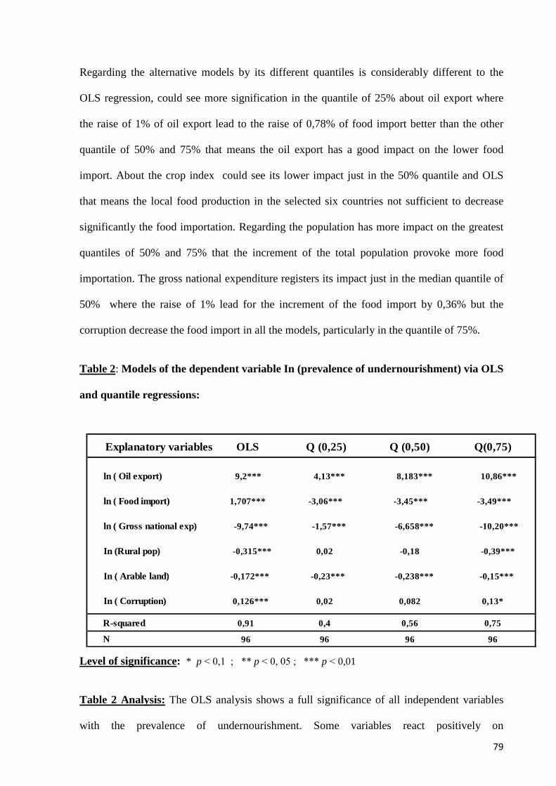
79

Regarding the alternative models by its different quantiles is considerably different to the

OLS regression, could see more signification in the quantile of 25% about oil export where

the raise of 1% of oil export lead to the raise of 0,78% of food import better than the other

quantile of 50% and 75% that means the oil export has a good impact on the lower food

import. About the crop index could see its lower impact just in the 50% quantile and OLS

that means the local food production in the selected six countries not sufficient to decrease

significantly the food importation. Regarding the population has more impact on the greatest

quantiles of 50% and 75% that the increment of the total population provoke more food

importation. The gross national expenditure registers its impact just in the median quantile of

50% where the raise of 1% lead for the increment of the food import by 0,36% but the

corruption decrease the food import in all the models, particularly in the quantile of 75%.

Table 2: Models of the dependent variable In (prevalence of undernourishment) via OLS

and quantile regressions:

Level of significance: * p ˂ 0,1 ; ** p ˂ 0, 05 ; *** p ˂ 0,01

Table 2 Analysis: The OLS analysis shows a full significance of all independent variables

with the prevalence of undernourishment. Some variables react positively on

Explanatory variables OLS Q (0,25) Q (0,50) Q(0,75)

ln ( Oil export) 9,2*** 4,13*** 8,183*** 10,86***

ln ( Food import) -1,707*** -3,06*** -3,45*** -3,49***

ln ( Gross national exp) -9,74*** -1,57*** -6,658*** -10,20***

In (Rural pop) -0,315*** 0,02 -0,18 -0,39***

In ( Arable land) -0,172*** -0,23*** -0,238*** -0,15***

In ( Corruption) 0,126*** 0,02 0,082 0,13*

R-squared 0,91 0,4 0,56 0,75

N 96 96 96 96

80

undernourishment level as food import, rural population, arable land, and gross national

expenditure in which its potential increment decreases the malnutrition significantly.

Paradoxically, the more oil exportation in the developing countries doesn’t influence on the

reduction of undernourishment positively. Moreover, the corruption remains the limiting

factor in its adversary impact on food import and undernourishment. The high R-squared of

the OLS model nearly 91,5% demonstrate the greater significance of the independent

variables.

The quantiles regressions for the prevalence of undernourishment also considerably different

to OLS regression and could show a significant results in all quantiles where the food imports

decease more the undernourishment in the median and higher quantiles ( 50% & 75%) but

regarding the oil export could see a contrary or negative relationship where coefficient is

positive that means the increment of oil exportation don’t decease the undernourishment,

particularly in the quantiles of 50% and 75%. This results confirm the theory of “the paradox

of plenty”. The rural population registers its positive impact just in the highest quantiles of

75% where the increment of rural population by 1% decrease the undernourishment by

0,39%. In the same time there are not any significance in the others quantiles. About the gross

national expenditure registers its positive impact in all quantiles, particularly in the greater

quantiles of undernourishment by more than 10% means the food availability in the selected

countries very related to the government subsidies. Regarding the lower availability of arable

land could see a lower positive impact on the higher level of undernourishment by 0,15% but

in the same time could register a significant impact in the lower quantiles under 25% of

undernourishment. About the impact of the corruption could see a more significant impact in

the quantiles of 75% that means the increment of the corruption increase the

undernourishment.

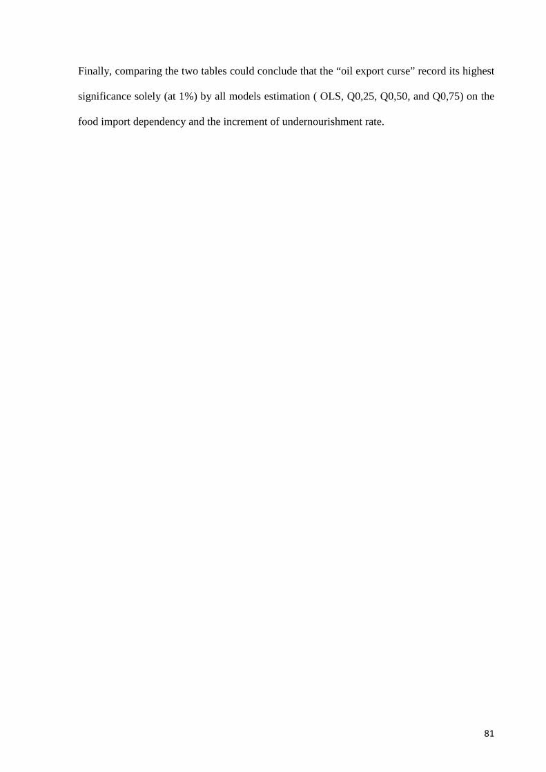
81

Finally, comparing the two tables could conclude that the “oil export curse” record its highest

significance solely (at 1%) by all models estimation ( OLS, Q0,25, Q0,50, and Q0,75) on the

food import dependency and the increment of undernourishment rate.

82

Conclusion:

Food dependence on oil finance opened an economic debate in oil-exporting politics. In

relative terms, imports of food products, which are increasingly expensive, led the oil

governments in recent decades to introduce strategies to increase the percentage of food self-

sufficiency. The analysis of this phenomenon allows the use of empirical models that favor

the study of trade relations between fuel countries and the exporting states of agri-food

products. To this end, the use of gravitational models allows taking into account distance,

population, GDP and other economic and non-economic factors that influence the flow of

import-export. For remedy this problem, the hydrocarbon governments put in place austerity

policies to support the financial budget. This system is, once again, a sign of economic

instability and food insecurity of the aggravated countries, the latter, from scarce or difficult

to use natural resources for agricultural production. In other words, being rich in natural

resources, have been neglected in the last decades due to the presumption of the durability of

the wealth derived from the oil that has proved to be not entirely truthful. A recent

intervention by the developing oil-rich government to ensure the food self-sufficiency has

been the sustainable modernization of the agricultural sector, allowing the exploitation of

some available resources such as uncultivated land and the groundwater. The implementation

of an efficient system of financing and crop insurance through the strengthening and

revitalization of banks and agricultural agencies to ensure more significant mobilization of the

credit of rural areas and for promoting agriculture in combination with higher economic

stability.

Agriculture could represent a viable alternative to oil in the developing countries where

industry and technology are limited. Not to be neglected, it will be the investment in human

capital as well as the stability of agricultural prices given the increase of the demands caused

by the demographic growth in all the world, particularly in the developing countries.

83

The question of food security is not limited to the agricultural sector but must accompany by a

growth of the whole economy. If the country wants a prosperous agriculture that contributes

to the improvement of food security and sovereignty, it will also have to develop other

strategic sectors such as services guaranteeing the funding sources that could satisfy the needs

of farmers and rural areas in general. Without an integrated national economy, there can be no

security or sustainable food sovereignty.

84

References

1. Aguilar-Millan. S., Ann, F., Oberg, A & Rudd, E. (2010). The post-scarcity world of

2050-2075. The futurist, 44 (01), 34-40.

2. Algeria. ( 2017, May). International Monetary Fund. Retrieved from htpp://www.imf.org/

3. Algeria. ( November, 2017). CIA-The World Factbook. Retrieved from

https://www.cia.gov/library/publications/the-world-factbook/geos/ag.html

4. Alfonso, J. P. P. ( 2003, May 22). The devil's excrement: Is oil wealth a blessing or a

curse?. The economist. Retrieved from www.economist.com/node/1795921

5. Akacem, M. & Cachanosky, N. (2017). The Myth of the Resource Curse: A Case Study

of Algeria. The Journal of Private Enterprise, 32(2), 1–15.

6. Akerkar, A. (2015). Etude de la mise en œuvre du plan nationale de développement

agricole et rurale ( PNDAR): cas de la wilaya de Bejaia. Revue nouvelle économie, 12,

15-29.

7. Akacem, M. & Cachanoaqsky, N. (2017). The Myth of the Resource Curse: A Case

Study of Algeria. The Journal of Private Enterprise, 32(2), 1–15.

8. Angola Oil, Broad-based Growth, and Equity. ( May, 2007). The World Bank. Retrieved

from https://elibrary.worldbank.org/

9. Anderson, J.E., Neary, P. J. (2003). The Mercantilist Index of Trade Policy. International

Economic Review, 44 (2 ), 627-649.

10. Angola. (2015, November). International monetary fund. Retrieved from

https://www.imf.org/external/pubs/ft/scr/2015/cr15301.pdf

11. Angola. (2017, February). International Monetary Fund. Retrieved from

https://www.imf.org/~/media/Files/Publications/CR/2017/cr1739.ashx

12. Annual Statistical Report. (2016). Organization of Arab Petroleum Exporting Countries.

Retrieved from htpp://www.oapecorg.org/

85

13. Anderson, J. (1979). A Theoretical Foundation for the Gravity Equation. American

Economic Review, 9, 106-116.

14. Anderson, J.E., Wincoop, V.E. (2003). Gravity with Gravitas: A Solution to the Border

Puzzle. The American Economic Review, 93(1), 170-192.

15. Arkolakis, C., Costinot, A., Rodriguez-Clare, A. (2008). Endogenous variety and the gains

from trade. American Economic Review, 98, 444-450.

16. Awokuse, T. O & Xie, R. (2015). Does Agriculture Really Matter for Economic Growth

in Developing Countries?. Canadian Journal of Agricultural Economics, (63), 77–99.

17. Bailey, R. (2012). Who will feed the extra 2 billion?. Royal Institute of International

Affairs, 68(2) , 38-39.

18. Baier, S.L., Bergstrand, J.H. (2007). Do free trade agreement actually increase

members’ international trade?. Journal of International Economics, 71, 72 -95.

19. Baier, S.L., Bergstrand, J.H. (2009). Bonus vetus OLS: A simple method for

approximating international trade-cost effects using the gravity equation. Journal of

International Economics, 77-85.

20. Beghin, J.C., Bureau, J.C. (2001). Quantitative Policy Analysis of Sanitary, Phytosanitary

and Technical Barriers to Trade. Économie Internationale, 87, 107-130.

21. Bergstrand, J. H. (1989). The Generalized Gravity Equation, Monopolistic

Competition and Factor Proportion Theory in International Trade. Review of Economic

and Statistics, 71, 143-53.

22. Barros, C.P. (2012). The resource curse and rent-seeking in Angola. ( CEsA Working

paper No. 102). Lisbona: Instituto Superior de Economia e Gestão.

23. Basedau, M & Lay, J. (2009). Resource Curse or Rentier Peace? The Ambiguous Effects

of Oil Wealth and Oil Dependence on Violent Conflict. Journal of Peace Research, 46(6),

757-776.

86

24. Bessaoud, O. (2006). La stratégie de développement rural en Algérie. Options

Méditerranéennes CIHEAM, 71, 79-89.

25. BP Statistical Review of World Energy. (2016). British Petroleum. Retrieved from

https://www.bp.com/content/dam/bp/pdf/energy-economics/statistical-review-2016/bp-

statistical-review-of-world-energy-2016-full-report.pdf

26. BP Statistical Review of World Energy. (2017). British Petroleum. Retrieved from

https://www.bp.com/content/dam/bp/en/corporate/pdf/energy-economics/statistical-

review-2017/bp-statistical-review-of-world-energy-2017-full-report.pdf

27. Bouët A., Decreux Y., Fontagné L., Jean S., Laborde D. (2008). Assessing Applied

Protection across the World. Review of International Economics, 16 (5), 850-863.

28. Bradford, S. (2003). Paying the Price: Final Goods Protection in OECD Countries. Review

of Economics and Statistics, 85(1), 24-37.

29. Bureau, J. C., Bernard, F., Gallezot, J., Gozlan, E. (2004). The measurement of protection

on the value added of processed food products in the EU, the US, Japan and South

Africa. A Preliminary Assessment of its Impact on Export of African Products, Final

Report, The World Bank, Washington DC.

30. Burger, M., van Oort, F., Linders, G. J. (2009). On the especification of the fravity model

of trade: zeros, excessive seros and zero-inflated estimators. Spatial Economic Analysis 4:

167-190.

31. Calvin, L., Krissof, B. (1998). Technical Barriers to Trade: A Case Study of Phytosanitary

Barriers and U.S.-Japanese Apple Trade. Journal of Agricultural and Resource

Economics, 23(2), 351-366.

32. Cameron, A.C., Trivedi, P.C. (2005). Microeconometrics: Methods and applications. New

york: Cambridge University Press.

87

33. Campbell, K., Gossette, R. (1994). A Study of Canada’s non-Tariff Trade Barriers: The

Equivalents of Quantitative Import Restrictions. Research Branch. Canadian International

Trade Tribunal.

34. Chakouri, S. M., Chibi, A. (2016). Algeria and the Natural Resource Curse: Oil

Abundance and Economic Growth. Economic research forum, working paper No 990.

35. Cipollina, M., Salvatici, L. (2008). Measuring Protection: Mission Impossible?.

Journal of Economic Surveys , 22(3), 577-616.

36. Cipollina, M.; Salvatici, L. (2010). Reciprocal Trade Agreement in Gravity Models: A

Meta-Analysis. Review of International Economics, 18(1), 63-80.

37. Cochet, Y., & Perrin, F. (2009). Pétrole: Pénurie ou Abondance ?. Revue internationale et

stratégique, 76 (4), 15-22.

38. Corruption Perceptions Index 2016. (January, 2017). Transparency International.

Retrieved from

https://www.transparency.org/news/feature/corruption_perceptions_index_2016

39. Country Analysis Brief: Angola. ( 2016, May). U.S. Energy Information Administration.

Retrieved from

https://www.ekonomi.gov.tr/portal/content/conn/UCM/uuid/dDocName:EK-246286

40. Dean, J.M., Feinberg, R., Signoret, J.E., Ferrantino, M.; Ludema, R. (2006). Estimating

the Price Effects of Non-Tariff Measures. Working paper No. 2006-06-A, Office

and Economics, U.S. International Trade Commission, Washington DC.

41. Deardoff, A. V. (1998). Determinants of Bilateral Trade: Does Gravity Work in a

Neoclassical World?. The Regionalization of the World Economy, University of Chicago

Press, JeffreyFrankel (Ed.).

42. Deardoff, A.V., Stern, R.M. (1997). Measurement of non-tariff barriers. OECD

Economics Department Working Paper 179 (OCDE/GD(97)/129). Paris: Organization

for Economic Cooperation and Development.

88

43. Desà, S.A., Belpaire, J.M. (2007). The Role of the Natural Resource Curse in Preventing

Development in Politically Unstable Countries: Case Studies of Angola and Bolivia.(

Development Research Working Paper Series No.11). Institute for advanced development

studies.

44. Disdier, A.C., Fontagné, L., Mimouni, M. (2008). The Impact of Regulation on

Agricultural Trade: Evidence from the SPS and TBT Agreements. American

Journal of Agricultural Economics , 90 (2), 336-350.

45. Dixit, A. K., Stiglitz, J. E. (1977). Monopolistic Competition and Optimum Product

Diversity. American Economic Review, 67(3), 297-308.

46. Dobransky, S. (2011). The United Arab Emirates and the black pearl model of economic

development. International Journal on World Peace, 28(2), 45-83.

47. Dollar, D., Kraay, A. (2004). Trade, growth and poverty. The Economic Journal, 114, 22-

49. Feenstra, R.C. (2009). Measuring the gains from trade under monopolistic

competition. Canadian Journal of Economics, 143, 1-28.

48. Downie, R. ( 2017, March). Growing the Agriculture Sector in Nigeria. A report of the

CSIS global food security project. Retrieved from https://www.csis.org/analysis/growing-

agriculture-sector-nigeria

49. Elhannani, F. E., Boussalem, A. B & Benbouziane. M. (2016). Financial development and

the oil curse: Evidence from Algeria. Topics in Middle Eastern and African Economies,

18 (1), 112-125.

50. Fathelrahman, E., Basarir, A., Gheblawi, M., Sherif, S., & Ascough, J. (2014). Economic

Risk and Efficiency Assessment of Fisheries in Abu-Dhabi, United Arab Emirates (UAE):

A Stochastic Approach. Sustainability, 6, 3878-3898. doi:10.3390/su6063878

51. Feenstra, R.C. (2009). Measuring the gains from trade under monopolistic

competition. Canadian Journal of Economics, 143, 1-28.

89

52. Fiaz, S., Noor, M.A., & Aldosri, F.O.( 2016). Achieving food security in the Kingdom of

Saudi Arabia through innovation: Potential role of agricultural extension. Journal of the

Saudi Society of Agricultural Sciences. Article in Press.

53. Fieler, A.C. (2011). Non-homotheticity and bilateral trade: evidence and a quantitative

explanation. Econometrica, 79 (4 ), 1069-1101.

54. Fuady, A. H. (2015). Aid and policy preferences in oil-rich countries: comparing

Indonesia and Nigeria. Third World Quarterly, 36 (7), 1349-1364.

55. Fontagné, L., Gaulier, G. & Zignago, S. (2008). Specialization across Varieties and

North-South Competition , Economic Policy, 51-91.

56. Fontagné, L., Kirchbach, V., F., Mimouni, M.(2005). An Assessment of

Environmentally- Related Non-Tariff Measures. World Economy, 28, 1417-39.

57. Frankel, J.A., Rose, A.K. (2000). Estimating the effect of Currency Unions on

trade and output. NBER Working Paper 7857.

58. Frynas, J.G., Wood., G. (2001). Oil and War in Angola. Review of African Political

Economy, 80 (28), 587-606.

59. Gardan, P.S. (2013). La stratégie économique du Qatar: Politique énergétique et

diversification économique. Confluences Méditerranée, 84 (1), 45-57.

60. Gary, I & Karl, T. L (2003, june). Bottom of the barrel: Africa’s Oil Boom and the Poor.

Catholic Relief Services, p.110. Retrieved from

http://www.relufa.org/savesite/programs/economicjustice/documents/CRSBottomoftheBar

relfulloilreport.pdf

61. Gibson, P., Wainio, J., Whitley, D., Bohman, M. (2001). Profiles of tariffs in global

agricultural markets. USDA Agricultural Economic Report 796, US Department of

Agriculture, Washington DC: Economic Research Service.

62. Goodwin, N., Nelson, J., Ackerman, F., & Weisskopf, T. (2009). Microeconomics in

Context (2d ed). M.E: Sharpe.

90

63. Harrigan, J. (1993). OECD Imports and Trade Barriers in 1983. Journal of

International Economics 35(1-2), 91-111.

64. Hawey, I. (2015, July 23). Food and Water Security in Qatar: Part 2 - Water Resources.

Future Directions International Pty Ltd. Retrieved from http://futuredirections.org.au/wp

content/uploads/2015/07/Qatar_Food_and_Water_Security_-_Part_2.pdf

65. Head, K. (2003). Gravity for Beginners. Faculty of Commerce, University of British

Columbia.

66. Head, K., & Mayer, T. (2000). Non Europe: The magnitude and causes of market

fragmentation in Europe. Review of World Economics - Weltwirschaftliches Archiv, 136,

285-314.

67. Head, K., Mayer, T. (2010). Gravity, market potential and economic development.

Journal of Economic Geography Advance Access, 1-14.

68. Heien, D., Sims, E. (2000). The impact of the Canada-United States Free Trade

Agreement on U.S. Wine Export. American Journal of Agricultural Economics, 82 (1),

173-182.

69. Helliwell, J. F. (1998). How Much Do National Borders Matter?. The Brookings

Institution, Washington D.C.

70. Helpman, E., Melitz, M., Rubinstein, Y. (2008). Estimating trade flows: trading partners

and trading volumes. Quarterly Journal of Economics, 73, 441-486.

71. Henderson D. J., Millimet, D. L. (2008). Is gravity linear?. Journal of Applied

Econometrics, 23, 137-172.

72. Henry de Frahan, B., Vancauteren, M. (2006). Harmonization of Food Regulation and

Trade in the Single Market: Evidence from Disaggregated Data. European Review of

Agricultural Economics ,33(3),337-60.

73. Hirschey, M. (2000). Managerial Economics. London : Dryden.

91

74. International Monetary Fund. (2015, September). Saudi Arabia. Retrieved from

https://www.imf.org/external/pubs/ft/scr/2015/cr15251.pdf

75. International Monetary Fund. (2016, July). United Arab Emirates. Retrieved from

https://www.imf.org/external/pubs/ft/scr/2016/cr16251.pdf

76. International Monetary Fund. (2016,October).Saudi Arabia. Retrieved from

http://www.imf.org/external/pubs/ft/scr/2016/cr16326.pdf

77. Iyiguna, S. ( 2016). Agrofood in North Africa: a strategic sector at nature’s mercy.

Coface MENA economist , 1-7.

78. Jank, M. S., Fuchsloch, I., Kutas, G. (2002). Agricultural liberalization in multilateral and

regional trade negotiations. Washington DC, Inter-American Development Bank.

79. Jayasinghe, S., Beghin, J. C., Moschini, G. (2010). Determinants of World Demand for

U.S. Corn Seeds: the Role of Trade Costs. American Journal of Agricultural Economics,

999-1010.

80. Johnson, M., Bell. F& Bennett. J (1980). Natural resource scarcity: empirical evidence

and public policy. J. Environmental Economics & Mgmt. , 7, 256-271.

81. Jones, R. W., (1971) . A three-factor model in theory, trade and history. in: J. Bhagwati et

al. (eds.), Trade, Balance of Payments and Growth, North-Holland, ch.1., 3-21.

82. Karl, T. L. (1997). The Paradox of Plenty. Oil Booms and Petro-States. Berkeley:

University of California Press.

83. Karl, T. L. (1999). The Perils of the Petro-State: Reflections on the Paradox of Plenty.

Journal of International Affairs, 53(1), 31-34.

84. Kee, H. L., Nicita, A., Olarreaga, M. (2006). Estimating Trade Restrictiveness Indices.

Policy Research Working paper No.3840, World Bank, Washington, DC.

85. Khiati, M. (2007). Stratégies, politiques et systèmes de connaissances agronomiques. Cfva

de Médéa, 6, 10-13.

86. Koenker, R., Bassett, G (1978). “Regression Quantiles,” Econometrica, 46, 33–50.

92

87. Krimly, R. (1999). The Political Economy of Adjusted Priorities: Declining Oil Revenues

and Saudi Fiscal. Middle East Journal, 53(2), 254-267.

88. Krugman, P. R. (1980). Scale Economies, Product Differentiation, and the Pattern of

Trade. American Economic Review, 70(5), 950-59.

89. Krugman, P. R. (1991). Increasing Returns and Economic Geography, Journal of

Political Economy ,99 (3), 483-499.

90. Krugman, P. R (2011). The New Economic Geography, Now Middle-aged. Regional

Studies, 45 (1), 1-7. DOI: 10.1080/00343404.2011.537127

91. Lai, H., Zhu, S. C. (2004). The determinants of bilateral trade. Canadian Journal of

Economics, 37, 459-483.

92. Leamer, E. E. (1974). Nominal Tariff Averages with Estimated Weights. Southern

Economic Journal ,41, 34-46.

93. Leamer, E. E. (1990). Latin America as a Target of Trade Barriers Erected by the Major

Developed Countries in 1983. Journal of Development Economics, 32(2), 337-68.

94. Leamer, E. E. (1990). Latin America as a Target of Trade Barriers Erected by the

Major Developed Countries in 1983. Journal of Development Economics, 32(2), 337-68.

95. Leamer, E. E., Levinsohn, J. (1994). International Trade Theory: The Evidence. NBER

Working Papers 4940. National Bureau of Economic Research, Inc.

96. Li, Y., Beghin, J.C. (2011). A meta-analysis of estimates of the impact of technical

barriers to trade. Journal of Policy Modelling.

97. Liu, L., Yue, C. (2009). Non-tariff Barriers to trade caused by SPS measures and customs

procedures with product quality changes. Journal of Agricultural and Resource

Economics 34(1), 196-212.

98. Maghni, B. (2013). Analyse des politiques de soutien à l’agriculture en Algérie,

Communication à présenter lors des 7 es journées de recherches en sciences sociales

INRA –SFER – CIRAD à Agrocampus Ouest (Centre d’Angers).

93

99. Maskus, K. E., Wilson, J. S., Otsuki, T. (2000). Quantifying the Impact of Technical

Barriers to Trade. A Framework for Analysis. Washington, D.C. : World Bank,

Development Research Group.

100. Mauzima, J.,& Gallardo, G. (2017). Angola. African economic outlook, AFDB,

OEDD, UNDP. Retriveid from http://www.africaneconomicoutlook.org/

101. McCallum, J. (1995). National Borders Matter: Canada-

U.S. Regional Trade Patterns. The American Economic Review, 85 (3), 615-623.

102. McMillan, J. (2006). Saudi Arabia and Iraq Oil, Religion, and an Enduring Rivalry.

United states institute of peace, Special report (157), 1-16. Retrieved from

https://www.usip.org/sites/default/files/McMillan_Saudi%20Arabia%20and%20Iraq_SR

%20157.pdf

103. Mission to Angola. ( 2015, August 25). International Monetary Fund, 388 (15).

Retrieved from https://www.imf.org/external/np/sec/pr/2015/ pr15388.htm.

104. Moenius, J. (2004). Information versus Product Adaptation: The Role of Standards in

Trade. Working paper, International Business & Markets Research Center, Northwestern

University, Evanston, IL.

105. Naylor, R. L., Liska, A. J., Burke, M. B., Falcon, W. P ., Gaskell, J. C., Rozelle, S. D &

Kenneth G. Cassman, K. G. (2007). The Ripple Effect: Biofuels, Food Security, and the

Environment. Environment: Science and Policy for Sustainable Development, 49(9), 30-

43, doi: 10.3200/ENVT.49.9.30-43

106. Nelson, G., Rosegrant, M., Palazzo, A., Gray, I., Ingersoll, C., Robertson, R.,…and You,

L. (2010). “ Food Security, Farming, and Climate Change to 2050: Scenarios, Results,

policy options”, IFPRI. Retrieved from https://dx.doi.org/10.2499/9780896291867

107. Nigeria and FAO. (2015, juin). Food and Agriculture Organization of the United

Nations. Retrieved from http://www.fao.org/3/a-az487e.pdf

94

108. Nogués, J. A., Olechowski, Winters, L. A. (1986). Extended of Non-Tariff Barriers to

Industrial Countries’ Imports. World Bank Economic Review, 1(1), 181-199.

109. Odetola, T., Etumnu, C. (2013, July). Contribution of Agriculture to Economic Growth

in Nigeria. The 18th Annual Conference of the African Econometric Society (AES)

Accra, Ghana at the session organized by the Association for the Advancement of African

Women Economists (AAAWE).

110. Odeh, L. E. (2011). Sino-Nigerian Economic Relations under the Obasanjo

Administration. Ilorin Journal of History and International Studies, 2 (1), 217-231

111. Obi, C. (2009). Nigeria’s Niger Delta: Understanding the Complex Drivers of Violent

Oil-related Conflict. Africa Development, 34 (2), 103-128

112. Olper, A., Raimondi, V. (2008a). Explaining National Border Effects in the QUAD Food

Trade. Journal of Agricultural Economics, 59( 3), 436-462.

113. Olper, A., Raimondi, V. (2008b). Agricultural market integration in the OECD: A

gravity- border effect approach. Food Policy, 33, 165-175.

114. Olper, A., Raimondi, V. (2009). Patterns and Determinant of International Trade Costs in

the Food Industry. Journal of Agricultural Economics, 60 ( 2), 273-297.

115. Onyeukwu, A. J. (2007). Resource Curse in Nigeria: Perception and Challenges. Central

european university, center for policy studies. Retrieved from https://core.ac.uk.

116. Onuka, O. I. (2017). Nigeria’s Food Import Dependency - Agricultural Transformation.

Agricultural Development, 2(1), 1-12.

117. Okpanachi, E. (2011). Confronting the Governance Challenges of Developing Nigeria’s

Extractive Industry: Policy and Performance in the Oil and Gas Sector. Review of Policy

Research, 28 (1), 25-47.

118. Osman, H., Osman, Ha. & Al-Hamar, Y, I. (2016). Sustainable Fodder Production for

Qatar’s Food Security. Journal of Scientific Research & Reports, 9(6), 1-9.

95

119. Otsuki, T., Wilson, J. S., Sewadeh, M. (2001). What Price Precaution? European

Harmonization of Aflatoxin Regulations and African Groundnut Exports. European

Review of Agricultural Economics, 28(3), 263-83.

120. Ouda, O. K. M. (2013). Towards Assessment of Saudi Arabia Public Awareness of

Water Shortage Problem. Resources and Environment, 3(1), 10-13.

121. Perrin, F., Cochet, Y. (2009). Pétrole: Pénurie ou Abondance?. Revue internationale et

stratégique, 76(4), 15-22. Doi 10.3917/ris.076.0015

122. Raimondi, V. & Olper, A. (2010). Trade Elasticity, Gravity and Trade Liberalization:

Evidence from the Food Industry. Journal of Agricultural Economics, 62( 3) , 525-550.

123. Raphaeli, N. (2005). Demands for Reforms in Saudi Arabia. Middle Eastern Studies.

41(4), 517-532.

124. Ringler, C., Zhu, T., Cai, X., Koo, J., & Wang, D. (2010). Climate Change Impacts on

Food Security in Sub-Saharan Africa. (IFPRI Discussion Paper 01042). Washington,

USA. The International Food Policy Reaserch Institute.

125. Sadik, A., El-Solh, M., & Saab, N. (2014). Arab environment: Food Security. Arab

environment: Food Security. Annual report of the Arab Forum for environment and

Development. Beirut, Lebanon. Technical Publications.

126. Samuelson, P. (1971). Ohlin Was Right. Swedish Journal of Economics, 73, 365-384.

127. Saudi Arabia Economy Profile. (2017). Index Mundi. Retrieved from

http://www.indexmundi.com/saudi_arabia/economy_profile.html

128. Saudi Arabia Terrorism index. (2017). Trading Economics. Retrieved from

https://tradingeconomics.com/saudi-arabia/terrorism-index

129. Saudi Arabia Open Budget index. (2015). International Budget Partnership. Retrieved

from http://survey.internationalbudget.org/availability/status/Saudi%20Arabia/embed

96

130. Shahin, S.M & Salem, M. A.(2015). Food Security In The United Arab Emirates (UAE):

The Great Competition between the Agricultural and Forestry Sector on Irrigation

Resources. International Journal of Research in Science, 1(1), 19-23.

131. Silva, S., Tenreyro, S. (2006). The Log of Gravity. The Review of Economics and

Statistics, 88(4), 641-658.

132. Suaré, P. (2006). The Rise of Trade Volumes, the “Origin Margin”, and Per Capita

Income.

133. Smith.V. K. (1979). Natural resource scarcity: a statistical analysis, Rev. Economics &

Statist, 61, 423-427.

134. The Global Competitiveness Report 2017–2018. ( 2017). World Economic Forum.

Retrieved from https://www.weforum.org/reports/the-global-competitiveness-report-2017-

2018

135. The end of fossil fuels. Britain’s greenest energy company. Retrieved from

https://www.ecotricity.co.uk/our-green-energy/energy-independence/the-end-of-fossil-

fuels

136. Thornton, P. k., Peter G. Jones, P. k., Ericksen, P. J., & Challinor, A.J. (2011).

Agriculture and food systems in sub-Saharan Africa in a 4°C+ world. The royal society,

1934 (369), 117-136.

137. Tinbergen, J. (1962). Shaping the world Economy: Suggestion for an International

Economy Policy. Twentieth Century Fund.

138. Tounsi, M. (1995). Industrialisation et sécurité alimentaire en Algérie. La sécurité

alimentaire en méditerranée. Options Méditerranéennes CIHEAM, 26, 61-69.

139. Tsui, K. K. (2011). More Oil, Less Democracy: Evidence from Worldwide Crude

Oil Discoveries. Economic Journal , 121, 89-115

140. United Arab Emirates. ( 2017, November). CIA-The World Factbook. Retrieved from

https://www.cia.gov/library/publications/resources/the-world-factbook/geos/ae.html

97

141. Uri, N.D. ( 1996). An Empirical Re-Examination of Natural Resource Scarcity and

Economic Growth . Energy Economics, (12), 45-61.

142. Wright, J. (2009). Sustainable agriculture and food security in an era of oil scarcity:

lessons from Cuba. London: Earthscan.

143. Xiong, B., Beghin, J. (2011a). Does European aflatoxin regulation hurt groundnut

exporters from Africa?. European Review of Agricultural Economics, 1-21.

144. Xiong, B., Beghin, J. (2011b). Disentangling the Demand-Enhancing Effect and Trade

Cost Effect of Technical Measures in Agricultural Trade Among OECD Countries.

Working Paper No. 11019.

145. Yue, C., Beghin, J. C., Jensen, H.H. (2006). Tariff Equivalent of Technical Barriers

to Trade with Imperfect Substitution and Trade Costs. American Journal of Agricultural

Economics, 88(4), 947-60.