nloptcontrol: a modeling language for solving optimal
TRANSCRIPT

1
NLOptControl: A modeling language for solvingoptimal control problems
Huckleberry Febbo, Paramsothy Jayakumar, Jeffrey L. Stein, and Tulga Ersal∗
Abstract—Current direct-collocation-based optimal controlsoftware is either easy to use or fast, but not both. This is amajor limitation for users that are trying to formulate complexoptimal control problems (OCPs) for use in on-line applications.This paper introduces NLOptControl, an open-source mod-eling language that allows users to both easily formulate andquickly solve nonlinear OCPs using direct-collocation methods.To achieve these attributes, NLOptControl (1) is written inan efficient, dynamically-typed computing language called Julia,(2) extends an optimization modeling language called JuMP toprovide a natural algebraic syntax for modeling nonlinear OCPs;and (3) uses reverse automatic differentiation with the acyclic-coloring method to exploit sparsity in the Hessian matrix. Thiswork explores the novel design features of NLOptControl andcompares its syntax and speed to those of PROPT. The syntaxcomparisons shows that NLOptControl models OCPs moreconcisely than PROPT. The speeds of various collocation methodswithin PROPT and NLOptControl are benchmarked over arange of collocation points using performance profiles; overall,NLOptControl’s single, two, and four interval pseudospectralmethods are roughly 14, 26, and 36 times faster than PROPT’s,respectively. NLOptControl is well-suited to improve existingoff-line and on-line control systems and to engender new ones.
I. INTRODUCTION
Optimal control software packages that implement direct-collocation methods are used in a number of off-line [1],[2], [3], [4], [5], [6] and on-line [7], [8] applications assummarized in Table I. The primary function of these packagesis to directly transcribe a human modeler’s formulation of anoptimal control problem (OCP) into a nonlinear programmingproblem (NLP). A key challenge with this process is enablinghuman modelers (i.e., users) to easily formulate new andcomplex problems while producing an NLP that can be quicklysolved by an external NLP solver. However, current direct-collocation-based optimal control software packages are gener-ally either fast or easy to use, but not both. Thus, these packageare not well suited for non-expert users trying to formulatecomplex problems for on-line applications, wherein speed iscritical. Therefore, there is a need for a direct-collocation-based optimal control software package that is both fast andeasy to use. In this paper, an approach to bridging this gap
The authors wish to acknowledge the financial support of the AutomotiveResearch Center (ARC) in accordance with Cooperative Agreement W56HZV-14-2-0001 U.S. Army Tank Automotive Research, Development and Engineer-ing Center (TARDEC) Warren, MI.,DISTRIBUTION A. Approved for publicrelease; distribution unlimited.
H. Febbo, J. L. Stein, and T. Ersal are with the Department of MechanicalEngineering, University of Michigan, Ann Arbor, MI 48109 USA (e-mail:[email protected]; [email protected]; [email protected]).
P. Jayakumar is with the U.S. Army RDECOM-TARDEC, Warren, MI48397 (email: [email protected])
∗Corresponding author ([email protected])
ApplicationsOff-line On-line Properties
Software Che
mic
alSp
ace
vehi
cle
Med
ical
Air
vehi
cle
Gro
und
vehi
cle
Rob
ot
Ope
n-so
urce
Easy
tous
eFa
st
GPOPS-ii [1] [1], [2] [17]† 7 3 7PROPT [3] [3] [3] 7 3 7GPOCS [4] [18]† 3 3 7DIDO [5] [18]† 7 7 7ACADO [8] 3 7 3CasADi [6] [7] 3 7 3Custom [19], [20]† 7 7 7NLOptControl [9] 3 3 3
TABLE I: Landscape of direct-collocation-based optimal con-trol software focusing on their applications and properties.† indicates that the software is too slow for use the on-lineapplication.
is presented and incorporated into a new, open-source optimalcontrol modeling language called NLOptControl [9].
As seen in Table I, some of the most well-known optimalcontrol software packages (GPOPS-ii , PROPT , DIDO )are closed-source and often require a licensing-fee. Thesedrawbacks limit their research value, since they are not freelyavailable to the entire research community, results may bedifficult to reproduce, and if the details of the underlyingalgorithms cannot both be seen and modified, then openvalidation and development of the these algorithms is not pos-sible [10], [11]. Fortunately, several noteworthy open-sourceoptimal control software packages exist. For completeness,this paper does not limit its discussions to these open-sourcepackages.
Optimal control packages with an algebraic syntax thatclosely resembles the Bolza form of OCPs [12] are categorizedas easy to use. It is noted that there are other design featuresthat affect ease of use; for instance, not having a built-ininitialization algorithm [13] reduces ease of use, but theseaspects of ease of use are not addressed in this paper. Table Ishows that this work categorizes the direct-collocation-basedoptimal control software packages GPOPS-ii [1], PROPT [3]and GPOCS [14] as easy to use and CasADi [15] and DIDO[16] as not easy to use.
For ease of use, modeling languages should have a syntaxthat closely resembles the class of problems for which theyhave been designed. Modeling languages like AMPL andGAMs are not embedded in a pre-existing computationallanguage, which allows for syntactical flexibility, when devel-oping them. However, this approach (1) makes development ofthe modeling language difficult and time-consuming, and (2)does not directly expose users to the breath of features avail-
arX
iv:2
003.
0014
2v2
[cs
.MS]
30
Apr
202
0

able in a computational language such as C++ or MATLAB.For these reasons, modeling languages are often embedded ina pre-existing computational language.
It can be difficult to establish a syntax for the modelingwithin the syntactical confines of a pre-existing computationallanguage. To overcome this issue, operator overloading can beused. For instance, a multiple-shooting method based optimalcontrol software package called ACADO [21] uses operatoroverloading to allow its user to define an OCP using symbolicexpressions that closely resemble the actual mathematicalexpressions of the problem. However, a naive implementa-tion of operator overloading can lead to performance issues[22]. Additionally, Moritz Dielhl, a researcher who developedACADO and MUSCOD-II, later acknowledges that, ACADOToolkit [21], DIRCOL [23], DyOS [24], and MUSCOD-II [25]restrict the problem formulations, particularly for users notinvolved with the development of these tools [15]. The aboveacknowledgment is included in a paper [15] that introducesCasADi. CasADi allows users to formulate OCPs with fewerrestrictions that ACADO. However, CasADi requires that userswrite the code for the transcription methods. Transcriptionmethods are a general class of numerical methods used to ap-proximate continuous-time OCPs; a direct-collocation methodis a type of transcription method. CasADi lets users to codetheir own transcription methods to avoid creating a "blackbox" OCP solver that is only capable of solving restrictiveformulations, as with ACADO. While this approach may bepedagogically valuable for users, it can lead to bugs and longdevelopment time [26] and it makes CasADi’s syntax notclosely resemble OCPs. For these reasons, this paper does notcategorize CasADi as easy to use. On similar grounds, DIDOis not categorized as easy to use.
For safety in on-line applications, the trajectory needs to beprovided to the plant in real-time. An on-line optimal controlexample is a nonlinear model predictive control (NMPC)problem. Real-time is achieved when the NLP solve-times areall less than the chosen execution horizon. Otherwise, the low-level controllers will not have a trajectory to follow. Despitethe need for small solve-times (i.e., speed), several imple-mentations of direct-collocation methods within the MATLABcomputational language are not able to achieve solve-timesthat are less than the execution horizon for a number ofNMPC applications. As seen in Table I, GPOCS, GPOPS-ii,and custom MATLAB software are not fast enough for NMPCapplications in aircraft [18], robot [17], and UGV [19], [20]systems, respectively. On the other hand, CasADi, which iswritten in C++, is fast enough for an NMPC application ina robot system [7]. Given this practical limitation, this paperwill now discuss why some direct-collocation-based optimalcontrol packages are fast while others are slow.
As seen in Table I, this work categorizes GPOPS-ii, PROPT,GPOCS, and DIDO as slow and CasADi as fast. If a packageuses sparse automatic differentiation methods implemented ina computation language that approaches the speeds of C, itis categorized as fast; the reasoning for this categorization isexplained below.
The main algorithmic step in direct method based numericaloptimal control is solving the NLP. The solve-time for this
step consists of two major parts: (1) the time spent runningoptimization algorithms within the NLP solver, and (2) thetime spent evaluating the nonlinear functions and their corre-sponding derivatives. Fortunately, low-level algorithms, whichare available within several prominent NLP solvers, such asKNITRO [27], IPOPT [28], and SNOPT [29], can be usedto reduce the time associated with running the optimizationalgorithms. The second component is discussed here in termsof current direct-collocation-based optimal control softwarepackages.
The speed of direct-method-based optimal control softwaredepends on the speed of the differentiation method within thecomputational language in which it is implemented. GPOPS-ii uses a sparse finite difference method [30] to calculate thederivatives using the MATLAB computational language. How-ever, finite difference methods, like the sparse finite differencemethod, are not only slow, but they are also inaccurate [31].In addition to this, the dynamically-typed MATLAB computa-tional language is typically slow in comparison to statically-compiled languages such as C and Fortran. Since GPOPS-iiuses a slow differentiation method within a relatively slowcomputational language, it is categorized as slow. PROPTuses either symbolic- or forward-automatic differentiation tocalculate the derivatives using MATLAB. While PROPT’smethods are more accurate and generally faster than finitedifference methods, they do not exploit the sparse structureof the Hessian matrices that is born from a direct-collocationmethod, like the sparse finite difference method in GPOPS-ii. Given this computational limitation and the slow speed ofMATLAB, this paper considers PROPT to be slow as well.On the other hand, CasADi uses the star-coloring method[32] to exploit the sparse structure of the Hessian matrix andreverse automatic differentiation implemented in C++ [15].Since CasADi employs a differentiation methods that is wellsuited for the sparse structure of the Hessian matrix and itis implemented in a fast computational language, CasADi iscategorized as fast. On similar grounds, this paper identifiesGPOCS and DIDO as slow.
In sum, there is no direct-collocation-based optimal controlsoftware package is both fast and easy to use. CasADi is fast,but not easy to use; and GPOPS-ii, PROPT, and GPOCS areeasy to use, but not fast. Thus, there is a need for a packagethat is both fast and easy to use.
This paper investigates an approach for improving bothspeed and ease of use of optimal control software. As de-scribed in detail in Section II, this approach uses recentadvances in computational languages and differentiation meth-ods in contrast to the computational languages and differ-entiation methods used by current direct-collocation-basedoptimal control software. Additionally, also unlike currentdirect-collocation-based optimal control software packages,this approach extends an optimization modeling language toinclude syntax for modeling OCPs. More specifically, thisapproach is as follows:
Approach
• For ease of use and speed, NLOptControl is embeddedin the fast, dynamically-typed Julia programming lan-
2
guage [33].• For increased ease of use, NLOptControl extends the
JuMP optimization modeling language [34], which iswritten in Julia, to include a natural syntax for modelingOCPs in Bolza form.
• For increased speed, NLOptControl uses the acyclic-coloring method [35] to exploit sparsity in the Hessianmatrix and reverse-automatic differentiation through theReverseDiff package [36], which is also written in Julia.
Therefore, this work addresses the following research ques-tion: Can the above outlined approach improve speed and easeof use of direct-collocation-based optimal control software?This question is answered by comparing NLOptControl’sspeed and ease of use to those of PROPT.NLOptControl was released as a free, open-source soft-
ware package in the summer of 2017 [9]. Since then, the liter-ature has shown that NLOptControl is fast and easy to use.For speed, NLOptControl was leveraged to solve complextrajectory planning problems for an unmanned ground vehiclesystem in real-time — solving these types of problems in real-time using MATLAB was not feasible in prior work [19], [20].For ease of use, NLOptControl was used to create a newoptimal control based learning algorithm [37] without any helpfrom the developers of NLOptControl.
The remainder of this paper is organized as follows. Sec-tion II further describes NLOptControl’s approach to bridg-ing the research gap. Section III describes the classes of off-line and on-line OCPs that can be solved using NLOptCon-trol. Section IV provides a brief background on numericaloptimal control and a mathematical description of the direct-collocation methods implemented within NLOptControl.Section VI provides an example that compares NLOpt-Control’s ease of use against PROPT’s and benchmarksNLOptControl’s speed against PROPT. Section VII an-swers the research question and discusses further implications.Finally, Section VIII summarizes the work and draws conclu-sions.
II. SOFTWARE ECOSYSTEM
Advances in computational languages, optimization mod-eling languages, and differentiation methods and tools madeit possible to create NLOptControl. This section describesthese software advances and shows how they can be leveragedto create a modeling language for a class of optimizationproblems.
A. Computational languages
Direct-collocation based optimal control software packagesare embedded in either a statically- or a dynamically typedcomputational language. Dynamically typed languages enableusers to quickly develop and explore new concepts, yet theyare typically slow; statically typed languages sacrifice theuser’s productivity for speed. Recently, however, a dynami-cally typed computing language called Julia has become apopular alternative to the computing languages that the currentoptimal control software packages are embedded in. It hasbecome popular, because it allows users to write high-level
code that closely resembles their mathematical formulas, whileproducing low-level machine code that approaches the speedof C and is often faster than Fortran [33]. The claim that Juliais not only fast, but also easy to use, motivates the investigationpresented in this paper. Specifically, this paper investigates theability of the Julia computational language to improve speedand ease of use for optimal control software.
B. Modeling optimization problems
In the late 1970’s, researchers using optimization softwarewere more concerned with the need to improve the software’sease of use than its speed [38]. Eventually, this concernled to the development a number of optimization modelinglanguages, such as GAMS [39] and AMPL [40]. The role ofan optimization modeling language is to translate optimizationproblems from a human-friendly language to a solver-friendlylanguage [41], [42]. In other words, optimization modelinglanguages do not solve optimization problems; they focus onmodeling problems at a high-level and passing optimizationproblems to external low-level solvers, which are the NLPsolvers and the differentiation tools in the context of this work.Similarly, in this work, the high-level problem is the NLP,given in Eqn. 1 - Eqn. 3 (i.e., the NLP model) as
minimizez∈Rn
f(z) (1)
subject to g(z) ≤ 0 (2)h(z) = 0 (3)
where the objective function f : Rn → R, with n definedas the number of design variables; the inequality constraintsg : Rn → Re; and the equality constraints h : Rn → Rq , areall assumed to be twice-continuously differentiable functions[28], [43].
A number of standard optimization problem classes do notfit readily into the NLP model. In addition to this, translatingthese standard problem classes into the NLP model canrequire significant work. Thus, for users interested in simplymodeling these standard problem classes, and not translatingthese problems into an NLP model, the NLP model shouldbe extended to include higher-level modeling languages forthese standard problem classes. However, most optimizationmodeling languages are not designed to be extended in thisfashion [42]. Because of this limitation, both the speed andease of use of optimal control packages have suffered. GPOCS,GPOPS-ii, and PROPT are slow because the sparse-automaticdifferentiation methods — typically available through an opti-mization modeling language — are not available in MATLAB;so, these packages use less efficient differentiation methods.Additionally, since these packages are not built upon anexisting NLP modeling language, the API tends to be overlyflexible, which can lead to modeling errors [21].
JuMP [22], a recent optimization modeling language that isembedded in the fast, dynamically-typed Julia programminglanguage [33], is designed to be extended to include newclasses of optimization problems. JuMP extensions include:parallel multistage stochastic programming [44], robust opti-mization [45], chance constraints [46], and sum of squares
3

Fig. 1: Proposed software framework for nonlinear OCPs.
[47]. Moreover, JuMP provides an interface for both theKNITRO and IPOPT NLP solvers as well the ReverseDiffdifferentiation tool. ReverseDiff [36] is also embedded in theJulia programming language and utilizes reverse automaticdifferentiation with the acyclic-coloring method [48] to exploitsparsity in the Hessian matrices. Research shows that theacyclic-coloring method is faster than the star-coloring method[48], which was used in the CasADi package [15]. Theseadvances are leveraged to create an optimal control modelinglanguage called NLOptControl.
C. Proposed software ecosystem
Fig. 1 presents NLOptControl’s software ecosystem andits function as an optimal control software package. In termsof this ecosystem, it is: embedded in Julia; extends JuMPto provide a natural syntax for modeling OCPs; leveragesReverseDiff ; and interfaces with KNITRO, IPOPT, and po-tentially other solvers to solve the automatically formulatedNLP problem. To use NLOptControl, users need onlyformulate their OCP into a syntax-based model of the OCP.This model is then approximated using one of the direct-collocation methods implemented in NLOptControl, whichat the time of this writing include: the Euler’s backwards,the trapezoidal, and the Radau collocation methods. After themodel has been approximated, the software ecosystem solvesthis approximation to determine an optimal trajectory. Thistrajectory can then be followed using low-level controllers tocontrol the plant for either an off-line or on-line tasks.
III. SCOPE OF NLOptControl
NLOptControl is designed for modeling OCPs and solv-ing them for either off-line or on-line applications. Thissection shows the types of problems that NLOptControlcan model, and demonstrates NLOptControl’s visualizationcapabilities and salient design features for on-line applications(e.g., NMPC problems).
A. Modeling OCPs
An important class of optimization problems is the OCP.NLOptControl models single-phase, continuous-time, OCP
in a Bolza form [12] that is tailored for NMPC problems andadds slack constraints on the initial and terminal states as
minimizex(t),u(t),x0s,xf s
tfM(x(t0 + tex), t0 + tex, x(tf ), tf )
+
∫ tf
t0+tex
L(x(t), u(t), t) dt
+ws0x0s + wsfxf s(4)
subject todxdt
(t)− F (x(t), u(t), t) = 0
(5)C(x(t), u(t), t) ≤ 0
(6)x0 − x0tol ≤ x(t0 + tex) ≤ x0 + x0tol
(7)xf − xftol ≤ x(tf ) ≤ xf + xftol
(8)xmin ≤ x(t) ≤ xmax
(9)umin ≤ u(t) ≤ umax
(10)tfmin ≤ tf ≤ tfmax
(11)x0 − x(t0 + tex) ≤ x0s
(12)x0 + x(t0 + tex) ≥ x0s
(13)xf − x(tf ) ≤ xf s
(14)xf + x(tf ) ≥ xf s
(15)
where t0 is the fixed initial time, tex is the fixed executionhorizon that is added to account for the non-negligible solve-times in NMPC applications, tf is the free final time, t is thetime, x(t) ∈ Rnst is the state, with nst defined as the numberof states, and u(t) ∈ Rnctr is the control, with nctr as thenumber of controls. xs0 ∈ Rnst and xsf ∈ Rnst are optionalslack variables for the initial and terminal states, respectively.The objective functional includesM : Rnst×R×Rnst×R→R and L : Rnst × Rnctr × R → R, which are the Mayerand Lagrangian terms, respectively. Here ws0x0s +wsfxf s isadded to the Bolza form to accommodate slack variables onthe initial and terminal conditions; this term is described indetail later in this section. x0s ∈ Rnst and xf s ∈ Rnst arevectors of weight terms on the slack variables for the initialand final state constraints. F : Rnst ×Rnctr ×R→ Rnst andC : Rnst × Rnctr × R → Rp denote the dynamic constraintsand the path constraints, respectively; p is the number of pathconstraints. x0 ∈ Rnst and xf ∈ Rnst denote the desired initialand final states, respectively. x0tol ∈ Rnst and xftol ∈ Rnst
establish tolerances on the initial and final state, respectively.Constant upper and lower bounds on the state, control, andfinal time are included with Eqn. 9, Eqn. 10, and Eqn. 11,respectively. Finally, NLOptControl adds Eqn. III-A - Eqn.
4
III-A to the Bolza form for optional slack constraints on theinitial and terminal states.NLOptControl is embedded in the Julia language and
specializes JuMP’s syntax to better suit the domain of optimalcontrol. JuMP leverages Julia’s syntactic macros [33] to enablea natural algebraic syntax for modeling optimization problems,without sacrificing performance or restricting problem formu-lations [22]. NLOptControl extends JuMP to include syntaxfor modeling OCPs in Boltza form in Eqn. 4 – Eqn. 11, withthe option of including slack constraints on the initial andterminal states through Eqn. – Eqn. .
For a basic example of this syntax, NLOptControl is nowused to model the Bryson-Denham problem, which is givenin mathematical form as
minimizea(t)
1
2
∫ 1
0
a(t)2dt
subject to
v(t) =a(t), x(t) =v(t), x(t) ≤ 1
12v(0) = −v(1) = 1,x(0) = x(1) = 0
The define() function is used to create a model object anddefine Eqn. 7 - Eqn. 10 asn = define(numStates = 2, numControls = 1, X0
↪→ = [0.,1.], XF = [0.,-1.], XL = [0.,NaN],↪→ XU = [1/12,NaN], CL = [NaN,NaN], CU = [↪→ NaN,NaN])
where n is an object that holds the entire optimal controlmodel, numStates and numControls are the number ofstates and controls, X0 and XF are arrays of the initial andfinal state constraint, XL and XU are arrays of any lower andupper state bounds, NaN indicates that a particular constraintis not applied, and CL and CU are an arrays of any lower andupper control bounds.
The dynamic constraints in Eqn. 5 are then added to themodel through the dynamics function asdynamics!(n, [:(x2[j]), :(u1[j])])
where the ! character indicates that the model object n is beingmodified by the function. The elements of the array :(x2[j↪→ ]) and :(u1[j]) represent v(t) and a(t); by default thestate and control variables are x1,x2,.. and u1,u2,.., butthey can be changed. Differential equations must be passedwithin an array of Julia expressions (i.e., [:(),:(),...,:()↪→ ]), and the index [j] must be appended to the state andcontrol variables. j is used within NLOptControl to indexparticular time discretization points ∈ [t0 + tex, tf ].
The next step is to indicate whether or not the final time tfis a design variable using the configure function asconfigure!(n; (:finalTimeDV => true))
where (:finalTimeDV=>true) indicates that the final timeis a design variable, which is the case for the Bryson-Denhamproblem. Additional options can be passed to the configurefunction. However, this paper is not a tutorial; for a tutorialsee NLOptControl’s documentation [9].
At this point, any path constraints in Eqn. 6 can be addedto the model using JuMP’s @NLconstraint macro. However,these constraints are not needed for this example.
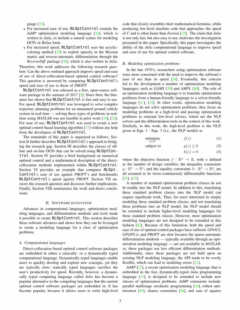
Fig. 2: Output of allPlots(n) command after modeling andsolving the Bryson-Denham problem using NLOptControl.Section A in the Appendices provides additional plots of theNLOptControl’s solution to the Bryson-Denham problemcompared to the analytical solution, including the costates.
Next, the objective function in Eqn. 4 is added to the model.To accommodate for a Lagrangian term, NLOptControlprovides the integrate function—similar to the dynamicsfunction, an expression must be passed and the [j] syntaxmust be appended to all state and control variables. For theBryson-Denham, the objective functional is modeled as
obj = integrate!(n, :(0.5*u1[j]^2))
The JuMP macro @NLobjective is used to add the objectivefunctional to the model as @NLobjective(n.ocp.mdl,Min↪→ ,obj). This problem is solved by passing the model n tothe optimize function as
optimize!(n)
a) Visualization: NLOptControl allows users quicklyplot the solutions to their problems. For plotting —bydefault— NLOptControl leverages GR [49] as a backend,but it can be configured to utilize matplotlib [50] instead.The command allPlots(n) plots the solution trajectoriesfor the states, controls, and costates1. Invoking this commandto visualize the solution to the Bryson-Denham problem thatis modeled above produces Fig. 2.
B. Nonlinear model predictive control
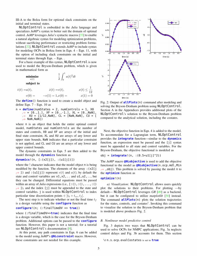
Fig. 3 depicts two ways that NLOptControl can beused to solve OCPs for NMPC applications; Fig. 3a neglectscontrol delays and Fig. 3b accounts for them. This section
1if n.s.ocp.evalCostates is set to true
5
(a) Neglecting control delay ts.
OCP Plant
ts�u(t)
Initilization
G, E
x0a
(b) Accounting for control delay ts using a fixed execution horizontex and a state prediction block.
OCP Plant
StatePrediction
tex�u(t)
Initilization
U0
G, E
x0a
x0
Fig. 3: Nonlinear model predictive control framework availablein NLOptControl.
describes these figures and discusses the design features thathelp NLOptControl users tackle NMPC problems.
Fig. 3a has three main components: the OCP, the plant, andthe initialization block. Three inputs G, E , and x0 are providedto the OCP to produce u(t); u(t) can be either a referencetrajectory or control signals for the plant. In the case that u(t)is a reference trajectory, then low-level controllers are addedto the plant to allow it to track the trajectory.
Description: III.1. Goal information G includes the finaldesired state of the plant, which may not be equal to xf . Forinstance, in an automated vehicle trajectory planning system,the goal range may be outside of the sensing range. In thiscase, the final desired state xf may be near the boundary ofthe sensing range.
Description: III.2. Environment information E includes anytransient data. For example, this data may include the obstacledata that helps establish the constraints on obstacle avoidancefor automated vehicle navigation problems.
The plant can be either physical or virtual, but in either caseis provided by the user. Because time can typically be allocatedto initialize NMPC problems, the initialization block permitsusers to warm start their optimization problems so that theinitial on-line solve time is much smaller. After initialization,at t0, the first control signal u(t) is sent to the plant and thefirst on-line OCP is solved. Each time an OCP-solve starts, t0is reset to the current time. An issue with this scheme is thatit does not take into account the solve time (i.e., control delayts). That is, the initial state of the OCP is constrained to bethe current state of the plant x0 at the initial time t0, so by thetime the OCP has been solved ts has elapsed, and the plantwill have evolved to a new state. If this control delay is small
relative to the time scale of the dynamics, then neglecting itwill not compromise the robustness. However, if the controldelay is relatively large, then it cannot be neglected.
Fig. 3b illustrates an approach that accounts for thesecontrol delays. This approach adds a block that predicts theplant state at the current time plus a fixed execution horizont0+tex. The execution horizon tex can be chosen based on thea heuristic upper limit on the solve times; often solve timesdo not change drastically when solved in a receding-horizonwith varying parameters for the initial conditions and pathconstraints. This approach avoids having to predict individualsolve times ts.NLOptControl provides various functionality tailored for
solving NMPC problems. The remainder of this section simul-taneously describes these features and provides an examplethat uses NLOptControl to formulate an OCP and solve itin a receding horizon. To this end, consider the moon landerOCP [51], which is given in without slack constraints in Eqn.16 as
minimizea(t), tf
∫ tf
0
a(t)dt
subject to x(t) = v(t), v(t) = a(t)− gx(t0) = 10, x(tf ) = 0
v(t0) = −2, v(tf ) = 0
0 ≤ x(t) ≤ 20, −20 ≤ v(t) ≤ 20
0 ≤ a(t) ≤ 3, 0.001 ≤ tf ≤ 400
(16)
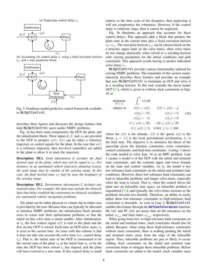
where the x(t) is the altitude, v(t) is the speed, a(t) is thethrust, g = 1.5 is the local gravitational acceleration, tf isthe final time. The objective is to minimize the thrust of thespaceship given the dynamic constraints, event constraints,control constraints, and final time constraints. Listing. 1 showsthe code needed to solve Eqn. 16 as an MPC problem. Line1 creates a model n of the OCP with the initial and terminalstate constraints, and the constant upper and lower boundson the state and control variables. As is, the model n haslow-tolerance hard constraints on the initial and terminal stateconditions. However, these low-tolerance hard constraints canlead to infeasible problems and longer solve-times, especiallywhen the loop is closed. That is, when the control drives theplant into an infeasible state space, an infeasible problem isengendered [52]; and typically, the solve-times increase as theproblems become less-feasible. Therefore, an ability to easilyadjust these low-tolerance constraints to high-tolerance hardconstraints is desirable. As seen in Line 2, NLOptControlenables this feature through the defineTolerances function.X0_tol and XF_tol are arrays that set the tolerances on theinitial x0tol and final states xftol , respectively.
When going from low- to high-tolerance hard constraints onthe initial and terminal states, slack constraints should also beadded. Because, when using these high-tolerance constraintswithout slack constraints, there is nothing pushing the initialand terminal states away from the edge of the infeasibleregion. Thus, infeasible problems are just as likely to occur.Adding slack constraints on the initial and terminal stateconstraints helps to mitigate these infeasible problems. Beforeslack constraints are added to the model, slack variables must
6
Listing 1: NLOptControl code needed to formulate and solve the moon lander as an MPC problem.n = define(numStates = 2, numControls = 1, X0 = [10., -2], XF = [0., 0.], CL = [0.], CU = [3.])
2 defineTolerances!(n; X0_tol = [0.01, 0.005], XF_tol = [0.01, 0.005])dynamics!(n,[:(x2[j]),:(u1[j]-1.5)])
4 configure!(n; (:finalTimeDV => true), (:xFslackVariables => true), (:x0slackVariables => true))obj = integrate!(n,:(u1[j]))
6 @NLobjective(n.ocp.mdl, Min, obj + 100*(n.ocp.x0s[1] + n.ocp.x0s[2] + n.ocp.xFs[1] + n.ocp.xFs↪→ [2]))
initOpt!(n)8 defineMPC!(n; tex = 0.2, predictX0 = true)function IPplant(n, x0, t, U, t0, tf)
10 spU = linearSpline(t, U[:,1])f = (dx, x, p, t) -> begin
12 dx[1] = x[2]dx[2] = spU[t] - 1.5
14 endreturn DiffEqBase.solve(ODEProblem(f, x0, (t0, tf)), Tsit5()), [spU]
16 enddefineIP!(n, IPplant)
18 simMPC!(n)
be added. The size of a slack variable corresponds to thesize of the respective constraint violation [53]. As seen inLine 4, NLOptControl allows such slack variable to beadded using the configure function. (:xFslackVariables↪→ =>true) and (:x0slackVariables=>true) adds slackvariables on the initial and final state constraint, respectively.Both the objective of the moon lander problem and the slackconstraints are added to model as on Line 6. n.ocp.x0s and n↪→ .ocp.xFs are arrays holding the slack variables on theinitial and terminal states, respectively, and all of the termsin ws0 and wsf (in Eqn. 4) are set to 100—these weights areset large enough such that the respective constraint violationsare nearly zero. On Line 7, NLOptControl warm starts theoptimization using the initOpt function; the initializationblock in Fig. 3 captures this step.
The defineMPC function adds several basic settings to themodel n. tex is the value of the fixed execution horizon andpredictX0 is a bool, which, when set to true, indicates thatthe the framework in Fig. 3b is used. Thus, a prediction ofthe initial state needs to be made either by the user or usingan internal model of the plant, which is added to n. In thissimple example, the differential equations in Eqn. 16 governthe OCP, the plant, and the state prediction function. The plantand prediction model are defined by the IPplant functionfrom Line 9 to Line 16 and passed to the model n using thedefineIP function on Line 17. Here the IPplant function isshowed for completeness, but its is not described in detail sinceit uses the well-documented DifferentialEquations packagein Julia [54]. For safety and reduced time in experimentaldevelopment, this initial step, i.e., making all of the modelsthe same and running a simulation-based experiment, shouldbe taken; especially when formulating more complex OCPsfor practical NMPC applications.
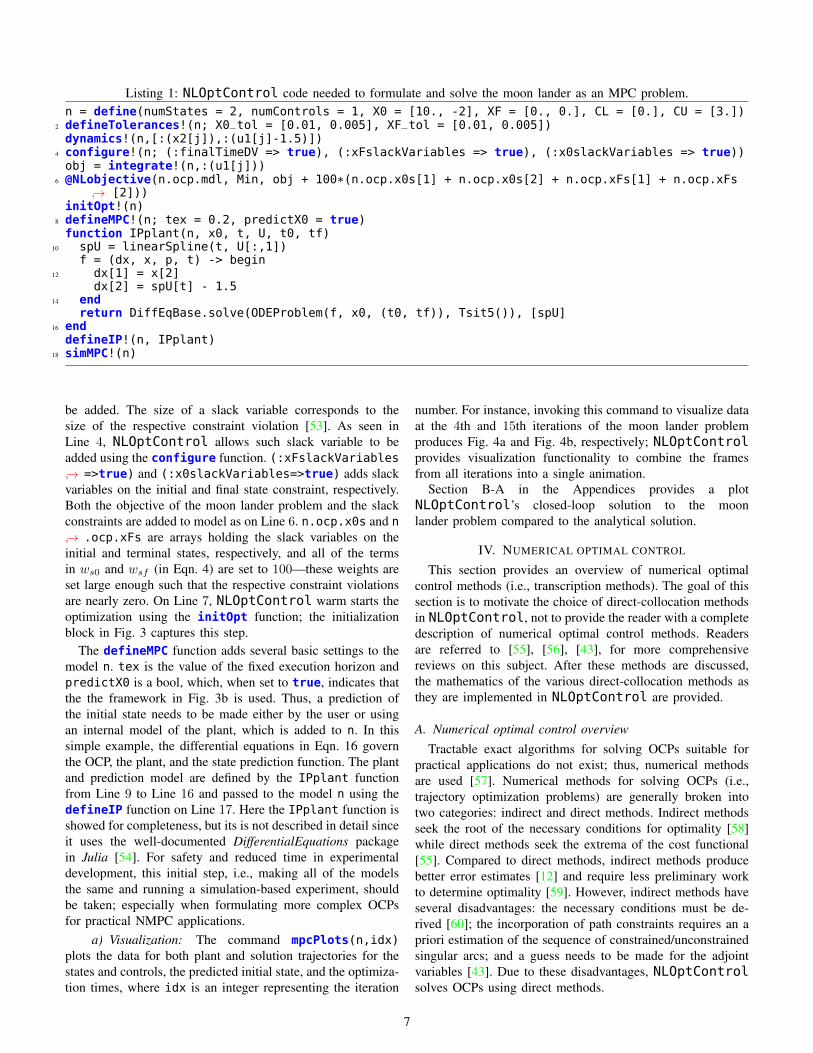
a) Visualization: The command mpcPlots(n,idx)plots the data for both plant and solution trajectories for thestates and controls, the predicted initial state, and the optimiza-tion times, where idx is an integer representing the iteration
number. For instance, invoking this command to visualize dataat the 4th and 15th iterations of the moon lander problemproduces Fig. 4a and Fig. 4b, respectively; NLOptControlprovides visualization functionality to combine the framesfrom all iterations into a single animation.
Section B-A in the Appendices provides a plotNLOptControl’s closed-loop solution to the moonlander problem compared to the analytical solution.
IV. NUMERICAL OPTIMAL CONTROL
This section provides an overview of numerical optimalcontrol methods (i.e., transcription methods). The goal of thissection is to motivate the choice of direct-collocation methodsin NLOptControl, not to provide the reader with a completedescription of numerical optimal control methods. Readersare referred to [55], [56], [43], for more comprehensivereviews on this subject. After these methods are discussed,the mathematics of the various direct-collocation methods asthey are implemented in NLOptControl are provided.
A. Numerical optimal control overview
Tractable exact algorithms for solving OCPs suitable forpractical applications do not exist; thus, numerical methodsare used [57]. Numerical methods for solving OCPs (i.e.,trajectory optimization problems) are generally broken intotwo categories: indirect and direct methods. Indirect methodsseek the root of the necessary conditions for optimality [58]while direct methods seek the extrema of the cost functional[55]. Compared to direct methods, indirect methods producebetter error estimates [12] and require less preliminary workto determine optimality [59]. However, indirect methods haveseveral disadvantages: the necessary conditions must be de-rived [60]; the incorporation of path constraints requires an apriori estimation of the sequence of constrained/unconstrainedsingular arcs; and a guess needs to be made for the adjointvariables [43]. Due to these disadvantages, NLOptControlsolves OCPs using direct methods.
7
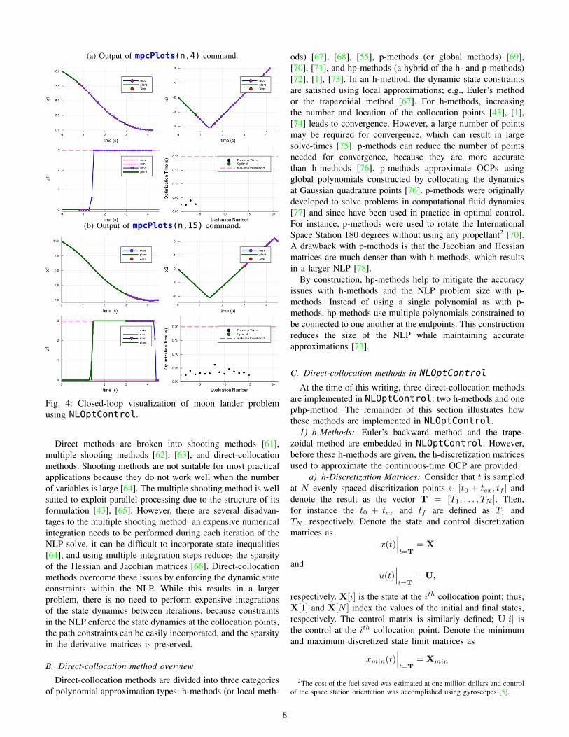
(a) Output of mpcPlots(n,4) command.
(b) Output of mpcPlots(n,15) command.
Fig. 4: Closed-loop visualization of moon lander problemusing NLOptControl.
Direct methods are broken into shooting methods [61],multiple shooting methods [62], [63], and direct-collocationmethods. Shooting methods are not suitable for most practicalapplications because they do not work well when the numberof variables is large [64]. The multiple shooting method is wellsuited to exploit parallel processing due to the structure of itsformulation [43], [65]. However, there are several disadvan-tages to the multiple shooting method: an expensive numericalintegration needs to be performed during each iteration of theNLP solve, it can be difficult to incorporate state inequalities[64], and using multiple integration steps reduces the sparsityof the Hessian and Jacobian matrices [66]. Direct-collocationmethods overcome these issues by enforcing the dynamic stateconstraints within the NLP. While this results in a largerproblem, there is no need to perform expensive integrationsof the state dynamics between iterations, because constraintsin the NLP enforce the state dynamics at the collocation points,the path constraints can be easily incorporated, and the sparsityin the derivative matrices is preserved.
B. Direct-collocation method overviewDirect-collocation methods are divided into three categories
of polynomial approximation types: h-methods (or local meth-
ods) [67], [68], [55], p-methods (or global methods) [69],[70], [71], and hp-methods (a hybrid of the h- and p-methods)[72], [1], [73]. In an h-method, the dynamic state constraintsare satisfied using local approximations; e.g., Euler’s methodor the trapezoidal method [67]. For h-methods, increasingthe number and location of the collocation points [43], [1],[74] leads to convergence. However, a large number of pointsmay be required for convergence, which can result in largesolve-times [75]. p-methods can reduce the number of pointsneeded for convergence, because they are more accuratethan h-methods [76]. p-methods approximate OCPs usingglobal polynomials constructed by collocating the dynamicsat Gaussian quadrature points [76]. p-methods were originallydeveloped to solve problems in computational fluid dynamics[77] and since have been used in practice in optimal control.For instance, p-methods were used to rotate the InternationalSpace Station 180 degrees without using any propellant2 [70].A drawback with p-methods is that the Jacobian and Hessianmatrices are much denser than with h-methods, which resultsin a larger NLP [78].
By construction, hp-methods help to mitigate the accuracyissues with h-methods and the NLP problem size with p-methods. Instead of using a single polynomial as with p-methods, hp-methods use multiple polynomials constrained tobe connected to one another at the endpoints. This constructionreduces the size of the NLP while maintaining accurateapproximations [73].
C. Direct-collocation methods in NLOptControl
At the time of this writing, three direct-collocation methodsare implemented in NLOptControl: two h-methods and onep/hp-method. The remainder of this section illustrates howthese methods are implemented in NLOptControl.
1) h-Methods: Euler’s backward method and the trape-zoidal method are embedded in NLOptControl. However,before these h-methods are given, the h-discretization matricesused to approximate the continuous-time OCP are provided.
a) h-Discretization Matrices: Consider that t is sampledat N evenly spaced discritization points ∈ [t0 + tex, tf ] anddenote the result as the vector T = [T1, . . . , TN ]. Then,for instance the t0 + tex and tf are defined as T1 andTN , respectively. Denote the state and control discretizationmatrices as
x(t)∣∣∣t=T
= X
andu(t)
∣∣∣t=T
= U,
respectively. X[i] is the state at the ith collocation point; thus,X[1] and X[N ] index the values of the initial and final states,respectively. The control matrix is similarly defined; U[i] isthe control at the ith collocation point. Denote the minimumand maximum discretized state limit matrices as
xmin(t)∣∣∣t=T
= Xmin
2The cost of the fuel saved was estimated at one million dollars and controlof the space station orientation was accomplished using gyroscopes [5].
8

andxmax(t)
∣∣∣t=T
= Xmax,
respectively. Similarly, the minimum and maximum controllimit matrices are denoted as
umin(t)∣∣∣t=T
= Umin
andumax(t)
∣∣∣t=T
= Umax,
respectively.b) Euler’s Backward Method: The dynamic constraints
in Eqn. 5 are locally approximated at (N − 1) points definedby T[2 : N ]. To accomplish this, (N − 1) × nst implicitconstraints are added as shown in Eqn. 17
0 = X[i+ 1]−X[i]− hF (X[i+ 1],U[i+ 1],T[i+ 1])(17)
= ηi, for i ∈ (1 : N − 1)
where h is the time-step size, which is determined by dividingthe time span (tf − t0 − tex) by N .
The integral term in the cost functional in Eqn. 4 isapproximated in Eqn. 18 as
I = h
N∑i=1
L(X[i],U[i], Ti) (18)
c) Trapezoidal Method: Similar to Euler’s backwardmethod, the dynamic constraints in Eqn. 5 are locally approx-imated at (N − 1) points defined by T[2 : N ]. To accomplishthis, the (N − 1) × nst implicit constraints in Eqn. 19 areenforced with
0 = X[i+ 1]−X[i]− h
2(F (X[i],U[i],T[i])+
F (X[i+ 1],U[i+ 1],T[i+ 1])) (19)= ηi, for i ∈ (1 : N − 1)
Next, the integral term in the cost functional in Eqn. 4 isapproximated in Eqn. 20 as
I =h
2
N∑i=1
(L(X[i],U[i], Ti) + L(X[i+ 1],U[i+ 1], Ti+1))
(20)
d) Discrete OCP: The h-method-based discrete OCP isgiven as
minimizeX, U, TN
M(X[1], T1,X[N ], TN ) + I (21)
subject to η = 0 (22)C(X,U,T) ≤ 0 (23)φ(X[1], T1,X[N ], TN ) = 0 (24)Xmin ≤ X ≤ Xmax (25)Umin ≤ U ≤ Umax (26)tfmin
≤ TN ≤ tfmax(27)
where slack constraints can be included with the Mayer termin Eqn. 21 and Eqn. 23.
2) p-Methods : For generality, this paper only describeshp-methods, since the single interval method (i.e., p-method)is merely the case where the number of intervals is equal toone.
3) hp-Methods : The form of Eqn. 4 – Eqn. 11 must bemodified to directly transcribe the OCP into an NLP usinghp-methods. To apply Gaussian quadrature the interval ofintegration must be transformed from [t0+tex, tf ] to [−1,+1].To accomplish this, τ ∈ [−1,+1] is introduced as a newindependent variable and a change of variable, for t in terms ofτ using the affine transformation, t =
tf−t0−tex2 τ+
tf+t0+tex2 .
Then, the interval τ ∈ [−1,+1] is divided into a mesh ofK intervals to accommodate for multiple intervals. With this,as in [75], an array of mesh points (M0, . . . ,MK) for theboundaries of these intervals is defined, which satisfy
−1 = M0 < M1 < M2 < · · · < MK−1 < MK = 1
Denote the continuous-time variables for the state and con-trol are on each mesh interval, k ∈ (1, . . . ,K), by thearrays x(k)(τ) and u(k)(τ), respectively. Next, denote ar-rays of continuous-time variables for both the minimum andmaximum state and control limits on each mesh interval,k ∈ (1, . . . ,K), as x
(k)min, x(k)max, u(k)min, and u
(k)max, respec-
tively. The state continuity between the mesh intervals isensured with the constraint x(k)(Mk) = x(k+1)(Mk) fork = (1, . . . ,K − 1) [73]. Similar to [1], this constraint isenforced programatically by making x(k)(Mk) be the samevariable as x(k+1)(Mk). To continue to describe the hp-methodimplemented in NLOptControl , the hp-discretization ma-trices are defined, which hold the discrete-time values of theapproximation to continuous-time problem.
a) hp-Discretization Matrices: First an array of timediscretization vectors, τ (k) = [τk1 , . . . , τ
kNk ], is defined by
evaluating the continuous functions at Nk specified τ ’s ∈[Mk−1,Mk) for k ∈ [1, . . . ,K], where Nk notates the numberof collocation points in mesh interval k; for instance, τ11 = −1.Let
N = [N1, N2, . . . , Nk, . . . , NK−1, NK ]
denote an array that holds the number of collocation pointswithin each mesh interval, where Nk can be adjusted accord-ing to the desired level of fidelity for the kth mesh interval.For k ∈ [1, . . . ,K], denote the state and control discretizationmatrix arrays as
x(k)(τ)∣∣∣τ=τ (k)
= X(k)
andu(k)(τ)
∣∣∣τ=τ (k)
= U(k),
respectively. Next, denote the minimum and maximum dis-cretized state limit matrix arrays as
x(k)min(τ)
∣∣∣τ=τ (k)
= X(k)min
andx(k)max(τ)
∣∣∣τ=τ (k)
= X(k)max,
9

respectively. Similarly, the minimum and maximum controllimit matrices are defined as
u(k)min(τ)
∣∣∣τ=τ (k)
= U(k)min
andu(k)max(τ)
∣∣∣τ=τ (k)
= U(k)max,
respectively.
To approximate the modified OCP that is modified forhp-methods, NLOptControl builds on the work donein [69], [79], [30], which was implemented in GPOPS-ii[1]. Specifically, NLOptControl implements the Legendre-Gauss-Radau quadrature collocation method (Radau collo-cation method). For completeness, this section will brieflydescribe this method, but for a more thorough explanation,the reader is referred to the seminal work done in [1], [69],[79], [30].
b) Radau Collocation Method: In hp-methods, the statesare approximated within each mesh interval with a Lagrangepolynomial as
x(k)(τ) ≈Nk+1∑j=1
X[j](k)L(k)j (τ), k ∈ [1, ..,K] (28)
with
Lkj (τ) =
Nk+1∏l=1l 6=j
τ − τklτkj − τkl
, k ∈ [1, ..,K] (29)
Lkj (τ) is the (kth, jth) Lagrange polynomial within a basisof Lagrange polynomials defined by j = (1, . . . , Nk + 1) andk = (1, . . . ,K), τ (k) = [τk1 , . . . , τ
kNk ] and is the kth set of the
LGR collocation points (also, called LGR nodes [80]), whichare defined on the kth mesh interval (τ ∈ [Mk−1,Mk)). Thento approximate the entire state, Mk is added as a noncollocatedpoint [69] for k ∈ (1, . . . ,K).
The derivative of the state can then be approximated foreach mesh interval as
dx(k)(τ)
dτ≈Nk+1∑j=1
X[j](k)dL(k)
j (τ)
dτ, k ∈ [1, ..,K] (30)
withdL(k)
j (τ)
dτ
∣∣∣τ=τk
j
= Dkij (31)
where Dkij is an element of the Nk ×Nk+1 Legendre-Gauss-
Radau differentiation matrix in the kth mesh interval, asdefined in [69].
Next, in order to approximate the integral of the Lagrangeterm in Eqn. 4, Gaussian-Legendre quadrature [81] is used as∫ tf
t0+tex
L(x(t), u(t), t) dt ≈
tf − t0 − tex2
K∑k=1
Nk∑j=1
Mk −Mk−1
2wkjL(X[j](k),U[j](k), . . .
τkj ; t0 + tex, tf ) (32)
where w(k) = [wk1 , . . . , wkNk
] is the kth array of LGRweights3.
Eqn. 32 is mathematically equivalent to the approximationsmade for the integral term in the cost functional in [73], butit is written in a slightly different form to reduce the compu-tations needed within the NLP. Specifically, the Mk−Mk−1
2 wkjterm is calculated outside of the NLP, for j ∈ (1, . . . , Nk) andk ∈ (1, . . . ,K). The result is stored in an array of vectors.Thus, the design variable tf is removed from the summationsin NLOptControl.
c) Discrete OCP: The p-method-based discrete OCP isshown in Eqn. 33 - Eqn. 39 as
minimizeX(k), U(k), tf
M(X[1](1), t0 + tex,X[NK+1](K), tK) + I
(33)subject toNk+1∑j=1
X(k)j D
(k)ij −
tf − t0 − tex2
f(X(k)i ,U
(k)i , τki ; t0 + tex, tf ) = 0
(34)
C(k)(X[i](k),U[i](k), τki ; t0 + tex, tf ) ≤ 0 (35)
φ(X[1](1), t0 + tex,X[NK+1](K), tf ) = 0 (36)
X[i](k)min ≤ X[i](k) ≤ X[i](k)max (37)
U[i](k)min ≤ U[i](k) ≤ U[i](k)max (38)
tfmin≤ tf ≤ tfmax
(39)
for (i = 1, . . . , Nk) and (k = 1, . . . ,K)4) Transforming to an NLP: Depending on the method,
either the discrete OCP in Eqn. 21 - Eqn. 27 or the discreteOCP in Eqn. 33 - Eqn. 39 is then transformed into a large andsparse NLP given by Eqn. 1 - Eqn. 3.
Now that design and methods of NLOptControl havebeen provided, the following two sections compares its easeof use and speed to existing commonly used optimal controlsoftware.
V. EVALUATION DESCRIPTION
The next section compares NLOptControl and PROPTin terms of ease of use and speed. This section describes theconditions under which these comparisons are made.
A. Ease of use
Claiming that a software package is easy to use is subjective;even with the definition provided for ease of use, i.e., syntaxthat closely resembles the underlying OCP. Therefore, therespective syntax in NLOptControl and PROPT needed tomodel the moon lander OCP, as given in Eqn. 16, is compared.
B. Benchmark
The conditions under which NLOptControl’s speed isbenchmarked against PROPT include the benchmark problem,methodology, and setup.
3To calculate both the LGR nodes and weights, NLOptControl leveragesFastGaussQuadrature [82], [80], which uses methods developed in [83].
10
1) Benchmark problem: An OCP suitable for an NMPC-based ground vehicle application is used to benchmarkNLOptControl against PROPT. The purpose of this prob-lem is to find the steering and acceleration commands thatdrive a kinematic bicycle model [84], [85] to a goal location(xg = 0 m, yg = 100 m) as fast as possible (i.e., in minimumtime) while avoiding crashing into a static obstacle. The costfunctional is shown in Eqn. 40 as
minimizeax(t), α(t)
(x(tf )− xg)2 + (y(tf )− yg)2 + tf (40)
The dynamic constraints are shown in Eqn. 41 as
x(t) = ux(t) cos(ψ(t) + β(t))
y(t) = ux(t) sin(ψ(t) + β(t))
ψ(t) =ux(t) sin(β(t))
lbux(t) = ax(t)
(41)
where x(t) and y(t) are the position coordinates, ψ(t) isthe yaw angle, ux(t) is the longitudinal velocity, α(t) is thesteering angle, β(t) = tan( la tan(α(t))
la+lb)−1, la = 1.58 m and
lb = 1.72 m are the distances from the center of gravity to thefront and rear axles, respectively. The path constraints ensurethat the vehicle avoids an obstacle, these constraints are shownin Eqn. 42 as
1 < (x(t)− xobsaobs +m
)2 + (y(t)− yobsbobs +m
)2 (42)
where xobs = 0 m and yobs = 50 m denote the position ofthe center of the obstacle, aobs = 5 m and bobs = 5 m denotethe semi-major and semi-minor axes, m = 2.5 m is the safetymargin that accounts for the footprint of the vehicle. Theevent constraints ensure that the vehicle starts at a particularinitial condition, these constraints are given in Eqn. 42 as
x(t0) = 0 m, y(t0) = 0 m, ψ(t0) =π
2rad
ux(t0) = 15m
s, ax(t0) = 0
m
s2, α(t0) = 0 rad
(43)
That is the vehicle is traveling straight ahead at a constantvelocity of 15 m
s . The state and control bound constraints aregiven in Eqn. 44 as
−100 m ≤ x(t) ≤ 100 m, −0.01 m ≤ y(t) ≤ 120 m
−2π rad ≤ ψ(t) ≤ 2π rad, 5m
s≤ ux(t) ≤ 29
m
s
−2m
s2≤ ax(t) ≤ 2
m
s2,
−30π
180rad ≤ α(t) ≤ 30π
180rad
(44)The final time is constrained to be 0.001 s ≤ tf ≤ 50 s.Solutions to Eqn. 40 - Eqn. 44 that are obtained in less than
0.5 s are deemed to be fast enough for real-time NMPC.2) Benchmark methodology: Using the problem described
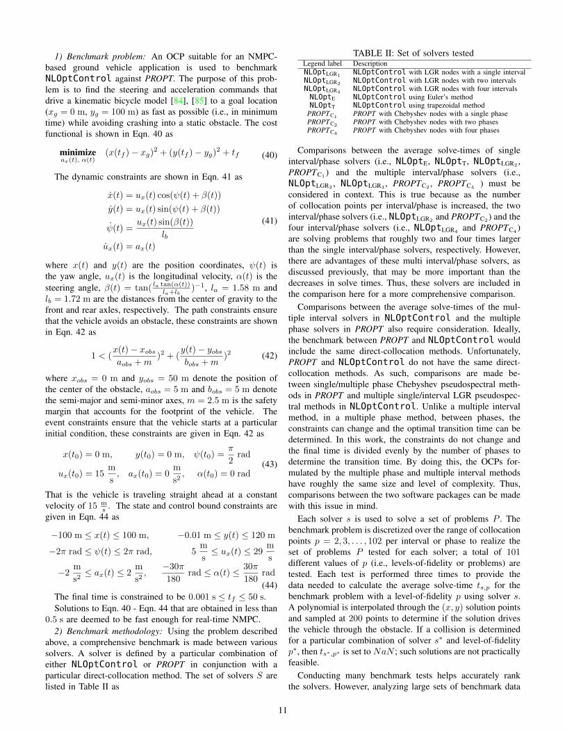
above, a comprehensive benchmark is made between varioussolvers. A solver is defined by a particular combination ofeither NLOptControl or PROPT in conjunction with aparticular direct-collocation method. The set of solvers S arelisted in Table II as
TABLE II: Set of solvers testedLegend label DescriptionNLOptLGR1 NLOptControl with LGR nodes with a single intervalNLOptLGR2 NLOptControl with LGR nodes with two intervalsNLOptLGR4 NLOptControl with LGR nodes with four intervalsNLOptE NLOptControl using Euler’s methodNLOptT NLOptControl using trapezoidal method
PROPTC1 PROPT with Chebyshev nodes with a single phasePROPTC2 PROPT with Chebyshev nodes with two phasesPROPTC4 PROPT with Chebyshev nodes with four phases
Comparisons between the average solve-times of singleinterval/phase solvers (i.e., NLOptE, NLOptT, NLOptLGR2
,PROPTC1
) and the multiple interval/phase solvers (i.e.,NLOptLGR2
, NLOptLGR4, PROPTC2
, PROPTC4) must be
considered in context. This is true because as the numberof collocation points per interval/phase is increased, the twointerval/phase solvers (i.e., NLOptLGR2
and PROPTC2) and the
four interval/phase solvers (i.e., NLOptLGR4and PROPTC4
)are solving problems that roughly two and four times largerthan the single interval/phase solvers, respectively. However,there are advantages of these multi interval/phase solvers, asdiscussed previously, that may be more important than thedecreases in solve times. Thus, these solvers are included inthe comparison here for a more comprehensive comparison.
Comparisons between the average solve-times of the mul-tiple interval solvers in NLOptControl and the multiplephase solvers in PROPT also require consideration. Ideally,the benchmark between PROPT and NLOptControl wouldinclude the same direct-collocation methods. Unfortunately,PROPT and NLOptControl do not have the same direct-collocation methods. As such, comparisons are made be-tween single/multiple phase Chebyshev pseudospectral meth-ods in PROPT and multiple single/interval LGR pseudospec-tral methods in NLOptControl. Unlike a multiple intervalmethod, in a multiple phase method, between phases, theconstraints can change and the optimal transition time can bedetermined. In this work, the constraints do not change andthe final time is divided evenly by the number of phases todetermine the transition time. By doing this, the OCPs for-mulated by the multiple phase and multiple interval methodshave roughly the same size and level of complexity. Thus,comparisons between the two software packages can be madewith this issue in mind.
Each solver s is used to solve a set of problems P . Thebenchmark problem is discretized over the range of collocationpoints p = 2, 3, . . . , 102 per interval or phase to realize theset of problems P tested for each solver; a total of 101different values of p (i.e., levels-of-fidelity or problems) aretested. Each test is performed three times to provide thedata needed to calculate the average solve-time ts,p for thebenchmark problem with a level-of-fidelity p using solver s.A polynomial is interpolated through the (x, y) solution pointsand sampled at 200 points to determine if the solution drivesthe vehicle through the obstacle. If a collision is determinedfor a particular combination of solver s∗ and level-of-fidelityp∗, then ts∗,p∗ is set to NaN ; such solutions are not practicallyfeasible.
Conducting many benchmark tests helps accurately rankthe solvers. However, analyzing large sets of benchmark data
11

can be overwhelming and the conclusions drawn from suchanalyses can be subjective. To help eliminate these issues, thiswork uses an optimization software benchmarking tool calledperformance profiles [86].
Performance profiles show the distribution function for aparticular performance metric. Here, the performance metric isthe ratio of the solver’s average solve-time to the best averagesolver solve-time given as
rs,p =ts,p
min(ts,p : s ∈ S)
where this performance metric is calculated for each solvers at each level-of-fidelity p = 2, 3, . . . , 102. If a solver doesnot solve a particular problem, then rs,p is set to rM . rM ischosen to be a large positive number; the choice of rM doesnot effect the evaluation [86].
To assess a solver’s overall performance on the set of prob-lems, the cumulative distribution function for the performanceratio is defined as
Ps(Γ) =1
101size(p ∈ P : rs,p ≤ Γ)
where Ps(Γ) is the probability that solver s can solve problemp within a factor Γ of the best ratio.
3) Setup: The setup is defined by the hardware platformand software stack. The results in this paper are producedusing a single machine running Ubuntu 16.04 with the fol-lowing hardware characteristics; an Intel Core i7 − 4910MQCPU @2.90GHz× 8, and 16GB of RAM. For software, bothNLOptControl 0.1.5 and PROPT use KNITRO 10.3 for theNLP solver with the default settings, except the maximumsolve-time, which is set to 300 s.
VI. RESULTS
A. Ease of use
Listing. 2 and Listing. 3 show the respective syntax inNLOptControl and PROPT needed to model the moonlander OCP in Eqn. 16. Section B in the Appendices showsNLOptControl’s and PROPT’s solutions compared to theanalytical solution.
Listing 2: NLOptControl code needed to formulate andsolve the moon lander problem. The ! character indicates thatthe function is modifying the model.n = define(numStates = 2, numControls = 1, X0
↪→ = [10, -2], XF = [0., 0.], XL = [0,↪→ -20], XU = [20, 20], CL = [0.], CU=[3.])↪→ ;
2 dynamics!(n,[:(x2[j]), :(u1[j] - 1.5)]);configure!(n;(:finalTimeDV => true));
4 obj = integrate!(n, :(u1[j]));@NLobjective(n.ocp.mdl, Min, obj);
6 optimize!(n);
NLOptControl can model OCPs more succinctly thanPROPT. NLOptControl models Eqn. 16 with 5 lines ofcode, while it takes PROPT 12 lines — there are two main rea-sons for this: (1) it takes PROPT 4 lines of code to include theinitial and final state conditions, and the upper and lower limitsof the states and controls, while this is accomplished with a
single line of code, with NLOptControl, and (2) severalof PROPT’s features are required, while in NLOptControlthey are optional; these features include an initial guess, anoptions structure, and the naming of the state and controlvariables. Additionally, PROPT has more verbose syntax thanNLOptControl — PROPT’s collocate(), initial(),and final() functions require many characters per line ofcode.
B. Speed
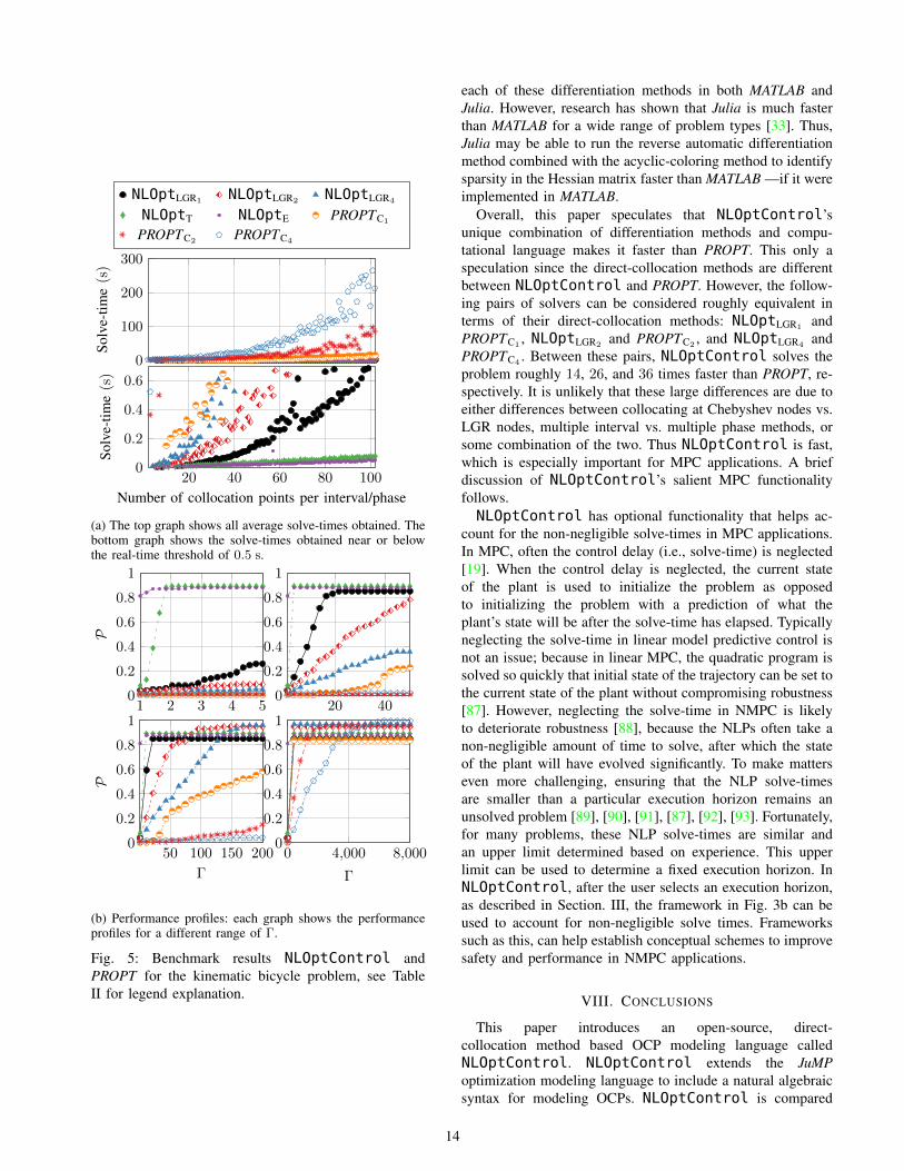
The performances of the solvers in Table II are now exam-ined on the set of problems realized by various discretizationsof Eqn. 40 – Eqn. 44, as described in Sec. V. The results forthese examinations are in Fig. 5a and Fig. 5b. Fig. 5a showsthe performance, or average solve-times ts,p, for each solvers on each problem p. Fig. 5b shows the performance profilesfor all of the solvers in four ranges of interest for Γ. Eachrange is on a separate plot. The purpose of this section is to(1) show the raw benchmark data in Fig. 5a and (2) providean objective analysis of this data in Fig. 5b. In the followingsection, this information will be used to draw conclusionsregarding the speed of NLOptControl and the best solverfor the benchmark problem.
Fig. 5a shows that NLOptControl’s solvers are fasterthan PROPT’s. At a high-level, NLOptControl solves 88%of the problems in real-time using h-methods (i.e., NLOptEand NLOptT) and 46% of the time using p/hp-methods(i.e., NLOptLGR2 , NLOptLGR2 , and NLOptLGR4 ). PROPT onlysolves 0.05% of the problems in real-time using p/hp-methods(i.e., PROPTC1
, PROPTC2, and PROPTC4
). At a lower-level,the zoomed-in subplot in the the bottom graph of Fig. 5a showsthat NLOptControl solves the benchmark problem in real-time when the number of collocation points per interval is lessthan: 80 for the single-interval case; 45 for the two-intervalcase; and 25 for the four-interval interval case. PROPT obtainsreal-time solutions when the number of collocation points perphase is less than 27 for the single-phase case and less than4 for the two-phase case. For the four-phase case, PROPTcannot solve any of the problems in real-time.
Fig. 5a also shows that as the number of intervals/phasesincrease from NLOptLGR1 to NLOptLGR4 and PROPTC1 toPROPTC4
, the solve-times increase exponentially. Due to thelarge solve-times with PROPT ’s solvers, these trends canonly be seen in the top graph of Fig. 5a — the bottom graphshows the trends for NLOptControl’s solvers. As discussedin the previous section, this increase in solve time is largelydue to the fact that with an increase in the intervals/phaseslarger problems are created and they take longer to solve.Even though the NLOptLGR4
solver is solving a problemthat is roughly four times larger than the PROPTC1
solver,NLOptLGR4 results in smaller solve-times.
Fig. 5a also shows that h-methods in NLOptControlare faster than the p-method for the benchmark problem. Asthe level-of-fidelity increases, the solve-times increase linearlywith h-methods and exponentially with the p-method. Addi-tionally, the number of collocation points needs to be greaterthan about 20 for the h-methods to ensure collision avoidance,
12

Listing 3: PROPT code needed to formulate and solve the moon lander problemtoms t t_f
2 p = tomPhase(’p’, t, 0, t_f, 30);setPhase(p);
4 tomStates x vtomControls a
6 cbox = {0.001<=t_f<=400, 0<=icollocate(x)<=20, -20<=icollocate(v)<= 20, 0<=collocate(a)<=3};ode = collocate({dot(x)==v, dot(v)==-1.5 + a});
8 cbnd = {initial(x == 10);initial(v == -2);final(x == 0);final(v == 0);};x0 = {t_f == 1.5, icollocate({x == 0 v == 0}), collocate(a == 0)};
10 objective = integrate(a);options = struct;
12 prob = sym2prob(objective, {cbox, ode, cbnd}, x0, options);result = tomRun(’knitro’, prob, 1);
while the p-methods need 23 and 27 for NLOptControl andPROPT, respectively.
The four plots in Fig 5b show the ranges of Γ whereincertain solvers dominate. Each profile in this figure showsthe probability P that a given solver s will solve the setof problems P the fastest within a factor of Γ. At Γ = 1,the solver that has the highest probability of being the fastestis NLOptE, with a probability of 0.881. NLOptE dominatesuntil about Γ = 1.8, at which point NLOptT has the highestprobability of being the fastest, with a probability of 0.891.NLOptT dominates until about Γ = 80. The remainingapproximate ranges of domination are as follows: NLOptLGR2
from 80 to 160, NLOptLGR4from 160 to 5, 000, PROPTC4
from 5, 000 onwards. Given enough time, PROPTC4 solves100% of the problems. For this benchmark problem, whilethe NLOptT and NLOptE solvers are much faster than theNLOptLGR2
, NLOptLGR4, and PROPTC4
solvers they are notas reliable. However, the NLOptT and NLOptE solvers areboth faster and more reliable than the NLOptLGR2 , PROPTC1 ,and PROPTC2 solvers.
VII. DISCUSSION
The approach detailed in Section II yields a direct-collocation-based optimal control modeling language that isboth faster and easier to use than PROPT. The results and thefollowing discussion support this claim.NLOptControl is easier to use than PROPT, because
its syntax is more concise, and focused on building a modelof the OCP in Bolza form. Differences between Listing. 2and Listing. 3, in terms of number of lines of code andthe number of characters per line of code, indicate thatNLOptControl models OCPs more succinctly than PROPT.This work speculates that PROPT requires more lines of codeto formulate other more practical problems as well.
In addition to PROPT’s verbosity, its syntax is flexible to theextent that modeling errors are easier to be made. This claimis made because its users can more easily formulate problemsthat do not fit into the Bolza OCP form. As an example,consider using PROPT to model the dynamic constraints inEqn. 5 for the moon lander problem — Line 7 in Listing. 3.When using PROPT, if the user were to forget to include thesecond differential equation as
ode = collocate({dot(x)==v});
an error would not be displayed; such overly flexible syntaxcan lead to modeling errors. If that same mistake wereattempted in NLOptControl, the user would be alerted as
1 julia> dynamics!(n,[:(x2[j])]);ERROR: The number of differential equations
↪→ must equal ocp.state.num.
Thus, NLOptControl helps avoid modeling errors betterthan PROPT, because NLOptControl’s syntax does notallow users to formulate problems that are not in the Bolzaform, while PROPT’s syntax does.
Both NLOptControl and PROPT can be used formulateOCPs, but PROPT takes a functional approach to this taskrather than a modeling approach, as with NLOptControl.Listing. 2 is compared to Listing. 3 to support this claim.Listing. 3 shows that, with PROPT, the user creates all of thecomponents of the OCP and finally assembles them on Line12. With NLOptControl, in Listing. 2, it is clear from thefirst line of code that a model named n is being built. Usingthis approach, NLOptControl can clearly model and solvemultiple OCPs at once. Such an object-oriented approach canfurther reduce potential modeling errors.
The benchmark results in Fig. 5a and Fig. 5b show thatNLOptControl is faster than PROPT. Differences betweenthese packages that affect speed include: differentiation meth-ods, underlying computational language, and available direct-collocation methods.
PROPT uses symbolic automatic differentiation to calcu-late the derivatives. However, the structure of the Hessianmatrices born from approximating an OCP using direct-collocation methods is sparse and symbolic automatic differ-entiation does not exploit this structure for speed. In contrast,NLOptControl uses the acyclic-coloring method to exploitthe sparse structure of the Hessian matrix in conjunction withreverse automatic differentiation. Based on this difference,NLOptControl is expected to be faster than PROPT, es-pecially when solving large problems that have a very sparsestructure.
PROPT’s differentiation methods are implemented in MAT-LAB and NLOptControl’s are implemented in Julia. Un-fortunately, the literature does not contain benchmarks of
13
0
100
200
300
Solv
e-tim
e(s
)
20 40 60 80 1000
0.2
0.4
0.6
Number of collocation points per interval/phase
Solv
e-tim
e(s
)
NLOptLGR1NLOptLGR2
NLOptLGR4
NLOptT NLOptE PROPTC1
PROPTC2 PROPTC4
(a) The top graph shows all average solve-times obtained. Thebottom graph shows the solve-times obtained near or belowthe real-time threshold of 0.5 s.
1 2 3 4 50
0.2
0.4
0.6
0.8
1
P
20 400
0.2
0.4
0.6
0.8
1
50 100 150 2000
0.2
0.4
0.6
0.8
1
Γ
P
0 4,000 8,0000
0.2
0.4
0.6
0.8
1
Γ
(b) Performance profiles: each graph shows the performanceprofiles for a different range of Γ.
Fig. 5: Benchmark results NLOptControl andPROPT for the kinematic bicycle problem, see TableII for legend explanation.
each of these differentiation methods in both MATLAB andJulia. However, research has shown that Julia is much fasterthan MATLAB for a wide range of problem types [33]. Thus,Julia may be able to run the reverse automatic differentiationmethod combined with the acyclic-coloring method to identifysparsity in the Hessian matrix faster than MATLAB —if it wereimplemented in MATLAB.
Overall, this paper speculates that NLOptControl’sunique combination of differentiation methods and compu-tational language makes it faster than PROPT. This only aspeculation since the direct-collocation methods are differentbetween NLOptControl and PROPT. However, the follow-ing pairs of solvers can be considered roughly equivalent interms of their direct-collocation methods: NLOptLGR1
andPROPTC1 , NLOptLGR2 and PROPTC2 , and NLOptLGR4 andPROPTC4 . Between these pairs, NLOptControl solves theproblem roughly 14, 26, and 36 times faster than PROPT, re-spectively. It is unlikely that these large differences are due toeither differences between collocating at Chebyshev nodes vs.LGR nodes, multiple interval vs. multiple phase methods, orsome combination of the two. Thus NLOptControl is fast,which is especially important for MPC applications. A briefdiscussion of NLOptControl’s salient MPC functionalityfollows.NLOptControl has optional functionality that helps ac-
count for the non-negligible solve-times in MPC applications.In MPC, often the control delay (i.e., solve-time) is neglected[19]. When the control delay is neglected, the current stateof the plant is used to initialize the problem as opposedto initializing the problem with a prediction of what theplant’s state will be after the solve-time has elapsed. Typicallyneglecting the solve-time in linear model predictive control isnot an issue; because in linear MPC, the quadratic program issolved so quickly that initial state of the trajectory can be set tothe current state of the plant without compromising robustness[87]. However, neglecting the solve-time in NMPC is likelyto deteriorate robustness [88], because the NLPs often take anon-negligible amount of time to solve, after which the stateof the plant will have evolved significantly. To make matterseven more challenging, ensuring that the NLP solve-timesare smaller than a particular execution horizon remains anunsolved problem [89], [90], [91], [87], [92], [93]. Fortunately,for many problems, these NLP solve-times are similar andan upper limit determined based on experience. This upperlimit can be used to determine a fixed execution horizon. InNLOptControl, after the user selects an execution horizon,as described in Section. III, the framework in Fig. 3b can beused to account for non-negligible solve times. Frameworkssuch as this, can help establish conceptual schemes to improvesafety and performance in NMPC applications.
VIII. CONCLUSIONS
This paper introduces an open-source, direct-collocation method based OCP modeling language calledNLOptControl. NLOptControl extends the JuMPoptimization modeling language to include a natural algebraicsyntax for modeling OCPs. NLOptControl is compared
14
against PROPT in terms of ease of use and speed. PROPT’ssyntax is shown to be more verbose and error-prone thanNLOptControl’s; thus NLOptControl is easier touse than PROPT. This ease of use is largely attributed toNLOptControl’s use of the JuMP optimization modelinglanguage. In addition to being easier to use, results fromthe benchmark tests show that NLOptControl is muchfaster than PROPT. NLOptControl’s superior performanceis likely due to the unique utility of the Julia programminglanguage and the reverse automatic differentiation method inconjunction with the acyclic-coloring method to exploit thesparsity of the Hessian matrices. NLOptControl emergesas an easy to use, fast, and open-source [9] optimal controlmodeling language that holds great potential for not onlyimproving existing off-line and on-line control systems butalso engendering a wide variety of new ones.
ACKNOWLEDGEMENTS
This work was supported by the Automotive ResearchCenter (ARC) in accordance with Cooperative AgreementW56HZV-14-2-0001 U.S. Army Tank Automotive Research,Development and Engineering Center (TARDEC) Warren, MI.Benoît Legat provided a thoughtful review of this paper anddiscussions with the several Julia developers including MilesLubin, Tony Kelman, and Chris Rackauckas were helpful.
REFERENCES
[1] M. A. Patterson, A. V. Rao, Gpops-ii: A matlab software for solvingmultiple-phase optimal control problems using hp-adaptive gaussianquadrature collocation methods and sparse nonlinear programming,ACM Transactions on Mathematical Software (TOMS) 41 (1) (2014)1.
[2] J. P. Sanchez, D. Garcia Yarnoz, Asteroid retrieval missions enabled byinvariant manifold dynamics, Acta Astronautica 127 (2016) 667 – 677,asteroid mission;Easily retrievable objects;Libration point orbits;Lowthrust;Trajectory designs;.URL http://dx.doi.org/10.1016/j.actaastro.2016.05.034
[3] M. M. E. Per E. Rutquist, PROPT - Matlab Optimal Control Software,Tomlab Optimization Inc., 1260 SE Bishop Blvd Ste E, Pullman, WA99163, USA, 1st Edition (June 2016).URL https://tomopt.com/docs/TOMLAB_PROPT.pdf
[4] T. Jorris, C. Schulz, F. Friedl, A. Rao, Constrained trajectory opti-mization using pseudospectral methods, in: AIAA Atmospheric FlightMechanics Conference and Exhibit, 2008, p. 6218.
[5] W. Kang, N. Bedrossian, Pseudospectral optimal control theory makesdebut flight, saves nasa 1 m in under three hours (2007).
[6] A. Holmqvist, F. Magnusson, Open-loop optimal control of batchchromatographic separation processes using direct collocation, Journalof Process Control 46 (2016) 55–74.
[7] T. Utstumo, T. W. Berge, J. T. Gravdahl, Non-linear model predictivecontrol for constrained robot navigation in row crops, in: IndustrialTechnology (ICIT), 2015 IEEE International Conference on, IEEE, 2015,pp. 357–362.
[8] J. V. Frasch, A. Gray, M. Zanon, H. J. Ferreau, S. Sager, F. Borrelli,M. Diehl, An auto-generated nonlinear mpc algorithm for real-timeobstacle avoidance of ground vehicles, in: European Control Conference,IEEE, 2013, pp. 4136–4141.
[9] H. Febbo, NLOptControl, https://github.com/JuliaMPC/NLOptControl.jl(2017).
[10] A. V. Rao, D. A. Benson, C. Darby, M. A. Patterson, C. Francolin,I. Sanders, G. T. Huntington, Algorithm 902: Gpops, a matlab softwarefor solving multiple-phase optimal control problems using the gausspseudospectral method, ACM Transactions on Mathematical Software(TOMS) 37 (2) (2010) 22.
[11] V. M. Becerra, Solving complex optimal control problems at no costwith psopt, in: Computer-Aided Control System Design (CACSD), 2010IEEE International Symposium on, IEEE, 2010, pp. 1391–1396.
[12] M. Kelly, An introduction to trajectory optimization: How to do yourown direct collocation, SIAM Review 59 (4) (2017) 849–904.
[13] J. T. Betts, S. L. Campbell, N. Kalla, Initialization of direct transcriptionoptimal control software, in: Decision and Control, 2003. Proceedings.42nd IEEE Conference on, Vol. 4, IEEE, 2003, pp. 3802–3807.
[14] A. V. Rao, User’s manual for gpocs c version 1.0: A matlab R© imple-mentation of the gauss pseudospectral method for solving multiple-phaseoptimal control problems (2007).
[15] J. Andersson, J. Åkesson, M. Diehl, Casadi: A symbolic package forautomatic differentiation and optimal control, in: Recent Advances inAlgorithmic Differentiation, Springer, 2012, pp. 297–307.
[16] I. M. Ross, A beginner’s guider to dido: A matlab application packagefor solving optimal control problem, http://www. elissar. ziz (2007).
[17] B. Ghannadi, N. Mehrabi, R. S. Razavian, J. McPhee, Nonlinear modelpredictive control of an upper extremity rehabilitation robot using atwo-dimensional human-robot interaction model, in: International Con-ference on Intelligent Robots and Systems, IEEE, 2017, pp. 502–507.
[18] G. Basset, Y. Xu, O. Yakimenko, Computing short-time aircraft maneu-vers using direct methods, Journal of Computer and Systems SciencesInternational 49 (3) (2010) 481–513.
[19] J. Liu, P. Jayakumar, J. L. Stein, T. Ersal, Combined speed and steeringcontrol in high-speed autonomous ground vehicles for obstacle avoid-ance using model predictive control, IEEE Transactions on VehicularTechnology 66 (10) (2017) 8746–8763.
[20] H. Febbo, J. Liu, P. Jayakumar, J. L. Stein, T. Ersal, Moving obstacleavoidance for large, high-speed autonomous ground vehicles, in: Amer-ican Control Conference, 2017, pp. 5568–5573.
[21] B. Houska, H. J. Ferreau, M. Diehl, ACADO toolkit: An open-sourceframework for automatic control and dynamic optimization, OptimalControl Applications and Methods 32 (3) (2011) 298–312.
[22] M. Lubin, I. Dunning, Computing in operations research using julia,INFORMS Journal on Computing 27 (2) (2015) 238–248. doi:10.1287/ijoc.2014.0623.
[23] O. von Stryk, Dircol, Internet/WWW (2001).[24] . e. RWTH Aachen University, Germany, DyOS User Manual, 2002.[25] M. Diehl, D. B. Leineweber, A. A. Schäfer, MUSCOD-II users’
manual, Universität Heidelberg. Interdisziplinäres Zentrum für Wis-senschaftliches âAe, 2001.
[26] V. Leek, An optimal control toolbox for matlab based on casadi (2016).[27] R. H. Byrd, J. Nocedal, R. A. Waltz, Knitro: An integrated package for
nonlinear optimization (2006).[28] L. T. B. Andreas Wachter, On the implementation of an interior-
point filter line-search algorithm for large-scale nonlinear programming(2004).
[29] P. E. Gill, W. Murray, M. A. Saunders, Snopt: An sqp algorithm forlarge-scale constrained optimization (2002).
[30] M. A. Patterson, A. V. Rao, Exploiting sparsity in direct collocationpseudospectral methods for solving optimal control problems, Journalof Spacecraft and Rockets 49 (2) (2012) 364–377.
[31] M. J. Tenny, J. B. Rawlings, R. Bindlish, Feasible real-time nonlinearmodel predictive control, in: AICHE SYMPOSIUM SERIES, New York;American Institute of Chemical Engineers; 1998, 2002, pp. 433–437.
[32] A. H. Gebremedhin, F. Manne, A. Pothen, What color is your jacobian?graph coloring for computing derivatives, SIAM review 47 (4) (2005)629–705.
[33] J. Bezanson, S. Karpinski, V. B. Shah, A. Edelman, Julia: A fast dy-namic language for technical computing, arXiv preprint arXiv:1209.5145(2012).
[34] I. Dunning, J. Huchette, M. Lubin, Jump: A modeling language formathematical optimization, SIAM Review 59 (2) (2017) 295–320. doi:10.1137/15M1020575.
[35] A. Griewank, D. Juedes, J. Utke, Algorithm 755: Adol-c: a packagefor the automatic differentiation of algorithms written in c/c++, ACMTransactions on Mathematical Software (TOMS) 22 (2) (1996) 131–167.
[36] J. Revels, Reversediff, https://github.com/JuliaDiff/ReverseDiff.jl(2017).
[37] L. Lessard, X. Zhang, X. Zhu, An optimal control approach to sequentialmachine teaching, arXiv preprint arXiv:1810.06175 (2018).
[38] R. Fourer, On the evolution of optimization modeling systems, Opti-mization Stories (2012) 377–388.
[39] R. E. Rosenthal, Gams–a user’s guide (2004).[40] R. Fourer, D. Gay, B. Kernighan, Ampl: A modeling language for
mathematical programming, 2002, Duxbury Press.[41] M. Udell, K. Mohan, D. Zeng, J. Hong, S. Diamond, S. Boyd, Convex
optimization in julia, in: Proceedings of the 1st First Workshop for HighPerformance Technical Computing in Dynamic Languages, IEEE Press,2014, pp. 18–28.
15

[42] E. Fragniere, J. Gondzio, R. Sarkissian, J.-P. Vial, A structure-exploitingtool in algebraic modeling languages, Management Science 46 (8)(2000) 1145–1158.
[43] J. T. Betts, Practical methods for optimal control and estimation usingnonlinear programming, Vol. 19, Siam, 2010.
[44] J. Huchette, M. Lubin, C. Petra, Parallel algebraic modeling for stochas-tic optimization, in: Proceedings of the 1st First Workshop for HighPerformance Technical Computing in Dynamic Languages, IEEE Press,2014, pp. 29–35.
[45] I. R. Dunning, Advances in robust and adaptive optimization: algorithms,software, and insights, Ph.D. thesis, Massachusetts Institute of Technol-ogy (2016).
[46] M. Lubin, Y. Dvorkin, S. Backhaus, A robust approach to chanceconstrained optimal power flow with renewable generation, IEEE Trans-actions on Power Systems 31 (5) (2016) 3840–3849.
[47] B. Legat, SumOfSquares, https://github.com/JuliaOpt/SumOfSquares.jl(2019).
[48] A. H. Gebremedhin, A. Tarafdar, A. Pothen, A. Walther, Efficient com-putation of sparse hessians using coloring and automatic differentiation,INFORMS Journal on Computing 21 (2) (2009) 209–223.
[49] J. Heinen, Gr, https://github.com/jheinen/GR.jl (2018).[50] E. F. M. D. John Hunter, Darren Dale, matplotlib, https://github.com/
matplotlib/matplotlib (2018).[51] J. Meditch, On the problem of optimal thrust programming for a lunar
soft landing, IEEE Transactions on Automatic Control 9 (4) (1964) 477–484.
[52] P. O. Scokaert, J. B. Rawlings, Feasibility issues in linear modelpredictive control, AIChE Journal 45 (8) (1999) 1649–1659.
[53] E. C. Kerrigan, J. M. Maciejowski, Soft constraints and exact penaltyfunctions in model predictive control, in: UKACC International Confer-ence, 2000.
[54] C. Rackauckas, Q. Nie, Differentialequations. jl–a performant andfeature-rich ecosystem for solving differential equations in julia, Journalof Open Research Software 5 (1) (2017).
[55] J. T. Betts, Survey of numerical methods for trajectory optimization,Journal of Guidance Control and Dynamics 21 (2) (1998) 193–207.
[56] L. T. Biegler, An overview of simultaneous strategies for dynamic opti-mization, Chemical Engineering and Processing: Process Intensification46 (11) (2007) 1043–1053.
[57] B. Paden, M. Cáp, S. Z. Yong, D. Yershov, E. Frazzoli, A survey ofmotion planning and control techniques for self-driving urban vehicles,IEEE Transactions on Intelligent Vehicles 1 (1) (2016) 33–55.
[58] L. S. Pontryagin, Mathematical theory of optimal processes, CRC Press,1987.
[59] D. Garg, Advances in global pseudospectral methods for optimal control,Ph.D. thesis, University of Florida USA (2011).
[60] D. G. Hull, Conversion of optimal control problems into parameteroptimization problems, Journal of Guidance, Control, and Dynamics20 (1) (1997) 57–60.
[61] M. R. Osborne, On shooting methods for boundary value problems,Journal of Mathematical Analysis and Applications 27 (2) (1969) 417–433.
[62] H. G. Bock, K.-J. Plitt, A multiple shooting algorithm for direct solutionof optimal control problems, IFAC Proceedings Volumes 17 (2) (1984)1603–1608.
[63] M. Diehl, H. G. Bock, H. Diedam, P.-B. Wieber, Fast direct multipleshooting algorithms for optimal robot control, in: Fast Motions inBiomechanics and Robotics, Springer, 2006, pp. 65–93.
[64] R. Sargent, Optimal control, Journal of Computational and AppliedMathematics 124 (1-2) (2000) 361–371.
[65] M. Diehl, H. G. Bock, J. P. Schlöder, R. Findeisen, Z. Nagy, F. Allgöwer,Real-time optimization and nonlinear model predictive control of pro-cesses governed by differential-algebraic equations, Journal of ProcessControl 12 (4) (2002) 577–585.
[66] J. T. Betts, W. P. Huffman, Exploiting sparsity in the direct transcriptionmethod for optimal control, Computational Optimization and Applica-tions 14 (2) (1999) 179–201.
[67] C. R. Hargraves, S. W. Paris, Direct trajectory optimization usingnonlinear programming and collocation, Journal of Guidance, Control,and Dynamics 10 (4) (1987) 338–342.
[68] W. W. Hager, Runge-kutta methods in optimal control and the trans-formed adjoint system, Numerische Mathematik 87 (2) (2000) 247–282.
[69] D. Garg, M. Patterson, W. W. Hager, A. V. Rao, D. A. Benson, G. T.Huntington, A unified framework for the numerical solution of optimalcontrol problems using pseudospectral methods, Automatica 46 (11)(2010) 1843–1851.
[70] F. Fahroo, I. M. Ross, Advances in pseudospectral methods for optimalcontrol, in: AIAA Guidance, Navigation and Control Conference, 2008,p. 7309.
[71] G. Huntington, D. Benson, A. Rao, A comparison of accuracy andcomputational efficiency of three pseudospectral methods, in: AIAAGuidance, Navigation and Control Conference, 2007, p. 6405.
[72] M. A. Patterson, W. W. Hager, A. V. Rao, A ph mesh refinement methodfor optimal control, Optimal Control Applications and Methods 36 (4)(2015) 398–421.
[73] C. L. Darby, W. W. Hager, A. V. Rao, An hp-adaptive pseudospectralmethod for solving optimal control problems, Optimal Control Applica-tions and Methods 32 (4) (2011) 476–502.
[74] S. Jain, P. Tsiotras, Trajectory optimization using multiresolution tech-niques, Journal of Guidance, Control, and Dynamics 31 (5) (2008) 1424–1436.
[75] C. L. Darby, A. V. Rao, A mesh refinement algorithm for solvingoptimal control problems using pseudospectral methods, Proceedingsof the AIAA (2009).
[76] G. Elnagar, M. A. Kazemi, M. Razzaghi, The pseudospectral legendremethod for discretizing optimal control problems, IEEE Transactions onAutomatic Control 40 (10) (1995) 1793–1796.
[77] M. Y. Hussaini, T. A. Zang, Spectral methods in fluid dynamics, AnnualReview of Fluid Mechanics 19 (1) (1987) 339–367.
[78] C. L. Darby, hp-Pseudospectral method for solving continuous-timenonlinear optimal control problems, University of Florida, 2011.
[79] D. Garg, W. W. Hager, A. V. Rao, Pseudospectral methods for solvinginfinite-horizon optimal control problems, Automatica 47 (4) (2011)829–837.
[80] M. Abramowitz, Stegun, Handbook of Mathematical Functions 55(1965) 888.
[81] C. F. Gauss, Methodus nova integralium valores per approximationeminveniendi, apvd Henricvm Dieterich, 1815.
[82] S. Olver, Fastgaussquadrature, https://github.com/ajt60gaibb/FastGaussQuadrature.jl (2017).
[83] N. Hale, A. Townsend, Fast and accurate computation of gauss–legendreand gauss–jacobi quadrature nodes and weights, SIAM Journal onScientific Computing 35 (2) (2013) A652–A674.
[84] R. Rajamani, Vehicle dynamics and control, Springer Science andBusiness Media, 2011.
[85] J. Gonzales, F. Zhang, K. Li, F. Borrelli, Autonomous drifting withonboard sensors, in: Advanced Vehicle Control, CRC Press, 2016, p.133.
[86] J. J. M. Elizabeth D. Dolan, Benchmarking optimization software withperformance profiles (2001).
[87] M. Diehl, H. J. Ferreau, N. Haverbeke, Efficient numerical methodsfor nonlinear mpc and moving horizon estimation, Nonlinear ModelPredictive Control 384 (2009) 391–417.
[88] L. L. Simon, Z. K. Nagy, K. Hungerbuehler, Swelling constrained con-trol of an industrial batch reactor using a dedicated nmpc environment:Optcon, in: Nonlinear Model Predictive Control, Springer, 2009, pp.531–539.
[89] M. Morari, J. H. Lee, Model predictive control: past, present and future,Computers & Chemical Engineering 23 (4) (1999) 667–682.
[90] A. Eskandarian, Handbook of Intelligent Vehicles, Springer, 2012.[91] T. Ohtsuka, K. Ozaki, Practical issues in nonlinear model predictive
control: real-time optimization and systematic tuning, in: NonlinearModel Predictive Control, Springer, 2009, pp. 447–460.
[92] J. Albersmeyer, D. Beigel, C. Kirches, L. Wirsching, H. G. Bock, J. P.Schlöder, Fast nonlinear model predictive control with an applicationin automotive engineering, in: Nonlinear Model Predictive Control,Springer, 2009, pp. 471–480.
[93] C. Kirches, L. Wirsching, S. Sager, H. G. Bock, Efficient numerics fornonlinear model predictive control, in: Recent Advances in Optimizationand its Applications in Engineering, Springer, 2010, pp. 339–357.
[94] H. Mirinejad, T. Inanc, An rbf collocation method for solvingoptimal control problems, Robotics and Autonomous Systems87 (Supplement C) (2017) 219 – 225. doi:https://doi.org/10.1016/j.robot.2016.10.015.URL http://www.sciencedirect.com/science/article/pii/S0921889015301639
APPENDIX ABRYSON-DENHAM PROBLEM
Fig. 6 shows the analytic solutions for the states, con-trol, as well as costates compared to the results obtained
16

with NLOptControl using a single interval with 30 LGRnodes. NLOptControl calculates these trajectories reason-ably well.
0
2
4
6
8
·10−2
x(t
)
−1
0
1
v(t
)
0 0.2 0.4 0.6 0.8 1
−8
−6
−4
−2
0
Time (s)
a(t
)
−40
−20
0
20
40
λx(t
)
0 0.2 0.4 0.6 0.8 1
0
2
4
6
8
Time (s)
λv(t
)
Optimalsolutioncoll. pts.
Fig. 6: State, control, and costate trajectories usingNLOptControl (with 30 LGR nodes) compared to theanalytical optimal solution for the Bryson Denham problem
The NLP solver for this example is IPOPT and an hp-method in NLOptControl is used with 4 intervals and 10LGR nodes.
APPENDIX BMOON LANDER PROBLEM
A. Closed-loop
Fig. 7 shows the closed-loop solution to the moon landerproblem using NLOptControl. The closed-loop trajectoryof the plant is very close to the analytic solution. Additionally,all of the solve-times are well below the chosen executionhorizon tex of 0.2 s; thus NLOptControl solves this NMPCproblem in real-time.
The NLP solver for this example is IPOPT and an hp-method in NLOptControl is used with 4 intervals and 10LGR nodes.
0 10 20
2
4
6
·10−2
Iterations
solv
e-tim
e(s
)
0 1 2 3 4
0
5
10
Time (s)x
(t)
−4
−2
0
v(t
)
0 1 2 3 4
0
1
2
3
Time (s)
a(t
)
Analytic solutionPlant
Fig. 7: Closed-loop trajectories for moon lander problemcompared to the analytic solution
B. Open-loop
In Fig. 8, it can be seen that both NLOptControland PROPT determine the analytic solution accurately, with30 LGR and Chebyshev nodes, respectively. However, thereis an overshoot in the solution of the control with bothNLOptControl and PROPT. This is due to the bang-bangnature of the analytic solution. It is noted that this overshootmay be mitigated using either mesh refinement [72], [75], [74]or radial basis functions [94].
APPENDIX CBENCHMARK PROBLEM
This section provides an example of the type of so-lutions that are obtained from the benchmark betweenNLOptControl and PROPT. For NLOptControl, the hp-method with LGR nodes and four intervals and 10 collocationpoints per interval is used. PROPT is set to use four phases and10 collocation points per phase and Chebyshev nodes. Fig. 9compares the results of these solvers, where it can be seen thatposition trajectories are close. Starting at a speed of 15 m
s , thesolutions obtained from both PROPT and NLOptControlapply maximum acceleration from t0 = 0 s to tf = 5.1 swhile avoiding collision with the obstacle and reaching thedesired goal position. The trajectories for NLOptControlexhibit large oscillations in the α trajectory. These oscillationsmay be an artifact of the Runge phenomenon and seem to bereduced with PROPT as it uses Chebyshev nodes.
There is no analytic solution to this problem.
17
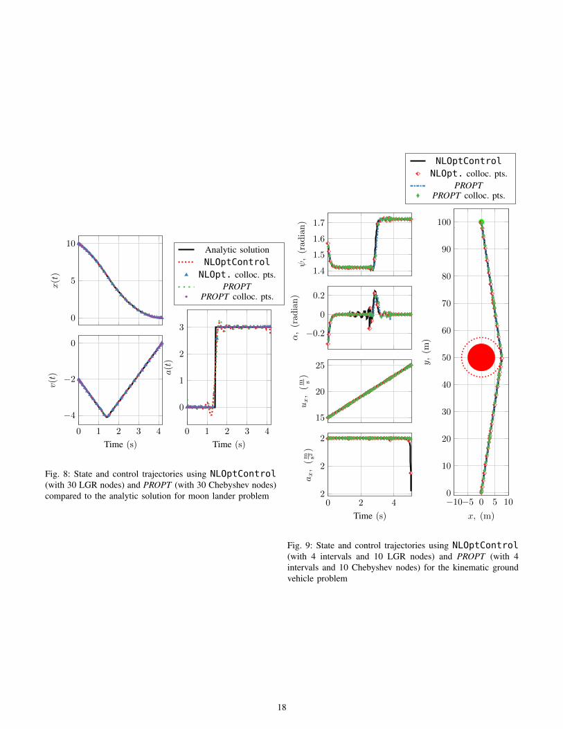
0
5
10
x(t
)
0 1 2 3 4
−4
−2
0
Time (s)
v(t
)
0 1 2 3 4
0
1
2
3
Time (s)
a(t
)
Analytic solutionNLOptControlNLOpt. colloc. pts.
PROPTPROPT colloc. pts.
Fig. 8: State and control trajectories using NLOptControl(with 30 LGR nodes) and PROPT (with 30 Chebyshev nodes)compared to the analytic solution for moon lander problem
1.4
1.5
1.6
1.7
ψ,
(rad
ian
)
−0.2
0
0.2α,
(rad
ian
)
15
20
25
ux,
(m s
)
0 2 42
2
2
Time (s)
ax,
(m s2
)
−10−5 0 5 100
10
20
30
40
50
60
70
80
90
100
Goal
x, (m)
y,
(m)
NLOptControlNLOpt. colloc. pts.
PROPTPROPT colloc. pts.
Fig. 9: State and control trajectories using NLOptControl(with 4 intervals and 10 LGR nodes) and PROPT (with 4intervals and 10 Chebyshev nodes) for the kinematic groundvehicle problem
18