nlpqlp: a new fortran implementation of a sequential quadratic
TRANSCRIPT

NLPQLP: A New Fortran Implementation of a
Sequential Quadratic Programming Algorithm
for Parallel Computing
Address: Prof. Dr. K. SchittkowskiDepartment of MathematicsUniversity of BayreuthD - 95440 Bayreuth
Phone: +921 553278 (office)+921 32887 (home)
Fax: +921 35557
E-mail: [email protected]: http://www.klaus-schittkowski.de
Abstract
The Fortran subroutine NLPQLP solves smooth nonlinear programmingproblems and is an extension of the code NLPQL. The new version is specif-ically tuned to run under distributed systems. A new input parameter l isintroduced for the number of parallel machines, that is the number of functioncalls to be executed simultaneously. In case of l = 1, NLPQLP is identicalto NLPQL. Otherwise the line search is modified to allow parallel functioncalls either for the line search or for approximating gradients by differenceformulae. The mathematical background is outlined, in particular the modifi-cation of line search algorithms to retain convergence under parallel systems.Numerical results show the sensitivity of the new version with respect to thenumber of parallel machines, and the influence of different gradient approxi-mations under uncertainty. The performance evaluation is obtained by morethan 300 standard test problems.
1
1 Introduction
We consider the general optimization problem, to minimize an objective function funder nonlinear equality and inequality constraints, i.e.
x ∈ IRn :
min f(x)gj(x) = 0 , j = 1, . . . ,me
gj(x) ≥ 0 , j = me + 1, . . . ,mxl ≤ x ≤ xu
(1)
where x is an n-dimensional parameter vector. To facilitate the subsequent notation,we assume that upper and lower bounds xu and xl are not handled separately, i.e.that they are considered as general inequality constraints. Then we get the nonlinearprogramming problem
x ∈ IRn :min f(x)gj(x) = 0 , j = 1, . . . ,me
gj(x) ≥ 0 , j = me + 1, . . . ,m(2)
called now NLP in abbreviated form. It is assumed that all problem functions f(x)and gj(x), j = 1, . . . ,m, are continuously differentiable on the whole IRn. Butbesides of this we do not suppose any further structure in the model functions.
Sequential quadratic programming methods are the standard general purposealgorithms for solving smooth nonlinear optimization problems, at least under thefollowing assumptions:
• The problem is not too big.
• The functions and gradients can be evaluated with sufficiently high precision.
• The problem is smooth and well-scaled.
The code NLPQL of Schittkowski [28] is a Fortran implementation of a sequentialquadratic programming (SQP) algorithm. The design of the numerical algorithmis founded on extensive comparative numerical tests of Schittkowski [21, 25, 23],Schittkowski et al. [34], Hock and Schittkowski [13], and on further theoretical in-vestigations published in [22, 24, 26, 27]. The algorithm is extended to solve alsononlinear least squares problems efficiently, see [31], and to handle problems withvery many constraints, cf. [32]. To conduct the numerical tests, a random test prob-lem generator is developed for a major comparative study, see [21]. Two collectionswith more than 300 academic and real-life test problems are published in Hock andSchittkowski [13] and in Schittkowski [29]. These test examples are now part of theCute test problem collection of Bongartz et al. [4]. More than 100 test problemsbased on a finite element formulation are collected for the comparative evaluationin Schittkowski et al. [34].
Moreover there exist hundreds of commercial and academic applications of NLPQL,for example
2

1. Mechanical structural optimization, see Schittkowski et al. [34] and Kneppe etal. [15],
2. Data fitting and optimal control of transdermal pharmaceutical systems, seeBoderke et al. [1] or Blatt and Schittkowski [3],
3. Computation of optimal feed rates for tubular reactors, see Birk et al. [2],
4. Food drying in a convection oven, see Frias et al. [11],
5. Optimal design of horn radiators for satellite communication, see Hartwanger,Schittkowski, Wolf [10],
6. Receptor-ligand binding studies, see Schittkowski [33].
The very first version of NLQPL developed in 1981, is still included in the IMSLLibrary [30], but meanwhile outdated because of numerous improvements and cor-rections made since then. Actual versions of NLPQL are part of commercial redis-tributed optimization systems like
- ANSYS/POPT (CAD-FEM, Grafing) for structural optimization,
- STRUREL (RCP, Munich) for reliability analysis,
- TEMPO (OECD Reactor Project, Halden) for control of power plants,
- Microwave Office Suit (Applied Wave Research, El Segundo) for electronic design,
- MOOROPT (Marintec, Trondheim) for the design of mooring systems,
- iSIGHT (Enginious Software, Cary, North Carolina) for multi-disciplinary CAE,
- POINTER (Synaps, Atlanta) for design automation.
Customers include Axiva, BASF, Bayer, Bell Labs, Chevron Research, DLR, DornierSystems, Dow Chemical, EADS, ENSIGC, EPCOS, ESOC, Eurocopter, FantoftProsess, General Electric, GLM Lasertechnik, Hoechst, IABG, IBM, INRIA, INRS-Telecommunications, Mecalog, MTU, NASA, Nevesbu, NLR, Norsk Hydro Research,Numerola, Peaktime, Philips, Rolls-Royce, SAQ Kontroll, SDRC, Siemens, TNO,Transpower, US Air Force, and in addition dozens of academic research institutionsall over the world.
The general availability of parallel computers and in particular of distributedcomputing through networks motivates a careful redesign of NLPQL, to allow si-multaneous function calls with predetermined arguments. The resulting code iscalled NLPQLP and its mathematical background and usage is documented in thispaper.
The iterative process of an SQP algorithm is highly sequential. Proceeding froma given initial design, new iterates are computed based only on the informationavailable from the previous iterate. Each step requires the evaluation of all modelfunctions f(xk) and gj(xk), j = 1, . . ., m, and of gradients ∇f(xk) and ∇gj(xk),
3

j ∈ Jk. xk is the current iterate and Jk ⊂ {1, . . . ,m} a suitable active set determinedby the algorithm.
The most effective possibility to exploit a parallel system architecture occurs,when gradients cannot be calculated analytically, but have to be approximated nu-merically, for example by forward differences, two-sided differences, or even higherorder methods. Then we need at least n additional function calls, where n is thenumber of optimization variables, or a suitable multiple of n. Assuming now thata parallel computing environment is available with l processors, we need only onesimultaneous function evaluation in each iteration for getting the gradients, if l ≥ n.In the most simple case, we have to execute the given simulation program to getf(xk + hikei) and gj(xk + hikei), j = 1, . . ., m, for all i = 1, . . ., n, on n differentprocessors, where hik is a small perturbation of the i-th unit vector scaled by theactual value of the i-th coefficient of xk. Subsequently the partial derivatives areapproximated by forward differences
1
hik
(f(xk + hikei)− f(xk)) ,1
hik
(gj(xk + hikei)− gj(xk))
for j ∈ Jk. Two-sided differences can be used, if 2n ≤ l, fourth-order differences incase of 4n ≤ l, etc.
Another reason for an SQP code to require function evaluations, is the linesearch. Based on the gradient information at an actual iterate xk ∈ IRn, a quadraticprogramming (QP) problem is formulated and solved to get a search direction dk ∈IRn. It must be ensured that the solution of the QP is a descent direction subject toa certain merit function. Then a sequential line search along xk + αdk is performedby combining quadratic interpolation and a steplength reduction. The iteration isstopped as soon as a sufficient descent property is satisfied, leading to a steplengthαk and a new iterate xk+1 = xk + αkdk. We know that the line search can berestricted to the interval 0 < α ≤ 1, since αk = 1 is expected close to a solution, seee.g. Spellucci [35], because of the local superlinear convergence of an SQP algorithm.Thus, the line search is always started at α = 1.
To outline the new approach, let us assume that functions can be computedsimultaneously on l different machines. Then l test values αi = βi−1 with β = ε1/(l−1)
are selected, i = 1, . . ., l, where ε is a guess for the machine precision. Next werequire l parallel function calls to get the corresponding model function values. Thefirst αi satisfying a sufficient descent property, is accepted as the new steplengthfor getting the subsequent iterate. One has to be sure, that existing convergenceresults of the SQP algorithm are not violated. For an alternative approach basedon pattern search, see Hough, Kolda, and Torczon [14].
The parallel model of parallelism is SPMD, i.e., Single Program Multiple Data.In a typical situation we suppose that there is a complex application code provid-ing simulation data, for example by an expensive finite element calculation. It issupposed that various instances of the simulation code providing function values,are executable on a series of different machines, so-called slaves, controlled by a
4

master program that executes NLPQLP. By a message passing system, for examplePVM, see Geist et al. [6], only very few data need to be transferred from the masterto the slaves. Typically only a set of design parameters of length n must to bepassed. On return, the master accepts new model responses for objective functionand constraints, at most m + 1 double precision numbers. All massive numericalcalculations and model data, for example all FE data, remain on the slave processorsof the distributed system.
The investigations of this paper do not require a special parallel system architec-ture. We present only a variant of an existing SQP code for nonlinear programming,that can be embedded into an arbitrary distributed environment. A realistic im-plementation depends highly on available hardware, operating system, or virtualmachine, and particularly on the underlying simulation package by which functionvalues are to be computed.
In Section 2 we outline the general mathematical structure of an SQP algorithm,and consider some details of quasi-Newton updates and merit functions in Section3. Sequential and parallel line search algorithms are described in Section 4. Itis shown how the traditional approach is replaced by a more restrictive one withpredetermined simultaneous function calls, nevertheless guaranteeing convergence.Numerical results are summarized in Section 5. First it is shown, how the parallelexecution of the merit function depends on the number of available machines. Alsowe compare the results with those obtained by full sequential line search. Sinceparallel function evaluations are highly valuable in case of numerical gradient com-putations, we compare also the effect of several difference formulae. Model functionsare often disturbed in practical environments, for example in case of iterative algo-rithms required for internal auxiliary computations. Thus, we add random errors tosimulate uncertainties in function evaluations, and compare the overall efficiency ofan SQP algorithm. The usage of the Fortran subroutine is documented in Section6 together with an illustrative example.
2 Sequential Quadratic Programming Methods
Sequential quadratic programming or SQP methods belong to the most powerfulnonlinear programming algorithms we know today for solving differentiable non-linear programming problems of the form (1) or (2), respectively. The theoreticalbackground is described e.g. in Stoer [36] in form of a review, or in Spellucci [35] inform of an extensive text book. From the more practical point of view SQP meth-ods are also introduced briefly in the books of Papalambros, Wilde [17] and Edgar,Himmelblau [5]. Their excellent numerical performance was tested and comparedwith other methods in Schittkowski [21], and since many years they belong to themost frequently used algorithms to solve practical optimization problems.
The basic idea is to formulate and solve a quadratic programming subproblemin each iteration which is obtained by linearizing the constraints and approximating
5

the Lagrangian function
L(x, u) := f(x)−m∑
j=1
ujgj(x) (3)
quadratically, where x ∈ IRn, and where u = (u1, . . . , um)T ∈ IRm is the multipliervector.
To formulate the quadratic programming subproblem, we proceed from giveniterates xk ∈ IRn, an approximation of the solution, vk ∈ IRm an approximation ofthe multipliers, and Bk ∈ IRn×n, an approximation of the Hessian of the Lagrangianfunction. Then one has to solve the following quadratic programming problem:
d ∈ IRn :
min 12dTBkd+∇f(xk)
Td
∇gj(xk)Td+ gj(xk) = 0 , j = 1, . . . ,me ,
∇gj(xk)Td+ gj(xk) ≥ 0 , j = me + 1, . . . ,m .
(4)
It is supposed that bounds are not available or included as general inequality con-straints to simplify the notation. Otherwise we proceed from (2) and pass thebounds to the quadratic program directly. Let dk be the optimal solution and uk
the corresponding multiplier. A new iterate is obtained by(xk+1
vk+1
):=
(xk
vk
)+ αk
(dk
uk − vk
), (5)
where αk ∈ (0, 1] is a suitable steplength parameter.The motivation for the success of SQP methods is found in the following ob-
servation: An SQP method is identical to Newton’s method to solve the necessaryoptimality conditions, if Bk is the Hessian of the Lagrangian function and if westart sufficiently close to a solution. The statement is easily derived in case of equal-ity constraints only, that is me = m, but holds also for inequality restrictions. Astraightforward analysis shows that if dk = 0 is an optimal solution of (4) and uk
the corresponding multiplier vector, then xk and uk satisfy the necessary optimalityconditions of (2).
Although we are able to guarantee that the matrix Bk is positive definite, it ispossible that (4) is not solvable due to inconsistent constraints. One possible remedyis to introduce an additional variable δ ∈ IR, leading to the modified problem
min 12dTBkd+∇f(xk)
Td+ σkδ2
d ∈ IRn, ∇gj(xk)Td+ (1− δ)gj(xk)
{=≥}0, j ∈ Jk ,
δ ∈ IR : ∇gj(xk(j))Td+ gj(xk) ≥ 0, j ∈ Kk
0 ≤ δ ≤ 1 .
(6)
σk is a suitable penalty parameter to force that the influence of the additionallyintroduced variable δ is as small as possible, cf. Schittkowski [26] for details. The
6

active set Jk is given by
Jk := {1, . . . ,me} ∪ {j : me < j ≤ m, gj(xk) < ε or ukj > 0} (7)
and Kk is the complement, i.e. Kk := {1, . . . ,m}\Jk.In (7), ε is any small tolerance to define the active constraints, and uk
j denotesthe j-th coefficient of uk. Obviously, the point d0 = 0, δ0 = 1 satisfies the linearconstraints of (6) which is then always solvable. Moreover it is possible to avoidunnecessary gradient evaluations by recalculating only those gradients of restrictionfunctions, that belong to the active set, as indicated by the index ‘k(j)’.
3 Merit Functions and Quasi-Newton Updates
The steplength parameter αk is required in (5) to enforce global convergence of theSQP method, i.e. the approximation of a point satisfying the necessary Karush-Kuhn-Tucker optimality conditions when starting from arbitrary initial values, e.g.a user-provided x0 ∈ IRn and v0 = 0, B0 = I. αk should satisfy at least a sufficientdecrease of a merit function φr(α) given by
φr(α) := ψr
((xv
)+ α
(d
u− v
))(8)
with a suitable penalty function ψr(x, v). Possible choices of ψr are the L1-penaltyfunction
ψr(x, v) := f(x) +me∑j=1
rj|gj(x)|+m∑
j=me+1
rj|min(0, gj(x))| , (9)
cf. Han [9] and Powell [18], or the augmented Lagrangian function
ψr(x, v) := f(x)−∑j∈J
(vjgj(x)− 1
2rjgj(x)
2)− 1
2
∑j∈K
v2j/rj , (10)
with J := {1, . . . ,me} ∪ {j : me < j ≤ m, gj(x) ≤ vj/rj} and K := {1, . . . ,m} \ J ,cf. Schittkowski [26]. In both cases the objective function is penalized as soon as aniterate leaves the feasible domain.
The corresponding penalty parameters that control the degree of constraint vi-olation, must be chosen in a suitable way to guarantee a descent direction of themerit function. Possible choices are
r(k)j := max(|u(k)
j | , 1
2(r
(k−1)j + |u(k)
j |) ,
see Powell [18] for the L1-merit function (9), or
r(k)j := max
2m(u
(k)j − v
(k)2
j
(1− δk)dTk Bkdk
, r(k−1)j
(11)
7

for the augmented Lagrangian function (10), see Schittkowski [26].Here δk is the additionally introduced variable to avoid inconsistent quadratic
programming problems, see (6). For both merit functions we get the followingdescent property that is essential to prove convergence:
φ′rk(0) = ψrk
(xk, vk)T
(dk
uk − vk
)< 0 (12)
For the proof see Han [9] or Schittkowski [26].Finally one has to approximate the Hessian matrix of the Lagrangian function
in a suitable way. To avoid calculation of second derivatives and to obtain a finalsuperlinear convergence rate, the standard approach is to update Bk by the BFGSquasi-Newton formula, cf. Powell [19] or Stoer [36]. The calculation of any newmatrix Bk+1 depends only on Bk and two vectors
qk := ∇xL(xk+1, uk)−∇xL(xk, uk) ,wk := xk+1 − xk ,
(13)
i.e.Bk+1 := Π(Bk, qk, wk) , (14)
where
Π(B, q, w) := B +qqT
qTw− BwwTB
wTBw. (15)
The above formula yields a positive definite matrix Bk+1 provided that Bk is positivedefinite and qT
k wk > 0. A simple modification of Powell [18] guarantees positivedefinite matrices even if the latter condition is violated.
There remains the question whether the convergence of an SQP method can beproved in a mathematically rigorous way. In fact there exist numerous theoreticalconvergence results in the literature, see e.g. Spellucci [35]. We want to give hereonly an impression about the type of these statements, and repeat two results thathave been stated in the early days of the SQP methods.
In the first case we consider the global convergence behaviour, i.e. the question,whether the SQP methods converges when starting from an arbitrary initial point.Suppose that the augmented Lagrangian merit function (8) is implemented and thatthe primal and dual variables are updated in the form (10).
Theorem 3.1 Let {(xk, vk)} be a bounded iteration sequence of the SQP algorithmwith a bounded sequence of quasi-Newton matrices {Bk} and assume that there arepositive constants γ and δ with
(i) dTk Bkdk ≥ γdT
k dk for all k and a γ > 0,
(ii) δk ≤ δ for all k,
(iii) σk ≥ ‖A(xk)vk‖2/γ(1− δ)2 for all k,
8

Then there exists an accumulation point of {(xk, vk)} satisfying the Karush-Kuhn-Tucker conditions for (2).
Assumption (i) is very well known from unconstrained optimization. It saysthat the angles between the steepest descent directions and the search directionsobtained from the quadratic programming subproblems, must be bounded awayfrom π/2. Assumptions (ii) and (iii) are a bit more technical and serve to controlthe additionally introduced variable δ for preventing inconsistency.
The proof of the theorem is found in Schittkowski [26]. The statement is quiteweak, but without any further information about second derivatives, we cannotguarantee that the approximated point is indeed a local minimizer.
To investigate now the local convergence speed, we assume that we start froman initial point x0 sufficiently close to an optimal solution. General assumptions forlocal convergence analysis are:
a) z� = (x�, u�) is a strong local minimizer of (2).
b) me = m, i.e. we know all active constraints.
c) f , g1, . . ., gm are twice continuously differentiable.
d) For zk := (xk, vk) we have limk→∞ zk = z�.
e) The gradients g1(x�), . . ., gm(x
�) are linearly independent, i.e. the con-straint qualification is satisfied.
f) dTBkd ≥ γdTd for all d ∈ Rn with A(xk)Td = 0, i.e. some kind of second order
condition for the Hessian approximation.
Powell [19] proved the following theorem for the BFGS update formula:
Theorem 3.2 Assume that
(i) 2xL(x
�, u�) is positive definite,
(ii) αk = 1 for all k,
then the sequence {xk} converges R-superlinearly, i.e.
limk→∞
‖xk+1 − x�‖1/k = 0 .
The R-superlinear convergence speed is somewhat weaker than the Q-superlinearconvergence rate defined below. It was Han [8] who proved the statement
limk→∞
‖zk+1 − z�‖‖zk − z�‖ = 0 .
for the so-called DFP update formula, i.e. a slightly different quasi-Newton method.In this case, we get a sequence βk tending to zero with
‖zk+1 − z�‖ ≤ βk‖zk − z�‖
9

4 Steplength Calculation
Let us consider in more detail, how a steplength αk is actually calculated. First weselect a suitable merit function, in our case the augmented Lagrangian (10), thatdefines a scalar function φr(α). For obvious reasons, a full minimization along α isnot possible. The idea is to get a sufficient decrease for example measured by theso-called Goldstein condition
φr(0) + αµ2φ′r(0) ≤ φr(α) ≤ φr(0) + αµ1φ
′r(0) (16)
or the Armijo condition
φr(σβi) ≤ φr(0) + σβiµφ′
r(0) , (17)
see for example Ortega and Rheinboldt [16]. The constants are from the ranges0 < µ1 ≤ 0.5 < µ2 < 1, 0 < µ < 0.5, 0 < β < 1, and 0 < σ ≤ 1. In the firstcase, we accept any α in the range given by (16), whereas the second condition isconstructive. We start with i = 0 and increase i, until (17) is satisfied for the firsttime, say at ik. Then the desired steplength is αk = σβik . Both approaches arefeasible because of the descent property φ′
r(0) < 0, see (12).All line search algorithms have to satisfy two requirements, which are somewhat
contradicting:
1. The decrease of the merit function must be sufficiently large, to accelerateconvergence.
2. The steplength must not become too small to avoid convergence against anon-stationary point.
The implementation of a line search algorithm is a critical issue when imple-menting a nonlinear programming algorithm, and has significant effect on the overallefficiency of the resulting code. On the one hand we need a line search to stabilizethe algorithm, on the other hand it is not advisable to waste too many functioncalls. Moreover the behaviour of the merit function becomes irregular in case onconstrained optimization, because of very steep slopes at the border caused by thepenalty terms. Even the implementation is more complex than shown above, iflinear constraints and bounds of the variables are to be satisfied during the linesearch.
Fortunately SQP methods are quite robust and accept the steplength one in theneighborhood of a solution. Typically the test parameter µ for the Armijo-typesufficient descent property (17) is very small, for example µ = 0.0001 in the presentimplementation of NLPQL. Nevertheless the choice of the reduction parameter βmust be adopted to the actual slope of the merit function. If β is too small, the linesearch terminates very fast, but on the other hand the resulting stepsizes are usuallytoo small leading to a higher number of outer iterations. On the other hand, a larger
10

value close to one requires too many function calls during the line search. Thus,we need some kind of compromise, which is obtained by applying first a polynomialinterpolation, typically a quadratic one, and use (16) or (17) only as a stoppingcriterion. Since φr(0), φ
′r(0), and φr(αi) are given, αi the actual iterate of the line
search procedure, we get easily the minimizer of the quadratic interpolation. Weaccept then the maximum of this value or the Armijo parameter as a new iterate,as shown by the subsequent code fragment implemented in NLPQL:
Algorithm 4.1:
Let β, µ with 0 < β < 1, 0 < µ < 0.5 be given.
Start: α0 := 1
For i = 0, 1, 2, . . . do
1) If φr(αi) < φr(0) + µαiφ′r(0), then stop.
2) Compute αi := 0.5α2iφ
′r(0)/(αiφ
′r(0)− φr(αi) + φr(0)).
3) Let αi+1 := max(βαi, αi).
Corresponding convergence results are found in Schittkowski [26]. αi is the min-imizer of the quadratic interpolation, and we use the Armijo descent property fortermination. Step 3) is required to avoid irregular values, since the minimizer ofthe quadratic interpolation may reside outside of the feasible domain (0, 1]. Thesearch algorithm is implemented in NLPQL together with additional safeguards, forexample to prevent violation of bounds. Algorithm 4.1 assumes that φr(1) is knownbefore calling the procedure, i.e., the corresponding function call is made in thecalling program. We have to stop the algorithm, if sufficient descent is not observedafter a certain number of iterations, say 10. If the tested stepsizes fall below machineprecision or the accuracy by which model function values are computed, the meritfunction cannot decrease further.
Now we come back to the question, how the sequential line search algorithm canbe modified to work under a parallel computing environment. Proceeding from anexisting implementation as outlined above, the answer is quite simple. To outlinethe new approach, let us assume that functions can be computed simultaneously onl different machines. Then l test values αi = βi with β = ε1/(l−1) are selected, i = 0,. . ., l − 1, where ε is a guess for the machine precision. Next we order l parallelfunction calls to get f(xk + αidk) and gj(xk + αidk), j = 1, . . ., m, for i = 0, . . .,l − 1. The first αi satisfying the sufficient descent property (17), is accepted as thesteplength for getting the subsequent iterate xk+1.
The proposed parallel line search will work efficiently, if the number of parallelmachines l is sufficiently large, and is summarized as follows:
Algorithm 4.2:
11

1
10
100
0 50 100 150 200 250 300 350
n
test problems
Figure 1: Number of Variables
Let β, µ with 0 < β < 1, 0 < µ < 0.5 be given.
Start: For αi = βi compute φr(αi) for i = 0, . . ., l − 1.
For i = 0, 1, 2, . . . do
1) If φr(αi) < φr(0) + µαiφ′r(0), then stop.
2) Let αi+1 := βαi.
5 Numerical Results
Our numerical tests use all 306 academic and real-life test problems published inHock and Schittkowski [13] and in Schittkowski [29]. The distribution of the di-mension parameter n, the number of variables, is shown in Figure 1. We see, forexample, that about 270 of 306 test problems have not more than 10 variables. Ina similar way, the distribution of the number of constraints is shown in Figure 2.
Since analytical derivatives are not available for all problems, we approximatethem numerically. The test examples are provided with exact solutions, either knownfrom analytical solutions or from the best numerical data found so far. The Fortrancode is compiled by the Compaq Visual Fortran Optimizing Compiler, Version 6.5,under Windows 2000, and executed on a Pentium III processor with 750 MHz. Sincethe calculation times are very short, about 15 sec for solving all 306 test problems,we count only function and gradient evaluations. This is a realistic assumption,since for the practical applications in mind calculation times for evaluating modelfunctions, dominate and the numerical efforts within NLPQLP are negligible.
12

1
10
100
50 100 150 200 250 300 350
m
test problems
Figure 2: Number of Constraints
First we need a criterion to decide, whether the result of a test run is consideredas a successful return or not. Let ε > 0 be a tolerance for defining the relativetermination accuracy, xk the final iterate of a test run, and x� the supposed exactsolution as reported by the two test problem collections. Then we call the outputof an execution of NLPQLP a successful return, if the relative error in objectivefunction is less than ε and if the sum of all constraint violations less than ε2, i.e., if
f(xk)− f(x�) < ε|f(x�)| , if f(x�) <> 0 ,
orf(xk) < ε , if f(x�) = 0 ,
and
r(xk) :=me∑j=1
|gj(xk)|+m∑
j=me+1
|min(0, gj(xk))| < ε2 .
We take into account that NLPQLP returns a solution with a better functionvalue than the known one, subject to the error tolerance of the allowed constraintviolation. However there is still the possibility that NLPQLP terminates at a lo-cal solution different from the one known in advance. Thus, we call a test run asuccessful one, if NLPQLP terminates with error message IFAIL=0, and if
f(xk)− f(x�) ≥ ε|f(x�)| , if f(x�) <> 0 ,
orf(xk) ≥ ε , if f(x�) = 0 ,
13

L SUCC NF NIT1 305 41 263 205 709 1784 250 624 1255 281 470 796 290 339 497 291 323 418 296 299 349 298 305 31
10 299 300 2812 300 346 2715 296 394 2520 298 519 2550 299 1,280 25
Table 1: Performance Results for Parallel Line Search
andr(xk) < ε2 .
For our numerical tests, we use ε = 0.01, i.e., we require a final accuracy ofone per cent. NLPQLP is executed with termination accuracy ACC=10−8, andMAXIT=500. Gradients are approximated by a fourth-order difference formula
∂
∂xi
f(x) ≈ 1
4!ηi
(2f(x−2ηiei)−16f(x−ηiei)+16f(x+ηiei)−2f(x+2ηiei)
), (18)
where ηi = ηmax(10−5, |xi|), η = 10−7, ei the i-th unit vector, and i = 1, . . ., n. Ina similar way, derivatives of the constraint functions are computed.
First we investigate the question, how the parallel line search influences theoverall performance. Table 1 shows the number of successful test runs SUCC, theaverage number of function calls NF, and the average number of iterations NIT,for increasing number of simulated parallel calls of model functions denoted by L.To get NF, we count each single function call, also in the case L > 1. However,function evaluations needed for gradient approximations, are not counted. Theiraverage number is 4×NIT.
L = 1 corresponds to the sequential case, when Algorithm 4.1 is applied forthe line search, consisting of a quadratic interpolation combined with an Armijo-type bisection strategy. Only one problem, TP108, could not be solved successfully,since a necessary regularity assumption called constraint qualification is violated atthe optimal solution. Since we need at least one function evaluation for the subse-quent iterate, we observe that the average number of additional function evaluationsneeded for the line search, is less than one.
14

In all other cases, L > 1 simultaneous function evaluations are made according toAlgorithm 4.2. Thus, the total number of function calls NF is quite big in Table 1.If, however, the number of parallel machines L is sufficiently large in a practicalsituation, we need only one simultaneous function evaluation in each step of theSQP algorithm. To get a reliable and robust line search, we need at least 5 parallelprocessors. No significant improvements are observed, if we have more than 10parallel function evaluations.
The most promising possibility to exploit a parallel system architecture occurs,when gradients cannot be calculated analytically, but have to be approximated nu-merically, for example by forward differences, two-sided differences, or even higherorder methods. Then we need at least n additional function calls, where n is thenumber of optimization variables, or a suitable multiple of n.
For our numerical tests, we implement 6 different approximation routines forderivatives. The first three are standard difference formulae of increasing order, thefinal three linear and quadratic approximations to attempt to eliminate the influenceof round-off errors:
1. Forward differences:
∂
∂xi
f(x) ≈ 1
ηi
(f(x+ ηiei)− f(x))
2. Two-sided differences:
∂
∂xi
f(x) ≈ 1
2ηi
(f(x+ ηiei)− f(x− ηiei)
3. Fourth-order formula:
∂
∂xi
f(x) ≈ 1
4!ηi
(2f(x− 2ηiei)− 16f(x− ηiei) + 16f(x+ ηiei)− 2f(x+ 2ηiei))
4. Three-point linear approximation:
mina,b∈IR
1∑r=−1
(a+ b(xi + rηi)− f(x+ rηiei))2 ,
∂
∂xi
f(x) ≈ b
5. Five-point quadratic approximation:
mina,b,c∈IR
2∑r=−2
(a+ b(xi + rηi) + c(xi + rηi))2 − f(x+ rηiei)
2 ,∂
∂xi
f(x) ≈ b+2cxi
6. Five-point linear approximation:
mina,b∈IR
2∑r=−2
(a+ b(xi + rηi)− f(xi + rηiei))2 ,
∂
∂xi
f(x) ≈ b
15

ETA=1E-7 ETA=5E-4 ETA=1E-2GA ERR SUCC NIT SUCC NIT SUCC NIT1 0.0 294 29 268 25 205 222 0.0 300 29 291 25 277 223 0.0 299 29 290 24 277 224 0.0 89 33 283 23 275 225 0.0 118 30 247 32 272 226 0.0 127 28 278 22 273 221 10−10 203 32 263 24 195 252 10−10 215 33 289 25 273 233 10−10 220 34 287 25 278 234 10−10 94 34 277 23 276 235 10−10 121 33 254 29 275 236 10−10 106 32 284 24 274 231 10−8 121 35 250 26 194 252 10−8 140 31 270 26 262 243 10−8 125 35 260 28 269 244 10−8 76 40 267 24 265 245 10−8 124 33 244 33 260 246 10−8 119 33 273 26 268 241 10−6 11 115 208 28 172 272 10−6 12 109 202 28 236 253 10−6 17 74 217 26 237 264 10−6 19 73 209 28 235 255 10−6 38 47 220 33 237 256 10−6 27 56 225 29 242 24
Table 2: Performance Results for Different Gradient Approximations
In the above formulae, i = 1, . . ., n is the index of the variables for which apartial derivative is to be computed, x = (x1, . . . , xn)
T the argument, ei the i-theunit vector, and ηi = ηmax(10−5, |xi|) the relative perturbation. In the same way,derivatives for constraints are approximated.
Table 2 shows the corresponding results for the six different procedures underconsideration (GA), and for increasing random perturbations (ERR). In particularwe are interested in the number of successful runs for three different perturbationsη (ETA). The termination tolerance of NLPQLP is set to ACC=0.01 × ETA. Boldentries show the three best gradient approximations. The number of simulatedparallel machines is set to 10.
16

6 Program Documentation
NLPQLP is implemented in form of a Fortran subroutine. The quadratic program-ming problem is solved by the code QL of the author, an implementation of theprimal-dual method of Goldfarb and Idnani [7] going back to Powell [20]. Modelfunctions and gradients are called by reverse communication.
Usage:
CALL NLPQLP(L,M,ME,MMAX,N,NMAX,MNN2,X,F,G,DF,DG,U,XL,XU,/ C,D,ACC,MAXFUN,MAXIT,IPRINT,MODE,IOUT,IFAIL,WA,LWA,/ KWA,LKWA,ACTIVE,LACTIV,QP)
Definition of the parameters:
L : Number of parallel systems, i.e. function calls during line searchat predetermined iterates.
M : Total number of constraints.ME : Number of equality constraints.MMAX : Row dimension of array DG containing Jacobian of constraints.
MMAX must be at least one and greater or equal to M.N : Number of optimization variables.NMAX : Row dimension of C. NMAX must be at least two and greater
than N.MNN2 : Must be equal to M+N+N+2 when calling NLPQLP.X(NMAX,L) : Initially, the first column of X has to contain starting values for
the optimal solution. On return, X is replaced by the currentiterate. In the driving program the row dimension of X hasto be equal to NMAX. X is used internally to store L differ-ent arguments for which function values should be computedsimultaneously.
F(L) : On return, F(1) contains the final objective function value. Fis used also to store L different objective function values to becomputed from L iterates stored in X.
G(MMAX,L) : On return, the first column of G contains the constraint func-tion values at the final iterate X. In the driving program therow dimension of G has to be equal to MMAX. G is used in-ternally to store L different set of constraint function values tobe computed from L iterates stored in X.
17

DF(NMAX) : DF contains the current gradient of the objective function.In case of numerical differentiation and a distributed system(L>1), it is recommended to apply parallel evaluations of F tocompute DF.
DG(MMAX,NMAX) : DG contains the gradients of the active constraints (AC-TIVE(J)=.true.) at a current iterate X. The remaining rowsare filled with previously computed gradients. In the drivingprogram the row dimension of DG has to be equal to MMAX.
U(MNN2) : U contains the multipliers with respect to the actual iteratestored in the first column of X. The first M locations containthe multipliers of the M nonlinear constraints, the subsequentN locations the multipliers of the lower bounds, and the finalN locations the multipliers of the upper bounds. At an optimalsolution, all multipliers with respect to inequality constraintsshould be nonnegative.
XL(N),XU(N) : On input, the one-dimensional arrays XL and XU must containthe upper and lower bounds of the variables.
C(NMAX,NMAX) : On return, C contains the last computed approximation of theHessian matrix of the Lagrangian function stored in form of anCholesky decomposition. C contains the lower triangular factorof an LDL factorization of the final quasi-Newton matrix (with-out diagonal elements, which are always one). In the drivingprogram, the row dimension of C has to be equal to NMAX.
D(NMAX) : The elements of the diagonal matrix of the LDL decompositionof the quasi-Newton matrix are stored in the one-dimensionalarray D.
ACC : The user has to specify the desired final accuracy (e.g. 1.0D-7).The termination accuracy should not be much smaller than theaccuracy by which gradients are computed.
STPMIN : Minimum steplength in case of L>1. Recommended is anyvalue in the order of the accuracy by which functions are com-puted.
MAXFUN : The integer variable defines an upper bound for the number offunction calls during the line search (e.g. 20). MAXFUN isonly needed in case of L=1.
MAXIT : Maximum number of outer iterations, where one iteration cor-responds to one formulation and solution of the quadratic pro-gramming subproblem, or, alternatively, one evaluation of gra-dients (e.g. 100).
18

IPRINT : Specification of the desired output level.0 - No output of the program.1 - Only a final convergence analysis is given.2 - One line of intermediate results is printed in each iteration.3 - More detailed information is printed in each iteration step,
e.g. variable, constraint and multiplier values.4 - In addition to ’IPRINT=3’, merit function and steplength
values are displayed during the line search.MODE : The parameter specifies the desired version of NLPQLP.
0 - Normal execution (reverse communication!).1 - The user wants to provide an initial guess for the multipliers
in U and for the Hessian of the Lagrangian function in C.IOUT : Integer indicating the desired output unit number, i.e. all write-
statements start with ’WRITE(IOUT,... ’.IFAIL : The parameter shows the reason for terminating a solution pro-
cess. Initially IFAIL must be set to zero. On return IFAIL couldcontain the following values:
-2 - Compute gradient values w.r.t. the variables stored in firstcolumn of X, and store them in DF and DG. Only deriva-tives for active constraints ACTIVE(J)=.TRUE. need to becomputed. Then call NLPQLP again, see below.
-1 - Compute objective function and all constraint values w.r.t.the variables found in the first L columns of X, and storethem in F and G. Then call NLPQLP again, see below.
0 - The optimality conditions are satisfied.1 - The algorithm has been stopped after MAXIT iterations.2 - The algorithm computed an uphill search direction.3 - Underflow occurred when determining a new approximation
matrix for the Hessian of the Lagrangian.4 - More than MAXFUN function evaluations are required dur-
ing the line search.5 - Length of a working array is too short. More detailed error
information is obtained with ’IPRINT>0’.6 - There are false dimensions, for example M>MMAX,
NgeqNMAX, or MNN2�=M+N+N+2.7 - The search direction is close to zero, but the current iterate
is still infeasible.8 - The starting point violates a lower or upper bound.
>10 - The solution of the quadratic programming subproblem hasbeen terminated with an error message IFQL>0 and IFAILis set to IFQL+10.
19
WA(LWA) : WA is a real working array of length LWA.LWA : Length of the real working array WA. LWA must be at least
3/2*NMAX*NMAX+6*MMAX+28*NMAX+100.KWA(LKWA) : KWA is an integer working array of length LKWA.LKWA : Length of the integer working array KWA. LKWA should be
at least MMAX+2*NMAX+20.ACTIVE(LACTIV) : The logical array indicates constraints, which NLPQLP con-
siders to be active at the last computed iterate, i.e. G(J,X) isactive, if and only if ACTIVE(J)=.TRUE., J=1,...,M.
LACTIV : Length of the logical array ACTIVE. The length LACTIV ofthe logical array should be at least 2*MMAX+15.
QP : External subroutine to solve the quadratic programming sub-problem.
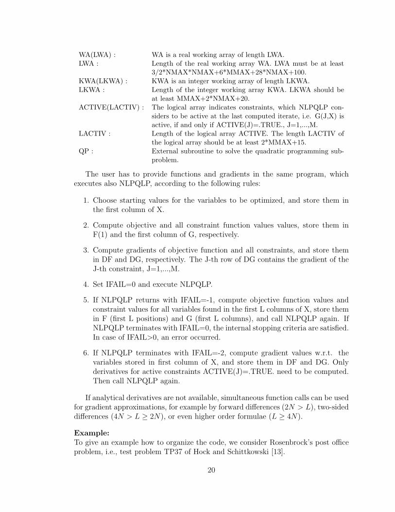
The user has to provide functions and gradients in the same program, whichexecutes also NLPQLP, according to the following rules:
1. Choose starting values for the variables to be optimized, and store them inthe first column of X.
2. Compute objective and all constraint function values values, store them inF(1) and the first column of G, respectively.
3. Compute gradients of objective function and all constraints, and store themin DF and DG, respectively. The J-th row of DG contains the gradient of theJ-th constraint, J=1,...,M.
4. Set IFAIL=0 and execute NLPQLP.
5. If NLPQLP returns with IFAIL=-1, compute objective function values andconstraint values for all variables found in the first L columns of X, store themin F (first L positions) and G (first L columns), and call NLPQLP again. IfNLPQLP terminates with IFAIL=0, the internal stopping criteria are satisfied.In case of IFAIL>0, an error occurred.
6. If NLPQLP terminates with IFAIL=-2, compute gradient values w.r.t. thevariables stored in first column of X, and store them in DF and DG. Onlyderivatives for active constraints ACTIVE(J)=.TRUE. need to be computed.Then call NLPQLP again.
If analytical derivatives are not available, simultaneous function calls can be usedfor gradient approximations, for example by forward differences (2N > L), two-sideddifferences (4N > L ≥ 2N), or even higher order formulae (L ≥ 4N).
Example:To give an example how to organize the code, we consider Rosenbrock’s post officeproblem, i.e., test problem TP37 of Hock and Schittkowski [13].
20

x1, x2 ∈ IR :
min−x1x2x3
x1 + 2x2 + 2x3 ≥ 072− x1 − 2x2 − 2x3 ≥ 00 ≤ x1 ≤ 1000 ≤ x2 ≤ 100
(19)
The Fortran source code for executing NLPQLP is listed below. Gradients areapproximated by forward differences. The function block inserted in the main pro-gram, can be replaced by a subroutine call. Also the gradient evaluation is easilyexchanged by an analytical one or higher order derivatives.
IMPLICIT NONE
INTEGER NMAX,MMAX,LMAX,MNN2X,LWA,LKWA,LACTIV
PARAMETER (NMAX=4,MMAX=2,LMAX=10)
PARAMETER (MNN2X = MMAX+NMAX+NMAX+2,
/ LWA=3*NMAX*NMAX/2+6*MMAX+28*NMAX+100,
/ LKWA=MMAX+2*NMAX+20,LACTIV=2*MMAX+15)
INTEGER KWA(LKWA),KL,N,ME,M,L,MNN2,MAXIT,MAXFUN,IPRINT,
/ IOUT,MODE,IFAIL,I,J,K,NFUNC
DOUBLE PRECISION X(NMAX,LMAX),F(LMAX),G(MMAX,LMAX),DF(NMAX),
/ DG(MMAX,NMAX),U(MNN2X),XL(NMAX),XU(NMAX),C(NMAX,NMAX),
/ D(NMAX),WA(LWA),ACC,STPMIN,EPS,EPSREL,FBCK,GBCK(MMAX),
/ XBCK
LOGICAL ACTIVE(LACTIV)
EXTERNAL QL0001
C
IOUT=6
ACC=1.0D-9
STPMIN=1.0E-10
EPS=1.0D-7
MAXIT=100
MAXFUN=10
IPRINT=2
N=3
M=2
ME=0
MNN2=M+N+N+2
DO I=1,N
X(I,1)=1.0D+1
XL(I)=0.0
XU(I)=1.0D+2
ENDDO
MODE=0
IFAIL=0
NFUNC=0
L=N
1 CONTINUE
C============================================================
C This is the main block to compute all function values
C simultaneously, assuming that there are L nodes.
C The block is executed either for computing a steplength
C or for approximating gradients by forward differences.
DO K=1,L
F(K)=-X(1,K)*X(2,K)*X(3,K)
G(1,K)=X(1,K) + 2.0*X(2,K) + 2.0*X(3,K)
G(2,K)=72.0 - X(1,K) - 2.0*X(2,K) - 2.0*X(3,K)
ENDDO
C============================================================
NFUNC=NFUNC+1
IF (IFAIL.EQ.-1) GOTO 4
21

IF (NFUNC.GT.1) GOTO 3
2 CONTINUE
FBCK=F(1)
DO J=1,M
GBCK(J)=G(J,1)
ENDDO
XBCK=X(1,1)
DO I=1,N
EPSREL=EPS*DMAX1(1.0D0,DABS(X(I,1)))
DO K=2,L
X(I,K)=X(I,1)
ENDDO
X(I,I)=X(I,1)+EPSREL
ENDDO
GOTO 1
3 CONTINUE
X(1,1)=XBCK
DO I=1,N
EPSREL=EPS*DMAX1(1.0D0,DABS(X(I,1)))
DF(I)=(F(I)-FBCK)/EPSREL
DO J=1,M
DG(J,I)=(G(J,I)-GBCK(J))/EPSREL
ENDDO
ENDDO
F=FBCK
DO J=1,M
G(J,1)=GBCK(J)
ENDDO
C
4 CALL NLPQLP(L,M,ME,MMAX,N,NMAX,MNN2,X,F,G,DF,DG,U,XL,XU,
/ C,D,ACC,STPMIN,MAXFUN,MAXIT,IPRINT,MODE,IOUT,IFAIL,
/ WA,LWA,KWA,LKWA,ACTIVE,LACTIV,QL0001)
IF (IFAIL.EQ.-1) GOTO 1
IF (IFAIL.EQ.-2) GOTO 2
C
WRITE(IOUT,1000) NFUNC
1000 FORMAT(’ *** Number of function calls: ’,I3)
C
STOP
END
When applying simultaneous function evaluations with L = N , only 20 functioncalls and 10 iterations are required to get a solution within termination accuracy10−10. A corresponding call with L = 1 would stop after 9 iterations. The followingoutput should appear on screen:
--------------------------------------------------------------------
START OF THE SEQUENTIAL QUADRATIC PROGRAMMING ALGORITHM
--------------------------------------------------------------------
Parameters:
MODE = 0
ACC = 0.1000D-08
MAXFUN = 3
MAXIT = 100
IPRINT = 2
Output in the following order:
IT - iteration number
F - objective function value
SCV - sum of constraint violations
NA - number of active constraints
22

I - number of line search iterations
ALPHA - steplength parameter
DELTA - additional variable to prevent inconsistency
KKT - Karush-Kuhn-Tucker optimality criterion
IT F SCV NA I ALPHA DELTA KKT
--------------------------------------------------------------------
1 -0.10000000D+04 0.00D+00 2 0 0.00D+00 0.00D+00 0.46D+04
2 -0.10003444D+04 0.00D+00 1 2 0.10D-03 0.00D+00 0.38D+04
3 -0.33594686D+04 0.00D+00 1 1 0.10D+01 0.00D+00 0.24D+02
4 -0.33818566D+04 0.16D-09 1 1 0.10D+01 0.00D+00 0.93D+02
5 -0.34442871D+04 0.51D-08 1 1 0.10D+01 0.00D+00 0.26D+03
6 -0.34443130D+04 0.51D-08 1 2 0.10D-03 0.00D+00 0.25D+02
7 -0.34558588D+04 0.19D-08 1 1 0.10D+01 0.00D+00 0.30D+00
8 -0.34559997D+04 0.00D+00 1 1 0.10D+01 0.00D+00 0.61D-03
9 -0.34560000D+04 0.00D+00 1 1 0.10D+01 0.00D+00 0.12D-07
10 -0.34560000D+04 0.00D+00 1 1 0.10D+01 0.00D+00 0.13D-10
--- Final Convergence Analysis ---
Objective function value: F(X) = -0.34560000D+04
Approximation of solution: X =
0.24000000D+02 0.12000000D+02 0.12000000D+02
Approximation of multipliers: U =
0.00000000D+00 0.14400000D+03 0.00000000D+00 0.00000000D+00
0.00000000D+00 0.00000000D+00 0.00000000D+00 0.00000000D+00
Constraint values: G(X) =
0.72000000D+02 0.35527137D-13
Distance from lower bound: XL-X =
-0.24000000D+02 -0.12000000D+02 -0.12000000D+02
Distance from upper bound: XU-X =
0.76000000D+02 0.88000000D+02 0.88000000D+02
Number of function calls: NFUNC = 10
Number of gradient calls: NGRAD = 10
Number of calls of QP solver: NQL = 10
*** Number of function calls: 20
In case of L = 1, NLPQLP is identical to NLPQL and stops after 9 iterations.The corresponding sequential implementation of the main program is as follows:
IMPLICIT NONE
INTEGER NMAX,MMAX,LMAX,MNN2X,LWA,LKWA,LACTIV
PARAMETER (NMAX=4,MMAX=2)
PARAMETER (MNN2X = MMAX+NMAX+NMAX+2,
/ LWA=3*NMAX*NMAX/2+6*MMAX+28*NMAX+100,
/ LKWA=MMAX+2*NMAX+20,LACTIV=2*MMAX+15)
INTEGER KWA(LKWA),KL,N,ME,M,L,MNN2,MAXIT,MAXFUN,IPRINT,
/ IOUT,MODE,IFAIL,I,J,K
DOUBLE PRECISION X(NMAX),F,G(MMAX),DF(NMAX),
/ DG(MMAX,NMAX),U(MNN2X),XL(NMAX),XU(NMAX),C(NMAX,NMAX),
/ D(NMAX),WA(LWA),ACC,STPMIN,EPS,EPSREL,FBCK,GBCK(MMAX)
LOGICAL ACTIVE(LACTIV)
EXTERNAL QL0001
C
IOUT=6
ACC=1.0D-9
STPMIN=0.0
EPS=1.0D-7
MAXIT=100
MAXFUN=10
IPRINT=2
N=3
M=2
23

ME=0
MNN2=M+N+N+2
DO I=1,N
X(I)=1.0D+1
XL(I)=0.0
XU(I)=1.0D+2
ENDDO
MODE=0
IFAIL=0
L=1
I=0
1 CONTINUE
C============================================================
C This is the main block to compute all function values.
C The block is executed either for computing a steplength
C or for approximating gradients by forward differences.
F=-X(1)*X(2)*X(3)
G(1)=X(1) + 2.0*X(2) + 2.0*X(3)
G(2)=72.0 - X(1) - 2.0*X(2) - 2.0*X(3)
C============================================================
IF (IFAIL.EQ.-1) GOTO 4
IF (I.GT.0) GOTO 3
2 CONTINUE
FBCK=F
DO J=1,M
GBCK(J)=G(J)
ENDDO
I=0
5 I=I+1
EPSREL=EPS*DMAX1(1.0D0,DABS(X(I)))
X(I)=X(I)+EPSREL
GOTO 1
3 CONTINUE
DF(I)=(F-FBCK)/EPSREL
DO J=1,M
DG(J,I)=(G(J)-GBCK(J))/EPSREL
ENDDO
X(I)=X(I)-EPSREL
IF (I.LT.N) GOTO 5
F=FBCK
DO J=1,M
G(J)=GBCK(J)
ENDDO
C
4 CALL NLPQLP(L,M,ME,MMAX,N,NMAX,MNN2,X,F,G,DF,DG,U,XL,XU,
/ C,D,ACC,STPMIN,MAXFUN,MAXIT,IPRINT,MODE,IOUT,IFAIL,
/ WA,LWA,KWA,LKWA,ACTIVE,LACTIV,QL0001)
IF (IFAIL.EQ.-1) GOTO 1
IF (IFAIL.EQ.-2) GOTO 2
C
STOP
END
7 Summary
We present a modification of an SQP algorithm designed for execution under a paral-lel computing environment (SPMD). Under the assumption that objective functionsand constraints are executed on different machines, a parallel line search procedure isproposed. Thus, the SQP algorithm is executable under a distributed system, whereparallel function calls are exploited for line search and gradient approximations.
24

The approach is outlined, the usage of the program is documented, and somenumerical tests are performed. It is shown that there are no significant performancedifferences between sequential and parallel line searches, if the number of parallelprocessors is sufficiently large. In both cases, about the same number of iterationsis performed, and the number of successfully solved problems is also comparable.The test results are obtained by a collection of 306 academic and real-life examples.
By a series of further tests, it is shown how the code behaves for 6 differentgradient approximations under additional random noise added to the model func-tions, to simulate realistic situations arising in practical applications. If a sufficientlylarge number of parallel processors is available, it is recommended to apply higherorder approximation formulae instead of forward differences. Linear and quadraticapproximations perform well in case of large round-off errors.
References
[1] Boderke P., Schittkowski K., Wolf M., Merkle H.P. (2000): Modeling of diffu-sion and concurrent metabolism in cutaneous tissue, Journal on TheoreticalBiology, Vol. 204, No. 3, 393-407
[2] Birk J., Liepelt M., Schittkowski K., Vogel F. (1999): Computation of opti-mal feed rates and operation intervals for tubular reactors, Journal of ProcessControl, Vol. 9, 325-336
[3] Blatt M., Schittkowski K. (1998): Optimal Control of One-Dimensional Par-tial Differential Equations Applied to Transdermal Diffusion of Substrates,in: Optimization Techniques and Applications, L. Caccetta, K.L. Teo, P.F.Siew, Y.H. Leung, L.S. Jennings, V. Rehbock eds., School of Mathematics andStatistics, Curtin University of Technology, Perth, Australia, Vol. 1, 81 - 93
[4] Bongartz I., Conn A.R., Gould N., Toint Ph. (1995): CUTE: Constrained andunconstrained testing environment, Transactions on Mathematical Software,Vol. 21, No. 1, 123-160
[5] Edgar T.F., Himmelblau D.M. (1988): Optimization of Chemical Processes,McGraw Hill
[6] Geist A., Beguelin A., Dongarra J.J., Jiang W., Manchek R., Sunderam V.(1995): PVM 3.0. A User’s Guide and Tutorial for Networked Parallel Com-puting, The MIT Press
[7] Goldfarb D., Idnani A. (1983): A numerically stable method for solving strictlyconvex quadratic programs, Mathematical Programming, Vol. 27, 1-33
25

[8] Han S.-P. (1976): Superlinearly convergent variable metric algorithms for gen-eral nonlinear programming problems Mathematical Programming, Vol. 11,263-282
[9] Han S.-P. (1977): A globally convergent method for nonlinear programmingJournal of Optimization Theory and Applications, Vol. 22, 297–309
[10] Hartwanger C., Schittkowski K., Wolf H. (2000): Computer aided optimal de-sign of horn radiators for satellite communication, Engineering Optimization,Vol. 33, 221-244
[11] Frias J.M., Oliveira J.C, Schittkowski K. (2001): Modelling of maltodextrinDE12 drying process in a convection oven, to appear: Applied MathematicalModelling
[12] Hock W., Schittkowski K. (1981): Test Examples for Nonlinear Program-ming Codes, Lecture Notes in Economics and Mathematical Systems, Vol.187, Springer
[13] Hock W., Schittkowski K. (1983): A comparative performance evaluation of27 nonlinear programming codes, Computing, Vol. 30, 335-358
[14] Hough P.D., Kolda T.G., Torczon V.J. (2001): Asynchronous parallel patternsearch for nonlinear optimization, to appear: SIAM J. Scientific Computing
[15] Kneppe G., Krammer J., Winkler E. (1987): Structural optimization oflarge scale problems using MBB-LAGRANGE, Report MBB-S-PUB-305,Messerschmitt-Bolkow-Blohm, Munich
[16] Ortega J.M., Rheinbold W.C. (1970): Iterative Solution of Nonlinear Equa-tions in Several Variables, Academic Press, New York-San Francisco-London
[17] Papalambros P.Y., Wilde D.J. (1988): Principles of Optimal Design, Cam-bridge University Press
[18] Powell M.J.D. (1978): A fast algorithm for nonlinearly constraint optimiza-tion calculations, in: Numerical Analysis, G.A. Watson ed., Lecture Notes inMathematics, Vol. 630, Springer
[19] Powell M.J.D. (1978): The convergence of variable metric methods for non-linearly constrained optimization calculations, in: Nonlinear Programming 3,O.L. Mangasarian, R.R. Meyer, S.M. Robinson eds., Academic Press
[20] Powell M.J.D. (1983): On the quadratic programming algorithm of Goldfarband Idnani. Report DAMTP 1983/Na 19, University of Cambridge, Cam-bridge
26

[21] Schittkowski K. (1980): Nonlinear Programming Codes, Lecture Notes in Eco-nomics and Mathematical Systems, Vol. 183 Springer
[22] Schittkowski K. (1981): The nonlinear programming method of Wilson, Hanand Powell. Part 1: Convergence analysis, Numerische Mathematik, Vol. 38,83-114
[23] Schittkowski K. (1981): The nonlinear programming method of Wilson, Hanand Powell. Part 2: An efficient implementation with linear least squaressubproblems, Numerische Mathematik, Vol. 38, 115-127
[24] Schittkowski K. (1982): Nonlinear programming methods with linear leastsquares subproblems, in: Evaluating Mathematical Programming Techniques,J.M. Mulvey ed., Lecture Notes in Economics and Mathematical Systems, Vol.199, Springer
[25] Schittkowski K. (1983): Theory, implementation and test of a nonlinear pro-gramming algorithm, in: Optimization Methods in Structural Design, H. Es-chenauer, N. Olhoff eds., Wissenschaftsverlag
[26] Schittkowski K. (1983): On the convergence of a sequential quadratic program-ming method with an augmented Lagrangian search direction, MathematischeOperationsforschung und Statistik, Series Optimization, Vol. 14, 197-216
[27] Schittkowski K. (1985): On the global convergence of nonlinear programmingalgorithms, ASME Journal of Mechanics, Transmissions, and Automation inDesign, Vol. 107, 454-458
[28] Schittkowski K. (1985/86): NLPQL: A Fortran subroutine solving constrainednonlinear programming problems, Annals of Operations Research, Vol. 5, 485-500
[29] Schittkowski K. (1987a): More Test Examples for Nonlinear Programming,Lecture Notes in Economics and Mathematical Systems, Vol. 182, Springer
[30] Schittkowski K. (1987): New routines in MATH/LIBRARY for nonlinear pro-gramming problems, IMSL Directions, Vol. 4, No. 3
[31] Schittkowski K. (1988): Solving nonlinear least squares problems by a generalpurpose SQP-method, in: Trends in Mathematical Optimization, K.-H. Hoff-mann, J.-B. Hiriart-Urruty, C. Lemarechal, J. Zowe eds., International Seriesof Numerical Mathematics, Vol. 84, Birkhauser, 295-309
[32] Schittkowski K. (1992): Solving nonlinear programming problems with verymany constraints, Optimization, Vol. 25, 179-196
27

[33] Schittkowski K. (1994): Parameter estimation in systems of nonlinear equa-tions, Numerische Mathematik, Vol. 68, 129-142
[34] Schittkowski K., Zillober C., Zotemantel R. (1994): Numerical Comparisonof Nonlinear Programming Algorithms for Structural Optimization, StructuralOptimization, Vol. 7, No. 1, 1-28
[35] Spellucci P. (1993): Numerische Verfahren der nichtlinearen Optimierung,Birkhauser
[36] Stoer J. (1985): Foundations of recursive quadratic programming methods forsolving nonlinear programs, in: Computational Mathematical Programming,K. Schittkowski, ed., NATO ASI Series, Series F: Computer and SystemsSciences, Vol. 15, Springer
28