nm7m tutorial – hp propagationmembers.chello.nl/t.beemsterboer/nm7m-hf-propagation… · web...
TRANSCRIPT

NM7M’s HF Propagation tutorialby Bob Brown, NM7M
Foreword by Thierry Lombry, ON4SKYProfessor Bob Brown, NM7M, worked as Physicist at University of California at Berkeley, as expert of the upper atmosphere and the geomagnetosphere. Now retired, he has celebrated his 81th birthday in 2004, he is still very interested in propagation, and works mainly on the top band of 160 meters.
In 1998 Bob Brown wrote a syllabus about HF propagation for his students that will become this tutorial in which Bob introduces us in the fascinating world of HF propagation.
To provide an accurate information to the reader, I took the freedom to add additional comments (referenced in notes) as some information changed over the years (e.g. an URL); new documents (studies, bulletin, models, images, etc) were released and are today available on the Internet as well as new propagation prediction programs, as many information that, I hope, will complete the already very useful information provided by the author. These updates were made in 2004. The HTML version of this document is fully illustrated and includes links to most of websites and programs discussed in the text.
I hope that this document will be become one of your bedside book.
Ready? Hop!, let's jump in the upper atmosphere in company with Bob.
Thierry Lombry, ON4SKY
IntroductionI have to agree there is a lot of information out there on the Internet; but what about understanding? Let me put out a few remarks that might help your understanding of propagation.
First, we depend on ionization of the upper atmosphere. That results from solar ultraviolet, "soft X-rays", "hard X-rays", and the influx of charged particles. Leaving the charged particles out of the discussion today, the solar photons have their origin largely in active regions on the sun.
Historically, active regions were first counted and tallied, then the next step was to measure their areas. Both methods have their problems with weather conditions and after WW-II it was found that the slowly-varying component of solar radio noise at 10.7 cm was statistically correlated with the method using sunspot counts. Later, with the Space Age, it was found possible to measure the "hard X-ray" flux coming from the sun in the 1-8 Angstrom range.
In my opinion, the 1-8 Angstrom background X-ray flux is a better measure of solar activity, at least for our radio purposes. Let me explain.
First, the X-ray flux has been found to come from regions more centrally located on the visible hemisphere of the sun; that means a significant fraction of their X-rays will reach our

NM7M's HF Propagation tutorial
atmosphere. Second, it takes 10 electron-Volts (eV) of energy to ionize any constituent in the atmosphere; the energy of 1-8 A X-ray photons exceeds that by over a factor of 100.
The energy of 10.7 cm photons is .00001 eV, a factor of 1,000,000 too LOW to ionize anything in our atmosphere. So the 10.7 cm flux only tells us about the presence of active regions on the sun, not directly about the state of ionization in the ionosphere. If that was not bad enough, it has been found that the 10.7 cm flux can come from the corona above regions which are behind the east and west limbs of the sun. Those regions are much less likely to have their ionizing radiation reach the ionosphere directly. So the 10.7 cm flux has its purpose, indicating the presence of active regions, and it is a mistake to think that changes in that flux are always associated directly with the state of our ionosphere.
Having said all that, let me conclude by pointing out the 1-8 A X-ray flux values are given by NOAA in ranges which differ by a factors of 10, such as A 2.3, B 4.0 or C 1.5. The numbers are the multipliers and the letters give the category. Now I have logged the 1-8 A X-ray flux through all of Cycle 22 and now into Cycle 23. The sum and substance of my experience is quite simple: the A-range is found around solar minimum, the B-range on the rising and falling parts of a cycle and the C-range during the peak of a cycle.
So what about Cycle 23? We suddenly moved out of the A-range (with sporadic B-outbursts) in August of '97, hovered in the low B-range until March '98, were in the mid-B range to the present time when there were recent outbursts in the C-range. It is still too early to say if solar activity has moved into the C- or solar maximum phase; several months of data will be needed before any such estimate can be made.
But logging the 1-8 A X-ray flux, with 4-cycle log paper, will give you insights as to the state of the ionosphere and recurrences in the plot will serve to point out good/bad times for DXing. While spikes in the 1-8 A diagram may suggest "hot times" for DXing, they can be brief and difficult to take advantage of. It is more productive to look at the broader peaks in flux in planning one's DXing. The flares and coronal mass ejections associated with outbursts of activity that take place now are more likely to give bad propagation conditions because of all the geomagnetic activity that follows. For DXing, the broad peaks are more productive.
All of the above involved words, no great mathematical exercises. But I like to tie it together mathematically using a simple proportion that everyone can grasp quickly:
When it comes to changes in the state of the ionosphere, X-rays are to solar noise as, with DXing, beam antennas are to dipoles. OK?
Having talked about the creation of ionization overhead, electrons and positive ions, all sorts of practical questions come up at once. And some theoretical ones too. We'll leave the theory to a later time, when DXing is slack and there is more time to spare. But when it comes to practical matters, we have to throw our frequency spectrum against the ionosphere and see how it all shakes out. Of course, all that was done more than 50 years ago, one frequency at a time, and the idea of critical frequencies emerged. Those were for signals going vertically upward into the various regions overhead, foE and foF2 for E- and F2-regions, and gave the heights and frequency limits beyond which signals kept on going into the next region or on to Infinity.
2/62

NM7M's HF Propagation tutorial
But we communicate by sending signals obliquely toward the horizon and that makes a difference, our higher frequencies penetrating more than the lower ones before being returned toward ground. And we have to note our RF excites the electrons in the ionosphere, jiggling them at the wave frequency, but they do collide with nearby atoms and molecules, transferring some energy derived from the waves to the atmosphere. That's how signals are absorbed, heating the atmosphere. But for electrons, there's a difference between being excited by 28 MHz RF and 1.8 MHz RF. For one thing, it depends on how often electrons bump into nearby atoms and molecules. At those high frequencies, say 28 MHz, the wave frequency is high compared to the collision frequency of electrons and absorption losses are relatively small. The same cannot be said for 1.8 MHz signals on the 160 meter band and the wave and collision frequencies are comparable, meaning that electrons take up RF energy and promptly deliver it over to the atmosphere.
One can go through all the mathematics but you can almost guess the answer: absorption is a limiting factor for the low bands, 160, 80 and 40 meters, and ionization or critical frequencies (MUFs) are the limiting factors for the high bands, 15, 12 and 10 meters. That makes the middle or transition bands, 30, 20 and 18 meters, ones where both absorption and ionization are important. We can phrase this in another, practical way - 160 meter operators do all their DXing in the dark of night when there's no solar UV or X-rays to create all those electrons that absorb RF. By the same token, the 10 meter crowd do their DXing in broad daylight, when entire paths are illuminated, and they couldn't care less. Those are the extremes but practicioneers on the "workhorse band", 20 meters, have to put up with both uncertainties in MUFs and the absorption by electrons. But in times like now, there is enough ionization up there to support DXing at dawn and dusk, when the absorption is at a minimum. For that band, Rudyard Kipling's ideas about "mad dogs and Englishmen go out in the noon day sun" would seem to apply. OK? Those ideas, darkness and sunlight on paths, bring up the matter of computing with mapping programs for checking darkness on 160 meter paths and daylight on 10 meter paths as well as MUF programs for bands from 10 MHz upward. But those last programs should also have a capability of giving signal/noise ratios for the bandwidths appropriate for the modes. After all, getting a signal from a DX location is not worth much if it cannot be read above the noise. For me, VOACAP is at the top of the list but it has offspring and there other programs that can fill the bill. But I cannot stress mapping programs enough; you just have to see where you're trying to go and the obstacles along the way, like the auroral zones.
But to use a MUF program, a measure of the current solar activity is needed and effective sunspot numbers (Effective SSN) were for a while available in "HF Prop" bulletins from the Air Force and the Space Environment Center of NOAA (SEC). Those numbers were derived from observations of actual propagation and amount to "pseudo-sunspot numbers". They were more to the point than using daily values of the 10.7 cm solar flux. However today only Part IV of this bulletin is still available via the Internet. Other products like IonoProbe from VE3NEA also provides the Effective SSN and other real-time solar data.
3/62

NM7M's HF Propagation tutorial
Note by ON4SKY. The U.S. Air Force no longer produces the "HF Prop" Bulletin. They stopped this some time back. However, the data in section Part IV of the old bulletin can be found on SEC website at a couple places.
For example, under ONLINE DATA click on "Near Earth". "Near Earth Alerts and Forecasts" have the daily Solar and Geophysical Activity Report and 3-day Forecast. This product contains the Observed/Forecast 10.7 cm flux and K/Ap.
Under the "Near-Earth Reports and Summaries", the Solar and Geophysical Activity Summary contains the Satellite Background and Sunspot Number (SSN) in section E and daily Indices (real-time preliminary/estimated values).
At last, recall that in recent propagation programs like "DX ToolBox" or GeoAlert-Extreme Wizard", some of these reports can be read from within the application (if you have an active connection to Internet of course).
Effects of the ionizationRight now, there's more than enough ionization up there to support DXing on the low bands, 160 to 40 meters. But the higher bands are still pretty spotty, mainly across low latitudes or in brief bursts of solar activity. But 10 meters will return; trust me.
The discussion so far has dealt with the creation of ionization and how various frequencies in our spectrum make out as far as propagation and absorption are concerned. There's one problem with that discussion, the omission of how, in the course of time, ionization reaches the steady-state electron densities overhead. So let's turn to that but do it as simply as possible. That means we'll focus on electrons, positive and negative ions. The solar UV and X-rays create those from the oxygen and nitrogen molecules in our atmosphere. I can say it is a big, complicated ion-chemistry lab up there but we'll stay at the generic level, nothing fancy, just electrons and positive ions. In simple terms, there is a competition between the production and loss of ionization, just like your bank balance where depositing paychecks and paying bills are in competition. So for us, there's a certain number of electrons created per second in a cubic meter of air in the ionosphere by the solar radiation and whatever the number of electrons present, some are being lost by recombining with positive ions to form neutral atoms or molecules again. If the two, gain and loss, are equal, there is a steady-state of ionization; otherwise, there will be a net gain or loss per second from some cause or other.
I haven't said so but the atmosphere is only lightly ionized, say one electron or positive ion per million neutral particles. So electrons have a greater chance to bump into a neutral particle (like in ionospheric absorption) than a positive ion, to recombine to make a neutral atom or molecule. And, of course, there's a vast difference in those rates between the lower parts of the ionosphere, the D-region below 90 km and the F2-region above 300 km. So electrons created by solar UV would be gobbled up rapidly in the D-region but linger on for the better part of a day up in the F2-region.
Good illustrations of the fast processes are found nowadays, solar flares illuminating half the earth with hard X-rays (like those in the 1-8 Angstrom range). They penetrate to the D-region, release electrons which rapidly transfer wave energy to the atmosphere. As soon as a
4/62

NM7M's HF Propagation tutorial
flare ends, the sudden ionospheric disturbance (SID) or radio black-out ends as the electrons in the D-region recombine rapidly and signal strengths return to normal. The lingering on of electrons in the F2-region is responsible, in part, for the fact that there's still ionization and propagation in hours of darkness. In short, electrons at high altitude recombine slowly after the sun sets. But there's more to the story than that, the role of the earth's magnetic field. Let me explain. The earth's atmosphere is immersed in the geomagnetic field so any charged particles, say ionization created by solar UV, will then experience a force from their motion in the field. For electrons, that means they will spiral around the field lines when released by UV and not fly off in any direction to another location, higher or lower in the ionosphere. In the propagation business, that is called geomagnetic control, meaning that the earth's field largely determines the distribution of electrons in the ionosphere. True, the solar UV creates them and they are most numerous where the sun is overhead but they are held on field lines and linger on after dark, to our great advantage. But the earth's field also creates problems, especially for the low-band operator. It turns out the gyro-frequency of electrons around field lines is about 1 MHz and comparable to frequencies in the 160 meter band. Thus, a more general approach has to be made in the theory of propagation at that frequency, adding the effects of the earth's field on ionospheric electrons. The results are quite complicated, with elliptically-polarized waves on low frequencies where linearly-polarized waves were the story earlier on high frequencies. That is a subject in itself and has to be left for a rainy day. But those are not the only ways that the earth's field enters into the propagation picture. Stay tuned.
Earlier, I said there were other ways that the earth's field enters into the propagation picture. But that's sort of getting ahead of my development so let's backtrack a bit and look at the historical picture. The study of geomagnetism goes back more than 100 years, well before the advent of radio. It was known that the occurrence of magnetic storms was related to the solar cycle and, by the same token, it wasn't long before it was realized that HF propagation was related to it too. The two really came together about 70 years ago when commercial radiotelephone service was established across the Atlantic Ocean. Then it soon became apparent that there were disruptions in service during magnetic storms. You can find all that discussed in the I.R.E. journals in the early '30s. In that period it was thought that the ionosphere was the result of solar UV, the photons reaching the earth 500 seconds after leaving the sun. And while magnetic storms were known to disrupt radio propagation, there was no obvious connection as experience showed magnetic storms occurred a couple days after the flash phase of a large flare on the sun. True, there was the idea of solar material, electrons and protons called "plasma", approaching the earth after a solar outburst and engulfing the geomagnetic field, even compressing it. But the two effects from plasma and UV seemed separable just because of differences in time-of-flight across "empty space" that were associated with the two effects.But all that changed with the Space Age when it was found that solar plasma was out there all the time, the solar wind, and that it blew past us with differents speeds, 200-1,200 km/sec, as well as different particle densities and even carried magnetic fields along. But for us earth-bound souls, the big surprise was that the solar plasma distorted the earth's magnetic field,
5/62

NM7M's HF Propagation tutorial
essentially taking some field lines on the sunward side and pulling them back behind the earth to form a magnetotail. Moreover, with the solar plasma coming at us, it became clear that a ordered, dipole field did not go on forever, only out to 8-12 earth-radii in the sunward direction and even that depended on solar activity.
So what does this have to do with propagation, you ask. Well remember I said geomagnetic control of the ionosphere means that electrons are held on magnetic field lines, making the earth's field something of a reservoir for ionospheric electrons. But if field lines can be distorted, that would surely affect the density of ionospheric electrons gyrating around them and propagation. The worst-case scenario is when field lines are dragged way back into the magneto-tail by an increase in solar wind pressure, taking ionospheric electrons with them. That field configuration is sketched crudely below where two compressed field lines are shown in front of the earth, in the solar direction, and two magnetotail field lines in the anti-solar direction:
Solar Wind ( <- Magneto-tail * * * * ( * . . . * * * ( <- * . . * * . * ( * . . * * . . * ( <- * . . * * . . * (* . (Earth) . * ( SUN * . . * * . . * ( * . . * * . . * ( <- * . . * * . * ( * . . . * * * ( <- * * * * ( ( <- That would mean a depletion of electrons at F2-region heights and drastic reductions in MUFs, affecting propagation. Fortunately, that fate is reserved primarily for sites at high latitudes, around the auroral zones and poleward.
What I described was what takes place during a major geomagnetic storm. The recovery is a slow process as ionospheric electrons have to be replaced in the usual way, by solar UV and day by day while the sun is up. So it can take days for the bands to recover when a strong magnetic storm reduces MUFs by a large fraction. Now to be practical again, magnetic activity on earth is caused by interactions of the solar wind out there at the front of the geomagnetic field. The field region around the earth is called the magnetosphere so we're talking about effects on high latitude field lines that go out to the magnetopause, the dividing surface between terrestrial and interplanetary regions. But it must be recognized that this sort of thing is not toggled on and off; it is going on all the time as the solar wind sweeps by. It is just a matter of degree. But how to deal with it in DXing?
The clue comes from an interaction within the magnetosphere, local electrons being accelerated to high energies and then spiralling down field lines to make visible aurora and ionization at E-region heights. Those events are triggered by solar wind interactions at the magnetopause and accompanied by horizontal currents in the E-region that show up in magnetic observations on the ground. It then becomes a matter of using the strength of the
6/62

NM7M's HF Propagation tutorial
local magnetic effects at auroral latitudes, with K- and A-indices like those you hear about on WWV, to judge the energy input from the solar wind.
To bring this to a conclusion, good propagation conditions are found when there is a strong UV input to the ionosphere and low magnetic indices, the 3-hour K-index less than 4 and the daily A-index less than 25. Dreadful propagation conditions were found recently in the magnetic storm of August 27 when K reached its limit, 9, and the planetary average of the A-index was 112. But it could have been worse! However, let's look at the brighter side next time, how signals get from A to B.
Let's leave a curved ionosphere to later and do some "Flat-Earth Physics" to see how signals get from point A to point B. For that we start with a simple model of the ionosphere in which the electron density increases upward and peaks at about 300 km altitude. That's something like a night-time ionosphere. Now it may seem strange but one can draw an analogy between the flight of a baseball and RF going up through that ionosphere. For the baseball, high school physics teaches you how to calculate how high a baseball would go if thrown vertically upward. In college, the ball is thrown or hit upward at an angle. The method is the same in both cases: the ball rises until the increase in its potential energy in the earth's gravitational field is equal to the kinetic energy it had from its initial vertical motion.
Neglecting friction, the baseball's path is a parabola that is symmetrical about its highest point and the ball returns to the ground at the same angle to the vertical as it was launched. While not really parabolic in shape, the flight of RF through that simple ionosphere is similar, reaching a peak altitude that is determined by the frequency and launch angle, symmetrical about the peak and returning to ground at the same angle. How does that happen? Let me explain. The flight of a baseball and the path of RF in a simple ionosphere are determined by gradients, of the gravitational energy of the ball in the first case and the electron density distribution in the second one. There is a gradient of either of those quantities if there's a change in value with altitude, say gravitational energy or electron density greater at higher altitudes than lower at altitudes. The gradients are responsible for the bending or curvature of the paths in the both cases and, numerically, they are given by the change in value per km change in altitude. OK? In spite of all the "Home Run Fury" these days, let's leave the baseball part of the analogy and focus on what happens to RF. So we see that hops, with RF rising and then returning to ground, are the result of the vertical gradient of the electron density in the ionosphere. On reflection at ground level, angles of incidence and reflection are equal and the path continues upward again. But there can be horizontal gradients as well, say across the terminator where there is more ionization on the sunlit side than the side in darkness. So if RF signals were sent initially parallel to the terminator, one would expect the RF to be bent away from the sunlit side, with its higher level of ionization, and toward the darkness. Right? That's skewing, pure and simple, with the RF refracted away from the region of greater ionization.
The height a baseball reaches depends on its speed and direction; for RF, that translates into frequency and launch angle. But one sees that from different arguments. Let me add a few
7/62

NM7M's HF Propagation tutorial
words there. At any height in the ionosphere, there are electrons and positive ions. If, by mystical powers, you could grab a handful of each and then pull them apart, they would be attracted to each other by the electrical forces between unlike charges and on release, they'd swish back and forth, carrying out an oscillatory motion. The frequency of that motion is called the plasma frequency and it depends on the density or number of particles per unit volume, N.
For the ionosphere, where ionization increases with height, the plasma frequency increases too. For our night-time case, the peak electron density in the F-region might correspond to a plasma or critical frequency of 7 MHz for the F-region. Now vertical ionospheric sounding shows that pulses of RF below 7 MHz would be returned to ground while any above 7 MHz would penetrate the peak of the ionosphere and go on to Infinity. For oblique propagation, we have to find the effective vertical frequency of the RF, just like the vertical component of the baseball's velocity. For RF, it's found the same way, multiplying the frequency by the cosine of the zenith angle at launch. So, in the "Flat Earth" approximation, 7 MHz RF launched from ground at 30 degrees above the horizon (or 60 degrees from the vertical) would have an effective vertical frequency of 3.5 MHz. OK, the "baseball analogy" would say that the RF going off obliquely would rise until it reached a height where the local plasma frequency is 3.5 MHz and then return to ground. Of course, it would be on a curved path, the RF would be moving parallel to the earth's surface at the top of the path and returning to ground at the same angle as when launched, just like the baseball problem.
In baseball, there's friction and that changes the flight of a baseball. We don't put "friction" in the RF problem. Instead, the electron density at a given height may vary along the path direction, say become smaller. That would serve to "tilt" levels of the ionosphere upward and weaken the density gradient. As a result, there would be less refraction or bending after the peak altitude than before, and that tilt serves to increase the length of a hop and change the RF angle on return to a lower value. In reality one would expect some change in electron density along any path, increasing as a path goes into sunlit regions or decreasing when going into the dark. So even if nothing else changed, one would not expect hop lengths nor radiation angles to always remain exactly the same all along a path. The above approach, equivalent to mirror reflections of RF, is Newtonian in the sense that the analogy treats a RF path like that of a particle (baseball) and not a wave. When the Maxwellian or wave approach is carried out, one finds that refraction is the same except that the effects vary inversely with the square of the wave frequency. So in a given part of the ionosphere, 80 meter RF paths are refracted or bent much more than 10 meter RF paths, either vertically or horizontally. OK?
MUF and RF attenuation OK, now we have the idea of critical frequencies and hops so it is no big deal to work out how propagation on a path may be open or closed for DXing on a given frequency. But to do that, we need at least map of where the RF is headed and an idea of how many hops would be involved. Beyond that, some ionospheric details are required, the critical frequencies along the path at the date and time in question.
8/62

NM7M's HF Propagation tutorial
If one gets into the mathematics of all this, it turns out that hops via the F-region may reach about 3,500 km and half that via the lower E-region. So using those ideas, one can estimate the hop situation, at least as long as there is not a mixture of E- and F-hops. So consider a path from my QTH in the Northwest to London, some 7,500 km in length. That would work out, to a first approximation, to 3 F-hops of 2,500 km each. Now what about the critical frequencies at the peaks of the hops; how high are they and what bands might be open to me, say at 1200 UTC? To answer that question, one would need some sort of database, an array of observations from which an estimate could be obtained by interpolation, or a mathematic simulation of the database that could be used to calculate the critical frequencies. Actually both methods are used in modern propagation prediction programs but either way, appropriate numerical values could be obtained for the peaks of the hops. But what to do with that data? For a one-hop path, the matter is simple; the effective vertical frequency of the RF that is launched must be less than the critical frequency for the path to be completed. No problem. For two hops, the effective vertical frequency of the RF must be less than the SMALLEST of the critical frequencies of the two hops to have a complete path. And the operating frequency that gives the highest effective vertical frequency that can complete the path is called the Maximum Useable Frequency (MUF) for the path at that time and for the corresponding solar conditions. But the path from my QTH to London involves 3 hops; what's the story there? Historically, the idea was handled like the 2-hop path, using the critical frequencies at the first and last hop to determine the MUF. The idea was that if propagation failed, it usually would be due to conditions at one end of the path or the other. Anyway, this is called the "control point" method and is used in most simple propagation programs. More sophisticated approaches would use critical frequencies at each and every hop and the lowest would be the important one that limits propagation.
It should be noted that the control point method would be quite satisfactory for MUF calculations so long as the critical frequency of the middle hop is not less than those at either end of the path. That would be the case for paths going across the more robust ionosphere at low latitudes where the sun is more overhead during a day. But MUF calculations using two control points for high latitude paths, like from the Northwest to London, can be misleading as the critical frequency for the middle hop (over Northern Canada and Greenland for the path to G-land) could be lower than at the end points and thus propagation not supported across the entire path using the MUF from control points.
The MUF calculations play an important part in propagation predictions but it must be remembered that signal strength, in comparison with noise, is an important consideration. As noted earlier, ionization and MUFS are more important for the higher ends of the amateur spectrum and signal/noise considerations for the lower end. In any event, for communication a path must be open or available and signals must be readable and reliable. All of the discussion up to this point has dealt with propagation from a conventional viewpoint - determined by the ionosphere that is overhead and, in turn, one controlled by the level of solar activity. Obviously, propagation is a complicated process and it may seem a bit naive but we try to make all our predictions on a given date using using databases which rest on only a few numbers - sunspot number and magnetic indices. It is not surprising that predictions are not 100% reliable. Such high expectations would deny the variability of the
9/62

NM7M's HF Propagation tutorial
original data input from ionospheric sounding and not reflect the roles of dynamic solar variables.
So far, this brief summary of the principal points that are involved in HF propagation has been largely centered on words and concepts. More advanced topics require a good deal of graphics so I will make appeal from time to time to a figure or two in one or more of the reference books given earlier. While figures are the best way to convey some of the material, I will also try to put the ideas in simple words that will carry most of the meaning.
To me, the study of ionosphere and propagation changed markedly with the advent of the Space Age. Thus, with the International Geophysical Year (IGY) in '57, high-altitude balloons, rockets and satellites began to probe the regions where only radio waves had been before. So the "Photochemical Era", where solar photons and atmospheric processes were thought to control the dynamics of the ionosphere, gave way to the "Plasma and Fields Era" we're in now, where the interaction of the solar wind with the earth's field and the atmosphere are the controlling factors for propagation.
In simple terms, hams no longer look out the window for their local weather, determined by the day, time and season, but now turn to the Internet to get a daily report on the Space Weather. In a sense, propagation and DXing just became less mysterious and even more interesting. That's what we'll be pointing toward in Propagation 201, preparing for all the details in Propagation 301. So go prowling around the Internet and see what you can pick up between now and then. School starts with the first session on October 1.
It's no secret that success in DXing means getting signals to and from a DX station and also having them heard and read at both ends of the path. But between those two ends, a lot of things happen in the ionosphere and some of them seem like well-kept secrets. So the hope is some of that can be dispelled by the discussion which follows. But we need a beginning and the question is where to start. Let's take the easy way and cover old ground first, the matter of ionospheric absorption that was discussed previously.So we go back to the idea that RF excites the electrons in going across the ionosphere, jiggling them at the wave frequency. And they collide with nearby atoms and molecules, transferring some energy derived from the waves to the atmosphere. That's how absorption takes place, mostly down in the D-region. But there's a frequency dependence we should talk about now, how absorption varies with the operating QRG and with height, since the collision frequency of the electrons is not constant; instead, it decreases with height and that's a help. So it's clear now that ionospheric absorption is a little more complicated than I first let on back in Prop. 101.
But one can get a handle on it by looking at the extremes, low in the D-region, say around 30 km where the collision frequency is greater than any of the frequencies in our spectrum. In that circumstance, collisions happen so often the electrons never have a chance to pick up any energy from the passing RF. On the other hand, at high altitudes, say around 100 km, collisions are quite infrequent and the electrons re-radiate most of the energy they acquire and transfer very little to the atmosphere by collisions.
So it is in between, where wave and collision frequencies are comparable, that electrons take up RF energy efficiently and then promptly deliver it over to the atmosphere. So with collision frequency falling with increasing altitude, 28 MHz RF is absorbed at lower altitudes than 3.5 MHz RF, as shown below:
10/62

NM7M's HF Propagation tutorial
Relative Absorption Efficiency per Electron
100 + + * * * * - 3.5 MHz + * * o - 28 MHz10+ * * + * o o * + * o o * + * o o *1 *o o * + o * + o *.1+ + + + + + + + + + + + + + + 30 40 50 60 70 80 90 100 Ht (km)
That graphic illustrates something that DXers know already, lower frequency signals are absorbed more than higher ones but it shows where it all happens. That's news, at least for some. To go beyond that qualitative result, one must have an analytical form to represent the curves, call it F(f,h) for frequency f and height h. Then multiply F(f,h) by the number N of electrons per cubic meter at height h and include the physical constants to give the right units, dB/km. When all is said and done, the result is:
Attenuation (dB/km) = 4.6E-2 * N * F(f,h) But that is only at one place, where the electron density is N. Our DXer's signal is attenuated by ALL the electrons encountered along the RF path from point A to point B so that means we need to know something about the propagation mode, the distribution of electrons and add up the results, km by km along the path. That's a tall order but when it's done, it will enable our DXer to find just how much of the radiated power P survived in going from A to B. But whether our DXer can be heard still depends on how well the attenuated signal compares with the noise power getting to the receiver at B. But I'm getting ahead of myself.
The crude graphic shown above can help in understanding a lot of simple things. For example, it is possible to identify various ionospheric disturbances just by the absorption they produce. One approach is to use an HF receiver to monitor the galactic radio noise coming in vertically on 30 MHz. Galactic noise gets right through the F-region as 30 MHz is above its critical frequency, even at equatorial latitudes where it might reach 20 MHz in a solar cycle. That instrument is called a riometer, for Relative Ionospheric Opacity METER, and they are generally deployed at high latitudes where ionospheric disturbances are most common.
So now, if some disturbance increases the electron density in the D- or E-region, we see that the galactic noise signal will be attenuated and indicate the presence of a disturbance. But there are disturbances and then there are DISTURBANCES. So the graphic also tells us that anything that disturbs the lower D-region will produce strong attenuation of the galactic radio noise and, electron for electron, the attenuation will be much less if the disturbance produces ionization at much higher altitudes.
11/62

NM7M's HF Propagation tutorial
The first case would be for polar cap absorption (PCA) events, like we all experienced in May of '98. In those events, solar protons produce lots of ionization around 40-50 km altitude and give rise to tens of dB of additional absorption on 30 MHz and blackout oblique communication paths going across the polar caps. Auroral events, say associated with magnetic storms, give rise to strong ionization above 100 km, where the graphic shows the absorption efficiency is much lower, and auroral absorption (AA) events show only a few dB of absorption of galactic noise on 30 MHz. Of course, there are other differences in the two types of events, how the ionization is distributed in latitude and longitude and how long they last. More on that later.
One last disturbance, again something that was within our recent experience with all the flare activity in the summer of '98, is sudden ionospheric disturbances (SID) from bursts of solar X-rays. Those X-rays, in the 1-8 Angstrom range discussed earlier, were incident on the sunlit hemisphere of the earth and literally swamped the normal distribution of ionization at low altitudes, giving intense absorption of signals going across the sunlit region. But experience shows, and the graphic indicates, that the effects were worst at the lower ends of the spectrum, wiping out 75 meter operations but having little effect on 28 MHz, except perhaps for some solar noise bursts associated with the flaring.
ll this would be quite academic, perhaps, were it not for the fact that one can use the Internet to see these events in action or shortly thereafter. Thus, records from the X-ray Flux Monitors on the GOES 8 and 10 satellites are shown at:
http://www.sec.noaa.gov/today.html giving more meaning to the idea of an SID. We'll get to that later on but the main thing for us in the records is that plots for 0 degrees tell what is going down into the atmosphere, making more ionization and affecting the ionosphere. The 90-degree plots involve particles trapped in radiation belts and are more colorful than informative.
While disturbances come and go, affecting our ability to work DX, we really need to know something about the normal situation, say the distribution of ionospheric electrons with height as well as latitude and longitude. That is a big order but, believe it or not, it can be contained in one HD computer disk. I'm talking about the International Reference Ionosphere (IRI), the summary of decades of ionospheric sounding all over the world. You can access the IRI model at this address :
http://www.ion.le.ac.uk/remote_sensing/models/tec.html
the NSSDC version displayed below being at professional use :
http://nssdc.gsfc.nasa.gov/space/model/models/iri.html
So it will provide data on the robust part of the ionosphere at low latitudes where the sun is more overhead and the mid-latitudes where the ionosphere is more seasonal in its properties.
12/62

NM7M's HF Propagation tutorial
But the model is not reliable at high latitudes, say from below the auroral zones and poleward. That region is under the constant influence of the solar wind and electron densities are highly variable, even hour by hour. So that model has its limits. But to bring the model to life, one needs a mapping program to show the vertical and global distribution of ionization. Fortunately, we now have such a program available to amateurs, the PropLab Pro program from Canada. I'll have more to say about that next time.
Reference Notes: A better representation of the relative absorption efficiency per electron as a function of height and frequency in the D-region is found in Figure 8.1 in my book, "Little Pistol". And a more detailed discussion of the analytical form, F(f,h), is found in Section 7.4 (Ionospheric Absorption) of Davies' book, "Ionospheric Radio", beginning on p. 214. Also, the variation of collision frequency with height is given in Figure 7.5 on p. 215.
Distribution of ionospheric electrons In the previous page, it was pointed out that further progress on propagation requires knowledge of how ionospheric electrons are distributed. Of course, that will be different, day and night, as well as with seasons and sunspot cycles. Again, it would be easy way to fall back on something in previous pages, say the night-time ionosphere and continue the discussion from there. But that would involve a tremendous leap over distance and logic that's not too productive. So let's talk/walk our way up to higher altitudes, starting from where we are now, the D-region.
For one thing, the D-region involves a lot of familiar ideas and we can work from there. For example, below the 90 km level, our atmosphere is pretty well mixed, about 78% nitgrogen molecules and 21% oxygen molecules, by volume. The remaining 1% is made up of permanent constituents, like the noble gases as well as hydrogen, methane and oxides of nitrogen. Of course, every schoolboy knows about the variable constituents, like water, carbon dioxide, ozone and various bits of industrial debris, smog, that are found in around heavily populated regions.
Global weather systems keep the lower atmosphere all stirred up, in a mechanical sense, but that is not to say that convection from solar heating is the only influence of the sun. Indeed, as was discussed earlier, there are electrons and positive ions in the lower D-region, released by solar EUV and X-rays. When the sun sets, one might think that all the ionization disappears by recombination and the region becomes de-ionized and neutral. Of course, the ionosphere is always electrically neutral, with the equal numbers of positive and negative charges, but recombination lowers their numbers. Still some ionization does remain, produced by other sources; those include UV and X-ray photons in starlight, sunlight scattered by the gas envelope (geocorona) surrounding the earth and even charged particles, the energetic protons in the galactic cosmic ray beam.
So it follows that ionospheric absorption would be greatly reduced after dark but does not go to zero. There is good news in this discussion, however, as some electrons are taken out of the absorption loop at night by becoming attached to oxygen molecules. Those negative ions are so massive that they can't be budged by RF going by and just do not participate in the absorption process.
13/62

NM7M's HF Propagation tutorial
And at night, the number of negative ions of molecular oxygen in the lower D-region grows to large numbers in going downward from the 85 km level. That is the very reason that those solar proton or PCA events mentioned previously show much less absorption when the sun sets. But when the sun comes up, solar photons detach electrons from the negative ions and absorption goes back to the daytime level again. That does not happen for auroral events and that is another story, about another region higher in the ionosphere. More on that later.
In any event, the frequency dependence is still in effect for whatever absorption occurs, taking a heavy toll on low frequency signals. But that is still not fatal to propagation, even on the low bands. Thus, everyone knows about broadcast stations coming in better after dark and those signals can be heard across very great distances, as many SWLs will testify. And even with more limited power, 160 meter operators can still work great DX. But in the last analysis, both SWL and low-band DXers run up against the same problem, noise. That also has its origins down at low altitudes so we can deal with that right now, while in the region.
Noise is described as broad-band radiation from electrical discharges, either man-made or natural in origin. Whatever the case, being a radio signal, noise will be propagated like any other signal on the same frequency. That means, for one thing, that noise signals that are below the critical frequency of the F-region overhead will be confined to the lower ionosphere, dissipate down there and not escape to Infinity. By the same token, noise signals above the critical frequency are lost and won't bother us very much on the higher HF bands. But the lower bands do have a problem; so let's talk about it. Noise of atmospheric origin comes from lightning strikes and will be seasonal and originate in fairly well-defined areas. Among the powerful sources of noise are low-latitude regions of South America, South Africa and Indonesia. But we have our own noise source, the southeastern states during the summer months. So broad-band noise originates from those regions and is propagated far and wide through regions in darkness. But once the sun comes up, ionospheric absorption takes over and the only noise heard is of local origin, static crashes from nearby lightning strikes.
The above points are not news to domestic DXers; they are quite familiar with their own situation and can work within its limits. But those going on DXpeditions often go into unfamiliar territory and don't always think about the atmospheric noise problem. So 160 meter operators on DXpeditions have been known to be greeted by S-9 noise the first time the receiver was turned on. That evokes instant panic and sets in motion efforts to ameliorate the problem, say trying different antennas and such. Those don't work every time and hindsight often proves the problem could have been avoided, in large measure, by planning the DXpedition for a time on the winter side of an equinox, not the summer side.
Of course, the other source of noise is quite local, man-made in origin and coming from various electrical devices. While the global dimensions of atmospheric noise have been investigated extensively over the last 50 years or so, the same is true of man-made noise and it can be categorized as to origin and even given a frequency dependence. As for origins, the worst situation is an industrial setting and then lesser problems are found with residential, rural and remote sites, in that order. In that regard, the VOACAP propagation program allows one to select the receiver siting and then takes that, as well as the
14/62

NM7M's HF Propagation tutorial
bandwidth (in Hz) of the operating mode, into consideration in calculating the signal/noise ratio that would be expected for a path.
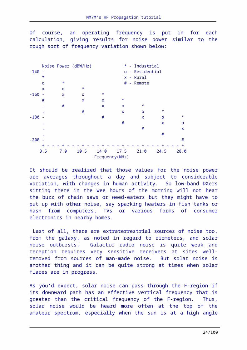
Of course, an operating frequency is put in for each calculation, giving results for noise power similar to the rough sort of frequency variation shown below:
Noise Power (dBW/Hz) * - Industrial-140 - o - Residential * x - Rural o * # - Remote x o *-160 - x o * # x o * . # x o * . # x o *-180 - # x o * . # x o . # x . #-200 - # + - - - + - - - + - - - + - - - + - - - + - - - + - - - + 3.5 7.0 10.5 14.0 17.5 21.0 24.5 28.0 Frequency(MHz) It should be realized that those values for the noise power are averages throughout a day and subject to considerable variation, with changes in human activity. So low-band DXers sitting there in the wee hours of the morning will not hear the buzz of chain saws or weed-eaters but they might have to put up with other noise, say sparking heaters in fish tanks or hash from computers, TVs or various forms of consumer electronics in nearby homes.
Last of all, there are extraterrestrial sources of noise too, from the galaxy, as noted in regard to riometers, and solar noise outbursts. Galactic radio noise is quite weak and reception requires very sensitive receivers at sites well-removed from sources of man-made noise. But solar noise is another thing and it can be quite strong at times when solar flares are in progress. As you'd expect, solar noise can pass through the F-region if its downward path has an effective vertical frequency that is greater than the critical frequency of the F-region. Thus, solar noise would be heard more often at the top of the amateur spectrum, especially when the sun is at a high angle in the sky. And it can be quite strong at times, whooshing sounds that rise and fall in intensity, even capable of overpowering CW and SSB signals on the higher bands. By way of illustration, solar noise was discovered by British scientists during WW-II and was first thought to be a new form of German radar jamming. OK?
Extraterrestrial noise sources are getting a bit far afield so we'd better get back down in the D-region and move on from there, going above 90 km and seeing how matters start to change.
Reference Note: A detailed discussion of radio noise, both atmospheric and man- made, is found in Section 12.2.4 of Davies book, Ionospheric Radio. In addition, McNamara shows how to calculate noise power for the various categories of sites on p.143 of his book, Radio Amateurs Guide to
15/62

NM7M's HF Propagation tutorial
the Ionosphere; in addition his Appendix A goes on to show how to find field strengths and S/N values on any path.Now we have to move up from the D-region, going above 90 km into greater heights. In doing that, it is necessary to not only talk about the ionosphere but also the underlying neutral atmosphere. A few words about the ionosphere will do for starters since that is something we've already covered. For example, the collision frequency of electrons with their neutral surroundings is quite important in discussing ionospheric absorption. And I mentioned that falls off with increasing altitude. The same is true of the collisions between the neutral constituents. So neutral-neutral collision frequency goes from about 6.9x10¹⁰/sec at sea level to 1.2x10⁴/sec at 90 km, dropping about six orders of magnitude. The same is true of the number density, going from 2.5x1025 particles/m3 at sea level to 5.9x10¹⁹ particles/m3 at 90 km.
Clearly, things thin out as we go up and collisions become much more infrequent. Of course, you suspected all that but now you know some of the numbers. But you may have not suspected how those changes would affect DXing on HF, even VHF. So stay tuned as I go a bit further; then I will get to the "nuts and bolts". To go on, I mentioned the atmosphere is lightly ionized and I also pointed out that recombination was the fate of electrons and positive ions, especially after dark. But it does go on even in the sunlight and one process involves recombination of positive molecular ions of oxygen (O++) with electrons. When that happens, the neutral molecule (O2) is re-formed but with excess energy; so it flies apart, into two oxygen atoms (O). But considering how lightly ionized things are in the ionosphere, that can hardly be considered as a strong source of oxygen atoms. OK?
But during the day, the atmosphere is bathed by energetic solar photons; some, as we know, ionize oxygen molecules and thus can contribute to the ionosphere. Others dissociate oxygen molecules into two atoms. But with such a low collision frequency at 90 km, an oxygen atom can linger around for about a week before finding another oxygen atom and recombine to form molecular oxygen again. So the long and short of it is that by the steady illumination of the atmosphere by the sun, atomic oxygen can build up to become an important constituent of the atmosphere above 90 km. One step further tells us the atomic oxygen ions, O+, will be created too by all those solar photons going by. So how long will those ions last? Good question; it depends on which process is considered, perhaps recombination with an electron to form a neutral atom. It turns out that if recombination were the only possible fate for O+ ions, they'd linger around a long time too. Something else seems to happen but before getting to that, let's look a bit deeper into the O+ situation up above 90 km. OK? The recombination of O+ with an electron is a radiative process, the excess energy being given off as a photon while the atom recoils to conserve momentum. But it is slow , I mean VERY SLOW in the scheme of things. And that seems to be the case for other similar radiative processes, like with metallic ions. It just seems to take forever for an electron and metallic ion to get it together and recombine. But now comes the PUNCH LINE; there are metallic ions in the upper atmosphere, meteoric debris that has drifted down and been ionized by solar photons.
16/62

NM7M's HF Propagation tutorial
And recombination being a slow process, they linger around a long time. In fact, they can linger around and be caught up in the occasional weather activity up around 100 km, wind shears. And being tied, as it were, to field lines, wind shear can compress them into a thin layer. But their electrons are not far away so that makes for a thin layer of electrons too. So now you guessed it; I'm talking about sporadic E layers up around 100 km or so. The electron population, being squeezed into a thin layer, looks sort of metallic too when it comes to wave propagation so RF is really reflected by those layers, the sort of thing we talked about back in Prop. 101, tilted reflecting layers. In the present case, the tilt would be that of the magnetic field lines that hold the charges. But the tilt is not so important to DXers; it's the presence of a strong, reflecting layer around 100 km altitude. Sporadic E is known to be a nuisance for HF propagation. By its presence, it can RF cut off from long paths via the F-region up around 300 km and thus disrupt long-haul communications. And the reflecting properties can be so great as to not only reflect RF from the top of the HF spectrum, to the annoyance of 28 MHz DXers, but also reflects RF in the VHF portion of the amateur spectrum, to the joy of the 50 MHz and 144 MHz DXers. I should add that some contestors love sporadic E as they can go to higher bands and make many short-haul contacts on bands that would be quite dead otherwise. All that from the fact that recombination is so slow for atomic oxygen and metallic ions.
Still speaking about the importance of atomic oxygen in the atmosphere above the D-region, its build-up by photo-dissociation of oxygen molecules serves to add it to the "targets" for the various forms of incoming radiation, photons or charged particles, that pass through the upper atmosphere. And just to make my remarks rather "timely", if you saw any bright aurora a couple weeks ago, at the end of September, the green color you saw was the 5577 Angstrom spectral line from atomic oxygen. How about that? I should add that the green aurora "washes out" to become gray aurora at great viewing distances. That's a property of the eye, they tell me.
And speaking of great viewing distances, the best atomic oxygen story I know of has to do with the early days of Rome. It seems a red glow was seen in the northern sky and the Romans figured it was the Huns, pillaging villages up north. So they saddled up, got in their chariots and roared off in the night. No Huns were found but the sky glowed again the next night. More riding, still no Huns. Nowadays, we know they were fooled by the red line of atomic oxygen, 6300 Angstroms found up around 1,000 km. You can do a simple graphical calculation to find the distance of the aurora from the Romans. (Using 6,371 for the radius of the earth and my plastic ruler/compass, I get about 3,300 km; that works out to about 30 degrees of latitude, putting the aurora up over the northern coast of Norway. Sounds right to me!)
But back to the ionosphere and the O+ ion. As I indicated, its recombination with electrons goes very slowly, meaning that it could undergo other, more likely processes. To make a long story quite short, an ion-atom interchange can take place in nitrogen molecules with O+
displacing a N atom and forming a positive nitric oxide ion, NO+. So now we have all the principal players in the ionospheric drama, electrons and negative ions of molecular oxygen as well as all the molecular ions, oxygen, nitrogen and, now we add, nitric oxide. It is the physics and chemistry of those ions, in the presence of the neutral atmosphere, that we have to look to understand all the mysteries of HF propagation.
17/62

NM7M's HF Propagation tutorial
But now with the full cast of characters, we have to work our way up above 90 km. So the next stop will be the E-region, up around 105 km. During the day, it is one of the levels of the full electron distribution shown below: Ht(km)
| * | * + * | * | * 300 + * | F2-Region * | * + * | * | * 200 + F1-Region * | * | * + * | * | * 100 + E-Region * | * * * * * * | * * * * * + * D-Region | | + - + - - - - + - - - - + - - - - + - - - - + - - - - + - - 1E+1 1E+2 1E+3 1E+4 1E+5 1E+6
electrons/cc
Reference Notes: A brief discussion of the occurrence of sporadic E layers is given in Section 3.5 of McNamara's book and a detailed discussion of the mechanisms related to sporadic E, complete with references, can be found in the October/November '97 issues of QST. The Roman aurora story as well as other interesting tales about the geomagnetic field may be found at the end of the second volume of "Geomagnetism" by Chapman and Bartels, Oxford University Press, 1940. Great reading!
18/62

NM7M's HF Propagation tutorial
We pick up where we left off, going up to the E-region. You will recall it is the first "step" in the ionosphere that lies above the D-region, essentially an inflection point in the curve that outlines the vertical distribution of electrons: Ht(km) + * | * | * 100 + E-Region * | * * * * * * | * * * * * + * D-Region | | 0 + - + - - - - + - - - - + - - - - + - - - - + - - - - + - - 1E+1 1E+2 1E+3 1E+4 1E+5 1E+6 electrons/cc
In the early days of ionospheric sounding, that inflection was enough to give an echo, making it stand out in the records like the peak of the F-region. And it is there all the time, the most well-known and studied part of ionosonde records. But there were also surprises in the same range of the records, sporadic E layers. But those are known for their irregular and unpredictable behaviour and make a separate study that will not concern us here.
But those sounders were calibrated in frequency, not electron density, and thus they provided data on critical frequencies. If one does a bit of ionospheric theory, the electron density and critical or plasma frequency are found to be related as follows:
fc = (9*E-6)*SQRT(N) where fc is in MHz and N in electrons/m3. Going to the curve above, the electron density at 100 km is roughly 8E+4 electrons/cc or 8E+10 electrons/m3, yielding a critical frequency of 2.6 MHz.
The electron density profile given above is for daytime conditions so signals incident on the bottom of the ionosphere would pass on to the F-region overhead if their effective vertical frequency were above 2.6 MHz. As an illustration, 7 MHz RF launched at 30° would have an effective vertical frequency of 3.5 MHz and make it through to the F-region easily while at 15°, the effective vertical frequency would only be 1.8 MHz and RF would be blocked or "cut-off" from the F-region. I'm sure you've heard that term before in connection with propagation programs.
Now I made a couple of points about the positive ion of atomic oxygen (O+): that its recombination rate is quite low and that it can undergo ion-atom interchange with molecular nitrogen to yield a positive ion of nitric oxide (NO+). Just to come up with some numbers, I checked on the situation here at my QTH, using the International Reference Ionosphere (IRI) program at local noon for the recent equinox. The atomic oxygen ion proved to be less than 1% of the positive ions at the 100 km level; also, using some rate coefficients from ion-chemistry, it turned out that the molecular ions recombine with electrons at a rate which is 150 time faster than that for the atomic oxygen ion. OK? See what I mean?
19/62

NM7M's HF Propagation tutorial
The relative rates will remain the same with solar zenith angle so that means that at low altitudes in the D-and E-region, the slow loss rate of O+ by recombination is not important and ionization largely disappears as molecular ions recombine with electrons when the sun sets. Put another way, the level of ionization in the E-region is really controlled by the zenith angle of the sun, being the greatest when the sun is highest angle in the sky and quickly disappears by electron recombination when the sun sets.
Of course, the phase of the solar cycle plays a role too so the experimental studies show that the critical frequency foE of the E-region during daytime hours is given by the following expression:
foE (MHz) = 0.9*[(180+1.44*SSN)*cos(Z)]0.25
where Z is the solar zenith angle, SSN is the sunspot number and the expression between square brackets it taken to the 1/4 power. It should be noted that this expression does not apply at high latitudes where auroral ionization in the same altitude range is common and would be added to that of solar origin. And it does not apply at night where there are special conditions just above the E-region. More on that later. But beyond those caveats, it should be borne in mind that the data on which that algorithm is based had some experimental uncertainty associated with it, say 5%-10% for individual foE entries from the raw ionosonde records. So it would be a mistake to give any reliance on the predictions that are inconsistent with the data input. This holds true throughout all of ionospheric work; the ionosphere is not a High-Q device and though results derived from the databases can be given to a large number of figures, not all of them are really significant. OK?
Critical frequency maps of the E- and F-regions Now, in your mind's eye, think of a spherical earth and the sun situated over some point between the Tropic of Cancer and the Tropic of Capricorn. Circles on the earth's surface centered on the sub-solar point would be locations having equal solar zenith angles and thus would have the same value for foE. Of course, the highest foE value would be at the sub-solar point. At the time of the recent equinox, when the effective SSN was about 75, that would give foE as 4.1 MHz for local noon at the equator. And foE would have the same value at local noon for times of the summer and winter solstices at the Tropics of Cancer and Capricorn, respectively, if the SSN remained the same.
If your QTH were on the sunlit hemisphere, you would be able to find foE for the ionosphere overhead by finding which circle your QTH was located on. Better yet, if you know about great-circle navigation, like some boating enthusiasts, you could calculate foE yourself. All you need to know is the date, time and your own coordinates to find the solar zenith angle with the aid of the your hand-held calculator or, better yet, the U.S. Navy Nautical Almanac computer program; the equation above tells the rest.
This last point brings to the fore that discussions making use of "Flat Earth Physics" must come to an end. To do things right, we really need to put in the curvature of the earth and the ionosphere. So from here on, we'll be treating the ionosphere as spherical and concentric with the earth. And while we're at it, we'd better put a bottom on the ionosphere, up there around 60-70 km where the D-region ionization rapidly heads toward zero. If nothing else, that is
20/62
NM7M's HF Propagation tutorial
needed to find the correct angle for the effective vertical frequency calculation or the fraction of a path that goes through ionization in the D-region.Those who know great-circle navigation can pretty well see how it would go but other geometers, skilled with a graduated compass and straight edge, can still see some important facts. For example, it is fairly easy to show that the angle of approach for RF incident on a curved ionospheric layer is smaller than for a plane layer, thus raising the effective vertical frequency and making it more likely that RF can punch through the region. It's also easy to show that the slant path through a curved ionosphere is longer than for a plane layer, thus having RF pass through more electrons along a path and increasing the amount of ionospheric absorption.
Whether the E-region is a problem or not depends on the operating frequency. Thus, at the high end of the amateur spectrum where MUFs of the F-region are important, the operating frequency is greater than foE and it is possible for RF to go right through the layer, on to the F-region at greater heights. But that is not to say that some bending/refraction does not occur in the passage through the E-region. It is just small compared to the refraction that brings oblique signals back down to ground level.
At the low end of the amateur spectrum, the E-region is the enemy, keeping signals on paths with short hops and high absorption. It is to be avoided at all costs by DXers so their operating times are all in hours when there is full darkness along the paths of interest. So come sunset, operations begin and come sunrise, they come to an end. It's as simple as that but a lot of sleep is lost in the process. It is the transition bands, 10-18 MHz, where both the E- and F- regions are important. Thus, operations are often arranged to coincide with dawn or dusk on the E-region but while critical frequencies of the F-region are still high. This is termed "gray line" operation and is particularly helpful to DXers interested in long-path propagation. More on that later.
Reference Notes: Numerical algorithms for critical frequencies are found in most ionospheric references that have any quantitative aspect to them. It should be recognized that while the various algorithms may appear different, they all give good representations of the experimental data. An excellent discussion of ionospheric sounding and ionograms is given in Chapter 5 of McNamara's book, Radio Amateurs Guide to the Ionosphere. Davies' book, Ionospheric Radio, also has a good discussion of ionogram scaling and interpretation in Section 4.9.
While I bought my copy of the International Reference Ionosphere, I remember that University of Leicester, U.K., (http://www.ion.le.ac.uk/remote_sensing/models/tec.html) provides an online web form of IRI that calculates the electron concentration (TEC) of the ionosphere and displays results on a world map.NSSDC (http://nssdc.gsfc.nasa.gov/space/model/models/iri.html) also provides a form, but simpler and at professional usage. The original program accessible for download from NSSDC does no more exist.
Mapping of RF propagation So far, we've been down in the D- and E-regions, talking about how electron collisions are responsible for absorption or attenuation of signals. Also, we got into comparing the effective
21/62

NM7M's HF Propagation tutorial
vertical frequency of a signal with the critical frequency of the E-region to determine whether the signal would be blocked or go up into the F-region. We even have an algorithm for the critical frequency for the E-region, at least when the sun is up. Now, at this point, any progress up into higher regions of the ionosphere has to wait until we settle some pressing questions: about paths from point A to B and how, when the sun is up, they are affected by ionization in the E-region. Put another way, we have to do some mapping - showing details of the path from point A to B and where it lies relative to the regions which are sunlit. Of course, mapping brings up the question of coordinates and how RF is propagated. Coordinates are easy; you just need a good atlas. But those are not always easy to find. For example, I spent a small fortune on a new atlas from the National Geographic Society only to learn that it did not have any information on coordinates. I mean "NONE!" I did get a Rand McNally atlas, "Today's World", as a birthday present and found that it had coordinate grids in it, 1 degree latitude by 1 degree longitude. I suppose that can be considered "Good enough for Government Work" or ionospheric propagation but I rely on Goode's World's Atlas that high schools used years ago. As for paths, they are taken, to a first approximation in radio work, as being along great-circles on the globe. That would be good except for the fact that I pointed out earlier that RF can suffer lateral deviations, skewing one way or the other, due to gradients of the electron density across the path. But in the HF range, that skewing is relatively minor so we can, at least for a start, go with the idea of great-circles being appropriate to show where RF goes.
In simplest terms, a great-circle is the trace on a sphere that results when it is sliced by a plane that also goes through the center of the sphere. Perhaps the best known great-circle is the terminator which divides the earth into regions which are sunlit and those which are not. So the sun illuminates half the earth and if you take the trace of that boundary, it also happens to be the intersection of a plane and the spherical earth. OK? Now radio paths are different in that they are only parts of the great-circle on the earth, that from A to B. That is called the short-path from A to B and the spherical arc can be up to about 20,000 km in length. But how does that path appear on maps is an interesting question; it depends on the type of projection.
Now I should say at the outset that if you look in the early part of any atlas, you will be treated to a discussion of the various types of map projections. The one we see often is the Mercator or rectangular projection. There, distortions increase with latitude and what are in reality two points, the North and South Poles, are ultimately distorted into lines at the top and bottom of the map. The division of sunlit and dark regions, given by the terminator, shows up as something resembling a sine curve, at least for times of the year away from the equinoxes. And, depending on length, a radio path will have that curved character too.
What is needed for our purposes is both a path and the terminator, for the date and time of interest. The part of the path in darkness will not suffer absorption to any extent while the part in the sunlit region is at risk, ionospherically speaking. Those who operate on the low bands, 40 meters down to 160 meters, are interested only in times when the entire path is in
22/62

NM7M's HF Propagation tutorial
darkness. While sunrise/sunset tables are of some help, this is really where mapping becomes important.
But, first, pause and look at sunrise/sunset tables, like the ones in the ARRL Operating Manuals. Assuming that a path falls fully within the dark hemisphere, operating times without the peril of severe absorption depend on whether the path is to the west or east of primary QTH. For a path toward DX to the west, there will be total darkness on the path after DX sunset and until the sun rises at your QTH. For DX to the east, it is just the opposite, from your sunset until the sun rises in the east. I have to say the use of tables is tedious and give not much resolution in time and locations, really a poor substitute for a mapping program. But some people still use them.
The mapping program I like best is one included in the MINIPROP PLUS propagation program. The entries are simple, date and time, and coordinates of the terminii. Usually one's coordinates are default to the calculation and the far terminus is either given by the call prefix, districts, if the country happens to cover a large area, or actual coordinates. The program then gives a Mercator map, with the terminator and sun clearly shown, and both short-and long paths. It also gives the times of sunrise and sunset at each end and it is a simple matter to find when the path would open and close as well as the number of hours of darkness. In that projection, paths and the terminator are sine-like curves and the terminator moves east to west with time. There are other programs, like DXAID, HF-Prop or WinCAP Wizard 3 in which the position of the terminator actually advances as you watch it in real-time. Some people swear by that option but I'm not very excited by it, being more interested in what I'm hearing on the air. There is another type of map which I find most helpful in my propagation work, the azimuthal equidistant projection. You see that type of map in the back of the ARRL Operating Manual, with the first one centered on W1AW. In contrast to the Mercator projection, where distortions increase in going toward the poles, the azimuthal equidistant map is centered on one point and the distortions increase with distance toward the antipodal point on the opposite side of the earth. In fact, the antipodal point is distorted into a circle, in contrast to the straight lines for the geographic poles in the Mercator projection. The advantage of the azimuthal equidistant map is that all great-circle paths going out from a QTH in the center are given by straight lines. In addition, the distance along the path is linear, out to the antipodal distance of 20,000 km. But the disadvantage of the azimuthal equidistant map is that it has to be created for each QTH. There is another projection in which ALL great circles are straight lines, no matter where on the map. That is the gnomonic projection, used occasionally in propagation work. The gnomonic projection is centered on one geographic pole or the other and its disadvantage is non-linearity, with distortions which increase in going to lower latitudes and the maps usually only cover 30-45 degrees of latitude going equatorward from the poles. Myself, I prefer the azimuthal equidistant projection in the DXAID program as it includes auroral zones based on the model used to display the NOAA auroral maps on the Internet. The NOAA auroral maps on the Internet are given in terms of auroral activity while the maps in DXAID use K-indices for the corresponding levels of magnetic activity. So in using it, one can tell whether a path is more tangential to the auroral zone, for a given level of magnetic
23/62
NM7M's HF Propagation tutorial
activity, or actually passes across the polar cap. With that kind of knowledge, one understands conditions far better just on hearing a signal. In spite of that preference for propagation purposes, I have to admit that I find the shape and motions of the terminator a bit odd in the azimuthal equidistant map projection, something that I have a hard time getting used to. In contrast to that, I have no problem with the terminator in the Mercator projection, its changes with time seem quite natural. So I have to say that each projection has its function as well as virtues and that one really needs a familiarity with both to deal with propagation problems.
Having said all of that, we have to move on, above the E-region and into ionization that's largely responsible for propagation, toward the F-region peak. That will take us right into the matter of propagation predictions by bands, from fundamentals as well as computer programs. Of course, I've already made the point that a full-service propagation program would include noise, say as signal/noise ratios. Now, I think you can understand it when I say a person interested in propagation cannot get along without a good mapping program. In the ideal case, both the forecasting and mapping programs would be on the same computer disk. Failing that, at least both ought to be readily available to a DXer.
Reference Notes: The MINIPROP PLUS program by W6EL has been available for some years as a DOS program and is now available for Windows 16 and 32 bit under the name W6ELProp". The Mercator projection maps in this program are extremely agile and fast, making it easy to make rapid comparisons of paths in time. Today, there are however programs much more accurate on the market.
"DXAID" for example has excellent graphics, particularly the azimuthal equidistant mapping version with auroral zones included. It also has a propagation module that is based on the F-layer algorithm due to Raymond Fricker of the BBC. However, like always in computing, today the auroral oval calculated by DXAID is outmoded and it can be advantageously replaced by the one provided by DXAtlas, one of the seldom application that matches exactly the auroral oval prediction calculated by SEC/NOAA.
All these programs and algorithms are of course regularly improved, making them more comparable to predictions that would be obtained from the International Reference Ionosphere. Earlier tests for example made in the '80s, show that Fricker's work, in MINIPROP and other programs, comes closer to mimicing propagation predictions by IONCAP than other programs available at the time. Today VOACAP predictions are still better, and some applications even rely on real-time ionospheric soundings.
Note by ON4SKY. Today, among the best (I mean accurate and flexible) propagation prediction programs recently released name "WinCAP Wizard 3", "GeoAlert-Extreme Wizard" and "DXAtlas", all three VOACAP-based running under Windows 32-bit and providing additional features (e.g. beacon monitoring, auroral oval, long-term statistical data, etc).
The ultimate test of paths is found in ray-tracing and the PropLab Pro program from Solar Terrestrial Dispatch is the only one that is presently available. The program not only traces
24/62

NM7M's HF Propagation tutorial
propagation paths but also provides details on the distribution of electrons, globally or vertically, and gives a foundation for all ionospheric work. Myself, I would be absolutely LOST without PropLab Pro. Ionization of the E and F regionsNow we have to get down to cases, dealing with the ionosphere above the D- and E-regions. But the transition is a smooth one, going from a well-mixed region largely made up of molecules and molecular ions to a region where collisions are less frequent, atoms become more abundant and constituents start to be sorted out by their chemical weight. We'll never really get up to the case where hydrogen is the dominant constituent but that is the idea, gravitational separation, in the upper reaches above us.
The ionization in the E-region is under solar control and was shown by the critical frequency depending on solar zenith angle. Now, in going higher, toward the F-region peak, solar control does continue, up to the F1-region at about 200 km altitude. So the critical frequency foF1 during daytime is expressed similarly:
foF1 (MHz) = [4.3 + 0.01*SSN]*[cos(Z)]0.2
As shown earlier, the electron density in the F1 region is greater than the E-region and the same is true of the critical frequency. And constant frequency contours will be centered about the sub-solar point. But at large zenith angles, the algorithm is less reliable and at night, the ionization in the F1-region decreases to low values. It does not go to down to a vanishing level but, instead, there is a "valley" in the electron density above the night-time E-region, as shown below:
Ht(km) + * | * | * 200 + * | * | * + * | * Valley | * 100 + * E-peak | * * * * * * * | + D-Region | | 0 + - + - - - - + - - - - + - - - - + - - - - + - - - - + - -
1E+1 1E+2 1E+3 1E+4 1E+5 1E+6 electrons/cc The origin of the valley is complex, related to the change from molecular ions of oxygen and nitrogen down low to the appearance of atomic oxygen and the ion-atom interchange above 90 km that produces the molecular ion of nitric oxice (NO). Again, the ionization in darkness has the same origin as the E-region.
25/62

NM7M's HF Propagation tutorial
Whether day or night, the ionization in the D-region is just not great enough to significantly bend or refract HF signals. On the other hand, during the day, ionization in the E-region can cut off signals from reaching the F-region. In short, signals like that go off on low-angle, shorter E-hops during the day. At night, HF signals will just pass through the weak ionization that remains in the E-region, shown above, just as if it were not there. That's another way of saying that the night-time value for foE is very low, even less than 0.5 MHz, and the region is no impediment to the advance of HF signals. On the other hand, that's NOT the case for signals in the 160 meter band. That will be VERY interesting but let's do some other things first. For example, let's look at how critical frequencies vary with sunspot number so we can put effects of the various ionospheric regions in perspective. For one thing, with the different heights for the regions, E-region around 100 km while the F1-region is around 200 km and the F2-peak up around 300 km, the frequency data will show how signals penetrate into the ionization overhead. That has a bearing on the lengths of the hops that result or, in more meaningful terms, on our ability to work DX on the various bands.
So let's look at a crude representation of some mid-latitude critical frequency data for daytime conditions: MHz 11 * | 10 * F2 | 9 * F2 | 8 * F2 | 7 * | F2 6 * F1 | 5 * F2 F1 | 4 * F1 E | E 3 * E | 2 * | 1 * - + - + - + - + - + - + - + - + - + - + - + - + - + - + - + 20 40 60 80 100 120 140 Sunspot Number
This crude graphic requires that you use your mind's eye to make connections between data points but the results is pretty clear: the lower E- and F1-regions which are under solar control show only modest changes in critical frequency or electron density as the sunspot number increases with solar activity. The F-region, on the other hand, shows large changes in critical frequency and is not under solar control, without any simple algorithm involving the solar zenith angle like the E- and F1-regions.
The best way to illustrate the difference between solar control of the E-region and the situation with the F-region is through the use of maps showing the iso-frequency contours for
26/62

NM7M's HF Propagation tutorial
the two regions. So the map below illustrates the situation for 0600 UTC on the spring or fall equinoxes. Of course, the sun is on the equator and at 0600 UTC, it is located at 90E longitude. The iso-frequency contours are illustrated below, circles centered on the sub-solar point (but distorted by the Mercator projection).
Accordingly, the left side of the figure is the sunlit portion of the earth, the right side is in darkness and terminator consists of two straight lines at 0E and 180 E longitude.
90N o++++o++++o++++o++++o++++o++++o++++o++++o++++o++++o++++o++++o . * * * * * | . . * * | 0600 UTC .60N . * o o o * | Fall or Spring . . * o o * | Equinox . . * o o * | .30N . * o x x x o * | Solar Control . . * o x x o * | E-region . . * o x S x o * | .Eqtr 0++++o++++o++( U )++o++++o++++o++++o++++o++++o++++o++++o++++0 . * o x N x o * | . . * o x x o * | .30S . * o x x x o * | * - 2 MHz . . * o o * | o - 3 MHz . . * o o * | x - 4 MHz .60S . * o o o * | . . * * | . . * * * * * | .90S o++++o++++o++++o++++o++++o++++o++++o++++o++++o++++o++++o++++o 0 60E 120E 180E 240E 300E 360E As noted above, the situation is similar for the F1-region except that the critical frequencies are somewhat higher. But the idea of solar control is clear from this type of figure; the ionization is where the sun shines and essentially nothing in darkness! Now as far as the F-region is concerned, its peak is up around the 300 km level and depends on the season, time of day and sunspot number. But at those heights, the electron collision frequency is low and the recombination rate of electrons with the positive ions (O2+ and NO+) is quite low. So ionization continues to exist after sunset; also, the geomagnetic control of the ionosphere is shown by the fact that the F-region map for critical frequency foF2 is organized better by geomagnetic coordinates rather than the usual geographical coordinates.
27/62

NM7M's HF Propagation tutorial
The maps shown below are admittedly crude, of necessity, but they convey how the shape of geomagnetic dip equator compares with the iso-frequency contour of the F-region at low latitudes: 90N o++++o++++o++++o++++o++++o++++o++++o++++o++++o++++o++++o++++o . | . . | .60N . | . . Geomagnetic Dip Equator | . . (exaggerated in scale) | .30N . | . ._ _ _ _ _ _ _ _ _ | _ _. . S - - - - - - | - - .Eqtr 0++++o++++o++( U )++o++++o++++o- - o++++o++++o++++o++--o++++0 . N | - - - - - - . . | - - - - .30S . | . . | . . | .60S . | . . | . . | .90S o++++o++++o++++o++++o++++o++++o++++o++++o++++o++++o++++o++++o 0 60E 120E 180E 240E 300E 360E
90N o++++o++++o++++o++++o++++o++++o++++o++++o++++o++++o++++o++++o . | . . x x x x x x x | Sample Contour .60N . x x | 10 MHz for SSN = 137 . . x x | 0600 UTC . . x x | Fall or Spring .30N . x F-region x| Equinox . . x |x x x . . x S | x x x .Eqtr 0+x++o++++o++( U )++o++++o++++o++++o++++o++x+o++++o++++o++++0 . x N | x x . . x | x .30S . x x x|x x . . x x | x x x x x . . x x | x x x x .60S . x x x x x x x x | . . | . . | .90S o++++o++++o++++o++++o++++o++++o++++o++++o++++o++++o++++o++++o 0 60E 120E 180E 240E 300E 360E The sunlit and dark hemispheres are the same as before but it is seen that F-region continues after sunset, particularly at low latitudes and along the direction of the geomagnetic dip equator. Such critical frequency maps demonstrate that the ionosphere is controlled by the geomagnetic field at great heights but down lower, the distribution of ionization is under solar control. The transition occurs in going up through the F1-region. As for DX propagation, it is controlled in quiet times by the geomagnetic field but it doesn't take much imagination to think that any sort of disturbance of the field would upset DXing. More later!
28/62
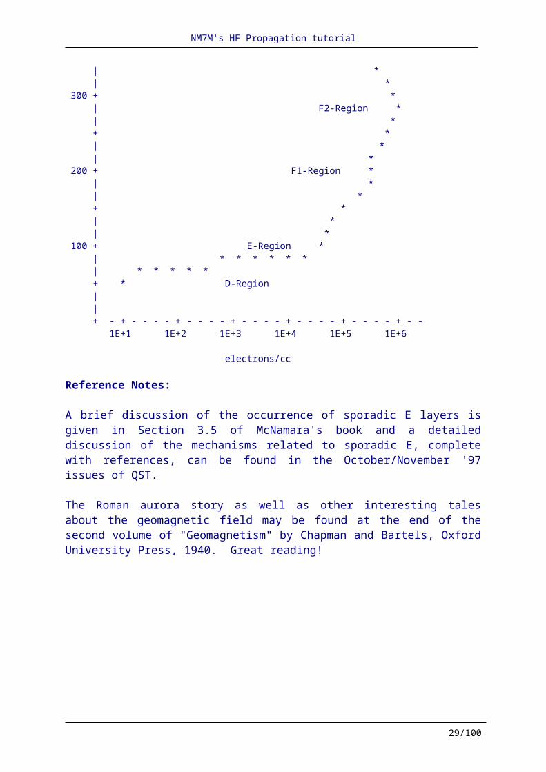
NM7M's HF Propagation tutorial
Reference Notes: Critical frequency maps of the E- and F-regions can be seen in my Little Pistol book. In addition, they will be found in books by McNamara and Davies.
Excellent critical frequency maps are obtained from the PropLab Pro program. In fact, that program gives a full complement of ionospheric maps and in several projections.
Down-Sizing of the Ionosphere In the previous pages, I showed one sample contour of a global map of the F-region, for 10 MHz when the SSN was 137. You can go back to the map to see how it spilled over into the hours of darkness. But that was only one contour. So the question comes down to the rest of the map, what other contours were like and their limits in critical frequency. Looking at the sample contour, it is easy to think that parts of the globe closer to the sub-solar point would have higher values of critical frequency, up to 16-17 MHz. After all, the sun was more overhead for there and the solar UV had less atmosphere to penetrate. But at larger zenith angles, particularly toward the polar regions, the critical frequencies would be lower, going down to 6-7 MHz. All that for a SSN of 137. What about lower SSN, say toward solar minimum? Then, for the region where the critical frequency was 10 MHz earlier, you can just put in 5-6 MHz and at higher latitudes, you can put in 3-4 MHz while at low latitudes, the value is 11-12 MHz. But whatever the SSN, the highest critical frequencies are always found at the lower latitudes. As a practical matter, that is an explanation why contest DXpeditions go toward equatorial regions; the bands are always open there and it is just a matter of how far their signals go poleward before running out of sufficient ionization. So I like to say that the low-latitude regions are the most robust of the ionosphere. But there is a difference between "robust" and "ROBUST", say for solar minimum and solar maximum.
Before getting to that, I should point out there are "islands of ionization" at low latitudes, as shown by the additional contours given below: 90N o++++o++++o++++o++++o++++o++++o++++o++++o++++o++++o++++o++++o . | . . x x x x x x x | Sample Contour .60N . x x | 10 MHz for SSN = 137 . . x x | 0600 UTC . . x x | Fall or Spring .30N . x +++++++++++ x| Equinox . . x + 17 MHz + |x x x . . x +++++++++++ | x x x .Eqtr 0+x++o++++o++(SUN)++o++++o++++o++++o++++o++x+o++++o++++o++++0 . x +++++++++++ | x x . . x + 16 MHz + | x .30S . x +++++++++++ x x|x x . . x x | x x x x x . . x x | x x x x .60S . x x x x x x x x | . . | . . | .90S o++++o++++o++++o++++o++++o++++o++++o++++o++++o++++o++++o++++o
0 60E 120E 180E 240E 300E 360E
29/62
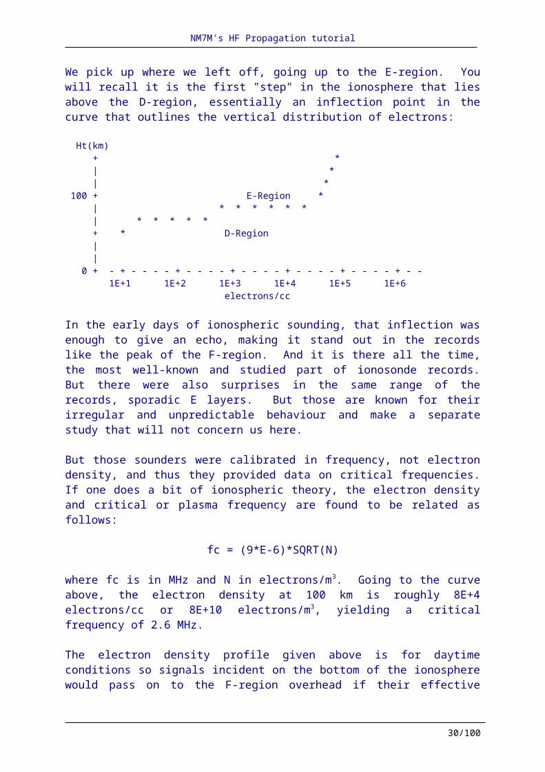
NM7M's HF Propagation tutorial
What I have shown is somewhat out of scale, too wide in latitude and poorly positioned in longitude, as you would see if you looked at the original global map of the F-region. But it conveys the idea, islands of strong ionization in the afternoon/evening hours. This is called the "equatorial anomaly" and has profound effects for propagation, giving rise to long, chordal hops on HF and DX on VHF. Those regions are a regular part of the ionosphere, day in and day out, and the high level of ionization there adds to the robustness that I spoke of earlier. A few paragraphs earlier, I made mention of the fact that global maps of the F-region change with solar activity. One way of making these ideas more vivid in one's mind is to think of them like relief maps, with a "frequency surface" that rises or falls in height as critical frequencies change with increasing or decreasing SSN.
The quantitative side of that approach can be shown by means of a N-S slice through the global maps that one obtains, say from the PropLab Pro program, for two different sunspot numbers:
foF2 (MHz) 15 + Equinox at 0600 UTC, 120E longitude | | ooo | ooo o oo | o o o .. ooo 10 + o .. o o . . ooo | o . . ooo . .. o | o . . . .. oo | ooooo . . . .. oo | ooo .. . .. oo 5 + ooooo ..... ... ooo | .. ... | ...... ... | . - SSN = 10 o - SSN = 100 | o++o++o++o++o++o++o++o++o++o++0++o++o++o++o++o++o++o++o++o++o 90S 60S 30S Eqtr 30N 60N 90N Those N-S cuts across the F-region maps show the two "islands" of the equatorial anomaly as well as the deep notch in between them. Also, it shows again the geomagnetic control of the ionosphere by the asymmetry of the ionosphere at 120E, due to the fact that the magnetic dip equator is about 5 degrees north of the geographic equator at that longitude. Admittedly, the above graphics are pretty crude but they cover the main aspects of the ionosphere - E-, F- and F2-region maps - showing how ionization is distributed and how it varies with changes in solar activity. It is within those regions that we are trying to propagate signals. So we should lay down some great-circles to see where the paths are going relative to the ionization. The test, of course, is if the effective vertical frequency along a path is less than the critical frequency encountered. As long as that's true, propagation will continue; otherwise, the RF will penetrate the F-region and be lost.
Looking at the last graphic, you can see that "the test" gets tougher at high latitudes where the critical frequency is on the low side, a few MHz. Thus, there will be angles at which the RF
30/62

NM7M's HF Propagation tutorial
penetrates the ionosphere and is not returned to ground level. That is "skip", discovered by John Reinartz back in the mid'20s, and obviously gets worse at higher frequencies. In that regard, there is one "side light" to that on the higher bands. Thus, it is quite easy to "pass the test" and work to the south on 21 MHz, for example, as the ionosphere is quite "robust" in the N-S direction. But looking at the last figure, one can see that the ionosphere is "puny" in the E-W direction, with very low critical frequencies. As a result, when chasing DX on 21 MHz, skip makes it impossible to hear the station east or west of you that got the South American contact that you were trying for.
At this point, our discussion comes down to exploring the aspects of the distribution of ionization, vertically and horizontally. The vertical distribution determines how signals are refracted or bent along a path while the horizontal distribution determines whether a hop is completed or how long it might be. There are two approaches we can follow, the rigorous one would be to trace ray paths through a model ionosphere while the practical one would be to use the model in a propagation program, looking at the critical frequencies at the two control points on a path to see what the MUF would be and whether one's RF passes the test.
Ray-tracing takes us back to the analogy between the flight of a baseball and RF across the ionosphere. Mathematically, the flight of the ball is worked out using Newton' Laws, with equations of motion in two or three dimensions. You should not be surprised if I tell you that equations of motion for RF can be worked out, with the ionosphere playing the role of gravity. So, like any baseball or even spacecraft, the methods of mechanics work with RF and the equations of motion solved, step by step, to find the path of RF. In that regard, the PropLab Pro program is outstanding; all you have to do is put in the locations of the terminii, the date and time as well as the sunspot number, and it solves those equations of motion and traces out the path of the RF. Just fantastic! But there is one more thing to add; PropLab Pro also includes the role of the geomagnetic field in the equations of motion. At the upper end of the HF spectrum, that is not important as the QRG is large compared to the electron gyro-frequency about the field lines. But down around 160 meters, the 1 MHz gyro-frequency is comparable to 1.8 MHz and the effects of the magnetic field no longer appear to be negligible in the equations of motion. There are some interesting consequences for wave polarization as well as signal absorption. In addition, signals can get trapped in that valley above the night-time E-region and ducted to great distances with low loss. But we'll get to that later; first, MUF programs.
ON4SKY's note. The correlation between the geomagnetic field and the electron gyro-frequency (EGF) explains the propagation of the lowest band. This correlation requests some explanations. EGF is a measure of the interaction between electrons present in the Earth atmosphere and the vertical component of the geomagnetic field (Z-field). The closer a transmitted AM or SSB frequency is to the electron gyro-frequency, the more energy is absorbed by the gyro electrons from that carrier wave frequency. This phenomenon mainly occurs with AM signals traveling perpendicular to the geomagnetic field (especially along high latitude NW and NE propagation paths). This kind of absorption is always present and cannot be avoided.
31/62

NM7M's HF Propagation tutorial
Reference Notes: Originals of all the figures mentioned above can be found in my article, "On the Down-Sizing of the Ionosphere", that appeared in the July/August '94 issue of The DX Magazine. Also, the two main F-region maps are on p. 29 of my book on long-path propagation and also found in Davies' book, "Ionospheric Radio". In addition, there are a number of ray traces shown in my Little Pistol book, illustrating skip and showing how RF hops vary with frequency as well as radiation angle.
Performance of ionospheric modelsNow we are in a position to talk about propagation predictions. I say that as you understand that predictions require some sort of representation of ionospheric maps, both E- and F-regions, and a method that looks at how effective vertical frequencies compare with critical frequencies along a great-circle path. I must admit that I have injected "effective vertical frequency" (EVF) into the discussion; you normally don't see that term when you read about propagation. In McNamara's book, he uses another form, "equivalent vertical incidence frequency", in his discussion but I find that just too wordy and besides, my choice of EVF fits the bill and tells the story. I hope you agree.
Anyway, we know the test which our RF undergoes as it ascends after launch: if its effective vertical frequency is less than the local critical frequency, it will be contained by the ionosphere and if not, it will go past the F-layer peak and be lost. The propagation prediction business has to do with how that test is carried out - to what approximation or detail the test is made and with what sort of model of the ionosphere. I've already mentioned the control point method in which the test is made at the first and last hops on a path. That method was developed back in WW-II, by Smith in the USA and Tremellen in the UK, and was based on the notion that if a path failed, it was usually at one end or the other. I pointed out that works well as long as any hops in the middle of the path do not have LOWER critical frequencies. Beyond that, you should remember that the method represented a great step forward at the time, even though it was when ionospheric mapping was in its infancy.
So the control point method was based on an approximation and its use involved a database which was both limited and uncertain, at least at the outset. Nowadays, the database has improved quite a bit but still will undergo some revisions in the future as the Internation Reference Ionosphere is updated from time to time. I really don't know the details of the first uses of the control point method but I am familiar with some at the present time. For example, the pioneer program in amateur radio circles was MINIMUF, with source code first published in QST in December '82. That method used M-factors, numbers between 3 and 4, for division of the QRG to obtain EVF for comparison with critical frequencies at about 2,000 km from the ends of the path; for that, MINIMUF used a database founded on oblique ionospheric sounding.
One can fault the source code of MINIMUF for not taking into account the earth's field, leaving out the equatorial anomaly and organizing the ionosphere only with geographic coordinates. Beyond that, the database was rather limited in scope. But MINIMUF caught the
32/62

NM7M's HF Propagation tutorial
imagination of the amateur radio community and all sorts of accessories were attached to MINIMUF, ionospheric absorption and man-made noise, to mention just a few. MINIMUF's shortcomings, the lack of geomagnetic control in the method and no consideration of radiation angle, placed it in a poor position to compete with other programs that came along and corrected those deficiencies. Here, I have in mind the work of Raymond Fricker of the BBC External Services. In the mid-80s, he published programs like MICROMUF and MAXIMUF which included the role of the geomagnetic field and put in radiation angles so one could compare MUF predictions for more than just the lowest mode.
Somewhat later, the Germans introduced a program, FTZMUF2, that used a grid point method to obtain critical frequencies from the CCIR database and used interpolation to obtain the spatial and temporal data for making predictions. They went on to show that FTZMUF2 gave a better representation of the CCIR-Atlas data for 3000 km MUFs than did MINIMUF. Beyond that, they incorporated FTZMUF2 in their own MUF prediction program, MINIFTZ4. Note by ON4SKY. Four years later, in 1991, Bernhard Büttner, DL6RAI, also used FTZMUF2 in his own applicated named Propagation Prediction, PP. This is one of the first DOS application to display MUF and other signal strength in a colored line graph. Then in 1994 Cedric Baechleris, HB9HFN, released HAMFTZ based on the same grid point method.
But Fricker used an entirely different approach when it came to the database for his calculations; he used mathematical functions to simulate the CCIR database, now in the International Reference Ionosphere. Then he used the functions to calculate foF2 at the midpoints of the first and last hops in his programs, MICROMUF 2+ and MAXIMUF, as in the control point method.
Those were the propagation prediction programs available until the IONCAP program developed in the late '70s by George Lane from VOA then by Teters and al. for NTIA/ITS was brought down to a smaller size where it could be incorporated in home computers. Unlike IONPRED, which Fricker's method was based only on F-region considerations - but that gave accurate results in its limitations - IONCAP deals with fluctuations of signal strength, it uses a D-region factor, and takes into account man-made noise. Today the only application always maintained and using a reduced set of IONCAP functions is PropView from DXLab suites.
Note by ON4SKY. In 1985, pressed by the broadcasters' interest, George Lane improved the IONCAP model, corrected some algorithms, added new functions, and after years of research and development created the famous VOACAP that was released free of right in 1993. Today VOACAP is considered as the best ionospheric model, the standard for comparison.
Then came all series of programs, some as accurate as the VOACAP model for Windows 16 and 32-bit plateforms. Most of them used the new functions devised by Raymond Fricker and other scientists or directly the VOACAP engine without additional algorithms.
In any event, the upshot of the comparisons, is today that Raymond Fricker's programs and the improvements made by George lane are close in agreement with the International Reference Ionosphere (IRI), then came all non-VOACAP-based applications that give a rough estimation of propagation conditions, and far behind all DOS executable like MINIFTZ4 and other MINIMUF considered as the poorest and displaying often few information.
33/62

NM7M's HF Propagation tutorial
But how well the underlying VOACAP database matches the real ionosphere compared with IRI, the best representation available at the present time ?
In that connection, I undertook a study of how the mathematical F-layer algorithm in Fricker's MAXIMUF compared with IRI, not just for a path or two but over the entire world. Thus, foF2 values were calculated at intervals of 5° in latitude and 5° in longitude from Fricker's mathematical functions and compared with corresponding values from IRI. That method showed where Fricker's values were low, where high and an overall measure of his methods.
The result was that Fricker's method, when used to make a map of the F-region, gave good agreement over the entire globe with the values from IRI, point by point, but the agreement could even be improved considerably by the simple offset of 1 MHz added to the foF2 values calculated by his methods. Put another way, Fricker's foF2 map was very much like the map from IRI, with details such as the islands of ionization showing up as well as various aspects of geomagnetic control, but the critical frequencies were a bit low. All in all, I found it amazing!
And that approach proves to be just another way of testing F-layer algorithms, seeing if they can make a good ionospheric map or not. MINIFTZ4's algorithm gets good marks in that regard but with problems from its interpolation methods while MINIMUF's F-region map has little resemblance to a real ionosphere on a global scale. That accounts for some of its erratic predictions for DXing.
Unfortunately, when I made my tests the F-layer algorithm of IONCAP was not available so comparisons with the IRI remain to be done with VOACAP which sources are available from NTIA/ITS. Perhaps some of the VOACAP developers will do that in the future. But whatever the outcome, VOACAP is always the best HF propagation program and provides some of the other aspects of propagation prediction that are important. Thus, in addition to having methods for calculating MUF, LUF and other HPF, it deals with the range of values of critical frequencies resulting from the statistical variations in the sounding data.
Here, I refer to statistical terms like the median as well as the upper and lower decile values of critical frequencies from the sounding data. In a propagation setting, the median value of the data at a particular hour during a month would be one such that half the observed values lie above it and half fall below it. If a median value is used in propagation calculations, one obtains what is termed the Maximum Useable Frequency (MUF) for the path. The upper and lower decile values of critical frequency have to do with the 90% and 10% limits. Thus, the upper decile value during a month of observation is a frequency which is exceeded only 10% of the time, 3 days, while the lower decile value during a month is a frequency which is exceeded 90% of the time, 27 days.
When those values are used in propagation calculations, one then obtains the Highest Possible Frequency (HPF) and the Frequency of Optimum Transmission (FOT) for the path.
34/62

NM7M's HF Propagation tutorial
A sample of that kind of calculation is given below (in MHz), for a path from Boulder, CO to St. Louis, MO in the month of January and when the SSN is 100 :
GMT FOT MUF HPF GMT FOT MUF HPF 1 10.7 13.6 17.4 13 6.4 7.5 8.4 3 7.4 9.6 12.0 15 13.0 15.3 17.1 5 5.7 6.9 8.7 17 16.6 19.3 22.0 7 6.1 7.4 9.7 19 18.1 21.1 24.0 9 6.5 8.0 9.4 21 17.7 20.6 23.5 11 5.0 6.1 7.2 23 15.9 18.5 21.1 Looking at those numbers, you can see that the HPF and FOT values lie about 15% above and below the MUF values. That should put you on notice; if the propagation program you use gives only MUF values, the real-time values for the ionosphere could differ by as much as +/-15%. And that is only from the statistical variations in the basic data; there are still the approximations in the method to worry about as well as geophysical disturbances. But those remarks apply mainly to the higher HF bands; down on 80 and 160 meters, ionization is not a concern on oblique paths. Instead, noise and ionospheric absorption limit what can be done. And propagation programs are useless for those bands as the main criterion is darkness along paths, not MUFs. But the role of the geomagnetic field is important and affects the modes that are possible. All that in due time. As for geophysical disturbances, those will be our main effort in next chapter and need not concern us at this point. We are really concentrating on the undisturbed ionosphere and its properties or modes, variable though they may be. And while still talking about the VOACAP program, it is worthwhile to note that its methods deal not only with the statistics of F-layer ionization, through MUFs and the like, but also down lower where absorption and noise become have their origin. So VOACAP has F-region methods which give not only the availability of a path, the fraction of days in a month it is open on a given frequency, but also D-region methods which give the reliability of a mode, the fraction of time the signal/noise ratio exceeds the minimum required for the mode.
This was not meant to be something just in praise of VOACAP but for me it is the best HF propagation analysis and prediction program that I have at my disposal in the perspective of a point-to-point prediction. True, there are other programs based on it and you will have to judge for yourself whether those programs meet your requirements or not. You should read the reviews out there, on ON4SKY's website, in QST and The DX Magazine, to get a feeling for what they can offer you in your pursuit of DX. If possible, check with a user to see if the program matches your goals or needs for DXing.
At this point, we've come to where ionospheric disturbances from the impact of the solar wind on the magnetosphere are of real importance. Needless to say, they add to the uncertainties that have been cited above. But in contrast to the statistical side of propagation, there are clues that help deal with the geophysical side of propagation. That will be our task in future sessions.
Propagation modes and DXingHaving spent some time with the ionosphere, now we have to be more practical, speaking of propagation modes and the things that can go wrong when DXing. But modes are the first
35/62

NM7M's HF Propagation tutorial
order of business. In that regard, everyone knows about HF hops from the various regions - in the range of 1,500-1,750 km from the E-region and about 3,000-3,500 km from the F-region. Of course, it depends on frequency and the radiation angle at which signals are launched.
The electron distribution, having greater density at the higher altitudes, always refracts signals downward. That may seem a bit strange but that is the case; rays which are ascending are bent back toward the earth and the same is true of rays which are going down. The rate of bending is greater at the higher altitudes, when rays are close to the greatest concentration of electrons, but it is always AWAY from the region of higher ionization. And as I indicated earlier, how far rays proceed in the ionosphere depends on the effective vertical frequency (EVF) when they were launched, just like the baseball. Remember? Let's take the case of some rays where the EVF is very close to the critical frequency at the peak of the F-layer. In the figure below, Ray A is one where the EVF is less that foF2 and it is bent back toward ground while Ray B is one where the EVF is greater than foF2 and it penetrates the F-peak and goes on to Infinity. But notice that both rays A and B are bent or refracted AWAY from the region where the ionization is the greatest, the F-layer peak. That's a general feature of refraction in the upper range of the HF spectrum. Now one other thing; it seems rays can be reversed in electromagnetic theory so Ray B could be the path for galactic radio noise which penetrates the F-region below. OK?
/ / / B EVF > foF2 / / / / / . - -> - - - -> - - - . F-peak / \ \ / \ \
/ \ \ / EVF < foF2 \ \ EVF = foF2 / \ \ / A A \ C \ / \ \/ \ \------------------------------------------------------------------Xmtr Ground RX #1 RX #2
Now we come to Ray C, one where the EVF is very, very close to the critical frequency of the F-layer. That type of ray, moving almost parallel to the earth's surface is called a Pedersen Ray. Those rays can give very long hops but they are essentially unstable in the sense that any little increase or decrease in the electron density and they diverge, going back to ground like Ray A or off through the F-peak to Infinity like Ray B. Just in case you missed the idea, Pedersen Rays at the peak of the F-region involve the upper portion of the HF spectrum as the oblique path must reach those altitudes; that is not possible for the bottom of the HF spectrum (3 MHz) as even vertical rays can't penetrate that far up in the ionosphere as foF2 is just too high.
36/62

NM7M's HF Propagation tutorial
But that is not to say that Pedersen Rays are impossible at the bottom of the HF spectrum; it's just that type of refraction takes place down around the E-region where the electron density levels off for a short range of altitude. So let's look at some ray paths there, for 80 and 160 meter signals with EVF close to the value of foE, especially at night: F-region - B / \ B
/ \ / \ . - -> - - - -> - - . E-region / \ \ / \ \ / \ \ / A \ A B \ / \ \/ \ \------------------------------------------------------------------Xmtr Ground RX #1 RX #2
Ray path A corresponds to a E-hop where EVF < foE and covers only a short distance to a receiver. But Ray B is one where the signal has an EVF that's very, very close to foE. But it penetrates the E-layer and ascends into the F-region; however, its EVF is still too low to reach the higher portions of the F-region and so it is refracted back down. If the down-going angle of the ray has not been affected, it will continue for a distance along the level of the E-region and then be returned to ground. In a sense, the path resembles that followed by a Pedersen Ray but there is that short excursion into the F-region making it an E-F path. Whether at the level of the E-region or the F-peak, paths which have Pedersen-like refraction cover greater distances than the simple E-or F-hops. As such, they would contribute to paths with few hops and stronger signals; however, as noted earlier, they may be unstable and only have brief existences. With the varied paths that amateurs use, such situations are not readily identified; however, for fixed paths in commercial use, it is a different story. In that regard, it is pointed out in Davies' book that HF Pedersen rays tend occur around local noon on fixed paths across the North Atlantic, when the density gradients along the path are at a minimum. So the above examples cover the simple, single hops that can occur, from short E-hops to long E-F hops, then F-hops and even long Pedersen hops. After that, we get into multiple hops; those are more complicated, of course, but there is some simplicity in the second and third hops in that reflections involve equal angles of incidence and reflection from a surface. But even then, there is the odd chance of complexity if the surface is not flat or not smooth. The former would, in effect, change the next launching angle of a ray, adding or subtracting the tilt of the surface to its original angle relative to the horizontal direction. As for rough surfaces, they can give a diffuse reflection and that serves to reduce the power carried forward in the original direction. At surface reflections, there can be some signal loss, depending on the signal polarization, surface material and the frequency. As you know, we distinguish between horizontally and vertically polarized waves, meaning the electric field of the wave is either parallel to the earth's surface or perpendicular to it, as for radiation from a horizontal dipole or a vertical antenna.
37/62
NM7M's HF Propagation tutorial
While there may be signal loss (in dB) on reflection, the process is discussed first in terms of reflection coefficients, meaning the amplitude of the reflected wave compared to the incident wave. The graphic below illustrates the case for good ground material and 14 MHz signals; clearly, the small reflection coefficient for vertical polarization around 25° means there would be a large signal loss for waves incident at that radiation angle. But horizontal polarization is much better in that regard and is the reason why most DXers prefer horizontally polarized antennas.
Reflection Coefficient
1.0 HV | Good ground, 14 MHz | H H - horizontal polarization 0.8 + V H V - Vertical polarization | H | V H 0.6 + H | V H | H 0.4 + V H H HV HV | V | V V 0.4 + V V | V V | V V +-----+-----+-----+-----+-----+-----+-----+-----+-----+ 0 10 20 30 40 50 60 70 80 90 Radiation Angle (degrees)
Of course, once signals leave an antenna, their progress is part of the discussion of propagation. Everyone knows that salt water is the best reflecting surface for RF and fortunately 78% of the earth is covered by oceans. That really helps DXing. But a significant fraction of ground (and amateur population) lies in the northern hemisphere and the rest of the earth involves ice and snow in the polar caps so the distribution of surface material shown below is of some interest to the propagation of signals: 0E 180E 360E North ************************************* .........GGGGG...............G.....** * = snow/ice .GGGGGGGGGGGGGGGGGG*GGGGGGGG*G..*.... .GGGGGGGGGGGGGG.........GGGG.GG.....G G = ground GGGGGGGGGGGGGGG.........GGGGGGG.....G G..GGGGGGGGGGGGGG........GGGG.......G . = salt water GGGGGGGGGGGG..............G........GG GGGGG..G..G.................G......GG for
GGGGG......G................GGGG....G .GGG........................GGGGG.... 10 deg x 10 deg .GGG..........G..............GGGG.... .GG.........GGGG..............GG..... areas over the ..............GG...............G..... ..................................... earth. ..................................... ..................................... ************************************* South ************************************* 0E 180E 360E
38/62

NM7M's HF Propagation tutorial
We'll do more with reflection loss later on but for the moment, it is important to know it is there and extracts signal strength with every bounce. But there is one more point to bear in mind; the angle of reflection can be as important as the polarization, the surface or frequency. Thus, losses off of water at low angles are about 1 dB, about 3 dB off of the various forms of ground and in excess of 6 dB off of snow/ice. The situation gets progressively worse at higher radiation angles so low radiation angles should be the order of the day. But you knew that, just because the hops are longer at low angles.
Finally, it should be noted that we've pretty well assumed the ionosphere to be concentric with the spherical earth. That is a simplification, of course, and we have to expect tilts in the ionosphere and those will have effects on waves returned from the higher altitudes. For one thing, a tilt ALONG the path will change the angle of return to the ground; for another, a tilt ACROSS the direction of a path will affect the polarization in the sense that what was a horizontally polarized wave may now have a vertical component to it. So the next ground reflection becomes a bit more complicated, the signal loss now depends on how the two polarizations are reflected. And then there are phase changes on reflection. But nobody said radio was simple, did they?.
Let's go on with multiple hops, putting in more of the details. One matter of interest is the radiation angle throughout a path. Thus, one might pick one angle, say at the peak of the antenna radiation pattern, and try to follow it along a path. But while the Laws of Optics apply, with angles equal for incidence and reflection from a surface, the angle may change due to a tilt of the ionosphere on one hop or change of inclination or slope of ground at a reflection point. So there could be some variability in the radiation angle. And, of course, the height of the ionosphere is not constant along a path, changing if the path goes from being in sunlight to being in darkness. All those aspects of the path serve to change the distance per hop or, for that matter, how close the path for a given radiation angle comes to the target QTH. Leaving aside the variations which result from surface reflections and the like, one can illustrate path structures by making various combinations of hops.
39/62

NM7M's HF Propagation tutorial
Without citing any particular type of the ionospheric circumstances, some common paths are shown below:
F-hop - / \ / \ E-hop / \ _ / \ / \ / \ / \ / \ / \ / \ / \ / \----------------------------------------------------------------- - - F-region / \ / \ / \ / \ / \ / \ / -- \ / Sporadic E \ / \ / \
/ \----------------------------------------------------------------- and various other combinations are possible. The modes shown above are specified as as E-F and F-Es-F. For longer paths, the number of E- and F-hops may be larger, depending on how the path is located relative to the terminator. As for desirability, the rule is that E-hops on a path are where most losses occur, with ionospheric absorption on the sunlit legs and ground losses, while F-hops in darkness have less loss, with fewer ground reflections for a given distance from point A to B.
The presence of a sporadic E reflection, without any intermediate ground reflection between reflections from the F-layer, brings up another type of path that contributes to long-path propagation.
Here, the idea is the same as with the Es reflection except that the ground reflection is missing because of ionospheric tilts, shown as dotted lines, between the two portions of the F-region:
. . . . F-tilt . - - - > - - - . F-tilt . / \ . . / \ . / \ / \ / \ / \ / \ / \ / \-----------------------------------------------------------------Xmtr Rcvr
40/62

NM7M's HF Propagation tutorial
The figure above is "Flat Earth Physics" but in reality, the ray reflected off the first part of the F-region did bend downward but it didn't go down far and the curved earth fell away from it so it missed the earth and went on to the F-region again. Make a curved sketch to see what I mean. OK? While the tilts shown above are exaggerated, such circumstances are found regularly on paths going across the geomagnetic equator in the afternoon/evening hours and give rise to long, chordal hops with correspondingly stronger signals. But it should be noted that "tilts" really are another way of representing the changes in the electron density distribution along a path. Thus, an upward tilt, one that gives a longer hop, really is the same as the case where the electron density DECREASES along a path direction and results in less downward refraction. That is called a negative gradient and, of course, a positive gradient is just the opposite. Finally, there is another interesting variation on path structure that results from a negative gradient along a path, ducting. In that case, the situation is like the E-F hop discussed last time but the excursions into the F-region are repeated several times: - - - - / \ / \ / \ / \ / \ / \ / \ / \ - - - - - - - - / E-layer / Ducting / / A------------------------------------------------------------------Xmtr Ground
Again, the above representation is "Flat Earth Physics" and involves a negative gradient, just like the chordal hop mentioned earlier. But those long hops are more characteristic of the upper end of the HF spectrum, 14 MHz and above, and require almost the full height of the ionosphere for their completion. That is the case as even a reduction in electron density along a path does not reduce refraction at the higher frequencies to a great extent.
The ducting shown above is for the low end of the HF spectrum and involves smaller vertical excursions of ray paths than the case for chordal hops. That is the case as refraction varies with the inverse-square of the frequency; thus, for the same gradient or reduction in electron density along the path, the change in the downward refraction is much greater at the low end of the HF spectrum and less of the ionosphere is required for the same type of effects. Now, having gone through a wide range of mode structures that are possible, one can use those ideas in dealing with propagation. But, face it, the RF from one's antenna pattern goes off into all the possible modes, be they E-, E-F or F-hops and, depending on the operating frequency, some of the exotic modes, like chordal hops or chordal ducting are possible too. But the mode that gets through for your DX contact is something of a "survivor", giving signals where the others have died out due to absorption or have the wrong radiation angles for the path or receiving antenna.
But at this point, about all we're prepared to think about are the more common modes and those would be in relatively calm, stable conditions. In short, we'd be looking at the indicators, SSN and the like, perhaps a map with great-circle paths on it and pointed our
41/62

NM7M's HF Propagation tutorial
beams in the right directions. But the "when, why and how" have yet to be discussed, to say nothing of circumstances that are out of the ordinary. Myself, I consider "when, why and how" to be the "propagation imperatives", the ideas that every DXer should have in mind before turning on the rig in pursuit of a "New One". In short, those ideas should be "Second Nature", the sort of thing you'd have in mind if shipwrecked on a desert island with nothing but the makings of a ham station at your disposal. You should be able to think of the DX QTH, have a feeling for what could be done on a given date and think of when to get on the band of your choice. Sometimes the answers are not to one's liking but an answer should be forthcoming without too much head-scratching. So let's see what we can do to get that right, at least for normal conditions, and then deal with disturbances and see what they'd mean for us. That won't be too burdensome as once the broad outlines are established, you'll have a propagation program to fill in the quantitative details, case by case.
Now we've discussed some of the general ideas behind propagation in the HF part of the spectrum and you should have a good grasp of what it all depends on - enough ionization overhead to refract signals downward, keeping them in the F-region, and signals getting through the ionization down in the D-region with enough strength to overcome the local noise. Case studyWith that in mind, let's explore propagation with a practical case, say making a contact between a central location in the USA and Togo, West Africa in the upcoming CQ WW CW contest in late November. That'd be a good test to see just how far we can go in predicting propagation using the simple ideas developed so far. That done, we can look at how computer programs do it and see what other details they offer.
So let's use Omaha, NE as our QTH in the USA; that's at 41°N, 96°W. Togo is a bit harder so we have to go to the ARRL Operating Manual or DXAtlas to find that it's located in the Horn of Africa, at 6°N, 1°E, close to the Greenwich Meridian. Looking at those coordinates, one thing is immediately clear - it's quite a ways from Omaha to Togo, more than 90° difference in longitude and more than 35° difference in latitude. Considering that the distance around the earth is about 40,000 km, one can conclude immediately that the distance to Togo from Omaha is better than 10,000 km, a quarter the way around the world. That's confirmed by going to the azimuthal equidistant map for Central USA in the ARRL Operating Manual or any logging program showing the world map (e.g. DX4Win); Togo is half way to the antipodal circle, making it quite a haul. But it's not all that hard if you're on the right band at the right time. Now we're talking about late November this year so we can take the effective sunspot number as around 80, judging by recent reports from NOAA. The chances of making a contact on the higher bands are pretty good when you consider that Togo is at a low latitude, where the the electron distribution of the F-region is quite robust. So we only have to worry about launching the high band RF from Omaha. As a first approximation, let's think of trying for a contact on 28 MHz. For that, ionization and the MUF are the important things and tell us that the contact should be tried during the
42/62

NM7M's HF Propagation tutorial
time the path is well illuminated. So with a longitude difference of about 97°, we'd like to have the sun at least midway between the two QTHs, say at about 47°W of longitude. With the sun advancing westward at 15° of longitude per hour, that means the time should be about 3 hours after 1200 UTC or 1500 UTC. But remember Togo is at a low latitude so the critical frequency of the F-region there is less of a problem than at Omaha. That being the case, it would be better to choose a later hour, one when the sun is closer to the longitude of Omaha, raising the critical frequency near there. But the time should not be so late as to have the sun set anywhere on the path. That means we have to look into the sunrise/sunset tables in the ARRL Operating Manual or any astronomical calendar, paper or program, and see when the sun would set at Togo. In that regard, the Operating Manual gives SR/SS data for November 21 and we can use that as an approximation, taking the ground sunset at Togo as 1736 UTC. That would suggest, as a first correction, that the 28 MHz band be tried between 1530 UTC and 1730 UTC. The same would apply for 21 MHz too, knowing that less ionization is needed for propagation on that band, so an operating window might be better if widened to start earlier and end later, say from 1500 UTC to 1800 UTC. As an aside, I should say that last idea has some generality to it, at least for the bands where MUF are important. So from a given QTH, the lowest bands open the earliest, the highest bands the latest, and band closing is in reverse order. Of course, that is just the availability of the path; the signal/noise situation still has to be looked at for the best times of operation. As for the transition bands, 10 MHz to 18 MHz, absorption plays a role there and good sense indicates the effect can be minimized by avoiding times when the path is well illuminated, with the sun around its midpoint. In addition, we know that ionization lingers after sunset, thanks to the role of the geomagnetic field and the slow recombination rate of electrons and positive ions up there in the F-region. As a result, propagation on those bands would be supported around sunset and on into the evening hours.In addition, the rising sun on the path near Omaha would open up propagation, at least until absorption became too great. That being the case, we can expect the bands to open shortly after the sunrise at Omaha, roughly 1350 UTC according to the Operating Manual. And with sunset around 1730 UTC at Togo, another two or three hours could be added to the operating time. Things are shaping up, at least for the bands where F-region ionization and D-region absorption are important. That would give a starting point as sunrise at Omaha, about 1400 UTC, and a closing time of about 2030 UTC for the transition bands. The higher bands would start later, of course, and end sooner, the general principle mentioned earlier. The lower bands, 160 meters - 40 meters, where D-region absorption dominates, would be open from sunset at Omaha til sunrise at Togo. Going to the Operating Manual, we find low-band operations could start at Omaha around 2300 UTC and end around 0545 UTC. But there is the question of noise, man-made or atmospheric in origin, to compete with signals. Here, experience shows that man- made noise is less as the hour goes past the end of the working day. And atmospheric noise, say at Togo, would be the lowest at times close to dawn. So low-band operation probably would be more productive in the later hours of the operating window. But in view of the high level of ionospheric absorption and distance
43/62

NM7M's HF Propagation tutorial
involved, it could be much more difficult to make a contact on the lower bands than the higher ones. In addition, antennas and power play a greater role in that part of the spectrum. Those resources are developed over time by DXers and related to their operating experience in that part of the amateur spectrum. Put another way, DXing on the lower bands, 80 and 160 meters, is tough and not always rewarding for casual operators. Now, to add a realistic twist to this discussion, let me say that I worked 5V7A on 20 CW last year at 2312 UTC on November 29. If you look into it, you will see that was over five hours AFTER ground level sunset at Togo!. (See? Ionization does linger on in the dark, especially at low latitudes!) I would hope you could do the same this year. At least, the above example shows how you can "sharpshoot" for a New One, even with only primitive tools at one's disposal. Give it a try. OK?My good friend, Carl/K9LA, did the propagation forecasting for them and you can see how you might be able to work them too. If you do, I'd like to hear about it, by e-mail, and would appreciate getting an analysis of your QSO. OK?
Note by ON4SKY. For a S/N ratio reliability (SNR) of 38 dB in CW and a required reliability of 90% at the specified date (Novembre 1997) and with a SSN of 40, VOACAP predicts a S/N ratio of 40 dB in Togo at the time of Bob's QSO with 5V7A at 2312 UTC. Taking into account the date and URSI/88 Coefficients, ICEPAC predicts for the opposite circuit a signal power in Omaha of -117 dBW, or close to S7. Both programs confirm that a QSO can be sched at that time with good signals on both sides. Bob selected the best time; according forecasts, signals were the strongest on 20m between 2100-2300 UTC as predicted "DX Toolbox" as well. Note that both circuits (K-5V or 5V-K) are quasi reciprocal with very light differences in the signal strength, MUF and FOT.
Now I didn't work out all the aspects of contest propagation for the 5V7A group; you'll see what their own propagation guru came up with but I'm sure it was based on the principles I outlined above. I have done that sort of thing before, for the recent 8Q7AA and 3B7RF DXpeditions. In that sort of circumstance, the idea is to forecast so they can "Work the World". So every time interval has to be looked and in every direction to find the best way for them to operate in the contest.The first one for the 8Q7AA group went very well, operations going essentially as predicted. But the second one for 3B7RF got into a bit of trouble; that was interesting in itself as it will lead us into the matter of ionospheric disturbances of geophysical origin. Leaving that to later, let's go beyond slow, mechanical methods, how "The Ancients" handled the propagation problem, and look at how it's done by computers. As you know, they do everything practically at the speed of light. But how well do they do it? That's a good question. As a matter of fact, given what you know now, you might wonder if they just do the old-fashioned calculations faster and not add much to the problem. So we'll go with that for a while, looking at how computers handle these questions and then look at a few new ideas.
Reference Notes: If DX contesting is the sort of thing that interests you, let me say that the 5V7A crew were kind enough to provide me with their '96 and '97 contest logs for analysis. I was more interested in them for the aspects of 160 meter propagation but you might look at my article in
44/62
NM7M's HF Propagation tutorial
the March/April '98 issue of The DX Magazine. It also shows how demographics overpowers propagation.
Propagation prediction programs Now the past little exercise used old-fashioned tools to do the 5V7A propagation prediction but at a miserably slow pace. Those really drew on three fundamental ideas - the presence of F-region ionization, D-region absorption limiting signal strengths and the geomagnetic field organizing the ionosphere. So using nothing more than the times of sunrise and sunset, those concepts gave a qualitative view of propagation. But without hard numbers, MUFs and signal/noise ratios, that would never meet the needs of the tough decision-making for a DXpedition or a DX contest operation.
With computers brought into the matter, the times of sunrise and sunset can be calculated with astronomical precision and DX windows found for working 5V7A on the low bands. The next big problem would be finding the sort of signal strength that could be expected. So a knowledge of the operating modes or hop structures is required, primarily a problem in two dimensions, in the plane of the great-circle path. That sort of thing is done very well by the ray-tracing in the PropLab Pro program.
On the higher bands, where MUFs, absorption and E-cutoffs are a concern, computer programs can do a decent job of finding how the ordinary modes would change in the course of a day, say E-hops during the day and F-hops at night as well as mixed modes across sunrise and sunset. But those programs cannot deal with the ionospheric effects from electron density gradients near the terminator or geomagnetic equator so certain modes, like chordal hops and ducting, would not included in their analysis. That's leaves a gap when it comes to having a complete prediction and so computers are fast but will not be as fully quantitative as hoped for in replacing the qualitative efforts used earlier. As you might expect, the earliest computer program in amateur use, MINIMUF, resembled the scheme with ionospheric maps from the Dept. of Commerce and just used the control point method for MUFs, via F-region propagation. Neither signal strength nor noise were considered so the method worked best at the top of the amateur spectrum and for very high levels of solar activity. That was unfortunate as amateurs used the same methods at low levels of solar activity, often with misleading or disappointing results. But MINIMUF fired the imagination of many amateurs and various accessories, including E-layer cutoff calculations, were added to the original code. For example, MINIPROP Version 1 used the F- layer model in MINIMUF and had calculations for E-cutoff and signal strength as well. The early work of Raymond Fricker, MICROMUF 2+ published by Radio Netherlands, was similar but the E-cutoff was regarded as giving values for the LUF, the lowest useable frequency. That's not right as LUF is a D-region matter. But there was a basic difference between Fricker's MICROMUF 2+ and MINIMUF, how the critical frequency information was obtained. Fricker's F-region algorithm used 13 mathematical functions to simulate the database for critical frequencies from vertical sounding while MINIMUF relied on just one function, adjusted to represent the results of a limited set of oblique soundings. In another program, IONPRED, Fricker introduced a novel scheme of hop-testing. Essentially, the program looked at each hop in detail, at the points where the E-layer was
45/62

NM7M's HF Propagation tutorial
crossed and at the highest point where the critical frequency of the F-region was important. So the hop-testing involved determining whether the mode was reliable by seeing if operating frequency was above or below the E-cutoff frequency by 5% and less than the critical frequency for F-region propagation by 5%.
With an initial choice of radiation angle, the path structure could be sorted according to E- and F-hops, depending on the outcome of the tests along the way. Fricker also adjusted the height of the F-region according to local time so hop lengths were not constant along a path. As a result, the path could over- or under-shoot the target QTH. If the error was more than 25 km, another radiation angle was chosen and the process started again. In IONPRED, Fricker also calculated the ionospheric absorption, in dB, and added that to the signal loss due to spatial spreading or attenuation and ground reflections. Another innovative feature of IONPRED was the use of availability of the path, the number of days of the month it would be open for reliable communication. That was something like the FOT-MUF-HPF idea discussed earlier but in the case of IONPRED, the number of days was treated as a continuous variable in contrast to the upper or lower decile approach with the FOT-MUF-HPF method. The IONCAP program has many other methods beside FOT-MUF-HPF and some give long-term availability figures, the fraction of a month the path would be open, as well as reliability values, the fraction of time the signal/noise ratio would exceed some minimum value. Thus, in contrast to Fricker's method which is based only on F-region considerations, IONCAP deals with fluctuations of signal strength, a D-region factor, as well as man-made noise. Nowadays, the method used by Fricker in IONPRED has been improved upon by the use of mode-searching in the MINIPROP PLUS program. There, the idea is to work up a number of successful modes and then find the one with the greatest signal strength. With computer speeds in the '80s, Fricker's method was extremely time-consuming, to say the least, but nowadays computer speeds are such that the whole process of mode-searching takes a second or two!Therefore many new propagation programs were released at the same time as W6ELPro and today, one generation after IONCAP over 50 applications are available to the amateur, among them VOACAP and other WinCAP Wizard 3. But come back a second on PropLab Pro.
In a sense, the ray-tracing in PropLab Pro is like hop-testing as it just goes forward for a given choice of radiation angle and the calculation stops if the trace is lost to Infinity or stops in the vicinity of the target QTH. As you might expect, the main problem with that approach is that the hops may either fall short or go beyond the target, making it a slow, iterative process to get the path for RF from point A with point B. Beside that, the user would have to evaluate the suitability of the path, whether the number of E-hops would make it too lossy or otherwise. For that reason, I admire how PropLab Pro goes about a problem but it's too slow for an impatient person like me. But we can use the ray-tracing in the PropLab Pro program to see paths in both two or three dimensions. It should be said the 2-D case comes fairly close to dealing with the problem in a proper sense by putting in the appropriate ionosphere for each hop on the path, considering date, time and SSN. But it does not take into account terrain, such as the slope of the ground nor the nature of the reflecting surface. Taking one hop at a time, the calculation does takes
46/62

NM7M's HF Propagation tutorial
into account the change in height of the ionosphere but not any tilts or gradients. That is left for the 3-D case. The three-dimensional ray-tracing is based on solving equations of motion for the ray path, just like Newtonian Mechanics finds the paths of satellites and spacecraft. There are equations for the path advance along and upward in the great-circle as well as the motion perpendicular to that plane. The skewing of paths is small in the HF range and thus, it is usually neglected in ray-tracing. That is because refraction goes inversely as the square of the frequency and electron density gradients across paths that occur in the quiet ionosphere are relatively small. The exception to that statement is the auroral zones where large gradients occur. But at lower frequencies, like 1.8 MHz in the 160 meter band, the refraction or bending of paths becomes larger because of the lower frequency and other effects become important. In particular, the gyration of ionospheric electrons around the geomagnetic field occurs at a rate which is comparable to the signal frequency. So the entire approach to the ionosphere has to be redone, put in more general terms without any approximations. That complete theory was due to Appleton, is called magneto-ionic theory and has been around for about 60 years. Polarization and RF coupling into the ionosphere Among the results of the more general theory are that propagation now depends on the angle between a ray path and the local magnetic field; further, the waves which are propagated in the medium are elliptically polarized, another way of saying they consist of two components at right angles to each other and which have a phase difference between them. Beyond that, there are two modes, with opposite senses of rotation of the electric field vector, the ordinary and extra-ordinary waves. The simple, linearly polarized waves that are so familiar in the discussion of HF signals are just a limiting case of elliptical polarization, when one of the two components at right angles has a very small amplitude compared to the other one. In magneto-ionic theory, that limiting type of polarization results when signals are sent perpendicular to the magnetic field. The other case is circular polarization, when signals are sent along the magnetic field direction. Then, the two components at right angles are equal in amplitude and out of phase by 90 degrees.
Those features of propagation were evident in the early days of ionospheric sounding as two echoes were returned for each signal sent upward, the ordinary and extra-ordinary waves, and you will see them on any ionograms that you may inspect. So magneto-ionic theory is a part of the reality of radio propagation. But, for DXers, there is something of a happy simplification as over long distances, the extra-ordinary wave is heavily absorbed and only the ordinary wave needs to be considered. There is another interesting aspect to propagation down on the 160 meter band, the coupling of RF into the ionosphere. As you know, there is a polarization to the waves emitted by an antenna and on 160 meters, vertical antennas are used most often. That is due to the wavelength being so long that most horizontal dipoles cannot be placed very high, in terms of wavelengths, and thus suffer from high radiation angles, being the so-called "cloud warmers". Now in magneto-ionic theory, the polarization of a wave changes continuously in the ionosphere as it is propagated through the geomagnetic field. But there are two limiting
47/62

NM7M's HF Propagation tutorial
polarizations, typically at altitudes around 60 km, where the wave enters the ionosphere near point A and where it leaves the ionosphere near point B. When worked out in detail, the theory says that there will be a signal loss, in dB, at entry because of any mismatch between the wave polarization from the antenna and the limiting (elliptical) polarization at entry point A. For example, signals going in the E-W direction from a vertical antenna at the equator are poorly coupled into the ionosphere because of the polarization mismatch, with vertically polarized waves going against the horizontal field lines. Similarly, there may be signal loss at the exit point B due to any mismatch between the limiting polarization on exit from the ionosphere and the polarization of the antenna at point B. As indicated, magneto-ionic theory is quite complicated, with elliptically polarized waves and all that, but for signals going from point A to point B, we need not concern ourselves about what goes on high up in the ionosphere between those two points, only the antenna types and the limiting polarizations at the endpoints of the path. That makes life a lot simpler. Another point about this frequency range; signals can become trapped in the electron density valley above the E-region at night. Thus, if they enter the region, they may be reflected back and forth between the bottom of the F-region and the lower limit at the top of the E-region. That means they'll rattle back and forth between those altitude limits like a ball sliding down a smooth trough. Only if the walls of the trough change in height can the ball get out or, equivalently, can signals get out of the duct if the lower ionosphere changes. In that regard, ducting is undoubtedly responsible for the long-haul DXing done on 160 meters as it avoids repeated ground reflections and traversals of the lower ionosphere which absorb signals at a very high rate.
Reference Notes: A review of various propagation programs can be found in the QST issues for September and October '96, and an updated review on ON4SKY’s website. The above discussion gives a very brief summary of the principal aspects of magneto-ionic theory, as it applies to propagation. An analytical summary of the theory is given in Davies' recent book, Ionospheric Radio; however, it really requires a strong background in electromagnetic theory at the level found in university courses in physics and engineering. It should be noted that the method of the theory has a broader application as it represents the first steps toward the study of plasmas in the solar system and in out space. A discussion and some quantitative aspects of polarization loss on 160 meters are given in my article in the March/April '98 issue of The DX Magazine. In addition, a fuller discussion of magneto-ionic theory and 160 meter DXing is given in Top Band Anthology, published recently by the Western Washington DX Club. You can contact me for details.
Radio propagation fundamentals We turn now to other aspects of propagation, from predictions to those circumstances which may disrupt propagation and make predictions go awry. But in doing that, a bit of history would help chart the course.
48/62

NM7M's HF Propagation tutorial
First, radio is more than 100 years old now and the course of events has been onward and upward, in frequency and into the ionosphere. Thus, the earliest signals were down in the kHz region and now technology has advanced to the point where amateurs are operating in the GHz part of the spectrum. But it has been a steady advance in frequency and as we know now, that means signals going higher and higher into the ionosphere as their effective vertical frequency increased. Amateur operations start in the medium frequency (MF) range with the 160 meter band, around 1.8-2.0 MHz. If one looks into the ray-traces for that band, it is clear that signals in normal communications circumstances stay below the 200 km level most of the time. Of course, ionospheric absorption on that band is so great that DX operations are attempted only on paths in full darkness. Going to the high frequency (HF) range, 3 - 30 MHz, signals go higher toward the F-region peak around 300-400 km and darkness becomes less of a necessity near the top part of the spectrum. In fact, solar radiation is needed to bring the level of ionization up to the level required for propagation. Historically, in the time that operating frequencies rose, the range of DX contacts increased and it became apparent that the solar cycle played a role in propagation. Moreover, various disturbances became apparent. So the early '20s had amateurs opening up trans-Atlantic operations and that was commercialized in the late '20s with the advent of radiotelephone circuits to Europe. In that time, it was found that the communication links failed during geomagnetic storms. Those could last for days but there were also strange blackouts that lasted anywhere from just a few minutes up to an hour. In 1937, those short wave fadeouts (SWF) were found to be associated with solar flares. Moreover, it was becoming apparent that the disruptions to magnetic storming came a day or so AFTER solar flares.
From all that, it became clear that the sun was a major player in the field of radio propagation and scientists began looking into the details. The SWF problem was fairly simple, just being the release of electrons in the ionosphere from the photoelectric effect of solar X-rays. The magnetic storm effect was a more subtle problem as it implied some slower process, not X-rays moving across the solar system at the speed of light. In that regard, those geophysicists who studied the earth's magnetic field proposed that there was a stream of matter sent out from the sun and then its encounter with the geomagnetic field was the triggering mechanism. From the time delays between flares and storms, first estimates were made of the speed of the solar matter. More than that, they could not say at the time.
Now that brings up the question of just how far out geomagnetic field lines extend from the earth. Of course, that goes to the model of the geomagnetic field in use at the time. That was, in simple terms, the sort of thing you get if you stuff a bar magnet into the earth and look at how the field lines extend past the surface of the earth. In short, the model back in the '40s and '50s was that for a centered dipole field that was tipped with respect to geographic coordinates, the dipole axis piercing the earth's surface at 79.3° N, 71.8° W at the north pole and the south pole through the corresponding antipodal point. That was the field used when the first Pioneer space shots took place after the IGY, an experiment looking at the strength and orientation of the earth's field as the spacecraft moved out, away from the earth. That flight produced a REAL surprise, with data showing the earth's field varying slowly and in an orderly fashion as the spacecraft moved outward but
49/62

NM7M's HF Propagation tutorial
then suddenly, when it reached something like 8 earth radii, the field became weaker and less organized, almost random in its orientation. Clearly, the orderly dipole field no longer described the situation at those distances, giving way to the presence of an interplanetary magnetic field. And what was previously considered as empty space, except for meteoritic dust and debris, was also found to contain of plasma (protons and electrons) that was streaming away from the sun. Now, before exploring that extreme, we should look at the dipole field and see what could be expected from it. As you know, say from your high school physics course, the field lines pass out of the southern hemisphere and then after going out some distance, they return and enter the northern hemisphere of the earth. That was the classical picture; so let's see what it says, at least until we get into trouble with the Pioneer data. Now the magnetic dipole has a system of coordinates of its own, related to the direction of its axis relative to the geographic axis and equatorial plane. With the dipole orientation given above, one can work out the magnetic coordinates of any point on the earth. For example, my location at 48.5° N and 122.6° W is one that corresponds to 54.4° N, 62.1° W in the dipole coordinates. OK? But let's look at the dipole and its field lines. They go out from the southern hemisphere and come back down into the northern hemisphere. But how far do they go out? That would be important when it comes to thinking about the collision of solar plasma and the dipole field, suggested by the geomagneticians. It's not hard to work out where the magnetic field lines cross the plane of the geomagnetic equator and there is a simple relation between that distance and the magnetic latitude where the field lines start:
¯L = 1 / cos
with as the magnetic latitude and L is the distance, measured in earth radii (Re). Now if you conjure up the image of a dipole, surrounded by its magnetic lines of force, you can see that low-latitude field lines do not go out very far from the surface of the earth. But it's a different story for high latitude field lines and if worked out, we obtain the following:
Mag Lat (degs) Distance (L in Re) 10 1.03 20 1.13 30 1.33 40 1.70 50 2.42 60 4.00 70 8.55 80 33.2 So the high latitude field lines are the ones in harm's way when it comes to the collision between the plasma coming from the sun and the earth's field. And, by the same token, the low-latitude field lines that go out only short distances from the center of the earth are pretty well protected from the direct effects of the collision between solar plasma and the geomagnetic field. Of course, that fits with your operating experience, paths going across the polar cap are far more subject to disruption than those going to low latitudes. Before getting to the nature of the various propagation effects that originate on the sun, we should note briefly that the view of the earth's field that I gave in the introduction is not quite
50/62

NM7M's HF Propagation tutorial
the full story. In particular, it was suggested that the solar wind blowing by the obstacle of the geomagnetic field is like the flow problem of a bullet in air, but now with the bullet (geomagnetic field) fixed and the air (solar wind) in relative motion. So it was suggested (and verified) that a bow shock in the solar wind was out there in front of the magnetosphere:
* * BOW SHOCK * Magneto-tail * * * * * <---- * . . . * * * * * . . * * . * * <---- * . . * * . . * * * . . * * . . * * <----* . Magnetosphere (Earth) . * * SUN * . . * * . . * * <---- * . . * * . . * * * . . * * . * * <---- * . . . * * * * * * * * * <---- * * SOLAR WIND
Now, to carry the aerodynamics a bit further, it was suggested that the position of the bow shock would vary, moving closer to the earth at higher speeds of the solar wind. And that proved to be the case, obtained by satellite observations after the original work with Pioneer I. But the geomagnetic field is a bit different than a hard obstacle and it was expected that the field could be compressed at times, particularly if the solar wind came at it asa sudden blast. And, as you guessed, that is the case as shown by magnetic sensors on geostationary satellites. During some severe magnetic storms, those satellites report conditions which put them right in the interplanetary magnetic field, showing that the magnetosphere has been compressed by the solar wind and that the magnetopause was temporarily inside 6.6 Re. Absolutely amazing!
Now, having told you about the troubles of geomagnetic field lines, think back a bit to what I said earlier: they are the things which hold your precious ionospheric electrons in place! So maybe all those disruptions in propagation during magnetic storms are not all that surprising, with field lines being pushed around by the solar wind. There's more to magnetic storm effects than just compressing the field lines in front of the earth. As I suggested way back in the introduction, field lines on the front of the magneto-sphere can be dragged into the magnetotail. In that process, the ionospheric electrons of the F-region on those field lines are removed from the front of the magnetosphere and, in essence, are distributed on much longer field lines on the rear of the magneto-sphere. On both counts, the high-latitude F-region suffers a loss in ionization and critical frequencies in the affected regions are reduced. Of course, the sun shines, day in and day out, so with some magnetic quiet, solar illumination will restore the regions and communications across those high latitudes returns to normal. Those words of explanation will have to suffice as the problems of the magnetosphere are quite complicated, with unfamiliar or non-classical ideas, and are best left for the magnetospheric physics-types to wrestle with. We need not get enmeshed in the details, only be able to recognize when there's a problem and consequences that will follow. In that regard,
51/62

NM7M's HF Propagation tutorial
the records of magnetometers at high latitudes are our best bet as they give vivid portrayals of the storms that develop, thanks to simultaneous, yet secondary effects which result. There, I am thinking of the aurora, both optical and radio, as well as the current systems which build up during a disturbance initiated by the solar wind. Again, the details need not concern us but the main features are what we note: optical emissions coming from above the 100 km layer, VHF reflections off of auroral displays, ionospheric absorption of signals going across an active auroral zone and strong magnetic disturbances observed on the ground from the current systems which develop along the ionized region. More on this next time. Research Notes:
A good historical account of the early days of radio can be found in the first chapter of McNamara's book, "Radio Amateurs Guide to the Ionosphere". And it's a good book too. Get a copy if you are serious about radio propagation.Add also the link to ON4SKY's History of amateur radio, appreciated by ARRL's staff and CQ Magazine's editors too.
Geomagnetic disturbances The end of the second volume of the book, "Geomagnetism" by Chapman and Bartels, has an interesting account dealing with the first days of magnetic observations in Sweden by Celsius and one of his graduate students. Knowing what we do now, I consider that as "Day One" of the Space Age. But I have to marvel that it took 75 years until Oersted came up with the idea of a current (like an ionospheric electrojet) giving rise to magnetic deflections (on the ground below an aurora) of a compass. Compare that time with the five years it took the French mathematicians to come to grips with the Biot-Savart Law for magnetic effects of currents. Interesting! Finally, an excellent discussion of early auroral observations in Norway can be found in the last chapter of Brekke's book, "Physics of the Upper Polar Atmosphere" published by Wiley & Sons in 1997. Brekke, being a Norwegian, pays homage to the works and tradition of good auroral physics established by Stoermer. It's worth a bit of reading time, believe me.
In the previous page we made note that magnetic storms give rise to auroral disturbances, with optical emissions coming from above the 100 km layer, VHF reflections off the ionization in auroral displays, ionospheric absorption of signals going across an active auroral zone and strong magnetic disturbances observed on the ground from the current systems which develop along the ionized region. All that from an enhancement in the solar wind, perhaps coming at a greater speed, with a greater particle density or with the interplanetary magnetic field pointing south with respect to the earth's field. Nowadays, we can read about all those changes on the Internet. But the most important one for magnetic storming has to do with the interplanetary field and its orientation. With the field pointing south, conditions when Bz is negative, the interplanetary field can merge with the terrestrial field (a non-classical concept) and field lines on the front of the magnetosphere then transferred to the tail region as the solar plasma sweeps by. These ideas came forward in the '50s, thanks to the efforts of J. Dungey of the U.K. and others. As I said earlier, they go beyond the elementary considerations we get in classical
52/62

NM7M's HF Propagation tutorial
courses on electromagnetic theory and are best left for the theorists to discuss. We only need to know what happens to the ionosphere and there, the news is BAD as the F-region loses ionization with the development of a magnetic storm. But the E-region can gain ionization, with the penetration of auroral electrons. Those particles are from here inside the magnetosphere itself, not directly from the solar wind, and are accelerated locally, going from a fraction of an electron-Volt up to tens of kilovolts energy. And their flux can be quite large, resulting in electron densities of a million or more per cc from electron collisions with atmospheric constituents in the tens of kilometres above the 100 km level. The colors of the aurora are testimony to the collisions with the neutral constituents and the electron densities that result can give rise to signal absorption. That last point may seem strange if you go back to the curves that were given page 10. There, the relative absorption efficiency per electron was dropping off quite rapidly above 100 km. But in the case of aurora, there are millions of electrons per cc up there and even if electron-neutral collisions are less frequent above 100 km, losses result just from the sheer amount of ionization that goes with an aurora. But to give some numbers, auroral absorption of up to 5 dB or so is found in the riometer records of 30 MHz galactic radio noise coming in vertically. But that is just for one pass through the ionosphere. For amateur communications, say on 28 MHz, that should be doubled for a complete hop, increased even further by a factor of 3-4 for the oblique angle of the path and adjusted for the inverse-square frequency variation. At lower frequencies, that last adjustment shows even greater losses on those bands. So it should be no real surprise that auroral absorption represents an adverse factor for amateur communications. Those remarks dealt with the electron density; one should also note the geometry and activity of the aurora. In regard to geometry, auroral activity at any given time is restricted to a narrow latitude range. (See Research Notes) But it can extend over a wide range of longitude and the type of activity varies from west to east. In evening hours, aurora tend to be quiet and not involve a lot of energetic particles (and ionization). Around midnight, the activity may increase dramatically, with displays flashing wildly overhead and in considerable motion. It is even possible to note from the distinct ray structures that the electron influx comes down the inclined magnetic field lines. Then in the morning hours, the aurora becomes more diffuse, shows some pulsating patches and more ionospheric absorption, slowly varying compared to that around midnight and much greater than before midnight.
HF signals that go across an auroral region will show effects characteristic of the activity - steady signals going across in local evening, considerable rapid absorption and flutter from the moving regions of ionization around local midnight and just strong absorption for local morning. Of course, all those ideas have to be tempered by the frequency involved, with devastating absorption on 160 meters and possible auroral reflections above the HF range. The magnetic disturbances at high latitudes which accompany aurora give qualitative measures of the energy input to the magnetosphere from the impact of the solar wind. Nowadays, one can go to NOAA satellite data and obtain numerical values for the power input from observations of the influx of auroral electrons with energies up to about 25 keV. The numbers can be quite large, from 1 to 500 Gigawatts over one hemisphere. Such inputs can have profound influences, auroral heating and magnetic activity, but our concern is only
53/62

NM7M's HF Propagation tutorial
with communications so we have to look at how frequently these events occur and if they can be anticipated. Recent data published by NOAA gives a summary of magnetic storm activity over Solar Cycles 17-22 to suggest how the levels of magnetic activity might vary, year by year, in Cycle 23. Now when it comes to magnetic activity, indices are used to characterize what level of disturbance (from quiet conditions) is in effect, say in a 3-hour period or averaged over a day. In that regard, a number of magnetic observatories have been selected to provide data for use in making planetary averages. The actual data sets are normalized to common scales, 0 to 9 for the 3-hour Kp-index and 0 to 400 for the daily Ap-index. One can obtain those data from the Internet and keep records to see if there is any recurrence tendencies. Indeed, there are and logging Ap indices is one way to anticipate possible disturbances that come from long-lived solar streams sweeping past the earth or stable active regions which are the source of increased levels of ionizing radiation. Magnetic storminess is categorized in terms of Ap values and minor storms correspond to elevated levels of Ap while actual storms correspond to Ap greater than 40 and severe storms are when Ap is greater than 100. In that regard, the storm of May 3, 1998 had an Ap level of 112 while the greatest storm ever recorded was in September 1941 and had an Ap value of 312! Like the March '89 storm which put the Province of Quebec in the dark for a day, that one affected the power grid in the Northeast. Nowadays, the power industry is keenly aware of the magnetic storm problem and tries to anticipate problems by getting solar wind data from satellites, out there ahead of the earth and in the solar wind.Anyway, both minor and major storms affect HF propagation for hours at a time or a day by their adverse effects on F-region ionization but severe storms reduce the bands to barren wastelands for days at a time. Propagation doesn't return until slow photo-ionization processes replace the F-region electrons.
As we told in the first pages, the propagation aspects of magnetic activity are found on the SEC website of the NOAA under the section "ONLINE DATA" and "Near Earth". This section displays the daily Solar and Geophysical Activity Report and 3-day Forecast. This product contains the Observed/Forecast 10.7 cm flux and K/Ap indices.
The effects of magnetic storming are the greatest, as you might suspect, at the higher latitudes and on the higher frequencies. For communications over any distance, differences in longitude mean that great-circle paths usually swing north and thus are at risk during magnetic activity. This is not too bad for short-path communications as the windows of opportunity can be rather wide. But that is not the case for long-path propagation; there, the path opens with the rise in F-region critical frequency with sunrise on the path and closes shortly thereafter as D-region absorption increases at lower altitudes. In short, if an opportunity is lost on a given day, one must wait for another day and try again. But having spent many happy hours in pursuit of long-path contacts, I can say it is worth it.
Turning to longer ranges in forecasts, the recent NOAA prediction for magnetic storminess during Cycle 23 is shown below:
54/62

NM7M's HF Propagation tutorial
Cycle 23 Magnetic Storms Minor Major Severe 1997 Year 1 12 4 1 1998 Year 2 15 7 2 1999 Year 3 24 17 4 2000 Year 4 29 18 3 2001 Year 5 26 11 3 2002 Year 6 30 23 5 2003 Year 7 33 16 3 2004 Year 8 34 12 2 2005 Year 9 42 17 2 2006 Year 10 34 6 1 2007 Year 11 15 4 1 Given that forecast, we can look forward to major storm activity rising to about 2 per month by Year 6 (2002) in Cycle 23. That is not a good prospect but there are uncertainties in forecasts so one can hope for less and see what happens.
Note by ON4SKY. As expected the first months of the year 2002 were as disturbed as 2000 with a solar flux 5% higher (F10.6 of 220 SFU vs. 210 SFU in 2000) but decreasing rapidly with sunflares of X-class ejecting fast particles that produced indirectly some intense and highly colored aurora over Alaska, Canada and Finland.
The 10.7 cm solar flux is an indication of active regions on the solar disk and that is a quantity that warrants logging. Early in a cycle, new active regions begin to appear but later, some regions are quite stable, particularly around solar maximum, and knowing when the flux may peak again is quite helpful to DXers. The origins of the magnetic activity differ throughout a solar cycle, however, with early part of the cycle giving more of the sporadic coronal mass ejections responsible for solar wind blasts hitting the magnetosphere. On the other hand, the latter part of a cycle is one characterized by fast streams from coronal holes sweeping past the earth. Those can be long-lasting so logging magnetic activity, with the A-index from Boulder for several solar rotations is a good idea, enabling one to avoid times of strong magnetic activity.
One aspect of strong magnetic activity is equatorward expansion of auroral displays, associated with the loss of magnetic field lines from the front of the magnetosphere to the magneto-tail. From the standpoint of propagation, that results in very low MUFs in the polar cap. But it is accompanied by an expansion of the polar cap that can bring on heavy, long-duration ionospheric absorption. That is the case with solar proton events, so-called polar cap absorption (PCA) events. Those events differ in striking ways with auroral absorption (AA) events but both can be present at the same time. Those events will be our next topic of discussion.
Research Notes: I have already given some words of praise for the book,"Physics of the Upper Polar Atmosphere", by A. Brekke. To that I would like to add that the front cover has an ABSOLUTELY FANTISTIC photo of an aurora taken from a satellite. There is a catch, however; the photo was made in Antarctica and the book must be turned upside down to get
55/62

NM7M's HF Propagation tutorial
the aurora positioned OVER the polar cap. But like Confucius said, "A graphic is worth many kilobytes of text."
Geomagnetic storms and aurora We are now into disturbances of propagation, those nasty things that can plague us, sometimes without our even knowing it. The last topic was magnetic storms and aurora. Those represent disturbances of the F- and E-regions, respectively. The effects of magnetic storms can be world-wide in the sense that ionospheric electrons are removed from field lines, lowering the MUFs on paths across great distances. The part of the ionosphere which is disturbed the most is in the polar cap as that is the region whose field lines are most at risk. And recovery from magnetic storms is a slow process, requiring the electrons in the F-region be re-supplied by sunlight, a slow, tedious process which can take days after a severe storm. The effects of an aurora, by itself, are much more localized in the sense that the increased ionization is confined to the field lines that guided auroral electrons downward. Short of being in a full-blown magnetic storm, the effects tend to be brief, measured in minutes or hours, and when the aurora ends, it is a fairly rapid process. Essentially, the problem is to have the electrons in the ionization recombine with the positive ions which were generated by the influx of energetic auroral electrons. But now we come to solar proton events. Those will affect the D-region and originate on the sun, with protons and other particles accelerated up to energies of millions, sometimes even billions, of electron-Volts (MeV or BeV). So solar proton energies, from acceleration on the sun, are high in contrast to those of auroral electrons which are accelerated locally, within the magnetosphere, up to tens of kiloelectron-Volts. The protons are accelerated in connection with some solar flares and then can leave the scene, passing through both the solar and the interplanetary field. The interplanetary field generally points toward or away from the sun and the outward progress of protons depends on the degree to which they go along the field lines or perpendicular to them as they leave the sun. But the interplanetary field is not well-ordered like the geomagnetic field close to the earth so protons will diffuse through the region and their progress will depend on their momentum or the radius of curvature of their path. The more energetic protons will have radii of curvature which are large compared to the scale-size of field variations so those protons will follow more rectilinear paths. On the other hand, less energetic protons will have smaller radii of curvature in the field and their progress will be more like diffusion, scattered by the small-scale, organized portions of the interplanetary field. All that is a way of saying that the high energy-protons will leave the region close to the sun faster and make their effects felt more promptly, albeit briefly. On the other hand, the low-energy protons will diffuse slowly through the field and their effects will be of longer duration. It should not be forgotten, however, that the duration of the acceleration process is of interest too. Generally, it is considered to be the same as the actual flare process but those can be brief, in minutes, or longer, measured in hours. Another way of saying the same thing is if the flare region is off the to the east of the solar disk, solar protons heading toward the earth will have to stagger through the field lines which
56/62

NM7M's HF Propagation tutorial
are more or less perpendicular to their paths. That is a slower process and protons can be held in the magnetic field region for times which are long compared to the acceleration process that started them. As an example, I had experience with one east limb event in August '79 where the solar protons finally reached the ionosphere 18 hours after the flare! Staggering, diffusion? Yep! On the other hand, flare sites toward the west limb of the sun send protons out into the field which generally trails behind the rotating sun and we get "sprayed", as it were, by protons going along the field lines. That is called the "garden hose" effect. The Great Solar Flare Event of February 23 1956 was a case in point, a west limb flare where the travel time was measured in minutes. Those were relativistic particles and had so much energy (over 10 BeV) that they penetrated to ground level, even at the magnetic equator! Been there, seen that! But what are their effects? Given the remarks in the last paragraph, one can expect that the duration of the proton bombardment of the earth will depend on the location of the flare site. That is one propagation clue that NOAA provides with every announcement of a solar flare, the solar longitude involved. So that is one item of interest, east or west of central meridian. But as to the effects of the protons, those depend on their flux or number per square-cm per second and proton energy. The low-flux, low-energy solar proton events were only conjecture until the Space Age but are detected nowadays by satellites and one can see the data in the Tiger Plots on a NOAA website. But events with higher fluxes and greater energies can penetrate the earth's field and get reach into the ionosphere, the atmosphere and, on rare occasions, they can reach ground level. Our interest, of course, is with ionospheric effects and being energetic charged particles, the protons will leave a wake of ionization as they plow through the atmosphere. The extent of the wake will depend on the relative numbers of protons in the various energy ranges - around 1 MeV, around 10 MeV, near 100 MeV and beyond. But generally, being both energetic and massive particles as compared to puny auroral electrons, protons penetrate deeper into the ionosphere (if they get that far through the geomagnetic field) and the heavy ionization near the end of their physical ranges can cause huge ionospheric absorption of signals because of the greater electron-neutral collision rate deep in the D-region. For solar protons to get down to the ionosphere, they must first enter the geomagnetic field out at the magnetopause and then follow field lines, according on their momentum. The present view of these matters is in sharp contrast with the early days of ionospheric radio. Then, the dipole model of the earth's field was taken as the standard and all discussions about the effects of solar protons were based on work done by the Carl Stoermer, the Norwegian auroral physicist. So the idea was that protons were sorted out according to momentum (or energy) by the field and there was a sharp cut-off energy which varied with latitude. But with the IGY, things changed; the use of riometers, looking at ionospheric absorption due to the protons, showed that the cut-off idea was all wrong and the polar cap was wide open, full of low-energy protons, all the way down to the auroral zones where the cut-off energy was supposed to be 100 MeV. That was one of the first clues that the earth's field was not that of a dipole; then measurements made by satellite-borne magnetometers gave the final story, with the field configuration I've sketched earlier.
The coverage of the large polar cap area with solar protons is in sharp contrast with the narrow latitudinal coverage of the auroral zones by energetic electrons; beyond that, there is
57/62
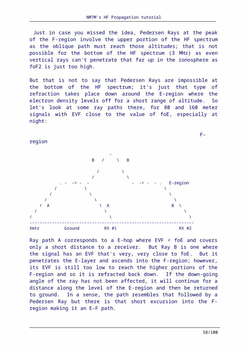
NM7M's HF Propagation tutorial
the difference in levels of absorption, tens of dB on 30 MHz for solar protons as compared to a few dB for the auroral electrons. So all in all, solar proton events that reach the ionosphere, so-called polar cap absorption (PCA) events, can be devastating when it comes to propagation across the high latitudes. But there are few more aspects to PCAs to think about. For example, the access for solar protons to the polar cap is one thing but it has been found that solar protons can get into the magnetosphere via the magnetotail. And the access to the two polar caps is not always equal for solar protons, judging by satellite data. So there can be different ionospheric reports from the two polar caps, depending on sunlight on each and the access of the protons. All this makes propagation interesting and confusing! When it comes to ham radio propagation, there is a propagation effect that can mask the access to the polar caps. Here, I refer to the fact that there is a reduction in ionospheric absorption in darkness, the number of dB in absorption going down by a factor the order of 5 or so. This is due to the fact that the electrons created by solar protons may attach themselves to oxygen molecules and form negative ions. Negative ions are so massive that they do not participate in the absorption process. So absorption in a darkened polar cap, at night or in winter, is less and might be interpreted as a low proton flux without satellite data to clarify the situation.
The electrons bound in negative ions are released when sunlight is restored to the D-region. That is the case for proton events but not for auroral electron events where the ionization is at much higher altitudes and electron detachment results from collisions with atomic oxygen, abundant above 100 km. So auroral absorption (AA) events do not show any day/night effect like PCA events. To summarize now and put things in perspective: auroral absorption events are limited in time and space, found during magnetic disturbances, large or small. Polar cap absorption covers a wide range of latitudes, the whole polar cap, and can last for days at a time after some solar flares. And the ionospheric absorption is large, making PCAs a real threat to ham radio communications. And if the polar cap expands in size in the late phase of a magnetic storm, solar protons can then reach down to much lower latitudes and have even greater effects of our HF propagation.The beauty of PCAs, if one would call it that, is that they are relatively infrequent. The real threat to ham radio communication is the effects of the solar wind, so I would say that magnetic storming is the thing to watch out for, by logging K-and A-indices to identify any possible repetitions and then by checking each day by whatever means are available. Magnetic storming is THE threat to our peace and quiet; what the sun provides in the way of higher critical frequencies by UV radiation can be taken away in a jiffy by a blast of the solar wind triggering a magnetic storm, minor or major.
So monitor/log the magnetic indices; they hold the key to success in high latitude DXing on the bands! But when the high latitudes are disrupted, try the other directions, say across the equator. That is pretty safe, the field lines there being shielded from the ravages of the solar wind. And there's a lot of rare DX there to make things interesting.
This is the end of the line and time to wrap up the discussion. It should be in two parts, the theoretical side which we compare with the experimental part. In regard to theory, the most general discussion would be one which uses ray-tracing with the best available model for the
58/62

NM7M's HF Propagation tutorial
ionosphere and geomagnetic field. That is simple to say but as you know, words come easy. But let's look at how it's done and what it means to us. Then we can go to the experimental part. Appleton's magneto-ionic theoryNow it may sound strange but the magneto-ionic theory that I mentioned earlier is all cast in terms of frequencies. Obviously, the operating frequency is of utmost importance. But then there are three other frequencies; how they compare with the operating frequency (QRG) determines features of propagation. The first frequency is the plasma frequency; for a given position in the ionosphere, it is another way of specifying the electron density. Plasma frequencies in the lower ionosphere increase with height, up to the F-region peak, and decrease with latitude toward the poles. And, in a complicated way, they depend on the earth's magnetic field and sunlight. But for signals to be contained, not penetrating into the topside of the ionosphere, their effective vertical frequency (EVF) must be less than the plasma frequency at the peak of the F-region. The second frequency is the collision frequency Fc between electrons and the neutral constituents which surround them. As you know, collision frequencies Fc determine ionospheric absorption and are greatest (<2 MHz region) in the lower ionosphere. The comparison of interest is the operating frequency QRG and Fc. If QRG >> Fc, then ionospheric absorption is not of great importance. And a good example of that would be up on the 10 meter band. But the plasma frequency is still of great importance as well as sunlight on a path. The third frequency is the electron gyro-frequency Fg, the number of times per second an electron goes around the local field lines. For the geomagnetic field, that ranges from 0.6 to about 1.6 MHz, in going from low latitudes to polar regions. And the comparison between QRG and Fg becomes very important down on the 160 meter band as 1.8 MHz is comparable to values of Fg along a path. The consequences of including the geomagnetic field in ionospheric theory are very important and should not be overlooked in thinking about propagation.
Before getting to them, we should recognize that geomagnetic effects have been neglected in almost all the discussion so far. True, it was pointed out that the earth's field serves to keep ionospheric electrons from running away, once released, but that was about it. So for most amateurs, theory is quite simple: some ionospheric absorption on the lower bands but otherwise, RF is linearly polarized, depending on the transmitting antenna. But all that changed when Appleton embarked on formulating a more general theory which included the geomagnetic field. The results are not to difficult to obtain but hard to comprehend, given that the earlier theory is so deeply ingrained in our thinking. But let's take a look at a few of them and see how things go. First, the strength and direction of the local magnetic field is important and propagation depends on the direction of wave travel relative to the magnetic field. That is a new idea to most hams but is the case as in the more general theory, RF waves are now elliptically polarized, depending on the direction of propagation. That may be hard to picture so think of a wave moving along with its E-field vector going around the direction of propagation but with varying amplitude as its tip traces out an ellipse.
59/62

NM7M's HF Propagation tutorial
Not only are waves elliptically polarized but there are two types, depending on the direction of rotation of the electric field - ordinary and extra-ordinary waves. The two waves propagate with different speeds and, oddly enough, are absorbed in the ionosphere (remember the collision frequency?) at different rates. Rather than leaving things as they stand at this point, it should be noted that the wave polarizations go over to simpler cases when propagation is along or perpendicular to the field direction. To use modern advertising parlance, there are also cases in the "not exactly" category, quasi-longitudinal and quasi-transverse propagation where the waves are close to, but "not exactly", the strict limits mentioned above. That makes magneto-ionic theory less stern and forbidding as the elliptically polarized waves are close to circular or linear in those cases. That is a brief summary of what happens to RF when the QRG is comparable to the electron gyro-frequency, say around 1.8 MHz. Added to that is the idea of limiting polarizations where RF enters or leaves the lower ionosphere. So there could be a mis-match between wave polarization at launch and the limiting polarization at the bottom of the D-region. In that case, the mis-match between the two polarizations means the coupling of RF into the ionosphere is less than 100% That is part of the "bad news" at the low end of the amateur spectrum. Of course, there is also the question of the how the polarization of the emerging wave matches that of the receiving antenna. And the other "bad news" is one mode, the extra-ordinary polarization, is heavily absorbed over distance, meaning that more power could be lost from that effect. All this emerged when Appleton worked through the more general theory of how ionospheric electrons respond to RF in the presence of the geomagnetic field. Once that is done, the next step is to incorporate the results into the "equations of motion" for waves and do ray-tracing with the best field model available. The consequences are interesting, as you can imagine, with the important result that ducting is possible just with the typical electron density gradients present in the ionosphere.
All this is probably more than you wanted to read about but you should know that the simple ideas that are abroad are not the final story. But one idea from magneto-ionic theory that applies at frequencies way beyond the electron gyro-frequency is the rotation of the plane of wave polarization. Ordinarily, changes in HF polarization are attributed to ionospheric tilts, not an effect from the magnetic field. But it is real, seen with satellites on VHF. The idea comes from sending linearly-polarized signals along the field direction. If you think about it, a linearly-polarized wave is the same as the sum of two circularly polarized-waves of equal amplitude but rotating in opposite directions. The rest is straight-forward as the two circular polarized waves travel with different speeds, meaning that one gets ahead of the other, and the polarization of the resultant linearly-polarized wave is rotated as it travels along. That is Faraday Rotation and is an important part of work on VHF where two circular polarizations can be present with essentially equal amplitudes. But a problem with Faraday Rotation comes up on the lower bands as the extra-ordinary wave is heavily absorbed and over any great distance, the ordinary wave is the only one that survives. So it is not so much a question of Faraday Rotation on 1.8 MHz but one of the remaining ordinary polarization and how it compares with the limiting polarizations at the bottom of the ionosphere and antenna polarizations.
60/62
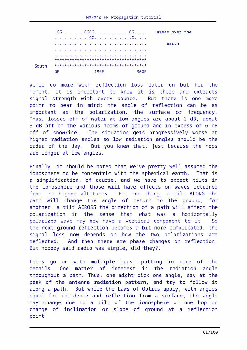
NM7M's HF Propagation tutorial
As for the experimental side, that really deals with what we know about our surroundings. Starting from the ground and going up - the geomagnetic field, the neutral atmosphere, how solar radiation affects the atmosphere and creates the ionosphere, the solar wind and its effects on (or in) the earth's field, the solar magnetic field and solar activity. There's a lot to know and more to the point, it's important to appreciate that we're dealing with a coupled system. So any effect that is dealt with in isolation may not be well understood. The present situation as far as propagation is concerned depends on the use of computers and that brings up the question about the programs that are available. For the geomagnetic field, there is the International Geomagnetic Reference Field (IGRF) while the models of the ionosphere are found in the International Reference Ionosphere (IRI-2001, available on the Internet at Uiversity of Leicester and at NSSDC). Those two serve as research sources but also find their way into software such as PropLab Pro or DXAtlas.
Then there are also the various propagation programs that are available at present. Viewed by themselves, they are efforts done in isolation with quiet-day representations of the ionosphere. So additional consideration must be given to the details of the critical frequencies all along a path and also the geomagnetic circumstances and any unusual ionization, say from solar protons. That's where mapping programs and the NOAA websites on the Internet prove their value. Without using that information, it is hardly possible to make a realistic prediction of anything.
As an example, the week of Nov. 8-14 was characterized as one of considerable magnetic activity and solar activity. Thus, the following A-indices were reported from the Boulder magnetometer: Sun: 68, Mon: 78, Tues: 6, Wed: 4, Thurs: 4, Fri: 60, Sat: 38Without that knowledge, the results for propagation conditions from a computer program, using only input with regard to sunspot counts, would make you think you live on a different planet as they would have little bearing on actual conditions. But that is not the whole story as the coronal mass ejection that was responsible for the magnetic activity also produced a solar proton event on November 14. Then, 10 MeV protons, which are capable of reaching the ionosphere, appeared at satellite altitudes around 0600 UTC. The proton flux peaked at 300 p.f.u. (proton flux units or protons/sq-cm/sec/ster) around 1245 UTC and continued coming out of the interplanetary field for more than a day. Also, there was a weak flux (6 p.f.u.) of 100 MeV protons, capable of reaching balloon altitudes (about 30 km), was present. In addition, there was a strong increase in 1-8 A X-ray background on the 13th. As I said, these are coupled systems and we have to look at more than one limited aspect if propagation is really our interest. Of course, as we go toward solar maximum, this will be the case more and more often. But on the cheery side, the week of Nov. 8-14 has to be an exception. For example, in the year that I spent in my long-path study around the maximum in Cycle 22 , something like 80% of the days were free of any significant disturbance and even with minor or major disturbances on the rest of the days, I was able to make a long-path contact on over 90% of the days. That suggests a cautious but optimistic approach is called for, watching all the disturbance indicators on a regular basis, "going for it" when propagation looks good and even "looking
61/62

NM7M's HF Propagation tutorial
around" when conditions may not be the most promising. I like to say "DXing is an intellectual pursuit" so it's worth a bit of study; that makes the rewards all the more enjoyable.Conclusion - I think I've said all I wanted to so let me close with words of a great man that I'm sure you'll recognize: "That's all folks!"
73,
Bob Brown, NM7M, 1998.
Updated and converted in Word format by Thierry Lombry, ON4SKY.Available in HTML format at http://www.astrosurf.com/lombry/qsl-hf-tutorial-nm7m.htmI warmly thanks Bob for his courtesy in allowing me to use his material
REFERENCESHere are some books that would be helpful in regard to learning about propagation. They are listed in ascending order of scope and difficulty: ARRL Handbook, American Radio Relay League (updated yearly)The ARRL Antenna Book, American Radio Relay League (updated yearly)Introduction to HF Radio propagation, PDF file from IPS, released in HTML format at G3YRC Radio Club or N1QSHF/MF Frequency radio propagation theory notes, KN4LFPhysics of the Upper Polar Atmosphere, by A. Brekke, John Wiley & Sons Inc, 1997The Little Pistol's Guide to HF Propagation, by Robert R. Brown, Worldradio Books, 1996 The New Shortwave Propagation Handbook, by Jacobs, Cohen and Rose, CQ Communications, Inc., 1995Radio Amateurs Guide to the Ionosphere, Leo F. McNamara, Krieger Publ.Corp.,1994Ionospheric Radio (IEE Electromagnetic Waves Series, Vol. 31) by K.Davies, Inspec/Iee, 1990 Radio Wave Propagation (Hf Bands): Radio Amateur's Guide, F.Judd, Butterworth-Heinemann; 1987
* **
62/62