no. 1155 2021
TRANSCRIPT
Raising College Access and Completion: How Much Can Free College Help?
By: Maria Marta Ferreyra Carlos Garriga Juan D. Martin-Ocampo
Angélica María Sánchez Díaz
No. 1155 2021
Raising College Access and Completion:How Much Can Free College Help? 1
Maria Marta FerreyraThe World Bank
Carlos GarrigaFederal Reserve Bank of St. Louis
Juan D. Martin-OcampoBanco de la Republica
Angelica Marıa Sanchez DıazGeorgetown University
The opinions contained in this document are the sole responsibility of theauthors and do not commit Banco de la Repuplica or its Board of Directors.
Abstract
Free college proposals have become increasingly popular in many countries of the world.
To evaluate their potential effects, we develop and estimate a dynamic model of college
enrollment, performance, and graduation. A central piece of the model, student effort,
has a direct effect on class completion, and an indirect effect in mitigating the risk of
not completing a class or not remaining in college. We estimate the model using rich,
student-level administrative data from Colombia, and use the estimates to simulate free
college programs that differ in eligibility requirements. Among these, universal free college
expands enrollment the most, but it does not affect graduation rates and has the highest
per-graduate cost. Performance-based free college, in contrast, delivers a slightly lower
enrollment expansion yet a greater graduation rate at a lower per-graduate cost. Relative
to universal free college, performance-based free college places a greater risk on students
but is precisely this feature that delivers better outcomes. Nonetheless, the modest increase
in graduation rates suggests that additional, complementary policies might be required to
elicit the large effort increase needed to raise graduation rates.
Keywords: Higher Education, free college, financial aid.JEL Classification: E24, I21
1We thank Kartik Athreya, Raquel Bernal, Adriana Camacho, Stephanie Cellini, Doug Harris, Oksana Leukhina,CJ Libassi, Alexander Ludwig, Fabio Sanchez, James Thomas, and Susan Vroman for useful comments andsuggestions. We thank Andrea Franco Hernandez for excellent research assistance. We benefited from seminarsat The World Bank, the St. Louis Fed, the DC Economics of Education Working Group, and UniversitatAutonoma de Barcelona, and by sessions at AEFP 2018, SED 2018, NASMES 2019, and LACEA 2018.
1
Aumentando el acceso y la complecion a la educacionsuperior: ¿Cuanto puede ayudar la educacion gratuita?
Maria Marta FerreyraThe World Bank
Carlos GarrigaFederal Reserve Bank of St. Louis
Juan D. Martin-OcampoBanco de la Republica
Angelica Marıa Sanchez DıazGeorgetown University
Las opiniones contenidas en el presente documento son responsabilidad exclu-siva de los autores y no comprometen al Banco de la Republica ni a su JuntaDirectiva.
Resumen
Las propuestas sobre educacion universitarias gratuita se han vuelto cada vez mas
populares en muchos paıses del mundo. Para evaluar sus efectos potenciales, desarrollamos
y estimamos un modelo dinamico de matrıcula, desempeno y graduacion universitaria.
Una pieza central del modelo, el esfuerzo de los estudiantes, tiene un efecto directo sobre
el desempeno y un efecto indirecto en la mitigacion del riesgo asociado. Estimamos el
modelo utilizando datos a nivel de estudiantes en Colombia, y usamos las estimaciones
para simular programas de universidad gratuita que difieren en requisitos de elegibilidad.
Entre estos, el programa sin requisitos es el que mas expande la inscripcion, pero no afecta
las tasas de graduacion y tiene el costo mas alto. El programa basado en rendimiento,
por el contrario, ofrece una expansion de matrıcula ligeramente menor pero una mayor
tasa de graduacion a un costo mas bajo. En relacion con el programa sin requisitos, aquel
basado en rendimiento supone un mayor riesgo para los estudiantes, pero es precisamente
esta la razon de los mejores resultados. No obstante, el modesto aumento en las tasas de
graduacion sugiere que podrıan ser necesarias polıticas complementarias adicionales para
incentivar el esfuerzo necesario para aumentar las tasas de graduacion.
Palabras clave: Educacion superior, universidad gratuita, ayuda financiera.Clasificacion JEL: E24, I21
2
1 Introduction
In modern economies, higher education is crucial role to the formation of skilled human capital.Not only can higher education raise a country’s productivity; it can also lower income inequality.By subsidizing access to higher education, policymakers can contribute to these two roles. Thequestion, of course, is how large a subsidy they should provide. Advocates of free college arguethat policymakers should provide a full subsidy, resulting in zero tuition for students. Whilefree college has existed for years in a number of countries,2 free college proposals have sproutedrecently in other countries, including the United States, Chile, and Colombia.
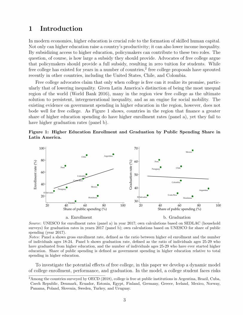
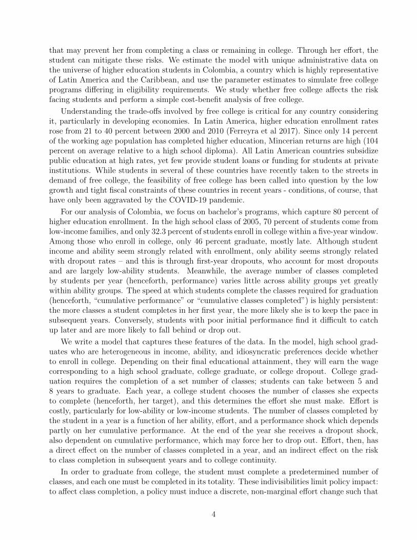
Free college advocates claim that only when college is free can it realize its promise, partic-ularly that of lowering inequality. Given Latin America’s distinction of being the most unequalregion of the world (World Bank 2016), many in the region view free college as the ultimatesolution to persistent, intergenerational inequality, and as an engine for social mobility. Theexisting evidence on government spending in higher education in the region, however, does notbode well for free college. As Figure 1 shows, countries in the region that finance a greatershare of higher education spending do have higher enrollment rates (panel a), yet they fail tohave higher graduation rates (panel b).
Figure 1: Higher Education Enrollment and Graduation by Public Spending Share inLatin America.
ArgentinaChile
Colombia
Costa Rica
El Salvador
Guyana
Honduras
MexicoParaguay
Peru
20
40
60
80
100
En
roll
men
t ra
te (
%)
20 40 60 80 100Share of public spending (%)
Argentina
Chile
Colombia
Costa RicaEl Salvador Honduras
Mexico
Paraguay
Peru
30
40
50
60
70
Gra
du
atio
n r
ate
(%)
20 40 60 80 100Share of public spending (%)
a. Enrollment b. Graduation
Source: UNESCO for enrollment rates (panel a) in year 2017; own calculations based on SEDLAC (householdsurveys) for graduation rates in yearn 2017 (panel b); own calculations based on UNESCO for share of publicspending (year 2017).Notes: Panel a shows gross enrollment rate, defined as the ratio between higher ed enrollment and the numberof individuals ages 18-24. Panel b shows graduation rate, defined as the ratio of individuals ages 25-29 whohave graduated from higher education, and the number of individuals ages 25-29 who have ever started highereducation. Share of public spending is defined as government spending in higher education relative to totalspending in higher education.
To investigate the potential effects of free college, in this paper we develop a dynamic modelof college enrollment, performance, and graduation. In the model, a college student faces risks
2Among the countries surveyed by OECD (2018), college is free at public institutions in Argentina, Brazil, Cuba,Czech Republic, Denmark, Ecuador, Estonia, Egypt, Finland, Germany, Greece, Iceland, Mexico, Norway,Panama, Poland, Slovenia, Sweden, Turkey, and Uruguay.
3
that may prevent her from completing a class or remaining in college. Through her effort, thestudent can mitigate these risks. We estimate the model with unique administrative data onthe universe of higher education students in Colombia, a country which is highly representativeof Latin America and the Caribbean, and use the parameter estimates to simulate free collegeprograms differing in eligibility requirements. We study whether free college affects the riskfacing students and perform a simple cost-benefit analysis of free college.
Understanding the trade-offs involved by free college is critical for any country consideringit, particularly in developing economies. In Latin America, higher education enrollment ratesrose from 21 to 40 percent between 2000 and 2010 (Ferreyra et al 2017). Since only 14 percentof the working age population has completed higher education, Mincerian returns are high (104percent on average relative to a high school diploma). All Latin American countries subsidizepublic education at high rates, yet few provide student loans or funding for students at privateinstitutions. While students in several of these countries have recently taken to the streets indemand of free college, the feasibility of free college has been called into question by the lowgrowth and tight fiscal constraints of these countries in recent years - conditions, of course, thathave only been aggravated by the COVID-19 pandemic.
For our analysis of Colombia, we focus on bachelor’s programs, which capture 80 percent ofhigher education enrollment. In the high school class of 2005, 70 percent of students come fromlow-income families, and only 32.3 percent of students enroll in college within a five-year window.Among those who enroll in college, only 46 percent graduate, mostly late. Although studentincome and ability seem strongly related with enrollment, only ability seems strongly relatedwith dropout rates – and this is through first-year dropouts, who account for most dropoutsand are largely low-ability students. Meanwhile, the average number of classes completedby students per year (henceforth, performance) varies little across ability groups yet greatlywithin ability groups. The speed at which students complete the classes required for graduation(henceforth, “cumulative performance” or “cumulative classes completed”) is highly persistent:the more classes a student completes in her first year, the more likely she is to keep the pace insubsequent years. Conversely, students with poor initial performance find it difficult to catchup later and are more likely to fall behind or drop out.
We write a model that captures these features of the data. In the model, high school grad-uates who are heterogeneous in income, ability, and idiosyncratic preferences decide whetherto enroll in college. Depending on their final educational attainment, they will earn the wagecorresponding to a high school graduate, college graduate, or college dropout. College grad-uation requires the completion of a set number of classes; students can take between 5 and8 years to graduate. Each year, a college student chooses the number of classes she expectsto complete (henceforth, her target), and this determines the effort she must make. Effort iscostly, particularly for low-ability or low-income students. The number of classes completed bythe student in a year is a function of her ability, effort, and a performance shock which dependspartly on her cumulative performance. At the end of the year she receives a dropout shock,also dependent on cumulative performance, which may force her to drop out. Effort, then, hasa direct effect on the number of classes completed in a year, and an indirect effect on the riskto class completion in subsequent years and to college continuity.
In order to graduate from college, the student must complete a predetermined number ofclasses, and each one must be completed in its totality. These indivisibilities limit policy impact:to affect class completion, a policy must induce a discrete, non-marginal effort change such that
4
the student completes at least one additional class. And, to affect graduation rates, the policymust induce a large enough effort increase to complete all the required classes. These discreteeffort changes may be simply too costly for some students.
We estimate the model using Simulated Method of Moments. We fit moments related todropout, graduation, and cumulative performance (including patterns of persistence, catchingup, and falling behind). The model evaluated at the parameter estimates (henceforth, thebaseline) fits the data well. According to our estimates, effort has much greater impact thanability on the production of classes completed. If effort were not modeled as an input to classescompleted, we would overestimate the role of ability by about 75 percent. From a policystandpoint, this would lead to an over-reliance on policies that promote selection of the mostable students (positive selection) rather than policies which explicitly promote effort.
We simulate multiple free college programs differing in eligibility requirements: 1) universal(all students), 2) need-based (low-income students), 3) ability-based (high-ability students),and 4) performance-based (all students eligible in the first year; eligibility conditional on pastcumulative performance in subsequent years). We also simulate a need-based version of (3) and(4). In each counterfactual we distinguish between existing students (who enroll in the baselineand the counterfactual) and new students (who do not enroll in the baseline but enroll in thecounterfactual) to assess the impact of free college on graduation.
By lowering tuition to zero, free college raises consumption during college. This enhancesthe attractiveness of the being a college student (the “college experience”) and has three effectson effort. First is the loss-of-urgency effect, whereby the student wishes to enjoy the enhancedcollege experience and loses the urgency to graduate. Second is the substitution effect, wherebythe enhanced consumption compensates for greater effort. Other things equal, the loss-of-urgency effect leads to lower effort, whereas the substitution effect leads to more effort. Thirdis the risk effect, as the effort changes induced by the other two effects lead to performancechanges which, in turn, affect the performance and dropout risks. Further, the longer thestudent stays in college, the more she exposes herself to risks. Which of these three effectsprevails varies across students and eligibility requirements.
At the aggregate level, all free college programs expand enrollment. The largest expansion isfor universal free college, followed by need-based and performance-based free college. Relativeto the baseline, these programs increase enrollment by 70-85 percent. In our simulations, onaverage new students are of lower income and ability than existing students. The exception isability- and ability-and-need-based free college, which induce positive selection of new studentsand attract new students who are more able, on average, than existing ones.
In contrast with these large enrollment rate effects, overall graduation rate effects are modest– between -2 and 7 percent relative to the baseline. For new students, the graduation rateeffect depends on the policy-induced type of selection. For existing students, only performance-based programs accomplish an effect substantially different from zero, raising graduation ratesbetween 9 and 14 percent relative to the baseline. This is because, by making free collegecontingent on performance, these programs incentivize effort and eliminate the loss-of-urgencyeffect, making students frontload effort in the early years. These results are consistent withthe literature on college financial aid in the U.S., which has generally found positive and largeeffects on enrollment, small or null effects on graduation, and larger graduation effects for
5
performance-based than unconditional financial aid.3
At the same time, these aggregate effects mask great heterogeneity across students. Con-sider, for instance, universal free college. Enrollment effects are largest for low- and middle-income students, and for mid-ability students. Hence, universal free college subsidizes manystudents who, by virtue of their ability or income, do not need the subsidy as they already enrollin the baseline. Graduation rate effects are similarly heterogeneous across students. They fallfor high-ability or high-income students, who experience a strong loss of urgency, while they risefor low-ability or low-income students, who experience a strong substitution effect. In contrastto universal free college, performance-based free college induces greater effort on the part of allstudents and leads them all to higher graduation rates.
Our counterfactual findings provide an explanation for the enrollment and graduation ratepatterns presented in Figure 1. Greater college funding substantially raises enrollment rateswhen a large fraction of high school graduates faces severe financial constraints, as they do inLatin America. It does not, however, raise graduation rates unless it is performance-based toincentivize effort, which is not the case in Latin America.
Interestingly, the higher effort and graduation rates induced by performance-based freecollege come at the cost of placing greater risk on students. We develop a measure of studentanticipated risk in each year (equal to the coefficient of variation of the value of college), andcompare it for the baseline and counterfactuals. We find that, in every scenario, anticipated riskfalls when students exert greater effort or accumulate more completed classes. Anticipated riskis high in the initial two years and decreases rapidly afterwards, once students survive the initialattrition and settle on a performance path. In the initial years, universal free college lowersstudents’ risk relative to the baseline by enhancing the college experience, whereas performance-based free college raises it by making the college experience contingent on performance. Facingthe students with this greater risk, however, induces them to exert greater effort, which istheir ultimate insurance mechanism. In other words, better college outcomes do not come fromproviding full but rather partial insurance to students.
At the same time, even the graduation rate increase from performance-based free college isrelatively small. This is, in part, due to a composition effect, as the new college students inseveral programs are less likely to graduate than the existing ones. But, even among existingstudents, graduation rates rise relatively little. In other words, free college alone cannot sub-stantially raise graduation rates. The indivisibilities discussed above help explain why: whilefree college might raise effort for some or even all students, it still fails to induce in manystudents the large effort increase needed to complete all graduation requirements.4
For a policymaker committed to providing free college, the question is how to choose amongthe programs presented here. We conduct a simple cost-benefit analysis to illuminate thisquestion, and compare the per-graduate cost across programs. We find that all programs raisethe per-graduate cost – if anything, because fewer students pay for college than in the baseline.For a policymaker who wishes to raise the fraction of high school graduates that finish collegewhile limiting costs, the best option is performance-based or even need-based free college – butnot universal free college. Nonetheless, the per-graduate cost of every scenario studied here is
3For recent reviews of this vast literature, see Avery et al (2019) and Dynarski and Scott-Clayton (2013).4This result is reminiscent of Oreopoulos and Petronijevic (2019), who find that even when students realize thatmore effort is needed to improve outcomes, they adjust by lowering expectations rather than increasing effort.
6
far from low – ranging from one (baseline) to 2.5 (universal free college) times the per capitaGDP – and should be considered with great care given current fiscal constraints.
By construction, our counterfactuals assume the most favorable scenario for free college. Weassume that colleges have no capacity constraints; the average and marginal cost of educatingnew and existing students are the same; and free college does not crowd out parental transfersto their children in college. Further, we do not model taxation (which might be required topay for free college programs), and assume that the wage of college graduates relative to highschool graduates (henceforth, the college premium) does not fall with more college graduates.5
Relaxing any of these assumptions would lead to less favorable free college outcomes.
The rest of the paper is organized as follows. Section 2 describes the related literature, andSection 3 describes our data. Section 4 presents our model, and Section 5 discusses its empiricalimplementation. Section 6 describes the estimation strategy and results. Section 7 presents thefree college counterfactuals, including analyses of anticipated risk, fiscal costs, and potentialgeneral equilibrium effects on the labor market. Section 8 concludes.
2 Related Literature
Our paper relates to a large literature estimating sequential schooling models under uncertainty,with seminal contributions by Keane and Wolpin (2001), Eckstein and Wolpin (1998), andKeane (2002). This literature models college enrollment, performance, and college outcomes,and uncovers structural parameters based on students’ observed choices during college. Inone strand of this literature, researchers model students as acquiring information (learning)throughout college – regarding, for instance, their ability and preferences for college or specificmajors, and their expected labor market performance. This literature includes, among others,Arcidiacono (2004), Arcidiacono et al (2016), Ozdagli and Trachter (2011), Stinebrickner andStinebrickner (2014), and Trachter (2015). As in these papers, students in our model learn abouttheir graduation probability based on their classes completed, and choose effort accordingly.
The idea that higher education is risky is not new (Levhari and Weiss 1974, Altonji 1993,Akyol and Athreya 2005), but the recent availability of college transcript data in the U.S. hashelped estimate the role of risk in students’ performance. These data reveal substantial andpersistent heterogeneity in students’ credit accumulation rates, which are strongly related tograduation probability. According to Hendricks and Leukhina (2017, 2018), based on theircredit accumulation rates more than 50 percent of college entrants should be able to forecastwhether they are at least 80 percent likely to graduate. According to Stange (2012), the largeuncertainty faced by students makes them place a high value on the ability to drop out at anypoint in college rather than pre-commit to completing all graduation requirements. Our paperis similar to these in the use of administrative data to track students’ performance, but differentin that the risk associated to class completion or college continuity is not fully exogenous as inthese two papers, but depends on an endogenous variable – student effort.
While the literature has placed much attention on the role of ability in performance andcollege outcomes, a growing line of research highlights the role of effort. Zamarro, Hitt, and
5In Section 7 we investigate potential general equilibrium effects associated with the greater supply of collegegraduates. Since we find them to be very small even in the medium run, we conclude that we can abstractaway from them in our analysis.
7
Mendez (2019) use data from the Program for International Student Assessment (PISA) toshow that different effort measures explain about a third of observed cross-country test scorevariation. Stinebrickner and Stinebrickner (2004) rely on time use surveys to estimate theeffects of study time on grades. Ariely et al (2009) show that the use of incentives can helpthe average student improve her test performance, though the effect is more limited on high-ability students. Beneito et al (2018) provide evidence that the tuition increase implementedby Spanish colleges in 2012 boosted student effort. Ahn et al (2019) model effort in response tograding policies. We contribute to this line of research by explicitly modeling the role of effortand embedding it in a dynamic setting, where it affects class accumulation and risk mitigation.
In an efficient and equitable world, college enrollment would depend on student ability ratherthan parental resources (Cameron and Heckman 1998 and 1999, Carneiro and Heckman 2002).In Colombia, as in other countries, parental resources matter greatly to college enrollment evencontrolling for ability. This provides strong evidence for credit constraints limiting college ac-cess, as discussed in a large literature. Lochner and Monge-Naranjo (2011) develop a model thathelps explain the rising importance of family income for college attendance in the U.S. even inthe presence of credit. Solis (2017) finds that relaxing credit constraints in Chile had an imme-diate impact on enrollment and number of college years completed, particularly for low-incomestudents. Parental resources and background, however, may be of limited importance. Hai andHeckman (2017) show that equalizing initial ability has larger effects on college outcomes andinequality than equalizing parental background. The importance of credit access weakens whenstudents can supply work as a source of funding college, as suggested by Garriga and Keightley(2007). Although Colombia is a large developing economy, the market for student loans is verylimited, covering only 7 percent of students in 2003 (ICETEX 2010). Lack of family resources,limited opportunities to work during college, and missing credit markets for student loans areclear impediments to college access in countries such as Colombia.
In this context, tuition subsidies appear as a simple tool to broaden college access. Our freecollege counterfactuals complement the literature on the recent free college policies in Chile(Bucarey 2018) and the elimination of free college in England (Murphy et al 2019). It also joinsin the vast literature of college financial aid,6 including the recent literature on free communitycollege and the so-called “Promise” programs implemented in multiple U.S. states.7
3 Data and descriptive statistics
In this section we describe the salient features of our data. These shape our model, and giverise to the moments we match in estimation.
3.1 The 2005 cohort
Our data consists of student- and program-level information drawn from three different admin-istrative datasets: Saber 11, SPADIES, and SNIES. The first one, Saber 11, contains students’
6For recent reviews of this vast literature, see Avery et al (2019) and Dynarski and Scott-Clayton (2013). Section7.5 contains further references.
7These programs provide zero tuition to eligible students for state or local community colleges or four-yearinstitutions. See, for instance, Carruthers et al (2018), Dynarski et al (2018), and Gurantz (2020).
8
test scores at the national mandatory high school exit exam (also named Saber 11), along withsocio-economic information reported by the students when taking the test. Saber 11 is a stan-dardized test that covers multiple academic fields and measures students’ academic readinessfor higher education. We average field scores and standardize the average by semester-year. Weuse the resulting standardized score as a measure of student ability, broadly understood as herpreparedness for higher education – reflecting not only her innate ability but also her primaryand secondary education quality. Family income is reported in brackets defined relative to themonthly legal minimum wage (MW), which is equal to 381,000 Colombian pesos (COP) in 2005(US$ 1 = 2,321 COP in 2005.)
The second dataset, SPADIES, tracks college students. For each semester, it records thenumber of classes for which a student registers and the number of classes she passes, as wellas her graduation or dropout date. It does not record the specific classes in which a studentenrolls, how many times a class is taken until passing, or class grades. The third dataset,SNIES, contains program-level information including institution, field, and tuition.
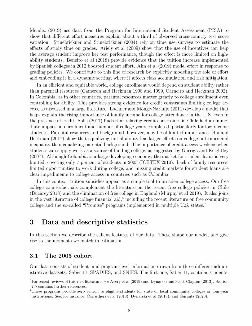
We focus on the 2005 cohort, which is the group of approximately 415,000 students ages15-22 who took Saber 11 in 2005. Since students typically graduate from high school the sameyear they take Saber 11, we can view this cohort as the high school graduates from 2005. Wecalculate deciles and quintiles of their ability distribution; in what follows, ability deciles andquintiles always refer to this distribution. For consistency with the model, in the statistics belowwe classify students into “student types” defined by combinations of student ability quintilesand family income brackets. Table 1 below shows the distribution of student types in the 2005cohort. It shows that, while a remarkable 70 percent of high school graduates come from thelowest two income brackets, less than 5 percent come from the top one. It also shows thathigh-income students are more likely to belong to high-ability levels than their lower-incomecounterparts due to the strong, positive correlation between income and ability.
Table 1: Family income and Ability Distribution of High School Graduates.
Income Ability quintileBracket 1 2 3 4 5 Total
5+ MW 0.21 0.31 0.48 0.90 3.15 5.053-5 MW 0.88 1.08 1.37 1.94 3.43 8.692-3 MW 2.72 2.94 3.30 3.69 3.95 16.601-2 MW 8.47 8.99 9.16 8.69 6.64 41.95<1 MW 7.95 6.89 5.80 4.58 2.49 27.71
Total 20.23 20.21 20.11 19.80 19.65 100.00
Source: Calculations based on Saber 11. The distribution refers to 415,269 high school graduates from 2005.Notes: Family income is reported in brackets; MW = monthly minimum wage. Ability is reported in quintilesof standardized Saber 11 scores. Quintile 1 is the lowest.
3.2 Enrollment rates
Although Colombia’s higher education offers short-cycle and bachelor’s programs (akin to two-and four-year programs in the U.S. respectively), we focus on bachelor’s programs, which cap-ture approximately 80 percent of the country’s total higher education enrollment. In what
9
follows, “college” refers to bachelor’s programs, and “college outcomes” to the final outcomes-graduation and dropout, along with their timing (e.g., on-time graduation). We classify astudent from the 2005 cohort as having enrolled in college if she did so between 2006 and 2010.8
In Colombia, as in our sample, enrollment in bachelor’s programs is almost evenly splitbetween public and private institutions. Since public institutions are heavily subsidized, theycharge much less than private institutions. For an individual with an annual family income oftwelve MWs, annual average tuition for a bachelor’s program at a public and private highereducation institution is equal to 24 and 135 percent of the familiy income, respectively.
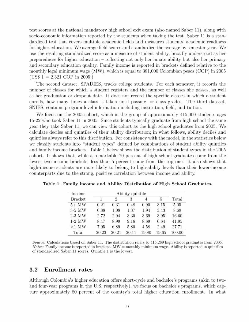
Table 2 shows enrollment rates by student type for the 2005 cohort. Although the overallenrollment rate is 32 percent, enrollment rates vary widely among student types, from 9 to 84percent.9 Enrollment rates rise both with income and ability. On average, the enrollment gapbetween the highest and lowest income brackets is equal to 55 percentage points (pp) - similarto the 50-pp point gap between the highest and lowest ability. These gaps suggest that freecollege may have ample room to raise enrollment.
Table 2: Enrollment Rates by Income and Ability.
Income Ability quintileBracket 1 2 3 4 5 Total
5+ MW 32.85 44.14 58.87 69.23 83.85 73.383-5 MW 28.71 39.75 48.41 62.99 79.24 62.032-3 MW 20.34 28.72 36.96 48.03 67.88 43.501-2 MW 13.94 18.36 23.85 33.84 54.22 28.05<1 MW 9.05 12.67 17.20 26.56 43.93 17.67
Total 13.43 19.15 26.20 38.93 63.74 32.29
Source: Calculations based on SPADIES and Saber 11, for 2005 high school graduates.Notes: Each cell reports percent of high school graduates from a given income bracket and ability quintilewho enrolled in a bachelor’s program between 2006 and 2010. Income reported in brackets; MW = monthlyminimum wage. Ability reported in quintiles of standardized Saber 11 scores; quintile 1 is the lowest.
3.3 Graduation and dropout rates
For the analysis of college outcomes and performance that follows, we focus on students fromthe 2006 college entry cohort that enroll in five-year bachelor’s programs.10 Our sample includes27,344 students, of whom only 45.7 percent graduates - 15.1 percent graduates on time (in fiveyears) and 30.6 percent graduates late (in 6-8 years).11 The dropout risk is thus substantial.
8Among the 2005 high school graduates that enroll in college within that five year window, only 35 percent doso immediately following high school. A five-year window, then, provides a more accurate enrollment rate.
9For comparison, in the US the enrollment rate of individuals ages 16-24 who graduated high school in 2005 is44.6 percent (Source: Digest of Education Statistics). If this enrollment rate allowed for a five-year window asin Colombia, it would clearly be higher.
10To analyze dropouts and cumulative performance, it is customary to focus on a group of students from thesame entry cohort who study programs of the same length. Five-year programs in Colombia capture aboutthree-quarters of the enrollment in bachelor’s programs. Dropout rates correspond to the student’s first highereducation program.
11For comparison, in the US 59.2 percent students from the 2006 cohort graduate within six years - 39 percenton time (in four years), and 20.2 percent late (in five or six years). Source: Digest of Education Statistics.
10
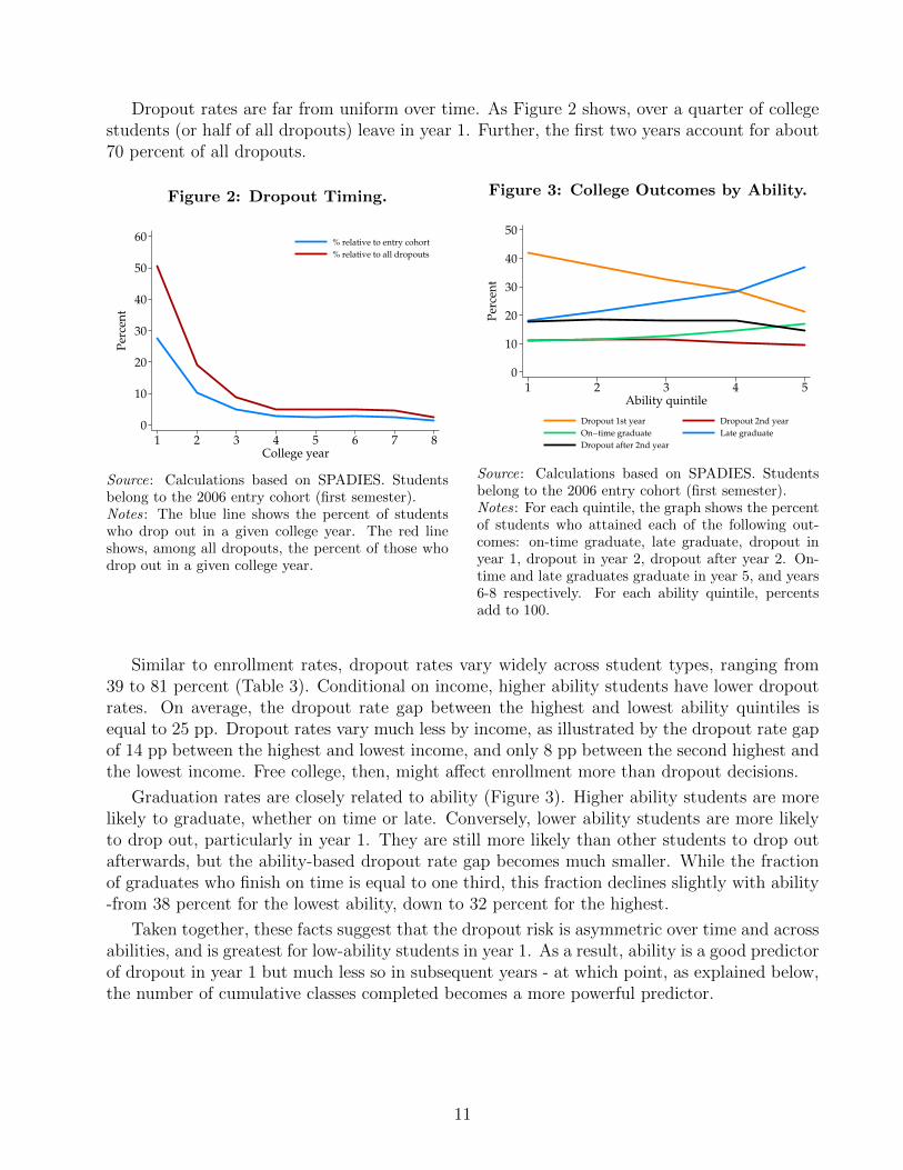
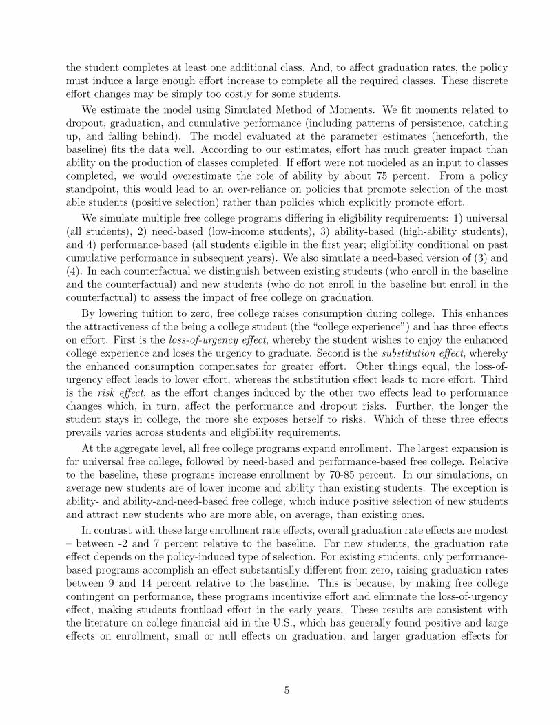
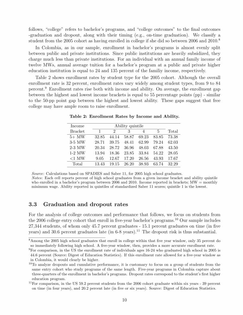
Dropout rates are far from uniform over time. As Figure 2 shows, over a quarter of collegestudents (or half of all dropouts) leave in year 1. Further, the first two years account for about70 percent of all dropouts.
Figure 2: Dropout Timing.
0
10
20
30
40
50
60
Per
cen
t
1 2 3 4 5 6 7 8College year
% relative to entry cohort
% relative to all dropouts
Source: Calculations based on SPADIES. Studentsbelong to the 2006 entry cohort (first semester).Notes: The blue line shows the percent of studentswho drop out in a given college year. The red lineshows, among all dropouts, the percent of those whodrop out in a given college year.
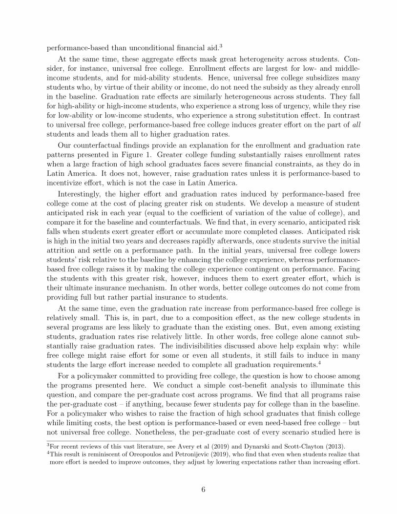
Figure 3: College Outcomes by Ability.
0
10
20
30
40
50
Per
cen
t
1 2 3 4 5Ability quintile
Dropout 1st year Dropout 2nd year
On−time graduate Late graduate
Dropout after 2nd year
Source: Calculations based on SPADIES. Studentsbelong to the 2006 entry cohort (first semester).Notes: For each quintile, the graph shows the percentof students who attained each of the following out-comes: on-time graduate, late graduate, dropout inyear 1, dropout in year 2, dropout after year 2. On-time and late graduates graduate in year 5, and years6-8 respectively. For each ability quintile, percentsadd to 100.
Similar to enrollment rates, dropout rates vary widely across student types, ranging from39 to 81 percent (Table 3). Conditional on income, higher ability students have lower dropoutrates. On average, the dropout rate gap between the highest and lowest ability quintiles isequal to 25 pp. Dropout rates vary much less by income, as illustrated by the dropout rate gapof 14 pp between the highest and lowest income, and only 8 pp between the second highest andthe lowest income. Free college, then, might affect enrollment more than dropout decisions.
Graduation rates are closely related to ability (Figure 3). Higher ability students are morelikely to graduate, whether on time or late. Conversely, lower ability students are more likelyto drop out, particularly in year 1. They are still more likely than other students to drop outafterwards, but the ability-based dropout rate gap becomes much smaller. While the fractionof graduates who finish on time is equal to one third, this fraction declines slightly with ability-from 38 percent for the lowest ability, down to 32 percent for the highest.
Taken together, these facts suggest that the dropout risk is asymmetric over time and acrossabilities, and is greatest for low-ability students in year 1. As a result, ability is a good predictorof dropout in year 1 but much less so in subsequent years - at which point, as explained below,the number of cumulative classes completed becomes a more powerful predictor.
11
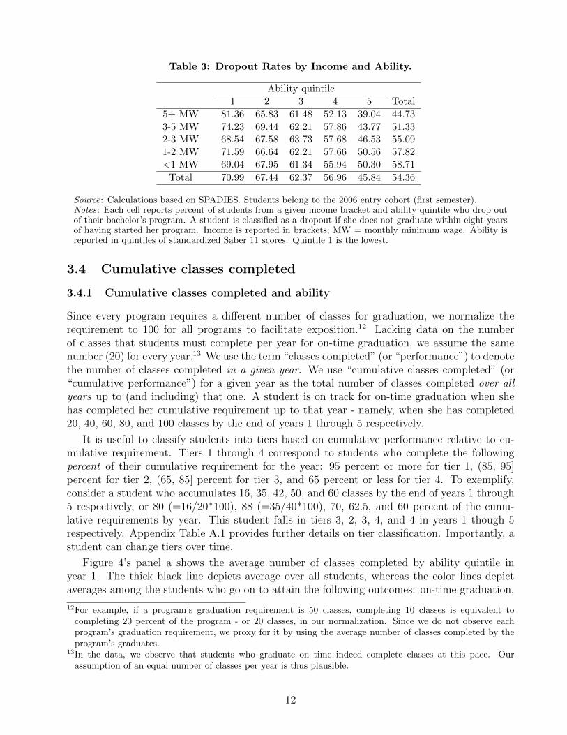
Table 3: Dropout Rates by Income and Ability.
Ability quintile1 2 3 4 5 Total
5+ MW 81.36 65.83 61.48 52.13 39.04 44.733-5 MW 74.23 69.44 62.21 57.86 43.77 51.332-3 MW 68.54 67.58 63.73 57.68 46.53 55.091-2 MW 71.59 66.64 62.21 57.66 50.56 57.82<1 MW 69.04 67.95 61.34 55.94 50.30 58.71
Total 70.99 67.44 62.37 56.96 45.84 54.36
Source: Calculations based on SPADIES. Students belong to the 2006 entry cohort (first semester).Notes: Each cell reports percent of students from a given income bracket and ability quintile who drop outof their bachelor’s program. A student is classified as a dropout if she does not graduate within eight yearsof having started her program. Income is reported in brackets; MW = monthly minimum wage. Ability isreported in quintiles of standardized Saber 11 scores. Quintile 1 is the lowest.
3.4 Cumulative classes completed
3.4.1 Cumulative classes completed and ability
Since every program requires a different number of classes for graduation, we normalize therequirement to 100 for all programs to facilitate exposition.12 Lacking data on the numberof classes that students must complete per year for on-time graduation, we assume the samenumber (20) for every year.13 We use the term “classes completed” (or “performance”) to denotethe number of classes completed in a given year. We use “cumulative classes completed” (or“cumulative performance”) for a given year as the total number of classes completed over allyears up to (and including) that one. A student is on track for on-time graduation when shehas completed her cumulative requirement up to that year - namely, when she has completed20, 40, 60, 80, and 100 classes by the end of years 1 through 5 respectively.
It is useful to classify students into tiers based on cumulative performance relative to cu-mulative requirement. Tiers 1 through 4 correspond to students who complete the followingpercent of their cumulative requirement for the year: 95 percent or more for tier 1, (85, 95]percent for tier 2, (65, 85] percent for tier 3, and 65 percent or less for tier 4. To exemplify,consider a student who accumulates 16, 35, 42, 50, and 60 classes by the end of years 1 through5 respectively, or 80 (=16/20*100), 88 (=35/40*100), 70, 62.5, and 60 percent of the cumu-lative requirements by year. This student falls in tiers 3, 2, 3, 4, and 4 in years 1 though 5respectively. Appendix Table A.1 provides further details on tier classification. Importantly, astudent can change tiers over time.
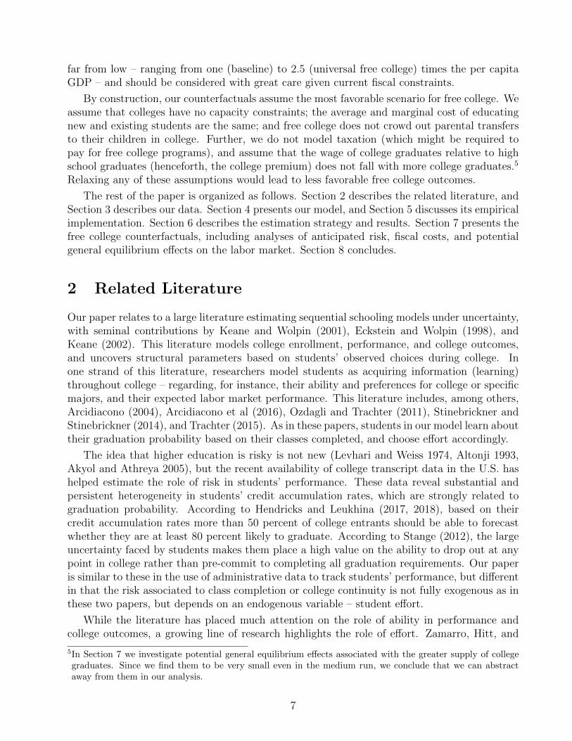
Figure 4’s panel a shows the average number of classes completed by ability quintile inyear 1. The thick black line depicts average over all students, whereas the color lines depictaverages among the students who go on to attain the following outcomes: on-time graduation,
12For example, if a program’s graduation requirement is 50 classes, completing 10 classes is equivalent tocompleting 20 percent of the program - or 20 classes, in our normalization. Since we do not observe eachprogram’s graduation requirement, we proxy for it by using the average number of classes completed by theprogram’s graduates.
13In the data, we observe that students who graduate on time indeed complete classes at this pace. Ourassumption of an equal number of classes per year is thus plausible.
12
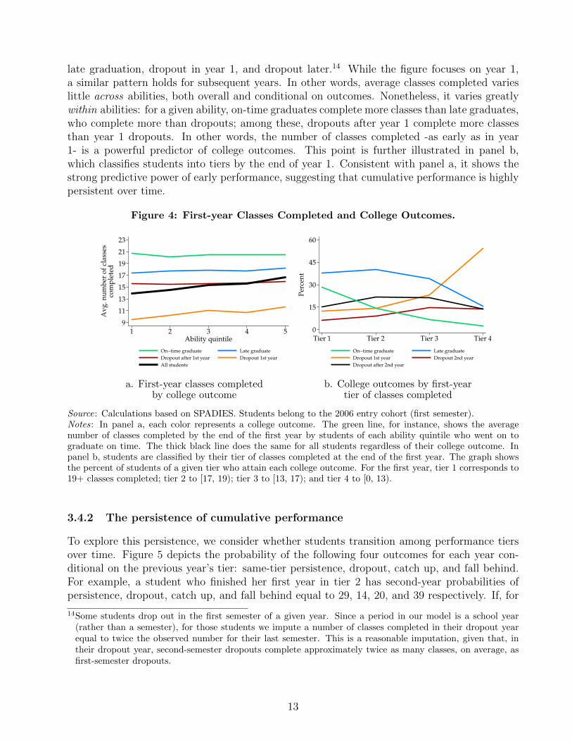
late graduation, dropout in year 1, and dropout later.14 While the figure focuses on year 1,a similar pattern holds for subsequent years. In other words, average classes completed varieslittle across abilities, both overall and conditional on outcomes. Nonetheless, it varies greatlywithin abilities: for a given ability, on-time graduates complete more classes than late graduates,who complete more than dropouts; among these, dropouts after year 1 complete more classesthan year 1 dropouts. In other words, the number of classes completed -as early as in year1- is a powerful predictor of college outcomes. This point is further illustrated in panel b,which classifies students into tiers by the end of year 1. Consistent with panel a, it shows thestrong predictive power of early performance, suggesting that cumulative performance is highlypersistent over time.
Figure 4: First-year Classes Completed and College Outcomes.
9
11
13
15
17
19
21
23
Av
g. n
um
ber
of
clas
ses
com
ple
ted
1 2 3 4 5Ability quintile
On−time graduate Late graduate
Dropout after 1st year Dropout 1st year
All students
0
15
30
45
60
Per
cen
t
Tier 1 Tier 2 Tier 3 Tier 4
On−time graduate Late graduate
Dropout 1st year Dropout 2nd year
Dropout after 2nd year
a. First-year classes completed b. College outcomes by first-yearby college outcome tier of classes completed
Source: Calculations based on SPADIES. Students belong to the 2006 entry cohort (first semester).Notes: In panel a, each color represents a college outcome. The green line, for instance, shows the averagenumber of classes completed by the end of the first year by students of each ability quintile who went on tograduate on time. The thick black line does the same for all students regardless of their college outcome. Inpanel b, students are classified by their tier of classes completed at the end of the first year. The graph showsthe percent of students of a given tier who attain each college outcome. For the first year, tier 1 corresponds to19+ classes completed; tier 2 to [17, 19); tier 3 to [13, 17); and tier 4 to [0, 13).
3.4.2 The persistence of cumulative performance
To explore this persistence, we consider whether students transition among performance tiersover time. Figure 5 depicts the probability of the following four outcomes for each year con-ditional on the previous year’s tier: same-tier persistence, dropout, catch up, and fall behind.For example, a student who finished her first year in tier 2 has second-year probabilities ofpersistence, dropout, catch up, and fall behind equal to 29, 14, 20, and 39 respectively. If, for
14Some students drop out in the first semester of a given year. Since a period in our model is a school year(rather than a semester), for those students we impute a number of classes completed in their dropout yearequal to twice the observed number for their last semester. This is a reasonable imputation, given that, intheir dropout year, second-semester dropouts complete approximately twice as many classes, on average, asfirst-semester dropouts.
13
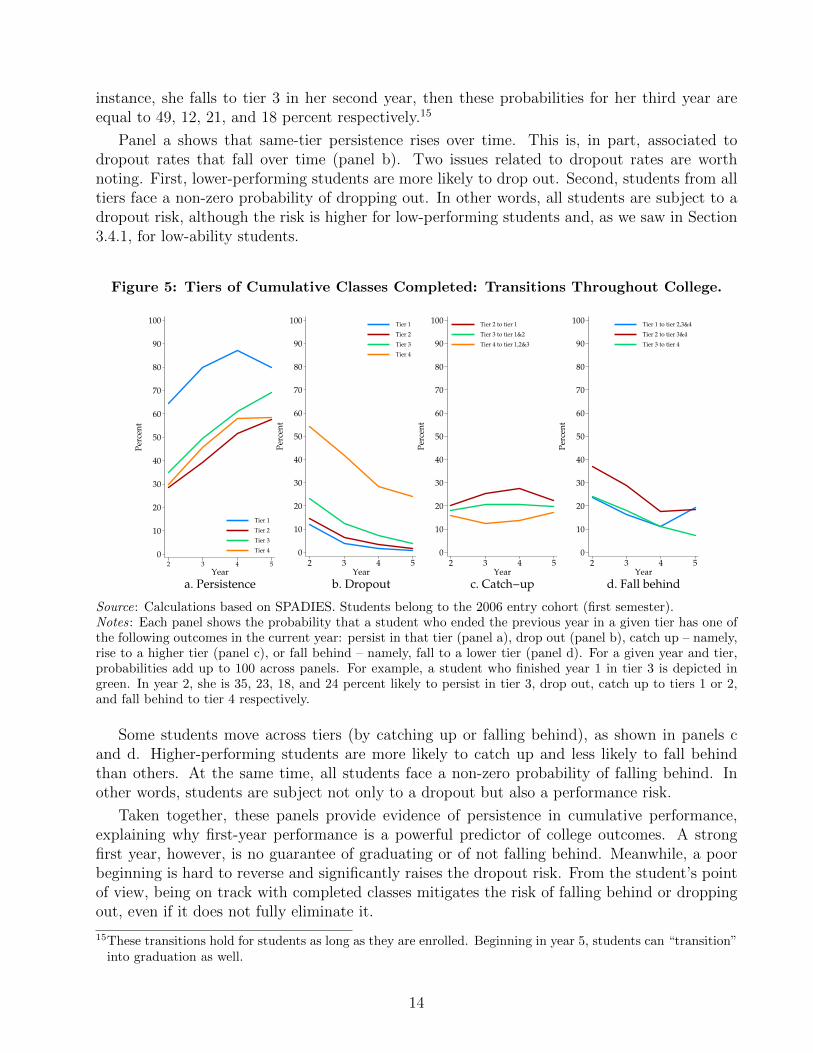
instance, she falls to tier 3 in her second year, then these probabilities for her third year areequal to 49, 12, 21, and 18 percent respectively.15
Panel a shows that same-tier persistence rises over time. This is, in part, associated todropout rates that fall over time (panel b). Two issues related to dropout rates are worthnoting. First, lower-performing students are more likely to drop out. Second, students from alltiers face a non-zero probability of dropping out. In other words, all students are subject to adropout risk, although the risk is higher for low-performing students and, as we saw in Section3.4.1, for low-ability students.
Figure 5: Tiers of Cumulative Classes Completed: Transitions Throughout College.
0
10
20
30
40
50
60
70
80
90
100
Per
cen
t
2 3 4 5
Year
Tier 1
Tier 2
Tier 3
Tier 4
a. Persistence
0
10
20
30
40
50
60
70
80
90
100
Per
cen
t
2 3 4 5Year
Tier 1
Tier 2
Tier 3
Tier 4
b. Dropout
0
10
20
30
40
50
60
70
80
90
100
Per
cen
t
2 3 4 5Year
Tier 2 to tier 1
Tier 3 to tier 1&2
Tier 4 to tier 1,2&3
c. Catch−up
0
10
20
30
40
50
60
70
80
90
100
Per
cen
t2 3 4 5
Year
Tier 1 to tier 2,3&4
Tier 2 to tier 3&4
Tier 3 to tier 4
d. Fall behind
Source: Calculations based on SPADIES. Students belong to the 2006 entry cohort (first semester).Notes: Each panel shows the probability that a student who ended the previous year in a given tier has one ofthe following outcomes in the current year: persist in that tier (panel a), drop out (panel b), catch up – namely,rise to a higher tier (panel c), or fall behind – namely, fall to a lower tier (panel d). For a given year and tier,probabilities add up to 100 across panels. For example, a student who finished year 1 in tier 3 is depicted ingreen. In year 2, she is 35, 23, 18, and 24 percent likely to persist in tier 3, drop out, catch up to tiers 1 or 2,and fall behind to tier 4 respectively.
Some students move across tiers (by catching up or falling behind), as shown in panels cand d. Higher-performing students are more likely to catch up and less likely to fall behindthan others. At the same time, all students face a non-zero probability of falling behind. Inother words, students are subject not only to a dropout but also a performance risk.
Taken together, these panels provide evidence of persistence in cumulative performance,explaining why first-year performance is a powerful predictor of college outcomes. A strongfirst year, however, is no guarantee of graduating or of not falling behind. Meanwhile, a poorbeginning is hard to reverse and significantly raises the dropout risk. From the student’s pointof view, being on track with completed classes mitigates the risk of falling behind or droppingout, even if it does not fully eliminate it.
15These transitions hold for students as long as they are enrolled. Beginning in year 5, students can “transition”into graduation as well.
14
3.4.3 More on the role of ability, performance, and college outcomes
In Section 3.4.1, we established that, while there is little variation in academic progressionacross abilities, there is much more variation within abilities. We now explore this further byrelying on our tiers.
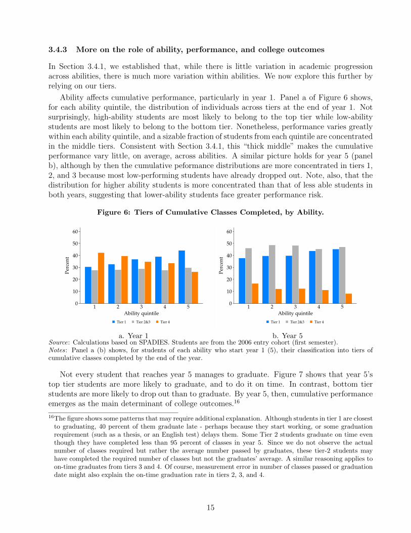
Ability affects cumulative performance, particularly in year 1. Panel a of Figure 6 shows,for each ability quintile, the distribution of individuals across tiers at the end of year 1. Notsurprisingly, high-ability students are most likely to belong to the top tier while low-abilitystudents are most likely to belong to the bottom tier. Nonetheless, performance varies greatlywithin each ability quintile, and a sizable fraction of students from each quintile are concentratedin the middle tiers. Consistent with Section 3.4.1, this “thick middle” makes the cumulativeperformance vary little, on average, across abilities. A similar picture holds for year 5 (panelb), although by then the cumulative peformance distributions are more concentrated in tiers 1,2, and 3 because most low-performing students have already dropped out. Note, also, that thedistribution for higher ability students is more concentrated than that of less able students inboth years, suggesting that lower-ability students face greater performance risk.
Figure 6: Tiers of Cumulative Classes Completed, by Ability.
0
10
20
30
40
50
60
Per
cen
t
1 2 3 4 5
Ability quintile
Tier 1 Tier 2&3 Tier 4
0
10
20
30
40
50
60
Per
cen
t
1 2 3 4 5
Ability quintile
Tier 1 Tier 2&3 Tier 4
a. Year 1 b. Year 5Source: Calculations based on SPADIES. Students are from the 2006 entry cohort (first semester).Notes: Panel a (b) shows, for students of each ability who start year 1 (5), their classification into tiers ofcumulative classes completed by the end of the year.
Not every student that reaches year 5 manages to graduate. Figure 7 shows that year 5’stop tier students are more likely to graduate, and to do it on time. In contrast, bottom tierstudents are more likely to drop out than to graduate. By year 5, then, cumulative performanceemerges as the main determinant of college outcomes.16
16The figure shows some patterns that may require additional explanation. Although students in tier 1 are closestto graduating, 40 percent of them graduate late - perhaps because they start working, or some graduationrequirement (such as a thesis, or an English test) delays them. Some Tier 2 students graduate on time eventhough they have completed less than 95 percent of classes in year 5. Since we do not observe the actualnumber of classes required but rather the average number passed by graduates, these tier-2 students mayhave completed the required number of classes but not the graduates’ average. A similar reasoning applies toon-time graduates from tiers 3 and 4. Of course, measurement error in number of classes passed or graduationdate might also explain the on-time graduation rate in tiers 2, 3, and 4.
15
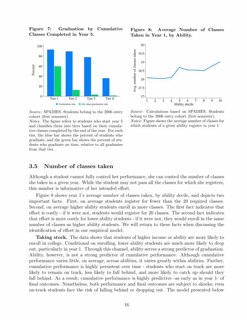
Figure 7: Graduation by CumulativeClasses Completed in Year 5.
0
20
40
60
80
100
Per
cen
t
Tier 1 Tier 2 Tier 3 Tier 4
Graduation rate On−time graduation rate
Source: SPADIES. Students belong to the 2006 entrycohort (first semester).Notes: The figure refers to students who start year 5and classifies them into tiers based on their cumula-tive classes completed by the end of the year. For eachtier, the blue bar shows the percent of students whograduate, and the green bar shows the percent of stu-dents who graduate on time, relative to all graduatesfrom that tier.
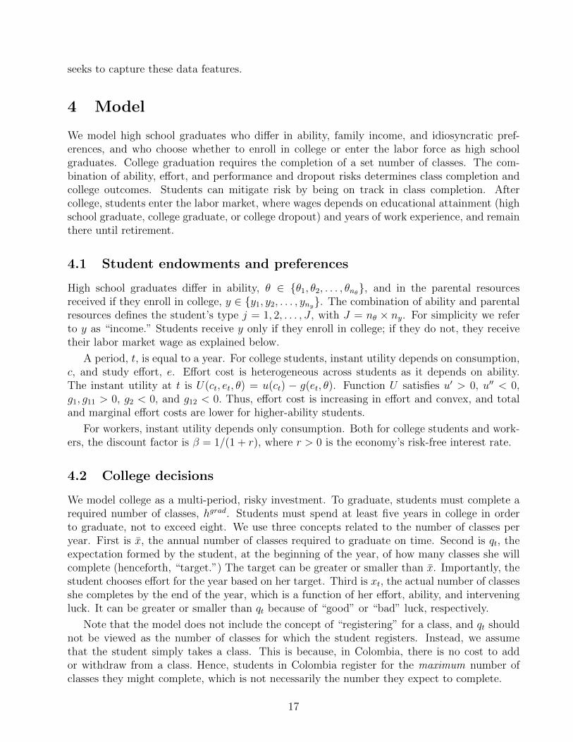
Figure 8: Average Number of ClassesTaken in Year 1, by Ability.
17
17.5
18
18.5
19
19.5
20
Av
g. n
um
ber
of
clas
ses
tak
en
1 2 3 4 5 6 7 8 9 10Ability decile
Source: Calculations based on SPADIES. Studentsbelong to the 2006 entry cohort (first semester).Notes: Figure shows the average number of classes forwhich students of a given ability register in year 1.
3.5 Number of classes taken
Although a student cannot fully control her performance, she can control the number of classesshe takes in a given year. While the student may not pass all the classes for which she registers,this number is informative of her intended effort.
Figure 8 shows year 1’s average number of classes taken, by ability decile, and depicts twoimportant facts. First, on average students register for fewer than the 20 required classes.Second, on average higher ability students enroll in more classes. The first fact indicates thateffort is costly - if it were not, students would register for 20 classes. The second fact indicatesthat effort is more costly for lower ability students - if it were not, they would enroll in the samenumber of classes as higher ability students. We will return to these facts when discussing theidentification of effort in our empirical model.
Taking stock. The data shows that students of higher income or ability are more likely toenroll in college. Conditional on enrolling, lower ability students are much more likely to dropout, particularly in year 1. Through this channel, ability serves a strong predictor of graduation.Ability, however, is not a strong predictor of cumulative performance. Although cumulativeperformance varies little, on average, across abilities, it varies greatly within abilities. Further,cumulative performance is highly persistent over time - students who start on track are morelikely to remain on track, less likely to fall behind, and more likely to catch up should theyfall behind. As a result, cumulative performance is highly predictive -as early as in year 1- offinal outcomes. Nonetheless, both performance and final outcomes are subject to shocks; evenon-track students face the risk of falling behind or dropping out. The model presented below
16
seeks to capture these data features.
4 Model
We model high school graduates who differ in ability, family income, and idiosyncratic pref-erences, and who choose whether to enroll in college or enter the labor force as high schoolgraduates. College graduation requires the completion of a set number of classes. The com-bination of ability, effort, and performance and dropout risks determines class completion andcollege outcomes. Students can mitigate risk by being on track in class completion. Aftercollege, students enter the labor market, where wages depends on educational attainment (highschool graduate, college graduate, or college dropout) and years of work experience, and remainthere until retirement.
4.1 Student endowments and preferences
High school graduates differ in ability, θ ∈ {θ1, θ2, . . . , θnθ}, and in the parental resourcesreceived if they enroll in college, y ∈ {y1, y2, . . . , yny}. The combination of ability and parentalresources defines the student’s type j = 1, 2, . . . , J , with J = nθ × ny. For simplicity we referto y as “income.” Students receive y only if they enroll in college; if they do not, they receivetheir labor market wage as explained below.
A period, t, is equal to a year. For college students, instant utility depends on consumption,c, and study effort, e. Effort cost is heterogeneous across students as it depends on ability.The instant utility at t is U(ct, et, θ) = u(ct) − g(et, θ). Function U satisfies u′ > 0, u′′ < 0,g1, g11 > 0, g2 < 0, and g12 < 0. Thus, effort cost is increasing in effort and convex, and totaland marginal effort costs are lower for higher-ability students.
For workers, instant utility depends only consumption. Both for college students and work-ers, the discount factor is β = 1/(1 + r), where r > 0 is the economy’s risk-free interest rate.
4.2 College decisions
We model college as a multi-period, risky investment. To graduate, students must complete arequired number of classes, hgrad. Students must spend at least five years in college in orderto graduate, not to exceed eight. We use three concepts related to the number of classes peryear. First is x, the annual number of classes required to graduate on time. Second is qt, theexpectation formed by the student, at the beginning of the year, of how many classes she willcomplete (henceforth, “target.”) The target can be greater or smaller than x. Importantly, thestudent chooses effort for the year based on her target. Third is xt, the actual number of classesshe completes by the end of the year, which is a function of her effort, ability, and interveningluck. It can be greater or smaller than qt because of “good” or “bad” luck, respectively.
Note that the model does not include the concept of “registering” for a class, and qt shouldnot be viewed as the number of classes for which the student registers. Instead, we assumethat the student simply takes a class. This is because, in Colombia, there is no cost to addor withdraw from a class. Hence, students in Colombia register for the maximum number ofclasses they might complete, which is not necessarily the number they expect to complete.
17
For example, a student may start two classes but expect to complete only one (qt = 1),perhaps because the other class is poorly taught. She may find out that that class is bettertaught than expected and complete the two classes (xt = 2); or that both classes are poorlytaught and complete none of them (xt = 0); or that her expectation was correct and completejust one (xt =1.) Since the student’s behavior is dictated by the number of classes she expectsto pass rather than the number she registers for, we model the former. In estimation we do usedata on the number of classes for which students register, viewing it is an upper bound for qt.
4.2.1 College technology
Let ht denote the cumulative number of classes completed up to the end of t, or ht =∑t
n=1 xn.Let ht denote the average number of classes completed per year up to end of t, or ht = ht/t.We assume that students start college with h0 = h0 = 0, and by the end of year 1 attainh1 = h1 = x1.
While enrolled in college, students complete classes in year t according to the followingproduction function:
xt = H(θ, et, zt) x. (1)
The function describes completed classes, xt, as a multiple of x. The scalar H(.) is a functionof ability, effort, and a shock to classes completed (or performance shock), zt > 0. We assumeH is nonnegative and can be lower or greater than one. The shock, drawn from a continuousdistribution known to the student, includes a random i.i.d. component, as well as a componentthat depends on the student’s ability, cumulative classes completed up to beginning of t, andyear. The dependence of the shock on past cumulative classes completed seeks to capture theobserved persistence of classes completed, described in Section 3. Students can thus affecttheir “luck” next period by accumulating as many classes as possible this period. We allowthe shock to depend on ability in order to capture the fact that ability may be correlated withother elements, not modeled, that systematically affect “luck.”17
If the student knew zt when choosing her effort, then choosing et would be equivalent tochoosing classes completed, xt. Since, as explained below, the student chooses et before zt isrealized, choosing effort is equivalent to choosing a target, qt, where qt = E(xt). Thus,
qt = E[H(zt, θ, et)] x. (2)
Assuming that H(·) is linear on zt so that it can be expressed as H(zt, θ, et) = ztH(θ, et), targetand effort are functions of E(zt):
qt = E(zt)H(θ, et) x and et = H−1e [θ, qt/(E(zt) x)]. (3)
Meanwhile, the actual number of classes completed, xt, is a function of the effort chosen giventhe target, and of the realized zt. Cumulative classes completed by the end of the year, ht, is
ht = ht−1 + xt. (4)
17For example, lower ability students may choose less selective programs than others, or may have lower levels ofthe non-cognitive skills necessary to succeed in college. These examples would lead to a negative and positiverelationship between ability and the shock, respectively. In our estimation we let the data identify the sign ofthe relationship.
18
Finally, we assume that the production function in (1) is such that, when the studentsupplies zero effort, she completes zero classes: H(zt, θ, 0) = 0. For every student type, therealways exists a level of effort, et, that allows her to complete x, or H(zt, θ, et) = 1. Also,students of low ability can compensate for it, or for expected “bad luck”, with high effort. Forinstance, consider students i and l , with θi < θl and E(zi) < E(zl). The low-ability student cancompensate with higher effort, ei > el, in order to have the same target as the other student,or E[H(zi, θi, ei)] = E[H(zl, θl, el)].
4.2.2 The student’s optimization problem
The student faces a sequential problem. We differentiate between the pre-graduation years(when she cannot yet graduate) and the graduation years (when she is eligible to graduatedepending on her cumulative number of classes completed). We divide each year into two sub-periods. In the first subperiod, the student chooses her target number of classes and hence effort.At the end of it she receives the shock to the number of classes completed, which determinesher actual (as opposed to target) number of classes completed and hence her cumulative classescompleted. In the second subperiod, she graduates if she has accumulated the required numberof classes; otherwise she draws a shock that determines whether she will remain in college nextyear or drop out (“dropout shock”). Thus, as long as she has not completed her graduationrequirements, the student draws two shocks per year – one to classes completed in the year, andanother to college continuity. The two shocks are endogenous in the sense that they depend onthe student’s cumulative performance, which she can affect through effort. In a given year, thestate vector for a college student is (t, ht−1, θ, y). Appendix Figure A.1 summarizes the timingof events and decisions, described in detail below.
Pre-Graduation Years (t = 1,...,4). During these years, students have not yet accumu-lated the required number of classes for graduation, or ht < hgrad. In year 1, students start zerocumulative classes completed, h0 = 0, and are heterogenous only in their type. Since studentsof a given type may vary in their first-year completed classes h1 (depending, as we will seebelow, on their z1 shock), from year 2 onwards students are heterogenous not only in their typebut also in their cumulative classes completed at the beginning of the year, ht−1.
At the beginning of the first subperiod, the student chooses et (and hence qt) before zt isrealized. As in (2), the chosen target is a function of the E(zt). At the end of the first subperiod,zt is realized and determines the number of cumulative classes completed, ht ≥ ht−1.
In the second subperiod, the student receives her dropout shock, ddropt = {0, 1}, which deter-mines whether she will remain in college next year or drop out, respectively. The probabilitythat this shock leads her to drop out is a function of her cumulative classes completed after therealization of zt, that is ht, as well as her type and the year:
Pr(ddropt = 1 | zt) = pd(t, ht, θ, y). (5)
We assume that, by the end of t, if the student has accumulated less than a pre-specified numberof classes for the year, hdropt , she must drop out: pd(t, ht < hdropt , θ, y) = 1. If, in contrast, shecompletes x classes each year and is on track for on-time graduation, her dropout probabilityis very low: pd(t, ht, θ, y) ≈ 0. In general, pd is decreasing in ht. Importantly, the student canlower pd by exerting effort, which raises ht.
19
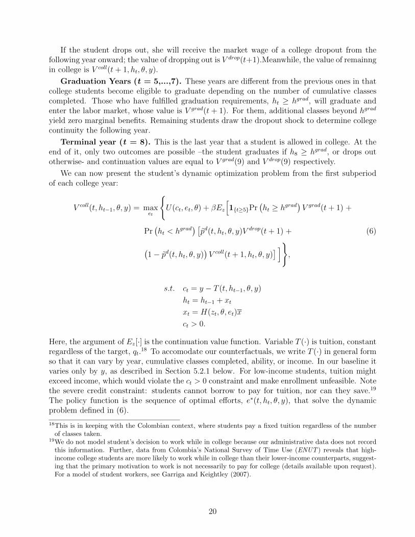
If the student drops out, she will receive the market wage of a college dropout from thefollowing year onward; the value of dropping out is V drop(t+1).Meanwhile, the value of remainngin college is V coll(t+ 1, ht, θ, y).
Graduation Years (t = 5,...,7). These years are different from the previous ones in thatcollege students become eligible to graduate depending on the number of cumulative classescompleted. Those who have fulfilled graduation requirements, ht ≥ hgrad, will graduate andenter the labor market, whose value is V grad(t + 1). For them, additional classes beyond hgrad
yield zero marginal benefits. Remaining students draw the dropout shock to determine collegecontinuity the following year.
Terminal year (t = 8). This is the last year that a student is allowed in college. At theend of it, only two outcomes are possible –the student graduates if h8 ≥ hgrad, or drops outotherwise- and continuation values are equal to V grad(9) and V drop(9) respectively.
We can now present the student’s dynamic optimization problem from the first subperiodof each college year:
V coll(t, ht−1, θ, y) = maxet
{U(ct, et, θ) + βEz
[1{t≥5}Pr
(ht ≥ hgrad
)V grad(t+ 1) +
Pr(ht < hgrad
) [pd(t, ht, θ, y)V drop(t+ 1) +
(1− pd(t, ht, θ, y)
)V coll(t+ 1, ht, θ, y)
] ]},
(6)
s.t. ct = y − T (t, ht−1, θ, y)
ht = ht−1 + xt
xt = H(zt, θ, et)x
ct > 0.
Here, the argument of Ez[·] is the continuation value function. Variable T (·) is tuition, constantregardless of the target, qt.
18 To accomodate our counterfactuals, we write T (·) in general formso that it can vary by year, cumulative classes completed, ability, or income. In our baseline itvaries only by y, as described in Section 5.2.1 below. For low-income students, tuition mightexceed income, which would violate the ct > 0 constraint and make enrollment unfeasible. Notethe severe credit constraint: students cannot borrow to pay for tuition, nor can they save.19
The policy function is the sequence of optimal efforts, e∗(t, ht, θ, y), that solve the dynamicproblem defined in (6).
18This is in keeping with the Colombian context, where students pay a fixed tuition regardless of the numberof classes taken.
19We do not model student’s decision to work while in college because our administrative data does not recordthis information. Further, data from Colombia’s National Survey of Time Use (ENUT ) reveals that high-income college students are more likely to work while in college than their lower-income counterparts, suggest-ing that the primary motivation to work is not necessarily to pay for college (details available upon request).For a model of student workers, see Garriga and Keightley (2007).
20
4.3 Workers
An individual can join the labor force after graduating from high school or college, or afterdropping out from college.20 The worker’s optimization problem, written in recursive form, is
V m(t) = maxct{u(ct) + βV m(t+ 1)}, (7)
s.t. ct = wmt ,
where V m(t) is the value function of a worker with educational attainmentm = {hs, grad, drop},denoting high school graduate, college graduate, and college dropout respectively. The worker’swage, wmt , is specific to educational attainment, and varies with t to allow for returns toexperience. Note that V m depends on t because of w, and because the value of working dependson the total number of years worked, given by the entry date into labor force.
4.4 Enrollment decision
In order to decide whether or not to enroll in college, a high school graduate compares theexpected payoff of two choices - going to college, or joining the labor force as a high schoolgraduate. The enrollment decision is a discrete choice problem, where the payoff associated toeach option is the sum of three components. The first component is the expected value of goingto college, V coll(t = 1, h0 = 0, θ, y) or of entering the labor force as a high school graduate, V hs.The second component is a type-specific preference for college enrollment, ξj = ξ(θj, yj), whichcaptures type-related unobserved factors, such as parental education, that affect enrollment.We normalize the unobserved preference for joining the labor force as a high school graduateto zero for all types. The third component is an idiosyncratic choice-specific shock for eachindividual, εhs and εcoll, corresponding to working as a high school graduate or enrolling incollege, respectively. Thus, all individuals face the same V hs, and individuals of a given typeface the same V coll and ξj; yet individuals within and across types differ in their idiosyncraticshocks. We assume that εhs and εcoll are iid and distributed Type I Extreme Value with ascaling factor of σε. The individual chooses to attend college if
V coll(1, 0, θj, yj) + ξj + σεεcoll
Value of going to college
≥ V hs + σεεhs
Value of working as a high school graduate(8)
As a result, the probability of college enrollment for an individual of type j is
P coll(θj, yj) =exp{(V coll(1, 0, θj, yj) + ξj)/σε}
exp{(V coll(1, 0, θj, yj) + ξj)/σε}+ exp{V hs/σε}, (9)
Its complement, P hs(θ, y) = 1−P coll(θ, y), is the probability of joining the labor force as a highschool graduate.
20We assume that workers consume all their earnings and do not have access to credit markets, which is anaccurate representation of developing economies. Since wages rise with experience and workers discount thefuture at the interest rate, they have no incentives to save.
21
5 Empirical implementation
In this section we describe the parameterization and computational version of the model. Wealso describe the algorithm to compute model predicted values for a given parameter point.
5.1 Functional forms
In the model, t = 1 corresponds to age 18. Retirement age is 65, or t = 48. Regardless of hereducational attainment or when she joined the labor force, the individual accrues returns toexperience (or becomes ”experienced”) from age 35 (t = 28) onwards.
The utility of college students is given by
U (c, e, θ) =(c+ c)1−ρ − 1
1− ρ− µ eγ
(1 + θ)k. (10)
where the need to meet the minimum consumption level, c, might limit low-income students’ability to enroll in college. To prevent this, we set c equal to one million COP.21 The utility ofworkers is given by
u(c) =c1−ρ − 1
1− ρ. (11)
We set r = 0.04, and assume σε = 1.
The production function to complete classes has constant returns to scale in ability andeffort:
xt = H(zt, θ, et)x = zt(θαe1−α
t )x, (12)
where α ∈ (0, 1) is the elasticity of classes completed with respect to ability. Consistent withthe model, we set x = 20 classes. We set the minimum number of classes required to graduate,hgrad, equal to 98.22
The functional form for the zt shock is as follows:
zt = exp{− exp{−(κ0 + κ1d1 + κhht−1 + κθθ + (σ + σ1d1 + σθθ)νt)}}, (13)
where ht−1 is a measure of past cumulative number of classes completed, with ht−1 = ln(ht−1)for every t > 1, and h0 = 0 for t = 1.The terms associated with d1 allow the shock distributionto differ in year 1, when d1 = 1.23 The shock also depends on an iid component, νt, drawnfrom the uniform distribution U(0, 1). The functional form in (13) ensures that zt ∈ (0, 1) forany combination of parameter values and for all h, θ ∈ R. Importantly, all the parameters in(13) affect the mean and variance of zt. In Section 6.3 below we discuss the effect of ht−1 and
21Our chosen value for c guarantees that, in our computational models, all students attain positive consumptionif they enroll in college. We can think of c as the minimum consumption guaranteed to college studentsthrough student subsidies, such as those for food and transportation.
22We set this requirement to 98 rather than 100 because we observe students who graduate with slightly fewerthan 100 classes - perhaps due to measurement error.
23In year 1, h0 = 0, whereas h is positive in subsequent years. This creates scaling problems in year 1, which wesolve through κ1. As documented in section 3.4.3, the variance of classes completed is higher in year 1 thanin other years, which we capture with σ1.
22
κθ on this mean and variance at our specific parameter estimates.
We parameterize the probability of dropping out as
pd(t, ht, θ, y) =exp{δ(t, θ, y) + πht}
1 + exp{δ(t, θ, y) + πht}, (14)
where δ(t, θ, y) is a year-, ability- and income- specific fixed effect, and ht measures cumulativeperformance over all periods, including the current one. Evaluating pd(t, ht, θ, y) at π = 0yields the “exogenous dropout probability” - namely, the dropout probability that students ofa given type would have, in a given year, if they had accumulated no classes. It is “exogenous”because it is independent of effort. For example, low-income, low-ability students may have ahigh exogenous dropout probability in year 1 -perhaps because they lack parental guidance onhow to navigate college- yet a lower one in subsequent years.
The model’s full parameter vector is Θ = (Θ, ξ, δ), where
Θ = (ρ, µ, γ, k, α, κ0, κy1 , κh, κθ, σ, σy1 , σθ, π) (15)
is the vector of parameters common across individuals. Vector ξJ×1 contains type-specific unob-served preferences for college, ξj (see (9)) and δ(J∗8)×1 contains exogenous dropout probabilityfixed effects, δ(t, θj, yj), for the J types and 8 years (see (14)).
5.2 Computational representation
5.2.1 Student types
To build the empirical distribution of ability and income for school graduates, Φ(y, θ), we startfrom Table 1, which classifies 2005 high school graduates by ability quintile and income bracket.We refine this table to work with ability deciles rather than quintiles, for a total of fifty studenttypes. To construct values for θ, we start from the distribution of standardized Saber 11 testscores and normalize them between 0 and 1.24 Our θ values are the 5th, 15th, ...95th percentilesfrom the normalized scores. We calculate the y value corresponding to each income bracket asthe average annual per-capita income for that bracket, computed from Colombia’s householdsurvey data (SEDLAC) on family income and size. Lacking student-level data on tuitionexpenses, we estimate the tuition paid by students of a given y as the average annual tuitionpaid by students from the corresponding income bracket at public institutions, calculated fromSNIES and SPADIES.25
Table 4 shows the resulting income and tuition corresponding to the underlying familyincome brackets. As the table shows, income varies greatly across income brackets. Althoughpublic institutions provide income-based tuition discounts, the highest income individuals donot pay proportionally to their income. While their per-capita income is about twenty timesas large as that of the lowest-income individuals, their tuition is only 2.5 times as large.
24Let sts denote the standardized test score. The normalized sts is equal to (sts − min(sts))/(max(sts) −min(sts)).
25We use tuition at public HEIs because there is always a public HEI that the student can attend. Modelingthe choice of college type (public or private) is beyond the scope of this paper.
23
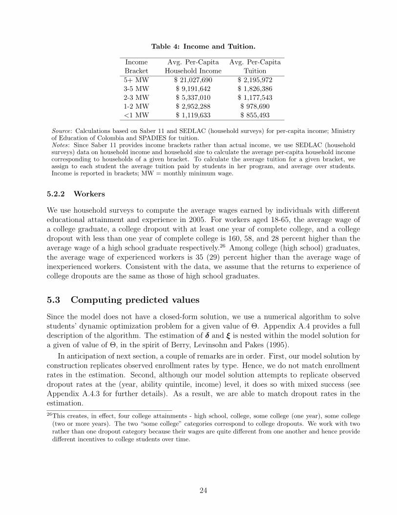
Table 4: Income and Tuition.
Income Avg. Per-Capita Avg. Per-CapitaBracket Household Income Tuition
5+ MW $ 21,027,690 $ 2,195,9723-5 MW $ 9,191,642 $ 1,826,3862-3 MW $ 5,337,010 $ 1,177,5431-2 MW $ 2,952,288 $ 978,690<1 MW $ 1,119,633 $ 855,493
Source: Calculations based on Saber 11 and SEDLAC (household surveys) for per-capita income; Ministryof Education of Colombia and SPADIES for tuition.Notes: Since Saber 11 provides income brackets rather than actual income, we use SEDLAC (householdsurveys) data on household income and household size to calculate the average per-capita household incomecorresponding to households of a given bracket. To calculate the average tuition for a given bracket, weassign to each student the average tuition paid by students in her program, and average over students.Income is reported in brackets; MW = monthly minimum wage.
5.2.2 Workers
We use household surveys to compute the average wages earned by individuals with differenteducational attainment and experience in 2005. For workers aged 18-65, the average wage ofa college graduate, a college dropout with at least one year of complete college, and a collegedropout with less than one year of complete college is 160, 58, and 28 percent higher than theaverage wage of a high school graduate respectively.26 Among college (high school) graduates,the average wage of experienced workers is 35 (29) percent higher than the average wage ofinexperienced workers. Consistent with the data, we assume that the returns to experience ofcollege dropouts are the same as those of high school graduates.
5.3 Computing predicted values
Since the model does not have a closed-form solution, we use a numerical algorithm to solvestudents’ dynamic optimization problem for a given value of Θ. Appendix A.4 provides a fulldescription of the algorithm. The estimation of δ and ξ is nested within the model solution fora given of value of Θ, in the spirit of Berry, Levinsohn and Pakes (1995).
In anticipation of next section, a couple of remarks are in order. First, our model solution byconstruction replicates observed enrollment rates by type. Hence, we do not match enrollmentrates in the estimation. Second, although our model solution attempts to replicate observeddropout rates at the (year, ability quintile, income) level, it does so with mixed success (seeAppendix A.4.3 for further details). As a result, we are able to match dropout rates in theestimation.
26This creates, in effect, four college attainments - high school, college, some college (one year), some college(two or more years). The two “some college” categories correspond to college dropouts. We work with tworather than one dropout category because their wages are quite different from one another and hence providedifferent incentives to college students over time.
24
6 Estimation
In this section we describe the estimation strategy and identification. We also present parameterestimates, describe the model’s fit, and address the role of effort given our estimates.
6.1 Estimation Strategy
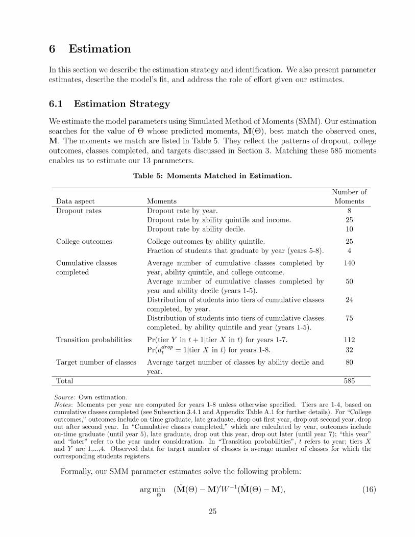
We estimate the model parameters using Simulated Method of Moments (SMM). Our estimationsearches for the value of Θ whose predicted moments, M(Θ), best match the observed ones,M. The moments we match are listed in Table 5. They reflect the patterns of dropout, collegeoutcomes, classes completed, and targets discussed in Section 3. Matching these 585 momentsenables us to estimate our 13 parameters.
Table 5: Moments Matched in Estimation.
Number ofData aspect Moments Moments
Dropout rates Dropout rate by year. 8Dropout rate by ability quintile and income. 25Dropout rate by ability decile. 10
College outcomes College outcomes by ability quintile. 25Fraction of students that graduate by year (years 5-8). 4
Cumulative classescompleted
Average number of cumulative classes completed byyear, ability quintile, and college outcome.
140
Average number of cumulative classes completed byyear and ability decile (years 1-5).
50
Distribution of students into tiers of cumulative classescompleted, by year.
24
Distribution of students into tiers of cumulative classes 75completed, by ability quintile and year (years 1-5).
Transition probabilities Pr(tier Y in t+ 1|tier X in t) for years 1-7. 112
Pr(ddropt = 1|tier X in t) for years 1-8. 32
Target number of classes Average target number of classes by ability decile andyear.
80
Total 585
Source: Own estimation.Notes: Moments per year are computed for years 1-8 unless otherwise specified. Tiers are 1-4, based oncumulative classes completed (see Subsection 3.4.1 and Appendix Table A.1 for further details). For “Collegeoutcomes,” outcomes include on-time graduate, late graduate, drop out first year, drop out second year, dropout after second year. In “Cumulative classes completed,” which are calculated by year, outcomes includeon-time graduate (until year 5), late graduate, drop out this year, drop out later (until year 7); “this year”and “later” refer to the year under consideration. In “Transition probabilities”, t refers to year; tiers Xand Y are 1,...,4. Observed data for target number of classes is average number of classes for which thecorresponding students registers.
Formally, our SMM parameter estimates solve the following problem:
arg minΘ
(M(Θ)−M)′W−1(M(Θ)−M), (16)
25
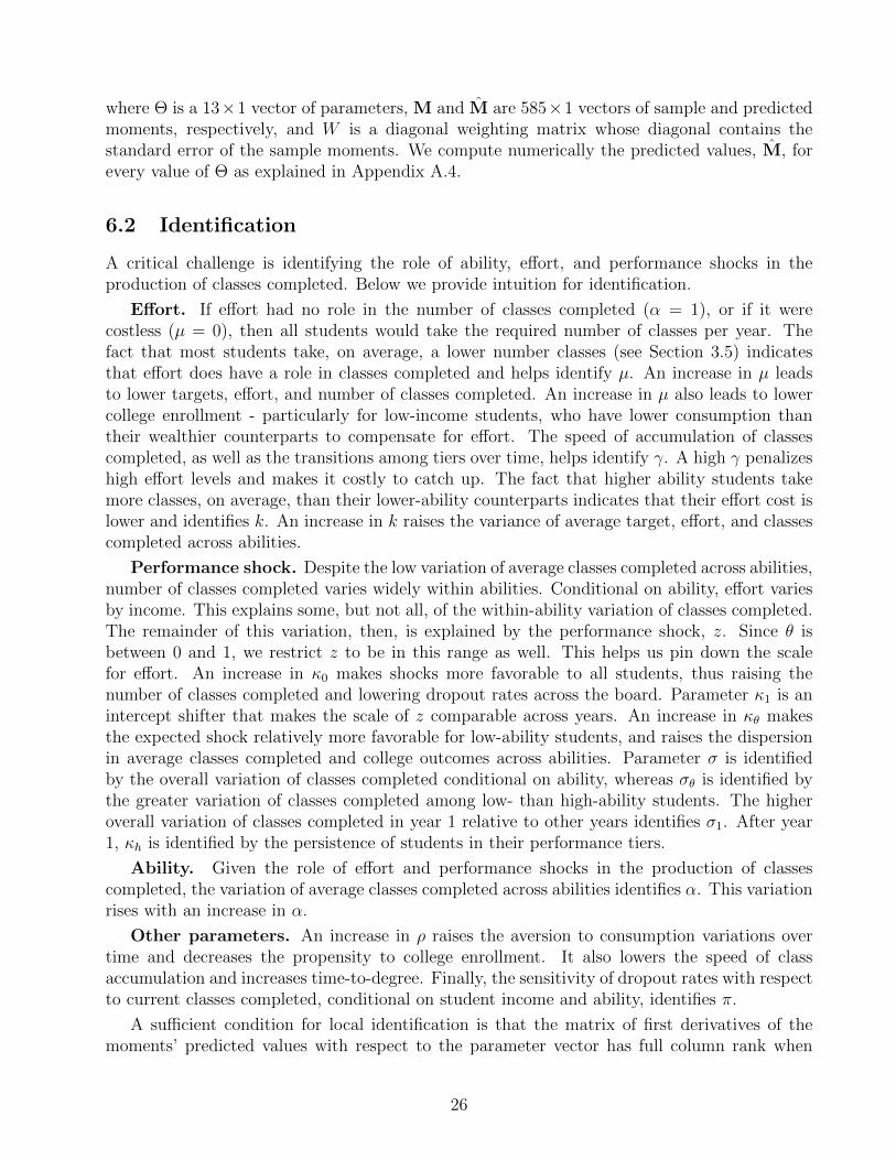
where Θ is a 13×1 vector of parameters, M and M are 585×1 vectors of sample and predictedmoments, respectively, and W is a diagonal weighting matrix whose diagonal contains thestandard error of the sample moments. We compute numerically the predicted values, M, forevery value of Θ as explained in Appendix A.4.
6.2 Identification
A critical challenge is identifying the role of ability, effort, and performance shocks in theproduction of classes completed. Below we provide intuition for identification.
Effort. If effort had no role in the number of classes completed (α = 1), or if it werecostless (µ = 0), then all students would take the required number of classes per year. Thefact that most students take, on average, a lower number classes (see Section 3.5) indicatesthat effort does have a role in classes completed and helps identify µ. An increase in µ leadsto lower targets, effort, and number of classes completed. An increase in µ also leads to lowercollege enrollment - particularly for low-income students, who have lower consumption thantheir wealthier counterparts to compensate for effort. The speed of accumulation of classescompleted, as well as the transitions among tiers over time, helps identify γ. A high γ penalizeshigh effort levels and makes it costly to catch up. The fact that higher ability students takemore classes, on average, than their lower-ability counterparts indicates that their effort cost islower and identifies k. An increase in k raises the variance of average target, effort, and classescompleted across abilities.
Performance shock. Despite the low variation of average classes completed across abilities,number of classes completed varies widely within abilities. Conditional on ability, effort variesby income. This explains some, but not all, of the within-ability variation of classes completed.The remainder of this variation, then, is explained by the performance shock, z. Since θ isbetween 0 and 1, we restrict z to be in this range as well. This helps us pin down the scalefor effort. An increase in κ0 makes shocks more favorable to all students, thus raising thenumber of classes completed and lowering dropout rates across the board. Parameter κ1 is anintercept shifter that makes the scale of z comparable across years. An increase in κθ makesthe expected shock relatively more favorable for low-ability students, and raises the dispersionin average classes completed and college outcomes across abilities. Parameter σ is identifiedby the overall variation of classes completed conditional on ability, whereas σθ is identified bythe greater variation of classes completed among low- than high-ability students. The higheroverall variation of classes completed in year 1 relative to other years identifies σ1. After year1, κh is identified by the persistence of students in their performance tiers.
Ability. Given the role of effort and performance shocks in the production of classescompleted, the variation of average classes completed across abilities identifies α. This variationrises with an increase in α.
Other parameters. An increase in ρ raises the aversion to consumption variations overtime and decreases the propensity to college enrollment. It also lowers the speed of classaccumulation and increases time-to-degree. Finally, the sensitivity of dropout rates with respectto current classes completed, conditional on student income and ability, identifies π.
A sufficient condition for local identification is that the matrix of first derivatives of themoments’ predicted values with respect to the parameter vector has full column rank when
26
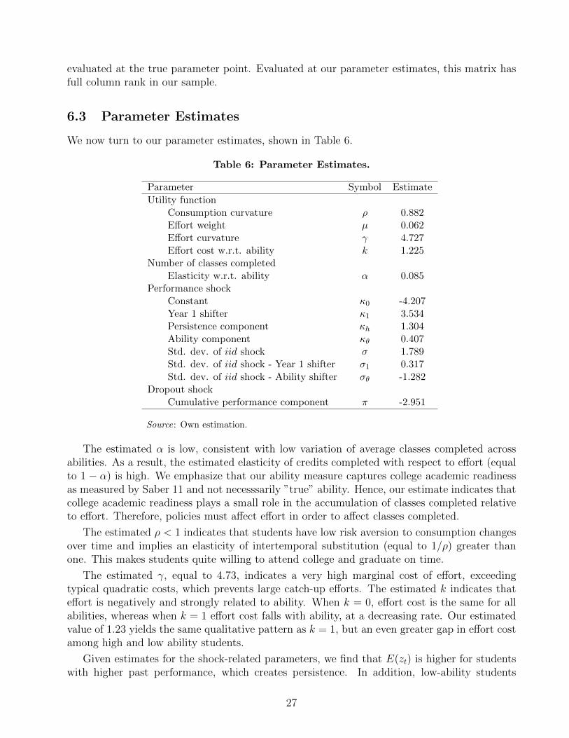
evaluated at the true parameter point. Evaluated at our parameter estimates, this matrix hasfull column rank in our sample.
6.3 Parameter Estimates
We now turn to our parameter estimates, shown in Table 6.
Table 6: Parameter Estimates.
Parameter Symbol Estimate
Utility functionConsumption curvature ρ 0.882Effort weight µ 0.062Effort curvature γ 4.727Effort cost w.r.t. ability k 1.225
Number of classes completedElasticity w.r.t. ability α 0.085
Performance shockConstant κ0 -4.207Year 1 shifter κ1 3.534Persistence component κh 1.304Ability component κθ 0.407Std. dev. of iid shock σ 1.789Std. dev. of iid shock - Year 1 shifter σ1 0.317Std. dev. of iid shock - Ability shifter σθ -1.282
Dropout shockCumulative performance component π -2.951
Source: Own estimation.
The estimated α is low, consistent with low variation of average classes completed acrossabilities. As a result, the estimated elasticity of credits completed with respect to effort (equalto 1 − α) is high. We emphasize that our ability measure captures college academic readinessas measured by Saber 11 and not necesssarily ”true” ability. Hence, our estimate indicates thatcollege academic readiness plays a small role in the accumulation of classes completed relativeto effort. Therefore, policies must affect effort in order to affect classes completed.
The estimated ρ < 1 indicates that students have low risk aversion to consumption changesover time and implies an elasticity of intertemporal substitution (equal to 1/ρ) greater thanone. This makes students quite willing to attend college and graduate on time.
The estimated γ, equal to 4.73, indicates a very high marginal cost of effort, exceedingtypical quadratic costs, which prevents large catch-up efforts. The estimated k indicates thateffort is negatively and strongly related to ability. When k = 0, effort cost is the same for allabilities, whereas when k = 1 effort cost falls with ability, at a decreasing rate. Our estimatedvalue of 1.23 yields the same qualitative pattern as k = 1, but an even greater gap in effort costamong high and low ability students.
Given estimates for the shock-related parameters, we find that E(zt) is higher for studentswith higher past performance, which creates persistence. In addition, low-ability students
27
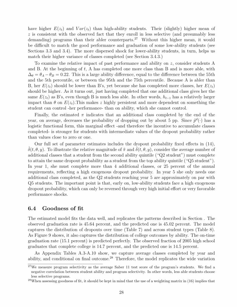
have higher E(zt) and V ar(zt) than high-ability students. Their (slightly) higher mean ofz is consistent with the observed fact that they enroll in less selective (and presumably lessdemanding) programs than their abler counterparts.27 Without this higher mean, it wouldbe difficult to match the good performance and graduation of some low-ability students (seeSections 3.3 and 3.4). The more dispersed shock for lower-ability students, in turn, helps usmatch their higher variance of classes completed (see Section 3.4.3.)
To examine the relative impact of past performance and ability on z, consider students Aand B. At the beginning of t, A has completed one more class than B and is more able, with∆θ = θA− θB = 0.22. This is a large ability difference, equal to the difference between the 55thand the 5th percentile, or between the 95th and the 75th percentile. Because A is abler thanB, her E(zt) should be lower than B’s, yet because she has completed more classes, her E(zt)should be higher. As it turns out, just having completed that one additional class gives her thesame E(zt) as B’s, even though B is much less able. In other words, ht−1 has a relatively largerimpact than θ on E(zt).This makes z highly persistent and more dependent on something thestudent can control -her performance- than on ability, which she cannot control.
Finally, the estimated π indicates that an additional class completed by the end of theyear, on average, decreases the probability of dropping out by about 5 pp. Since pd(·) has alogistic functional form, this marginal effect -and therefore the incentive to accumulate classescompleted- is stronger for students with intermediate values of the dropout probability ratherthan values close to zero or one.
Our full set of parameter estimates includes the dropout probability fixed effects in (14),δ(t, θ, y). To illustrate the relative magnitude of π and δ(t, θ, y), consider the average number ofadditional classes that a student from the second ability quintile (“Q2 student”) must completeto attain the same dropout probability as a student from the top ability quintile (“Q5 student”).In year 1, she must complete more than 4 additional classes, or 25 percent of the annualrequirements, reflecting a high exogenous dropout probability. In year 5 she only needs oneadditional class completed, as the Q2 students reaching year 5 are approximately on par withQ5 students. The important point is that, early on, low-ability students face a high exogenousdropout probability, which can only be reversed through very high initial effort or very favorableperformance shocks.
6.4 Goodness of fit
The estimated model fits the data well, and replicates the patterns described in Section . Theobserved graduation rate is 45.64 percent, and the predicted one is 45.02 percent. The modelcaptures the distribution of dropouts over time (Table 7) and across student types (Table 8).As Figure 9 shows, it also captures the distribution of college outcomes by ability. The on-timegraduation rate (15.1 percent) is predicted perfectly. The observed fraction of 2005 high schoolgraduates that complete college is 14.7 percent, and the predicted one is 14.5 percent.
As Appendix Tables A.3-A.10 show, we capture average classes completed by year andability, and conditional on final outcome.28 Therefore, the model replicates the wide variation
27We measure program selectivity as the average Saber 11 test score of the program’s students. We find anegative correlation between student ability and program selectivity. In other words, less able students chooseless selective programs.
28When assessing goodness of fit, it should be kept in mind that the use of a weighting matrix in (16) implies that
28
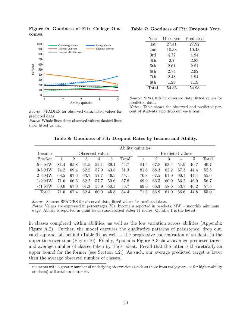
Figure 9: Goodness of Fit: College Out-comes.
0
10
20
30
40
50
60
70
80
90
100
Per
cen
t
1 2 3 4 5Ability quintile
On−time graduate Late graduate
Dropout 2nd year Dropout 1st year
Dropout after 2nd year
Source: SPADIES for observed data; fitted values forpredicted data.Notes: Whole lines show observed values; dashed linesshow fitted values.
Table 7: Goodness of Fit: Dropout Year.
Year Observed Predicted
1st 27.41 27.922nd 10.38 10.433rd 4.77 4.944th 2.7 2.835th 2.61 2.816th 2.74 2.927th 2.48 1.948th 1.28 1.19
Total 54.36 54.98
Source: SPADIES for observed data; fitted values forpredicted data.Notes: Table shows the observed and predicted per-cent of students who drop out each year.
Table 8: Goodness of Fit: Dropout Rates by Income and Ability.
Ability quintilesIncome Observed values Predicted valuesBracket 1 2 3 4 5 Total 1 2 3 4 5 Total
5+ MW 81.4 65.8 61.5 52.1 39.1 44.7 84.4 67.8 63.4 51.9 40.7 46.73-5 MW 74.2 69.4 62.2 57.9 43.8 51.3 81.6 68.3 62.2 57.3 44.4 52.52-3 MW 68.5 67.6 63.7 57.7 46.5 55.1 70.8 67.5 61.9 60.1 44.4 55.61-2 MW 71.6 66.6 62.2 57.7 50.6 57.8 69.9 66.5 60.9 56.2 46.9 56.7<1 MW 69.0 67.9 61.3 55.9 50.3 58.7 69.6 66.3 58.6 53.7 46.2 57.5
Total 71.0 67.4 62.4 60.0 45.8 54.4 71.3 66.9 61.0 56.6 44.8 55.0
Source: Source: SPADIES for observed data; fitted values for predicted data.Notes: Values are expressed in percentages (%). Income is reported in brackets; MW = monthly minimumwage. Ability is reported in quintiles of standardized Saber 11 scores. Quintile 1 is the lowest.
in classes completed within abilities, as well as the low variation across abilities (AppendixFigure A.2). Further, the model captures the qualitative patterns of persistence, drop out,catch-up and fall behind (Table 9), as well as the progressive concentration of students in theupper tiers over time (Figure 10). Finally, Appendix Figure A.3 shows average predicted targetand average number of classes taken by the student. Recall that the latter is theoretically anupper bound for the former (see Section 4.2.) As such, our average predicted target is lowerthan the average observed number of classes.
moments with a greater number of underlying observations (such as those from early years, or for higher-abilitystudents) will attain a better fit.
29
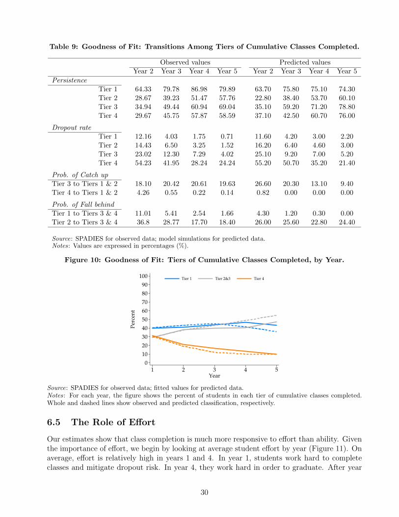
Table 9: Goodness of Fit: Transitions Among Tiers of Cumulative Classes Completed.
Observed values Predicted valuesYear 2 Year 3 Year 4 Year 5 Year 2 Year 3 Year 4 Year 5
PersistenceTier 1 64.33 79.78 86.98 79.89 63.70 75.80 75.10 74.30Tier 2 28.67 39.23 51.47 57.76 22.80 38.40 53.70 60.10Tier 3 34.94 49.44 60.94 69.04 35.10 59.20 71.20 78.80Tier 4 29.67 45.75 57.87 58.59 37.10 42.50 60.70 76.00
Dropout rateTier 1 12.16 4.03 1.75 0.71 11.60 4.20 3.00 2.20Tier 2 14.43 6.50 3.25 1.52 16.20 6.40 4.60 3.00Tier 3 23.02 12.30 7.29 4.02 25.10 9.20 7.00 5.20Tier 4 54.23 41.95 28.24 24.24 55.20 50.70 35.20 21.40
Prob. of Catch upTier 3 to Tiers 1 & 2 18.10 20.42 20.61 19.63 26.60 20.30 13.10 9.40Tier 4 to Tiers 1 & 2 4.26 0.55 0.22 0.14 0.82 0.00 0.00 0.00
Prob. of Fall behindTier 1 to Tiers 3 & 4 11.01 5.41 2.54 1.66 4.30 1.20 0.30 0.00Tier 2 to Tiers 3 & 4 36.8 28.77 17.70 18.40 26.00 25.60 22.80 24.40
Source: SPADIES for observed data; model simulations for predicted data.Notes: Values are expressed in percentages (%).
Figure 10: Goodness of Fit: Tiers of Cumulative Classes Completed, by Year.
0
10
20
30
40
50
60
70
80
90
100
Percen
t
1 2 3 4 5
Year
Tier 1 Tier 2&3 Tier 4
Source: SPADIES for observed data; fitted values for predicted data.Notes: For each year, the figure shows the percent of students in each tier of cumulative classes completed.Whole and dashed lines show observed and predicted classification, respectively.
6.5 The Role of Effort
Our estimates show that class completion is much more responsive to effort than ability. Giventhe importance of effort, we begin by looking at average student effort by year (Figure 11). Onaverage, effort is relatively high in years 1 and 4. In year 1, students work hard to completeclasses and mitigate dropout risk. In year 4, they work hard in order to graduate. After year
30
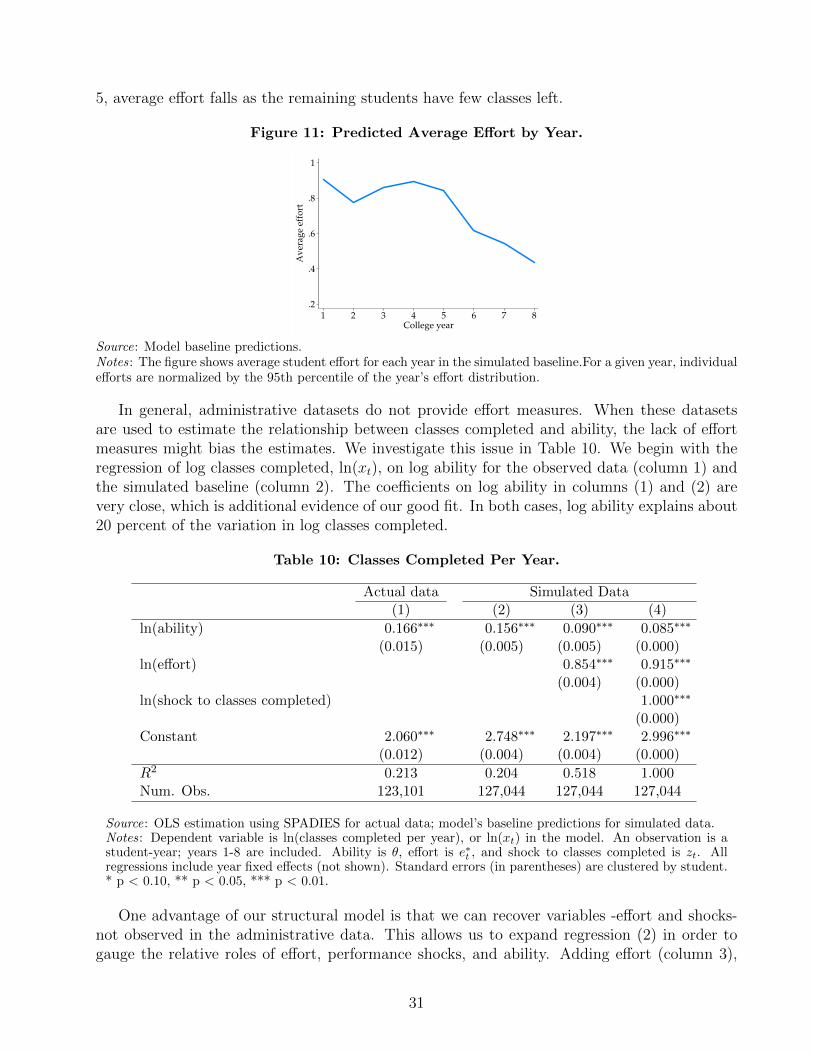
5, average effort falls as the remaining students have few classes left.
Figure 11: Predicted Average Effort by Year.
.2
.4
.6
.8
1
Av
erag
e ef
fort
1 2 3 4 5 6 7 8College year
Source: Model baseline predictions.Notes: The figure shows average student effort for each year in the simulated baseline.For a given year, individualefforts are normalized by the 95th percentile of the year’s effort distribution.
In general, administrative datasets do not provide effort measures. When these datasetsare used to estimate the relationship between classes completed and ability, the lack of effortmeasures might bias the estimates. We investigate this issue in Table 10. We begin with theregression of log classes completed, ln(xt), on log ability for the observed data (column 1) andthe simulated baseline (column 2). The coefficients on log ability in columns (1) and (2) arevery close, which is additional evidence of our good fit. In both cases, log ability explains about20 percent of the variation in log classes completed.
Table 10: Classes Completed Per Year.
Actual data Simulated Data(1) (2) (3) (4)
ln(ability) 0.166∗∗∗ 0.156∗∗∗ 0.090∗∗∗ 0.085∗∗∗
(0.015) (0.005) (0.005) (0.000)ln(effort) 0.854∗∗∗ 0.915∗∗∗
(0.004) (0.000)ln(shock to classes completed) 1.000∗∗∗
(0.000)Constant 2.060∗∗∗ 2.748∗∗∗ 2.197∗∗∗ 2.996∗∗∗
(0.012) (0.004) (0.004) (0.000)
R2 0.213 0.204 0.518 1.000Num. Obs. 123,101 127,044 127,044 127,044
Source: OLS estimation using SPADIES for actual data; model’s baseline predictions for simulated data.Notes: Dependent variable is ln(classes completed per year), or ln(xt) in the model. An observation is astudent-year; years 1-8 are included. Ability is θ, effort is e∗t , and shock to classes completed is zt. Allregressions include year fixed effects (not shown). Standard errors (in parentheses) are clustered by student.* p < 0.10, ** p < 0.05, *** p < 0.01.
One advantage of our structural model is that we can recover variables -effort and shocks-not observed in the administrative data. This allows us to expand regression (2) in order togauge the relative roles of effort, performance shocks, and ability. Adding effort (column 3),
31
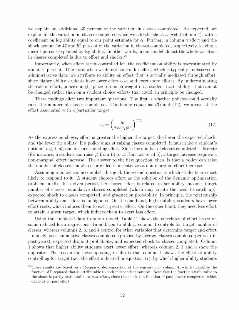
we explain an additional 30 percent of the variation in classes completed. As expected, weexplain all the variation in classes completed when we add the shock as well (column 4), with acoefficient on log ability equal to our point estimate for α. Further, in column 4 effort and theshock acount for 47 and 52 percent of the variation in classes completed, respectively, leaving amere 1 percent explained by log ability. In other words, in our model almost the whole variationin classes completed is due to effort and shocks.29
Importantly, when effort is not controlled for, the coefficient on ability is overestimated byabout 75 percent. Therefore, when we do not control for effort, which is typically unobserved inadministrative data, we attribute to ability an effect that is actually mediated through effort,since higher ability students have lower effort cost and exert more effort). By underestimatingthe role of effort, policies might place too much weight on a student trait -ability- that cannotbe changed rather than on a student choice -effort- that could, in principle be changed.
These findings elicit two important questions. The first is whether policies could actuallyraise the number of classes completed. Combining equations (3) and (12), we arrive at theeffort associated with a particular target:
et =
(qt
xE(zt)θα
) 11−α
. (17)
As the expression shows, effort is greater the higher the target, the lower the expected shock,and the lower the ability. If a policy aims at raising classes completed, it must raise a student’soptimal target, q∗t , and its corresponding effort. Since the number of classes completed is discrete(for instance, a student can raise q∗t from 14 to 15, but not to 14.5), a target increase requires anon-marginal effort increase. The answer to the first question, then, is that a policy can raisethe number of classes completed provided it incentivizes a non-marginal effort increase.
Assuming a policy can accomplish this goal, the second question is which students are mostlikely to respond to it. A student chooses effort as the solution of the dynamic optimizationproblem in (6). In a given period, her chosen effort is related to her ability, income, targetnumber of classes, cumulative classes completed (which may create the need to catch up),expected shock to classes completed, and graduation probability. In principle, the relationshipbetween ability and effort is ambiguous. On the one hand, higher-ability students have lowereffort costs, which induces them to exert greater effort. On the other hand, they need less effortto attain a given target, which induces them to exert less effort.
Using the simulated data from our model, Table 11 shows the correlates of effort based onsome reduced-form regressions. In addition to ability, column 1 controls for target number ofclasses, whereas columns 2, 3, and 4 control for other variables that determine target and effort– namely, past cumulative classes completed (proxied by average classes completed per year inpast years), expected dropout probability, and expected shock to classes completed. Column1 shows that higher ability students exert lower effort, whereas column 2, 3 and 4 show theopposite. The reason for these opossing results is that column 1 shows the effect of abilitycontrolling for target (i.e., the effect indicated in equation 17), by which higher ability students
29These results are based on a R-squared decomposition of the regression in column 4, whcih quantifies thefraction of R-squared that is attributable to each independent variable. Note that the fraction attributable tothe shock is partly attributable to past effort, since the shock is a function of past classes completed, whichdepends on past effort.
32
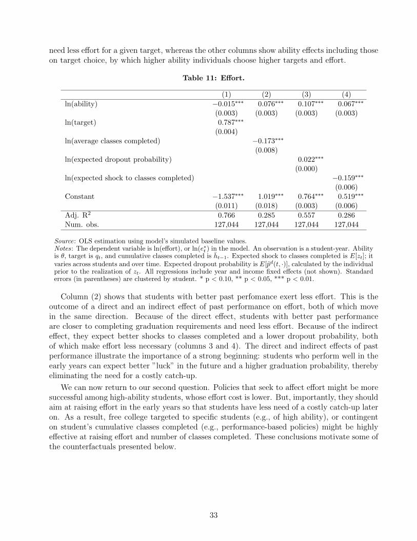
need less effort for a given target, whereas the other columns show ability effects including thoseon target choice, by which higher ability individuals choose higher targets and effort.
Table 11: Effort.
(1) (2) (3) (4)
ln(ability) −0.015∗∗∗ 0.076∗∗∗ 0.107∗∗∗ 0.067∗∗∗
(0.003) (0.003) (0.003) (0.003)ln(target) 0.787∗∗∗
(0.004)ln(average classes completed) −0.173∗∗∗
(0.008)ln(expected dropout probability) 0.022∗∗∗
(0.000)ln(expected shock to classes completed) −0.159∗∗∗
(0.006)Constant −1.537∗∗∗ 1.019∗∗∗ 0.764∗∗∗ 0.519∗∗∗
(0.011) (0.018) (0.003) (0.006)
Adj. R2 0.766 0.285 0.557 0.286Num. obs. 127,044 127,044 127,044 127,044
Source: OLS estimation using model’s simulated baseline values.Notes: The dependent variable is ln(effort), or ln(e∗t ) in the model. An observation is a student-year. Abilityis θ, target is qt, and cumulative classes completed is ht−1. Expected shock to classes completed is E[zt]; itvaries across students and over time. Expected dropout probability is E[pd(t, ·)], calculated by the individualprior to the realization of zt. All regressions include year and income fixed effects (not shown). Standarderrors (in parentheses) are clustered by student. * p < 0.10, ** p < 0.05, *** p < 0.01.
Column (2) shows that students with better past perfomance exert less effort. This is theoutcome of a direct and an indirect effect of past performance on effort, both of which movein the same direction. Because of the direct effect, students with better past performanceare closer to completing graduation requirements and need less effort. Because of the indirecteffect, they expect better shocks to classes completed and a lower dropout probability, bothof which make effort less necessary (columns 3 and 4). The direct and indirect effects of pastperformance illustrate the importance of a strong beginning: students who perform well in theearly years can expect better ”luck” in the future and a higher graduation probability, therebyeliminating the need for a costly catch-up.
We can now return to our second question. Policies that seek to affect effort might be moresuccessful among high-ability students, whose effort cost is lower. But, importantly, they shouldaim at raising effort in the early years so that students have less need of a costly catch-up lateron. As a result, free college targeted to specific students (e.g., of high ability), or contingenton student’s cumulative classes completed (e.g., performance-based policies) might be highlyeffective at raising effort and number of classes completed. These conclusions motivate some ofthe counterfactuals presented below.
33
7 Free college simulations
In this section we present counterfactual simulations of alternative free college programs. Webegin by describing their setup as well as the theoretical impact of free college on studentdecisions. Then we describe free college’s aggregate effects on enrollment and graduation, andexamine effort in order to understand graduation rate effects. We then turn to the heterogeneityof free college effects by student type, and relate our counterfactual results with findings fromthe empirical literature on college financial aid. We analyze the role of risk, both in the baselineand under free college. We conduct a simple cost-benefit analysis of free college, and concludewith an examination of the possible long-run effects of free college.
7.1 Counterfactuals’ setup
We simulate the following free college programs, which provide free tuition to the studentslisted below:
• Universal free college: all college students.
• Need-based free college: low-income students, defined as those from the lowest twoincome brackets.
• Ability-based free college: high-ability students, defined as those from the highestability quintile.
• Ability- and need-based free college: students who are both low income and highability – namely, students from the lowest two income brackets and the highest abilityquintile.
• Performance-based free college: all students in year 1, but only high-performingstudents afterwards. In a given year, a high-performing student is one who finished theprevious year in tiers 1 or 2 based on her cumulative performance. Note that a studentmay be high-performing in one year but not in another, depending on her cumulativeclasses completed.
• Performance- and need-based free college: all low-income students (from the lowesttwo income brackets) in year 1, but only to students who are both low-income and high-performing afterwards.
Note that, by design, performance-based and performance- and need-based free college entaila risk for the student, as the zero tuition is not guaranteed but must be attained throughperformance. In contrast, the other free college programs guarantee zero tuition based onex-ante student traits, which are not contingent on performance.
As we analyze these counterfactuals, it is convenient to distinguish between two groups ofstudents–existing and new. For a given counterfactual, we define existing students as thosewho enroll both in the baseline and at least in year 1 of the counterfactual. In contrast, newstudents are those who do not enroll in the baseline but enroll in the counterfactual.
34
Three important assumptions hold in our counterfactuals. First, we assume a perfectlyelastic higher education supply, whereby institutions can adjust capacity as needed in order toabsorb additional students at a constant marginal cost, and tuition does not rise in responseto greater demand. If there were capacity constraints, institutions would need to ration freecollege. Second, we assume that parents continue to transfer the same y to their children incollege even when college becomes free. In other words, public college funding does not crowdout private funding at all. If, in contrast, parents reduce their transfers one-for-one (full crowd-out), free college has no effects and is similar to the baseline. More generally, crowding out ofany degree is analogous to a reduction in tuition subsidy.30 Third, we assume that the averagecost of educating new and existing students is the same. This does not hold, for instance, whennew students need additional services, such as remedial education or non-academic supports.If new students are more costly, then a government with fixed resources cannot fund as manystudents. Since these assumptions provide the most favorable setting possible for free college,the results presented below are best viewed as an upper bound on free college effects.
7.2 Free college and student choices
Free college affects students on the extensive and intensive margins. On the extensive marginit raises college entry by adding new students, thereby affecting the size and composition of thestudent body. On the intensive margin, it affects student effort via the following channels:
1. Loss-of-urgency effect. By raising consumption during college, free college enhancesthe ”college experience,” as it raises the value of being a student relative to joining thelabor force and makes the student less eager to leave college. Other things equal, thiseffect leads to lower effort.
2. Substitution effect. Since free college raises consumption while in college, it allowsstudents to exert more effort without losing utility – in other words, it provides additionalconsumption to compensate for greater effort. Other things equal, this effect leads tohigher effort.
3. Risk effect. The performance and dropout shocks, zt and ddropt respectively, depend onthe number of cumulative classes completed, which in turn depends on effort. To theextent that free college raises (lowers) effort, it also lowers (raises) risk. Further, thelonger (shorter) a student spends in college, the greater (lower) her exposure to risks.
At the extensive margin, free college affects enrollment. At the intensive margin, it affectsgraduation; whether graduation rises or falls depends on the net effect on effort. Importantly,performance- and performance-and-need based free college provide a direct incentive to studenteffort by making tuition contingent on performance. As a result, they eliminate the loss-of-urgency effect.
30There is a large literature endogenizing parental transfers as a function of education cost and labor marketreturns. See, for instance, Keane and Wolpin (2001), Restuccia and Urrutia (2004), and Abbot et al (2013).
35
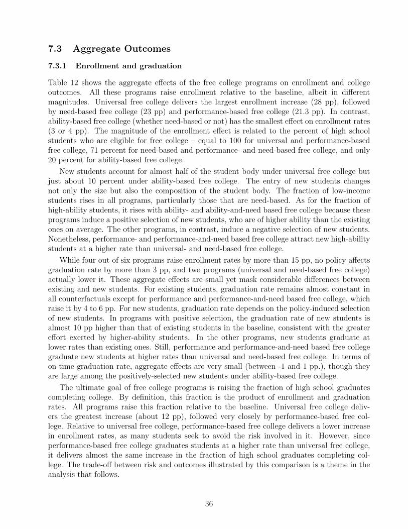
7.3 Aggregate Outcomes
7.3.1 Enrollment and graduation
Table 12 shows the aggregate effects of the free college programs on enrollment and collegeoutcomes. All these programs raise enrollment relative to the baseline, albeit in differentmagnitudes. Universal free college delivers the largest enrollment increase (28 pp), followedby need-based free college (23 pp) and performance-based free college (21.3 pp). In contrast,ability-based free college (whether need-based or not) has the smallest effect on enrollment rates(3 or 4 pp). The magnitude of the enrollment effect is related to the percent of high schoolstudents who are eligible for free college – equal to 100 for universal and performance-basedfree college, 71 percent for need-based and performance- and need-based free college, and only20 percent for ability-based free college.
New students account for almost half of the student body under universal free college butjust about 10 percent under ability-based free college. The entry of new students changesnot only the size but also the composition of the student body. The fraction of low-incomestudents rises in all programs, particularly those that are need-based. As for the fraction ofhigh-ability students, it rises with ability- and ability-and-need based free college because theseprograms induce a positive selection of new students, who are of higher ability than the existingones on average. The other programs, in contrast, induce a negative selection of new students.Nonetheless, performance- and performance-and-need based free college attract new high-abilitystudents at a higher rate than universal- and need-based free college.
While four out of six programs raise enrollment rates by more than 15 pp, no policy affectsgraduation rate by more than 3 pp, and two programs (universal and need-based free college)actually lower it. These aggregate effects are small yet mask considerable differences betweenexisting and new students. For existing students, graduation rate remains almost constant inall counterfactuals except for performance and performance-and-need based free college, whichraise it by 4 to 6 pp. For new students, graduation rate depends on the policy-induced selectionof new students. In programs with positive selection, the graduation rate of new students isalmost 10 pp higher than that of existing students in the baseline, consistent with the greatereffort exerted by higher-ability students. In the other programs, new students graduate atlower rates than existing ones. Still, performance and performance-and-need based free collegegraduate new students at higher rates than universal and need-based free college. In terms ofon-time graduation rate, aggregate effects are very small (between -1 and 1 pp.), though theyare large among the positively-selected new students under ability-based free college.
The ultimate goal of free college programs is raising the fraction of high school graduatescompleting college. By definition, this fraction is the product of enrollment and graduationrates. All programs raise this fraction relative to the baseline. Universal free college deliv-ers the greatest increase (about 12 pp), followed very closely by performance-based free col-lege. Relative to universal free college, performance-based free college delivers a lower increasein enrollment rates, as many students seek to avoid the risk involved in it. However, sinceperformance-based free college graduates students at a higher rate than universal free college,it delivers almost the same increase in the fraction of high school graduates completing col-lege. The trade-off between risk and outcomes illustrated by this comparison is a theme in theanalysis that follows.
36
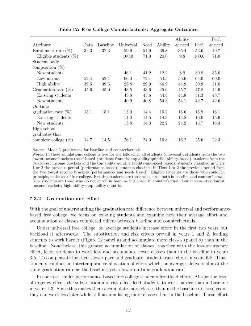
Table 12: Free College Counterfactuals: Aggregate Outcomes.
Ability Perf.Attribute Data Baseline Universal Need Ability & need Perf. & need
Enrollment rate (%) 32.3 32.3 59.9 54.9 36.8 35.4 53.6 49.7Eligible students (%) 100.0 71.0 20.0 9.8 100.0 71.0
Student bodycomposition (%)
New students 46.1 41.2 12.2 8.9 39.8 35.0Low income 52.4 52.4 66.0 72.1 54.5 56.6 64.0 69.0High ability 39.5 39.5 28.8 29.0 46.9 44.9 30.9 31.0
Graduation rate (%) 45.6 45.0 43.5 43.6 45.6 45.7 47.8 44.9Existing students 45.8 45.6 44.4 44.8 51.3 48.7New students 40.9 40.8 54.3 54.1 42.7 42.6
On-timegraduation rate (%) 15.1 15.1 13.9 14.4 15.2 15.6 15.9 16.1
Existing students 14.0 14.5 14.3 14.8 16.0 15.9New students 13.8 14.3 22.2 24.2 15.7 16.4
High schoolgraduates thatcomplete college (%) 14.7 14.5 26.1 24.0 16.8 16.2 25.6 22.3
Source: Model’s predictions for baseline and counterfactuals.Notes: In these simulations, college is free for the following: all students (universal); students from the twolowest income brackets (need-based); students from the top ability quintile (ability-based), students from thetwo lowest income brackets and the top ability quintile (ability-and-need based); students classified in Tiers1 or 2 the previous period (performance-based), students classified in Tiers 1 or 2 the previous period fromthe two lowest income brackets (performance- and need- based). Eligible students are those who could, inprinciple, make use of free college. Existing students are those who enroll both in baseline and counterfactual.New students are those who do not enroll in baseline but enroll in counterfactual. Low income=two lowestincome brackets; high ability=top ability quintile.
7.3.2 Graduation and effort
With the goal of understanding the graduation rate difference between universal and performance-based free college, we focus on existing students and examine how their average effort andaccumulation of classes completed differs between baseline and counterfactuals.
Under universal free college, on average students increase effort in the first two years butbackload it afterwards. The substitution and risk effects prevail in years 1 and 2, leadingstudents to work harder (Figure 12 panel a) and accumulate more classes (panel b) than in thebaseline. Nonetheless, this greater accumulation of classes, together with the loss-of-urgencyeffect, leads students to work less and accumulate fewer classes than in the baseline in years3-5. To compensate for their slower pace and graduate, students raise effort in years 6-8. Thus,students conduct an intertemporal re-allocation of effort which, on average, delivers almost thesame graduation rate as the baseline, yet a lower on-time-graduation rate.
In contrast, under performance-based free college students frontload effort. Absent the loss-of-urgency effect, the substitution and risk effect lead students to work harder than in baselinein years 1-3. Since this makes them accumulate more classes than in the baseline in those years,they can work less later while still accumulating more classes than in the baseline. These effort
37
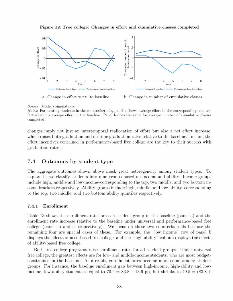
Figure 12: Free college: Changes in effort and cumulative classes completed
−.04
−.02
0
.02
.04C
han
ge
in e
ffo
rt
1 2 3 4 5 6 7 8Year
Universal free college Performance−base free college
−1
−.5
0
.5
1
Ch
ang
e in
nu
mb
er o
f cu
mu
l.cl
asse
s co
mp
lete
d
1 2 3 4 5 6 7 8Year
Universal free college Performance−base free college
a. Change in effort w.r.t. to baseline b. Change in number of cumulative classes
Source: Model’s simulations.Notes: For existing students in the counterfactuals, panel a shows average effort in the corresponding counter-factual minus average effort in the baseline. Panel b does the same for average number of cumulative classescompleted.
changes imply not just an intertemporal reallocation of effort but also a net effort increase,which raises both graduation and on-time graduation rates relative to the baseline. In sum, theeffort incentives contained in performance-based free college are the key to their success withgraduation rates.
7.4 Outcomes by student type
The aggregate outcomes shown above mask great heterogeneity among student types. Toexplore it, we classify students into nine groups based on income and ability. Income groupsinclude high, middle and low-income–corresponding to the top, two middle, and two bottom in-come brackets respectively. Ability groups include high, middle, and low-ability–correspondingto the top, two middle, and two bottom ability quintiles respectively.
7.4.1 Enrollment
Table 13 shows the enrollment rate for each student group in the baseline (panel a) and theenrollment rate increase relative to the baseline under universal and performance-based freecollege (panels b and c, respectively). We focus on these two counterfactuals because theremaining four are special cases of these. For example, the “low income” row of panel bdisplays the effects of need-based free college, and the “high ability” column displays the effectsof ability-based free college.
Both free college programs raise enrollment rates for all student groups. Under universalfree college, the greatest effects are for low- and middle-income students, who are most budget-constrained in the baseline. As a result, enrollment rates become more equal among studentgroups. For instance, the baseline enrollment gap between high-income, high-ability and low-income, low-ability students is equal to 70.2 = 83.8 − 13.6 pp, but shrinks to 49.5 = (83.8 +
38
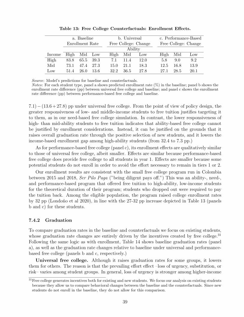
Table 13: Free College Counterfactuals: Enrollment Effects.
a. Baseline b. Universal c. Performance-BasedEnrollment Rate Free College: Change Free College: Change
AbilityIncome High Mid Low High Mid Low High Mid Low
High 83.8 65.5 39.3 7.1 11.4 12.0 5.8 9.0 9.2Mid 73.1 47.4 27.3 15.0 21.1 18.3 12.5 16.8 13.9Low 51.4 26.0 13.6 32.2 36.5 27.8 27.1 28.5 20.1
Source: Model’s predictions for baseline and counterfactuals.Notes: For each student type, panel a shows predicted enrollment rate (%) in the baseline; panel b shows theenrollment rate difference (pp) between universal free college and baseline; and panel c shows the enrollmentrate difference (pp) between performance-based free college and baseline.
7.1)− (13.6 + 27.8) pp under universal free college. From the point of view of policy design, thegreater responsiveness of low- and middle-income students to free tuition justifies targeting itto them, as in our need-based free college simulation. In contrast, the lower responsiveness ofhigh- than mid-ability students to free tuition indicates that ability-based free college cannotbe justified by enrollment considerations. Instead, it can be justified on the grounds that itraises overall graduation rate through the positive selection of new students, and it lowers theincome-based enrollment gap among high-ability students (from 32.4 to 7.3 pp.)
As for performance-based free college (panel c), its enrollment effects are qualitatively similarto those of universal free college, albeit smaller. Effects are similar because performance-basedfree college does provide free college to all students in year 1. Effects are smaller because somepotential students do not enroll in order to avoid the effort necessary to remain in tiers 1 or 2.
Our enrollment results are consistent with the small free college program run in Colombiabetween 2015 and 2018, Ser Pilo Paga (”being diligent pays off.”) This was an ability-, need-,and performance-based program that offered free tuition to high-ability, low-income studentsfor the theoretical duration of their program; students who dropped out were required to paythe tuition back. Among the eligible population, the program raised college enrollment ratesby 32 pp (Londono et al 2020), in line with the 27-32 pp increase depicted in Table 13 (panelsb and c) for these students.
7.4.2 Graduation
To compare graduation rates in the baseline and counterfactuals we focus on existing students,whose graduation rate changes are entirely driven by the incentives created by free college.31
Following the same logic as with enrollment, Table 14 shows baseline graduation rates (panela), as well as the graduation rate changes relative to baseline under universal and performance-based free college (panels b and c, respectively.)
Universal free college. Although it raises graduation rates for some groups, it lowersthem for others. The reason is that the prevailing effort effect –loss of urgency, substitution, orrisk– varies among student groups. In general, loss of urgency is stronger among higher-income
31Free college generates incentives both for existing and new students. We focus our analysis on existing studentsbecause they allow us to compare behavioral changes between the baseline and the counterfactuals. Since newstudents do not enroll in the baseline, they do not allow for this comparison.
39
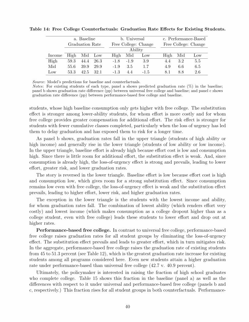
Table 14: Free College Counterfactuals: Graduation Rate Effects for Existing Students.
a. Baseline b. Universal c. Performance-BasedGraduation Rate Free College: Change Free College: Change
AbilityIncome High Mid Low High Mid Low High Mid Low
High 59.3 44.4 26.3 -1.8 -1.9 3.9 4.4 3.2 5.5Mid 55.6 39.9 29.9 -1.9 3.5 1.7 4.9 6.6 6.5Low 53.3 42.5 32.1 -1.3 4.4 -1.5 8.1 8.8 2.6
Source: Model’s predictions for baseline and counterfactuals.Notes: For existing students of each type, panel a shows predicted graduation rate (%) in the baseline;panel b shows graduation rate difference (pp) between universal free college and baseline; and panel c showsgraduation rate difference (pp) between performance-based free college and baseline.
students, whose high baseline consumption only gets higher with free college. The substitutioneffect is stronger among lower-ability students, for whom effort is more costly and for whomfree college provides greater compensation for additional effort. The risk effect is stronger forstudents with fewer cumulative classes completed, particularly when the loss of urgency has ledthem to delay graduation and has exposed them to risk for a longer time.
As panel b shows, graduation rates fall in the upper triangle (students of high ability orhigh income) and generally rise in the lower triangle (students of low ability or low income).In the upper triangle, baseline effort is already high because effort cost is low and consumptionhigh. Since there is little room for additional effort, the substitution effect is weak. And, sinceconsumption is already high, the loss-of-urgency effect is strong and prevails, leading to lowereffort, greater risk, and lower graduation rates.
The story is reversed in the lower triangle. Baseline effort is low because effort cost is highand consumption low, which gives room for a strong substitution effect. Since consumptionremains low even with free college, the loss-of-urgency effect is weak and the substitution effectprevails, leading to higher effort, lower risk, and higher graduation rates.
The exception in the lower triangle is the students with the lowest income and ability,for whom graduation rates fall. The combination of lowest ability (which renders effort verycostly) and lowest income (which makes consumption as a college dropout higher than as acollege student, even with free college) leads these students to lower effort and drop out athigher rates.
Performance-based free college. In contrast to universal free college, performance-basedfree college raises graduation rates for all student groups by eliminating the loss-of-urgencyeffect. The substitution effect prevails and leads to greater effort, which in turn mitigates risk.In the aggregate, performance-based free college raises the graduation rate of existing studentsfrom 45 to 51.3 percent (see Table 12), which is the greatest graduation rate increase for existingstudents among all programs considered here. Even new students attain a higher graduationrate under performance-based than universal free college (42.7 v. 40.9 percent).
Ultimately, the policymaker is interested in raising the fraction of high school graduateswho complete college. Table 15 shows this fraction in the baseline (panel a) as well as thedifferences with respect to it under universal and performance-based free college (panels b andc, respectively.) This fraction rises for all student groups in both counterfactuals. Performance-
40
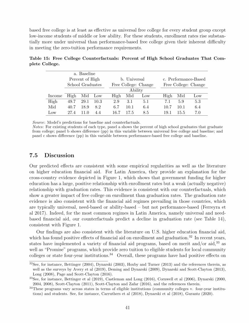
based free college is at least as effective as universal free college for every student group exceptlow-income students of middle or low ability. For these students, enrollment rates rise substan-tially more under universal than performance-based free college given their inherent difficultyin meeting the zero-tuition performance requirements.
Table 15: Free College Counterfactuals: Percent of High School Graduates That Com-plete College.
a. BaselinePercent of High b. Universal c. Performance-Based
School Graduates Free College: Change Free College: ChangeAbility
Income High Mid Low High Mid Low High Mid Low
High 49.7 29.1 10.3 2.9 3.1 5.1 7.1 5.9 5.3Mid 40.7 18.9 8.2 6.7 10.1 6.4 10.7 10.1 6.4Low 27.4 11.0 4.4 16.7 17.5 8.5 19.1 15.5 7.0
Source: Model’s predictions for baseline and counterfactuals.Notes: For existing students of each type, panel a shows the percent of high school graduates that graduatefrom college; panel b shows difference (pp) in this variable between universal free college and baseline; andpanel c shows difference (pp) in this variable between performance-based free college and baseline.
7.5 Discussion
Our predicted effects are consistent with some empirical regularities as well as the literatureon higher education financial aid. For Latin America, they provide an explanation for thecross-country evidence depicted in Figure 1, which shows that government funding for highereducation has a large, positive relationship with enrollment rates but a weak (actually negative)relationship with graduation rates. This evidence is consistent with our counterfactuals, whichshow a greater impact of free college on enrollment than graduation rates. The graduation rateevidence is also consistent with the financial aid regimes prevailing in those countries, whichare typically universal, need-based or ability-based – but not performance-based (Ferreyra etal 2017). Indeed, for the most common regimes in Latin America, namely universal and need-based financial aid, our counterfactuals predict a decline in graduation rate (see Table 14),consistent with Figure 1.
Our findings are also consistent with the literature on U.S. higher education financial aid,which has found positive effects of financial aid on enrollment and graduation.32 In recent years,states have implemented a variety of financial aid programs, based on merit and/or aid,33 aswell as “Promise” programs, which provide zero tuition to eligible students for local communitycolleges or state four-year institutions.34 Overall, these programs have had positive effects on
32See, for instance, Bettinger (2004), Dynarski (2003), Hoxby and Turner (2013) and the references therein, aswell as the surveys by Avery et al (2019), Deming and Dynarski (2009), Dynarski and Scott-Clayton (2013),Long (2008), Page and Scott-Clayton (2016).
33See, for instance, Bettinger et al (2019), Castleman and Long (2016), Cornwell et al (2006), Dynarski (2000,2004, 2008), Scott-Clayton (2011), Scott-Clayton and Zafar (2016), and the references therein.
34These programs vary across states in terms of eligible institutions (community colleges v. four-year institu-tions) and students. See, for instance, Carruthers et al (2018), Dynarski et al (2018), Gurantz (2020).
41
enrollment and graduation. Also consistent with our counterfactuals, the literature has foundgreater effects of financial aid on enrollment than on graduation, with the latter ranging from 0to 6-7 pp.35 As in our counterfactuals, the literature has found that performance-based financialaid improves college outcomes more than unconditional aid.36
Even though performance-based free college raises graduation rates more than other freecollege programs in our simulations, it still delivers a relatively small graduation rate increase(between 6 and 14 percent of the baseline graduation rate depending on whether we considerexisting or new students, and whether it is need-based). Further, graduation rate effects aresmall not only in our counterfactuals but also in the literature, as discussed above. Such smalleffects beg the question of why free college (or financial aid, in general) fails to substantiallyraise graduation rates.
The answer emerging from our model is that free college fails to deliver a large, non-marginaleffort increase. As Table 11 shows, students who need to catch up exert more effort. Particu-larly when the student has fallen far behind, catching up is difficult (see Section 3.4.2), whichrenders performance incentives of limited use. This suggests that additional supports promotingclass completion, particularly in year 1, may be needed.37 These include remedial education,advising, mentoring, and tutoring.38 Recent evidence (Deming and Walters 2017) indicates theeffectiveness of directing funding to institutions for these supports. Indeed, in their examina-tion of possible policies to raise graduation rates in the U.S., Avery et al (2019) conclude thatneed-based free college combined with higher funding to institutions might be the most cost-effective policy. A cautionary tale, however, comes from Oreopoulos and Petronijevic (2019),who find that these supports help students realize the need for greater effort but have littleeffect on college continuity or graduation. The reason is that students respond not by raisingeffort, but by expecting less of themselves.
Moreover, our counterfactuals have assumed two highly favorable – perhaps unrealistic –conditions. First, we have assumed no capacity constraints in higher education. Free college,however, would likely meet capacity constraints – in which case institutions would ration access.Bucarey (2018) explores the potential effects of free college (gratuidad) in Chile, where it wasintroduced in 2016 for the bottom 60 percent of the income distribution. Data prior to 2016shows that when low-income students are given additional financial aid, institutions respondby becoming more selective, thereby leading to a lower share of low-income students. Using hisstructural model, Bucarey (2018) predicts that capacity-constrained institutions would followa similar strategy in the presence of free college, with similar effects. Second, we have im-plicitly assumed that college quality remains the same after college becomes free. This mightnot happen, for instance, if the policymaker reimburses colleges for less than the full tuition.Murphy et al (2019) provide evidence that higher education quality rose in England when freecollege ended. The reason is that, under free college, the institutions were not receiving enoughfunding. The abolition of free college has been implemented as an income-contingent loan fromthe government, which covers full per-student costs throughout college. Murphy et al (2019)
35For recent, well-identified studies, see Bettinger et al (2019), Denning (2017), Mayer et al (2015), and Scott-Clayton (2011).
36See Dynarski and Scott Clayton (2013).37In the context of our model, these policies would amount to changing parameters from the distribution of z
in order to reach higher E(z) and lower V (z).38Clotfelter et al (2018), Evans et al (2017), Scrivener et al (2015) and Sommo et al (2018) document positive
effects of these supports on graduation rates.
42
show that the new system has led to higher enrollment, greater participation of lower-incomestudents, and higher per-student funding.
7.6 Free college and anticipated risk
For students, college is a risky investment. They are uncertain about the number of classes theywill be able to complete in a given year as well as their chances to remain enrolled from year toyear. In this section we investigate whether free college can mitigate risk. Free college affectsrisk through two channels. First, it raises the value of remaining in college relative to droppingout by raising consumption during college and enhancing the ”college experience.” Second, itaffects effort through the loss-of-urgency, substitution, and risk effects described above. Effortchanges affect the number of classes completed, which in turn affects the future shocks to classescompleted and the dropout probability.
These consumption and effort changes are distinctive of our setting. Consumption changesare of great importance in Colombia’s severely credit-constrained economy. In an economywith credit, consumption is more closely related to lifetime income (as in standard Ben-Porathmodels), and this channel is hence more muted. Effort changes, in turn, are not present inmodels with exogenous risk, in which risk is unrelated to effort (e.g. Hendricks and Leukhina2017).
In our model, these consumption and effort changes affect the distribution of the valueof college, V coll(t, ht−1, θ, y), defined in (6). Whereas V coll(t, ht−1, θ, y) is calculated for thestudent’s optimal effort, e∗t , while taking expectation over zt, we now define the college payofffrom any given effort and realization of zt:
V coll(t, ht−1, θ, y; zt, et) = U(ct, et, θ) + β
[1{t≥5}Pr
(ht−1 +H(zt, θ, et) x ≥ hgrad
)V grad(t+ 1)+
Pr(ht−1 +H(zt, θ, et) x < hgrad
) (pd(t, ht−1 +H(zt, θ, et) x, θ, y)V drop(t+ 1)+
(1− pd(t, ht−1 +H(zt, θ, et) x, θ, y)
)V coll(t+ 1, ht−1 +H(zt, θ, et) x, θ, y)
)].
(18)
From here, it follows that Ez[Vcoll(t, ht−1, θ, y; zt, e
∗t )] = V coll(t, ht−1, θ, y).
Our proposed measure of anticipated risk for student i, at the beginning of period t underscenario p (baseline or counterfactual) is the coefficient of variation of her college payoffs:
CV pit =
√Varz
[V coll(t, hit−1, θ, y; zit, e∗it) | p
]Ez
[V coll(t, hit−1, θ, y; zit, e∗it) | p
] , (19)
where the right-hand side is the ratio between the standard deviation and expected value ofcollege payoffs, calculated for the student’s optimal effort, e∗it, chosen under scenario p. Givene∗it, the randomness in V coll(·) comes from the performance and dropout shocks, z and ddrop
respectively, which are associated with cumulative classes completed and therefore effort. Notethat anticipated risk varies across students and programs, and over time.
An important question is whether, in our baseline, effort lowers anticipated risk. To inves-
43
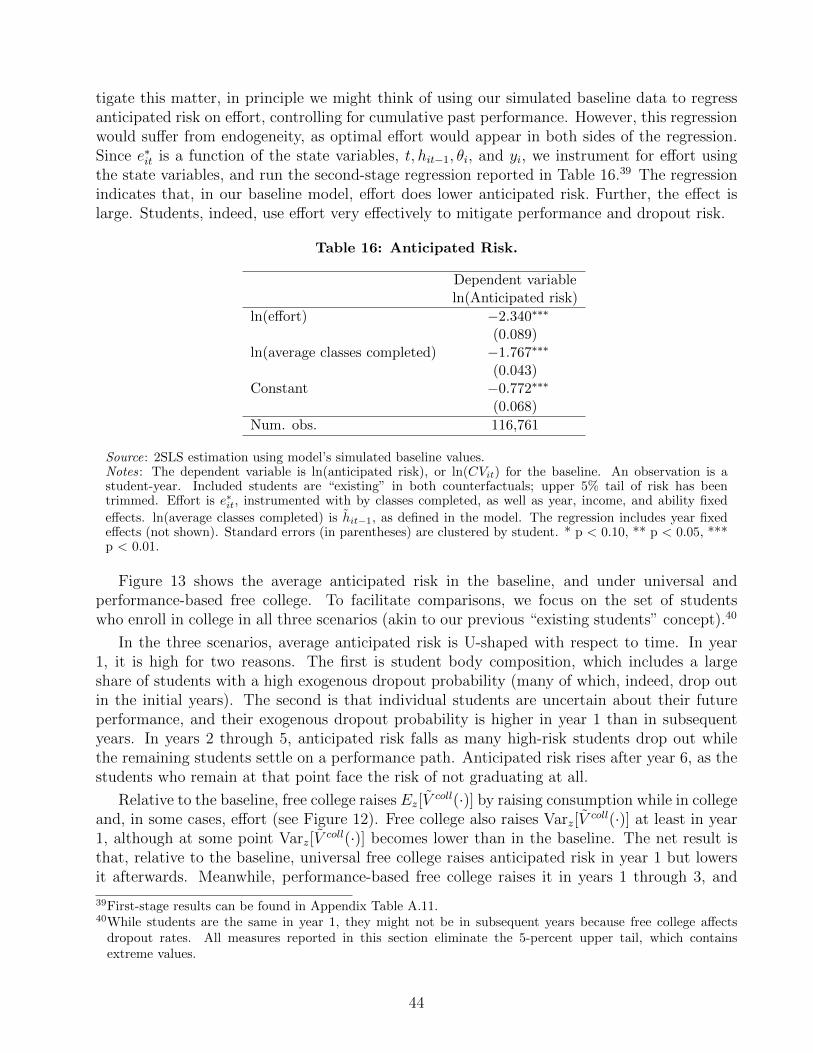
tigate this matter, in principle we might think of using our simulated baseline data to regressanticipated risk on effort, controlling for cumulative past performance. However, this regressionwould suffer from endogeneity, as optimal effort would appear in both sides of the regression.Since e∗it is a function of the state variables, t, hit−1, θi, and yi, we instrument for effort usingthe state variables, and run the second-stage regression reported in Table 16.39 The regressionindicates that, in our baseline model, effort does lower anticipated risk. Further, the effect islarge. Students, indeed, use effort very effectively to mitigate performance and dropout risk.
Table 16: Anticipated Risk.
Dependent variableln(Anticipated risk)
ln(effort) −2.340∗∗∗
(0.089)ln(average classes completed) −1.767∗∗∗
(0.043)Constant −0.772∗∗∗
(0.068)
Num. obs. 116,761
Source: 2SLS estimation using model’s simulated baseline values.Notes: The dependent variable is ln(anticipated risk), or ln(CVit) for the baseline. An observation is astudent-year. Included students are “existing” in both counterfactuals; upper 5% tail of risk has beentrimmed. Effort is e∗it, instrumented with by classes completed, as well as year, income, and ability fixed
effects. ln(average classes completed) is hit−1, as defined in the model. The regression includes year fixedeffects (not shown). Standard errors (in parentheses) are clustered by student. * p < 0.10, ** p < 0.05, ***p < 0.01.
Figure 13 shows the average anticipated risk in the baseline, and under universal andperformance-based free college. To facilitate comparisons, we focus on the set of studentswho enroll in college in all three scenarios (akin to our previous “existing students” concept).40
In the three scenarios, average anticipated risk is U-shaped with respect to time. In year1, it is high for two reasons. The first is student body composition, which includes a largeshare of students with a high exogenous dropout probability (many of which, indeed, drop outin the initial years). The second is that individual students are uncertain about their futureperformance, and their exogenous dropout probability is higher in year 1 than in subsequentyears. In years 2 through 5, anticipated risk falls as many high-risk students drop out whilethe remaining students settle on a performance path. Anticipated risk rises after year 6, as thestudents who remain at that point face the risk of not graduating at all.
Relative to the baseline, free college raises Ez[Vcoll(·)] by raising consumption while in college
and, in some cases, effort (see Figure 12). Free college also raises Varz[Vcoll(·)] at least in year
1, although at some point Varz[Vcoll(·)] becomes lower than in the baseline. The net result is
that, relative to the baseline, universal free college raises anticipated risk in year 1 but lowersit afterwards. Meanwhile, performance-based free college raises it in years 1 through 3, and
39First-stage results can be found in Appendix Table A.11.40While students are the same in year 1, they might not be in subsequent years because free college affects
dropout rates. All measures reported in this section eliminate the 5-percent upper tail, which containsextreme values.
44
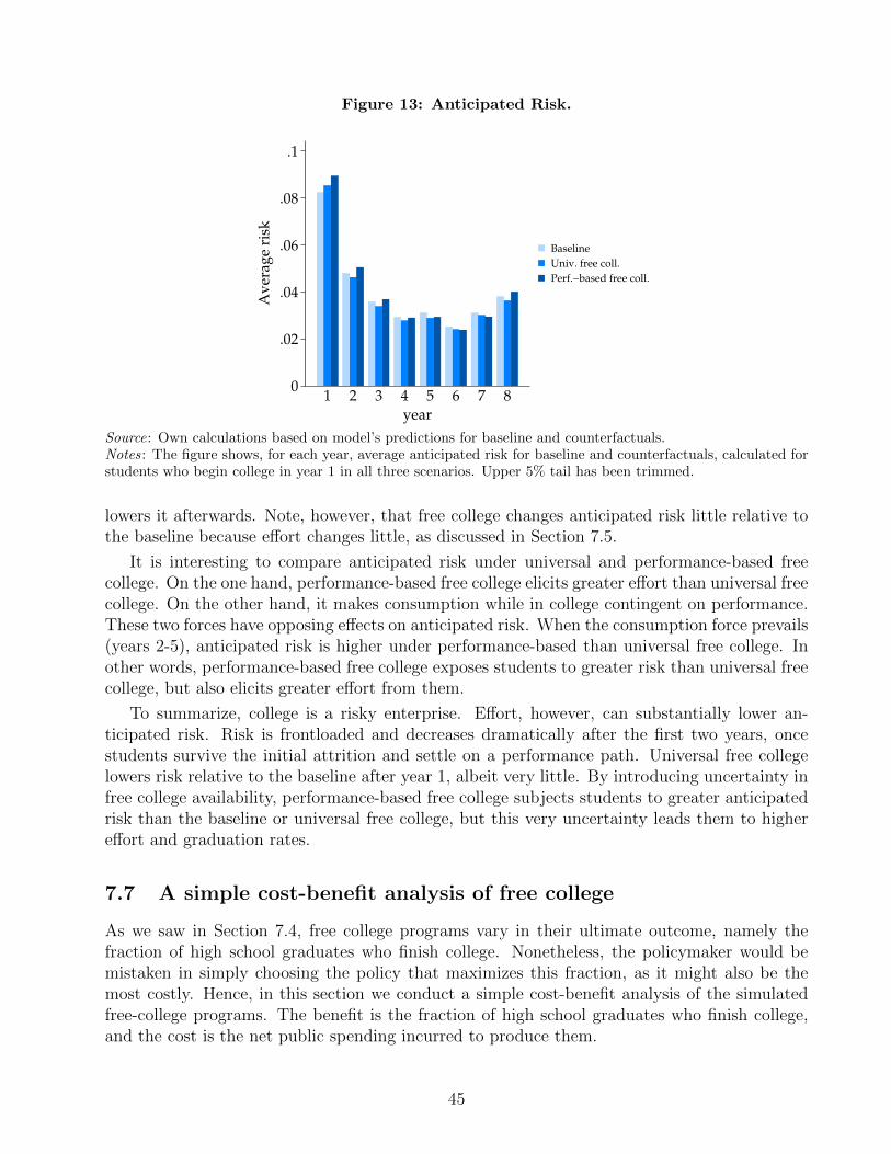
Figure 13: Anticipated Risk.
0
.02
.04
.06
.08
.1
Av
erag
e ri
sk
1 2 3 4 5 6 7 8
year
Baseline
Univ. free coll.
Perf.−based free coll.
Source: Own calculations based on model’s predictions for baseline and counterfactuals.Notes: The figure shows, for each year, average anticipated risk for baseline and counterfactuals, calculated forstudents who begin college in year 1 in all three scenarios. Upper 5% tail has been trimmed.
lowers it afterwards. Note, however, that free college changes anticipated risk little relative tothe baseline because effort changes little, as discussed in Section 7.5.
It is interesting to compare anticipated risk under universal and performance-based freecollege. On the one hand, performance-based free college elicits greater effort than universal freecollege. On the other hand, it makes consumption while in college contingent on performance.These two forces have opposing effects on anticipated risk. When the consumption force prevails(years 2-5), anticipated risk is higher under performance-based than universal free college. Inother words, performance-based free college exposes students to greater risk than universal freecollege, but also elicits greater effort from them.
To summarize, college is a risky enterprise. Effort, however, can substantially lower an-ticipated risk. Risk is frontloaded and decreases dramatically after the first two years, oncestudents survive the initial attrition and settle on a performance path. Universal free collegelowers risk relative to the baseline after year 1, albeit very little. By introducing uncertainty infree college availability, performance-based free college subjects students to greater anticipatedrisk than the baseline or universal free college, but this very uncertainty leads them to highereffort and graduation rates.
7.7 A simple cost-benefit analysis of free college
As we saw in Section 7.4, free college programs vary in their ultimate outcome, namely thefraction of high school graduates who finish college. Nonetheless, the policymaker would bemistaken in simply choosing the policy that maximizes this fraction, as it might also be themost costly. Hence, in this section we conduct a simple cost-benefit analysis of the simulatedfree-college programs. The benefit is the fraction of high school graduates who finish college,and the cost is the net public spending incurred to produce them.
45
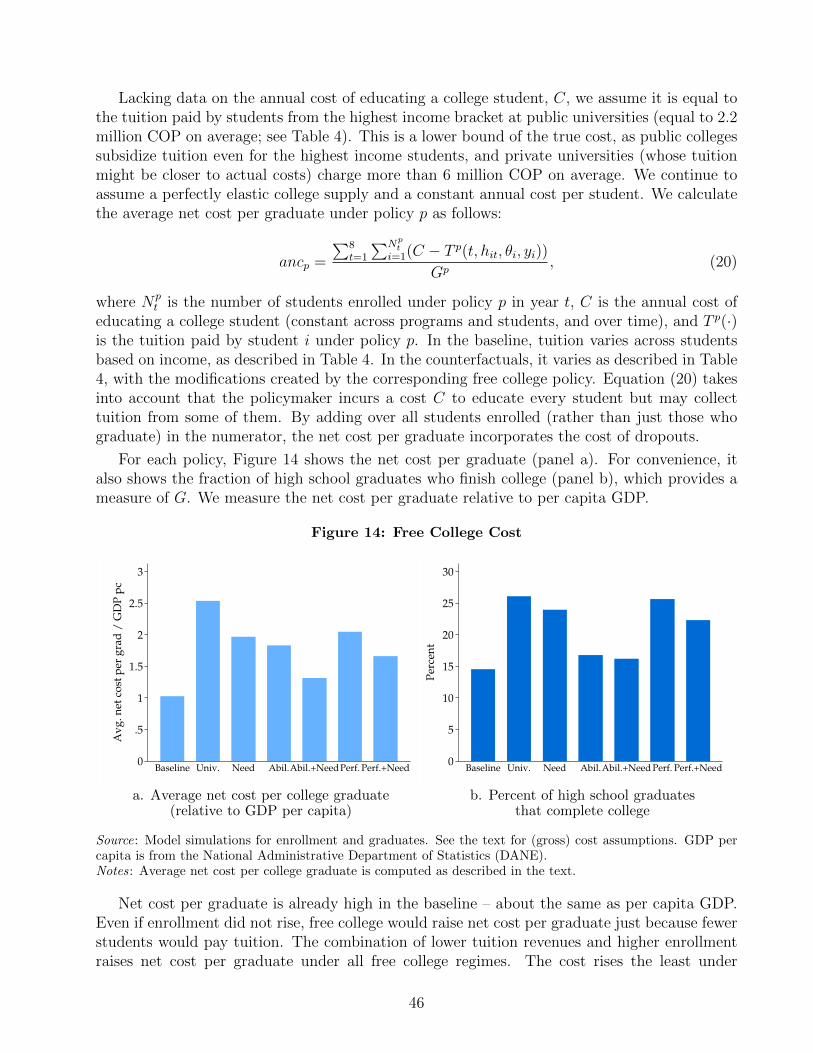
Lacking data on the annual cost of educating a college student, C, we assume it is equal tothe tuition paid by students from the highest income bracket at public universities (equal to 2.2million COP on average; see Table 4). This is a lower bound of the true cost, as public collegessubsidize tuition even for the highest income students, and private universities (whose tuitionmight be closer to actual costs) charge more than 6 million COP on average. We continue toassume a perfectly elastic college supply and a constant annual cost per student. We calculatethe average net cost per graduate under policy p as follows:
ancp =
∑8t=1
∑Npt
i=1(C − T p(t, hit, θi, yi))Gp
, (20)
where Npt is the number of students enrolled under policy p in year t, C is the annual cost of
educating a college student (constant across programs and students, and over time), and T p(·)is the tuition paid by student i under policy p. In the baseline, tuition varies across studentsbased on income, as described in Table 4. In the counterfactuals, it varies as described in Table4, with the modifications created by the corresponding free college policy. Equation (20) takesinto account that the policymaker incurs a cost C to educate every student but may collecttuition from some of them. By adding over all students enrolled (rather than just those whograduate) in the numerator, the net cost per graduate incorporates the cost of dropouts.
For each policy, Figure 14 shows the net cost per graduate (panel a). For convenience, italso shows the fraction of high school graduates who finish college (panel b), which provides ameasure of G. We measure the net cost per graduate relative to per capita GDP.
Figure 14: Free College Cost
0
.5
1
1.5
2
2.5
3
Av
g. n
et c
ost
per
gra
d /
GD
P p
c
Baseline Univ. Need Abil.Abil.+NeedPerf. Perf.+Need0
5
10
15
20
25
30
Percen
t
Baseline Univ. Need Abil.Abil.+Need Perf. Perf.+Need
a. Average net cost per college graduate b. Percent of high school graduates(relative to GDP per capita) that complete college
Source: Model simulations for enrollment and graduates. See the text for (gross) cost assumptions. GDP percapita is from the National Administrative Department of Statistics (DANE).Notes: Average net cost per college graduate is computed as described in the text.
Net cost per graduate is already high in the baseline – about the same as per capita GDP.Even if enrollment did not rise, free college would raise net cost per graduate just because fewerstudents would pay tuition. The combination of lower tuition revenues and higher enrollmentraises net cost per graduate under all free college regimes. The cost rises the least under
46
ability-and-need based free college, and the most under universal free college.This is, of course,a reflection of the number of graduates from each policy: while universal free college adds themost graduates relative to the baseline, ability-and-need based free college adds the least.
Consider, now, a policymaker who is interested in maximizing the number of graduatessubject to a budget constraint. Universal and performance-based free college maximize thenumber of graduates, yet performance-based free college does it at a lower per-graduate costthan universal free college. This is because the incentives embedded in performance-based freecollege produce fewer dropouts and graduate students faster than universal free college. Byadopting performance-based rather than universal free college, the policymaker would save noless than 50 percent of per capita GDP in each graduate. Further, he would raise efficiencyrelative to the baseline by incentivizing effort and focusing public spending on the studentswho, given their performance, are most likely to graduate.
Despite these public savings and efficiency gains, the policymaker might be reluctant toadopt performance-based free college due, perhaps, to political considerations. Indeed, stu-dents throughout Latin America have been clamoring for unconditional, universal free college(gratuidad). As Figure 14 shows, universal free college raises the number of graduates onlyslightly more than need-based free college yet costs an additional 50 percent of per capitaGDP per graduate. The reason is that universal free college provides a transfer to medium-and high-income students who would attend college even anyway. Therefore, when having tochoose between universal and need-based free college, the latter is preferrable.
One caveat is in order before finishing this section. College dropouts seem to acquire humancapital during their time in college, as given by their wage premium relative to high schoolgraduates (see Section 5.2.2). This may motivate the policymaker to raise enrollment regardlessof graduation. The question, then, is whether starting but not completing a bachelor’s programis the most efficient way of acquiring human capital beyond high school. A short-cycle program,lasting two or three years, might be a more cost-effective option, and one that would avoid thepsychic cost for students derived from starting but not finishing a bachelor’s program. It wouldalso avoid the overcrowding of bachelor’s programs during the initial years, which are critical tofinal outcomes. The policymaker might consider providing free college for short-cycle programs,in the spirit of the relativley higher tuition subsidies provided for community colleges ratherthan bachelor’s programs at public institutions in the United States (Denning 2017).
7.8 Long-run effects
One limitation of the current analysis is the assumption that, despite the greater supply ofcollege graduates due to free college, the college premium does not change. In reality, however,the college premium might fall, thereby reducing the incentives to attend college. In addition,financing free college might require taxes, which would further depress after-tax wages forcollege graduates. In other words, free college might unleash general equilibrium effects thatcould undermine some of the effects previously described.41
To analyze the equilibrium relationship between the college premium and the number ofcollege graduates, we postulate a production function following Katz and Murphy (1992),
41Heckman et al (1998) conclude that ignoring general equilibrium effects can bias the estimated effects oftuition subsidies.
47
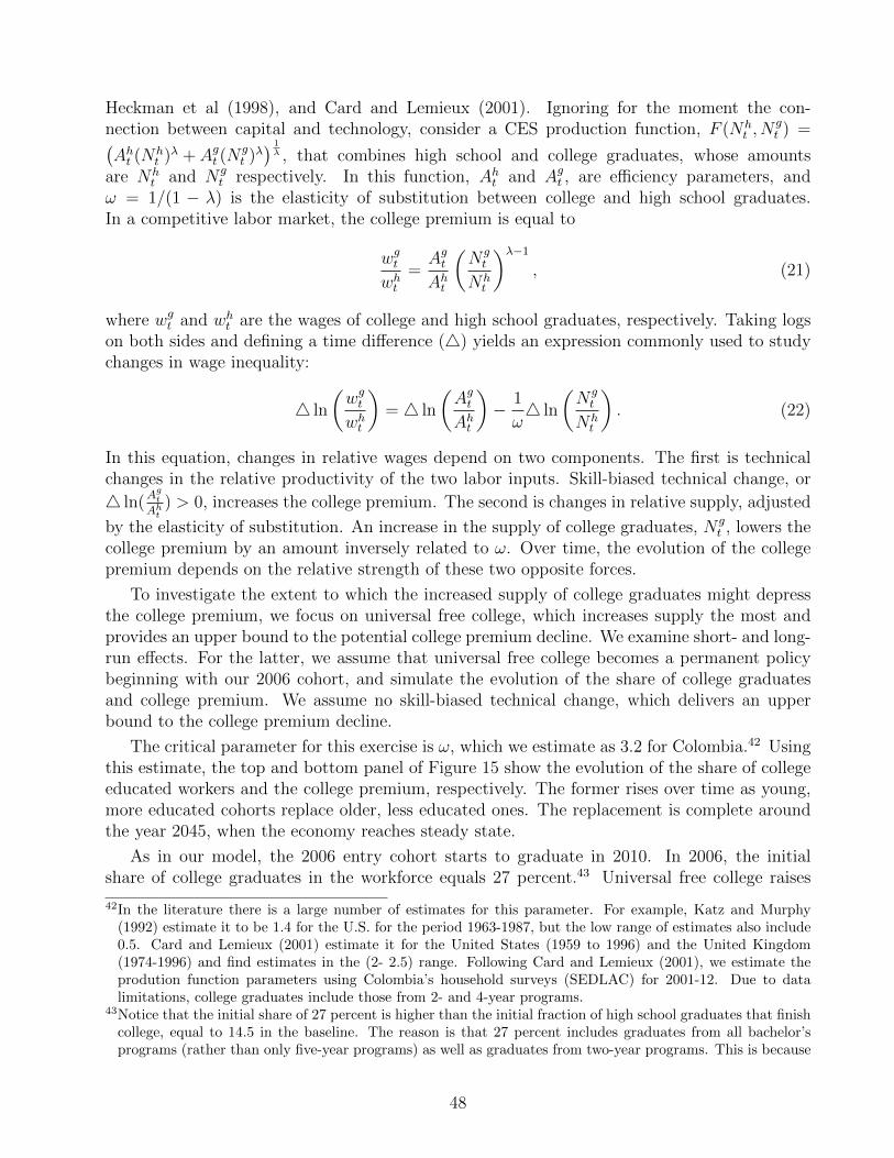
Heckman et al (1998), and Card and Lemieux (2001). Ignoring for the moment the con-nection between capital and technology, consider a CES production function, F (Nh
t , Ngt ) =(
Aht (Nht )λ + Agt (N
gt )λ) 1λ , that combines high school and college graduates, whose amounts
are Nht and N g
t respectively. In this function, Aht and Agt , are efficiency parameters, andω = 1/(1 − λ) is the elasticity of substitution between college and high school graduates.In a competitive labor market, the college premium is equal to
wgtwht
=AgtAht
(N gt
Nht
)λ−1
, (21)
where wgt and wht are the wages of college and high school graduates, respectively. Taking logson both sides and defining a time difference (4) yields an expression commonly used to studychanges in wage inequality:
4 ln
(wgtwht
)= 4 ln
(AgtAht
)− 1
ω4 ln
(N gt
Nht
). (22)
In this equation, changes in relative wages depend on two components. The first is technicalchanges in the relative productivity of the two labor inputs. Skill-biased technical change, or
4 ln(AgtAht
) > 0, increases the college premium. The second is changes in relative supply, adjusted
by the elasticity of substitution. An increase in the supply of college graduates, N gt , lowers the
college premium by an amount inversely related to ω. Over time, the evolution of the collegepremium depends on the relative strength of these two opposite forces.
To investigate the extent to which the increased supply of college graduates might depressthe college premium, we focus on universal free college, which increases supply the most andprovides an upper bound to the potential college premium decline. We examine short- and long-run effects. For the latter, we assume that universal free college becomes a permanent policybeginning with our 2006 cohort, and simulate the evolution of the share of college graduatesand college premium. We assume no skill-biased technical change, which delivers an upperbound to the college premium decline.
The critical parameter for this exercise is ω, which we estimate as 3.2 for Colombia.42 Usingthis estimate, the top and bottom panel of Figure 15 show the evolution of the share of collegeeducated workers and the college premium, respectively. The former rises over time as young,more educated cohorts replace older, less educated ones. The replacement is complete aroundthe year 2045, when the economy reaches steady state.
As in our model, the 2006 entry cohort starts to graduate in 2010. In 2006, the initialshare of college graduates in the workforce equals 27 percent.43 Universal free college raises
42In the literature there is a large number of estimates for this parameter. For example, Katz and Murphy(1992) estimate it to be 1.4 for the U.S. for the period 1963-1987, but the low range of estimates also include0.5. Card and Lemieux (2001) estimate it for the United States (1959 to 1996) and the United Kingdom(1974-1996) and find estimates in the (2- 2.5) range. Following Card and Lemieux (2001), we estimate theprodution function parameters using Colombia’s household surveys (SEDLAC) for 2001-12. Due to datalimitations, college graduates include those from 2- and 4-year programs.
43Notice that the initial share of 27 percent is higher than the initial fraction of high school graduates that finishcollege, equal to 14.5 in the baseline. The reason is that 27 percent includes graduates from all bachelor’sprograms (rather than only five-year programs) as well as graduates from two-year programs. This is because
48
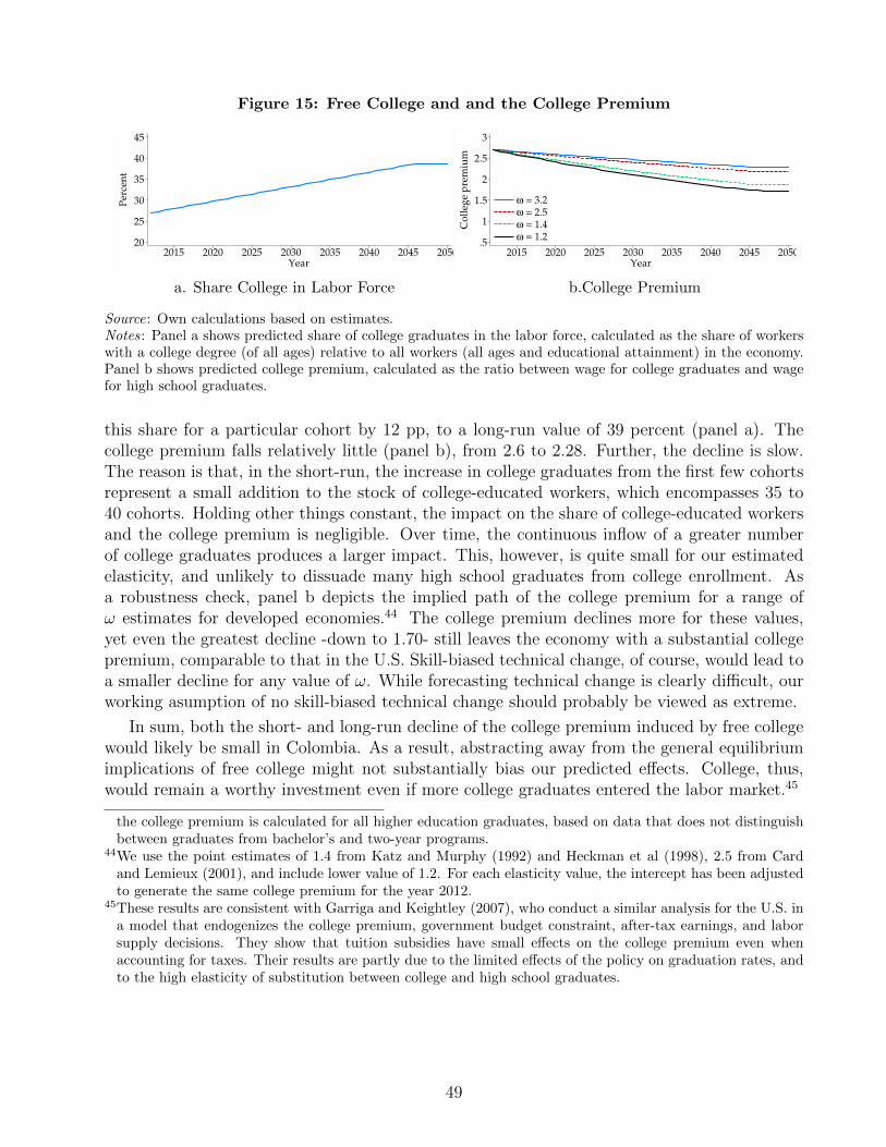
Figure 15: Free College and and the College Premium
20
25
30
35
40
45
Percen
t
2015 2020 2025 2030 2035 2040 2045 2050
Year
.5
1
1.5
2
2.5
3
Co
lleg
e p
rem
ium
2015 2020 2025 2030 2035 2040 2045 2050Year
ω = 3.2ω = 2.5ω = 1.4ω = 1.2
a. Share College in Labor Force b.College Premium
Source: Own calculations based on estimates.Notes: Panel a shows predicted share of college graduates in the labor force, calculated as the share of workerswith a college degree (of all ages) relative to all workers (all ages and educational attainment) in the economy.Panel b shows predicted college premium, calculated as the ratio between wage for college graduates and wagefor high school graduates.
this share for a particular cohort by 12 pp, to a long-run value of 39 percent (panel a). Thecollege premium falls relatively little (panel b), from 2.6 to 2.28. Further, the decline is slow.The reason is that, in the short-run, the increase in college graduates from the first few cohortsrepresent a small addition to the stock of college-educated workers, which encompasses 35 to40 cohorts. Holding other things constant, the impact on the share of college-educated workersand the college premium is negligible. Over time, the continuous inflow of a greater numberof college graduates produces a larger impact. This, however, is quite small for our estimatedelasticity, and unlikely to dissuade many high school graduates from college enrollment. Asa robustness check, panel b depicts the implied path of the college premium for a range ofω estimates for developed economies.44 The college premium declines more for these values,yet even the greatest decline -down to 1.70- still leaves the economy with a substantial collegepremium, comparable to that in the U.S. Skill-biased technical change, of course, would lead toa smaller decline for any value of ω. While forecasting technical change is clearly difficult, ourworking asumption of no skill-biased technical change should probably be viewed as extreme.
In sum, both the short- and long-run decline of the college premium induced by free collegewould likely be small in Colombia. As a result, abstracting away from the general equilibriumimplications of free college might not substantially bias our predicted effects. College, thus,would remain a worthy investment even if more college graduates entered the labor market.45
the college premium is calculated for all higher education graduates, based on data that does not distinguishbetween graduates from bachelor’s and two-year programs.
44We use the point estimates of 1.4 from Katz and Murphy (1992) and Heckman et al (1998), 2.5 from Cardand Lemieux (2001), and include lower value of 1.2. For each elasticity value, the intercept has been adjustedto generate the same college premium for the year 2012.
45These results are consistent with Garriga and Keightley (2007), who conduct a similar analysis for the U.S. ina model that endogenizes the college premium, government budget constraint, after-tax earnings, and laborsupply decisions. They show that tuition subsidies have small effects on the college premium even whenaccounting for taxes. Their results are partly due to the limited effects of the policy on graduation rates, andto the high elasticity of substitution between college and high school graduates.
49
8 Conclusions
In this paper we have developed and estimated a dynamic model of college enrollment, per-formance, and graduation. A central piece of the model, student effort, has a direct effect onthe completion of classes, and an indirect effect mitigating the risk of not completing a classor not remaining enrolled. We have estimated the model using rich administrative data forColombia. According to our estimates, effort has much greater impact than ability on classcompletion. Failing to model effort as an input to class completion leads to overestimating therole of ability by about 75 percent, and to favoring policies that promote positive selection ofnew students rather than effort. We have used our parameter estimates to simulate free collegeprograms differing in eligibility. According to our simulations, universal free college expandsenrollment the most but has the highest per-graduate cost and does not raise graduation rates.Performance-based free college, in contrast, delivers a slightly lower enrollment expansion buthas a greater graduation rate and a lower per-graduate cost. Performance-based free collegefaces students with greater risks than the current baseline or universal free college, but preciselyfor this reason elicits greater effort and graduation rates.
For existing students, free college has little impact on effort and graduation rates, evenwhen it is performance-based. This suggests that additional, complementary policies mightbe needed. Given the high persistence of performance, improving first-year performance andretention is critical. Supports such as tutoring, remedial education, mentoring, and advisingmight be helpful, particularly for the most disadvantaged students. Further, most collegeprograms in Latin America start with classes specific to the major or field, and rarely includegeneral education requirements that transfer easily across majors. As a result, changing majorstypically implies starting from scratch, which leads many students to abandon higher education.Shortening bachelor’s programs (which last five or six years) and connecting them with the labormarket might raise effort and graduation rates as well.
Finally, there might be an additional reason why free college fails to elicit large effort changes:particularly for low-income students, free college might not be enough. For them, the effortnecessary to complete college might require not only free tuition but also an additional, generousstipend. In countries with limited fiscal resources, providing this additional stipend mightrequire lowering the existing college subsidies for affluent students – a redistribution that, whilepolitically costly, would nonetheless enhance equity and efficiency.
50
References
[1] Abbot, B., Gallipoli, G., Meghir, C., & Violante, G. (2013). Education decisions and inter-generational transfers in equilibrium (Working Paper). New York: New York University.
[2] Ahn, T., Arcidiacono, P., Hopson, A., & Thomas, J. R. (2019). Equilibrium grade inflationwith implications for female interest in stem majors. NBER Working Paper No. w26556.
[3] Akyol, A. & Athreya, K. (2005). Risky higher education and subsidies. Journal of EconomicDynamics and Control, 29(6), pp. 979-1023.
[4] Altonji, J. (1993). The demand for and return to education when education outcomes areuncertain. Journal of Labor Economics, 11(1), pp. 48-83.
[5] Arcidiacono, P. (2004). Ability sorting and the returns to college major. Journal of Econo-metrics, 121(1-2), pp.343-375
[6] Arcidiacono, P., E. Aucejo, A. Maurel, & T. Ransom (2016). College attrition and thedynamics of information revelation. NBER Working Paper No. 22325.
[7] Ariely, D., U. Gneezy, G. Loewenstein, & N. Mazar (2009). Large stakes and big Mistakes.Review of Economic Studies, 76(2), pp. 451-469.
[8] Avery, C., Howell, J., Pender, M., & Sacerdote, B. (2019). Policies and payoffs to addressingAmerica’s college graduation deficit. In BPEA Conference Draft, Fall.
[9] Beneito, P., J. Bosca & J. Ferri (2018). Tuition fees and student effort at university.Economics of Education Review, 64(C), pp. 114-128.
[10] Berry, S., J. Levinsohn, A. Pakes (1995). Automobile prices in market equilibrium, Econo-metrica, pp: 841–890
[11] Bettinger, E. (2004). How financial aid affects persistence. In College choices: The eco-nomics of where to go, when to go, and how to pay for it (pp. 207-238). University ofChicago Press.
[12] Bettinger, E., Gurantz, O., Kawano, L., Sacerdote, B., & Stevens, M. (2019). The long-run impacts of financial aid: Evidence from California’s Cal Grant. American EconomicJournal: Economic Policy, 11(1), 64-94.
[13] Bucarey, A. (2018). Who pays for college? Crowding out on campus. Working Paper,Massachusetts Institute of Technology.
[14] Cameron S.V. & Heckman, J. J. (1998). Life cycle schooling and dynamic selection bias:Models and evidence for five cohorts of American males. The Journal of Political Economy,106(2). pp. 262-333.
[15] Cameron S.V. & Heckman, J. J. (1999).The dynamics of educational attainment for blacks,hispanics and whites (Working Paper 7249). Cambridge, MA: National Bureau of EconomicResearch.
51
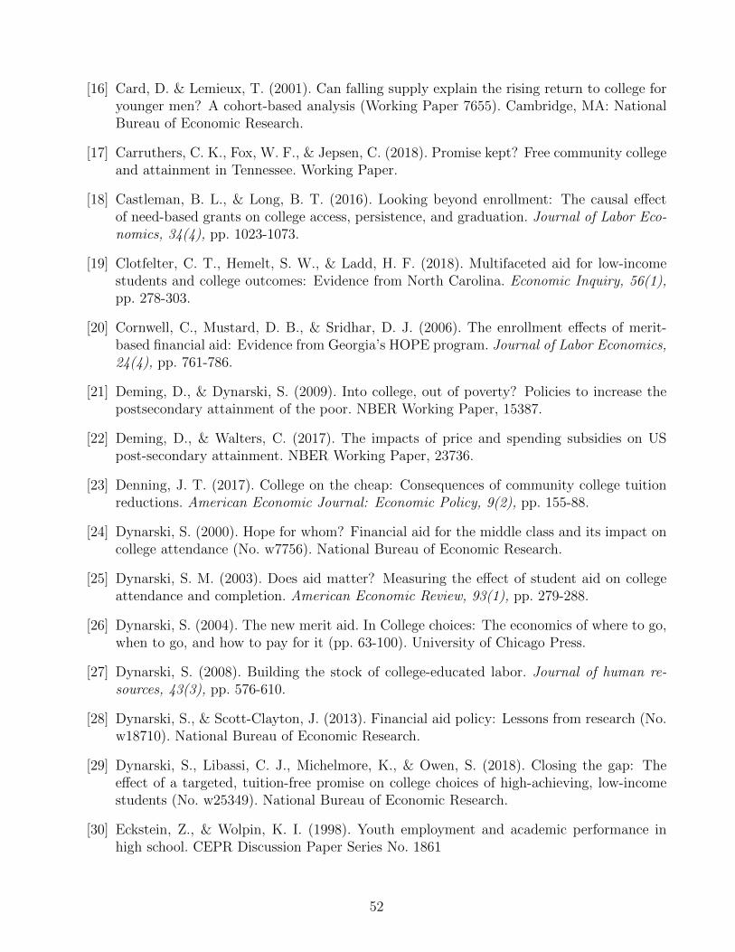
[16] Card, D. & Lemieux, T. (2001). Can falling supply explain the rising return to college foryounger men? A cohort-based analysis (Working Paper 7655). Cambridge, MA: NationalBureau of Economic Research.
[17] Carruthers, C. K., Fox, W. F., & Jepsen, C. (2018). Promise kept? Free community collegeand attainment in Tennessee. Working Paper.
[18] Castleman, B. L., & Long, B. T. (2016). Looking beyond enrollment: The causal effectof need-based grants on college access, persistence, and graduation. Journal of Labor Eco-nomics, 34(4), pp. 1023-1073.
[19] Clotfelter, C. T., Hemelt, S. W., & Ladd, H. F. (2018). Multifaceted aid for low-incomestudents and college outcomes: Evidence from North Carolina. Economic Inquiry, 56(1),pp. 278-303.
[20] Cornwell, C., Mustard, D. B., & Sridhar, D. J. (2006). The enrollment effects of merit-based financial aid: Evidence from Georgia’s HOPE program. Journal of Labor Economics,24(4), pp. 761-786.
[21] Deming, D., & Dynarski, S. (2009). Into college, out of poverty? Policies to increase thepostsecondary attainment of the poor. NBER Working Paper, 15387.
[22] Deming, D., & Walters, C. (2017). The impacts of price and spending subsidies on USpost-secondary attainment. NBER Working Paper, 23736.
[23] Denning, J. T. (2017). College on the cheap: Consequences of community college tuitionreductions. American Economic Journal: Economic Policy, 9(2), pp. 155-88.
[24] Dynarski, S. (2000). Hope for whom? Financial aid for the middle class and its impact oncollege attendance (No. w7756). National Bureau of Economic Research.
[25] Dynarski, S. M. (2003). Does aid matter? Measuring the effect of student aid on collegeattendance and completion. American Economic Review, 93(1), pp. 279-288.
[26] Dynarski, S. (2004). The new merit aid. In College choices: The economics of where to go,when to go, and how to pay for it (pp. 63-100). University of Chicago Press.
[27] Dynarski, S. (2008). Building the stock of college-educated labor. Journal of human re-sources, 43(3), pp. 576-610.
[28] Dynarski, S., & Scott-Clayton, J. (2013). Financial aid policy: Lessons from research (No.w18710). National Bureau of Economic Research.
[29] Dynarski, S., Libassi, C. J., Michelmore, K., & Owen, S. (2018). Closing the gap: Theeffect of a targeted, tuition-free promise on college choices of high-achieving, low-incomestudents (No. w25349). National Bureau of Economic Research.
[30] Eckstein, Z., & Wolpin, K. I. (1998). Youth employment and academic performance inhigh school. CEPR Discussion Paper Series No. 1861
52
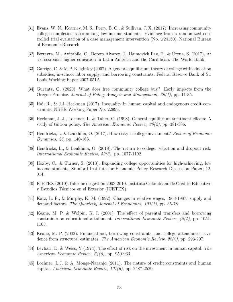
[31] Evans, W. N., Kearney, M. S., Perry, B. C., & Sullivan, J. X. (2017). Increasing communitycollege completion rates among low-income students: Evidence from a randomized con-trolled trial evaluation of a case management intervention (No. w24150). National Bureauof Economic Research.
[32] Ferreyra, M., Avitabile, C., Botero Alvarez, J., Haimovich Paz, F., & Urzua, S. (2017). Ata crossroads: higher education in Latin America and the Caribbean. The World Bank.
[33] Garriga, C. & M.P. Keightley (2007). A general equilibrium theory of college with educationsubsidies, in-school labor supply, and borrowing constraints. Federal Reserve Bank of St.Louis Working Paper 2007-051A.
[34] Gurantz, O. (2020). What does free community college buy? Early impacts from theOregon Promise. Journal of Policy Analysis and Management, 39(1), pp. 11-35.
[35] Hai, R., & J.J. Heckman (2017). Inequality in human capital and endogenous credit con-straints. NBER Working Paper No. 22999.
[36] Heckman, J. J., Lochner, L. & Taber, C. (1998). General equilibrium treatment effects: Astudy of tuition policy. The American Economic Review, 88(2), pp. 381-386.
[37] Hendricks, L. & Leukhina, O. (2017). How risky is college investment? Review of EconomicDynamics, 26, pp. 140-163.
[38] Hendricks, L., & Leukhina, O. (2018). The return to college: selection and dropout risk.International Economic Review, 59(3), pp. 1077-1102.
[39] Hoxby, C., & Turner, S. (2013). Expanding college opportunities for high-achieving, lowincome students. Stanford Institute for Economic Policy Research Discussion Paper, 12,014.
[40] ICETEX (2010). Informe de gestion 2003-2010. Instituto Colombiano de Credito Educativoy Estudios Tecnicos en el Exterior (ICETEX).
[41] Katz, L. F., & Murphy, K. M. (1992). Changes in relative wages, 1963-1987: supply anddemand factors. The Quarterly Journal of Economics, 107(1), pp. 35-78.
[42] Keane, M. P. & Wolpin, K. I. (2001). The effect of parental transfers and borrowingconstraints on educational attainment. International Economic Review, 42(4), pp. 1051-1103.
[43] Keane, M. P. (2002). Financial aid, borrowing constraints, and college attendance: Evi-dence from structural estimates. The American Economic Review, 92(2), pp. 293-297.
[44] Levhari, D. & Weiss, Y (1974). The effect of risk on the investment in human capital. TheAmerican Economic Review, 64(6), pp. 950-963.
[45] Lochner, L.J. & A. Monge-Naranjo (2011). The nature of credit constraints and humancapital. American Economic Review, 101(6), pp. 2487-2529.
53
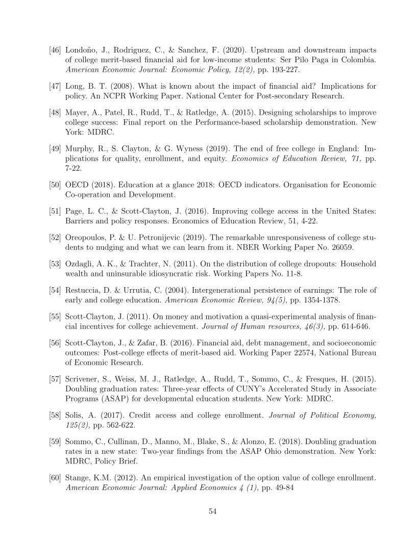
[46] Londono, J., Rodriguez, C., & Sanchez, F. (2020). Upstream and downstream impactsof college merit-based financial aid for low-income students: Ser Pilo Paga in Colombia.American Economic Journal: Economic Policy, 12(2), pp. 193-227.
[47] Long, B. T. (2008). What is known about the impact of financial aid? Implications forpolicy. An NCPR Working Paper. National Center for Post-secondary Research.
[48] Mayer, A., Patel, R., Rudd, T., & Ratledge, A. (2015). Designing scholarships to improvecollege success: Final report on the Performance-based scholarship demonstration. NewYork: MDRC.
[49] Murphy, R., S. Clayton, & G. Wyness (2019). The end of free college in England: Im-plications for quality, enrollment, and equity. Economics of Education Review, 71, pp.7-22.
[50] OECD (2018). Education at a glance 2018: OECD indicators. Organisation for EconomicCo-operation and Development.
[51] Page, L. C., & Scott-Clayton, J. (2016). Improving college access in the United States:Barriers and policy responses. Economics of Education Review, 51, 4-22.
[52] Oreopoulos, P. & U. Petronijevic (2019). The remarkable unresponsiveness of college stu-dents to nudging and what we can learn from it. NBER Working Paper No. 26059.
[53] Ozdagli, A. K., & Trachter, N. (2011). On the distribution of college dropouts: Householdwealth and uninsurable idiosyncratic risk. Working Papers No. 11-8.
[54] Restuccia, D. & Urrutia, C. (2004). Intergenerational persistence of earnings: The role ofearly and college education. American Economic Review, 94(5), pp. 1354-1378.
[55] Scott-Clayton, J. (2011). On money and motivation a quasi-experimental analysis of finan-cial incentives for college achievement. Journal of Human resources, 46(3), pp. 614-646.
[56] Scott-Clayton, J., & Zafar, B. (2016). Financial aid, debt management, and socioeconomicoutcomes: Post-college effects of merit-based aid. Working Paper 22574, National Bureauof Economic Research.
[57] Scrivener, S., Weiss, M. J., Ratledge, A., Rudd, T., Sommo, C., & Fresques, H. (2015).Doubling graduation rates: Three-year effects of CUNY’s Accelerated Study in AssociatePrograms (ASAP) for developmental education students. New York: MDRC.
[58] Solis, A. (2017). Credit access and college enrollment. Journal of Political Economy,125(2), pp. 562-622.
[59] Sommo, C., Cullinan, D., Manno, M., Blake, S., & Alonzo, E. (2018). Doubling graduationrates in a new state: Two-year findings from the ASAP Ohio demonstration. New York:MDRC, Policy Brief.
[60] Stange, K.M. (2012). An empirical investigation of the option value of college enrollment.American Economic Journal: Applied Economics 4 (1), pp. 49-84
54
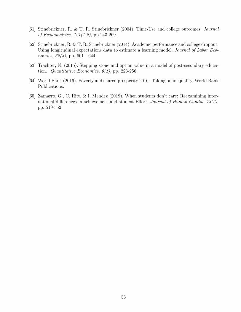
[61] Stinebrickner, R. & T. R. Stinebrickner (2004). Time-Use and college outcomes. Journalof Econometrics, 121(1-2), pp 243-269.
[62] Stinebrickner, R. & T. R. Stinebrickner (2014). Academic performance and college dropout:Using longitudinal expectations data to estimate a learning model. Journal of Labor Eco-nomics, 32(3), pp. 601 - 644.
[63] Trachter, N. (2015). Stepping stone and option value in a model of post-secondary educa-tion. Quantitative Economics, 6(1), pp. 223-256.
[64] World Bank (2016). Poverty and shared prosperity 2016: Taking on inequality. World BankPublications.
[65] Zamarro, G., C. Hitt, & I. Mendez (2019). When students don’t care: Reexamining inter-national differences in achievement and student Effort. Journal of Human Capital, 13(2),pp. 519-552.
55
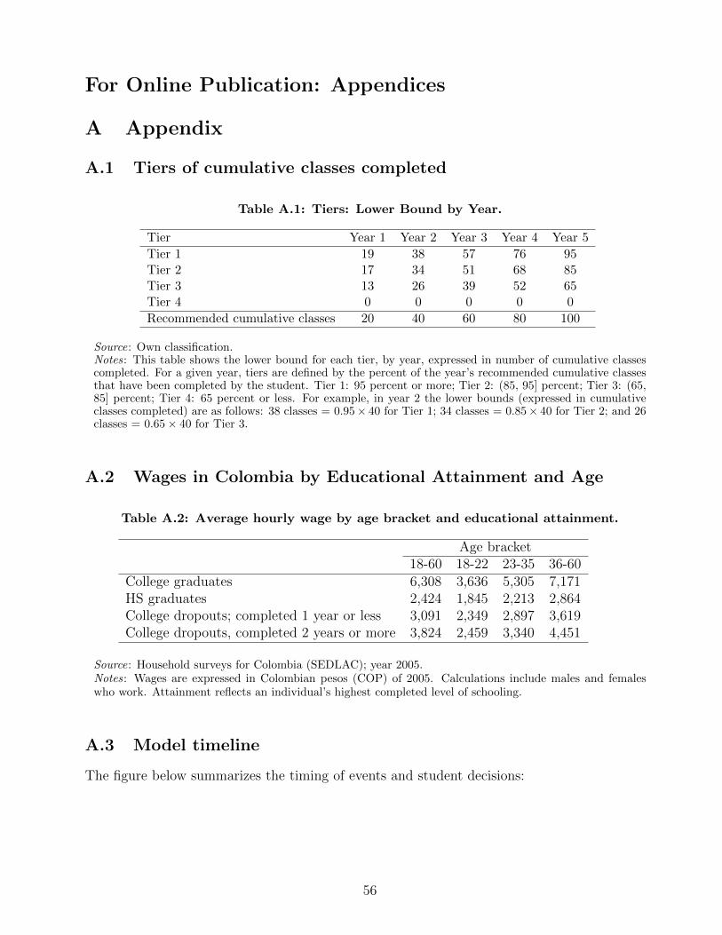
For Online Publication: Appendices
A Appendix
A.1 Tiers of cumulative classes completed
Table A.1: Tiers: Lower Bound by Year.
Tier Year 1 Year 2 Year 3 Year 4 Year 5
Tier 1 19 38 57 76 95Tier 2 17 34 51 68 85Tier 3 13 26 39 52 65Tier 4 0 0 0 0 0
Recommended cumulative classes 20 40 60 80 100
Source: Own classification.Notes: This table shows the lower bound for each tier, by year, expressed in number of cumulative classescompleted. For a given year, tiers are defined by the percent of the year’s recommended cumulative classesthat have been completed by the student. Tier 1: 95 percent or more; Tier 2: (85, 95] percent; Tier 3: (65,85] percent; Tier 4: 65 percent or less. For example, in year 2 the lower bounds (expressed in cumulativeclasses completed) are as follows: 38 classes = 0.95× 40 for Tier 1; 34 classes = 0.85× 40 for Tier 2; and 26classes = 0.65× 40 for Tier 3.
A.2 Wages in Colombia by Educational Attainment and Age
Table A.2: Average hourly wage by age bracket and educational attainment.
Age bracket18-60 18-22 23-35 36-60
College graduates 6,308 3,636 5,305 7,171HS graduates 2,424 1,845 2,213 2,864College dropouts; completed 1 year or less 3,091 2,349 2,897 3,619College dropouts, completed 2 years or more 3,824 2,459 3,340 4,451
Source: Household surveys for Colombia (SEDLAC); year 2005.Notes: Wages are expressed in Colombian pesos (COP) of 2005. Calculations include males and femaleswho work. Attainment reflects an individual’s highest completed level of schooling.
A.3 Model timeline
The figure below summarizes the timing of events and student decisions:
56
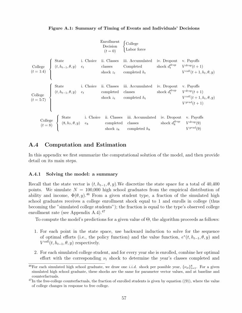
Figure A.1: Summary of Timing of Events and Individuals’ Decisions
EnrollmentDecision(t = 0)
{College
Labor force
College(t = 1:4)
State i. Choice ii. Classes iii. Accumulated iv. Dropout v. Payoffs
(t, ht−1, θ, y) et classes Completed shock ddropt V drop(t+ 1)
shock zt completed ht V coll(t+ 1, ht, θ, y)
College(t = 5:7)
State i. Choice ii. Classes iii. Accumulated iv. Dropout v. Payoffs
(t, ht−1, θ, y) et completed classes shock ddropt V drop(t+ 1)
shock zt completed ht V coll(t+ 1, ht, θ, y)
V grad(t+ 1)
College(t = 8)
State i. Choice ii. Classes iii. Accumulated iv. Dropout v. Payoffs
(8, h7, θ, y) e8 completed classes shock ddrop8 V drop(9)
shock z8 completed h8 V grad(9)
A.4 Computation and Estimation
In this appendix we first summarize the computational solution of the model, and then providedetail on its main steps.
A.4.1 Solving the model: a summary
Recall that the state vector is (t, ht−1, θ, y).We discretize the state space for a total of 40,400points. We simulate N = 100,000 high school graduates from the empirical distribution ofability and income, Φ(θ, y).46 From a given student type, a fraction of the simulated highschool graduates receives a college enrollment shock equal to 1 and enrolls in college (thusbecoming the ”simulated college students”); the fraction is equal to the type’s observed collegeenrollment rate (see Appendix A.4).47
To compute the model’s predictions for a given value of Θ, the algorithm proceeds as follows:
1. For each point in the state space, use backward induction to solve for the sequenceof optimal efforts (i.e., the policy function) and the value function, e∗(t, ht−1, θ, y) andV coll(t, ht−1, θ, y) respectively.
2. For each simulated college student, and for every year she is enrolled, combine her optimaleffort with the corresponding νt shock to determine the year’s classes completed and
46For each simulated high school graduate, we draw one i.i.d. shock per possible year, {νit}8t=1. For a givensimulated high school graduate, these shocks are the same for parameter vector values, and at baseline andcounterfactuals.
47In the free-college counterfactuals, the fraction of enrolled students is given by equation ((9)), where the valueof college changes in response to free college.
57
probability of dropping out, pd(t, ht, θ, y). Draw the binary dropout shock; the shock isequal to 1 with probability pd(t, ht, θ, y).
3. Based on step 2, aggregate the simulated dropout decisions to obtain a predicted dropoutrate for each of the 400 (t, θ, y)-combinations.
4. Find the vector δ that minimizes the distance between the predicted and observed dropoutrate for each (t, θ, y)-combination, using the contraction mapping algorithm described inAppendix A.4.3.
5. By comparing the value of going and not going to college for each type, V coll(1, 0, θ, y)and V hs, respectively, find the type-specific college enrollment shock, ξj, that renders thetype indifferent between going and not going to college. Further details are provided inAppendix A.4.4.
Solving steps 1-5 of the dynamic optimization problem for 100, 000 simulated high schoolgraduates and 40, 400 states takes approximately 8 minutes in a 1.4 GHz Intel Core i5 processor.Since the model does not have a closed-form solution, in estimation the problem must be solvedanew for each value of Θ. Note that the estimation of δ and ξ is nested within the modelsolution for a given of value of Θ, in the spirit of Berry et al (1995), as described in AppendixA.4.3.
A.4.2 Further details on solving the model
The solution of the dynamic problem and computation of predicted outcomes for a given valueof Θ involve three steps: calculating the value of working by educational attainment, solvingfor the policy and value functions, and simulating college students.
Calculating the value of working by educational attainment Since we solve the stu-dent’s dynamic programming problem by backward induction, we begin by calculating the finalvalue of the individuals’ finite horizon problem. We calculate the value of future discountedpayoffs of working as a college graduate, high school graduate, college dropout with one yearof college, and college dropout with two or more years of college. In the timing of the model,t = 1 when the individual is 18 years old, and either starts college or joins the labor force as ahigh school graduate. The value of working as a high school graduate since t = 1 onward is
V hs =L∑t=1
βt−1u(whst ), (23)
where whst is the average wage for a high school graduate in year t, and L is retirement age(65 years old, or L = 48). For this and the other educational attainments, we allow the wageto vary over time to incorporate returns to experience (which accrue after age 35, that is fort > 17). Similarly, the value of working as a college dropout who has completed n years ofcollege is
V drop(n+ 1) =L∑
t=n+1
βt−n−1u(wdropt ), (24)
58
where wdropt is the wage an individual who dropped out of college receives in year t. Finally,the value of working as a college graduate who took n years to graduate is:
V grad(n+ 1) =L∑
t=n+1
βt−n−1u(wgradt ), (25)
Solving for the policy and value functions Since the state, (t, ht−1, θ, y), has four di-mensions, we build two-four dimensional grids - one for the policy function, e∗(t, ht−1, θ, y),which contains the optimal effort choice for each state, and another for the optimal payoffs,V coll(t, ht−1, θ, y) associated with e∗(t, ht−1, θ, y). The grid includes 8 points (years) for t, 101points for h (to represent 0, 1, 2, . . . , 100 credits completed), ten points (ability deciles) for θ,and five points for y for a total of 40,400 points. Each ability decile is represented by its median.In other words, θ takes on values corresponding to the 5th, 15th, .... 95th percentile of theability distribution.
We use backward induction to solve the Bellman equation for each period. Starting fromthe last year of college, t = 8, when students must either graduate or drop out, the Bellmanequation is:
V coll(8, h7, θ, y) = U(c8, e8, θ) +βEz
[Pr(h8 ≥ hgrad
)V grad(9) + Pr
(h8 < hgrad
)V drop(9)
]. (26)
By choosing e8 to maximize V coll for every state, (8, h7, θ, y), we find both the policy functionand the value function, e∗(8, h7, θ, y) and V coll(8, h7, θ, y).
Moving backwards to t = 7, we proceed analogously
V coll(7, h6, θ, y) = U(c7, e7, θ) + βEz
[Pr(h7 ≥ hgrad
)V grad(8)+
Pr(h7 < hgrad
) (pd(7, h7, θ, y)V drop(8)+
(1− pd(7, h7, θ, y)
)V coll(8, h7, θ, y)
)],
(27)
where all outcomes V grad(8), V drop(8) and V grad(8, ·) are already known. We continue this proce-dure for t = 6, . . . , 1 in order to complete the calculation of e∗(t, ht−1, θ, y) and V coll(t, ht−1, θ, y)for all possible states.
We use the resulting policy function, e∗(t, ht−1, θ, y), whenever we need to compute a stu-dent’s optimal effort during estimation or counterfactuals. In addition, we use the resultingvalue function at t = 1, that is, V coll(1, 0, θ, y), to calculate the value of enrolling in college,which is to be compared with the value of joining the workforce as a high school graduate, V hs,following equation (8).
Simulating college students We simulate N = 100,000 high school graduates. We makedraws from the joint distribution of ability of parental transfers of high school graduates in 2005,Φ (θj, yj) . Recall that a student type j is given by a (θj, yj) combination. We have J = 50 types.
59
For each type, let P coll(θj, yj), equal to the actual, observed share of individuals of that typethat enrolls in college. Note that P coll(θj, yj) varies across types, as illustrated by Table 1.Consider individual i who belongs to type j. For each simulated individual, we draw a binaryvariable, denri , to determine whether the student goes to college or not. More specifically,
denri =
{1, i goes to college, with probability P coll(θj, yj)
0, i does not goes to college, with probability 1− P coll(θj, yj)(28)
Simulated students who receive denri = 1 are those who enroll in college. In other words, theproportion of simulated students of a given type who receive denri = 1 is the same as theproportion of actual students of that type who enroll in college.48 For students who do notenroll in college, the value function is V hs. For those who enroll in college, we simulate classescompleted and dropout shocks as described below.
For t = 1, we use the policy function e∗(1, 0, θj, yj) corresponding to every student type j.Since all students start at t = 1 with zero accumulated credits, h0 = 0, the policy functionassigns the same effort to all students of a given type, j. Then, we draw the iid shock νi1 foreach student; this, in turn, yields a value for the zi1 shock. The combination of the student’sability, effort, and zi1 shock yields the number of completed credits, hi1. Because of the z shock,individuals of a given type attain different values of h by the end of the first period.
For student i, we use the realized hit to establish whether the student drops out before thesecond period. The student receives a draw of the binary variable ddropit ; if the draw is equal to1, she drops out. The probability of ddropit = 1 is a function of student type, year, and averageperformance up to (and including) the corresponding year:
ddropit =
{1, i drops out of college, with probability pd(t, hit, θj, yj)
0, i continues in college, with probability 1− pd(t, hit, θj, yj)(29)
where pd is defined as in (14). The binary variable dgradit indicates whether a student graduates;the graduation requirement is hgrad = 98.Whenever t ≥ 5 and hit ≥ hgrad, we set dgradit = 1 andddropit = 0. In other words, a student in year 5 or beyond who has completed at least 98 creditsis no longer subject to the risk of dropping out, and automatically graduates. In addition,a student who reaches t = 8 without having completed at least 98 classes cannot graduate(dgradit = 0) and must drop out (ddropit = 1).
The final outcome of the simulation is a “dataset” with N = 100,000 simulated high schoolgraduates, some of whom enroll in college. For those who enroll, we obtain their numberof classes completed by year, final outcome (graduation or drop out), along with the periodin which they either drop out or graduate. This dataset mimics our observed student-leveladministrative data.
48For a large number of simulations such as ours, this is asymptotically equivalent to simply assigning denri = 1to a fraction of simulated students from a given type equal to the type’s observed enrollment rate.
60
A.4.3 Estimation of fixed effects in the dropout probability
We now describe the estimation of the time- and type-specific fixed effects that enter in thedropout probability, δ(t, θ, y). This estimation is nested within the estimation Θ,as it must takeplace for every possible value of Θ.
From the simulation of college students described above, we compute the predicted dropoutrates by year, ability quintile, and income. This is the predicted fraction of students of type jwho drop out in every t, or pdropjt = fd(δ(t, θ, y); Θ). We compare these predicted rates with the
observed ones, denoted by pdropjt , and compute a measure of distance between them.
For each pair of predicted and observed dropout rates, we calculate the fixed effects δ(t, θ, y)that minimize this distance. We do so through an iterative contraction mapping, in the spirit ofBerry et al (1995). While Berry et al (1995) uses a contraction mapping to find the unobservedproduct characteristics that make predicted market shares for each product equal to theirobserved counterparts, we search for the time- and type-fixed effects that make observed dropoutrates as close as possible to their observed counterparts for each period and student type.
Formally, we use a contraction mapping algorithm to find the vector δ = [δ(t, θ, y)]J(8)×1
that fulfills the following condition:
‖fd(δ; Θ)− pdrop‖ ≤ εd, (30)
where εd is our chosen tolerance level. Below are the algorithm steps; recall that they areconditional on a given parameter point, Θ:
1. Define an initial guess for the fixed effects vector, δ(0).
2. Solve the dynamic optimization problem (see Appendix A.4.)
3. With the resultant panel data of simulated outcomes, compute the predicted vector ofdrop out rates fd(δ(0); Θ) = pdrop.
4. Using the observed drop out rates, compute the components of the updated fixed effectsvector, δ(1), as follows:
δ(1)(t, θj, yj) = ln
(pdropjt
fd(δ(0)(t, θj, yj); Θ)
). (31)
5. Using δ(1) as the new initial guess, repeat steps 1 through 4 until condition (30) is satisfiedor a predetermined maximum number iterations is reached.
The algorithm may not be able to meet (30) due to non-convexities in the model. Forinstance, in t = 8, dropping out in the model is a deterministic function of the number ofcredits completed, whereas in the data we observe some individuals graduate without havingcompleted all credits (due, perhaps, to measurement errors in number of classes completed.)Another non-convexity arises because, in the Berymodel, the student must meet a minimumnumber of cumulative credits per period, hdropt . If she does not complete them, she must dropout. In the data, in contrast, some students remain enrolled even though they do not meet thatrequirement.
61
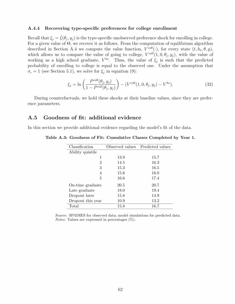
A.4.4 Recovering type-specific preferences for college enrollment
Recall that ξj = ξ(θj, yj) is the type-specific unobserved preference shock for enrolling in college.For a given value of Θ, we recover it as follows. From the computation of equilibrium algorithmdescribed in Section A.4 we compute the value function, V coll(·), for every state (t, ht, θ, y),which allows us to compare the value of going to college, V coll(1, 0, θj, yj), with the value ofworking as a high school graduate, V hs. Thus, the value of ξj is such that the predictedprobability of enrolling to college is equal to the observed one. Under the assumption thatσε = 1 (see Section 5.1), we solve for ξj in equation (9):
ξj = ln
(P coll(θj, yj)
1− P coll(θj, yj)
)− (V coll(1, 0, θj, yj)− V hs). (32)
During counterfactuals, we hold these shocks at their baseline values, since they are prefer-ence parameters.
A.5 Goodness of fit: additional evidence
In this section we provide additional evidence regarding the model’s fit of the data.
Table A.3: Goodness of Fit: Cumulative Classes Completed by Year 1.
Classification Observed values Predicted values
Ability quintile1 13.9 15.72 14.5 16.33 15.3 16.54 15.6 16.05 16.6 17.4
On-time graduate 20.5 20.7Late graduate 18.0 19.4Dropout later 15.8 14.9Dropout this year 10.9 13.2
Total 15.8 16.7
Source: SPADIES for observed data; model simulations for predicted data.Notes: Values are expressed in percentages (%).
62
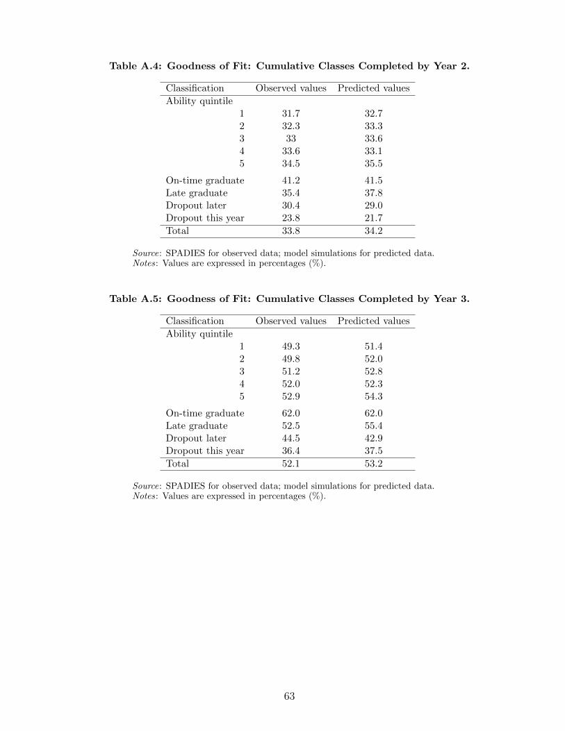
Table A.4: Goodness of Fit: Cumulative Classes Completed by Year 2.
Classification Observed values Predicted values
Ability quintile1 31.7 32.72 32.3 33.33 33 33.64 33.6 33.15 34.5 35.5
On-time graduate 41.2 41.5Late graduate 35.4 37.8Dropout later 30.4 29.0Dropout this year 23.8 21.7
Total 33.8 34.2
Source: SPADIES for observed data; model simulations for predicted data.Notes: Values are expressed in percentages (%).
Table A.5: Goodness of Fit: Cumulative Classes Completed by Year 3.
Classification Observed values Predicted values
Ability quintile1 49.3 51.42 49.8 52.03 51.2 52.84 52.0 52.35 52.9 54.3
On-time graduate 62.0 62.0Late graduate 52.5 55.4Dropout later 44.5 42.9Dropout this year 36.4 37.5
Total 52.1 53.2
Source: SPADIES for observed data; model simulations for predicted data.Notes: Values are expressed in percentages (%).
63

Table A.6: Goodness of Fit: Cumulative Classes Completed by Year 4.
Classification Observed values Predicted values
Ability quintile1 67.2 68.32 68.2 69.93 69.2 70.64 70.3 70.65 71.8 72.0
On-time graduate 82.8 82.1Late graduate 70.1 72.0Dropout later 59.3 53.9Dropout this year 46.4 55.6
Total 70.6 71.0
Source: SPADIES for observed data; model simulations for predicted data.Notes: Values are expressed in percentages (%).
Table A.7: Goodness of Fit: Cumulative Classes Completed by Year 5.
Classification Observed values Predicted values
Ability quintile1 83.9 83.12 85.7 85.73 85.9 86.64 87.1 86.95 88.6 87.6
On-time graduate 99.0 99.5Late graduate 86.6 87.1Dropout later 72.4 64.4Dropout this year 69.7 64.5
Total 87.5 86.9
Source: SPADIES for observed data; model simulations for predicted data.Notes: Values are expressed in percentages (%).
64
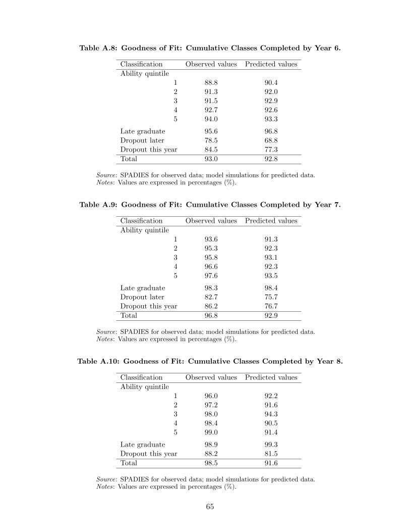
Table A.8: Goodness of Fit: Cumulative Classes Completed by Year 6.
Classification Observed values Predicted values
Ability quintile1 88.8 90.42 91.3 92.03 91.5 92.94 92.7 92.65 94.0 93.3
Late graduate 95.6 96.8Dropout later 78.5 68.8Dropout this year 84.5 77.3
Total 93.0 92.8
Source: SPADIES for observed data; model simulations for predicted data.Notes: Values are expressed in percentages (%).
Table A.9: Goodness of Fit: Cumulative Classes Completed by Year 7.
Classification Observed values Predicted values
Ability quintile1 93.6 91.32 95.3 92.33 95.8 93.14 96.6 92.35 97.6 93.5
Late graduate 98.3 98.4Dropout later 82.7 75.7Dropout this year 86.2 76.7
Total 96.8 92.9
Source: SPADIES for observed data; model simulations for predicted data.Notes: Values are expressed in percentages (%).
Table A.10: Goodness of Fit: Cumulative Classes Completed by Year 8.
Classification Observed values Predicted values
Ability quintile1 96.0 92.22 97.2 91.63 98.0 94.34 98.4 90.55 99.0 91.4
Late graduate 98.9 99.3Dropout this year 88.2 81.5
Total 98.5 91.6
Source: SPADIES for observed data; model simulations for predicted data.Notes: Values are expressed in percentages (%).
65
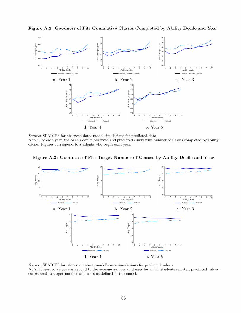
Figure A.2: Goodness of Fit: Cumulative Classes Completed by Ability Decile and Year.
12
14
16
18
20A
cad
emic
pro
gre
ss
1 2 3 4 5 6 7 8 9 10Ability decile
Observed Predicted
28
30
32
34
36
38
Aca
dem
ic p
rog
ress
1 2 3 4 5 6 7 8 9 10Ability decile
Observed Predicted
44
46
48
50
52
54
56
Aca
dem
ic p
rog
ress
1 2 3 4 5 6 7 8 9 10Ability decile
Observed Predicted
a. Year 1 b. Year 2 c. Year 3
62
64
66
68
70
72
74
Aca
dem
ic p
rog
ress
1 2 3 4 5 6 7 8 9 10Ability decile
Observed Predicted
78
80
82
84
86
88
90
Aca
dem
ic p
rog
ress
1 2 3 4 5 6 7 8 9 10Ability decile
Observed Predicted
d. Year 4 e. Year 5
Source: SPADIES for observed data; model simulations for predicted data.Note: For each year, the panels depict observed and predicted cumulative number of classes completed by abilitydecile. Figures correspond to students who begin each year.
Figure A.3: Goodness of Fit: Target Number of Classes by Ability Decile and Year
0
5
10
15
20
Av
g. T
arg
et
1 2 3 4 5 6 7 8 9 10Ability decile
Observed Predicted
0
5
10
15
20
Av
g. T
arg
et
1 2 3 4 5 6 7 8 9 10Ability decile
Observed Predicted
0
5
10
15
20
Av
g. T
arg
et
1 2 3 4 5 6 7 8 9 10Ability decile
Observed Predicted
a. Year 1 b. Year 2 c. Year 3
0
5
10
15
20
Av
g. T
arg
et
1 2 3 4 5 6 7 8 9 10Ability decile
Observed Predicted
0
5
10
15
20
Av
g. T
arg
et
1 2 3 4 5 6 7 8 9 10Ability decile
Observed Predicted
d. Year 4 e. Year 5
Source: SPADIES for observed values; model’s own simulations for predicted values.Note: Observed values correspond to the average number of classes for which students register; predicted valuescorrespond to target number of classes as defined in the model.
66
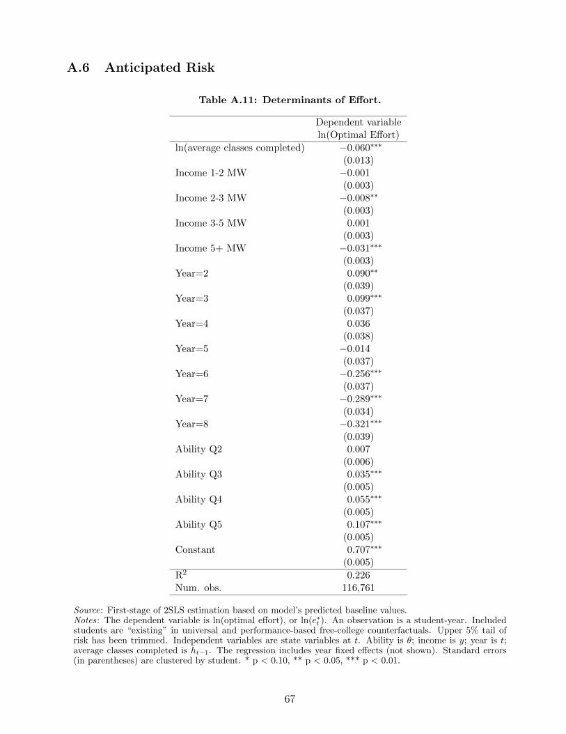
A.6 Anticipated Risk
Table A.11: Determinants of Effort.
Dependent variableln(Optimal Effort)
ln(average classes completed) −0.060∗∗∗
(0.013)Income 1-2 MW −0.001
(0.003)Income 2-3 MW −0.008∗∗
(0.003)Income 3-5 MW 0.001
(0.003)Income 5+ MW −0.031∗∗∗
(0.003)Year=2 0.090∗∗
(0.039)Year=3 0.099∗∗∗
(0.037)Year=4 0.036
(0.038)Year=5 −0.014
(0.037)Year=6 −0.256∗∗∗
(0.037)Year=7 −0.289∗∗∗
(0.034)Year=8 −0.321∗∗∗
(0.039)Ability Q2 0.007
(0.006)Ability Q3 0.035∗∗∗
(0.005)Ability Q4 0.055∗∗∗
(0.005)Ability Q5 0.107∗∗∗
(0.005)Constant 0.707∗∗∗
(0.005)
R2 0.226Num. obs. 116,761
Source: First-stage of 2SLS estimation based on model’s predicted baseline values.Notes: The dependent variable is ln(optimal effort), or ln(e∗t ). An observation is a student-year. Includedstudents are “existing” in universal and performance-based free-college counterfactuals. Upper 5% tail ofrisk has been trimmed. Independent variables are state variables at t. Ability is θ; income is y; year is t;average classes completed is ht−1. The regression includes year fixed effects (not shown). Standard errors(in parentheses) are clustered by student. * p < 0.10, ** p < 0.05, *** p < 0.01.
67
ogotá -