no-arbitrage approach to pricing credit spread derivatives

SPRING 2003 THE JOURNAL OF DERIVATIVES 51

No arbitrage in the case of pricing credit spreadderivatives refers to determination of the time-depen-dent drift terms in the mean reversion stochastic pro-cesses of the instantaneous spot rate and spot spreadby fitting the current term structures of default-freeand defaultable bond prices. The riskless rate and thecredit spread of a reference entity are taken to be cor-related stochastic state variables in this pricing model.

When the spot rate and spot spread both follow theHull and White model, one can derive an analyticrepresentation for the time-dependent drift terms andanalytic price formulas for credit spread options. Algo-rithms for the numerical valuation of credit spreadderivatives are developed, and the pricing behaviorsof credit spread options are examined.

Credit spread derivatives are creditrate-sensitive financial instrumentsdesigned to hedge against or cap-italize on changes in the credit

spread of a reference entity such as a riskybond. The credit spread of a risky bond is thedifference between the current yield of therisky bond and a benchmark rate of compa-rable maturity. The spread represents the riskpremium the market demands for holding therisky bond.

Unlike default swaps, credit spreadderivatives do not depend upon any specificcredit event occurring. The buyer of a creditspread option pays an up-front premium, andin return the writer agrees to pay an amount

should the actual spot spread breach somestrike level. Alternatively, the payoff maydepend on the difference between the spotspreads of two reference entities. Credit spreadoptions may be used either to earn incomefrom the option premium, to bet one’s viewon credit spread change, or to target the pur-chase of a reference entity on a forward basisat a favored price.

By following a reduced-form approachthat models the occasion of default as a pointprocess, Jarrow, Lando, and Turnbull [1997]construct a Markov chain model for valuationof risky debt and credit derivatives that incor-porates the credit ratings of a firm as an indi-cator of the likelihood of default. The Markovmodel provides the evolution of an arbitrage-free term structure of the credit spread.

Problems arise in numerical implemen-tation of the model because bonds with highcredit ratings may experience no default withinthe sample period, so the risk premium adjust-ments become ill-defined as the estimateddefault probabilities are zero. Kijima andKomoribayashi [1998] propose a technique ofrisk premium adjustment to overcome this dif-ficulty with high-rated bonds.

In related work, Duffie and Singleton[1999] and Schönbucher [1998] use intensitymodels to analyze the term structure ofdefaultable bonds and compute the price ofcredit derivatives. Schönbucher [1999] con-structs a two-factor tree model for fitting bothdefaultable and default-free term structures of

No-Arbitrage Approach to PricingCredit Spread DerivativesCHI CHIU CHU AND YUE KUEN KWOK

CHI CHIU CHU

is a Ph.D. student inmathematics at HongKong University of Sci-ence and Technology inHong Kong, China. [email protected]

YUE KUEN KWOK

is an associate professor ofmathematics at HongKong University of Sci-ence and Technology. [email protected]

bond prices, following the Hull and White frameworkwith time-dependent drift terms. He uses the Hull andWhite [1990] model for the dynamics of the risk-freeinterest rate and default intensity. Garcia, van Gindersen,and Garcia [2001] use a two-factor tree algorithm that iscomposed of a Hull and White tree for the risk-freeinterest rate dynamics and a Black and Karasinski [1991]tree for the intensity dynamics.

Das and Sundaram [2000] propose a discrete-timeHeath-Jarrow-Morton [1992] model for valuation ofcredit derivatives. They derive risk-neutral drifts for theprocesses of the risk-free forward rate and forward spread.Combining a recovery of market value condition, theyobtain a recursive representation of drifts that are path-dependent.

This formulation has the advantage that it can easilyhandle the American exercise feature in the pricing ofthe credit derivatives, and the corresponding algorithm alsoincludes information about default probabilities inferredfrom market data. Its major disadvantage is that its com-putational complexity grows exponentially with thenumber of time steps, since the corresponding binomialtree is non-recombining.

A structural approach derives the term structure ofthe credit spread of a credit entity by examining the creditquality of the issuer. In structural models, the credit spreadis not one of the state variables in the model, but ratheris a derived quantity. Default occurs when the issuer firmvalue falls below some threshold value. The structuralapproach has been used by Das [1995] to price credit riskderivatives.

Longstaff and Schwartz [1995] develop a valuationmodel for pricing credit spread derivatives by assuming thatthe riskless interest rate and the spread follow correlatedmean reversion diffusion processes. From empirical analysisof observed credit spreads, they argue that the logarithm ofthe credit spread follows a mean reversion process. Theyassume the parameters in the characterization of the pro-cesses to be constant, and derive closed-form price formulasfor the credit spread options. A disadvantage of the processis that their model does not incorporate information aboutthe current term structures of bond prices.

Chacko and Das [2002] have since then derivedprice formulas for credit spread options based on theuncorrelated Cox-Ingersoll-Ross [1985] processes for thespot rate and spot spread, and again the parameters in thestochastic processes are assumed to be constant. Tahani[2000] models the process of the logarithm of credit spreadusing the GARCH model and obtains closed-form price

formulas for credit spread options. Mougeot [2000]extends the two-factor Longstaff-Schwartz model to athree-factor model for pricing options on the spread ofthe values of two reference assets.

We extend the Longstaff and Schwartz model byassuming time-dependent drift functions in the meanreversion diffusion processes of the riskless interest rateand credit spread. The spot riskless interest rate is takento follow the Hull-White model, while the spot creditspread can be taken to follow either the Hull-White model[1990] or the Black-Karasinski model [1991]. When bothstate variables follow the Hull-White model, we canderive analytic expressions for the time-dependent driftfunctions that fit the current term structures of default-free and defaultable bond prices. Also, we can obtain ana-lytic pricing formulas for credit spread options.

Unfortunately, the time-dependent drift functionin the spot spread process is not analytically tractable whenthe logarithm of the spot spread is assumed to follow amean-reverting diffusion (this is the assumption in theBlack-Karasinski model). By extending the Hull-Whitetrinomial tree fitting methodologies [1994], we extendthe fitting algorithms to allow numerical valuation ofcredit spread options.

I. CONTINUOUS MODELS

We begin with the pricing of credit spread deriva-tives under the Hull-White [1990] model. This is an exten-sion of the one-factor Hull-White model to the two-factorversion, where both the instantaneous spot riskless interestrate and the credit spread follow a mean-reverting modelwith time-dependent drift terms. Like the one-factor ver-sion, the two-factor model exhibits nice analyticaltractability and ease of numerical implementation.

Pricing Framework Under Two-Factor Hull-White Model

We specify the processes of the instantaneous spotriskless interest rate r and the spot spread s to follow theextended Vasicek [1977] model, where the drift terms areassumed to be time-dependent functions. Under a risk-neutral valuation framework, we assume that the stochasticprocesses followed by r and s are given by

(1-A)dr = [θ(t)− ar]dt+ σrdWr,

52 NO-ARBITRAGE APPROACH TO PRICING CREDIT SPREAD DERIVATIVES SPRING 2003

(1-B)

where θ(t) and φ(t) are time-dependent functions, and aand b are positive constant parameters that give the ratesof mean reversion of r and s, respectively. Further, σr andσs are the constant volatility parameters for the spot rater and spot spread s, respectively, and dWr and dWs are stan-dard Brownian motions under the risk-neutral measureP. Let ρ denote the correlation coefficient between dWrand dWs; that is, dWrdWs = ρdt.

Determination of the Time-Dependent Drift Terms.Hull and White [1990] demonstrate how to determine thetime-dependent function θ(t) in the drift term of thedefault-free spot rate by fitting the current term structureof default-free bond prices. Their procedure can be sum-marized as follows. Let P(t, T ) denote the price at time tof a discount bond maturing at time T, which is given by:

(2)

where EP denotes the expectation under the risk-neutralmeasure P. By taking the risk-neutral expectation in Equa-tion (2), where r is defined in Equation (1-A), one obtains:

(3)

Differentiating Equation (3) with respect to T twice,we obtain:

(4)

This equation gives the dependence of the drift termθ(t) using the information of the current term structure ofthe default-free bond price P(t, T ) over the period [t, T ].Suppose we write the process followed by P(t, T ) as:

(5)dP (t, T )

P(t, T )= rdt+ σP (t, T )dWr,

θ(T ) =σ2r

2a[1− e−2a(T−t)]−

∂2

∂T 2lnP(t, T)− a

∂

∂TlnP (t, T ).

∫ T

t

θ(u)1− e−a(T−u)

adu+

∫ T

t

σ2r

2a2[1− e−a(T−u)]2 du

)P (t, T ) = exp

(−

r(t)

a[1− e−a(T−t)]−

P(t, T ) = EP[exp(−

∫T

t

r(u) du)],

ds = [φ(t)− bs]dt+ σsdWs,then

(6)

By following a similar procedure, it is possible todetermine the other time-dependent function φ(t) in themean reversion process of s by fitting the current termstructure of defaultable bond prices. This is achieved bychanging the probability measure to the forward-adjustedmeasure QT with delivery at future time T. Let D(t, T )denote the price at time t of a defaultable bond maturingat time T. By the Girsanov theorem, we have:

(7)

Accordingly, the process followed by the spot spreads under the forward measure QT is given by

(8)

where dWT is a standard Brownian motion under QT.Under the process defined in Equation (8), the quantity∫T

ts(u) du follows the normal distribution with mean:

(9-A)

and variance

(9-B)

Since

var

[∫ T

t

s(u) du

]=

∫ T

t

σ2s

b2[1− e−b(T−u)]2 du.

∫T

t

[φ(u) + ρσsσP (u,T )]1− e−b(T−u)

bdu

EQT

[∫T

t

s(u) du

]=

s(t)

b

[1− e−b(T−t)

]+

ds = [φ(t)− bs+ ρσsσP (t, T )]dt+ σsdWT ,

= P(t, T )EQT

[exp

(−

∫ T

t

s(u) du

)]D(t, T ) = EP

[exp

(−

∫ T

t

[r(u) + s(u)] du

)]

σP (t, T ) = −σr

a[1− e−a(T−t)].


(10-A)

we obtain

(10-B)

Again, by differentiating Equation (10-B) withrespect to T twice and observing Equation (6), we obtain:

(11)

Credit Spread Put Option. Let psp(r, s, t) denote theprice of the credit spread put option, whose terminalpayoff is given by

(12)

Here K is the strike spread at which the option holder hasthe right to put the risky bond to the option writer. Itis called a credit spread put option although the terminalpayoff resembles a call payoff. When the spot credit spreadis higher than the strike spread, this signifies that the priceof the underlying risky bond drops below the strike priceof the bond corresponding to the strike spread. Since theterminal payoff depends only on s, we may use the defaultfree bond price as the numeraire and obtain:

(13)

Suppose we define ξ(t) = s(t)exp(–b[T – t]). Thenξ follows the stochastic process:

psp(r, s, t) = P(t, T )EQT

[max(s−K, 0)].

psp(r, s, T ) = max(s−K, 0).

φ(T ) =σ2s

2b[1− e−2b(T−t)]− b

∂

∂T

[ln

D(t, T )

P(t, T )

]−

∂2

∂T 2

[ln

D(t, T )

P(t, T )

]

+ ρσsσr

[1− e−a(T−t)

a+ e−a(T−t)

1− e−b(T−t)

b

].

D(t, T )

P (t, T )=exp

(−

s(t)

b[1− e−b(T−t)]−

∫ T

t

[φ(u) + ρσsσP (u,T )]

(1− e−b(T−u)

b

)du

+

∫ T

t

σ2s

2b2[1− e−b(T−u)]2 du

).

exp

(−EQ

T

[∫ T

t

s(u) du

]+

1

2var

[∫ T

t

s(u) du

])EQ

T

[exp

(−

∫ T

t

s(u) du

)]=

(14)

Note that ξT is conditionally normally distributedwith mean µξ and variance σ2

ξ, where:

+

(15-A)

(15-B)

Note that µξ depends not only on the time to expi-ration T – t but also on the current time t. Once the meanand variance of ξT are available, the price formula for thecredit spread put is given by:

�

(16)

Combined Hull-White and Black-Karasinski Model

Longstaff and Schwartz [1995)] propose that theinterest rate and the logarithm of the credit spread followmean-reverting Vasicek processes. We extend their modelby assuming time-dependent functions in the drift terms;that is, we choose the Hull-White model for the interestrate process and the Black-Karasinski model for the creditspread process. Assume that y = ln s, and the stochasticprocesses followed by r and y are governed by:

(17-A)dr = [θ(t)− ar]dt+ σrdWr ,

[σξ√2π

e−(K−µξ)2/2σ2

ξ + (µξ −K)N

(µξ −K

σξ

)]psp(r, s, t) = P (t, T )

σ2ξ =σ2s2b

[1− e−2b(T−t)].

−

e−(a+b)te−b(T−t)[1− e−a(T−t)]

b

},

+ρσsσr

a

{1− e−(a+b)(T−t)

a + b−

1− e−b(T−t)

b−

e−at[e−a(T−t) − e−b(T−t)]

b

=σ2s2b2

[1− e−b(T−t)][1− e−2bte−b(T−t)]−∂

∂T

[ln

D(t, T )

P(t, T )

]

∫ T

t

φ(u)e−b(T−u) du

µξ = s(t)e−b(T−t) +ρσsσr

a

[1− e−(a+b)(T−t)

a+ b−

1− e−b(T−t)

b

]

dξ = [φ(t) + ρσsσP (−b(T − t))dt

+ σss(t (−b(T − t))dW T .

(t, T )]s(t)

)


(17-B)

where c is the rate of mean reversion of y, σy is the con-stant volatility parameter for y, and dWrdWy = ρdt. Unfor-tunately, the Black-Karasinski model lacks the level ofanalytic tractability exhibited by the Hull-White model.Under the Black-Karasinski assumption of the credit spreadprocess, we find that Equation (7) has to be modified as:

(18)

Unlike ∫Tts(u) du, however, the quantity ∫T

texp[y(u)]duis no longer normally distributed. Hence, there is not a simplerelation between [D(t, T )]/[P(t, T )] and the time-depen-dent drift function ψ(t), like that shown in Equation (11).

If θ(t) and ψ(t) are known functions, we may derivethe price formula for the credit spread put option. Interms of y, the terminal payoff of the credit spread put isgiven by max(ey – K, 0). The put price formula takes theusual Black-Scholes form:

(19-A)

where

(19-B)

Similar to µξ and σ2ξ as given in Equations (15-A)

and (15-B), the mean µξ and variance σ2ξ are given by:

�

(20-A)∫ T

t

ψ(u)e−c(T−u) du,

[1− e−(a+c)(T−t)

a+ c−

1− e−c(T−t)

c

]+

µζ = y(t)e−c(T−t) +ρσyσr

a

d =− lnK + µζ + σ2ζ

σζ.

psp(s, r, t) = P(t, T )[eµζ+σ

2

ζ/2N(d)−KN(d− σζ)]

D(t, T )

P (t, T )= EQ

T

[exp

(−

∫ T

t

exp(y(u)) du

)].

dy = [ψ(t)− cy]dt+ σydWy,(20-B)

Heath-Jarrow-Morton Model

The two-factor extended Vasicek model is a specialcase of the Heath-Jarrow-Morton (HJM) model corre-sponding to a specific choice of the volatility structures.First, we present the general HJM formulation of thepricing model with the two state variables r and s.

Let f(t, T ) denote the riskless instantaneous forwardrate. Following the HJM framework, the dynamic of f(t, T )is assumed to be

df (21)

where αf is the drift, and σf is the volatility. Also, dW1 isa standard Brownian motion under the risk-neutral mea-sure P. Under the no-arbitrage condition, the drift αfand volatility σf must observe:

(22)

From the dynamics of the risky bond prices, wecan define the risky instantaneous forward rate fd(t, T ) inthe same manner as the risk-free instantaneous forwardrate. Next, the instantaneous forward spread h(t, T ) isdefined to be fd(t, T ) – f(t, T ); accordingly, the spot spreads(t) = fd(t, t) – f(t, t). Assume that h(t, T ) follows thestochastic process:

(23)

where αh is the drift, σh1 and σh2 are volatilities, and dW1and dW2 are independent standard Brownian motionsunder the risk-neutral measure P. Again, the no-arbi-trage condition dictates that αh, σh1, and σh2, satisfy (seeSchönbucher [1998]):

dh(t, T ) = αh(t, T )dt+ σh1(t, T)dW1 + σh2(t, T )dW2,

αf(t, T) = σf(t, T)

∫ T

t

σf (t, u) du.

(t, T ) = αf(t, T )dt+ σf(t, T )dW1,

σ2ζ =σ2y

2c[1− e−2c(T−t)].


+

(24)

By recalling that s(t) = h(t, t), one can show that theprocess followed by s is governed by:

+

+

+

(25)

Equation (25) reveals that the drift term of s is in gen-eral path-dependent. If instead we choose the volatilitystructures of the riskless instantaneous forward rate and theinstantaneous forward spread to be:

(26-A)

(26-B)

(26-C)

then the process of s becomes Markovian. By comparingthe resulting expression for ds and that given in Equation(1-B), we obtain:

+

(27)

This is consistent with the expression given in Equa-tion (11) by noting that:

(28)h(t, T ) = −∂

∂T

[ln

D(t, T )

P(t, T )

].

ρσsσr

[1− e−a(T−t)

a+ e−a(T−t)

1− e−b(T−t)

b

]φ(T ) =σ2s2b

[1− e−2b(T−t)

]+ bh(t, T ) +

∂h(t, T )

∂T

σh2(t, T ) =√1− ρ2σse

−b(T−t),

σh1(t, T ) = ρσse−b(T−t),

σf (t, T ) = σre−a(T−t),

2∑i=1

σhi(T,T )dWi(T ).

σf(u, v)∂σh1(u,T )

∂T

]dv du+

2∑i=1

∫ T

t

∂σhi(u,T )

∂TdWi(u)

}dT

∫ T

t

∫ T

u

[2∑

i=1

σhi(u, v)

∂σhi(u,T )

∂T+ σh1(u, v)

∂σf (u,T )

∂T

ds(T ) =

{∂h(t, T )

∂T+

∫ T

t

[2∑

i=1

σ2hi(u, T ) + 2σhi

(u,T )σf(u,T )

]du

σf (t, T )

∫ T

t

σh1(t, u) du.

αh(t, T ) =2∑

i=1

σhi(t, T )

∫ T

t

σhi(t, u) du + σh1(t, T)

∫ T

t

σf (t, u) duII. CONSTRUCTION OF NUMERICALALGORITHMS

Now we can extend the Hull and White [1994]methodology to fitting the current term structures ofdefault-free and defaultable bond prices.

Two-Factor Algorithms

Let x = x(r) and z = z(s) be some specified func-tions of the spot interest rate and spot credit spread, respec-tively. Assume that both x and z follow mean reversionprocesses:

(29-A)

(29-B)

where dWxdWz = ρ~dt. We would like to construct a two-factor tree that fits the current term structures of prices ofdefault-free and defaultable bonds through numerical pro-cedures. For example, the combined Hull-White and Black-Karasinski model corresponds to x(r) = r and z(s) = ln s.

We first briefly review some of the key steps in theHull-White fitting procedure for the one-factor tree, andfollow by generalization to the two-factor tree. In theone-factor Hull-White tree, we first build the trinomialtree for the process x* with x0 = 0 that corresponds to~θ(t) = 0, where:

(30-A)

Note that [x*(t + ∆t) – x*(t)] is normally distributedwith mean Mx and variance Vx as given by

Mx = –[1 – e–a~∆ t]x*(t)

and

(30-B)Vx =σ2x2a

[1− e−2a∆t].

dx∗ = −ax∗dt+ σxdWx, x∗(0) = 0.

dz = [φ(t)− b ]dt+ σzdWz ,z

dx = [θ(t)− ax]dt+ σxdWx,


We first construct a trinomial tree that simulates theprocess x*. The node probabilities are obtained by equatingthe mean and variance of the discrete tree process and thecontinuous process as given by Equation (30-B).

A key step in the Hull-White fitting procedure isdetermination of the time-varying drift αm at time tm sothat the lattice tree can price default-free bonds at dif-ferent maturities as observed in the market at the currenttime. Let Ym be the current yield of a default-free bondmaturing at time tm; Qm, j be the state price of node (m,j), which is the present value of a security that pays off $1 if node (m, j) is reached and zero otherwise; and (m, j )indicates the node at time tm at which x = αm + j∆x. Ini-tially, we have Q0, 0 = 1, α0 = x(Y1). Also, we define rm, j= x-1(αm + j∆x), where x-1 denotes the inverse functionof x(r).

If we have obtained αm–1 and Qm–1,j for all values ofj, the state price at time tm is given by:

(31)

where pij* is the node probability of moving from node xj*

at time tm–1 to node xj at time tm, and the summation istaken over all values of j * for which the nodes x*

j are con-nected to the node xj.

From the relation in Equation (2), we deduce that:

(32)

where n(j)m is the number of nodes on each side of the cen-

tral node at time tm. The time-varying drift αm can thenbe determined numerically in a recursive manner.

When x = r, αm can be solved explicitly by:

(33)

Moreover, the value of the time-dependent drift~θ(tm) can be estimated by:

(34)θm =αm − αm−1

∆t+ aαm,

αm =ln(∑n(j)m

j=−n(j)m

Qm,je−j∆r∆t

)∆t

+ (m+ 1)Ym+1.

e−Ym+1(m+1)∆t =

n(j)m∑j=−n

(j)m

Qm,je−x−1(αm+j∆x)∆t,

Qm,j =∑j∗

Qm−1,j∗pjj∗e

−rm−1,j∗∆t,

where α~ is the mean reversion rate of x [see Equation(29-A)].

In the combined two-factor tree that simulates thecorrelated evolution of r and s, there are nine branchesemanating from the (m, j, k) node at tm = m∆t, xj = j∆x,and zk = k∆z. We use the Hull-White approach of con-structing probability matrices that give the node proba-bilities of moving from a node at tm to the different ninenodes at tm+1. We let βm denote the time-varying drift forthe discrete credit spread process. Similarly, we try todetermine βm numerically by fitting the current termstructure of defaultable bond prices.

Let Qm,j,k denote the state price of the (m, j, k) node and ~Ym be the current yield of a defaultable bond maturingat time tm. At initiation, β0 = z(~Y1 – Y1); and the succes-sive βm, m ≥ 1, are obtained recursively by the relationship:

(35)

where n(k)m is defined similarly as n(j)

m. When z(s) = s, βmcan be solved explicitly by the formula:

(36)

Once βm is known, the value of φ∼(tm) can be esti-mated by:

(37)

where ~b is the mean reversion rate of z [see Equation (29-B)].When the state prices are known at the nodes, the

value of any European-style credit derivative at time t0whose value depends on r and s can be obtained by:

(38)

where psp(rM,j, sM,k, tM) is the terminal payoff at maturitydate tM, and the summation is taken over all terminalnodes.

psp(r0, s0, t0) =∑j

∑k

QM,j,kpsp(rM,j , sM,k, tM),

φm =βm − βm−1

∆t+ bβm,

βm =ln(∑n(j)m

j=−n(j)m

∑n(k)m

k=−n(k)m

Qm,j,ke−(rm,j+k∆s)∆t

)∆t

+ (m+ 1)Ym+1.

e−Ym+1(m+1)∆t =

n(j)m∑j=−n

(j)m

n(k)m∑k=−n

(k)m

Qm,j,ke−(rm,j+z

−1(βm+k∆z))∆t,


It is quite computationally demanding to calculatethe state prices since this two-factor algorithm requires asearch process at each node. When x(r) = r and z(s) = s,one can derive explicit formulas for the time drifts αm andβm without calculating the state prices. Further, when theterminal payoff of a credit derivative is independent of theinterest rate, we can develop a one-factor fitting algorithmvia the use of valuation in the forward-adjusted risk-neu-tral measure. This reduced one-factor fitting algorithm canbe considered an extension of the Grant-Vora [2001]approach to derive an explicit analytic expression for thetime drift function of the one-factor Hull-White model.

One-Factor Tree for Joint Extended Vasicek Processes

The no-arbitrage fitting procedure developed by Grantand Vora [2001] is indeed the discrete analogue of the ana-lytic procedure for deriving the time-dependent drift θ(t).The discrete analogue of the extended Vasicek process forr as defined in Equation (1-A) can be represented by:

(39)

where the mean Mr and variance Vr are defined much thesame as in Equation (30-B), Zm is a standard normal vari-able, and δm is an adjustment parameter for the no-arbi-trage fitting procedure. Note that αm is equal to EP[rm].

Deductively, we obtain:

(40)

where the normal variables Zj, j = 0, …, m – 1, are inde-pendently and identically distributed.

From Equation (39), one can deduce that:

(41)

Let γ 2m∆t be the variance of Σ

m

j=0rj∆t. It can be shown

that

δm = EP[rm+1]− (1 +Mr)EP[rm].

m−1∑j=0

√Vr(1 +Mr)

m−1−jZj ,

rm = r0(1 +Mr)m +

m−1∑j=0

(1 +Mr)m−1−jδj +

∆rm = rm+1 − rm =Mrrm + δm +√VrZm,

(42)

Since the price at time t0 of a default-free bondmaturing at time tm+1 is given by:

(43-A)

so that

(43-B)we then have

(44)

which gives the time-varying drift αm. As in the continuous model, we can reduce the two-

factor algorithm to a one-factor version by choosing thedefault-free bond price as the numeraire. First, we wouldlike to find the time-varying drift βm of the spot spreadprocess under the risk-neutral measure P and the forwardmeasure QT. Note from Equations (1-B) and (8) that thetwo measures are related by

(45)

where the last term

(46)

represents the drift adjustment required for effecting thechange of measure.

Xj,m,M =

∫ tm

tj

ρσsσP (u, tM)e−b(tm−u) du

EQT

[s(tm)] = EP[s(tm)] +X0,m,M ,

EP[rm] = −

1

∆tln

P (t0, tm+1)

P (t0, tm)+

γ2m − γ2m−12

,

EP[rm] = −

lnP (t0, tm+1)

∆t−

m−1∑j=0

EP[rj ] +γ2m2,

P(t0, tm+1) = EP

exp

−

m∑j=0

rj∆t

+m(1− e−2a∆t)].

2e−a∆t(1− e−am∆t)(1 + e−a∆t)

γ2m =σ2r

2a(1− e−a∆t)2[e−2a∆t(1− e−2am∆t)−


Using the bond volatility σP(t, T) defined in Equation(6), and assuming constant values for ρ and σs, we have

(47)

The discrete analogue of the extended Vasicek pro-cess followed by s can be represented by

(48)

where Ms, Vs, and ξm are defined in an analogous manneras in Equation (39). Similarly, the adjustment parameterξm is determined by fitting the term structure of default-able bond prices.

Solution of the recursive relation (48) gives

+

(49)

The discrete version of Equation (7) is seen to be

(50)

from which we deduce the formula for EP[sm] (this is equalto βm, the time-varying drift for the credit spread process):

–

(51) where ~γ 2

m, is defined similarly as γ 2m, except that rm, a, and

σr are replaced by sm, b, and σs, respectively. Under the forward measure, the time t0 price of a

credit spread derivative is given by:

m−1∑j=0

Xj,j+1,m

Ms

[(1 +Ms)m−j

− 1] +γ2m2,

EP[sm] = −1

∆tln

D(t0, tm+1)

P(t0, tm+1)−

m−1∑j=0

EP [sj ]

D(t0, tm) = P(t0, tm)EQtm

exp

−m−1∑

j=0

sj∆t

m−1∑j=0

√Vs(1 +Ms)

m−1−jZj .

sm = s0(1 +Ms)m +

m−1∑j=0

(1 +Ms)m−1−j(ξj +Xj,j+1,M)

∆sm = sm+1 − sm =Mssm + ξm + Xm,m+1,M +√VsZm,

Xj,m,M =ρσsσr

a

[e−a(tM−tm) − e−atM−btm+(a+b)tj

a+ b−

1− e−b(tm−tj)

b

](52)

where psp(sM,k, tM) is the terminal payoff on maturity datetM, and UM,k is the cumulative probability under the for-ward measure reaching the (M, k) node from the starting(0, 0) node. Note that U0,0 = 1, sm,k = βm + k∆s, and βm =ξm + χ0,m,m.

III. NUMERICAL RESULTS

We implement the two-factor and one-factor fittingalgorithms using current term structures of default-free anddefaultable yield curves so as to check the accuracy and theeffectiveness of the numerical algorithms against the ana-lytic price formulas. In our numerical experiments, we gen-erate the current yield of the default-free Treasury bond by:

(53)

We use the Briys and de Varenne [1997] intertem-poral default model to generate the yield for a high-ratedbond and a low-rated bond. The spread curves areobtained by subtracting the yield of the default-free Trea-sury bonds from the yield curves of the defaultable bonds.Note that the yield curves of the default-free Treasurybond and the high-rated bond increase monotonicallywith time to maturity, while the yield curve of the low-rated bond exhibits the typical hump shape.

These yield curves (shown in Exhibit 1) are used asinput in all subsequent calculations.

In Exhibits 2-A and 2-B, we plot the time-depen-dent drift function φ(t) in the mean reversion of the spotspread process, obtained by fitting the yield curves of thehigh-rated bond and the low-rated bond, respectively. Thedrift φ(t) is shown to be an increasing function of the spotspread volatility σs for both high-rated and low-rated bonds.

Since the spread approaches zero as time approachesmaturity, the drift goes to zero as t tends to zero. Thedrift functions for both high-rated and low-rated bondsreach some peak value, then decline at a higher value oft and settle at some asymptotic value at infinite t.

The drift is greater for the low-rated bond since thecorresponding spot spread has a higher value. Also, the driftshows less sensitivity to the spot spread volatility for thelow-rated bond.

Y (T ) = 0.08− 0.05e−1.8T .

psp(r0, s0, t0) = P (t0, tM)∑k

UM,kpsp(sM,k, tM),



E X H I B I T 1Yield Curve Plots

0 0.2 0.4 0.6 0.8 1 1.2 1.4 1.6 1.8 20

0.02

0.04

0.06

0.08

0.1

0.12

Time to Maturity

Treasury yield

Yie

ld /

Sp

read

high-rated yield

high-rated yield spread

low-rated yield

low-rated yield spread

E X H I B I T 2 - ATime-Dependent Drift Function for High-Rated Bond

0 0.2 0.4 0.6 0.8 1 1.2 1.4 1.6 1.8 20.02

0

0.02

0.04

0.06

0.08

0.1

t

φ(t)

σs= 0.1

σs = 0.2

σs = 0.3

To test the convergence of the two-factor and one-factor fitting algorithms, we apply the algorithms to pricea credit spread put with payoff as given in Equation (12).We use different combinations of parameter values in thepricing model, and compare the numerical results withthe results obtained from the analytic price formula inEquation (16) with varying numbers of time steps.

Exhibit 3 shows the convergence behaviors of thetwo fitting algorithms in terms of average relative errors(in percentages). The relative errors have relatively lowvalues that decline in a roughly linear manner withincreasing numbers of time steps.

The one-factor algorithm provides better accuracy.In terms of computational complexity, the one-factoralgorithm is O(M2), while the two-factor algorithm is

O(M3), where M is the number of time steps. This prop-erty of a polynomial order of complexity is highly desir-able, as numerical implementation does not take anunreasonable amount of computation time.

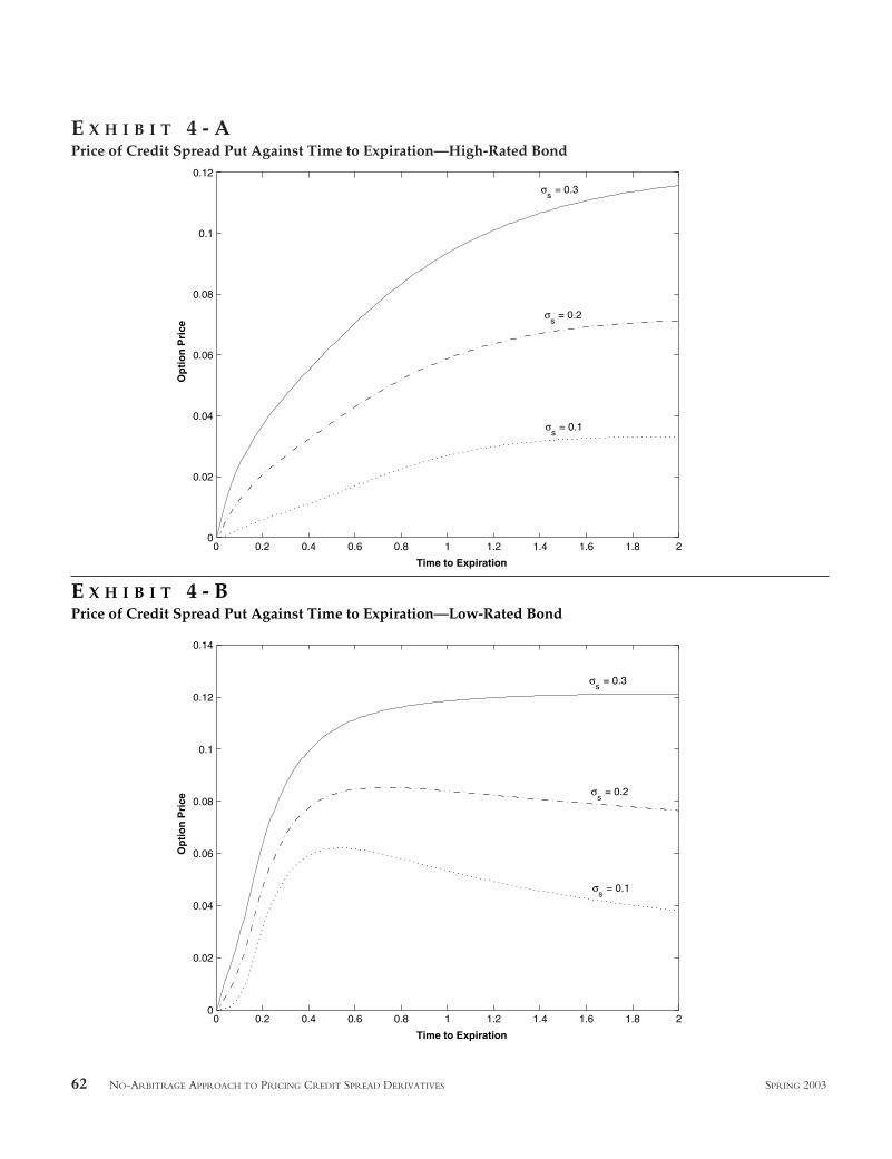
We also investigate the pricing behavior of the creditspread put option with respect to time to expiration andspot spread volatility. In Exhibit 4-A, we plot the spreadput option function against time to expiration with varyingspot spread volatility where the underlying is a high-ratedbond. The spread put price increases with longer time toexpiration and higher spot spread volatility.

When the underlying is a low-rated bond, however,the time-dependent behavior of the spread put priceexhibits a humped shape (see Exhibit 4-B). This may bedue to a declining credit spread at very long maturities for


E X H I B I T 2 - BTime-Dependent Drift Function for Low-Rated Bond

0 0.2 0.4 0.6 0.8 1 1.2 1.4 1.6 1.8 20.1

0

0.1

0.2

0.3

0.4

0.5

0.6

t

φ(t)

σs = 0.1

σs = 0.2

σs = 0.3

E X H I B I T 3Comparison of One-Factor and Two-Factor Tree Calculations

Average Relative Errors in Average Relative Errors inNumber of Time Steps Two-Factor Tree Calculations One-Factor Tree Calculations

8 3.18% 2.92%16 1.175% 1.63%32 1.10% 1.03%


E X H I B I T 4 - APrice of Credit Spread Put Against Time to Expiration—High-Rated Bond

0 0.2 0.4 0.6 0.8 1 1.2 1.4 1.6 1.8 20

0.02

0.04

0.06

0.08

0.1

0.12

Time to Expiration

Op

tio

n P

rice

σs = 0.1

σs = 0.2

σs = 0.3

E X H I B I T 4 - BPrice of Credit Spread Put Against Time to Expiration—Low-Rated Bond

0 0.2 0.4 0.6 0.8 1 1.2 1.4 1.6 1.8 20

0.02

0.04

0.06

0.08

0.1

0.12

0.14

Time to Expiration

Op

tio

n P

rice

σs = 0.1

σs = 0.2

σs = 0.3

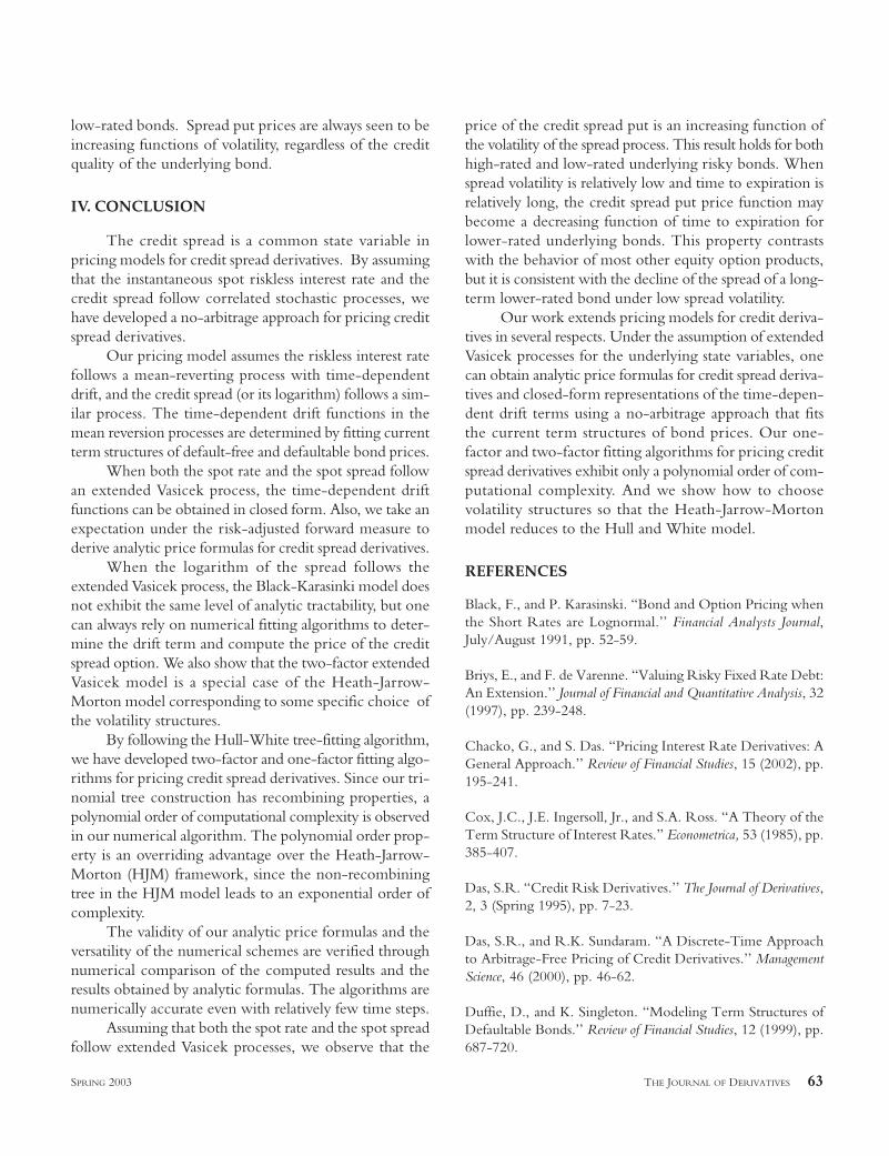
low-rated bonds. Spread put prices are always seen to beincreasing functions of volatility, regardless of the creditquality of the underlying bond.

IV. CONCLUSION

The credit spread is a common state variable inpricing models for credit spread derivatives. By assumingthat the instantaneous spot riskless interest rate and thecredit spread follow correlated stochastic processes, wehave developed a no-arbitrage approach for pricing creditspread derivatives.

Our pricing model assumes the riskless interest ratefollows a mean-reverting process with time-dependentdrift, and the credit spread (or its logarithm) follows a sim-ilar process. The time-dependent drift functions in themean reversion processes are determined by fitting currentterm structures of default-free and defaultable bond prices.

When both the spot rate and the spot spread followan extended Vasicek process, the time-dependent driftfunctions can be obtained in closed form. Also, we take anexpectation under the risk-adjusted forward measure toderive analytic price formulas for credit spread derivatives.

When the logarithm of the spread follows theextended Vasicek process, the Black-Karasinki model doesnot exhibit the same level of analytic tractability, but onecan always rely on numerical fitting algorithms to deter-mine the drift term and compute the price of the creditspread option. We also show that the two-factor extendedVasicek model is a special case of the Heath-Jarrow-Morton model corresponding to some specific choice ofthe volatility structures.

By following the Hull-White tree-fitting algorithm,we have developed two-factor and one-factor fitting algo-rithms for pricing credit spread derivatives. Since our tri-nomial tree construction has recombining properties, apolynomial order of computational complexity is observedin our numerical algorithm. The polynomial order prop-erty is an overriding advantage over the Heath-Jarrow-Morton (HJM) framework, since the non-recombiningtree in the HJM model leads to an exponential order ofcomplexity.

The validity of our analytic price formulas and theversatility of the numerical schemes are verified throughnumerical comparison of the computed results and theresults obtained by analytic formulas. The algorithms arenumerically accurate even with relatively few time steps.

Assuming that both the spot rate and the spot spreadfollow extended Vasicek processes, we observe that the

price of the credit spread put is an increasing function ofthe volatility of the spread process. This result holds for bothhigh-rated and low-rated underlying risky bonds. Whenspread volatility is relatively low and time to expiration isrelatively long, the credit spread put price function maybecome a decreasing function of time to expiration forlower-rated underlying bonds. This property contrastswith the behavior of most other equity option products,but it is consistent with the decline of the spread of a long-term lower-rated bond under low spread volatility.

Our work extends pricing models for credit deriva-tives in several respects. Under the assumption of extendedVasicek processes for the underlying state variables, onecan obtain analytic price formulas for credit spread deriva-tives and closed-form representations of the time-depen-dent drift terms using a no-arbitrage approach that fitsthe current term structures of bond prices. Our one-factor and two-factor fitting algorithms for pricing creditspread derivatives exhibit only a polynomial order of com-putational complexity. And we show how to choosevolatility structures so that the Heath-Jarrow-Mortonmodel reduces to the Hull and White model.

REFERENCES

Black, F., and P. Karasinski. “Bond and Option Pricing whenthe Short Rates are Lognormal.’’ Financial Analysts Journal,July/August 1991, pp. 52-59.

Briys, E., and F. de Varenne. “Valuing Risky Fixed Rate Debt:An Extension.’’ Journal of Financial and Quantitative Analysis, 32(1997), pp. 239-248.

Chacko, G., and S. Das. “Pricing Interest Rate Derivatives: AGeneral Approach.’’ Review of Financial Studies, 15 (2002), pp.195-241.

Cox, J.C., J.E. Ingersoll, Jr., and S.A. Ross. “A Theory of theTerm Structure of Interest Rates.” Econometrica, 53 (1985), pp.385-407.

Das, S.R. “Credit Risk Derivatives.’’ The Journal of Derivatives,2, 3 (Spring 1995), pp. 7-23.

Das, S.R., and R.K. Sundaram. “A Discrete-Time Approachto Arbitrage-Free Pricing of Credit Derivatives.’’ ManagementScience, 46 (2000), pp. 46-62.

Duffie, D., and K. Singleton. “Modeling Term Structures ofDefaultable Bonds.’’ Review of Financial Studies, 12 (1999), pp.687-720.


Garcia, J., H. van Gindersen, and R. Garcia. “On the Pricingof Credit Spread Options: A Two-Factor HW-BK Algorithm.’’Working paper, Artesia BC and University of California atBerkeley, 2001.

Grant, D. and G. Vora. “An Analytical Implementation of theHull and White Model.’’ The Journal of Derivatives, Winter 2001,pp. 54-60.

Heath, D., R. Jarrow, and A. Morton. “Bond Pricing and theTerm Structure of Interest Rates: A New Methodology forContingent Claims Valuation.” Econometrica, 60 (1992), pp.77-105.

Hull, J., and A. White. “Numerical Procedures for Imple-menting Term Structure Models II: Two-Factor Models.’’ TheJournal of Derivatives, Winter 1994, pp. 37-48.

——. “Pricing Interest-Rate-Derivative Securities.’’ Review ofFinancial Studies, 3, 4 (1990), pp. 573-592.

Jarrow, R., D. Lando, and S.M. Turnbull. “A Markov Modelfor the Term Structure of Credit Risk Spreads.’’ Review ofFinancial Studies, 10 (1997), pp. 481-523.

Kijima, M., and K. Komoribayashi. “A Markov Chain Modelfor Valuing Credit Risk Derivatives.’’ The Journal of Derivatives,Fall 1998, pp. 97-108.

Longstaff, F.A., and E.S. Schwartz. “Valuing Credit Deriva-tives.’’ The Journal of Fixed Income, June 1995, pp. 6-12.

Mougeot, N. “Credit Spread Specification and the Pricing ofSpread Options.’’ Working paper, Ecole des HEC, 2000.

Schönbucher, P.J. “Term Structure Modeling of DefaultableBonds.’’ Review of Derivatives Research, 2 (1998), pp. 161-192.

——. “A Tree Implementation of a Credit Spread Model forCredit Derivatives.’’ Working paper, Bonn University, 1999.

Tahani, N. “Estimating and Valuing Credit Spread Optionswith GARCH Models.’’ Working paper, HEC Montreal, 2000.

Vasicek, O. “An Equilibrium Characterization of the TermStructure.” Journal of Financial Economics, 5 (1977), pp. 177-188.

To order reprints of this article, please contact Ajani Malik [email protected] or 212-224-3205.


no-arbitrage approach to pricing credit spread derivatives

Documents