no news is good news - ludger hentschel · · 2015-12-31no news is good news: an asymmetric model...

No News is Good News:

An Asymmetric Model of Changing

Volatility in Stock Returns

John Y. Campbella and Ludger Hentschelb

aWoodrow Wilson School, Princeton University, Princeton, NJ 08540–1013and nber, Cambridge, MA 02138–5398

bDepartment of Economics, Princeton University, Princeton, NJ 08540–1021

May 1992

First Draft: March 1990

Abstract: It seems plausible that an increase in stock market volatility raisesrequired stock returns, and thus lowers stock prices. We develop a formal modelof this volatility feedback effect using a simple model of changing variance (aquadratic generalized autoregressive conditionally heteroskedastic, or QGARCH,model). Our model is asymmetric and helps to explain the negative skewness andexcess kurtosis of U.S. monthly and daily stock returns over the period 1926-88.We find that volatility feedback normally has little effect on returns, but it canbe important during periods of high volatility.

Keywords: autoregressive conditional heteroskedasticity, crashes, skewness,stock returns, volatility.

The first version of this paper was written while the authors were visiting the Financial Markets

Group at the London School of Economics and Political Science. We are grateful to the

Financial Markets Group for its hospitality; to John Ammer for suggesting the first part of our

title; to James Davidson, Phil Dybvig, Ben Friedman, Andrew Harvey, Ravi Jagannathan, Jan

Magnus, Bill Schwert, Sushil Wadhwani, and particularly Robert Engle and the referee, Daniel

Nelson, for helpful comments; to Bill Schwert and Enrique Sentana for sharing their data and

computer programs; and to Kristin Butcher for computer assistance. We acknowledge financial

support from the National Science Foundation and the Sloan Foundation (Campbell) and the

John M. Olin Program for the Study of Economic Organization and Public Policy at Princeton

University (Hentschel).

Contents

1 Introduction . . . . . . . . . . . . . . . . . . . . . . . . . . 1

2 An Asymmetric Model of Changing Volatility . . . . . . . . . . . . 7

2.1 The Campbell-Shiller Framework . . . . . . . . . . . . . . . 72.2 News About Dividends and News About Volatility . . . . . . . . 92.3 Characteristics of the Returns Process . . . . . . . . . . . . 13

3 Application to U.S. Stock Market Data . . . . . . . . . . . . . . 18

3.1 Data and Estimation Method . . . . . . . . . . . . . . . . 183.2 Basic Empirical Results . . . . . . . . . . . . . . . . . . 193.3 The Economic Importance of Volatility Feedback . . . . . . . 243.4 Alternative Models of Volatility Feedback . . . . . . . . . . . 29

4 Conclusion . . . . . . . . . . . . . . . . . . . . . . . . . . 35

References . . . . . . . . . . . . . . . . . . . . . . . . . . 36

Appendix A: The QGARCH(p, q) Model . . . . . . . . . . . . . 39

Appendix B: Maximum Likelihood Estimation . . . . . . . . . . . 41

ii

1 Introduction

One striking characteristic of the stock market is that the volatility of returns

can be very different at different times. Estimates of the standard deviation

of monthly stock returns reported in French, Schwert, and Stambaugh (1987),

Schwert (1989), and below range from a low of 2% in the early 1960’s to a high

of 20% in the early 1930’s. Daily volatility also fluctuates and can change very

rapidly: we estimate that the standard deviation of daily returns increased from

about 1% to almost 7% in the few days around the stock market crash of October

1987. These seven- to- tenfold changes in standard deviation correspond to 50-

to- 100-fold changes in variance.

It seems plausible that changes in volatility of this magnitude may have

important effects on required stock returns and thus on the level of stock prices.

This “volatility feedback” effect has been emphasized by Pindyck (1984) and

French, Schwert, and Stambaugh (1987). Volatility feedback is an appealing

idea because it has the potential to help explain some other facts about stock

returns. For example, large negative stock returns are more common than large

positive ones, so stock returns are negatively skewed. This skewness, or con-

temporaneous asymmetry, shows up clearly in the pattern of extreme moves in

stock prices in the postwar period. Of the five largest one-day movements in the

S&P 500 index since World War II, four are declines in the index and only one

is an increase; of the ten largest movements, eight are declines and only two are

increases [Cutler, Poterba, and Summers (1989)]. A similar but weaker pattern

is visible in the history of daily stock returns over a longer period starting in

1885: six of the ten largest movements in this period are declines and four are

increases [Schwert (1990b)].

In addition, extreme stock market movements are more common than

would be expected if stock returns were drawn from a normal distribution. This

excess kurtosis is not just the result of changing volatility, because it is still

present after returns are normalized by their estimated conditional standard de-

viations [Bollerslev (1987)]. The stock market decline on October 19, 1987 was

a large drop even conditional on price movements observed earlier that month.

Finally, volatility is typically higher after the stock market falls than after

1

2 No News is Good News

it rises, so stock returns are negatively correlated with future volatility. This

correlation, or predictive asymmetry, was first discussed by Black (1976), who

argued that it could be due to the increase in leverage that occurs when the

market value of a firm declines. However, it seems that the leverage effect is too

small to fully account for this phenomenon [Christie (1982), Schwert (1989)].

In principle, volatility feedback can explain these characteristics of re-

turns even if the underlying shocks to the market are conditionally normally

distributed. Suppose there is a large piece of good news about future dividends.

Large pieces of news tend to be followed by other large pieces of news (volatility

is persistent), so this piece of news increases future expected volatility, which in

turn increases the required rate of return on stock and lowers the stock price,

dampening the positive impact of the dividend news. Now consider a large piece

of bad news about future dividends. Once again, the stock price falls because

higher volatility raises the required rate of return on stock, but now the volatility

effect amplifies the negative impact of the dividend news. Large negative stock

returns are therefore more common than large positive ones, and the amplifica-

tion of negative returns can produce excess kurtosis. In contrast, the arrival of

a small piece of news lowers future expected volatility and increases the stock

price. In the extreme case in which no news arrives, the market rises because “no

news is good news” about future volatility. Volatility feedback therefore implies

that stock price movements are correlated with future volatility.

A number of authors have explored these ideas. Brown, Harlow, and

Tinic (1988) show that stock price reactions to unfavorable news events tend

to be larger than reactions to favorable events. They attribute this finding to

volatility feedback. Poterba and Summers (1986), on the other hand, argue that

volatility feedback could not be important because changes in volatility are too

short-lived to have a major effect on stock prices. French, Schwert, and Stam-

baugh (1987) regress stock returns on innovations in volatility and find a neg-

ative coefficient, which they attribute to volatility feedback. Haugen, Talmor,

and Torous (1991) report a similar result. Early research uses moving aver-

age measures of volatility, but recent work [Akgiray (1989), Bollerslev (1987),

Chou (1988), and French, Schwert, and Stambaugh (1987)] uses the “generalized

autoregressive conditionally heteroskedastic” or garch model of Engle (1982)

Sec. 1] Introduction 3

and Bollerslev (1986). garch estimates of stock market variance are typically

more persistent than moving average estimates, which allows a greater role for

volatility feedback. Attanasio and Wadhwani (1989) and Chou (1988) present

some Monte Carlo evidence that garch estimates of persistence in variance are

superior to moving average estimates in finite samples.

Despite the volume of reserach on the subject, this paper is the first to

present a fully worked out formal model of volatility feedback. Earlier papers

have at most discussed volatility feedback informally, using it to interpret esti-

mates of garch models for stock returns. The basic garch model assumes a

constant mean stock return, so it does not capture the mechanism underlying

volatility feedback. The “garch-in-mean” or garch-m model [Engle, Lilien,

and Robins (1987)] allows the conditional mean stock return to depend on the

conditional variance of the return, but when innovations are assumed to be con-

ditionally normal this model still imposes zero correlation between returns and

future volatility, as well as zero conditional skewness and zero excess kurtosis.

French, Schwert, and Stambaugh (1987) estimate a garch-m model with con-

ditionally normal innovations and find a significant positive relation between

the conditional mean and variance of stock returns. They argue that it would

be desirable to take account of negative skewness from volatility feedback (pp.

22–23), but they do not try to do this. Chou (1988) also combines an informal

discussion of the negative effect of volatility on prices with a formal garch-m

model that does not accommodate this effect.

There are some second-generation garch models that allow returns to be

correlated with future volatility, notably the “exponential garch” or egarch

model of Nelson (1991) and the “quadratic garch” or qgarch model of En-

gle (1990) and Sentana (1991), as well as the Markov switching model of Turner,

Startz, and Nelson (1989). We take the qgarch model as our starting point,

since it is analytically tractable and captures the phenomenon of predictive asym-

metry without appealing to volatility feedback, which seems desirable since the

leverage effect is a plausible explanation for at least some of the predictive asym-

metry observed in the data. The basic qgarch model has conditionally normal

innovations, however, so it does not fit the negative skewness or excess kurtosis

of returns. We therefore build a model of volatility feedback that amplifies the


predictive asymmetry of the basic qgarch model and creates negative skew-

ness and excess kurtosis in returns. Our work is distinguished from statistical

models with nonnormal return innovations [Engle and Gonzalez-Rivera (1989),

Nelson (1991)] by the fact that the nonnormality in our model comes exclusively

from volatility feedback and is pinned down by the model parameters describing

first and second moments: no new parameters are introduced to fit the third and

fourth moments of returns.

Much of the work we have described applies a statistical model directly

to stock returns. Of course, an economic explanation of the behavior of stock

returns requires that a statistical model be applied to exogenous variables, with

the behavior of stock returns emerging from the solution of an economic model.

Our paper takes a step in this direction. We do not work with a full general

equilibrium model of the economy, but rely on two simple assumptions. First,

we assume that news about stock dividends follows a qgarch model. Second,

we assume that the expected return on a stock is a linear function of the con-

ditional variance of the news about dividends. (As we explain further below,

this assumption can be weakened: we can allow for other sources of variation

in expected returns, which appear to be important in practice, provided that a

qgarch process adequately characterizes the innovations in stock prices caused

by dividend news and by non-volatility-induced changes in expected returns.)

We combine these two assumptions with the log-linear approximate asset pric-

ing framework of Campbell and Shiller (1988) and Campbell (1991) to get an

implied process for stock returns.

Table 1 illustrates the nonnormality of U.S. stock return data. The table

reports skewness and excess kurtosis for raw stock returns and for the normalized

residuals of a qgarch-m model. Stock returns are log excess returns on the

Center for Research in Securities Prices (crsp) value-weighted index of New

York Stock Exchange and American Stock Exchange stocks over a one-month

Treasury bill, measured at monthly and daily intervals over the period 1926–88

as well as over the subperiods 1926–51 and 1952–88. The table clearly shows that

neither log excess returns nor residuals from a qgarch-m model are normal or

symmetric. In particular, there is evidence that log excess returns are negatively

skewed and leptokurtic.

Sec. 1] Introduction 5

Table 1Moments of monthly and daily stock returns

Excess

Data Set Mean Variance Skewness Kurtosis

Monthly crsp er 4.797 3.240 −0.443 6.877

1/26–12/88 (2.070) (0.167) (0.089) (0.178)

Monthly qgarch-m −0.016 1.014 −0.865 2.936

1/26–12/88 (0.037) (0.052) (0.089) (0.178)

Monthly crsp er 5.213 5.306 −0.342 4.933

1/26–12/51 (4.124) (0.425) (0.139) (0.277)

Monthly qgarch-m −0.039 1.039 −0.903 2.379

1/26–12/51 (0.058) (0.083) (0.139) (0.277)

Monthly crsp er 4.505 1.796 −0.648 3.086

1/52–12/88 (2.011) (0.121) (0.116) (0.232)

Monthly qgarch-m 0.002 1.003 −0.498 1.354

1/52–12/88 (0.048) (0.067) (0.116) (0.232)

Daily crsp er 0.215 0.128 −0.344 19.926

1/2/26–12/30/88 (0.087) (0.001) (0.019) (0.038)

Daily qgarch-m −0.010 1.005 −0.516 4.398

1/2/26–12/30/88 (0.008) (0.011) (0.019) (0.038)

Daily crsp er 0.213 0.204 0.016 10.909

1/2/26–12/31/51 (0.163) (0.003) (0.028) (0.056)

Daily qgarch-m −0.013 1.006 −0.442 2.824

1/2/26–12/31/51 (0.011) (0.016) (0.028) (0.056)

Daily crsp er 0.216 0.066 −1.782 45.515

1/2/52–12/30/88 (0.084) (0.001) (0.025) (0.051)

Daily qgarch-m −0.011 1.010 −0.467 5.079

1/2/52–12/30/88 (0.010) (0.015) (0.025) (0.051)

Excess returns (er) are log excess returns on the value-weighted crsp index over a one-month

Treasury bill return. qgarch-m residuals are the residuals from the qgarch(1, 1)-m and

qgarch(1, 2)-m models estimated in tables 2a and 2b, divided by their estimated standard

deviation. If the qgarch, models are correctly specified, these residuals should have a stan-

dard normal distribution. Mean and variance have been multiplied by 1000 for excess returns.

Standard errors are computed under the null hypothesis that returns or residuals are normally

distributed.

The qgarch(1, 1)-m model for monthly excess returns is obtained by setting λ = 0 in eq. (12)

in the text.

ht+1 = µ+ γσ2t + ηd,t+1

σ2t = ω + α(ηd,t − b)2 + βσ2

t−1, (6)

where ht+1 is the monthly log excess return and σ2t is the conditional variance of ht+1.

The qgarch(1, 2)-m model for daily excess returns is given by the qgarch(1, 2) analogues of

the above equations.

ht+1 = µ+ γσ2t + ηd,t+1

σ2t = ω + α1(ηd,t − b)2 + α2(ηd,t−1 − b)2 + βσ2

t−1,

where ht+1 is the daily log excess return and σ2t is the conditional variance of ht+1.


Figure 1: Sample skewness, 1926–88.The circles plot the sample skewness of qgarch(1, 1)-m residuals, ηd,t+1, normalized by their

conditional standard deviations, σt. The residuals are taken from the model estimated in table

2a, top panel, row 1, using monthly log excess returns on the value-weighted crsp index over

a one-month Treasury bill return. Skewness is computed in each of the seven calendar decades

during the period January 1926–December 1988. The error bars give the 95% confidence

intervals. The qgarch(1, 1)-m model for monthly excess returns is obtained by setting λ = 0

in eqs. (6) and (12′) in the text:

ht+1 = µ+ γσ2t + ηd,t+1

σ2t = ω + α(ηd,t − b)2 + βσ2

t−1,

where ht+1 is the monthly log excess return and σ2t is the conditional variance of ht+1.

The dashed line plots the sample skewness of qgarch(1, 2)-m residuals, ηd,t+1, normalized by

their conditional standard deviations, σt. The residuals are taken from the model estimated in

table 2b, top panel, row 1, using daily log excess returns on the value-weighted crsp index over

a one-month Treasury bill return. Skewness is computed in each of the sixty-three calendar

years during the period January 2, 1926–December 30, 1988. The qgarch(1, 2)-m model for

daily excess returns is obtained by setting λ = 0 in the qgarch(1, 2) analogues of eqs. (6) and

(12′) in the text:

ht+1 = µ+ γσ2t + ηd,t+1


t−1,


The strong evidence for negative skewness reported here does not depend on

our use of a qgarch-m model rather than a garch-m or a simple garch model.

[garch-m models were estimated in the first version of this paper, Campbell and

Sec. 2] An Asymmetric Model of Changing Volatility 7

Hentschel (1991), and the residuals were, if anything, slightly more skewed.] The

evidence for skewness does, however, depend on our using log returns rather than

simple returns. The log return is the appropriate concept, since the standard

geometric Brownian motion model of stock prices implies that the log return,

not the simple return measured in discrete time, is normally distributed. The

evidence for negative skewness is robust to sample period, as we show in fig. 1 by

plotting the sample skewness of standardized qgarch-m residuals over shorter

subsamples. The standardized residuals for monthly log excess returns are neg-

atively skewed in each of the decades of our sample. Although the evidence for

daily data is weaker, there is still negative skewness in the great majority of

years.

In the next section, we explain our model of volatility feedback. In section

3, we apply our model to U.S. stock market data. Section 4 summarizes our

conclusions and discusses some interesting directions for further research.

2 An Asymmetric Model of Changing Volatility

2.1 The Campbell-Shiller Framework

If we are to model the effect of changing volatility on stock prices, we need

a framework that allows prices to be affected by changing expectations about

both dividends and required returns. The difficulty is that the standard present

value relation is nonlinear when expected returns vary through time making it

intractable except in a few special cases.

Campbell and Shiller (1988) propose a log-linear approximation to the stan-

dard model. They argue that the approximation is both tractable and surpris-

ingly accurate. Campbell and Shiller originally derived their approximation for a

beginning-of-period (cum dividend) stock price, but we follow Campbell (1991)

and work with an end-of-period price, which is more standard in the finance

literature. We define the one-period natural log real holding return on a stock as

ht+1 ≡ log(Pt+1 +Dt+1)− log(Pt), where Pt is the real stock price measured at

the end of period t (ex dividend), and Dt is the real dividend paid during period

t. The right hand side of this identity is a nonlinear function of the log stock


price and the log dividend; it can be approximated, using a first-order Taylor

expansion, as

ht+1 ≈ k + ρpt+1 + (1− ρ)dt+1 − pt, (1)

where lower-case letters are used for logs. The parameter ρ is the average ratio of

the stock price to the sum of the stock price and the dividend, a number slightly

smaller than one, and the constant k is a nonlinear function of ρ. Eq. (1) replaces

the log of the sum of price and dividend with a weighted average of log price and

log dividend. Intuitively, the future log stock price gets a much larger weight

than the future log dividend because a given percentage change is absolutely

larger when it occurs in the stock price than when it occurs in the dividend.

Eq. (1) can be thought of as a difference equation relating pt to pt+1,

dt+1, and ht+1. It holds ex post , but it also holds ex ante as an expectational

difference equation. Campbell and Shiller impose the terminal condition that

limi→∞Etρipt+i = 0. This condition rules out “rational bubbles” which would

cause explosive behavior of the log stock price. With this terminal condition,

the ex ante version of (1) can be solved forward to obtain

pt =k

1− ρ + (1− ρ) Et∞∑j=0

ρjdt+1+j − Et∞∑j=0

ρjht+1+j . (2)

This equation is useful because it enables one to calculate the effect on the stock

price of a change in expected stock returns. It says that the log stock price pt

can be written as an expected discounted value of all future dividends dt+1+j less

future returns ht+1+j , discounted at the constant rate ρ plus a constant k/(1−ρ).

If the stock price is high today, this must mean that future expected dividends

are high unless returns are expected to be low in the future. Note that eq. (2) is

not an economic model, but has been derived by approximating an identity and

imposing a terminal condition. It is best thought of as a consistency condition

that must be satisfied by any reasonable set of expectations.

Campbell (1991) uses eq. (2) to substitute pt and pt+1 out of (1). This

gives another useful expression:

ht+1 − Etht+1 = (Et+1 − Et)∞∑j=0

ρj∆dt+1+j − (Et+1 − Et)∞∑j=1

ρjht+1+j , (3)


or in more compact notation,

vh,t+1 = ηd,t+1 − ηh,t+1, (4)

where vh,t+1 denotes the unexpected stock return at time t+ 1, and ηd,t+1 and

ηh,t+1 denote news about dividends and future returns respectively. Once again,

this equation should be thought of as a consistency condition for expectations.

If the unexpected stock return is negative, then either expected future dividend

growth must be lower, or expected future stock returns must be higher, or both.

There is no behavioral model behind eq. (4); it is simply an approximation to

an identity.

We work below with excess log stock returns, measured relative to a short-

term interest rate. Campbell (1991) shows that the decomposition (4) is equally

valid for excess stock returns, provided that ηd,t+1 is reinterpreted to include

news about real interest rates as well as news about real dividends. In this paper

we use the notation of eq. (4) and refer to ηd,t+1 as “news about dividends”. In

our empirical work, however, we do not directly measure ηd,t+1. It is a residual

term that may contain real interest rate shocks as well as other shocks that we

do not explicitly model. In practice, we believe that changes in expected excess

stock returns, arising from some other source than changing volatility, are an

important component of the shock we write as ηd,t+1. The shock we write as

ηh,t+1 should be thought of as capturing the volatility feedback effect, but not

necessarily all changes in expected excess stock returns. We discuss this point

further in section 4 below.

2.2 News About Dividends and News About Volatility

The first determinant of the stock return in eq. (4) is the news about future

dividends, ηd,t+1. We treat this as an exogenous shock which follows a condi-

tionally normal qgarch process [Engle (1990), Sentana (1991)]. For simplicity

we describe the qgarch(1, 1) case and generalize to the qgarch(p, q) case in

appendix A. The qgarch(1, 1) model is

ηd,t+1 ∼ N(0, σ2t ), (5)


σ2t = ω + α(ηd,t − b)2 + βσ2

t−1. (6)

In order to ensure that the conditional variance is always positive, the parame-

ters ω, α, and β must all be positive. The parameter α measures the extent to

which a squared return today feeds through into future volatility, while the sum

α + β measures the persistence of volatility. The unconditional variance of the

process is (ω + αb2)/(1− (α+ β)

).

The qgarch model introduces a parameter b that is absent from the simple

garch model; when b = 0, the qgarch model reduces to the garch model.

Our prior expectation is that b is positive, although this is by no means required.

A positive b creates a negative correlation between the dividend news, ηd,t, and

the conditional volatility of next period’s dividend news, σ2t , because a negative

return will increase volatility more than a positive return of the same size. Thus

the qgarch model captures the phenomenon of predictive asymmetry.

The other determinant of the stock return in eq. (4) is the news about

future expected returns. We assume that the conditional expected return Etht+1

is determined by the volatility of the news variable ηd,t+1:

Etht+1 = µ+ γEtη2d,t+1 = µ+ γσ2

t . (7)

As we shall see, this is not quite equivalent to the conventional assumption that

the expected return is linear in the volatility of the return itself, but our empirical

estimates imply that the discrepancy is small.

Following Merton (1980), the coefficient γ in eq. (7) is usually interpreted

as the coefficient of relative risk aversion. Even ignoring the difference between

the stock return and the news variable ηd,t+1, eq. (7) can be derived in general

equilibrium only under restrictive assumptions. In a model that distinguishes

the coefficient of relative risk aversion from the elasticity of intertemporal substi-

tution, Campbell (1992) shows that eq. (7) holds for the market portfolio, with

γ equal to relative risk aversion, if the elasticity of intertemporal substitution is

one. Campbell also discusses other circumstances under which eq. (7) holds as

an approximation.

Eq. (7) and the qgarch(1, 1) process (6) imply that the expected return


at any date in the future can be written as

Etht+1+j = µ+ γω + αb2

1− (α+ β)+ γ (α+ β)j

(σ2t −

ω + αb2

1− (α+ β)

). (8)

The second term on the right hand side of eq. (8) is γ times the unconditional

variance of the news process. The third term is γ times the deviation of today’s

conditional variance from the unconditional variance, discounted using the per-

sistence of volatility α+ β. Eq. (8) implies that the discounted sum of all future

expected returns is

Et

∞∑j=0

ρjht+1+j =µ

1− ρ

+γ

1− ρ

(ω + αb2

1− (α+ β)

)+

γ

1− ρ(α+ β)

(σ2t −

ω + αb2

1− (α+ β)

). (9)

This discounted sum of expected returns helps determine the level of the stock

price in eq. (2). The second and third terms on the right hand side of eq. (9) can

be interpreted as the “volatility discount” on the stock price, or the extent to

which the price is lower than it would be if there were no uncertainty about future

dividends. The second term is the unconditional mean volatility discount, while

the third term represents the variation in the discount caused by the changing

conditional volatility of news about dividends.

These equations describe the levels of expected returns. It is also straight-

forward to calculate the revision from time t to time t+1 in the discounted value

of future returns. This is

ηh,t+1 ≡ (Et+1 − Et)∞∑j=1

ρjht+1+j = λ(η2d,t+1 − σ2

t − 2bηd,t+1

), (10)

where λ is related to the other parameters of the model by

λ =γρα

1− ρ(α+ β). (11)

At time t+ 1, the innovation to volatility is the difference between the squared

innovation η2d,t+1 and its conditional expectation σ2

t , minus 2b times the differ-

ence between the return ηd,t+1 and its conditional expectation of zero. This last


linear term appears in the qgarch model but not in the simpler garch model

which sets b = 0. To obtain the revision in the discounted value of future stock

returns, one multiplies the volatility innovation by the parameter λ; λ in turn

depends on the effect of volatility on the expected stock return, γ, the effect

of an innovation on next period’s volatility, α, and the persistence of volatility,

α + β. Since ρ is less than unity, λ is well defined even if volatility has infinite

persistence and follows an integrated garch model with α+ β = 1.

Eqs. (4), (7), (10), and (11) can now be combined to write the stock return

as

ht+1 = µ+ γσ2t + ηd,t+1 − λ

(η2d,t+1 − σ2

t − 2b ηd,t+1

)(12)

= µ+ γσ2t + κ ηd,t+1 − λ

(η2d,t+1 − σ2

t

), (12′)

where κ = 1 + 2λb. The first three terms in eq. (12) comprise the standard

garch-m model that has previously been used to describe stock returns. The

final term, which is new, says that an unusually large realization of dividend

news, of either sign, will increase volatility, lower the stock price, and cause a

negative unexpected stock return; moreover, a positive piece of dividend news

will tend to reduce volatility and increase the stock return (when b is positive).

The strength of this volatility feedback effect is measured by the parameter λ.

Eq. (12′) rewrites eq. (12) to show that the stock return is a quadratic function

of the underlying news with linear coefficient κ and quadratic coefficient λ. κ is

greater than one when the qgarch parameter b is positive, but it is always very

close to one for the parameter values estimated below.

Our analysis so far has assumed a qgarch(1, 1) process for volatility.

However, we show in appendix A that eq. (12′) holds for any qgarch(p, q)

process provided that the parameters κ and λ are appropriately redefined in

terms of the underlying parameters governing the evolution of variance. In the

qgarch(1, 2) model which we use for daily data, for example, the variance pro-

cess is σ2t = α1(ηd,t − b)2 + α2(ηd,t−1 − b)2 + βσ2

t−1. The coefficient λ has the

form given in eq. (11) except that α is replaced by α1 +ρα2, while κ remains un-

changed in terms of b and λ. Thus eq. (12′) is quite general and we can proceed


Figure 2: Unexpected returns and news.The straight dashed line is a 45◦ line which gives the relation between unexpected returns

and news when λ = 0. The solid curve gives the relation between unexpected returns and

news when λ = 2.398, the value estimated over the second subsample in table 2b, bottom

panel, row 2. The relation plotted is given by the last two terms on the right hand side of

eq. (12′) in the text: κηd,t+1 − λ(η2d,t+1 − σ2

t ), where ηd,t+1 is the news at time t + 1.

The conditional standard deviation σt = 0.05, and the horizontal range of the figure is three

conditional standard deviations on either side of zero.

to discuss its implications for the behavior of stock returns.

2.3 Characteristics of the Returns Process

To understand eq. (12′), it is helpful to plot the relationship between the cash flow

news ηd,t+1 and the unexpected stock return vh,t+1 = κηd,t+1 − λ(η2d,t+1 − σ2

t

).

Fig. 2 plots the stock return against the news for parameter values that we es-

timate below (in table 2b) using postwar daily U.S. data. The coefficient λ is

2.398, while κ is 1.012. The figure assumes that the conditional standard devi-

ation σt is 0.05 (close to the postwar maximum reached during October 1987).

The horizontal range of fig. 2 is three standard deviations on either side of zero,

so that news events lying outside the range of the figures are exceedingly unlikely.

Since κ is so close to one, the unexpected stock return is almost exactly the

news less λ(η2d,t+1−σ2

t

). Thus the unexpected stock return (the solid curve) lies


above the 45◦ line in the middle of the figure, where the absolute value of the

news is less than its conditional standard deviation. This is the “no news is good

news” effect. If there is no dividend news at all, the stock market rises because

the absence of dividend news implies that volatility and required returns will

tend to be lower in the future. Conversely, the unexpected return lies below the

45◦ line at the left and the right of the figure, where the dividend news is large in

absolute value. Large declines in stock prices are amplified, while large increases

are dampened. In fact, the model implies that the maximum possible return is

µ+(γ+λ)σ2t +κ2/(4λ), which is achieved when ηd,t+1 = κ/(2λ) = b+1/(2λ). Any

larger piece of good dividend news actually gives a lower stock return because

the indirect volatility effect outweighs the direct dividend effect. Whether this

behavior is relevant for observed stock returns depends on the parameters b

and λ and the range of σ2t . In our empirical work we assume that all observed

returns are generated by underlying shocks ηd,t+1 less than b+1/(2λ). We obtain

moderate estimates of λ, for which this assumption is not restrictive.

The degree of curvature in the relation between news and returns depends

on the level of σ2t . If σ2

t is small, then η2d,t+1 is almost always small and the

quadratic term has little weight relative to the linear term in eq. (12). Thus for

low levels of volatility the solid line in fig. 2 is closer to the 45◦ diagonal and

exhibits less curvature over the relevant range. On the other hand, if σ2t is large,

the quadratic term becomes much more important. To understand this point

more generally, observe that eq. (12) can be rewritten as

vh,t+1

σt= (κ+ λσt)

[κ

κ+ λσt

{ηd,t+1

σt

}+

λσtκ+ λσt

{1−

(ηd,t+1

σt

)2}]. (13)

The variable ηd,t+1/σt has a standard normal distribution. The distribution of

unexpected returns, normalized by σt, is thus a mixture of a normal distribution

and a demeaned, negative χ2(1). The normal distribution has relative weight

κ/(κ+λσt), while the negative χ2(1) has relative weight λσt/(κ+λσt). In times

of low volatility, returns is very close to normal, but in periods of high volatility

returns take on some of the characteristics of a negative χ2(1) distribution.

This shifting distribution of returns is the result of an important property

of both the garch and qgarch models: the volatility of variance increases very


Figure 3:The conditional standard deviation of dividend news, 1926–88.

The solid line plots the monthly average of the conditional standard deviation of daily news

implied by the restricted model estimated over the full sample (table 2b, top panel, row 2). The

dashed line is the monthly average conditional standard deviation implied by the restricted

model estimated over subsamples (Table 2b, bottom two panels, row 2). The model for daily

excess returns is given by the qgarch(1, 2) analogues of eqs. 6), (11), and (12′) in the text:

ht+1 = µ+ γσ2t + κηd,t+1 − λ(η2

d,t+1 − σ2t )


t−1

λ =γρ(α1 + ρα2)

1− ρ(α1 + ρα2 + β)

κ = 1 + 2λb,


rapidly with the level of variance. To see this for the garch(1, 1) case, lead

eq. (6) by one period and set b = 0 to obtain

σ2t+1 = ω + ασ2

t

{(ηd,t+1

σt

)2

− 1}

+ (α+ β)σ2t . (14)

The innovations to σ2t+1 are the product of ασ2

t and a demeaned χ2(1) random

variable. The conditional variance of σ2t+1 is therefore proportional to σ4

t . This

feature of the garch model enables it to generate long periods of calm with oc-

casional episodes of high and rapidly changing volatility, as seen in fig. 3. It also

means that volatility feedback distorts the distribution of returns away from the


normal more strongly when volatility is high than when it is low. As volatility in-

creases, the variance of news about dividends increases with σ2t , but the variance

of news about variance, which creates the nonnormality of returns, increases with

σ4t . What is important here is not that the variance of garch variance increases

with its level—this is characteristic of many stochastic processes which are con-

strained to be positive—but that the variance of garch variance increases more

than proportionally with its level. This feature of garch processes extends to

the qgarch model, in which the nonzero b merely introduces an additional lower

order term.

Further insight can be gained by deriving the conditional moments of the

returns process. The conditional mean return has already been given in eq. (7).

The conditional variance of the return changes through time in the manner of

the underlying garch process for dividend news. The return variance is in fact

slightly higher and more variable than the news variance:

Vart(ht+1) = κ2σ2t + 2λ2σ4

t . (15)

For small σ2t the second, higher order term is small relative to the underlying

news variance and the conditional variance of excess returns is approximately

proportional to the conditional variance of dividend news.1

The returns process is negatively skewed, and the skewness increases with

the conditional variance. The expression for skewness is complicated by the fact

that the conditional variance of returns does not equal σ2t . It is

Skewt(ht+1) = −2λσt3κ2 + 4λ2σ2

t

(κ2 + 2λ2σ2t )3/2

, (16)

which increases in absolute value with λσt, approaching a limit of −2√

2 which

is the skewness of a negative χ2(1) distribution.

The conditional distribution of stock returns has fat tails even though the

garch process for dividend news is conditionally normal. The conditional excess

1 It is also possible to derive the unconditional variance of stock returns, but unlike the

conditional moments, this is specific to the particular garch model used. The main appeal of

the calculation is that it enables us to measure the contribution of volatility feedback to the

unconditional variance of returns.


kurtosis of returns is

EKt(ht+1) = 48λ2σ2t

κ2 + λ2σ2t

(κ2 + 2λ2σ2t )2

, (17)

which again increases with λσt, approaching a limit of 12 which is the excess

kurtosis of a χ2(1) distribution.

Comparing eqs. (15), (16), and (17), it is noteworthy that for small λ the

conditional excess variance and kurtosis of returns approach zero at a rate pro-

portional to λ2. The skewness of returns approaches zero at a rate proportional

to λ, however, so in this sense our model generates “first-order” skewness but

only “second-order” excess variance and kurtosis.

These calculations show that our model can explain the contemporaneous

asymmetry and excess kurtosis of stock returns. The model also generates a form

of predictive asymmetry. The correlation between today’s return and tomorrow’s

volatility is

Corrt(ht+1, σ2t+1) = −

√2(κb+ λσ2

t )√2(κb+ λσ2

t )2 + (κ− 2λb)2σ2t

. (18)

There are two sources of correlation between returns and future volatility. The

first is the qgarch effect: even when λ = 0, the correlation between returns and

future volatility equals −√

2(b)/√σ2t + 2b2. When b is nonzero, this correlation

approaches zero as volatility σ2t increases but approaches±1 as volatility declines.

The reason for this behavior is that the qgarch model achieves asymmetry

by a horizontal shift in the parabola relating news to future volatility. Any

given shift produces more asymmetry when shocks are tightly clustered around

zero than when shocks are widely dispersed. The second source of correlation

between returns and future volatility is the volatility feedback effect: even when

b = 0, the correlation in eq. (18) is −√

2(λσt)/√

1 + 2λ2σ2t . When λ is positive

this correlation approaches −1 as volatility increases but approaches zero as

volatility declines. The reason for this behavior is the characteristic of garch

and qgarch models discussed above that news about variance becomes more

important relative to underlying news as the level of variance increases.

We note also that a stronger form of predictive asymmetry does not hold

in our model. It is not true that for any squared return h2t+1, future volatility


is higher if the return is positive than if it is negative. To see this, consider

fig. 2. To get a zero unexpected return, the underlying news must be slightly

negative. This means that for small squared returns, positive returns correspond

to larger declines in volatility. On the other hand, the curvature of the news-

return relation means that relatively larger underlying pieces of news are required

for large positive returns than for large negative returns. Since large pieces of

news raise volatility, positive returns correspond to greater increases in volatility

when the squared return is large.

3 Application to U.S. Stock Market Data

3.1 Data and Estimation Method

In this section we apply our model to monthly and daily data on excess stock

returns over the period 1926–88. The monthly excess return series is the log

return on the value-weighted crsp index, less the log return on a one-month

Treasury bill as reported by Ibbotson Associates (1989). The daily return series

is the log value-weighted crsp index return from July 3, 1962, spliced to Schw-

ert’s (1990a) daily index return for the earlier part of the sample period. These

daily returns include dividends. To form a daily excess return we subtract 1/Nj

times the log return on the Ibbotson one-month Treasury bill rate, where Nj is

the number of trading days in month j.

We report results for the full 1926–88 sample period as well as for the sub-

samples before and after the end of 1951. The 1951 break point corresponds

to a change in interest rate regime with the Fed-Treasury Accord, and it sepa-

rates the Great Depression from the bulk of the postwar period [see Pagan and

Schwert (1990) for evidence that the behavior of volatility was different during

the Great Depression period]. Campbell (1991) uses the same break point and

French, Schwert, and Stambaugh (1987) use a similar one. As a further check

on robustness, we estimated monthly models over the period 1952–86, thereby

excluding the stock market crash of October 1987. We do not report the 1952–86

results since they were generally similar to those for 1952–88, although parame-

ters were less precisely estimated when we excluded the crash.

Sec. 3] Application to U.S. Stock Market Data 19

We estimate our model using numerical maximum likelihood. This pro-

cedure is subject to the same caveat that applies to all empirical work with

garch-m models, namely that sufficient regularity conditions for consistency

and asymptotic normality of the maximum likelihood estimator are not yet avail-

able. Recent work by Lumsdaine (1990) proves both consistency and asymptotic

normality for a class of garch and integrated garch models, but these results

cannot be directly extended to garch-m models. Below we treat our estimates

as if they are indeed asymptotically normal.

In appendix B we derive the likelihood function for our model. Several

complications arise from the quadratic relation between excess returns ht+1 and

dividend news ηd,t+1. First, the likelihood function needs to include a Jacobian

term to account for the fact that the observed variable ht+1 is a nonlinear func-

tion of the underlying conditionally normal variable ηd,t+1, where the functional

relation depends on the unknown parameters of the model. Second, for certain

parameter values the observed return may exceed the maximum that can be

generated by our model. We handle this by imposing a prohibitive penalty on

the likelihood for parameters which cause this problem. In practice this means

that the estimated parameters cannot imply too much curvature; the maximum

possible return must be larger than any observed return, so that the relevant part

of the news-return relationship is upward-sloping, as it is in fig. 2. Third, for any

observed return there are two possible realizations of ηd,t+1. We assume that

the probability of the larger root, on the downward-sloping part of the news-

return relationship, is zero, so that we always pick the smaller root. Strictly

speaking, this means that our estimation procedure is only an approximation

to maximum likelihood. However, our procedure is an extremely accurate ap-

proximation when the model has the moderate curvature we estimate from the

data. After estimating the parameters, we can compute the implied probabil-

ity at each point in the sample of a shock greater than the larger root. This

probability never exceeds 10−7 in any of the models we estimate.

3.2 Basic Empirical Results

Tables 2a and 2b report maximum likelihood parameter estimates for monthly

and daily data respectively. In each table the top panel gives results for the full


sample period 1926–88, the middle panel gives results for the first subsample

1926–51, and the bottom panel gives results for the second subsample 1952–88.

Within each panel, the top row reports parameter estimates for the standard

qgarch-m model [eq. (12) with λ = 0 but nonzero γ]. The second row esti-

mates our asymmetric qgarch-m model with λ restricted as in eq. (11), and

the third row estimates a more general model in which λ is a free parameter.

Preliminary exploration of the data suggested that a qgarch(1, 1) model is suf-

ficient for monthly data, while a qgarch(1, 2) model is required to capture the

dynamics of the variance in daily data.2 Accordingly, table 2a reports a monthly

qgarch(1, 1) specification, while table 2b reports a daily qgarch(1, 2).

In the daily qgarch(1, 2) estimation we allowed the coefficient on the

lagged error, α2, to be negative. Coefficients in garch models are often re-

stricted to be nonnegative in order to guarantee that the variance σ2t is posi-

tive; however, this restriction is stronger than necessary. In a qgarch(1, 2) or

garch(1, 2) model, σ2t is positive if ω, α1, and β are nonnegative and−α2 ≤ βα1.

We find that allowing a negative α2 significantly improves the fit of the model

without violating the positivity restriction on σ2t .

Most of our results are quite similar in monthly and daily data and in

our different sample periods, but there are some anomalous results for monthly

data in the period 1952–88. In this period the likelihood function is not well

behaved; after extensive search in the parameter space we report the parameters

that deliver the highest likelihood value, but very different parameters, similar

to those reported for daily data and for other monthly sample periods, give

almost as high a likelihood. We suspect that even with 444 postwar monthly

observations there may be finite-sample problems with estimation in this period.

For this reason we place greater emphasis on results obtained from daily data.

Our results can be summarized as follows. First, the estimates of the

parameters that govern the dynamics of variance, ω, α (or α1 and α2), and β,

are generally little affected by the changes in specification across rows of the

tables. The sum α + β (or α1 + α2 + β), which governs the persistence of the

2 At an early stage of our research, we tried to account for possible nontrading effects

in daily returns by first removing a short moving average from returns and then estimating

garch models on the transformed series. The results were very similar to garch results for

the raw series.


Table 2aMonthly estimates of the volatility feedback effect

Model ω × 105 α b× 102 β µ× 103 γ λ

(SE) (SE) (SE) (SE) (SE) (SE) (SE)

Sample period: January 1926 to December 1988; number of observations: 756

λ = 0 8.173 0.109 1.694 0.852 5.340 0.306 0.000

(3.015) (0.021) (0.684) (0.024) (2.597) (1.024)

λ restricted 7.870 0.120 1.694 0.836 5.366 0.316 0.789

(2.889) (0.022) (0.575) (0.025) (1.598) (0.146) (0.102)

λ free 8.680 0.120 1.567 0.833 2.910 1.669 0.871

(3.027) (0.022) (0.557) (0.025) (2.695) (1.203) (0.131)


λ = 0 9.568 0.113 2.456 0.845 11.119 −0.478 0.000

(6.066) (0.032) (1.747) (0.032) (4.225) (1.148)

λ restricted 10.865 0.131 1.892 0.823 9.152 0.263 0.695

(5.306) (0.022) (1.270) (0.035) (2.953) (0.177) (0.166)

λ free 10.960 0.132 1.878 0.822 8.956 0.344 0.670

(5.492) (0.032) (1.278) (0.036) (4.115) (1.196) (0.180)


λ = 0 54.389 0.137 8.071 0.087 12.219 −4.371 0.000

(31.714) (0.054) (2.256) (0.107) (4.096) (2.512)

λ restricted 8.581 0.072 3.480 0.796 0.116 3.717 1.982

(5.916) (0.028) (1.123) (0.060) (3.210) (2.608) (0.534)

λ free 30.155 0.130 6.798 0.113 11.500 −5.980 1.675

(21.999) (0.047) (1.364) (0.113) (3.988) (3.801) (0.734)

Maximum likelihood parameter estimates for monthly crspvalue-weighted index returns in

excess of one-month Treasury bill returns. All returns are measured in logarithms. The values

in parentheses are asymptotic standard errors. The model for monthly excess returns, ht+1, is

ht+1 = µ+ γσ2t + κηd,t+1 − λ(η2

d,t+1 − σ2t ) (12′)

σ2t = ω + α(ηd,t − b)2 + βσ2

t−1 (6)

κ = 1 + 2λb,

where σ2t is the conditional variance of ht+1 and the parameter λ measures the volatility

feedback effect. The restricted model sets

λ =γρα

1− ρ(α+ β). (11)

garch process, is typically close to one, although we can strongly reject the

hypothesis that the sum equals one. The estimates of α (or α1 +α2) range from

0.05 to 0.14, while the estimates of β are between 0.90 and 0.95 in daily data

and are typically between 0.80 and 0.85 in monthly data. The exception to this

is that we estimate much smaller values of β for postwar monthly data when λ


Table 2bDaily estimates of the volatility feedback effect

Model ω × 107 α1 α2 b× 103 β µ× 104 γ λ

(SE) (SE) (SE) (SE) (SE) (SE) (SE) (SE)

Sample period: January 2, 1926 to December 30, 1988; number of observations: 16,980

λ = 0 2.615 0.146 −0.078 2.604 0.926 3.531 0.223 0.000

(0.809) (0.009) (0.010) (0.193) (0.004) (0.686) (0.813)

λ restricted 2.229 0.144 −0.076 2.626 0.926 3.596 0.094 1.090

(0.762) (0.009) (0.010) (0.188) (0.004) (0.545) (0.023) (0.113)

λ free 2.220 0.145 −0.076 2.624 0.926 3.588 0.116 1.089

(0.780) (0.009) (0.010) (0.189) (0.004) (0.682) (0.816) (0.113)


λ = 0 6.632 0.113 −0.022 4.509 0.893 3.876 0.416 0.000

(2.167) (0.009) (0.008) (0.335) (0.005) (1.306) (0.951)

λ restricted 5.780 0.114 −0.024 4.477 0.894 4.088 0.124 0.715

(2.908) (0.012) (0.013) (0.435) (0.008) (1.013) (0.036) (0.163)

λ free 5.926 0.114 −0.024 4.493 0.894 3.605 0.718 0.723

(2.966) (0.012) (0.013) (0.437) (0.008) (1.277) (0.996) (0.163)


λ = 0 0.959 0.170 −0.117 2.431 0.941 3.734 −0.282 0.000

(0.744) (0.013) (0.013) (0.227) (0.005) (0.979) (1.901)

λ restricted 0.768 0.156 −0.100 2.460 0.938 3.442 0.289 2.398

(0.722) (0.012) (0.013) (0.216) (0.005) (0.640) (0.077) (0.284)

λ free 0.792 0.156 −0.100 2.452 0.937 3.418 0.390 2.340

(0.753) (0.013) (0.013) (0.218) (0.005) (0.978) (1.977) (0.282)

Maximum likelihood parameter estimates for daily Schwert (1990a) index returns spliced to

daily crsp value-weighted index returns. The returns are measured in excess of the monthly

one-month Treasury bill return divided by the number of trading days in the month. All

returns are measured in logarithms. The values in parentheses are asymptotic standard errors.

The model for daily excess returns, ht+1, is given by the qgarch(1, 2) analogues of eqs. (6),

(11), and (12′) in the text:

ht+1 = µ+ γσ2t + κηd,t+1 − λ(η2

d,t+1 − σ2t )


t−1

κ = 1 + 2λb,

where σ2t is the conditional variance of ht+1 and the parameter λ measures the volatility

feedback effect. The restricted model sets


1− ρ(α1 + ρα2 + β).

is set equal to zero or is left unrestricted.

Our estimates imply that a volatility shock has a half-life between 12 and 18

months in monthly data over the full sample and the prewar subsample. In the


postwar monthly data, the implied half-life of a shock varies across specifications

for the reasons given above: it is five months in the restricted λ model, but

less than one month in the other models. In daily data the half-life is about

six months over the full sample, two months in the prewar subsample, and six

months in the postwar subsample. These half-life estimates tend to be greater

than those reported by Poterba and Summers (1986), which were just over two

months for the full sample period and just over one month for the postwar period.

The difference is probably due to Poterba and Summers’ use of an ARIMA model

for a moving average of squared daily returns. Chou (1988), estimating a garch

model on weekly data in the period 1962–85, found a volatility half-life of about

one year.

Although there is some variation in the estimated persistence of volatil-

ity in different sample periods, the fitted values of volatility are similar for the

whole period and the subperiods. Fig. 3 shows monthly averages of estimated

daily values of σt. (We use daily data because we feel that the daily parameter

estimates are more reliable than the monthly parameter estimates; we then aver-

age the daily standard deviations within each month to obtain a series that can

be plotted.) The solid line is based on full sample estimates of our restricted λ

model, while the dashed line is based on subsample estimates of the same model.

The two lines are always very close together.

Turning to the parameter b, which governs predictive asymmetry in the

qgarch model, we find that b is always estimated to be positive. The estimates

are significantly different from zero at the 5% level or better, except for monthly

data in the prewar period. As one would expect from these estimates, likelihood

ratio tests strongly reject the garch model in favor of the qgarch model ex-

cept in the prewar monthly data set. The qgarch model appears to capture

most of the predictive asymmetry in the data. A simple measure of predictive

asymmetry is the correlation between today’s realization of a random variable Xt

and tomorrow’s squared realization X2t+1. When we calculate this correlation for

normalized residuals of daily qgarch and garch models, we find that it always

lies between −0.05 and −0.07 for simple garch specifications, but is between

−0.01 and −0.02 for qgarch specifications. Allowing for volatility feedback has

almost no effect on this measure of predictive asymmetry.


A third result is that the coefficient γ is imprecisely estimated in the first

and third rows of each panel. In these rows the only information on γ comes

from the changing conditional mean return. This is not sufficient to identify γ

well, given that our information set includes only the past history of returns. In

the full sample our estimates of γ are positive but insignificantly different from

zero, while in the postwar period our γ estimates are sometimes negative (but

again insignificantly different from zero). Likelihood ratio tests do not reject a

model imposing γ = 0 against the alternative of a free γ with λ = 0. French,

Schwert, and Stambaugh (1987) also found weak evidence against the hypothesis

that γ = 0.

Fourth, the coefficient λ is highly significant in the models in which it

appears. In monthly data λ is at least four standard errors from zero (except for

the free λ in postwar monthly data, which is only 2.3 standard errors from zero),

and in daily data λ is at least four and more commonly almost ten standard

errors from zero. When λ and γ are linked together by the restriction (11), γ

becomes positive and is precisely estimated. In the postwar period, λ tends to

be larger than in the full sample or the prewar period.

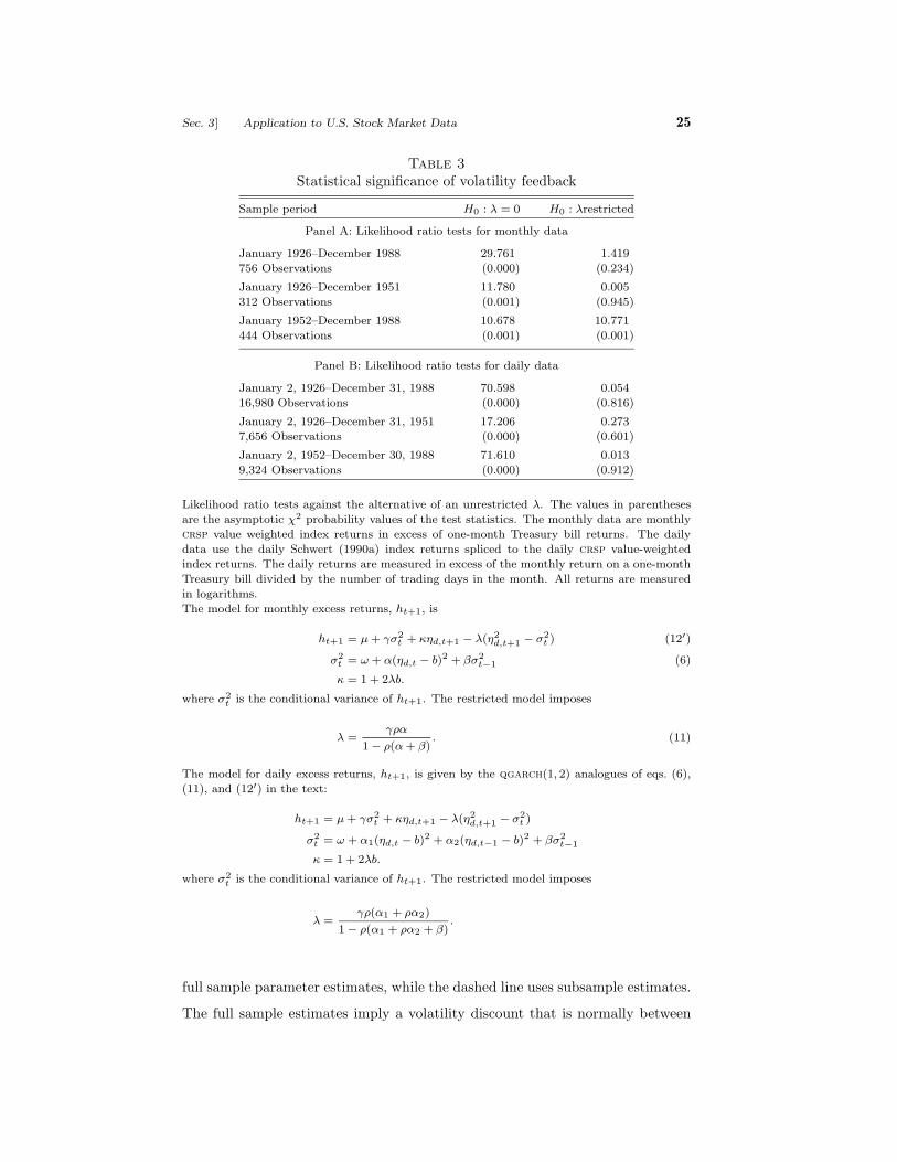
Table 3 reports likelihood ratio tests of models that restrict λ against more

general alternatives. Again the results are quite similar for monthly and daily

data. The data strongly reject models with λ = 0 against models with nonzero

λ. The restriction relating λ to the other parameters, by contrast, is rejected

only in the anomalous monthly postwar data.

3.3 The Economic Importance of Volatility Feedback

We have shown that volatility feedback is statistically significant, but what is its

economic significance? In this section we present several measures of the effect

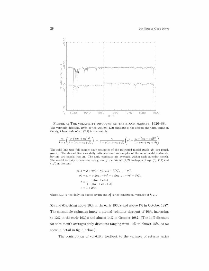
of volatility feedback on stock prices. We begin in fig. 4 by plotting the volatil-

ity discount implied by our model at each point in the sample. The volatility

discount is defined as the log difference between the actual stock price and the

price that would prevail in the absence of uncertainty about future dividends.

It is given by the second two terms on the right-hand side of eq. (9). As in

fig. 3, we use daily restricted λ models to obtain daily volatility discounts; we

then average these within each month before plotting. The solid line is based on


Table 3Statistical significance of volatility feedback

Sample period H0 : λ = 0 H0 : λrestricted

Panel A: Likelihood ratio tests for monthly data

January 1926–December 1988 29.761 1.419

756 Observations (0.000) (0.234)


312 Observations (0.001) (0.945)


444 Observations (0.001) (0.001)

Panel B: Likelihood ratio tests for daily data

January 2, 1926–December 31, 1988 70.598 0.054

16,980 Observations (0.000) (0.816)


7,656 Observations (0.000) (0.601)


9,324 Observations (0.000) (0.912)

Likelihood ratio tests against the alternative of an unrestricted λ. The values in parentheses

are the asymptotic χ2 probability values of the test statistics. The monthly data are monthly

crsp value weighted index returns in excess of one-month Treasury bill returns. The daily

data use the daily Schwert (1990a) index returns spliced to the daily crsp value-weighted

index returns. The daily returns are measured in excess of the monthly return on a one-month

Treasury bill divided by the number of trading days in the month. All returns are measured

in logarithms.

The model for monthly excess returns, ht+1, is

ht+1 = µ+ γσ2t + κηd,t+1 − λ(η2

d,t+1 − σ2t ) (12′)

σ2t = ω + α(ηd,t − b)2 + βσ2

t−1 (6)

κ = 1 + 2λb.

where σ2t is the conditional variance of ht+1. The restricted model imposes

λ =γρα

1− ρ(α+ β). (11)

The model for daily excess returns, ht+1, is given by the qgarch(1, 2) analogues of eqs. (6),

(11), and (12′) in the text:

ht+1 = µ+ γσ2t + κηd,t+1 − λ(η2

d,t+1 − σ2t )


t−1

κ = 1 + 2λb.

where σ2t is the conditional variance of ht+1. The restricted model imposes


1− ρ(α1 + ρα2 + β).

full sample parameter estimates, while the dashed line uses subsample estimates.

The full sample estimates imply a volatility discount that is normally between


Figure 4: The volatility discount on the stock market, 1926–88.The volatility discount, given by the qgarch(1, 2) analogue of the second and third terms on

the right hand side of eq. (2.9) in the text, is

γ

1− ρ

(ω + (α1 + α2)b2

1− (α1 + α2 + β)

)+

γ

1− ρ(α1 + α2 + β)

(σ2t −

ω + (α1 + α2)b2

1− (α1 + α2 + β)

).

The solid line uses full sample daily estimates of the restricted model (table 2b, top panel,

row 2). The dashed line uses daily estimates over subsamples of the same model (table 2b,

bottom two panels, row 2). The daily estimates are averaged within each calendar month.

The model for daily excess returns is given by the qgarch(1, 2) analogues of eqs. (6), (11) and


ht+1 = µ+ γσ2t + κηd,t+1 − λ(η2

d,t+1 − σ2t )


t−1


1− ρ(α1 + ρα2 + β)

κ = 1 + 2λb,


5% and 6%, rising above 10% in the early 1930’s and above 7% in October 1987.

The subsample estimates imply a normal volatility discount of 10%, increasing

to 12% in the early 1930’s and almost 14% in October 1987. (The 14% discount

for that month averages daily discounts ranging from 10% to almost 25%, as we

show in detail in fig. 6 below.)

The contribution of volatility feedback to the variance of returns varies


with the level of volatility, but it is generally very small, which is what one

would expect given the fairly stable volatility discounts shown in fig. 4. Eq. (15)

expresses the conditional variance of returns, divided by the conditional variance

of dividend news, as κ2 + 2λ2σ2t . In our restricted λ models, estimated on daily

data, κ ranges from 1.005 in the full sample to 1.012 in the postwar sample, so

κ2 is in the range 1.010 to 1.024. Thus the qgarch effect increases the volatility

of returns by 1-2%. The term 2λ2σ2t is normally even smaller, less than 0.1% at

the median level of daily volatility although it reaches a maximum of just over

4% in October 1987. In monthly data the excess variance terms are somewhat

larger but still modest: over the full sample κ is 1.027, κ2 is 1.055, and 2λ2σ2t

has a median of 0.2% and never exceeds 5%. These small numbers for excess

variance suggest that there is little difficulty with our assumption (7) that the

expected return on the market depends on the news variance rather than the

overall return variance. They also suggest that volatility feedback cannot explain

the findings of Campbell and Shiller (1988) and Campbell (1991) that returns

are considerably more variable than revisions of dividend forecasts.

Volatility feedback has a more important effect on the skewness of returns.

This is shown in fig. 5, which averages daily estimates in the same manner as

figs. 3 and 4. The median conditional skewness of returns is about −0.05 in full

sample estimates or −0.09 in postwar estimates, but skewness reaches −0.28 in

the early 1930’s and −0.84 in October 1987. Due to the within-month averaging,

fig. 5 does not reveal these extreme values but nonetheless shows the pattern

of variation over time. Conditional excess kurtosis (not shown in a figure) is

normally less than 0.1 in daily estimates, but it reaches 0.3 in the early 1930’s

and almost 1.0 in October 1987. These moments are generated by the mixture

of a normal and a χ2(1) distribution given in eq. (13), where the weight on the

χ2(1) is usually 1-2%, rising to 5% in the early 1930’s and 13% in October 1987.

These results give an interesting perspective on the debate between Pindyck

(1984) and Poterba and Summers (1986) over the importance of volatility feed-

back for stock market movements. According to our estimates, Poterba and

Summers are generally correct in that changing volatility has little effect on the

level of stock prices. But during periods of high volatility, the feedback effect

can become dramatically more important. Furthermore, the importance of the


Figure 5:The conditional skewness of stock returns, 1926–88.

Conditional skewness is given by

Skewt(ht+1) = −2λσt3κ2 + 4λ2σ2

t

(κ2 + 2λ2σ2t )3/2

. (16)


row 2). The dashed line uses daily estimates over subsamples of the same model (table 2b,

bottom two panels, row 2).The daily estimates are averaged within each calendar month. The

model for daily excess returns is given by the qgarch(1, 2) analogues of eqs. (6), (11), and


ht+1 = µ+ γσ2t + κηd,t+1 − λ(η2

d,t+1 − σ2t )


t−1


1− ρ(α1 + ρα2 + β)

κ = 1 + 2λb,


feedback effect is not limited by the low persistence of volatility. When we re-

strict λ to be the appropriate function of ρ, γ, and the variance parameters, our

estimates of γ generally become small (less than 0.3 in daily models). Since the

volatility discount is proportional to γ, it would be possible to have a strong

volatility feedback effect with reasonable levels of risk aversion.

The previous discussion has emphasized the behavior of stock returns over


long periods of time. However, we can also use the daily data to look more

carefully at the behavior of the stock market around the stock market crash of

October 1987. Volatility feedback is more important when volatility is high and

so should have an important role to play in this period.

The conditional standard deviation of daily news, σt, hovered close to 1%

during September 1987 and the first part of October but then rapidly rose to

almost 7% on the day of the crash, October 16, 1987. The sudden increase in

volatility was followed by a gradual decline back to 1.5% at the end of Jan-

uary 1988. (As noted by other authors, the decline in volatility after the crash

was more rapid than normal; our estimates imply that the normal half-life of a

volatility shock is about six months in postwar daily data.) For this period, as

well as others, estimates of the conditional standard deviation based on the full

sample differ very little from estimates of σt using only postwar data.

The implied volatility discount for September 1, 1987 to January 31, 1988

is shown in fig. 6. Full sample estimates show the discount increasing from about

6% to a maximum of 13%, and then gradually declining. Postwar estimates show

the discount increasing from 9% to a maximum of almost 25%. The difference is

due to the fact that the coefficients γ and λ are larger in postwar data. These dis-

counts are large enough to play an important auxiliary role in our understanding

of the crash period. Although they did not cause the crash (large discounts are

obtained only when large underlying news shocks occur), they help to explain

the severity of the market decline.

3.4 Alternative Models of Volatility Feedback

In this section we discuss the robustness of our results to some alternative spec-

ifications. We show that although our model of volatility feedback has a con-

siderably better fit than similar models without feedback, it cannot completely

account for the observed average levels of negative skewness and leptokurtosis.

However, explicit attempts to remedy this shortcoming without resorting to a

purely statistical description—using a skewed and leptokurtic distribution for

the news—do not significantly improve the model. We also show that the sig-

nificance of volatility feedback is not merely an artifact of the manner in which

our particular volatility process fits the predictive asymmetry of the data.


Figure 6: The daily volatility discount on the stock market,September 1987 to January 1988.

The sample period for this figure is September 1, 1987 to January 29, 1988. The volatility

discount, given by the qgarch(1, 2) analogue of the second and third terms on the right hand

side of eq. (2.9) in the text, is

γ

1− ρ

(ω + (α1 + α2)b2

1− (α1 + α2 + β)

)+

γ

1− ρ(α1 + α2 + β)

(σ2t −

ω + (α1 + α2)b2

1− (α1 + α2 + β)

).


row 2). The dashed line uses daily estimates over the postwar subsample of the same model

(table 2b, bottom panel, row 2). The model for daily excess returns is given by the qgarch(1, 2)

analogues of eqs. (6), (11), and (12′) in the text:

ht+1 = µ+ γσ2t + κηd,t+1 − λ(η2

d,t+1 − σ2t )


t−1


1− ρ(α1 + ρα2 + β)

κ = 1 + 2λb,


One measure of the adequacy of our model of volatility feedback is its

ability to produce model residuals that have the standard normal distribution

implied by the underlying theory. For each model we divide the residuals by

their estimated standard deviations. We compute the mean, variance, skewness,

and excess kurtosis of the normalized residuals for all of the estimated models.


If a particular model is well specified, then its normalized residuals should have

a standard normal distribution with zero mean, unit variance, and zero skewness

and excess kurtosis.

Almost all our estimated models have negative mean residuals, but none of

these means are significantly different from zero. For the monthly models, the

mean residuals range from a low of −0.051, with a standard error of 0.058, to

0.002, with a standard error of 0.048. The means of the daily residuals range

from −0.013, with a standard error of 0.011, to −0.010 with a standard error

of 0.008. French, Schwert, and Stambaugh (1987) note that a standard garch-

m model produces residuals with a significantly negative mean, i.e. the model

overestimates the average stock return. They conjecture that a model allowing

for skewness might correct for this. In fact, the generalization to qgarch is

critical in eliminating this problem. In the first version of this paper [Camp-

bell and Hentschel (1991)], in which we estimated simple garch models with

volatility feedback, we obtained significantly negative mean residuals that were

typically three or four times as large as those reported here. The addition of

volatility feedback alone clearly has little effect on the mean residuals of garch

and qgarch models.

Although all of the models have sample residual variances which exceed

unity the deviations from one are always well within a single standard error.

The variances of the standardized monthly residuals range from 1.003 to 1.039,

while those of the standardized daily residuals are between 1.005 and 1.010.

The addition of volatility feedback has only small effects on the variances of the

normalized residuals.

Volatility feedback is much more important in eliminating negative skew-

ness and excess kurtosis from model residuals. The residuals from models with

volatility feedback have only about one-half the skewness of the residuals from

simple qgarch models. For the full sample, the monthly model without volatil-

ity feedback (λ = 0) has normalized residuals with skewness of −0.865. When

we allow for the volatility feedback effect according to our model (λ restricted),

skewness is reduced to −0.439. If the parameter λ is freely estimated, skewness

falls to −0.417. Given our sample size, the standard error for the skewness of

N(0, 1) variates is 0.089. In the pre- and postwar subsamples, the results are


very similar except that in the postwar subsample skewness is lower for all three

models.

The normalized residuals from the daily model exhibit very similar pat-

terns. In the full sample the standard error for skewness is 0.019. The estimated

skewness for the model without volatility feedback (λ = 0) is −0.516. The intro-

duction of volatility feedback according to our model reduces skewness to −0.356

and freely estimating λ does not reduce skewness further. Once again the results

for the subsamples are very similar to those reported for the full sample.

Excess kurtosis is also greatly reduced in most sample periods. For the

monthly full sample, the standard error for excess kurtosis is 0.178. The esti-

mated excess kurtosis of the normalized residuals is 2.936 when we do not allow

for volatility feedback. When volatility feedback is introduced the excess kurtosis

falls to 1.681 and 1.509 for the restricted λ and unrestricted λ models, respec-

tively. The reductions of excess kurtosis are very similar in the subsamples with

the exception of the anomalous monthly postwar sample; in this period excess

kurtosis is reduced from 1.354 for the model without volatility feedback to 0.703

when λ is unrestricted. When we restrict the parameter λ, excess kurtosis ac-

tually increases to 1.730. However, given the standard error of 0.232 for the

estimates of excess kurtosis with this sample size, the increase from 1.354 to

1.730 is insignificant.

The reductions of excess kurtosis for the daily models are somewhat smaller

but nonetheless significant. In the full sample the standard error for excess

kurtosis is 0.038. The introduction of volatility feedback according to either the

restricted or free λ models reduces estimated excess kurtosis from 4.398 to 3.816.

In the prewar subsample the reduction is slightly less, from 2.824 to 2.789 and

2.779 for the restricted λ and the free λ models, respectively. However, in the

postwar subsample the reduction is much more substantial, from 5.079 to 3.446

and 3.441, respectively.

The volatility feedback effect could account for more of the observed skew-

ness and leptokurtosis if λ and γ were larger. The reason that we do not estimate

larger values of λ and γ seems to be that the skewness and excess kurtosis of

stock returns do not increase with volatility in the way required by our model.

When we regress the third and fourth powers of standard qgarch model resid-


uals onto qgarch variance estimates, our model predicts that we should find

negative and positive coefficients respectively [eqs. (16) and (17)]. In fact, we

tend to obtain the reverse sign pattern, although the coefficients are not generally

significant. What this means is that our model cannot fully explain the average

level of skewness and excess kurtosis without predicting exaggerated levels of

skewness and excess kurtosis in periods of high volatility. With high values of

λ, our model would not be able to account for rebounds following large stock

market crashes because the constraint on the maximum possible return would

become binding.

To address this issue, we have tried to develop models in which volatility

feedback does not become more important as volatility increases. In particu-

lar, we have applied our basic approach to other models of changing variance

[Hentschel (1992)]. Models of volatility feedback are only tractable when long-

horizon forecasts are linearly related to short-horizon forecasts of some volatility

measure, and when the expected stock return is linear in this same measure.

In the qgarch model used in this paper, forecasts of conditional variance are

linear in current information and the expected return must be linear in variance.

Alternatively, one can use a model in which the conditional standard deviation

of returns follows a garch-like process but in which the shocks are absolute

values of returns rather than squared returns. This can be combined with the

assumption that the expected return is linear in conditional standard deviation,

as suggested by French, Schwert, and Stambaugh (1987), among others.3 When

volatility feedback is incorporated into the model, one obtains a tent-shaped

rather than a parabolic news-return relationship, implying that the conditional

skewness and excess kurtosis of returns are constant rather than increasing in

conditional standard deviation. Unfortunately, the nondifferentiability of the ab-

solute value function means that the absolute value model has a discontinuous

likelihood function once volatility feedback is incorporated which greatly com-

plicates estimation and inference. Hentschel (1992) reports preliminary results

for this model and finds that it does not fit the data substantially better than

3 Nelson (1991) has recently proposed a model in which the log conditional standard

deviation follows a linear process. Unfortunately, one cannot introduce volatility feedback into

Nelson’s model without making the unorthodox assumption that the expected return is linear

in the log conditional standard deviation of returns.


the model studied in this paper.

We have also considered alternative models of predictive asymmetry. Our

qgarch model with volatility feedback fits the correlation between stock re-

turns and future volatility in two different ways. First, the news process itself

displays predictive asymmetry as shown by eq. (18) setting λ = 0. This predic-

tive asymmetry is generated by a nonzero qgarch parameter b, and it is more

important when conditional volatility σ2t is low than when it is high because the

qgarch model horizontally shifts the parabola relating shocks today to volatil-

ity tomorrow. (A given shift is more important when shocks cluster around zero

than when shocks are widely dispersed.) Second, the volatility feedback effect

contributes additional predictive asymmetry as shown by eq. (18) setting b = 0.

This predictive asymmetry is more important when conditional volatility σ2t is

high than when it is low, because (as noted earlier) the variance of the variance

of a garch or qgarch process increases more than proportionally with the level

of the variance of the process. Thus news about the variance becomes more im-

portant relative to underlying news when the variance is already high than when

it is low.

These effects of volatility on predictive asymmetry are somewhat arbitrary

and raise the possibility that our estimates of λ are significant only because we

have allowed no other means for the model to fit predictive asymmetry in high-

volatility periods. Our daily estimates imply that at mean or lower levels of

volatility the predictive asymmetry coming from volatility feedback is trivially

small relative to the predictive asymmetry coming from qgarch. At the mean

daily standard deviation of 0.095, for example, the full-sample estimates imply a

correlation between news and future volatility of −0.364, almost exactly the same

as the correlation between returns and future volatility. At a standard deviation

of 0.07, however, close to the maximum in the sample, the correlation between

news and future volatility is −0.053 while the correlation between returns and

future volatility is −0.159. Thus volatility feedback does add modestly to the

ability of the model to fit predictive asymmetry at high levels of volatility.

In order to ensure that our estimates of λ are not sensitive to the way in

which our model relates volatility and predictive asymmetry, we have estimated

a variant of the qgarch model (suggested to us by Daniel Nelson) in which

Sec. 4] Conclusion 35

the shift parameter b applies to normalized news rather than raw news. In this

model, eq. (6) is replaced by

σ2t = ω + ασ2

t−1

( ηd,tσt−1

− b)2

+ βσ2t−1, (19)

while the other equations of the model are unchanged. This makes the condi-

tional correlation of news and future volatility constant. It leads to a return

process of the form (12)’, but with a time-varying coefficient κt = 1 + 2λbσt

and with a more complicated relationship between λ and the underlying param-

eters of the model: λ = γρα/(1 − ρ(α(1 + b2) + β)

). We have estimated the

qgarch(1, 1) form of this model on both monthly and daily data and obtain

similar results to those reported in the paper, with strong evidence that λ is

nonzero but only weak evidence against the restriction relating λ to the other

parameters of the model. The only important change in the results is that the

latter restriction is rejected in monthly data over the full sample, although not

in monthly data in the postwar period. We note also that the time-variation

in κt in this model makes the variance of returns a less successful proxy for the

variance of underlying news. Thus our assumption (7) that expected returns are

linear in news variance is less appealing in the context of the model (19), which

is one reason that we do not use it as our main specification.

The first version of this paper [Campbell and Hentschel (1991)] employed a

standard symmetric garch process. There we also obtained very similar results

for the magnitude and significance of volatility feedback. We conclude that

volatility feedback estimates are not very sensitive to the specification of the

variance process.

4 Conclusion

We have estimated a model of volatility feedback in stock returns using a qgarch

model of changing variance that has recently been proposed by Engle (1990) and

Sentana (1991). Unlike the simple garch model, the qgarch model fits the

negative correlation between stock returns and future volatility of returns, and

it produces residuals with means close to zero. We show that the model fits U.S.

stock return data significantly better when it incorporates a volatility feedback


or “no news is good news” effect. Volatility feedback explains somewhat less

than half the skewness and excess kurtosis of qgarch model residuals, without

introducing any new parameters specifically to fit these moments. Our estimates

of volatility discounts on stock prices are generally fairly stable at around 10%,

but they can increase dramatically during episodes of high volatility. During

October 1987, for example, the volatility discount reached a maximum of almost

25%.

We conclude with one caveat about the interpretation of our results. Our

formal model assumes that changing expected excess returns are driven by chang-

ing volatility. The remaining component of returns is treated as being driven

by news about dividends (strictly speaking, dividends and real interest rates).

However it is quite possible that the underlying shock which we write as ηd,t+1

also contains innovations in required excess returns arising from some source

other than changing volatility. The only way to distinguish this possibility from

the dividend news interpretation of ηd,t+1 is by testing for the constancy of

the volatility-adjusted conditional mean excess stock return for which the meth-

ods of this paper are not well suited. Earlier work reported in Campbell and

Shiller (1988) and Campbell (1991) finds that changing expected stock returns

are an important source of variation in unexpected stock returns, but in this

paper we find that volatility feedback contributes little to the unconditional

variance of returns. We therefore believe that much of the variance of ηd,t+1 is

in fact due to other changes in expected excess returns, and not to news about

future dividends.

References

Akgiray, Vedat, 1989, “Conditional heteroscedasticity in time series of stockreturns: Evidence and forecasts.” Journal of Business 62, 55–80.

Attanasio, Orazio and Sushil Wadhwani, 1989, “Risk and the predictabil-ity of stock market returns.” Working paper (Stanford University, Stan-ford, CA and London School of Economics and Political Science, London,UK .

Black, Fischer, 1976, “Studies of stock price volatility changes.” Proceedingsof the 1976 Meetings of the Business and Economics Statistics Section,American Statistical Association, 177–181.

References 37

Bollerslev, Tim, 1986, “Generalized autoregressive conditional heteroskedas-ticity.” Journal of Econometrics 31, 307–328.

Bollerslev, Tim, 1987, “A conditionally heteroskedastic time series modelof security prices and rates of return data.” Review of Economics andStatistics 59, 542–547.

Brown, Keith C., W.V. Harlow, and Seha M. Tinic, 1988, “Risk aver-sion, uncertain information, and market efficiency.” Journal of FinancialEconomics 22, 355–385.

Campbell, John Y., 1991, “A variance decomposition for stock returns.” The1990 H.G. Johnson Lecture to the Royal Economic Society, EconomicJournal 101, 157–179.

Campbell, John Y., 1992, “Intertemporal asset pricing without consumptiondata.” NBER Working Paper No. 3989.

Campbell, John Y. and Ludger Hentschel, 1991, “No news is good news:An asymmetric model of changing volatility in stock returns.” NBERWorking Paper No. 3742.

Campbell, John Y. and Robert J. Shiller, 1988, “The dividend-price ratioand expectations of future dividends and discount factors.” Review ofFinancial Studies 1, 195–228.

Chou, Ray, 1988, “Volatility persistence and stock valuations: Some empiricalevidence using GARCH.” Journal of Applied Econometrics 3, 279–294.

Christie, Andrew A., 1982, “The stochastic behavior of common stock vari-ances: Value, leverage, and interest rate effects.” Journal of FinancialEconomics 10, 407–432.

Cutler, David M., James M. Poterba, and Lawrence H. Summers,1989, “What moves stock prices?” Journal of Portfolio Management 15,4–12.

Engle, Robert F., 1982, “Autoregressive conditional heteroskedasticity withestimates of the variance of United Kingdom inflation.” Economet-rica 50, 987–1007.

Engle, Robert F., 1990, “Discussion: Stock market volatility and the crash of’87.” Review of Financial Studies 3, 103–106.

Engle, Robert F. and Gloria Gonzalez-Rivera, 1989, “SemiparametricARCH models.” Working paper (University of California San Diego, LaJolla, CA.

Engle, Robert F., David M. Lilien, and Russell P. Robins, 1987, “Es-timating time varying risk premia in the term structure: The ARCH-Mmodel.” Econometrica 55, 391–407.

Flavin, Marjorie A., 1981, “The adjustment of consumption to changingexpectations about future income.” Journal of Political Economy 89,974–1009.


French, Kenneth R., G. William Schwert, and Robert F. Stambaugh,1987, “Expected stock returns and volatility.” Journal of Financial Eco-nomics 19, 3–29.

Hansen, Lars Peter and Thomas J. Sargent, 1981, “A note on Wiener-Kolmogorov prediction formulas for rational expectations models.” Eco-nomics Letters 8, 255–260.

Haugen, Robert A., Eli Talmor, and Walter N. Torous, 1991, “Theeffect of volatility changes on the level of stock prices and subsequentexpected returns.” Journal of Finance 46, 985–1007.

Hentschel, Ludger, 1992, “Models of asymmetric volatility in stock returns.”Unpublished Ph.D. dissertation (Princeton University, Princeton, NJ).

Ibbotson Associates, 1989, “Stocks, bonds, bills, and inflation: 1989 Year-book.” Chicago.

Lumsdaine, Robin L., 1990, “Asymptotic properties of the quasi-maximumlikelihood estimator in GARCH(1, 1) and IGARCH(1, 1) models.” Work-ing paper (Harvard University, Cambridge, MA.

Merton, Robert C., 1980, “On estimating the expected return on the market:An exploratory analysis.” Journal of Financial Economics 8, 323–361.

Nelson, Daniel, 1991, “Conditional heteroskedasticity in asset returns: A newapproach.” Econometrica 59, 347–370.

Pagan, Adrian R. and G. William Schwert, 1990, “Alternative models forconditional stock volatility.” Journal of Econometrics 45, 267–290.

Pindyck, Robert S., 1984, “Risk, inflation, and the stock market.” AmericanEconomic Review 74, 335–351.

Poterba, James M. and Lawrence H. Summers, 1986, “The persistenceof volatility and stock market fluctuations.” American Economic Re-view 76, 1142–1151.

Schwert, G. William, 1989, “Why does stock market volatility change overtime?” Journal of Finance 44, 1115–1153.

Schwert, G. William, 1990a, “Indexes of United States stock prices from 1802to 1987.” Journal of Business 63, 399–426.

Schwert, G. William, 1990b, “Stock volatility and the crash of ’87.” Reviewof Financial Studies 3, 77–102.

Sentana, Enrique, 1991, “Quadratic ARCH models: A potential reinterpreta-tion of ARCH models as second-order Taylor approximations.” Workingpaper (London School of Economics and Political Science, London, UK).

Turner, Christopher M., Richard Startz, and Charles R. Nelson,1989, “A Markov model of heteroskedasticity, risk, and learning in thestock market.” Journal of Financial Economics 25, 3–22.

The QGARCH(p, q) Model 39

Appendix A: The QGARCH(p, q) Model

The text discusses the case of qgarch(1, 1) in considerable detail. Here we

extend the model to accommodate more general qgarch(p, q) processes. Still

more general forms of qgarch, which allow for interactions of lagged shocks, are

discussed in Sentana (1991); these can be handled by a straightforward extension

of our approach.

For a qgarch(p, q) process the variance is described by

σ2t = ω +

q∑i=1

αi(ηd,t+1−i − bi)2 +p∑j=1

βjσ2t−j . (A.1)

Some algebraic manipulations allow us to solve (A.1) for η2d,t+1 in the following

form:

η2d,t+1 = ω′ +

max{p,q}∑i=1

(αi + βi)η2d,t+1−i − 2

q∑i=1

αibiηd,t+1−i

+ (η2d,t+1 − σ2

t )−p∑j=1

βj(η2d,t+1−j − σ2

t−j), (A.2)

where βj = 0 for j > p, αi = 0 for i > q, and ω′ = ω +∑qi=1 αib

2i .

For canonical garch processes bi = 0 and eq. (A.2) is an ARMA(max{p, q},p) process for η2

d,t+1 with mean zero innovations (η2d,t+1−j − σ2

t−j):

η2d,t+1 = ω′ +

max{p,q}∑i=1

φiη2d,t+1−i + εt+1 +

p∑j=1

θjεt+1−j , (A.3)

where φi = (αi + βi) and θj = −βj . In this ARMA case we can apply well-

known results for the discounted sum of revisions in the expected future values

of ARMA processes [Flavin (1981), Hansen and Sargent (1981)] to find ηh,t+1.

Unfortunately, when bi 6= 0 there are additional terms of the form

−2αibiηt+1−i preventing an ARMA representation. Nonetheless, we can find

a state space representation for η2d,t+1, such that η2

d,t+1 is the first element in

the state vector Zt+1 which follows the transition equation

Zt+1 = ω′e1 + TZt +RUt+1, (A.4)


where

T =

φ1 −2α1b1 . . . − 2αpbp... Im−1 0

φm−1

φm 0 . . . 0 0 . . . 00 0 . . . 0 0 . . . 00 0... 0 Ip−1

...

0 0

,

R =

1 0

θ1 0...

...

θm−1 0

0 1

0 0...

...

0 0

, Ut+1 =

(η2d,t+1 − σ2

t

ηd,t+1

),

and e1 = (1, 0, . . . , 0)′. The error term Ut has zero mean and is serially uncorre-

lated. Eq. (A.4) can be used to form the expectation of ht+1+j for any horizon

since EtUt+1 = 0.

Et+1ht+1+j = µ+ γEt+1η2d,t+1+j

= µ′ + γe′1TjZt+1. (A.5)

The innovations in the expectations of ht+1+j are given by

(Et+1 − Et)ht+1+j = γe′1Tj (Zt+1 − TZt)

= γe′1TjRUt+1, (A.6)

which says that the innovations in expectations for the qgarch model of

eq. (A.1) are in general a linear combination of ηd,t+1 and (η2d,t+1 − σ2

t ).

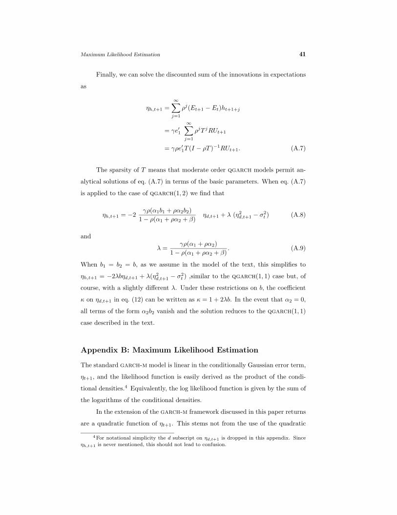
Maximum Likelihood Estimation 41

Finally, we can solve the discounted sum of the innovations in expectations

as

ηh,t+1 =∞∑j=1

ρj(Et+1 − Et)ht+1+j

= γe′1

∞∑j=1

ρjT jRUt+1

= γρe′1T (I − ρT )−1RUt+1. (A.7)

The sparsity of T means that moderate order qgarch models permit an-

alytical solutions of eq. (A.7) in terms of the basic parameters. When eq. (A.7)

is applied to the case of qgarch(1, 2) we find that

ηh,t+1 = −2γρ(α1b1 + ρα2b2)

1− ρ(α1 + ρα2 + β)ηd,t+1 + λ (η2

d,t+1 − σ2t ) (A.8)

and


1− ρ(α1 + ρα2 + β). (A.9)

When b1 = b2 = b, as we assume in the model of the text, this simplifies to

ηh,t+1 = −2λbηd,t+1 + λ(η2d,t+1 − σ2

t ) ,similar to the qgarch(1, 1) case but, of

course, with a slightly different λ. Under these restrictions on b, the coefficient

κ on ηd,t+1 in eq. (12) can be written as κ = 1 + 2λb. In the event that α2 = 0,

all terms of the form α2b2 vanish and the solution reduces to the qgarch(1, 1)

case described in the text.

Appendix B: Maximum Likelihood Estimation

The standard garch-m model is linear in the conditionally Gaussian error term,

ηt+1, and the likelihood function is easily derived as the product of the condi-

tional densities.4 Equivalently, the log likelihood function is given by the sum of

the logarithms of the conditional densities.

In the extension of the garch-m framework discussed in this paper returns

are a quadratic function of ηt+1. This stems not from the use of the quadratic

4 For notational simplicity the d subscript on ηd,t+1 is dropped in this appendix. Since

ηh,t+1 is never mentioned, this should not lead to confusion.


garch model but from the presence of the term λ(η2t+1 − σ2

t ) in eq. (12). Due

to this quadratic relation the derivation of the likelihood function requires the

use of some basic results for the transformation of random variables.

Recall that for a one-to-one transformation y = g(x) the distribution of y,

fy(y), is given by

fy(y) =∣∣∣∣ ddy g−1(y)

∣∣∣∣fx(g−1(y))

(B.1)

where fx(x) is the distribution of x. Furthermore, if the transformation is not

one-to-one, so that there are multiple roots g−1i (y), we can find the density

of the transformed random variable by summing over all regions for which the

transformation is one-to-one. Thus

fy(y) =∑i

∣∣∣∣ ddy g−1i (y)

∣∣∣∣fx(g−1(y)), (B.2)

where g−1i (y) are the roots of the transformation.

In our model the observed variable y is the stock return ht+1, and the

underlying variable is the news ηt+1. The transformation g is

ht+1 = g(ηt+1) = −λη2t+1 + κηt+1 + µ+ (γ + λ)σ2

t . (B.3)

As shown in fig. 2, this has the form of an inverted parabola, with two roots.

The smaller root is associated with a positive slope.

When (B.2) is applied to (B.3) we find that

fh(ht+1) =(κ2 − 4λ

[ht+1 − µ− (γ + λ)σ2

t

])− 12

×(fη(g−1

1 (ht+1))

+ fη(g−1

2 (ht+1))), (B.4)

where

g−11 (ht+1) =

κ−√κ2 − 4λ

[ht+1 − µ− (γ + λ)σ2

t

]2λ

and

Maximum Likelihood Estimation 43

g−12 (ht+1) =

κ+√κ2 − 4λ

[ht+1 − µ− (γ + λ)σ2

t

]2λ

. (B.5)

We assume that observed returns always have a positive derivative with

respect to the underlying shocks which generate them. In other words, the

shocks occur in the range for which the inverted parabola in fig. 2 is upward

sloping. Consequently, we always pick the smaller of the two roots above, ηt+1 ≡g−1

1 (ht+1), which amounts to assuming fη(g−1

2 (ht+1))

= 0. Since dy/dx =

(dx/dy)−1 we can write the conditional density of ht+1 as

fh(ht+1) = (κ− 2ληt+1)−1 fη(ηt+1). (B.6)

Finally we can write the conditional log likelihood function of ht+1 as a function

of the conditionally normal errors ηt+1 as

L(ht+1) = − log(κ− 2ληt+1)− 12

log(2π)− 12

log(σ2t )− 1

2η2t+1

σ2t

. (B.7)

This is the log likelihood function of the standard garch model for the implied

shock ηt+1, plus an additional term arising from the Jacobian of the quadratic

transformation.

Note that the likelihood function reduces to the standard garch-m case

when λ, the coefficient on the quadratic term, is zero.

When the roots g−11 (ht+1) and g−1

2 (ht+1) are real and distinct, κ−2ληt+1 >

0 and the likelihood is well defined. The cases of identical or complex roots

correspond to a situation in which an observed return equals or exceeds the

maximum return which can be produced by the model. This situation is ruled

out by penalizing the log likelihood function whenever the current parameter

values imply κ− 2ληt+1 ≤ 0.

After estimating the parameters of the model, we can check the accuracy

of the approximation that fη(g−1

2 (ht+1))

= 0 by calculating at each point in

the sample the probability of a shock larger than g−12 (ht+1), conditional on the

model parameters and our current estimate of the state variable σ2t . When we

do this we find that the probability never exceeds 10−7, so there should be only

trivial error introduced by our approximate method.

no news is good news - ludger hentschel · · 2015-12-31no news is good news: an asymmetric model...

Documents