NOAA Technical Memorandum ERL PMEL-39

DATA INTERCOMPARISON THEORY

II. TRINITY STATISTICS FOR LOCATION t SPREAD AND PATTERN DIFFERENCES

Rudolph W. PreisendorferCurtis D. Mobley

Pacific Marine Environmental LaboratorySeattle t WashingtonDecember 1982

UNITED STATESDEPARTMENT OF COMMERCE

Malcolm Baldrige.secretary

NATIONAL OCEANIC ANDATMOSPHERIC ADMINISTRATION

John V. Byrne,Administrator

Environmental ResearchLaboratories

George H. LudwigDirector

NOTICE

Mention of a commercial company or product does not constitutean endorsement by NOAA Environmental Research Laboratories.Use for publicity or advertising purposes of information fromthis publication concerning proprietary products or the testsof such products is not authorized.

Contribution No. 601 from NOAA's Pacific Marine Environmental Laboratory

ii

TABLE OF CONTENTS

Introduction . . .

Page

1

2.

3.

4.

5.

6.

7.

8.

Trinity Statistics

Reference Distributions in Adequate Settings (lOP)

Reference Distributions in Semi-Adequate Settings (EOP)

Reference Distributions in Borderline Settings (APP) . .

Reference Distributions in Semi-Inadequate Settings (PPP)

Reference Distributions in Inadequate Settings (CIP)

Power Curves of Trinity Statistics via ClassicalSampling Procedures .

9

14

20

26

35

40

43

9. Comparison of APP and PPP Distributions with ReferenceMCP Distributions

10. References ....

66

88

Appendix A: A Model/Data Matrix Generator for ControlledExperiments with Statistical Techniques

iii

89

Abstract

In this report, the second in a series of five on data intercomparison

theory, we examine three basic measures of data-set separation and procedures

by which these measures can be assigned statistical significance. The three

measures are for the distances between means (SITES), variances (SPRED), and

patterns (SHAPE) of space-time geophysical multivariate data sets. The patterns,

in turn, are resolved into spatial and temporal patterns.

The problem of determining procedures to generate reference distributions,

by which statistical significance is decided, is resolved into five parts,

depending on the amount of data available for use. We classify availability

of data into five categories: adequate, semi-adequate, borderline, semi­

inadequate, and inadequate. For each of these settings we develop procedures

to generate reference distributions for SITES and SPRED, and determine the

power curves for these two statistics under selected procedures. These power

curves are compared with those generated by some classical tests for the

relative location and spread of multivariate data sets. The proposed statistics

SITES and SPRED and some of their distribution-producing procedures appear to

be relatively powerful and robust.

v

Data Intercomparison Theory

II. Trinity Statistics for Location, Spread and Pattern Differences

Rudolph W. Preisendorfer

Curtis D. Mobley

1. Introduction

The central problem of data intercomparison theory in climate studies is

two-fold: given two (often spatially extensive) data sets D and ~, each in

the form (say) of p time series of some physical field sampled n times, it is

required first of all to gauge the "distance" (in some sense) between D and ~,

and then to decide if this distance is "significantly large" or not. The

outcome of such a decision could for example lead (if the "distance" is not

large) to the acceptance of some dynamical hypothesis about the field; or it

could in another instance be instrumental (if the "distance" is too large) in

discarding or modifying a computer model attempting to simulate the physical

processes of the field. It is therefore a matter of considerable importance

in the study of climate processes to have some confidence in the adequacy of

the statistical decision procedures by which a theory will stand or fall, or

by which a model is declared faithful or not. More often than not, the classical

statistical tools of gaussian reference distributions and their various derivates,

and even the oft-invoked declarations of statistical independence, are not

adequate to the tasks of modern climatology. In this note we examine the

general problem of defining distance gauges between various attributes (location,

spread, pattern) of pairs of geophysical data sets. This problem leads directly

to that of constructing the reference distribution for the statistic, the

means by which significance decisions are made.

§1

There are no unique solutions to these problems, no solutions that are

maximally powerful in all settings encountered in practice. We therefore

cannot emphasize just one procedure by which the general intercomparison

problem may be solved. Rather we will develop some general principles of data

intercomparison activity which can serve to guide the construction of inter­

comparison procedures for a wide range of specific settings.

This wide range of settings can be split up into a set of five categories.

These are defined loosely by the relative size of the data sets that are

available within them for constructing the reference distributions. These

categories are arranged in order of decreasing availability of real data sets,

as follows: adequate, semi-adequate, borderline, semi-inadequate, and inadequate.

We shall illustrate a reference-distribution building-procedure for each of

these categories. The procedures begin with the ideal case of adequate real

data sets. This is the real counterpart to the theoretical setting wherein a

classical distribution (e.g. normal, chi square, etc.) serves as the reference

distribution from which an arbitrary, unlimited number of samples can be

drawn. In some real data sets now becoming available (e.g. the HSSTP assembled

at CIRES by Fletcher and colleagues at Boulder, CO) we have adequate numbers

of data values which fall into this first category, for some (but not all)

statistical studies. In this setting all statistical questions, by definition,

can be answered in adequate detail. Next come the semi-adequate data settings

where there are "almost enough" samples to constitute a sample space of statistic

values. By means of a simple and natural permutation procedure such a setting

can be made to blossom into an adequate one, and from which statistical decisions

can be drawn. Next come two categories, the borderline and semi-inadequate

cases, where, despite the absence of further data or dynamic principles,

relatively powerful measures can still be taken to generate the requisite

2

§1

reference distributions. These two cases are perhaps the more important of

the five categories studied here and accordingly we shall give them most of

our attention, developing respectively the auto-cross, and the pool, permutation

procedures (APP, PPP, resp.) for the borderline and semi-inadequate cases.

The fifth (the "inadequate") category of data availability represents such a

barren setting for reference distribution construction that we mention it only

for completeness and consider in passing some of the (admittedly desperate)

measures that one may invoke in order to generate a statistical background for

a given statistic. Nevertheless, knowing that something can be done even in

this setting may occasionally lead an investigator to a not unreasonable

conclusion about his data set or model.

In the pursuit of all these matters it is occasionally helpful to have in

mind a simple geometric visualization of the data sets being intercompared.

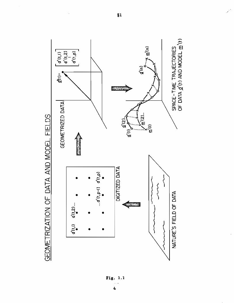
The geometrization of a data set is illustrated in Fig. 1.1. There are four

activities in the process of visualization: assembling raw data, producing

digitized data (which is also filtered at this stage), the compression of a

synoptic pattern into a point of E (p-dimensional euclidean space), andp

producing the space-time trajectory of the point. In this last stage, two

data sets Q, ~, originally in the form of p time series (of sea surface

temperature, or sea level air pressure, say) sampled n times, are now seen as

two trajectories in E , discretely sampled at times t=I, ... ,n.p

These geometric visualizations are heuristic, in the sense of suggesting

to an investigator various possible definitions of measures of distance between

the main attributes (location, spread, shape) of data sets. However, human

ability to effectively visualize these attributes is limited to E2 or Es .

When the number of time series, say, increases to four or more, resort must be

made to objective reasoning by analogy and by symbol-manipulations. To illustrate

3

GE

OM

ETR

IZA

TIO

NO

FD

ATA

AND

MO

DE

LFI

ELD

S

~~~/

...d

l(t,

p-I

)d

'(t,

p)

••

••

d'(t

,1)

d'(

t,2

)...

••

•

CO

tt-

I

[dIU'()]

d'(

t,2

)

dl(

t,p

)

Q't)

=

l~ :·'t'

~:

SPAC

E-

TIM

ETR

AJE

CTO

RIE

SO

FD

ATA

d'(

t}A

ND

MO

DE

Lm

l(t}

d'(

I-

2)"

,Q

(I);rf

f~,

...~

-~,

(m' (2

L

m'(l

)

"'-

GE

OM

ETR

IZE

DD

ATA

f1L'lf'~~~

:-\y

,&";

y";

••

•

DIG

ITIZ

ED

DAT

A

t· '. .... I:~. ..

••

NA

TUR

E'S

FIE

LDO

FD

ATA

~ ....~

~ t-I . t-I

§1

the necessity of such objective measures, we have prepared three visual experiments

and recorded them in Figs. 1.2, 1.3, 1.4. In each of the figures we started

from the same data set shown by the circles. Each circle summarizes the

simultaneous temperature (say) at two stations on the ocean surface. There

were 48 such observations made at each station. In one of the figures the

circles were all displaced a fixed amount parallel to one of the axes and

their final locations marked by crosses. In another figure, the circles were

rotated by 20° in a certain direction about their centroid. In still another

figure the set of circles was subject to a transformation affecting only the

overall variance of the set. Can the reader discern, visually, which diagram

illustrates which of these transformations? This example may serve to indicate

the occasional need for objective measures of distance between the various

commonly used attributes of data sets. Visual examples could be made to

illustrate the need for an even more subtle concept of data intercomparison

theory, that of statistical significance. But perhaps this set of three

diagrams will serve to make the point of this discussion.

Acknowledgments

Our interest in the data intercomparison problem is due largely to stimulating

discussions over the past years by one of us (RWP) with Dr. Tim P. Barnett of

the Climate Research Group at Scripps Institution of Oceanography. Moreover,

the example in §6J is drawn from a joint study by Dr. Barnett and the authors.

Ryan Whitney of PMEL typed the manuscript and Gini May of PMEL drew the figures.

5

x

§1

x0

E) 0

X (T")

XXx XX

X 0XE) 0

~X N

E)~E)

Xx XE)

E)E)X X X X

E) :<- X 0

XX0

E) .....E) >s<

~~ X

X X X

XE)E) E)

X E) E)

x>g3.......

X EX 0

E)E) X C!L:X o I-<

X Eb E) E) E) 0E)

E)E) E) X

E)XE) E) Xx E) 0

E) C!X X E) .....

E) I

E)E)

E) €\8 00

E) E) NI

00

(T")I

00"£ 00"2 00" r 00"0 00'[- 00"2- 00"£-Z I,.JIO

Fig. 1.2

6

§1

0

80

(T)

X8

00

8 N

8X8 8

X 88X8 0 X X 0

8X

08

8 X Elf XX

88Xx8 x X ~X0fJ 8 ...--<0

88 XX C?L:

~~ X~ X 01---<8 8 0

8X X X~8 X ~X X

X 8 8 8 X 00

X 8 8 -8 X I

8 XxXX

X 88 EB 0

0

8 8 NI

00

(T)I

OO'E 00'2 00' 1 00'0 00'1- OO'Z- OO'E-ZWIO

Fig. 1.3

7

§1

0

E) 0

(T)

X

E) 00

E)X X N

E)

XX ~E) E) E)

X XE) X 0

X E) 0E) XE) X X

......

EX:E) E) X~~

~x X

><8 EY<E) E) ......X 0

~Ef< X C?L:

~X E)X X E) E) X0 ........

E)X 0

>tE) E) XE) XE)

XE) EX E) 0E)~

0

X ......E) I

X E)X~x xE) x EB 0

0

X E) E) NX I

00

(T)I

00"£ 00"2 oo"r 00"0 oo"r- 00"2- 00"£-2: WID

Fig. 1.4

8

§2

2. Trinity Statistics

In the geometrization process of a data set described in the Introduction,

we begin with two data sets in raw observation form. After objective analysis,

each data set is in digitized form (the primes in Fig. 1.1 have been dropped

for brevity):

D: {d(t , x) : t=1, ... , n ; x=1, ... , p }

M: {m(t,x): t=l, ... ,n; x=l, ... ,p}

(2.1)

(2.2)

Here t, x are time and space indexes. We may think of D and M either as DXp

matrices, as points in euclidean space E of dimension np, or as two swarmsnp

of n points each in euclidean space E of dimension p. Each of these represen­p

tations will be used in the developments below.

The basic measure of separation L(Q,~) of two points in E , such as Q,~np

in (2.1), (2.2), is defined via

n pL2(Q,~) _ I I [d(t,x) - m(t,x)]2 .

t=l x=l(2.3)

On the other hand, we may visualize Q,~ as n-point swarms in E , i.e., asp

D: {~(t): t=l, ,n}

M: {~(t): t=l, ,n}

where (with "T" denoting transpose):

(2.4)

(2.5)

~(t)

~(t)

T_ [d(t,l), ... ,d(t,p)]

T- [m(t,l), ... ,m(t,p)]

(2.6)

(2.7)

The measure of distance II!!-! II between points !!,!, of Ep may be defined via

9

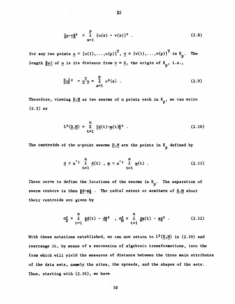
§2

P1I~_YIl2 _ I [u(x) - v(x)]2 .

x=l(2.8)

T Tfor any two points u =[u(l), ... ,u(p)] , Y =[v(l), ... ,v(p)] in E. Thep

length II~II of u is its distance from y = Q, the origin of Ep ' Le.,

11~12PI u 2 (x) .

x=l(2.9)

Therefore, viewing ~'~ as two swarms of n points each in E , we can writep

(2.3) as

nL2(~,~) = I 11.~(t)-!!!(t)1I2 .

t=l(2.10)

The centroids of the n-point swarms ~,~ are the points in E defined byp

nd - n- 1 I ~(t)

t=l

nm - n- 1 I !!!(t)

t=l(2.11)

These serve to define the locations of the swarms in E. The separation ofp

swarm centers is then II~-!!!II. The radial extent or scatters of ~'~ about

their centroids are given by

nafi - I II~(t) - ~1I2

t=l, a~

n_ I 1I!!!(t) - !!!1I 2 .

t=l(2.12)

With these notations established, we can now return to L2(~,~) in (2.10) and

rearrange it, by means of a succession of algebraic transformations, into the

form which will yield the measures of distance between the three main attributes

of the data sets, namely the sites, the spreads, and the shapes of the sets.

Thus, starting with (2.10), we have

10

§2

nL2(~,~) = I ~~(t) - ~(t)~2

t=l

n n n= I {(~(t)_~)T (~(t)-~) + I (~(t)_~)T (~(t)-~) + I (~_~)T (~-~)

t=l t=l t=l

n(~(t)_~)T

n(~(t)_~)T- I (~(t)-~) - I (~-~)

t=l t=l

n T n T- I (~(t)-~) (~(t)-~) + I (~(t)-~) (~-~)

t=l t=l

n T n T- I (~-~) (~(t)-~) + I (~-~) (~(t)-~)t=l t=l

(2.13)

This reduces to

n n+ I ~~(t)_~"2 + I "~(t)_~"2

t=l t=l

n- 2I [~(t)_~]T [~(t)-~]

t=l

(site)

(spread)

(shape) (2.14)

This may be rearranged further into the following form with the help of (2.12):

nL2(~,~) = n 1I~_~"2 + (a

D-a

M)2 + 2{a

Da

M- I [~(t)_~]T [~(t)-~]} .

t=1(2.15)

In order to obtain dimensionless measures of separation of the site, spread

and shape terms, (2.15) suggests division of each term by aDaM. When this is

done we will have attained the trinity of statistics of the present study, and

(2.15) becomes

11

§2

DIST2 = SITES + SPRED + SHAPE

where we have written

"DIST2" for L2 <!!,~n/ODOM

"SITES" for n 1I~-!!!1I2/0DOM

"SPRED" for (OD-OM)2/0DOM

T

"SHAPE" for 2 1 _ ~ [~(tl-~] [!!'(tl-!!']t=1 °D OM

(2.16)

(2.17)

(2.18)

(2.19)

(2.20)

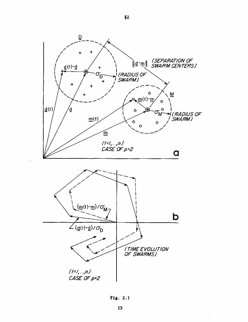
The trinity of statistics {SITES, SPRED, SHAPE}, which have been carved

out of DIST2, will serve as our measures of separation of the three main

attributes of Q,~, namely location, radial scale, and pattern. Fig. 2.1

illustrates, for the case p = 2, the various concepts defined in the present

discussion. Here we have a schematic depiction of Q,~ as 8-point swarms in

E2 • Their centroids are shown in part (a) of Fig. 2.1 as ~,!!!, being separated

by distance II~-!!II The radii of D,M are schematically shown (and not to

scale) by 0D' OM. In part (b) of the figure the essential terms of the statistic

SHAPE are interpreted graphically. Thus the vectors ~(t) = [~(t)-~]/OD and

~(t) = [!!(t)-!!]/OM are vectors in Ep for each time t =1, ... ,n. They are placed

end-to-end to simulate successive displacements of the data points in E. IfP

~(t) and ~(t) happen to point in the same direction for every t, and in particular

~(t)-~ =(OD/OM)(!!(t)-!!), we deduce from (2.20) that SHAPE =O. Thus in this

instance the spatial patterns spun out in time by the ~(t) and !!(t) points are

identical, even though the swarms may have different locations and spreads

about their centroids. Returning to Figs. 1.2, 1.3, 1.4, and recalling their

manner of construction, the reader may verify that SHAPE =0 for the three pairs

of data sets shown in these figures.

12

§2

a

(SEPARATION OFSWARM CENTERS)

(f=/, ...,n)CASEOFp=2

+

+

+

+

+'\.

\\\\I

0"0----" (RADIUS OF+ / SWARM)

/ ---/' .......// / 0 '\ M

,/ I -____-' I m(t}-m 0 \

/ \1 0 .01\ O"M--'" (RADIUS OF\ I SWARM)

o /o /

'- ./....... _-_/

Q,/,,----- ..... ,

//

//III\\\

/'./

/./

(\\\ (m(t}-m)/G:

M~~-----7

~

--

(TIME EVOLUTIONOF SWARMS)

b

(t=/, ...,n)CASEOFp=2

Fig. 2.1

13

§3

In the present study we shall concentrate mostly on SITES and SPRED,

being the simpler members of the trinity within DIST2. The statistic SHAPE,

as it turns out, because of its more complex internal structure, is less

powerful than SITES or SPRED using the presently adopted reference-distribution

building-procedures. Its detailed examination and that of its various logical

descendants will be made in part III of the present series of Data Intercomparison

Theory Studies.

3. Reference Distributions in Adequate Settings (lOP)

We shall give two examples of adequate settings arising in climate work

wherein the data are sufficient to the task of deciding on the statistical

significance of some event. When such data sets are encountered then they can

be mined for all the statistical information they possess. We shall refer to

this process as the "Ideal Observation Procedure (lOP)." The most basic form

of statistical information is of course in the cumulative distribution function

of the statistic of interest, from which all the moments of the distribution

and other derivates can be obtained. The longer the time series (or the data

gathering activity) has been in existence, the more detailed can be the structures

of the extracted distributions. In some statistical-gathering activities

(such as actuarial, astronomical, and some but not all aspects of meteorology

and oceanography) very detailed statistical tables are available for use in

diagnostic and prediction research. Here are two representative examples that

illustrate this basic mode of distribution-construction. One example is from

a routine collection of observed records, the other is from model-building

records.

14

§3

A. Example of lOP: Significant Temperature Rise in Homer, Alaska

A meteorologist on a TV weather program is often heard to make a statement

to the effect that today was a record breaker for hot (or cold) days, for this

date in a period of, say, twenty years. If one has the appropriate record of

temperatures, then it is a simple matter to deduce or verify the statement

made. On another occasion a less simple and more thought-provoking statement

may be that: during the first three weeks of the past month there was a

significant rise in temperature of early mornings, and that rise occurred over

the first couple of days of the second week. On first reading, the statement

may well appear cryptic. Then, as the sense of it emerges, some questions

arise. What could "significant rise" mean in this case?

In what follows we give an everyday type of example of how such a judgment

of significance in temperature changes can be given a precise, verifiable

meaning. We went to the monthly weather summaries that are routinely compiled

for each major U.S. city by the NOAA National Climate Center at Asheville, NC,

and randomly chose a city and a month. It turned out to be Homer, Alaska, for

October, 1979 (whose temperature record served as the basis of the above italicized

remark, and the analysis, below). We selected the first twenty-five days of

the month and graphed the temperatures in the city as they were recorded at

0200 hrs local time each day. These temperatures are shown as solid dots in

the upper graph of Fig. 3.1. We then took an average of these temperatures

for each successive pairs of days. These averages are shown as open circles.

This averaging was done because it was known that the speaker of the italicized

observation above was referring (implicitly at least) to temperature averages

over successive days. Next, since he had made a statement about temperature

changes over pairs of days, we took the differences of these averages by

subtracting the earlier average from the later. The results are graphed in

15

DA

ILY

(LO

CA

L,0

20

0H

OU

RS)

TEM

PE

RA

TUR

EO

BS

ER

VA

TIO

NS

ATH

OM

ER

,A

LAS

KA

1-2

5O

CTO

BER

1979

§3

the lower of the two diagrams and are indicated as circled dots. The range of

these differences is shown on the vertical axis to the left of the graph. The

frequencies of occurrence of these differences (classified in bins on the \OF

marks) are shown on the axis to the right of the graph. The frequencies of

occurrence of temperature rises occur on the upper half of the axis. Out of

the 10 rises, that at 5\OF was the greatest and of the smallest frequencg of

occurrence (whence the significance of the event). This event occurred between

the eighth and ninth days of the month. Thus we could, on this basis, and

with confidence 90% (since it occurred once out of 10 trials) make the italicized

statement about the event at the outset of this example. In fact this is what

we agree is meant by the statement, and in particular what is meant by the

words "significant rise" in that statement.

A quite different approach to that above, which would also be instructive,

would be to obtain a great many October temperature records for Homer, pool

the data, make a histogram just as above, but now for all pooled temperatures,

and then make the same analysis. That would produce a larger data base on

which to make the italicized claim above. In the example, as given, we are

content to use only one month as a basis for the italicized remark, for we are

at the moment interested in illustrating an idea, that of an adequate data

setting.

This example, although of simple content, contains the essence of the

activity involved in any verifiable statistical statement in climate studies:

(i) an adequate record of a specific physical field; (ii) at a given location;

(iii) over a particular time period (or an ensemble of time periods), of such

extent that the appropriate statistics can be compiled into: (iv) a distribution

from which the statement may then be read, its significance gauged, and from

which the confidence of that assertion can be deduced.

17

§3

B. Example of lOP: Significant Interannual Differences of a Computer

Simulation of Regional Temperatures

A computer model of a temperature field over a certain region yields a

sample of 360 readings at each of 24 stations of that region. (The model is

described in Appendix A, and will be used for other examples in this work.)

The samples spaced in time are intended to represent monthly averages, and

hence the period of time simulates 30 years of observations. The object of

the study is to determine the range and distribution of simulated interannual

differences in average yearly temperature over the 24 station network, and

specifically to note the manner in which significantlg large differences (on

the 5% level) in these multivariate interannual means are distributed throughout

the 30-gear period.

In order to analyze the computer output of the model in accordance with

the above goals we must define quantitatively the several key terms in the

italicized statement. Towards this end, let ~(t) be the 24-component vector

of temperatures at time t in the output record, where t =1, ... ,360. These

are formed via (Al.9) in Appendix A. For this example, a gear of temperature

records is any set {~(t+l),... , ~(t+12)} of temperature vectors with

o ~ t < t + 12 ~ 360. Hence two adjacent gears of temperature records are

given by

~j = {~(t): t =j+l, ,j+12} (3.1)

~j = {~(t): t =j+13, ,j+24} - {~(t): t =j+l, ... ,j+12}

for j =0, ... ,360 - 2x12 =336.

The jth interannual temperature difference over the region is given by

S. - SITES(D.,M.), j =0, ... ,336.J -J -J

18

N = 12

§3

P = 24 R = 337oo

..,....-----------------:::::::0"1-.

o

lL.. 0

o~Uo

I/)N.o

oo.+---~--___It__--"+----'--__;

en.OO 0.10 0.20 0.30 0.40SITES

OCCURRENCE IN TIME OF SIGNIFICANT DIFFERENCES OFANNUAL MEANS OF TWO SUCCESSIVE YEARS OVER 30 YEARS

a

6034 59

28 5527 51

122120

119 164

257256 318

255 282 311

o 50 100 150 200

MONTH

250 300b

336 360

1sf YEAR 2nd YEAR

Fig. 3.2

19

§4

The italicized statement above then directs us to order the S. in increasingJ

size, and select the largest 17 of them (since S% of 337 is 17, to the nearest

integer). The result is a cumulative distribution function (cdf) of the S ..J

The graph in Fig. 3.2(a) gives the cdf of S. values in this example, whileJ

Fig. 3.2(b) displays the seventeen years (i.e., the indexes j in (3.1» which

produced a significantly large multivariate mean difference over the 24-point

region. The largest 17 SITES values can be seen from Fig. 3.2(a) to range

from 0.296 to 0.338. The fields associated with these'S% significant values

were distributed in time over the 30 years as shown in Fig. 3.2(b). Thus the

first significant difference in annual means occurred over the 24 month period

beginning with month 27. The last occurred over the 24 month period beginning

~ith month 318. It is clear that the significantly large differences can

occur in clusters of 3 to 4, and that these clusters and the singletons occur

fairly uniformly over the years. It is not our intent here to analyze further

this interesting clustering behavior (it is a function of the choice of the

fundamental periods in the deterministic part of the model, the signal to

noise ratio built into it, the significance level, and the sampling procedure).

The main point of this example, however, has now been made: that under ideal

conditions, i.e., with an adequatelg large data set, basic questions of

significant behavior of a statistic (SITES in this case) can be fullg explored

without resort to the usual classical statistical constructs (gaussianitg,

independence, etc.).

4. Reference Distributions in Semi-Adequate Settings (EOP)

The present EOP (Empirical Observation Procedure) setting is one in which

the available data set is not large enough to directly make the requisite

20

§4

distributions in the fullness that is possible in the lOP settings of §3 above.

Yet there is enough information in the typical data set of this setting to

allow a simple permutation procedure to expand the data set into the requisite

sample space. The outline of the procedure is given below, followed by

explanatory comments and an example.

A. Given: nxp data sets ~,~ over region R , time interval I where p =no.o 0

points in R , n =no. samples at each point.o

B. Question: Is STSTC(~,~) significantly large? (STSTC =SITES, or SPRED)

C. Data Space: Available collection ~1""'~' 0 ~ 15 of nxp data sets overregion R and time interval I, which are relevant to pars A, Babove.

D. Sample Space: All ordered pairs (D.,D.), i, j = 1, ... ,0 ~ 15, i * j- - ~~

E. Statistics: Form Sk =STSTC(D.,D.), k =1, ... ,r ~ w =~(0-1)~~

F. Reference Distribution: Order the Sk of par E according to increasing size

and relabel:

S(I) ~ S(2) ~ ••• ~ S(crit) ~ ••• ~ S(r)' crit = (l-a)r

where a is the significance level of the test,o < a < 1.

G. Null HyPothesis H: (~,~) is in the sample spaceo

H. Accept Ho : if STSTC(~,~) ~ S(crit)

Reject Ho : if STSTC(~,~) > S(crit)

In the latter case, STSTC(~,~) is significantly large; in the former case

it is not.

I. Comments

The central feature of EOP, the one that distinguishes it from APP and

PPP below, is step C wherein it is explicitly required that there are available

at least 15 nxp data sets D. which are phgsicallg relevant to the given data~

sets ~,~. This means, e.g., that if D and M are arrays of SLP measurements

21

§4

over some region R of the Pacific and consist of monthly averages, then soo

But they need not always be overtoo should the D. be SLP monthly averages.-J

the same spatial or temporal domain as M and D. There is accordingly, in the

gathering of the data space ~l, ••• ,DO' considerable freedom as to choice of R

and I, as long as the choice leads to a mathematically well-defined and physically

reasonable sample space. Note that the sample space constructed in step D is

open-ended in that more elements can be added beyond those generated from the

present selection of the data space. We also observe that the sample space is

built on the assumption that the temporal order of the D. is immaterial to the-J

question at hand. Thus when forming H we are not interested in the fact thato

D. may precede D. in time, but only in some measure of separation STSTC(D.,D.)-1 -J -1 -J

of D. and D.. If in some investigation the time order of D. ,D. is important,-1 -J -1 -J

this should be stated in the question of par B and the appropriate sample

space in par D constructed. (For example, the illustrations of the lOP in §3

took congnizance of time ordering of the data sets.) In this extension of EOP

to questions of temporal order, the condition on 0 (i.e. ~ 15) may have to be

changed. The present choice of 0 ~ 15 assures that w ~ 105 so that a reasonably

detailed cumulative distribution curve can be obtained and its (say) 5%

significance level determined.

J. Example of EOP: model-model intercomparison

We use the model of Appendix A to generate 15 realizations of an nXp data

set ~; where n = 36, p = 24, a = 1, ~ = 0, and a = 1.000. Let the jth of

these sets be denoted by II~j", j = 1, ... ,15. From this we form the 105 points

of the BOP reference distribution made up of the values SITES(D.,D.), i,-1 -J

j =1, ..• ,15, i ~ j. This distribution is aenerated to answer the question of

22

§4

whether the pair (Q,~) (say) is in the sample space of 105 pairs (Qi,Qj) where

~ is generated by the same model but with ~ =0.300. Figure 4.1 shows the

reference distribution of SITES values formed, and Table 4.1 shows the values

of SITES(D.,M), j =1, ... ,15. From Fig. 4.1 we see that the critical value of-J -

SITES for the 5% significance level is at SITES = 0.063. From Table 4.1 we

find SITES(Ql'~) =0.106. Hence in this case we would discard H , and concludeo

that the centroids of ~ and Ql are significantly far apart. In other words,

increasing ~ of the model from 0.000 to 0.300 produces a significant change in

the mean value of the two resultant data sets. Indeed, if we go systematically

through the entire given set of 15 D. data matrices, and examine SITES(D.,M),J J-

j =1, ... ,15, then, as seen from Table 4.1, except for indexes 7,8, every one

of these SITES values is significant on the 5% level. The important exception

is SITES(Q7'~) =0.008.

In summary, we have shown that a small population of data sets (such as

the D.) can be augmented bg a simple pairing and permutation procedure so asJ

to generate a collection of ordered pairs (such as (D.,D.), i ~ j) which then~J

provide a reference distribution against which the statistic of some given pair

(Qk'~) can be compared for significant size.

23

§4

EOP DISTRIBUTION FOR SITES (Qjl M)ESTABLISHING 5% SIGNIFICANCELEVEL FOR ENTRIES IN TABLE 4.1

N = 36 P = 24 R = 105oo-

u.. 0

Cl~uo

II)N.o

oo'+---~--+----f-L----1

9b.00 0.02 0.04 0.06 0.08SITES

Fig. 4.1

24

§4

TABLE 4.1

List of sites (D.,M) values for j = 1, ... ,15,-J -

for the EOP model-model intercomparison example.

INDEX j SITES (D. ,M)-J -

1 0.106

2 0.065

3 0.117

4 0.096

5 0.123

6 0.075

7 0.008

8 0.063

9 0.082

10 0.090

11 0.064

12 0.083

13 0.083

14 0.122

15 0.102

25

§5

5. Reference Distributions in Borderline Settings (APP)

We consider now a borderline setting in the sense that we have only one

nxp data set Q to generate the reference distribution, in contrast to the 15

or more realizations of Q available for the EOP of §4, and the 337 samples of

§3. The present setting is, moreover, on the average, somewhat richer than

that considered in §6 below, in that n for the present case should on average

in practice be twice the n in the procedure* of §6. We call the present

procedure the "Auto-cross Permutation Procedure (APP)." Some further discussion

of this procedure is given in the comments below, and an example is appended

to illustrate its use.

A. Given: nxp data sets Q,~ over region R , time Intervalop = no. points in R , n = no.

h. 0at eac p01nt

I , whereoof samples

B. Question: is STSTC(Q,~) significantly large? (STSTC =SITES, or SPRED)

C. Data Space: Q only

D. Sample Space: The present elements of this are constructed from Q,~,

as follows.

(i) Represent Q as {~(I), ,~(n)} and

Mas {~(I), ,~(n)}

where ~(t), ~(t), t =1, ... ,n, are vectors in E .P

(ii) Construct a random permutation ~ of the set of integers 1, ... ,n.Let n =2m.

(iii) Partition D,M via ~ and form new nxp data sets. Thus formeither the-sets

- {~(~(I», ,~(~(m»}, {~(~(m+l», ,~(~(n»}1

- {~(~(I», ,~(~(m»}, {~(~(m+l», ,~(~(n»}

D-basedpartitions

* This is only a crude intuitive rule of thumb. Subsequent comparativestudies of APP and PPP under varying n-conditions should provide abetter rule.

26

§5

or, alternately, form the sets

~1'~2 - {~(~(l», ,~(~(m»}, {~(~(m+l», ,~(~(n»}

~1'~2 - {~(~(l», ,~(~(m»}, {~(~(m+l», ,~(~(n»}

M-basedpartitions

(For the case of n =2m+l, partition according to [~(l), ... ,~(m+l)],

[~(m+2), ... ,~(n)])

(iv) Repeat (ii), (iii) r times, r ~ 100, thereby forming r orderedpairs (~1'~2)1'... '(~1'~2)r along with (~1'~2)1'... '(~1'~2)r from

the ~-based sets (say). These two collections of ordered pairsform the sample spaces of current interest and are respectivelythe auto and cross sample spaces.

E. Statistics: Form the statistics Ak =STSTC(~1'~2)k'

Cf =STSTC (~1'~2)f ' k,f = l, ... ,r

F. Reference Distribution:

size and relabel.form the sequence

Order the auto statistics Ak of par E in increasing

Do likewise with the cross statistics Cf . Thus

A(l) ~ A(2) ~ ••• ~ A(crit) ~ ••• ~ A(r) , crit = [(l-a)r]

where a is the significance level of the test, and the sequence

C(l) ~ C(2) ~ ••• ~ C(r/2) ~ ••• ~ C(r) , C(r/2) =median

Here r/2 is taken to the nearest larger integer. The A(j) sequence

above produces the auto-reference (or DD) cumulative distributionfunction (cdf), while the C(j) produce the cross-reference (or DM)

cumulative distribution function (cdf).

G. Null Hypothesis H : (~1'~2)f' f = (r/2), is in the auto sample space0

H. Accept H : if C(r/2) ~ A(crit)0

Reject H: if C(r/2) > A( .)0 cr1t

In the latter case, at least 50% of the time will a randomly selected element(~1'~2)k of the cross sample space lie beyond the critical level of the auto

sample space. Thus we would conclude that, with at least probability 0.50,STSTC(~,~) is significantly large, with significance level a.

I. Comments

The rationale for this procedure is as follows. First of all,

the time order of the samples is presumed immaterial to the present procedure.

27

§5

If both D and ~ are drawn from the same population then, as before in EOP, the

switching of identity-tags on the elements ~(t) and ~(t) of ~ and ~ is permissible.

One can readily see this by visualizing the ~ and ~ as n-point swarms in some

common euclidean space E. The null hypothesis H in effect says that thep 0

labels U!!(t),U and u!!(t)" used to identify the points on each swarm are inter-

changeable in arbitrary ways. In principle there are up to n! points that can

be in the present sample spaces. However we will usually only need r ~ 100 or

so. The auto reference distribution provides a standard by which the location

of the cross reference distribution is gauged. If the median of the cross

distribution lies beyond (to the right of) the critical value of the auto

distribution, then we would have reason to believe that ~,~ are drawn from

different populations. Observe that we have used only the D-based partitions

in this exposition. We know, from statistical reasoning and also numerical

experiments, that for given parent distributions from which ~,~ are drawn, on

the average, the cross distribution for ~1'~2 equals that of ~1'~2; and moreover

that the M-based partitions will, on the average, produce the same results as

the D-based partitions. Thus either set of partitions may be used in practice.

If the time order of the samples is relevant to a study, then the present

procedure does not apply and must be modified accordingly.

J. Example of APP: Testing Effects of Different Objective Analysis Procedures

on a Raw Data Set

In a recent study, Liu (1982) developed an improved Cressman type objective

analysis procedure (Cressman, 1959) and applied it to raw data for sea surface

temperature (SST) over a rectangle of the equatorial Pacific from 25°N to

300 S, and from the western coastline of the Americas to 150oE, and in the time

28

§5

interval 1975 to 1980, inclusive. The analysis yielded 144 realizations of

\-month-averaged SST fields over the whole domain, and each realization was

contoured for surface isotherms. The fields therefore included the weak El

Nino of 1976 and its post period. This is a well-produced set of data fields

of high quality that can be used, among other things, to examine the non-seasonal

SST variation over the space-time extent of the data set.

In this example we will consider the effect of Liu's objective analysis

procedure on the mean-value and the variance of the final processed field. We

will compare the final Liu data set with two others arrived at in different

ways and which we will designate as "Modified Levitus-Oort" and "Original

Levitus-Oort." The second of these designations refers to the objective

analysis scheme of Levitus and Oort (1977) which Liu extended to his present

form. The first scheme was produced for this example by modifying Liu's

scheme as explained below. All these schemes are variations of the Cressman

procedure.

Table 5.1 below summarizes the salient features of each scheme. On the

left column of Table 5.1 we list the basic operations that occur in Liu's

procedure. It is not essential for our present example that the reader know

the detailed mathematical forms of these operations. (They may be reviewed in

Liu's (1982) study, or in more detail in DIT(V) of this series by Preisendorfer

and Mobley.) The XIS in Table 5.1 denote those operations of the left column

that (as far as possible) are common to all three objective analysis schemes.

It is seen then that the novelty in Liu's approach is fivefold: the "corrector

on grid" operator (a basic feature of Cressman's original scheme) is (i) made

SST gradient dependent, (ii) there is an outlier cutoff feature, (iii) the

various data entering the corrector scheme are weighted in importance of

quality, and (iv) the diffuser-smoother operator, absent in the original

29

w o

Tab

le5

.1D

efin

ing

the

thre

eo

bje

cti

ve

an

aly

sis

sche

mes

tob

ein

terc

om

par

ed

BASI

CO

PERA

TIO

NS

ONO

RIG

.DA

TAO

RIG

.LE

V-O

RTM

ODF.

LEV

-ORT

LIU

GRI

DTO

RACK

INTE

R-

XX

XPO

LATO

R

CORR

ECTO

RON

GRI

DSS

TGR

ADIE

NTIN

DEPE

NDSS

TGR

ADIE

NTIN

DEPE

NDSS

TGR

ADIE

NTDE

PEND

NOO

UTL

IER

CUTO

FFO

UTL

IER

CUTO

FFO

UTL

IER

CUTO

FF

NODA

TAW

GTNO

DATA

WGT

DATA

WGT

DIF

FUSE

R-SM

OO

THER

NONE

SST

GRAD

IENT

INDE

PEND

SST

GRAD

IENT

DEPE

ND

UPDA

TER

XX

X

CURV

ATUR

E-CO

RREC

TOR

NONE

XX

LAPL

ACIA

N-SM

OOTH

ERX

XX

em U1

§5

Levitus-Oort (and Cressman) scheme, is added in Liu's scheme and made dependent

on the SST gradient. Finally, (v) a curvature-corrector term is added to

Liu's scheme, relative to the original Levitus-Oort procedure.

The main motivation of this example is to see what happens to the average

values and variance of the raw data set as it is passed through the three

objective analysis schemes described in Table 5.1. In particular, we ask

whether the SST gradient-dependence of the "corrector on the grid" and

"diffuser-smoother" operators is important to the mean and variance attributes

of the data set. Accordingly we shut off these features of the Liu scheme and

also dropped the data weight feature. The result is the "modified Levitus-Oort"

scheme. Subsequently we dropped from the latter scheme the outlier cutoff

feature and dropped both the diffuser-smoother and curvature-corrector operators,

thereby reverting back to the original Levitus-Oort scheme.

After defining the above three schemes, we selected four regions in the

Pacific over which we would intercompare the results of the three schemes.

Each of these four regions is a rectangle of extent 5° x 10° in the north x east

directions, and with the properties as summarized in Table 5.2. The data sets

defined on these regions were of the nXp form ~,~, where p = 24 and n = 36.

Thus in each of the four regions we looked at 24 time series of 36 \-month

averages starting in January 1975 and extending 18 months through June 1976.

~,~ then took on the forms of the three possible distinct combinations, as

shown in the three left boxes of Table 5.3. The size of the significance

level a in the intercomparison was taken as 0.10, and r was taken as 100. We

applied the APP to each of these three pairs of data sets.

31

§5

Table 5.2

Four 5° x 10° Regions of p = 24 points each for DataIntercomparison of Liu's Objective Analyses Scheme withOriginal Levitus-Oort and Modified Levitus-Oort Schemes

Location of SW corner General Area Quality of Originalof Rectangle where Located Data in Rectangle

15°N, 1200 W Mexico coast High data densityLarge SST gradient

15°N, 1100 W Hawaii High data densitySmall SST gradient

2\oS, 1700 W Below Hawaii Moderate data densityon Equator Small SST gradient

2\oS, 1100 W On dateline Low data densityon Equator Small SST gradient

A study of the results in Table 5.3 suggests the following interesting

features of the three objective analyses schemes (of Table 5.1) applied to

data sets in regions 1-4 defined in Table 5.2.

First of all, the locations (i.e. mean values) of the resultant data sets

are not significantly affected by relaxing the gradient-dependent smoothing

operations of Liu's scheme. This is signified by the "A"s (for H "accepted")o

in the "SITES RESULT" column of Table 5.2. The actual sample means in region

1, e.g., are 24.97°C for Liu's set and 25.03°C for the original Lev-Oort set,

as shown in the Table. This amounts to a 0.06°C average difference over the

24 points and 18 month period. The fact that the SITES test, using APP,

32

§5

Table 5.3

Intercomparison of SITES and SPRED attributes of three pairsof data sets defined on the regions of Table 5.2 and producedusing the schemes of Table 5.1. APP was used to produce thistable. A = Accept H , R = Reject H .o 0

SAMPLE SITES SAMPLE SPREDDATA SETS REGION MEANS RESULT STD DEVS RESULT

LIU VS. ORIG 1 24.97°c A 1. 154°C RLEV-OORT 25.03 1.663

2 25.75 A 0.839 R25.23 1.414

3 27.17 A 0.7513 R27.05 1.338

4 28.25 A 0.566 R28.25 1.096

LIU VS.1 24.97 A 1.154 AMODIFIED 24.80 1.145

LEV-OORT

2 25.75 A 0.839 A25.75 0.832

327.17 A 0.7513 A27.16 0.755

4 28.25 A 0.566 A28.21 0.522

MODIFIED 1 24.80 A 1.145 RLEV-OORT 25.03 1.663VS.

ORIGINAL25.75 0.832LEV-OORT 2 25.83 A 0.414 R

327.16 A 0.755 R27.05 1.338

4 28.21 A 0.522 R28.25 1.096

33

§S

accepted H in this case is therefore intuitively reasonable. We conclude ino

particular that data density and SST gradient properties do not play an important

role in determining the mean structure of the present data sets via the defined

objective analysis schemes.

On turning to the "SPRED RESULT" column, we encounter another story. In

the Liu-vs-original Lev-Oort box we see (by the listed rejections R of H )o

that by omitting the new features of Liu's procedure, we produce significantly

different variance properties in the final data sets (as gauged by SPRED via

APP). The °C differences in sample standard deviations in this case are on

the order of O.SoC in region 1. When we return some of these features to the

Original Lev-Oort procedure to obtain the modified Lev-Oort scheme, we see, by

the Liu-vs-Modified Lev-Oort box, that the spreads of the fields are no longer

significantly different (the "A"s are denoting acceptance of H ) and theo

sample standard deviations are differing by O.OloC in region 1. The conclusion

we reach in this aspect of the study is that: relaxing just the SST gradient

dependent smoothing properties of the Liu objective analysis scheme does not

significantly affect the variance properties of the Liu data set in any of the

various regions. However, by dropping the new smoothing operations altogether,

and other features (see Table 5.1), so as to revert to the Original Levitus-Oort

scheme, the variance properties are significantly affected in all regions and

by amounts that are climatologically important (i.e., on the order of O.SOC).

The preceding conclusion leads us to the next consideration (which,

however, is beyond the scope of this study): which of the two schemes (Original

Levitus-Oort, or Liu) is to be preferred in the objective analysis of the

equatorial data? The tests have made their decisions as to the disparate

SPRED properties of the resultant data sets. Table 5.3 indicates that the

application of the new smoothing operations in the Liu scheme reduces the

34

§6

average standard deviations of the resultant sets by the order of O.SoC. The

detailed pursuit of this consideration, however, will not be made here.

6. Reference Distributions in Semi-Inadequate Settings (PPP)

We descend now to the setting where the number n of samples may be so low

that it may no longer be feasible to split up the Q and ~ sets, as in the APP

of §S, in order to generate the reference distribution. Instead we go the

other way: we pool the n-point swarms in E first, and then repeatedly partitionp

their union to generate the requisite reference distribution. We shall call

this the "pool permutation procedure (PPP)." The details follow.

A. Given: nxp data sets Q,~ over region R , time intervalop = no. points in R , n = no.at each point 0

I whereo

of samples

B. Question: is STSTC(Q,~) significantly large? (STSTC =SITES or SPRED)

C. Data Space: Q only

D. Sample Space: The elements of the sample space are constructed fromQ,~ as follows.

(i) Represent D as {~(l), ... ,~(n)} and

M as {~(l), ... ,~(n)}

where ~(t), ~(t), t = 1, ... ,n, are vectors in Ep

(ii) Form the union of Q,~, i.e., pool the ~(t) and ~(t) vectorsto find

- {~(l), ... ,~(n), !!!(l), ... ,!!(n)}

(iii) Construct a random permutation ~ of the set of integers1, ... ,2n. Arrange the permuted set in the order: ~(1), ... ,~(n),~(n+l), ... ,~(2n).

(iv) Partition ~ via ~:

35

§6

(v) Repeat (iii), (iv) r times, r ~ 100, thereby forming r orderedpairs (U1,U2)1,""(U1 ,U2). These constitute elements of the- - - - rsample space.

E. Statistics: Form the statistic values Sk =STSTC (~1'~2)k' k =1, ... ,r.

F. Reference Distribution: Order the Sk of par E according to increasingsize; and relabel:

S < S ~ ••• < S < ••• < S cr't(1) = (2) - = (crit) = = (r)' 1

where a is the significance level of the test.

G. Null Hypothesis H: (~,~) is in the sample spaceo

= I(l-a)r]

H. Accept Ho : if STSTC(~,~) ~ S(crit)

Reject Ho: if STSTC(~,~) > S(crit)

In the latter case, STSTC(Q,~) is significantlg large; in the former case,it is not.

I. Comments

The present scheme has the following rationale. For the purpose of

forming Ho ' we envision the two data sets ~,~ as being produced by some common,

statistically steady physical process. Thus under this assumption the sets

~1'~2 in step D(iv) above are just as likely to have evolved under this process

as Q,~. This assumption is tantamount to saying tht the labels "~(t),"

"!!!(t)," used to identify the points of each swarm, are interchangeable in

arbitrary ways within the union ~ of step D(ii). Granted this, the sample

space may be constructed and, ultimately, one of the decisions concerning Ho

is reached.

Looking at this decision process more closely and thinking specifically

of the range of values SITES(~1'~2)k' k =1, ... ,r (of step E), we observe the

following: if ~ and ~ have their centroids separated a distance that is large

compared to 0D'OM (recall Fig. 2.1a), then when we pool ~,~ and produce a

partition {~1'~2}' the centroids of ~1 and ~2 will tend on the average to have

SITES(~1'~2) smaller than SITES(~,~). If the latter value is significantly

36

§6

large (in the sense that it exceeds S(crit)) then in step H we would reject

H .o

A similar intuitive review of the decision process in step H can be made

for the range of values SPRED(~1'~2)k' k = 1, ... ,r. For this purpose it is

helpful to write SPRED(~,~) as (aD/aM) + (aM/aD) - 2. Then it is clear that

if aD and aM are markedly different, SPRED will be relatively large. As these

swarms ~'~ (with large SPRED) are pooled and partitioned in various ways, we

produce ~1'~2 with SPRED values that are, more often than not, less than

SPRED(~,~). If the latter value is significantly large (i.e. if it exceeds

S(crit)) then in Step H we would reject Ho . This may be visualized by

experimenting with a figure like that in Fig. 2.1a. A preliminary numerical

analysis of the power of SPRED under various conditions on centroid separation,

sample size n, and number of positions p in space is made in §8, below.

Similar numerical analyses for the power of SITES are also found in that

section.

It should be noted that the number of elements of the sample space formed

in step D can be quite large even for modest sample sizes n in D and M. For

example, if n = 10, then there are (2n!)/(n!)2 = 184,756 distinct partitions

that can be made and added to the sample space. Our experience shows that the

number of elements in the sample space can be considerably smaller, say on the

order of r = 100, from which the general shape and location of the distribution

function is already discernable and, indeed, useable.

Observe, finally, that the temporal order of (~,~) and hence of (~1'~2)

is presumed immaterial to the question at hand. Tests sensitive to the temporal

order of D and M can be constructed in the above framework of PPP (analogously

as in the case of the other procedures); but this matter will not be considered

here.

37

§6

J. Example* of PPP: Simulation of January sea level pressure by a GCM

A general circulation model may be used to simulate atmospheric and or

oceanographic time series in a region and epoch of interest, and the results

compared with reality. For example, we were interested in comparing with real

observations a GCM simulation of a typical January sea level pressure in the

relatively energetic region between 20 0 -80 0 N and 100 ·1800 W. A series of runs,

in the space-time domain, of an early version of the NCAR GCM was provided us

by R. Chervin. These were realizations obtained by five separate integrations

starting from the same initial conditions. Each realization was the last 30

days of a 60-day integration. The model output was projected onto a 50 latitude

by 100 longitude grid, of dimensions 36 x 33. The model matrix M was therefore

of dimensions n =5, p =1188.

We selected from the observed data five Januarys that were closest to the

long-term average January. The method was as follows: let p(!,t) be the sea

level pressure at location x and time t. Twenty-four years of January data

were used. Define

1- 24

where x gives the coordinates of a typical point in the 36 x 33 grid defined

above, and t indexes the January of interest. The standard deviation at x is

a(x) = I-.!- 23

24I

t=l

A separation index yet) was defined by

yet) =Ix

* This example is drawn from a joint study by T. P. Barnett and the authors.

38

.50

.99

.90

>-I---.-.Jm<rmo0:::0....W> .10

ti-.-.J::::J~a .01

o

§6

GeM vs DATA

REFERENCE DISTRIBUTIONVIA PPP

0.5 1.0 1.5SITES SITES (D,M)

Fig. 6.1

39

§7

The five Januarys with the smallest values of yet) were selected for the test,

and considered "typical." This produced the 5 x 1188 matrix ~.

The question posed was, "Did the GCM reproduce the observed mean January

sea level pressure field in the domain of interest?" This question was answered

by the PPP using SITES. Specifically, we asked (as in Step B of PPP) "is

SITES(~,~) significantly large?" The answer resides in Fig. 6.1. In that

figure is the resultant cumulative distribution curve formed, as in Step F,

using r =100 realizations out of the possible 252 values formed by pooling

the two 5-point swarms in EIISS • The SITES(Q,~) value is shown on the

abscissa of the graph, and is seen to lie beyond the 99% critical level. We

therefore reject H and conclude with confidence exceeding 99% that, in theo

region of interest, the GeM's "typical" Januarg sea level pressure (SLP) field

is different, in the sense of mean value, from a "typical" observed Januarg

SLP.

7. Reference Distributions in Inadequate Settings (CIP)

We come now to the rock-bottom of the hierarchy of data settings. This

is typified by data-model matrix pairs of the following two kinds

(a) 2 x p

(b) 1 x p

D

D

1 x P

1 x P

M

M

Thus, in (a) we have ~ consisting of two maps of some physical field at a

common set of p points, while the "model" set M consists of one map over the

same set of points. The object of the intercomparison test is to see if M in

some sense (say, location or dispersion) "belongs" to the pair of ~ maps, or

more generally whether the three maps belong to some parent population. In

40

§7

situation (b) we literally hit rock-bottom in the number of maps to be inter-

compared, where we inquire whether the map of D and the map of ~ belong to

some common population.

It is quite possible that the situation in (a) can arise where D is for

example the result of two very expensive GCM runs simulating January SLP

(recall §6J). What can be done in this case? Since we have now only 3 points

in E , a PPP-type approach will yield only 3 points in the sample space.p

Clearly this is not a feasible approach in this case.

One interesting possibility that may yield something to work with in case

(a) is the following. Imagine the values of the first row of ~ to stick up

like toothpicks of different lengths from a table top. These are the values

of the field at the p points. Similarly for the second row of D. Then randomly

permute the vertical toothpicks in the first map. Do likewise with the second

map. In this way form two new (permuted) maps. If the euclidean distances

between the maps of ~ and ~ are of interest then find the distance between

these two permuted maps of~. Do this permutation and distance determination

r (~ 100) times* and form the cdf of the distances. Then see where on this

cdfaxis the two distances between the map of ~ and each of the maps of ~

fall. If there is any real discrepancy between the values of the rows of D

and the row of ~, these two distances will fall in the right tail of the cdf

and this procedure may show it up.

Implicit in this procedure is the assumption that the individual values

of the ~ maps are drawn from some common univariate population. If the nature

of this population is assumed gaussian, e.g., then a gaussian bell shaped

curve fit can be made to the p values of each row of D (thought of as independent

* If p = 5, then there are already 120 such permutations for each map of ~,

and so on the order of (120)2 = 14,400 points for the cdf.

41

§7

samples) and the two gaussian curves intercompared. If there is reasonable

agreement between the two, then some standard classical tests clearly could be

applied to the rows of ~ and that of ~ for consideration of membership of

field values (singly or in map form) in a common population.

When we turn to case (b), it is clear that a similar tactic of map-value

permutation can be carried out on the values of the map of ~, with euclidean

distances between these maps and the original ~ map noted and arranged in a

cdf. At the same time, distances between the map of the original ~ and each

new permuted ~ map can be noted and arranged in a cdf. Then the two cdfs can

be compared. If the median of the M-produced cdf lies beyond the a level of

the D-prQduced map then (as in APP) we would decide that D and M are significantly

separated.

Another possibility for case (b) is to make some working assumption about

the population from which the values of ~ were drawn, the kind of assumption

that abounds in routine, cook-book approaches to statistics. This would lead

to the use of classical type tests for the intercomparison of the two maps.

(Hence the generic name for the present procedure: CIP =Classic Intercomparison

Procedure.) It should be noted that once ang clearly stated working assumption

of this kind is made, then the intercomparison is readily and rigorously (but

not necessarily meaningfully) executable. It is therefore the choice of the

working assumption and its defence bg the chooser that lies at the base of a

Classic Intercomparison Procedure in the present setting. The likelihood of

the success of any such Classic Intercomparison Procedure rests heavily on

prior knowledge by the investigator of the statistics of the values of ~ (as

in the instance where the row or rows of D are the result of GCM runs, or

where D has strong thermodynamic or dynamic constraints placed on its values

by a priori reasoning). With these remarks we leave this unfinished matter

here.

42

§8

8. Power Curves of Trinity Statistics via Classical Sampling Procedures,

APP and PPP

A. The Notion of a Power Curve

There is a way of testing a new statistical procedure (as, e.g., SITES

via APP) , before it is applied to real data, to obtain a preliminary impression

of how "powerful" it is in discerning whether some given null hypothesis H iso

false. Suppose we have two very populous swarms in E (see, e.g., Fig. 2.1(a) ­p

but now there are, say, hundreds of times more points than M and ~'s 8 points

in the respective populations that contain ~ and ~). One of these we will

call the "~-population," the other the "~-population." To begin a power test,

say for SITES via APP, we would place the centroids of the two populations

together, i.e., the ~-population and the ~-population have the same average

value. Next we would sample n-point swarms M and D randomly from each

population, find SITES(~,~), and the associated cdf for SITES via APP. We

would then be able to make a decision to accept or reject H at a giveno

significance level a, 0 < a < 1. We would repeat this random drawing and

arrive at the H -decision altogether, say, ten times and note how many timeso

out of ten H is rejected. If the statistical procedure is a flawless one,o

then H (which says that, as far as SITES is concerned, the ~- and ~-populationso

are the same) would never be rejected under the present centroid separation

condition. However it is clear there is a definite built-in probability that

H could be rejected under these conditions. This is the significance levelo

a, the probability of a Type I error. Next, the ~- and ~-population centroids

are separated by various amounts (so that H is false) and the entire testingo

procedure repeated, obtaining for each centroid separation the fraction of

times out of ten that H is rejected. The probability p of accepting H wheno 0

H is false measures the Type II error. Now, of two statistical procedureso

43

§8

being tested (say, SITES via APP vs. SITES via PPP) the one that on average

has a higher probability of H -rejection (a smaller P), when H is false, iso 0

the more powerful of the two. The power P we measure, below*, is defined as

1-p. With this general overview of the notion of a power test, we consider

some specific cases of interest.

B. Power Curves for DIST2 when Sampling Populations are Purely Random

(i) (DIST2) As a first experiment we considered the case of p =2, which

is relatively easy to visualize as taking place in a plane. Two gaussian

populations were generated, each of unit variance and zero mean at the outset.

Then one was displaced so that the distance between centroids was 1.75 units

(in the same scale as the variance was measured). Next, n =50 points were

randomly drawn from each population, and the procedure, outlined in par A,

carried out. In all, ten such trials were made using DIST2 as the statistic.

Four out of those 10 times H was rejected with confidence I-a =0.9. Thiso

determined the point (1.75, 0.4) in the power curve of DIST2 shown in the

upper left part of Fig. 8.1. Three more sets of ten trials were made, namely

for a spatial offset Ax of centroids by amounts 1.85, 1.90, and 2.00. Once

again decisions were made on the I-a =0.90 confidence level, as in all the

tests below. The resultant power curve for DIST2 is faired in as shown in

Fig. 8.1 (upper left). This test is disappointing, as regards DIST2 as a

measure of separation of two swarms. The results say e.g., that we must move

* In some practical applications of power tests, the probability p is usedinstead of P. Sometimes P is called the operating characteristic of astatistical procedure (Crow, Davis, Maxfield, 1960). A basic principlein statistics is: of two tests having the same a, that which has thesmaller P (greater power) is to be preferred.

44

§8

the Q and ~ populations 1.75 a-units apart before we can, on average, detect

with probability 0.4 that they are indeed apart. We conclude that the power

of DIST2 under straightforward random sampling is too low for practical applications.

(ii) (DIST2) As a second experiment we considered the case p = 2, n = 50

once again, but now we multiplied each member of one of the swarms by a scale

factor, in effect decreasing the swarm's radius (its standard deviation). The

lower left curve of Fig. 8.1 shows the results of 5 experiments, each consisting

of ten trials of the kind outlined in par A. It was not until after we contracted

the radius (std dev) of one of the populations by a factor 0.30, that DIST2

woke up to the fact that the two swarms had different radii. Once again DIST2

was disappointing in its power.

(iii) (DIST2) As a third experiment, we multiplied only one of the

components (the x component) of each point of one of the two dimensional

swarms by a scalar factor e (the "ellipticity"). The results of the power

test of DIST2 in this case are shown by the three points of the upper right

curve of Fig. 8.1.

(iv) (DIST2) The fourth experiment consisted of random samples of n =50

from each population and then rotating one of these samples by various amounts

before applying the power test procedure. The results are shown in the lower

right curve of Fig. 8.1.

The net conclusion of the four power tests described above is that the

test based on DIST2, under random sampling conditions, is a low power test for

differences in location, spread, and shape of two data sets.

45

§8

DIST 2 TESTS

1.0

cr:w3= 0.5oa..

O.O-+-_---oOIl:;......, ..---__......,....--__---,

1.60 1.70 1.80 1.90 2.00

SPATIAL OFFSET, ~X (UNITS OF 0- =I)n=50,p=2

3.5 4.0

ELLIPTICITY en=50, p=2

4.5

1.0

cr:w3= 0.5oa..

O.O-l--I~~----.---___,

1.00 0.30 0.29 0.28

SCALE FACTOR 0- (DATA HAS 0- =I)n=50,p=2

Fig. 8.1

46

75° 80° 85°

SPATIAL ROTATION ANGLE 8sn=50,p=2

§8

This conclusion motivated the search for alternate measures of differences

in location, spread, and shape and resulted in the trinity of statistics

SITES, SPRED, and SHAPE defined in §2. The results of power tests for these

statistics, under various n-sampling of gaussian populations, of various

p-dimensions, are shown in Fig. 8.2, 8.3, 8.4. We will now discuss each of

these in turn.

c. Power Curves for SITES when Sampling Populations are Purely Random

SITES power curves are shown in Fig. 8.2. These curves were produced

following the same procedure used for the DIST2 curves. These are all based

on a = 0.10, as also are all the tests below. For p = 2, we see in the upper

figure that unit power of SITES already exists when Ax (the population centroid

separation) is 0.1. In the corresponding case for DIST2 (upper left, Fig. 8.1)

Ax had to be increased to 2.00 before unit power of DIST2 was attained. It

seems that the act of splitting SITES off from DIST2 was an effective move

toward a more powerful location test. Observe, however, that increasing p to

10 and then to 30 resulted in a marked decrease in power of SITES for a given

Ax. Yet, even for p = 30, SITES has unit power when, under the same sampling

(n =50) conditions, DIST2 still has zero power. In the lower panel of Fig. 8.2,

we briefly explore the n-dependence of the power of the SITES test. Here

p = 10 and, as may be expected, power decreases (for a fixed Ax) as the sample

size goes down. Notice that the middle curve (for n =50) in the lower panel

is identical to the p = 10 curve in the upper panel (as it should be).

47

§8

SITES TEST

1.0

p=30p=IOp=2

0.1O.O-+-- -..........n_~- ___.____~.,.____r_~

o 0.1 0.2 0.3 0.4 0.5 0.6 0.7 0.8 0.9 1.0

~X (UNITS OF 0-)n=50,0-=1.0

0::W~ 0.5oD...

n=IOO n=501.0

0.10.0-I-----~ .eL_r-........______r_____.-......____r______.

0::W~ 0.5oD...

o 0.1 0.2 0.3 0.4 0.5 0.6 0.7 0.8 0.9 1.0

~X

p=IO

Fig. 8.2

48

§8

SPRED TEST(FU NCTION OF (T ) (FUNCTION OF e)

1.0 1.02 1.06

ELLIPTICITY en=50

1.0

0.5

0./0.0 -;---,-__-,

(T

n=50 (T FACTOR APPLIED TO EACH DIRECTION IN Ep+: n=50, p=30 BUT (T APPLIED TO 10 DIMENSIONSONLY

0.10.0 +-----..~------rl--__,I

1.0 .998 .994 .990

0::W3: 0.5oa..

1.0

0::W3: 0.5oa..

0.0 -+----+-__--,-_-----,1.0 .998 .994 .990

(T

p=10, e=I.O

1.0

0.5

0.0 -+----,--__-,

1.0 1.02 1.06

ELLIPTICITY ep=IO

Fig. 8.3

49

§8

SHAPE TESTS(FUNCTION OF 8T ) (FUNCTION OF 8s )

p=30

80° 85° 90°

SPATIAL ROTATION ANGLE 8sn=50

p=IO

\.0

0.0 -+---4tL----.----e'-r---....,

75° 80° 85° 90°

TEMPORAL ROTATION ANGLE 8Tn=50

0:::W3: 0.5oa..

80° 90°

ROTATION ANGLE 8sp=2

75° 80° 85° 70°

ROTATION ANGLE 8Tp=2

0.0 -I----.....::.---,----.....=:....-r-----,

70°

1.0

0:::W3: 0.5oa..

Fig. 8.4

50

§8

D. Power Curves for SPRED when Sampling Populations are Purely Random

The differences in the populations drawn from were in their radii (variances).

One was held fixed while the other was multiplied by a factor a. SPRED power

curves under various testing conditions are shown in Fig. 8.3. In the upper

left panel we explore power as a function of a for n = 50. Each curve is the

result of a different choice of p. Notice how, in each curve, very little a

must be decreased before the power of SPRED reaches one. The '+' points are

explained in the caption. Once again it is clear that in going from DIST2 to

SPRED we have gained much power (compare the p =2 curve in the upper left of

Fig. 8.3 with the lower left curve of Fig. 8.1). Notice that the power of

SPRED (for fixed a) increases with p. This is inverse to the behavior of

SITES with p (upper panel, Fig. 8.2). In the upper right panel of Fig. 8.3 we

examine the power of SPRED when one of the spherical gaussian populations is

expanded along a single direction by a factor e (ellipticity). Here, power

(above a fixed e abscissa) decreases with increasing p. In the panel below,

power of SPRED is seen to increase with n, for a given ellipticity e.

E. Power Curves for SHAPE when Sampling Populations are Purely Random

The SHAPE power curves are shown in Fig. 8.4. In this case the natural

transformation needed to change the SHAPE of a swarm is not a centroid change

nor a radial scale change. It is e.g., a rotation in p-space, or in n-space

that is required. That is, if M is an nxp matrix, we can subject it to two

different kinds of rotations.* For example, if ! is an nXn orthogonal matrix

then ! ~ has been rotated temporally away from~. It is possible to characterize

* These will be considered in detail in DIT(III).

51

§8

such a rotation by [n/2] rotation angles 8 1 , ••• ,8.£, .£ = [n/2] within a suitable

basis for E (here "[x]" denotes the largest integer in x). A simple instancen

of such a rotation is a homogeneous rotation wherein 81 - ••• - 8 This is- -'£'

the kind of rotation used to produce the left panels in Fig. 8.4.

In more detail, the curves in the left panels of Fig. 8.4 were found as

follows. First of all, a reference distribution for SHAPE was made by generating

100 realizations of nxp matrices M and D. Each realization consisted of n

samples from N (0,1). If M(i) ,D(i) are the ith realizations of M and D,p--p - - - -

then SHAPE (Q(i) ,~(i» was obtained and all 100 of these values arranged in

ascending order to form the reference cdf. The null hypothesis then is that

Q,~ are drawn from the same population. Next, ten more pairs of realizations

of M and D were made in the same way and the M-member of each pair was rotated

temporally a fixed amount to produce !~. (The rotation was homogeneous and

for a given 8, as indicated in the graphs.) Each of the ten SHAPE(Q,! ~)

values for a given 8 was compared to the upper 10% critical value of the

reference cdf for SHAPE constructed above, and the number of rejections of Ho

were noted. For example, when 8 was chosen as 800 and we had p =2, n =50,

it happened that 4 out of 10 times H was rejected. This formed the pointo

(800, 0.4) on the curve in the upper left panel of Fig. 8.4.

Notice how the power of SHAPE decreases drastically with increasing p or

n. Even more basically, notice how far a homogeneous rotation of one of the

populations must be carried out before the power of SHAPE rises to 0.5!

The second kind of rotation is spatial and is effected by pxp orthogonal

matrices S such that M S. The rotation ~ may be characterized by [p/2] angles

81 , •.. ,8.£, .£ = [p/2] (with respect to a suitable basis for Ep> and we may

specialize these to homogeneous rotations. Such rotations were used on a

gaussian population to separate it rotationally from another, exactly in the

52

§8

manner described above for temporal rotations. Samplings were then made to

produce the curves in the right panel of Fig. 8.4. Once again the power of

SHAPE is disappointingly low.

Before drawing our final conclusion here, and in fairness to the SHAPE

test, we should observe that it was examined under the most stringent conditions:

the populations from which the D(i) and M(i) were drawn were spherical.

Therefore, on rotating ~(i) temporally or spatially we were producing,

statistically, a very slight difference. Fuller studies of SHAPE must still

be made wherein the populations N (O,I) have I other than I. Undoubtedly thep-- - ~

power of SHAPE will be greater, all other factors the same, when the ellipsoid

associated with ~ has greater eccentricity. However, there are further

indications, beyond the examinations made here, that SHAPE does indeed have

relatively low-power tests. This matter will be discussed further in DIT(III).

In conclusion, the power of the SHAPE tests under random sampling conditions

from spherical gaussian populations is low for both homogeneous temporal and

homogeneous spatial rotations.

This conclusion has led to a search for more powerful tests than the

SHAPE tests and which continue to look for differences in attributes other than

location and scale. The search has resulted in the S-phase and T-phase tests,

and their descendants, to be reported on in DIT(III). Consequently, no further

discussion of the SHAPE statistic or its reference distributions is made in

the present work.

53

§8

F. Power Curves for SITES and SPRED via APP

Further power tests of SITES and SPRED were made using APP and PPP.

Rather than using classical random samplings from gaussian populations, as in

the preceding paragraphs, we generated a data set that represented a mix of

deterministic and random activity. With APP and PPP involved, this was a

somewhat more expensive undertaking than the earlier experiments. For this

puspose we used the data generator described in Appendix A. The parameters n,

p, a, along with ~, a were selected, and corresponding data values for D and

~(~,a) generated. From these, 10 power curve trials were made to produce each

point on the curves below. Ten trials constitute an experiment. Recall from

§5 that APP also requires random permutations ~ of the first n integers. One

hundred permutations were required for each trial. These permutations were

computed and stored for use prior to the tests. Moreover, the ~1'~2 matrices

(see Appendix A) were computed at the outset and used later when variations in

~ and a were needed. In this way (pre-computing and storing) we could gain a

general initial impression of the power curves as functions of ~ and a without

having to generate totally new realizations for permutations and random sets

for each choice of ~ and a in each trial of the experiment. The resultant

curves are still representative of the results obtainable under fully rigorous

sampling conditions.

For those readers intending to reproduce our results and perhaps go beyond

them, we summarize here the activity required to produce a typical power curve

point in the present setting. Consider the n =24 curve in Fig. 8.5(a).

First of all, at the outset of our experiments, we constructed three master

matrices: a 3600 x 24 matrix! generated as described in Appendix A, and two

independently produced 3600 x 24 random matrices ~1'~ obtained by repeated

random drawings from N(O,l). (These matrices were to be used also for the

54

§8

APP SITES POWER CURVES

p=24a- =1.0a =0.1

0.4 0.50.2 0.3fL

0.1

(0)o--t----...,-----.""'--------4I~<--___,_--__r_--___,

o

1.0

0::W3= 0.5o0..

1.0

n::w3= 0.5o0..

o-+--'------,r---~~~-.......,....__----:....(----=..,b)

o 0.1 0.2 0.3 0.4 0.5fL

p=24n=360.=0.1

Fig- 8.5

55

§8

experiments in §9.) Next, setting a =1.0 and ~ =0.25, and snipping off the

top 240 rows of F and ~1'~2' we found the 240 x 24 matrix M*(~,a) as given in

(A1.6), and the 240 x 24 matrix D* as given in (A1.5). Starting at the top of

D* and ~(~,a) we successively separated off 24 x 24 disjoint matrices, obtaining

in all ten 24 x 24 realizations of ~,~(~,a). These were the basis for our ten

trials. Each of the ten 24 x 24 matrix pairs (~,~(~,a)) was put into the APP

hopper for the statistic SITES. The result was one rejection of H , and nineo

acceptances. This resulted in the first point (0.25, 0.10) of the n =24

curve in Fig. 8.5(a). All other points were found in exactly analogous ways.

(For larger n values, we generated IOn x 24 matrices.) We now turn to a

discussion of the results.

In Fig. 8.5(a) we have the power curves for SITES as generated by APP.

Here p =24, a =1.0 (in ~(~,a)) and the significance level of the tests is

a =0.10. Now, for n =24, and a sequence of ~ values the points of the curve

n =24 were generated (as described above). Each point is the result of 10

trials with 10 realizations of ~ and ~(~,a) using the pre-stored random matrices

and permutations. It is seen that the power of SITES becomes non zero after

~ = 0.20, and rises to 1 by about ~ = 0.50. Once again, as in Fig. 8.2 (lower

panel) power increases with increasing n.

In Fig. 8.5(b) some power curves for SITES via APP were generated for the

three choices of a. This represents a new wrinkle in the tests relative to

the earlier ones. We wanted to see how SITES' power behaved when the radii of

the swarms (as gauged by a) changed. The power behavior is fairly smooth and

it increases at a fixed ~ as a increases.

Fig. 8.6 shows SPRED power curves indexed by various n values. Comparison

of this set of curves with those in the lower left panel of Fig. 8.3 is instructive.

56

§8

(f) ~

w>Ct::JU 1'0·

Ct:W bS0 C\J

·0-

0WCt: -0- ·(f)

0-0-« 0-

0 L{) 0d

~3MOd

Fig. 8.6

57

§8

The a's of course are differently interpreted but observe the very much lower

power of SPRED in the present more realistic sampling situation. There is

even a Type I error in the n = 72 curve (i.e., H is true there, but it waso

rejected once in the 10 trials).

G. Power Curves for SITES and SPRED via PPP

The introductory remarks for the present set of curves are precisely

parallel to those of APP in par F. Hence we may proceed directly to the

discussion of the results. First of all we notice that Fig. 8.7 and Fig. 8.5

are constructed with exactly the same sets of parameters so as to facilitate

intercomparisons of the two families of SITES power curves. Consider in

particular those for n = 72 in the upper panels. Despite their different

shapes, these two curves are fairly close in power content: they both start

at about 0.12-0.14 and rise to unit power somewhere between 0.25, 0.30.

Similar gross resemblances exist between the pairs for n =36 and n =24 in

each Figure. We may thus conclude that APP and PPP produce SITES power curves

of closely comparable strength. A similar conclusion is evident on comparing

the two lower panels in Figs. 8.5, 8.7. The cross-over of the two curves in

the lower panel of Fig. 8.7 (along with the plateau of points at 0.95 power)

is most likely an artifact of the present somewhat economical power curve

construction policy (explained in par F). The PPP power curves for SPRED are

shown in Fig. 8.8. The curves of the top panel are comparable to those in

Fig. 8.6. Once again the familial resemblance between the two sets of curves

is evident and we conclude that APP and PPP generate SPRED power curves of

comparable strength under the present test data conditions. The curves in the

lower panel of Fig. 8.8 are the result of some curiosity on our part as to how

58

§8

PPP SITES POWER CURVES

p=240-= 1.0a=O.1

0.5

(a)

0.40.30.20.1O-+-----~-.----4I~-----.----r------.

o

\.0

0::W~ 0.5a0...

p=24n=36a=O.1

0.5

(b)0.40.30.20.1

o-+-----...,...----<:i~t__-_____r--____._--___.

o

1.0

0::W~ 0.5a0...

Fig. 8.7

59

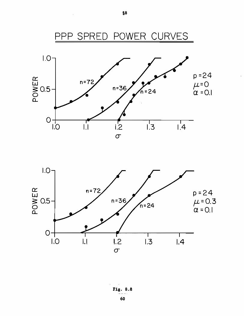
§8

PPP SPRED POWER CURVES

p=24fL=Oa =0.1

1.41.31.2a-

1.10-+-------wF---------r-------r---

1.0

1.0

0:::w~0.5oa..

p=24fL=0.3a =0.1

1.41.31.2a-

1.1O-+-----=T----------~------r--

1.0

1.0

0:::W~ 0.5oa..

Fig_ 8.8

60

§8

SPRED would do if ~ * O. The reader should note that there is no SPRED counter­

part possible to such a curve in APP. Accordingly we set ~ =0.30, and ran

out the PPP-produced curves. These may be compared with those in the upper

panel of Fig. 8.8. Only minor differences exist. Hence offsetting the two

populations by ~ =0.30 does not seem to affect PPP's SPRED power curves in

any material way. A moment's thought (on reviewing the definitions of SPRED

and PPP) shows that, in principle, such a ~-change can affect the SPRED power

curves. But evidently under the present sampling conditions this effect is

minor.

We conclude that the SITES and SPRED power curves for APP are comparable

in strength to those for PPP under the present set of data conditions (Appendix A).

H. Power Curves for some Classical Statistics for Location (T2) and Spread (M/b)

We examined the power of the classical T2 test for location (Anderson,

1958; see also Appendix B in DIT(I)) using the same artificial data set as in

pars F and G. In this way we could compare, under identical working conditions,

the T2 power curves with the APP- and PPP-produced power curves for SITES.

The classical power curves are shown in Fig. 8.9(b). These are to be compared

to those in Fig. 8.5(b) (for APP) and Fig. 8.7(b) (for PPP). At first glance,

the T2 curves seem to have higher power than their APP and PPP counterparts

(see, e.g., the curve labeled "0 =2.0"). But this high power is spurious

since it is bound up with high Type I errors near ~ =O. The classical T2

test is known to have lower power and erratic behavior when the covariances of

the two populations are not alike (hence the anomalous behavior of the 0 =0.5,

2.0 curves in Fig. 8.9(b)). When 0 =1.0, as in Fig. 8.9(a), all is well and

the curves of the T2 test are competitive with the n =72,36 curves in Figs. 8.5(a),

8.7(a). However the T2 test again has problems near n = 24 (where it doesn't

61

§8

2 .POWER CURVES FOR T (Location) TEST

a

p=24(J =1.0a=O.1

0.40.302

f.L01

n=26O~~=:r==:=::;::::::==::::;:===:00

1.0

a::w3= 0.5oa..

b0.40.30.2

f.L01

0.........=='-----------.-------,----..-------.

o

1.0

p=24a:: n=36w3= 05 a=O.10a..

M/b (Spread) POWER CURVES

c

p=24f.L=0a=O.l

3.02.52.0(J

1.5O........-----4I~---r------r---____r------,

1.0

1.0

a::w3= 0.5oa..

Fig. 8.9

62

§8

exist). In sum, we would generallg tend to trust the APP and PPP SITES tests

more than the classical T2 test for location.

Finally we looked at a much-cited classical test for detecting spread

differences in data sets (Pearson, 1969; Korin, 1969; Box, 1949). Before we

ran the power curves for this test we examined for validity the basic approximations

underlying the test. First of all, the test is built around the statistic M

where

kM - (n-1) log 1~1 i~l Ni log I~J (8.1)

and where N. =n.-1, and the bars denote determinants. For our purposes,1 1

k =2, since we are comparing two populations with sample covariance matrices

~1'~2. Moreover, we set nl =n2 =n. Under the hypothesis that we are sampling

from the same population to form ~1'~2' it is asserted (see above references)

that, approximately,

(8.2)

where

A _ (2p 2+3p -1)(k+1)1 - 6(p+1)k(n-1)

f =\P(p+1)(k-1)

It is claimed that this approximation to X~ is good for lower values of p.

Since, often in oceanography and meteorology our range of p values is typically

24 or more, we were interested in the validity of the approximation (8.1) in

this range. Accordingly, we conducted a Monte Carlo experiment in which

n =26, k =2, and for values p =6, 12, 18, 20, 24. The M and D matrices

were obtained by random samplings from N(O,l). These matrices were then used

63

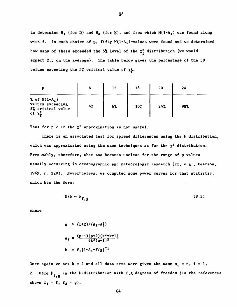
§8

to determine ~t (for ~) and ~2 (for ~), and from which M(l-At ) was found along

with f. In each choice of p, fifty M(l-At )-values were found and we determined

how many of these exceeded the 5% level of the Xi distribution (we would

expect 2.5 on the average). The table below gives the percentage of the 50

values exceeding the 5% critical value of X~.

p

%of M(l-A t )values exceeding5% critical valueof X2

f

6 12 18

10%

20

24%

24

98%

Thus for p > 12 the X2 approximation is not useful.

There is an associated test for spread differences using the F distribution,

which was approximated using the same techniques as for the X2 distribution.

Presumably, therefore, that too becomes useless for the range of p values

usually occurring in oceanographic and meteorologic research (cf, e.g., Pearson,

1969, p. 220). Nevertheless, we computed some power curves for that statistic,

which has the form:

M/b - Ff,g

where

A2 = (p-l)(p+2)(k2+k+1)6kZ(n-1)2

b =f t [l-At -f/gj-t

(8.3)

2.

Once again we set k =2 and all data sets were given the same n. =n, i =1,1

Here F is the F-distribution with f,g degrees of freedom (in the referencesf,g

above f t =f, f 2 =g).

64

§8

Fig. 8.9(c) shows the results of power curve computations based on ~ and

~(~,a) of Appendix A, for the case p =24, ~ =0, and significance level

a =0.10. Three choices of n are shown over a range of a values. Notice the

high Type I error at ~ =0 for n =26. This set of curves may be compared to

their APP and PPP counterparts in Figs. 8.6, 8.8. Since APP and PPP generallg

agree on SPUD's power for the present data set (Appendix A), we conclude that

the Mlb statistic is inadequate to gauge significant spread differences between

data sets with n and p values in the range of geophgsical interest.

I. On the Use of Power Curves in Practice

Our present approach toward power tests and their use may now be stated.

When a new statistic (e.g. SITES, SPRED) is defined, and a means (e.g. APP,

PPP) of constructing reference distributions for this statistic is devised,

and a particular family of nxp data matrices (e.g. D ,M ) is to be intercompared,. -0 -0

then proceed as follows. Construct an artificial-data-set family ~,~(~,a) in

which n,p match the given n,p. Moreover, ~,a are chosen such as to yield sets

of centroids and spreads that are representative of and embed those of the

given D ,M sets. Next, produce SITES and SPRED power curves via APP, PPP at-0 -0

some significance level a. Then choose the procedure (APP, PPP, e.g.) that

produces for SITES the higher-power curves; and also the procedure (APP, PPP,

e.g.) that produces for SPRED the higher power curves. Use these procedures

on D ,M to reach the conclusions about significant values of SITES (D ,M )-0 -0 -0 -0

and SPRED (D ,M ).-0 -0

Knowledge of the approximate power of these SITES and SPRED statistics

allows an estimate of the risk and cost of a conclusion based on a significance

decision.* This kind of thinking on the part of oceanographers and meteorologists

* See, e.g. (Crow, Davis, Maxfield, 1960)

65

§9

may yet be a long way off. But someday their understanding of air/sea/land/

cryosphere interactions will have matured. Then predictions will have to be

made of the values of important climatological variables bearing on fuel and

food supplies, and people will want to know the risks and costs of a wrong

decision. In the meanwhile, good statistical techniques, perhaps such as

those studied here, or their modifications, will aid in formulating dynamical

hypotheses about how these interactions work.

9. COmparison of APP and PPP Distributions with Reference MCP Distributions

A. Introduction

Suppose we had an adequate data setting such as that in §3, and we extracted

from it relatively small nXp sample realizations of D and M. Suppose further

that we applied APP or PPP to these extracted ~,~ and gauged their separation

with respect to either SITES or SPRED. In these comparison procedures, as a

matter of course, cumulative distribution functions (cdfs) are produced for

SITES or SPRED. The question then arises as to the visual comparison of these

APP- (or PPP)-produced cdfs with those cdfs that would be produced bg straight­

forward "onte Carlo procedures on the entire adequate data set. In this

section we present the results of a detailed study of this question. Our aim

is to see how the APP- (or PPP-)produced cdfs compare (in the sense of location

and dispersion) with those that would be generated using a relatively "exact"

method, such as the Monte Carlo procedure (MCP) under adequate data conditions.

66

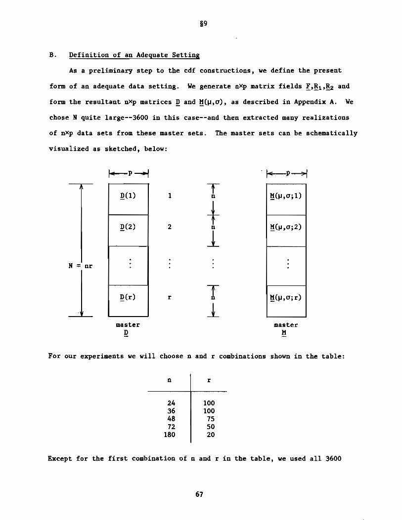
§9

B. Definition of an Adequate Setting

As a preliminary step to the cdf constructions, we define the present

form of an adequate data setting. We generate nXp matrix fields !,Rl,R2 and

form the resultant nxp matrices Q and ~(~,a), as described in Appendix A. We

chose N quite large--3600 in this case--and then extracted many realizations

of nXp data sets from these master sets. The master sets can be schematically

visualized as sketched, below:

N =nr

Q(l)

Q(2)

···

Q(r)

1

2

r

Tn

+n1

Tn

~

~(~,a;l)

~(~,a;2)

···

~(~,a;r)

masterD

masterM

For our experiments we will choose nand r combinations shown in the table:

n r

24 10036 10048 7572 50

180 20

Except for the first combination of nand r in the table, we used all 3600

67

§9

rows of the master matrix Q and master matrix ~ in each experiment (so that

N =nr). If each row of the master matrices Q and ~ represented monthly

averages of some field over p points, then these matrices would summarize 300

years of data. These data were generated by a statistically stationary process,

as described in Appendix A, which is part deterministic, part random.

C. Comparing APP and MCP cdfs

The results of our calculations are summarized in Figs. 9.1 to 9.6. The

graphs intercompare the cdfs generated by APP and a Monte Carlo procedure

(MCP). There were 24 runs made in all, and these are arranged 4 to a figure,

with the run-number shown on each diagram along with the identification of the

parameters chosen for each run. Thus, the symbols "MU," "SIGMA" and "COEF1"

refer respectively to the parameters ~,a and a, and which are defined in

Appendix A. ~ governs the centroid separation, while a governs the radial

scale, or spread separation of the data sets. Moreover the symbols "N," "P"

and "R" refer respectively to the parameters n, p and r as also used in Appendix A

and this section. Each run was executed in the following eight steps:

(i) Choose nand r (see table in par B above)

(ii) Choose ~,a

(iii) For a given w, 1 ~ w ~ r, construct the nXp matrices Q(w),

~(~,a;w) (see the diagram in par B above)

(iv) Partition Q(W) , ~(~,a;w) using a random permutation ~ in accordance

with APP (§5). The results are schematically defined as in the

following figure

68

§9

~p~ ~P-4f

T !!l(W) ~l(~,(J;W)

n

1 !!2(W) ~2(~,(J;W)

The identity transformation ~ leaves !! and ~ unchanged and as they appear

in the above sketch. This fact will be used in (viii) below.

(v) For each w in (iv) find the cdfs of SITES (or SPRED) using APP

(§5). In particular, use !!l(W), ~2(~,(J;w) to generate the "DM"

cdf of the APP.

(vi)

(vii)

(viii)

Repeat (v) for w = 1, ... ,10

Plot all 10 cdfs found in (vi)

Generate a Monte Carlo Procedure (MCP) cdf as follows: Find

SITES (or SPRED) for each pair !!l(W), ~2(~,(J;W), W=1, ... ,r.

These are the results of the identity permutation on !!(w) and

~(~,(J;w). Order these SITES (or SPRED) numbers and thereby

find the resultant MCP cdt associated with the current choice

of n, r, ~, (J.

The numbers N =3600 and p =24 are fixed throughout all the calculations.

The 24 runs in Figs. 9.1-9.6 fall naturally together into subgroups. The

following Table gives an overview of the runs and the subgroups.

69

§9

Table 9.1 Parameters for APP/MCP Runs 1-24 in Figs. 9.1-9.6

RUN DATA SETS

12

34567

89

101112

1314

1516171819

2021222324

~ =0, a =0, a =0

~ =0, a = 1.25, a = 1

~ =0, a = 1.25, a = 1

~ =0, a = 0, a = 0

J.I = 0.3, a = 1.0

~ =0.3, a =1.0

STATISTIC

SPRED

SPRED

PSPRED

SITES

SITES

PSITES

n

24180

24364872

180

24364872

180

24180

24364872

180

24364872

180

P

2424

2424242424

2424242424

2424

2424242424

2424242424

r

10020

100100

755020

100100

755020

10020

100100

755020

100100

755020

One point of interest of the study was to see how changes in the parameter

n--presumably increases in n--would improve the resemblances between the APP

cdfs and the MCP cdfs. The way we have arranged the n, r variations is to

start with a relatively small n and a large r. Thus in run 1 we have n = 24

and r = 100. We would expect in this circumstance to have a well-stabilized

MCP cdf of SPRED, for there are r =100 realizations of each ~(w) and ~(~,a;w),

w =1, ••. ,100 from which to form the MCP cdf. On the other hand the APP uses

a 24x24 version of ~ and ~(~,a) and works within them to generate the cdf for

SPRED. This was done 10 times. These 10 APP-produced curves are displayed in

70

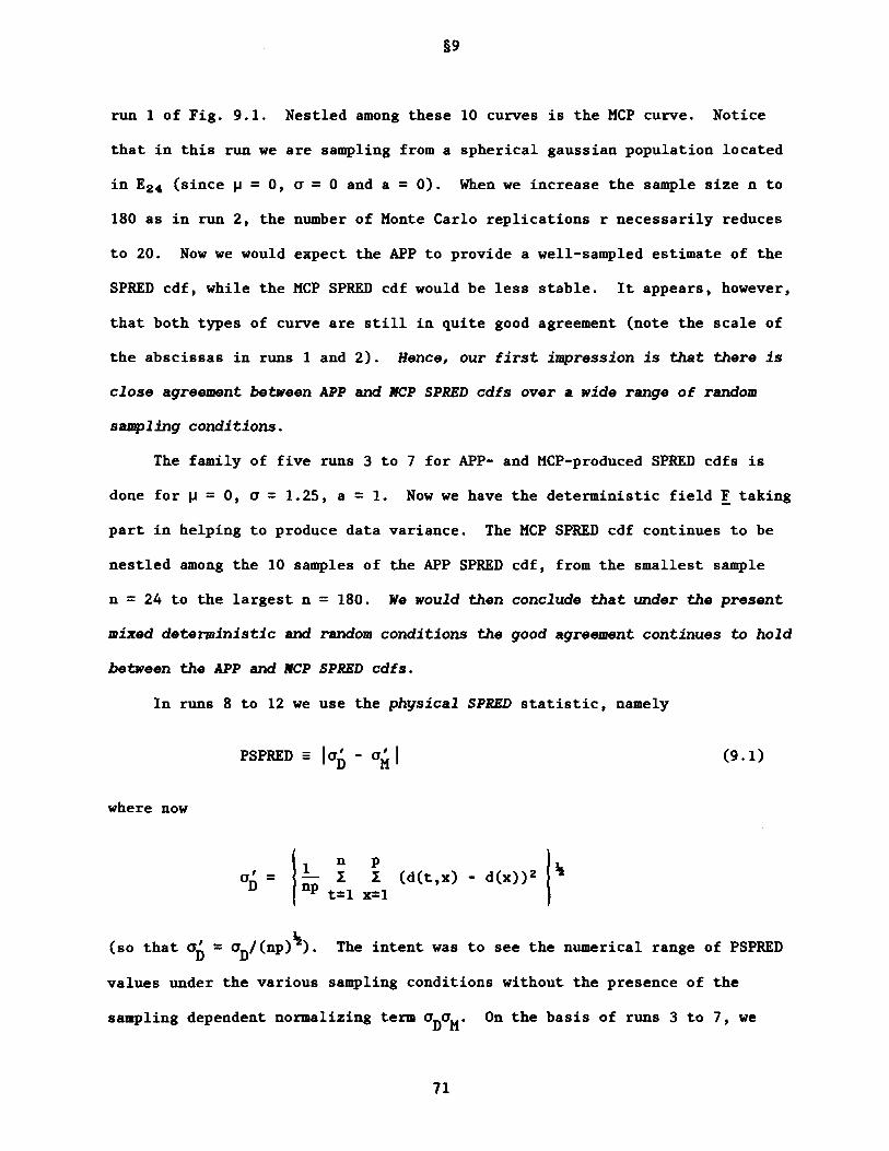
§9

run 1 of Fig. 9.1. Nestled among these 10 curves is the MCP curve. Notice

that in this run we are sampling from a spherical gaussian population located

in E24 (since ~ =0, U =0 and a =0). When we increase the sample size n to

180 as in run 2, the number of Monte Carlo replications r necessarily reduces

to 20. Now we would expect the APP to provide a well-sampled estimate of the

SPRED cdf, while the MCP SPRED cdf would be less stable. It appears, however,

that both types of curve are still in quite good agreement (note the scale of

the abscissas in runs 1 and 2). Hence, our first impression is that there is

close agreement between APP and MCP SPRED cdfs over a wide range of random

sampling conditions.

The family of five runs 3 to 7 for APP- and MCP-produced SPRED cdfs is

done for ~ = 0, U = 1.25, a = 1. Now we have the deterministic field! taking

part in helping to produce data variance. The MCP SPRED cdf continues to be

nestled among the 10 samples of the APP SPRED cdf, from the smallest sample

n = 24 to the largest n = 180. lie would then conclude that under the present

mixed deterministic and random conditions the good agreement continues to hold

between the APP and MCP SPRED cdfs.

In runs 8 to 12 we use the physical SPRED statistic, namely

where now

PSPRED - IUD - uMI (9.1)

0' =D

1 n p 1\-- I I (d(t,x) - d(x»Znp t=1 x=1

\(so that UD=uD/(np». The intent was to see the numerical range of PSPRED

values under the various sampling conditions without the presence of the

sampling dependent normalizing term uDuM. On the basis of runs 3 to 7, we

11

§9

would expect the location and dispersion of the APP and MCP cdfs to once again

be closely related, i.e., that the curves closely intermingle, and have the

same shape, and this is borne out.* Notice how in runs 8 to 12, the 0.50 level

of the APP and MCP cdfs (the median of the density distribution) stays sensibly

constant (around PSPRED =0.08) while the dispersions of the APP cdfs (their

individual left to right extents) considerably contract as n goes from 24 to

180, as would be expected under larger and larger samplings of a homogeneous

population. The MCP cdfs, interestingly, undergo about the same dispersion

contraction as the replication number r decreases from 100 to 20. Thus even

in the absence of the denominator product aDaM' the APP·prodUced PSPRED cdf

has a close resemblance to its MCP-produced counterpart, as regards location

and dispersion properties under a wide range of sampling conditions.

Runs 13 to 24 repeat the SPRED study in all details but now for SITES.

Thus in runs 13, 14 we have cdfs generated by purely random noise, with good

agreement in the variously produced cdfs for SITES.

In runs 15 to 19, where now ~ =0.300, a =1.000, and a =1, we observe a

migration of both MCP and APP SITES cdfs down the SITES scale from about 0.20

for n =24, to 0.08 for n =180. At the beginning of the sequence, the APP

curves are somewhat displaced from the reference MCP curve, although they have

about the same shape. At the end of the run the agreement between the cdfs is

quite good, after the 10 APP curves have essentially migrated as a group into

the vicinity of the MCP reference curve.

* It may then be asked, "If PSPRED seems to be so intuitively close toSPRED, why not just choose PSPRED as a statistic to work with, since itis simpler?" Unfortunately, this is not possible. In some experimentswith PSPRED, and particularly with PSITES, defined in (9.2), below, theAPP is adversely affected. It was found that the DD and MD curves couldreverse order, so that MD<DD, in the PSITES context. (This follows fromthe possibility in the PSITES context of having DD«MM.)

72

§9

In runs 20 to 24, we repeat the setting of runs 15 to 19, but now with

the phgsical SITES statistic, namely

1 P \PSITES - I (d(x) - m(x))Z (9.2)p x=l

il nwhere d(x) - n- 1 I d(t,x), m(x) = n- 1 I m(t,x)

t=l t=l

In this way we can check on our expectation that for large sample size n,

PSITES should center around 0.300 (since ~ = 0.300), which it does for both

APP and MCP SITES cdfs. Once again, now for PSITES, agreement in location of

the APP-produced cdfs improves with increasing n and, throughout, the shapes

of the cdfs remain remarkablg alike.

D. Comparing PPP and MCP cdfs

The results of our calculations are summarized in Figs. 9.7 to 9.12.

This series of graphs intercompares the cdfs generated by PPP and a Monte

Carlo Procedure (MCP). There are 24 runs in all: from 25 to 48, inclusive.

The parameters used are largely those used for the APP study, and are summarized

by Table 9.2.

Table 9.2 Parameters for PPP/MCP Runs 25-48 in Figs. 9.7-9.12

RUN DATA SETS STATISTIC n p r

25 ~ = 0, C1 = 0, a = 0 SITES 24 24 10026 180 24 20

27 ~ = 0.3, a = 1.0 SITES 24 24 10028 36 24 10029 48 24 7530 72 24 5031 180 24 20

73

§9

32 IJ =0.3, a = 1.0 PSITES 24 24 10033 36 24 10034 48 24 7535 72 24 5036 180 24 20

37 IJ =0, a =0, a =0 SPRED 24 24 10038 180 24 20

39 IJ = 0, a = 1.25 SPRED 24 24 10040 36 24 10041 48 24 7542 72 24 5043 180 24 20

44 IJ =0, a = 1.25 PSPRED 24 24 10045 36 24 10046 48 24 7547 72 24 5048 180 24 20

On turning to the graphs we see that runs 25, 26 show good agreement between

the MCP and PPP SITES cdfs, over the entire range.

In the sequence of runs 27 to 31 we see that there is a systematic difference

in location of the MCP and PPP SITES cdfs. Whereas in the corresponding APP

runs 15 to 19 the two classes of cdfs intermingled, here they remain apart

over the whole range of n samples, and the gap is insensitive to n. The

shapes of the two types of curves, however, are alike and they are broad for

small n, narrow for large n. It is this feature of like shape for APP and MCP

curves that is important to maintaining the power of the PPP at a workably

high level, relative to the reference curves of MCP.

The disparity between the PPP and MCP SITES cdfs is maintained in the run

sequence 32 to 36 (note the'change in abscissa scale). Observe how the MCP

curve homes in on PSITES =0.30, as expected, but the PPP settles at a definitely

smaller estimate of PSITES. While there was some discrepancy in PSITES locations

of the APP and MCP cdfs (runs 20 to 24), it decreased there with increasing

sample size, as expected, unlike the present discrepancy.

74

§9

In runs 37, 38 (a random setting) we have good agreement of SPRED cdfs as

produced by MCP and PPP. The SPRED statistic's cdf tends to have a long right

tail as found in either procedure. For larger samples such as n = 180, the

natural tendency of the cdfs is to move nearer to the origin, with median

values around 0.001, which therefore are down by an order of magnitude from

the n = 24 case.

The cdf graphs of the SPRED runs 39 to 43 display a dramatic difference

(relative to those witnessed in the preceding 38 runs) in the locations of the

two cdfs. The MCP cdf medians migrate slightly, as n goes from 24 to 180,

from about 0.005 to 0.007. By contrast, the PPP cdf medians move slightly

toward the origin, widening the gap between the two families of cdfs. The

runs throughout this sequence accordingly show two very different kinds of cdf

belonging to the MCP and the PPP.

In runs 44 to 48 a general repetition of the preceding five runs is

observed, now for the PSPRED statistic, showing once again disparate PSPRED

cdfs produced by PPP and MCP remaining disparate throughout the entire sequence.

In sum, the APP distributions for both SITES and SPRED generallg shared

the same location and dispersion properties as the relativelg trustworthg MCP

distributions. The closeness of resemblance increased with increasing sample

size n of Q and !(~,o) over the range of n, p, ~ and 0 values studied. On the

other hand, the PPP distributions for both SITES and SPRED were generallg of

different location than the RCP distributions. The PPP SPRED distributions

were, in addition, of different dispersion than the RCP distributions. In

general, on the basis of these intercomparisons, we conclude that, under

similar n, p, ~, 0, and statisticallg-stationarg adequate-sampling conditions,

the APP cdfs will more closelg resemble the MCP (and presumablg the 'true')

cdfs than the PPP cdfs.

75

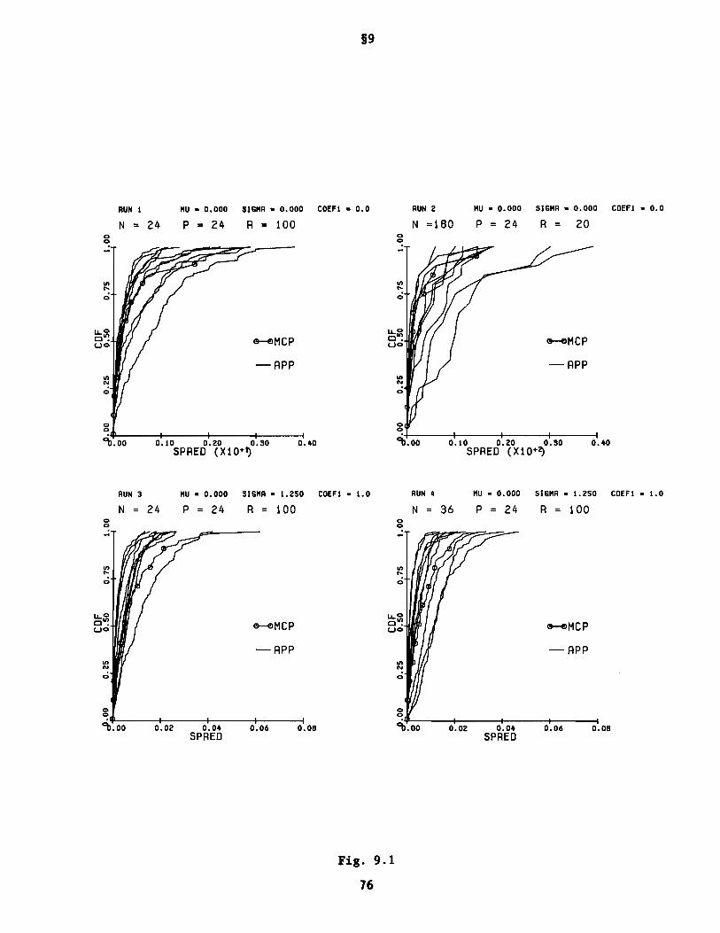
§9

MU • 0.000 SIGMA. 0.000 COEFI. 0.0 MU • 0.000 SIGMA. 0.000 COEFI. 0.0RUN I

N = 24 P = 24 R = 100AUN 2

N =180 P = 24 R = 20oo-

on on.. ...; .;

~o ~o

CJ~ e--elMCP CJ~ e--elMCPuO uO

-APP -APPon onN N

.; .;

0 00 0

91.00 0.10 0.20 0.30 0.40 91.00 0.10 0.20 0.30 0.40SPRED (Xl0+!) SPRED (Xl0+2)

RUN 3 MU • 0.000 SIGMA· 1.250 COEFI • 1.0 RUN II MU • 0.000 SIGMA. 1.250 COEFI • I. 0

N = 24 P = 24 R = 100 N = 36 P = 24 R = 10000-on...;

~o ~o

CJ~ e--elMCP CJ~ e--elMCPuO uO

-RPP -APPon onN N

.; .;

00

91.00 0.02 0.04 0.06 0.08 91.00 0.02 0.04 0.06 0.08SPRED SPRED

Fig. 9.1

76

§9

0.32

-APP

0.240.08 0.16PSPRED

o°1fL-----+---+-----+-----4

111N

o

111...o

u.. OCl~woMCP

0.05 0.10 0.15SPRED (X10+1)

RUN 5 "U • 0.000 SIG"R • 1.250 COEFI • I. 0 RUN 6 "U • 0.000 SIG"A • 1.250 COEFI • 1.0

N = 48 P = 24 R = 75 N = 72 P = 24 R = 50° 0

~ ~- -111 111... ...0 0

u.. 0 u.. 0

Cl~ ~MCPCl~

~MCPwO wO

-APP -APP111 111N N

0 0

0 00 °

0.02 0.04 0.06 0.08 9>.00 0.10 0.20 0.30 0.40SPRED SPRED (Xl0+ 1)

RUN 7 "U • 0.000 SIG"R • 1.250 COEFI • I. 0 RUN 8 "U • 0.000 SIG"R • I. 250 COEFI • I. 0

N =180 P = 24 R = 20 N = 24 P = 24 R = 100°~-

Fig. 9.2

77

§9

RUN 9 flU • 0.000 SIGflR • I. 250 COEFI • I. 0 RUN 10 flU • 0.000 SIGflR • 1.250 COEFI • I. 0

N = 36 P = 24 R = 100 N = 48 P = 24 R = 750 0

~0

- -II> II>... ...0 0

IJ..O IJ..OCl~ ~MCP

Cl~wo wo

-APPII> II>N N

0 0

0 00 0

0.08 0.16 0.2. 0.32 0.08 0.16 0.2. 0.32PSPRED PSPRED

RUN II flU • 0.000 SIGflR • 1.250 COEFI • I. 0 RUN 12 flU • 0.000 SIGflR • 1.250 COEFI • I. 0

N = 72 P = 24 R = 50 N =180 P = 24 R = 2000-

II> II>... ...0 0

IJ..O IJ..OCl~ ~MCP Cl~ MCPwo wO

-APPII> II>N N

0 0

0 00 0

0.08 0.16 0.2. 0.32 '11.00 0.05 0.10 0.15 0.20PSPRED PSPRED

Fig. 9.3

78

§9

AUN 13 I1U • 0.000 SIGI1A • 0.000 (OEFI • 0.0 AUN 14 I1U • 0.000 SIGI1A • 0.000 (OEFI • 0.0

N = 24 P = 24 R = 100 N =180 P = 24 R = 20° 0

~ ~- -II'l II'l.... .....; .;

lL.. 0 lL.. 0

o"! (.'l---4!)MCP o"! (.'l---4!)MCPwo wo

-APP -APPII'l II'lN N

.; .;

0 00 °91.00 0.10 0.20 0.30 0.40 91.00 0.10 0.20 0.30 0.40

SITES SITES (Xl0+ 1)

AUN IS I1U • .300 SIGI1A • I. 000 (OEFI • I. 0 AUN 16 I1U • .300 SIGI1A • I. 000 (OEFI • I. 0

N = 24 P = 24 R = 100 N = 36 P = 24 R = 100° 0

~ ~- -II'l II'l.... .....; .;

lL.. 0 lL.. 0

o"! (.'l---4!)MCP o"! (.'l---4!)MCPwO wo

-APP -APPII'l II'lN N

.; .;

0 00 °

0.40 0.80 1.20 1.60 91.00 0.20 0.40 0.60 0.80SITES SITES

Fig. 9.4

79

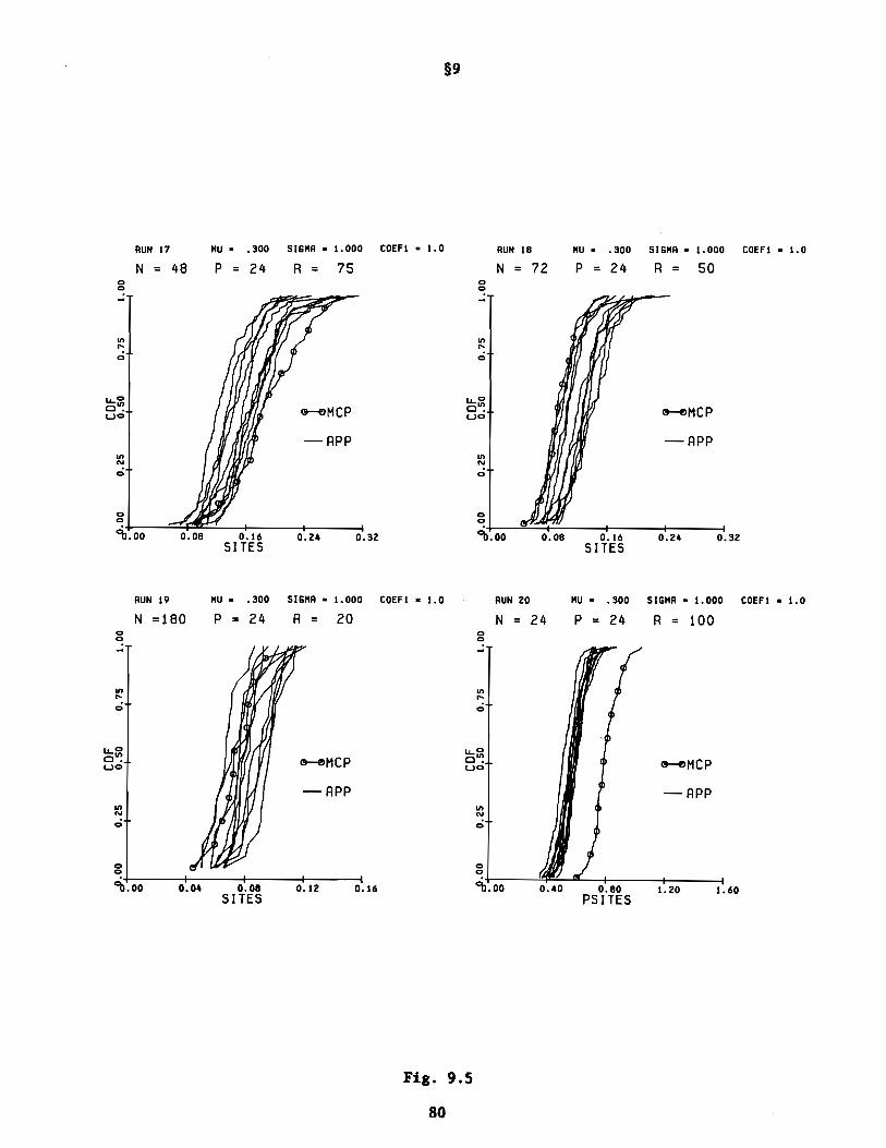
§9

RUN 17 NU • •300 SIGNR • 1.000 tOEFl • I. 0 RUN 18 NU • •300 SIGNR • 1.000 tOEFl • I. 0

N = 48 P = 24 R = 75 N = 72 P = 24 R = 50° 00 0- -'" '".... ....0 0

lJ..O lJ..OCl~ C9---eMCP Cl~ C9---eMCPwO wo

-APP -APP

'" '"N N

0 0

0 00 °91.00 0.08 0.16 O.Z" 0.3Z 91.00 0.08 0.16 O.Z" 0.3Z

SITES SITES

RUN 19 NU • .300 SIGNR • 1.000 tOEFl. 1.0 RUN ZO NU • .300 SIGNA· I. 000 tOEFl • I. 0

N =180 P = 24 R = 20 N = 24 P = 24 R = 100° 00 °..: -'" '".... ....0 0

u.. 0 lJ..OCl~ C9---eMCP Cl~ C9---eMCPwo wo

-APP -APP'" '"N N

0 0

0 00 °91.00 0.0" 0.08 O.IZ 0.16 91.00 0."0 0.80 I.ZO 1.60

SITES PSITES

Fig. 9.5

80

§9

RUN ZI MU • .300 SlliMR • I. 000 COEFI • I. 0 RUN ZZ MU • •300 SlliMR • 1.000 COEFI • I. 0

N = 36 P = 24 R = 100 N = 48 P = 24 R = 7S° 00 ~- -II> II>.... ....0 0

u. 0 u. 0

Cl~ Cl~ t!l---eMCPwO wO

-APPII> II>N N

0 0

0 00 °"b.oo O.ZO 0.40 0.60 0.80 "b.ZO 0.40 0.60 0.80 1.00

PSITES PSITES

RUN Z3 MU • . 300 SIGMR • 1.000 COEFI • I. 0 RUN Z4 MU • .300 SIGMR • 1.000 COEFI • I. 0

N = 72 P = 24 R = 50 N =180 P = 24 R = 20° 00

~.: -II> II>.... ....0 0

u. 0 u. 0

Cl~ t!l---eMCP Cl~ t!l---eMCPwo wo

-APP -APPII> II>N N

0 0

0 00 °"b.ZO 0.30 0.40 0.50 0.60 "b.ZO 0.Z8 0.36 0.44 0.5Z

PSITES PSITES

Fig. 9.6

81

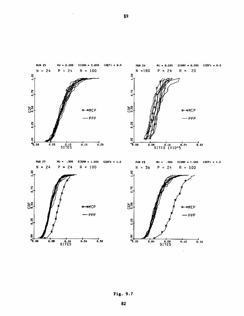
§9

RUN 2S NU • 0.000 SIGNA - 0.000 COEFI • 0.0 RUN 26 NU • 0.000 SIGNA· 0.000 COEFI • 0.0

N = 24 P = 24 R = 100 N =180 P = 24 R = 20° 00 ~..; -II> II>..... ......,; .,;

u.. o u.. 0

c~ C9---i!lMCP c~ C9---i!lMCPwO wo

-PPP -PPPII> II>N N

.,; .,;

0 00 °91.00 0.10 O.IS 0.20 91.00 0.08 0.16 0.2~ 0.32

SITES SITES (XI0+1)

RUN 21 NU • .300 SIGNA. 1.000 COEFI • 1.0 RUN n NU • .300 SIGNA. 1.000 COEFI • 1. 0

N = 24 P = 24 R = 100 N = 36 P = 24 R = 100° 00 0..;

II> II>..... .....0 0

u.. 0 u.. 0

c~~MCP c~ C9---i!lMCPwO wO

-PPP -PPPII> II>N N

0 .,;

0 00 °91.00 0.08 0.16 0.2~ 0.32 91.00 O.O~ 0.08 0.12 0.16

SITES SITES

Fig. 9.7

82

§9

RUN 29 NU • .300 SIGNR • 1.000 COEFI • 1.0 RUN 30 NU • .300 SIGNR • 1.000 COEFI • 1.0

N = 48 P = 24 R = 75 N = 72 P = 24 R = 500 00 ~- -II'l II'l... ...0 0

u.. 0 u.. 0

c"l C9--elMCP c"l C9--elMCPwO wO

-PPP -PPPII'l II'lN N

0 0

0 00 0

'11.00 0.0. O.OB 0.12 0.16 0.0. O.OB 0.12 0.16SITES SITES

RUN 31 NU • .300 SIGNR • 1.000 COEFI • 1. 0 RUN 32 NU • .300 SIGNR • 1.000 COEFI • 1.0

N =180 P = 24 R = 20 N = 24 P = 24 R = 10000-II'l...0

u.. 0

~MCP c"l C9--elMCPwO

-PPP -PPPII'lN

0

0 00 0

0.0. 0.08 0.12 0.16 '11.10 0.30 0.50 0.70 0.90SITES PSITES

Fig. 9.8

83

§9

AUN 33 HU • .300 SIGHA • 1. 000 tOEFl • 1. 0 AUN 34 HU • .300 SIGHA • 1.000 tOEFl • 1. 0

N = 36 P = 24 R = 100 N = 48 P = 24 R = 75

° 00 ~- -III III... ...ci ci

LL.0 LL.0

o"! o"! ~MCPwO wO

-PPPIII IIIN N

0 ci

0 00 °~.10 0.20 0.30 0.40 O.SO ~.10 0.20 0.30 0.40 O.SO

PS ITES PSITES

AUN 35 HU • . 300 SIGHR • 1.000 tOEFl • 1.0 RUN 36 HU • .300 SIGHR • 1.000 tOEFl • 1. 0

N = 72 P = 24 R = 50 N =180 P = 24 R = 20° 00

~- -III III... ...ci ci

LL.0 LL.0o"! MCP o"!wo wo

III IIIN N

ci ci

0 00 °

0.18 0.26 0.34 0.42 ~.OO 0.10 0.20 0.30 0.40PS ITES PSITES

Fig. 9.9

84

§9

AUN 31 NU • 0.000 SIGNA. 0.000 COEFI • 0.0 AUN 38 NU • 0.000 SIGNA. 0.000 COEFI • 0.0

N = 24 P = 24 R = 100 N =180 P = 24 R = 20° 00 0- -III III... ...0 0

u.. 0 u.. oc~ ct---t>MCP c~ ct---t>MCP(.JO (.JO

-PPP -PPPIII IIIN N

0 0

0 00 0

9>.00 0.05 0.10 0.15 0.20 91.00 0.05 0.10 0.15 0.20SPRED (Xl0"l) SPRED (Xl0"2)

AUN 39 NU • 0.000 SIGNA • 1. 250 COEFI • 1.0 AUN .0 NU • 0.000 SIGNA • 1. 250 COEFI • 1.0

N ::I 24 P = 24 R = 100 N = 36 P = 24 R = 100

0.32

-PPP

ct---t>MCP

0.08 0.16 0.2.SPRED (Xl0"l)

o

°:...---+---+-----+------4

u.. oc~(.JO

0.08

-PPP

0.060.02 0.0.SPRED

glp---+---+---+------l

91.00

Fig. 9.10

85

§9

0.32

-PPP

0.2_0.08 0.16PSPRED

II> II>... ...ei ei

u.o u.oo~ ~MCP o~wo wo

-PPPII> II>N N

0 0

0 00 0

9>.00 0.0_ 0.08 0.12 0.16SPRED (Xl0+l)

RUN _1 NU • 0.000 SIGNR • 1.250 COEFI • 1.0 RUN U NU • 0.000 SIGNA. 1.250 COEFI • 1.0

N = 48 P = 24 R = 75 N = 72 P = 24 R = 500 0

~ ~- -II> II>... ...ei ei

u.o u.oo~

~MCP o~ ~MCPwO wo

-PPP -PPPII> II>N N

0 ei

0 00 0

0.08 0.16 0.2_ 0.32 0.05 0.10 0.15 0.20SPRED (Xl0+l) SPRED (Xl0+l)

RUN _, NU • 0.000 SIGNA • 1.250 COEFI • 1. 0RUN __

NU • 0.000 SIGNA. 1.250 COEFI • 1. 0

N =180 P = 24 R = 20 N = 24 P = 24 R = 1000 00 0- -

Fig. 9.11

86

§9

RUN .5 MU • 0.000 SIGMA. 1.ZSO tOEFl • 1. 0 RUN .6 MU • 0.000 SIGMA • 1.ZsO tOEFl • 1. 0

N = 36 P = 24 R = 100 N = 48 P = 24 R = 750 00 ~-II) II).... ....0 0

u.. o u.. 0

e~ G-flMCP e"! G-flMCPwo wO

-PPP -PPPII) II)

N N

c:: c::

0 00 0

0.08 0.16 O.Z. 0.3Z 91.00 0.05 0.10 0.15 O.ZOPSPRED PSPRED

AUN .7 MU • 0.000 SIGMA. 1.ZsO tOEFl. 1.0 AUN .8 MU • 0.000 SIGMA • 1.ZS0 tOEFl • 1. 0

N = 72 P = 24 A = 50 N =180 P = 24 R = 200 0

~ 0- -II) II).... ....0 0

u.. 0 u.. 0

e~ G-flMCP e~ G-flMCPwO wO

-PPP -PPPII) II)N N

c:: c::

0 00 0

91.00 0.05 0.10 0.15 O.ZO 91.00 0.0. 0.08 0.1Z 0.16PSPRED PSPRED

Fig. 9.12

87

§10

10. References

Works in this series on Data Intercomparison Theory (NOAA Technical

Memorandums, ERL-PMEL) are:

DIT(I): Minimal Spanning Tree Tests for Location and Scale Differences.

DIT(II): Trinity Statistics for Location, Spread and Pattern Differences.

DIT(III): S-Phase and T-Phase Tests for Spatial Pattern and Temporal Evolution

Differences.

DIT(IV) :

DIT(V):

Tercile Tests for Location, Spread and Pattern Differences.

Case Study: Effects of Objective Analysis on a Tropical Pacific Sea

Surface Temperature Set.

Anderson, T.W. (1958) An Introduction to Multivariate Statistical Analysis,

Wiley, N.Y.

Box, G.E.P. (1949) "A General Distribution Theory for a class of likelihood

criteria." Biometrika 36, 317.

Cressman, G. (1959) "An Operational Objective Analysis System." Mon. Wea. Rev.

87, 367.

Crow, E.L., F.A. Davis, M.W. Maxfield (1960) Statistics Manual, Dover, N.Y.

Korin, B.P. (1969) "On testing the equality of k covariance matrices." Biometrika

56, 216.

Levitus, S., A. Oort (1977) "Global Analysis of Oceanographic Data." Bull. Am.

Met. Soc. 58, 1270.

Liu, C-T. (1982) Analysis of Tropical Pacific Sea Surface Temperatures for

1975 to 1980. Tech. Memo ERL PMEL-34, Pacific Marine Environmental

Laboratory, Seattle, WA.

Pearson, E.G. (1969) "Some comments on the accuracy of Box·s approximations to the

distribution of M." Biometrika 56, 219.

88

APPENDIX A

A Model/Data Matrix Generator for Controlled Experiments

with Statistical Techniques

1. The data-set generator is defined via

d(t,x) =f(t,x) + rl(t,x)

for t =1, ... ,n, and x =1, ... ,p, where

(Al.1)

f(t,x)p

=a Ij=l

u. (x)v. (t)J J

(Al. 2)

u.(x) = [ 2 ]\ . (jnx)J (p+1) S1n p+1

r. =sin (jn/2(p+1))/sin(pn/2(p+1))J

Here M is an adjustable parameter fixed throughout these constructions as

M = 12. The constant a adjusts the signal-to-noise ratio. The present system

has many combined periods (via the various values of r.). The shortest naturalJ

period is

/ . ( pn )T - n S1n 2(p+1)

Choosing M =12 then divides the time axis into 12ths of T.

(A1.3)

The time index t

then gives the multiples of T by which time progresses in this system. Hence

the quickest natural oscillatory changes of the system are still resolved into

12 instants. Finally, rl(t,x) is a random sample, at t and x, drawn from a

89

normal population of zero mean and unit variance. That is, for each t and x,

rl(t,x) - N(O,I).

B. The model-set generator is defined via

(AI.4)

t = l, ... ,n x =l, ... ,p.

Here ~, a are specifiable parameters. By varying ~, we can make the centroids

of the sampled D and M swarms in E change distance. By varying a, the radiusp

of the sampled M swarm can be changed. Here r2(t,x) - N(O,I), and is a random

variable sampled independently of r2(t,x).

c. We can write (AI. 1), (AI.4) in nxp matrix form:

(AI.5)

(AI.6)

where E is an nxp matrix of unit entries. By setting ~ =0, a =0, and a =0,

we obtain

D =~1

M=~2

(AI.7)

(AI.B)

two random nxp matrices representing independent samples of n points each in

E drawn from N (O,! ), i.e., a multivariate unit spherical gaussian populationp p-~

in E , centered on the origin.p

D. In general, we may write ~ as {~(l), ... ,~(n)}, i.e., as an n-point swarm

(or set) in E. Each ~(t), t =1, ... ,n, is a vector:p

90

APPENDIX A

T~(t) =[d(t,I), d(t,2), ... , d(t,p)] (AI.9)

the elements being formed via (AI. I). Similar notation holds for the vectors

~(t) associated with M.

91

NOAA ERL technical reports, technical memoranda, and data reportspublished by authors at Pacific Marine Environmental Laboratory inSeattle, Washington, are listed below. Microfiche copies are avail­able from the USDOC, National Technical Information Service (NTIS),5285 Port Royal Road, Springfield, Virginia 22161 (703-487-4650).Hard copies of some of these publications are available from theERL Library in Boulder, Colorado (303-497-3271). Hard copies ofsome of the technical reports are sold by the Superintendent ofDocuments, U.S. Government Printing Office, Washington, D.C. 20402(202-275-9251).

NOAA Technical Report Series

ERL232-POLI0 Stevens, H. R., Jr. (1972)RP-I-OC-71 Northeast Pacific geophysical survey.91 pp.NTIS: COH-72-50677.

ERL234-POLJI Lucas, William H. (1972)Juan de Fuca Ridge and Sovanco fracture zone.RP-5-0C-71, 39 pp.NTIS: COH-72-50854.

ERL247-POLI3 Cannon, G. A. and Norman P. Laird (1972)Observations of currents and water properties in PugetSound, 1972, 42 pp.NTIS: COH-73-50402.

ERL259-POLI6 Ryan, T. V., N. P. I.aird, G. A. Cannon (1973)RP-6-0C-71 Data Report: Oceanographic conditions off theWashinston coasl, Oclober-November 1971, 43 pp.NT! S: COH-73-50922

ERL260-POLI7 Cannon, Glenn A. (1973)Observations of currents in Puget Sound, 1970, 77 pp.NTIS: COH-73-50666/9.

ERL261-POL18 Stevena, H. R. Jr., (1973)RP-I-OC-70 Southeast Pacific geophysical survey. 60 pp.NTIS: not available.

ERL325-PHEL22 Halpern, D., J. H. Helseth, J. R. Holbrook, andR. H. Reynolds (1975)Sur~ace wave height measurements made near the Oregon coastdunng August 1972, and July and Auguat 1973 168 ppNTIS: COH-75-10900/9. ,.

ERL327-PHEL23 Laird, N. P., and Jerry A. Galt (1975)Observations of currents and water properties in PugetSound, 1973, 141 pp.NTIS: COH-73-50666/9.

ERL333-PHEL24 Schumacher, J. D., and R. H. Reynolds (1975)STD, current meter, and drogue observations in RosarioStrait, January-Harch 1974, 212 pp.NTIS: COH-75-1l391/0.

ERL339-PHEL25 Galt, J. A. (1975)Development of a simplified diagnostic model for inter"pretation of oceanographic data.NTIS: P8-247 357/7.

ERL352-PHEL26 Reed, R. K., (1975)An evaluation of formulas for estimating clear-sky insol­ation over the ocean, 25 pp.NTIS: P8-253 055/8.

ERL384-PHEL27 Garwood, Roland (1977)A general model of the ocean mixed layer using a two"component turbulent kinetic energy budget with meanturbulent field closure, 81 pp.NTIS: P8-265 434/1.

ERL390-PHEL28 Hayes, S. P., and W. Zenk (1977)Observations of the Antarctic Polar Front by a mooredarray during FDRAKE-76, 47 pp.NTIS: P8-281 460/6.

ERL390-PHEL29 Hayes, S. P., and W. Zenk (1977)Observations of the Antarctic Polar Front by a mooredarray during FDRAKE- 76, 49 pp.NTIS: P8-281 460/6.

ERL403-PllEL30 Chester, Alexander J. (1978)Kicrozooplankton in the surface waters of the Strait ofJuan de Fuca, 26 pp.NTIS: P8 297233/AS.

ERL271-POLI9 Reed, Ronald K., and David Halpern (1973)sm observations in the northeast Pacific September-October 1972, 58 pp. 'NTIS: COH-73-50923/4.

ERL292-PHEL20 Reed, R. K. (1973)Distcibution and variation of physical properties alongthe SEAHAP standard section, 16 pp.NTIS: COH-74-50334/3.

ERL323-PHEL21 Erickson, 8. H. (1975)Nazca plate program of the international decade of oceanexploration--OCEANOGRAPHER Cruise-RP 2-0C-73 78 pp.NTIS: COH-7540911/6. '

Rea, David K. (1970)8athymetry and magnetics of a region (POL-421-3) 29° to35°N, 155° to 165°W.NTIS: COH-71-00173.

Reed, R.K. (1970)Resul ts from some parachute drogue measurements in thecentral North Pacific Ocean, 1961-1962, 9 pp.NTIS: COH-71-50020.

Halpern, David (1972)Description of an experimental investigation on thethe response of the upper ocean to variable winds, 51 pp.NTIS: COH-72-50452.

Halpern, David (1972)Current meter observations in Massachusetts Bay, 36 pp.NTIS: AD-745 465.

Lucas, William H. (1971)Gravity anomalies and tht>ir relation to major tectonicfeatures in the North Central Pacific, 19 pp.NTIS: COH-71-50409.

Lucas, William H. (1972)South Pacific RP-7-SU-71 Pago Pago to Callao to Seattle.NTIS: COH-72-50454.

Naugler, Frederic P. (1968)8athymetry of a region (PORL-421-2) North of theHaws i ian RidRe, pr~-NTIS.

Grim, Paul J. (1968)Seamap deep-sea channel, Jan. 1969, 2 824 50 060,pre-NTIS.

Le Hehaute, 8ernard (1969)An introduction to hydrodynamics and water waves, 2 yols.725 pp.NTIS: P8192 065, P8192 066.

ERL231- POL9

ERLI91-POL5

ERL229-POL7

ERL230-POL8

ERL214-POL6

ERLI46-POL4

ERL240-POLI2 Halpern, David (1972)Wind recorder, current meter and thermistor chain meas­urements in the northeast Pacific-August/September 1971,37 pp.NTIS: COH-73-50107.

ERL93-POL2

ERL252-POLI4 Cannon, G. A., N. P. Laird, T. V. Ryan (1973)Currents observed in Juan de Fuca submarine canyon andvicinity, 1971. 57 pp.NTIS: COH-73-5040 I.

ERL1l8-POL3

ERL82-POLI

ERL258-POLI5 Lucas, William H., and Richard R. Uhlhorn (1973)Bathymetric and magnetic data from the northeast Pacific40° to 58aN, 125° to 1600 w. 9 pp.NTIS: COH-73-50577.

ERL404-PIlEL31 Schumacher, J. D., R. Sillcox, D. Dreves, andR. D. Muench (1978)Winter circulation and hydrography over the continentalshelf of the northweat Gulf of Alaaka, 16 pp.NTIS: P8 296 914/AS.

ERL407-PIlEL32 Overland, J. E., M. H. Hitchman, and Y. J. Han (1979)A regional surface wind IIOdel for mountainOUB coastalareas t 34 pp.NTIS: PB 80 146 152.

ERL412-PIlEL33 Holbrook, J. R., R. D. Muench, D. G. Kachel,and C. Wri8ht (1980)Circulation in the Strait of Juan de Fuca: Recent oceano­graphic observations in the Eastern Basin, 42 pp.NTIS: PB 81-135352.

ERL415-PIlEL34 Feely, R. A., and G. J. Maasoth (1982)Sources, composition, and transport of suspended partic­ulate lDatter in lower Cook Inlet and northern ShelikofStrait, Alaska, 28 pp.NTIS: PB 82-193263

ERL417-PIlEL35 Baker, E. T. (1982)Suapended particulate utter in Elliott Bay, 44 pp.NTIS: PB 82-246943.

ERL419-PIlEL36 Pease, C. J., S. A. Schoenber8, J. E. Overland (1982)A climatology of the Bering Sea and its relation to leaice extent, 29 pp.NTIS: not yet available.

ERL422-PHEL37 Reed, R. K. (1982)Energy fluxes over the eastern tropical Pacific Ocean,1979-1982, 15 pp.NTIS: PB 83 138305

NOAA Data Report Series

ERL PIlEL-1

ERL PIlEL-2

ERL PIIlL-3

ERL PIlEL-4

ERL PIlEL-5

ERL PIlEL-6

Man81111, L., N. N. Soreide, B. D. Davies, B. D. Spell,and S. P. Hayea (1980)eTD/oa .I.uremeats during the equatorial Pacific Oceanclimate 8tudy (EPOCS) in 1979, 643 pp.NTIS: PB 81 211203.

Katl, C. N., and J. D. Cline (1980)Low 1I01ecular weight hydrocarbon concentrations (el-c.. >,Ala8kan continental 8helf, 1975-1979, 328 pp.NTIS: PB 82 154211.

Taft, B. A., and P. Xovala (1981)Vertical sections of tellperature .•alinity. thermo8tericanouly, and lonol ge08trophic velocity from NORPAX8huttle experiment, part I, 98 pp.NTIS: PB 82 163106.

Pullen, P. E., and H. Hichael Byrne (1982)Hydrographic .e88Urelllent8 during the 1978 cooperativeSoviet"'AlDerican tauna.i expedition, 168 pp.NTIS: not yet 8vailable.

Taft, B.A., P. itov81o, and A. Cant08-Figuerola (1982)Vertical sectioDs of tellperature, salinity, tbenDOllteric8naaly 8nd zonol ge08trophic velocity froll NORPAXShuttle Experi.ent--Part 2, 94 pp.NTIS:

X8tZ, C.N., J.D. Cline, 8nd X. Xelly-Han8en (1982)Dissolved lletune concentratioDs in the southeastern BerinlSea, 1980 and 1981, 194 pp.NTIS:

HOAA Technical Memorandum Series

ERL PIlEL-1 Sokolowski, T. J. and G. R. lIiller (1968)Deep sea release mechanism, Joint Tsunami ResearcbEffort, pre-NTIS.

ERL PIlEL-21 Salo, S. A., C. H. Pease, and R. W. Lindsay (1980)Physical environment of the eastern Bering Sea, Harch1979, 127 pp.NTIS: PB81-148496.

ERL PIlEL-2 Halpern, David (1972)STD observations in the northeast Pacific near 47°N r

128·W (August/September 1971), 28 pp.NTIS, COII-72-10839.

ERL PIlEL-22 lIuench, R. D., and J. D. Schumacher (1980)Physical oceanographic and meteorological conditionsin the northw~st Gulf of Alaska, 147 pp.NTIS: PB81-199473.

ERL PIlEL-3 Reynolds, R. lIichael and Bernard Walter, Jr. (1975)Current meter measurements in the Gulf of A18ska--Part I:Results from NEGOA moorings 60, 61, 62A, 28 pp.NTIS: PB-247 922/8.

ERL PIlEL-23 Wright, Cathleen (1980)Observations in the Alaskan Stream during 1980, 34 pp.NTIS: PB81-207441.

ERL PIlEL-4 Tracy, Dan E. (1975)STD and current meter observations in the north San Juanlslands, October 1973.NTIS: PB-248 825/2.

ERL PllEL-24 IIcNutt, L. (1980)Ice conditions in the eastern Bering Sea from NOAA andLAllDSAT imagery: Winter conditions 1974, 1976, 1977,1979, 179 pp.NTIS: PB81-220188.

ERL PIlEL-5 Holbrook, James R. (1975)srn measurements off Washington and Vancouver Islandduring September 1973.NTIS: PB-249 918/4.

ERL PIlEL-25 Wright, C., and R. K. Reed (1980)Comparison of ocean and island rainfall in the tropicalSouth Pacific, Atlantic, and Indian Oceans, 17 pp.NTIS: PB81-225401.

ERL PIlEL-6 Charne11 , R. L. and G. A. Krancus (1976)A processing system for Aanderaa current meter data,53 pp.NTIS: PB-259 589/0.

ERL PIlEL-26 Katz, C. N. and J. D. Cline (1980)Processes affecting distribution of low-molecular-weightaliphatic hydrocarbons in Cook Inlet, Alaska, 84 pp.NTIS: not yet available.

ERL PIlEL-7

ERL PIlEL-8

1I0fjeld, Harold O. and Dennis lIayer (1976)Formulas used to analyze wind-driven currents as first­order autoregressive processes, 22 pp.NTIS: PB-262 463/3.

Reed, R. K. (1976)An evaluation of cloud factors for estimating insolationover the ocean, 23 pp.NTIS: PB-264 174/4.

ERL PIlEL-27

ERL PIlEL-28

feely, R. A., G. J. lIassoth, A. J. Paulson (1981)Distribution and elemental composition of suspendedmatter in Alaskan coastal waters, 119 pp.NTIS: PB82-124538.

lIuench, R. D., J. D. Schumacher, and C. A. Pearson (1980)Circulation in the lower Cook Inlet, Alaska, 26 pp.NTIS: PB82-126418.

Hamilton, S. E., and J. D. Cline (1981)Hydrocarbons associated with suspended matter in theGreen River~ Washington, 116 pp.NTIS: PB82-148677.

Liu, Cho-Teng (1982)Tropical Pacific sea surface temperature measured bySEASAT microwave radiometer and by ships, 160 pp.NTIS: not yet available.

Ikeda, 1I0toyoshi (1982)Eddies detached from a jet crossing over a submarineridge: A stUdy using a simple nlDt!rical model 38 pp.NTIS: PB82-217563. •

Pease, C. H., and S. A. Salo (1981)Drift characteristics of northeastern Bering Sea iceduring 1980, 79 pp.NTIS: PB 83 112466

Pearson, C. A. (1981)Guide to R2D2--Rapid retrieval data display, 148 pp.NTIS: PB82-150384.

Reynolds, R. II., S. A. lIacklin, and T. R. Heister (1981)Observations of South Alaskan coastal winds, 49 pp.NTIS: PB82-164823.

ERL PIIEL-29

ERL PIlEL-33

ERL PIlEL- 34

ERL PIlEL-31

ERL PIlEL-30

ERL PIlEL-32

ERL PIlEL-35 Lindsay, R.W., and A.L. Comiskey (1982):Surface and upper-air observations in the eastern BeringSea, 90 pp.NTIS: not yet available.

ERL PIlEL-36 Preisendorfer, R., and C. E. 1I0bley (1982)Climate forecast verifications off the U. S. mainland~1974-1982, 225 pp.NTIS: not yet available.

Schumacher, J. D., R. K. Reed, H. Grigsby,D. Dreves (1979)Circulation and hydrography near Kodiak Island~ Septemberto November 1977, 52 pp.NTIS: PB 297421/AS.

Han, Y.-J. and J. A. Galt (1979)A numerical investigation of the Bering Sea circulationusing a linear homogeneous model, 40 pp.NTIS: PB 299884/AS.

Pashinski, D. J., and R. L. Charne11 (1979)Recovery record for surface drift cards released in thePuget Sound-Strait of Juan de Fuca system during calendaryears 1976-1977, 32 pp.NTIS: PB 299047/AS.

Nakamura, A. 1. and R. R. Harvey (1978)Conversion from film to magnetic cassette recording forthe Geodyne 102 current meter, 17 pp.NTIS, PB-283 349/9.

Hayes, S. P., J. Glenn, N. Soreide (1978)A shallow water pressure-temperature gage (PTG): Design~

calibration, and operation~ 35 pp.NTIS: PB 286 754/7.

Nakamura, A. 1. and R. R. Harvey (1977)Versatile release timer for free vehicle instrUllentationover the ocean, 21 pp.NTIS: PB 270321/AS.

Holbrook, James R. and David Halpern (1977)A compilation of wind, current, bottom pressure, aDdSTD/Crn measurements in the northeast Gulf of Alaska,february-llay 1975.NTIS: PB 270285.

ERL PIlEL-14

ERL PIlEL-12

ERL PIlEL-IO

ERL PIlEL-13

ERL PIlEL-ll

ERL PIlEL-9

ERL PIlEL-15

ERL PIlEL-16 Loomis, Harold G. (1979)A primer on tsunamis written for boaters in Hawaii, 10 pp.NTIS: PB80-161003.

ERL PIlEL-17 lIuench, R. D. and J. D. Schumacher (1980);(Hayes ~ Charnell, Lagerloef, and Pearson, contributors)Some observations of physical oceanographic conditions onthe northeast Gulf of Alaska continental shelf, 90 pp.NTIS: PB81-102584.

ERL PIlEL-18 Gordon, Howard R., ed. (1980)Ocean remote sensing using lasers, 205 pp.NTIS: PB80-223282.

ERL PIlEL-19 Cardone, V. J. (1980)Case studies of four severe Gulf of Alaska storms,58 pp.NTIS: PB81-102519.

ERL PIlEL-20 Overland, J. E., R. A. Brown, and C. D. lIobley (1980)IIETLIB--A program library for calculating and plottingmarine boundary layer wind fields ~ 82 pp.NTIS: PB81-141038.