Noise in attractor networks in the brain produced bygraded firing rate representations

Tristan J. Webb, University of Warwick, Complexity Science, Coventry CV4 7AL, UK

Edmund T. Rolls, Oxford Centre for Computational Neuroscience, Oxford, UK∗

and University of Warwick, Department of Computer Science, Coventry CV4 7AL, UK

Gustavo Deco, Universitat Pompeu Fabra, Theoretical and Computational NeuroscienceRoc Boronat 138, 08018 Barcelona, Spain

andJianfeng Feng, University of Warwick, Department of Computer Science, Coventry CV4 7AL, UK

Keywords: decision-making, noise, stochastic neurodynamics, neural encoding,attractor network, firing rate distribution, graded representation

∗Corresponding author. Oxford Centre for Computational Neuroscience, Oxford, UK. Email: Ed-mund.Rolls@oxcns.org, url: http://www.oxcns.org

1

Abstract

Representations in the cortex are often distributed with graded firing rates inthe neuronal populations. The firing rate probability distribution of each neu-ron to a set of stimuli is often exponential or gamma. In processes in the brainsuch as decision-making that are influenced by the noise produced by the closeto random spike timings of each neuron for a given mean rate, the noise withthis graded type of representation may be larger than with the binary firing ratedistribution that is usually investigated. In integrate-and-fire simulations of anattractor decision-making network, we show that the noise is indeed greater fora given sparseness of the representation for graded, exponential, than for binaryfiring rate distributions. The greater noise was measured by faster escaping timesfrom the spontaneous firing rate state when the decision cues are applied, andthis corresponds to faster decision or reaction times. The greater noise was alsoevident as less stability of the spontaneous firing state before the decision cuesare applied. The implication is that spiking-related noise will continue to be afactor that influences processes such as decision-making, signal detection, short-term memory, and memory recall even with the quite large networks found in thecerebral cortex. In these networks there are several thousand recurrent collateralsynapses onto each neuron. The greater noise with graded firing rate distributionshas the advantage that it can increase the speed of operation of cortical circuitry.

Author SummaryDifferent neurons fire at different rates to represent information in the brain. We

show that this graded firing rate representation differs importantly from a binary firingrate representation where all the neurons active to represent a stimulus fire at a highrate, and the other neurons at a low rate. We show that the graded firing rates producemore randomness or noise related to the spiking times of the neurons. This extra noiseof graded representations can make the operation of brain systems involved in decisionsand memory recall faster, and this can be advantageous. The extra noise can alsoreduce the stability of networks in the brain, sometimes making them fire when theyshould not, and sometimes reducing their firing when they should continue firing tomaintain short-term memory and attention. An implication is that neuronal spiking-related noise will continue to be a factor that influences processes such as decision-making, signal detection, short-term memory, and memory recall even with the quitelarge networks found in the cerebral cortex. Noise is therefore an important principleof cortical function. The findings have implications for understanding states in whichthere may be too little stability, such as schizophrenia.

2

1 Introduction

If an autoassociation or attractor network is provided with two or more inputs, as il-lustrated in Fig. 1a and b, each biasing an attractor population of neurons with largeintra-population excitatory connection strengths, then this forms a biased competitionmodel of decision-making in which a high firing rate of one of the possible attractorstates represents a decision [1–4]. An attractor state is a stable high firing rate stateof one of the populations of neurons, and nearby firing rate patterns in the space areattracted towards the firing rates specified by the connection strengths between theneurons in the winning population [4–6].

Many processes in the brain are influenced by the noise or variability of neuronalspike firing [4, 7, 8]. The action potentials are generated in a way that frequently ap-proximates a Poisson process, in which the spikes for a given mean firing rate occur attimes that are essentially random (apart from a small effect of the refractory period),with a coefficient of variation of the interspike interval distribution (CV) near 1.0 [4,9].The sources of the noise include quantal transmitter release, and noise in ion channelopenings [7]. The membrane potential is often held close to the firing threshold, andthen small changes in the inputs and the noise in the neuronal operations cause spikesto be emitted at almost random times for a given mean firing rate. Spiking neuronalnetworks with balanced inhibition and excitation currents and associatively modifiedrecurrent synaptic connections can be shown to possess a stable attractor state whereneuron spiking is approximately Poisson too [10,11]. The noise caused by the variabil-ity of individual neuron spiking which then affects other neurons in the network canplay an important role in the function of such recurrent attractor networks, by causingfor example an otherwise stable network to jump into a decision state [2,4]. The noisein the operation of the system makes the decision-making process non-deterministic,with the system choosing one of the attractor states with a probability that depends onthe relative strengths of the different input biases λ1, λ2 etc [1, 2]. The randomness orstochasticity in the operation of the system can be advantageous, not only by providinga basis for probabilistic decision-making in which each decision will be sampled ina way that depends on the relative strengths of the inputs, but also in memory recallwhich by being probabilistic allows different memories to be recalled from occasion tooccasion, helping with creative thought processes as these become non-deterministic,and with signal detection which can become more sensitive than a fixed threshold sys-tem in the process known as stochastic resonance [4].

For these advantageous stochastic processes to be realized in the brain, the amountof noise must be significant. One factor that affects the amount of noise is the numberof neurons in the fully connected network. As the number of neurons approaches in-finity and if their responses are uncorrelated, the noise or statistical fluctuations causedby the neuronal firing decreases to zero, and the mathematically convenient mean-fieldapproximation holds, allowing many properties of the system to be calculated analyt-ically [1, 2, 4, 12]. Using integrate-and-fire attractor network simulations of decision-making which include the spiking-related noise, we have shown that the stochasticfluctuations in a finite-sized system are still a significant influence to produce prob-abilistic decision-making with networks with 4096 neurons and 4096 synapses perneuron [2]. This is biologically relevant in that neocortical neurons are likely to havein this order (4,000–9,000) of recurrent collateral excitatory connections from otherpyramidal cells [13–16].

Another factor that may influence the noise is the distribution of the firing ratesof the population of neurons. In most analyses of integrate-and-fire attractor neuronal

3

networks, a binary distribution of the firing rates of the neuronal populations is used,partly because this is consistent with the mean-field approximation that allows analyticcalculation [1, 2, 4, 12, 17], and partly because the code is simpler and more efficient.With a binary firing rate distribution, a proportion of the neurons has the same highrate, and the remainder have a low rate. The sparseness of the representation can thenbe defined as the proportion of neurons with a high rate, that is, the proportion ofthe neurons in any one of the attractors stored in the network [16, 18, 19]. However,representations in the brain are not binary, with one or a number of neurons with thesame high firing rate for any one stimulus, and the remainder of the neurons with a lowspontaneous rate of firing. Instead representations provided by populations of neuronsin the brain are often graded with firing rates in which for each stimulus or event a fewneurons fire fast, and more and more neurons fire with lower rates [16]. This has beenfound for representations of visual stimuli in the inferior temporal visual cortex [20–22]and the primary visual cortex [22]; of olfactory stimuli in the orbitofrontal cortex [23];of taste and oral texture stimuli in the primary taste cortex [24], orbitofrontal cortex [25,26] and amygdala [27, 28]; and of spatial view in the primate hippocampus [29]. Thefiring rate probability distribution of each neuron to a set of stimuli is often exponential(or gamma if there is higher spontaneous activity) [22, 30, 31]. Across a population ofneurons, the probability distribution of the firing rates for any one stimulus is alsoclose to exponential [30, 31]. The graded nature of the firing rates of a population ofinferior temporal neurons to one stimulus from a set of 20 stimuli is illustrated in Fig.1d [16, 31].

The important question that then arises is how the noise present in a graded pop-ulation firing rate representation, as frequently found in the brain, compares with thebinary firing rate representations. In this paper we investigate this by developing newintegrate-and-fire simulations of neuronal networks that allow graded, close to expo-nential as found in the brain, representations to be used, and then measuring the timetaken to reach a decision, which measures the noise-influenced escaping time fromthe spontaneous state, as illustrated in Fig. 1c [4]. We perform this investigation ina system in which the spontaneous state, even when the decision cues are being ap-plied, is stable, so that it is only noise that provokes an escape from the spontaneousstate to a high firing rate attractor state. We are careful to control the sparseness of thegraded rate representation, to allow direct comparison with the binary representation.We show that there is more noise with graded as compared with binary rate repre-sentations. We draw out the implications for understanding noise, decision-making,and related phenomena in the brain. The implications include the fact that, given thatgraded rate representations are more noisy than binary rate representations, spiking-related stochastic dynamics will continue to be a principle of brain function that makesa contribution even up to realistically large neuronal networks as found in the brain,with in the order of thousands of recurrent collateral synapses onto each neuron [4].

The amount of noise in neuronal networks that are biologically realistic and itseffects on the stability of the networks is an important issue with medical, societal, andeconomic impact, for recent approaches to schizophrenia and obsessive-compulsivedisorder have suggested that a contribution to these states is too little and too muchstability respectively [32–36]. The research described here is very relevant to thisissue, for it investigates how much spiking-related noise there is with graded firing ratedistribution representations (which are found in the brain [16, 20, 30, 31, 37]), ratherthan the binary firing rate distribution systems more commonly studied [1,2,4,38,39].

4

2 Methods

2.1 The integrate-and-fire attractor neuronal network model of decision-making

The probabilistic decision-making network we use is a spiking neuronal network modelwith a mean-field equivalent [1], but instead set to operate with parameters determinedby the mean-field analysis that ensure that the spontaneous firing rate state is stableeven when the decision-cues are applied, so that it is only the noise that provokes atransition to a high firing rate attractor state, allowing the effects of the noise to beclearly measured [2, 4]. The reasons for using this particular integrate-and-fire spikingattractor network model are that this is an established model with (in the binary case) amean-field equivalent allowing mathematical analysis; that many studies of short-termmemory, decision-making and attention have been performed with this model whichcaptures many aspects of experimental data (in a number of cases because, for example,NMDA receptors are included); and that it captures many aspects of cortical dynamicswell [1–4, 12, 32, 34, 38–42].

The fully connected network consists of separate populations of excitatory and in-hibitory neurons as shown in Fig. 1. Two sub-populations of the excitatory neurons arereferred to as decision pools, ‘D1’ and ‘D2’. The decision pools each encode a decisionto one of the stimuli, and receive as decision-related inputs λ1 and λ2. The remainingexcitatory neurons are called the ‘non-Specific’ neurons, and do not respond to thedecision-making stimuli used, but do allow a given sparseness of the representationof the decision-attractors to be achieved. (These neurons might in the brain respondto different stimuli, decisions, or memories.) A description of the network follows,and we further provide a description according to the recommendations of [43] in theSupplementary Material.

In our initial simulations, the network contained N = 500 neurons, with NE =0.8N excitatory neurons, and NI = 0.2N inhibitory neurons. The two decision poolsare equal size sub-populations with the proportion of the excitatory neurons in a de-cision pool, or the sparseness of the representation with binary encoding, f = 0.1,resulting in the number of neurons in a decision pool NEf = 40. The neuron poolsare non-overlapping, meaning that the neurons in each pool belong to one pool only.

We structure the network by establishing the strength of interactions between poolsto take values that could occur through a process of associative long-term potentiation(LTP) and long-term depression (LTD). Neurons that respond to the same stimulus, orin other words ones that are in the same decision pool, will have stronger connections.The connection strength between neurons will be weaker if they respond to differentstimuli. The synaptic weights are set effectively by the presynaptic and post-synapticfiring rate reflecting associative connectivity [16]. In the binary representation caseneurons in the same decision pool are connected to each other with a strong averageweight w+, and are connected to neurons in the other excitatory pools with a weakaverage weight w−. All other synaptic weights are set to unity. Using a mean-fieldanalysis which applies to the binary firing rate distribution case [2], we chose w+ to benear 2.1, and w− to be near 0.877 to achieve a stable spontaneous state (in the absenceof noise) even when the decision cues were being applied, and stable high firing ratedecision states. In particular, w− = 0.8−fS1w+

0.8−fS1[1, 2, 4, 12, 32].

5

2.2 Neuron model

Neurons in our network use Integrate-and-Fire (IF) dynamics [1, 2, 4, 12, 44, 45] todescribe the membrane potential of neurons. We chose biologically realistic constantsto obtain firing rates that are comparable to experimental measurements of actual neuralactivity. IF neurons integrate synaptic current into a membrane potential, and then firewhen the membrane potential reaches a voltage threshold. The equation that governsthe membrane potential of a neuron Vi is given by

CmdVi(t)

dt= −gm(Vi(t)− VL)− Isyn(t), (1)

where Cm is the membrane capacitance, gm is the leak conductance, VL is the leakreversal potential, and Isyn is the total synaptic input. A spike is produced by a neuronwhen its membrane potential exceeds a threshold Vthr = −50 mV and its membranepotential is reset to a value Vreset = −55 mV. Neurons are held at Vreset for a refractoryperiod τrp immediately following a spike.

2.3 Synapses

The synaptic current flowing into each neuron is described in terms of neurotransmit-ter components. The four families of receptors used are GABA, NMDA, AMPArec,and AMPAext. The neurotransmitters released from a presynaptic excitatory neuronact through AMPA and NMDA receptors, while inhibitory neurons activate ion chan-nels through GABA receptors. Each neuron in the network has Cext = 800 externalsynapses that deliver input information and background spontaneous firing from otherparts of the brain. Each neuron receives via each of these 800 synapses external inputsa spike train modeled by a Poisson process with rate 3.0 Hz, making the total externalinput 2400 Hz per neuron.

The synaptic current is given by a sum of glutamatergic, AMPA (IAMPA,rec) andNMDA (INMDA,rec) mediated, currents from the excitatory recurrent collateral connec-tions; an AMPA (IAMPA,ext) mediated external excitatory current; and an inhibitoryGABAergic current (IGABA):

Isyn(t) = IAMPA,ext(t) + IAMPA,rec(t) + INMDA,rec(t) + IGABA(t)

in which

IAMPA,ext(t) = gAMPA,ext(V (t)− VE)

Cext∑j=1

sAMPA,extj (t)

IAMPA,rec(t) = gAMPA,rec(V (t)− VE)

CE∑j=1

wjsAMPA,recj (t)

INMDA,rec(t) =gNMDA(V (t)− VE)

1 + [Mg++] exp(−0.062V (t))/3.57×

CE∑j=1

wjsNMDAj (t)

IGABA(t) = gGABA(V (t)− VI)

CI∑j=1

sGABAj (t),

6

where VE and VI are reversal potentials for excitatory and inhibitory PSPs, the g termsrepresent synaptic conductances, sj are the fractions of open synaptically activatedion channels at synapse j, and weights wj represent the structure of the synaptic con-nections. (The index j above refers to different synapses, external, recurrent, AMPA,NMDA, GABA etc as indicated.)

Post-synaptic potentials are generated by the opening of channels triggered by theaction potential of the presynaptic neuron. As mentioned above, the dynamics of thesechannels are described by the gating variables sj . The dynamics of these variables aregiven by

dsAMPAj (t)

dt= −

sAMPAj (t)

τAMPA+

∑k

δ(t− tkj )

dsNMDAj (t)

dt= −

sNMDAj (t)

τNMDA,decay+ αxj(t)(1− sNMDA

j (t))

dxj(t)

dt= − xj(t)

τNMDA,rise+

∑k

δ(t− tkj )

dsGABAj (t)

dt= −

sGABAj (t)

τGABA+∑k

δ(t− tkj )

where the sums over k represent a sum over spikes formulated as δ-Peaks (δ(t)) emittedby presynaptic neuron j at time tkj .

The constants used in the simulations are shown in Table 1.

2.4 Graded Weight Patterns

In an attractor network, the synaptic weights of the recurrent connections are set by anassociative (or Hebbian) synaptic modification rule with the form

δwij = αrirj (2)

where δwij is the change of synaptic weight from presynaptic neuron j onto postsy-naptic neuron i, α is a learning rate constant, rj is the presynaptic firing rate, and ri isthe postsynaptic firing rate when a pattern is being trained [5, 16, 46]. To achieve thisfor the firing rate distributions investigated, we imposed binary and graded firing rateson the network by selecting the distribution of the recurrent synaptic weights in eachof the two decision pools. To achieve a binary firing pattern all the weights within adecision pool were set uniformly to the same value w+ .

Graded firing patterns were achieved by setting the synaptic weights of the re-current connections within each of the decision pools to be in the form of a discreteexponential-like firing rate (r) distribution generated using methods taken from [47].

P (r) =

43aβe

−2(r+r0) for r > 0

1−∑

ri∈r:i>0

43aβe

−2(ri+r0) for r = 0 (3)

where a is the sparseness of the pattern defined in Equation 4, and r0 is the firingrate of the lowest discretized level. In simulations we use a=0.1 to correspond to thefraction of excitatory neurons that are in a single decision pool. We chose 10 equal-spaced discretized levels to evaluate the distribution (0, 13 − r0,

23 − r0, . . . , 3 − r0).

7

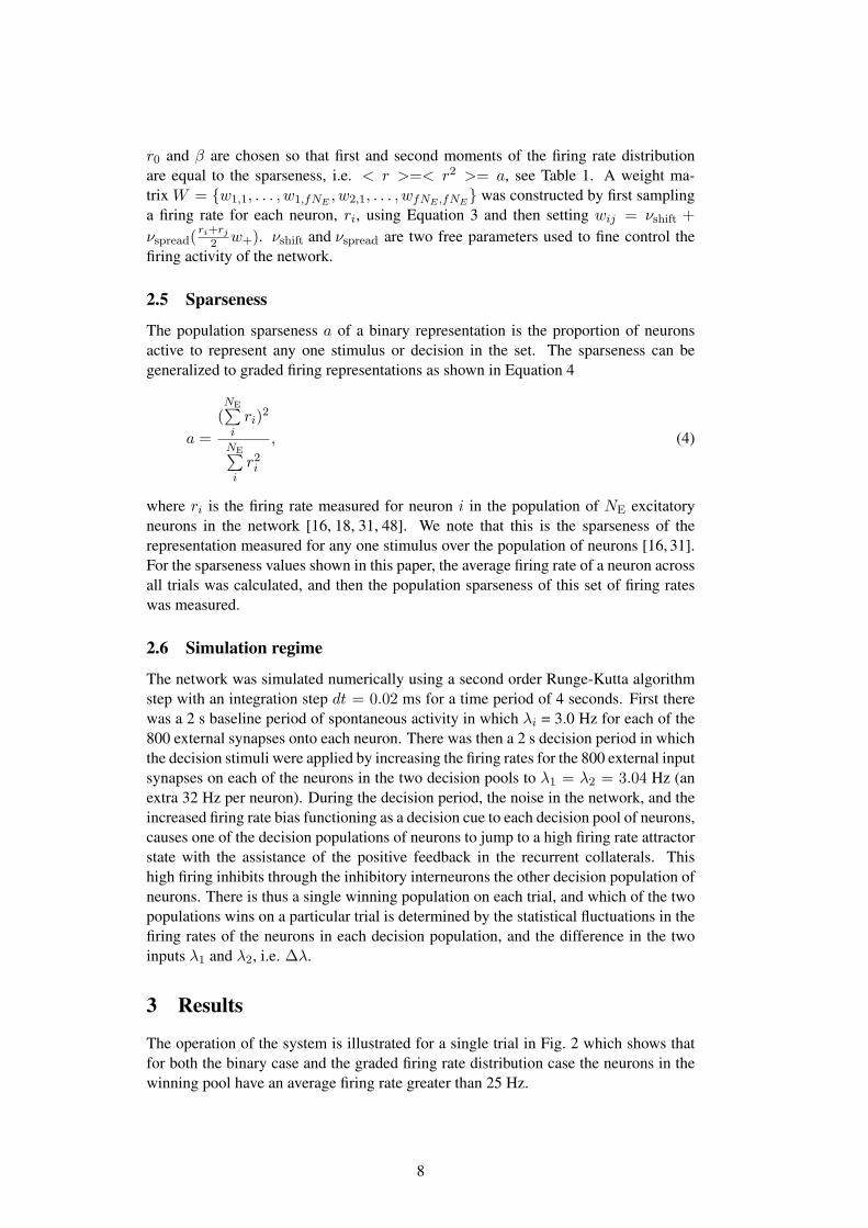
r0 and β are chosen so that first and second moments of the firing rate distributionare equal to the sparseness, i.e. < r >=< r2 >= a, see Table 1. A weight ma-trix W = {w1,1, . . . , w1,fNE

, w2,1, . . . , wfNE ,fNE} was constructed by first sampling

a firing rate for each neuron, ri, using Equation 3 and then setting wij = νshift +

νspread(ri+rj

2 w+). νshift and νspread are two free parameters used to fine control thefiring activity of the network.

2.5 Sparseness

The population sparseness a of a binary representation is the proportion of neuronsactive to represent any one stimulus or decision in the set. The sparseness can begeneralized to graded firing representations as shown in Equation 4

a =

(NE∑iri)

2

NE∑ir2i

, (4)

where ri is the firing rate measured for neuron i in the population of NE excitatoryneurons in the network [16, 18, 31, 48]. We note that this is the sparseness of therepresentation measured for any one stimulus over the population of neurons [16, 31].For the sparseness values shown in this paper, the average firing rate of a neuron acrossall trials was calculated, and then the population sparseness of this set of firing rateswas measured.

2.6 Simulation regime

The network was simulated numerically using a second order Runge-Kutta algorithmstep with an integration step dt = 0.02 ms for a time period of 4 seconds. First therewas a 2 s baseline period of spontaneous activity in which λi = 3.0 Hz for each of the800 external synapses onto each neuron. There was then a 2 s decision period in whichthe decision stimuli were applied by increasing the firing rates for the 800 external inputsynapses on each of the neurons in the two decision pools to λ1 = λ2 = 3.04 Hz (anextra 32 Hz per neuron). During the decision period, the noise in the network, and theincreased firing rate bias functioning as a decision cue to each decision pool of neurons,causes one of the decision populations of neurons to jump to a high firing rate attractorstate with the assistance of the positive feedback in the recurrent collaterals. Thishigh firing inhibits through the inhibitory interneurons the other decision population ofneurons. There is thus a single winning population on each trial, and which of the twopopulations wins on a particular trial is determined by the statistical fluctuations in thefiring rates of the neurons in each decision population, and the difference in the twoinputs λ1 and λ2, i.e. ∆λ.

3 Results

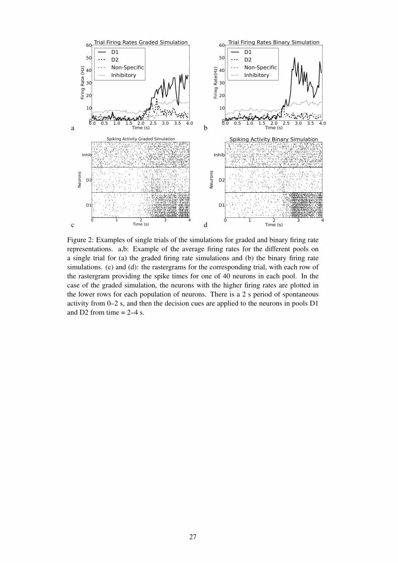
The operation of the system is illustrated for a single trial in Fig. 2 which shows thatfor both the binary case and the graded firing rate distribution case the neurons in thewinning pool have an average firing rate greater than 25 Hz.

8

3.1 Firing rate distribution

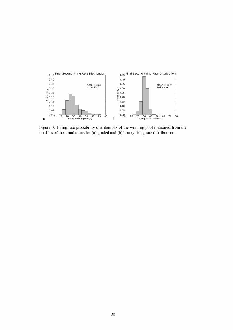
Fig. 3a,b shows for the graded (a) and binary (b) rate distribution simulations the firingrate the firing rate probability distributions achieved by the weight matrix we selected.The firing rates were measured in the last 1 s of the simulation (time = 3–4 s). Thedistribution of firing rates for the binary case has low variance, with nearly identicalmean firing rates for each of the individual neurons in the winning pool. In contrast,the graded rate distribution simulations show more variation in the distribution. Theexponential-like shape occurs in both the spontaneous and decision states, but is morepronounced in the decision state. The parameters were set to achieve this set of gradeddistribution firing rates, rather than a perfectly exponential distribution, because wewished to ensure that the mean firing rate and sparseness of the representation weresimilar in the binary and graded rate distribution cases, while at the same time havingclearly graded distribution firing rates for the graded simulations so that the effects ofgraded vs binary firing rate distributions could be measured under conditions where themean rate, and the sparseness, were essentially identical. The mean firing rates for thegraded case (a) were 30.3 spikes/s and for the binary rate distribution case were 31.0spikes/s, showing that the parameters for the recurrent weights had been selected tomake the firing rates very similar in these two cases. This was an aim, as higher firingrates can reflect increased excitation in the network which could decrease decisiontimes. As was also an aim, the standard deviation of the firing rate distribution washigher for the graded case (10.7 Hz) than for the binary case (4.9 Hz).

As the sparseness of the representation might influence the noise in the networkand the measured decision time (with sparse representations with small values of aexpected to be more noisy), we were careful to ensure that the sparseness of the repre-sentation for the binary and graded cases were similar. (They were set by the choice ofthe recurrent synaptic weights in the two decision populations, which is the distributionthat produced the graded firing rates.) The sparseness measured using Equation 4 fromboth sets of simulations was very similar. The final steady state value with one of thepools in its winning attractor state was close to the theoretical value of 0.1, due to therebeing 40 neurons in each decision pool in a population of 400 excitatory neurons.

The variability of the firing was measured by computing the coefficient of variation(CV) of the firing rates for single neurons (using 50 ms bins) for different temporalperiods. The CV measured in the second before the decision cues were applied (theperiod of spontaneous firing) was 0.018 for the binary and was 0.042 for the gradedrate distributions. In the final second of simulation for the winning attractor the CV was0.010 for the binary and was 0.018 for the graded rate distributions. The variability bythis measure was consistently higher for the graded simulations than for binary ratedistributions.

3.2 Decision time

An important measure of the noise in the system is the escaping time of the systemafter the decision cues are applied from the spontaneous state to a decision state. In-creased noise will decrease the escaping time, and thus the decision or reaction time,as illustrated in Fig. 1c. ∆λ was 0 Hz per neuron for these simulations.

To address the issue of the amount of noise in the system with graded vs binaryfiring rate distribution representations, we show in Fig. 4 the decision times of thenetwork with graded and binary rate distribution representations. The decision (or re-action) time was measured by the time it took from the time at which the decision cues

9

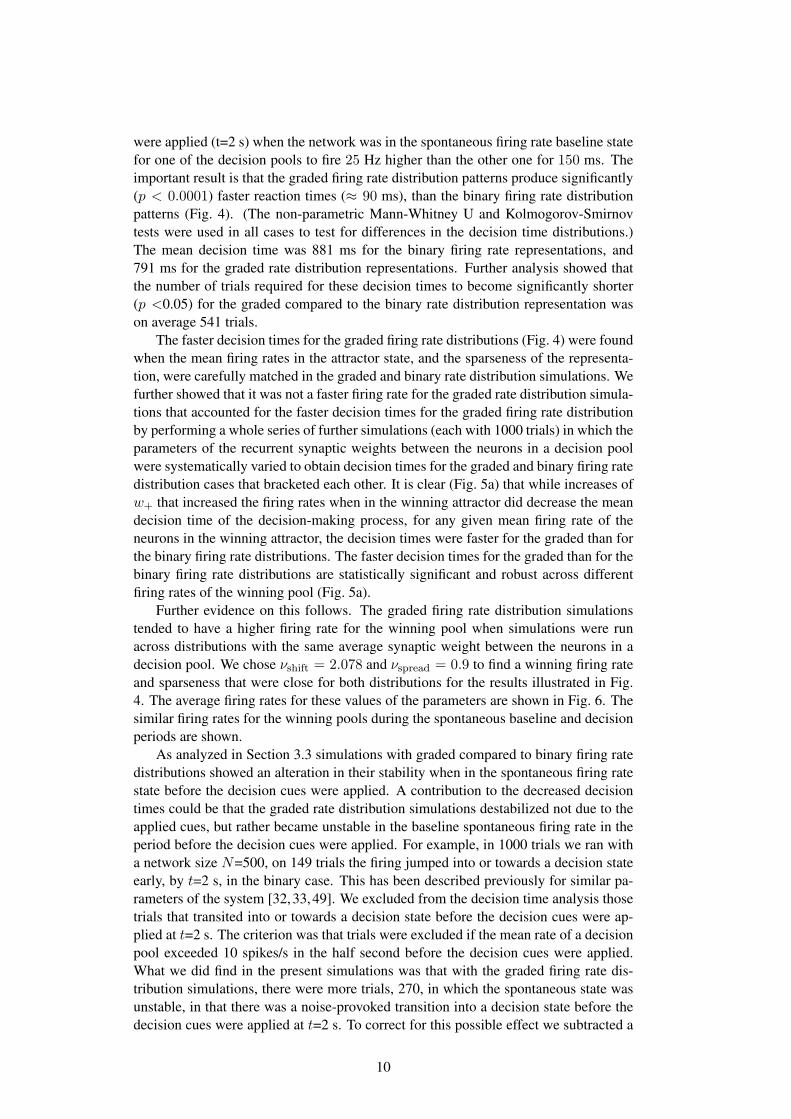
were applied (t=2 s) when the network was in the spontaneous firing rate baseline statefor one of the decision pools to fire 25 Hz higher than the other one for 150 ms. Theimportant result is that the graded firing rate distribution patterns produce significantly(p < 0.0001) faster reaction times (≈ 90 ms), than the binary firing rate distributionpatterns (Fig. 4). (The non-parametric Mann-Whitney U and Kolmogorov-Smirnovtests were used in all cases to test for differences in the decision time distributions.)The mean decision time was 881 ms for the binary firing rate representations, and791 ms for the graded rate distribution representations. Further analysis showed thatthe number of trials required for these decision times to become significantly shorter(p <0.05) for the graded compared to the binary rate distribution representation wason average 541 trials.

The faster decision times for the graded firing rate distributions (Fig. 4) were foundwhen the mean firing rates in the attractor state, and the sparseness of the representa-tion, were carefully matched in the graded and binary rate distribution simulations. Wefurther showed that it was not a faster firing rate for the graded rate distribution simula-tions that accounted for the faster decision times for the graded firing rate distributionby performing a whole series of further simulations (each with 1000 trials) in which theparameters of the recurrent synaptic weights between the neurons in a decision poolwere systematically varied to obtain decision times for the graded and binary firing ratedistribution cases that bracketed each other. It is clear (Fig. 5a) that while increases ofw+ that increased the firing rates when in the winning attractor did decrease the meandecision time of the decision-making process, for any given mean firing rate of theneurons in the winning attractor, the decision times were faster for the graded than forthe binary firing rate distributions. The faster decision times for the graded than for thebinary firing rate distributions are statistically significant and robust across differentfiring rates of the winning pool (Fig. 5a).

Further evidence on this follows. The graded firing rate distribution simulationstended to have a higher firing rate for the winning pool when simulations were runacross distributions with the same average synaptic weight between the neurons in adecision pool. We chose νshift = 2.078 and νspread = 0.9 to find a winning firing rateand sparseness that were close for both distributions for the results illustrated in Fig.4. The average firing rates for these values of the parameters are shown in Fig. 6. Thesimilar firing rates for the winning pools during the spontaneous baseline and decisionperiods are shown.

As analyzed in Section 3.3 simulations with graded compared to binary firing ratedistributions showed an alteration in their stability when in the spontaneous firing ratestate before the decision cues were applied. A contribution to the decreased decisiontimes could be that the graded rate distribution simulations destabilized not due to theapplied cues, but rather became unstable in the baseline spontaneous firing rate in theperiod before the decision cues were applied. For example, in 1000 trials we ran witha network size N=500, on 149 trials the firing jumped into or towards a decision stateearly, by t=2 s, in the binary case. This has been described previously for similar pa-rameters of the system [32,33,49]. We excluded from the decision time analysis thosetrials that transited into or towards a decision state before the decision cues were ap-plied at t=2 s. The criterion was that trials were excluded if the mean rate of a decisionpool exceeded 10 spikes/s in the half second before the decision cues were applied.What we did find in the present simulations was that with the graded firing rate dis-tribution simulations, there were more trials, 270, in which the spontaneous state wasunstable, in that there was a noise-provoked transition into a decision state before thedecision cues were applied at t=2 s. To correct for this possible effect we subtracted a

10

reaction time distribution without the application of decision cues from the distributionwith decision cues. Simulations were repeated with the same parameters, except thatno cues were applied. The distribution of the reaction times of these ‘no cues’ simu-lations was computed. The ‘corrected distributions’ were computed by subtracting thenumber of times the ‘no cues’ simulation reacted in a given period from the numberof times the simulation reacted in the same period in the ‘with cues’ simulations. Thisprovided a decision time distribution that is corrected for the possibility of simulationtrials jumping purely from the baseline spontaneous rate to a high firing rate state.When this correction is applied, we still observed that the decision times are faster forthe graded than for the binary firing rate distribution cases, as shown in Figs. 4c,d and5b.

In summary, faster decision times are found with graded than with binary firingrate distributions, and this is not likely to be due to any increase in firing rate duringthe spontaneous period, nor is it due to faster firing rates during the decision-makingperiod.

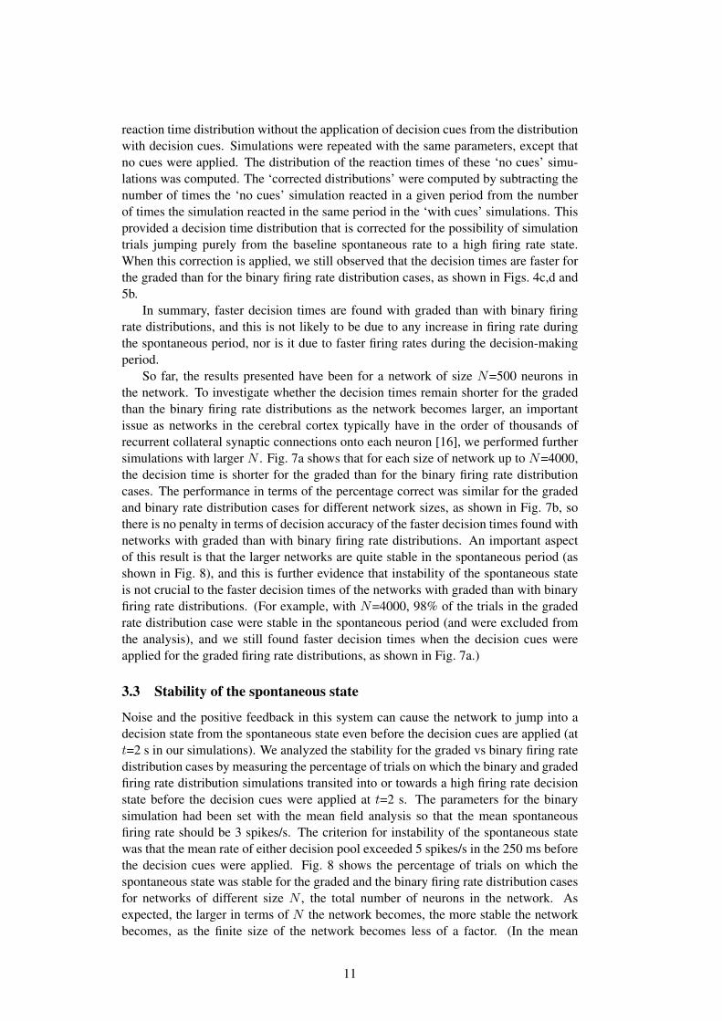
So far, the results presented have been for a network of size N=500 neurons inthe network. To investigate whether the decision times remain shorter for the gradedthan the binary firing rate distributions as the network becomes larger, an importantissue as networks in the cerebral cortex typically have in the order of thousands ofrecurrent collateral synaptic connections onto each neuron [16], we performed furthersimulations with larger N . Fig. 7a shows that for each size of network up to N=4000,the decision time is shorter for the graded than for the binary firing rate distributioncases. The performance in terms of the percentage correct was similar for the gradedand binary rate distribution cases for different network sizes, as shown in Fig. 7b, sothere is no penalty in terms of decision accuracy of the faster decision times found withnetworks with graded than with binary firing rate distributions. An important aspectof this result is that the larger networks are quite stable in the spontaneous period (asshown in Fig. 8), and this is further evidence that instability of the spontaneous stateis not crucial to the faster decision times of the networks with graded than with binaryfiring rate distributions. (For example, with N=4000, 98% of the trials in the gradedrate distribution case were stable in the spontaneous period (and were excluded fromthe analysis), and we still found faster decision times when the decision cues wereapplied for the graded firing rate distributions, as shown in Fig. 7a.)

3.3 Stability of the spontaneous state

Noise and the positive feedback in this system can cause the network to jump into adecision state from the spontaneous state even before the decision cues are applied (att=2 s in our simulations). We analyzed the stability for the graded vs binary firing ratedistribution cases by measuring the percentage of trials on which the binary and gradedfiring rate distribution simulations transited into or towards a high firing rate decisionstate before the decision cues were applied at t=2 s. The parameters for the binarysimulation had been set with the mean field analysis so that the mean spontaneousfiring rate should be 3 spikes/s. The criterion for instability of the spontaneous statewas that the mean rate of either decision pool exceeded 5 spikes/s in the 250 ms beforethe decision cues were applied. Fig. 8 shows the percentage of trials on which thespontaneous state was stable for the graded and the binary firing rate distribution casesfor networks of different size N , the total number of neurons in the network. Asexpected, the larger in terms of N the network becomes, the more stable the networkbecomes, as the finite size of the network becomes less of a factor. (In the mean

11

field case, or with an infinite number of neurons in the spiking simulations, the noiseeffects would diminish to zero.) Fig. 8 shows that the network with the graded firingrate distribution is for each value of N less stable in the spontaneous period than thenetwork with the binary firing rate distribution.

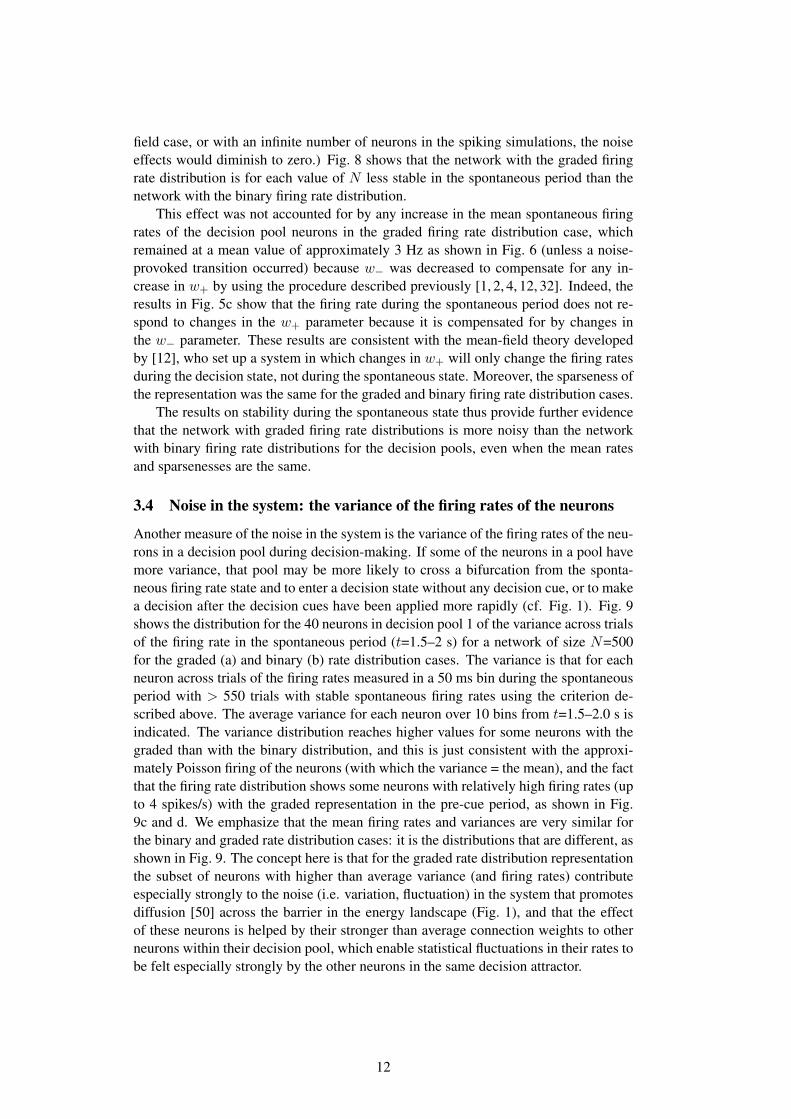
This effect was not accounted for by any increase in the mean spontaneous firingrates of the decision pool neurons in the graded firing rate distribution case, whichremained at a mean value of approximately 3 Hz as shown in Fig. 6 (unless a noise-provoked transition occurred) because w− was decreased to compensate for any in-crease in w+ by using the procedure described previously [1, 2, 4, 12, 32]. Indeed, theresults in Fig. 5c show that the firing rate during the spontaneous period does not re-spond to changes in the w+ parameter because it is compensated for by changes inthe w− parameter. These results are consistent with the mean-field theory developedby [12], who set up a system in which changes in w+ will only change the firing ratesduring the decision state, not during the spontaneous state. Moreover, the sparseness ofthe representation was the same for the graded and binary firing rate distribution cases.

The results on stability during the spontaneous state thus provide further evidencethat the network with graded firing rate distributions is more noisy than the networkwith binary firing rate distributions for the decision pools, even when the mean ratesand sparsenesses are the same.

3.4 Noise in the system: the variance of the firing rates of the neurons

Another measure of the noise in the system is the variance of the firing rates of the neu-rons in a decision pool during decision-making. If some of the neurons in a pool havemore variance, that pool may be more likely to cross a bifurcation from the sponta-neous firing rate state and to enter a decision state without any decision cue, or to makea decision after the decision cues have been applied more rapidly (cf. Fig. 1). Fig. 9shows the distribution for the 40 neurons in decision pool 1 of the variance across trialsof the firing rate in the spontaneous period (t=1.5–2 s) for a network of size N=500for the graded (a) and binary (b) rate distribution cases. The variance is that for eachneuron across trials of the firing rates measured in a 50 ms bin during the spontaneousperiod with > 550 trials with stable spontaneous firing rates using the criterion de-scribed above. The average variance for each neuron over 10 bins from t=1.5–2.0 s isindicated. The variance distribution reaches higher values for some neurons with thegraded than with the binary distribution, and this is just consistent with the approxi-mately Poisson firing of the neurons (with which the variance = the mean), and the factthat the firing rate distribution shows some neurons with relatively high firing rates (upto 4 spikes/s) with the graded representation in the pre-cue period, as shown in Fig.9c and d. We emphasize that the mean firing rates and variances are very similar forthe binary and graded rate distribution cases: it is the distributions that are different, asshown in Fig. 9. The concept here is that for the graded rate distribution representationthe subset of neurons with higher than average variance (and firing rates) contributeespecially strongly to the noise (i.e. variation, fluctuation) in the system that promotesdiffusion [50] across the barrier in the energy landscape (Fig. 1), and that the effectof these neurons is helped by their stronger than average connection weights to otherneurons within their decision pool, which enable statistical fluctuations in their rates tobe felt especially strongly by the other neurons in the same decision attractor.

12

3.5 Performance with graded firing rate distributions and diluted con-nectivity

Up to this point, the network was studied with fully connectivity of its neurons. In orderto investigate a more biologically plausible scenario, we conducted simulations withdiluted connectivity. In order to keep the mean input to each neuron the same in dilutedsimulations as it was in fully connected simulations, for the diluted connectivity wekept the same number of connections C per neuron as in the fully connected network,but increased the number of neurons in the decision pools. We parameterized dilutionby a connectivity level, 0 < c ≤ 1. c=1 corresponds to the fully connected case.Diluted networks with dilution c would have the number of neurons in the decisionpool set to NEf

1c . The C connections to a neuron were received from a randomly

selected set of the NEf1c neurons in the same decision pool.

We measured decision times for two values of c. As described elsewhere [51],smaller values of c resulted in slower decision times. One of the new findings reportedhere is that for diluted connectivity, graded firing rate representations produced fasterdecision times than binary rate distribution representations. In particular, for c = 0.10,the mean decision time in the graded case was 1124 ms (SE 33 sd 335 ms), and in thebinary case it was 1192 ms (SE 32 sd 320 ms). For c = 0.25, the mean decision timein the graded case was 984 ms (SE 16 sd 345 ms), and in the binary case it was 1077ms (SE 15 sd 332 ms) (p < 10−5).

In summary, in networks with diluted connectivity, just as in fully connected net-works, graded firing rate distribution representations produced faster decision timesthan binary firing rate representations. This is consistent with more noise in attractornetworks with graded than with binary firing rate distribution representations.

3.6 Performance during decision-making with ∆λ = 0 Hz

So far we have shown results mainly for ∆λ = 0 Hz, that is when the inputs duringthe decision-making period to D1 and D2 are equal. The performance of the networkis close to the expected 50% correct, that is D1 wins on approximately 50% of thetrials, and D2 on approximately 50% of the trials. However, the evidence for the twodecisions is often not equal, and in this section we consider whether when runningwith ∆λ > 0, different effects occur. For example, if the graded rate distributionsystem is more excitable and responds faster than the binary rate distribution system,there might be a speed-accuracy tradeoff of the type investigated for many decades inpsychology [52]. It would be of interest if for example the graded rate distributionsystem with its faster decision times was less accurate (in terms of percentage correct),though also interesting if it maintained its accuracy even when the reaction times werefaster.

Fig. 7a shows that for different sizes of network up to N=4000, the decision timeis shorter for the graded than for the binary firing rate distribution cases with ∆λ=16Hz per neuron. The performance in terms of the percentage correct was similar for thegraded and binary rate distribution cases for different network sizes, as shown in Fig.7b, and for different values of ∆λ as shown in Fig. 7c, so there is no penalty in termsof decision accuracy of the faster decision times found with networks with graded thanwith binary firing rate distributions within these parameter ranges.

13

3.7 Performance for different levels of firing rate gradation

Up to this point we have only presented graded rate distribution simulations with avalue of gradation that was small enough to keep the firing rates and stability closeto the results in the binary simulations. We have in addition simulated networks withhigher amounts of gradation. We parameterized the amount of gradation in the networkby ∆ν = whi − wlow, where whi is the highest recurrent weight, and wlow was thelowest recurrent weight. The other results in this paper have ∆ν approximately 0.81.In further investigations With moderate dilution, c = 0.25, and ∆ν = 2.1, decisiontimes decreased to a mean value of 445 ms, and stability during the spontaneous periodwas reduced to 37%, compared to a mean decision time of 984 ms (p < 10−32) and98% stability for the same simulation but with ∆ν = 0.81.

Thus increasing the range of firing rates in the graded distribution representationdecreased the decision time and decreased the stability of the spontaneous firing ratestate. This is evidence that increasing the range of the firing rate distributions intro-duces more noise into the neuronal network.

3.8 Noise with graded firing rate distribution representations in largernetworks

As spiking attractor networks are increased in size, the statistical fluctuations causedby the close to Poisson spiking times of the neurons become smaller, until with aninfinite number of neurons the noise becomes 0 [4]. We have shown that in practice,measures of the noise such as the decision (escaping) time do decrease as the number ofneurons is increased to 4000, but that there is still noise due to the spiking fluctuationswith this size of network, in which C=NE=3200 [2, 38, 39]. However, the numberof connections C for the recurrent collateral synapses which provide for the attractordynamics is in the order of 9,000 in the neocortex, and 12,000 in the CA3 neurons inthe hippocampus [16]. To check that the findings in the present paper apply in principleto these larger networks, we were able to perform further simulations with as many as8000 neurons in the network, which then had NE=6400 excitatory neurons, and 6400recurrent collateral synapses onto each excitatory neuron.

We simulated scaled up networks with 8000 neurons, and therefore 320 neurons ineach specific decision population. With w+ left at 2.1 as in the earlier simulations, thedecision times were faster with the graded (mean 947 sd 332 ms) than with the binary(mean 1073 sd 312 ms) firing rate distributions (p < 10−7 with 320 trials). Thus gradedfiring rate distributions do introduce more noise into the system than binary firing ratedistributions, even with large networks that are the same order as the size of networksfound in the cerebral cortex. Further analysis showed that these decision times becamesignificantly shorter (p <0.05) for the graded compared to the binary rate distributionrepresentation with on average 21 trials.

With w+=2.1 and 8000 neurons, the spontaneous state was much more stable, andindeed there were no unstable trials in the spontaneous period for the graded and forthe binary rate distribution representations. To test whether the graded rate distributionwas inherently more unstable in the spontaneous state even at this large size of network,we ran further simulations with 8000 neurons, but with w+=2.25 to promote moreinstability. This revealed more instability with the graded (only 87% stable) than withthe binary firing rate distribution representations (97% stable, p < 0.02).

14

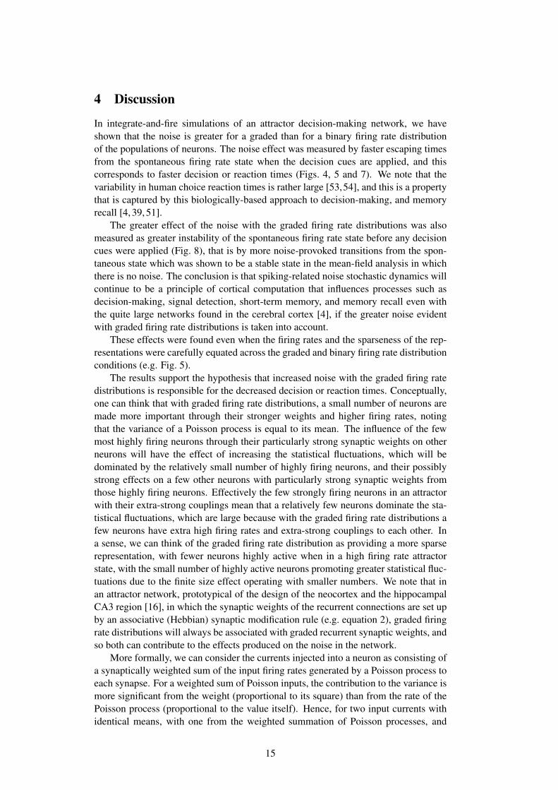
4 Discussion

In integrate-and-fire simulations of an attractor decision-making network, we haveshown that the noise is greater for a graded than for a binary firing rate distributionof the populations of neurons. The noise effect was measured by faster escaping timesfrom the spontaneous firing rate state when the decision cues are applied, and thiscorresponds to faster decision or reaction times (Figs. 4, 5 and 7). We note that thevariability in human choice reaction times is rather large [53,54], and this is a propertythat is captured by this biologically-based approach to decision-making, and memoryrecall [4, 39, 51].

The greater effect of the noise with the graded firing rate distributions was alsomeasured as greater instability of the spontaneous firing rate state before any decisioncues were applied (Fig. 8), that is by more noise-provoked transitions from the spon-taneous state which was shown to be a stable state in the mean-field analysis in whichthere is no noise. The conclusion is that spiking-related noise stochastic dynamics willcontinue to be a principle of cortical computation that influences processes such asdecision-making, signal detection, short-term memory, and memory recall even withthe quite large networks found in the cerebral cortex [4], if the greater noise evidentwith graded firing rate distributions is taken into account.

These effects were found even when the firing rates and the sparseness of the rep-resentations were carefully equated across the graded and binary firing rate distributionconditions (e.g. Fig. 5).

The results support the hypothesis that increased noise with the graded firing ratedistributions is responsible for the decreased decision or reaction times. Conceptually,one can think that with graded firing rate distributions, a small number of neurons aremade more important through their stronger weights and higher firing rates, notingthat the variance of a Poisson process is equal to its mean. The influence of the fewmost highly firing neurons through their particularly strong synaptic weights on otherneurons will have the effect of increasing the statistical fluctuations, which will bedominated by the relatively small number of highly firing neurons, and their possiblystrong effects on a few other neurons with particularly strong synaptic weights fromthose highly firing neurons. Effectively the few strongly firing neurons in an attractorwith their extra-strong couplings mean that a relatively few neurons dominate the sta-tistical fluctuations, which are large because with the graded firing rate distributions afew neurons have extra high firing rates and extra-strong couplings to each other. Ina sense, we can think of the graded firing rate distribution as providing a more sparserepresentation, with fewer neurons highly active when in a high firing rate attractorstate, with the small number of highly active neurons promoting greater statistical fluc-tuations due to the finite size effect operating with smaller numbers. We note that inan attractor network, prototypical of the design of the neocortex and the hippocampalCA3 region [16], in which the synaptic weights of the recurrent connections are set upby an associative (Hebbian) synaptic modification rule (e.g. equation 2), graded firingrate distributions will always be associated with graded recurrent synaptic weights, andso both can contribute to the effects produced on the noise in the network.

More formally, we can consider the currents injected into a neuron as consisting ofa synaptically weighted sum of the input firing rates generated by a Poisson process toeach synapse. For a weighted sum of Poisson inputs, the contribution to the variance ismore significant from the weight (proportional to its square) than from the rate of thePoisson process (proportional to the value itself). Hence, for two input currents withidentical means, with one from the weighted summation of Poisson processes, and

15

the other from the simple summation of Poisson processes, we should expect that theweighted sum in general would have a larger variance. More precisely, let us considertwo synaptic inputs I1 and I2

I1(t) =

K∑i=1

w+Ni(t); I2(t) =

K∑i=1

wiNi(t)

where K is the number of synapses, Ni(t) in the binary case is a Poisson processwith firing rate λ and weight w+, and in the graded rate distribution case Ni(t) isanother Poisson process with firing rate λi with weight wi. (N(t) counts the numberof spikes in a time interval (0, t). For a Poisson process, N(t) is drawn from a Poissondistribution with parameter λ.) The means of these two types of input are

EI1(t) = Kw+λt = EI2(t) =

K∑i

wiλit

which yields

w+λ =

∑Ki wiλi

K. (5)

For simplicity, and it is the actual case in our simulations here, we further assume thatλi = awi, λ = aw+, where a is a positive scaling number. Hence Eq. (5) turns out tobe

w+ =

√∑Ki w2

i

K.

The variances of the two synaptic inputs are

var(I1(t)) = Kw2+λt; var(I2(t)) =

K∑i

w2i λit

respectively. We can see that in general the second term above, var(I2(t)), is largerthan the first, var(I1(t)), since

var(I1(t)) = Kw2+λt = tKaw+

3 = tKa

{∑Ki w2

i

K

}3/2

≤ tKa

∑Ki (w2

i )3/2

K

= tKa

∑Ki w3

i

K

= tK

∑Ki w2

i λi

K= var(I2(t))

.

The inequality above is due to Jensen’s inequality which states that for any convexfunction ϕ, ϕ

(∑w2

iK

)≤

∑ϕ(w2

i )K . In our case ϕ(x) = x3/2. Thus the weighted sum

of Poisson processes has greater variance than the sum of Poisson processes when theexpected means are equal. Accordingly we would expect more variance of the currentsinjected into neurons with a graded firing rate and weight distribution than with thebinary firing rate and weight distribution when the injected currents are the same. This

16

analysis is supported by our finding that the variance of the NMDA currents injectedinto each neuron of pools 1 and 2 in the spontaneous period was greater in the gradedthan the binary rate distribution case (300 vs 254 nA2, p < 10−10), whereas the meanswere similar (48.3 vs 48.4 nA).

We emphasize that the mean firing rates and mean variances of the decision popu-lations of neurons are very similar for the binary and graded rate distribution cases: itis the distributions that are different, as shown in Fig. 9. The concept here is that forthe graded rate distribution representation the subset of neurons with higher than aver-age variance (and firing rates) contribute especially strongly to the noise (i.e. variation,fluctuation) in the system that promotes diffusion [50] across the barrier in the energylandscape (Fig. 1), and that the effect of these neurons is helped by their stronger thanaverage connection weights to other neurons within their decision pool, which enablestatistical fluctuations in their rates to be felt especially strongly by the other neuronsin the same decision attractor.

To clarify, the descent into the decision attractor basin first has to overcome theenergy barrier that keeps the system in the spontaneous stable state (Fig. 1c). Greatervariation in the system will mean that this transition is more likely to happen quickly.This is due to the fact that many coincident spikes are needed to overcome this energybarrier. Increased noise means that we are more likely to observe the right set ofcoincident spikes occurring earlier.

The work described here shows that a potentially useful property of the gradeddistribution firing rate representations found in the brain [16, 31] is the faster decisiontimes found than with binary firing rate distributions. Given that attractor networks inthe cortex have to be large, with thousands of recurrent collateral synapses onto eachneuron, as this is the leading factor that determines the number of different memoriesthat can be stored and correctly retrieved [16,18,19], the graded firing rate distributionsmay enable the finite size statistical fluctuations to still influence the processing, andindeed make the processing faster than it would be with binary firing rate distributions.This speed is important, for recurrent collateral processing may be useful at every stageof each sensory hierarchy of cortical processing, yet there may be time for only 20–25ms of processing at each cortical stage of the hierarchy [16, 55–58]. The functions towhich the noisy graded firing rate distributions contribute in cortical attractor networksinclude memory recall, probabilistic decision-making, the facilitation of perceptualdetection by stochastic resonance, creative thought, disengagement of attention, andan element of unpredictability of behaviour that can be advantageous [4].

The framework used here can be extended very naturally to account for the prob-abilistic decisions taken when there are multiple, that is more than two, choices. Onesuch extension models choices between continuous variables in a continuous or lineattractor network [59, 60] to account for the responses of lateral intraparietal cortexneurons in a 4-choice random dot motion decision task [61]. In another approach, anetwork with multiple discrete attractors [62] can account well for the same data. Theeffects described in the current paper, that the greater spiking-related noise of gradedthan of binary rate distribution representations can reduce the stability, and increasethe speed of decision-making, will apply directly to the discrete attractor scenario, inwhich greater noise will decrease the escaping time from one state to another in theenergy landscape (Fig. 1c) [4].

The graded nature of the firing rate representations in the cortex may of coursebe adaptive for other reasons than the speed of processing, which might be an addedbenefit if there are other reasons for graded distribution firing rate representations. Ifthe number of spikes recorded in a fixed time window is taken to be constrained by

17

a fixed maximum rate, one can try to interpret the distribution observed in terms ofoptimal information transmission [63], by making the additional assumption that thecoding is noiseless. An exponential distribution, which maximizes entropy (and henceinformation transmission for noiseless codes) is the most efficient in terms of energyconsumption if its mean takes an optimal value that is a decreasing function of the rela-tive metabolic cost of emitting a spike [64]. This argument would favour sparser codingschemes the more energy expensive neuronal firing is (relative to rest). Although thetail of actual firing rate distributions is often approximately exponential [21, 22, 31],the maximum entropy argument cannot apply as such, because noise is present and thenoise level varies as a function of the rate, which makes entropy maximization differentfrom information maximization. Moreover, a mode at low but non-zero rate, which isoften observed [16, 21, 31] is inconsistent with the energy efficiency hypothesis.

In conclusion, we have investigated the effects of graded distribution firing ratepatterns in a recurrent spiking neural network attractor model of decision-making. Thegraded rate distributions for the patterns we produced in the numerical simulations tooka similar form to those found neurophysiologically. The main finding is that the tran-sition time to an attractor state, or reaction time, is decreased when neurons fire withthe more biologically realistic graded firing rates across the neuronal populations. Oneadvantage of these graded firing rate representations is that they provide a sparse dis-tributed representation with independence of the information provided by each neuron,allowing for the useful properties in associative networks of generalization, comple-tion, and graceful degradation [16, 37]. It has been argued elsewhere [64] that gradeddistribution firing rates may also maximize information transmission for a given meanrate of firing, and therefore energy consumption, given that high average firing ratesrequire more metabolic expenditure. [However, an alternative account of the gradeddistributions is that they arise with integrate-and-fire neurons with slow fluctuations inthe inputs (reflecting different stimuli) and fast fluctuations in the inputs (reflecting forexample trial-by-trial variability in the response to a given stimulus, to which the ef-fects of the spiking-related, close to Poisson, high entropy, fluctuations in the numberof spikes in a short time window analyzed in this paper could contribute) [30]. Thelong tail of graded firing rate probability distributions may also be required for cost ef-ficiency [65].] The results described here show that an additional useful property of thegraded representations found in the brain is that they may increase the speed of deci-sions, reducing the time required for many processes such as memory recall as well asmore conventionally understood decision-making [4]. Given that cortical computationfrequently requires a hierarchical series of cortical stages in each of which attractorprocesses may contribute, the cumulative effect on the increased speed of processingof graded firing rate representations over a series of cortical stages may be consider-able [16, 57].

We emphasize that it is important to understand the effects of noise in networks inthe brain, and its implications for the stability of neuronal networks in the brain. Forexample, a stochastic neurodynamical approach to schizophrenia holds that there isless stability of cortical attractor networks involved in short-term memory and attentiondue to reduced functioning of the glutamate system, which decreases the firing ratesof neurons in the prefrontal cortex, and therefore, given the spiking-related noise thatis present, the depth of the basins of attraction. This it is suggested contributes tothe cognitive changes in schizophrenia, which include impaired short-term memoryand attention [32, 33, 35]. In another example, a stochastic neurodynamical approachto obsessive compulsive disorder holds that there is overstability in some networksin prefrontal cortex and connected areas due to hyperglutamatergia [34, 36]. In both

18

these cases, and also in normal brain function in relation to decision-making, memoryrecall, etc, it is important to know to what extent noise contributed by randomness inthe spiking times of individual neurons for a given mean rate contributes to stochasticeffects found in the brain which affect decision-making, stability, and which may ifthe stability is disturbed contribute to neuropsychiatric disorders. In this context, thefindings described in this paper are important for understanding normal and disorderedbrain function. In particular, a very interesting implication of the findings describedhere is that there is more noise with the graded rate distribution representations found inthe brain (see [16] Appendix 3 on information encoding in the brain) than with binaryfiring rate distributions (which are often used in simulations, because they are amenableto mean-field analyses [1, 2]). Thus when noise is found to be a significant factor inthe operation of integrate-and-fire decision-making networks with binary firing ratesup to sizes that have been tested of 4096 neurons each with 4096 synapses per neuron,then it is likely that with graded firing rates, spiking-related noise will continue to be afactor in the operation of cortical circuitry even up to the larger numbers of recurrentcollateral synapses onto each neuron. For example, in the cerebral cortex there aretypically in the order of 9,000 recurrent collateral synapses onto onto each corticalpyramidal cell, from a total of in the order of 18,000 synapses [13, 16].

19

References

1. Wang XJ (2002) Probabilistic decision making by slow reverberation in corticalcircuits. Neuron 36: 955–968.

2. Deco G, Rolls ET (2006) A neurophysiological model of decision-making andWeber’s law. European Journal of Neuroscience 24: 901–916.

3. Wang XJ (2008) Decision making in recurrent neuronal circuits. Neuron 60:215–234.

4. Rolls ET, Deco G (2010) The Noisy Brain: Stochastic Dynamics as a Principleof Brain Function. Oxford: Oxford University Press.

5. Hopfield JJ (1982) Neural networks and physical systems with emergent collec-tive computational abilities. Proc Nat Acad Sci USA 79: 2554–2558.

6. Amit DJ (1989) Modeling Brain Function. The World of Attractor Neural Net-works. Cambridge: Cambridge University Press.

7. Faisal A, Selen L, Wolpert D (2008) Noise in the nervous system. Nature Re-views Neuroscience 9: 292–303.

8. Deco G, Rolls ET, Romo R (2009) Stochastic dynamics as a principle of brainfunction. Progress in Neurobiology 88: 1–16.

9. Softky WR, Koch C (1993) The highly irregular firing of cortical cells is incon-sistent with temporal integration of random EPSPs. Jpurnal of Neuroscience 13:334–350.

10. Amit DJ, Brunel N (1997) Dynamics of a recurrent network of spiking neuronsbefore and following learning. Network 8: 373–404.

11. Miller P, Wang XJ (2006) Power-law neuronal fluctuations in a recurrent net-work model of parametric working memory. Journal of Neurophysiology 95:1099–1114.

12. Brunel N, Wang XJ (2001) Effects of neuromodulation in a cortical networkmodel of object working memory dominated by recurrent inhibition. Journal ofComputational Neuroscience 11: 63–85.

13. Abeles M (1991) Corticonics: Neural Circuits of the Cerebral Cortex. Cam-bridge: Cambridge University Press.

14. Braitenberg V, Schutz A (1991) Anatomy of the Cortex. Berlin: Springer-Verlag.

15. Elston GN, Benavides-Piccione R, Elston A, Zietsch B, Defelipe J, et al. (2006)Specializations of the granular prefrontal cortex of primates: implications forcognitive processing. Anatomical Record A Discov Mol Cell Evol Biol 288:26–35.

16. Rolls ET (2008) Memory, Attention, and Decision-Making. A Unifying Com-putational Neuroscience Approach. Oxford: Oxford University Press.

20

17. Brody C, Romo R, Kepecs A (2003) Basic mechanisms for graded persistentactivity: discrete attractors, continuous attractors, and dynamic representations.Current Opinion in Neurobiology 13: 204–211.

18. Treves A, Rolls ET (1991) What determines the capacity of autoassociativememories in the brain? Network 2: 371–397.

19. Rolls ET, Treves A (1998) Neural Networks and Brain Function. Oxford: Ox-ford University Press.

20. Rolls ET, Tovee MJ (1995) Sparseness of the neuronal representation of stimuliin the primate temporal visual cortex. Journal of Neurophysiology 73: 713–726.

21. Rolls ET, Treves A, Tovee M, Panzeri S (1997) Information in the neuronal rep-resentation of individual stimuli in the primate temporal visual cortex. Journalof Computational Neuroscience 4: 309–333.

22. Baddeley RJ, Abbott LF, Booth MJA, Sengpiel F, Freeman T, et al. (1997) Re-sponses of neurons in primary and inferior temporal visual cortices to naturalscenes. Proceedings of the Royal Society B 264: 1775–1783.

23. Rolls ET, Critchley HD, Treves A (1996) The representation of olfactory in-formation in the primate orbitofrontal cortex. Journal of Neurophysiology 75:1982–1996.

24. Verhagen JV, Kadohisa M, Rolls ET (2004) The primate insular taste cortex:neuronal representations of the viscosity, fat texture, grittiness, and the taste offoods in the mouth. Journal of Neurophysiology 92: 1685–1699.

25. Rolls ET, Verhagen JV, Kadohisa M (2003) Representations of the texture offood in the primate orbitofrontal cortex: neurons responding to viscosity, gritti-ness, and capsaicin. Journal of Neurophysiology 90: 3711–3724.

26. Rolls ET, Critchley H, Verhagen JV, Kadohisa M (2010) The representation ofinformation about taste and odor in the primate orbitofrontal cortex. Chemosen-sory Perception 3: 16–33.

27. Kadohisa M, Rolls ET, Verhagen JV (2005) The primate amygdala: neuronalrepresentations of the viscosity, fat texture, grittiness and taste of foods. Neuro-science 132: 33–48.

28. Kadohisa M, Rolls ET, Verhagen JV (2005) Neuronal representations of stimuliin the mouth: the primate insular taste cortex, orbitofrontal cortex, and amyg-dala. Chemical Senses 30: 401–419.

29. Rolls ET, Treves A, Robertson RG, Georges-Francois P, Panzeri S (1998) Infor-mation about spatial view in an ensemble of primate hippocampal cells. Journalof Neurophysiology 79: 1797–1813.

30. Treves A, Panzeri S, Rolls ET, Booth M, Wakeman EA (1999) Firing rate dis-tributions and efficiency of information transmission of inferior temporal cortexneurons to natural visual stimuli. Neural Computation 11: 601–631.

21

31. Franco L, Rolls ET, Aggelopoulos NC, Jerez JM (2007) Neuronal selectivity,population sparseness, and ergodicity in the inferior temporal visual cortex. Bi-ological Cybernetics 96: 547–560.

32. Loh M, Rolls ET, Deco G (2007) A dynamical systems hypoth-esis of schizophrenia. PLoS Computational Biology 3: e228.doi:10.1371/journal.pcbi.0030228.

33. Rolls ET, Loh M, Deco G, Winterer G (2008) Computational models ofschizophrenia and dopamine modulation in the prefrontal cortex. Nature Re-views Neuroscience 9: 696–709.

34. Rolls ET, Loh M, Deco G (2008) An attractor hypothesis of obsessive-compulsive disorder. European Journal of Neuroscience 28: 782–793.

35. Rolls ET, Deco G (2011) A computational neuroscience approach to schizophre-nia and its onset. Neuroscience and Biobehavioral Reviews 35: 1644–1653.

36. Rolls ET (2011) Glutamate, obsessive-compulsive disorder, schizophrenia, andthe stability of cortical attractor neuronal networks. Pharmacology, Biochem-istry and Behavior : Epub 23 June.

37. Rolls ET, Treves A (2011) Information encoding in the brain. Progress in Neu-robiology : , in revision.

38. Rolls ET, Grabenhorst F, Deco G (2010) Choice, difficulty, and confidence inthe brain. Neuroimage 53: 694–706.

39. Rolls ET, Grabenhorst F, Deco G (2010) Decision-making, errors, and confi-dence in the brain. Journal of Neurophysiology 104: 2359–2374.

40. Deco G, Rolls ET (2005) Synaptic and spiking dynamics underlying rewardreversal in the orbitofrontal cortex. Cerebral Cortex 15: 15–30.

41. Buehlmann A, Deco G (2008) The neuronal basis of attention: rate versus syn-chronization modulation. Journal of Neuroscience 28: 7679–7686.

42. Smerieri A, Rolls ET, Feng J (2010) Decision time, slow inhibition, and thetarhythm. Journal of Neuroscience 30: 14173–14181.

43. Nordlie E, Gewaltig MO, Plesser HE (2009) Towards reproducible descriptionsof neuronal network models. PLoS Computational Biology 5: e1000456.

44. Knight B (2000) Dynamics of encoding in neuron populations: some generalmathematical features. Neural Computation 12: 473–518.

45. Burkitt AN (2006) A review of the integrate-and-fire neuron model: I. Homo-geneous synaptic input. Biological Cybernetics 95: 1–19.

46. Hertz J, Krogh A, Palmer RG (1991) Introduction to the Theory of Neural Com-putation. Wokingham, U.K.: Addison Wesley.

47. Rolls ET, Treves A, Foster D, Perez-Vicente C (1997) Simulation studies ofthe CA3 hippocampal subfield modelled as an attractor neural network. NeuralNetworks 10: 1559–1569.

22

48. Rolls ET, Treves A (1990) The relative advantages of sparse versus distributedencoding for associative neuronal networks in the brain. Network 1: 407–421.

49. Loh M, Rolls ET, Deco G (2007) Statistical fluctuations in attractor networksrelated to schizophrenia. Pharmacopsychiatry 40: S78–84.

50. Marti D, Deco G, Mattia M, Gigante G, Del Giudice P (2008) A fluctuation-driven mechanism for slow decision processes in reverberant networks. PLoSONE 3: e2534. doi:10.1371/journal.pone.0002534.

51. Rolls ET, Webb TJ (2011) Cortical attractor network dynamics with diluted con-nectivity. Brain Research : , in revision.

52. Beamish D, Bhatti S, MacKenzie I, Wu J (2006) Fifty years later: a neuro-dynamic explanation of Fitts’ law. Journal of The Royal Society Interface 3:649–654.

53. Ratcliff R, Rouder JF (1998) Modeling response times for two-choice decisions.Psychological Science 9: 347–356.

54. Ratcliff R, Zandt TV, McKoon G (1999) Connectionist and diffusion models ofreaction time. Psychological Reviews 106: 261–300.

55. Panzeri S, Biella G, Rolls ET, Skaggs WE, Treves A (1996) Speed, noise, infor-mation and the graded nature of neuronal responses. Network 7: 365–370.

56. Rolls ET, Tovee MJ, Panzeri S (1999) The neurophysiology of backward visualmasking: information analysis. Journal of Cognitive Neuroscience 11: 335–346.

57. Panzeri S, Rolls ET, Battaglia F, Lavis R (2001) Speed of feedforward and recur-rent processing in multilayer networks of integrate-and-fire neurons. Network:Computation in Neural Systems 12: 423–440.

58. Rolls ET (2003) Consciousness absent and present: a neurophysiological explo-ration. Progress in Brain Research 144: 95–106.

59. Furman M, Wang XJ (2008) Similarity effect and optimal control of multiple-choice decision making. Neuron 60: 1153–1168.

60. Liu YH, Wang XJ (2008) A common cortical circuit mechanism for perceptualcategorical discrimination and veridical judgment. PLoS Computational Biol-ogy : e1000253.

61. Churchland AK, Kiani R, Shadlen MN (2008) Decision-making with multiplealternatives. Nature Neuroscience 11: 693–702.

62. Albantakis L, Deco G (2009) The encoding of alternatives in multiple-choicedecision making. Proceedings of the National Academy of Sciences USA 106:10308–10313.

63. Shannon CE (1948) A mathematical theory of communication. AT&T BellLaboratories Technical Journal 27: 379–423.

64. Levy WB, Baxter RA (1996) Energy efficient neural codes. Neural Computation8: 531–543.

23

65. de Polavieja GG (2002) Errors drive the evolution of biological signalling tocostly codes. Journal of Theoretical Biology 214: 657–664.

24

Global constantsVL = −70 mV Vthr = −50 mV Vreset = −55 mV VI = −70 mVVE = 0 mV α = 0.5ms−1 β = 0.73809763 r0 = 0.00017755

Inhibitory neuron constantsCm = 0.2 nF gm = 20 nS τrp = 1 ms τm = 10 msgAMPA,ext = 1.62 nS gAMPA,rec = 0.162 nS gNMDA = 0.516 nS gGABA = 1.946 nSτAMPA = 2 ms τNMDA,decay = 100 ms τNMDA,rise = 2 ms τGABA = 10 ms

Excitatory neuron constantsCm = 0.5 nF gm = 25 nS τrp = 2 ms τm = 20 msgAMPA,ext = 2.08 nS gAMPA,rec = 0.208 nS gNMDA = 0.654 nS gGABA = 2.5 nSτAMPA = 2 ms τNMDA,decay = 100 ms τNMDA,rise = 2 ms τGABA = 10 ms

Table 1: Simulation constants

25

= dendritic

= output firing

activationhi

yi

output axons

ijwyj

recurrent

collateral

axonscell bodies

dendrites

recurrentcollateralsynapses w

ij

S D2

a

c

b

Spontaneous

state

Decision state

attractor

D1

Decision state

attractor

'Pote

ntial'

Firing rate0 5 10 15 20 25 30

0

5

10

15

20

25

30

Cell index

Norm

aliz

ed firin

g r

ate

(sp

ikes/

s)

d

D1 D2

Figure 1: Attractor or autoassociation single network architecture for decision-making.(a) The network. The evidence for decision 1 is applied via the λ1 inputs, and fordecision 2 via the λ2 inputs. The synaptic weights wij have been associatively modifiedduring training in the presence of λ1 and at a different time of λ2. When λ1 and λ2

are applied, each attractor competes through the inhibitory interneurons (not shown),until one wins the competition, and the network falls into one of the high firing rateattractors that represents the decision. The noise in the network caused by the randomspiking times of the neurons (for a given mean rate) means that on some trials, forgiven inputs, the neurons in the decision 1 (D1) attractor are more likely to win, andon other trials the neurons in the decision 2 (D2) attractor are more likely to win.This makes the decision-making probabilistic, for, as shown in (c), the noise influenceswhen the system will jump out of the spontaneous firing stable (low energy) state S, andwhether it jumps into the high firing state for decision 1 (D1) or decision 2 (D2). (b)The architecture of the integrate-and-fire network used to model decision-making (seetext). (c) A multistable ‘effective energy landscape’ for decision-making with stablestates shown as low ‘potential’ basins. Even when the inputs are being applied to thenetwork, the spontaneous firing rate state is stable, and noise provokes transitions fromthe low firing rate spontaneous state S into the high firing rate decision attractor stateD1 or D2. If the noise is greater, the escaping time to a decision state, and thus thedecision of reaction time, will be shorter (see Rolls and Deco 2010). (d) The firingrates of a population of inferior temporal cortex neurons to any one stimulus from a setof 20 face and non-face stimuli. The rates of each neuron were normalized to the sameaverage value of 10 spikes/s, then for each stimulus, the cell firing rates were placed inrank order, and then the mean firing rates of the first ranked cell, second ranked cell,etc. were taken. The graph thus shows, for any one stimulus picked at random, theexpected normalized firing rates of the population of neurons. (Panel (d) after Franco,Rolls, Aggelopoulos and Jerez 2007.)

26

a0.0 0.5 1.0 1.5 2.0 2.5 3.0 3.5 4.0

Time (s)

0

10

20

30

40

50

60

Firing Rate (Hz)

Trial Firing Rates Graded Simulation

D1

D2

Non-Specific

Inhibitory

b0.0 0.5 1.0 1.5 2.0 2.5 3.0 3.5 4.0

Time (s)

0

10

20

30

40

50

60

Firing Rate(Hz)

Trial Firing Rates Binary Simulation

D1

D2

Non-Specific

Inhibitory

c0 1 2 3 4

Time (s)

D1

D2

Inhib

Neuro

ns

Spiking Activity Graded Simulation

d0 1 2 3 4

Time (s)

D1

D2

Inhib

Neurons

Spiking Activity Binary Simulation

Figure 2: Examples of single trials of the simulations for graded and binary firing raterepresentations. a,b: Example of the average firing rates for the different pools ona single trial for (a) the graded firing rate simulations and (b) the binary firing ratesimulations. (c) and (d): the rastergrams for the corresponding trial, with each row ofthe rastergram providing the spike times for one of 40 neurons in each pool. In thecase of the graded simulation, the neurons with the higher firing rates are plotted inthe lower rows for each population of neurons. There is a 2 s period of spontaneousactivity from 0–2 s, and then the decision cues are applied to the neurons in pools D1and D2 from time = 2–4 s.

27

a0 10 20 30 40 50 60 70 80

Firing Rate (spikes/s)

0.00

0.05

0.10

0.15

0.20

0.25

0.30

0.35

0.40

0.45

Probability

Mean = 30.3Std = 10.7

Final Second Firing Rate Distribution

b0 10 20 30 40 50 60 70 80

Firing Rate (spikes/s)

0.00

0.05

0.10

0.15

0.20

0.25

0.30

0.35

0.40

0.45

Probability

Mean = 31.0Std = 4.9

Final Second Firing Rate Distribution

Figure 3: Firing rate probability distributions of the winning pool measured from thefinal 1 s of the simulations for (a) graded and (b) binary firing rate distributions.

28

Figure 4: Decision times. Histograms of decision times for 1000 graded and 1000binary firing rate distribution simulations. The criterion for a decision time was thatthe average firing rate of one decision pool should be 25 Hz higher than that of the otherdecision pool for three consecutive 50 ms periods. p < 0.0002 for graded vs binaryfiring rate distributions using Kolmogorov-Smirnov tests, t-tests, and Mann-WhitneyU tests of the two distributions. The mean decision time was 791±430 (sd) ms for thegraded case, and 881 ±420 ms for the binary case.

29

a26 28 30 32 34

Winning Pool Final Second Firing Rate (Hz)

600

650

700

750

800

850

900

950

1000

React

ion T

ime (m

s)

Reaction Times vs Firing Rates

Graded Simulations

Binary Simulations

b26 28 30 32 34

Winning Pool Final Second Firing Rate (Hz)

600

650

700

750

800

850

900

950

1000

React

ion T

ime (m

s)

Reaction Times vs Firing Rates

Graded Simulations

Binary Simulations

c0 1 2 3 4 5Winning Pool Spontaneous Period Rate (Hz)

0

200

400

600

800

1000

1200

1400

Reaction Tim

e (ms)

Reaction Times vs Firing Rates

Graded Simulations

Binary Simulations

Figure 5: Decision times. (a) Decision times of 1000 simulations for each point witha shifted w+ parameter and thus different firing rates for the winning pool in the finalsecond, for the graded and binary firing rate distribution cases. b. The same as (a)except that distributions corrected for premature decisions were used (see text). Theerror bars signify the estimated standard error of the firing rate and reaction time. (c)The same plot as (a) except that the firing rate is measured during the spontaneousperiod.

30

a0.0 0.5 1.0 1.5 2.0 2.5 3.0 3.5 4.0

Time (s)

0

10

20

30

40

50

Firing Rate (Hz)

Pool Firing Rates Graded Simulations

Winning Pool

Losing Pool

b0.0 0.5 1.0 1.5 2.0 2.5 3.0 3.5 4.0

Time (s)

0

10

20

30

40

50

Firing Rate (Hz)

Pool Firing Rates Binary Simulations

Winning Pool

Losing Pool

Figure 6: Similar firing rates for (a) graded and (b) binary simulations. Mean firingrates over 1000 trials for the winning and losing pools in graded (a) and binary (b)firing rate distributions. The decision cues were turned on at t=2 s. The error barsshow the standard deviations. The winning pool is chosen to be the pool with averagefiring rate 10 Hz greater than the competing pool in the last 1 s of the simulation. ∆λwas 0 Hz for these simulations.

31

a0 500 1000 1500 2000 2500 3000 3500 4000

Network size (neurons)

500

600

700

800

900

1000

Time (ms)

Decision time for diff. size network

Graded

Binary

b500 1000 1500 2000 2500 3000 3500 4000

Network size (neurons)

0

20

40

60

80

100

Percentage correct

Percentage correct for diff. size network

Graded

Binary

c0 2 4 6 8 10 12 14 16

∆λ (Hz)

50

60

70

80

90

100Pe

rcentage correct

Percentage of correct decisions

Graded

Binary

Figure 7: Decision times for networks of different sizes with graded and binary firingrate representations. (a) Decision times of 500 simulations for networks of differentsize N , the number of neurons in the network, for the graded and binary firing ratedistribution cases. The means and standard deviations are shown. c = 1.0 (fullyconnected). Gradation level ∆ν=0.81. ∆λ=16 Hz. (b). The percentage correct fornetworks of different size N , the number of neurons in the network, for the graded andbinary firing rate distribution cases. c = 1.0. Gradation level ∆ν=0.81. ∆λ=16 Hz.(c) The percentage correct for 500 simulations with different values of ∆λ; N = 1000,c = 0.25, and Gradation level ∆ν=2.1.

32

500 1000 1500 2000 2500 3000 3500 4000Network size (neurons)

0

20

40

60

80

100Percentage stable

Percentage stable for diff. size network

Graded

Binary

Figure 8: Less stability for graded than for binary firing rate distributions. The percent-age of trials in which the spontaneous state was stable for the graded and the binaryfiring rate distribution cases for networks of different size N , the total number of neu-rons in the network. The lower curve is for the graded case.

33

a.1 1.5 2 2.5 3 3.5 4

0

5

10

15

Variance

Fre

qu

en

cy

Variance of the neuronal firing rates for D1

b.1 1.5 2 2.5 3 3.5 4

0

5

10

15

Variance

Fre

qu

en

cy

Variance of the neuronal firing rates for D1

c.1 1.5 2 2.5 3 3.5 4

0

5

10

15

Firing rate (spikes/s)

Fre

qu

en

cy

Firing rate distribution of neurons in D1

d.1 1.5 2 2.5 3 3.5 4

0

5

10

15

Firing rate (spikes/s)

Fre

qu

en

cy

Firing rate distribution of neurons in D1

Figure 9: The firing rate and variance distributions for the graded (left) and binary(right) firing rate distributions in the spontaneous period before the decision cues wereapplied. The distribution for the set of 40 neurons in decision pool 1 of the varianceacross trials of the firing rate in the spontaneous period (t=1.5–2.0 s) for a network ofsize N=500 for the graded (a) and binary (b) cases. The variance for each neuron acrosstrials is that of the firing rates measured for a 50 ms bin during the spontaneous periodwith > 550 trials with stable spontaneous firing rates using the criterion described inthe text. The average variance for each neuron over 10 bins from t=1.5-2.0 s is shown.(c, d) Firing rate probability distributions for the spontaneous firing rate in the sameperiod for the graded (c) and binary (d) cases.

34