The Pennsylvania State University

The Graduate School

College of Engineering

NOISE RADAR TOMOGRAPHY: SYSTEM DESIGN

AND DATA COLLECTION

A Thesis in

Electrical Engineering

by

Mark A. Asmuth

© 2015 Mark A. Asmuth

Submitted in Partial Fulfillment of the Requirements

for the Degree of

Master of Science

December 2015

! ii!

The thesis of Mark A. Asmuth was reviewed and approved* by the following: Ram M. Narayanan Professor of Electrical Engineering Thesis Advisor Timothy Kane Professor of Electrical Engineering Kultegin Aydin Professor of Electrical Engineering Head of the Electrical Engineering Department * Signatures are on file in the Graduate School

! iii!

ABSTRACT

A hardware system has been developed to perform ultrawideband (UWB) noise radar

tomographic imaging over the 3–5 GHz frequency range. The system has been tested on

a variety of target objects that have been concealed in both cardboard and wood. The

system utilizes RF hardware to transmit multiple independent and identically distributed

(iid) UWB random noise waveforms. A 3–5 GHz band-limited signal is generated using

an arbitrary waveform generator and the waveform is then amplified and transmitted

through a horn antenna. A linear scanner with a single antenna is used in place of an

antenna array to collect backscatter. The backscattered data are collected from the

transmission of each waveform and reconstructed to form an image. The images that

result from each scan are averaged to produce a single tomographic image of the target.

After background subtraction, the scans are averaged to improve the image quality. The

experimental results are compared to the theoretical predictions. The system is able to

successfully image metallic and dielectric cylinders of different cross sections.

! iv!

Table of Contents List of Figures v List of Tables vi Acknowledgements vii 1 Introduction and Background 1 2 System Design and Implementation 3 3.1 Transmission and Reception . . . . . . . . . . . . . . . . . . . . . . . . . . . . . . . 3 3.2 Turntable and Linear Scanner . . . . . . . . . . . . . . . . . . . . . . . . . . . . . . 6 3 Data Collection and Processing 11 4 Experimental Results 13 5 Future Work and Conclusions 5.1 Future Work . . . . . . . . . . . . . . . . . . . . . . . . . . . . . . . . . . . . . . . . . . . 19

5.2 Conclusions . . . . . . . . . . . . . . . . . . . . . . . . . . . . . . . . . . . . . . . . . . . 21 Appendix Images of test objects 22 Computer programs 30 References 74

! v!

List of Figures

1 Transmit and receive block diagrams 5

2 Frequency spectrum comparison 6

3 System picture 7

4 Tomographic image rotational resolution comparison 8

5 Tomographic images metal vs dielectric cylinders 13

6 Tomographic images metal vs dielectric boxes 14

7 Tomographic images metal of metal cylinder with triangular cross section 15

8 Tomographic images of objects in a cardboard box 16

9 Tomographic images of objects in a wooden box 18

10 High frequency transmitting system 20

11 High frequency receiving system 20

12 Metal Rectangular Box 1 22

13 Metal Rectangular Box 2 23

14 Metal Cylinder 1 24

15 Metal Cylinder 2 25

16 Dielectric Rectangular Box 26

17 Dielectric Cylinder 27

18 Dielectric Semicircle 28

19 Metal Cylinder with Triangular Cross Section 29

! vi!

List of Tables

1 Hardware Characteristics 4

2 Test objects imaged by the noise tomography system 9

! vii!

Acknowledgments

I would like to thank my advisor Dr. Ram Narayanan for his help and guidance and my

committee member Dr. Timothy Kane for providing useful comments. I would like to

thank my project partner Hee Jung Shin for assisting with the data collection and data

analysis. I would also like to thank my fellow lab mates: Scott Wilson, Travis Butler,

Kyle Gallagher, Brian Phelan and the rest of the Radar Communications lab for all their

help. The support of the US Air Force Office of Scientific Research (AFOSR) through

Grant # FA9550-12-1-0164 is gratefully acknowledged. Finally, I would like to thank Dr.

Muralidhar Rangaswamy of the US Air Force Research Laboratory (AFRL) for providing

assistance in all aspects of the research.

! !

! 1!

1. INTRODUCTION

Microwave tomography has been developed and refined over the past few decades to

obtain high-resolution images of metallic targets and dielectric contrasts embedded

within a dielectric medium. The objective of active microwave tomography is to

reconstruct the dielectric properties of a body illuminated with microwaves from a

measurement of the scattered fields. Conventional microwave tomography systems are

based on illuminating the body with a plane wave and measuring the scattered fields with

a linear array of probes. A practical requirement when using this method is the need for

mechanical rotation of either the body or the antenna in order to obtain measurements in

different views1. Every object, when inserted into an electromagnetic field, causes a well-

defined field change, and diffraction occurs when the wavelength of the microwave

radiation is of the order of the dimension of the object. A one-to-one relationship relating

the scattered field to the object complex permittivity can be obtained within the Born

approximation, via a Fourier transform using the so-called Fourier Diffraction Theorem2.

Microwave imaging has been studied for malignant breast cancer detection3-5. Several

hardware systems have been developed and implemented over the years. A microwave

tomographic system consisting of 64 circularly arranged electronically scanned antennas,

divided into 32 transmitters and 32 receivers, operating at a frequency of 2.45 GHz was

developed for biological tissue imaging6. A C-band system operating at 7.5 GHz was

developed for imaging weakly scattering objects, such as paper cylinders7. More recently,

a four-port imaging system using a vector network analyzer (VNA) operating over the

! 2!

7.5–12.5 GHz frequency range was used to reconstruct images of continuous and discrete

conducting objects and a B-52 model aircraft8. A 2D UWB microwave imaging system

3–6 GHz frequency range using 24 antenna elements connected to a VNA via a 2×24 port

matrix switch was able to quantitatively reconstruct dielectric objects9. A time-domain

UWB tomographic imaging system transmitting a differentiated cosine-modulated

Gaussian pulse with a carrier frequency of 1 GHz was used to reconstruct plastic

phantoms of different sizes and shapes immersed in a tank filled with pipe water10.

Tomographic reconstruction has been used in many settings, such as medical and

infrastructure11–13.

Noise waveforms have been used in radar for many years14–15. Noise waveforms provide

several advantages for covert applications due to their low probability of intercept (LPI)

and low probability of detection (LPD) characteristics16–19. These attributes come from

the fact the random noise signal changes constantly and does not repeat20. Radar

tomography using an UWB Gaussian noise waveform has been proposed as a covert

tomographic imaging technique. Using either resistors or noise diodes and then

amplifying the thermal noise it is possible to cheaply generate the noise21. This process

relies on the properties of the noise used in the waveform. The method uses band-limited

independent and identically distributed (iid) white Gaussian Noise (WGN) for the

waveform. The approach utilizes the fact that WGN has a flat frequency spectrum. To

actually achieve the flat frequency spectrum in hardware, multiple WGN waveforms

must be averaged together. Using Fourier diffraction theory, it has been shown that is

indeed possible to construct a tomographic image of the object22.

! 3!

This thesis discusses a UWB noise tomographic system specially developed by us to

generate tomographic images of various objects and presents the experimental results

from this system. Chapter 2 describes the hardware implementation. Chapter 3 presents

the data collection and processing approach. Chapter 4 shows experimental tomographic

images on a variety of metallic and dielectric targets, both under open and concealed

conditions. Chapter 5 presents conclusions and future work.

! 4!

2. IMPLEMENTATION OF THE HARDWARE SYSTEM

The data collection system is controlled using a single computer. The computer is

directly connected to four devices. The computer directly controls two Arduinos, an

Arbitrary Waveform Generator (AWG), and an oscilloscope. Before the data collection

process begins, the computer uploads a noise waveform to the AWG using a MATLAB

code. The AWG continuously transmits that noise waveform for the duration of the test.

The two Arduinos are used to control the position of the turntable that the test object is

placed on and the receiving antenna. The Arduino in control of the turntable rotates the

object a certain number of degrees that is selected using MATLAB using a stepper motor.

The second Arduino controls a linear scanner that has the receiving antenna mounted on

it. The scanner stops at each point that is designated in MATLAB so data can be

collected at that point. The receiving antenna is connected directly to the oscilloscope

for sampling. The oscilloscope collects time-domain data and then passes that data back

to the computer.

2.1 Transmission and Reception

The block diagram for the transmit and the receive portions of the system are shown in

Figure 1. The computer uploads an iid Gaussian Noise Waveform to the AWG. The

AWG is an Agilent M8190A system mounted on a M9602A chassis. The AWG

continuously transmits the noise waveform at an output power of 0 dBm. The iid

Gaussian noise waveform is then amplified through a Mini-Circuits ZVE-8G+ amplifier

having a gain of 30 dB across the operating band of 3–5 GHz. The output of the

! 5!

amplifier is at +30 dBm. The cable between the AWG and the amplifier is 1.52 m (5 ft)

long and has 1.6 dB of insertion loss over the 3-5 GHz frequency range. The amplified

waveform is transmitted through an A-Info dual-polarization horn antenna. The dual-

polarized horn antenna operates over the frequency range of 2–18 GHz. The antenna has

a gain of approximately 10 dB over our 3–5 GHz operating range. There is another 1.6

dB of loss between the amplifier and the antenna due to cable loss. The receiving side of

the system uses an identical antenna to collect the scattered power. The receive antenna

is connected to an Agilent Infinium DS090804A oscilloscope which has a maximum

sampling rate of 40 GSa/s. For this case the oscilloscope sampled at 20 GSa/s. The cable

between the receiving antenna and the oscilloscope is 1.83 m (6 ft) long and adds another

2 dB of insertion loss. The oscilloscope then collects and directly samples the reflected

waveform and then sends it to the computer for processing. A comparison of the output

of the AWG and the reflection from an aluminum cylinder are presented in Figure 2.

TABLE 1: HARDWARE CHARACTERISTICS

3 dB Beamwidth (deg) 44.75-40.07

Antenna Gain 10 dB

Amplifier Gain 30 dB

Cable Insertion Loss 5.2 dB

AWG Output Power 0 dBm

! 6!

(a)

(b)

Figure 1: Block diagram of (a) transmitter and (b) receiver.

(a)

! 7!

(b)

(c)

Figure 2: (a) Noise waveform taken directly out of the AWG, (b) averaged noise waveform taken

directly from the AWG, and (c) reflected and averaged waveform off of a metal cylinder.

2.2 Turntable and Linear Scanner

The receiving antenna is placed on a linear scanner in place of an antenna array, as shown

in Figure 3. The scanner stops at 55 points (locations) for the majority of the collected

data. We also experimented with 29 points for the antenna but the image was noticeably

! 8!

worse than the 55-point image, as shown in Figure 4 for a metallic rectangular box.

Therefore, we used 55 points to collect all subsequent data.

Figure 3: A metal cylinder placed on the turntable. Also shown are the transmitting and receiving

antenna and microwave absorber behind the target to minimize reflections from the back.

! 9!

(a) (b)

Figure 4: Tomographic image of a metallic rectangular box imaged with (a) 55 lateral points, and

(b) 29 lateral points. Note that the imaging with 55 points is much better and cleaner than the one

with 29 points. All of the data presented in this document used 55 lateral points for imaging.

The test objects consisted of simple geometric shapes of different sizes. The test objects

were made out of two different materials. The metal test objects were constructed from

sheets of aluminum. The dielectric objects were made out of solid concrete. The test

objects were placed on the center of the turntable one at a time. Table I shows the test

objects for which the images are presented herein. The photographic images of the test

object are included in the appendix.

! 10!

TABLE 2: TEST OBJECTS IMAGED BY THE TOMOGRAPHIC NOISE SYSTEM

DESCRIPTION DIMENSIONS

Metal Rectangular Box 1 20.3 cm × 20.3 cm × 60.96 cm (8” × 8” × 24”)

Metal Rectangular Box 2 30.48 cm × 30.48 cm × 30.48 cm (12” × 12” ×

12”)

Metal Cylinder 1 15.24 cm diameter × 60.96 cm height (6” diameter

× 24” height)

Metal Cylinder 2 20.32 cm diameter × 40.64 cm height (8” diameter

× 16” height)

Dielectric Rectangular Box 15.24 cm × 15.24 cm × 30.48 cm (6” × 6” × 12”)

Dielectric Cylinder 15.24 cm diameter × 30.48 cm height (6” diameter

× 12” height)

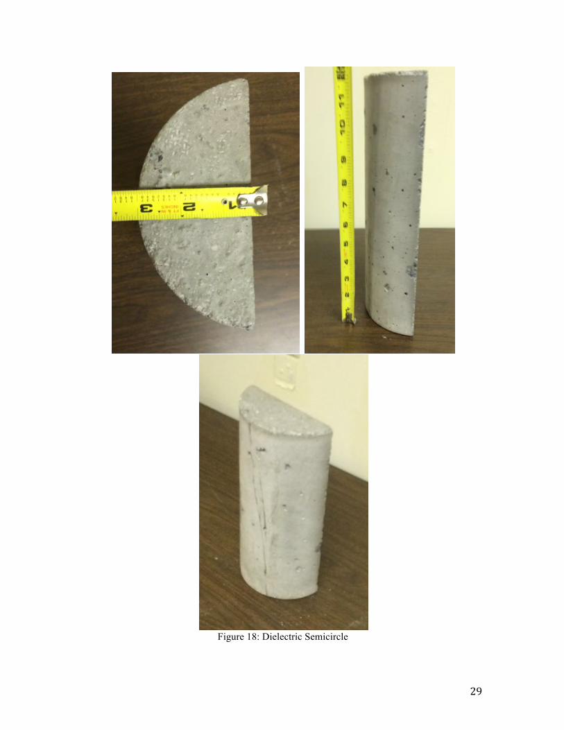
Dielectric Semicircle 7.62 cm radius × 30.48 cm height (3” radius × 12”

height)

Metal Cylinder of Triangular

Cross Section

15.24" cm side × 30.48 cm height (6” side × 12” height)

! 11!

The tomographic images for a metal rectangular box with dimensions 20.3 cm × 20.3 cm

× 60.96 cm are shown in Figure 4(a). At each point, the antenna stops in order to ensure

that the oscilloscope has time to collect a sufficient amount of data. After all 55 point of

data are collected, the linear scanner moves back to its initial position. As the linear

scanner is moving back to the first point, the turntable rotates by 9 degrees. The linear

scanner then starts and stops at the same 55 points as before. This rotation and then

linear scan process are continued until the object has rotated by a full 360 degrees. In the

data presented in this document, a total of 40 angular measurements are made (360÷9 =

40). The number of scanning points and the angle of rotation were chosen as a tradeoff

between data collection time and image resolution. The turntable is controlled by a

stepper motor and is able to rotate in any multiple of 1.8 degrees.

! 12!

3. DATA COLLECTION AND PROCESSING

The target object is placed on the center of a turntable in front of a wall made of

microwave absorbent foam. Both the transmitting and the receiving antennas point

towards the foam wall. The turntable is pictured with a metal cylinder on it in Figure 3.

The data collection process starts with the Gaussian noise waveform being uploaded to

the AWG. The AWG automatically transmits the most recently uploaded waveform. The

noise waveform is not identical between tests. The waveform is also not saved. The

processing only requires that the transmitted waveform be iid and white Gaussian. The

waveform is then amplified and then transmitted from a stationary antenna located at the

center of the window. The linear scanner then moves to each one of the 55 designated

points stopping at each one. Each time the linear scanner stops, the oscilloscope collects

a total of 363,000 amplitude samples. After a single line scan has been taken, the

turntable rotates 9 degrees and the process repeats. The data are stored as they comes in

and they are then saved in a 40×363,000 array for processing at a later point in time.

Each 363,000 point sample is split into 200 segments for processing. The collected

waveform has to be split up due to the memory limitations of the computer. Each of the

200 segments is then averaged and processed to create an image. An image is created for

each angle at which the turntable stops. For the data presented in this document, there

were 40 images created for each object. Using image processing, these 40 images were

combined into one final image such as those presented in this document.

A long sample length or the averaging of multiple samples is necessary to achieve a flat

frequency spectrum. Fourier diffraction theory is used to construct a tomography image

! 13!

of the object. If too little data are used, then the spectrum is no longer flat and it is not

possible to create a recognizable image. In Figure 2(a), the Fourier transform of a single

sample of length 1815 shows that the spectrum is not really flat, as desired. In Figure

2(b), 200 segments are averaged together to create a much flatter frequency spectrum,

which has been shown to be absolutely necessary to create a good image19.

! 14!

4. EXPERIMENTAL RESULTS

The noise tomography system was used to acquire data from targets with rectangular,

cylindrical, and triangular cross sections. The images of the objects were successfully

reconstructed. As expected, there is less scattered power from the dielectric test objects

compared to the metallic objects.

Figure 5 shows the reconstructed tomographic image of a metal cylinder and a dielectric

(i.e. concrete) cylinder. We note that the circular cross-section is clearly seen in both

cases. The metal cylinder shows a much stronger and clearer image with very low noise

outside its physical extent. In the case of the dielectric cylinder, the shape can be clearly

inferred; however, there is observed noise outside its physical extent, owing to its lower

scattered power.

!

(a) (b)

Figure 5: Tomographic image of (a) aluminum cylinder, and (b) dielectric cylinder.

! 15!

The system also successfully imaged rectangular boxes made of both types of materials,

as seen in Figure 6. The rectangular objects have a large amount of diffraction from their

edges, which can be seen as plumes. Again, the cross-section of the metal box is well

imaged compared to the dielectric box; however, there is more diffraction from the edges

of the metal box compared to the dielectric box.

Figure 7 shows the image of a metal cylinder having a triangular cross-section. Its shape

can be seen as also the wave diffraction from its edges.

! !

(a) (b)

Figure 6: Tomographic image of (a) aluminum rectangular box, and (b) dielectric rectangular

box.

! 16!

Figure 7: Tomographic image of a triangular metal cylinder.

Some objects were also imaged when concealed within a cardboard box of size 50.8 cm ×

40.64 cm × 54.07 cm. Figures 8(a) and 8(b) show the images of metal triangular and

circular cylinders inside the cardboard box, respectively. By comparing Figures 7 and

8(a) and also Figures 5(a) and 8(b), it can be observed that that while the cardboard adds

a small amount of noise, the target object is still clearly visible and discernible.

! 17!

(a) (b)

Figure 8: Tomographic image of (a) triangular metal cylinder in a cardboard box, and (b) circular

metal cylinder in a cardboard box.

Objects were concealed in a wooden box with sides that are 1.27 cm thick. The

dimensions of the box are 38.1 cm x 38.1 cm x 38.1 cm. Figure 9 a-e shows metal

objects in the wooden box. The wooden box adds more noise but the target objects are

still visible and recognizable.

! 18!

(a) (b)

(c) (d)

(e) (f)

! 19!

(g)

Figure 9 a) metal cylinder 1 b) metal cylinder 2 c) metal rectangular box 1 d) metal rectangular

box 2 e) metal cylinder with triangular cross section f) Dielectric cylinder g) dielectric rectangular

box

!!

! 20!

5. CONCLUSIONS AND FUTURE WORK !

5.1 Future Work

Some work has been done towards developing a higher frequency version of the noise

radar tomography system. The system operates from 8-10 GHz. The block diagram for

the transmit and the receive portions of the system are shown in Figures 10 and 11. The

computer uploads an iid Gaussian Noise Waveform to the AWG. The AWG is an

Agilent M8190A system mounted on a M9602A chassis. The AWG continuously

transmits the noise waveform at an output power of 0 dBm. The Gaussian waveform is

transmitted at 2-4 GHz through two Minicircuit filters. The waveform in then mixed

with a 6 GHz tone from a signal generator. 3 dB attenuators are located on each terminal

of the mixer. The resulting waveform is 8-10 GHz. The waveform is then filtered again

before being transmitted through two cascaded amplifiers. The amplifiers have a 7 dB

attenuator in between them to prevent saturation in the second amplifier. The first

amplifier is a Mini-Circuits ZX60-24-S+ with a gain of 24 dB. The second amplifier is a

Miteq AMF-5B-8012-29P with a gain of 28 dB. The waveform is finally transmitted

through an A-info dual-polarized horn antenna.

An identical antenna is used to collect the backscatter off of the target object. The

waveform is amplified using a Minicircuits ZX60-24-S+ with gain 24 dB. The waveform

is then filtered and passed to the Agilent Infinium DS090804A oscilloscope.

! 21!

Figure 10 : High frequency transmitting system

Figure 11: High frequency receiving

! 22!

5.2 Conclusions

The UWB noise tomography hardware system designed by us was able to successfully

image a variety of shapes and materials using a relatively simple setup. It was

demonstrated that an iid WGN waveform can be used to correctly image target objects.

This shows that radar tomography can be accomplished while maintaining LPI and LPD

properties. This document described a successful data collection system for noise radar

tomography. Even with obstructions such as a wooden box, the system was able to

image objects quite clearly.

! 23!

Appendix A Images of Test Objects

Figure 12: Metal Rectangular Box 1

! 24!

Figure 13: Metal Rectangular Box 2

! 25!

Figure 14: Metal Cylinder 1

! 26!

Figure 15:Metal Cylinder 2

! 27!

Figure 16: Dielectric Rectangular Box

! 28!

Figure 17: Dielectric Circular Cylinder

! 29!

Figure 18: Dielectric Semicircle

! 30!

Figure 20: Metal Cylinder of Triangular Cross Section

! 31!

Appendix B

Computer Programs

% Original code written by Scott Wilson modified for radar tomography by Mark Asmuth function varargout = ScannerGUI(varargin) % SCANNERGUI M-file for ScannerGUI.fig % SCANNERGUI, by itself, creates a new SCANNERGUI or raises the existing % singleton*. % % H = SCANNERGUI returns the handle to a new SCANNERGUI or the handle to % the existing singleton*. % % SCANNERGUI('CALLBACK',hObject,eventData,handles,...) calls the local % function named CALLBACK in SCANNERGUI.M with the given input arguments. % % SCANNERGUI('Property','Value',...) creates a new SCANNERGUI or raises the % existing singleton*. Starting from the left, property value pairs are % applied to the GUI before ScannerGUI_OpeningFcn gets called. An % unrecognized property name or invalid value makes property application % stop. All inputs are passed to ScannerGUI_OpeningFcn via varargin. % % *See GUI Options on GUIDE's Tools menu. Choose "GUI allows only one % instance to run (singleton)". % % See also: GUIDE, GUIDATA, GUIHANDLES % Edit the above text to modify the response to help ScannerGUI % Last Modified by GUIDE v2.5 29-Oct-2013 14:16:00 % Begin initialization code - DO NOT EDIT gui_Singleton = 1;

! 32!

gui_State = struct('gui_Name', mfilename, ... 'gui_Singleton', gui_Singleton, ... 'gui_OpeningFcn', @ScannerGUI_OpeningFcn, ... 'gui_OutputFcn', @ScannerGUI_OutputFcn, ... 'gui_LayoutFcn', [] , ... 'gui_Callback', []); if nargin && ischar(varargin{1}) gui_State.gui_Callback = str2func(varargin{1}); end if nargout [varargout{1:nargout}] = gui_mainfcn(gui_State, varargin{:}); else gui_mainfcn(gui_State, varargin{:}); end % End initialization code - DO NOT EDIT %%%%%%%%%%%%%%%%%%%%%%%%%%%%%%%%%%%%%%%%%%%%%%%%%%%%%%%%%%%%%%%%%%%%%%%%%%% % --- Executes just before ScannerGUI is made visible. function ScannerGUI_OpeningFcn(hObject, eventdata, handles, varargin) % This function has no output args, see OutputFcn. % hObject handle to figure % eventdata reserved - to be defined in a future version of MATLAB % handles structure with handles and user data (see GUIDATA) % varargin command line arguments to ScannerGUI (see VARARGIN) % Choose default command line output for ScannerGUI handles.output = hObject; set(gcf,'CloseRequestFcn',@CloseGuiFcn) handles.root_dir = 'C:\Holograms2\'; axes(handles.holAxes); axis image; % colormap(bone); axes(handles.imAxes); axis image; % colormap(bone);

! 33!

try % OSC = visa('agilent', 'GPIB0::8::INSTR'); % % handles.OSC = OSC; % set(OSC, 'InputBufferSize', 1e8); % OSC.Timeout=10; % OSC.ByteOrder='littleEndian'; % % fopen(OSC); % fprintf(OSC,'*RST; :AUTOSCALE'); % idn='Oscilloscope'; OSC = visa('agilent', 'TCPIP::130.203.252.125::INSTR'); handles.OSC = OSC; set(OSC, 'InputBufferSize', 1e7); set (OSC,'timeout', 20); OSC.Timeout=20; OSC.ByteOrder='littleEndian'; fopen(OSC); fprintf(OSC,'*RST; :AUTOSCALE'); idn='Oscilloscope'; msg = msgbox(['Connected to ',idn],'OSC Connected'); osc= handles.OSC; set(handles.vnaConnStatText,'String','Connected','ForegroundColor','g'); fprintf(osc,'*RST; :AUTOSCALE'); fprintf(osc,':WAVEFORM:SOURCE CHAN1'); % Specify data from Channel 1 % Set up VNA frequency scale fprintf(osc,':TIMEBASE:REFERENCE CENTER'); % Display reference at center fprintf(osc,':TIMEBASE:RANGE 1e-5'); % Time base to 100 ns full scale fprintf(osc,':TIMEBASE:DELAY 0'); % Delay to zero fprintf(osc,':CHANNEL1:RANGE 2.5'); % Vertical range to 1.6 V full scale fprintf(osc,':CHANNEL1:OFFSET 0'); fprintf(osc,':WAVEFORM:TYPE? RAW'); fprintf(osc,':ACQUIRE:POINTS 363000'); fprintf(osc,':WAVEFORM:BYTEORDER LSBFirst'); % Set the byte order on the instrument as well pause(10);

! 34!

uiwait(msg); catch ME msg = msgbox('Unable to connect to GPIB0::8:INSTR !','Connection Error'); uiwait(msg); end try s = serial('COM10','BaudRate',9600); % Connect to Arduino via Serial handles.s = s; set(s,'InputBufferSize',512); fopen(s); % Open serial port set(handles.scanConnStatText,'String','Connected','ForegroundColor','g'); fgets(s); % Clear junk data set_xy_position(s,2377,2377,0,300); msg = msgbox('Connected to XY positioner !'); uiwait(msg); catch ME msg = msgbox('Error connecting to XY positioner !','Connection Error'); uiwait(msg); end % Update handles structure guidata(hObject, handles); % UIWAIT makes ScannerGUI wait for user response (see UIRESUME) % uiwait(handles.figure1); %%%%%%%%%%%%%%%%%%%%%%%%%%%%%%%%%%%%%%%%%%%%%%%%%%%%%%%%%%%%%%%%%%%%%%%%%%% %%%%%%%%%%%%%%%%%%%%%%%%%%%%%%%%%%%%%%%%%%%%%%%%%%%%%%%%%%%%%%%%%%%%%%%%%%% % Close request callback for exiting with Close button. function CloseGuiFcn(hObject, eventdata, handles)

! 35!

fclose(instrfind); delete(instrfind); delete(hObject); clear all; % close all; %%%%%%%%%%%%%%%%%%%%%%%%%%%%%%%%%%%%%%%%%%%%%%%%%%%%%%%%%%%%%%%%%%%%%%%%%%% % --- Outputs from this function are returned to the command line. function varargout = ScannerGUI_OutputFcn(hObject, eventdata, handles) % varargout cell array for returning output args (see VARARGOUT); % hObject handle to figure % eventdata reserved - to be defined in a future version of MATLAB % handles structure with handles and user data (see GUIDATA) % Get default command line output from handles structure varargout{1} = handles.output; % -------------------------------------------------------------------- function menuBar_Callback(hObject, eventdata, handles) % hObject handle to menuFile (see GCBO) % eventdata reserved - to be defined in a future version of MATLAB % handles structure with handles and user data (see GUIDATA) % -------------------------------------------------------------------- function menuFile_Callback(hObject, eventdata, handles) % hObject handle to menuFile (see GCBO) % eventdata reserved - to be defined in a future version of MATLAB % handles structure with handles and user data (see

! 36!

GUIDATA) % -------------------------------------------------------------------- function menuEdit_Callback(hObject, eventdata, handles) % hObject handle to menuEdit (see GCBO) % eventdata reserved - to be defined in a future version of MATLAB % handles structure with handles and user data (see GUIDATA) % -------------------------------------------------------------------- function editParams_Callback(hObject, eventdata, handles) % hObject handle to editParams (see GCBO) % eventdata reserved - to be defined in a future version of MATLAB % handles structure with handles and user data (see GUIDATA) % -------------------------------------------------------------------- function editSave_Callback(hObject, eventdata, handles) % hObject handle to editSave (see GCBO) % eventdata reserved - to be defined in a future version of MATLAB % handles structure with handles and user data (see GUIDATA) %%%%%%%%%%%%%%%%%%%%%%%%%%%%%%%%%%%%%%%%%%%%%%%%%%%%%%%%%%%%%%%%%%%%%%%%%%% % --- Executes on slider movement. function fSlider_Callback(hObject, eventdata, handles) % hObject handle to fSlider (see GCBO) % eventdata reserved - to be defined in a future version of MATLAB % handles structure with handles and user data (see GUIDATA) % Hints: get(hObject,'Value') returns position of slider

! 37!

% get(hObject,'Min') and get(hObject,'Max') to determine range of slider try NofFreqs = length(handles.freqs); if(NofFreqs > 1) set(handles.fSlider,'Visible','on'); f_ind = get(handles.fSlider,'Value'); set(handles.fSliderText,'String',num2str(handles.freqs(f_ind)/10^9,2)); else set(handles.fSlider,'Visible','off'); end axes(handles.imAxes); imagesc(handles.x, handles.y, abs(handles.recon_data(:,:,f_ind))); colormap(bone) axes(handles.holAxes); imagesc(handles.x, handles.y, abs(handles.hol_data(:,:,f_ind))/(2*pi)); colormap(bone) catch ME end %%%%%%%%%%%%%%%%%%%%%%%%%%%%%%%%%%%%%%%%%%%%%%%%%%%%%%%%%%%%%%%%%%%%%%%%%%% %%%%%%%%%%%%%%%%%%%%%%%%%%%%%%%%%%%%%%%%%%%%%%%%%%%%%%%%%%%%%%%%%%%%%%%%%%% % --- Executes on slider movement. function zSlider_Callback(hObject, eventdata, handles) % hObject handle to zSlider (see GCBO) % eventdata reserved - to be defined in a future version of MATLAB % handles structure with handles and user data (see GUIDATA) % Hints: get(hObject,'Value') returns position of slider % get(hObject,'Min') and get(hObject,'Max') to determine range of slider

! 38!

z = get(handles.zSlider,'Value'); set(handles.zSliderText,'String',num2str(z,3)); zo = z; NofFreqs = length(handles.freqs); if(NofFreqs > 1) set(handles.fSlider,'Visible','on'); f_ind = get(handles.fSlider,'Value'); else set(handles.fSlider,'Visible','off'); end x = handles.x * handles.dx; y = handles.y * handles.dy; if(NofFreqs > 1) handles.recon_data = Fourier3D(handles.hol_data, [], [], handles.kz, zo); axes(handles.imAxes); imagesc(handles.x, handles.y, abs(handles.recon_data(:,:,f_ind))); axes(handles.holAxes); imagesc(handles.x, handles.y, abs(handles.hol_data(:,:,f_ind))); else handles.recon_data = Fourier2D(handles.hol_data, handles.kz, zo); axes(handles.imAxes); imagesc(x, y, abs(handles.recon_data)); axes(handles.holAxes); imagesc(x, y, abs(handles.hol_data)); end % Update handles structure guidata(hObject, handles); %%%%%%%%%%%%%%%%%%%%%%%%%%%%%%%%%%%%%%%%%%%%%%%%%%%%%%%%%%%%%%%%%%%%%%%%%%%

! 39!

%%%%%%%%%%%%%%%%%%%%%%%%%%%%%%%%%%%%%%%%%%%%%%%%%%%%%%%%%%%%%%%%%%%%%%%%%%% % --- Executes on button press in loadDataFileBtn. function loadDataFileBtn_Callback(hObject, eventdata, handles) % hObject handle to loadDataFileBtn (see GCBO) % eventdata reserved - to be defined in a future version of MATLAB % handles structure with handles and user data (see GUIDATA) global clims; file = get(handles.loadDataFileText,'String'); if(exist(file,'file')) Root = load(file,'-mat'); fields = fieldnames(Root); % get parent name Root = getfield(Root,fields{1}); fields = fieldnames(Root); for ii = 1:length(fields) % cycle through each member handles = setfield( handles, fields{ii}, getfield(Root,fields{ii}) ); end handles.hol_data = handles.hol_data/max(max(max(abs(handles.hol_data)))); NofFreqs = length(handles.freqs); BW = handles.f_stop - handles.f_start; handles.R_max = (3e8*NofFreqs)/(4*BW); handles.R_res = handles.R_max / NofFreqs; axes(handles.holAxes); imagesc(handles.x, handles.y, abs(handles.hol_data(:,:,1))); axes(handles.imAxes); imagesc(handles.x, handles.y, abs(handles.hol_data(:,:,1))); try set(handles.zSlider, 'Value', 0); set(handles.zSlider, 'Min', 0);

! 40!

set(handles.zSlider, 'Max', 2); set(handles.zSlider, 'SliderStep', [0.005 0.1]); if(NofFreqs > 1) set(handles.fSlider,'Visible','on'); set(handles.fSlider,'Value',1); set(handles.fSlider,'Min',1); set(handles.fSlider,'Max',NofFreqs); set(handles.fSlider,'SliderStep', [1/(NofFreqs-1) 0.1]); temp = get(handles.fSlider,'Value') * (NofFreqs-1) + 1; else set(handles.fSlider,'Visible','off'); end catch ME set(handles.zSlider, 'Max',1); set(handles.zSlider, 'SliderStep', [0.01 0.1]); set(handles.fSlider,'Min',0); set(handles.fSlider,'Max',NofFreqs); set(handles.fSlider,'SliderStep', [0.1 0.1]); end Nx = length(handles.x); Ny = length(handles.y); [handles.kx handles.ky handles.kz] = calc_wavenums(handles.freqs, Ny, Nx); zo = Root.zo(1); % hol_data_cart = sphere2cart_gridinterp(handles.hol_data,handles.freqs); if(NofFreqs > 1) handles.recon_data = Fourier3D(handles.hol_data, handles.kx, handles.ky, handles.kz, zo); else handles.recon_data = Fourier2D(handles.hol_data, handles.kz, zo); end % handles.est_targ_dist = estimate_target_distance(handles.recon_data); else msgbox('Please select a data file.','Unable to load file'); end

! 41!

% Update handles structure guidata(hObject, handles); %%%%%%%%%%%%%%%%%%%%%%%%%%%%%%%%%%%%%%%%%%%%%%%%%%%%%%%%%%%%%%%%%%%%%%%%%%%%% % --- Executes during object creation, after setting all properties. function zSlider_CreateFcn(hObject, eventdata, handles) % hObject handle to zSlider (see GCBO) % eventdata reserved - to be defined in a future version of MATLAB % handles empty - handles not created until after all CreateFcns called % Hint: slider controls usually have a light gray background. if isequal(get(hObject,'BackgroundColor'), get(0,'defaultUicontrolBackgroundColor')) set(hObject,'BackgroundColor',[.9 .9 .9]); end % --- Executes during object creation, after setting all properties. function fSlider_CreateFcn(hObject, eventdata, handles) % hObject handle to fSlider (see GCBO) % eventdata reserved - to be defined in a future version of MATLAB % handles empty - handles not created until after all CreateFcns called % Hint: slider controls usually have a light gray background. if isequal(get(hObject,'BackgroundColor'), get(0,'defaultUicontrolBackgroundColor')) set(hObject,'BackgroundColor',[.9 .9 .9]);

! 42!

end % --- Executes on button press in render3dBtn. function render3dBtn_Callback(hObject, eventdata, handles) % hObject handle to render3dBtn (see GCBO) % eventdata reserved - to be defined in a future version of MATLAB % handles structure with handles and user data (see GUIDATA) figure; isosurface(abs(handles.recon_data)); %%%%%%%%%%%%%%%%%%%%%%%%%%%%%%%%%%%%%%%%%%%%%%%%%%%%%%%%%%%%%%%%%%%%%%%%%%% % --- Executes on button press in startScanBtn. function startScanBtn_Callback(hObject, eventdata, handles) % hObject handle to startScanBtn (see GCBO) % eventdata reserved - to be defined in a future version of MATLAB % handles structure with handles and user data (see GUIDATA) pause(2); x_max = str2double(get(handles.scanWidthText,'String')); y_max = str2double(get(handles.scanWidthText,'String')); angle = 0; % = 90; % H-pol or V-pol m = str2double(get(handles.XsamplesText,'String')); n = str2double(get(handles.YsamplesText,'String')); handles.x_max = x_max; handles.y_max = y_max; handles.m = m; handles.n = n; handles.x = linspace(0,x_max,m); handles.y = linspace(0,y_max,n); handles.angle = angle; axes(handles.holAxes); imagesc(zeros(m,n)); [file p_data p_ind] = create_position_data(m, n, x_max, y_max, angle);

! 43!

handles.p_ind = p_ind; % indices for scan position handles.a_data = check_position_data(p_data); handles.hol_data = run_scan(hObject, handles); handles.lastSavePath = save_hol_data(handles); axes(handles.imAxes); % Update handles structure guidata(hObject, handles); %%%%%%%%%%%%%%%%%%%%%%%%%%%%%%%%%%%%%%%%%%%%%%%%%%%%%%%%%%%%%%%%%%%%%%%%%%% % --- Executes on button press in browseBtn. function pushbutton4_Callback(hObject, eventdata, handles) % hObject handle to browseBtn (see GCBO) % eventdata reserved - to be defined in a future version of MATLAB % handles structure with handles and user data (see GUIDATA) function fileTextbox_Callback(hObject, eventdata, handles) % hObject handle to fileTextbox (see GCBO) % eventdata reserved - to be defined in a future version of MATLAB % handles structure with handles and user data (see GUIDATA) % Hints: get(hObject,'String') returns contents of fileTextbox as text % str2double(get(hObject,'String')) returns contents of fileTextbox as a double % --- Executes during object creation, after setting all properties. function fileTextbox_CreateFcn(hObject, eventdata, handles) % hObject handle to fileTextbox (see GCBO)

! 44!

% eventdata reserved - to be defined in a future version of MATLAB % handles empty - handles not created until after all CreateFcns called % Hint: edit controls usually have a white background on Windows. % See ISPC and COMPUTER. if ispc && isequal(get(hObject,'BackgroundColor'), get(0,'defaultUicontrolBackgroundColor')) set(hObject,'BackgroundColor','white'); end %%%%%%%%%%%%%%%%%%%%%%%%%%%%%%%%%%%%%%%%%%%%%%%%%%%%%%%%%%%%%%%%%%%%%%%%%%% % --- Executes on button press in browseBtn. function browseBtn_Callback(hObject, eventdata, handles) % hObject handle to browseBtn (see GCBO) % eventdata reserved - to be defined in a future version of MATLAB % handles structure with handles and user data (see GUIDATA) [filename, filepath] = uigetfile('*.mat','Select a file','C:\Holograms\'); if(filename ~= 0) set(handles.loadDataFileText,'String',[filepath filename]); end %%%%%%%%%%%%%%%%%%%%%%%%%%%%%%%%%%%%%%%%%%%%%%%%%%%%%%%%%%%%%%%%%%%%%%%%%%% function ScanWidthBox_Callback(hObject, eventdata, handles) % hObject handle to ScanWidthBox (see GCBO)

! 45!

% eventdata reserved - to be defined in a future version of MATLAB % handles structure with handles and user data (see GUIDATA) % Hints: get(hObject,'String') returns contents of ScanWidthBox as text % str2double(get(hObject,'String')) returns contents of ScanWidthBox as a double % --- Executes during object creation, after setting all properties. function ScanWidthBox_CreateFcn(hObject, eventdata, handles) % hObject handle to ScanWidthBox (see GCBO) % eventdata reserved - to be defined in a future version of MATLAB % handles empty - handles not created until after all CreateFcns called % Hint: edit controls usually have a white background on Windows. % See ISPC and COMPUTER. if ispc && isequal(get(hObject,'BackgroundColor'), get(0,'defaultUicontrolBackgroundColor')) set(hObject,'BackgroundColor','white'); end function ScanHeightBox_Callback(hObject, eventdata, handles) % hObject handle to ScanHeightBox (see GCBO) % eventdata reserved - to be defined in a future version of MATLAB % handles structure with handles and user data (see GUIDATA) % Hints: get(hObject,'String') returns contents of ScanHeightBox as text % str2double(get(hObject,'String')) returns contents of ScanHeightBox as a double % --- Executes during object creation, after setting all properties. function ScanHeightBox_CreateFcn(hObject, eventdata,

! 46!

handles) % hObject handle to ScanHeightBox (see GCBO) % eventdata reserved - to be defined in a future version of MATLAB % handles empty - handles not created until after all CreateFcns called % Hint: edit controls usually have a white background on Windows. % See ISPC and COMPUTER. if ispc && isequal(get(hObject,'BackgroundColor'), get(0,'defaultUicontrolBackgroundColor')) set(hObject,'BackgroundColor','white'); end function XsamplesBox_Callback(hObject, eventdata, handles) % hObject handle to XsamplesBox (see GCBO) % eventdata reserved - to be defined in a future version of MATLAB % handles structure with handles and user data (see GUIDATA) % Hints: get(hObject,'String') returns contents of XsamplesBox as text % str2double(get(hObject,'String')) returns contents of XsamplesBox as a double % --- Executes during object creation, after setting all properties. function XsamplesBox_CreateFcn(hObject, eventdata, handles) % hObject handle to XsamplesBox (see GCBO) % eventdata reserved - to be defined in a future version of MATLAB % handles empty - handles not created until after all CreateFcns called % Hint: edit controls usually have a white background on Windows. % See ISPC and COMPUTER. if ispc && isequal(get(hObject,'BackgroundColor'), get(0,'defaultUicontrolBackgroundColor')) set(hObject,'BackgroundColor','white'); end

! 47!

function YsamplesBox_Callback(hObject, eventdata, handles) % hObject handle to YsamplesBox (see GCBO) % eventdata reserved - to be defined in a future version of MATLAB % handles structure with handles and user data (see GUIDATA) % Hints: get(hObject,'String') returns contents of YsamplesBox as text % str2double(get(hObject,'String')) returns contents of YsamplesBox as a double % --- Executes during object creation, after setting all properties. function YsamplesBox_CreateFcn(hObject, eventdata, handles) % hObject handle to YsamplesBox (see GCBO) % eventdata reserved - to be defined in a future version of MATLAB % handles empty - handles not created until after all CreateFcns called % Hint: edit controls usually have a white background on Windows. % See ISPC and COMPUTER. if ispc && isequal(get(hObject,'BackgroundColor'), get(0,'defaultUicontrolBackgroundColor')) set(hObject,'BackgroundColor','white'); end % --- Executes on button press in SingleFreqRadio. function SingleFreqRadio_Callback(hObject, eventdata, handles) % hObject handle to SingleFreqRadio (see GCBO) % eventdata reserved - to be defined in a future version of MATLAB % handles structure with handles and user data (see GUIDATA) % Hint: get(hObject,'Value') returns toggle state of SingleFreqRadio % --- Executes on button press in MultiFreqRadio. function MultiFreqRadio_Callback(hObject, eventdata, handles)

! 48!

% hObject handle to MultiFreqRadio (see GCBO) % eventdata reserved - to be defined in a future version of MATLAB % handles structure with handles and user data (see GUIDATA) % Hint: get(hObject,'Value') returns toggle state of MultiFreqRadio function stopFreqBox_Callback(hObject, eventdata, handles) % hObject handle to stopFreqBox (see GCBO) % eventdata reserved - to be defined in a future version of MATLAB % handles structure with handles and user data (see GUIDATA) % Hints: get(hObject,'String') returns contents of stopFreqBox as text % str2double(get(hObject,'String')) returns contents of stopFreqBox as a double % --- Executes during object creation, after setting all properties. function stopFreqBox_CreateFcn(hObject, eventdata, handles) % hObject handle to stopFreqBox (see GCBO) % eventdata reserved - to be defined in a future version of MATLAB % handles empty - handles not created until after all CreateFcns called % Hint: edit controls usually have a white background on Windows. % See ISPC and COMPUTER. if ispc && isequal(get(hObject,'BackgroundColor'), get(0,'defaultUicontrolBackgroundColor')) set(hObject,'BackgroundColor','white'); end function startFreqBox_Callback(hObject, eventdata, handles) % hObject handle to startFreqBox (see GCBO) % eventdata reserved - to be defined in a future version of MATLAB % handles structure with handles and user data (see

! 49!

GUIDATA) % Hints: get(hObject,'String') returns contents of startFreqBox as text % str2double(get(hObject,'String')) returns contents of startFreqBox as a double % --- Executes during object creation, after setting all properties. function startFreqBox_CreateFcn(hObject, eventdata, handles) % hObject handle to startFreqBox (see GCBO) % eventdata reserved - to be defined in a future version of MATLAB % handles empty - handles not created until after all CreateFcns called % Hint: edit controls usually have a white background on Windows. % See ISPC and COMPUTER. if ispc && isequal(get(hObject,'BackgroundColor'), get(0,'defaultUicontrolBackgroundColor')) set(hObject,'BackgroundColor','white'); end function FsamplesBox_Callback(hObject, eventdata, handles) % hObject handle to FsamplesBox (see GCBO) % eventdata reserved - to be defined in a future version of MATLAB % handles structure with handles and user data (see GUIDATA) % Hints: get(hObject,'String') returns contents of FsamplesBox as text % str2double(get(hObject,'String')) returns contents of FsamplesBox as a double % --- Executes during object creation, after setting all properties. function FsamplesBox_CreateFcn(hObject, eventdata, handles) % hObject handle to FsamplesBox (see GCBO) % eventdata reserved - to be defined in a future version of MATLAB % handles empty - handles not created until after all

! 50!

CreateFcns called % Hint: edit controls usually have a white background on Windows. % See ISPC and COMPUTER. if ispc && isequal(get(hObject,'BackgroundColor'), get(0,'defaultUicontrolBackgroundColor')) set(hObject,'BackgroundColor','white'); end % --- Executes on button press in abortScanBtn. function abortScanBtn_Callback(hObject, eventdata, handles) % hObject handle to abortScanBtn (see GCBO) % eventdata reserved - to be defined in a future version of MATLAB % handles structure with handles and user data (see GUIDATA) function scanWidthText_Callback(hObject, eventdata, handles) % hObject handle to scanWidthText (see GCBO) % eventdata reserved - to be defined in a future version of MATLAB % handles structure with handles and user data (see GUIDATA) % Hints: get(hObject,'String') returns contents of scanWidthText as text % str2double(get(hObject,'String')) returns contents of scanWidthText as a double % --- Executes during object creation, after setting all properties. function scanWidthText_CreateFcn(hObject, eventdata, handles) % hObject handle to scanWidthText (see GCBO) % eventdata reserved - to be defined in a future version of MATLAB % handles empty - handles not created until after all CreateFcns called % Hint: edit controls usually have a white background on Windows. % See ISPC and COMPUTER.

! 51!

if ispc && isequal(get(hObject,'BackgroundColor'), get(0,'defaultUicontrolBackgroundColor')) set(hObject,'BackgroundColor','white'); end function scanHeightText_Callback(hObject, eventdata, handles) % hObject handle to scanHeightText (see GCBO) % eventdata reserved - to be defined in a future version of MATLAB % handles structure with handles and user data (see GUIDATA) % Hints: get(hObject,'String') returns contents of scanHeightText as text % str2double(get(hObject,'String')) returns contents of scanHeightText as a double % --- Executes during object creation, after setting all properties. function scanHeightText_CreateFcn(hObject, eventdata, handles) % hObject handle to scanHeightText (see GCBO) % eventdata reserved - to be defined in a future version of MATLAB % handles empty - handles not created until after all CreateFcns called % Hint: edit controls usually have a white background on Windows. % See ISPC and COMPUTER. if ispc && isequal(get(hObject,'BackgroundColor'), get(0,'defaultUicontrolBackgroundColor')) set(hObject,'BackgroundColor','white'); end function XsamplesText_Callback(hObject, eventdata, handles) % hObject handle to XsamplesText (see GCBO) % eventdata reserved - to be defined in a future version of MATLAB % handles structure with handles and user data (see GUIDATA)

! 52!

% Hints: get(hObject,'String') returns contents of XsamplesText as text % str2double(get(hObject,'String')) returns contents of XsamplesText as a double % --- Executes during object creation, after setting all properties. function XsamplesText_CreateFcn(hObject, eventdata, handles) % hObject handle to XsamplesText (see GCBO) % eventdata reserved - to be defined in a future version of MATLAB % handles empty - handles not created until after all CreateFcns called % Hint: edit controls usually have a white background on Windows. % See ISPC and COMPUTER. if ispc && isequal(get(hObject,'BackgroundColor'), get(0,'defaultUicontrolBackgroundColor')) set(hObject,'BackgroundColor','white'); end function YsamplesText_Callback(hObject, eventdata, handles) % hObject handle to YsamplesText (see GCBO) % eventdata reserved - to be defined in a future version of MATLAB % handles structure with handles and user data (see GUIDATA) % Hints: get(hObject,'String') returns contents of YsamplesText as text % str2double(get(hObject,'String')) returns contents of YsamplesText as a double % --- Executes during object creation, after setting all properties. function YsamplesText_CreateFcn(hObject, eventdata, handles) % hObject handle to YsamplesText (see GCBO) % eventdata reserved - to be defined in a future version of MATLAB % handles empty - handles not created until after all CreateFcns called

! 53!

% Hint: edit controls usually have a white background on Windows. % See ISPC and COMPUTER. if ispc && isequal(get(hObject,'BackgroundColor'), get(0,'defaultUicontrolBackgroundColor')) set(hObject,'BackgroundColor','white'); end function edit5_Callback(hObject, eventdata, handles) % hObject handle to fileTextbox (see GCBO) % eventdata reserved - to be defined in a future version of MATLAB % handles structure with handles and user data (see GUIDATA) % Hints: get(hObject,'String') returns contents of fileTextbox as text % str2double(get(hObject,'String')) returns contents of fileTextbox as a double % --- Executes during object creation, after setting all properties. function edit5_CreateFcn(hObject, eventdata, handles) % hObject handle to fileTextbox (see GCBO) % eventdata reserved - to be defined in a future version of MATLAB % handles empty - handles not created until after all CreateFcns called % Hint: edit controls usually have a white background on Windows. % See ISPC and COMPUTER. if ispc && isequal(get(hObject,'BackgroundColor'), get(0,'defaultUicontrolBackgroundColor')) set(hObject,'BackgroundColor','white'); end % --- Executes on button press in singleFreqRadio. function singleFreqRadio_Callback(hObject, eventdata, handles) % hObject handle to singleFreqRadio (see GCBO) % eventdata reserved - to be defined in a future version of MATLAB

! 54!

% handles structure with handles and user data (see GUIDATA) % Hint: get(hObject,'Value') returns toggle state of singleFreqRadio % --- Executes on button press in multiFreqRadio. function multiFreqRadio_Callback(hObject, eventdata, handles) % hObject handle to multiFreqRadio (see GCBO) % eventdata reserved - to be defined in a future version of MATLAB % handles structure with handles and user data (see GUIDATA) % Hint: get(hObject,'Value') returns toggle state of multiFreqRadio function startFreqText_Callback(hObject, eventdata, handles) % hObject handle to startFreqText (see GCBO) % eventdata reserved - to be defined in a future version of MATLAB % handles structure with handles and user data (see GUIDATA) % Hints: get(hObject,'String') returns contents of startFreqText as text % str2double(get(hObject,'String')) returns contents of startFreqText as a double % --- Executes during object creation, after setting all properties. function startFreqText_CreateFcn(hObject, eventdata, handles) % hObject handle to startFreqText (see GCBO) % eventdata reserved - to be defined in a future version of MATLAB % handles empty - handles not created until after all CreateFcns called % Hint: edit controls usually have a white background on Windows. % See ISPC and COMPUTER.

! 55!

if ispc && isequal(get(hObject,'BackgroundColor'), get(0,'defaultUicontrolBackgroundColor')) set(hObject,'BackgroundColor','white'); end function stopFreqText_Callback(hObject, eventdata, handles) % hObject handle to stopFreqText (see GCBO) % eventdata reserved - to be defined in a future version of MATLAB % handles structure with handles and user data (see GUIDATA) % Hints: get(hObject,'String') returns contents of stopFreqText as text % str2double(get(hObject,'String')) returns contents of stopFreqText as a double % --- Executes during object creation, after setting all properties. function stopFreqText_CreateFcn(hObject, eventdata, handles) % hObject handle to stopFreqText (see GCBO) % eventdata reserved - to be defined in a future version of MATLAB % handles empty - handles not created until after all CreateFcns called % Hint: edit controls usually have a white background on Windows. % See ISPC and COMPUTER. if ispc && isequal(get(hObject,'BackgroundColor'), get(0,'defaultUicontrolBackgroundColor')) set(hObject,'BackgroundColor','white'); end function FsamplesText_Callback(hObject, eventdata, handles) % hObject handle to FsamplesText (see GCBO) % eventdata reserved - to be defined in a future version of MATLAB % handles structure with handles and user data (see GUIDATA) % Hints: get(hObject,'String') returns contents of

! 56!

FsamplesText as text % str2double(get(hObject,'String')) returns contents of FsamplesText as a double % --- Executes during object creation, after setting all properties. function FsamplesText_CreateFcn(hObject, eventdata, handles) % hObject handle to FsamplesText (see GCBO) % eventdata reserved - to be defined in a future version of MATLAB % handles empty - handles not created until after all CreateFcns called % Hint: edit controls usually have a white background on Windows. % See ISPC and COMPUTER. if ispc && isequal(get(hObject,'BackgroundColor'), get(0,'defaultUicontrolBackgroundColor')) set(hObject,'BackgroundColor','white'); end % --- Executes during object creation, after setting all properties. function loadDataFileText_CreateFcn(hObject, eventdata, handles) % hObject handle to loadDataFileText (see GCBO) % eventdata reserved - to be defined in a future version of MATLAB % handles empty - handles not created until after all CreateFcns called % Hint: edit controls usually have a white background on Windows. % See ISPC and COMPUTER. if ispc && isequal(get(hObject,'BackgroundColor'), get(0,'defaultUicontrolBackgroundColor')) set(hObject,'BackgroundColor','white'); end % --- Executes on button press in browseBtn. function pushbutton6_Callback(hObject, eventdata, handles) % hObject handle to browseBtn (see GCBO) % eventdata reserved - to be defined in a future version of MATLAB

! 57!

% handles structure with handles and user data (see GUIDATA) function loadDataFileText_Callback(hObject, eventdata, handles) % hObject handle to loadDataFileText (see GCBO) % eventdata reserved - to be defined in a future version of MATLAB % handles structure with handles and user data (see GUIDATA) % Hints: get(hObject,'String') returns contents of loadDataFileText as text % str2double(get(hObject,'String')) returns contents of loadDataFileText as a double % --- If Enable == 'on', executes on mouse press in 5 pixel border. % --- Otherwise, executes on mouse press in 5 pixel border or over render3dBtn. function render3dBtn_ButtonDownFcn(hObject, eventdata, handles) % hObject handle to render3dBtn (see GCBO) % eventdata reserved - to be defined in a future version of MATLAB % handles structure with handles and user data (see GUIDATA) figure; isosurface(handles.recon_data);

! 58!

function set_xy_position(s, x, y, z, delay) stepsPerInch = 520; %Define scanner resolution stepsPerDegree = 67; %fgets(s); %sit and wait for device to say it has reset to (0,0,0) %while(s.BytesAvailable == 0) ; end %fgets(s); % clear serial buffer x_value = num2str(x); %Write the x-value of that position as a string. y_value = num2str(y); %Write the y-value of that position as a string. z_value = num2str(z); %Write the z-value of that position as a string. delay_value = num2str(delay); %Write the y-value of that position as a string. string2Arduino = strcat(x_value,';',y_value,';',z_value,';', delay_value,';'); %Combine x, y and z together, separated by ;'s. query(s,string2Arduino); %disp(string2Arduino); disp(['Current Point: x = ', num2str((x/stepsPerInch)), ', y = ', num2str((y/stepsPerInch)), ', z = ', num2str((z/stepsPerDegree))]); disp(' '); %This sits and wiats for data to be available... % while(s.BytesAvailable == 0) %While the buffer is empty (no data has been sent back) %No OPeration NOOP % end %Continuously wait (infinite loop). % fgets(s); %Gets ok signal from Arduino to proceed. end

! 59!

function [saveFilePath] = save_hol_data(h) root_dir = h.root_dir; hol_data = h.hol_data; saveYesOrNo = questdlg('Keep data?','Save data','Yes','No','Yes'); if( strcmp(saveYesOrNo,'Yes') ) % Create data structure for saving % Root. Root.m = h.m; Root.n = h.n; Root.x_max = h.x_max; Root.y_max = h.y_max; Root.x = h.x; Root.y = h.y; Root.dx = h.x_max / h.m; Root.dy = h.y_max / h.n; Root.zo = 0; Root.img = 0; % needed to run through simulation model Root.angle = h.angle; Root.p_ind = h.p_ind; Root.hol_data = h.hol_data; p = 0; saveFilePath = [root_dir 'hol_scan_' num2str(p,'%04d') '.mat']; while(exist(saveFilePath,'file') ) p = p + 1; saveFilePath = [root_dir 'hol_scan_' num2str(p,'%04d') '.mat']; end save(saveFilePath,'Root','-mat'); end uiwait(msgbox(['Data saved as: ' saveFilePath],'Data Saved','modal')); end function [hol_data] = run_scan(hObject, handles)

! 60!

root_dir_turntable = 'C:\Holograms3\'; % osc= handles.OSC; % fprintf(osc,'*RST; :AUTOSCALE'); osc= handles.OSC; s = handles.s; a_data = handles.a_data; m = handles.m; n = handles.n; s2 = serial('COM4','BaudRate',9600); % Connect to Arduino via Serial set(s2,'InputBufferSize',512); fopen(s2); % Open serial port x=-400; delay=20; x_value = num2str(x); %Write the x-value of that position as a string. %y_value = num2str(y); %Write the y-value of that position as a string. %z_value = num2str(z); %Write the z-value of that position as a string. delay_value = num2str(delay); %Write the y-value of that position as a string. string2Arduino = strcat(x_value,';', delay_value,';'); %Combine x, y and z together, separated by ;'s. %query(s2,string2Arduino); x=400; x_value = num2str(x); %Write the x-value of that position as a string. %y_value = num2str(y); %Write the y-value of that position as a string. %z_value = num2str(z); %Write the z-value of that position as a string. delay_value = num2str(delay); %Write the y-value of that position as a string. string2Arduino = strcat(x_value,';', delay_value,';'); %Combine x, y and z together, separated by ;'s. %query(s2,string2Arduino); % fprintf(osc,'*RST; :AUTOSCALE'); % % fprintf(osc,':WAVEFORM:SOURCE CHAN1'); % Specify data from Channel 1 %

! 61!

% % Set up VNA frequency scale % fprintf(osc,':TIMEBASE:REFERENCE CENTER'); % Display reference at center % fprintf(osc,':TIMEBASE:RANGE 75E-9'); % Time base to 100 ns full scale % fprintf(osc,':TIMEBASE:DELAY 0'); % Delay to zero % fprintf(osc,':CHANNEL1:RANGE 1.6'); % Vertical range to 1.6 V full scale % fprintf(osc,':CHANNEL1:OFFSET 0'); % fprintf(osc,':WAVEFORM:TYPE? RAW'); % fprintf(osc,':WAVEFORM:BYTEORDER LSBFirst'); % Set the byte order on the instrument as well % % % % if(length(f) > 1) % % fprintf(vna,['STAR ' num2str(min(f)*10^9)] ); % Set start freq % % fprintf(vna,['STOP ' num2str(max(f)*10^9)] ); % Set start freq % fprintf(osc,'LINFREQ;'); % Set to linear-sweep mode % % fprintf(vna,['POIN ' num2str(length(f)) ';'] ); % % fprintf(vna,'MANTRIG;'); % Enable manual sweep trigger % else % % fprintf(vna,'SENS:SWEEP:TYPE CW'); % Put analyzer in CW mode % fprintf(osc,['CWFREQ ' num2str(f*10^9)]); % end % % Get the nr of trace points % Get the reference level % fprintf(osc,':WAVEFORM:DATA?'); % WaveformRawData = fscanf(osc); % temp = str2num(WaveformRawData); % holLength=length(temp) rotations=10; scan_iterations=1; % meas_data = zeros( length(a_data),length(f) ); fprintf(osc,':WAVEFORM:DATA?'); WaveformRawData = fscanf(osc); temp = str2num(WaveformRawData); hol_data = zeros(n, m,scan_iterations, length(temp)); axes(handles.holAxes); x_ind = handles.p_ind(:,2); % indices switched for

! 62!

imagesc()... y_ind = handles.p_ind(:,1); x = a_data(1,1); y = a_data(1,2); angle = a_data(1,3); delay = a_data(1,4); set_xy_position(s,x,y,angle,delay); pause x = a_data(1,1); y = a_data(1,2); angle = a_data(1,3); delay = a_data(1,4); set_xy_position(s,x,y,angle,delay); pause(10) for c=1:rotations for i = 1:length(a_data) x = a_data(i,1); y = a_data(i,2); angle = a_data(i,3); delay = a_data(i,4); set_xy_position(s,x,y,angle,delay); pause(1); %query(pxa,'OPC?;SING;') % Wait till op. complete % fprintf(osc,':WAVEFORM:DATA?'); % WaveformRawData = fscanf(osc); % length(str2num(WaveformRawData)) % % hol_data(x_ind(i),y_ind(i), :) = str2num(WaveformRawData); % % % for j=1:scan_iterations % fprintf(osc,':WAVEFORM:DATA?'); % WaveformRawData = fscanf(osc); % temp = str2num(WaveformRawData); % hol_data(x_ind(i),y_ind(i),c,j,:) = temp; % pause(2) % end for j=1:scan_iterations fprintf(osc,':WAVEFORM:DATA?'); WaveformRawData = fscanf(osc); temp = str2num(WaveformRawData); hol_data(x_ind(i),y_ind(i),j,:) = temp;

! 63!

pause(2) end % figure(1) % imagesc(abs(hol_data(:,:,c,1))); % axis image; % guidata(hObject, handles.holAxes); pause(0.01); data=hol_data(x_ind(i),y_ind(i),1,:); data=squeeze(data); dt=10*10^-9; fs=1/dt; N=length(temp); df=1/(N*dt); freqs=(0:N/2)*40000000; Fx=fft(temp); Fx2=Fx(1:(N/2+1)); % figure(2) % stem(freqs(1:500),Fx2(1:500)) % figure(3) % stem(abs(Fx2(1:3198))) mvariable=abs(Fx2(1:3198)); for k=3:(length(mvariable)-3) meanvariable(k)=(mvariable(k-2)+mvariable(k-1)+mvariable(k)+mvariable(k+1)+mvariable(k+2))/5; end meanvariable(1)=0; meanvariable(2)=0; meanvariable=20*log10(meanvariable); %figure(4) %plot(meanvariable(1:500)) % activate the grid lines % Disconnect an clean up end fclose(s); s = serial('COM10','BaudRate',9600); % Connect to Arduino via Serial set(s,'InputBufferSize',512); fopen(s); % Open serial port fgets(s); % Clear junk data x=40; x_value = num2str(x); %Write the x-value of that position as a string. %y_value = num2str(y); %Write the y-value of that position as a string. %z_value = num2str(z); %Write the z-value of that position

! 64!

as a string. delay_value = num2str(delay); %Write the y-value of that position as a string. string2Arduino = strcat(x_value,';', delay_value,';'); %Combine x, y and z together, separated by ;'s. query(s2,string2Arduino); pause(120) p = 0; saveFilePath = [root_dir_turntable 'hol_scan_' num2str(p,'%04d') '.mat']; while(exist(saveFilePath,'file') ) p = p + 1; saveFilePath = [root_dir_turntable 'hol_scan_' num2str(p,'%04d') '.mat']; end save(saveFilePath,'hol_data','-mat'); end fclose(s2); guidata(hObject, handles);

! 65!

function [file, pos_data, pos_ind] = create_pos_data(NofXpts, NofYpts, Xrange, Yrange, angle) delay = 300; % delay between measurements, milliseconds X = linspace(0,Xrange,NofXpts); Y = linspace(0,Yrange,NofYpts); file = 'xy_pos_data.txt'; delete(file); fid = fopen(file,'w'); pos_data = zeros(length(X)*length(Y), 4); pos_ind = zeros(length(X)*length(Y), 3); n = 1; for i = 1:length(angle) for j = 1:length(Y) if( mod(j,2) ) for k = 1:1:length(X) pos_ind(n,1) = k; pos_ind(n,2) = j; pos_ind(n,3) = i; pos_data(n,1) = X(k); pos_data(n,2) = Y(j); pos_data(n,3) = angle; pos_data(n,4) = delay; fprintf(fid,'%2.3f %2.3f %2.3f %4.0f \n',X(k),Y(j),angle,delay); n = n + 1; end else for k = length(X):-1:1 pos_ind(n,1) = k; pos_ind(n,2) = j; pos_ind(n,3) = i; pos_data(n,1) = X(k); pos_data(n,2) = Y(j); pos_data(n,3) = angle; pos_data(n,4) = delay; fprintf(fid,'%2.3f %2.3f %2.3f %4.0f \n',X(k),Y(j),angle,delay); n = n + 1; end end end

! 66!

end fclose(fid); end

! 67!

function [Arduino_data] = check_position_data(position_data) %Define the limits in inches of the scanner x_limit = 35.6; y_limit = 35.6; z_limit = 360; %Find the indices of values that are outside of the scanner bounds ix1 = find(position_data(:,1) > x_limit); iy1 = find(position_data(:,2) > y_limit); iz1 = find(position_data(:,3) > z_limit); %make sure the value are positive.... ix2 = find(position_data(:,1) < 0); iy2 = find(position_data(:,2) < 0); iz2 = find(position_data(:,3) < 0); %put the bad data indicies together ix = [ix1 ix2]; iy = [iy1 iy2]; iz = [iz1 iz2]; %Find the x and y values that are outside of the scanner bounds bad_x_vals = position_data(ix,1); bad_y_vals = position_data(iy,2); bad_z_vals = position_data(iz,3); if ( (length(ix) ~= 0) || (length(iy) ~=0) || (length(iz) ~=0) ) %If there is at least one value outside of the range for c = 1:length(ix) %Display x-values and indices that exceed range disp(['Your x value of ' num2str(bad_x_vals(c)) ' inches in point number ' ... num2str(ix(c)) ' are out of the ' num2str(x_limit) ' inch range. Please revise.']) end for c = 1:length(iy) %Display y-values and indices that exceed range disp(['Your y value of ' num2str(bad_y_vals(c)) ' inches in point number ' ... num2str(iy(c)) ' are out of the ' num2str(y_limit) ' inch range. Please revise.']) end for c = 1:length(iz) %Display z-values and indices that

! 68!

exceed range disp(['Your z value of ' num2str(bad_z_vals(c)) ' degrees in point number ' ... num2str(iz(c)) ' are out of the ' num2str(z_limit) ' degree range. Please revise.']) end error('Exiting m-file') %Exit the m-file35 else %If no values are outside the range disp('All values are within bounds of scanner!') %Let the user know the scan will proceed end %Convert position data to step information stepsPerInch = 520; %Define scanner resolution stepsPerDegree = 67; step_data_x = round(stepsPerInch*position_data(:,1) ); %Convert x direction to steps step_data_y = round(stepsPerInch*position_data(:,2) ); %Convert to steps step_data_z = round(stepsPerDegree*position_data(:,3)); %Convert to steps delay = position_data(:,4); %Add in delay column Arduino_data = [step_data_x step_data_y step_data_z delay]; end

! 69!

function [kx ky kz] = calc_wavenums(freqs, Ny, Nx) freqs = freqs; c = 3e8; % speed of light k = 2*pi*freqs/c; % wave number(s) NofFreqs = length(freqs); kx = zeros(Ny,Nx,NofFreqs); ky = kx; kz = kx; for i = 1:NofFreqs for j = 1:Ny kx(j,:,i) = linspace(-2*k(i), 2*k(i), Nx); end for j = 1:Nx ky(:,j,i) = linspace(-2*k(i), 2*k(i), Ny); end kz(:,:,i) = sqrt(4*k(i)^2 - kx(:,:,i).^2 - ky(:,:,i).^2); end end

! 70!

#define xpinClk 6 #define xpinDir 8 #define ypinClk 5 #define ypinDir 7 #define zpinClk 4 #define zpinDir 9 #define pinStop 2 #define pinsensor 10 int StepsX; int StepsY; int StepsZ; int PauseBtwPoints; int targetStepsX; int targetStepsY; int targetStepsZ; int xPos = 0; int yPos = 0; int zPos = 0; int endStop; int MoveDelay = 500; //This controls the speed of the scanner. int sensor; void setup() { pinMode(xpinClk,OUTPUT); pinMode(xpinDir,OUTPUT); pinMode(ypinClk,OUTPUT); pinMode(ypinDir,OUTPUT); pinMode(zpinClk,OUTPUT); pinMode(zpinDir,OUTPUT); pinMode(pinStop,INPUT); pinMode(pinsensor,INPUT); digitalWrite(pinStop,HIGH); Serial.begin(9600); Serial.setTimeout(10); Serial.flush(); Serial.println(digitalRead(sensor)); SetToHome(); Serial_flush(); // once home is set, set the serial port to let matlab know } void loop() { //This is the main code that will run for each coordinate. while(Serial.available() < 1){ //Wait for a data point

! 71!

to be sent over serial } StepsX = Serial.parseInt(); //X value in steps StepsY = Serial.parseInt(); //Y value in steps StepsZ = Serial.parseInt(); //Z value in steps PauseBtwPoints = Serial.parseInt(); //Delay in milliseconds if(StepsX > xPos) digitalWrite(xpinDir,LOW); else digitalWrite(xpinDir,HIGH); if(StepsY < yPos) digitalWrite(ypinDir,LOW); else digitalWrite(ypinDir,HIGH); targetStepsX = abs(StepsX - xPos); //Calculate target X value using current X position. targetStepsY = abs(StepsY - yPos); //Calculate target Y value using current Y position. targetStepsZ = abs(StepsZ - zPos); //Calculate target Z value using current Z position. MoveXMot(targetStepsX); MoveYMot(targetStepsY); MoveRotMot(targetStepsZ); xPos = StepsX; yPos = StepsY; zPos = StepsZ; Serial_flush(); } void MoveRotMot(int stepsZ) { int k = 1; if(stepsZ > 0){ digitalWrite(zpinDir,HIGH); for( k; k <=(stepsZ); k++) { digitalWrite(zpinClk,HIGH); delayMicroseconds(MoveDelay); digitalWrite(zpinClk,LOW); delayMicroseconds(MoveDelay); }

! 72!

digitalWrite(zpinClk,HIGH); } else{ if(stepsZ < 0){ digitalWrite(zpinDir,LOW); for( k; k >=(stepsZ); k--) { digitalWrite(zpinClk,LOW); delayMicroseconds(MoveDelay); digitalWrite(zpinClk,HIGH); delayMicroseconds(MoveDelay); } digitalWrite(zpinClk,LOW); } } } void Serial_flush(){ while(Serial.available()>0){ Serial.read(); } delay(PauseBtwPoints); //Delay to give positions time to settle. Serial.println(1); //Print value to line telling MATLAB to continue } void SetToHome(){ //Set X Home endStop = digitalRead(pinStop); digitalWrite(xpinDir,HIGH); while(endStop != 1){ endStop = digitalRead(pinStop); digitalWrite(xpinClk,HIGH); delayMicroseconds(MoveDelay); digitalWrite(xpinClk,LOW); delayMicroseconds(MoveDelay); } delay(500); digitalWrite(xpinDir,LOW); for(int j=1;j<=50;j++){ digitalWrite(xpinClk,HIGH); delayMicroseconds(MoveDelay); digitalWrite(xpinClk,LOW); delayMicroseconds(MoveDelay); }

! 73!

delay(1000); xPos = 0; //Set Y home endStop = digitalRead(pinStop); digitalWrite(ypinDir,LOW); while(endStop != 1){ endStop = digitalRead(pinStop); digitalWrite(ypinClk,HIGH); delayMicroseconds(MoveDelay); digitalWrite(ypinClk,LOW); delayMicroseconds(MoveDelay); } digitalWrite(ypinDir,HIGH); delay(500); for(int l=1;l<=50;l++){ digitalWrite(ypinClk,HIGH); delayMicroseconds(MoveDelay); digitalWrite(ypinClk,LOW); delayMicroseconds(MoveDelay); } delay(1000); yPos = 0; //Set Z Home /* sensor = digitalRead(pinsensor); while(sensor != 0) { digitalWrite(zpinClk,HIGH); delayMicroseconds(MoveDelay); digitalWrite(zpinClk,LOW); delayMicroseconds(MoveDelay); sensor = digitalRead(pinsensor); } delay(200); digitalWrite(zpinDir,HIGH); for(int j=1;j<=450;j++){ digitalWrite(zpinClk,HIGH); delayMicroseconds(MoveDelay); digitalWrite(zpinClk,LOW); delayMicroseconds(MoveDelay); } zPos=0; delay(500); */

! 74!

Serial_flush(); } void e_STOP(){ digitalWrite(xpinClk,LOW); digitalWrite(ypinClk,LOW); while(1){ } } void MoveXMot(int stepsX) { endStop = digitalRead(pinStop); if(endStop == 1) e_STOP(); for( int k=0; k <= stepsX; k++) { digitalWrite(xpinClk,HIGH); delayMicroseconds(MoveDelay); digitalWrite(xpinClk,LOW); delayMicroseconds(MoveDelay); } } void MoveYMot(int stepsY) { endStop = digitalRead(pinStop); if(endStop == 1) e_STOP(); for( int k=0; k <= stepsY; k++) { digitalWrite(ypinClk,HIGH); delayMicroseconds(MoveDelay); digitalWrite(ypinClk,LOW); delayMicroseconds(MoveDelay); } }

! 75!

REFERENCES

[1] Broquetas, A., Jordi, R., Rius, J.M., Elias-Fuste, A.R., Cardama, A., and Jofre, L.,

“Cylindrical geometry: a further step in active microwave tomography,” IEEE

Transactions on Microwave Theory and Techniques 39, 836-844 (1991).

[2] Bolomey, J.-C., and Pichot, C., “Microwave tomography: from theory to practical

imaging systems,” International Journal of Imaging Systems and Technology 2, 144-

156 (1990).

[3] T.M. Grzegorczyk, P.M. Meaney, P.A. Kaufman, R.M. di Florio-Alexander, and

K.D. Paulsen, "Fast 3-D tomographic microwave imaging for breast cancer

detection," IEEE Transactions on Medical Imaging, vol. 31, pp. 1584–1592, 2012.

[4] M.H. Khalil, W. Shahzad, and J.D. Xu, "In the medical field detection of breast

cancer by microwave imaging is a robust tool," in Proceedings of the 25th

International Vacuum Nanoelectronics Conference (IVNC), Jeju, South Korea, July

2012, 2 pages, doi: 10.1109/IVNC.2012.6316913.

[5] Z. Wang, E.G. Lim, Y.Tang, and M. Leach, "Medical applications of microwave

imaging," The Scientific World Journal, Article ID 147016, vol. 2014, 2014, 7

pages, doi: 10.1155/2014/147016.

[6] Semenov, S.Y., Svenson, R.H., Boulyshev, A.E., Souvorov, A.E., Borisov, V.Y.,

Sizov, Y., Starostin, A.N., Dezern, K.R., Tatsis, G.P., and Baranov, V.Y.,

“Microwave tomography: two-dimensional system for biological imaging, IEEE

Transactions on Biomedical Engineering 43, 869-877 (1996).

! 76!

[7] Verity, A., Gavirilov, S., Adigüzel, T., Voynovskyy, I., Yüceer, G., and Salman,

A.O. (1999). “C-band tomography system for imaging of cylindrical objects,” in

[Proc. SPIE Conference on Subsurface Sensors and Applications], Denver, CO, 224-

230 (1999).

[8] Tseng, C.-H., and Chu, T.-H., “An effective usage of vector network analyzer for

microwave imaging,” IEEE Transactions on Microwave Theory and Techniques 53,

2884-2891 (2005).

[9] Gilmore, C., Mojabi, P., Zakaria, A., Ostadrahimi, M., Kaye, C., Noghanian, S.,

Shafai, L., Pistorius, S., and LoVetri, J. (2009). “An ultra-wideband microwave

tomography system: preliminary results,” in [Proc. Annual International Conference

of the IEEE Engineering in Medicine and Biology Society (EMBC 2009)],

Minneapolis, MN, 2288-2291 (2009).

[10] Abdullah, M.Z., Binajjaj, S.A., Zanoon, T.F., and Peyton, A.J., “High-resolution

imaging of dielectric profiles by using a time-domain ultra wideband radar sensor,”

Measurement 44, 859-870 (2011).

[11] Kim, Y.J., Jofre, L., De Flaviis, F., and Feng, M.Q., “Microwave reflection

tomographic array for damage detection of civil structures,” IEEE Transactions on

Antennas and Propagation 51, 3022-3032 (2003).

[12] Zimdars, D., and White, J.S. (2004). “Terahertz reflection imaging for package and

personnel inspection,” in [Proc. SPIE Conf. on Terahertz for Military and Security

Applications II], Orlando, FL, 78-83 (2004).

! 77!

[13] Li, X., Bond, E.J., Van Veen, B.D., and Hagness, S.C., “An overview of ultra-

wideband microwave imaging via space-time beamforming for early-stage breast-

cancer detection,” IEEE Antennas and Propagation Magazine 47(1), 19-34 (2005).

[14] Horton, B.M., “Noise-modulated distance measuring systems,” Proceedings of the

IRE 47, 821-828 (1959).

[15] Grant, M.P., Cooper, G.R., and Kamal, A.K., “A class of noise radar systems,”

Proceedings of the IEEE 51, 1060- 1061 (1963).

[16] Lukin, K.A., “Noise radar technology,” Telecommunications and Radio Engineering

55, 8-16 (2001).

[17] Narayanan, R.M., and Xu, X. (2003). “Principles and applications of coherent

random noise radar technology,” In [Proc. SPIE Conference on Noise in Devices and

Circuits], Santa Fe, NM, 503-514 (2003).

[18] Axelsson, S.R.J., “Noise radar using random phase and frequency modulation,”

IEEE Transactions on Geoscience and Remote Sensing 42, 2370-2384 (2004).

[19] Turner, L. (1991). “The evolution of featureless waveforms for LPI

communications,” in [Proc. IEEE 1991 National Aerospace and Electronics

Conference (NAECON)], Dayton, OH, 1325-1331 (1991).

[20] Vela, R., Narayanan, R.M., Gallagher, K.A., and Rangaswamy, M. (2012). “Noise

radar tomography,” In [Proc. IEEE Radar Conference], Atlanta, GA, 720-724

(2012).

[21] Shin, H.J., Narayanan, R.M., and Rangaswamy, M., “Ultrawideband noise radar

imaging of impenetrable cylindrical objects using diffraction tomography,”

! 78!

International Journal of Microwave Science and Technology 2014, 601659, doi:

10.1155/2014/601659 (2014).

[22] Shin, H.J., Narayanan, R.M., and Rangsawamy, M. (2014). “Ultra-wideband noise

radar imaging of cylindrical PEC objects using diffraction tomography,” in [Proc.

SPIE Conference on Radar Sensor Technology XVIII], Baltimore, MD, 90770J1-

90770J10 (2014).

!